Elasticity and Buoyancy of Taxation in Nepal: A Revisit of ... · PDF fileA Revisit of the Empirical Evidence ... (2011) used OLS method to estimate the tax elasticity and buoyancy

NRB Working Paper No. 40

April 2017

Elasticity and Buoyancy of Taxation in Nepal:

A Revisit of the Empirical Evidence

Nepal Rastra Bank

Research Department*

ABSTRACT

In this paper, we use autoregressive distributed lag (ARDL) approach to cointegration

developed by Pesaran et al. (1999) to estimate the elasticity and buoyancy coefficients of

various revenue heads. We find that long-run buoyancy coefficients are greater than unity

for all revenue heads except for custom duty whereas elasticity coefficients except for

VAT are smaller than unity. Short-run buoyancy and elasticity coefficients for all revenue

heads are found smaller than unity. We find OLS estimates of these coefficients to be

spurious for the sample 1975-2016. These coefficients will be biased if data generating

process (DGP) excludes tax exemption. All components of revenue besides income tax

and VAT are found to be neutral to inflation. Empirical evidence suggests that custom

reform should get top priority in the reform of revenue administration.

JEL Classification: C01, C22, E62, H2, H20

Key Words: Taxation, Buoyancy, Elasticity

* This study is conducted by a team of staff at Research Department of the bank. The team comprises Director

Pitambar Bhandari, Deputy Director Madhav Dangal, and Assistant Directors Dr. Tap Prasad Koirala and

Sajana Silpakar. Email: [email protected]

© 2017 Nepal Rastra Bank

Elasticity and Buoyancy of Taxation in Nepal: A Revisit of the Empirical Evidence NRBWP40

2

I. INTRODUCTION

The need for higher revenue mobilization for developing countries is substantial. They need

to spend a significant amount of public resources to meet high development aspirations of

people without compromising macroeconomic balance and debt sustainability. Fiscal and

debt sustainability of a country largely depends on to what extent an output growth can

generate revenue. When a country has buoyancy and elasticity of taxation greater than unity,

it has a revenue growth larger than the growth rate of national income. Buoyant and elastic

tax system raises tax-to-GDP ratio and helps to keep fiscal and debt position consolidated,

and reduces foreign dependence for development financing. Less buoyant and inelastic tax

system warrants to enhancing allocative efficiency, fiscal reforms and strengthening

institutional capacity to generate more resources.

The growth rate of national output raises revenue but the degree to which it raises revenue is

also determined by the level of tax avoidance and tax evasion prevailing in the country. These

leakages bring down both tax buoyancy and elasticity coefficients. The provisions of tax

exemptions also reduce tax collection. While tax exemptions are necessary to encourage

private investments in desired sectors and motivate workers for higher performance, they also

make the tax system less buoyant and inelastic. If revenue side of the budget is less

responsive to economic growth, this raises risk of increasing fiscal deficit and the debt level

and the trajectory may develop ultimately to the extent of fiscal and debt crisis.

One of the major concerns in the areas of fiscal management is to understand how the fiscal

position in the long-run would develop if the current tax structure and expenditure pattern

continues. Elasticity and buoyancy are two important measures often used to answer these

concerns. The elasticity coefficient refers to the tax system that is capable of generating

maximum revenue from changes only in economic conditions, keeping the institutional set-

up, tax rates and bases intact, while the tax buoyancy measures the revenue effect of both

changes in economic conditions and exogenous policy changes including administrative

reform. If sizes of these coefficients are larger than one, the tax system has the capacity to

generate primary resources that constrain public debt to grow unlimitedly and helps the fiscal

position keep consolidated. A rising tax-to-GDP ratio will help to reduce both fiscal deficit

and debt level.

The tax buoyancy and elasticity for the short and long-run may be different. The short run

buoyancy is closely related to the stabilization function of fiscal policy (Belinga, Benedek,

Mooij and Norregard, 2014). The short run buoyancy larger than one refers to the tax system

as a good stabilizer whereas long run buoyancy is used to assess the role of economic growth

on fiscal and debt sustainability (Belinga et al., 2014). For the reliable prediction of revenues,

the estimates of these coefficients should be consistent and efficient; otherwise the prediction

can be misleading.


3

Empirical findings of the elasticity and buoyancy coefficients depend on the sample size and

estimation methods. Bilquees (2004), Gillani (1986), Upender (2008), Rajaraman (2006) and

Acharya (2011) used OLS method to estimate the tax elasticity and buoyancy in Pakistan and

India. Bilquees (2004) found tax elasticity and buoyancy less than unity in Pakistan during

1975 to 2004 whereas Gillani (1986) had found Pakistan's tax system elastic and buoyant

during the period 1971-82. Upender (2008) found higher tax buoyancy during the pre-reform

period in India compared to the post tax reform period. Ashraf and Sarwar (2016) employed

pool OLS estimator to examine the role of institutions on tax buoyancy using a panel data set

from fifty developing countries. Their findings were: corruption has distortionary effects on

tax collection while tax buoyancy and elasticity were found to be high in countries having

democratic system of governance. Yousuf and Huq (2013) used cointegration technique and

found buoyancy coefficients higher than elasticity coefficients in Bangladesh. Bruce, Fox,

and Tuttle (2006) computed long-run elasticity for sales and income tax for each state using a

single-equation cointegration method, namely dynamic ordinary least square (DOLS) (Stock

and Watson, 1993).

There have been some empirical studies done in the context of Nepal to estimate elasticity

and buoyancy coefficients. Adhikari (1995) transformed the data by the first order

autoregressive process AR(1) to eliminate serial correlation and then applied OLS to the

transformed data to estimate the size of the elasticity and buoyancy coefficients. He found the

elasticity and buoyancy estimates to be 0.65 and 1.10 respectively in the data between 1975

and 1994. Similarly, Timsina (2006) first transformed the data by autoregressive and moving

average ARMA (1,1) process to eliminate serial correlation and estimated the size of

elasticity and buoyancy for the extended period from 1975 to 2005. The elasticity and

buoyancy coefficients for this period were found to be 0.59 and 1.14 respectively. A study

report by Inland Revenue Department (IRD, 2015) mentions the size of tax elasticity and

buoyancy to be 0.64 and 1.27 respectively for 1999-2014. As period is extended in the

empirical analysis the sizes of elasticity and buoyancy coefficients are found in an increasing

order which suggests that the Nepalese tax system has been gradually improving to be better

automatic stabilizer.


4

Table 1: Summary of Empirical Results

Author Country Sample Estimator Method Result

Ram P. Adhikari Nepal 1975-

1994 GLS

Proportional

Adjustment

Method

Elasticity= 0.65

Buoyancy=1.1

Neelam Timsina Nepal 1975-

2005 GLS

Proportional

Adjustment

Method

Elasticity= 0.59

Buoyancy=1.14

Ministry of

Finance Nepal

1998-

2013 GLS

Proportional

Adjustment

Method

Elasticity= 0.64

Buoyancy=1.27

Faiz Bilquees Pakistan 1975-

2003 VAR Divisia Index

Elasticity= 0.88

Buoyancy=0.92

Hem Acharya India 1991-

2010 OLS

Proportional

Adjustment

Method

Elasticity= 1.2

Buoyancy= 1.3

Mohammed and

others

Banglades

h

1980-

2011 OLS

Exponential

Smoothing

Method

Elasticity>1

Donald Bruce and

others USA

1967-

2000

DOLS and

ECM

Short-run

Elasticities are

found asymmetry

across states.

II. A SHORT OVERVIEW OF REVENUE MOBILIZATION IN NEPAL

Figure 1 shows Nepal's five years' average growth rate of real GDP and revenue. Average

growth rate of real revenue is higher than average growth rate of GDP between 1980 and

2014. Figure 2 shows the alignment of government resources. Expenditure for social security

and general administration is increasing and for development it is decreasing. Recurrent

expenditure has reached 85 percent of total revenues in 2015 against 55 percent in 2000

(MoF, 2016). This pattern shows that the distribution of the tax revenue is biasing towards

current expenditure which is less productive relative to capital expenditure. This is a


5

worrisome situation for Nepal's development effort and may pose risks to fiscal

sustainability. In the context of ever increasing regular expenditure and the need for heavy

capital investment, government needs rebalancing public expenditure and create a stable and

efficient tax system so that tax-to-GDP ratio increases autonomously and fiscal position does

not deteriorate. The efficient tax system does not correspond only to the collection side of the

revenue, but also to its uses side.

Contrary to the expenditure side, progress to the revenue side of the budget is encouraging.

The share of the revenue in the national income is increasing (see Appendix 1). The tax

structure is also shifting to the "ability to pay" base as the share of direct tax to the total tax is

increasing. The share of the direct tax to GDP has reached 4.1 percent of GDP while it was

0.3 percent in 1975 . The GoN has strengthened revenue administration, rationalized tax

rates, introduced new bases and implemented institutional reform programs since the

adoption of liberal policies to develop a good tax system for collecting maximum revenue,

controlling tax leakages, and ensuring its efficiency, equity, effectiveness, and flexibility. For

these reforms to have positive effect on the tax system, the buoyancy and elasticity of the tax

with respect to the base should have improved. In this context, this study aims to revisit the

empirical evidence of the earlier studies done in Nepal.

Figure 1: Growth of Real GDP and Real Revenue


6

Figure 2: Recurrent and Capital Expenditure (% of Total Tax)

III. MODEL DESIGN AND ECONOMETRIC METHODOLOGY

Tax system has a dynamic relationship. Beyond having the impact of national income and

other tax base on revenue growth, peoples' taxpaying habit and culture have also effects on

both revenue growth and growth of national income. For example, condition on the tax base,

improvement in tax habit could raise revenue growth. The impacts of such behavioral factors

last long. Therefore, for consistent estimates of the elasticity and buoyancy coefficients, we

should take care of such dynamic relationship. Econometrically, we can partly control these

effects by introducing an autoregressive structure in the tax system. So, our specification of

the DGP for tax revenue is:

……… (1)

The lagged dependent variable is assumed to capture behavioral factors, including habit and

culture, and the effects of institutional reform and policy changes introduced in the past. We

transform equation '1' into a single error correction form by subtracting the lag of dependent

variable both sides, and adding and subtracting the lag of explanatory variables. Then our

final estimating equation turns out to be;

……… (2)

Where and refers to the adjustment parameter. Vector error correction rank test

(Appendix 4) shows only one cointegrating relation and theory helps us to identify this

cointegrating relation to be as specified in equation 2. Since we have only one cointegrating

equation, we use ARDL approach to cointegration to estimate equation '2'. The advantages

of using ARDL method are: we can a) estimate a single error correction model, b) estimate


7

both short-run and long-run coefficients, c) remove serial correlation and reduce to some

extent endogeneity bias by choosing the appropriate order of and

We have chosen the order of and by the Bayesian information criterion. We

have also checked the predictive content of GDP over tax and tax over GDP by granger

causality test (see Appendix 5). Further, we also augment variables such as changes in tax

rates and bases in equation 2 as additional control variables that could affect both national

income and revenue through various channels. The main motivation for including these

variables is to avoid the misspecification problem. Further, we add inflation as an additional

conditioning variable in equation 2 to examine whether revenue is neutral to inflation. If tax

is neutral to inflation, it does not matter whether real or nominal variables are used to predict

tax revenue for budgetary or planning purposes.

All scale variables have been transformed into logarithmic scale. Empirical results are based

on annual data from 1975 to 2016 taken from Nepal Rastra Bank, Ministry of Finance and

Central Bureau of Statistics.

IV. DISCUSSION OF THE RESULTS

Table 2 reports the unit root test. The test shows that all variables included in the DGP are

integrated of order one (I(1)) in level and they are first difference stationary. Table 3 reports

the bound test for equation 2. Bound test (Pesaran , Shin and Smith, 2001) shows that tax and

tax-base are cointegrated (Table 3) in level for the sub-period 1975-2009, but they are not

cointegrated for the full sample (1975-2016). VEC rank test (Appendix 4) also supports this

result. This might be due to a shift in intercept term after 2009. We controlled this shift by

using a level dummy (D=1(year>=2009)) and, then, the relationship between tax revenue and

tax-base are found to have cointegrating relationship. Breaks for the VAT and income tax are

controlled by level dummies; D=1(year>=1997) and D=1(year>=2008) respectively.

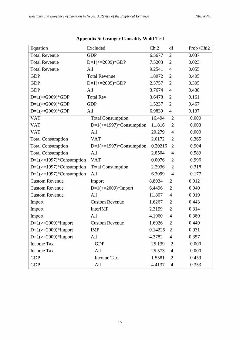
Appendix 5 reports the granger causality test. The test rejects the null of GDP has no

predictive content on tax and fails to reject the null of tax has no predictive content on GDP.

Therefore, this test, to some extent, leaves less space for endogeneity concern.


8

Table 2: Unit Root Test1

Variables (log) Level First Difference

With drift Result With drift Result

Gross Domestic Product (GDP) -0.17 I(1) -5.91 I(0)

Consumption 0.3 I(1) -6.53 I(0)

Total revenue 0.52 I(1) -6.21 I(0)

Custom duty -0.47 I(1) -6.61 I(0)

Value-added tax -0.13 I(1) -6.71 I(0)

Income tax 0.82 I(1) -7.04 I(0)

Export duty 1.53 I(1) -6.2 I(0)

Import tax -1.1 I(1) -5.84 I(0)

Consumer Price Index -0.23 I(1) -4.88 I(0)

Table 3: ARDL Bound Test

Sample F-value Remarks

1975-2009

1975-2015

13.99

1.34

F>Critical,Cointegrated

F<Critical, not cointegrated

1975-2015b 9.7 F>critical, cointegrated

b refers to the control of break by level dummy for 2009-2015

Table 4 and 4.1 report the OLS and ARDL regression results. The first and second columns

in Table 4 report the results of the baseline model. Engle-Granger two-step procedures

(Appendix 2) show that OLS residuals are non-stationary and therefore OLS results of the

baseline model will be spurious. We cannot rely on these estimates. ARDL bound test also

confirms this result. Therefore, for all baseline models which are not cointegrated we control

the break. Model 1 controls break at D=1(year>=2009) in the regression of total revenue on

GDP. Comparison of the model 1, model 2 and model 3 reveal that a simple regression of tax

only on a tax-base will be misspecified if the DGP excludes tax exemption. Except for

custom duty, long-run buoyancy coefficients for all taxes are found greater than unity

whereas short-run buoyancy coefficients are found smaller than unity.

1 Mackinnon (1996) critical value


9

Table 4: Long-run and Short-run Buoyancy Coefficients

Buoyancy

Coefficients

Baseline

Model

Baseline

Model Model 1# Model 2 Model 3

(OLS) (ARDL) (ARDL) (ARDL) (ARDL)

Total Revenue : base GDP

Long Run Buoyancy 1.17*** 1.52 1.13*** 1.16*** 1.16***

Short Run Buoyancy

1.01*** 0.51*** 0.49*** 0.46***

Speed of Adjustment

-0.03 -0.45** -0.43*** 0

ARDL Bound Test

Not

cointegrated Cointegrated Cointegrated# Cointegrated#

OLS Residual I(1)

Conditioning

Variables

Income Tax

Exemption

Income Tax

Exemption,

Inflation

* Significant at 10 percent level, ** at 5 percent level and *** at 1 percent level

# Controls shift in intercept

The long-run buoyancy is found to be 1.13 with marginal increment (coefficient of

D=1(year>=2009) of 0.022 after 2009. These results are invariant for model 2 and model 3

(see Table 4.1). This marginal increment indicates the effect of reform ongoing in our tax

system, but progressing at a very slow pace. For the reasons we discussed above, we

introduced the level of tax exemption allowed to high income bracket as additional

conditioning variables. Conditioning on the tax exemption marginally improves the buoyancy

coefficient for the period after 2009 even if it itself is not found statistically significant.

Though not statistically significant, the marginal increment in the buoyancy coefficient after

controlling income tax exemption is an indicative of the positive impact of tax rationalization

on revenue mobilization.

Model 3 has inflation as an additional conditioning variable. If the revenue is neutral to

inflation, inflation term should not be statistically significant and buoyancy coefficient should

not change. Results support this condition for total revenue, custom duty and income tax

whereas value-added tax is found to be non-neutral to inflation. Inflation brings down

buoyancy of VAT in both short-run and long-run.


10

Table 4.1: Long-run and Short-run Buoyancy Coefficients

Buoyancy

Coefficients

Baseline

Model

(OLS)

Baseline

Model

(ARDL)

Model 1#

(ARDL)

Model 2

(ARDL)

Model 3

(ARDL)

VAT: base consumption

Long Run Buoyancy 1.27*** 1.28*** 1.13*** 1.10*** 1.00***

Short Run Buoyancy 0.98*** 0.35*** 0.38*** 0.28***

Speed of Adjustment -0.13*** -0.31*** -0.35*** -0.28***

ARDL Bound Test Not

Cointegrated

Not

Cointegrated Cointegrated# Cointegrated#

OLS Residual I(1)

Custom Duty: base Import

Long Run Buoyancy 0.88*** 0.89*** 0.81*** 0.81***

Short Run Buoyancy 0.39*** 0.49*** 0.49***

Speed of Adjustment -0.44*** -0.60*** -0.60***

ARDL Bound Test Cointegrated

Cointegrated Cointegrated

OLS Residual I(0)*

Income Tax: Base GDP

Long Run Buoyancy 1.44*** 1.48*** 1.31*** 1.31***

Short Run Buoyancy 0.56*** 0.51*** 0.46***

Speed of Adjustment -0.38*** -0.38*** -0.37***


Cointegrated

Not

Cointegrated

OLS Residual I(0)*

Conditioning

Variables

Income Tax

Exemption

Income Tax

Exemption,

Inflation

* Significant at 10 percent level, ** at 5 percent level and *** at 1 percent level.


Table 5 and 5.1 report the long-run and short-run elasticity coefficients. These coefficients

are estimated based on the tax series derived by removing a part of the tax announced by the

government in the budget speech to be collected from administrative reform and changes. As

in Adhikari (1995) and Timsina (2007), we also applied Sahota (1961) method to remove the

exogenous part of the revenue. Since actual tax collection from administrative reform and

changes is not observed and if the adjusted tax significantly deviates away from reality,

estimates of the elasticity coefficients will be biased. The degree of the biasedness depends

on the magnitude of the adjustment error. If the adjustment error is high, results will be


11

seriously distorted. Therefore, emphasis is given to overall revenue forecast rather than the

revenue forecast based on endogenous economic changes excluding the impact of

administrative changes and reforms.

Table 5: Long-run and Short-run Elasticity Coefficients

Elasticity

Coefficients

Baseline

Model

Baseline

Model Model 1# Model 2 Model 3

(OLS) (ARDL) (ARDL) (ARDL) (ARDL)

Total Revenue : base GDP

Long Run Buoyancy 0.63*** 0.67*** 0.57*** 0.93*** 0.87***

Short Run Buoyancy

0.16*** 0.19*** 0.33*** -0.67

Speed of Adjustment

-0.23*** -0.33** -0.35*** -0.47***

ARDL Bound Test

Not

cointegrated Cointegrated Cointegrated# Cointegrated#

OLS Residual I(1)

Conditioning

Variables

Income Tax

Exemption

Income Tax

Exemption,

Inflation

* Significant at 10 percent level, ** at 5 percent level and *** at 1 percent level


In our empirical results, elasticity coefficients for all revenue heads except for VAT are found

to be less than unity. Engle-Granger two step procedures (Appendix 3) show that OLS

estimates for adjusted total revenue and income tax are spurious. For all baseline models

which are not cointegrated we control the break. This is the model 1. Model 2 augments

income tax exemption in model 1 and model 3 augments income tax exemption and inflation.

Augmentation of inflation to model 2 for the DGP of income tax breaks down the

cointegrating relation, suggesting that this tax does not share a common trend with inflation

in the long run. We suggest discarding all models which are not cointegrated. Empirical

results show that inflation and income tax exemption have mixed effects. Inflation reduces

long-run elasticity of total revenue, VAT and income tax while tax exemption improves long-

run elasticity of total revenue, VAT and custom duty.

Important messages are in order from our empirical evidence illustrated in Table 4.1 and 5.1.

Long-run buoyancy coefficient is highest for income tax and is lowest for custom duty. Long-

run buoyancy coefficient for custom duty is not only the lowest, but it is also less than unity.

Long-run elasticity coefficient for custom duty is also the lowest. We are not sure whether the

low elasticity of custom revenue is due to reduction in custom taxes or leakage. But what we

certainly infer from this empirical evidence is that reform in custom administration should get

top priority in our fiscal reform program.


12

Table 5.1: Long-run and Short-run Elasticity Coefficients

Elasticity

Coefficients

Baseline

Model

(OLS)

Baseline

Model

(ARDL)

Model 1#

(ARDL)

Model 2

(ARDL)

Model 3

(ARDL)

VAT: base Consumption

Long Run Elasticity 0.69*** 0.66*** 1.10*** 1.33*** 1.20***

Short Run Elasticity

0.13** 0.24*** 0.24** 0.31**

Speed of Adjustment

-0.20** -0.22** -0.18** -0.26***

ARDL Bound Test

Not

Cointegrated Cointegrated Cointegrated# Cointegrated#

OLS Residual I(0)

Custom Duty: base Import

Long Run Elasticity 0.49*** 0.47***

0.57*** 0.65***


0.20***

0.25*** 0.24***

Speed of Adjustment

-0.42***

-0.44*** -0.38**



OLS Residual I(0)*

Income Tax: Base GDP

Long Run Elasticity 0.57*** 0.69*** 0.47*** 1.05* 0.98*


0.12** -1.34 0.19* 0.20**

Speed of Adjustment

-0.17** -0.37*** -0.18* -0.20*

ARDL Bound Test

Not


Not

Cointegrated#

Not

Cointegrated#

OLS Residual I(1)*

Conditioning

Variables

Income Tax

Exemption

Income Tax

Exemption,

Inflation

*Significant at 10 percent level, ** at 5 percent level and *** at 1 percent level

#Controls break,

Finally, for the forecast of total revenue we suggest using model 2 or model 3 depending on

whether revenue components (Custom, VAT etc.) are neutral or non-neutral to inflation. For

total revenue forecast either model 2 or model 3 can be used. Long-run buoyancy coefficient

should be used to estimate the revenue effects of output growth. Table 6 reports the summary

statistics of actual revenue and revenue predicted by the model 2 in Table 4. The mean of

actual revenue and predicted revenue exactly coincide when we use GDP and interaction of

GDP with level dummy (D=1 if year>=2009) as the predictors of the total revenue.


13

Table 6: Summary of Actual Revenue and Predicted Revenue, (log)

Variable Obs Mean S.D. Min Max

Total Revenue 42 9.930812 1.819648 6.91612 13.08724

Total Revenue

(Prediction) 42 9.930812 1.818018 7.104651 12.8966

V. CONCLUSION

We found a break in the the relationship between total revenue and income from 2009.

Therefore, OLS estimates of the elasticity and buoyancy coefficients for the sample 1975-

2016 will be spurious. The cointegrating relationship exists when we control the break by

level dummy (D=1(year>=2009)). All coefficients for interaction term are positive, though

marginal, and statistically significant, implying a gradual improvement in our revenue

administration. Further, we found estimates to be biased if the DGP is not conditioned by

income tax exemption. Empirical results show that long-run buoyancy and elasticity

coefficients for custom duty are the lowest, indicating the areas of reform to be focused in

revenue administration. Results also show that some components of revenue heads are non-

neutral to inflation. Inflation reduces buoyancy coefficients of income tax and VAT, and

elasticity coefficients of all taxes besides custom duty in the long-run.


14

REFERENCES

Acharya, H. (2011, January). The Measurement of Tax Elasticity in India: A Time Series

Approach. Faculty of Management Studies .

Adhikari, R. P. (1995). Tax Elasticity and Buoyancy in Nepal. Economic Review , 8.

Ashraf, M., and Sarwar, D. S. (2016). Institutional Determinants of Tax Buoyancy in

Developing Nations. Journal of Emerging Economies and Islamic Research , 4 (1).

Belinga, V., Benedek, D., Mooij, R. d., and Norregard, J. (2014). Tax Buoyancy in OECD

Countries. International Monetary Fund, Working paper , 14 (10).

Bilquees, F. (2004). Elasticity and Buoyancy of the Tax System in Pakistan. The Pakistan

Development Review , 1 (43), 73-93.

Bruce, D., Fox, W. F., and Tuttle, M. H. (2006). Tax Base Elasticities: A Multi-State

Analysis of Long-Run and Short-Run Dynamics. Southern Economic Journal , 73 (2),

315-341.

Dahal, M. (1984). Built-in Flexiblity and Sensitivity of the the Tax Yields in Nepal's Tax

System. The Economic Journal of Nepal , 2.

G.S., S. (1961). Indian Tax Structure and Economic Development.

Gillani, S. F. (1986). Elasticity and Buoyancy of Federal Taxes in Pakistan. The Pakistan

Development Review , XXV (2).

M., U. (2008). Degree of Tax Buoyancy in India: An Empirical Study. International Journal

of Applied Econometrics and Quantitative Studies , 5 (2).

M.H. Pesaran, and Shin, Y. (1999). An Autoregressive Distributed Lag Modelling Approach

to Cointegration Analysis. In S. S., Econometrics and Economic Theory in the 20th

Century:The Ragnar Frisch Centennial Symposium. Cambridge,U.K.: Cambridge

University Press.

M.H., Pesaran, Shin, Y., and Smith, R. (2001). Bounds Testing Approaches to the Analysis of

Level Relationship. Journal of Applied Econometrics , 16 (3), 289-326.

MoF. (2014). High Level Tax System Review Report. Kathmandu, Nepal: Ministry of

Finance, Government of Nepal.

Rajaraman, I., Goyal, R., and Khundrakpam, J. K. (2006). Tax Buoyancy Estimates for

Indian States. Economic and Political Weekly , 41 (16), 1570-1573.

Timsina, N. (2007). Tax Elasticity and Buoyancy in Nepal: A Revisit. Economic Review , 19.

Yousuf, M., and Huq, S. M. (2013). Elasticity and Buoyancy of Major Tax Categories:

Evidence from Bangladesh and Its Policy Implications. Research Study Series No. FDRS

03/2013 .


15

APPENDICES

Appendix 1: Revenue Mobilization as percentage of Gross Domestic Product

Year Custom VAT Income Excise Other Direct Indirect

1975 2.0 1.1 0.3 0.7 0.9 0.3 4.8

1980 2.6 1.7 0.4 0.9 0.4 0.4 6.2

1985 2.3 1.8 0.7 1.0 0.7 0.7 6.1

1990 2.6 1.5 0.9 0.0 0.9 0.9 6.2

1995 3.2 2.8 1.2 0.8 1.2 1.2 7.8

2000 2.8 2.8 2.1 0.9 2.1 2.1 6.7

2005 2.3 3.3 1.7 1.0 1.7 1.7 7.1

2010 2.6 4.5 3.1 1.9 3.1 3.1 9.9

2014 3.5 5.2 4.1 2.4 4.1 4.1 12.2

Appendix 2: Engle-Granger test for cointegration between

Total Revenue and GDP

Sample Pd: 1975-2015

N(1st Step) = 42

N (test) = 41 test

Test

Statistic

1% critical

value

5% critical

value 10% critical value

Z(t) -1.185 -4.177 -3.489 -3.15

Critical values from MacKinnon (1990, 2010)

Appendix 3: Engle-Granger test for cointegration between

adj. total Revenue and GDP

Sample Pd: 1975-2015

N(1st Step) = 42

N (test) = 41 test

Test

Statistic

1% critical

value

5% critical

value 10% critical value

Z(t) 1.798 -4.177 -3.489 -3.15

Critical values from MacKinnon (1990, 2010)


16

Appendix 4: Vector Error Correction (VEC) Rank Test

(Total Revenue and Gross Domestic Product)

Johansen Test for Cointegration (1977-2008)

Trend: Constant No. of obs.:32

Lags: 2

Maximum

Rank Parms LL

Eigen

values

Trace

Statistic

5%

critical

value

0 6 123.4207

16.0668 15.41

1 9 131.2631 0.38747 0.382 3.76

2 10 131.4541 0.01187

Johansen Test for Cointegration (1977-2016)


Lags: 2

Maximum

Rank Parms LL

Eigen

values

Trace

Statistic

5%

critical

value

0 6 155.66341

4.6695 15.41

1 9 157.94429 0.10778 0.1078 3.76

2 10 157.99818 0.00269

Johansen Test for Cointegration with D=1(year>=2009)

and Interaction Term


Lags: 2

Maximum

Rank Parms LL

Eigen

values

Trace

Statistic

5%

critical

value

0 20 296.35472

64.5449 47.21

1 27 316.55290 0.63575 24.1486 29.68

2 32 325.62717 0.36474 6.0000 15.41

3 35 328.62087 0.139.2 0.0126 3.76

4 36 328.62718 0.00032


17

Appendix 5: Granger Causality Wald Test

Equation Excluded Chi2 df Prob>Chi2

Total Revenue GDP 6.5677 2 0.037

Total Revenue D=1(>=2009)*GDP 7.5203 2 0.023

Total Revenue All 9.2541 4 0.055

GDP Total Revenue 1.8072 2 0.405

GDP D=1(>=2009)*GDP 2.3757 2 0.305

GDP All 3.7674 4 0.438

D=1(>=2009)*GDP Total Rev 3.6478 2 0.161

D=1(>=2009)*GDP GDP 1.5237 2 0.467

D=1(>=2009)*GDP All 6.9839 4 0.137

VAT Total Consumption 16.494 2 0.000

VAT D=1(>=1997)*Consumption 11.816 2 0.003

VAT All 20.279 4 0.000

Total Consumption VAT 2.0172 2 0.365

Total Consumption D=1(>=1997)*Consumption 0.20216 2 0.904

Total Consumption All 2.8504 4 0.583

D=1(>=1997)*Consumption VAT 0.0076 2 0.996

D=1(>=1997)*Consumption Total Consumption 2.2936 2 0.318

D=1(>=1997)*Consumption All 6.3099 4 0.177

Custom Revenue Import 8.8034 2 0.012

Custom Revenue D=1(>=2009)*Import 6.4496 2 0.040

Custom Revenue All 11.807 4 0.019

Import Custom Revenue 1.6267 2 0.443

Import InterIMP 2.3159 2 0.314

Import All 4.1960 4 0.380

D=1(>=2009)*Import Custom Revenue 1.6026 2 0.449

D=1(>=2009)*Import IMP 0.14225 2 0.931

D=1(>=2009)*Import All 4.3782 4 0.357

Income Tax GDP 25.139 2 0.000

Income Tax All 25.573 4 0.000

GDP Income Tax 1.5581 2 0.459

GDP All 4.4137 4 0.353

Documents

Elasticity and Buoyancy of Taxation in Nepal: A Revisit of ... · PDF fileA Revisit of the Empirical Evidence ... (2011) used OLS method to estimate the tax elasticity and buoyancy