ELECTORAL UNCERTAINTY, FISCAL POLICY

AND ECONOMIC GROWTH

Theory and evidence from the UK and a panel of

parliamentary democracies••

Dimitrios Asteriou∗

George Economides**

Apostolis Philippopoulos** ***

and

Simon Price*

December 2000

Abstract: We study the link between elections, fiscal policy and economic growth. The set-up is a general equilibrium model of endogenous growth and optimal fiscal policy, in which two political parties can alternate in power. The party in power chooses jointly how much to tax and how to allocate its total expenditure between productive and non-productive activities. The main prediction is that as the probability of re-election falls, forward-looking governments find it optimal to follow relatively shortsighted fiscal policies, and that this is bad for private investment and economic growth. This prediction is tested by using government popularity data for the UK, and data on the duration of governments for 20 parliamentary democracies. The results are consistent with the theory. Keywords: Political uncertainty, economic growth, optimal policy, the composition of public expenditure. JEL classification numbers: D9, E6, H1, H5.

• We thank Tryphon Kollintzas, Jim Malley and Hyun Park for comments and discussions. D. Asteriou and S. Price are also grateful to the ESRC for financial support under grant no. R000237922. All errors are ours. ∗ City University, London, UK. ** Athens University of Economics and Business, Athens, Greece. *** Corresponding author: Apostolis Philippopoulos, Athens University of Economics and Business, 76 Patission street, Athens 10434, Greece. Tel: +30-1-8203413. Fax: +30-1-8214122. Email: aphil@aueb.gr

1

I. INTRODUCTION

There is clear evidence in most OECD countries for two propositions.1 Firstly,

the size of the public sector (total government expenditures as a share of GDP) has

increased substantially since the early 1960s. Secondly, public investment as a share

of GDP shows a declining trend, while other components of government spending

(e.g. government consumption, transfers and government wages) show a sharply

upward movement. The consequently higher tax burden and the changes in the

composition of government expenditure are sometimes argued to have reduced

economic growth.2 In this paper, we offer an explanation for this by developing a

general equilibrium model that looks at the impact of electoral uncertainty, and

specifically re-election probabilities, on the conduct of fiscal policies and economic

growth. Empirical evidence from a number of countries is consistent with the model.

The idea that sociopolitical instability hinders economic growth is not new.3

One argument is that it increases uncertainty and that this reduces growth through

lower investment. Empirical growth regressions have employed various sociopolitical

indices (e.g. measures of democracy, political violence and government stability) as

growth determinants [see Barro (1991) and Chen and Feng (1996)]. Barro (1996),

Levine and Zervos (1996) and Easterly and Rebelo (1993) add indicators of political

instability to cross-section regressions in which the dependent variable is either

growth or investment. Hibbs (1973), Gupta (1990) and Alesina and Perotti (1996)

measure political instability by constructing indices which summarise data on the

occurrence of political violence and unrest. Brunetti (1998) provides a comparative

test of different measures of policy volatility in cross-country growth regressions and

concludes that all these measures are negatively related to economic growth.

But our explanation and evidence differ. We look at the government’s joint

decisions on how much to tax and how to allocate its total expenditure between

consumption and production activities. Forward-looking governments, with uncertain

prospects of re-election, find it optimal to follow relatively shortsighted fiscal

policies, and this is eventually bad for economic growth through lower private capital

1 See e.g. Alesina (1999) and the references cited therein. 2 See e.g. Kneller, Bleaney and Gemmell (1999), Alesina (1999) and the references cited therein. 3 A recent survey of this literature is in Drazen (2000, chapter 11.6).

2

accumulation.4 Also, to the extend that we test how economic growth is affected by

re-election probabilities (measured by the incumbent’s popularity), we provide

evidence different from that of the literature that has mostly focused on the effects of

sociopolitical instability.

We construct a general equilibrium model of endogenous growth and optimal

fiscal policy, in which the government imposes income taxes to finance both public

consumption services (that provide direct utility to households) and public production

services (that provide production externalities to firm’s capital, and hence generate

Barro-type long-term growth). Two political parties can alternate in power according

to an exogenous re-election probability. The elected party forms a government that

chooses the income tax rate and the allocation of total tax revenues between public

consumption and public production services during its term in office. Parties aim to

maximize utility of a representative household. In doing so, the political parties play

Nash vis-à-vis each other, and Stackelberg vis-à-vis households and firms. We solve

for Markov strategies, and hence a Markov-perfect general equilibrium in which

optimal policies are time consistent.5

The main results are as follows. When the probability of being re-elected

decreases, the total government expenditure-to-output ratio (and the associated

required tax rate) increases, while the share of tax revenue used to finance public

production services decreases. Both fiscal policy instruments work in the same

direction, so that - in equilibrium - a lower re-election probability leads to lower

private capital accumulation and output growth. The mechanism is as follows. When

there is electoral uncertainty and the political parties do not care (or care relatively

little) about economic outcomes when out of power, they effectively face a quasi-

4 The theoretical literature on politics and fiscal policy is very rich [for surveys, see Alesina et al. (1997) and Persson and Tabellini (1999)]. Here, the focus is on the link between elections, fiscal policy and growth [see also e.g. Devereux and Wen (1998) and Darby, Li and Muscatelli (1998)]. Other related papers include Calvo and Drazen (1997) who show how political instability distorts the future path of private investment decisions, and Svensson (1993) who studies how political instability makes governments less inclined to make improvements to the legal system. 5 Darby et al. (1998) also study the case in which the incumbent government chooses both the tax policy and the allocation between the two types of government activities. One difference from our paper is that they assume no private capital. By contrast, here we use a standard general equilibrium model of endogenous growth and optimal fiscal policy, in which productive government expenditures can stimulate economic growth by increasing the productivity of private capital. That is, we extend Barro’s (1990) popular model of endogenous growth and public finance [see also Park and Philippopoulos (2000)]. Our model also differs from Devereux and Wen (1998) and Economides and Philippopoulos (1999), because here we include both consumption and production government activities. In terms of modeling the electoral system, our paper is close to Alesina and Tabellini (1990) and Lockwood et al. (1996).

3

finite time horizon.6 The higher the electoral uncertainty (i.e. the smaller the

probability of being re-elected), the less they care about the future. As a result, when

in power, they go for shortsighted, inefficient policies; inefficiency here takes the

form of a relatively high tax burden, a preference for non-productive activities with

short-term benefits, and eventually lower economic growth through lower private

capital accumulation.7

To test this model we do not require indices of political instability, as such, but

instead measures of re-election probabilities. We examine two data sets. We start

with a single country (the UK) where, uniquely, there is both an effective two-party

system and good data on government’s popularity [see Price and Sanders (1994)]. By

using popularity, as a measure of ex ante re-election probabilities, we remain faithful

to the theoretical model. Then, we also use a more general framework where electoral

uncertainty is measured by an ex post measure of governmental duration, for a small

panel of twenty parliamentary democracies.8 The main theoretical prediction, i.e. that

lower re-election probabilities lead to lower GDP growth, cannot be rejected by the

data.

There is an obvious link with one strand of the political business cycle.

Alesina et al. (1997, chapter 5) have been unique in modelling re-election

probabilities explicitly in a rational partisan model of surprise inflation and

unemployment.9 They look at US presidential elections and calculate the probability

6 The mechanism is as in Lockwood et al. (1996), who also provide support from the political science literature that this is indeed the case [see Laver and Hunt (1992)]. Darby et al. (1998) also show the effects of political uncertainty on the government’s effective discount rate and on policies chosen. Note that this mechanism is different from that in Rogoff and Sibert (1988) where the incumbent government manipulates policy instruments in an attempt to increase its re-election probability, or from that in Persson and Svensson (1989) and Alesina and Tabellini (1990) where the incumbent government uses strategically the state variables (e.g. public debt) to reduce the choices of its successor [for a survey, see e.g. Persson and Tabellini (1994)]. 7 Here, we take elections as given, and ask how electoral uncertainty affects the macro-economy. Then, elections are typically inefficient. Of course, there are clear arguments supporting the endogenous evolution of elections. For instance, elections control the moral hazard of policymakers, help voters to select the most competent policymaker, or help voters to choose the policymaker whose ideology is closer to the majority of the voters [for a survey, see e.g. Persson and Tabellini (1994)]. 8 Standard sociopolitical indices (e.g. measures of democracy, political violence, strikes, etc) measure something else; namely, instability,and therefore policy uncertainty. Duration of government is related to instability, but nevertheless the probability of the governement falling in any period is given by the inverse of duration. Thus, duration is related to what we want to measure, the probability of the government falling (it is ex post, of course). We continue to be faithful to the theoretical model. 9 In the rational partisan model, private agents anticipate the inflation bias associated with political parties, when they make their nominal contracts. The bias is related to the parties’ preferences; arguably left-leaning parties have a larger inflation bias than right parties. Before an election, the electoral outcome, and hence the inflation bias, is unknown. Thus, there is a post-election inflation surprise, which leads to temporary and variable output effects. Most studies test this model with a

4

of electoral victory by using a simple formula taken from option pricing theory.10

Here, we also estimate re-election probabilities for the UK. But our model differs. In

the rational partisan model there are only surprise post-election demand effects that

have an expected value of zero. In our model, election probabilities have a

permanent, long-run effect upon real variables. Thus, it is not electoral surprises that

matter for growth, but re-election probabilities themselves. We proxy these with

contemporaneous electoral support, and subsume partisan post-election effects into

the error term.11 There is no reason to suppose that this will bias our results.

The rest of the paper is organized as follows. Section II solves for a

competitive equilibrium. Section III solves for optimal fiscal policies in a political

equilibrium. Empirical results are in section IV. Section V closes the paper.

II. THE ECONOMY AND COMPETITIVE EQUILIBRIUM

We set up a closed economy with a private sector and two political parties.

The private sector consists of a representative household and a representative firm.

The household consumes, works and saves in the form of capital. The firm uses

capital and labor to produce a single good. The party in power finances the provision

of public services by taxing the household’s income. We assume discrete time and

infinite time-horizons. In this section, we solve for a competitive equilibrium, given

economic policy and the electoral process.

Behavior of the household

The representative household maximizes intertemporal utility:

β tt

ttu c h( , )

=

∞

∑0

(1a)

simple post-election dummy. However, it is clear that the surprise depends upon the ex ante re-election probability. 10 In turn, Alesina et al. use their estimated probabilities to estimate the impact of electoral surprises on post-election outcomes (like growth and unemployment). They find that the more surprised is the public, the larger the post-election impact, as is predicted by the rational partisan model. See below for more discussion. 11 Our reading is that evidence for rational partisan political business cycles is rather weak so this is a reasonable assumption. For a rather rich model applied to the UK, see Alogoskoufis et al. (1992).

5

where c t and ht are respectively private consumption and public consumption at time

t , and 0 1< <β is the discount rate. The utility function is increasing and concave in

its two arguments, and also satisfies the Inada conditions. For algebraic simplicity,

we assume that u(.) is additively separable and logarithmic. Thus,

u c h c ht t t t( , ) log log= + δ (1b)

where 0≥δ is the weight given to public consumption services relative to private

consumption.

At any t , the household rents its predetermined capital, k t , to the firm and

receives r kt t , where rt is the market return to capital at t . It also supplies

inelastically one unit of labor services per time-period so that the labor income is wt .

Further, it receives profits, π t . Thus, the budget constraint at time t is:

( )( )k c r k wt t t t t t t+ + = − + +1 1 θ π (2)

where 10 << tθ is the income tax rate. For algebraic simplicity, we assume full

capital depreciation. The initial capital stock, k0 , is given.

The household acts competitively by taking prices, tax policy and public

services as given. We will solve the household’s optimization problem by using

dynamic programming. From the household’s viewpoint, the state variables at time t

are the predetermined capital stock, k t , and current economic policy. As we show

below, the independent policy instruments at any t are the income tax rate, tθ , and

the share of total tax revenues used to finance public production services, tb . Then,

let ( )ttt bkV ,;θ denote the value function of the household at any t . This value

function must satisfy the Bellman equation:

( ) ( )[ ]111 , ;loglogmax,;1 ,

+++++=+

tttttkc

ttt bkVhcbkVtt

θβδθ (3)

6

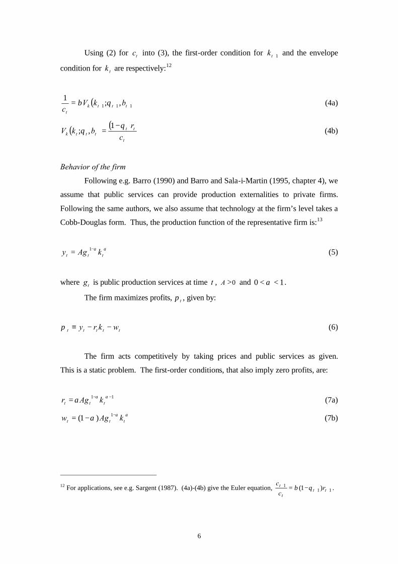
Using (2) for ct into (3), the first-order condition for k t +1 and the envelope

condition for k t are respectively:12

( )111 ,;1

+++= tttkt

bkVc

θβ (4a)

( ) ( )t

tttttk c

rbkV

θθ

−=

1,; (4b)

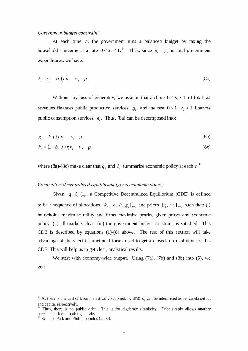
Behavior of the firm

Following e.g. Barro (1990) and Barro and Sala-i-Martin (1995, chapter 4), we

assume that public services can provide production externalities to private firms.

Following the same authors, we also assume that technology at the firm’s level takes a

Cobb-Douglas form. Thus, the production function of the representative firm is:13

ααttt kAgy −= 1 (5)

where gt is public production services at time t , A >0 and 0 1< <α .

The firm maximizes profits, π t , given by:

π t t t t ty r k w≡ − − (6)

The firm acts competitively by taking prices and public services as given.

This is a static problem. The first-order conditions, that also imply zero profits, are:

11 −−= ααα ttt kAgr (7a)

ααα ttt kAgw −−= 1)1( (7b)

12 For applications, see e.g. Sargent (1987). (4a)-(4b) give the Euler equation, 111 )1( ++

+ −= ttt

t rc

cθβ .

7

Government budget constraint

At each time t , the government runs a balanced budget by taxing the

household’s income at a rate 10 << tθ .14 Thus, since h gt t+ is total government

expenditures, we have:

( )h g r k wt t t t t t t+ = + +θ π (8a)

Without any loss of generality, we assume that a share 10 << tb of total tax

revenues finances public production services, g t , and the rest 110 <−< tb finances

public consumption services, ht . Thus, (8a) can be decomposed into:

( )ttttttt wkrbg πθ ++= (8b)

( ) ( )ttttttt wkrbh πθ ++−= 1 (8c)

where (8a)-(8c) make clear that tθ and tb summarize economic policy at each t .15

Competitive decentralized equilibrium (given economic policy)

Given ∞=0, ttt bθ , a Competitive Decentralized Equilibrium (CDE) is defined

to be a sequence of allocations ∞=+ 01 ,, , ttttt ghck and prices , r wt t t =

∞0 such that: (i)

households maximize utility and firms maximize profits, given prices and economic

policy; (ii) all markets clear; (iii) the government budget constraint is satisfied. This

CDE is described by equations (1)-(8) above. The rest of this section will take

advantage of the specific functional forms used to get a closed-form solution for this

CDE. This will help us to get clear, analytical results.

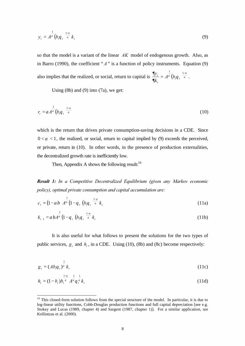
We start with economy-wide output. Using (7a), (7b) and (8b) into (5), we

get:

13 As there is one unit of labor inelastically supplied, ty and tk can be interpreted as per capita output and capital respectively. 14 Thus, there is no public debt. This is for algebraic simplicity. Debt simply allows another mechanism for smoothing activity. 15 See also Park and Philippopoulos (2000).

8

( ) tttt kbAy αα

α θ−

=11

(9)

so that the model is a variant of the linear AK model of endogenous growth. Also, as

in Barro (1990), the coefficient “ A ” is a function of policy instruments. Equation (9)

also implies that the realized, or social, return to capital is ( ) αα

α θ∂∂ −

=11

ttt

t bAk

y.

Using (8b) and (9) into (7a), we get:

( ) αα

α θα−

=11

ttt bAr (10)

which is the return that drives private consumption-saving decisions in a CDE. Since

0 1< <α , the realized, or social, return to capital implied by (9) exceeds the perceived,

or private, return in (10). In other words, in the presence of production externalities,

the decentralized growth rate is inefficiently low.

Then, Appendix A shows the following result:16

Result 1: In a Competitive Decentralized Equilibrium (given any Markov economic

policy), optimal private consumption and capital accumulation are:

( ) ( )( ) ttttt kbAc αα

α θθαβ−

−−=11

11 (11a)

( )( ) ttttt kbAk αα

α θθαβ−

+ −=11

1 1 (11b)

It is also useful for what follows to present the solutions for the two types of

public services, g t and ht , in a CDE. Using (10), (8b) and (8c) become respectively:

tttt kAbg αθ1

)(= (11c)

ttttt kAbbh αααα

θ111

)1(−

−= (11d)

16 This closed-form solution follows from the special structure of the model. In particular, it is due to log-linear utility functions, Cobb-Douglas production functions and full capital depreciation [see e.g. Stokey and Lucas (1989, chapter 4) and Sargent (1987, chapter 1)]. For a similar application, see Kollintzas et al. (2000).

9

To summarize this section, equations (11a), (11b), (11c) and (11d) give ct ,

k t +1 , g t and ht respectively in a CDE. This is for any Markov fiscal policy, where

the latter is summarized by the current tax rate, θ t , and the current allocation of tax

revenues between public production and public consumption services, tb . The next

section will endogenize the choice of θ t and tb . Note that the CDE is a function of

the predetermined capital stock, tk , and the current policy instruments, θ t and tb .

This will make the political parties’ optimization problem recursive and hence

policies will be time consistent.17

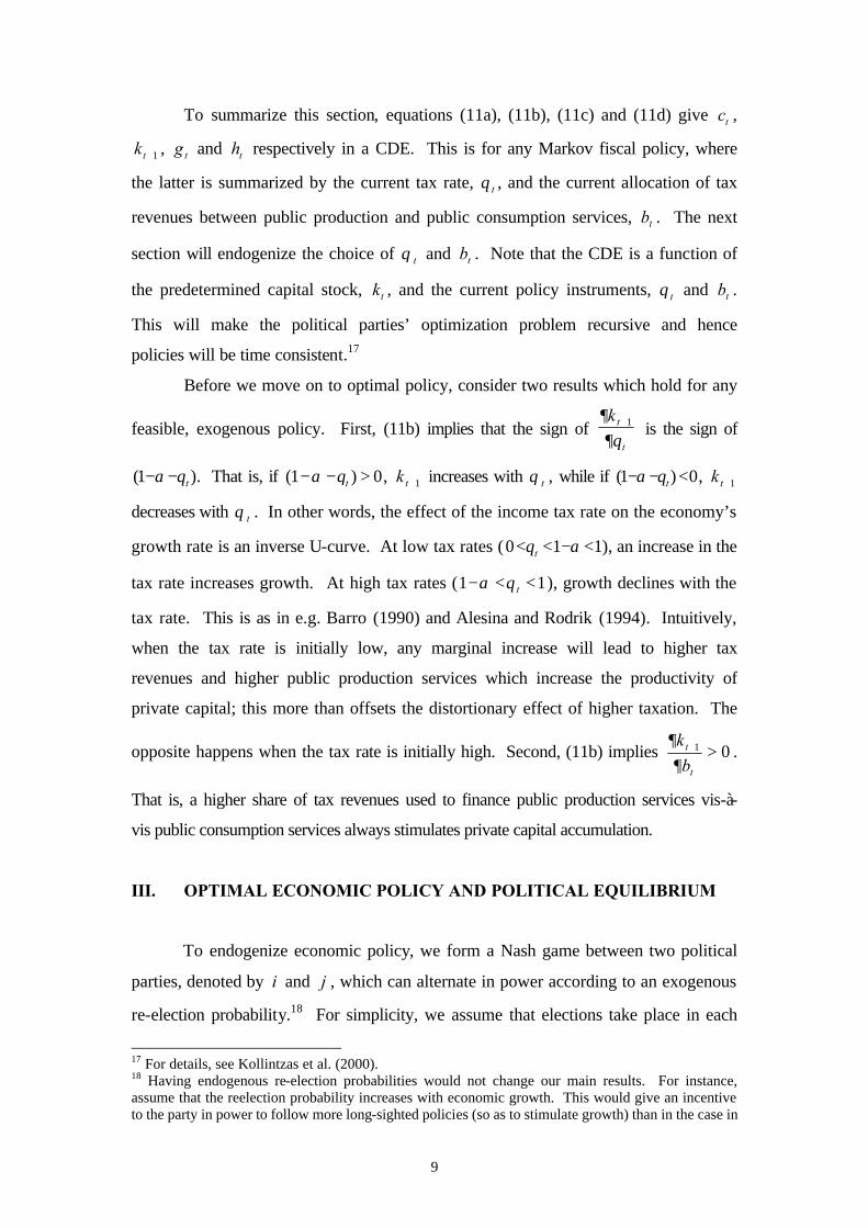
Before we move on to optimal policy, consider two results which hold for any

feasible, exogenous policy. First, (11b) implies that the sign of ∂∂θk t

t

+1 is the sign of

).1( tθα−− That is, if ( )1 0− − >α θt , k t +1 increases with θ t , while if 0)1( <−− tθα , k t +1

decreases with θ t . In other words, the effect of the income tax rate on the economy’s

growth rate is an inverse U-curve. At low tax rates ( 110 <−<< αθt ), an increase in the

tax rate increases growth. At high tax rates ( 11 <<− tθα ), growth declines with the

tax rate. This is as in e.g. Barro (1990) and Alesina and Rodrik (1994). Intuitively,

when the tax rate is initially low, any marginal increase will lead to higher tax

revenues and higher public production services which increase the productivity of

private capital; this more than offsets the distortionary effect of higher taxation. The

opposite happens when the tax rate is initially high. Second, (11b) implies 01 >+

t

t

b

k

∂∂

.

That is, a higher share of tax revenues used to finance public production services vis-à-

vis public consumption services always stimulates private capital accumulation.

III. OPTIMAL ECONOMIC POLICY AND POLITICAL EQUILIBRIUM

To endogenize economic policy, we form a Nash game between two political

parties, denoted by i and j , which can alternate in power according to an exogenous

re-election probability.18 For simplicity, we assume that elections take place in each

17 For details, see Kollintzas et al. (2000). 18 Having endogenous re-election probabilities would not change our main results. For instance, assume that the reelection probability increases with economic growth. This would give an incentive to the party in power to follow more long-sighted policies (so as to stimulate growth) than in the case in

10

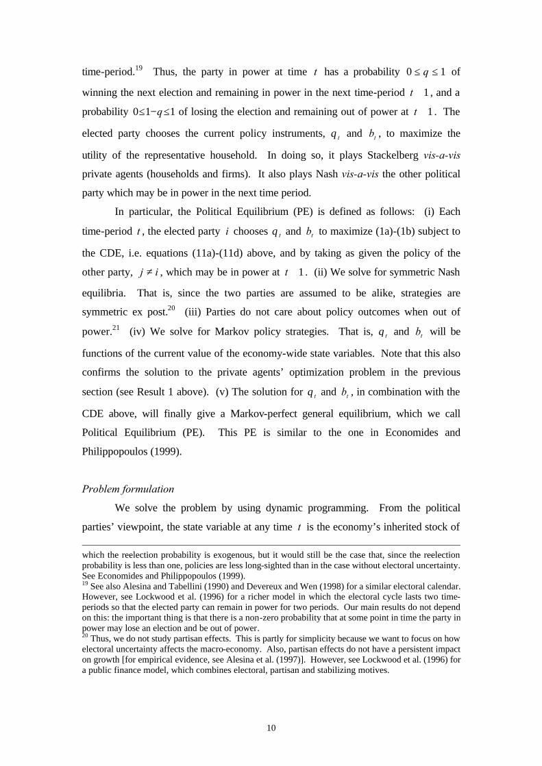
time-period.19 Thus, the party in power at time t has a probability 0 1≤ ≤q of

winning the next election and remaining in power in the next time-period t + 1 , and a

probability 0 1 1≤ − ≤q of losing the election and remaining out of power at t + 1 . The

elected party chooses the current policy instruments, tθ and tb , to maximize the

utility of the representative household. In doing so, it plays Stackelberg vis-a-vis

private agents (households and firms). It also plays Nash vis-a-vis the other political

party which may be in power in the next time period.

In particular, the Political Equilibrium (PE) is defined as follows: (i) Each

time-period t , the elected party i chooses tθ and tb to maximize (1a)-(1b) subject to

the CDE, i.e. equations (11a)-(11d) above, and by taking as given the policy of the

other party, ij ≠ , which may be in power at t + 1 . (ii) We solve for symmetric Nash

equilibria. That is, since the two parties are assumed to be alike, strategies are

symmetric ex post.20 (iii) Parties do not care about policy outcomes when out of

power.21 (iv) We solve for Markov policy strategies. That is, θ t and tb will be

functions of the current value of the economy-wide state variables. Note that this also

confirms the solution to the private agents’ optimization problem in the previous

section (see Result 1 above). (v) The solution for θ t and tb , in combination with the

CDE above, will finally give a Markov-perfect general equilibrium, which we call

Political Equilibrium (PE). This PE is similar to the one in Economides and

Philippopoulos (1999).

Problem formulation

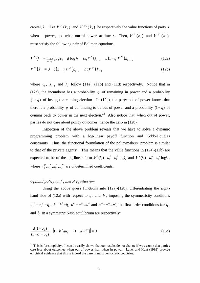
We solve the problem by using dynamic programming. From the political

parties’ viewpoint, the state variable at any time t is the economy’s inherited stock of

which the reelection probability is exogenous, but it would still be the case that, since the reelection probability is less than one, policies are less long-sighted than in the case without electoral uncertainty. See Economides and Philippopoulos (1999). 19 See also Alesina and Tabellini (1990) and Devereux and Wen (1998) for a similar electoral calendar. However, see Lockwood et al. (1996) for a richer model in which the electoral cycle lasts two time-periods so that the elected party can remain in power for two periods. Our main results do not depend on this: the important thing is that there is a non-zero probability that at some point in time the party in power may lose an election and be out of power. 20 Thus, we do not study partisan effects. This is partly for simplicity because we want to focus on how electoral uncertainty affects the macro-economy. Also, partisan effects do not have a persistent impact on growth [for empirical evidence, see Alesina et al. (1997)]. However, see Lockwood et al. (1996) for a public finance model, which combines electoral, partisan and stabilizing motives.

11

capital, k t . Let )( tP kV i and )( t

N kV i be respectively the value functions of party i

when in power, and when out of power, at time t . Then, )( tP kV i and )( t

N kV i

must satisfy the following pair of Bellman equations:

( ) ( ) ( ) ( )[ ]11,

1loglogmax ++ −+++= tN

tP

ttb

tP kVqkqVhckV ii

tt

i ββδθ

(12a)

( ) ( ) ( ) ( )V k q V k qV kNt

Pt

Nt

i i i= + − ++ +0 1 1 1β β (12b)

where ct , k t +1 and ht follow (11a), (11b) and (11d) respectively. Notice that in

(12a), the incumbent has a probability q of remaining in power and a probability

)1( q− of losing the coming election. In (12b), the party out of power knows that

there is a probability q of continuing to be out of power and a probability )1( q− of

coming back to power in the next election.22 Also notice that, when out of power,

parties do not care about policy outcomes; hence the zero in (12b).

Inspection of the above problem reveals that we have to solve a dynamic

programming problem with a log-linear payoff function and Cobb-Douglas

constraints. Thus, the functional formulation of the policymakers’ problem is similar

to that of the private agents’. This means that the value functions in (12a)-(12b) are

expected to be of the log-linear form tPP

tP kuukV log)( 10 += and t

NNt

N kuukV log)( 10 += ,

where NNPP uuuu 1010 ,,, are undetermined coefficients.

Optimal policy and general equilibrium

Using the above guess functions into (12a)-(12b), differentiating the right-

hand side of (12a) with respect to θ t and tb , imposing the symmetricity conditions

θ θ θti

tj

t= ≡ , tj

ti

t bbb ≡= , PPjPi uuu ≡= and NNjNi uuu ≡= , the first-order conditions for θ t

and tb in a symmetric Nash equilibrium are respectively:

[ ] 0])1([1)1(

)1(11 =−+++

−−− NP

t

t uqquβθα

θδ (13a)

21 This is for simplicity. It can be easily shown that our results do not change if we assume that parties care less about outcomes when out of power than when in power. Laver and Hunt (1992) provide empirical evidence that this is indeed the case in most democratic countries.

12

[ ] 0])1([1)1)(1(

)1(11 =−+++

−−−− NP

t

t uqqub

bβ

ααδ

(13b)

so that it directly follows:

)1(

)1(

t

t

θαθ−−

−0

)1)(1(

)1(<

−−−−

=t

t

b

b

αα

(13c)

The optimality conditions (13a)-(13c) imply three things: First, αθ −>1t and

α−>1tb . That is, along the optimal path, both policy instruments are higher than the

productivity of public production services. By contrast, in Barro (1990)-type models,

αθ −= 1t all the time. This is because here there are also public consumption services.

Second, since 0)1( <−− tθα , it follows from (11b) that k t +1 decreases with θ t along

the optimal path. Intuitively, when policy is chosen endogenously, it is not possible

any further increases in tax policy actions to be welfare-increasing.23 Third, the two

policy instruments, tθ and tb , move in opposite direction in each period. Intuitively,

when the government allocates a larger share of tax revenues to public production

services (i.e. tb increases), it can afford a lower tax rate (i.e. tθ decreases) since

public production services stimulate private investment and hence increase the tax

base. That is, tθ and tb are substitutes along the optimal path.24

In turn, Appendix B shows:

Result 2: In a Political Equilibrium, the income tax rate, tθ , and the share of total tax

revenues used to finance public production services, tb , are constant over time and

equal to:

1)1(

1 <Ω+

Ω−+=≡<−

δαδ

θθα t (14a)

1)1(

))(1(1 <

Ω−+Ω+−

=≡<−αδ

δαα bbt (14b)

22 That is, if 5.0>q , the incumbent has an electoral advantage. See Alogoskoufis et al. (1992). 23 When policy was exogenous in the end of the previous section this was true only for particular parameters. Now it follows from the first-order conditions. 24 See also Park and Philippopoulos (2000) for similar results in a different model.

13

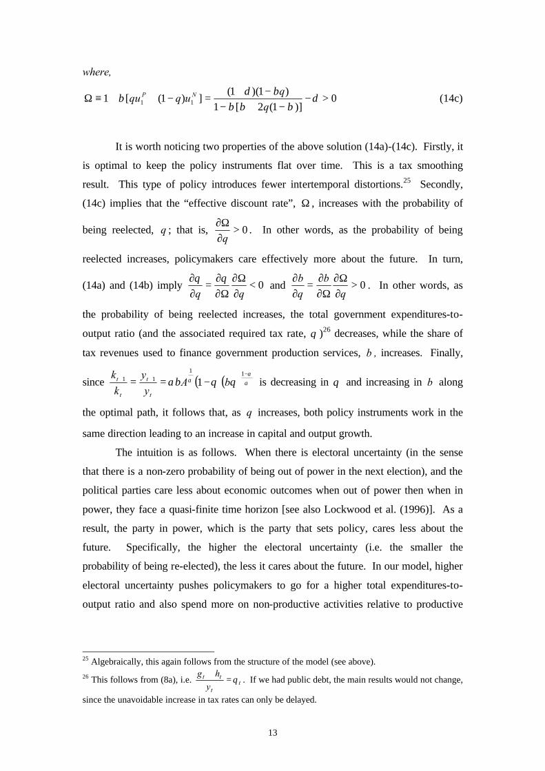
where,

0)]1(2[1

)1)(1(])1([1 11 >−

−+−−+

=−++≡Ω δβββ

βδβ

qq

uqqu NP (14c)

It is worth noticing two properties of the above solution (14a)-(14c). Firstly, it

is optimal to keep the policy instruments flat over time. This is a tax smoothing

result. This type of policy introduces fewer intertemporal distortions.25 Secondly,

(14c) implies that the “effective discount rate”, Ω , increases with the probability of

being reelected, q ; that is, 0>∂Ω∂q

. In other words, as the probability of being

reelected increases, policymakers care effectively more about the future. In turn,

(14a) and (14b) imply 0<∂Ω∂

Ω∂∂

=∂∂

qqθθ

and 0>∂Ω∂

Ω∂∂

=∂∂

qb

qb

. In other words, as

the probability of being reelected increases, the total government expenditures-to-

output ratio (and the associated required tax rate, θ )26 decreases, while the share of

tax revenues used to finance government production services, b , increases. Finally,

since ( )( ) αα

α θθαβ−

++ −==11

11 1 bAy

y

k

k

t

t

t

t is decreasing in θ and increasing in b along

the optimal path, it follows that, as q increases, both policy instruments work in the

same direction leading to an increase in capital and output growth.

The intuition is as follows. When there is electoral uncertainty (in the sense

that there is a non-zero probability of being out of power in the next election), and the

political parties care less about economic outcomes when out of power then when in

power, they face a quasi-finite time horizon [see also Lockwood et al. (1996)]. As a

result, the party in power, which is the party that sets policy, cares less about the

future. Specifically, the higher the electoral uncertainty (i.e. the smaller the

probability of being re-elected), the less it cares about the future. In our model, higher

electoral uncertainty pushes policymakers to go for a higher total expenditures-to-

output ratio and also spend more on non-productive activities relative to productive

25 Algebraically, this again follows from the structure of the model (see above).

26 This follows from (8a), i.e. tt

tt

y

hgθ=

+. If we had public debt, the main results would not change,

since the unavoidable increase in tax rates can only be delayed.

14

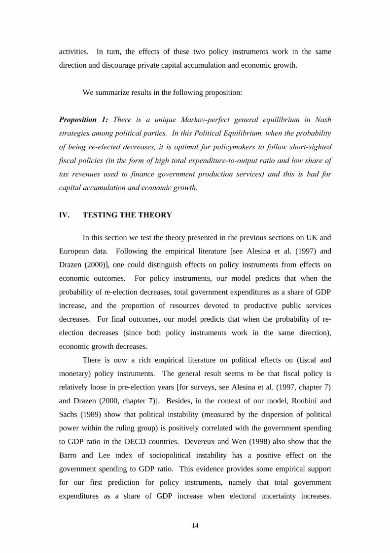
activities. In turn, the effects of these two policy instruments work in the same

direction and discourage private capital accumulation and economic growth.

We summarize results in the following proposition:

Proposition 1: There is a unique Markov-perfect general equilibrium in Nash

strategies among political parties. In this Political Equilibrium, when the probability

of being re-elected decreases, it is optimal for policymakers to follow short-sighted

fiscal policies (in the form of high total expenditure-to-output ratio and low share of

tax revenues used to finance government production services) and this is bad for

capital accumulation and economic growth.

IV. TESTING THE THEORY

In this section we test the theory presented in the previous sections on UK and

European data. Following the empirical literature [see Alesina et al. (1997) and

Drazen (2000)], one could distinguish effects on policy instruments from effects on

economic outcomes. For policy instruments, our model predicts that when the

probability of re-election decreases, total government expenditures as a share of GDP

increase, and the proportion of resources devoted to productive public services

decreases. For final outcomes, our model predicts that when the probability of re-

election decreases (since both policy instruments work in the same direction),

economic growth decreases.

There is now a rich empirical literature on political effects on (fiscal and

monetary) policy instruments. The general result seems to be that fiscal policy is

relatively loose in pre-election years [for surveys, see Alesina et al. (1997, chapter 7)

and Drazen (2000, chapter 7)]. Besides, in the context of our model, Roubini and

Sachs (1989) show that political instability (measured by the dispersion of political

power within the ruling group) is positively correlated with the government spending

to GDP ratio in the OECD countries. Devereux and Wen (1998) also show that the

Barro and Lee index of sociopolitical instability has a positive effect on the

government spending to GDP ratio. This evidence provides some empirical support

for our first prediction for policy instruments, namely that total government

expenditures as a share of GDP increase when electoral uncertainty increases.

15

However, our second prediction for policy instruments, namely that the proportion of

resources devoted to productive public services decreases when electoral uncertainty

increases, is more difficult to test.

In particular, were we able to distinguish and measure productive and

unproductive government expenditures directly, we could try to explain their ratio in

terms of electoral uncertainty. Unfortunately, although there is an important literature

on the role of public investment and infrastructure capital (discussed briefly in

Appendix C), it is very difficult to identify these two categories. Even investment in

infrastructure is not necessarily productive; we would need to know the rate of return

at the margin in order to assess this. And much of current “unproductive” expenditure

is certainly productive (and even has the characteristics of investment in many cases).

Examples include expenditure on education, or expenditure on social security

programs [see e.g. Atkinson (1999)]. Given these problems (discussed in more detail

in Appendix C), we are forced to look for evidence in outcomes, and in particular in

economic growth.27 In other words, we adopt a reduced-form approach.

Before we move on, it is worth noting that Drazen (2000) follows a similar

approach, when he studies the effect of income inequality on growth. In particular, he

also decomposes the reduced-form effect into two effects (see pp. 517-8): the effect of

inequality on redistributive policies (he calls it “political mechanism”) and, in turn,

the effect of policies on economic growth (he calls it “economic mechanism”). He

reports that empirical support for the two mechanisms is weak. He therefore focuses

on reduced-form effects from sociopolitical instability on growth, which are

significant. He also reports a positive relation between income inequality and

sociopolitical instability.

Therefore, we look for effects on outcomes. The prediction is that GDP

growth decreases as the probability of re-election declines.28 Our first task is to

measure the re-election probability. The obvious mechanism is to use opinion poll

27 Despite our reservations, we did experiment with the idea that popularity affects the composition of government spending (broken down into transfers, current expenditure and capital formation) in the UK. We found no evidence of any effects. For example, a regression in ECM form of the log ratio of transfers and current spending to public investment yields an ECM coefficient of -0.023 with t-ratio –0.16. 28 There is already a big empirical literature on the effects of political variables on economic outcomes [for a survey, see Alesina et al. (1997, chapter 6)]. Although the argument is not concluded, it seems that there is little evidence of an electoral cycle in growth or unemployment. However, here we test for the effects of re-election probabilities on growth, not for electoral effects.

16

evidence of government popularity.29 Although such series are not available for all

countries on a consistent basis for long periods, there are data for the UK. The UK

has another useful characteristic; namely, the simple majority electoral system

encourages the existence of large parties, so that power in the UK has alternated

between Conservative and Labour administrations over the post-war period. This

means that the government lead over the opposition is a simple and unambiguous

indication of future electoral success.30 Note that the only other bi-party system

where good data exists is the US. As we said above, Alesina et al. (1997, chapter 5)

have modeled re-election probabilities explicitly by looking at US presidential

elections.31 However, here the question relates to presidential ratings. There is no

opposition as such for most of the President’s term, so the “lead” is not well defined.

Moreover, the US system has profound checks and balances, including mid-term

elections to the House of Representatives and the Senate. There is clear evidence [see

Alesina and Rosenthal (1995)] that US voters use mid-term elections to balance the

ticket. In the UK, there is some evidence that voters use by-elections to achieve the

same effect [see Price and Sanders (1998)]. They may use local and European

elections in the same way, but the centralised structure of the UK government means

that one can disregard these influences.

For other countries, this kind of data is not only unavailable, but is also

inappropriate, as electoral systems typically do not have only two parties alternating

in government. However, an alternative measure of ex-post stability exists. This is

the duration of a government in parliamentary democracies. Woldendorp, Keman and

29 See Nannestad and Paldam (1994) for a survey of the international literature which seeks to explain this and related variables. 30 There are some issues to consider. Opinion poll data is based on the reply to the question: “If there were an election tomorrow, for which party would you vote?”. There is evidence that sampling and other methods have introduced bias at some points. Moreover, the question refers to the present, rather than to the future election date. However, popularity is very close to a random walk [see Chrystal and Peel (1986)], so the figure today is a good estimate of future popularity. 31 Alesina et al. assume poll results are distributed normally and follow a random walk with drift. Under these assumptions, the probability of electoral victory can be calculated by using a simple formula from option pricing theory. The problem is particularly simple in their case, as there are simply two presidential candidates, either of whom requires a simple majority, and the election date is known. In principle, what matters is the probability that at the time of the future election, the vote share exceeds 50% (although in the light of the 2000 election, it is clear there is still a margin of uncertainty from the electoral college and mismeasured votes). If the vote share is 51% ten minutes before the election, then (ignoring sampling error) the probability of victory is close to one. Thus, the closer is the election, the closer is the probability to one or zero. At points distant from an election, then (disregarding any drift) the probability tends to a half. For parliamentary democracies the problem is more complex, because the election victory depends on seats won. In the case of countries like the UK, the problem is complicated further by the endogeneity of election dates.

17

Budge (1993) provide data on precisely this for 20 countries in the post-war period.

We will therefore use this for cross-sectional tests of our hypothesis.

Time series results for the UK

Our first test examines the relationship between UK growth and a

transformation of the government lead over the opposition. Our regressions are

reduced forms where all factors, apart from government popularity and some cyclical

effects, are captured in the dynamics. We adopt two approaches of filtering GDP:

firstly, working in growth rates; and secondly, with a Hodrick Prescott filter.

Following the literature [see Drazen (2000)], we begin with a general

regression of the form:

∑ ∑ ∑ −−− +++=4

1

4

1

4

1itiitiitit gdzcxbax (15)

where x is GDP growth, z is the deviation of GDP from the Hodrick-Prescott filtered

trend and g is a logit transformation of popularity.32 If p denotes the government’s

share of support (where the denominator is Labour plus Conservative support; i.e. we

ignore third parties, which is a reasonable assumption in the UK), then the link

between g and p is given by:

−

=t

tt p

pg

1ln (16)

The logit is the standard “log-odds” transform used in popularity studies and many

other applications. Derived from an underlying logistic distribution of voter

preferences, it implies that the effect of a rise in support is greatest at the 50% support

level. By contrast, at very low or very high levels of popularity, an extra vote makes

very little difference to the outcome.33

There is clearly an issue of causality. High growth may itself lead to a higher

lead. To address this, the lead is lagged in this regression. It is also relevant that,

32 z is included to capture cyclical effects not modelled in the dynamics. 33 We tried three other alternative transforms but as the results were essentially the same, we only report those for the logit.

18

although there is clear evidence that popularity is related to several economic factors,

there is some evidence that for the UK growth is not one of these [see Price and

Sanders (1994)].

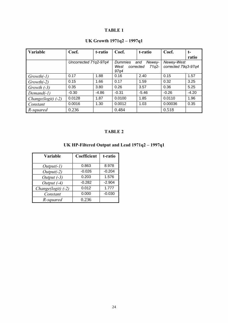
Table 1 below reports the results of estimating this relationship, excluding

insignificant lags on popularity. The results are precisely what we expect. Growth in

popularity leads to a positive coefficient significant at 5% level on a one-sided test.

There is no evidence for serial correlation: the F version of the LM test for 8th order

autocorrelation has a p value of 0.21. Moreover, the equation is stable. A Chow test

with a breakpoint at 1979q4 has a p value of 0.34, and 0.61 at 1989q4. On the other

hand, there are outliers in 1973q1 and 1979q2, easily explicable in terms of British

economic history.34 Dummying those out introduces serial correlation that cannot be

removed with a more complex lag structure. The table reports the results after the

Newey West correction has been applied. The conclusions are unchanged. The final

results presented show the results from 1979q3 on, a watershed in UK politics. The

results are once again very much the same. It is remarkable that this very simple

model produces results, which show that a rise in the probability of being re-elected

raises growth in the UK.

Table 1 here

An alternative method is to look at innovations to GDP and the lead defined in

terms of deviations from the HP filter. The results are similar to the growth

regressions, and are reported in Table 2 below. Once again, the base equation has no

autocorrelation (p value 0.28) and is stable (with breakpoint 1979:4, p value 0.47;

1989q4, 0.72).

Table 2 here

34 Specifically, the year 1973 marked the Barber “dash for growth”, associated with extremely expansionary policies leading to a record growth of GDP. The year 1979 marked the transition to Mrs Thatcher’s new monetarist policy.

19

Cross-sectional results for a small panel

We now turn to the cross-sectional evidence. We have data for 20 countries

between 1970 and 1990.35 Annual macroeconomic data exist, but it would not be

sensible to use the government duration figures at this frequency, so we work with

decennial figures. This provides a panel of 60 observations. Again, we work with

growth rates as the dependent variable. We regress itx on government duration, using

a fixed effect model. We account for heteroscedasticity with GLS. As we are

working in decennial averages, we do not model dynamics. In estimation, we allow

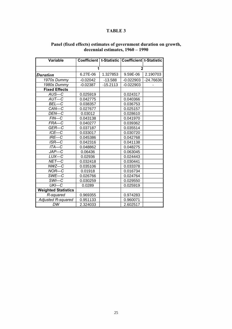
for a slow-down in productivity growth after 1970. The results are reported in Table

3 below. Column 1 shows that there is insignificant evidence for a positive effect of

government duration on growth. The coefficients on the decennial trend growth

coefficients are very close, and when we impose identical coefficients36 (column 2)

duration becomes significant. So we can again identify a positive link between

growth and government duration, in line with the theoretical predictions of the model.

Table 3 here

However, inference is not entirely straightforward, as there is a problem of

simultaneity; governments that successfully achieve high growth may last longer.

Unlike in the time series, we cannot lag duration, which may well be caused by

growth. Instrumental variable estimation is the obvious solution, but it is hard to

think of valid instruments (that are highly correlated with government duration but are

not caused by, or cause, growth). Thus, our results are supportive of the model but

cannot confirm it.

V. CONCLUSIONS AND EXTENSIONS

In this paper, we developed a political economy general equilibrium model

that looked at the impact of electoral uncertainty on fiscal policies, and consequently

economic growth. Our main theoretical prediction is that low re-election probabilities

induce incumbent policymakers to follow shortsighted policies (here, in the form of

35 Australia, Austria, Belgium, Canada, Denmark, Finland, France, Germany, Iceland, Ireland, Israel, Italy, Japan, Luxembourg, the Netherlands, New Zealand, Norway, Sweden, Switzerland and the UK. 36 The formal test of equality is F(1,48)=3.85 which is just insignificant at 5%: p=.0542.

20

too large public sectors and too high non-productive activities), and this is bad for

capital accumulation and output growth. We also found empirical evidence that low

re-election probabilities are associated with low GDP growth.

There are two possible extensions. First, the mechanism that drove our results

was the effective discount rate. That is, electoral uncertainty pushes the political

parties to effectively care relatively little about the future. Other mechanisms can be

influential lobbies, special interest groups, bureaucracy, etc [see e.g. Alesina (1999)

and Drazen (2000, chapter 14)]. It would therefore be interesting to add more

political distortions of this type, and then try to identify which one is responsible for

shortsighted economic policies. Second, because of lack of meaningful data on

economic policy instruments, and their exact role, we were forced to look for

reduced-form evidence on economic outcomes. However, the task still remains to go

back to effects on policy instruments, and try to check how political distortions affect

the allocation between productive policies with medium- and long-term benefits (e.g.

public education, training, etc) and non-productive policies with only short-term

benefits (e.g. transfers, subsidies, unemployment benefits, etc).

21

APPENDICES

Appendix A: Proof of Result 1

Inspection of the log-linear objective function [see equation (1b)] and the

Cobb-Douglas constraint [see equation (9)], and given that economic policy is

Markov, implies that the conjecture:

( ) ttttttt buuukuubkV logloglog, ; 43210 ++++= θθθ

where 43210 ,,,, uuuuu are undetermined coefficients, can be a solution of the dynamic

programming problem in (3).

Using this conjecture, the optimality conditions (4a) and (4b), together with

(7a)-(7b), give (11b) in the text. In turn, (11b) and (2) give (11a). Then, plugging

(11a) and (11b) back into (3), using the above conjecture, and equating coefficients on

both sides of the Bellman equation, we can solve for 43210 ,,,, uuuuu . For instance,

we get 01

11 >

−=

βu . Note that the above conjecture for the value function can solve

the dynamic programming problem because fiscal policies are assumed to be Markov

(as indeed is the case when we solve the policymakers’ optimization problem in

Appendix B below). That is, the values of 4320 ,,, uuuu cannot be fully determined

before we also solve for optimal policy. This is as it should be, since this is a general

equilibrium model in which policy instruments are chosen endogenously [see also

Economides and Philippopoulos (1999) and Kollintzas et al. (2000)]. By contrast,

when policy is exogenous, we only need to assume a statistical process that drives

policy instruments over time [see e.g. Sargent (1987, chapters 1 and 3)].

Appendix B: Proof of Result 2

(13a) and (13b) directly imply (14a) and (14b) respectively. So, the problem

is to solve for ])1([1 11NP uqqu −++≡Ω β . Inspection of the first-order conditions (13a)

and (13b) reveals that, if the conjectures tPP

tP kuukV log)( 10 += and t

NNt

N kuukV log)( 10 +=

can solve the dynamic programming problem (12a)-(12b), then tθ and tb have to be

constant along the optimal path. Plugging (13a) and (13b) into (12a)-(12b) and

equating coefficients, we get the Riccati equations, ])1([1 111NPP uqquu −+++= βδ and

22

])1([ 111PNN uqquu −+= β , which are solved for Pu1 and Nu1 . Thus, 0

)]1(2[1)1)(1(

1 >−+−

−+=

ββββδ

qq

uP

and 0)]1(2[1

)1)(1(1 >

−+−−+

=βββ

δβq

quN . In turn, δ

ββββδ

δβ −−+−

−+=−=−++≡Ω

)]1(2[1)1)(1(

])1([1 111 qq

uuqqu PNP . This

also completes the solution for the CDE in Appendix A above.

Appendix C: Productive vs. non-productive government expenditures

There is a rich literature that examines the composition of government

expenditure and the effect on economic growth.37 Most of this draws a simple

distinction between government consumption and infrastructure investment, assuming

that the latter is productive. Easterly and Rebello (1993) follow the approach

pioneered by Barro, and run regressions explaining the rate of growth for around 100

countries, with government spending as an explanatory variable. They break down

expenditures into different categories. Infrastructure investment, and especially

transport and communication, are correlated with growth. Naturally, this can not

immediately be used to infer anything about causality. However, the problem with

their results is arguably not that there are no effects, but that the coefficient is

implausibly large, a recurrent theme in the literature. In a carefully executed paper,

Devarajan, Swaroop and Zou (1996) look at 43 developing countries and find that an

increase in current expenditure has a positive effect on growth, but public investment

has a negative one.38 This supports our view that a simple identification of

“investment” and “productive” is inappropriate.39

Other evidence is from the many attempts to estimate production structures,

usually for a single country. In an influential but controversial paper, Aschauer

(1989b) estimated a production function for the US private business sector. He

reports that “a ‘core’ infrastructure of streets, highways, airports, mass transit sewers,

water systems, etc, has most explanatory power for productivity”. Aschauer (1989c)

produced similar results for G7 countries. In a related paper for the US, Aschauer

(1989a) looks at the relation between public and private investment. On the other

hand, Holtz-Eakin (1994) finds that there are no public sector capital productivity

effects using US state level panel data. He argues that, once state effects are

37 A recent survey of the empirical growth literature is in Temple (1999). 38 This is not necessarily to imply all public capital is unproductive; these are marginal changes. 39 For some related discussion see Balassone and Franco (2000).

23

accounted for, there is essentially no relationship. Many of these studies suffer from a

failure to allow for non-stationarity. Other authors estimate cost functions, which is a

more satisfactory approach, embodying more economic theory. Examples include

Lynde and Richmond (1992, 1993a, 1993b) and Nadiri and Mamuneas (1996).

Recently, Demetriades and Mamuneas [2000] have studied the effects of public

capital in 12 OECD economies by estimating a system of equations derived from an

intertemporal profit maximisation framework; they find positive effects (see also their

paper for a good survey of the literature). Some of the estimates in these papers seem

to be implausibly large. This is especially true when one does not take full account of

the financing constraints associated with the government budget constraint.

We therefore believe that the general consensus is that the effect of

government investment on growth is far from being well measured and understood.

As we argued in the main text, it is not clear which components of expenditures can

be treated as productive or unproductive. Given these problems, we side-step the

composition issue, and look for effects on economic outcomes.

24

TABLE 1

UK Growth 1971q2 – 1997q1

Variable Coef. t-ratio Coef. t-ratio Coef. t-ratio

Uncorrected 71q2-97q4 Dummies and Newey-West corrected 71q2-97q4

Newey-West corrected 79q3-97q4

Growth(-1) 0.17 1.88 0.16 2.40 0.15 1.57

Growth(-2) 0.15 1.66 0.17 1.59 0.32 3.25

Growth (-3) 0.35 3.80 0.26 3.57 0.36 5.25

Demand(-1) -0.30 -4.86 -0.31 -5.46 -0.26 -4.20

Change(logit) (-2) 0.0128 1.87 0.0100 1.85 0.0110 1.96

Constant 0.0016 1.30 0.0012 1.03 0.00036 0.35

R-squared 0.236 0.484 0.518

TABLE 2

UK HP-Filtered Output and Lead 1971q2 – 1997q1

Variable Coefficient t-ratio

Output(-1) 0.863 8.978

Output(-2) -0.026 -0.204

Output (-3) 0.203 1.576

Output (-4) -0.282 -2.904

Change(logit) (-2) 0.012 1.777

Constant 0.000 -0.030

R-squared 0.236

25

TABLE 3

Panel (fixed effects) estimates of government duration on growth,

decennial estimates, 1960 – 1990

Variable Coefficient t-Statistic Coefficient t-Statistic

1 2

Duration 6.27E-06 1.327853 9.59E-06 2.190703

1970s Dummy -0.02042 -13.588 -0.022903 -24.76636 1980s Dummy -0.02387 -15.2113 -0.022903 - Fixed Effects

AUS—C 0.025919 0.024317 AUT—C 0.042775 0.040366 BEL—C 0.038357 0.036753 CAN—C 0.027677 0.025157 DEN—C 0.03012 0.028610 FIN—C 0.043138 0.041970 FRA—C 0.040277 0.039362 GER—C 0.037187 0.035514 ICE—C 0.033017 0.030720 IRE—C 0.045386 0.042768 ISR—C 0.042316 0.041138 ITA—C 0.048862 0.048275 JAP—C 0.06436 0.063045 LUX—C 0.02936 0.024443 NET—C 0.032418 0.030441 NWZ—C 0.035106 0.033378 NOR—C 0.01918 0.016734 SWE—C 0.026766 0.024764 SWI—C 0.030259 0.029550 UKI—C 0.0289 0.025919

Weighted Statistics R-squared 0.969355 0.974283

Adjusted R-squared 0.951133 0.960071 DW 2.324033 2.602517

26

REFERENCES

Alesina A. (1999): Too large and too small governments, in Economic Policy and Equity, edited by V. Tanzi, K. Chu and S. Gupta. International Monetary Fund. Alesina A. and R. Perotti (1996): Income distribution, political instability and investment, European Economic Review, 40, 1203-1228. Alesina A. and D. Rodrik (1994): Distributive politics and economic growth, Quarterly Journal of Economics, 109, 465-490. Alesina A. and H. Rosenthal (1995): Partisan Politics, Divided Government and the Economy. Cambridge University Press, Cambridge. Alesina A., N. Roubini and G. Cohen (1997): Political Cycles and the Macroeconomy. The MIT Press. Alesina A. and G. Tabellini (1990): A positive theory of fiscal deficits and government debt, Review of Economic Studies, 57, 403-414. Alogoskoufis G., B. Lockwood and A. Philippopoulos (1992): Wage inflation, electoral uncertainty and the exchange rate regime: theory and UK evidence, Economic Journal, 102, 1370-1394. Aschauer D. A. (1989a): Does public capital crowd out private capital?, Journal of Monetary Economics, 24, 171-188. Aschauer D. A. (1989b): Is public expenditure productive?, Journal of Monetary Economics, 23, 177-200. Aschauer D. A. (1989c): Public investment and productivity growth in the group of seven, FRB Chicago - Economic Perspectives, 13, 7-25. Atkinson A. (1999): The Economic Consequences of Rolling Back the Welfare State. The MIT Press and CES. Balassone F. and D. Franco (2000): Public investment, the stability pact and the “Golden Rule”, Fiscal Studies, 21, 207-229. Barro R. (1990): Government spending in a simple model of endogenous growth, Journal of Political Economy, 98, S103-S125. Barro R. (1991): Economic growth in a cross-section of countries, Quarterly Journal of Economics, 106, 407-443. Barro R. (1996): Democracy and growth, Journal of Economic Growth, 1, 1-27. Barro R. and X. Sala-i-Martin (1995): Economic Growth. McGraw Hill, New York.

27

Brunetti A. (1998): Policy volatility and economic growth: a comparative empirical analysis, European Journal of Political Economy, 14, 35-52. Calvo G. and A. Drazen (1997): Uncertain duration of reform: dynamic implications, NBER, Working Paper, no. 5925. Chen B. and Y. Feng (1996): Some political determinants of economic growth: theory and empirical implications, European Journal of Political Economy, 12, 609-627. Chrystal A. and D. Peel (1986): What can economics learn from political science, and vice versa?, American Economic Review, 76, 62-65. Darby J., C. Li and A. Muscatelli (1998): Political uncertainty, public expenditure and growth, University of Glasgow, Discussion Paper, no. 9822. Demetriades P. and T. Mamuneas (2000): Intertemporal output and employment effects of public infrastructure capital: evidence from 12 OECD economies, Economic Journal, 110, 687-712. Devarajan S., V. Swaroop and H. Zou (1996): The composition of public expenditure and economic growth, Journal of Monetary Economics, 37, 313-344. Devereux M. and J-F. Wen (1998): Political instability, capital taxation and growth, European Economic Review, 42, 1635-1651. Drazen A. (2000): Political Economy in Macroeconomics. Princeton University Press, Princeton.

Easterly W. and S. Rebelo (1993): Fiscal policy and economic growth: an empirical investigation, Journal of Monetary Economics, 32, 417-458.

Economides G. and A. Philippopoulos (1999): Elections, fiscal policy and growth, Athens University of Economics and Business, Discussion Paper, no. 99-05, Athens.

Gupta D. (1990): The Economics of Political Violence. Praeger, New York. Hibbs D. (1973): Mass Political Violence: A Cross-Sectional Analysis. Wiley, New York. Holtz-Eakin D. (1994): Public-sector capital and the productivity puzzle, Review of Economics and Statistics, 76, 2-21. Kneller R., M. Bleaney and N. Gemmell (1999): Fiscal policy and growth: evidence from OECD countries, Journal of Public Economics, 74, 171-190. Kollintzas T., A. Philippopoulos and V. Vassilatos (2000): Is tax policy coordination necessary?, Center for Economic Policy Research, Discussion Paper, no. 2348. Laver M. and B. Hunt (1992): Policy and Party Competition. Routledge, London.

28

Levine, R. and S. Zervos (1996): Stock market development and long-run growth, The World Bank Economic Review, 10, 323-339. Lockwood B., A. Philippopoulos and A. Snell (1996): Fiscal policy, public debt stabilization and politics: theory and UK evidence, Economic Journal, 106, 894-911. Lynde C. and J. Richmond (1992): The role of public capital in production, Review of Economics and Statistics, 74, 37-44. Lynde C. and J. Richmond (1993a): Public capital and long-run costs in U.K. manufacturing, Economic Journal, 103, 880-893. Lynde C. and J. Richmond (1993b): Public capital and total factor productivity, International Economic Review, 34, 401-44. Nadiri M. and I. Mamuneas (1996): Contribution of highway capital to industry and national productivity growth, prepared for Apogee Research Inc. for the Federal Highway Administration. Nannestad P. and M. Paldam (1994): The VP-function: a survey of the literature on vote and popularity functions after 25 years, Public Choice, 79, 213-245. Park H. and A. Philippopoulos (2000): On the dynamics of growth and fiscal policy with redistributive transfers, forthcoming in Journal of Public Economics. Persson T. and L. Svensson (1989): Why a stubborn conservative would run a deficit: policy with time-inconsistent preferences, Quarterly Journal of Economics, 104, 325-345. Persson T. and G. Tabellini, editors, (1994): Monetary and Fiscal Policy, vol. 2. The MIT Press, Cambridge, Mass. Persson T. and G. Tabellini (1999): Political economics and macroeconomic policy, in Handbook of Macroeconomics, vol. 1C, edited by J. Taylor and M. Woodford. North-Holland, Amsterdam. Price S. and D. Sanders (1994): Economic competence, rational expectations and government popularity in post-war Britain, Manchester School, 62, 296-312. Price S. and D. Sanders (1998): By-elections, changing fortunes, uncertainty and the mid-term blues, Public Choice, 95, 131-148. Rogoff K. and A. Sibert (1988): Elections and macroeconomic policy cycles, Review of Economic Studies, LV, 1-16. Roubini N. and J. Sachs (1989): Fiscal Policy, Economic Policy, 8, 99-132. Sargent T. (1987): Dynamic Macroeconomic Theory. Harvard University Press, Cambridge, Mass.

29

Stokey N. and R. Lucas (1989): Recursive Methods in Economic Dynamics. Harvard University Press, Cambridge, Mass. Svensson J. (1993): Investment, property rights and political instability: theory and evidence, European Economic Review, 43, 1317-1341. Tabelini G. and A. Alesina (1990): Voting on the budget deficit, American Economic Review, 80, 37-49. Temple J. (1999): The new growth evidence, Journal of Economic Literature, 37, 112-156. Woldendorp J., H. Keman and I. Budge (1993): Political data 1945-1990: party government in 20 democracies, European Journal of Political Research, 24, 1-120.