Embed Size (px)
Citation preview
ELECTRIC CONDUCTIVITY FOR LABORATORY AND FIELD
MONITORING OF INDUCED PARTIAL SATURATION
(IPS) IN SANDS
A dissertation presented
by
Hadi Kazemiroodsari
to
Department of Civil and Environmental Engineering
in partial fulfillment of the requirements
for the degree of
Doctor of Philosophy
in the field of
Civil Engineering
Northeastern University
Boston, Massachusetts
March, 2016
ELECTRIC CONDUCTIVITY PROBE FOR LABORATORY
AND FIELD MONITORING OF INDUCED PARTIAL
SATURATION (IPS) IN SANDS
A dissertation presented
by
Hadi Kazemiroodsari
to
Department of Civil and Environmental Engineering
in partial fulfillment of the requirements
for the degree of
Doctor of Philosophy
in the field of
Civil Engineering
Northeastern University
Boston, Massachusetts
March, 2016
ii
ABSTRACT
Liquefaction is loss of shear strength in fully saturated loose sands caused by build-
up of excess pore water pressure, during moderate to large earthquakes, leading to
catastrophic failures of structures. Currently used liquefaction mitigation measures are
often costly and cannot be applied at sites with existing structures. An innovative,
practical, and cost effective liquefaction mitigation technique titled “Induced Partial
Saturation” (IPS) was developed by researchers at Northeastern University. The IPS
technique is based on injection of sodium percarbonate solution into fully saturated
liquefaction susceptible sand. Sodium percarbonate dissolves in water and breaks down
into sodium and carbonate ions and hydrogen peroxide which generates oxygen gas
bubbles. Oxygen gas bubbles become trapped in sand pores and therefore decrease the
degree of saturation of the sand, increase the compressibility of the soil, thus reduce its
potential for liquefaction.
The implementation of IPS required the development and validation of a
monitoring and evaluation technique that would help ensure that the sands are indeed
partially saturated. This dissertation focuses on this aspect of the IPS research. The
monitoring system developed was based on using electric conductivity fundamentals and
probes to detect the transport of chemical solution, calculate degree of saturation of sand,
and determine the final zone of partial saturation created by IPS. To understand the
fundamentals of electric conductivity, laboratory bench-top tests were conducted using
electric conductivity probes and small specimens of Ottawa sand. Bench-top tests were
used to study rate of generation of gas bubbles due to reaction of sodium percarbonate
solution in sand, and to confirm a theory based on which degree of saturation were
calculated. In addition to bench-top tests, electric conductivity probes were used in a
relatively large sand specimen prepared in a specially manufactured glass tank. IPS was
implemented in the prepared specimen to validate the numerical simulation model and
explore the use of conductivity probes to detect the transport of chemical solution, estimate
iii
degree of saturation achieved due to injection of chemical solution, and evaluate final zone
of partial saturation. The conductivity probe and the simulation results agreed well.
To study the effect of IPS on liquefaction response of the sand specimen, IPS was
implemented in a large (2-story high) sand specimen prepared in the laminar box of
NEES@Buffalo and then the specimen was subjected to harmonic shaking. Electric
conductivity probes were used in the specimen treatment by controlling the duration and
spacing of injection of the chemical solution, in monitoring the transport of chemical
solution, in the estimation of zone of partial saturation achieved, and in the estimation of
degree of saturation achieved due to implementation of IPS. The conductivity probes
indicated partial saturation of the specimen. The shaking tests results confirmed the partial
saturation state of the sand specimen.
In addition, to the laboratory works, electric conductivity probes were used in field
implementation of IPS in a pilot test at the Wildlife Liquefaction Array (WLA) of
NEES@UCSB site. The conductivity probes in the field test helped decide the optimum
injection pressure, the injection tube spacing, and the degree of saturation that could be
achieved in the field.
The various laboratory and field tests confirmed that electric conductivity and the
probes devised and used can be invaluable in the implementation of IPS, by providing
information regarding transport of the chemical solution, the spacing of injection tubes,
duration of injection, and the zone and degree of partial saturation caused by IPS.

iv
ACKNOWLEDGEMENTS
I would like to express my sincere gratitude and appreciation to my academic advisor
Professor Mishac K. Yegian for his invaluable guidance, help, and support during my
graduate studies. I am thankful to him for giving me the opportunity to work on this
research and for helping me to improve my professional communication and presentation
skills. I always will use his great and valuable advices throughout my career.
I would also like to thank my academic co-advisor Professor Akram Alshawabkeh for
his invaluable support and care during my graduate studies. I appreciate Professor Thomas
Sheahan and Professor Philip Larese Casanova for serving on my dissertation committee.
In 2011, the National Science Foundation (NSF) through the program George E.
Brown, Jr. Network for Earthquake Engineering Simulation (NEES) funded a large
research project entitled “Induced Partial Saturation (IPS) through Transport and
Reactivity for Liquefaction Mitigation”. This research is part of the mentioned project. I
would like to express appreciation for the support of NSF program directors Dr. Richard
Fragaszy and DR. Joy M. Pauschke. I would like to express my appreciation to the project
collaborators Professor S. Thevanayagam, of the State University of New York at Buffalo,
Professor Kenneth H. Stokoe of the University of Texas at Austin, Dr. Jamison Steidl of
the University of California at Santa Barbara and Professor Leslie Youd, formerly of
Brigham Young University.
I would like to thank Michael McNeil and Kurt Braun for their help and support in
manufacturing tools and equipment used in the experiment portion of this research. I
appreciate their dedication for the success of this research.
I would like to thank my colleagues Ph.D. students Seda Gokyer and Fritz Nababan,
for their support and help in the project. Not only they were great colleagues but also they
were awesome and unforgettable friends for me. I would like to thank Master student Ata
Firat Karamanli for his help and support in this research. I am also grateful to NSF REU

v
funded undergraduate students; Olivia Deterling, Kelsey Dunn, Danielle Didomizio, and
Camila Simons for their help in this research.
I would like to dedicate this dissertation to my parents Mohsen Kazemiroodsari and
Maryam Vahabzade for their care and love in my life. I am grateful to them for their
priceless and true love and support during my graduate studies abroad. I want to thank
my elder brother Amir Kazemiroodsari for his great support and love and wish him a life
filled with joy and happiness.
vi
TABLE OF CONTENTS
ABSTRACT ii
ACKNOWLADGEMENTS .............................................................................................. iv
LIST OF FIGURES ........................................................................................................... ix
LIST OF TABLES ............................................................................................................ xv
Chapter 1 Introduction and Overview ............................................................................ 1
1.1 Introduction ........................................................................................... 1
1.2 Overview of this Dissertation ............................................................... 4
Chapter 2 Electric Conductivity and Probes.................................................................. 7
2.1 Introduction .......................................................................................................... 7
2.2 Electrical conductivity theory .............................................................................. 8
2.3 Application of electric conductivity concept in soil ............................................. 9
2.4 Application of electric conductivity in IPS ........................................................ 10
2.4.1 Detecting arrival and concentration of IPS chemical ................................. 10
2.4.2 Estimating degree of saturation and rate of generation of gas bubbles ...... 10
2.4.2.1 Archie’s law ......................................................................................... 11
2.5 Milwaukee electric conductivity probe and meter ............................................. 13
2.5.1 Accuracy check of SE502 probe and MW320 meter .................................. 14
2.5.2 Extending cable of Milwaukee electric conductivity probe ....................... 19
Chapter 3 Bench-Top Laboratory Tests Using Electric Conductivity Probe to Study
Rate of Gas Generation and Degree of Saturation in Sand ........................................ 21
3.1 Overview ................................................................................................................. 21
3.2 Verification of the procedure for calculating degree of saturation ......................... 21
3.3 Determine rate of gas generation ............................................................................ 28
3.4 Effect of void ratio on degree of saturation ............................................................. 34
3.5 Summary and Conclusion ....................................................................................... 37
Chapter 4 Use of Electric Conductivity Probes for Monitoring IPS in “Glass Tank”
Sand Specimens ............................................................................................................... 39
4.1 Overview ............................................................................................................ 39
4.2 Test set up and specimen preparation procedure ............................................... 40
4.3 Test Results ....................................................................................................... 43
4.3.1 Test 1 (1% concentration) ........................................................................... 44
vii
4.3.1.1 Transport of chemical solution during injection ....................................... 44
4.3.1.2 Degree of saturation .................................................................................. 50
4.3.2 Test 2 (0.5% concentration) ........................................................................ 57
4.3.2.1 Transport of chemical solution during injection ....................................... 57
4.3.2.2 Degree of saturation .................................................................................. 64
4.4 Summary and Conclusions ................................................................................. 71
Chapter 5 Use of Electric Conductivity Probes for Monitoring IPS in Large-Scale
Laminar Box Sand Specimens ....................................................................................... 73
5.1 Overview ................................................................................................................. 73
5.2 Introduction to the Laminar Box ............................................................................ 74
5.3 Preparation of fully saturated sand specimens ........................................................ 76
5.4 Preparation and injection of chemical solution ....................................................... 77
5.5 Typical electric conductivity test result from the laminar box ................................ 81
5.6 Electric conductivity results from laminar box Test 1 ............................................ 83
5.6.1 Specimen preparation: Test 1 ........................................................................... 83
5.6.2 IPS treatment: Test 1 ........................................................................................ 86
5.6.3 Electric conductivity results: Test 1 ................................................................. 89
5.6.3.1 Transport of solution: Test 1 ..................................................................... 90
5.6.3.2 Degree of saturation: Test 1 ...................................................................... 93
5.6.3.3 Effect of shaking on gas bubble escape: Test 1 ...................................... 107
5.7 Electric conductivity results from laminar box Test 2 ..................................... 110
5.7.1 Specimen preparation: Test 2 .................................................................... 110
5.7.2 IPS treatment: Test 2 ................................................................................. 112
5.7.3 Electric conductivity results: Test 2 .......................................................... 115
5.7.3.1 Transport of solution: Test 2 ................................................................... 116
5.7.3.2 Degree of saturation ................................................................................ 118
5.7.3.3 Effect of shaking on gas bubble escape: Test 2 ...................................... 144
5.8 Summery and conclusions ................................................................................ 146
Chapter 6 Use of Electric Conductivity Probes for Monitoring IPS in Pilot Field
Test at Wildlife Liquefaction Array (WLA) ............................................................... 149
6.1 Overview .......................................................................................................... 149
6.2 Introduction to Wildlife Liquefaction Array (WLA) ....................................... 150
6.3 Summary of findings from the first and second trips ....................................... 152
6.3.1 Site condition ............................................................................................ 153
viii
6.3.2 Injection/extraction tube installation methods .......................................... 154
6.3.3 River and ground water quality ................................................................. 155
6.4 Pilot Field IPS Test .......................................................................................... 167
6.4.1 Pilot test set-up .......................................................................................... 168
6.4.2 Installation of conductivity probes ............................................................ 169
6.4.3 Pilot test results ......................................................................................... 170
6.5 Summery and conclusions ................................................................................ 175
Chapter 7 Preliminary Laboratory Tests Using a Prototype Field Electric
Conductivity Probe to Estimate Degree of Saturation .............................................. 177
7.1 Overview .......................................................................................................... 177
7.2 Prototype field electric conductivity probe ...................................................... 178
7.2.1 Comparison of electric conductivities measured by Milwaukee and
FieldScout probes .................................................................................................... 179
7.2.2 Design details of prototype field electric conductivity probe ................... 180
7.3 Laboratory tests to evaluate the performance of the prototype field electric
conductivity probe ....................................................................................................... 182
7.4 Summery and conclusion ................................................................................. 186
Chapter 8 Summery and Conclusions.................................................................... 188
REFERENCES ………………………………………………………………………. . 194
LIST OF FIGURES
Figure 1-1 Overall process of IPS. Black ovals highlight the IPS monitoring system, which was the focus of this dissertation. ....................................................................................... 3 Figure 2-1 Principle of electic conductivity meter in soil ................................................... 9 Figure 2-2 Typical electeric conductivity plot showing arrival of the sodium per carbonate solution and generation effect of gas bubbles ................................................................... 12 Figure 2-3 a) Milwaukee electric conductivity meter and probe b) calibration solution .. 14 Figure 2-4 Orion 4 star-Thermo Scientific electric conductivity meter and probe........... 15 Figure 2-5 Bench top experiment set up to compare Milwaukee and Thermo Scientific electric conductivity meters and probes ............................................................................ 16 Figure 2-6 (a) Comparison of Milwaukee and Thermo Scientific electric conductivity readings, (b) Degree of saturation based on Archi’s law compared with based on volume calculations ....................................................................................................................... 16 Figure 2-7 Degree of saturation computed using volume calculations and phase relationships ...................................................................................................................... 18 Figure 2-8 SE520 Milwaukee probe with extended cable ................................................ 20 Figure 2-9 Comparison of SE 520 probe results with short- and long-cables .................. 20 Figure 3-1 Typical electric conductivity plot from bench-top test ................................... 22 Figure 3-2 Preparation of Sodium per carbonate solution using magnetic stirrer ............ 23 Figure 3-3 Grain size distribution of Ottawa sand (ASTM C778) ................................... 23 Figure 3-4 Prepared specimen of bench-top test............................................................... 23 Figure 3-5 Electric conductivity (on the left) and degree of saturation (on the right) for various concentrations of chemical solution. .................................................................... 25 Figure 3-6 Final degree of saturation for concentrations between 0.5% and 4% ............. 27 Figure 3-7 Schematic for exponential decomposition of solute resulting in gas bubble generation .......................................................................................................................... 28 Figure 3-8 Electric conductivity data and fitted lines based on Equation 3-4 for concentrations of: 0.5%, 1%, 1.2%, 1.5%, and 4% .......................................................... 31 Figure 3-9 Rate parameter versus concentration .............................................................. 32 Figure 3-10 Effect of concentration of chemical on the rate of reaction and gas generation: (a) normalized electric conductivity data, (b) normalized fitted lines using r values from Table 3-1 ........................................................................................................................... 34 Figure 3-11 Electric conductivity and degree of saturation for void ratios of: 0.55, 0.62, 0.69, and 0.78 .................................................................................................................... 36 Figure 3-12 Degree of saturation for different void ratios, and 1% concentration. .......... 37 Figure 4-1 Empty glass tank with injection tube and electric conductivity probes .......... 40 Figure 4-2 Electric conductivity probes in the glass tank specimen ................................. 41 Figure 4-3 Glass tank specimen preparation, Test 1 ......................................................... 42 Figure 4-4 a) Marriot bottle b) IPS experimental set up ................................................... 42
ix
Figure 4-5 A schematic drawing of the glass tank and the IPS injection components ..... 43 Figure 4-6 Electric conductivity results during 13 minutes of injection, Test1................ 45 Figure 4-7 Zone of influence predicted by SUTRA-Bubble, Test 1 ................................. 46 Figure 4-8 Rise in concentration as a result of advection-dispersion flow ....................... 47 Figure 4-9 Comparisons of normalized conductivity based on experimental data, or normalized concentration based on Model, Test 1. .......................................................... 50 Figure 4-10 Electric conductivity and degree of saturation at probe locations CP1 and CP2, for Test 1 ........................................................................................................................... 51 Figure 4-11 Electric conductivity and degree of saturation at probe locations CP3 and CP5, for Test 1 ........................................................................................................................... 52 Figure 4-12 Electric conductivity and degree of saturation at probe locations CP4 and CP8, fir Test 1 ............................................................................................................................ 53 Figure 4-13 Electric conductivity and degree of saturation at probe locations CP6 and CP7, for Test 1 ........................................................................................................................... 54 Figure 4-14 Electric conductivity and degree of saturation at probe location CP9, for Test 1......................................................................................................................................... 55 Figure 4-15 Final degree of saturation calculated at each probe location, Test 1 ............ 56 Figure 4-16 Electric conductivity results during 13 minutes of injection Test 2.............. 58 Figure 4-17 zone of influence predicted by SUTRA-Bubble Test 2 ................................ 60 Figure 4-18 Comparisons of normalized conductivity based on experimental data, or normalized concentration based on Model, Test 2. .......................................................... 62 Figure 4-19 Comparison of normalized conductivity based on experiment data, or normalized concentration based on Model for CP8 .......................................................... 63 Figure 4-20 Electric conductivity and degree of saturation at probe locations CP1 and CP2, for Test 2 ........................................................................................................................... 65 Figure 4-21 Electric conductivity and degree of saturation at probe locations CP3 and CP4, for Test 2 ........................................................................................................................... 66 Figure 4-22 Electric conductivity and degree of saturation at probe locations CP4 and CP8, for Test 2 ........................................................................................................................... 67 Figure 4-23 Electric conductivity and degree of saturation at probe locations CP6 and CP7, for Test 2 ........................................................................................................................... 68 Figure 4-24 Electric conductivity and degree of saturation at probe location CP9, for Test 2......................................................................................................................................... 69 Figure 4-25 Final degree of saturation calculated at each probe location, Test 2 ............ 70 Figure 5-1 Plan and elevation views of the laminar box .................................................. 75 Figure 5-2 a) the laminar box and b) instrumented laminates .......................................... 76 Figure 5-3 Chemical solution preparation and pumping system ...................................... 78 Figure 5-4 Brix probe to check concentration of chemical solution ................................. 78 Figure 5-5 Electric conductivity versus concentration of sodium per carbonate solution 79
x
Figure 5-6 Experiment set up for studying the reaction of sodium per carbonate in water........................................................................................................................................... 80 Figure 5-7 Rate of reaction of sodium percarbonate solution in clean water ................... 80 Figure 5-8 Typical electric conductivity plot with explanations of detected events. ....... 81 Figure 5-9 a) steel wire mesh with conductivity probes attached, b) Milwaukee conductivity probes with extended cables, and c) ten probe meters used in Test 1 ........ 83 Figure 5-10 PVC and steel meshes hanging from the steel truss above the laminar box, in Test 1 ................................................................................................................................. 84 Figure 5-11 Plan and elevation views of the laminar box showing locations of electric conductivity probes, in Test 1 ........................................................................................... 85 Figure 5-12 Photograph of injection tube IT2, IT4, and IT5 ............................................ 86 Figure 5-13 Locations of six injection tubes and the treated zone by the tubes, in Test 1 87 Figure 5-14 Locations of injection points used to treat the top 2m of the specimen, in Test 1......................................................................................................................................... 88 Figure 5-15 a) jetting of surface injection tube and b) injection of solution, for Test 1 ... 89 Figure 5-16 Electric conductivity plots from Test 1 ......................................................... 90 Figure 5-17 Distances between CP 6 and IT3 and CP9 and IT6, Test 1 .......................... 91 Figure 5-18 CP1 electric conductivity, probe location relative to injection tubes, and degree of saturation, Test 1........................................................................................................... 94 Figure 5-19 CP2 electric conductivity, probe location relative to injection tubes, and degree of saturation, Test 1........................................................................................................... 95 Figure 5-20 CP3 electric conductivity and degree of saturation, Test 1 ........................... 96 Figure 5-21 CP4 electric conductivity, probe location relative to injection tubes, and degree of saturation, Test 1........................................................................................................... 97 Figure 5-22 CP5 electric conductivity, probe location relative to injection tubes, and degree of saturation, Test 1........................................................................................................... 98 Figure 5-23 CP6 electric conductivity and degree of saturation, Test 1 ........................... 99 Figure 5-24 CP7 electric conductivity, probe location relative to injection tubes, and degree of saturation, Test 1......................................................................................................... 100 Figure 5-25 CP8 electric conductivity, probe location relative to injection tubes, and degree of saturation, Test 1......................................................................................................... 101 Figure 5-26 CP9 electric conductivity, probe location relative to injection tubes, and degree of saturation, Test 1......................................................................................................... 102 Figure 5-27 CP10 electric conductivity, probe location relative to injection tubes, and degree of saturation, Test 1 ............................................................................................. 103 Figure 5-28 Calculated degree of saturation including bubble escape, Test 1 ............... 105 Figure 5-29 Electric conductivity records showing data before and after shaking of sand specimen, Test 1.............................................................................................................. 107 Figure 5-30 Plan and elevation views of the laminar box showing locations of electric conductivity probes, in Test 2 ......................................................................................... 111
xi
Figure 5-31 Injection tube used to treat the sand specimen of Test 2............................. 112 Figure 5-32 IPS treatment zone during the first two days of injection ........................... 113 Figure 5-33 IPS treatment zone during the third day of injection .................................. 113 Figure 5-34 IPS treatment zone during the fourth day of injection ................................ 114 Figure 5-35 IPS treatment zone during the fifth day of injection ................................... 114 Figure 5-36 Locations of injection tube for bottom treatment (IT1 through IT13) and for surface treatment (IT14 through IT32), in Test 2 ........................................................... 115 Figure 5-37 Electric conductivity plots of CP1 through CP13 ....................................... 116 Figure 5-38 Electric conductivity plots of CP14 through CP21 ..................................... 117 Figure 5-39 CP1 electric conductivity, probe location relative to injection tubes, and degree of saturation, Test 2......................................................................................................... 119 Figure 5-40 CP2 electric conductivity, probe location relative to injection tubes, and degree of saturation, Test 2......................................................................................................... 120 Figure 5-41 CP3 electric conductivity, probe location relative to injection tubes, and degree of saturation, Test 2......................................................................................................... 121 Figure 5-42 CP4 electric conductivity, probe location relative to injection tubes, and degree of saturation, Test 2......................................................................................................... 122 Figure 5-43 CP5 electric conductivity, probe location relative to injection tubes, and degree of saturation, Test 2......................................................................................................... 123 Figure 5-44 CP6 electric conductivity, probe location relative to injection tubes, and degree of saturation, Test 2......................................................................................................... 124 Figure 5-45 CP7 electric conductivity, probe location relative to injection tubes, and degree of saturation, Test 2......................................................................................................... 125 Figure 5-46 CP8 electric conductivity, probe location relative to injection tubes, and degree of saturation, Test 2......................................................................................................... 126 Figure 5-47 CP9 electric conductivity, probe location relative to injection tubes, and degree of saturation, Test 2......................................................................................................... 127 Figure 5-48 CP10 electric conductivity, probe location relative to injection tubes, and degree of saturation, Test 2 ............................................................................................. 128 Figure 5-49 CP11 electric conductivity, probe location relative to injection tubes, and degree of saturation, Test 2 ............................................................................................. 129 Figure 5-50 CP12 electric conductivity, probe location relative to injection tubes, and degree of saturation, Test 2 ............................................................................................. 130 Figure 5-51 CP13 electric conductivity, probe location relative to injection tubes, and degree of saturation, Test 2 ............................................................................................. 131 Figure 5-52 CP14 electric conductivity, probe location relative to injection tubes, and degree of saturation, Test 2 ............................................................................................. 132 Figure 5-53 CP15 electric conductivity, probe location relative to injection tubes, and degree of saturation, Test 2 ............................................................................................. 133
xii
Figure 5-54 CP16 electric conductivity, probe location relative to injection tubes, and degree of saturation, Test 2 ............................................................................................. 134 Figure 5-55 CP17 electric conductivity, probe location relative to injection tubes, and degree of saturation, Test 2 ............................................................................................. 136 Figure 5-56 CP18 electric conductivity, probe location relative to injection tubes, and degree of saturation, Test 2 ............................................................................................. 137 Figure 5-57 CP19 electric conductivity, probe location relative to injection tubes, and degree of saturation, Test 2 ............................................................................................. 138 Figure 5-58 CP20 electric conductivity, probe location relative to injection tubes, and degree of saturation, Test 2 ............................................................................................. 139 Figure 5-59 CP21 electric conductivity, probe location relative to injection tubes, and degree of saturation, Test 2 ............................................................................................. 140 Figure 5-60 Escaping gas bubbles observed at the surface of the sand specimen of Test 2......................................................................................................................................... 141 Figure 5-61 Calculated degree of saturation including bubble escape, Test 2 ............... 143 Figure 5-62 Electric conductivity records of probes CP1 through CP13, before and after shaking of sand specimen, Test 2 ................................................................................... 144 Figure 5-63 Electric conductivity records of probes CP14 through CP21, before and after
shaking of sand specimen, Test 2………………………………………………………145
Figure 6-1 Locations of WLA, NEES@UCSB, USGS, and IPS field test sites ............. 151 Figure 6-2 Locations of IPS field test sites ..................................................................... 152 Figure 6-3 Idealized soil column showing the various soil layers at the IPS test site .... 153 Figure 6-4 Installation of Injection tube by a) jetting metal tube and b) driving and then washing inside the PVC tube .......................................................................................... 154 Figure 6-5 Sodium percarbonate solution in tap water and ground water and visual observation of generation of gas bubbles (2.2% concentration) ..................................... 158 Figure 6-6 WLA sand saturated in 2.5% concentration of the Sodium percarbonate solution with ground water from WLA ........................................................................................ 159 Figure 6-7 Electric conductivity in WLA sand in chemical solution prepared with WLA ground water ................................................................................................................... 159 Figure 6-8 Schematic drawing of sand with high and low tortuosity ............................. 160 Figure 6-9 Rate of reaction in WLA ground water and in clean regular water for 1% concentration ................................................................................................................... 161 Figure 6-10 Bench-top experiment with WLA sand and 1% concentration of sodium percarbonate solution with ground water from WLA ..................................................... 162 Figure 6-11 Comparison of electric conductivity and degree of saturation from specimens prepared with WLA sand and ground water and Ottawa sand and regular clean water. 162 Figure 6-12 Test setup for simulating the field test conducted to test ability of a pushed conductivity probe to detect the arrival of chemical solution ......................................... 164
xiii

Figure 6-13 Electric conductivity of solution collected from outflow ........................... 164 Figure 6-14 Electric conductivity measured inside the specimen, 7.5 cm from top of the specimen ......................................................................................................................... 165 Figure 6-15 location of pilot test relative to IPS full production site ............................. 167 Figure 6-16 Spacing and depths of the injection and extraction tubes and conductivity probes in the pilot test ..................................................................................................... 168 Figure 6-17 Photo and details of the pilot test set-up ..................................................... 169 Figure 6-18 Procedure for installation of conductivity probes at WLA site ................... 170 Figure 6-19 IPS chemical solution preparation and injection at WLA ........................... 171 Figure 6-20 Electric conductivity measured at each probe location during the pilot test172 Figure 6-21 Electric conductivity of the outflow from the extraction tube……………173
Figure 7-1 FieldScout electric conductivity meter and probe ......................................... 178 Figure 7-2 Bench-top test using FieldScout and Milwaukee electric conductivity probes and meters ....................................................................................................................... 179 Figure 7-3 Comparison of readings from FieldScout and Milwaukee probes ................ 180 Figure 7-4 Prototype field conductivity probe with the FieldScout probe at its tip ....... 181 Figure 7-5 Drive coupler (a) with a slot to pass probe cable, and (b) rod extension for driving ............................................................................................................................. 181 Figure 7-6 Locations of electric conductivity probes used in the laboratory experiment......................................................................................................................................... 184 Figure 7-7 Electric conductivity and calculated degree of saturation at each of the Milwaukee probe locations ............................................................................................. 184 Figure 7-8 Comparison of degree of saturation obtained by the Milwaukee and prototype field probes...................................................................................................................... 186
xiv
LIST OF TABLES
Table 2-2 MW320 meter specifications ............................................................................ 14 Table 2-2 Orion 4 stTable 5ar Thermo Scientific specifications ...................................... 15 Table 3-1 Rate parameter and coefficient of determination ............................................. 32 Table 5-1 Degree of saturation with and without gas bubble escape from Test 1 .......... 105 Table 5-2 Degree of saturation with and without gas bubble escape from Test 2 .......... 142 Table 6-1 Water quality of Alamo River ........................................................................ 156 Table 6-2 Comparison of test results on regular water and ground water from WLA ... 157 Table 7-1 Technical specification of FieldScout electric conductivity meter and probe 179 Table 7-2 Electric conductivity data from the laboratory tests ....................................... 185 Table 7-3 Comparison of degree of saturation obtained by the Milwaukee and prototype field probes………………………………………………………………………….…..185
xv
1
Chapter 1
Introduction and Overview
This chapter presents an introduction of the research project on liquefaction
mitigation, and an overview of the research reported in this dissertation, as part of the larger
project.
1.1 Introduction
Large-scale liquefaction related damage to the built environment that was
experienced during the 2011 Christchurch, New Zealand earthquake is a recent reminder
that there is an urgent need to develop practical and cost-effective liquefaction mitigation
measures. Liquefaction of saturated loose sands during an earthquake is associated with
increase in pore water pressures as a result of ground shaking leading to loss of shearing
strength of the sand. Liquefaction can lead to dramatic failures of buildings, bridges, earth
dams, slopes, and other structures. Current liquefaction mitigation methods used in
practice are often expensive and can only be implemented at sites where there are no
structures.
Yegian et al., 2007 and Eseller-Bayat et al., 2012(a and b), proposed an innovative
liquefaction mitigation measure that can be cost-effective and could be implemented under
structures vulnerable to liquefaction-induced failures. The techniques is referred to
Induced Partial Saturation (IPS), which involves generating small amount of minute gas
bubbles within the pores of initially fully-saturated sand, thus increasing the
compressibility of the pore water and reducing its tendency to generate excess pore water
pressures, typically associated with significant intensity of ground shaking.
In 2011, The National Science Foundation (NSF) through the program George E.
Brown, Jr. Network for Earthquake Engineering Simulation (NEES) awarded Professors
Yegian and Alshawabkeh of Northeastern University a research grant to understand the
fundamentals of IPS and explore its potential benefits as a liquefaction mitigation measure
when applied under large-scale laboratory and field conditions. The project collaborators
2
included: Professor S. Thevanayagam, from NEES@Buffalo, Professor Kenneth H.
Stokoe, from NEES@UT, Dr. Jamison Steidl, from NEES@UCSB, and Professor Leslie
Youd, formerly of Brigham Young University.
The title of the research project is: “Induced Partial Saturation Through Transport
and Reactivity for Liquefaction Mitigation”. This technique involves injecting a chemical
solution into a fully saturated liquefaction susceptible sand, and through transport of the
solution and the chemical reactivity, oxygen gas bubbles are generated within the pores of
the sand. The presence of the gas bubbles, reduce the degree of saturation, increases the
compressibility of the pore water leading to reduction in the tendency of the excess pore
pressure generation under ground excitation.
The chemical used for the generation of gas bubbles was sodium percarbonate
(Na2CO3.1.5H2O2). The chemical dissolves in water and breaks down into sodium and
carbonate ions, and hydrogen peroxide, which generates oxygen gas bubbles, as shown
below in the chemical reaction.
in water
in water
(at the end of reaction)
( ideal conditions - 100% efficient)
+1 2-Na CO .1.5H O 2Na + CO + 1.5H O
2 3 2 2 3 2 2
1.5H O 1.5H O + O2 2 2 2
0.75
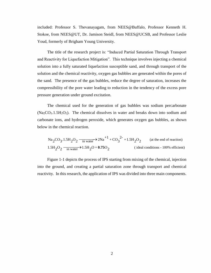
Figure 1-1 depicts the process of IPS starting from mixing of the chemical, injection
into the ground, and creating a partial saturation zone through transport and chemical
reactivity. In this research, the application of IPS was divided into three main components.
3
Figure 1-1 Overall process of IPS. Black ovals highlight the IPS monitoring
system, which was the focus of this dissertation.
The first component was developing and evaluating the efficiency of a delivery
system consisting of: controlled mixing of the solution to obtain a desired concentration,
installation of injection tubes, pumping of solution, reducing degree of saturation, and
evaluating the benefits of partial saturation on liquefaction potential. A soon to be
published dissertation by Fritz Nababan describes this component of the research. The
second component was developing a numerical simulation model and a computer program
to obtain the design parameters for IPS field implementation including: the design level of
chemical concentration, pumping pressure, duration of injection, duration of wait period
for the generation of oxygen, and predictions of the zone of partial saturation and the degree
of saturation achieved. This component of the research was recently published in the
dissertation of Seda Gokyer (2015). The third component of the IPS research entailed
developing and implementing a monitoring system that assured the desired concentration
of the chemical injected, and confirmed the duration of the injection and wait periods, zone
of partial saturation, and the degree of saturation actually achieved within the treated zone.
Monitoring of IPS
4
The focus of this dissertation was on this component of the research, as shown in Figure 1-
1.
1.2 Overview of this Dissertation
The IPS monitoring system that was described as the third main component of the
research project was based on using electric conductivity to detect transport of the
chemical, the rate of chemical reaction that generates gas, the generation of gas within
voids of sand and consequent reduction in degree of saturation, and finally zone of partial
saturation achieved. To explore the applicability and benefits of using electric
conductivity, laboratory tests on small and large sand specimen, as well as a pilot field test
were conducted.
Initially, bench-top laboratory tests were conducted using electric conductivity
probes and small specimens of Ottawa sand to understand the fundamentals of electric
conductivity as applied in IPS monitoring, and to determine rate of gas generation due to
sodium percarbonate reaction. Also, tests were conducted to confirm the theory based
upon which degree of saturation was calculated using electric conductivity tests results.
Following the bench-top laboratory tests, electric conductivity probes were used in a
large sand specimen (91 cm x 13.5 cm x 55 cm) prepared in a especially manufactured
glass tank. The purpose of the laboratory test in the glass tank was two folds: 1) to
implement IPS and use the test results to validate the numerical simulation model (second
main component of the research project), and 2) to further explore the use of conductivity
probes in determining zone of partial saturation and reduction in degree of saturation due
to injection of solution of sodium percarbonate; detection of gas bubble escape from the
specimen; and evaluation of diffusion of the chemical ions due to differences in
concentration within the specimen.
Further evaluation of the applicability of electric conductivity in monitoring IPS was
made by instrumenting a very large sand specimen (5 m x 2.75 m x 5m)) prepared in the
laminar box of NEES@Buffalo. The placement of electric conductivity probes in the
laminar box was for the purpose of: 1) monitoring the IPS delivery system developed by
Fritz Nababan, including concentration of chemical solution, duration of injection and
5
duration of wait time for gas generation; 2) estimation of the zones of partial saturation
achieved and determining the required spacing of the injection tubes to treat the entire sand
specimen; and 3) estimation of short- and long-term degree of saturation and detection of
potential gas escape and diffusion of the chemical solution. The results of these tests helped
validate the fundament theories and interpretation of conductivity probe results in
monitoring large-scale implementation of IPS.
The ability of electric conductivity probes to monitor field implementation of IPS
was also explored in a pilot test conducted at the NEES@UCSB Wildlife Refuge site, in
southern California. The field test using conductivity probes helped determine the
optimum injection pressure, injection tube spacing, and size of zone of partial saturation.
Based on these findings, the details of the final design of IPS implemented at the Wildlife
Refuge were defined.
The conductivity probes used in all the laboratory and field tests described above
were typical probes that are used in a laboratory. These probes were either inserted prior
to the placement of the sand specimens or in the case of field applications, were installed
in a pre-drilled borehole. A new field probe was manufactured to measure electric
conductivity in the field, where the probe is pushed into the IPS treated sand. This
technique avoids pre-drilling a borehole and disturbing the sand while installing the electric
conductivity probe. Preliminary laboratory tests were conducted to evaluate if the field
electric conductivity probe that is pushed into the sand can indeed accurately measure
degree of saturation.
This dissertation presents the results of research on developing the theory and
techniques of using electric conductivity to monitor application of IPS.
Chapter 2 presents an introduction of electric conductivity and its application in
estimating degree of saturation. Chapter 3 presents descriptions of the various bench-top
laboratory tests conducted to understand the rate of chemical reaction and to develop
degree of saturation as a function of concentration of the chemical solution. Chapter 4
presents the results of electric conductivity probes used in the glass tank laboratory IPS
tests. Chapter 5 presents the application of electric conductivity in the laminar box and
6
demonstrates how the probes are valuable tools in monitoring of implementation of IPS.
Chapter 6 summarizes the details of the pilot test performed at the NEES@UCSB Wildlife
Refuge field site, where electric conductivity probes were helpful in determining the design
parameters for field application of IPS. Chapter 7 presents the results from the preliminary
tests conducted in the laboratory using the new field probe to estimate degree of saturation
using electric conductivity. Chapter 8 summarizes the research results and presents
conclusions and recommendations for future research.
7
Chapter 2
Electric Conductivity and Probes
2.1 Introduction
Successful implementation of IPS will require ability to monitor the
chemical reaction that generates oxygen gas bubbles and to detect its effect on
the degree of saturation in the treated sand. This dissertation is focused on
developing techniques to achieve these goals. Electric conductivity is a
common laboratory approach to detect the presence of ions in soils. Typically,
a probe will measure the conductivity of a soil-fluid system between two
electrodes. A dry soil will have low conductivity compared with a soil
saturated with clean (ion-free) water. Similarly, the presence of ions in the
pore fluid of a soil will increase the electric conductivit y. In the case of IPS,
presence of gas bubbles within the pores of a sand-fluid mixture will reduce
the electric conductivity. In this dissertation these capabilities of electric
conductivity probes were advanced and implemented to understand the
fundamentals of the chemical reaction of sodium per carbonate that generates
oxygen bubble, and to develop methods to monitor the rate of decrease in
degree of saturation and to detect gas bubble generation or inadvertent gas
bubble escape from the sand.
This chapter briefly introduces the theory behind using electric
conductivity to detect presence of ions and to estimate degree of saturation.
The chapter also includes details of the electric conductivity probe used in this
research and demonstrates its ability to predict degree of saturation under
application of IPS.
8
2.2 Electrical conductivity theory
In 1827, George Simon Ohm discovered that electric current between two points along
a conductance relates directly to the potential difference between the points. Equation 2-1
represents Ohm’s law:
V = I × R (2-1)
In which, V is the potential in Volt, I is the current in Amp, and R is the resistance in ohm,
Ω. The resistance of the conductance (R) is directly proportional to length, L and inversely
proportional to cross section area, A (Equation 2-2).
R = ρ ×L
A (2-2)
In Equation 2-2, ρ is a constant which is the property of the conductance and is called
electrical resistivity. Resistivity has the unit of ohm m (Ω .m).
Electrical conductivity, σ has unit of Siemens per meter (S/m) and is defined as
reciprocal of electrical resistivity, ρ (Equation 2-3).
σ =1
ρ (2-3)
By combining Equations 2-2 and 2-3, Equation 2-4 is derived.
σ =L
R×A (2-4)
Electrical conductivity, σ is the property of the material, which represents the ability
to conduct an electric current. In soils, the value of electrical conductivity depends on
properties of the soil such as, porosity, degree of saturation, mineralogy including shape
and size of particles, soil structure including fabric and cementation and conductivity of
pore fluid (Mitchell, James Kenneth, and Kenichi Soga, 1976).
By combining Equations (2-1) and (2-4), Ohm’s law can be presented as in Equation
2-5:
9
I = σ ×V
L× A (2-5)
Equation 2-5 represents the flow of electricity through a conductance, be it a wire or a soil
fluid mixture. V/L represents the electrical gradient between the two electrodes, and A
represents the general area of the electric field.
2.3 Application of electric conductivity concept in soil
As mentioned in Section 2.2, electric conductivity can be used in a sand-fluid mixture
in the case of application of IPS.
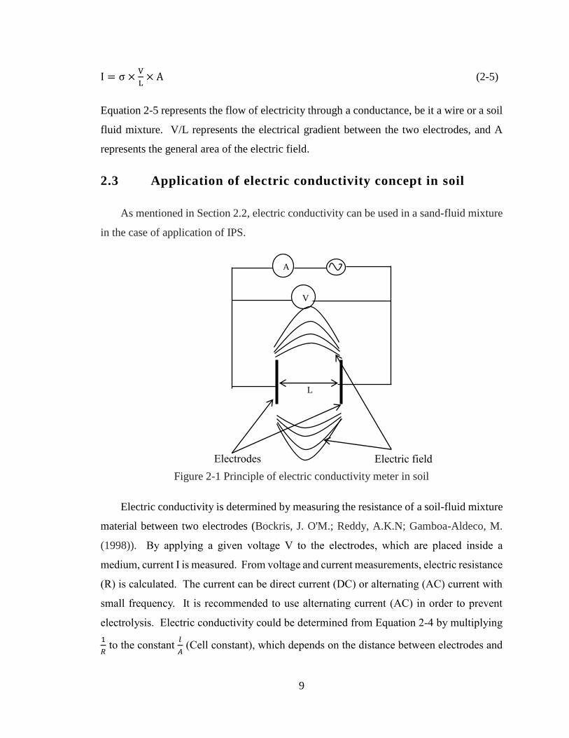
Figure 2-1 Principle of electric conductivity meter in soil
Electric conductivity is determined by measuring the resistance of a soil-fluid mixture
material between two electrodes (Bockris, J. O'M.; Reddy, A.K.N; Gamboa-Aldeco, M.
(1998)). By applying a given voltage V to the electrodes, which are placed inside a
medium, current I is measured. From voltage and current measurements, electric resistance
(R) is calculated. The current can be direct current (DC) or alternating (AC) current with
small frequency. It is recommended to use alternating current (AC) in order to prevent
electrolysis. Electric conductivity could be determined from Equation 2-4 by multiplying
1
𝑅 to the constant
𝑙
𝐴 (Cell constant), which depends on the distance between electrodes and
Electrodes Electric field
V
A
L
10
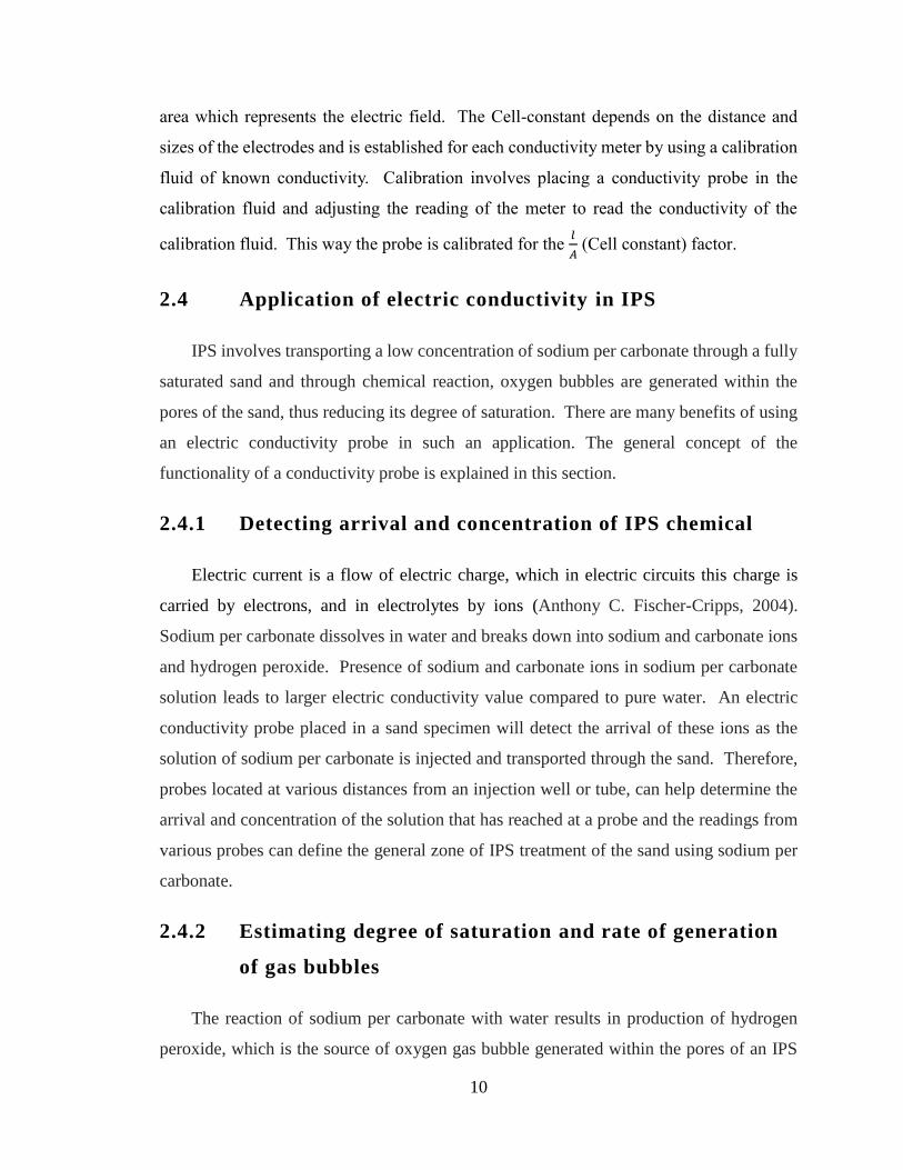
area which represents the electric field. The Cell-constant depends on the distance and
sizes of the electrodes and is established for each conductivity meter by using a calibration
fluid of known conductivity. Calibration involves placing a conductivity probe in the
calibration fluid and adjusting the reading of the meter to read the conductivity of the
calibration fluid. This way the probe is calibrated for the 𝑙
𝐴 (Cell constant) factor.
2.4 Application of electric conductivity in IPS
IPS involves transporting a low concentration of sodium per carbonate through a fully
saturated sand and through chemical reaction, oxygen bubbles are generated within the
pores of the sand, thus reducing its degree of saturation. There are many benefits of using
an electric conductivity probe in such an application. The general concept of the
functionality of a conductivity probe is explained in this section.
2.4.1 Detecting arrival and concentration of IPS chemical
Electric current is a flow of electric charge, which in electric circuits this charge is
carried by electrons, and in electrolytes by ions (Anthony C. Fischer-Cripps, 2004).
Sodium per carbonate dissolves in water and breaks down into sodium and carbonate ions
and hydrogen peroxide. Presence of sodium and carbonate ions in sodium per carbonate
solution leads to larger electric conductivity value compared to pure water. An electric
conductivity probe placed in a sand specimen will detect the arrival of these ions as the
solution of sodium per carbonate is injected and transported through the sand. Therefore,
probes located at various distances from an injection well or tube, can help determine the
arrival and concentration of the solution that has reached at a probe and the readings from
various probes can define the general zone of IPS treatment of the sand using sodium per
carbonate.
2.4.2 Estimating degree of saturation and rate of generation
of gas bubbles
The reaction of sodium per carbonate with water results in production of hydrogen
peroxide, which is the source of oxygen gas bubble generated within the pores of an IPS
11
treated sand. Because of the minute sizes of these gas bubbles, they are trapped within the
pores of the sand and cause a reduction in the electric conductivity of the sand-fluid mixture
from what it was before the reaction started. The rate of decrease in electric conductivity
represents the rate of generation of bubbles.
The change in electric conductivity due to bubble generation can be used to estimate
the change in the degree of saturation of the sand. The relation between electric
conductivity and degree of saturation of soil has been presented by Archie in 1942.
2.4.2.1 Archie’s law
Running experiments on clean sand, Archie (1942) expressed that the resistivity of
sand is directly proportional to the pore brine. Archie defined Equation 2-6 as a linear
relation between resistivity of sand and resistivity of brine.
F =ρ
ρw (2-6)
Where, ρ and ρw represent resistivity of sand and brine, respectively, and F is a formation
factor. Archie also provided a relationship between formation factor (F) and porosity of
clean sand, as well as degree of saturation of sand (Equation 2-7).
F =ρ
ρw= a × φ−m × S−n (2-7)
In which, 𝜑 and S are porosity and degree of saturation of sand, respectively, a, m, and n
are soil factors. a is called tortuosity factor and is meant for correction for compaction pore
structure and grain size. The value of a is typically between 0.5-1.5 (Winsauer et al. 1952).
m is called cementation exponent and can vary from 1.3 for loose sands to 2 for highly
cemented sandstones (Mitchell, James Kenneth, and Kenichi Soga, 1976). n is saturation
exponent determined experimentally. Archie suggested n=2 for clean sands.
As was shown in Equation 2-3, electric conductivity σ is defined as reciprocal of
resistivity ρ. Therefore, Equation 2-8 can be driven from Equation 2-7.
𝜎 =1
𝑎× 𝜎𝑤 × 𝜑𝑚 × 𝑠𝑛 (2-8)
12
In Equation 2-8, σ and σw represent electric conductivity of sand and electric conductivity
of brine, respectively. Equation 2-8 can be used in IPS application to calculate degree of
saturation of sand specimen.
To demonstrate the application of Archi’s law in IPS application, a typical electric
conductivity plot is sketched in Figure 2-2.
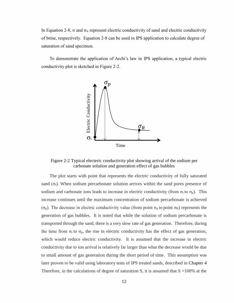
Figure 2-2 Typical electeric conductivity plot showing arrival of the sodium per
carbonate solution and generation effect of gas bubbles
The plot starts with point that represents the electric conductivity of fully saturated
sand (σi). When sodium percarbonate solution arrives within the sand pores presence of
sodium and carbonate ions leads to increase in electric conductivity (from σi to σp). This
increase continues until the maximum concentration of sodium percarbonate is achieved
(σp). The decrease in electric conductivity value (from point σp to point σR) represents the
generation of gas bubbles. It is noted that while the solution of sodium percarbonate is
transported through the sand, there is a very slow rate of gas generation. Therefore, during
the time from σi to σp, the rise in electric conductivity has the effect of gas generation,
which would reduce electric conductivity. It is assumed that the increase in electric
conductivity due to ion arrival is relatively far larger than what the decrease would be due
to small amount of gas generation during the short period of time. This assumption was
later proven to be valid using laboratory tests of IPS treated sands, described in Chapter 4
Therefore, in the calculations of degree of saturation S, it is assumed that S =100% at the
σi
Time
Ele
ctri
c C
onduct
ivit
y
13
time of peak electric conductivity, (σp). Another assumption is made that the Tortuosity
factor, cementation exponent, porosity and saturation exponent don’t change significantly
during the generation of bubbles (from point σp to point σR), an assumption also validated
using laboratory tests of IPS, described in Chapter 3.
By applying Equation 2-8 at any time during gas generation, between σp and σR the
degree of saturation of that specific time can be calculated. Equation 2-9 gives the
expression for the final degree of saturation SR achieved at point σR. Equation 2-9, assumes
that the saturation exponent, n= 2. This assumption also was validated using laboratory
test results Described in Chapter 3.
SR = √σR
σP (2-9)
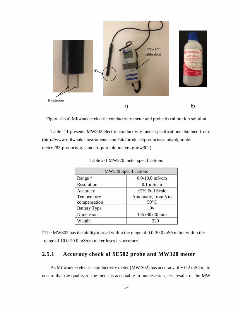
2.5 Milwaukee electric conductivity probe and meter
The electric conductivity probes and meters which were used in this research were
SE502 and MW302 respectively, manufactured by Milwaukee Instruments. The
calibration fluid is an international calibration solution with electric conductivity value of
1413µS/cm. The calibration of a probe entails immersing the electrodes in the calibration
fluid without touching the fluid container. The reading of the meter is then adjusted be to
an electric conductivity value of 1413µS/cm, using a small screw located on the meter.
Figure 2-3 shows the electric conductivity probe (SE502), meter (MW302) and calibration
solution (1413µS/cm), used in this research.
14
a) b)
Figure 2-3 a) Milwaukee electric conductivity meter and probe b) calibration solution
Table 2-1 presents MW302 electric conductivity meter specifications obtained from:
(http://www.milwaukeeinstruments.com/site/products/products/standardportable-
meters/83-products-g-standard-portable-meters-g-mw302).
Table 2-1 MW320 meter specifications
MW320 Specifications
Range * 0.0-10.0 mS/cm
Resolution 0.1 mS/cm
Accuracy ±2% Full Scale
Temperature
compensation
Automatic, from 5 to
50°C
Battery Type 9v
Dimension 145x80x40 mm
Weight 220
*The MW302 has the ability to read within the range of 0.0-20.0 mS/cm but within the
range of 10.0-20.0 mS/cm meter loses its accuracy.
2.5.1 Accuracy check of SE502 probe and MW320 meter
As Milwaukee electric conductivity meter (MW 302) has accuracy of ± 0.2 mS/cm, to
ensure that the quality of the meter is acceptable in our research, test results of the MW
Electrodes
Screw for
calibration
15
302 meter along with its probe, SE520, were compared with a more accurate electric
conductivity meter and probe (Orion 4 star -Thermo Scientific).
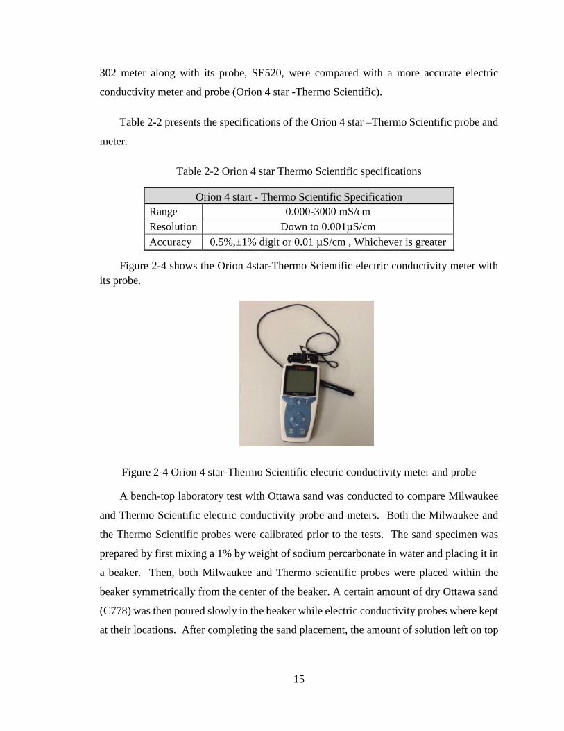
Table 2-2 presents the specifications of the Orion 4 star –Thermo Scientific probe and
meter.
Table 2-2 Orion 4 star Thermo Scientific specifications
Figure 2-4 shows the Orion 4star-Thermo Scientific electric conductivity meter with
its probe.
Figure 2-4 Orion 4 star-Thermo Scientific electric conductivity meter and probe
A bench-top laboratory test with Ottawa sand was conducted to compare Milwaukee
and Thermo Scientific electric conductivity probe and meters. Both the Milwaukee and
the Thermo Scientific probes were calibrated prior to the tests. The sand specimen was
prepared by first mixing a 1% by weight of sodium percarbonate in water and placing it in
a beaker. Then, both Milwaukee and Thermo scientific probes were placed within the
beaker symmetrically from the center of the beaker. A certain amount of dry Ottawa sand
(C778) was then poured slowly in the beaker while electric conductivity probes where kept
at their locations. After completing the sand placement, the amount of solution left on top
Orion 4 start - Thermo Scientific Specification
Range 0.000-3000 mS/cm
Resolution Down to 0.001µS/cm
Accuracy 0.5%,±1% digit or 0.01 µS/cm , Whichever is greater
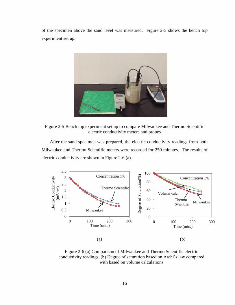
16
of the specimen above the sand level was measured. Figure 2-5 shows the bench top
experiment set up.
Figure 2-5 Bench top experiment set up to compare Milwaukee and Thermo Scientific
electric conductivity meters and probes
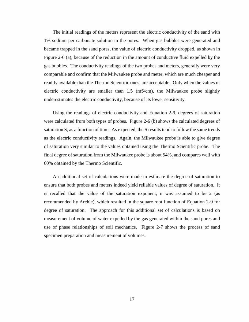
After the sand specimen was prepared, the electric conductivity readings from both
Milwaukee and Thermo Scientific meters were recorded for 250 minutes. The results of
electric conductivity are shown in Figure 2-6 (a).
(a) (b)
Figure 2-6 (a) Comparison of Milwaukee and Thermo Scientific electric
conductivity readings, (b) Degree of saturation based on Archi’s law compared
with based on volume calculations
0
0.5
1
1.5
2
2.5
3
3.5
0 100 200 300
Ele
ctri
c C
on
du
ctiv
ity
(mS
/cm
)
Time (min.)
Concentration 1%
Thermo Scientific
Milwaukee
0
20
40
60
80
100
0 100 200 300
Deg
ree
of
Sat
ura
tio
n(%
)
Time (min.)
Concentration 1%
Volume calc.
Milwaukee Thermo
Scientific
17
The initial readings of the meters represent the electric conductivity of the sand with
1% sodium per carbonate solution in the pores. When gas bubbles were generated and
became trapped in the sand pores, the value of electric conductivity dropped, as shown in
Figure 2-6 (a), because of the reduction in the amount of conductive fluid expelled by the
gas bubbles. The conductivity readings of the two probes and meters, generally were very
comparable and confirm that the Milwaukee probe and meter, which are much cheaper and
readily available than the Thermo Scientific ones, are acceptable. Only when the values of
electric conductivity are smaller than 1.5 (mS/cm), the Milwaukee probe slightly
underestimates the electric conductivity, because of its lower sensitivity.
Using the readings of electric conductivity and Equation 2-9, degrees of saturation
were calculated from both types of probes. Figure 2-6 (b) shows the calculated degrees of
saturation S, as a function of time. As expected, the S results tend to follow the same trends
as the electric conductivity readings. Again, the Milwaukee probe is able to give degree
of saturation very similar to the values obtained using the Thermo Scientific probe. The
final degree of saturation from the Milwaukee probe is about 54%, and compares well with
60% obtained by the Thermo Scientific.
An additional set of calculations were made to estimate the degree of saturation to
ensure that both probes and meters indeed yield reliable values of degree of saturation. It
is recalled that the value of the saturation exponent, n was assumed to be 2 (as
recommended by Archie), which resulted in the square root function of Equation 2-9 for
degree of saturation. The approach for this additional set of calculations is based on
measurement of volume of water expelled by the gas generated within the sand pores and
use of phase relationships of soil mechanics. Figure 2-7 shows the process of sand
specimen preparation and measurement of volumes.
18
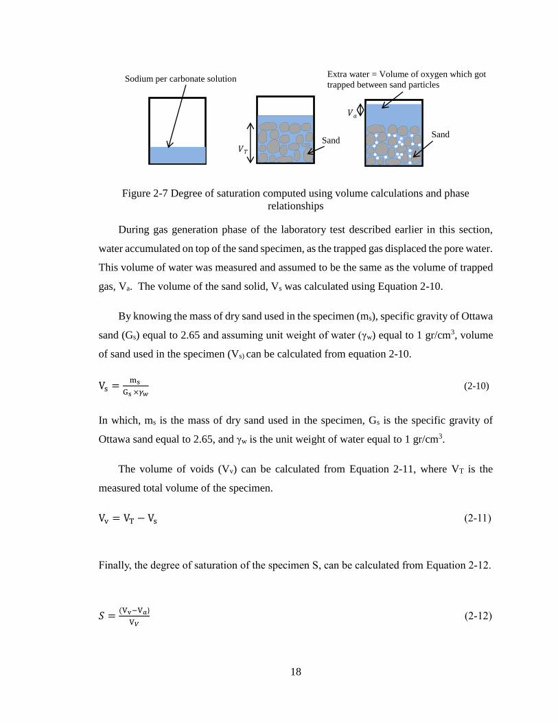
Figure 2-7 Degree of saturation computed using volume calculations and phase
relationships
During gas generation phase of the laboratory test described earlier in this section,
water accumulated on top of the sand specimen, as the trapped gas displaced the pore water.
This volume of water was measured and assumed to be the same as the volume of trapped
gas, Va. The volume of the sand solid, Vs was calculated using Equation 2-10.
By knowing the mass of dry sand used in the specimen (ms), specific gravity of Ottawa
sand (Gs) equal to 2.65 and assuming unit weight of water (γw) equal to 1 gr/cm3, volume
of sand used in the specimen (Vs) can be calculated from equation 2-10.
Vs =ms
Gs ×𝛾𝑤 (2-10)
In which, ms is the mass of dry sand used in the specimen, Gs is the specific gravity of
Ottawa sand equal to 2.65, and γw is the unit weight of water equal to 1 gr/cm3.
The volume of voids (Vv) can be calculated from Equation 2-11, where VT is the
measured total volume of the specimen.
Vv = VT − Vs (2-11)
Finally, the degree of saturation of the specimen S, can be calculated from Equation 2-12.
𝑆 =(Vv−V𝑎)
V𝑉 (2-12)
Sodium per carbonate solution
Sand 𝑉𝑇
Sand
Extra water = Volume of oxygen which got
trapped between sand particles
𝑉𝑎
19
Figure 2-6 (b) includes the results of degree of saturation calculated using volume
measurements and phase relationships. The results from volume calculations compare well
with those obtained using the electric conductivity probes, considering the difficulties in
measuring small volumes in the laboratory experiment.
Degree of saturation calculated based on Archi’s law, using Milwaukee and Thermo
Scientific conductivity kits can be compared with degree of saturation calculated based on
volume calculation.
In summary, the experimental test results shown in Figure 2-6 confirm that the
Milwaukee probe readings of electric conductivity together with Equation 2-9, which
assumes that the saturation exponent is n = 2 can indeed provide reliable and reasonably
accurate rate of decrease in degree of saturation during gas generation, as well as final
degree of saturation when gas generation is completed.
2.5.2 Extending cable of Milwaukee electric conductivity
probe
SE 520 electric conductivity probe which is manufactured by Milwaukee Instrument
comes with 1 meter long cable. These probes were used in small-scale laboratory
specimens without extending the factory connected cables. The probes were also used in
large-scale laboratory and field applications, which necessitated the extending of the cables
from 1 meter to as long as 10 to 15 meters. It was of interest to know, if extending the
cables of the Milwaukee probes with new connecters would have adverse effect on the
electric conductivity readings. Figure 2-8 shows SE520 Milwaukee probe with a long
extended cable.
Milwaukee
20
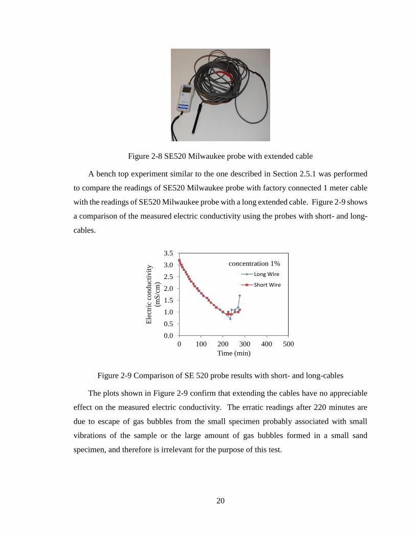
Figure 2-8 SE520 Milwaukee probe with extended cable
A bench top experiment similar to the one described in Section 2.5.1 was performed
to compare the readings of SE520 Milwaukee probe with factory connected 1 meter cable
with the readings of SE520 Milwaukee probe with a long extended cable. Figure 2-9 shows
a comparison of the measured electric conductivity using the probes with short- and long-
cables.
Figure 2-9 Comparison of SE 520 probe results with short- and long-cables
The plots shown in Figure 2-9 confirm that extending the cables have no appreciable
effect on the measured electric conductivity. The erratic readings after 220 minutes are
due to escape of gas bubbles from the small specimen probably associated with small
vibrations of the sample or the large amount of gas bubbles formed in a small sand
specimen, and therefore is irrelevant for the purpose of this test.
0.0
0.5
1.0
1.5
2.0
2.5
3.0
3.5
0 100 200 300 400 500
Ele
ctri
c co
nd
uct
ivit
y
(mS
/cm
)
Time (min)
concentration 1%
Long Wire
Short Wire
𝑅2=0.96
e=0.64
21
Chapter 3
Bench-Top Laboratory Tests Using Electric Conductivity
Probe to Study Rate of Gas Generation and Degree of
Saturation in Sand
3.1 Overview
Bench-top laboratory experiments were conducted on small specimens of Ottawa sand
partially saturated using varying concentrations of sodium per carbonate solution.
Measurements of electric conductivity were made to: 1) verify the procedure for
calculating the degree of saturation using electric conductivity data; 2) determine the rate
of gas generation; and 3) determine if the void ratio of a specimen has an effect on the
reduction in degree of saturation induced by gas generation.
This chapter describes the details of the laboratory tests conducted, and presents the
electric conductivity data to evaluate each of the three goals stated above.
3.2 Verification of the procedure for calculating degree of
saturation
One of the main purposes of using electric conductivity probes in this research is to
monitor the generation of gas bubbles in a sand, leading to reduction in electric
conductivity, and hence reduction in degree of saturation. The calculation of degree of
saturation induced by IPS is based on Archie’s law and a number of assumptions. Details
of the application of Archie’s law and the assumptions made were presented in Chapter 2.
Equation 2-9 from Chapter 2 is replicated herein as Equation 3-1, which is used to calculate
degree of saturation, S.
SR = √σR
σP (3-1)
22
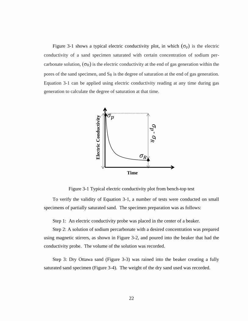
Figure 3-1 shows a typical electric conductivity plot, in which (σp) is the electric
conductivity of a sand specimen saturated with certain concentration of sodium per-
carbonate solution, (σR) is the electric conductivity at the end of gas generation within the
pores of the sand specimen, and SR is the degree of saturation at the end of gas generation.
Equation 3-1 can be applied using electric conductivity reading at any time during gas
generation to calculate the degree of saturation at that time.
Figure 3-1 Typical electric conductivity plot from bench-top test
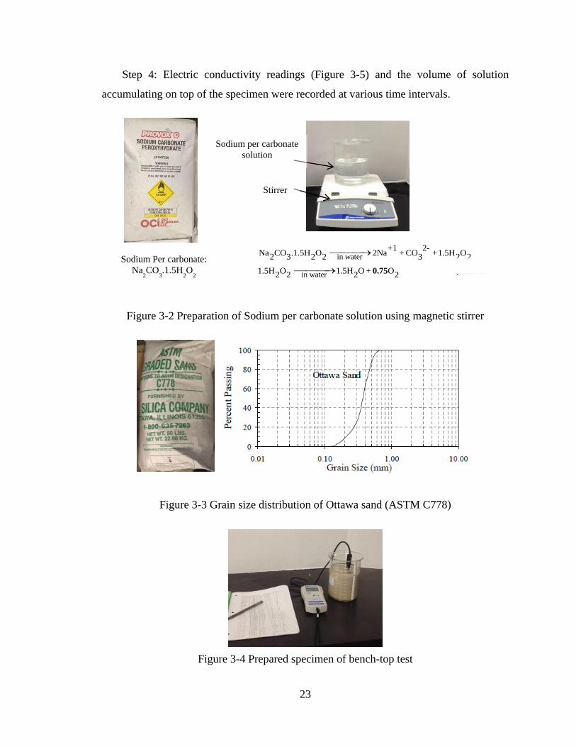
To verify the validity of Equation 3-1, a number of tests were conducted on small
specimens of partially saturated sand. The specimen preparation was as follows:
Step 1: An electric conductivity probe was placed in the center of a beaker.
Step 2: A solution of sodium percarbonate with a desired concentration was prepared
using magnetic stirrers, as shown in Figure 3-2, and poured into the beaker that had the
conductivity probe. The volume of the solution was recorded.
Step 3: Dry Ottawa sand (Figure 3-3) was rained into the beaker creating a fully
saturated sand specimen (Figure 3-4). The weight of the dry sand used was recorded.
Time
Ele
ctri
c C
on
du
ctiv
ity
-
23
Step 4: Electric conductivity readings (Figure 3-5) and the volume of solution
accumulating on top of the specimen were recorded at various time intervals.
Figure 3-2 Preparation of Sodium per carbonate solution using magnetic stirrer
Figure 3-3 Grain size distribution of Ottawa sand (ASTM C778)
Figure 3-4 Prepared specimen of bench-top test
Sodium Per carbonate:
Na2CO
3.1.5H
2O
2
Sodium per carbonate
solution
Stirrer
in water
in water
(at the end of reaction)
( ideal conditions - 100% efficient)
+1 2-Na CO .1.5H O 2Na + CO + 1.5H O
2 3 2 2 3 2 2
1.5H O 1.5H O + O2 2 2 2
0.75
24
0
20
40
60
80
100
0 100 200 300 400 500
Deg
ree
of
Sat
ura
tion (
%)
Time (min)
Concentration 1%
Based on
volume calc. Based on electric
conductivity
e=0.62
0.0
0.5
1.0
1.5
2.0
2.5
3.0
0 100 200 300 400 500
Ele
ctri
c co
nd
uct
ivit
y
(mS
/cm
)
Time (min)
Concentration1%
e=0.62
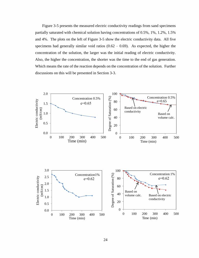
Figure 3-5 presents the measured electric conductivity readings from sand specimens
partially saturated with chemical solution having concentrations of 0.5%, 1%, 1.2%, 1.5%
and 4%. The plots on the left of Figure 3-5 show the electric conductivity data. All five
specimens had generally similar void ratios (0.62 – 0.69). As expected, the higher the
concentration of the solution, the larger was the initial reading of electric conductivity.
Also, the higher the concentration, the shorter was the time to the end of gas generation.
Which means the rate of the reaction depends on the concentration of the solution. Further
discussions on this will be presented in Section 3-3.
0
20
40
60
80
100
0 100 200 300 400 500
Deg
ree
of
Sat
ura
tion (
%)
Time (min)
Concentration 0.5%e=0.65
Based on electric
conductivity Based on
volume calc.
0.0
0.5
1.0
1.5
2.0
0 100 200 300 400 500
Ele
ctri
c co
nd
uct
ivit
y
(mS
/cm
)
Time (min)
Concentration 0.5%
e=0.65e=0.65
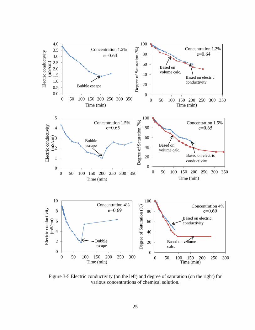
25
0
2
4
6
8
10
0 50 100 150 200 250 300
Ele
ctri
c co
nd
uct
ivit
y
(mS
/cm
)
Time (min)
Concentration 4%
Bubble
escape
e=0.69
0
20
40
60
80
100
0 50 100 150 200 250 300
Deg
ree
of
Sat
ura
tion (
%)
Time (min)
Concentration 4%e=0.69
Based on volume
calc.
Based on electric
conductivity
0
1
2
3
4
5
0 50 100 150 200 250 300 350
Ele
ctri
c co
nd
uct
ivit
y
(mS
/cm
)
Time (min)
Concentration 1.5%
e=0.65
Bubble
escape
0
20
40
60
80
100
0 50 100 150 200 250 300 350
Deg
ree
of
Sat
ura
tio
n (
%)
Time (min)
Concentration 1.5%
Based on
volume calc.
Based on electric
conductivity
0
20
40
60
80
100
0 50 100 150 200 250 300 350
Deg
ree
of
Sat
ura
tio
n (
%)
Time (min)
Concentration 1.2%
e=0.64
Based on
volume calc.
Based on electric
conductivity
0.0
0.5
1.0
1.5
2.0
2.5
3.0
3.5
4.0
0 50 100 150 200 250 300 350
Ele
ctri
c co
nd
uct
ivit
y
(mS
/cm
)
Time (min)
Concentration 1.2%
Bubble escape
e=0.64
Figure 3-5 Electric conductivity (on the left) and degree of saturation (on the right) for
various concentrations of chemical solution.
e=0.65
26
It is also noted from the electric conductivity data of Figure 3-5 that when the
concentration of the chemical solution was high (> 1.2%), gas bubbles tended to escape
from the specimens. The larger the concentration, the more bubbles escaped. This bubble
escape is attributed to the ease of gas escaping along the smooth housing of the electric
conductivity probe. Thus, most likely this situation was local to the probe and hence had
pronounced impact on the probe’s reading.
Using the electric conductivity data of Figure 3-5 and Equation 3-1 the degree of
saturation as a function of time were calculated for each of the five sand specimens. The
results are presented in the plots shown on the right side of Figure 3-5. The reduction in
degree of saturation as a result of gas generation can be observed. The calculations were
made till the time prior to gas bubble escape giving the general degree of saturation of the
specimens at that time. As expected, the plots indicate that the higher the concentration of
the solution, the lower is the final degree of saturation. Also, the higher the concentration,
the faster is the time to final degree of saturation. These observations expectedly are
consistent with those made based on the raw data of electric conductivity.
To verify that the procedure for the calculation of degree of saturation is valid, the
measurements of the mass of the dry sand, the initial volume of solution, volume of the
specimen, as well as volume of the solution accumulated at the surface of each specimen
as a result of gas generation, were used and the degree of saturation were calculated, using
equations of phase relations. The results of these calculations of degree of saturation are
plotted on the right side of Figure 3-5. The plots are labeled “based on volume
calculations”.
The comparisons made between the degree of saturation plots based on electric
conductivity and based on volume calculations lead to the following observations:
1- The two methods yield reasonably similar degree of saturation for during and end
of gas generation periods.
2- In general, the degree of saturation based on electric conductivity is slightly larger
than based on volume calculations. This can be due to a number of factors: 1-
inaccuracy in measuring small changes in the volume of the expelled water due to
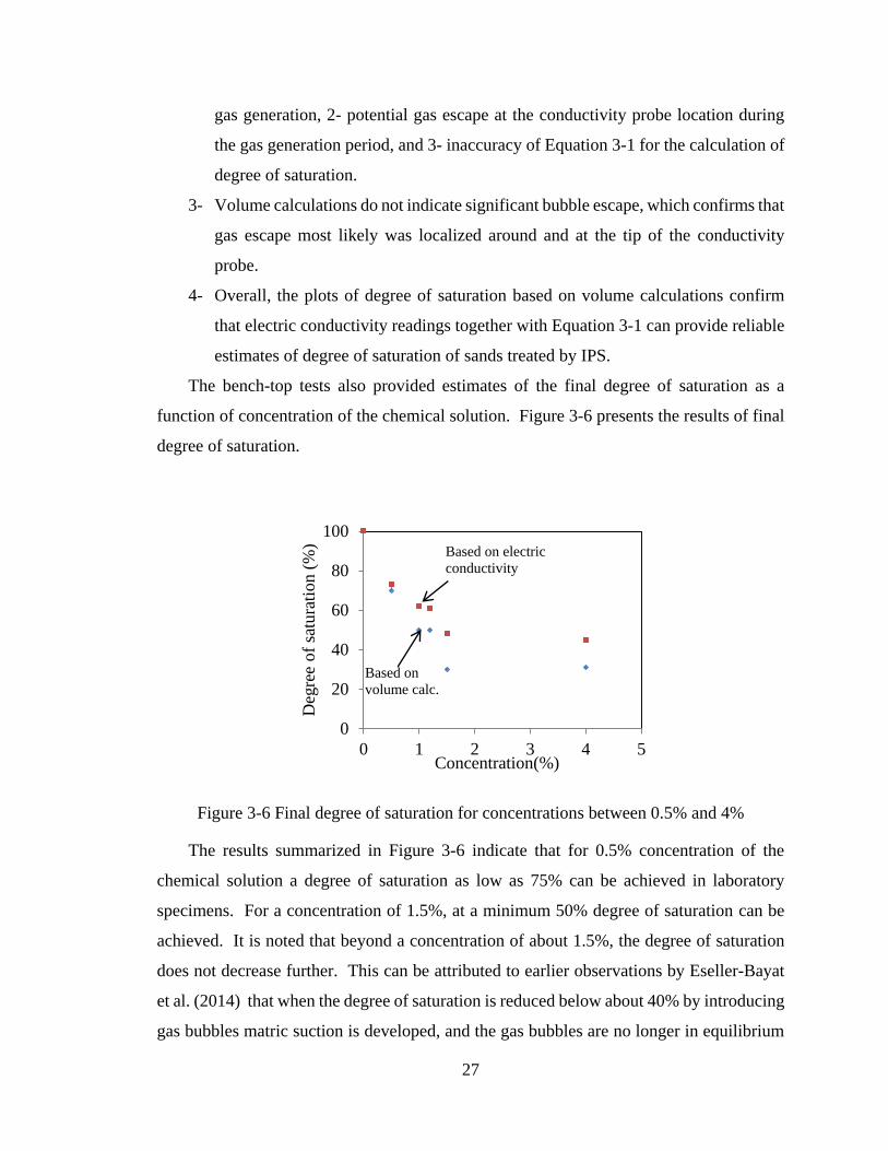
27
gas generation, 2- potential gas escape at the conductivity probe location during
the gas generation period, and 3- inaccuracy of Equation 3-1 for the calculation of
degree of saturation.
3- Volume calculations do not indicate significant bubble escape, which confirms that
gas escape most likely was localized around and at the tip of the conductivity
probe.
4- Overall, the plots of degree of saturation based on volume calculations confirm
that electric conductivity readings together with Equation 3-1 can provide reliable
estimates of degree of saturation of sands treated by IPS.
The bench-top tests also provided estimates of the final degree of saturation as a
function of concentration of the chemical solution. Figure 3-6 presents the results of final
degree of saturation.
Figure 3-6 Final degree of saturation for concentrations between 0.5% and 4%
The results summarized in Figure 3-6 indicate that for 0.5% concentration of the
chemical solution a degree of saturation as low as 75% can be achieved in laboratory
specimens. For a concentration of 1.5%, at a minimum 50% degree of saturation can be
achieved. It is noted that beyond a concentration of about 1.5%, the degree of saturation
does not decrease further. This can be attributed to earlier observations by Eseller-Bayat
et al. (2014) that when the degree of saturation is reduced below about 40% by introducing
gas bubbles matric suction is developed, and the gas bubbles are no longer in equilibrium
0
20
40
60
80
100
0 1 2 3 4 5
Deg
ree
of
satu
rati
on (
%)
Concentration(%)
Based on electric
conductivity
Based on
volume calc.
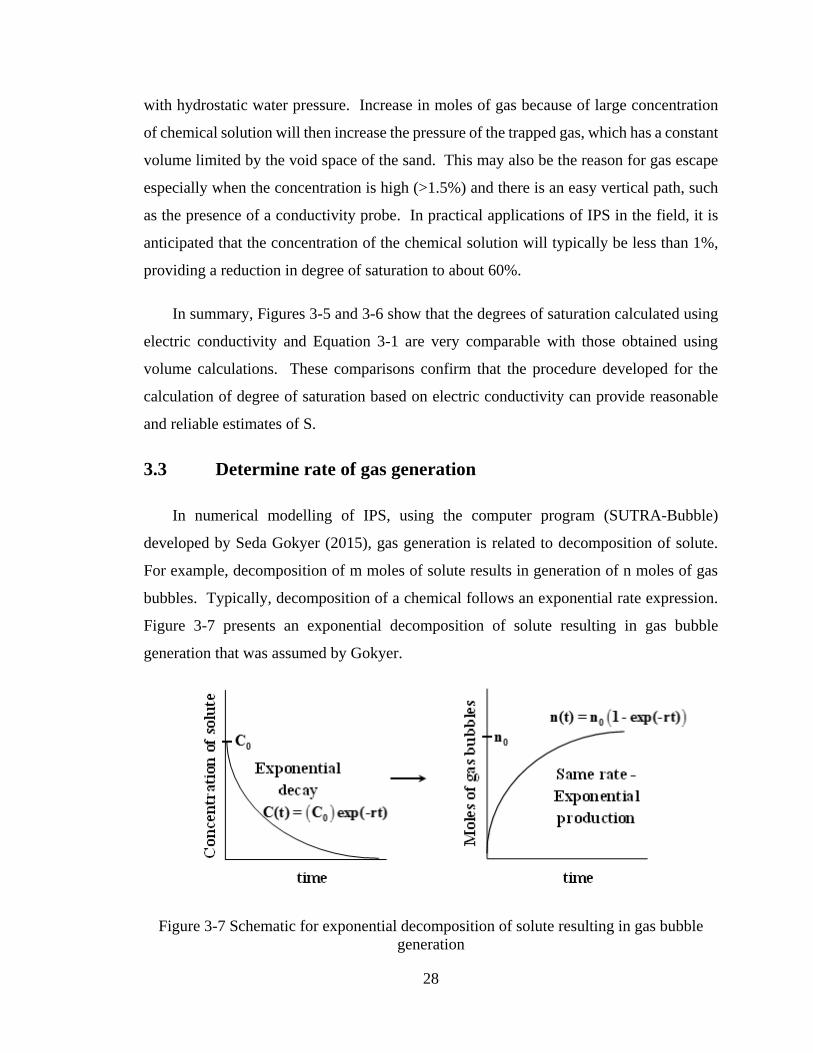
28
with hydrostatic water pressure. Increase in moles of gas because of large concentration
of chemical solution will then increase the pressure of the trapped gas, which has a constant
volume limited by the void space of the sand. This may also be the reason for gas escape
especially when the concentration is high (>1.5%) and there is an easy vertical path, such
as the presence of a conductivity probe. In practical applications of IPS in the field, it is
anticipated that the concentration of the chemical solution will typically be less than 1%,
providing a reduction in degree of saturation to about 60%.
In summary, Figures 3-5 and 3-6 show that the degrees of saturation calculated using
electric conductivity and Equation 3-1 are very comparable with those obtained using
volume calculations. These comparisons confirm that the procedure developed for the
calculation of degree of saturation based on electric conductivity can provide reasonable
and reliable estimates of S.
3.3 Determine rate of gas generation
In numerical modelling of IPS, using the computer program (SUTRA-Bubble)
developed by Seda Gokyer (2015), gas generation is related to decomposition of solute.
For example, decomposition of m moles of solute results in generation of n moles of gas
bubbles. Typically, decomposition of a chemical follows an exponential rate expression.
Figure 3-7 presents an exponential decomposition of solute resulting in gas bubble
generation that was assumed by Gokyer.
Figure 3-7 Schematic for exponential decomposition of solute resulting in gas bubble
generation
29
Equation 3-2 represents the decomposition of solute:
C(t) = C0 × exp(−rt) (3-2)
In Equation 3-2, C(t) is the concentration of the solute at time t, C0 is the initial
concentration of the solute and r is a rate parameter.
Differentiating Equation 3-2, the rate of decomposition of the solute is given by
Equation 3-3.
∆𝐶(𝑡)
∆𝑡= −r(C0) × exp(−rt) = −rC(t) (3-3)
The computer program SUTRA-Bubble uses Equation 3-3 to estimate moles of gas
bubble generated over time. More details about the decomposition of hydrogen peroxide
(the source of oxygen gas generation) and the rate parameter are presented in the
dissertation of Seda Gokyer.
To determine the rate parameter r, bench-top tests were run on sand specimens
partially saturated by sodium percarbonate solution introduced into the specimens. An
electric conductivity probe was used to monitor and record the rate of gas generation, as
was described in Section 3-2.
As it was explained earlier, the reduction in electric conductivity (σp to σR in Figure 3-
1) is related to gas bubble generation due the decay of hydrogen peroxide. Therefore, an
exponential trend similar to the trend of decay of hydrogen peroxide is expected to be
observed in electric conductivity plots over time. This exponential trend can be formulated
as in Equation 3-4:
𝜎(t) = (𝜎p − 𝜎𝑅) × exp(−rt) + 𝜎𝑅
or,
𝜎(t) − 𝜎𝑅 = (𝜎p − 𝜎𝑅) × exp(−rt) (3-4)
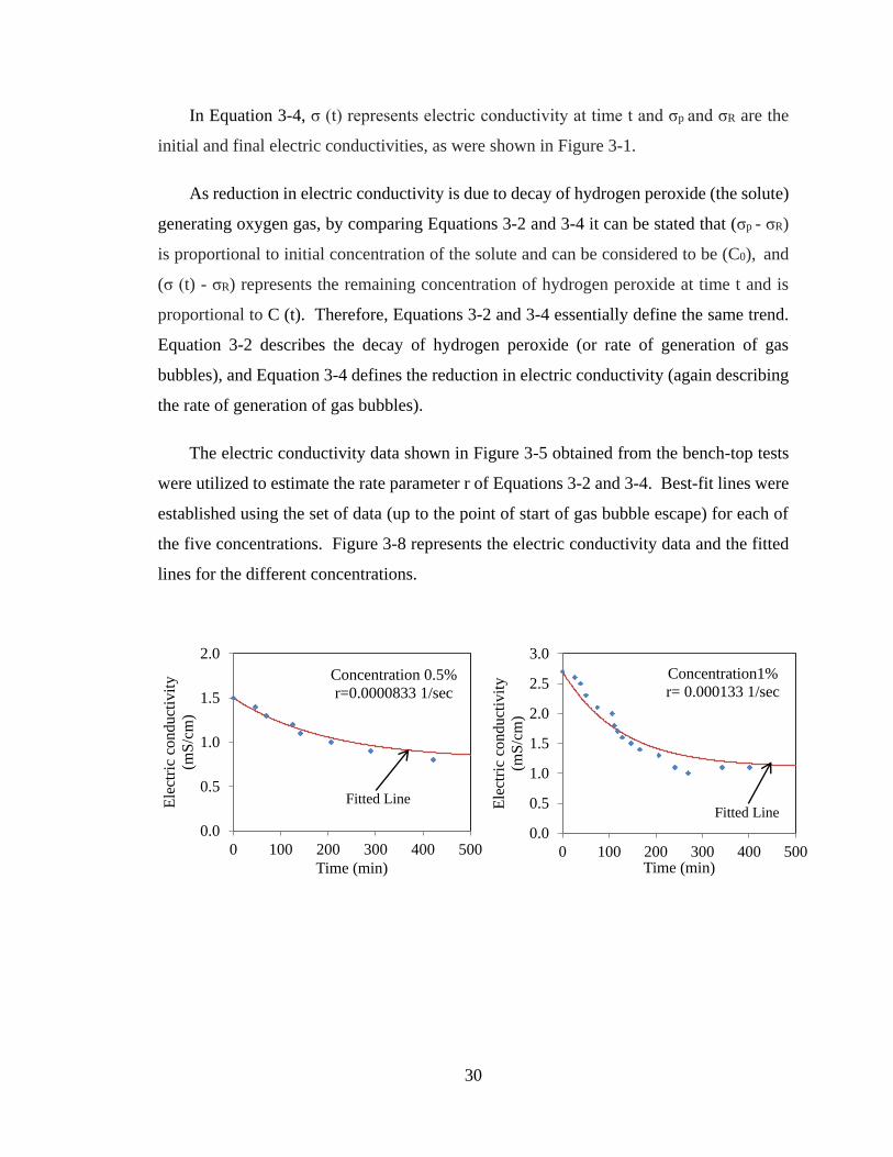
30
In Equation 3-4, σ (t) represents electric conductivity at time t and σp and σR are the
initial and final electric conductivities, as were shown in Figure 3-1.
As reduction in electric conductivity is due to decay of hydrogen peroxide (the solute)
generating oxygen gas, by comparing Equations 3-2 and 3-4 it can be stated that (σp - σR)
is proportional to initial concentration of the solute and can be considered to be (C0), and
(σ (t) - σR) represents the remaining concentration of hydrogen peroxide at time t and is
proportional to C (t). Therefore, Equations 3-2 and 3-4 essentially define the same trend.
Equation 3-2 describes the decay of hydrogen peroxide (or rate of generation of gas
bubbles), and Equation 3-4 defines the reduction in electric conductivity (again describing
the rate of generation of gas bubbles).
The electric conductivity data shown in Figure 3-5 obtained from the bench-top tests
were utilized to estimate the rate parameter r of Equations 3-2 and 3-4. Best-fit lines were
established using the set of data (up to the point of start of gas bubble escape) for each of
the five concentrations. Figure 3-8 represents the electric conductivity data and the fitted
lines for the different concentrations.
0.0
0.5
1.0
1.5
2.0
0 100 200 300 400 500
Ele
ctri
c co
nd
uct
ivit
y
(mS
/cm
)
Time (min)
Concentration 0.5%
r=0.0000833 1/sec
Fitted Line
0.0
0.5
1.0
1.5
2.0
2.5
3.0
0 100 200 300 400 500
Ele
ctri
c co
nd
uct
ivit
y
(mS
/cm
)
Time (min)
Concentration1%
r= 0.000133 1/sec
Fitted Line
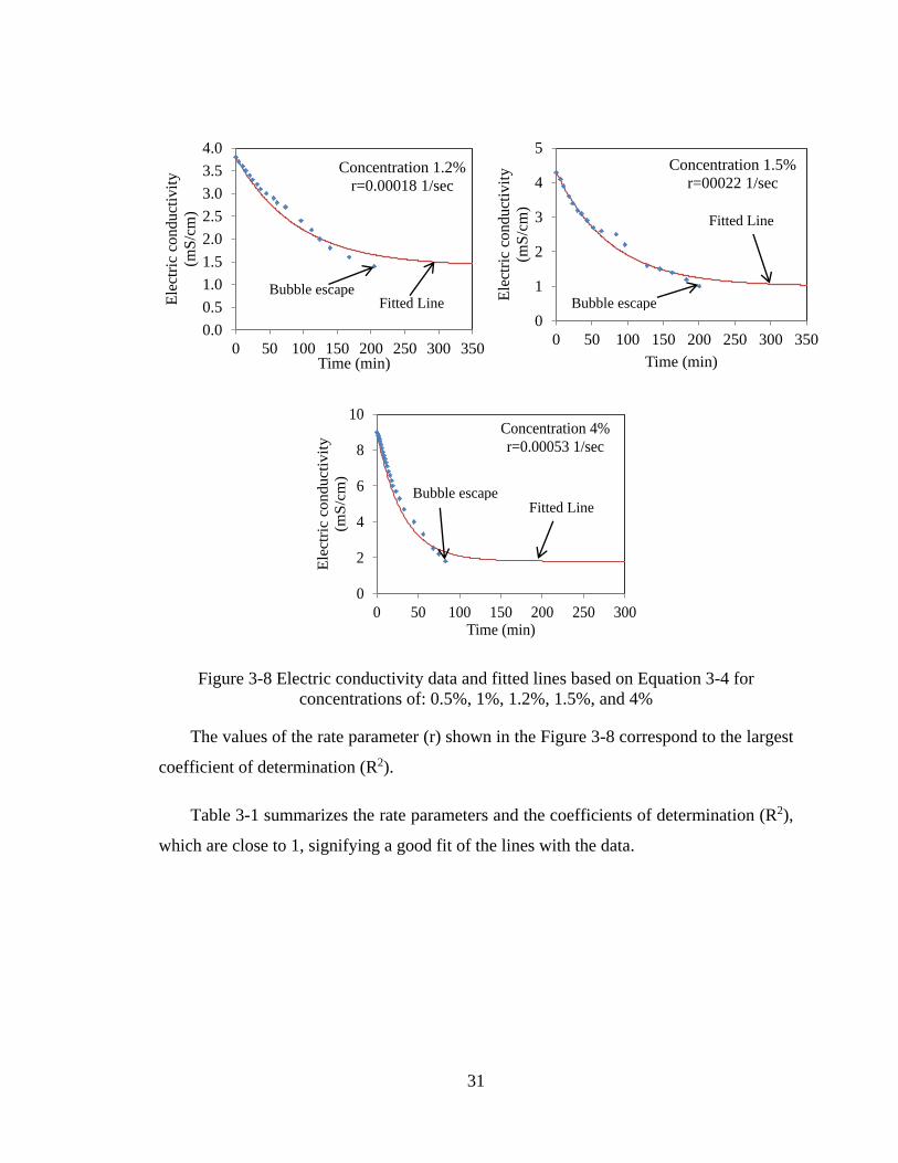
31
Figure 3-8 Electric conductivity data and fitted lines based on Equation 3-4 for
concentrations of: 0.5%, 1%, 1.2%, 1.5%, and 4%
The values of the rate parameter (r) shown in the Figure 3-8 correspond to the largest
coefficient of determination (R2).
Table 3-1 summarizes the rate parameters and the coefficients of determination (R2),
which are close to 1, signifying a good fit of the lines with the data.
0.0
0.5
1.0
1.5
2.0
2.5
3.0
3.5
4.0
0 50 100 150 200 250 300 350
Ele
ctri
c co
nd
uct
ivit
y
(mS
/cm
)
Time (min)
Concentration 1.2%
r=0.00018 1/sec
Fitted Line Bubble escape
0
1
2
3
4
5
0 50 100 150 200 250 300 350
Ele
ctri
c co
nd
uct
ivit
y
(mS
/cm
)
Time (min)
Concentration 1.5%
r=00022 1/sec
Fitted Line
Bubble escape
0
2
4
6
8
10
0 50 100 150 200 250 300
Ele
ctr
ic c
onducti
vit
y
(mS
/cm
)
Time (min)
Concentration 4%
r=0.00053 1/sec
Fitted Line Bubble escape
𝑅2=0.96
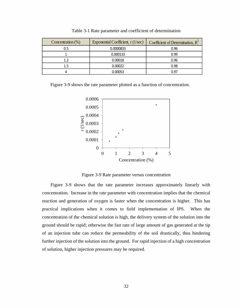
32
Table 3-1 Rate parameter and coefficient of determination
Figure 3-9 shows the rate parameter plotted as a function of concentration.
Figure 3-9 Rate parameter versus concentration
Figure 3-9 shows that the rate parameter increases approximately linearly with
concentration. Increase in the rate parameter with concentration implies that the chemical
reaction and generation of oxygen is faster when the concentration is higher. This has
practical implications when it comes to field implementation of IPS. When the
concentration of the chemical solution is high, the delivery system of the solution into the
ground should be rapid; otherwise the fast rate of large amount of gas generated at the tip
of an injection tube can reduce the permeability of the soil drastically, thus hindering
further injection of the solution into the ground. For rapid injection of a high concentration
of solution, higher injection pressures may be required.
Concentration (%) Exponential Coefficient, r (1/sec) Coefficient of Determination, R2
0.5 0.0000833 0.96
1 0.000133 0.99
1.2 0.00018 0.96
1.5 0.00022 0.98
4 0.00053 0.97
0
0.0001
0.0002
0.0003
0.0004
0.0005
0.0006
0 1 2 3 4 5
r (1
/sec
)
Concentration (%)
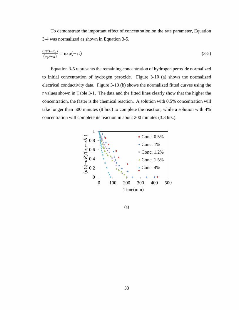
33
To demonstrate the important effect of concentration on the rate parameter, Equation
3-4 was normalized as shown in Equation 3-5.
(𝜎(t)−𝜎𝑅)
(𝜎p−𝜎𝑅)= exp(−rt) (3-5)
Equation 3-5 represents the remaining concentration of hydrogen peroxide normalized
to initial concentration of hydrogen peroxide. Figure 3-10 (a) shows the normalized
electrical conductivity data. Figure 3-10 (b) shows the normalized fitted curves using the
r values shown in Table 3-1. The data and the fitted lines clearly show that the higher the
concentration, the faster is the chemical reaction. A solution with 0.5% concentration will
take longer than 500 minutes (8 hrs.) to complete the reaction, while a solution with 4%
concentration will complete its reaction in about 200 minutes (3.3 hrs.).
(a)
0
0.2
0.4
0.6
0.8
1
0 100 200 300 400 500
( (t
)−
)/(
p−
)
Time(min)
Conc. 0.5%
Conc. 1%
Conc. 1.2%
Conc. 1.5%
Conc. 4%
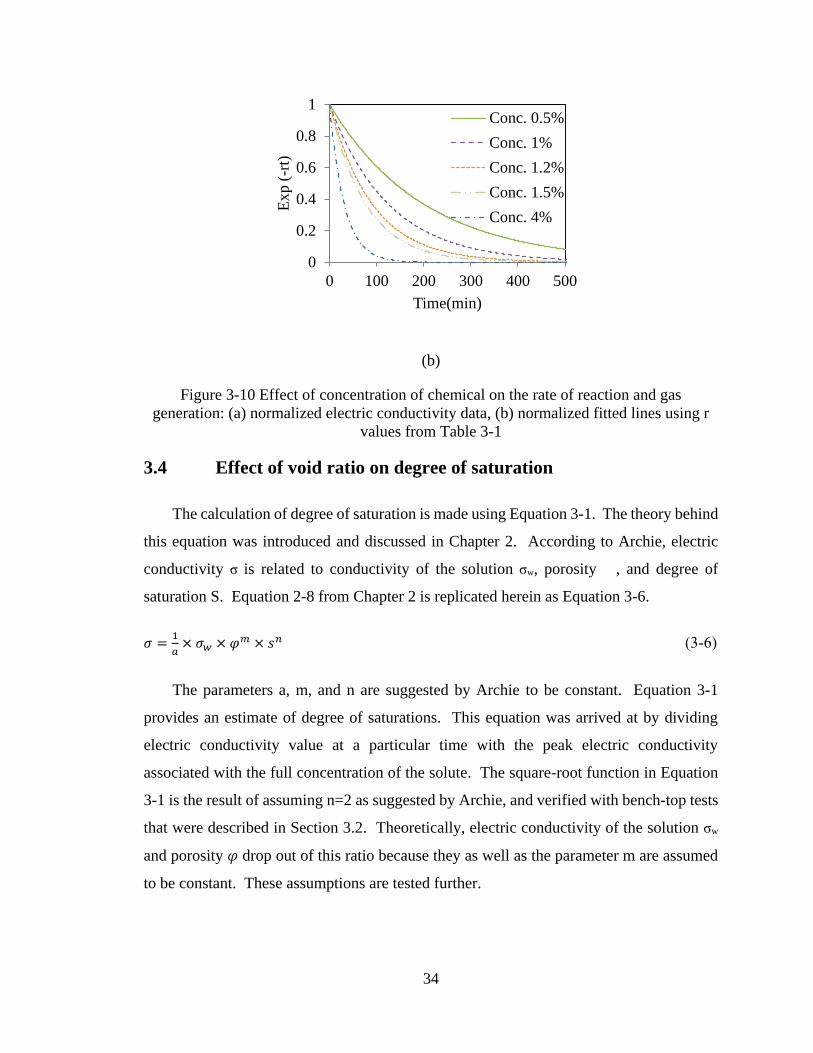
34
(b)
Figure 3-10 Effect of concentration of chemical on the rate of reaction and gas
generation: (a) normalized electric conductivity data, (b) normalized fitted lines using r
values from Table 3-1
3.4 Effect of void ratio on degree of saturation
The calculation of degree of saturation is made using Equation 3-1. The theory behind
this equation was introduced and discussed in Chapter 2. According to Archie, electric
conductivity σ is related to conductivity of the solution σw, porosity , and degree of
saturation S. Equation 2-8 from Chapter 2 is replicated herein as Equation 3-6.
𝜎 =1
𝑎× 𝜎𝑤 × 𝜑𝑚 × 𝑠𝑛 (3-6)
The parameters a, m, and n are suggested by Archie to be constant. Equation 3-1
provides an estimate of degree of saturations. This equation was arrived at by dividing
electric conductivity value at a particular time with the peak electric conductivity
associated with the full concentration of the solute. The square-root function in Equation
3-1 is the result of assuming n=2 as suggested by Archie, and verified with bench-top tests
that were described in Section 3.2. Theoretically, electric conductivity of the solution σw
and porosity 𝜑 drop out of this ratio because they as well as the parameter m are assumed
to be constant. These assumptions are tested further.
0
0.2
0.4
0.6
0.8
1
0 100 200 300 400 500E
xp (
-rt)
Time(min)
Conc. 0.5%
Conc. 1%
Conc. 1.2%
Conc. 1.5%
Conc. 4%
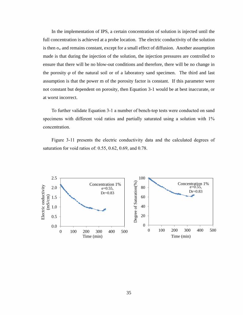
35
In the implementation of IPS, a certain concentration of solution is injected until the
full concentration is achieved at a probe location. The electric conductivity of the solution
is then σw and remains constant, except for a small effect of diffusion. Another assumption
made is that during the injection of the solution, the injection pressures are controlled to
ensure that there will be no blow-out conditions and therefore, there will be no change in
the porosity 𝜑 of the natural soil or of a laboratory sand specimen. The third and last
assumption is that the power m of the porosity factor is constant. If this parameter were
not constant but dependent on porosity, then Equation 3-1 would be at best inaccurate, or
at worst incorrect.
To further validate Equation 3-1 a number of bench-top tests were conducted on sand
specimens with different void ratios and partially saturated using a solution with 1%
concentration.
Figure 3-11 presents the electric conductivity data and the calculated degrees of
saturation for void ratios of: 0.55, 0.62, 0.69, and 0.78.
0
20
40
60
80
100
0 100 200 300 400 500
Deg
ree
of
Sat
ura
tio
n(%
)
Time (min)
Concentration 1%e=0.55,
Dr=0.83
0.0
0.5
1.0
1.5
2.0
2.5
0 100 200 300 400 500
Ele
ctri
c onduct
ivit
y
(mS
/cm
)
Time (min)
Concentration 1%e=0.55,
Dr=0.83
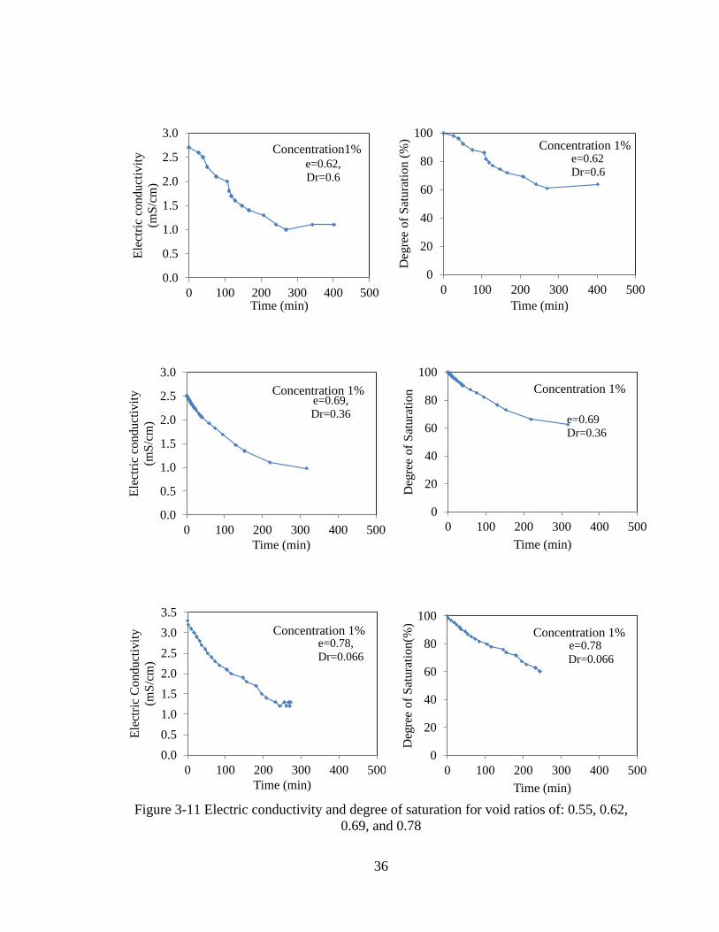
36
Figure 3-11 Electric conductivity and degree of saturation for void ratios of: 0.55, 0.62,
0.69, and 0.78
0.0
0.5
1.0
1.5
2.0
2.5
3.0
3.5
0 100 200 300 400 500
Ele
ctri
c C
onduct
ivit
y
(mS
/cm
)
Time (min)
Concentration 1%
0
20
40
60
80
100
0 100 200 300 400 500
Deg
ree
of
Sat
ura
tion(%
)
Time (min)
Concentration 1%e=0.78 Dr=0.066
e=0.78,
Dr=0.066
0
20
40
60
80
100
0 100 200 300 400 500
Deg
ree
of
Sat
ura
tion
(%
)
Time (min)
Concentration 1%
0.0
0.5
1.0
1.5
2.0
2.5
3.0
0 100 200 300 400 500
Ele
ctri
c co
nd
uct
ivit
y
(mS
/cm
)
Time (min)
Concentration1% e=0.62,
Dr=0.6
e=0.62
Dr=0.6
0.0
0.5
1.0
1.5
2.0
2.5
3.0
0 100 200 300 400 500
Ele
ctri
c co
nd
uct
ivit
y
(mS
/cm
)
Time (min)
Concentration 1%
0
20
40
60
80
100
0 100 200 300 400 500
Deg
ree
of
Sat
ura
tion
Time (min)
Concentration 1%e=0.69,
Dr=0.36 e=0.69
Dr=0.36
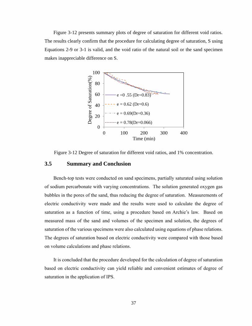
37
Figure 3-12 presents summary plots of degree of saturation for different void ratios.
The results clearly confirm that the procedure for calculating degree of saturation, S using
Equations 2-9 or 3-1 is valid, and the void ratio of the natural soil or the sand specimen
makes inappreciable difference on S.
Figure 3-12 Degree of saturation for different void ratios, and 1% concentration.
3.5 Summary and Conclusion
Bench-top tests were conducted on sand specimens, partially saturated using solution
of sodium percarbonate with varying concentrations. The solution generated oxygen gas
bubbles in the pores of the sand, thus reducing the degree of saturation. Measurements of
electric conductivity were made and the results were used to calculate the degree of
saturation as a function of time, using a procedure based on Archie’s law. Based on
measured mass of the sand and volumes of the specimen and solution, the degrees of
saturation of the various specimens were also calculated using equations of phase relations.
The degrees of saturation based on electric conductivity were compared with those based
on volume calculations and phase relations.
It is concluded that the procedure developed for the calculation of degree of saturation
based on electric conductivity can yield reliable and convenient estimates of degree of
saturation in the application of IPS.
0
20
40
60
80
100
0 100 200 300 400
Deg
ree
of
Sat
ura
tion(%
)
Time (min)
e =0 .55 (Dr=0.83)
e = 0.62 (Dr=0.6)
e = 0.69(Dr=0.36)
e = 0.78(Dr=0.066)
38
The bench-top test results of electric conductivity were also used to investigate the rate
of generation of oxygen gas using sodium percarbonate. Analysis of the data was made
assuming the rate of increase in gas bubbles, or the rate of decrease in degree of saturation
follows an exponential function defined with a rate parameter r.
It is concluded that the rate of decay of the chemical and generation of gas indeed
follows approximately an exponential function. The rate parameter, r depends on the
concentration of the solution used to generate gas in the pores of the sand specimens. The
higher the concentration, the faster is the reaction and hence the reduction in degree of
saturation.
Additional bench-top tests were conducted on specimens of sand with varying void
ratios. The specimens were partially saturated using a 1% concentration of sodium
percarbonate. The purpose of the tests was to determine if void ratio of the specimens had
an effect on the procedure for the calculation of degree of saturations based on electric
conductivity.
It is concluded that void ratio, as long as it remains constant during IPS injection, has
no appreciable effect on the calculated degree of saturation.
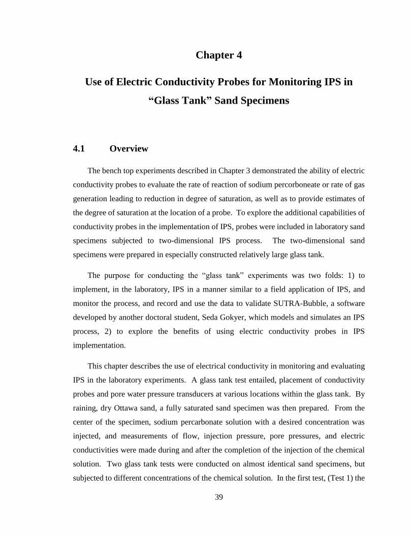
39
Chapter 4
Use of Electric Conductivity Probes for Monitoring IPS in
“Glass Tank” Sand Specimens
4.1 Overview
The bench top experiments described in Chapter 3 demonstrated the ability of electric
conductivity probes to evaluate the rate of reaction of sodium percorboneate or rate of gas
generation leading to reduction in degree of saturation, as well as to provide estimates of
the degree of saturation at the location of a probe. To explore the additional capabilities of
conductivity probes in the implementation of IPS, probes were included in laboratory sand
specimens subjected to two-dimensional IPS process. The two-dimensional sand
specimens were prepared in especially constructed relatively large glass tank.
The purpose for conducting the “glass tank” experiments was two folds: 1) to
implement, in the laboratory, IPS in a manner similar to a field application of IPS, and
monitor the process, and record and use the data to validate SUTRA-Bubble, a software
developed by another doctoral student, Seda Gokyer, which models and simulates an IPS
process, 2) to explore the benefits of using electric conductivity probes in IPS
implementation.
This chapter describes the use of electrical conductivity in monitoring and evaluating
IPS in the laboratory experiments. A glass tank test entailed, placement of conductivity
probes and pore water pressure transducers at various locations within the glass tank. By
raining, dry Ottawa sand, a fully saturated sand specimen was then prepared. From the
center of the specimen, sodium percarbonate solution with a desired concentration was
injected, and measurements of flow, injection pressure, pore pressures, and electric
conductivities were made during and after the completion of the injection of the chemical
solution. Two glass tank tests were conducted on almost identical sand specimens, but
subjected to different concentrations of the chemical solution. In the first test, (Test 1) the
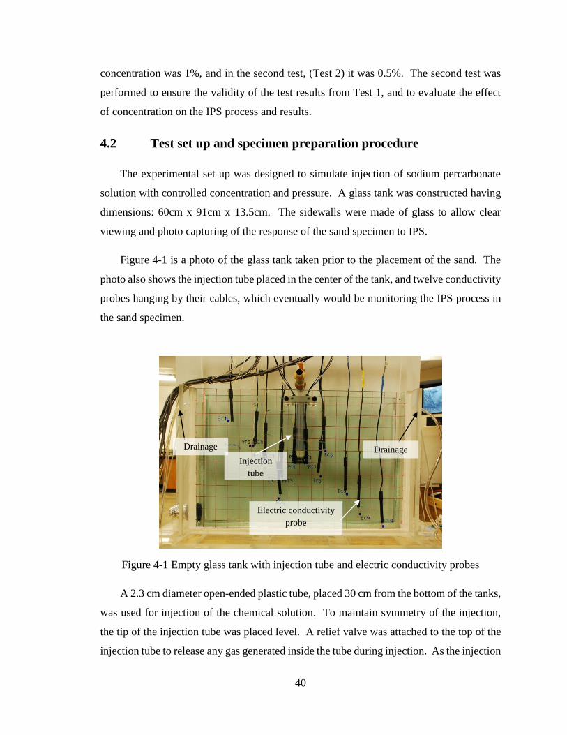
40
concentration was 1%, and in the second test, (Test 2) it was 0.5%. The second test was
performed to ensure the validity of the test results from Test 1, and to evaluate the effect
of concentration on the IPS process and results.
4.2 Test set up and specimen preparation procedure
The experimental set up was designed to simulate injection of sodium percarbonate
solution with controlled concentration and pressure. A glass tank was constructed having
dimensions: 60cm x 91cm x 13.5cm. The sidewalls were made of glass to allow clear
viewing and photo capturing of the response of the sand specimen to IPS.
Figure 4-1 is a photo of the glass tank taken prior to the placement of the sand. The
photo also shows the injection tube placed in the center of the tank, and twelve conductivity
probes hanging by their cables, which eventually would be monitoring the IPS process in
the sand specimen.
Figure 4-1 Empty glass tank with injection tube and electric conductivity probes
A 2.3 cm diameter open-ended plastic tube, placed 30 cm from the bottom of the tanks,
was used for injection of the chemical solution. To maintain symmetry of the injection,
the tip of the injection tube was placed level. A relief valve was attached to the top of the
injection tube to release any gas generated inside the tube during injection. As the injection
Drainage Drainage
Electric conductivity
probe
Injection
tube
41
duration was short in both tests (13 minutes), the amount of gas accumulated in the
injection tube was very small and the relief valve was rarely used. The tip of the injection
tube was covered with geotextile to prevent sand penetrating the tube. The electric
conductivity probes were essential components of the experiments and allowed monitoring
of the IPS process from arrival of the chemical solution to gas generation, and ultimately
estimating the degree of saturation at the probe locations. Figure 4-2 identifies the probe
numbers and their locations within the glass tank.
Figure 4-2 Electric conductivity probes in the glass tank specimen
A fully saturated sand was prepared by raining approximately 100 kg of dry Ottawa
sand (C778) into clean water placed in the glass tank. This method resulted in a very loose
fully saturated sand specimen. The void ratios of the two specimens were: 0.69 in Test 1,
and 0.72 in Test 2. Figure 4-3 shows the process of specimen preparation and the final size
of the specimen in Test 1.
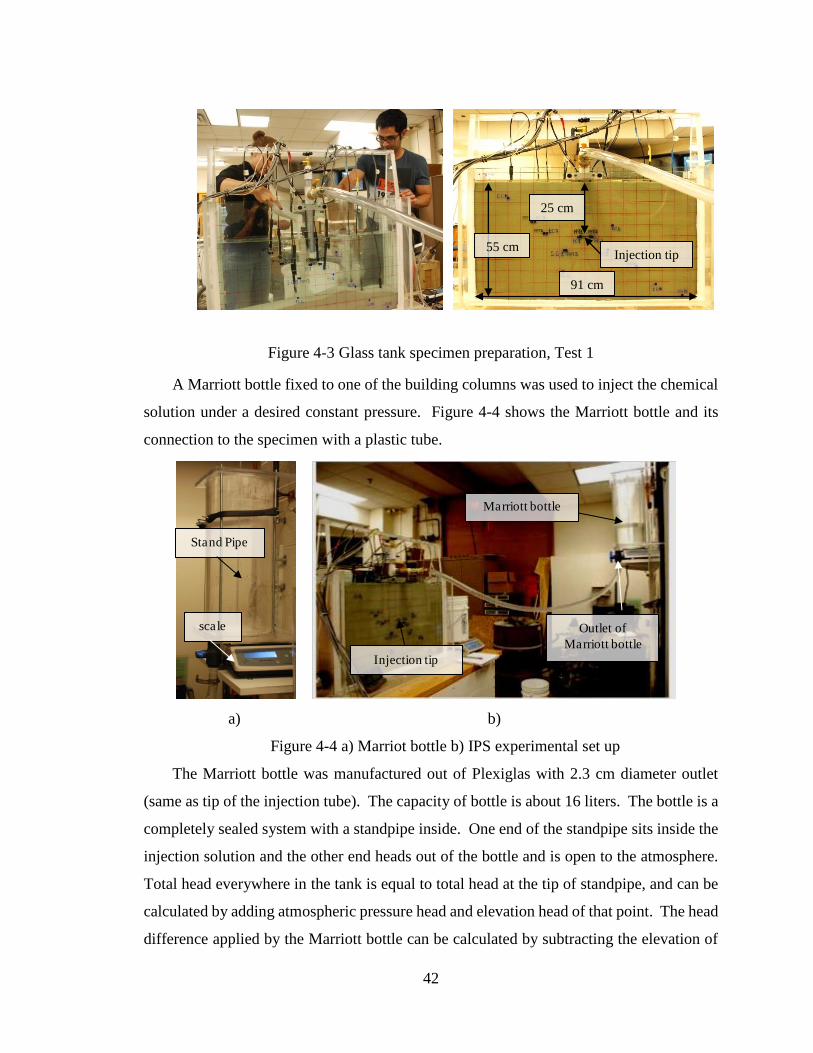
42
Figure 4-3 Glass tank specimen preparation, Test 1
A Marriott bottle fixed to one of the building columns was used to inject the chemical
solution under a desired constant pressure. Figure 4-4 shows the Marriott bottle and its
connection to the specimen with a plastic tube.
a) b)
Figure 4-4 a) Marriot bottle b) IPS experimental set up
The Marriott bottle was manufactured out of Plexiglas with 2.3 cm diameter outlet
(same as tip of the injection tube). The capacity of bottle is about 16 liters. The bottle is a
completely sealed system with a standpipe inside. One end of the standpipe sits inside the
injection solution and the other end heads out of the bottle and is open to the atmosphere.
Total head everywhere in the tank is equal to total head at the tip of standpipe, and can be
calculated by adding atmospheric pressure head and elevation head of that point. The head
difference applied by the Marriott bottle can be calculated by subtracting the elevation of
Marriott bottle
Outlet of
Marriott bottle
Injection tip
Stand Pipe
scale
25 cm
55 cm
91 cm
Injection tip
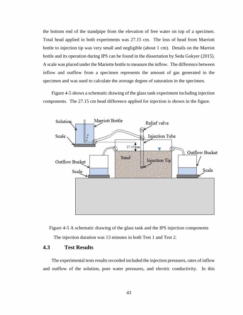
43
the bottom end of the standpipe from the elevation of free water on top of a specimen.
Total head applied in both experiments was 27.15 cm. The loss of head from Marriott
bottle to injection tip was very small and negligible (about 1 cm). Details on the Marriot
bottle and its operation during IPS can be found in the dissertation by Seda Gokyer (2015).
A scale was placed under the Mariette bottle to measure the inflow. The difference between
inflow and outflow from a specimen represents the amount of gas generated in the
specimen and was used to calculate the average degree of saturation in the specimen.
Figure 4-5 shows a schematic drawing of the glass tank experiment including injection
components. The 27.15 cm head difference applied for injection is shown in the figure.
Figure 4-5 A schematic drawing of the glass tank and the IPS injection components
The injection duration was 13 minutes in both Test 1 and Test 2.
4.3 Test Results
The experimental tests results recorded included the injection pressures, rates of inflow
and outflow of the solution, pore water pressures, and electric conductivity. In this
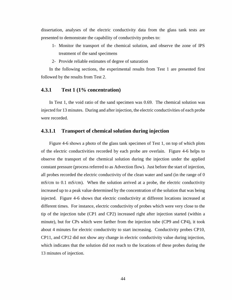
44
dissertation, analyses of the electric conductivity data from the glass tank tests are
presented to demonstrate the capability of conductivity probes to:
1- Monitor the transport of the chemical solution, and observe the zone of IPS
treatment of the sand specimens
2- Provide reliable estimates of degree of saturation
In the following sections, the experimental results from Test 1 are presented first
followed by the results from Test 2.
4.3.1 Test 1 (1% concentration)
In Test 1, the void ratio of the sand specimen was 0.69. The chemical solution was
injected for 13 minutes. During and after injection, the electric conductivities of each probe
were recorded.
4.3.1.1 Transport of chemical solution during injection
Figure 4-6 shows a photo of the glass tank specimen of Test 1, on top of which plots
of the electric conductivities recorded by each probe are overlain. Figure 4-6 helps to
observe the transport of the chemical solution during the injection under the applied
constant pressure (process referred to as Advection flow). Just before the start of injection,
all probes recorded the electric conductivity of the clean water and sand (in the range of 0
mS/cm to 0.1 mS/cm). When the solution arrived at a probe, the electric conductivity
increased up to a peak value determined by the concentration of the solution that was being
injected. Figure 4-6 shows that electric conductivity at different locations increased at
different times. For instance, electric conductivity of probes which were very close to the
tip of the injection tube (CP1 and CP2) increased right after injection started (within a
minute), but for CPs which were farther from the injection tube (CP9 and CP4), it took
about 4 minutes for electric conductivity to start increasing. Conductivity probes CP10,
CP11, and CP12 did not show any change in electric conductivity value during injection,
which indicates that the solution did not reach to the locations of these probes during the
13 minutes of injection.
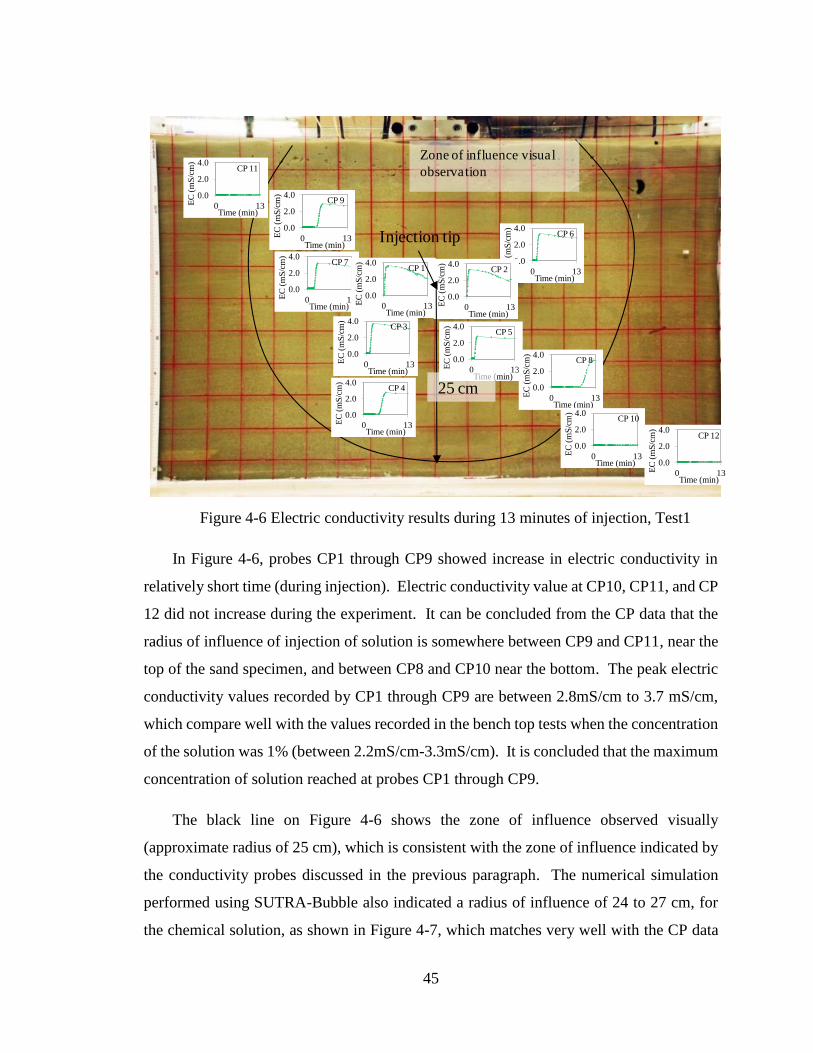
45
Figure 4-6 Electric conductivity results during 13 minutes of injection, Test1
In Figure 4-6, probes CP1 through CP9 showed increase in electric conductivity in
relatively short time (during injection). Electric conductivity value at CP10, CP11, and CP
12 did not increase during the experiment. It can be concluded from the CP data that the
radius of influence of injection of solution is somewhere between CP9 and CP11, near the
top of the sand specimen, and between CP8 and CP10 near the bottom. The peak electric
conductivity values recorded by CP1 through CP9 are between 2.8mS/cm to 3.7 mS/cm,
which compare well with the values recorded in the bench top tests when the concentration
of the solution was 1% (between 2.2mS/cm-3.3mS/cm). It is concluded that the maximum
concentration of solution reached at probes CP1 through CP9.
The black line on Figure 4-6 shows the zone of influence observed visually
(approximate radius of 25 cm), which is consistent with the zone of influence indicated by
the conductivity probes discussed in the previous paragraph. The numerical simulation
performed using SUTRA-Bubble also indicated a radius of influence of 24 to 27 cm, for
the chemical solution, as shown in Figure 4-7, which matches very well with the CP data
0.0
2.0
4.0
0 13EC
(m
S/c
m)
Time (min)
CP 3
0.0
2.0
4.0
0 13EC
(m
S/c
m)
Time (min)
CP 4
0.0
2.0
4.0
0 13EC
(m
S/c
m)
Time (min)
CP 5
0.0
2.0
4.0
0 13EC
(m
S/c
m)
Time (min)
CP 6
0.0
2.0
4.0
0 13EC
(m
S/c
m)
Time (min)
CP 2
0.0
2.0
4.0
0 13EC
(m
S/c
m)
Time (min)
CP 7
0.0
2.0
4.0
0 13EC
(m
S/c
m)
Time (min)
CP 1
0.0
2.0
4.0
0 13EC
(m
S/c
m)
Time (min)
CP 8
0.0
2.0
4.0
0 13EC
(m
S/c
m)
Time (min)
CP 9
0.0
2.0
4.0
0 13EC
(m
S/c
m)
Time (min)
CP 10
0.0
2.0
4.0
0 13EC
(m
S/c
m)
Time (min)
CP 11
0.0
2.0
4.0
0 13EC
(m
S/c
m)
Time (min)
CP 12
25 cm
Zone of influence visual
observation
Injection tip
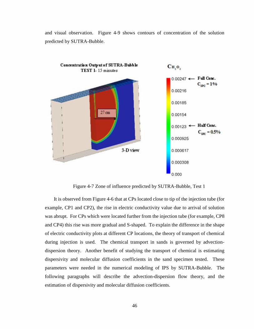
46
and visual observation. Figure 4-9 shows contours of concentration of the solution
predicted by SUTRA-Bubble.
Figure 4-7 Zone of influence predicted by SUTRA-Bubble, Test 1
It is observed from Figure 4-6 that at CPs located close to tip of the injection tube (for
example, CP1 and CP2), the rise in electric conductivity value due to arrival of solution
was abrupt. For CPs which were located further from the injection tube (for example, CP8
and CP4) this rise was more gradual and S-shaped. To explain the difference in the shape
of electric conductivity plots at different CP locations, the theory of transport of chemical
during injection is used. The chemical transport in sands is governed by advection-
dispersion theory. Another benefit of studying the transport of chemical is estimating
dispersivity and molecular diffusion coefficients in the sand specimen tested. These
parameters were needed in the numerical modeling of IPS by SUTRA-Bubble. The
following paragraphs will describe the advection-dispersion flow theory, and the
estimation of dispersivity and molecular diffusion coefficients.
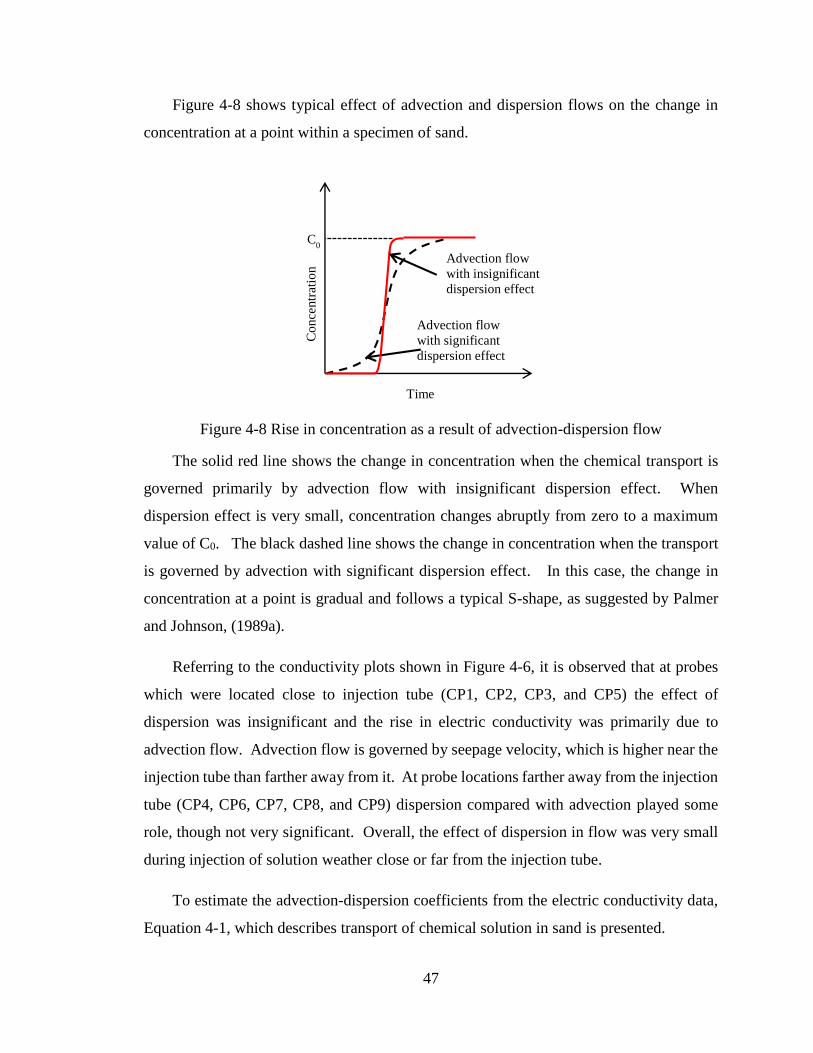
47
Figure 4-8 shows typical effect of advection and dispersion flows on the change in
concentration at a point within a specimen of sand.
Figure 4-8 Rise in concentration as a result of advection-dispersion flow
The solid red line shows the change in concentration when the chemical transport is
governed primarily by advection flow with insignificant dispersion effect. When
dispersion effect is very small, concentration changes abruptly from zero to a maximum
value of C0. The black dashed line shows the change in concentration when the transport
is governed by advection with significant dispersion effect. In this case, the change in
concentration at a point is gradual and follows a typical S-shape, as suggested by Palmer
and Johnson, (1989a).
Referring to the conductivity plots shown in Figure 4-6, it is observed that at probes
which were located close to injection tube (CP1, CP2, CP3, and CP5) the effect of
dispersion was insignificant and the rise in electric conductivity was primarily due to
advection flow. Advection flow is governed by seepage velocity, which is higher near the
injection tube than farther away from it. At probe locations farther away from the injection
tube (CP4, CP6, CP7, CP8, and CP9) dispersion compared with advection played some
role, though not very significant. Overall, the effect of dispersion in flow was very small
during injection of solution weather close or far from the injection tube.
To estimate the advection-dispersion coefficients from the electric conductivity data,
Equation 4-1, which describes transport of chemical solution in sand is presented.
C0
Co
nce
ntr
atio
n
Time
Advection flow
with insignificant
dispersion effect
Advection flow
with significant
dispersion effect
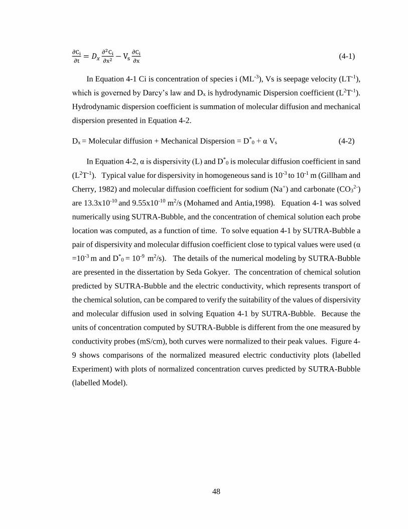
48
∂Ci
∂t= 𝐷𝑥
∂2Ci
∂x2− Vs
∂Ci
∂x (4-1)
In Equation 4-1 Ci is concentration of species i (ML-3), Vs is seepage velocity (LT-1),
which is governed by Darcy’s law and Dx is hydrodynamic Dispersion coefficient (L2T-1).
Hydrodynamic dispersion coefficient is summation of molecular diffusion and mechanical
dispersion presented in Equation 4-2.
Dx = Molecular diffusion + Mechanical Dispersion = D*0 + α Vs (4-2)
In Equation 4-2, α is dispersivity (L) and D*0 is molecular diffusion coefficient in sand
(L2T-1). Typical value for dispersivity in homogeneous sand is 10-3 to 10-1 m (Gillham and
Cherry, 1982) and molecular diffusion coefficient for sodium (Na+) and carbonate (CO32-)
are 13.3x10⁻¹⁰ and 9.55x10⁻¹⁰ m2/s (Mohamed and Antia,1998). Equation 4-1 was solved
numerically using SUTRA-Bubble, and the concentration of chemical solution each probe
location was computed, as a function of time. To solve equation 4-1 by SUTRA-Bubble a
pair of dispersivity and molecular diffusion coefficient close to typical values were used (α
=10-3 m and D*0 = 10-9 m2/s). The details of the numerical modeling by SUTRA-Bubble
are presented in the dissertation by Seda Gokyer. The concentration of chemical solution
predicted by SUTRA-Bubble and the electric conductivity, which represents transport of
the chemical solution, can be compared to verify the suitability of the values of dispersivity
and molecular diffusion used in solving Equation 4-1 by SUTRA-Bubble. Because the
units of concentration computed by SUTRA-Bubble is different from the one measured by
conductivity probes (mS/cm), both curves were normalized to their peak values. Figure 4-
9 shows comparisons of the normalized measured electric conductivity plots (labelled
Experiment) with plots of normalized concentration curves predicted by SUTRA-Bubble
(labelled Model).
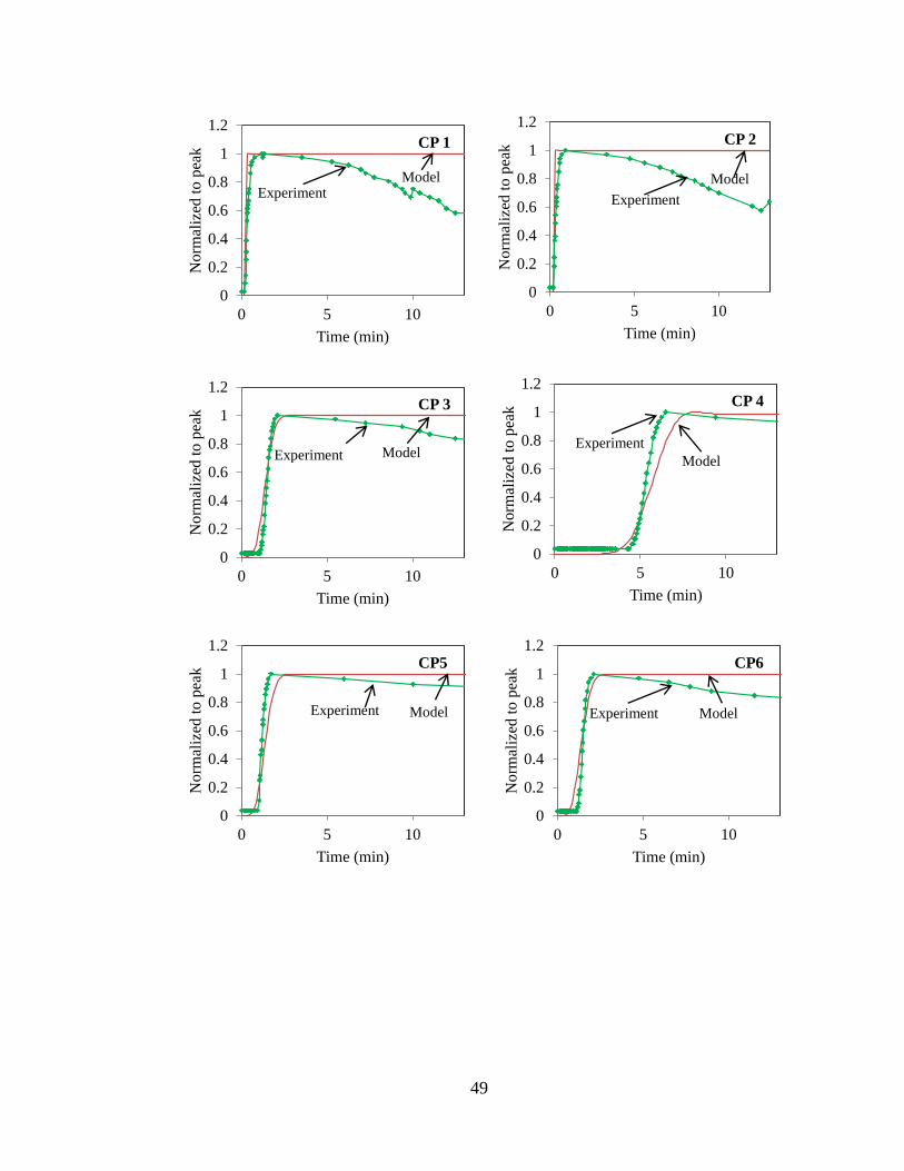
49
0
0.2
0.4
0.6
0.8
1
1.2
0 5 10
Norm
aliz
ed t
o p
eak
Time (min)
CP 1
Experiment Model
0
0.2
0.4
0.6
0.8
1
1.2
0 5 10
Norm
aliz
ed t
o p
eak
Time (min)
CP 2
Experiment
Model
0
0.2
0.4
0.6
0.8
1
1.2
0 5 10
Norm
aliz
ed t
o p
eak
Time (min)
CP 3
Experiment Model
0
0.2
0.4
0.6
0.8
1
1.2
0 5 10
Norm
aliz
ed t
o p
eak
Time (min)
CP 4
Model
Experiment
0
0.2
0.4
0.6
0.8
1
1.2
0 5 10
No
rmal
ized
to
pea
k
Time (min)
CP5
Experiment Model
0
0.2
0.4
0.6
0.8
1
1.2
0 5 10
Norm
aliz
ed t
o p
eak
Time (min)
CP6
Experiment Model
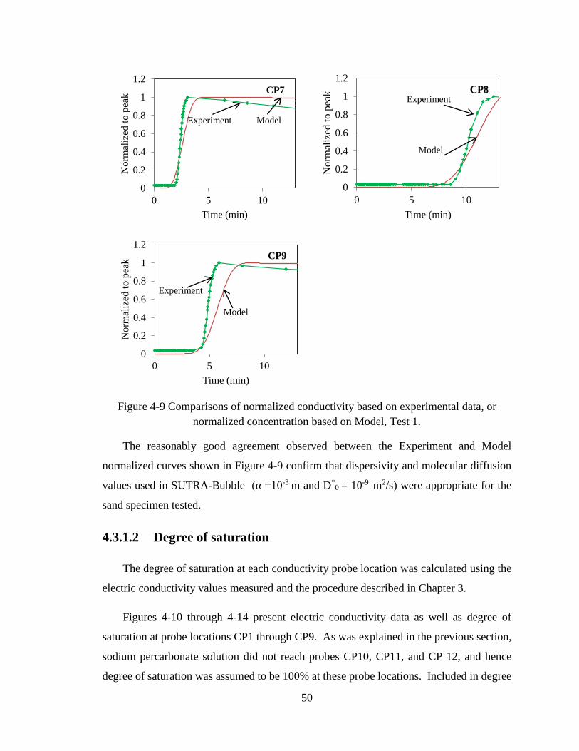
50
Figure 4-9 Comparisons of normalized conductivity based on experimental data, or
normalized concentration based on Model, Test 1.
The reasonably good agreement observed between the Experiment and Model
normalized curves shown in Figure 4-9 confirm that dispersivity and molecular diffusion
values used in SUTRA-Bubble (α =10-3 m and D*0 = 10-9 m2/s) were appropriate for the
sand specimen tested.
4.3.1.2 Degree of saturation
The degree of saturation at each conductivity probe location was calculated using the
electric conductivity values measured and the procedure described in Chapter 3.
Figures 4-10 through 4-14 present electric conductivity data as well as degree of
saturation at probe locations CP1 through CP9. As was explained in the previous section,
sodium percarbonate solution did not reach probes CP10, CP11, and CP 12, and hence
degree of saturation was assumed to be 100% at these probe locations. Included in degree
0
0.2
0.4
0.6
0.8
1
1.2
0 5 10
Norm
aliz
ed t
o p
eak
Time (min)
CP7
Experiment Model
0
0.2
0.4
0.6
0.8
1
1.2
0 5 10
No
rmali
zed
to
peak
Time (min)
CP8
Model
Experiment
0
0.2
0.4
0.6
0.8
1
1.2
0 5 10
Norm
aliz
ed t
o p
eak
Time (min)
CP9
Experiment
Model
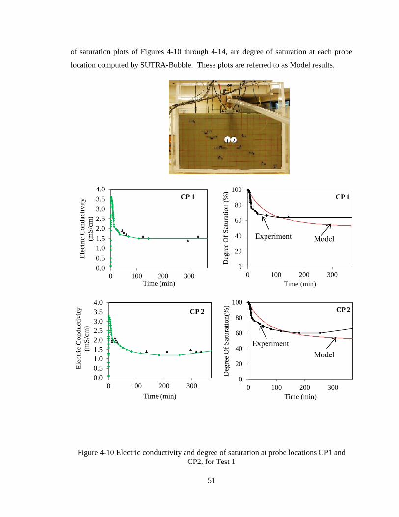
51
of saturation plots of Figures 4-10 through 4-14, are degree of saturation at each probe
location computed by SUTRA-Bubble. These plots are referred to as Model results.
Figure 4-10 Electric conductivity and degree of saturation at probe locations CP1 and
CP2, for Test 1
0.0
0.5
1.0
1.5
2.0
2.5
3.0
3.5
4.0
0 100 200 300
Ele
ctri
c C
on
du
ctiv
ity
(mS
/cm
)
Time (min)
CP 1
0
20
40
60
80
100
0 100 200 300
Deg
ree
Of
Sat
ura
tion (
%)
Time (min)
CP 1
Model Experiment
0.0
0.5
1.0
1.5
2.0
2.5
3.0
3.5
4.0
0 100 200 300
Ele
ctri
c C
on
du
ctiv
ity
(mS
/cm
)
Time (min)
CP 2
0
20
40
60
80
100
0 100 200 300
Deg
ree
Of
Sat
ura
tion(%
)
Time (min)
CP 2
Model
Experiment
2 1
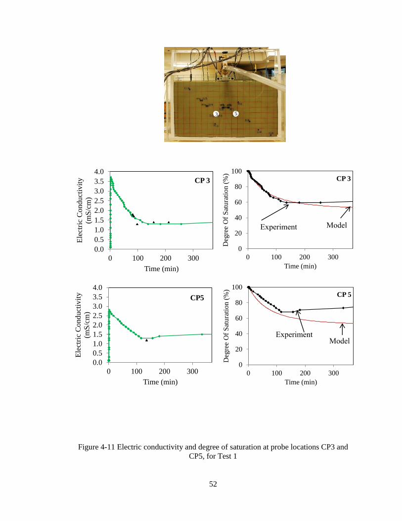
52
Figure 4-11 Electric conductivity and degree of saturation at probe locations CP3 and
CP5, for Test 1
0.0
0.5
1.0
1.5
2.0
2.5
3.0
3.5
4.0
0 100 200 300
Ele
ctri
c C
on
du
ctiv
ity
(mS
/cm
)
Time (min)
CP5
0.0
0.5
1.0
1.5
2.0
2.5
3.0
3.5
4.0
0 100 200 300
Ele
ctri
c C
on
du
ctiv
ity
(mS
/cm
)
Time (min)
CP 3
0
20
40
60
80
100
0 100 200 300
Deg
ree
Of
Sat
ura
tion (
%)
Time (min)
CP 3
Experiment Model
0
20
40
60
80
100
0 100 200 300
Deg
ree
Of
Sat
ura
tion (
%)
Time (min)
CP 5
Experiment Model
5
3
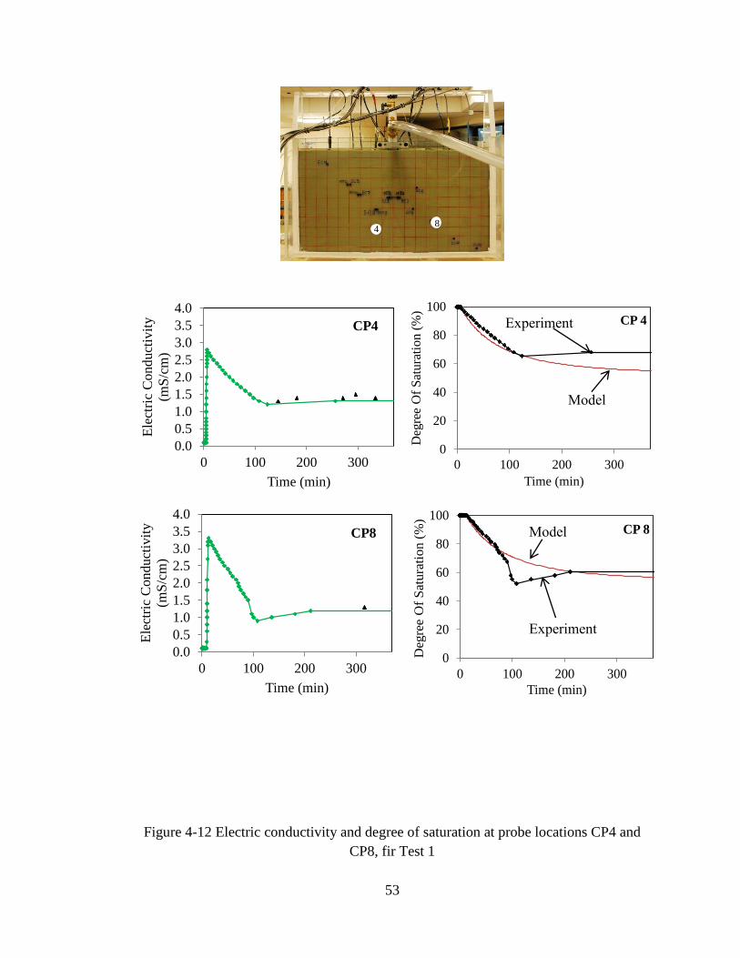
53
Figure 4-12 Electric conductivity and degree of saturation at probe locations CP4 and
CP8, fir Test 1
0.0
0.5
1.0
1.5
2.0
2.5
3.0
3.5
4.0
0 100 200 300
Ele
ctri
c C
on
du
ctiv
ity
(mS
/cm
)
Time (min)
CP4
0
20
40
60
80
100
0 100 200 300
Deg
ree
Of
Sat
ura
tion (
%)
Time (min)
CP 4Experiment
Model
0.0
0.5
1.0
1.5
2.0
2.5
3.0
3.5
4.0
0 100 200 300
Ele
ctri
c C
on
du
ctiv
ity
(mS
/cm
)
Time (min)
CP8
0
20
40
60
80
100
0 100 200 300
Deg
ree
Of
Sat
ura
tion (
%)
Time (min)
CP 8
Experiment
Model
8
4

54
Figure 4-13 Electric conductivity and degree of saturation at probe locations CP6 and
CP7, for Test 1
0.0
0.5
1.0
1.5
2.0
2.5
3.0
3.5
4.0
0 100 200 300
Ele
ctri
c C
onduct
ivit
y
(mS
/cm
)
Time (min)
CP6
0
20
40
60
80
100
0 100 200 300
Deg
ree
Of
Sat
ura
tion (
%)
Time (min)
CP 6
Experiment Model
0.0
0.5
1.0
1.5
2.0
2.5
3.0
3.5
4.0
0 100 200 300
Ele
ctri
c C
on
du
ctiv
ity
(mS
/cm
)
Time (min)
CP7
0
20
40
60
80
100
0 100 200 300
Degre
e O
f S
atu
rati
on (
%)
Time (min)
CP 7
Experiment Model
6
7
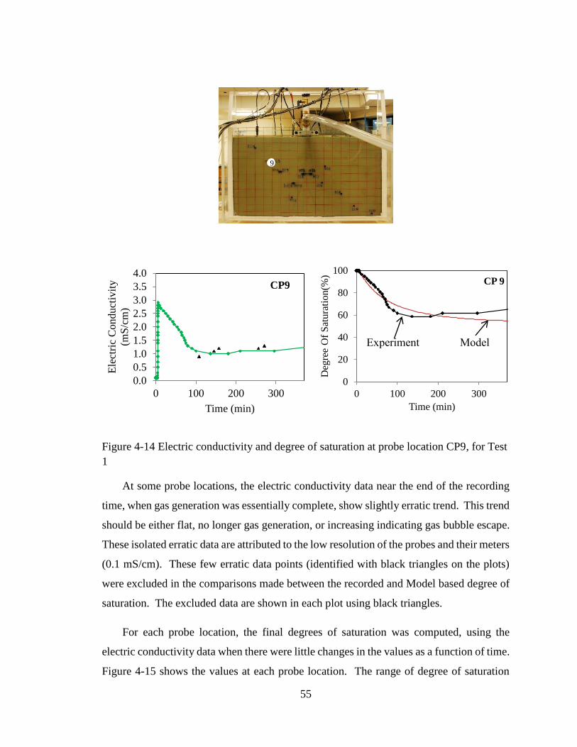
55
Figure 4-14 Electric conductivity and degree of saturation at probe location CP9, for Test
1
At some probe locations, the electric conductivity data near the end of the recording
time, when gas generation was essentially complete, show slightly erratic trend. This trend
should be either flat, no longer gas generation, or increasing indicating gas bubble escape.
These isolated erratic data are attributed to the low resolution of the probes and their meters
(0.1 mS/cm). These few erratic data points (identified with black triangles on the plots)
were excluded in the comparisons made between the recorded and Model based degree of
saturation. The excluded data are shown in each plot using black triangles.
For each probe location, the final degrees of saturation was computed, using the
electric conductivity data when there were little changes in the values as a function of time.
Figure 4-15 shows the values at each probe location. The range of degree of saturation
0.0
0.5
1.0
1.5
2.0
2.5
3.0
3.5
4.0
0 100 200 300
Ele
ctri
c C
on
du
ctiv
ity
(mS
/cm
)
Time (min)
CP9
0
20
40
60
80
100
0 100 200 300
Deg
ree
Of
Sat
ura
tion(%
)
Time (min)
CP 9
Experiment Model
9
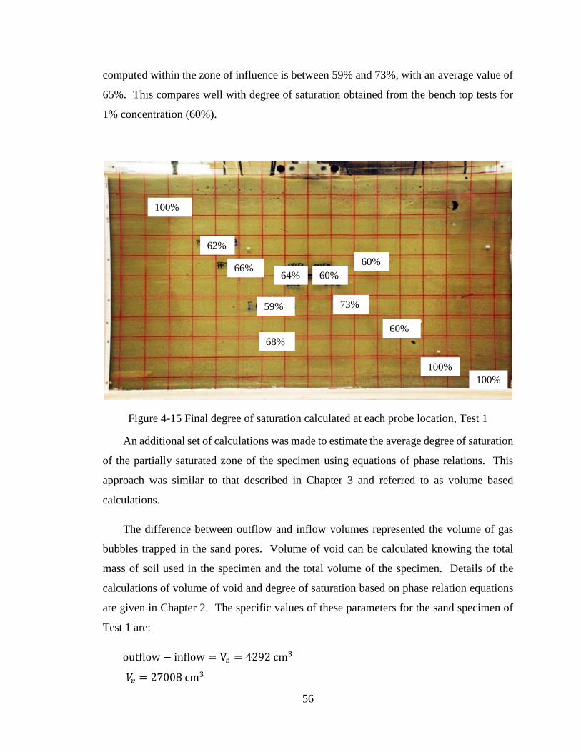
56
computed within the zone of influence is between 59% and 73%, with an average value of
65%. This compares well with degree of saturation obtained from the bench top tests for
1% concentration (60%).
Figure 4-15 Final degree of saturation calculated at each probe location, Test 1
An additional set of calculations was made to estimate the average degree of saturation
of the partially saturated zone of the specimen using equations of phase relations. This
approach was similar to that described in Chapter 3 and referred to as volume based
calculations.
The difference between outflow and inflow volumes represented the volume of gas
bubbles trapped in the sand pores. Volume of void can be calculated knowing the total
mass of soil used in the specimen and the total volume of the specimen. Details of the
calculations of volume of void and degree of saturation based on phase relation equations
are given in Chapter 2. The specific values of these parameters for the sand specimen of
Test 1 are:
outflow − inflow = Va = 4292 cm3
𝑉𝑣 = 27008 cm3
64% 60%
59%
68%
73%
60% 66%
60%
62%
100%
100%
100%
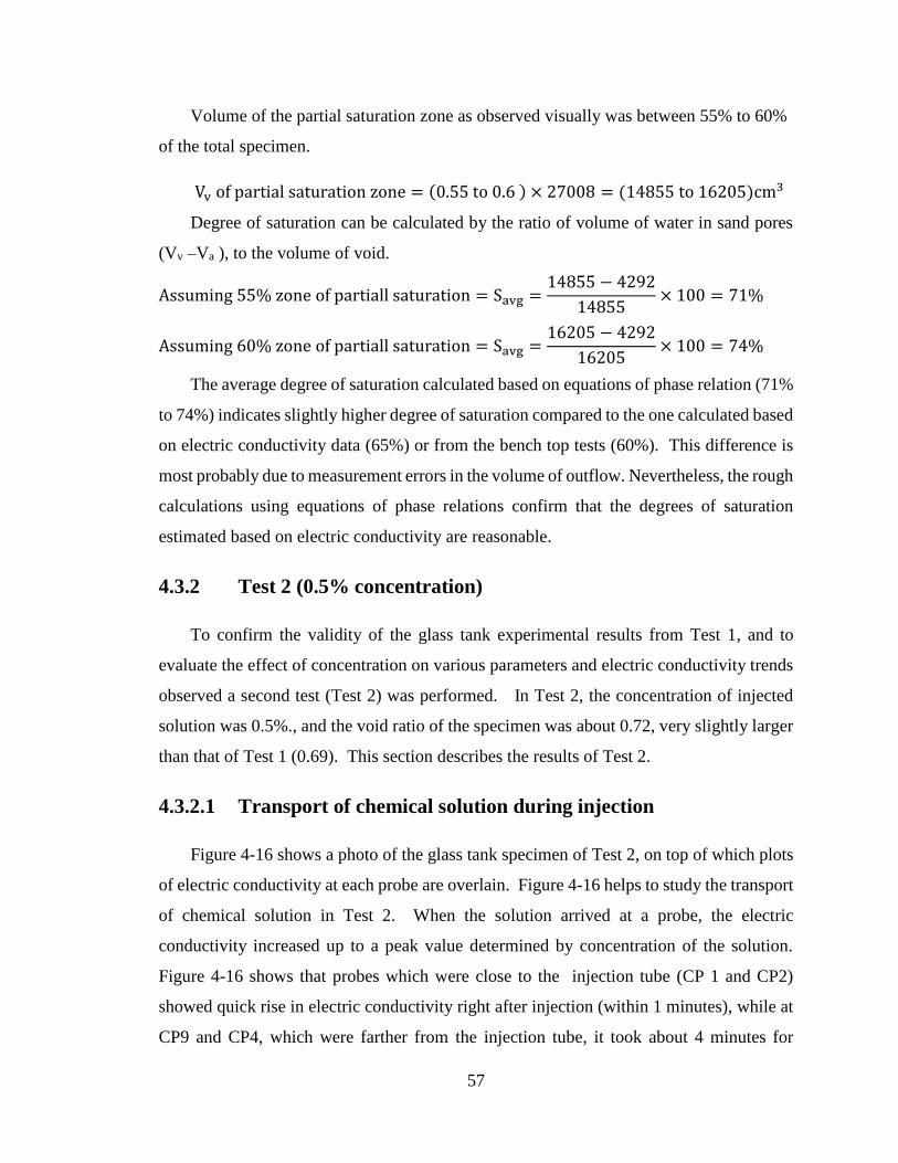
57
Volume of the partial saturation zone as observed visually was between 55% to 60%
of the total specimen.
Vv of partial saturation zone = (0.55 to 0.6 ) × 27008 = (14855 to 16205)cm3
Degree of saturation can be calculated by the ratio of volume of water in sand pores
(Vv –Va ), to the volume of void.
Assuming 55% zone of partiall saturation = Savg =14855 − 4292
14855× 100 = 71%
Assuming 60% zone of partiall saturation = Savg =16205 − 4292
16205× 100 = 74%
The average degree of saturation calculated based on equations of phase relation (71%
to 74%) indicates slightly higher degree of saturation compared to the one calculated based
on electric conductivity data (65%) or from the bench top tests (60%). This difference is
most probably due to measurement errors in the volume of outflow. Nevertheless, the rough
calculations using equations of phase relations confirm that the degrees of saturation
estimated based on electric conductivity are reasonable.
4.3.2 Test 2 (0.5% concentration)
To confirm the validity of the glass tank experimental results from Test 1, and to
evaluate the effect of concentration on various parameters and electric conductivity trends
observed a second test (Test 2) was performed. In Test 2, the concentration of injected
solution was 0.5%., and the void ratio of the specimen was about 0.72, very slightly larger
than that of Test 1 (0.69). This section describes the results of Test 2.
4.3.2.1 Transport of chemical solution during injection
Figure 4-16 shows a photo of the glass tank specimen of Test 2, on top of which plots
of electric conductivity at each probe are overlain. Figure 4-16 helps to study the transport
of chemical solution in Test 2. When the solution arrived at a probe, the electric
conductivity increased up to a peak value determined by concentration of the solution.
Figure 4-16 shows that probes which were close to the injection tube (CP 1 and CP2)
showed quick rise in electric conductivity right after injection (within 1 minutes), while at
CP9 and CP4, which were farther from the injection tube, it took about 4 minutes for
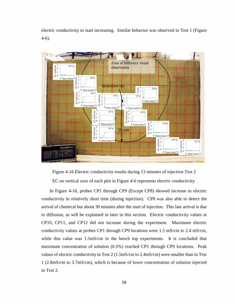
58
electric conductivity to start increasing. Similar behavior was observed in Test 1 (Figure
4-6).
Figure 4-16 Electric conductivity results during 13 minutes of injection Test 2
EC on vertical axes of each plot in Figure 4-6 represents electric conductivity.
In Figure 4-16, probes CP1 through CP9 (Except CP8) showed increase in electric
conductivity in relatively short time (during injection). CP8 was also able to detect the
arrival of chemical but about 30 minutes after the start of injection. This late arrival is due
to diffusion, as will be explained in later in this section. Electric conductivity values at
CP10, CP11, and CP12 did not increase during the experiment. Maximum electric
conductivity values at probes CP1 through CP9 locations were 1.5 mS/cm to 2.4 mS/cm,
while this value was 1.5mS/cm in the bench top experiments. It is concluded that
maximum concentration of solution (0.5%) reached CP1 through CP9 locations. Peak
values of electric conductivity in Test 2 (1.5mS/cm to 2.4mS/cm) were smaller than in Test
1 (2.8mS/cm to 3.7mS/cm), which is because of lower concentration of solution injected
in Test 2.
Zone of influence visual
observation
0
1
2
3
0 13
EC
(m
S/c
m)
Time (min)
CP 3
0
1
2
3
0 13
EC
(m
S/c
m)
Time (min)
CP 4
0
1
2
3
0 13E
C (
mS
/cm
)Time (min)
CP 5
0
1
2
3
0 13
EC
(m
S/c
m)
Time (min)
CP 6
0
1
2
3
0 13
EC
(m
S/c
m)
Time (min)
CP 2
0
1
2
3
0 13
EC
(m
S/c
m)
Time (min)
CP 7
0
1
2
3
0 13
EC
(m
S/c
m)
Time (min)
CP 1
0
1
2
3
0 13
EC
(m
S/c
m)
Time (min)
CP 8
0
1
2
3
0 13
EC
(m
S/c
m)
Time (min)
CP 9
0
1
2
3
0 13
EC
(m
S/c
m)
Time (min)
CP 10
0
1
2
3
0 13
EC
(m
S/c
m)
Time (min)
CP 11
0
1
2
3
0 13
EC
(m
S/c
m)
Time (min)
CP 12
Injection tip
20 cm
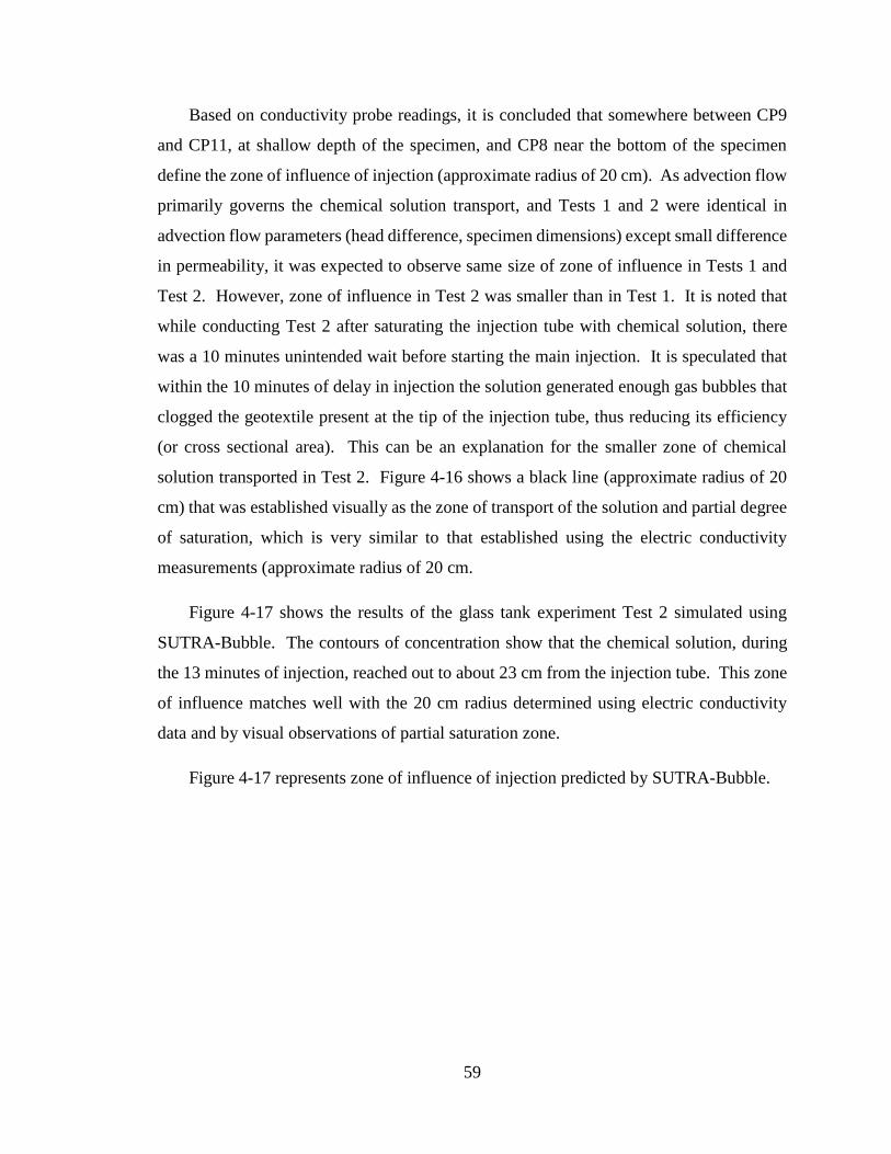
59
Based on conductivity probe readings, it is concluded that somewhere between CP9
and CP11, at shallow depth of the specimen, and CP8 near the bottom of the specimen
define the zone of influence of injection (approximate radius of 20 cm). As advection flow
primarily governs the chemical solution transport, and Tests 1 and 2 were identical in
advection flow parameters (head difference, specimen dimensions) except small difference
in permeability, it was expected to observe same size of zone of influence in Tests 1 and
Test 2. However, zone of influence in Test 2 was smaller than in Test 1. It is noted that
while conducting Test 2 after saturating the injection tube with chemical solution, there
was a 10 minutes unintended wait before starting the main injection. It is speculated that
within the 10 minutes of delay in injection the solution generated enough gas bubbles that
clogged the geotextile present at the tip of the injection tube, thus reducing its efficiency
(or cross sectional area). This can be an explanation for the smaller zone of chemical
solution transported in Test 2. Figure 4-16 shows a black line (approximate radius of 20
cm) that was established visually as the zone of transport of the solution and partial degree
of saturation, which is very similar to that established using the electric conductivity
measurements (approximate radius of 20 cm.
Figure 4-17 shows the results of the glass tank experiment Test 2 simulated using
SUTRA-Bubble. The contours of concentration show that the chemical solution, during
the 13 minutes of injection, reached out to about 23 cm from the injection tube. This zone
of influence matches well with the 20 cm radius determined using electric conductivity
data and by visual observations of partial saturation zone.
Figure 4-17 represents zone of influence of injection predicted by SUTRA-Bubble.
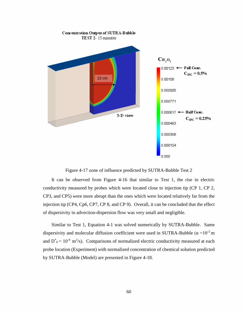
60
Figure 4-17 zone of influence predicted by SUTRA-Bubble Test 2
It can be observed from Figure 4-16 that similar to Test 1, the rise in electric
conductivity measured by probes which were located close to injection tip (CP 1, CP 2,
CP3, and CP5) were more abrupt than the ones which were located relatively far from the
injection tip (CP4, Cp6, CP7, CP 8, and CP 9). Overall, it can be concluded that the effect
of dispersivity in advection-dispersion flow was very small and negligible.
Similar to Test 1, Equation 4-1 was solved numerically by SUTRA-Bubble. Same
dispersivity and molecular diffusion coefficient were used in SUTRA-Bubble (α =10-3 m
and D*0 = 10-9 m2/s). Comparisons of normalized electric conductivity measured at each
probe location (Experiment) with normalized concentration of chemical solution predicted
by SUTRA-Bubble (Model) are presented in Figure 4-18.
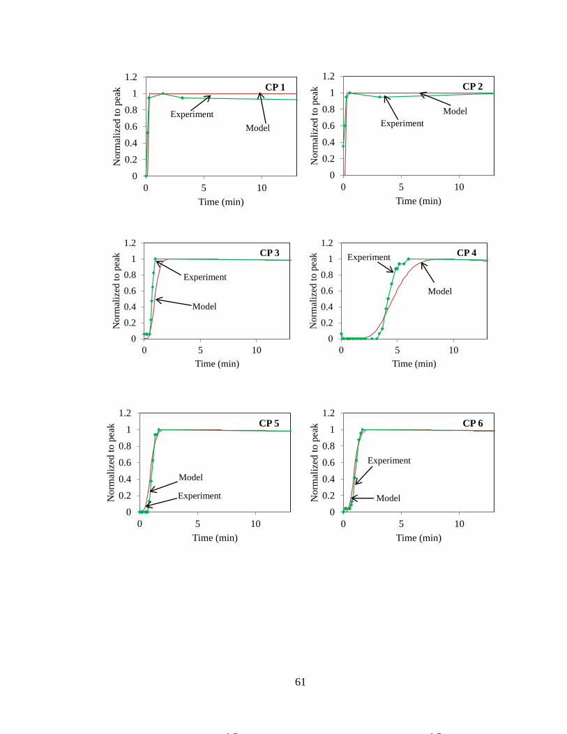
61
0
0.2
0.4
0.6
0.8
1
1.2
0 5 10
Norm
aliz
ed t
o p
eak
Time (min)
CP 1
Experiment
Model
0
0.2
0.4
0.6
0.8
1
1.2
0 5 10
No
rmal
ized
to
pea
k
Time (min)
CP 2
Experiment
Model
0
0.2
0.4
0.6
0.8
1
1.2
0 5 10
No
rmal
ized
to
pea
k
Time (min)
CP 3
Experiment
Model
0
0.2
0.4
0.6
0.8
1
1.2
0 5 10
Norm
aliz
ed t
o p
eak
Time (min)
CP 4
Model
Experiment
0
0.2
0.4
0.6
0.8
1
1.2
0 5 10
Norm
aliz
ed t
o p
eak
Time (min)
CP 6
0
0.2
0.4
0.6
0.8
1
1.2
0 5 10
No
rmal
ized
to
pea
k
Time (min)
CP 5
0
0.2
0.4
0.6
0.8
1
1.2
0 5 10
Norm
aliz
ed t
o p
eak
Time (min)
CP 6
Experiment
Model
0
0.2
0.4
0.6
0.8
1
1.2
0 5 10
No
rmal
ized
to
pea
k
Time (min)
CP 5
Model
Experiment
62
Figure 4-18 Comparisons of normalized conductivity based on experimental data, or
normalized concentration based on Model, Test 2.
The agreements between the Experimental and Model results are good except for CP8.
Figure 4-19 shows the data for CP8 for longer duration, up to 150 minutes.
0
0.2
0.4
0.6
0.8
1
1.2
0 5 10
No
rmal
ized
to
pea
k
Time (min)
CP 7
Experiment
Model
0
0.2
0.4
0.6
0.8
1
1.2
0 5 10
Norm
aliz
ed t
o p
eak
Time (min)
CP 8
Experiment
Model
0
0.2
0.4
0.6
0.8
1
1.2
0 5 10
Norm
aliz
ed t
o p
eak
Time (min)
CP 9
Model
Experiment
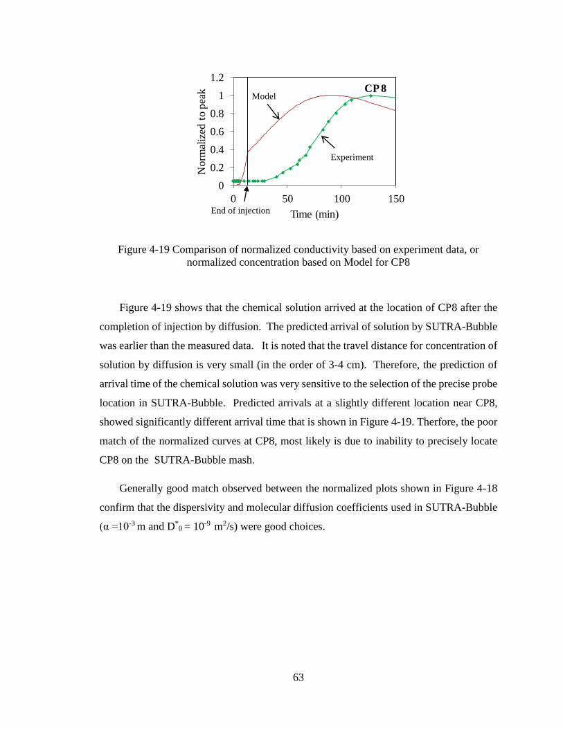
63
Figure 4-19 Comparison of normalized conductivity based on experiment data, or
normalized concentration based on Model for CP8
Figure 4-19 shows that the chemical solution arrived at the location of CP8 after the
completion of injection by diffusion. The predicted arrival of solution by SUTRA-Bubble
was earlier than the measured data. It is noted that the travel distance for concentration of
solution by diffusion is very small (in the order of 3-4 cm). Therefore, the prediction of
arrival time of the chemical solution was very sensitive to the selection of the precise probe
location in SUTRA-Bubble. Predicted arrivals at a slightly different location near CP8,
showed significantly different arrival time that is shown in Figure 4-19. Therfore, the poor
match of the normalized curves at CP8, most likely is due to inability to precisely locate
CP8 on the SUTRA-Bubble mash.
Generally good match observed between the normalized plots shown in Figure 4-18
confirm that the dispersivity and molecular diffusion coefficients used in SUTRA-Bubble
(α =10-3 m and D*0 = 10-9 m2/s) were good choices.
0
0.2
0.4
0.6
0.8
1
1.2
0 50 100 150N
orm
aliz
ed t
o p
eak
Time (min)
CP 8
End of injection
Experiment
Model
64
4.3.2.2 Degree of saturation
Similar to Test 1, the degree of saturation at each conductivity probe location was
calculated using the electric conductivity values measured and the procedure described in
Chapter 3.
This section describes degree of saturation calculated based on electric conductivity
values for Tests 2. Figures 4-20 through 4-24 present electric conductivity data as well as
degree of saturation for probe locations CP1 through CP9. As it was explained in the
previous section, the chemical solution did not reach probes CP10, CP11, and CP12, and
therefore degree of saturation was assumed 100 % at these probe locations. In Figures 4-
20 through 4-24, degree of saturation computed by SUTRA-Bubble at each probe location
are included. These plots are referred to as Model results.
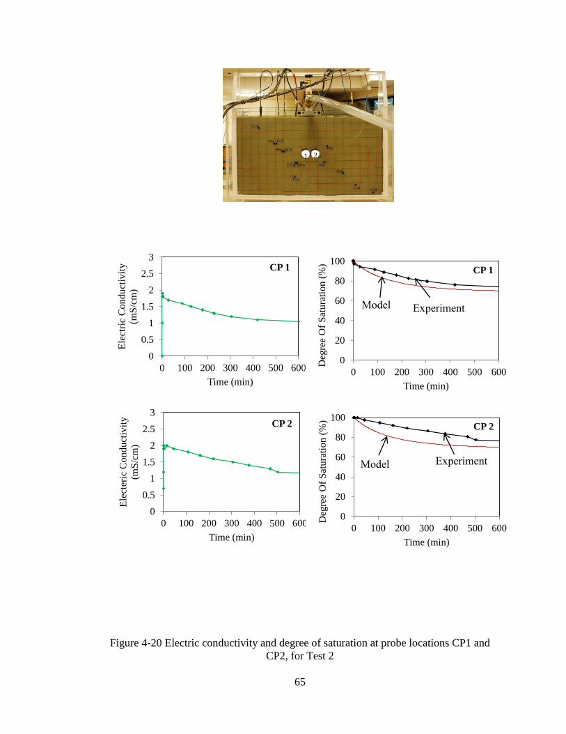
65
Figure 4-20 Electric conductivity and degree of saturation at probe locations CP1 and
CP2, for Test 2
0
0.5
1
1.5
2
2.5
3
0 100 200 300 400 500 600
Ele
cter
ic C
on
du
ctiv
ity
(mS
/cm
)
Time (min)
CP 2
0
0.5
1
1.5
2
2.5
3
0 100 200 300 400 500 600
Ele
ctri
c C
on
du
ctiv
ity
(mS
/cm
)
Time (min)
CP 1
0
20
40
60
80
100
0 100 200 300 400 500 600
Deg
ree
Of
Sat
ura
tion (
%)
Time (min)
CP 1
Experiment Model
0
20
40
60
80
100
0 100 200 300 400 500 600
Deg
ree
Of
Sat
ura
tio
n (
%)
Time (min)
CP 2
Experiment Model
2 1
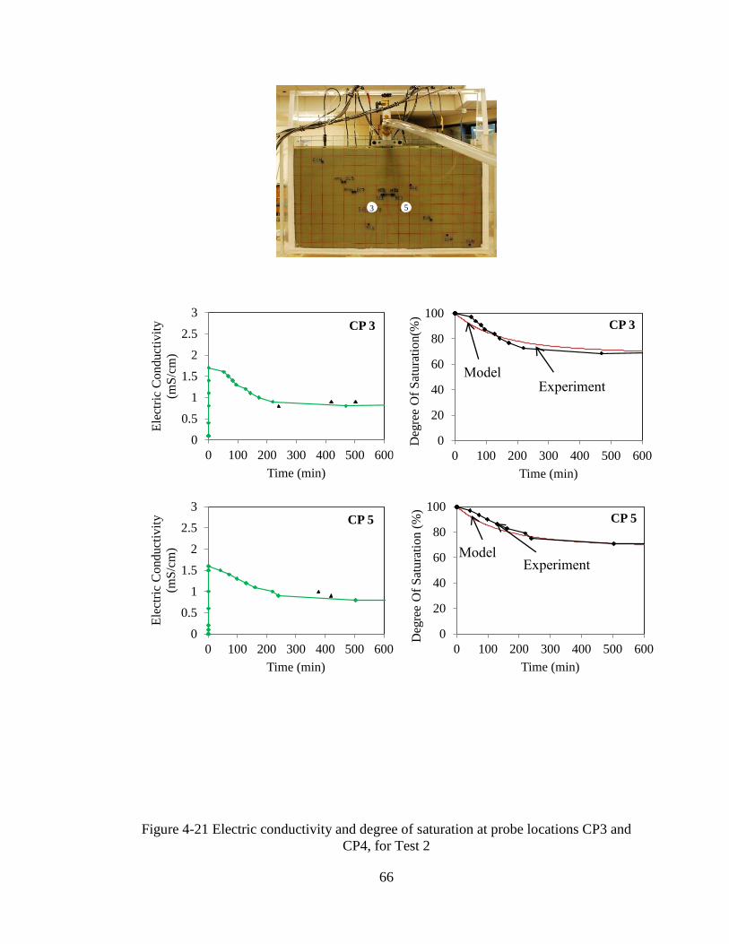
66
Figure 4-21 Electric conductivity and degree of saturation at probe locations CP3 and
CP4, for Test 2
0
0.5
1
1.5
2
2.5
3
0 100 200 300 400 500 600
Ele
ctri
c C
onduct
ivit
y
(mS
/cm
)
Time (min)
CP 3
0
0.5
1
1.5
2
2.5
3
0 100 200 300 400 500 600
Ele
ctri
c C
onduct
ivit
y
(mS
/cm
)
Time (min)
CP 5
0
20
40
60
80
100
0 100 200 300 400 500 600
Deg
ree
Of
Sat
ura
tion(%
)
Time (min)
CP 3
Experiment Model
0
20
40
60
80
100
0 100 200 300 400 500 600
Deg
ree
Of
Sat
ura
tio
n (
%)
Time (min)
CP 5
Experiment Model
5 3

67
Figure 4-22 Electric conductivity and degree of saturation at probe locations CP4 and
CP8, for Test 2
0
0.5
1
1.5
2
2.5
3
0 100 200 300 400 500 600
Ele
ctri
c C
on
du
ctiv
ity
(mS
/cm
)
Time (min)
CP 4
0
0.5
1
1.5
2
2.5
3
0 100 200 300 400 500 600
Ele
ctri
c C
on
du
ctiv
ity
(mS
/cm
)
Time (min)
CP 8
0
20
40
60
80
100
0 100 200 300 400 500 600
Deg
ree
Of
Sat
ura
tion (
%)
Time (min)
CP 4
Experiment
Model
0
20
40
60
80
100
0 100 200 300 400 500 600
Deg
ree
Of
Sat
ura
tio
n (
%)
Time (min)
CP 8
Experiment Model
8
4

68
Figure 4-23 Electric conductivity and degree of saturation at probe locations CP6 and
CP7, for Test 2
0
0.5
1
1.5
2
2.5
3
0 100 200 300 400 500 600
Ele
ctri
c C
on
du
ctiv
ity
(mS
/cm
)
Time (min)
CP 6
0
0.5
1
1.5
2
2.5
3
0 100 200 300 400 500 600
Ele
ctri
c C
on
du
ctiv
ity
(mS
/cm
)
Time (min)
CP 7
0
20
40
60
80
100
0 100 200 300 400 500 600
Deg
ree
Of
Sat
ura
tio
n (
%)
Time (min)
CP 6
Experiment
Model
0
20
40
60
80
100
0 100 200 300 400 500 600
Deg
ree
Of
Sat
ura
tio
n (
%)
Time (min)
CP 7
Experiment
Model
6
7
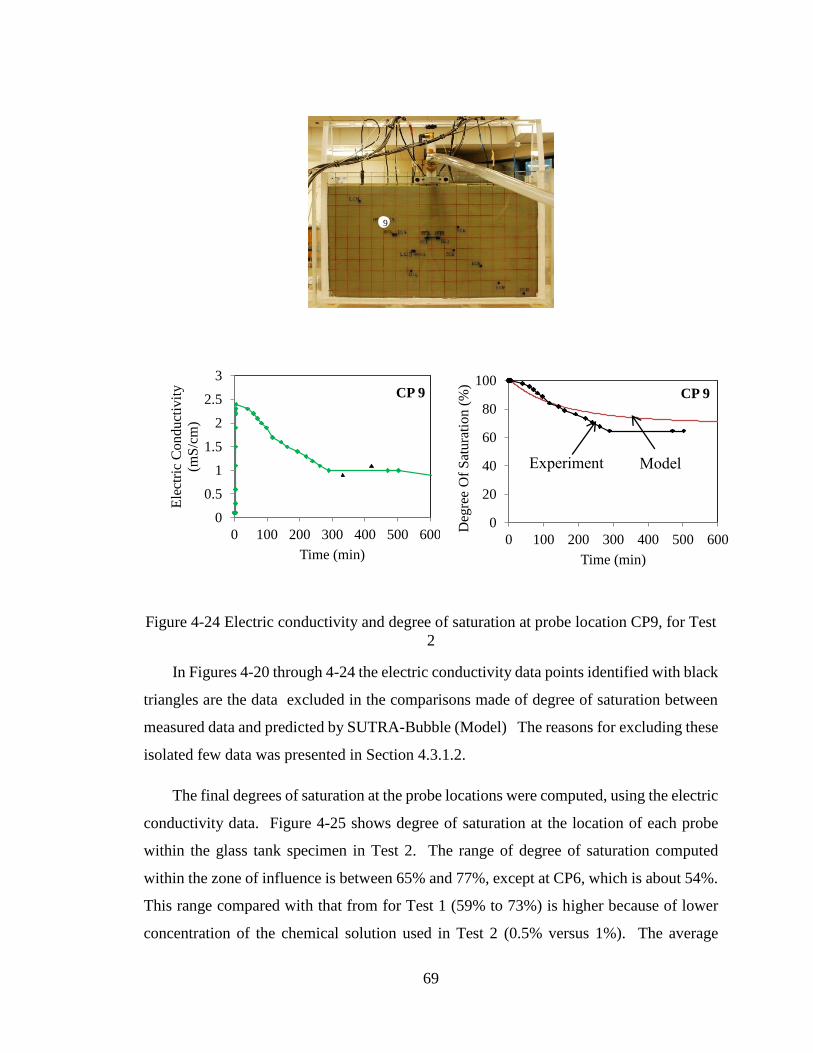
69
Figure 4-24 Electric conductivity and degree of saturation at probe location CP9, for Test
2
In Figures 4-20 through 4-24 the electric conductivity data points identified with black
triangles are the data excluded in the comparisons made of degree of saturation between
measured data and predicted by SUTRA-Bubble (Model) The reasons for excluding these
isolated few data was presented in Section 4.3.1.2.
The final degrees of saturation at the probe locations were computed, using the electric
conductivity data. Figure 4-25 shows degree of saturation at the location of each probe
within the glass tank specimen in Test 2. The range of degree of saturation computed
within the zone of influence is between 65% and 77%, except at CP6, which is about 54%.
This range compared with that from for Test 1 (59% to 73%) is higher because of lower
concentration of the chemical solution used in Test 2 (0.5% versus 1%). The average
0
0.5
1
1.5
2
2.5
3
0 100 200 300 400 500 600
Ele
ctri
c C
on
du
ctiv
ity
(mS
/cm
)
Time (min)
CP 9
0
20
40
60
80
100
0 100 200 300 400 500 600
Deg
ree
Of
Sat
ura
tion (
%)
Time (min)
CP 9
Experiment Model
9
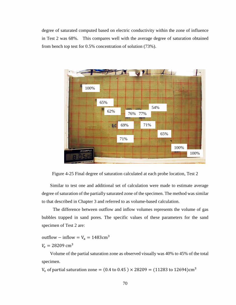
70
degree of saturated computed based on electric conductivity within the zone of influence
in Test 2 was 68%. This compares well with the average degree of saturation obtained
from bench top test for 0.5% concentration of solution (73%).
Figure 4-25 Final degree of saturation calculated at each probe location, Test 2
Similar to test one and additional set of calculation were made to estimate average
degree of saturation of the partially saturated zone of the specimen. The method was similar
to that described in Chapter 3 and referred to as volume-based calculation.
The difference between outflow and inflow volumes represents the volume of gas
bubbles trapped in sand pores. The specific values of these parameters for the sand
specimen of Test 2 are:
outflow − inflow = Va = 1483cm3
𝑉𝑣 = 28209 cm3
Volume of the partial saturation zone as observed visually was 40% to 45% of the total
specimen.
Vv of partial saturation zone = (0.4 to 0.45 ) × 28209 = (11283 to 12694)cm3
76% 77%
69%
71%
71%
54% 62%
65%
65%
100%
100%
100%
71
Assuming 40% zone of partiall saturation = Savg =11283 − 1483
11283× 100 = 86%
Assuming 45% zone of partiall saturation = Savg =12694 − 1483
12694× 100 = 88%
The average degree of saturation calculated based on equation of phase relation (86%
to 88%) indicates higher degree of saturation compared to the one calculated based on
electric conductivity data (68%) as well as from bench top tests (73%). This difference is
most probably due to measurement errors in volume calculation method especially
measurement of outflow which is smaller in Test 2 and harder to capture the water and
measure its volume accurately.
4.4 Summary and Conclusions
Electric conductivity probes were implemented in relatively large sand specimens
prepared in a glass tank to monitor laboratory application of IPS and to determine the
benefits of measuring electric conductivity in defining the zone of partial saturation, and
providing estimates of degree of saturation. Two tests were conducted with the only
difference in the concentration of the chemical solution used in inducing partial saturation
(1% and 0.5%).
Based on the experimental test results, the following conclusions are made:
1- Conductivity probes placed at varying distances from an injection tube can help
establish the zone of partial saturation.
2- Electric conductivity reading and the procedure for calculating degree of
saturation, can yield reasonable estimates of degree of saturation comparable
with what is predicted with numerical simulation of two-dimensional application
of IPS.
3- Electric conductivity readings obtained from two-dimensional application of IPS
in a large sand specimen and from bench top tests are similar for a given
concentration of the chemical solution.
4- Advection flow dominates chemical transport in sands and the effect of diffusion
and dispersivity are very small. Dispersivity and molecular diffusion coefficients
are two main parameters in advection-dispersion equation which are essential in
numerical modeling by SUTRA-Bubble. These parameters can be back
72
calculated by fitting the theoretical data from solving advection-dispersion
equation to measured electric conductivity data. For the sand specimens tested,
dispersivity and molecular diffusion coefficients were α =10-3 m and D*0 = 10-9
m2/s, respectively.
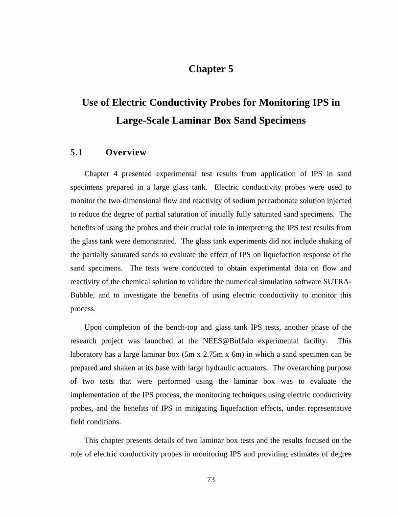
73
Chapter 5
Use of Electric Conductivity Probes for Monitoring IPS in
Large-Scale Laminar Box Sand Specimens
5.1 Overview
Chapter 4 presented experimental test results from application of IPS in sand
specimens prepared in a large glass tank. Electric conductivity probes were used to
monitor the two-dimensional flow and reactivity of sodium percarbonate solution injected
to reduce the degree of partial saturation of initially fully saturated sand specimens. The
benefits of using the probes and their crucial role in interpreting the IPS test results from
the glass tank were demonstrated. The glass tank experiments did not include shaking of
the partially saturated sands to evaluate the effect of IPS on liquefaction response of the
sand specimens. The tests were conducted to obtain experimental data on flow and
reactivity of the chemical solution to validate the numerical simulation software SUTRA-
Bubble, and to investigate the benefits of using electric conductivity to monitor this
process.
Upon completion of the bench-top and glass tank IPS tests, another phase of the
research project was launched at the NEES@Buffalo experimental facility. This
laboratory has a large laminar box (5m x 2.75m x 6m) in which a sand specimen can be
prepared and shaken at its base with large hydraulic actuators. The overarching purpose
of two tests that were performed using the laminar box was to evaluate the
implementation of the IPS process, the monitoring techniques using electric conductivity
probes, and the benefits of IPS in mitigating liquefaction effects, under representative
field conditions.
This chapter presents details of two laminar box tests and the results focused on the
role of electric conductivity probes in monitoring IPS and providing estimates of degree
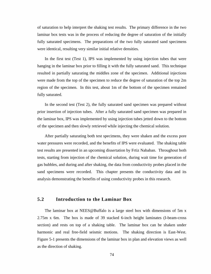
74
of saturation to help interpret the shaking test results. The primary difference in the two
laminar box tests was in the process of reducing the degree of saturation of the initially
fully saturated specimens. The preparations of the two fully saturated sand specimens
were identical, resulting very similar initial relative densities.
In the first test (Test 1), IPS was implemented by using injection tubes that were
hanging in the laminar box prior to filling it with the fully saturated sand. This technique
resulted in partially saturating the middles zone of the specimen. Additional injections
were made from the top of the specimen to reduce the degree of saturation of the top 2m
region of the specimen. In this test, about 1m of the bottom of the specimen remained
fully saturated.
In the second test (Test 2), the fully saturated sand specimen was prepared without
prior insertion of injection tubes. After a fully saturated sand specimen was prepared in
the laminar box, IPS was implemented by using injection tubes jetted down to the bottom
of the specimen and then slowly retrieved while injecting the chemical solution.
After partially saturating both test specimens, they were shaken and the excess pore
water pressures were recorded, and the benefits of IPS were evaluated. The shaking table
test results are presented in an upcoming dissertation by Frtiz Nababan. Throughout both
tests, starting from injection of the chemical solution, during wait time for generation of
gas bubbles, and during and after shaking, the data from conductivity probes placed in the
sand specimens were recorded. This chapter presents the conductivity data and its
analysis demonstrating the benefits of using conductivity probes in this research.
5.2 Introduction to the Laminar Box
The laminar box at NEES@Buffalo is a large steel box with dimensions of 5m x
2.75m x 6m. The box is made of 39 stacked 6-inch height laminates (I-beam-cross
section) and rests on top of a shaking table. The laminar box can be shaken under
harmonic and real free-field seismic motions. The shaking direction is East-West.
Figure 5-1 presents the dimensions of the laminar box in plan and elevation views as well
as the direction of shaking.
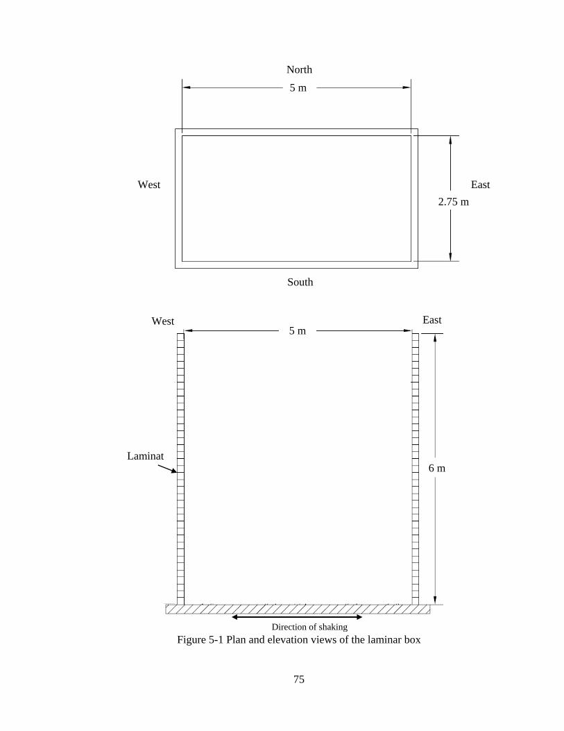
75
Figure 5-1 Plan and elevation views of the laminar box
West East
6 m
5 m
West
North
East
South
CP 1, 2 CP 10
CP 6, 7, 8
CP 3, 4, 5 CP 9
5 m
2.75 m
m
Laminat
es
Direction of shaking
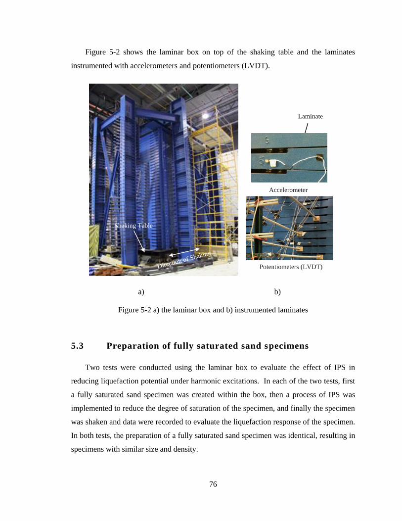
76
Figure 5-2 shows the laminar box on top of the shaking table and the laminates
instrumented with accelerometers and potentiometers (LVDT).
a) b)
Figure 5-2 a) the laminar box and b) instrumented laminates
5.3 Preparation of fully saturated sand specimens
Two tests were conducted using the laminar box to evaluate the effect of IPS in
reducing liquefaction potential under harmonic excitations. In each of the two tests, first
a fully saturated sand specimen was created within the box, then a process of IPS was
implemented to reduce the degree of saturation of the specimen, and finally the specimen
was shaken and data were recorded to evaluate the liquefaction response of the specimen.
In both tests, the preparation of a fully saturated sand specimen was identical, resulting in
specimens with similar size and density.
Laminate
Potentiometers (LVDT)
Accelerometer
Shaking Table
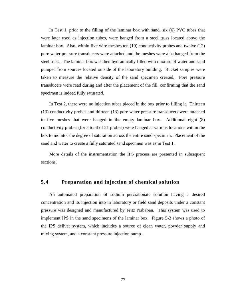
77
In Test 1, prior to the filling of the laminar box with sand, six (6) PVC tubes that
were later used as injection tubes, were hanged from a steel truss located above the
laminar box. Also, within five wire meshes ten (10) conductivity probes and twelve (12)
pore water pressure transducers were attached and the meshes were also hanged from the
steel truss. The laminar box was then hydraulically filled with mixture of water and sand
pumped from sources located outside of the laboratory building. Bucket samples were
taken to measure the relative density of the sand specimen created. Pore pressure
transducers were read during and after the placement of the fill, confirming that the sand
specimen is indeed fully saturated.
In Test 2, there were no injection tubes placed in the box prior to filling it. Thirteen
(13) conductivity probes and thirteen (13) pore water pressure transducers were attached
to five meshes that were hanged in the empty laminar box. Additional eight (8)
conductivity probes (for a total of 21 probes) were hanged at various locations within the
box to monitor the degree of saturation across the entire sand specimen. Placement of the
sand and water to create a fully saturated sand specimen was as in Test 1.
More details of the instrumentation the IPS process are presented in subsequent
sections.
5.4 Preparation and injection of chemical solution
An automated preparation of sodium percrabonate solution having a desired
concentration and its injection into in laboratory or field sand deposits under a constant
pressure was designed and manufactured by Fritz Nababan. This system was used to
implement IPS in the sand specimens of the laminar box. Figure 5-3 shows a photo of
the IPS deliver system, which includes a source of clean water, powder supply and
mixing system, and a constant pressure injection pump.
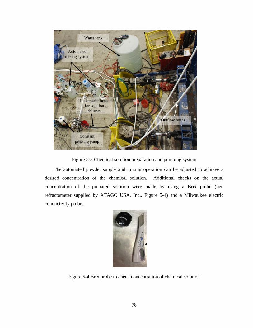
78
Figure 5-3 Chemical solution preparation and pumping system
The automated powder supply and mixing operation can be adjusted to achieve a
desired concentration of the chemical solution. Additional checks on the actual
concentration of the prepared solution were made by using a Brix probe (pen
refractometer supplied by ATAGO USA, Inc., Figure 5-4) and a Milwaukee electric
conductivity probe.
Figure 5-4 Brix probe to check concentration of chemical solution
Automated
mixing system
Constant
pressure pump
1” diameter hoses
for solution
delivery
Outflow hoses
Water tank
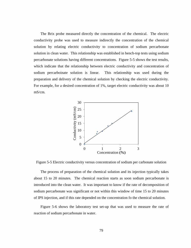
79
The Brix probe measured directly the concentration of the chemical. The electric
conductivity probe was used to measure indirectly the concentration of the chemical
solution by relating electric conductivity to concentration of sodium percarbonate
solution in clean water. This relationship was established in bench-top tests using sodium
percarbonate solutions having different concentrations. Figure 5-5 shows the test results,
which indicate that the relationship between electric conductivity and concentration of
sodium percarboinate solution is linear. This relationship was used during the
preparation and delivery of the chemical solution by checking the electric conductivity.
For example, for a desired concentration of 1%, target electric conductivity was about 10
mS/cm.
Figure 5-5 Electric conductivity versus concentration of sodium per carbonate solution
The process of preparation of the chemical solution and its injection typically takes
about 15 to 20 minutes. The chemical reaction starts as soon sodium percarbonate is
introduced into the clean water. It was important to know if the rate of decomposition of
sodium percarbonate was significant or not within this window of time 15 to 20 minutes
of IPS injection, and if this rate depended on the concentration fo the chemical solution.
Figure 5-6 shows the laboratory test set-up that was used to measure the rate of
reaction of sodium percarbonate in water.
0
5
10
15
20
25
30
0 1 2 3
Conduct
ivit
y (
mS
/cm
)
Concentration (%)
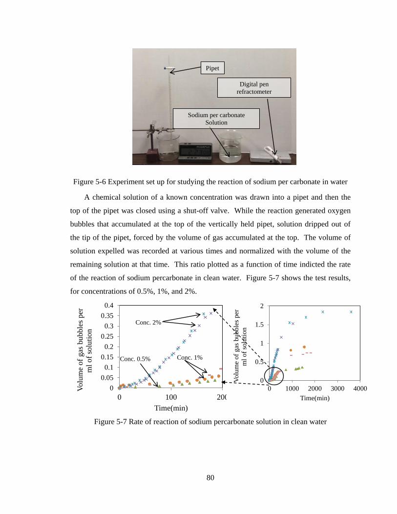
80
Pipet
Sodium per carbonate
Solution
Digital pen
refractometer
Figure 5-6 Experiment set up for studying the reaction of sodium per carbonate in water
A chemical solution of a known concentration was drawn into a pipet and then the
top of the pipet was closed using a shut-off valve. While the reaction generated oxygen
bubbles that accumulated at the top of the vertically held pipet, solution dripped out of
the tip of the pipet, forced by the volume of gas accumulated at the top. The volume of
solution expelled was recorded at various times and normalized with the volume of the
remaining solution at that time. This ratio plotted as a function of time indicted the rate
of the reaction of sodium percarbonate in clean water. Figure 5-7 shows the test results,
for concentrations of 0.5%, 1%, and 2%.
Figure 5-7 Rate of reaction of sodium percarbonate solution in clean water
0
0.05
0.1
0.15
0.2
0.25
0.3
0.35
0.4
0 100 200
Volu
me
of
gas
bu
bb
les
per
ml
of
solu
tion
Time(min)
Conc. 2%
Conc. 1% Conc. 0.5%
0
0.5
1
1.5
2
0 1000 2000 3000 4000
Volu
me
of
gas
bubble
s per
ml
of
solu
tion
Time(min)
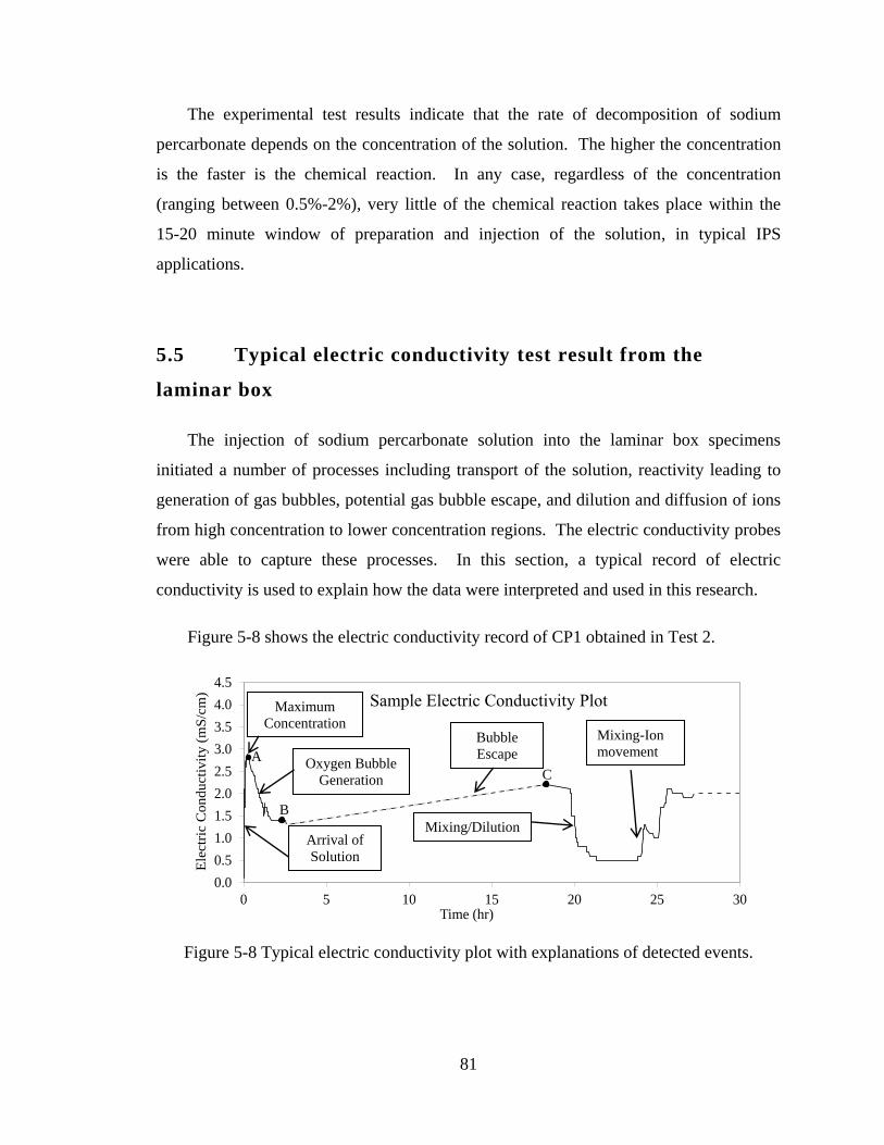
81
The experimental test results indicate that the rate of decomposition of sodium
percarbonate depends on the concentration of the solution. The higher the concentration
is the faster is the chemical reaction. In any case, regardless of the concentration
(ranging between 0.5%-2%), very little of the chemical reaction takes place within the
15-20 minute window of preparation and injection of the solution, in typical IPS
applications.
5.5 Typical electric conductivity test result from the
laminar box
The injection of sodium percarbonate solution into the laminar box specimens
initiated a number of processes including transport of the solution, reactivity leading to
generation of gas bubbles, potential gas bubble escape, and dilution and diffusion of ions
from high concentration to lower concentration regions. The electric conductivity probes
were able to capture these processes. In this section, a typical record of electric
conductivity is used to explain how the data were interpreted and used in this research.
Figure 5-8 shows the electric conductivity record of CP1 obtained in Test 2.
Figure 5-8 Typical electric conductivity plot with explanations of detected events.
0.0
0.5
1.0
1.5
2.0
2.5
3.0
3.5
4.0
4.5
0 5 10 15 20 25 30
Ele
ctr
ic C
on
du
cti
vit
y (
mS
/cm
)
Time (hr)
Maximum
Concentration Bubble
Escape
Mixing/Dilution
Mixing-Ion
movement Oxygen Bubble
Generation
Arrival of
Solution
A
B
C
Sample Electric Conductivity Plot
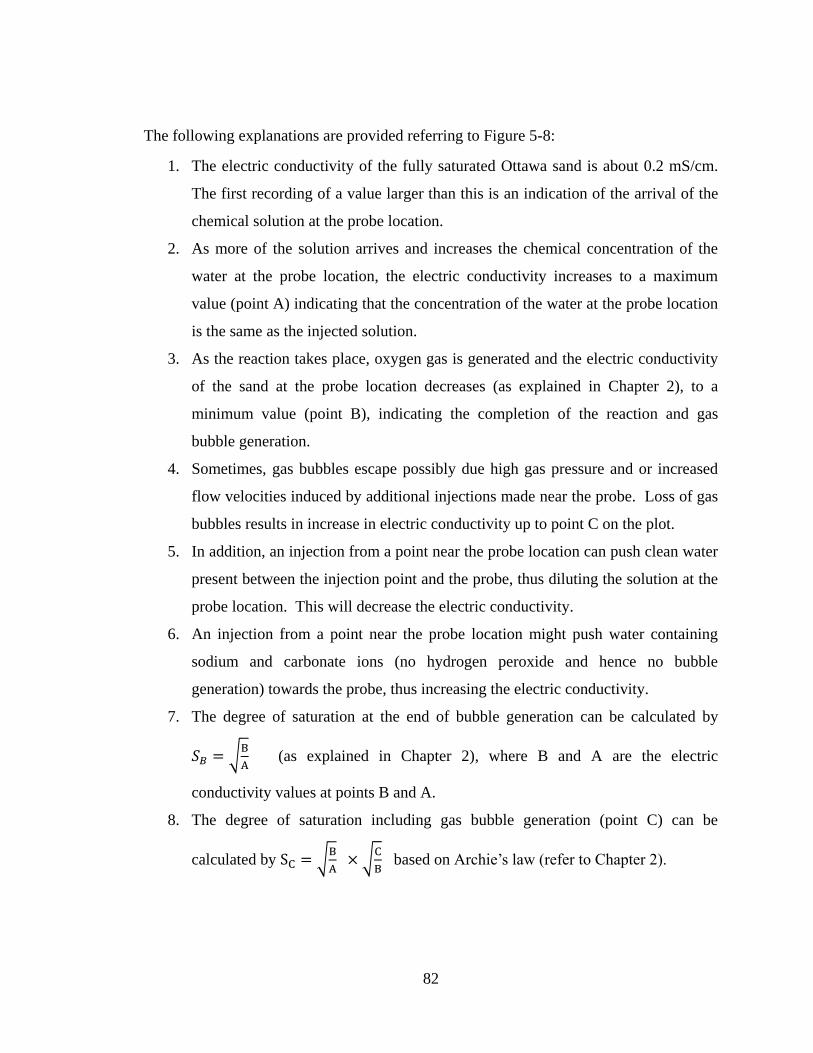
82
The following explanations are provided referring to Figure 5-8:
1. The electric conductivity of the fully saturated Ottawa sand is about 0.2 mS/cm.
The first recording of a value larger than this is an indication of the arrival of the
chemical solution at the probe location.
2. As more of the solution arrives and increases the chemical concentration of the
water at the probe location, the electric conductivity increases to a maximum
value (point A) indicating that the concentration of the water at the probe location
is the same as the injected solution.
3. As the reaction takes place, oxygen gas is generated and the electric conductivity
of the sand at the probe location decreases (as explained in Chapter 2), to a
minimum value (point B), indicating the completion of the reaction and gas
bubble generation.
4. Sometimes, gas bubbles escape possibly due high gas pressure and or increased
flow velocities induced by additional injections made near the probe. Loss of gas
bubbles results in increase in electric conductivity up to point C on the plot.
5. In addition, an injection from a point near the probe location can push clean water
present between the injection point and the probe, thus diluting the solution at the
probe location. This will decrease the electric conductivity.
6. An injection from a point near the probe location might push water containing
sodium and carbonate ions (no hydrogen peroxide and hence no bubble
generation) towards the probe, thus increasing the electric conductivity.
7. The degree of saturation at the end of bubble generation can be calculated by
𝑆𝐵 = √B
A (as explained in Chapter 2), where B and A are the electric
conductivity values at points B and A.
8. The degree of saturation including gas bubble generation (point C) can be
calculated by SC = √B
A × √
C
B based on Archie’s law (refer to Chapter 2).
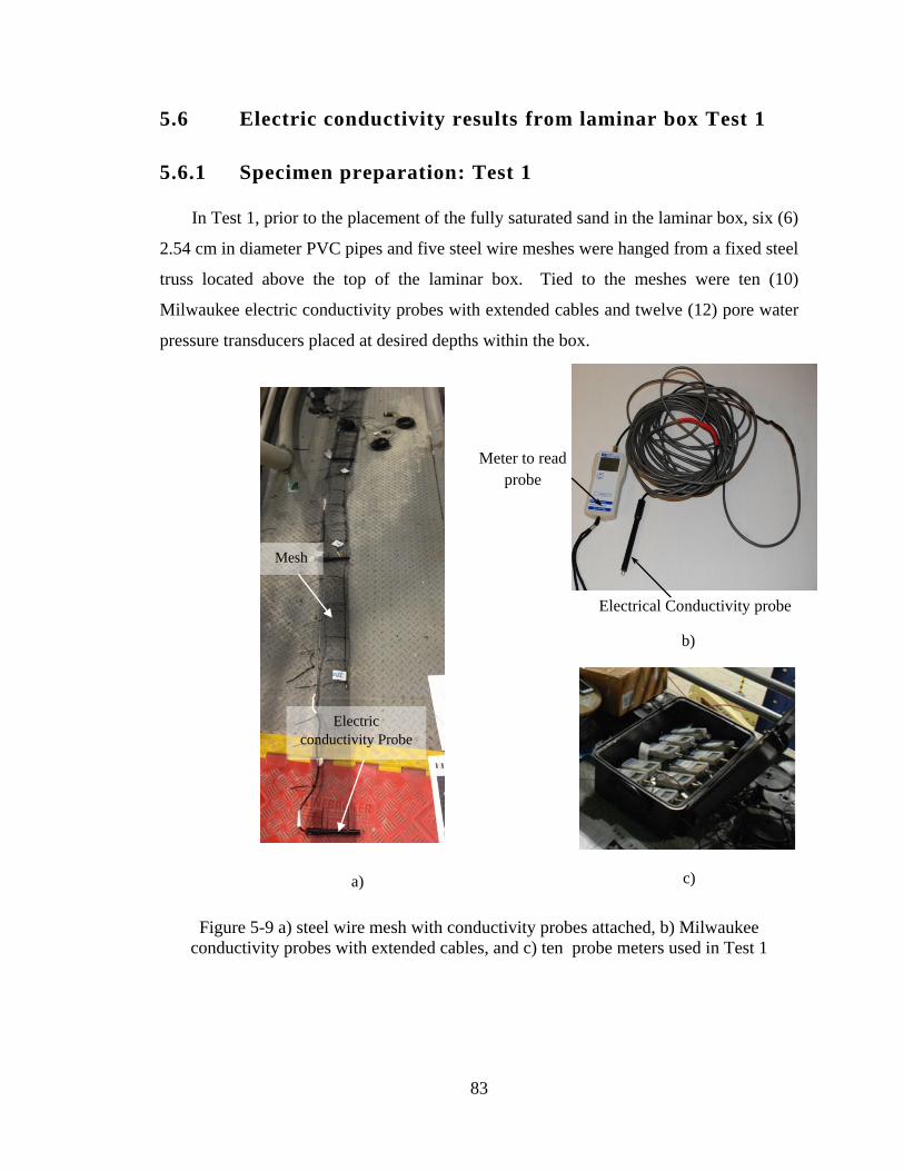
83
Electrical Conductivity probe
Meter to read
probe
5.6 Electric conductivity results from laminar box Test 1
5.6.1 Specimen preparation: Test 1
In Test 1, prior to the placement of the fully saturated sand in the laminar box, six (6)
2.54 cm in diameter PVC pipes and five steel wire meshes were hanged from a fixed steel
truss located above the top of the laminar box. Tied to the meshes were ten (10)
Milwaukee electric conductivity probes with extended cables and twelve (12) pore water
pressure transducers placed at desired depths within the box.
Figure 5-9 a) steel wire mesh with conductivity probes attached, b) Milwaukee
conductivity probes with extended cables, and c) ten probe meters used in Test 1
Electric
conductivity Probe
Mesh
a) c)
b)
84
Figure 5-9 shows a steel wire mesh prior to hanging in the laminar box, a typical
conductivity probe, and the ten probe meters used to record the data. The locations of the
ten CPs were selected to be near the pore pressure transducers fixed in the five steel wire
meshes.).
Figure 5-10 shows the PVC injection tubes and steel meshes hanging from the steel
truss, at desired positions within the laminar box.
Figure 5-10 PVC and steel meshes hanging from the steel truss above the laminar
box, in Test 1
A fully saturated sand specimen was prepared by hydraulically filling the laminar
box with Ottawa sand until the height of the specimen was 4.88m (16 feet). Figure 5-11
shows the size of the sand specimen and the locations of the 10 electric conductivity
probes (CPs).
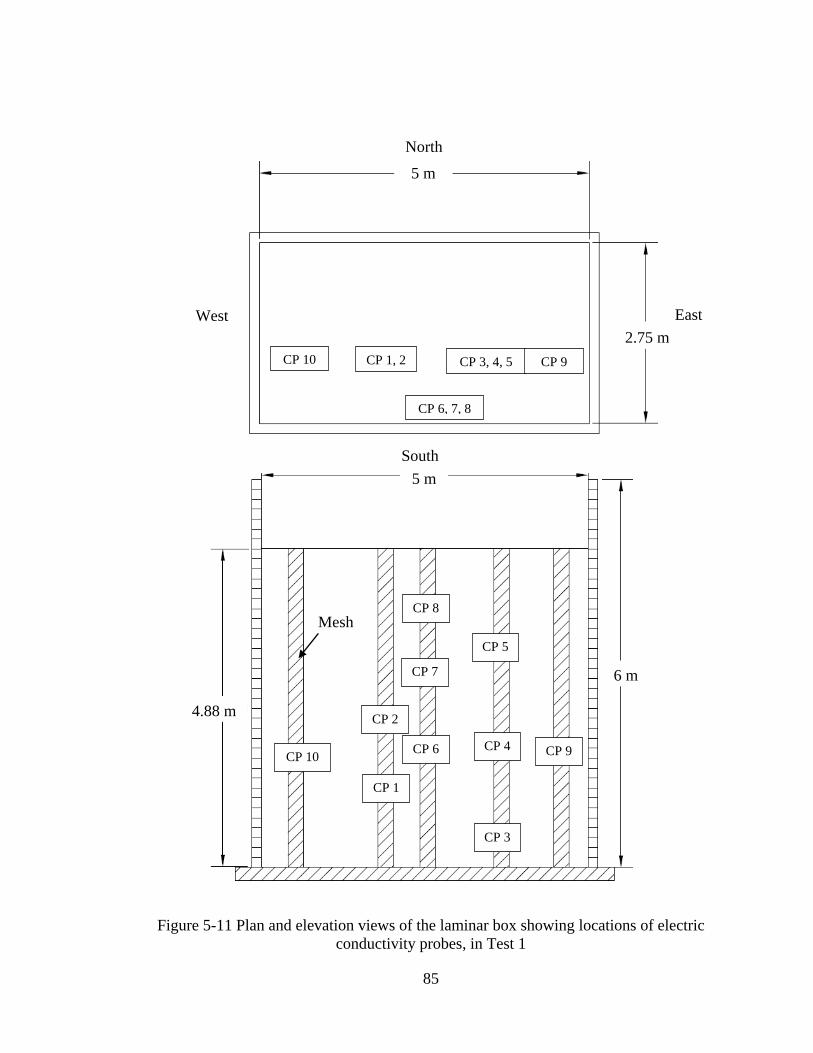
85
Figure 5-11 Plan and elevation views of the laminar box showing locations of electric
conductivity probes, in Test 1
West
North
East
South
CP 1, 2 CP 10
CP 6, 7, 8
CP 3, 4, 5 CP 9
2.75 m
5 m
CP 10
CP 2
CP 1
CP 8
CP 7
CP 6
CP 3
CP 4
CP 5
CP 9
6 m
4.88 m
5 m
Mesh
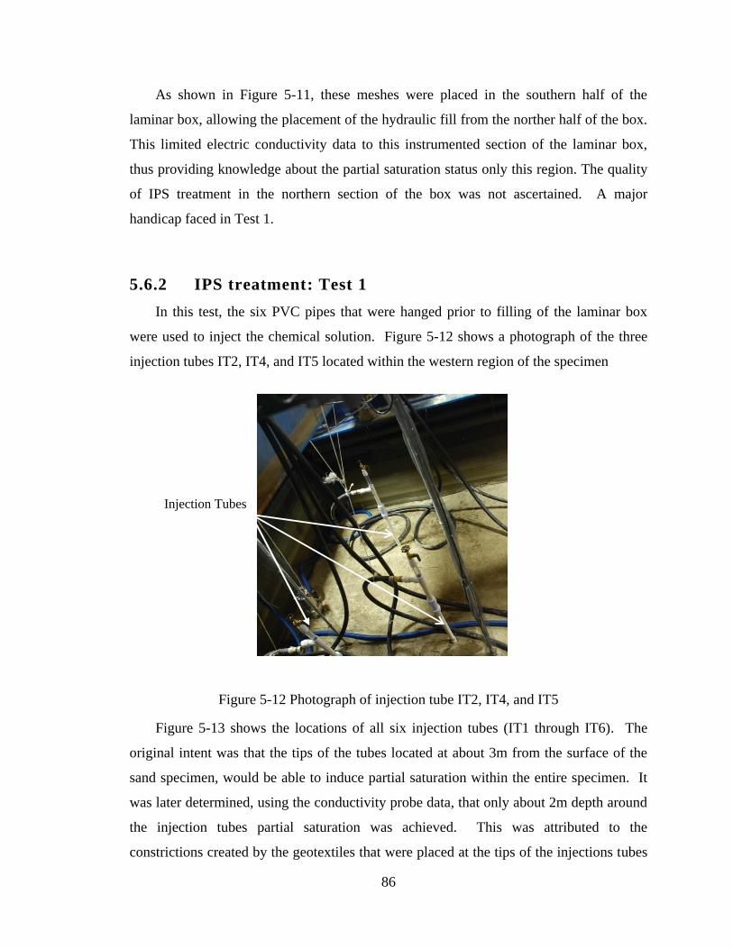
86
As shown in Figure 5-11, these meshes were placed in the southern half of the
laminar box, allowing the placement of the hydraulic fill from the norther half of the box.
This limited electric conductivity data to this instrumented section of the laminar box,
thus providing knowledge about the partial saturation status only this region. The quality
of IPS treatment in the northern section of the box was not ascertained. A major
handicap faced in Test 1.
5.6.2 IPS treatment: Test 1
In this test, the six PVC pipes that were hanged prior to filling of the laminar box
were used to inject the chemical solution. Figure 5-12 shows a photograph of the three
injection tubes IT2, IT4, and IT5 located within the western region of the specimen
Figure 5-12 Photograph of injection tube IT2, IT4, and IT5
Figure 5-13 shows the locations of all six injection tubes (IT1 through IT6). The
original intent was that the tips of the tubes located at about 3m from the surface of the
sand specimen, would be able to induce partial saturation within the entire specimen. It
was later determined, using the conductivity probe data, that only about 2m depth around
the injection tubes partial saturation was achieved. This was attributed to the
constrictions created by the geotextiles that were placed at the tips of the injections tubes
Injection Tubes
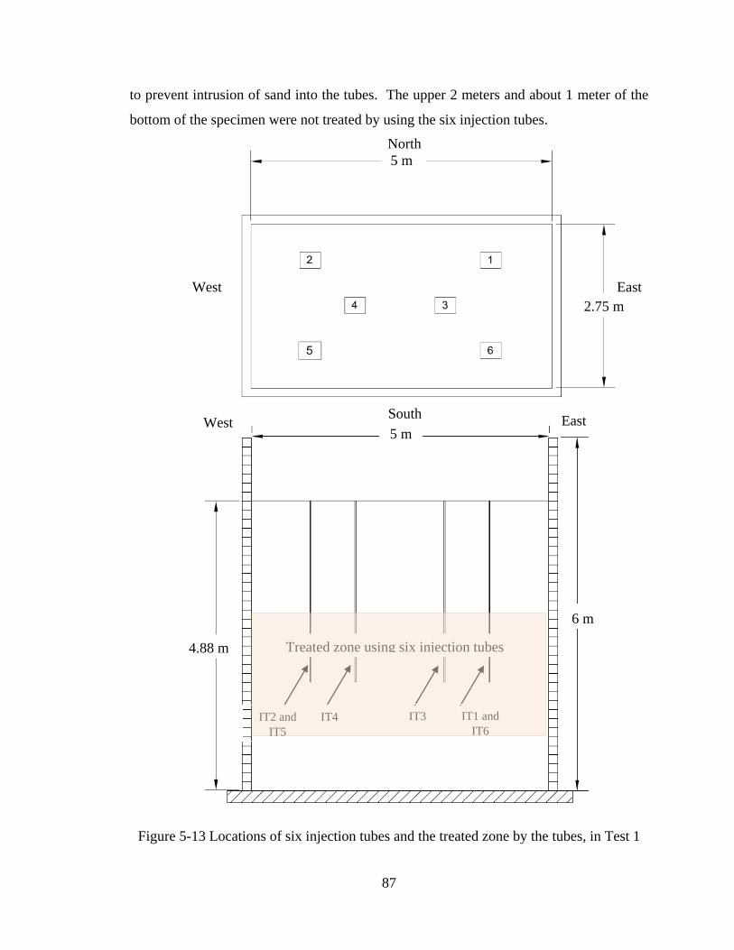
87
to prevent intrusion of sand into the tubes. The upper 2 meters and about 1 meter of the
bottom of the specimen were not treated by using the six injection tubes.
Figure 5-13 Locations of six injection tubes and the treated zone by the tubes, in Test 1
South
2.75 m
5 m
North
West East
IT2 and
IT5
IT4 IT3 IT1 and
IT6
6 m
4.88 m Treated zone using six injection tubes
5 m East West
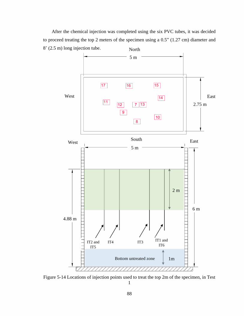
88
After the chemical injection was completed using the six PVC tubes, it was decided
to proceed treating the top 2 meters of the specimen using a 0.5” (1.27 cm) diameter and
8’ (2.5 m) long injection tube.
Figure 5-14 Locations of injection points used to treat the top 2m of the specimen, in Test
1
North
East West
South
5 m
2.75 m
IT2 and
IT5
IT4 IT3 IT1 and
IT6
6 m
4.88 m
5 m
East West
2 m
1m Bottom untreated zone
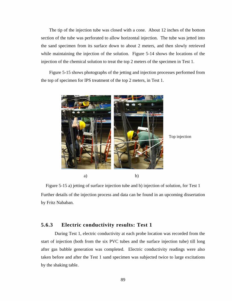
89
The tip of the injection tube was closed with a cone. About 12 inches of the bottom
section of the tube was perforated to allow horizontal injection. The tube was jetted into
the sand specimen from its surface down to about 2 meters, and then slowly retrieved
while maintaining the injection of the solution. Figure 5-14 shows the locations of the
injection of the chemical solution to treat the top 2 meters of the specimen in Test 1.
Figure 5-15 shows photographs of the jetting and injection processes performed from
the top of specimen for IPS treatment of the top 2 meters, in Test 1.
a) b)
Figure 5-15 a) jetting of surface injection tube and b) injection of solution, for Test 1
Further details of the injection process and data can be found in an upcoming dissertation
by Fritz Nababan.
5.6.3 Electric conductivity results: Test 1
During Test 1, electric conductivity at each probe location was recorded from the
start of injection (both from the six PVC tubes and the surface injection tube) till long
after gas bubble generation was completed. Electric conductivity readings were also
taken before and after the Test 1 sand specimen was subjected twice to large excitations
by the shaking table.
Top injection
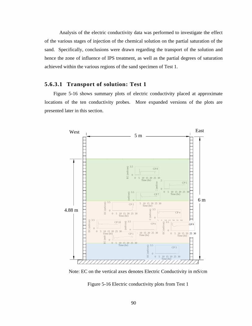
90
Analysis of the electric conductivity data was performed to investigate the effect
of the various stages of injection of the chemical solution on the partial saturation of the
sand. Specifically, conclusions were drawn regarding the transport of the solution and
hence the zone of influence of IPS treatment, as well as the partial degrees of saturation
achieved within the various regions of the sand specimen of Test 1.
5.6.3.1 Transport of solution: Test 1
Figure 5-16 shows summary plots of electric conductivity placed at approximate
locations of the ten conductivity probes. More expanded versions of the plots are
presented later in this section.
Note: EC on the vertical axes denotes Electric Conductivity in mS/cm
Figure 5-16 Electric conductivity plots from Test 1
IT2 and
IT5
IT4
IT3 IT1 and
IT6
6 m
4.88 m
5 m East West
0
3.5
0 5 10 15 20 25 30EC
(m
S/c
m)
Time (hr)
CP 5
0
3.5
0 5 10 15 20 25 30EC
(m
S/c
m)
Time (hr)
CP 7
0
3.5
0 5 10 15 20 25 30EC
(m
S/c
m)
Time (hr)
CP 8
0
3.5
0 5 10 15 20 25 30EC
(m
S/c
m)
Time (hr)
CP 2
0
3.5
0 5 10 15 20 25 30EC
(m
S/c
m)
Time (hr)
CP 4
0
3.5
0 5 10 15 20 25 30EC
(m
S/c
m)
Time (hr)
CP 6
0
3.5
0 5 10 15 20 25 30EC
(m
S/c
m)
Time (hr)
CP 1
0
3.5
0 5 10 15 20 25 30EC
(m
S/c
m)
Time (hr)
CP 10
0
3.5
0 5 10 15 20 25 30EC
(m
S/c
m)
Time (hr)
CP 3
0
3.5
0 5 10 15 20 25 30EC
(m
S/c
m)
Time (hr)
CP 9
91
In Test 1, the IPS injection process was conducted in two days. During the first day,
the injection was through the six PVC tubes (IT1 through IT6), and it took about 2.5
hours to complete. After this, surface injection started at IT7 (5 hours after zero time
considered as the start of injection from the PVC tubes) and was completed at IT10 at
about 7 hours from zero time. On the second day of injection, the remaining surface
injections at IT11 through IT17 were completed at about 27 hours from zero time. In the
electric conductivity plots shown in Figure 5-16, the dashed lines represent the night
between first day and second day of injection when no data was recorded.
The electric conductivity plots shown in Figure 5-16 indicate that the chemical
solution arrived at CP1, CP4, CP9, and CP10 during injection from the six PVC tubes
(IT1 through IT6). These probes are close to the injection tips of the PVC tubes. CP5,
CP7, and CP8 detected the arrival of the chemical solution during surface injection at IT7
through IT10. CP2 detected the arrival of the chemical solution during the second day
surface injection at IT11 through IT17. Electric conductivity readings of CP3 and CP6
did not change during the injections leading to the conclusion that the chemical solution
did not reach the locations of CP3 and CP6. This observation helped determine the zone
of influence of the IPS treatment, as will be explained later in this section.
An effort was made to keep the concentration of the chemical solution during the
injection close to 1%. The peak values of electric conductivity measured by the probes
where the chemical solution reached were between 2.3 mS/cm and 3.5 mS/cm, very
similar to values measure from the bench-top and glass tank tests. This electric
conductivity values from the bench-top tests for 1% concentration were between
2.2mS/cm and 3.3 mS/cm, and from the glass tank tests were between 2.8mS/cm and
3.7mS/cm. It was concluded that the mixing and delivery system worked very well and
was able to provide chemical solution with a steady concentration of 1%.
The electric conductivity plots shown in Figure 5-16 also show regions where the
chemical solution did not reach and therefore the sand remained fully saturated. For
example, the reading of CP3, which was located 14.5 feet (4.4 m) from the top of the
specimen (within the bottom 1 meter), did not change during the injections, indicating
that at this probe location, and most likely within the bottom 1 meter of the specimen, the
92
degree of saturation remained 100%. CP1 which was located about 12 feet (3.65 m) from
the surface of specimen was the deepest probe that showed change in electric
conductivity during injections from the PVC tubes indicating that the sand between 12
and 14.5 feet (3.65 to 4.4m) from the surface most likely was treated.
The electric conductivity of CP6 did not change during the injections. This fact can
be explained by the relatively large lateral distances between CP6 and the injection tubes.
It was concluded that, the mid-region of the sand specimen along close to south wall was
not treated and degree of saturation remained 100%. Assuming symmetry, the mid-
region close to the north wall was also not treated.
CP2 reading shows an increase in electric conductivity only after 25 hours from the
start of the injections. This increase was attributed to arrival of chemical solution without
any residual hydrogen peroxide (source of for gas generation). As was explained in
Section 5.5, this was due to Mixing-Ion movement. But CP4 and CP7, which are 0.4m
below and 0.7m above the location of CP2 were able to detect the arrival of the chemical
solution with hydrogen peroxide during bottom and top injections. It was concluded that
a thin layer of the sand specimen at the elevation of CP2 (2.6 m) from the surface of the
specimen was not treated.
To study the zone of influence of the IPS treatment using the PVC injection tubes,
the electric conductivity results (shown in Figure 5-16) and the horizontal distances of
CP6 and CP9 from to the PVC injection tubes IT3 and IT6 (shown in Figure 5-17) are
used. CP6 did not detect arrival of the chemical solution, and its smallest distance from
an injection tube is 1.2m from IT3. CP9 detected the chemical solution and its largest
distance from an injection tube is 0.6m from IT6. It is concluded that the radius of
influence of injection from the PVC tubes was between 0.6 to 1.2 m.
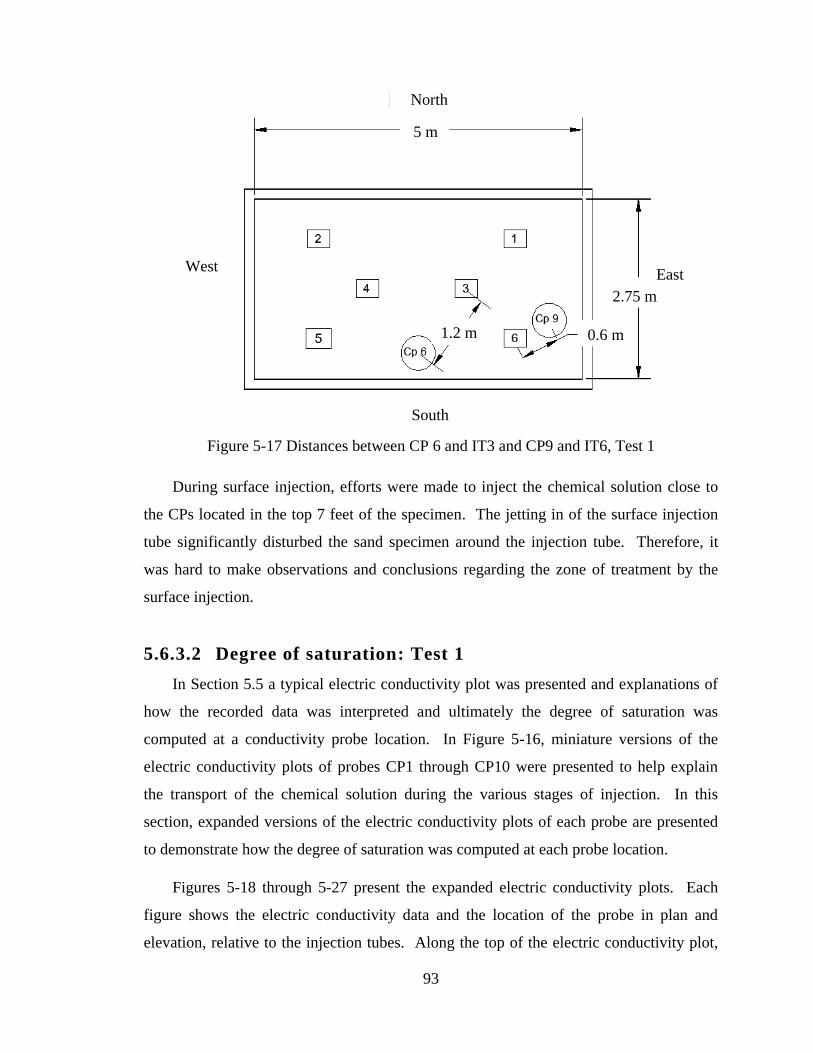
93
Figure 5-17 Distances between CP 6 and IT3 and CP9 and IT6, Test 1
During surface injection, efforts were made to inject the chemical solution close to
the CPs located in the top 7 feet of the specimen. The jetting in of the surface injection
tube significantly disturbed the sand specimen around the injection tube. Therefore, it
was hard to make observations and conclusions regarding the zone of treatment by the
surface injection.
5.6.3.2 Degree of saturation: Test 1
In Section 5.5 a typical electric conductivity plot was presented and explanations of
how the recorded data was interpreted and ultimately the degree of saturation was
computed at a conductivity probe location. In Figure 5-16, miniature versions of the
electric conductivity plots of probes CP1 through CP10 were presented to help explain
the transport of the chemical solution during the various stages of injection. In this
section, expanded versions of the electric conductivity plots of each probe are presented
to demonstrate how the degree of saturation was computed at each probe location.
Figures 5-18 through 5-27 present the expanded electric conductivity plots. Each
figure shows the electric conductivity data and the location of the probe in plan and
elevation, relative to the injection tubes. Along the top of the electric conductivity plot,
North
South
West
5 m
East
2.75 m
1.2 m 0.6 m
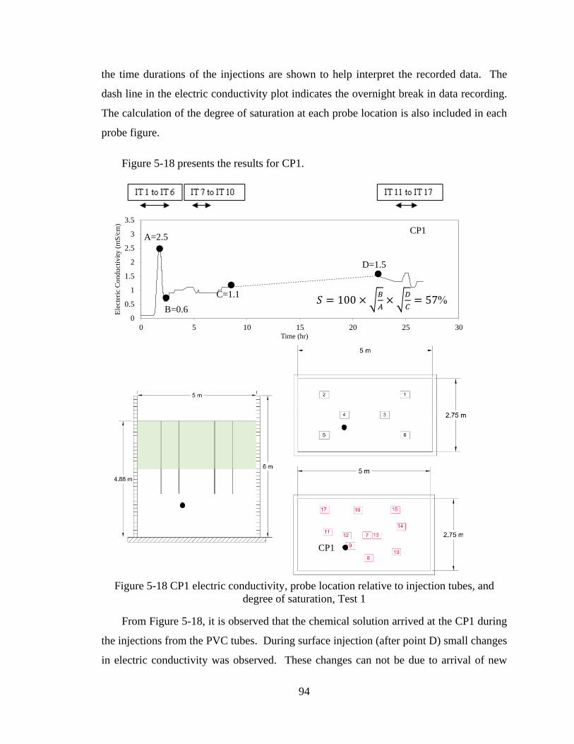
94
the time durations of the injections are shown to help interpret the recorded data. The
dash line in the electric conductivity plot indicates the overnight break in data recording.
The calculation of the degree of saturation at each probe location is also included in each
probe figure.
Figure 5-18 presents the results for CP1.
Figure 5-18 CP1 electric conductivity, probe location relative to injection tubes, and
degree of saturation, Test 1
From Figure 5-18, it is observed that the chemical solution arrived at the CP1 during
the injections from the PVC tubes. During surface injection (after point D) small changes
in electric conductivity was observed. These changes can not be due to arrival of new
0
0.5
1
1.5
2
2.5
3
3.5
0 5 10 15 20 25 30
Ele
cter
ic C
on
du
ctiv
ity (
mS
/cm
)
Time (hr)
CP 1A=2.5
C=1.1
𝑆 = 100 × √𝐵
𝐴× √
𝐷
𝐶= 57%
B=0.6
D=1.5
CP1
CP1
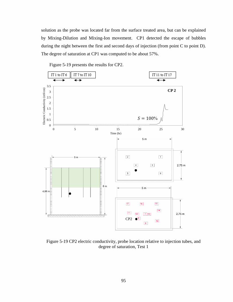
95
solution as the probe was located far from the surface treated area, but can be explained
by Mixing-Dilution and Mixing-Ion movement. CP1 detected the escape of bubbles
during the night between the first and second days of injection (from point C to point D).
The degree of saturation at CP1 was computed to be about 57%.
Figure 5-19 presents the results for CP2.
Figure 5-19 CP2 electric conductivity, probe location relative to injection tubes, and
degree of saturation, Test 1
CP2
0
0.5
1
1.5
2
2.5
3
3.5
0 5 10 15 20 25 30
Ele
cter
ic C
on
du
ctiv
ity
(m
S/c
m)
Time (hr)
CP 2
𝑆 = 100%
CP2
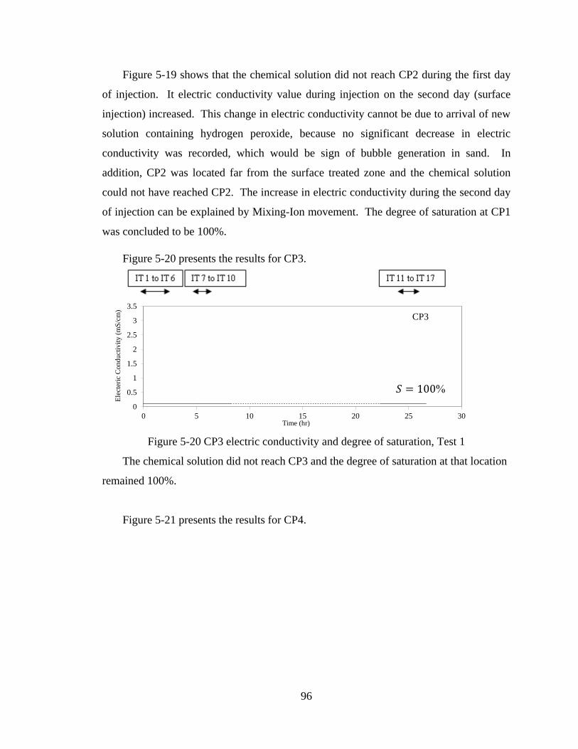
96
Figure 5-19 shows that the chemical solution did not reach CP2 during the first day
of injection. It electric conductivity value during injection on the second day (surface
injection) increased. This change in electric conductivity cannot be due to arrival of new
solution containing hydrogen peroxide, because no significant decrease in electric
conductivity was recorded, which would be sign of bubble generation in sand. In
addition, CP2 was located far from the surface treated zone and the chemical solution
could not have reached CP2. The increase in electric conductivity during the second day
of injection can be explained by Mixing-Ion movement. The degree of saturation at CP1
was concluded to be 100%.
Figure 5-20 presents the results for CP3.
Figure 5-20 CP3 electric conductivity and degree of saturation, Test 1
The chemical solution did not reach CP3 and the degree of saturation at that location
remained 100%.
Figure 5-21 presents the results for CP4.
0
0.5
1
1.5
2
2.5
3
3.5
0 5 10 15 20 25 30
Ele
cter
ic C
on
du
ctiv
ity
(m
S/c
m)
Time (hr)
CP 3
𝑆 = 100%
CP3
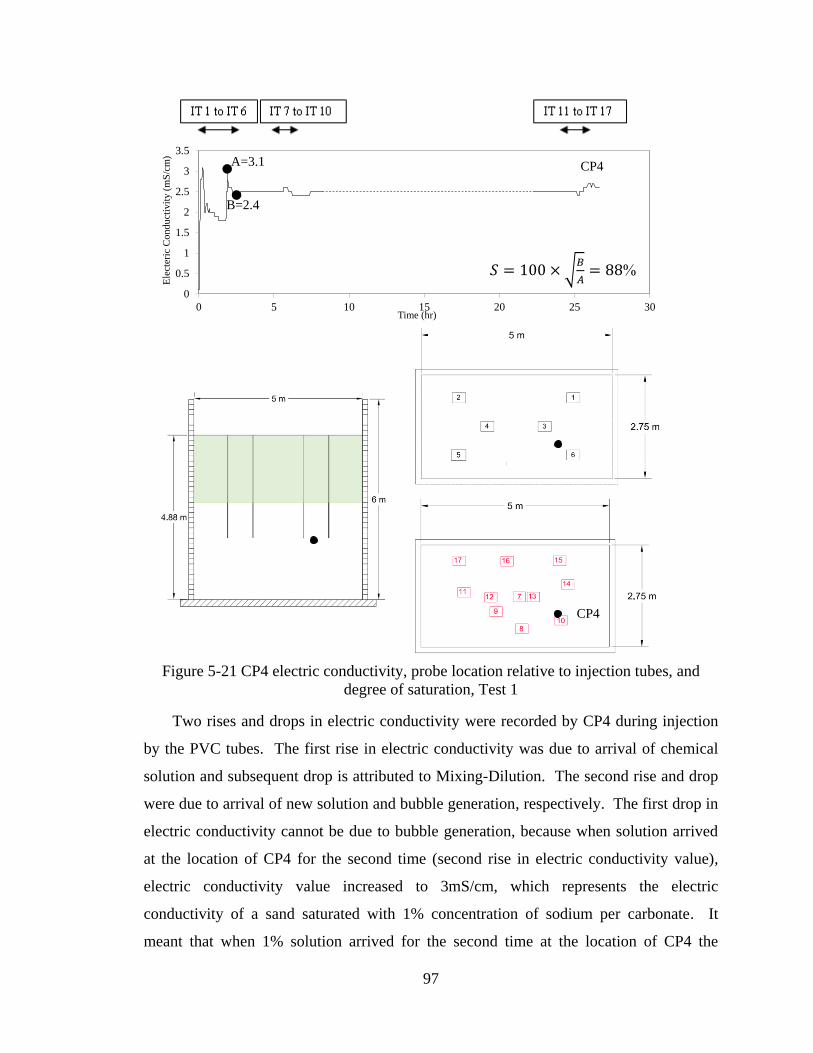
97
Figure 5-21 CP4 electric conductivity, probe location relative to injection tubes, and
degree of saturation, Test 1
Two rises and drops in electric conductivity were recorded by CP4 during injection
by the PVC tubes. The first rise in electric conductivity was due to arrival of chemical
solution and subsequent drop is attributed to Mixing-Dilution. The second rise and drop
were due to arrival of new solution and bubble generation, respectively. The first drop in
electric conductivity cannot be due to bubble generation, because when solution arrived
at the location of CP4 for the second time (second rise in electric conductivity value),
electric conductivity value increased to 3mS/cm, which represents the electric
conductivity of a sand saturated with 1% concentration of sodium per carbonate. It
meant that when 1% solution arrived for the second time at the location of CP4 the
0
0.5
1
1.5
2
2.5
3
3.5
0 5 10 15 20 25 30
Ele
cter
ic C
on
du
ctiv
ity
(m
S/c
m)
Time (hr)
CP 4A=3.1
B=2.4
𝑆 = 100 × √𝐵
𝐴= 88%
CP4
CP4
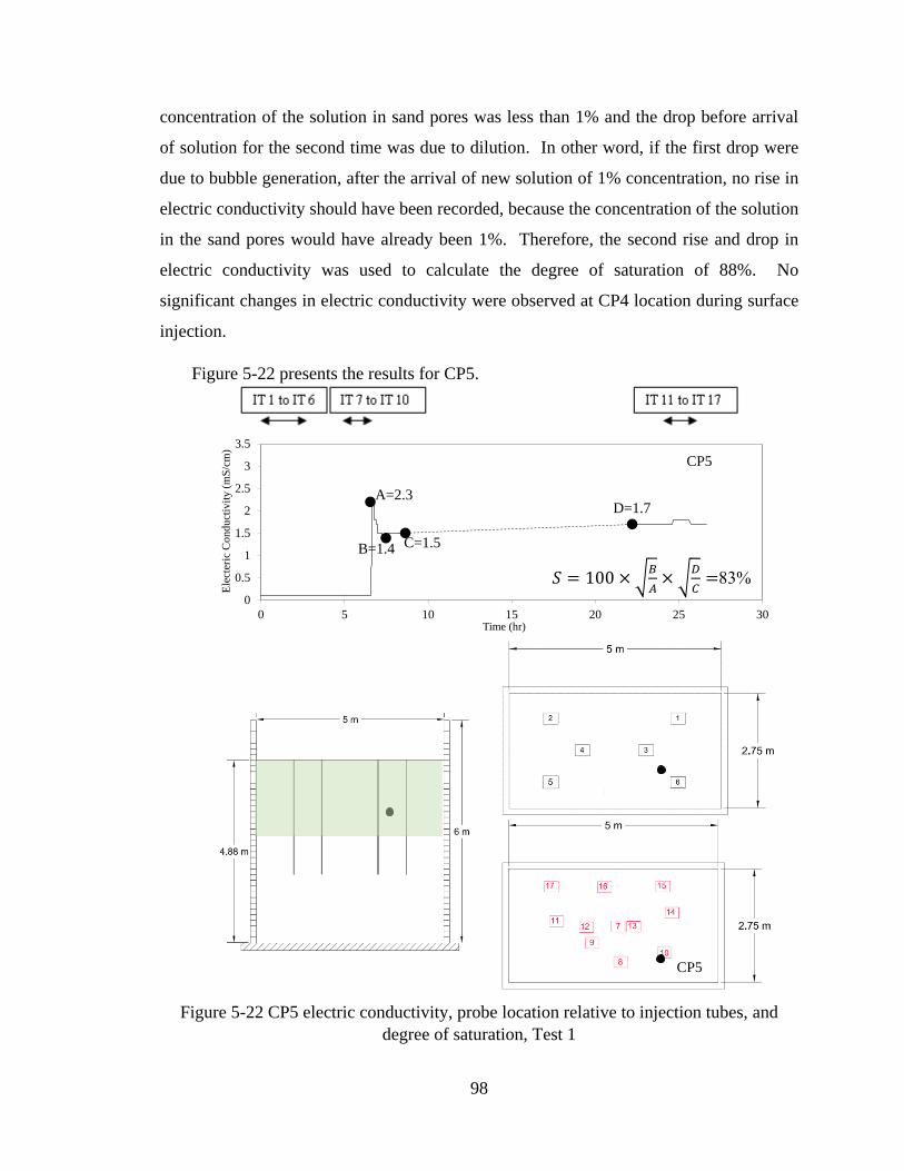
98
concentration of the solution in sand pores was less than 1% and the drop before arrival
of solution for the second time was due to dilution. In other word, if the first drop were
due to bubble generation, after the arrival of new solution of 1% concentration, no rise in
electric conductivity should have been recorded, because the concentration of the solution
in the sand pores would have already been 1%. Therefore, the second rise and drop in
electric conductivity was used to calculate the degree of saturation of 88%. No
significant changes in electric conductivity were observed at CP4 location during surface
injection.
Figure 5-22 presents the results for CP5.
Figure 5-22 CP5 electric conductivity, probe location relative to injection tubes, and
degree of saturation, Test 1
0
0.5
1
1.5
2
2.5
3
3.5
0 5 10 15 20 25 30
Ele
cter
ic C
on
du
ctiv
ity
(m
S/c
m)
Time (hr)
CP 5
A=2.3
B=1.4 C=1.5
D=1.7
𝑆 = 100 × √𝐵
𝐴× √
𝐷
𝐶=83%
CP5
CP5
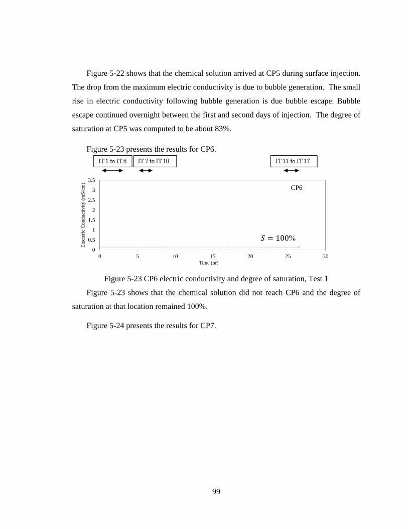
99
Figure 5-22 shows that the chemical solution arrived at CP5 during surface injection.
The drop from the maximum electric conductivity is due to bubble generation. The small
rise in electric conductivity following bubble generation is due bubble escape. Bubble
escape continued overnight between the first and second days of injection. The degree of
saturation at CP5 was computed to be about 83%.
Figure 5-23 presents the results for CP6.
Figure 5-27 Electric conductivity plot by time for CP6 probe
Figure 5-23 CP6 electric conductivity and degree of saturation, Test 1
Figure 5-23 shows that the chemical solution did not reach CP6 and the degree of
saturation at that location remained 100%.
Figure 5-24 presents the results for CP7.
0
0.5
1
1.5
2
2.5
3
3.5
0 5 10 15 20 25 30
Ele
cter
ic C
on
du
ctiv
ity
(m
S/c
m)
Time (hr)
CP 6
𝑆 = 100%
CP6
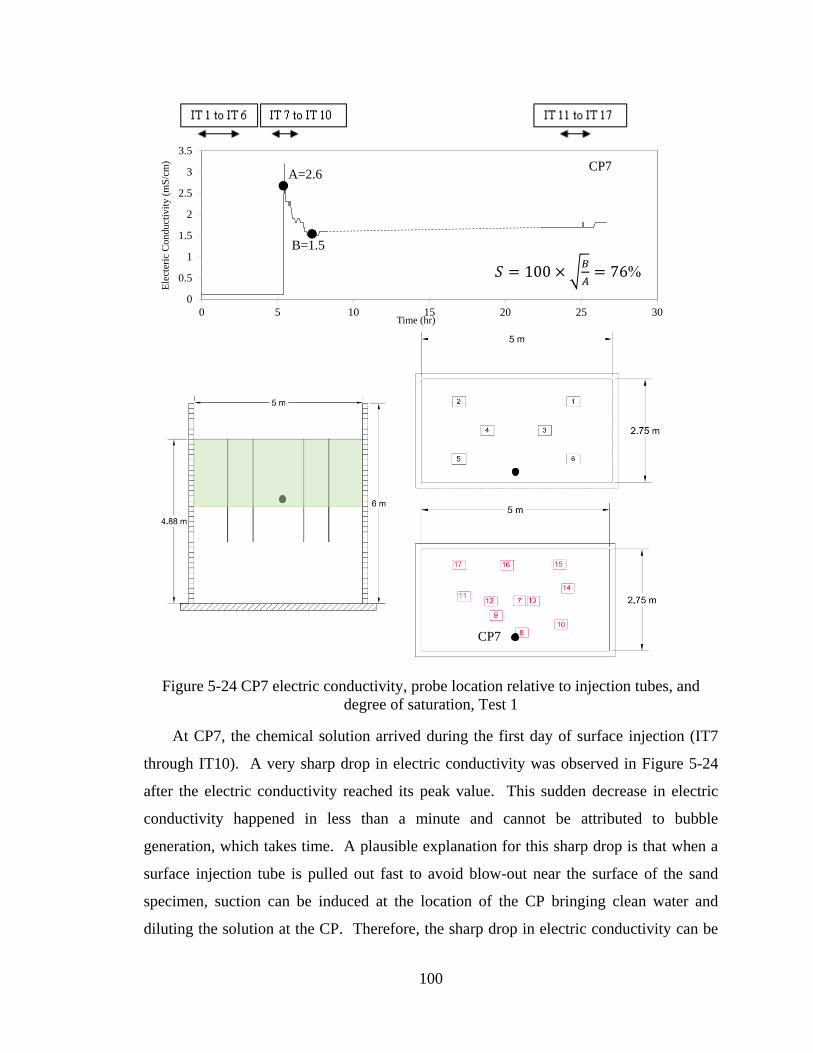
100
Figure 5-24 CP7 electric conductivity, probe location relative to injection tubes, and
degree of saturation, Test 1
At CP7, the chemical solution arrived during the first day of surface injection (IT7
through IT10). A very sharp drop in electric conductivity was observed in Figure 5-24
after the electric conductivity reached its peak value. This sudden decrease in electric
conductivity happened in less than a minute and cannot be attributed to bubble
generation, which takes time. A plausible explanation for this sharp drop is that when a
surface injection tube is pulled out fast to avoid blow-out near the surface of the sand
specimen, suction can be induced at the location of the CP bringing clean water and
diluting the solution at the CP. Therefore, the sharp drop in electric conductivity can be
0
0.5
1
1.5
2
2.5
3
3.5
0 5 10 15 20 25 30
Ele
cter
ic C
on
du
ctiv
ity
(m
S/c
m)
Time (hr)
CP 7A=2.6
B=1.5
𝑆 = 100 × √𝐵
𝐴= 76%
CP7
CP7
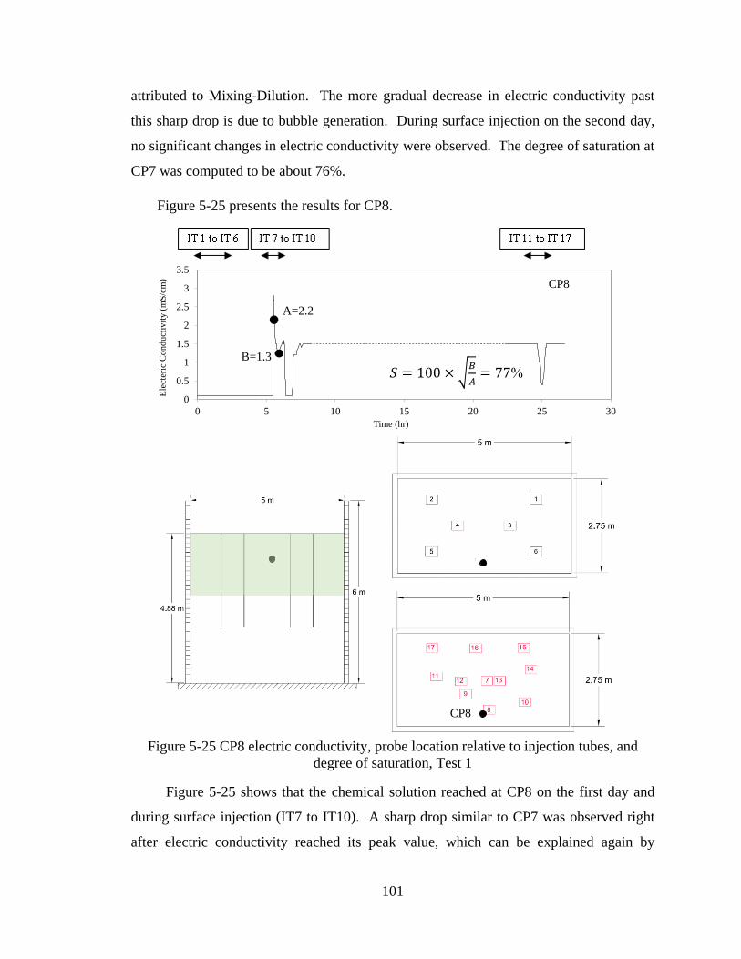
101
attributed to Mixing-Dilution. The more gradual decrease in electric conductivity past
this sharp drop is due to bubble generation. During surface injection on the second day,
no significant changes in electric conductivity were observed. The degree of saturation at
CP7 was computed to be about 76%.
Figure 5-25 presents the results for CP8.
Figure 5-25 CP8 electric conductivity, probe location relative to injection tubes, and
degree of saturation, Test 1
Figure 5-25 shows that the chemical solution reached at CP8 on the first day and
during surface injection (IT7 to IT10). A sharp drop similar to CP7 was observed right
after electric conductivity reached its peak value, which can be explained again by
B=1.3
0
0.5
1
1.5
2
2.5
3
3.5
0 5 10 15 20 25 30
Ele
cter
ic C
on
du
ctiv
ity
(m
S/c
m)
Time (hr)
CP 8
A=2.2
B=1.3
𝑆 = 100 × √𝐵
𝐴= 77%
CP8
CP8
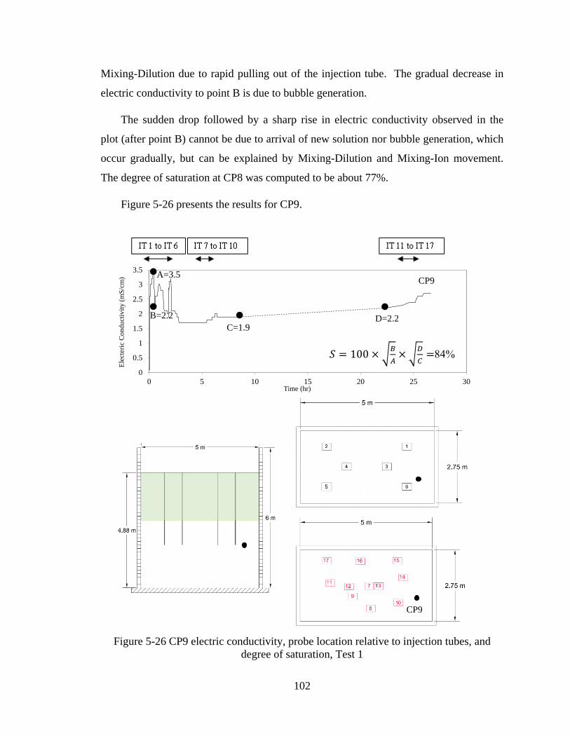
102
Mixing-Dilution due to rapid pulling out of the injection tube. The gradual decrease in
electric conductivity to point B is due to bubble generation.
The sudden drop followed by a sharp rise in electric conductivity observed in the
plot (after point B) cannot be due to arrival of new solution nor bubble generation, which
occur gradually, but can be explained by Mixing-Dilution and Mixing-Ion movement.
The degree of saturation at CP8 was computed to be about 77%.
Figure 5-26 presents the results for CP9.
Figure 5-26 CP9 electric conductivity, probe location relative to injection tubes, and
degree of saturation, Test 1
0
0.5
1
1.5
2
2.5
3
3.5
0 5 10 15 20 25 30
Ele
cter
ic C
on
du
ctiv
ity
(m
S/c
m)
Time (hr)
CP 9A=3.5
C=1.9 D=2.2 B=2.2
𝑆 = 100 × √𝐵
𝐴× √
𝐷
𝐶=84%
CP9
CP9
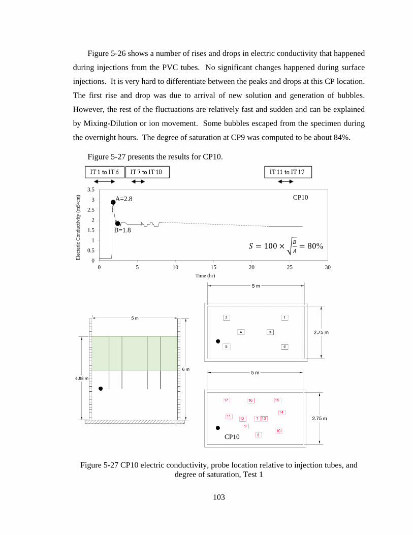
103
Figure 5-26 shows a number of rises and drops in electric conductivity that happened
during injections from the PVC tubes. No significant changes happened during surface
injections. It is very hard to differentiate between the peaks and drops at this CP location.
The first rise and drop was due to arrival of new solution and generation of bubbles.
However, the rest of the fluctuations are relatively fast and sudden and can be explained
by Mixing-Dilution or ion movement. Some bubbles escaped from the specimen during
the overnight hours. The degree of saturation at CP9 was computed to be about 84%.
Figure 5-27 presents the results for CP10.
Figure 5-27 CP10 electric conductivity, probe location relative to injection tubes, and
degree of saturation, Test 1
0
0.5
1
1.5
2
2.5
3
3.5
0 5 10 15 20 25 30
Ele
cter
ic C
on
du
ctiv
ity
(m
S/c
m)
Time (hr)
CP 10A=2.8
B=1.8
𝑆 = 100 × √𝐵
𝐴= 80%
CP10
CP10
104
At CP10, the chemical solution arrived during injections from the PVC tubes and
was followed by a drop in electric conductivity due to bubble generation. The degree of
saturation at CP10 was computed to be about 80%.
The electric conductivity data from CP1, CP5, and CP9 (Figures 5-18, 5-22, and 5-
26) indicated escape of gas bubble especially after the injection was completed at the end
of the first and second days. The pore void space created by escape of bubbles was filled
with free water present above and immediately below the surface of the sand specimen.
While other probes did not indicate bubble escape at the tips of the probes, loss of gas
bubbles in the regions of other probes cannot be precluded.
The evaluation of the shaking test results in terms of benefits of IPS in liquefaction
mitigation needed estimates of the degree of saturation within the sand specimen, in
particular near where the pore water transducers were located. To obtain specimen-wide
degree of saturation including the effect of gas bubble escape, measured volumes of
inflow of the injected solution, outflow from the specimen, and infiltration of water back
into the specimen filling the void spaces created by escaped bubbles were used. An
average increase of 4% in degree of saturation S, due to bubble escape, was computed.
This average increase in S was added to all computed S values from the conductivity
probes that did not show bubble escape. Details of the computation of increase in S due
to bubble escape can be found in the dissertation of Fritz Nababan.
Table 5-1 presents summary values of degree of saturation S without and with
bubble escape. The first column in Table 5-1 shows the S values computed from the
electric conductivity data of each probe, without using the increase due to bubble escape,
if recorded. The second column shows the adjusted final values of S based on electric
conductivity data that included increases due to bubble escape, if recorded (denoted with
single asterisk), or values adjusted by adding 4% to the S values of probes that did not
record bubble escape (denoted with double asterisk).
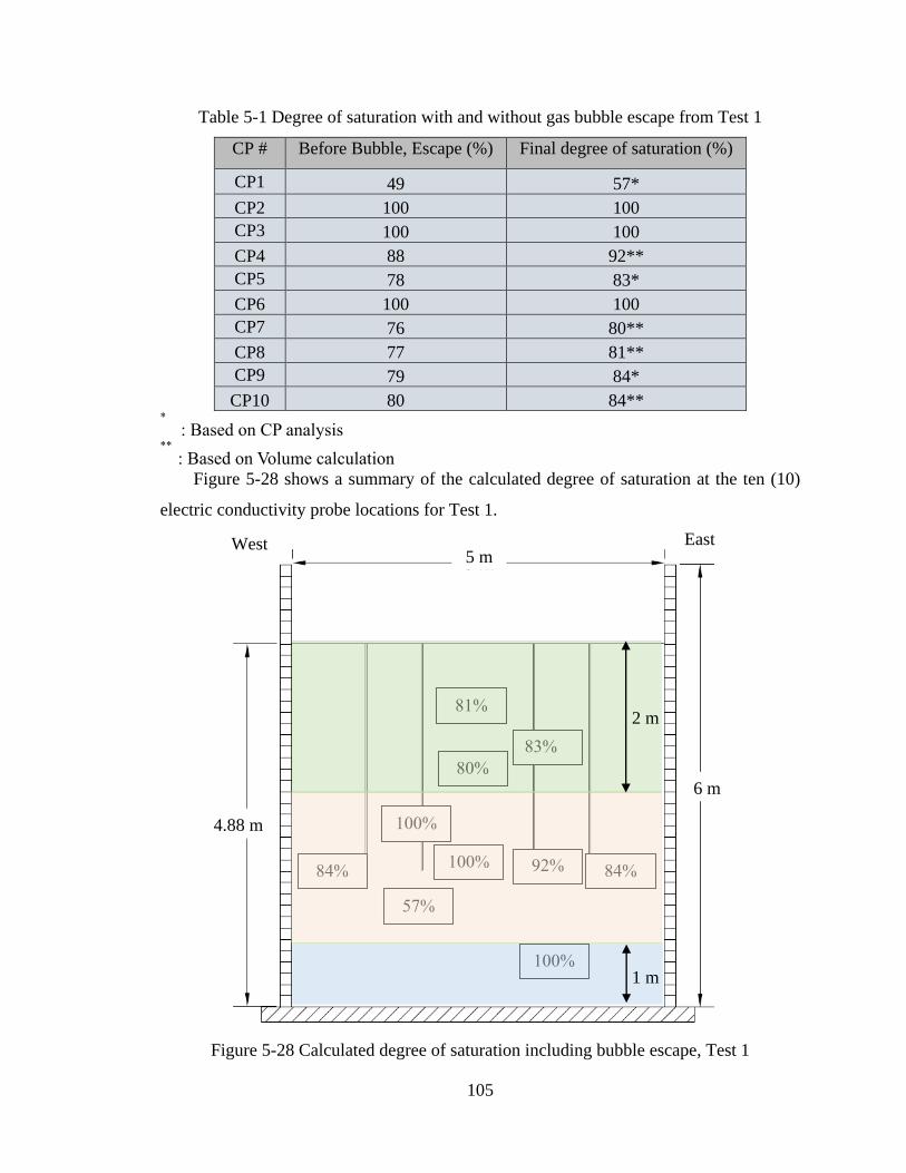
105
Table 5-1 Degree of saturation with and without gas bubble escape from Test 1
CP # Before Bubble, Escape (%) Final degree of saturation (%)
CP1 49 57*
CP2 100 100
CP3 100 100
CP4 88 92**
CP5 78 83*
CP6 100 100
CP7 76 80**
CP8 77 81**
CP9 79 84*
CP10 80 84** *
: Based on CP analysis **
: Based on Volume calculation
Figure 5-28 shows a summary of the calculated degree of saturation at the ten (10)
electric conductivity probe locations for Test 1.
Figure 5-28 Calculated degree of saturation including bubble escape, Test 1
6 m
4.88 m
5 m East West
100%
83%
Mesh
81%
80%
100%
Pre-
100%
D=1.57%
84% 92% B=0.
84%
2 m
1 m
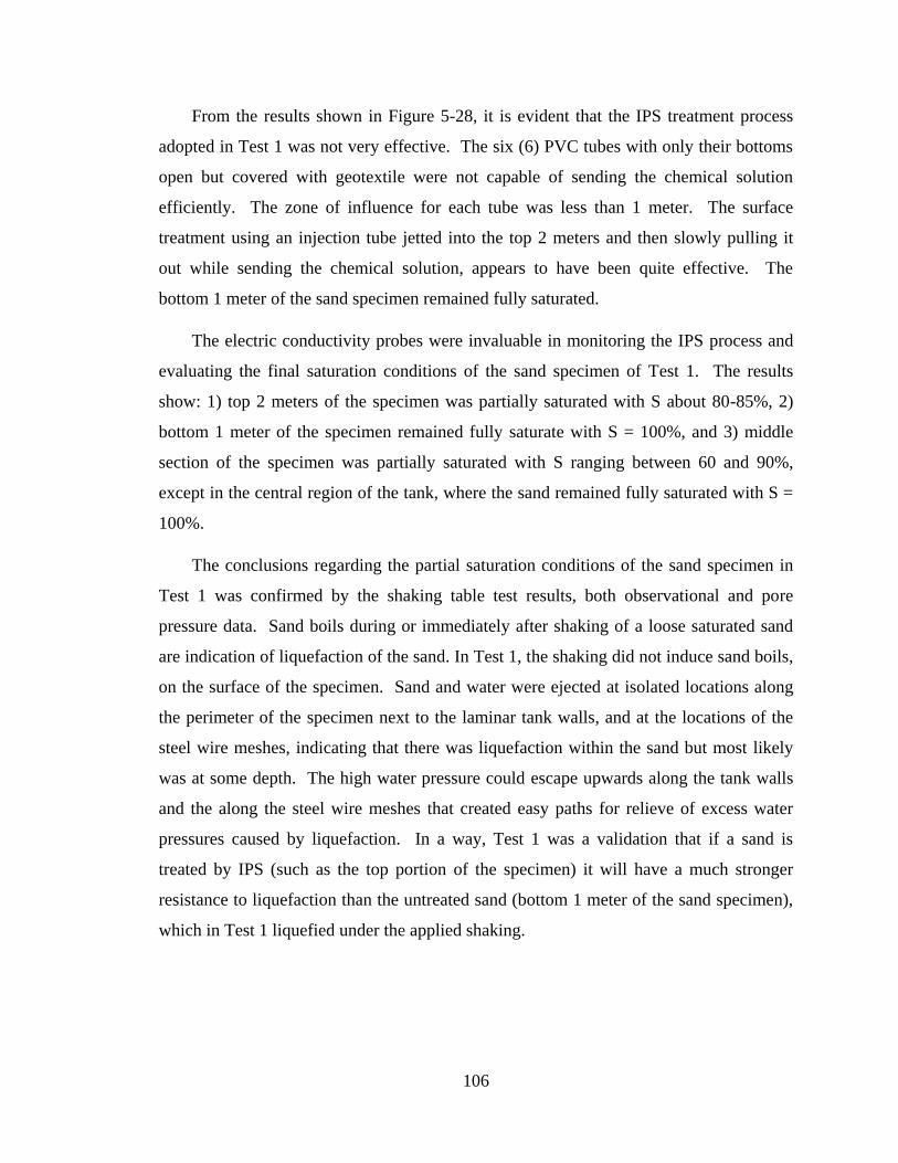
106
From the results shown in Figure 5-28, it is evident that the IPS treatment process
adopted in Test 1 was not very effective. The six (6) PVC tubes with only their bottoms
open but covered with geotextile were not capable of sending the chemical solution
efficiently. The zone of influence for each tube was less than 1 meter. The surface
treatment using an injection tube jetted into the top 2 meters and then slowly pulling it
out while sending the chemical solution, appears to have been quite effective. The
bottom 1 meter of the sand specimen remained fully saturated.
The electric conductivity probes were invaluable in monitoring the IPS process and
evaluating the final saturation conditions of the sand specimen of Test 1. The results
show: 1) top 2 meters of the specimen was partially saturated with S about 80-85%, 2)
bottom 1 meter of the specimen remained fully saturate with S = 100%, and 3) middle
section of the specimen was partially saturated with S ranging between 60 and 90%,
except in the central region of the tank, where the sand remained fully saturated with S =
100%.
The conclusions regarding the partial saturation conditions of the sand specimen in
Test 1 was confirmed by the shaking table test results, both observational and pore
pressure data. Sand boils during or immediately after shaking of a loose saturated sand
are indication of liquefaction of the sand. In Test 1, the shaking did not induce sand boils,
on the surface of the specimen. Sand and water were ejected at isolated locations along
the perimeter of the specimen next to the laminar tank walls, and at the locations of the
steel wire meshes, indicating that there was liquefaction within the sand but most likely
was at some depth. The high water pressure could escape upwards along the tank walls
and the along the steel wire meshes that created easy paths for relieve of excess water
pressures caused by liquefaction. In a way, Test 1 was a validation that if a sand is
treated by IPS (such as the top portion of the specimen) it will have a much stronger
resistance to liquefaction than the untreated sand (bottom 1 meter of the sand specimen),
which in Test 1 liquefied under the applied shaking.
107
5.6.3.3 Effect of shaking on gas bubble escape: Test 1
Two days after completing the IPS treatment of Test 1, the laminar box was
subjected twice to 15 cycles of 2Hz base excitation of about 0.1g. In both cases,
evidences of liquefaction were observed in the form of sand and water ejections along the
tank wall/sand boundaries, mainly on the west side of the box. Readings of the electric
conductivity were made just before the first shaking and subsequently at the end of both
shaking of the Test 1 specimen. The purpose of these readings was to explore if electric
conductivity probes could provide information on potential loss of gas bubbles as a result
of shaking of the specimen.
Figure 5-29 presents summary plots from the ten (10) conductivity probes.
Figure 5-29 Electric conductivity records showing data before and after shaking of
sand specimen, Test 1
East West
6 m
4.88 m
0.0
3.5
0 1 2 3 4 5
EC
(m
S/c
m)
Time (hr)
CP 3
0.0
3.5
0 1 2 3 4 5
EC
(m
S/c
m)
Time (hr)
CP 4
0.0
3.5
0 1 2 3 4 5
EC
(m
S/c
m)
Time (hr)
CP 5
0.0
3.5
0 1 2 3 4 5
EC
(m
S/c
m)
Time (hr)
CP 6
0.0
3.5
0 1 2 3 4 5
EC
(m
S/c
m)
Time (hr)
CP 7
0.0
3.5
0 1 2 3 4 5
EC
(m
S/c
m)
Time (hr)
CP 8
0.0
3.5
0 1 2 3 4 5
EC
(m
S/c
m)
Time (hr)
CP 9
0.0
3.5
0 1 2 3 4 5
EC
(m
S/c
m)
Time (hr)
CP 10
0.0
3.5
0 1 2 3 4 5
EC
(m
S/c
m)
Time (hr)
CP 1
0.0
3.5
0 1 2 3 4 5
EC
(m
S/c
m)
Time (hr)
CP 2
108
In each of the CP plots shown in Figure 5-29 there are four points. The triangular
data points at time zero are the electric conductivity values recorded long after injections
were completed and gas generation ceased. The first square data point at time zero is the
reading taken about 48 hours after injection and gas generation were completed, and
about 1.5 hours before the first shaking of the sand specimen. The second and third
square data points are the electric conductivity readings taken immediately after the two
shakings.
The electric conductivity data points shown in Figure 5-29 lead to the following
observations and conclusions:
1. Comparisons of the electric conductivity data taken at the end of injection
and bubble generation (triangular points) and just before the first shaking
(sqaure points) show only slight changes in the readings, except at CP3.
Since during this 48-hour wait time there were no observations of bubbles
escaping, these slight changes in electric conductivities at the nine CP
locations are attributed to ion movements from higher to lower
concentration regions. CP3 is located within the bottom 1 meter of the
specimen, which was not treated and initially after injection had a reading
of 0.2 mS/cm, a value corresponding to clean water and sand. The
significant jump in the electric conductivity after 48 hours of wait period is
unexplainable. The value of the electric conductivity just before shaking at
CP3 is about 2.5 mS/cm, a value typical for sand with 1% sodium
percarbnate solution. It appears that the solution from the treated region
above CP3 made contact, possibly through the steel wire mesh within which
CP3 was fixed.
2. Comparisons of the electric conductivity data before and after the two
shakings show six CPs (CP2, CP4, CP5, CP7, CP8, and CP9) with no
appreciable changes, while the remaining four CPs (CP1, CP3, CP6, and
CP10) show significant changes.
3. The CPs that did not record changes in electric conductivity before and after
the shaking, (CP2, CP4, CP5, CP7, CP8, and CP9) are in the IPS treated
109
zones. This indicates that gas bubbles were not lost due to the shaking. In
fact, the visual observations made during and after each shaking confirmed
this, because there were no evidences of gas bubbles escaping nor sand
boils forming in the regions of these CPs. Therefore, IPS treated sand with
S = 80%-90% not only did not liquefy, but also did not lose any gas
bubbles, even under large shaking that caused the untreated sand in the
specimen to liquefy.
4. The electric conductivity readings of CP1, CP6, and CP10, increased
because of the first shaking. This can be attributed to the liquefaction of the
bottom 1 meter sand layer, which caused sand boils manifested on the
surface of the specimen, mostly along the west side wall of the laminar box.
Sand boils would have dramatically increased the void ratios of the sands at
the tips of the conductivity probes (thus increasing the volume of the
conductive fluid) leading to increase in electric conductivity. Electric
conductivity of these three probes decreased due to the second shaking.
This can be attributed to decrease in the void ratio, which was evident by
the settlements observed at the surface mostly near the western region of the
laminar box.
5. The electric conductivity of CP3 decreased because of both shaking. Again,
this probe data is difficult to interpret. A possible reason for this decrease
could be densification of the sand resulting smaller void ratio and decrease
in electric conductivity. It is noted that the degree of saturation at CP3 was
recorded to be 100%. Therefore, the sand at this location should have
liquefied.
110
5.7 Electric conductivity results from laminar box Test 2
The electric conductivity readings of the ten (10) probes used in Test 1 clearly
indicated that the IPS treatment of the sand specimen in Test 1 was limited to primarily
the upper portion of the sand in the laminar box. This is the reason why, during the
shaking of the specimen evidences of liquefaction were observed and recorded. The six
PVC injection tubes were not effective in treating the entire sand specimen. Surface
injection was employed in which an injection tube was jetted down to about 2 meters
below the surface of the specimen and then slowly retrieved, while injecting the sodium
percrbonate solution. The conductivity probe data showed that the IPS process of the
sand specimen of Test 1 was partially effective, by reducing degree of saturation in some
regions, while other regions remained fully saturated. Therefore, it was decided to
repeat the laminar box test (Test 2) in which the entire sand specimen would be IPS
treated using an injection tube jetted in from the surface of the specimen.
5.7.1 Specimen preparation: Test 2
In Test 2, twenty one (21) Milwaukee conductivity probes were used to monitor the
IPS within the entire sand specimen. Thirteen CPs (CP1 through CP13) were fixed inside
five steel meshes that also included pore water pressure transducers. As in Test 1, the
steel meshes were hanged prior to placement of the sand from a steel truss fixed above
the laminar box. The meshes were located in the southern region of the laminar box to
allow placement of the sand from the norther side of the box.
Figure 5-30 shows the locations of the five (5) steel meshes and the first 13
conductivity probes. Additional eight (8) conductivity probes (CP14 through CP21) were
also installed about 0.5m from the southern and northern walls of the box to ensure that
the entire sand specimen from west to east and near the northern and southern walls could
be monitored during the IPS process. These probes were individually held by their cables
during the sand placement to ensure their desired locations within the specimen. Figure
5-30 shows the eight CPs along the northern and southern walls of the laminar box.
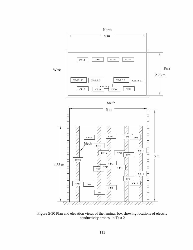
111
Figure 5-30 Plan and elevation views of the laminar box showing locations of electric
conductivity probes, in Test 2
West
North
South
East
2.75 m
5 m
CP14 CP15 CP16 CP17
CP18 CP21
CPs12 ,13 CPs1,2, 3 CPs7,8,9 CPs10, 11
CPs4,5,6 CP19 CP20
6 m
4.88 m
5 m
Mesh
CP14 CP6
CP13
CP12 CP18
CP1
CP3
CP15
CP2 CP19
CP5
CP4
CP20
CP16
CP17
CP7
CP8
CP11
CP9
CP10
CP21
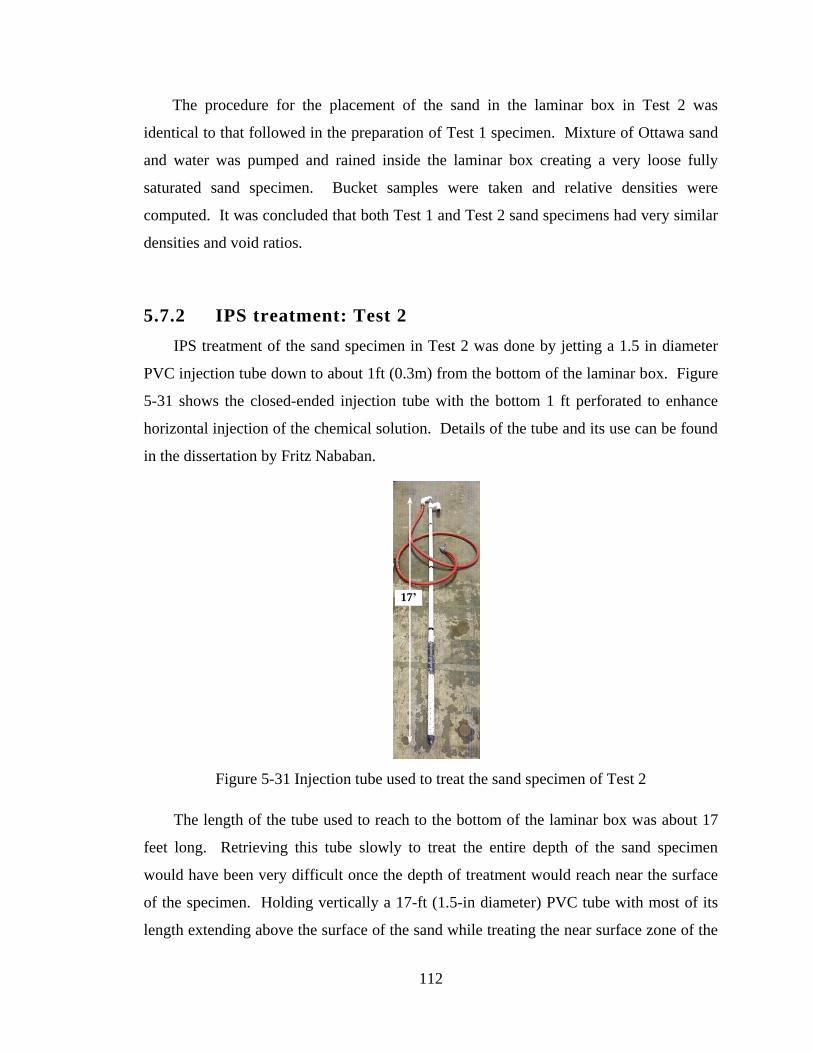
112
17’
The procedure for the placement of the sand in the laminar box in Test 2 was
identical to that followed in the preparation of Test 1 specimen. Mixture of Ottawa sand
and water was pumped and rained inside the laminar box creating a very loose fully
saturated sand specimen. Bucket samples were taken and relative densities were
computed. It was concluded that both Test 1 and Test 2 sand specimens had very similar
densities and void ratios.
5.7.2 IPS treatment: Test 2
IPS treatment of the sand specimen in Test 2 was done by jetting a 1.5 in diameter
PVC injection tube down to about 1ft (0.3m) from the bottom of the laminar box. Figure
5-31 shows the closed-ended injection tube with the bottom 1 ft perforated to enhance
horizontal injection of the chemical solution. Details of the tube and its use can be found
in the dissertation by Fritz Nababan.
Figure 5-31 Injection tube used to treat the sand specimen of Test 2
The length of the tube used to reach to the bottom of the laminar box was about 17
feet long. Retrieving this tube slowly to treat the entire depth of the sand specimen
would have been very difficult once the depth of treatment would reach near the surface
of the specimen. Holding vertically a 17-ft (1.5-in diameter) PVC tube with most of its
length extending above the surface of the sand while treating the near surface zone of the
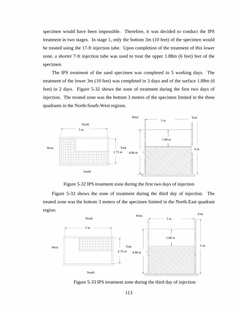
113
East West
South
North
5 m
2.75 m
1.88 m
4.88 m 6 m
5 m East West
specimen would have been impossible. Therefore, it was decided to conduct the IPS
treatment in two stages. In stage 1, only the bottom 3m (10 feet) of the specimen would
be treated using the 17-ft injection tube. Upon completion of the treatment of this lower
zone, a shorter 7-ft injection tube was used to treat the upper 1.88m (6 feet) feet of the
specimen.
The IPS treatment of the sand specimen was completed in 5 working days. The
treatment of the lower 3m (10 feet) was completed in 3 days and of the surface 1.88m (6
feet) in 2 days. Figure 5-32 shows the zone of treatment during the first two days of
injection. The treated zone was the bottom 3 meters of the specimen limited in the three
quadrants in the North-South-West regions.
Figure 5-32 IPS treatment zone during the first two days of injection
Figure 5-33 shows the zone of treatment during the third day of injection. The
treated zone was the bottom 3 meters of the specimen limited in the North-East quadrant
region.
Figure 5-33 IPS treatment zone during the third day of injection
1.88 m
6 m
5 m
East West
West East
2.75 m
5 m
North
South
4.88 m
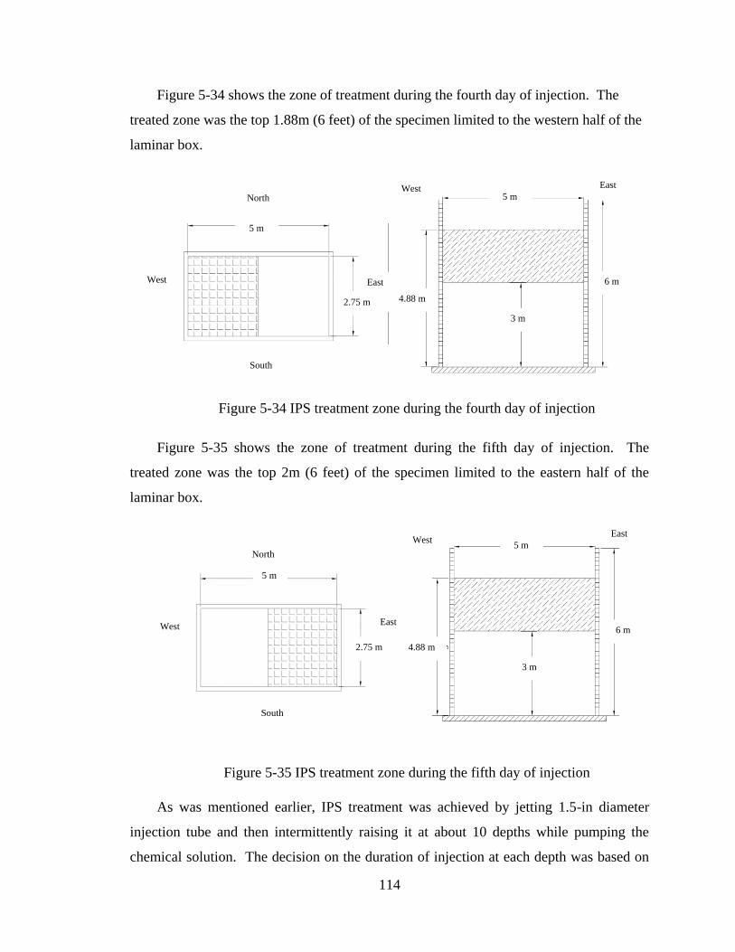
114
Figure 5-34 shows the zone of treatment during the fourth day of injection. The
treated zone was the top 1.88m (6 feet) of the specimen limited to the western half of the
laminar box.
Figure 5-34 IPS treatment zone during the fourth day of injection
Figure 5-35 shows the zone of treatment during the fifth day of injection. The
treated zone was the top 2m (6 feet) of the specimen limited to the eastern half of the
laminar box.
Figure 5-35 IPS treatment zone during the fifth day of injection
As was mentioned earlier, IPS treatment was achieved by jetting 1.5-in diameter
injection tube and then intermittently raising it at about 10 depths while pumping the
chemical solution. The decision on the duration of injection at each depth was based on
South
North
East
2.75 m
5 m
West
East West 5 m
6 m
3 m
4.88 m
m
East West
5 m
6 m
3 m
4.88 m
m
2.75 m
East West
North
South
5 m
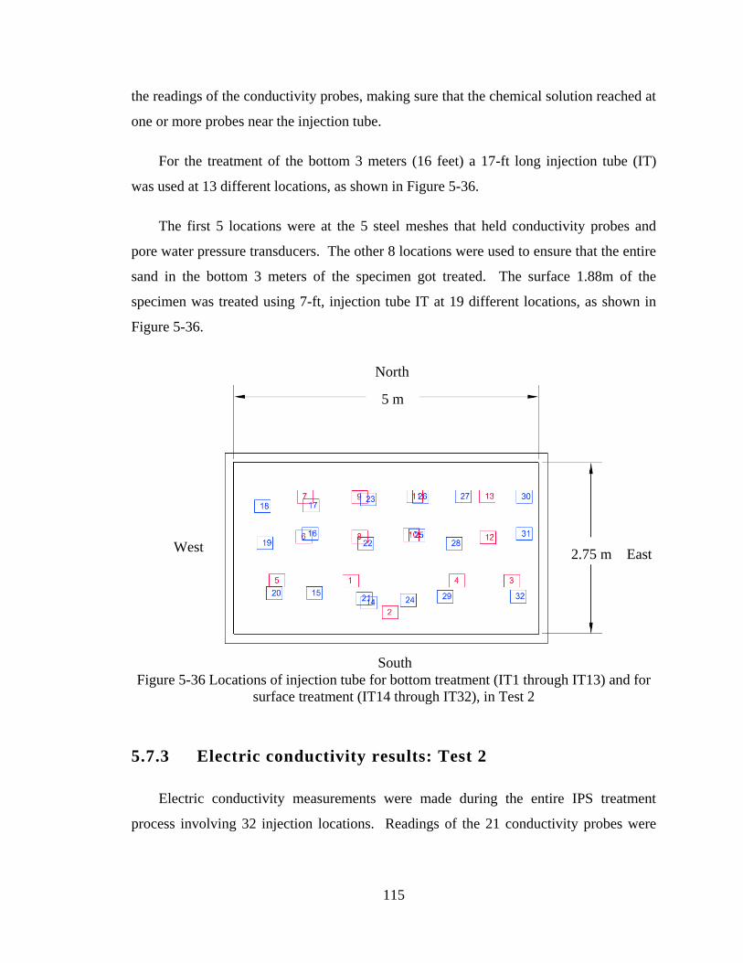
115
the readings of the conductivity probes, making sure that the chemical solution reached at
one or more probes near the injection tube.
For the treatment of the bottom 3 meters (16 feet) a 17-ft long injection tube (IT)
was used at 13 different locations, as shown in Figure 5-36.
The first 5 locations were at the 5 steel meshes that held conductivity probes and
pore water pressure transducers. The other 8 locations were used to ensure that the entire
sand in the bottom 3 meters of the specimen got treated. The surface 1.88m of the
specimen was treated using 7-ft, injection tube IT at 19 different locations, as shown in
Figure 5-36.
Figure 5-36 Locations of injection tube for bottom treatment (IT1 through IT13) and for
surface treatment (IT14 through IT32), in Test 2
5.7.3 Electric conductivity results: Test 2
Electric conductivity measurements were made during the entire IPS treatment
process involving 32 injection locations. Readings of the 21 conductivity probes were
North
East 2.75 m
5 m
West
South
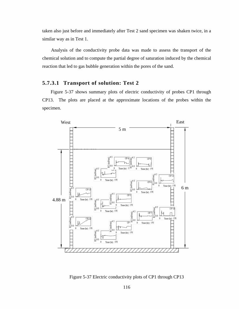
116
6 m
5 m
4.88 m
East West
taken also just before and immediately after Test 2 sand specimen was shaken twice, in a
similar way as in Test 1.
Analysis of the conductivity probe data was made to assess the transport of the
chemical solution and to compute the partial degree of saturation induced by the chemical
reaction that led to gas bubble generation within the pores of the sand.
5.7.3.1 Transport of solution: Test 2
Figure 5-37 shows summary plots of electric conductivity of probes CP1 through
CP13. The plots are placed at the approximate locations of the probes within the
specimen.
Figure 5-37 Electric conductivity plots of CP1 through CP13
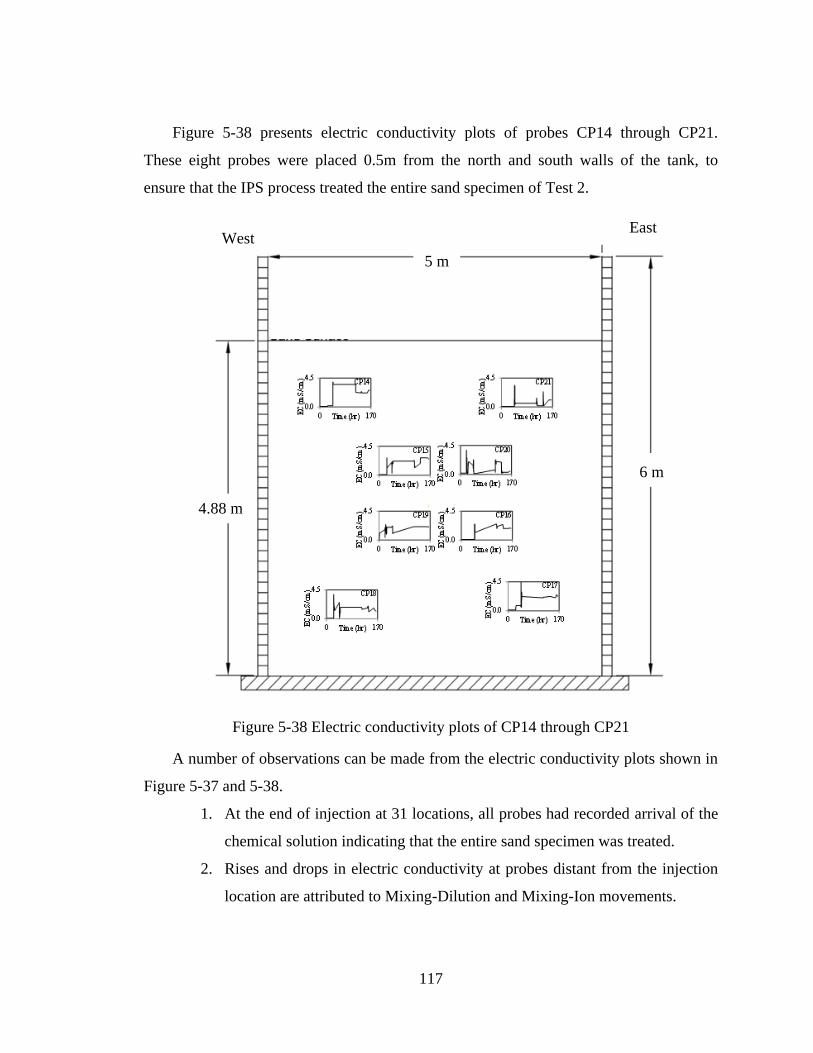
117
Figure 5-38 presents electric conductivity plots of probes CP14 through CP21.
These eight probes were placed 0.5m from the north and south walls of the tank, to
ensure that the IPS process treated the entire sand specimen of Test 2.
Figure 5-38 Electric conductivity plots of CP14 through CP21
A number of observations can be made from the electric conductivity plots shown in
Figure 5-37 and 5-38.
1. At the end of injection at 31 locations, all probes had recorded arrival of the
chemical solution indicating that the entire sand specimen was treated.
2. Rises and drops in electric conductivity at probes distant from the injection
location are attributed to Mixing-Dilution and Mixing-Ion movements.
6 m
4.88 m
5 m
East West
118
3. When probes were near an injection location, they detected the arrival of
solution in less than 10 to 15 minutes.
4. Probes that were less than 1m from an injection tube recorded the arrival of
the solution. For example, at the time of injection from IT1, probes CP1,
CP2, CP3, CP4, CP5, and CP19 (<1m from the injection location) recorded
the arrival of the solution. Probes CP12, CP13, and CP18 (>1.3m from the
injection location) did not detect the solution that was being pumped from
IT1. It is noted that the duration of injection at a depth was controlled by the
observation of arrival of the solution to the nearby conductivity probes. In
the case of IT1, had the injection continued further the solution might have
arrived at CP12, CP13, and CP18. In general, it was observed that a 15-
minute injection was adequate to transport the solution about 1 meter away
from the injection tube.
5. The peak values of electric conductivity measured by the probes ranged
between 2.2 mS/cm and 4 mS/cm. This range from the laminar box Test 1
was 2.3 mS/cm and 3.5 mS/cm. From the bench-top tests, for a 1%
concentration was between 2.2 mS/cm and 3.3 mS/cm. From the glass tank
test, the range for 1% concentration was 2.8 mS/cm and 3.7 mS/cm. It
appears that in the laminar box Test 2, the upper value of electric
conductivity is slightly larger than that corresponding to 1% concentration
solution as measured in all other tests. This indicates, that at times, the
solution pumped in Test 2 may have had concentration as large as 1.2% (a
value determined from bench-top tests described in Chapter 3).
5.7.3.2 Degree of saturation
In this section, expanded versions of the electric conductivity plots of each probe are
presented to demonstrate how the degree of saturation was computed at each probe
location. Figures 5-39 through 5-59 present the expanded electric conductivity plots.
Each figure shows the electric conductivity data and the location in plan of the probe
relative to the injection tubes. Along the top of an electric conductivity plot, the time
duration of the injections are shown to help interpret the data. The dash lines in the
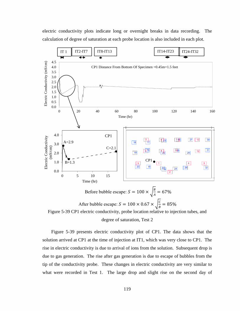
119
electric conductivity plots indicate long or overnight breaks in data recording. The
calculation of degree of saturation at each probe location is also included in each plot.
Figure 5-39 CP1 electric conductivity, probe location relative to injection tubes, and
degree of saturation, Test 2
Figure 5-39 presents electric conductivity plot of CP1. The data shows that the
solution arrived at CP1 at the time of injection at IT1, which was very close to CP1. The
rise in electric conductivity is due to arrival of ions from the solution. Subsequent drop is
due to gas generation. The rise after gas generation is due to escape of bubbles from the
tip of the conductivity probe. These changes in electric conductivity are very similar to
what were recorded in Test 1. The large drop and slight rise on the second day of
0.0
1.0
2.0
3.0
4.0
0 5 10 15
Ele
ctri
c C
on
du
ctiv
ity
(mS
/cm
)
Time (hr)
IT 1 IT2-IT7 IT8-IT13 IT14-IT23 IT24-IT32
0.0
0.5
1.0
1.5
2.0
2.5
3.0
3.5
4.0
4.5
0 20 40 60 80 100 120 140 160
Ele
ctri
c C
onduct
ivit
y (
mS
/cm
)
Time (hr)
CP1 Distance From Bottom Of Specimen =0.45m=1.5 feet
A=2.9
B=1.3
C=2.1
Before bubble escape: 𝑆 = 100 × 𝐵
𝐴= 67%
After bubble escape: 𝑆 = 100 × 0.67 × 𝐶
𝐵= 85%
CP1
CP1
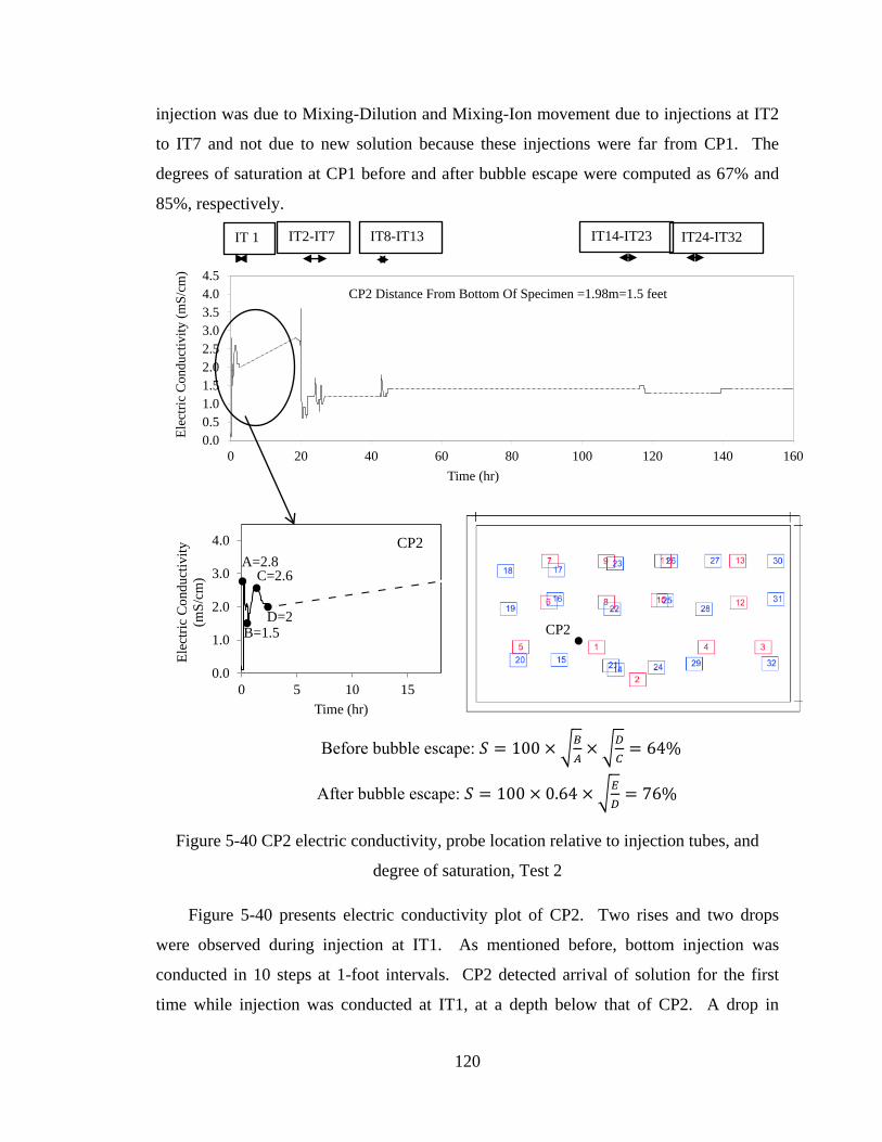
120
injection was due to Mixing-Dilution and Mixing-Ion movement due to injections at IT2
to IT7 and not due to new solution because these injections were far from CP1. The
degrees of saturation at CP1 before and after bubble escape were computed as 67% and
85%, respectively.
Figure 5-40 CP2 electric conductivity, probe location relative to injection tubes, and
degree of saturation, Test 2
Figure 5-40 presents electric conductivity plot of CP2. Two rises and two drops
were observed during injection at IT1. As mentioned before, bottom injection was
conducted in 10 steps at 1-foot intervals. CP2 detected arrival of solution for the first
time while injection was conducted at IT1, at a depth below that of CP2. A drop in
Before bubble escape: 𝑆 = 100 × 𝐵
𝐴×
𝐷
𝐶= 64%
After bubble escape: 𝑆 = 100 × 0.64 × 𝐸
𝐷= 76%
IT 1 IT2-IT7 IT8-IT13 IT14-IT23 IT24-IT32
0.0
0.5
1.0
1.5
2.0
2.5
3.0
3.5
4.0
4.5
0 20 40 60 80 100 120 140 160
Ele
ctri
c C
ond
uct
ivit
y (
mS
/cm
)
Time (hr)
CP2 Distance From Bottom Of Specimen =1.98m=1.5 feet
0.0
1.0
2.0
3.0
4.0
0 5 10 15
Ele
ctri
c C
on
du
ctiv
ity
(mS
/cm
)
Time (hr)
A=2.8
B=1.5
C=2.6
D=2
CP2
CP2
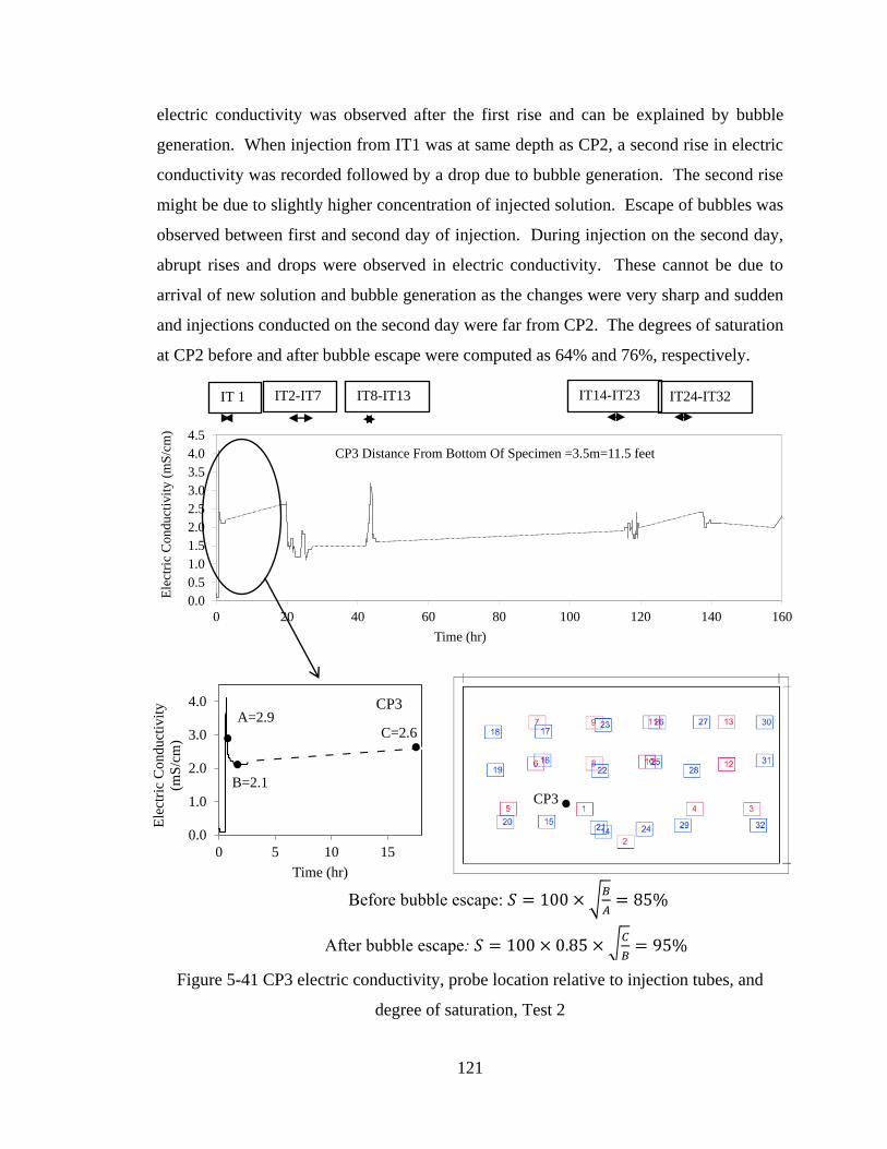
121
electric conductivity was observed after the first rise and can be explained by bubble
generation. When injection from IT1 was at same depth as CP2, a second rise in electric
conductivity was recorded followed by a drop due to bubble generation. The second rise
might be due to slightly higher concentration of injected solution. Escape of bubbles was
observed between first and second day of injection. During injection on the second day,
abrupt rises and drops were observed in electric conductivity. These cannot be due to
arrival of new solution and bubble generation as the changes were very sharp and sudden
and injections conducted on the second day were far from CP2. The degrees of saturation
at CP2 before and after bubble escape were computed as 64% and 76%, respectively.
Figure 5-41 CP3 electric conductivity, probe location relative to injection tubes, and
degree of saturation, Test 2
0.0
0.5
1.0
1.5
2.0
2.5
3.0
3.5
4.0
4.5
0 20 40 60 80 100 120 140 160
Ele
ctri
c C
onduct
ivit
y (
mS
/cm
)
Time (hr)
CP3 Distance From Bottom Of Specimen =3.5m=11.5 feet
IT 1 IT2-IT7 IT8-IT13 IT14-IT23 IT24-IT32
0.0
1.0
2.0
3.0
4.0
0 5 10 15
Ele
ctri
c C
onduct
ivit
y
(mS
/cm
)
Time (hr)
CP3 A=2.9
B=2.1
C=2.6
Before bubble escape: 𝑆 = 100 × 𝐵
𝐴= 85%
After bubble escape: 𝑆 = 100 × 0.85 × 𝐶
𝐵= 95%
CP3
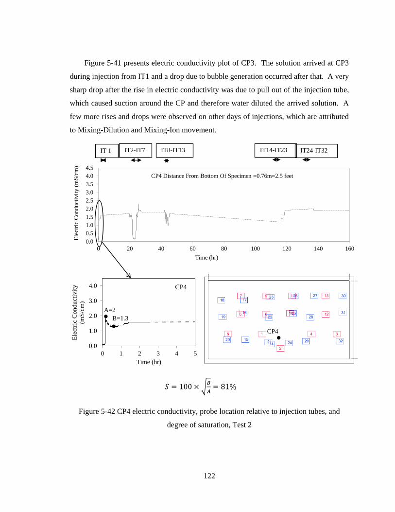
122
Figure 5-41 presents electric conductivity plot of CP3. The solution arrived at CP3
during injection from IT1 and a drop due to bubble generation occurred after that. A very
sharp drop after the rise in electric conductivity was due to pull out of the injection tube,
which caused suction around the CP and therefore water diluted the arrived solution. A
few more rises and drops were observed on other days of injections, which are attributed
to Mixing-Dilution and Mixing-Ion movement.
Figure 5-42 CP4 electric conductivity, probe location relative to injection tubes, and
degree of saturation, Test 2
0.0
0.5
1.0
1.5
2.0
2.5
3.0
3.5
4.0
4.5
0 20 40 60 80 100 120 140 160
Ele
ctri
c C
on
du
ctiv
ity (
mS
/cm
)
Time (hr)
CP4 Distance From Bottom Of Specimen =0.76m=2.5 feet
IT 1 IT2-IT7 IT8-IT13 IT14-IT23 IT24-IT32
0.0
1.0
2.0
3.0
4.0
0 1 2 3 4 5
Ele
ctri
c C
onduct
ivit
y
(mS
/cm
)
Time (hr)
B=1.3 A=2
𝑆 = 100 × 𝐵
𝐴= 81%
CP4
CP4
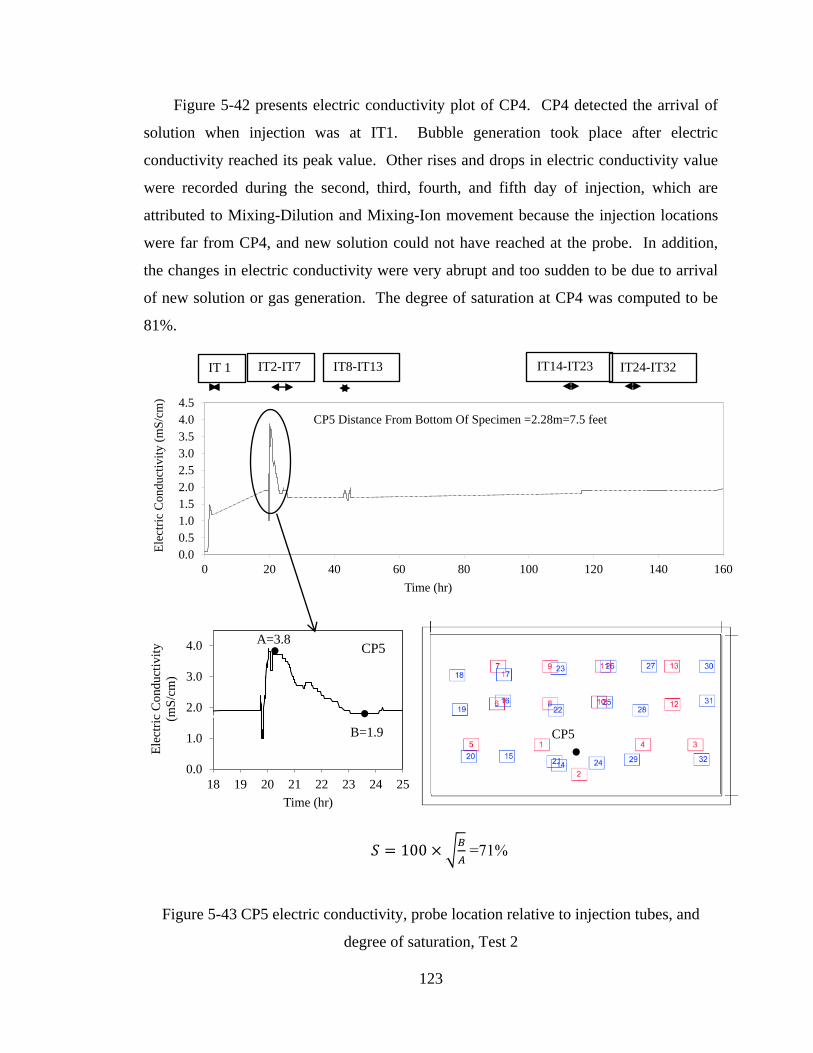
123
Figure 5-42 presents electric conductivity plot of CP4. CP4 detected the arrival of
solution when injection was at IT1. Bubble generation took place after electric
conductivity reached its peak value. Other rises and drops in electric conductivity value
were recorded during the second, third, fourth, and fifth day of injection, which are
attributed to Mixing-Dilution and Mixing-Ion movement because the injection locations
were far from CP4, and new solution could not have reached at the probe. In addition,
the changes in electric conductivity were very abrupt and too sudden to be due to arrival
of new solution or gas generation. The degree of saturation at CP4 was computed to be
81%.
Figure 5-43 CP5 electric conductivity, probe location relative to injection tubes, and
degree of saturation, Test 2
0.0
0.5
1.0
1.5
2.0
2.5
3.0
3.5
4.0
4.5
0 20 40 60 80 100 120 140 160
Ele
ctri
c C
on
du
ctiv
ity
(m
S/c
m)
Time (hr)
CP5 Distance From Bottom Of Specimen =2.28m=7.5 feet
IT 1 IT2-IT7 IT8-IT13 IT14-IT23 IT24-IT32
0.0
1.0
2.0
3.0
4.0
18 19 20 21 22 23 24 25
Ele
ctri
c C
onduct
ivit
y
(mS
/cm
)
Time (hr)
B=1.9
A=3.8 CP5
𝑆 = 100 × 𝐵
𝐴 =71%
CP5
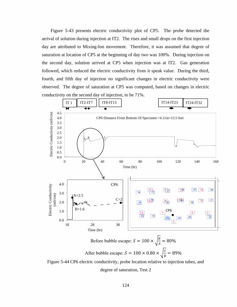
124
Figure 5-43 presents electric conductivity plot of CP5. The probe detected the
arrival of solution during injection at IT2. The rises and small drops on the first injection
day are attributed to Mixing-Ion movement. Therefore, it was assumed that degree of
saturation at location of CP5 at the beginning of day two was 100%. During injection on
the second day, solution arrived at CP5 when injection was at IT2. Gas generation
followed, which reduced the electric conductivity from it speak value. During the third,
fourth, and fifth day of injection no significant changes in electric conductivity were
observed. The degree of saturation at CP5 was computed, based on changes in electric
conductivity on the second day of injection, to be 71%.
Figure 5-44 CP6 electric conductivity, probe location relative to injection tubes, and
degree of saturation, Test 2
0.0
1.0
2.0
3.0
4.0
18 28 38
Ele
ctri
c C
onduct
ivit
y
(mS
/cm
)
Time (hr)
B=1.6
A=2.5 C=2
Before bubble escape: 𝑆 = 100 × 𝐵
𝐴= 80%
After bubble escape: 𝑆 = 100 × 0.80 × 𝐶
𝐵= 89%
0.0
0.5
1.0
1.5
2.0
2.5
3.0
3.5
4.0
4.5
0 20 40 60 80 100 120 140 160
Ele
ctri
c C
on
du
ctiv
ity
(m
S/c
m)
Time (hr)
CP6 Distance From Bottom Of Specimen =4.11m=13.5 feet
IT 1 IT2-IT7 IT8-IT13 IT14-IT23 IT24-IT32
CP6
CP6
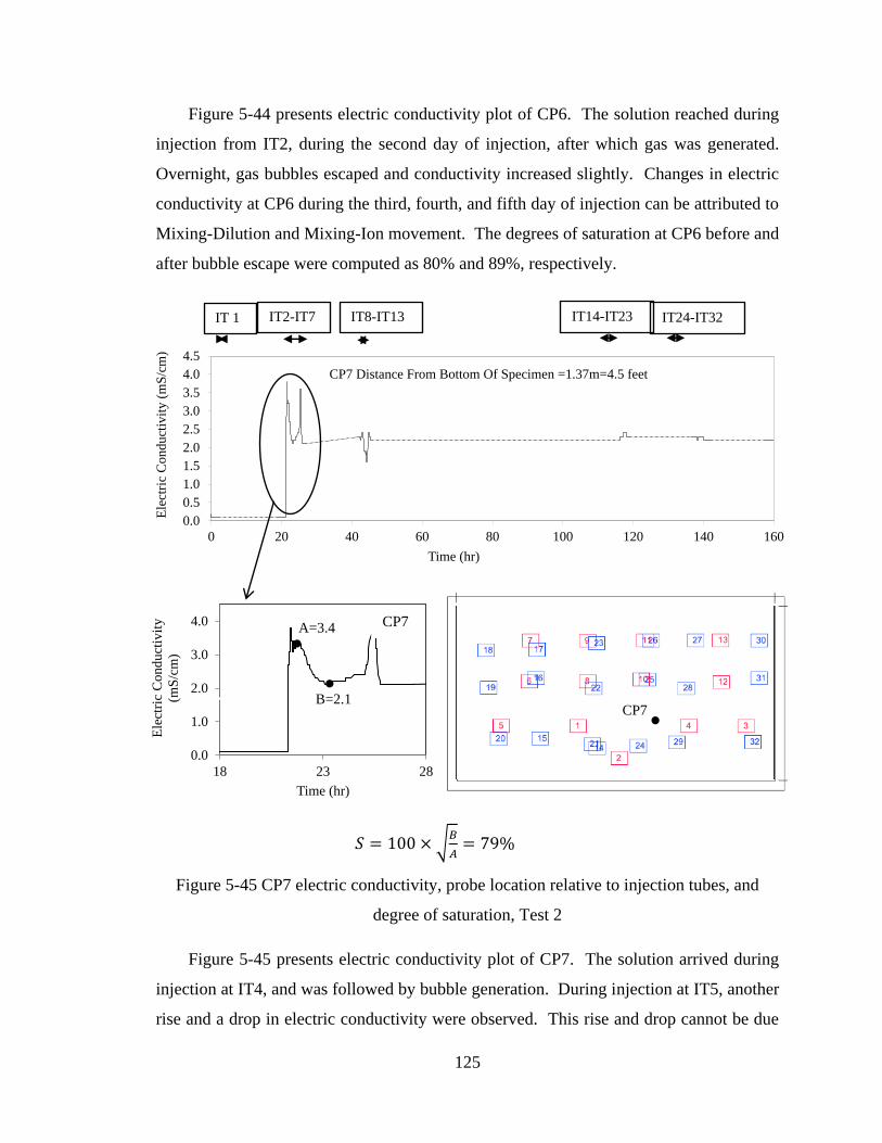
125
Figure 5-44 presents electric conductivity plot of CP6. The solution reached during
injection from IT2, during the second day of injection, after which gas was generated.
Overnight, gas bubbles escaped and conductivity increased slightly. Changes in electric
conductivity at CP6 during the third, fourth, and fifth day of injection can be attributed to
Mixing-Dilution and Mixing-Ion movement. The degrees of saturation at CP6 before and
after bubble escape were computed as 80% and 89%, respectively.
Figure 5-45 CP7 electric conductivity, probe location relative to injection tubes, and
degree of saturation, Test 2
Figure 5-45 presents electric conductivity plot of CP7. The solution arrived during
injection at IT4, and was followed by bubble generation. During injection at IT5, another
rise and a drop in electric conductivity were observed. This rise and drop cannot be due
0.0
0.5
1.0
1.5
2.0
2.5
3.0
3.5
4.0
4.5
0 20 40 60 80 100 120 140 160
Ele
ctri
c C
on
du
ctiv
ity
(m
S/c
m)
Time (hr)
CP7 Distance From Bottom Of Specimen =1.37m=4.5 feet
IT 1 IT2-IT7 IT8-IT13 IT14-IT23 IT24-IT32
0.0
1.0
2.0
3.0
4.0
18 23 28
Ele
ctri
c C
on
du
ctiv
ity
(mS
/cm
)
Time (hr)
CP7 A=3.4
B=2.1
𝑆 = 100 × 𝐵
𝐴= 79%
CP7
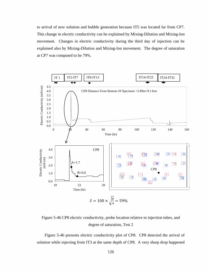
126
to arrival of new solution and bubble generation because IT5 was located far from CP7.
This change in electric conductivity can be explained by Mixing-Dilution and Mixing-Ion
movement. Changes in electric conductivity during the third day of injection can be
explained also by Mixing-Dilution and Mixing-Ion movement. The degree of saturation
at CP7 was computed to be 79%.
Figure 5-46 CP8 electric conductivity, probe location relative to injection tubes, and
degree of saturation, Test 2
Figure 5-46 presents electric conductivity plot of CP8. CP8 detected the arrival of
solution while injecting from IT3 at the same depth of CP8. A very sharp drop happened
0.0
0.5
1.0
1.5
2.0
2.5
3.0
3.5
4.0
4.5
0 20 40 60 80 100 120 140 160
Ele
ctri
c C
on
du
ctiv
ity
(m
S/c
m)
Time (hr)
CP8 Distance From Bottom Of Specimen =2.89m=9.5 feet
IT 1 IT2-IT7 IT8-IT13 IT14-IT23 IT24-IT32
0.0
1.0
2.0
3.0
4.0
18 23 28
Ele
ctri
c C
on
du
ctiv
ity
(mS
/cm
)
Time (hr)
CP8
B=0.6
A=1.7
𝑆 = 100 × 𝐵
𝐴= 59%
CP8
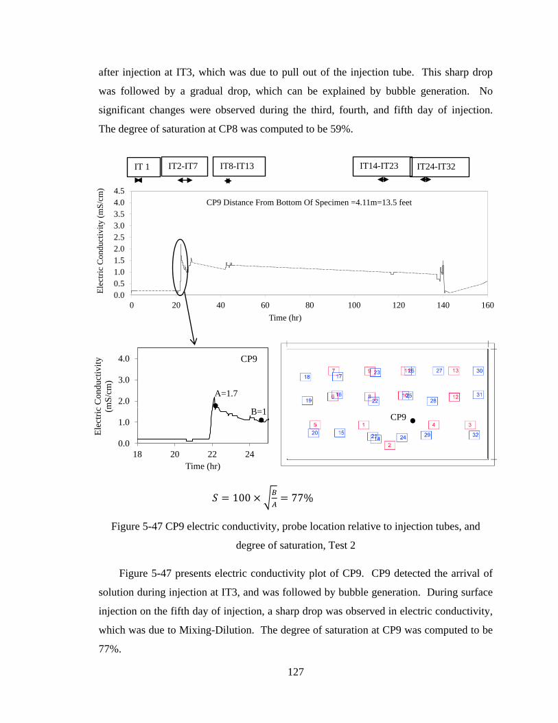
127
after injection at IT3, which was due to pull out of the injection tube. This sharp drop
was followed by a gradual drop, which can be explained by bubble generation. No
significant changes were observed during the third, fourth, and fifth day of injection.
The degree of saturation at CP8 was computed to be 59%.
Figure 5-47 CP9 electric conductivity, probe location relative to injection tubes, and
degree of saturation, Test 2
Figure 5-47 presents electric conductivity plot of CP9. CP9 detected the arrival of
solution during injection at IT3, and was followed by bubble generation. During surface
injection on the fifth day of injection, a sharp drop was observed in electric conductivity,
which was due to Mixing-Dilution. The degree of saturation at CP9 was computed to be
77%.
0.0
0.5
1.0
1.5
2.0
2.5
3.0
3.5
4.0
4.5
0 20 40 60 80 100 120 140 160
Ele
ctri
c C
ond
uct
ivit
y (
mS
/cm
)
Time (hr)
CP9 Distance From Bottom Of Specimen =4.11m=13.5 feet
IT 1 IT2-IT7 IT8-IT13 IT14-IT23 IT24-IT32
0.0
1.0
2.0
3.0
4.0
18 20 22 24
Ele
ctri
c C
onduct
ivit
y
(mS
/cm
)
Time (hr)
A=1.7
B=1
CP9
𝑆 = 100 × 𝐵
𝐴= 77%
CP9
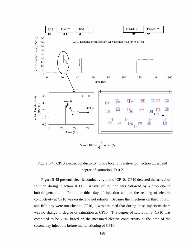
128
Figure 5-48 CP10 electric conductivity, probe location relative to injection tubes, and
degree of saturation, Test 2
Figure 5-48 presents electric conductivity plot of CP10. CP10 detected the arrival of
solution during injection at IT3. Arrival of solution was followed by a drop due to
bubble generation. From the third day of injection and on the reading of electric
conductivity at CP10 was erratic and not reliable. Because the injections on third, fourth,
and fifth day were not close to CP10, it was assumed that during those injections there
was no change in degree of saturation at CP10. The degree of saturation at CP10 was
computed to be 76%, based on the measured electric conductivity at the time of the
second day injection, before malfunctioning of CP10.
0.0
0.5
1.0
1.5
2.0
2.5
3.0
3.5
4.0
4.5
0 20 40 60 80 100 120 140 160
Ele
ctri
c C
onduct
ivit
y (
mS
/cm
)
Time (hr)
CP10 Distance From Bottom Of Specimen =1.67m=5.5 feet
IT 1 IT2-IT7 IT8-IT13 IT14-IT23 IT24-IT32
0.0
1.0
2.0
3.0
4.0
18 20 22 24
Ele
ctri
c C
ond
uct
ivit
y
(mS
/cm
)
Time (hr)
CP10
A=2.6
B=1.5
𝑆 = 100 × 𝐵
𝐴= 76%
CP10
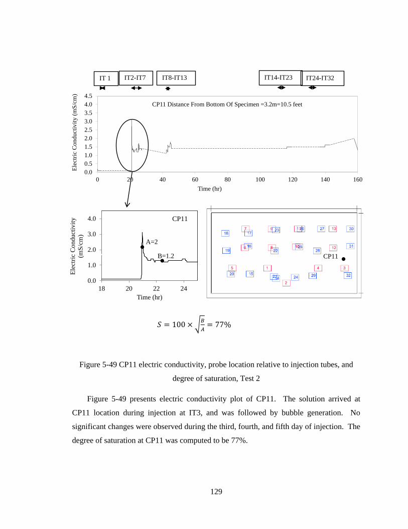
129
Figure 5-49 CP11 electric conductivity, probe location relative to injection tubes, and
degree of saturation, Test 2
Figure 5-49 presents electric conductivity plot of CP11. The solution arrived at
CP11 location during injection at IT3, and was followed by bubble generation. No
significant changes were observed during the third, fourth, and fifth day of injection. The
degree of saturation at CP11 was computed to be 77%.
0.0
0.5
1.0
1.5
2.0
2.5
3.0
3.5
4.0
4.5
0 20 40 60 80 100 120 140 160
Ele
ctri
c C
onduct
ivit
y (
mS
/cm
)
Time (hr)
CP11 Distance From Bottom Of Specimen =3.2m=10.5 feet
IT 1 IT2-IT7 IT8-IT13 IT14-IT23 IT24-IT32
0.0
1.0
2.0
3.0
4.0
18 20 22 24
Ele
ctri
c C
onduct
ivit
y
(mS
/cm
)
Time (hr)
A=2
B=1.2
CP11
𝑆 = 100 × 𝐵
𝐴= 77%
CP11
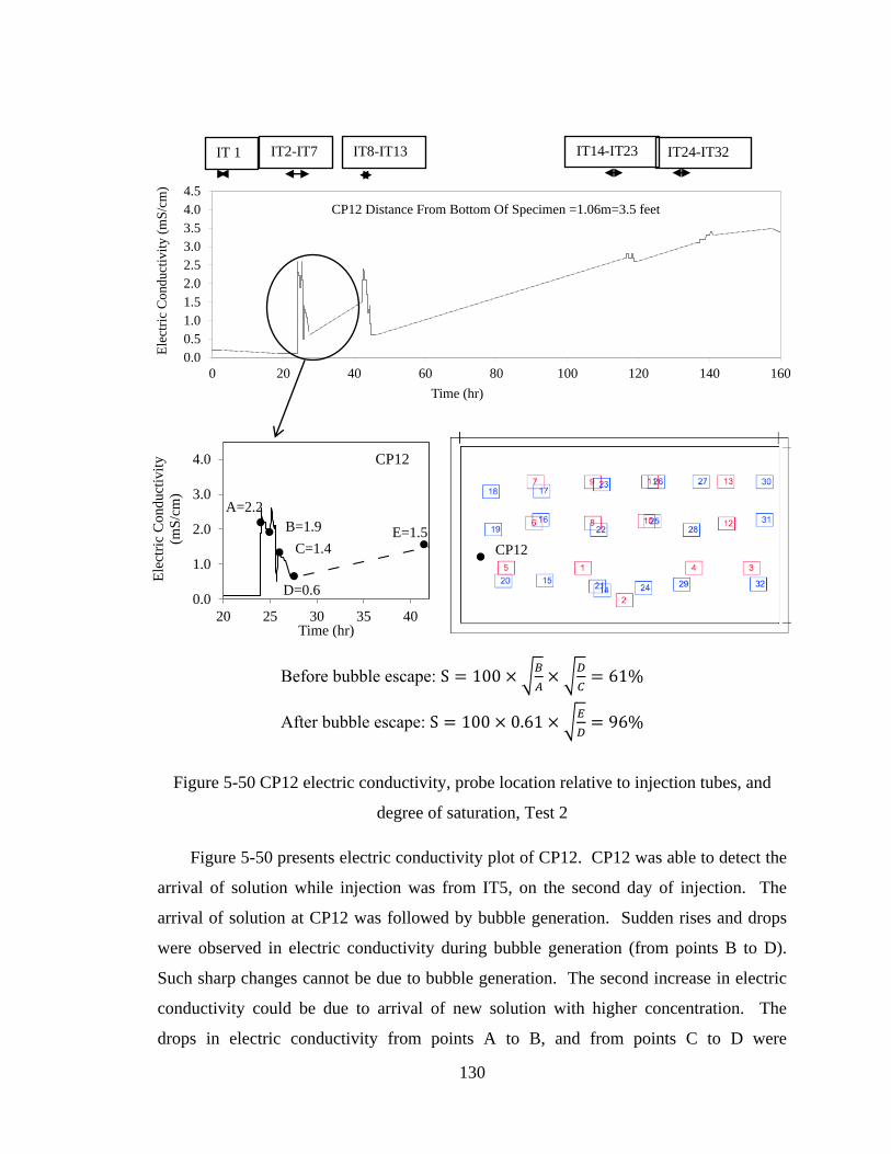
130
Figure 5-50 CP12 electric conductivity, probe location relative to injection tubes, and
degree of saturation, Test 2
Figure 5-50 presents electric conductivity plot of CP12. CP12 was able to detect the
arrival of solution while injection was from IT5, on the second day of injection. The
arrival of solution at CP12 was followed by bubble generation. Sudden rises and drops
were observed in electric conductivity during bubble generation (from points B to D).
Such sharp changes cannot be due to bubble generation. The second increase in electric
conductivity could be due to arrival of new solution with higher concentration. The
drops in electric conductivity from points A to B, and from points C to D were
0.0
1.0
2.0
3.0
4.0
20 25 30 35 40
Ele
ctri
c C
on
du
ctiv
ity
(mS
/cm
)
Time (hr)
D=0.6
E=1.5 C=1.4
A=2.2 B=1.9
CP12
0.0
0.5
1.0
1.5
2.0
2.5
3.0
3.5
4.0
4.5
0 20 40 60 80 100 120 140 160
Ele
ctri
c C
onduct
ivit
y (
mS
/cm
)
Time (hr)
CP12 Distance From Bottom Of Specimen =1.06m=3.5 feet
IT 1 IT2-IT7 IT8-IT13 IT14-IT23 IT24-IT32
Before bubble escape: S = 100 × 𝐵
𝐴×
𝐷
𝐶= 61%
After bubble escape: S = 100 × 0.61 × 𝐸
𝐷= 96%
CP12
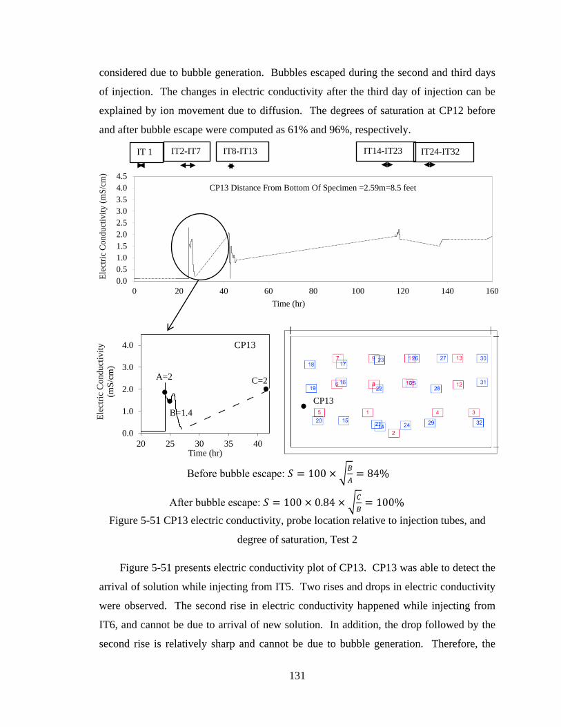
131
considered due to bubble generation. Bubbles escaped during the second and third days
of injection. The changes in electric conductivity after the third day of injection can be
explained by ion movement due to diffusion. The degrees of saturation at CP12 before
and after bubble escape were computed as 61% and 96%, respectively.
Figure 5-51 CP13 electric conductivity, probe location relative to injection tubes, and
degree of saturation, Test 2
Figure 5-51 presents electric conductivity plot of CP13. CP13 was able to detect the
arrival of solution while injecting from IT5. Two rises and drops in electric conductivity
were observed. The second rise in electric conductivity happened while injecting from
IT6, and cannot be due to arrival of new solution. In addition, the drop followed by the
second rise is relatively sharp and cannot be due to bubble generation. Therefore, the
0.0
0.5
1.0
1.5
2.0
2.5
3.0
3.5
4.0
4.5
0 20 40 60 80 100 120 140 160
Ele
ctri
c C
onduct
ivit
y (
mS
/cm
)
Time (hr)
CP13 Distance From Bottom Of Specimen =2.59m=8.5 feet
IT 1 IT2-IT7 IT8-IT13 IT14-IT23 IT24-IT32
0.0
1.0
2.0
3.0
4.0
20 25 30 35 40
Ele
ctri
c C
onduct
ivit
y
(mS
/cm
)
Time (hr)
CP13
A=2
B=1.4
C=2
Before bubble escape: 𝑆 = 100 × 𝐵
𝐴= 84%
After bubble escape: 𝑆 = 100 × 0.84 × 𝐶
𝐵= 100%
CP13
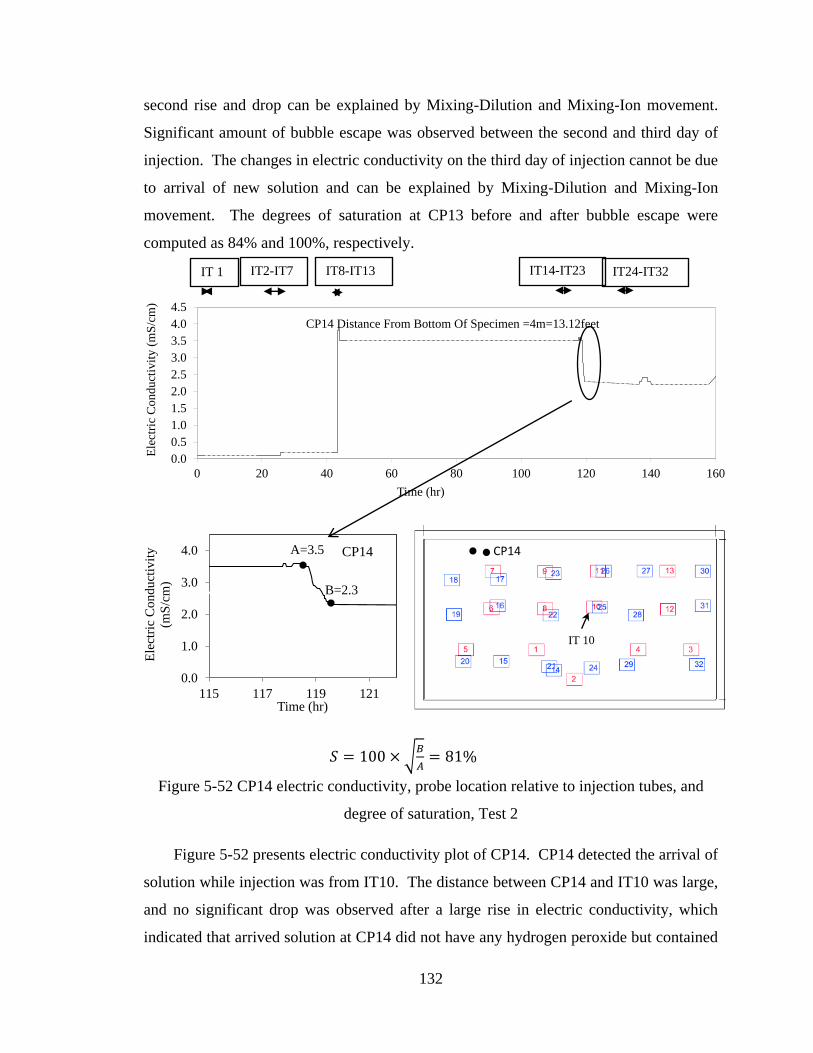
132
second rise and drop can be explained by Mixing-Dilution and Mixing-Ion movement.
Significant amount of bubble escape was observed between the second and third day of
injection. The changes in electric conductivity on the third day of injection cannot be due
to arrival of new solution and can be explained by Mixing-Dilution and Mixing-Ion
movement. The degrees of saturation at CP13 before and after bubble escape were
computed as 84% and 100%, respectively.
Figure 5-52 CP14 electric conductivity, probe location relative to injection tubes, and
degree of saturation, Test 2
Figure 5-52 presents electric conductivity plot of CP14. CP14 detected the arrival of
solution while injection was from IT10. The distance between CP14 and IT10 was large,
and no significant drop was observed after a large rise in electric conductivity, which
indicated that arrived solution at CP14 did not have any hydrogen peroxide but contained
0.0
0.5
1.0
1.5
2.0
2.5
3.0
3.5
4.0
4.5
0 20 40 60 80 100 120 140 160
Ele
ctri
c C
onduct
ivit
y (
mS
/cm
)
Time (hr)
CP14 Distance From Bottom Of Specimen =4m=13.12feet
IT 1 IT2-IT7 IT8-IT13 IT14-IT23 IT24-IT32
IT 10
0.0
1.0
2.0
3.0
4.0
115 117 119 121
Ele
ctri
c C
on
du
ctiv
ity
(mS
/cm
)
Time (hr)
A=3.5
B=2.3
CP14
𝑆 = 100 × 𝐵
𝐴= 81%
CP14
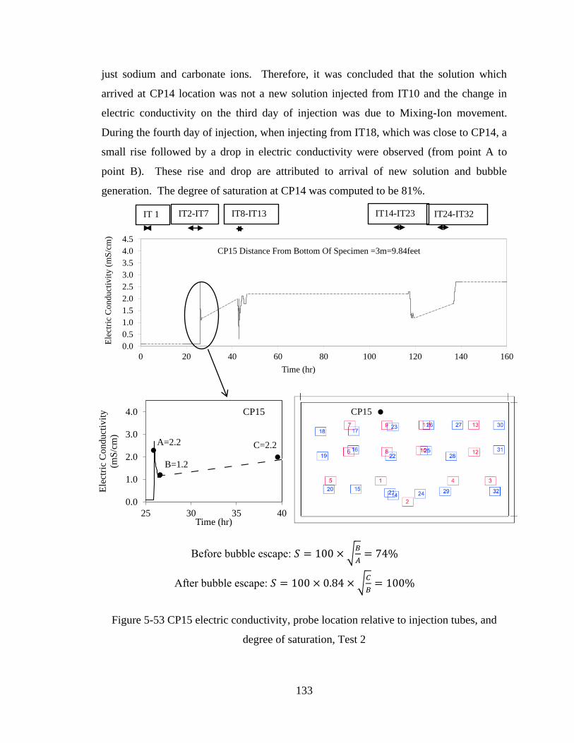
133
just sodium and carbonate ions. Therefore, it was concluded that the solution which
arrived at CP14 location was not a new solution injected from IT10 and the change in
electric conductivity on the third day of injection was due to Mixing-Ion movement.
During the fourth day of injection, when injecting from IT18, which was close to CP14, a
small rise followed by a drop in electric conductivity were observed (from point A to
point B). These rise and drop are attributed to arrival of new solution and bubble
generation. The degree of saturation at CP14 was computed to be 81%.
Figure 5-53 CP15 electric conductivity, probe location relative to injection tubes, and
degree of saturation, Test 2
0.0
1.0
2.0
3.0
4.0
25 30 35 40
Ele
ctri
c C
onduct
ivit
y
(mS
/cm
)
Time (hr)
A=2.2
B=1.2
C=2.2
0.0
0.5
1.0
1.5
2.0
2.5
3.0
3.5
4.0
4.5
0 20 40 60 80 100 120 140 160
Ele
ctri
c C
onduct
ivit
y (
mS
/cm
)
Time (hr)
CP15 Distance From Bottom Of Specimen =3m=9.84feet
IT 1 IT2-IT7 IT8-IT13 IT14-IT23 IT24-IT32
CP15
Before bubble escape: 𝑆 = 100 × 𝐵
𝐴= 74%
After bubble escape: 𝑆 = 100 × 0.84 × 𝐶
𝐵= 100%
CP15
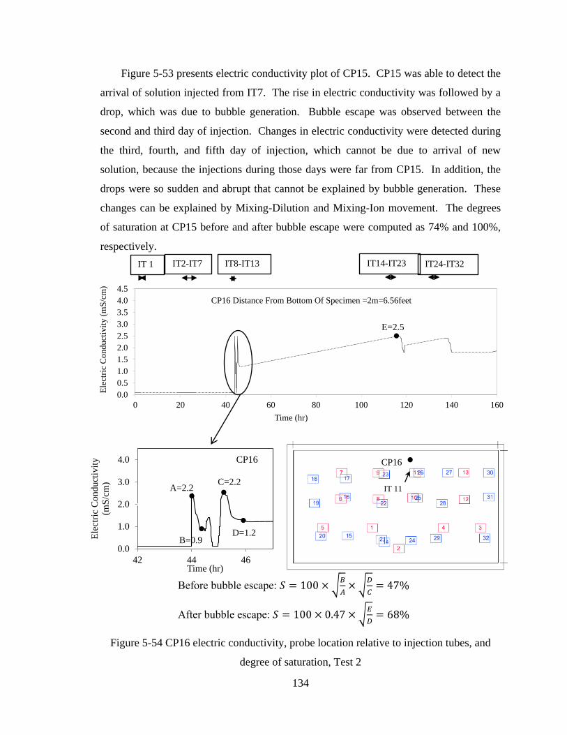
134
Figure 5-53 presents electric conductivity plot of CP15. CP15 was able to detect the
arrival of solution injected from IT7. The rise in electric conductivity was followed by a
drop, which was due to bubble generation. Bubble escape was observed between the
second and third day of injection. Changes in electric conductivity were detected during
the third, fourth, and fifth day of injection, which cannot be due to arrival of new
solution, because the injections during those days were far from CP15. In addition, the
drops were so sudden and abrupt that cannot be explained by bubble generation. These
changes can be explained by Mixing-Dilution and Mixing-Ion movement. The degrees
of saturation at CP15 before and after bubble escape were computed as 74% and 100%,
respectively.
Figure 5-54 CP16 electric conductivity, probe location relative to injection tubes, and
degree of saturation, Test 2
0.0
1.0
2.0
3.0
4.0
42 44 46
Ele
ctri
c C
onduct
ivit
y
(mS
/cm
)
Time (hr)
A=2.2
B=0.9
C=2.2
D=1.2
0.0
0.5
1.0
1.5
2.0
2.5
3.0
3.5
4.0
4.5
0 20 40 60 80 100 120 140 160
Ele
ctri
c C
onduct
ivit
y (
mS
/cm
)
Time (hr)
CP16 Distance From Bottom Of Specimen =2m=6.56feet
IT 1 IT2-IT7 IT8-IT13 IT14-IT23 IT24-IT32
E=2.5
CP16
Before bubble escape: 𝑆 = 100 × 𝐵
𝐴×
𝐷
𝐶= 47%
After bubble escape: 𝑆 = 100 × 0.47 × 𝐸
𝐷= 68%
IT 11
CP16
135
Figure 5-54 presents electric conductivity plot of CP16. The solution arrived at
CP16 while injection was from IT11. The rise in electric conductivity was followed by a
drop, which was due to bubble generation. During injection from IT12 which was far
from CP16 small increase followed by a sharp drop in electric conductivity were
observed. The drop was very abrupt and the conductivity decreased to 0.1 mS/cm, which
represented the conductivity of sand saturated with clean water. These rise and drop
were considered due to Mixing-Dilution and Mixing-Ion movement. During injection
from IT13 a large rise followed by a gradual drop in electric conductivity was observed,
which are attributed to arrival of new solution from IT13 and bubble generation. During
the night between the third and fourth day of injection, rise in electric conductivity due to
escape of bubbles was observed. During the fourth and fifth day of injection, no
significant changes in electric conductivity were observed because injection locations
were far from CP16. The degrees of saturation at CP16 before and after bubble escape
were computed as 47% and 68%, respectively.
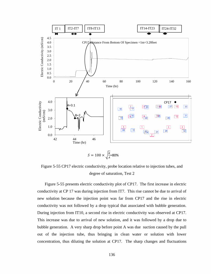
136
Figure 5-55 CP17 electric conductivity, probe location relative to injection tubes, and
degree of saturation, Test 2
Figure 5-55 presents electric conductivity plot of CP17. The first increase in electric
conductivity at CP 17 was during injection from IT7. This rise cannot be due to arrival of
new solution because the injection point was far from CP17 and the rise in electric
conductivity was not followed by a drop typical that associated with bubble generation.
During injection from IT10, a second rise in electric conductivity was observed at CP17.
This increase was due to arrival of new solution, and it was followed by a drop due to
bubble generation. A very sharp drop before point A was due suction caused by the pull
out of the injection tube, thus bringing in clean water or solution with lower
concentration, thus diluting the solution at CP17. The sharp changes and fluctuations
IT 10
0.0
0.5
1.0
1.5
2.0
2.5
3.0
3.5
4.0
4.5
0 20 40 60 80 100 120 140 160
Ele
ctri
c C
onduct
ivit
y (
mS
/cm
)
Time (hr)
CP17 Distance From Bottom Of Specimen =1m=3.28feet
IT 1 IT2-IT7 IT8-IT13 IT14-IT23 IT24-IT32
0.0
1.0
2.0
3.0
4.0
42 44 46
Ele
ctri
c C
on
du
ctiv
ity
(mS
/cm
)
Time (hr)
A=3.1
B=2
0.0
0.5
1.0
1.5
2.0
2.5
3.0
3.5
4.0
4.5
0 20 40 60 80 100 120 140 160
Ele
ctri
c C
onduct
ivit
y (
mS
/cm
)
Time (hr)
CP17 Distance From Bottom Of Specimen =1m=3.28feet
0.0
1.0
2.0
3.0
4.0
42 44 46
Ele
ctri
c C
on
du
ctiv
ity
(mS
/cm
)
Time (hr)
A=3.1
B=2
𝑆 = 100 × 𝐵
𝐴=80%
CP17
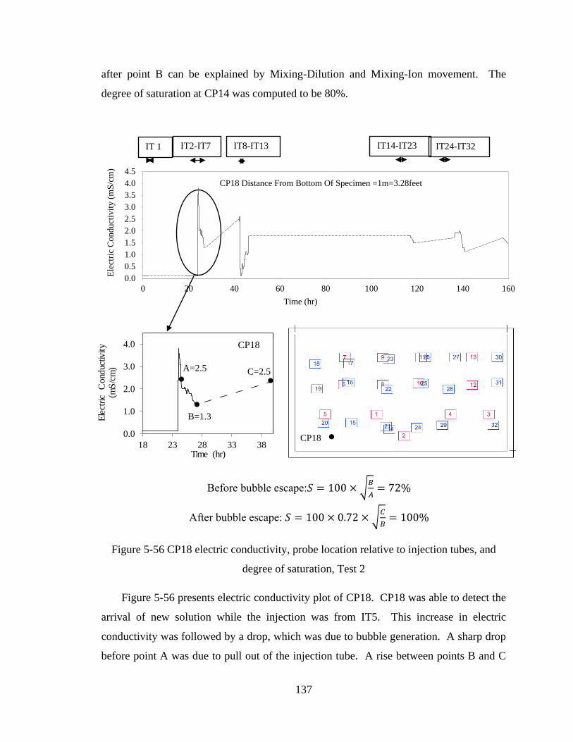
137
after point B can be explained by Mixing-Dilution and Mixing-Ion movement. The
degree of saturation at CP14 was computed to be 80%.
Figure 5-56 CP18 electric conductivity, probe location relative to injection tubes, and
degree of saturation, Test 2
Figure 5-56 presents electric conductivity plot of CP18. CP18 was able to detect the
arrival of new solution while the injection was from IT5. This increase in electric
conductivity was followed by a drop, which was due to bubble generation. A sharp drop
before point A was due to pull out of the injection tube. A rise between points B and C
0.0
1.0
2.0
3.0
4.0
18 23 28 33 38
Ele
ctric
Cond
uctiv
ity
(mS
/cm
)
Time (hr)
A=2.5
B=1.3
C=2.5
CP18
0.0
0.5
1.0
1.5
2.0
2.5
3.0
3.5
4.0
4.5
0 20 40 60 80 100 120 140 160
Ele
ctri
c C
onduct
ivit
y (
mS
/cm
)
Time (hr)
CP18 Distance From Bottom Of Specimen =1m=3.28feet
IT 1 IT2-IT7 IT8-IT13 IT14-IT23 IT24-IT32
Before bubble escape:𝑆 = 100 × 𝐵
𝐴= 72%
After bubble escape: 𝑆 = 100 × 0.72 × 𝐶
𝐵= 100%
CP18
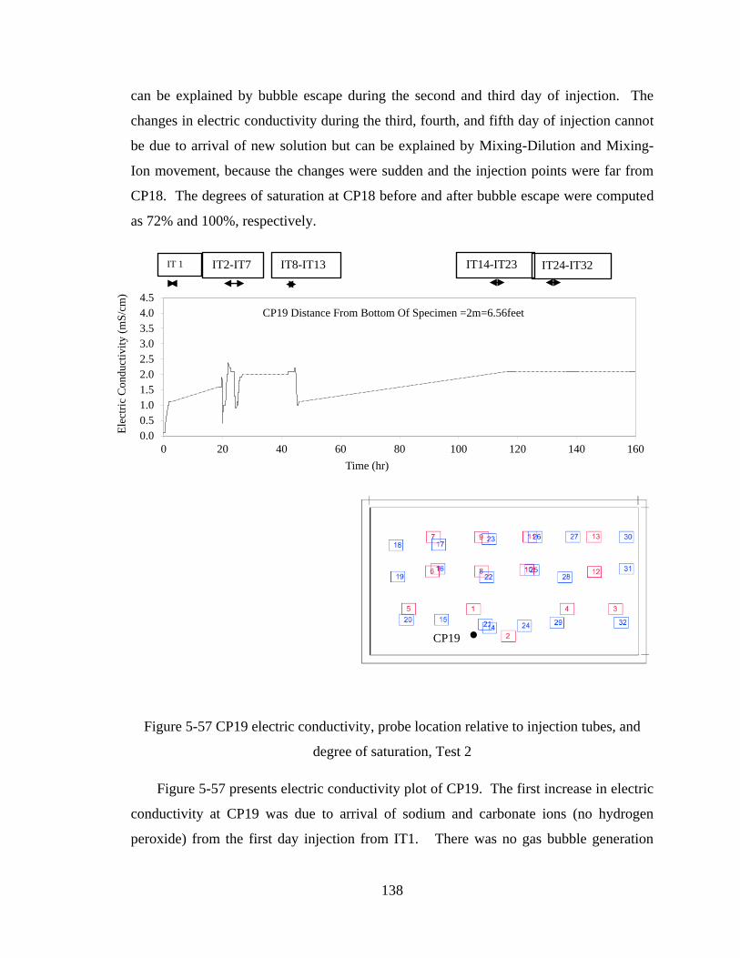
138
can be explained by bubble escape during the second and third day of injection. The
changes in electric conductivity during the third, fourth, and fifth day of injection cannot
be due to arrival of new solution but can be explained by Mixing-Dilution and Mixing-
Ion movement, because the changes were sudden and the injection points were far from
CP18. The degrees of saturation at CP18 before and after bubble escape were computed
as 72% and 100%, respectively.
Figure 5-57 CP19 electric conductivity, probe location relative to injection tubes, and
degree of saturation, Test 2
Figure 5-57 presents electric conductivity plot of CP19. The first increase in electric
conductivity at CP19 was due to arrival of sodium and carbonate ions (no hydrogen
peroxide) from the first day injection from IT1. There was no gas bubble generation
0.0
0.5
1.0
1.5
2.0
2.5
3.0
3.5
4.0
4.5
0 20 40 60 80 100 120 140 160
Ele
ctri
c C
onduct
ivit
y (
mS
/cm
)
Time (hr)
CP19 Distance From Bottom Of Specimen =2m=6.56feet
IT 1 IT2-IT7 IT8-IT13 IT14-IT23 IT24-IT32
CP19
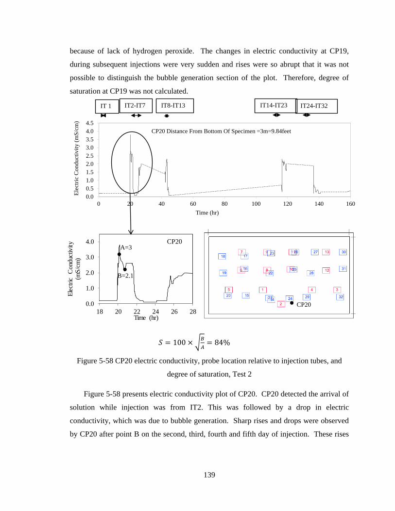
139
because of lack of hydrogen peroxide. The changes in electric conductivity at CP19,
during subsequent injections were very sudden and rises were so abrupt that it was not
possible to distinguish the bubble generation section of the plot. Therefore, degree of
saturation at CP19 was not calculated.
Figure 5-58 CP20 electric conductivity, probe location relative to injection tubes, and
degree of saturation, Test 2
Figure 5-58 presents electric conductivity plot of CP20. CP20 detected the arrival of
solution while injection was from IT2. This was followed by a drop in electric
conductivity, which was due to bubble generation. Sharp rises and drops were observed
by CP20 after point B on the second, third, fourth and fifth day of injection. These rises
IT 1 IT2-IT7 IT8-IT13 IT14-IT23 IT24-IT32
0.0
0.5
1.0
1.5
2.0
2.5
3.0
3.5
4.0
4.5
0 20 40 60 80 100 120 140 160
Ele
ctri
c C
onduct
ivit
y (
mS
/cm
)
Time (hr)
CP20 Distance From Bottom Of Specimen =3m=9.84feet
0.0
1.0
2.0
3.0
4.0
18 20 22 24 26 28
Ele
ctri
c C
ond
uctiv
ity
(mS
/cm
)
Time (hr)
A=3
B=2.1
CP20
𝑆 = 100 × 𝐵
𝐴= 84%
CP20
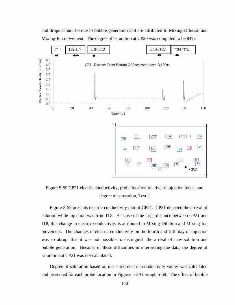
140
and drops cannot be due to bubble generation and are attributed to Mixing-Dilution and
Mixing-Ion movement. The degree of saturation at CP20 was computed to be 84%.
Figure 5-59 CP21 electric conductivity, probe location relative to injection tubes, and
degree of saturation, Test 2
Figure 5-59 presents electric conductivity plot of CP21. CP21 detected the arrival of
solution while injection was from IT8. Because of the large distance between CP21 and
IT8, this change in electric conductivity is attributed to Mixing-Dilution and Mixing-Ion
movement. The changes in electric conductivity on the fourth and fifth day of injection
was so abrupt that it was not possible to distinguish the arrival of new solution and
bubble generation. Because of these difficulties in interpreting the data, the degree of
saturation at CP21 was not calculated.
Degree of saturation based on measured electric conductivity values was calculated
and presented for each probe location in Figures 5-39 through 5-59. The effect of bubble
0.0
0.5
1.0
1.5
2.0
2.5
3.0
3.5
4.0
4.5
0 20 40 60 80 100 120 140 160
Ele
ctri
c C
onduct
ivit
y (
mS
/cm
)
Time (hr)
CP21 Distance From Bottom Of Specimen =4m=13.12feet
IT 1 IT2-IT7 IT8-IT13 IT14-IT23 IT24-IT32
CP21
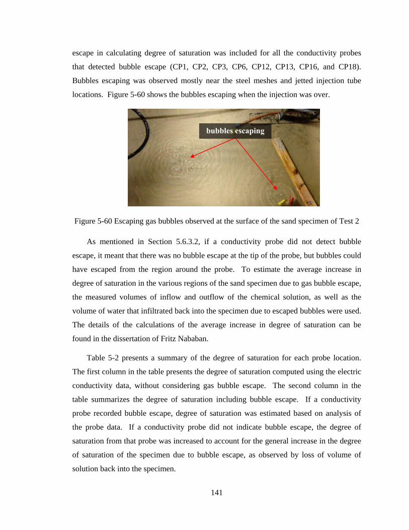
141
escape in calculating degree of saturation was included for all the conductivity probes
that detected bubble escape (CP1, CP2, CP3, CP6, CP12, CP13, CP16, and CP18).
Bubbles escaping was observed mostly near the steel meshes and jetted injection tube
locations. Figure 5-60 shows the bubbles escaping when the injection was over.
Figure 5-60 Escaping gas bubbles observed at the surface of the sand specimen of Test 2
As mentioned in Section 5.6.3.2, if a conductivity probe did not detect bubble
escape, it meant that there was no bubble escape at the tip of the probe, but bubbles could
have escaped from the region around the probe. To estimate the average increase in
degree of saturation in the various regions of the sand specimen due to gas bubble escape,
the measured volumes of inflow and outflow of the chemical solution, as well as the
volume of water that infiltrated back into the specimen due to escaped bubbles were used.
The details of the calculations of the average increase in degree of saturation can be
found in the dissertation of Fritz Nababan.
Table 5-2 presents a summary of the degree of saturation for each probe location.
The first column in the table presents the degree of saturation computed using the electric
conductivity data, without considering gas bubble escape. The second column in the
table summarizes the degree of saturation including bubble escape. If a conductivity
probe recorded bubble escape, degree of saturation was estimated based on analysis of
the probe data. If a conductivity probe did not indicate bubble escape, the degree of
saturation from that probe was increased to account for the general increase in the degree
of saturation of the specimen due to bubble escape, as observed by loss of volume of
solution back into the specimen.
bubbles escaping
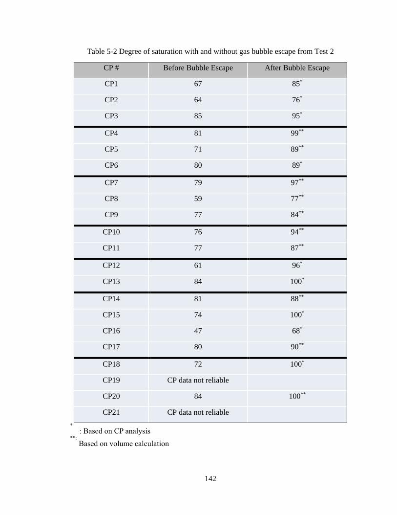
142
Table 5-2 Degree of saturation with and without gas bubble escape from Test 2
CP # Before Bubble Escape After Bubble Escape
CP1 67 85*
CP2 64 76*
CP3 85 95*
CP4 81 99**
CP5 71 89**
CP6 80 89*
CP7 79 97**
CP8 59 77**
CP9 77 84**
CP10 76 94**
CP11 77 87**
CP12 61 96*
CP13 84 100*
CP14 81 88**
CP15 74 100*
CP16 47 68*
CP17 80 90**
CP18 72 100*
CP19 CP data not reliable
CP20 84 100**
CP21 CP data not reliable
*
: Based on CP analysis **:
Based on volume calculation
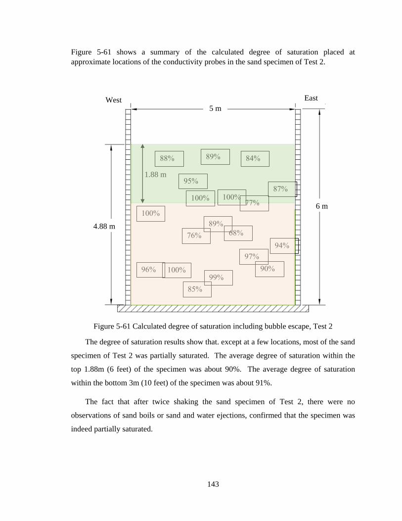
143
Figure 5-61 shows a summary of the calculated degree of saturation placed at
approximate locations of the conductivity probes in the sand specimen of Test 2.
Figure 5-61 Calculated degree of saturation including bubble escape, Test 2
The degree of saturation results show that. except at a few locations, most of the sand
specimen of Test 2 was partially saturated. The average degree of saturation within the
top 1.88m (6 feet) of the specimen was about 90%. The average degree of saturation
within the bottom 3m (10 feet) of the specimen was about 91%.
The fact that after twice shaking the sand specimen of Test 2, there were no
observations of sand boils or sand and water ejections, confirmed that the specimen was
indeed partially saturated.
West East
6 m
4.88 m
5 m
88% 89% 84%
95%
100% 100% 77%
87%
89%
100%
68%
97%
94%
90% 99%
100% 96%
85%
76%
1.88 m
m
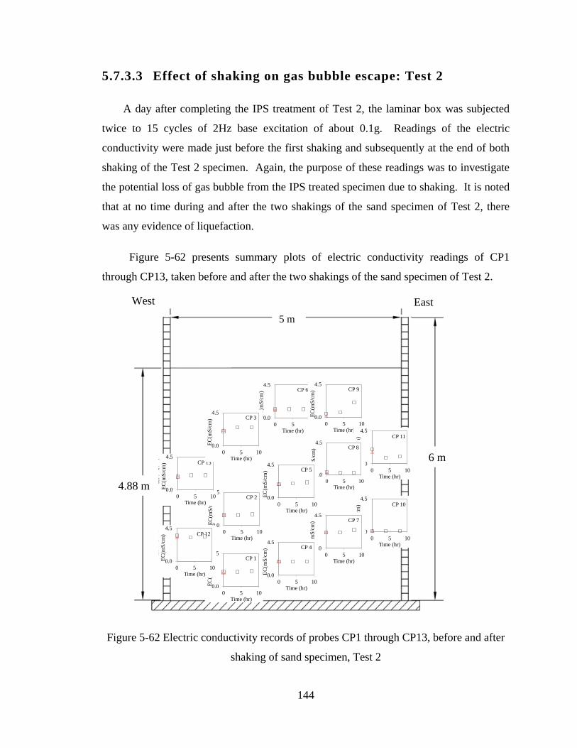
144
5.7.3.3 Effect of shaking on gas bubble escape: Test 2
A day after completing the IPS treatment of Test 2, the laminar box was subjected
twice to 15 cycles of 2Hz base excitation of about 0.1g. Readings of the electric
conductivity were made just before the first shaking and subsequently at the end of both
shaking of the Test 2 specimen. Again, the purpose of these readings was to investigate
the potential loss of gas bubble from the IPS treated specimen due to shaking. It is noted
that at no time during and after the two shakings of the sand specimen of Test 2, there
was any evidence of liquefaction.
Figure 5-62 presents summary plots of electric conductivity readings of CP1
through CP13, taken before and after the two shakings of the sand specimen of Test 2.
a)
Figure 5-62 Electric conductivity records of probes CP1 through CP13, before and after
shaking of sand specimen, Test 2
5 m
0.0
4.5
0 5 10
EC
(mS
/cm
)
Time (hr)
CP 1
0.0
4.5
0 5 10
EC
(mS
/cm
)
Time (hr)
CP 2
0.0
4.5
0 5 10
EC
(mS
/cm
)
Time (hr)
CP 6
0.0
4.5
0 5 10
EC
(mS
/cm
)
Time (hr)
CP 9
0.0
4.5
0 5 10
EC
(mS
/cm
)
Time (hr)
CP 10
0.0
4.5
0 5 10
EC
(mS
/cm
)
Time (hr)
CP 11
0.0
4.5
0 5 10
EC
(mS
/cm
)
Time (hr)
CP 12
0.0
4.5
0 5 10
EC
(mS
/cm
)
Time (hr)
CP 13
0.0
4.5
0 5 10
EC
(mS
/cm
)
Time (hr)
CP 8
0.0
4.5
0 5 10
EC
(mS
/cm
)
Time (hr)
CP 7
0.0
4.5
0 5 10
EC
(mS
/cm
)
Time (hr)
CP 4
0.0
4.5
0 5 10
EC
(mS
/cm
)
Time (hr)
CP 5
0.0
4.5
0 5 10
EC
(mS
/cm
)
Time (hr)
CP 3
6 m
5 m
4.88 m
m
West East
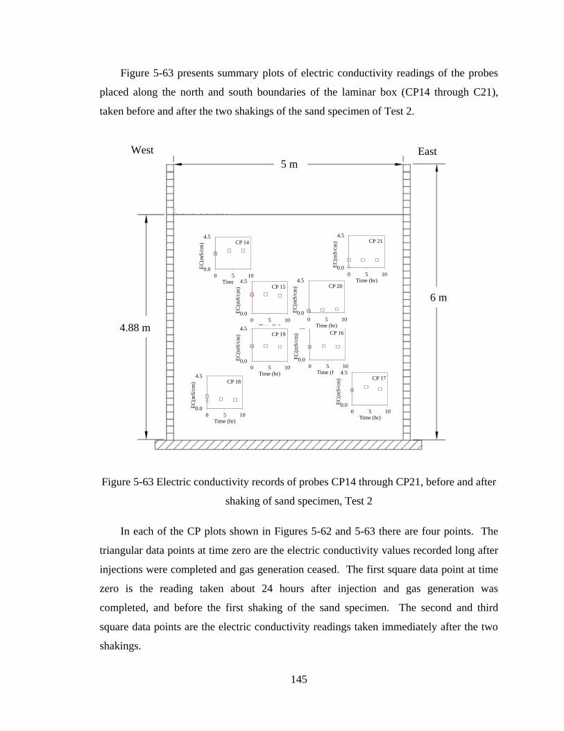
145
Figure 5-63 presents summary plots of electric conductivity readings of the probes
placed along the north and south boundaries of the laminar box (CP14 through C21),
taken before and after the two shakings of the sand specimen of Test 2.
Figure 5-63 Electric conductivity records of probes CP14 through CP21, before and after
shaking of sand specimen, Test 2
In each of the CP plots shown in Figures 5-62 and 5-63 there are four points. The
triangular data points at time zero are the electric conductivity values recorded long after
injections were completed and gas generation ceased. The first square data point at time
zero is the reading taken about 24 hours after injection and gas generation was
completed, and before the first shaking of the sand specimen. The second and third
square data points are the electric conductivity readings taken immediately after the two
shakings.
0.0
4.5
0 5 10
EC
(mS
/cm
)
Time (hr)
CP 14
0.0
4.5
0 5 10
EC
(mS
/cm
)
Time (hr)
CP 15
0.0
4.5
0 5 10
EC
(mS
/cm
)
Time (hr)
CP 16
0.0
4.5
0 5 10
EC
(mS
/cm
)
Time (hr)
CP 17
0.0
4.5
0 5 10
EC
(mS
/cm
)
Time (hr)
CP 21
0.0
4.5
0 5 10
EC
(mS
/cm
)
Time (hr)
CP 20
0.0
4.5
0 5 10
EC
(mS
/cm
)
Time (hr)
CP 19
0.0
4.5
0 5 10
EC
(mS
/cm
)
Time (hr)
CP 18
6 m
5 m
4.88 m
m
West East
146
The electric conductivity data points shown in Figures 5-62 and 5-63 lead to the
following observations and conclusions:
1. At all probes, the electric conductivity readings from end of injection to just
before the first shaking, (24 hours of wait time) did not change appreciably.
This indicates that there were no gas bubble escape and the degree of
saturation of the specimen remained unchanged.
2. Except at CP9 and CP11, no significant changes in electric conductivity
were observed during and after both shakings of the specimen. Therefore,
there were no bubble movement or escape due to the shaking.
3. At CP9, increases in electric conductivity were recorded after both
shakings. Because no sand boils nor other evidences of liquefaction were
observed, these increases cannot be attributed to gas escape. A likely
explanation is that increases in pore water pressures due to both shaking
could have induced flow of high ion concentration solution towards the CP9
location.
4. At CP11, decrease in electric conductivity was observed because of the first
shaking. A likely explanation can be that clean water or solution with low
concentration of ions, could have flowed towards CP11, again induced by
increases in pore water pressures because of the shaking.
5. The conductivity probes located about 0.5m from the north and south walls
of the laminar box did not show appreciable changes due to the shakings.
This is indicative that there was no liquefaction or gas bubble loss, as was
the case in Test 1, especially along the tank walls. The visual observations
of no sand boils or sand-water ejections anywhere including along the tank
walls made in Test 2 are consistent with the electric conductivity data of
CP14 though CP 21.
5.8 Summery and conclusions
Electric conductivity probes were used in the implementation of Induced Partial
Saturation (IPS) in the laminar box of NEES@Buffalo, at the State University of New
147
York in Buffalo. Two tests (Test 1 and Test2) were conducted, which differed only in the
process of inducing partial saturation in the sand specimens. The purpose of the laminar
box tests was two folds: 1) to evaluate the IPS process and equipment designed to reduce
degree of saturation of a large sand specimen, under representative field conductions and
2) to evaluate the effectiveness of IPS as a liquefaction mitigation measure, by shaking
the IPS treated specimens employing the shaking table upon which the laminar box
rested.
Electric conductivity probes were used extensively to monitor the IPS process, and
to determine the partial degree of saturation of the specimens and its spatial distribution.
The tests also created opportunities to demonstrate many benefits of using conductivity
probes in the implementation of IPS.
The following observations and conclusions are drawn from analyses of the electric
conductivity data from the two laminar box tests:
1. The Milwaukee conductivity probes with extended cables functioned
extremely well under rough and long-term conditions.
2. Zone of IPS treatment can be determined by observing the arrival of the
chemical solution at the probe locations.
3. IPS process in terms of making decisions about injection location, pressure,
and injection duration can be established by monitoring the probe readings
and observing the arrival or not of the chemical solution.
4. Zones where treatment was not effective or could not be reached can be
identified and alternative or additional injection procedures can be
implemented, to ensure treatment of an entire specimen.
5. Degree of saturation can be determined at each probe location, providing
crucial data needed in the interpretation of the effectiveness of IPS as
liquefaction mitigation.
6. Probes can detect gas escape from the sand specimen, and provide estimates
of final degree of saturation that includes the effect of gas escape.
148
7. Specimens or regions of specimens that the probes indicated were partially
saturated, did not liquefy during large enough shaking under which a fully
saturated specimen liquefied. The partial saturation conditions determined
by the probes were confirmed by the shaking table responses of the
specimens.
8. Effects of dilution and ion movements can be detected by the probes.
9. Probes can be used to determine the rate of chemical reaction and hence the
time duration within which the injection needs to be completed before
significant gas bubbles are generated.
10. Probe readings can provide estimate of the concentration of the chemical
solution reaching the pores of the sand, at a probe location.
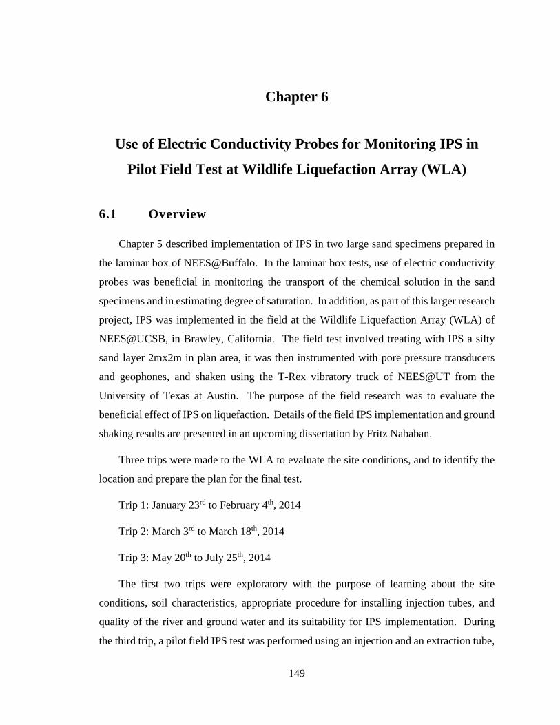
149
Chapter 6
Use of Electric Conductivity Probes for Monitoring IPS in
Pilot Field Test at Wildlife Liquefaction Array (WLA)
6.1 Overview
Chapter 5 described implementation of IPS in two large sand specimens prepared in
the laminar box of NEES@Buffalo. In the laminar box tests, use of electric conductivity
probes was beneficial in monitoring the transport of the chemical solution in the sand
specimens and in estimating degree of saturation. In addition, as part of this larger research
project, IPS was implemented in the field at the Wildlife Liquefaction Array (WLA) of
NEES@UCSB, in Brawley, California. The field test involved treating with IPS a silty
sand layer 2mx2m in plan area, it was then instrumented with pore pressure transducers
and geophones, and shaken using the T-Rex vibratory truck of NEES@UT from the
University of Texas at Austin. The purpose of the field research was to evaluate the
beneficial effect of IPS on liquefaction. Details of the field IPS implementation and ground
shaking results are presented in an upcoming dissertation by Fritz Nababan.
Three trips were made to the WLA to evaluate the site conditions, and to identify the
location and prepare the plan for the final test.
Trip 1: January 23rd to February 4th, 2014
Trip 2: March 3rd to March 18th, 2014
Trip 3: May 20th to July 25th, 2014
The first two trips were exploratory with the purpose of learning about the site
conditions, soil characteristics, appropriate procedure for installing injection tubes, and
quality of the river and ground water and its suitability for IPS implementation. During
the third trip, a pilot field IPS test was performed using an injection and an extraction tube,
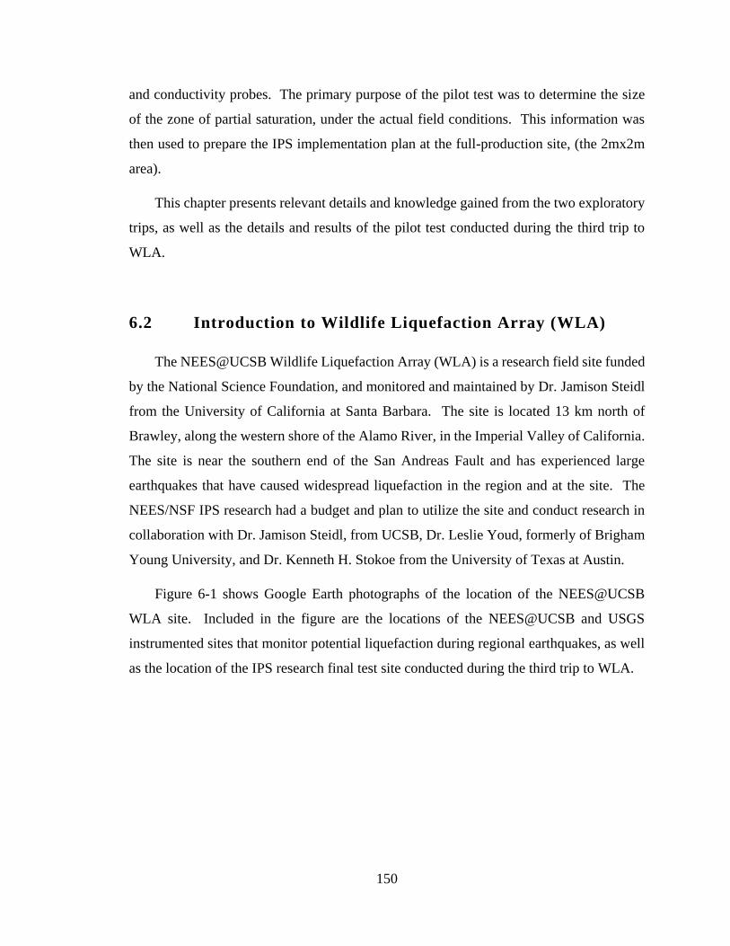
150
and conductivity probes. The primary purpose of the pilot test was to determine the size
of the zone of partial saturation, under the actual field conditions. This information was
then used to prepare the IPS implementation plan at the full-production site, (the 2mx2m
area).
This chapter presents relevant details and knowledge gained from the two exploratory
trips, as well as the details and results of the pilot test conducted during the third trip to
WLA.
6.2 Introduction to Wildlife Liquefaction Array (WLA)
The NEES@UCSB Wildlife Liquefaction Array (WLA) is a research field site funded
by the National Science Foundation, and monitored and maintained by Dr. Jamison Steidl
from the University of California at Santa Barbara. The site is located 13 km north of
Brawley, along the western shore of the Alamo River, in the Imperial Valley of California.
The site is near the southern end of the San Andreas Fault and has experienced large
earthquakes that have caused widespread liquefaction in the region and at the site. The
NEES/NSF IPS research had a budget and plan to utilize the site and conduct research in
collaboration with Dr. Jamison Steidl, from UCSB, Dr. Leslie Youd, formerly of Brigham
Young University, and Dr. Kenneth H. Stokoe from the University of Texas at Austin.
Figure 6-1 shows Google Earth photographs of the location of the NEES@UCSB
WLA site. Included in the figure are the locations of the NEES@UCSB and USGS
instrumented sites that monitor potential liquefaction during regional earthquakes, as well
as the location of the IPS research final test site conducted during the third trip to WLA.
151
Figure 6-1 Locations of WLA, NEES@UCSB, USGS, and IPS field test sites
UCSB NEES WLA
USGS Site Northeastern IPS Site
(Final test)
152
Figure 6-2 shows the locations of the three sites where the IPS research
project team conducted exploratory (first and second trips) and final tests
(third trip).
Figure 6-2 Locations of IPS field test sites
6.3 Summary of findings from the first and second trips
During the first two trips, exploratory tests were conducted to evaluate the general site
conditions, the challenges that are present with regards to site accessibility, supply of water
and its quality, type of injection tube to use and the proper installation procedure to follow,
and the adequacy of the chemical solution preparation and delivery system. Details of the
findings and knowledge gained in all these explorations are presented in the dissertation of
Fritz Nababan.
This section focuses on presenting knowledge gained in three areas (site condition,
injection tube installation, and river and ground water quality) that were relevant to the use
and implementation of conductivity probes in the pilot test conducted during the third trip.
Exploratory Test Site (First trip)
Exploratory Test Site (Second trip)
Final Test Site (Third trip)
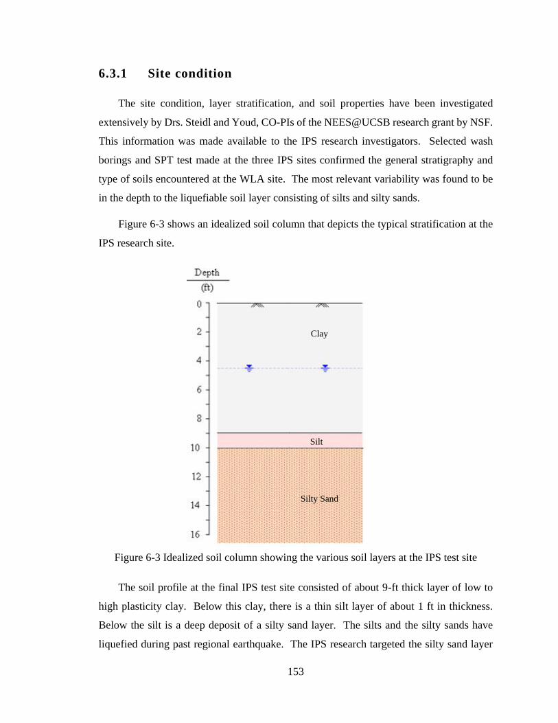
153
6.3.1 Site condition
The site condition, layer stratification, and soil properties have been investigated
extensively by Drs. Steidl and Youd, CO-PIs of the NEES@UCSB research grant by NSF.
This information was made available to the IPS research investigators. Selected wash
borings and SPT test made at the three IPS sites confirmed the general stratigraphy and
type of soils encountered at the WLA site. The most relevant variability was found to be
in the depth to the liquefiable soil layer consisting of silts and silty sands.
Figure 6-3 shows an idealized soil column that depicts the typical stratification at the
IPS research site.
Figure 6-3 Idealized soil column showing the various soil layers at the IPS test site
The soil profile at the final IPS test site consisted of about 9-ft thick layer of low to
high plasticity clay. Below this clay, there is a thin silt layer of about 1 ft in thickness.
Below the silt is a deep deposit of a silty sand layer. The silts and the silty sands have
liquefied during past regional earthquake. The IPS research targeted the silty sand layer
Clay
Silt
Silty Sand
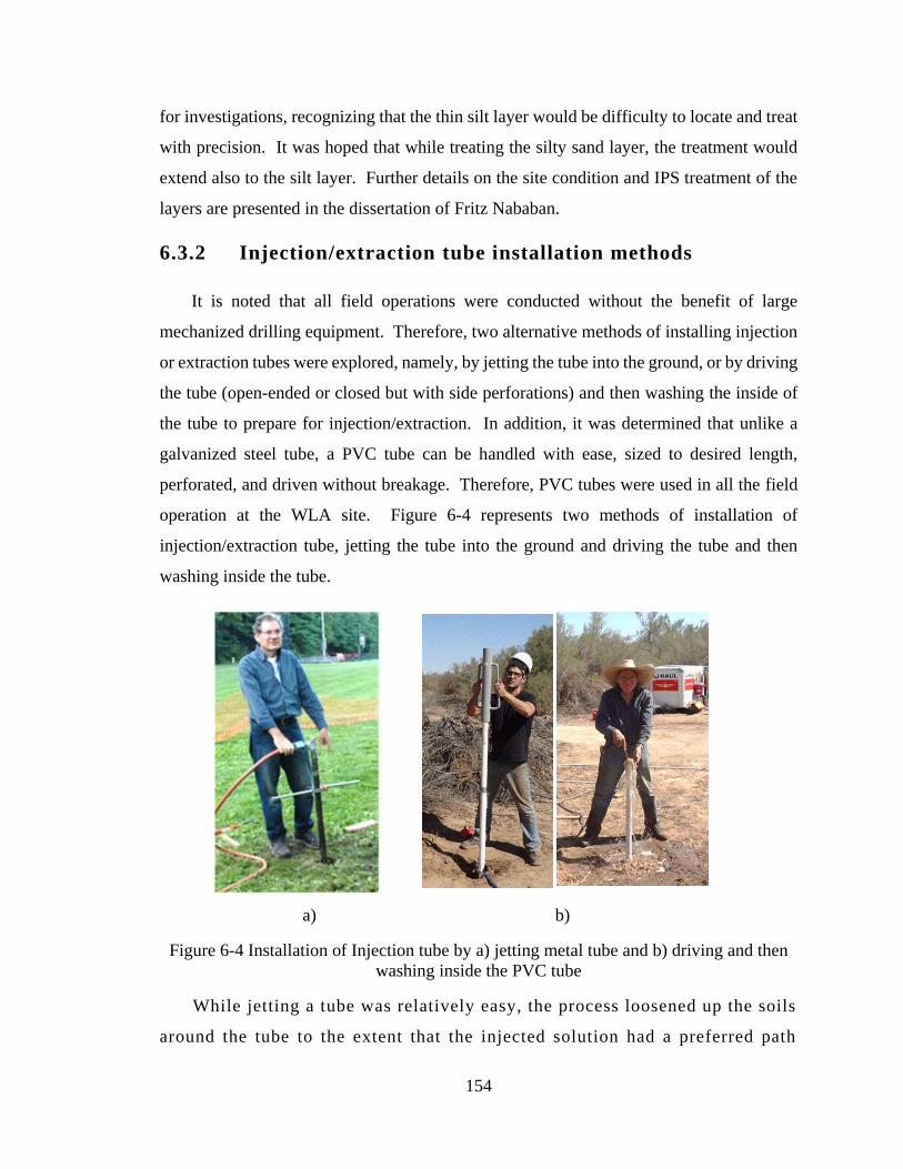
154
for investigations, recognizing that the thin silt layer would be difficulty to locate and treat
with precision. It was hoped that while treating the silty sand layer, the treatment would
extend also to the silt layer. Further details on the site condition and IPS treatment of the
layers are presented in the dissertation of Fritz Nababan.
6.3.2 Injection/extraction tube installation methods
It is noted that all field operations were conducted without the benefit of large
mechanized drilling equipment. Therefore, two alternative methods of installing injection
or extraction tubes were explored, namely, by jetting the tube into the ground, or by driving
the tube (open-ended or closed but with side perforations) and then washing the inside of
the tube to prepare for injection/extraction. In addition, it was determined that unlike a
galvanized steel tube, a PVC tube can be handled with ease, sized to desired length,
perforated, and driven without breakage. Therefore, PVC tubes were used in all the field
operation at the WLA site. Figure 6-4 represents two methods of installation of
injection/extraction tube, jetting the tube into the ground and driving the tube and then
washing inside the tube.
a) b)
Figure 6-4 Installation of Injection tube by a) jetting metal tube and b) driving and then
washing inside the PVC tube
While jetting a tube was relatively easy, the process loosened up the soils
around the tube to the extent that the injected solution had a preferred path
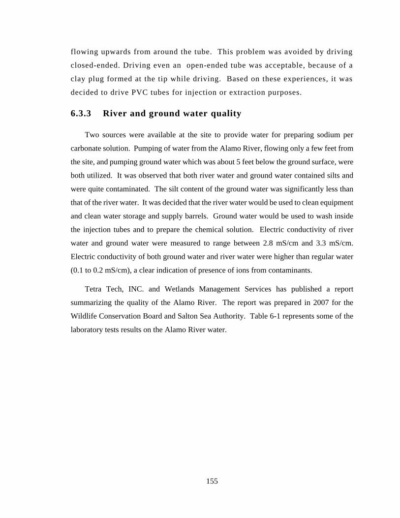
155
flowing upwards from around the tube. This problem was avoided by driving
closed-ended. Driving even an open-ended tube was acceptable, because of a
clay plug formed at the tip while driving. Based on these experiences, it was
decided to drive PVC tubes for injection or extraction purposes.
6.3.3 River and ground water quality
Two sources were available at the site to provide water for preparing sodium per
carbonate solution. Pumping of water from the Alamo River, flowing only a few feet from
the site, and pumping ground water which was about 5 feet below the ground surface, were
both utilized. It was observed that both river water and ground water contained silts and
were quite contaminated. The silt content of the ground water was significantly less than
that of the river water. It was decided that the river water would be used to clean equipment
and clean water storage and supply barrels. Ground water would be used to wash inside
the injection tubes and to prepare the chemical solution. Electric conductivity of river
water and ground water were measured to range between 2.8 mS/cm and 3.3 mS/cm.
Electric conductivity of both ground water and river water were higher than regular water
(0.1 to 0.2 mS/cm), a clear indication of presence of ions from contaminants.
Tetra Tech, INC. and Wetlands Management Services has published a report
summarizing the quality of the Alamo River. The report was prepared in 2007 for the
Wildlife Conservation Board and Salton Sea Authority. Table 6-1 represents some of the
laboratory tests results on the Alamo River water.
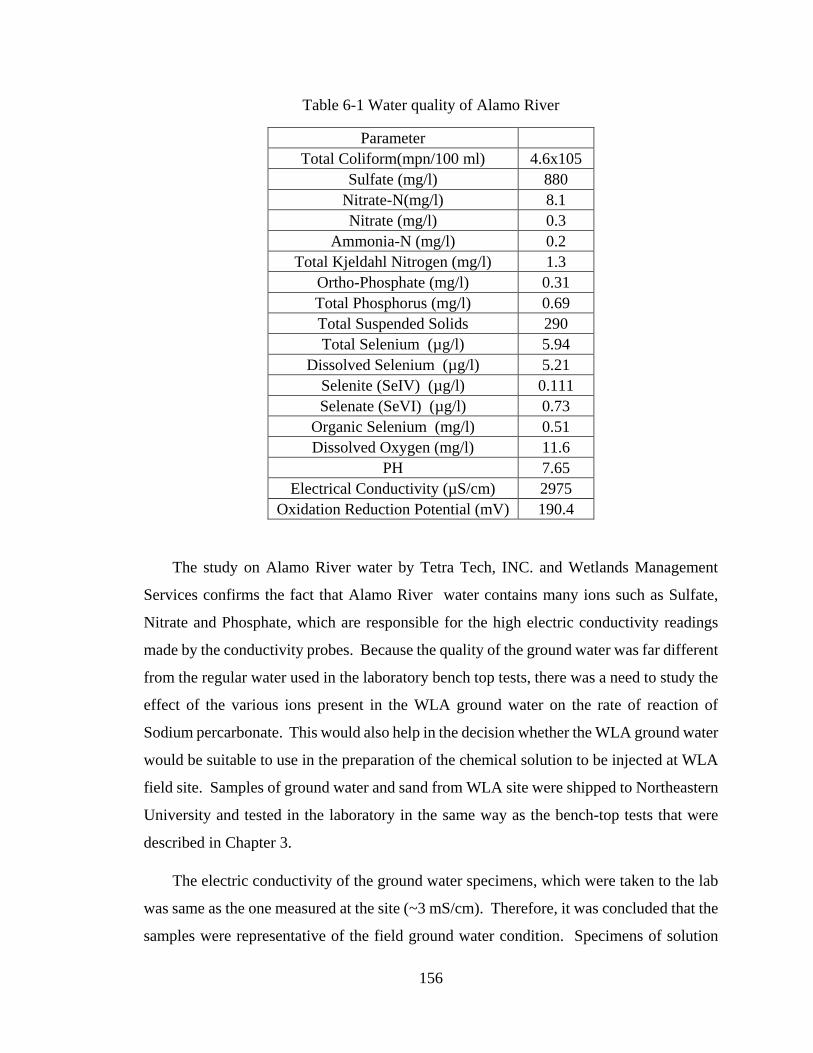
156
Table 6-1 Water quality of Alamo River
Parameter
Total Coliform(mpn/100 ml) 4.6x10⁵
Sulfate (mg/l) 880
Nitrate-N(mg/l) 8.1
Nitrate (mg/l) 0.3
Ammonia-N (mg/l) 0.2
Total Kjeldahl Nitrogen (mg/l) 1.3
Ortho-Phosphate (mg/l) 0.31
Total Phosphorus (mg/l) 0.69
Total Suspended Solids 290
Total Selenium (µg/l) 5.94
Dissolved Selenium (µg/l) 5.21
Selenite (SeIV) (µg/l) 0.111
Selenate (SeVI) (µg/l) 0.73
Organic Selenium (mg/l) 0.51
Dissolved Oxygen (mg/l) 11.6
PH 7.65
Electrical Conductivity (µS/cm) 2975
Oxidation Reduction Potential (mV) 190.4
The study on Alamo River water by Tetra Tech, INC. and Wetlands Management
Services confirms the fact that Alamo River water contains many ions such as Sulfate,
Nitrate and Phosphate, which are responsible for the high electric conductivity readings
made by the conductivity probes. Because the quality of the ground water was far different
from the regular water used in the laboratory bench top tests, there was a need to study the
effect of the various ions present in the WLA ground water on the rate of reaction of
Sodium percarbonate. This would also help in the decision whether the WLA ground water
would be suitable to use in the preparation of the chemical solution to be injected at WLA
field site. Samples of ground water and sand from WLA site were shipped to Northeastern
University and tested in the laboratory in the same way as the bench-top tests that were
described in Chapter 3.
The electric conductivity of the ground water specimens, which were taken to the lab
was same as the one measured at the site (~3 mS/cm). Therefore, it was concluded that the
samples were representative of the field ground water condition. Specimens of solution
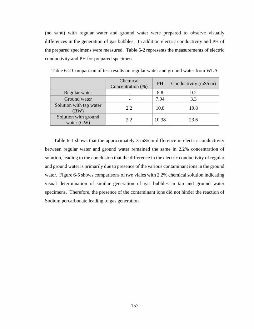
157
(no sand) with regular water and ground water were prepared to observe visually
differences in the generation of gas bubbles. In addition electric conductivity and PH of
the prepared specimens were measured. Table 6-2 represents the measurements of electric
conductivity and PH for prepared specimen.
Table 6-2 Comparison of test results on regular water and ground water from WLA
Chemical
Concentration (%) PH Conductivity (mS/cm)
Regular water - 8.8 0.2
Ground water - 7.94 3.3
Solution with tap water
(RW) 2.2 10.8 19.8
Solution with ground
water (GW) 2.2 10.38 23.6
Table 6-1 shows that the approximately 3 mS/cm difference in electric conductivity
between regular water and ground water remained the same in 2.2% concentration of
solution, leading to the conclusion that the difference in the electric conductivity of regular
and ground water is primarily due to presence of the various contaminant ions in the ground
water. Figure 6-5 shows comparisons of two viales with 2.2% chemical solution indicating
visual determination of similar generation of gas bubbles in tap and ground water
specimens. Therefore, the presence of the contaminant ions did not hinder the reaction of
Sodium percarbonate leading to gas generation.
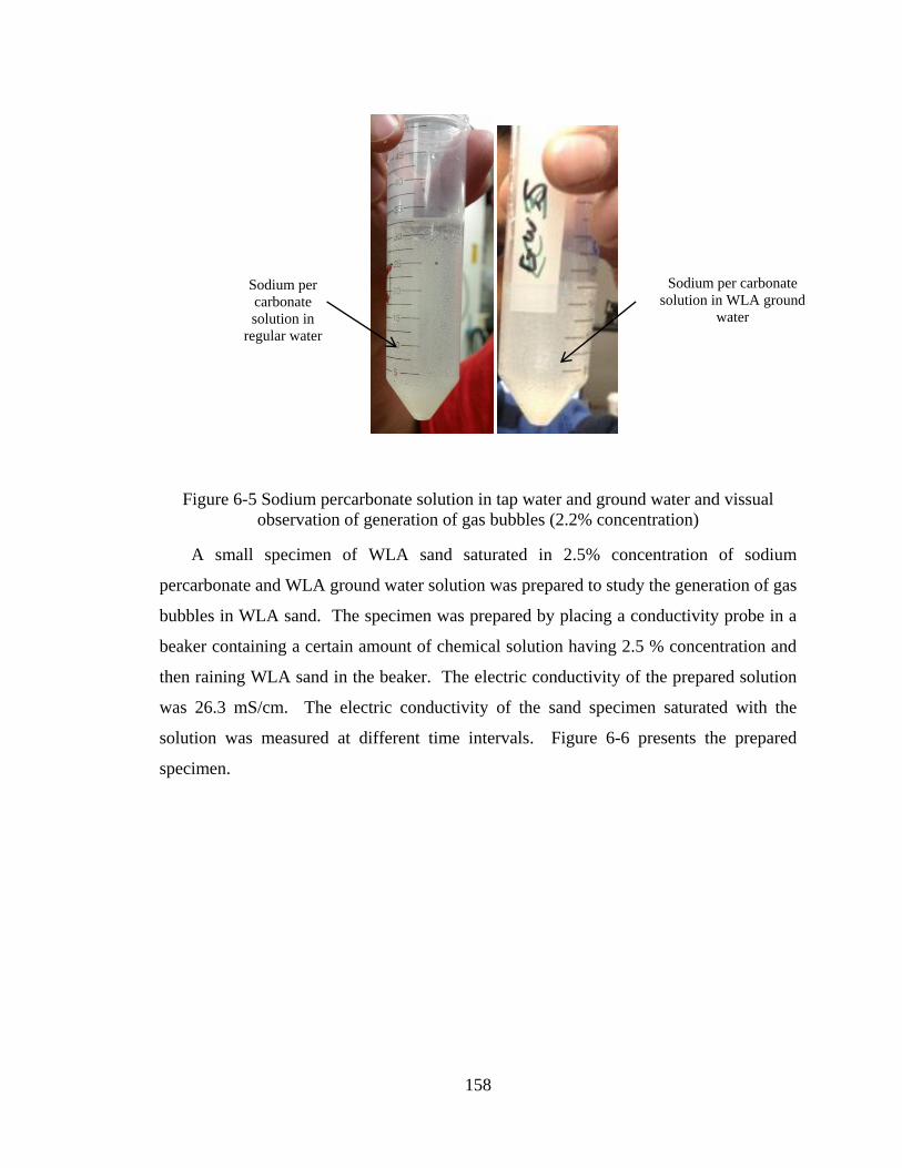
158
Figure 6-5 Sodium percarbonate solution in tap water and ground water and vissual
observation of generation of gas bubbles (2.2% concentration)
A small specimen of WLA sand saturated in 2.5% concentration of sodium
percarbonate and WLA ground water solution was prepared to study the generation of gas
bubbles in WLA sand. The specimen was prepared by placing a conductivity probe in a
beaker containing a certain amount of chemical solution having 2.5 % concentration and
then raining WLA sand in the beaker. The electric conductivity of the prepared solution
was 26.3 mS/cm. The electric conductivity of the sand specimen saturated with the
solution was measured at different time intervals. Figure 6-6 presents the prepared
specimen.
Sodium per
carbonate
solution in
regular water
Sodium per carbonate
solution in WLA ground
water
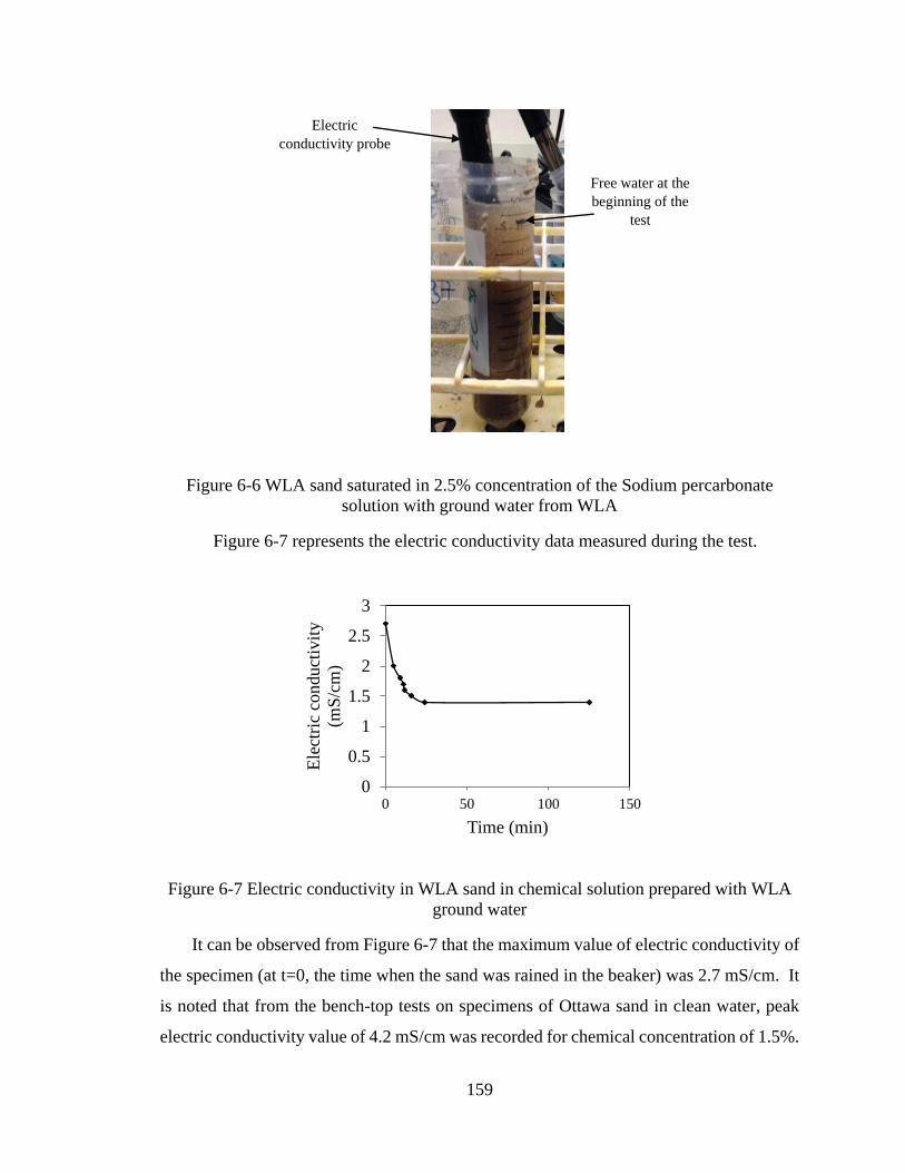
159
Figure 6-6 WLA sand saturated in 2.5% concentration of the Sodium percarbonate
solution with ground water from WLA
Figure 6-7 represents the electric conductivity data measured during the test.
Figure 6-7 Electric conductivity in WLA sand in chemical solution prepared with WLA
ground water
It can be observed from Figure 6-7 that the maximum value of electric conductivity of
the specimen (at t=0, the time when the sand was rained in the beaker) was 2.7 mS/cm. It
is noted that from the bench-top tests on specimens of Ottawa sand in clean water, peak
electric conductivity value of 4.2 mS/cm was recorded for chemical concentration of 1.5%.
0
0.5
1
1.5
2
2.5
3
0 50 100 150
Ele
ctri
c co
nduct
ivit
y
(mS
/cm
)
Time (min)
Electric
conductivity probe
Free water at the
beginning of the
test
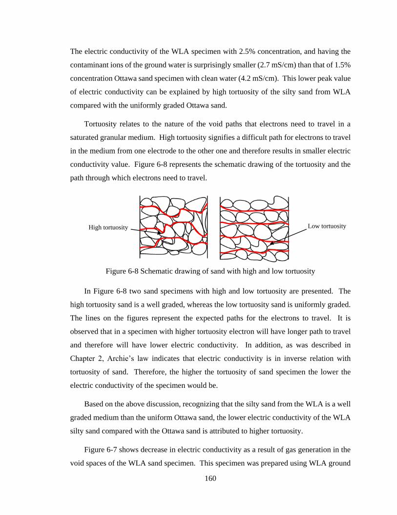
160
The electric conductivity of the WLA specimen with 2.5% concentration, and having the
contaminant ions of the ground water is surprisingly smaller (2.7 mS/cm) than that of 1.5%
concentration Ottawa sand specimen with clean water (4.2 mS/cm). This lower peak value
of electric conductivity can be explained by high tortuosity of the silty sand from WLA
compared with the uniformly graded Ottawa sand.
Tortuosity relates to the nature of the void paths that electrons need to travel in a
saturated granular medium. High tortuosity signifies a difficult path for electrons to travel
in the medium from one electrode to the other one and therefore results in smaller electric
conductivity value. Figure 6-8 represents the schematic drawing of the tortuosity and the
path through which electrons need to travel.
Figure 6-8 Schematic drawing of sand with high and low tortuosity
In Figure 6-8 two sand specimens with high and low tortuosity are presented. The
high tortuosity sand is a well graded, whereas the low tortuosity sand is uniformly graded.
The lines on the figures represent the expected paths for the electrons to travel. It is
observed that in a specimen with higher tortuosity electron will have longer path to travel
and therefore will have lower electric conductivity. In addition, as was described in
Chapter 2, Archie’s law indicates that electric conductivity is in inverse relation with
tortuosity of sand. Therefore, the higher the tortuosity of sand specimen the lower the
electric conductivity of the specimen would be.
Based on the above discussion, recognizing that the silty sand from the WLA is a well
graded medium than the uniform Ottawa sand, the lower electric conductivity of the WLA
silty sand compared with the Ottawa sand is attributed to higher tortuosity.
Figure 6-7 shows decrease in electric conductivity as a result of gas generation in the
void spaces of the WLA sand specimen. This specimen was prepared using WLA ground
High tortuosity Low tortuosity
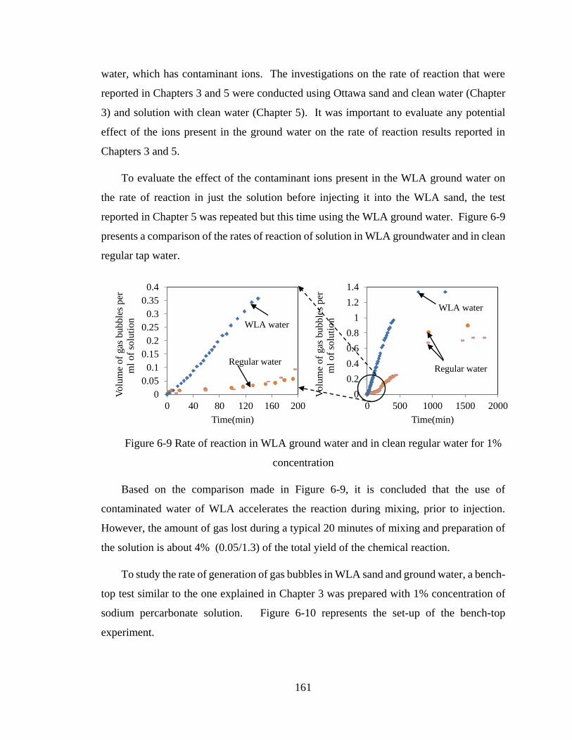
161
water, which has contaminant ions. The investigations on the rate of reaction that were
reported in Chapters 3 and 5 were conducted using Ottawa sand and clean water (Chapter
3) and solution with clean water (Chapter 5). It was important to evaluate any potential
effect of the ions present in the ground water on the rate of reaction results reported in
Chapters 3 and 5.
To evaluate the effect of the contaminant ions present in the WLA ground water on
the rate of reaction in just the solution before injecting it into the WLA sand, the test
reported in Chapter 5 was repeated but this time using the WLA ground water. Figure 6-9
presents a comparison of the rates of reaction of solution in WLA groundwater and in clean
regular tap water.
Figure 6-9 Rate of reaction in WLA ground water and in clean regular water for 1%
concentration
Based on the comparison made in Figure 6-9, it is concluded that the use of
contaminated water of WLA accelerates the reaction during mixing, prior to injection.
However, the amount of gas lost during a typical 20 minutes of mixing and preparation of
the solution is about 4% (0.05/1.3) of the total yield of the chemical reaction.
To study the rate of generation of gas bubbles in WLA sand and ground water, a bench-
top test similar to the one explained in Chapter 3 was prepared with 1% concentration of
sodium percarbonate solution. Figure 6-10 represents the set-up of the bench-top
experiment.
0
0.05
0.1
0.15
0.2
0.25
0.3
0.35
0.4
0 40 80 120 160 200
Vo
lum
e o
f gas
bu
bb
les
per
ml
of
solu
tio
n
Time(min)
0
0.2
0.4
0.6
0.8
1
1.2
1.4
0 500 1000 1500 2000
Vo
lum
e o
f gas
bu
bb
les
per
ml
of
solu
tio
n
Time(min)
WLA water
Regular water
WLA water
Regular water
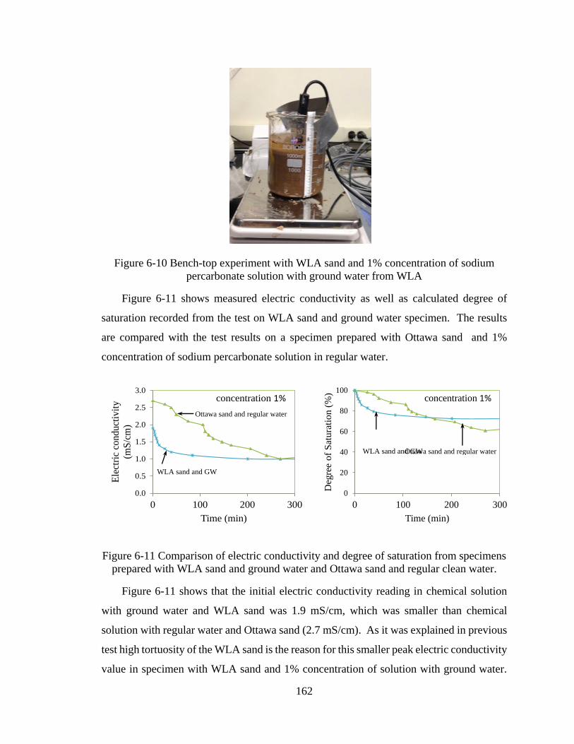
162
Figure 6-10 Bench-top experiment with WLA sand and 1% concentration of sodium
percarbonate solution with ground water from WLA
Figure 6-11 shows measured electric conductivity as well as calculated degree of
saturation recorded from the test on WLA sand and ground water specimen. The results
are compared with the test results on a specimen prepared with Ottawa sand and 1%
concentration of sodium percarbonate solution in regular water.
Figure 6-11 Comparison of electric conductivity and degree of saturation from specimens
prepared with WLA sand and ground water and Ottawa sand and regular clean water.
Figure 6-11 shows that the initial electric conductivity reading in chemical solution
with ground water and WLA sand was 1.9 mS/cm, which was smaller than chemical
solution with regular water and Ottawa sand (2.7 mS/cm). As it was explained in previous
test high tortuosity of the WLA sand is the reason for this smaller peak electric conductivity
value in specimen with WLA sand and 1% concentration of solution with ground water.
0.0
0.5
1.0
1.5
2.0
2.5
3.0
0 100 200 300
Ele
ctri
c co
nduct
ivit
y
(mS
/cm
)
Time (min)
concentration 1%
WLA sand and GW
Ottawa sand and regular water
0
20
40
60
80
100
0 100 200 300
Deg
ree
of
Sat
ura
tion (
%)
Time (min)
concentration 1%
Ottawa sand and regular water WLA sand and GW
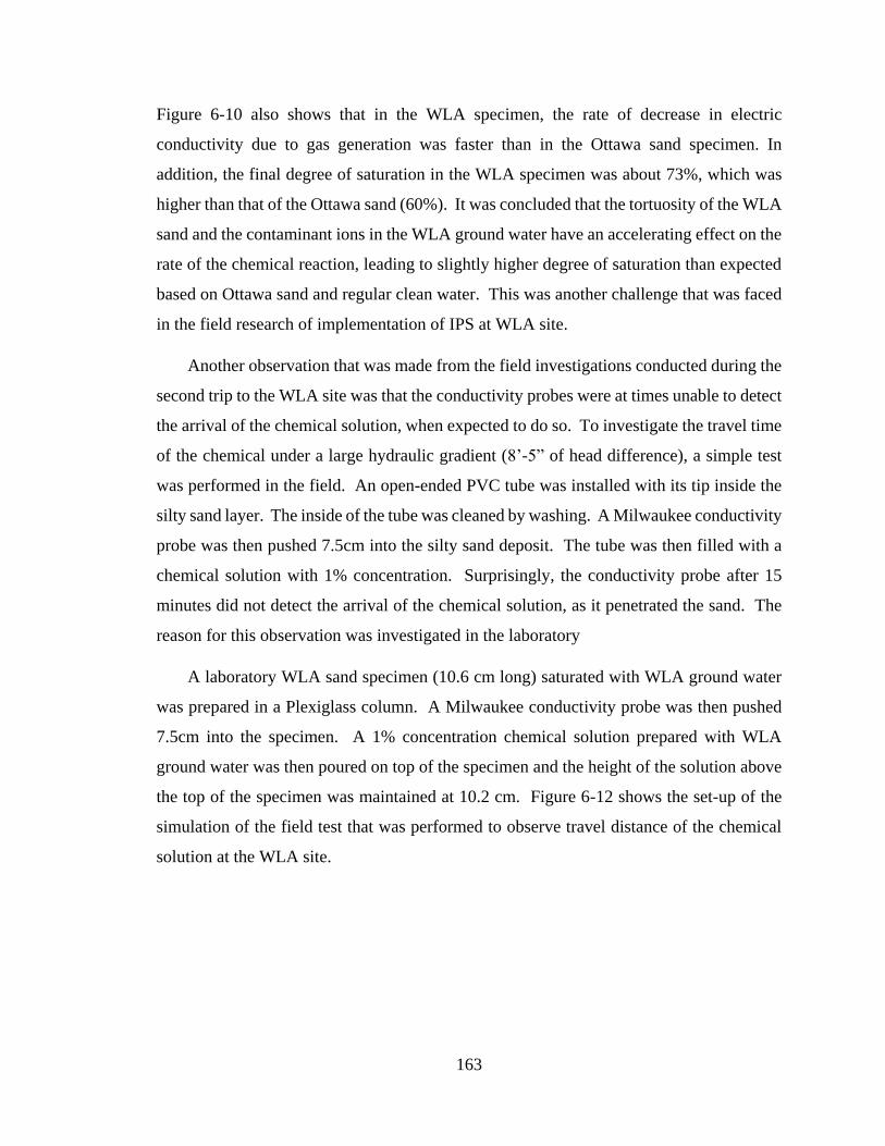
163
Figure 6-10 also shows that in the WLA specimen, the rate of decrease in electric
conductivity due to gas generation was faster than in the Ottawa sand specimen. In
addition, the final degree of saturation in the WLA specimen was about 73%, which was
higher than that of the Ottawa sand (60%). It was concluded that the tortuosity of the WLA
sand and the contaminant ions in the WLA ground water have an accelerating effect on the
rate of the chemical reaction, leading to slightly higher degree of saturation than expected
based on Ottawa sand and regular clean water. This was another challenge that was faced
in the field research of implementation of IPS at WLA site.
Another observation that was made from the field investigations conducted during the
second trip to the WLA site was that the conductivity probes were at times unable to detect
the arrival of the chemical solution, when expected to do so. To investigate the travel time
of the chemical under a large hydraulic gradient (8’-5” of head difference), a simple test
was performed in the field. An open-ended PVC tube was installed with its tip inside the
silty sand layer. The inside of the tube was cleaned by washing. A Milwaukee conductivity
probe was then pushed 7.5cm into the silty sand deposit. The tube was then filled with a
chemical solution with 1% concentration. Surprisingly, the conductivity probe after 15
minutes did not detect the arrival of the chemical solution, as it penetrated the sand. The
reason for this observation was investigated in the laboratory
A laboratory WLA sand specimen (10.6 cm long) saturated with WLA ground water
was prepared in a Plexiglass column. A Milwaukee conductivity probe was then pushed
7.5cm into the specimen. A 1% concentration chemical solution prepared with WLA
ground water was then poured on top of the specimen and the height of the solution above
the top of the specimen was maintained at 10.2 cm. Figure 6-12 shows the set-up of the
simulation of the field test that was performed to observe travel distance of the chemical
solution at the WLA site.
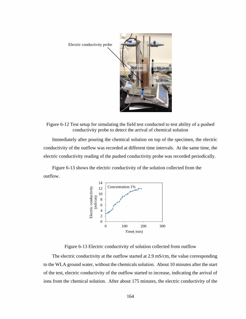
164
Figure 6-12 Test setup for simulating the field test conducted to test ability of a pushed
conductivity probe to detect the arrival of chemical solution
Immediately after pouring the chemical solution on top of the specimen, the electric
conductivity of the outflow was recorded at different time intervals. At the same time, the
electric conductivity reading of the pushed conductivity probe was recorded periodically.
Figure 6-13 shows the electric conductivity of the solution collected from the
outflow.
Figure 6-13 Electric conductivity of solution collected from outflow
The electric conductivity at the outflow started at 2.9 mS/cm, the value corresponding
to the WLA ground water, without the chemicals solution. About 10 minutes after the start
of the test, electric conductivity of the outflow started to increase, indicating the arrival of
ions from the chemical solution. After about 175 minutes, the electric conductivity of the
0
2
4
6
8
10
12
14
0 100 200 300
Ele
ctri
c co
nduct
ivit
y
(mS
/cm
)
Time( min)
Concentration 1%
Electric conductivity probe
10.6 cm
20.8 cm 10.2cm
Outflow
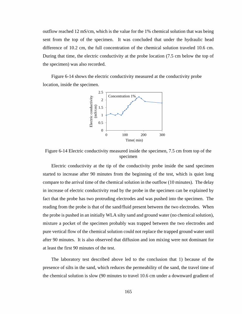
165
outflow reached 12 mS/cm, which is the value for the 1% chemical solution that was being
sent from the top of the specimen. It was concluded that under the hydraulic head
difference of 10.2 cm, the full concentration of the chemical solution traveled 10.6 cm.
During that time, the electric conductivity at the probe location (7.5 cm below the top of
the specimen) was also recorded.
Figure 6-14 shows the electric conductivity measured at the conductivity probe
location, inside the specimen.
Figure 6-14 Electric conductivity measured inside the specimen, 7.5 cm from top of the
specimen
Electric conductivity at the tip of the conductivity probe inside the sand specimen
started to increase after 90 minutes from the beginning of the test, which is quiet long
compare to the arrival time of the chemical solution in the outflow (10 minutes). The delay
in increase of electric conductivity read by the probe in the specimen can be explained by
fact that the probe has two protruding electrodes and was pushed into the specimen. The
reading from the probe is that of the sand/fluid present between the two electrodes. When
the probe is pushed in an initially WLA silty sand and ground water (no chemical solution),
mixture a pocket of the specimen probably was trapped between the two electrodes and
pure vertical flow of the chemical solution could not replace the trapped ground water until
after 90 minutes. It is also observed that diffusion and ion mixing were not dominant for
at least the first 90 minutes of the test.
The laboratory test described above led to the conclusion that 1) because of the
presence of silts in the sand, which reduces the permeability of the sand, the travel time of
the chemical solution is slow (90 minutes to travel 10.6 cm under a downward gradient of
0
0.5
1
1.5
2
2.5
0 100 200 300
Ele
ctri
c co
nduct
ivit
y
(mS
/cm
)
Time( min)
Concentration 1%
166
20.8/10.8 = 1.9) and 2) installation of a Milwaukee probe into sand by pushing renders the
probe ineffective, for all practical purposes.
In summary, various tests were conducted to evaluate the quality of the Alamo River
and ground water at the WLA site. Conductivity probes were invaluable in evaluating the
suitability of the ground water in the IPS implementation at the WLA site. The following
observations and conclusions are made:
1- Water pumped from both the river and ground water contain silts, The silt
content in the ground water is significantly less than that of the river water.
2- Both river and ground water are contaminated, having significant amount of
various ions, which are responsible for the high readings of electric
conductivity.
3- Visual observation demonstrated that the ground water even though
contaminated when used to prepare sodium percarbonate solution was still able
to generate gas bubbles.
4- The electric conductivity readings in the WLA silty sand even with the
contaminant ions, was smaller than that of Ottawa sand and clean water. This
was attributed to the higher tortuosity of the well graded WLA silty sand.
5- The rate of the chemical reaction and gas generation in the WLA silty sand and
ground water was faster than in the Ottawa sand and clean water. This implies
that there is less time available to prepare and inject the solution as well as
shorter wait time before the gas bubble generation is complete.
6- For a given concentration of the chemical solution, the final degree of
saturation in the WLA silty sand and ground water is larger than in Ottawa sand
and clean water.
7- Flow of the chemical solution through WLA silty sand and ground water is
slow. Under vertical gradient of almost 2, the solution took 90 minutes to travel
10.6cm.
8- Installation of the Milwaukee conductivity probe that has two protruding
electrodes by pushing into the silty sand layer, is not recommended.
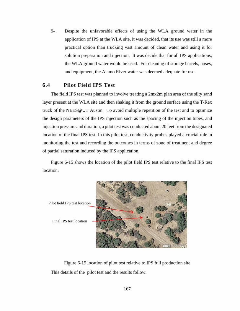
167
9- Despite the unfavorable effects of using the WLA ground water in the
application of IPS at the WLA site, it was decided, that its use was still a more
practical option than trucking vast amount of clean water and using it for
solution preparation and injection. It was decide that for all IPS applications,
the WLA ground water would be used. For cleaning of storage barrels, hoses,
and equipment, the Alamo River water was deemed adequate for use.
6.4 Pilot Field IPS Test
The field IPS test was planned to involve treating a 2mx2m plan area of the silty sand
layer present at the WLA site and then shaking it from the ground surface using the T-Rex
truck of the NEES@UT Austin. To avoid multiple repetition of the test and to optimize
the design parameters of the IPS injection such as the spacing of the injection tubes, and
injection pressure and duration, a pilot test was conducted about 20 feet from the designated
location of the final IPS test. In this pilot test, conductivity probes played a crucial role in
monitoring the test and recording the outcomes in terms of zone of treatment and degree
of partial saturation induced by the IPS application.
Figure 6-15 shows the location of the pilot field IPS test relative to the final IPS test
location.
Figure 6-15 location of pilot test relative to IPS full production site
This details of the pilot test and the results follow.
Pilot field IPS test location
Final IPS test location
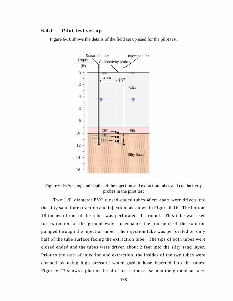
168
6.4.1 Pilot test set-up
Figure 6-16 shows the details of the field set up used for the pilot test.
Figure 6-16 Spacing and depths of the injection and extraction tubes and conductivity
probes in the pilot test
Two 1.5” diameter PVC closed-ended tubes 40cm apart were driven into
the silty sand for extraction and injection, as shown in Figure 6-16. The bottom
18 inches of one of the tubes was perforated all around. This tube was used
for extraction of the ground water to enhance the transport of the solution
pumped through the injection tube. The injection tube was perforated on only
half of the tube surface facing the extraction tube. The tips of both tubes were
closed ended and the tubes were driven about 2 feet into the silty sand layer.
Prior to the start of injection and extraction, the insides of the two tubes were
cleaned by using high pressure water garden hose inserted into the tubes.
Figure 6-17 shows a phot of the pilot test set up as seen at the ground surface.
Clay
Silt
Silty Sand
30 cm 10 cm
Extraction tube Injection tube
Conductivity probes
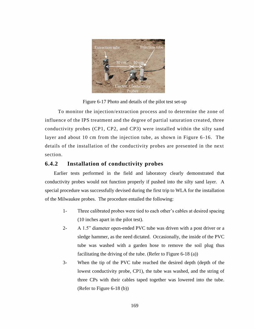
169
Figure 6-17 Photo and details of the pilot test set-up
To monitor the injection/extraction process and to determine the zone of
influence of the IPS treatment and the degree of partial saturation created, three
conductivity probes (CP1, CP2, and CP3) were installed within the silty sand
layer and about 10 cm from the injection tube, as shown in Figure 6 -16. The
details of the installation of the conductivity probes are presented in the next
section.
6.4.2 Installation of conductivity probes
Earlier tests performed in the field and laboratory clearly demonstrated that
conductivity probes would not function properly if pushed into the silty sand layer. A
special procedure was successfully devised during the first trip to WLA for the installation
of the Milwaukee probes. The procedure entailed the following:
1- Three calibrated probes were tied to each other’s cables at desired spacing
(10 inches apart in the pilot test).
2- A 1.5” diameter open-ended PVC tube was driven with a post driver or a
sledge hammer, as the need dictated. Occasionally, the inside of the PVC
tube was washed with a garden hose to remove the soil plug thus
facilitating the driving of the tube. (Refer to Figure 6-18 (a))
3- When the tip of the PVC tube reached the desired depth (depth of the
lowest conductivity probe, CP1), the tube was washed, and the string of
three CPs with their cables taped together was lowered into the tube.
(Refer to Figure 6-18 (b))
10 cm 30 cm
Injection tube Extraction tube
Electric Conductivity
Probes
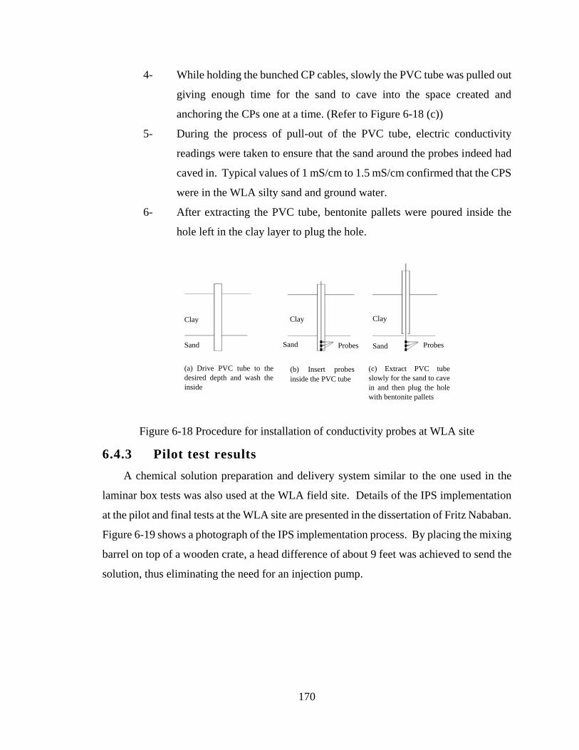
170
4- While holding the bunched CP cables, slowly the PVC tube was pulled out
giving enough time for the sand to cave into the space created and
anchoring the CPs one at a time. (Refer to Figure 6-18 (c))
5- During the process of pull-out of the PVC tube, electric conductivity
readings were taken to ensure that the sand around the probes indeed had
caved in. Typical values of 1 mS/cm to 1.5 mS/cm confirmed that the CPS
were in the WLA silty sand and ground water.
6- After extracting the PVC tube, bentonite pallets were poured inside the
hole left in the clay layer to plug the hole.
Figure 6-18 Procedure for installation of conductivity probes at WLA site
6.4.3 Pilot test results
A chemical solution preparation and delivery system similar to the one used in the
laminar box tests was also used at the WLA field site. Details of the IPS implementation
at the pilot and final tests at the WLA site are presented in the dissertation of Fritz Nababan.
Figure 6-19 shows a photograph of the IPS implementation process. By placing the mixing
barrel on top of a wooden crate, a head difference of about 9 feet was achieved to send the
solution, thus eliminating the need for an injection pump.
Probes Probes
Clay
layer
Clay
layer
Clay
layer
Sand Sand Sand
(a) Drive PVC tube to the
desired depth and wash the
inside
(b) Insert probes
inside the PVC tube
(c) Extract PVC tube
slowly for the sand to cave
in and then plug the hole
with bentonite pallets
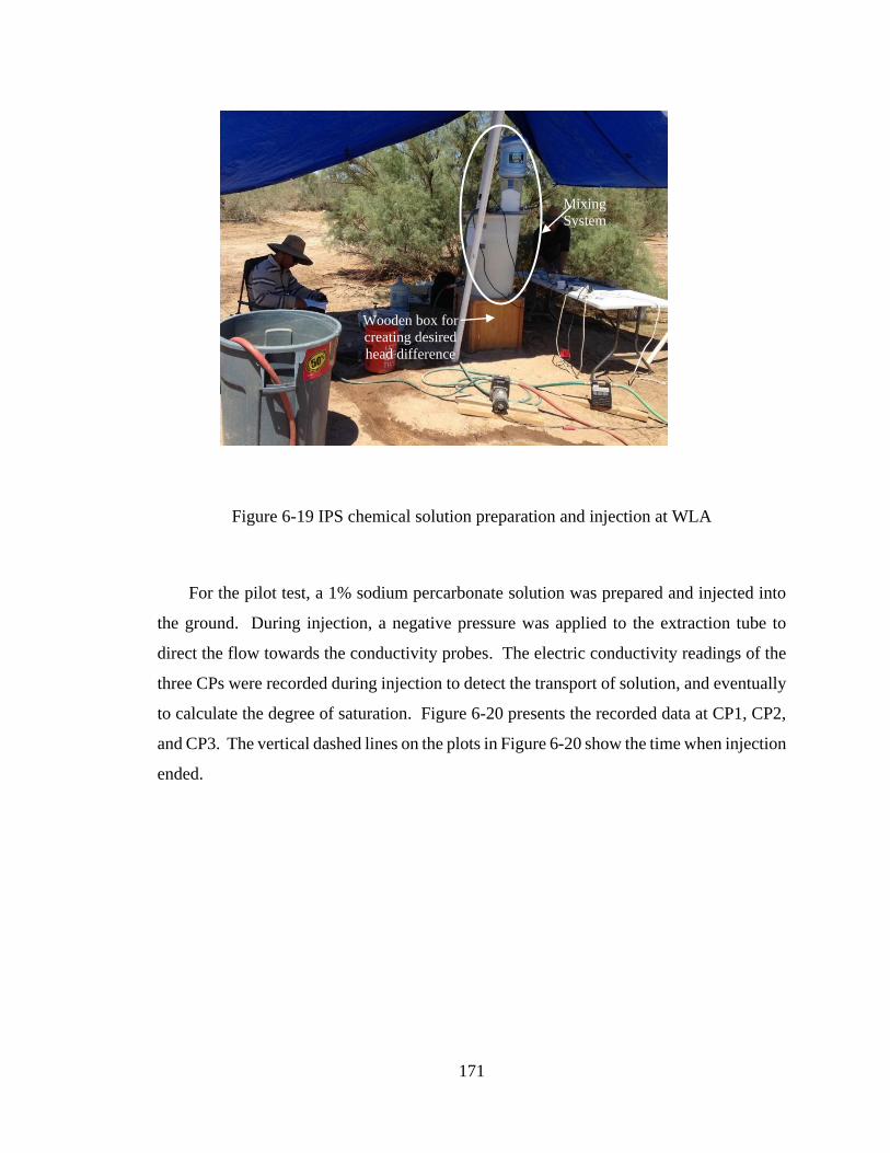
171
Figure 6-19 IPS chemical solution preparation and injection at WLA
For the pilot test, a 1% sodium percarbonate solution was prepared and injected into
the ground. During injection, a negative pressure was applied to the extraction tube to
direct the flow towards the conductivity probes. The electric conductivity readings of the
three CPs were recorded during injection to detect the transport of solution, and eventually
to calculate the degree of saturation. Figure 6-20 presents the recorded data at CP1, CP2,
and CP3. The vertical dashed lines on the plots in Figure 6-20 show the time when injection
ended.
Mixing
System
Wooden box for
creating desired
head difference
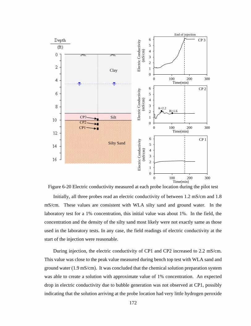
172
Figure 6-20 Electric conductivity measured at each probe location during the pilot test
Initially, all three probes read an electric conductivity of between 1.2 mS/cm and 1.8
mS/cm. These values are consistent with WLA silty sand and ground water. In the
laboratory test for a 1% concentration, this initial value was about 1%. In the field, the
concentration and the density of the silty sand most likely were not exactly same as those
used in the laboratory tests. In any case, the field readings of electric conductivity at the
start of the injection were reasonable.
During injection, the electric conductivity of CP1 and CP2 increased to 2.2 mS/cm.
This value was close to the peak value measured during bench top test with WLA sand and
ground water (1.9 mS/cm). It was concluded that the chemical solution preparation system
was able to create a solution with approximate value of 1% concentration. An expected
drop in electric conductivity due to bubble generation was not observed at CP1, possibly
indicating that the solution arriving at the probe location had very little hydrogen peroxide
Clay
Silt
Silty Sand
0
1
2
3
4
5
6
0 100 200 300
Ele
ctri
c C
onduct
ivit
y
(mS
/cm
)
Time(min)
CP 1
0
1
2
3
4
5
6
0 100 200 300
Ele
ctri
c C
onduct
ivit
y
(mS
/cm
)
Time(min)
CP 2
A=2.2 B=1.6
0
1
2
3
4
5
6
0 100 200 300
Ele
ctri
c C
onduct
ivit
y
(mS
/cm
)
Time(min)
CP 3
End of injection
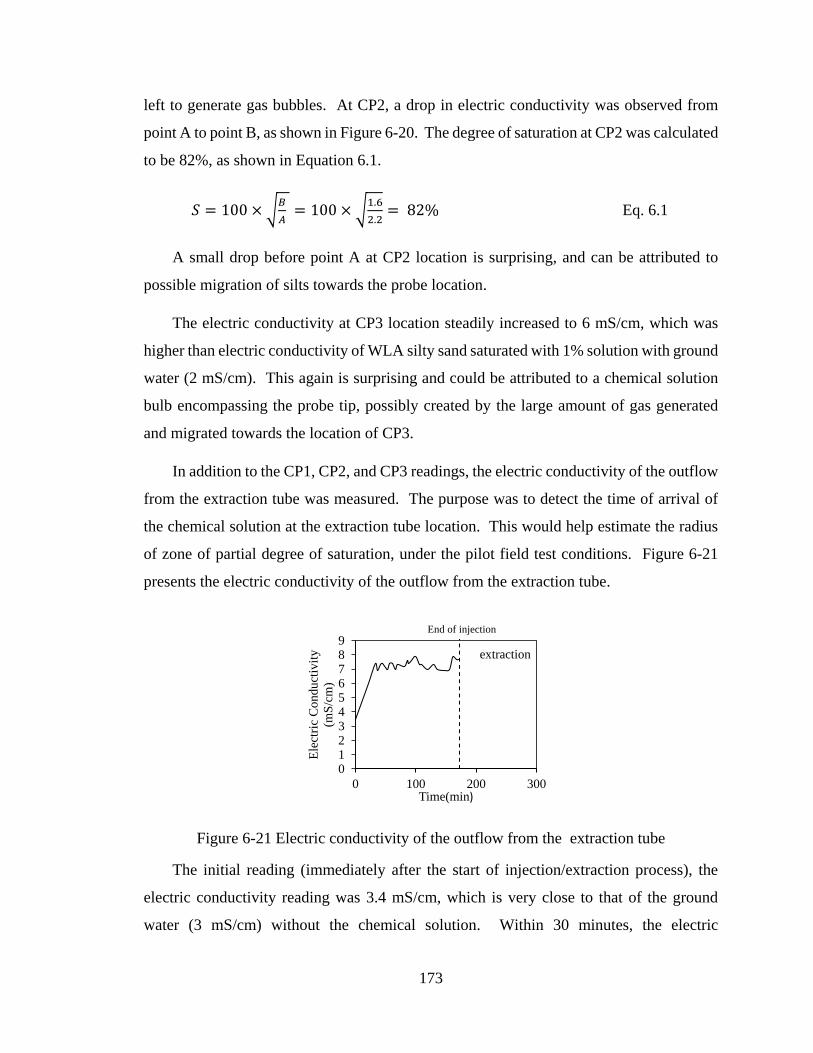
173
left to generate gas bubbles. At CP2, a drop in electric conductivity was observed from
point A to point B, as shown in Figure 6-20. The degree of saturation at CP2 was calculated
to be 82%, as shown in Equation 6.1.
𝑆 = 100 × √𝐵
𝐴 = 100 × √
1.6
2.2= 82% Eq. 6.1
A small drop before point A at CP2 location is surprising, and can be attributed to
possible migration of silts towards the probe location.
The electric conductivity at CP3 location steadily increased to 6 mS/cm, which was
higher than electric conductivity of WLA silty sand saturated with 1% solution with ground
water (2 mS/cm). This again is surprising and could be attributed to a chemical solution
bulb encompassing the probe tip, possibly created by the large amount of gas generated
and migrated towards the location of CP3.
In addition to the CP1, CP2, and CP3 readings, the electric conductivity of the outflow
from the extraction tube was measured. The purpose was to detect the time of arrival of
the chemical solution at the extraction tube location. This would help estimate the radius
of zone of partial degree of saturation, under the pilot field test conditions. Figure 6-21
presents the electric conductivity of the outflow from the extraction tube.
Figure 6-21 Electric conductivity of the outflow from the extraction tube
The initial reading (immediately after the start of injection/extraction process), the
electric conductivity reading was 3.4 mS/cm, which is very close to that of the ground
water (3 mS/cm) without the chemical solution. Within 30 minutes, the electric
0123456789
0 100 200 300
Ele
ctri
c C
on
du
ctiv
ity
(mS
/cm
)
Time(min)
extraction
End of injection
174
conductivity of the outflow from the extraction tube reached a value of 7.5 mS/cm, and
remained steady, with a peak value of 7.9 mS/cm. This value of electric conductivity is
smaller than that of the chemical solution with 1% concentration that was sent through the
injection tube (~12.5 mS/cm). This can be explained by the fact that while the injection
tube aimed the chemical solution in the direction of the extraction tube, the extraction tube
sucked water from all around it, thus diluting the arriving chemical solution with ground
water from the backside of the extraction tube.
In summary, conductivity probes were used in the pilot IPS field test to evaluate
parameters needed to design and implement the final IPS field test at the WLA site. The
conductivity measurements led to the following observations:
1. The field procedure devised for the installation of conductivity probe was
successful. The procedure entailed: driving an open-ended PVC tube, cleaning
the inside by washing, placing a string of conductivity probes inside the tube,
pulling up the PVC tube slowly to allow the sand around the probes to cave in
and anchor the probes, and finally plugging the hole left by the removal of the
PVC with bentonite pallets.
2. A head difference of 9 feet with extraction was sufficient to inject and transport
the chemical solution to at least 10 cm in 15 minutes (location of the
conductivity probes).
3. Measurement of electric conductivity of the outflow from an extraction tube
can be used to detect the first arrival of the chemical solution.
4. A head difference of 9 feet with extraction was sufficient to inject and transport
the chemical solution to at least 40 cm in 30 minutes (location of the extraction
tube).
5. Chemical solution of 1% concentration can reduce the degree of saturation to
82%, although at two of the three probes, the degree of saturation could not be
computed, because of lack of evidence of presence of gas bubbles.
6. The IPS delivery system developed and implemented in the laminar box tests
was successfully used in the pilot test and therefore was extensively utilized
during the final IPS test at the WLA site.
175
7. No changes in electric conductivity was observed after the injection process
was stopped, and therefore no significant effect of dilution and Ion movement
was detected in the field
6.5 Summery and conclusions
This research project on IPS included field tests at the NEES@UCSB Wildlife refuge
site, referred to as the Wildlife Liquefaction Array, WLA site. In all, three trips were made
to complete the field tests. The first two were exploratory; the third trip included a pilot
IPS field test and the final IPS test in which the treated site was shaken by T-Rex shaker
of NEES@UT. This Chapter presented details of the research activities at WLA site that
involved the use of electric conductivity probes. The Chapter demonstrated the crucial role
conductivity probes played in monitoring and evaluating the outcome of the IPS process in
the field. Summary findings are listed below.
1. The well known site conditions at the WLA site determined by other
investigators were confirmed by exploratory borings conducted by the IPS
research team. Electric conductivity readings also provided confirmation of
the depths of the various layers of soil (sand/clay) encountered in the
exploratory holes and inside PVC tubes at the IPS test locations.
2. Driving injection tubes was the preferred installation procedure. Jetting a tube
into the ground resulted in loose soil around the tube that allowed leakage of
injected solution. Conductivity probes confirmed the leaked water to be
chemical solution.
3. Both Alamo River water and the ground water at WLA are silty and
contaminated. The silt content was less in the ground water than in the River
water and therefore ground water was pumped and used in the preparation of
the chemical solution for IPS treatment.
4. Installation of a conductivity probe into the sand by pushing was not an
acceptable procedure. The readings of the probe were not indicative of the
true chemical and electric conductivity conditions in the silty sand at the
location of the probe.
176
5. WLA silty sand treated with chemical solution prepared with the ground water
containing contaminant ions exhibited slightly faster rate of reaction than that
observed in Ottawa sand and chemical solution prepared with regular tap
water. In addition, for the same concentration of chemical solution, the partial
degree of saturation in WLA specimen was slightly larger than in the Ottawa
sand specimen. Despite these slightly unfavorable conditions resulting from
the use of WLA ground water, it was decided to use the ground water for field
IPS treatment instead of trucking clean water to the site, which would have
been costly and impractical.
177
Chapter 7
Preliminary Laboratory Tests Using a Prototype Field Electric
Conductivity Probe to Estimate Degree of Saturation
7.1 Overview
Chapter 6 described the application of electric conductivity probes in the field tests
conducted at the Wildlife Liquefaction Array (WLA). For this purpose, Milwaukee probes,
which are typically for use in laboratory tests, were implemented. The installation of the
Milwaukee probes in the field was challenging and often resulted in questionable
functionality and test results. To install Milwaukee probes, initially a PVC tube had to be
driven and cleaned the inside. Then a maximum of three probes (because of limited space
available in the tube) with their cables bundled were lowered and the tube carefully lifted
to ensure that the probes remained within the soil deposit. There were a number of
difficulties and undesirable situation encountered in the field installation of the probes.
The driving of a 1.5” diameter PVC tube was very difficult. Washing the inside of the tube
to remove the soil plug at times washed also the sand encountered at the tip of the tube,
thus loosening the natural sand deposit into which the probes were placed. There was no
assurance that the sand caved in around the probes and that there were no pockets of just
ground water at the tip of the probes. The bundled three probes limited the recording of
data at only three depths.
It was evident that the Milwaukee probes would not be suitable or convenient to use
in field application of Induced Partial Saturation (IPS). An alternate field probe was
explored, which entailed driving a hollow metal tube with a cone at its tip. The tube would
have near its cone tip two electrodes embedded on the surface of the tube, with their cables
extended from the inside of the tube to a hand-held meter.
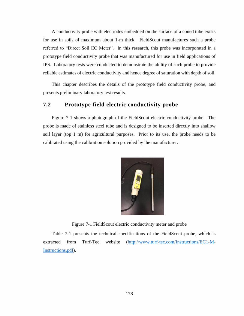
178
A conductivity probe with electrodes embedded on the surface of a coned tube exists
for use in soils of maximum about 1-m thick. FieldScout manufactures such a probe
referred to “Direct Soil EC Meter”. In this research, this probe was incorporated in a
prototype field conductivity probe that was manufactured for use in field applications of
IPS. Laboratory tests were conducted to demonstrate the ability of such probe to provide
reliable estimates of electric conductivity and hence degree of saturation with depth of soil.
This chapter describes the details of the prototype field conductivity probe, and
presents preliminary laboratory test results.
7.2 Prototype field electric conductivity probe
Figure 7-1 shows a photograph of the FieldScout electric conductivity probe. The
probe is made of stainless steel tube and is designed to be inserted directly into shallow
soil layer (top 1 m) for agricultural purposes. Prior to its use, the probe needs to be
calibrated using the calibration solution provided by the manufacturer.
Figure 7-1 FieldScout electric conductivity meter and probe
Table 7-1 presents the technical specifications of the FieldScout probe, which is
extracted from Turf-Tec website (http://www.turf-tec.com/Instructions/EC1-M-
Instructions.pdf).
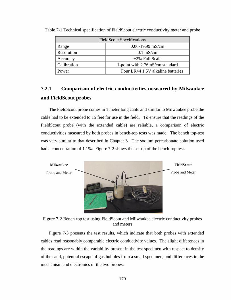
179
Table 7-1 Technical specification of FieldScout electric conductivity meter and probe
FieldScout Specifications
Range 0.00-19.99 mS/cm
Resolution 0.1 mS/cm
Accuracy ±2% Full Scale
Calibration 1-point with 2.76mS/cm standard
Power Four LR44 1.5V alkaline batteries
7.2.1 Comparison of electric conductivities measured by Milwaukee
and FieldScout probes
The FieldScout probe comes in 1 meter long cable and similar to Milwaukee probe the
cable had to be extended to 15 feet for use in the field. To ensure that the readings of the
FieldScout probe (with the extended cable) are reliable, a comparison of electric
conductivities measured by both probes in bench-top tests was made. The bench top-test
was very similar to that described in Chapter 3. The sodium percarbonate solution used
had a concentration of 1.1%. Figure 7-2 shows the set-up of the bench-top test.
Figure 7-2 Bench-top test using FieldScout and Milwaukee electric conductivity probes
and meters
Figure 7-3 presents the test results, which indicate that both probes with extended
cables read reasonably comparable electric conductivity values. The slight differences in
the readings are within the variability present in the test specimen with respect to density
of the sand, potential escape of gas bubbles from a small specimen, and differences in the
mechanism and electronics of the two probes.
FieldScout
Probe and Meter
Milwaukee
Probe and Meter
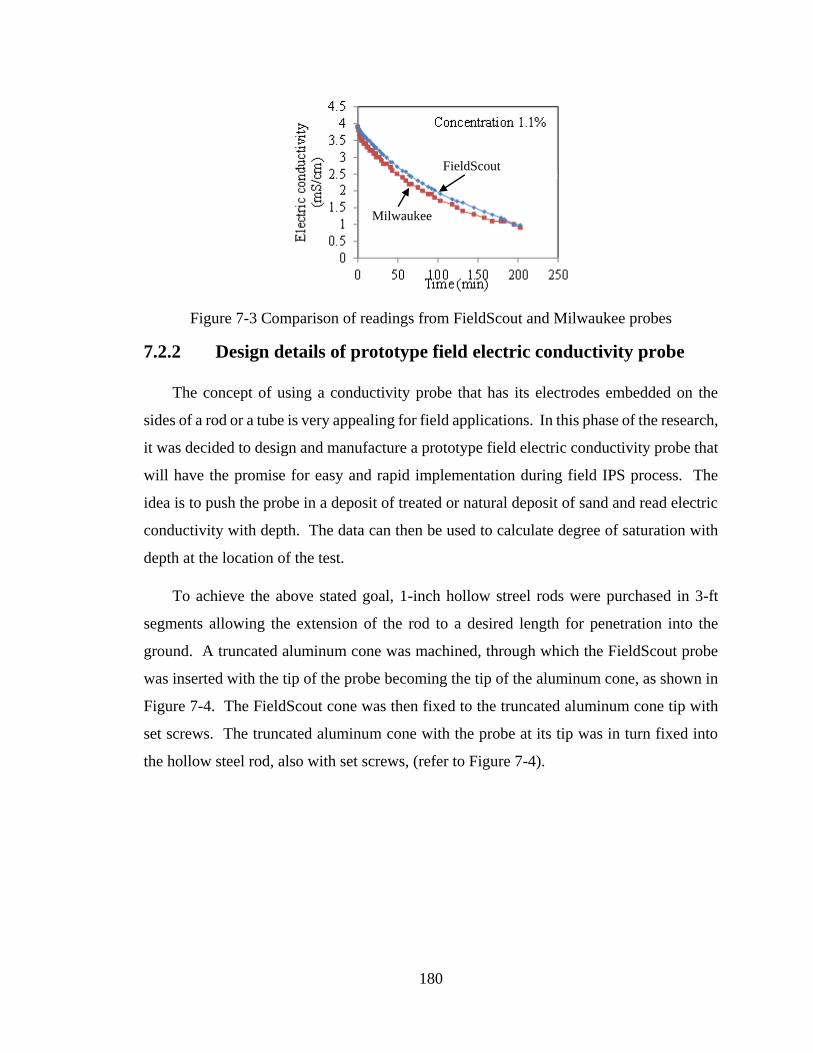
180
Figure 7-3 Comparison of readings from FieldScout and Milwaukee probes
7.2.2 Design details of prototype field electric conductivity probe
The concept of using a conductivity probe that has its electrodes embedded on the
sides of a rod or a tube is very appealing for field applications. In this phase of the research,
it was decided to design and manufacture a prototype field electric conductivity probe that
will have the promise for easy and rapid implementation during field IPS process. The
idea is to push the probe in a deposit of treated or natural deposit of sand and read electric
conductivity with depth. The data can then be used to calculate degree of saturation with
depth at the location of the test.
To achieve the above stated goal, 1-inch hollow streel rods were purchased in 3-ft
segments allowing the extension of the rod to a desired length for penetration into the
ground. A truncated aluminum cone was machined, through which the FieldScout probe
was inserted with the tip of the probe becoming the tip of the aluminum cone, as shown in
Figure 7-4. The FieldScout cone was then fixed to the truncated aluminum cone tip with
set screws. The truncated aluminum cone with the probe at its tip was in turn fixed into
the hollow steel rod, also with set screws, (refer to Figure 7-4).
Milwaukee
FieldScout
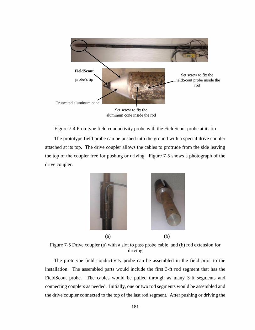
181
Figure 7-4 Prototype field conductivity probe with the FieldScout probe at its tip
The prototype field probe can be pushed into the ground with a special drive coupler
attached at its top. The drive coupler allows the cables to protrude from the side leaving
the top of the coupler free for pushing or driving. Figure 7-5 shows a photograph of the
drive coupler.
(a) (b)
Figure 7-5 Drive coupler (a) with a slot to pass probe cable, and (b) rod extension for
driving
The prototype field conductivity probe can be assembled in the field prior to the
installation. The assembled parts would include the first 3-ft rod segment that has the
FieldScout probe. The cables would be pulled through as many 3-ft segments and
connecting couplers as needed. Initially, one or two rod segments would be assembled and
the drive coupler connected to the top of the last rod segment. After pushing or driving the
Set screw to fix the
aluminum cone inside the rod
FieldScout
probe’s tip Set screw to fix the
FieldScout probe inside the
rod
Truncated aluminum cone
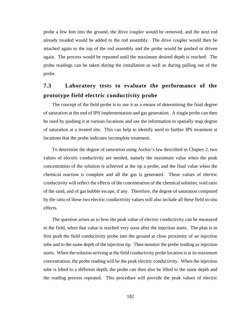
182
probe a few feet into the ground, the drive coupler would be removed, and the next rod
already treaded would be added to the rod assembly. The drive coupler would then be
attached again to the top of the rod assembly and the probe would be pushed or driven
again. The process would be repeated until the maximum desired depth is reached. The
probe readings can be taken during the installation as well as during pulling out of the
probe.
7.3 Laboratory tests to evaluate the performance of the
prototype field electric conductivity probe
The concept of the field probe is to use it as a means of determining the final degree
of saturation at the end of IPS implementation and gas generation. A single probe can then
be used by pushing it at various locations and use the information to spatially map degree
of saturation at a treated site. This can help to identify need to further IPS treatment at
locations that the probe indicates incomplete treatment.
To determine the degree of saturation using Archie’s law described in Chapter 2, two
values of electric conductivity are needed, namely the maximum value when the peak
concentration of the solution is achieved at the tip a probe, and the final value when the
chemical reaction is complete and all the gas is generated. These values of electric
conductivity will reflect the effects of the concentration of the chemical solution, void ratio
of the sand, and of gas bubble escape, if any. Therefore, the degree of saturation computed
by the ratio of these two electric conductivity values will also include all these field in-situ
effects.
The question arises as to how the peak value of electric conductivity can be measured
in the field, when that value is reached very soon after the injection starts. The plan is to
first push the field conductivity probe into the ground at close proximity of an injection
tube and to the same depth of the injection tip. Then monitor the probe reading as injection
starts. When the solution arriving at the field conductivity probe location is at its maximum
concentration, the probe reading will be the peak electric conductivity. When the injection
tube is lifted to a different depth, the probe can then also be lifted to the same depth and
the reading process repeated. This procedure will provide the peak values of electric
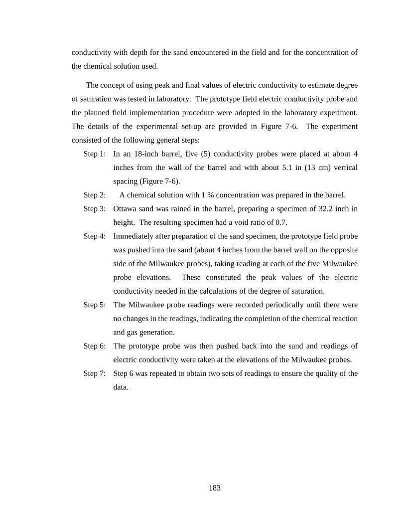
183
conductivity with depth for the sand encountered in the field and for the concentration of
the chemical solution used.
The concept of using peak and final values of electric conductivity to estimate degree
of saturation was tested in laboratory. The prototype field electric conductivity probe and
the planned field implementation procedure were adopted in the laboratory experiment.
The details of the experimental set-up are provided in Figure 7-6. The experiment
consisted of the following general steps:
Step 1: In an 18-inch barrel, five (5) conductivity probes were placed at about 4
inches from the wall of the barrel and with about 5.1 in (13 cm) vertical
spacing (Figure 7-6).
Step 2: A chemical solution with 1 % concentration was prepared in the barrel.
Step 3: Ottawa sand was rained in the barrel, preparing a specimen of 32.2 inch in
height. The resulting specimen had a void ratio of 0.7.
Step 4: Immediately after preparation of the sand specimen, the prototype field probe
was pushed into the sand (about 4 inches from the barrel wall on the opposite
side of the Milwaukee probes), taking reading at each of the five Milwaukee
probe elevations. These constituted the peak values of the electric
conductivity needed in the calculations of the degree of saturation.
Step 5: The Milwaukee probe readings were recorded periodically until there were
no changes in the readings, indicating the completion of the chemical reaction
and gas generation.
Step 6: The prototype probe was then pushed back into the sand and readings of
electric conductivity were taken at the elevations of the Milwaukee probes.
Step 7: Step 6 was repeated to obtain two sets of readings to ensure the quality of the
data.
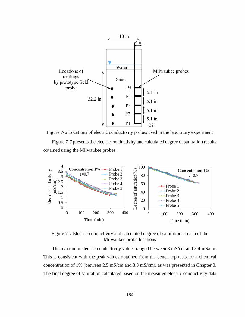
184
Figure 7-6 Locations of electric conductivity probes used in the laboratory experiment
Figure 7-7 presents the electric conductivity and calculated degree of saturation results
obtained using the Milwaukee probes.
Figure 7-7 Electric conductivity and calculated degree of saturation at each of the
Milwaukee probe locations
The maximum electric conductivity values ranged between 3 mS/cm and 3.4 mS/cm.
This is consistent with the peak values obtained from the bench-top tests for a chemical
concentration of 1% (between 2.5 mS/cm and 3.3 mS/cm), as was presented in Chapter 3.
The final degree of saturation calculated based on the measured electric conductivity data
0
0.5
1
1.5
2
2.5
3
3.5
4
0 100 200 300 400
Ele
ctri
c co
nd
uct
ivit
y
(mS
/cm
)
Time (min)
Concentration 1%
e=0.7Probe 1Probe 2Probe 3Probe 4Probe 5
0
20
40
60
80
100
0 100 200 300 400
Deg
ree
of
satu
rati
on
(%)
Time (min)
Concentration 1%
e=0.7
Probe 1Probe 2Probe 3Probe 4Probe 5
2 in
5.1 in
5.1 in
5.1 in
5.1 in
18 in
32.2 in
P1
P2
P3
P4
P5
4 in
Sand
Water Milwaukee probes Locations of
readings
by prototype field
probe
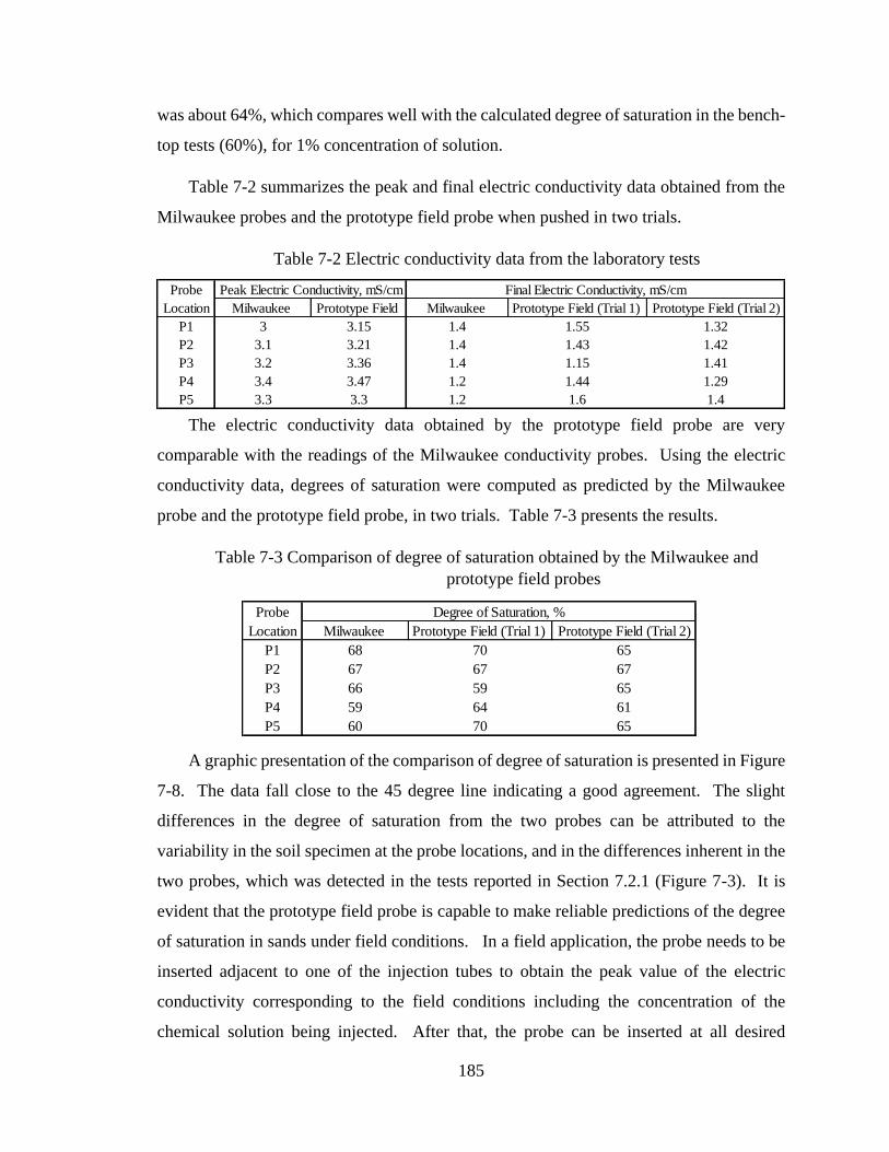
185
Probe
Location Milwaukee Prototype Field Milwaukee Prototype Field (Trial 1) Prototype Field (Trial 2)
P1 3 3.15 1.4 1.55 1.32
P2 3.1 3.21 1.4 1.43 1.42
P3 3.2 3.36 1.4 1.15 1.41
P4 3.4 3.47 1.2 1.44 1.29
P5 3.3 3.3 1.2 1.6 1.4
Peak Electric Conductivity, mS/cm Final Electric Conductivity, mS/cm
was about 64%, which compares well with the calculated degree of saturation in the bench-
top tests (60%), for 1% concentration of solution.
Table 7-2 summarizes the peak and final electric conductivity data obtained from the
Milwaukee probes and the prototype field probe when pushed in two trials.
Table 7-2 Electric conductivity data from the laboratory tests
The electric conductivity data obtained by the prototype field probe are very
comparable with the readings of the Milwaukee conductivity probes. Using the electric
conductivity data, degrees of saturation were computed as predicted by the Milwaukee
probe and the prototype field probe, in two trials. Table 7-3 presents the results.
Table 7-3 Comparison of degree of saturation obtained by the Milwaukee and
prototype field probes
A graphic presentation of the comparison of degree of saturation is presented in Figure
7-8. The data fall close to the 45 degree line indicating a good agreement. The slight
differences in the degree of saturation from the two probes can be attributed to the
variability in the soil specimen at the probe locations, and in the differences inherent in the
two probes, which was detected in the tests reported in Section 7.2.1 (Figure 7-3). It is
evident that the prototype field probe is capable to make reliable predictions of the degree
of saturation in sands under field conditions. In a field application, the probe needs to be
inserted adjacent to one of the injection tubes to obtain the peak value of the electric
conductivity corresponding to the field conditions including the concentration of the
chemical solution being injected. After that, the probe can be inserted at all desired
Probe
Location Milwaukee Prototype Field (Trial 1) Prototype Field (Trial 2)
P1 68 70 65
P2 67 67 67
P3 66 59 65
P4 59 64 61
P5 60 70 65
Degree of Saturation, %
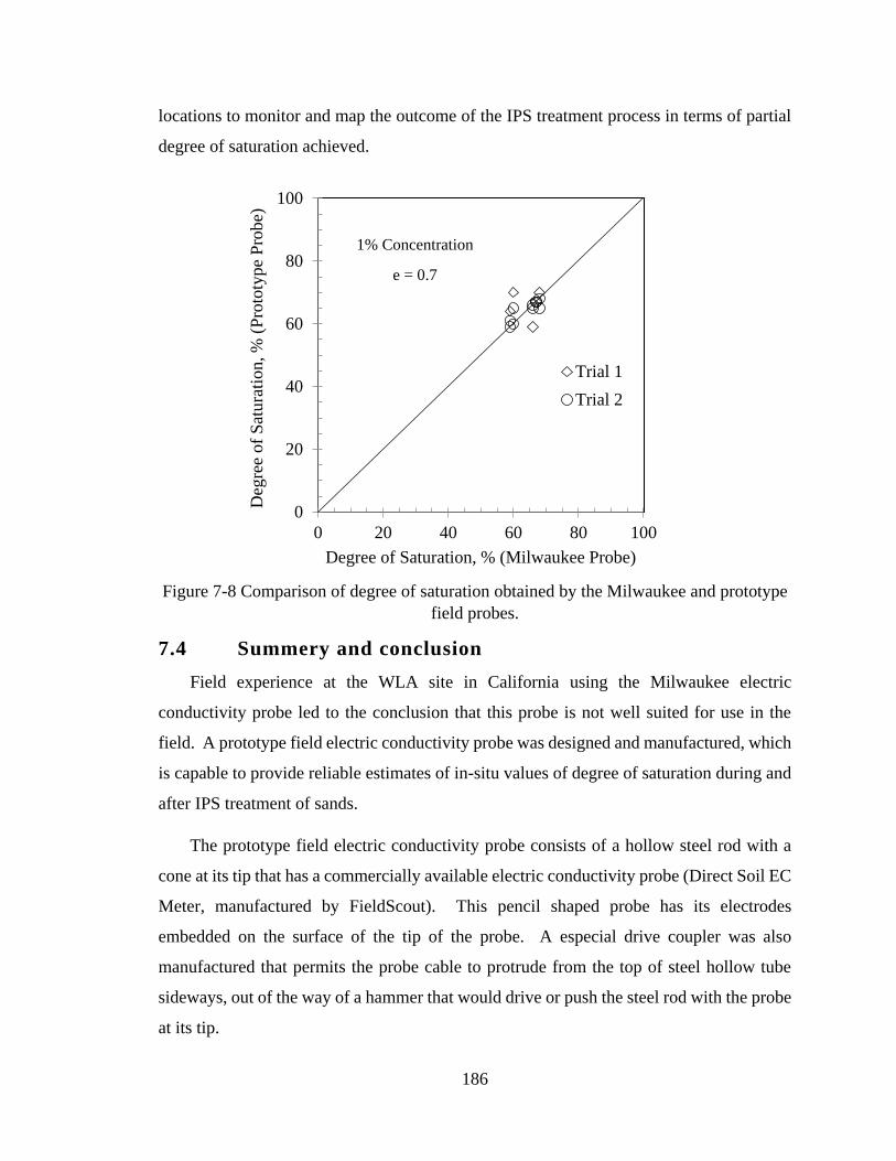
186
0
20
40
60
80
100
0 20 40 60 80 100
Deg
ree
of
Sat
ura
tion, %
(P
roto
type
Pro
be)
Degree of Saturation, % (Milwaukee Probe)
Trial 1
Trial 2
locations to monitor and map the outcome of the IPS treatment process in terms of partial
degree of saturation achieved.
Figure 7-8 Comparison of degree of saturation obtained by the Milwaukee and prototype
field probes.
7.4 Summery and conclusion
Field experience at the WLA site in California using the Milwaukee electric
conductivity probe led to the conclusion that this probe is not well suited for use in the
field. A prototype field electric conductivity probe was designed and manufactured, which
is capable to provide reliable estimates of in-situ values of degree of saturation during and
after IPS treatment of sands.
The prototype field electric conductivity probe consists of a hollow steel rod with a
cone at its tip that has a commercially available electric conductivity probe (Direct Soil EC
Meter, manufactured by FieldScout). This pencil shaped probe has its electrodes
embedded on the surface of the tip of the probe. A especial drive coupler was also
manufactured that permits the probe cable to protrude from the top of steel hollow tube
sideways, out of the way of a hammer that would drive or push the steel rod with the probe
at its tip.
1% Concentration
e = 0.7
187
This prototype field electric conductivity probe was tested in a laboratory setting
following the procedure planed for field implementation. Tests were conducted in which
the electric conductivity values were obtained by both Milwaukee and the prototype field
probes. The results of the two probes were very comparable and consistent with the electric
conductivity values measured in laboratory bench-top tests using a chemical solution of
1% concentration.
Degrees of saturation were computed using the electric conductivity data from both
the Milwaukee and the prototype field probes. The results from the two probes were very
comparable, with an average difference of about 6%.
Based on the laboratory test results, it can be concluded that the prototype field electric
conductivity probe is capable of providing reliable estimates of degree of saturation with
depth of soil. Field tests will require to confirm the robustness and ease of use of this
probe.
188
Chapter 8
Summary and Conclusions
This dissertation describes a system developed for monitoring the implementation of
an innovative liquefaction mitigation measure referred to as Induced Partial Saturation
(IPS). IPS involves injection of sodium percarbonate solution into a potentially liquefiable
sand, and through transport of the solution and its reactivity generate gas bubbles within
the void spaces of the sand, thus reducing the degree of saturation of the otherwise fully
saturated sand. IPS was proposed by Yegian et al., 2007 and through preliminary
laboratory tests its beneficial effect on liquefaction resistance was demonstrated.
This research was part of a larger project on evaluating the effectiveness of IPS as a
liquefaction mitigation measure. The project was funded by the National Science
Foundation (NSF) through the Program George E. Brown Jr. Network for Earthquake
Engineering Simulation (NEES). Professors M. K. Yegian and A. Alshawabkeh, the PI
and CO PI of the project collaborated with Professor S. Thevanayagam, of the State
University of New York at Buffalo, Professor Kenneth H. Stokoe of the University of
Texas at Austin, Dr. Jamison Steidl of the University of California at Santa Barbara, and
Professor Leslie Youd, formerly of Brigham Young University.
To ensure the effectiveness of and the proper implementation of IPS, a monitoring
system was designed that utilizes electric conductivity probes. The probes were used to
control the concentration of the chemical solution being injected, to monitor the transport
of the solution away from the injection point, to detect the rate of generation of gas bubbles
and its effect on degree of partial saturation of the sand, to detect potential loss of gas
bubbles and its effect on degree of partial saturation, and to estimate the zone of partial
saturation created.
The monitoring system developed and the method of calculating the degree of
saturation were tested in small- and large-scale laboratory experiments, and in a pilot field
test.
Small-scale (bench-top) laboratory experiments were conducted on specimens of
Ottawa sand treated by sodium percarbonate. Milwaukee electric conductivity probes were
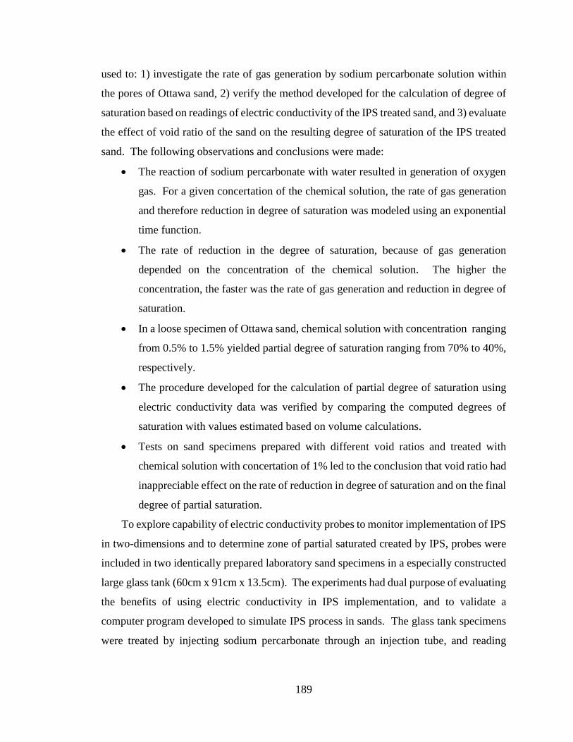
189
used to: 1) investigate the rate of gas generation by sodium percarbonate solution within
the pores of Ottawa sand, 2) verify the method developed for the calculation of degree of
saturation based on readings of electric conductivity of the IPS treated sand, and 3) evaluate
the effect of void ratio of the sand on the resulting degree of saturation of the IPS treated
sand. The following observations and conclusions were made:
The reaction of sodium percarbonate with water resulted in generation of oxygen
gas. For a given concertation of the chemical solution, the rate of gas generation
and therefore reduction in degree of saturation was modeled using an exponential
time function.
The rate of reduction in the degree of saturation, because of gas generation
depended on the concentration of the chemical solution. The higher the
concentration, the faster was the rate of gas generation and reduction in degree of
saturation.
In a loose specimen of Ottawa sand, chemical solution with concentration ranging
from 0.5% to 1.5% yielded partial degree of saturation ranging from 70% to 40%,
respectively.
The procedure developed for the calculation of partial degree of saturation using
electric conductivity data was verified by comparing the computed degrees of
saturation with values estimated based on volume calculations.
Tests on sand specimens prepared with different void ratios and treated with
chemical solution with concertation of 1% led to the conclusion that void ratio had
inappreciable effect on the rate of reduction in degree of saturation and on the final
degree of partial saturation.
To explore capability of electric conductivity probes to monitor implementation of IPS
in two-dimensions and to determine zone of partial saturated created by IPS, probes were
included in two identically prepared laboratory sand specimens in a especially constructed
large glass tank (60cm x 91cm x 13.5cm). The experiments had dual purpose of evaluating
the benefits of using electric conductivity in IPS implementation, and to validate a
computer program developed to simulate IPS process in sands. The glass tank specimens
were treated by injecting sodium percarbonate through an injection tube, and reading
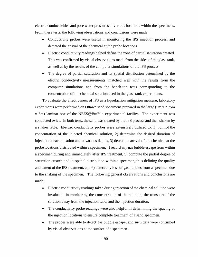
190
electric conductivities and pore water pressures at various locations within the specimens.
From these tests, the following observations and conclusions were made:
Conductivity probes were useful in monitoring the IPS injection process, and
detected the arrival of the chemical at the probe locations.
Electric conductivity readings helped define the zone of partial saturation created.
This was confirmed by visual observations made from the sides of the glass tank,
as well as by the results of the computer simulations of the IPS process.
The degree of partial saturation and its spatial distribution determined by the
electric conductivity measurements, matched well with the results from the
computer simulations and from the bench-top tests corresponding to the
concentration of the chemical solution used in the glass tank experiments.
To evaluate the effectiveness of IPS as a liquefaction mitigation measure, laboratory
experiments were performed on Ottawa sand specimens prepared in the large (5m x 2.75m
x 6m) laminar box of the NEES@Buffalo experimental facility. The experiment was
conducted twice. In both tests, the sand was treated by the IPS process and then shaken by
a shaker table. Electric conductivity probes were extensively utilized to: 1) control the
concentration of the injected chemical solution, 2) determine the desired duration of
injection at each location and at various depths, 3) detect the arrival of the chemical at the
probe locations distributed within a specimen, 4) record any gas bubble escape from within
a specimen during and immediately after IPS treatment, 5) compute the partial degree of
saturation created and its spatial distribution within a specimen, thus defining the quality
and extent of the IPS treatment, and 6) detect any loss of gas bubbles from a specimen due
to the shaking of the specimen. The following general observations and conclusions are
made:
Electric conductivity readings taken during injection of the chemical solution were
invaluable in monitoring the concentration of the solution, the transport of the
solution away from the injection tube, and the injection duration.
The conductivity probe readings were also helpful in determining the spacing of
the injection locations to ensure complete treatment of a sand specimen.
The probes were able to detect gas bubble escape, and such data were confirmed
by visual observations at the surface of a specimen.
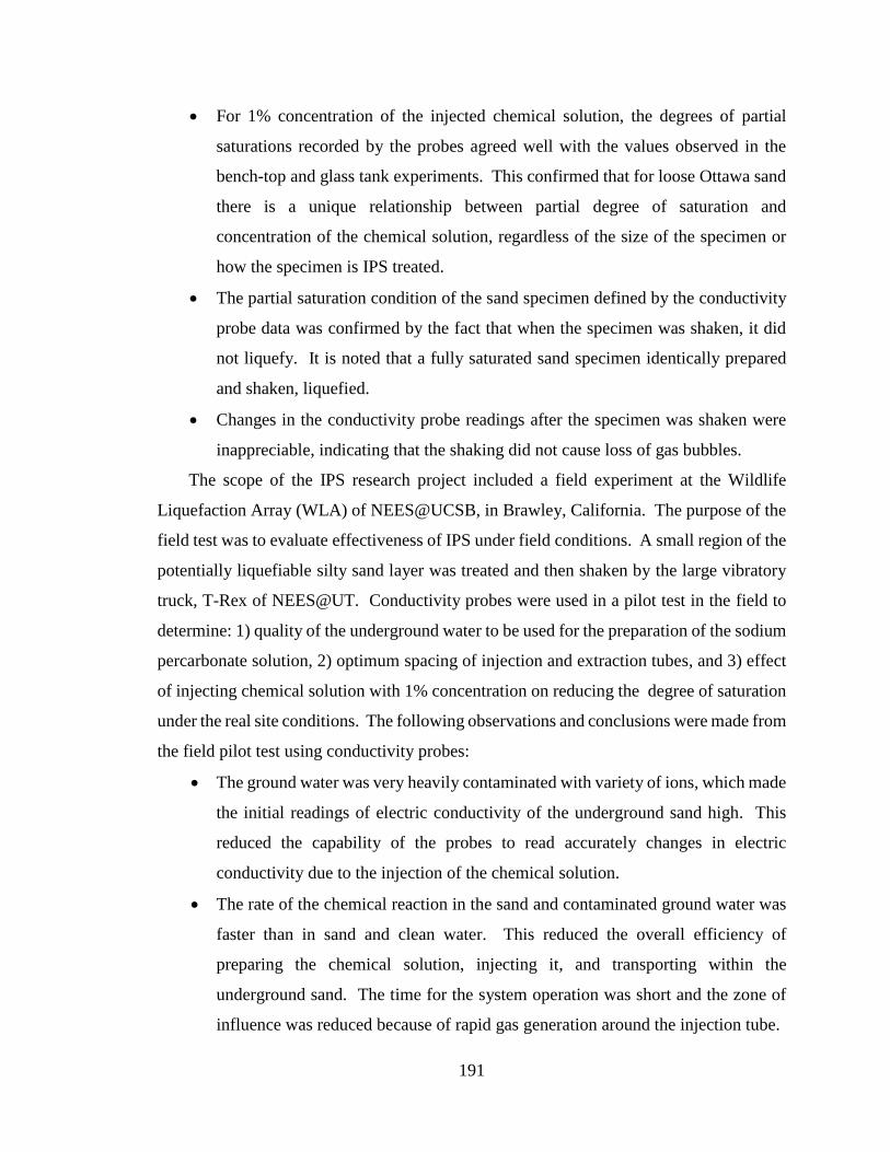
191
For 1% concentration of the injected chemical solution, the degrees of partial
saturations recorded by the probes agreed well with the values observed in the
bench-top and glass tank experiments. This confirmed that for loose Ottawa sand
there is a unique relationship between partial degree of saturation and
concentration of the chemical solution, regardless of the size of the specimen or
how the specimen is IPS treated.
The partial saturation condition of the sand specimen defined by the conductivity
probe data was confirmed by the fact that when the specimen was shaken, it did
not liquefy. It is noted that a fully saturated sand specimen identically prepared
and shaken, liquefied.
Changes in the conductivity probe readings after the specimen was shaken were
inappreciable, indicating that the shaking did not cause loss of gas bubbles.
The scope of the IPS research project included a field experiment at the Wildlife
Liquefaction Array (WLA) of NEES@UCSB, in Brawley, California. The purpose of the
field test was to evaluate effectiveness of IPS under field conditions. A small region of the
potentially liquefiable silty sand layer was treated and then shaken by the large vibratory
truck, T-Rex of NEES@UT. Conductivity probes were used in a pilot test in the field to
determine: 1) quality of the underground water to be used for the preparation of the sodium
percarbonate solution, 2) optimum spacing of injection and extraction tubes, and 3) effect
of injecting chemical solution with 1% concentration on reducing the degree of saturation
under the real site conditions. The following observations and conclusions were made from
the field pilot test using conductivity probes:
The ground water was very heavily contaminated with variety of ions, which made
the initial readings of electric conductivity of the underground sand high. This
reduced the capability of the probes to read accurately changes in electric
conductivity due to the injection of the chemical solution.
The rate of the chemical reaction in the sand and contaminated ground water was
faster than in sand and clean water. This reduced the overall efficiency of
preparing the chemical solution, injecting it, and transporting within the
underground sand. The time for the system operation was short and the zone of
influence was reduced because of rapid gas generation around the injection tube.
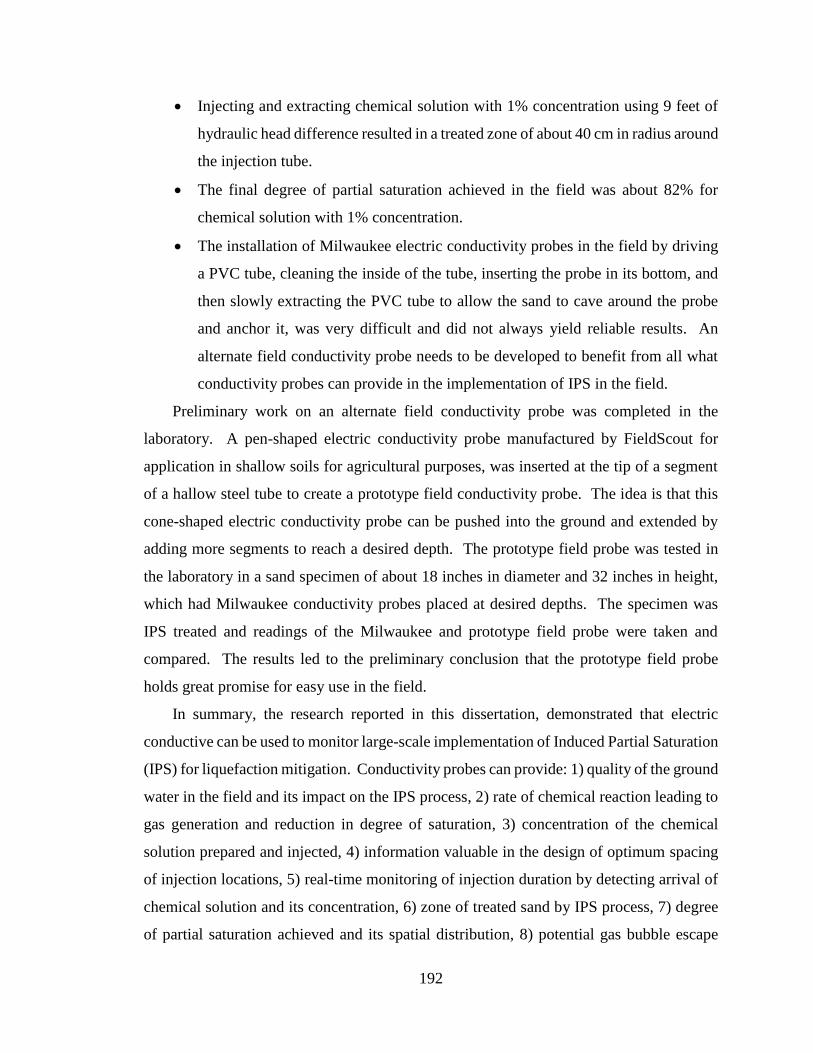
192
Injecting and extracting chemical solution with 1% concentration using 9 feet of
hydraulic head difference resulted in a treated zone of about 40 cm in radius around
the injection tube.
The final degree of partial saturation achieved in the field was about 82% for
chemical solution with 1% concentration.
The installation of Milwaukee electric conductivity probes in the field by driving
a PVC tube, cleaning the inside of the tube, inserting the probe in its bottom, and
then slowly extracting the PVC tube to allow the sand to cave around the probe
and anchor it, was very difficult and did not always yield reliable results. An
alternate field conductivity probe needs to be developed to benefit from all what
conductivity probes can provide in the implementation of IPS in the field.
Preliminary work on an alternate field conductivity probe was completed in the
laboratory. A pen-shaped electric conductivity probe manufactured by FieldScout for
application in shallow soils for agricultural purposes, was inserted at the tip of a segment
of a hallow steel tube to create a prototype field conductivity probe. The idea is that this
cone-shaped electric conductivity probe can be pushed into the ground and extended by
adding more segments to reach a desired depth. The prototype field probe was tested in
the laboratory in a sand specimen of about 18 inches in diameter and 32 inches in height,
which had Milwaukee conductivity probes placed at desired depths. The specimen was
IPS treated and readings of the Milwaukee and prototype field probe were taken and
compared. The results led to the preliminary conclusion that the prototype field probe
holds great promise for easy use in the field.
In summary, the research reported in this dissertation, demonstrated that electric
conductive can be used to monitor large-scale implementation of Induced Partial Saturation
(IPS) for liquefaction mitigation. Conductivity probes can provide: 1) quality of the ground
water in the field and its impact on the IPS process, 2) rate of chemical reaction leading to
gas generation and reduction in degree of saturation, 3) concentration of the chemical
solution prepared and injected, 4) information valuable in the design of optimum spacing
of injection locations, 5) real-time monitoring of injection duration by detecting arrival of
chemical solution and its concentration, 6) zone of treated sand by IPS process, 7) degree
of partial saturation achieved and its spatial distribution, 8) potential gas bubble escape
193
from sand pores during injection or after shaking of a treated sand, and the resulting
increase in degree of saturation.
194
REFERENCES
Archie, Gustave E. "The electrical resistivity log as an aid in determining some reservoir
characteristics." Transactions of the AIME 146.01 (1942): 54-62.
Archie, Gustave Erdman. "Electrical resistivity an aid in core-analysis
interpretation." AAPG Bulletin 31.2 (1947): 350-366.
Authority, Salton Sea. "NEW AND ALAMO RIVER WETLANDS MASTER PLAN."
Prepared for Wildlife Conservation Board, Sacramento, CA and Salton Sea
Authority LaQuinta, CA, by Tetra Tech, Inc. Lafayette, CA and Wetlands
Management Services , Chelsea, MI, (2007).
Bockris, John O'M., Amulya KN Reddy, and Maria Gamboa-Aldeco. Modern
Electrochemistry 2B: Electrodics in Chemistry, Engineering, Biology and
Environmental Science. Vol. 2. Springer Science & Business Media, (2001).
Direct Soil EC Meter specifications manufactured by FieldScout, available at Turf-Tec
website (http://www.turf-tec.com/Instructions/EC1-M-Instructions.pdf).
Eseller-Bayat, E., Yegian, M., Alshawabkeh, A., and Gokyer, S. Liquefaction Response
of Partially Saturated Sands. I: Experimental Results. Journal of Geotechnical and
Geoenvironmental Engineering, Vol. 139, No.6 (2013) , pp. 863–871.
195
Eseller-Bayat, E., et al. "Bender Elements and Bending Disks for Measurement of Shear
and Compression Wave Velocities in Large Fully and Partially Saturated Sand
Specimens." Geotechnical Testing Journal. Vol. 36. No. 2. ASTM International,
(2013). 1-8.
Fischer-Cripps, Anthony C. The Electronics Companion: Devices and Circuits for
Physicists and Engineers. CRC Press, (2014).
Gillham, R. W. and J. A. Cherry. Contaminant migration in saturated unconsolidated
geologic deposits. Geological Society of America (Special Paper 189) (1982) pp
31-62.
Gokyer, S. Numerical simulation of partial saturation in sands induced by flow and
chemical reactivity. Ph.D. dissertation, Northeastern University, Boston (2015).
Mitchell, James Kenneth, and Kenichi Soga. Fundamentals of soil behavior. New York:
Wiley, (1976).
Mohamed, Abdel-Mohsen Onsy, and Hogan E. Antia. Geoenvironmental engineering.
Elsevier, (1998).
196
MW302 electric conductivity meter manufactured by Milwaukee Instruments available:
(http://www.milwaukeeinstruments.com/site/products/products/standardportable
-meters/83-products-g-standard-portable-meters-g-mw302)
Ohm, Georg Simon. Die galvanische Kette, mathematisch bearbeitet. Riemann, (1827).
Palmer, C. D., and R. L. Johnson. "Physical processes controlling the transport of non-
aqueous phase liquids in the subsurface." Seminar Publication: Transport and fate
of contaminants in the subsurface. (1989).
Winsauer, Weldon Otto, et al. "Resistivity of brine-saturated sands in relation to pore
geometry." AAPG bulletin 36.2 (1952): 253-277.
Yegian, M. K., et al. "Induced-partial saturation for liquefaction mitigation: experimental
innvestigation." Journal of geotechnical and geoenvironmental
engineering 133.4 (2007): 372-380.