Embed Size (px)
Citation preview

ELECTRIC POWER MARKET AGENT DESIGN
A Dissertation
Presented to the Faculty of the Graduate School
of Cornell University
In Partial Fulfillment of the Requirements for the Degree of
Doctor of Philosophy
by
HyungSeon Oh
May 2005

© 2005 HyungSeon Oh
ALL RIGHTS RESERVED

ELECTRIC POWER MARKET AGENT DESIGN
A Dissertation
Presented to the Faculty of the Graduate School
of Cornell University
In Partial Fulfillment of the Requirements for the Degree of
Doctor of Philosophy
by
HyungSeon Oh
May 2005

ELECTRIC POWER MARKET AGENT DESIGN
HyungSeon Oh, Ph. D. Cornell University 2005
The electric power industry in many countries has been restructured in the hope of a
more economically efficient system. In the restructured system, traditional operating
and planning tools based on true marginal cost do not perform well since information
required is strictly confidential. For developing a new tool, it is necessary to
understand offer behavior. The main objective of this study is to create a new tool for
power system planning. For the purpose, this dissertation develops models for a
market and market participants.
A new model is developed in this work for explaining a supply-side offer curve, and
several variables are introduced to characterize the curve. Demand is estimated using a
neural network, and a numerical optimization process is used to determine the values
of the variables that maximize the profit of the agent. The amount of data required for
the optimization is chosen with the aid of nonlinear dynamics. To suggest an optimal
demand-side bidding function, two optimization problems are constructed and solved
for maximizing consumer satisfaction based on the properties of two different types of
demands: price-based demand and must-be-served demand. Several different
simulations are performed to test how an agent reacts in various situations. The offer
behavior depends on locational benefit as well as the offer strategies of competitors.

iii
BIOGRAPHICAL SKETCH
HyungSeon Oh was born on December 25, 1968 in Seoul, the capital city of
Republic of Korea. After completing high school, he enrolled in the Department of
Ceramic Engineering at Yonsei University in Seoul, and graduated in 1992. He then
joined in a master’s program with a concentration on solid state chemistry at Seoul
National University and received an MS degree at 1994. After three-year mandatory
military service, he enrolled in an MS/Ph. D. program in the Department of Materials
Science and Engineering at Cornell University in Ithaca, New York, in January 1998
and received an MS degree at 2002. After then he transferred into the Department of
Electrical and Computer Engineering.

iv
TO MY FAMILY

v
ACKNOWLEDGEMENTS
I received a degree of Master of Science a while ago, and now I am about to receive
a degree of Doctor of Philosophy. Ever since I thought about getting into a Ph. D.
program, I have has a question to myself: Does it make sense? Before getting a Ph. D.,
a person was a master of science, i.e., science is a slave. Then Ph. D. turns the person
only into a lover to the former slave. I would have liked to remain a master rather than
a lover. After seven and half years in a Ph. D. program, I realize that a lover is much
more powerful than a master. A slave is willing to work harder for a lover rather than
a master. Now I hope that the name can bring what it means. I want to live with
science and seek something good for both my lover and myself.
I would like to appreciate those who contributed to this finding. Fist of all, I want to
thank my advisor, Professor Robert J. Thomas, for his patience, encouragement and
guidance during this work. I would like to express my appreciation for Professor
James S. Thorp and Professor Thomas F. Coleman for serving my special committee. I
also thank Cornell University for giving me a chance to find the very best committee
members.
I am grateful to all the colleagues for friendship. Jie was a good friend as well as an
excellent teacher. Without help from Ray, this work could not even begin. I also thank
Ms. Sally Bird for wonderful help during entire of my stay. My gratitude is due to
Dr. Franklin Baez and Jassim Alseddiqui for correcting some of my English writing.
My sincere appreciation goes to my grandparents and parents for continuous support
and encouragement in pursuing my graduate study in the United States. An advice
from my grandfather brought me here, and I hope he enjoys what his grandson

vi
achieves: I admire you. When I decided to leave materials science, my sister was
really helpful to get into this program: Thank you very much.
Finally, but not least, I would like to thank my wife and daughter, Youjin Wang and
Sooyoun Oh. I know that living more than seven years as a spouse and a daughter of a
student is very hard time. They have been pretending it is not: Thank you. I know my
English is poor, but I realize that my Korean is not rich either: I cannot find a proper
word to deliver my feeling to you in either language – Thank you again.

vi
TABLE OF CONTENTS
BIOGRAPHICAL SKETCH………………………………………………………iii
ACKNOWLEDGEMENTS………………………………………………………....v
TABLE OF CONTENTS…………………………………………………………..vii
LIST OF TABLES…………………………………………………………………..x
LIST OF FIGURES………………………………………………………………...xi
CHAPTER ONE: INTRODUCTION………………………………………………….1
CHAPTER TWO: MODELING FOR AN OFFER AND A BID..……………………5
2.1. Literature Review……………………………………………………………..5
2.2. Model for Supply-side Offer Behaviors………………………………………..9
2.2.1. Flattening factor………………………………………………………22
2.2.2. Quantity evaluating the market condition…………………………….24
2.2.3. Boundary effect……………………………………………………….26
2.3. Model for Demand-side Bid Behaviors…………………………….………...26
CHAPTER THREE: EARNING ESTIMATION…………………………………….46
3.1. Mapping Offers to Earnings…………………………………………………..46
3.2. Market Modeling……………………………………………………………47
3.2.1. Classification of offer strategies………………………………….…48
3.2.2. Market modeling………………...……………………………………49
3.3 Mapping Function for Stationary Markets…………………………………..51

vii
CHAPTER FOUR: MARKET DYNAMICS………………………………………55
4.1. Current Market Monitoring Tool……………………………………………55
4.2. Chaos and Fractals……………….…………………………………………...57
4.3. Nonlinear Time Series Analysis….……………………………………..........60
CHAPTER FIVE: SIMULATION RESULTS AND DISCUSSION……………….71
5.1. Agent Classification Based on Its Performance…………………………….71
5.1.1. Standardized agents…………………………………………………...71
5.1.2. Classification of an agent……………………………………………..74
5.1.3. An example…………………………………………………………...74
5.1.4. Expected earning……………………………………………………...77
5.1.5. Simulation results and discussion...…………………………………..78
5.2. Evaluation of Dimension by Using Price………………………………….….85
5.3. Results from Simulations with Demand-side Agent and Discussion……...…88
5.4. Simulation Results with Adaptive Supply-side Agents and Discussion..…….92
5.4.1. Description of adaptive supply-side agents………………………...94
5.4.2. Simulation detail and results………………………………………..98
5.4.3. Simulation with no change in the strategies of competitors………...102
5.4.4. Simulation with the change in the strategies of competitors………..109
5.4.5. Simulation with unknown external flow…………………………….118
5.4.6. Simulation with an agent representing a firm without locational
benefit………………………………………………………………..123
CHAPTER SIX: CONCLUSIONS AND FUTURE WORK…………………….129

viii
APPENDIX A: GENERATION SENSITIVITY MATRIX FROM A
NETWORK TOPOLOGY…………………………………..134
APPENDIX B: ERROR MINIMIZATION WITH 2-NORM………………..143
APPENDIX C: TRUST REGION METHOD………………………………..146
APPENDIX D: CHAOS AND NONLINEAR DYNAMICS………………...157
APPENDIX E: STOCK MARKET AND CHAOS………………………….167
REFERNCES………………………………………………………………………..169

ix
LIST OF TABLES
Table 5. 1. Block-by-block offer structure for standardized agents; The table shows
the offer strategies of standardized agents when the fairshare block is the jth block out
of n available blocks. MCO, S and W stand for a marginal cost offer, speculate on
price and withhold the block, respectively…..…………………………….………..73

x
LIST OF FIGURES
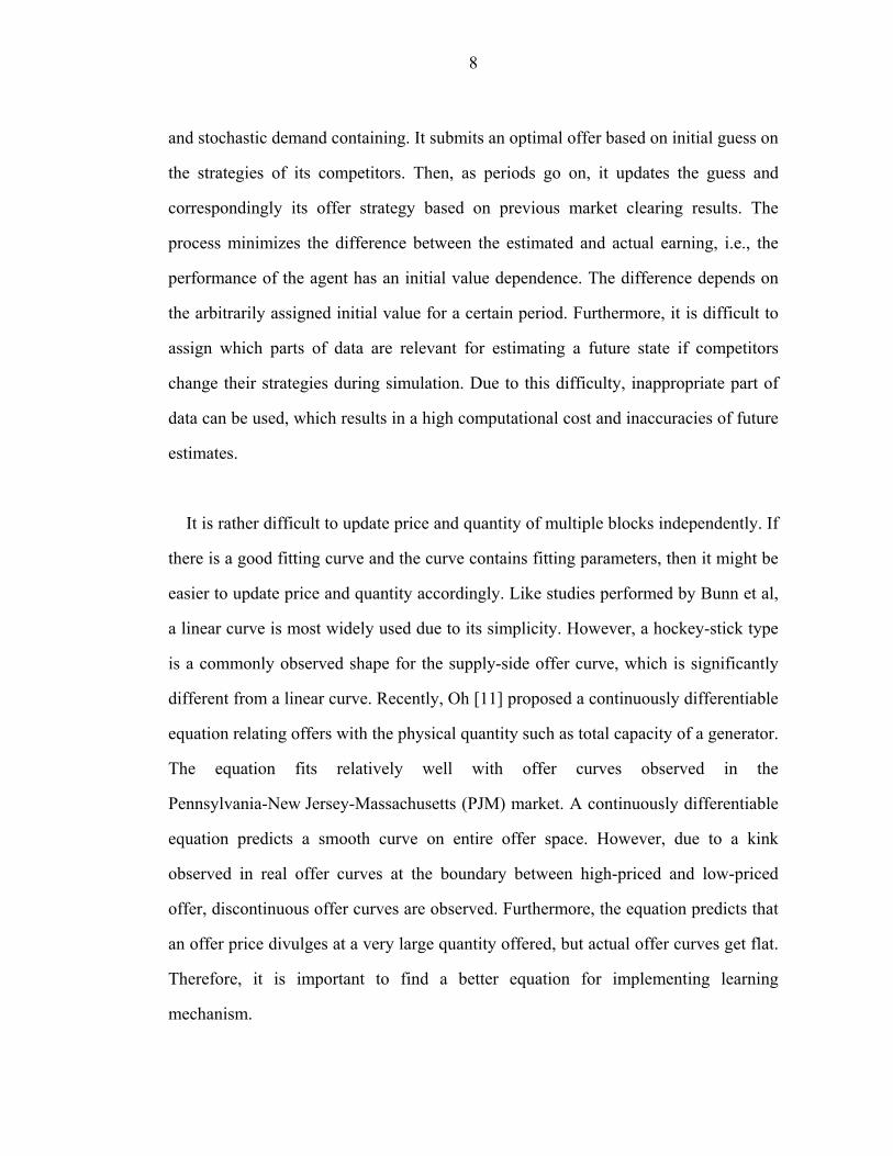
Figure 2. 1. Two commonly observed offer curves. Connecting lines are for visual
guidance. These specific offer curves were found in the PJM market where D8 and Y6
are the company code known only to PJM…………………………………………...10
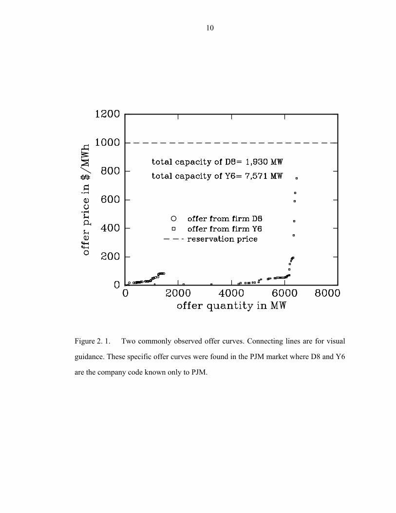
Figure 2. 2. Schematic diagram modeling marginal cost offer as well as speculating
offer. D denotes the flattening factor of the block representing how easily the price get
flat as market condition changes, and q and p refer offer quantity and price,
respectively…………………………………………………………………………...12
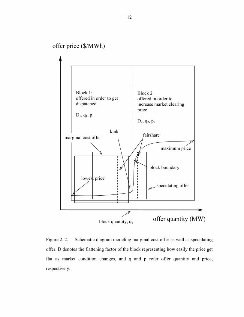
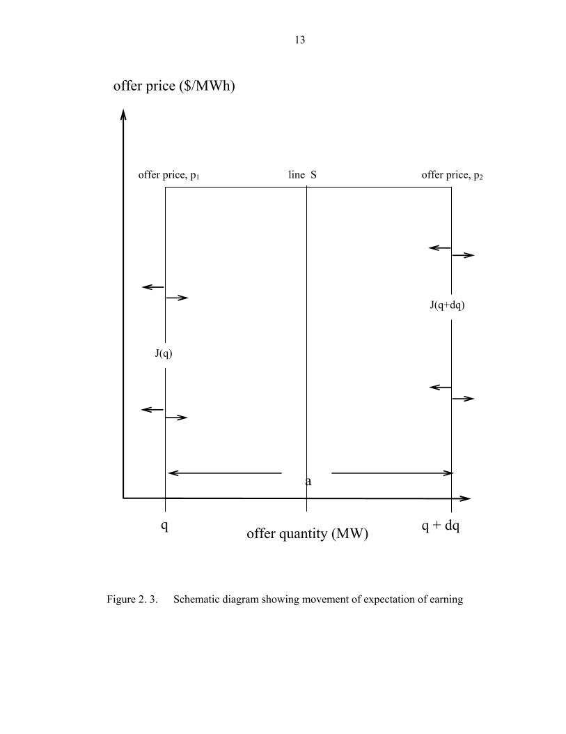
Figure 2. 3. Schematic diagram showing movement of expectation of earning ….13
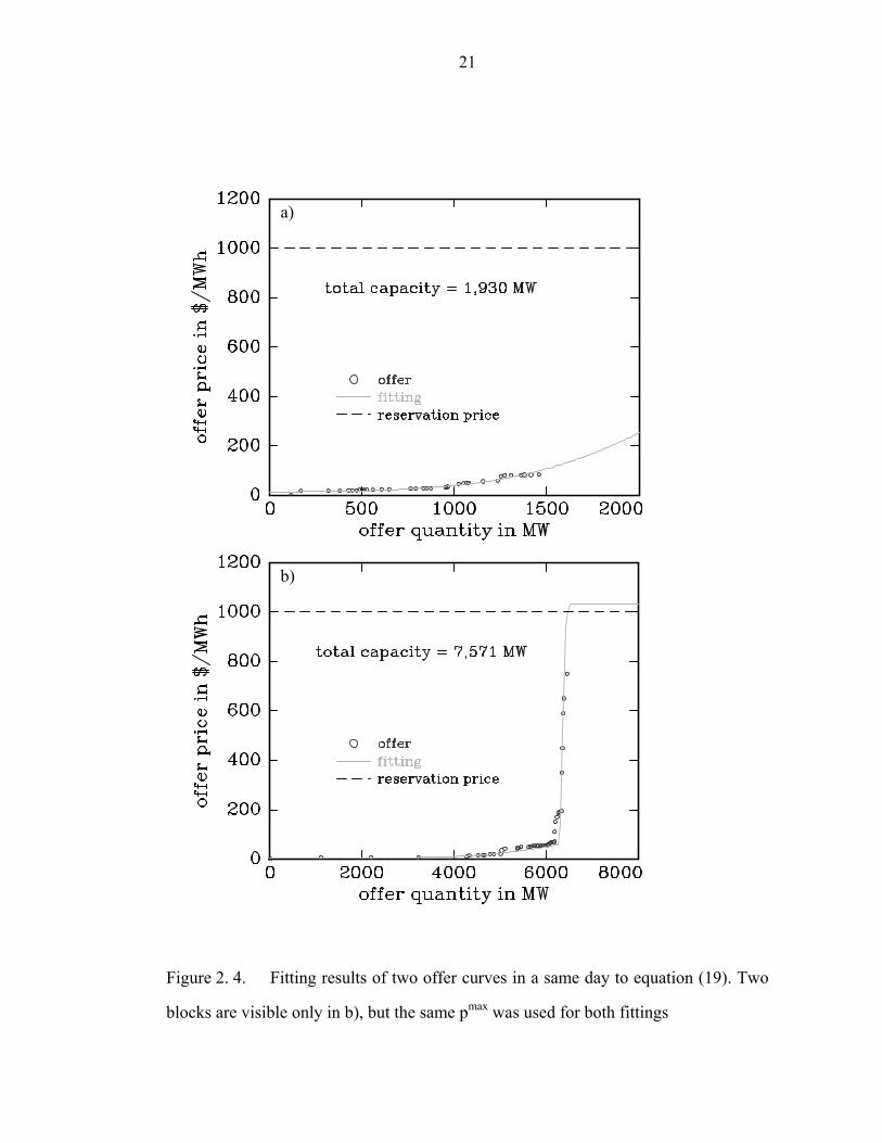
Figure 2. 4. Fitting results of two offer curves in a same day to equation (19). Two
blocks are visible only in b), but the same pmax was used for both fittings…………...21
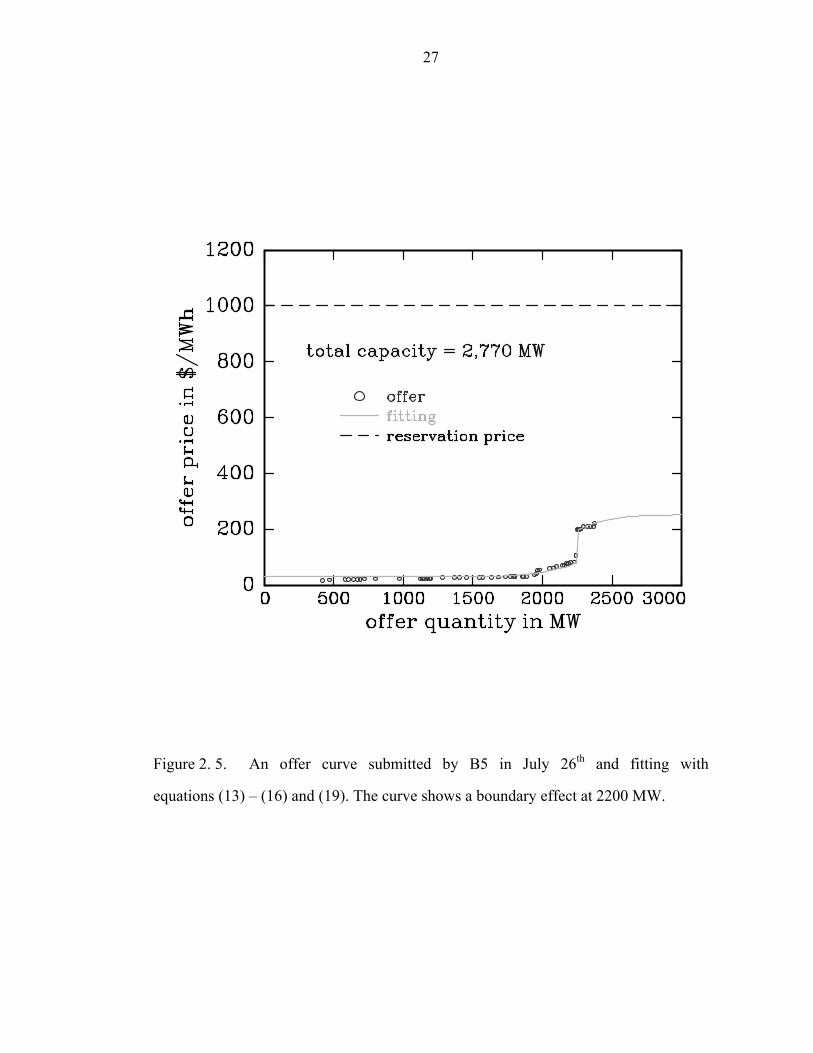
Figure 2. 5. An offer curve submitted by B5 in July 26th and fitting with
equations (13) – (16) and (19). The curve shows a boundary effect at 2200 MW…...27
Figure 2. 6. An optimal bidding curve for a) price-based demands and b)
must-be-served demand………………………………………………………………43
Figure 2. 7. Change in bidding after one period subject to the occurrence of an
energy PRL……………………………………………………………………………45

xi
Figure 4. 1. Nodal prices of various generators – data obtained from NYISO web
site on http://mis.nyiso.com/public/P-24Blist.htm during summer 2003 ....................58
Figure 4.2. Electricity market as a signal processing where input and output signal
are offer and dispatch result and demand forecast, respectively…………………….59
Figure 4.3. Schematic diagram showing how to calculate C(ε) for a flow. Some
neighboring points lying on dynamically uncorrelated parts of the data exist for point
A, but point B has only direct images and pre-images of B resulting in dimension of 1.
To avoid the incorrect calculation of C(ε) for estimating dimension, all neighbors over
time where |i – j| is less than nmin need to be ignored…………………………………64
Figure 4. 4. A schematic diagram showing evolution of two trajectories of a system
with a positive Liapunov exponent. At the beginning, both trajectories were close with
each other, but after some time their trajectories are far apart………………………..66
Figure 4. 5. A schematic diagram show how to calculate Liapunov exponent; a) at
t = 0, several points, 0ns ,
1ns and 2ns were selected and trajectories starting from the
points were tracked as the system evolves, b) many points inside ε-ellipsoid
(0su ,
1su and
2su ) were selected and similar to the procedure described in a) was
performed (picture taken from Ref [34])……………………………………………68
Figure 4. 6. Estimation of the Liapunov exponent of the NMR laser data in
embedded dimension of 2 (upper plot) and 3 ~ 5 (lower plot). The linear parts of the
curves are well described by an exponential with λ = 0.3. [37]………………………70

xii
Figure 5. 1. Earnings of the standardized agents and the agent of interest………76
Figure 5. 2. Example of a performance of the software agents: in the plot, red
square, green and blue circle stand for the earning in a period of MC, WS and SS,
respectively…………………………………………………………………………...80
Figure 5. 3. Example of a performance of the human agents: red square, green and
blue circle stand for the earning in a period of MC, WS and SS, respectively……….82
Figure 5. 4. Actual earning vs. Expected earnings calculated from simulation…84
Figure 5. 5. Correlation integral for the market clearing price data obtained from the
simulation with 500 periods…………………………………………………………..86
Figure 5. 6. Correlation dimension for various price data obtained from n-period
simulation……………………………………………………………………………..87
Figure 5. 7 The change in systems which agents, York-Warbesse and Cornell,
faced during June 2003. While system of Cornell did not change significantly, that of
York-Warbasse evolved………………………………………………………………89
Figure 5. 8. Modified IEEE 30 bus system with six suppliers. Capacities of lines
connecting Area 1–Area 2 and Area 3–Area 2 are lower than those of other lines…..90

xiii
Figure 5. 9. Two typical simulation results with inelastic demand without
demand-side participation (red line) and with elastic demand with demand-side
participation (blue line). Case a) shows the results in a more competitive market than
that for Case b)………………………………………………………………………93
Figure 5. 10 Simulated historical data for nodal prices at the Bus 23 (Firm 5) in the
case that 4 marginal cost offer agents in Area 1 and 3 exist while Firm 6 is a) a
marginal cost offer agent or b) speculator with different predetermined the degree of
speculation……………………………………………………………………………99
Figure 5. 11 Simulated historical data for nodal prices at the Bus 23 (Firm 5) in the
same cases in Fig. 8. 1., but nearest competitor (Firm 6) changes its strategy
completely a) from MC to speculator and b) speculator to MC…………………….100
Figure 5. 12. Simulated historical data for nodal prices at the Bus 1 (Firm 1) when
there is injection at Bus 28 and withdrawal at Bus 16 from the period of 253……...101
Figure 5. 13. Simulated historical data for nodal prices at the Bus 23 (Firm 5) which
has no locational benefit; a competitor in Area 2 (Firm 6) changes its strategy in a
more speculative way completely at the period of 253……………………………...103
Figure 5. 14. Daily dimension checks for the historical nodal price data obtained
from the simulation described in Figure 5. 10 a) and b), respectively………………105

xiv
Figure 5. 15 The results of Liapunov exponent calculation performed with the
historical nodal price data obtained from the simulations described in Fig. 5. 10 a) and
b), respectively………………………………………………………………………107
Figure 5. 16 Simulated historical data for the actual and expected earning of Firm 5
from the cases described in Fig. 5. 10 in blue and red line, respectively……………108
Figure 5. 17. Daily dimension check for the historical nodal price data obtained from
the simulation described in Figure 5. 11.……………………………………………110
Figure 5. 18 The results of Liapunov exponent calculation performed with the
historical nodal price data obtained from the simulations described in Fig. 5. 11 a) and
b), respectively………………………………………………………………………111
Figure 5. 19 Simulated historical data for the actual and expected earning of Firm 5
from the cases described in Fig. 5. 11 in blue and red lines, respectively…………..114
Figure 5. 20 The degree of speculation and the maximum offer price changes over
periods obtained from the simulation described in Fig. 5. 11 a) and b), respectively;
black lines indicate the mean values of the variables within the period shown in the
horizontal axis……………………………………………………………………….116
Figure 5. 21. The ratio of the maximum offer price to the degree of speculation over
the periods shown in the horizontal axis; the corresponding values of both variables
were shown in Fig. 5. 20…………………………………………………………….117

xv
Figure 5. 22. Daily check for a) dimension and b) Liapunov exponent calculated with
the simulated historical nodal price data obtained from the simulations described in
Fig. 5. 12…………………………………………………………………………….119
Figure 5. 23. The main variables and the ratio between the variables over periods
obtained from the simulation described in Fig. 5. 12; the black lines in a) represents
the mean values of the variables during the period………………………………….121
Figure 5. 24 Simulated historical data for the actual and expected earning of Firm 5
from the cases described in Fig. 5. 12 in blue and red lines, respectively…………..122
Figure 5. 25. Daily check for a) dimension and b) Liapunov exponent calculated with
the simulated historical nodal price data plotted in Fig. 5. 13…………………….124
Figure 5. 26. The main variables and the ratio between the variables over periods
obtained from the simulation described in Fig. 5. 13; the black lines in a) represents
the mean values of the variables during the period………………………………….126
Figure 5. 27 Simulated historical data for the actual and expected earning of Firm 1
from the cases described in Fig. 5. 13 in blue and red lines, respectively…………..128
Figure A-1. A schematic diagram for explaining how to determine a weight factor
distribution, x, a) by using traditional LU-factorization and b) by using
LU-factorization where b’ = L-1(PTb). The thick arrows show where zeros could be
assigned in the vector x, and eliminating R rows from U and the assigned elements
from x yields U’ and x’, respectively………………………………………………..145

xvi
Figure A-2. Solution of the Lorenz equation (in color) and xy, yz and zx
two-dimensional projections which show artifact crosses…………………………..158
Figure A-3 Start with the closed interval S0, [0, 1], and remove the open middle
third resulting in closed interval S1. The same procedure is kept performed to produce
S2, S3 and so on. The limiting set S∞ is the Cantor Set…………………...………….159
Figure A-4 Start with a line segment S0, [0, 1], and delete the middle third and
replace with the other two sides of an equilateral triangle, S1. Then repeat the same
step to generate S2, S3 and so on. The limiting set S∞ is the von Koch curve….……161
Figure A-5 a) The coast of the southern part of Norway. The square grid indicated
has a spacing of δ ~ 50 km (taken from the Figure 2. 1 of [J. Feder, “Fractals”, Plenum
Press, New York and London (1998)]) and b) The measured length of the as a function
of the size δ of the δ×δ squares used to cover the coastline on the map. The straight
line in this log-log plot corresponds to the relation L(δ) = aδ1-D ; L, δ and D
correspond to N, ε and d in equation (A.67)……………...........................................163
Figure A-6 Log-log plot to estimate the correlation dimension of a fractal.
Typically, the plot shows two bends both at lower values of ε and at higher values of
ε……………………………………………………………………………………...166

1
CHAPTER ONE INTRODUCTION
The traditional vertically integrated electricity power system has been defined as a
natural monopoly. Under several constraints such as spinning reserve, thermal unit
constraints and hydro constraints etc., operation and planning of the system was
performed toward declining long-term costs, high threshold investment, and
technological conditions that limit the number of potential entrants. In the vertically
integrated environment, therefore, a utility would determine generation setpoints based
on real costs of operation. Unified control of generation, transmission, and distribution
was considered to be the most efficient way of providing service, and as a result, most
people were served by a vertically integrated utility. However, as the electric utility
industry has evolved, there has been a growing belief that the historic classification of
electric utilities as natural monopolies has been overtaken. It has been believed that
market forces might replace some of the traditional economic regulatory structure. For
example, vertical integration has not been necessary for providing efficient electric
service if utilities that do not own all of their generating facilities exist. Moreover,
recent changes in electric utility regulation and improved technologies have allowed
additional generating capacity to be provided by independent firms rather than utilities.
Over several decades, there has been a major change in direction concerning
generation. Improved technologies have reduced the cost of generating electricity as
well as the size of generating facilities. Prior preference for large-scale generators has
been supplanted by a preference for small-scale ones that can be brought online more
quickly and cheaply with fewer regulatory impediments. Consequently, the entry

2
barrier to electricity generation has been lowered to permit non-utility entities to build
profitable facilities. Recent changes in electric utility regulation and improved
technologies have allowed additional generating capacity to be provided by
independent firms rather than utilities. Therefore, it was hoped that the transition to the
restructured markets would make the efficiency of the system increase. With the hope
for a more efficient system, the electric power industry has been restructuring in many
countries.
In all restructured markets, auctions play a major role in determining both the price
of electricity and the quantity of electricity dispatched by individual generating units.
In the new regime, generation setpoints are determined by market forces rather than by
engineering design. Consequently, it is necessary to create new tools for planning and
operating that take account the nature of the market environment. In a traditional
system setting, a generator’s setpoint is determined by current demand and its
marginal cost1 to produce the next megawatt under several constraints listed above. In
the case, all participating agents selected by a unit commitment process are guaranteed
to get dispatched. However, it is unlikely that true operating costs will be revealed
because of the hedging needed to accommodate uncertainty and opportunities offered
by the interconnecting network for exercising market power. A generators’ setpoint
can be found from the result of an optimization process minimizing total system cost.
In the new market setting, each agent representing a generating firm submits price and
quantity offer at which it is willing to sell its electric power. For an independent
system operator (ISO) who does not have access to the true cost of each generator in
the setting, the offer replaces each unit’s true marginal cost in the process of
1 marginal cost is the cost of the additional inputs needed to produce that output, i.e., the cost of producing one more MW

3
determining a setpoint. Because participating generators can change their offers in
each period, the tools used for operation and planning in the traditional markets are no
longer useful for the new markets. Therefore, it is important to understand the offer
behavior of human agents if we are to be successful in designing new tools.
The objective of each generator in the market is to maximize its own profit. An
agent can find its optimal offer if actual demand is given and if the competitors’ offer
strategies are known. When there is a change in the offer strategies of competitors, the
optimal offer of the agent will change. Therefore, it is possible to find an optimal offer
with proper information, and to figure out when to change the behavior of the agent if
needed. However, the information listed above is strictly confidential to an agent.
The main goal of this study is to develop a theory and examples for new
agent-based components as an approach to creating new tools for power system
planning and operation. Specifically, we seek to develop a planning tool that relies on
software agents as a replacement for the human agents that exist in the real world to
submit offer energy price and quantity into a market. Well-designed software agents
can be used to emulate the offer behavior of human agents provided that it can be
shown that, in some sense, their behavior is roughly identical. At a given market
environment, there are several types of offer/bid strategies of a human agent. A
software agent needs to show a similar behavior at the identical environment. When
the environment changes such as the change in the offer/bid strategies of the
competitors, a software agent should react to optimize the profit.
In this dissertation, there are six chapters including the introduction. Chapter 2
describes modeling for offer/bid behaviors. Chapter 3 deals with constructing a

4
mapping function from offer to earning. In the chapter, a theoretical model for an
electricity power market in a steady state is developed. Chapter 4 describes tools i) to
detect if there is any change in the market due to various reasons such as strategies of
the competitors and/or network, and ii) to find whether the change results in another
steady state or a chaotic state. Chapter 5 shows several results from different
simulations performed with the agents developed in this study. Conclusions and future
works are presented in Chapter 6. Several related topics are described in Appendix 1
to 5. Appendix 1 deals with constructing a generation sensitivity matrix by using
network parameters. In Appendix 2, a method for an error minimization is described.
Trust region method for a numerical function is presented in Appendix 3. In Appendix
4, a method to evaluate dimension and Liapunov exponent presented. Appendix 5
describes a nonlinear time series analysis performed for stock markets.

5
CHAPTER TWO MODELING FOR AN OFFER AND A BID
2.1. Literature Review
A human agent will update his/her offer behavior based on experience and available
information. If competitors do not change their strategies, the auction is similar to a
repeated game in game theory. For such a game, the competitors’ strategies can be
revealed from the result and his/her strategy used during previous play. In the case, a
player can update the strategy based on the result of previous play. If competitors do
not change their strategies, and all other conditions such as demand do not change,
then an agent can find an optimal strategy for the circumstance. However, since the
strategies of competitors and other conditions are subject to change in a real market, it
is important to have an agent find out hidden information quickly from publicly
available data such as the history of the market clearing result. It is easier in studying
dynamics to simulate markets with known types of competitors. However, an agent
only explores relatively restricted area defined by the types in the market in such a
case.
Usually human agents update offer strategies to determine price and quantity
according to some process they believe to be profit maximizing. To mimic the ability,
several different learning algorithms have been studied. Reinforcement algorithms [1-
3] and genetic algorithms [4-6] are most widely studied. Hill climbing is one of the
most commonly used reinforcement algorithms. In it, one moves along the direction to
which the value of an objective function increases in the previous step. They are

6
relatively easy to implement since they require small computational cost in terms of
computation time and data storage. In any reinforcement algorithm, trial-error
experience will contribute differently to any future strategy based on the previous
results. A genetic algorithm has a similar property, but it is a little more complicated
due to the choice of fitness function and selection mechanism [7]. It is difficult to
assess which parameters are most sensitive to the performance index. In other words,
mapping prices and quantities of multiple blocks to earning is difficult. For example,
consider a non-discriminatory auction which is the most commonly used pricing rule
in electricity power markets. In such markets, only marginal blocks set the price.
Consequently, the offer prices of other blocks are not relevant to profits.
By its nature, demand is stochastic and any demand forecast will be in error.
Typically, load is forecasted by using weather data on an hourly basis as an input such
as temperature, humidity, cloud cover and wind. The uncertain and stochastic nature
of the demand brings another difficulty in an agent design for electricity markets. In
the method discussed above, the nature of the demand is not considered.
Sheble et al [4-6] designed an agent using a genetic algorithm that operates in a
significantly simplified market and with zero demand forecast error. In the market,
each agent, including suppliers and consumers, can submit price and quantity for only
one block of energy. Independent system operator (ISO) clears the market, then, and
the agents are paid according to the rules of a discriminatory auction2. In such a setup,
one can construct a relationship between the offer price to and the price to be paid.
2 All the units dispatched are paid according to their offer price; therefore, they might be paid differently. Unlike discriminatory auction, in a uniform auction, they are paid at a same price

7
From the procedure, it is possible to connect the offer to the profit, which allows the
agent to update the offer in a future period. However, the assumptions of one block
offers, no forecast error and discriminative auction are not valid in any real markets in
operation today.
An “autonomous” agent designed by Bunn et al [8-10] has been applied in a market
which is a little closer to a real one. Like in the work of Sheble et al, a lossless
network, no line constraints, no error in demand forecast and discriminatory auction
were used, but the agent can offer several blocks. Two points on an offer space
comprised of offer price and quantity define a linear offer curve. It is possible to
evaluate prices and quantities of multiple blocks if quantity of each block is identical.
By using a simple reinforcement algorithm, the agent updates the end points based on
the result of market clearing. The market is assumed to be a Markov chain, i.e., current
state contains all the relevant information so that the future state can be estimated by
using the current state and relevant forecast. Consequently, the reinforcement
algorithm is used to create the parameters that determine offer price and quantity of
the blocks. Once all the offers are submitted, ISO clears the market. The simple nature
of reinforcement algorithm allows the agent to work in a non-discriminatory auction.
However, an agent characterized by a linear offer curve may not emulate the real
market successfully since widely observed shape of an offer is a hockey-stick. Another
problem in the study is that the period of Markov chain is arbitrarily assigned to one
day with no reason.
There is another agent developed by Oh [11] which works well in a relatively more
realistic market. Like other agents discussed above, a lossless network with no line
constraints is used, but it can operate in a market with non-negligible forecast error
8
and stochastic demand containing. It submits an optimal offer based on initial guess on
the strategies of its competitors. Then, as periods go on, it updates the guess and
correspondingly its offer strategy based on previous market clearing results. The
process minimizes the difference between the estimated and actual earning, i.e., the
performance of the agent has an initial value dependence. The difference depends on
the arbitrarily assigned initial value for a certain period. Furthermore, it is difficult to
assign which parts of data are relevant for estimating a future state if competitors
change their strategies during simulation. Due to this difficulty, inappropriate part of
data can be used, which results in a high computational cost and inaccuracies of future
estimates.
It is rather difficult to update price and quantity of multiple blocks independently. If
there is a good fitting curve and the curve contains fitting parameters, then it might be
easier to update price and quantity accordingly. Like studies performed by Bunn et al,
a linear curve is most widely used due to its simplicity. However, a hockey-stick type
is a commonly observed shape for the supply-side offer curve, which is significantly
different from a linear curve. Recently, Oh [11] proposed a continuously differentiable
equation relating offers with the physical quantity such as total capacity of a generator.
The equation fits relatively well with offer curves observed in the
Pennsylvania-New Jersey-Massachusetts (PJM) market. A continuously differentiable
equation predicts a smooth curve on entire offer space. However, due to a kink
observed in real offer curves at the boundary between high-priced and low-priced
offer, discontinuous offer curves are observed. Furthermore, the equation predicts that
an offer price divulges at a very large quantity offered, but actual offer curves get flat.
Therefore, it is important to find a better equation for implementing learning
mechanism.

9
Most current markets have supply-side participation only, and a hockey-stick type
offer is generally observed in those markets. In such a situation, price spikes have
been observed frequently. Generally speaking, 10%3 reduced demand might prevent
the appearance of most price spikes. Unless the 10% reduction cause bigger drop in
profit, a demand-side agent has motivation to reduce its demand since the reduction
may increase its profit by purchasing electricity at a lower price.
2.2. Model for Supply-side Offer Behaviors
Figure 2.1 shows different offer behaviors, i.e., one with low-priced offer only (D8)
and the other with high-priced offer as well (Y6). It is difficult to classify the type of
agents since the load forecast data is not provided. If the fairshare4 [12] of D8 were
less than 1,500 MW and that of Y6 were larger than 6,100 MW, D8 and Y6 would be
classified as a marginal cost offer agent and a speculator, respectively.
As is shown in Figure 2. 1, there exist at least two different types of agents in a real
market. There are two different blocks in the offer curve of Y6: one block with low
priced offers with a flat curve and the other with high priced offers with a steep curve
in offer price. In the offer curve of D8, only the first block showed up. To model these
different types of agents consistently, one should consider the objects of two blocks.
The first block is submitted at a low price in order to be dispatched while the second is
done to attempt to raise the dispatched price. Due to these objectives, the very
beginning of the first block (Block 1) is set to the minimum offer price, and the end of 3 private talk from Prof. T. Mount 4 the faireshare of an agent is the market share of the agent if all the participating agents offer all the quantities at the same price
10
Figure 2. 1. Two commonly observed offer curves. Connecting lines are for visual
guidance. These specific offer curves were found in the PJM market where D8 and Y6
are the company code known only to PJM.

11
the second (Block 2) is done to the maximum price of which an agent might think.
In comparing the two blocks, the second block is more sensitive to a change in
market condition defined by the competitiveness of the market. Suppose there is no
limitation such as maximum generator capacity and reservation price, i.e., all agents
are allowed to submit any offer. In the situation, there would appear two blocks in an
offer curve. However, an agent cannot submit an offer price higher than a reservation
price, and quantity larger than its maximum capacity. With the limitation, an agent
decides where to locate a window on an offer curve to maximize its profit.
Furthermore, it can also partially close the window by withholding its capacity.
Figure 2. 2 shows the procedure locating and partially closing window based on an
optimization process of each agent.
As the market condition changes, it is reasonable to assume that a change in an offer
price depends on the first derivative of offer price with respect to the offer quantity.
Note that there is no reason two blocks should be paid differently. Therefore, there
exists tendency to flatten expected earning5, i.e., an agent expects the same earning
from both blocks. By adding one small block with an infinitesimally small size dq,
expected earnings increase by pdq where the block is offered at a price of p. The
expected earning at q might be calculated from the prices of q – dq and q + dq. By the
same argument, driving forces6 acting on expected earning at q + ½ dq exist.
Figure 2. 3 illustrates the change in an expected earning across a line S. The offer
prices at the two ends of the block are p1 and p2. Note that p2 is greater than p1.
5 earning from the block of interest if the block is dispatched 6 the tendency to make two different expected earning at nearby blocks equal
12
Figure 2. 2. Schematic diagram modeling marginal cost offer as well as speculating
offer. D denotes the flattening factor of the block representing how easily the price get
flat as market condition changes, and q and p refer offer quantity and price,
respectively.
Block 1: offered in order to get dispatched D1, q1, p1
Block 2: offered in order to increase market clearing price D2, q2, p2
maximum price
offer quantity (MW)
block boundary
block quantity, qb
lowest price
kink
offer price ($/MWh)
marginal cost offer
speculating offer
fairshare
13
Figure 2. 3. Schematic diagram showing movement of expectation of earning
offer price, p1 offer price, p2 line S
offer price ($/MWh)
offer quantity (MW)
a
J(q+dq)
J(q)
q q + dq

14
Driving forces at q and q + dq affect the expected earnings at both left and right
neighbor. However, the effect from the right side is more than that from the left side
since the expected earning is higher at the right one. Consequently, there is a net
change to the left, i.e., down the offer price gradient.
For a more competitive market, price tends not to increase abruptly since the
probability not to get dispatched increases significantly for a high-priced offer.
Therefore, the affection rate to the left is given quantitatively by
[ ] νν 12 21
21/$ nnhmcJ −= (1)
where ν is a constant evaluating the effect from a unit of driving force in [mc-1] and
mc is the unit of evaluating the market condition.
The two terms on the right hand side give the affection rate starting from p1 end and
p2 end to the middle block, respectively. Note that ½ came from the fact that the
flattening effect from one ends to line S takes only half of the change from one end to
the other end. The quantity n1 and n2 in [$/h] refer to the expected earning from the
blocks offered at p1 and p2, respectively. Therefore,
( )1212 21
21
21 ppannJ −=−= ννν (2)
If the offer price does not vary rapidly inside the dq block, the term in the
parenthesis can be approximated by Taylor’s approximation:
qpapp
∂∂
−≈− 12 (3)

15
When equations (2) and (3) are combined, one can find following equation:
( )qpD
qpappannJ
∂∂
−=∂∂
−=−=−= 21212 2
121
21
21 νννν (4)
where D [ ]mcMW /in 2 is the flattening factor of the block representing how easily the
price gets flat as market condition changes.
For the dual blocks, the offer price obeys the following equations:
qpDJ
qpDJ
p
p
∂∂
−=
∂∂
−=
22
11
2
1
(5)
where J represents an affection rate, and subscript 1 and 2 stand for the 1st and the 2nd
block as shown in Figure 2. 2.
Consider that there is a block with quantity coordinates q and q + dq as shown in
Figure 2. 3. Let there be a change in the market condition with magnitude of dy, and
let the affection rates from right to left be J(q + dq) and J(q) at q + dq and q,
respectively. The total change in expected earning on plane S over the change in the
market condition dy is:
( ) ( )[ ] dqdyqJdyqJdqqJ
∂∂
−=++− (6)
Note that J(q) is the flow leaving the plane at q, i.e., the gain in the S plane from p
plane is –J(p).

16
The effect in the expected earning by offering S block under a change in market
condition dy is then obtained by applying the formula for a differential:
( ) ( )[ ] dqdyypdqypdyyp ⎥
⎦
⎤⎢⎣
⎡∂∂
=−+ (7)
This quantity must equal the change of the integrated offer in the block such that
setting the two expressions equal gives
yp
qJ
∂∂
−=∂∂ (8)
Since the flattening factor, D, depends only on the property of the block, the value of
D does not change with market condition and block size. Combining equations (4) and
(8) gives:
2
2
qpD
qpD
qqJ
yp
∂∂
=⎥⎦
⎤⎢⎣
⎡⎟⎟⎠
⎞⎜⎜⎝
⎛∂∂
−∂∂
−=⎟⎟⎠
⎞⎜⎜⎝
⎛∂∂
−=∂∂ (9)
Equation (9) applies to the dual blocks:
22
2
22
21
2
11
qp
Dy
pqp
Dyp
∂∂
=∂
∂
∂∂
=∂∂
(10)

17
The first block is offered in order to get dispatched. The price can be determined by
various parameters related to generators such as operating cost. The second block is
offered in the attempt to increase the market clearing price. Since there is no limit in
the quantity offered, the maximum price of the block approaches the maximum
possible price. Therefore, the offers for the second block are related to the market
situation more closely rather than parameters of a generator. The situation is similar to
the following case in diffusion. Consider a cylindrical solid with an inner and outer
layer exposed to a specific atmospheric condition for a long time. At some time, the
outside atmosphere is abruptly changed to a different one, and maintained during some
time. The state inside the cylinder is fixed in equilibrium with the initial atmosphere
while the state outside is adjusted to the new one. The state from inside to outside
smoothly changes from one equilibrium state to the other. By analogy, the situation for
an agent is the following: a generator which has two blocks played a role in the
traditional market, and then moves into a new market. Consequently, the price of the
lowest offer by the generator should be same as a true marginal cost in the traditional
market, and that of the highest offer should be the maximum possible offer. Therefore,
the boundary conditions for equation (10) can be described by:
( ) [ ]( ) [ ]MWhpyqqp
MWhpyqqp/$,/$,
maxmax
minmin
====
(11)
where y evaluates market condition.
At the boundary between low-price and high-priced offers, offer price and
affection rate must be continuous since adding an indefinitely small sized quantity
does not change both abruptly. The situation defines a condition at the boundary;

18
( ) ( )
+− ==
+−
∂∂
=∂∂
===
bb qqqq
bb
qpD
qpD
yqqpyqqp
22
11
,, (12)
With the given conditions, solving equation (10) gives an expression for offer price as
a function of market condition, y, and quantity, q, for two blocks. Note that for the 1st
block, q is less than qb where qb is the boundary quantity between two blocks) [13]
( )⎥⎥⎦
⎤
⎢⎢⎣
⎡−
⎟⎟⎠
⎞⎜⎜⎝
⎛ −
+
−= bb p
yDqq
erfcDD
ppqyp 1
121
minmax1
2/1, (13)
where
( ) ( )[ ]
⎟⎟⎠
⎞⎜⎜⎝
⎛+=
⎟⎟⎠
⎞⎜⎜⎝
⎛+
−+−=
2
1
11
111
12
111
1
and
2exp,
DD
Dkh
yDhyDqqerfcyDhqqhqyp b
bb
(14)
and for the 2nd block where q is greater than qb
( )⎪⎭
⎪⎬⎫
⎪⎩
⎪⎨⎧
⎥⎥⎦
⎤
⎢⎢⎣
⎡+⎟
⎟⎠
⎞⎜⎜⎝
⎛ −+
+−
= bb pyD
qqerfDD
DDppqyp 2
21
2
21
minmax2 2
1/1
, ( 15 )
where

19
( ) ( )[ ]
⎟⎟⎠
⎞⎜⎜⎝
⎛+=
⎟⎟⎠
⎞⎜⎜⎝
⎛+
−+−=
1
2
22
222
22222
1
and
2exp,
DD
Dkh
yDhyD
qqerfcyDhqqhqyp b
bb
(16)
where the superscript b represents boundary effect, which comes from the different
characteristics of two different blocks, and k stands for the boundary constant
quantifying the boundary effect7.
If a generator (or a firm) has only one decision maker submitting its offer, there
should be no boundary effect, i.e., ∞→k . In such a case, both bp1 and bp2 approach
zero, and the expressions for offer prices are
( )⎥⎥⎦
⎤
⎢⎢⎣
⎡
⎟⎟⎠
⎞⎜⎜⎝
⎛ −−
+
−=
yDqq
erfDD
ppqyp b
121
minmax1
21
/1, (17)
( )⎥⎥⎦
⎤
⎢⎢⎣
⎡⎟⎟⎠
⎞⎜⎜⎝
⎛ −+
+−
=yD
qqerfDD
DDppqyp b
21
2
21
minmax2 2
1/1
, (18)
Offer curves could be fitted to the following equation:
( ) ( ) ( ) ( ) ( )qypqquqypqquqyp bb ,,, 21 −+−= (19)
where u is the unit step function;
7 if two blocks have different properties, boundary effects might be present, i.e., the offer curve might not be continuous

20
( )⎩⎨⎧ <
=otherwise 1
0 x if 0xu (20)
The data shown in Figure 2. 1 was used to fit equation (19), and the results are
shown in Fig. 2. 4. The cutoff quantity, qc, can be defined as an agent’s maximum
offer quantity. The cutoff quantities for D8 and Y6 were about 1,500 and 6,200 MW,
respectively. The qc of D8 was larger than the quantity at the boundary, qb, while that
of Y6 was smaller than qc. In order to characterize the behavior of an agent, it is useful
to define the deviation quantity, { }bcd qqq ,min≡ . Then, the distance from the
fareshare to the deviation quantity is a measure of the degree of speculation (DOS).
DOS is an important factor to classify offer behavior. For example, even if an offer
curve of an agent contains a high-priced offer as well as a low-priced one, the agent
might make the market more competitive if the block containing fairshare is offered at
a lower price. DOS is defined as the relative location of boundary from the fareshare:
⎪⎪⎩
⎪⎪⎨
⎧
<−×
×
≥−
−×
=fairshare q if
fairshareq fairshare2
50
fairshare q if fairshare capacity
q capacity 50
DOSb
b
bb
(21)
To define DOS, it is crucial to calculate fairshare based on demand forecast. For a
lossless system with no network, this is easy since fairshare can be the simply capacity
ratio of an agent. For a real system, the simple ratio of capacity does not work since
real systems always have loss, line constraints and distributed load. However, an agent
could calculate fairshare by running an AC optimal power flow (OPF) with identical
offer curves for all the participating generators once network is known to the agent.
21
Figure 2. 4. Fitting results of two offer curves in a same day to equation (19). Two
blocks are visible only in b), but the same pmax was used for both fittings
a)
b)

22
The dispatched quantity from OPF gives approximate for the fairshare at given load
forecast
With this model, it is possible to submit a price according to a quantity. There are
several factors that make use of the model quantitatively in designing an agent such as
the flattening factor (D) and market condition (y).
2.2.1. Flattening factor
Flattening factor (D) dictates the slope of the offer curve. D in an offer curve
describes how fast a quantity offered at a same price changes as a market condition
changes. Therefore, an agent with a higher D quickly responds to change in the market
condition since it is easy for such an agent to change price for all the quantity in an
offer space.
There are several factors determining the magnitude of the tendency. The flattening
is an activated process, which means that there are two competing forces to govern the
tendency: a flattening force and an ordering force. More flat curves will be obtained as
a flattening force increases and/or an ordering force decreases.
Similar to solid state physics, for an activated process as was mentioned before,
there exists an Arrehnius type equation to describe the process;
( ) ⎟⎠⎞
⎜⎝⎛−=
kTEDTD exp0 (22)

23
where D0, E and kT are the flattening factor with infinitely high disordering force,
ordering and disordering forces, respectively. D0 may depend on the generator itself
due to its operating cost since an operating cost itself has a slope.
In this modeling, ordering force is a quantification of regulations, and disordering
force is that of the tendency toward risk8. Regulations in existing markets apply to all
the market participants equally, and make participants difficult to speculate, which
results in a flat curve in offer space. For a given agent, the introduction can be
implemented by adding Enew:
( )
⎟⎟⎠
⎞⎜⎜⎝
⎛−=
⎟⎟⎠
⎞⎜⎜⎝
⎛−⎥
⎦
⎤⎢⎣
⎡⎟⎠⎞
⎜⎝⎛−=⎥
⎦
⎤⎢⎣
⎡ +−=
kTED
kTE
kTED
kTEEDD
newold
newnewnew
exp
expexpexp 00
(23)
Therefore, in real markets, regulation is additive by nature.
The tendency toward risk differs for each individual supplier statistically. The
tendency might be changed in case of a change in ownership and/or in mind of a
decision maker. A change in tendency toward risk alters offer curves completely, i.e.,
a new flattening factor must be re-evaluated. There are three categories in tendency to
consider: risk-averse, risk-neutral and risk-seeking. To model these different
tendencies, utility functions are introduced by Bernoulli [14]. Grayson found a good
fit between Bernoulli’s logarithmic function and the actual utility function [15]. An
agent having a utility function with concave shape like logarithmic function is referred
8 Each agent has different tendency toward risk; risk-averse, risk-neutral and risk-seeking. The tendency can be evaluated based on its utility function which maps benefit that the earning brought from earning

24
as risk-averse since its evaluation on uncertain earning is less than that on the same
amount of actual earning. Other tendencies such as risk-neutral and risk-seeking have
linear and convex curve for utility functions. The value of T in equation (22) increases
as tendency changes from risk-averse to risk-seeking since a risk-seeking agent is
willing to increase an offer price of a lower block, which results in a flat offer curve.
2.2.2. Quantity evaluating the market condition
Flattening phenomena considered here is a process connecting two different
equilibrium states. For a given market condition y0, system stays in one state, and the
state changes toward a new equilibrium state as the condition changes to different
condition, y1. Suppose there is a sufficiently small change in a market condition. With
the small change, the resulting price-quantity profile depends on a flattening factor of
a block considered (D) and a market condition y. The profile built contains all the
equilibria between two states. For example, if the price at one equilibrium state is 0
and that at the other is 100, then the profile at the change in a market condition y
contains all the values of price from 0 to 100.
Market condition y is a term quantifying degree allowed for a price of a block to
change from one state to another. As mentioned before, a block that was in one
equilibrium state becomes another in a different state. For example, offer in a
traditional market was a true marginal cost, but that in a totally deregulated market
with no regulation should be different from marginal cost such as a speculative one.
Market condition may allow an agent to exploit the market. For example, once an

25
agent finds its competitors are speculators, then it will submit a more flat offer in order
to take advantage of the less competitive market environment.
Publicly available information such as historical data of nodal price is chosen to
determine the value of a market condition since price is considered most unbiased and
relevant information. However, the price might be different according to the location
of an agent. But, the change in y should be in common among all agents since all
prices are correlated with each other9. If the agent of interest is the only agent which
speculates in the market, y should not be high since the environment that the agent
faces actually competitive in spite of high prices. To compensate this effect,
dispatched quantity is also added to estimate y in this study:
pp
y recent
sharefair share
= (24)
where share , recentp and p stand for the quantity dispatched, mean of recent nodal
prices and mean of nodal prices in the same state, respectively. In this study, recentp is
chosen as the mean price over most recent one week. It is noteworthy that an actual
value for recentp does not change significantly with the choice of the period.
If the system evolves, all state properties including market condition cannot be
invariant. Therefore, it is worthwhile to mention that both recentp and p must contain
data only in the same state.
9 Relationship among price can be driven during the derivation of the generation sensitivity matrix with respect to price; for a detailed derivation, see Appendix A

26
2.2.3. Boundary effect
Typical offer behaviors without boundary effect have been discussed. Note that k in
such case approaches infinity in equations (14) and (16). However, it is possible for an
offer to show such an effect. In the PJM market, Fig. 2. 5 shows a discontinuous offer
curve found on July 26th by B5 after a first price spike observed on June 7th. Before
the first price spike, the firm had submitted low-price offer only. The discontinuity can
be modeled as a boundary effect which is resulted in by no perfect communication
between two blocks. The fitting is performed by using equations (13), (15) and (19).
2.3. Model for Demand-side Bid Behaviors
As was described earlier, a boundary quantity is defined as non-differential points
of an offer curve, i.e., the point where offer curve departs from a lower price. When
fairshare is located higher than the boundary quantity, the agent is classified as a
speculator. Approximately 10% reduced demand results in shifting fairshare far down
to the boundary quantity at the given offer curve. Therefore, demand-side participation
is suggested for potential efficiency improvement of a market. For practical reasons, a
new method for demand-side participation might includes following features; 1) end
consumers do not need to evaluate electricity all the times like 24 times in a day, 2)
small discrepancy between dispatch and actual demand does not matter much for a
consumer, 3) some consumers are willing to sacrifice reliability to reduce an electric
bill to some degree, 4) some don’t mind paying a high price for a reliability such as
hospital or synchrotron, etc. such demands are termed must-be-served demands while
others are defined as price-based demands.
27
Figure 2. 5. An offer curve submitted by B5 in July 26th and fitting with
equations (13) – (16) and (19). The curve shows a boundary effect at 2200 MW.

28
To develop a demand-side model, one must bear in mind that consumers sacrifice
reliability marginally (e.g., 10 %) to reduce an electric bill, but too frequent serious
price-response-load (PRL) must be avoided. As was mentioned in feature 1), the
method reducing demand should be easily performed or another agent should take
over the job for consumers. For a given market structure, a distributor (e.g., NYSEG)
may submit bids for consumers, and buy electric power from generators, and then
distribute electric power based on priorities to fulfill elementary demands. After each
period, the distributor checks the discrepancy between dispatch and actual demand. If
the discrepancy does not exceed predetermined value, it can assume all the demand
were successfully fulfilled. Otherwise, it declares a PRL. A predetermined value for
PRL needs to be defined in a contract made between the distributor and end
consumers. Every given period, it signs a new contract with consumers. For example,
every year it makes a contract that fulfilling 90% of demand is acceptable, but
fulfilling less than that is claimed as a PRL. Suppose no more than 10 times of PRL in
a month is allowed. For 10 times, an agent does not need to satisfy all the demands.
Consequently, the agent has freedom not to satisfy all demands proportional to the
remaining allowed number of PRL. The freedom is inversely proportional to the
number of remaining periods before current contract period ends since there is a
non-negligible possibility of a PRL for more remaining periods. For a simple
summary, an agent would have a contract with end consumers in the category of price-
based demand containing following terms; 1) it can have nPRL-times allowed PRL’s in
a given period like a month, 2) where the term PRL is defined the case that only less
than a predetermined percentage of forecast and/or actual demand is served, 3) after
nPRL-times of PRL in the given period, the bid should be same as an inelastic demand
curve, and finally 4) big penalty should be given if the agent does not serve electricity

29
properly more than nPRL-times while it can. An agent might offer several options for
different values of nPRL to accommodate various needs of end consumers.
If an end consumer does not want to sacrifice reliability, then it is also possible to
have another type of contract such that a distributor always serve such a customer
before serving any other demands if price is below a certain price, pc. Demands
associated with such contracts are called must-be-served demands. Since the demand
forecast is not always accurate and must-be-served demand prefers being served even
in the situation of underestimated forecast, the contract should include another price
for insurance. Note that the price for insurance is less than pc. For example, a contract
defines ξ and pm in a way that the consumer agreed to pay for electricity to fulfill
actual demand up to (1+ξ) times of forecasted demand if price is less than or equal to
pm.
Before developing a demand model, one needs to consider the characteristics of
electricity as well as demand. There is a minimum quantity of energy to satisfy an
individual demand. Consequently, elementary individual demand can be quantized and
ranked in terms of priority which is evaluated in terms of bidding price. For example,
one wants to turn on an electric bulb and a fan which need 150 Watts each. If only 150
Watts is available, only one demand between turning on the bulb and on the fan can be
fulfilled, not both. Since elementary demand has such a repelling property there exists
an exclusion principle in case that available quantity is limited. When all the
elementary needs are augmented according to their priorities, one can construct a
bidding function, i.e., demand curve which represents a willingness to pay for
electricity. Note that there is no limit in available quantity for must-be-served demands.
Consequently, an exclusion principle does not apply to such demands.

30
In general, prices are increasing with respect to quantity offered. With a given
supply curve, quantities to fulfill demands occupy different state according to their
prices offered. The state is called quantity state. For constructing problem, consider a
system of demands with allowed quantity state qi to satisfy individual demand ni. Note
that higher state corresponds to higher price. Let gi be the number of allowed demand
at quantity state qi, and ni be the actual number of demand fulfilled. Note that the
values of qi and gi are fixed, and the value of ni is random according to the particular
demand arrangement. In this problem, both the number of all individual demands and
that of total quantity state are fixed. From thermodynamic theory, a system is most
stable when its entropy is maximized. Without external forces, configuration entropy
is the largest portion of the total entropy. Configuration entropy is evaluated in terms
of the number of possible configurations in a following way [16].
WkS log= (25)
where S, k and W stand for system entropy, Boltzmann constant and the number of
possible configurations, respectively.
For a demand-side agent, most stable configuration is to distribute fulfilled demand
that maximizes profit of demand-side. Therefore, the distribution is optimal. The
bidding function describes the distribution. The optimal distribution must satisfy two
constraints: total fulfilled demand should be no more than the total demand, and total
quantity state for fulfilling demand should be no more than the quantity state defined
by offered quantity. With given setup, one wants to optimize the distribution of
fulfilled demand based on the preference:

31
( )
toti
ii
toti
i
in
Qqn
Nn
nWi
≤
≤
∑
∑
subject to
klog max
(26)
where Ntot and Qtot denote the number of all individual demand and total quantity state.
As was mentioned earlier, on the distributors’ point of view individual demand is
equal entity. Each individual demand cannot share elementary quantity and not
distinguishable either. Therefore, for a demand fulfilling state ( ),...,, 321 nnnn =r 10, the
conditional probability that a state at a given quantity qi to be fulfilled is
( ) iii gnnqf /| =r , and the distribution ( )iqf is following;
( ) ( ) ( ) ( ) ( ) ( ) ( )nWnqfWW
nWnqfnpnqfqfn
itotn tot
in
iirr
rrrr
rrr∑∑∑ === |1|| (27)
where ( ) totWnW and r denote the number of such fulfillment and that of total possible
fulfillment, respectively.
To calculate the distribution for fulfillment ( )nW r , count the number of combination
to place ni fulfilled demand into gi offered quantity state when gi > ni. Note that the
number of total offered quantity state is total capacity to accommodate demand. Since
the number of fulfilled demands at ith quantity state cannot exceed the capacity, there
should be occupied and unoccupied demands at ith quantity state. The number of
possible combinations to arrange those occupied and unoccupied sites is:
( ) ( ) !!!
iii
i
i
ii nng
gng
nw−
=⎟⎟⎠
⎞⎜⎜⎝
⎛= (28)
10 the demands in the parenthesis are fulfilled

32
Since each combination for ni in the distribution nr is independent with each other, the
overall distribution to have nr state, ( )nW r is
( ) ( ) ( )∏ ∏ −==
i i iii
ii nng
gnwnW
!!!r (29)
One can evaluate equation (29) by using Stirling approximation for a sufficiently large
N:
( ) ⎟⎠⎞
⎜⎝⎛ ++−≅ ...
121exp2! 2/1
NNNNN Nπ (30)
Taking logarithm on both sides of equation (30) gives:
( )N
NNNN12
1log212log
21!log +−⎟
⎠⎞
⎜⎝⎛ ++≅ π (31)
For a large value of N, a further approximation can be done for simplification in a
following way
NNNN −≅ log!log (32)
For simplicity, the Boltzmann constant in the original optimization problem shown in
equation (26) can be dropped since it is a positive constant:
( )
toti
ii
toti
i
in
Qqn
Nn
nWi
≤
≤
∑
∑
subject to
log max
(33)
33
Lagrange method is a well known procedure to solve an optimization process like
equation (33). A Lagrangian with undetermined multipliers can be formed;
( ) ( )
( )( ) ( )[ ] ( ){ }
⎟⎠
⎞⎜⎝
⎛−+⎟
⎠
⎞⎜⎝
⎛−+
−−−=
⎟⎠
⎞⎜⎝
⎛−+⎟
⎠
⎞⎜⎝
⎛−+⎥
⎦
⎤⎢⎣
⎡−
=
⎟⎠
⎞⎜⎝
⎛−+⎟
⎠
⎞⎜⎝
⎛−+=
∑∑
∑
∑∑∏
∑∑
iiitot
iitot
iiiii
iiitot
iitot
i iii
i
iiitot
iitot
qnQnN
nngg
qnQnNnng
g
qnQnNnWnL
21
21
21
!log!log!log
!!!
log
log
µµ
µµ
µµrr
(34)
By using equation (32), the Lagrangian can be approximated by:
( ) ( ) ( )[ ]
⎟⎠
⎞⎜⎝
⎛−+⎟
⎠
⎞⎜⎝
⎛−+
−−−−=
∑∑
∑
iiitot
iitot
iiiiiiiii
qnQnN
nnngngggnL
21
logloglog
µµ
r
(35)
From maximization, one finds Kuhn-Tucker multipliers (µ1 and µ2) as well as critical
points for individual demand. Kuhn-Tucker condition11 [17] gives
11 Assume that f(x), gi(x) are differentiable functions satisfying certain regularity condition2. Then x* can be an optimal solution for the nonlinear programming problem only if there exist m numbers u1, u2, …, um such that all the following conditions are satisfied:
( )( )[ ]
0 and 0 5.
m ..., 2, 1, for 0 4.0 .3
n ..., 2, 1, for at 0 2.
0 .1
*
*
*
*
1
*
1
≥≥
=⎭⎬⎫
=−≤−
==
⎪⎪
⎭
⎪⎪
⎬
⎫
=⎥⎥⎦
⎤
⎢⎢⎣
⎡⎟⎟⎠
⎞⎜⎜⎝
⎛
∂∂
−∂∂
≤⎟⎟⎠
⎞⎜⎜⎝
⎛
∂∂
−∂∂
∑
∑
=
=
ij
iii
ii
m
i j
ii
jj
m
i j
ii
j
ux
ibxgubxg
jxx
xg
xfx
xg
xf
µ
µ

34
( )
0
0
0log
2
1
21
=⎟⎠
⎞⎜⎝
⎛−
=⎟⎠
⎞⎜⎝
⎛−
=⎥⎦
⎤⎢⎣
⎡−−⎟⎟
⎠
⎞⎜⎜⎝
⎛ −=
⎥⎥⎦
⎤
⎢⎢⎣
⎡
∂∂
∑
∑
iiitot
iitot
ii
iii
ii
qnQ
nN
qn
ngn
nnLn
µ
µ
µµ
(36)
Since fulfilled demand ni is nonzero by definition, the first part in equation (36) allows
( ) ( )ii
i
i
qqf
gn
21exp11
µµ ++=≡ (37)
The distribution described in equation (37) optimizes the profile of fulfilled demand.
From the knowledge of optimization, the Kuhn-Tucker multipliers are shadow
prices of corresponding constraints. Fulfilling one additional demand increases
demand-side profit while requiring more electricity might increase market clearing
price. In other word, addition of one more demand increases Lagrangian by µ1 if the
constraint is binding, but increase in demand reduces profit of demand-side by
requiring more electricity. Consequently, µ1 takes a negative value. On the other hand,
adding one additional quantity to the system increases profit of demand-side by µ2.
This addition results in different satisfaction to individual demand since ith demand
needs qi quantity to fulfill. In demand-side perspective, market clearing prices tend to
be low when more electricity is available, which results in increasing demand-side
profit.
When a demand must be served such as in hospital, synchrotron etc., any quantity
state can accommodate many demands. In such a case, there is no limit to the
occupation number at each level, i.e., no exclusion principle exists. For finding

35
optimal fulfilling distribution for such demands, one calculates the number of ways to
assign ni fulfilled demands in qi quantity states. Note that all the demands are
indistinguishable to a demand-side agent. Since price is not important to fulfill such
demands, all the quantity states are identical if the prices for the states are acceptable.
Then all available state can be fulfilled regardless qi. After fulfilling, one can find the
fulfillment configuration by finding which state is occupied. Therefore the problem is
distributing identical demands on various sites where there is no limit. The situation is
identical to putting ni identical balls into gi sites or to arranging ni identical balls and
(gi – 1) identical barriers. For getting an analogy to the case described in the last
sentence, suppose that there are (gi – 1) partitioned sites in a same quantity state and
assign ni identical demands. This is identical to the number of combinations that there
are (ni + gi – 1) white balls sitting on each site and one picks up ni balls and paints
them with red color. Finally, there are (gi – 1) white balls remaining. In the case, the
number of possible configurations to arrange red and white balls is:
( ) ( )( )!1!
!11−−+
=⎟⎟⎠
⎞⎜⎜⎝
⎛ −+=
ii
ii
i
iii gn
gnngn
nw (38)
Then one can construct an optimization problem with the same constraints used in the
previous case. Thus, the Lagrange method for the problem gives:
( ) ( )
( )( )
( )[ ] ( ) ( )[ ]{ }
⎟⎠
⎞⎜⎝
⎛−+⎟
⎠
⎞⎜⎝
⎛−+
−−−−+=
⎟⎠
⎞⎜⎝
⎛−+⎟
⎠
⎞⎜⎝
⎛−+⎥
⎦
⎤⎢⎣
⎡−−+
=
⎟⎠
⎞⎜⎝
⎛−+⎟
⎠
⎞⎜⎝
⎛−+=
∑∑
∑
∑∑∏
∑∑
iiitot
iitot
iiiii
iiitot
iitot
i ii
ii
iiitot
iitot
qnQnN
gngn
qnQnNgngn
qnQnNnWnL
21
21
21
!1log!log!1log
!1!!1
log
log
µµ
µµ
µµrr
(39)

36
Since ni and gi are sufficiently large, 1 in equation (39) can be ignored and applying
equation (32) allows the Lagrangian approximated:
( ) ( ) ( )[ ]
⎟⎠
⎞⎜⎝
⎛−+⎟
⎠
⎞⎜⎝
⎛−+
−−++=
∑∑
∑
iiitot
iitot
iiiiiiiii
qnQnN
ggnngngnnL
21
logloglog
µµ
r
(40)
For maximization, one needs to find optimality conditions for individual demand as
well as Lagrange multipliers:
( )
0
0
0log
2
1
21
=⎟⎠
⎞⎜⎝
⎛−
=⎟⎠
⎞⎜⎝
⎛−
=⎥⎦
⎤⎢⎣
⎡−−⎟⎟
⎠
⎞⎜⎜⎝
⎛ +=
⎥⎥⎦
⎤
⎢⎢⎣
⎡
∂∂
∑
∑
iiitot
iitot
ii
iii
ii
qnq
nN
qn
gnn
nnLn
µ
µ
µµ
(41)
As was mentioned earlier, ni cannot be zero. Then, the first part in equation (41)
allows
( ) ( ) 1exp1
21 −+=≡
ii
i
i
qqf
gn
µµ (42)
Note that the Lagrange multipliers are associated with the same constraints as before.
One can find an analogy in statistical physics similar to these distribution functions.
The distribution, equation (37), for price-based demand has a similar form as Fermi-
Dirac distribution12 that a particle obeys following exclusion principle [18]: 12 a distribution that indistinguishable particles following Pauli’s exclusion principle obey

37
( )⎟⎠⎞
⎜⎝⎛ −
+=
kTEE
EfFexp1
1 (43)
where (E – EF)/k and T are ordering and randomizing forces, respectively.
In equation (43), EF is a reference energy state, called Fermi Energy. Loosely
speaking, Fermi energy represents the energy state that a particle can occupy the state
with probability of ½ for a given randomizing force. Since f(E) is the distribution
function of a particle, f(E)dE stands for the probability that a particle can be found in
an energy state between [ ]dEEE +, . The probability is proportional to how many
particles to accommodate by adding dE more energy state. One can derive following
equation of differential accommodation
( )
⎪⎪⎭
⎪⎪⎬
⎫
⎪⎪⎩
⎪⎪⎨
⎧
⎥⎥⎥⎥
⎦
⎤
⎢⎢⎢⎢
⎣
⎡
⎟⎠⎞
⎜⎝⎛+
⎟⎠⎞
⎜⎝⎛
=⎟⎠⎞
⎜⎝⎛ −
+=
kTE-Eexp1
kTE-Eexp
lnd exp1
1F
F
kTdE
kTEE
dEEfF
(44)
The change in accommodation decreases with increasing E, i.e., system wants to
prevent higher energy state.
One can define a priority function or a willingness to pay function, B(q),
representing true evaluation to the electricity of individual needs. Then B(q)dq
represents the amount of demands can be accommodated by dispatching more quantity
by dq.

38
( )⎟⎟⎠
⎞⎜⎜⎝
⎛ −+
=
⎪⎪⎭
⎪⎪⎬
⎫
⎪⎪⎩
⎪⎪⎨
⎧
⎥⎥⎥⎥⎥
⎦
⎤
⎢⎢⎢⎢⎢
⎣
⎡
⎟⎟⎠
⎞⎜⎜⎝
⎛ −+
⎟⎟⎠
⎞⎜⎜⎝
⎛ −
=
frqq
dq
frqq
frqq
frdqqBFF
F
exp1exp1
explnd (45)
From this analogy, a bidding function can be defined as a similar way in the
Fermi-Dirac distribution:
( )⎟⎟⎠
⎞⎜⎜⎝
⎛ −+
=
frqq
qBFexp1
1 (46)
where fr stands for freedom of an agent for the period.
One can find the similarity between equations (43) and (46). The bidding function
is the distribution function that optimizes demand-side satisfaction. By comparison,
Kuhn-Tucker multipliers are identified in a following way;
fr
frqF
12
1
=
−=
µ
µ (47)
As was described earlier, the value of µ1 is negative with the magnitude of weighted
reference quantity which individual demand has on average. µ2 is positive with a value
of inverse of freedom that demand-side agent has. When a demand-side agent has
more freedom, it does not add one more quantity, i.e., less value for µ2.
For an agent, priority of an individual demand is important only because it reflects
true evaluation in terms of bidding price, i.e., B = p/pmax where B, p and pmax represent

39
a priority of each demand, bidding price and the maximum possible bidding price for a
current period, respectively. A distributor needs to get electric power to meet demand.
For example, suppose NYSEG has five more remaining periods before contract
expires, but it has six more allowed PRL’s In such a case, NYSEG may not need to
satisfy all the demands. Then freedom, fr, can be defined
⎪⎩
⎪⎨⎧
≥∞
<=N n if
N n if Nnmfr (48)
where m is a positive constant, and n and N stands for the number of allowed PRL
remained and remaining periods for next bid, respectively.
One unaddressed subject is the reference quantity, qF. Every period, an agent is
informed a demand forecast from ISO. By using a forecast qf, a bidding function can
be written;
( )⎟⎟⎠
⎞⎜⎜⎝
⎛ −+
=
frqq
r
pqp
fexp1
max (49)
where ⎟⎟⎠
⎞⎜⎜⎝
⎛ −≡
frqq
r Ffexp .
To evaluate r, consider two following extreme cases; 1) an agent has no freedom,
i.e., the agent exhausted all allowed PRL’s before current contract expires, and 2) an
agent has infinite freedom i.e., the number of unused PRL’s is greater than that of
remaining periods. For the first case, ( ) 0 /m 0 n
===
Nnfr which leads the following

40
equation, which explains the reason an agent must accept any price because it cannot
afford any more PRL’s:
( )⎩⎨⎧ ≤
=
⎟⎟⎠
⎞⎜⎜⎝
⎛ −+
=
→
otherwise 0 if
exp1
max
0
max f
fr
f
qqp
frqq
r
pqp (50)
For the second case, an agent offers a reasonable price, pr, for all the quantities, i.e.:
( ) r
fr
f
pr
p
frqq
r
pqp =
+=
⎟⎟⎠
⎞⎜⎜⎝
⎛ −+
=
∞→
1exp1
maxmax (51)
which leads r
r
pppr −
= max . Therefore, a bidding function is written
( )
⎟⎟⎟⎟
⎠
⎞
⎜⎜⎜⎜
⎝
⎛−−
+
=
Nnm
qqp
pp
pqp
f
r
r exp1 max
max (52)
For must-be-served demands, there exists a similar form in statistical physics, the
Bose-Einstein distribution13 [18], which is shown in the following equation:
( )1exp
1
−⎟⎠⎞
⎜⎝⎛ −
=
kTEE
EfF
(53)
13 a distribution when there is no limit to the occupation number at each level of quantum state for indistinguishable particles

41
By the same analogy as before, a bidding function can be written for a given forecast
qf
( )1exp
max
−⎟⎟⎠
⎞⎜⎜⎝
⎛ −=
frqq
h
pqp
f
(54)
where ⎟⎟⎠
⎞⎜⎜⎝
⎛ −≡
frqq
h Ffexp .
To evaluate h, consider the prices for the quantity at q = qf and at q = (1+ξ)qf, which
was promised to the consumer by contract. For the first case, p = pc which leads to the
following equation.
( ) c
f
php
frqq
h
pqp
f
=−
=
−⎟⎟⎠
⎞⎜⎜⎝
⎛ −=
=
11exp
maxmax (55)
which leads to
c
c
ppp
h+
= max (56)
For the second case, the offer price should be pm according to the contract, i.e.:
( )
( )
mf
c
c
f
p
frq
ppp
p
frqq
h
pqp
f
=
−⎟⎟⎠
⎞⎜⎜⎝
⎛+=
−⎟⎟⎠
⎞⎜⎜⎝
⎛ −=
+=
1exp1exp max
max
1
max
ξ
ξ
(57)
which leads to

42
ηξξ f
c
c
m
m
f q
ppp
ppp
qfr =
⎥⎦
⎤⎢⎣
⎡⎟⎟⎠
⎞⎜⎜⎝
⎛+⎟⎟
⎠
⎞⎜⎜⎝
⎛ +=
max
maxln (58)
where
⎥⎦
⎤⎢⎣
⎡⎟⎟⎠
⎞⎜⎜⎝
⎛+⎟⎟
⎠
⎞⎜⎜⎝
⎛ +=
c
c
m
m
ppp
ppp
max
maxlnη (59)
Note that η > 0 since pc > pm. Consequently, a bidding function can be written as:
( )1expmax
max
−⎥⎥⎦
⎤
⎢⎢⎣
⎡⎟⎟⎠
⎞⎜⎜⎝
⎛ −+=
f
f
c
c
qqq
ppp
pqp
ξη
(60)
The shape of the bidding function, equation (60), is very steep curve similar to an
inelastic demand curve. This can be understood since the demand is must-be-served.
Fig. 2. 6 illustrates the shapes of two demand bidding curves.
In statistical physics, the particles following equations (43) and (53) are called
fermion and boson, respectively. When temperature approaches to zero, Bose-Einstein
condensation14 occurs. A similar condensation occurs in this modeling also as the
freedom fr approaches to zero. The values for bidding prices for both types of demand
go to maximum price since the demand-side agent must fulfill all demands including
price-based demand.
The value for constant m can be obtained by fitting observed willingness to pay for
an additional 1 MW for an hour. The willingness to pay depends on actual customers.
14 a phenomenon that occurs at low temperatures in systems consisted of large numbers of bosons whose total number is conserved in collisions
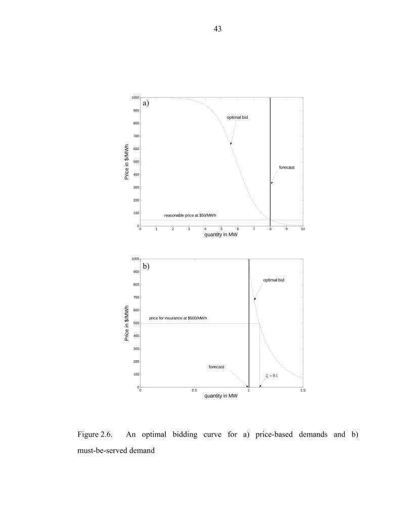
43
Figure 2.6. An optimal bidding curve for a) price-based demands and b)
must-be-served demand
0 1 2 3 4 5 6 7 8 9 100
100
200
300
400
500
600
700
800
900
1000
Pric
e in
$/M
Wh
quantity in MW
forecast
optimal bid
reasonable price at $50/MWh
0 0.5 1 1.50
100
200
300
400
500
600
700
800
900
1000
Pric
e in
$/M
Wh
quantity in MW
forecast
optimal bid
ξ = 0.1
price for insurance at $500/MWh
b)
a)

44
Consequently, the value is different among consumers, and furthermore it may vary
with time even for an identical consumer. The basic idea of the algorithm is simply to
capture the most important aspects of a real problem facing a learning agent
interacting with its environment to maintain reliability in an economic way. Clearly
the demand-side agent can sense the market state to some extent and take actions by
adjusting its bid. In this study, an agent updates the value for m according to
reinforcement algorithm15. The duration of contract and the number of allowed PRL
are divided into N1 segments. After each segment, the number of PRL declared is
checked, and then the agent adjusts the value of m in a following way:
∆⎟⎟⎠
⎞⎜⎜⎝
⎛−+=+
11 N
nnsignmm total
kkk (61)
where ∆ denotes a step size.
There is no need for an agent to bid for a quantity more than needed. For a security
purpose, an agent might bid up to a certain fraction of forecast than needed, and then
bid price drops down to zero beyond the fraction. Figure 2. 7 shows different bidding
curves for several cases. Blue line stands for the bid curve submitted at nth period. If
there was no PRL at the period, freedom increases only slightly from n/N to n/(N-1).
Consequently, bid price is reduced in a very small amount. On the other hand, an
occurrence of PRL significantly reduces the value of freedom, and then bid curve
becomes much steeper.
15 reinforcement algorithm is learning how to map situations to actions so as to maximize a numerical reward signal; the agent is not told which actions to take, but instead must discover which actions yield the most reward by trying them
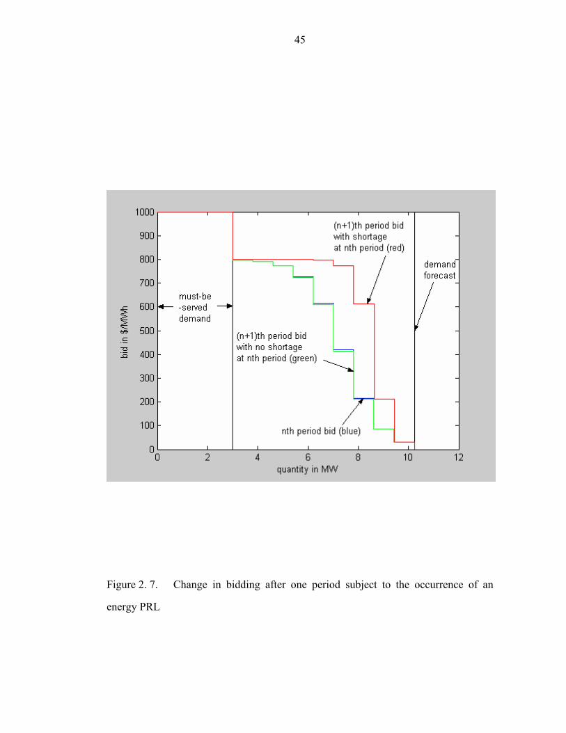
45
Figure 2. 7. Change in bidding after one period subject to the occurrence of an
energy PRL

46
CHAPTER THREE EARNING ESTIMATION
3.1. Mapping Offers to Earnings
The objective of a supply-side agent is to maximize its earning by submitting an
optimal offer. Finding an optimal solution is a maximization problem with several
constraints such as generation limits and power balance equations16, etc if there is a
way to estimate earnings for given offers. There are several algorithms to find an
optimal solution for a given objective function and constraints, e.g., the Lagrangian
relaxation method. Therefore, it is important to construct a mapping function from
control variable to objective function value. As was shown in chapter two, the offer
curve is highly nonlinear which leads to a nonlinear objective function. Even though
competitors’ offers are required to construct an objective function, they are unknown
to an agent. Residual demand approach is widely used because of its convenience to
deal with unknown strategies of competitors in a firm-level optimization process [19-
23]. However, it is difficult to construct the realistic curve since both actual demand
and the offers submitted by other firms are not known. In this chapter, it is discussed
how to construct a numerical mapping function from offers to earnings, and then how
to find an optimal solution.
Another issue to construct a mapping function in a firm level is related to the size of
the electric power system. There exist several tens of thousand generators for an ISO.
Since the number of competitors is large, the number of possible combinations of their
16 Total generation is sum of total demand and loss

47
strategies is too enormous to compute the value of mapping function in a real time. A
useful concept to deal with such a situation is cluster analysis17 . A transmission
network might be decomposed into sub-regions based on the network topology, and
then a group of firms located in the same sub-region can be clustered together.
3.2. Market Modeling
A mapping function from offers to earning can be constructed by analyzing the
characteristics of the market in which an agent participates. Market is a combinatory
sum of each market participant for a given transmission network and demand profile,
etc. Therefore, it is possible to construct a mapping function if offer behaviors of
market participants are known for a given network and demand profile. In this study, it
was assumed that information related to transmission network is estimated with a good
precision. In this section, behavior of market participants will be discussed and
modeled in terms of their influence.
17 The term cluster analysis actually encompasses a number of different classification algorithms. A general question facing researchers in many areas of inquiry is how to organize observed data into meaningful structures, that is, to develop taxonomies. For example, biologists have to organize the different species of animals before a meaningful description of the differences between animals is possible. According to the modern system employed in biology, man belongs to the primates, the mammals, the amniotes, the vertebrates, and the animals. Note how in this classification, the higher the level of aggregation the less similar are the members in the respective class. Man has more in common with all other primates than it does with the more distant members of the mammals, etc.

48
3.2.1. Classification of offer strategies
In a regulated electricity market, ISO decides each generator setpoint based on the
costs of all participating generators. The marginal cost of different generators plays an
important role in determining price. In a restructured market, offers based on marginal
cost are often observed especially when the market is competitive.
An agent offering marginal cost without withholding its capacity from the market is
called a marginal cost agent (MC). This type of agent might withhold capacity when
there is a strong possibility of not being dispatched if offered. When an agent
withholds more capacity than necessary in an attempt to increase prices, it is classified
as a “Cournot competitor”. Offer behavior of this type is similar to that of an MC in
that all submitted offers are low-priced. However, the effect on the market is
practically identical to that of a speculator to be discussed [12].
A third type of agent, called a speculator, is one whose offers are mixed between
high-priced and low-priced offers. Usually, most of the quantities are offered at a
lower price and only small quantities are at a high price. Because of the shape, its offer
curve is sometimes called a “hockey-stick”. Speculators are willing to take the risk of
not being dispatched in an attempt to raise the market clearing price.
These three types of behavior are the most commonly observed offer behaviors in a
real market. There have been several attempts to fit the offer curves. Figure 2. 1 of
previous chapter shows a typical offer curve of a speculator (D8) observed in the PJM
market. The most striking feature of the curve is the existence of a “kink point”
between low-priced and high-priced offer.

49
3.2.2. Market modeling
The three types of agents are commonly observed from all over the uniform price
auction market. However, their effects vary with different market, which makes some
markets more stable than others. For example, a Cournot-type agent helps a speculator
to gain market power. In some scenarios, Oh et al. [12] classified the agent as a
speculator according to the withheld quantity with respect to the fairshare. However,
in a very competitive market the performance of the identical agent is similar to that of
a marginal cost offer agent. Consequently, Oh et al. proposed that an agent must be
classified based not on the shape of offer curves but on the performance in the market
considered since the same offer strategy has different effect on a market according to
the types of the competitors of the agent. The behavior of an unknown agent was
classified by comparing the performance with those of standardized agent18.
To explain experimental results performed on unknown complex system, one of the
most powerful and commonly used techniques is to try and form a basis set that spans
the unknown system. When there exists a basis set to span, a unknown system φ can
be spanned in terms of the known set ϕ :
∑=j
jiji c ϕφ (62)
where c is a probability distribution.
It is possible to identify an offer behavior for player i, iφ , in terms of a basis set. If
the basis set is orthonormal, the probability, cij, is simply an inner product between ith
18 an agent offering all the quantity with no withholding at “standardized” price based on the degree of speculation

50
and jth states. However, the form of the basis set is unknown, which means that the
form is not necessarily expressed in an offer curve. Suppose there is an offer basis set
to express an offer behavior like weak speculator (WS), strong speculator (SS). Then
elements in the offer basis set can be spanned in terms of the basis set. If the set is
complete to span an offer space, there exists an inverse relation that allows inverse
expansion which is projection of the basis set into the offer space:
∑=k
kjkj d φϕ (63)
Note that the offer basis set is not orthonormal, but it spans in an offer space.
Consequently, one can find an expansion of a unknown offer behavior in terms of
known offer set by combining equations. (62) and (63):
∑ ∑∑ ∑∑
∑∑∑ ∑∑
=⎟⎟⎠
⎞⎜⎜⎝
⎛==
=⎟⎠
⎞⎜⎝
⎛==
k kkik
kk
jijjk
jkijjk
j kkjkij
j kkjkij
jjiji
Vcdcd
dcdcc
φφφ
φφϕφ
(64)
where V is a weight factor distribution which is not a probability distribution any
more.
Therefore, it is possible to classify an offer behavior as long as there are enough
elements in the offer basis set. An insufficient offer basis set results in proper
classification with large error instead of wrong classification. Inconsistent offer
behavior will lead an overall offer behavior, but it might be classified properly if
different behaviors are properly divided and analyzed.

51
Similarly, the state of a market is a cumulative sum of the effects of an individual
agent in the market. It is easier to model an individual agent than an unknown market
especially when network effects are considered. Suppose there is a system iΦ with
known offer behaviors of its m market participants. Then, the system can be expressed
in terms of the offer basis set in a following way:
∑∑∑ ∑
∑∑∑
==
⎟⎠
⎞⎜⎝
⎛⎟⎠
⎞⎜⎝
⎛⎟⎠
⎞⎜⎝
⎛==Φ
iii
k k kkkkM
kkmk
kkk
kkkmi
WKKK
VVV
m
mψφφφ
φφφφφφ
1 2
21;...;;......
...;...;;
21
2121
(65)
where iψ is a cumulative offer behavior of competitors in the offer basis set, which
is a scenario set.
3.3. Mapping Function for Stationary Markets
A system with unknown offer behavior can be spanned in terms of known offer
behavior as follows:
∑=
=ΨN
iiip
1ψ (66)
where Ψ represents an unknown system expressed in terms of iψ which is ith
elements in the scenario set, and pi stands for the probability that the unknown system
is in the ith scenario. Then the experimental observations can be interpreted as:
∑=
=ΨN
iijij HpH
1ψφφ (67)
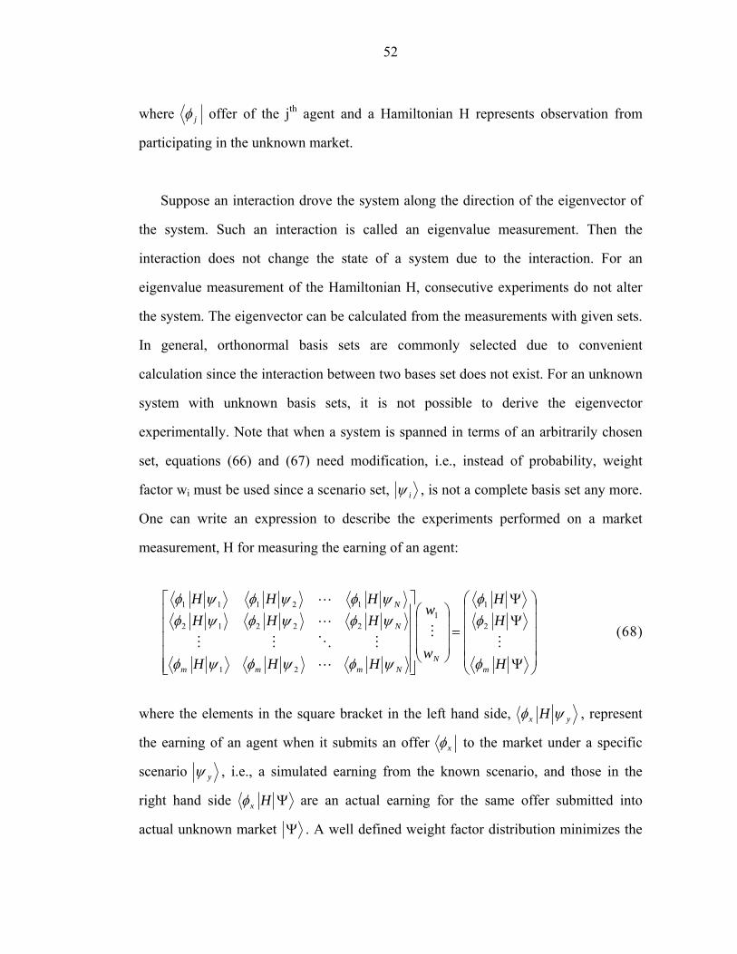
52
where jφ offer of the jth agent and a Hamiltonian H represents observation from
participating in the unknown market.
Suppose an interaction drove the system along the direction of the eigenvector of
the system. Such an interaction is called an eigenvalue measurement. Then the
interaction does not change the state of a system due to the interaction. For an
eigenvalue measurement of the Hamiltonian H, consecutive experiments do not alter
the system. The eigenvector can be calculated from the measurements with given sets.
In general, orthonormal basis sets are commonly selected due to convenient
calculation since the interaction between two bases set does not exist. For an unknown
system with unknown basis sets, it is not possible to derive the eigenvector
experimentally. Note that when a system is spanned in terms of an arbitrarily chosen
set, equations (66) and (67) need modification, i.e., instead of probability, weight
factor wi must be used since a scenario set, iψ , is not a complete basis set any more.
One can write an expression to describe the experiments performed on a market
measurement, H for measuring the earning of an agent:
⎟⎟⎟⎟⎟
⎠
⎞
⎜⎜⎜⎜⎜
⎝
⎛
Ψ
ΨΨ
=⎟⎟⎟
⎠
⎞
⎜⎜⎜
⎝
⎛
⎥⎥⎥⎥⎥
⎦
⎤
⎢⎢⎢⎢⎢
⎣
⎡
H
HH
w
w
HHH
HHHHHH
mN
Nmmm
N
N
φ
φφ
ψφψφψφ
ψφψφψφψφψφψφ
MM
L
MOMM
L
L
2
11
21
22212
12111
(68)
where the elements in the square bracket in the left hand side, yx H ψφ , represent
the earning of an agent when it submits an offer xφ to the market under a specific
scenario yψ , i.e., a simulated earning from the known scenario, and those in the
right hand side ΨHxφ are an actual earning for the same offer submitted into
actual unknown market Ψ . A well defined weight factor distribution minimizes the
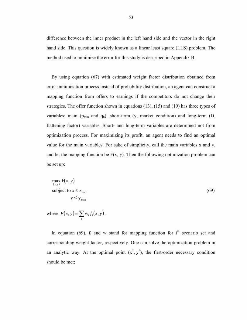
53
difference between the inner product in the left hand side and the vector in the right
hand side. This question is widely known as a linear least square (LLS) problem. The
method used to minimize the error for this study is described in Appendix B.
By using equation (67) with estimated weight factor distribution obtained from
error minimization process instead of probability distribution, an agent can construct a
mapping function from offers to earnings if the competitors do not change their
strategies. The offer function shown in equations (13), (15) and (19) has three types of
variables; main (pmin and qb), short-term (y, market condition) and long-term (D,
flattening factor) variables. Short- and long-term variables are determined not from
optimization process. For maximizing its profit, an agent needs to find an optimal
value for the main variables. For sake of simplicity, call the main variables x and y,
and let the mapping function be F(x, y). Then the following optimization problem can
be set up:
( )( )
max
max
,
yy subject to
,F max
≤≤ xx
yxyx
(69)
where ( ) ( )∑=i
ii yxfwyxF ,, .
In equation (69), fi and w stand for mapping function for ith scenario set and
corresponding weight factor, respectively. One can solve the optimization problem in
an analytic way. At the optimal point (x*, y*), the first-order necessary condition
should be met;
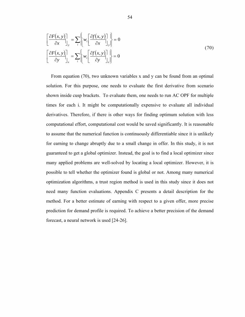
54
( ) ( )
( ) ( )∑
∑
=⎪⎭
⎪⎬⎫
⎪⎩
⎪⎨⎧
⎥⎦
⎤⎢⎣
⎡∂
∂=⎥
⎦
⎤⎢⎣
⎡∂
∂
=⎪⎭
⎪⎬⎫
⎪⎩
⎪⎨⎧
⎥⎦⎤
⎢⎣⎡
∂∂
=⎥⎦⎤
⎢⎣⎡
∂∂
i xi
x
i yi
y
yyxfw
yyxF
xyxfw
xyxF
0,,
0,,
(70)
From equation (70), two unknown variables x and y can be found from an optimal
solution. For this purpose, one needs to evaluate the first derivative from scenario
shown inside cusp brackets. To evaluate them, one needs to run AC OPF for multiple
times for each i. It might be computationally expensive to evaluate all individual
derivatives. Therefore, if there is other ways for finding optimum solution with less
computational effort, computational cost would be saved significantly. It is reasonable
to assume that the numerical function is continuously differentiable since it is unlikely
for earning to change abruptly due to a small change in offer. In this study, it is not
guaranteed to get a global optimizer. Instead, the goal is to find a local optimizer since
many applied problems are well-solved by locating a local optimizer. However, it is
possible to tell whether the optimizer found is global or not. Among many numerical
optimization algorithms, a trust region method is used in this study since it does not
need many function evaluations. Appendix C presents a detail description for the
method. For a better estimate of earning with respect to a given offer, more precise
prediction for demand profile is required. To achieve a better precision of the demand
forecast, a neural network is used [24-26].

55
CHAPTER FOUR MARKET DYNAMICS
In the previous chapter, a mapping function was constructed for a stationary market
in which competitors do not change their strategies. However, the strategies are
subject to change due to a fluctuation in demand or various reasons such as ownership
changes of competing generators. In a current market, there are several market
monitoring systems based on a snap-shot approach19. However, inconsistent change in
offer strategies or stochastically driven change might get caught by the approach while
they do not affect the earning of an agent on average. On the other hand, small and
slow but consistent change affects the earning significantly, but the monitoring
systems do not capture such a change. Furthermore, sudden and consistent change in
the strategies of other competitors might not affect the earning of an agent if the
change is not effective to alter the market state. Therefore, it is desirable to construct a
toolbox to capture only consistent and effective changes, which affects the earning of
the agent of interest.
4.1. Current Market Monitoring Tool
California ISO provides a web site20 explaining its market monitoring system. The
easy-to-calculate snap-shot approach gives a quick check on the market. When
19 an approach to analyze a system at a fixed time 20 California Independent System Operator, “ISO Market Monitoring & Information Protocol”, on http://www.caiso.com/docs/2002/02/12/2002021215391318952.pdf (2002)

56
anomalous market behavior21 is observed, it will take further action. According to the
web site “… The evidence of such behavior may be derived from a number of
circumstances, including; withholding of Generation capacity under circumstances in
which it would normally be offered in a competitive market; unexplained or unusual
re-declarations of availability by generators; unusual trades or transactions; pricing
and bidding patterns that are inconsistent with prevailing supply and demand
conditions; unusual activity or circumstances relating to imports from or exports to
other markets or exchanges…”. This means that to analyze market properly ISO
should have correct and up-to-date knowledge about other economic situation such as
gas price. Proper knowledge is also important when ISO takes a further action since
market participants may claim the information that ISO has is not correct. Even with
proper information, there are other problems associated with the snap shot approach.
Suppose there is a market operating at the situation when a little more withholding
results in a price spike. Suppose an agent in the market slowly changes its strategy
from a marginal cost offer to Cournot-type offer. At a certain point, the market has
price spikes, but ISO cannot figure out what causes the price spikes with a snap-shot
approach. This might be a shortcoming in the usage of the tool since a current tool
requires for ISO to identify causes responsible for the occurrence of price spikes.
Another problem is a false alarm, i.e., even if some price spikes are inevitable due to
load profile and network constraints, the current market monitoring possibly requires a
further investigation. To monitor a change in the market state, a proper tool must be
sensitive enough only for a consistent and successful change.
21 according to its web site [27], behavior that departs significantly from the normal behavior in competitive markets that do not require continuing regulation or behavior leading to unusual or unexplained market outcomes

57
II. Chaos and Fractals
As was mentioned in chapter two, market clearing price is a good measure to
analyze a change in the market state. Figure 4. 1. shows several nodal prices observed
in the NY ISO over a month during summer in 2003. During the summer, demands for
electricity increase due to hot weather, which gives more chance for an agent to get a
higher price. Consequently, speculators change their strategies early in summer to take
the chance.
Nodal price is greatly dependent on the offers from the generators located at the
bus. Therefore, a nodal price is an indicator to check if there is any change in
strategies of the agents located at the bus. Visual inspection of Fig. 4. 1 gives that
there were about 25 times of price spikes for both generators. Background prices also
increased about two times in comparison to those at early in June. One can claim that
there are changes in both systems during the time period.
Figure 4. 2 illustrates how an agent interacts through price signal. The top graph
shows data flow in an electricity market. Agents get information from ISO on demand
forecast and historical market clearing data, and submit offers into ISO. Then, ISO
collects the offers to clear the market and declares the results. The bottom graph
illustrates the translation of the market operation into a signal processing point of view.
An observer sends an input signal to the system and receives an output signal, i.e., an
agent submits offers and then receives market clearing results.
Game theory has dealt with an auction and bidding strategies, which are closely
related to the deregulated electricity market. In game theory, the most commonly
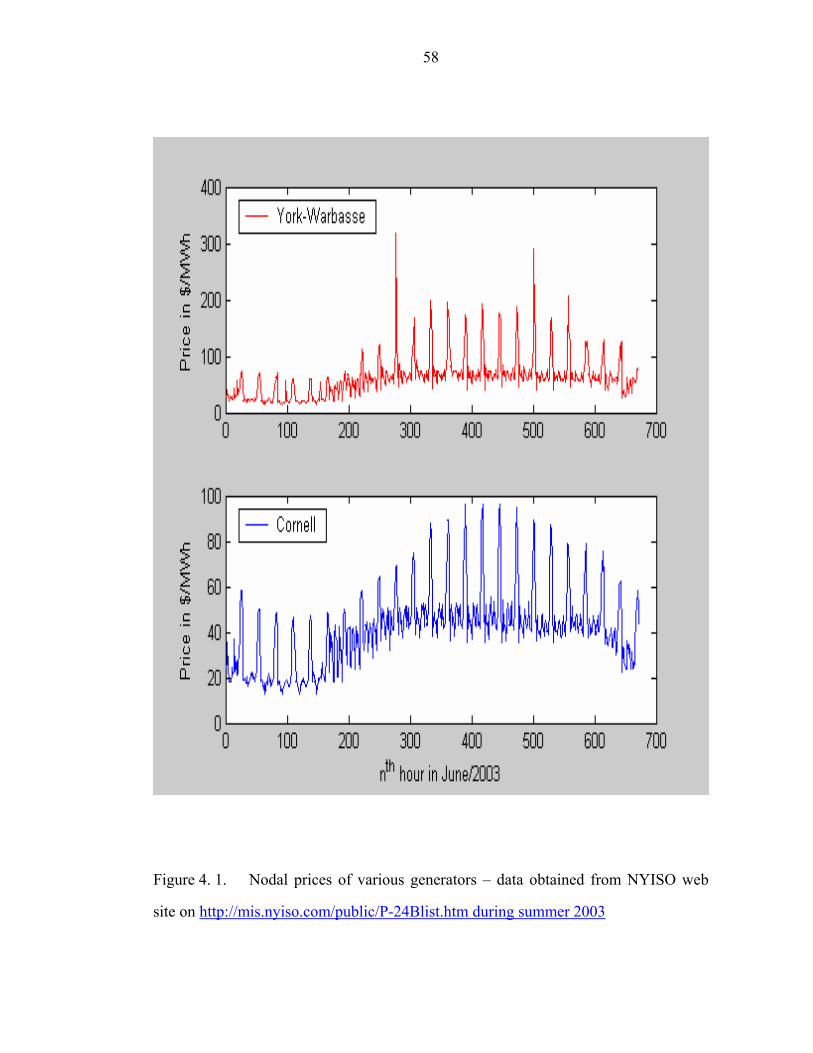
58
Figure 4. 1. Nodal prices of various generators – data obtained from NYISO web
site on http://mis.nyiso.com/public/P-24Blist.htm during summer 2003
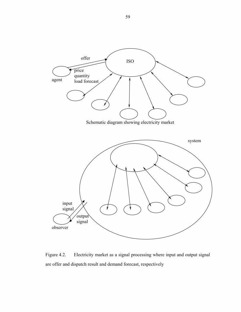
59
Schematic diagram showing electricity market
Figure 4.2. Electricity market as a signal processing where input and output signal
are offer and dispatch result and demand forecast, respectively
offer
price quantity load forecast
ISO
agent
input signal
output signal
system
observer

60
discussed type of equilibrium for this market is Nash equilibrium22 [28-29] for a very
simplified situation. Game theory is not practical for a very complicated system like a
deregulated electricity market due to the multi-dimensional strategic space and the
uncertainty associated with a market. For a real market, it is not even clear if the
system moves toward any equilibrium state. It seems that the system exhibits aperiodic
behavior that depends on the initial condition sensitively. Consequently, it is
impossible to perform a long-term prediction. This type of behavior of a system is
called chaos [30-31], which is a term describing aperiodic long-term behavior23 in a
deterministic24 system that exhibits sensitive dependence on initial conditions25. It
would be better to monitor; i) any change in the market state, ii) forecasting a future
state, e.g., a new equilibrium or a chaos if there is any change and iii) assigning how
recent data are relevant for estimating a future state.
4.3. Nonlinear Time Series Analysis
Self-similarity is one of characteristics in describing a chaotic behavior, so called
fractal. Dimension is defined the minimum number of independent variables to
describe fractal. Two different fractals may have a same value of dimension, but two
fractals with different values of dimension are guaranteed to be different.
Consequently, the value of dimension is a signature of a change in the system state.
22 Nash equilibrium is a term used in the game theory – a state after playing a game for a long time when all the players in a game follow the way described below; each player looks at the behavior of opponents, and determines the best response to the behaviors of the opponents’. 23 there are trajectories which does not settle down to fixed points, periodic orbits or quasi-periodic orbits as time diverges 24 the system has no random or noisy inputs or parameters 25 nearby trajectories separates exponentially – positive Liapunov exponent

61
Therefore, monitoring the value of dimension would give an answer for i). ii) and iii)
can be assigned by monitoring time response after a change. There is a quantity to
measure for a fractal such a time response, so called the Liapunov exponent26.
It has been shown that dimension can be defined in several ways for describing
fractals as is described in Appendix D. However, it is not clear where the definitions
are useful for analyzing experimental data. Most frequently used technique for
analyzing consecutive data set is a linear time series analysis due to its simplicity. The
basic assumption underlying linear methods is linear correlations, i.e., the intrinsic
dynamics of the system are governed by the linear paradigm that small causes lead to
small effects. Furthermore, only exponential change or periodic oscillation can be
obtained from linear equations, and then all aperiodic behavior needs to be assigned to
the results of an external force. Some idea of the system or failure on using linear
model have brought people consider nonlinear dynamics which is greatly related to
chaos. Deterministic chaos provides a striking explanation for irregular behavior and
anomalies in systems which do not seem to be inherently stochastic.
Similar to a stock market [32] discussed in Appendix E, the electricity market also
shows nonlinear behavior since there exists highly nonlinear relationship between
offers submitted by suppliers and the market clearing price. However, in comparison
to Hurst exponent [33] used for a stock market, the quantities like Liapunov exponent
and the dimension of a fractal are much less affected by error due to the ordered
structure of electricity markets. Therefore, it is possible to evaluate values of the
parameters reflecting the state of the market without the “filter process” as described
in Appendix E, and to characterize market based on the values of the parameters.
26 an index showing how fast neighboring trajectories separate exponentially
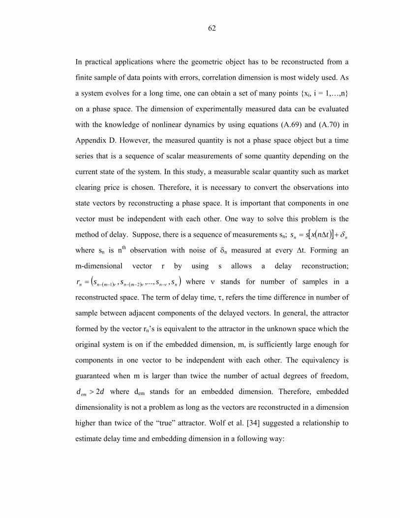
62
In practical applications where the geometric object has to be reconstructed from a
finite sample of data points with errors, correlation dimension is most widely used. As
a system evolves for a long time, one can obtain a set of many points {xi, i = 1,…,n}
on a phase space. The dimension of experimentally measured data can be evaluated
with the knowledge of nonlinear dynamics by using equations (A.69) and (A.70) in
Appendix D. However, the measured quantity is not a phase space object but a time
series that is a sequence of scalar measurements of some quantity depending on the
current state of the system. In this study, a measurable scalar quantity such as market
clearing price is chosen. Therefore, it is necessary to convert the observations into
state vectors by reconstructing a phase space. It is important that components in one
vector must be independent with each other. One way to solve this problem is the
method of delay. Suppose, there is a sequence of measurements sn; ( )[ ] nn tnxss δ+∆=
where sn is nth observation with noise of δn measured at every ∆t. Forming an
m-dimensional vector r by using s allows a delay reconstruction;
( ) ( )( )nnmnmnn ssssr ,,...,, 21 ννν −−−−−= where ν stands for number of samples in a
reconstructed space. The term of delay time, τ, refers the time difference in number of
sample between adjacent components of the delayed vectors. In general, the attractor
formed by the vector rn’s is equivalent to the attractor in the unknown space which the
original system is on if the embedded dimension, m, is sufficiently large enough for
components in one vector to be independent with each other. The equivalency is
guaranteed when m is larger than twice the number of actual degrees of freedom,
ddem 2> where dem stands for an embedded dimension. Therefore, embedded
dimensionality is not a problem as long as the vectors are reconstructed in a dimension
higher than twice of the “true” attractor. Wolf et al. [34] suggested a relationship to
estimate delay time and embedding dimension in a following way:

63
Qm =×τ (71)
where Q stands for mean orbital period27.
A reasonable rule of thumb to choose Q is the time where the autocorrelation
function decays to 1/e. [35] In this study, correlation dimension of a fractal can be
evaluated by using the following equation:
( ) ( ) ( ) dN
i
N
nijji xxH
NNC εεε ∝−−
−≡ ∑ ∑
= +=1 min1
2 (72)
where nmin is the minimum number of measurement satisfying ttn ∆= /minmin ; tmin and
∆t represent autocorrelation time28 and time delay of measurement, respectively.
Another important term for analyzing a fractal and estimating for future events is the
Liapunov exponent. The Liapunov exponent shows how far two initially adjacent
trajectories stay near. Consequently, two trajectories starting very close with each
other are somewhat near within the Liapunov exponent. When a current state is
properly analyzed, an estimate to near future within Liapunov exponent is valid since
real and estimated state are close. Suppose there is a trajectory on an attractor, and x(t)
is a point on the attractor and x(t) + δ(t) is located close to x(t) with an initial
separation length ||δ0||. For the Lorenz attractor, one finds that:
( ) ( )tt λδδ exp0∝ (73)
27 Suppose the situation that the pairs entering the sum are not statistically independent. For time series data with nonzero autocorrelations, independence cannot be assumed; embedding vectors at successive times are often close in phase space – see Figure 4. 3 28 the time where the autocorrelation function decays to 1/e
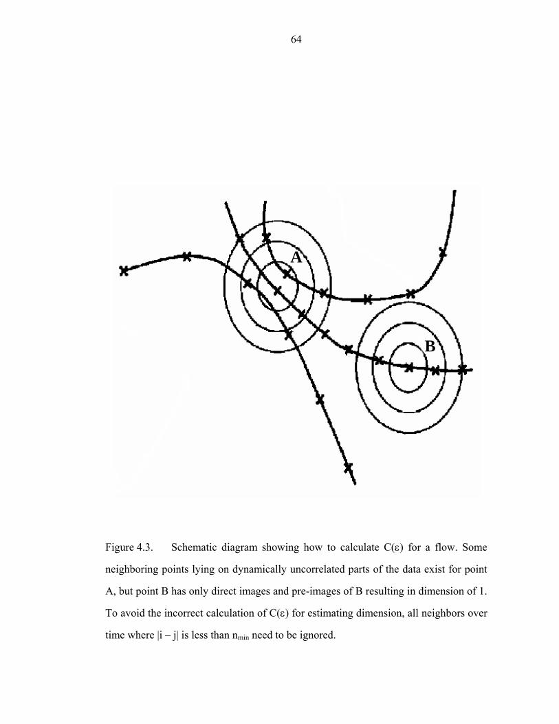
64
Figure 4.3. Schematic diagram showing how to calculate C(ε) for a flow. Some
neighboring points lying on dynamically uncorrelated parts of the data exist for point
A, but point B has only direct images and pre-images of B resulting in dimension of 1.
To avoid the incorrect calculation of C(ε) for estimating dimension, all neighbors over
time where |i – j| is less than nmin need to be ignored.
A
B
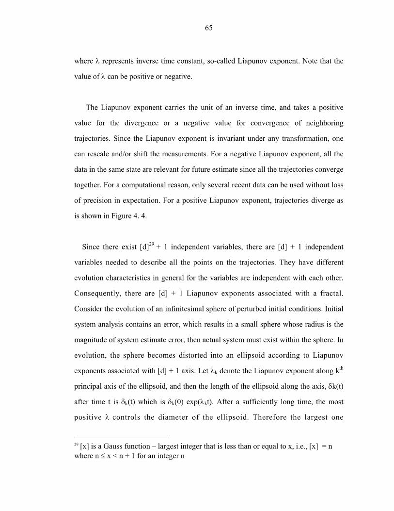
65
where λ represents inverse time constant, so-called Liapunov exponent. Note that the
value of λ can be positive or negative.
The Liapunov exponent carries the unit of an inverse time, and takes a positive
value for the divergence or a negative value for convergence of neighboring
trajectories. Since the Liapunov exponent is invariant under any transformation, one
can rescale and/or shift the measurements. For a negative Liapunov exponent, all the
data in the same state are relevant for future estimate since all the trajectories converge
together. For a computational reason, only several recent data can be used without loss
of precision in expectation. For a positive Liapunov exponent, trajectories diverge as
is shown in Figure 4. 4.
Since there exist [d]29 + 1 independent variables, there are [d] + 1 independent
variables needed to describe all the points on the trajectories. They have different
evolution characteristics in general for the variables are independent with each other.
Consequently, there are [d] + 1 Liapunov exponents associated with a fractal.
Consider the evolution of an infinitesimal sphere of perturbed initial conditions. Initial
system analysis contains an error, which results in a small sphere whose radius is the
magnitude of system estimate error, then actual system must exist within the sphere. In
evolution, the sphere becomes distorted into an ellipsoid according to Liapunov
exponents associated with [d] + 1 axis. Let λk denote the Liapunov exponent along kth
principal axis of the ellipsoid, and then the length of the ellipsoid along the axis, δk(t)
after time t is δk(t) which is δk(0) exp(λkt). After a sufficiently long time, the most
positive λ controls the diameter of the ellipsoid. Therefore the largest one
29 [x] is a Gauss function – largest integer that is less than or equal to x, i.e., [x] = n where n ≤ x < n + 1 for an integer n
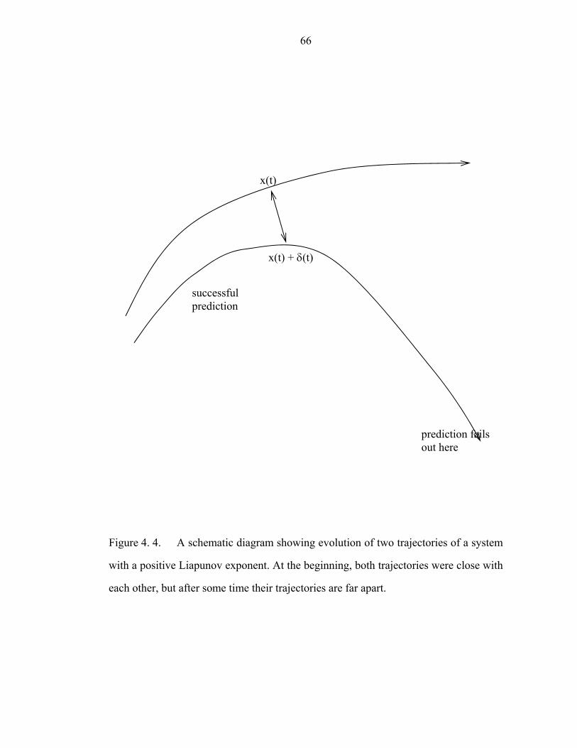
66
Figure 4. 4. A schematic diagram showing evolution of two trajectories of a system
with a positive Liapunov exponent. At the beginning, both trajectories were close with
each other, but after some time their trajectories are far apart.
x(t)
x(t) + δ(t)
prediction fails out here
successful prediction

67
among Liapunov exponents is most important to estimate a state in near future. As was
shown in Fig. 4. 4, prediction breaks down after inverse largest Liapunov exponent.
As was mentioned earlier, an attractor does not shrink/diverge at the same rate
everywhere. The Liapunov exponent is an average of the local divergence rates over
the whole data. Generally speaking, experimental data contain noise of which effect
can be minimized by an appropriate averaging statistics. From experiments, only one
trajectory can be obtained from the time series measurement from one initial point.
However, a vector close to the point can be considered as a new initial point which
shows different trajectory since the trajectory is equally valid if it started from the new
initial point. Figure 4. 5 illustrates the evolution and replacement procedure used to
estimate Liapunov exponent from experimental data. Let 0ns be a point of the time
series in the embedding space. Reference embedding vector after embedded dimension
is determined by using equation (72). One can calculate the average distance of all
neighbors to the reference part of the trajectory as a function of the relative time. The
logarithm of the average distance at time t is effective expansion rate over the time
span containing all the deterministic fluctuations due to projection and dynamics.
Repeat this calculation for many values of n0, and then the fluctuation of the expansion
rates will be average out. The Liapunov exponent λ can be obtained in the following
equation [36-37]:
( ) ( ) ( ) ( )( )
( )ttstssuN
tSN
n susnn
n nn
λexp1log110 0
0
0
∝⎥⎥⎦
⎤
⎢⎢⎣
⎡−= ∑ ∑
= ∈
(74)
where u(0ns ) stands for the neighborhood of
0ns within ε, and 0ns (t) and ns (t)
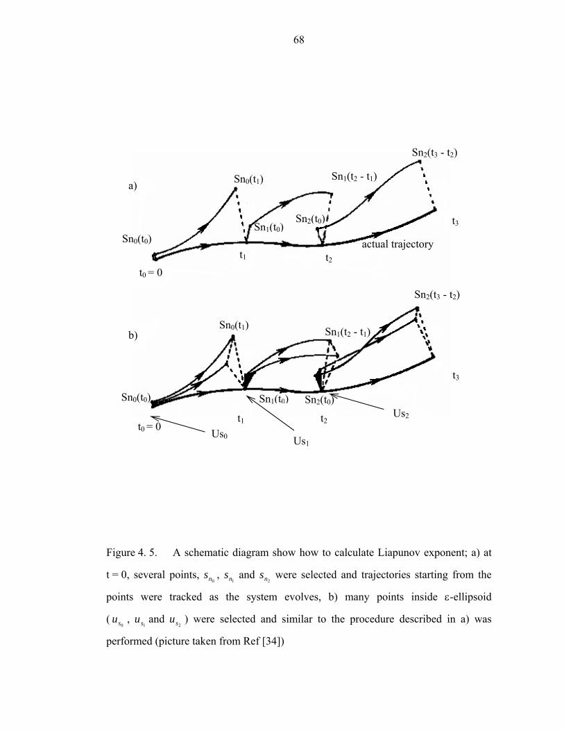
68
Figure 4. 5. A schematic diagram show how to calculate Liapunov exponent; a) at
t = 0, several points, 0ns ,
1ns and 2ns were selected and trajectories starting from the
points were tracked as the system evolves, b) many points inside ε-ellipsoid
(0su ,
1su and
2su ) were selected and similar to the procedure described in a) was
performed (picture taken from Ref [34])
a)
b)
t0 = 0 t1 t2
Sn1(t0)Sn2(t0)
Sn0(t1) Sn1(t2 - t1)
Sn0(t0) t3
actual trajectory
Sn2(t3 - t2)
t0 = 0 t1 t2
t3
Sn0(t0)
Sn0(t1) Sn1(t2 - t1)
Sn2(t3 - t2)
Sn1(t0) Sn2(t0)
Us0 Us1
Us2

69
represent embedded vector after time t evolved from 0ns and ns , respectively.
The size of neighborhood, ε, should be as small as possible, but large enough to
contain enough points to calculate its neighborhood. Figure 4. 6 shows an example for
estimation of the maximal Liapunov exponent from a data set.
After calculating correlation dimension and largest Liapunov exponent, an agent
decides how recent data are relevant for estimating a future state. For a negative
Liapunov exponent, all the data obtained from the same state are useful, and then an
agent is free to choose the amount of data for computation. For a positive Liapunov
exponent, a system evolves with time, and then initial system analysis is valid within
the exponent inverse. Consequently, an agent has a guideline how recent data need to
be added.
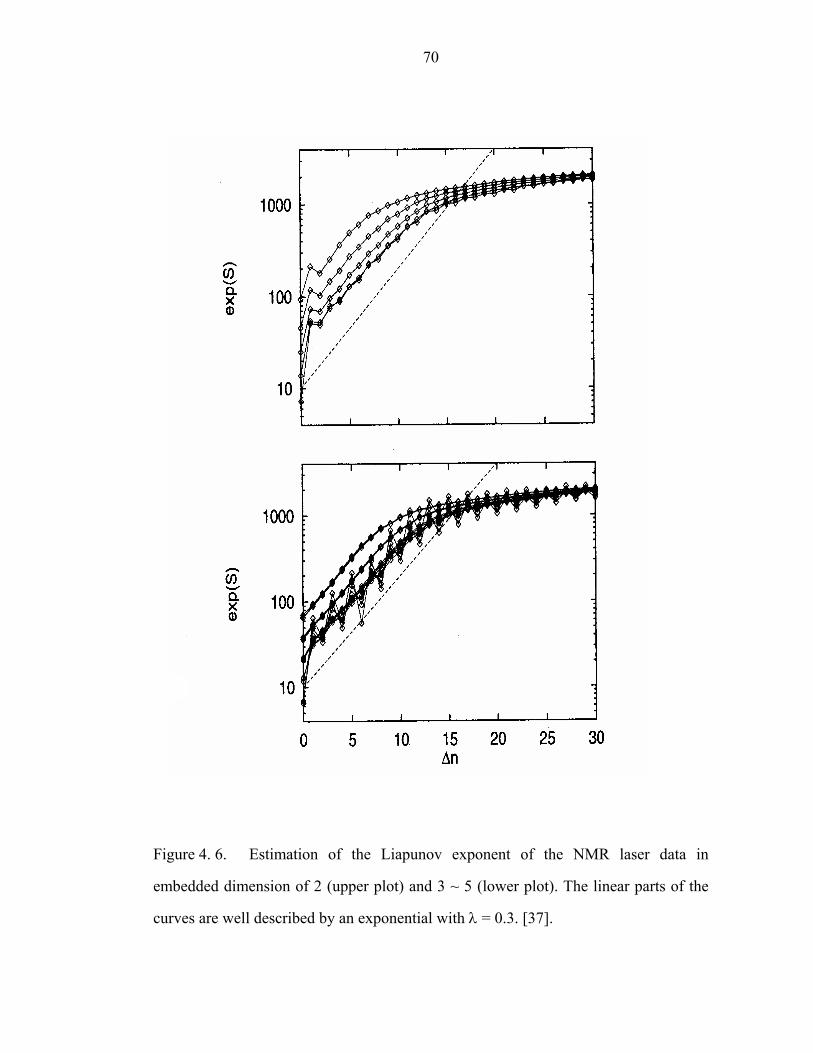
70
Figure 4. 6. Estimation of the Liapunov exponent of the NMR laser data in
embedded dimension of 2 (upper plot) and 3 ~ 5 (lower plot). The linear parts of the
curves are well described by an exponential with λ = 0.3. [37].

71
CHAPTER FIVE SIMULATION RESULTS AND DISCUSSION
5.1. Agent Classification Based on Its Performance
To find proper number of elements in offer basis set, several different types of
agents were simulated with known types of agent. For a large enough number of
elements, the agents can be classified properly in terms of its performance. If a
classification is properly performed, the agents classified in the same group must show
similar performance, i.e., the actual earning of the agents must be highly correlated
with expected earning based on the classification.
5.1.1. Standardized agents
To develop a simulation environment, five standardized agents are implemented
consisting of one marginal cost offer agent and four speculators. That is, human or
software agent with unknown behavior can be classified based on its play against
known agent types. Marginal cost offer agent is an agent that offers all of its blocks at
marginal cost without withholding any of them. The speculator agents exhibit different
degrees of price and quantity speculation. In order to be classified as a speculator, at
least one block must be consistently offered at a high price. It is crucial that a
speculator be able to consistently determine which block or blocks are to be offered at
a high price and which blocks are to be withheld. Speculators are classified based on
the amount of risk they are willing to take. For simplicity, any offer submitted at a

72
high price is made at the same price regardless of the type of speculation. A fairshare
of the market is calculated based on a load forecast. The block in which the fairshare
quantity falls is termed the “fairshare block”. If this were the last block chosen for the
unit by the auction, then it would be the units’ marginal block. Thus, the fairshare
calculation is just a means for trying to predict a unit’s marginal block a period ahead
and any calculation to accomplish that prediction is suitable for the purpose we have
in mind.
The strategies for offers of the standardized agents are shown in Table 5. 1. The
standardized agent with the weakest degree of speculation, called a weak speculator
(WS), was designed to speculate with the block that is adjacent to and more expensive
than its fairshare block. If the load forecast had no significant error, the behavior of a
WS agent was found to be similar to that of an MC agent with some withholding
capacity. Since no speculator could speculate less than a WS, the agent is called weak
speculator. The agent with a stronger DOS than a WS, termed a strong speculator
(SS), offers a high price for its fairshare block. This agent is willing to take the risk of
not being dispatched for the chance of a higher market clearing price. Two stronger
speculators (SS2, SS3) were also implemented. SS3 speculates with all the blocks to
the fairshare block while SS2 submits (j-1)th block at a high price where jth block is a
faieshare block.

73
Table 5. 1. Block-by-block offer structure for standardized agents; The table shows
the offer strategies of standardized agents when the fairshare block is the jth block out
of n available blocks. MCO, S and W stand for a marginal cost offer, speculate on
price and withhold the block, respectively
j-k block;
2 ≤ k ≤ j-1
(j – 1)th
block
jth
block
(j+1)th
block
j+k block;
2 ≤ k ≤ n-j
MC MCO MCO MCO MCO MCO
WS MCO MCO MCO S W
SS MCO MCO S W W
SS2 MCO S W W W
SS3 S S S W W
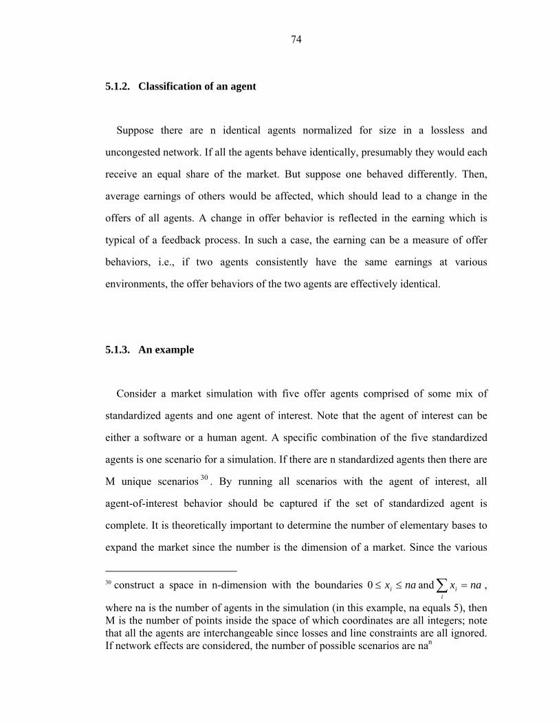
74
5.1.2. Classification of an agent
Suppose there are n identical agents normalized for size in a lossless and
uncongested network. If all the agents behave identically, presumably they would each
receive an equal share of the market. But suppose one behaved differently. Then,
average earnings of others would be affected, which should lead to a change in the
offers of all agents. A change in offer behavior is reflected in the earning which is
typical of a feedback process. In such a case, the earning can be a measure of offer
behaviors, i.e., if two agents consistently have the same earnings at various
environments, the offer behaviors of the two agents are effectively identical.
5.1.3. An example
Consider a market simulation with five offer agents comprised of some mix of
standardized agents and one agent of interest. Note that the agent of interest can be
either a software or a human agent. A specific combination of the five standardized
agents is one scenario for a simulation. If there are n standardized agents then there are
M unique scenarios 30 . By running all scenarios with the agent of interest, all
agent-of-interest behavior should be captured if the set of standardized agent is
complete. It is theoretically important to determine the number of elementary bases to
expand the market since the number is the dimension of a market. Since the various
30 construct a space in n-dimension with the boundaries naxnax
iii =≤≤ ∑ and 0 ,
where na is the number of agents in the simulation (in this example, na equals 5), then M is the number of points inside the space of which coordinates are all integers; note that all the agents are interchangeable since losses and line constraints are all ignored. If network effects are considered, the number of possible scenarios are nan

75
set comprised of standardized agents is chosen for convenience rather than theoretic
analysis, the expansion might be either redundant or insufficient.
However, a market can be expressed in terms of a scenario set if the set contains all
possible offer behaviors. For each scenario, the six agents competed for 200 periods
and their earnings plotted as a function the earnings of the agent of interest for each
period. Figure 5. 1 illustrates a possible plot of the earnings of the participating agents
for one scenario. The six lines show how corresponding agents performed in each
period. All lines have different slopes, which characterizes the type of agent. Among
the lines, the y = x represents the earning of the agent of interest. If the y = x line is
“close” to one of lines showing the earnings of a standardized agent, the agent of
interest is classified as an agent whose behavior is similar to that of the standardized
agent that produced that line. For example, the agent shown in Figure 5. 1 is classified
as a strong speculator (SS).
In the scenario that produced this plot, an MC earned the most while an SS3 earned
the least. Note that an SS3 is the speculator with the strongest degree of speculation.
In simulations with software agents, this feature was found to be true in general. As
an agent gets less speculative, the market becomes more competitive and consequently
everyone including the agent itself earns less. This might encourage an agent to
speculate if it wants to maximize its own profit without concern for the earnings of
others.
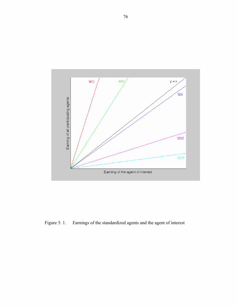
76
Figure 5. 1. Earnings of the standardized agents and the agent of interest
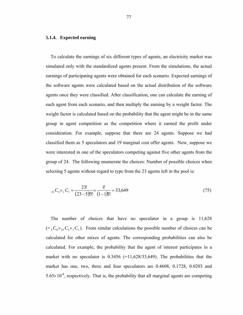
77
5.1.4. Expected earning
To calculate the earnings of six different types of agents, an electricity market was
simulated only with the standardized agents present. From the simulations, the actual
earnings of participating agents were obtained for each scenario. Expected earnings of
the software agents were calculated based on the actual distribution of the software
agents once they were classified. After classification, one can calculate the earning of
each agent from each scenario, and then multiply the earning by a weight factor. The
weight factor is calculated based on the probability that the agent might be in the same
group in agent competition as the competition where it earned the profit under
consideration. For example, suppose that there are 24 agents. Suppose we had
classified them as 5 speculators and 19 marginal cost offer agents. Now, suppose we
were interested in one of the speculators competing against five other agents from the
group of 24. The following enumerate the choices: Number of possible choices when
selecting 5 agents without regard to type from the 23 agents left in the pool is:
( ) ( ) 649,33!1!11
!1!5!523
!2311523 =
−×
−=× CC (75)
The number of choices that have no speculator in a group is 11,628
(= 1151904 CCC ×× ). From similar calculations the possible number of choices can be
calculated for other mixes of agents. The corresponding probabilities can also be
calculated. For example, the probability that the agent of interest participates in a
market with no speculator is 0.3456 (=11,628/33,649). The probabilities that the
market has one, two, three and four speculators are 0.4608, 0.1728, 0.0203 and
5.65×10⁻⁴, respectively. That is, the probability that all marginal agents are competing

78
with the chosen speculative agent is 0.3456. Note that there are no speculators in the
competition other than the chosen speculative agent. If, for example, the agent of
interest earns $100, $300, $700, $1,800 and $2,500 in each of 5 competitions where
each has a different mix of competing agents as listed above, then the weighted
earning of agent k, Ek, is about:
∑∈
≈×=
grouppossiblei
ki
ki
k epE 332$ (76)
where pik is the probability that agent k is in group i and ei
k is the earnings for agent k
if the agent k competes against standardized agents in the group i, respectively. The
expected earnings obtained in this way were used for a further comparison of the
actual earnings.
5.1.5. Simulation results and discussion
In the fall of 2002, fourteen different software agents were submitted by the
students taking the class ECE 551/AEM655 (Electricity Markets) at Cornell
University. These agents competed in a class competition and were subsequently used
as early tests of the classification ideas. From experiments performed in the same class
with the students, it was believed that MC, WS and SS were the most common types
of agents. Therefore, only those types of standardized agents were used.
After performing simulations in which all possible combinations of three
standardized agents were used, the classifications of each agent of interest by certain
of those simulations were found to be redundant, i.e., classifications using one

79
scenario and that using a different one were identical. If the agent of interest behaves
consistently, the result from each scenario should indicate identical classification. By
noting that human subject might be inconsistent, six scenarios were chosen to produce
distinctive classifications: 4 WS + 1 MC, 3 WS + 2 MC, 4 SS + 1 MC, 3 SS + 2 MC,
1 SS + 2 WS + 2 MC and 1 SS + 1 WS + 3 MC. One randomly selected set of
forecasted and actual load was assigned for the scenario. Average load was 470 MW,
and the maximum error between forecast and actual load was 20 MW.
Each of the fourteen software agents and five standardized agents formed a group
for the simulation, and corresponding plots were generated based on the results of the
simulations. According to the plots, the fourteen agents were classified into three
groups, which are 5 MC, 4 WS and 5 SS. It seemed that most agents tested were
speculators to some extent with the degree of speculation somewhere between WS and
SS. It is worthwhile noting that from the scenario the earnings of an agent were close
to those of the standardized agents classified as the same type as the agent.
Figure 5. 2 shows a plot of the earnings of a randomly selected software agent
classified as SS for four scenarios. The classification of the software agents was
straight forward since the strategy used was consistent for a given scenario. In other
words, no learning algorithms were implemented. For most of the agents, strategies
seemed not to change for different scenarios, i.e., different type of competitors. It was
also found that no agents developed by the students used learning algorithms which
would alter the results significantly. Since the agent code is available, it is possible to
check the results.
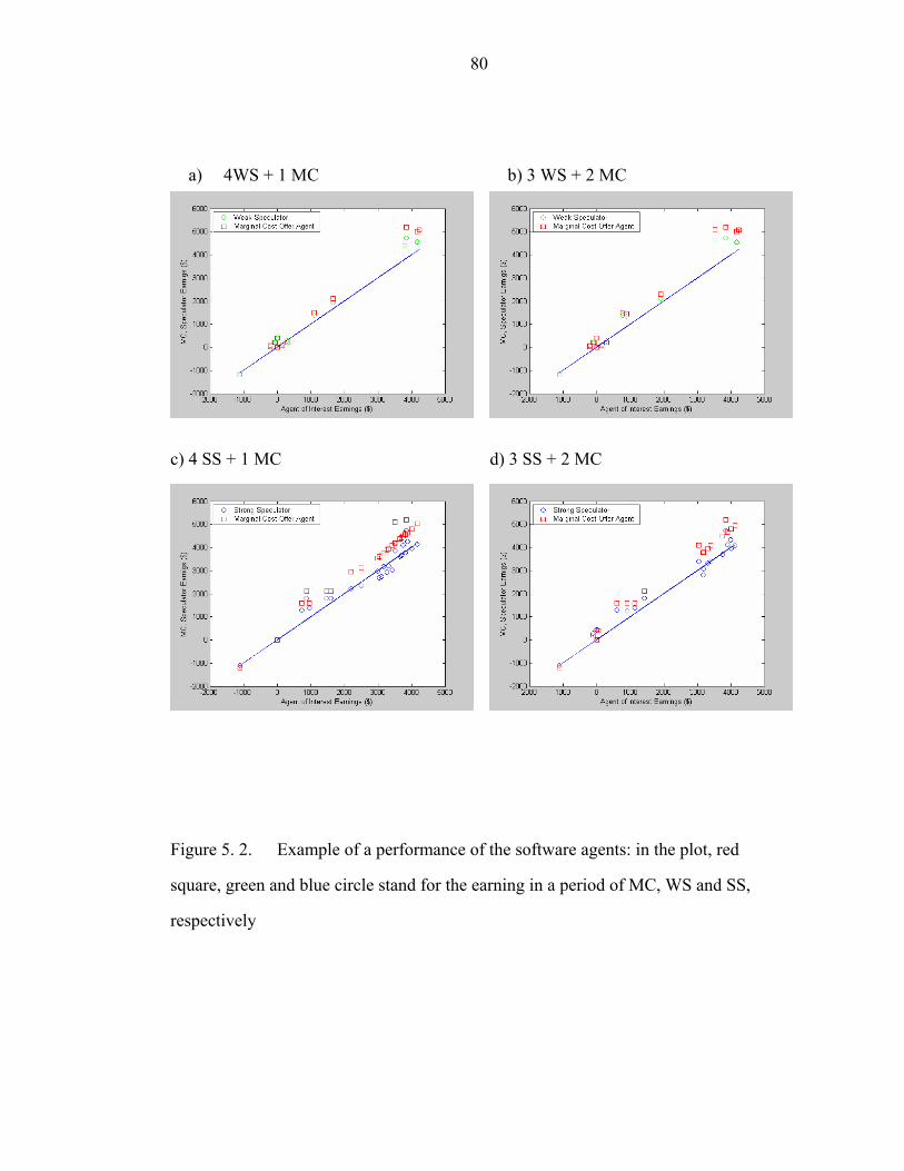
80
a) 4WS + 1 MC b) 3 WS + 2 MC
c) 4 SS + 1 MC d) 3 SS + 2 MC
Figure 5. 2. Example of a performance of the software agents: in the plot, red
square, green and blue circle stand for the earning in a period of MC, WS and SS,
respectively

81
For a simulation with a human subject, twenty students were recruited from the
class ECE 451, electric power systems, at Cornell University. Each of twenty students
participated in the simulation with five standardized agents just like the software
agents. The purpose of this experiment was to find out if the same technique that was
successful for classifying software agents could be used to determine human
strategies. The same sets of forecast and actual load were used for the simulation.
They learned from experience, and were consistent only in some scenarios. Therefore,
the data obtained only after a period of learning was useful for classification of the
scenarios. After examining earning data, ten periods were assigned to the learning
period. It was also found that the offer behavior of one student was similar to that of
an SS in some scenarios while the same student behaves like a WS in other scenarios,
i.e. different strategies were used when competing against different types of
competitors, which is logical behavior. Strategies other than ones used by the
standardized agents were also observed. The conclusion was that the set of
standardized agents was not rich enough and that it was possible to classify some of
the different strategies by adding the speculating agents SS2 and SS3 to the mix. A
typical simulation result is shown in Figure 5. 3.
In the case of a) and b), one was classified as SS2 and SS3 while the same one was
classified WS and SS in the case of c) and d), respectively. When SS3, a standardized
agent with the strongest degree of speculation, participated in the scenario described
above, a common feature was shown in plot b). What SS3 did was effectively
withhold its entire capacity from the market unless the market clearing price was high.
Therefore the market clearing price was high even in the low demand period, which
caused the earnings of all competitors to increase considerably. Even though this type
of strategy seemed not to be reasonable, it was often observed, especially when the
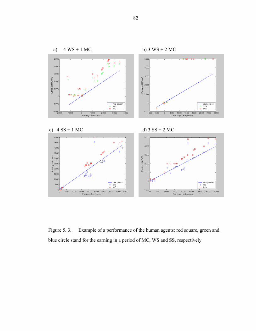
82
a) 4 WS + 1 MC b) 3 WS + 2 MC
c) 4 SS + 1 MC d) 3 SS + 2 MC
Figure 5. 3. Example of a performance of the human agents: red square, green and
blue circle stand for the earning in a period of MC, WS and SS, respectively

83
market was very competitive, i.e., for markets with an agent mix such as
3 WS + 2 MC that is in aggregate not very speculative. In less competitive mixes, such
as 4 WS + 1 MC or 3 SS + 2 MC, the strategy was rarely used.
For the case in which it was possible to classify a human agent, the total earnings
ofa human agent from the scenario was compared to that of the standardized agent of
the same type from the same scenario. The comparison between the two earnings is
shown in Figure 5. 4. The line corresponds a perfect correlation, which is y = x.
The correlation between two earnings was checked for both a software agent and a
human agent as long as it was possible to classify the agent of interest. It is critically
important to include all the standardized agents with extreme offer behaviors in order
to classify an agent of interest. Otherwise, some agent might not be properly classified.
For example, the agent of which earning is plotted in Fig. 5. 3. b) is not classified
properly since the agent of interest is far more speculative than WS and/or MC.
Another difficulty in classification is consistency. If the offer behavior of the agent of
interest is not consistent, the classification method described here would be judged not
reliable.
There was one interesting software agent worthy of special note. The agent offered
some of its capacity into the market at marginal cost, but started to withhold some
from its fairshare block. Therefore, its offer function was similar to that of SS except
that it withheld capacity from the fairshare block instead of offering it at a high price.
This offer behavior is termed a Cournot speculation. This agent was classified as SS as
long as at least one speculator exists in the market regardless of type such as WS or
SS.
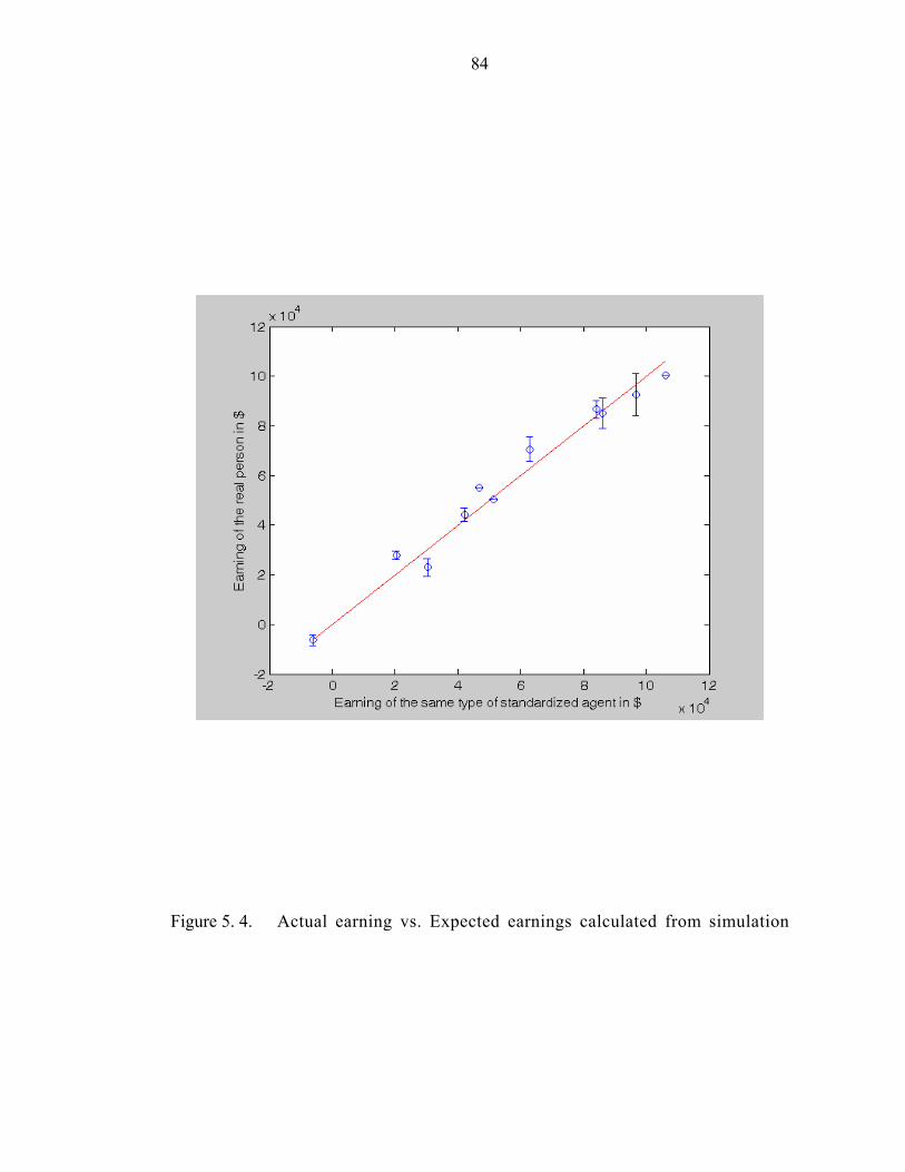
84
Figure 5. 4. Actual earning vs. Expected earnings calculated from simulation

85
5.2. Evaluation of Dimension by Using Price
Simulation results obtained from Ref. [12] were used for evaluating dimension of
the data. Since the price is a measure of the market considered, the dimension
evaluated is an estimate of the dimension of the market. The value for the mean of
demand was 490, and the error of demand forecast was 50. Price data obtained from
simulation of 300 to 1,000 periods were used for the dimension analysis. To estimate
d, C(ε) and ε is plotted in log-log scale in the range of ε from 10-2 to 106 as is shown in
Figure 5. 5, and power law is used. If the relation equation (72) were valid for all ε’s,
there should be a straight line of slope d. In this case like other practical cases, the
power law holds only over an intermediate range of ε. The curve saturates at large ε
because the balls with radius of ε surround the whole attractor and therefore the
number of neighborhood within ε cannot grow any further. On the other hand, the
balls with extremely small radius ε contains x only. Therefore, the power law holds
only in the intermediate scaling region. Data only in the intermediate region were
chosen for evaluating dimension.
From the analytical process, fractal dimension was obtained as a function of the
embedded dimension as is shown in Figure 5. 6. The true dimension was determined
about 2. Therefore, an embedded dimension of 5 should indicate a true dimension.
Fig. 5. 6 shows that the true dimension at the embedded dimension is about 2 which is
properly evaluated. The value for dimension depends on precision of demand forecast
as well as the types of market participants. In other word, dimension is a quantity
reflecting whole system under consideration. Once there is any change affecting the
system, dimension analysis will identify the occurrence of the change even though it
cannot tell what causes the change. The value of dimension is most sensitive to the
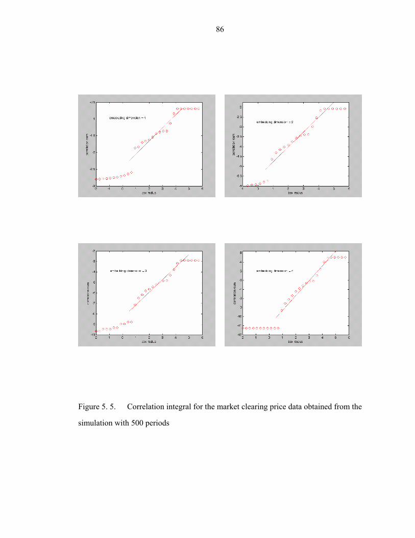
86
Figure 5. 5. Correlation integral for the market clearing price data obtained from the
simulation with 500 periods
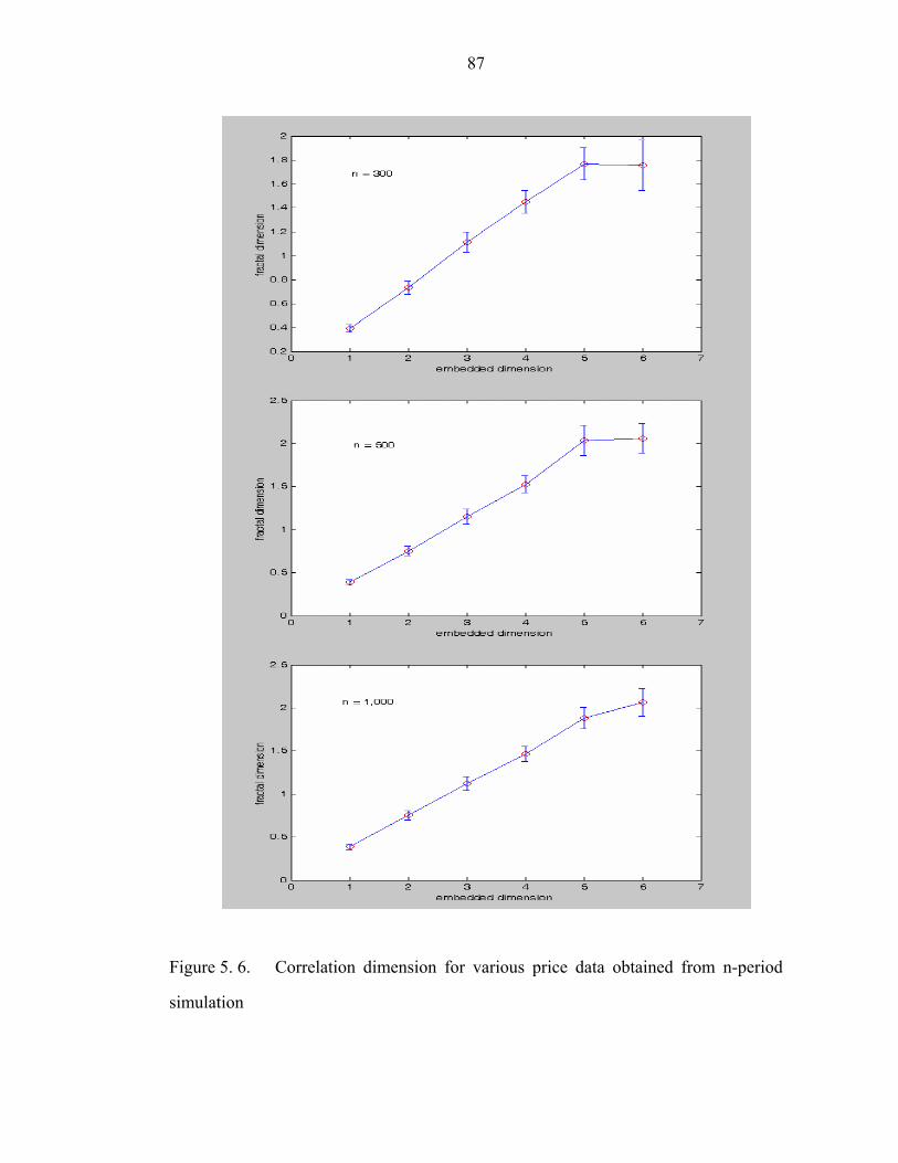
87
Figure 5. 6. Correlation dimension for various price data obtained from n-period
simulation

88
type of market participants. Besides, change in the precision of demand forecast or
other changes can be captured by other statistical tools too. Therefore, given results of
other analysis, it is possible to tell if the strategies of market participants have been
changed.
Figure 4. 1 shows several nodal price data obtained from the NY ISO’s web site.
The data were analyzed to estimate the value of correlation dimension and the
Liapunov exponent. When summer came, some agents changed their strategies to
increase clearing price. Then system dimension should change accordingly, which
results in the change in clearing price. But, the nodal price is more closely related to
the strategy of the agents located at the bus. As is shown in Fig. 5. 7, the state of York-
Warbasse changed during the period while that of Cornell did not. There might be
several reasons to change the state beside change in the strategy, i.e., a change in
network or offer strategies of other agents. However, only interest here is to check if
the system state which an agent must deal with has been changed. During the period,
York-Warbasse faced a different market from that before the period while Cornell did
the same or unnoticeably different market. Both cases, the Liapunov exponent had a
negative value which means the markets were settling down to a new equilibrium,
consequently all the data were relevant to estimate a future state.
5.3. Results from Simulations with Demand-side Agent and Discussion
A modified IEEE 30 bus system with 6 generators and 20 loads was used for a
simulation. Fig. 5. 8 shows the transmission network used in this study. In the system,
there are three different areas divided due to line constraints. A closer look to data for

89
Figure 5. 7 The change in systems which agents, York-Warbesse and Cornell,
faced during June 2003. While system of Cornell did not change significantly, that of
York-Warbasse evolved.
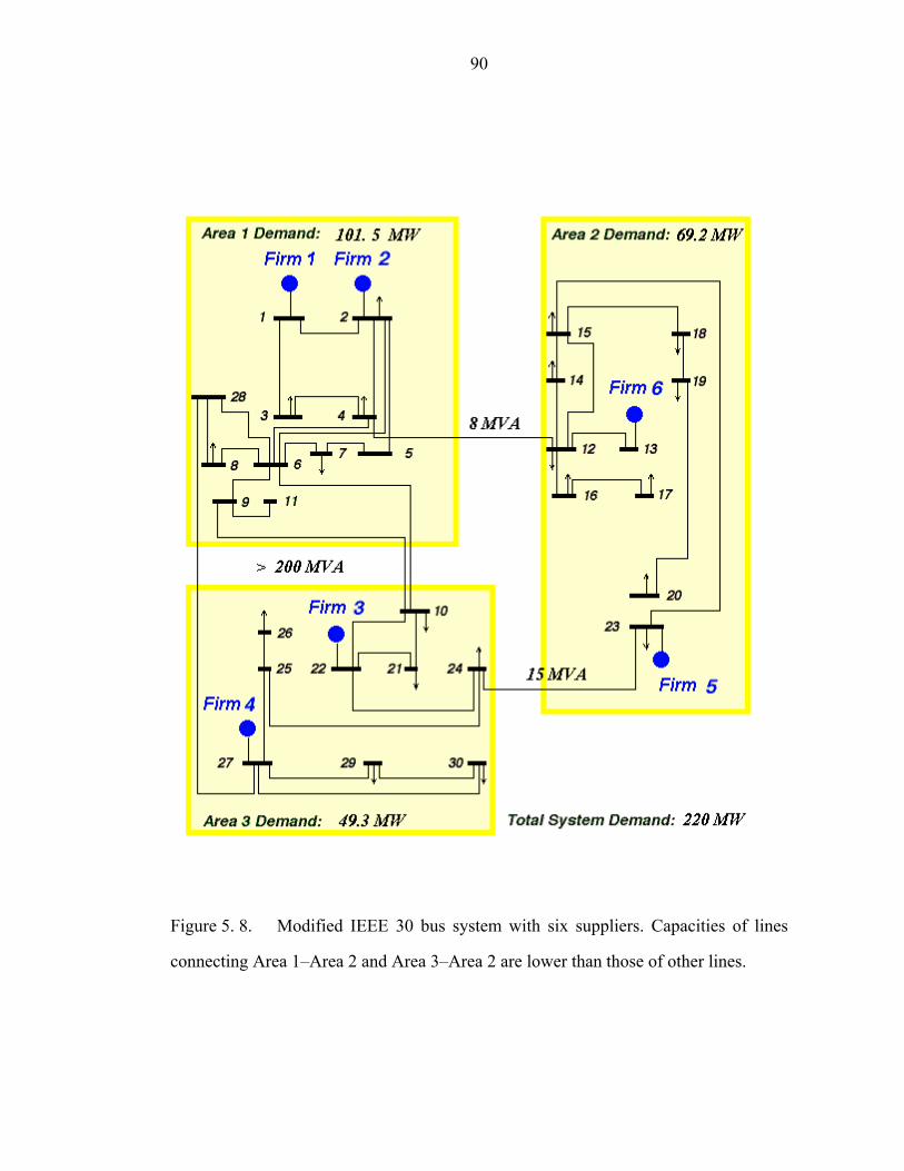
90
Figure 5. 8. Modified IEEE 30 bus system with six suppliers. Capacities of lines
connecting Area 1–Area 2 and Area 3–Area 2 are lower than those of other lines.

91
line constraints allows clustering between Area 1 and 3 with no significant loss of
generosity since line capacities between the two areas are large. Due to strict line
constraints between Area 2 and the clustered area, Firm 5 and 6 have a locational
benefit in case of heavy load in the Area 2, which implies a potentially duopoly
situation. Actual demand seems to have weekly and hourly periodicities. To mimic
these periodic behaviors, a convolution between two sine functions added with small
values of random number were taken for an actual demand. For the purpose,
convolution of two functions f(x) and g(x) over a finite range [0, t] is performed in the
following way:
( ) ( )∫ −≡⊗t
dtgfgf0
τττ (77)
where the symbol gf ⊗ denotes convolution of f and g.
To emulate the periodic behaviors of load as well as stochastic behaviors, the
functions f and g were taken as
( )
( ) weekweekweek
week
daydayday
day
BtA
tg
BtA
tf
δτ
π
δτ
π
+⎥⎦
⎤⎢⎣
⎡+⎟⎟
⎠
⎞⎜⎜⎝
⎛=
+⎥⎥⎦
⎤
⎢⎢⎣
⎡+⎟
⎟⎠
⎞⎜⎜⎝
⎛=
12sin2
12sin2
(78)
where A, B denote fluctuation of load for periodic part and that for stochastic part,
respectively, and τ and δ stand for periodicity and for random value in [0, 1],
respectively, and subscripts represent time period.
Several simulations with various types of supply-side agents have been performed.
There are two extreme cases in the simulations: all suppliers are marginal cost offer

92
agents or all speculators. For the first case, there is no need to include demand side
participation since a market clearing price is already low enough. On the other hand,
there is no need for demand side participation for the second case either because
demand-side participation can make little improvement on the situation since
must-be-served unit needs power regardless price and dispatching only the unit
already requires a high market clearing price. To get a more realistic simulation result,
two scenarios were selected based on the types of real suppliers observed in PJM
market shown in Figure 5. 9. For Case a) which is the more competitive market, while
the average market clearing price is about $ 550/MWh with inelastic demand without
demand-side participation, it was less than $ 100/MWh with a demand-side
participation. Case b) is more interesting in that there were many price spikes to meet
inelastic demand due to highly volatile market. Demand-side participation lowers the
number of price spikes as well as average price in both cases. Some price spikes are
eliminated by backing up less than 10 % of load while some are reduced by a
significant amount that requires declaring PRL. When significant deduction occurs,
the number of allowed PRL is decreased by one which resulted in a decrease in
freedom. Consequently, a bid curve approaches the inelastic demand curve. When
number of allowed PRL goes to zero, the bid curve of demand-side agent looks
identical to that of inelastic demand. Therefore, market clearing price are same. For
example, the results with elastic demand after 720 periods is equal to those without.
5.4. Simulation Results with Adaptive Supply-side Agents and Discussion
In this section, implementation detail for a supply-side agent is presented.
Furthermore, several simulation results with the agents designed in this study are
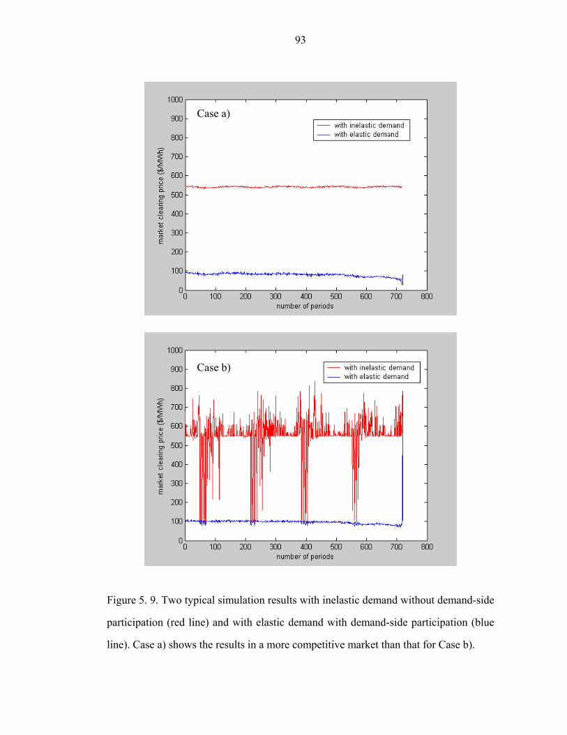
93
Figure 5. 9. Two typical simulation results with inelastic demand without demand-side
participation (red line) and with elastic demand with demand-side participation (blue
line). Case a) shows the results in a more competitive market than that for Case b).
Case a)
Case b)

94
presented and discussed.
5.4.1. Description of adaptive supply-side agents
With no change in behavior of all the participants, the state of a market remains
unaltered even under stochastic demands as long as the distribution of demand does
not change significantly. However, by the nature of a market, there is always a change
in the strategy of market participants. Once there exists such a change in the market,
the change acts as a new driving force leading to a change in the market state.
Consequently, future state somewhat deviates from an expectation if the expectation
was extrapolated from the observation made on the previous state of a system.
Therefore, the offers in learning period must be carefully selected in order not to
disturb the market. Otherwise, the observation made is not useful for the estimate of
future market. Since current market rules do not allow communication amongst
market participants, the only way to collect data is participating in the market. Once
the agent participates in the market to collect data, the participation inevitably drives a
system into a new state, which makes its collection of data irrelevant. The best way to
solve this dilemma31 is minimizing the difference between current and new state. For a
dynamic system, it is well known that the degree of the change in system
proportionally depends on the magnitude of the driving force. There are two ways to
minimize the magnitude of the driving force: minimizing driving forces in each period
and minimizing the sum of driving forces. Withholding most capacity from the market
for all the periods may introduces a minimal change in the system when the
31 to collect data, an agent needs to participate in the market, but participation may change the system which makes collecting data useless

95
perturbation due to the introduction of the agent is small enough not to alter market
much. However, this should be avoided since such participation results in exploring
only limited area of a search space of mapping function. A better way is the second
choice: exploring more search space while the offer does not alter the state much.
When significantly many random vectors are summed over, the net vector has a very
small magnitude since they are canceled out with each other [18]. With given values
of short-term and long-term variables, the main variables are randomized in a
following way: for n learning periods, equally distributed vectors a and b32 are chosen
from distributed from minimum to maximum values of each variable, and then the
elements in two vectors are randomly selected for an offer.
Each period in a learning process, the element in a matrix for simulated earning, A,
is calculated based on initial scenarios. After learning period, the scenario set is
evaluated to test its validity. Since the scenario set is not the complete basis set, a
wrongly chosen one cannot represent the actual market properly. From an error
minimization process with simulated and actual earning A and b, the weight factor x is
estimated. When the process does not give a satisfactory result33, the scenario set will
be altered based on the contribution to expected earning. The actual earnings are more
closely related to the competitor(s) located at the same area. Therefore, only the
portion of scenarios for the competitors will be modified while the portion of scenarios
for “far apart” agents which are located in different area are intact. It is noteworthy to
mention that all the extremes must be included in the scenario sets even after the 32 [ ] [ ]maxmax , and , ppbdda ∈∈ where d, pmax xx and stand for degree of speculation, maximum offer price, minimum and maximum value of the variable x, respectively
33 2
2
2 ofminimizati theofresult theis x where bAxb
bAx−≤
−δ and δ is the
satisfactory limit

96
modification in order to guarantee that the scenario set represents the actual
competitors.
When a learning period ends, an agent finds a proper scenario set minimizing the
error of 2
bAx − . With the modified scenario set, it finds an optimal offer for each
period. For the optimization process, the expected demand for a coming period is
obtained by using neural networks. To achieve this, the data obtained during learning
process is eliminated for a better estimate since its offer strategy after learning period
is not randomly distributed anymore. For this period, the new offer strategy might
make the whole market evolve. Therefore, a dimensionality check during learning and
this period is not required since the new state is not guaranteed to be relevant to
previous ones. The dimensionality check is performed after another k periods. It is
possible that the state after k periods might be different from that of the state before
since the new strategy during k periods may system evolve. However, the state cannot
be far from the last state since the strategy of the agent did not change over k periods.
Consequently, the expectation based on similar state should work well.
After the first dimension check, the agent keeps checking dimension every day to
see if there is any change in the market. If it finds no significant change in dimension,
it assumes that the current state is not far away from former state, and then keeps using
the current data set with more added market clearing results. When there is change in
the value of the dimension, there assumed three main possibilities which make system
changed: change in the strategy of its own, those of competitors and condition of
market such as network change, etc. The first possibility is easiest to detect since the
agent already knows even before the check. Note that dimensionality check will give a
clue on the effects of the change in its strategy if there is any. The third possibility is

97
also easily found by assumption that the agent has good knowledge on network by
using external information, e.g., Genscape34. Once the agent detects the change in
dimensionality and also finds the reason is not any of those two above, and then it
assumes the change in the strategies of its competitor(s) makes the state of the system
evolve. In the case that there is unknown change in network resulting in a change in
the system state, it will get a wrong reason about the change. Consequently, the weight
factor distribution from the error minimization 2
min bAxx
− might cause a bigger
error. However, as far as its earning concerned, the weight factor distribution performs
well in the optimization process since the distribution came from the process of the
error minimization. Once it detects the change in the state for any reason, scenario sets
and matrix A need to be modified for a better system estimate.
When an agent finds any change in the state, there may not be enough data obtained
from a new system. In such a case, the number of row in A is less than that of column,
i.e., an underdetermined system. In treating a underdetermined system in the matrix
computation, the weight factor distribution inevitably contains many zeros which may
lead inappropriate representation to a real market. To avoid this problem, the most
recent data obtained from the old state are added to the new data under assumption
that old state might not be too different from the new one. To have the new data more
impact on the weight factor distribution, heavy weight is given to the new data by
adding many copies of the new data into the matrix A and the vector b. If difference
between the two states is significantly different, the weight factor distribution might
results in a bigger error for a mapping function from offer to earning. However, if this
is the case, the market is very unstable, and then no agent performs well in the
circumstance.
34 http://www.genscape.com/na/index.shtml

98
5.4.2. Simulation detail and results
Several simulations have been performed with the supply-side and demand-side
agents described here. All demand-side agents have must-be-served demand about
10 % of their total demands. To see the performance, only one supply-side agent was
placed on the Bus 23, and standardized agents represented other firms. To emulate
different situations, several markets with different types of competitors have been
simulated. Figure 5. 10 shows simulated historical nodal price data both competitive
and volatile markets. In these simulations, none of competitors change their strategies,
but it is common for each agent to exercise market power by trying other strategies.
To test how an agent reacts against a permanent and consistent change, after some
periods, a competitor changes its strategy consistently. The results are shown in Figure
5. 11. For the current market, it is allowed for a buyer to purchase electricity from a
seller from outside. When there exists such an independent contract, external flow
must be injected through network. The external flow might not be known to all the
supply-side agents, but it changes power flow to some extent. The change results in a
virtual change in the network. If a supply-side agent does not know the existence of
the flow, its ability to find a change of the market state needs to be tested.
Furthermore, it might be useful to know how the agent reacts against the change if it
finds. To check this ability, a simulation with five standardized agents and one supply-
side agent from outside has been performed in a following way: no change in the
strategies of the standardized agents was made, but after 200 periods external flows
about 10 MW from the Bus 28 to the Bus 20 are injected. Figure 5. 12 shows the
prices obtained from the simulation. Above three different simulations, the agents of
interest always have locational benefit. For testing the performance in case without
locational benefit, a simulation was performed with an agent on behalf of Firm 1 in the
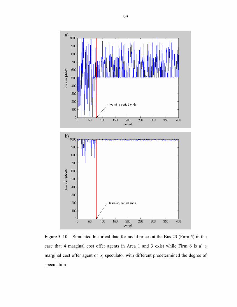
99
Figure 5. 10 Simulated historical data for nodal prices at the Bus 23 (Firm 5) in the
case that 4 marginal cost offer agents in Area 1 and 3 exist while Firm 6 is a) a
marginal cost offer agent or b) speculator with different predetermined the degree of
speculation
a)
b)
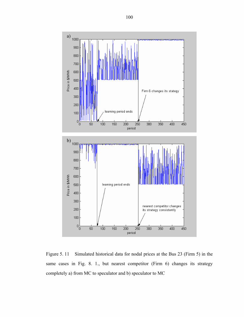
100
Figure 5. 11 Simulated historical data for nodal prices at the Bus 23 (Firm 5) in the
same cases in Fig. 8. 1., but nearest competitor (Firm 6) changes its strategy
completely a) from MC to speculator and b) speculator to MC
b)
a)
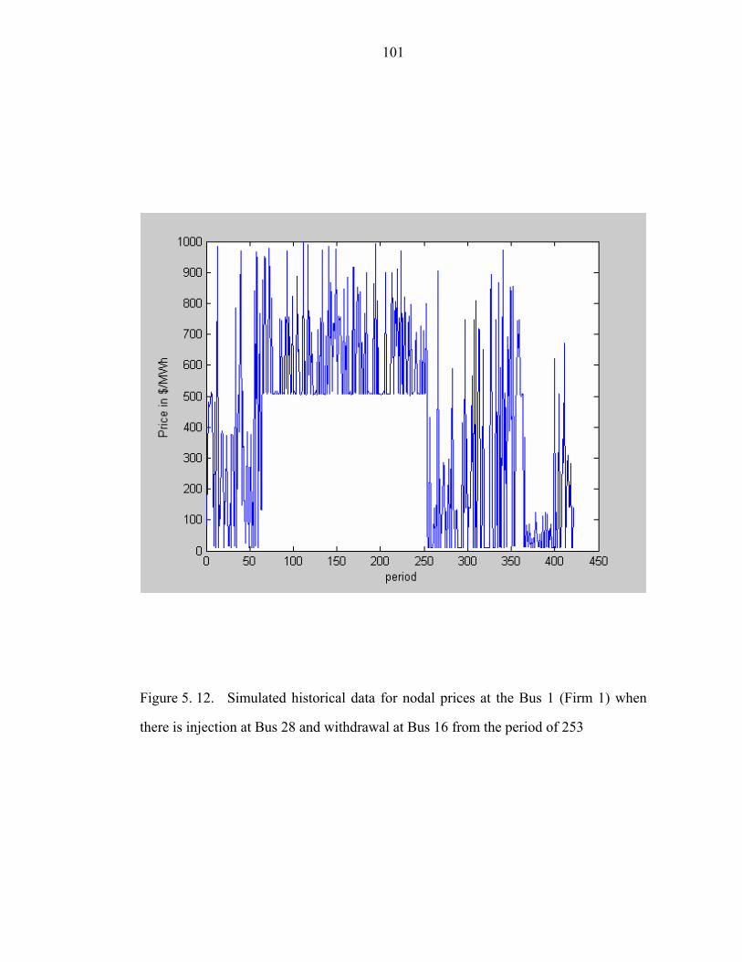
101
Figure 5. 12. Simulated historical data for nodal prices at the Bus 1 (Firm 1) when
there is injection at Bus 28 and withdrawal at Bus 16 from the period of 253

102
same situation described in Figure 5. 11. The results are shown in Figure 5. 13.
5.4.3. Simulation with no change in the strategies of competitors
The competitors have differently assigned DOS; for Firm 1 – 4 were 20, 10, 25
and 15 respectively, and that for Firm 6 was 25 for a) and 85 for b). During learning
periods, the nodal price data for the agent representing Firm 5 fluctuate from its
marginal cost to reservation price with mean of about $ 400/MWh and $ 900/MWh,
respectively. After learning periods, it updates the scenario set based on the error
minimization process. Original matrices A contain simulated earnings from equally
distributed scenario sets, and the relative errors ( )22
/ bbAx −= were about 52 %
and 38 % for a) and b), respectively. Note that equal distribution of strategy set was
assumed before participating in the market. The matrices A were modified based on
the contribution to expected earnings of each scenario. For a), the second most
speculative scenario with the value of 75 for DOS was discarded and replaced with a
scenario between most and second most competitive scenarios with DOS of 12.5. On
the other hand, the second most competitive scenario with DOS of 25 was replaced
with one of 87.5 for DOS for b). The modification of scenario set reduces error to 46
% and 27 %. With the new modified scenario set, the agent tried to find an optimal
offer at given load forecast.
On a daily basis, the dimension was checked for detecting if there is a change in
the market state. Figure 5. 14 shows the result of the dimension check. Since 100 data
points are needed for a reliable dimension check for a dimension with a value of 2,
only after 8 days the value for a dimension is reliable. From a), the dimension check
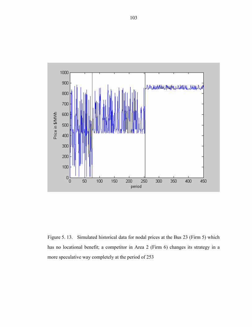
103
Figure 5. 13. Simulated historical data for nodal prices at the Bus 23 (Firm 5) which
has no locational benefit; a competitor in Area 2 (Firm 6) changes its strategy in a
more speculative way completely at the period of 253

104
does not detect any conceivable change in the state of market after the 8th day, which
was true in fact. The false alarm on day 7th may cause unnecessary consideration on
Day 8th as well as Day 7th. On both days, the agent checks the dimension and finds a
change in the state. Then, the agent selects the part of data for estimate based on its
data selecting algorithm discussed in chapter four. The selected data contain the
information of the same state which the agent must observe from. Therefore, the
performance of an agent should not be affected by the false alarm in this case. There is
a possibility that malfunctioning of the tool may cause wrong selection of data causing
silence after a change in the market state. In the current setup, the probability is very
low since the tool should not inform a change for many days. Note that the agent
evaluates dimension everyday. The dimension check shown in b) gives almost
identical case except to exhibit relatively larger errors which makes the result less
reliable. An agent might be uncertain if there is any change in the state. All the
experimental data contain error, and correspondingly, an analysis made on such data
has reliability issue when noise over signal ratio gets bigger. In the simulation for b),
the change in the nodal price is relatively. In such a case, the dimension check may
give unclear conclusion due to large error. Since two adjacent points in Fig. 5. 14 b)
are overlapped in error range, the probability that the system is not changed is more
than 10 % which is not small enough to ignore. Consequently, an agent assumes there
is no change in the market state.
When the dimension check does not detect any change in the state of the market,
an agent needs data for the matrix A and vector b for finding weight factor
distribution, which might contain too many rows. It is not economic to carry too much
data for a computation. To select proper amount of data for estimating a future state,
the Liapunov exponent calculation was performed. Figure 5. 15 shows the results of
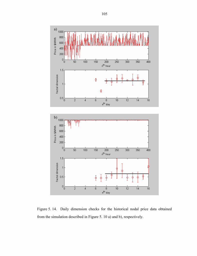
105
Figure 5. 14. Daily dimension checks for the historical nodal price data obtained
from the simulation described in Figure 5. 10 a) and b), respectively.
a)
b)

106
the Liapunov exponent calculation. Both a) and b) shows no positive exponent clearly,
and especially for b), the values are clearly negative. A negative exponent implies that
the system settles into an equilibrium or a strange attractor. In such a case, all the data
are relevant for estimating a future state, but for computational convenience, only part
of the data is taken for calculating weight factor distribution. Note that default value in
this study is 100 when the number of scenarios in a scenario set is 25. In both cases, an
agent can check whether or not the system evolves based on a dimension check and
then Liapunov exponent.
With a given weight factor distribution, an agent finds an optimal offer to
maximize its profit for a given forecast. As was shown in Fig. 5. 10 a), the agent
manages to keep the nodal price no less than $ 500/MWh while the price fluctuates
from $ 10 to $ 1,000/MWh when random offers were submitted. The similar situation
occurs in Fig. 5. 10 b). Figure 5. 16 shows the simulated historical earnings for both
cases from the simulation as was described in Fig. 5. 10. For b), the nearest competitor
offers its quantity at a high price, and consequently the market that the agent
representing Firm 5 faces must accept offers submitted by Firm 5 unless its offer is too
high. Therefore, average earning from learning period are not much different from that
after the period. About 30 % increase in earning was achieved. When a market is more
competitive like in a), earning depends more on the offer by the agent. Average
earning in the learning period was $ 6,000/h, but that after the period was about
$ 10,000/h which was approximately 70 % increase. To show how well the market
modeling is done, the expected earnings is plotted also in red line. The relative errors
during learning period are 46 % and 27 % as was mentioned before, but those after the
learning period are 19 % and 1 %. During the learning period, an agent searches all the
space available by submitting random offers. After the period, an optimization process
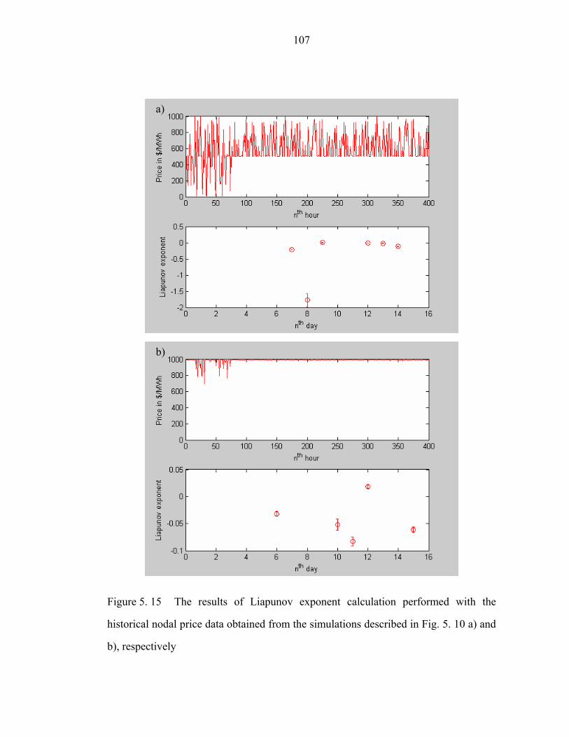
107
Figure 5. 15 The results of Liapunov exponent calculation performed with the
historical nodal price data obtained from the simulations described in Fig. 5. 10 a) and
b), respectively
a)
b)
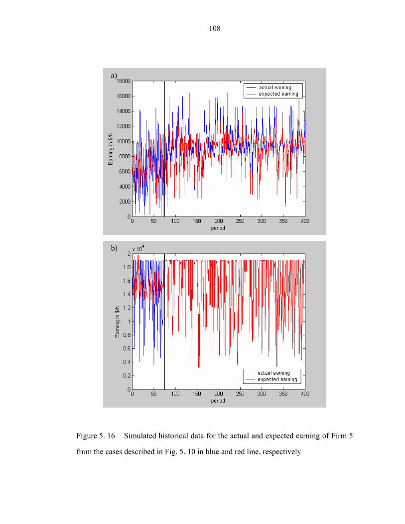
108
Figure 5. 16 Simulated historical data for the actual and expected earning of Firm 5
from the cases described in Fig. 5. 10 in blue and red line, respectively
a)
b)

109
restricts the search space into a small area, which is well defined. Therefore, the
relative error should become significantly small. When the market gets less
competitive, the optimizing strategy is selling more quantity to the market by offering
lower price. Then, the search space is very limited, and then the error should be
significantly small, which was 1 % in comparison to 19 % for a more competitive
market.
5.4.4. Simulation with the change in the strategies of competitors
Before Firm 6 changes its strategy, the agent representing Firm 5 behaves
approximately identical to the case described in Section 5.4.3. The relative errors were
about 65 % and 33 % for a) and b), respectively. Modifying scenario set as described
in Section 5.4.3 makes error reduced to 59 % and 28 %, respectively. With the new
modified scenario set, the agent tried to find an optimal offer at given load forecast.
A dimension check was performed everyday in order to detect if there was a change
in the market state. The results are plotted in Figure 5. 17. For a), a dimension check
detects a conceivable change in the market state 4 days after Firm 6 changes its
strategy. A dimension check shown in b) gives almost identical case as was before. A
dimension check detects the change in the market state reliably in both cases. When
the state of the market changes, it is important to find how long the change takes to
settle into a new equilibrium state. The question can be answered by evaluating
Liapunov exponent. In general, it takes two times of the inverse exponent for the
system to reach another equilibrium. Figure 5. 18 shows the results of evaluation to
the exponents. In both cases, the exponents after the change was made are very small
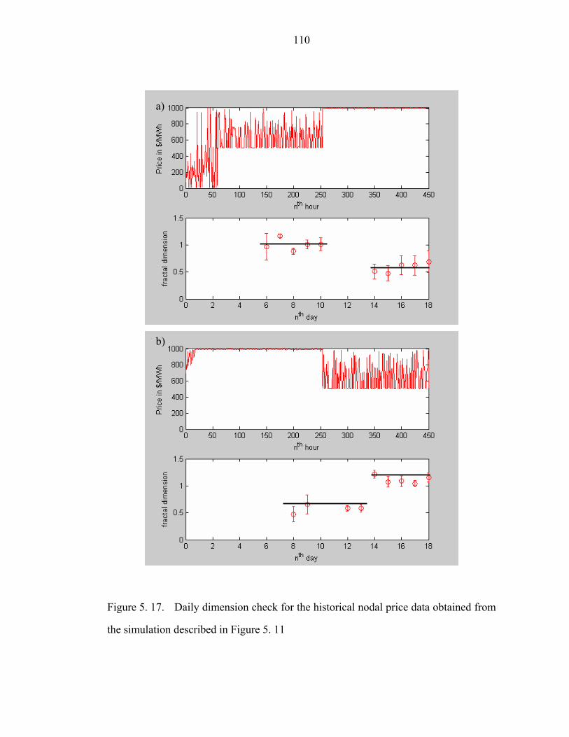
110
Figure 5. 17. Daily dimension check for the historical nodal price data obtained from
the simulation described in Figure 5. 11
a)
b)
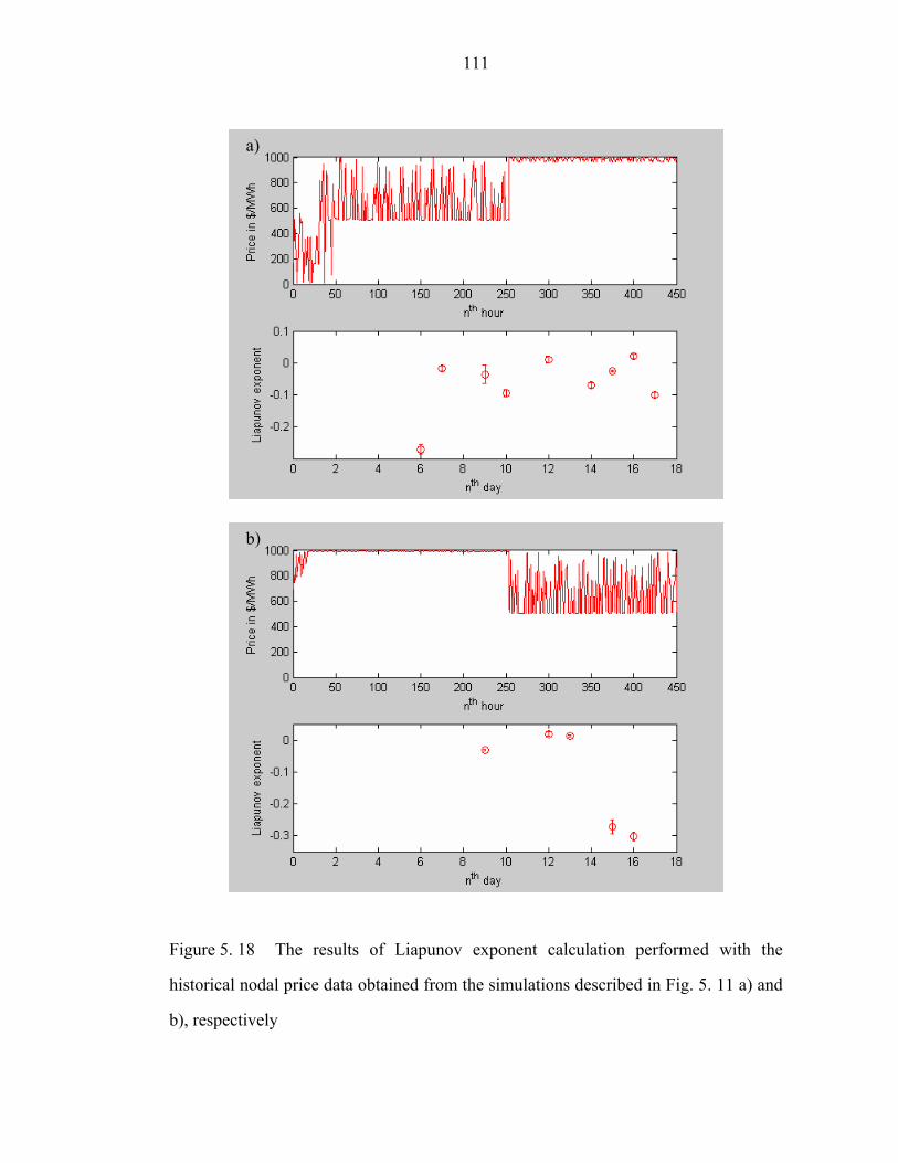
111
Figure 5. 18 The results of Liapunov exponent calculation performed with the
historical nodal price data obtained from the simulations described in Fig. 5. 11 a) and
b), respectively
a)
b)
112
positive numbers. For example, the values of the exponents at day 12 and 16 for a) and
b) are very small and positive. In evaluating the Liapunov exponent, only a few points
were randomly taken to avoid choosing biased data, and the actual value of the
exponent greatly depends on the choice in the point selection. Consequently, the value
of the exponent is less reliable especially when it is small. For negative or zero values
of the exponent, an agent chooses only a small number of data to calculate weight
factor rather than whole data for saving computational effort. When the exponent has a
large positive value with small error, it implies that a system divulges very fast. A
small positive value of exponent, like in these cases, implies that the dynamics is very
slow, and then approximately 2 times of inverse exponent of data points are relevant
for estimating a future state. Since the exponent tells how recent data are relevant to
estimate a future state, it only gives an upper limit for the number of data that an agent
should take. In both cases here, more than 100 and 200 data points are upper limits for
a) and b), respectively. It is noteworthy that for b), the dimension was approximately
1, and the embedded dimension was 2. Correspondingly, one point in embedded
space is composed of two data points, which results in 200 data points of upper limit
for b). Therefore, a default value was taken for estimating weight factor distribution.
From the results of the dimension check, the performance of an agent before
finding the change in the market state seems as good as that after finding. Dimension
check and the Liapunov exponent give an agent a guideline to select the amount of
data. Before the change of the market state, dimension check gives no change and the
Liapunov exponent calculation gives a negative value, which allows an agent to take
only 100 data points. Before the agent realizes the change in the state, several new
data has been added into the 100 data points. Consequently, the effect of the new
addition is not negligible. Without using the dimension and exponent, the agent should

113
carry all the data, and then the effect is small enough to be ignored since the fraction
of the new data is small in comparison to the amount of data obtained from the former
state. Thus, the performance could not be so good as an optimal one. For a randomly
generated offer, the nodal price fluctuates a lot in a). The price during a learning
period represents the nodal price in case of a random offer. It also fluctuates between $
700/ MWh and $ 1,000/MWh for b) during the period. Once the agent finds a proper
weight factor distribution, the price never go below $ 500/MWh and $ 990/MWh for
against competition with MC and speculator representing Firm 6, respectively. DOS
for Firm 6 was changed from 25 to 85 for a) and from 85 to 25 for b) while DOS’s for
other firms were unchanged.
The agent finds an optimal offer to maximize its profit for a given weight factor
distribution and forecast. As was mentioned before, the agent manages to keep the
nodal price no less than $ 500/MWh and $ 990/MWh for a) and b), respectively. Note
that price fluctuates when random offers were submitted during a learning period.
Figure 5. 19 shows the historical earnings for both cases from the simulation as was
described in Fig. 5. 11. The results were almost identical to the cases described in the
section 5.4.3 when Firm 6 behaves in the same way as was in the section. The errors
after the learning period and before the change in the strategy of Firm 6 were 17 %
and 1 %, respectively, and those after the change were 1 % and 21 %, respectively. A
more inefficient market allows an agent to explore larger offer-earning space. From
Fig. 5. 19 a), the earning recovers to an optimal one very quickly. When the agent
faces a more competitive market, the search space it explores is less limited, and it
should take a long time to find a new optimal strategy. As was shown in Fig. 5. 19 b),
after a sudden change in the market state, the earning shows a typical initial stage of a
relaxation curve. However, the relaxation was not fully developed because the agent
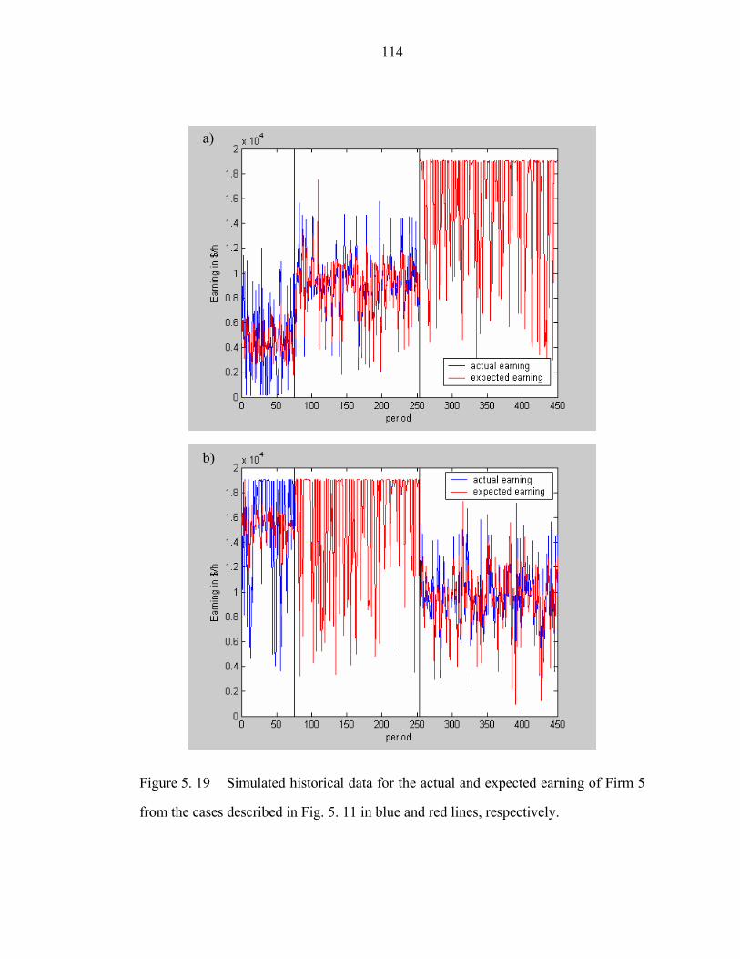
114
Figure 5. 19 Simulated historical data for the actual and expected earning of Firm 5
from the cases described in Fig. 5. 11 in blue and red lines, respectively.
b)
a)

115
adjusted its strategy quickly. It is noteworthy that the performance of the agent after
the sudden change in the strategy of Firm 6 quickly recovers to the optimal one.
Though Firm 6 does not change its strategy from period 1 to 253, there were many
fluctuations in the nodal price as shown in Fig. 5 .11 b). When the market is monitored
by a snap-shot type tool such as one currently used in several ISO’s, an agent should
check the change of a system and adjust its strategy accordingly. The unnecessary
check would cost in computation, and the adjustment would make its performance
worse.
To study the strategy of the agent, the degree of speculation and the maximum
offer price (MOP) were plotted from learning period, and periods before and after the
sudden change of the strategy in Firm 6 as shown in Figure 5. 20. The figures in the
first row in both Figs. 5. 20 a) and b) show the variables chosen for offers during the
learning period. Figures in the second and third rows illustrate the variables before and
after the sudden changes described in Fig. 5. 21. Second row in a) and the third row in
b) correspond to the simulation against more competitive agents, while third row in a)
and second row in b) do against less competitive markets. The variables from the
simulations against more competitive agents seem to fluctuate more often, but it is
difficult to find a difference in patterns observed both before and after the change. For
getting a clearer insight, the ratio between the two variables, MOP/DOS, was
calculated and plotted in Figure 5. 21. Both figures clearly show that the ratio
increases as the competitor gets more and more speculative, and consequently, the
market that the agent faces becomes less competitive. For a less competitive market,
the agent can take advantage of the other agents by being less speculative; i) by
reducing DOS and/or ii) by offering more quantity into the market, accordingly
increasing MOP. In both i) and ii) cases, the ratio increases by decreasing denominator
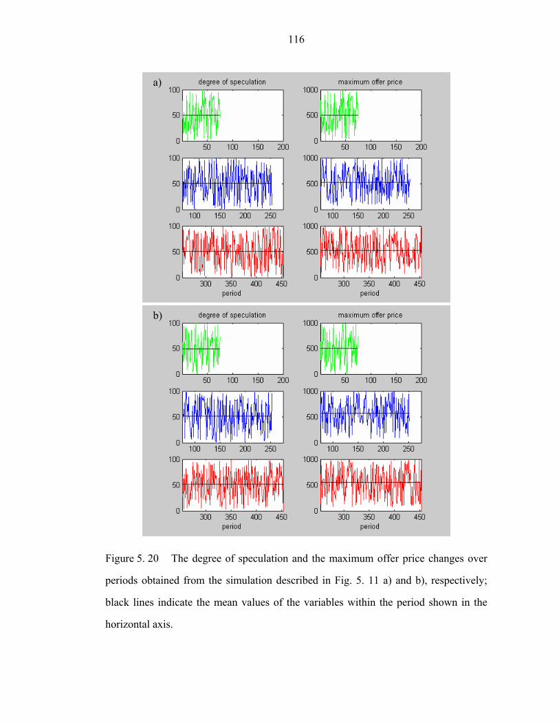
116
Figure 5. 20 The degree of speculation and the maximum offer price changes over
periods obtained from the simulation described in Fig. 5. 11 a) and b), respectively;
black lines indicate the mean values of the variables within the period shown in the
horizontal axis.
b)
a)
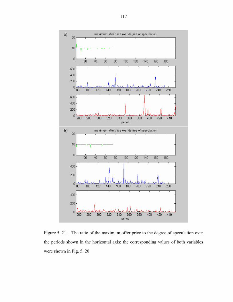
117
Figure 5. 21. The ratio of the maximum offer price to the degree of speculation over
the periods shown in the horizontal axis; the corresponding values of both variables
were shown in Fig. 5. 20
a)
b)

118
and increasing nominator from the former and latter case, respectively. Contrarily, the
agent would increase its earning in a competitive market by being more speculative; i)
by withholding more quantity from the market resulting in decreasing MOP and/or ii)
by increasing DOS. In both cases, the ratio decreases.
5.4.5. Simulation with unknown external flow
Before an external flow exists, the price behavior is practically identical to the case
described in last section. Modification on the scenario set reduces error to 58 % from
62 %. After the learning period and before the occurrence of the injection, the error is
reduced to 16 %. After an external power injected into the system, the relative error
increases up to 72 % of the relative error. As was shown in Fig. 5. 12, the prices after
the occurrence of unknown injection fluctuate from zero to reservation price. When
the prices are compared to those during learning period, the market seems even more
stable due to the unknown external flow.
Figure 5. 22 a) shows the result of dimension check for finding any change in the
market state. A conceivable change in the market state is detected by evaluating a
dimension. As is shown in Figure 5. 22 b), the values of most Liapunov exponents are
negative. Two points are positive with less than 0.1, which means that a system
evolved fairly fast. With 0.1 of Liapunov exponent, only about 20 data points were
relevant to predict a future state, which is less than a default of 100. In such cases, data
obtained from the previous state are added to form A and b while more importance is
given to the new data. Since it does not know there was an introduction of an external
flow and other possible changes and it did not change its own strategy on purpose, the
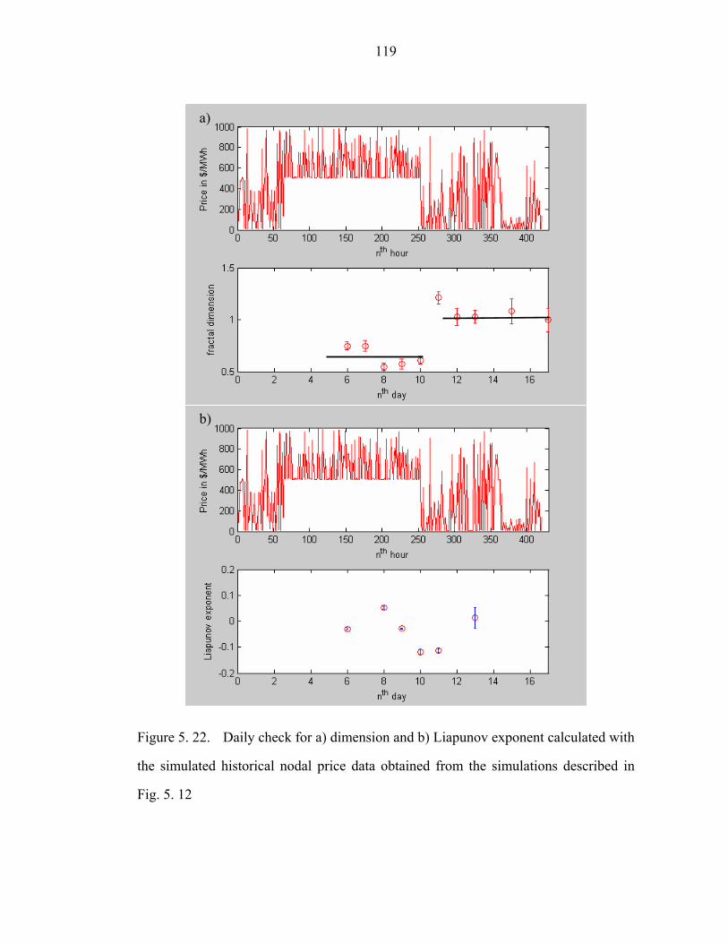
119
Figure 5. 22. Daily check for a) dimension and b) Liapunov exponent calculated with
the simulated historical nodal price data obtained from the simulations described in
Fig. 5. 12
a)
b)

120
agent assumes the change in the state is due to a change in the strategies of its
competitors. Demand forecast provided by ISO includes the demand fulfilled by the
external injection. Consequently, the demand contributes the value of fairshare,
resulting in an overestimate for fairshare even if the demand is not fulfilled by any
agents in the network. From the overestimated fairshare, the agent assumes that the
market gets more competitive. Note that the information on quantity served by the
competitors is not publicly available.
Consequently, the same value of the weight factor distribution does not properly
map offer to earning. The agent updates the weight factor distribution and modifies the
scenario set as well. As a result, the matrix A contains wrongly calculated values, and
the weight factor distribution does accordingly. To compete against the “changed”
competitors, the agent updates its strategy according to the way described in the last
section: to decrease the ratio between MOP and DOS. The changes in the main
variables and the ratio are shown in Figure 5. 23. Even if the error minimization finds
the optimal weight factor distribution, the error must be significantly large according
to the magnitude of the injection.
Figure 5. 24 shows the difference between the actual and expected earning. The
actual earning after the change fluctuates more than that of expected earning. The
reason is the actual system is spanned with a quite irrelevant scenario set. The relative
errors during a learning period, before and after the injection occurs, were 58, 16 and
71 %, respectively. Significantly high values for the relative error between expected
and actual earning (78 %) is a signature of the wrongly chosen scenario set. However,
the same choice worked well with the error of 16 %. Therefore, it is possible for the
agent to conclude that there is a change which needs updating the basis set instead of
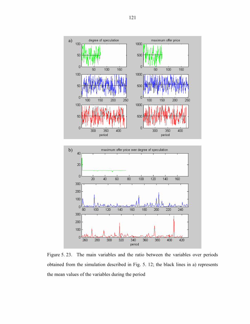
121
Figure 5. 23. The main variables and the ratio between the variables over periods
obtained from the simulation described in Fig. 5. 12; the black lines in a) represents
the mean values of the variables during the period
a)
b)
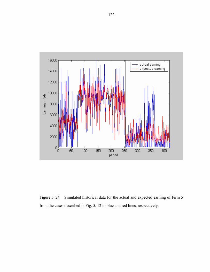
122
Figure 5. 24 Simulated historical data for the actual and expected earning of Firm 5
from the cases described in Fig. 5. 12 in blue and red lines, respectively.

123
adjusting the weight factor distribution. Once it gets the information, the agent should
find the proper reason why the market state changed. As was discussed in Section
5.4.1, there are three reasons why the market state changes: change in the strategies of
market participants and the other reasons like change in network. Most likely, the
other reasons could be considered further to explain the change in the state of the
system.
5.4.6. Simulation with an agent representing a firm without locational benefit
Similar to Section 5.4.4, the prices at the Bus 1 where an adaptive agent is located
change approximately identically to the case shown in Figure 5. 11. a). Both height
and frequency of the price spikes are a little lower than those in Fig. 5. 11. a). Before
Firm 6 changes its strategy, the relative error was about 58 %. For a better estimate,
the agent modifies the scenario set modeling its neighboring competitors located in
Area 1 and 3 while leaving scenarios for Firm 5 and 6 unchanged. Modification of the
scenario set described above makes error reduced to 51 %. With the new modified
scenario set, the agent tried to find an optimal offer at given load forecast.
Daily dimension analysis was performed in order to check if there was a change in
the market state. The results are shown in Figure 5. 25. The dimension check detects a
conceivable change in the market state a couple of days after Firm 6 changes its
strategy. For the market after the change, the agent needs to find how long the change
takes to settle into a new equilibrium state or to divulge by evaluating the Liapunov
exponent. Figure 5. 25 b) shows the results of evaluation to the exponents. No
exponents before and after the change are positive with sufficiently large value, i.e.,
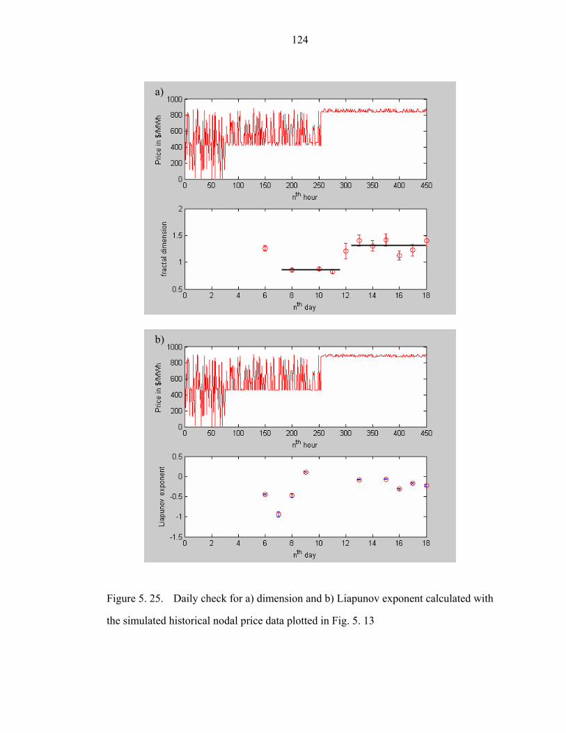
124
Figure 5. 25. Daily check for a) dimension and b) Liapunov exponent calculated with
the simulated historical nodal price data plotted in Fig. 5. 13
b)
a)

125
bigger than 0.5. From both results, the agent finds that there was a consistent change
in the strategies of its competitors, and the system settled into a new equilibrium. At
Day 9, the Liapunov exponent shows a positive value, but the dimension check shows
no change in the state. In such a case the Liapunov exponent is ignored since the
dimension check is more reliable.
For showing the offer behavior of the agent, the main variables were plotted in
Figure 5. 26. a). The pictures in the left hand side show the degree of speculation and
those in the right hand side illustrate the maximum offer price, respectively. In the
situation for second rows in the figure, competitors are less speculative, and the
chance that the agent gets price spikes is much lower than that in the 3rd row. The ratio
between the two variables was calculated and plotted in Figure 5. 26. b). The figures
clearly show that the ratio decreases when the competitor gets more speculative, i.e.,
the market that the agent faces becomes less competitive accordingly. It is an
interesting result since the ratio changed in the opposite direction in comparison to the
case for the agent with locational benefit. When the market is less competitive, the
agent can take advantage of its competitors if it can. However, the market does not
become sufficiently volatile due to the change in the strategy of Firm 6. Consequently,
the agent may have options; it makes the market more volatile by submitting more
speculative offer, or it takes a small advantage out of the change. Optimization process
finds a better way in maximizing its profit. In such a situation, the process finds that
more speculative is a better way to maximize its earning. For cooperating with the
Firm 6 that changed the strategy, the agent tries to help by withholding more, or being
more speculative. Note that the agent may do both. The former decreases the MOP,
while the latter increases DOS. Therefore, both cases result in decreasing the ratio of
MOP/DOS.
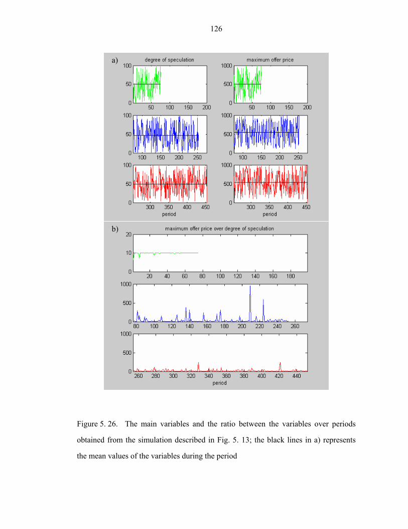
126
Figure 5. 26. The main variables and the ratio between the variables over periods
obtained from the simulation described in Fig. 5. 13; the black lines in a) represents
the mean values of the variables during the period
b)
a)

127
For a more competitive situation, the ratio increases in order to compete the
“updated” competitors. For an agent without locational benefit, the unit that it owns
may not be required to meet the demand. In such a case like competitive market and
no locational benefit, speculation may increase the probability of not being dispatched.
In order to avoid being de-committed, it tries to compete against its competitors. Then,
it may decrease DOS or withhold less quantity, and accordingly increase MOP.
Therefore, the ratio increases, which is the opposite case when the agent has locational
benefit.
The agent manages to keep the nodal price about $ 500/MWh and $ 900/MWh for
before and after the change in the strategy of Firm 6, respectively. Figure 5. 27 shows
the simulated historical earnings for both cases from the simulation as was described
in Fig. 5. 13. The results were almost identical to the cases described in the
Section 5.4.4. The error after learning period and before the change in the strategy of
Firm 6 was 19 %, and that after the change was 1 %.
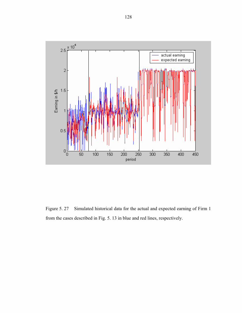
128
Figure 5. 27 Simulated historical data for the actual and expected earning of Firm 1
from the cases described in Fig. 5. 13 in blue and red lines, respectively.
129
CHAPTER SIX CONCLUSIONS AND FUTURE WORK
Restructuring of electricity systems has been ongoing around the world for several
decades. New auction based markets are considered more efficient, but less efficiency
have been observed. Demand-side participation was claimed to make market more
efficient due to the fact that only small portion of reduction in demand can reduce the
number of price spikes significantly. For a better design, the implementation of such
an agent must be in favor of end consumers such as less involvement and higher
earning. To maximize demand-side profit with less involvement, distributors, such as
NYSEG, participate in the market on behalf of end consumers, and submit an optimal
bid. This dissertation has discussed the properties of demand and developed an
optimal bidding function. A simulation with such demand-side agents shows a
significant increase in market efficiency.
When a supply-side agent is introduced into a new unknown market, it tries to find
what is happening. With available information, it can have a good knowledge on the
market including network. However, the state of a market including the strategies of
competitors is subject to change. The change in the market state might be either
consistent or fluctuating. An optimal strategy should not change for simple
fluctuations. Under the rule that no communication is allowed amongst suppliers, the
agent should monitor the market state due to any consistent change based only on
publicly available data such as nodal price. However, the data are affected in a way
due to unknown offer strategies of competitors and network. The complicated nature
of electric power markets makes a systematic study on the field difficult. This

130
dissertation primarily investigates finding an optimal strategy for a supply-side agent
by using theoretically derived modeling and a market dynamic toolbox.
For a supply-side modeling, the objective of offer for quantity was discussed. Based
on the discussion, a new model was developed and a differential equation was
constructed to find an offer function. The resulting offer function theoretically derived
from modeling fits existing offer data obtained from the
Pennsylvania-New Jersey-Massachusetts market in 1999 successfully. Only small
number of variables is needed to describe an offer curve instead of many quantity and
price pairs for all the blocks submitted. Consequently, it is possible to assign the
earning from each period into the number of variables.
As long as a system stays an equilibrium state, it is possible to estimate the market
state with a relatively small error. In the case, time is not a variable to specify the
state, i.e., it is not important when one explored the market. Therefore, all the data or
any part of data observed are relevant to specify the system. For a given system in an
equilibrium state, one needs some number of independent variables to describe the
system, dimension. The value of dimension does not change if the system stays in the
same equilibrium state or even a strange attractor. The number is closely related to the
degree of freedom which the system has. Once the system evolves, one must check if
the system settles into a new equilibrium or a chaotic state. In both cases, the degree of
freedom changes as the system evolves, and consequently the dimension changes too.
For the former case, relaxation time is an important quantity evaluating how long it
will take for the system to reach another equilibrium. A similar quantity exists in the
latter case such as a Liapunov exponent quantifying how long it will take for initially
close states to separate far apart. The new quantities such as the dimension and a

131
Liapunov exponent gives an agent a way how to check the change in system as well as
to decide which part of data should be used for estimating a future state. Those
quantities were evaluated with the nodal price data obtained from the New York ISO
web site during spring-summer 2003. The results tells that a systematic change
occurred for the market state that a generator located in NYC area faced as season
changed from spring to summer as demand increased consistently.
To construct a mapping function from an offer to earning, an unknown market was
linearly superposed in terms of known types of competitors. The known types of
agents are implemented based on the fact that the degree of speculation is the most
important factor to affect earning. With the setup, an agent has an implicit way to
recognize the market which it participates in. The linear superposition allowed a
numerical mapping function and numerical optimization process.
Four different categories of simulations were performed for different competitors;
one nearest competitor 1) did not change the strategy, 2) changed strategy
consistently, and 3) external flow existed without knowledge of the agent of interest.
All the simulations in the different setups with a supply-side agent showed that its
performance is significantly better than that of random offer. Once a competitor
changes the strategy, the dimension and a Liapunov exponent give a signal to an agent
to inform the change. With help from the tools, an agent adjusts its scenario set for
spanning the real world to have a better understanding on the real world. After the
adjustment, an agent re-evaluated all the quantities such as scenario set and weight
factor distribution. When it has no information on the network change, such as change
due to an external flow, it assumes only change in competitors’ strategies alters the
market state. As a result, the discrepancy between the inner and the real world gets
132
bigger. In all the simulations, the agent found an optimal offer to maximize its profit,
and it maintained the nodal price above a certain level depending on its competitors.
The supply-side agent designed in this study is a unique agent able to properly deal
with transmission network, and it also performs well under stochastic demand. The
strategy used by the agent under unknown situation was found to be consistent, which
explains why it performs well. In the analysis of the offer behavior, the degree of
speculation and the maximum offer price are key features to show how the agent
reacts against the change in the market state. The ratio between them indicates the
offer strategy of the agent in maximizing its profit.
Due to its computational expense, a larger system than IEEE 30-bus system was not
tried in this study. Most computational burden in this study was function evaluation
since it needs to run for multiple AC OPF’s. However, each run can be parallelized
which result in less computation time and space.
When an agent assigns a wrong reason for the change in the state of market, its
performance is not good. In such a case, the error between estimated and actual
earning is rather high, which is a signature of wrong reasoning. A new tool is required
to detect such a signal in order to improve the performance of the agent.
Appendix A gives a way to an agent to check if a generator or subset of generators
have market power. Once the agent finds out it has market power, there is a way to
exercise its market power to increase its earning. If a subgroup has market power, the
agent can construct a long term strategy for an investigation. In this study, such a long

133
term plan is not considered. However, it is reasonable for an agent to get such a plan
as long as the plan might increase long-term profit.
With properly designed agents with tools mentioned above, the market behavior
such as price can be forecasted. Based on the forecast, it is possible to construct a
toolbox for operating and planning a power system.

134
APPENDIX A GENERATION SENSITIVITY MATRIX FROM A NETWORK
TOPOLOGY
Based on offers submitted by participating generators, a system operator finds an
optimal solution to minimize whole system cost while all constrains are met such as
power balance equations and voltage constraints etc. From the solution, a generation
setpoint which comprised of generation and price is determined. Consider a following
economic dispatch problem:
( )lossD
T
iii
T
g
PPg
capacitygFflow
gc
+=
≤=
1
subject to
min
(A.1)
where F is part of PTDF matrixA1 whose dimension is (number of lines)-by-(number
of dispatched generators, n),
Lagrange relaxation technique is a well developed technology to solve such an
optimization problem by forming a Lagranian:
( ) ( )
**** and ,,
1
σµλ
σµ
g
WgflgPPgcL TlossD
T
→
−+−++= (A.2)
where g, λ, µ and σ stand for real power injection, locational marginal pricing (LMP,
λ), shadow price of power balance equation and shadow price of binding line
constrains, respectively.
A1 Power transfer distribution factor, sometime it is called a shift factor
135
From the solution, g and λ are sensitivities of total system cost with respect to
LMP and real power injection, respectively. It is possible to construct a sensitivity
matrix of generation (real power injection) with respect to LMP, i.e.,
( ) λλλλλλ ∆=∆↔∇=∇∇=∇≡ MgZZgM (A.3)
Note that M is a Hessian matrix with a dimension of n-by-n. Consequently, M is
symmetric, i.e., MT = M. Since (A.1) is degree one homogeneous in price, M has only
one structural eigenvector, corresponding eigenvalue is zero. Therefore, change in
price along LMP does not alter generation.
0** ==∆=∆
=∆λλ
λλcMMg
c (A.4)
where c is non zero scalar.
One can write following Kuhn Tucker optimality conditions:
( ) 01 *** =−∇−−=∇= σµλ Tlossgg EPLf (A.5.1)
01 ** =−−=∇= lossDT PPgLh µ (A.5.2)
0* =−=∇= EgflowLfl σ (A.5.3)
where E is part of F matrix for congested lines; the dimension of E matrix is m’-by-n.
E is comprised of row vectors of F matrix only for the lines whose constraints are
binding, i.e., congested lines.
By solving equations (A.5.1), (A.5.2) and (A.5.3), generation setpoints as well as
all shadow prices can be obtained. If offers in the original optimization problem (A.1)
is replaced with LMP and then re-solved, the solution should be invariant due to the
definition of LMP.
136
Suppose that the price replaced is perturbed from the exact LMP. Then all the
parameters like real power injection and shadow prices (µ and σ) will be changed.
However, by the property of optimization with a linear objective function and with
convex constraints, the subset of active constraints does not change. Note that a linear
programming, LP, with convex constraints finds solution at one of extreme pointsA1.
Therefore, the optimality condition is only perturbed around the original points:
( ) ( )
( )[ ] σµ
µλµ
σµµλ
∆∆
−∆∇+∆∆
=∇−→
=∆−∇−∆−∆∇+∆=∆
Tlossgglossg
Tlossglossgg
EgPP
EPgPf111
01
***
***
(A.6.1)
( ) 01 * =∆∇−=∆ gPh Tlossg (A.6.2)
( ) 0** =∆=−∆+=∆ gEEgggEfl (A.6.3)
Combining equations (A.6.1) and (A.6.2) gives,
( ) ( )[ ] 0111 *** =∆∆∆
−∆∆∇+∆∆
=∆∇− gEggPgP TTlossgg
Tlossg σ
µµλ
µ (A.7)
Since the second term in equation (A.7) vanishes by using equation (A.6.3) and ∆µ
is a scalar, equation (A.7) gives a following expression for M matrix by using the
definition of M matrix as given in equation (A.3):
( )[ ] 0** =∆∇+∆ λµλ MMPI Tlossgg
T (A.8)
Note that equation (A.8) needs to be satisfied for all ∆λ. Consequently, one can write a
following equation:
A1 The corners or vertices of the feasible region

137
[ ] ( ) 00*1 =↔==+− BAMMBAMBMB TTTTµ (A.9)
where **1 and lossgg PBMBA ∇≡+≡ − µ
Note that B matrix is symmetric since B is a Hessian matrix of loss, and
consequently so are B-1 and A. From the definition of A matrix, one can find the inner
product of A and LMP:
[ ] *1***1**1* λλµλλµλ −−− =+=+= BMBMBA (A.10)
Congestion makes the power system restricted in a certain way such that only
certain patterns of perturbation in generation are allowed. Therefore, in this study,
uncongested case and congested case will be discussed separately.
Uncongested network
If there is no binding line constraint, the system is similar to networkless except
loss. In the case, LMP is the sum of the system marginal cost of generation and
delivery cost. Since no line constraint is binding, delivery cost is not high. Therefore,
each price has similar value with each other. From the last expression in equation
(A.9), one can find following relations for each column of the resulting matrix (BA):
( ) 0=jbaM for j = 1,…, n (A.11)
where ba is a column vector of BA matrix.

138
As was discussed earlier, M matrix has only one structural eigenvector which is
parallel to LMP for an uncongested case. Consequently, all the columns of BA matrix
must be parallel to the structural eigenvector which is also parallel to LMP. Therefore,
all the columns of BA matrix are parallel to LMP, i.e.:
[ ] nnnBA ××== 11***
1 αλλαλα L (A.12)
where α is a row vector whose elements are all proportionality constants of each
column vector of BA matrix.
Since B is given and invertible matrix, one can rewrite equation (A.12) in a following
way:
nnnnBA ××××− == 1111*1 αδαλ (A.13)
where δ = B-1λ*. Since A is symmetric, Aij = Aji, i.e.:
ik
kiijjijiij AA δ
δα
ααδαδ ⎟⎟⎠
⎞⎜⎜⎝
⎛=→=== (A.14)
Therefore,
[ ] T
k
knA δδ
δα
δαδα ⎟⎟⎠
⎞⎜⎜⎝
⎛== L1 (A.15)
By using equation (A.10), one finds:
*1**
*1***
11λλλδδ
α
δλδλδδα
λδδδα
λ
−
−
==⎟⎟⎠
⎞⎜⎜⎝
⎛→
==⎥⎦
⎤⎢⎣
⎡⎟⎟⎠
⎞⎜⎜⎝
⎛=⎟⎟
⎠
⎞⎜⎜⎝
⎛=
B
BA
TTk
k
T
k
kT
k
k
(A.16)

139
From equations (A.15) and (A.16), A and M matrix can be found:
*1*
1**1
λλλλ
−
−−
=B
BBA T
T (A.17)
⎟⎟⎠
⎞⎜⎜⎝
⎛−= −
−−
IB
BBM T
T
*1*
1**
*
1
λλλλ
µ (A.18)
Congested network
From equation (A.6.3), one finds
00 =→=∆=∆ EMEMgE λ (A.19)
Note that left hand side of arrow holds for all perturbation of LMP. Since LMP stays
on the null space of M matrix, the null space of M is composed of LMP and row
vectors of E matrix. From equation (A.9), ATBTM = ABM = 0 since A and B are
symmetric matrices. Consequently, each row vector of AB matrix lies on the null
space of M matrix, i.e., each row vector if AB matrix is linear combination of ej (j = 1,
…, m’) and λ*T where e is a row vector of E matrix. Therefore, AB matrix can be
expressed in terms of E and LMP in a following way:
( ) ( ) LE
e
e
ee
eeee
AB
mmn
mm
Tmmn
mm
T
nm
n
nm
n
m
m
Tnmm
nm
n
Tmmm
Tmmm
⎥⎦
⎤⎢⎣
⎡=⎟⎟
⎠
⎞⎜⎜⎝
⎛⎥⎦
⎤⎢⎣
⎡=
⎟⎟⎟⎟⎟
⎠
⎞
⎜⎜⎜⎜⎜
⎝
⎛
⎟⎟⎟⎟⎟
⎠
⎞
⎜⎜⎜⎜⎜
⎝
⎛
=
⎟⎟⎟⎟⎟
⎠
⎞
⎜⎜⎜⎜⎜
⎝
⎛
+++
++++++
=
×−
×
×−
×
×−
×
−−
−−
−−
2
1*
2
1
*
11
11
1
221
111
*1111
*21
211
21
*11
111
11
α
αλα
α
λαα
αααα
λααα
λαααλααα
M
L
MOM
L
L
L
MOM
L
L
(A.20)

140
where α’s stand for proportionality factors, m equals to m’ + 1, and L represents an E
matrix with one additional row of LMP.
By multiplying B-1 on both sides, one will get:
( ) ( )( )[ ] ⎟⎟
⎠
⎞⎜⎜⎝
⎛=⎥
⎦
⎤⎢⎣
⎡=⎥
⎦
⎤⎢⎣
⎡= −××
×−
×−
×−
×
2212
211121
2
11
2
1
GGGG
GGLBA mnmmmmmn
mm
mmn
mm
αααα
αα
αα
(A.21)
where G is defined LB-1.
Since A is symmetric, one can get:
( ) 1111111111 GGGGG TTTTT ααααα −=→== (A.22.1)
( ) 1121
1122121221 αααααα TTTTTTT GGGGGGG −− ==→== (A.22.2)
Combining equations (A.21) and (A.22.2) gives:
( ) GGGGGGG
A TTTT 1121
112
1 αα
α −− =⎟⎟
⎠
⎞⎜⎜⎝
⎛= (A.23)
Note that G is known, then only unknown in equation (A.23) is α1.
By using equation (A.10), one finds:
*
11**1*
11* λαλλλαλ GGBGIBGGGA TTTT −−− =→== (A.24)
Note that:

141
( ) ( )*22
*111*
2
1*1
21* λλ
λλ
λ GGGGG mn
m
+=⎥⎦
⎤⎢⎣
⎡=
×−
×
(A.25)
Let C be BGTG1-T, then:
( ) ( ) ⎥⎦
⎤⎢⎣
⎡=⎥
⎦
⎤⎢⎣
⎡==
×−
×−
×−
×−
mmn
mmTT
nmn
nmTT
CC
GGB
BGBGC
2
11
2
11 (A.26)
Combining equations (A.24) and (A.26) gives:
*1
112
*2*
12
*11*
1*2
*1 λλ
λαλα
λαλλ −=→⎟⎟
⎠
⎞⎜⎜⎝
⎛==⎟⎟
⎠
⎞⎜⎜⎝
⎛CC
GCGC
GC (A.27)
Equation (A.27) shows that only m prices among n are independent and rest can be
calculated from the m price by using network parameters.
One can also find price explicitly in a following way:
*1
11*
11
12
*1
*2
*1* λ
λλ
λλ
λ −−
=⎟⎟⎠
⎞⎜⎜⎝
⎛=⎟⎟
⎠
⎞⎜⎜⎝
⎛= CC
CC (A.28)
By substituting expressions for C’s as given in equation (A.26), LMP is:
( )( ) ( )( ) ( )[ ] ( ) *
111
1*1
11
11
*1
11
*1
1111
*
λλ
λλλ−−
−−−
−−−−
==
==
TTTT
TTTTT
LBBLLBBLBB
GBBGGGBGBG (A.29)
Equations (A.27) and (A.29) can be combined to lead to:
( )[ ] *1
*1
1111
*11 λλαλα IGBBGGCGC TT ==
− (A.30)
Equation (A.30) is valid for all *1λ , which results in:

142
( )( ) ( ) ( )( ) ( ) 11
11
111
11
111
−−−−−− === TTTTTTTT GBGGGBGGBGGBGBGGBCα (A.31)
A and M matrix can be found by combining equations (A.23) and (A.31) in a
following way:
( ) ( ) ( ) ( )[ ] ( )( ) 1111
11
111111
−−−−
−−
−−−−−
=
===
LBLLBLB
LBLBBLBLBGGBGGGGGATT
TTTTTT α (A.32)
( )[ ] ⎟⎟⎠
⎞⎜⎜⎝
⎛=−= −−−
−
TTT E
LILBLLBLBM *111
*
1
where λµ
(A.33)
M matrix can be calculated by using equations (A.18) and (A.33) with publicly
available and predictable data such as LMP, B and PTDF matrix.
Market power is very closely related to M matrix since change in revenue
according to change in price can be calculated in a following way:
( )
( )[ ] ( )[ ]iiii
iij
jijiiiiiiii
gDiagMDiag
gMgggr
λλλ
λλλλλλ
∆+∆=
∆+⎟⎟⎠
⎞⎜⎜⎝
⎛∆=∆+∆=∆=∆ ∑
**
****
(A.34)
( ) ( )[ ] λλ ∆+=∆ **ii gDiagMDiagr (A.35)
If an agent owns multiple generators, then by using equation (A.35) it can find if it
has market power as a group and furthermore can have a guideline of the way to
exercise market power before submitting its offers.
143
APPENDIX B
ERROR MINIMIZATION WITH 2-NORM
A good weight factor distribution gives an estimate to the market providing which
norm should be chosen. In this study, 2 norm is chosen. QR-factorization is a very
stable way to solve LLS, where Q is an orthogonal matrixA2 and R is upper triangular
matrixA3.
( ) ( )
( )( )
( )2
1
2
122
222
222
min
min
minmin
min min min
bQRx
bQRxRQ
bQxRQbQxRQ
bQQxRQbIxRQbxA
T
T
TT
T
⋅⋅−↔
⋅−=
⋅−⋅=⋅−⋅⋅=
⋅⋅−⋅⋅=⋅−⋅⋅=−⋅
−
− (A.36)
When only n number of components exists in the set, non-zero elements in R matrix
are n2 and multiplying QTb costs only m-by-n since the multiplication is only between
matrix and vector. Beside the computational efficiency, orthogonal matrix Q could be
well defined even for an ill-defined matrix.
Another approach is LU-factorization. When matrix A is m-by-n matrix with m
greater than n, L is m-by-n and U is n-by-n matrix. While the diagonal element in L is
ones, all the ill-defined property enters into U, i.e. there are r zeros in the diagonal of
U matrix if r columns are a linear combination of (n – r) columns. Since r columns are
dependent, there is only (n – r) information available which means that r variables in x
vector cannot be uniquely defined. Note that one can arbitrarily assign values for
A2 a matrix containing column vectors orthogonal with each other, i.e.,
IQQQQ T =⋅=⋅ −1 where T stands for transpose and I is an identity matrix A3 a matrix that all the elements under the diagonal are zeros

144
undetermined variables without increasing error. From the properties of U matrix
being an upper triangular matrix, the corresponding elements to the zero diagonal
element in U matrix can be set to zero arbitrarily. Then the r columns in U matrix are
meaningless to determine elements in x since the columns are multiplied with zeros. A
reduced U matrix that is the U matrix where those r columns were deleted is well
defined. Consequently, the LLS problem for the reduced U matrix and vectors x and
b’ (= L-1(PTb)) yields a 2-norm minimizing weight factor distribution vector x.
( )
( )21
111
2
1
22
min
min
min min
bLxU
bLxU
bxULbxA
⋅−⋅↔
⋅−⋅↔
−⋅⋅=−⋅
−
− (A.37)
Figure A-1 illustrates the procedure described in equation (A.37) schematically. It
should be noted that the above argument is only valid for a stationary system.
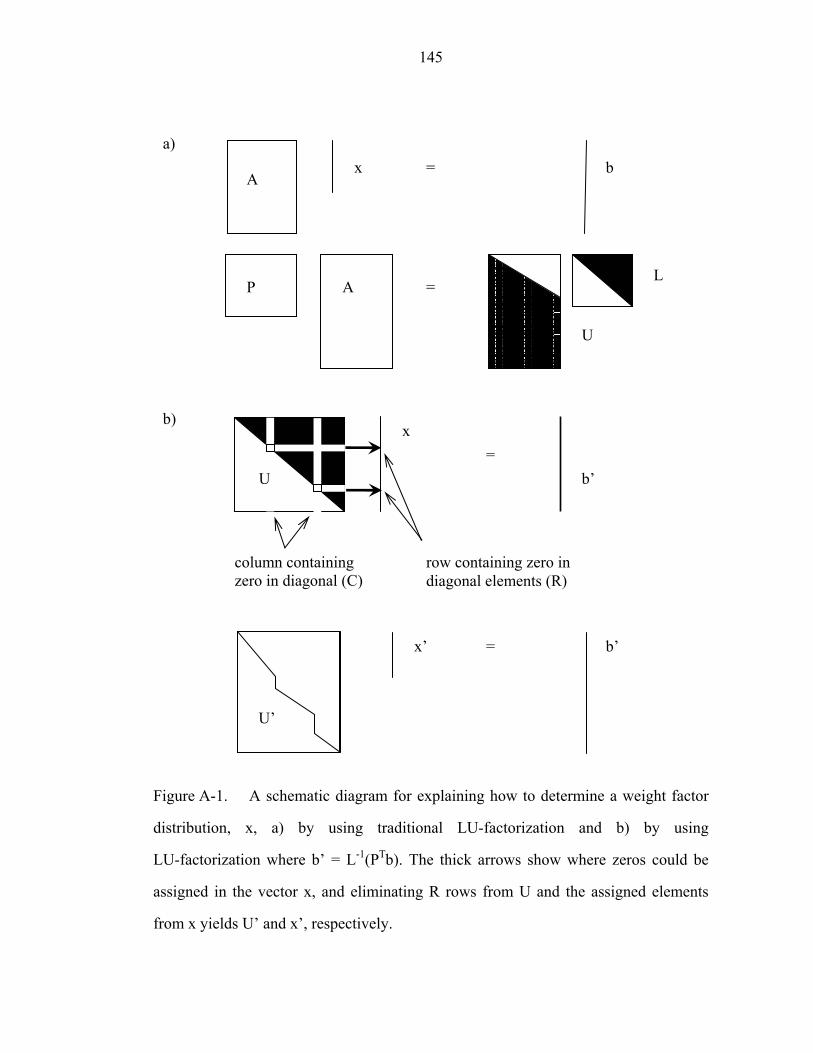
145
Figure A-1. A schematic diagram for explaining how to determine a weight factor
distribution, x, a) by using traditional LU-factorization and b) by using
LU-factorization where b’ = L-1(PTb). The thick arrows show where zeros could be
assigned in the vector x, and eliminating R rows from U and the assigned elements
from x yields U’ and x’, respectively.
= x
b’
row containing zero in diagonal elements (R)
column containing zero in diagonal (C)
U
A
P A
U
b x =
=
= x’ b’
a)
L
b)
U’

146
APPENDIX CA4 TRUST REGION METHOD
Trust Region Method for Unconstrained Minimization Problems
Trust region methods are widely and successfully used for unconstrained
optimization process due to its strong convergence and fewer numbers of iterations.
However, the cost of the linear algebra for the methods is higher. Consequently, trust
region methods are effective on highly nonlinear problems of which function has high
cost to evaluate. This method is recently proven to work successfully in solving
problems to the large-scale setting.
When a function f is twice continuously differentiable, Taylor series expansion of f
gives
( ) ( ) ( )22
21 sosfssfxfsxf k
TTkkk +∇+∇+=+ (A.38)
where o(x) stands for the quantity approaches zeros faster than x when x goes to zero.
Consequently, sfssf kTT
k2
21
∇+∇ equals to the change in f, ( ) ( )kk xfsxf −+ ,
approximately around xk ∈ Rn. The trust region subproblem can be defined at xk;
⎭⎬⎫
⎩⎨⎧ ∆≤∇+∇ kk
TTk ssfssf
22 :
21min (A.39)
Note that equation (A.39) is a little bit different from general trust region
subproblem in that 2-norm is used because 2-norm may allow an efficient global A4 Most part of Appendix II were taken from the textbook [T. F. Colman and A. Verma, “The Solution of Large-Scale Optimiztion Problems”, Cornell University, Ithaca, NY 2003) 54-61]
147
solution. Equation (A.39) defines a trial step for sufficiently small ∆k and
( ) ( )kkk xfsxf <+ . It is noteworthy that the subproblem is well defined regardless of
kf2∇ enough not to assume that kf2∇ is positive definiteA5. There are three different
cases for kf2∇ . For a positive definite kf2∇ , the solution to the subproblem is the
Newton step, ( ) kk ff ∇∇−−12 for a large value of ∆k. When the smallest eigenvalue of
kf2∇ is negative, the solution sk satisfies ||sk || = ∆kA6. If the smallest eigenvalue is
zero, a (not unique) solution exists on the surface of n-ellipsoid. A general procedure
of trust region method is following; solve equation (A.39) for trial step sk, and
calculate ( )kk sxf + , kkTkk
Tk sfssf 22/1 ∇+∇ and
( ) ( )[ ] [ ]kkTkk
Tkkkk sfssfxfsxf 22/1/ ∇+∇−+ , and then adjust the size of n-ellipsoid,
∆k; for a large ratio, ( ) ( )[ ] [ ]kkTkk
Tkkkk sfssfxfsxf 22/1/ ∇+∇−+ , decrease the size,
and for a small ratio, increase the size, and otherwise, maintain the size. Repeat these
procedures until stopping criteria is met. The constants to define the size of ratio and
to decide how much increase or decrease are predetermined and do not change with
the period k. The main advantage of the trust region method (less number of function
evaluation) comes from updating algorithm: update kkk sxx +=+1 only for positive
ratioA7 (whenever moving by sk decreases the value of f). Generally speaking, the ratio
tells how well the solution to equation (A.39) predicts the real change in f; the higher
value the ratio is, the better the performance is.
A5 positive definite matrix means a matrix of which eigenvalues are all positive A6 if kks ∆< , sk is an unconstrained local minimizer of an indefinite quadratic function which is impossible A7 for non-positive ratio, ( ) ( )kkk xfsxf ≥+ since kk
Tkk
Tk sfssf 2
21
∇+∇ is negative;
note that sk is the solution of the subproblem (equation (A.39)). Since equation (A.39) is minimization problem and zero is a trivial solution for equation (A.39) satisfying
the constraint, kks ∆≤ when sk = 0, kkTkk
Tk sfssf 2
21
∇+∇ must be negative

148
Suppose there are s* and λ* satisfying following equations:
( ) gsIH −=+ λ (A.40)
( ) positive is IH λ+ semi-definite (A.41)
∆≤2
s (A.42)
( ) 02
=∆− λs (A.43)
From equations (A.40) and (A.41), s* is the unconstraint minimizer of the quadratic
function ( )sIHssg TT*2
1 λ++ . Consequently, one can find a following inequality:
( )2
2*2
2*
*** 221
21 ssHsssgHsssg TTTT −++≤+
λ (A.44)
For all feasible s, ( ) 2/2
2*2
2* ss −λ is non-positiveA8, i.e., s* is the global solution to
the subproblem. Since s* is the global solution, applying equation (A.40) in equation
(A.44) allows:
( ) ( )( )
( ) ( ) 022
21
21
21
21
221
21
***
*****
*****
2
2*2*
***
≥−+−+−+
−+−+−=
−+−+−
ssssssssssss
HssHssHssHssssg
ssHssHssssg
TTTTTT
TTTTT
sTTT
λλ
λ
(A.45)
Since *HssT and *ssT is a scalar, they equal to their transpose
( ( ) HsssHsHss TTTTT*** == A9 and ( ) ssss TTT
** = ). By the same argument,
( )[ ] ( ) ( )****** ssHsssHsHsss TTTTTT −=−=− . Consequently, one obtains:
A8 from equation (A.43), λ* = 0 or ||s*||2 = ∆, and ||s||2 ≤ ∆ for all feasible s from
equation (A.42), consequently, ( )2
2*2
2*
2ss −
λ is non-positive
A9 H is a Hessian matrix which is symmetric, i.e., HT = H
149
( ) ( )( )
( ) ( ) 022
121
221
21
21
21
***
*
***
*****
≥−⎥⎦⎤
⎢⎣⎡ ++++=
−++−+−+−
ssssHsHsg
ssssHssHssHssHssssg
TTTT
TTTTTTT
λ
λ
(A.46)
From equation (A.40), the expression for the transpose of g is obtained;
( )[ ] ( ) ( )IHsIHssIHg TTTTTTT***** λλλ +−=+−=+−= . Therefore, an inequality is
derived from equation (A.46) in a following way:
( ) ( )
( ) ( ) ( ) ( )
( ) ( )( ) 021
221
221
21
***
***
***
***
*
≥−+−=
−⎥⎦⎤
⎢⎣⎡ +++++−=
−⎥⎦⎤
⎢⎣⎡ ++++
ssIHss
ssssHssIHs
ssssHsHsg
T
TTTT
TTTT
λ
λλ
λ
(A.47)
Equation (A.47) implies that the matrix H + λ*I is positive semi-definite.A10
Suppose H = VΛVT where the columns of V are orthonormal eigenvectors of HA11.
Then, equation (A.40) and substitution of sVs T= allow:
A10 from [D. Sorenson, “Trust Region Methods for Unconstrained Optimization”, SIAM J. Numer. Anal., 19 (1982) 409 – 426] A11 for a symmetric matrix H,
real) is ( 1
2∑=
=↔==↔=n
ii
TT vvvHvvvHv λλλλλλ , then there is a set of
orthonormal eigenvectors of H, i.e., qi for i = 1 ~ n such that ijjTiiii qqqAq δλ == , ; in
a matrix form, there is an orthogonal V such that TT VVHHVVHVV Λ=↔Λ==−1 where Λ is a diagonal matrix of which diagonal elements are the eigenvalues of the matrix H

150
( ) ( ) ( ) ( )( ) gVsI
gsIVsVVIVsVIHsIHT
TT
−=+Λ≡↔
−=+Λ=+Λ=+=+
λα
λλλλ (A.48)
Since H + λI is a positive semi-definite matrix by equation (A.41), all the λ must be
bigger than or equal to the smallest eigenvalue of H, λ1. Consequently, all vectors
satisfying equations (A.40) and (A.41) are expressed in a following way:
{ }{ }∑ ∑
>+ =+
+⎟⎟⎠
⎞⎜⎜⎝
⎛+
=0: 0:λλ λλ
βλλ
α
i ji jjji
i
i vvs (A.49)
By assuming the form for s is given in equation (A.49), setting ||s|| = ∆ gives an
algorithm to find a trial stepA12. There are different cases depending on the smallest
eigenvalue of H (λ1) for obtaining expression for s. For positive λ1, if the Newton step
is inside the n-ellipsoid, ||H-1g|| ≤ ∆, the optimal solution is the Newton step,
gHs 1*
−−= and 0* =λ , otherwise, ( ) ∑=
⎟⎟⎠
⎞⎜⎜⎝
⎛+
=n
ii
i
i vs1 λλ
αλ for non-negative λA13. For
non-positive λ1, there are two different cases depending on α (when denominator in
equation (A.49) equals to zero), αi is zero or it is not. If αi is zero, then set
( ) ∑=
⎟⎟⎠
⎞⎜⎜⎝
⎛+
=n
ii
i
i vs1 λλ
αλ leading to one solution to ||s|| = ∆A14. If αi is not zero, the
expression for s(λ) does not hold since it diverges at λ = –λ1. To make use of general
A12 note that if ||s|| ≠ ∆, λ = 0 by equation (A.33) and ||s|| < ∆ by equation (A.32) which gives a trivial solution A13 note that ||s(λ)|| approaches zero as λ diverges
A14 ( ) ∞→⎟⎟⎠
⎞⎜⎜⎝
⎛+
= ∑=−→−→ ++
n
ii
i
i vs1
limlimλλ
αλλλλλ
, ( ) 0limlim1
→⎟⎟⎠
⎞⎜⎜⎝
⎛+
= ∑=
∞→∞→
n
ii
i
i vsλλ
αλ
λλ and
the convexity of ||s(λ)|| imply that ||s(λ)|| intersects ∆ in exactly one place for λ > –λ1

151
form of s, equation (A.49), s1(λ) is defined as ( ){ }
∑>+
⎟⎟⎠
⎞⎜⎜⎝
⎛+
=0:
1λλ λλ
αλ
iii
i
i vs , and then if
( ){ }
∆≥⎟⎟⎠
⎞⎜⎜⎝
⎛−
=− ∑> 1: 1
11λλ λλ
αλ
iii
i
i vs , there exist λ satisfying ||s|| = ∆ then
( ) ( ){ }
∑>+
⎟⎟⎠
⎞⎜⎜⎝
⎛+
==0:
1λλ λλ
αλλ
iii
i
i vss , otherwise, ( ){ }{ }
∑ ∑> =+
+⎟⎟⎠
⎞⎜⎜⎝
⎛−
=1: 0:1λλ λλ
βλλ
αλ
i ji jjji
i
i vvs
with a proper choiceA15 of β to satisfy ||s|| = ∆.
Minimization Problems with Box ConstraintsA16
As was mentioned in chapter two, an offer equation has two short term variables
bounded with box constraints. Trust region method is described for unconstrained
problems here. When constrains have been added to a problem, finding a solution gets
more difficult. There was an approach to solve such nonlinear problems by using
interior trust region method, which gives strong convergence.
The problem considered here is following: ( ) uxlxf
nRx≤≤
∈ subject to min (A.50)
A15 { }
∑ ∑>
⎟⎟⎠
⎞⎜⎜⎝
⎛−
−∆=i i
ii
ii
i
v1: 1
22
λλ λλα
β – from orthogonality – and 1* λλ −=
A16 Most part taken from [T. F. Coleman and Y. Li, “An Interior Trust Region Approach for Nonlinear Minimization Subject to Bounds”, SIAM J. Optimization, 6 (1998) 418 – 445]

152
where l and u are lower and upper limits for x, and the objective function f is the
negative value of earning.
Among feasible set, int(F) is defined as ( ) { }uxlxF <<≡ :int which is whole feasible
region excluding the boundary. Let define a vector v(x) ∈ Rn and a diagonal matrix
Diag(x) for each component 1 ≤ i ≤ n;
( ) ( ) ⎟⎠⎞
⎜⎝⎛≡
⎪⎪⎩
⎪⎪⎨
⎧
−∞=≥∞=<−
−∞>≥−∞<<−
≡
−21
i
i
ii
ii
and 0 g if 1 and 0 g if 1 and 0 g if
and 0 g if
xvdiagxDiag
lullxuux
v
i
i
ii
ii
i
(A.51)
where g is the first derivative of f(x).
By using the definitions, the first-order necessary conditionsA17 for a local
minimizer x* can be expressed in a following way:
( ) ( ) 0 if 0 if 0
if 02
**
**
**
=⇔⎪⎩
⎪⎨
⎧
=≥=≤<<=
− xgxDiaglxguxguxlg
iii
iii
iiii
(A.52)
By the definition of Diag(x), the points where vi equals to zero must be avoided. It can
be easily done by letting x to be in int(F). If x is in int(F), one can find a Newton step
satisfying equation (A.52):
( ) ( )[ ] kkkvkkkk gDiagdJgdiagxfDiag 222 −− −=+∇ (A.53)
A17 for an continuously differentiable function f on an open set , nRDiag ⊆ , a local minimizer x* satisfies ( ) 0* =∇ xf
153
where Jv is the Jacobian matrix of |v(x)|.
Let the ith row of Jv set to be zero, and then all the points are differentiable if all the
elements of the vector gk since vi is not zero for x inside int(F). Consequently, for the
problems with finite constraints, ( )[ ]gsigndiagJ v = . Coleman et alA18 developed a
quadratic model:
( ) sTssgs kTT
kk 21
+≡ψ (A.54)
where ( ) kvkkkkk DiagJgdiagDiagHT +≡
The trust region subproblem with constraints is;
( ){ }kkk
RssDiags
n∆≤
∈:min ψ (A.55)
By substituting variables in equation (A.54), one can modify equation (A.55);
( )
( )( ) ( )( )( )
( ) ( ) ( ) ( )( )
( )ssTssg
sDiagDiagTDiagsDiagsDiaggDiag
sDiagDiagTDiagDiagssDiagDiagg
sTssgs
kkTT
k
kkkkT
kkT
kk
kkkkkT
kkTk
kTT
kk
ˆˆˆˆˆ21ˆˆ
21
21
21
111
111
ψ
ψ
≡+=
+=
+=
+≡
−−−
−−−
(A.56)
where ( ) v
kkkkkkkkk
kkkkkk
JgdiagvdiagHvdiagDiagTDiagT
sDiagsgvdiaggDiagg
+⎟⎠⎞
⎜⎝⎛
⎟⎠⎞
⎜⎝⎛==
=⎟⎠⎞
⎜⎝⎛==
−−
−
21
21
11
21
1
ˆ
ˆ ,ˆ (A.57)
A18 T. F. Coleman and Y. Li, “On the Convergence of Reflective Newton Methods for Large-Scale Nonlinear Minimization Subject to Bounds”, Math. Programming, 67(1994) 189 - 224

154
Consequently, one can write a trust region subproblem in a following way, which is
the same form as that for unconstraint problem:
( ){ }kk
Rsss
n∆≤
∈ˆ:ˆˆmin
ˆψ (A.58)
A solution to equation (A.58) gives a trial step for the trust region method. Let dk be a
trial step obtained from the solution to equation (A.58). Since the control variable x is
constrained, x needs to be in the boundary; there is bound for a step-size
⎭⎬⎫
⎩⎨⎧
≤≤⎥⎦
⎤⎢⎣
⎡ −−≡ ni
dxu
dxl
ki
kii
ki
kiik 1:,maxminα (A.59)
The minimum value of ψk(s) along the direction dk within the trust region is
( ) ( ) ( ){ }FdxdDiagddd kkkkkkkkkkk ∈+∆≤≡= τττψτψψ k** and :min (A.60)
In order to guarantee strict feasibility (x ∈ int(F)), a new step obtained from dk with
step back θkA19 is defined:
( ) kkkkk dd ** τθα ≡ (A.61)
Similar to unconstrained problem, trial step is taken only under following
circumstance in order to make sure that enough value of function f is reduced if the
step taken:
A19 if a trial vector leads to a point on the boundary of constraints , step back makes the step take partial movement along the trial step, i.e.,
[ ) ( ) ( )FdxdO kkkkkklk intfor 1 and 1,1, * ∈+==−∈ τθθθθ
155
( ) ( ) ( )( ) µ
ψρ >
+−+=
kk
kkvkkk
Tkkkk
fk s
sDiagJgdiagDiagsxfsxf21
(A.62)
where µ is a positive constant.
For significant reduction of ψk(s), Coleman et alA20 proposed to use a step along the
scaled steepest descent direction and to take the step only when the value of ψk(s) is
significantly decreased:
( )
[ ] βψ
ψρ >−
= −kkk
kkCk gDiag
s2* (A.63)
where β is a positive constant
Only a trial step satisfying equations (A.62) and (A.63) will be taken, i.e.,
double-trust region method. The algorithm is following; Assign positive constants
quantities defined in unconstrained problems and ( )Fx int and 1,0 0 ∈<<> ηβµ . At
kth step, Compute ( ) ( ) kvkkkkkk DiagJgdiagDiagHgxf and ,, to define
( ) sTssgs kTT
kk 21
+=ψ , and then find a solution to equation (A.55) (pk). With the
solution calculate following quantities:
[ ] ( )[ ]
( ) ( ) ( )( )kk
kkvkkk
Tkkkk
fk
kkk
kkCkkkk
s
sDiagJgdiagDiagsxfsxf
gDiagsps
ψ
ρψ
ψρα
21
,, 2**
+−+=
−== −
(A.64)
A20 T. F. Coleman and Y. Li, “An Interior Trust Region Approach for Nonlinear Minimization Subject to Bounds”, SIAM J. Optimization, 6 (1998) 418 - 445
156
Only for a step satisfying equations (A.62) and (A.63) is taken; kkk sxx +=+1 .
Finally choose the size (∆k+1) of the n-ellipsoidal trust region in a following way for
21 10 γγ <<< :
( ][ ] ( )[ ][ ]( ]⎪
⎪⎪
⎩
⎪⎪⎪
⎨
⎧
≥≥∆<<≥∆∆≥≥∆∆
∈∆∆≤≤∆
∈∆ +
βρηργηρβηργηρηργ
ηµργβρµργ
Ck
fkk
Ck
fkkk
Ck
fkkk
fkkk
Ck
fkk
k
and if ,0 and if ,
and if ,, if ,
or if ,0
1
1
2
1
1
1 (A.65)
Then repeat these procedures until stopping criteria is met.

157
APPENDIX D CHAOS AND NONLINEAR DYNAMICS
Lorenz equation
Lorenz introduced an equation (so called Lorenz equationA21) of which solution
settles down to a complicated set in phase space as shown in Figure A-2. The complex
geometric shape with fine structure at arbitrarily small scale is referred to as fractals.
When a small part of the shape is magnified, it shows reminiscent feature of the whole.
The Cantor set is one of most famous examples showing self-similarity. Figure A-3
illustrates the way how to construct the Cantor set. When a small part of the Cantor set
is taken and magnified, the part reproduces the whole regardless of the place where the
part is originally located. The Cantor set is made from a line, closed interval of [0, 1].
It is interesting to perform any measurement on the set: usually a physical
measurement on 1 dimensional space is length. To calculate the length of Cantor set, it
is more convenient to calculate the sum of length of the parts taken and then to
subtract the sum from the length of the original interval, unity. The sum of the length
of left over parts is
1
321
131
32
32
321
31
818
274
92
31 32
=−
=⎥⎥⎦
⎤
⎢⎢⎣
⎡+⎟
⎠⎞
⎜⎝⎛+⎟
⎠⎞
⎜⎝⎛++=++++ LL .
A21
( )
bzxytz
xzyrxty
xytx
yx
xz
zy
−=⎟⎠⎞
⎜⎝⎛
∂∂
−−=⎟⎠⎞
⎜⎝⎛
∂∂
−=⎟⎠⎞
⎜⎝⎛
∂∂
,
,
,
σ
, where σ, r and b are all positive parameters from Ref. [31]

158
Figure A-2. Solution of the Lorenz equation (in color) and xy, yz and zx
two-dimensional projections which show artifact crosses
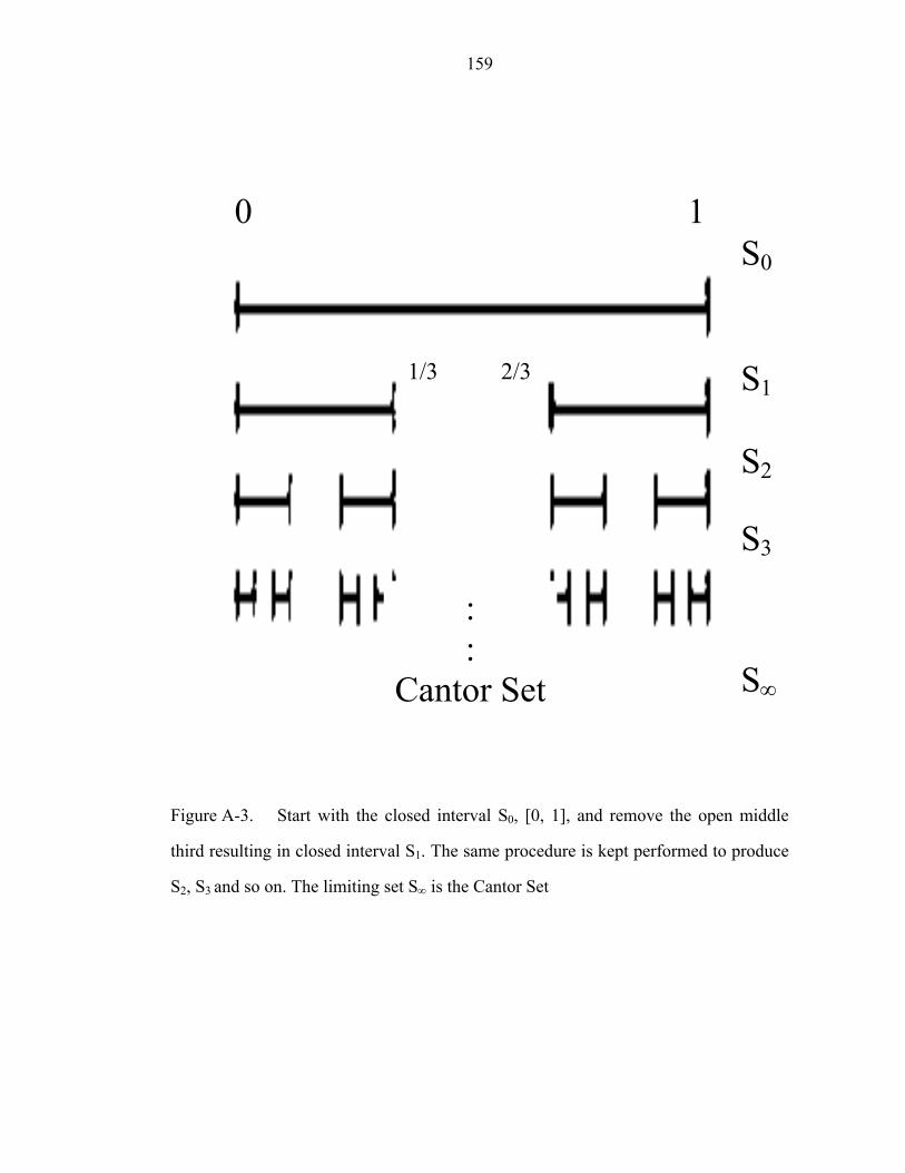
159
Figure A-3. Start with the closed interval S0, [0, 1], and remove the open middle
third resulting in closed interval S1. The same procedure is kept performed to produce
S2, S3 and so on. The limiting set S∞ is the Cantor Set
0
1
S0
S1
S2
S3
S∞
: :
Cantor Set
1/3 2/3

160
Consequently, the length of the Cantor set is zero which might imply a line with
no length. One may find a contradiction since the set was supposed to be a line. The
problem in measuring anything in fractals is not confined to 1 dimension. To see the
problem in higher dimension, consider the von Koch curve (Figure A-4). The length of
the von Koch curve can be calculated since the length increases 4/3 in every step. As
the number of step diverges, the length diverges also; ( ) ∞→∞→ nn as 3/4 , but the
curve does not cover the whole surface. Therefore, the von Koch curve is infinitely
long curve confined to limited area. Note that the curve is not 2 dimensional object
This puzzle could be understood when the dimension of the Cantor set is not 1 and
that of the von Koch curve is not 2. It is noteworthy that the dimensions are 0.63 and
1.26, respectively which are non-integer. Since the Cantor set contains infinitely many
points but not many enough to form 1 dimension, the length is zero. To describe
fractals correctly, dimension need to be defined in a following way; the minimum
number of coordinates needed to describe every points in the set. This definition
provides an enumeration of characteristics related to fractals (similarity dimension).
Suppose that a self-similar set is composed of m copies of itself scaled down by a
factor of r. Then the similarity dimension is defined in a following way:
rmd
loglog
= (A.66)
Equation (A.66) is convenient to define dimension of fractals with self-similarity.
However, self-similarity is difficult to define for objects in real life. To deal with
fractals with not evident self-similarity, generalized definition is needed like box
dimension as was proposed by FalconerA22. Let S be a subset of d-dimensional space,
A22 K. Falconer, “Fractal Geometry: Mathematical Foundations and Applications”, Whiley, Chichester, England (1990)
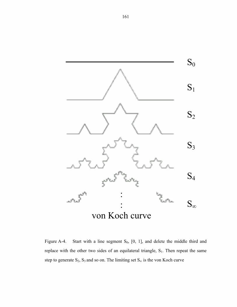
161
Figure A-4. Start with a line segment S0, [0, 1], and delete the middle third and
replace with the other two sides of an equilateral triangle, S1. Then repeat the same
step to generate S2, S3 and so on. The limiting set S∞ is the von Koch curve
S∞
S0
S1
S2
S3
S4
: :
von Koch curve

162
and N(ε) be the minimum number of d-dimensional cubes of side ε needed to cover S.
As ε decreases, more d-dimensional cubes are required. The box dimension is defined
in a following way:
( )
( )εε
ε /1logloglim
0
Nd→
= (A67)
To see how it can be used for quantifying fractals in a real life, consider the length
of the coast of Norway shown in Fig. A-5. There can be many ways to define the
length of the coast, but it is impossible to measure when all the small interfaces
between water and sand grain is considered. A good way is shown in Figure A-5:
count the number of 2-dimensional box to cover whole coast as a function of the
length of one side of the square. As was shown in the 2nd graph of Figure A-5, the
coast of Norway shows a linear relationship with dimension of 1.52.
The dimensions discussed before are convenient to define static fractals, but not
applicable to the chaotic system settling down to a strange attractorA23 in phase space.
Practical way for describing a dynamic system, a pointwise dimension is introduced.
For a fixed point x, define Nx(ε) to be the number of points inside a ball of radius ε
around x. Most of points in the ball come from later parts that just happen to pass
close to x, and they are unrelated to the immediate portion of the trajectory through x.
( ) dxN εε ∝ where d stands for the pointwise dimension at x.
( )
εε
ε loglog
lim0
xNd
→= (A.68)
A23 an attractor that exhibits sensitive dependence on initial condition
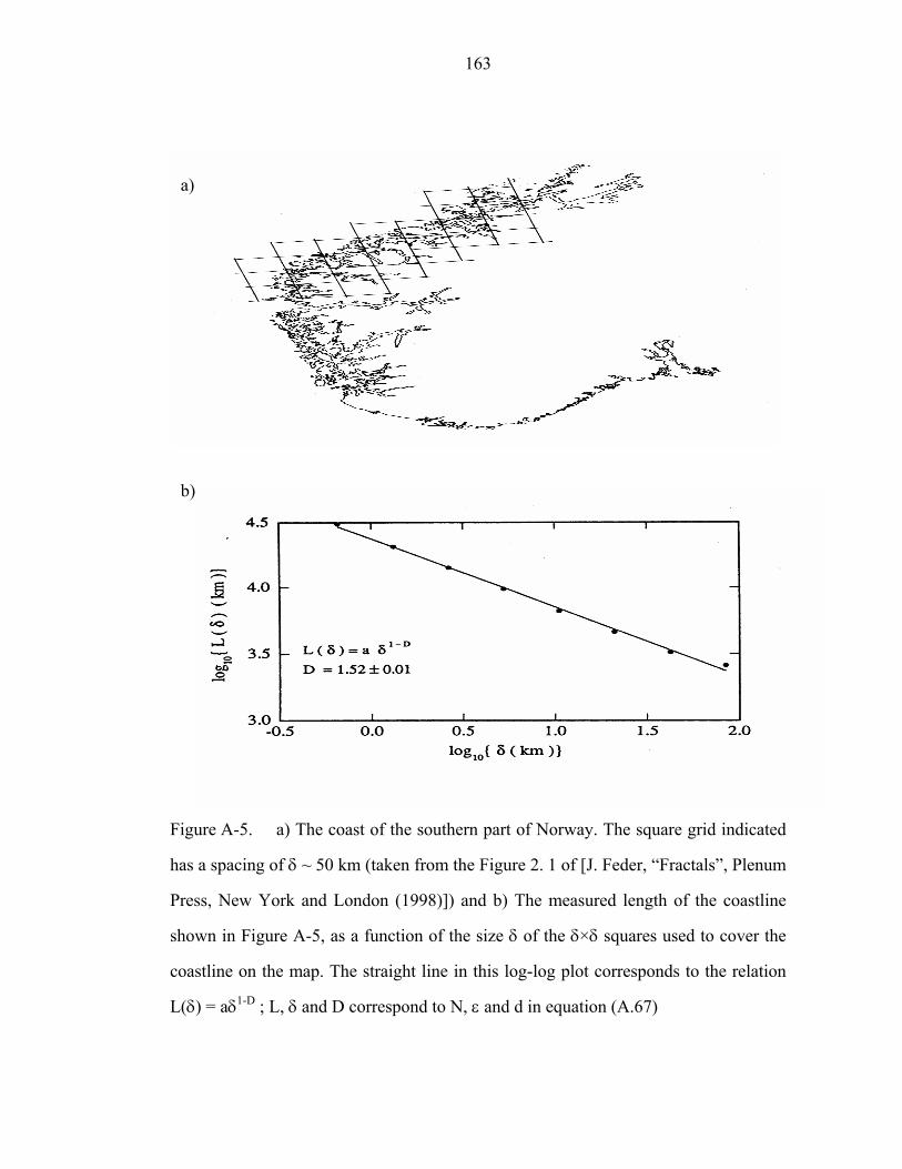
163
Figure A-5. a) The coast of the southern part of Norway. The square grid indicated
has a spacing of δ ~ 50 km (taken from the Figure 2. 1 of [J. Feder, “Fractals”, Plenum
Press, New York and London (1998)]) and b) The measured length of the coastline
shown in Figure A-5, as a function of the size δ of the δ×δ squares used to cover the
coastline on the map. The straight line in this log-log plot corresponds to the relation
L(δ) = aδ1-D ; L, δ and D correspond to N, ε and d in equation (A.67)
a)
b)

164
The pointwise dimension may not be a global quantity since it can depend on x.
Furthermore, there are many practical applications where the geometric object has to
be reconstructed from a finite sample of data points with errors. In such cases,
correlation dimension is most widely used. As a system evolves for a long time, one
can obtain a set of many points {xi, i = 1,…,n} on a phase space. Grassberger and
Procaccia proposed a way to evaluate dimensions like correlation dimensionA24. For
an overall dimension, the x-dependent Nx(ε) can be averaged in a following way;
( ) ( ) ( )∑ ∑= +=
−−−
≡N
i
N
ijji xxu
NNC
1 112 εε (A.69)
where u stands for a unit step function.
The correlation dimension can be derived from an empirical relationship between
correlation sum, C(ε), and ε; ( ) dC εε ∝ where d is the correlation dimension.
Consequently, one can calculate the correlation dimension in the following way:
( )[ ]εε
loglogd
Cdd = (A.70)
The correlation dimension involves an invariant measure supported on a fractal,
not just fractal itself, i.e., it takes into account of the density of points on the attractor
resulting in differing from the box dimension by weighing all occupied box equally
regardless of the number of points. If equation (A.70) were valid for whole range of ε,
there should be a straight line in log C(ε) vs. log ε - slope d. In most practical cases,
the power law holds only over an intermediate range. The curve saturates at large
A24 Grassberger, P., and Procaccia, I. “Measuring the strangeness of strange attractors”, Physica D 9 (1983) 189

165
values of ε because the balls with radius of ε surround the whole attractor and
therefore Nx(ε) cannot grow any further. On the other hand, the balls with extremely
small radius of ε contains x only. Therefore, the power law holds only in the
intermediate scaling region. Typical log C(ε) vs. log ε plot is shown in Figure A-6.
Data only in the region need to be chosen for an evaluation for the correlation
dimension.
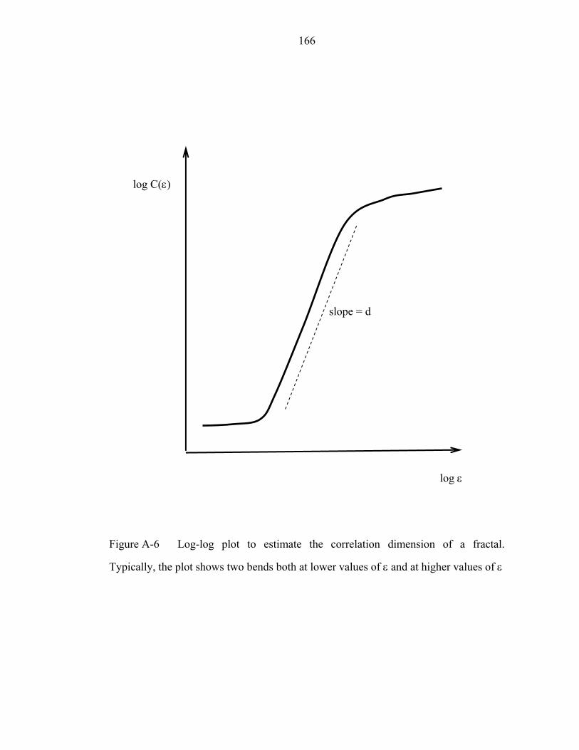
166
Figure A-6 Log-log plot to estimate the correlation dimension of a fractal.
Typically, the plot shows two bends both at lower values of ε and at higher values of ε
slope = d
log C(ε)
log ε

167
APPENDIX E STOCK MARKET AND CHAOS
One of early examples is Hurst exponent in Ref. [33] for measuring heights of
river. Hurst was an English hydrologist, who worked in the early 20th century on the
Nile River Dam project. When designing a dam, the yearly changes in the water level
are of particular concern in order to adapt the dam's storage capacity according to the
natural environment. Studying an Egyptian 847-year record of the Nile River's
overflows, Hurst observed that flood occurrences could be characterized as persistent,
i.e. heavier floods were accompanied by above average flood occurrences, while
below average occurrences were followed by minor floods. In the process of this
finding, he developed the rescaled range (R/S) analysis. Suppose there exists a time
series, t, with u observations:
( )∑=
−=t
uNuNt MeX
1, (A.71)
where Xt, N, eu and MN stand for cumulative deviation over N periods, influx in year u
and average eu over N periods, respectively.
The range becomes the difference between the maximum and minimum levels
attained in equation (A.71):
( ) ( )NtNt XXR ,, minmax −= (A.72)
where R stands for range of X.
Then Hurst found a following relation
HNSR ∝/ (A.73)

168
where S and H represent the standard deviation of the original observation and Hurst
exponent, respectively. The Hurst exponent has an inverse dependence with the fractal
dimension. Hurst’s idea of R/S analysis was recently used in analyzing stock markets.
Peters tried to get a fractal dimension of some stock markets in US, UK, Japan and
German by using historical S&P 500 data, and found they were between 2 and 3 (see
Ref. [32] for detail). He claimed the method might be useful to estimate likelihood that
two consecutive events are likely to occur, and tried to show the stock markets did not
follow a random process. For above stock markets, dimensions were evaluated, and
then independent variables were identified. Note that a dimension is the minimum
number of variables to describe all the points in the fractal of interest. However, for
this technique, it is usually not possible to evaluate the Liapunov exponent and the
dimension of a fractal without pretreatment since the measured data contain a large
error. Thus, it is necessary to eliminate or reduce the effect of error. First, based on
assumption that the distribution of errors was known, it adds the known type of error
to the measurement. Then, measured data are “filtered out” in order to reduce error.
This error reduction process gives rise to major criticismA25, and makes analysis on a
stock market arbitrary.
A25 if added error does not follow the original error distribution and it has a bigger contribution to the values for the quantity to be estimated than original signal, “filtering out” process may wash off the original signal and leftover value represents only the arbitrary added error
169
REFERENCES
[1]. R. A. Bettis and C. K. Prahalad, “The Dominant Logic: Retrospective and
Extension”, Strategic Manage. J., Vol. 16, No. 1 (1995) 5-14
[2] A. E. Rot and I. Erev, “Learning in Extensive-form Games: Experimental Data
and Simple Dynamic Models in the Intermediate Term”, Games Econom.
Behav., Vol. 8, No. 1, (1995) 164-212
[3]. I. Erev and A. E. Rot, “Predicting How People Play Games: Reinforcement
Learning in Experimental Games with Unique, Mixed Strategy Equilibria”,
Amer. Econom. Rev., Vol. 88, No. 4 (1998) 848-881
[4]. C. Richter and G. Sheblè, “Genetic Algorithm Evolution of Utility Bidding
Strategies for the Competitive Marketplace”, IEEE Trans. Power Syst., Vol. 13,
No. 1. (1998) 256 – 261
[5]. C. Richter, G. Sheblé and D. Ashlock, “Comprehensive Bidding Strategies
with Genetic Programming/Finite State Automata”, IEEE Trans. On Power
Syst., Vol. 14, No. 4 (1999) 1207 – 1212
[6]. C. Ritcher and G. Sheblè, “A Profit-Based Unit Commitment GA for the
Competitive Environment”, IEEE Trans. On Power Syst., Vol. 15, No. 2 (2000)
715 – 721
170
[7]. Z. Michalewicz, “Genetic Algorithms + Data Structures = EvolutionPrograms”,
2nd Ed., Berlin, Germany, Springer-Verlag (1992)
[8]. D. W. Bunn and F. S. Oliveira, “Agent-based simulation-an application to the
new electricity trading arrangements of England and Wales”, IEEE Trans. Evol.
Comp., Vol. 5 (2001 ) 493 – 503
[9]. D. W. Bunn, “Forecasting loads and prices in competitive power markets”,
Proc. IEEE Vol. 88, (2000) 163 – 169
[10]. D. W. Bunn, “Evaluation of market power using agent based simulation”,
Power Eng. Soc. General Meeting, Vol. 1, (2003) 506 - 508
[11]. H.-N. Oh, “Simulation Methods for Modeling Offer Behavior and Spot Prices
in Restructured Markets for Electricity”, dissertation, Cornell University (2003)
[12]. H. Oh, R. J. Thomas, B. Leiseutre and T. D. Mount, “A method for classifying
offer strategies observed in an electricity market”, J. Decision Support System,
(2005) (in press)
[13]. J. Crank, “The Mathematics of Diffusion”, Second Edition, Clarendon Press,
Oxford (1975) 38 – 40
[14]. D. Bernoulli, “Specimen Theoriae Novae Demensura Sortis”, (1738)
Proceedings of the St. Petersburg Imperial Academy of Science, 5 – translated
into English (1954)
171
[15]. C. J. Grayson, “Decisions under Uncertainty: Drilling Decisions by Oil and
Gas Operators”, Technical Report, Division of Research, Harvard Business
School, Boston (1960)
[16]. R. A. Swalin, “Thermodynamics of Solids”, 2nd Ed., New York John Wiley &
Sons (1972)
[17]. H. W. Kuhn and A. W. Tucker, “Nonlinear Programming”, in Jerzy Neyman,
Proceedings of the Second Berkeley Symposium, University of California
Press, Berkeley (1951) 481 - 492
[18]. C. Kittel, “Thermal Physics”, 2nd Ed., (1980) W H Freeman & Company,
San Fransisco (1980)
[19]. T. D. Mount, “Strategic Behavior in Spot Markets for Electricity When Load is
Stochastic”, presented as a selected paper at the Hawaii International
Conference on System Science, Maui. (2000)
[20]. R. Baldick and W. Hogan, “Capacity Constrained Supply Function
Equilibrium Models of Electricity Markets: Stability, Non-Decreasing
Constraints, and Function Space Iterations”, POWER working paper on
http://www.ucei.berkeley.edu/ucei/pubs-pwp.html (2001)
172
[21]. R. Rajaraman and F. Alvarado, “Optimal Bidding Strategy in Electricity
Markets Under Uncertain Energy and Reserve Prices”, Power System
E n g i n e e r i n g R e s e a r c h C e n t e r ( P S E R C ) o n
h t t p : / / w w w . p s e r c . w i s c . e d u / c g i - p s e r c / g e t b i g / p u b l i c a t i o / r e p o r t s /
2 0 0 3 r e p o r t / a l v a r a d o _ b i d d i n g _ r e p o r t _ 0 4 1 1 . p d f ( 2 0 0 3 )
[22]. S. de la Torre, J. M. Arroyo, A. J. Conejo and J. Contreras, “Price Maker
Self-Scheduling in a Pool-Based Electricity Market: A Mixed-Integer LP
Approach”, IEEE Transactions on Power Syst., Vol. 17, No. 4, (2002)
[23]. J. Contreras, O. Candiles, J. Fuente and T. Gómez, “A Coweb Bidding Model
for Competitive Electricity Markets”, IEEE Trans. On Power Syst., Vol/ 17,
No. 1 (2002) 148-153
[24]. T. L. Fine, “Feedforward Neural Network Methodology”, Springer-Verlag,
New York (1999)
[25]. Smith, “Neural Networks for Statistical Modeling”, Boston International
Thomson Computer Press (1996)
[26]. S. Geman., E. Bienenstock. and R. Doursat, “Neural Networks and the
Bias/Variance Dilemma”, Neural Computation, 4 (1992) 1-58.
[27]. California Independent System Operator, “ISO Market Monitoring &
Information Protocol”, on
http://www.caiso.com/docs/2002/02/12/2002021215391318952.pdf (2002)
173
[28.] C. A. Berry, B. F. Hobbs, W. A. Meroney, R. P. O’Neill and W. R. Steward,
“Analyzing Strategic Bidding Behavior in Transmission Networks”, Game
Theory Application in Electricity Markets, 99TP-136-0, IEEE PES Winter
Meeting (1999) 7-32
[29]. J. D. Weber and T. J. Overbye, “A Two-Level Optimization Problem for
Analysis of Market Bidding Strategies”, Power Engineering Society Summer
Meeting, IEEE, Vol. 2, (1999) 682 – 687
[30]. S. H. Strogatz, “Nonlinear Dynamics and Chaos”, Westerview, Cambridge
(2000)
[31]. E. N. Lorenz, “Deterministic Nonperiodic Flow”, J. Atmos. Sci., 20 (1963) 130
[32]. Peters, E. “Chaos and Order in the Capital Markets A New View of Cycles,
Prices, and Market Volatility”, New York, John Wiley & Sons, Inc (1991)
[33]. H. E. Hurst, “Long-Term Storage of Reservoirs”, Transactions of the
American Society of Civil Engineers (1951) 116
[34]. A. Wolf, J. B. Swift, H. L. Swinney and J. A. Vastano, “Determining
Lyapunov Exponents from a Time Series”, Physica 16D (1985) 285-317
[35]. Kantz, H. and Schreiber, T. “Nonlinear Time Series Analysis”, Cambridge,
Cambridge Univ. Press (1999)

174
[36]. S. Collins and C. J. De Luca, “Upright, Correlated Random Walk: A
Statistical-Biomechanics Approach to the Human Postural Control System”,
CHAOS, 5 (1995) 57
[37]. H. Kantz, “A Robust Method to Estimate the Maximal Lyapunov Exponent of
a Time Series”, Phys. Lett. A., 185 (1994) 77
[38]. R. S. Sutton, “Reinforcement Learning: an Introduction” MIT Press,
Cambridge Mass. (1998); electronic version can be found at
http://encompass.library.cornell.edu/cgi-
bin/checkIP.cgi?access=gateway_standard%26url=http://encompass.library.cor
nell.edu/cgi-bin/scripts/ebooks.cgi?bookid=1094