Embed Size (px)
Citation preview
Universitat Politècnica de València
Electrical and Anatomical Modeling of the Specialized
Cardiac Conduction System. A Simulation Study.
PREDOCTORAL RESEARCH THESIS
Biomedical Engineering
PhD Program in Health and Welfare
LYDIA DUX-SANTOY HURTADO
Director:
Dr. Jose M. Ferrero de Loma-Osorio
Co-director:
Dr. Rafael Sebastián Aguilar
Grupo de Bioelectrónica-I3BH
Universitat Politècnica de València
March 2011

“Ego quid sciam quaero, non quid credam”
Yo investigo para saber algo, no para pensarlo
San Agustín, Soliloquia, I, III., 8

5
TABLE OF CONTENTS
TABLE OF CONTENTS ................................................................................................................ 5
TABLE OF FIGURES ................................................................................................................... 7
ACRONYMS ............................................................................................................................ 11
1. INTRODUCTION ...................................................................................................... 13
A- Motivation and Aims .............................................................................................. 13
B- Anatomy and electrophysiology of the Specialized Cardiac Conduction System . 15
The electrical sequence of activation ........................................................................... 15
Anatomy and histology ................................................................................................ 19
Cellular Electrophysiology ........................................................................................... 24
C- Structural models of the Purkinje system ............................................................... 25
D- Pseudo-ECG ........................................................................................................... 28
E- Arrhythmias and drugs. Case study: dofetilide ...................................................... 29
2. OBJECTIVES ............................................................................................................ 31
3. MATERIAL AND METHODS ................................................................................. 33
A- Anatomical model of the ventricles ........................................................................ 33
B- Action Potential models ......................................................................................... 35
Purkinje Fiber cell model by Stewart et al. .................................................................. 35
Ventricular cells model by Ten-Tusscher et al............................................................. 36
C- Drug modeling: Dofetilide ..................................................................................... 37
D- Mathematical formulation of the electrical activity of the heart ............................ 38
Propagation equations. Monodomain model ................................................................ 38
E- Stimulation protocol ............................................................................................... 40
Without Purkinje system: ventricles stimulation ......................................................... 40
With Purkinje system ................................................................................................... 41
F- Pseudo-ECG calculation ........................................................................................ 41
G- Computational simulations ..................................................................................... 43
Pre-processing. Inclusion of Purkinje model ............................................................... 43
Processing simulations (EMOS) .................................................................................. 44
Post-processing of cardiac simulations ........................................................................ 45
4. PURKINJE NETWORK GENERATION ALGORITHM ........................................ 47
A- Segmentation of endocardial nodes ........................................................................ 47
6
B- Purkinje network layout ......................................................................................... 47
C- Definition of the Bundle of His .............................................................................. 48
D- Algorithms to create the core Purkinje network ..................................................... 51
Nearest neighbor .......................................................................................................... 53
PMJ inhomogeneity and additional ―intermediate‖ terminals ..................................... 53
―Looping‖ structures in the network ............................................................................ 54
5. RESULTS .................................................................................................................. 55
A- Characteristics of the generated Purkinje networks ............................................... 55
B- The simulation study .............................................................................................. 56
C- Effects of the His and proximal bundles ................................................................ 57
D- Cellular and Tissue level ........................................................................................ 59
E- Organ level ............................................................................................................. 70
6. DISCUSSION ............................................................................................................ 75
A- Multi-scale results .................................................................................................. 75
B- Limitations ............................................................................................................. 77
7. CONCLUSIONS ........................................................................................................ 79
8. APPENDIX ................................................................................................................ 81
A- Anatomy of the heart .............................................................................................. 81
B- Diffusion Tensor Magnetic Resonance (DTMRI) .................................................. 82
C- Computational simulation ...................................................................................... 83
Pre-processed ............................................................................................................... 83
Processed (EMOS) ....................................................................................................... 84
Post-processed .............................................................................................................. 88
9. BIBLIOGRAPHY ...................................................................................................... 91
7
TABLE OF FIGURES
Figure 1. A graphical representation of the electrical conduction system of the heart showing
the Sinoatrial node, Atrioventricular node, HB, PK fibers, and Bachmann's bundle. ...... 13
Figure 2. Specialized electrical conduction system of the heart. Yellow arrows indicate the path
followed by the electrical impulses from the SAN to the PK fibers. ................................ 16
Figure 3. Representation of activation sequence by means of isochronal maps at different
horizontal cuts of a human isolated heart obtained by Durrer using microelectrodes. Scale
is in milliseconds. .............................................................................................................. 17
Figure 4. Activation of (a) the right ventricular free wall and (b) the left ventricular septum. . 18
Figure 5. Ventricular and atrial isochrones. Ventricular epicardial isochrones from subjects
nos. 1 (A), 3 (B), and 4 (C). Numbers indicate location of early activation sites. ............ 18
Figure 6. Serial examination of section of HB and initial branches from a human heart. ........ 20
Figure 7. Pertinent anatomic features of the proximal left ventricular conducting system shown
by Myerburg. ..................................................................................................................... 20
Figure 8. HB described by Tawara [7]. Figure taken from [11]. ............................................... 21
Figure 9. PK network in the LV. Tawara’s illustration is very similar to the real network in the
photograph. (a) Tawara’s illustration, showing the three divisions in human LBB. (b) PK
network of a calf heart. ..................................................................................................... 21
Figure 10. PK cells within the right and left ventricular free walls of a sheep heart. The
specialized myocyte with distinctive morphologies (open arrows) are found in both the
inner and the outer layers of the ventricular walls. ........................................................... 22
Figure 11. Scanning electron micrograph of the transitional cells of the sheep subendocardial
network (a) and a close-up view of the ruled area(b). P (Purkinje), M (Myocardium), T
(Transitional). .................................................................................................................... 23
Figure 12. Schematic of the preparation including the position for the recording array (a) and
(b) means ±SD for the number of sites with P deflections during sinus mapping and
endocardial pacing experiments. ....................................................................................... 23
Figure 13. AP from a canine PK fiber strand and ventricular muscle fine electrode recording,
paced at BCL=500 ms and [K]o=4 mM. Figure taken from [30]. ..................................... 25
Figure 14. Two-dimensional representation of the model with a damaged region in the LV
represented by the light gray area. Image from [37]. ........................................................ 26
Figure 15. A 2-D representation of the left and right PK network superimposed on the flattened
left and right endocardial surfaces. Post. Indicates posterior wall; Ant., anterior wall.
From [40] .......................................................................................................................... 27
Figure 16. Normal excitation with propagation from the HB downstream past the bundle
branches and into the right and left septum, and finally into the myocardium. Numbers
indicate milliseconds. From [40]....................................................................................... 27
Figure 17. The geometry of the conduction system observed from different angles. (a) Model
from Simelius [41] and (b) Model from Ten-Tusscher [3]. The PMJs are shown as light
green spheres. .................................................................................................................... 28
Figure 18. CCS and its relation to ECG. Figure taken from [43] .............................................. 28
Figure 19. Normal ECG in precordial leads .............................................................................. 29
8
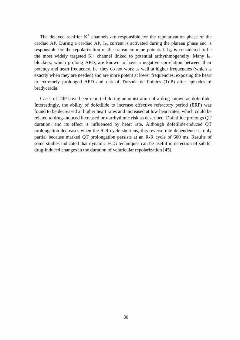
Figure 20. Ventricular human heart model built from a DTMRI stack. (a) Right and left
ventricles were segmented and meshed with hexahedral elements. (b) Myocardial fiber
orientation represented by small vectors. .......................................................................... 33
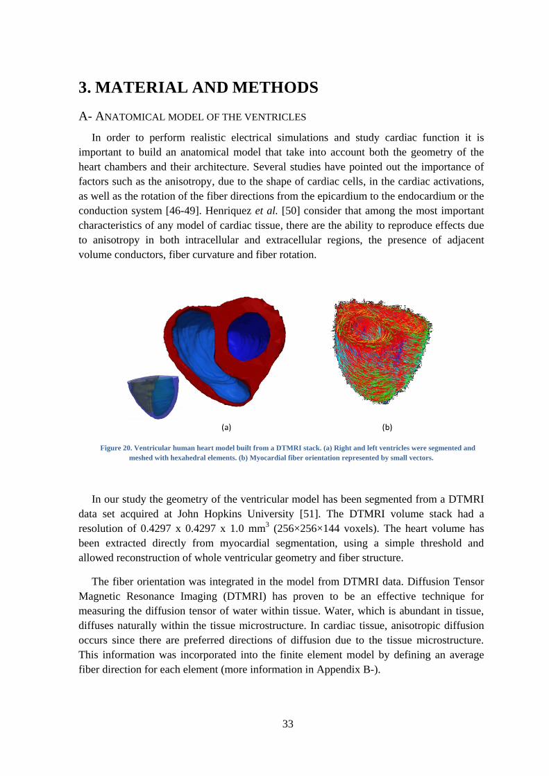
Figure 21. Biventricular geometry. (a) Labeled regions, LV endocardium and epicardium and
RV endocardium and epicardium. (b) Detail of the lateral wall mesh showing the
hexahedral elements. ......................................................................................................... 34
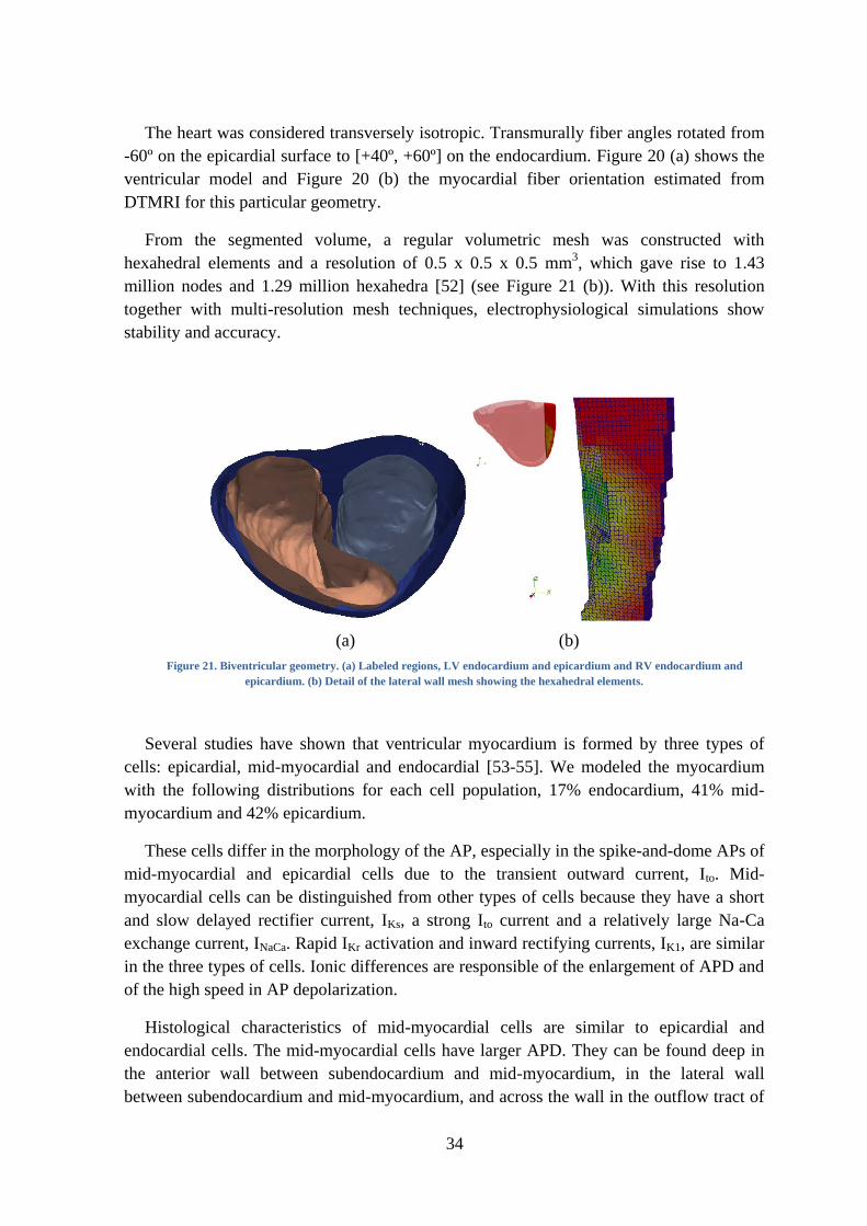
Figure 22. Schematic diagram of the PK cell model of Stewart ............................................... 35
Figure 23. Schematic diagram of ventricular cell model of Ten-Tusscher ............................... 36
Figure 24. Time courses of APs for M, endocardial and epicardial guinea pig cellular models
for 100 nM of dofetilide at a BCL=1000 ms, from the application of dofetilide (CNT, t=0)
until steady-state is achieved). Figure modified from [60] ............................................... 37
Figure 25. Normal ECG and ECG with IKr block (long QT)..................................................... 37
Figure 26. Points of the stimulation protocol. The color of each point represents the activation
time. ................................................................................................................................... 41
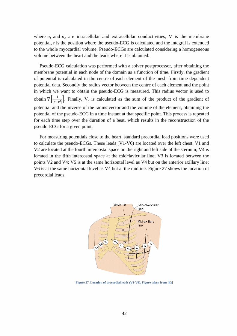
Figure 27. Location of precordial leads (V1-V6). Figure taken from [43] ............................... 42
Figure 28. CS2H05_PK.dat file ................................................................................................ 44
Figure 29. Extraction of endocardial hexahedra. One element thick hexahedra shown in blue
inside heart volume in red. ................................................................................................ 47
Figure 30. Location of the AVN in the ventricular model ........................................................ 48
Figure 31. Configuration HB4 of the HB .................................................................................. 50
Figure 32. Configuration HB5 of the HB .................................................................................. 50
Figure 33. Configuration HB6 of the HB .................................................................................. 50
Figure 34. Diagram of the algorithm to create PK networks .................................................... 52
Figure 35. Terminal nodes. (a) Distribution of terminal nodes in the ventricular model. (b)
Detail of terminal nodes and their connections ................................................................. 54
Figure 36. View of a modeled PK network showing "looping" structures ............................... 54
Figure 37. Examples of generated PK networks (a) Uncovering the superior basal third and (b)
Covering the whole endocardium in the model. ............................................................... 55
Figure 38. Pseudo-ECGs obtained in precordial leads in two different CCSs created with the
same algorithm parameters but with different number of net-nodes in each ventricle (and
different number of PMJ) .................................................................................................. 57
Figure 39. Simulated pseudo-ECGs for configuration HB5 of the HB ..................................... 58
Figure 40. Simulated pseudo-ECGs for (a) configurations HB4 and (b) HB6 of the HB ......... 59
Figure 41. Evolution of APD dispersion for several consecutive heart beats (5 pulses,
BCL=1000 ms) for simulations including the CCS with D=100 nM of dofetilide. .......... 60
Figure 42. Simulated AP for (a) different cell types in physiological conditions and for
physiological conditions and different doses of dofetilide in (b) PK fiber. (c) M cell AP in
simulations without the CCS. (d) M cell AP in simulations including the CCS............... 61
Figure 43. Activation of the ventricular wall in contact with PMJs in the neighboring region of
PMJs. Color indicates the time of the activation in ms. .................................................... 62
Figure 44. Three dimensional isochronic representation of the activation reported by Durrer.
Color indicates time of activation in ms. Figure from [1] ................................................. 62
Figure 45. Two examples of epicardial excitation maps in human hearts. Hearts (a) and (b) are
presented showing (1) an anterior view, (2) a left lateral view and (3) a posterior view.
Color indicates time of activation in ms. Figure from [1] ................................................. 63
9
Figure 46. Epicardial excitation maps in simulation including CCS for control case. The heart
model is presented showing (a) an anterior view, (b) a left lateral view and (c) a posterior
view. Color indicates time of activation in ms. ................................................................. 63
Figure 47. Isochrone maps (left) and APD maps (right) of posterior view in simulations
without the CCS for different doses of dofetilide. Isochrone maps show that Ikr has no
effect in the activation time, while APD maps show that Ikr block increases the duration of
the AP. Larger APD maps figures have a common APD colormap range, while others
APD maps figures have their own colormap range. Dofetilide doses applied were (a) D=0
nM, (b) D=10 nM, (c) D=100 nM. Color indicates time of activation in ms in the
isochrone maps and AP duration in ms in APD maps. ..................................................... 65
Figure 48. Section in two different human hearts showing the endo-to-epi activation pattern.
Color indicates activation time in ms. Figure from [1] ..................................................... 66
Figure 49. Isochrone maps of posterior view along with the CCS for different doses of
dofetilide showing that Ikr block has no effect in the activation time. Dofetilide doses
applied were (a) D=0 nM, (b) D=10 nM, (c) D=100 nM. Color indicates time of
activation in ms. ................................................................................................................ 68
Figure 50. APD maps of posterior view along with the CCS for different doses of dofetilide
showing that Ikr block increases the duration of the AP. Larger size figures have a
common APD colormap range, while others have their own colormap range. Dofetilide
doses applied were (a) D=0 nM, (b) D=10 nM, (c) D=100 nM. Color indicates the
duration of the AP in ms. .................................................................................................. 69
Figure 51. Different behavior of epicardial, endocardial and mid-myocardial cell types. APD
dispersion as a function of the dofetilide concentration for (a) ventricular model without
the CCS and (b) ventricular model including the CCS. .................................................... 71
Figure 52. Simulated pseudo-ECGs in the precordial leads for different doses of dofetilide
obtained with (a) the ventricular model without the CCS and (b) the ventricular model
including the CCS ............................................................................................................. 72
Figure 53. (a) 3D volume rendering from CT and (b) multiplanar reconstruction. An oblique
view aims to visualize the membranous septum (arrow). RA = right atrium; RV = right
ventricle; Ao = aorta; LV = left ventricle. ........................................................................ 81
Figure 54. Anatomy of the heart and associated vessels ........................................................... 82
Figure 55. DTMRI short axis cut showing RV and LB. (a) Gray level image from DTI and (b)
reconstruction of fiber orientation in plane. ...................................................................... 83
Figure 56. File #NODES in CS2H05_PK.dat ........................................................................... 85
Figure 57. File #ELEMENTS in CS2H05_PK.dat .................................................................... 86
Figure 58. File #STIMULUS in CS2H05_PK.dat ..................................................................... 87
Figure 59. Post_config.dat file .................................................................................................. 89

10
11
ACRONYMS
AP Action potential
APD Action potential duration
AVN Atrio-ventricular node
BCL Basic Cycle length
CCS Cardiac conduction system
D Dofetilide concentration
ECG Electrocardiogram
HB Bundle of His
LBB Left bundle branch
LBBB Left bundle branch block
LV Left ventricle
PK Purkinje
PMJ Purkinje-myocardial junction
RBB Right bundle branch
RV Right ventricle
SAN Sino-atrial node

12
13
1. INTRODUCTION
A- MOTIVATION AND AIMS
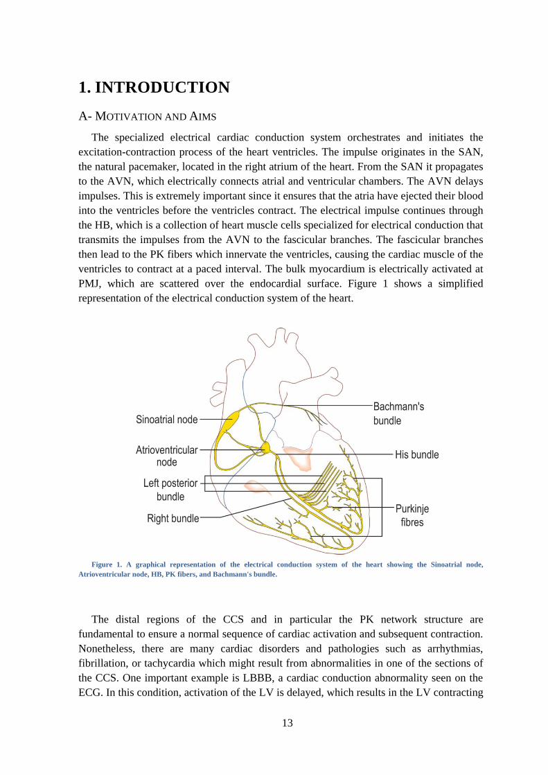
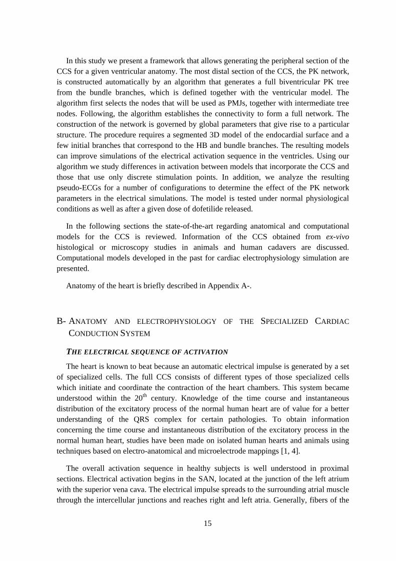
The specialized electrical cardiac conduction system orchestrates and initiates the
excitation-contraction process of the heart ventricles. The impulse originates in the SAN,
the natural pacemaker, located in the right atrium of the heart. From the SAN it propagates
to the AVN, which electrically connects atrial and ventricular chambers. The AVN delays
impulses. This is extremely important since it ensures that the atria have ejected their blood
into the ventricles before the ventricles contract. The electrical impulse continues through
the HB, which is a collection of heart muscle cells specialized for electrical conduction that
transmits the impulses from the AVN to the fascicular branches. The fascicular branches
then lead to the PK fibers which innervate the ventricles, causing the cardiac muscle of the
ventricles to contract at a paced interval. The bulk myocardium is electrically activated at
PMJ, which are scattered over the endocardial surface. Figure 1 shows a simplified
representation of the electrical conduction system of the heart.
Figure 1. A graphical representation of the electrical conduction system of the heart showing the Sinoatrial node,
Atrioventricular node, HB, PK fibers, and Bachmann's bundle.
The distal regions of the CCS and in particular the PK network structure are
fundamental to ensure a normal sequence of cardiac activation and subsequent contraction.
Nonetheless, there are many cardiac disorders and pathologies such as arrhythmias,
fibrillation, or tachycardia which might result from abnormalities in one of the sections of
the CCS. One important example is LBBB, a cardiac conduction abnormality seen on the
ECG. In this condition, activation of the LV is delayed, which results in the LV contracting
14
after the RV, and a decrease the cardiac ejection. Other important negative effects of
abnormal activation of the CCS are the generation of electrical macro or micro re-entries.
This type of reentry is due to a unidirectional block in the CCS and can give rise to
ventricular tachycardia. Another source of problems might originate from the PK system
itself, which has been reported to produce subendocardial focal activity i.e. early after-
depolarizations (EADs) and delayed after-depolarizations (DADs), or microreentry under
certain conditions.
Although the role of the CCS in the normal electrical sequence of activation is well
known, its functioning in abnormal conditions, or its interaction with electrical disorders
which have their origin in other pathologies, such as infarctions, is not well understood yet.
In order to better understand the underlying mechanisms that lead to certain types of
arrhythmia, it is crucial to look for new tools that allow studying in detail the electrical
coupling of the CCS and the myocardium under normal and pathological conditions in an
easy way.
ICT tools and integrative multi-scale computational models of the heart may help to
improve understanding, diagnosis, treatment planning and interventions for cardio vascular
disease. Biophysical models of cardiac electrophysiology are available at different scales
and are able to reproduce the electrical activation and propagation in cardiac soft tissues.
The opportunity of multi-scale modeling spanning multiple anatomical levels (sub-cellular
level up to whole heart) is to provide a consistent, biophysically-based framework for the
integration of the huge amount of fragmented and inhomogeneous data currently available.
The combination of biophysical and patient-specific anatomical models of atria and
ventricles allows simulating cardiac electrical activations for a given patient and has the
potential for helping in decision taking processes for electrical therapies such as cardiac
resynchronization therapy or radio-frequency ablation.
One of the main drawbacks of current cardiac models is the impossibility of obtaining
patient-specific data for all the anatomical components that take part in the electrical
activation of the heart. Among them the CCS has remained largely elusive due to the
difficulty to observe it in-vivo and the little amount of information available in the
literature. As a result, the CCS is often not modeled in computational models or is
oversimplified. Among the most common approaches followed to avoid explicitly
modeling the PK system, though still synchronously activating the ventricles, is the use of
excitation points. In this approach, a set of discrete scattered excitation points is placed all
over the endocardium. Following the measurements from ex-vivo electrical mapping
studies, such as Durrer [1] the points are activated, as small pacemakers, creating a virtual
activation map. More sophisticated approaches build simplistic PK trees that define the
locations of the PMJs based on electrical landmarks [2, 3]. Although simple geometrical
models allow including specific PK cellular models and PMJs, none of them tried to
reproduce the pattern or structure of the PK system, or its complexity.
15
In this study we present a framework that allows generating the peripheral section of the
CCS for a given ventricular anatomy. The most distal section of the CCS, the PK network,
is constructed automatically by an algorithm that generates a full biventricular PK tree
from the bundle branches, which is defined together with the ventricular model. The
algorithm first selects the nodes that will be used as PMJs, together with intermediate tree
nodes. Following, the algorithm establishes the connectivity to form a full network. The
construction of the network is governed by global parameters that give rise to a particular
structure. The procedure requires a segmented 3D model of the endocardial surface and a
few initial branches that correspond to the HB and bundle branches. The resulting models
can improve simulations of the electrical activation sequence in the ventricles. Using our
algorithm we study differences in activation between models that incorporate the CCS and
those that use only discrete stimulation points. In addition, we analyze the resulting
pseudo-ECGs for a number of configurations to determine the effect of the PK network
parameters in the electrical simulations. The model is tested under normal physiological
conditions as well as after a given dose of dofetilide released.
In the following sections the state-of-the-art regarding anatomical and computational
models for the CCS is reviewed. Information of the CCS obtained from ex-vivo
histological or microscopy studies in animals and human cadavers are discussed.
Computational models developed in the past for cardiac electrophysiology simulation are
presented.
Anatomy of the heart is briefly described in Appendix A-.
B- ANATOMY AND ELECTROPHYSIOLOGY OF THE SPECIALIZED CARDIAC
CONDUCTION SYSTEM
THE ELECTRICAL SEQUENCE OF ACTIVATION
The heart is known to beat because an automatic electrical impulse is generated by a set
of specialized cells. The full CCS consists of different types of those specialized cells
which initiate and coordinate the contraction of the heart chambers. This system became
understood within the 20th
century. Knowledge of the time course and instantaneous
distribution of the excitatory process of the normal human heart are of value for a better
understanding of the QRS complex for certain pathologies. To obtain information
concerning the time course and instantaneous distribution of the excitatory process in the
normal human heart, studies have been made on isolated human hearts and animals using
techniques based on electro-anatomical and microelectrode mappings [1, 4].
The overall activation sequence in healthy subjects is well understood in proximal
sections. Electrical activation begins in the SAN, located at the junction of the left atrium
with the superior vena cava. The electrical impulse spreads to the surrounding atrial muscle
through the intercellular junctions and reaches right and left atria. Generally, fibers of the
16
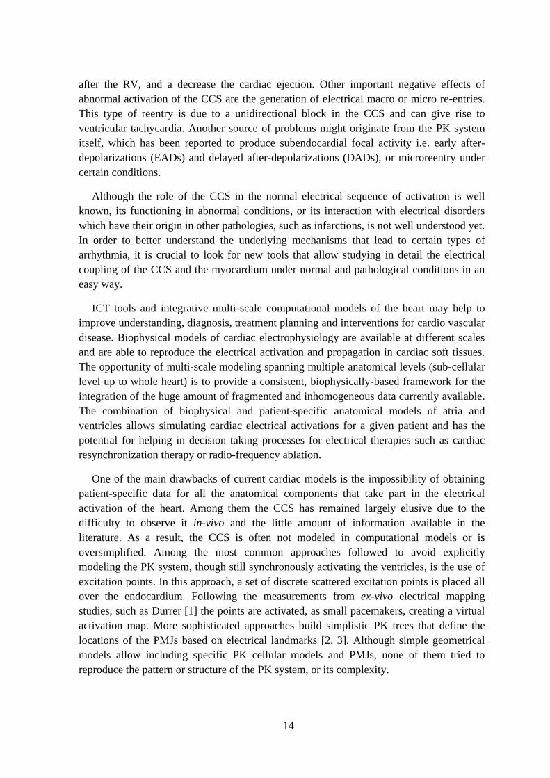
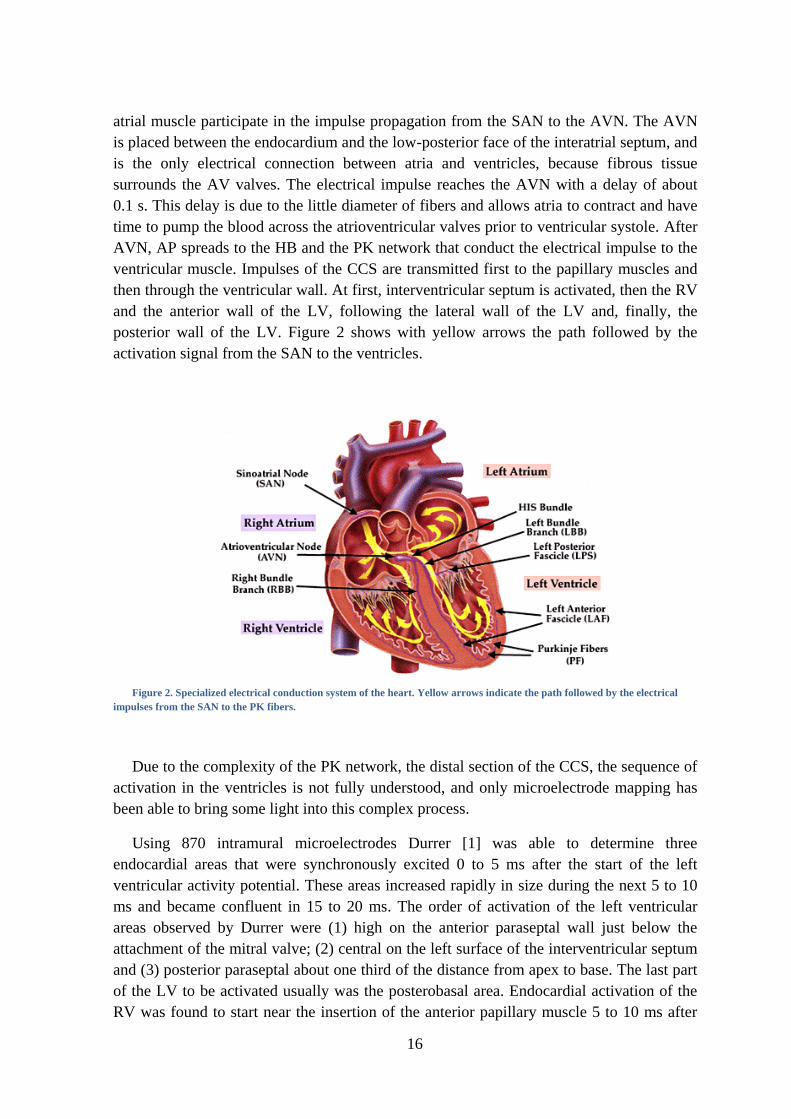
atrial muscle participate in the impulse propagation from the SAN to the AVN. The AVN
is placed between the endocardium and the low-posterior face of the interatrial septum, and
is the only electrical connection between atria and ventricles, because fibrous tissue
surrounds the AV valves. The electrical impulse reaches the AVN with a delay of about
0.1 s. This delay is due to the little diameter of fibers and allows atria to contract and have
time to pump the blood across the atrioventricular valves prior to ventricular systole. After
AVN, AP spreads to the HB and the PK network that conduct the electrical impulse to the
ventricular muscle. Impulses of the CCS are transmitted first to the papillary muscles and
then through the ventricular wall. At first, interventricular septum is activated, then the RV
and the anterior wall of the LV, following the lateral wall of the LV and, finally, the
posterior wall of the LV. Figure 2 shows with yellow arrows the path followed by the
activation signal from the SAN to the ventricles.
Figure 2. Specialized electrical conduction system of the heart. Yellow arrows indicate the path followed by the electrical
impulses from the SAN to the PK fibers.
Due to the complexity of the PK network, the distal section of the CCS, the sequence of
activation in the ventricles is not fully understood, and only microelectrode mapping has
been able to bring some light into this complex process.
Using 870 intramural microelectrodes Durrer [1] was able to determine three
endocardial areas that were synchronously excited 0 to 5 ms after the start of the left
ventricular activity potential. These areas increased rapidly in size during the next 5 to 10
ms and became confluent in 15 to 20 ms. The order of activation of the left ventricular
areas observed by Durrer were (1) high on the anterior paraseptal wall just below the
attachment of the mitral valve; (2) central on the left surface of the interventricular septum
and (3) posterior paraseptal about one third of the distance from apex to base. The last part
of the LV to be activated usually was the posterobasal area. Endocardial activation of the
RV was found to start near the insertion of the anterior papillary muscle 5 to 10 ms after
17
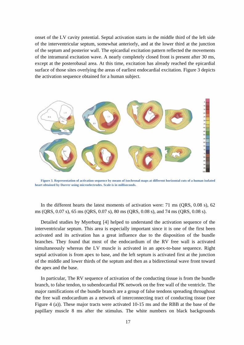
onset of the LV cavity potential. Septal activation starts in the middle third of the left side
of the interventricular septum, somewhat anteriorly, and at the lower third at the junction
of the septum and posterior wall. The epicardial excitation pattern reflected the movements
of the intramural excitation wave. A nearly completely closed front is present after 30 ms,
except at the posterobasal area. At this time, excitation has already reached the epicardial
surface of those sites overlying the areas of earliest endocardial excitation. Figure 3 depicts
the activation sequence obtained for a human subject.
Figure 3. Representation of activation sequence by means of isochronal maps at different horizontal cuts of a human isolated
heart obtained by Durrer using microelectrodes. Scale is in milliseconds.
In the different hearts the latest moments of activation were: 71 ms (QRS, 0.08 s), 62
ms (QRS, 0.07 s), 65 ms (QRS, 0.07 s), 80 ms (QRS, 0.08 s), and 74 ms (QRS, 0.08 s).
Detailed studies by Myerburg [4] helped to understand the activation sequence of the
interventricular septum. This area is especially important since it is one of the first been
activated and its activation has a great influence due to the disposition of the bundle
branches. They found that most of the endocardium of the RV free wall is activated
simultaneously whereas the LV muscle is activated in an apex-to-base sequence. Right
septal activation is from apex to base, and the left septum is activated first at the junction
of the middle and lower thirds of the septum and then as a bidirectional wave front toward
the apex and the base.
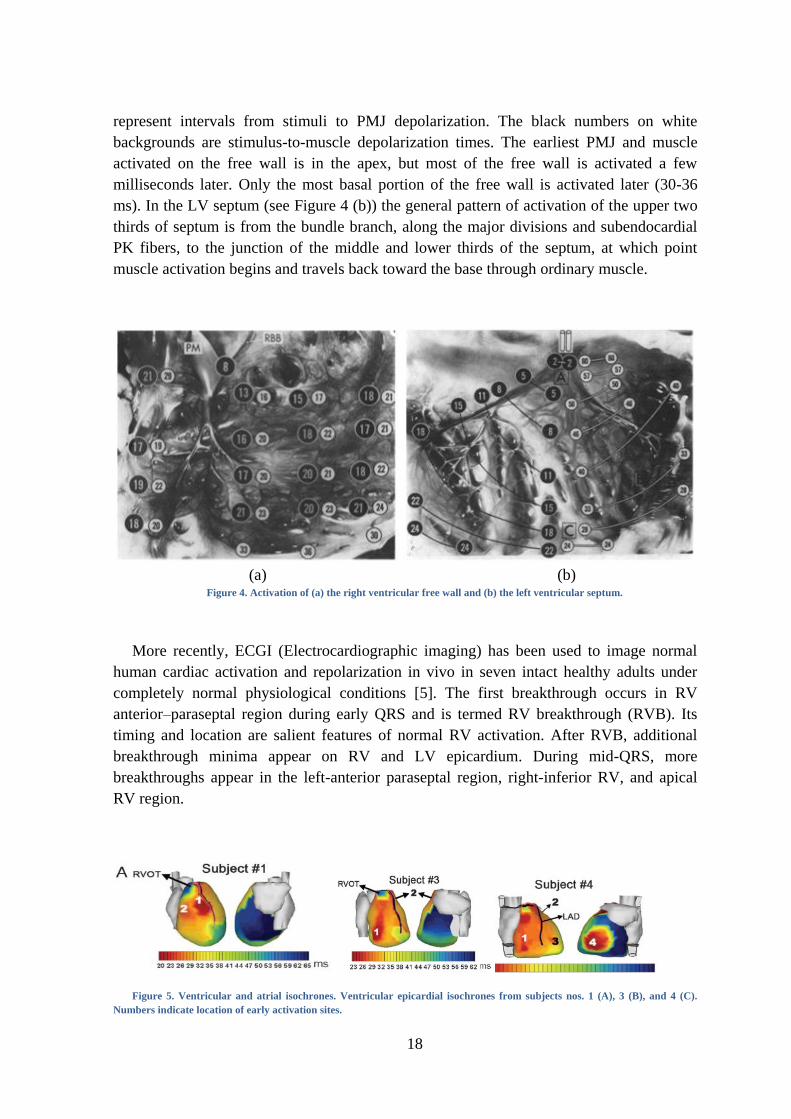
In particular, The RV sequence of activation of the conducting tissue is from the bundle
branch, to false tendon, to subendocardial PK network on the free wall of the ventricle. The
major ramifications of the bundle branch are a group of false tendons spreading throughout
the free wall endocardium as a network of interconnecting tract of conducting tissue (see
Figure 4 (a)). These major tracts were activated 10-15 ms and the RBB at the base of the
papillary muscle 8 ms after the stimulus. The white numbers on black backgrounds
18
represent intervals from stimuli to PMJ depolarization. The black numbers on white
backgrounds are stimulus-to-muscle depolarization times. The earliest PMJ and muscle
activated on the free wall is in the apex, but most of the free wall is activated a few
milliseconds later. Only the most basal portion of the free wall is activated later (30-36
ms). In the LV septum (see Figure 4 (b)) the general pattern of activation of the upper two
thirds of septum is from the bundle branch, along the major divisions and subendocardial
PK fibers, to the junction of the middle and lower thirds of the septum, at which point
muscle activation begins and travels back toward the base through ordinary muscle.
(a) (b)
Figure 4. Activation of (a) the right ventricular free wall and (b) the left ventricular septum.
More recently, ECGI (Electrocardiographic imaging) has been used to image normal
human cardiac activation and repolarization in vivo in seven intact healthy adults under
completely normal physiological conditions [5]. The first breakthrough occurs in RV
anterior–paraseptal region during early QRS and is termed RV breakthrough (RVB). Its
timing and location are salient features of normal RV activation. After RVB, additional
breakthrough minima appear on RV and LV epicardium. During mid-QRS, more
breakthroughs appear in the left-anterior paraseptal region, right-inferior RV, and apical
RV region.
Figure 5. Ventricular and atrial isochrones. Ventricular epicardial isochrones from subjects nos. 1 (A), 3 (B), and 4 (C).
Numbers indicate location of early activation sites.
19
ANATOMY AND HISTOLOGY
Because of the difficulty in identifying conduction tissue, there has been considerable
wheel spinning over the last century. People thought they saw things, others did not, and
controversy abounded. This is partly because of the lack of markers for this specific tissue.
The understanding of the PK pattern was delayed for a long time. In 1845 Jan Evangelista
Purkinje published his discovery of a part of the heart conduction system that we call PK
fibers [6]. He observed these fibers in sheep’s hearts.
In 1906, Sunao Tawara published the results of his two and a half year research. In his
publication he described anatomy and histology of the electrical conduction system in
several animal specimens and in humans and emphasized the morphological unit of
transfer of the AVN to the atrioventricular bundle, bundle branches and PK network [7].
His research was really important for the knowledge of the CCS and PK fibers. Two years
later, Einthoven used Tawara’s research in the interpretation of the ECG [8].
In 1910, Aschoff [9] and Mönckeberg [10] defined the three conditions to identify a
structure as a part of the CCS: 1) the cells of the tract needed to be histologically discrete
when compared to their neighbors, 2) the cells should be able to be traced from section to
section in the histological series, 3) the cells of the tract should be insulated from their
neighbors by a sheath of fibrous tissue. The cells of the SAN and of the AVN satisfied the
first two criteria, whereas the pathways for ventricular conduction system satisfy all the
three.
Several studies describe the anatomy of the HB and its branches [1, 7, 11-14]. To
observe the net structure it is necessary to apply subendocardial injections of ink or stains.
It is very difficult to observe the Purkinje-net system in humans, because these fibers do
not stain well. Ex-vivo histological and microscopy animal data of the PK network is
available thanks to the use of specific stains such as Indian Ink [15], Goldner Trichrome
Stain [16] or immunolabeling markers [17], which can be analyzed afterwards from
histological and microscopy images.
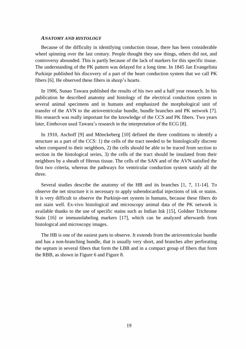
The HB is one of the easiest parts to observe. It extends from the atrioventricular bundle
and has a non-branching bundle, that is usually very short, and branches after perforating
the septum in several fibers that form the LBB and in a compact group of fibers that form
the RBB, as shown in Figure 6 and Figure 8.
20
Figure 6. Serial examination of section of HB and initial branches from a human heart.
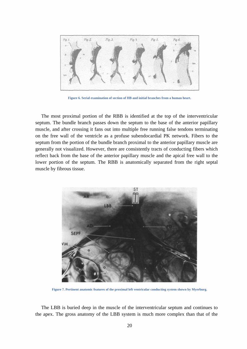
The most proximal portion of the RBB is identified at the top of the interventricular
septum. The bundle branch passes down the septum to the base of the anterior papillary
muscle, and after crossing it fans out into multiple free running false tendons terminating
on the free wall of the ventricle as a profuse subendocardial PK network. Fibers to the
septum from the portion of the bundle branch proximal to the anterior papillary muscle are
generally not visualized. However, there are consistently tracts of conducting fibers which
reflect back from the base of the anterior papillary muscle and the apical free wall to the
lower portion of the septum. The RBB is anatomically separated from the right septal
muscle by fibrous tissue.
Figure 7. Pertinent anatomic features of the proximal left ventricular conducting system shown by Myerburg.
The LBB is buried deep in the muscle of the interventricular septum and continues to
the apex. The gross anatomy of the LBB system is much more complex than that of the
21
right system. The short main LBB divides into two or three divisions high on the left side
of the interventricular septum. Large portions of the anterior (superior) division and the
posterior (inferior) division course directly toward the two papillary muscles. A profuse
subendocardial network of interlacing PK fibers courses through the septal endocardium
bordered by the two major divisions and the papillary muscles. Figure 7 depicts the main
LBB and how it bifurcates into an anterior division (AD) and a posterior division (PD)
which course toward the apical portions of both papillary muscles (out of picture). A
network of subendocardial PK fibers (SEPF) is present between the two divisions. The
endocardial true ventricular muscle tissue (VM) can be seen between the tracts of
conducting tissue. In humans, it usually forks into three divisions: anterior, medial and
posterior. The anterior bundle continues to the apex and forms a subendocardial plexus in
the area of the anterior papillary muscle. The posterior bundle goes to the area of the
posterior papillary muscle, divides into a subendocardial plexus and extends to the rest of
the LV. All divisions pass to PK network of the ventricle [18].
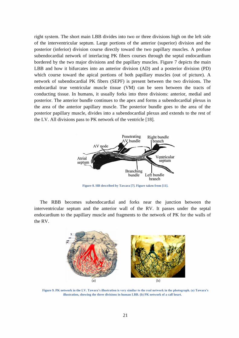
Figure 8. HB described by Tawara [7]. Figure taken from [11].
The RBB becomes subendocardial and forks near the junction between the
interventricular septum and the anterior wall of the RV. It passes under the septal
endocardium to the papillary muscle and fragments to the network of PK for the walls of
the RV.
Figure 9. PK network in the LV. Tawara’s illustration is very similar to the real network in the photograph. (a) Tawara’s
illustration, showing the three divisions in human LBB. (b) PK network of a calf heart.
22
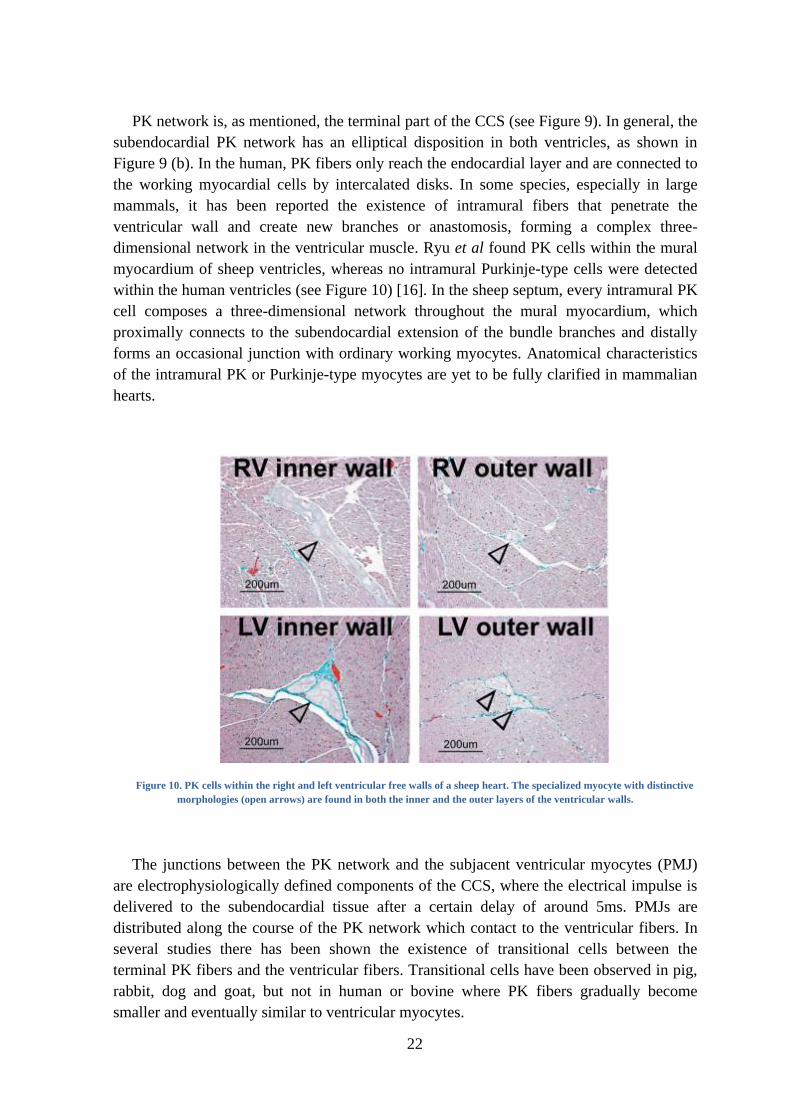
PK network is, as mentioned, the terminal part of the CCS (see Figure 9). In general, the
subendocardial PK network has an elliptical disposition in both ventricles, as shown in
Figure 9 (b). In the human, PK fibers only reach the endocardial layer and are connected to
the working myocardial cells by intercalated disks. In some species, especially in large
mammals, it has been reported the existence of intramural fibers that penetrate the
ventricular wall and create new branches or anastomosis, forming a complex three-
dimensional network in the ventricular muscle. Ryu et al found PK cells within the mural
myocardium of sheep ventricles, whereas no intramural Purkinje-type cells were detected
within the human ventricles (see Figure 10) [16]. In the sheep septum, every intramural PK
cell composes a three-dimensional network throughout the mural myocardium, which
proximally connects to the subendocardial extension of the bundle branches and distally
forms an occasional junction with ordinary working myocytes. Anatomical characteristics
of the intramural PK or Purkinje-type myocytes are yet to be fully clarified in mammalian
hearts.
Figure 10. PK cells within the right and left ventricular free walls of a sheep heart. The specialized myocyte with distinctive
morphologies (open arrows) are found in both the inner and the outer layers of the ventricular walls.
The junctions between the PK network and the subjacent ventricular myocytes (PMJ)
are electrophysiologically defined components of the CCS, where the electrical impulse is
delivered to the subendocardial tissue after a certain delay of around 5ms. PMJs are
distributed along the course of the PK network which contact to the ventricular fibers. In
several studies there has been shown the existence of transitional cells between the
terminal PK fibers and the ventricular fibers. Transitional cells have been observed in pig,
rabbit, dog and goat, but not in human or bovine where PK fibers gradually become
smaller and eventually similar to ventricular myocytes.
23
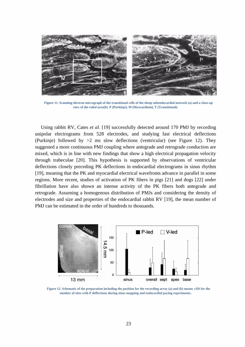
Figure 11. Scanning electron micrograph of the transitional cells of the sheep subendocardial network (a) and a close-up
view of the ruled area(b). P (Purkinje), M (Myocardium), T (Transitional).
Using rabbit RV, Cates et al. [19] successfully detected around 170 PMJ by recording
unipolar electrograms from 528 electrodes, and studying fast electrical deflections
(Purkinje) followed by >2 ms slow deflections (ventricular) (see Figure 12). They
suggested a more continuous PMJ coupling where antegrade and retrograde conduction are
mixed, which is in line with new findings that show a high electrical propagation velocity
through trabeculae [20]. This hypothesis is supported by observations of ventricular
deflections closely preceding PK deflections in endocardial electrograms in sinus rhythm
[19], meaning that the PK and myocardial electrical wavefronts advance in parallel in some
regions. More recent, studies of activation of PK fibers in pigs [21] and dogs [22] under
fibrillation have also shown an intense activity of the PK fibers both antegrade and
retrograde. Assuming a homogenous distribution of PMJs and considering the density of
electrodes and size and properties of the endocardial rabbit RV [19], the mean number of
PMJ can be estimated in the order of hundreds to thousands.
Figure 12. Schematic of the preparation including the position for the recording array (a) and (b) means ±SD for the
number of sites with P deflections during sinus mapping and endocardial pacing experiments.
24
CELLULAR ELECTROPHYSIOLOGY
Action potential
Cardiac excitation involves generation of the AP by individual cells and its conduction
from cell-to-cell through intercellular gap junctions. The combination of a locally
regenerative process (AP generation) with the transmission of this process through flow of
electric charge is common to a broad class of reaction-diffusion processes. AP generation
is accomplished through a complex interplay between nonlinear membrane ionic currents
and the ionic milieu of the cell.
The discovery by Hodgkin and Huxley (principles of nerve excitation), made it possible
to relate important properties of membrane ion channels to the generation of the AP. Later,
evidence for electric coupling of cardiac cells through low-resistance gap junctions was
established. This property is crucial for the propagation of the cardiac impulse. Over the
past three decades, researchers have employed reductionist approaches to define the
multitude of ion channels that contribute to transmembrane currents that generate the
cardiac AP.
For a single cardiac cell under space-clamp conditions, the following equation relates
the transmembrane potential (Vm) to the total transmembrane ionic current (Iion)
(1.1)
where Cm is the membrane capacitance (1 µF/cm2) provided by the charge separation
across the lipid bilayer and Istim is the externally applied stimulus current.
There have been reported differences between AP in PK cells and the rest of myocardial
cells. APD is longer in PK fibers than in ventricular cells [23-25]. The AP morphology
observed in rabbit and kid, exhibit a prominent phase 1 of repolarization, a more negative
plateau and a significantly longer APD90 compared to ventricular cells [26]. The
prolongation of the APD in PK cells compared to ventricular cells also has also been
observed in canine fibers [27-29] (Figure 13). The total amplitude of the AP and the
maximal rate of rise of the AP upstroke (Vmax) are much larger in PK fibers than in
ventricular cells.
25
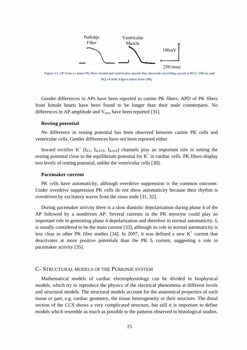
Figure 13. AP from a canine PK fiber strand and ventricular muscle fine electrode recording, paced at BCL=500 ms and
[K]o=4 mM. Figure taken from [30].
Gender differences in APs have been reported in canine PK fibers. APD of PK fibers
from female hearts have been found to be longer than their male counterparts. No
differences in AP amplitude and Vmax have been reported [31].
Resting potential
No difference in resting potential has been observed between canine PK cells and
ventricular cells. Gender differences have not been reported either.
Inward rectifier K+ (IK1, IKATP, IKAch) channels play an important role in setting the
resting potential close to the equilibrium potential for K+ in cardiac cells. PK fibers display
two levels of resting potential, unlike the ventricular cells [30].
Pacemaker current
PK cells have automaticity, although overdrive suppression is the common outcome.
Under overdrive suppression PK cells do not show automaticity because their rhythm is
overdriven by excitatory waves from the sinus node [31, 32].
During pacemaker activity there is a slow diastolic depolarization during phase 4 of the
AP followed by a nondriven AP. Several currents in the PK myocyte could play an
important role in generating phase 4 depolarization and therefore in normal automaticity. If
is usually considered to be the main current [33], although its role in normal automaticity is
less clear in other PK fiber studies [34]. In 2007, it was defined a new K+ current that
deactivates at more positive potentials than the PK If current, suggesting a role in
pacemaker activity [35].
C- STRUCTURAL MODELS OF THE PURKINJE SYSTEM
Mathematical models of cardiac electrophysiology can be divided in biophysical
models, which try to reproduce the physics of the electrical phenomena at different levels
and structural models. The structural models account for the anatomical properties of each
tissue or part, e.g. cardiac geometry, the tissue heterogeneity or their structure. The distal
section of the CCS shows a very complicated structure, but still it is important to define
models which resemble as much as possible to the patterns observed in histological studies.

26
The simplest CCS models used to stimulate the ventricles lacked of any structure, and
only aimed at reproducing the electrical activation patterns described in other
electrophysiology studies by means of early activated sites. This is still the technique used
by many researchers that use phenomenological electrical models or fast endocardial
conductivities to simulate an infinite dense PK system.
CCS models that included some structure date from the late eighties and incorporated
the HB and a few branches. Aoki et al. [36] model was composed of approximately 50000
cell units (spatial resolution of 1.5 mm.) arranged in a cubic close-packed structure
according to anatomical data. The conduction system was composed of the bundle
branches and PK fibers, consisting of a few hundred elements.
Abboud et al. [37, 38] developed a finite-element three-dimensional model of the
ventricles with a fractal conducting system. The two ventricles were modeled as prolate
spheroids with a resolution of 0.3-0.4 m, containing around half a million elements. The
PK system was modeled like a self-similar fractal tree, assuming that the shortening factor
and the bifurcation angle are the same for each generation, as depicted in Figure 14. The
model was used to simulate the high-resolution QRS complex of the ECG under normal
conditions and ischemia.
Figure 14. Two-dimensional representation of the model with a damaged region in the LV represented by the light gray
area. Image from [37].
Pollard and Barr [39] developed an anatomically based model of the human conduction
system with almost 35000 cylindrical elements, although it was not incorporated in a
ventricular model. The model was validated with activation time data. In their model, they
defined a set of 35 endocardial points from which only 4 were extracted from studies of
cardiac activation and draw a set of cables to connect them. The cables were highly refined
to form small elements suitable for cardiac electrical simulation, and all the PMJ in the
model were fully connected forming a closed network. The model did not show a high
correlation with experiments, probably due to the little coupling and the scattered and low
number of PMJ used.
27
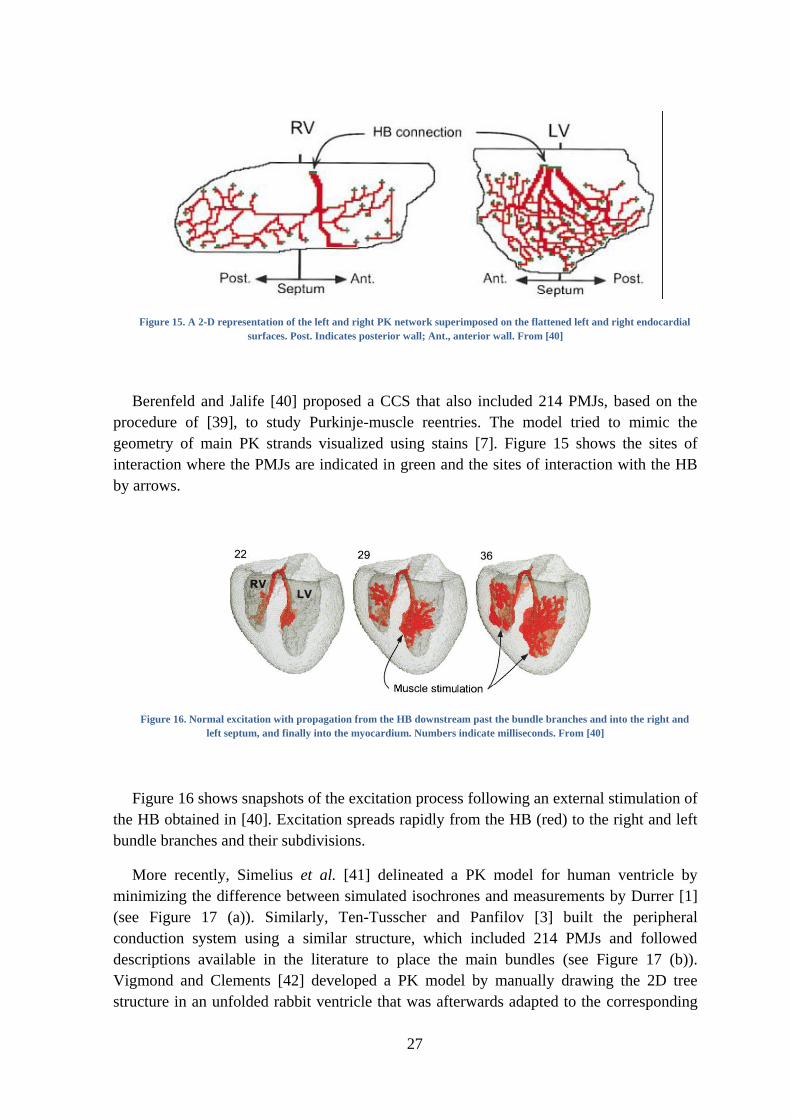
Figure 15. A 2-D representation of the left and right PK network superimposed on the flattened left and right endocardial
surfaces. Post. Indicates posterior wall; Ant., anterior wall. From [40]
Berenfeld and Jalife [40] proposed a CCS that also included 214 PMJs, based on the
procedure of [39], to study Purkinje-muscle reentries. The model tried to mimic the
geometry of main PK strands visualized using stains [7]. Figure 15 shows the sites of
interaction where the PMJs are indicated in green and the sites of interaction with the HB
by arrows.
Figure 16. Normal excitation with propagation from the HB downstream past the bundle branches and into the right and
left septum, and finally into the myocardium. Numbers indicate milliseconds. From [40]
Figure 16 shows snapshots of the excitation process following an external stimulation of
the HB obtained in [40]. Excitation spreads rapidly from the HB (red) to the right and left
bundle branches and their subdivisions.
More recently, Simelius et al. [41] delineated a PK model for human ventricle by
minimizing the difference between simulated isochrones and measurements by Durrer [1]
(see Figure 17 (a)). Similarly, Ten-Tusscher and Panfilov [3] built the peripheral
conduction system using a similar structure, which included 214 PMJs and followed
descriptions available in the literature to place the main bundles (see Figure 17 (b)).
Vigmond and Clements [42] developed a PK model by manually drawing the 2D tree
structure in an unfolded rabbit ventricle that was afterwards adapted to the corresponding
28
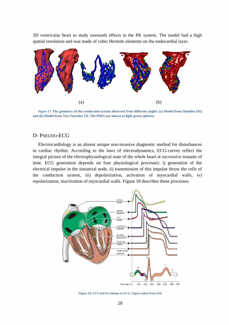
3D ventricular heart to study sawtooth effects in the PK system. The model had a high
spatial resolution and was made of cubic Hermite elements on the endocardial layer.
(a) (b)
Figure 17. The geometry of the conduction system observed from different angles. (a) Model from Simelius [41]
and (b) Model from Ten-Tusscher [3]. The PMJs are shown as light green spheres.
D- PSEUDO-ECG
Electrocardiology is an almost unique non-invasive diagnostic method for disturbances
in cardiac rhythm. According to the laws of electrodynamics, ECG-curves reflect the
integral picture of the electrophysiological state of the whole heart at successive instants of
time. ECG generation depends on four physiological processes: i) generation of the
electrical impulse in the sinoatrial node, ii) transmission of this impulse throw the cells of
the conduction system, iii) depolarization, activation of myocardial walls, iv)
repolarization, inactivation of myocardial walls. Figure 18 describes these processes.
Figure 18. CCS and its relation to ECG. Figure taken from [43]
29
Pseudo-ECG are a rough approximation calculation of the gradient of the potential field
and, performed for the whole surface of electrically activated myocardium, simulates to
some degree one of the first hypotheses of ECG genesis in accordance with which the
ECG-curve is considered as the ―difference of two monophasic curves‖, in this case it is
the average cell transmembrane activity potentials from two areas of the epicardial surface
of the heart.
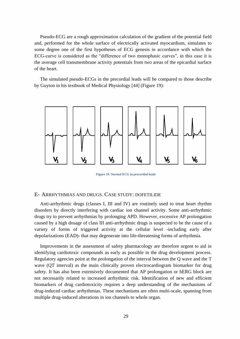
The simulated pseudo-ECGs in the precordial leads will be compared to those describe
by Guyton in his textbook of Medical Physiology [44] (Figure 19):
Figure 19. Normal ECG in precordial leads
E- ARRHYTHMIAS AND DRUGS. CASE STUDY: DOFETILIDE
Anti-arrhythmic drugs (classes I, III and IV) are routinely used to treat heart rhythm
disorders by directly interfering with cardiac ion channel activity. Some anti-arrhythmic
drugs try to prevent arrhythmias by prolonging APD. However, excessive AP prolongation
caused by a high dosage of class III anti-arrhythmic drugs is suspected to be the cause of a
variety of forms of triggered activity at the cellular level -including early after
depolarizations (EAD)- that may degenerate into life-threatening forms of arrhythmia.
Improvements in the assessment of safety pharmacology are therefore urgent to aid in
identifying cardiotoxic compounds as early as possible in the drug development process.
Regulatory agencies point at the prolongation of the interval between the Q wave and the T
wave (QT interval) as the main clinically proven electrocardiogram biomarker for drug
safety. It has also been extensively documented that AP prolongation or hERG block are
not necessarily related to increased arrhythmic risk. Identification of new and efficient
biomarkers of drug cardiotoxicity requires a deep understanding of the mechanisms of
drug-induced cardiac arrhythmias. These mechanisms are often multi-scale, spanning from
multiple drug-induced alterations in ion channels to whole organ.
30
The delayed rectifier K+ channels are responsible for the repolarization phase of the
cardiac AP. During a cardiac AP, IKr current is activated during the plateau phase and is
responsible for the repolarization of the transmembrane potential. IKr is considered to be
the most widely targeted K+ channel linked to potential arrhythmogeneity. Many IKr
blockers, which prolong APD, are known to have a negative correlation between their
potency and heart frequency, i.e. they do not work as well at higher frequencies (which is
exactly when they are needed) and are more potent at lower frequencies, exposing the heart
to extremely prolonged APD and risk of Torsade de Pointes (TdP) after episodes of
bradycardia.
Cases of TdP have been reported during administration of a drug known as dofetilide.
Interestingly, the ability of dofetilide to increase effective refractory period (ERP) was
found to be decreased at higher heart rates and increased at low heart rates, which could be
related to drug-induced increased pro-arrhythmic risk as described. Dofetilide prolongs QT
duration, and its effect is influenced by heart rate. Although dofetilide-induced QT
prolongation decreases when the R-R cycle shortens, this reverse rate dependence is only
partial because marked QT prolongation persists at an R-R cycle of 600 ms. Results of
some studies indicated that dynamic ECG techniques can be useful in detection of subtle,
drug-induced changes in the duration of ventricular repolarization [45].

31
2. OBJECTIVES
This research work has been carried out within the Cardiac Modeling Group (CMG) of
the Bioelectronics Group (GBIO) in the I3BH. The CMG has been working in the
development of a realistic computational heart model for electrophysiology studies over
the last sixteen years. The 3D ventricular model used today has been built from a diffusion
tensor magnetic resonance dataset (DTMRI) which includes the fiber anisotropy, an
important feature with great influence in the activation sequence of the heart. It also takes
into account the different cell populations of endocardial, mid-myocardial and epicardial
cells. However, it presents an important limitation: it does not integrate the CCS of the
heart (HB and PK fibers).
The general objective of this work is to demonstrate the need of incorporating the CCS
in a heart model meant to perform electrophysiology simulations. Furthermore, the
inclusion of the system will improve the electrical activation sequence and will allow
studying different heart conditions and diseases that we cannot model at the moment, such
as bundle branch block.
Several partial objectives are posed in order to reach the general objective. First of all, a
literature review of the HB and the PK system. In this study we consider histological,
anatomical and electrical data in order to obtain a good description of the CCS of the heart.
We define several models of the anatomy of the HB based on this bibliographic review.
Before designing the algorithm that generates the PK network, an in-depth review of the
state of the art was done. We analyzed approaches of several researchers and then designed
a new algorithm to create the PK network. The implementation of this algorithm is made in
several steps, leading at each step to a model which describes more accurately the real
anatomical structure of the system. It allows generating randomly different PK networks
that we include in the whole ventricular model.
To prove the effect of the CCS, we carry out a simulation study comparing simulations
with and without this system. In addition, we show an application of the model to study the
global effect of a drug called dofetilide in the heart. Three different scenarios are evaluated
and compared: i) control case; and drug cases with ii) 10 nM of dofetilide and iii) 100 nM
of dofetilide (a drug that blocks IKr current). Activation sequence, activation time,
repolarization time, isochrones maps and APD maps, and pseudo-ECGs in precordial leads
are analyzed for each scenario.

32
33
3. MATERIAL AND METHODS
A- ANATOMICAL MODEL OF THE VENTRICLES
In order to perform realistic electrical simulations and study cardiac function it is
important to build an anatomical model that take into account both the geometry of the
heart chambers and their architecture. Several studies have pointed out the importance of
factors such as the anisotropy, due to the shape of cardiac cells, in the cardiac activations,
as well as the rotation of the fiber directions from the epicardium to the endocardium or the
conduction system [46-49]. Henriquez et al. [50] consider that among the most important
characteristics of any model of cardiac tissue, there are the ability to reproduce effects due
to anisotropy in both intracellular and extracellular regions, the presence of adjacent
volume conductors, fiber curvature and fiber rotation.
Figure 20. Ventricular human heart model built from a DTMRI stack. (a) Right and left ventricles were segmented and
meshed with hexahedral elements. (b) Myocardial fiber orientation represented by small vectors.
In our study the geometry of the ventricular model has been segmented from a DTMRI
data set acquired at John Hopkins University [51]. The DTMRI volume stack had a
resolution of 0.4297 x 0.4297 x 1.0 mm3 (256×256×144 voxels). The heart volume has
been extracted directly from myocardial segmentation, using a simple threshold and
allowed reconstruction of whole ventricular geometry and fiber structure.
The fiber orientation was integrated in the model from DTMRI data. Diffusion Tensor
Magnetic Resonance Imaging (DTMRI) has proven to be an effective technique for
measuring the diffusion tensor of water within tissue. Water, which is abundant in tissue,
diffuses naturally within the tissue microstructure. In cardiac tissue, anisotropic diffusion
occurs since there are preferred directions of diffusion due to the tissue microstructure.
This information was incorporated into the finite element model by defining an average
fiber direction for each element (more information in Appendix B-).
34
The heart was considered transversely isotropic. Transmurally fiber angles rotated from
-60º on the epicardial surface to [+40º, +60º] on the endocardium. Figure 20 (a) shows the
ventricular model and Figure 20 (b) the myocardial fiber orientation estimated from
DTMRI for this particular geometry.
From the segmented volume, a regular volumetric mesh was constructed with
hexahedral elements and a resolution of 0.5 x 0.5 x 0.5 mm3, which gave rise to 1.43
million nodes and 1.29 million hexahedra [52] (see Figure 21 (b)). With this resolution
together with multi-resolution mesh techniques, electrophysiological simulations show
stability and accuracy.
(a) (b)
Figure 21. Biventricular geometry. (a) Labeled regions, LV endocardium and epicardium and RV endocardium and
epicardium. (b) Detail of the lateral wall mesh showing the hexahedral elements.
Several studies have shown that ventricular myocardium is formed by three types of
cells: epicardial, mid-myocardial and endocardial [53-55]. We modeled the myocardium
with the following distributions for each cell population, 17% endocardium, 41% mid-
myocardium and 42% epicardium.
These cells differ in the morphology of the AP, especially in the spike-and-dome APs of
mid-myocardial and epicardial cells due to the transient outward current, Ito. Mid-
myocardial cells can be distinguished from other types of cells because they have a short
and slow delayed rectifier current, IKs, a strong Ito current and a relatively large Na-Ca
exchange current, INaCa. Rapid IKr activation and inward rectifying currents, IK1, are similar
in the three types of cells. Ionic differences are responsible of the enlargement of APD and
of the high speed in AP depolarization.
Histological characteristics of mid-myocardial cells are similar to epicardial and
endocardial cells. The mid-myocardial cells have larger APD. They can be found deep in
the anterior wall between subendocardium and mid-myocardium, in the lateral wall
between subendocardium and mid-myocardium, and across the wall in the outflow tract of
35
the RV. Mid-myocardial cells are also present in papillary muscles, trabeculae and
interventricular septum.
B- ACTION POTENTIAL MODELS
PURKINJE FIBER CELL MODEL BY STEWART ET AL.
In many species PK fiber cell APs have unique features, including a larger upstroke
velocity, lower plateau and longer AP duration, and also they can present automaticity due
to slow spontaneous diastolic depolarization. These differences are associated with
different kinetics and current densities in a number of major ion channels. It is necessary to
use a biophysically detailed model for the electrical APs of PK, since they have an
important role in ensuring normal ventricular excitation.
We have used the AP model for PK cells developed by Stewart et al. [56]. This model is
based on the Ten-Tusscher et al. [57] and Ten-Tusscher & Panfilov [58] model of human
ventricular myocytes, and incorporates experimental voltage-clamp data recorded from
human PK cells [59].
The model updates conductance, steady-state activation and inactivation curves and
time constants for Ito, IKr, IKs and IK1 and incorporates two additional ionic currents: a
hyperpolarization-activated pacemaker current, If, and sustained potassium current, Isus,
absent in the ventricular cell models but present in PK cells. The resultant model
reproduces AP characteristics and is consistent with experimental recordings. The included
pacemaker current, If, produces auto-rhythmic APs with a cycle length that is consistent
with experimental data. The model also reproduces the all-or-nothing repolarization
phenomenon observed in PK tissues and the overdrive suppression phenomenon. A
schematic diagram describing the ion movement across the cell surface membrane and the
sarcoplasmic reticulum in the model is presented below (Figure 22). For a detailed
description of the model see [56].
Figure 22. Schematic diagram of the PK cell model of Stewart
36
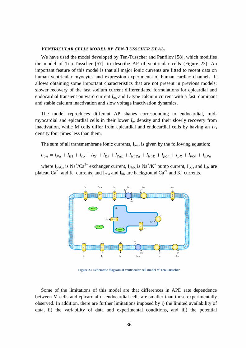
VENTRICULAR CELLS MODEL BY TEN-TUSSCHER ET AL.
We have used the model developed by Ten-Tusscher and Panfilov [58], which modifies
the model of Ten-Tusscher [57], to describe AP of ventricular cells (Figure 23). An
important feature of this model is that all major ionic currents are fitted to recent data on
human ventricular myocytes and expression experiments of human cardiac channels. It
allows obtaining some important characteristics that are not present in previous models:
slower recovery of the fast sodium current differentiated formulations for epicardial and
endocardial transient outward current Ito, and L-type calcium current with a fast, dominant
and stable calcium inactivation and slow voltage inactivation dynamics.
The model reproduces different AP shapes corresponding to endocardial, mid-
myocardial and epicardial cells in their lower Ito density and their slowly recovery from
inactivation, while M cells differ from epicardial and endocardial cells by having an IKs
density four times less than them.
The sum of all transmembrane ionic currents, Iion, is given by the following equation:
where INaCa is Na+/Ca
2+ exchanger current, INaK is Na
+/K
+ pump current, IpCa and IpK are
plateau Ca2+
and K+ currents, and IbCa and IbK are background Ca
2+ and K
+ currents.
Figure 23. Schematic diagram of ventricular cell model of Ten-Tusscher
Some of the limitations of this model are that differences in APD rate dependence
between M cells and epicardial or endocardial cells are smaller than those experimentally
observed. In addition, there are further limitations imposed by i) the limited availability of
data, ii) the variability of data and experimental conditions, and iii) the potential
37
deleterious effects of cell isolation. Furthermore, formulation of ICaL time constants is
taken from a model based on animal experimental data, since there were no data available.
C- DRUG MODELING: DOFETILIDE
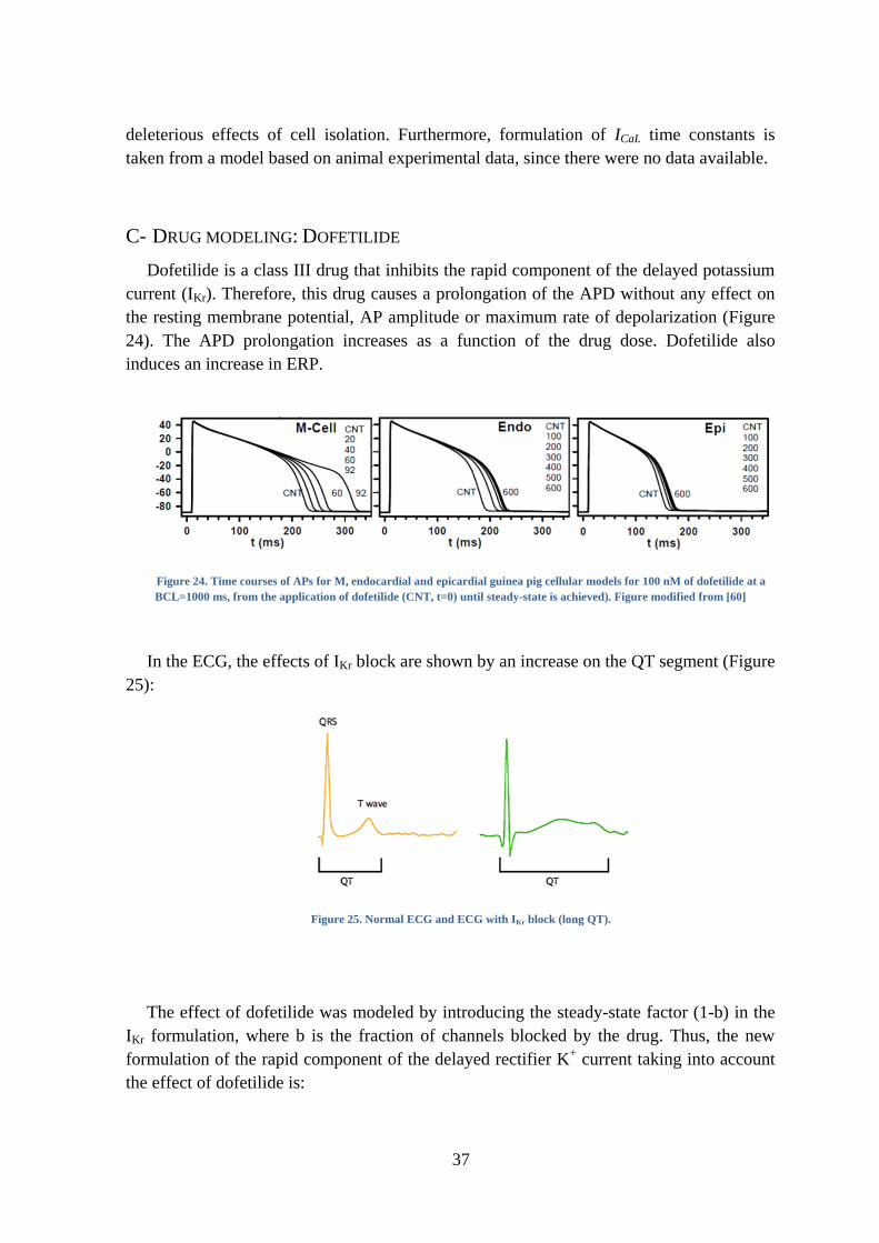
Dofetilide is a class III drug that inhibits the rapid component of the delayed potassium
current (IKr). Therefore, this drug causes a prolongation of the APD without any effect on
the resting membrane potential, AP amplitude or maximum rate of depolarization (Figure
24). The APD prolongation increases as a function of the drug dose. Dofetilide also
induces an increase in ERP.
Figure 24. Time courses of APs for M, endocardial and epicardial guinea pig cellular models for 100 nM of dofetilide at a
BCL=1000 ms, from the application of dofetilide (CNT, t=0) until steady-state is achieved). Figure modified from [60]
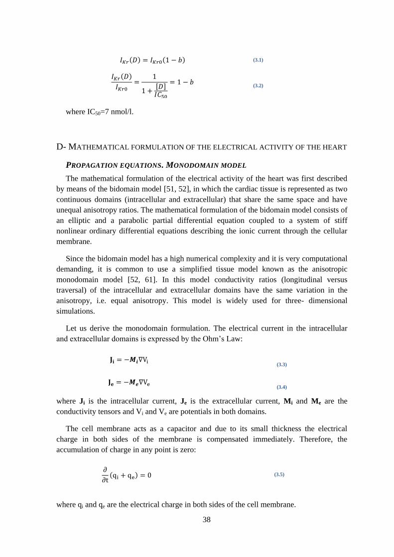
In the ECG, the effects of IKr block are shown by an increase on the QT segment (Figure
25):
Figure 25. Normal ECG and ECG with IKr block (long QT).
The effect of dofetilide was modeled by introducing the steady-state factor (1-b) in the
IKr formulation, where b is the fraction of channels blocked by the drug. Thus, the new
formulation of the rapid component of the delayed rectifier K+ current taking into account
the effect of dofetilide is:
38
( ) ( ) (3.1)
( )
[ ]
(3.2)
where IC50=7 nmol/l.
D- MATHEMATICAL FORMULATION OF THE ELECTRICAL ACTIVITY OF THE HEART
PROPAGATION EQUATIONS. MONODOMAIN MODEL
The mathematical formulation of the electrical activity of the heart was first described
by means of the bidomain model [51, 52], in which the cardiac tissue is represented as two
continuous domains (intracellular and extracellular) that share the same space and have
unequal anisotropy ratios. The mathematical formulation of the bidomain model consists of
an elliptic and a parabolic partial differential equation coupled to a system of stiff
nonlinear ordinary differential equations describing the ionic current through the cellular
membrane.
Since the bidomain model has a high numerical complexity and it is very computational
demanding, it is common to use a simplified tissue model known as the anisotropic
monodomain model [52, 61]. In this model conductivity ratios (longitudinal versus
traversal) of the intracellular and extracellular domains have the same variation in the
anisotropy, i.e. equal anisotropy. This model is widely used for three- dimensional
simulations.
Let us derive the monodomain formulation. The electrical current in the intracellular
and extracellular domains is expressed by the Ohm’s Law:
(3.3)
(3.4)
where Ji is the intracellular current, Je is the extracellular current, Mi and Me are the
conductivity tensors and Vi and Ve are potentials in both domains.
The cell membrane acts as a capacitor and due to its small thickness the electrical
charge in both sides of the membrane is compensated immediately. Therefore, the
accumulation of charge in any point is zero:
( ) (3.5)
where qi and qe are the electrical charge in both sides of the cell membrane.
39
The electrical current in each point is equal to the ratio of the accumulation of charge in
both domains
(3.6)
(3.7)
where Iion is the current through the membrane and χ is the relation of membrane area for
unit of volume. The sign of the ionic current is positive when it goes from the intracellular
to the extracellular space.
Combining equations (3.6) and (3.7) in (3.5) we have the current conservation equation,
(3.8)
and substituting (3.3) and (3.4) in (3.8) we obtain:
( ) ( ) (3.9)
The charge in the cell membrane directly depends on the difference of membrane
potential V=Vi-Ve and the membrane capacitance
(3.10)
where Cm is the membrane capacitance and
(3.11)
Combining the last two equations and deriving with respect to the time we have,
( )
which combined with (3.5) leads to:
And substituting this expression in (3.4) and using (3.1) and Di=Mi/χ we obtain:
( )
(3.12)
40
If we eliminate Vi (Vi=V+Ve) in (3.9) and (3.12), apply the monodomain assumption
De=λDi and combine the two resulting equations we obtain the monodomain standard
formulation:
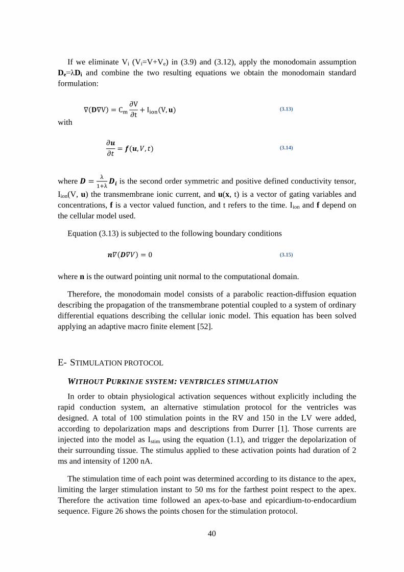
( )
( ) (3.13)
with
( ) (3.14)
where
is the second order symmetric and positive defined conductivity tensor,
Iion(V, u) the transmembrane ionic current, and u(x, t) is a vector of gating variables and
concentrations, f is a vector valued function, and t refers to the time. Iion and f depend on
the cellular model used.
Equation (3.13) is subjected to the following boundary conditions
( ) (3.15)
where n is the outward pointing unit normal to the computational domain.
Therefore, the monodomain model consists of a parabolic reaction-diffusion equation
describing the propagation of the transmembrane potential coupled to a system of ordinary
differential equations describing the cellular ionic model. This equation has been solved
applying an adaptive macro finite element [52].
E- STIMULATION PROTOCOL
WITHOUT PURKINJE SYSTEM: VENTRICLES STIMULATION
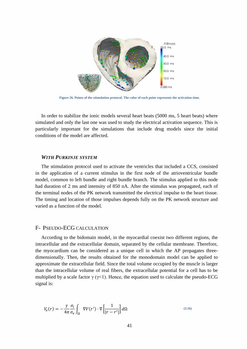
In order to obtain physiological activation sequences without explicitly including the
rapid conduction system, an alternative stimulation protocol for the ventricles was
designed. A total of 100 stimulation points in the RV and 150 in the LV were added,
according to depolarization maps and descriptions from Durrer [1]. Those currents are
injected into the model as Istim using the equation (1.1), and trigger the depolarization of
their surrounding tissue. The stimulus applied to these activation points had duration of 2
ms and intensity of 1200 nA.
The stimulation time of each point was determined according to its distance to the apex,
limiting the larger stimulation instant to 50 ms for the farthest point respect to the apex.
Therefore the activation time followed an apex-to-base and epicardium-to-endocardium
sequence. Figure 26 shows the points chosen for the stimulation protocol.
41
Figure 26. Points of the stimulation protocol. The color of each point represents the activation time.
In order to stabilize the ionic models several heart beats (5000 ms, 5 heart beats) where
simulated and only the last one was used to study the electrical activation sequence. This is
particularly important for the simulations that include drug models since the initial
conditions of the model are affected.
WITH PURKINJE SYSTEM
The stimulation protocol used to activate the ventricles that included a CCS, consisted
in the application of a current stimulus in the first node of the atrioventricular bundle
model, common to left bundle and right bundle branch. The stimulus applied to this node
had duration of 2 ms and intensity of 850 nA. After the stimulus was propagated, each of
the terminal nodes of the PK network transmitted the electrical impulse to the heart tissue.
The timing and location of those impulses depends fully on the PK network structure and
varied as a function of the model.
F- PSEUDO-ECG CALCULATION
According to the bidomain model, in the myocardial coexist two different regions, the
intracellular and the extracellular domain, separated by the cellular membrane. Therefore,
the myocardium can be considered as a unique cell in which the AP propagates three-
dimensionally. Then, the results obtained for the monodomain model can be applied to
approximate the extracellular field. Since the total volume occupied by the muscle is larger
than the intracellular volume of real fibers, the extracellular potential for a cell has to be
multiplied by a scale factor γ (γ<1). Hence, the equation used to calculate the pseudo-ECG
signal is:
( )
∫ ( ) [
]
(3.16)
42
where and are intracellular and extracellular conductivities, V is the membrane
potential, r is the position where the pseudo-ECG is calculated and the integral is extended
to the whole myocardial volume. Pseudo-ECGs are calculated considering a homogeneous
volume between the heart and the leads where it is obtained.
Pseudo-ECG calculation was performed with a solver postprocessor, after obtaining the
membrane potential in each node of the domain as a function of time. Firstly, the gradient
of potential is calculated in the centre of each element of the mesh from time-dependent
potential data. Secondly the radius vector between the centre of each element and the point
in which we want to obtain the pseudo-ECG is measured. This radius vector is used to
obtain [
]. Finally, Ve is calculated as the sum of the product of the gradient of
potential and the inverse of the radius vector and the volume of the element, obtaining the
potential of the pseudo-ECG in a time instant at that specific point. This process is repeated
for each time step over the duration of a beat, which results in the reconstruction of the
pseudo-ECG for a given point.
For measuring potentials close to the heart, standard precordial lead positions were used
to calculate the pseudo-ECGs. These leads (V1-V6) are located over the left chest. V1 and
V2 are located at the fourth intercostal space on the right and left side of the sternum; V4 is
located in the fifth intercostal space at the midclavicular line; V3 is located between the
points V2 and V4; V5 is at the same horizontal level as V4 but on the anterior axillary line;
V6 is at the same horizontal level as V4 but at the midline. Figure 27 shows the location of
precordial leads.
Figure 27. Location of precordial leads (V1-V6). Figure taken from [43]
43
G- COMPUTATIONAL SIMULATIONS
PRE-PROCESSING. INCLUSION OF PURKINJE MODEL
The pre-processing step is implemented in MATLAB, and it is necessary to include a
PK structural model in the cardiac model and format it for the simulator.
First, the nodes from the endocardium of the cardiac model are extracted. Following, we
specify the HB configuration that is going to be used from a pre-defined set, and a matrix
of endocardial nodes that will be potential nodes of the PK network. Several options are
available to ensure anatomical observations such as areas with reduced amount of PMJs
(whole endocardial, not nodes in the basal region…). Finally, we can run the algorithm to
create the PK network.
The construction algorithm is controlled by the following parameters:
1. index of nodes: points where the net starts its growing,
2. searching radius distance: to define branch growing and PMJs,
3. regions with predefined terminals: index of the central node, radius of the region
and percentage of predefined terminals,
4. probability of an intermediate node to be the origin of a little bundle ended in a
terminal,
5. probability of forming ―elliptical structures‖: it is related to the probability of
connect again a node that is already connected with a neighbor).
After running the algorithm to construct the PK network, this network is processed
giving the following outputs:
1) .dat intermediate outputs:
- PKpoints_RV, PKpoints_LV: candidate node that form the PK network (its
number is set by the user).
- endoRV, endoLV: final nodes of the PK network in each ventricle.
Composed of PKpoints plus the additional nodes that the algorithm may
define as terminals.
- conneRV, conneLV: connectivity between the nodes of the PK network
(endoRV, endoLV) in each ventricle.
- hisnodes: nodes that form the HB.
- conneHis: connectivity between the nodes that form the HB.
- termiRV, termiLV: indices of terminal nodes (PMJs) in each ventricle.
2) .dat final outputs (inputs for ELVIRA processed):
- CS2H05_nod_PK: specifies the PK network nodes.
- CS2H05_elm_PK: specifies the PK network elements.
- nodesPK_vsim: nodes for the whole ventricular simulation, including the
CCS.
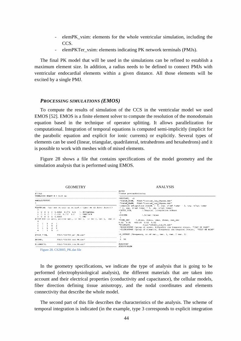
44
- elemPK_vsim: elements for the whole ventricular simulation, including the
CCS.
- elemPKTer_vsim: elements indicating PK network terminals (PMJs).
The final PK model that will be used in the simulations can be refined to establish a
maximum element size. In addition, a radius needs to be defined to connect PMJs with
ventricular endocardial elements within a given distance. All those elements will be
excited by a single PMJ.
PROCESSING SIMULATIONS (EMOS)
To compute the results of simulation of the CCS in the ventricular model we used
EMOS [52]. EMOS is a finite element solver to compute the resolution of the monodomain
equation based in the technique of operator splitting. It allows parallelization for
computational. Integration of temporal equations is computed semi-implicitly (implicit for
the parabolic equation and explicit for ionic currents) or explicitly. Several types of
elements can be used (linear, triangular, quadrilateral, tetrahedrons and hexahedrons) and it
is possible to work with meshes with of mixed elements.
Figure 28 shows a file that contains specifications of the model geometry and the
simulation analysis that is performed using EMOS.
In the geometry specifications, we indicate the type of analysis that is going to be
performed (electrophysiological analysis), the different materials that are taken into
account and their electrical properties (conductivity and capacitance), the cellular models,
fiber direction defining tissue anisotropy, and the nodal coordinates and elements
connectivity that describe the whole model.
The second part of this file describes the characteristics of the analysis. The scheme of
temporal integration is indicated (in the example, type 3 corresponds to explicit integration
GEOMETRY ANALYSIS
Figure 28. CS2H05_PK.dat file
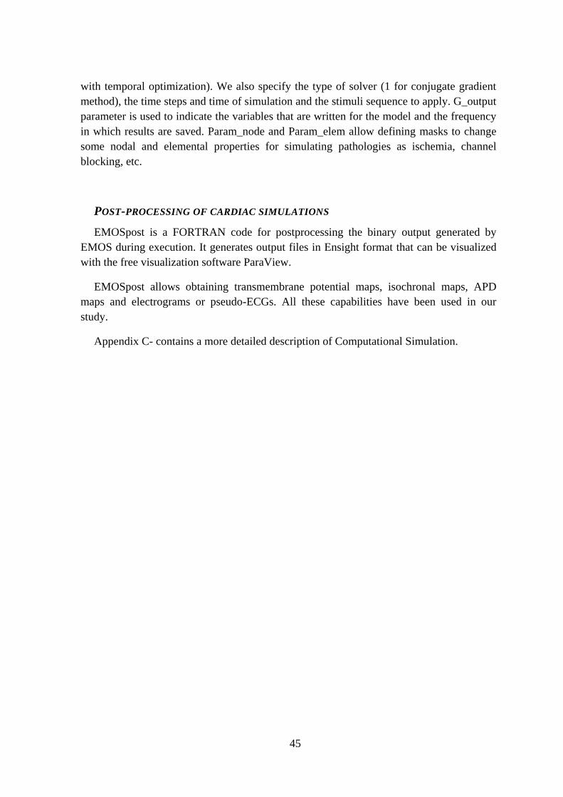
45
with temporal optimization). We also specify the type of solver (1 for conjugate gradient
method), the time steps and time of simulation and the stimuli sequence to apply. G_output
parameter is used to indicate the variables that are written for the model and the frequency
in which results are saved. Param_node and Param_elem allow defining masks to change
some nodal and elemental properties for simulating pathologies as ischemia, channel
blocking, etc.
POST-PROCESSING OF CARDIAC SIMULATIONS
EMOSpost is a FORTRAN code for postprocessing the binary output generated by
EMOS during execution. It generates output files in Ensight format that can be visualized
with the free visualization software ParaView.
EMOSpost allows obtaining transmembrane potential maps, isochronal maps, APD
maps and electrograms or pseudo-ECGs. All these capabilities have been used in our
study.
Appendix C- contains a more detailed description of Computational Simulation.

46
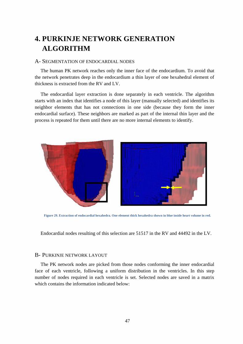
47
4. PURKINJE NETWORK GENERATION
ALGORITHM
A- SEGMENTATION OF ENDOCARDIAL NODES
The human PK network reaches only the inner face of the endocardium. To avoid that
the network penetrates deep in the endocardium a thin layer of one hexahedral element of
thickness is extracted from the RV and LV.
The endocardial layer extraction is done separately in each ventricle. The algorithm
starts with an index that identifies a node of this layer (manually selected) and identifies its
neighbor elements that has not connections in one side (because they form the inner
endocardial surface). These neighbors are marked as part of the internal thin layer and the
process is repeated for them until there are no more internal elements to identify.
Figure 29. Extraction of endocardial hexahedra. One element thick hexahedra shown in blue inside heart volume in red.
Endocardial nodes resulting of this selection are 51517 in the RV and 44492 in the LV.
B- PURKINJE NETWORK LAYOUT
The PK network nodes are picked from those nodes conforming the inner endocardial
face of each ventricle, following a uniform distribution in the ventricles. In this step
number of nodes required in each ventricle is set. Selected nodes are saved in a matrix
which contains the information indicated below:
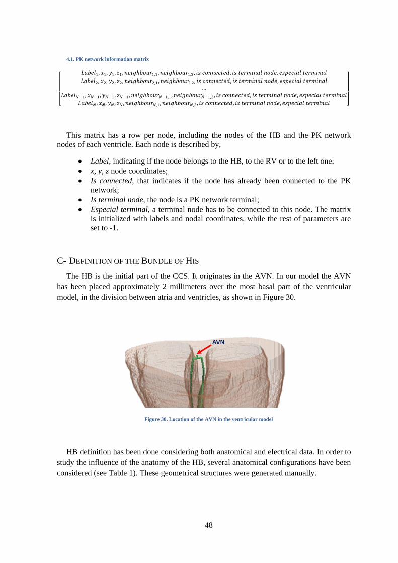
48
4.1. PK network information matrix
[
]
This matrix has a row per node, including the nodes of the HB and the PK network
nodes of each ventricle. Each node is described by,
Label, indicating if the node belongs to the HB, to the RV or to the left one;
x, y, z node coordinates;
Is connected, that indicates if the node has already been connected to the PK
network;
Is terminal node, the node is a PK network terminal;
Especial terminal, a terminal node has to be connected to this node. The matrix
is initialized with labels and nodal coordinates, while the rest of parameters are
set to -1.
C- DEFINITION OF THE BUNDLE OF HIS
The HB is the initial part of the CCS. It originates in the AVN. In our model the AVN
has been placed approximately 2 millimeters over the most basal part of the ventricular
model, in the division between atria and ventricles, as shown in Figure 30.
Figure 30. Location of the AVN in the ventricular model
HB definition has been done considering both anatomical and electrical data. In order to
study the influence of the anatomy of the HB, several anatomical configurations have been
considered (see Table 1). These geometrical structures were generated manually.
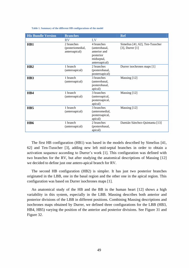
49
Table 1. Summary of the different HB configurations of the model
His Bundle Version Branches Ref
RV LV
HB1 2 branches
(posteriomedial,
anteroapical)
4 branches
(anterobasal,
anterior and
posterior
midseptal,
anteroapical)
Simelius [41, 62], Ten-Tusscher
[3], Durrer [1]
HB2 1 branch
(anteroapical)
2 branches
(posterobasal,
posteroapical)
Durrer isochrones maps [1]
HB3 1 branch
(anteroapical) 3 branches
(anterobasal,
posterobasal,
apical)
Massing [12]
HB4 1 branch
(anteroapical) 3 branches
(anteroapical,
posteroapical,
apical)
Massing [12]
HB5 1 branch
(anteroapical) 3 branches
(anteromedial,
posteroapical,
apical)
Massing [12]
HB6 1 branch
(anteroapical) 2 branches
(posterobasal,
apical)
Damián Sánchez-Quintanta [13]
The first HB configuration (HB1) was based in the models described by Simelius [41,
62] and Ten-Tusscher [3], adding new left mid-septal branches in order to obtain a
activation sequence according to Durrer’s work [1]. This configuration was defined with
two branches for the RV, but after studying the anatomical descriptions of Massing [12]
we decided to define just one antero-apical branch for RV.
The second HB configuration (HB2) is simpler. It has just two posterior branches
originated in the LBB, one in the basal region and the other one in the apical region. This
configuration was based on Durrer isochrones maps [1].
An anatomical study of the HB and the BB in the human heart [12] shows a high
variability in this system, especially in the LBB. Massing describes both anterior and
posterior divisions of the LBB in different positions. Combining Massing descriptions and
isochrones maps obtained by Durrer, we defined three configurations for the LBB (HB3,
HB4, HB5) varying the position of the anterior and posterior divisions. See Figure 31 and
Figure 32.
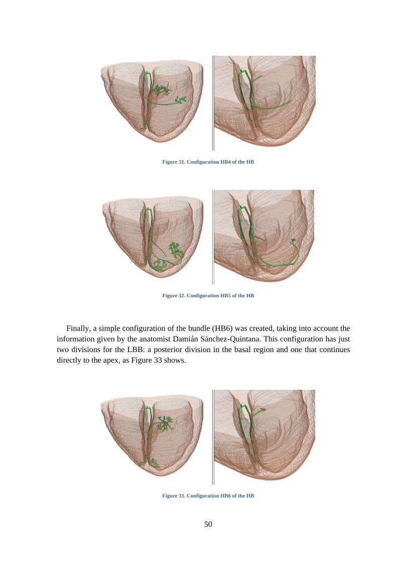
50
Figure 31. Configuration HB4 of the HB
Figure 32. Configuration HB5 of the HB
Finally, a simple configuration of the bundle (HB6) was created, taking into account the
information given by the anatomist Damián Sánchez-Quintana. This configuration has just
two divisions for the LBB: a posterior division in the basal region and one that continues
directly to the apex, as Figure 33 shows.
Figure 33. Configuration HB6 of the HB
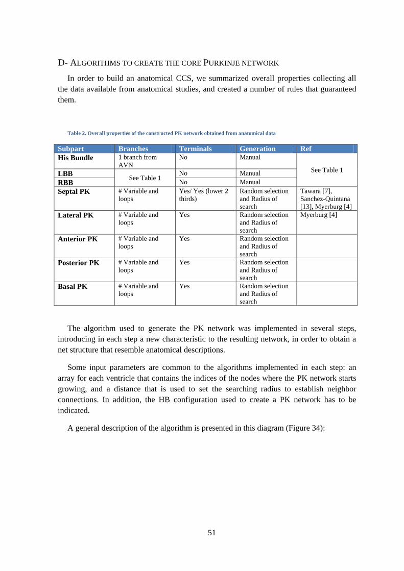
51
D- ALGORITHMS TO CREATE THE CORE PURKINJE NETWORK
In order to build an anatomical CCS, we summarized overall properties collecting all
the data available from anatomical studies, and created a number of rules that guaranteed
them.
Table 2. Overall properties of the constructed PK network obtained from anatomical data
Subpart Branches Terminals Generation Ref
His Bundle 1 branch from
AVN
No Manual
See Table 1 LBB
See Table 1 No Manual
RBB No Manual
Septal PK # Variable and
loops
Yes/ Yes (lower 2
thirds)
Random selection
and Radius of
search
Tawara [7],
Sanchez-Quintana
[13], Myerburg [4]
Lateral PK # Variable and
loops
Yes Random selection
and Radius of
search
Myerburg [4]
Anterior PK # Variable and
loops
Yes Random selection
and Radius of
search
Posterior PK # Variable and
loops
Yes Random selection
and Radius of
search
Basal PK # Variable and
loops
Yes Random selection
and Radius of
search
The algorithm used to generate the PK network was implemented in several steps,
introducing in each step a new characteristic to the resulting network, in order to obtain a
net structure that resemble anatomical descriptions.
Some input parameters are common to the algorithms implemented in each step: an
array for each ventricle that contains the indices of the nodes where the PK network starts
growing, and a distance that is used to set the searching radius to establish neighbor
connections. In addition, the HB configuration used to create a PK network has to be
indicated.
A general description of the algorithm is presented in this diagram (Figure 34):
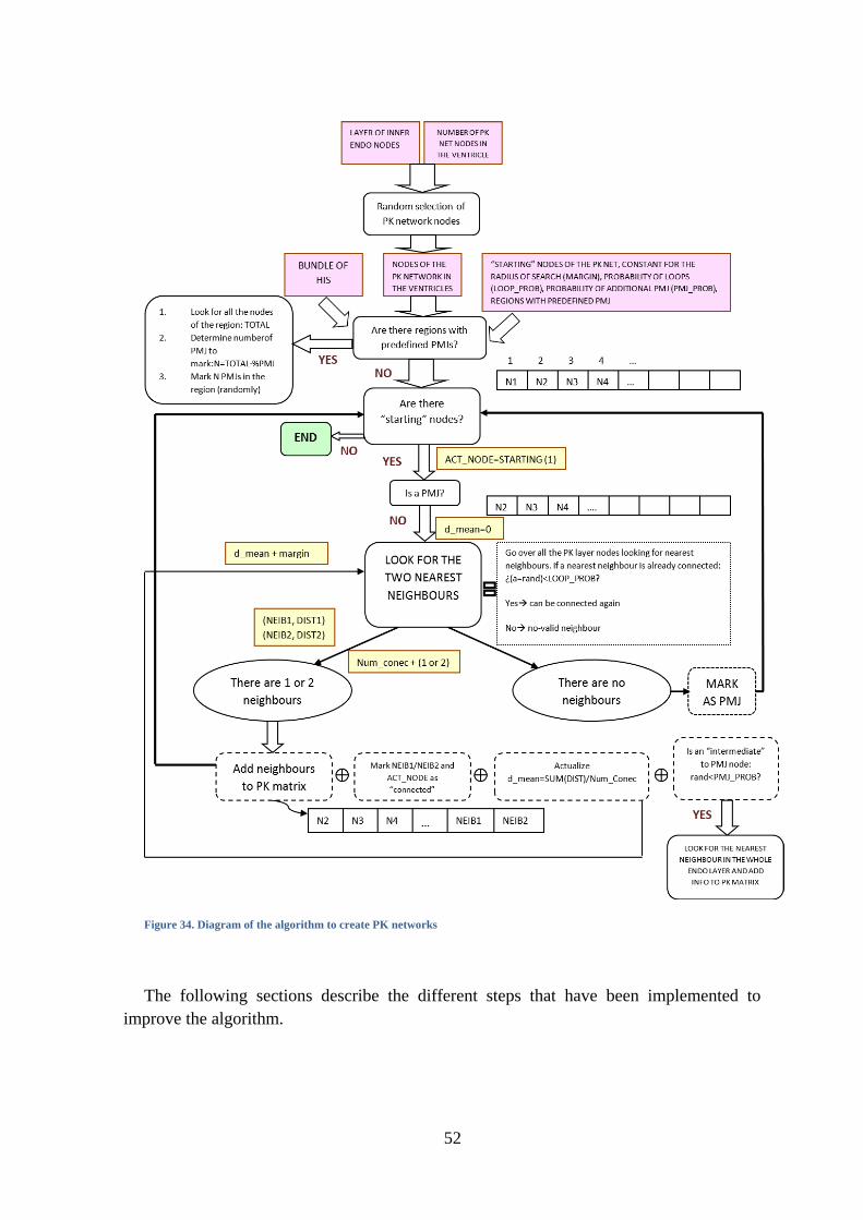
52
Figure 34. Diagram of the algorithm to create PK networks
The following sections describe the different steps that have been implemented to
improve the algorithm.
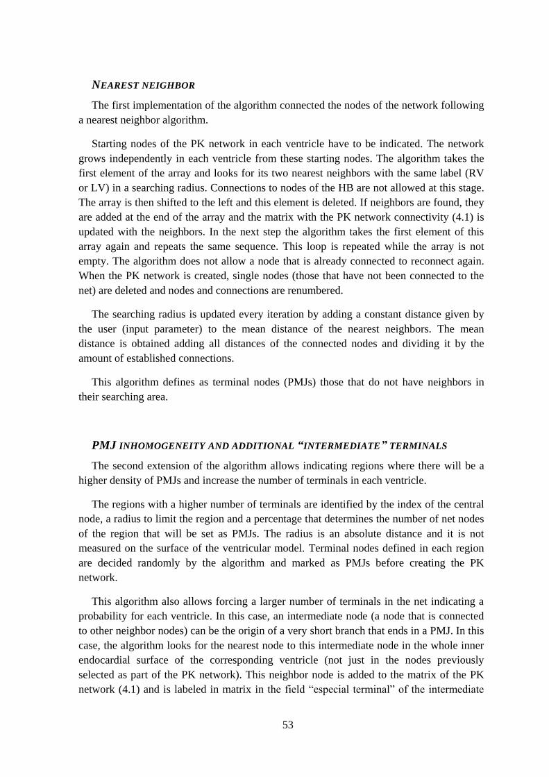
53
NEAREST NEIGHBOR
The first implementation of the algorithm connected the nodes of the network following
a nearest neighbor algorithm.
Starting nodes of the PK network in each ventricle have to be indicated. The network
grows independently in each ventricle from these starting nodes. The algorithm takes the
first element of the array and looks for its two nearest neighbors with the same label (RV
or LV) in a searching radius. Connections to nodes of the HB are not allowed at this stage.
The array is then shifted to the left and this element is deleted. If neighbors are found, they
are added at the end of the array and the matrix with the PK network connectivity (4.1) is
updated with the neighbors. In the next step the algorithm takes the first element of this
array again and repeats the same sequence. This loop is repeated while the array is not
empty. The algorithm does not allow a node that is already connected to reconnect again.
When the PK network is created, single nodes (those that have not been connected to the
net) are deleted and nodes and connections are renumbered.
The searching radius is updated every iteration by adding a constant distance given by
the user (input parameter) to the mean distance of the nearest neighbors. The mean
distance is obtained adding all distances of the connected nodes and dividing it by the
amount of established connections.
This algorithm defines as terminal nodes (PMJs) those that do not have neighbors in
their searching area.
PMJ INHOMOGENEITY AND ADDITIONAL “INTERMEDIATE” TERMINALS
The second extension of the algorithm allows indicating regions where there will be a
higher density of PMJs and increase the number of terminals in each ventricle.
The regions with a higher number of terminals are identified by the index of the central
node, a radius to limit the region and a percentage that determines the number of net nodes
of the region that will be set as PMJs. The radius is an absolute distance and it is not
measured on the surface of the ventricular model. Terminal nodes defined in each region
are decided randomly by the algorithm and marked as PMJs before creating the PK
network.
This algorithm also allows forcing a larger number of terminals in the net indicating a
probability for each ventricle. In this case, an intermediate node (a node that is connected
to other neighbor nodes) can be the origin of a very short branch that ends in a PMJ. In this
case, the algorithm looks for the nearest node to this intermediate node in the whole inner
endocardial surface of the corresponding ventricle (not just in the nodes previously
selected as part of the PK network). This neighbor node is added to the matrix of the PK
network (4.1) and is labeled in matrix in the field ―especial terminal‖ of the intermediate
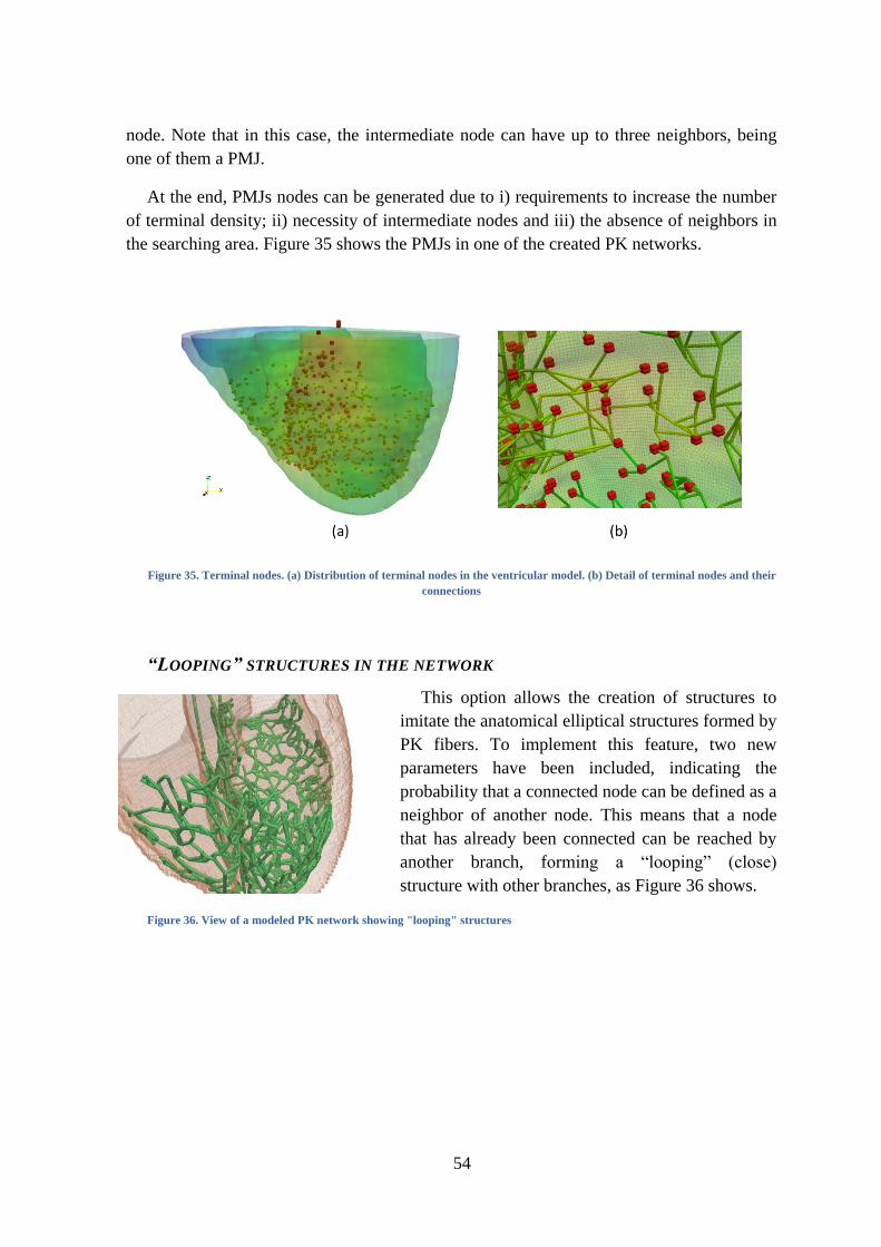
54
node. Note that in this case, the intermediate node can have up to three neighbors, being
one of them a PMJ.
At the end, PMJs nodes can be generated due to i) requirements to increase the number
of terminal density; ii) necessity of intermediate nodes and iii) the absence of neighbors in
the searching area. Figure 35 shows the PMJs in one of the created PK networks.
Figure 35. Terminal nodes. (a) Distribution of terminal nodes in the ventricular model. (b) Detail of terminal nodes and their
connections
“LOOPING” STRUCTURES IN THE NETWORK
This option allows the creation of structures to
imitate the anatomical elliptical structures formed by
PK fibers. To implement this feature, two new
parameters have been included, indicating the
probability that a connected node can be defined as a
neighbor of another node. This means that a node
that has already been connected can be reached by
another branch, forming a ―looping‖ (close)
structure with other branches, as Figure 36 shows.
Figure 36. View of a modeled PK network showing "looping" structures
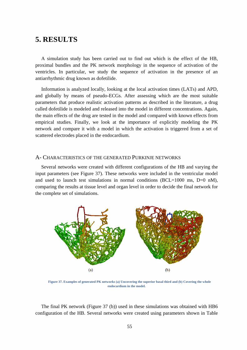
55
5. RESULTS
A simulation study has been carried out to find out which is the effect of the HB,
proximal bundles and the PK network morphology in the sequence of activation of the
ventricles. In particular, we study the sequence of activation in the presence of an
antiarrhythmic drug known as dofetilide.
Information is analyzed locally, looking at the local activation times (LATs) and APD,
and globally by means of pseudo-ECGs. After assessing which are the most suitable
parameters that produce realistic activation patterns as described in the literature, a drug
called dofetilide is modeled and released into the model in different concentrations. Again,
the main effects of the drug are tested in the model and compared with known effects from
empirical studies. Finally, we look at the importance of explicitly modeling the PK
network and compare it with a model in which the activation is triggered from a set of
scattered electrodes placed in the endocardium.
A- CHARACTERISTICS OF THE GENERATED PURKINJE NETWORKS
Several networks were created with different configurations of the HB and varying the
input parameters (see Figure 37). These networks were included in the ventricular model
and used to launch test simulations in normal conditions (BCL=1000 ms, D=0 nM),
comparing the results at tissue level and organ level in order to decide the final network for
the complete set of simulations.
Figure 37. Examples of generated PK networks (a) Uncovering the superior basal third and (b) Covering the whole
endocardium in the model.
The final PK network (Figure 37 (b)) used in these simulations was obtained with HB6
configuration of the HB. Several networks were created using parameters shown in Table
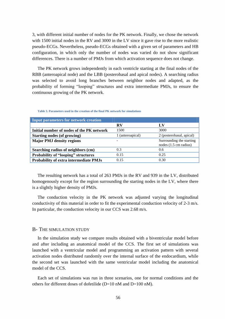
56
3, with different initial number of nodes for the PK network. Finally, we chose the network
with 1500 initial nodes in the RV and 3000 in the LV since it gave rise to the more realistic
pseudo-ECGs. Nevertheless, pseudo-ECGs obtained with a given set of parameters and HB
configuration, in which only the number of nodes was varied do not show significant
differences. There is a number of PMJs from which activation sequence does not change.
The PK network grows independently in each ventricle starting at the final nodes of the
RBB (anteroapical node) and the LBB (posterobasal and apical nodes). A searching radius
was selected to avoid long branches between neighbor nodes and adapted, as the
probability of forming ―looping‖ structures and extra intermediate PMJs, to ensure the
continuous growing of the PK network.
Table 3. Parameters used in the creation of the final PK network for simulations
Input parameters for network creation
RV LV
Initial number of nodes of the PK network 1500 3000
Starting nodes (of growing) 1 (anteroapical) 2 (posterobasal, apical)
Major PMJ density regions - Surrounding the starting
nodes (1.5 cm radius)
Searching radius of neighbors (cm) 0.3 0.6
Probability of “looping” structures 0.15 0.25
Probability of extra intermediate PMJs 0.15 0.30
The resulting network has a total of 263 PMJs in the RV and 939 in the LV, distributed
homogenously except for the region surrounding the starting nodes in the LV, where there
is a slightly higher density of PMJs.
The conduction velocity in the PK network was adjusted varying the longitudinal
conductivity of this material in order to fit the experimental conduction velocity of 2-3 m/s.
In particular, the conduction velocity in our CCS was 2.68 m/s.
B- THE SIMULATION STUDY
In the simulation study we compare results obtained with a biventricular model before
and after including an anatomical model of the CCS. The first set of simulations was
launched with a ventricular model and programming an activation pattern with several
activation nodes distributed randomly over the internal surface of the endocardium, while
the second set was launched with the same ventricular model including the anatomical
model of the CCS.
Each set of simulations was run in three scenarios, one for normal conditions and the
others for different doses of dofetilide (D=10 nM and D=100 nM).
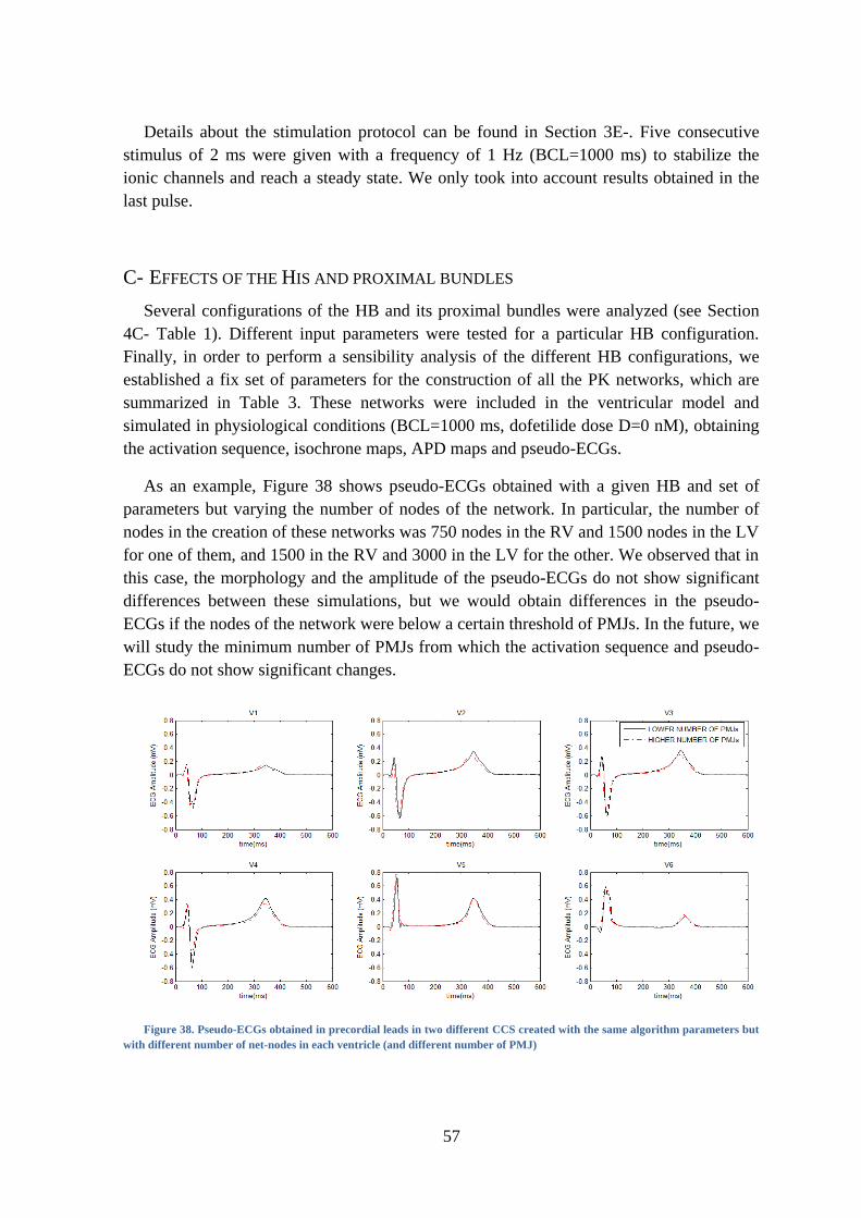
57
Details about the stimulation protocol can be found in Section 3E-. Five consecutive
stimulus of 2 ms were given with a frequency of 1 Hz (BCL=1000 ms) to stabilize the
ionic channels and reach a steady state. We only took into account results obtained in the
last pulse.
C- EFFECTS OF THE HIS AND PROXIMAL BUNDLES
Several configurations of the HB and its proximal bundles were analyzed (see Section
4C- Table 1). Different input parameters were tested for a particular HB configuration.
Finally, in order to perform a sensibility analysis of the different HB configurations, we
established a fix set of parameters for the construction of all the PK networks, which are
summarized in Table 3. These networks were included in the ventricular model and
simulated in physiological conditions (BCL=1000 ms, dofetilide dose D=0 nM), obtaining
the activation sequence, isochrone maps, APD maps and pseudo-ECGs.
As an example, Figure 38 shows pseudo-ECGs obtained with a given HB and set of
parameters but varying the number of nodes of the network. In particular, the number of
nodes in the creation of these networks was 750 nodes in the RV and 1500 nodes in the LV
for one of them, and 1500 in the RV and 3000 in the LV for the other. We observed that in
this case, the morphology and the amplitude of the pseudo-ECGs do not show significant
differences between these simulations, but we would obtain differences in the pseudo-
ECGs if the nodes of the network were below a certain threshold of PMJs. In the future, we
will study the minimum number of PMJs from which the activation sequence and pseudo-
ECGs do not show significant changes.
Figure 38. Pseudo-ECGs obtained in precordial leads in two different CCS created with the same algorithm parameters but
with different number of net-nodes in each ventricle (and different number of PMJ)
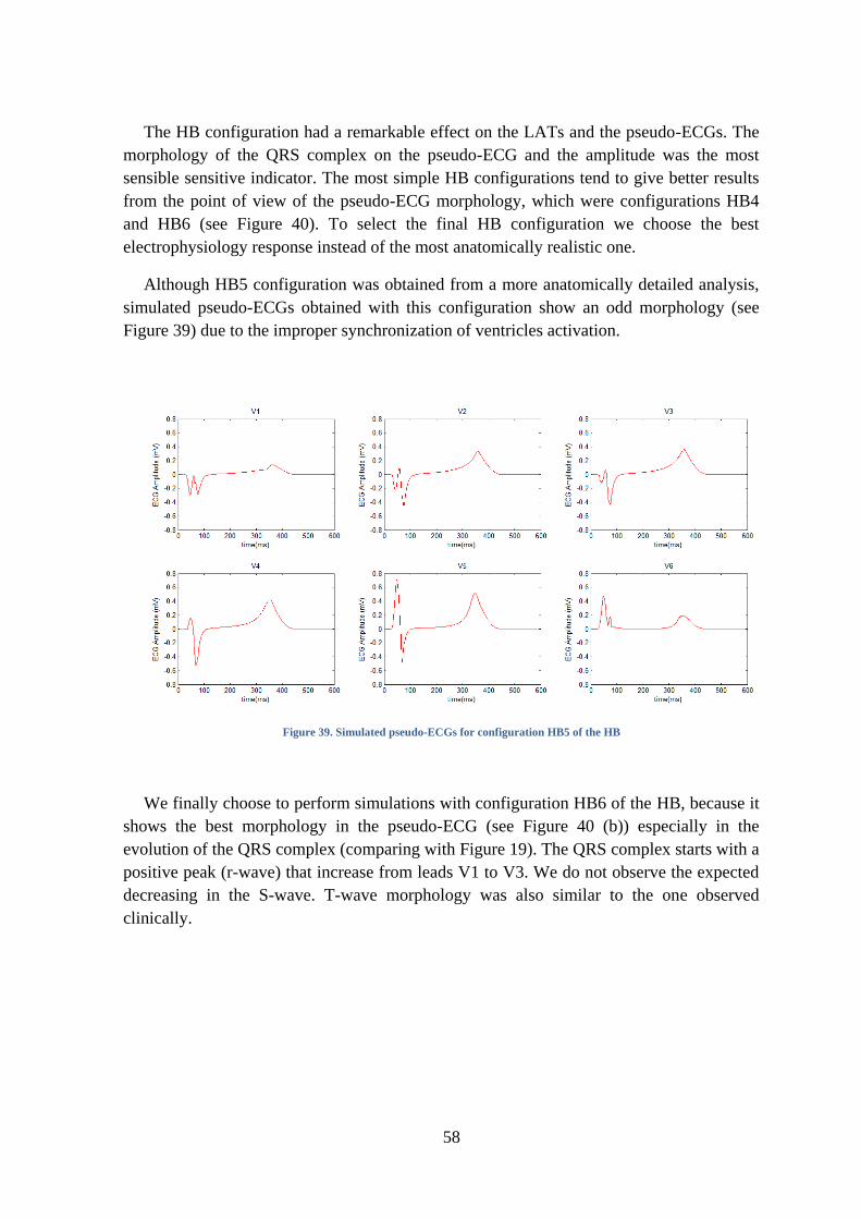
58
The HB configuration had a remarkable effect on the LATs and the pseudo-ECGs. The
morphology of the QRS complex on the pseudo-ECG and the amplitude was the most
sensible sensitive indicator. The most simple HB configurations tend to give better results
from the point of view of the pseudo-ECG morphology, which were configurations HB4
and HB6 (see Figure 40). To select the final HB configuration we choose the best
electrophysiology response instead of the most anatomically realistic one.
Although HB5 configuration was obtained from a more anatomically detailed analysis,
simulated pseudo-ECGs obtained with this configuration show an odd morphology (see
Figure 39) due to the improper synchronization of ventricles activation.
Figure 39. Simulated pseudo-ECGs for configuration HB5 of the HB
We finally choose to perform simulations with configuration HB6 of the HB, because it
shows the best morphology in the pseudo-ECG (see Figure 40 (b)) especially in the
evolution of the QRS complex (comparing with Figure 19). The QRS complex starts with a
positive peak (r-wave) that increase from leads V1 to V3. We do not observe the expected
decreasing in the S-wave. T-wave morphology was also similar to the one observed
clinically.
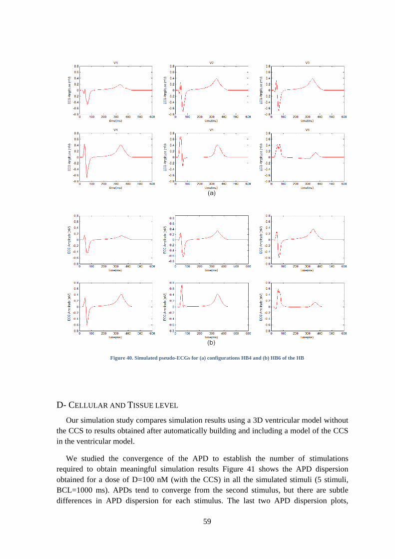
59
Figure 40. Simulated pseudo-ECGs for (a) configurations HB4 and (b) HB6 of the HB
D- CELLULAR AND TISSUE LEVEL
Our simulation study compares simulation results using a 3D ventricular model without
the CCS to results obtained after automatically building and including a model of the CCS
in the ventricular model.
We studied the convergence of the APD to establish the number of stimulations
required to obtain meaningful simulation results Figure 41 shows the APD dispersion
obtained for a dose of D=100 nM (with the CCS) in all the simulated stimuli (5 stimuli,
BCL=1000 ms). APDs tend to converge from the second stimulus, but there are subtle
differences in APD dispersion for each stimulus. The last two APD dispersion plots,
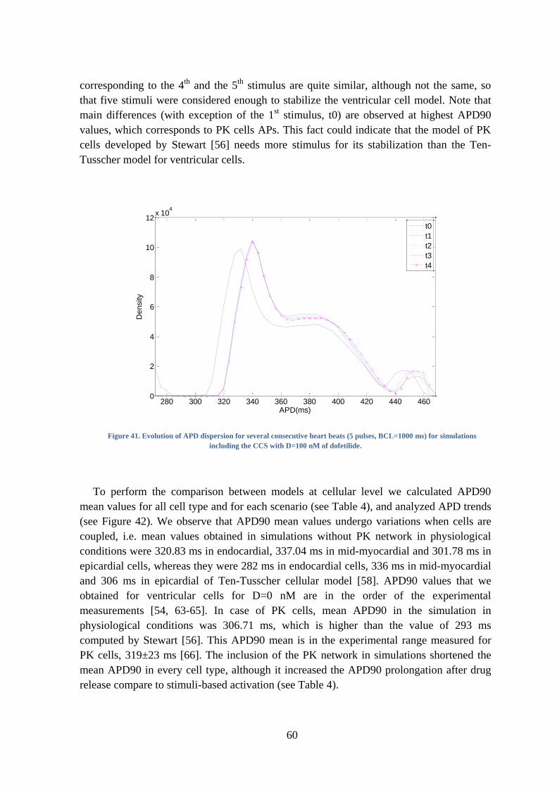
60
corresponding to the 4th
and the 5th
stimulus are quite similar, although not the same, so
that five stimuli were considered enough to stabilize the ventricular cell model. Note that
main differences (with exception of the 1st stimulus, t0) are observed at highest APD90
values, which corresponds to PK cells APs. This fact could indicate that the model of PK
cells developed by Stewart [56] needs more stimulus for its stabilization than the Ten-
Tusscher model for ventricular cells.
Figure 41. Evolution of APD dispersion for several consecutive heart beats (5 pulses, BCL=1000 ms) for simulations
including the CCS with D=100 nM of dofetilide.
To perform the comparison between models at cellular level we calculated APD90
mean values for all cell type and for each scenario (see Table 4), and analyzed APD trends
(see Figure 42). We observe that APD90 mean values undergo variations when cells are
coupled, i.e. mean values obtained in simulations without PK network in physiological
conditions were 320.83 ms in endocardial, 337.04 ms in mid-myocardial and 301.78 ms in
epicardial cells, whereas they were 282 ms in endocardial cells, 336 ms in mid-myocardial
and 306 ms in epicardial of Ten-Tusscher cellular model [58]. APD90 values that we
obtained for ventricular cells for D=0 nM are in the order of the experimental
measurements [54, 63-65]. In case of PK cells, mean APD90 in the simulation in
physiological conditions was 306.71 ms, which is higher than the value of 293 ms
computed by Stewart [56]. This APD90 mean is in the experimental range measured for
PK cells, 319±23 ms [66]. The inclusion of the PK network in simulations shortened the
mean APD90 in every cell type, although it increased the APD90 prolongation after drug
release compare to stimuli-based activation (see Table 4).
280 300 320 340 360 380 400 420 440 4600
2
4
6
8
10
12x 10
4
APD(ms)
Density
t0
t1
t2
t3
t4
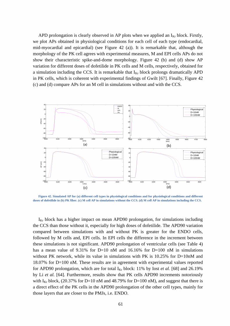
61
APD prolongation is clearly observed in AP plots when we applied an IKr block. Firstly,
we plot APs obtained in physiological conditions for each cell of each type (endocardial,
mid-myocardial and epicardial) (see Figure 42 (a)). It is remarkable that, although the
morphology of the PK cell agrees with experimental measures, M and EPI cells APs do not
show their characteristic spike-and-dome morphology. Figure 42 (b) and (d) show AP
variation for different doses of dofetilide in PK cells and M cells, respectively, obtained for
a simulation including the CCS. It is remarkable that IKr block prolongs dramatically APD
in PK cells, which is coherent with experimental findings of Gwilt [67]. Finally, Figure 42
(c) and (d) compare APs for an M cell in simulations without and with the CCS.
Figure 42. Simulated AP for (a) different cell types in physiological conditions and for physiological conditions and different
doses of dofetilide in (b) PK fiber. (c) M cell AP in simulations without the CCS. (d) M cell AP in simulations including the CCS.
IKr block has a higher impact on mean APD90 prolongation, for simulations including
the CCS than those without it, especially for high doses of dofetilide. The APD90 variation
compared between simulations with and without PK is greater for the ENDO cells,
followed by M cells and, EPI cells. In EPI cells the difference in the increment between
these simulations is not significant. APD90 prolongation of ventricular cells (see Table 4)
has a mean value of 9.31% for D=10 nM and 16.16% for D=100 nM in simulations
without PK network, while its value in simulations with PK is 10.25% for D=10nM and
18.07% for D=100 nM. These results are in agreement with experimental values reported
for APD90 prolongation, which are for total IKr block: 11% by Iost et al. [68] and 26.19%
by Li et al. [64]. Furthermore, results show that PK cells APD90 increments notoriously
with IKr block, (20.37% for D=10 nM and 48.79% for D=100 nM), and suggest that there is
a direct effect of the PK cells in the APD90 prolongation of the other cell types, mainly for
those layers that are closer to the PMJs, i.e. ENDO.
4000 4100 4200 4300 4400 4500 4600-100
-80
-60
-40
-20
0
20
40
t(ms)
AP
(mV
)
ENDO
M
EPI
PK
4000 4100 4200 4300 4400 4500 4600 4700 4800-80
-60
-40
-20
0
20
40
t(ms)
AP
(mV
)
Normal
D=10nM
D=100nM
4000 4100 4200 4300 4400 4500 4600-100
-80
-60
-40
-20
0
20
40
t(ms)
AP
(mV
)
Normal
D=10nM
D=100nM
(a) (b)
(c) (d)
4000 4100 4200 4300 4400 4500 4600-100
-80
-60
-40
-20
0
20
40
t (ms)
AP
(m
V)
Normal
D=10nM
D=100nM
0 100 200 300 400 500 600-20
0
20
40
60
80
100
120
Physiological
D=10nM
D=100nM
0 100 200 300 400 500 600-20
0
20
40
60
80
100
120
Physiological
D=10nM
D=100nM
0 100 200 300 400 500 600-20
0
20
40
60
80
100
120
Physiological
D=10nM
D=100nM
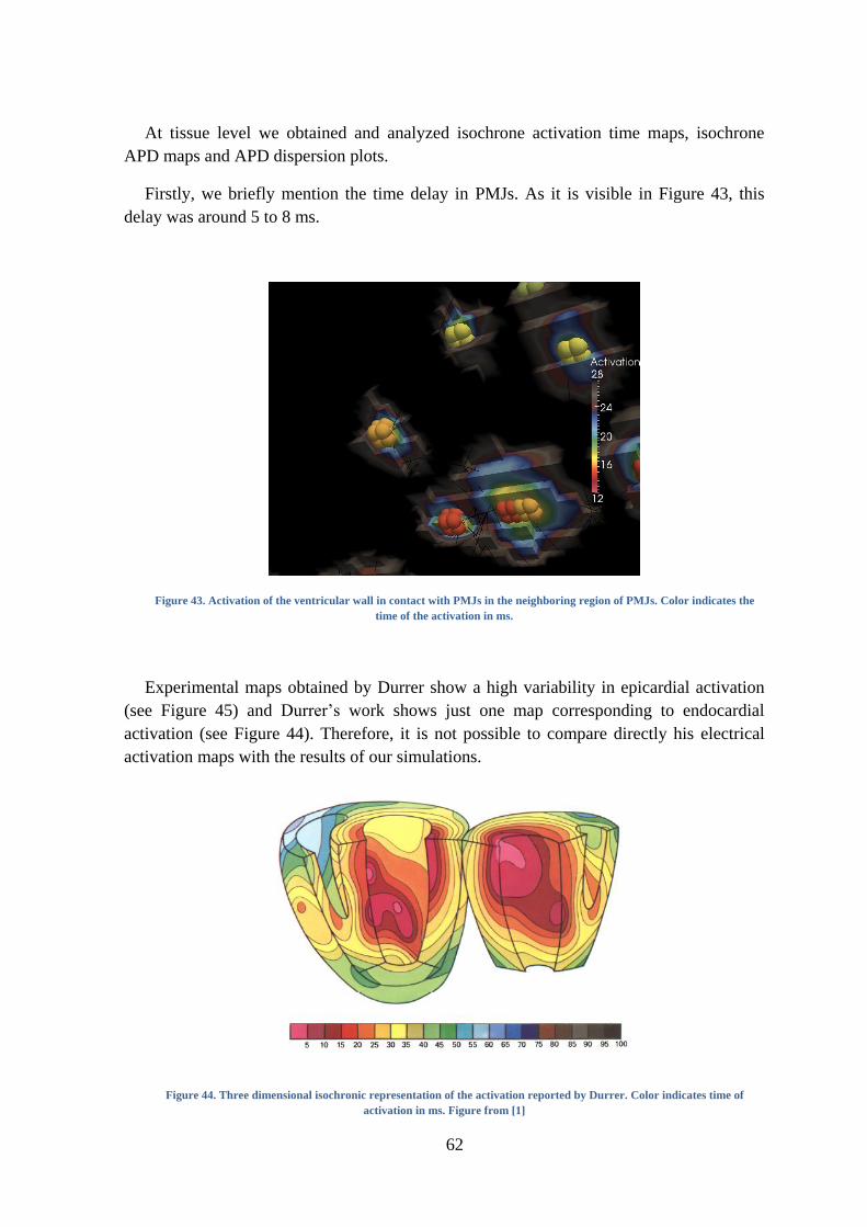
62
At tissue level we obtained and analyzed isochrone activation time maps, isochrone
APD maps and APD dispersion plots.
Firstly, we briefly mention the time delay in PMJs. As it is visible in Figure 43, this
delay was around 5 to 8 ms.
Figure 43. Activation of the ventricular wall in contact with PMJs in the neighboring region of PMJs. Color indicates the
time of the activation in ms.
Experimental maps obtained by Durrer show a high variability in epicardial activation
(see Figure 45) and Durrer’s work shows just one map corresponding to endocardial
activation (see Figure 44). Therefore, it is not possible to compare directly his electrical
activation maps with the results of our simulations.
Figure 44. Three dimensional isochronic representation of the activation reported by Durrer. Color indicates time of
activation in ms. Figure from [1]
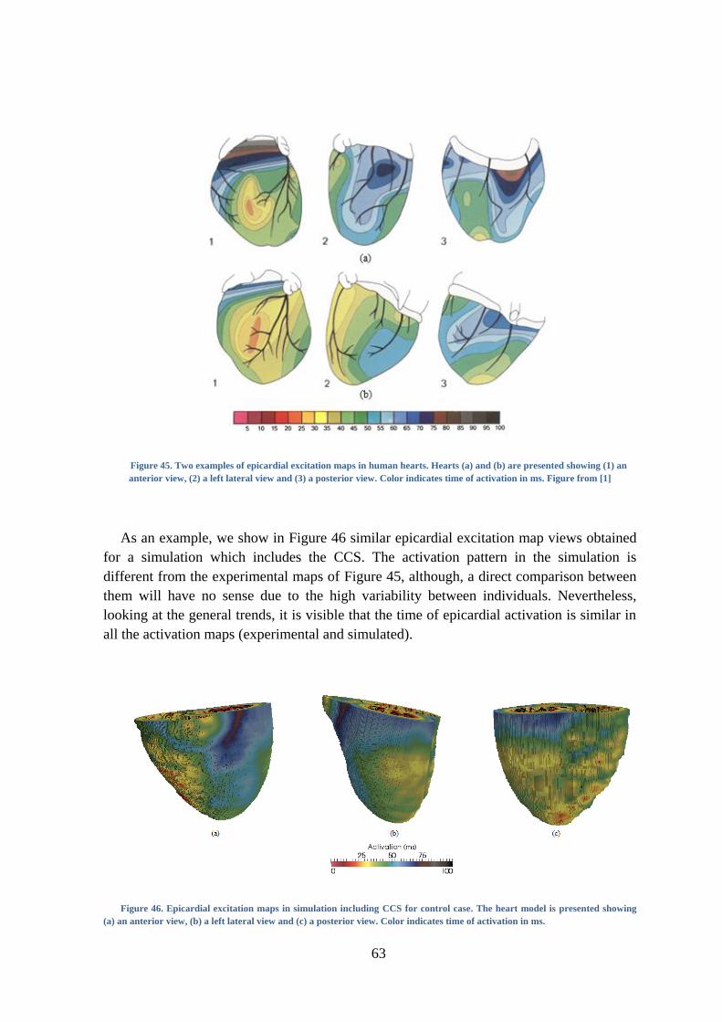
63
Figure 45. Two examples of epicardial excitation maps in human hearts. Hearts (a) and (b) are presented showing (1) an
anterior view, (2) a left lateral view and (3) a posterior view. Color indicates time of activation in ms. Figure from [1]
As an example, we show in Figure 46 similar epicardial excitation map views obtained
for a simulation which includes the CCS. The activation pattern in the simulation is
different from the experimental maps of Figure 45, although, a direct comparison between
them will have no sense due to the high variability between individuals. Nevertheless,
looking at the general trends, it is visible that the time of epicardial activation is similar in
all the activation maps (experimental and simulated).
Figure 46. Epicardial excitation maps in simulation including CCS for control case. The heart model is presented showing
(a) an anterior view, (b) a left lateral view and (c) a posterior view. Color indicates time of activation in ms.
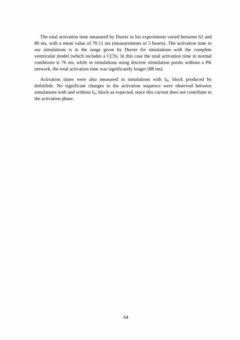
64
The total activation time measured by Durrer in his experiments varied between 62 and
80 ms, with a mean value of 70.11 ms (measurements in 5 hearts). The activation time in
our simulations is in the range given by Durrer for simulations with the complete
ventricular model (which includes a CCS). In this case the total activation time in normal
conditions is 76 ms, while in simulations using discrete stimulation points without a PK
network, the total activation time was significantly longer (88 ms).
Activation times were also measured in simulations with IKr block produced by
dofetilide. No significant changes in the activation sequence were observed between
simulations with and without IKr block as expected, since this current does not contribute to
the activation phase.
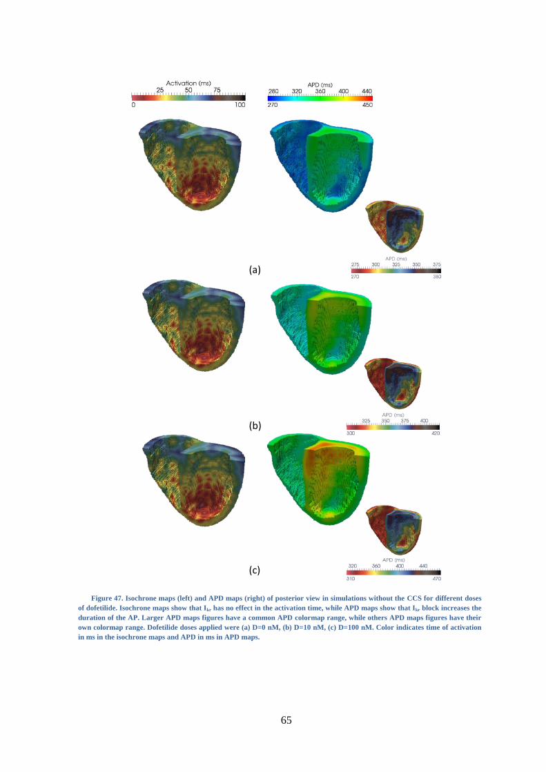
65
Figure 47. Isochrone maps (left) and APD maps (right) of posterior view in simulations without the CCS for different doses
of dofetilide. Isochrone maps show that Ikr has no effect in the activation time, while APD maps show that Ikr block increases the
duration of the AP. Larger APD maps figures have a common APD colormap range, while others APD maps figures have their
own colormap range. Dofetilide doses applied were (a) D=0 nM, (b) D=10 nM, (c) D=100 nM. Color indicates time of activation
in ms in the isochrone maps and APD in ms in APD maps.
(a)
(b)
(c)
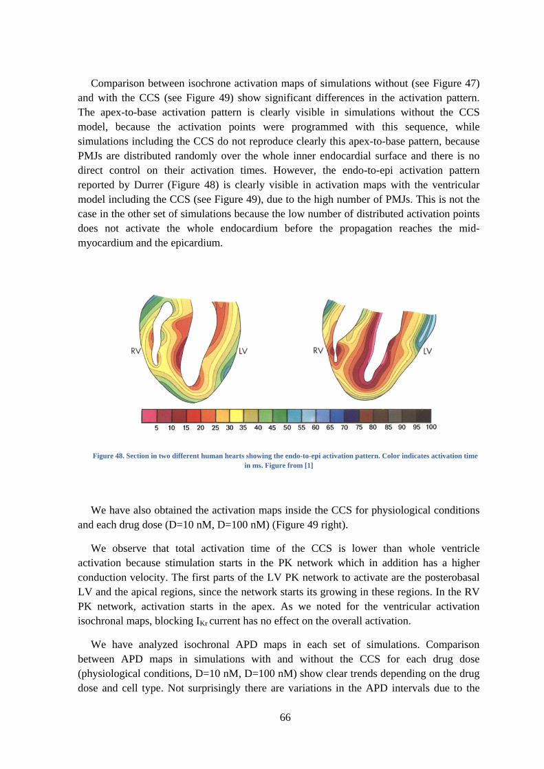
66
Comparison between isochrone activation maps of simulations without (see Figure 47)
and with the CCS (see Figure 49) show significant differences in the activation pattern.
The apex-to-base activation pattern is clearly visible in simulations without the CCS
model, because the activation points were programmed with this sequence, while
simulations including the CCS do not reproduce clearly this apex-to-base pattern, because
PMJs are distributed randomly over the whole inner endocardial surface and there is no
direct control on their activation times. However, the endo-to-epi activation pattern
reported by Durrer (Figure 48) is clearly visible in activation maps with the ventricular
model including the CCS (see Figure 49), due to the high number of PMJs. This is not the
case in the other set of simulations because the low number of distributed activation points
does not activate the whole endocardium before the propagation reaches the mid-
myocardium and the epicardium.
Figure 48. Section in two different human hearts showing the endo-to-epi activation pattern. Color indicates activation time
in ms. Figure from [1]
We have also obtained the activation maps inside the CCS for physiological conditions
and each drug dose (D=10 nM, D=100 nM) (Figure 49 right).
We observe that total activation time of the CCS is lower than whole ventricle
activation because stimulation starts in the PK network which in addition has a higher
conduction velocity. The first parts of the LV PK network to activate are the posterobasal
LV and the apical regions, since the network starts its growing in these regions. In the RV
PK network, activation starts in the apex. As we noted for the ventricular activation
isochronal maps, blocking IKr current has no effect on the overall activation.
We have analyzed isochronal APD maps in each set of simulations. Comparison
between APD maps in simulations with and without the CCS for each drug dose
(physiological conditions, D=10 nM, D=100 nM) show clear trends depending on the drug
dose and cell type. Not surprisingly there are variations in the APD intervals due to the
67
coupling with the CCS. Nevertheless, APD trends between different types of cells are still
kept in the APD maps (see Figure 47 and Figure 50, small figures on the right), with
independence of the drug doses. The reason is that the ventricular model is the same in
both cases, with a cell population distribution of 17% endocardium, 41% mid-myocardium
and 42% epicardium. Coupling the CCS modifies the APD range in the endocardial and
mid-myocardial cell types but do not affect its pattern.
We observe differences in APD inside the CCS, although the cell model is the same,
probably due to the coupling of the fibers and the interaction with the ventricle at the
PMJs, but these differences are limited to a narrow range.
APD maps in Figure 47 (left) and Figure 50 (left) have the same colormap scale for (a)
D=0 nM, (b) D=10 nM and (c) D=100 nM. APD prolongation produced by IKr block when
adding dofetilide is clearly visible in these plots. APD maps with common colormap of the
PK network (Figure 50) show a pronounced APD prolongation in PK cells when blocking
IKr.
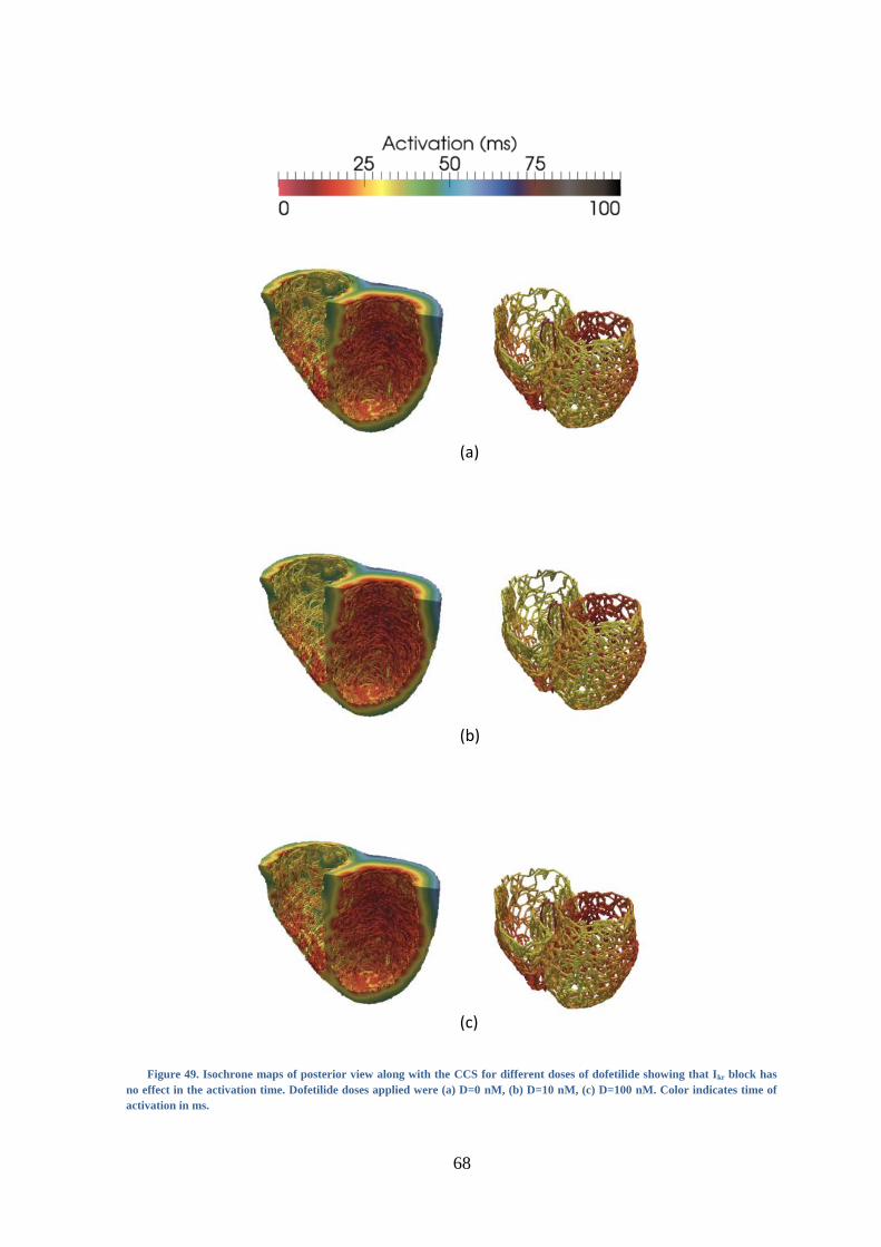
68
Figure 49. Isochrone maps of posterior view along with the CCS for different doses of dofetilide showing that Ikr block has
no effect in the activation time. Dofetilide doses applied were (a) D=0 nM, (b) D=10 nM, (c) D=100 nM. Color indicates time of
activation in ms.
(a)
(b)
(c)
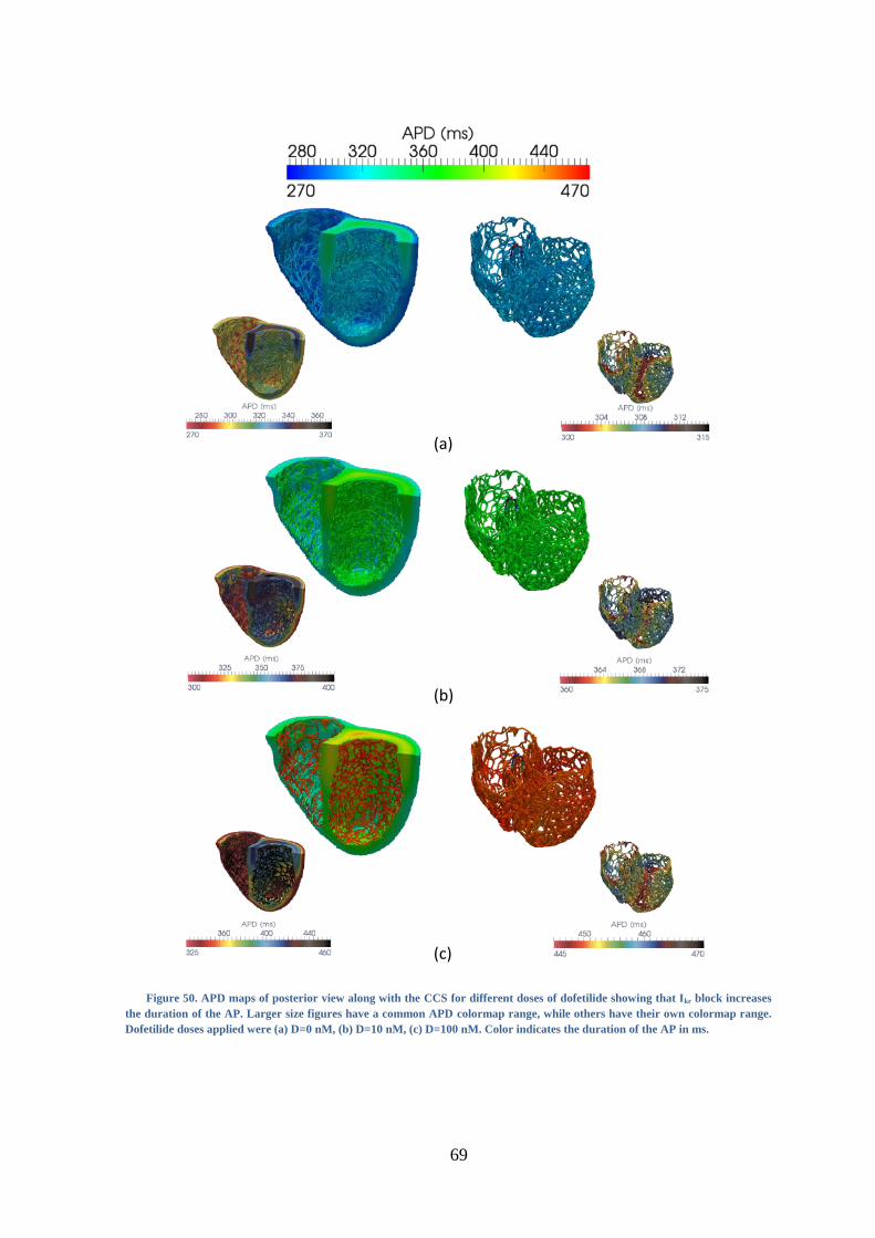
69
Figure 50. APD maps of posterior view along with the CCS for different doses of dofetilide showing that Ikr block increases
the duration of the AP. Larger size figures have a common APD colormap range, while others have their own colormap range.
Dofetilide doses applied were (a) D=0 nM, (b) D=10 nM, (c) D=100 nM. Color indicates the duration of the AP in ms.
(a)
(b)
(c)
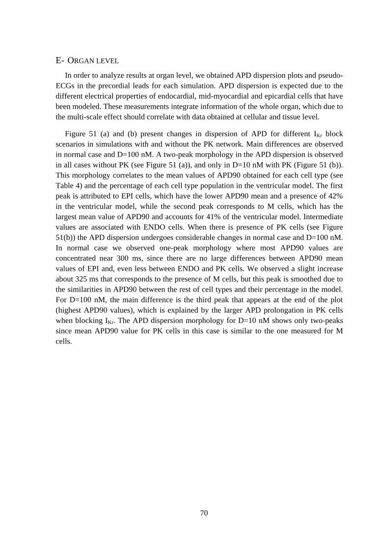
70
E- ORGAN LEVEL
In order to analyze results at organ level, we obtained APD dispersion plots and pseudo-
ECGs in the precordial leads for each simulation. APD dispersion is expected due to the
different electrical properties of endocardial, mid-myocardial and epicardial cells that have
been modeled. These measurements integrate information of the whole organ, which due to
the multi-scale effect should correlate with data obtained at cellular and tissue level.
Figure 51 (a) and (b) present changes in dispersion of APD for different IKr block
scenarios in simulations with and without the PK network. Main differences are observed
in normal case and D=100 nM. A two-peak morphology in the APD dispersion is observed
in all cases without PK (see Figure 51 (a)), and only in D=10 nM with PK (Figure 51 (b)).
This morphology correlates to the mean values of APD90 obtained for each cell type (see
Table 4) and the percentage of each cell type population in the ventricular model. The first
peak is attributed to EPI cells, which have the lower APD90 mean and a presence of 42%
in the ventricular model, while the second peak corresponds to M cells, which has the
largest mean value of APD90 and accounts for 41% of the ventricular model. Intermediate
values are associated with ENDO cells. When there is presence of PK cells (see Figure
51(b)) the APD dispersion undergoes considerable changes in normal case and D=100 nM.
In normal case we observed one-peak morphology where most APD90 values are
concentrated near 300 ms, since there are no large differences between APD90 mean
values of EPI and, even less between ENDO and PK cells. We observed a slight increase
about 325 ms that corresponds to the presence of M cells, but this peak is smoothed due to
the similarities in APD90 between the rest of cell types and their percentage in the model.
For D=100 nM, the main difference is the third peak that appears at the end of the plot
(highest APD90 values), which is explained by the larger APD prolongation in PK cells
when blocking IKr. The APD dispersion morphology for D=10 nM shows only two-peaks
since mean APD90 value for PK cells in this case is similar to the one measured for M
cells.
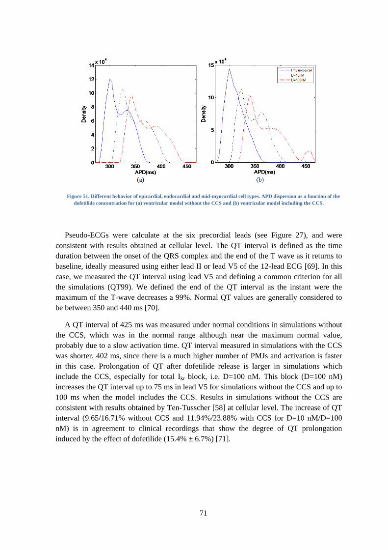
71
Figure 51. Different behavior of epicardial, endocardial and mid-myocardial cell types. APD dispersion as a function of the
dofetilide concentration for (a) ventricular model without the CCS and (b) ventricular model including the CCS.
Pseudo-ECGs were calculate at the six precordial leads (see Figure 27), and were
consistent with results obtained at cellular level. The QT interval is defined as the time
duration between the onset of the QRS complex and the end of the T wave as it returns to
baseline, ideally measured using either lead II or lead V5 of the 12-lead ECG [69]. In this
case, we measured the QT interval using lead V5 and defining a common criterion for all
the simulations (QT99). We defined the end of the QT interval as the instant were the
maximum of the T-wave decreases a 99%. Normal QT values are generally considered to
be between 350 and 440 ms [70].
A QT interval of 425 ms was measured under normal conditions in simulations without
the CCS, which was in the normal range although near the maximum normal value,
probably due to a slow activation time. QT interval measured in simulations with the CCS
was shorter, 402 ms, since there is a much higher number of PMJs and activation is faster
in this case. Prolongation of QT after dofetilide release is larger in simulations which
include the CCS, especially for total Ikr block, i.e. D=100 nM. This block (D=100 nM)
increases the QT interval up to 75 ms in lead V5 for simulations without the CCS and up to
100 ms when the model includes the CCS. Results in simulations without the CCS are
consistent with results obtained by Ten-Tusscher [58] at cellular level. The increase of QT
interval (9.65/16.71% without CCS and 11.94%/23.88% with CCS for D=10 nM/D=100
nM) is in agreement to clinical recordings that show the degree of QT prolongation
induced by the effect of dofetilide (15.4% ± 6.7%) [71].
72
Figure 52. Simulated pseudo-ECGs in the precordial leads for different doses of dofetilide obtained with (a) the ventricular
model without the CCS and (b) the ventricular model including the CCS
Is also remarkable that amplitude of pseudo-ECGs obtained when adding the CCS is in
the range of millivolts (see Figure 52 (b)), which is the normal range of amplitude values,
while the amplitude obtained in the model without the CCS is in the order of microvolts
(Figure 52 (a)).This difference might be due to the different number of PMJs used (stimuli
nodes) in each model.
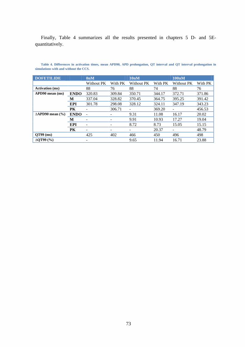
73
Finally, Table 4 summarizes all the results presented in chapters 5 D- and 5E-
quantitatively.
Table 4. Differences in activation times, mean APD90, APD prolongation, QT interval and QT interval prolongation in
simulations with and without the CCS.
DOFETILIDE 0nM 10nM 100nM
Without PK With PK Without PK With PK Without PK With PK
Activation (ms) 88 76 88 74 88 76
APD90 mean (ms) ENDO 320.83 309.84 350.71 344.17 372.71 371.86
M 337.04 328.82 370.45 364.75 395.25 391.42
EPI 301.78 298.08 328.12 324.11 347.19 343.23
PK - 306.71 - 369.20 - 456.53
∆APD90 mean (%) ENDO - - 9.31 11.08 16.17 20.02
M - - 9.91 10.93 17.27 19.04
EPI - - 8.72 8.73 15.05 15.15
PK - - - 20.37 - 48.79
QT99 (ms) 425 402 466 450 496 498
∆QT99 (%) - 9.65 11.94 16.71 23.88

74
75
6. DISCUSSION
A- MULTI-SCALE RESULTS
In this study we have built a computational model of the human heart ventricles and
carried out electrophysiology simulations to elucidate the effect of key ventricular
structures such as the CCS in the presence of a drug called dofetilide. We compare it with a
configuration in which the CCS was reduced to a set of scattered stimuli on the
endocardium.
Due to the lack of knowledge regarding the conduction system several models of the
CCS with diverse configurations of the HB and characteristics of the distal section (for
each ventricle: number of nodes of the network, radius of neighbors searching, starting
nodes of growing of the network, regions with higher density of PMJs, probabilities of
forming ―looping‖ structures and of defining intermediate PMJs nodes) have been modeled
and simulated.
We have found out that the configuration of the HB is critical in order to obtain a
correct sequence of activation and properly shaped pseudo-ECGs. Among the
configurations of the HB, the one that included more anatomical details from an
anatomical study [12] does not produce the expected results regarding ventricles activation
and synchronization, giving as a result an incorrect morphology in pseudo-ECGs
calculated in the six precordial leads. Better results were obtained with a simpler HB
configuration, and this was the critical point to decide the final HB configuration and the
PK network used for the complete set of simulations with dofetilide.
We create PK networks with higher number of nodes in LV, considering studies and
information by the cardiac anatomist Damián Sánchez-Quintana, who in addition affirms
that the number of PMJs is higher in the LV than in the RV. In addition, we observed that
pseudo-ECG morphology and amplitude was not significantly modified when varying the
number of nodes of the network in each ventricle. Similar pseudo-ECGs were obtained for
a PK network with 1500 nodes in the RV and 3000 in the LV, and a PK network with
exactly half of them. This indicates that there are a number of terminals from which
activation does not change its pattern.
Other parameters, like the radius of neighbors searching, the probability of forming
―loops‖ and the probability of defining extra PMJs from intermediate nodes of the network
were chosen mainly to fully cover the endocardium and to get PK branches in the order of
millimeters. In the future we will perform a complete sensibility analysis of the model
parameters, in order to study how much they affect the results.
Modeling and adding the CCS to the ventricular model improves considerably the
activation time. In this case, we obtain an activation time of 76 ms, so activation is faster
and in the range of normal activation values reported by Durrer [1]. Nevertheless, we have
to consider that obtaining a faster activation time in this case is also due to the higher

76
number of PMJs, because the ventricular model with scattered activation points has just
100 activation points in the RV and 150 in the LV. The conductivity in PK cells was
adjusted to obtain a conduction velocity in the range of 2-3 m/s.
Multi-scale qualitative analysis of the results is consistent with experimental data in
both models. From cell to organ level, we observe the effects of blocking IKr by the effect
of dofetilide as i) an APD prolongation in every type of cell (observe in APD90 plots and
isochronal APD90 maps), ii) no variation in the activation time and pattern (in isochronal
activation time maps) and iii) prolongation of the repolarization time and of the QT
interval.
When plotting AP for the different type of cells, i.e. extracting voltage data from a
random point of each region, we observed that the typical spike-and-dome configuration of
M and EPI cells was not visible. This result is probably due to both the coupling between
cells and the temporal resolution used in our simulations. In fact, comparing this
observation with results reported by Decker [72] points to this conclusion. Decker shows
simulated APs for epicardial dog cells and tissue and reports experimental results from
other researchers, showing that at one-dimensional tissue level the spike-and-dome
morphology is preserved but smoothed. Probably the absence of the spike-and-dome in M
and EPI cells in our simulations is caused by the two-dimensional coupling.
We also noted that PK cells interact with the ventricular model incrementing the APD90
prolongation in a major degree for surrounding cells (ENDO, followed by M and finally
EPI cells). Stewart did not presented in his paper on the PK cell modeling [56] quantitative
results for the APD90 when blocking IKr. However, our simulations shown that APD90 of
PK cells is highly prolonged when blocking IKr, which is consistent with experimental
results [67].
It is not possible to compare overall activation patterns observed in simulations with
experimental data. The reference studies in this sense are those by Durrer [1], but his
results show a high variability in the epicardial activation pattern and there is just one
example of the endocardial activation pattern. The endo-to-epi activation pattern visible in
Durrer’s maps is well reproduced by our simulations with the CCS, while the apex-to-base
activation pattern is better reproduced by the simulation without the CCS, because
activation points were distributed to obtain this pattern. However, activation times between
simulations and Durrer measurements are comparable.
Isochronal APD90 maps show that its heterogeneity principally depends on the
distribution of the different cell types. Our simulations, with and without CCS, have the
same cell distribution (ENDO, M, EPI) in the ventricles and this is visible comparing
APD90 maps. These maps are very similar in simulations with and without PK system for
the same scenario (D=0 nM, D=10 nM and D=100 nM). IKr block in the presence of PK
fibers has an effect in the prolongation of APD90, but do not modify the APD90 pattern
comparing APD90 maps between models for each dofetilide dose (see Figure 47 right and
Figure 50 left).
77
APD90 dispersion plots show a similar morphology for each dose of dofetilide, having
two-peak morphology in simulations without PK fibers. This morphology is not observed
in simulations with PK fibers. APD90 values of PK cells are similar to APD90 values of
ENDO, M and EPI cells in simulations for physiological conditions. For D=100 nM the
pronounced prolongation of APD90 in PK cells causes a third peak. In addition, plotting of
APD dispersion for the 5 simulated consecutive pulses clearly shows the necessity of
stabilizing the model and suggests that PK cell model needs a larger number of pulses to
reach the steady-state.
The morphology of the calculated pseudo-ECGs was correct for both sets of
simulations, while the amplitude was in the normal scale of millivolts for simulations
including the CCS. Measurement of QT interval gave a value in the normal range in both
simulations for the control conditions and was shorter for the simulation including the CCS
due to its faster activation. QT prolongation was in the range measured by Okada [71],
although it is significantly higher in simulations including the PK fibers.
A complete sensibility analysis of the configuration of the HB and its proximal bundles
is still needed in order to obtain a more realistic morphology and amplitude in the
simulated pseudo-ECGs.
B- LIMITATIONS
First, we want to mention limitations associated with the main part of this work, which
is the development of an anatomical model of the CCS. Main limitations are due to limited
available data. The PK network is a certainly unknown anatomical structure, especially in
humans. There is no consistent anatomical data available, so its modeling is principally
based in observations done in animal hearts and oriented to obtaining adequate simulation
results (activation maps, APD maps, pseudo-ECGs). It is not possible to know how much
real the created PK network is, and even to know if a more realistic network would give
better results. In fact, as we have seen in this study, the more anatomically detailed HB that
we created do not obtain better results in the activation sequence and pseudo-ECGs.
Parameters used for creating networks were tested observing the results of
electrophysiology simulations and were not based in anatomical studies, although we
limited some parameters such as the radius of neighbors searching and create ―looping‖
structures to reproduce the PK structure observed in animal hearts (dog and calf). There is
no information on the real number of PMJs in human hearts, so this number has also been
established observing the results of test simulations.
The CCS model has been added to a ventricular model which considers transmural
heterogeneities (M, ENDO and EPI cells), but not variations in ionic currents from apex-
to-base. The anatomical models of the ventricles and the CCS have been associated to
cellular models. In this case, simulations have been done with the model of Ten-Tusscher
[58] for ventricular cells and the model of Stewart for PK cells [56]. Consequently, there
78
are limitations inherent to the use of these cellular models, which are greatly conditioned
by the limited availability of data, the variability of data and experimental conditions and
the potential deleterious effects of cell isolation.
For example, Stewart model of PK fibers is based on modifications of the Ten-Tusscher
ventricular cell model taking into account experimental data of hearts affected by heart-
failure [59]. Several assumptions have to be done to develop the model, as considering that
heart-failure ion channel remodeling in PK fibers is consistent with remodeling in
ventricular myocytes in order to adjust some channel parameters to reproduce a normal PK
cell model. Due to the mathematical models used differences in APD90 between the
different types of cells, especially when comparing PK cells with ventricular cells, are not
what experimental studies mention. APD90 in the PK cell model does not have a larger
value than APD90 in ventricular cells. Ten-Tusscher values for APD90 [57, 58] are 282 ms
for ENDO cells, 336 ms for M cells and 306 ms for EPI cells at BCL=1000 ms, while the
computed value of PK cell model of Stewart [56] is 293 ms (lower than experimental
APD90), which is shorter than the computed APD90 for M and EPI cells. Differences in
APD90 between ventricular cells are lower than differences observed experimentally.
However, when blocking IKr the APD90 of PK cells overcomes APD90 of ventricular cells
since its prolongation is more pronounced. In addition, Ten-Tusscher model for ventricular
cells has an inaccurate behavior when blocking IKr or IKs.
Furthermore, the model of dofetilide that has been used in these simulations is also very
simple. We have applied a factor multiplying IKr, current. This factor is inversely related to
the dose of dofetilide. Other simplification that has been assumed is the application of the
same blocking factor in PK cells than in ventricular cells, although it is not clear if the
effect of dofetilide is equivalent for this cell type.
At organ level, we have obtained pseudo-ECGs, which are comparable with real ECGs
in morphology but not in amplitude. To obtain simulated ECGs it is necessary to introduce
the heart model in a complete torso model, taking into account different tissue
heterogeneities between the heart and the torso.
There are also computational limitations. We have simulated 5 stimuli with a
BCL=1000 ms (a total of 5000 ms). Approximately 24 hours have been necessary to
perform every simulation using 48 cores. Therefore, it is not possible to launch the number
of stimuli probably needed to stabilize the model (maybe 1000 stimuli).
Finally, it is difficult to validate cell and tissue results with experimental data, especially
for PK cells, and quantitative comparisons are limited by the lack of experimental values
and its variability. There are also difficulties for validating these results at organ level (by
pseudo-ECGs), cause there are no much experimental studies. In addition, it is obvious that
this kind of studies cannot be tested in-vivo because it would be highly invasive and it is
not ethical to administrate dofetilide or other drugs to test their effect.
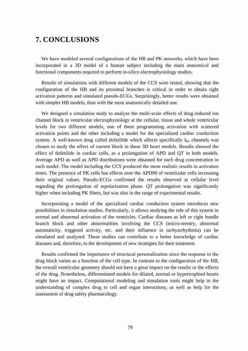
79
7. CONCLUSIONS
We have modeled several configurations of the HB and PK networks, which have been
incorporated in a 3D model of a human subject including the main anatomical and
functional components required to perform in-silico electrophysiology studies.
Results of simulations with different models of the CCS were tested, showing that the
configuration of the HB and its proximal branches is critical in order to obtain right
activation patterns and simulated pseudo-ECGs. Surprisingly, better results were obtained
with simpler HB models, than with the most anatomically detailed one.
We designed a simulation study to analyze the multi-scale effects of drug-induced ion
channel block in ventricular electrophysiology at the cellular, tissue and whole ventricular
levels for two different models, one of them programming activation with scattered
activation points and the other including a model for the specialized cardiac conduction
system. A well-known drug called dofetilide which affects specifically IKr channels was
chosen to study the effect of current block in these 3D heart models. Results showed the
effect of dofetilide in cardiac cells, as a prolongation of APD and QT in both models.
Average APD as well as APD distributions were obtained for each drug concentration in
each model. The model including the CCS produced the more realistic results in activation
times. The presence of PK cells has effects over the APD90 of ventricular cells increasing
their original values. Pseudo-ECGs confirmed the results observed at cellular level
regarding the prolongation of repolarization phase. QT prolongation was significantly
higher when including PK fibers, but was also in the range of experimental results.
Incorporating a model of the specialized cardiac conduction system introduces new
possibilities in simulation studies. Particularly, it allows studying the role of this system in
normal and abnormal activation of the ventricles. Cardiac diseases as left or right bundle
branch block and other abnormalities involving the CCS (micro-reentry, abnormal
automaticity, triggered activity, etc. and their influence in tachyarrhythmia) can be
simulated and analyzed. These studies can contribute to a better knowledge of cardiac
diseases and, therefore, to the development of new strategies for their treatment.
Results confirmed the importance of structural personalization since the response to the
drug block varies as a function of the cell type. In contrast to the configuration of the HB,
the overall ventricular geometry should not have a great impact on the results or the effects
of the drug. Nonetheless, differentiated models for dilated, normal or hypertrophied hearts
might have an impact. Computational modeling and simulation tools might help in the
understanding of complex drug to cell and organ interactions, as well as help for the
assessment of drug safety pharmacology.

80
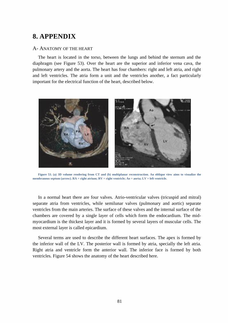
81
8. APPENDIX
A- ANATOMY OF THE HEART
The heart is located in the torso, between the lungs and behind the sternum and the
diaphragm (see Figure 53). Over the heart are the superior and inferior vena cava, the
pulmonary artery and the aorta. The heart has four chambers: right and left atria, and right
and left ventricles. The atria form a unit and the ventricles another, a fact particularly
important for the electrical function of the heart, described below.
Figure 53. (a) 3D volume rendering from CT and (b) multiplanar reconstruction. An oblique view aims to visualize the
membranous septum (arrow). RA = right atrium; RV = right ventricle; Ao = aorta; LV = left ventricle.
In a normal heart there are four valves. Atrio-ventricular valves (tricuspid and mitral)
separate atria from ventricles, while semilunar valves (pulmonary and aortic) separate
ventricles from the main arteries. The surface of these valves and the internal surface of the
chambers are covered by a single layer of cells which form the endocardium. The mid-
myocardium is the thickest layer and it is formed by several layers of muscular cells. The
most external layer is called epicardium.
Several terms are used to describe the different heart surfaces. The apex is formed by
the inferior wall of the LV. The posterior wall is formed by atria, specially the left atria.
Right atria and ventricle form the anterior wall. The inferior face is formed by both
ventricles. Figure 54 shows the anatomy of the heart described here.
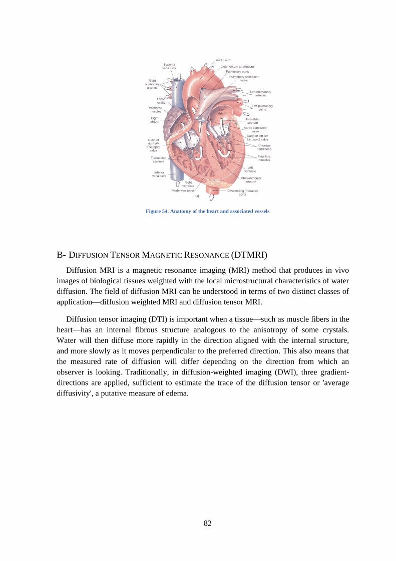
82
Figure 54. Anatomy of the heart and associated vessels
B- DIFFUSION TENSOR MAGNETIC RESONANCE (DTMRI)
Diffusion MRI is a magnetic resonance imaging (MRI) method that produces in vivo
images of biological tissues weighted with the local microstructural characteristics of water
diffusion. The field of diffusion MRI can be understood in terms of two distinct classes of
application—diffusion weighted MRI and diffusion tensor MRI.
Diffusion tensor imaging (DTI) is important when a tissue—such as muscle fibers in the
heart—has an internal fibrous structure analogous to the anisotropy of some crystals.
Water will then diffuse more rapidly in the direction aligned with the internal structure,
and more slowly as it moves perpendicular to the preferred direction. This also means that
the measured rate of diffusion will differ depending on the direction from which an
observer is looking. Traditionally, in diffusion-weighted imaging (DWI), three gradient-
directions are applied, sufficient to estimate the trace of the diffusion tensor or 'average
diffusivity', a putative measure of edema.
83
Figure 55. DTMRI short axis cut showing RV and LB. (a) Gray level image from DTI and (b) reconstruction of fiber
orientation in plane.
C- COMPUTATIONAL SIMULATION
PRE-PROCESSED
The pre-processed is implemented in MATLAB. The previous step to execute the
algorithm is to select endocardial nodes from those which form the whole ventricular
model. After this selection, we run the algorithm that creates the PK network. In the
execution we must specify the HB configuration that is used and the matrix of endocardial
nodes from which PK network nodes are selected (whole endocardial, not nodes in the
basal region…).
Before running the algorithm, we have to indicate the value of the following parameters
for each ventricle: index of the nodes where the net starts its growing, distance that will be
used to compute the searching radius, regions with predefined terminals (index of the
central node, radius of the region and percentage of predefined terminals), probability of a
intermediate node to be the origin of a little bundle ended in a terminal, probability of
forming ―elliptical structures‖ (it is related to the probability of connect again a node that is
already connected with a neighbor).
After running the algorithm we indicate the number of nodes that will form the PK
network in each ventricle. With these parameters, the algorithm computes the network and
gives the next outputs:
1) .dat intermediate outputs:
- PKpoints_RV, PKpoints_LV: candidate node that form the PK network (its
number is set by the user).
- endoRV, endoLV: final nodes of the PK network in each ventricle.
Composed of PKpoints plus the additional nodes that the algorithm may
define as terminals.
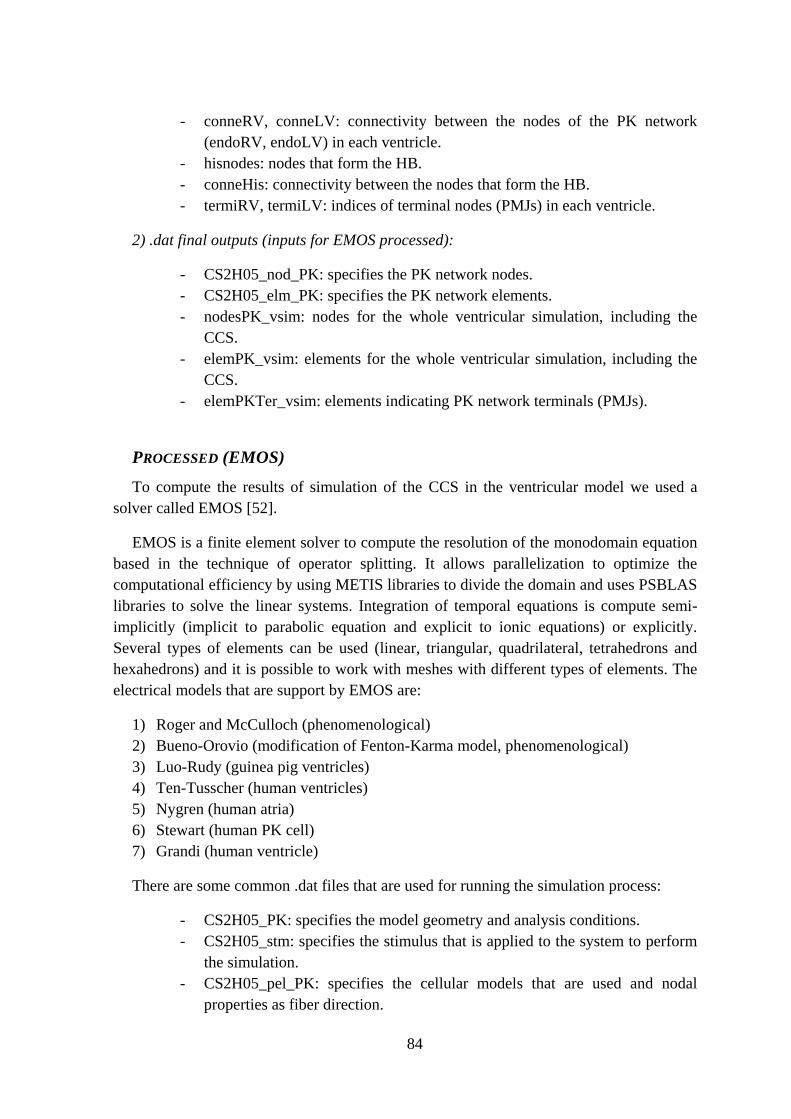
84
- conneRV, conneLV: connectivity between the nodes of the PK network
(endoRV, endoLV) in each ventricle.
- hisnodes: nodes that form the HB.
- conneHis: connectivity between the nodes that form the HB.
- termiRV, termiLV: indices of terminal nodes (PMJs) in each ventricle.
2) .dat final outputs (inputs for EMOS processed):
- CS2H05_nod_PK: specifies the PK network nodes.
- CS2H05_elm_PK: specifies the PK network elements.
- nodesPK_vsim: nodes for the whole ventricular simulation, including the
CCS.
- elemPK_vsim: elements for the whole ventricular simulation, including the
CCS.
- elemPKTer_vsim: elements indicating PK network terminals (PMJs).
PROCESSED (EMOS)
To compute the results of simulation of the CCS in the ventricular model we used a
solver called EMOS [52].
EMOS is a finite element solver to compute the resolution of the monodomain equation
based in the technique of operator splitting. It allows parallelization to optimize the
computational efficiency by using METIS libraries to divide the domain and uses PSBLAS
libraries to solve the linear systems. Integration of temporal equations is compute semi-
implicitly (implicit to parabolic equation and explicit to ionic equations) or explicitly.
Several types of elements can be used (linear, triangular, quadrilateral, tetrahedrons and
hexahedrons) and it is possible to work with meshes with different types of elements. The
electrical models that are support by EMOS are:
1) Roger and McCulloch (phenomenological)
2) Bueno-Orovio (modification of Fenton-Karma model, phenomenological)
3) Luo-Rudy (guinea pig ventricles)
4) Ten-Tusscher (human ventricles)
5) Nygren (human atria)
6) Stewart (human PK cell)
7) Grandi (human ventricle)
There are some common .dat files that are used for running the simulation process:
- CS2H05_PK: specifies the model geometry and analysis conditions.
- CS2H05_stm: specifies the stimulus that is applied to the system to perform
the simulation.
- CS2H05_pel_PK: specifies the cellular models that are used and nodal
properties as fiber direction.

85
Figure 28 shows CS2H05_PK.dat file, that is the file which contains specifications of
the model geometry and the simulation analysis that is perform.
GEOMETRY
-analysistype label, value 1 indicates an electrophysiological analysis.
-material. As is indicate, we use three materials. The first column is the number of the
material, the three following columns are not used and the fourth column indicates the
number of data that define the corresponding material. There are three data (longitudinal
conductance, ratio between transversal en longitudinal conductance, and capacitance) for
myocardial and PK materials, and one data (longitudinal conductance) for the Purkinje-
muscle junction. PK longitudinal conductance has been set to 0.180, giving this value a
conduction velocity of 2.68 m/s in the PK network.
-prop_nod, specifies the type of the cellular model that is used in each node. In these
simulations, there are four types of nodal properties. The first column refers to the number
of the property and the second column refers to the type of property that is pointed. The
third column is always 1 in electrophysiological simulations, indicating the number of
integer data to be defined. The fourth column is the number of real data to be defined, that
is 0 in our case. The last column is the integer defined data and indicates the cellular type:
1, 2 and 3 are endo, mid and epi cellular Ten-Tusscher models and 11 indicates PK cell
Stewart model.
-prop_elem loads a file that contains fiber direction of each element.
-nodes loads a file containing all the nodes of the PK network. The first line indicates
the total number of nodes, its type (this value is not used) and its dimension (3D in this
case). The second line indicates the number of nodes to be defined. Following rows
indicate for each node its identification number, its nodal property (associated cellular
model) and nodal coordinates (x,y,z). An extract of a nodal file example is shown in Figure
56.
…
Figure 56. File #NODES in CS2H05_PK.dat
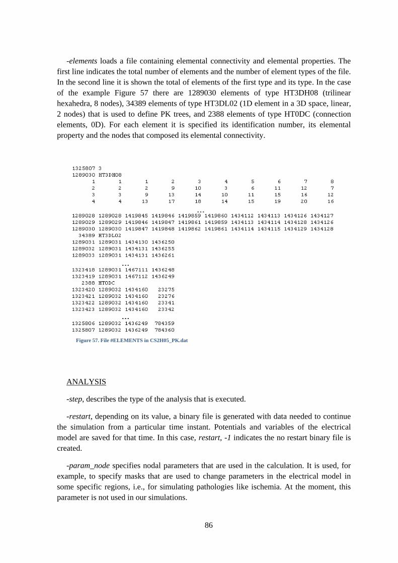
86
-elements loads a file containing elemental connectivity and elemental properties. The
first line indicates the total number of elements and the number of element types of the file.
In the second line it is shown the total of elements of the first type and its type. In the case
of the example Figure 57 there are 1289030 elements of type HT3DH08 (trilinear
hexahedra, 8 nodes), 34389 elements of type HT3DL02 (1D element in a 3D space, linear,
2 nodes) that is used to define PK trees, and 2388 elements of type HT0DC (connection
elements, 0D). For each element it is specified its identification number, its elemental
property and the nodes that composed its elemental connectivity.
ANALYSIS
-step, describes the type of the analysis that is executed.
-restart, depending on its value, a binary file is generated with data needed to continue
the simulation from a particular time instant. Potentials and variables of the electrical
model are saved for that time. In this case, restart, -1 indicates the no restart binary file is
created.
-param_node specifies nodal parameters that are used in the calculation. It is used, for
example, to specify masks that are used to change parameters in the electrical model in
some specific regions, i.e., for simulating pathologies like ischemia. At the moment, this
parameter is not used in our simulations.
…
…
…
Figure 57. File #ELEMENTS in CS2H05_PK.dat
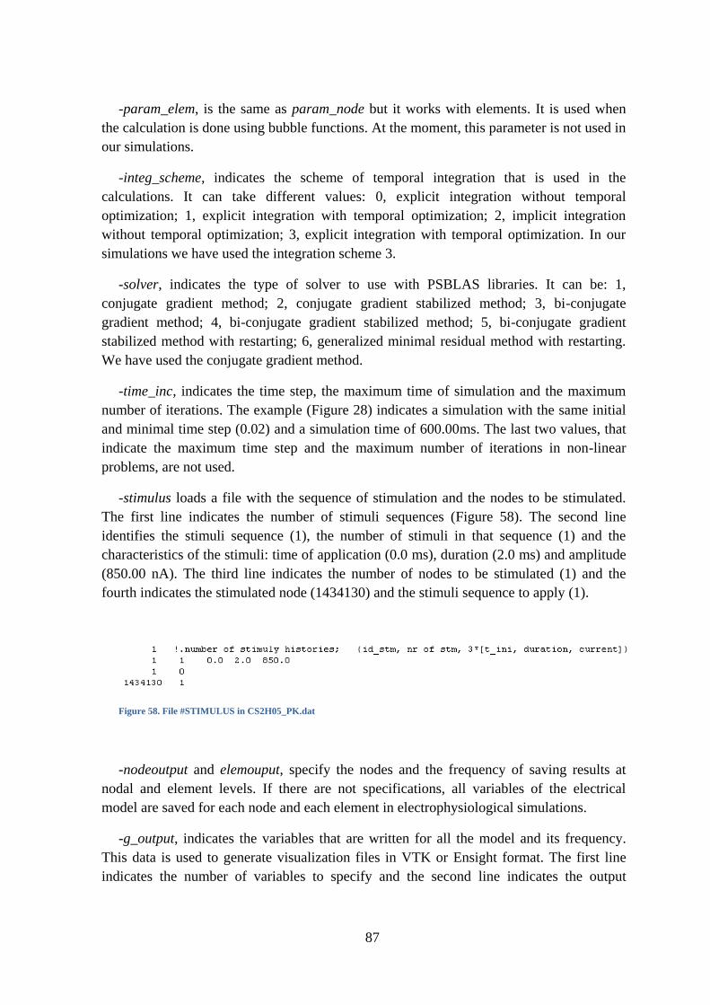
87
-param_elem, is the same as param_node but it works with elements. It is used when
the calculation is done using bubble functions. At the moment, this parameter is not used in
our simulations.
-integ_scheme, indicates the scheme of temporal integration that is used in the
calculations. It can take different values: 0, explicit integration without temporal
optimization; 1, explicit integration with temporal optimization; 2, implicit integration
without temporal optimization; 3, explicit integration with temporal optimization. In our
simulations we have used the integration scheme 3.
-solver, indicates the type of solver to use with PSBLAS libraries. It can be: 1,
conjugate gradient method; 2, conjugate gradient stabilized method; 3, bi-conjugate
gradient method; 4, bi-conjugate gradient stabilized method; 5, bi-conjugate gradient
stabilized method with restarting; 6, generalized minimal residual method with restarting.
We have used the conjugate gradient method.
-time_inc, indicates the time step, the maximum time of simulation and the maximum
number of iterations. The example (Figure 28) indicates a simulation with the same initial
and minimal time step (0.02) and a simulation time of 600.00ms. The last two values, that
indicate the maximum time step and the maximum number of iterations in non-linear
problems, are not used.
-stimulus loads a file with the sequence of stimulation and the nodes to be stimulated.
The first line indicates the number of stimuli sequences (Figure 58). The second line
identifies the stimuli sequence (1), the number of stimuli in that sequence (1) and the
characteristics of the stimuli: time of application (0.0 ms), duration (2.0 ms) and amplitude
(850.00 nA). The third line indicates the number of nodes to be stimulated (1) and the
fourth indicates the stimulated node (1434130) and the stimuli sequence to apply (1).
Figure 58. File #STIMULUS in CS2H05_PK.dat
-nodeoutput and elemouput, specify the nodes and the frequency of saving results at
nodal and element levels. If there are not specifications, all variables of the electrical
model are saved for each node and each element in electrophysiological simulations.
-g_output, indicates the variables that are written for all the model and its frequency.
This data is used to generate visualization files in VTK or Ensight format. The first line
indicates the number of variables to specify and the second line indicates the output
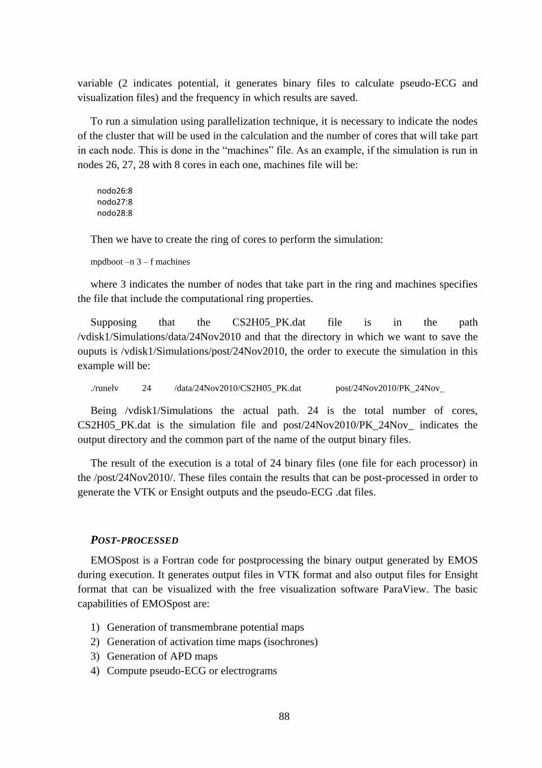
88
variable (2 indicates potential, it generates binary files to calculate pseudo-ECG and
visualization files) and the frequency in which results are saved.
To run a simulation using parallelization technique, it is necessary to indicate the nodes
of the cluster that will be used in the calculation and the number of cores that will take part
in each node. This is done in the ―machines‖ file. As an example, if the simulation is run in
nodes 26, 27, 28 with 8 cores in each one, machines file will be:
Then we have to create the ring of cores to perform the simulation:
mpdboot –n 3 – f machines
where 3 indicates the number of nodes that take part in the ring and machines specifies
the file that include the computational ring properties.
Supposing that the CS2H05_PK.dat file is in the path
/vdisk1/Simulations/data/24Nov2010 and that the directory in which we want to save the
ouputs is /vdisk1/Simulations/post/24Nov2010, the order to execute the simulation in this
example will be:
./runelv 24 /data/24Nov2010/CS2H05_PK.dat post/24Nov2010/PK_24Nov_
Being /vdisk1/Simulations the actual path. 24 is the total number of cores,
CS2H05_PK.dat is the simulation file and post/24Nov2010/PK_24Nov_ indicates the
output directory and the common part of the name of the output binary files.
The result of the execution is a total of 24 binary files (one file for each processor) in
the /post/24Nov2010/. These files contain the results that can be post-processed in order to
generate the VTK or Ensight outputs and the pseudo-ECG .dat files.
POST-PROCESSED
EMOSpost is a Fortran code for postprocessing the binary output generated by EMOS
during execution. It generates output files in VTK format and also output files for Ensight
format that can be visualized with the free visualization software ParaView. The basic
capabilities of EMOSpost are:
1) Generation of transmembrane potential maps
2) Generation of activation time maps (isochrones)
3) Generation of APD maps
4) Compute pseudo-ECG or electrograms
nodo26:8
nodo27:8
nodo28:8
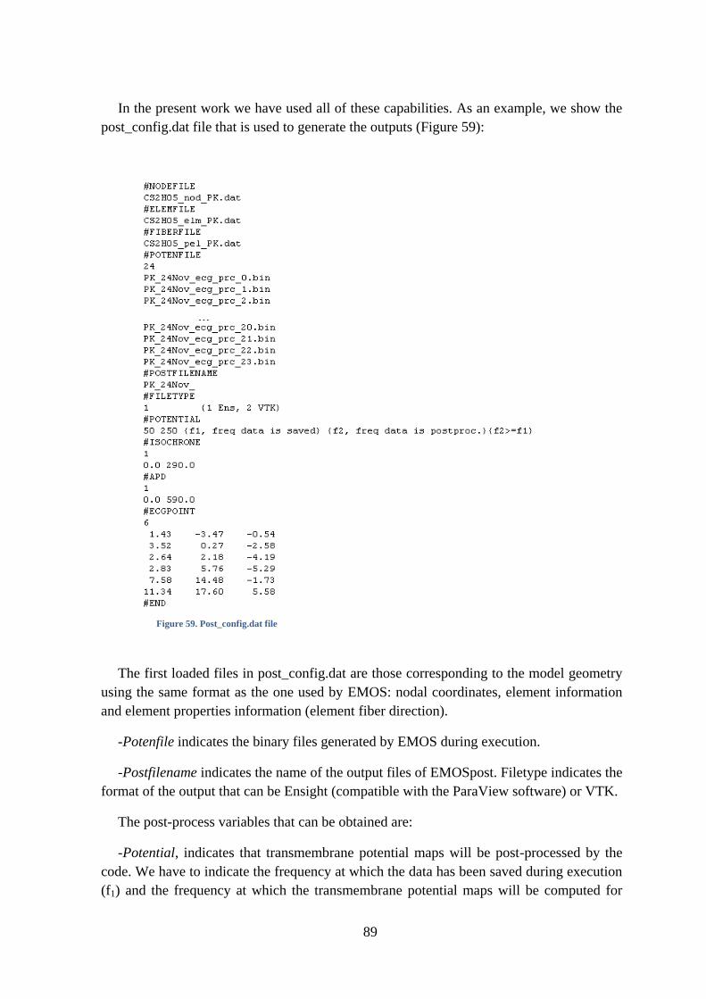
89
In the present work we have used all of these capabilities. As an example, we show the
post_config.dat file that is used to generate the outputs (Figure 59):
The first loaded files in post_config.dat are those corresponding to the model geometry
using the same format as the one used by EMOS: nodal coordinates, element information
and element properties information (element fiber direction).
-Potenfile indicates the binary files generated by EMOS during execution.
-Postfilename indicates the name of the output files of EMOSpost. Filetype indicates the
format of the output that can be Ensight (compatible with the ParaView software) or VTK.
The post-process variables that can be obtained are:
-Potential, indicates that transmembrane potential maps will be post-processed by the
code. We have to indicate the frequency at which the data has been saved during execution
(f1) and the frequency at which the transmembrane potential maps will be computed for
…
Figure 59. Post_config.dat file
90
visualization (f2), being f2≥f1. Transmembrane potential maps are generated at each node as
a function of time.
-Isochrone, indicates that isochrones maps will be post-processed by the code. The first
line data line indicates the number of isochrones maps to be generated and the remaining
lines are composed by an initial time instant and a final time instant, indicating the
beginning and end of the time window in which the isochrones map will be generated. The
code considers a cell has activated if the transmembrane potential, Vm, is greater than zero.
-APD, indicates that APD90 maps will be post-processed by the code. The first data line
indicates the number of APD maps to be generated and the remaining lines indicate the
time window in which APD maps will be generated. APD90 is computed as the elapsed
time between the maximum upstroke and when Vm=0.9·(Vmax-Vrest), where Vmax is the
maximum of the AP of the cell and Vrest is potential reached by the cell at rest (without
being stimulated).
-ECGPOINT, indicates that pseudo-ECGs will be computed at the given points. The
first data line indicates the number of points in which the pseudo-ECG will be computed
and the remaining lines indicate the global Cartesian coordinates X,Y,Z of the point where
the pseudo-ECG will be computed.
Following the example of the PROCESSED paragraph, the order to obtain the
processed files would be:
./runpost data/24Nov2010/post_config.dat post/24Nov2010/
91
9. BIBLIOGRAPHY
1. D. Durrer, R. Van Dam, G. Freud et al., "Total excitaton of the Isolated Human
Heart." Circulation vol. 41, pp. 899-912. 1970.
2. A. Pollard and R. Barr, "Computer Simulations of Activation in an Anatomically
Based Model of the Human Ventricular Conduction System." IEEE Transactions on
Biomedical Engineering vol. 38 no. 10, pp. 982-996. 1991.
3. K. Ten Tusscher and A. Panfilov, "Modelling of the ventricular conduction system."
Progress in Biophysics and Molecular Biology vol. 96, pp. 152-170. 2008.
4. R. Myerburg, K. Nilsson, and H. Gelband, "Physiology of Canine Intraventricular
Conduction and Endocardial Excitation." Circulation Research vol. XXX, pp. 217-
243. Feb. 1972.
5. C. Ramanathan, P. Jia, R. Ghanem et al., "Activation and repolarization of the normal
human heart under complete physiological conditions." Proceedings of the National
Academy of Sciences of the United States of America vol. 103 no. 16, pp. 6309-
6314. Apr. 2006.
6. J. Purkinje, " Mikroskopisch-neurologische Beobachtungen." Archiv für Anatomie,
Physiologie and wissenschaftliche Medicin vol. 12, pp. 281-295. 1845.
7. S. Tawara, The Conduction System of the Mammalian Heart. An Anatomico-
histological Study of the Atrioventricular Bundle and the Purkinje Fibers:
Cardiopulmonary Medicine from Imperial College Press, 1906.
8. W. Einthoven, "Weiteres über das Elektrokardiogran." Pflüger Archiv Ges Physiol
vol. 122, pp. 517-548. 1908.
9. L. Aschoff, "Referat uber die Herzstorungen in ihren Beziehungen zu den
Spezifischen Muskelsystem des Herzens." Verh Dtsch Pathol Ges vol. 14, pp. 3-35.
1910.
10. J. Mönckeberg, "Beitrage zur normalen und pathologischen Anatomie des Herzens."
Verh Dtsch Pathol Ges vol. 14, pp. 64-71. 1910.
11. R. Anderson and S. Yen Ho, "The morphology of the cardiac conduction system."
Development of Cardiac Conduction System. pp. 18-36. 2003. Novartis Foundation
Symposium no 250.
12. G. Massing and T. James, "Anatomical configuration of the His bundle and bundle
branches in the human heart." Circulation vol. 53 no. 4. 1976.
13. D. Sánchez-Quintana and S. Yen Ho, "Anatomía de los nodos cardíacos y del sistema
de conducción específico auriculoventricular." Revista Española de Cardiología vol.
56 no. 11. 2003.
92
14. M. Spach, S. Huang, and S. Amstrong, "Demonstration of Peripheral Conduction
System in Human Hearts." Circulation vol. 28, pp. 333-338. 1963.
15. A. Ansari, S. Yen Ho, and R. Anderson, "Distribution of the Purkinje fibres in the
sheep heart." The Anatomical Record vol. 254, pp. 92-97. 1999.
16. S. Ryu, S. Yamamoto, C. Andersen et al., "Intramural Purkinje cell network of sheep
ventricles as the terminal pathway of conduction system." The Anatomical Record
vol. 292 no. 1, pp. 12-22. Jan. 2009.
17. V. Christoffels and A. Moorman, "Development of the Cardiac Conduction System.
Why are some regions of the heart more arrhythmogenic than others?" Circulation:
Arrhythmia and Electrophysiology vol. 2 no. 2, pp. 195-207. Apr. 2009.
18. O. Eliska, "Purkinje fibers of the Heart Conduction System." Casopis Lékarú Ceských
vol. 145 no. 4. 2006.
19. A. Cates, W. Smith, R. Ideker et al., "Purkinje and ventricular contributions to
endocardial activation sequence in perfused rabbit right ventricle." American Journal
of Physiology.Heart and Circulatory Physiology vol. 281 no. 2, pp. 490-505. Aug.
2001.
20. A. Moorman, F. de Jong, M. Denyn et al., "Development of the Cardiac Conduction
System." Circulation Research vol. 82, pp. 629-644. 1998.
21. D. Dosdall, K. Cheng, J. Huang et al., "Transmural and endocardial Purkinje
activation in pigs before local myocardial activation after defibrillation shocks."
Heart Rhythm Society vol. 4 no. 6, pp. 758-765. June 2007.
22. P. Tabereaux, G. Walcott, J. Rogers et al., "Activation patterns of Purkinje fibers
during long-duration ventricular fibrillation in an isolated canine heart model."
Circulation vol. 116 no. 10, pp. 1113-1119. Sept. 2007.
23. B. Baláti, A. Varro, and J. Papp, "Comparison of the cellular electrophysiological
characteristics of canine left ventricular epicardium, M cells, endocarium and
Purkinje fibers." Acta Physiologica Scandinavica vol. 164 no. 2, pp. 181-190. Oct.
1998.
24. A. Burashnikov and C. Antzelevitch, "Differences in the electrophysiologic response
of four canine ventricular cell types to α1- adrenergic agonists." Cardiovascular
Research vol. 43, pp. 901-908. 1999.
25. G. Schram, M. Pourrier, P. Melnyk et al., "Differential distribution of cardiac ion
channel expression as a basis for regional specialization in electrical function."
Circulation Research vol. 90, pp. 939-950. 2002.
26. F. Persson, B. Andersson, G. Duker et al., "Functional effects of the late sodium
current inhibition by AZD7009 and lidocaine in rabbit isolated atrial and ventricular
tissue and Purkinje fibre." European Journal of Pharmacology vol. 558, pp. 133-
143. 2007.
93
27. R. Robinson, P. Boyden, B. Hoffman et al., "Electrical restitution process in
dispersed canine cardiac Purkinje and ventricular cells." The American Journal of
Physiology vol. 253 no. H, pp. 1018-1025. 1987.
28. G. Tseng, R. Robinson, and B. Hoffman, "Passive properties and membrane currents
of canine ventricular myocytes." The Journal of Physiology vol. 90, pp. 671-701.
1987.
29. A. Varro, B. Balati, N. Iost et al., "The role of the delayed rectifier component IKs in
dog ventricular muscle and Purkinje fiber repolarization." The Journal of Physiology
vol. 523, pp. 67-81. 2000.
30. W. Dun and P. Boyden, "The Purkinje Cell; 2008 style." Journal of Molecular and
Cellular Cardiology vol. 45, pp. 617-624. 2008.
31. P. Boyden, M. Hirose, and W. Dun, "Cardiac Purkinje cells." Heart Rhythm Society
vol. 7, pp. 127-135. 2010.
32. M. Vassalle, H. u, and I. Cohen, "The pacemaker current in cardiac Purkinje
myocytes." The Journal of General Physiology vol. 106 no. 3, pp. 559-578. 1995.
33. E. Lakatta and D. DiFrancesco, "What keeps us ticking, a funny current, a calcium
clock or both?" Journal of Molecular and Cellular Cardiology vol. 47 no. 2, pp.
157-170. 2009.
34. K. Dangman and D. Miura, "Does If control normal automatic rate in canine cardiac
Purkinje fibres? Studies on the negative chronotropic effects of lidoflazine." Journal
of Cardiovascular Pharmacology vol. 10 no. 3, pp. 332-340. 1987.
35. M. Vassalle, "The vicissitudes of the pacemaker current IKdd of cardiac Purkinje
fibers." Journal of Biomedical Science vol. 14 no. 6, pp. 699-716. 2007.
36. M. Aoki, Y. Okamoto, T. Musha et al., "3-dimensional computer simulation of
depolarization and repolarization processes in the myocardium." Japanese Heart
Journal vol. 27 no. Suppl 1, pp. 225-234. Nov. 1986.
37. S. Abboud, O. Berenfeld, and D. Sadeh, "Simulation of high-resolution QRS complex
using a ventricular model with a fractal conduction system. Effects of ischemia on
high-frequency QRS potentials." Circulation Research vol. 68, pp. 1751-1760.
1991.
38. O. Berenfeld, D. Sadeh, and S. Abboud, "Modeling of the Heart's Ventricular
Conduction System Using Fractal Geometry: Spectral Analysis of the QRS complex."
Annals of Biomedical Engineering vol. 21, pp. 125-134. 1993.
39. A. Pollard and R. Barr, "The Construction of an Anatomically Based Model of the
Human Ventricular Conduction System." IEEE Transactions on Biomedical
Engineering vol. 37 no. 12, pp. 1173-1185. 1990.
94
40. O. Berenfeld and J. Jalife, "Purkinje-Muscle Reentry as a Mechanism of Polymorphic
Ventricular Arrhytmias in a 3-Dimensional Model of the Ventricles." Circulation
Research vol. 82, pp. 1063-1077. 1998.
41. K. Simelius, J. Nenonen, and B. Horacek, "Modeling Cardiac Ventricular
Activation." International Journal of Bioelectromagnetism vol. 3 no. 2, pp. 51-58.
2001.
42. E. Vigmond and C. Clements, "Construction of a Computer Model to Investigate
Sawtooth Effects in the Purkinje System." IEEE Transactions on Biomedical
Engineering vol. 54 no. 3, pp. 389-399. 2007.
43. J. Malmivuo and R. Plonsey, Bioelectromagnetism. Principles and Applications of
Bioelectric and Biomagnetic Fields: Oxford University Press, 1995.
44. A. Guyton and J. Hall, "Electrocardiograma normal." Tratado de fisiología médica.
vol. 11 no. 11, pp. 123-130. 2006. Elservier España.
45. G. Lande, P. Maison-Blanche, J. Fayn et al., "Dynamic analysis of dofetilide-induced
changes in ventricular repolarization." Clinical Pharmacology and Therapeutics vol.
64 no. 3, pp. 312-321. Sept. 1998.
46. P. Franzone, L. Guerri, and S. Tentoni, "Mathematical modeling of the excitation
process in myocardial tissue: influence of fiber rotation on wavefront propagation and
potential field." Mathematical Biosciences vol. 101 no. 2, pp. 155-235. Oct. 1990.
47. P. Franzone, L. Guerri, and B. Taccardi, "Spread of excitation in a myocardial
volume: simulation studies in a model of anisotropic ventricular muscle activated by
point stimulation." Journal of Cardiovascular Electrophysiology vol. 4 no. 2, pp.
144-160. Apr. 1993.
48. P. Franzone, L. Guerri, M. Pennachio et al., "Spread of excitation in 3-D models of
the anisotropic cardiac tissue. II. Effects of fiber architecture and ventricular
geometry." Mathematical Biosciences vol. 147 no. 2, pp. 131-171. Jan. 1998.
49. B. Taccardi, R. Lux, P. Ershler et al., "Anatomical architecture and electrical activity
of the heart." Acta Cardiologica vol. 52 no. 2, pp. 91-105. 1997.
50. C. Henriquez, A. Muzikant, and C. Smoak, "Anisotropy, fiber curvature, and bath
loading effects on activation in thin and thick cardiac tissue preparations: simulations
in a three-dimensional bidomain model." Journal of Cardiovascular
Electrophysiology vol. 7 no. 5, pp. 424-444. May 1996.
51. P. Helm, "A novel technique for quantifying variability of cardiac anatomy
application to the dyssynchronous failing heart,", John Hopkins University, 2005.
52. E. Heidenreich, J. Ferrero, M. Doblaré et al., "Adaptive Macro Finite Elements for
the Numerical Solution of Monodomain Equations in Cardiac Electrophysiology."
Annals of Biomedical Engineering vol. 38 no. 7, pp. 2331-2345. 2010.
95
53. C. Antzelevitch, S. Sicouri, S. Litovsky et al., "Heterogeneity within the ventricular
wall. Electrophysiology and pharmacology of epicardial, endocardial and m cells."
Circulation Research vol. 69 no. 6, pp. 1427-1449. 1991.
54. E. Drouin, F. Charpentier, C. Gauthier et al., "Electrophysiologic characteristics of
cells spanning the left ventricular wall of human heart: evidence for presence of m
cells." Journal of the American College of Cardiology vol. 26 no. 1, pp. 185-192.
2005.
55. S. Sicouri, J. Fish, and C. Antzelevitch, "Distribution of m cells in the canine
ventricle." Journal of Cardiovascular Electrophysiology vol. 5 no. 10, pp. 824-837.
1994.
56. P. Stewart, O. Aslanidi, D. Noble et al., "Mathematical models of the electrical action
potential of Purkinje fibre cells." Phylosophical Transactions of the Reyal Society A
vol. 367, pp. 2225-2255. 2009.
57. K. Ten Tusscher, D. Noble, P. Noble et al., "A model for human ventricular tissue."
American Journal of Physiology.Heart and Circulatory Physiology vol. 286, pp.
1573-1589. 2004.
58. K. Ten Tusscher and A. Panfilov, "Alternans and spiral breakup in a human
ventricular tissue model." American Journal of Physiology.Heart and Circulatory
Physiology vol. 291, pp. 1088-1100. 2006.
59. W. Han, L. Zhang, G. Schram et al., "Properties of potassium currents in Purkinje
cells of failing human hearts." American Journal of Physiology.Heart and
Circulatory Physiology vol. 283, pp. 2495-2503. 2002.
60. J. Saiz, J. Gomis Tena, M. Montserrat et al., "Effects of the Antiarrhytmic Drug
Dofetilide on Transmural Dispersion of Repolarization in Ventriculum. A Computer
Modeling Study." IEEE Transactions on Biomedical Engineering vol. 58 no. 1, pp.
43-53. Jan. 2011.
61. M. Potse, B. Dubé, J. Richer et al., "A Comparison of Monodomain and Bidomain
Reaction-Diffusion Models for Action Potential Propagation in the Human Heart."
IEEE Transactions on Biomedical Engineering vol. 53 no. 12, pp. 2425-2435. 2006.
62. K. Simelius, J. Nenonen, R. Hren et al., "Implementation of a Conduction System in a
Model of Ventricular Myocardium." Computers in Cardiology vol. 26, pp. 193-196.
1999.
63. R. Gilmour, J. Heger, E. Prystowsky et al., "Cellular electrophysilogic abnormalities
of diseased human ventricular myocardium." The American Journal of Cardiology
vol. 51, pp. 137-144. 1983.
64. G. Li, J. Feng, L. Yue et al., "Evidence for two components of delayed rectifier K+
current in human ventricular myocytes." Circulation Research vol. 78, pp. 689-696.
1996.
96
65. G. Li, J. Feng, L. Yue et al., "Transmural heterogeneity of action potentials and Ito in
myocytes isolated from the human right ventricle." American Journal of
Physiology.Heart and Circulatory Physiology vol. 275, pp. 369-377. 1998.
66. F. Lee, J. Wei, J. Wang et al., "Electromechanical properties of Purkinje fiber strands
isolated from human ventricular endocardium." The Journal of Heart and Lung
Transplantation vol. 23 no. 6, pp. 737-744. June 2004.
67. M. Gwilt, J. Arrowsmith, K. Blackburn et al., "Uk-68, 798: a novel, potent and highly
selective class III antiarrhythmic agent which blocks potassium channels in cardiac
cells." The Journal of pharmacology and experimental therapeutics vol. 256, pp.
318-324. Jan. 1991.
68. N. Iost, L. Virag, M. Opincariu et al., "Delayed rectifier potassium current in
undiseased human ventricular myocytes." Cardiovascular Research vol. 40, pp.
508-515. 1998.
69. J. Johnson and M. Ackerman, "QTc: how long is too long?" British Journal of Sports
Medicine vol. 43, pp. 657-662. 2009.
70. I. Goldenberg, A. Moss, and W. Zareba, "QT interval: how to measure it and what is
"normal"." Journal of Cardiovascular Electrophysiology vol. 17 no. 3, pp. 333-336.
Mar. 2006.
71. Y. Okada, S. Ogawa, T. Sadanaga et al., "Assessment of Reverse Use-Dependent
Blocking Actions of Class III Antiarrhythmic Drugs by 24-Hour Holter
Electrocardiography." Journal of the American College of Cardiology vol. 27 no. 1,
pp. 84-89. Jan. 1996.
72. K. Decker, J. Heijman, J. Silva et al., "Properties and ionic mechanisms of action
potential adaptation, restitution, and accommodation in canine epicardium." American
Journal of Physiology.Heart and Circulatory Physiology vol. 296, pp. 1017-1026.
2009.