Electrical methods Lecture (20-01-10)

8/7/2019 Electrical methods Lecture (20-01-10)

http://slidepdf.com/reader/full/electrical-methods-lecture-20-01-10 1/21

Two of electrical resistivity surveying techniques are

(i) Profiling

and

(ii) Sounding

Profiling :

In this case, the spacing between the electrodes remains fixed and the entire

array is moved along the profile.

This gives some information about lateral changes in the subsurfaceresistivity at fixed depth.

It cannot detect vertical changes in the resistivity.

Interpretation of data from profiling surveys is mainly qualitative.

Sounding :

In this case, the spacing between the electrodes is not fixed as measurements

are made along the profile.

Sounding provides information about vertical changes in the subsurface

resistivity as a function depth (due to variable electrode spacing).

It cannot detect lateral changes in the resistivity. This is the most severe

limitation of the resistivity sounding technique

In many engineering and environmental studies, the subsurface geology is

very complex where the resistivity can change rapidly over short distances.



The resistivity sounding method might not be sufficiently accurate for such

situations.

However, 2-D and even 3-D electrical surveys are now practical commercial

techniques with the relatively recent development of multi-electrode

resistivity surveying instruments (Griffiths et al. 1990) and fast computer

inversion software (Loke 1994).

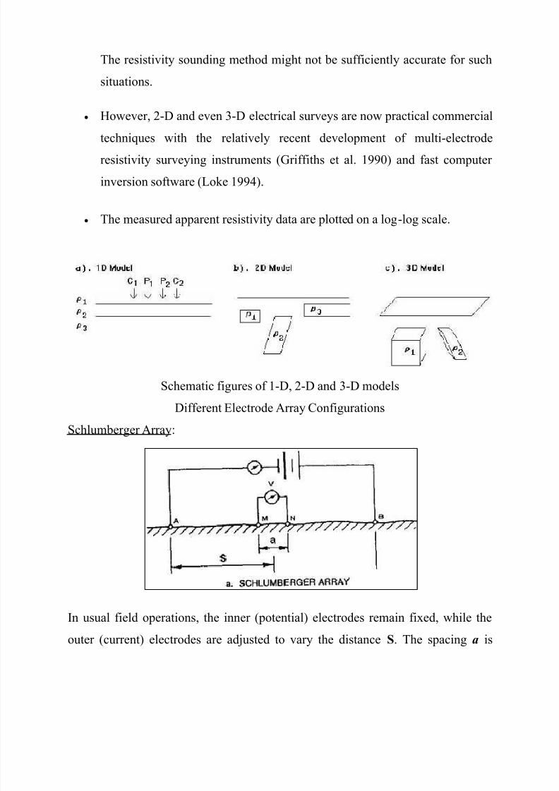
The measured apparent resistivity data are plotted on a log-log scale.

Schematic figures of 1-D, 2-D and 3-D models

Different Electrode Array Configurations

Schlumberger Array:

In usual field operations, the inner (potential) electrodes remain fixed, while the

outer (current) electrodes are adjusted to vary the distance S. The spacing a is



adjusted when it is needed because of decreasing sensitivity of measurement. The

spacing a usually be not taken larger than 0.4S. In practice, the sensitivity of the

instruments limits the ratio of S to a and usually keeps it within the limits of about

3 to 30. Also, the a spacing may sometimes be adjusted with S held constant in

order to detect the presence of local inhomogeneities or lateral changes in the

neighborhood of the potential electrodes.

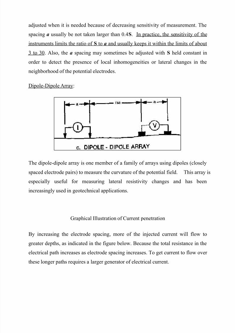
Dipole-Dipole Array:

The dipole-dipole array is one member of a family of arrays using dipoles (closely

spaced electrode pairs) to measure the curvature of the potential field. This array isespecially useful for measuring lateral resistivity changes and has been

increasingly used in geotechnical applications.

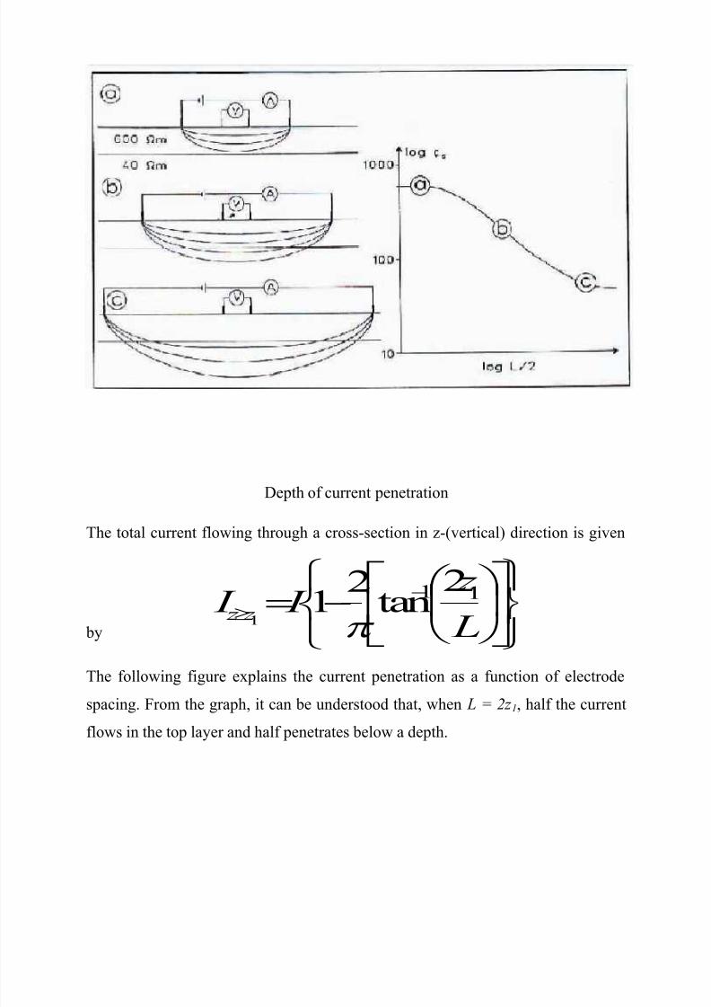
Graphical Illustration of Current penetration

By increasing the electrode spacing, more of the injected current will flow to

greater depths, as indicated in the figure below. Because the total resistance in the

electrical path increases as electrode spacing increases. To get current to flow over

these longer paths requires a larger generator of electrical current.



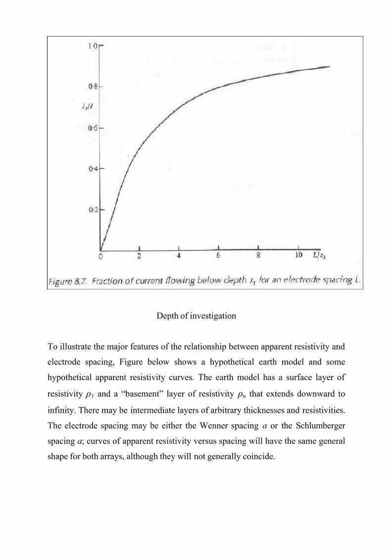
Depth of current penetration

The total current flowing through a cross-section in z-(vertical) direction is given

by

L

z I I

z z

112

tan2

11

The following figure explains the current penetration as a function of electrode

spacing. From the graph, it can be understood that, when L = 2z 1, half the current

flows in the top layer and half penetrates below a depth.



Depth of investigation

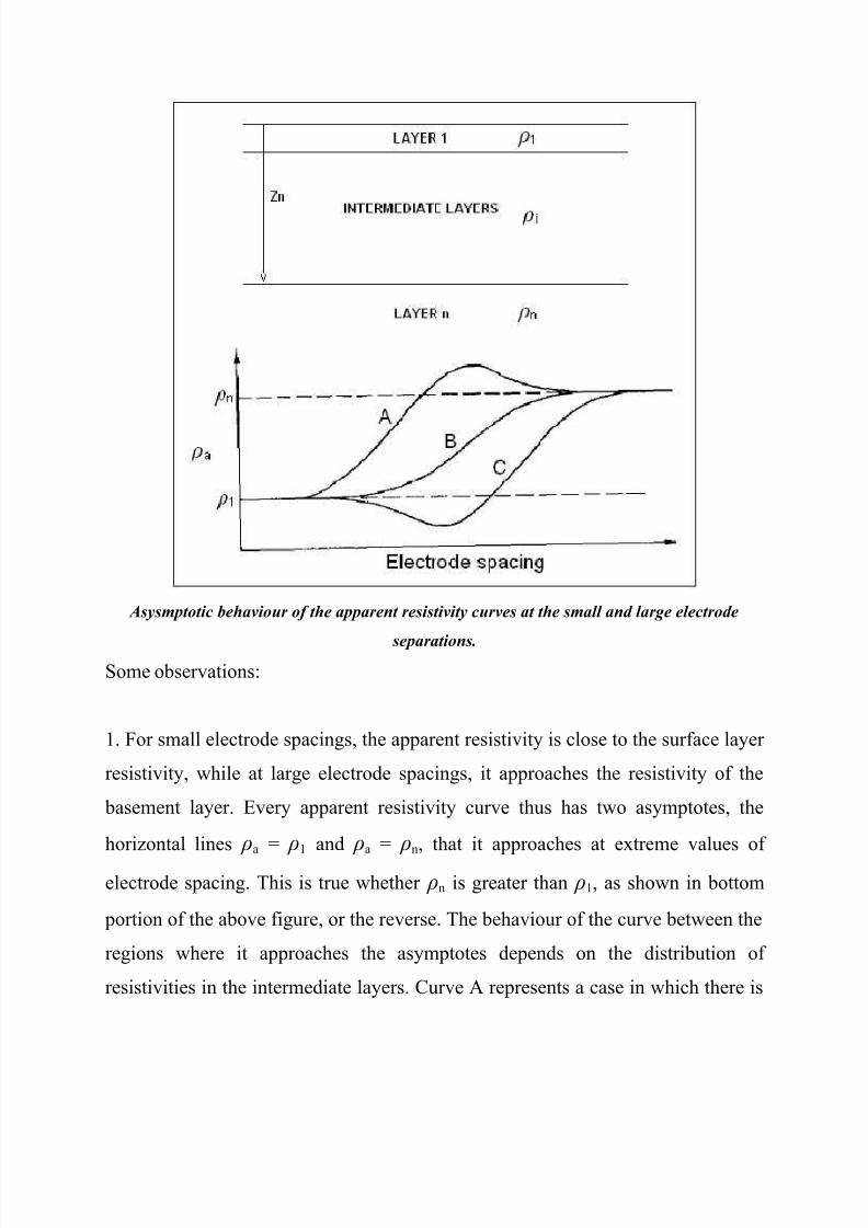
To illustrate the major features of the relationship between apparent resistivity and

electrode spacing, Figure below shows a hypothetical earth model and some

hypothetical apparent resistivity curves. The earth model has a surface layer of

resistivity ρ1 and a “basement” layer of resistivity ρn that extends downward to

infinity. There may be intermediate layers of arbitrary thicknesses and resistivities.

The electrode spacing may be either the Wenner spacing a or the Schlumberger

spacing a; curves of apparent resistivity versus spacing will have the same general

shape for both arrays, although they will not generally coincide.



Asysmptotic behaviour of the apparent resistivity curves at the small and large electrode

separations.

Some observations:

1. For small electrode spacings, the apparent resistivity is close to the surface layer

resistivity, while at large electrode spacings, it approaches the resistivity of the

basement layer. Every apparent resistivity curve thus has two asymptotes, the

horizontal lines ρa = ρ1 and ρa = ρn, that it approaches at extreme values of

electrode spacing. This is true whether ρn is greater than ρ1, as shown in bottom

portion of the above figure, or the reverse. The behaviour of the curve between the

regions where it approaches the asymptotes depends on the distribution of

resistivities in the intermediate layers. Curve A represents a case in which there is



an intermediate layer with a resistivity greater than ρn. The behavior of curve B

resembles that for the two-layer case or a case where resistivities increase from the

surface down to the basement. The curve might look like curve C if there were an

intermediate layer with resistivity lower than ρ1. Unfortunately for the interpreter,

neither the maximum of curve A nor the minimum of curve C reach the true

resistivity values for the intermediate layers, though they may be close if the layers

are very thick.

2. There is no simple relationship between the electrode spacing at which features

of the apparent resistivity curve are located and the depths to the interfaces

between layers. The depth of investigation will ALWAYS be less than the

electrode spacing. Typically, a maximum electrode spacing of three or more times

the depth of interest is necessary to assure that sufficient data have been obtained.

Relationship between Resistivity and Geology

To understand the obtained resistivity values and to relate them with the

prevailing geology, we must have an a priori knowledge of resistivities of

different types of materials and the geology of the surveyed region.

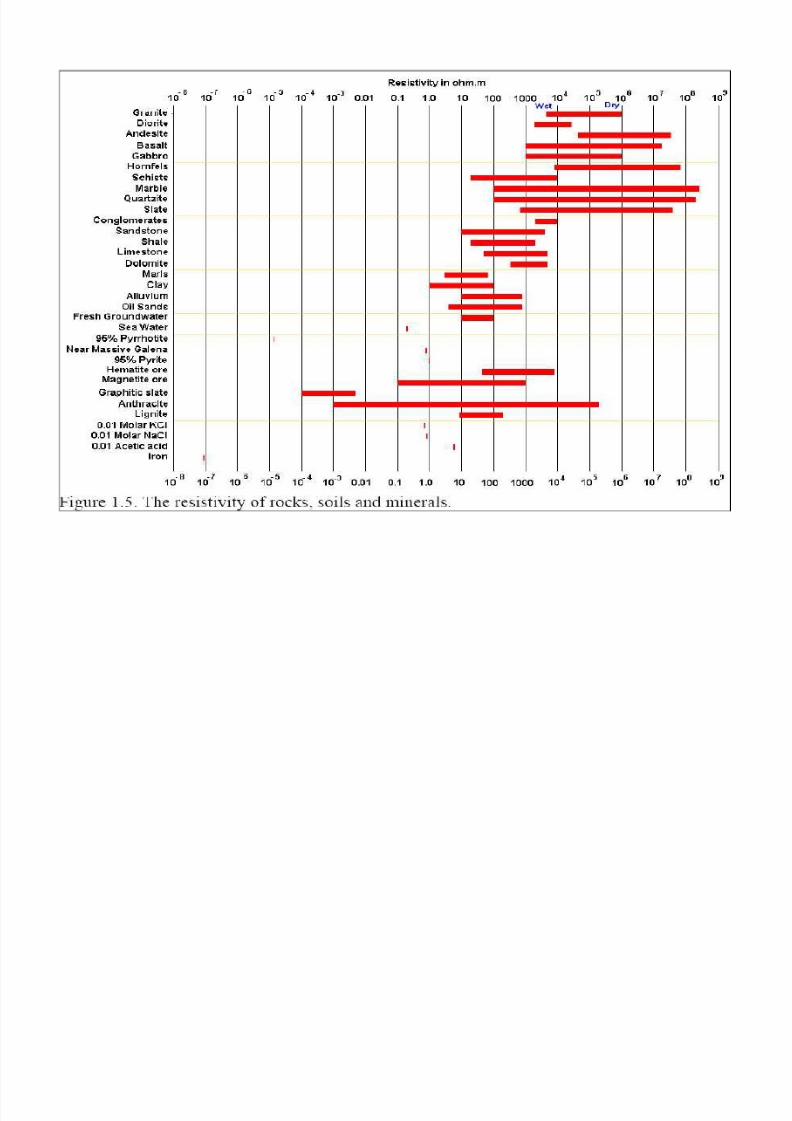
Igneous and Metamorphic Rocks:

These rocks typically have high resistivity values. The resistivity of

these rocks is greatly dependent on the degree of fracturing, and the

percentage of the fractures filled with ground water. Thus a given

rock type can have a large range of resistivity, from about 1000 to 10

million Ω-m, depending on whether it is wet or dry. This characteristic

is useful in the detection of fracture zones and other weathering

features, such as in engineering and groundwater surveys.



Sedimentary rocks:

Sedimentary rocks, which are usually more porous and have higher

water content, normally have lower resistivity values compared to

igneous and metamorphic rocks.

The resistivity values range from 10 to about 10000 Ω-m, with most

values below 1000 Ω-m. The resistivity values are largely dependent

on the porosity of the rocks, and the salinity of the contained water.

Unconsolidated sediments generally have even lower resistivity

values than sedimentary rocks.

Wet soils and fresh ground water have even lower resistivity values,

with the resistivity of latter varying from 10 to 100 Ω-m depending on

the concentration of dissolved salts.

Clayey soil normally has a lower resistivity value than sandy soil.

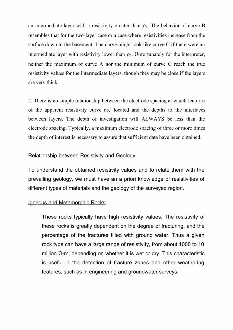
Material Resistivity (Ω-m)

Igneous and Metamorphic Rocks Granite

Basalt

Slate

Marble

Quartzite

SedimentaryRocks

Sandstone

Shale

Limestone

Soils and waters

Clay

Alluvium

Groundwater (fresh)

Sea water

Chemicals

Iron

5x10^3- 10^610^3- 10^66x10^2- 4x10^710^2- 2.5x10^810^2- 2x10^8

8 - 4x10^320 - 2x10^350 - 4x10^2

1 - 10010 - 80010 - 1000.2

9.074x10^-8



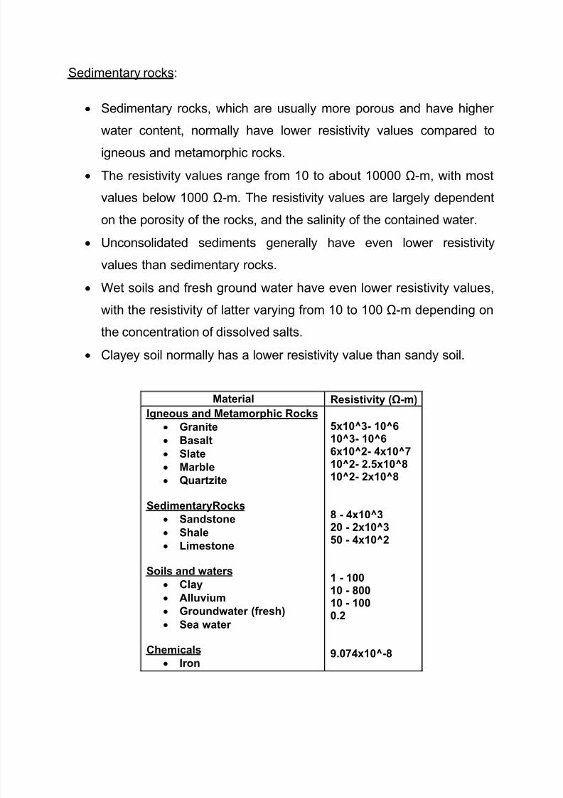
Potassium chloride

Sodium chloride

acetic acid

Xylene

0.7080.8436.136.998x10^16

Note the low resistivity (about 0.2 Ω-m) of sea water due to the relatively

high salt content. This makes the resistivity method an ideal technique

for mapping the saline and fresh water interface in coastal areas.

Note the overlap in the resistivity values of the different classes of rocks

and soils. This is because the resistivity of a particular rock or soil sample

depends on a number of factors such as the porosity, the degree of water

saturation and the concentration of dissolved salts.





Electrical Imaging surveys:

The greatest limitation of the resistivity sounding method is that it

does not take into account, the horizontal changes in the subsurface

resistivity.

A more accurate model of the subsurface is a two-dimensional (2-D)

model where the resistivity changes in the vertical direction, as well

as in the horizontal direction along the survey line. In this case, it is

assumed that resistivity does not change in the direction that is

perpendicular to the survey line. In many situations, particularly for

surveys over elongated geological bodies, this is a reasonable

assumption.

Presently, 2-D surveys are the most practical economic compromise

between obtaining very accurate results and keeping the survey costs

down.

While typical 1-D resistivity sounding surveys usually involve about

10 to 20 readings, 2-D imaging surveys involve about 100 to 1000

measurements. (3-D surveys even more). The cost of a typical 2-D

survey could be several times the cost of a 1-D sounding survey, and

is probably comparable with a seismic survey.

In many geological situations, 2-D electrical imaging surveys can give

useful results that are complementary to the information obtained by

other geophysical method. Thus, they should be used in conjunction

with seismic or GPR surveys as they provide complementary

information about the subsurface.



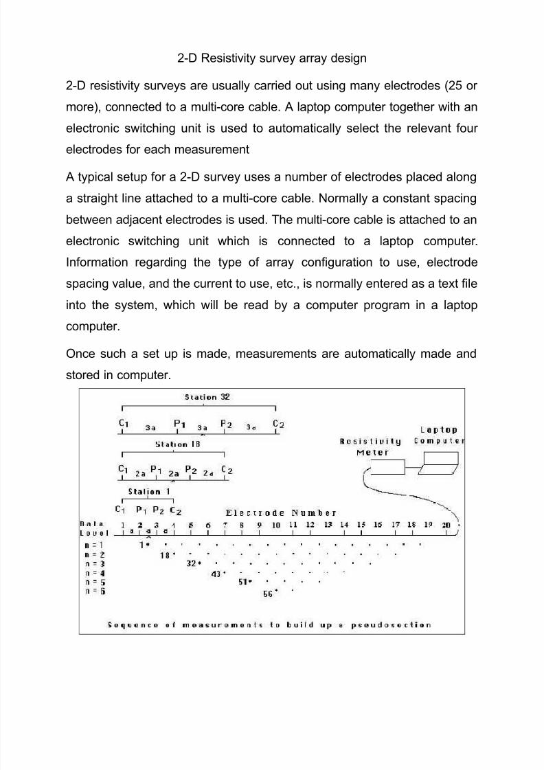
2-D Resistivity survey array design

2-D resistivity surveys are usually carried out using many electrodes (25 or

more), connected to a multi-core cable. A laptop computer together with an

electronic switching unit is used to automatically select the relevant four electrodes for each measurement

A typical setup for a 2-D survey uses a number of electrodes placed along

a straight line attached to a multi-core cable. Normally a constant spacing

between adjacent electrodes is used. The multi-core cable is attached to an

electronic switching unit which is connected to a laptop computer.

Information regarding the type of array configuration to use, electrode

spacing value, and the current to use, etc., is normally entered as a text file

into the system, which will be read by a computer program in a laptop

computer.

Once such a set up is made, measurements are automatically made and

stored in computer.



Survey methodology (Example of Wenner array):

The first step is to make all the possible measurements with the Wenner

array with an electrode spacing of “1a”.

For the first measurement, electrodes number 1, 2, 3 and 4 are used.

The electrode 1 is used as the first current electrode C1, electrode 2 as

the first potential electrode P1, electrode 3 as the second potential

electrode P2 and electrode 4 as the second current electrode C2.

For the second measurement, electrodes number 2, 3, 4 and 5 are used

for C1, P1, P2 and C2 respectively.

This is repeated down the line of electrodes until electrodes 17, 18, 19

and 20 are used for the last measurement with “1a” spacing. For a

system with 20 electrodes, note that there are 17 (20–3) possible

measurements with “1a” spacing for the Wenner array.

After completing the sequence of measurements with “1a” spacing, the

next sequence of measurements with “2a” electrode spacing is made.

First electrodes 1, 3, 5 and 7 are used for the first measurement. The

electrodes are so chosen that the spacing between adjacent electrodesis now “2a”.

For the second measurement, electrodes 2, 4, 6 and 8 are used. This

process is repeated down the line until electrodes 14, 16, 18 and 20 are

used for the last measurement with spacing “2a”. For a system with 20

electrodes, note that there are 14 (20 - 2x3) possible measurements

with “2a” spacing. This is repeated for measurements with “3a”, “4a”,

“5a”, etc. spacing.



Survey methodology (example of dipole-dipole array):

Methodology for dipole-dipole electrode configuration is different from that

of Wenner configuration. In this method

First, the measurement usually starts with a spacing of “1a” between

the C1-C2 (and also the P1-P2) electrodes.

The first sequence of measurements is made with a value of 1 for the

“n” factor (which is the ratio of the distance between the C1-P1 electrodes to

the C1-C2 dipole spacing ), followed by “n” equals to 2 while keeping the

C1-C2 dipole pair spacing fixed at “1a”.

When “n” = 2, the distance of the C1 electrode from the P1 electrode

is twice the C1-C2 dipole pair spacing. For subsequent

measurements, the “n” spacing factor is usually increased to a

maximum value of about 6, after which accurate measurements of

the potential are difficult due to very low potential values.

To increase the depth of investigation, the spacing between the C1-

C2 dipole pair is increased to “2a”, and another series of

measurements with different values of “n” is made. If necessary, this

can be repeated with larger values of the spacing of the C1-C2 (and

P1-P2) dipole pairs.

A similar survey technique can be used for the Wenner-Schlumberger

and pole-dipole arrays where different combinations of the “a”

spacing and “n” factor can be used.



Roll-along technique:

If you have a system with limited number of electrodes, then the 2-D

technique used to cover the area for survey is called “Roll-along”

technique.

In this technique, after completing the sequence of measurements, the

cable is moved past one end of the line by several unit electrode spacings.

All the measurements which involve the electrodes on part of the cable

which do not overlap the original end of the survey line are repeated.

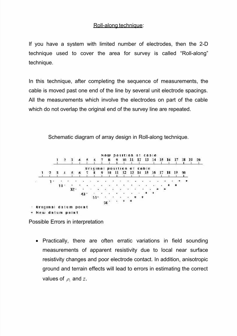
Schematic diagram of array design in Roll-along technique.

Possible Errors in interpretation

Practically, there are often erratic variations in field sounding

measurements of apparent resistivity due to local near surface

resistivity changes and poor electrode contact. In addition, anisotropic

ground and terrain effects will lead to errors in estimating the correct

values of 1 and z .



Suppression: This is particularly a problem when three or more

layers are present and their resistivities are ascending or descending

with depth. The middle intermediate layer may not be evident on the

field curve.

Principle of Equivalence: It is impossible to distinguish between two

highly resistive beds of different1 and z values if their product is

same or between two highly conductive beds if the z/ρ is

same.

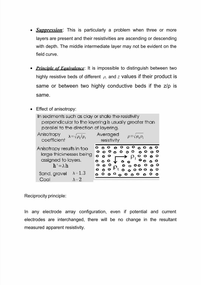
Effect of anisotropy:

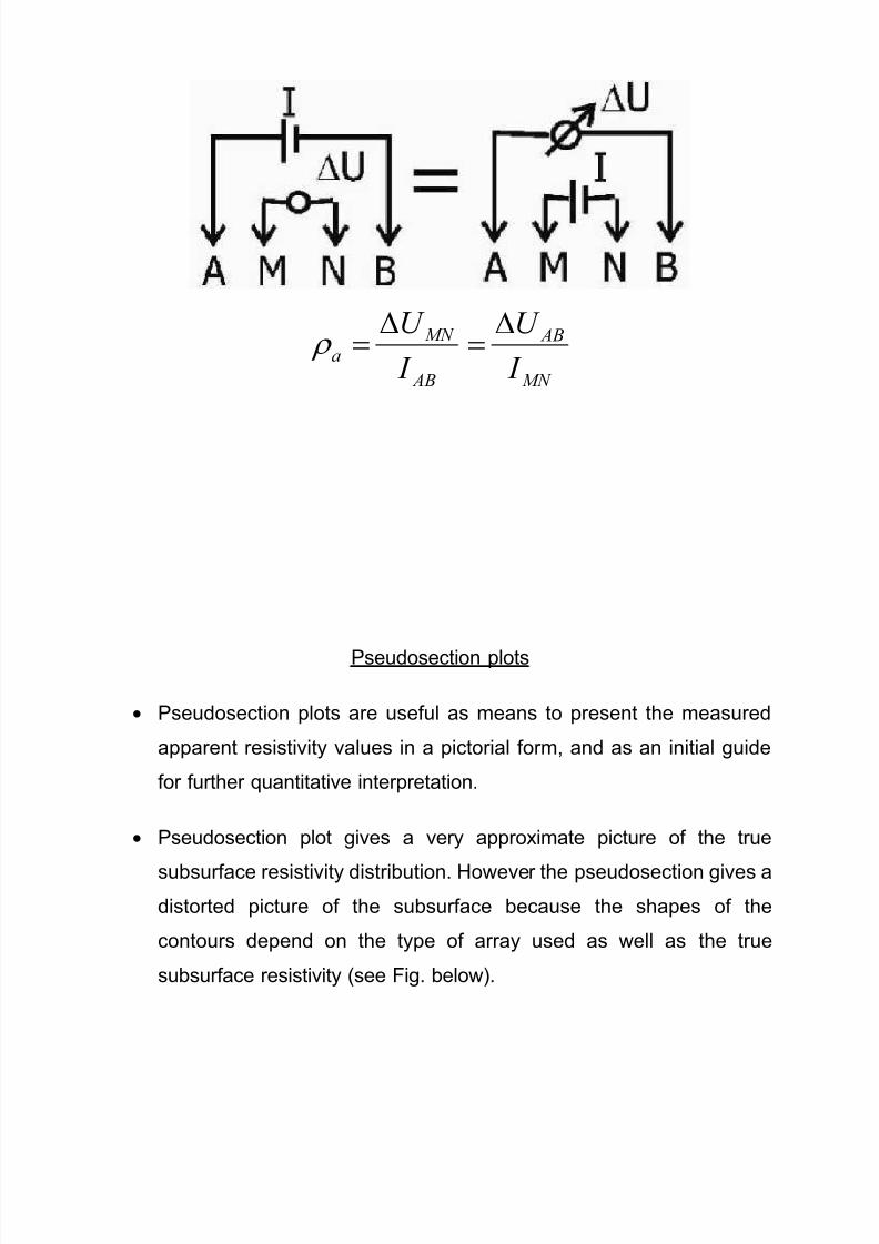
Reciprocity principle:

In any electrode array configuration, even if potential and current

electrodes are interchanged, there will be no change in the resultant

measured apparent resistivity.



MN

AB

AB

MN

a

I

U

I

U

Pseudosection plots

Pseudosection plots are useful as means to present the measured

apparent resistivity values in a pictorial form, and as an initial guide

for further quantitative interpretation.

Pseudosection plot gives a very approximate picture of the true

subsurface resistivity distribution. However the pseudosection gives a

distorted picture of the subsurface because the shapes of the

contours depend on the type of array used as well as the true

subsurface resistivity (see Fig. below).



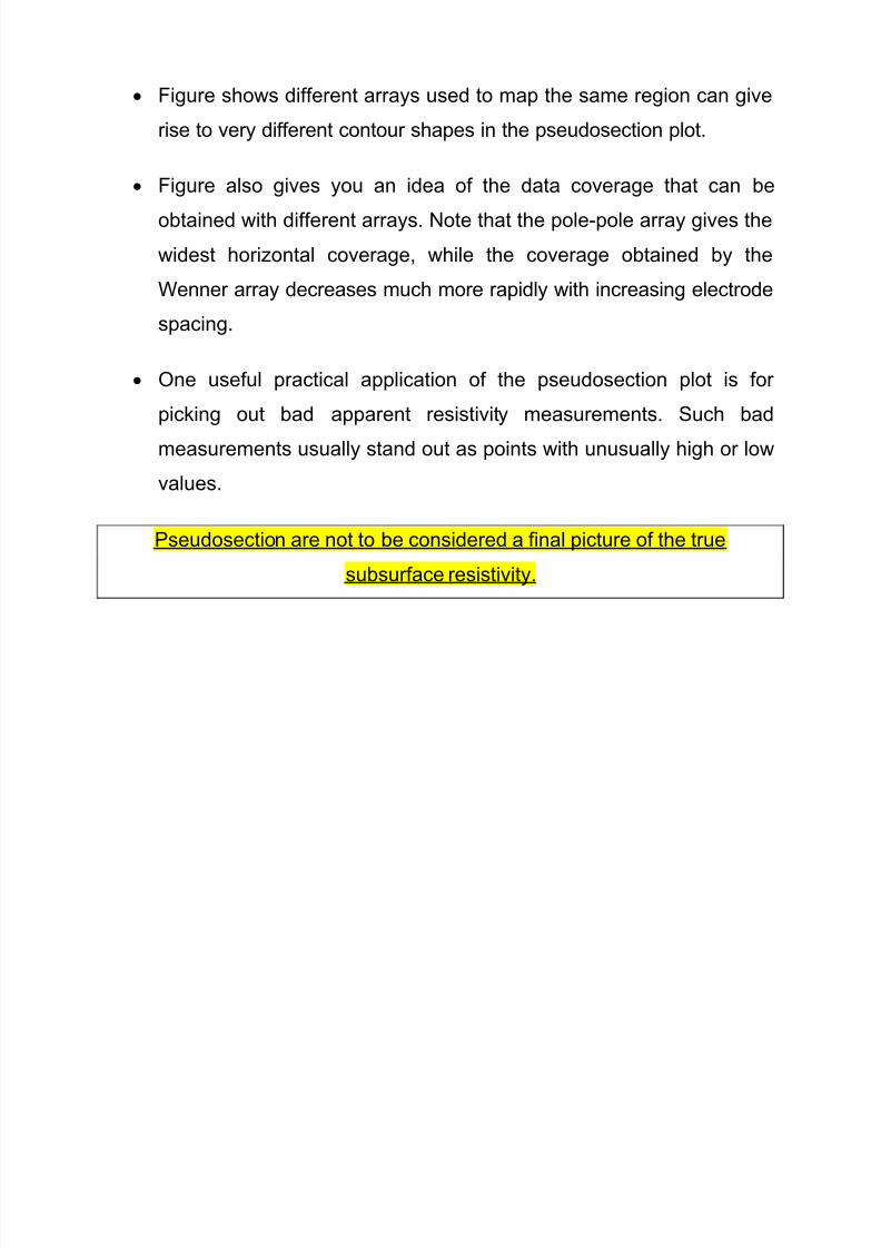
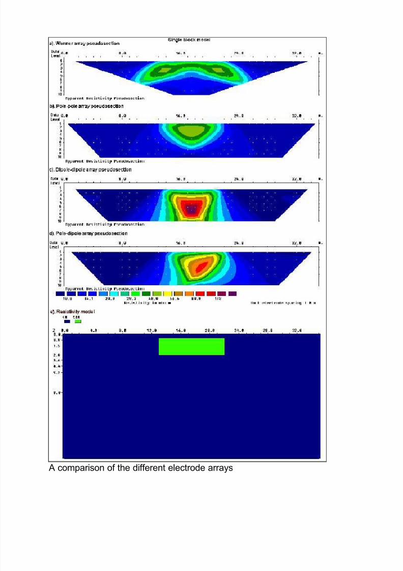
Figure shows different arrays used to map the same region can give

rise to very different contour shapes in the pseudosection plot.

Figure also gives you an idea of the data coverage that can be

obtained with different arrays. Note that the pole-pole array gives the

widest horizontal coverage, while the coverage obtained by the

Wenner array decreases much more rapidly with increasing electrode

spacing.

One useful practical application of the pseudosection plot is for

picking out bad apparent resistivity measurements. Such bad

measurements usually stand out as points with unusually high or low

values.

Pseudosection are not to be considered a final picture of the true

subsurface resistivity.



A comparison of the different electrode arrays



As shown earlier in the Fig., the shape of the contours in the pseudosection

produced by the different arrays over the same structure can be very

different. The choice of the “best” array for a field survey depends on the

type of structure to be mapped, the sensitivity of the resistivity meter and

the background noise level. In practice, the arrays that are most commonly

used for 2-D imaging surveys are the

(a) Wenner

(b) dipole-dipole

(c) Wenner-Schlumberger

(d) pole-pole and

(d) pole-dipole.

Among the characteristics of an array that should be considered are

(i) the depth of investigation(ii) the sensitivity of the array to vertical and horizontal changes

in the subsurface resistivity

(iii) the horizontal data coverage and

(iv) the signal strength.



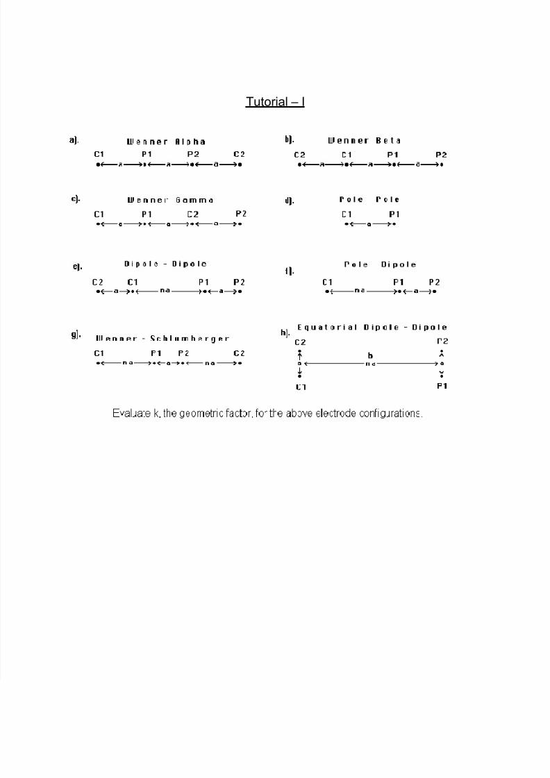
Tutorial – I

Documents

Electrical methods Lecture (20-01-10)