Contents lists available at ScienceDirect

Electrical Power and Energy Systems

journal homepage: www.elsevier.com/locate/ijepes

Detection of unidentified appliances in non-intrusive load monitoring usingsiamese neural networks

Leen De Baets⁎, Chris Develder, Tom Dhaene, Dirk DeschrijverIDLab, Department of Information Technology, Ghent University – imec, Technologiepark-Zwijnaarde 15, 9052 Ghent, Belgium

A R T I C L E I N F O

Keywords:Non-intrusive load monitoringAppliance classificationVoltage-current trajectorySiamese neural network

A B S T R A C T

Non-intrusive load monitoring methods aim to disaggregate the total power consumption of a household intoindividual appliances by analyzing changes in the voltage and current measured at the grid connection point ofthe household. The goal is to identify the active appliances, based on their unique fingerprint. Most state-of-the-art classification algorithms rely on the assumption that all events in the data stream are triggered by knownappliances, which is often not the case. This paper proposes a method capable of detecting previously uni-dentified appliances in an automated way. For this, appliances represented by their VI trajectory are mapped to anewly learned feature space created by a siamese neural network such that samples of the same appliance formtight clusters. Then, clustering is performed by DBSCAN allowing the method to assign appliance samples toclusters or label them as ‘unidentified’. Benchmarking on PLAID and WHITED shows that an F macro1, -measure ofrespectively 0.90 and 0.85 can be obtained for classifying the unidentified appliances as ‘unidentified’.

1. Introduction

In October 2014, EU leaders agreed upon three key targets for theyear 2030 [1]: (1) a reduction of at least 40% cuts in greenhouse gasemissions, (2) a save of at least 27% share for renewable energy, and (3)at least 27% improvement in energy efficiency. Energy monitoringproves a useful aid to reach these targets by providing an accurate,detailed view of energy consumption. It helps because: (1) if this in-formation is given to households, studies have shown that they couldsave up to 12% of electrical energy and thereby reduce the emissions[2] (also useful for non-residential buildings [3]), (2) this informationallows us to assess and exploit the flexibility of power consumption,which in turn is important for demand response systems that are re-sponsible for an increased penetration of distributed renewable energysources, (3) energy monitoring is one major prerequisite for energyefficiency measures [4].

In order to achieve the required energy monitoring cost-effectively,i.e., without relying on per-device monitoring equipment, non-intrusiveload monitoring (NILM) provides an elegant solution [5]. NILM iden-tifies the per-appliance energy consumption by first measuring the ag-gregated energy trace at a single, centralized point in the home using asensor and then disaggregating this power consumption for individualdevices, using machine learning techniques.

Several supervised and unsupervised methods have been developed

to recognise the appliances and to compute the total power consump-tion [6,7,5]. However, to our knowledge, most classification algorithmsdescribed in the literature can not handle unidentified appliances.These will be assigned a label and power consumption that correspondsto the appliance having the most similar features. This paper suggest amethod that is capable of detecting unidentified appliances, which arelabeled as ‘unidentified’. When such an appliance is detected, the usercan be queried for information about the appliance (i.e., the class label).In this paper, appliances are characterised by their binary VI trajectoryimage [8,9], although other representations can also be considered.

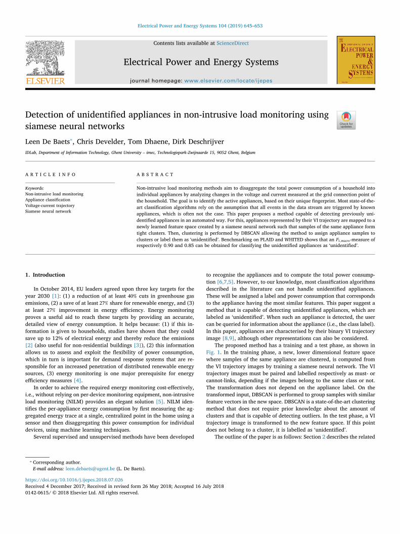
The proposed method has a training and a test phase, as shown inFig. 1. In the training phase, a new, lower dimensional feature spacewhere samples of the same appliance are clustered, is computed fromthe VI trajectory images by training a siamese neural network. The VItrajectory images must be paired and labelled respectively as must- orcannot-links, depending if the images belong to the same class or not.The transformation does not depend on the appliance label. On thetransformed input, DBSCAN is performed to group samples with similarfeature vectors in the new space. DBSCAN is a state-of-the-art clusteringmethod that does not require prior knowledge about the amount ofclusters and that is capable of detecting outliers. In the test phase, a VItrajectory image is transformed to the new feature space. If this pointdoes not belong to a cluster, it is labelled as ‘unidentified’.

The outline of the paper is as follows: Section 2 describes the related

https://doi.org/10.1016/j.ijepes.2018.07.026Received 4 December 2017; Received in revised form 26 May 2018; Accepted 16 July 2018

⁎ Corresponding author.E-mail address: leen.debaets@ugent.be (L. De Baets).

Electrical Power and Energy Systems 104 (2019) 645–653

0142-0615/ © 2018 Elsevier Ltd. All rights reserved.

T

work concerning NILM classification algorithms. Section 3 explains theconcept of siamese neural networks and how they can be used to learn anew feature space. Section 4 explains the DBSCAN clustering algorithm.Section 5 benchmarks the quality of the clustering, the capability ofdetecting unidentified appliances and the generalization property of themethod. Additionally, it also discusses how this method can be used in aquasi real-time solution. Finally, Section 6 concludes this paper.

2. Related work

A specific application of NILM is appliance detection. Hart [10] wasthe first to describe the several steps in this process: (1) measuring theaggregated power consumption with a sensor attached to the mainpower cable, (2) detecting state-transitions of appliances (events) fromthe captured data using a robust statistical test [11], (3) describingtransitions using a well-chosen feature vector, e.g., VI trajectories, (4)recognizing and monitoring each appliance using supervised and un-supervised methods. It must be noted that for some NILM algorithms,the event detection is a side effect of the approach, and not a separatemodule in the algorithm itself.

Feature definition. After detecting state-transitions of appliances,these must be described by a well-chosen feature vector. The type offeatures depends strongly on the sampling rate of the measurements.When using low frequency data (⩽1 Hz), the most common features arethe power levels and the ON/OFF durations [12]. A drawback of thisapproach is that only energy-intensive appliances can be detected.When using higher frequency data, it is possible to calculate featureslike the harmonics [13] and the frequency components [14] from thesteady-state and transient behaviour of the current and voltage signal,enabling the algorithm to also detect non energy-intensive appliances.More recently, the possibility to consider voltage-current (VI) trajec-tories has also been considered [8,9,15].

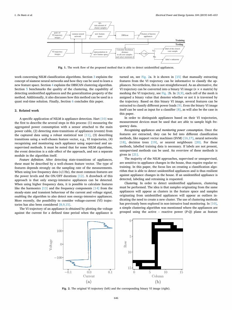
The VI trajectory of an appliance is obtained by plotting the voltageagainst the current for a defined time period when the appliance is

turned on, see Fig. 2a. It is shown in [15] that manually extractingfeatures from the VI trajectory can be informative to classify the ap-pliances. Nevertheless, this is not straightforward. As an alternative, theVI trajectory can be converted into a binary VI image ( ×n n matrix) bymeshing the VI trajectory, see Fig. 2b. In [8,9], each cell of the mesh isassigned a binary value that denotes whether or not it is traversed bythe trajectory. Based on this binary VI image, several features can beextracted to classify different power loads [9]. Even the binary VI imageitself can be used as input for a classifier [8], as will also be the case inthis paper.

In order to distinguish appliances based on their VI trajectories,measurement devices must be used that are able to sample high fre-quency data.

Recognizing appliances and monitoring power consumption. Once thefeatures are extracted, they can be fed into different classificationmethods, like support vector machines (SVM) [16,17], neural networks[18], decision trees [19], or nearest neighbours [20]. For thesemethods, labelled training data is necessary. If labels are not present,unsupervised methods can be used. An overview of these methods isgiven in [21].

The majority of the NILM approaches, supervised or unsupervised,are sensitive to appliance changes in the house, thus require regular re-training. In this paper, the focus lies on creating a classification algo-rithm that is able to detect unidentified appliances and is thus resilientagainst appliance changes in the house. If an unidentified appliance isdetected, labeling and retraining is requested.

Clustering. In order to detect unidentified appliances, clusteringmust be performed. The idea is that samples originating from the sameappliances will appear as clusters in the feature space and samplesoriginating from unidentified appliances will appear as outliers in-dicating the need to create a new cluster. The use of clustering methodshas previously been explored in non-intrusive load monitoring. In [10],a simple clustering algorithm was mentioned where the appliances aregrouped using the active – reactive power (P-Q) plane as feature

Fig. 1. The work flow of the proposed method that is able to detect unidentified appliances.

Fig. 2. The original VI trajectory (left) and the corresponding binary VI image (right).

L. De Baets et al. Electrical Power and Energy Systems 104 (2019) 645–653

646

representation space. Despite its simplicity, it is incapable of re-cognizing appliances with overlapping P and Q consumption. In [22],the P-Q plane is also used for genetic k-means and agglomerativeclustering. This method has problems in distinguishing appliances withsmall P and Q consumptions as their steady-state changes tend to clustertogether. In [23], mean-shift clustering is proposed on features that areextracted from the power signal. The resulting clusters are classifiedinto different appliance classes.

None of these clustering algorithms exploit their capability to detectunidentified appliances, and none are capable of clustering on appli-ance-level with high accuracy. The proposed method uses a novelclustering work flow to cope with these two shortcomings. Section 3explains how a higher accuracy can be obtained by learning a newfeature space using siamese neural networks. Section 4 explains howunidentified appliances can be detected.

3. Siamese neural network

The ability of clustering algorithms to detect small power con-suming appliances can be improved by adding more features. However,clustering is sensitive to the curse of dimensionality as it relies on thecomputation of a distance function like the Euclidean distance. In ahigh-dimensional case, the differences in distance become less ap-parent, making the clustering method unusable. For clustering to work,it is thus key to find a low dimensional feature space where the clustersare well separated. To this end, siamese neural networks can be used.These are a special kind of neural networks [24].

A siamese network consists of two identical NN, meaning that eachof them has the same architecture, parameter values and weights. Asinput, two binary VI images must be given and as label, a binary valueindicating whether or not the images belong to the same class. Theoutput of the siamese network are two vectors, forming a lower-di-mensional representation of the two input images. The idea is to learnthe representation in such a way, that the distance between these re-presentations will be smaller than a given threshold if the two belong tothe same class and larger if not. This leads to the use of the so-calledcontrastive loss function:

= × + − × −L y d y d y m d( , ) 12

( (1 ) max{ , 0}) (1)

where y is the binary output, d is the distance between the two inputfeature vectors, and m is the margin determining when samples aredissimilar: dissimilar input vectors only contribute to the loss function iftheir distance is smaller than the margin.

Siamese networks are ideally suited to find a relationship betweentwo comparable samples. This is the case in one-shot learning [25],where classification needs to be done with only one example of eachclass or signature verification [26], where the authenticity of a sig-nature is checked. In this paper, the siamese neural network is used fordimensionality reduction, like in [27]. This method of dimension re-duction is different from classical approaches, such as local linear em-bedding (LLE) and principal component analysis (PCA), as the siameseneural network learns a function that is capable of consistently mappingunseen samples to the learned feature space and as the siamese neuralnetwork is not constrained by a simple distance function like the Eu-clidean distance.

After the training phase, the siamese neural network can be used tocalculate a nout-dimensional representation of new VI binary images.These are obtained by using the output of just one cNN.

4. DBSCAN

After learning the feature space, unidentified appliances can bedetected by performing clustering. Namely, if a new sample is toodistant from present clusters (representing known appliances), then it isconsidered as unidentified.

Density-based spatial clustering of applications with noise(DBSCAN) is a density-based clustering algorithm: points forming acluster will be close together, whereas the outliers will only have re-latively far away neighbours [28]. The algorithm starts by picking onerandom sample out of the dataset. If there are not enough close byneighbours, then the point will be labeled as an outlier and the processcontinues by selecting a new sample. If there are sufficient close byneighbours, they are all added to the same cluster. The algorithmcontinues by iterating over all new added points, if these have sufficientclose by neighbours, these are also added to the same cluster. Thiscontinues until no more samples are added to this cluster. Then a newunvisited random sample is selected and the process is iterated until allpoints belong to a cluster or are labeled as outliers (noise). Three ele-ments needs to be defined for DBSCAN: (1) the amount of sufficientclose by points, mintPts, (2) the distance function, and (3) the maximaldistance to a close by sample, ∊. These last two points define if a sampleis close by or not.

The advantages of DBSCAN are that the number of clusters does notneed to be specified by the user (unlike, e.g., for K-means clustering),clusters can be of any shape (not just the circular ones), and outliers arenot forced to belong to a cluster but are identified as such. The algo-rithm is also robust against an imbalance in the occurrence of samplesfrom different clusters. DBSCAN is one of the most common clusteringalgorithms and was awarded the test of time award at the leading datamining conference, KDD [29].

In this paper, the transformed input samples are clustered withDBSCAN. The used distance metric is the Euclidean distance. Theparameters mintPts and ∊ are not trained but heuristically set to re-spectively 5 and 0.2.

To determine which cluster a test sample belongs to (if any), itsfeature vector is first transformed to the calculated lower-dimensionalspace. Next, the Euclidean distance is calculated to all core samples andthe minimal distance is selected. If this distance is smaller thanthreshold ∊, then the sample belongs to the same cluster as the closestcore sample. Otherwise, it will be assigned the label ‘unidentified’.

5. Results

This section first describes the used datasets in Subsection 5.1 andspecifies the input and architecture of the siamese neural network inSubsection 5.2. To benchmark the described method on the data, sev-eral checks must be performed. First, it must be examined if the learnedfeature space separates the different classes well, see Subsection 5.3.Second, the capability of detecting unidentified appliances is tested byusing data of an unidentified appliance as test data, see Subsection 5.4.Lastly, the generalization property of the method is checked by usingthe data from other (unseen) houses as test data, see Subsection 5.5. Toconclude this section, a discussion concerning the time usage of thisalgorithm is given in Subsection 5.6.

5.1. Benchmark dataset

The performance of the proposed algorithm is validated on the Plug-Load Appliance Identification Dataset (PLAID) [30] and the WorldwideHousehold and Industry Transient Energy Dataset (WHITED) [31].

• PLAID is a public dataset including sub-metered current and voltagemeasurements sampled at 30 kHz for 11 different appliance types.For each appliance type, at least 38 individual appliances areavailable, captured in 55 households. For each appliance, at least 5start-up events are measured, resulting in a total of 1074 measure-ments.

• WHITED is a public dataset including sub-metered current andvoltage measurements sampled at 44 kHz for 46 different appliancetypes. For each appliance type, 1 to 9 different appliances areavailable. For each appliance, 10 start-up events are measured,

L. De Baets et al. Electrical Power and Energy Systems 104 (2019) 645–653

647

resulting in a total of 1100 measurements. For training and testingpurposes, it is required that at least two different appliances aremeasured per type. For 24 appliance types, only one appliance wasavailable and these are thus omitted. The final number of used ap-pliances in WHITED is 22, resulting in 860 measurements.

5.2. Input and architecture of siamese neural network

In this paper, the input of the siamese networks consists of pairs ofbinary VI trajectory images with size ×n n. In order to obtain thebinary VI images for PLAID and WHITED, the voltage and current aremeasured over a time interval of 20 cycles when the appliances reachsteady-state, resulting in respectively 10000 and 17600 samples. Thevoltage is plotted against the current and the methodology described inthe related work is used to create binary VI images. Fig. 5 gives ex-amples of binary VI images for the appliance types present in PLAID.

The architecture of the siamese network is shown in Fig. 3. For thesiamese neural network, the proposed method uses two convolutionalneural network (cNN). cNNs are a type of neural networks (NNs) thatare often used in computer vision because they are highly suitable toclassify images [32]. The used cNN is depicted in Fig. 4 and takes asinput an ×n n binary image. This is transformed by a convolutionallayer which uses 20 filters, each considering regions of ×5 5 pixels.After the convolutional layer, there is a maximal pooling layer with asliding window of ×2 2. This combination of a convolutional layerfollowed by a pooling layer is repeated, and finally, a dense layer isadded with nout nodes. In total, five layers are present. The trainableweights and biases of the network are initialized by sampling from aGaussian distribution with zero mean and a standard deviation of 0.05.The margin m used in the loss function is set to 50. The results are fairlyinsensitive to the choice of m.

5.3. Scenario 1

To determine if the learned feature space from the siamese neuralnetwork separates the classes well, the rand index (RI) of the clustersfound by the DBSCAN algorithm is calculated. The RI is a measure ofsimilarity between two data clusterings X and Y:

=+

+ + +RI a b

a b c d (2)

where a and b are respectively the number of pairs of elements that arein the same/different cluster(s) in both clusterings X and Y, and c and dare respectively the number of pairs that are in the same cluster for X/Y,but in a different one for Y/X. Higher values of RI (max. value 1) in-dicate a better match of clusterings.

Fig. 6a and b show the RI for respectively PLAID and WHITED fordifferent parameter configurations of the siamese neural network thatlearns the representation from binary images of the VI trajectories. Theinput size of the VI image ×n n( ) and the dimension nout of the learnedrepresentation are altered. For this, all data samples of the PLAID da-taset are fed into the siamese neural network to calculate the mappingfunction. Increasing nout (for fixed values of n) has little impact on theRI values. In contrast, changes in the value of n (for fixed values of nout)have a strong impact. The best RI values for both datasets are obtainedfor ⩾n 30 with a maximum of 0.996 for PLAID and 0.879 for WHITED.The RI value for WHITED is lower than the one for PLAID. A possibleexplanation is that the number of appliances is much larger forWHITED, introducing more chance for confusion. The high RI valuesconfirm the capability of the siamese neural network to learn a featurespace where the clusters are well separated and confirm the ability ofthe DBSCAN algorithm to find these clusters. Fig. 7 shows an exampleof the learned three dimensional feature space ( =n 3out for the ease ofvisualization) for PLAID and the corresponding clustering. Each axis of

Fig. 3. The architecture of the siamese network.

Fig. 4. The architecture of the cNN that is used in the siamese network.

L. De Baets et al. Electrical Power and Energy Systems 104 (2019) 645–653

648

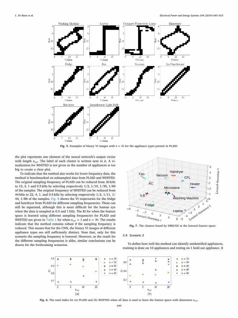
the plot represents one element of the neural network’s output vectorwith length nout. The label of each cluster is written next to it. A vi-sualization for WHITED is not given as the number of appliances is toobig to create a clear plot.

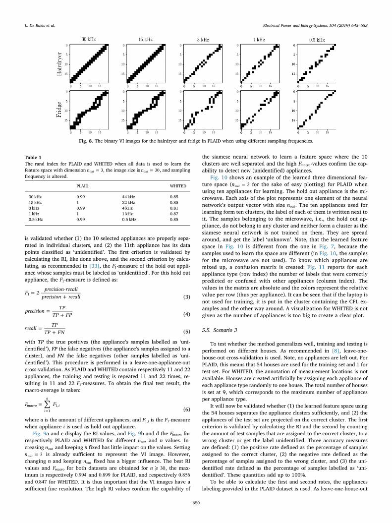
To indicate that the method also works for lower frequency data, themethod is benchmarked on subsampled data from PLAID and WHITED.The original sampling frequency of PLAID can be reduced from 30 kHzto 15, 3, 1 and 0.5 kHz by selecting respectively 1/2, 1/10, 1/30, 1/60of the samples. The original frequency of WHITED can be reduced from44 kHz to 22, 4, 1, and 0.5 kHz by selecting respectively 1/2, 1/11, 1/44, 1/88 of the samples. Fig. 8 shows the VI trajectories for the fridgeand hairdryer from PLAID for different sampling frequencies. These canstill be separated, although this is more difficult for the human eyewhen the data is sampled at 0.5 and 1 kHz. The RI for when the featurespace is learned using different sampling frequencies for PLAID andWHITED are given in Table 1 for when =n 3out and =n 30. The resultsindicate that the method remains robust if the sampling frequency isreduced. This means that for the CNN, the binary VI images of differentappliance types are still sufficiently distinct. Note that, only for thisscenario the sampling frequency is lowered. However, as the result forthe different sampling frequencies is alike, similar conclusions can bedrawn for the forthcoming scenarios.

5.4. Scenario 2

To define how well the method can identify unidentified appliances,training is done on 10 appliances and testing on 1 hold out appliance. It

Fig. 5. Examples of binary VI images with =n 20 for the appliance types present in PLAID.

Fig. 6. The rand index for (a) PLAID and (b) WHITED when all data is used to learn the feature space with dimension nout .

Fig. 7. The clusters found by DBSCAN in the learned feature space.

L. De Baets et al. Electrical Power and Energy Systems 104 (2019) 645–653

649

is validated whether (1) the 10 selected appliances are properly sepa-rated in individual clusters, and (2) the 11th appliance has its datapoints classified as ‘unidentified’. The first criterion is validated bycalculating the RI, like done above, and the second criterion by calcu-lating, as recommended in [33], the F1-measure of the hold out appli-ance whose samples must be labeled as ‘unidentified’. For this hold outappliance, the F1-measure is defined as:

=+

Fprecision recall

precision recall2·

·1

(3)

=+

precision TPTP FP (4)

=+

recall TPTP FN (5)

with TP the true positives (the appliance’s samples labelled as ‘uni-dentified’), FP the false negatives (the appliance’s samples assigned to acluster), and FN the false negatives (other samples labelled as ‘uni-dentified’). This procedure is performed in a leave-one-appliance-outcross-validation. As PLAID and WHITED contain respectively 11 and 22appliances, the training and testing is repeated 11 and 22 times, re-sulting in 11 and 22 F1-measures. To obtain the final test result, themacro-average is taken:

∑==

F Fmacroi

a

i1

1,(6)

where a is the amount of different appliances, and F i1, is the F1-measurewhen appliance i is used as hold out appliance.

Fig. 9a and c display the RI values, and Fig. 9b and d the Fmacro forrespectively PLAID and WHITED for different nout and n values. In-creasing nout and keeping n fixed has little impact on the values. Setting

=n 3out is already sufficient to represent the VI image. However,changing n and keeping nout fixed has a bigger influence. The best RIvalues and Fmacro for both datasets are obtained for ⩾n 30, the max-imum is respectively 0.994 and 0.899 for PLAID, and respectively 0.856and 0.847 for WHITED. It is thus important that the VI images have asufficient fine resolution. The high RI values confirm the capability of

the siamese neural network to learn a feature space where the 10clusters are well separated and the high Fmacro-values confirm the cap-ability to detect new (unidentified) appliances.

Fig. 10 shows an example of the learned three dimensional fea-ture space ( =n 3out for the sake of easy plotting) for PLAID whenusing ten appliances for learning. The hold out appliance is the mi-crowave. Each axis of the plot represents one element of the neuralnetwork’s output vector with size nout. The ten appliances used forlearning form ten clusters, the label of each of them is written next toit. The samples belonging to the microwave, i.e., the hold out ap-pliance, do not belong to any cluster and neither form a cluster as thesiamese neural network is not trained on them. They are spreadaround, and get the label ‘unknown’. Note, that the learned featurespace in Fig. 10 is different from the one in Fig. 7, because thesamples used to learn the space are different (in Fig. 10, the samplesfor the microwave are not used). To know which appliances aremixed up, a confusion matrix is created: Fig. 11 reports for eachappliance type (row index) the number of labels that were correctlypredicted or confused with other appliances (column index). Thevalues in the matrix are absolute and the colors represent the relativevalue per row (thus per appliance). It can be seen that if the laptop isnot used for training, it is put in the cluster containing the CFL ex-amples and the other way around. A visualization for WHITED is notgiven as the number of appliances is too big to create a clear plot.

5.5. Scenario 3

To test whether the method generalizes well, training and testing isperformed on different houses. As recommended in [8], leave-one-house-out cross-validation is used. Note, no appliances are left out. ForPLAID, this means that 54 houses are used for the training set and 1 fortest set. For WHITED, the annotation of measurement locations is notavailable. Houses are created artificially by assigning each appliance ofeach appliance type randomly to one house. The total number of housesis set at 9, which corresponds to the maximum number of appliancesper appliance type.

It will now be validated whether (1) the learned feature space usingthe 54 houses separates the appliance clusters sufficiently, and (2) theappliances of the test set are projected on the correct cluster. The firstcriterion is validated by calculating the RI and the second by countingthe amount of test samples that are assigned to the correct cluster, to awrong cluster or get the label unidentified. Three accuracy measuresare defined: (1) the positive rate defined as the percentage of samplesassigned to the correct cluster, (2) the negative rate defined as thepercentage of samples assigned to the wrong cluster, and (3) the uni-dentified rate defined as the percentage of samples labelled as ‘uni-dentified’. These quantities add up to 100%.

To be able to calculate the first and second rates, the applianceslabeling provided in the PLAID dataset is used. As leave-one-house-out

Fig. 8. The binary VI images for the hairdryer and fridge in PLAID when using different sampling frequencies.

Table 1The rand index for PLAID and WHITED when all data is used to learn thefeature space with dimension =n 3out , the image size is =n 30out , and samplingfrequency is altered.

PLAID WHITED

30 kHz 0.99 44 kHz 0.8515 kHz 1 22 kHz 0.853 kHz 0.99 4 kHz 0.811 kHz 1 1 kHz 0.870.5 kHz 0.99 0.5 kHz 0.85

L. De Baets et al. Electrical Power and Energy Systems 104 (2019) 645–653

650

cross-validation is performed on 55 houses, there are 55 test scores (onefor each house). To obtain the final test result, these values are aver-aged.

Figs. 12a and 13a show the RI values for different nout and n valuesfor respectively PLAID and WHITED. Again, for both datasets, it can beconcluded that the clusters are separated sufficiently for higher n va-lues. Changing nout has little impact on the result.

Fig. 12b, c and d show the three accuracies defining how much testsamples are respectively assigned to the correct, incorrect or no clusterfor PLAID. Again, changing nout does not change the results sig-nificantly. When using =n 16, a large part of the test samples >( 50%)are assigned to the correct cluster, but also a significant part of them∽( 22.5%) are classified incorrectly. When using a larger =n 50, theamount of correctly assigned test samples is much smaller, namelyaround 38.7%, but so are the incorrectly assigned samples ∼( 1.3%). As aconsequence, the amount of samples labeled as unidentified is larger(around 60%).

Fig. 13b, c and d show the three accuracies defining how much testsamples are respectively assigned to the correct, incorrect or no clusterfor WHITED. Again, changing nout does not change the results sig-nificantly. For WHITED, the highest obtained positive rate is 73% forwhen =n 50. The corresponding negative rate and unidentified rate are6%, and 20%. So the parameter setting leading the best positive rate, alsoleads to the best negative rate and a good unidentified rate. This incontrast to PLAID.

Although the RI values for WHITED are lower than those for PLAID,the third scenario obtains the best result for WHITED. An observationthat can explain this, is that the different appliances for each appliancetype are more alike in WHITED than in PLAID. Thus, an appliance of aknown appliance type is more likely to fall in the center of the cluster.While for PLAID, these appliances of a known appliance type will driftaround the cluster. This can be checked by calculating the rank of thecorrect cluster for each test sample labeled as unidentified. First, allclusters are ranked by calculating the distance dij from the given samplei to each of the clusters j, and sorting these distances in ascending order.Ideally, the test sample’s appliance cluster should be on the first posi-tion. Fig. 14a shows the rank that is averaged over the 55 folds. For allthe different parameter combinations, this result shows that the correctcluster is the closest or second closest cluster. Fig. 14b shows the boxplot of the rank of the correct cluster for all the test samples labeled as‘unidentified’ in all the test houses (1074 ranks) when =n 50. As thesebox plots show, their is very little variance on the rank of the correctcluster, making the average a valid measure. This result is importantbecause it implies that if the method labels a sample as unidentified, it

Fig. 9. The RI values and Fmacro for different nout and n values when leave-one-appliance-out cross-validation is used for PLAID (a)–(b), and WHITED (c)–(d).

Fig. 10. The 10 clusters and unidentified points found by DBSCAN in thelearned feature space representing respectively the 10 seen appliances and the 1hold out appliance.

Fig. 11. The confusion matrix when leave-one-appliance-out cross-validation isused.

L. De Baets et al. Electrical Power and Energy Systems 104 (2019) 645–653

651

can query the user to confirm if it is a new appliances or not, whileimmediately suggesting a label (e.g., listing the top-3 of the ranked list).If the sample originates from an existing appliance, the correct appli-ance (cluster) will be in this top.

5.6. Quasi real-time solution

The presented results were obtained in an offline manner. However,in practice, this method needs to be used in an online manner (quasireal-time). For an operational deployment, we start from a trainedsiamese neural network. This implies a learned feature space, and

Fig. 12. The RI values, and the positive, negative and unidentified rate for PLAID for different nout and n values when leave-one-house-out cross-validation is used.

Fig. 13. The RI values, and the positive, negative and unidentified rate for WHITED for different nout and n values when leave-one-house-out cross-validation is used.

Fig. 14. (a) The average rank of the correct cluster for the samples of PLAID labeled as ‘unidentified’ for different nout and n values when using leave-one-house-outcross-validation. (b) The box plots of the rank of the correct cluster for all samples of PLAID labeled as ‘unidentified’ for =n 50 and different nout values.

L. De Baets et al. Electrical Power and Energy Systems 104 (2019) 645–653

652

available appliance clusters (for the already known appliances). Toapply this, a system needs to perform the following steps:

1. real-time event detection [34] to identify the activation or deacti-vation of an appliance,

2. extraction of the appliance specific current and voltage signal whenit reached steady-state behaviour, as discussed in [35],

3. creation of the binary VI image, as described in [8],4. transformation of the image to the learned feature space by feeding

the image as input to the convolutional neural network part of thesiamese neural network,

5. in this feature space, calculation of the distance of the detecteddevice to all known appliances.(a) If the distance to all of the clusters is bigger than a threshold,

then mark the device as ‘unidentified’, else(b) label the device as the type of the closest cluster.

6. saving the VI image for (re) training the siamese neural networklater,

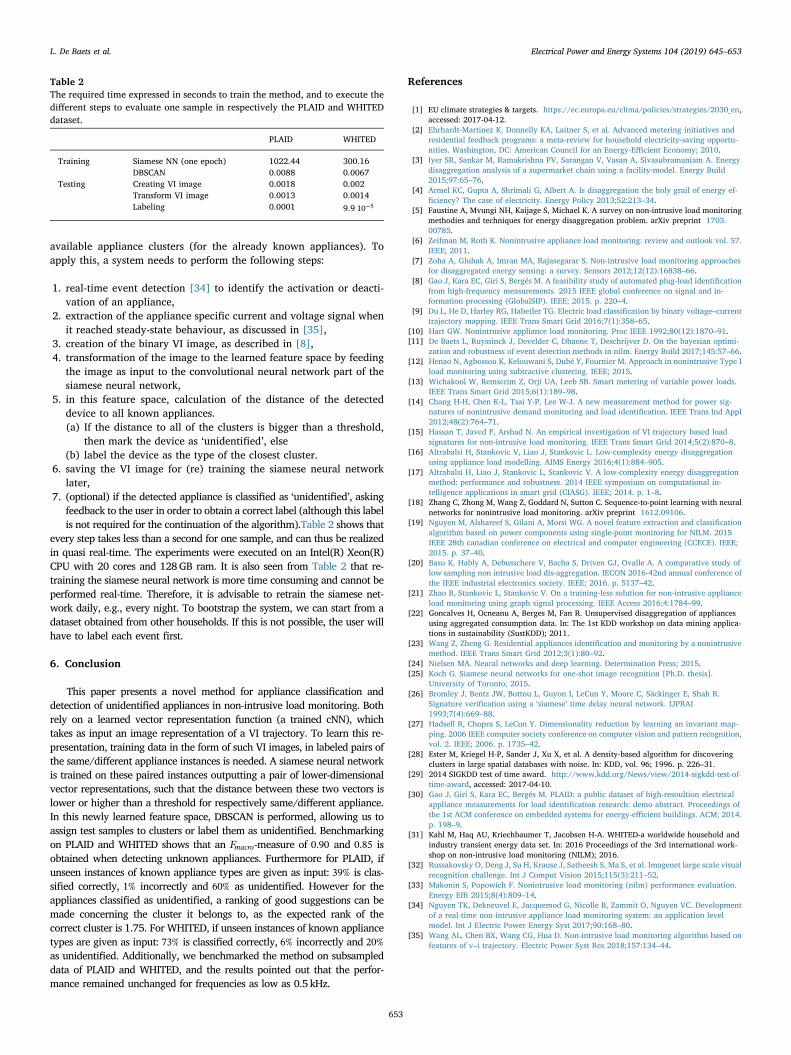
7. (optional) if the detected appliance is classified as ‘unidentified’, askingfeedback to the user in order to obtain a correct label (although this labelis not required for the continuation of the algorithm).Table 2 shows that

every step takes less than a second for one sample, and can thus be realizedin quasi real-time. The experiments were executed on an Intel(R) Xeon(R)CPU with 20 cores and 128GB ram. It is also seen from Table 2 that re-training the siamese neural network is more time consuming and cannot beperformed real-time. Therefore, it is advisable to retrain the siamese net-work daily, e.g., every night. To bootstrap the system, we can start from adataset obtained from other households. If this is not possible, the user willhave to label each event first.

6. Conclusion

This paper presents a novel method for appliance classification anddetection of unidentified appliances in non-intrusive load monitoring. Bothrely on a learned vector representation function (a trained cNN), whichtakes as input an image representation of a VI trajectory. To learn this re-presentation, training data in the form of such VI images, in labeled pairs ofthe same/different appliance instances is needed. A siamese neural networkis trained on these paired instances outputting a pair of lower-dimensionalvector representations, such that the distance between these two vectors islower or higher than a threshold for respectively same/different appliance.In this newly learned feature space, DBSCAN is performed, allowing us toassign test samples to clusters or label them as unidentified. Benchmarkingon PLAID and WHITED shows that an Fmacro-measure of 0.90 and 0.85 isobtained when detecting unknown appliances. Furthermore for PLAID, ifunseen instances of known appliance types are given as input: 39% is clas-sified correctly, 1% incorrectly and 60% as unidentified. However for theappliances classified as unidentified, a ranking of good suggestions can bemade concerning the cluster it belongs to, as the expected rank of thecorrect cluster is 1.75. For WHITED, if unseen instances of known appliancetypes are given as input: 73% is classified correctly, 6% incorrectly and 20%as unidentified. Additionally, we benchmarked the method on subsampleddata of PLAID and WHITED, and the results pointed out that the perfor-mance remained unchanged for frequencies as low as 0.5 kHz.

References

[1] EU climate strategies & targets. https://ec.europa.eu/clima/policies/strategies/2030_en,accessed: 2017-04-12.

[2] Ehrhardt-Martinez K, Donnelly KA, Laitner S, et al. Advanced metering initiatives andresidential feedback programs: a meta-review for household electricity-saving opportu-nities. Washington, DC: American Council for an Energy-Efficient Economy; 2010.

[3] Iyer SR, Sankar M, Ramakrishna PV, Sarangan V, Vasan A, Sivasubramaniam A. Energydisaggregation analysis of a supermarket chain using a facility-model. Energy Build2015;97:65–76.

[4] Armel KC, Gupta A, Shrimali G, Albert A. Is disaggregation the holy grail of energy ef-ficiency? The case of electricity. Energy Policy 2013;52:213–34.

[5] Faustine A, Mvungi NH, Kaijage S, Michael K. A survey on non-intrusive load monitoringmethodies and techniques for energy disaggregation problem. arXiv preprint 1703.00785.

[6] Zeifman M, Roth K. Nonintrusive appliance load monitoring: review and outlook vol. 57.IEEE; 2011.

[7] Zoha A, Gluhak A, Imran MA, Rajasegarar S. Non-intrusive load monitoring approachesfor disaggregated energy sensing: a survey. Sensors 2012;12(12):16838–66.

[8] Gao J, Kara EC, Giri S, Bergés M. A feasibility study of automated plug-load identificationfrom high-frequency measurements. 2015 IEEE global conference on signal and in-formation processing (GlobalSIP). IEEE; 2015. p. 220–4.

[9] Du L, He D, Harley RG, Habetler TG. Electric load classification by binary voltage–currenttrajectory mapping. IEEE Trans Smart Grid 2016;7(1):358–65.

[10] Hart GW. Nonintrusive appliance load monitoring. Proc IEEE 1992;80(12):1870–91.[11] De Baets L, Ruyssinck J, Develder C, Dhaene T, Deschrijver D. On the bayesian optimi-

zation and robustness of event detection methods in nilm. Energy Build 2017;145:57–66.[12] Henao N, Agbossou K, Kelouwani S, Dubé Y, Fournier M. Approach in nonintrusive Type I

load monitoring using subtractive clustering. IEEE; 2015.[13] Wichakool W, Remscrim Z, Orji UA, Leeb SB. Smart metering of variable power loads.

IEEE Trans Smart Grid 2015;6(1):189–98.[14] Chang H-H, Chen K-L, Tsai Y-P, Lee W-J. A new measurement method for power sig-

natures of nonintrusive demand monitoring and load identification. IEEE Trans Ind Appl2012;48(2):764–71.

[15] Hassan T, Javed F, Arshad N. An empirical investigation of VI trajectory based loadsignatures for non-intrusive load monitoring. IEEE Trans Smart Grid 2014;5(2):870–8.

[16] Altrabalsi H, Stankovic V, Liao J, Stankovic L. Low-complexity energy disaggregationusing appliance load modelling. AIMS Energy 2016;4(1):884–905.

[17] Altrabalsi H, Liao J, Stankovic L, Stankovic V. A low-complexity energy disaggregationmethod: performance and robustness. 2014 IEEE symposium on computational in-telligence applications in smart grid (CIASG). IEEE; 2014. p. 1–8.

[18] Zhang C, Zhong M, Wang Z, Goddard N, Sutton C. Sequence-to-point learning with neuralnetworks for nonintrusive load monitoring. arXiv preprint 1612.09106.

[19] Nguyen M, Alshareef S, Gilani A, Morsi WG. A novel feature extraction and classificationalgorithm based on power components using single-point monitoring for NILM. 2015IEEE 28th canadian conference on electrical and computer engineering (CCECE). IEEE;2015. p. 37–40.

[20] Basu K, Hably A, Debusschere V, Bacha S, Driven GJ, Ovalle A. A comparative study oflow sampling non intrusive load dis-aggregation. IECON 2016-42nd annual conference ofthe IEEE industrial electronics society. IEEE; 2016. p. 5137–42.

[21] Zhao B, Stankovic L, Stankovic V. On a training-less solution for non-intrusive applianceload monitoring using graph signal processing. IEEE Access 2016;4:1784–99.

[22] Goncalves H, Ocneanu A, Berges M, Fan R. Unsupervised disaggregation of appliancesusing aggregated consumption data. In: The 1st KDD workshop on data mining applica-tions in sustainability (SustKDD); 2011.

[23] Wang Z, Zheng G. Residential appliances identification and monitoring by a nonintrusivemethod. IEEE Trans Smart Grid 2012;3(1):80–92.

[24] Nielsen MA. Neural networks and deep learning. Determination Press; 2015.[25] Koch G. Siamese neural networks for one-shot image recognition [Ph.D. thesis].

University of Toronto; 2015.[26] Bromley J, Bentz JW, Bottou L, Guyon I, LeCun Y, Moore C, Säckinger E, Shah R.

Signature verification using a ‘siamese’ time delay neural network. IJPRAI1993;7(4):669–88.

[27] Hadsell R, Chopra S, LeCun Y. Dimensionality reduction by learning an invariant map-ping. 2006 IEEE computer society conference on computer vision and pattern recognition,vol. 2. IEEE; 2006. p. 1735–42.

[28] Ester M, Kriegel H-P, Sander J, Xu X, et al. A density-based algorithm for discoveringclusters in large spatial databases with noise. In: KDD, vol. 96; 1996. p. 226–31.

[29] 2014 SIGKDD test of time award. http://www.kdd.org/News/view/2014-sigkdd-test-of-time-award, accessed: 2017-04-10.

[30] Gao J, Giri S, Kara EC, Bergés M. PLAID: a public dataset of high-resoultion electricalappliance measurements for load identification research: demo abstract. Proceedings ofthe 1st ACM conference on embedded systems for energy-efficient buildings. ACM; 2014.p. 198–9.

[31] Kahl M, Haq AU, Kriechbaumer T, Jacobsen H-A. WHITED-a worldwide household andindustry transient energy data set. In: 2016 Proceedings of the 3rd international work-shop on non-intrusive load monitoring (NILM); 2016.

[32] Russakovsky O, Deng J, Su H, Krause J, Satheesh S, Ma S, et al. Imagenet large scale visualrecognition challenge. Int J Comput Vision 2015;115(3):211–52.

[33] Makonin S, Popowich F. Nonintrusive load monitoring (nilm) performance evaluation.Energy Effi 2015;8(4):809–14.

[34] Nguyen TK, Dekneuvel E, Jacquemod G, Nicolle B, Zammit O, Nguyen VC. Developmentof a real-time non-intrusive appliance load monitoring system: an application levelmodel. Int J Electric Power Energy Syst 2017;90:168–80.

[35] Wang AL, Chen BX, Wang CG, Hua D. Non-intrusive load monitoring algorithm based onfeatures of v–i trajectory. Electric Power Syst Res 2018;157:134–44.

Table 2The required time expressed in seconds to train the method, and to execute thedifferent steps to evaluate one sample in respectively the PLAID and WHITEDdataset.

PLAID WHITED

Training Siamese NN (one epoch) 1022.44 300.16DBSCAN 0.0088 0.0067

Testing Creating VI image 0.0018 0.002Transform VI image 0.0013 0.0014Labeling 0.0001 9.9 −10 5

L. De Baets et al. Electrical Power and Energy Systems 104 (2019) 645–653

653