ELECTRICAL SUBMERSIBLE PUMP

SURVIVAL ANALYSIS

MICHELLE PFLUEGER

Petroleum Engineer, Chevron Corp. & Masters Degree Candidate

Advisor Dr. Jianhua Huang

With help from PHD Candidate Sophia Chen

Department of Statistics, Texas A&M, College Station

MARCH 2011

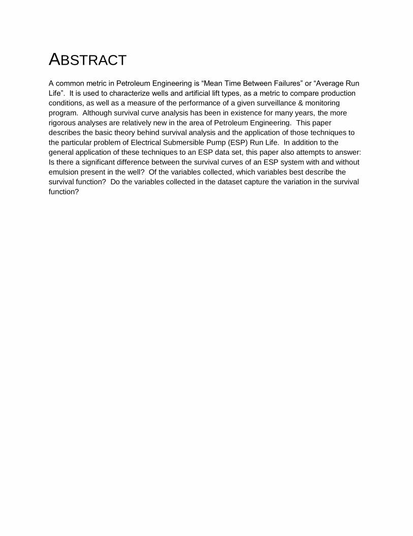
ABSTRACT

A common metric in Petroleum Engineering is “Mean Time Between Failures” or “Average Run

Life”. It is used to characterize wells and artificial lift types, as a metric to compare production

conditions, as well as a measure of the performance of a given surveillance & monitoring

program. Although survival curve analysis has been in existence for many years, the more

rigorous analyses are relatively new in the area of Petroleum Engineering. This paper

describes the basic theory behind survival analysis and the application of those techniques to

the particular problem of Electrical Submersible Pump (ESP) Run Life. In addition to the

general application of these techniques to an ESP data set, this paper also attempts to answer:

Is there a significant difference between the survival curves of an ESP system with and without

emulsion present in the well? Of the variables collected, which variables best describe the

survival function? Do the variables collected in the dataset capture the variation in the survival

function?

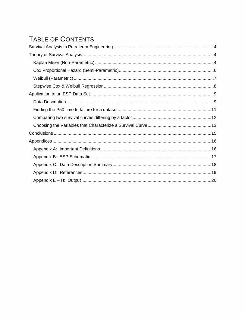
TABLE OF CONTENTS Survival Analysis in Petroleum Engineering ................................................................................4

Theory of Survival Analysis .........................................................................................................4

Kaplan Meier (Non-Parametric) ...............................................................................................4

Cox Proportional Hazard (Semi-Parametric) ............................................................................6

Weibull (Parametric) ................................................................................................................7

Stepwise Cox & Weibull Regression ........................................................................................8

Application to an ESP Data Set ...................................................................................................9

Data Description ......................................................................................................................9

Finding the P50 time to failure for a dataset...........................................................................11

Comparing two survival curves differing by a factor ...............................................................12

Choosing the Variables that Characterize a Survival Curve ...................................................13

Conclusions ..............................................................................................................................15

Appendices ...............................................................................................................................16

Appendix A: Important Definitions .........................................................................................16

Appendix B: ESP Schematic ................................................................................................17

Appendix C: Data Description Summary ...............................................................................18

Appendix D: References .......................................................................................................19

Appendix E – H: Output ........................................................................................................20

SURVIVAL ANALYSIS IN PETROLEUM ENGINEERING

A common metric in Petroleum Engineering is “Mean Time Between Failure” or “Average Run

Life”. It is used to characterize the average “life span” of wells and artificial lift types, as a metric

to compare production conditions (which ones give better run life), as well as a measure of the

performance of a given surveillance and monitoring program (improved surveillance and

monitoring should extend run life). Although survival curve analysis has been in existence for

many years, the more rigorous analyses are relatively new in the area of Petroleum

Engineering. As an example of the growth of these analysis techniques in the petroleum

industry, Electrical Submersible Pump (ESP) survival analysis has been sparsely documented

in technical journals for the last 20 years:

First papers on the fitting of Weibull & Exponential curves to ESP run life data in 1990

(Upchurch) & 1993 (Patterson)

Papers discussing the inclusion of censored data in 1996 (Brookbank) & 1999 (Sawaryn)

Paper discussing the use of Cox Regression in 2005 (Bailey)

Unfortunately, the papers applying these techniques did little to transfer the knowledge to the

practicing Petroleum Engineers. They shared the technical concepts and equations, but not the

practical knowledge of how to apply them to real life problems or why these analyses improved

upon the “take the average of the run life of failed wells” technique most commonly used.

THEORY OF SURVIVAL ANALYSIS

Survival analysis models the time it takes for events to occur and focuses on the distribution of

the survival times. It can be used in many fields of study where survival time can indicate

anything from time to death (medical studies) to time to equipment failure (reliability metrics).

This paper will present three methodologies for estimating survival distributions as well as a

technique for modeling the relationship between the survival distribution and one or more

predictor variables (both covariates and factors). Appendix A has a list of important definitions

relevant to survival analysis.

KAPLAN MEIER (NON-PARAMETRIC)

Non-parametric survival analysis characterizes survival functions without assuming an

underlying distribution. The analysis is limited to reliability estimates for the failure times

included in the data set (not prediction outside the range of data values) and comparison of

survival curves one factor at a time (not multiple explanatory variables).

A common non-parametric analysis is Kaplan Meier (KM). KM is characterized by a decreasing

step function with jumps at the observed event times. The size of the jump depends on the

number of events at that time t and the number of survivors prior to time t. The KM estimator

provides the ability to estimate survival functions for right censored data.

ti is the time at which a “death” occurs. di is the number of deaths that occur at time ti. When

there is no censoring, ni is the number of survivors just prior to time ti. With censoring, ni is the

number of survivors minus the number of censored units. The resulting curve, as noted, is a

decreasing step function with jumps at the times of “death” ti. The MTBF is the area under the

resulting curve; the P50 (median) time to failure is (t) 0.5.

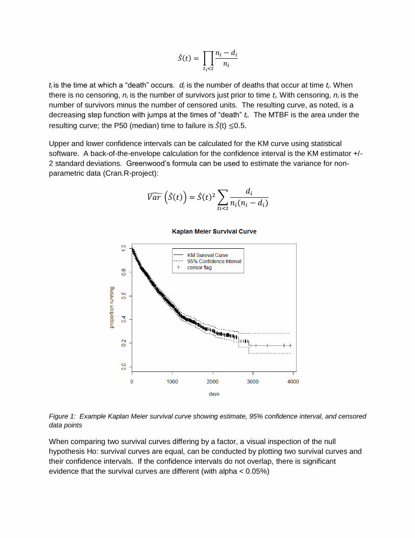
Upper and lower confidence intervals can be calculated for the KM curve using statistical

software. A back-of-the-envelope calculation for the confidence interval is the KM estimator +/-

2 standard deviations. Greenwood’s formula can be used to estimate the variance for non-

parametric data (Cran.R-project):

Figure 1: Example Kaplan Meier survival curve showing estimate, 95% confidence interval, and censored

data points

When comparing two survival curves differing by a factor, a visual inspection of the null

hypothesis Ho: survival curves are equal, can be conducted by plotting two survival curves and

their confidence intervals. If the confidence intervals do not overlap, there is significant

evidence that the survival curves are different (with alpha < 0.05%)

COX PROPORTIONAL HAZARD (SEMI-PARAMETRIC)

Semi-Parametric analysis enables more insight than the Non-Parametric method. It can

estimate the survival curve from a set of data as well as account for right censoring, but it also

conducts regression based on multiple factors/covariates as well a judge the contribution of a

given factor/covariate to a survival curve. CPH is not as efficient as a parametric model

(Weibull or Exponential), but the proportional hazards assumption is less restrictive than the

parametric assumptions (Fox).

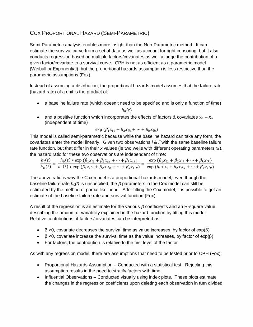
Instead of assuming a distribution, the proportional hazards model assumes that the failure rate

(hazard rate) of a unit is the product of:

a baseline failure rate (which doesn’t need to be specified and is only a function of time)

and a positive function which incorporates the effects of factors & covariates xi1 – xik

(independent of time)

This model is called semi-parametric because while the baseline hazard can take any form, the

covariates enter the model linearly. Given two observations i & i’ with the same baseline failure

rate function, but that differ in their x values (ie two wells with different operating parameters xk),

the hazard ratio for these two observations are independent of time:

The above ratio is why the Cox model is a proportional-hazards model; even though the

baseline failure rate h0(t) is unspecified, the β parameters in the Cox model can still be

estimated by the method of partial likelihood. After fitting the Cox model, it is possible to get an

estimate of the baseline failure rate and survival function (Fox).

A result of the regression is an estimate for the various β coefficients and an R-square value

describing the amount of variability explained in the hazard function by fitting this model.

Relative contributions of factors/covariates can be interpreted as:

β >0, covariate decreases the survival time as value increases, by factor of exp(β)

β <0, covariate increase the survival time as the value increases, by factor of exp(β)

For factors, the contribution is relative to the first level of the factor

As with any regression model, there are assumptions that need to be tested prior to CPH (Fox):

Proportional Hazards Assumption – Conducted with a statistical test. Rejecting this

assumption results in the need to stratify factors with time.

Influential Observations – Conducted visually using index plots. These plots estimate

the changes in the regression coefficients upon deleting each observation in turn divided

by the coefficient’s standard error. Comparing the magnitudes of the largest values in

the plot to the regression coefficients illustrates if any of the observations is influential.

Non-Linearity – Conducted visually using residual plots. These plots illustrate if the

factors are non-linear with time. If so, that factor would need to be treated as time series

data or with a different model (quadratic, etc).

There are special considerations and treatments for:

Time series data (factors not consistent over time, an example is the number and timing

of ESP restarts prior to failure)

Factors/covariates that do not meet the proportional hazards assumption

The treatment of time series data or data sets that do not meet the proportional hazards

assumption are not discussed in this paper, however these methodologies are documented in

Fox’s paper “Cox Proportional-Hazards Regression for Survival Data”.

WEIBULL (PARAMETRIC)

Parametric survival modeling assumes a distributional form. As previously noted, for ESP run

life data, papers have been written on the use of both Weibull and Exponential distributions for

the modeling of survival data. This paper will focus on the use of the Weibull distribution as it is

the more widely used distribution in reliability and life/failure data analysis due to its versatility.

Parametric survival analysis is more efficient than Semi or Non-Parametric survival curve

estimation but it has more restrictive assumptions. Parametric analysis is important in situations

where extrapolation of results is necessary to enable prediction of failure under different

conditions to those present in the original study. All other functionality provided by Parametric

modeling is also available in the more flexible Semi-Parametric approach, but with lower

efficiency (Fox).

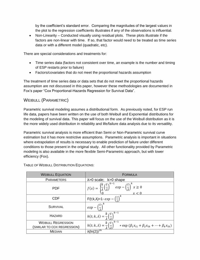
TABLE OF WEIBULL DISTRIBUTION EQUATIONS:

WEIBULL EQUATION FORMULA

PARAMETERS λ>0 scale; k>0 shape

PDF

CDF F(t;k,λ)=1-

SURVIVAL

HAZARD

WEIBULL REGRESSION (SIMILAR TO COX REGRESSION)

MEDIAN λ(ln(2))1/k

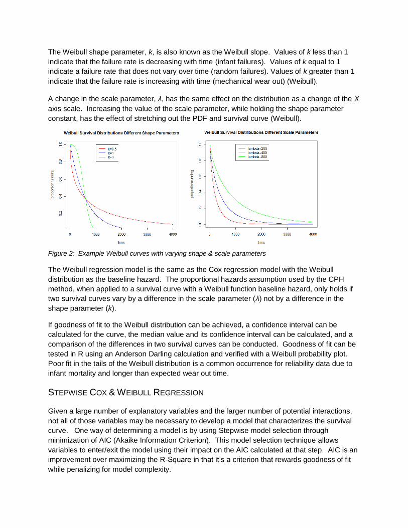
The Weibull shape parameter, k, is also known as the Weibull slope. Values of k less than 1

indicate that the failure rate is decreasing with time (infant failures). Values of k equal to 1

indicate a failure rate that does not vary over time (random failures). Values of k greater than 1

indicate that the failure rate is increasing with time (mechanical wear out) (Weibull).

A change in the scale parameter, λ, has the same effect on the distribution as a change of the X

axis scale. Increasing the value of the scale parameter, while holding the shape parameter

constant, has the effect of stretching out the PDF and survival curve (Weibull).

Figure 2: Example Weibull curves with varying shape & scale parameters

The Weibull regression model is the same as the Cox regression model with the Weibull

distribution as the baseline hazard. The proportional hazards assumption used by the CPH

method, when applied to a survival curve with a Weibull function baseline hazard, only holds if

two survival curves vary by a difference in the scale parameter (λ) not by a difference in the

shape parameter (k).

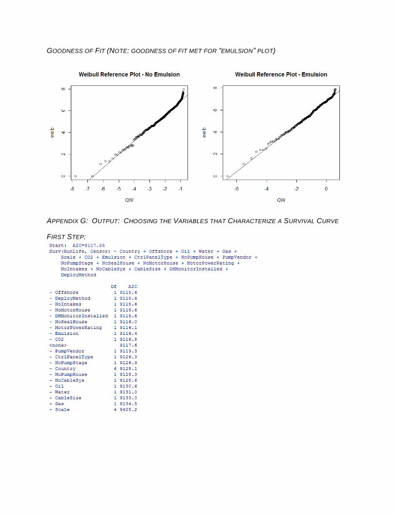
If goodness of fit to the Weibull distribution can be achieved, a confidence interval can be

calculated for the curve, the median value and its confidence interval can be calculated, and a

comparison of the differences in two survival curves can be conducted. Goodness of fit can be

tested in R using an Anderson Darling calculation and verified with a Weibull probability plot.

Poor fit in the tails of the Weibull distribution is a common occurrence for reliability data due to

infant mortality and longer than expected wear out time.

STEPWISE COX & WEIBULL REGRESSION

Given a large number of explanatory variables and the larger number of potential interactions,

not all of those variables may be necessary to develop a model that characterizes the survival

curve. One way of determining a model is by using Stepwise model selection through

minimization of AIC (Akaike Information Criterion). This model selection technique allows

variables to enter/exit the model using their impact on the AIC calculated at that step. AIC is an

improvement over maximizing the R-Square in that it’s a criterion that rewards goodness of fit

while penalizing for model complexity.

APPLICATION TO AN ESP DATA SET

As stated previously, these survival analysis techniques can be applied to many types of data in

many industries ranging from survival data for people in a medical study to survival data for

equipment in a reliability study. These methodologies have many uses in the petroleum

industry; from surface equipment system and component reliability used by facility and reliability

engineers, to well and downhole system and component reliability used by petroleum and

production engineers.

As an example, this paper illustrates the use of these techniques on the run life of Electrical

Submersible Pumps (ESP). ESPs are a type of artificial lift for bringing produced liquids to the

surface from within a wellbore. Appendix B includes a diagram of an ESP. For this paper, the

run life will refer to the run life of an ESP system, not the individual components within the ESP

system. While this paper focuses on ESP systems, these same techniques could be applied to

other areas of Petroleum Engineer interests including run life of individual ESP components,

other types of artificial lift, entire well systems, etc.

DATA DESCRIPTION

ESP-RIFTS JIP (Electrical Submersible Pump Reliability Information and Failure Tracking

System Joint Industry Project) is a group of 14 international oilfield operators who have joined

efforts to gain a better understanding of circumstances that lead to a success or failure in a

specific ESP application. The JIP includes access to a data set of 566 oil fields, 27861 wells,

89232 ESP installations, and 182 explanatory factors/covariates related to either the description

of the ESP application or the description of the ESP failure.

For the analysis described in this paper, a subset of the data has been used, restricted to:

Observations related to Chevron operated fields

observations with no conflicting information (as defined by the JIP’s data validation

techniques)

factors that were related to the description of the ESP application (excluded 27)

factors not confounded with or multiples of other factors (excluded 30)

factors with a large number (>90%) of non-missing data points (excluded 78)

factors that were not free-form comment fields (excluded 27)

Appendix C has a list of the original 182 variables with comments on why they were removed

from the analyzed data set, below is a table of the 20 remaining explanatory variables included

in this analysis.

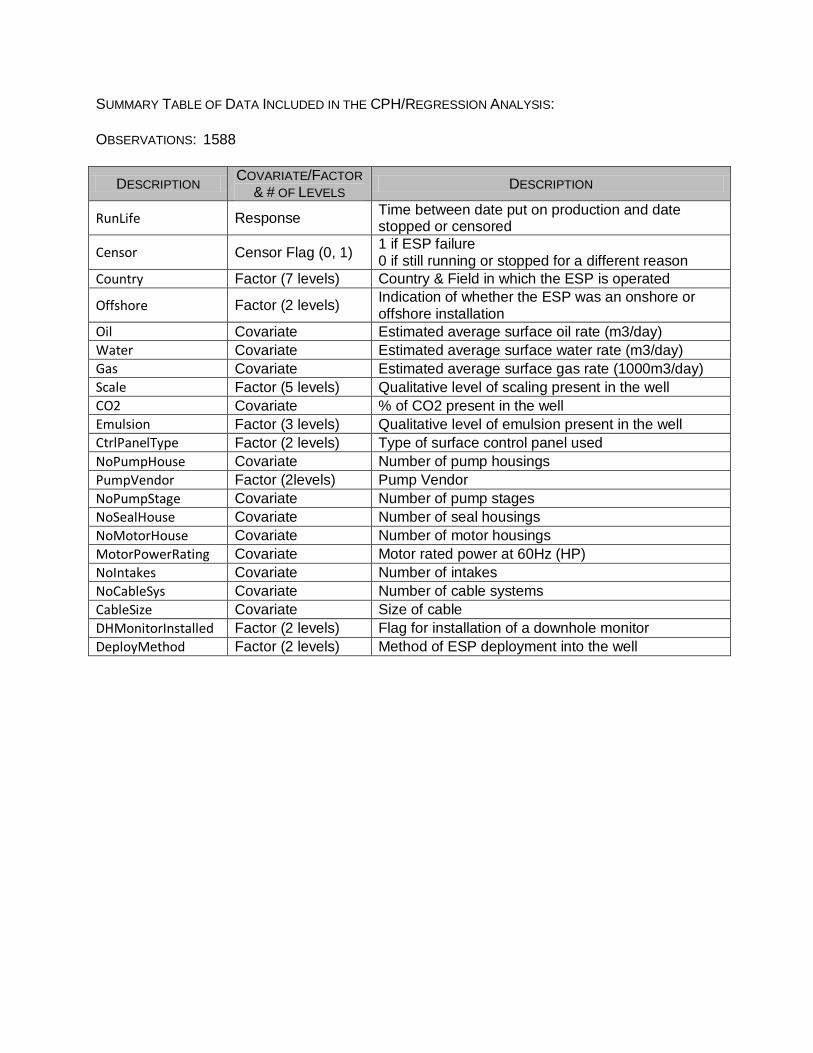
SUMMARY TABLE OF DATA INCLUDED IN THE CPH/REGRESSION ANALYSIS:

OBSERVATIONS: 1588

DESCRIPTION COVARIATE/FACTOR

& # OF LEVELS DESCRIPTION

RunLife Response Time between date put on production and date stopped or censored

Censor Censor Flag (0, 1) 1 if ESP failure 0 if still running or stopped for a different reason

Country Factor (7 levels) Country & Field in which the ESP is operated

Offshore Factor (2 levels) Indication of whether the ESP was an onshore or offshore installation

Oil Covariate Estimated average surface oil rate (m3/day)

Water Covariate Estimated average surface water rate (m3/day)

Gas Covariate Estimated average surface gas rate (1000m3/day)

Scale Factor (5 levels) Qualitative level of scaling present in the well

CO2 Covariate % of CO2 present in the well

Emulsion Factor (3 levels) Qualitative level of emulsion present in the well

CtrlPanelType Factor (2 levels) Type of surface control panel used

NoPumpHouse Covariate Number of pump housings

PumpVendor Factor (2levels) Pump Vendor

NoPumpStage Covariate Number of pump stages

NoSealHouse Covariate Number of seal housings

NoMotorHouse Covariate Number of motor housings

MotorPowerRating Covariate Motor rated power at 60Hz (HP)

NoIntakes Covariate Number of intakes

NoCableSys Covariate Number of cable systems

CableSize Covariate Size of cable

DHMonitorInstalled Factor (2 levels) Flag for installation of a downhole monitor

DeployMethod Factor (2 levels) Method of ESP deployment into the well

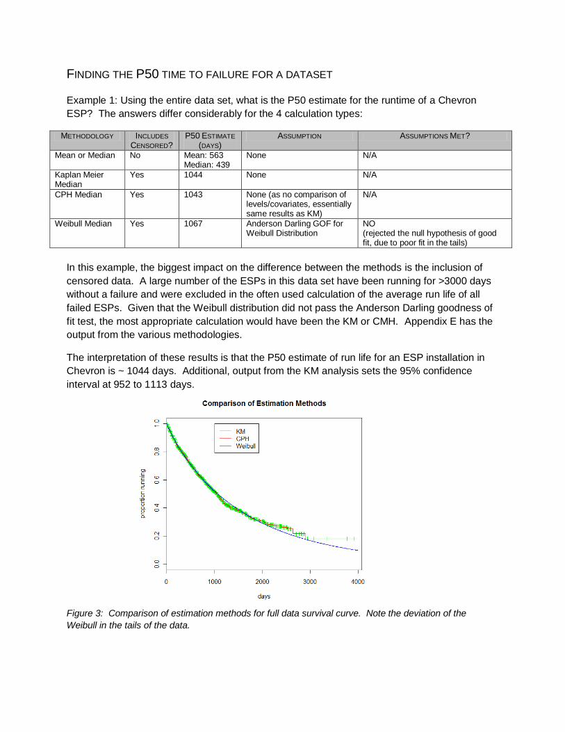
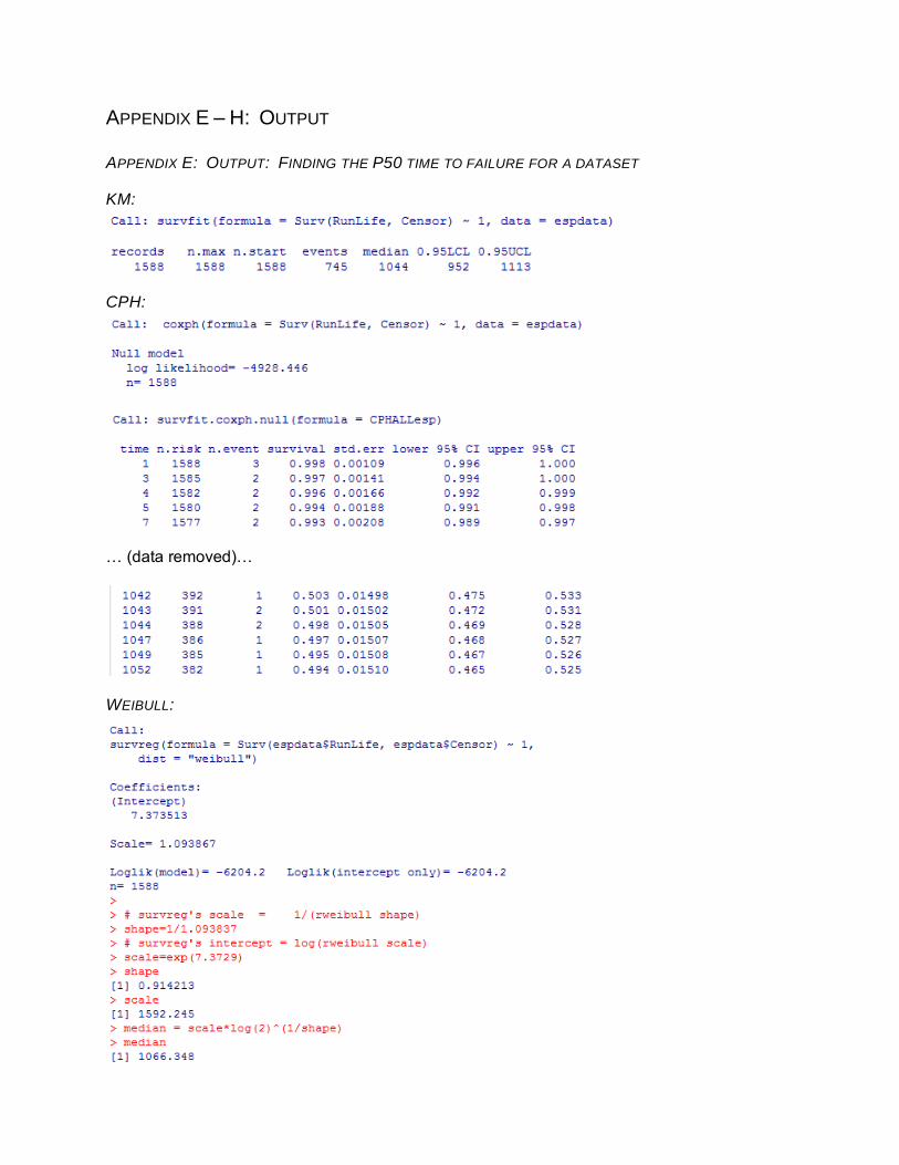
FINDING THE P50 TIME TO FAILURE FOR A DATASET

Example 1: Using the entire data set, what is the P50 estimate for the runtime of a Chevron

ESP? The answers differ considerably for the 4 calculation types:

METHODOLOGY INCLUDES

CENSORED? P50 ESTIMATE

(DAYS) ASSUMPTION ASSUMPTIONS MET?

Mean or Median No Mean: 563 Median: 439

None N/A

Kaplan Meier Median

Yes 1044 None N/A

CPH Median Yes 1043 None (as no comparison of levels/covariates, essentially same results as KM)

N/A

Weibull Median Yes 1067 Anderson Darling GOF for Weibull Distribution

NO (rejected the null hypothesis of good fit, due to poor fit in the tails)

In this example, the biggest impact on the difference between the methods is the inclusion of

censored data. A large number of the ESPs in this data set have been running for >3000 days

without a failure and were excluded in the often used calculation of the average run life of all

failed ESPs. Given that the Weibull distribution did not pass the Anderson Darling goodness of

fit test, the most appropriate calculation would have been the KM or CMH. Appendix E has the

output from the various methodologies.

The interpretation of these results is that the P50 estimate of run life for an ESP installation in

Chevron is ~ 1044 days. Additional, output from the KM analysis sets the 95% confidence

interval at 952 to 1113 days.

Figure 3: Comparison of estimation methods for full data survival curve. Note the deviation of the

Weibull in the tails of the data.

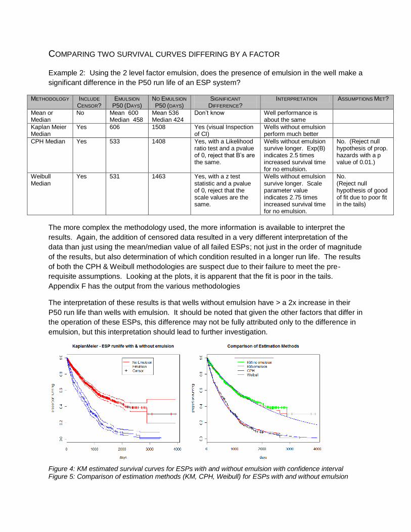
COMPARING TWO SURVIVAL CURVES DIFFERING BY A FACTOR

Example 2: Using the 2 level factor emulsion, does the presence of emulsion in the well make a

significant difference in the P50 run life of an ESP system?

METHODOLOGY INCLUDE

CENSOR? EMULSION

P50 (DAYS) NO EMULSION P50 (DAYS)

SIGNIFICANT

DIFFERENCE? INTERPRETATION ASSUMPTIONS MET?

Mean or Median

No Mean 600 Median 458

Mean 536 Median 424

Don’t know Well performance is about the same

Kaplan Meier Median

Yes 606 1508 Yes (visual Inspection of CI)

Wells without emulsion perform much better

CPH Median Yes 533 1408 Yes, with a Likelihood ratio test and a pvalue of 0, reject that B’s are the same.

Wells without emulsion survive longer. Exp(B) indicates 2.5 times increased survival time for no emulsion.

No. (Reject null hypothesis of prop. hazards with a p value of 0.01.)

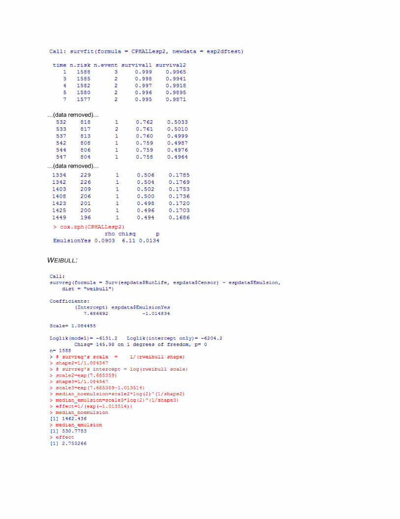
Weibull Median

Yes 531 1463 Yes, with a z test statistic and a pvalue of 0, reject that the scale values are the same.

Wells without emulsion survive longer. Scale parameter value indicates 2.75 times increased survival time for no emulsion.

No. (Reject null hypothesis of good of fit due to poor fit in the tails)

The more complex the methodology used, the more information is available to interpret the

results. Again, the addition of censored data resulted in a very different interpretation of the

data than just using the mean/median value of all failed ESPs; not just in the order of magnitude

of the results, but also determination of which condition resulted in a longer run life. The results

of both the CPH & Weibull methodologies are suspect due to their failure to meet the pre-

requisite assumptions. Looking at the plots, it is apparent that the fit is poor in the tails.

Appendix F has the output from the various methodologies

The interpretation of these results is that wells without emulsion have > a 2x increase in their

P50 run life than wells with emulsion. It should be noted that given the other factors that differ in

the operation of these ESPs, this difference may not be fully attributed only to the difference in

emulsion, but this interpretation should lead to further investigation.

Figure 4: KM estimated survival curves for ESPs with and without emulsion with confidence interval Figure 5: Comparison of estimation methods (KM, CPH, Weibull) for ESPs with and without emulsion

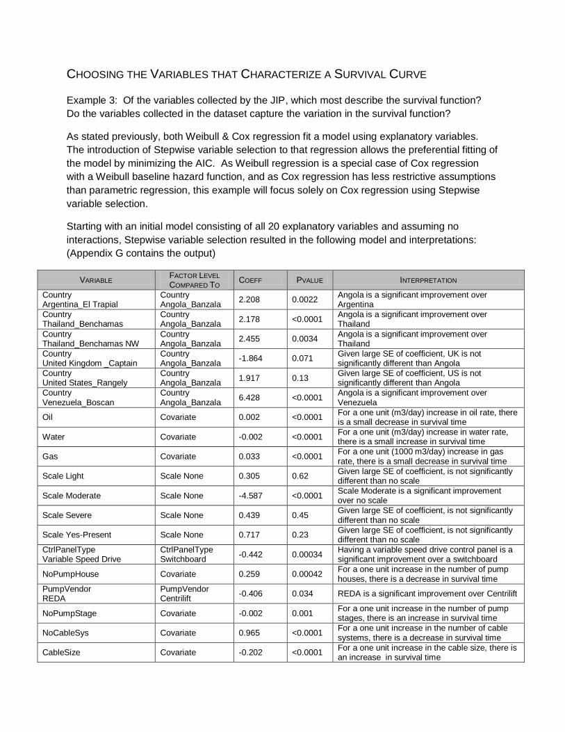
CHOOSING THE VARIABLES THAT CHARACTERIZE A SURVIVAL CURVE

Example 3: Of the variables collected by the JIP, which most describe the survival function?

Do the variables collected in the dataset capture the variation in the survival function?

As stated previously, both Weibull & Cox regression fit a model using explanatory variables.

The introduction of Stepwise variable selection to that regression allows the preferential fitting of

the model by minimizing the AIC. As Weibull regression is a special case of Cox regression

with a Weibull baseline hazard function, and as Cox regression has less restrictive assumptions

than parametric regression, this example will focus solely on Cox regression using Stepwise

variable selection.

Starting with an initial model consisting of all 20 explanatory variables and assuming no

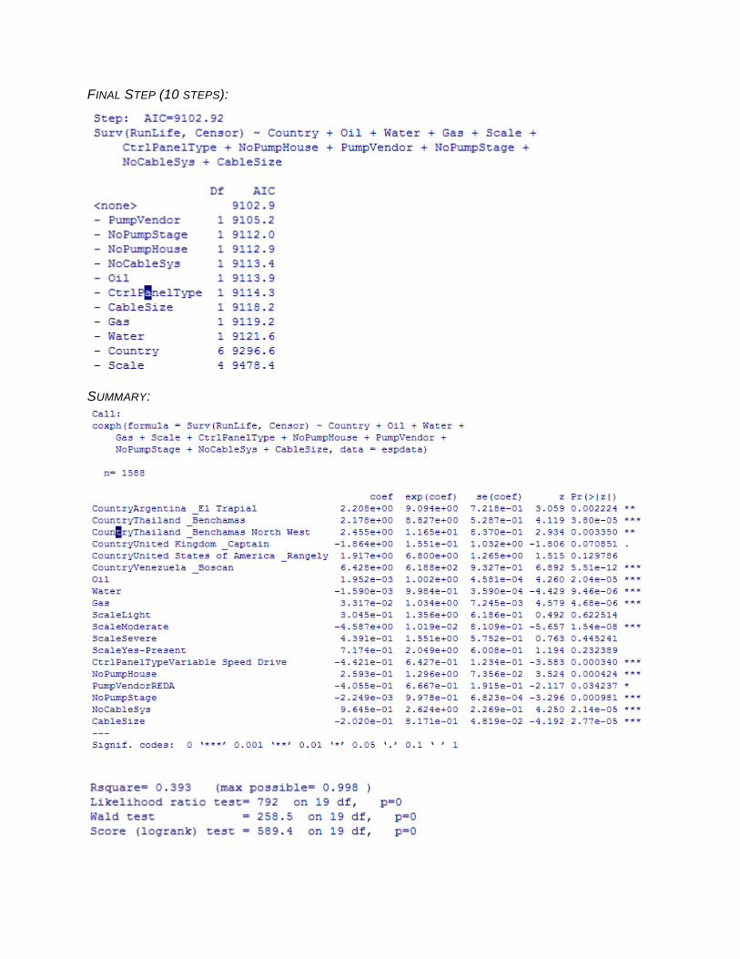
interactions, Stepwise variable selection resulted in the following model and interpretations:

(Appendix G contains the output)

VARIABLE FACTOR LEVEL

COMPARED TO COEFF PVALUE INTERPRETATION

Country Argentina_El Trapial

Country Angola_Banzala

2.208 0.0022 Angola is a significant improvement over Argentina

Country Thailand_Benchamas

Country Angola_Banzala

2.178 <0.0001 Angola is a significant improvement over Thailand

Country Thailand_Benchamas NW

Country Angola_Banzala

2.455 0.0034 Angola is a significant improvement over Thailand

Country United Kingdom _Captain

Country Angola_Banzala

-1.864 0.071 Given large SE of coefficient, UK is not significantly different than Angola

Country United States_Rangely

Country Angola_Banzala

1.917 0.13 Given large SE of coefficient, US is not significantly different than Angola

Country Venezuela_Boscan

Country Angola_Banzala

6.428 <0.0001 Angola is a significant improvement over Venezuela

Oil Covariate 0.002 <0.0001 For a one unit (m3/day) increase in oil rate, there is a small decrease in survival time

Water Covariate -0.002 <0.0001 For a one unit (m3/day) increase in water rate, there is a small increase in survival time

Gas Covariate 0.033 <0.0001 For a one unit (1000 m3/day) increase in gas rate, there is a small decrease in survival time

Scale Light Scale None 0.305 0.62 Given large SE of coefficient, is not significantly different than no scale

Scale Moderate Scale None -4.587 <0.0001 Scale Moderate is a significant improvement over no scale

Scale Severe Scale None 0.439 0.45 Given large SE of coefficient, is not significantly different than no scale

Scale Yes-Present Scale None 0.717 0.23 Given large SE of coefficient, is not significantly different than no scale

CtrlPanelType Variable Speed Drive

CtrlPanelType Switchboard

-0.442 0.00034 Having a variable speed drive control panel is a significant improvement over a switchboard

NoPumpHouse Covariate 0.259 0.00042 For a one unit increase in the number of pump houses, there is a decrease in survival time

PumpVendor REDA

PumpVendor Centrilift

-0.406 0.034 REDA is a significant improvement over Centrilift

NoPumpStage Covariate -0.002 0.001 For a one unit increase in the number of pump stages, there is an increase in survival time

NoCableSys Covariate 0.965 <0.0001 For a one unit increase in the number of cable systems, there is a decrease in survival time

CableSize Covariate -0.202 <0.0001 For a one unit increase in the cable size, there is an increase in survival time

Writing out the final model:

(2.208 * Argentina_El Trapial + 2.178 * Thailand_Benchamas + 2.455 *

Thailand_Benchamas NW + -1.864 * United Kingdom _Captain + 1.917 * United

States_Rangely + 6.428 * Venezuela_Boscan + 0.001952 * Oil + -0.00159 * Water + 0.03317 *

Gas + 0.3045 * ScaleLight + -4.587 * ScaleModerate + 0.4391 * ScaleSevere + 0.7174 *

ScaleYes-Present + -0.4421 * CtrlPanelTypeVariableSpeedDrive + 0.2593 * NoPumpHouse +

-0.4055 * PumpVendorREDA + -0.002249 * NoPumpStage + 0.9645 * NoCableSys + -0.202 *

CableSize

To use the model, a 0 or 1 is used for the factor explanatory variables and the actual value for

the covariates.

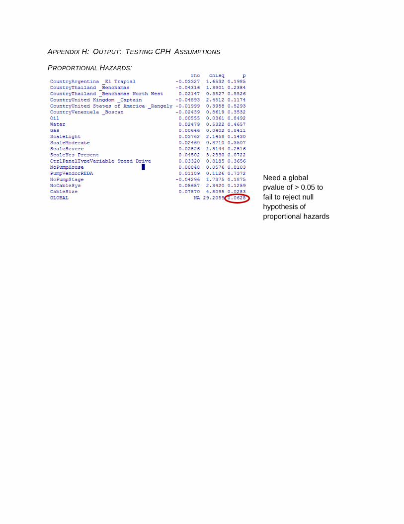
As stated previously, there are assumptions that need to be tested to use CPH or Cox

regression. Appendix H has the output and plots necessary to test the following assumptions:

Proportional Hazards Assumption – The global p-value for the chi-square test for Ho:

proportional hazards assumption holds is 0.0628, therefore we fail to reject the null

hypothesis. The proportional hazards assumption holds.

Influential Observations – Conducted visually using an index plot. Comparing the

magnitudes of the largest values in the plot to the regression coefficients shows there

aren’t any significant influencers other than in the levels of Scale. Reviewing the plots

leads me to believe there are issues with the comparative level of Scale-None (possible

data-miscoding). No action taken, however given those plots coupled with the fact that

the response led to a non-intuitive interpretation, a recommendation to the JIP could be

made that they put more stringent controls on scale data and re-evaluate.

Non-Linearity – Conducted visually using a residual plot. Comparing the distribution of

the residuals to a line with mean zero, there are a few points for both oil and gas that

may indicate quadratic behavior in the upper ranges. If this model was going to be used

rigorously, further investigation would need to go into those points.

The R-square value for this model is calculated to be 0.393. This means only 39.3% of the

variation was captured by this model and that there are potentially other explanatory variables

that would need to be measured to more fully explain the variation.

As a Petroleum Engineering practitioner, there are a few things that surprised me about these

results:

Downhole monitor flag was removed from the model: This is a technology that is

believed to extend the runlife of ESPs because a quicker reaction to downhole

conditions can be achieved.

Emulsion was removed from the model: Given what we saw previously that no emulsion

was a significant improvement on run life, the fact that it does not show up in the final

model indicates that its effect can be explained using other factors in the model.

Scale Moderate improved run life and the others were not significantly different from no

scale: Scale in a wellbore fouls an ESP system and is thought to be one of the key

reasons an ESP system might fail. As noted after looking at the influential residual plots,

there may be underlying issues with the data collection for the Scale data.

No support for difficulty operating in less developed countries: ESPs in Angola did not

have a significantly different run life than ESPs in the US & UK, and were significantly

better than Thailand & Venezuela. It should be noted that country is confounded by a

significant amount of reservoir characterization data so it cannot be determined with this

data set if differences between countries is due to the skill of the workforce or the

difficulties associated with the reservoir.

Only 39.3% of the variation in the survival curve was characterized by this model: As

previously stated, of the 182 variables tracked by the JIP, only 20 could be used due to

confounding and missing data. A more concerted study should be kicked off to

determine if there is other information that should be collected and/or why the

participating companies do not record all 182 variables.

Knowing that this is an observational data set and not a controlled experiment, it is difficult to

draw more conclusions from the data than already stated. However, these conclusions alone

should be enough to spur significant discussion within the JIP and additional data capture to

understand some of the surprising results.

CONCLUSIONS

Understanding and applying different levels of survival analysis methodologies to petroleum

industry run life data could lead to new insights and interpretations of old data sets. Historical

use of straight means and/or medians of failed systems and interpreting them as P50 run life

can be very misleading when there is a significant amount of censored data that is not taken

into account. Although the use of more complex methodologies, such as Weibull regression

and CPH or Cox regression, brings more information to the analysis of run life data, even the

expansion of the usage of the Kaplan Meier technique would improve upon the current practice

of calculating MTTF and could be managed in an existing toolset (Microsoft Excel). The use of

R-square alone as a goodness of fit measure may not point out lack of fit in the tails. JIPs and

other groups investigating explanatory effects on run life could benefit from these tools by using

them not only to analyze their data, but also to better target the range of explanatory variables

they capture to make their data collection efforts more effective.

APPENDICES

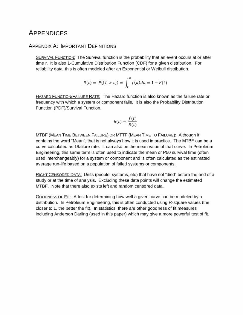
APPENDIX A: IMPORTANT DEFINITIONS

SURVIVAL FUNCTION: The Survival function is the probability that an event occurs at or after

time t. It is also 1-Cumulative Distribution Function (CDF) for a given distribution. For

reliability data, this is often modeled after an Exponential or Weibull distribution.

HAZARD FUNCTION/FAILURE RATE: The Hazard function is also known as the failure rate or

frequency with which a system or component fails. It is also the Probability Distribution

Function (PDF)/Survival Function.

MTBF (MEAN TIME BETWEEN FAILURE) OR MTTF (MEAN TIME TO FAILURE): Although it

contains the word “Mean”, that is not always how it is used in practice. The MTBF can be a

curve calculated as 1/failure rate. It can also be the mean value of that curve. In Petroleum

Engineering, this same term is often used to indicate the mean or P50 survival time (often

used interchangeably) for a system or component and is often calculated as the estimated

average run-life based on a population of failed systems or components.

RIGHT CENSORED DATA: Units (people, systems, etc) that have not “died” before the end of a

study or at the time of analysis. Excluding these data points will change the estimated

MTBF. Note that there also exists left and random censored data.

GOODNESS OF FIT: A test for determining how well a given curve can be modeled by a

distribution. In Petroleum Engineering, this is often conducted using R-square values (the

closer to 1, the better the fit). In statistics, there are other goodness of fit measures

including Anderson Darling (used in this paper) which may give a more powerful test of fit.

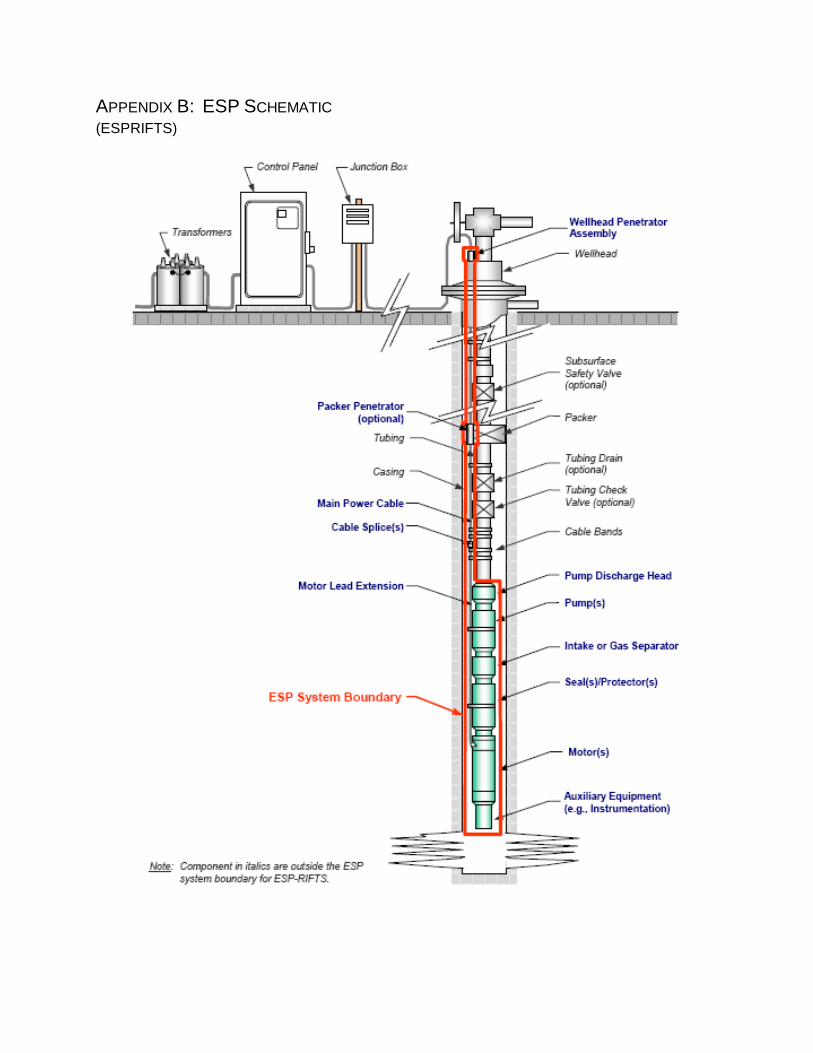
APPENDIX B: ESP SCHEMATIC (ESPRIFTS)

APPENDIX C: DATA DESCRIPTION SUMMARY Variables that characterized ESP failure (Removed):

Reason For Pull: General Reason For Pull: Specific Primary Failed Item

Primary Failed Item - Major Component Primary Failure Descriptor

Secondary Failure Descriptor Primary Contaminant Failure Cause: General

Failure Cause: Specific

Failure Comments Pump Pull Condition Pump Primary Failure Descriptor

Seal Pull Condition Seal Primary Failure Descriptor Motor Pull Condition

Motor Primary Failure Descriptor Pump Intake Pull Condition Pump Intake Primary Failure

Descriptor

Cable Pull Condition Cable Primary Failure Descriptor MLE Pull Condition

Cable Splice Pull Condition Pothead Pull Condition Wellhead Penetrator Pull Condition

Packer Penetrator Pull Condition DH Monitoring System Pull Condition DH Monitoring System Primary

Failure Descriptor

Explanatory variables confounded with other explanatory variables (Removed):

Field Name

Pad or Platform Name Location of ESP Supply Centre (Country)

Location of ESP Teardown Facility (Country) Oil Density at STP (°API)

Dead Oil Viscosity at STP (cp) Live Oil Viscosity at Reservoir Conditions (cp)

Oil Bubble Point Pressure (kPa,abs)

Reservoir/Zone Name

Reservoir Type Reservoir Consolidation Reservoir Recovery Mechanism

Reservoir Temperature (°C) Well Type (Geometry) Well Location (Onshore/Offshore)

Wellhead Location Production Casing Outer Diameter (mm)

Production Casing Weight (kg/m)

Completion Type

Sand Control Type Free Gas at Pump Intake (%) Company Installing ESP System

Seal Vendor Motor Vendor Pump Intake Vendor

Cable Vendor

Variables with >10% missing data (Removed):

Pump Intake Pressure (kPa,g) Producing Fluid Level (mKB to Fluid)

Reservior Static Pressure (Latest) (kPa,g) Productivity Index (PI)

Pump Intake Temperature (°C) Wellhead Pressure (kPa,g) Wellhead Temperature (°C)

Casing Head Pressure (kPa,g) Surface Sand Rate (m³/d) Sand Cut (%)

Other Solids Concentration Total Solids Concentration Solids?

Paraffin/Wax? Asphaltenes? H2S (% by Volume) (%)

Water pH Water Salinity (Cl- ppm) Sand?

Corrosion? Motor Frequency (Hz) Motor Voltage (Volts)

Motor Current (Amps) Percent Deviation from Motor Rated Current

Number of Restarts During Period

Control Panel Vendor Control Panel Model

Control Panel Power Rating (kVA) Power Source Power Quality

Power supply frequency (Hz) Pump Series Pump Type/Model

Pump Operator Option Suffix Pump Housing Pump Trim

Pump Impeller Type Pump New/Used Seal Series

Seal Type/Model Seal Trim Seal New/Used

Motor Series Motor Type/Model Motor Rated Voltage @ 60 Hz

Motor Rated Current @ 60 Hz Motor Trim Motor New/Used

Pump Intake Type Pump Intake Series Pump Intake Type/Model

Pump Intake Trim

Pump Intake New/Used Cable Type (Round/Flat)

Cable Type/Model Cable Power Rating Cable Armour

Cable Material Type Cable New/Used MLE Type/Model

Wellhead Penetrator Type/Model Packer Penetrator Type/Model DH Monitoring System Vendor

DH Monitoring System New/Used Shroud Installed? Shroud Casing Outer Diameter (mm)

Tubing Outer Diameter (mm) Tubing Weight (kg/m) Packer Installed?

Packer Depth Y-Tool Installed? Pump Seating Depth MD (mKB)

Pump Seating Depth TVD (mKB) Inclination at PSD (°) Maximum Dogleg (°/30m)

Number of ESP Systems In Well ESP System Configuration (Single/Parallel/Series)

First ESP System Installed in Well?

Non-informative or comment fields (Removed):

ProductionPeriodID Company Name

Division Name Field Comments Number of Reservoirs

Reservoir Comments Well Name Production Period Number

Production Role

Well Comments Period Comments

Control Panel Serial Number Control Panel Part Number Control Panel Comments

Pump Serial Number Pump Comments Seal Serial Number

Seal Comments

Motor Serial Number Motor Comments

Pump Intake Serial Number Pump Intake Comments Cable Serial Number

Cable Comments DH Monitoring System Comments Artificial Lift Type

Qualification Status

Variables that were multiples of other variables (Removed):

Total Flow Rate (m³/d) Water Cut (%) GOR & GLR (m³/m³)

APPENDIX D: REFERENCES

Bailey, W.J, et al.: “Survival Analysis: The Statistically Rigorous Method for Analyzing

Electrical Submersible Pump System Performance,” paper presented at the 2005 SPE Annual

Technical Conference and Exhibition, Dallas, Texas October 9 – 12, SPE96772

Brookbank, B.: “How Do you Measure Run Life?”, presented at the ESP Workshop May 1 – 3

1996 North Side Branch of Gulf Coast Chapter, SPE

Cran.R-project.org: “CRAN Task View: Survival Analysis”, Version 2010-07-30

ESPRIFTS.com: Electric Submersible Pump Joint Industry Project data access

Fox, John “Cox Proportional-Hazards Regression for Survival Data”, February 2002

Longnecker, M: STAT 641 Lecture Notes, Fall 2009

Patterson, M.M.: “A Model for Estimating the Life of Electrical Submersible Pumps”, SPE

Production & Facilities, November 1993, 247

Sawaryn, S.J, et al.: “The Analysis and Prediction of Electric-Submersible-Pump Failures in the

Milne Point Field, Alaska”, paper presented at the 1999 SPE Annual Technical Conference and

Exhibition, Houston Texas October 3 – 6, SPE56663

Upchurch, E.R.: “Analyzing Electrical Submersible Pump Failures in the East Wilmington Field

of California,” paper presented at the 1991 SPE Electrical Submersible Pump Workshop,

Houston, Texas April 30-May2, SPE20675

Weibull.com: “Characteristics of the Weibull Distribution”, Reliability Hot Wire, Issue 14, April

2002

APPENDIX E – H: OUTPUT

APPENDIX E: OUTPUT: FINDING THE P50 TIME TO FAILURE FOR A DATASET

KM:

CPH:

… (data removed)…

WEIBULL:

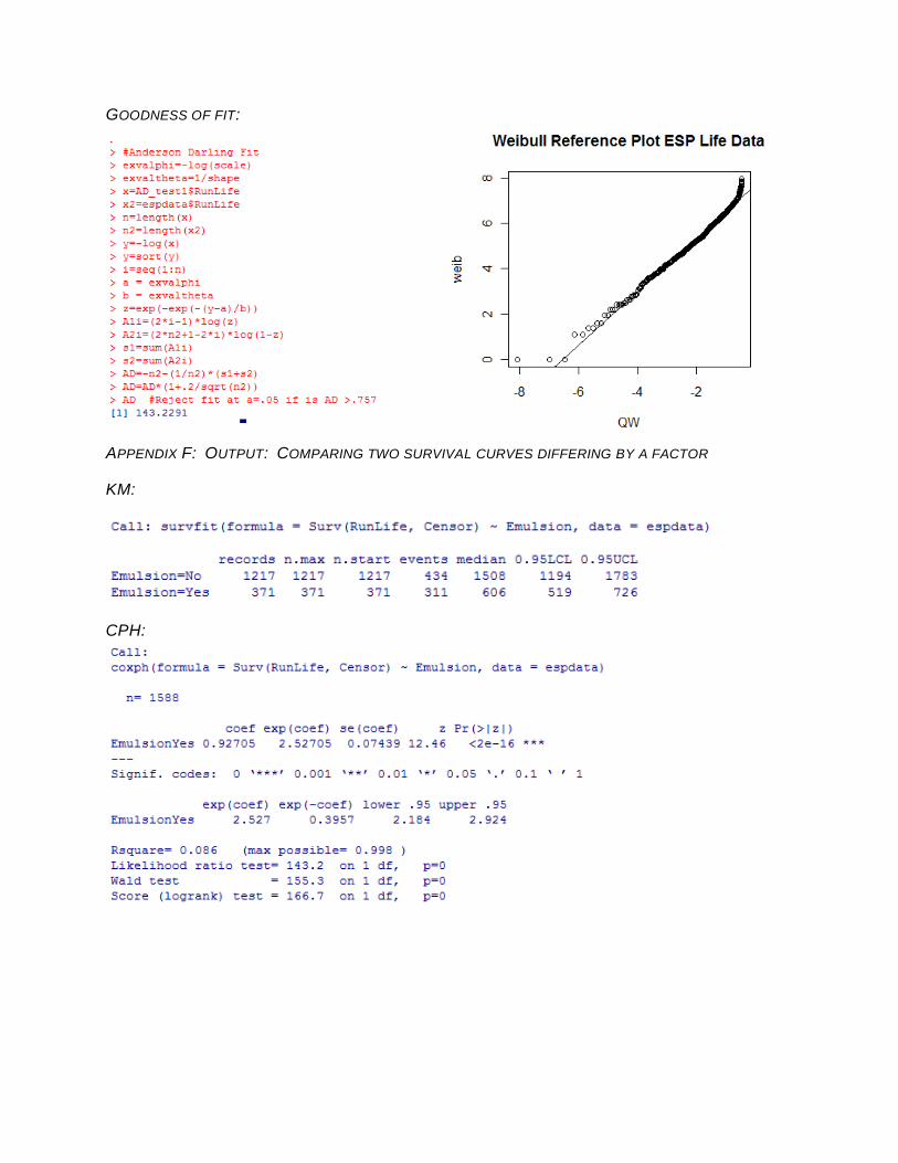
GOODNESS OF FIT:

APPENDIX F: OUTPUT: COMPARING TWO SURVIVAL CURVES DIFFERING BY A FACTOR

KM:

CPH:

…(data removed)…

…(data removed)…

WEIBULL:

GOODNESS OF FIT (NOTE: GOODNESS OF FIT MET FOR “EMULSION” PLOT)

APPENDIX G: OUTPUT: CHOOSING THE VARIABLES THAT CHARACTERIZE A SURVIVAL CURVE

FIRST STEP:

FINAL STEP (10 STEPS):

SUMMARY:

APPENDIX H: OUTPUT: TESTING CPH ASSUMPTIONS

PROPORTIONAL HAZARDS:

Need a global

pvalue of > 0.05 to

fail to reject null

hypothesis of

proportional hazards

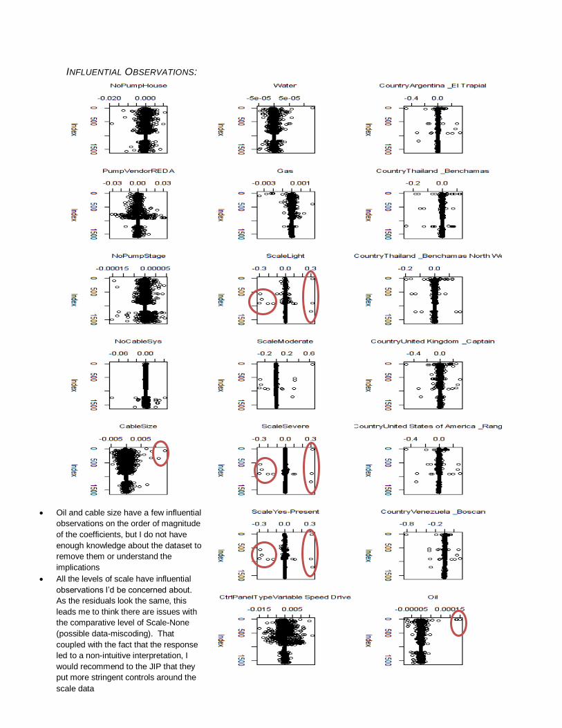
INFLUENTIAL OBSERVATIONS:

Oil and cable size have a few influential

observations on the order of magnitude

of the coefficients, but I do not have

enough knowledge about the dataset to

remove them or understand the

implications

All the levels of scale have influential

observations I’d be concerned about.

As the residuals look the same, this

leads me to think there are issues with

the comparative level of Scale-None

(possible data-miscoding). That

coupled with the fact that the response

led to a non-intuitive interpretation, I

would recommend to the JIP that they

put more stringent controls around the

scale data

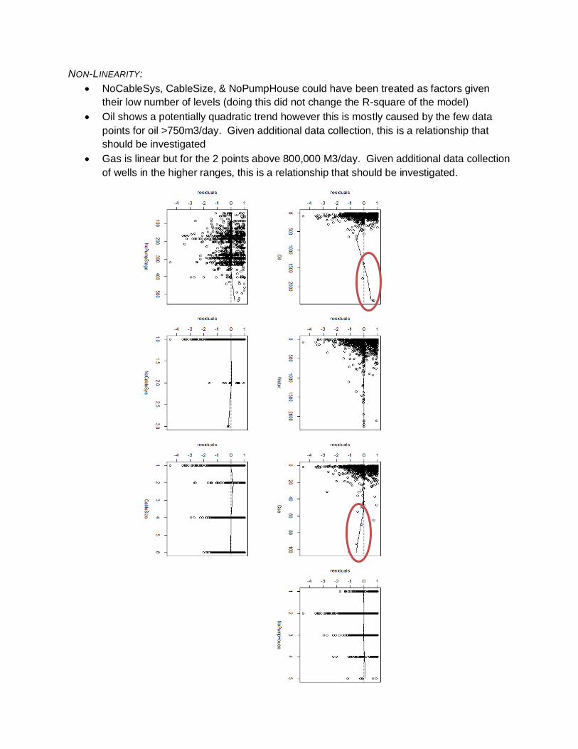
NON-LINEARITY:

NoCableSys, CableSize, & NoPumpHouse could have been treated as factors given

their low number of levels (doing this did not change the R-square of the model)

Oil shows a potentially quadratic trend however this is mostly caused by the few data

points for oil >750m3/day. Given additional data collection, this is a relationship that

should be investigated

Gas is linear but for the 2 points above 800,000 M3/day. Given additional data collection

of wells in the higher ranges, this is a relationship that should be investigated.