Embed Size (px)
Citation preview

ELECTRICAL TRACKING OVER SOLID
INSULATING MATERIALS FOR
AEROSPACE APPLICATIONS
A thesis submitted to The University of Manchester for
the degree of
Doctor of Philosophy
in the Faculty of Engineering and Physical Sciences
2011
Lei Zhang
School of Electrical and Electronic Engineering
1
LIST OF CONTENTS
LIST OF FIGURES ............................................................................................................ 6
LIST OF TABLES ............................................................................................................. 12
LIST OF MAIN ABBREVIATIONS ................................................................................. 14
ABSTRACT ....................................................................................................................... 15
DECLARATION ................................................................................................................ 16
COPYRIGHT .................................................................................................................... 17
ACKNOWLEDGEMENTS............................................................................................... 18
Chapter 1 Introduction........................................................................................................ 19
1.1. Overview........................................................................................................... 19
1.2. Aims and objectives of the research.................................................................. 28
1.3. The AIMEA program ........................................................................................ 30
1.4. Organization of the thesis.................................................................................. 31
Chapter 2 Review Electrical Discharge, Characteristics, and Relevant Test Techniques .. 33
2.1. Introduction....................................................................................................... 33
2.2. Electrical breakdown in gases........................................................................... 34
2.2.1. Useful definitions in gas kinetic theory...................................................35
2.2.2. The appearance and disappearance of the charged particles in gases .....37
2.2.3. Electron avalanche and Townsend’s first ionization coefficient .............45
2.2.4. Townsend’s second ionization .................................................................46
2.2.5. Townsend mechanism–transition from non-self-sustained discharges to
breakdown .................................................................................................................47
2.2.6. Paschen’s law...........................................................................................48
2.2.7. Breakdown in non-uniform fields............................................................51
2.2.8. Partial discharge (PD)..............................................................................53
2.3. Electrical tracking ............................................................................................. 54
2.4. Existing design standards.................................................................................. 58
2.5. Test techniques for electrical tracking...............................................................60
2.5.1. A.S.T.M. D 495 “High Voltage, Low Current Arc Resistance of Solid
2
Electrical Insulating Materials” [59] ...................................................................................61
2.5.2. IEC 60112:2003 Comparative Tracking Index Tests...............................61
2.5.3. IEC 60587 inclined plane test..................................................................62
2.5.4. Dust-fog test ............................................................................................63
2.5.5. Test methods discussion ..........................................................................64
2.6. Conclusion ........................................................................................................ 65
Chapter 3 Clearances and Creepage Distances to Avoid Dry Flashover ............................ 66
3.1. Introduction....................................................................................................... 66
3.2. Review of IEC 60664-1:2003 ........................................................................... 68
3.2.1. Introduction .............................................................................................68
3.2.2. Determination of clearance......................................................................68
3.2.3. Dimensioning of creepage distances .......................................................72
3.3. Review of IPC 2221.......................................................................................... 74
3.3.1. Introduction .............................................................................................74
3.3.2. Electrical clearances ................................................................................74
3.4. Uniform field breakdown tests.......................................................................... 76
3.4.1. Test circuit ...............................................................................................77
3.4.2. Test apparatus and procedure...................................................................78
3.4.3. Test results and discussion.......................................................................79
3.5. Non-uniform field breakdown tests .................................................................. 84
3.5.1. Test apparatus and procedure...................................................................84
3.5.2. Summary of test results ...........................................................................85
3.5.3. Discussion................................................................................................86
3.6. Flashover on printed circuit boards under dry Conditions................................ 89
3.6.1. Test procedure..........................................................................................89
3.6.2. Test results and discussion.......................................................................90
3.7. Conclusion ........................................................................................................ 93
Chapter 4 Modeling of Tracking Process under Wet Conditions ....................................... 95
4.1. Introduction....................................................................................................... 95
4.2. Electrical tracking under wet conditions........................................................... 96
3
4.3. Theoretical model of electrical tracking ........................................................... 99
4.4. Theoretical model analysis.............................................................................. 107
4.4.1. Static thermal analysis ...........................................................................107
4.4.2. Application of static thermal simulation results to the environments of
varying pressure ...............................................................................................................110
4.4.3. Application of static thermal simulation results to the environments of
varying pressure, contaminant resistivity and ambient temperature .................................115
4.4.4. Dynamic thermal analysis .....................................................................119
4.5. Discussion ....................................................................................................... 120
4.6. Conclusion ...................................................................................................... 122
Chapter 5 Experimental Investigation I: Standard CTI Tests on FR-4 and ABS Materials
.......................................................................................................................................... 123
5.1. Introduction..................................................................................................... 123
5.2. Experimental conditions.................................................................................. 125
5.2.1. Test Circuit.............................................................................................125
5.2.2. Test specimens.......................................................................................126
5.2.3. Electrodes ..............................................................................................127
5.2.4. Dropping devices and test solution........................................................128
5.2.5. Leakage current and voltage recording .................................................129
5.2.6. Test procedure........................................................................................129
5.3. Experimental results and discussion ............................................................... 131
5.3.1. Behaviour of FR-4 samples at the atmospheric pressure ......................131
5.3.2. Behaviour of ABS samples at the atmospheric pressure .......................148
5.4. Summary of discussion ................................................................................... 152
5.4.1. Four Modes of Electrical Discharges ....................................................152
5.4.2. Comparison of the withstand voltages to electrical tracking between the
test results and the standards .............................................................................................153
5.4.3. Visual damages on the specimens .........................................................154
5.5 Conclusion ...................................................................................................... 154
Chapter 6 Experimental Investigation II: CTI tests under the Conditions of Lower Pressure
4
and Varying Conductivity of Contamination.................................................................... 157
6.1. Introduction..................................................................................................... 157
6.2. Low pressure CTI tests.................................................................................... 158
6.2.1. Experiment conditions...........................................................................158
6.2.2. Experimental results for the 100 mbar tests ..........................................162
6.2.3. Discussion of the results ........................................................................164
6.3. Atmospheric pressure CTI tests with a solution of the half conductivity of the
solution A.................................................................................................................. 165
6.3.1. Experiment conditions...........................................................................166
6.3.2. Experimental results ..............................................................................166
6.3.3. Discussion of the results ........................................................................167
6.4. Atmospheric pressure CTI tests with a solution of the double conductivity of the
solution A.................................................................................................................. 168
6.4.1. Experiment conditions...........................................................................168
6.4.2. Experimental results ..............................................................................169
6.4.3. Discussion of the results ........................................................................170
6.5. Discussion ....................................................................................................... 171
6.6. Conclusion ...................................................................................................... 173
Chapter 7 Experimental Investigation III: CTI tests Developed for Varying Creepage
Distances........................................................................................................................... 175
7.1. Introduction..................................................................................................... 175
7.2. Selection of a wetting technique for the varying creepage distance tracking test
......................................................................................................................... 176
7.3. Experimental conditions.................................................................................. 178
7.4. 4mm gap tracking test at the atmospheric pressure ........................................ 179
7.4.1. Experimental results ..............................................................................180
7.4.2. Discussion of the results ........................................................................185
7.5. 2mm gap tracking test at the atmospheric pressure ........................................ 186
7.5.1. Experimental Results.............................................................................186
7.5.2. Discussion of Results.............................................................................189

5
7.6. 8 mm Gap Tracking Test under Atmospheric Pressure ................................... 191
7.6.1. Experimental Results.............................................................................191
7.6.2. Discussion of Results.............................................................................194
7.7. Conclusion ...................................................................................................... 195
Chapter 8: Conclusion and Future Work .......................................................................... 198
8.1. Summary ......................................................................................................... 198
8.1.1. Validation of clearances and creepage distances in standards..................... 198
8.1.2. Electrical tracking under wet conditions ..................................................... 200
8.1.3. Selection of wet condition electrical tracking test techniques..................... 203
8.2. Suggestions for Future Work...........................................................................204
8.3. Conclusion ...................................................................................................... 206
Reference........................................................................................................................ 209
Appendix A ...................................................................................................................... 215
Appendix B...................................................................................................................... 226

6
LIST OF FIGURES
Figure 1.1 Schematic of conventional airplane power distribution [4]………….…..…….19
Figure 1.2 Conventional aircraft electrical subsystems…………………………..……..…21
Figure 1.3 Current trend of the MEA [4]…………..………………………………….…..22
Figure 1.4 The MEA electrical power subsystems……………………………….….….…22
Figure 1.5 Candidate electrical power generation types…………………………….….....23
Figure 2.1 Variation of ionization cross-sections for, and with electron energy…………...38
Figure 2.2 Breakdown voltage in air for a given air pressure - distance product according to
Paschen’s law……………………………………………………..………………….........49
Figure 2.3 Partial discharge between an aerospace cable and a grounded electrode (left), and
erosion of an insulating material due to partial discharge (right)………….………………54
Figure 2.4 Basic process of tracking across an insulating surface contaminated with an
aqueous layer………………………………………………………………….........….….56
Figure 2.5 IEC 60112 test rig sketch………………………………………….……..….…61
Figure 2.6 Incline plate plan sample and electrodes configurations……….………..……..63
Figure 2.7 Dust-fog test rig sketch…………………………………………..…..……..….64
Figure 3.1 Sketch of clearance and creepage distance………………………………...…...66
Figure 3.2 Flow chart of dimensioning clearance for the equipments in low-voltage
systems................................................................................................................................69
Figure 3.3 Clearances specified in IEC 60664 for varying altitude application under uniform
electric field condition………………………………………………............................….71
Figure 3.4 Clearances specified in IEC 60664 for varying altitude application under
non-uniform electric field condition…………………………….......…………….......…..72
Figure 3.5 Electrical spacing specified in IPC 2221 for varying altitude application….......76
Figure 3.6 Sketch of the test circuit for breakdown of air gap……………………….....….77
Figure 3.7 Sketch of the test rig for uniform electric field breakdown in air…..….……….78
Figure 3.8 Uniform field breakdown test results for 0.065 inch………………………...…80
Figure 3.9 Uniform field breakdown test results for 0.02 inch……………………...…..…80
7
Figure 3.10 Uniform field breakdown test results for 0.1 inch………………………...…..81
Figure 3.11 Uniform field breakdown test results for 0.1 inch…………………......…..….81
Figure 3.12 Comparison of Normal distribution treatment results and Theoretical Paschen’s
curve……………………………….………………………………………………...……82
Figure 3.13 Comparison of Normal distribution treatment results and Theoretical Paschen’s
curve and IEC 60664 clearances requirements………………………………………...….83
Figure 3.14 Test Circuit for non-uniform electric field breakdown and partial discharge
tests……………………………………………………………………..………..………..84
Figure 3.15 The inception voltages measured at the conditions of various pressures for
different electrode separations…………………………………………………..…..….…85
Figure 3.16 Breakdown voltages measured at the conditions of various pressures for
different electrode separation….………………………………………..............................86
Figure 3.17 Comparison of the IEC values of the inception voltages with the measurements
at 1Bar…………………………………...……………………..……………..…..….....…87
Figure 3.18 Comparison of the IEC values of the inception voltages with the measurements
at 100mBar……………………………………………………………………….…….....87
Figure 3.19 Comparison of the IEC values of breakdown voltage with the measurements at
100mBar……………………………………………………………………………..........88
Figure 3.20 Comparison of Paschen’s curve of breakdown voltage with the measurements at
varying pressures………………………………………..…………………………….......88
Figure 3.21 Polyimide printed circuit board with 0.01 inch gap……………...….…..........90
Figure 3.22 Comparison of the IEC/IPC values of breakdown voltage and theoretical
Paschen’s values with the measurements for 0.01/0.02 inch tests…...………….……........90
Figure 3.23 Comparison of the IEC/IPC values of breakdown voltage and theoretical
Paschen’s values with the measurements for 0.03/0.04 inch tests…………………..…..…91
Figure 3.24 Comparison of the IEC/IPC values of breakdown voltage and theoretical
Paschen’s values with the measurements for 0.05/0.06 inch tests……………………..…..92
Figure 3.25 Comparison of the IEC/IPC values of breakdown voltage and theoretical
Paschen’s values with the measurements for 0.07/0.08 inch tests………………...…….....92
Figure 3.26 Comparison of the IEC/IPC values of breakdown voltage and theoretical
8
Paschen’s values with the measurements for 0.09/0.10 inch tests…….…………...…..…..93
Figure 4.1 Sketch of a typical model for electrical tracking on an insulation material with a
film of aqueous contamination ……………………………………………..…………..…96
Figure 4.2 Time variations of current and voltage for 4A arc, less than 4mm long, in air
between two conductive contamination covered brass electrodes ….…………..….....…...99
Figure 4.3 - Electrical equivalent circuit of Obenaus' model .[71]………………….…....100
Figure 4.4 the sketch of L. Warren’s pre-discharge conditions…………………..……….101
Figure 4.5: Vector Field OPERA static electrical tracking modeler…………..……...…..108
Figure 4.6 a three-dimensional model for research on heat transfer from conductive liquid
film on insulation surface under electric stress to surrounding media…………………....109
Figure 4.7 three-dimensional displayed temperature distribution of the static model with
temperature contour label band…………………………………………………..…....…110
Figure 4.8 the relationship of air pressure with the altitude………………………......…..111
Figure 4.9: The relationship between boiling points and air pressure for deionized water and
solution…………………………………………………………………………………..112
Figure 4.10: The relationship between the voltages required to instigate tracking and air
pressure by using pure deionized water…………………………..……………...…….... 113
Figure 4.11: The relationship between the voltages required to instigate tracking and air
pressure by using solution A defined in IEC 60112……………………………...…...….114
Figure 4.12: The relationship between the conductivity of deionized water and
temperature………………………………………………………………..….……..…...116
Figure 4.13: The relationship between conductivity of solution A in IEC 60112 and
temperature……………………………………………………………..………..…...….116
Figure 4.14: Required voltages as a function of pressure at different ambient temperature for
deionized water of conductivity of 0.0008S/m………………...………………………....117
Figure 4.15: Required voltages as function of pressure at different ambient temperatures for
solution A with conductivity of 0.258S/m……………………………………..………....118
Figure 5.1: Sketch of the test circuit……………………………………………..….........125
Figure 5.2 Leakage current trip circuit……………………………………………….......126
Figure 5.3 Test electrodes setup and direction on the surface of stack of FR-4
9
specimens……………………………………………………………………………......128
Figure 5.4 Illustration of CTI test dropping system and test rig…………………….…...129
Figure 5.5: Summarized voltage vs. time plots for the three times’ test at 50V and
1000mbar on FR-4………………………………………………………….….…..….....132
Figure 5.6: Summarized current vs. time plots forthree times’ test at 50V and 1000mbar on
FR-4…………………………………………………………………………………...…133
Figure 5.7: Single phase transformer equivalent circuit…………………………...….….134
Figure 5.8 Raw current waveform signals vs. time plots for the test at 50V and 1000mbar on
FR-4………………………………………………………………………………...……135
Figure 5.9 Infra-red Camera Image taken during testing at 50V ambient pressure at 08:24
moment…………………………………………………………………………......…....136
Figure 5.10 Relation between the thermal meter reading and Infra-red camera readings.137
Figure 5.11 Varying Temperature vs Time after correction for 50V CTI test……............137
Figure 5.12 Summarized current vs. time plots for the three times’ test at 70V and 1000mbar
on FR-4..............................................................................................................................139
Figure 5.13 Raw current data vs. Time for the test at 70V, 1000mbar on FR-4……….....140
Figure 5.14 Varying Temperature vs. Time after correction for the test at 70V, 1000mbar on
FR-4…………………………………………………………………………….……..…140
Figure 5.15 Summarized current vs. time plots for the three times’ test at 100V and
1000mbar on FR-4………………………………………………………….…...….........142
Figure 5.16 A typical raw current waveform for current spikes……………………..…...143
Figure 5.17 Varying Temperature vs. Time after correction for the test at 100V, 1000mbar on
FR-4……………………………………………………………………………….....…..143
Figure 5.18 RMS current vs. time plot for the tests at 60V, 80V, 90V, 200V at 1000mbar on
FR-4 (reading from left to right)………………………………………………….….…..147
Figure 5.19 Summarized current vs. time plot for the test at 50V and 1000mbar on
ABS………………………………………………………………………………...……149
Figure 5.20 Summarized current vs. time plot for the test at 60V and 1000mbar on
ABS…………………………………………………………………...……………...….149
Figure 5.21 Summarized current vs. time plot for the test at 70V and 1000mbar on
10
ABS……………………………………………………………………...……..………..150
Figure 5.22 Summarized current vs. time plot for the test at 80V and 1000mbar on
ABS………………………………………………………………………….……....…..151
Figure 5.23 Summarized current vs. time plot for the test at 90V and 1000mbar on
ABS…………………………………………………………………………..…..…..….151
Figure 5.24 Summarized current vs. time plot for the test at 90V and 1000mbar on
ABS…………………………………………………………………………...……........152
Figure 6.1 Illustration of CTI test dropping system and test rig in the environment chamber
for lower air pressure testing……………………………………………………………..160
Figure 6.2 Comparison of summarized current vs. time plots for the tests at both 20V,
100mbar and 50V, 1000mbar on FR-4…………………………………………………...162
Figure 6.3 Comparison of summarized current vs. time plots for the tests at both 30V,
100mbar and 70V, 1000mbar on FR-4……………………………………………….…..163
Figure 6.4 Summarized current vs. time plots for the tests at, 40V, 80Vand 100mbar on
FR-4 …………………………………………….…………………………….....…..…..163
Figure 6.5 Summarized current vs. time plot for the test at 99V(a), 113V(b), 141V(c) and
198V(d) at 1000mbar on FR-4 with the solution of 790 ± 5Ω ·cm………………………166
Figure 6.6 Summarized current vs. time plot for the tests at 56V(a), 70V(b), 84V(c) and
198V(d) at 1000mbar onFR-4 with the solution of 197.5 ± 5Ω ·cm.....…………….........169
Figure 7.1 Illustration of the CTI test dropping system and test rig…………….….....…..178
Figure 7.2 Comparison of the summarized current vs. time plots for three times’ tests at 50V
using the new CTI test methods for a 4mm gap and the standardized CTI test at
1000mbar………………………………………….…………………………..….……...180
Figure7.3 Comparison of the summarized current vs. time plots for three times’ tests at 70V
using the new CTI test methods for a 4mm gap and the standardized CTI test at
1000mbar……………………………………………………………………..………….181
Figure7.4 Comparison of the summarized current vs. time plots for three times’ tests at 80V
using the new CTI test methods for a 4mm gap and the standardized CTI test at
1000mbar………………………………………………………………….…..……...….183
Figure7.5 Comparison of the summarized current vs. time plots for three times’ tests at
11
100V using the new CTI test methods for a 4mm gap and the standardized CTI test at
1000mbar……………………………………………………………………...…..…..…184
Figure7.6 The summarized current vs. time plot for the test using the new CTI test methods
for a 2mm gap at 40V 1000mbar………………………………………………….…..….186
Figure7.7 The summarized current vs. time plot for the test using the new CTI test methods
for a 2mm gap at 50V 1000mbar………………………………………………...…….....187
Figure7.8 The summarized current vs. time plot for the test using the new CTI test methods
for a 2mm gap at 60V 1000mbar………………………………………………...….........188
Figure7.9 The summarized current vs. time plot for the test using the new CTI test methods
for a 2mm gap at 100V 1000mbar………………………………………………..………189
Figure7.10 The summarized current vs. time plot for the test using the new CTI test methods
for an 8mm gap at 80V 1000mbar………………………………………………………..191
Figure7.11. The summarized current vs. time plot for the test using the new CTI test
methods for an 8mm gap at 90V 1000mbar…………………………………….….…….192
Figure7.12 The summarized current vs. time plot for the test using the new CTI test methods
for an 8mm gap at 100V 1000mbar……………………………………………………....193
Figure7.13 The summarized current vs. time plot for the test using the new CTI test methods
for an 8mm gap at 150V 1000mbar……………………………………………………....194
12
LIST OF TABLES
Table 2. 1 Work function for typical elements [42]……………………………....……..…42
Table 2. 2 Electron affinities of some elements [42]……………………………….….......44
Table 2. 3 minimum sparking constants for various gases………………………....…..….50
Table 3.1Clearance distances to withstand impulse and steady state voltages in a
homogeneous and inhomogeneous filed…………………..………………...………...…..70
Table 3.2 Altitude correction factors………………………………………………….…...71
Table 3.3 Creepage distances to avoid failure due to tracking……………………………..73
Table 3.4 Electrical Conductor Spacing………………………………………………..….75
Table 4.1 tracking process sketch with current and voltage waveforms at different
stages……………………………………………………………………………………...97
Table 4.2: Thermal property of different components used in Opera model…….......…...108
Table 5.1: Thermal property of different components of the surrounding heat transfer
media……………………………………………..…………………………......…….…144
Table 5.2 the theoretical calculation results of heat capacity of those surrounding
media…………………………………………..………………………………...…...….145
Table 5.3 Comparison of withstand voltages of IEC 60664, IPC 2221 and test results for
4mm gap at 1000mbar……………………………………..…………..….………......…154
Table 5.4: Comparison of the damage observed on FR-4 and ABS under atmospheric
pressure………………………………………………….………………...…….….........154
Table 6.1: Comparison of the damage observed on plain circuit boards (FR-4) at varying
pressure……………………………………………….……………………...………..…164
Table 6.2: Damage observed on plain circuit boards (FR-4) at atmospheric pressure with the
solution of 790 ± 5Ω ·cm………………………………………........................………...167
Table 6.3: Damage observed on plain circuit boards (FR-4) at atmospheric pressure with the
solution of 197.5 ± 5Ω ·cm………………………….…………..……………….............170
13
Table 6.4 Comparison of withstand voltages of IEC 60664, IPC 2221 and test results for
4mm gap on FR-4 at both 1000mbar and 100mabar……………………………..……..171
Table 6.5 Comparison of withstand voltages of IEC 60664, IPC 2221 and test results for
4mm gap on FR-4 at 1000mbar……………………………………………………….….172
Table 6.6 Comparison of withstand voltages of calculated result in Chapter 4 and test results
for 4mm gap on FR-4 at both 1000mbar and 100mabar…………………………….......173
Table 7.1: Comparison of the damage observed on plain circuit boards (FR4) for 4 mm gap
test with the new CTI method…………………………………………………….……...185
Table 7.2: Comparison of the damage observed on plain circuit boards (FR4) for 2 mm gap
test with the new CTI method…………………………………………………..…..……190
Table 7.3: Comparison of the damage observed on plain circuit boards (FR4) for the 8 mm
gap test with the new CTI method……………………………………………..…….......195
Table 7.4: Comparison of withstand voltages of IEC 60664, IPC 2221 and the test results for
2mm, 4mm and 8mm gaps on FR-4 at 1000mbar……………………………..............…197

14
LIST OF MAIN ABBREVIATIONS
AEA All Electric Airport CF Constant Frequency CSD Constant Speed Drive EHA Electric-hydraulic Actuator EMA Electromechanical Actuator IDG Integrated Drive Generator MEA More Electric Aircraft MEE More Electric Engine MOET More Open Electrical Technologies (Project) PMG Permanent Magnet Generator POA Power Optimized Aircraft VF Variable Frequency VSCF Variable Speed Constant Frequency WAI Wing Anti-Icing
15
ABSTRACT
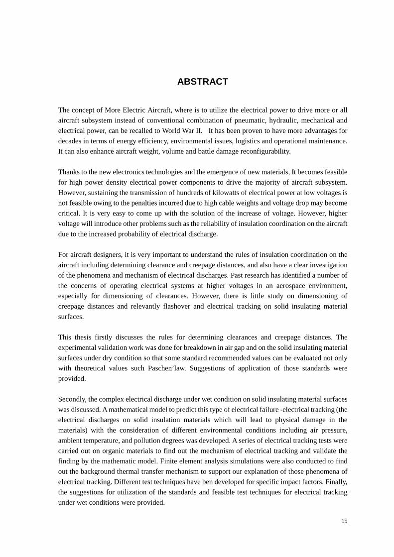
The concept of More Electric Aircraft, where is to utilize the electrical power to drive more or all
aircraft subsystem instead of conventional combination of pneumatic, hydraulic, mechanical and
electrical power, can be recalled to World War II. It has been proven to have more advantages for
decades in terms of energy efficiency, environmental issues, logistics and operational maintenance.
It can also enhance aircraft weight, volume and battle damage reconfigurability.
Thanks to the new electronics technologies and the emergence of new materials, It becomes feasible
for high power density electrical power components to drive the majority of aircraft subsystem.
However, sustaining the transmission of hundreds of kilowatts of electrical power at low voltages is
not feasible owing to the penalties incurred due to high cable weights and voltage drop may become
critical. It is very easy to come up with the solution of the increase of voltage. However, higher
voltage will introduce other problems such as the reliability of insulation coordination on the aircraft
due to the increased probability of electrical discharge.
For aircraft designers, it is very important to understand the rules of insulation coordination on the
aircraft including determining clearance and creepage distances, and also have a clear investigation
of the phenomena and mechanism of electrical discharges. Past research has identified a number of
the concerns of operating electrical systems at higher voltages in an aerospace environment,
especially for dimensioning of clearances. However, there is little study on dimensioning of
creepage distances and relevantly flashover and electrical tracking on solid insulating material
surfaces.
This thesis firstly discusses the rules for determining clearances and creepage distances. The
experimental validation work was done for breakdown in air gap and on the solid insulating material
surfaces under dry condition so that some standard recommended values can be evaluated not only
with theoretical values such Paschen’law. Suggestions of application of those standards were
provided.
Secondly, the complex electrical discharge under wet condition on solid insulating material surfaces
was discussed. A mathematical model to predict this type of electrical failure -electrical tracking (the
electrical discharges on solid insulation materials which will lead to physical damage in the
materials) with the consideration of different environmental conditions including air pressure,
ambient temperature, and pollution degrees was developed. A series of electrical tracking tests were
carried out on organic materials to find out the mechanism of electrical tracking and validate the
finding by the mathematic model. Finite element analysis simulations were also conducted to find
out the background thermal transfer mechanism to support our explanation of those phenomena of
electrical tracking. Different test techniques have ben developed for specific impact factors. Finally,
the suggestions for utilization of the standards and feasible test techniques for electrical tracking
under wet conditions were provided.

16
DECLARATION
No portion of the work referred to in this thesis has been submitted
in support of an application for another degree or qualification of this or
any other university, or institution of learning
17
COPYRIGHT
The author of the thesis (including any appendices and/or schedules to this thesis) owns
certain copyright or related rights in it (the “Copyright”) and s/he has given the University of
Manchester certain right to use such Copyright including for any administrative purposes.
Copies of this thesis, either in full or in extracts and whether in hard or electronic copy,
may be made only in accordance with the Copyright, Designs and Patents Act 1988 (as
amended) and regulations issued under it or, where appropriate, in accordance with
licensing agreements which the University has from time to time. This page must form part
any such copies made.
The ownership of certain Copyright, patents, designs, trade marks and any and other
intellectual property (the “intellectual Property”) and any reproductions of copyright works in
the thesis, for example graphs and tables (“reproductions”), which maybe described in this
thesis, may not be owned by the author and may be owned by third parties. Such
Intellectual Property Rights and Reproductions cannot and must not be made available for
use without the prior written permission of the owner(s) of the relevant Intellectual Property
Rights and/or Reproductions.
Further information on the conditions under which disclosure, publication and exploitation
of this thesis, the Copyright and any Intellectual Property Rights and/or Reproductions
described in it may take place is available from in the university IP policy (see
http://www.campus.manchester.ac.uk/medialibrary/policies/intellectualproperty.pdf), in any
relevant thesis restriction declarations deposited in the University Library, The University
Library’s regulations (see http://www.manchester.ac.uk/library/aboutus/regulations) and in
The University’s policy on presentation of Theses.

18
ACKNOWLEDGEMENTS
Initially, I wish to express my sincere gratitude to my supervisor, Prof. Ian Cotton
who gives me an opportunity to do this research, and make this thesis possible. I
also would like to sincerely thank him for his valuable guidance and continuous
encouragement, which were essential to the completion of this PhD research study.
I am also very grateful to Mr. Frank Hogan in the high voltage laboratory for his
warm and selfless advice, help and patience. Many thanks also to my other
colleagues in the laboratory, particularly Dr. Ningyan Wang, Dr. Sanjay
Bahadoorsingh, Xiaolei Cai,Vidyadhar Peesapati, Ilias Christou, Riccardo Giussani
for providing such a stimulating and relaxed research environment and fun stuffs in
Manchester.
Many thanks to Mr Steve and mechanical workshop stuff for their kindly smiles and
instant response whenever I asked for supporting my research in the department.
Finally , very special thanks are also due to my dad and mum in Baotou, China, Jing
Wang, Dan Wang, Qianqian, Judith, James and all of my friends in the UK for their
great support and encouragement in whole remarkable days.
Many thanks to everybody who ever gave me help and support.
Chapter 1 Introduction
19
Chapter 1 Introduction
1.1. Overview
The concept of “all-electric aircraft”/”more electric aircraft” aircraft (AEA/MEA) is far
from new. Since World War II, military aircraft designers have been aware of this concept
[1-3]. MEA means that more power off-takes from the aircraft are electrical in nature, which
means the need for on-engine hydraulic power generation and bleed air off-takes is removed.
By adopting the concept, advantages in terms of energy efficiency, environmental issues,
logistics and operational maintenance can be achieved. It can also enhance aircraft weight,
volume and battle damage reconfigurability.
Conventional aircraft architectures used for civil aircraft are comprised of a combination of
systems dependent on mechanical, hydraulic, pneumatic and electrical sources. The
resulting conventional equipment is the product of decades of development by system
suppliers.
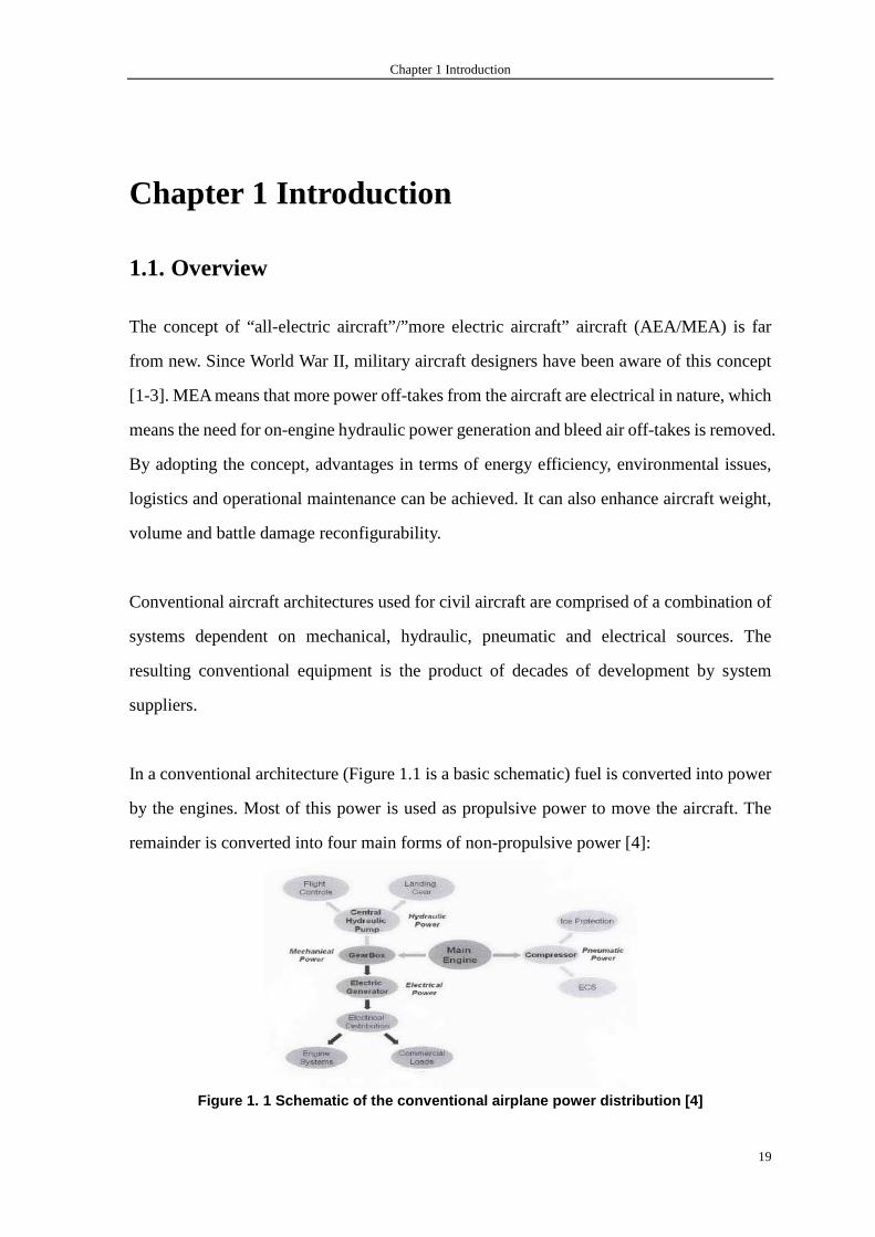
In a conventional architecture (Figure 1.1 is a basic schematic) fuel is converted into power
by the engines. Most of this power is used as propulsive power to move the aircraft. The
remainder is converted into four main forms of non-propulsive power [4]:
Figure 1. 1 Schematic of the conventional airplane power distribution [4]
Chapter 1 Introduction
20
• Pneumatic power, obtained from the engines’ high-pressure compressors. This kind
of energy is conventionally used to power the Environmental Control System (ECS)
and supply hot air for Wing Anti-Icing (WAI) systems. Its drawbacks are low
efficiency and a difficulty in detecting leaks.
• Mechanical power, which is transferred (by means of the mechanical gearboxes)
from the engines to central hydraulic pumps, to local pumps for engine equipment
and other mechanically driven subsystems, and to the main electrical generator.
• Hydraulic power, which is transferred from the central hydraulic pumps,: to the
actuation systems for primary and secondary flight control; to landing gear for
deployment, retraction, and braking; to engine auction; and to numerous ancillary
systems. Hydraulic systems have a high power density and are very robust. Their
drawbacks are a heavy and inflexible infrastructure (piping) and the potential
leakage of dangerous and corrosive fluids.
• Electrical power, which is obtained from the main generator in order to power the
avionics cabin and aircraft lighting, galleys and other commercial loads (such as
entertainment systems). Electrical power does not require a heavy infrastructure and
is very flexible. Its main drawbacks are that conventionally it has a lower power
density than hydraulic power, and results in a higher risk of fire (in the case of a
short circuit) [4].
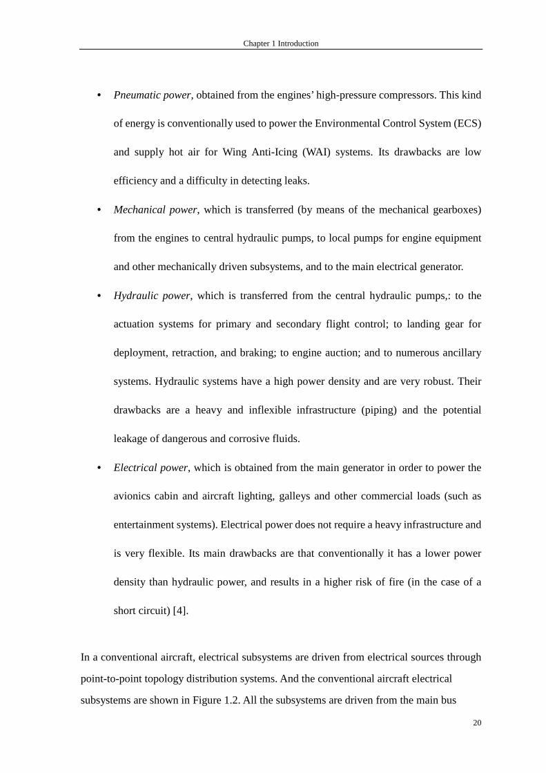
In a conventional aircraft, electrical subsystems are driven from electrical sources through
point-to-point topology distribution systems. And the conventional aircraft electrical
subsystems are shown in Figure 1.2. All the subsystems are driven from the main bus
Chapter 1 Introduction
21
through relays and switches. This kind of distribution network leads to expensive
complicated and heavy wiring circuits.
Figure 1.2 Conventional aircraft electrical subsyst ems
As time has gone by, each system has become more complex, and interactions between
different pieces of equipments reduce the efficiency of the whole system. A simple leak in
the pneumatic or hydraulic system may lead to the outage of every user of that network,
resulting in a grounded aircraft and flight delays. The leak is generally difficult to locate and
once located it cannot be addressed easily.
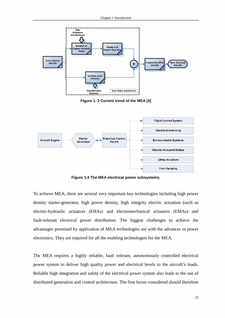
The trend is to move towards “all-electric aircraft”/”more electric aircraft” aircraft
(AEA/MEA) as shown in Figure 1.3. The drives for civil aircraft and fast military jets to
apply the concept of MEA are to maximize dynamic performance and its efficiency while
minimizing equipment volume and mass. Meanwhile, due to the difficult economy
environment, the affordability is key consideration in terms of cost of the development,
manufacture, operation, maintenance, and personnel. Removal of pneumatic and hydraulic
systems with electrical systems results in improvement in fuel efficiency. And electrical
subsystems can be used only when needed. Figure 1.3 shows the manners to realize the
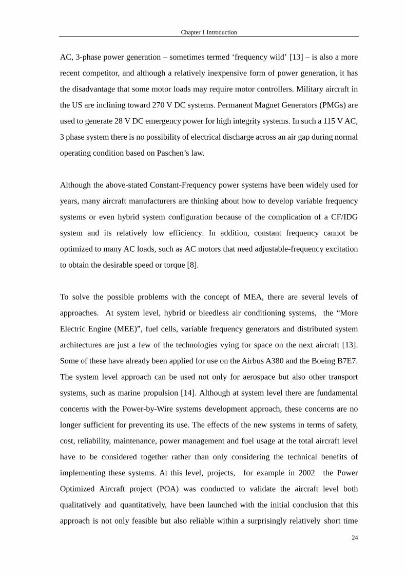
concept of MEA [4]. And MEA electrical power subsystems are illustrated in Figure 1.4.
Chapter 1 Introduction
22
Figure 1. 3 Current trend of the MEA [4]
Figure 1.4 The MEA electrical power subsystems.
To achieve MEA, there are several very important key technologies including high power
density starter-generator, high power density, high integrity electric actuation (such as
electric-hydraulic actuators (EHAs) and electromechanical actuators (EMAs) and
fault-tolerant electrical power distribution. The biggest challenges to achieve the
advantages promised by application of MEA technologies are with the advances in power
electronics. They are required for all the enabling technologies for the MEA.
The MEA requires a highly reliable, fault tolerant, autonomously controlled electrical
power system to deliver high quality power and electrical levels to the aircraft’s loads.
Reliable high integration and safety of the electrical power system also leads to the use of
distributed generation and control architecture. The first factor considered should therefore

Chapter 1 Introduction
23
be the large amount of power electronics for power conversions and power users that MEA
will involve: at least 1.6MW for a next generation 300 pax aircraft [5]. Further, one major
evolutionary technological advance which has contributed heavily to the feasibility of an
electrically-cased aircraft non-propulsive power system has been the development of
reliable, solid state, high power density, power related electronics, since the power
transferred to the load is processed almost three times [5-8].
Much literature [9-12] has already proven that even without the advent of more electrical
aircraft, the power level of the airplane has been increased. In order to provide a clearer
view of contemporary electrical generation for the airplane, the different types of electrical
power generation currently being considered and proposed civil and military aircraft
platforms through the 1990s are shown in Figure 1.5.
Figure 1.5 Candidate electrical power generation ty pes
From Figure 1.5, we can see that the Constant Frequency (CF) 115 V AC, 3-phase, 400 Hz
options consist of the Integrated Drive Generator (IDG), Variable Speed Constant
Frequency (VSCF) cycle-converter and DC link options. Variable Frequency (VF) 115 V
Chapter 1 Introduction
24
AC, 3-phase power generation – sometimes termed ‘frequency wild’ [13] – is also a more
recent competitor, and although a relatively inexpensive form of power generation, it has
the disadvantage that some motor loads may require motor controllers. Military aircraft in
the US are inclining toward 270 V DC systems. Permanent Magnet Generators (PMGs) are
used to generate 28 V DC emergency power for high integrity systems. In such a 115 V AC,
3 phase system there is no possibility of electrical discharge across an air gap during normal
operating condition based on Paschen’s law.
Although the above-stated Constant-Frequency power systems have been widely used for
years, many aircraft manufacturers are thinking about how to develop variable frequency
systems or even hybrid system configuration because of the complication of a CF/IDG
system and its relatively low efficiency. In addition, constant frequency cannot be
optimized to many AC loads, such as AC motors that need adjustable-frequency excitation
to obtain the desirable speed or torque [8].
To solve the possible problems with the concept of MEA, there are several levels of
approaches. At system level, hybrid or bleedless air conditioning systems, the “More
Electric Engine (MEE)”, fuel cells, variable frequency generators and distributed system
architectures are just a few of the technologies vying for space on the next aircraft [13].
Some of these have already been applied for use on the Airbus A380 and the Boeing B7E7.
The system level approach can be used not only for aerospace but also other transport
systems, such as marine propulsion [14]. Although at system level there are fundamental
concerns with the Power-by-Wire systems development approach, these concerns are no
longer sufficient for preventing its use. The effects of the new systems in terms of safety,
cost, reliability, maintenance, power management and fuel usage at the total aircraft level
have to be considered together rather than only considering the technical benefits of
implementing these systems. At this level, projects, for example in 2002 the Power
Optimized Aircraft project (POA) was conducted to validate the aircraft level both
qualitatively and quantitatively, have been launched with the initial conclusion that this
approach is not only feasible but also reliable within a surprisingly relatively short time
Chapter 1 Introduction
25
span compared to a system level approach. Although there is a trend for aircraft electrical
systems being heavier it is possible for a MEA to provide a reduction in fuel usage at the
aircraft level [15]. These results indicate that it is inevitable to have a high degree of
integration of equipment systems in the MEA and points the way towards an intensively
integrated approach to designing new aircraft.
A number of programs have been launched in this field [16]. For example, the US Air Force
MEA Program aims to investigate providing more electrical capability for fighter aircrafts;
in the late nineties, the Division of Militaries Aircrafts of Norhrop/Grumman developed the
MADMEL project, related to the power distribution system and power management for
more electric aircraft [17]. Power Optimized Aircraft (POA), the first important integration
initiative in Europe, aims to optimize the management of electrical power on aircraft. One of
the main research lines has been the introduction of electrical loads management, which
permits the introduction of new technologies in onboard systems, power electronics [18].
Meanwhile, the European Commission of Community Research has initiated a dynamic
program named European Technology/Research and Product Development in Aeronautics
(EUR/TD in Aeronautics). From 1990 up to 2006, a total of six Framework programs had
proceeded successfully. The seventh Framework program was launched in 2007 and is
supposed to be accomplished in 2013. The recent program aims to develop an integrated
“greener” and “smarter” pan-European transport system for the benefit of citizens and
society, respecting the environment and natural resources so that the leading role attained by
the European industries in the global market can be developed and extended. For
aeronautics and air transport, the Aeronautic Joint Technology Initiative has been proposed
with the aim of providing a step forward in the technological capability of environmentally
friendly Air Transport Systems (ATS), improving overall ATS impact on the environment
including noise, emission reduction and fuel consumption. Other minor projects performed
in Europe are the TIMES and DEPMA programs [19, 20].
Recently, Boeing, in collaboration with the European Research Center located in Madrid,
Chapter 1 Introduction
26
has developed a totally electric propeller aircraft, promoted by a hybrid power system. The
system is based on a fuel cell in combination with an Ion-Lithium battery which provides
the energy to an electric engine, connected to a conventional propeller. The fuel cell is able
to supply the overall energy during the cruise-flight stage. During takeoff or landing, the
energy is provided by both the fuel cell and the ion-lithium battery [21].
In the aircraft, different kinds of load require different power supplies. Even in conventional
examples there are different voltage types, normally commercial aircraft 115 V AC with
some components requiring 28 V DC. In the advanced future aircraft, higher voltage levels
will be employed such as 270 V DC and 230VAC, so far used in military aircraft, and to be
used in commercial aircraft in the future [7, 17, 22, 24, 25]. Other approaches are focused on
applications with higher voltage levels like 540 V DC [26]. Whereas 270 V DC is obtained
from rectification of the traditional 115 V AC, 230 V AC could be easily obtained by
doubling the existing voltage level provided by the generator, 115 VAC. Regarding 540 V
DC, voltage level is a consequence of using the differential voltage provided by two buses
of ± 270 V DC with a common reference on ground.. Therefore future aircraft electrical
system will use a multi-voltage level hybrid DC and AC system. The electrical system is no
longer only comprised of components which convert electrical power from one form to
another, but also components which convert the supply to a higher or lower voltage level.
As a result, the modern aircraft has all kinds of power electronics converters such as AC/DC
rectifier, DC/AC inverters, and DC/DC choppers. In addition, in the variable speed constant
frequency (VSCF) systems, solid-state bi-directional converters are used to condition
variable-frequency power into a fixed frequency and voltage. Moreover, bi-directional
DC/DC converters are used in battery charge/discharge units. Therefore MEA electrical
distribution systems are mainly in the form of multi-converter power electronic systems.
Due to extensive interconnection of components, a large variety of dynamic interactions is
possible [28].
Increases in the operating voltage of an aircraft have been gradual. Aircraft electrical
systems, from operating at 14.25 V DC in 1936, rose to 28 V DC in 1946 [3] and ultimately
Chapter 1 Introduction
27
became the common 115/200 V AC 400 Hz systems in use in the majority of civil aircraft
today. 270 V DC was used by the military to provide further weight savings in the 1980s
[29].
The current aircraft being designed with a more electric architecture include the Boeing 787,
which will have 250 kVA of electrical generation capability in each engine. Along with the
auxiliary power generation, the total available generation is in the order of 1500 kVA [27].
The Airbus A350 is expected to have a power generation capability in the order of 800 kVA.
To support these generation levels, Boeing have moved from a 115V AC 400Hz system to a
combined 230 V AC 360-800Hz and +/- 270 VDC (540 V DC) system. [27].
Since the concept of MEA involves the power level increasing, sustaining the transmission
of hundreds of kilowatts of electrical power at low voltages is not feasible owing to the
penalties incurred due to high cable weights [13] and voltage drop may become critical. It is
very easy to come up with the solution of the increase of voltage. However, higher voltage
will introduce other problems such as the reliability of insulation coordination on the
aircraft due to the increased probability of electrical discharge.
Past research has identified a number of the concerns of operating electrical systems at
higher voltages in an aerospace environment. Bilodeau, Dunbar and Sarjeant discussed the
increased demand for higher voltage usage in space power systems owing to the need to
reduce the weight that would result from the use of lower voltage systems and the necessary
test regimes[30]. Many papers examine some of the basic issues relating to the operation /
testing of higher voltage systems in a low pressure environment. Dunbar [31] stressed a
wire with high voltage to determine the effect of high frequency at high altitudes. His results
indicate a reduction in the partial discharge inception voltage of around 15% at frequencies
above 40 kHz for an altitude of 33000 ft. Dunbar states in another paper [32] that partial
discharge can cause significant numbers of failures in high voltage systems. Brockschmidt
[33]also discusses the problems associated with the operation of higher voltage systems in a
low pressure environment and states that the voltage required to sustain partial discharge
Chapter 1 Introduction
28
can be lower than that required to initiate it. Karady et al [34] examined the corona inception
voltage of simple electrode geometries including ones that involved thin layers of electrical
insulation. The authors show that for certain experimental arrangements, corona inception
can take place at voltages lower than Paschen’s minimum. Hammoud and Stavnes [35]
conducted breakdown tests on different types of aerospace cable observing a reduction in
the breakdown voltage of 20% occurred when using a testing frequency of 400 Hz at 200 ºC.
A study was conducted on polypropylene cable by [36] at different frequencies, ranging
from 50 to 400 Hz. The results of these tests correlated with [35] in that breakdown voltages
of such insulation could fall as a function of frequency.
A key document, although dated, provides excellent information across many of the
pertinent issues; this was produced by Dunbar [37]. This describes the operating
environment of an aircraft, the types of electrical discharge that could take place and
provides guidelines and precautions to be taken into consideration in the insulation design
of electrical and electronic equipment. It also provides guidelines for monitoring and testing.
Dunbar recognized that all types of discharges lead to the deterioration of the insulation of
machines, drives and cabling – something that could lead to premature failure of the aircraft
system. In designing insulation systems, factors such as out-gassing, and thermal and high
voltage field stresses on materials have to be taken into account. In addition the effects of
“temperature cycling, high density packaging, frequency and long mission durations” have
to be investigated.
1.2. Aims and objectives of the research
In order to get deep understating of insulation coordination of electrical systems in More
Electrical Aircraft, a considerable amount of research works has been done in my
department such as the PhD research work of Dr. Andrew Nelms has dealt with the cabling
systems, and Miss Rui Rui is now working on the machinery systems. My research
concentrated on the electrical discharges on any surfaces that electrical fields cross, such as

Chapter 1 Introduction
29
the printed circuit boards, connectors or outside of power electronics modules. This
inevitably comes down to dimensioning of clearances and creepage distances with regard to
its application and in relation to its surroundings. The term clearance has come to be used to
refer to the shortest distance in air between two conductive parts. Creepage distances can be
defined as the shortest distance along the surface of the insulating material between two
conductive parts.
First of all, the project will focus on studying the determination of clearances and creepage
distances under dry condition. The rules of the dimensioning of clearances and creepage
distances will be reviewed according to the understanding of the IEC 60664 and IPC 2221.
And then experimental test results will be presented and compared with the values
suggested in those standards to validate and explain the standards deeply. My work will
provide science basis of allocation of those standard values for aircraft designers.
Secondly, the project will mainly concentrate on tracking phenomena under wet condition.
To develop a mathematical model to predict this type of electrical failure -electrical tracking
(the electrical discharges on solid insulation materials which will lead to physical damage in
the materials) with the consideration of different environmental conditions including air
pressure, ambient temperature, and pollution degrees. A series of electrical tracking tests
will be carried out on organic materials to find out the mechanism of electrical tracking and
validate the finding by the mathematic model. Finite element analysis simulations will also
be conducted to find out the background thermal transfer mechanism to support my
explanation of those phenomena of electrical tracking. Different test techniques will be
developed for specific impact factors. Contribution will be made to:
• establishing the electrical tracking behavior of surfaces that exist in power switches and
the power electronic cores used in aircraft,
• determining models describing it,
• providing guidelines for better electrical tracking testing methods for creepage distances,
Chapter 1 Introduction
30
and
• Generating design rules for the mitigation of electrical tracking for next-generation
aircraft.
1.3. The AIMEA program
The research was sponsored by the project called More Open Electrical Technologies
(MOET) which was launched successfully on July 2006. MOET aims to establish a new
industrial standard for electrical system design in commercial aircraft. This will strengthen
the competitiveness of the EU’s aerospace industry. One of MOET’s important design
objectives is to improve operational aircraft capacity. Its Power-by-Wire (PbW) concept
will enhance aircraft design and electrical power flexibility.
The main result of the three-year project will be the validation of scalable electrical
networks up to 1 MW for future air, actuation and electrical systems, considering new
voltage levels and advanced concepts. To achieve its goals, MOET will need to develop new
design principles, technologies and standards. The entire project will run under the overall
management of Airbus France.
The Electrical Energy and Power Systems group at the University of Manchester is a
participant in this joint development project by 61 companies in the EU’s Framework
Programme 6. My contribution will be in work package 3.32, which aims to: establish the
partial discharge behaviour of existing power switches and the power electronic core;
determine models describing partial discharge in power switches and power electronic core;
and also generate design rules for mitigation of partial discharge.
On 14th December 2004 AIMEA was formed by four UK Universities, including the
University of Manchester, the University of Sheffield, the University of Nottingham, and
the University of Bristol. It is the second largest partner in MOET in term of man-hours and
Chapter 1 Introduction
31
fifth in terms of costs.
1.4. Organization of the thesis
The thesis is subdivided into 8 chapters. In Chapter 1, the background of the project is
outlined, including an introduction to More Electrical Aircraft, and the sponsoring
organization. A brief literature review of More Electrical Aircraft and the challenges
coming up with it is presented.
In Chapter 2, the literature survey is conducted on different types of electrical discharges
and their characteristics. In addition, some test methods are also represented. Problems
faced at present are further explained.
In Chapter 3, the design of insulation coordination in low-voltage equipment including
dimensioning of clearances and creepage distances specified in both IEC 60664 and IPC
2221 is presented in detail. The requirements in the existing guidelines are evaluated and
validated against the test results attained from breakdown of air gap tests under both
uniform fields and non-uniform fields and dry breakdown tests on solid insulation materials.
Paschen’s curve is also used to compare these test results. Finally, recommendations of
employing these standards are summarized.
In Chapter 4, the mathematical model of initiating electrical tracking on solid insulation
material is developed. Different impact factors are discussed by applying the model and
finite element analysis simulation is conducted to not only find out the static analysis of this
model but also to look into the dynamic status of electrical progressing.
In Chapter 5, standardized comparative tracking index test techniques are employed to
investigate the mechanism of electrical tracking under aqueous contamination environment,
and a comparison is done between the test results and theoretical calculation results by using
Chapter 1 Introduction
32
the model developed in Chapter 4. Thermal images are recorded and discussed to correlate
the initial electrical discharges and electrical tracking under wet conditions.
Chapter 6 focuses on the test results under lower air pressure environmental condition. The
same aqueous contamination and similar test methods are used, and the environment
chamber is used to change the ambient air pressure. The influence of air pressure, which is a
unique factor to be considered for aerospace application, is also discussed.
To generate a guideline of clearance and creepage distances, the standardized comparative
tracking test technique is not applicable due to its gap distance limitation of 4mm. Chapter 7
shows the development of test techniques on electrical tracking to varying gap distance on
solid insulation. The repeatability of the test results is compared with the previous test
results from standardized tests. Test results provide a guideline of creepage distances under
atmospheric pressure. The comparison is also conducted against those in IEC 60664 and
IPC 2221.
Finally, some conclusions based on the test results are given, and last but not least areas of
future work are discussed.
Chapter 2 Review Electrical Discharges, Characteristics, and Relevant Test Techniques
33
Chapter 2 Review Electrical Discharge,
Characteristics, and Relevant Test Techniques
2.1. Introduction
The aim of our research was to firstly examine and validate existing guidelines for
dimensioning clearances and creepage distances for aerospace applications, especially for
advanced More Electrical Aircraft electrical systems operating at higher voltages. These
clearances and creepage distances must be specified to avoid all kinds of electrical
discharge. A brief review of IEC 60664: 2003 “Insulation Coordination For Equipments
Within Low-voltage Systems” and IPC 2221 “Generic Standard on Printed Board Design”
will be presented in this chapter. By doing this, we can show that it is necessary to
re-validate those rules so that more precise ones with more detailed environmental
conditions will help in future electrical system design for large More Electrical Aircraft.
Generally speaking, electrical discharges can be classified into three major types: disruptive
discharges, partial discharges and tracking. As shown in the following detailed information,
we can see that all of them are directly or indirectly agree to Paschen’s law to some extent.
To understand Paschen’s law, it is important to review the fundamental principle of
breakdown in the air under uniform and non-uniform fields, following this, each discharge
type will be discussed. The approach employed in “High Voltage Engineering
Fundamentals” written by E. Kuffel, W. S. Zaengl and J. Kuffel is followed in this
section[38]. For partial discharge, we only give a very brief review since it will not be my
research focus. Electrical tracking will be explained in detail.
Relevant test techniques will also be discussed. The electrical breakdown test method,
specified in IEC 60: 1989”High-voltage Testing Techniques” has been widely accepted by
Chapter 2 Review Electrical Discharges, Characteristics, and Relevant Test Techniques
34
most researchers as the method to study breakdown. In this thesis it will not emphatically
state. However, for electrical tracking tests, to date various methods have been developed
to measure inception voltage for tracking or just to observe the behaviour of it. The
standardized test methods including A.S.T.M D 495”High voltage low current arc
resistance of solid electrical insulating materials”, IEC 60112 ”comparative tracking index
test”, IEC 60587 inclined plane test will be discussed in detail and further method ,such as
dust-fog test, developed by different organizations also presented.
2.2. Electrical breakdown in gases
This section will elaborate the mechanism of ionization and decay processes which are
critical to promote conduction in gases, and then a complete breakdown and spark
formation. Before proceeding to discuss electrical breakdown in gases it is appropriate to
introduce some import fundamental definitions relevant to kinetic theory of gases.
At ambient pressure and temperature, most gases have very good insulation properties. E.
Kuffel claimed in the book [38] the conduction in air at low field is between
1610− - 1710− A/ 2cm (on page 294). This minor conductive effect is from cosmic radiation and
radioactive substances present in the earth and the atmosphere.
Historically the electron collision ionization was first explained by Townsend [39]. It is the
most important ionization processes leading to breakdown of gases under high electric
field. As explained electrons always exist in atmospheric space. Under higher electrical
fields, those free electrons could gain sufficient kinetic energy ( eW eEλ∆ = ) which must
be at least equal to the ionization energy of the molecule ( ieV ) between collisions to cause
ionization on impact with neutral molecules. Hence, the amount of energy gained by an
electron depends on the distances through which the electron is accelerated by the electrical
force between collisions and determines the effectiveness of ionizations. The average
distance can be defined as the free path (λ ). For an electron, this parameter is a stochastic

Chapter 2 Review Electrical Discharges, Characteristics, and Relevant Test Techniques
35
quantity and the mean free path (λ ) depends on the nature of the gases and their density.
The impact of attachments and recombination and the cathode effect to the ionization
processes is also illustrated in this section to give a whole picture.
The derivation of theoretical ionization equations for initiating discharge is also provided
by considering the Townsend first ionization coefficientα , the attachment coefficientη
and Townsend second ionization coefficientγ , where α α η= − represents the effective
ionization coefficient. This is called the Townsend criterion for spark formation or
Townsend breakdown criterion. The criteria of conductive current between two electrodes
to become self-sustaining discharge indicate the initial one electron through electron
avalanche and secondary electron emission by photo impact at cathode can produce at
least one electron which can consequently cause a repetition of the avalanche. The
expression for breakdown voltage for uniform field gaps as a function of gap length and
gas pressure can be derived based on the Townsend breakdown criteria, which is named
Paschen’s law.
Finally the mechanism of breakdown under non-uniform field and partial discharges were
illustrated.
2.2.1. Useful definitions in gas kinetic theory
There are two types of collision between gas particles. One is called elastic or simple
mechanical collisions in which the energy exchange is always kinetic. The other is inelastic,
in which some of the kinetic energy of the collision particles is transferred into the potential
energy of the struck particle or vice versa. The latter includes excitation, ionization,
attachments, etc, closely connected to electrical breakdown in gases.
The Mean Free Path λ of molecules and electrons
The free path (λ ) is defined as the distance molecules or particles travel between collisions.
Chapter 2 Review Electrical Discharges, Characteristics, and Relevant Test Techniques
36
The free path is a random quantity, and it will be shown that the mean free path depends
upon the concentration of particles or the density of the gas.
The relation between the effective diameter of a molecule and the concentration of particles
can be expressed that at room temperature and air pressure (27 C , 510 Pa), the larger the
diameter of molecule, the more likely collision is, and the smaller the average free path.
Further, the relationship with temperature T and pressure p is that, when temperature is
kept constant, an increase in pressure results in the mean free path decreasing. Additionally,
with constant pressure, the mean free path is directly proportional to the temperature.
Numerically speaking, to derive the mean free path, we can assume an assembly of
stationary molecules of radius1r , and a moving layer of smaller particles of radius 2r as
particles move. As the smaller particles move, their density will decrease due to scatting
caused by collision with gas molecules. We can therefore deduce the expression of the mean
free path based on the probability of the free path of length x being equal to the probability
of collisions between x tox dx+ . For mean free path, therefore:
0
( )x
x xf x dxλ∞
=
= = ∫
2
1 2( )21 2
0
( ) N r r x
x
N r r xe dxππ∞
− +
=
= + ∫
2
1 2
1
( )N r rπ=
+…………… (2.1)
The denominator in eqn. 2.1 has represents the dimensions of area and the value 21 2( )r rπ +
is usually called the cross-section for interception or simply collision cross-section, and is
defined by σ
1
Nσ
λ−= ………….(2.2)
Chapter 2 Review Electrical Discharges, Characteristics, and Relevant Test Techniques
37
As we know that /N p kT= , it follows that the mean free path is directly proportional to
temperature and inversely proportional to the gap pressure.
00
0
( , )p T
p Tp T
λ λ= ………. (2.3)
2.2.2. The appearance and disappearance of the charged
particles in gases
Ionization by collision
The state of equilibrium of a gas can be upset by the application of a sufficiently high field.
At higher fields charged particles are accelerated by electrical field force. However, they
cannot keep building up their kinetic energy, due to collisions. On one hand, during elastic
collisions, they lose little energy and kinetic energy can still accumulate. On the other hand,
however, some of the particles that have already gained enough energy will have inelastic
collisions. As a result, a large fraction of their kinetic energy is transferred into potential
energy, causing, for example, ionization of the struck molecule. Electrons in gases are
always at a much high velocity than those very big molecular. They can more easily collect
kinetic energy and cause ionization, which is the most important process leading to
breakdown of gases. The effectiveness of ionization by electron impact depends upon the
energy that an electron can gain along the mean free path in the direction of the field.
If eλ is the mean free path in the field direction of strength E then the average energy
gained over a distance λ is eW eEλ∆ = . This quantity is proportional to /E p since
1/e pλ ∝ . To cause ionization on impact the energy W∆ must be at least equal to the
ionization energy of the molecule (ieV ) which may excite the particle; the excited particles
on collision with electrons of low energy may become ionized. Furthermore, not all
electrons having gained energy iW eV∆ ≥ upon collision will cause ionization. This
Chapter 2 Review Electrical Discharges, Characteristics, and Relevant Test Techniques
38
simple model is not applicable for quantitative calculations, because ionization by collision,
as with all other processes in gas discharges, is a probability phenomenon, and is generally
expressed in terms of cross-section for ionization defined as the product i iPσ σ= where
iP the probability of ionization on impact is and σ is the molecular or atomic
cross-sectional area for interception defined. The cross-section iσ is measured using
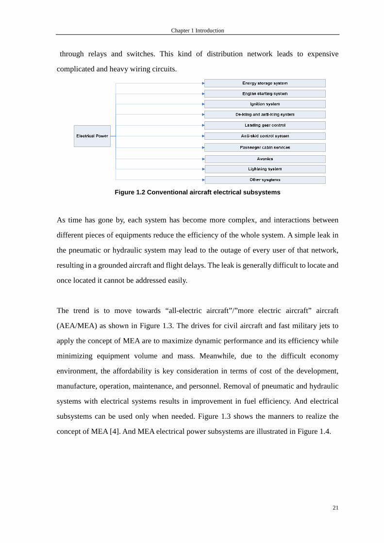
monoenergetic electron beams of different energies. The variation of ionization
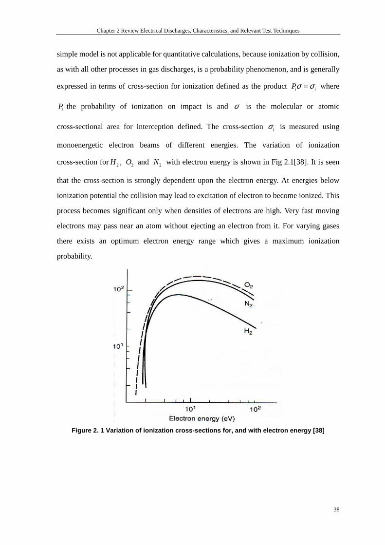
cross-section for 2H , 2O and 2N with electron energy is shown in Fig 2.1[38]. It is seen
that the cross-section is strongly dependent upon the electron energy. At energies below
ionization potential the collision may lead to excitation of electron to become ionized. This
process becomes significant only when densities of electrons are high. Very fast moving
electrons may pass near an atom without ejecting an electron from it. For varying gases
there exists an optimum electron energy range which gives a maximum ionization
probability.
Figure 2. 1 Variation of ionization cross-sections for, and with electron energy [38]
Chapter 2 Review Electrical Discharges, Characteristics, and Relevant Test Techniques
39
Photoionization
Electrons of lower energy than the ionization energy ieV may on collision excite the gas
atoms to higher states. The reaction may be symbolically represented as A e K+ + energy
*A e→ + ; *A A hυ→ + ; *A represents the atom in an excited state. On recovering
from the excited state in some 7 1010 10− −− sec, the atom radiates a quantum of energy of
photon (hυ ) which in turn may ionize another atom whose ionization potential energy is
equal to or less than the photon energy. The process is known as photoionization and may be
represented as A h A eυ ++ → + , where A represents a neutral atom or molecule in the
gas and hυ the photon energy. For ionization to occur ih eVυ ≥ or the photon
wavelength 0 / ic h eVλ ≤ , 0c being the velocity of light and h being Planck’s constant.
Therefore, only very short wavelength light quanta can cause photoionization of gas. For
example, the shortest wavelength radiated from a UV light with quartz envelope is 145nm,
which corresponds to 8.5ieV eV= , lower than the ionization potential of most gases.
The probability of photon ionization of a gas or molecule is maximum when ( )ih eVυ − is
small(0.1 1 )eV− . Photoionization is a secondary ionization process and may be acting in
the Townsend breakdown mechanism, as explained in section 2.1.3.2, and is essential in the
streamer breakdown mechanism in some corona discharges. If the photon energy is less than
ieV it may still be absorbed by the atom and raise the atom to a higher energy level. This
process is known as photoexcitation.
Ionization by interaction of metastables with atoms
In certain elements the lifetime in some of the excited electronic states extends to seconds.
These states are known as metastable states and the atoms in these states are simply referred
to as metastables, represented bymA . Metastables have relatively high potential energy and

Chapter 2 Review Electrical Discharges, Characteristics, and Relevant Test Techniques
40
are therefore able to ionize neutral particles. IfmV , the energy of a metastablemA , exceeds
iV , the ionization of another atom B , then on collision ionization may result according to
the reaction:
mA B A B e++ → + + ……….. (2.4)
For mV of atom miA V⟨ of an atom B the reaction may lead to the exciting of the atom B
which may be represented by
*mA B A B+ → + ………… (2.5)
Another possibility for ionization by metastables is when 2 mV for mA is greater than iV
for A. The reaction may proceed as:
. .m mA A A A e K E++ → + + + ………… (2.6)
The last reaction is important only when the density of metastables is high.
Another reaction may follow as:
*22mA A A A+ → + ………… (2.7)
*2A A A hυ→ + + …………… (2.8)
The photon released in the last reaction is of too low energy to cause ionization in pure gas,
but it may release electrons from the cathode.
Ionization by metastable interactions comes into operation long after excitation, and it has
been shown that these reactions are responsible for long time lags but within the region of
610− - 710− observed in some gases. It is effective in gas mixtures.
Thermal ionization
The term thermal ionization, in general, applies to the ionizing actions of molecular
collisions, radiation and electron collisions occurring in gases at high temperature. If a gas is
heated to sufficiently high temperature many of the gas atoms or molecules acquire
Chapter 2 Review Electrical Discharges, Characteristics, and Relevant Test Techniques
41
sufficiently high velocity to cause ionization on collision with other atoms or molecules.
Thermal ionization is the principal source of ionization in flames and high-pressure arcs.
Cathode process –secondary effect
Electrodes, in particular the cathode, play a very important role in gas discharge by
supplying electrons for the initiation, for sustaining and for the completion of a discharge.
Under normal conditions electrons are prevented from leaving the solid electrode by the
electrostatic forces between the electrons and the ions in the lattice. The energy required to
remove an electron from a Fermi level is known as the work function and is a characteristic
of a given material. There are several ways in which the required energy may be supplied to
release the electrons.
• Photoelectric emission
Photons incident upon the cathode surface whose energy exceeds the work function may
eject electrons from the surface. For most metals the critical frequency 0υ lies in the UV
range. When the photon energy exceeds the work function, the excess energy may be
transferred to electron kinetic energy according to the Einstein relation:
20
1
2 emu h hυ υ= = ………. (2.9)
where m is the electron mass, eu its velocity and 0 ah Wυ = the work function.
• Electron emission by collision of positive ions with the cathode
• When positive ions collide with the cathode, electrons will be emitted from the
metal material of the cathode. This phenomenon can occur when the transmitting
energy, including the kinetic energy and potential energy of the positive ion, is at
least twice as large as the work function of the cathode’s metal material. The key
mechanism of this kind of electron emission is that the impinging ion must release
two electrons, one of which is used to combine with the positive ion thus becoming a
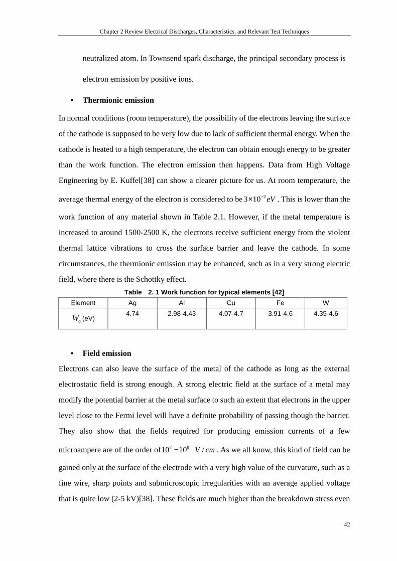
Chapter 2 Review Electrical Discharges, Characteristics, and Relevant Test Techniques
42
neutralized atom. In Townsend spark discharge, the principal secondary process is
electron emission by positive ions.
• Thermionic emission
In normal conditions (room temperature), the possibility of the electrons leaving the surface
of the cathode is supposed to be very low due to lack of sufficient thermal energy. When the
cathode is heated to a high temperature, the electron can obtain enough energy to be greater
than the work function. The electron emission then happens. Data from High Voltage
Engineering by E. Kuffel[38] can show a clearer picture for us. At room temperature, the
average thermal energy of the electron is considered to be 23 10 eV−× . This is lower than the
work function of any material shown in Table 2.1. However, if the metal temperature is
increased to around 1500-2500 K, the electrons receive sufficient energy from the violent
thermal lattice vibrations to cross the surface barrier and leave the cathode. In some
circumstances, the thermionic emission may be enhanced, such as in a very strong electric
field, where there is the Schottky effect.
Table 2. 1 Work function for typical elements [42]
Element Ag Al Cu Fe W
aW (eV) 4.74 2.98-4.43 4.07-4.7 3.91-4.6 4.35-4.6
• Field emission
Electrons can also leave the surface of the metal of the cathode as long as the external
electrostatic field is strong enough. A strong electric field at the surface of a metal may
modify the potential barrier at the metal surface to such an extent that electrons in the upper
level close to the Fermi level will have a definite probability of passing though the barrier.
They also show that the fields required for producing emission currents of a few
microampere are of the order of7 810 10− /V cm. As we all know, this kind of field can be
gained only at the surface of the electrode with a very high value of the curvature, such as a
fine wire, sharp points and submicroscopic irregularities with an average applied voltage
that is quite low (2-5 kV)[38]. These fields are much higher than the breakdown stress even

Chapter 2 Review Electrical Discharges, Characteristics, and Relevant Test Techniques
43
in concentrated gases.
Deionization by recombination
Wherever there are positively and negatively charged particles present, recombination takes
place. The potential energy and relative kinetic energy of the recombination electron-ion is
released as a quantum of radiation. Symbolically the reaction may be represented as:
or m
A e A h
A e A h
υυ
+
+
+ → +
+ → + radiation recombination
Alternatively a third body C may be involved and may absorb the excess energy released
in the recombination. The third body C may be another heavy particle or electron.
Symbolically:
*A C e A C A C hυ+ + + → + → + + ……….. (2.10)
Or
*A e e A e A e hυ+ + + → + → + + ………… (2.11)
Deionization by attachment-electron affinity
Certain atoms or molecules in their gaseous state can readily acquire a free electron to form
a stable negative ion. Gases, whether atomic or molecular, that have this tendency are those
that are lacking one or two electrons in their outer shell and are known as electronegative
gases. Examples include the halogens (F, Cl, Br, I and At) with one electron missing in their
outer shell, and O, S, and Se, with two electrons deficient in the outer shell.
For a negative ion to remain stable for some time, total energy must be lower than that of an
atom in the ground state. The change in energy that occurs when an electron is added to a
gaseous atom or molecule is called the electron affinity of the atom and is designated byaW .
This energy is released as a quantum or kinetic energy upon attachment. Table 2.2 shows the
electron affinities of some elements.
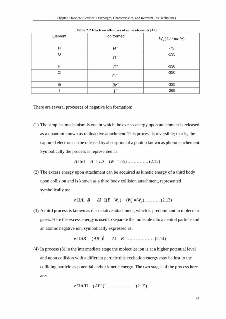
Chapter 2 Review Electrical Discharges, Characteristics, and Relevant Test Techniques
44
Table 2.2 Electron affinities of some elements [42]
Element Ion formed aW ( /kJ mole)
H H − -72
O O−
-135
F F − -330
Cl Cl−
-350
Br Br− -325
I I − -295
There are several processes of negative ion formation:
(1) The simplest mechanism is one in which the excess energy upon attachment is released
as a quantum known as radioactive attachment. This process is reversible; that is, the
captured electron can be released by absorption of a photon known as photodetachement.
Symbolically the process is represented as:
A e A hυ−+ ⇔ + ( )aW hυ= ………….. (2.12)
(2) The excess energy upon attachment can be acquired as kinetic energy of a third body
upon collision and is known as a third body collision attachment, represented
symbolically as:
( )ke A B A B W−+ + → + + ( )a kW W= ………. (2.13)
(3) A third process is known as dissociative attachment, which is predominant in molecular
gases. Here the excess energy is used to separate the molecule into a neutral particle and
an atomic negative ion, symbolically expressed as:
*( )e AB AB A B− −+ ⇔ ⇔ + ……………… (2.14)
(4) In process (3) in the intermediate stage the molecular ion is at a higher potential level
and upon collision with a different particle this excitation energy may be lost to the
colliding particle as potential and/or kinetic energy. The two stages of the process here
are:
*( )e AB AB−+ ⇔ ………………. (2.15)

Chapter 2 Review Electrical Discharges, Characteristics, and Relevant Test Techniques
45
*( ) ( ) k pAB A AB A W W− −+ ⇔ + + + ……….. (2.16)
Other processes of negative ion formation include splitting of a molecule into positive and
negative ions upon impact of an electron without attaching the electron:
e AB A B e+ −+ ⇔ + + …………. (2.17)
And a charge transfer following heavy particle collision, yielding an ion pair according to:
A B A B+ −+ → + …………… (2.18)
All the above electron attachment processes are reversible, leading to electron detachment.
2.2.3. Electron avalanche and Townsend’s first ionization
coefficient
The electron avalanche is essential to the dielectric breakdown. It starts with the first
electron accelerated by an electric field, ionizing the medium’s atoms by collision to
produce the second generation electrons, which continuously undergo the same process in
successive cycles. More and more generation free electrons can be produced, just like an
avalanche. This process can culminate in corona discharges, streamers, or a continuous arc
that completely bridges the gas. Most of the free electrons are collected at the head of the
cone due to electrons’ higher velocity than that of the positive ions, which always gather at
the tail of the cone.
Townsend first studied the variation of gas current measured between two parallel plate
electrodes as a function of applied voltage. He observed that at the beginning of an increase
of the voltage between two electrodes the gas current increased nearly directly
proportionally. It then remains constant 0i until voltage reaches a higher value. The current
then increased above the value 0i at an exponential rate.

Chapter 2 Review Electrical Discharges, Characteristics, and Relevant Test Techniques
46
Te explain this phenomenon, Townsend introduced a quantityα , known as Townsend’s first
ionization coefficient, defined as the number of electrons produced by an electron per unit
length of path in the direction of the field.
Assume that an electron can produce n free electrons of n within the distance of x from
the cathode in the field direction. According to the specification of Townsend’s first
ionization coefficient, the increase in electrons dn in the additional distance dx is given
by:
dn n dxα= ………. (2.19)
Integration over the distance (d ) from the cathode to anode gives:
0dn n eα= ………… (2.20)
Where 0n is the number of primary electrons generated at the cathode, in terms of current,
with 0I the current leaving the cathode, equation (2.20) becomes:
0dI I eα= ……………. (2.21)
The term deα in the equation is called the electron avalanche and it represents the number
of electrons produced by one electron in traveling from the cathode to the anode.
2.2.4. Townsend’s second ionization
When a beam of positive ions collides with the surface of a cathode, secondary electron
emission is likely to occur. Townsend measured this effect of the secondary process in the
same experiment that he measured/ pα . In his experiment, he found that with the voltage
applied between two parallel plates increasing, the rate of the increase of current was higher
than given in equation (2.21). To explain this departure from linearity Townsend postulated
that a second mechanism must be affecting the current, which was firstly considered to be
the liberation of electrons in gas by the collision of positive ions, but later was attributed to
the liberation of electrons from the cathode by positive ion bombardment according to the
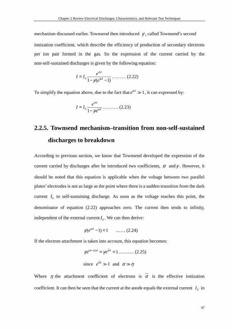
Chapter 2 Review Electrical Discharges, Characteristics, and Relevant Test Techniques
47
mechanism discussed earlier. Townsend then introduced γ , called Townsend’s second
ionization coefficient, which describe the efficiency of production of secondary electrons
per ion pair formed in the gas. So the expression of the current carried by the
non-self-sustained discharges is given by the following equation:
0 1 ( 1)
d
d
eI I
e
α
αγ=
− −……… (2.22)
To simplify the equation above, due to the fact that 1deα≫ , it can expressed by:
0 1
d
d
eI I
e
α
αγ=
−………. (2.23)
2.2.5. Townsend mechanism–transition from non-self-sustained
discharges to breakdown
According to previous section, we know that Townsend developed the expression of the
current carried by discharges after he introduced two coefficients, α andγ . However, it
should be noted that this equation is applicable when the voltage between two parallel
plates’ electrodes is not as large as the point where there is a sudden transition from the dark
current 0I to self-sustaining discharge. As soon as the voltage reaches this point, the
denominator of equation (2.22) approaches zero. The current then tends to infinity,
independent of the external current0I . We can then derive:
( 1) 1deαγ − = …… (2.24)
If the electron attachment is taken into account, this equation becomes:
( ) 1d de eα η αγ γ− = = ………. (2.25)
since 1deα≫ and α η≫
Where η the attachment coefficient of electrons is α is the effective ionization
coefficient. It can then be seen that the current at the anode equals the external current 0I in
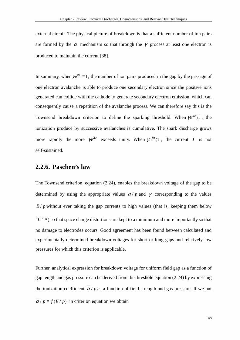
Chapter 2 Review Electrical Discharges, Characteristics, and Relevant Test Techniques
48
external circuit. The physical picture of breakdown is that a sufficient number of ion pairs
are formed by the α mechanism so that through the γ process at least one electron is
produced to maintain the current [38].
In summary, when 1deαγ = , the number of ion pairs produced in the gap by the passage of
one electron avalanche is able to produce one secondary electron since the positive ions
generated can collide with the cathode to generate secondary electron emission, which can
consequently cause a repetition of the avalanche process. We can therefore say this is the
Townsend breakdown criterion to define the sparking threshold. When 1deαγ ⟩ , the
ionization produce by successive avalanches is cumulative. The spark discharge grows
more rapidly the more deαγ exceeds unity. When 1deαγ ⟨ , the current I is not
self-sustained.
2.2.6. Paschen’s law
The Townsend criterion, equation (2.24), enables the breakdown voltage of the gap to be
determined by using the appropriate values / pα and γ corresponding to the values
/E pwithout ever taking the gap currents to high values (that is, keeping them below
710− A) so that space charge distortions are kept to a minimum and more importantly so that
no damage to electrodes occurs. Good agreement has been found between calculated and
experimentally determined breakdown voltages for short or long gaps and relatively low
pressures for which this criterion is applicable.
Further, analytical expression for breakdown voltage for uniform field gap as a function of
gap length and gas pressure can be derived from the threshold equation (2.24) by expressing
the ionization coefficient / pα as a function of field strength and gas pressure. If we put
/ ( / )p f E pα = in criterion equation we obtain
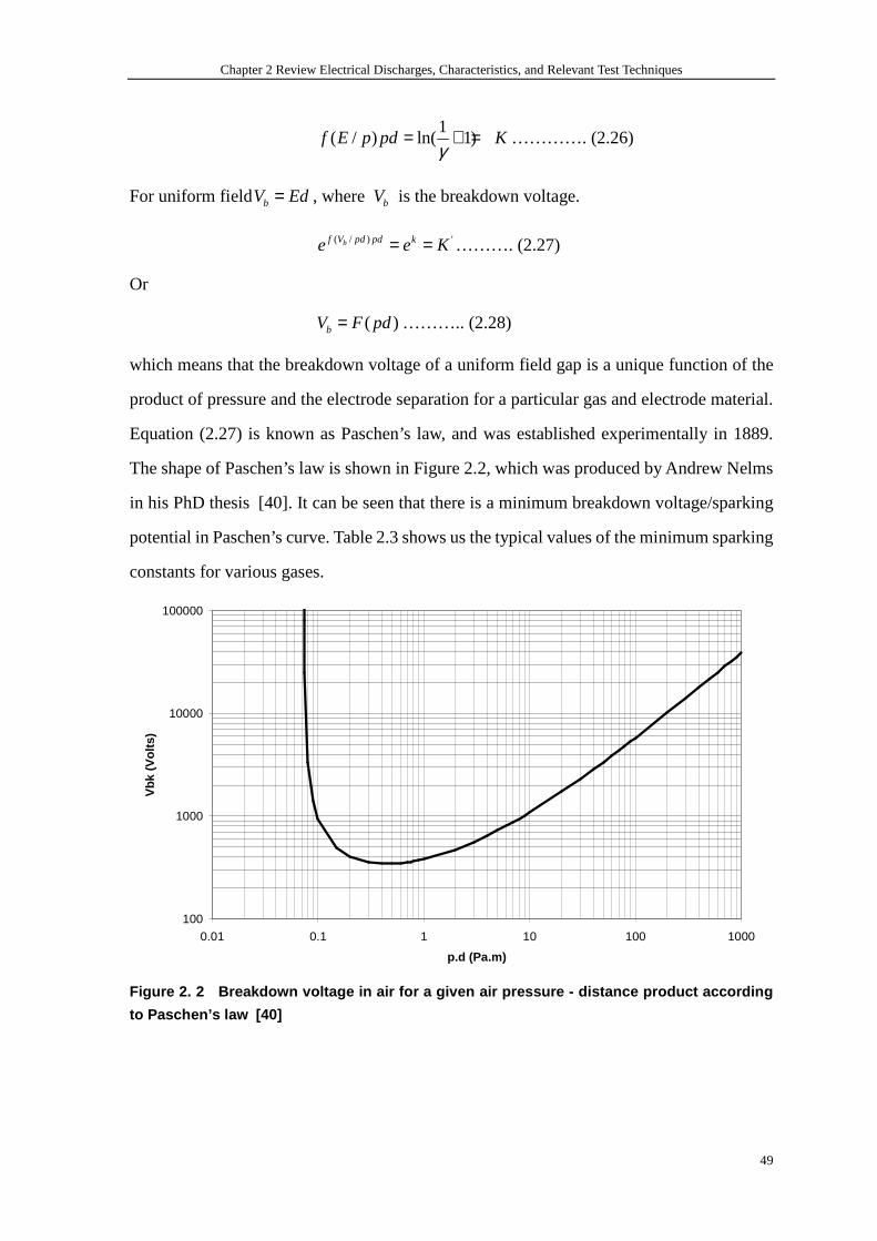
Chapter 2 Review Electrical Discharges, Characteristics, and Relevant Test Techniques
49
1( / ) ln( 1)f E p pd K
γ= + = …………. (2.26)
For uniform field bV Ed= , where bV is the breakdown voltage.
( / ) 'bf V pd pd ke e K= = ………. (2.27)
Or
( )bV F pd= ……….. (2.28)
which means that the breakdown voltage of a uniform field gap is a unique function of the
product of pressure and the electrode separation for a particular gas and electrode material.
Equation (2.27) is known as Paschen’s law, and was established experimentally in 1889.
The shape of Paschen’s law is shown in Figure 2.2, which was produced by Andrew Nelms
in his PhD thesis [40]. It can be seen that there is a minimum breakdown voltage/sparking
potential in Paschen’s curve. Table 2.3 shows us the typical values of the minimum sparking
constants for various gases.
100
1000
10000
100000
0.01 0.1 1 10 100 1000
p.d (Pa.m)
Vbk
(V
olts
)
Figure 2. 2 Breakdown voltage in air for a given a ir pressure - distance product according
to Paschen’s law [40]
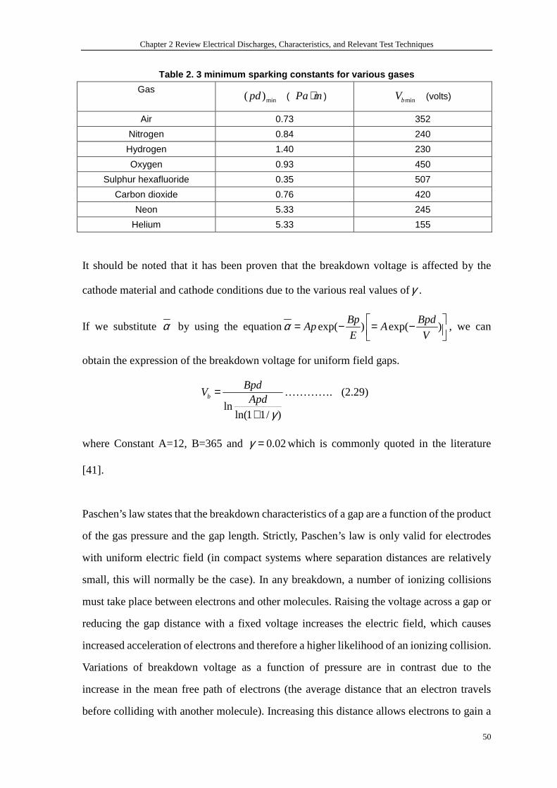
Chapter 2 Review Electrical Discharges, Characteristics, and Relevant Test Techniques
50
Table 2. 3 minimum sparking constants for various g ases
Gas min( )pd ( Pa m⋅ ) minbV (volts)
Air 0.73 352
Nitrogen 0.84 240
Hydrogen 1.40 230
Oxygen 0.93 450
Sulphur hexafluoride 0.35 507
Carbon dioxide 0.76 420
Neon 5.33 245
Helium 5.33 155
It should be noted that it has been proven that the breakdown voltage is affected by the
cathode material and cathode conditions due to the various real values ofγ .
If we substitute α by using the equation exp( ) exp( )Bp Bpd
Ap AE V
α = − = − , we can
obtain the expression of the breakdown voltage for uniform field gaps.
lnln(1 1/ )
b
BpdV
Apd
γ
=
+
…………. (2.29)
where Constant A=12, B=365 and 0.02γ = which is commonly quoted in the literature
[41].
Paschen’s law states that the breakdown characteristics of a gap are a function of the product
of the gas pressure and the gap length. Strictly, Paschen’s law is only valid for electrodes
with uniform electric field (in compact systems where separation distances are relatively
small, this will normally be the case). In any breakdown, a number of ionizing collisions
must take place between electrons and other molecules. Raising the voltage across a gap or
reducing the gap distance with a fixed voltage increases the electric field, which causes
increased acceleration of electrons and therefore a higher likelihood of an ionizing collision.
Variations of breakdown voltage as a function of pressure are in contrast due to the
increase in the mean free path of electrons (the average distance that an electron travels
before colliding with another molecule). Increasing this distance allows electrons to gain a
Chapter 2 Review Electrical Discharges, Characteristics, and Relevant Test Techniques
51
higher velocity before collision and therefore be more likely to cause an ionizing collision.
Paschen’s curve for air is shown in Figure 2.2. As the pressure is reduced breakdown
voltage initially falls. It reaches a minimum and then, as pressure is further reduced, rises
steeply again. This rise in strength of a gap is reached once the mean free path of an electron
becomes comparable with the size of the gap (meaning the likelihood of ionizing collisions
is very low).
The minimum point of this curve is Paschen's minimum. In air, this is 327V for a pressure
distance product of 0.754 Pa.m [45]. Below this voltage, breakdowns cannot take place,
hence the lack of consideration given to some forms of electrical discharges in previous
designs of aircraft operating at lower levels of voltage.
In modern aircraft electrical systems, the voltages between two electrodes can be higher
than Paschen’s minimum and this means that air gaps between electrodes could
breakdown should these not be kept a sufficient distance apart. Such a discharge would be
classed as a disruptive discharge since it would result in a flow of fault current between
the electrodes and would usually necessitate the operation of some form of power system
protection to clear the fault.
2.2.7. Breakdown in non-uniform fields
Non-uniform fields usually can be produced between the gap of a point /sphere/stick and
plane electrodes or coaxial cylinders. The characteristic of this kind of field is that the field
strength and hence the effective ionization coefficientα vary across the gap.
The characteristics of the breakdown in non-uniform fields
In general, breakdown in non-uniform fields presents a very significant polarity effect,
which means that the different polarity applied to the electrodes influences the process of
ionization and breakdown voltage very significantly. In the following table the difference is
Chapter 2 Review Electrical Discharges, Characteristics, and Relevant Test Techniques
52
illustrated in brief. Another characteristic is that usually it takes a longer time to break down
the gap.
The electron multiplication is governed by the integral of α over the path ( dxα∫ ). At low
pressure the Townsend criterion for spark takes the form:
0exp( ) 1 1
ddxγ α − = ∫ ………. (2.30)
where d is the gap length. The integration must be taken along the line of the highest fields’
strength. The expression is valid also for higher pressure if the field is only slightly
non-uniform. In the strongly divergent fields there will be at first a region of high values of
/E pover which / 0pα ⟩ . When the field falls below a given strength cE the integral
dxα∫ ceases to exist. Townsend’s mechanism then loses its validity when the criterion
relies solely on the γ effect, especially when the field strength at the cathode is low.
In reality breakdown or inception discharge is still possible if taking the photoionization
processes into account. The criterion can be written as:
0ln 18 20
cx d
crdx Nα⟨
= = −∫ ……… (2.31) ([38,40])
where crN is the critical electron concentration in an avalanche giving rise to initiation of a
streamer. (It was shown to be approx.810 ). xc
is the path of avalanche to reach this size and
d the gap length.
The process of the breakdown in short gaps
The process of the breakdown between short gaps is that at first there will be a corona
discharge occurring around the region of high field strength, then streamer is produced until
it reaches the opposite electrode and finally breakdown. It has a significant polarity effect
due to the difference of field distortion for different polarity of the electrodes. We specify
the positive polarity gap stands for the setting where the point electrode is positive, and a
negative polarity gap means that the negative potential is applied on the point electrodes.
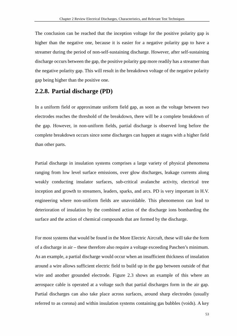
Chapter 2 Review Electrical Discharges, Characteristics, and Relevant Test Techniques
53
The conclusion can be reached that the inception voltage for the positive polarity gap is
higher than the negative one, because it is easier for a negative polarity gap to have a
streamer during the period of non-self-sustaining discharge. However, after self-sustaining
discharge occurs between the gap, the positive polarity gap more readily has a streamer than
the negative polarity gap. This will result in the breakdown voltage of the negative polarity
gap being higher than the positive one.
2.2.8. Partial discharge (PD)
In a uniform field or approximate uniform field gap, as soon as the voltage between two
electrodes reaches the threshold of the breakdown, there will be a complete breakdown of
the gap. However, in non-uniform fields, partial discharge is observed long before the
complete breakdown occurs since some discharges can happen at stages with a higher field
than other parts.
Partial discharge in insulation systems comprises a large variety of physical phenomena
ranging from low level surface emissions, over glow discharges, leakage currents along
weakly conducting insulator surfaces, sub-critical avalanche activity, electrical tree
inception and growth to streamers, leaders, sparks, and arcs. PD is very important in H.V.
engineering where non-uniform fields are unavoidable. This phenomenon can lead to
deterioration of insulation by the combined action of the discharge ions bombarding the
surface and the action of chemical compounds that are formed by the discharge.
For most systems that would be found in the More Electric Aircraft, these will take the form
of a discharge in air – these therefore also require a voltage exceeding Paschen’s minimum.
As an example, a partial discharge would occur when an insufficient thickness of insulation
around a wire allows sufficient electric field to build up in the gap between outside of that
wire and another grounded electrode. Figure 2.3 shows an example of this where an
aerospace cable is operated at a voltage such that partial discharges form in the air gap.
Partial discharges can also take place across surfaces, around sharp electrodes (usually
referred to as corona) and within insulation systems containing gas bubbles (voids). A key
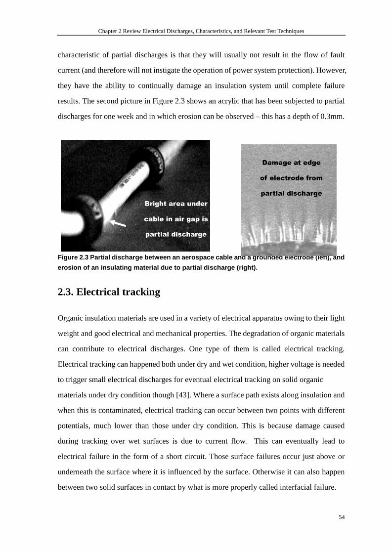
Chapter 2 Review Electrical Discharges, Characteristics, and Relevant Test Techniques
54
characteristic of partial discharges is that they will usually not result in the flow of fault
current (and therefore will not instigate the operation of power system protection). However,
they have the ability to continually damage an insulation system until complete failure
results. The second picture in Figure 2.3 shows an acrylic that has been subjected to partial
discharges for one week and in which erosion can be observed – this has a depth of 0.3mm.
Figure 2.3 Partial discharge between an aerospace c able and a grounded electrode (left), and
erosion of an insulating material due to partial di scharge (right).
2.3. Electrical tracking
Organic insulation materials are used in a variety of electrical apparatus owing to their light
weight and good electrical and mechanical properties. The degradation of organic materials
can contribute to electrical discharges. One type of them is called electrical tracking.
Electrical tracking can happened both under dry and wet condition, higher voltage is needed
to trigger small electrical discharges for eventual electrical tracking on solid organic
materials under dry condition though [43]. Where a surface path exists along insulation and
when this is contaminated, electrical tracking can occur between two points with different
potentials, much lower than those under dry condition. This is because damage caused
during tracking over wet surfaces is due to current flow. This can eventually lead to
electrical failure in the form of a short circuit. Those surface failures occur just above or
underneath the surface where it is influenced by the surface. Otherwise it can also happen
between two solid surfaces in contact by what is more properly called interfacial failure.
Bright area under
cable in air gap is
partial discharge
Damage at edge
of electrode from
partial discharge
Chapter 2 Review Electrical Discharges, Characteristics, and Relevant Test Techniques
55
Many researches [44-46] have studied surface discharge and electrical tracking under dry
condition with the influences of ambient environmental factors such as the ambient
temperature, contamination such as both pure liquids and particular contaminants of many
kinds deposited on the surface of electrical insulation to represent reality, and magnetic
fields. And the limitation of this research is they do not consider air pressure effects. It is
known that electrical systems on aircraft will always operate under extremely rapid airframe
ascent/descent. Research [47] showed that the corona discharges on PCB occur more
readily under low air pressure around the highest electrical stress area with a large effect on
the degradation of solid insulation materials. B. X. Du with other researchers [47-51] also
investigated the surface breakdown phenomenon of printed circuit boards with increasing
temperature from o23 C up to o150 C and atmospheric pressure from 100 kPa to 1 kPa. It is
found that smaller insulation distances are necessary to ensure the insulation reliability
under lower pressure. The mechanism they were looked into was the electrical tracking
under dry condition on PCBs but not wet conditions.
The research on the electrical tracking under wet condition showed that when the
carbonized deposits bridge the electrodes, the dielectric breakdown phenomenon called
tracking failure will occur, which can cause an abrupt reduction in the insulating
resistace.[52]
All of the literatures stated above focused on the dielectric endurance. In other words, their
researches was interested in finding out failure time and erosion left due to the electrical
tracking either under dry or wet conditions. Even in a recent paper published in 2008 with
the topic of effect of ambient pressure on the mechanism of electrical tracking failure
written by X. Du. and Yong Liu [53] was to investigate the failure time rather than the
behaviour of initiation of electrical tracking. In my PhD thesis, the focus will be on the
initiation of discharges between two electrodes on solid insulation surfaces and hence the
initiation of tracking. The ultimate long-term degradation due to initiation of discharges on
Chapter 2 Review Electrical Discharges, Characteristics, and Relevant Test Techniques
56
the surfaces has been studied in abovementioned research already.
The surfaces of insulation material are supposed to be ideal smooth and perfect. The process
of tracking across a small gap contaminated with a conductive aqueous contaminant is
illustrated in Figure 2.4. When a liquid layer is deposited between two electrodes, a current
will flow in the liquid. Heating of this liquid layer will lead to evaporation. This will often
take place in the middle of the gap away from the electrodes which stabilize the temperature
of the nearby liquid. As the liquid evaporates, a spark will develop across the new dry band
due to the interruption of current flow. In other words, at least one spark will occur when a
liquid layer dries out. The spark, if energetic enough, can damage the underlying insulation.
It should be noted that the insulation material type is not the key factor to influence the
initiation of dry band spark but the evaporation rate. However, the severity of damages is
dependent on the solid insulation itself. With continuous contaminant deposited on the
surface, should carbonaceous deposits develop, this can accelerate further damage owing to
the reduction in the ‘healthy’ insulation within the gap. The severity of the damage will
depend on the voltage and current of the arc along with the characteristics of the material
itself.
Figure 2.4 – Basic process of tracking across an in sulating surface contaminated with an
aqueous layer
The breakdown of an insulation gap where gaseous insulation exists in the gap between two
Chapter 2 Review Electrical Discharges, Characteristics, and Relevant Test Techniques
57
electrodes is determined by Paschen’s law. As previously explained, a minimum voltage is
therefore required to cause a breakdown in this gap.
In contrast, a surface that is wet sees current flow through the contaminant as previously
described. When this current causes evaporation of the liquid, an arc is drawn and damage
can be result the underlying surface by this arc. The voltage across the gap that leads to this
process taking place depends on the resistance of the liquid layer and the level of current
needed to cause evaporation. There is no requirement for a voltage at the level of Paschen’s
minimum since an arc is being drawn when the liquid layer separates.
Higher voltages are more likely to cause electrical tracking owing to the increased level of
heating that can occur in contamination deposited in a given size gap. In addition, having a
voltage above Paschen’s minimum means that there is a chance of re-ignition of the arc
(particularly important in an AC system where it will extinguish every half cycle). However
the differentiation between breakdown of an insulation gap such as an air gap leading to
Paschen’s law and interruption of a current leading to discharge in a wet test at lower
voltage is attributed to differences in their mechanism. The former is to breakdown the
dielectric strength of gas insulation. And the latter is the due to interrupt a current. The
electric arc at atmospheric pressure is familiar in appearance to most of us. It consists of a
bright column that is highly visible to the naked eye. At its heart are ionized gases that allow
the electric current to flow between two electrodes. The presence of ionised gas correctly
suggests that there is a very high temperature at the core of the arc.
In an AC electrical circuit with an existing arc, the arc voltage and arc current are in nature
passing through the locations around a voltage/current zero every half cycle. When the arc
current is approaching zero, the arc voltage is equal to the system voltage, which results in
current zero. When the current is zero, there is no new charge/energy in gases so that the
insulation could cool down and the dielectric strength between electrodes could recover.
The re-ignition of arc is dependent on the competition between the dielectric recovery rate
and system voltage increases. If the former rate is bigger, then re-ignition will not occur.

Chapter 2 Review Electrical Discharges, Characteristics, and Relevant Test Techniques
58
Hence the frequencies of the voltage applied have impact on the electrical tracking. The
higher frequency, the less severe the physical damage would be since the re-ignition is not
achieved with very high frequency. But with power frequency, it can be always expected to
have re-ignition as long as the voltage is above the Paschen’s minimum. While with DC
voltages, damages will be very badly since there will be no extinction at all as long as the arc
takes place. As liquid boiling points lower with decreasing pressure, larger separations of
electrodes become necessary at altitude since more contaminants within larger separation
need more heat to dry out. Otherwise systems can be characterized to whether they are
located in an environment that will not be subject to ingress of liquids in any form.
In aircraft systems, existing standards deal with the phenomena of arc tracking on cabling
including wet arc tracking, dry arc tracking and series arc tracking. Generally, these events
take place in locations where the insulation system has been compromised. Discharge
activity in the form of an arc then burns surrounding insulation allowing damage to
propagate over long distances. More details of these phenomena can be found in [54].
All of these forms of electrical discharge must be considered in the design process to ensure
that the electrical system remains functional over its intended lifetime.
2.4. Existing design standards
A range of standards also exist that can support the design of high voltage aerospace
systems. However, not all aspects of high voltage design for aerospace environments are yet
fully covered by standards and it is likely that this is an area on which the industry will need
to focus in the coming years.
IEC 60664 ‘Insulation Coordination for Equipment within Low Voltage Systems’ defines
the required clearances for equipment operating at a range of voltages for altitudes of up to
2000 m [55]. This is done for DC, AC and lightning voltages. The use of an altitude
correction factor contained in the standard can convert this data for use at higher altitudes
Chapter 2 Review Electrical Discharges, Characteristics, and Relevant Test Techniques
59
even though the standard is not strictly applicable for aerospace use. The standard does not
differentiate the gap size required according to the type of voltage (i.e. steady state DC/AC
or lightning), as the breakdown voltage (based on the peak voltage) is the same for all
voltage types for small gaps. The standard also contains a useful discussion on the
dimensioning of air insulation that is required to withstand high frequency voltage stress
(such as would be found in a power electronic converter switching square waves). The
voltage withstand capability with increasing frequency arises due to the limited velocity of
heavy positive ions [56]. The maximum effect of an increase in frequency above the critical
value is to reduce the breakdown voltage of a uniform field gap by around 20%. It would
therefore be prudent in an aerospace application to base clearances on a voltage roughly
25% higher than the value expected to account for this effect.
IEC 60664 also provides guidelines for dimensioning creepage distances along surfaces (to
prevent tracking). The guidelines are based on empirical data and are not applicable to
equipment installed in low pressure environments.
In a similar way IPC 2221 provides information on the distances between tracks on printed
circuit boards design [57]. It covers all total aspects of design details using organic materials
or organic material in combination with inorganic materials like metal, glass, ceramic, etc.,
as well as electronic packaging issues.
Aerospace Standard AS50881 [58] provides guidance for choosing conductor and
insulation sizes for aerospace wiring. Conductor size is based on an analysis of the required
current carrying capability and takes the impact of altitude and the use of conductor bundles
into account. Insulation size is determined by examining the required operating voltage, the
insulation selected being thick enough to withstand partial discharges.
From the above-mentioned background of design development trends within the aerospace
industries, it can be summarized that reduction of weight and volume of the greater number
of electronic components on the aircraft is absolutely critical. Due to much better electrical
Chapter 2 Review Electrical Discharges, Characteristics, and Relevant Test Techniques
60
and mechanical properties, solid insulation, especially those using organic insulation
materials, are widely used to save significant insulating space. Higher power supply and
voltage level has been applied. Additionally, to employ much higher frequencies, an
increasing number of electronic converters and high frequency switch power supplies will
be applied. The recent rapid development in electronic component technologies has
heightened the need for evaluation of the electrical strength of solid insulation to guarantee
the reliability and safety of operation of aircrafts.
2.5. Test techniques for electrical tracking
Since the majority of the work in the thesis is about electrical tracking, the series of test
techniques for electrical tracking under wet condition are discussed in this section. At
present, there are four major laboratory test methods to evaluate electrical tracking and
erosion under surface discharge and dry band arc. A.T.S.M. D495 “High Voltage, Low
Current Arc Resistance of Solid Electrical Insulating Materials” [59] specifies dry arc test
methods, which are very widely used. IEC 60112: 2003 [60] is a standardized comparative
tracking index test to evaluate the performance of organic materials by finding out the
comparative tracking index values. However, there is a limitation in that only a 4mm gap
can be set, since the dropping system for pollution liquids is particularly defined to that
measurement. With a much bigger gap, the inclined plane test specified in IEC 587: 1984
[61] is the most comprehensive test for tracking and erosion. However, since the resistor
connected in the electrical circuit of this test simulates the healthy insulation materials that
are usually on the insulators and that have very large resistance values, it cannot be applied
to printed circuit board failure where short-circuit path usually forms when tracking occurs
between the tiny gaps between tracks on the boards. Mist-fog test techniques evaluate the
degradation of insulating materials with a test period from a few hours up to 200 hours or
even more, which is very time consuming.
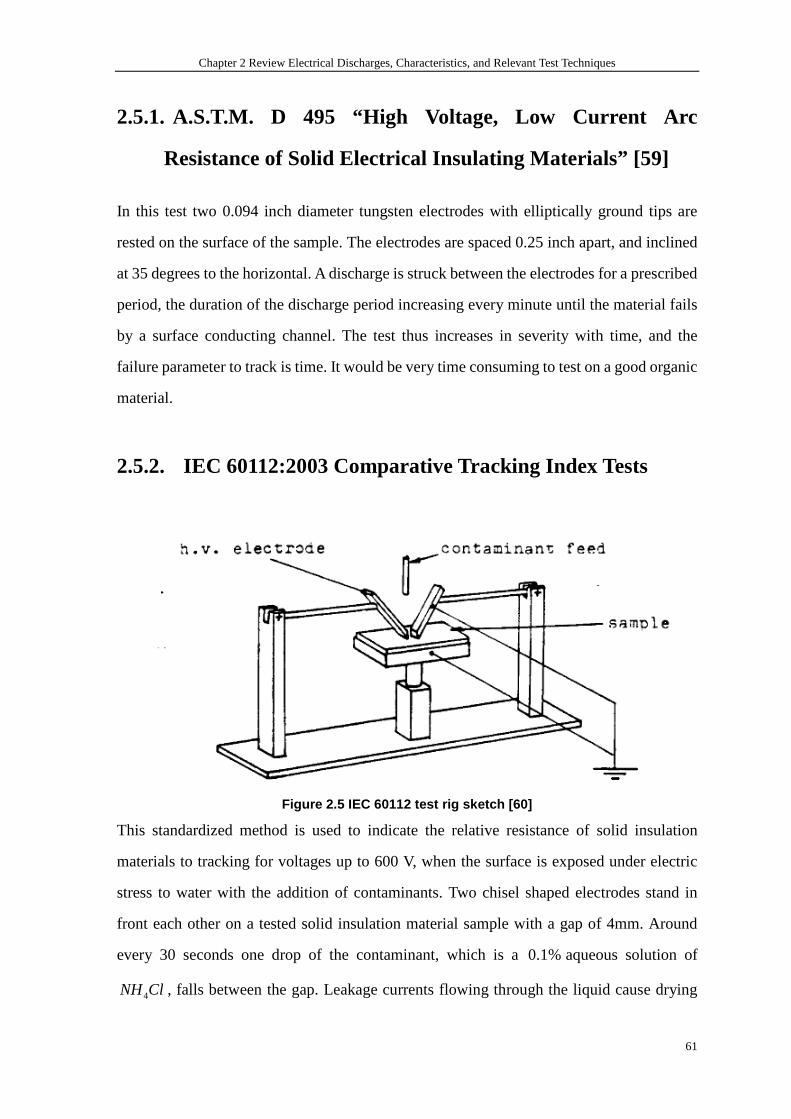
Chapter 2 Review Electrical Discharges, Characteristics, and Relevant Test Techniques
61
2.5.1. A.S.T.M. D 495 “High Voltage, Low Current Arc
Resistance of Solid Electrical Insulating Materials” [59]
In this test two 0.094 inch diameter tungsten electrodes with elliptically ground tips are
rested on the surface of the sample. The electrodes are spaced 0.25 inch apart, and inclined
at 35 degrees to the horizontal. A discharge is struck between the electrodes for a prescribed
period, the duration of the discharge period increasing every minute until the material fails
by a surface conducting channel. The test thus increases in severity with time, and the
failure parameter to track is time. It would be very time consuming to test on a good organic
material.
2.5.2. IEC 60112:2003 Comparative Tracking Index Tests
Figure 2.5 IEC 60112 test rig sketch [60]
This standardized method is used to indicate the relative resistance of solid insulation
materials to tracking for voltages up to 600 V, when the surface is exposed under electric
stress to water with the addition of contaminants. Two chisel shaped electrodes stand in
front each other on a tested solid insulation material sample with a gap of 4mm. Around
every 30 seconds one drop of the contaminant, which is a 0.1%aqueous solution of
4NH Cl , falls between the gap. Leakage currents flowing through the liquid cause drying
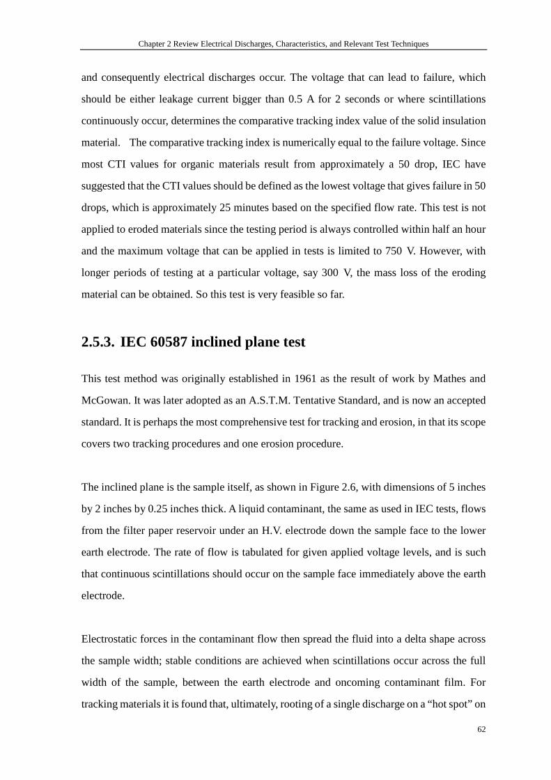
Chapter 2 Review Electrical Discharges, Characteristics, and Relevant Test Techniques
62
and consequently electrical discharges occur. The voltage that can lead to failure, which
should be either leakage current bigger than 0.5 A for 2 seconds or where scintillations
continuously occur, determines the comparative tracking index value of the solid insulation
material. The comparative tracking index is numerically equal to the failure voltage. Since
most CTI values for organic materials result from approximately a 50 drop, IEC have
suggested that the CTI values should be defined as the lowest voltage that gives failure in 50
drops, which is approximately 25 minutes based on the specified flow rate. This test is not
applied to eroded materials since the testing period is always controlled within half an hour
and the maximum voltage that can be applied in tests is limited to 750 V. However, with
longer periods of testing at a particular voltage, say 300 V, the mass loss of the eroding
material can be obtained. So this test is very feasible so far.
2.5.3. IEC 60587 inclined plane test
This test method was originally established in 1961 as the result of work by Mathes and
McGowan. It was later adopted as an A.S.T.M. Tentative Standard, and is now an accepted
standard. It is perhaps the most comprehensive test for tracking and erosion, in that its scope
covers two tracking procedures and one erosion procedure.
The inclined plane is the sample itself, as shown in Figure 2.6, with dimensions of 5 inches
by 2 inches by 0.25 inches thick. A liquid contaminant, the same as used in IEC tests, flows
from the filter paper reservoir under an H.V. electrode down the sample face to the lower
earth electrode. The rate of flow is tabulated for given applied voltage levels, and is such
that continuous scintillations should occur on the sample face immediately above the earth
electrode.
Electrostatic forces in the contaminant flow then spread the fluid into a delta shape across
the sample width; stable conditions are achieved when scintillations occur across the full
width of the sample, between the earth electrode and oncoming contaminant film. For
tracking materials it is found that, ultimately, rooting of a single discharge on a “hot spot” on
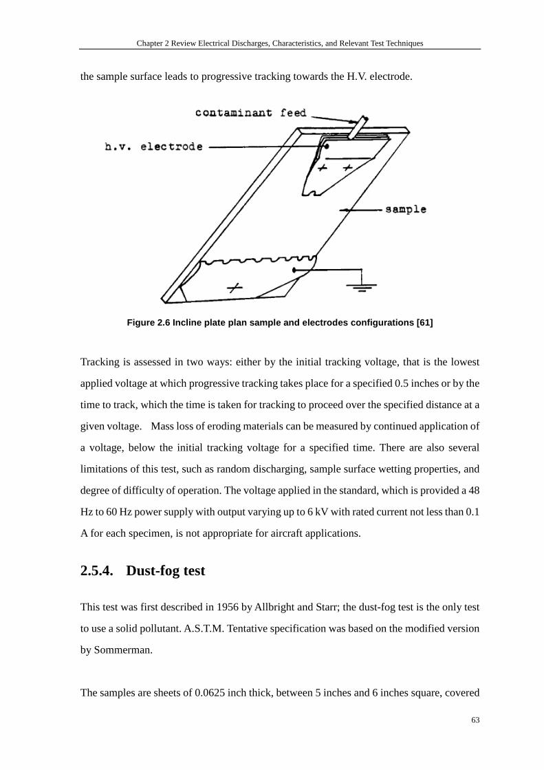
Chapter 2 Review Electrical Discharges, Characteristics, and Relevant Test Techniques
63
the sample surface leads to progressive tracking towards the H.V. electrode.
Figure 2.6 Incline plate plan sample and electrodes configurations [61]
Tracking is assessed in two ways: either by the initial tracking voltage, that is the lowest
applied voltage at which progressive tracking takes place for a specified 0.5 inches or by the
time to track, which the time is taken for tracking to proceed over the specified distance at a
given voltage. Mass loss of eroding materials can be measured by continued application of
a voltage, below the initial tracking voltage for a specified time. There are also several
limitations of this test, such as random discharging, sample surface wetting properties, and
degree of difficulty of operation. The voltage applied in the standard, which is provided a 48
Hz to 60 Hz power supply with output varying up to 6 kV with rated current not less than 0.1
A for each specimen, is not appropriate for aircraft applications.
2.5.4. Dust-fog test
This test was first described in 1956 by Allbright and Starr; the dust-fog test is the only test
to use a solid pollutant. A.S.T.M. Tentative specification was based on the modified version
by Sommerman.
The samples are sheets of 0.0625 inch thick, between 5 inches and 6 inches square, covered
Chapter 2 Review Electrical Discharges, Characteristics, and Relevant Test Techniques
64
by a dust layer to a uniform depth, 0.02 to 0.035 inch, with the recommended composition
by weight of 85% flint dust, 9% clay, 3% salt and 3% paper fibers. The sample is first
mounted to the electrodes shown in Figure 2.6 and then coated with the above mentioned
pollutant. The whole test rig is put into a chamber, where a discrete water spray or fog can
be generated. A dry band arc can occur when a voltage is applied to the electrodes. The
surface pollutant is maintained by the continuous wetting of the sample surface at a rate
within close limits of the rate of evaporation by the discharge and surface leakage currents
in the contaminant film. Initially big discharges occur, but because of the loss of salt from
the film, the final applied voltage is specified as 1.5 kV with a discharge current of 10 mA.
By applying this method, tracking materials can be categorized to different degrees of
resistant to tracking by whether the material can erode or fail, and the time period.
Figure 2.7 Dust-fog test rig sketch [70]
Some materials can be expected to erode after hundreds of hours. During so long a period,
the sample has to be re-coated with pollutant. The test is unique in that a sample under
voltage is stressed dielectrically between the H.V. electrode and the lower electrodes.
2.5.5. Test methods discussion
At present, many other tests exist to investigate the behaviour of surface discharge or
electrical tracking. They all suffer the drawback of a lack of reproducibility and
Chapter 2 Review Electrical Discharges, Characteristics, and Relevant Test Techniques
65
repeatability of results. We must therefore admit that accelerated laboratory testing under
polluted conditions is only successful in determining tracking or erosion materials in those
processes.
However, in our research for More Electrical Aircraft applications, the IEC 60112 test
method is the most appropriate one to employ. The limit of voltage of 750 V is not a
problem at all for both maximum 15/200 VAC 400 Hz conventional commercial systems,
28 V DC or 270 V DC for military usage and a combined 230 V AC 360-800 Hz and +/- 270
V DC (540 V DC) new systems on future large More Electrical Aircraft. The most
important reason to employ this method is that it can be used in a environmental chamber
where the impact of air pressure can be evaluated.
The first and biggest challenge is how we can control the repeatability and reproducibility to
some acceptable extent when we upgrade this method to any creepage distances. The next
challenge is how laboratory testing environments can reflect real circumstances.
2.6. Conclusion
This chapter has given not only the fundamental knowledge of different types of electrical
discharges but most importantly has shown how the failure types will have an impact on the
future electrical system on large More Electrical Aircraft. The existing design rules have
also been investigated and their limitations show that we have to re-validate both clearance
and creepage distance dimensioning guidelines for much higher pressures with more precise
values. It is very straightforward to evaluate clearances by using the IEC 60: 1989
standardized method while different tracking test techniques were discussed. Considering
execution and application, IEC 60112’s specified method was chosen for my research to
investigate mechanisms of electrical tracking at varying air pressures, pollution degrees and
even different ambient temperatures.
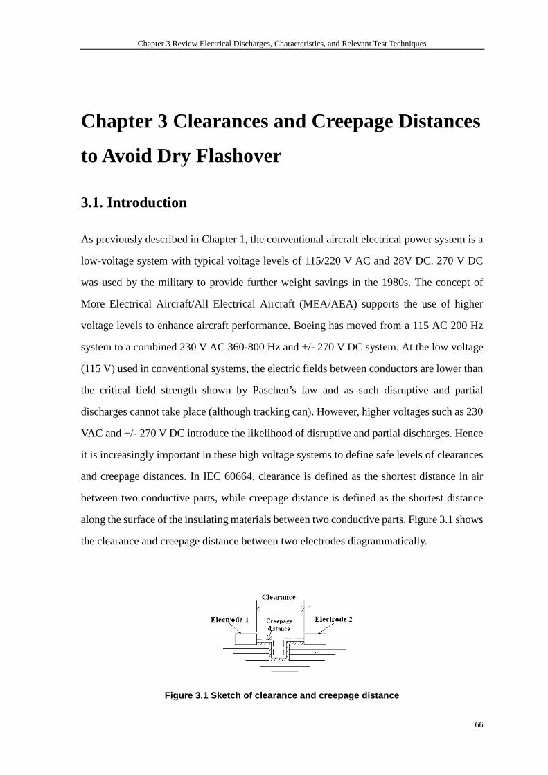
Chapter 3 Review Electrical Discharges, Characteristics, and Relevant Test Techniques
66
Chapter 3 Clearances and Creepage Distances
to Avoid Dry Flashover
3.1. Introduction
As previously described in Chapter 1, the conventional aircraft electrical power system is a
low-voltage system with typical voltage levels of 115/220 V AC and 28V DC. 270 V DC
was used by the military to provide further weight savings in the 1980s. The concept of
More Electrical Aircraft/All Electrical Aircraft (MEA/AEA) supports the use of higher
voltage levels to enhance aircraft performance. Boeing has moved from a 115 AC 200 Hz
system to a combined 230 V AC 360-800 Hz and +/- 270 V DC system. At the low voltage
(115 V) used in conventional systems, the electric fields between conductors are lower than
the critical field strength shown by Paschen’s law and as such disruptive and partial
discharges cannot take place (although tracking can). However, higher voltages such as 230
VAC and +/- 270 V DC introduce the likelihood of disruptive and partial discharges. Hence
it is increasingly important in these high voltage systems to define safe levels of clearances
and creepage distances. In IEC 60664, clearance is defined as the shortest distance in air
between two conductive parts, while creepage distance is defined as the shortest distance
along the surface of the insulating materials between two conductive parts. Figure 3.1 shows
the clearance and creepage distance between two electrodes diagrammatically.
Figure 3.1 Sketch of clearance and creepage distanc e

Chapter 3 Clearances and Creepage Distances to Avoid Dry Flashover
67
A determination of clearance in air can be precisely defined for a certain electrode geometry
based on Paschen’s law. The fundamentals of Paschen’s law have been discussed in section
2.2. It relates the electrical breakdown strength with the pressure and gap distance between
electrodes in which a uniform field is present. By considering the density of a gas, Paschen’s
law can also be used to explain the relationship between the breakdown strength and
temperature.
A limitation of Paschen’s law is that it is only applicable to disruptive discharges in uniform
electrical fields. Should non-uniform fields be present, different dimensions of clearances
will be expected in different electric fields to avoid both disruptive and partial discharge.
However, it is expected that for the majority of clearances in an aircraft power system where
space is limited, short gaps will be common and as a good approximation, the electric fields
between these short gaps can be accepted as uniform so that Paschen’s law can be applied.
In contrast to determining clearances, determination of creepage distances is more complex
and cannot rely on Paschen’s law in all cases. When a surface is contaminated, tracking
behaviour can take place – creepage distances to avoid this are examined in more detail in
Chapters 4, 5 and 6. While tracking over dry surfaces is possible, the nature of a flashover
on a dry surface over a short gap will usually be similar to a flashover in air. Some
researchers believed that the dry tracking method is more suitable for determing the
material properties since there is no artificial environment affecting the behaviors of
tracking and the reproducibility of the tests is much better [62]. However, they also admitted
that the testing voltage to start tiny discharges from the surfaces of insulators is extremely
high. In other word, creepage distances required to avoid flashover in air in dry
conditions will generally be much smaller than the distances needed to avoid tracking across
the surface when wet, and the evaluation of creepage distances for dry conditions is
therefore limited in application to situations where aqueous contamination is not present.
In this chapter, we will review the design rules for clearances and creepage distances under
dry conditions as specified in IEC 60664 and IPC 2221. The values stated in both the
Chapter 3 Clearances and Creepage Distances to Avoid Dry Flashover
68
standards are compared against experimental test results using both an air gap and printed
circuit board samples for different air pressures and varying gap widths.
3.2. Review of IEC 60664-1:2003
3.2.1. Introduction
IEC 60664 deals with the insulation coordination for equipment within low voltage systems.
It applies to equipments for up to 2000 m above sea level having a rated voltage up to AC
1000 V with rated frequency up to 30 kHz or rated voltage up to DC 1500 V. The design
rules for clearances, creepage distances and solid insulation for equipment based on their
performance criteria has been specified.
As the standard is not applicable for equipment used over 2000 m, it is clearly not intended
for use in aerospace equipment design. However, air pressure factors are specified in the
standard for correction of clearance distances in any design used above 2000 m (with a
maximum altitude of 20000 m being described).
3.2.2. Determination of clearance
The flow chart given in Figure 3.2 shows that clearances should be selected by first
considering the highest transient voltage that will be applied to the equipment. It should be
noted that if the equipment is energized directly to the low-voltage supply mains (obviously
not the case for an aerospace system), the rated impulse voltage is given in tables. The
impulse voltage is used to derive a clearance distance from a table (such as that shown in
Table 4.1). In addition, the steady-state (working) voltage is used to derive a second
clearance distance and the largest of these two is selected as the required dimension.
In many systems, impulse voltages will be higher than the steady state rated working
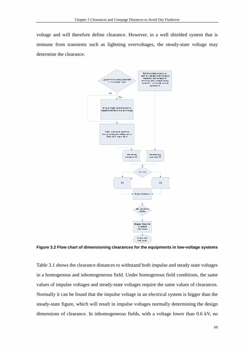
Chapter 3 Clearances and Creepage Distances to Avoid Dry Flashover
69
voltage and will therefore define clearance. However, in a well shielded system that is
immune from transients such as lightning overvoltages, the steady-state voltage may
determine the clearance.
Figure 3.2 Flow chart of dimensioning clearances fo r the equipments in low-voltage systems
Table 3.1 shows the clearance distances to withstand both impulse and steady state voltages
in a homogenous and inhomogeneous field. Under homogenous field conditions, the same
values of impulse voltages and steady-state voltages require the same values of clearances.
Normally it can be found that the impulse voltage in an electrical system is bigger than the
steady-state figure, which will result in impulse voltages normally determining the design
dimensions of clearance. In inhomogeneous fields, with a voltage lower than 0.6 kV, no
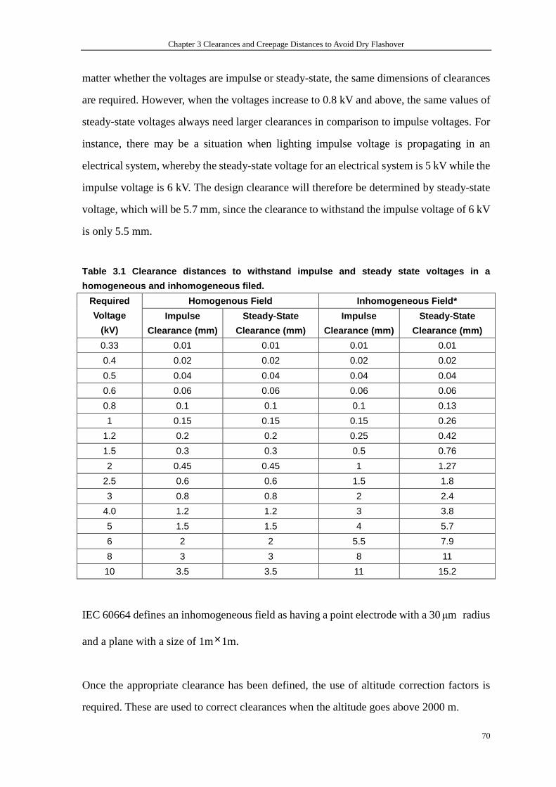
Chapter 3 Clearances and Creepage Distances to Avoid Dry Flashover
70
matter whether the voltages are impulse or steady-state, the same dimensions of clearances
are required. However, when the voltages increase to 0.8 kV and above, the same values of
steady-state voltages always need larger clearances in comparison to impulse voltages. For
instance, there may be a situation when lighting impulse voltage is propagating in an
electrical system, whereby the steady-state voltage for an electrical system is 5 kV while the
impulse voltage is 6 kV. The design clearance will therefore be determined by steady-state
voltage, which will be 5.7 mm, since the clearance to withstand the impulse voltage of 6 kV
is only 5.5 mm.
Table 3.1 Clearance distances to withstand impulse and steady state voltages in a
homogeneous and inhomogeneous filed.
Homogenous Field Inhomogeneous Field* Required
Voltage
(kV)
Impulse
Clearance (mm)
Steady-State
Clearance (mm)
Impulse
Clearance (mm)
Steady-State
Clearance (mm)
0.33 0.01 0.01 0.01 0.01
0.4 0.02 0.02 0.02 0.02
0.5 0.04 0.04 0.04 0.04
0.6 0.06 0.06 0.06 0.06
0.8 0.1 0.1 0.1 0.13
1 0.15 0.15 0.15 0.26
1.2 0.2 0.2 0.25 0.42
1.5 0.3 0.3 0.5 0.76
2 0.45 0.45 1 1.27
2.5 0.6 0.6 1.5 1.8
3 0.8 0.8 2 2.4
4.0 1.2 1.2 3 3.8
5 1.5 1.5 4 5.7
6 2 2 5.5 7.9
8 3 3 8 11
10 3.5 3.5 11 15.2
IEC 60664 defines an inhomogeneous field as having a point electrode with a 30µm radius
and a plane with a size of 1m×1m.
Once the appropriate clearance has been defined, the use of altitude correction factors is
required. These are used to correct clearances when the altitude goes above 2000 m.
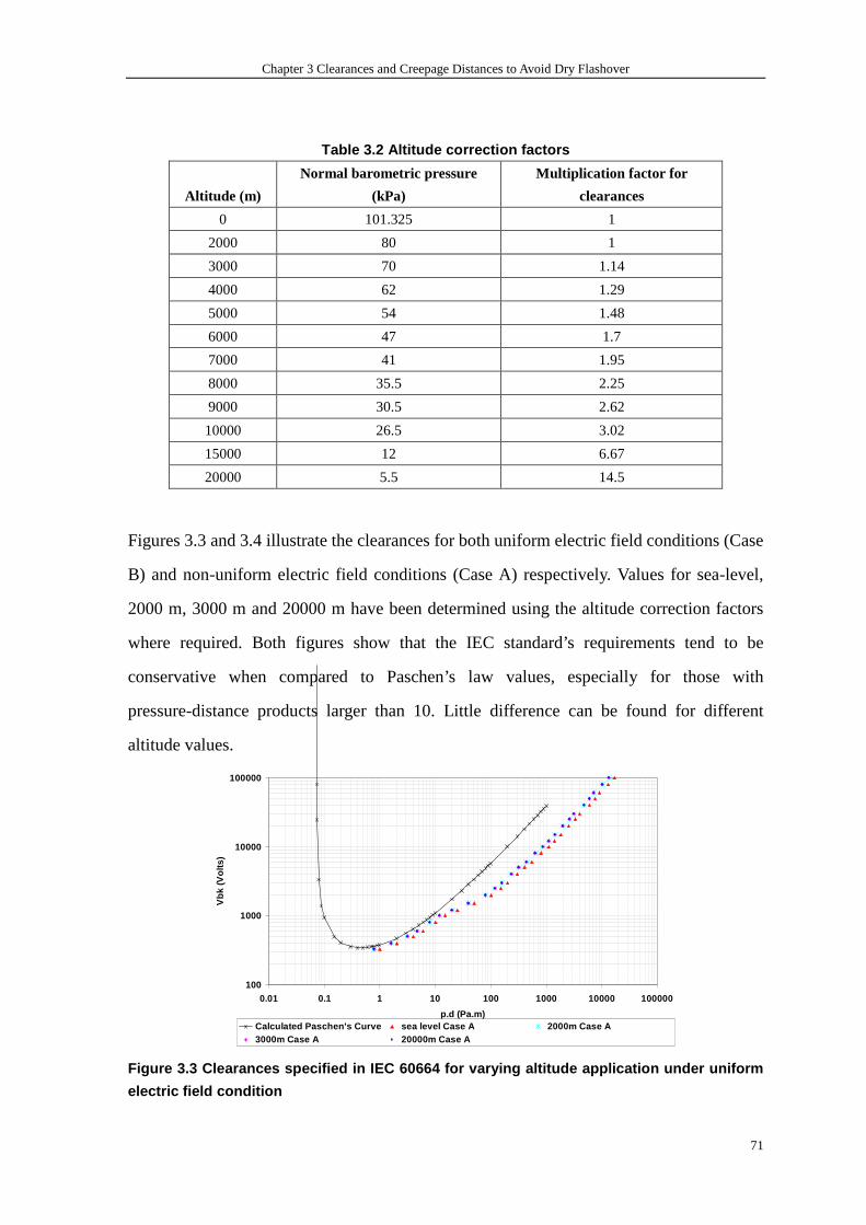
Chapter 3 Clearances and Creepage Distances to Avoid Dry Flashover
71
Table 3.2 Altitude correction factors
Altitude (m)
Normal barometric pressure
(kPa)
Multiplication factor for
clearances
0 101.325 1
2000 80 1
3000 70 1.14
4000 62 1.29
5000 54 1.48
6000 47 1.7
7000 41 1.95
8000 35.5 2.25
9000 30.5 2.62
10000 26.5 3.02
15000 12 6.67
20000 5.5 14.5
Figures 3.3 and 3.4 illustrate the clearances for both uniform electric field conditions (Case
B) and non-uniform electric field conditions (Case A) respectively. Values for sea-level,
2000 m, 3000 m and 20000 m have been determined using the altitude correction factors
where required. Both figures show that the IEC standard’s requirements tend to be
conservative when compared to Paschen’s law values, especially for those with
pressure-distance products larger than 10. Little difference can be found for different
altitude values.
100
1000
10000
100000
0.01 0.1 1 10 100 1000 10000 100000
p.d (Pa.m)
Vbk
(Vol
ts)
Calculated Paschen's Curve sea level Case A 2000m Case A3000m Case A 20000m Case A
Figure 3.3 Clearances specified in IEC 60664 for va rying altitude application under uniform
electric field condition

Chapter 3 Clearances and Creepage Distances to Avoid Dry Flashover
72
100
1000
10000
100000
0.01 0.1 1 10 100 1000 10000
p.d (Pa.m)
Vbk
(Vol
ts)
Calculated Paschen's Curve sea level Case B 2000m Case B3000m Case B 20000m Case B
Figure 3.4 Clearances specified in IEC 60664 for va rying altitude application under
non-uniform electric field condition
3.2.3. Dimensioning of creepage distances
Creepage distances are determined using the steady-state voltage. Transient overvoltages
which normally last only a few milliseconds for dimensioning for creepage distances are
neglected since they do not influence the tracking phenomenon. Temporary overvoltages
have to be considered if their duration and frequency of occurrence has an impact on
tracking.
The creepage distance is not just a function of voltage but is also based on the degree of
surface pollution and the material group used to make the equipment. The former defines
the level of conductivity on the sample surface while the latter defines the response of the
material to arcing damage. However, for determination of the creepage distance in dry
conditions, the material property is not used. The values of creepage distances to avoid
failure in dry conditions are therefore given by the standard as shown in Table 3.3
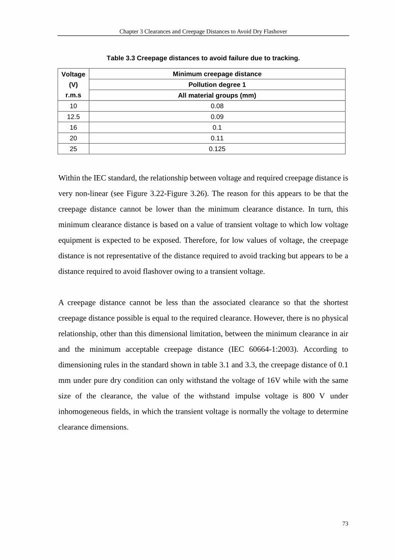
Chapter 3 Clearances and Creepage Distances to Avoid Dry Flashover
73
Table 3.3 Creepage distances to avoid failure due t o tracking.
Minimum creepage distance
Pollution degree 1
Voltage
(V)
r.m.s All material groups (mm)
10 0.08
12.5 0.09
16 0.1
20 0.11
25 0.125
Within the IEC standard, the relationship between voltage and required creepage distance is
very non-linear (see Figure 3.22-Figure 3.26). The reason for this appears to be that the
creepage distance cannot be lower than the minimum clearance distance. In turn, this
minimum clearance distance is based on a value of transient voltage to which low voltage
equipment is expected to be exposed. Therefore, for low values of voltage, the creepage
distance is not representative of the distance required to avoid tracking but appears to be a
distance required to avoid flashover owing to a transient voltage.
A creepage distance cannot be less than the associated clearance so that the shortest
creepage distance possible is equal to the required clearance. However, there is no physical
relationship, other than this dimensional limitation, between the minimum clearance in air
and the minimum acceptable creepage distance (IEC 60664-1:2003). According to
dimensioning rules in the standard shown in table 3.1 and 3.3, the creepage distance of 0.1
mm under pure dry condition can only withstand the voltage of 16V while with the same
size of the clearance, the value of the withstand impulse voltage is 800 V under
inhomogeneous fields, in which the transient voltage is normally the voltage to determine
clearance dimensions.
Chapter 3 Clearances and Creepage Distances to Avoid Dry Flashover
74
3.3. Review of IPC 2221
3.3.1. Introduction
IPC 2221 “Generic Standard on Printed Boards Design” provides generic requirements for
the design of organic printed boards and other forms of components, mounting or
interconnecting structures to eliminate the misunderstanding between manufacturers and
purchasers, facilitating interchangeability and improvement of products, and assisting the
purchaser in selecting and obtaining with minimum delay the proper product for his
particular need. To design the physical features and select materials for a printed wiring
board, not only should factors such as electrical, mechanical and thermal properties be
considered but also reliability of performance, manufacturing and cost, which have to be
balanced at the same time.
3.3.2. Electrical clearances
First of all, it should be noted that the term “electrical clearance” in IPC 2221 here
designates the different spacing as specified by the same term in IEC 60664. In IPC 2221,
clearance standards are given for spacing either between two conductors on an individual
layer, between conductive patterns, for layer to layer conductive spaces, and between
conductive materials (such as conductive markings or mounting hardware) and conductors.
It states that spacing between conductors on an individual layer should be maximized
whenever possible. Otherwise, table 3.4 should be applied.
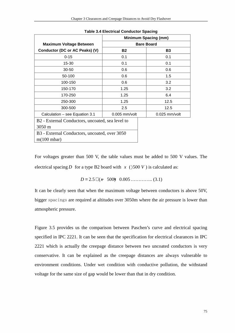
Chapter 3 Clearances and Creepage Distances to Avoid Dry Flashover
75
Table 3.4 Electrical Conductor Spacing
Minimum Spacing (mm)
Bare Board Maximum Voltage Between
Conductor (DC or AC Peaks) (V) B2 B3
0-15 0.1 0.1
15-30 0.1 0.1
30-50 0.6 0.6
50-100 0.6 1.5
100-150 0.6 3.2
150-170 1.25 3.2
170-250 1.25 6.4
250-300 1.25 12.5
300-500 2.5 12.5
Calculation – see Equation 3.1 0.005 mm/volt 0.025 mm/volt
B2 - External Conductors, uncoated, sea level to 3050 m B3 - External Conductors, uncoated, over 3050 m(100 mbar)
For voltages greater than 500 V, the table values must be added to 500 V values. The
electrical spacingD for a type B2 board with x ( 500⟩ V ) is calculated as:
2.5 ( 500) 0.005D x= + − × ………….. (3.1)
It can be clearly seen that when the maximum voltage between conductors is above 50V,
bigger spacings are required at altitudes over 3050m where the air pressure is lower than
atmospheric pressure.
Figure 3.5 provides us the comparison between Paschen’s curve and electrical spacing
specified in IPC 2221. It can be seen that the specification for electrical clearances in IPC
2221 which is actually the creepage distance between two uncoated conductors is very
conservative. It can be explained as the creepage distances are always vulnerable to
environment conditions. Under wet condition with conductive pollution, the withstand
voltage for the same size of gap would be lower than that in dry condition.
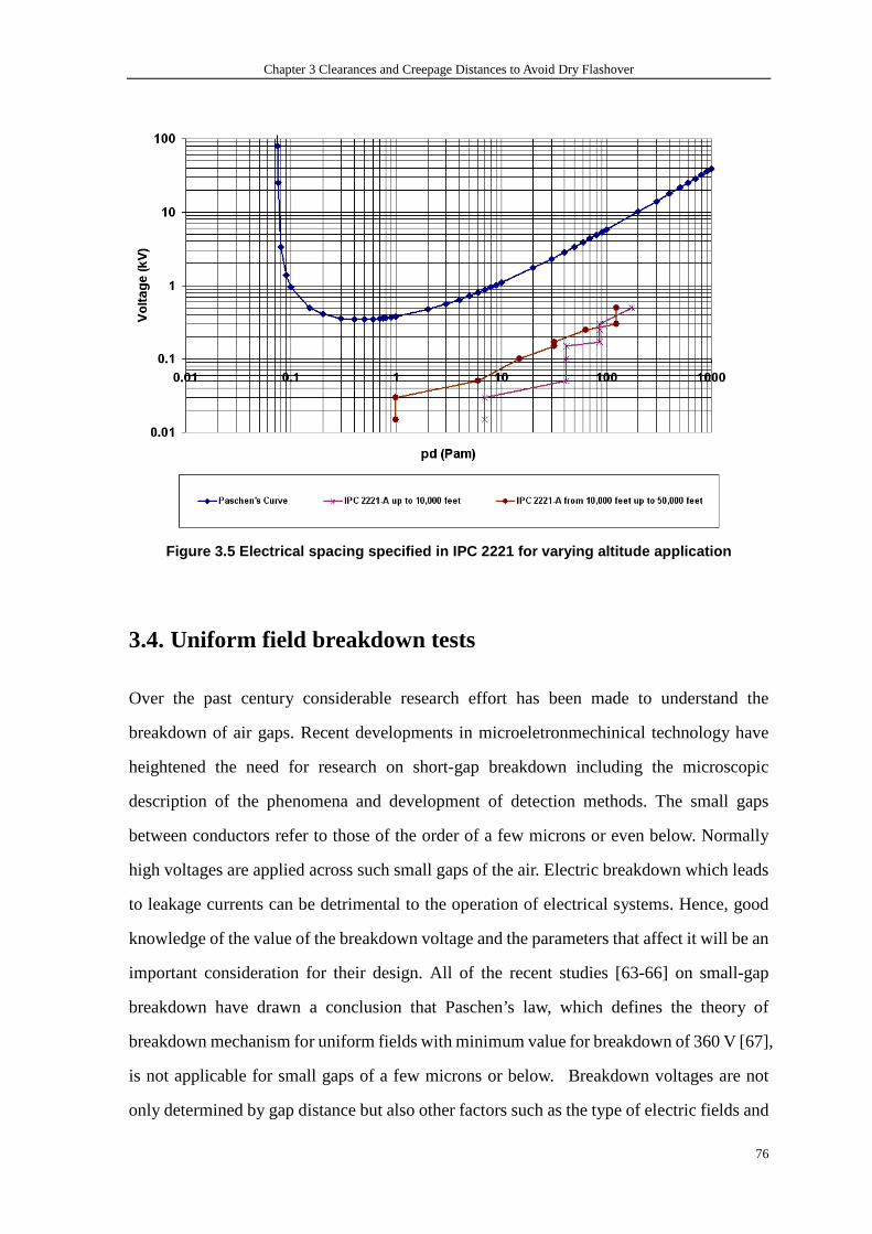
Chapter 3 Clearances and Creepage Distances to Avoid Dry Flashover
76
Figure 3.5 Electrical spacing specified in IPC 2221 for varying altitude application
3.4. Uniform field breakdown tests
Over the past century considerable research effort has been made to understand the
breakdown of air gaps. Recent developments in microeletronmechinical technology have
heightened the need for research on short-gap breakdown including the microscopic
description of the phenomena and development of detection methods. The small gaps
between conductors refer to those of the order of a few microns or even below. Normally
high voltages are applied across such small gaps of the air. Electric breakdown which leads
to leakage currents can be detrimental to the operation of electrical systems. Hence, good
knowledge of the value of the breakdown voltage and the parameters that affect it will be an
important consideration for their design. All of the recent studies [63-66] on small-gap
breakdown have drawn a conclusion that Paschen’s law, which defines the theory of
breakdown mechanism for uniform fields with minimum value for breakdown of 360 V [67],
is not applicable for small gaps of a few microns or below. Breakdown voltages are not
only determined by gap distance but also other factors such as the type of electric fields and
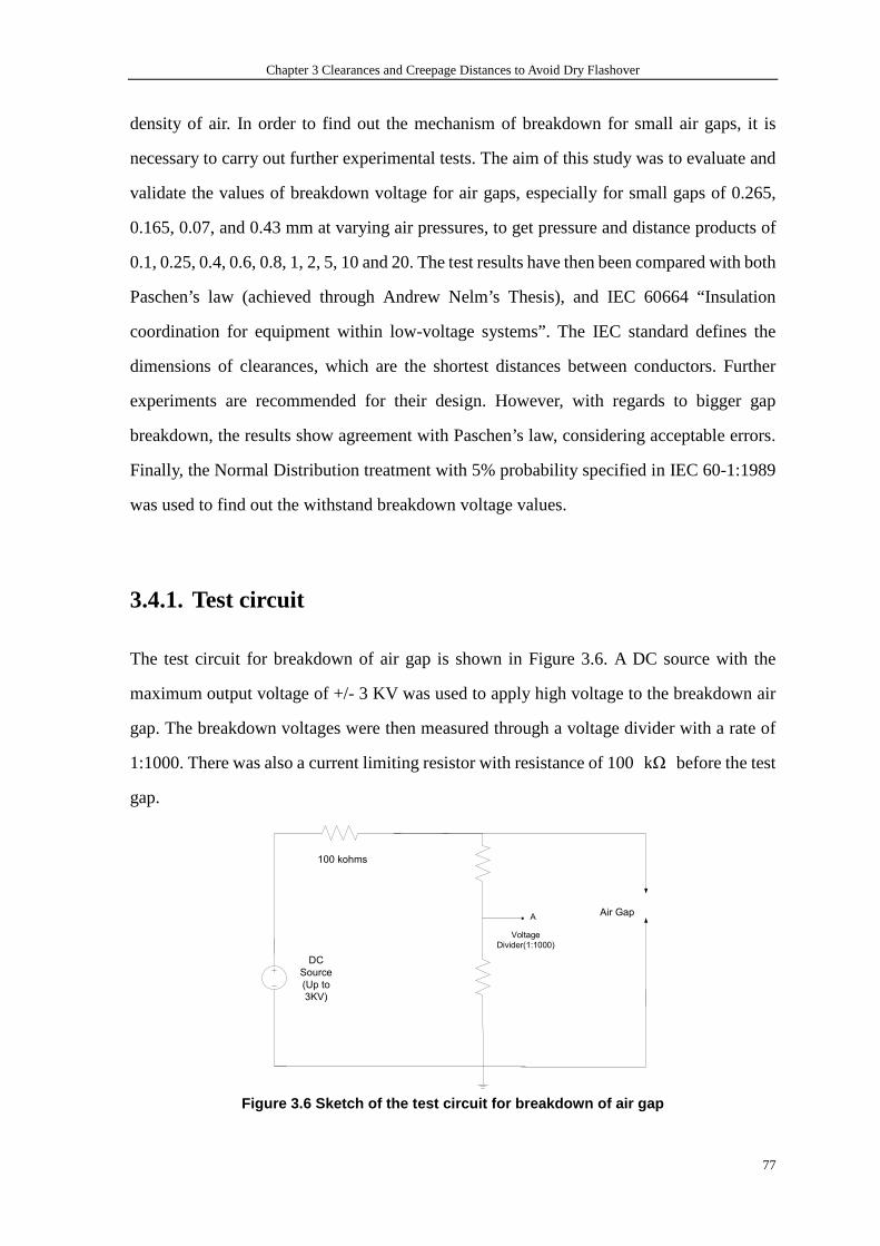
Chapter 3 Clearances and Creepage Distances to Avoid Dry Flashover
77
density of air. In order to find out the mechanism of breakdown for small air gaps, it is
necessary to carry out further experimental tests. The aim of this study was to evaluate and
validate the values of breakdown voltage for air gaps, especially for small gaps of 0.265,
0.165, 0.07, and 0.43 mm at varying air pressures, to get pressure and distance products of
0.1, 0.25, 0.4, 0.6, 0.8, 1, 2, 5, 10 and 20. The test results have then been compared with both
Paschen’s law (achieved through Andrew Nelm’s Thesis), and IEC 60664 “Insulation
coordination for equipment within low-voltage systems”. The IEC standard defines the
dimensions of clearances, which are the shortest distances between conductors. Further
experiments are recommended for their design. However, with regards to bigger gap
breakdown, the results show agreement with Paschen’s law, considering acceptable errors.
Finally, the Normal Distribution treatment with 5% probability specified in IEC 60-1:1989
was used to find out the withstand breakdown voltage values.
3.4.1. Test circuit
The test circuit for breakdown of air gap is shown in Figure 3.6. A DC source with the
maximum output voltage of +/- 3 KV was used to apply high voltage to the breakdown air
gap. The breakdown voltages were then measured through a voltage divider with a rate of
1:1000. There was also a current limiting resistor with resistance of 100 kΩ before the test
gap.
Voltage
Divider(1:1000)
AAir Gap
DC
Source
(Up to
3KV)
100 kohms
Figure 3.6 Sketch of the test circuit for breakdown of air gap
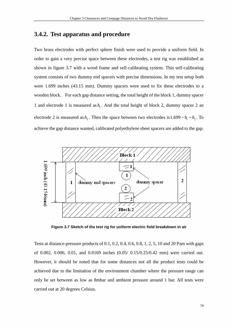
Chapter 3 Clearances and Creepage Distances to Avoid Dry Flashover
78
3.4.2. Test apparatus and procedure
Two brass electrodes with perfect sphere finish were used to provide a uniform field. In
order to gain a very precise space between these electrodes, a test rig was established as
shown in figure 3.7 with a wood frame and self-calibrating system. This self-calibrating
system consists of two dummy end spacers with precise dimensions. In my test setup both
were 1.699 inches (43.15 mm). Dummy spacers were used to fix these electrodes to a
wooden block. For each gap distance setting, the total height of the block 1, dummy spacer
1 and electrode 1 is measured as1h . And the total height of block 2, dummy spacer 2 an
electrode 2 is measured as2h . Then the space between two electrodes is 1 21.699 h h− − . To
achieve the gap distance wanted, calibrated polyethylene sheet spacers are added to the gap.
Figure 3.7 Sketch of the test rig for uniform elect ric field breakdown in air
Tests at distance-pressure products of 0.1, 0.2, 0.4, 0.6, 0.8, 1, 2, 5, 10 and 20 Pam with gaps
of 0.002, 0.006, 0.01, and 0.0169 inches (0.05/ 0.15/0.25/0.42 mm) were carried out.
However, it should be noted that for some distances not all the product tests could be
achieved due to the limitation of the environment chamber where the pressure range can
only be set between as low as 8mbar and ambient pressure around 1 bar. All tests were
carried out at 20 degrees Celsius.
Chapter 3 Clearances and Creepage Distances to Avoid Dry Flashover
79
A DC voltage was applied using a generator with an output of +/- 3 kV. The National
Instrument Labview program was used to control the output of the generator with the ramp
rate of 10 kV per minute. The breakdown voltage was measured with ten breakdown voltage
measurements at each pressure-distance product being carried out.
3.4.3. Test results and discussion
The recorded breakdown voltages are shown in the following figures from Figure 3.8 to
Figure 3.11, which all present the results for a different gap distance. These figures are the
average of ten measurements. Error bars are also displayed to show the maximum and
minimum values at each pressure and distance product. It can be seen that Paschen’s
minimum appears to be shifted to a lower pressure distance product place. It is known that
the breakdown in air not only has the character that Paschen’s law describes and also relies
on two impact factors which include device geometry and surface roughness of
electrodes[68]. Device geometry will determine the shape of electrical fields while surface
roughness will lead to amplification of the electrical field at the sharp points. That is why
measurements of breakdown tests can have more or less shift from the theoretical values.
However, the data ties in with Paschen’s law which shows a similar trend to the right hand
side of Paschen’s law. A probable shift in the minimum location data at low pd values
was not collected to confirm this.
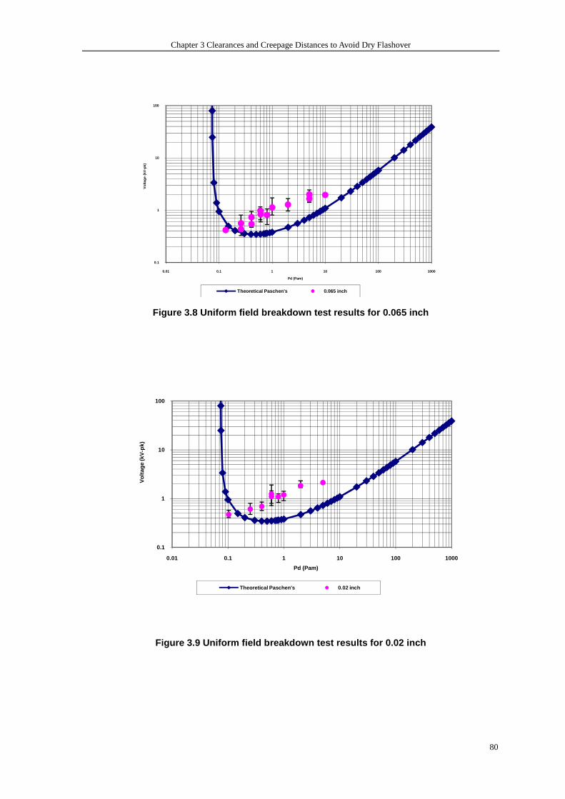
Chapter 3 Clearances and Creepage Distances to Avoid Dry Flashover
80
0.1
1
10
100
0.01 0.1 1 10 100 1000
Vol
tage
(kV
-pk)
Pd (Pam)
Theoretical Paschen's 0.065 inch
Figure 3.8 Uniform field breakdown test results for 0.065 inch
0.1
1
10
100
0.01 0.1 1 10 100 1000
Vol
tage
(kV
-pk)
Pd (Pam)
Theoretical Paschen's 0.02 inch
Figure 3.9 Uniform field breakdown test results for 0.02 inch

Chapter 3 Clearances and Creepage Distances to Avoid Dry Flashover
81
0.1
1
10
100
0.01 0.1 1 10 100 1000
Pd (Pam)
Vol
tage
(kV
-pk)
Theoretical Paschen's 0.1 inch
Figure 3.10 Uniform field breakdown test results fo r 0.1 inch
0.1
1
10
100
0.01 0.1 1 10 100 1000
Pd (Pam)
Vol
tage
(kV
-pk)
Theoretical Paschen's 0.165 inch
Figure 3.11 Uniform field breakdown test results fo r 0.1 inch
The test results were then used to determine the withstand voltage at each pressure-distance
product as detailed in IEC 60060-1: 1989 High-voltage testing techniques [69]. For a
Gaussian (or Normal) distribution, estimates of the parameters 50U and z are given by:
*50 /iU U n=∑ ………..3.1
( )1/ 22* *
50 /( 1)iz U U n = − − ∑ …………3.2
The confidence limits for Gaussian distributions may be found using the Student’s t or

Chapter 3 Clearances and Creepage Distances to Avoid Dry Flashover
82
Chi-squared distributions as described in the technical literature.
Normal (or Gaussian) distribution in statistics is the most widely used probability
distribution. It is normally used as a first approximation to describe a group of random
variables that tend to gather around a single mean value. Its probability density function is
“bell” shape with the expression as shown in the equation 3.3.
2
2
( )
2
2
1( )
2
x
f x eµ
σ
πσ
−−= ……3.3
Where parameter µ is the mean (location of peak) and 2σ is the variance (the measure of
the width of the distribution). In our case, the mean is calculated from all the measurements
taken from the tests. The variance is calculated by apply the equation 3.2 above. In my
research the 5% chance of flashover for the estimates of 05U and z obtained from a test
are used to calculate the withstand breakdown voltages shown in following figure. The
methods are shown in detail in Appendix B.
The limitation of usage of normal distribution to predict the 5% probable breakdown
voltage is that with higher variance of the distribution the values of the calculated value
could be close to zero which is not true in reality.
0.1
1
10
100
0.01 0.1 1 10 100 1000
Pd (Pam)
Vol
tage
(kV
-pk)
Theoretical Paschen's Normal Distribution Treatment results
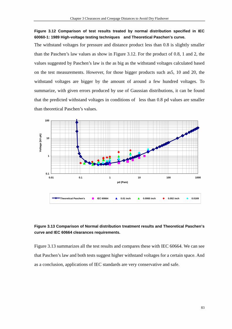
Chapter 3 Clearances and Creepage Distances to Avoid Dry Flashover
83
Figure 3.12 Comparison of test results treated by n ormal distribution specified in IEC
60060-1: 1989 High-voltage testing techniques and Theoretical Paschen’s curve.
The withstand voltages for pressure and distance product less than 0.8 is slightly smaller
than the Paschen’s law values as show in Figure 3.12. For the product of 0.8, 1 and 2, the
values suggested by Paschen’s law is the as big as the withstand voltages calculated based
on the test measurements. However, for those bigger products such as5, 10 and 20, the
withstand voltages are bigger by the amount of around a few hundred voltages. To
summarize, with given errors produced by use of Gaussian distributions, it can be found
that the predicted withstand voltages in conditions of less than 0.8 pd values are smaller
than theoretical Paschen’s values.
0.1
1
10
100
0.01 0.1 1 10 100 1000
pd (Pam)
Vol
tage
(kV
-pk)
Theoretical Paschen's IEC 60664 0.01 inch 0.0065 inch 0.002 inch 0.0169
Figure 3.13 Comparison of Normal distribution treat ment results and Theoretical Paschen’s
curve and IEC 60664 clearances requirements.
Figure 3.13 summarizes all the test results and compares these with IEC 60664. We can see
that Paschen’s law and both tests suggest higher withstand voltages for a certain space. And
as a conclusion, applications of IEC standards are very conservative and safe.
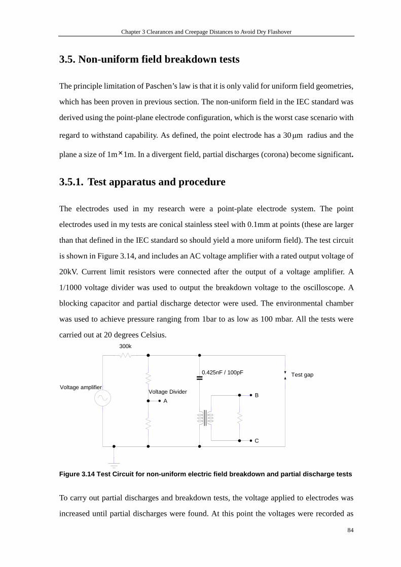
Chapter 3 Clearances and Creepage Distances to Avoid Dry Flashover
84
3.5. Non-uniform field breakdown tests
The principle limitation of Paschen’s law is that it is only valid for uniform field geometries,
which has been proven in previous section. The non-uniform field in the IEC standard was
derived using the point-plane electrode configuration, which is the worst case scenario with
regard to withstand capability. As defined, the point electrode has a 30µm radius and the
plane a size of 1m×1m. In a divergent field, partial discharges (corona) become significant.
3.5.1. Test apparatus and procedure
The electrodes used in my research were a point-plate electrode system. The point
electrodes used in my tests are conical stainless steel with 0.1mm at points (these are larger
than that defined in the IEC standard so should yield a more uniform field). The test circuit
is shown in Figure 3.14, and includes an AC voltage amplifier with a rated output voltage of
20kV. Current limit resistors were connected after the output of a voltage amplifier. A
1/1000 voltage divider was used to output the breakdown voltage to the oscilloscope. A
blocking capacitor and partial discharge detector were used. The environmental chamber
was used to achieve pressure ranging from 1bar to as low as 100 mbar. All the tests were
carried out at 20 degrees Celsius.
0.425nF / 100pF
Voltage amplifierVoltage Divider
AB
C
Test gap
300k
Figure 3.14 Test Circuit for non-uniform electric f ield breakdown and partial discharge tests
To carry out partial discharges and breakdown tests, the voltage applied to electrodes was
increased until partial discharges were found. At this point the voltages were recorded as
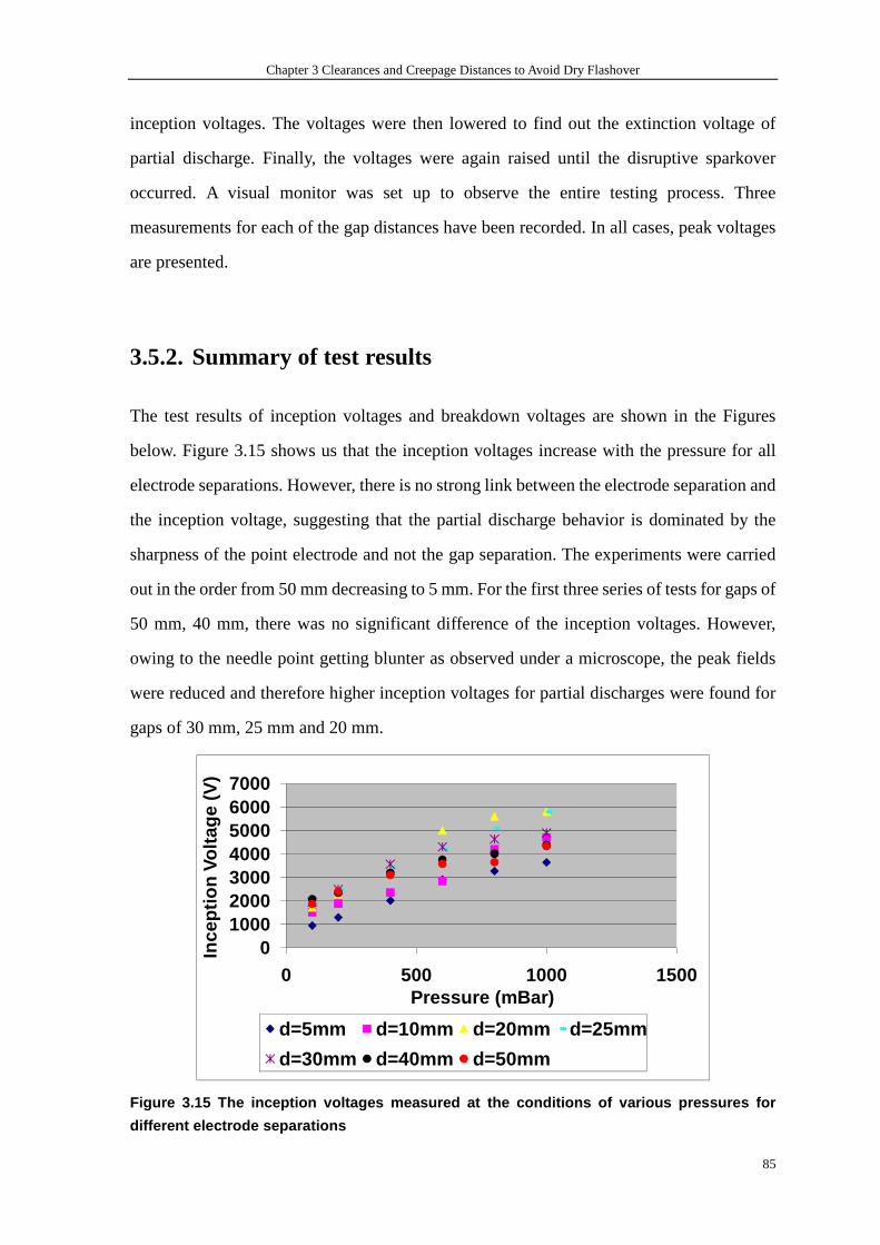
Chapter 3 Clearances and Creepage Distances to Avoid Dry Flashover
85
inception voltages. The voltages were then lowered to find out the extinction voltage of
partial discharge. Finally, the voltages were again raised until the disruptive sparkover
occurred. A visual monitor was set up to observe the entire testing process. Three
measurements for each of the gap distances have been recorded. In all cases, peak voltages
are presented.
3.5.2. Summary of test results
The test results of inception voltages and breakdown voltages are shown in the Figures
below. Figure 3.15 shows us that the inception voltages increase with the pressure for all
electrode separations. However, there is no strong link between the electrode separation and
the inception voltage, suggesting that the partial discharge behavior is dominated by the
sharpness of the point electrode and not the gap separation. The experiments were carried
out in the order from 50 mm decreasing to 5 mm. For the first three series of tests for gaps of
50 mm, 40 mm, there was no significant difference of the inception voltages. However,
owing to the needle point getting blunter as observed under a microscope, the peak fields
were reduced and therefore higher inception voltages for partial discharges were found for
gaps of 30 mm, 25 mm and 20 mm.
01000200030004000500060007000
0 500 1000 1500
Ince
ptio
n Vo
ltage
(V
)
Pressure (mBar)
d=5mm d=10mm d=20mm d=25mm
d=30mm d=40mm d=50mm
Figure 3.15 The inception voltages measured at the conditions of various pressures for
different electrode separations
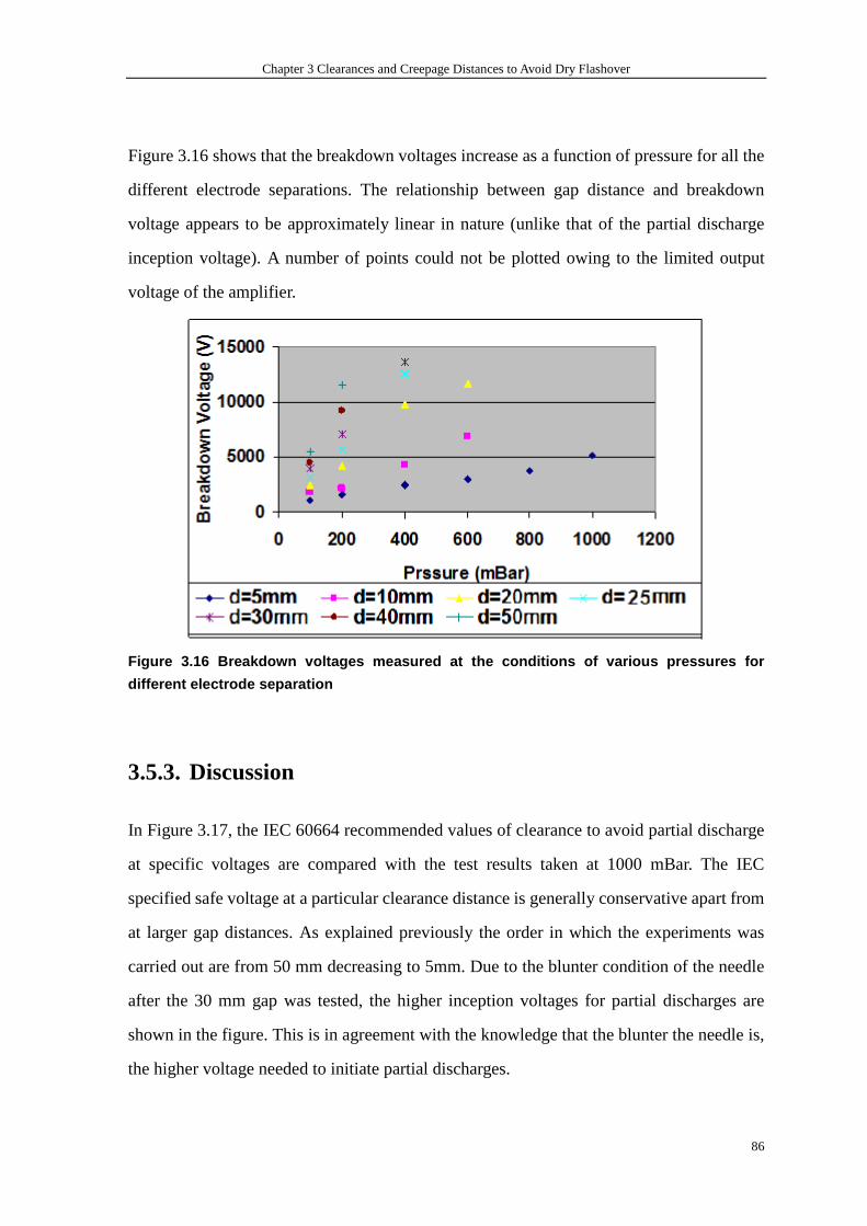
Chapter 3 Clearances and Creepage Distances to Avoid Dry Flashover
86
Figure 3.16 shows that the breakdown voltages increase as a function of pressure for all the
different electrode separations. The relationship between gap distance and breakdown
voltage appears to be approximately linear in nature (unlike that of the partial discharge
inception voltage). A number of points could not be plotted owing to the limited output
voltage of the amplifier.
Figure 3.16 Breakdown voltages measured at the cond itions of various pressures for
different electrode separation
3.5.3. Discussion
In Figure 3.17, the IEC 60664 recommended values of clearance to avoid partial discharge
at specific voltages are compared with the test results taken at 1000 mBar. The IEC
specified safe voltage at a particular clearance distance is generally conservative apart from
at larger gap distances. As explained previously the order in which the experiments was
carried out are from 50 mm decreasing to 5mm. Due to the blunter condition of the needle
after the 30 mm gap was tested, the higher inception voltages for partial discharges are
shown in the figure. This is in agreement with the knowledge that the blunter the needle is,
the higher voltage needed to initiate partial discharges.
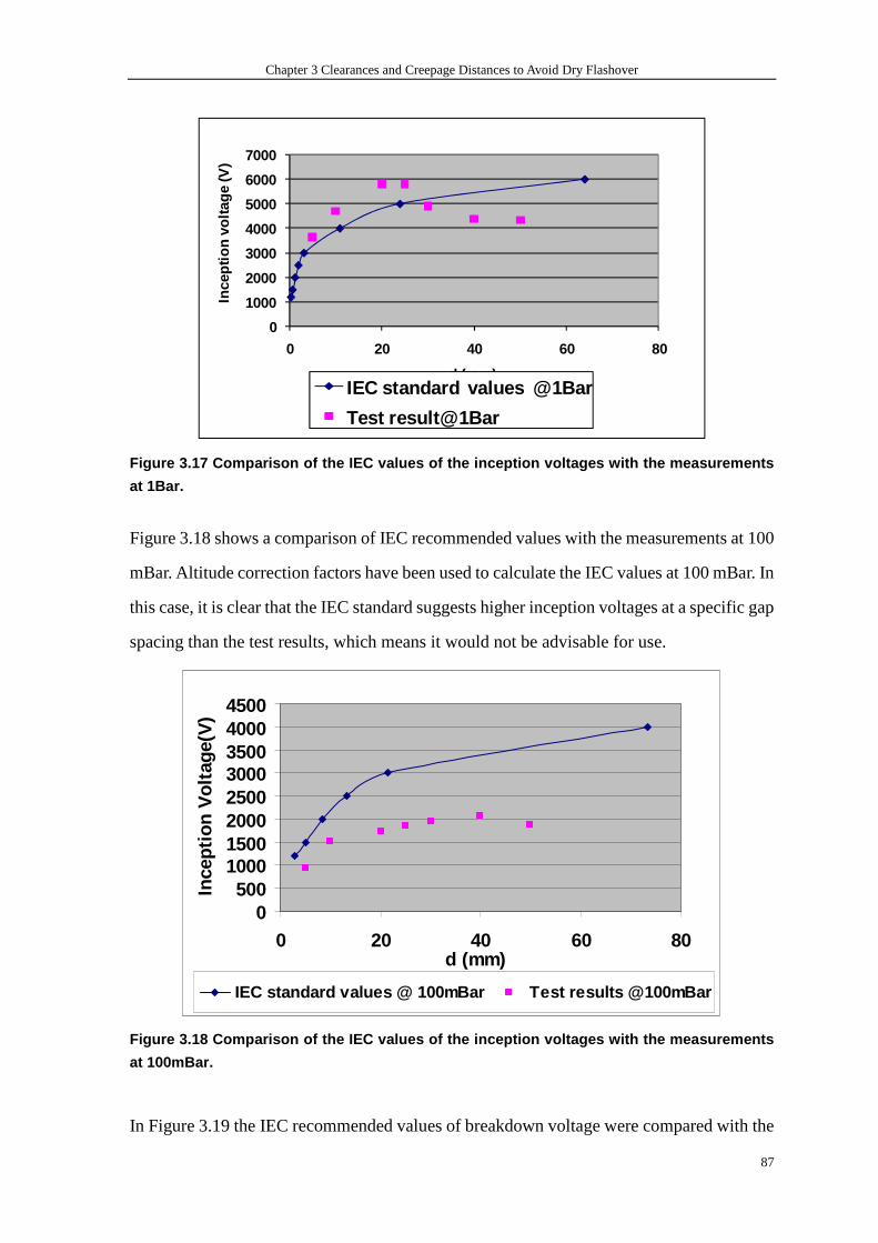
Chapter 3 Clearances and Creepage Distances to Avoid Dry Flashover
87
0
1000
2000
3000
4000
5000
6000
7000
0 20 40 60 80
Ince
ptio
n vo
ltage
(V)
d (mm)IEC standard values @1Bar
Test result@1Bar
Figure 3.17 Comparison of the IEC values of the inc eption voltages with the measurements
at 1Bar.
Figure 3.18 shows a comparison of IEC recommended values with the measurements at 100
mBar. Altitude correction factors have been used to calculate the IEC values at 100 mBar. In
this case, it is clear that the IEC standard suggests higher inception voltages at a specific gap
spacing than the test results, which means it would not be advisable for use.
0500
10001500200025003000350040004500
0 20 40 60 80d (mm)
Ince
ptio
n V
olta
ge(V
)
IEC standard values @ 100mBar Test results @100mBar
Figure 3.18 Comparison of the IEC values of the inc eption voltages with the measurements
at 100mBar.
In Figure 3.19 the IEC recommended values of breakdown voltage were compared with the
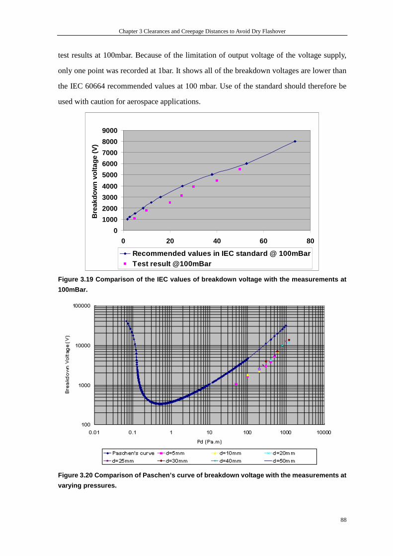
Chapter 3 Clearances and Creepage Distances to Avoid Dry Flashover
88
test results at 100mbar. Because of the limitation of output voltage of the voltage supply,
only one point was recorded at 1bar. It shows all of the breakdown voltages are lower than
the IEC 60664 recommended values at 100 mbar. Use of the standard should therefore be
used with caution for aerospace applications.
0
1000
2000
3000
4000
5000
6000
7000
8000
9000
0 20 40 60 80
d (mm)
Bre
akdo
wn
volta
ge (
V)
Recommended values in IEC standard @ 100mBarTest result @100mBar
Figure 3.19 Comparison of the IEC values of breakdo wn voltage with the measurements at
100mBar.
Figure 3.20 Comparison of Paschen’s curve of breakd own voltage with the measurements at
varying pressures.
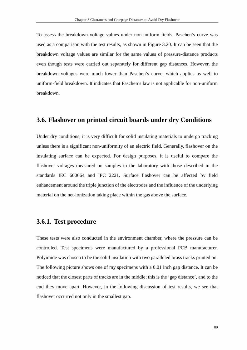
Chapter 3 Clearances and Creepage Distances to Avoid Dry Flashover
89
To assess the breakdown voltage values under non-uniform fields, Paschen’s curve was
used as a comparison with the test results, as shown in Figure 3.20. It can be seen that the
breakdown voltage values are similar for the same values of pressure-distance products
even though tests were carried out separately for different gap distances. However, the
breakdown voltages were much lower than Paschen’s curve, which applies as well to
uniform-field breakdown. It indicates that Paschen’s law is not applicable for non-uniform
breakdown.
3.6. Flashover on printed circuit boards under dry Conditions
Under dry conditions, it is very difficult for solid insulating materials to undergo tracking
unless there is a significant non-uniformity of an electric field. Generally, flashover on the
insulating surface can be expected. For design purposes, it is useful to compare the
flashover voltages measured on samples in the laboratory with those described in the
standards IEC 600664 and IPC 2221. Surface flashover can be affected by field
enhancement around the triple junction of the electrodes and the influence of the underlying
material on the net-ionization taking place within the gas above the surface.
3.6.1. Test procedure
These tests were also conducted in the environment chamber, where the pressure can be
controlled. Test specimens were manufactured by a professional PCB manufacturer.
Polyimide was chosen to be the solid insulation with two paralleled brass tracks printed on.
The following picture shows one of my specimens with a 0.01 inch gap distance. It can be
noticed that the closest parts of tracks are in the middle; this is the ‘gap distance’, and to the
end they move apart. However, in the following discussion of test results, we see that
flashover occurred not only in the smallest gap.
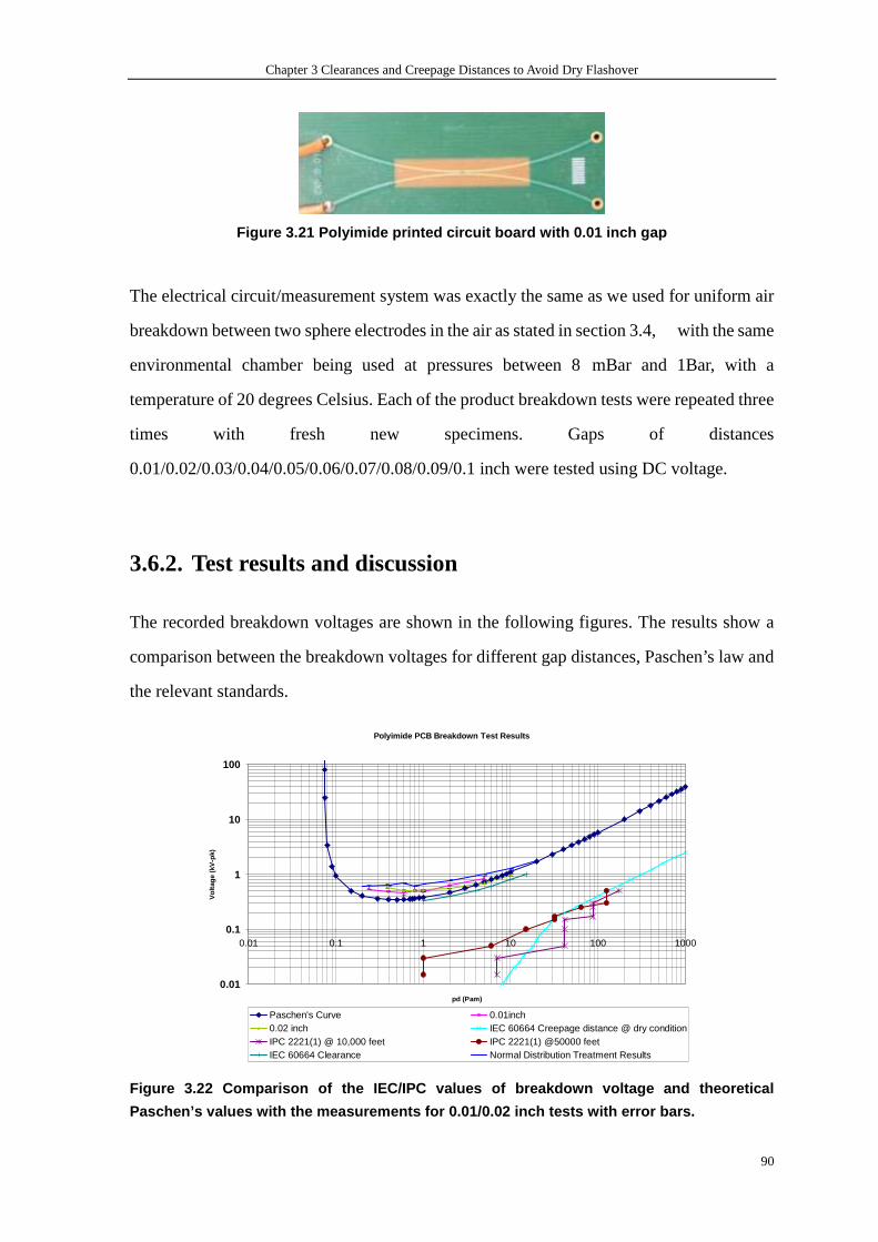
Chapter 3 Clearances and Creepage Distances to Avoid Dry Flashover
90
Figure 3.21 Polyimide printed circuit board with 0. 01 inch gap
The electrical circuit/measurement system was exactly the same as we used for uniform air
breakdown between two sphere electrodes in the air as stated in section 3.4, with the same
environmental chamber being used at pressures between 8 mBar and 1Bar, with a
temperature of 20 degrees Celsius. Each of the product breakdown tests were repeated three
times with fresh new specimens. Gaps of distances
0.01/0.02/0.03/0.04/0.05/0.06/0.07/0.08/0.09/0.1 inch were tested using DC voltage.
3.6.2. Test results and discussion
The recorded breakdown voltages are shown in the following figures. The results show a
comparison between the breakdown voltages for different gap distances, Paschen’s law and
the relevant standards.
Polyimide PCB Breakdown Test Results
0.01
0.1
1
10
100
0.01 0.1 1 10 100 1000
pd (Pam)
Vol
tage
(kV
-pk)
Paschen's Curve 0.01inch0.02 inch IEC 60664 Creepage distance @ dry conditionIPC 2221(1) @ 10,000 feet IPC 2221(1) @50000 feetIEC 60664 Clearance Normal Distribution Treatment Results
Figure 3.22 Comparison of the IEC/IPC values of bre akdown voltage and theoretical
Paschen’s values with the measurements for 0.01/0.0 2 inch tests with error bars.
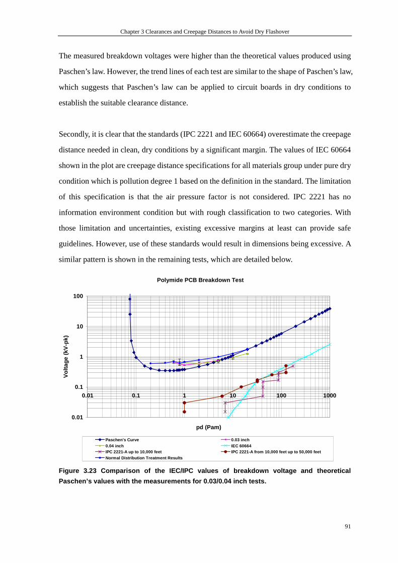
Chapter 3 Clearances and Creepage Distances to Avoid Dry Flashover
91
The measured breakdown voltages were higher than the theoretical values produced using
Paschen’s law. However, the trend lines of each test are similar to the shape of Paschen’s law,
which suggests that Paschen’s law can be applied to circuit boards in dry conditions to
establish the suitable clearance distance.
Secondly, it is clear that the standards (IPC 2221 and IEC 60664) overestimate the creepage
distance needed in clean, dry conditions by a significant margin. The values of IEC 60664
shown in the plot are creepage distance specifications for all materials group under pure dry
condition which is pollution degree 1 based on the definition in the standard. The limitation
of this specification is that the air pressure factor is not considered. IPC 2221 has no
information environment condition but with rough classification to two categories. With
those limitation and uncertainties, existing excessive margins at least can provide safe
guidelines. However, use of these standards would result in dimensions being excessive. A
similar pattern is shown in the remaining tests, which are detailed below.
Polymide PCB Breakdown Test
0.01
0.1
1
10
100
0.01 0.1 1 10 100 1000
pd (Pam)
Vol
tage
(kV
-pk)
Paschen's Curve 0.03 inch0.04 inch IEC 60664IPC 2221-A up to 10,000 feet IPC 2221-A from 10,000 feet up to 50,000 feetNormal Distribution Treatment Results
Figure 3.23 Comparison of the IEC/IPC values of bre akdown voltage and theoretical
Paschen’s values with the measurements for 0.03/0.0 4 inch tests.
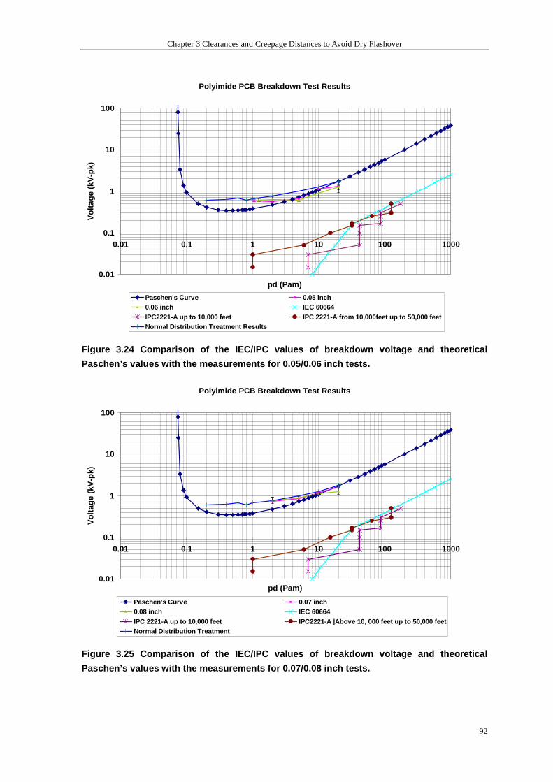
Chapter 3 Clearances and Creepage Distances to Avoid Dry Flashover
92
Polyimide PCB Breakdown Test Results
0.01
0.1
1
10
100
0.01 0.1 1 10 100 1000
pd (Pam)
Vol
tage
(kV
-pk)
Paschen's Curve 0.05 inch0.06 inch IEC 60664IPC2221-A up to 10,000 feet IPC 2221-A from 10,000feet up to 50,000 feet Normal Distribution Treatment Results
Figure 3.24 Comparison of the IEC/IPC values of bre akdown voltage and theoretical
Paschen’s values with the measurements for 0.05/0.0 6 inch tests.
Polyimide PCB Breakdown Test Results
0.01
0.1
1
10
100
0.01 0.1 1 10 100 1000
pd (Pam)
Vol
tage
(kV
-pk)
Paschen's Curve 0.07 inch0.08 inch IEC 60664IPC 2221-A up to 10,000 feet IPC2221-A |Above 10, 000 feet up to 50,000 feetNormal Distribution Treatment
Figure 3.25 Comparison of the IEC/IPC values of bre akdown voltage and theoretical
Paschen’s values with the measurements for 0.07/0.0 8 inch tests.
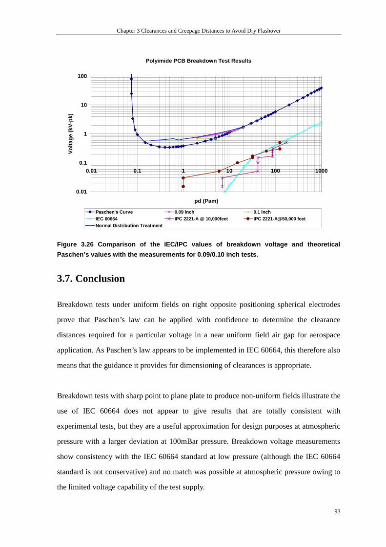
Chapter 3 Clearances and Creepage Distances to Avoid Dry Flashover
93
Polyimide PCB Breakdown Test Results
0.01
0.1
1
10
100
0.01 0.1 1 10 100 1000
pd (Pam)
Vol
tage
(kV
-pk)
Paschen's Curve 0.09 inch 0.1 inchIEC 60664 IPC 2221-A @ 10,000feet IPC 2221-A@50,000 feetNormal Distribution Treatment
Figure 3.26 Comparison of the IEC/IPC values of bre akdown voltage and theoretical
Paschen’s values with the measurements for 0.09/0.1 0 inch tests.
3.7. Conclusion
Breakdown tests under uniform fields on right opposite positioning spherical electrodes
prove that Paschen’s law can be applied with confidence to determine the clearance
distances required for a particular voltage in a near uniform field air gap for aerospace
application. As Paschen’s law appears to be implemented in IEC 60664, this therefore also
means that the guidance it provides for dimensioning of clearances is appropriate.
Breakdown tests with sharp point to plane plate to produce non-uniform fields illustrate the
use of IEC 60664 does not appear to give results that are totally consistent with
experimental tests, but they are a useful approximation for design purposes at atmospheric
pressure with a larger deviation at 100mBar pressure. Breakdown voltage measurements
show consistency with the IEC 60664 standard at low pressure (although the IEC 60664
standard is not conservative) and no match was possible at atmospheric pressure owing to
the limited voltage capability of the test supply.
Chapter 3 Clearances and Creepage Distances to Avoid Dry Flashover
94
At last, breakdown tests on Polyimide printed boards show us that under dry conditions, the
breakdown voltage is close to that expected using Paschen’s law but also that it far exceeds
that predicted using IEC 60664 or IPC 2221. Usage of the standards will lead to big margin
for safety but in term of insulating materials size, it is not very economic to apply.
Chapter 4 Modelling of Tracking Process under Wet Conditions
95
Chapter 4 Modeling of Tracking Process under Wet Conditions
4.1. Introduction
The previous chapter discussed flashover over solid insulating surfaces under dry
conditions. Through discussion of the test results and comparison with theoretical Paschen’s
law values, we concluded that flashovers on dry solid insulating surfaces are consistent with
it.
This chapter deals with theoretical modeling of the tracking threat to insulation systems that
results from aqueous contamination being deposited on surfaces along which an electric
field exists. This aqueous contamination can be from direct water contact (rain, leaking
pipework) or can occur in humid conditions where moisture condenses onto a surface. This
contamination coupled with a degree of conductivity inherent in the water contaminant
itself or through the mixing of water with surface pollution on the board can lead to
electrical tracking.
This section first of all looks the mechanism of electrical tracking in wet conditions,
especially under conductive aqueous contaminant conditions. A theoretical classical
mathematical model is then introduced. This model will in the following chapter be
tested and verified in a series of practical tests on solid insulating materials. Inception
voltages of electrical tracking are then calculated for certain specific environmental
conditions, including air pressure, ambient temperature, conductivity of aqueous
contaminant liquid, and even system inherent impedance.
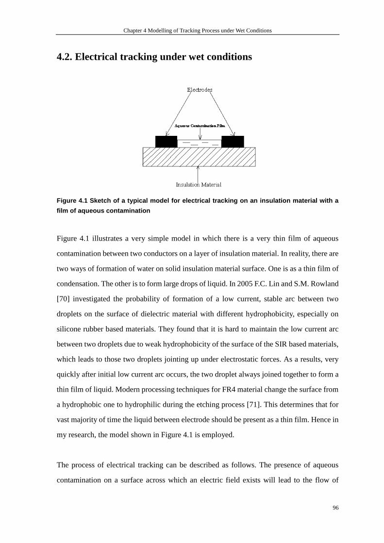
Chapter 4 Modelling of Tracking Process under Wet Conditions
96
4.2. Electrical tracking under wet conditions
Figure 4.1 Sketch of a typical model for electrical tracking on an insulation material with a
film of aqueous contamination
Figure 4.1 illustrates a very simple model in which there is a very thin film of aqueous
contamination between two conductors on a layer of insulation material. In reality, there are
two ways of formation of water on solid insulation material surface. One is as a thin film of
condensation. The other is to form large drops of liquid. In 2005 F.C. Lin and S.M. Rowland
[70] investigated the probability of formation of a low current, stable arc between two
droplets on the surface of dielectric material with different hydrophobicity, especially on
silicone rubber based materials. They found that it is hard to maintain the low current arc
between two droplets due to weak hydrophobicity of the surface of the SIR based materials,
which leads to those two droplets jointing up under electrostatic forces. As a results, very
quickly after initial low current arc occurs, the two droplet always joined together to form a
thin film of liquid. Modern processing techniques for FR4 material change the surface from
a hydrophobic one to hydrophilic during the etching process [71]. This determines that for
vast majority of time the liquid between electrode should be present as a thin film. Hence in
my research, the model shown in Figure 4.1 is employed.
The process of electrical tracking can be described as follows. The presence of aqueous
contamination on a surface across which an electric field exists will lead to the flow of
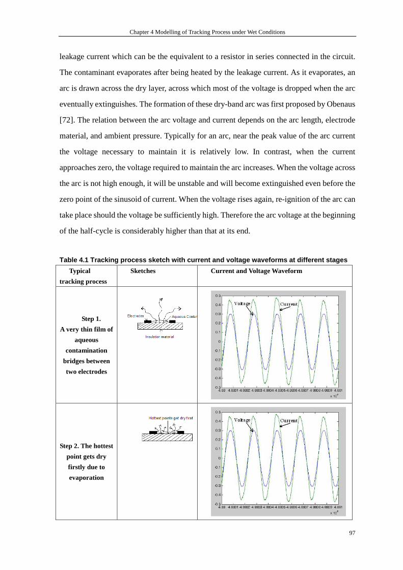
Chapter 4 Modelling of Tracking Process under Wet Conditions
97
leakage current which can be the equivalent to a resistor in series connected in the circuit.
The contaminant evaporates after being heated by the leakage current. As it evaporates, an
arc is drawn across the dry layer, across which most of the voltage is dropped when the arc
eventually extinguishes. The formation of these dry-band arc was first proposed by Obenaus
[72]. The relation between the arc voltage and current depends on the arc length, electrode
material, and ambient pressure. Typically for an arc, near the peak value of the arc current
the voltage necessary to maintain it is relatively low. In contrast, when the current
approaches zero, the voltage required to maintain the arc increases. When the voltage across
the arc is not high enough, it will be unstable and will become extinguished even before the
zero point of the sinusoid of current. When the voltage rises again, re-ignition of the arc can
take place should the voltage be sufficiently high. Therefore the arc voltage at the beginning
of the half-cycle is considerably higher than that at its end.
Table 4.1 Tracking process sketch with current and voltage waveforms at different stages
Typical
tracking process
Sketches Current and Voltage Waveform
Step 1.
A very thin film of
aqueous
contamination
bridges between
two electrodes
Step 2. The hottest
point gets dry
firstly due to
evaporation
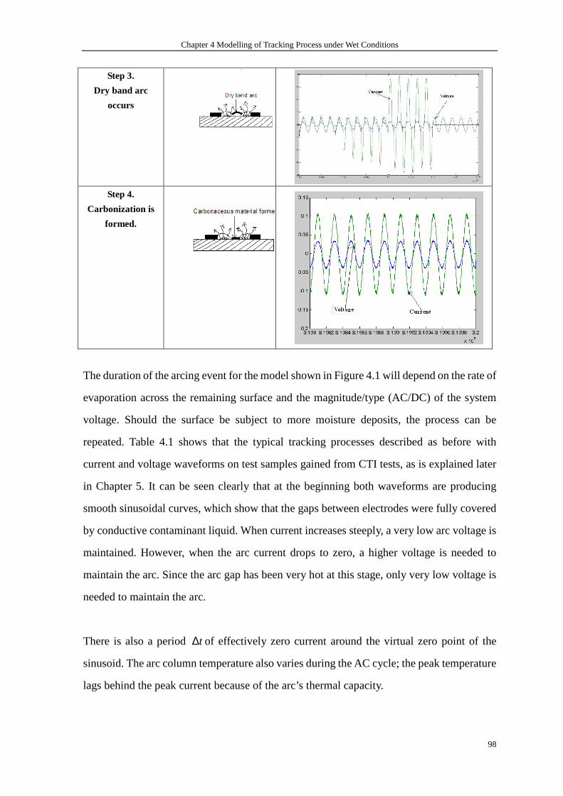
Chapter 4 Modelling of Tracking Process under Wet Conditions
98
Step 3.
Dry band arc
occurs
Step 4.
Carbonization is
formed.
The duration of the arcing event for the model shown in Figure 4.1 will depend on the rate of
evaporation across the remaining surface and the magnitude/type (AC/DC) of the system
voltage. Should the surface be subject to more moisture deposits, the process can be
repeated. Table 4.1 shows that the typical tracking processes described as before with
current and voltage waveforms on test samples gained from CTI tests, as is explained later
in Chapter 5. It can be seen clearly that at the beginning both waveforms are producing
smooth sinusoidal curves, which show that the gaps between electrodes were fully covered
by conductive contaminant liquid. When current increases steeply, a very low arc voltage is
maintained. However, when the arc current drops to zero, a higher voltage is needed to
maintain the arc. Since the arc gap has been very hot at this stage, only very low voltage is
needed to maintain the arc.
There is also a period t∆ of effectively zero current around the virtual zero point of the
sinusoid. The arc column temperature also varies during the AC cycle; the peak temperature
lags behind the peak current because of the arc’s thermal capacity.
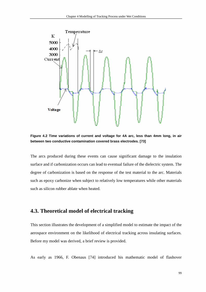
Chapter 4 Modelling of Tracking Process under Wet Conditions
99
Figure 4.2 Time variations of current and voltage f or 4A arc, less than 4mm long, in air
between two conductive contamination covered brass electrodes. [73]
The arcs produced during these events can cause significant damage to the insulation
surface and if carbonization occurs can lead to eventual failure of the dielectric system. The
degree of carbonization is based on the response of the test material to the arc. Materials
such as epoxy carbonize when subject to relatively low temperatures while other materials
such as silicon rubber ablate when heated.
4.3. Theoretical model of electrical tracking
This section illustrates the development of a simplified model to estimate the impact of the
aerospace environment on the likelihood of electrical tracking across insulating surfaces.
Before my model was derived, a brief review is provided.
As early as 1966, F. Obenaus [74] introduced his mathematic model of flashover
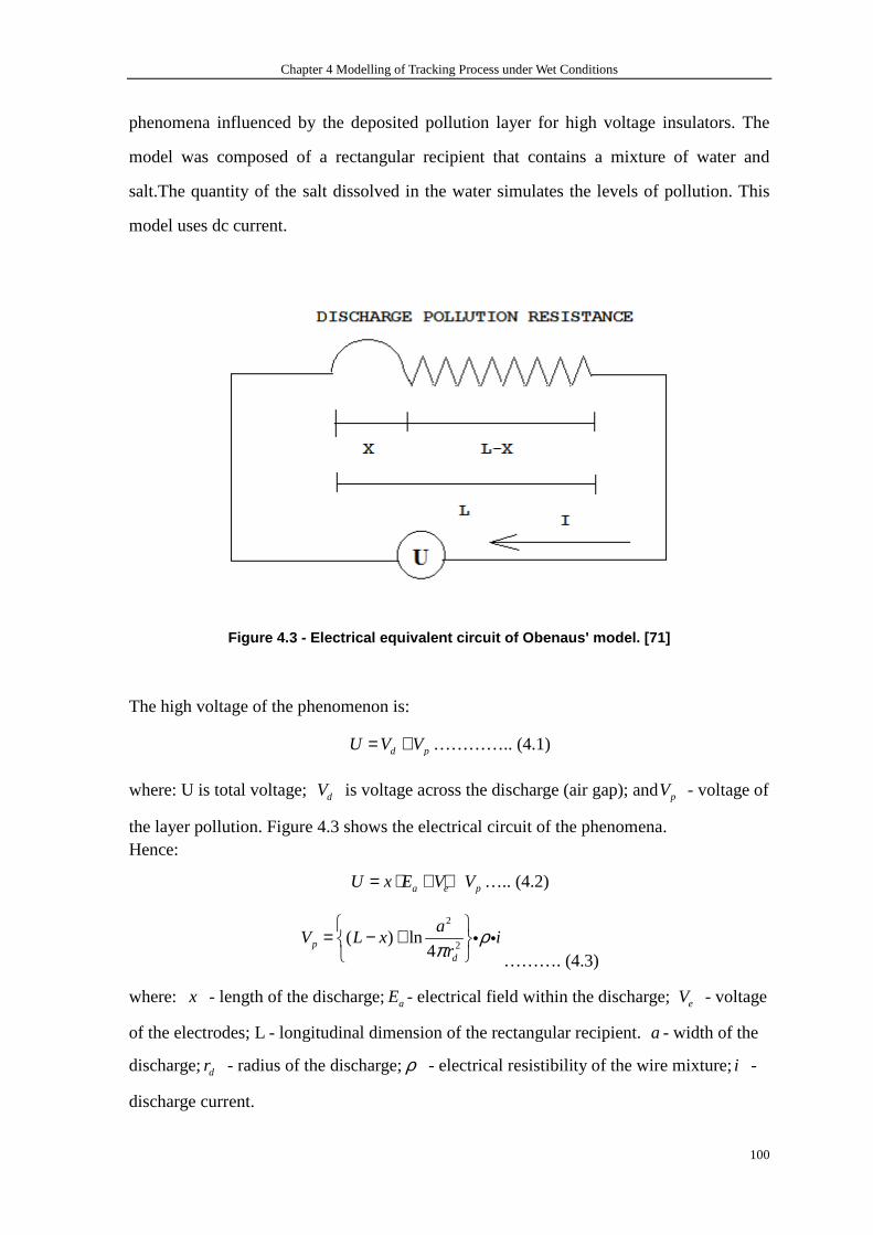
Chapter 4 Modelling of Tracking Process under Wet Conditions
100
phenomena influenced by the deposited pollution layer for high voltage insulators. The
model was composed of a rectangular recipient that contains a mixture of water and
salt.The quantity of the salt dissolved in the water simulates the levels of pollution. This
model uses dc current.
Figure 4.3 - Electrical equivalent circuit of Obena us' model. [71]
The high voltage of the phenomenon is:
d pU V V= + ………….. (4.1)
where: U is total voltage; dV is voltage across the discharge (air gap); andpV - voltage of
the layer pollution. Figure 4.3 shows the electrical circuit of the phenomena. Hence:
a e pU x E V V= ⋅ + + ….. (4.2)
2
2( ) ln
4pd
aV L x i
rρ
π
= − +
i i
………. (4.3)
where: x - length of the discharge;aE - electrical field within the discharge; eV - voltage
of the electrodes; L - longitudinal dimension of the rectangular recipient. a - width of the
discharge;dr - radius of the discharge;ρ - electrical resistibility of the wire mixture;i -
discharge current.

Chapter 4 Modelling of Tracking Process under Wet Conditions
101
In 1995, Oscar Armando Maldonado Astorga and Afonso Jose do Prado [75] presented
their results of dynamic behaviour of the flashover phenomenon on the high voltage
polluted insulators from a mathematical and an experimental model that introduce the
variable thickness influence of the layer pollution deposited on the high voltage insulator
surface to the Obenuas model. However, one limitation of Obenaus’s model is that air
pressure is not a parameter influencing behaviour, while the mathematic model here will
consist of the impact of this parameter shown in the following section.
My model is based on one originally developed by Warren [76] This model shown in
Figure 4.4 consists of a layer of aqueous contaminant film on a solid insulation surface
with electrical fields running through it. Warren focused on the pre-discharge conditions
required to evaporate the liquid layer as being an event required for tracking to start; that
is the technique adopted in this work.
Figure 4.4 the sketch of L. Warren’s pre-discharge conditions[76].
As it is seen in Figure 4.4, the aqueous contaminant film with height of h is supposed to be
heated up from the existing temperature T until its boiling point bt before pollution layer
is boiling. Underneath the pollution film, the insulating material with elemental width is
Chapter 4 Modelling of Tracking Process under Wet Conditions
102
also a medium to transfer heat generated by the electrical currents. Surrounding air is
another effective heat transfer medium. Then pre-discharge condition can be expressed by
input power and output power equilibrium equation as follows.
The heat equilibrium equation is:
2 ( ) ( )v a a
dT TE T h c k H T T
dt zσ ρ ∂= ⋅ + + −
∂……….. (4.4)
At or after boiling of the contamination, this becomes:
2 ( ) ( )b v a b a
dh TE T k H T T
dt zσ ρ ∂= + + −
∂…………. (4.5)
The input power 2 ( )E Tσ on the left hand side is the electrical power due to the electrical
currents through the pollution layer in which E is the voltage applied and
( )Tσ conductance. It can be seen that the conductance is dependent on the existing
temperature T of the contamination.
On the right side of the equation 4.1 expresses the output power from the pollution layer.
When heat is transferred by a circulation of fluids due to buoyancy from the density
changes induced by heating itself, then the process is know as nature convection or free
convection. Natural convection occurs when a system becomes unstable and therefore
begins to mix by the movement of mass [77]. The convectionRacan be expressed by the
following equation 4.6.
30Ra=g TLρ ακµ
∆………. (4.6)
where L is the characteristic length-scale of convection, and 3L is the volume of the
medium. In the case of L.Warren’s pre-discharge situation, it will be the volume of the
pollution layer which can expressed ash c⋅ . T∆ is the temperature difference across the
medium. Since all the items in the equation such as 0ρ ( the reference density, typically
picked to the average density of the medium), g ( the local gravitational acceleration), α
( the coefficient of thermal expansion), κ ( a thermal diffusivity) and µ ( the dynamic
viscosity) are constant, in L.Warren’s equation 4.4, they are shorted to a single item vρ .
Chapter 4 Modelling of Tracking Process under Wet Conditions
103
Then the first item on the right hand side of equation 4.1- heat convection of the pollution
layer-can be expressed asv
dTh c
dtρ ⋅ . The second item is
Tk
z
∂∂
is the heat transfer to the
underlying material (this will be based on the specific heat capacity of the specimen). The
last item ( )a aH T T− is to illustrate the heat conduction to the air where aH is the heat
transfer coefficient of air and aT T− is the difference between the current temperature of
the pollution T and air temperature aT .
In the following paragraphs, it can be seen that the mathematical model in my research
does not include the dynamic behaviour of heat transferred to the underlying material and
electrodes and the heat leading to temperature changes.
The model is built based on the geometry illustrated in Figure 4.5, which is based on the test
geometry from IEC 60112. Two electrodes are placed on a piece of insulating material. An
aqueous contaminant of a specific resistivity falls into place between the two electrodes. To
simplify this analysis, the contaminant layer is taken to have uniform thickness and a
uniform width across the gap between the two electrodes in a rectangular shape, and
contains salt and water to make it conductive. Arc formation will only take place should the
contaminant layer be evaporated, i.e. when a dry band develops.
The input power to the aqueous conductive contamination film is the power converted from
electrical energy due to leakage current flowing through the equivalent resistance of the film.
The film between two electrodes has a dimension of l w h× × where l is the length, w is
the width and h is the height. The resistance of the film therefore is:
lR
whρ= ………. (4.7)
If we consider the system to be uniform and examine the steady state energy balance, then
the heat into the system will equal the heat loss as given in Equation 4.8 where ‘V ’ is the
voltage across the gap, and ‘( )Tρ ’ is the resistivity of the contaminant expressed as a
function of temperature. According to the power dissipation equation, we can then attain the
Chapter 4 Modelling of Tracking Process under Wet Conditions
104
equation 4.5 to show the input power to the film:
2 22
( )in
V V whP I R
R T lρ⋅= ⋅ = = ……. (4.8)
The output power consists of heat transferred through the surrounding air, output of the
underlying material and even from the electrodes (especially when these are large). As was
explained in the previous section, in L. Warren’s model, dynamic behaviors of heat transfer
to different media should be included to get a full picture of the voltage required for tracking
as a function of time. However, in my research the static model ignores the influence of heat
capacity, which would only serve to increase the voltage needed for tracking, while the
electrodes/specimens act as a heat sink and therefore limit the temperature rise of the
contaminant layer. The latent heat, is the energy absorbed during a change of state without a
change of temperature, which here is boiling of water or evaporation. The magnitude of the
latent heat would on the energy required to evaporate the water drop is 2260kJ/kg. This
magnitude will determine the power required after the contaminant liquid reaches to boiling.
As explained before, the phenomena in my research focus on the initiation of discharge for
the system. We suppose that as soon as the boiling point is achieved, the dry band appears.
[78-82]
Although in my research the static model ignores the influence of heat capacity, a theoretical
calculation of the time for the film between electrodes to evaporate can be carried out by
considering both heat capacity of the water film and its latent heat. It should be noted that
the increase of the amount of water between electrodes in the calculation has been ignored.
First of all, the heat energy needed for the liquid with dimension of 5 4 1mm mm mm× × and
weight of 0.02g to be heated up to boiling point can be calculated. It is known that the heat
capacity for the liquid is 4183 / /J kg K shown in table 4.2 in chapter 4. Hence the output
energy used for the liquid to reach boiling point is calculated as
34183 0.02 10 (373 293) 6.7−× × × − = J . Then output energy for the liquid to evaporate to
vapor is calculated as 45.2 J ( 0.02 2260= × ) since the likely magnitude of latent heat for
water drop to evaporate is 2260 kJ/kg . As a conclusion, the total output energy is the sum

Chapter 4 Modelling of Tracking Process under Wet Conditions
105
of the two output energy, which is 51.9J .
The contaminant liquid used is the solution specified in the section 5.2.4 in chapter 5 and its
resistivity at 23 ± 1 °C is 395 ± 5Ω ·cm. Hence the resistance for length of 4 mm film
between electrodes is 3160Ω . So the energy in to the liquid under applied 50 V on the
electrodes is 250
3160t⋅ J where t is the time. Finally the time for 0.02 g of liquid under
50V to reach boiling point is about 73 s. If the applied voltage rises to 70 V, the time for the
certain amount of the liquid to evaporate is about 33 s. It can be seen that with a low voltage
such as 50V, the liquid will not evaporate within 72 s. In chapter 5, the dropping system
specified in the IEC 60112 standard can produce one liquid drop every 30 s, which is much
less than 72 s. As a result, it is expected that the amount of liquid will keep increasing during
the whole test period. However, when the voltage is raised to 70 V, the evaporation time for
the liquid is around 33 s, which is close to the dropping rate. In this case, the evaporation
rate and replenishment rate of the liquid reach to equilibrium. The amount of the liquid on
the solid insulation material should stay pretty much the same. From the calculation above,
it can also be seen that the energy needed for the liquid to reach boiling point compared to
the energy for the liquid to change to vapor is relatively low. It will not have big effect on
the process. In my research, the arc will occur as soon as the continuity of film is broken.
Higher applied voltages will increase the input power to the liquid which will lead to
shorter time for the liquid to evaporate. As a result, with higher voltages the first arc will
be ready to occur much more quickly. And the time for the next liquid to replenish will be
longer. This will eventually lead to arc reignition and more severe tracking damages on the
solid insulation.
In the static state the electrodes and specimens have been heated up to their maximum heat
capacity (based on the maximum temperature of the liquid). This heat transfer does not need
to be modeled but the heat lost through the electrodes and specimen to the air must be
accounted for. An equivalent thermal resistance of the film to the surroundings (accounting
for conduction, radiation and convection, and including the losses not just from the liquid
Chapter 4 Modelling of Tracking Process under Wet Conditions
106
but also from the electrodes and the specimen) is introduced as ‘ TR ’.
The output power can therefore be expressed as in equation 4.9 where ‘T ’ is the
temperature of the liquid or the surroundings as indicated by the subscript.
( ) /out air TP T T R= − …………. (4.9)
TR is taken to be the equivalent thermal resistance as calculated by equation 4.10 and
representing conductive, radiative and convective losses (although it is noted that these will
not be linear effects).
11 1 1
air material electrodes
T
T T T
R
R R R
=+ +
………. (4.10)
To begin the tracking process, liquidT must be raised to the boiling point of the liquid. We
can therefore achieve equation 4.11, which expresses the thermal equilibrium at boiling
state of the static model.
( )2
/( ) boiling ambient T
V whT T R
T lρ⋅ = − …………….(4.11)
The equation shows that the tracking process is highly dependent on the ambient
temperature. A lower voltage will be required to raise the liquid to a temperature at which it
will evaporate when the ambient temperature is high. The current standards such as IEC
60664 and IPC 2221 state one specific requirement for creepage distance and do not vary
this as a function of ambient temperature.
The process is also dependent on the boiling point of the liquid. Given that pressure changes
the boiling point of a liquid and as the pressure falls the boiling point reduces, it is expected
that a lower voltage will be required to evaporate the contaminant at lower pressures.
Chapter 4 Modelling of Tracking Process under Wet Conditions
107
In reality, a number of other factors exist that mean the exact relationship between the
voltage and the boiling point will not be as straightforward as that presented. The resistivity
of the contaminant will change as a function of time as it changes temperature (the higher
the resistivity of the contaminant, the lower the heat input for a given unit voltage).
As described, there will also be a significant impact of the test sample and the electrodes
owing to the heat capacity that they exhibit. The heat flow will therefore change as a
function of time as the electrodes and the test specimen heat up. This is discussed in the
following section 4.5.
4.4. Theoretical model analysis
The static model expressed in equation 4.11 clearly shows that the significant factors
influencing electrical tracking are the applied voltage, resistivity of aqueous contamination,
dimensioning of film between electrodes, boiling temperature of the contamination,
ambient temperature and equivalent thermal resistance. A number of these factors are
inter-dependent, which consequently makes it even more complicated to understand the
electrical tracking mechanism and draw Conclusion.
4.4.1. Static thermal analysis
A static thermal analysis was run on the Finite Element Analysis software ‘Vector Field
Opera version 11’ to determine the thermal resistance between the liquid layer and the
surrounding air while including the effects of heat loss through the electrodes and the
specimen (once the system had reached a steady state).
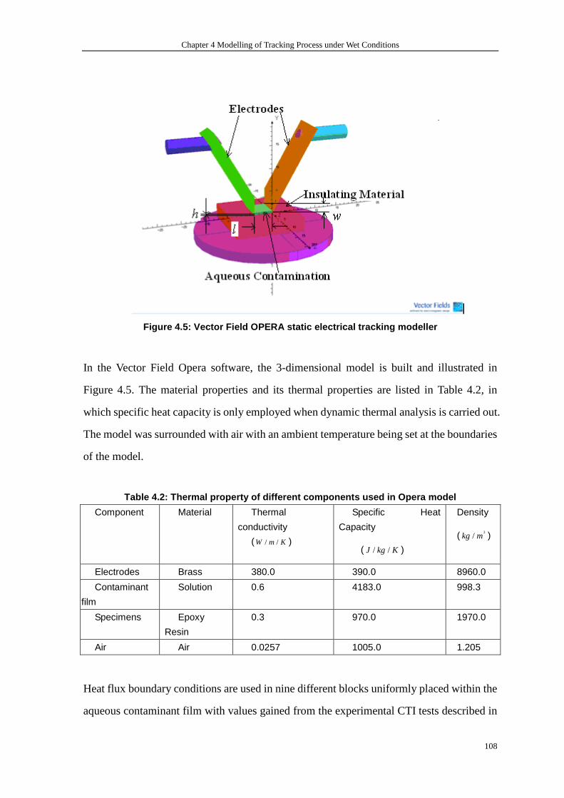
Chapter 4 Modelling of Tracking Process under Wet Conditions
108
Figure 4.5: Vector Field OPERA static electrical tr acking modeller
In the Vector Field Opera software, the 3-dimensional model is built and illustrated in
Figure 4.5. The material properties and its thermal properties are listed in Table 4.2, in
which specific heat capacity is only employed when dynamic thermal analysis is carried out.
The model was surrounded with air with an ambient temperature being set at the boundaries
of the model.
Table 4.2: Thermal property of different components used in Opera model
Component Material
Thermal
conductivity
( / /W m K )
Specific Heat
Capacity
( / /J kg K )
Density
( 3/kg m )
Electrodes Brass 380.0 390.0 8960.0
Contaminant
film
Solution 0.6 4183.0 998.3
Specimens Epoxy
Resin
0.3 970.0 1970.0
Air Air 0.0257 1005.0 1.205
Heat flux boundary conditions are used in nine different blocks uniformly placed within the
aqueous contaminant film with values gained from the experimental CTI tests described in

Chapter 4 Modelling of Tracking Process under Wet Conditions
109
Chapter 5 at 50 V (and using the voltage and current to work out the power input). The
following figures show us the model once meshed.
Figure 4.6 a three-dimensional model for research o n heat transfer from conductive liquid
film on insulation surface under electric stress to surrounding media.
After the model has been meshed, the static thermal analysis called TEMPO is run. In the
following Figure 4.7 a 3-dimensional temperature distribution of the model is shown with
temperature contour and its value band. It can be seen that the highest temperature around
329 K is found at the middle of the contamination film. With distances further from the
middle part of film, the temperatures gradually decrease to 293 K, which is room
temperature. The temperature change of electrodes around 20 K indicates that electrodes
do have an impact on the voltage required for tracking since they dissipate heat into the
surrounding air effectively, which will lower the thermal resistance of the water film to the
surroundings.
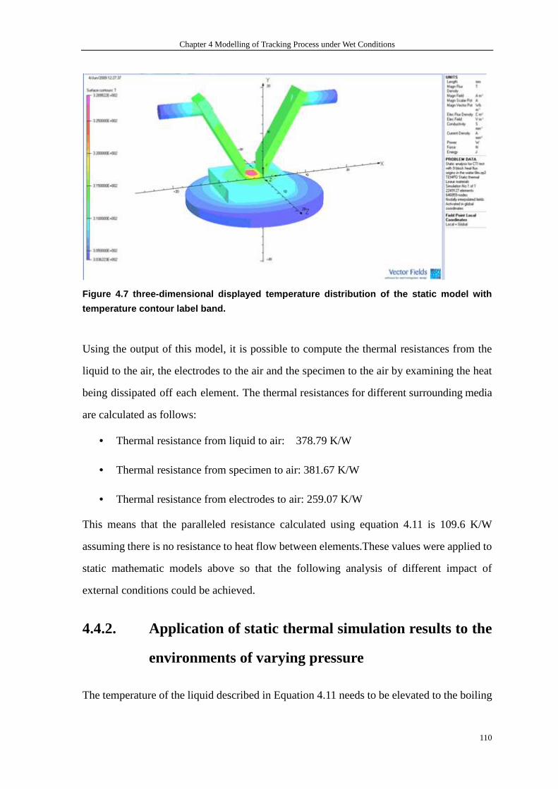
Chapter 4 Modelling of Tracking Process under Wet Conditions
110
Figure 4.7 three-dimensional displayed temperature distribution of the static model with
temperature contour label band.
Using the output of this model, it is possible to compute the thermal resistances from the
liquid to the air, the electrodes to the air and the specimen to the air by examining the heat
being dissipated off each element. The thermal resistances for different surrounding media
are calculated as follows:
• Thermal resistance from liquid to air: 378.79 K/W
• Thermal resistance from specimen to air: 381.67 K/W
• Thermal resistance from electrodes to air: 259.07 K/W
This means that the paralleled resistance calculated using equation 4.11 is 109.6 K/W
assuming there is no resistance to heat flow between elements.These values were applied to
static mathematic models above so that the following analysis of different impact of
external conditions could be achieved.
4.4.2. Application of static thermal simulation results to the
environments of varying pressure
The temperature of the liquid described in Equation 4.11 needs to be elevated to the boiling

Chapter 4 Modelling of Tracking Process under Wet Conditions
111
point for tracking to occur (some liquid needs to be evaporated to allow the boiling point to
be reached). The differences between the room temperature and boiling point determine the
maximum output power. The boiling point will vary as a function of pressure. Therefore
when the influence of air pressure is studied, the varying boiling with air pressure should be
carefully looked into. In an aerospace application, the air pressure may reach as low as 1165
Pa at an altitude of 15,255 m (50,000 feet). The relationship of air pressure with altitude is
shown in Figure 4.8, which indicates that the air pressure decreases with altitude
increasing. For the solution used in the IEC 60112 test described in Chapter 5, the boiling
point is 54.3 ºC at 1000 Pa (100 mbar) and 101.5 ºC at 100,000 Pa (1000 mbar) as the
measurement result from testing carried by myself. This section shows the pressure impact
on withstand voltage for electrical tracking by ignoring conductivity changes of aqueous
contamination with temperature.
Figure 4.8 the relationship of air pressure with th e altitude.
To identify the impact of pressure on the voltage that will instigate electrical tracking, the
formula given as Equation 4.11 was used, where the water film is simplified as a cuboids
with 4mm of length by 5mm of width by 0.5mm of height, boiling points of deionized water
and solution as a function of pressure as shown in Figure 4.9, and ambient temperature is
293 K (20 °C).
To achieve the relationship between the boiling point of two types of liquids including
deionized water (0.0008 S/m) and solution A specified in IEC 60112 (0.258 S/m) and
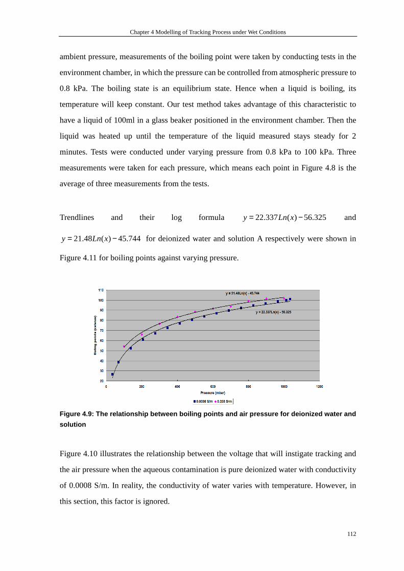
Chapter 4 Modelling of Tracking Process under Wet Conditions
112
ambient pressure, measurements of the boiling point were taken by conducting tests in the
environment chamber, in which the pressure can be controlled from atmospheric pressure to
0.8 kPa. The boiling state is an equilibrium state. Hence when a liquid is boiling, its
temperature will keep constant. Our test method takes advantage of this characteristic to
have a liquid of 100ml in a glass beaker positioned in the environment chamber. Then the
liquid was heated up until the temperature of the liquid measured stays steady for 2
minutes. Tests were conducted under varying pressure from 0.8 kPa to 100 kPa. Three
measurements were taken for each pressure, which means each point in Figure 4.8 is the
average of three measurements from the tests.
Trendlines and their log formula 22.337 ( ) 56.325y Ln x= − and
21.48 ( ) 45.744y Ln x= − for deionized water and solution A respectively were shown in
Figure 4.11 for boiling points against varying pressure.
Figure 4.9: The relationship between boiling points and air pressure for deionized water and
solution
Figure 4.10 illustrates the relationship between the voltage that will instigate tracking and
the air pressure when the aqueous contamination is pure deionized water with conductivity
of 0.0008 S/m. In reality, the conductivity of water varies with temperature. However, in
this section, this factor is ignored.
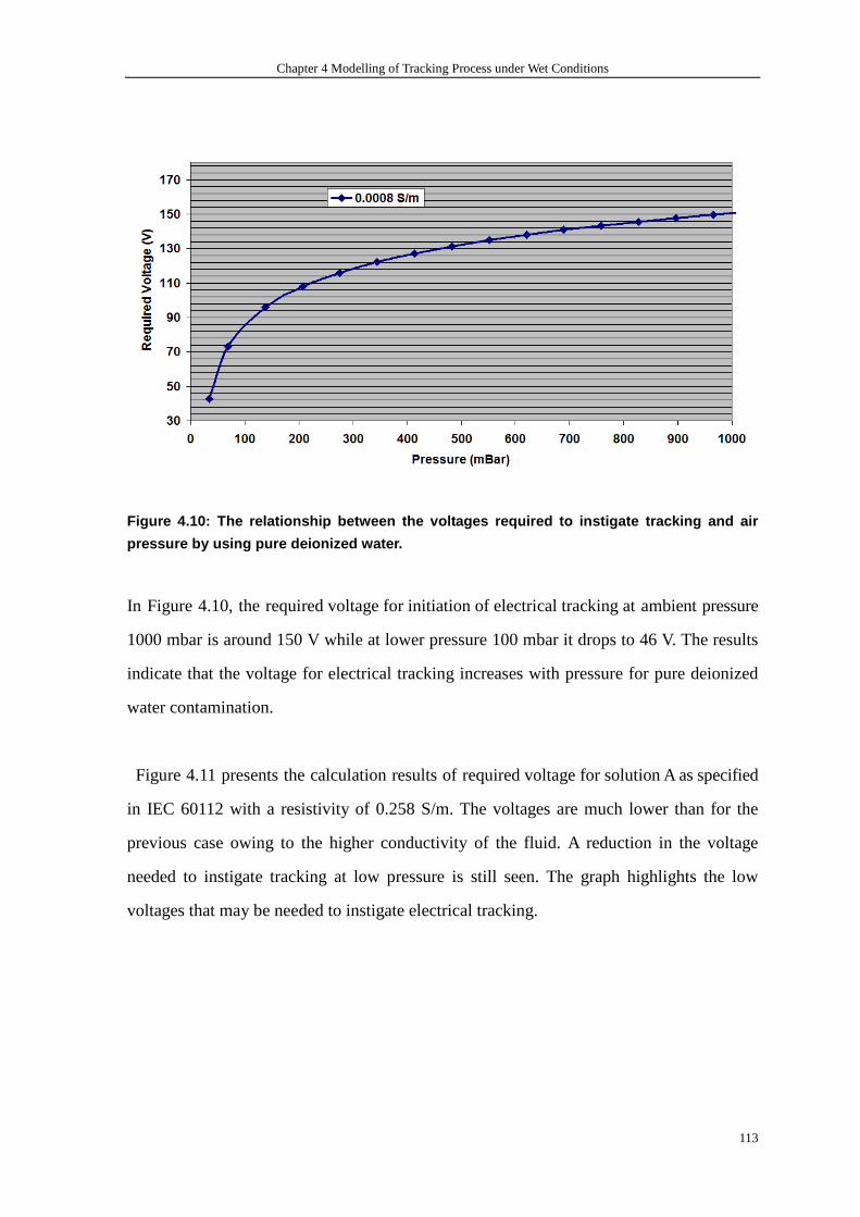
Chapter 4 Modelling of Tracking Process under Wet Conditions
113
Figure 4.10: The relationship between the voltages required to instigate tracking and air
pressure by using pure deionized water.
In Figure 4.10, the required voltage for initiation of electrical tracking at ambient pressure
1000 mbar is around 150 V while at lower pressure 100 mbar it drops to 46 V. The results
indicate that the voltage for electrical tracking increases with pressure for pure deionized
water contamination.
Figure 4.11 presents the calculation results of required voltage for solution A as specified
in IEC 60112 with a resistivity of 0.258 S/m. The voltages are much lower than for the
previous case owing to the higher conductivity of the fluid. A reduction in the voltage
needed to instigate tracking at low pressure is still seen. The graph highlights the low
voltages that may be needed to instigate electrical tracking.
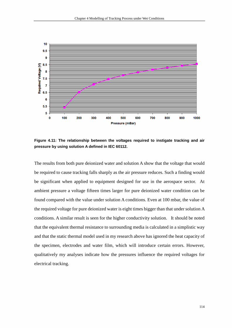
Chapter 4 Modelling of Tracking Process under Wet Conditions
114
Figure 4.11: The relationship between the voltages required to instigate tracking and air
pressure by using solution A defined in IEC 60112.
The results from both pure deionized water and solution A show that the voltage that would
be required to cause tracking falls sharply as the air pressure reduces. Such a finding would
be significant when applied to equipment designed for use in the aerospace sector. At
ambient pressure a voltage fifteen times larger for pure deionized water condition can be
found compared with the value under solution A conditions. Even at 100 mbar, the value of
the required voltage for pure deionized water is eight times bigger than that under solution A
conditions. A similar result is seen for the higher conductivity solution. It should be noted
that the equivalent thermal resistance to surrounding media is calculated in a simplistic way
and that the static thermal model used in my research above has ignored the heat capacity of
the specimen, electrodes and water film, which will introduce certain errors. However,
qualitatively my analyses indicate how the pressures influence the required voltages for
electrical tracking.
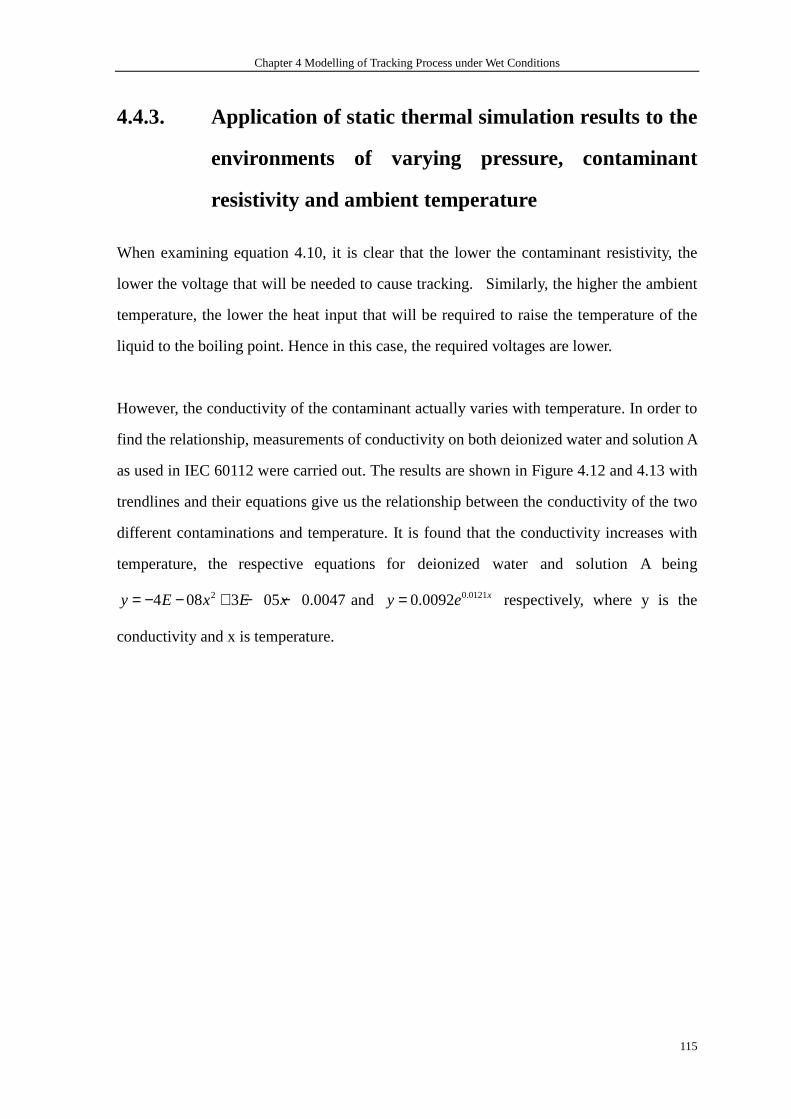
Chapter 4 Modelling of Tracking Process under Wet Conditions
115
4.4.3. Application of static thermal simulation results to the
environments of varying pressure, contaminant
resistivity and ambient temperature
When examining equation 4.10, it is clear that the lower the contaminant resistivity, the
lower the voltage that will be needed to cause tracking. Similarly, the higher the ambient
temperature, the lower the heat input that will be required to raise the temperature of the
liquid to the boiling point. Hence in this case, the required voltages are lower.
However, the conductivity of the contaminant actually varies with temperature. In order to
find the relationship, measurements of conductivity on both deionized water and solution A
as used in IEC 60112 were carried out. The results are shown in Figure 4.12 and 4.13 with
trendlines and their equations give us the relationship between the conductivity of the two
different contaminations and temperature. It is found that the conductivity increases with
temperature, the respective equations for deionized water and solution A being
24 08 3 05 0.0047y E x E x= − − + − − and 0.01210.0092 xy e= respectively, where y is the
conductivity and x is temperature.

Chapter 4 Modelling of Tracking Process under Wet Conditions
116
Figure 4.12: The relationship between the conductiv ity of deionized water and temperature.
y = 0.0092e0.0121x
0
0.1
0.2
0.3
0.4
0.5
0.6
0.7
0.8
0.9
280 290 300 310 320 330 340 350 360 370 380
Temperature (K)
Con
duct
ivity
(S
/m)
Figure 4.13: The relationship between conductivity of solution A in IEC 60112 and
temperature.
This relationship between conductivity and temperature is then included in the static
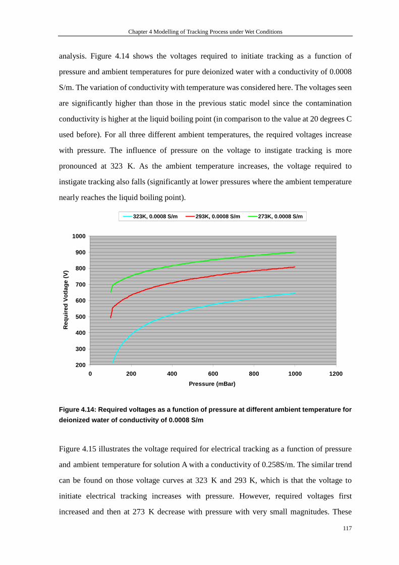
Chapter 4 Modelling of Tracking Process under Wet Conditions
117
analysis. Figure 4.14 shows the voltages required to initiate tracking as a function of
pressure and ambient temperatures for pure deionized water with a conductivity of 0.0008
S/m. The variation of conductivity with temperature was considered here. The voltages seen
are significantly higher than those in the previous static model since the contamination
conductivity is higher at the liquid boiling point (in comparison to the value at 20 degrees C
used before). For all three different ambient temperatures, the required voltages increase
with pressure. The influence of pressure on the voltage to instigate tracking is more
pronounced at 323 K. As the ambient temperature increases, the voltage required to
instigate tracking also falls (significantly at lower pressures where the ambient temperature
nearly reaches the liquid boiling point).
200
300
400
500
600
700
800
900
1000
0 200 400 600 800 1000 1200
Pressure (mBar)
Req
uire
d V
otla
ge (
V)
323K, 0.0008 S/m 293K, 0.0008 S/m 273K, 0.0008 S/m
Figure 4.14: Required voltages as a function of pre ssure at different ambient temperature for
deionized water of conductivity of 0.0008 S/m
Figure 4.15 illustrates the voltage required for electrical tracking as a function of pressure
and ambient temperature for solution A with a conductivity of 0.258S/m. The similar trend
can be found on those voltage curves at 323 K and 293 K, which is that the voltage to
initiate electrical tracking increases with pressure. However, required voltages first
increased and then at 273 K decrease with pressure with very small magnitudes. These
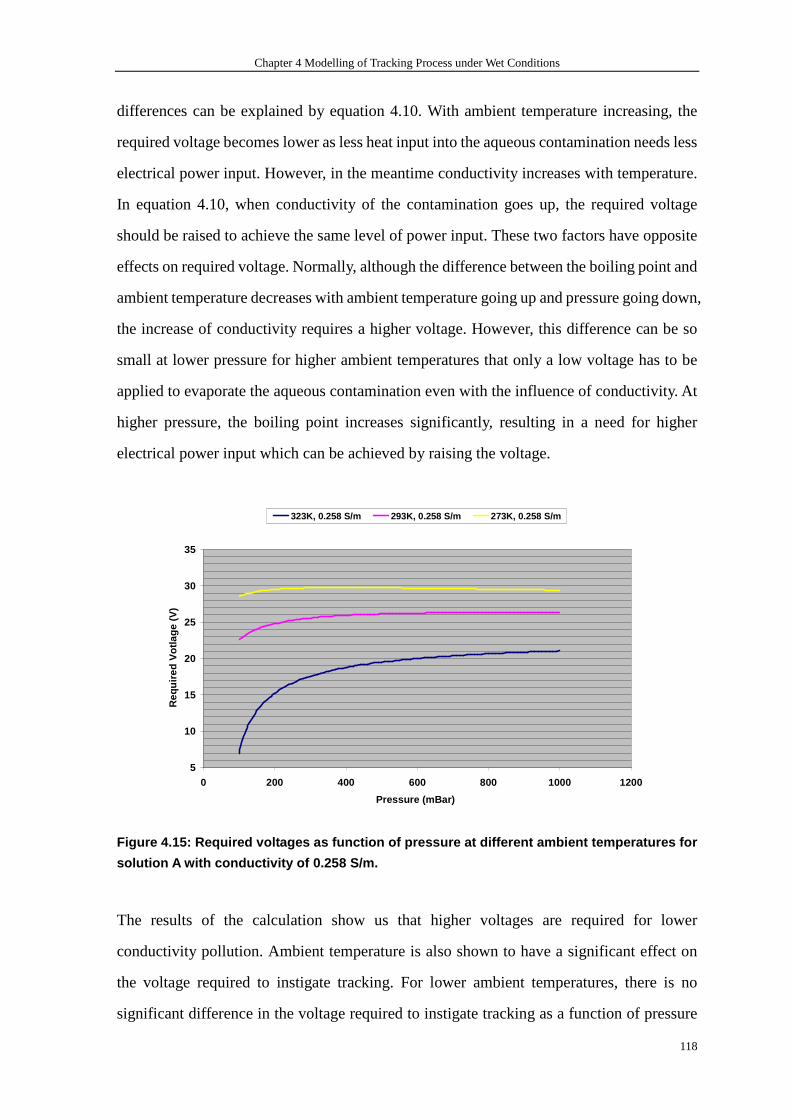
Chapter 4 Modelling of Tracking Process under Wet Conditions
118
differences can be explained by equation 4.10. With ambient temperature increasing, the
required voltage becomes lower as less heat input into the aqueous contamination needs less
electrical power input. However, in the meantime conductivity increases with temperature.
In equation 4.10, when conductivity of the contamination goes up, the required voltage
should be raised to achieve the same level of power input. These two factors have opposite
effects on required voltage. Normally, although the difference between the boiling point and
ambient temperature decreases with ambient temperature going up and pressure going down,
the increase of conductivity requires a higher voltage. However, this difference can be so
small at lower pressure for higher ambient temperatures that only a low voltage has to be
applied to evaporate the aqueous contamination even with the influence of conductivity. At
higher pressure, the boiling point increases significantly, resulting in a need for higher
electrical power input which can be achieved by raising the voltage.
5
10
15
20
25
30
35
0 200 400 600 800 1000 1200
Pressure (mBar)
Req
uire
d V
otla
ge (
V)
323K, 0.258 S/m 293K, 0.258 S/m 273K, 0.258 S/m
Figure 4.15: Required voltages as function of press ure at different ambient temperatures for
solution A with conductivity of 0.258 S/m.
The results of the calculation show us that higher voltages are required for lower
conductivity pollution. Ambient temperature is also shown to have a significant effect on
the voltage required to instigate tracking. For lower ambient temperatures, there is no
significant difference in the voltage required to instigate tracking as a function of pressure
Chapter 4 Modelling of Tracking Process under Wet Conditions
119
(this being due to the change in conductivity of the contaminant as a function of
temperature).
These results suggest that the use of both the standards [44,45] detailed in this paper, which
do not account for ambient temperature or contaminant conductivity, must be performed
with caution.
4.4.4. Dynamic thermal analysis
In the previous sections of this chapter, the impact factors of various environmental
situations have been discussed based on the static model of electrical tracking developed.
The static mathematical model shown in Equation 4.11 ignores two dynamic items
v
dTh c
dtρ ⋅ and
Tk
z
∂∂
in contrast to L.Warren’s Model. As explained before, the former
represents the heat convection of depending on temperature increase, and latter shows the
heat transfer to the underlying material. Both of them indicate the control of temperature
on the transfer of heat to surrounding heat dissipating media. To find out the influence of
these dynamic processes depending on the temperature changes to the required voltages
for electrical tracking, the same model in Vector Field software but with more material
properties and boundary conditions than in the static thermal simulation shown before.
The dynamic modeling analysis was run on the same Finite Element Analysis software
‘Vector Field Opera version 11’ since the software has the capability of running both static
and dynamic analysis. However, the material properties and boundary conditions have a
few differences. Specific heat capacities for surrounding heat transfer media indicated in
Table 4.2 are now employed to determine the dynamic processes of heat transfer
controlled by their temperature. Heat flux boundary conditions are used in nine different
blocks uniformly placed within the aqueous contaminant film with values gained from the
experimental CTI tests described in Chapter 5 at 50 V (and using the voltage and current to
work out the power input). The simulation time steps were set to 1 s, 2 s, 3 s, 5 s, 15 s, 20 s,
30 s, 60 s, and 120 s. After the model had been meshed both on the surfaces and within
Chapter 4 Modelling of Tracking Process under Wet Conditions
120
volumes, the dynamic thermal analysis was run.
It is known that initially all the surrounding media were at room temperature. When the
leakage current flowed through the aqueous liquid, heat was generated and transferred to
the surrounding heat transfer media including air, electrodes and insulating material at the
bottom. Heat capacity characterizes the amount of heat that is required to change a body‘s
temperature by a given amount. Calculation of this is very complicated due to
consideration of more than one state variable or physical property for thermodynamic
systems unless a particular infinitesimal path had been defined including the definition of
changes of temperature, pressure, volume, number of particles and any other relevant
macroscopic variable. If the system has more than just a simple homogenous structure,
each part of the system should be defined separately. Therefore to study thermal dynamic
heat transfer behaviors which would influence electrical tracking is not straightforward
after initial simulation with the software.
4.5. Discussion
The static mathematical model to initiate electrical tracking in this chapter has been
developed based on L. Warren’s model by ignoring heat transfer to surrounding heat
transfer media depending on temperature. Both the static and dynamic thermal simulations
were done in the Finite Element Analysis software ‘Vector Field Opera version 11’. The
static simulation was used to find out the equivalent heat transfer resistance while the
dynamic simulation was used to help predict the possible changes of required voltages to
initiate electrical tracking.
The static mathematical model was then employed to analyze different impact factors of
environments. Electrical tracking could happen when the continuity of the conductive path
– in this case, the aqueous contamination – is broken. Due to the boiling of the liquid, the
conductive path will be pulled apart most probably at the hottest point. It has been proven
that the boiling points increase with ambient pressure for both deionized water and
Chapter 4 Modelling of Tracking Process under Wet Conditions
121
solution A, defined in IEC 60112: 2003. Hence the required voltage to initiate electrical
tracking also increases with pressure. The value of voltages at ambient pressure 1000mbar
was around 150 V while at lower pressure 100 mbar it dropped to 46 V for deionized
water; it was 8.4 V for the highly conductive solution A at 10000mbar and 5.5 V at 100
mbar. This also represents the fact that the more conductive the aqueous contamination,
the lower the voltages are that are needed for electrical tracking.
Ambient temperature also plays a very important role in determining the electrical
tracking and its required voltages. Theoretical calculation results show that at higher
ambient temperatures, less voltage is required to initiate electrical tracking. The most
interesting results are those values of voltages required at 273 K for the highly conductive
solution A, which shows that the voltage actually decreases with pressure going up. This
result can be attributed to the combination of the influence of ambient temperature,
pressure and the conductivity of the aqueous contamination. Especially, these impact
factors are inter-dependent. This therefore proves that the mathematic model does predict
this complicated relationship.
Dynamic thermal analysis was presented to find out the influence of the thermodynamic
processes before the thermal equilibrium was reached. The heat capacities of
surrounding heat dissipating media are critical properties to consider. Again it is not a
simple variable, but varies with temperature, pressure and volume. My initial study
according to the simulation results with the software show us that the required voltage to
initiate electrical tracking before the surrounding electrodes are heated up is higher than
that when all the surrounding media has been at the same high temperature.
Finally, if we compare those calculated withstand voltage at atmospheric pressure to avoid
electrical tracking with those specified in IEC 60664, we can find for pollution degree 3
(conductive pollution occurs or dry non-conductive pollution occurs which becomes
conductive due to condensation which is to be expected, which is close to the situation of
use of solution A in my calculation) and material group III, the withstand voltage in
Chapter 4 Modelling of Tracking Process under Wet Conditions
122
standard is 250 V (320 V for material group I and bigger than 250 but less than 320 for
material group II ) while the results from the model is only 25 V. And the withstand
voltage under pollution degree 2 ( only non-conductive pollution occurs expect that
occasionally a temporary conductive caused by condensation is to be expected, which is
close to the situation of use of deionized water in my calculation) which is equal to the
deionized water pollution situation is 400 V while the calculated voltage is around 780 V.
Comparing to the values in Table A6 in appendix A from IPC 2221, it can be seen that
without considering any pollution degree difference, the withstand voltage for 4mm gap
above sea level up to 3050 m (around 696.4 mbar) is 800 V while my calculated voltage is
25 V for very conductive pollution condition, and around 740 V for deionized water
pollution condition. For any case above 3050m, the withstand voltage in the standard is
170 V. All the standard have no consideration of the impact of ambient temperature.
4.6. Conclusion
The computational model developed in my research can predict the inception voltages of
discharges for wet condition electrical tracking model considering the impact of air pressure,
ambient temperature, and pollution degree (through the conductivity of contaminants).
Those environment factors are very important for aerospace application, especially for the
MEA concept with higher voltage levels. And boiling point of liquid pollution is a very
critical parameter to influence the start electrical discharges and hence electrical tracking.
However, one major drawback of this model is that the thermal dynamic processes have
been ignored, which are believed to have effect on the initiation of discharge on insulation
surfaces between electrodes.

Chapter 5 Experimental Investigation I: Standard CTI Tests on FR-4 and ABS Materials
123
Chapter 5 Experimental Investigation I:
Standard CTI Tests on FR-4 and ABS
Materials
5.1. Introduction
Experimental verification is highly necessary to prove the results and conclusions gained
from the previous computer simulation and computation. Furthermore, it is clearly helpful
for promoting understanding of the mechanism of electrical tracking under different
micro-environmental conditions. Many factors that affect the behaviour of electrical
discharges on organic insulating material surfaces should be identified further by testing.
The various tracking resistance test methods has been developed as described in Chapter 2,
It generally can be divided into two classes: wet and dry methods. Dry test is based on the
idea that the tracking phenomenon developed from tiny electrical discharges on the solid
insulating surfaces. They are repeated until the whole path between the two conductors
becomes tracking. The dry method has characteristics of repeatability since the method is
very simple. The disadvantage of dry method is that very high applied voltage is needed and
time-consuming. The biggest concern of the dry method is that the electrical tracking
mechanism is different from electrical tracking under pollution condition in real life.
Wet condition tracking test method obviously has advantage in term of simulating the
environment condition in real life closely by utilizing artificial contamination. However, the
biggest challenge for wet tracking tests is that the reproducibility of the test results is not
acceptable. Therefore the repeatability of the test results will be inspected in this chapter by
Chapter 5 Experimental Investigation I: Standard CTI Tests on FR-4 and ABS Materials
124
repeating the same test for three times for all the tests.
Organic insulation materials are used in a variety of electrical apparatus owing to their
lightweight and useful electrical and mechanical properties.The experimental work was
carried out on two kinds of organic insulating materials widely used in power electronics
equipments on modern aircraft, which are FR-4 and Acrylonitrile butadiene styrene (ABS).
FR-4 is made of woven fiberglass cloth with an epoxy resin binder that is flame resistant.
FR-4 glass epoxy is a popular and versatile high pressure thermoset plastic laminate grade
with good strength to weight ratios. It is most commonly used as an electrical insulator
with near zero water absorption and considerable mechanical strength. All these attributes
make it a very good insulation material for printed circuit boards. It is usually used as a
substrate with a copper layer. The FR-4 used in PCBs is typically UV stabilized with a
tetra-functional epoxy resin system. It is typically a transparent yellowish color - the green,
red and sometimes blue color of a finished board comes from the solder mask. FR-4
manufactured strictly as an insulator (without copper cladding) is typically a di-functional
epoxy resin system and a greenish color.
ABS is a very commonly used thermoplastic, used to make light, rigid, molded products
with different CTI values of greater than 600 from FR-4 with CTI value of between 175
and 249 [83-85]. Hence CTI tests were carried on both materials to find out the
mechanism of electrical tracking and also the relation to the material groups.
The experiments were carried out while strictly following the instruction in IEC
:60112 2003. The standard provides a method to evaluate the resistance of solid electrical
insulating materials to electrical tracking or erosion for voltages up to 600 V when the
surface is exposed under electric stress to water with the addition of contaminants. The
comparative tracking indices are those values of applied voltages leading to the leakage
current flowing through the surfaces above a particular threshold (0.5 A) or scintillation
fire. However, my research focused on finding out the mechanism of electrical tracking on
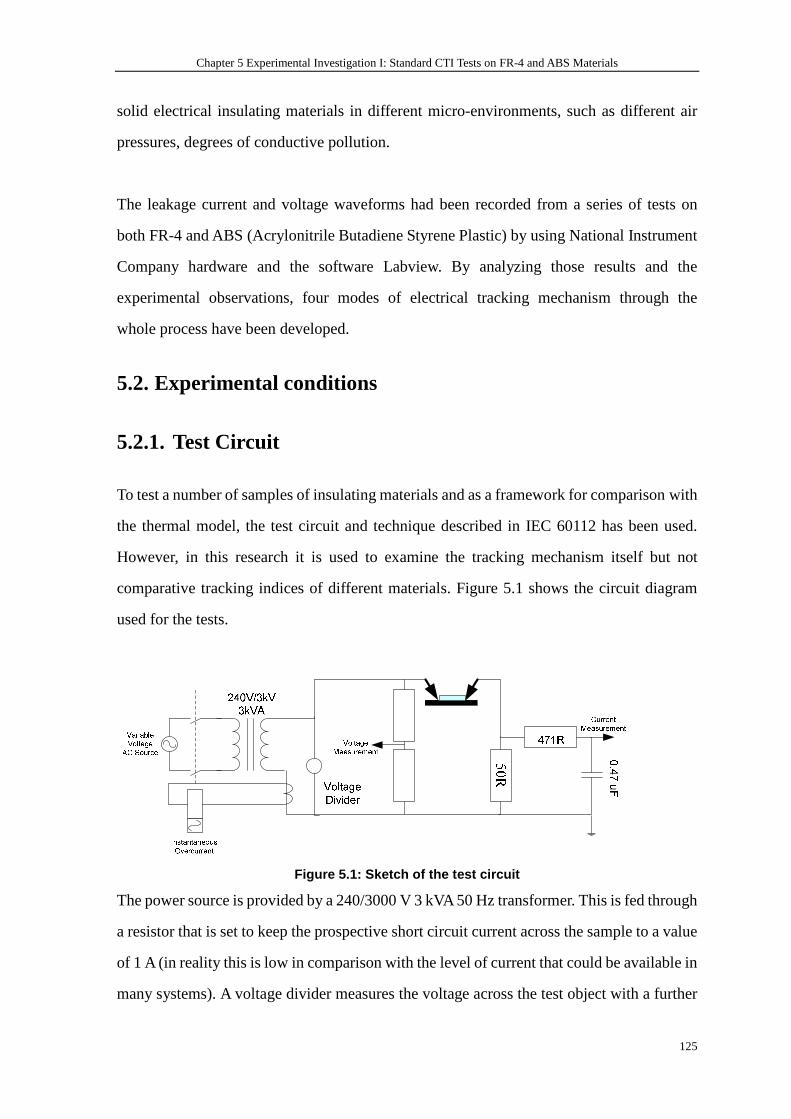
Chapter 5 Experimental Investigation I: Standard CTI Tests on FR-4 and ABS Materials
125
solid electrical insulating materials in different micro-environments, such as different air
pressures, degrees of conductive pollution.
The leakage current and voltage waveforms had been recorded from a series of tests on
both FR-4 and ABS (Acrylonitrile Butadiene Styrene Plastic) by using National Instrument
Company hardware and the software Labview. By analyzing those results and the
experimental observations, four modes of electrical tracking mechanism through the
whole process have been developed.
5.2. Experimental conditions
5.2.1. Test Circuit
To test a number of samples of insulating materials and as a framework for comparison with
the thermal model, the test circuit and technique described in IEC 60112 has been used.
However, in this research it is used to examine the tracking mechanism itself but not
comparative tracking indices of different materials. Figure 5.1 shows the circuit diagram
used for the tests.
Figure 5.1: Sketch of the test circuit
The power source is provided by a 240/3000 V 3 kVA 50 Hz transformer. This is fed through
a resistor that is set to keep the prospective short circuit current across the sample to a value
of 1 A (in reality this is low in comparison with the level of current that could be available in
many systems). A voltage divider measures the voltage across the test object with a further
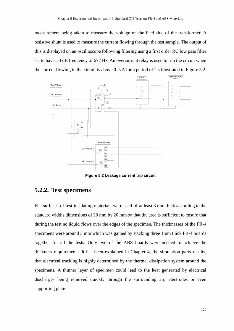
Chapter 5 Experimental Investigation I: Standard CTI Tests on FR-4 and ABS Materials
126
measurement being taken to measure the voltage on the feed side of the transformer. A
resistive shunt is used to measure the current flowing through the test sample. The output of
this is displayed on an oscilloscope following filtering using a first order RC low pass filter
set to have a 3 dB frequency of 677 Hz. An overcurrent relay is used to trip the circuit when
the current flowing in the circuit is above 0 .5 A for a period of 2 s illustrated in Figure 5.2.
240 V Live
240 Neutral
240 Earth
4
8
6
5
7
240 V Live
240 Neutral
A1
A2
Overcurrent Relay
Variac Transformer (240/
3000V)
E3
(+)
M
(-)
11
12
1 5
1 5
3
4
2
2
43
Figure 5.2 Leakage current trip circuit
5.2.2. Test specimens
Flat surfaces of test insulating materials were used of at least 3 mm thick according to the
standard widths dimensions of 20 mm by 20 mm so that the area is sufficient to ensure that
during the test no liquid flows over the edges of the specimen. The thicknesses of the FR-4
specimens were around 3 mm which was gained by stacking three 1mm thick FR-4 boards
together for all the tests. Only two of the ABS boards were needed to achieve the
thickness requirements. It has been explained in Chapter 4, the simulation parts results,
that electrical tracking is highly determined by the thermal dissipation system around the
specimens. A thinner layer of specimen could lead to the heat generated by electrical
discharges being removed quickly through the surrounding air, electrodes or even
supporting plate.
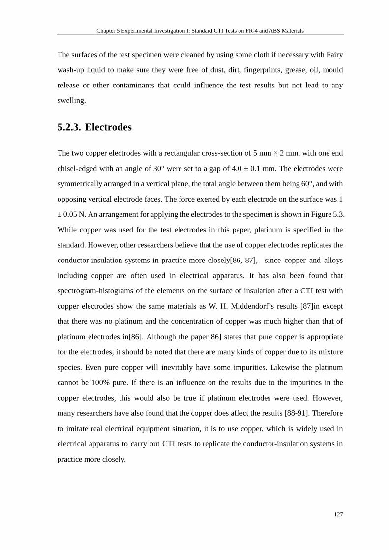
Chapter 5 Experimental Investigation I: Standard CTI Tests on FR-4 and ABS Materials
127
The surfaces of the test specimen were cleaned by using some cloth if necessary with Fairy
wash-up liquid to make sure they were free of dust, dirt, fingerprints, grease, oil, mould
release or other contaminants that could influence the test results but not lead to any
swelling.
5.2.3. Electrodes
The two copper electrodes with a rectangular cross-section of 5 mm × 2 mm, with one end
chisel-edged with an angle of 30° were set to a gap of 4.0 ± 0.1 mm. The electrodes were
symmetrically arranged in a vertical plane, the total angle between them being 60°, and with
opposing vertical electrode faces. The force exerted by each electrode on the surface was 1
± 0.05 N. An arrangement for applying the electrodes to the specimen is shown in Figure 5.3.
While copper was used for the test electrodes in this paper, platinum is specified in the
standard. However, other researchers believe that the use of copper electrodes replicates the
conductor-insulation systems in practice more closely[86, 87], since copper and alloys
including copper are often used in electrical apparatus. It has also been found that
spectrogram-histograms of the elements on the surface of insulation after a CTI test with
copper electrodes show the same materials as W. H. Middendorf’s results [87]in except
that there was no platinum and the concentration of copper was much higher than that of
platinum electrodes in[86]. Although the paper[86] states that pure copper is appropriate
for the electrodes, it should be noted that there are many kinds of copper due to its mixture
species. Even pure copper will inevitably have some impurities. Likewise the platinum
cannot be 100% pure. If there is an influence on the results due to the impurities in the
copper electrodes, this would also be true if platinum electrodes were used. However,
many researchers have also found that the copper does affect the results [88-91]. Therefore
to imitate real electrical equipment situation, it is to use copper, which is widely used in
electrical apparatus to carry out CTI tests to replicate the conductor-insulation systems in
practice more closely.
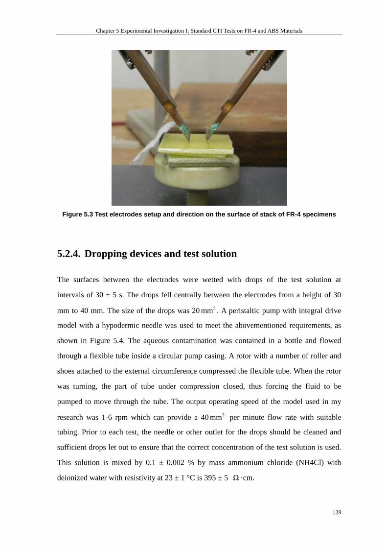
Chapter 5 Experimental Investigation I: Standard CTI Tests on FR-4 and ABS Materials
128
Figure 5.3 Test electrodes setup and direction on t he surface of stack of FR-4 specimens
5.2.4. Dropping devices and test solution
The surfaces between the electrodes were wetted with drops of the test solution at
intervals of 30 ± 5 s. The drops fell centrally between the electrodes from a height of 30
mm to 40 mm. The size of the drops was 203mm . A peristaltic pump with integral drive
model with a hypodermic needle was used to meet the abovementioned requirements, as
shown in Figure 5.4. The aqueous contamination was contained in a bottle and flowed
through a flexible tube inside a circular pump casing. A rotor with a number of roller and
shoes attached to the external circumference compressed the flexible tube. When the rotor
was turning, the part of tube under compression closed, thus forcing the fluid to be
pumped to move through the tube. The output operating speed of the model used in my
research was 1-6 rpm which can provide a 403mm per minute flow rate with suitable
tubing. Prior to each test, the needle or other outlet for the drops should be cleaned and
sufficient drops let out to ensure that the correct concentration of the test solution is used.
This solution is mixed by 0.1 ± 0.002 % by mass ammonium chloride (NH4Cl) with
deionized water with resistivity at 23 ± 1 °C is 395 ± 5 Ω ·cm.
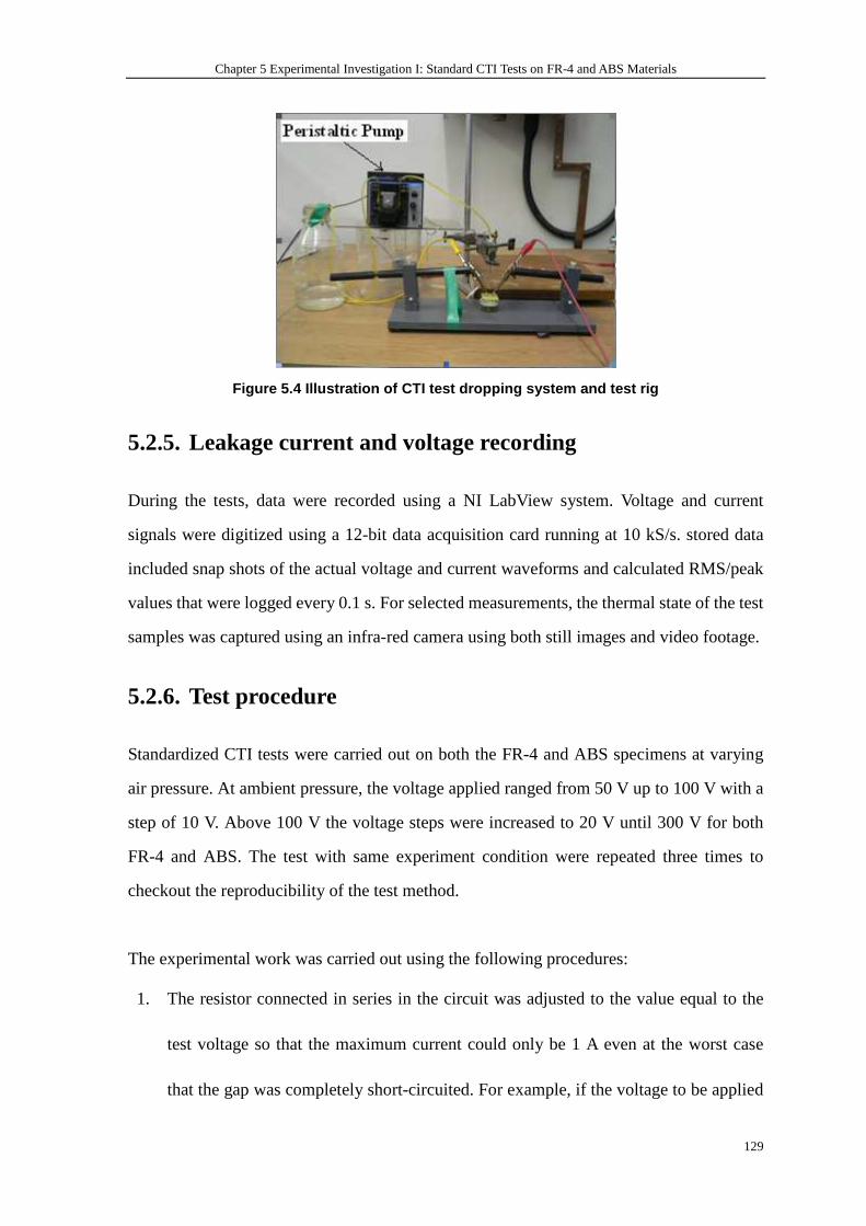
Chapter 5 Experimental Investigation I: Standard CTI Tests on FR-4 and ABS Materials
129
Figure 5.4 Illustration of CTI test dropping system and test rig
5.2.5. Leakage current and voltage recording
During the tests, data were recorded using a NI LabView system. Voltage and current
signals were digitized using a 12-bit data acquisition card running at 10 kS/s. stored data
included snap shots of the actual voltage and current waveforms and calculated RMS/peak
values that were logged every 0.1 s. For selected measurements, the thermal state of the test
samples was captured using an infra-red camera using both still images and video footage.
5.2.6. Test procedure
Standardized CTI tests were carried out on both the FR-4 and ABS specimens at varying
air pressure. At ambient pressure, the voltage applied ranged from 50 V up to 100 V with a
step of 10 V. Above 100 V the voltage steps were increased to 20 V until 300 V for both
FR-4 and ABS. The test with same experiment condition were repeated three times to
checkout the reproducibility of the test method.
The experimental work was carried out using the following procedures:
1. The resistor connected in series in the circuit was adjusted to the value equal to the
test voltage so that the maximum current could only be 1 A even at the worst case
that the gap was completely short-circuited. For example, if the voltage to be applied
Chapter 5 Experimental Investigation I: Standard CTI Tests on FR-4 and ABS Materials
130
is 50 V, then the resistance of the slide rheostat should be set to 50Ω , which is the
possible worst case if a short circuit occurs.
2. The three pieces of FR-4 specimens or two pieces of ABS specimens were cleaned
by the cloth if necessary; domestic cleanser was used to clean fingerprints, grease or
oil off the surfaces.
3. The gap distances were set to 4mm by using the slide caliper. The stack of specimens
was then clipped onto the plastic plate with some pressure applied by insulating tape
on the electrode extensions.
4. The flow rate of aqueous contaminant was set to one droplet every 30± 5 seconds. It
was allowed to run for a while until the flow was stable.
5. Using a multimeter to test the applied voltage at the output points of the transformer
the value expected before the specimens were wetted by the test solutions was found.
6. Tests were carried out until the leakage current reached the threshold. The circuit
was cut off by a control circuit including timer, circuit breaker and overcurrent relay
in series. Otherwise when 50 drops of aqueous contamination had fallen, the circuit
was cut off based on the timer record.
7. Labview software and hardware were used to record the leakage currents and
voltages. Fifty water drops were applied to each specimen with 30 s between each
droplet. During the tests, data was recorded using an NI LabView system. Voltage and
current signals were digitized using a 12-bit data acquisition card running at 10kS/s.
Stored data included snap shots of the actual voltage and current waveforms and
calculated RMS/peak values that were logged every 0.1 s.
Chapter 5 Experimental Investigation I: Standard CTI Tests on FR-4 and ABS Materials
131
8. For selected measurements, the thermal state of the test samples was captured using an
infra-red camera using both still images and video footage.
5.3. Experimental results and discussion
5.3.1. Behaviour of FR-4 samples at the atmospheric pressure
FR-4 samples were tested at 100,000 Pa and 20 °C using voltages from 50 V upwards until
100 V with steps of 10 V. Then with steps of 20 V the voltage applied was increased up to
300 V. By using National Instrument hardware and the software Labview, summarized
voltage and current signal files with testing period were recorded. The raw current and
voltage waveforms were also recoded. To verify my theoretical explanation of the
electrical tracking mechanism, the infra-red camera was employed for atmospheric testing
to obtain the thermal images from tests, from which we can see the temperatures of
different part of the CTI test rig, test specimens, and even the aqueous contaminants so
that we can further prove my theory stated in Chapter 4.
50 V Testing
For the 50 V case, Figures 5.5 and Figure 5.6 show the voltage across the test gap and the
leakage current measured of three times respectively during the test period of 30 minutes.
The sample did not fail and no damage was observed on the surface of the sample shown
in Table 5.2 in the section 5.4.3.
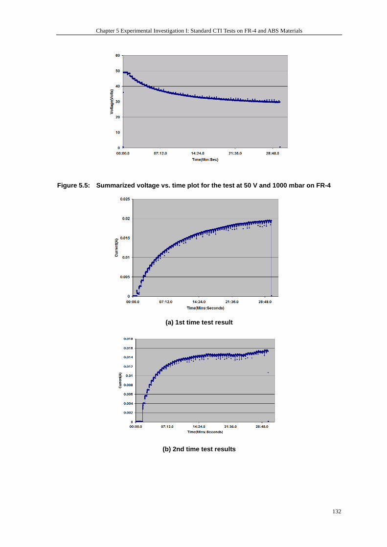
Chapter 5 Experimental Investigation I: Standard CTI Tests on FR-4 and ABS Materials
132
Figure 5.5: Summarized voltage vs. time plot for t he test at 50 V and 1000 mbar on FR-4
(a) 1st time test result
(b) 2nd time test results
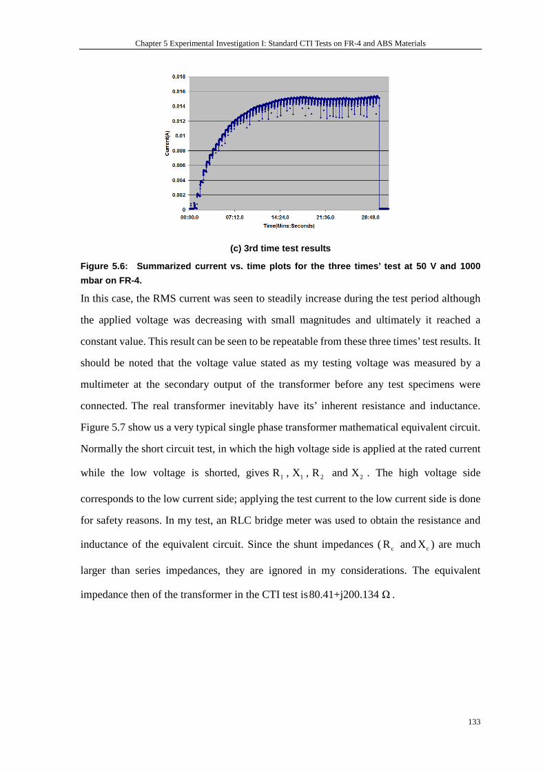
Chapter 5 Experimental Investigation I: Standard CTI Tests on FR-4 and ABS Materials
133
(c) 3rd time test results
Figure 5.6: Summarized current vs. time plots for the three times’ test at 50 V and 1000
mbar on FR-4.
In this case, the RMS current was seen to steadily increase during the test period although
the applied voltage was decreasing with small magnitudes and ultimately it reached a
constant value. This result can be seen to be repeatable from these three times’ test results. It
should be noted that the voltage value stated as my testing voltage was measured by a
multimeter at the secondary output of the transformer before any test specimens were
connected. The real transformer inevitably have its’ inherent resistance and inductance.
Figure 5.7 show us a very typical single phase transformer mathematical equivalent circuit.
Normally the short circuit test, in which the high voltage side is applied at the rated current
while the low voltage is shorted, gives1R , 1X , 2R and 2X . The high voltage side
corresponds to the low current side; applying the test current to the low current side is done
for safety reasons. In my test, an RLC bridge meter was used to obtain the resistance and
inductance of the equivalent circuit. Since the shunt impedances ( cR and cX ) are much
larger than series impedances, they are ignored in my considerations. The equivalent
impedance then of the transformer in the CTI test is80.41+j200.134Ω .
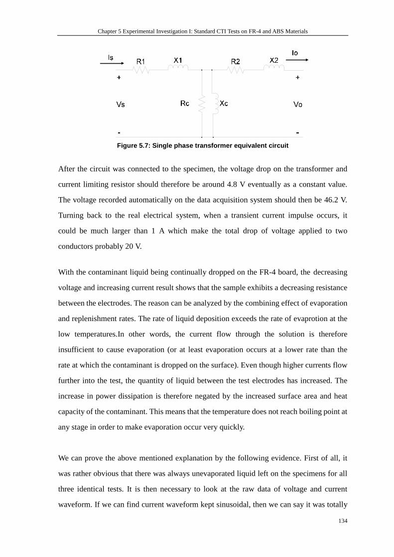
Chapter 5 Experimental Investigation I: Standard CTI Tests on FR-4 and ABS Materials
134
Figure 5.7: Single phase transformer equivalent cir cuit
After the circuit was connected to the specimen, the voltage drop on the transformer and
current limiting resistor should therefore be around 4.8 V eventually as a constant value.
The voltage recorded automatically on the data acquisition system should then be 46.2 V.
Turning back to the real electrical system, when a transient current impulse occurs, it
could be much larger than 1 A which make the total drop of voltage applied to two
conductors probably 20 V.
With the contaminant liquid being continually dropped on the FR-4 board, the decreasing
voltage and increasing current result shows that the sample exhibits a decreasing resistance
between the electrodes. The reason can be analyzed by the combining effect of evaporation
and replenishment rates. The rate of liquid deposition exceeds the rate of evaprotion at the
low temperatures.In other words, the current flow through the solution is therefore
insufficient to cause evaporation (or at least evaporation occurs at a lower rate than the
rate at which the contaminant is dropped on the surface). Even though higher currents flow
further into the test, the quantity of liquid between the test electrodes has increased. The
increase in power dissipation is therefore negated by the increased surface area and heat
capacity of the contaminant. This means that the temperature does not reach boiling point at
any stage in order to make evaporation occur very quickly.
We can prove the above mentioned explanation by the following evidence. First of all, it
was rather obvious that there was always unevaporated liquid left on the specimens for all
three identical tests. It is then necessary to look at the raw data of voltage and current
waveform. If we can find current waveform kept sinusoidal, then we can say it was totally
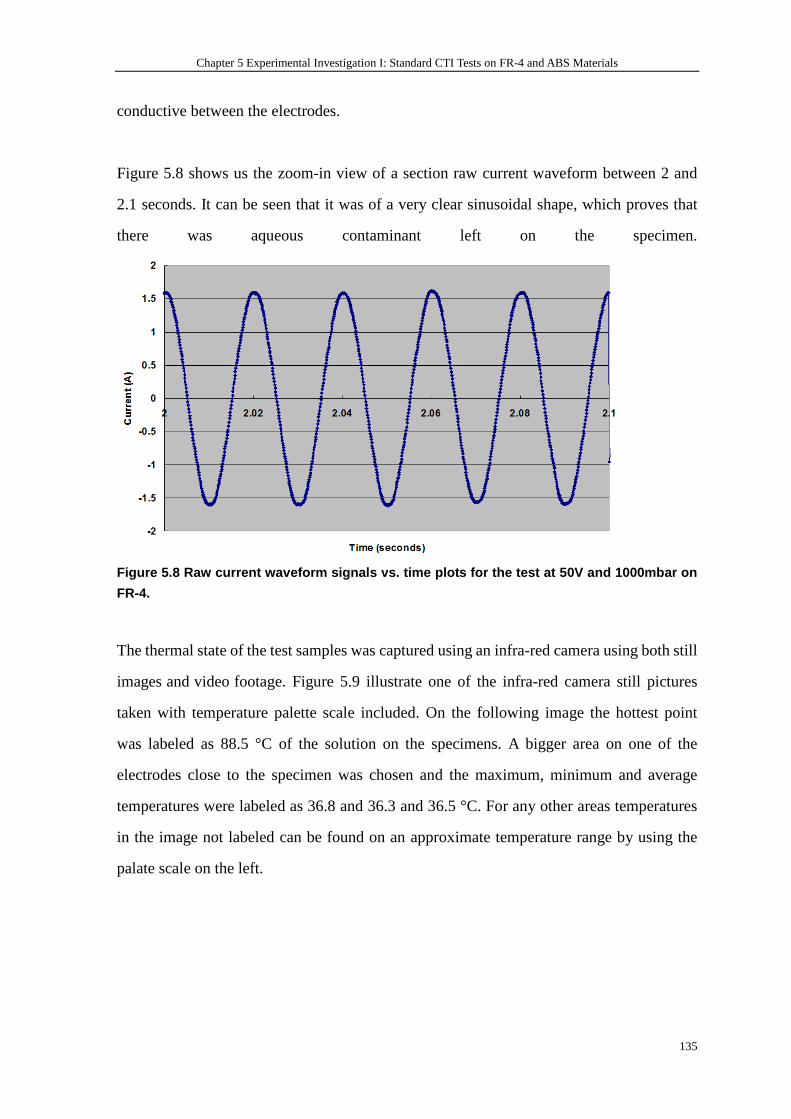
Chapter 5 Experimental Investigation I: Standard CTI Tests on FR-4 and ABS Materials
135
conductive between the electrodes.
Figure 5.8 shows us the zoom-in view of a section raw current waveform between 2 and
2.1 seconds. It can be seen that it was of a very clear sinusoidal shape, which proves that
there was aqueous contaminant left on the specimen.
Figure 5.8 Raw current waveform signals vs. time pl ots for the test at 50V and 1000mbar on
FR-4.
The thermal state of the test samples was captured using an infra-red camera using both still
images and video footage. Figure 5.9 illustrate one of the infra-red camera still pictures
taken with temperature palette scale included. On the following image the hottest point
was labeled as 88.5 °C of the solution on the specimens. A bigger area on one of the
electrodes close to the specimen was chosen and the maximum, minimum and average
temperatures were labeled as 36.8 and 36.3 and 36.5 °C. For any other areas temperatures
in the image not labeled can be found on an approximate temperature range by using the
palate scale on the left.
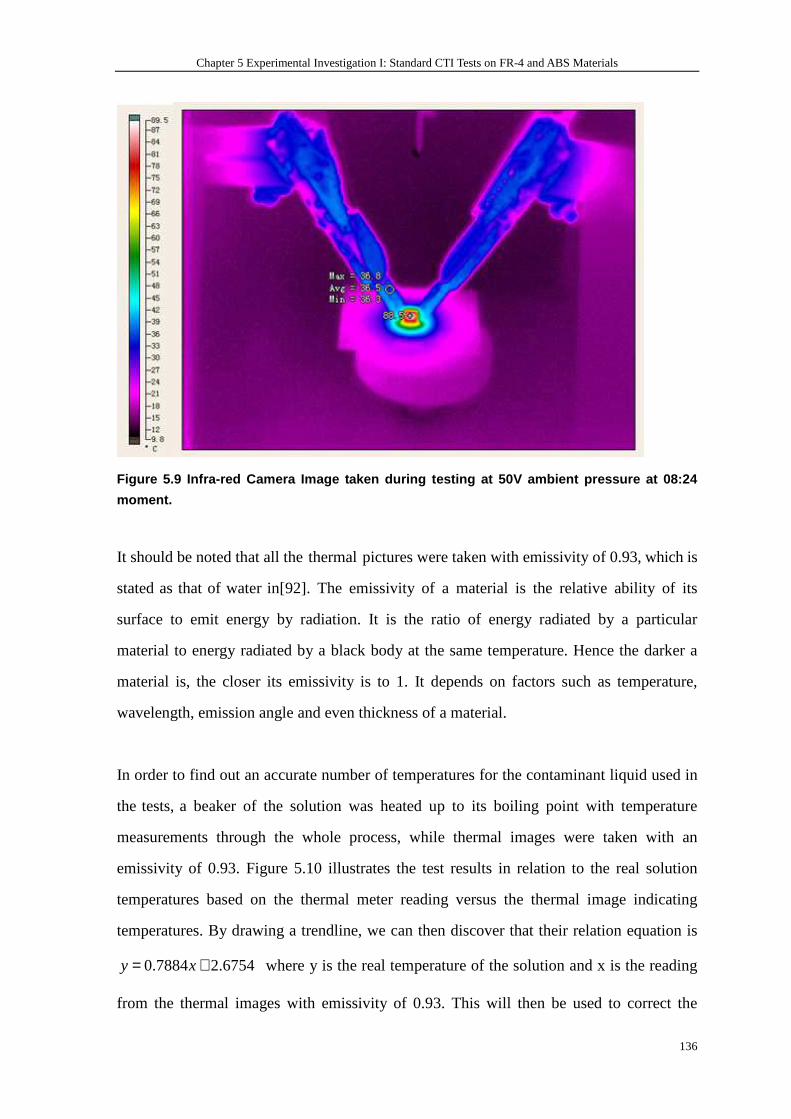
Chapter 5 Experimental Investigation I: Standard CTI Tests on FR-4 and ABS Materials
136
Figure 5.9 Infra-red Camera Image taken during test ing at 50V ambient pressure at 08:24
moment.
It should be noted that all the thermal pictures were taken with emissivity of 0.93, which is
stated as that of water in[92]. The emissivity of a material is the relative ability of its
surface to emit energy by radiation. It is the ratio of energy radiated by a particular
material to energy radiated by a black body at the same temperature. Hence the darker a
material is, the closer its emissivity is to 1. It depends on factors such as temperature,
wavelength, emission angle and even thickness of a material.
In order to find out an accurate number of temperatures for the contaminant liquid used in
the tests, a beaker of the solution was heated up to its boiling point with temperature
measurements through the whole process, while thermal images were taken with an
emissivity of 0.93. Figure 5.10 illustrates the test results in relation to the real solution
temperatures based on the thermal meter reading versus the thermal image indicating
temperatures. By drawing a trendline, we can then discover that their relation equation is
0.7884 2.6754y x= + where y is the real temperature of the solution and x is the reading
from the thermal images with emissivity of 0.93. This will then be used to correct the
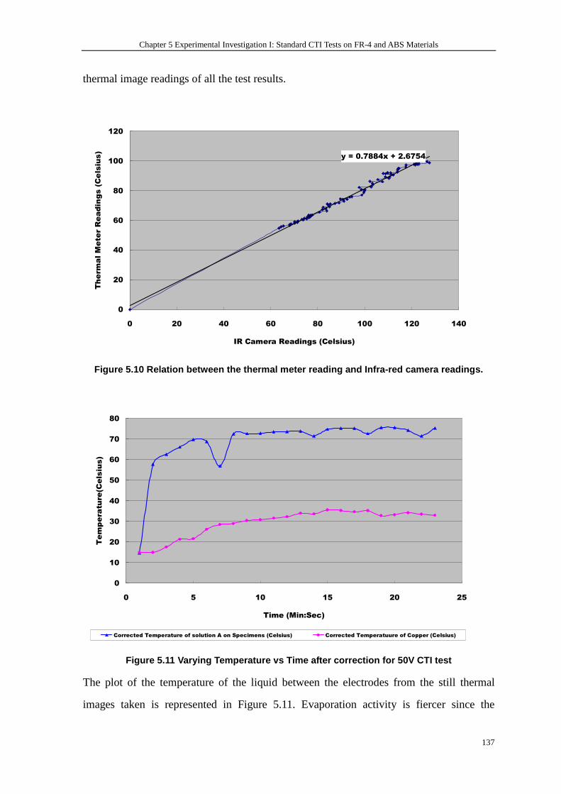
Chapter 5 Experimental Investigation I: Standard CTI Tests on FR-4 and ABS Materials
137
thermal image readings of all the test results.
y = 0.7884x + 2.6754
0
20
40
60
80
100
120
0 20 40 60 80 100 120 140
IR Camera Readings (Celsius)
Therm
al Meter Readings (Celsius)
Figure 5.10 Relation between the thermal meter read ing and Infra-red camera readings.
0
10
20
30
40
50
60
70
80
0 5 10 15 20 25
Time (Min:Sec)
Temperature(Celsius)
Corrected Temperature of solution A on Specimens (Celsius) Corrected Temperatuure of Copper (Celsius)
Figure 5.11 Varying Temperature vs Time after corre ction for 50V CTI test
The plot of the temperature of the liquid between the electrodes from the still thermal
images taken is represented in Figure 5.11. Evaporation activity is fiercer since the

Chapter 5 Experimental Investigation I: Standard CTI Tests on FR-4 and ABS Materials
138
temperature of the solution has been raised higher than room temperature (20C ). The
boiling point of the solution used in the CTI tests with resistivity of 395 ± 5 Ω ·cm at
ambient temperature is 101.5C . We can see that through the whole testing period, there is
no moment at which the temperature of the solution could reach to boiling point. This is
because that the function of the conductive solution replenishment is larger than that of
evaporation of liquid. With the volume of the liquid increasing, according to the definition
of resistance, the bigger the crossing area and the smaller the resistance; consequently,
with almost the same applied voltage, the current flow was increasing. However, in terms
of power generated to heat up the liquid, the magnitude of the decreased resistance was
larger than that of the square increased current, which leads to insufficient power
generated to heat up the liquid to boiling before the next drop of fresh liquid arrives. The
other interesting phenomenon is that the temperature of the electrode in this case was
increasing by quite a big stride from 15 °C to almost 35 °C during 30 minutes’ test period.
70 V testing
When the test voltage is increased to 70 V, the RMS current varies as shown in Figure 5.12
including three times’ test results which indicate the repeatability of test method. Initially,
the current was increasing gradually which indicate the aqueous contamination was
collecting on the surface. This also can be proven by the raw current waveform from 0 to
0.01 A with pure sinusoid shape show in Figure 5.13 (a). Then the current reaches a steady
state before falling after around 20 minutes, which also have a sinusoid shape of raw current
waveform with higher magnitude of almost 0.0 2 A show in Figure 5.13 (b). In this case, the
applied voltage is thought to generate a level of heating that evaporates some of the solution,
the evaporation rate being roughly equal to the rate of replenishment. This leads to a steady
state current flow. However, after a certain period of time, the electrodes start to reach
thermal equilibrium and act as less of a heat sink, meaning increased levels of heat can act to
evaporate the contaminant resulting in the increased circuit resistance and lower current
flow seen after 20 minutes, which is also illustrated in Figure 5.13 (c). No sample damage

Chapter 5 Experimental Investigation I: Standard CTI Tests on FR-4 and ABS Materials
139
was observed at this voltage and the maximum water temperature observed during the final
five minutes of the test was 95 ˚C.
(a) 1st time test result
(b) 2nd time test result
(c) 3rd time test result
Figure 5.12 Summarized current vs. time plots for t he three times’ test at 70 V and 1000 mbar
on FR-4
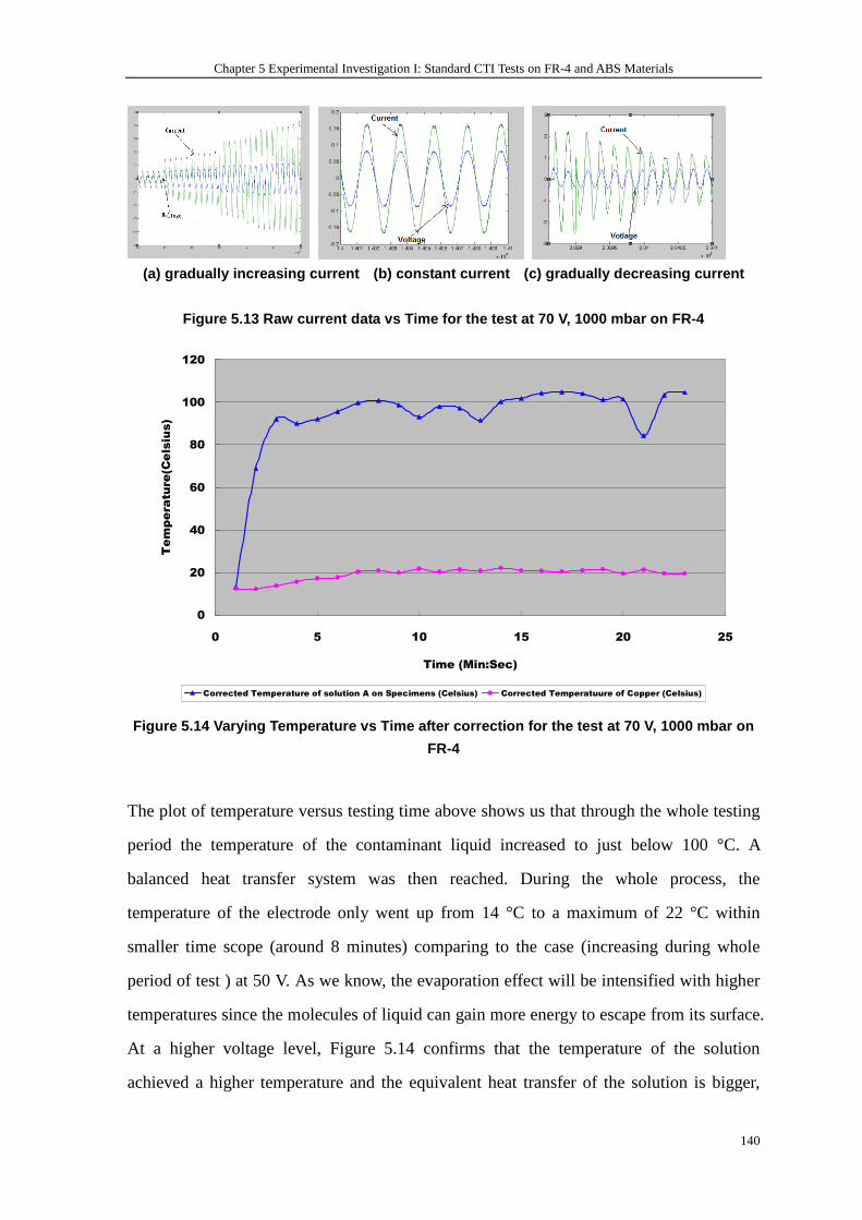
Chapter 5 Experimental Investigation I: Standard CTI Tests on FR-4 and ABS Materials
140
(a) gradually increasing current (b) constant curr ent (c) gradually decreasing current
Figure 5.13 Raw current data vs Time for the test a t 70 V, 1000 mbar on FR-4
0
20
40
60
80
100
120
0 5 10 15 20 25
Time (Min:Sec)
Temperature(Celsius)
Corrected Temperature of solution A on Specimens (Celsius) Corrected Temperatuure of Copper (Celsius)
Figure 5.14 Varying Temperature vs Time after corre ction for the test at 70 V, 1000 mbar on
FR-4
The plot of temperature versus testing time above shows us that through the whole testing
period the temperature of the contaminant liquid increased to just below 100 °C. A
balanced heat transfer system was then reached. During the whole process, the
temperature of the electrode only went up from 14 °C to a maximum of 22 °C within
smaller time scope (around 8 minutes) comparing to the case (increasing during whole
period of test ) at 50 V. As we know, the evaporation effect will be intensified with higher
temperatures since the molecules of liquid can gain more energy to escape from its surface.
At a higher voltage level, Figure 5.14 confirms that the temperature of the solution
achieved a higher temperature and the equivalent heat transfer of the solution is bigger,
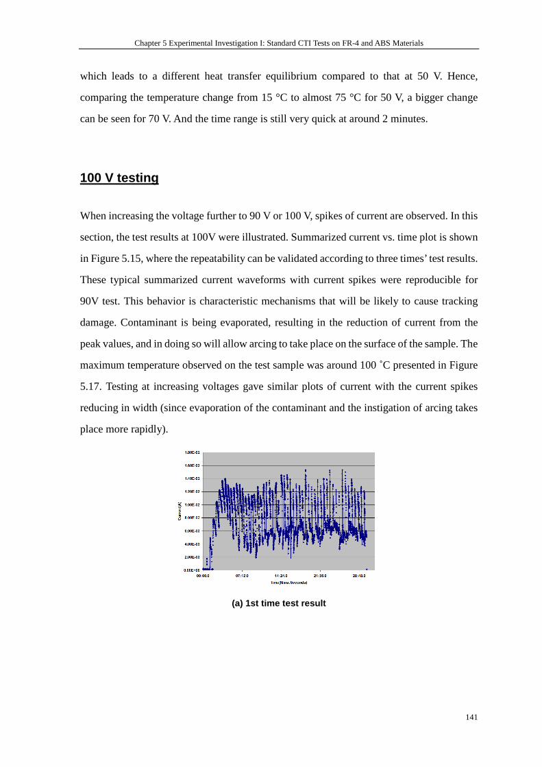
Chapter 5 Experimental Investigation I: Standard CTI Tests on FR-4 and ABS Materials
141
which leads to a different heat transfer equilibrium compared to that at 50 V. Hence,
comparing the temperature change from 15 °C to almost 75 °C for 50 V, a bigger change
can be seen for 70 V. And the time range is still very quick at around 2 minutes.
100 V testing
When increasing the voltage further to 90 V or 100 V, spikes of current are observed. In this
section, the test results at 100V were illustrated. Summarized current vs. time plot is shown
in Figure 5.15, where the repeatability can be validated according to three times’ test results.
These typical summarized current waveforms with current spikes were reproducible for
90V test. This behavior is characteristic mechanisms that will be likely to cause tracking
damage. Contaminant is being evaporated, resulting in the reduction of current from the
peak values, and in doing so will allow arcing to take place on the surface of the sample. The
maximum temperature observed on the test sample was around 100 ˚C presented in Figure
5.17. Testing at increasing voltages gave similar plots of current with the current spikes
reducing in width (since evaporation of the contaminant and the instigation of arcing takes
place more rapidly).
(a) 1st time test result
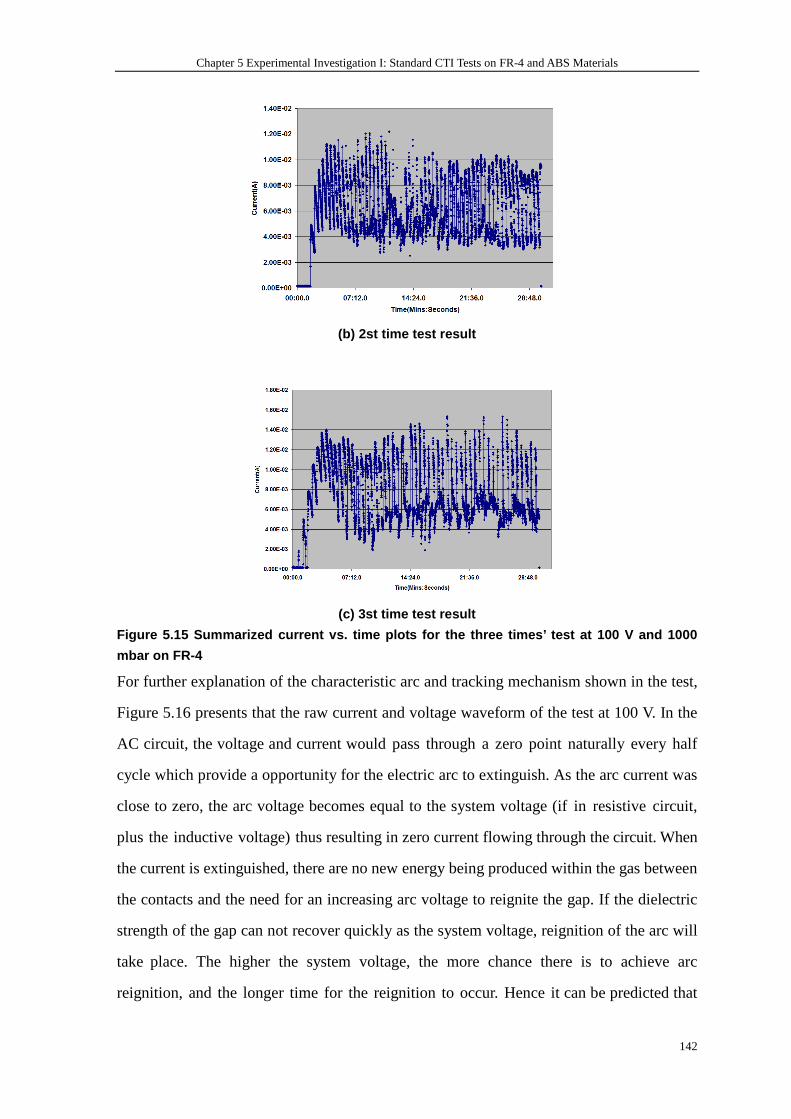
Chapter 5 Experimental Investigation I: Standard CTI Tests on FR-4 and ABS Materials
142
(b) 2st time test result
(c) 3st time test result
Figure 5.15 Summarized current vs. time plots for t he three times’ test at 100 V and 1000
mbar on FR-4
For further explanation of the characteristic arc and tracking mechanism shown in the test,
Figure 5.16 presents that the raw current and voltage waveform of the test at 100 V. In the
AC circuit, the voltage and current would pass through a zero point naturally every half
cycle which provide a opportunity for the electric arc to extinguish. As the arc current was
close to zero, the arc voltage becomes equal to the system voltage (if in resistive circuit,
plus the inductive voltage) thus resulting in zero current flowing through the circuit. When
the current is extinguished, there are no new energy being produced within the gas between
the contacts and the need for an increasing arc voltage to reignite the gap. If the dielectric
strength of the gap can not recover quickly as the system voltage, reignition of the arc will
take place. The higher the system voltage, the more chance there is to achieve arc
reignition, and the longer time for the reignition to occur. Hence it can be predicted that
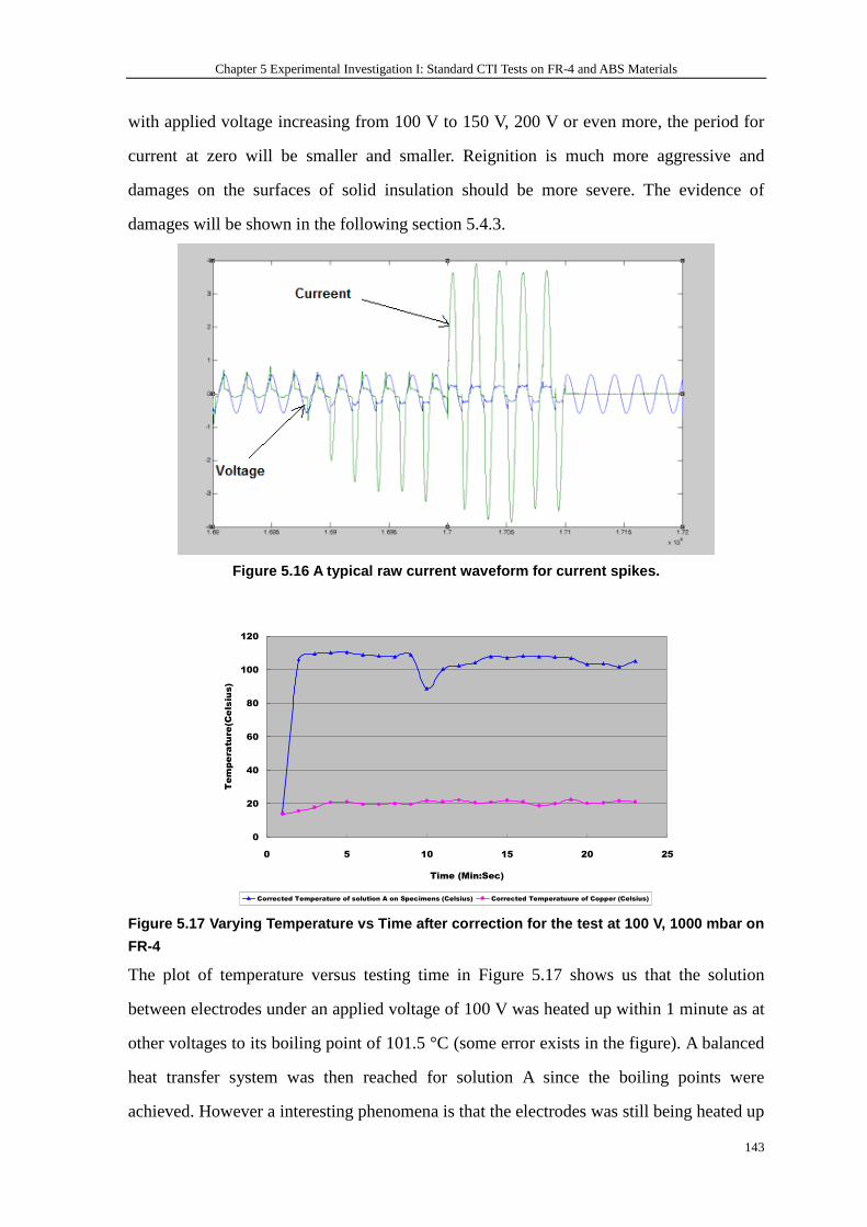
Chapter 5 Experimental Investigation I: Standard CTI Tests on FR-4 and ABS Materials
143
with applied voltage increasing from 100 V to 150 V, 200 V or even more, the period for
current at zero will be smaller and smaller. Reignition is much more aggressive and
damages on the surfaces of solid insulation should be more severe. The evidence of
damages will be shown in the following section 5.4.3.
Figure 5.16 A typical raw current waveform for curr ent spikes.
0
20
40
60
80
100
120
0 5 10 15 20 25
Time (Min:Sec)
Temperature(Celsius)
Corrected Temperature of solution A on Specimens (Celsius) Corrected Temperatuure of Copper (Celsius) Figure 5.17 Varying Temperature vs Time after corre ction for the test at 100 V, 1000 mbar on
FR-4
The plot of temperature versus testing time in Figure 5.17 shows us that the solution
between electrodes under an applied voltage of 100 V was heated up within 1 minute as at
other voltages to its boiling point of 101.5 °C (some error exists in the figure). A balanced
heat transfer system was then reached for solution A since the boiling points were
achieved. However a interesting phenomena is that the electrodes was still being heated up
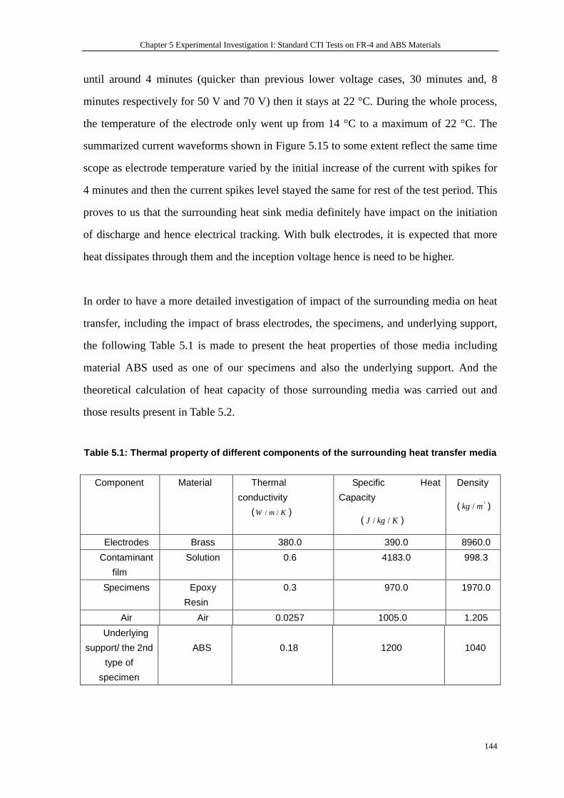
Chapter 5 Experimental Investigation I: Standard CTI Tests on FR-4 and ABS Materials
144
until around 4 minutes (quicker than previous lower voltage cases, 30 minutes and, 8
minutes respectively for 50 V and 70 V) then it stays at 22 °C. During the whole process,
the temperature of the electrode only went up from 14 °C to a maximum of 22 °C. The
summarized current waveforms shown in Figure 5.15 to some extent reflect the same time
scope as electrode temperature varied by the initial increase of the current with spikes for
4 minutes and then the current spikes level stayed the same for rest of the test period. This
proves to us that the surrounding heat sink media definitely have impact on the initiation
of discharge and hence electrical tracking. With bulk electrodes, it is expected that more
heat dissipates through them and the inception voltage hence is need to be higher.
In order to have a more detailed investigation of impact of the surrounding media on heat
transfer, including the impact of brass electrodes, the specimens, and underlying support,
the following Table 5.1 is made to present the heat properties of those media including
material ABS used as one of our specimens and also the underlying support. And the
theoretical calculation of heat capacity of those surrounding media was carried out and
those results present in Table 5.2.
Table 5.1: Thermal property of different components of the surrounding heat transfer media
Component Material
Thermal
conductivity
( / /W m K )
Specific Heat
Capacity
( / /J kg K )
Density
( 3/kg m )
Electrodes Brass 380.0 390.0 8960.0
Contaminant
film
Solution 0.6 4183.0 998.3
Specimens Epoxy
Resin
0.3 970.0 1970.0
Air Air 0.0257 1005.0 1.205
Underlying
support/ the 2nd
type of
specimen
ABS
0.18
1200
1040
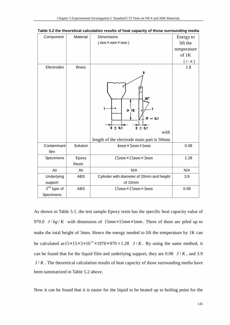
Chapter 5 Experimental Investigation I: Standard CTI Tests on FR-4 and ABS Materials
145
Table 5.2 the theoretical calculation results of he at capacity of those surrounding media
Component Material
Dimensions
( mm mm mm× × )
Energy to lift the
temperature of 1K
( /J K )
Electrodes Brass
with
length of the electrode main part is 50mm
1.8
Contaminant
film
Solution 4 5 1mm mm mm× × 0.08
Specimens Epoxy
Resin
15 15 3mm mm mm× × 1.28
Air Air N/A N/A
Underlying
support
ABS Cylinder with diameter of 20mm and height
of 10mm
3.9
2nd type of
Specimens
ABS 15 15 3mm mm mm× × 0.08
As shown in Table 5.1, the test sample Epoxy resin has the specific heat capacity value of
970.0 / /J kg K with dimension of 15 15 1mm mm mm× × . Three of them are piled up to
make the total height of 3mm. Hence the energy needed to lift the temperature by 1K can
be calculated as 915 15 3 10 1970 970 1.28−× × × × × = /J K . By using the same method, it
can be found that for the liquid film and underlying support, they are 0.08 /J K , and 3.9
/J K . The theoretical calculation results of heat capacity of those surrounding media have
been summarized in Table 5.2 above.
Now it can be found that it is easier for the liquid to be heated up to boiling point for the
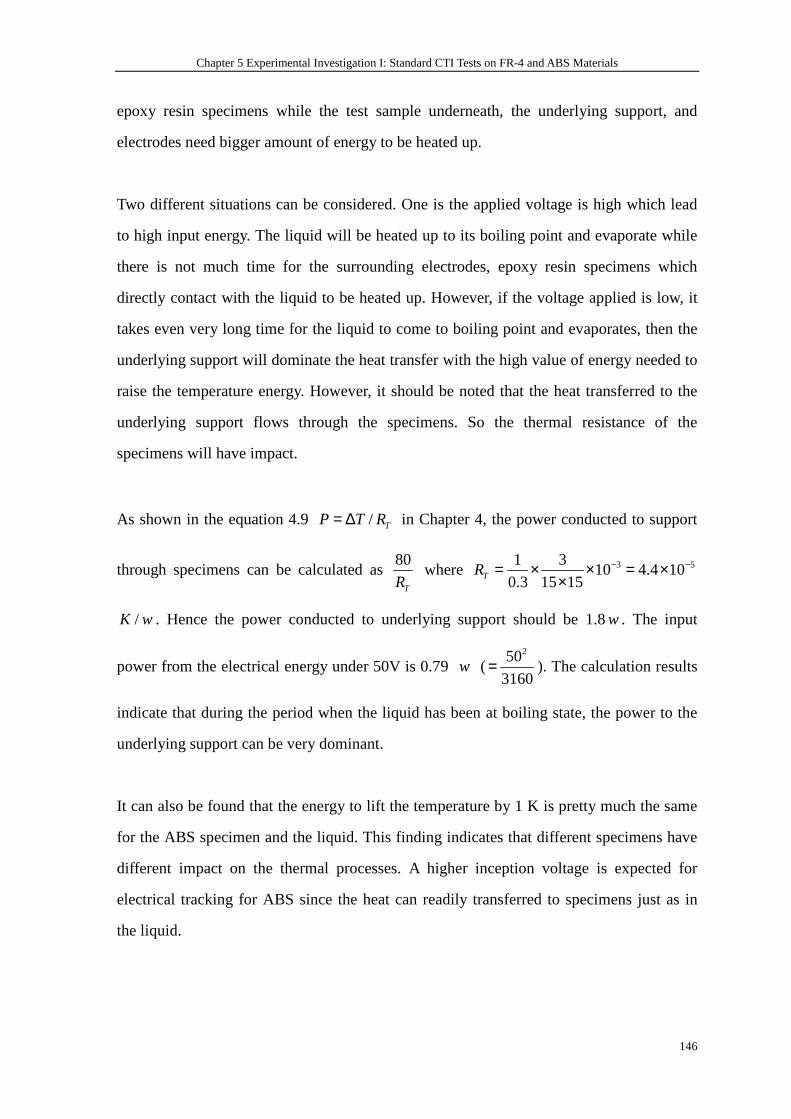
Chapter 5 Experimental Investigation I: Standard CTI Tests on FR-4 and ABS Materials
146
epoxy resin specimens while the test sample underneath, the underlying support, and
electrodes need bigger amount of energy to be heated up.
Two different situations can be considered. One is the applied voltage is high which lead
to high input energy. The liquid will be heated up to its boiling point and evaporate while
there is not much time for the surrounding electrodes, epoxy resin specimens which
directly contact with the liquid to be heated up. However, if the voltage applied is low, it
takes even very long time for the liquid to come to boiling point and evaporates, then the
underlying support will dominate the heat transfer with the high value of energy needed to
raise the temperature energy. However, it should be noted that the heat transferred to the
underlying support flows through the specimens. So the thermal resistance of the
specimens will have impact.
As shown in the equation 4.9 / TP T R= ∆ in Chapter 4, the power conducted to support
through specimens can be calculated as 80
TR where 3 51 3
10 4.4 100.3 15 15TR − −= × × = ×
×
/K w . Hence the power conducted to underlying support should be 1.8w . The input
power from the electrical energy under 50V is 0.79 w (250
3160= ). The calculation results
indicate that during the period when the liquid has been at boiling state, the power to the
underlying support can be very dominant.
It can also be found that the energy to lift the temperature by 1 K is pretty much the same
for the ABS specimen and the liquid. This finding indicates that different specimens have
different impact on the thermal processes. A higher inception voltage is expected for
electrical tracking for ABS since the heat can readily transferred to specimens just as in
the liquid.

Chapter 5 Experimental Investigation I: Standard CTI Tests on FR-4 and ABS Materials
147
Other voltage testing
All the other voltage testing results are illustrated in Figure 5.18. It can be summarized
that the inception voltage for electrical tracking is 90 V in the specified environmental
circumstances in the standard, including the specific pollution degree specified, room
temperature and ambient pressure. This also can be proved by the evidence of damages on
the specimens show in Table 5.2 in Section 5.4.2 since the test level at 90 V was the first at
which damage was seen on the FR-4 sample. We can always see that the current
continuously increased during the whole testing period when 60 V was applied. And then
as it has been shown in section 5.3.1.2, it was a transient situation when 70 V was applied.
It is believed that there are also some voltages just less than 70 V that could make this
system reach equilibrium, so that the current went up initially and then as time passed it
remained constant at a particular value.
Figure 5.18 RMS current vs. time plot for the tests at 60 V, 80 V, 90 V, 200 V at 1000 mbar on
FR-4 (reading from left to right)
For each voltage applied, three measurements were carried out. Although the problem
with wet electrical tracking test is that the data of tracking resistance fluctuates greatly, my
research shows repeatability, which is reflected in the similarity of the three times’ test
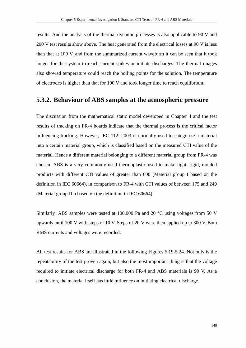
Chapter 5 Experimental Investigation I: Standard CTI Tests on FR-4 and ABS Materials
148
results. And the analysis of the thermal dynamic processes is also applicable to 90 V and
200 V test results show above. The heat generated from the electrical losses at 90 V is less
than that at 100 V, and from the summarized current waveform it can be seen that it took
longer for the system to reach current spikes or initiate discharges. The thermal images
also showed temperature could reach the boiling points for the solution. The temperature
of electrodes is higher than that for 100 V and took longer time to reach equilibrium.
5.3.2. Behaviour of ABS samples at the atmospheric pressure
The discussion from the mathematical static model developed in Chapter 4 and the test
results of tracking on FR-4 boards indicate that the thermal process is the critical factor
influencing tracking. However, IEC 112: 2003 is normally used to categorize a material
into a certain material group, which is classified based on the measured CTI value of the
material. Hence a different material belonging to a different material group from FR-4 was
chosen. ABS is a very commonly used thermoplastic used to make light, rigid, molded
products with different CTI values of greater than 600 (Material group I based on the
definition in IEC 60664), in comparison to FR-4 with CTI values of between 175 and 249
(Material group IIIa based on the definition in IEC 60664).
Similarly, ABS samples were tested at 100,000 Pa and 20 °C using voltages from 50 V
upwards until 100 V with steps of 10 V. Steps of 20 V were then applied up to 300 V. Both
RMS currents and voltages were recorded.
All test results for ABS are illustrated in the following Figures 5.19-5.24. Not only is the
repeatability of the test proven again, but also the most important thing is that the voltage
required to initiate electrical discharge for both FR-4 and ABS materials is 90 V. As a
conclusion, the material itself has little influence on initiating electrical discharge.
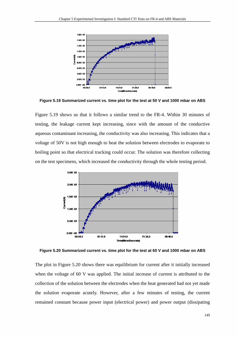
Chapter 5 Experimental Investigation I: Standard CTI Tests on FR-4 and ABS Materials
149
Figure 5.19 Summarized current vs. time plot for th e test at 50 V and 1000 mbar on ABS
Figure 5.19 shows us that it follows a similar trend to the FR-4. Within 30 minutes of
testing, the leakage current kept increasing, since with the amount of the conductive
aqueous contaminant increasing, the conductivity was also increasing. This indicates that a
voltage of 50V is not high enough to heat the solution between electrodes to evaporate to
boiling point so that electrical tracking could occur. The solution was therefore collecting
on the test specimens, which increased the conductivity through the whole testing period.
Figure 5.20 Summarized current vs. time plot for th e test at 60 V and 1000 mbar on ABS
The plot in Figure 5.20 shows there was equilibrium for current after it initially increased
when the voltage of 60 V was applied. The initial increase of current is attributed to the
collection of the solution between the electrodes when the heat generated had not yet made
the solution evaporate acutely. However, after a few minutes of testing, the current
remained constant because power input (electrical power) and power output (dissipating
Chapter 5 Experimental Investigation I: Standard CTI Tests on FR-4 and ABS Materials
150
heat) reached equilibrium. This equilibrium would remain as long as the whole thermal
equilibrium was not broken.
Figure 5.21 Summarized current vs. time plot for th e test at 70 V and 1000 mbar on ABS
When the test voltage is increased to 70 V, the current varies, as shown in Figure 5.21.
Initially, the current reaches a steady state before falling after around 10 minutes. In this
case, the applied voltage is thought to generate a level of heating that evaporates some
contaminant, the evaporation rate being roughly equal to the rate of replenishment. This
leads to a steady state current flow. However, after a certain period of time, the electrodes
start to reach thermal equilibrium and act as less of a heat sink, meaning increased levels of
heat can act to evaporate the contaminant thus resulting in the increased circuit resistance
and lower current flow seen after twenty minutes. No sample damage was observed at this
voltage and the maximum water temperature observed during the final five minutes of the
test was 95 ˚C.
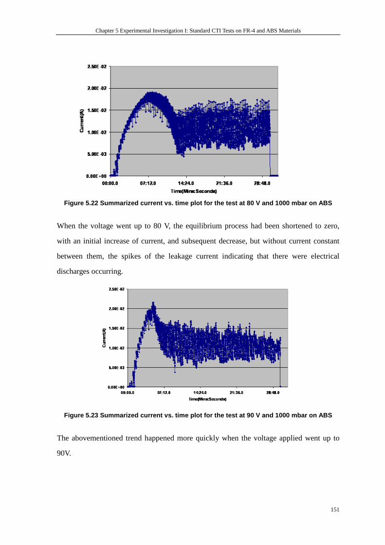
Chapter 5 Experimental Investigation I: Standard CTI Tests on FR-4 and ABS Materials
151
Figure 5.22 Summarized current vs. time plot for th e test at 80 V and 1000 mbar on ABS
When the voltage went up to 80 V, the equilibrium process had been shortened to zero,
with an initial increase of current, and subsequent decrease, but without current constant
between them, the spikes of the leakage current indicating that there were electrical
discharges occurring.
Figure 5.23 Summarized current vs. time plot for th e test at 90 V and 1000 mbar on ABS
The abovementioned trend happened more quickly when the voltage applied went up to
90V.
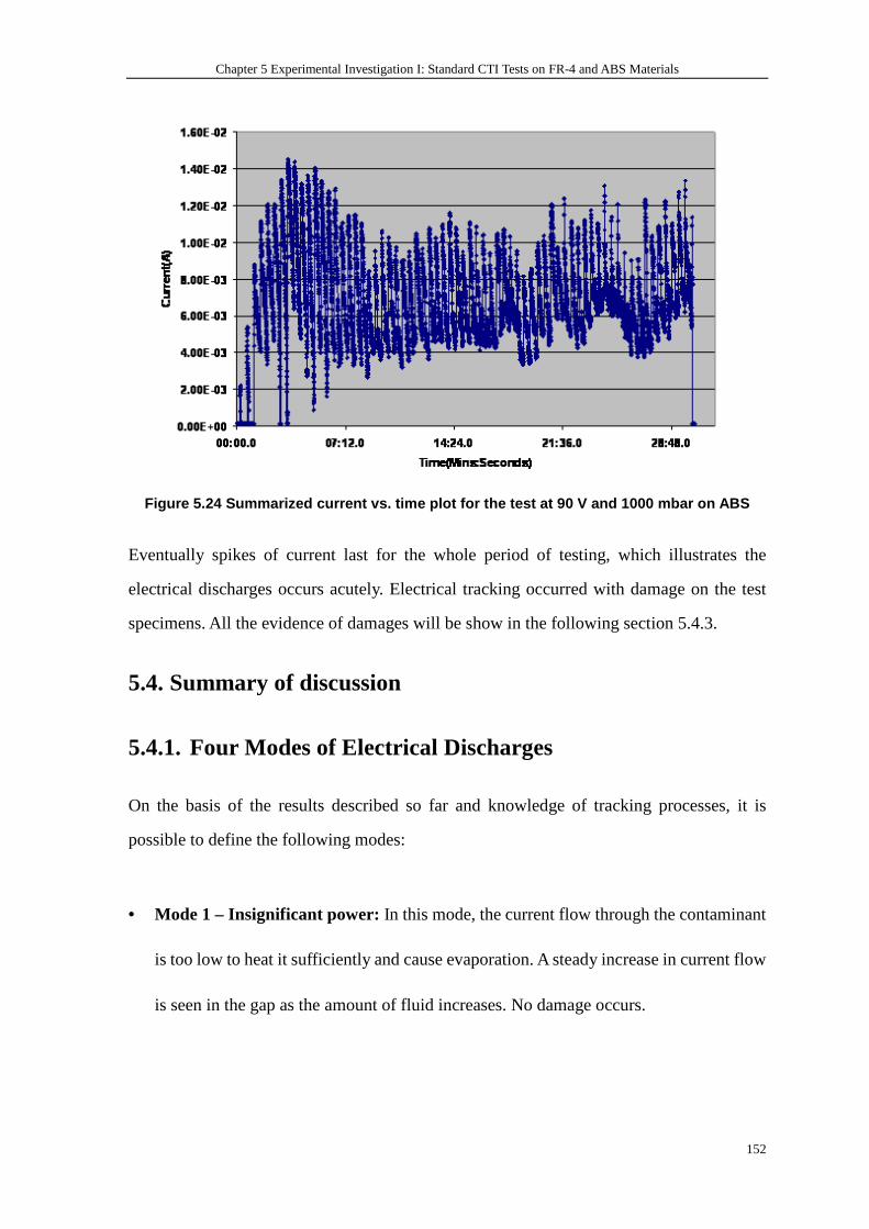
Chapter 5 Experimental Investigation I: Standard CTI Tests on FR-4 and ABS Materials
152
Figure 5.24 Summarized current vs. time plot for th e test at 90 V and 1000 mbar on ABS
Eventually spikes of current last for the whole period of testing, which illustrates the
electrical discharges occurs acutely. Electrical tracking occurred with damage on the test
specimens. All the evidence of damages will be show in the following section 5.4.3.
5.4. Summary of discussion
5.4.1. Four Modes of Electrical Discharges
On the basis of the results described so far and knowledge of tracking processes, it is
possible to define the following modes:
• Mode 1 – Insignificant power: In this mode, the current flow through the contaminant
is too low to heat it sufficiently and cause evaporation. A steady increase in current flow
is seen in the gap as the amount of fluid increases. No damage occurs.
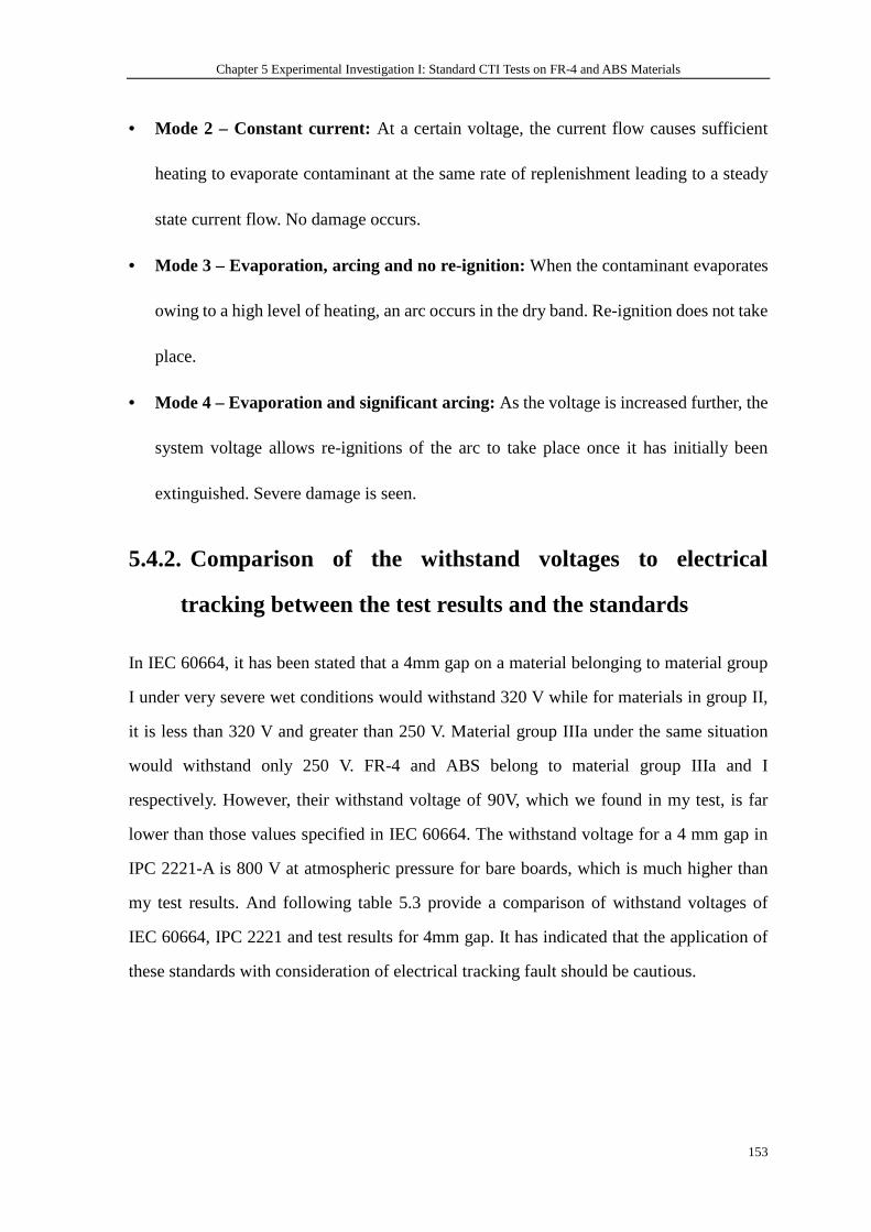
Chapter 5 Experimental Investigation I: Standard CTI Tests on FR-4 and ABS Materials
153
• Mode 2 – Constant current: At a certain voltage, the current flow causes sufficient
heating to evaporate contaminant at the same rate of replenishment leading to a steady
state current flow. No damage occurs.
• Mode 3 – Evaporation, arcing and no re-ignition: When the contaminant evaporates
owing to a high level of heating, an arc occurs in the dry band. Re-ignition does not take
place.
• Mode 4 – Evaporation and significant arcing: As the voltage is increased further, the
system voltage allows re-ignitions of the arc to take place once it has initially been
extinguished. Severe damage is seen.
5.4.2. Comparison of the withstand voltages to electrical
tracking between the test results and the standards
In IEC 60664, it has been stated that a 4mm gap on a material belonging to material group
I under very severe wet conditions would withstand 320 V while for materials in group II,
it is less than 320 V and greater than 250 V. Material group IIIa under the same situation
would withstand only 250 V. FR-4 and ABS belong to material group IIIa and I
respectively. However, their withstand voltage of 90V, which we found in my test, is far
lower than those values specified in IEC 60664. The withstand voltage for a 4 mm gap in
IPC 2221-A is 800 V at atmospheric pressure for bare boards, which is much higher than
my test results. And following table 5.3 provide a comparison of withstand voltages of
IEC 60664, IPC 2221 and test results for 4mm gap. It has indicated that the application of
these standards with consideration of electrical tracking fault should be cautious.
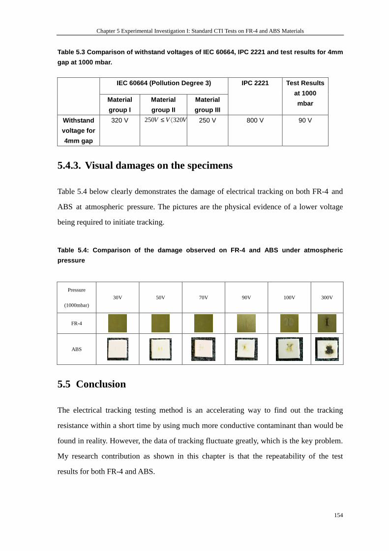
Chapter 5 Experimental Investigation I: Standard CTI Tests on FR-4 and ABS Materials
154
Table 5.3 Comparison of withstand voltages of IEC 6 0664, IPC 2221 and test results for 4mm
gap at 1000 mbar.
IEC 60664 (Pollution Degree 3)
Material
group I
Material
group II
Material
group III
IPC 2221 Test Results
at 1000
mbar
Withstand
voltage for
4mm gap
320 V 250 320V V V≤ ⟨
250 V 800 V 90 V
5.4.3. Visual damages on the specimens
Table 5.4 below clearly demonstrates the damage of electrical tracking on both FR-4 and
ABS at atmospheric pressure. The pictures are the physical evidence of a lower voltage
being required to initiate tracking.
Table 5.4: Comparison of the damage observed on FR- 4 and ABS under atmospheric
pressure
5.5 Conclusion
The electrical tracking testing method is an accelerating way to find out the tracking
resistance within a short time by using much more conductive contaminant than would be
found in reality. However, the data of tracking fluctuate greatly, which is the key problem.
My research contribution as shown in this chapter is that the repeatability of the test
results for both FR-4 and ABS.
Pressure
(1000mbar)
30V 50V 70V 90V 100V 300V
FR-4
ABS
Chapter 5 Experimental Investigation I: Standard CTI Tests on FR-4 and ABS Materials
155
A test rig was developed that allowed to apply AC voltage up to 600 V to the contaminated
gap on the organic insulating material FR-4 and ABS for certain test period, 30 minutes in
my tests. And both raw leakage current/voltage and summarized current data on the test
objective were designed to be recorded automatically by the Labview program.
Although different materials belonging to different categories of the material group
according to their CTI values were tested by using the standard test methods, we found
that the material itself was not the critical factor for initiating electrical tracking. For both
FR-4 and ABS, at 50 V the testing showed a gradually increasing leakage current during
the testing period. There was no any damage found on the specimens. At around 60 V and
70 V for both materials, due to the equal rate of the replenishment and evaporation, the
leakage currents for both cases were presented a constant trend after initial increase for 7
minutes. Then with time going, after 20 minutes’ testing the current dropped again. Finally,
At 90 V, the summarized current plots illustrated there were spikes which is the
characteristic mechanism of electrical arc and the evidence of damages were found for
both materials. In this chapter the very typical raw data at 100 V also proved that there
was arc taking place. It also should be noted that according to all the three times’ repeated
test results the reproducibility of the test method has been proven.
When these numbers above mentioned are compared the standard, we see that withstand
voltage of 90 V for 4mm gap on both FR-4 and ABS in my tests is much lower that the
value of 320 V for material group I and less than 320 V but above 250 for material group
II and 250 V for material group IIIa under pollution degree 3 (conductive pollution
occurs or dry non-conductive pollution occurs which becomes conductive due to
condensation which is to be expected, which is close to the situation of use of solution A
in my tests) in IEC 60664 and 800V in IPC 2221.It suggested that the application of the
dimensioning of creepage distances in these standards should not be applied.
The comparison also can be done with the calculated withstand voltages in chapter 4. It
can be seen that the calculated value under pollution degree3 at atmospheric pressure of 25
Chapter 5 Experimental Investigation I: Standard CTI Tests on FR-4 and ABS Materials
156
V is even lower than test result of 90 V. However, the dynamic thermal processes were not
considered in my mathematic model, which could be the reason of this difference.
Finally, it should be emphasized that the reason for electrical tracking on the organic
materials is that the conductive pollution layer can lead to electrical current flowing
through. With different voltage levels, the pollution layer dried at different rates, and the
rate of replenishment is the critical factor. The voltage and replenishment of pollution
together have a big effect on the mechanism of initiation of electrical tracking. So as a
conclusion the voltage level of any system and potential pollution degree are very
important to evaluate whether a system can survive and operate reliably. Then when any
dimensioning rules in any standards are employed, these two factors should be evaluated
very carefully.
Chapter 6 Experimental Investigation II: CTI Tests under the Conditions of Lower Pressure and Varying conductivity of Contamination
157
Chapter 6 Experimental Investigation II: CTI
tests under the Conditions of Lower Pressure
and Varying Conductivity of Contamination
6.1. Introduction
The static mathematical model and computer simulation studies in Chapter 4 show that
macro-environmental factors such air pressure, ambient temperature and pollution degree
have an impact on electrical tracking formation and hence the values of required voltage.
In Chapter 5, the standardized CTI tests have been discussed under atmospheric pressure
conditions. It has been proven that the test method used in my research is repeatable,
which provides a reliable test method to study further the influences of those
environmental factors on electrical tracking.
For aerospace applications, air pressure is a highly critical environmental impact factor. In
this chapter we will see a series of CTI tests undertaken in the environment chamber where
the surrounding air pressure could vary from atmospheric pressure 1000 mbar (100000 Pa)
to as low as 100 mbar (10000 Pa), which is approximately 51,806 feet above sea level.
According to the static mathematical model in Equation 4.7 in Chapter 4, the boiling point
of aqueous contaminations determine the amount of heat needed to heat the contamination
up to boiling point. It is known that air pressure has a big effect on boiling point, as shown
in Figure 4.10 in Chapter 4. The lower the pressure, the lower the boiling point would be,
and accordingly less heat would be needed to heat the contamination up to boiling.
Similarly therefore, under lower pressure less electrical power input is needed for
electrical tracking to take place (if we assume both the ambient temperature and pollution
degree are constant). By using the same test method as in Chapter 5 but under a lower
Chapter 6 Experimental Investigation II: CTI Tests under the Conditions of Lower Pressure and Varying conductivity of Contamination
158
pressure, we should expect lower voltages to initiate electrical tracking.
The impact of pollution degree has also been evaluated based on the test results by
employing contamination with varying conductivity. These tests were carried out at room
temperature and atmospheric pressure. The conductivity of contamination, which is
solution A in my research, represents different degrees of pollution. It directly influences the
resistance of the electrical conductive path, and consequently would have effect on the
value of leakage current flows through it. According to the static model in Equation 4.7 in
Chapter 4, the electrical power input would be larger with a more conductive aqueous
contamination. Therefore a lower voltage is needed to heat up the contamination to its
boiling status, which leads to a higher level of evaporation and consequent formation of
electrical tracking. As a conclusion, we should expect lower voltage for higher conductivity
solution tests and higher voltages for lower conductivity solution tests compared to
standardized CTI test results.
Low pressure experiment conditions and procedures are presented in this chapter first
Discussion of the results and comparison with IEC 60664 and IPC 2221 will be provided
afterwards. And then the tests employing the contamination of varying conductivities will
be then shown with the discussion of test results at last.
6.2. Low pressure CTI tests
To evaluate the impact of air pressure, experimental tests by using the same test methods
as explained in Chapter 5 were carried out. In the following section 6.2.1 the differences
of experiment conditions from the standardized ones are presented firstly. Then the test
results are illustrated and then discussed.
6.2.1. Experiment conditions
Test Circuit
Figure 5.1 in Chapter 5 shows the circuit diagram used for the tests. The test gaps for lower
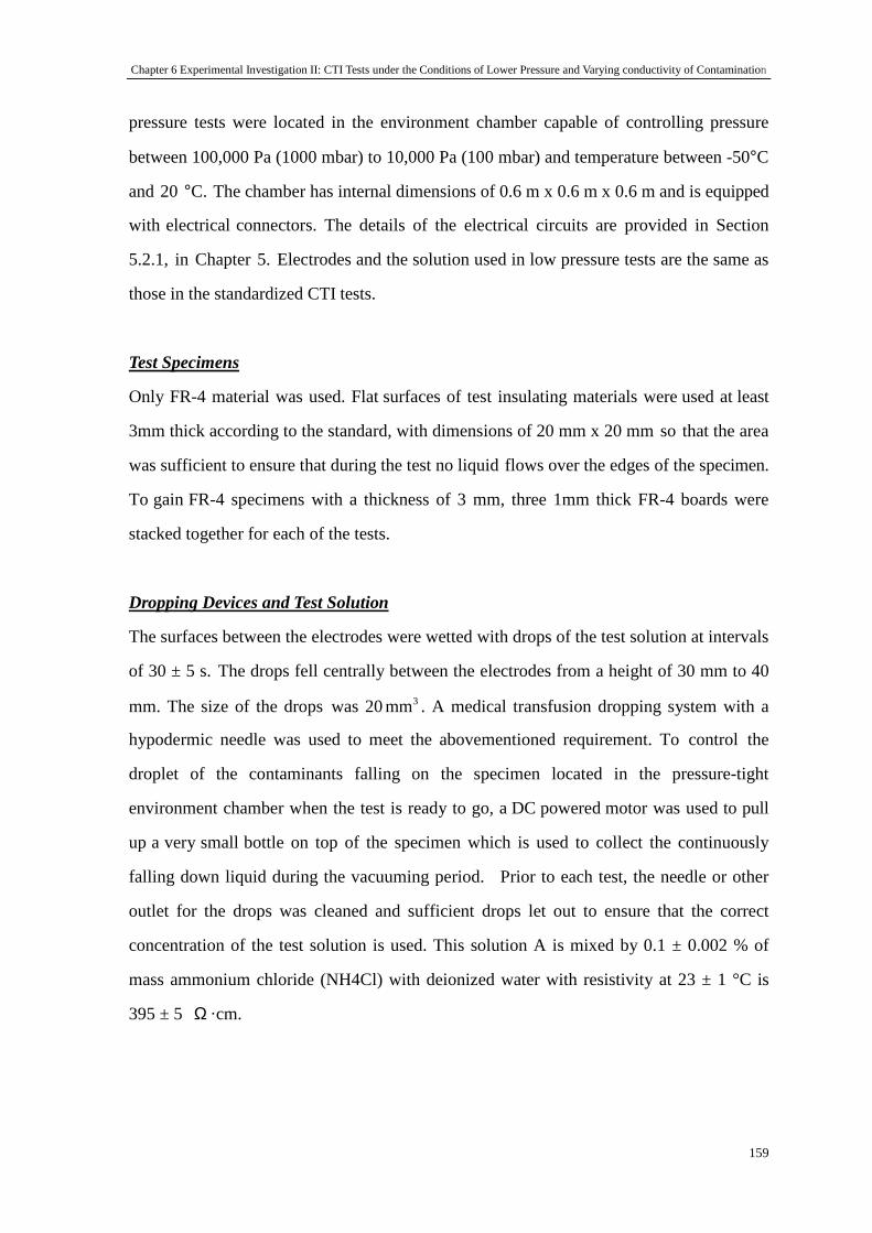
Chapter 6 Experimental Investigation II: CTI Tests under the Conditions of Lower Pressure and Varying conductivity of Contamination
159
pressure tests were located in the environment chamber capable of controlling pressure
between 100,000 Pa (1000 mbar) to 10,000 Pa (100 mbar) and temperature between -50°C
and 20 °C. The chamber has internal dimensions of 0.6 m x 0.6 m x 0.6 m and is equipped
with electrical connectors. The details of the electrical circuits are provided in Section
5.2.1, in Chapter 5. Electrodes and the solution used in low pressure tests are the same as
those in the standardized CTI tests.
Test Specimens
Only FR-4 material was used. Flat surfaces of test insulating materials were used at least
3mm thick according to the standard, with dimensions of 20 mm x 20 mm so that the area
was sufficient to ensure that during the test no liquid flows over the edges of the specimen.
To gain FR-4 specimens with a thickness of 3 mm, three 1mm thick FR-4 boards were
stacked together for each of the tests.
Dropping Devices and Test Solution
The surfaces between the electrodes were wetted with drops of the test solution at intervals
of 30 ± 5 s. The drops fell centrally between the electrodes from a height of 30 mm to 40
mm. The size of the drops was 20 3mm . A medical transfusion dropping system with a
hypodermic needle was used to meet the abovementioned requirement. To control the
droplet of the contaminants falling on the specimen located in the pressure-tight
environment chamber when the test is ready to go, a DC powered motor was used to pull
up a very small bottle on top of the specimen which is used to collect the continuously
falling down liquid during the vacuuming period. Prior to each test, the needle or other
outlet for the drops was cleaned and sufficient drops let out to ensure that the correct
concentration of the test solution is used. This solution A is mixed by 0.1 ± 0.002 % of
mass ammonium chloride (NH4Cl) with deionized water with resistivity at 23 ± 1 °C is
395 ± 5 Ω ·cm.
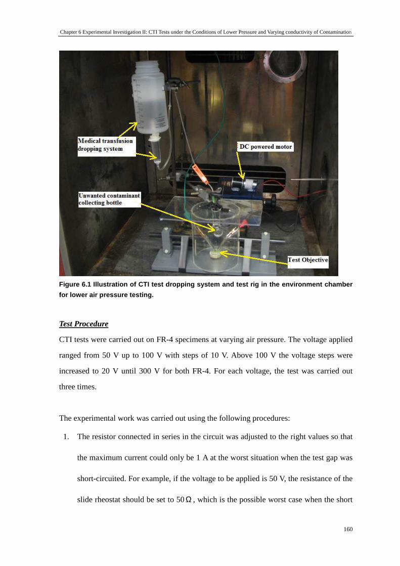
Chapter 6 Experimental Investigation II: CTI Tests under the Conditions of Lower Pressure and Varying conductivity of Contamination
160
Figure 6.1 Illustration of CTI test dropping system and test rig in the environment chamber
for lower air pressure testing.
Test Procedure
CTI tests were carried out on FR-4 specimens at varying air pressure. The voltage applied
ranged from 50 V up to 100 V with steps of 10 V. Above 100 V the voltage steps were
increased to 20 V until 300 V for both FR-4. For each voltage, the test was carried out
three times.
The experimental work was carried out using the following procedures:
1. The resistor connected in series in the circuit was adjusted to the right values so that
the maximum current could only be 1 A at the worst situation when the test gap was
short-circuited. For example, if the voltage to be applied is 50 V, the resistance of the
slide rheostat should be set to 50Ω , which is the possible worst case when the short
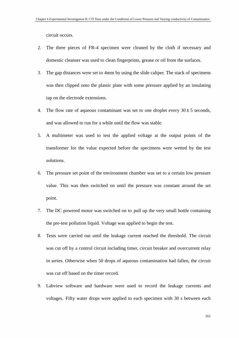
Chapter 6 Experimental Investigation II: CTI Tests under the Conditions of Lower Pressure and Varying conductivity of Contamination
161
circuit occurs.
2. The three pieces of FR-4 specimen were cleaned by the cloth if necessary and
domestic cleanser was used to clean fingerprints, grease or oil from the surfaces.
3. The gap distances were set to 4mm by using the slide caliper. The stack of specimens
was then clipped onto the plastic plate with some pressure applied by an insulating
tap on the electrode extensions.
4. The flow rate of aqueous contaminant was set to one droplet every 30± 5 seconds,
and was allowed to run for a while until the flow was stable.
5. A multimeter was used to test the applied voltage at the output points of the
transformer for the value expected before the specimens were wetted by the test
solutions.
6. The pressure set point of the environment chamber was set to a certain low pressure
value. This was then switched on until the pressure was constant around the set
point.
7. The DC powered motor was switched on to pull up the very small bottle containing
the pre-test pollution liquid. Voltage was applied to begin the test.
8. Tests were carried out until the leakage current reached the threshold. The circuit
was cut off by a control circuit including timer, circuit breaker and overcurrent relay
in series. Otherwise when 50 drops of aqueous contamination had fallen, the circuit
was cut off based on the timer record.
9. Labview software and hardware were used to record the leakage currents and
voltages. Fifty water drops were applied to each specimen with 30 s between each
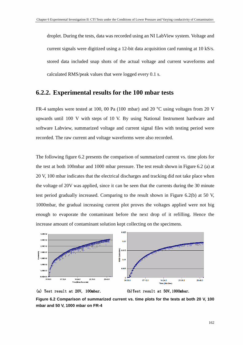
Chapter 6 Experimental Investigation II: CTI Tests under the Conditions of Lower Pressure and Varying conductivity of Contamination
162
droplet. During the tests, data was recorded using an NI LabView system. Voltage and
current signals were digitized using a 12-bit data acquisition card running at 10 kS/s.
stored data included snap shots of the actual voltage and current waveforms and
calculated RMS/peak values that were logged every 0.1 s.
6.2.2. Experimental results for the 100 mbar tests
FR-4 samples were tested at 100, 00 Pa (100 mbar) and 20 °C using voltages from 20 V
upwards until 100 V with steps of 10 V. By using National Instrument hardware and
software Labview, summarized voltage and current signal files with testing period were
recorded. The raw current and voltage waveforms were also recorded.
The following figure 6.2 presents the comparison of summarized current vs. time plots for
the test at both 100mbar and 1000 mbar pressure. The test result shown in Figure 6.2 (a) at
20 V, 100 mbar indicates that the electrical discharges and tracking did not take place when
the voltage of 20V was applied, since it can be seen that the currents during the 30 minute
test period gradually increased. Comparing to the result shown in Figure 6.2(b) at 50 V,
1000mbar, the gradual increasing current plot proves the voltages applied were not big
enough to evaporate the contaminant before the next drop of it refilling. Hence the
increase amount of contaminant solution kept collecting on the specimens.
(a) Test result at 20V, 100mbar. (a) Test result at 20V, 100mbar. (a) Test result at 20V, 100mbar. (a) Test result at 20V, 100mbar. (b)Test result at 50V,1000mbar. (b)Test result at 50V,1000mbar. (b)Test result at 50V,1000mbar. (b)Test result at 50V,1000mbar.
Figure 6.2 Comparison of summarized current vs. tim e plots for the tests at both 20 V, 100
mbar and 50 V, 1000 mbar on FR-4
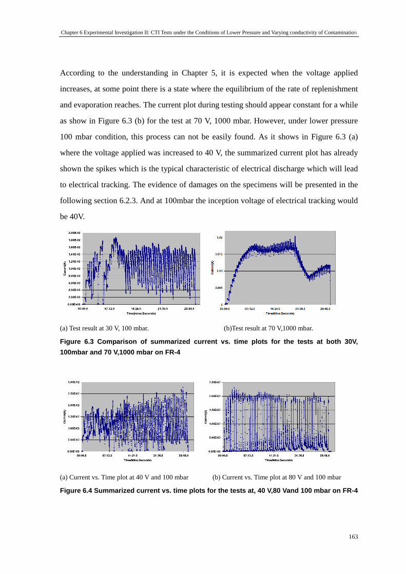
Chapter 6 Experimental Investigation II: CTI Tests under the Conditions of Lower Pressure and Varying conductivity of Contamination
163
According to the understanding in Chapter 5, it is expected when the voltage applied
increases, at some point there is a state where the equilibrium of the rate of replenishment
and evaporation reaches. The current plot during testing should appear constant for a while
as show in Figure 6.3 (b) for the test at 70 V, 1000 mbar. However, under lower pressure
100 mbar condition, this process can not be easily found. As it shows in Figure 6.3 (a)
where the voltage applied was increased to 40 V, the summarized current plot has already
shown the spikes which is the typical characteristic of electrical discharge which will lead
to electrical tracking. The evidence of damages on the specimens will be presented in the
following section 6.2.3. And at 100mbar the inception voltage of electrical tracking would
be 40V.
(a) Test result at 30 V, 100 mbar. (b)Test result at 70 V,1000 mbar.
Figure 6.3 Comparison of summarized current vs. tim e plots for the tests at both 30V,
100mbar and 70 V,1000 mbar on FR-4
(a) Current vs. Time plot at 40 V and 100 mbar (b) Current vs. Time plot at 80 V and 100 mbar
Figure 6.4 Summarized current vs. time plots for th e tests at, 40 V,80 Vand 100 mbar on FR-4
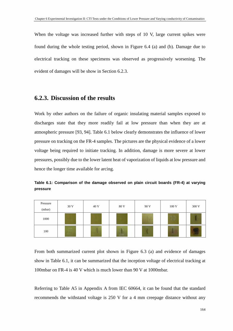
Chapter 6 Experimental Investigation II: CTI Tests under the Conditions of Lower Pressure and Varying conductivity of Contamination
164
When the voltage was increased further with steps of 10 V, large current spikes were
found during the whole testing period, shown in Figure 6.4 (a) and (b). Damage due to
electrical tracking on these specimens was observed as progressively worsening. The
evident of damages will be show in Section 6.2.3.
6.2.3. Discussion of the results
Work by other authors on the failure of organic insulating material samples exposed to
discharges state that they more readily fail at low pressure than when they are at
atmospheric pressure [93, 94]. Table 6.1 below clearly demonstrates the influence of lower
pressure on tracking on the FR-4 samples. The pictures are the physical evidence of a lower
voltage being required to initiate tracking. In addition, damage is more severe at lower
pressures, possibly due to the lower latent heat of vaporization of liquids at low pressure and
hence the longer time available for arcing.
Table 6.1: Comparison of the damage observed on pla in circuit boards (FR-4) at varying
pressure
From both summarized current plot shown in Figure 6.3 (a) and evidence of damages
show in Table 6.1, it can be summarized that the inception voltage of electrical tracking at
100mbar on FR-4 is 40 V which is much lower than 90 V at 1000mbar.
Referring to Table A5 in Appendix A from IEC 60664, it can be found that the standard
recommends the withstand voltage is 250 V for a 4 mm creepage distance without any
Pressure
(mbar) 30 V 40 V 80 V 90 V 100 V 300 V
1000
100
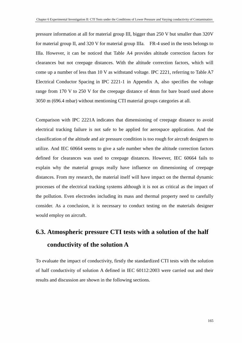
Chapter 6 Experimental Investigation II: CTI Tests under the Conditions of Lower Pressure and Varying conductivity of Contamination
165
pressure information at all for material group III, bigger than 250 V but smaller than 320V
for material group II, and 320 V for material group IIIa. FR-4 used in the tests belongs to
IIIa. However, it can be noticed that Table A4 provides altitude correction factors for
clearances but not creepage distances. With the altitude correction factors, which will
come up a number of less than 10 V as withstand voltage. IPC 2221, referring to Table A7
Electrical Conductor Spacing in IPC 2221-1 in Appendix A, also specifies the voltage
range from 170 V to 250 V for the creepage distance of 4mm for bare board used above
3050 m (696.4 mbar) without mentioning CTI material groups categories at all.
Comparison with IPC 2221A indicates that dimensioning of creepage distance to avoid
electrical tracking failure is not safe to be applied for aerospace application. And the
classification of the altitude and air pressure condition is too rough for aircraft designers to
utilize. And IEC 60664 seems to give a safe number when the altitude correction factors
defined for clearances was used to creepage distances. However, IEC 60664 fails to
explain why the material groups really have influence on dimensioning of creepage
distances. From my research, the material itself will have impact on the thermal dynamic
processes of the electrical tracking systems although it is not as critical as the impact of
the pollution. Even electrodes including its mass and thermal property need to carefully
consider. As a conclusion, it is necessary to conduct testing on the materials designer
would employ on aircraft.
6.3. Atmospheric pressure CTI tests with a solution of the half
conductivity of the solution A
To evaluate the impact of conductivity, firstly the standardized CTI tests with the solution
of half conductivity of solution A defined in IEC 60112:2003 were carried out and their
results and discussion are shown in the following sections.
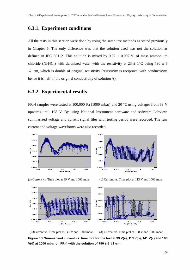
Chapter 6 Experimental Investigation II: CTI Tests under the Conditions of Lower Pressure and Varying conductivity of Contamination
166
6.3.1. Experiment conditions
All the tests in this section were done by using the same test methods as stated previously
in Chapter 5. The only difference was that the solution used was not the solution as
defined in IEC 60112. This solution is mixed by 0.02 ± 0.002 % of mass ammonium
chloride (NH4Cl) with deionized water with the resistivity at 23 ± 1°C being 790 ± 5
Ω ·cm, which is double of original resistivity (resistivity is reciprocal with conductivity,
hence it is half of the original conductivity of solution A).
6.3.2. Experimental results
FR-4 samples were tested at 100,000 Pa (1000 mbar) and 20 °C using voltages from 69 V
upwards until 198 V. By using National Instrument hardware and software Labview,
summarized voltage and current signal files with testing period were recorded. The raw
current and voltage waveforms were also recorded.
(a) Current vs. Time plot at 99 V and 1000 mbar (b) Current vs. Time plot at 113 V and 1000 mbar
(C)Current vs. Time plot at 141 V and 1000 mbar (d) Current vs. Time plot at 198 V and 1000 mbar
Figure 6.5 Summarized current vs. time plot for the test at 99 V(a), 113 V(b), 141 V(c) and 198
V(d) at 1000 mbar on FR-4 with the solution of 790 ± 5 Ω ·cm.

Chapter 6 Experimental Investigation II: CTI Tests under the Conditions of Lower Pressure and Varying conductivity of Contamination
167
When the conductivity of the solution was halved (the resistivity was doubled), leakage
current flowing through the conductive path was lower. Therefore higher voltages were
needed to heat the same amount of the liquid. It should be noted that conductivity also
influenced the boiling points as show in Figure 4.10 in Chapter 4. The test results shown in
Figure 6.5(a) indicate that electrical tracking did not even take place when the voltage of 99
V was applied, since there are no large current spikes found. Current first increased to its
peak, then dropped for seven minutes and finally reached a constant. From the analysis in
Chapter 5, the increase stage is due to increase in the amount of the solution collecting on
the specimens. It takes time for the system to reach the final thermal equilibrium, when we
can see that the current became constant.
When the voltage was raised to 113 V, the large current spikes indicate that electrical
tracking occurred, and it also can be seen that the current increase and drop period was
shortened. It took less time for the system to reach thermal equilibrium. However, in this
case, the voltage was enough to trigger electrical discharges and hence electrical tracking.
With higher and higher voltages applied, figures (c) and (d) clearly show the phenomena
explained previously. Damage on specimens also provides evidence of the electrical
tracking, as shown in Table 6.2. As a summary, the inception voltage of electrical tracking
at atmospheric pressure but with the solution of half conductivity of original one is 113 V.
Table 6.2: Damage observed on plain circuit boards (FR-4) at atmospheric pressure with the
solution of 790 ± 5 Ω ·cm.
6.3.3. Discussion of the results
The pictures in Table 6.2 are the physical evidence of a higher voltage (113 V) being
Pressure
(mbar) 99 V 113 V 127 V 141 V 198 V
1000
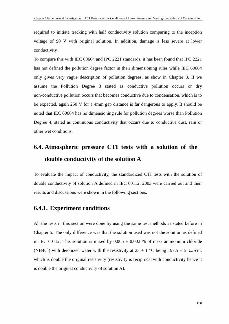
Chapter 6 Experimental Investigation II: CTI Tests under the Conditions of Lower Pressure and Varying conductivity of Contamination
168
required to initiate tracking with half conductivity solution comparing to the inception
voltage of 90 V with original solution. In addition, damage is less severe at lower
conductivity.
To compare this with IEC 60664 and IPC 2221 standards, it has been found that IPC 2221
has not defined the pollution degree factor in their dimensioning rules while IEC 60664
only gives very vague description of pollution degrees, as show in Chapter 3. If we
assume the Pollution Degree 3 stated as conductive pollution occurs or dry
non-conductive pollution occurs that becomes conductive due to condensation, which is to
be expected, again 250 V for a 4mm gap distance is far dangerous to apply. It should be
noted that IEC 60664 has no dimensioning rule for pollution degrees worse than Pollution
Degree 4, stated as continuous conductivity that occurs due to conductive dust, rain or
other wet conditions.
6.4. Atmospheric pressure CTI tests with a solution of the
double conductivity of the solution A
To evaluate the impact of conductivity, the standardized CTI tests with the solution of
double conductivity of solution A defined in IEC 60112: 2003 were carried out and their
results and discussions were shown in the following sections.
6.4.1. Experiment conditions
All the tests in this section were done by using the same test methods as stated before in
Chapter 5. The only difference was that the solution used was not the solution as defined
in IEC 60112. This solution is mixed by 0.005 ± 0.002 % of mass ammonium chloride
(NH4Cl) with deionized water with the resistivity at 23 ± 1 °C being 197.5 ± 5 Ω ·cm,
which is double the original resistivity (resistivity is reciprocal with conductivity hence it
is double the original conductivity of solution A).
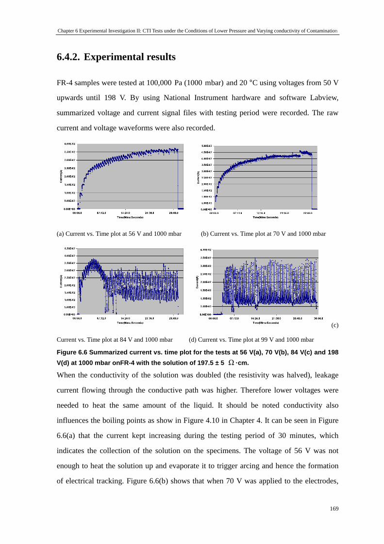
Chapter 6 Experimental Investigation II: CTI Tests under the Conditions of Lower Pressure and Varying conductivity of Contamination
169
6.4.2. Experimental results
FR-4 samples were tested at 100,000 Pa (1000 mbar) and 20 °C using voltages from 50 V
upwards until 198 V. By using National Instrument hardware and software Labview,
summarized voltage and current signal files with testing period were recorded. The raw
current and voltage waveforms were also recorded.
(a) Current vs. Time plot at 56 V and 1000 mbar (b) Current vs. Time plot at 70 V and 1000 mbar
(c)
Current vs. Time plot at 84 V and 1000 mbar (d) Current vs. Time plot at 99 V and 1000 mbar
Figure 6.6 Summarized current vs. time plot for the tests at 56 V(a), 70 V(b), 84 V(c) and 198
V(d) at 1000 mbar onFR-4 with the solution of 197.5 ± 5 Ω ·cm.
When the conductivity of the solution was doubled (the resistivity was halved), leakage
current flowing through the conductive path was higher. Therefore lower voltages were
needed to heat the same amount of the liquid. It should be noted conductivity also
influences the boiling points as show in Figure 4.10 in Chapter 4. It can be seen in Figure
6.6(a) that the current kept increasing during the testing period of 30 minutes, which
indicates the collection of the solution on the specimens. The voltage of 56 V was not
enough to heat the solution up and evaporate it to trigger arcing and hence the formation
of electrical tracking. Figure 6.6(b) shows that when 70 V was applied to the electrodes,
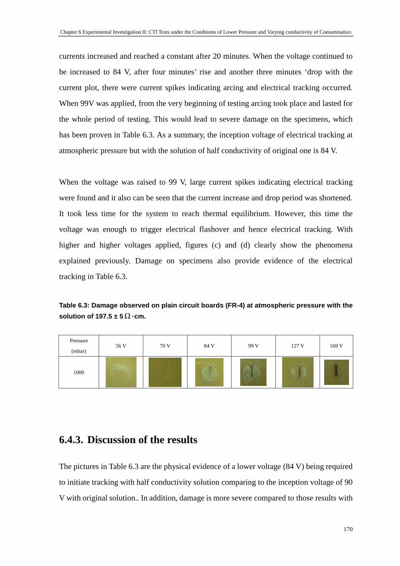
Chapter 6 Experimental Investigation II: CTI Tests under the Conditions of Lower Pressure and Varying conductivity of Contamination
170
currents increased and reached a constant after 20 minutes. When the voltage continued to
be increased to 84 V, after four minutes’ rise and another three minutes ‘drop with the
current plot, there were current spikes indicating arcing and electrical tracking occurred.
When 99V was applied, from the very beginning of testing arcing took place and lasted for
the whole period of testing. This would lead to severe damage on the specimens, which
has been proven in Table 6.3. As a summary, the inception voltage of electrical tracking at
atmospheric pressure but with the solution of half conductivity of original one is 84 V.
When the voltage was raised to 99 V, large current spikes indicating electrical tracking
were found and it also can be seen that the current increase and drop period was shortened.
It took less time for the system to reach thermal equilibrium. However, this time the
voltage was enough to trigger electrical flashover and hence electrical tracking. With
higher and higher voltages applied, figures (c) and (d) clearly show the phenomena
explained previously. Damage on specimens also provide evidence of the electrical
tracking in Table 6.3.
Table 6.3: Damage observed on plain circuit boards (FR-4) at atmospheric pressure with the
solution of 197.5 ± 5 Ω ·cm.
6.4.3. Discussion of the results
The pictures in Table 6.3 are the physical evidence of a lower voltage (84 V) being required
to initiate tracking with half conductivity solution comparing to the inception voltage of 90
V with original solution.. In addition, damage is more severe compared to those results with
Pressure
(mbar) 56 V 70 V 84 V 99 V 127 V 169 V
1000

Chapter 6 Experimental Investigation II: CTI Tests under the Conditions of Lower Pressure and Varying conductivity of Contamination
171
a half conductivity solution due to the longer time available for arcing.
Again there is no any information regarding the pollution degree in IPC 2221. Additionally,
IEC 60064’s dimensioning rules are based on a very vague description of the pollution
degrees. 250 V for a 4mm creepage distance is not applicable when compared with my test
results.
6.5. Discussion
The comparison of the inception voltages of electrical tracking at 100mbar with the IEC
60664 and IPC 2221 is presented in Table 6.4. IEC 60064 has no information regarding
pressure influence at all in its dimensioning rules of creepage distances. However, it can
be noticed that Table A4 provides altitude correction factors for clearances in IEC 60064
but not creepage distances. If employing the altitude correction factors, which will come
up a very small number of less than 10 V as withstand voltage comparing to existing
numbers show in the table. Then this will show that IEC 60664 would be very
conservative in term of definition of withstand voltage of 4mm creepage distances for
lower air pressure. Compared with IPC 2221’s creepage distance of 4 mm for 3050 m
(696.4 mbar), the voltage of 170 V-250 V is much higher than the withstand voltage of 40
V found in my tests. The use of IPC 2221 need to be cautious.
Table 6.4 Comparison of withstand voltages of IEC 6 0664, IPC 2221 and test results for 4mm
gap on FR-4 at both 1000mbar and 100mabar.
IEC 60664 (Pollution Degree 3) IPC 2221 Test Results
Material
group I
Material
group II
Material
group III
Above sea
level up
to 3050 m
(696.4
mbar)
Above
3050 m
(696.4
mbar)
1000
mbar
100m
bar
Withstand
voltage for
4mm gap
320 V 250 320V V V≤ ⟨
250 V 800 V 170-250
V
90 V 40 V
When conductivity of the solution was doubled (the resistivity was halved), leakage
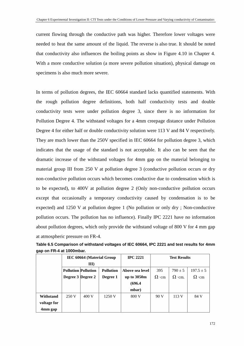
Chapter 6 Experimental Investigation II: CTI Tests under the Conditions of Lower Pressure and Varying conductivity of Contamination
172
current flowing through the conductive path was higher. Therefore lower voltages were
needed to heat the same amount of the liquid. The reverse is also true. It should be noted
that conductivity also influences the boiling points as show in Figure 4.10 in Chapter 4.
With a more conductive solution (a more severe pollution situation), physical damage on
specimens is also much more severe.
In terms of pollution degrees, the IEC 60664 standard lacks quantified statements. With
the rough pollution degree definitions, both half conductivity tests and double
conductivity tests were under pollution degree 3, since there is no information for
Pollution Degree 4. The withstand voltages for a 4mm creepage distance under Pollution
Degree 4 for either half or double conductivity solution were 113 V and 84 V respectively.
They are much lower than the 250V specified in IEC 60664 for pollution degree 3, which
indicates that the usage of the standard is not acceptable. It also can be seen that the
dramatic increase of the withstand voltages for 4mm gap on the material belonging to
material group III from 250 V at pollution degree 3 (conductive pollution occurs or dry
non-conductive pollution occurs which becomes conductive due to condensation which is
to be expected), to 400V at pollution degree 2 (Only non-conductive pollution occurs
except that occasionally a temporary conductivity caused by condensation is to be
expected) and 1250 V at pollution degree 1 (No pollution or only dry ; Non-conductive
pollution occurs. The pollution has no influence). Finally IPC 2221 have no information
about pollution degrees, which only provide the withstand voltage of 800 V for 4 mm gap
at atmospheric pressure on FR-4.
Table 6.5 Comparison of withstand voltages of IEC 6 0664, IPC 2221 and test results for 4mm
gap on FR-4 at 1000mbar.
IEC 60664 (Material Group
III)
IPC 2221 Test Results
Pollution
Degree 3
Pollution
Degree 2
Pollution
Degree 1
Above sea level
up to 3050m
(696.4
mbar)
395
Ω ·cm
790 ± 5
Ω ·cm.
197.5 ± 5
Ω ·cm
Withstand
voltage for
4mm gap
250 V 400 V 1250 V 800 V 90 V 113 V 84 V
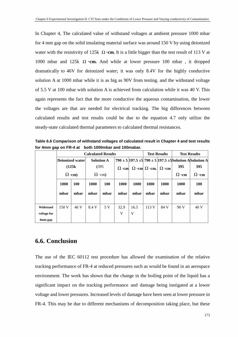
Chapter 6 Experimental Investigation II: CTI Tests under the Conditions of Lower Pressure and Varying conductivity of Contamination
173
In Chapter 4, The calculated value of withstand voltages at ambient pressure 1000 mbar
for 4 mm gap on the solid insulating material surface was around 150 V by using deionized
water with the resistivity of 125k Ω ·cm. It is a little bigger than the test result of 113 V at
1000 mbar and 125k Ω ·cm. And while at lower pressure 100 mbar , it dropped
dramatically to 46V for deionized water; it was only 8.4V for the highly conductive
solution A at 1000 mbar while it is as big as 90V from testing. and the withstand voltage
of 5.5 V at 100 mbar with solution A is achieved from calculation while it was 40 V. This
again represents the fact that the more conductive the aqueous contamination, the lower
the voltages are that are needed for electrical tracking. The big differences between
calculated results and test results could be due to the equation 4.7 only utilize the
steady-state calculated thermal parameters to calculated thermal resistances.
Table 6.6 Comparison of withstand voltages of calcu lated result in Chapter 4 and test results
for 4mm gap on FR-4 at both 1000mbar and 100mabar.
Calculated Results Test Results Test Results
Deionized water
(125k
Ω ·cm)
Solution A
(395
Ω ·cm)
790 ± 5
Ω ·cm
197.5 ±5
Ω ·cm
790 ± 5
Ω ·cm.
197.5 ±5
Ω ·cm
Solution A
395
Ω ·cm
Solution A
395
Ω ·cm
1000
mbar
100
mbar
1000
mbar
100
mbar
1000
mbar
1000
mbar
1000
mbar
1000
mbar
1000
mbar
100
mbar
Withstand
voltage for
4mm gap
150 V 46 V 8.4 V 5 V 32.9
V
16.5
V
113 V 84 V 90 V 40 V
6.6. Conclusion
The use of the IEC 60112 test procedure has allowed the examination of the relative
tracking performance of FR-4 at reduced pressures such as would be found in an aerospace
environment. The work has shown that the change in the boiling point of the liquid has a
significant impact on the tracking performance and damage being instigated at a lower
voltage and lower pressures. Increased levels of damage have been seen at lower pressure in
FR-4. This may be due to different mechanisms of decomposition taking place, but these
Chapter 6 Experimental Investigation II: CTI Tests under the Conditions of Lower Pressure and Varying conductivity of Contamination
174
processes need to be more clearly understood.
The computational simulation and experimental data confirm that the guidelines for
creepage distances in IEC 60664 and IPC 2221 are not applicable for aerospace application
considering the environment impact. The calculation results here tend to be lower than those
from the standard because dynamic thermal processes have not accounted for in my model.
Chapter 7 Experimental Investigation III: CTI Tests Developed for Varying Creepage Distances
175
Chapter 7 Experimental Investigation III:
CTI tests Developed for Varying Creepage
Distances
7.1. Introduction
The standard CTI tests discussed before were carried out on a limited 4mm gap distance.
The reason for that is firstly this test method was designed to indicate the relative
resistances of different solid electrical insulating materials to tracking for a voltage up to
600V when the surface is exposed to water mixed with the addition of contaminations
under electrical stress, but not to find out withstand voltages for varying creepage
distances. Hence, the parameter of the gap distance should be the same for the purpose.
Secondly, the flow rate of the dropping solution was also particularly designed for the
4mm gap so that it is just right to allow the liquid film formed between the two electrodes
to evaporate at certain voltages applied to initiate electrical tracking under a certain time.
By changing the original gap distance to a shorter one, the flow rate used now will be so
large that there is no time for the aqueous contaminant to evaporate to initiate electrical
tracking, although the voltage needed would be much lower. If the gap was longer than
4mm, the flow rate would be too low to actually form any continuous conductive current
path between the electrodes. All the difficulties make it challenging to extend the CTI test
method to varying gap distances.
My research developed a way to upgrade the CTI test method to be used for varying gap
distances under atmospheric pressure. Two key changes to the original method are with
dropping devices and the shape of the specimen. Apart from the successfully developed
test technique for varying gaps, a range of possible test techniques were tried to resemble
Chapter 7 Experimental Investigation III: CTI Tests Developed for Varying Creepage Distances
176
the real pollution wet condition.
This chapter first presented the section of test techniques for varying creepage distance
tracking tests. Their limitation and the reason of failure to application would be discussed.
And then a range of test cases were shown consequently. Those test results with the
upgraded CTI test method for a 4mm gap were compared with those by using the
standardized CTI test method. The repeatability of the test result with the upgraded CTI
test method is validated. Two gap distances 2mm and 8mm were tested and their test
results were presented and discussed. Finally the test results were discussed and
compared with dimensioning rules in IEC 60664 and IPC 2221.
7.2. Selection of a wetting technique for the varying creepage
distance tracking test
As explained in introduction section of the chapter, a system to produce the pollution
environment with a right flow rate, the same as the rate defined by standardized CTI test
in IEC 60112:2003, is needed to design. The key objective is that the pollution should not
have orientation, which is different from droplet falling on the solid insulting material
surface between two electrodes.
Initially, the idea was simply based on the utilization of a small water pump to make the
aqueous contaminant circulating from a container and transferring pipes. Those pipes were
equipped with various nozzles with different designs and sizes. It was hoped that the
nozzles would provide fine mists to the testing space. However, the first challenge was
lack of enough water pressure to make the mists to be really fine. As a result, this simple
design of mist system could only give a bundle of big droplets and they normally ejected
to a same area with a big diameter.
Then we found a pond mister produced by professional manufacturers. The idea was to
produce a mini pond mister system in the aqueous contaminant container. The pond mister
Chapter 7 Experimental Investigation III: CTI Tests Developed for Varying Creepage Distances
177
was located underneath the water level in a container. By changing the distance from the
mister to the water level, the flow rate of the mist generated can be roughly controlled.
And then the test objective which was FR-4 board in my research would be positioned just
above the water level submerging in the fog. This time we achieved very fine mist
environment. Then the next parameter of the system, the flow rate of the mist, was
checkout.
The flow rate of mist was checked by measuring the liquid gathered in a Petri dish (This
method was also used for the following humidifier method). It was positioned at the same
location where the test objective will be placed. And within certain time the weights of the
liquid collected in the Petri dishes were measured. And then the flow rate was calculated
with unit of 3mm /minute. As it is known that the flow rate of the standardized CTI test is
40 3mm /minute. Considering the area of Petri dish was different, so the unit for
evaluation of the flow rate was included the per typical specimen area (20 mm×20 mm).
Unfortunately, it was found that it is very difficult to achieve the same flow rate used in
the standardized CTI tests. Hence No further research was continued by using this
technique. This technique is still a possibility to improve the standardized technique.
Finally, instead of the devices to provide droplets with intermittent time period (every 30
seconds), a domestic humidifier was introduced. It can provide continuous very fine mists.
With condensation, we achieved a very uniform flow rate of liquid film between
electrodes and also comparative to the original flow rate as specified in IEC 60112: 2003.
The most important thing is the mist generated by the humidifier does not have orientation
so no matter how big or small the gap would be; the same flow rate should be achieved.
However, the surface tension of liquid should be taken into consideration if the two
electrodes are very close too each other especially in order a few millimeter or even less.
These challenges has been successfully solved by the test technique presented in this
chapter later and what is more is that the technique can be applied in environment
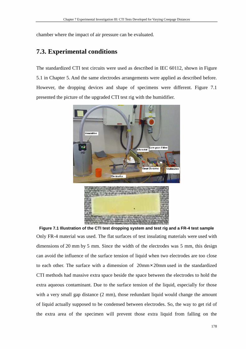
Chapter 7 Experimental Investigation III: CTI Tests Developed for Varying Creepage Distances
178
chamber where the impact of air pressure can be evaluated.
7.3. Experimental conditions
The standardized CTI test circuits were used as described in IEC 60112, shown in Figure
5.1 in Chapter 5. And the same electrodes arrangements were applied as described before.
However, the dropping devices and shape of specimens were different. Figure 7.1
presented the picture of the upgraded CTI test rig with the humidifier.
Figure 7.1 Illustration of the CTI test dropping sy stem and test rig and a FR-4 test sample
Only FR-4 material was used. The flat surfaces of test insulating materials were used with
dimensions of 20 mm by 5 mm. Since the width of the electrodes was 5 mm, this design
can avoid the influence of the surface tension of liquid when two electrodes are too close
to each other. The surface with a dimension of 20mm 20mm× used in the standardized
CTI methods had massive extra space beside the space between the electrodes to hold the
extra aqueous contaminant. Due to the surface tension of the liquid, especially for those
with a very small gap distance (2 mm), those redundant liquid would change the amount
of liquid actually supposed to be condensed between electrodes. So, the way to get rid of
the extra area of the specimen will prevent those extra liquid from falling on the

Chapter 7 Experimental Investigation III: CTI Tests Developed for Varying Creepage Distances
179
specimens. By doing validating tests with the 4mm gap, shown in the following section, it
will prove that this design does prevent the variation of the flow rate of the contaminant,
and consequently repeatable test results can be gained.
The surfaces of the test specimens were cleaned by using a cloth if necessary with domestic
cleanser to make sure they were free of dust, dirt, fingerprints, grease, oil, mould release, or
other contaminants which can influence the test results but not lead to any swelling.
The surfaces between the electrodes were wetted with fine mist generated by the humidifier,
as shown in Figure 7.1. The humidifier caller NScessity Digital Combination Warm Mist
and Humidifier was bought from Argos with the following specifications of 8 hours timer,
3.5 L water tank, warm mist and ultrasonic humidifier. The flow rate was controlled by
the humidity setting on the humidifier. However, the difficulty is to generate the
continuous flow of mist since the domestic humidifier itself is controlled by the inner
sensor which will automatically switch on/off the humidifier due to the humidity of the
environment humidity. By using the long tube, as shown in Figure 7.1, the inner-side
environment of the humidifier was stable, which would not be changed according to the
amount of mist generated. By collecting the condensed solution using a Petri dish, the
flow rate was controlled to the same flow rated stated in IEC 60112. The same humidity
level was always used. The solution was mixed by 0.1 ± 0.002 % by mass ammonium
chloride (NH4Cl) with deionized water with the resistivity at 23 ± 1 °C is 395 ± 5 Ω ·cm.
7.4. 4mm gap tracking test at the atmospheric pressure
Similar to the standardized CTI tests, the new test method was employed to carry out the
testing on FR-4 specimens with a 4mm gap from 50 V with a voltage step of 10 V until
150 V when electrical tracking can definitely lead to damages on the specimens. Each
voltage tests were repeated for three times. All the current and voltage raw data were
recorded by the Labview program designed for the previous standard CTI tests. However,
we are more interested in the summarized current plot vs. time plot so that they can be
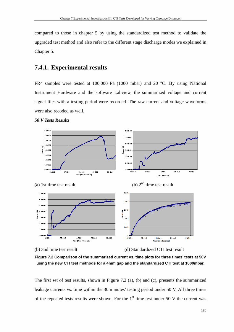
Chapter 7 Experimental Investigation III: CTI Tests Developed for Varying Creepage Distances
180
compared to those in chapter 5 by using the standardized test method to validate the
upgraded test method and also refer to the different stage discharge modes we explained in
Chapter 5.
7.4.1. Experimental results
FR4 samples were tested at 100,000 Pa (1000 mbar) and 20 °C. By using National
Instrument Hardware and the software Labview, the summarized voltage and current
signal files with a testing period were recorded. The raw current and voltage waveforms
were also recoded as well.
50 V Tests Results
(a) 1st time test result (b) 2nd time test result
(b) 3nd time test result (d) Standardized CTI test result
Figure 7.2 Comparison of the summarized current vs. time plots for three times’ tests at 50V
using the new CTI test methods for a 4mm gap and th e standardized CTI test at 1000mbar.
The first set of test results, shown in Figure 7.2 (a), (b) and (c), presents the summarized
leakage currents vs. time within the 30 minutes’ testing period under 50 V. All three times
of the repeated tests results were shown. For the 1st time test under 50 V the current was
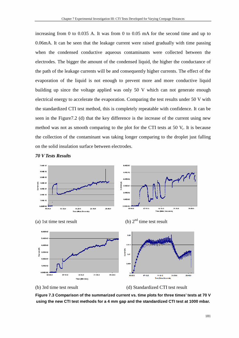
Chapter 7 Experimental Investigation III: CTI Tests Developed for Varying Creepage Distances
181
increasing from 0 to 0.035 A. It was from 0 to 0.05 mA for the second time and up to
0.06mA. It can be seen that the leakage current were raised gradually with time passing
when the condensed conductive aqueous contaminants were collected between the
electrodes. The bigger the amount of the condensed liquid, the higher the conductance of
the path of the leakage currents will be and consequently higher currents. The effect of the
evaporation of the liquid is not enough to prevent more and more conductive liquid
building up since the voltage applied was only 50 V which can not generate enough
electrical energy to accelerate the evaporation. Comparing the test results under 50 V with
the standardized CTI test method, this is completely repeatable with confidence. It can be
seen in the Figure7.2 (d) that the key difference is the increase of the current using new
method was not as smooth comparing to the plot for the CTI tests at 50 V,. It is because
the collection of the contaminant was taking longer comparing to the droplet just falling
on the solid insulation surface between electrodes.
70 V Tests Results
(a) 1st time test result (b) 2nd time test result
(b) 3rd time test result (d) Standardized CTI test result
Figure 7.3 Comparison of the summarized current vs. time plots for three times’ tests at 70 V
using the new CTI test methods for a 4 mm gap and t he standardized CTI test at 1000 mbar.
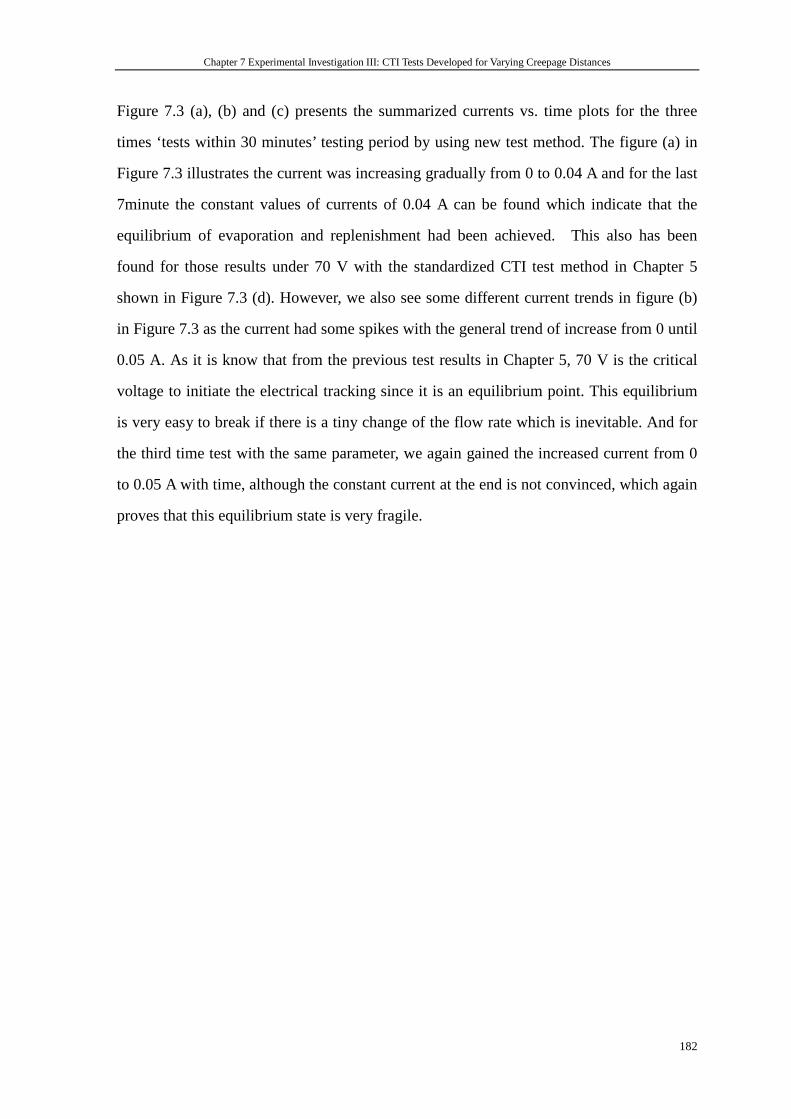
Chapter 7 Experimental Investigation III: CTI Tests Developed for Varying Creepage Distances
182
Figure 7.3 (a), (b) and (c) presents the summarized currents vs. time plots for the three
times ‘tests within 30 minutes’ testing period by using new test method. The figure (a) in
Figure 7.3 illustrates the current was increasing gradually from 0 to 0.04 A and for the last
7minute the constant values of currents of 0.04 A can be found which indicate that the
equilibrium of evaporation and replenishment had been achieved. This also has been
found for those results under 70 V with the standardized CTI test method in Chapter 5
shown in Figure 7.3 (d). However, we also see some different current trends in figure (b)
in Figure 7.3 as the current had some spikes with the general trend of increase from 0 until
0.05 A. As it is know that from the previous test results in Chapter 5, 70 V is the critical
voltage to initiate the electrical tracking since it is an equilibrium point. This equilibrium
is very easy to break if there is a tiny change of the flow rate which is inevitable. And for
the third time test with the same parameter, we again gained the increased current from 0
to 0.05 A with time, although the constant current at the end is not convinced, which again
proves that this equilibrium state is very fragile.
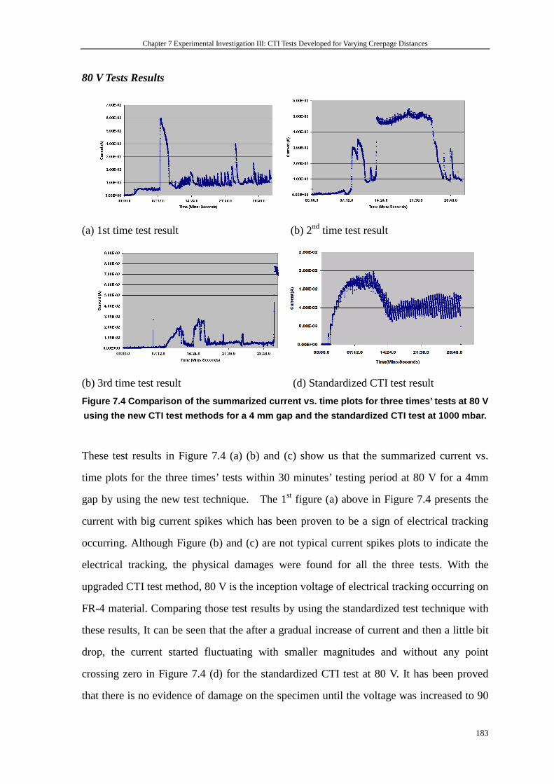
Chapter 7 Experimental Investigation III: CTI Tests Developed for Varying Creepage Distances
183
80 V Tests Results
(a) 1st time test result (b) 2nd time test result
(b) 3rd time test result (d) Standardized CTI test result
Figure 7.4 Comparison of the summarized current vs. time plots for three times’ tests at 80 V
using the new CTI test methods for a 4 mm gap and t he standardized CTI test at 1000 mbar.
These test results in Figure 7.4 (a) (b) and (c) show us that the summarized current vs.
time plots for the three times’ tests within 30 minutes’ testing period at 80 V for a 4mm
gap by using the new test technique. The 1st figure (a) above in Figure 7.4 presents the
current with big current spikes which has been proven to be a sign of electrical tracking
occurring. Although Figure (b) and (c) are not typical current spikes plots to indicate the
electrical tracking, the physical damages were found for all the three tests. With the
upgraded CTI test method, 80 V is the inception voltage of electrical tracking occurring on
FR-4 material. Comparing those test results by using the standardized test technique with
these results, It can be seen that the after a gradual increase of current and then a little bit
drop, the current started fluctuating with smaller magnitudes and without any point
crossing zero in Figure 7.4 (d) for the standardized CTI test at 80 V. It has been proved
that there is no evidence of damage on the specimen until the voltage was increased to 90
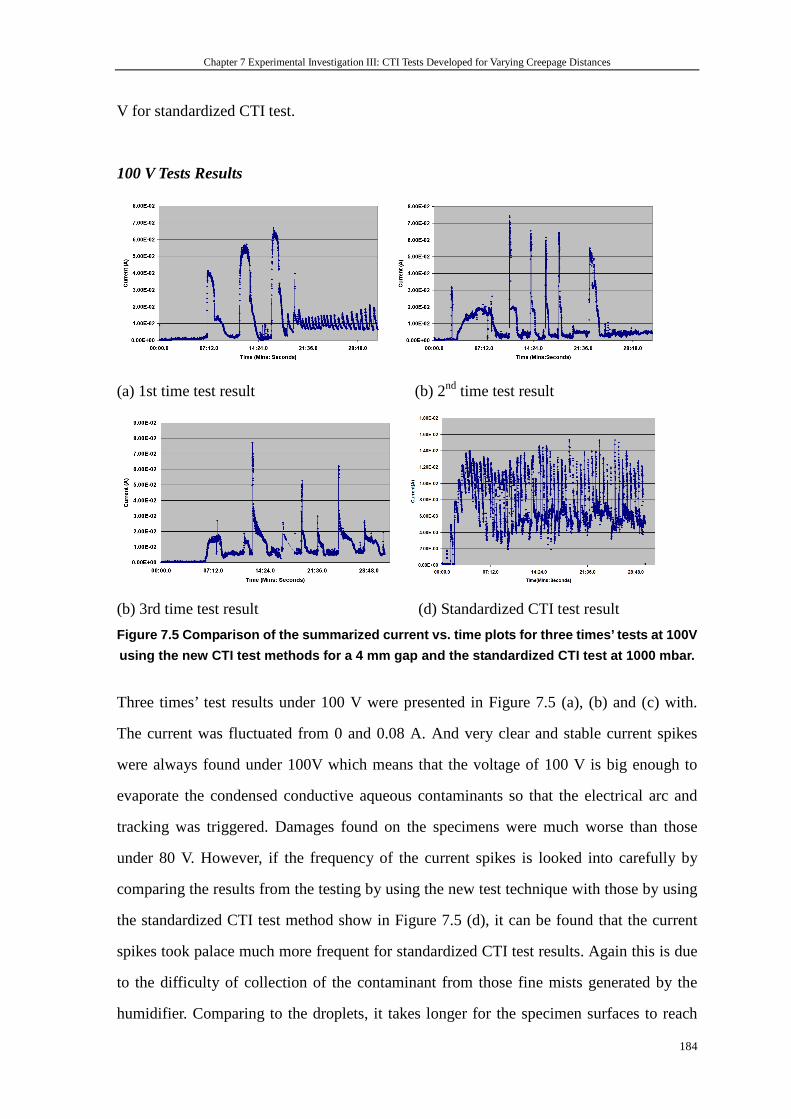
Chapter 7 Experimental Investigation III: CTI Tests Developed for Varying Creepage Distances
184
V for standardized CTI test.
100 V Tests Results
(a) 1st time test result (b) 2nd time test result
(b) 3rd time test result (d) Standardized CTI test result
Figure 7.5 Comparison of the summarized current vs. time plots for three times’ tests at 100V
using the new CTI test methods for a 4 mm gap and t he standardized CTI test at 1000 mbar.
Three times’ test results under 100 V were presented in Figure 7.5 (a), (b) and (c) with.
The current was fluctuated from 0 and 0.08 A. And very clear and stable current spikes
were always found under 100V which means that the voltage of 100 V is big enough to
evaporate the condensed conductive aqueous contaminants so that the electrical arc and
tracking was triggered. Damages found on the specimens were much worse than those
under 80 V. However, if the frequency of the current spikes is looked into carefully by
comparing the results from the testing by using the new test technique with those by using
the standardized CTI test method show in Figure 7.5 (d), it can be found that the current
spikes took palace much more frequent for standardized CTI test results. Again this is due
to the difficulty of collection of the contaminant from those fine mists generated by the
humidifier. Comparing to the droplets, it takes longer for the specimen surfaces to reach
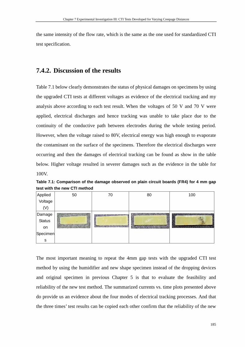
Chapter 7 Experimental Investigation III: CTI Tests Developed for Varying Creepage Distances
185
the same intensity of the flow rate, which is the same as the one used for standardized CTI
test specification.
7.4.2. Discussion of the results
Table 7.1 below clearly demonstrates the status of physical damages on specimens by using
the upgraded CTI tests at different voltages as evidence of the electrical tracking and my
analysis above according to each test result. When the voltages of 50 V and 70 V were
applied, electrical discharges and hence tracking was unable to take place due to the
continuity of the conductive path between electrodes during the whole testing period.
However, when the voltage raised to 80V, electrical energy was high enough to evaporate
the contaminant on the surface of the specimens. Therefore the electrical discharges were
occurring and then the damages of electrical tracking can be found as show in the table
below. Higher voltage resulted in severer damages such as the evidence in the table for
100V.
Table 7.1: Comparison of the damage observed on pla in circuit boards (FR4) for 4 mm gap
test with the new CTI method
Applied
Voltage
(V)
50 70 80 100
Damage
Status
on
Specimen
s
The most important meaning to repeat the 4mm gap tests with the upgraded CTI test
method by using the humidifier and new shape specimen instead of the dropping devices
and original specimen in previous Chapter 5 is that to evaluate the feasibility and
reliability of the new test method. The summarized currents vs. time plots presented above
do provide us an evidence about the four modes of electrical tracking processes. And that
the three times’ test results can be copied each other confirm that the reliability of the new

Chapter 7 Experimental Investigation III: CTI Tests Developed for Varying Creepage Distances
186
test results. Finally, in this section the table of the status of damages on specimens double
proves my explanation. As a conclusion, the new test method for electrical tracking has
been validated to be not feasible but also reliable when to be applied to varying gap
distances.
7.5. 2mm gap tracking test at the atmospheric pressure
The Previous section proves that the test method with the humidifier and new shape
specimens can produce repeatable electrical tracking results as the standardized CTI test
method does. Therefore, the upgraded CTI test method in this section will be applied to
specimens with a 2 mm gap distance between two electrodes. By doing different gap
distance tests with the upgraded test methods, it is expected that a general test method can
be developed to study the dimensioning rules of creepage distances. Similar to the
standardized CTI tests, the new test method was employed to carry out the testing on FR-4
specimens with a 2mm gap from 40V with voltage step of 10 V until 100 V when the
electrical tracking can definitely lead to damages on the specimens. Each voltage tests
were repeated for three times. All the current and voltage raw data were recorded by the
Labview program designed for previous standard CTI tests.
7.5.1. Experimental Results
40V Tests Results
Figure 7.6 The summarized current vs. time plot for the test using the new CTI test methods
for a 2 mm gap at 40 V 1000 mbar.
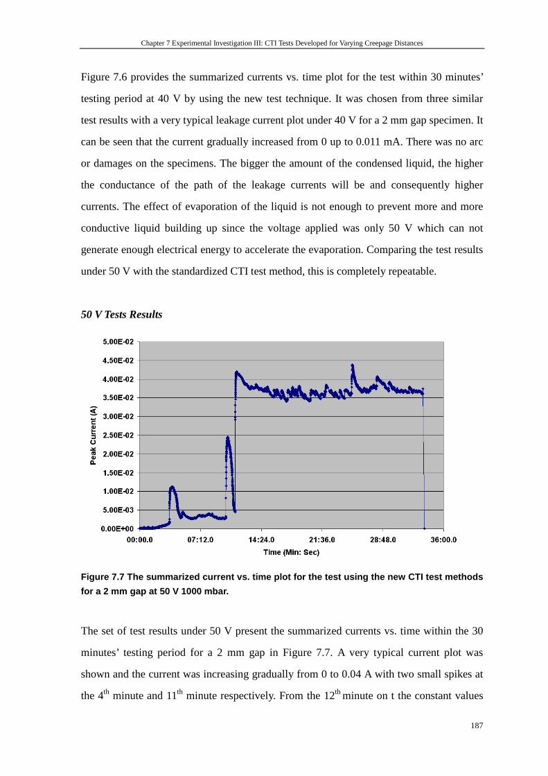
Chapter 7 Experimental Investigation III: CTI Tests Developed for Varying Creepage Distances
187
Figure 7.6 provides the summarized currents vs. time plot for the test within 30 minutes’
testing period at 40 V by using the new test technique. It was chosen from three similar
test results with a very typical leakage current plot under 40 V for a 2 mm gap specimen. It
can be seen that the current gradually increased from 0 up to 0.011 mA. There was no arc
or damages on the specimens. The bigger the amount of the condensed liquid, the higher
the conductance of the path of the leakage currents will be and consequently higher
currents. The effect of evaporation of the liquid is not enough to prevent more and more
conductive liquid building up since the voltage applied was only 50 V which can not
generate enough electrical energy to accelerate the evaporation. Comparing the test results
under 50 V with the standardized CTI test method, this is completely repeatable.
50 V Tests Results
Figure 7.7 The summarized current vs. time plot for the test using the new CTI test methods
for a 2 mm gap at 50 V 1000 mbar.
The set of test results under 50 V present the summarized currents vs. time within the 30
minutes’ testing period for a 2 mm gap in Figure 7.7. A very typical current plot was
shown and the current was increasing gradually from 0 to 0.04 A with two small spikes at
the 4th minute and 11th minute respectively. From the 12th minute on t the constant values
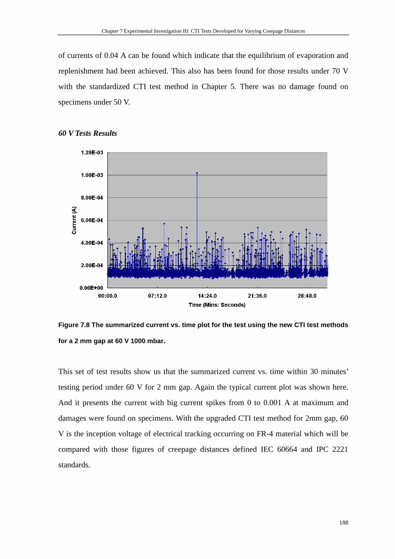
Chapter 7 Experimental Investigation III: CTI Tests Developed for Varying Creepage Distances
188
of currents of 0.04 A can be found which indicate that the equilibrium of evaporation and
replenishment had been achieved. This also has been found for those results under 70 V
with the standardized CTI test method in Chapter 5. There was no damage found on
specimens under 50 V.
60 V Tests Results
Figure 7.8 The summarized current vs. time plot for the test using the new CTI test methods
for a 2 mm gap at 60 V 1000 mbar .
This set of test results show us that the summarized current vs. time within 30 minutes’
testing period under 60 V for 2 mm gap. Again the typical current plot was shown here.
And it presents the current with big current spikes from 0 to 0.001 A at maximum and
damages were found on specimens. With the upgraded CTI test method for 2mm gap, 60
V is the inception voltage of electrical tracking occurring on FR-4 material which will be
compared with those figures of creepage distances defined IEC 60664 and IPC 2221
standards.

Chapter 7 Experimental Investigation III: CTI Tests Developed for Varying Creepage Distances
189
100 V Tests Results
Figure 7.9 The summarized current vs. time plot for the test using the new CTI test methods
for a 2 mm gap at 100 V 1000 mbar.
Test results under 100 V were presented in Figure 7.9 for a 2 mm gap with the upgraded
CTI test method. The current was fluctuated from 0 and 0.0025 A at a maximum. And very
clear and stable current spikes were always found under 100 V which means that the
voltage of 100 V is big enough to evaporate the condensed conductive aqueous
contaminants so that the electrical arc and tracking was triggered. Damages found on the
specimens were much worse than those 4 mm gap tests under 100 V.
7.5.2. Discussion of Results
Again, Table 7.2 below provides us with the damage status of the specimens used in the
2mm gap tests with the upgraded CTI test method. The pictures are the physical evidence
of the voltages being required to initiate tracking.
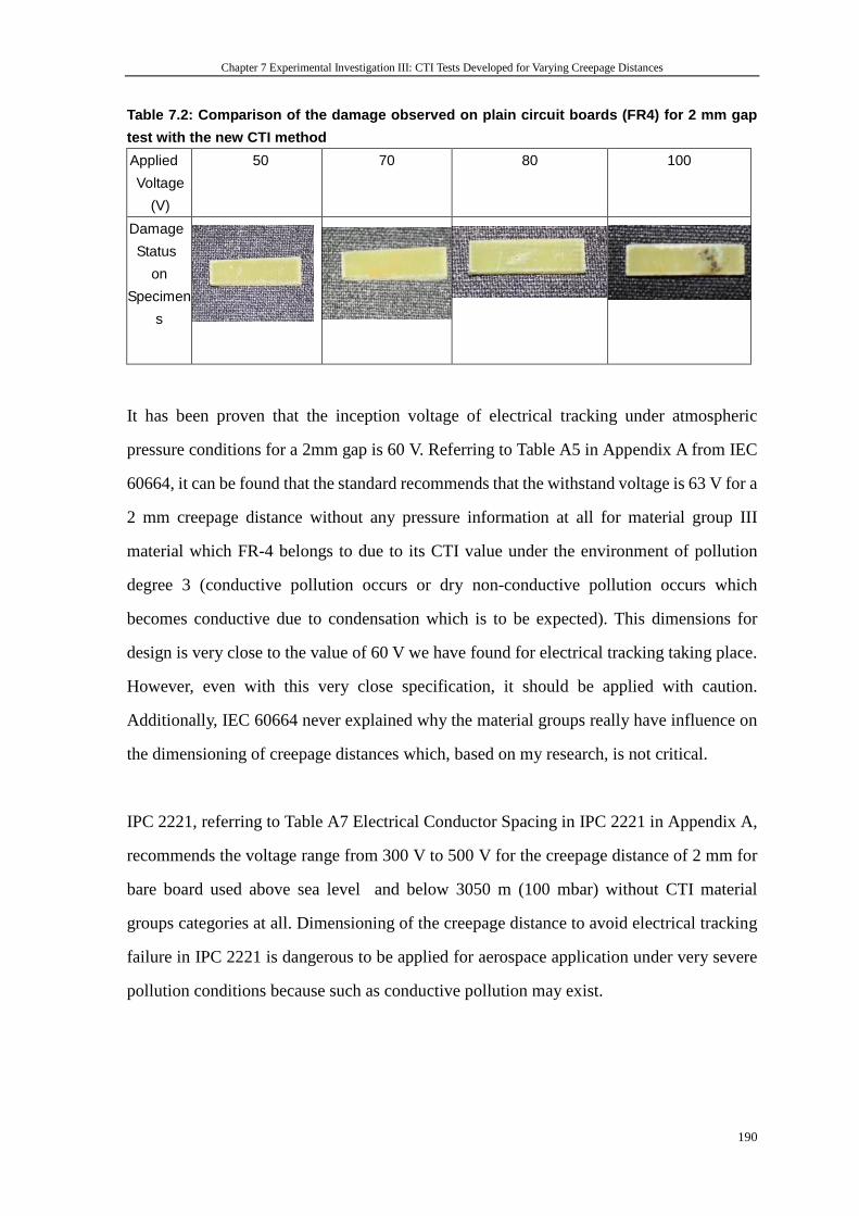
Chapter 7 Experimental Investigation III: CTI Tests Developed for Varying Creepage Distances
190
Table 7.2: Comparison of the damage observed on pla in circuit boards (FR4) for 2 mm gap
test with the new CTI method
Applied
Voltage
(V)
50 70 80 100
Damage
Status
on
Specimen
s
It has been proven that the inception voltage of electrical tracking under atmospheric
pressure conditions for a 2mm gap is 60 V. Referring to Table A5 in Appendix A from IEC
60664, it can be found that the standard recommends that the withstand voltage is 63 V for a
2 mm creepage distance without any pressure information at all for material group III
material which FR-4 belongs to due to its CTI value under the environment of pollution
degree 3 (conductive pollution occurs or dry non-conductive pollution occurs which
becomes conductive due to condensation which is to be expected). This dimensions for
design is very close to the value of 60 V we have found for electrical tracking taking place.
However, even with this very close specification, it should be applied with caution.
Additionally, IEC 60664 never explained why the material groups really have influence on
the dimensioning of creepage distances which, based on my research, is not critical.
IPC 2221, referring to Table A7 Electrical Conductor Spacing in IPC 2221 in Appendix A,
recommends the voltage range from 300 V to 500 V for the creepage distance of 2 mm for
bare board used above sea level and below 3050 m (100 mbar) without CTI material
groups categories at all. Dimensioning of the creepage distance to avoid electrical tracking
failure in IPC 2221 is dangerous to be applied for aerospace application under very severe
pollution conditions because such as conductive pollution may exist.
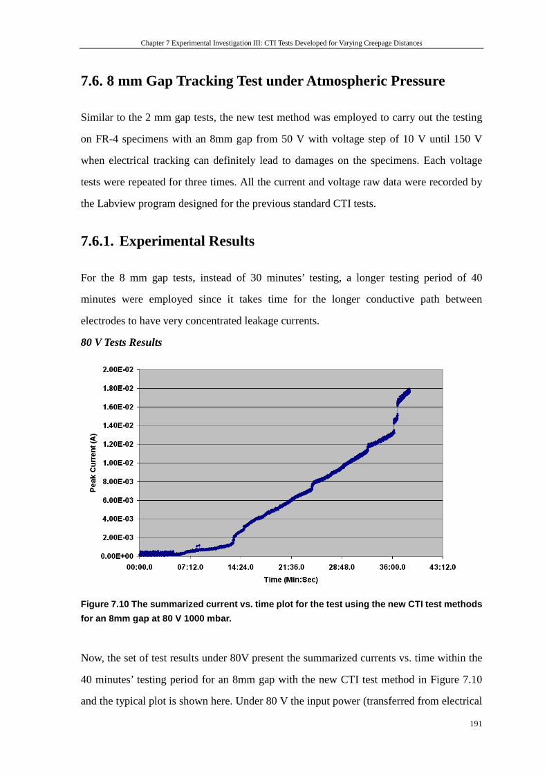
Chapter 7 Experimental Investigation III: CTI Tests Developed for Varying Creepage Distances
191
7.6. 8 mm Gap Tracking Test under Atmospheric Pressure
Similar to the 2 mm gap tests, the new test method was employed to carry out the testing
on FR-4 specimens with an 8mm gap from 50 V with voltage step of 10 V until 150 V
when electrical tracking can definitely lead to damages on the specimens. Each voltage
tests were repeated for three times. All the current and voltage raw data were recorded by
the Labview program designed for the previous standard CTI tests.
7.6.1. Experimental Results
For the 8 mm gap tests, instead of 30 minutes’ testing, a longer testing period of 40
minutes were employed since it takes time for the longer conductive path between
electrodes to have very concentrated leakage currents.
80 V Tests Results
Figure 7.10 The summarized current vs. time plot fo r the test using the new CTI test methods
for an 8mm gap at 80 V 1000 mbar.
Now, the set of test results under 80V present the summarized currents vs. time within the
40 minutes’ testing period for an 8mm gap with the new CTI test method in Figure 7.10
and the typical plot is shown here. Under 80 V the input power (transferred from electrical
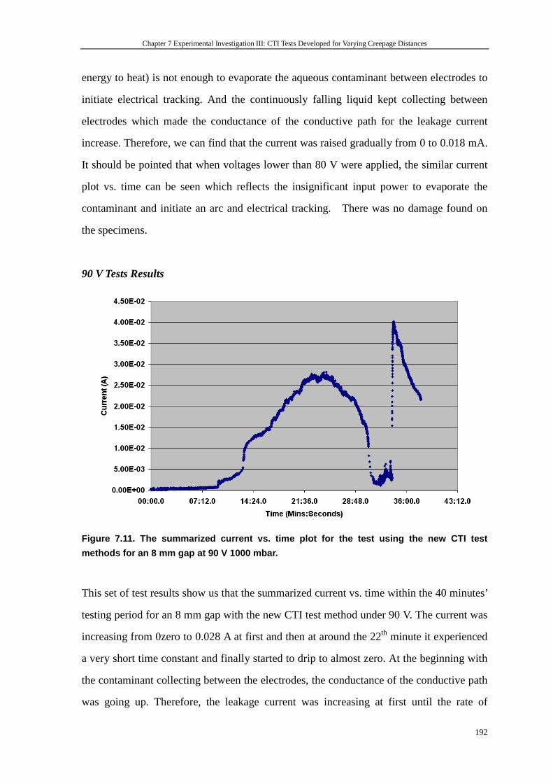
Chapter 7 Experimental Investigation III: CTI Tests Developed for Varying Creepage Distances
192
energy to heat) is not enough to evaporate the aqueous contaminant between electrodes to
initiate electrical tracking. And the continuously falling liquid kept collecting between
electrodes which made the conductance of the conductive path for the leakage current
increase. Therefore, we can find that the current was raised gradually from 0 to 0.018 mA.
It should be pointed that when voltages lower than 80 V were applied, the similar current
plot vs. time can be seen which reflects the insignificant input power to evaporate the
contaminant and initiate an arc and electrical tracking. There was no damage found on
the specimens.
90 V Tests Results
Figure 7.11. The summarized current vs. time plot f or the test using the new CTI test
methods for an 8 mm gap at 90 V 1000 mbar.
This set of test results show us that the summarized current vs. time within the 40 minutes’
testing period for an 8 mm gap with the new CTI test method under 90 V. The current was
increasing from 0zero to 0.028 A at first and then at around the 22th minute it experienced
a very short time constant and finally started to drip to almost zero. At the beginning with
the contaminant collecting between the electrodes, the conductance of the conductive path
was going up. Therefore, the leakage current was increasing at first until the rate of
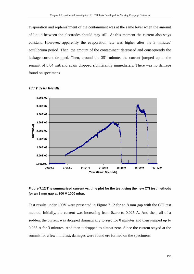
Chapter 7 Experimental Investigation III: CTI Tests Developed for Varying Creepage Distances
193
evaporation and replenishment of the contaminant was at the same level when the amount
of liquid between the electrodes should stay still. At this moment the current also stays
constant. However, apparently the evaporation rate was higher after the 3 minutes’
equilibrium period. Then, the amount of the contaminant decreased and consequently the
leakage current dropped. Then, around the 35th minute, the current jumped up to the
summit of 0.04 mA and again dropped significantly immediately. There was no damage
found on specimens.
100 V Tests Results
Figure 7.12 The summarized current vs. time plot fo r the test using the new CTI test methods
for an 8 mm gap at 100 V 1000 mbar.
Test results under 100V were presented in Figure 7.12 for an 8 mm gap with the CTI test
method. Initially, the current was increasing from 0zero to 0.025 A. And then, all of a
sudden, the current was dropped dramatically to zero for 8 minutes and then jumped up to
0.035 A for 3 minutes. And then it dropped to almost zero. Since the current stayed at the
summit for a few minutest, damages were found ere formed on the specimens.
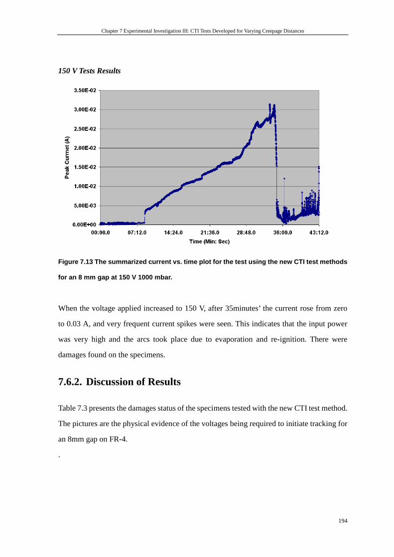
Chapter 7 Experimental Investigation III: CTI Tests Developed for Varying Creepage Distances
194
150 V Tests Results
Figure 7.13 The summarized current vs. time plot fo r the test using the new CTI test methods
for an 8 mm gap at 150 V 1000 mbar.
When the voltage applied increased to 150 V, after 35minutes’ the current rose from zero
to 0.03 A, and very frequent current spikes were seen. This indicates that the input power
was very high and the arcs took place due to evaporation and re-ignition. There were
damages found on the specimens.
7.6.2. Discussion of Results
Table 7.3 presents the damages status of the specimens tested with the new CTI test method.
The pictures are the physical evidence of the voltages being required to initiate tracking for
an 8mm gap on FR-4.
.
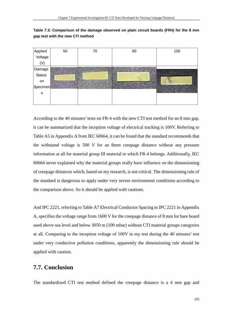
Chapter 7 Experimental Investigation III: CTI Tests Developed for Varying Creepage Distances
195
Table 7.3: Comparison of the damage observed on pla in circuit boards (FR4) for the 8 mm
gap test with the new CTI method
Applied
Voltage
(V)
50 70 80 100
Damage
Status
on
Specimen
s
According to the 40 minutes’ tests on FR-4 with the new CTI test method for an 8 mm gap,
it can be summarized that the inception voltage of electrical tracking is 100V. Referring to
Table A5 in Appendix A from IEC 60664, it can be found that the standard recommends that
the withstand voltage is 500 V for an 8mm creepage distance without any pressure
information at all for material group III material to which FR-4 belongs. Additionally, IEC
60664 never explained why the material groups really have influence on the dimensioning
of creepage distances which, based on my research, is not critical. The dimensioning rule of
the standard is dangerous to apply under very severe environment conditions according to
the comparison above. So it should be applied with cautions.
And IPC 2221, referring to Table A7 Electrical Conductor Spacing in IPC 2221 in Appendix
A, specifies the voltage range from 1600 V for the creepage distance of 8 mm for bare board
used above sea level and below 3050 m (100 mbar) without CTI material groups categories
at all. Comparing to the inception voltage of 100V in my test during the 40 minutes’ test
under very conductive pollution conditions, apparently the dimensioning rule should be
applied with caution.
7.7. Conclusion
The standardized CTI test method defined the creepage distance is a 4 mm gap and
Chapter 7 Experimental Investigation III: CTI Tests Developed for Varying Creepage Distances
196
accordingly the dropping devices and flow rate of the contaminant are particularly designed
for this length of gap. An electrical tracking testing method has been developed based on the
standardized CTI tests with manipulating the dropping device to a domestic humidifier and
the shape of organic insulating material board from 20mm 20mm× to 20mm 5mm× with
which the width of the specimen is as big as the width of the contacting electrode.
The challenge of accelerated electrical tracking tests is always attribute to the big
fluctuation of test results. Therefore, not only the feasibility but also reliability of the new
CTI test method has been confirmed in the thesis by recognizing the four modes of initiation
of discharges on solid insulation material surface. The 4 mm gap tests with the new CTI
test method firstly have been shown with comparisons with the test results with those by
using the standardized CTI test method. It can clearly be seen that even with the new
dropping device and new shape of the specimens, the similar summarized current vs. time
plots can be found under the same amount of voltage applied. And four modes of electrical
tracking processes can be reflected by the results. The repeatability also has been achieved
by comparison of the three times of repeating the tests for each voltage.
Then, the new CTI test method was applied to a 2 mm gap and an 8 mm gap. The test results
were used to compare with the specifications defined in IEC 60664 and IPC 2221. The
measurement of the inception voltage of electrical tracking for a 2 mm gap is 60 V, which is
just around the 63 V defined in IEC 60664 for material group III which FR-4 belongs to
under pollution degree conditions without any information on air pressure impact and much
lower than 300 V to 500 V, as defined in IPC 2221, for applications above sea level and
below 3050 m without the pollution degrees information. And the measurement of the
inception voltage of electrical tracking for an 8mm gap is 100 V, which is much smaller than
the 500 V defined in IEC 60664 for material group III which FR-4 belongs to under
pollution degree conditions without any information on air pressure impact, and is much
lower than 1600 V as defined in IPC 2221 for applications above sea level and below 3050
m without the pollution degrees information. As a conclusion, the application of the
dimensions of creepage distance in the standards should be considered with the

Chapter 7 Experimental Investigation III: CTI Tests Developed for Varying Creepage Distances
197
environment conditions where the electrical apparatus will operate with significant caution.
And the best resolution for any specific design is to conduct the accelerated electrical
tracking test by using the upgraded CTI test method discussed in the thesis. The comparison
of withstand voltages of IEC 60664, IPC 2221 and the test results for 2mm, 4mm and 8mm
gaps on FR-4 at 1000mbar was summarized in the Table 7.4.
Table 7.4: Comparison of withstand voltages of IEC 60664, IPC 2221 and the test results for 2
mm, 4 mm and 8 mm gaps on FR-4 at 1000 mbar.
IEC 60664 (Material Group
III)
IPC 2221 Test Results
Pollution Degree 3 Above sea
level up to
3050m (696.4
mbar)
395
Ω ·cm
Withstand
voltage for
4mm gap
250 V 800 V 90 V
Withstand
voltage for
2mm gap
63 V 300-500 V 60 V
Withstand
voltage for
8mm gap
500 V 1600 V 100 V

Chapter 8 Conclusion and Future Work
198
Chapter 8: Conclusion and Future Work
8.1. Summary
8.1.1. Validation of clearances and creepage distances in
standards
One of the objectives of the thesis was the evaluation of the reliability of the existing
standards for the dimensioning of clearances and creepage distances, including IEC 60664,
‘Insulation coordination for equipment within low-voltage systems’, and IPC 2221,
‘Generic Standard on Printed Circuit Board’. This was carried out in Chapter 3 based on:
A. Interpreting the dimensioning rules specified in IEC 60664 and IPC 2221 for
clearance and creepage distances.
B. Measuring the withstand voltages for varying lengths of clearances and creepage
distances under varying air pressure under dry conditions for aerospace
applications.
C. Comparing the measured data with IEC 60664 and IPC 2221 specifications.
D. Comparing the measured data with Paschen’s curve values.
IEC 60664 deals with the insulation coordination for equipment within low voltage
systems. It applies to equipment up to 2000 m above sea level having a rated voltage up
to AC 1000 V with a rated frequency up to 30 kHz or rated voltage up to DC 1500 V. As
the standard is not applicable for equipment used over 2000 m, it is clearly not intended
for use in aerospace equipment design. And Table A5 in Appendix A provides the
Chapter 8 Conclusion and Future Work
199
dimensions of creepage distances for different material groups’ materials under
different pollution degrees. Apart from a lack of information on the impact of air
pressure for aerospace applications, there is no explanation of the reason why the
material groups have an influence on withstand voltages for electrical tracking, which
have been proven to be not very relevant in the thesis.
IPC 2221, ‘Generic Standard on Printed Boards Design’, provides generic requirements
for the design of organic printed boards and other forms of components, mounting or
interconnecting structures to eliminate the misunderstanding between manufacturers
and purchasers, facilitating the interchangeability and improvement of products, and
assisting the purchaser in selecting and obtaining with minimum delay the proper
product for a particular need. The dimensions of electrical clearances given in Table A7
in Appendix A provide two categories of situations for below 3050 m and above 3050
m. However, there is no any information on the pollution degrees which is very critical
to trigger electrical tracking.
A determination of clearance in air can be precisely defined for a certain electrode
geometry based on Paschen’s law for a uniform electrical field. As Paschen’s law
appears to be implemented in IEC 60664, this therefore also means that the guidance it
provides for the dimensioning of clearances is appropriate.
For non-uniform fields, the use of IEC 60664 to determine clearances does not appear
to give results that are totally consistent with experimental tests, but they are a useful
approximation for design purposes at atmospheric pressure with a larger deviation at
Chapter 8 Conclusion and Future Work
200
100mBar pressure. Breakdown voltage measurements show consistency with the IEC
60664 standard at low pressure (although the IEC 60664 standard is not conservative)
and no match was possible at atmospheric pressure owing to the limited voltage
capability of the test supply.
However, determining the creepage distances in both standards somehow has its
limitations. For creepage distances under dry conditions, the test results on printed
circuit board with a polyimide substrate and varying creepage gap printed on show that
the breakdown voltage is close to that expected using Paschen’s law, but also that it far
exceeds that predictions used in IEC 60664 or IPC 2221.
8.1.2. Electrical tracking under wet conditions
The most important objective of the thesis is the exploration and development of the
understanding of electrical tracking with the consideration of different environmental
conditions, including air pressure, and pollution degrees for aerospace applications. An
series of studies have been carried out. The required voltage levels and the mechanism to
trigger an arc and electrical tracking and in consequence, discussed in Chapter 4, 5 and 6,
are based on:
A. Establishing the mathematical calculation model of initiating electrical tracking
with parameters of the pollution degrees, ambient temperature, and ambient
pressure. By analysing the influences of different impact parameters, the
mechanism of electrical tracking has been understood to have a very close
relationship with the heat transfer mechanism.
B. Employing the standardized CTI test method at various air pressures to measure
the leakage currents during the testing period to find out the behaviour of electrical
Chapter 8 Conclusion and Future Work
201
tracking under electrical stresses. Furthermore, the measurements of the inception
voltage for electrical tracking can also provide the inception voltage for a 4mm gap
under very severe pollution environment conditions. The impact of air pressure
can be judged according to the test results.
C. Comparing the measured inception voltage for a 4 mm gap with that calculated
using the mathematic formula and IEC 60664 and IPC 2221 so that the
dimensioning rules of the standards can be evaluated.
The development of the mathematic model of initiating electrical tracking indicates that
electrical tracking originally starts from a dry-band arc. The first dry-band arc can take
place due to the break of the continuous leakage current path. This can occur at very
low voltage even under Paschen’s minimum. To have this first dry-band arc, the
aqueous contaminant film should evaporate until the dry band appears. As it is known,
leakage current can lead to energy transferred from electrical energy to heat, which
would accelerate the effect of evaporation of the aqueous contaminant. As a result, the
electrical tracking, evaporation and electrical input power have been interconnected.
Therefore, the model was established based on the mechanism explained which is the
equilibrium between the input electrical power and output power of evaporation. My
study also has been proven by L. Warren in his paper. By interpreting Warren’s model
with dynamic heat transfer, a static mathematical model has been developed, as shown
in equation 4.7.
( )2
/( ) boiling ambient T
V whT T R
T lρ⋅ = −
By analysing the influences of different impact parameters such as the resistivity of the
Chapter 8 Conclusion and Future Work
202
conductive contaminant( )Tρ , the boiling point of the contaminantboilingT , ambient
temperature, and equivalent thermal resistance TR , the required voltage needed cannot
determined linearly by air pressure, resistivity and the boiling point of the contaminant
since the mentioned parameters are inter-dependent to each other. The resistivity of the
contaminant increases with the rise of the temperature, while the boiling point is
determined by contaminant itself and air pressure. The static simulation done by
running the program in the Finite Element Analysis software ‘Vector Field Opera
version 11’ was used to find out the equivalent heat transfer resistance while the
dynamic simulation was used to help predict the possible changes of required voltages
to initiate electrical tracking.
The required voltage to initiate electrical tracking increases with pressure according to
the mathematical calculation. The value of voltages at ambient pressure 1000 mbar
was around 150 V, while at lower pressure 100mbar it dropped to 46 V for deionized
water; it was 8.4 V for the highly conductive solution A specified in IEC 60112: 2003
at 10000 mbar and 5.5 V at 100mbar. This also represents the fact that the more
conductive the aqueous contamination, the lower the voltages that are needed for
electrical tracking. Theoretical calculation results show that at higher ambient
temperatures, less voltage is required to initiate electrical tracking. The most
interesting results are those values of voltages required at 273 K for the highly
conductive solution A, which shows that the voltage actually decreases with pressure
going up.
The electrical tracking testing method specified in IEC 60112 is an accelerating way
Chapter 8 Conclusion and Future Work
203
to find out the tracing resistance within a short time by using a much more conductive
contaminant than would be found in reality. However, the data of the tracking
fluctuated greatly, which is the key problem. My research contribution, as shown in
this chapter, is the repeatability of the test results for both FR-4 and ABS.
Comparisons of the values of inception voltage for electrical tracking at various air
pressures with the test results with the mathematical calculation results have been
discussed.
Comparison of the values of inception voltage for electrical tracking at various air
pressures with the test results with the standard recommended values have been
discussed.
8.1.3. Selection of wet condition electrical tracking test
techniques
The last objective of the thesis was to provide guidelines for better electrical tracking testing
methods for varying creepage distances. The standardized CTI test method defined the
creepage distance as a 4mm gap and accordingly the dropping devices and flow rate of the
contaminant are particularly designed for this length of gap. A better electrical tracking
testing method has been developed based on the standardized CTI tests by manipulating the
dropping device to a domestic humidifier and the shape of organic insulating material board
from 20mm 20mm× to 20mm 5mm× with which the width of the specimens are as big as
the width of the contacting electrode.
The challenge of accelerated electrical tracking tests always attribute to the big fluctuation
of test results. Therefore, not only the feasibility but also the reliability of the new CTI test
method has been confirmed in the thesis. The 4mm gap tests with the new CTI test method
Chapter 8 Conclusion and Future Work
204
firstly have been shown by a comparison with the test results using the standardized CTI test
method. It can clearly be seen that even with the new dropping device and new shape of
specimen, the similar summarized current vs. time plots can be found under the same
amount of voltage applied. And four modes of electrical tracking processes can be reflected
by the results. The repeatability also has been achieved by a comparison of the three repeat
tests for each voltage.
Then, the new CTI test method was applied to a 2 mm gap and an 8 mm gap. The test results
were used to compare with the specifications defined in IEC 60664 and IPC 2221. The
measurement of the inception voltage of electrical tracking for the 2mm gap is 60 V, which
is around the 63 V defined in IEC 60664 for material group III which FR-4 belongs to under
pollution degree conditions without any information on air pressure impact, and much lower
than 300 V to 500 V as defined in IPC 2221 for applications above sea level and below 3050
m without the pollution degree information. And the measurement of the inception voltage
of electrical tracking for an 8 mm gap is 100 V, which is much smaller than the 500 V
defined in IEC 60664 for material group III which FR-4 belongs to under pollution degree
conditions without any information on air pressure impact, and much lower than the 1600 V
defined in IPC 2221 for applications above sea level and below 3050 m without the
pollution degree information. As a conclusion, the application of dimensions of creepage
distance in the standards should be considered as the environment condition where the
electrical apparatus will operate with significant caution. And the best resolution for any
specific design is to conduct the accelerated electrical tracking test by using the upgraded
CTI test method discussed in the thesis.
8.2. Suggestions for Future Work
The insulation coordination of an electrical power system for aerospace applications is
comprised of the determining of clearance and creepage distance under varying air
pressures. Breakdown tests on air gaps under either uniform or non-uniform electrical fields
have been well developed for many years. An exploration of the mechanism and behaviour
Chapter 8 Conclusion and Future Work
205
of electrical tracking is always a very challenging research area since electrical tracking by
its nature is much more complicated.
The research described in this PhD thesis focused on the interpretation of the behaviour of
the electrical tracking on organic insulating materials. Further researches on the following
points are needed to implement the idea presented in this thesis to wider aerospace
applications.
• Further dynamic thermal analyses for the accelerated electrical tracking test rig are
required to improve my understanding of the influence of the heat capacity of
different surrounding heat dissipating media on the evaporation and the first
dry-band arc for real life applications.
• It is necessary to find out the formation and existence of actual pollution on real
aircraft.
• More organic material belonging to different material groups is required to be
tested with the standardized CTI test method to double check the findings of my
research that the insulating material itself has minimal impact on initiating the first
dry-band arc and consequent electrical tracking.
• More different lengths of gaps on organic insulating materials are required to be
tested to validate the upgraded electrical tracking test method.
• Low pressure electrical tracking test methods for varying gaps on organic insulating
materials are required to be developed for aerospace applications.
• At present, more and more power electronics components such as printed circuit
boards employ conformal coating to avoid the macro-environment influence on
their functioning. However, this protection could be become fatal if there is some
Chapter 8 Conclusion and Future Work
206
defect occurring, such as a hole at some point in the complete conformal coating
film. Therefore, the impact of conformal coating on the insulation coordination of
electrical systems on aircraft should be studied further.
• Non-50Hz and non-sinusoid voltages could be applied to find out the impact of
the different voltages on breakdown and electrical tracking.
A test technique to determine safe creepage distances for utilization in aerospace
applications should be generated with various air pressures.
8.3. Conclusion
This thesis has used theory, simulation and laboratory experiment, to investigate
phenomena of the electrical tracking under wet condition for aerospace application. The
new mathematical model to express the energy transfer within the contaminant liquid under
applied voltage between the two electrodes had been built when the system reaches the
static state which means the temperature of electrodes and specimens keep constant after the
initial increase. The effects and their relationship of influencing parameters including the
applied voltages, the conductivity of the contaminant, air pressure, ambient temperature,
contaminant temperature and equivalent heat resistant have been analysed based on the
model. Within all the parameters, the equivalent heat resistance were calculated based on
the simulation results. We have found that the required voltage to initiate electrical tracking
increases with pressure, the more conductive the aqueous contamination, the lower the
voltages that are needed for electrical tracking and at higher ambient temperatures, less
voltage is required to initiate electrical tracking. The most interesting results are those
values of voltages required at 273 K for the highly conductive solution A, which shows that
the voltage actually decreases with pressure going up. This result can be attributed to the
combination of the influence of ambient temperature, pressure and the conductivity of the
aqueous contamination. Especially, these impact factors are inter-dependent. This therefore
proves that the mathematical model does predict this complicated relationship.
Chapter 8 Conclusion and Future Work
207
The limitation of the research is that the dynamic processes before static state has been
achieved have been ignored. The heat capacities of surrounding heat dissipating media are
critical properties to consider. Again, it is not a simple variable, but varies with temperature,
pressure and volume. However, in the case of my model, the volume and pressure are
supposed to be constant.
I have presented that selection of the electrical tracking test methods under lower voltage up
to 1000 V. The contaminant dropping system has been proven to be the critical part of
design. At atmospheric pressure, the dropping system has employed normal peristaltic
pump with integral drive model with a hypodermic needle. However, to prevent impact of
the circulating air in the environment chamber, it is better to use the medical transfusion
dropping system for lower pressure electrical tracking tests.
I have also presented the experimental accelerating tracking test results for 4mm gap
including the current and voltage data and also the thermal images to investigate the
temperature changes during the testing periods. Four modes of electrical tracking processes
can be reflected by the results. The repeatability also has been achieved by a comparison of
the three repeat tests for each voltage. It also can be concluded that the lower pressure, the
lower voltage required to initiate electrical tracking. Under lower pressure, the damages
were seen much more severe. Different conductivity contaminant test results have proved
that with higher conductivity, the lower voltages were required to initiate electrical tracking.
According the comparison with the mathematic model results, it has been found that our
calculation results are much lower than the experimental results. The comparisons with the
IEC 60664 and IPC 2221 show that it is not safe to apply the dimensioning rules
recommended.
Although different materials belonging to different categories of the material group
according to their CTI values were tested by using the standard test methods, we found that
the material itself was not the critical factor for initiating electrical tracking. The reason for
Chapter 8 Conclusion and Future Work
208
electrical tracking on the organic materials is that the conductive pollution layer can lead to
electrical current flowing. With different voltage levels, the pollution layer dried at different
rates, and the rate of replenishment is the critical factor. The voltage and replenishment of
pollution together have a big effect on the mechanism of initiation of electrical tracking. So,
as a conclusion the voltage level of any system and potential pollution degree are very
important to evaluate whether a system can survive and operate reliably. Then, when any
dimensioning rules in any standards are employed, these two factors should be evaluated
very carefully.
At last I have shown that the new electrical tracking test method based on the IEC 60112
method but with the humidifier instead of original dropping system to generate approximate
uniform fog environment for wider range of gap distances tests. 2mm, and 8mm gap
distances test results including current and voltage data has shown that the bigger the gap,
the higher voltage needed to initiate the electrical tracking. According to the comparisons
with calculated test results, the higher voltages were presented. And the recommended
values in both IEC 60664 and IPC 2221 are not applicable.
Reference
209
Reference
[1] R. I. Jones, "The More Electric Aircraft: The Past and the Future," the Institution of Electrical Engineers, 1999.
[2] Joseph A. Weimer and Aright Patterson AFB “Past, Present & Future of Aircraft Electrical Power Systems”, Power Division, Propulsion Directorate, Air Force Research Laboratory, AIAA 2001-1147, 39th Aerospace Sciences Meeting & Exhibit, 8-11 January 2001, Reno, Nevada.
[3] J. A. Weimer, "Electrical Power Technology for the More Electric Aircraft," Digital Avionics Systems Conferecne, 1993, 12th DASC AIAA/IEEE,25-28th Oct, pp. 445-450.
[4] J. A. O. J.A. Rosero, E. Aldabas, & L. Romeral, "Moving Towards a More Electric Aircraft," IEEE A&E SYSTEMS MAGAZINE, March 2007.
[5] M. D. Kankam, "A Survey of Power Electronics Applications in Aerospace Technologies," 36th Intersociety Energy Conversion Engineering Conference cosponsored by the ASME, IEEE, AIChE, ANS, SAE, and AIAA Savannah,Georgia, July 29-August 2, 2001.
[6] J. S. Cloyd and W. L. United States Air Force, "Status of United States Air Force's More Electric Aircraft Initiative," IEEE AES System Magazine, Aptd 1998 17 Authorized.
[7] J. A. Weimer, "Power Management and Distribution for the More Electric Aircraft," Proceedings of the 30th Intersociety Energy Conversion Engineering Conference, 1995: 273-277.
[8] C. Jie, "Outlook of Roles and Necessicities of Power Eelectronics for VF-Power System of Future Large Aircraft," IEEE.
[9] A. C. Newton and I. Moir, "Practical Consideration for the More-Electric Aircraft," in ERA Avionics Systems Conference, 1998.
[10] I. Moir, "Future Trends in Aircraft Electrical Systems," in ERA Avionics Conference. London Heathrow, 19-20th November 1997.
[11] I. Moir, "The Challenges of Now Technologies for Aircraft Electrical Systems," in New Challenges in Aircraft Maintenance and ENgineering Conference. Singapore, 1998.
[12] T. Glennon, "Fault Tolerant Generating and Distribution System Architecture," IEE, 1998.
[13] I. Moir, "More-Electric Aircraft- System Considerations," IEE, 1999. [14] N. H. M. Bailey, G. Ucerpi, J. A. Hunt, S. Mollov, and A. Forsyth, "Distributed
Electrical Power Management Architecture (DEPMA). Electrical Machines and Systems for the More Electric Aircraft," IEE Colloquium, November 9, 1999: 7/1-7/4.
[15] M. Howse, "All Electric Aircraft," Power Engineer, vol. 17, pp. 35-37,2003 [16] L. Faleiro, "Initial Research towards a More Electrical Aircraft," in More Electrical
Reference
210
Aircraft Conference: Royal Aeroautics Society, April 2004. [17] M. A. e. a. Maldonado, "Power Management and Distribution System for a More
Electric Aircraft (MADMEL) - Program Status," Intersociety Energy Conversion Engineering Conf., August 1997: 274-279.
[18] L. F. Faleiro, "Trends towards a More Electrical Aircraft," Liebherr_Aerospace Lindenberg GmbH and The Royal Aeronautical Society, 2004.
[19] S. J. Cutts, "Totally Integrated More Electric Systems (TIMES) Refer to: A Collaborative Approach to the More Electric Aircraft," Power Electronics, Machines and Drives.International Conference, on 4-7 June 2002: 223-228.
[20] M. Bailey, N. Hale, G. Ucerpi, J. A. Hunt, S. Mollov, and A. Forsyth, "Distributed Electrical Power Management Architecture (DEPMA). Electrical Machines and Systems for the More Electric Aircraft," IEE Colloquium, November 9, 1999: 7/1-7/4.
[21] M. G. Friend and D. L. Daggett, "Fuel Cell Demonstrator Airplane," AIAA/ICAS International Air and Space Symposium and Exposition: Dayton, Ohio., 14-17 July 2003.
[22] KOJORI, Hassan, A., "Electrical Energy Management System on a Vehicle E.G. a More Electric Aircraft (MEA)," HONEYWELL INTERNATIONAL INC. WO 2006/024006 A1. International Application published under the patent cooperation treaty (PCT). March 2, 2006.
[23] Emadi, K. Ehsani, M., "Aircraft Power Systems:"Technology, State of the Art and Future Trends," Aerospace and Electronic Systems Magazine, IEEE, Volume 15, Issue 1,January 2000: 28-32.
[24] Sriram Chandrasekaran, Douglas K. Lindner,, "Subsystem Interaction Analysis in Power Distribution Systems of Next Generation Airlifters," IEEE Power Electronic Specialist Conference, September 1999.
[25] R. G. Michalko, "Electrical Starting Generation Conversion and Distribution System Architecture for a More Electric Vehicle," HONEYWELL INTERNATIONAL INC. US2006/0061213 A1. United States Patent Application Publication, March 23, 2006.
[26] Cotton, I.; Nelms, A. , "Higher Voltage Aircraft Power Systems," IEEE Aerospace and Electronics Systems Magazine, February 2008.
[27] Boeing Commercial Airplanes, “AERO Magazine”, issue QTR-0407 [28] A. Emadi and M. Ehsani, "Aircraft Power Systems: Technology, State of Art and
Trends," IEEE AES Systems Magazine, January 2000. [29] Ian Moir and Allan Seabridge, “Aircraft Systems: Mechanical, Electrical and
Avionics Subsystems Integration”, ISBN: 1 86058 289 3, 2nd edition 2001. [30] T. M. Bilodeau, W. G. Dunbar, and W. J. SarjeantIEEE, ""High-voltage and partial
discharge testing techniques for space power system," Electrical Insulation Magazine,IEEE, vol. 5, pp. 12, 1989.
[31] W. G. Dunbar, D. L. Schweickart, J. C. Horwath, and L. C. A. W. L. C. Walko, "High frequency breakdown characteristics of various electrode geometries in air," Power Modulator Symposium, Conference Record of the 1998 Twenty-Third International, 1998.
Reference
211
[32] W. Dunbar and A. A. t. h. v. p. s. d. J. A. Rugama, " presented at Energy Conversion Engineering Conference, 1989. IECEC-89., Proceedings of the 24th Intersociety, 1989., "Applying AVIP to high voltage power supply designs," Energy Conversion Engineering Conference, IECEC-89., Proceedings of the 24th Intersociety, 1989.
[33] A. Brockschmidt and I. C. I. presented at Electric Machines and Drives, 1999., "Electrical environments in aerospace applications," Electric Machines and Drives, International Conference IEMD '99, 1999.
[34] G. G. Karady, M. D. Sirkis, and L. Li, ""Investigation of corona initiation voltage at reduced pressures,"" Aerospace and Electronic Systems, IEEE Transactions, vol. 30, pp. 144-150, 1994.
[35] A. N. Hammoud, M. W. Stavnes, J. L. Suthar, W. A. K. W. Khachen, and J. R. A. L. J. R. Leghari, "Testing of cable insulation for aerospace applications",Conference Record of the 1994 IEEE International Symposium,1994.
[36] W. Khachen and p. a. E. I. J. R. Laghari, 1990., Conference Record of the 1990 IEEE International Symposium on, 1990., "Polypropylene for high voltage high frequency airborne applications," Electrical Insulation, Conference Record of the 1990 IEEE International Symposium, 1990.
[37] W. G. Dunbar Boeing Report D180-15179-1, "High Voltage Design Criteria," Boeing Report D180-15179-1, 1972.
[38] E. Kuffel, W. S. Zaengl, and J. Kuffel, High Voltage Engineering: Fundamentals,1984.
[39] J.S. Townsend Electricity in Gases, Oxford Press. 1914. [40] Andrew J. Nelms “Electrical discharges in the more electric aircraft” PhD thesis,
University of Manchester, 2006. [41] J. J. Thomas and G. P. Thomson. Conduction of Electricity through Gases. 2vol.
New York: Dover Publications Inc. 1969 (Paper Edition) [42] G. L. Weissler, "Photoeletric emission from solids," Encyclopedia of Pyhysics, vol.
16, pp. 342. [43] M. Y. Saito, IEEE, Taro Hino, Member, IEEE, AND Mai Suzuki, "A Dry Tracking
Resistance Test Method Using a Trigger Discharge," IEEE Tranctions ON Electrical Insulation, vol. EI-3, NO. 1, Feburary 1968.
[44] B. X. Du, K. Kato, F. Kaneko and S. Kobayashi, "Temperature Effect of Surface Breakdown of Printed Wiring Board", J. Japan Inst. Electronic Packaging, Vol.5, No.4, pp.401-404, 2002 (In Japan).
[45] Y. Yamano and Y. Takaoka, "Surge Endurance Characteristics between Foil Conductors on Printed Wiring Board", Trans. IEE Japan, Vol.123, No.11, pp.1130-1135, 2003 (In Japan).
[46] B. X. Du and S. Kbayashi, "Effects of Magnetic Field on Surface Dielectric Breakdown of Contaminated Printed Wiring Board", Trans. IEE Japan, Vol.123, No.6, pp.562 -567, 2003 [In Japanese].
[47] G. G. Karady, M. D. Sirkis and J .R. Olivva, "Degrading Effect of High-altitude Corona on Electronic Circuit Boards", IEEE Trans. Electrical Insulation, Vol.26, pp.1206-1208, 1991.
[48] B. X. Du, K. Kato, F. Kaneko and S. Kobayashi, "Discharge Characteristic of Printed
Reference
212
Wring Board under Decreased Pressure", J. Japan Inst. Electronic Packaging, Vol.5, No.6, pp.604-608, 2002 (In Japan).
[49] B. X. Du and S. Kobayashi, "Analysis of Discharge Current in Surface Breakdown of Contaminated Printed Circuit Board", Trans. IEE Japan, Vol.117-A, No.7, pp.783-784, 1997 (In Japanese).
[50] B. X. Du and D. S. Dong, "Recurrent Plot Analysis of Discharge Current in Tracking Test of Gamma-ray Irradiated Polymers", IEEE Trans. Dielectric Electrical Insulation, Vol.15, pp.974-981, 2008.
[51] B. X. Du, L. Gu, D. S. Dong and X. L. Zheng, "Recurrent Plot Analysis of Discharge Sequences in Tracking Test of Polybutylene Polymers", J. Phys. D: Appl. Phys.,
[52] B. X. Du and Y. Yamano, "Effects of Atmospheric Pressure on dc Tracking of Polymer Insulating Materials", IEEE Trans. Dielectric Electrical Insulation, Vol.12, pp.1162-1171, 2005.
[53] B. X. Du, Yong Liu and H. J. Liu, "Effects of Low Pressure on Tracking Failure of Printed Circuit Boards", IEEE Trans. Dielectric Electrical Insulation, Vol.15, pp.1379-1384, 2008. Vol.41, No.19, 195412 (7pp), 2008.
[54] E. A. Brian G.Moffat, Marc P.Y Desmulliez, Dennis Koltsov and Andrew Richardson, "Failure Mechanisms of Legacy Aircraft Wiring and Interconnects," IEEE Transactions on Dielectrics and Electrical Insulation, Vol. 15, No. 3, June 2008.
[55] "Insulation coordination for Equipment within low-voltage systems," IEC Standard 60664, 2003.
[56] G. W. John, "Wiley Encyclopedia of Electrical and Electronics Engineering," pp. P125, P162, 1999.
[57] "IPC-2221A Generic Standard on Printed Circuit Board," IPC 2221 Task Group of the Rigid Printed Circuit Board Committee, 1998.
[58] "SAE AS 50881C Wiring Aerospace Vehicle," Oct 1, 2006. [59] A.S.T.M D495 “Test method for high voltage low current dry arc resistance of solid
electrical insulation” [60] IEC 60112:2003 “Determining of the comparative and proof tracking indices of
solid insulating materials under moist conditions” [61] IEC 587:1984 “Method for evaluating the resistance to tracking and erosion for solid
insulating materials used under severe ambient conditions ” [62] Y. Saito, T. Hino, and M. Suzuki, "A Dry Tracking Resistance Test Method Using a
Trigger Discharge," IEEE Transactions On Electrical Insualtion, vol., EI-3, February,1968.
[63] R. T. Lee, H. H. Chung, and Y. C. Chiou, “Arc erosion of silver electric contacts in a
single arc discharge across a static gap,” in Proc. IEE Sci., Meas. Technol., vol. 148, no. 1, pp. 8–14, Jan. 2001.
[64] P. G. Slade and E. D. Taylor, “Electrical breakdown in atmospheric air between closely spaced (0.2um-40um) electrical contacts” Proc. 47th IEEE Holm Conf. Electrical Contacts, Montreal,2001 Edited by K. Leung, 245-250
[65] J.-M. Torres and R. S. Dhariwal, " Electric field breakdown at micrometre separations", Nanotechnology 10, 102. 1999
Reference
213
[66] A. Wallash and L. Levit,”Electrical breakdown and ESD phenomena for devices with nanometer-to-micron gaps” Proc. SPIE, Vol 4980, pp. 87, 2003.
[67] J. Dillon, Gaseous Conductors: Theory and Engineering Applications, 1958. [68] E. Hourdakis, B. J. Simonds, and N. M. Zimmerman, "Submicron gap capacitor for
measurement of breakdown voltage in air," Review of Science Instrument 77, 034702, 24 March 2006.
[69] IEC 60060-1: 1989 High-voltage testing techniques. [70] F.C. Lin, S. M. Rowland, “Study on Low Current Arcs on Surfaces of Dielectric
Materials”, 2005 Annual Report Conference on Electrical Insulation and Dielectric Phenomena,pp 136-139.
[71] Dengke Cai and Andreas Neyer, “Large-Scale Silicone-Rubber-Based Optical Interconnect Packaged with FR4”, Journal of Microelectromechniacal Systems, Vol. 19, No. 6,
December 2010. [72] F. Obenaus, "The influence of surface deposited on flashover voltage of insulators,"
vol. 56, pp. 369, 1935. [73] Ruben D. Garzon “High voltage circuit breakers-Design and applications” Marcel
Dekker Inc. New York, 2002 [74]. F. Obenaus, H. Boehme, "Essais de contournement surisolateurs pollues en
laboratoire et en lieu de service du point de vue de la conception d'une model d'amorcage par courant rampant", CIGRE, 1966.
[75] Oscar Armando Maldonado Astorga and Afonso Jose do Prado “The Flashover Phenomena: An Analysis With Influence of The Thickness of The Lalyer Polluiton of The High Voltage Polluted Insulators” Conference Record of the 1994 IEEE Intemational Symposium on Electrical Insulation, Pittsburgh, PA USA, June 5-8, 1994
[76] L.Warren, "Testing for Tracking," Insulation Diagnostics - Methods for Determining Quality, Remnant Life and Proof Testing, IEE Colloquium on, 25 Mar 1991.
[77] Wikipedia, "Convection," Retrived on 05 August 2010. [78] Perrot, Pierre (1998). A to Z of Thermodynamics. Oxford University Press.
ISBN 0-19-856552-6. [79] Clark, John, O.E. (2004). The Essential Dictionary of Science. Barnes & Noble
Books. ISBN 0-7607-4616-8. [80] J. P. Joule (1884), The Scientific Paper of James Prescott Joule, The Physical Society
of London, p. 274, "I am inclined to believe that both of these hypotheses will be found to hold good,—that in some instances, particularly in the case of sensible heat, or such as is indicated by the thermometer, heat will be found to consist in the living force of the particles of the bodies in which it is induced; whilst in others, particularly in the case of latent heat, the phenomena are produced by the separation of particle from particle, so as to cause them to attract one another through a greater space." , Lecture on Matter, Living Force, and Heat. May 5 and 12, 1847
[81] Textbook: Young and Geller College Physics, 8e, Pearson Education [82] Cubic fit to Table 2.1,p.16, Textbook: R.R.Rogers & M.K. Yau, A Short Course in
Cloud Physics, 3e,(1989), Pergamon press
Reference
214
[83] " http://www.taiwan-leader.com/crm_faq.asp retrieved on 26th May 2010." [84]"<http://www.richter-elektronik.de/en/content/technische-informationen/basismaterial-
kennwerte.php?navanchor=1010047> retrived on 26th May 2010." [85]"http://www.precoplat.com/tec_tpl/technik_tpl.php?cnt=./faqs/faq_texte/faq.php&nav
=5&faq=1&faq_b=f retrived on 26th May 2010." [86] W. H. Middendorf, "The Use of Copper Electrodes for the Comparative Tracking
Index Test," Electrical Insulation, IEEE Transactions on, Aug. 1986. [87] W. H. Middendorf, "The use of copper electrodes for eh cooperative tracing index
test," IEEE Transactions on Electrical Insulation, vol. Vol. EI-20 No.3, June 1985. [88] S. Takeda and Y. Saito, "The Infulence of Electrodes Materials to Tracking
Resistance," IEEJ Tookyo Convention, pp. 117, 1966. [89] T. R. o. I. o. Japan, "Tracking Phenomena and Sate of the Art on Test Methods of
tracking Resistance," Technical Report (I), 1968. [90] T. r. o. I. Japan, "Testing Method for Tracking Resistance of Insulating Materials
Based on IEC Pub1.112," Technical Report (II), 1981. [91] J. S. o. P. Technology, " Interim report on study in the Testing Method for Tracking
Resistance of Plastics Insulating Materials," 1985. [92]"http://www.coleparmer.com/techinfo/techinfo.asp?htmlfile=Emissivity.htm&ID=254
#anchor73 retrieved on 20th Nov 2009." [93] G. G. Karady, M. D. Sirkis, and J. R. Oliva, "Degrading Effect of High altitude
Corona on Electronic Circuit Boards," IEEE Transactions on Electrical insulation, vol. 26, December1991.
[94] R. Bartnikas and E. J. MacMahon, "Corona Measurements and Interpretation," Engineering Dielectrics, ASTM STP669, Vol. I, 1979
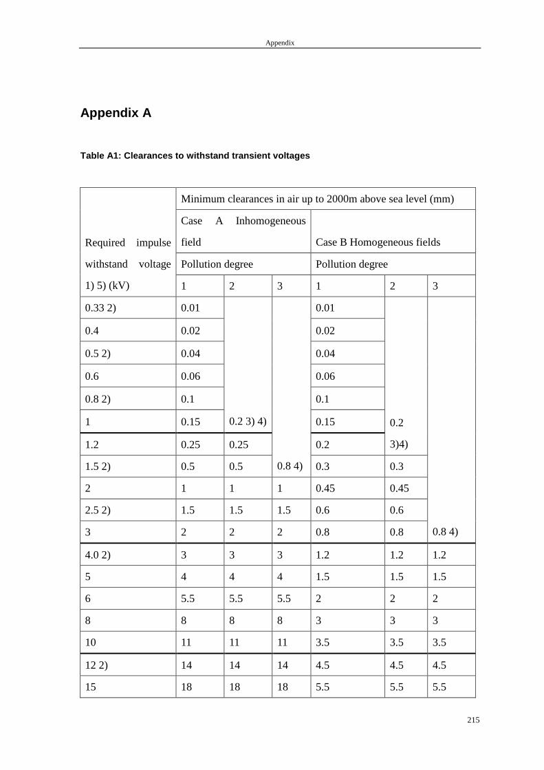
Appendix
215
Appendix A
Table A1: Clearances to withstand transient voltage s
Minimum clearances in air up to 2000m above sea level (mm)
Case A Inhomogeneous
field Case B Homogeneous fields
Pollution degree Pollution degree
Required impulse
withstand voltage
1) 5) (kV) 1 2 3 1 2 3
0.33 2) 0.01 0.01
0.4 0.02 0.02
0.5 2) 0.04 0.04
0.6 0.06 0.06
0.8 2) 0.1 0.1
1 0.15 0.2 3) 4) 0.15
1.2 0.25 0.25 0.2
0.2
3)4)
1.5 2) 0.5 0.5 0.8 4) 0.3 0.3
2 1 1 1 0.45 0.45
2.5 2) 1.5 1.5 1.5 0.6 0.6
3 2 2 2 0.8 0.8 0.8 4)
4.0 2) 3 3 3 1.2 1.2 1.2
5 4 4 4 1.5 1.5 1.5
6 5.5 5.5 5.5 2 2 2
8 8 8 8 3 3 3
10 11 11 11 3.5 3.5 3.5
12 2) 14 14 14 4.5 4.5 4.5
15 18 18 18 5.5 5.5 5.5
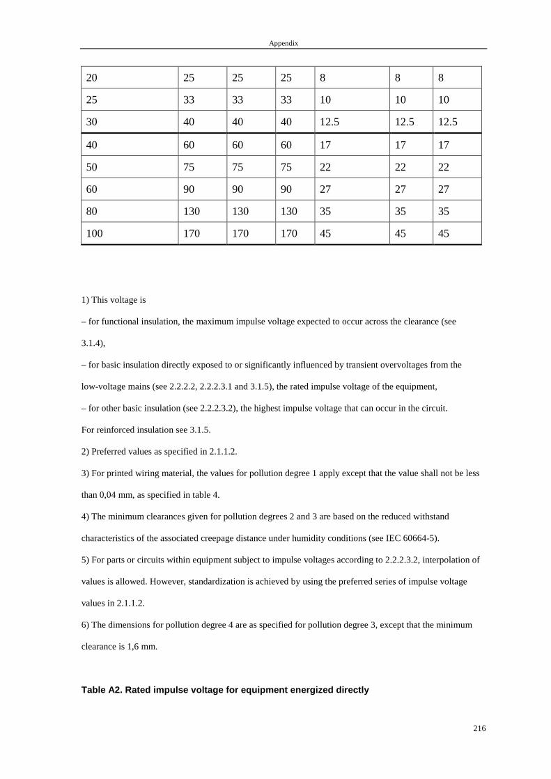
Appendix
216
20 25 25 25 8 8 8
25 33 33 33 10 10 10
30 40 40 40 12.5 12.5 12.5
40 60 60 60 17 17 17
50 75 75 75 22 22 22
60 90 90 90 27 27 27
80 130 130 130 35 35 35
100 170 170 170 45 45 45
1) This voltage is
– for functional insulation, the maximum impulse voltage expected to occur across the clearance (see
3.1.4),
– for basic insulation directly exposed to or significantly influenced by transient overvoltages from the
low-voltage mains (see 2.2.2.2, 2.2.2.3.1 and 3.1.5), the rated impulse voltage of the equipment,
– for other basic insulation (see 2.2.2.3.2), the highest impulse voltage that can occur in the circuit.
For reinforced insulation see 3.1.5.
2) Preferred values as specified in 2.1.1.2.
3) For printed wiring material, the values for pollution degree 1 apply except that the value shall not be less
than 0,04 mm, as specified in table 4.
4) The minimum clearances given for pollution degrees 2 and 3 are based on the reduced withstand
characteristics of the associated creepage distance under humidity conditions (see IEC 60664-5).
5) For parts or circuits within equipment subject to impulse voltages according to 2.2.2.3.2, interpolation of
values is allowed. However, standardization is achieved by using the preferred series of impulse voltage
values in 2.1.1.2.
6) The dimensions for pollution degree 4 are as specified for pollution degree 3, except that the minimum
clearance is 1,6 mm.
Table A2. Rated impulse voltage for equipment energ ized directly
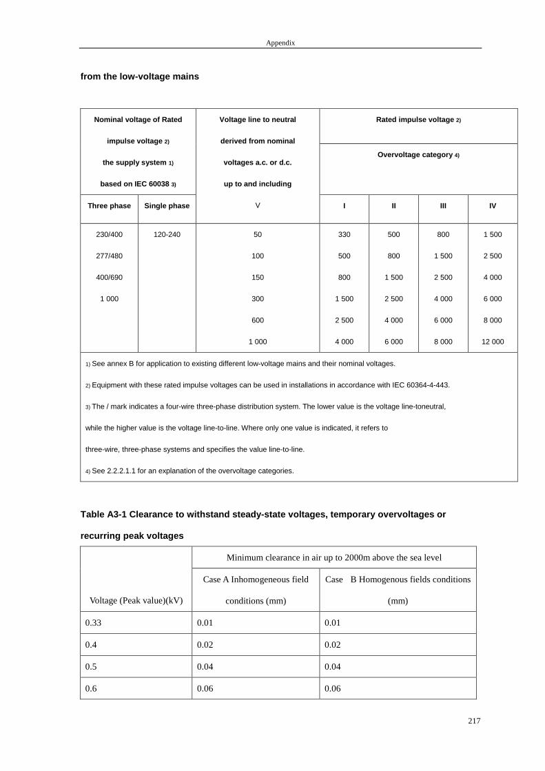
Appendix
217
from the low-voltage mains
Rated impulse voltage 2) Nominal voltage of Rated
impulse voltage 2)
the supply system 1)
based on IEC 60038 3)
Overvoltage category 4)
Three phase Single phase
Voltage line to neutral
derived from nominal
voltages a.c. or d.c.
up to and including
V I II III IV
230/400
277/480
400/690
1 000
120-240 50
100
150
300
600
1 000
330
500
800
1 500
2 500
4 000
500
800
1 500
2 500
4 000
6 000
800
1 500
2 500
4 000
6 000
8 000
1 500
2 500
4 000
6 000
8 000
12 000
1) See annex B for application to existing different low-voltage mains and their nominal voltages.
2) Equipment with these rated impulse voltages can be used in installations in accordance with IEC 60364-4-443.
3) The / mark indicates a four-wire three-phase distribution system. The lower value is the voltage line-toneutral,
while the higher value is the voltage line-to-line. Where only one value is indicated, it refers to
three-wire, three-phase systems and specifies the value line-to-line.
4) See 2.2.2.1.1 for an explanation of the overvoltage categories.
Table A3-1 Clearance to withstand steady-state volt ages, temporary overvoltages or
recurring peak voltages
Minimum clearance in air up to 2000m above the sea level
Voltage (Peak value)(kV)
Case A Inhomogeneous field
conditions (mm)
Case B Homogenous fields conditions
(mm)
0.33 0.01 0.01
0.4 0.02 0.02
0.5 0.04 0.04
0.6 0.06 0.06
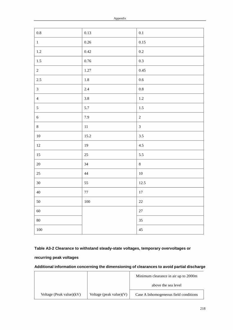
Appendix
218
0.8 0.13 0.1
1 0.26 0.15
1.2 0.42 0.2
1.5 0.76 0.3
2 1.27 0.45
2.5 1.8 0.6
3 2.4 0.8
4 3.8 1.2
5 5.7 1.5
6 7.9 2
8 11 3
10 15.2 3.5
12 19 4.5
15 25 5.5
20 34 8
25 44 10
30 55 12.5
40 77 17
50 100 22
60 27
80 35
100 45
Table A3-2 Clearance to withstand steady-state volt ages, temporary overvoltages or
recurring peak voltages
Additional information concerning the dimensioning of clearances to avoid partial discharge
Minimum clearance in air up to 2000m
above the sea level
Voltage (Peak value)(kV) Voltage (peak value)(V) Case A Inhomogeneous field conditions
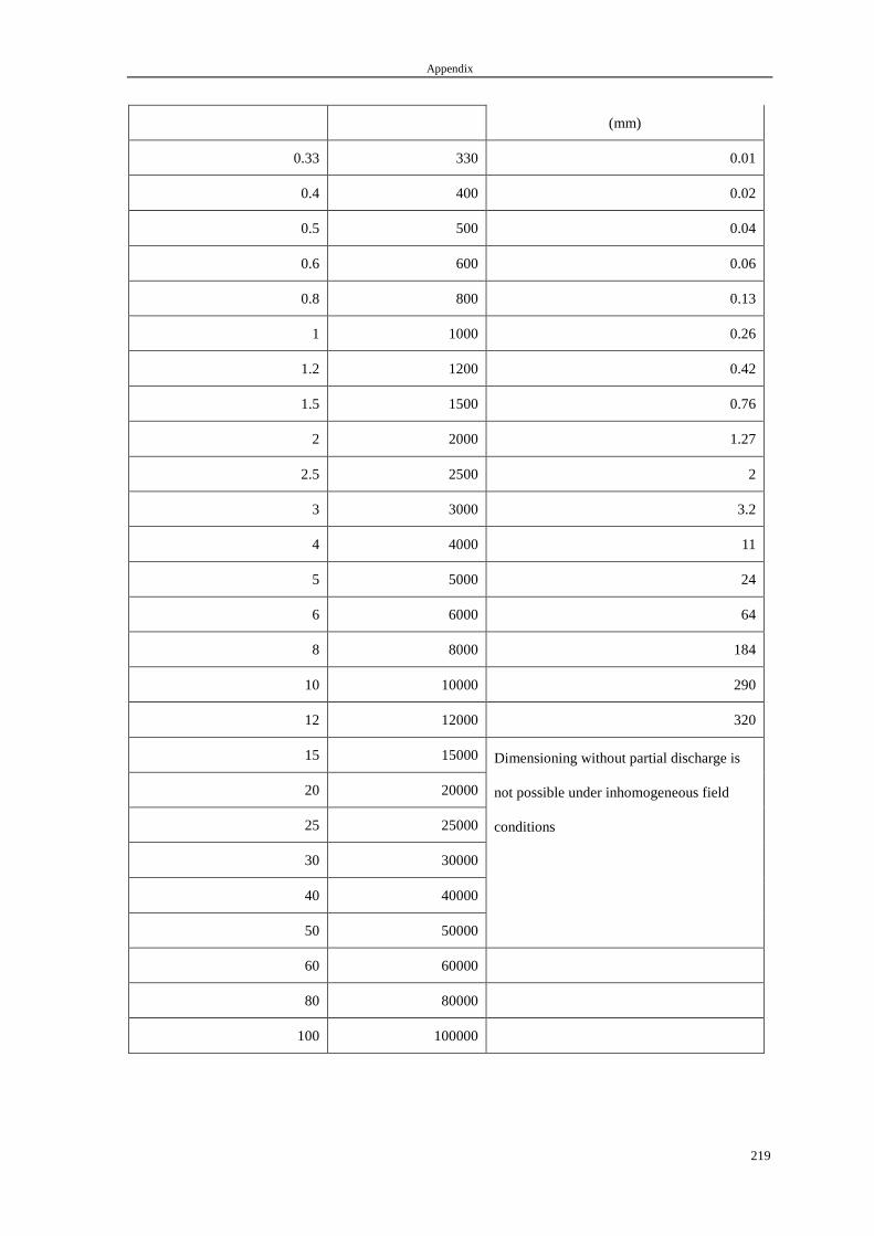
Appendix
219
(mm)
0.33 330 0.01
0.4 400 0.02
0.5 500 0.04
0.6 600 0.06
0.8 800 0.13
1 1000 0.26
1.2 1200 0.42
1.5 1500 0.76
2 2000 1.27
2.5 2500 2
3 3000 3.2
4 4000 11
5 5000 24
6 6000 64
8 8000 184
10 10000 290
12 12000 320
15 15000
20 20000
25 25000
30 30000
40 40000
50 50000
Dimensioning without partial discharge is
not possible under inhomogeneous field
conditions
60 60000
80 80000
100 100000
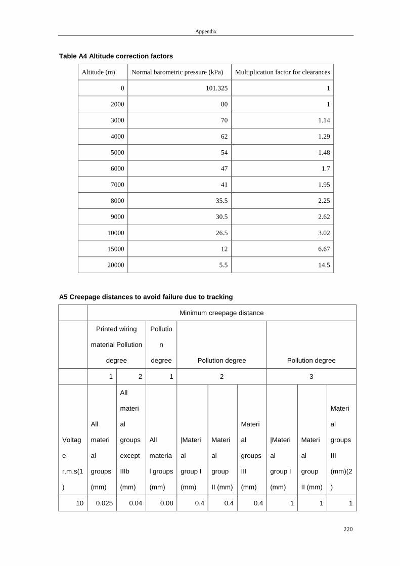
Appendix
220
Table A4 Altitude correction factors
Altitude (m) Normal barometric pressure (kPa) Multiplication factor for clearances
0 101.325 1
2000 80 1
3000 70 1.14
4000 62 1.29
5000 54 1.48
6000 47 1.7
7000 41 1.95
8000 35.5 2.25
9000 30.5 2.62
10000 26.5 3.02
15000 12 6.67
20000 5.5 14.5
A5 Creepage distances to avoid failure due to track ing
Minimum creepage distance
Printed wiring
material Pollution
degree
Pollutio
n
degree Pollution degree Pollution degree
1 2 1 2 3
Voltag
e
r.m.s(1
)
All
materi
al
groups
(mm)
All
materi
al
groups
except
IIIb
(mm)
All
materia
l groups
(mm)
|Materi
al
group I
(mm)
Materi
al
group
II (mm)
Materi
al
groups
III
(mm)
|Materi
al
group I
(mm)
Materi
al
group
II (mm)
Materi
al
groups
III
(mm)(2
)
10 0.025 0.04 0.08 0.4 0.4 0.4 1 1 1
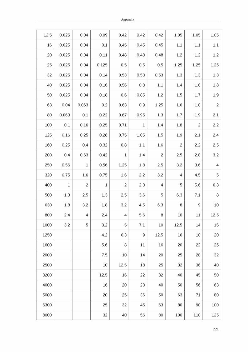
Appendix
221
12.5 0.025 0.04 0.09 0.42 0.42 0.42 1.05 1.05 1.05
16 0.025 0.04 0.1 0.45 0.45 0.45 1.1 1.1 1.1
20 0.025 0.04 0.11 0.48 0.48 0.48 1.2 1.2 1.2
25 0.025 0.04 0.125 0.5 0.5 0.5 1.25 1.25 1.25
32 0.025 0.04 0.14 0.53 0.53 0.53 1.3 1.3 1.3
40 0.025 0.04 0.16 0.56 0.8 1.1 1.4 1.6 1.8
50 0.025 0.04 0.18 0.6 0.85 1.2 1.5 1.7 1.9
63 0.04 0.063 0.2 0.63 0.9 1.25 1.6 1.8 2
80 0.063 0.1 0.22 0.67 0.95 1.3 1.7 1.9 2.1
100 0.1 0.16 0.25 0.71 1 1.4 1.8 2 2.2
125 0.16 0.25 0.28 0.75 1.05 1.5 1.9 2.1 2.4
160 0.25 0.4 0.32 0.8 1.1 1.6 2 2.2 2.5
200 0.4 0.63 0.42 1 1.4 2 2.5 2.8 3.2
250 0.56 1 0.56 1.25 1.8 2.5 3.2 3.6 4
320 0.75 1.6 0.75 1.6 2.2 3.2 4 4.5 5
400 1 2 1 2 2.8 4 5 5.6 6.3
500 1.3 2.5 1.3 2.5 3.6 5 6.3 7.1 8
630 1.8 3.2 1.8 3.2 4.5 6.3 8 9 10
800 2.4 4 2.4 4 5.6 8 10 11 12.5
1000 3.2 5 3.2 5 7.1 10 12.5 14 16
1250 4.2 6.3 9 12.5 16 18 20
1600 5.6 8 11 16 20 22 25
2000 7.5 10 14 20 25 28 32
2500 10 12.5 18 25 32 36 40
3200 12.5 16 22 32 40 45 50
4000 16 20 28 40 50 56 63
5000 20 25 36 50 63 71 80
6300 25 32 45 63 80 90 100
8000 32 40 56 80 100 110 125
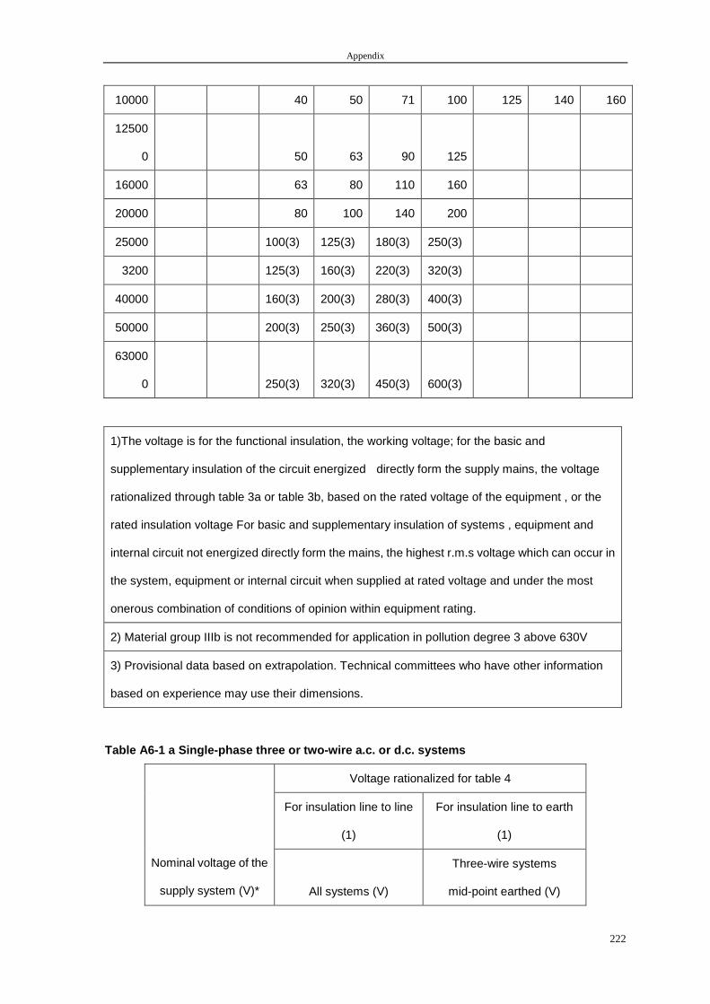
Appendix
222
10000 40 50 71 100 125 140 160
12500
0 50 63 90 125
16000 63 80 110 160
20000 80 100 140 200
25000 100(3) 125(3) 180(3) 250(3)
3200 125(3) 160(3) 220(3) 320(3)
40000 160(3) 200(3) 280(3) 400(3)
50000 200(3) 250(3) 360(3) 500(3)
63000
0 250(3) 320(3) 450(3) 600(3)
1)The voltage is for the functional insulation, the working voltage; for the basic and
supplementary insulation of the circuit energized directly form the supply mains, the voltage
rationalized through table 3a or table 3b, based on the rated voltage of the equipment , or the
rated insulation voltage For basic and supplementary insulation of systems , equipment and
internal circuit not energized directly form the mains, the highest r.m.s voltage which can occur in
the system, equipment or internal circuit when supplied at rated voltage and under the most
onerous combination of conditions of opinion within equipment rating.
2) Material group IIIb is not recommended for application in pollution degree 3 above 630V
3) Provisional data based on extrapolation. Technical committees who have other information
based on experience may use their dimensions.
Table A6-1 a Single-phase three or two-wire a.c. or d.c. systems
Voltage rationalized for table 4
For insulation line to line
(1)
For insulation line to earth
(1)
Nominal voltage of the
supply system (V)* All systems (V)
Three-wire systems
mid-point earthed (V)
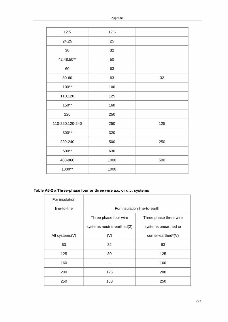
Appendix
223
12.5 12.5
24,25 25
30 32
42,48,50** 50
60 63
30-60 63 32
100** 100
110,120 125
150** 160
220 250
110-220,120-240 250 125
300** 320
220-240 500 250
600** 630
480-960 1000 500
1000** 1000
Table A6-2 a Three-phase four or three wire a.c. or d.c. systems
For insulation
line-to-line For insulation line-to-earth
All systems(V)
Three phase four wire
systems neutral-earthed(2)
(V)
Three phase three wire
systems unearthed or
corner-earthed*(V)
63 32 63
125 80 125
160 - 160
200 125 200
250 160 250
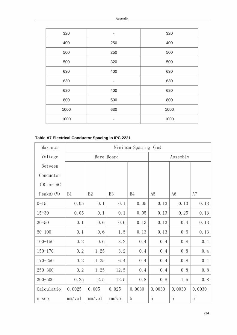
Appendix
224
320 - 320
400 250 400
500 250 500
500 320 500
630 400 630
630 - 630
630 400 630
800 500 800
1000 630 1000
1000 - 1000
Table A7 Electrical Conductor Spacing in IPC 2221
Minimum Spacing (mm)
Bare Board Assembly
Maximum
Voltage
Between
Conductor
(DC or AC
Peaks)(V) B1 B2 B3 B4 A5 A6 A7
0-15 0.05 0.1 0.1 0.05 0.13 0.13 0.13
15-30 0.05 0.1 0.1 0.05 0.13 0.25 0.13
30-50 0.1 0.6 0.6 0.13 0.13 0.4 0.13
50-100 0.1 0.6 1.5 0.13 0.13 0.5 0.13
100-150 0.2 0.6 3.2 0.4 0.4 0.8 0.4
150-170 0.2 1.25 3.2 0.4 0.4 0.8 0.4
170-250 0.2 1.25 6.4 0.4 0.4 0.8 0.4
250-300 0.2 1.25 12.5 0.4 0.4 0.8 0.8
300-500 0.25 2.5 12.5 0.8 0.8 1.5 0.8
Calculatio
n see
0.0025
mm/vol
0.005
mm/vol
0.025
mm/vol
0.0030
5
0.0030
5
0.0030
5
0.0030
5
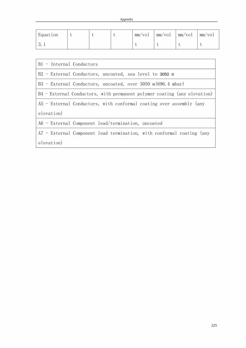
Appendix
225
Equation
3.1
t t t mm/vol
t
mm/vol
t
mm/vol
t
mm/vol
t
B1 - Internal Conductors
B2 - External Conductors, uncoated, sea level to 3050 m
B3 - External Conductors, uncoated, over 3050 m(696.4 mbar)
B4 - External Conductors, with permanent polymer coating (any elevation)
A5 - External Conductors, with conformal coating over assembly (any
elevation)
A6 - External Component lead/termination, uncoated
A7 - External Component lead termination, with conformal coating (any
elevation)
Appendix
226
Appendix B
Disruptive discharges test procedures can be divided into three classes for the purpose of
statistical evaluation.
Class 1: multi-level tests
im Substantially equal voltage stresses (e.g. lighting impulses) are applied at each of n
voltage levels iU . While this procedure is usually employed with impulse voltages, some
tests with alternating and direct voltage also fall into this class.
Class 2: Up-and-down tests
N groups of m substantially equal voltage stresses are applied at voltage levels iU . The
voltage level for each succeeding group of stresses is increased or decreased by a small
amount U∆ according to the result of the previous group of stresses.
Class 3: Successive Discharge Tests
A procedure leading to a disruptive discharge on the test object is applied n times. The Test
voltage may be increased continuously until a disruptive discharge occurs or held constant
at some level until a disruptive discharge is observed.
Statistical Behaviour of Disruptive Discharge
When p, the probability of a disruptive discharge during a given test procedure, depends
only on the test voltage, U, the behaviour of the test object can be characterized by a
function p(U) determined by the processes of discharge development. In practice, this
function, the disruptive discharge probability function, can be represented mathematically
by expressions depending on at least two parameters U50 and z. U50 is the 50 %
discharge voltage for which p(U) = 0,5 and z is the conventional deviation; z = U50 – U16
where U16 is the voltage for which p(U) = 0,16.
NOTE 1 Examples of p(U) can be derived from the Gaussian (or Normal), the Weibull or the
Appendix
227
Gumbel probability distribution functions. Experience shows that for 0,15 < p < 0,85 most
theoretical distributions can be considered equivalent. Special Weibull or Gumbel
distributions are acceptable approximations to a Gaussian distribution having given U50
and z for p lying between 0,02 and 0,98. Beyond these limits little information is available.
NOTE 2 Sometimes p is a function of two or more parameters, e.g., U and dU/dt. In such
cases no simple function can be used to describe p. Details of such cases may be found in
the technical literature. The function p(U) and the parameters U50 and z can be found from
tests with very large numbers of voltage applications, provided that the characteristics of
the test object remain constant throughout the tests. In practice the number of voltage
applications is usually limited and the estimates of U50 and z based on an assumed form of
p(U) will be subject to statistical uncertainties.
Confidence limits and statistical error
If a parameter y is estimated from n test results, upper and lower confidence limits yU and
yL can be defined, with the probability C that the true value of y is within these limits. C is
termed the confidence level and the half width er = (yU – yL)/2 of the confidence band is
called the statistical error. Usually C is taken as 0,95 (or 0,90) and the corresponding limits
are called the 95 % (or 90 %) confidence limits. The statistical errorer depends on both n
and the value of the conventional deviation z. The conventional deviation z should be
estimated when possible from tests made under realistic conditions. In general, the larger
the number of tests made, the better will be the estimate of z. It should, however, be
remembered that during a protracted test series, ambient conditions may change to an
extent which offsets the gain in accuracy from the increased number of tests.Since
accurate estimation of z from a limited series of tests is not possible, values estimated from
the pooled results of many tests are often given by the relevant Technical Committees. The
statistical error er may be combined with estimates of other errors (e.g., measuring errors)
to define the overall error limits for the determination of a particular parameter.
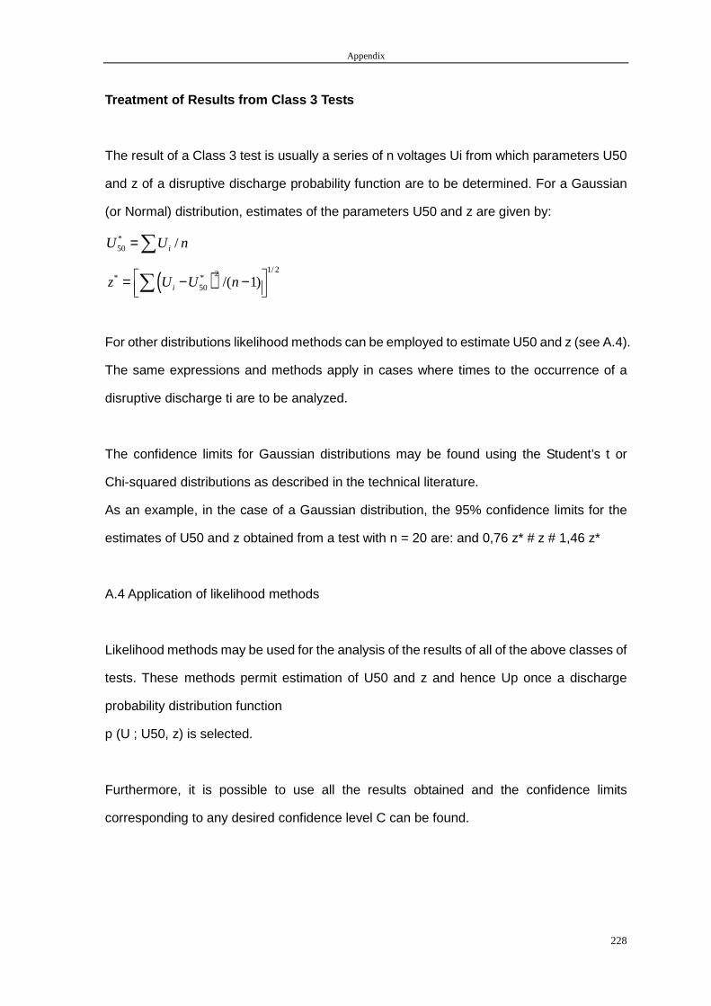
Appendix
228
Treatment of Results from Class 3 Tests
The result of a Class 3 test is usually a series of n voltages Ui from which parameters U50
and z of a disruptive discharge probability function are to be determined. For a Gaussian
(or Normal) distribution, estimates of the parameters U50 and z are given by:
*50 /iU U n=∑
( )1/ 22* *
50 /( 1)iz U U n = − − ∑
For other distributions likelihood methods can be employed to estimate U50 and z (see A.4).
The same expressions and methods apply in cases where times to the occurrence of a
disruptive discharge ti are to be analyzed.
The confidence limits for Gaussian distributions may be found using the Student’s t or
Chi-squared distributions as described in the technical literature.
As an example, in the case of a Gaussian distribution, the 95% confidence limits for the
estimates of U50 and z obtained from a test with n = 20 are: and 0,76 z* # z # 1,46 z*
A.4 Application of likelihood methods
Likelihood methods may be used for the analysis of the results of all of the above classes of
tests. These methods permit estimation of U50 and z and hence Up once a discharge
probability distribution function
p (U ; U50, z) is selected.
Furthermore, it is possible to use all the results obtained and the confidence limits
corresponding to any desired confidence level C can be found.