Electricity and Magnetism - Drexel University · Electricity and Magnetism A Two-week Course for Middle School Teachers John D. Carpinelli Department of Electrical and Computer …

Electricity and Magnetism

A Two-week Course for Middle School Teachers

John D. Carpinelli Department of Electrical and Computer Engineering

New Jersey Institute of Technology University Heights

Newark, New Jersey, 07102-1982

Development of this manual and course was funded in part by the National Science Foundation through the Gateway Engineering Education Coalition and the New Jersey Commission on Higher Education.

Page ii

Electricity and Magnetism – Course Outline Day 1 8:30-9:00 Welcome/Introduction/Course Outline/Pre-course Survey 9:00-9:30 What is Engineering?

• Differences between engineering and science • Some famous engineers in engineering • Some famous engineers outside of engineering

9:30-10:00 Design Exercise – Paper Drop Design #1 10:00-11:00 Engineering Design and Problem Solving

• Problem solving process • Case Study – getting kids interested in bowling • Case Study – Wright Brothers

11:00-11:30 Design Exercise (continued) 11:30-12:30 LUNCH 12:30-1:30 Paper Drop Competition #1

• GITC 1st and 2nd floors 1:30-2:30 Engineering Accomplishments

• Videotape – Inventions – The Wonders of Electricity • Top 20 engineering accomplishments of the 20th century

Day 2 8:30-9:30 Engineering Accomplishments (continued)

• Pre-20th century accomplishments • Case Study – Thomas Edison

9:30-10:00 Design Exercise – Paper Drop Design #2 10:00-11:00 Pedagogy – External Speaker 11:00-11:30 Design Exercise (continued) 11:30-12:30 LUNCH 12:30-1:30 Paper Drop Competition #2

• GITC 1st and 2nd floors 1:30-2:30 Videotape – Hot Line – All About Electricity

• Class discussion Day 3 8:30-9:30 Introduction to Electricity

• Electrons, Charge, and Current • AC and DC electricity

9:30-11:30 Resistors • Current, voltage, and resistance • Color codes for resistors • Series and parallel circuits • Potentiometers

11:30-12:30 LUNCH 12:30-2:30 Laboratory Exercise – Resistor Circuits

Page iii

Day 4 8:30-9:30 Introduction to Magnetism

• Videotape – Physical Science in Action - Magnetism • Magnetism in Nature

9:30-10:30 Electromagnetism • Creating magnetism using electricity • Applications of electromagnetism in everyday life

10:30-11:30 Career Awareness – External Speaker 11:30-12:30 LUNCH 12:30-2:30 Laboratory Experiment - Electromagnets Day 5 8:30-10:30 Boolean Logic

• Basic functions • Truth tables

10:30-11:30 Digital Logic • Representation of basic gates • TTL chips

11:30-12:30 LUNCH 12:30-2:30 Laboratory Experiment – TTL chips Day 6 8:30-10:30 Boolean Functions 10:30-11:30 Programmable Logic Devices 11:30-12:30 LUNCH 12:30-2:30 Laboratory Experiment – Game Design Day 7 8:30-10:30 More Complex Digital Components

• Binary numbers • Registers, decoders, counters (binary & decimal),

encoders, multiplexers 10:30-11:30 Demonstration – “Stopwatch” circuit 11:30-12:30 LUNCH 12:30-2:30 Laboratory Experiment – “Boardwalk” Wheel Design Day 8 8:30-10:30 More complex circuits

• BCD to 7-segment decoders 10:30-11:30 Demonstration – Improved “Stopwatch” circuit 11:30-12:30 LUNCH 12:30-1:30 Analog to Digital Converters 1:30-2:30 Course Wrap-up/Post-course Survey

Page iv

Table of Contents

1 Introduction to Engineering ................................................1 1.1 What is Engineering?.......................................................................................................1

1.1.1 Some famous engineers ...........................................................................................1 1.1.2 Some engineers famous outside of engineering ......................................................7

1.2 Be the Engineer – Paper Drop Design #1 ......................................................................10 1.2.1 Design Specification..............................................................................................10 1.2.2 Scoring...................................................................................................................10 1.2.3 Acknowledgments .................................................................................................11

1.3 Engineering Design and Problem Solving.....................................................................12 1.3.1 Problem solving process ........................................................................................12 1.3.2 Case Study – Getting Kids Interested in Bowling .................................................12 1.3.3 Case Study: Wright Brothers .................................................................................14

1.4 Engineering Accomplishments ......................................................................................15

2 Introduction to Engineering (Continued) ........................22 2.1 Electrical Engineering Accomplishments......................................................................22

2.1.1 A Brief History of Electrical Engineering – 1600 to 1900 ....................................22 2.1.2 Case Study: Thomas Edison..................................................................................24

2.2 Be the Engineer Again – Paper Drop Design #2 ...........................................................24

3 Introduction to Electricity .................................................25 3.1 Electrons, Charge, and Current......................................................................................25

3.1.1 Atomic Structure....................................................................................................25 3.1.2 Charge ....................................................................................................................26 3.1.3 Current ...................................................................................................................26 3.1.4 Voltage ...................................................................................................................27 3.1.5 Direct Current and Alternating Current .................................................................27 3.1.6 Conductors and Insulators .....................................................................................28

3.2 Resistors.........................................................................................................................28 3.2.1 Current, Voltage, and Resistance – Ohm’s Law....................................................28 3.2.2 Resistor Color Codes .............................................................................................31 3.2.3 Series Resistance ...................................................................................................34 3.2.4 Parallel Resistance .................................................................................................34 3.2.5 Series-Parallel Resistance ......................................................................................35 3.2.6 Potentiometers .......................................................................................................37

3.3 Laboratory Exercise – Resistor Circuits ........................................................................37

4 Introduction to Magnetism................................................40 4.1 Magnetism in Nature .....................................................................................................40

4.1.1 Poles and Magnetic Fields .....................................................................................40 4.1.2 What Really Causes Magnetism............................................................................41 4.1.3 Magnetism in Nature .............................................................................................41

4.2 Electromagnetism ..........................................................................................................42 4.2.1 Using Electricity to Create Magnetism..................................................................42 4.2.2 Electromagnetism in Everyday Life ......................................................................43

Page v

4.3 Laboratory Exercise .......................................................................................................44

5 Boolean and Digital Logic Fundamentals ........................47 5.1 Introduction to Boolean Logic .......................................................................................47

5.1.1 The Logical AND Function...................................................................................47 5.1.2 The Logical OR Function......................................................................................48 5.1.3 The Logical Exclusive-OR Function.....................................................................48 5.1.4 The Logical NOT Function ...................................................................................49

5.2 Truth Tables ...................................................................................................................51 5.3 Complementary Functions – NAND, NOR, and Exclusive-NOR ................................51 5.4 Digital Logic ..................................................................................................................54 5.5 TTL Chips......................................................................................................................55 5.6 Where Boolean Logic Meets Digital Logic ...................................................................56 5.7 Laboratory Exercise – Digital Logic .............................................................................57

6 More Complex Boolean Functions....................................61 6.1 Combining Logical Operations ......................................................................................61 6.2 Modeling Real-world Situations ....................................................................................61 6.3 Truth Tables for Combined Functions ...........................................................................62

6.3.1 Creating the Exclusive-OR Function.....................................................................62 6.3.2 Determining Functions from Truth Tables ............................................................65 6.3.3 Simplifying Functions ...........................................................................................67

6.4 Programmable Devices ..................................................................................................69 6.5 Laboratory Exercise – Guess the Pattern Game ............................................................70

7 More Complex Digital Components .................................73 7.1 Binary Numbers .............................................................................................................73

7.1.1 Binary Values ........................................................................................................73 7.1.2 Binary Coded Decimal (BCD)...............................................................................74

7.2 Components ...................................................................................................................76 7.2.1 Multiplexers ...........................................................................................................76 7.2.2 Decoders ................................................................................................................76 7.2.3 Encoders ................................................................................................................77 7.2.4 Registers ................................................................................................................78 7.2.5 Counters .................................................................................................................78

7.3 Stopwatch Circuit #1 .....................................................................................................79 7.4 Laboratory Exercise – The Boardwalk Wheel...............................................................80

8 Digital Circuits – Interfacing with the Real World.........81 8.1 BCD to 7-Segment Decoder ..........................................................................................81 8.2 Stopwatch Circuit #2 .....................................................................................................85 8.3 Analog Interfaces ...........................................................................................................85

8.3.1 Analog to Digital Converters .................................................................................86 8.3.2 Creating the Analog Voltage Input ........................................................................86 8.3.3 Example – A Digital Thermometer .......................................................................86

Page 1

1 Introduction to Engineering Most people have heard of engineering, but many don’t know or understand what engineering is. This chapter examines engineering, what it is, some famous engineers (and some engineers famous outside of engineering), and the problem solving process.

1.1 What is Engineering? Engineering is the art of applying scientific and mathematical principles, experience, judgment, and common sense to make things that benefit people. Engineers design bridges and important medical equipment as well as processes for cleaning up toxic spills and systems for mass transit. In other words, engineering is the process of producing a technical product or system to meet a specific need. (Source: American Society for Engineering Education precollege web site, www.asee.org/precollege/engineering.cfm.) Many people think of engineering and science as the same thing. There is a difference between the two, but it can be difficult to see. The general objective of science is to discover the composition and behavior of the physical world. In contract, the general objective of engineering is to design useful things. Theodore Von Karman succinctly described this difference: “Scientists discover the world that exists; engineers create the world that never was.” Since “useful things” must obey the laws of nature, engineers study science as part of their preparation to practice engineering. There is some overlap in their practice as well. Some scientists help develop instruments that will be used in scientific study, clearly an engineering role. Conversely, engineers may practice basic science as part of their engineering endeavors. Fields such as semiconductor research involve both engineers and scientists, often working on the same problems. Engineering is a great profession. There is the fascination of watching a figment of imagination emerge through the aid of science to a plan on paper. Then it moves to realization in stone or metal or energy. Then it creates homes and jobs, elevates the standard of living and adds to the comforts of life. That is the engineer’s high privilege. – Herbert Hoover, 31st president of the United States and mining engineer.

1.1.1 Some famous engineers Many famous people have been engineers. Below is a list of a few famous engineers and their accomplishments. (Source: ASEE web site, www.asee.org/precollege/famous.cfm.)

• Edwin Howard Armstrong – His crowning achievement (1933) was the invention of wide-band frequency modulation, now known as FM radio. Armstrong earned a degree in electrical engineering from Columbia University in 1913.

• Alexander Graham Bell – inventor of the telephone. He also worked in medical research and invented techniques for teaching speech to the dear. In 1888 he founded the National Geographic Society.

Page 2

• Henry Bessemer – English inventor and engineer who invented the first process for mass-producing steel inexpensively - essential to the development of skyscrapers.

• Joseph Armand Bombardier – manufacturer of the first successful snowmobile.

• Philip Condit – CEO, The Boeing Company, mechanical/aeronautical engineering.

• American engineer and inventor Willis Haviland Carrier developed the formulae and equipment that made air conditioning possible. Carrier attended Cornell University and graduated with an M.E. in 1901.

• William D. Coolidge 's name is inseparably linked with the X-ray tube - popularly called the 'Coolidge tube.' This invention completely revolutionized the generation of X-rays and remains to this day the model upon which all X-ray tubes for medical applications are patterned. Coolidge, born in Hudson, Mass., graduated from the Massachusetts Institute of Technology in 1896, majoring in electrical engineering. At General Electric, he invented ductile tungsten, the filament material still used in lamps, and worked on high-quality magnetic steel, improved ventilating fans and the electric blanket.

• Seymour Cray – After a brief service during World War II, he went to the University of Minnesota where he studied engineering. In 1951 he joined Engineering Research Associates, which was developing computers for the Navy. Later he co-founded Control Data Corporation, and in 1972 he founded CRAY Research. Seymour Cray unveiled the CRAY-1 in 1976, considered the first supercomputer.

• George de Mestral – attended the Ecole Polytechnique Federale de Lausanne, Switzerland where he gradua ted as an electrical engineer. In 1955 the "hook and loop fastener" he created was patented under the name Velcro which was derived from two French words: velour and crochet ("velvet" and "hooks").

• Though best known for his invention of the pressure- ignited heat engine that bears his name, the French-born Rudolf Diesel was also an eminent thermal engineer.

• Ray Dolby – audio system innovator and founder of Dolby Laboratories. His technical expertise has won him both an Academy Award and a Grammy!

• Bonnie Dunbar – NASA astronaut who earned her B.S. and M.S. degrees in ceramic engineering from the University of Washington and a doctorate in mechanical/biomedical engineering from the University of Houston. While working at Rockwell International, Dr. Dunbar helped to develop the ceramic tiles that enable space shuttles to survive re-entry. She has had an opportunity to test those tiles first hand as a four-time astronaut, including a stint on the first shuttle mission to dock with the Russian Space Station Mir.

• Reginald A. (Aubrey) Fessenden – Canadian-born American physicist and electrical engineer who is known for his early work in wireless communication. He began his research at the University of Pittsburgh; after designing a high-frequency alternator, he broadcast (1906) the first program of speech and music ever transmitted by radio. That same year, he established two-way transatlantic wireless telegraph communication.

Page 3

Fessenden also invented the heterodyne system of radio reception, the sonic depth finder, the radio compass, submarine signaling devices, the smoke cloud (for tank warfare), and the turboelectric drive (for battleships).

• Sir Sanford Fleming – a civil engineer and scientist, played a key role in developing the Canadian railway system and created the worldwide system of standard time.

• Henry Ford held many patents on automotive mechanisms but is best remembered for helping devise the factory assembly approach to production that revolutionized the auto industry by greatly reducing the time required to assemble a car. Born in Wayne County, Mich., Ford showed an early interest in mechanics, constructing his first steam engine at the age of 15. In 1891, Ford became an engineer with the Edison Illuminating Company in Detroit. He became Chief Engineer in 1893 and this position allowed him to devote attention to his personal experiments on internal combustion engines. In 1893 he built his first internal combustion engine, a small one-cylinder gasoline model, and in 1896 he built his first automobile. In June 1903, Ford helped establish Ford Motor Company. He served as president of Ford from 1906 to 1919 and from 1943 to 1945.

• Jay W. Forrester was a pioneer in early digital computer development and invented random-access, coincident-current magnetic storage, which became the standard memory device for digital computers. He received a B.S. degree in Electrical Engineering in 1939 from the University of Nebraska and a M.S. degree from the Massachusetts Institute of Technology in 1945.

• Yuan-Cheng Fung – Fung is widely recognized as the father of biomechanics, having established the fundamentals of biomechanical properties in many of the human body's organs and tissues. He founded the bioengineering program at the University of California, San Diego. In November 2001 he became the first bioengineer to receive the President's National Medal of Science, the nation's highest scientific honor.

• Robert Hutchings Goddard pioneered modern rocketry and space flight and founded a whole field of science and engineering. Goddard's interest in rockets began in 1899, when he was 17. He conducted static tests with small solid-fuel rockets at Worcester Tech as early as 1908, and in 1912 he developed the detailed mathematical theory of rocket propulsion. In 1915 he proved that rocket engines could produce thrust in a vacuum and therefore make space flight possible. He succeeded in developing several types of solid-fuel rockets to be fired from handheld or tripod-mounted launching tubes, which were the basis of the bazooka and other powerful rocket weapons of World War II. At the time of his death Goddard held 214 patents in rocketry.

• Andrew Grove – co-founder, Intel, chemical engineer.

• William Hewlett and David Packard – co-founders of Hewlett-Packard.

• Beulah Louise Henry was known in the 1920s and 30s as "the lady Edison" for the many inventions she patented, including a vacuum ice cream freezer, a typewriter that made multiple copies without carbon paper, and a bobbinless lockstitch sewing machine.

Page 4

Henry founded manufacturing companies to produce her creations, making a fortune in the process.

• Grace Murray Hopper, a computer engineer and Rear Admiral in the U.S. Navy, developed the first computer compiler in 1952 and the computer program language COBOL. Upon discovering that a moth had jammed the works of an early computer, Hopper popularized the term "bug." In 1983, by special presidential appointment, Hopper was promoted to the rank of Commodore. Two years later, she became one of the first women to be elevated to the rank of Rear Admiral. In 1986, after forty-three years of service, RADM Grace Hopper ceremoniously retired on the deck of the USS Constitution. At 80 years, she was the oldest active duty officer at that time. She spent the remainder of her life as a senior consultant to Digital Equipment Corporation. Hopper received numerous honors over the course of her lifetime. In 1969, the Data Processing Management Association awarded her the first Computer Science Man-of-the-Year Award. She became the first person from the United States and the first woman to be made a Distinguished Fellow of the British Computer Society in 1973. She also received multiple honorary doctorates from universities across the nation. The Navy christened a ship in her honor. In September 1991, she was awarded the National Medal of Technology, the nation's highest honor in engineering and technology.

• Clarence "Kelly" Johnson – played a leading role in the design of more than 40 aircraft and set up a Skunk Works-type operation to develop a Lockheed satellite--the Agena-D--that became the nation's workhorse in space. His achievements over almost six decades captured every major aviation design award and the highest civilian honors of the U.S. government and made him an aerospace legend. He was elected to the National Academy of Sciences in 1965, was enshrined in the National Aviation Hall of Fame in 1974, and was awarded the Medal of Freedom in 1964 by President Lyndon Johnson recognizing, his "significant contributions to the quality of American life."

• Bill Joy – co-founder of Sun Microsystems, electrical engineer. He received a B.S.E.E. in electrical engineering from the University of Michigan in 1975, after which he attended graduate school at U.C. Berkeley where he was the principal designer of Berkeley UNIX (BSD) and received a M.S. in electrical engineering and computer science. The Berkeley version of UNIX became the standard in education and research, garnering development support from DARPA, and was notable for introducing virtual memory and Internet working using TCP/IP to UNIX. In 1997, Joy was appointed by President Clinton as co-chairman of the Presidential Information Technology Advisory Committee.

• Jack Kilby – inventor of the integrated circuit. Kilby received a B.S.E.E. degree from the University of Illinois in 1947 and an M.S.E.E. from the University of Wisconsin in 1950. In 2000, he received the Nobel Prize in Physics for his work with the integrated circuit.

• William LeMessurier – structural designer of the Citicorp building, structural engineer.

• Elijah McCoy was a Black inventor who was awarded over 57 patents. The son of runaway slaves from Kentucky, he was born in Canada and lived there as a youth. Educated in Scotland as a mechanical engineer he returned to Detroit and in 1872

Page 5

invented a lubricator for steam engines. His new oiling device revolutionized the industrial machine industry by allowing machines to remain in motion while being oiled. This device, although imitated by other designers, was so successful that people inspecting new equipment would ask if it contained the real McCoy.

• Guglielmo Marconi – The "Father of Radio" - Marconi received many honors including the Nobel Prize for Physics in 1909.

• James Morgan – CEO, Applied Materials, mechanical engineer. In 1996 he received the National Medal of Technology for his industry leadership and for his vision in building Applied Materials into the world's leading semiconductor equipment company, a major exporter and a global technology pioneer which helps enable the Information Age.

• Bill Nye – worked for Boeing before he became the "science guy", Mechanical engineering degree from Cornell University.

• Kevin Olmstead – world-record game show payoff winner – $2,180,000 winner, "Who Wants to be a Millionaire?" – and environmental engineer. After acquiring chemical engineering degrees from Case Western Reserve University and the Massachusetts Institute of Technology, Olmstead earned a doctorate degree in environmental engineering from the University of Michigan. He also taught civil and environmental engineering and is currently a senior project engineer with Tetra Tech MPS, an international consulting firm specializing in infrastructure and communications systems.

• Kenneth Olsen – inventor of magnetic core memory, co-founder, Digital Equipment Corporation. After serving in the Navy between 1944 and 1946, he attended the Massachusetts Institute of Technology, where he earned a B.S. (1950) and an M.A. (1952) in electrical engineering.

• Arati Prabhakar – director, National Institute of Standards and Technology (NIST), U.S. Department of Commerce. Prabhakar was appointed the 10th NIST Director in May 1993. NIST promotes U.S. economic growth by working with industry to develop and apply technology, measurements, and standards. Previously, Prabhakar served as director of the Microelectronics Technology Office in the Defense Department's Advanced Research Projects Agency (ARPA). She holds the distinction of being the first woman with a doctorate from the California Institute of Technology, and was also the youngest director of the institute.

• Ludwig Prandtl – the father of fluid mechanics, mechanical engineer.

• Edmund T. Pratt, Jr. – former CEO of Pfizer, Inc., electrical engineer.

• Judith Resnik – Challenger astronaut, electrical engineer. Received a Bachelor of Science degree in electrical engineering from Carnegie-Mellon University in 1970 and a doctorate in electrical engineering from the University of Maryland in 1977.

• Hyman G. Rickover – the "Father of the Nuclear Navy" he led the development of the Navy nuclear submarine fleet. Masters in electrical engineering from Columbia

Page 6

University. During World War II, he headed the electrical section of the Navy's Bureau of Ships, and in 1946 was enlisted into the U.S. atomic program. The next year he returned to the Navy to manage its nuclear-propulsion program. Regarded as a fanatic by his detractors, he completed the world's first nuclear submarine--the USS Nautilus--ahead of schedule in 1955. While continuing his work with the Navy, he helped build the first major civilian nuclear power plant at Shippingport, PA. Always an outspoken advocate of U.S. nuclear supremacy, he was promoted to the rank of vice admiral in 1959 and admiral in 1973. He retired from the Navy in 1982 after serving as an officer for a record 63 years. Throughout his long naval career his decorations included the Distinguished Service Medal, Legion of Merit, Navy Commendation Medal, two Congressional Gold Medals, as well as the title of Honorary Commander of the Military Division of the Most Excellent Order of the British Empire. In 1980, President Jimmy Carter presented him the Presidential Medal of Freedom, the nation's highest non-military honor.

• Norbert Rillieux – revolutionized in the sugar industry by inventing a refining process that reduced the time, cost, and safety risk involved in producing sugar from cane and beets. His inventions protected lives by ending the older dangerous methods of sugar production. As the son of a French planter/inventor and a slave mother, Norbert Rillieux was born in New Orleans, LA. He was educated at the L'Ecole Central in Paris, France in 1830, were he studied evaporating engineering and served as an educator.

• Washington Roebling – completed the Brooklyn Bridge which was started by his father, civil engineer.

• Katherine Stinson – the first female graduate of NC State University's College of Engineering. Initially denied admission as a freshman, Stinson went on to become one of NC State's most distinguished and active alumni. Graduating vice president of her class, she was soon hired by the Civil Aeronautics Administration as its first female engineer. Later, she served as technical assistant chief in its Engineering and Manufacturing Division until her retirement in 1973. She went on to found the Society of Women Engineers.

• Nikola Tesla – invented the induction motor with rotating magnetic field that made unit drives for machines feasible and made AC power transmission an economic necessity.

• Stephen Timoshenko – the father of engineering mechanics, engineering scientist.

• Theodore von Karman – Dr. von Karman was one of the world's foremost aerodynamicsts and scientists and is widely recognized as the father of modern aerospace science. He was a professor of aeronautics at the California Institute of Technology and was one of the principal founders of NASA's Jet Propulsion Laboratory, Pasadena, California.

• George Westinghouse – invented a system of air brakes that made travel by train safe and built one of the greatest electric manufacturing organizations in the United States. In 1886, he founded the Westinghouse Electric Company, foreseeing the possibilities of alternating current as opposed to direct current, which was limited to a radius of two or

Page 7

three miles. Westinghouse enlisted the services of Nikola Tesla and other inventors in the development of alternating current motors and apparatus for the transmission of high-tension current, pioneering large-scale municipal lighting.

• American inventor, pioneer, mechanical engineer, and manufacturer Eli Whitney is best remembered as the inventor of the cotton gin. He also affected the industrial development of the United States when, in manufacturing muskets for the government, he translated the concept of interchangeable parts into a manufacturing system, giving birth to the American mass-production concept.

• Steve Wozniak cofounded Apple Computer, Inc. in 1976 with the Apple I computer. Wozniak's Apple II personal computer - introduced in 1977 and featuring a central processing unit (CPU), keyboard, floppy disk drive, and a $1,300 price tag - helped launch the PC industry. In 1980, just a little more than four years after being founded, Apple went public. Wozniak left Apple in 1981 and went back to Berkeley and finished his degree in electrical engineering/computer science. Since then, he has been involved in various business and philanthropic ventures, focusing primarily on computer capabilities in schools, including an initiative in 1990 to place computers in schools in the former Soviet Union.

1.1.2 Some engineers famous outside of engineering As with any college major, some people that major in engineering end up working in fields not directly related to their college majors. Below is a list of some people with engineering backgrounds that are famous for non-engineering achievements. (Source: ASEE web site, www.asee.org/precollege/famous.cfm.)

• Yasser Arafat - Palestinian leader and Nobel Peace Prize Laureate. Graduated as a civil engineer from the University of Cairo.

• Neil Alden Armstrong - became the first man to walk on the moon on July 20, 1969, at 10:56 p.m. EDT. He and "Buzz" Aldren spent about two and one-half hours walking on the moon, while pilot Michael Collins waited above in the Apollo 11 command module. Armstrong received his B.S. in aeronautical engineering from Purdue University and an M.S. in aerospace engineering from the University of Southern California.

• Rowan Atkinson - A British comedian, best known for his starring roles in the television series "Blackadder" and "Mr. Bean," and several films includ ing Four Weddings and a Funeral. Atkinson attended first Manchester then Oxford University on an electrical engineering degree.

• Leonid Brezhnev - leader of the former Soviet Union, metallurgical engineer.

• Alexander Calder - a native of Pennsylvania, received his degree in mechanical engineering from Stevens Institute of Technology, Hoboken, New Jersey, and shortly thereafter moved to Paris, where he studied art and began to create his now-famous mobiles. Many of his large sculptures are on permanent outdoor display at the

Page 8

Massachusetts Institute of Technology, where the first major retrospective of his work was held in 1950.

• Frank Capra - film director - "It Happened One Night", "Mr. Smith Goes to Washington", "It's a Wonderful Life" - college degree in chemical engineering.

• Jimmy Carter - 39th President of the United States. Attended Georgia Southwestern College and the Georgia Institute of Technology and received a B.S. degree from the United States Naval Academy in 1946. In the Navy he became a submariner, serving in both the Atlantic and Pacific fleets and rising to the rank of lieutenant. Chosen by Admiral Hyman Rickover for the nuclear submarine program, he was assigned to Schenectady, N.Y., where he took graduate work at Union College in reactor techno logy and nuclear physics and served as senior officer of the pre-commissioning crew of the Seawolf.

• Roger Corman -film director, industrial engineering degree from Stanford University. He started direct involvement in films in 1953 as a producer and screenwriter, making his debut as director in 1955. Between then and his official retirement in 1971 he directed dozens of films, often as many as six or seven per year, typically shot extremely quickly on leftover sets from other, larger productions. His probably unbeatable record for a professional 35mm feature film was two days and a night to shoot the original version of "The Little Shop of Horrors".

• Leonardo Da Vinci - Florentine artist, one of the great masters of the High Renaissance, celebrated as a painter, sculptor, architect, engineer, and scientist. His profound love of knowledge and research was the keynote of both his artistic and scientific endeavors. His innovations in the field of painting influenced the course of Italian art for more than a century after his death, and his scientific studies - particularly in the fields of anatomy, optics, and hydraulics - anticipated many of the developments of modern science.

• Thomas Edison - Edison patented 1,093 inventions in his lifetime, earning him the nickname "The Wizard of Menlo Park." The most famous of his inventions was an incandescent light bulb. Besides the light bulb, Edison developed the phonograph and the kinetoscope, a small box for viewing moving films. He also improved upon the original design of the stock ticker, the telegraph, and Alexander Graham Bell's telephone. Edison was quoted as saying, "Genius is one percent inspiration and 99 percent perspiration."

• Lillian Gilbreth - is considered a pioneer in the field of time-and-motion studies, showing companies how to increase efficiency and production through budgeting of time, energy, and money. Dr. Gilbreth received her Ph.D. in psychology from Brown University and was a professor at Purdue's School of Mechanical Engineering, Newark School of Engineering and the University of Wisconsin. She is "Member No. 1" of the Society of Women Engineers. She and her husband used their industrial engineering skills to run their household, and those efforts are the subject of the book and family film "Cheaper by the Dozen."

Page 9

• Roberto C. Goizueta - former chairman and chief executive of Coca-Cola. Chemical engineering degree from Yale University.

• Herbie Hancock - jazz musician.

• Alfred Hitchcock - British-born American director and producer of many brilliantly contrived films, most of them psychological thrillers including "Psycho", "The Birds", "Rear Window", and "North by Northwest." He was born in London and trained there as an engineer at Saint Ignatius College. Although Hitchcock never won an Academy Award for his direction, he received the Irving Thalberg Award of the Academy of Motion Picture Arts and Sciences in 1967 and the American Film Institute's Life Achievement Award in 1979. During the final year of his life, he was knighted by Queen Elizabeth II, even though he had long been a naturalized citizen of the United States.

• Herbert Hoover - having graduated from Stanford University in California, Hoover was a 26 -year-old mining engineer in Tientsin, China, when the city was attacked by 5,000 Chinese troops and 25,000 members of the martial arts group known as the Boxers. (The Boxer Rebellion was a violent 1900 uprising against foreign business interests in China.) Hoover took charge of setting up barricades to protect Tientsin until its rescue after 28 days of bombardment. Thirty years later, Herbert Hoover became the 31st President of the United States; he and his wife continued to speak Chinese when they wanted privacy in the White House.

• Lee Iacocca - former chairman and CEO of Chrysler Corp. Iacocca graduated from Lehigh University, Bethlehem, Pa., in 1945 and received a master's degree in engineering from Princeton University in 1946. Best known for his helmsmanship at Chrysler Motors, Iacocca started out as a sales manager at the Ford Motor Co. in 1946 and by 1970 was president of the company. Joining Chrysler in 1978, Iacocca helped drag the troubled company from the brink of extinction by helping secure $1.5 billion in government loans. Iacocca's legendary status in the automobile industry is reinforced by his role in the introduction of that American icon: the Ford Mustang. He was also one of the first CEOs to proselytise his company's products on national television with the K car campaign.

• Bill Koch - yachtsman and winning America's Cup captain in 1992, as well as the chairman of the America3 Foundation.

• Tom Landry - former Dallas Cowboys coach.

• Hedy Lamarr - a famous 1940s actress not formally trained as an engineer, Lamarr is credited with several sophisticated inventions, among them a unique anti- jamming device for use against Nazi radar. Years after her patent had expired, Sylvania adapted the design for a device that today speeds satellite communications around the world. She is also credited with the line: "Any girl can be glamorous. All you have to do is stand still and look stupid."

• Jair Lynch - 1992 and 1996 Olympic gymnast. Civil Engineering degree from Stanford University.

Page 10

• Arthur Nielsen - developer of Nielsen rating system.

• Tom Scholtz - leader of the rock band Boston. Master's degree from MIT in mechanical engineering.

• John Sununu - former White House Chief of Staff for President George Bush, former governor of New Hampshire, current CNN commentator on "Crossfire ."

• Boris Yeltsin - former president of Russia.

• John F. Welch, Jr. - received his engineering undergraduate degree in his home-state at the University of Massachusetts. After he earned his Ph.D. in chemical engineering from the University of Illinois, he accepted a job offer from General Electric. The rest is history -- he became cha irman and CEO of General Electric in 1981.

• Montel Williams - a highly decorated former Naval engineer and Naval Intelligence Officer, he is now an author of inspirational books and host of a popular syndicated television talk show.

1.2 Be the Engineer – Paper Drop Design #1 In this exercise, you will play the role of the engineer. You are given a goal and must design a solution to achieve that goal.

1.2.1 Design Specification Each team is required to design and construct a “flying” device. There are two design criteria for this device. 1. The device must stay in the air as long as possible. 2. The device must land as close as possible to a given target. Each team must construct their device using any or all of the following materials.

• Three sheets of 8½" x 11" paper • Adhesive tape • One 3" x 5" index card • Four paper clips • A pair of scissors

1.2.2 Scoring The competition will be held on two floors of NJIT’s GITC building. One member of each team will go to the upper floor and launch the device over the balcony toward a target on the lower

Page 11

floor. The time will be recorded from when the device is launched until it hits the ground. Then the distance will be measured from the device to the target. Each team will perform three drop runs; the times and distances will be totaled for each team. The scoring for this competition emphasizes flight time over accuracy. The length of time before reaching the ground comprises 70% of the overall score, and the distance from the target accounts for the other 30% of the score. The scores are scaled by the slowest and fastest times or closest and farthest distances. The formula for calculating the time portion of the score, a maximum of 70 points, is as follows.

To illustrate how this works, consider three teams with total times of 4, 8, and 11 seconds. The formula becomes

For the three teams, this is

The longest time always earns 70 points and the shortest time receives no points. Other times earn varying numbers of points; the closer they are to the maximum time, the greater the number of points they earn. The distance scores are calculated in a similar manner using the following formula.

1.2.3 Acknowledgments Thanks to Stephen Tricamo, Professor of Industrial and Manufacturing Engineering at NJIT, for allowing us to adapt this experiment from one he developed for his FED 101 class.

70 time)seam'Shortest t - timeseam'(Longest t

time)seam'Shortest t - times'(Your team score Time ×=

70seconds) 4 - seconds (11

seconds) 4 - times'(Your team score Time ×=

points070seconds) 4 - seconds (11seconds) 4 - seconds (4

score Time =×=


score Time =×=


score Time =×=

30distance) seam'Shortest t - distance seam'(Longest t

distance) sYour team' - distance seam'(Longest t score Distance ×=

Page 12

1.3 Engineering Design and Problem Solving

1.3.1 Problem solving process Engineers solve problems. To do this, they perform some sequence of actions collectively referred to as the problem solving process. The actual steps in the process may vary, depending on the problem, and two people may have different steps in their problem solving processes. Here is a general set of steps in a problem solving process that is applicable to any problem. 1. Determine the problem to be solved. This isn’t always as simple as it sounds. It is often difficult to distinguish between a problem and one of its symptoms. A solution that corrects the symptom, but not the underlying problem, may not be satisfactory in the long run. 2. Determine possible solutions One good way to do this is called brainstorming. People trying to solve a problem meet and suggest possible solutions. Some solutions may be straightforward, while others are completely off-the-wall, but all solutions are recorded without criticism. 3. Evaluate possible solutions Next, evaluate all possible solutions and determine one (or a few) solutions to pursue. Typically, you must consider several factors when evaluating solutions, such as cost, functions, and manufacturability. The relative importance of these factors may lead you to choose one solution over another. For example, a great product that costs too much won’t succeed. Similarly, an inexpensive product that doesn’t do much might not succeed either. 4. Design the solution Once you’ve decided how to solve a problem, the next step is to design the actual solution. This might be an electric circuit, or a mechanical device, or a computer program. 5. Test, revise, test After building your proposed solution, you must test it to ensure that it works properly. It may be necessary to modify your design if it does not work properly. Several revisions may be needed to achieve an acceptable design.

1.3.2 Case Study – Getting Kids Interested in Bowling The bowling industry had a problem. Participation in bowling was declining nationwide, and bowling alleys were closing at an alarming rate. Just as important, children weren’t interested in bowling. Their bowling balls always rolled into the gutter and they found bowling to be boring.

Page 13

Children preferred other sports, and bowling was losing its next generation of participants. Children that didn’t bowl would grow up to become adults that didn’t bowl. The bowling industry decided that children’s lack of interest in bowling, rather than overall declining participation, was their greatest problem. Further, they determined that the boredom caused by rolling gutter balls repeatedly was a major contributor to this problem. They reasoned that getting rid of gutter balls would make bowling more interesting to children, and that they would like bowling more. The bowling industry developed several different solutions. Lanes could be redesigned to remove gutters altogether. Gutters could be retrofitted with mechanical devices that pop up on demand to block the edges of the gutters. Here we’ll examine a different solution: gutter bumpers.

Figure 1.1: Gutter bumpers

As shown in Figure 1.1, a gutter bumper is essentially a long, large balloon that lies in the

gutter of a bowling lane. Children roll bowling balls very slowly, so slow in fact that such a ball would bounce off the gutter bumper and stay in the land, ultimately knocking down some pins. These might not work for adult bowlers, whose faster shots might roll over the gutter bumper on to the next land, but they weren’t designed for adults. Gutter bumpers offer several advantages over other designs.

• They are relatively easy to manufacture. They use materials already used for other products. The manufacturing consists of cutting the material, sealing the edges, and adding an air valve.

• They are easy to ship to bowling alleys (deflated!). • Once at the alleys, they can be set up simply by inflating the bumpers. A standard air

pump is the only “tool” needed.

Page 14

• Since the bumpers are just placed in the gutters to set up the lane, the lanes do not have to be modified in any way. It is easy to convert lanes for use by children or adults.

For this problem, a relatively low-tech solution is one of the best ways to achieve the desired result.

1.3.3 Case Study: Wright Brothers We look back now, and it’s so obvious that December 17, 1903, was the date flight happened. It wasn’t so obvious back then. The Wrights were just two people, really, among a large number of tinkerers, scientists, and adventurers around the world who were fascinated by the problem of flight. At the time, the brothers’ claim that they had flown 852 feet in 59 seconds that chilly day at Kitty Hawk was merely one of many reported attempts to fly. The fierce rivalry to be first in the air included far more prominent, better funded men than the Wright brothers, bachelors who owned a bicycle shop in Dayton, Ohio, and lived with their father. Alexander Graham Bell (not satisfied with having invented the telephone) promoted his tetrahedral-cell kites as “possessing automatic stability in the air.” Newspapers followed Brazilian Alberto Santos-Dumont as he steered gas-powered airships over Paris beginning in 1898. (Source: James Tobin, To Conquer the Air: The Wright Brothers and the Great Race for Flight.) One of the reasons the Wright brothers succeeded where others failed was their approach to solving the problem of achieving powered flight. Others concentrated on designing a light and powerful engine, all but ignoring the intricacies of the frame design. The Wright brothers, on the other hand, defined the problem as one of balance and steering foremost. They experimented with gliders to resolve these problems first, and then turned their attention to the engine needed to propel the airplane. The Wright brother spent four summers in North Carolina working on their designs. Winters were spent at home in Dayton refining designs and manufacturing parts. To get ideas for the design of their aircraft, the brothers initially spent time watching birds in flight, mainly gulls, eagles, hawks, and buzzards. They determined that it was the birds’ skill, more than the shape of the wing, that enabled them to achieve prolonged flight. Nevertheless, they needed functional wings for their design. The brothers designed several wings and tested them as kites. Testing refining, and retesting their designs, they optimized the wing designs. They then used the wings to build a glider, which they also tested as a kite. Once satisfied with the design of their glider, they experimented with unpowered, manned flight. This led to their development of the controls needed to keep the glider level, as well as wing elevators and a movable tail. They achieved prolonged glides of over 600 feet as they validated their frame design. Their long glides had grown out of their aptitude for learning how to do a difficult thing. It was a simple method but rare. They broke a job into its parts and proceeded one part at a time. They practiced each small task until they mastered it, then moved on. The best example was their habit of staying very close to the ground in their glides, sometimes just inches off the sand. “While the high flights were more spectacular, the low ones were fully as valuable for training purposes,” Wilbur said. “Skill comes by the constant repetition of familiar feats rather

Page 15

than by a few overbold attempts at feats for which the performer is yet poorly prepared.” They were conservative daredevils, cautious prophets. “A thousand glides is equivalent to about four hours of steady practice,” Wilbur said, “far too little to give anyone a complete mastery of the art of flying. The brothers next had to design their own engine and propellers. The propeller design was quite difficult, and the brothers had to develop new theories on propeller design; previous design work was geared toward the propellers used for boats. As with all their endeavors, their methodical approach and hard work led to their ultimate success.

1.4 Engineering Accomplishments In February 2000, the National Academy of Engineering unveiled its list of the 20 Greatest Engineering Achievements of the 20th Century. The list was announced by astronaut/engineer Neil Armstrong at a National Press Club luncheon held during National Engineers Week. The primary selection criterion was the impact of the engineering achievement on the quality of life in the 20th century. William A. Wulf, president of the National Academy of Engineering, summed it up as follows.

Engineering is all around us, so people often take it for granted, like air and water. Ask yourself,

what do I touch that is not engineered? Engineering develops and delivers consumer goods, builds the networks of highways, air and rail travel, and the Internet, mass produces antibiotics, creates artificial heart valves, builds lasers, and offers such wonders an imaging technology and conveniences like microwave ovens and compact discs. In short, engineers make our quality of

life possible.

Page 16

Worksheet 1.1 – Greatest Engineering Achievements Below is a list of the 20 greatest engineering achievements of the 20th century; the achievements are listed alphabetically, not in rank order. Select the ten that you consider to be the greatest of the great. Do not order your selections.

1. Agricultural Mechanization 2. Air Conditioning and Refrigeration

3. Airplane

4. Automobile

5. Computers

6. Electrification

7. Electronics

8. Health Technologies

9. High Performance Materials

10. Household Appliances

11. Imaging Technologies

12. Internet

13. Interstate Highways

14. Laser and Fiber Optics

15. Nuclear Technologies

16. Petroleum and Gas Technologies

17. Radio and Television

18. Safe and Abundant Water

19. Space Exploration

20. Telephone

Page 17

Worksheet 1.2 – Ranked Greatest Engineering Achievements List the top ten engineering achievements, as given by your instructor, from 1 (most important) to 10.

1. ________________________________________

2. ________________________________________

3. ________________________________________

4. ________________________________________

5. ________________________________________

6. ________________________________________

7. ________________________________________

8. ________________________________________

9. ________________________________________

10. ________________________________________

Page 18

The Complete, Ordered List Here is the complete, ordered list of The 20 Greatest Engineering Achievements of the 20th Century, including brief descriptions of the achievements. (Source: ASEE precollege web site, www.asee.org/precollege/engineering.cfm; also available at www.greatachievements.org.)

#20 - High Performance Materials

From the building blocks of iron and steel to the latest advances in polymers, ceramics, and composites, the 20th century has seen a revolution in materials. Engineers have tailored and enhanced material properties for uses in thousands of applications.

#19 - Nuclear Technologies

The harnessing of the atom changed the nature of war forever and astounded the world with its awesome power. Nuclear technologies also gave us a new source of electric power and new capabilities in medical research and imaging.

#18 - Laser and Fiber Optics

Pulses of light from lasers are used in industrial tools, surgical devices, satellites, and other products. In communications, highly pure glass fibers now provide the infrastructure to carry information via laser-produced light, a revolutionary technical achievement. Today, a single fiber-optic cable can transmit tens of millions of phone calls, data files, and video images.

#17 - Petroleum and Gas Technologies

Petroleum has been a critical component of 20th century life, providing fuel for cars, homes, and industries. Petrochemicals are used in products ranging from aspirin to zippers. Spurred on by engineering advances in oil exploration and processing, petroleum products have had an enormous impact on world economies, people, and politics.

#16 - Health Technologies

Advances in 20th century medical technology have been astounding. Medical professionals now have an arsenal of diagnostic and treatment equipment at their disposal. Artificial organs, replacement joints, imaging technologies, and bio-materials are but a few of the engineered products that improve the quality of life for millions.

#15 - Household Appliances

Engineering innovation produced a wide variety of devices, including electric ranges, vacuum cleaners, dishwashers, and dryers. These and other products give us more free time, enable more people to work outside the home, and contribute significantly to our economy.

Page 19

#14 - Imaging Technologies

From tiny atoms to distant galaxies, imaging technologies have expanded the reach of our vision. Probing the human body, mapping ocean floors, tracking weather patterns, all are the result of engineering advances in imaging technologies.

#13 - Internet

The Internet is changing business practices, educational pursuits, and personal communications. By providing global access to news, commerce, and vast stores of information, the Internet brings people together globally while adding convenience and efficiency to our lives.

#12 - Space Exploration

From early test rockets to sophisticated satellites, the human expansion into space is perhaps the most amazing engineering feat of the 20th century. The development of spacecraft has thrilled the world, expanded our knowledge base, and improved our capabilities. Thousands of useful products and services have resulted from the space program, including medical devices, improved weather forecasting, and wireless communications.

#11 - Interstate Highways

Highways provide one of our most cherished assets - the freedom of personal mobility. Thousands of engineers built the roads, bridges, and tunnels that connect our communities, enable goods and services to reach remote areas, encourage growth, and facilitate commerce.

#10 - Air Conditioning and Refrigeration

Air conditioning and refrigeration changed life immensely in the 20th century. Dozens of engineering innovations made it possible to transport and store fresh foods, for people to live and work comfortably in sweltering climates, and to create stable environments for the sensitive components that underlie today's information-technology economy.

#9 - Telephone

The telephone is a cornerstone of modern life. Nearly instant connections - between friends, families, businesses, and nations - enable communications that enhance our lives, industries, and economies. With remarkable innovations, engineers have brought us from copper wire to fiber optics, from switchboards to satellites, and from party lines to the Internet.

#8 - Computers

The computer has transformed businesses and lives around the world by increasing productivity and opening access to vast amounts of knowledge. Computers have relieved the drudgery of

Page 20

routine daily tasks, and brought new ways to handle complex ones. Engineering ingenuity fueled this revolution, and continues to make computers faster, more powerful, and more affordable.

#7 - Agricultural Mechanization

The machinery of farms - tractors, cultivators, combines, and hundreds of others - dramatically increased farm efficiency and productivity in the 20th century. At the start of the century, four U.S. farmers could feed about ten people. By the end, with the help of engineering innovation, a single farmer could feed more than 100 people.

#6 - Radio and Television

Radio and television were major agents of social change in the 20th century, opening windows to other lives, to remote areas of the world, and to history in the making. From wireless telegraph to today's advanced satellite systems, engineers have developed remarkable technologies that inform and entertain millions every day.

#5 - Electronics

Electronics provide the basis for countless innovations - CD players, TVs, and computers, to name a few. From vacuum tubes to transistors, to integrated circuits, engineers have made electronics smaller, more powerful, and more efficient, paving the way for products that have improved the quality and convenience of modern life.

#4 - Safe and Abundant Water

The availability of safe and abundant water literally changed the way Americans lived and died during the last century. In the early 1900s, waterborne diseases like typhoid fever and cholera killed tens-of-thousands of people annually, and dysentery and diarrhea, the most common waterborne diseases, were the third largest cause of death. By the 1940s, however, water treatment and distribution systems devised by engineers had almost totally eliminated these diseases in American and other developed nations. They also brought water to vast tracts of land that would otherwise have been uninhabitable.

#3 - Airplane

Modern air travel transports goods and people quickly around the globe, facilitating our personal, cultural, and commercial interaction. Engineering innovation - from the Wright brothers' airplane to today's supersonic jets - has made it all possible.

#2 - Automobile

The automobile may be the ultimate symbol of personal freedom. It's also the world's major transporter of people and goods, and a strong source of economic growth and stability. From early Tin Lizzies to today's sleek sedans, the automobile is a showcase of 20th century engineering ingenuity, with countless innovations made in design, production, and safety.

Page 21

#1 - Electrification

Electrification powers almost every pursuit and enterprise in modern society. It has literally lighted the world and impacted countless areas of daily life, including food production and processing, air conditioning and heating, refrigeration, entertainment, transportation, communication, health care, and computers. Thousands of engineers made it happen, with innovative work in fuel sources, power generating techniques, and transmission grids.

Page 22

2 Introduction to Engineering (Continued) In the previous chapter we looked at engineering in general. This chapter examines electrical engineering, some famous electrical engineering accomplishments, and electrical engineering design and problem solving.

2.1 Electrical Engineering Accomplishments

2.1.1 A Brief History of Electrical Engineering – 1600 to 1900 Although traditional electrical engineering has a relatively short history, less than 400 years, electricity itself has a history spanning thousands of years. The ancient Greeks noted that if they rubbed a piece of amber, feathers would stick to it; this is the first recorded application of static electricity, and is similar to what happens when you rub a balloon on your head or clothes and it sticks to the wall. Static electricity was the only form of electricity known for a long time. In the 1660’s, German inventor Otto von Guericke created the first electrostatic generator using cloth and a ball made of sulfur. His generator produced sparks on demand and was used by scientists to study static electricity. In 1746, Pieter van Musschenbroek of Leyden, Holland, invented the Leyden Jar, a jar filled with water and wrapped with metal foil. This jar stored electricity; it was the first capacitor. Six years later, Benjamin Franklin made use of the Leyden Jar when he performed his famous kite- flying experiment. There is a popular misconception about this experiment. Many people believe he flew the kite during a thunderstorm. This is a myth!!! He actually flew the kite in a storm-threatening sky. As a thundercloud moved by, it sparked the key attached to his kite, proving that lightning was really static electricity. If you’ve ever seen pictures of Benjamin Franklin from the time of the American Revolution, you know that he was elderly at that time. People that fly kites with keys attached to them during thunderstorms generally don’t live long enough to become elderly! Never, never fly a kite during a thunderstorm! The 1700s also saw an increase in experimentation using electricity. Luigi Galvani used electric current to move a dead frog’s legs. Unfortunately, he thought the animal tissue generated electricity when it came in contact with the metal probes; he also suggested that the soul was actually electricity. This sounds silly now, but it seemed quite plausible at the time. Fellow Italian Allesandro Volta doubted Galvani’s conclusions. He theorized that the electric current in Galvani’s experiment was actually caused by the interaction of the metal probes with the water and chemicals in the animal tissue. He created a stack of metal disks separated by cardboard soaked in salt water, his voltaic pile, which produced electricity, thus verifying his theory. This was the first battery. This invention was so integral to the development of electrical innovations that the volt is named in his honor; if Galvani had developed a better theory, our houses might use 110 Galvanis AC instead of 110 Volts AC. Electricity and magnetism as strongly interrelated. Electricity can be used to create magnetism, and magnetism can be used to perform useful work. Their interaction was one of the driving forces in the industrial revolution.

Page 23

American inventor John Henry was one of the first people to use electricity and magnetism for industrial purposes. He created a large electromagnet that could be used to lift hundreds of pounds of metal. Such a machine had many uses in industrial settings, where power was previously supplied only by horses, people, steam engines, and water wheels. To use Henry’s electromagnet, however, one needed a source of electricity. Several inventors in the 1800’s, including Hippolyte Pixii and Floris Nollet, developed generators capable of producing electricity. One of the most important electromagnetic inventions of the 1800’s was the electric motor. Although invented in the 1830’s by Thomas Davenport, electric motors didn’t come into widespread industrial use until the 1880’s. They found a wide variety of applications, ranging from small machines to automobiles. (In 1900, electric cars still outsold gasoline powered automobiles. With increased focus on reducing automotive emissions, electric cars are starting to make a comeback.) The 1800’s saw the use of electricity for applications in communications. The telegraph was the first invention to use electricity for communication over long distances. The telegraph device is quite simple, consisting of a switch, a battery, and a small electromagnet. Pressing the switch turned on the electromagnet, creating current on a wire which was transmitted to another telegraph station. By pressing the switch for short (dot) and longer (dash) amounts of time, the telegraph operator could transmit a message using Morse Code over long distances. Still, people really wanted to transmit voice, and hear people rather than just read a transcript of their message. This led to Alexander Graham Bell’s invention of the telephone. The key to his invention was finding a way to convert sound waves to current, and then converting that current back to sound. The original telephones were connected in pairs, and you could only call the other person connected to your telephone. Telephone exchanges changed this, allowing all people connected to an exchange to call each other, although with operator intervention. Automatic switching systems were invented in 1891, and allowed people to “dial” other phones directly. Electric lighting was another invention that changed the way we live. Although most people believe that Thomas Edison invented electric lights, incandescent lights (those that use electrical current to cause a filament to glow) were invented before he began his work. Incandescent lights of the time had a fatal problem; their light lasted only a few minutes before the filaments burned out. Edison’s contribution was to find a way to make the filaments burn for a much longer time. All of these innovations wouldn’t be useful without some way to generate and distribute electricity. Edison did much work in this area, as did Nikola Tesla and George Westinghouse. There was a great competition between Edison and Westinghouse; Edison favored direct current (DC) electricity while Westinghouse developed machines for alternating current (AC) electricity. The competition reached the absurd when Edison actually electrocuted an elephant using AC electricity to demonstrate its “dangerous” properties. Today electricity is commonly used in everyday life. From household appliances, to radio and television, to computers and the Internet, electricity and electrical engineering have radically changed the quality of life for all of us.

Page 24

2.1.2 Case Study: Thomas Edison Thomas Alva Edison, the “Wizard of Menlo Park,” is America’s most prolific inventor. He has held almost 1,100 patents on a wide variety of inventions. His name is synonymous with perseverance, ingenuity, and hard work. Born in 1847 in Milan, Ohio, Edison didn’t have much in the way of formal education. He was home schooled by his parents and developed a thirst for knowledge, becoming a voracious reader. By age 13 he took a steady job working for a local railroad. During the next 10 years or so, he worked as a telegraph operator, traveling from town to town and taking short-term jobs. Throughout his travels he always visited the local library to read books on science and technology. Edison’s first real invention came at age 20, when he invented a device that embossed incoming telegraph messages on paper. The device then played back the messages more slowly so he could practice receiving Morse Code. He improved this invention, along with other innovations related to telegraphy, developing a telegraph printing machine that became the then-modern stock ticker at his facilities in New York City and Newark, NJ! Around that time, 1869, he quit working for the telegraph companies to become a full-time inventor. A few years after this, Edison set up his research laboratory at Menlo Park, NJ. Here he developed his most famous inventions. He stressed innovation in this lab, stocking it with all sorts of equipment and supplies; it was almost like an inventor’s playground. He encouraged his workers to “think outside the box” when trying to solve problems. This approach was crucial to the success of his lab. This lab produced the phonograph, improved electrical lights, motion pictures, and new methods of electric power generation.

2.2 Be the Engineer Again – Paper Drop Design #2 Sometimes changing the relative importance of design criteria completely changes the final design. Here, each team will design a “flying” device to meet the same design specifications as in yesterday’s competition. However, this time accuracy takes precedence over flight time. For this competition, accuracy accounts for 70% of the overall score and time comprises the remaining 30% of the score. The revised equations for calculating the scores are shown below.

In the real world, engineers try to account for all possibilities, considering both factors within the design and factors outside of the design that could affect its performance. What external factors could affect t he accuracy and/or flight time of your design? Try to anticipate unknown conditions that could affect your design; at least one unknown condition will be present in this competition!

30 time)seam'Shortest t - timeseam'(Longest t

time)seam'Shortest t - times'(Your team score Time ×=

70distance) seam'Shortest t - distance seam'(Longest t

distance) sYour team' - distance seam'(Longest t score Distance ×=

Page 25

3 Introduction to Electricity This chapter introduces the physical phenomenon of electricity. First it examines the overall structure of the atom, the most fundamental basis for studying electricity. Next, it examines the basics of electricity – charge, current, and voltage. The two types of current electricity, direct current and alternating current, are introduced, along with differences between conductors and insulators. Next, this chapter introduces the topic of resistance, and its relation to voltage and current. The color codes for resistors are presented, and circuits using resistors in series and in parallel are examined. Potentiometers, resisters whose values can be varied, are introduced. The chapter concludes with a laboratory exercise on resistors.

3.1 Electrons, Charge, and Current

3.1.1 Atomic Structure To understand current, it is necessary to first understand the basic structure of the atom. An atom is composed of three basic types of particles. The nucleus, or center of the atom, contains some number of protons and neutrons. The protons are positively charged particles, and the number of protons in an atom determines the type of atom. For example, all hydrogen atoms have exactly one proton, and all atoms with 13 protons are aluminum. Most atoms (except for most hydrogen atoms) have one or more neutrons in their nuclei as well. Neutrons have no charge, and the number of neutrons in an atom may vary. Atoms with the same number of protons but different numbers of neutrons are called isotopes. Outside of the nucleus, negatively charged particles called electrons orbit the nucleus. Electrons are much smaller and lighter than protons. The attraction between the positively charged protons in the nucleus and the negatively charged electrons normally keeps the electrons in orbit around the nucleus. The number of electrons is usually the same as the number of protons, and the positive and negative charges cancel out; the atom has no net charge. A typical atom is shown in Figure 3.1.

Figure 3.1: Basic atomic structure

Sometimes an electron can escape from the orbit of its atom and be captured by another atom. The original atom now has one less electron and the atom has a net positive charge. The atom that captures the electron has one more electron than it has protons, resulting in a net negative charge. These are called ions, a general term that applies to all atoms with non-zero net charge, either positive or negative.

Page 26

This last phenomenon, electrons moving between atoms, is the basis for electricity. Electricity is created by the flow of electrons from atom to atom. We’ll examine this in the following subsections.

3.1.2 Charge In the previous section we mentioned that electrons have a negative charge, but how much is this charge? To quantify charge, scientists have defined a Coulomb as the amount of charge contained by 6,250,000,000,000,000,000 (6.25 × 1018) electrons. Although this sounds like a lot of electrons, keep in mind that one mole of hydrogen atoms, 6.023 × 1023 atoms, weighs only one gram, and the vast majority of that gram comes from the protons! The charge of a single electron is much too small to be of any practical use. Charge is typically denoted as Q. Coulombs is abbreviated C; for example, a charge of 12 Coulombs is denoted as Q = 12C.

3.1.3 Current Electric current is the flow of charged particles in a specific direction. In liquids and gases, these charged particles can be electrons or ions. In solids, such as the wire used in electrical circuits, electrons are the charged particles that cause electric current. To visualize how current flows, consider a simple desk toy, a set of metal balls suspended from fishing wire, as shown in Figure 3.2. Each ball represents an electron. As one electron moves, it is added to another atom, making it a negative ion. Atoms are more stable when they have no net charge, and this ion may soon lose a different electron (or even the same electron). That electron is captured by another atom, and the process is continually repeated. This is modeled by the transfer of energy from one metal ball the next, finally resulting in the last ball swinging out.

Figure 3.2: A desk toy to illustrate the flow of electricity

Page 27

If you blocked the view of all the balls except the first, it would appear that the first ball swings down and then immediately comes out the othe r end, swinging up. In fact, that did not happen; the first ball struck the second ball, which in turn struck yet another ball, and so on until one ball on the end swung out. This is how electricity works too. The flow of electricity is virtually instantaneous, traveling nearly at the speed of light. However, individual electrons actually travel very slowly, often requiring minutes to travel one meter in a wire. There is one important difference between this analogy and how electricity actually flows through a wire. In the metal ball example, the balls all travel in a straight line. However, in a wire, electrons do not always move in a straight line. They often take a curved and irregular path from one end of the wire to the other. Note that they do always flow from one end of the wire to the other in net, resulting in a current flow. Current is typically denoted as I (for intensity). Current is the amount of charge flowing per unit time. This can be denoted by the equation:

The same amount of charge flowing over a longer period of time would produce a smaller current, just as having a street where 20 cars pass through an intersection in one minute would be considered to have greater traffic than having the same 20 cars pass through the same intersection in an hour. The basic unit of current is the Ampere, or Amp, denoted as A. One Ampere is defined as the flow of one Coulomb of charge per second.

3.1.4 Voltage Voltage, also called the electromotive force or potential difference, is the force that causes current to flow. It can be helpful to visualize voltage as a difference in potential energy caused by differences in charges. Consider a simple battery; it has positive and negative terminals. Chemicals inside the battery cause positive charges to congregate near the positive terminal and negative charges to collect near the negative terminal. If we connected a wire from one terminal to the other, electrons would flow from the negative terminal to the positive terminal, creating a current in the wire. Eventually the charges on each side of the battery will become more neutral, and the battery will die out. (This point is really important. Although the electrons flow from the negative terminal to the positive terminal, the current flows from the positive terminal to the negative terminal. The electrons carry a negative charge, and the current is positive. This is sort of like subtracting 1 and -1. 1 - (-1) is the same as 1 + (+1). The negative charge of the electrons and the current flowing in the opposite direction of the electrons essentially cancel each other out. Voltage is defined as energy per unit charge. The basic unit of voltage is the Volt, abbreviated as V. One volt is equal to one joule per Coulomb. The more volts a battery has, the more joules of energy it supplies per coulomb.

3.1.5 Direct Current and Alternating Current Two types of electric current are used in everyday life. Direct current, or DC, always flows in the same direction. This is the type of current created by batteries. The other type of current is

tQ

I =

Page 28

alternating current, or AC. This is the current used to power household appliances and lights. This type of current periodically changes direction, once every 1/120 seconds in the United States (or once every 1/100 seconds in Europe).

3.1.6 Conductors and Insulators Some materials allow electrons to flow more freely than others. Conductors are materials that give up electrons easily, offering little opposition (resistance) to current flow. Copper is a very good conductor; that is why house wiring is usually made of copper. Other materials, called insulators, do not yield electrons easily. They offer high resistance to current flow. They are not perfect; some electrons do flow in insulators. However, the amount is so small that, for all practical purposes, virtually no current flows. Insulators are useful for wrapping wires, causing all current to flow from one end of the wire to the other and not allowing current to escape from within the wire. This is why an extension cord that is plugged into a wall outlet can be handled safely, as long as there is no break in the insulation!

3.2 Resistors Resistors are a fundamental component in electric circuit design. As their name implies, they resist the flow of current in a circuit. This section examines resistors, their color codes, and circuits that use resistors in series, in parallel, or in both configurations. Potentiometers, resistors whose values can be varied, are also described.

3.2.1 Current, Voltage, and Resistance – Ohm’s Law To examine the relationship between the voltage, current, and resistance in a circuit, we will start with the simple circuit shown in Figure 3.3.

Figure 3.3: A simple 1-resistor circuit

The box on the left hand side of the figure is a power source. It has a voltage of 1.5V, the voltage level of a standard battery. The positive terminal of the battery is connected via a wire, represented by straight lines, to one end of a resistor, which is denoted by the zigzag lines. The other end of the resistor is connected to the negative terminal of the battery with wires, completing the circuit. The value of the resistor is based on how well it resists the flow of electrons. A higher resistance allows fewer electrons to flow through the resistor in a given time, reducing the current. The basic unit of measure of resistance is the Ohm, denoted by O, the Greek letter Omega. One Ohm is defined as one volt per Ampere. The resistor in this circuit has a value of 100 O.

Page 29

Ohm’s Law defines the relationship between voltage, current, and resistance. It was developed by German physicist Georg Ohm, for whom both Ohm’s Law and the unit of measure for resistance were named. It states that the voltage (V) in a circuit is equal to the product of the current (I) and the resistance (R), or

V = I × R Manipulating this equation, we can express the current or resistance as a function of the other terms in the equation as follows.

RV

I =

IV

R =

Now let’s look back at the circuit in Figure 3.3. With a voltage of 1.5V and a resistance of 100 O, we can calculate its current as

mAAV

RV

I 15015.0100

5.1==

Ω==

The symbol mA stands for milliAmperes, or one-thousandths of an Ampere.

Page 30

Worksheet 3.1 – Single-Resistor Circuit For the circuit shown below, show the missing values for each set of given values.

1. V = 10V I = 0.5A R = ________ 2. V = 2V I = ________ R = 400 O 3. V = _______ I = 0.1A R = 1KO (=1000 O) 4. V = 25V I = 0.125A R = ________ 5. V = 8V I = ________ R = 640 O 6. V = _______ I = 1.2A R = 120 O

Page 31

3.2.2 Resistor Color Codes If you look at a resistor, you won’t see a number stamped on it indicating its value. Instead, it has several colored stripes that indicate its resistance. There may be three, four, or five stripes on a resistor. In this section we’ll examine how these stripes represent the resistor’s value. Each stripe can be one of several colors. For the first two stripes (or the first three stripes for resistors with five stripes), the colors represent digits from zero to nine. The colors corresponding to each digit are shown in Table 3.1.

Color Digit Black 0 Brown 1

Red 2 Orange 3 Yellow 4 Green 5 Blue 6

Violet 7 Grey 8 White 9

Table 3.1: Resistor colors and digit values for resistor magnitudes

These digits give the base value of the resistor. For example, consider a resistor with four stripes with colors red, black, yellow, and gold, respectively. The first color, red, represents the digit 2, and black corresponds to 0. Together they give a resistance value of 20. However, the next stripe changes this value considerably. The value corresponding to yellow is 4, but this 4 is not added to the end of the 20 to create 204. Instead, it means that 20 is multiplied by 104, or 10,000; the actual resistance is 20 × 104, or 200,000 O, or 200 KO. Table 3.2 shows the exponent values for this stripe. Note that the values are the same as in Table 3.1, except two new colors are available. Gold, representing 10-1, and silver, which corresponds to 10-2, are used for very small resistances.

Page 32

Color Multiplier Black 100 Brown 101

Red 102 Orange 103 Yellow 104 Green 105 Blue 106

Violet 107 Grey 108 White 109 Gold 10-1 Silver 10-2

Table 3.2: Resistor colors and values for resistor multipliers

It is very unlikely that this resistor is exactly 200,000 O. Manufacturing processes aren’t perfect, and the actual resistance may be greater than or less than its stated value. For the four and five stripe resistors, the last stripe indicates the tolerance of the resistor. The tolerance specifies the percentage that the actual resistance may vary from its marked value. Table 3.3 shows the more common tolerance values. For our 200 KO resistor, the gold stripe indicates a tolerance of ±5%, so our resistor may have any value from 200 KO – 5%, or 190 KO, up to a maximum of 200 KO + 5%, or 210 KO.

Color Tolerance Brown ±1%

Red ±2% Gold ±5% Silver ±10%

Table 3.3: Resistor colors and values for resistor tolerances

Resistors with tolerances of 5% or 10% have four stripes. Resistors with tolerances of 2% or less have five stripes. A resistor with only three stripes does not display a tolerance explicitly. By default, its tolerance is 20%.

Page 33

Worksheet 3.2 – Resistor Color Codes What are the resistances, and tolerances, of resistors with the following colored stripes? 1. Green, Blue, Red 2. White, Yellow, Green, Silver 3. Brown, Orange, Violet, Yellow, Brown Show the colors found on resistors with the following values and tolerances. 1. 1.2 KO ±20% 2. 8.8 O ±5% 3. 3.14 KO ±2%

Page 34

3.2.3 Series Resistance A typical circuit will have more than one resistor. Resistors in a circuit may be configured in one of two ways: in series, or in parallel. This section examines resistors connected in series; parallel resistance is examined in the next section. Resistors that are connected end-to-end are said to be connected in series. Figure 3.4 shows a circuit with two resistors connected in series. One hallmark of series resistance is that the same current that flows through one resistor must flow through the other resistor as well. There is only one path for the current to flow in this circuit.

Figure 3.4: Circuit with two resistors in series

When two resistors are connected in series, their overall resistance is the sum of their individual resistances. For the circuit in Figure 3.4, the two series resistors have values of 100 O and 50 O; their overall resistance is 100 O + 50 O = 150 O. Using Ohm’s Law, we can calculate the current in the circuit using this combined resistance.

mAAV

RV

I 1001.0150

5.1==

Ω==

3.2.4 Parallel Resistance Resistors are not always connected in series; they can also be connected in parallel. Figure 3.5 shows a circuit with two resistors connected in parallel. Notice that both ends of the two resistors are connected together.

Figure 3.5: Circuit with two resistors in parallel

Although it might not seem to make sense, the overall resistance of two resistors connected in parallel is less than the resistance of either resistor! The basic reason this is true has to do with the current flow; adding another resistor in parallel increases the amount of current flowing in the circuit. From Ohm’s Law, I = V/R; as current (I) increases and the voltage (V) remains the same, the overall resistance (R) must decrease.

Page 35

Let’s look at the circuit in Figure 3.5. Each resistor is connected directly to the positive and negative terminals of the battery, so each has a voltage of 1.5V. The 100 O resistor has a current of 1.5V/100 O = 15 mA, and the 50 O resistor has a current of 1.5V/50 O = 30 mA. Together the circuit has a current of 15mA + 30 mA = 45 mA. For the overall circuit, using Ohm’s Law, we find R = 1.5V/45mA = 33.3 O. A standard formula, called the reciprocal formula, is used to calculate the net resistance of two or more resistors in parallel. The reciprocal of the overall resistance is equal to the sum of the reciprocals of the individual resistors, or

L+++=321

1111RRRROVERALL

This formula can be simplified for circuits with only two resistors. The formula becomes

21

21

RRRR

ROVERALL +=

3.2.5 Series-Parallel Resistance As their name implies, series-parallel circuits have resistors in series and in parallel. Figure 3.6 shows two series-parallel circuits.

Figure 3.6: Two series-parallel circuits

We can analyze series-parallel circuits by breaking them into their individual series and parallel components. For the circuit in Figure 3.6(a), the 50 O and 100 O resistors are in parallel; their net resistance, calculated using the reciprocal formula, is 33.3 O. That equivalent resistance is in series with the 200 O resistor, producing a net resistance of 233.3 O in the circuit. This yields a current of 6.4mA. For the circuit in Figure 3.6(b), we first combine the 50 O and 100 O series resistors, which results in a net resistance of 150 O. Combining this in parallel with the 150 O resistor yields a net resistance of 75 O, and a current of 20mA.

Page 36

Worksheet 3.3 – Circuit Analysis What is the net resistance and overall current for the following circuits? 1.

2.

3.

4.

Page 37

3.2.6 Potentiometers For some circuits, it would be preferable to allow a user to change the value of the resistance without having to re-wire the circuit. This is the role of the potentiometer. It is a variable resistor whose value can be changed, typically by turning a shaft or sliding a switch. There are several applications for potentiometers. Dimmer switches used to vary the intensity of lights are typically potentiometers, or their close relatives rheostats. Volume control knobs on older radios and televisions are also potentiometers.

3.3 Laboratory Exercise – Resistor Circuits In this experiment you will examine several resistor circuits. Using an ammeter, you will measure the current in the circuits to determine their overall resistances. You will also determine values for unknown resistances in several pre-wired circuits. PARTS LIST:

• Protoboard and wires • Power supply (one D-cell battery can be used here) • Various 100O, 330O, and 1KO resistors • Black tape to cover “unknown” resistors

Part I – Known Circuits In this part of the experiment, you will examine three known circuits. These circuits are pre-wired on your protoboard. The schematics for these circuits are shown in Figure 3.7.

Figure 3.7: Circuits to be tested

Page 38

After you have powered up each circuit, connect the leads of the ammeter to the two terminals of the power supply. This will give the current flowing through the entire circuit. Record the current reading from the ammeter on the laboratory worksheet, and then use Ohm’s Law to calculate the overall resistance of each circuit. Part II – Unknown Circuits This part uses the same circuits as the first part of this laboratory exercise, but with different resistances. Also, notice that one resistor in each circuit is covered with black electrical tape so you can’t see its value. Proceed as in Part I, reading the current and determining the overall resistance in the circuit. Then use the rules for combining series and parallel resistors, introduced earlier in this chapter, to determine the value of the unknown resistor.

Page 39

Laboratory Worksheet – Resistor Circuits Part I: Circuit #1: I = ____________ ROVERALL = ____________ Circuit #2: I = ____________ ROVERALL = ____________ Circuit #3: I = ____________ ROVERALL = ____________ Part II: Circuit #1: I = ____________ ROVERALL = ____________ RUNKNOWN = ____________ Circuit #2: I = ____________ ROVERALL = ____________ RUNKNOWN = ____________ Circuit #3: I = ____________ ROVERALL = ____________ RUNKNOWN = ____________

Page 40

4 Introduction to Magnetism Electricity and magnetism, although separate, are strongly interrelated. Electricity creates a magnetic field, and magnets can be used to create electricity. This chapter examines magnetism as it exists in nature. It also introduces electromagnetism, the creation of magnetism using an electric current. Electromagnetism is the basis for many modern inventions. The chapter concludes with a laboratory exercise.

4.1 Magnetism in Nature Magnetism is a force that acts on some, but not all materials. Magnets are physical devices that possess this force, and materials attracted by magnets are called ferromagnetic. This section introduces magnets and magnetic poles, as well as natural occurrences of magnetism.

4.1.1 Poles and Magnetic Fields Almost every magnet has two opposite ends, or poles. We label these poles North and South for convenience. The magnetic field of a magnet extends from one pole to the other, as shown in Figure 4.1. The lines in this figure are lines of force that comprise the magnetic field; they are known as the magnetic flux. Note that the lines are most dense at the poles. This is where the magnetic field is strongest. Also note that the lines are actually complete loops. They do not end at the poles of the magnet, but they continue on through the inside of the magnet to complete the loops.

Figure 4.1: Magnetic field and poles

Magnetic north and south poles are attracted to each other by the magnetic field. However, two north poles do not attract each other; they repel each other. Two south poles also repel each other. Opposites really do attract, at least for magnets. A typical magnet is not one single domain. It is actually composed of many small magnetic domains, all of which have their own north and south poles. The domains are lined up so that one domain’s north pole is adjacent to another domain’s south pole; again, opposites

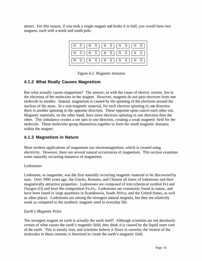
Page 41

attract. For this reason, if you took a single magnet and broke it in half, you would have two magnets, each with a north and south pole.

Figure 4.2: Magnetic domains

4.1.2 What Really Causes Magnetism But what actually causes magnetism? The answer, as with the cause of electric current, lies in the electrons of the molecules in the magnet. However, magnets do not pass electrons from one molecule to another. Instead, magnetism is caused by the spinning of the electrons around the nucleus of the atom. In a non-magnetic material, for each electron spinning in one direction there is another spinning in the opposite direction. These opposite spins cancel each other out. Magnetic materials, on the other hand, have more electrons spinning in one direction than the other. This imbalance creates a net spin in one direction, creating a weak magnetic field for the molecule. These molecules group themselves together to form the small magnetic domains within the magnet.

4.1.3 Magnetism in Nature Most modern applications of magnetism use electromagnetism, which is created using electricity. However, there are several natural occurrences of magnetism. This section examines some naturally occurring instances of magnetism. Lodestones Lodestone, or magnetite, was the first naturally occurring magnetic material to be discovered by man. Over 2000 years ago, the Greeks, Romans, and Chinese all knew of lodestones and their magnetically attractive properties. Lodestones are composed of iron (chemical symbol Fe) and Oxygen (O) and have the composition Fe3O4. Lodestones are commonly found in nature, and have been found in large quantities in Scandinavia, South Africa, and the United States, as well as other places. Lodestones are among the strongest natural magnets, but they are relatively weak as compared to the synthetic magnets used in everyday life. Earth’s Magnetic Poles The strongest magnet on earth is actually the earth itself! Although scientists are not absolutely certain of what causes the earth’s magnetic field, they think it is caused by the liquid outer core of the earth. This is mostly iron, and scientists believe it flows in currents; the motion of the molecules in these currents is theorized to create the earth’s magnetic field.

Page 42

The earth’s magnetic poles are not at the same places as its geographic poles. The north magnetic pole is actually in far northern Canada, about 800 miles from the North Pole, and the south magnetic pole is off the coast of Antarctica, about 1600 miles from the geographic South Pole. The magnetic poles tend to wander a bit, sometimes as much as 50 miles in a day. This is due to the interaction of the earth and the solar wind. In addition to the daily variations, the earth’s magnetic poles sometimes reverse themselves, with the north magnetic pole become south and vice versa. When this happens, the earth’s magnetic field changes direction (and the sale of compasses increases dramatically). This happens about every 500,000 years. Speaking of compasses, why do compasses point north? The needle of a compass is actually a small permanent magnet. The “north” tip of the compass needle is the north pole of its magnet, and is attracted to the north magnetic pole. The north pole of the magnet should not be attracted to the north magnetic pole if both are north poles. Similar poles should repel each other, yet the north pole of the compass magnet does indeed point north. In reality, what we call the north magnetic pole is actually the south pole of the earth’s magnetic field! Similarly, the so-called south magnetic pole is actually a north pole. Magnetosphere and Auroras The earth’s magnetosphere is a region above the earth’s surface containing charged particles that are affected by the earth’s magnetic field. It plays an important role in one of nature’s most picturesque magnetic phenomena, the auroras. Sunspots emit a large number of high-energy charged particles, some of which make their way through the earth’s magnetosphere. These articles create an overload of charged particles in the lower Van Allen belt, which is basically a belt of radiation trapped around the earth. These excess charged particles enter the atmosphere near the earth’s magnetic poles and collide with gas molecules in the atmosphere. These collisions make the molecules emit energy in the form of visible light. This happens for many molecules; their resulting light display is an aurora. In the northern hemisphere this display is called the Aurora Borealis, or northern lights. The equivalent southern lights are called the Aurora Australis.

4.2 Electromagnetism Naturally occurring magnets are not used much these days. Most magnets are man-made; among these, electromagnets are the most useful. This section examines electromagnets, how they use electricity to create magnetism, and some practical applications in everyday life.

4.2.1 Using Electricity to Create Magnetism When current flows through a wire, it creates a magnetic field. The field is perpendicular to the wire; you could envision the field as a series of tubes surrounding the wire at all points. This particula r configuration, having current flow through a straight piece of wire, doesn’t offer too many practical applications for its magnetic field. However, we can bend and twist the wire to concentrate its magnetic field. In particular, you can strengthen the field by

Page 43

bending the wire into a series of loops and wrapping the loops around something like a nail. The magnetic field is still perpendicular to the wire, but now it travels along the nail. The field is more concentrated and thus stronger than the field generated by a straight wire. We’ll see more about this in the laboratory exercise at the end of this chapter.

4.2.2 Electromagnetism in Everyday Life Electromagnetism plays in an important role in everyday life. Here are a few devices you might have encountered recently that use electromagnetism. Speakers Almost all devices with speakers use electromagnetism to convert electricity to sound. In radios and stereos, the incoming electrical signal was derived from some sound, and must be converted back to sound. An electromagnet on a speaker uses the electric signal to create a magnetic field. This field causes the speaker to vibrate, producing the original sound. There are also speakers in many other devices, including televisions, telephones, and computers. The speakers on these devices convert electricity to sound in the same way. Television In addition to generating sound using electromagnetism, a standard television set also uses electricity to show a picture on its screen. The screen is coated with phosphors of different colors. A beam of electrons strikes the correct phosphors to display the desired image. Now this is where electromagnetism plays a role. The television screen includes an electromagnet in the shape of a ring. The beam of electrons passes through the ring. The current in the ring is varied, which in turn varies the electromagnetic field. This variation affects the electron beam, causing it to bend up, down, right, or left. By supplying varying amounts of current to the ring, it steers the electron beam, which makes it draw its picture on the entire screen. This discussion only holds true for televisions that use cathode ray tubes. Never televisions, such as LCD flat panels, use other technologies to create the images on their screens. Motors Motors are used in many different devices, from household appliances to large, industrial machines. Regardless of size, they almost all use electromagnetism to turn the center shaft of the motor; this physical rotation is then used to perform useful work. In these motors, electricity is used to create magnetic fields. The fields are varied, which ultimately causes the shaft of the motor to turn. Motors can use either alternating current (AC), direct current (DC), or both types of current. Solenoids

Page 44

A solenoid uses electromagnetism to push a shaft up or down. If your car has power door locks, it probably uses solenoids. They can also be found in pinball machines, where they cause the bumpers to bump.

4.3 Laboratory Exercise In this experiment you will build and test an electromagnet. By varying the voltage and current, and spacing of the wire loops, we will examine their effect on the strength of the magnetic field. PARTS LIST:

• Build an Electromagnet Kit (Kelvin.com, item number 840709, $5.95 each) • Power supply • Graph paper

Part 1 – Constructing the Electromagnet The electromagnet for this experiment is constructed from the kit listed in the parts list. Follow the instructions included with the kit, except for the power connections. The kit used eight AA batteries to supply power. For this experiment we will use only two batteries first, then four, six, and eight batteries. This will allow us to vary the voltage to determine its effect on magnetism. For the first part of this experiment, loop the wire around the conductive nail 15 times. Leave a little space between the loops so they do not touch each other. Use only two batteries to set the voltage to 3V. This creates an electromagnetic field. Now use the electromagnet to pick up as many paper clips as possible at the same time. The number of paper clips will be used to show the relative strength of the electromagnet. Record the number of paper clips on the laboratory worksheet. Now use four batteries to change the voltage to 6V and repeat the procedure. Repeat this procedure for six batteries (9V) and eight batteries (12V). Part 2 – Electromagnet without Gaps between the Wires In the first part of this experiment we left a small gap between the loops of wire. Now we will remove these gaps to determine their effect on the magnetic field. Take the electromagnet from the first part of this experiment and slide the wire loops together so they touch each other. Now repeat the procedure in Part 1, using voltages of 3V, 6V, 9V, and 12V. Again, record the number of paper clips picked up by the electromagnet on the laboratory worksheet. Part 3 – Data Analysis Now we will graph this data and draw some conclusions about the effects of voltage and wire spacing on the strength of the electromagnetic field. First graph the voltage vs. the number of paper clips picked up for Part 1. Then do the same for the data from Part 2. From these graphs, what conclusions can you draw about the effect of voltage on the strength of the electromagnetic field?

Page 45

Next, let’s look at the spacing of the wire loops on field strength. Graph the number of paper clips picked up by the electromagnets with a source voltage of 3V, both the electromagnet with space between the wire loops and the electromagnet without gaps. Repeat this for the source voltages of 6V, 9V, and 12V. What effect does the spacing of the loops have on the strength of the electromagnetic field?

Page 46

Laboratory Worksheet – Electromagnets

Part 1: Voltage # of paper clips picked up

3V

_____________________

6V

_____________________

9V

_____________________

12V

_____________________

Part 2: Voltage

# of paper clips picked up

3V

_____________________

6V

_____________________

9V

_____________________

12V

_____________________

Page 47

5 Boolean and Digital Logic Fundamentals One of the most recent introductions in electrical devices is the personal computer. As with all computers, this relies on voltages and currents, but uses levels to represent binary and Boolean values. In this chapter we look at Boolean values and Boolean logic, and basic digital logic devices that realize Boolean operations.

5.1 Introduction to Boolean Logic Boolean logic is the basis for digital system design, from the simplest circuits to the most advanced computer systems. From a logic standpoint, a Boolean value can be true or false; on or off; yes or no; “maybe” is not allowed. You can think of this like a light switch that can be either on or off; no dimmer switches allowed. In digital logic, true is usually represented by a 1 and false is denoted as 0. Having a Boolean value of 0 or 1 is good in and of itself, but it isn’t very useful on its own. To perform useful work with Boolean values, and ultimately the digital circuits we design, we must be able to perform functions that combine different values to produce desired results. There are several basic functions for Boolean values, including the AND, OR, Exclusive-OR, and NOT functions.

5.1.1 The Logical AND Function The AND function is one of the most commonly used functions in Boolean algebra. It takes two or more Boolean values as its inputs and generates a single Boolean output. This output is 1 (on) only if all of its inputs are 1; if any input is 0 (off) then the output is 0, even if all of the other inputs are 1. This is similar to what you might see if you serve on a jury. For criminal trials, the jury must return a unanimous verdict to convict the defendant. Here, every juror must vote guilty (1) to produce a verdict (output) of guilty. If any juror votes not guilty (0), there can be no guilty verdict. As another example, consider the extreme example of an AND function with one million inputs. If 999,999 of these input values are 1, but the other input is 0, the AND function outputs a 0. The AND function can be represented using several notation. The AND of Boolean values A and B can be represented as A ∧ B, A⋅B, or simply AB. One way to visualize the AND function is as a circuit consisting of a battery, a light bulb, and two or more switches in series, as shown in Figure 5.1. The switches represent the input values to the Boolean function; a closed switch represents a 1 (on) and an open switch represents a 0 (off). The light bulb corresponds to the output of the AND function. The bulb is on when the function outputs a 1. Figure 5.1(a) gives an example where input A = 1 and input B = 0, producing an output of 0. Figure 5.1(b) shows the same circuit, except A = 1 and B = 1, producing an output of 1 and lighting the bulb.

Page 48

Figure 5.1: Illustration of the AND function producing results of (a) 0, and (b) 1

5.1.2 The Logical OR Function The OR function is more tolerant of its input values. Its output is 1 if any of its inputs are 1. Returning to our extreme, one million input function, if 999,999 of the inputs are 0 but the remaining input is 1, the OR function outputs a 1. The OR of Boolean values A and B can be represented as A ∨ B or A + B. Be careful with the latter notation. Here, A + B is not arithmetic. In standard arithmetic, 1 + 1 = 2; however, in Boolean logic, 1 + 1 = 1. To visualize this function, consider the circuits shown in Figure 5.2. The switches representing A and B are connected in parallel; setting either switch to 1 completes the circuit and lights the bulb. Figure 5.2(a) shows input values of A = 1 and B = 0, which produces an output of 1. Figure 5.2(b) shows inputs of A = 0 and B = 0, generating a result of 0.

Figure 5.2: Illustration of the OR function producing results of (a) 1, and (b) 0

5.1.3 The Logical Exclusive-OR Function The Exclusive-OR, XOR, function, is based on the OR function. Unlike the OR function, however, for the Exclusive-OR function the number of inputs that are 1 does matter. If two inputs are 1, their XOR is equal to 0, not 1; the logical OR of two inputs with values of 1 is 1. When more than two input values are Exclusive-ORed, the output if 1 if an odd number of inputs are 1 and 0 if the number of inputs with values of 1 is even. The Exclusive-OR of Boolean values A and B is represented as A ⊕ B.

Page 49

The Exclusive-OR function is similar to a 3-way switch you might find at the top and bottom of a stairway in a house. If one switch is up and the other is down, the light is off. If both switches are up, or both are down, the light is lit. (This may be reversed in some houses. My house has two sets of 3-way switches. The upstairs light is lit when the switches are in opposite positions; the downstairs light is only lit when both switches are in the same position.) Figure 5.3 shows an Exclusive-OR configuration in which the switches must be in opposite positions to light the bulb, or output a 1. In Figure 5.3(a), A = 0, B = 1, and the output is 1. Figure 5.3(b) shows A = 1, B = 1, and an output of 0.

Figure 5.3: Illustration of the XOR function producing results of (a) 1, and (b) 0

5.1.4 The Logical NOT Function Unlike the AND, OR, and XOR functions, which received two or more inputs, the NOT function operates on a single input. Its output is the opposite of its input value. An input of 0 produces an output of 1, and an input value of 1 generates a 0 output. The NOT of Boolean value A can be represented as A', /A, or !A. Figure 5.4 illustrates a NOT function for input values of 0 and 1.

Figure 5.4: Illustration of the NOT function producing results of (a) 1, and (b) 0

Page 50

Worksheet 5.1 – Boolean Logic Calculations Show the values of each function for the given values of A, B, and C. 1. A = 0, B = 0: A ∧ B = _______ A ∨ B = _______ A ⊕ B = _______ A' = _______ B' = _______ 2. A = 0, B = 1: A ⋅ B = _______ A + B = _______ A ⊕ B = _______ /A = _______ /B = _______ 3. A = 1, B = 0: AB = _______ A ∨ B = _______ A ⊕ B = _______ !A = _______ !B = _______ 4. A = 1, B = 1: A ∧ B = _______ A + B = _______ A ⊕ B = _______ A' = _______ B' = _______ 5. A = 1, B = 0, C = 1: A ⋅ B ⋅ C = _______ A ∨ B ∨ C = _______ A ⊕ B ⊕ C = _______ 6. A = 0, B = 1, C = 0: A ⋅ B ⋅ C = _______ A ∨ B ∨ C = _______ A ⊕ B ⊕ C = _______

Page 51

5.2 Truth Tables Truth tables are a mechanism used to express the operations of a function for all possible input values. In the previous worksheet, we calculated the values of the functions A ∧ B, A ∨ B, A ⊕ B, A', and B' for all possible values of A and B. Truth tables show these values in a convenient format. A truth table has two groups of columns, and several rows of data. The left-hand group of columns consists of all inputs. Each row of the table shows a different combination of input values. For example, a table with two inputs, A and B, would have values of A = 0 and B = 0 in its first row, followed by A and B of 0 and 1; 1 and 0; and 1 and 1, as shown in Table 5.1.

A B Function 0 0 0 1 1 0 1 1

Table 5.1: A generic truth table for a 2-input function

Consider the truth table for the 2- input AND function shown in Table 5.2(a). The left

hand side shows the two inputs, A and B, and all possible combinations of values for these inputs, one combination per row. The first row shows A = 0 and B = 0, followed by rows for A = 0 and B = 1, A = 1 and B = 0, and A = 1 and B = 1. The right hand side of the table shows the output of the AND function for these input values. The AND function only outputs a 1 when A = 1 and B = 1. It outputs a 0 at all other times. Tables 5.2(b), (c), and (d) show the truth tables for the OR, XOR, and NOT functions.

A B A ∧ B A B A ∨ B A B A ⊕ B A A′ 0 0 0 0 0 0 0 0 0 0 1 0 1 0 0 1 1 0 1 1 1 0 1 0 0 1 0 1 1 0 1 1 1 1 1 1 1 1 1 0

(a) (b) (c) (d)

Table 5.2: Truth tables for the (a) AND, (b) OR, (c) XOR, and (d) NOT functions

5.3 Complementary Functions – NAND, NOR, and Exclusive-NOR In addition to the AND, OR, XOR, and NOT functions, there are three common, complementary functions. The NAND function is the opposite of the AND function; it may help to think of the NAND as the NOT-AND function. The NAND of two or more inputs is 0 if all of the inputs are 1; if any input is 0, the output of the NAND is 1. Table 5.3(a) shows the truth table for the 2-input NAND function. Note that its outputs are exactly the opposite of those for the AND function of Table 5.2(a)

Page 52

A B NAND A B NOR A B XNOR 0 0 1 0 0 1 0 0 1 0 1 1 0 1 0 0 1 0 1 0 1 1 0 0 1 0 0 1 1 0 1 1 0 1 1 1

(a) (b) (c)

Table 5.3: Truth tables for the (a) NAND, (b) NOR and (c) XNOR functions There are also complementary functions for the OR and XOR functions. The NOR function produces an output of 1 only when all of its inputs are 0. Its truth table is shown in Table 5.3(b); as with the NAND and AND functions, the outputs of the NOR function are exactly the opposite of the OR function. The Exclusive-NOR, or XNOR, function outputs a 1 when an even number of inputs are 1, and 0 when an odd number of inputs are 1. Its truth table is shown in Table 5.3(c). Again, the outputs of the XNOR function are exactly the opposite of those of the XOR function in Table 5.2(c). Note that the output of the 2- input XNOR function is 1 whenever the two inputs are the same. For this reason, the 2-input XNOR function is sometimes referred to as the equivalence function.

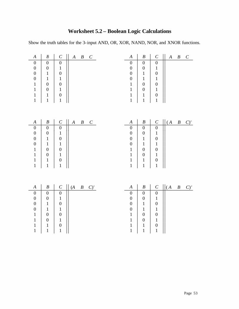
Page 53

Worksheet 5.2 – Boolean Logic Calculations Show the truth tables for the 3- input AND, OR, XOR, NAND, NOR, and XNOR functions.

A B C A ∧ B ∧ C A B C A ∨ B ∨ C 0 0 0 0 0 0 0 0 1 0 0 1 0 1 0 0 1 0 0 1 1 0 1 1 1 0 0 1 0 0 1 0 1 1 0 1 1 1 0 1 1 0 1 1 1 1 1 1

A B C A ⊕ B ⊕ C A B C ( A ∧ B ∧ C)' 0 0 0 0 0 0 0 0 1 0 0 1 0 1 0 0 1 0 0 1 1 0 1 1 1 0 0 1 0 0 1 0 1 1 0 1 1 1 0 1 1 0 1 1 1 1 1 1

A B C (A ∨ B ∨ C)' A B C ( A ⊕ B ⊕ C)' 0 0 0 0 0 0 0 0 1 0 0 1 0 1 0 0 1 0 0 1 1 0 1 1 1 0 0 1 0 0 1 0 1 1 0 1 1 1 0 1 1 0 1 1 1 1 1 1

Page 54

5.4 Digital Logic Logic gates are digital components that implement the logic functions described earlier. They are usually represented by the symbols shown in Figure 5.5. For functions with more than two inputs, the gate symbols are the same, except more inputs are added to the gate. (The NOT gate is an exception; it can never have more than one input.) Each gate always has one output regardless of the number of inputs.

Figure 5.5: Logic symbols for the (a) AND, (b) OR, (c) XOR, (d) NOT, (e) NAND, (f) NOR, and (g) XNOR gates

Notice that the NOT, NAND, NOR, and XNOR gates have small circles at their outputs.

This indicates that the output of the gate is complemented, or inverted. For example, consider the AND and NAND gates. They look the same, except the NAND gate has a small circle at its output. Remember, as shown in the truth tables, the output of the NAND gate is the complement of the output of the AND gate. Logically, you can consider the NAND gate to be an AND gate which sends its output to a NOT gate, as shown in Figure 5.6(a). The reverse is also true; an AND gate has the same logical function as a NAND gate that sends its output to a NOT gate as shown in Figure 5.6(b).

Figure 5.6: Logical implementation of (a) a NAND function using AND and NOT gates, and (b)

an AND function using NAND and NOT gates

Page 55

5.5 TTL Chips To build logic circuits, designers can use Integrated Circuit chips, or ICs, or chips. Different ICs are available with the gates we’ve seen so far, as well as more advanced components. A chip may look like the chip shown in Figure 5.7(a). The black box in the center of the chip contains the circuitry that implements the chip’s functions. The metal strips on the sides of the chip are its pins. These pins interface the logic gates in the chip to the rest of the circuit. For a NAND gate with two inputs, two of the chip’s pins would connect to the inputs of the NAND gate, and the output of the NAND gate would connect to another pin. By connecting the pins of the chip, we incorporate the NAND gate into a circuit.

(a) (b)

Figure 5.7: (a) A 7400 Quad 2- input NAND gate, and (b) its logic diagram

Figure 5.7(b) shows the logical organization of a 7400 TTL chip. This chip has four, 2-

input NAND gates. For each NAND gate, two pins are connected to the gate’s inputs and one pin connects to its output. This accounts for 12 of the chip’s 14 pins. The other two pins are used for power connections. Notice that the pins are numbered counterclockwise around the chip starting in the upper left corner. Chips usually have a dot by pin 1 or a notch at the top of the chip, such as the notch shown in the figure, so you can tell how to connect it in your circuit. The logic gates require power in order to function; we use the two power pins to supply power to the chip and its gates. Recall from the circuits covered earlier, those consisting of switches and light bulbs, that a circuit must be completed from the battery’s positive terminal to its negative terminal in order for current to flow. One of the two power pins, denoted Vcc, is connected to the positive terminal. The other power pin, Gnd or ground, is connected to the negative terminal. For TTL chips, the voltage of the battery or power supply is 5 volts, denoted 5V.

Page 56

5.6 Where Boolean Logic Meets Digital Logic A TTL chip doesn’t know what binary values 0 and 1 are. To input a 1 to a gate, we supply a voltage at a given level. For TTL chips, logic 1 is a voltage at or near 5V, the voltage of the chip’s power supply. A voltage near 0V is used for logic 0. The same voltage values are used for the inputs and outputs. Other Logic Chips Now let’s look at some other chips. The 7402 chip has four NOR gates; its logic diagram is shown in Figure 5.8(a). The 7404 is a hex inverter, having six NOT gates. It is shown in Figure 5.8(b). Figure 5.8(c) shows the 7408 chip, which has four AND gates. The quad OR, XOR, and XNOR chips, the 7432, 7486, and 74266, respectively, are shown in Figures 5.8(d), (e), and (f).

(a) (b)

(c) (d)

(e) (f) Figure 5.8: Logic diagrams for the (a) 7402, (b) 7404, (c) 7408, (d) 7432, (e) 7486, and (f) 74266

chips

Page 57

5.7 Laboratory Exercise – Digital Logic In this laboratory exercise, students will test several logic chips to verify their functions. Students will also test an “unknown” chip to determine the Boolean function it realizes. PARTS LIST:

• Protoboard and wires • Power supply and leads • Logic probe • 7408 (AND gates), 7432 (OR gates), and 7486 (XOR gates) chips • One additional TTL chip, either 7400, 7402, 7404, 7408, 7432, or 7486 • Black tape to cover one “unknown” chip

Background To perform this experiment, students will need to become familiar with the protoboard and logic probe they will use. Both are described in this section.

We can construct a circuit using digital logic chips, but we need a surface to secure the chips and wires that comprise the circuit. This is the function of the protoboard. Chips and wires are plugged into the protoboard and can be rearranged easily as the design is modified. (Final circuits are wired on breadboards. Protoboards are typically used during the design of prototypes, hence its name.) A typical protoboard is shown in Figure 5.9.

Figure 5.9: A typical protoboard

The terminals at the top of the protoboard are used to connect the power supply (Vcc and Gnd) to the circuit. One pair of cables connects the power supply to these terminals, and wires connect the terminals to the protoboards. The main protoboard surface consists of a grid of holes. The pins of the chips in a circuit are plugged into these holes; for reasons that will be explored shortly, the chips must straddle the relatively large channels, or gutters, separating columns of holes. The chips cannot be placed so that they are in the leftmost nor rightmost two columns. These special columns are reserved for Vcc and Gnd. The protoboard has connections embedded within its structure so that certain holes are always connected to each other. As a result, wires and pins plugged in to connected holes are also connected. This greatly simplifies the task of wiring up circuits. Any hole is connected to

Page 58

all other holes in the same row between the same two channels; this is illustrated in Figure 5.10. This is the reason that chips must straddle the gutters, to avoid inadvertently connecting pins on the same chip. The power columns are also connected, but in a different way. Here, holes are connected to other holes in the same column. Designers can connect wires from the two terminals connected to Vcc and Gnd to these columns, and then connect wires from these

columns to the power pins of each chip.

Figure 5.10: Protoboard internal connections

We will use a logic probe to test the functions of our chips. First we must connect the logic probe’s Vcc and Gnd clips so the probe has power. We can clip them directly to the terminals of the protoboard. Then we touch the tip of the logic probe to the pin we wish to test. The logic probe has two LEDs that will be used in this experiment. When the probe detects a 0, its “Low” LED lights up; the “High” LED lights when a logic 1 is detected. We can use the logic probe to check the input and output values of a chip. Figure 5.11 shows a typical logic probe.

Figure 5.11: Logic probe To test our chips, we will need to input values to the gates. To input a 1, we will connect a wire between the chip’s input and Vcc. We can input a 0 by connecting the wire from the chip’s input to Gnd.

Page 59

Part 1 – Testing Known Chips In the first part of this exercise, students will test several logic chips. Each group of students has a protoboard with three known chips: a 7408 (AND gates), 7432 (OR gates), and 7486 (XOR gates). The chips have been pre-wired to Vcc and Gnd, and wires have been connected to the two inputs of one gate for each chip. Power supplies have been set up; students only need to connect the power cables from the power supply to the protoboard. Starting with the AND gate, connect both inputs to Gnd, producing a logic 0 for each input. Use the logic probe to verify these input values, and then check the output values for the gate. Record your output values on the worksheet for this exercise. Next, change one of the inputs to Vcc, changing it to logic 1. Again verify your input values and determine your output value using the logic probe, and record your output value on the worksheet. Repeat this for all possible combinations of the input values, and then verify that your values match those in the truth table for the AND function. Repeat this procedure for the OR and XOR gates. Part 2 – Testing an Unknown Chip The protoboard for this exercise also contains a chip which has tape covering its surface. Here you will determine its function without removing the tape. To do this, follow the same procedure you used in the first part of this exercise. Vary the values of the inputs to the chip and record its outputs on the worksheet. Then compare the truth table for your unknown chip to those given earlier in this chapter and find the table that matches the unknown chip’s table. What is the function of your unknown chip?

Page 60

Laboratory Worksheet – Digital Logic Chips AND gate OR gate XOR gate

A B Output A B Output A B Output 0 0 0 0 0 0 0 1 0 1 0 1 1 0 1 0 1 0 1 1 1 1 1 1

Unknown gate

A B Output 0 0 0 1 1 0 1 1 Gate type: ______________________

Page 61

6 More Complex Boolean Functions The Boolean functions introduced in the previous chapter are the most basic Boolean functions available. In this chapter we examine ways of combining these basic functions to realize more complex functions that model real-world situations.

6.1 Combining Logical Operations The AND, OR, XOR, and NOT functions introduced in the previous chapter are useful in their own right, but they are most useful when combined to form more complex functions. In the real world, situations that cannot be described with a single AND or OR function often can be modeled by combining logical operations. For example, consider the following scenario. A teenager wants to buy a car but doesn’t have any money for a down payment. Ignoring options that involve borrowing money from his parents, winning the lottery, or robbing a bank, the teenager has two options. One is to earn more money, possibly by working more hours or taking a second job. The other is to earn the same amount of money and spend less, maybe by giving up his cell phone. We could express these options by combining the logical AND and OR operations as follows.

Get $ to buy car = (Earn more $) OR (Earn same $ AND Spend less $)

6.2 Modeling Real-world Situations

We can design a circuit to model this function. We would need three switches, one each for Earn more $, Earn same $, and Spend less $. We would also need one light bulb to represent the output Get $ to buy car and a battery to supply power to the circuit. The circuit would light the bulb if Earn more $ is TRUE (1), or if both Earn same $ and Spend less $ are true. The circuit to do this is shown in Figure 6.1. Notice that this circuit combines elements of the AND and OR circuits from the previous chapter. The light can be lit if both Earn same $ and Spend less $ are on (TRUE). This is the AND function. The light can also be lit if Earn more $ is true. Having either option light the bulb is an OR function.

Figure 6.1: Circuit to generate the Get $ to buy car function

Page 62

6.3 Truth Tables for Combined Functions Just as with any logic function, we can create a truth table for our car buying example. Here the variables are the three conditions Earn more $, Earn same $, and Spend less $, which we represented as switches in our circuit. There is one output for this function, Get $ to buy car; this was represented as a light bulb in our circuit. Each input, and the output, can be either TRUE or FALSE. The truth table for this scenario is shown in Table 6.1. Table 6.1(a) shows the truth table with values of TRUE and FALSE. Table 6.1(b) shows the same table with binary values 1 and 0; 1 represents TRUE and 0 corresponds to FALSE.

Earn more $

Earn same $

Spend less $

Get $ to buy car

Earn more $

Earn same $

Spend less $

Get $ to buy car

FALSE FALSE FALSE FALSE 0 0 0 0 FALSE FALSE TRUE FALSE 0 0 1 0 FALSE TRUE FALSE FALSE 0 1 0 0 FALSE TRUE TRUE TRUE 0 1 1 1 TRUE FALSE FALSE TRUE 1 0 0 1 TRUE FALSE TRUE TRUE 1 0 1 1 TRUE TRUE FALSE TRUE 1 1 0 1 TRUE TRUE TRUE TRUE 1 1 1 1

(a)

(b)

Table 6.1: Truth tables for the Get $ to buy car function

6.3.1 Creating the Exclusive-OR Function Let’s look at another way of creating the exclusive-OR function. Instead of using an XOR gate, we will construct this function using AND, OR, and NOT operations. (As we’ll see later in this chapter, programmable logic devices, chips that can be programmed to perform different logical functions, do exactly that.) First we start with the truth table for the exclusive-OR function, shown in Table 6.2.

A B A ⊕ B 0 0 0 0 1 1 1 0 1 1 1 0

Table 6.2: Truth table for the XOR function

To create the XOR function, we will develop functions that generate each 1 output

separately and then logically OR these functions together. Looking at the table, we can see that A ⊕ B = 1 twice, when A = 0 and B = 1, and when A = 1 and B = 0. First we will create the

Page 63

function to generate the first 1. This function is 1 when A = 0 and B = 1, or when A' = 1 and B = 1. (Remember that A' is the NOT of A; if A = 0 then A' = 1, and if A = 1 then A' = 0.) We can implement this function as A' ^ B, or A'B. Its truth table is shown in Table 6.3(a).

A B A'B A B AB' A B A'B + AB' = A ⊕ B

0 0 0 0 0 0 0 0 0 0 1 1 0 1 0 0 1 1 1 0 0 1 0 1 1 0 1 1 1 0 1 1 0 1 1 0

(a) (b) (c)

Table 6.3: Truth tables for the functions (a) A'B, (b) AB', and (c) A'B + AB' = A ⊕ B

Next we calculate the function for the second 1. This occurs when A = 1 and B = 0, or if A = 1 and B' = 1. Its function is AB', and its truth table is shown in Table 6.3(b).

Finally, we logically OR these two functions together to produce a single, combined function. Here this function is A'B + AB', which is true whenever either A'B or AB' is true. Its truth table is shown in Table 6.3(c). Note that this truth table is identical to the truth table for A ⊕ B given in Table 6.2. Therefore, A ⊕ B = A'B + AB'.

Page 64

Worksheet 6.1 – Truth Tables

Show the truth tables for the following functions.

A B C A + B + C A B C AB BC AB + BC 0 0 0 0 0 0 0 0 1 0 0 1 0 1 0 0 1 0 0 1 1 0 1 1 1 0 0 1 0 0 1 0 1 1 0 1 1 1 0 1 1 0 1 1 1 1 1 1

A B C A'BC A'C' A'BC + A'C' A B C A'C BC A'B A'C + BC + A'B 0 0 0 0 0 0 0 0 1 0 0 1 0 1 0 0 1 0 0 1 1 0 1 1 1 0 0 1 0 0 1 0 1 1 0 1 1 1 0 1 1 0 1 1 1 1 1 1

A B C ABC ABC' A'B ABC + ABC' + A'B 0 0 0 0 0 1 0 1 0 0 1 1 1 0 0 1 0 1 1 1 0 1 1 1

Page 65

6.3.2 Determining Functions from Truth Tables Besides using functions to create truth tables, we can also work in the other direction. We can use truth tables to determine its function. Consider, for example, the truth table shown in Table 6.4. This function has three inputs, A, B, and C, and one output function.

A B C Function 0 0 0 1 0 0 1 0 0 1 0 1 0 1 1 0 1 0 0 0 1 0 1 0 1 1 0 0 1 1 1 1

Table 6.4: Truth table for an unknown function

Three different combinations of input values cause this function to be 1. The first occurs when A = 0, B = 0, and C = 0, or A' = 1, B' = 1, and C' = 1. This can be expressed as A' ^ B' ^ C', or A'B'C'. The function is also 1 when A = 0, B = 1, and C = 0, or A' = 1, B = 1, and C' = 1. This is A'BC'. Finally, the function is 1 when A = 1, B = 1, and C = 1, or ABC. We can combine them to form a single function that matches this truth table, A'B'C' + A'BC' + ABC. Table 6.5 shows a truth table for each individual component of the function and the overall function.

A B C A'B'C' A'BC' ABC A'B'C' + A'BC' + ABC 0 0 0 1 0 0 1 0 0 1 0 0 0 0 0 1 0 0 1 0 1 0 1 1 0 0 0 0 1 0 0 0 0 0 0 1 0 1 0 0 0 0 1 1 0 0 0 0 0 1 1 1 0 0 1 1

Table 6.5: Truth table for the function and its components

Page 66

Worksheet 6.2 – Truth Tables Show the functions for the following truth tables. Express each entry in the truth table that generates an output of 1 as a separate term.

A B C Function 0 0 0 1 0 0 1 1 0 1 0 1 0 1 1 1 1 0 0 1 1 0 1 1 1 1 0 1 1 1 1 0 Overall function: ______________________________



Page 67

6.3.3 Simplifying Functions Sometimes we can simplify a function by combining some of its terms. For the truth table in Table 6.5, take a look at the first two lines that produce outputs of 1. The inputs for these two lines are A = 0, B = 0, and C = 0, and A = 0, B = 1, and C = 0. Notice that both A = 0 and C = 0 in both cases. As long as A and C are both 0, the function should produce a 1, regardless of the value of B. If B = 0, then A = 0, B = 0, and C = 0, and A'B'C' is 1. If B = 1, then A = 0, B = 1, and C = 0, and A'BC' is 1. We can replace these two terms by the single term A'C'. Our function would then become A'C' + ABC; its truth table is shown in Table 6.6.

A B C A'C' ABC A'C' + ABC 0 0 0 1 0 1 0 0 1 0 0 0 0 1 0 1 0 1 0 1 1 0 0 0 1 0 0 0 0 0 1 0 1 0 0 0 1 1 0 0 0 0 1 1 1 0 1 1

Table 6.6: Truth table for the simplified function

In general it is desirable to simplify functions. If you implement a function using logic

gates, simplifying the function usually results in simpler circuits.

Page 68

Worksheet 6.3 – Truth Tables Show the simplified functions for the following truth tables. Express each entry in the truth table that generates an output of 1 as a separate term.

A B C Function 0 0 0 1 0 0 1 1 0 1 0 1 Original function: ______________________________ 0 1 1 1 1 0 0 1 1 0 1 1 1 1 0 1 1 1 1 0 Simplified function: ____________________________



Page 69

6.4 Programmable Devices If you were designing a digital circuit to implement a logical function, you could use the 7400, 7402, and other chips introduced in Chapter 5. For complex functions, this can result in large circuits that use many chips. It would be better if you could create the circuit using fewer chips. It would be smaller, would require less power, and would be cheaper to build. Chip designers created Programmable Logic Devices, PLDs, for this reason. A PLD contains many logic gates, usually AND, OR, and NOT gates. Instead of wiring up individual chips, you program connections inside the chip to “wire up” your circuit. The designer uses a software program on a personal computer or workstation to determine the connections, and the program and computer work together to program the chip. A typical PLD has large numbers of AND gates. The inputs of the chip, and their NOTted values, can be connected to the inputs of these AND gates. The outputs of the AND gates can be connected to the inputs of OR gates, and the outputs of these gates produce the outputs of the chip. Consider, for example, the function A'C' + ABC that we generated earlier. We can configure one AND gate of a PLD to have A' and C' as its inputs, and another AND gate to have A, B, and C as its inputs. The outputs of these AND gates are then input to an OR gate to generate the function A'C' + ABC.

Figure 6.2 shows how this would look inside a PLD. The boxes represent connections within the chip. A chip input (or its complement) connected to the input of an AND gate is denoted by a filled in box. The outputs of AND gates are connected to the inputs of OR gates in the same way. In this figure, the leftmost AND gate generates the term A'C', the rightmost AND gate produces the term ABC, and the OR gate generates the final function.

Figure 6.2: Implementing the function A'C' + ABC in a PLD

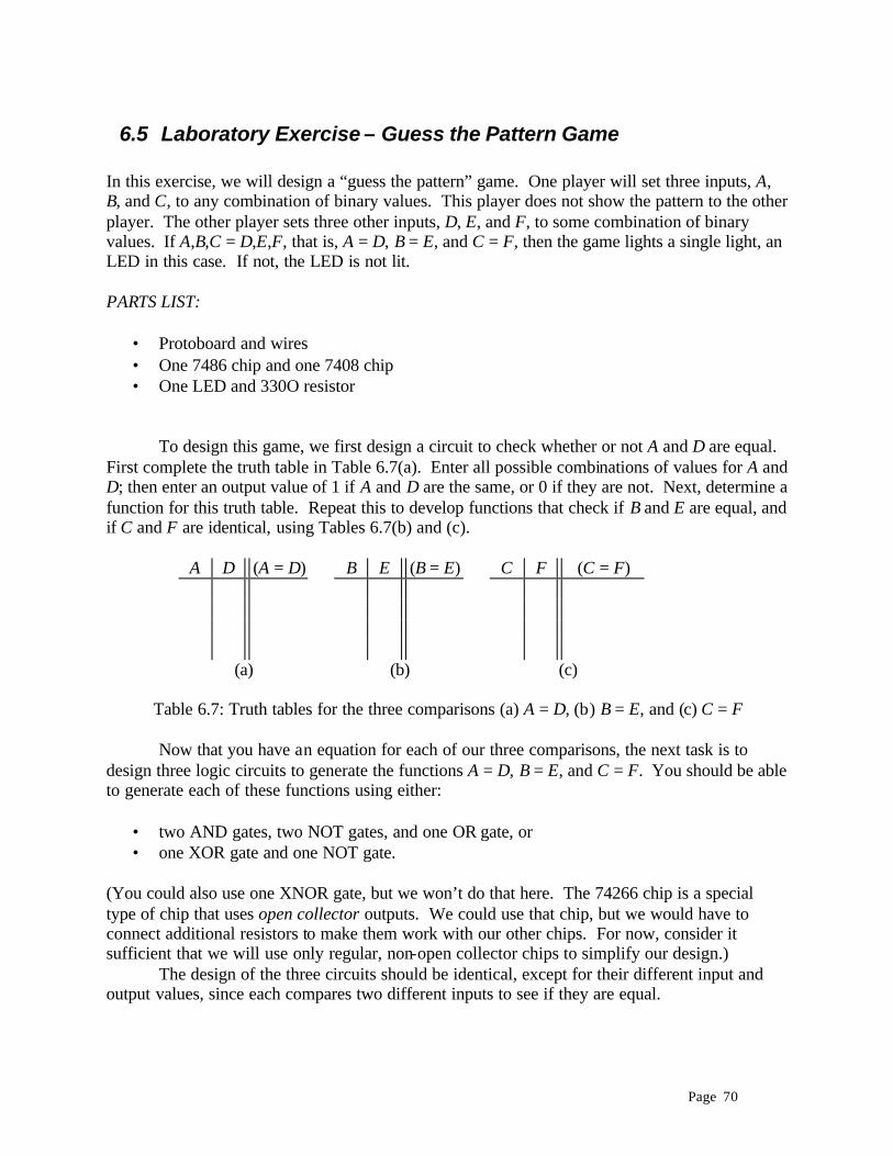
Page 70

6.5 Laboratory Exercise – Guess the Pattern Game In this exercise, we will design a “guess the pattern” game. One player will set three inputs, A, B, and C, to any combination of binary values. This player does not show the pattern to the other player. The other player sets three other inputs, D, E, and F, to some combination of binary values. If A,B,C = D,E,F, that is, A = D, B = E, and C = F, then the game lights a single light, an LED in this case. If not, the LED is not lit. PARTS LIST:

• Protoboard and wires • One 7486 chip and one 7408 chip • One LED and 330O resistor

To design this game, we first design a circuit to check whether or not A and D are equal. First complete the truth table in Table 6.7(a). Enter all possible combinations of values for A and D; then enter an output value of 1 if A and D are the same, or 0 if they are not. Next, determine a function for this truth table. Repeat this to develop functions that check if B and E are equal, and if C and F are identical, using Tables 6.7(b) and (c).

A D (A = D) B E (B = E) C F (C = F)

(a) (b) (c)

Table 6.7: Truth tables for the three comparisons (a) A = D, (b) B = E, and (c) C = F Now that you have an equation for each of our three comparisons, the next task is to design three logic circuits to generate the functions A = D, B = E, and C = F. You should be able to generate each of these functions using either:

• two AND gates, two NOT gates, and one OR gate, or • one XOR gate and one NOT gate.

(You could also use one XNOR gate, but we won’t do that here. The 74266 chip is a special type of chip that uses open collector outputs. We could use that chip, but we would have to connect additional resistors to make them work with our other chips. For now, consider it sufficient that we will use only regular, non-open collector chips to simplify our design.) The design of the three circuits should be identical, except for their different input and output values, since each compares two different inputs to see if they are equal.

Page 71

After designing and building these three circuits, test them using a logic probe. Vary the inputs to check every combination in the truth tables. Verify that each circuit correctly outputs a 1 whenever and only when it inputs are the same. Now we must take the three circuit outputs and combine them, outputting a 1 only when (A = D), (B = E), and (C = F) are all 1. First complete the truth table in Table 6.8. The inputs (A = D), (B = E), and (C = F) would be generated by the circuits we just designed. The truth table should have output (ABC = DEF) equal to 1 only when all three inputs are 1.

(A = D) (B= E) (C = F) (ABC = DEF)

Table 6.8: Truth table for the overall function (ABC = DEF)

Next we design a circuit to take these three inputs and output a 1 only when all three are 1. This is a relatively straightforward design. After designing this circuit, test all possible combinations of input values with a logic probe to verify that it generates an output of 1 only when all three inputs are 1. Now connect the sections of your circuits together as shown in Figure 6.3. The first three circuits check whether A = D, B = E, and C = F. The outputs of these circuits are input to the last circuit, which checks whether all three pairs of bits are the same. It outputs a 1 if the player has guessed the pre-set pattern, or 0 otherwise.

Page 72

Figure 6.3: Block diagram of the “guess the pattern” game Finally, we connect the (ABC = DEF) output to the LED, as shown in Figure 6.3. This is pre-wired on your protoboard; you only need to connect the wire from the LED to the output of your circuit. Notice the resistor in this circuit. This is needed to keep the LED from receiving too much current and burning out.

Page 73

7 More Complex Digital Components The digital components we’ve seen so far are fairly basic. Although they can perform some useful work on their own, they are rather limited. This chapter examines some more complex digital components that can be used to perform more complex functions. It looks at some components that change their outputs as the inputs change; these components include multiplexers, decoders, and encoders. It also presents some components that can store data for future use, including registers and counters. Finally, this chapter concludes with a laboratory experiment that uses some of the components described in this chapter. Note that some of the material in this chapter was adapted from Computer Systems Organization and Architecture, by John D. Carpinelli (Addison Wesley, Boston, MA, 2001).

7.1 Binary Numbers Many digital circuits deal with data. To understand how these circuits work, we must first understand how binary data works. In this section we will examine the binary representations of data. We will study the direct storage of data in binary, as well as the binary coded decimal, BCD, data format.

7.1.1 Binary Values In decimal notation, each digit has a specific value. This value depends on the digit itself, as well as its position. For example, the 1 in 12 is much less than the 1 in 1,234,567. The decimal number 1,234,567 can be thought of as 1,000,000 + 200,000 +30,000 + 4,000 + 500 + 60 + 7. Each digit is followed by some number of zeroes. In reality, the digit is actually multiplied by 10 raised to some power. That power depends on the location of the digit. For example, the 7 is multiplied by 100, or 1, since it is the rightmost digit. The 6 is one position to the left, so it is multiplied by 101, or 10, to produce a value of 60. The five is multiplied by 102, and so on. We could also express 1,234,567, as follows.

(1×106) + (2×105) + (3×104) + (4×103) + (5×102) + (6×101) + (7×100) The same holds true for binary values. However, since they use base 2 instead of base 10, we multiply the individual digits by powers of 2 instead of powers of 10. Consider the binary value 10111. This can be expressed as (1×24) + (0×23) + (1×22) + (1×21) + (1×20), which is 16 + 0 + 4 + 2 + 1 = 23 in decimal. Binary values can get very large very fast. For convenience, we sometimes use hexadecimal notation to express binary values. Each group of four bits, starting at the right hand side of the number, is represented as a single hexadecimal digit. For binary values from 0000 to 1001, we use the standard decimal digits 0 to 9; 0 = 0000, 1 = 0001, 2 = 0010, 3 = 0011, 4 = 0100, 5 = 0101, 6 = 0110, 7 = 0111, 8 = 1000, and 9 = 1001. However, binary values from 1010 to 1111 do not have obvious decimal equivalents. For that reason, we use the letters A through F to represent these values; A is 1010, B is 1011, C is 1100, D is 1101, E is 1110, and F is 1111.

Page 74

7.1.2 Binary Coded Decimal (BCD) Some applications require decimal data. Typical of these applications are those with digital displays. We could store such data in binary format, and convert the binary values to decimal to display the data, but there is a better way. Binary Coded Decimal, or BCD, notation stores each decimal digit as four binary bits. The binary value only uses the bit patterns 0000 to 1001 to represent 0 to9. The binary patterns corresponding to hexadecimal values A to F are not used. In this way we can store decimal data directly and operate on the data in decimal. To illustrate the differences between binary and BCD, consider the binary value 00100111. As a binary value, this would be (0×27) + (0×26) + (1×25) + (0×24) + (0×23) + (1×22) + (1×21) + (1×20), or 39. However, let’s say this is actually a BCD value. The low four bits, 0111, would represent a single decimal digit, 7. The next four bits, 0010, also represent a decimal digit, 2 in this case. Concatenating these values, we see that this represents 27 in BCD, which is quite different from the value of 39 of the binary representation.

Page 75

Worksheet 7.1: Binary and BCD values What are the decimal equivalents of the following binary values? 1. Binary: 01011001 Decimal: ____________________ 2. Binary: 10011001 Decimal: ____________________ 3. Binary: 00000001 Decimal: ____________________ What are the decimal equivalents of the following BCD values? 1. Binary: 01011001 Decimal: ____________________ 2. Binary: 10011001 Decimal: ____________________ 3. Binary: 00000001 Decimal: ____________________ Show the 8-bit binary values for the following decimal values. 1. Decimal: 43 Binary: _____________________ 2. Decimal: 71 Binary: _____________________ 3. Decimal: 53 Binary: _____________________ Show the 8-bit BCD values for the following decimal values. 1. Decimal: 43 Binary: _____________________ 2. Decimal: 71 Binary: _____________________ 3. Decimal: 53 Binary: _____________________

Page 76

7.2 Components There are some standard functions that are frequently used in digital circuits. To simplify the design task, developers have created several chips to implement these functions. A few of these are described in this section.

7.2.1 Multiplexers A multiplexer, or MUX, is a selector. It chooses one of its data inputs and passes it through to its output. To illustrate its operation, consider the 4 to 1 multiplexer shown in Figure 7.1. Four binary data values are passed to the inputs of the multiplexer. Two select signals, S1 and S0, determine which of the four inputs is passed through to the output. If S1 = 0 and S0 = 0, input 0 is passed through to the output. Similarly, setting S1 and S0 to 01, 10 or 11 would pass input 1, 2, or 3, respectively to the output.

Figure 7.1: A 4-1 multiplexer

7.2.2 Decoders A decoder, as its name implies, accepts a value and decodes it. It has n inputs and 2n outputs, numbered from 0 to 2n – 1. Each output represents one possible value of the inputs. The output corresponding to the value of the n inputs is activated. For example, a decoder with 3 inputs and 8 outputs will activate output 6 when the input values are 110.

Figure 7.2 shows a 2 to 4 decoder. For inputs S1S0 = 00, 01, 10 and 11, outputs 0, 1, 2 and 3, respectively, are active.

Page 77

Figure 7.2: A 2-4 decoder

7.2.3 Encoders The encoder is the exact opposite of the decoder. It receives 2n inputs and outputs an n-bit value corresponding to the one input which has a value of 1. The 4 to 2 encoder is shown in Figure 7.3. Notice that there is a third output, V. This value indicates whether any of the inputs are active.

Figure 7.3: A 4-2 encoder This encoder works if exactly zero or one inputs are active, but fails if more than one is high. For instance, if inputs 1 and 2 are high, the encoder might set S1S0 = 01, S1S0 = 10, or some other value which represents neither input. When more than one input can be active, a different type of encoder must be used. This is the role of the priority encoder.

Page 78

A priority encoder works just like a regular encoder, with one exception. Whenever more than one input is active, the output is set to correspond to the highest active input. For example, if inputs 0, 1 and 3 are active, the output is set to S1S0 = 11, corresponding to input 3

7.2.4 Registers The components presented so far in this section are combinatorial. Once their inputs are changed, their outputs may also change. When values must be stored for later use, sequential logic is needed. Unlike combinatorial logic, sequential components can retain their output values even when their inputs change. The most fundamental sequential components are the registers. They store one or more bits of data and make them available to other components. A 1-bit register is often called a latch or flip-flop. Most registers have a clock input. The clock input is usually derived from an oscillator or other circuit which alternates its output between 0 and 1. It is used to synchronize the flow of data in a digital system. When the clock input changes from 0 to 1, the data on the input of the register is loaded into it. The data is made available via output Q. Some variants also have a load signal (LD), which must be high as the clock changes from 0 to 1 in order for data to be loaded into the flip-flop.

7.2.5 Counters A counter does exactly what its name implies, it counts. It stores a binary value and, when signaled to do so, arithmetically increments or decrements its value. Some counters do only one or the other, while other counters can do both. Like other registers, counters can be loaded with an externally supplied value. Some counters can also be cleared. Figure 7.4 shows one implementation of a 4-bit up counter, along with its truth table. It uses four flip-flops to store the 4-bit value. The CLR control signal clears the counter. Setting INC = 1 increments the counter as the clock changes from 0 to 1. Signal Cout is set to 1 as the count increments from 1111 to 0000.

Figure 7.4: A 4-bit counter and its truth table

Page 79

Sometimes we wish to have a counter that does not count in binary. Rather, it would count in decimal, outputting BCD values instead. There are special counters, called decade counters, designed just for this purpose. They count from zero to nine, and then go back to zero; the next six binary values are not used since they don’t correspond to valid decimal digits. Decade counters are useful in devices which require counting in decimal, such as digital clocks. We’ll see how these counters can be used in the following section.

7.3 Stopwatch Circuit #1 In this section we will examine a simple “stopwatch” circuit. Our stopwatch will have the ability to count from 00 to 99 seconds, and its output will be displayed in BCD on LEDs. We have already seen decade counters earlier in this chapter. They count from 0 to 9, and then go back to zero. We could wire up an oscillator to cause this chip to count up once every second, but we’ll use a pushbutton switch instead for simplicity. This counter will work well for the one’s digit of our stopwatch, but what about the 10’s digit? What can we use for that digit? We can actually use the same type of counter for the tens digit. We just have to increment it differently. If we increment it using the pushbutton, as we did for the one’s digit, our sequence would be 00, 11, 22, 33… 88, 99, which is not what we want at all. Clearly we need a different way to increment the ten’s digit counter. The key to solving this problem is to notice that the ten’s digit is incremented whenever the ones digit goes from nine to zero. The decade counter has a carry output signal that is set to logic 1 when this occurs. We can then use that signal on the 1’s counter to cause the counter of the 10’s digit to increment. This is exactly how we want our counter to function. The circuit to do this is shown in Figure 7.5.

Figure 7.5: 2-digit decimal counter and display using LEDs

Page 80

7.4 Laboratory Exercise – The Boardwalk Wheel PARTS LIST:

• Breadboard • Power supply and wires • 4-bit counter • One chip described earlier in this chapter (to be selected by the student) • Eight LEDs and 330O resistors

The Boardwalk wheel is a game of chance. It is a wheel with a pointer at its center; the outside of the wheel is divided into many different spaces. Players place their bets on which space the pointer will point to when it is done, and the pointer of the wheel is spun. It eventually slows down and comes to a stop. Whatever space the pointer points to when it stops is the winner. Here in New Jersey, such wheels are common in the amusement areas of boardwalks near the beaches, but they are also found at carnivals and amusement areas throughout the world. In this experiment, we will create an electronic version of the Boardwalk wheel. There will be only eight spaces on our wheel. Instead of using a pointer, each space will have a single LED. The eight LEDs are pre-wired for this experiment. To design this wheel, we must create a circuit that lights one LED, then the next, and so on, until the “wheel” eventually stops with one LED lit. This design can be created using only two chips: a counter and one other chip. A counter can generate a sequence of outputs that varies from 0000 to 1111. If we only concern ourselves with the three low-order bits, it will generate the sequence 000, 001, 010, 011, 100, 101, 110, 111, and then start the sequence over again. This sequence contains one value for each of the eight LEDs. Now we must use one of the components described earlier in this chapter to convert the three-bit value into eight separate signals. One signal will be active when the inputs are 000, another is active when they are 001, and so on. These eight signals will each light one LED when active. What component can perform this task? Design and wire up your circuit. Connect it to the pre-wired LED “wheel” and verify that it works properly.

Page 81

8 Digital Circuits – Interfacing with the Real World As digital circuits become more complex, they can handle more complicated tasks. Many of these tasks require some interaction with the real world. They must be able to output data in a form that is easy for people to understand, much easier than the individual LEDs in the stopwatch circuit in the previous chapter. They must also be able to input data that might not be in digital form. This chapter examines ways to interface digital circuits to the real world, including digital displays and analog interfaces.

8.1 BCD to 7-Segment Decoder The stopwatch circuit in the last chapter does function properly, but nobody wants to convert from binary to decimal to figure out what data is displayed. It would be much better if the data was displayed visually as a digit, rather than a binary bit pattern. For this reason, 7-segment LED displays were created. A 7-segment LED display can display a single digit from 0 to 9. Figure 8.1 shows a simple display and the segments that are lit to represent the decimal digits. Note that the segments are labeled a through g. We will use these labels as we design the circuitry needed to convert data so it can be shown on these displays.

Figure 8.1: (a) 7-segment display and (b) its display patterns

A 7-segment LED display is usually connected to a circuit that stores data in BCD format. To display the data, we need to convert the BCD value to the values needed to light the seven segments of the LED. This is a common function, and designers have developed chips to perform this conversion; they are called BCD to 7-segment decoders. The decoder would take four bits of data and generate seven outputs. Each output would be used to light one of the seven segments of the display. A typical configuration of the display and decoder is shown in Figure 8.2.

Page 82

Figure 8.2: Displaying BCD data on a 7-segment display using a BCD to 7-segment decoder To show how these decoders work, first assume that our input binary value is stored as the four bits KLMN. For a value of 0, KLMN is equal to 0000; for 5 KLMN = 0101; KLMN = 1001 for 9, and so on. To figure out how to display the data, we will create seven different circuits, one for each segment of the display. First let’s look at segment a. It is lit when displaying the values 0, 2, 3, 5, 6, 7, 8, and 9. It is not lit for 1 and 4. Table 8.1 shows the truth table for this function, as well as the other segments.

K L M N a b c d e f g 0 0 0 0 1 1 1 1 1 1 0 0 0 0 1 0 1 1 0 0 0 0 0 0 1 0 1 1 0 1 1 0 1 0 0 1 1 1 1 1 1 0 0 1 0 1 0 0 0 1 1 0 0 1 1 0 1 0 1 1 0 1 1 0 1 1 0 1 1 0 1 0 1 1 1 1 1 0 1 1 1 1 1 1 0 0 0 0 1 0 0 0 1 1 1 1 1 1 1 1 0 0 1 1 1 1 0 0 1 1

Table 8.1: Truth table for the 7-segment display

Now that we know which values of K, L, M, and N light segment a, we can design a logic circuit to perform the conversion. As we did in earlier chapters, we first develop an equation that treats every input combination as a separate term, and then logically OR those terms together. For example, the first term is K'L'M'N'; when all four values are 0 this condition is true and segment a should be lit. Doing the same for the other values yields the logic function

a = K'L'M'N' + K'L'MN' + K'L'MN + K'LM'N + K'LMN' + K'LMN + KL'M'N' + KL'M'N Also as we did before, we can combine terms to reduce the total number of terms in our design, and the complexity of these terms. For example, the first two terms, K'L'M'N' and K'L'MN', can be combined to remove M, yielding the single term K'L'N'. We can further simplify this function by combining the following values. Note that it is OK to combine a value with other values more than once. This will just cause it to be lit if either condition is met.

Page 83

• 2, 3, 6, and 7 (K'M) • 5 and 7 (K'LN) • 8 and 9 (KL'M')

The simplified equation then becomes

a = K'L'N' + K'M + K'LN + KL'M'

Page 84

Worksheet 8.1 – BCD to 7-segment Decoder Design 1. Show the basic functions to light segments b, c, d, e, f, and g of the 7-segment LED display. b = __________________________________________________ c = __________________________________________________ d = __________________________________________________ e = __________________________________________________ f = __________________________________________________ g = __________________________________________________ 2. Simplify the functions to light segments b, c, d, e, f, and g of the 7-segment LED display. b = __________________________________________________ c = __________________________________________________ d = __________________________________________________ e = __________________________________________________ f = __________________________________________________ g = __________________________________________________

Page 85

8.2 Stopwatch Circuit #2 Now let’s take another look at the stopwatch circuit we developed in the last chapter. Remember that the original circuit uses two counters to generate a 2-digit decimal value, and then outputs its BCD bit values to eight individual LEDs to represent the total value. A company that marketed a stopwatch with that display wouldn’t sell too many stopwatches, probably none at all. People don’t want to convert from binary to decimal; they want the stopwatch to do this for them. They want a decimal display like the 7-segment LEDs described in the previous section. In this section we’ll look at how to modify the stopwatch so it includes a decimal display. The good news is that we’ve already done much of the design for this version of the stopwatch. The counters that generate the BCD values from 00 to 99 are the same in both versions of the stopwatch. We want them to count exactly the same; they only differ in how they display their data. Instead of outputting the data from the counters directly to individual LEDs, we can output this data to BCD to 7-segment decoders. Each decoder receives one digit’s 4-bit value and outputs the seven values needed to light the segments of the LED display. Combining the design of the counters from the previous chapter with the BCD to 7-segment decoders and displays, as shown in Figure 8.2, we can create the circuit shown in Figure 8.3.

Figure 8.3: Stopwatch circuit with digital displays

8.3 Analog Interfaces It is much easier to interface a digital circuit to a source of digital data than it is to interface the circuit to non-digital data. However, the real world is not digital. Things like temperature, light intensity, and other real-world conditions are analog, that is, they don’t come in binary

Page 86

quantities. They can vary by any amount. Still, we would like to be able to interface a digital circuit with the real world for some applications. For example, a digital thermometer displays the temperature in digital form, but it must first sense the temperature as an analog value. It converts the analog value to a digital value, and then displays that digital value.

8.3.1 Analog to Digital Converters Engineers have designed chips called analog to digital converters, or A to D converters, that do just that. They take some analog value and create an equivalent digital value. The digital circuit can then read in the digital value and display it or perform some other operation on the data. A typical A to D converter might take in some analog value, usually some voltage level, and convert it to an 8-bit binary value. The value represents the percentage of the maximum that this input value has. For example, assume an A to D converter has a maximum input voltage of 5V. If the input voltage is exactly half of that, 2.5V, and it has an 8-bit output, the converter will output the binary value 1000 0000, about half of its highest value of 1111 1111. A value of 1.25V is one fourth of the maximum voltage, so the chip would output the value 0100 0000, which is about 25% of the maximum output.

8.3.2 Creating the Analog Voltage Input Now that we have a chip that could convert an analog voltage to a digital value, it might seem that we are ready to interface to the real world. However, there is one more step in the process. Most real world analog values are not voltages. For a thermometer, the real world analog value is the temperature, which is not measured in volts. We have to convert the temperature to a voltage first, and then input that voltage to the analog to digital converter in order for a digital circuit to use the value. There are different types of sensors that can convert real-world values to voltages which can then be converted to digital values. For temperature, there is a device called a thermistor. A thermistor is a variable resistor, much like a potentiometer. However, instead of turning a shaft to vary the resistance, a thermistor’s resistance varies based on the temperature. We can create a simple resistor circuit that uses a thermistor to generate a voltage value that varies based on the temperature. That voltage can be input to an A to D converter to generate a digital value, and that digital value can be used by a circuit to display the data or otherwise process the data. There are other types of sensors that can be used to convert other physical measurements to voltages, and ultimately digital data. For example, there are pressure sensors that are used in altimeters, strain gauges to measure pressure, and photodiodes to measure light intensity.

8.3.3 Example – A Digital Thermometer This section presents the design of the input section of a very simple digital thermometer. It uses a thermistor to generate a resistance that is a function of the temperature, and then converts that value to a voltage. The voltage is sent to an analog to digital converter to produce a digital value that can then be input by a digital circuit.

Page 87

First let’s look at a typical thermistor, a Radio Shack #271-110. This thermistor operates at temperatures from -50°C to 110°C, and its resistance becomes lower as the temperature increases. Table 8.2 shows the resistance values for various temperatures.

Temperature Resistance -50°C 329.2KO -40°C 188.4KO -30°C 111.3KO -20°C 67.74KO -10°C 42.45KO 0°C 27.28KO 10°C 17.96KO 20°C 12.09KO 25°C 10.00KO 30°C 8.313KO 40°C 5.828KO 50°C 4.161KO 60°C 3.021KO 70°C 2.229KO 80°C 1.669KO 90°C 1.226KO 100°C 937.5O 110°C 757.9O

Table 8.2: Resistance values for the 271-110 thermistor at different temperatures

Now we need to design a circuit to convert the thermistor’s value into a voltage value that can be further converted to a digital value. Figure 8.4 shows a simple circuit to do this. It consists of the thermistor and a 10KO resistor in series. When the value of the thermistor is very high, the voltage at the point where they meet will be low, approaching 0V for the large resistances at very low temperatures. However, when the temperature rises, the resistance of the thermistor goes down and the voltage at that point increases. A simple way to think of this is that the voltage output from the point between the resistor and thermistor increases as the temperature increases. This type of circuit is called a voltage divider.

Figure 8.4: A voltage divider to convert temperature to voltage

7KHUPLVWRU

?

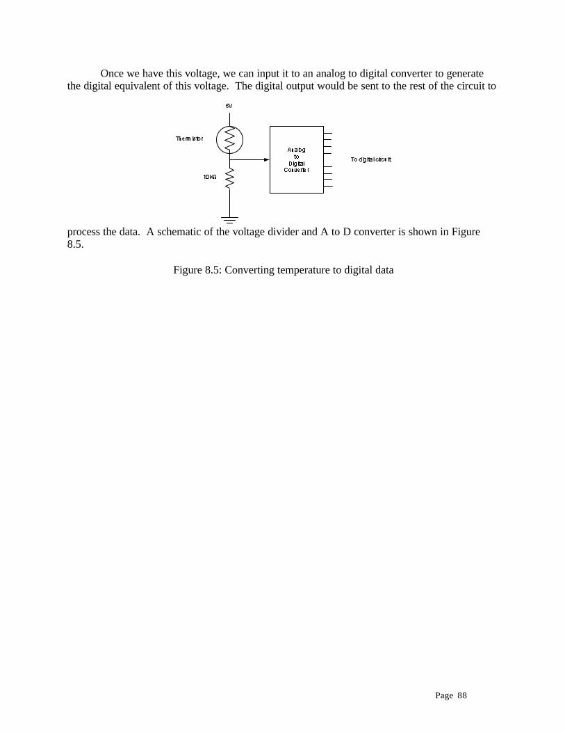
Page 88

Once we have this voltage, we can input it to an analog to digital converter to generate the digital equivalent of this voltage. The digital output would be sent to the rest of the circuit to

process the data. A schematic of the voltage divider and A to D converter is shown in Figure 8.5.

Figure 8.5: Converting temperature to digital data

Documents

Electricity and Magnetism - Drexel University · Electricity and Magnetism A Two-week Course for Middle School Teachers John D. Carpinelli Department of Electrical and Computer …