Embed Size (px)
Citation preview
SEEDS SURREY Surrey Energy Economics ENERGY Discussion paper Series ECONOMICS CENTRE
Electricity Demand for Sri Lanka: A Time Series Analysis
Himanshu A. Amarawickrama
and Lester C Hunt
October 2007
SEEDS 118 Department of Economics ISSN 1749-8384 University of Surrey

The Surrey Energy Economics Centre (SEEC) consists of members of the Department of Economics who work on energy economics, environmental economics and regulation. The Department of Economics has a long-standing tradition of energy economics research from its early origins under the leadership of Professor Colin Robinson. This was consolidated in 1983 when the University established SEEC, with Colin as the Director; to study the economics of energy and energy markets.
SEEC undertakes original energy economics research and since being established it has conducted research across the whole spectrum of energy economics, including the international oil market, North Sea oil & gas, UK & international coal, gas privatisation & regulation, electricity privatisation & regulation, measurement of efficiency in energy industries, energy & development, energy demand modelling & forecasting, and energy & the environment. SEEC also encompasses the theoretical research on regulation previously housed in the department's Regulation & Competition Research Group (RCPG) that existed from 1998 to 2004.
SEEC research output includes SEEDS - Surrey Energy Economic Discussion paper Series (details at www.seec.surrey.ac.uk/Research/SEEDS.htm) as well as a range of other academic papers, books and monographs. SEEC also runs workshops and conferences that bring together academics and practitioners to explore and discuss the important energy issues of the day.
SEEC also attracts a large proportion of the department’s PhD students and oversees the MSc in Energy Economics & Policy. Many students have successfully completed their MSc and/or PhD in energy economics and gone on to very interesting and rewarding careers, both in academia and the energy industry.
Enquiries: Director of SEEC and Editor of SEEDS: Lester C Hunt SEEC, Department of Economics, University of Surrey, Guildford GU2 7XH, UK. Tel: +44 (0)1483 686956 Fax: +44 (0)1483 689548 Email: [email protected] www.seec.surrey.ac.uk
i
___________________________________________________________
Surrey Energy Economics Centre (SEEC)
Department of Economics University of Surrey
SEEDS 118 ISSN 1749-8384
___________________________________________________________
ELECTRICITY DEMAND FOR SRI LANKA: A TIME SERIES ANALYSIS
Himanshu A. Amarawickrama
and Lester C Hunt
October 2007 ___________________________________________________________
This paper may not be quoted or reproduced without permission.

ii
ABSTRACT
This study estimates electricity demand functions for Sri Lanka using six econometric techniques. It shows that the preferred specifications differ somewhat and there is a wide range in the long-run price and income elasticities with the estimated long-run income elasticity ranging from 1.0 to 2.0 and the long run price elasticity from 0 to –0.06. There is also a wide range of estimates of the speed with which consumers would adjust to any disequilibrium, although the estimated impact income elasticities tended to be more in agreement ranging from 1.8 to 2.0. Furthermore, the estimated effect of the underlying energy demand trend varies between the different techniques; ranging from being positive to zero to predominantly negative. Despite these differences the forecasts generated from the six models up until 2025 do not differ significantly. Thus on one hand it is encouraging that the Sri Lanka electricity authorities can have some faith in econometrically estimated models used for forecasting. However, by the end of the forecast period in 2025 there is a variation of around 452MW in the base forecast peak demand; which, in relative terms for a small electricity generation system like Sri Lanka’s, represents a considerable difference. JEL Classification: Q48, Q41 Key Words: Developing Countries, Electricity Demand Estimation, Sri Lanka
Electricity Demand for Sri Lanka Page 1 of 39
Electricity Demand for Sri Lanka: A Time Series Analysis
Himanshu A. Amarawickrama a&b,*, Lester C. Hunt a
a Surrey Energy Economics Centre (SEEC), Department of Economics, University of Surrey, Guildford, GU2 7XH, Surrey, UK
b Infrastructure Advisory, Ernst and Young LLP, 1 More London Place, London, SE1 2AF, UK * Corresponding author, Fax: +44(0)1483 686954, e-mail address: [email protected]
1 INTRODUCTION
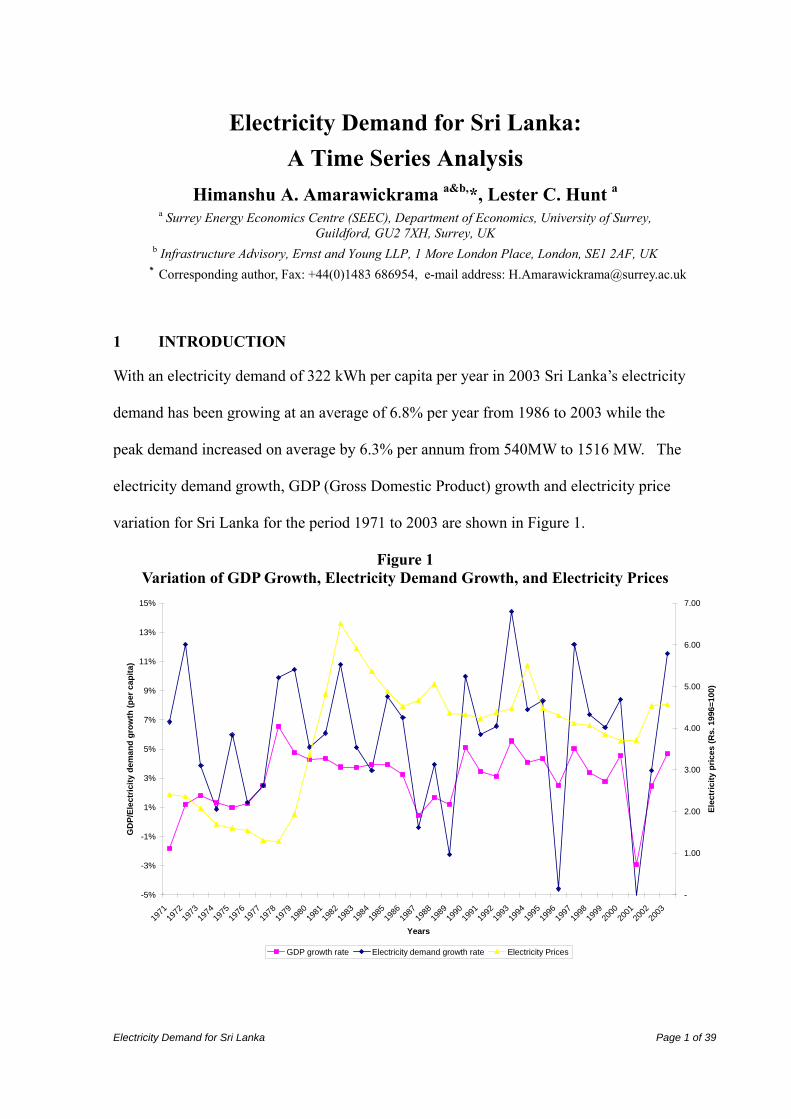
With an electricity demand of 322 kWh per capita per year in 2003 Sri Lanka’s electricity
demand has been growing at an average of 6.8% per year from 1986 to 2003 while the
peak demand increased on average by 6.3% per annum from 540MW to 1516 MW. The
electricity demand growth, GDP (Gross Domestic Product) growth and electricity price
variation for Sri Lanka for the period 1971 to 2003 are shown in Figure 1.
Figure 1 Variation of GDP Growth, Electricity Demand Growth, and Electricity Prices
-5%
-3%
-1%
1%
3%
5%
7%
9%
11%
13%
15%
1971
1972
1973
1974
1975
1976
1977
1978
1979
1980
1981
1982
1983
1984
1985
1986
1987
1988
1989
1990
1991
1992
1993
1994
1995
1996
1997
1998
1999
2000
2001
2002
2003
Years
GD
P/El
ectr
icity
dem
and
grow
th (p
er c
apita
)
-
1.00
2.00
3.00
4.00
5.00
6.00
7.00
Elec
tric
ity p
rices
(Rs.
199
6=10
0)
GDP growth rate Electricity demand growth rate Electricity Prices

Electricity Demand for Sri Lanka Page 2 of 39
This illustrates the relatively moderate Sri Lankan GDP growth (averaging 3.5% per
annum from 1978 to 2003), but despite this, Sri Lanka’s per capita electricity consumption
is still somewhat lower than that of its neighbours India and Pakistan although both
countries have experienced much lower per capita income levels.1 Although these
economies are not directly comparable with the Sri Lankan economy, they are the closest
geographical neighbours to Sri Lanka with some direct cultural and trade links.
In 2003 about 68% of Sri Lankan households were connected to the electricity grid with
household electricity consumption accounting for about 35% of total electricity
consumption, and household and industrial sector consumption combined accounting for
about 65% of the total 6,209 GWh [2]. Further details about the institutional background
of the Sri Lankan Electricity Supply Industry (ESI) may be found in Amarawickrama and
Hunt (2005) [3] (hereafter AH). Building on AH, this paper focuses on estimating and
analysing Sri Lankan electricity demand that is the basis for forecasts of future demand up
to 2025.
Previous statistical analysis of Sri Lankan electricity demand is extremely limited. As far
is known there are only four previous attempts to analyse Sri Lankan electricity demand.
An early attempt was by Jayatissa (1994) [4] who estimated a number of models for both
the Sri Lankan residential and industrial sectors, given that combined these two sectors
accounted for about 60% of total electricity demand in 1992. Using pooled cross section-
time series data of 178 household consumers from January 1993 to December 1993 and
1 According to Athalage et al In 1996 [1] the per capita energy consumption of Sri Lanka was about 60% lower than that of India and Pakistan.

Electricity Demand for Sri Lanka Page 3 of 39
monthly time series data from February 1980 to October 1993 Jayatissa estimated a model
for the Sri Lankan residential sector using Ordinary Least Squares (OLS).2 Consequently,
Jayatissa generated a number of different elasticity estimates, but concluded that for both
data sets household demand for electricity in Sri Lanka is generally neither income nor
price elastic in both the short and long run. For the industrial sector Jayatissa primarily
used annual data for the period 1971-1992 and again estimated a number of electricity
demand models using OLS and concluded that in general industrial demand was neither
output nor price elastic in the short or long run.3
Using annual data for the period 1960-1998 Hope and Morimoto (2004) [5] investigated
the causal relationship between electricity supply and GDP using Granger causality
analysis and concluded that changes in electricity supply have a significant impact on
change in real GDP in Sri Lanka and therefore every MWh increase in electricity supply
will contribute to an extra output of around US$ 1120-1740.
Using annual data for the period 1971-2001, AH estimated an electricity demand function
using the Engle and Granger two-step methodology and found the estimated long run
income elasticity to be 1.1 and the estimated long run price elasticity to be -0.003. This
was used as the basis for an indicative forecast for electricity demand as part of their
analysis of proposed electricity industry reforms for Sri Lanka.
2 Although it should be noted that Jayatissa did experiment with a number of alternative estimation approaches, including correcting for serial correlation (Cochrane-Orcutt procedure, Hildruth-Lu procedure, etc.) and Instrumental variables. 3 Jayatissa also used a monthly micro data set for 80 individual consumers from the industrial sector but this did not include individual firms’ output for the individual consumers since this was not available. Consequently, the estimated models were poorly defined.
Electricity Demand for Sri Lanka Page 4 of 39
Finally, the generation planning branch of the Ceylon Electricity Board (CEB)4 provide
electricity demand forecasts of Sri Lankan electricity demand, but the exact methodology
is not detailed.
Accurate and reliable energy demand forecasts are vital to a capital constrained developing
country where the capability for the import and export of electricity is severely limited
both in the present and the near future.5 Sri Lanka, which is an island, does not have any
sub sea cables from main subcontinent and, at the time of writing, there are no plans to
build one given the political unrest in the north of Sri Lanka. This study therefore explores
this issue by investigating how different time-series estimation methods perform in terms
of modelling past electricity demand, estimating the key income and price elasticities, and
hence forecasting future electricity consumption in the context of the Sri Lankan ESI. This
allows for the different forecast electricity demand using these different econometric
techniques to be compared indicating if the policy decisions might vary according to the
chosen econometric method.
The next Section of the paper therefore discusses the different methods analyzed. Section
3 presents and explains the estimation results, with the forecasts of electricity demand for
Sri Lanka up to 2025 from the different models presented and compared in Section 4.
Section 5 summarizes and concludes the study.
4 The electricity utility in Sri Lanka, which generates transmits and supplies for around 80% of Sri Lankan Electricity users. 5 Wijayathunga et al, 2001 [6].
Electricity Demand for Sri Lanka Page 5 of 39
2 METHODOLOGY
2.1 Electricity Demand Function
It is assumed that there exists for Sri Lanka a simple long-run equilibrium relationship
between electricity consumption, economic activity and the real electricity price
characterized by:
E = f (Y, P, μ) (1)6
where: E = per capita electricity demand;
Y = per capita GDP;
P = the real electricity price; and
μ = the underlying energy demand trend (UEDT).7
In order to econometrically estimate equation (1) the conventional log-linear specification
is assumed for the long-run equilibrium Sri Lankan electricity demand function as follows:
et = β1yt + β2pt + μt + εt (2)8
where: et = Ln (Et);
yt = Ln (Yt);
pt = Ln (Pt).
β1 = the long-run income elasticity of electricity demand;
β2 = the long-run price elasticity of electricity demand; and
6 This is the standard ‘demand’ specification used by many previous demand studies. AH did explore whether there was a role for the additional variables ‘average annual temperature’ and ‘rainfall’, but they were never found to be significant and so they have not been included in the analysis here. 7 Exact definitions and sources of the data are given as we explain them below. 8 This constant elasticity demand function is standard in energy demand estimation, favoured for its simplicity, straightforward interpretation and limited data requirements and, according Pesaran et al. (1998) [7] it generally outperforms more complex specifications.
Electricity Demand for Sri Lanka Page 6 of 39
εt = a random error term.
In the most general specification the UEDT is stochastic (μt), however this can only be
estimated via the Structural Time Series Model (see below) whereas for the cointegration
methods the trend in the general model is deterministic and hence collapses to β0 + β3 t so
that the most general equation (with a deterministic trend) becomes:
et = β0 + β1yt + β2pt + β3 t + εt (3)
where: β3 = the annual rate of change in the (linear) UEDT.
The relationships specified in equations (2) and (3) are consistent with a number of
previous studies of energy demand in general and electricity demand in particular, but it
could be argued that these actually represent supply relationships. However, given the
nature of electricity production and supply in Sri Lanka this is unlikely to be the case.
Over the estimation period the ESI in Sri Lanka was (and remains at the time of writing) a
largely government owned and run vertically integrated monopoly, with the government
setting prices (and supply during periods of output constraints); consequently, equations (2)
and (3) may be regarded as demand relationships. This framework is therefore used to
estimate appropriate equations for Sri Lankan electricity demand and hence produce
suitable forecasting equations using a variety of cointegration methods as follows:
• Static Engle and Granger method (Static EG)
• Dynamic Engle and Granger method (Dynamic EG)
• Fully Modified Ordinary Least Squares method (FMOLS)
• Pesaran, Shin and Smith method (PSS)

Electricity Demand for Sri Lanka Page 7 of 39
• Johansen method (Johansen)
In addition the alternative approach advocated by Harvey (1989 & 1997) [8, 9] is also
adopted:
• Structured Time Series Method (STSM)
The various approaches are now introduced and briefly explained.
2.2 Unit root tests
For most of the cointegration techniques the time series properties of the individual
variables need to be investigated. In particular it needs to be determined whether the
variables are stationary in levels and therefore integrated of order zero, I(0) or are non
stationary and hence have a unit root and hence require differencing to achieve stationarity
and are therefore integrated of order d, I(d) where d is the number of time the variable
needs differencing to achieve stationarity. This is required since modelling with non-
stationary variables can result in spurious relationships, whereas a combination of non-
stationary variables can, in certain circumstances, result in cointegration and hence an
appropriate relationship (see below).
To test for the presence of a unit root the most commonly used test is the Augmented
Dickey-Fuller (ADF) test which involves estimating a form of the following equation by
OLS:
Δxt = γ0 + γ1t + φxt-1 + ϕ1 Δxt-1 + … + ϕq Δxt-q + εt (4)
where Δ is the difference operator.
Electricity Demand for Sri Lanka Page 8 of 39
The t-statistic for the estimated coefficient φ in equation (4) is the ADF statistic. However
the ADF does not have a conventional student-t distribution, instead the ADF must be
compared with specific tables such as those in MacKinnon (1996) [10]. Equation (4)
involves the most general specification with q lags. The results below for et, yt, and pt are
therefore obtained by starting with q equal to four9 and then systematically omitting
insignificant variables (lags, constant, and/or trend) ensuring that there is no serial
correlation in the residuals. Once the preferred equation has been obtained in this way,
using a combination of the software PCGive 10.4 and Eviews 5.0, the t-statistic gives the
ADF statistics in the results section below. This therefore gives an indication of the time
series properties of the individual variable, but if the variables are found to be non-
stationary in levels a similar procedure is undertaken to test the variables in first
differences Δet, Δyt, and Δpt. If, as is the case below, the variables are found to be
stationary in first differences (that is the variables in levels, et, yt, and pt, are I(1) in that
they need to be differenced once to achieve stationarity) then this allows progression to the
cointegration techniques discussed below.
2.3 Estimation of the long-run cointegrating relationships
2.3.1 Engle-Granger two step method (Static EG)
If all the variables are found to be I(1) then Engle and Granger (1987) [12] have shown
that a long-run relationship such as equation (3) may be estimated by OLS and if the
resulting residuals are stationary, I(0), then the variables e, y and p are said to co-integrate;
hence the estimated equation may be regarded as a valid long-run equilibrium
9 The choice of lag length is somewhat arbitrary, however given the sample size the choice of q=4 is seen as a prudent lag length to begin the testing down procedure. Furthermore, the formulae suggested by Schwert (1989, p. 151) [11] would suggest that given the sample size used here q should be set at 3, which is within the framework used here.
Electricity Demand for Sri Lanka Page 9 of 39
cointegrating vector. The ADF test outlined above (omitting the constant and the trend) is
used to conduct the test. These are computed using a combination of the software PCGive
10.4 and Eviews 5.0.
It has been shown by Engle and Granger (1987) [12], that this approach produces a
consistent estimate of the long-run steady state relationship between the variables due to
the ‘superconsistency’ property of the OLS estimator. However, it is not possible to
conduct conventional inference such as t-tests since the lack of any dynamics renders the
standard-errors and t-statistics biased and misleading. Thus a major drawback with this
technique is the need just to take the estimated coefficients and long-run elasticities as
given without being able to confirm whether they are significantly different from zero or
not. This is an issue addressed below in some of the alternative cointegration techniques.
This has summarized the first of the Engle-Granger two step procedure. The second step
involves using the information from the estimated long-run equation in a short-run
dynamic equation. This is explained in more detail below following the introduction of all
the long-run cointegration methods since the short-run methodology is applied consistently
across all the different techniques and hence discussed after the methods to estimate the
long run relationships have been introduced first.
2.3.2 Dynamic Engle-Granger method (Dynamic EG)
As discussed above the Static EG method produces a consistent estimate of the long-run
steady state relationship between the variables due to the ‘superconsistency’ property of the
OLS estimator. However, in finite samples these estimates will be biased and Banerjee et
al. (1993) [13] and Inder (1993) [14] have shown that the bias could often be substantial.
Electricity Demand for Sri Lanka Page 10 of 39
An alternative is therefore used to estimate an over-parameterised dynamic model and
derive the long-run parameters by solving the estimated Auto Regressive Distributed Lag
(ARDL) since this reduces any bias, giving precise estimates of the long-run parameters.
Moreover, Inder (1993) [14] has shown that this procedure provides valid t-tests and hence
tests of significance on the long-run parameters may be undertaken. In addition, it is
possible to carry out a unit root test of no cointegration since the sum of the coefficients on
the distributed lag of et must be less than one for the dynamic model to converge to a long-
run solution. Therefore dividing this sum by the sum of the associated standard errors
gives the PcGive unit root test, which is a t-type test that can be compared against critical
values given in Banerjee et al. (1993) [13].10
Hence an ARDL version of equation (3) is estimated using PCGive 10.4 with a lag of 4 on
all the variables and the implicit long-run coefficients and associated t-statistics derived
accordingly; with the equation also tested to ensure it does not suffer from any serial
correlation and non-normality. Furthermore, given the long-run coefficients have valid t-
statistics, variables found to be insignificant in the long-run are eliminated from the
estimated equation.
2.3.3 Fully modified ordinary least squares method (FMOLS)
The FMOLS method is a semi-parametric approach developed by Philips and Hansen
(1990) [16] for the estimation of a single cointegrating relationship with a combination of
I(1) variables; such as equation (3). It makes appropriate corrections to circumvent the
inference problems with the Static EG method discussed above, hence t-tests for the
10 This explanation relies heavily on Harris and Sollis (2003, pp. 89 - 90) [15].
Electricity Demand for Sri Lanka Page 11 of 39
estimated long-run coefficients are valid. The software package Microfit 4.0 is used to
estimate various versions of equation (3) with a two year lag. In addition to specifying the
lag, two further choices are made: firstly, whether any of the variables included are I(1)
with or without drift (which is determined by the ADF tests discussed above); secondly the
type of weights used for the correction.
2.3.4 Pesaran, Shin and Smith method (PSS)
Pesaran, Shin and Smith (2001) [17] developed a method to test the existence of level
relationship between a dependent variable and regressors where there is an uncertainty as
to whether the regressors are trend stationary or first difference stationary. The first stage
involves testing for the existence of an acceptable cointegrating vector and the second
stage the estimation of the vector and the associated long-run elasticities; both of which are
done using the software package Microfit 4.0.
To test for the existence of an acceptable cointegrating vector PSS developed the ‘Bounds
Test’. For the application undertaken here it involves the estimation of the following
equation:
11
1111
0 −=
−−−=
−=
− ∑∑∑ +++Δ+Δ+Δ++=Δ tp
j
ityteiti
j
iiti
j
iititt pyepfydebtaae τττ (5)
and testing the null hypothesis of ‘non-existence of the long run relationship’ defined by τe
= τy = τp = 0. The calculated F-statistic from the restriction does not have a standard
distribution but contains ‘bounds’ depending upon whether the variables are I(0) or

Electricity Demand for Sri Lanka Page 12 of 39
I(1).11,12 If the null is rejected for equation (5) then it suggests that there is a long run
relationship between e, y and p and that y and p may be regarded as the ‘forcing variables’.
If the existence of a long-run cointegrating vector is established the second stage of the
PSS technique involves the estimation of the long-run relationship in a similar way to the
dynamic EG outlined above. However, although it is possible to stipulate the number of
lags, Microfit 4.0 allows for a systematic selection of the appropriate number of lags based
upon various information criteria.13
2.3.5 Johansen method (Johansen)
The Johansen (1988) [19] approach estimates cointegrating relationships between non-
stationary variables using a maximum likelihood procedure. This technique tests for the
number of distinct cointegrating vectors in a multivariate setting and estimates the
parameters of these cointegrating relationships. For the application here, this consists of
the following three-dimensional vector autoregressive model:
Xt = Α1Xt-1 + … + AkXt-k + εt , t = 1,.........,T, (6)
where Xt = [e, y, p]t as defined above, Xt are fixed and εt ~ IN(0, Σ). Equation (6) can be
re-written in error correction form as:
11 Note that the intercept and/or trend may also be omitted (i.e. a0 and/or at set equal to zero) which require different tabulated values. 12 Hence there is no real need to test the time series properties of the variables prior to testing for cointegration, however, the cointegration test can result in inconclusive results thus requiring more information about the variables properties.
Electricity Demand for Sri Lanka Page 13 of 39
ΔXt = Γ1ΔXt-1 + … + Γk-1ΔXt-k+1 + ΠXt-k + εt , t = 1,........,T, (7)
If the data {Xt}are integrated of order one, I(1), then Δ{Xt} is I(0) and the reduced form
model (2) is balanced only if ΠXt-k is I(0). Thus, matrix Π has to be of reduced rank:
Π = αβ’ , (8)
where β may be interpreted as the m × n matrix of cointegrating vectors and α is the m x n
matrix of loading weights.
Given the unit root tests suggest that e, p and y are I(1) (see below) they are entered as
endogenous variables in the unrestricted VAR (Vector Auto Regression) equation (6) with a
lag length of two years, using PcGive 10.4 and Eviews 5. This produces both the
Maximum Eigen and the Trace statistics to test for the number of cointegrating vectors.
Once this has been determined it is imposed on the system to produce the cointegrating
vector(s) and associated statistics given below in the results section.
2.4 Estimation of the short-run dynamic equations for the various cointegration methods
As indicated above, the estimated cointegrating vectors represent the long-run equilibrium
relationships, so that the difference from the ‘predicted’ values and the actual values of et
represent the annual disequilibrium errors or the error correction term, ECt, as follows:
13 Once the long-run cointegrating vector has been identified and estimated the short-run dynamic equation may also be estimated in Microfit 4.0 [18]. However, for consistency this is done in PCGive 10.4 along with
Electricity Demand for Sri Lanka Page 14 of 39
tpyeEC tttt 3
^
2
^
1
^
0
^ββββ −−−−= (9)14
Given the tests for cointegration, ECt will be I(0) and is therefore included in a short-run
dynamic equation with the original variables e, y, and p in first difference, which given the
unit root testing can be regarded as I(0) – hence avoiding the spurious regression problem.
The general specification is therefore given by:
Δet = α0+α1Δet-1+ .. +α4Δet-3+α5Δyt+ .. +α9Δyt-3+α10Δpt+ .. +α14Δpt-3+α12ECt-1+εt (10)
The preferred equation is found by selecting a restricted model by testing down from the
over-parameterized model of equation (10) that satisfies parameter restrictions without
violating a range of diagnostic tests using PcGive 10.4 and Eviews 5. In particular, the
equation residuals are tested for the presence of non-normality, serial correlation,
heteroscedasticity and instability. In addition, intervention dummy variables are also
included for certain time periods such as severe power shortages experienced due to
droughts in 1996.
2.4.1 Structural time series modelling method (STSM)
The STSM differs in a number of ways from the cointegration approaches discussed
above. In particular, the order of integration of the individual variables is not crucial, it
allows for an unobservable stochastic trend and the short-run and long-run effects are
all other short-run equations (see below). 14 Note this is the most general specification, whereas in the actual results not all variables are included (see the results section below for details) and due to this and different estimates of the β’s the ECt terms will be different for each cointegration technique.

Electricity Demand for Sri Lanka Page 15 of 39
estimated via one equation, hence a dynamic version of equation (2) for Sri Lankan
electricity demand is specified as follows:
et = µt + δ1et-1 + … +δ4et-4 + δ5yt + … + δ9yt-4 + δ10pt + …+ δ14pt-4 + εt (11)
Where µt is assumed to have the following stochastic process:
tttt ηπμμ ++= −− 11 , tη ~ ),0( 2ησNID (12)
ttt ςππ += −1 , tξ ~ ),0( 2ξσNID . (13)
Equation (12) represents the level of the trend driven by the white noise disturbance term,
ηt and equation (13) represents the slope of the trend driven by the white noise disturbance
term ξt. The shape of the underlying trend is determined by σξ2 and ση
2, known as the
hyperparameters.15 Its most restrictive form occurs when both σξ2 and ση
2 are zero and the
model converts to the traditional deterministic trend model similar to equation (3).
The estimated equation consists of equation (11) with (12) and (13). All the disturbance
terms are assumed to be independent and mutually uncorrelated with each other. As seen
above, the hyperparameters ση2, σξ
2, and σε2 have an important role to play and govern the
basic properties of the model. The hyperparameters, along with the other parameters of the
model are estimated by a combination of maximum likelihood and the Kalman filter. The
optimal estimate of the trend over the whole sample period is further calculated by the
smoothing algorithm of the Kalman filter. For model evaluation, equation residuals are
estimated (which are estimates of the equation disturbance term, similar to those from
Electricity Demand for Sri Lanka Page 16 of 39
ordinary regression) plus a set of auxiliary residuals. The auxiliary residuals include
smoothed estimates of the equation disturbance (known as the irregular residuals), the
smoothed estimates of the level disturbances (known as the level residuals) and smoothed
estimates of the slope disturbances (known as the slope residuals).16 The software package
STAMP 6.3 (Koopman et al., 2004 [20]) is used to estimate the model.
3 ESTIMATION RESULTS
3.1 Data
Data used in the estimation consists of annual data over the period 1970 – 2003 inclusive.17
Electricity consumption data for Sri Lanka were taken from the MOPE (Ministry of Power
and Energy) data base18 for 1970 – 2000 and from the Statistical Digest, CEB [21] and the
Central Bank of Sri Lanka Annual Reports (CBSLAR) thereafter. These were divided by
the population data taken from CBSLAR 2005 (Special Statistical Appendix), to give per
capita consumption, Et. Data for GDP at 1996 prices were again taken from the Special
Statistical Appendix of the CBSL AR, 2003 and divided by population data to give the
variable Yt. Data for the average nominal electricity price per unit were taken from the
MOPE data base for 1970 – 2000 and from the Statistical Digest, CEB and the Central
Bank of Sri Lanka Annual Report thereafter. These were deflated by the GDP deflator
taken from Special Statistical Appendix to give Pt. Since electricity users in different
sectors are normally faced with different tariffs it is arguably advisable to estimate demand
15 σε
2 is also a hyperparameter 16 In practice the level and slope residuals are only estimated if the level and slope components are present in the model, i.e. ηt and/or ξt are non-zero. 17 It would have been interesting had the estimation been done on monthly data instead of annual data, but no reliable monthly data for the period of 1970-2003 is available to the authors.
Electricity Demand for Sri Lanka Page 17 of 39
relationships for the domestic, industrial, commercial and other sectors separately.
However for simplicity the average electricity tariff has been utilised; nevertheless it is
appreciated that sector wise estimation might be more appropriate in certain circumstances.
3.2 Unit root tests
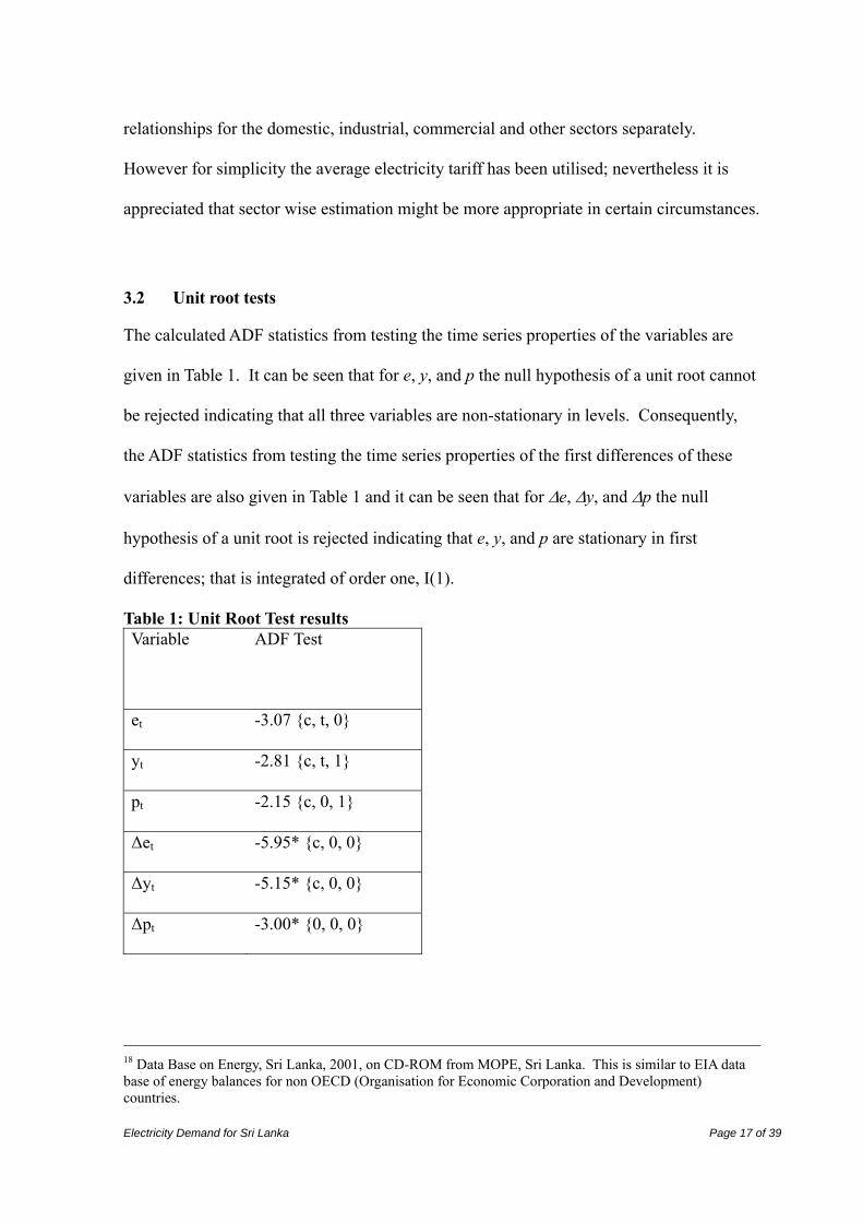
The calculated ADF statistics from testing the time series properties of the variables are
given in Table 1. It can be seen that for e, y, and p the null hypothesis of a unit root cannot
be rejected indicating that all three variables are non-stationary in levels. Consequently,
the ADF statistics from testing the time series properties of the first differences of these
variables are also given in Table 1 and it can be seen that for Δe, Δy, and Δp the null
hypothesis of a unit root is rejected indicating that e, y, and p are stationary in first
differences; that is integrated of order one, I(1).
Table 1: Unit Root Test results Variable ADF Test
et -3.07 {c, t, 0}
yt -2.81 {c, t, 1}
pt -2.15 {c, 0, 1}
Δet -5.95* {c, 0, 0}
Δyt -5.15* {c, 0, 0}
Δpt -3.00* {0, 0, 0}
18 Data Base on Energy, Sri Lanka, 2001, on CD-ROM from MOPE, Sri Lanka. This is similar to EIA data base of energy balances for non OECD (Organisation for Economic Corporation and Development) countries.
Electricity Demand for Sri Lanka Page 18 of 39
NB: {c, t, n} indicates the inclusion of a constant (c), the inclusion of a time trend (t) and
the number of lags (n) in the ADF regression and * indicates the rejection of the null
hypothesis of a unit root at the 1% level (based upon MacKinnon (1996) [10]).
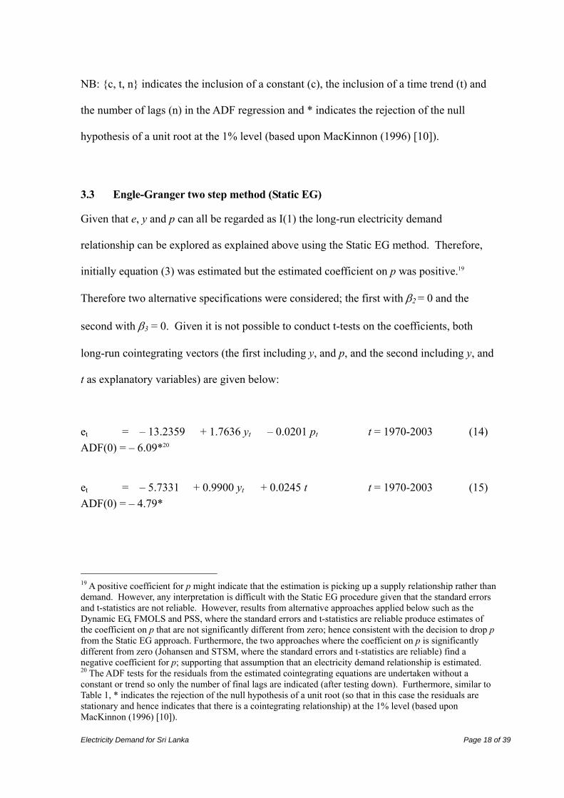
3.3 Engle-Granger two step method (Static EG)
Given that e, y and p can all be regarded as I(1) the long-run electricity demand
relationship can be explored as explained above using the Static EG method. Therefore,
initially equation (3) was estimated but the estimated coefficient on p was positive.19
Therefore two alternative specifications were considered; the first with β2 = 0 and the
second with β3 = 0. Given it is not possible to conduct t-tests on the coefficients, both
long-run cointegrating vectors (the first including y, and p, and the second including y, and
t as explanatory variables) are given below:
et = – 13.2359 + 1.7636 yt – 0.0201 pt t = 1970-2003 (14) ADF(0) = – 6.09*20
et = – 5.7331 + 0.9900 yt + 0.0245 t t = 1970-2003 (15) ADF(0) = – 4.79*
19 A positive coefficient for p might indicate that the estimation is picking up a supply relationship rather than demand. However, any interpretation is difficult with the Static EG procedure given that the standard errors and t-statistics are not reliable. However, results from alternative approaches applied below such as the Dynamic EG, FMOLS and PSS, where the standard errors and t-statistics are reliable produce estimates of the coefficient on p that are not significantly different from zero; hence consistent with the decision to drop p from the Static EG approach. Furthermore, the two approaches where the coefficient on p is significantly different from zero (Johansen and STSM, where the standard errors and t-statistics are reliable) find a negative coefficient for p; supporting that assumption that an electricity demand relationship is estimated. 20 The ADF tests for the residuals from the estimated cointegrating equations are undertaken without a constant or trend so only the number of final lags are indicated (after testing down). Furthermore, similar to Table 1, * indicates the rejection of the null hypothesis of a unit root (so that in this case the residuals are stationary and hence indicates that there is a cointegrating relationship) at the 1% level (based upon MacKinnon (1996) [10]).
Electricity Demand for Sri Lanka Page 19 of 39
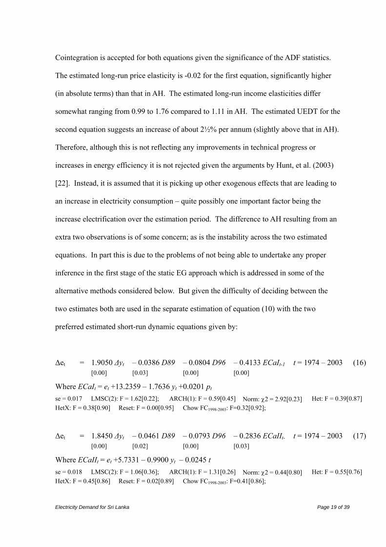
Cointegration is accepted for both equations given the significance of the ADF statistics.
The estimated long-run price elasticity is -0.02 for the first equation, significantly higher
(in absolute terms) than that in AH. The estimated long-run income elasticities differ
somewhat ranging from 0.99 to 1.76 compared to 1.11 in AH. The estimated UEDT for the
second equation suggests an increase of about 2½% per annum (slightly above that in AH).
Therefore, although this is not reflecting any improvements in technical progress or
increases in energy efficiency it is not rejected given the arguments by Hunt, et al. (2003)
[22]. Instead, it is assumed that it is picking up other exogenous effects that are leading to
an increase in electricity consumption – quite possibly one important factor being the
increase electrification over the estimation period. The difference to AH resulting from an
extra two observations is of some concern; as is the instability across the two estimated
equations. In part this is due to the problems of not being able to undertake any proper
inference in the first stage of the static EG approach which is addressed in some of the
alternative methods considered below. But given the difficulty of deciding between the
two estimates both are used in the separate estimation of equation (10) with the two
preferred estimated short-run dynamic equations given by:
Δet = 1.9050 Δyt – 0.0386 D89 – 0.0804 D96 – 0.4133 ECaIt-1 t = 1974 – 2003 (16) [0.00] [0.03] [0.00] [0.00]
Where ECaIt = et +13.2359 – 1.7636 yt +0.0201 pt se = 0.017 LMSC(2): F = 1.62[0.22]; ARCH(1): F = 0.59[0.45] Norm: χ2 = 2.92[0.23] Het: F = 0.39[0.87] HetX: F = 0.38[0.90] Reset: F = 0.00[0.95] Chow FC1998-2003: F=0.32[0.92];
Δet = 1.8450 Δyt – 0.0461 D89 – 0.0793 D96 – 0.2836 ECaIIt- t = 1974 – 2003 (17) [0.00] [0.02] [0.00] [0.03]
Where ECaIIt = et +5.7331 – 0.9900 yt – 0.0245 t se = 0.018 LMSC(2): F = 1.06[0.36]; ARCH(1): F = 1.31[0.26] Norm: χ2 = 0.44[0.80] Het: F = 0.55[0.76] HetX: F = 0.45[0.86] Reset: F = 0.02[0.89] Chow FC1998-2003: F=0.41[0.86];
Electricity Demand for Sri Lanka Page 20 of 39
Where: D89 = intervention dummy variable for 1989
D96 = intervention dummy variable for 1996
Both equations pass all diagnostic tests but both required intervention dummies for 1989
and 1996 to take account for the restricted demand due to planned power cuts in drought
years. All coefficients are statistically significant in both equations with the coefficients on
the error correction terms both of the right sign, but with a variation in size; equation (16)
suggests that just over 40% of any disequilibrium is adjusted in each year whereas
equation (17) suggests over 25%. This compares to just less than 75% in AH. No role
could be found for the change in prices (Δp) in either equation whereas there is a strong
estimated impact income elasticity in both equations of 1.9 and 1.8 respectively; compared
to 1.5 in AH. The differences between this estimation and that in AH are due to the
different data periods, but also the inclusion of the intervention dummies for 1989 and
1996.
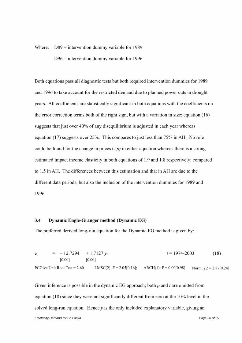
3.4 Dynamic Engle-Granger method (Dynamic EG)
The preferred derived long-run equation for the Dynamic EG method is given by:
et = – 12.7294 + 1.7127 yt t = 1974-2003 (18) [0.00] [0.00]
PCGive Unit Root Test = 2.60 LMSC(2): F = 2.05[0.16]; ARCH(1): F = 0.00[0.98] Norm: χ2 = 2.87[0.24]
Given inference is possible in the dynamic EG approach; both p and t are omitted from
equation (18) since they were not significantly different from zero at the 10% level in the
solved long-run equation. Hence y is the only included explanatory variable, giving an
Electricity Demand for Sri Lanka Page 21 of 39
estimated long-run income elasticity of 1.71; similar to equation (14) for the static EG
method. Furthermore, the actual estimated over parametised equation with lags of four
does not suffer from any serial correlation or non-normality problems. However, the
PCGive unit root test for cointegration is very low, suggesting that cointegration does not
exist.
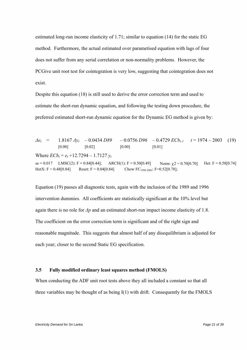
Despite this equation (18) is still used to derive the error correction term and used to
estimate the short-run dynamic equation, and following the testing down procedure, the
preferred estimated short-run dynamic equation for the Dynamic EG method is given by:
Δet = 1.8167 Δyt – 0.0434 D89 – 0.0756 D96 – 0.4729 ECbt-1 t = 1974 – 2003 (19) [0.00] [0.02] [0.00] [0.01]
Where ECbt = et +12.7294 – 1.7127 yt se = 0.017 LMSC(2): F = 0.84[0.44]; ARCH(1): F = 0.50[0.49] Norm: χ2 = 0.70[0.70] Het: F = 0.58[0.74] HetX: F = 0.48[0.84] Reset: F = 0.04[0.84] Chow FC1998-2003: F=0.52[0.78];
Equation (19) passes all diagnostic tests, again with the inclusion of the 1989 and 1996
intervention dummies. All coefficients are statistically significant at the 10% level but
again there is no role for Δp and an estimated short-run impact income elasticity of 1.8.
The coefficient on the error correction term is significant and of the right sign and
reasonable magnitude. This suggests that almost half of any disequilibrium is adjusted for
each year; closer to the second Static EG specification.
3.5 Fully modified ordinary least squares method (FMOLS)
When conducting the ADF unit root tests above they all included a constant so that all
three variables may be thought of as being I(1) with drift. Consequently for the FMOLS
Electricity Demand for Sri Lanka Page 22 of 39
estimation this option was chosen along with a two year lag and the ‘Bartlett weights’.21 In
all models p was not significantly different from zero at the 10% level and hence was
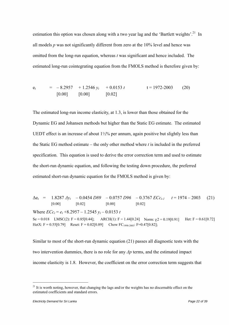
omitted from the long-run equation, whereas t was significant and hence included. The
estimated long-run cointegrating equation from the FMOLS method is therefore given by:
et = – 8.2957 + 1.2546 yt + 0.0153 t t = 1972-2003 (20) [0.00] [0.00] [0.02]
The estimated long-run income elasticity, at 1.3, is lower than those obtained for the
Dynamic EG and Johansen methods but higher than the Static EG estimate. The estimated
UEDT effect is an increase of about 1½% per annum, again positive but slightly less than
the Static EG method estimate – the only other method where t is included in the preferred
specification. This equation is used to derive the error correction term and used to estimate
the short-run dynamic equation, and following the testing down procedure, the preferred
estimated short-run dynamic equation for the FMOLS method is given by:
Δet = 1.8287 Δyt – 0.0454 D89 – 0.0757 D96 – 0.3767 ECct-1 t = 1974 – 2003 (21) [0.00] [0.02] [0.00] [0.02]
Where ECct = et +8.2957 – 1.2545 yt – 0.0153 t Se = 0.018 LMSC(2): F = 0.85[0.44]; ARCH(1): F = 1.44[0.24] Norm: χ2 = 0.19[0.91] Het: F = 0.61[0.72] HetX: F = 0.55[0.79] Reset: F = 0.02[0.89] Chow FC1998-2003: F=0.47[0.82];
Similar to most of the short-run dynamic equation (21) passes all diagnostic tests with the
two intervention dummies, there is no role for any Δp terms, and the estimated impact
income elasticity is 1.8. However, the coefficient on the error correction term suggests that
21 It is worth noting, however, that changing the lags and/or the weights has no discernable effect on the estimated coefficients and standard errors.
Electricity Demand for Sri Lanka Page 23 of 39
just over a third of any disequilibrium is adjusted for each; above the first Static EG
estimate but below the rest.
3.6 Pesaran, Shin and Smith method (PSS)
Finding evidence of a unique cointegrating vector for Sri Lankan electricity demand
proved difficult. Although initial results from the PSS Bounds tests suggested that a long
run relationship might exist between all three variables e, y, and p whenever the long-run
relationship was estimated the price variable (and trend) always proved to be insignificant.
Hence the long run analysis was restricted to just e and y so that a number of different lags
were considered for equation (5) (including up to j=4) but dropping the p and trend terms.
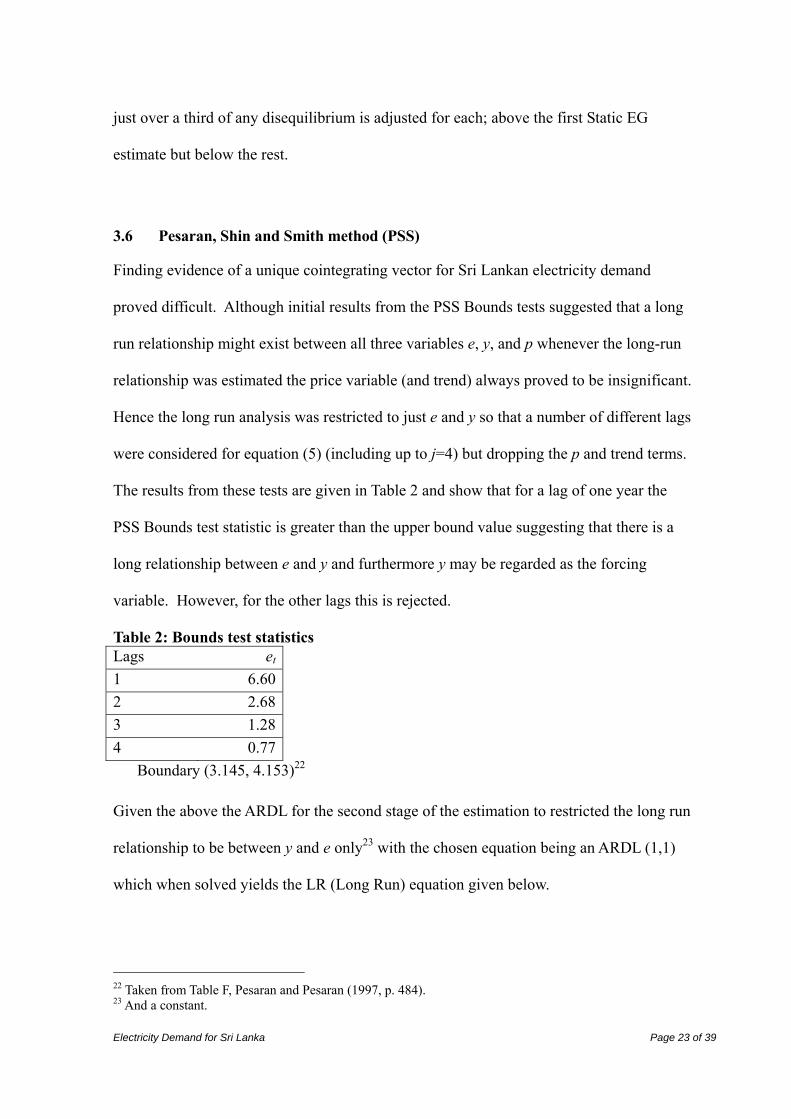
The results from these tests are given in Table 2 and show that for a lag of one year the
PSS Bounds test statistic is greater than the upper bound value suggesting that there is a
long relationship between e and y and furthermore y may be regarded as the forcing
variable. However, for the other lags this is rejected.
Table 2: Bounds test statistics Lags et 1 6.60 2 2.68 3 1.28 4 0.77
Boundary (3.145, 4.153)22 Given the above the ARDL for the second stage of the estimation to restricted the long run
relationship to be between y and e only23 with the chosen equation being an ARDL (1,1)
which when solved yields the LR (Long Run) equation given below.
22 Taken from Table F, Pesaran and Pesaran (1997, p. 484). 23 And a constant.

Electricity Demand for Sri Lanka Page 24 of 39
et = -12.6747 + 1.7069 yt T = 1971-2003 (22) [0.00] [0.00]
This gives an estimated long run income elasticity of 1.71; very similar to that obtained for
equation (14) for the Static EG, the Dynamic EG, and the Johansen approaches. Equation
(22) is used to form the error correction series and estimate the short-run dynamic
equation, with the preferred specification given as follows:
Δet = 1.8517 Δyt – 0.0737 D96 – 0.4701 ECdt-1 t = 1974 – 2003 (23) [0.00] [0.00] [0.01]
Where ECdt = et +12.6747 – 1.7069 yt se = 0.019 LMSC(2): F = 0.06[0.94]; ARCH(1): F = 1.19[0.29] Norm: χ2 = 0.65[0.72] Het: F = 0.60[0.70] HetX: F = 0.48[0.82] Reset: F = 0.23[0.63] Chow FC1998-2003: F=0.55[0.77];
Equation (23) passes all diagnostic tests, but in this case only the 1996 intervention dummy
is needed. Again there is no role for Δp but the coefficients for all remaining variables are
statistically significant at the 10% level at least. The estimated short-run impact income
elasticity is about 1.9 and the coefficient on the error correction term suggests that almost
half of any disequilibrium is adjusted for each year, similar to the second specification for
the Static EG method and the Dynamic EG method.
3.7 Johansen Method (Johansen)
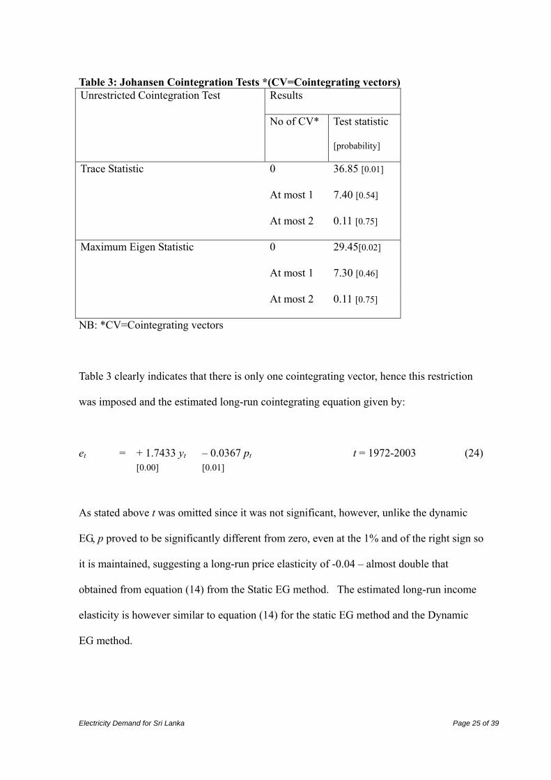
Table 3 shows the Trace and Maximum Eigenvalue statistics to test for the number of
cointegrating equations from a VAR with a two year lag that includes e, y and p but no
trend. As explained above, initially a restricted trend was specified but since the
coefficient on the trend was always not significantly different from zero at the 10% level it
was omitted.
Electricity Demand for Sri Lanka Page 25 of 39
Table 3: Johansen Cointegration Tests *(CV=Cointegrating vectors) Unrestricted Cointegration Test Results
No of CV* Test statistic
[probability]
Trace Statistic 0 36.85 [0.01]
At most 1 7.40 [0.54]
At most 2 0.11 [0.75]
Maximum Eigen Statistic 0 29.45[0.02]
At most 1 7.30 [0.46]
At most 2 0.11 [0.75]
NB: *CV=Cointegrating vectors
Table 3 clearly indicates that there is only one cointegrating vector, hence this restriction
was imposed and the estimated long-run cointegrating equation given by:
et = + 1.7433 yt – 0.0367 pt t = 1972-2003 (24) [0.00] [0.01]
As stated above t was omitted since it was not significant, however, unlike the dynamic
EG, p proved to be significantly different from zero, even at the 1% and of the right sign so
it is maintained, suggesting a long-run price elasticity of -0.04 – almost double that
obtained from equation (14) from the Static EG method. The estimated long-run income
elasticity is however similar to equation (14) for the static EG method and the Dynamic
EG method.

Electricity Demand for Sri Lanka Page 26 of 39
Equation (24) is therefore used to derive the error correction term and used to estimate the
short-run dynamic equation, and following the testing down procedure, the preferred
estimated short-run dynamic equation for the Johansen method is given by:
Δet = – 6.2027 + 1.8289 Δyt – 0.0746 D96 – 0.4772 ECet-1 t = 1974 – 2003 (25) [0.01] [0.00] [0.00] [0.01]
Where ECet = et – 1.7433 yt + 0.0367 pt se = 0.019 LMSC(2): F = 0.11[0.89]; ARCH(1): F = 1.23[0.28] Norm: χ2 = 0.10[0.95] Het: F = 0.73[0.61] HetX: F = 0.58[0.74] Reset: F = 0.21[0.65] Chow FC1998-2003: F=0.34[0.91];
Equation (25) passes all diagnostic tests, but in this case with only the 1996 intervention
dummy, All coefficients are statistically significant at the 10% level but yet again there is
no role for Δp and an estimated short-run impact income elasticity of 1.8 The coefficient
on the error correction term is significant and of the right sign and magnitude – suggesting
that almost half of any disequilibrium is adjusted for each year, similar to the second
specification for the static EG method and the dynamic EG method.
3.8 Structural time series model method (STSM)
Unlike most of the above, the short-run and long-run are estimated by the same equation
with the STSM method. Following the testing down procedure outlined above the
preferred equation is given by:
et = 1.9578 yt – 0.0625 pt-2 – 0.0446 D96 + 0.0732 Lvl82 + μt t = 1974-2003 (26) [0.00] [0.04] [0.01] [0.01]
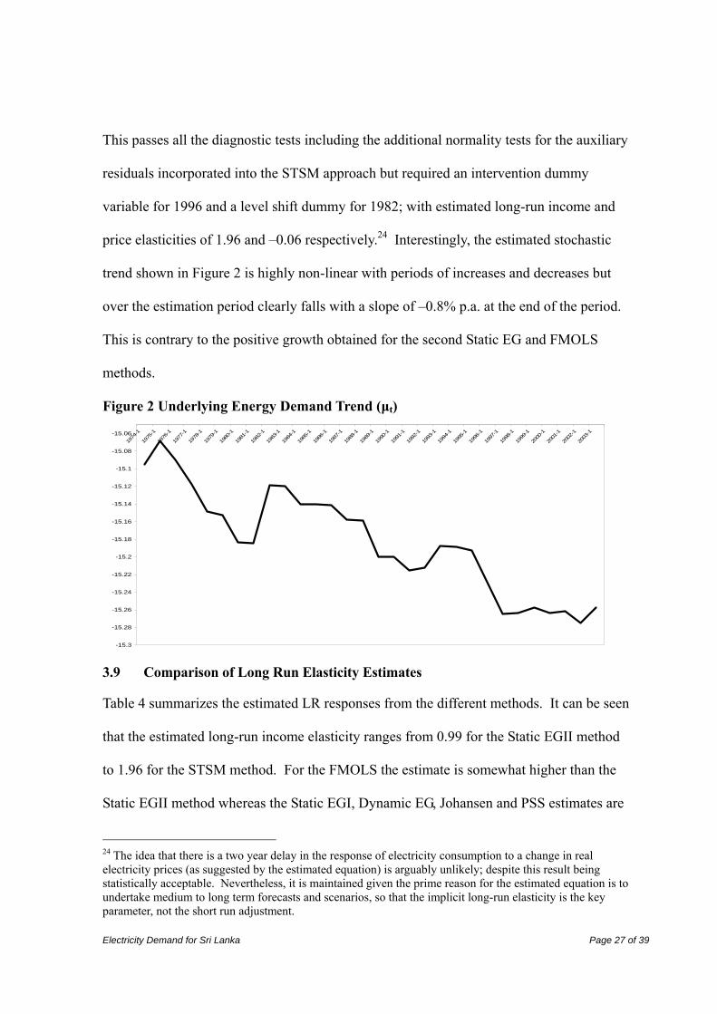
Where μt = –15.257 with a slope of –0.0081 at the end of the period. Se = 0.019 r(1) = 0.10[0.31] r(2) = 0.15[0.22] R(3) = –0.22[0.12] r(4) = Q(10): χ2 = 5.02[0.76] Het: F = 0.89[0.56] Norm(Res): χ2 = 1.62[0.44] Norm(Irr): χ2 = 0.65[0.73] Norm(Lvl): χ2 = 0.90[0.64] Failure(1998): χ2 = 3.18[0.79] Where: Lvl82 = level shift dummy variable for 1982
Electricity Demand for Sri Lanka Page 27 of 39
This passes all the diagnostic tests including the additional normality tests for the auxiliary
residuals incorporated into the STSM approach but required an intervention dummy
variable for 1996 and a level shift dummy for 1982; with estimated long-run income and
price elasticities of 1.96 and –0.06 respectively.24 Interestingly, the estimated stochastic
trend shown in Figure 2 is highly non-linear with periods of increases and decreases but
over the estimation period clearly falls with a slope of –0.8% p.a. at the end of the period.
This is contrary to the positive growth obtained for the second Static EG and FMOLS
methods.
Figure 2 Underlying Energy Demand Trend (μt)
-15.3
-15.28
-15.26
-15.24
-15.22
-15.2
-15.18
-15.16
-15.14
-15.12
-15.1
-15.08
-15.0619
74-1
1975
-1
1976
-1
1977
-1
1978
-1
1979
-1
1980
-1
1981
-1
1982
-1
1983
-1
1984
-1
1985
-1
1986
-1
1987
-1
1988
-1
1989
-1
1990
-1
1991
-1
1992
-1
1993
-1
1994
-1
1995
-1
1996
-1
1997
-1
1998
-1
1999
-1
2000
-1
2001
-1
2002
-1
2003
-1
3.9 Comparison of Long Run Elasticity Estimates
Table 4 summarizes the estimated LR responses from the different methods. It can be seen
that the estimated long-run income elasticity ranges from 0.99 for the Static EGII method
to 1.96 for the STSM method. For the FMOLS the estimate is somewhat higher than the
Static EGII method whereas the Static EGI, Dynamic EG, Johansen and PSS estimates are
24 The idea that there is a two year delay in the response of electricity consumption to a change in real electricity prices (as suggested by the estimated equation) is arguably unlikely; despite this result being statistically acceptable. Nevertheless, it is maintained given the prime reason for the estimated equation is to undertake medium to long term forecasts and scenarios, so that the implicit long-run elasticity is the key parameter, not the short run adjustment.
Electricity Demand for Sri Lanka Page 28 of 39
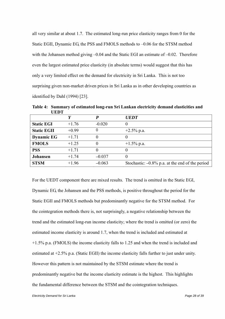
all very similar at about 1.7. The estimated long-run price elasticity ranges from 0 for the
Static EGII, Dynamic EG, the PSS and FMOLS methods to –0.06 for the STSM method
with the Johansen method giving –0.04 and the Static EGI an estimate of –0.02. Therefore
even the largest estimated price elasticity (in absolute terms) would suggest that this has
only a very limited effect on the demand for electricity in Sri Lanka. This is not too
surprising given non-market driven prices in Sri Lanka as in other developing countries as
identified by Dahl (1994) [23].
Table 4: Summary of estimated long-run Sri Lankan electricity demand elasticities and UEDT
Y P UEDT Static EGI +1.76 -0.020 0 Static EGII +0.99 0 +2.5% p.a. Dynamic EG +1.71 0 0 FMOLS +1.25 0 +1.5% p.a. PSS +1.71 0 0 Johansen +1.74 –0.037 0 STSM +1.96 –0.063 Stochastic: –0.8% p.a. at the end of the period
For the UEDT component there are mixed results. The trend is omitted in the Static EGI,
Dynamic EG, the Johansen and the PSS methods, is positive throughout the period for the
Static EGII and FMOLS methods but predominantly negative for the STSM method. For
the cointegration methods there is, not surprisingly, a negative relationship between the
trend and the estimated long-run income elasticity; where the trend is omitted (or zero) the
estimated income elasticity is around 1.7, when the trend is included and estimated at
+1.5% p.a. (FMOLS) the income elasticity falls to 1.25 and when the trend is included and
estimated at +2.5% p.a. (Static EGII) the income elasticity falls further to just under unity.
However this pattern is not maintained by the STSM estimate where the trend is
predominantly negative but the income elasticity estimate is the highest. This highlights
the fundamental difference between the STSM and the cointegration techniques.
Electricity Demand for Sri Lanka Page 29 of 39
Moreover, it illustrates that when trying to forecast future electricity demand or construct
various scenarios a range of techniques should be used where there is no clear statistical
rationale for favouring one over another rather than just having a blind faith in just one
technique. Hence this is the approach undertaken in the next section.
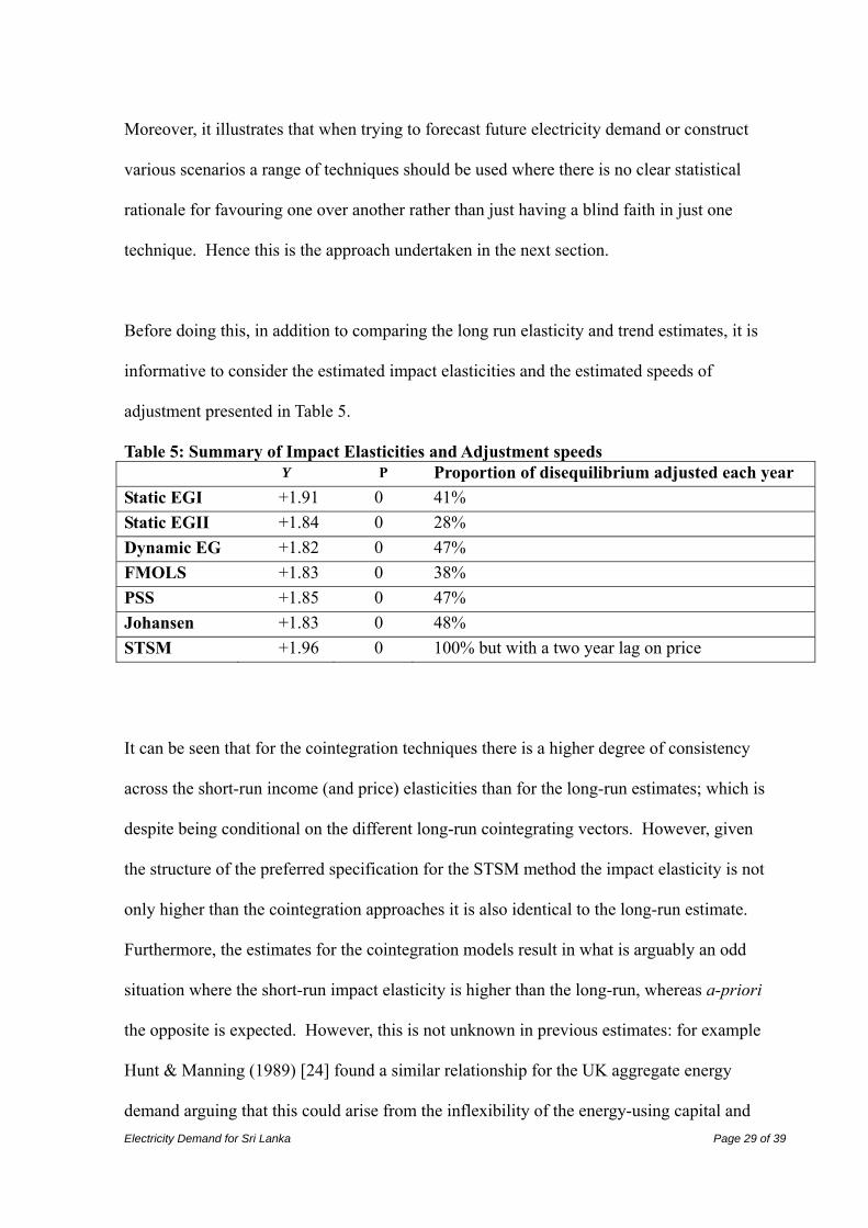
Before doing this, in addition to comparing the long run elasticity and trend estimates, it is
informative to consider the estimated impact elasticities and the estimated speeds of
adjustment presented in Table 5.
Table 5: Summary of Impact Elasticities and Adjustment speeds Y P Proportion of disequilibrium adjusted each year Static EGI +1.91 0 41% Static EGII +1.84 0 28% Dynamic EG +1.82 0 47% FMOLS +1.83 0 38% PSS +1.85 0 47% Johansen +1.83 0 48% STSM +1.96 0 100% but with a two year lag on price
It can be seen that for the cointegration techniques there is a higher degree of consistency
across the short-run income (and price) elasticities than for the long-run estimates; which is
despite being conditional on the different long-run cointegrating vectors. However, given
the structure of the preferred specification for the STSM method the impact elasticity is not
only higher than the cointegration approaches it is also identical to the long-run estimate.
Furthermore, the estimates for the cointegration models result in what is arguably an odd
situation where the short-run impact elasticity is higher than the long-run, whereas a-priori
the opposite is expected. However, this is not unknown in previous estimates: for example
Hunt & Manning (1989) [24] found a similar relationship for the UK aggregate energy
demand arguing that this could arise from the inflexibility of the energy-using capital and

Electricity Demand for Sri Lanka Page 30 of 39
appliance stock of firms and households so that an increase in income results in an
immediate increase in the derived demand for energy in the short-run, but this derived
demand reduces in the longer term as more energy efficient machines are installed. This
might therefore be the case of the electricity using appliances in Sri Lanka and the
efficiency improvement and energy saving programmes implemented over the past years
by CEB and other energy sector organisations. Although, it is worth noting that it may be
the effect of inadequately modelling the effect of energy efficiency on Sri Lankan
electricity demand in the cointegration techniques where the underlying energy demand
trend is either omitted or restricted to be constant over the whole estimation period;
whereas the STSM attempts to take account of this phenomenon, hence the identical short-
run and long-run elasticities.25 Finally, despite the similar short-run impact elasticities the
speeds of adjustment do differ somewhat given the different long-run elasticities and hence
error correction terms.
4 FORECASTING RESULTS
4.1 Final forecast equations
For the cointegration techniques the error correction equations are substituted into the
short-run dynamic equations and simplified and consolidated to give the equations used for
the forecasts. These are shown in Table 6 along with the forecasting equation for the
STSM method which is just the estimated equation above, with the trend declining by the
estimated slope at the end of the estimation period. These are therefore used to drive the
forecasts and scenarios below.
25 More discussion about this argument can be found in Hunt et al (2003) [25]
Electricity Demand for Sri Lanka Page 31 of 39
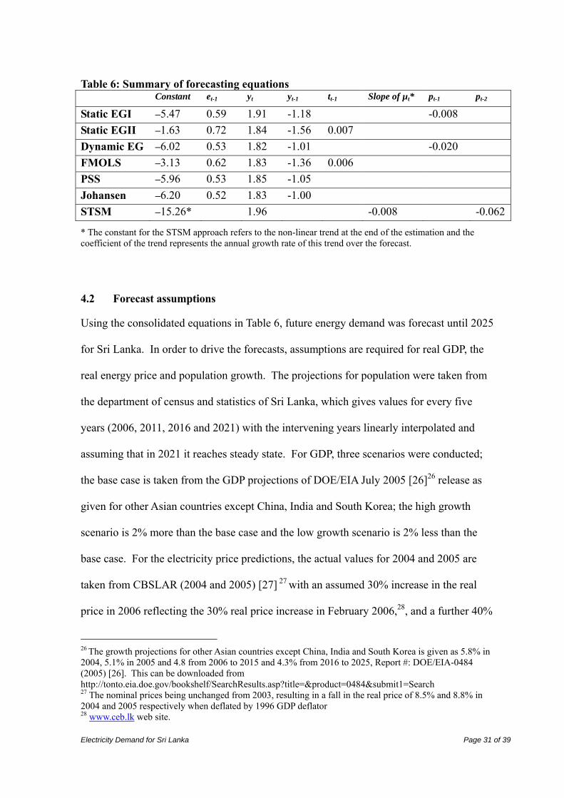
Table 6: Summary of forecasting equations Constant et-1 yt yt-1 tt-1 Slope of µt* pt-1 pt-2
Static EGI –5.47 0.59 1.91 -1.18 -0.008 Static EGII –1.63 0.72 1.84 -1.56 0.007 Dynamic EG –6.02 0.53 1.82 -1.01 -0.020 FMOLS –3.13 0.62 1.83 -1.36 0.006 PSS –5.96 0.53 1.85 -1.05 Johansen –6.20 0.52 1.83 -1.00 STSM –15.26* 1.96 -0.008 -0.062
* The constant for the STSM approach refers to the non-linear trend at the end of the estimation and the coefficient of the trend represents the annual growth rate of this trend over the forecast.
4.2 Forecast assumptions
Using the consolidated equations in Table 6, future energy demand was forecast until 2025
for Sri Lanka. In order to drive the forecasts, assumptions are required for real GDP, the
real energy price and population growth. The projections for population were taken from
the department of census and statistics of Sri Lanka, which gives values for every five
years (2006, 2011, 2016 and 2021) with the intervening years linearly interpolated and
assuming that in 2021 it reaches steady state. For GDP, three scenarios were conducted;
the base case is taken from the GDP projections of DOE/EIA July 2005 [26]26 release as
given for other Asian countries except China, India and South Korea; the high growth
scenario is 2% more than the base case and the low growth scenario is 2% less than the
base case. For the electricity price predictions, the actual values for 2004 and 2005 are
taken from CBSLAR (2004 and 2005) [27] 27 with an assumed 30% increase in the real
price in 2006 reflecting the 30% real price increase in February 2006,28, and a further 40%
26 The growth projections for other Asian countries except China, India and South Korea is given as 5.8% in 2004, 5.1% in 2005 and 4.8 from 2006 to 2015 and 4.3% from 2016 to 2025, Report #: DOE/EIA-0484 (2005) [26]. This can be downloaded from http://tonto.eia.doe.gov/bookshelf/SearchResults.asp?title=&product=0484&submit1=Search 27 The nominal prices being unchanged from 2003, resulting in a fall in the real price of 8.5% and 8.8% in 2004 and 2005 respectively when deflated by 1996 GDP deflator 28 www.ceb.lk web site.
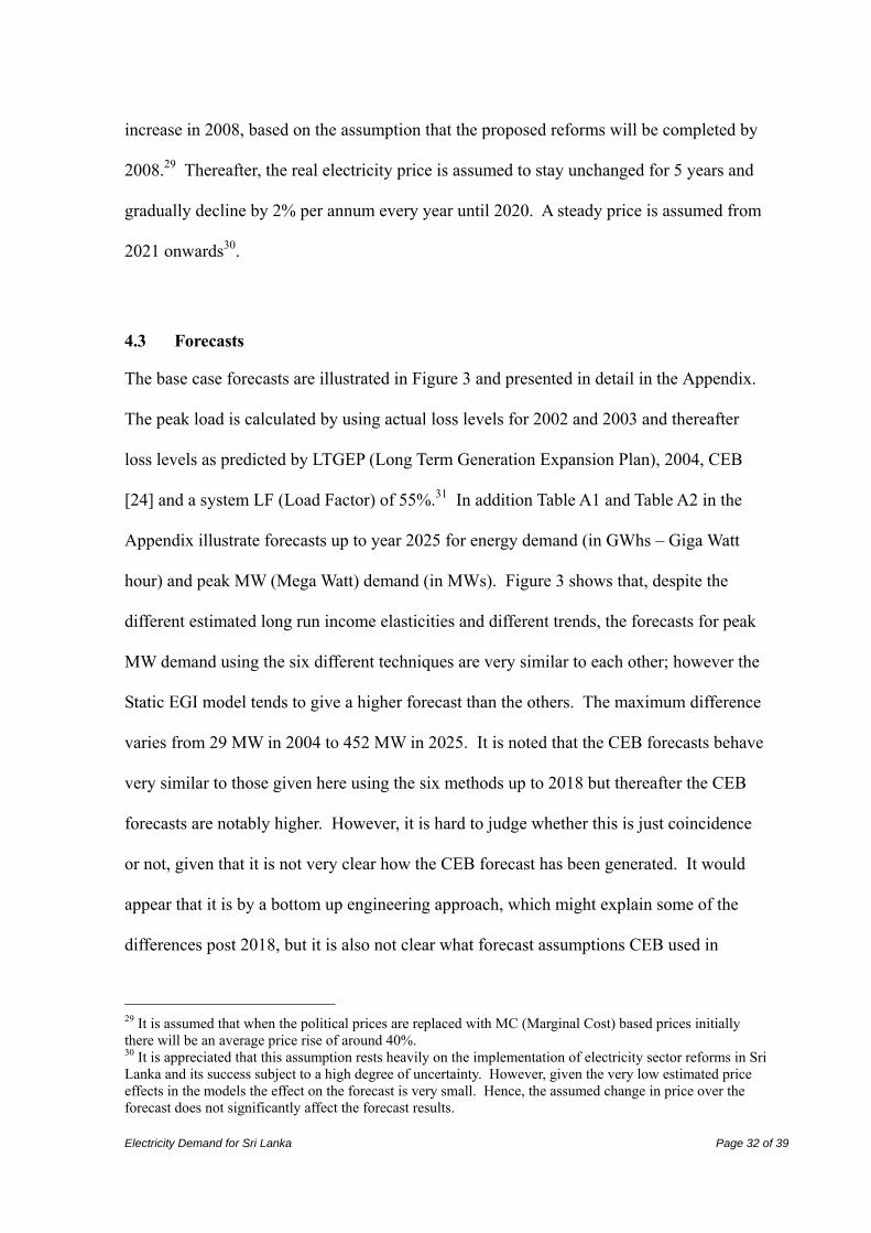
Electricity Demand for Sri Lanka Page 32 of 39
increase in 2008, based on the assumption that the proposed reforms will be completed by
2008.29 Thereafter, the real electricity price is assumed to stay unchanged for 5 years and
gradually decline by 2% per annum every year until 2020. A steady price is assumed from
2021 onwards30.
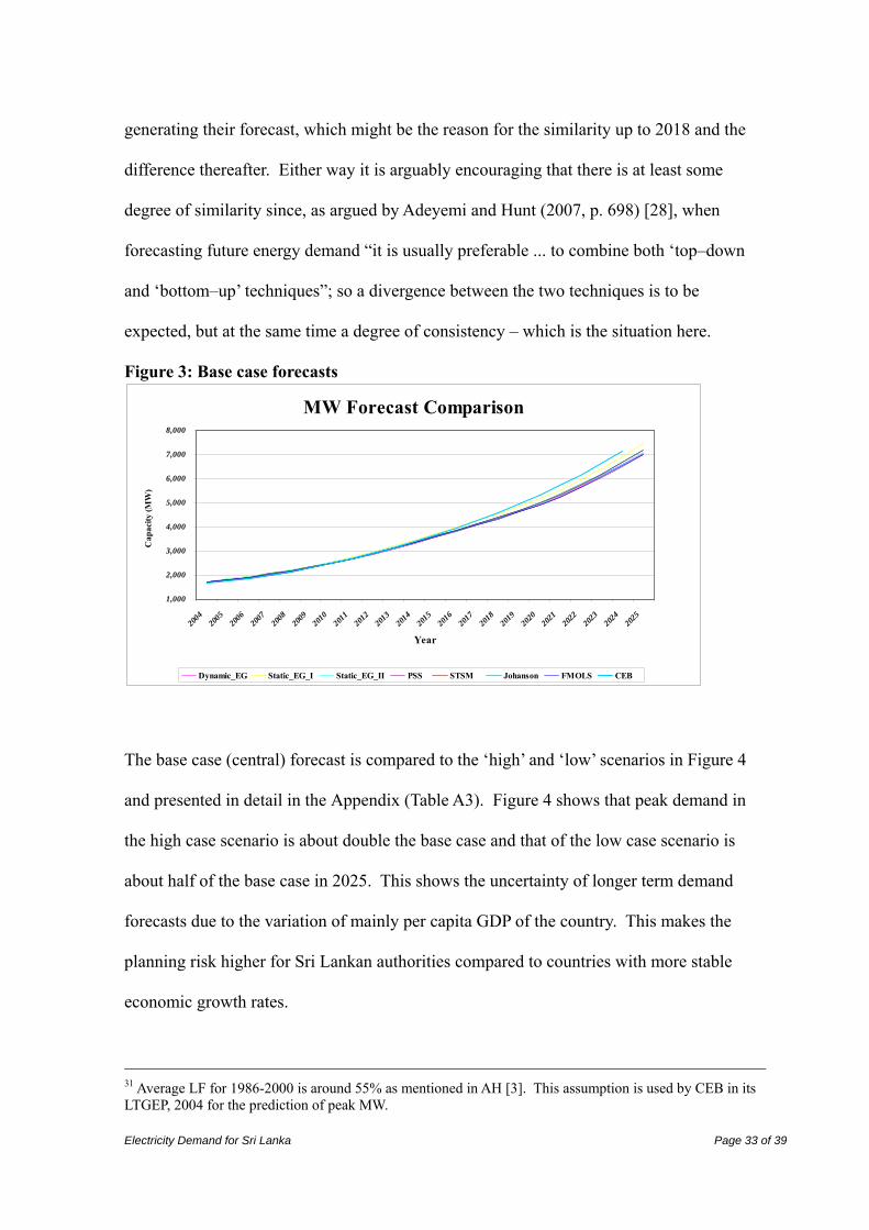
4.3 Forecasts
The base case forecasts are illustrated in Figure 3 and presented in detail in the Appendix.
The peak load is calculated by using actual loss levels for 2002 and 2003 and thereafter
loss levels as predicted by LTGEP (Long Term Generation Expansion Plan), 2004, CEB
[24] and a system LF (Load Factor) of 55%.31 In addition Table A1 and Table A2 in the
Appendix illustrate forecasts up to year 2025 for energy demand (in GWhs – Giga Watt
hour) and peak MW (Mega Watt) demand (in MWs). Figure 3 shows that, despite the
different estimated long run income elasticities and different trends, the forecasts for peak
MW demand using the six different techniques are very similar to each other; however the
Static EGI model tends to give a higher forecast than the others. The maximum difference
varies from 29 MW in 2004 to 452 MW in 2025. It is noted that the CEB forecasts behave
very similar to those given here using the six methods up to 2018 but thereafter the CEB
forecasts are notably higher. However, it is hard to judge whether this is just coincidence
or not, given that it is not very clear how the CEB forecast has been generated. It would
appear that it is by a bottom up engineering approach, which might explain some of the
differences post 2018, but it is also not clear what forecast assumptions CEB used in
29 It is assumed that when the political prices are replaced with MC (Marginal Cost) based prices initially there will be an average price rise of around 40%. 30 It is appreciated that this assumption rests heavily on the implementation of electricity sector reforms in Sri Lanka and its success subject to a high degree of uncertainty. However, given the very low estimated price effects in the models the effect on the forecast is very small. Hence, the assumed change in price over the forecast does not significantly affect the forecast results.
Electricity Demand for Sri Lanka Page 33 of 39
generating their forecast, which might be the reason for the similarity up to 2018 and the
difference thereafter. Either way it is arguably encouraging that there is at least some
degree of similarity since, as argued by Adeyemi and Hunt (2007, p. 698) [28], when
forecasting future energy demand “it is usually preferable ... to combine both ‘top–down
and ‘bottom–up’ techniques”; so a divergence between the two techniques is to be
expected, but at the same time a degree of consistency – which is the situation here.
Figure 3: Base case forecasts
MW Forecast Comparison
1,000
2,000
3,000
4,000
5,000
6,000
7,000
8,000
2004
2005
2006
2007
2008
2009
2010
2011
2012
2013
2014
2015
2016
2017
2018
2019
2020
2021
2022
2023
2024
2025
Year
Cap
acity
(MW
)
Dynamic_EG Static_EG_I Static_EG_II PSS STSM Johanson FMOLS CEB
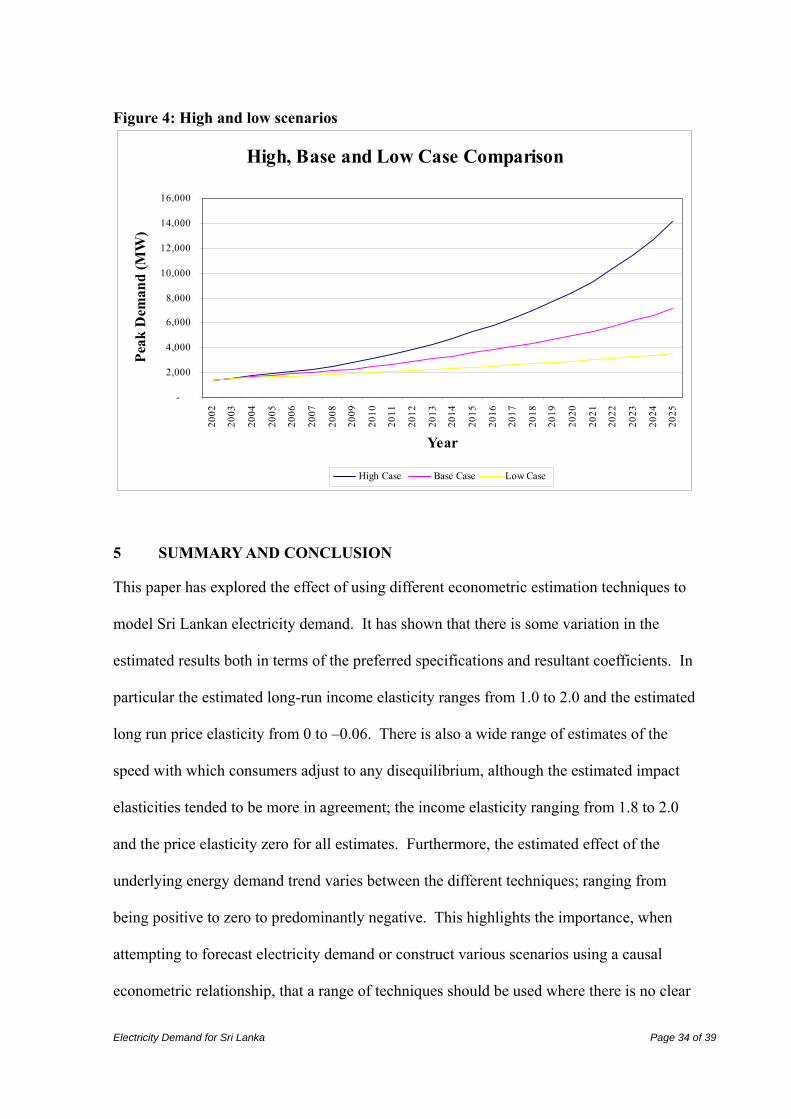
The base case (central) forecast is compared to the ‘high’ and ‘low’ scenarios in Figure 4
and presented in detail in the Appendix (Table A3). Figure 4 shows that peak demand in
the high case scenario is about double the base case and that of the low case scenario is
about half of the base case in 2025. This shows the uncertainty of longer term demand
forecasts due to the variation of mainly per capita GDP of the country. This makes the
planning risk higher for Sri Lankan authorities compared to countries with more stable
economic growth rates.
31 Average LF for 1986-2000 is around 55% as mentioned in AH [3]. This assumption is used by CEB in its LTGEP, 2004 for the prediction of peak MW.
Electricity Demand for Sri Lanka Page 34 of 39
Figure 4: High and low scenarios
High, Base and Low Case Comparison
-
2,000
4,000
6,000
8,000
10,000
12,000
14,000
16,00020
02
2003
2004
2005
2006
2007
2008
2009
2010
2011
2012
2013
2014
2015
2016
2017
2018
2019
2020
2021
2022
2023
2024
2025
Year
Peak
Dem
and
(MW
)
High Case Base Case Low Case
5 SUMMARY AND CONCLUSION
This paper has explored the effect of using different econometric estimation techniques to
model Sri Lankan electricity demand. It has shown that there is some variation in the
estimated results both in terms of the preferred specifications and resultant coefficients. In
particular the estimated long-run income elasticity ranges from 1.0 to 2.0 and the estimated
long run price elasticity from 0 to –0.06. There is also a wide range of estimates of the
speed with which consumers adjust to any disequilibrium, although the estimated impact
elasticities tended to be more in agreement; the income elasticity ranging from 1.8 to 2.0
and the price elasticity zero for all estimates. Furthermore, the estimated effect of the
underlying energy demand trend varies between the different techniques; ranging from
being positive to zero to predominantly negative. This highlights the importance, when
attempting to forecast electricity demand or construct various scenarios using a causal
econometric relationship, that a range of techniques should be used where there is no clear
Electricity Demand for Sri Lanka Page 35 of 39
statistical rationale for favouring one over another rather than just having a blind faith in
one technique.
Despite these differences the forecasts from the six different techniques look fairly similar
up to 2025 which will be encouraging for the Sri Lanka electricity authorities who can
have some faith in the models used for forecasting.32 However, as shown in Section 4 by
the end of the forecast period in 2025 the difference between the base case lowest and
highest forecasts amounts to around 452 MW in forecast peak demand; which, considering
its current status, for a small electricity generation system like Sri Lanka’s with the single
largest generation unit size is around 120 MW, represents a fairly considerable difference
of about 6%. Hence the chosen econometric work potentially has a significant impact of
the policy decisions in the Sri Lankan electricity supply industry in the long run.
In summary, there is a huge uncertainty of the longer term demand forecasts due to the
variation of mainly per capita GDP of the country. This makes the planning risk higher for
Sri Lankan authorities compared to countries with more consistent economic growth rates.
Acknowledgements
The authors are grateful for the valuable comments received on an earlier draft of the paper presented at the 10th International Conference on Sri Lanka Studies on the 17th December 2005, University of Kelaniya, Kelaniya, Sri Lanka. The authors would also like to thank Professor Priyantha DC Wijayatunga from University of Moratuwa and Dr. Thilak Siyambalapitiya from Resource Management Associates (Private) Limited for their help towards providing the data on electricity demand and price. Of course any errors and omissions are due to the authors.
32 This, however, should be seen as a specific result for the Sri Lankan ESI and should not be generalised.
Electricity Demand for Sri Lanka Page 36 of 39
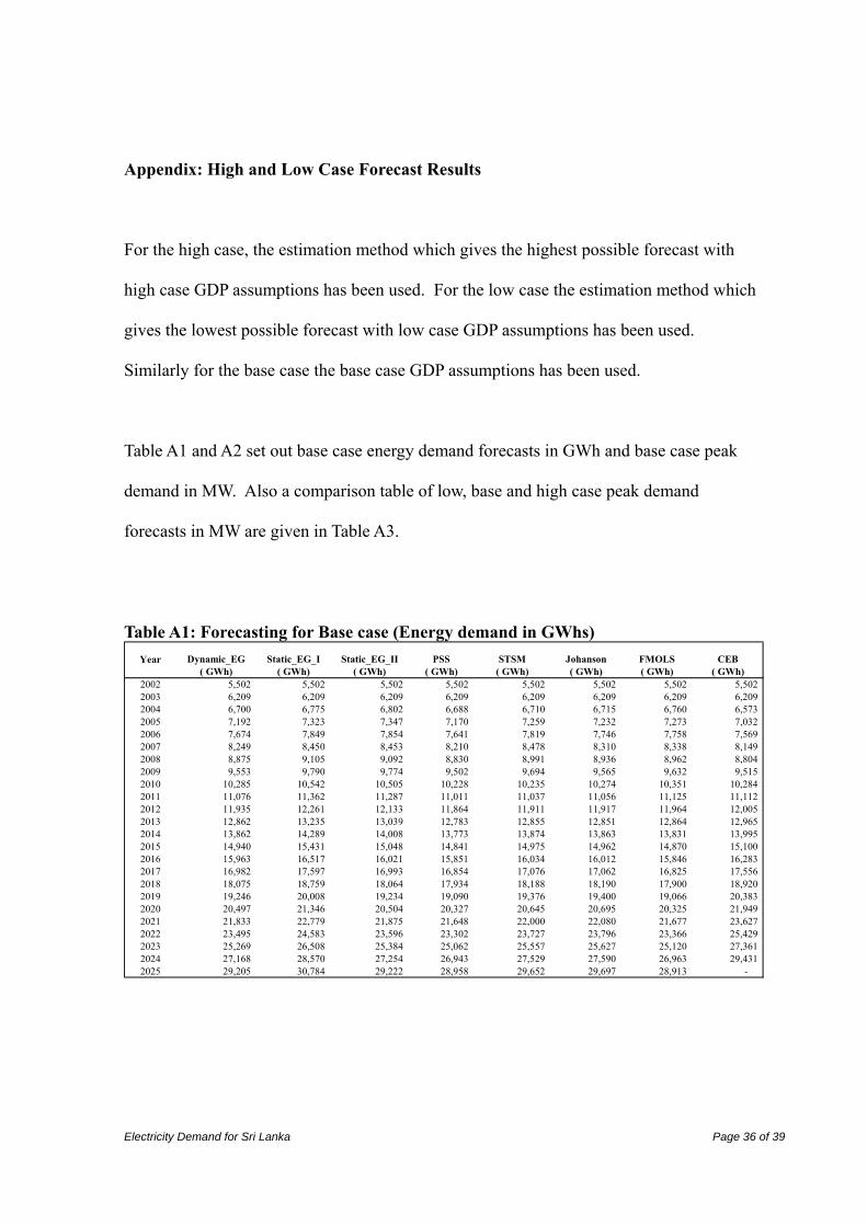
Appendix: High and Low Case Forecast Results
For the high case, the estimation method which gives the highest possible forecast with
high case GDP assumptions has been used. For the low case the estimation method which
gives the lowest possible forecast with low case GDP assumptions has been used.
Similarly for the base case the base case GDP assumptions has been used.
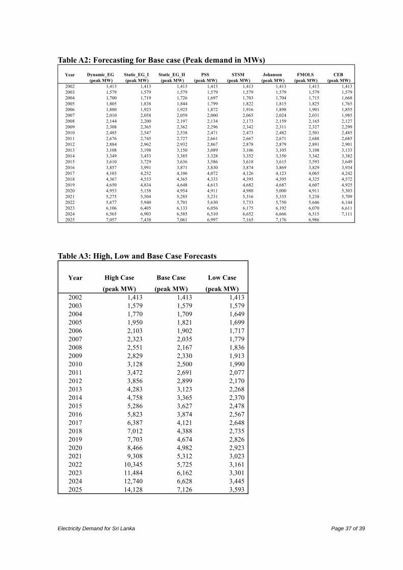
Table A1 and A2 set out base case energy demand forecasts in GWh and base case peak
demand in MW. Also a comparison table of low, base and high case peak demand
forecasts in MW are given in Table A3.
Table A1: Forecasting for Base case (Energy demand in GWhs)
Year Dynamic_EG Static_EG_I Static_EG_II PSS STSM Johanson FMOLS CEB( GWh) ( GWh) ( GWh) ( GWh) ( GWh) ( GWh) ( GWh) ( GWh)
2002 5,502 5,502 5,502 5,502 5,502 5,502 5,502 5,502 2003 6,209 6,209 6,209 6,209 6,209 6,209 6,209 6,209 2004 6,700 6,775 6,802 6,688 6,710 6,715 6,760 6,573 2005 7,192 7,323 7,347 7,170 7,259 7,232 7,273 7,032 2006 7,674 7,849 7,854 7,641 7,819 7,746 7,758 7,569 2007 8,249 8,450 8,453 8,210 8,478 8,310 8,338 8,149 2008 8,875 9,105 9,092 8,830 8,991 8,936 8,962 8,804 2009 9,553 9,790 9,774 9,502 9,694 9,565 9,632 9,515 2010 10,285 10,542 10,505 10,228 10,235 10,274 10,351 10,284 2011 11,076 11,362 11,287 11,011 11,037 11,056 11,125 11,112 2012 11,935 12,261 12,133 11,864 11,911 11,917 11,964 12,005 2013 12,862 13,235 13,039 12,783 12,855 12,851 12,864 12,965 2014 13,862 14,289 14,008 13,773 13,874 13,863 13,831 13,995 2015 14,940 15,431 15,048 14,841 14,975 14,962 14,870 15,100 2016 15,963 16,517 16,021 15,851 16,034 16,012 15,846 16,283 2017 16,982 17,597 16,993 16,854 17,076 17,062 16,825 17,556 2018 18,075 18,759 18,064 17,934 18,188 18,190 17,900 18,920 2019 19,246 20,008 19,234 19,090 19,376 19,400 19,066 20,383 2020 20,497 21,346 20,504 20,327 20,645 20,695 20,325 21,949 2021 21,833 22,779 21,875 21,648 22,000 22,080 21,677 23,627 2022 23,495 24,583 23,596 23,302 23,727 23,796 23,366 25,429 2023 25,269 26,508 25,384 25,062 25,557 25,627 25,120 27,361 2024 27,168 28,570 27,254 26,943 27,529 27,590 26,963 29,431 2025 29,205 30,784 29,222 28,958 29,652 29,697 28,913 -
Electricity Demand for Sri Lanka Page 37 of 39
Table A2: Forecasting for Base case (Peak demand in MWs)
Year Dynamic_EG Static_EG_I Static_EG_II PSS STSM Johanson FMOLS CEB (peak MW) (peak MW) (peak MW) (peak MW) (peak MW) (peak MW) (peak MW) (peak MW)
2002 1,413 1,413 1,413 1,413 1,413 1,413 1,413 1,413 2003 1,579 1,579 1,579 1,579 1,579 1,579 1,579 1,579 2004 1,700 1,719 1,726 1,697 1,703 1,704 1,715 1,668 2005 1,805 1,838 1,844 1,799 1,822 1,815 1,825 1,765 2006 1,880 1,923 1,925 1,872 1,916 1,898 1,901 1,855 2007 2,010 2,058 2,059 2,000 2,065 2,024 2,031 1,985 2008 2,144 2,200 2,197 2,134 2,173 2,159 2,165 2,127 2009 2,308 2,365 2,362 2,296 2,342 2,311 2,327 2,299 2010 2,485 2,547 2,538 2,471 2,473 2,482 2,501 2,485 2011 2,676 2,745 2,727 2,661 2,667 2,671 2,688 2,685 2012 2,884 2,962 2,932 2,867 2,878 2,879 2,891 2,901 2013 3,108 3,198 3,150 3,089 3,106 3,105 3,108 3,133 2014 3,349 3,453 3,385 3,328 3,352 3,350 3,342 3,382 2015 3,610 3,729 3,636 3,586 3,618 3,615 3,593 3,649 2016 3,857 3,991 3,871 3,830 3,874 3,869 3,829 3,934 2017 4,103 4,252 4,106 4,072 4,126 4,123 4,065 4,242 2018 4,367 4,533 4,365 4,333 4,395 4,395 4,325 4,572 2019 4,650 4,834 4,648 4,613 4,682 4,687 4,607 4,925 2020 4,953 5,158 4,954 4,911 4,988 5,000 4,911 5,303 2021 5,275 5,504 5,285 5,231 5,316 5,335 5,238 5,709 2022 5,677 5,940 5,701 5,630 5,733 5,750 5,646 6,144 2023 6,106 6,405 6,133 6,056 6,175 6,192 6,070 6,611 2024 6,565 6,903 6,585 6,510 6,652 6,666 6,515 7,111 2025 7,057 7,438 7,061 6,997 7,165 7,176 6,986
Table A3: High, Low and Base Case Forecasts
Year High Case Base Case Low Case
(peak MW) (peak MW) (peak MW)2002 1,413 1,413 1,413 2003 1,579 1,579 1,579 2004 1,770 1,709 1,649 2005 1,950 1,821 1,699 2006 2,103 1,902 1,717 2007 2,323 2,035 1,779 2008 2,551 2,167 1,836 2009 2,829 2,330 1,913 2010 3,128 2,500 1,990 2011 3,472 2,691 2,077 2012 3,856 2,899 2,170 2013 4,283 3,123 2,268 2014 4,758 3,365 2,370 2015 5,286 3,627 2,478 2016 5,823 3,874 2,567 2017 6,387 4,121 2,648 2018 7,012 4,388 2,735 2019 7,703 4,674 2,826 2020 8,466 4,982 2,923 2021 9,308 5,312 3,023 2022 10,345 5,725 3,161 2023 11,484 6,162 3,301 2024 12,740 6,628 3,445 2025 14,128 7,126 3,593

Electricity Demand for Sri Lanka Page 38 of 39
REFERENCES
[1] Athalage RA, Wijayathunga PDC. Sri Lanka electricity industry: long term thermal generation fuel options, Centre for Energy studies, University of Moratuwa, Sri Lanka, 2002.
[2] Long Term Generation Expansion Plan (LTEG) 2005-2019, Generation Planning Branch, Ceylon Electricity Board, Colombo, Sri Lanka, 2004.
[3] Amarawickrama HA, Hunt LC. Sri Lanka Electricity Supply Industry: A critique of the proposed reforms. Journal of Energy and Development 2005; 30(2): 239-278.
[4] Jayatissa PVIP. Econometric analysis of electricity demand: the case of Sri Lanka, AIT Thesis ET-94-18, Asian Institute of Technology, Bangkok, Thailand, 1994.
[5] Morimoto R, Hope C. The impact of electricity supply on economic growth in Sri Lanka. Energy Economics 2004; 26(1):77-85.
[6] Wijayathunga PDC, Wijeratne DGDC. Sri Lanka energy supply status and cross boarder energy trade issues, Workshop on Regional Power Trade, SARI/Energy, USAID, Kathmandu, Nepal, 2001.
[7] Pesaran H, Smith RP, Akiyama T. Energy Demand in Asian Developing Economies, Oxford University Press, Oxford, UK 1998
[8] Harvey AC. Forecasting, Structural Time Series Models and the Kalman Filter, Cambridge, UK: Cambridge University Press, 1989.
[9] Harvey AC. Trends, Cycles and Autoregressions. Economic Journal 1997; 107(440): 192-201
[10] MacKinnon JG. Numerical Distribution Functions for Unit Root and Cointegration Tests. Journal of Applied Econometrics 1996; 11: 601-618.
[11] Schwert GW, Test for Unit Roots: A Monte Carlo investigation, Journal of Business and Economic Statistics, American Statistical Association, 1989, 7 [2], 147-159
[12] Engle RF, Granger CWJ. Co-integration and Error Correction: Representation, Estimation and Testing. Econometrica 1987; 55(2): 251-76.
[13] Banerjee A, Dolado JJ, Gailbraith JW, Hendry DF. Co-integration, Error-Correction, and the Econometric Analysis of Non-Stationary Data, Advanced Texts in Econometrics (Oxford University Press), 1993.
[14] Inder B. Estimating Long-run Relationship in Economics: A Comparison of Different Approaches. Journal of Econometrics 1993, 57(1-3): 53-68.
[15] Harris R, Sollis R. Applied Time Series Modelling and Forecasting, John Wiley & Sons Ltd, Chichester, UK, 2003.
[16] Phillips PCB, Hansen BE. Statistical inference in Instrumental variables regression with I(1) processes. Review of Economic Studies 1990; 57(1): 99-125
Electricity Demand for Sri Lanka Page 39 of 39
[17] Pesaran MH, Shin Y, Smith RJ. Bounds testing approaches to the analysis of level relationships. Journal of Applied Econometrics 2001; 16(3): 289-326
[18] Pesaran, MH, Pesaran B. Working with Microfit 4.0, Interactive Econometric Analysis, Oxford University Press, Oxford, UK, 1997.
[19] Johansen S. Statistical analysis of cointegration vectors. Journal of Economic Dynamics and Control 1988; 12 (2-3):231-254.
[20] Koopman SJ, Harvey AC, Doornik JA, Shephard N. STAMP 6, International Thompson Business Press, London, 2004.
[21] Statistical Digest 2001-2004, Statistical Unit, Information Management Branch, Ceylon Electricity Board, Colombo, Sri Lanka, 2005.
[22] Hunt LC, Judge G, Ninomiya Y. Underlying trends and seasonality in UK energy demand: a sectoral analysis. Energy Economics 2003; 25(1): 93-118
[23] Dahl C. A survey of energy demand elasticities for the developing world. Journal of Energy and Development 1994; 18(1): 1-47
[24] Hunt LC, Manning N. Energy Price- and Income-Elasticities of Demand: Some Estimates for the UK using the Cointegration Procedure. Scottish Journal of Political Economy1989; 36(2): 183-193.
[25] Hunt LC, Ninomiya Y. Modelling underlying Energy Demand Trend and Stochastic Seasonality: An Econometric Analysis of Transport Oil Demand in the UK and Japan. The Energy Journal 2003; 24(3): 63-96
[26] US International Energy Outlook 2005, Report #: DOE/EIA-0484(2005), Energy Information Administration, Department of Energy, July 2005.
[27] Central Bank of Sri Lanka Annual Report, (CBSLAR) 2000 to 2005, Published in April of each year, 2001-2005, http://www.cbsl.gov.lk/info/10_publication/p_1.htm
[28] Adeyemi OI, Hunt LC. Modelling OECD industrial energy demand: Asymmetric price responses and energy-saving technical change. Energy Economics 2007; 29(4): 693-709


Note: This paper may not be quoted or reproduced
without permission
Surrey Energy Economics Centre (SEEC) Department of Economics
University of Surrey Guildford
Surrey GU2 7XH

SURREY
ENERGY
ECONOMICS
DISCUSSION PAPER
SERIES
For further information about SEEC please go to:
www.seec.surrey.ac.uk