Embed Size (px)
Citation preview

Electrified engine air intake system: modeling,optimization and controlMarinkov, S.
Published: 27/01/2016
Document VersionPublisher’s PDF, also known as Version of Record (includes final page, issue and volume numbers)
Please check the document version of this publication:
• A submitted manuscript is the author's version of the article upon submission and before peer-review. There can be important differencesbetween the submitted version and the official published version of record. People interested in the research are advised to contact theauthor for the final version of the publication, or visit the DOI to the publisher's website.• The final author version and the galley proof are versions of the publication after peer review.• The final published version features the final layout of the paper including the volume, issue and page numbers.
Link to publication
Citation for published version (APA):Marinkov, S. (2016). Electrified engine air intake system: modeling, optimization and control Eindhoven:Eindhoven University of Technology
General rightsCopyright and moral rights for the publications made accessible in the public portal are retained by the authors and/or other copyright ownersand it is a condition of accessing publications that users recognise and abide by the legal requirements associated with these rights.
• Users may download and print one copy of any publication from the public portal for the purpose of private study or research. • You may not further distribute the material or use it for any profit-making activity or commercial gain • You may freely distribute the URL identifying the publication in the public portal ?
Take down policyIf you believe that this document breaches copyright please contact us providing details, and we will remove access to the work immediatelyand investigate your claim.
Download date: 28. May. 2018

Electrified engine air intake system:modeling, optimization and control

The research reported in this thesis is part of the research program of the Dutch
Institute of Systems and Control (DISC). The author has successfully completed the
educational program of the Graduate School DISC.
This research was financially supported by the EUREKA program – project
WETREN #5765.
Electrified engine air intake system: modeling, optimization and control – PhD thesis
by Sava Marinkov, Eindhoven University of Technology.
A catalogue record is available from the Eindhoven University of Technology Library.
ISBN: 978-90-386-3997-0
Typeset by the author using the pdf LATEX documentation system.
Cover design: Sava Marinkov.
Reproduction: CPI Koninklijke Wohrmann, Zutphen, The Netherlands.
Copyright © 2015 by Sava Marinkov. All rights reserved.

Electrified engine air intake system:modeling, optimization and control
PROEFSCHRIFT
ter verkrijging van de graad van doctor aan de
Technische Universiteit Eindhoven, op gezag van de
rector magnificus, prof.dr.ir. F.P.T. Baaijens, voor een
commissie aangewezen door het College voor
Promoties, in het openbaar te verdedigen
op woensdag 27 januari 2016 om 16.00 uur
door
Sava Marinkov
geboren te Novi Sad, Servie

Dit proefschrift is goedgekeurd door de promotoren en de samenstelling van de
promotiecommissie is als volgt:
voorzitter: prof.dr. L.P.H. de Goey
promotor: prof.dr.ir. M. Steinbuch
copromotor: dr.ir. A.G. de Jager
leden: prof.dr. C. Onder (ETH Zurich, Switzerland)
prof.dr. J. Sjoberg (Chalmers University of Technology, Sweden)
prof.dr.ir. N. van de Wouw
adviseur: dr.ir. M. Boot
Het onderzoek dat in dit proefschrift wordt beschreven is uitgevoerd in overeenstemming
met de TU/e Gedragscode Wetenschapsbeoefening.
Contents
Societal summary ix
1 Introduction 1
1.1 General introduction . . . . . . . . . . . . . . . . . . . . . . . . . . . . . 1
1.1.1 Electric supercharging . . . . . . . . . . . . . . . . . . . . . . . . 3
1.1.2 Regenerative throttling . . . . . . . . . . . . . . . . . . . . . . . . 5
1.1.3 Switched Reluctance Machines . . . . . . . . . . . . . . . . . . . . 7
1.2 Research objectives . . . . . . . . . . . . . . . . . . . . . . . . . . . . . . 10
1.3 Contributions and outline . . . . . . . . . . . . . . . . . . . . . . . . . . 11
1.4 Interconnections between topics of research . . . . . . . . . . . . . . . . . 14
1.5 List of publications . . . . . . . . . . . . . . . . . . . . . . . . . . . . . . 15
2 Convex modeling and sizing of electrically supercharged internal com-
bustion engine powertrains 17
2.1 Introduction . . . . . . . . . . . . . . . . . . . . . . . . . . . . . . . . . . 17
2.2 The powertrain sizing problem . . . . . . . . . . . . . . . . . . . . . . . . 19
2.3 Quasistatic vehicle model . . . . . . . . . . . . . . . . . . . . . . . . . . . 21
2.3.1 Vehicle . . . . . . . . . . . . . . . . . . . . . . . . . . . . . . . . . 22
2.3.2 Wheels & brakes . . . . . . . . . . . . . . . . . . . . . . . . . . . 23
2.3.3 Gearbox . . . . . . . . . . . . . . . . . . . . . . . . . . . . . . . . 23
2.3.4 Mechanical power link . . . . . . . . . . . . . . . . . . . . . . . . 23
2.3.5 ICE & air-fuel control . . . . . . . . . . . . . . . . . . . . . . . . 24
2.3.6 Air system . . . . . . . . . . . . . . . . . . . . . . . . . . . . . . . 26
2.3.7 Alternator and MCU motor . . . . . . . . . . . . . . . . . . . . . 28
2.3.8 Electric power link . . . . . . . . . . . . . . . . . . . . . . . . . . 30
2.3.9 Electric buffer . . . . . . . . . . . . . . . . . . . . . . . . . . . . . 30
2.4 Optimization problem formulation . . . . . . . . . . . . . . . . . . . . . . 32
2.4.1 Convex optimization problem . . . . . . . . . . . . . . . . . . . . 33
v
vi Contents
2.4.2 Gear selection strategy . . . . . . . . . . . . . . . . . . . . . . . . 35
2.5 Case study results . . . . . . . . . . . . . . . . . . . . . . . . . . . . . . . 36
2.5.1 Optimal component sizes . . . . . . . . . . . . . . . . . . . . . . . 36
2.5.2 Optimal state and control trajectories . . . . . . . . . . . . . . . . 37
2.6 Conclusions . . . . . . . . . . . . . . . . . . . . . . . . . . . . . . . . . . 37
3 Convex modeling and optimization of a vehicle powertrain equipped
with a generator-turbine throttle unit 39
3.1 Introduction . . . . . . . . . . . . . . . . . . . . . . . . . . . . . . . . . . 39
3.2 Quasistatic vehicle model . . . . . . . . . . . . . . . . . . . . . . . . . . . 41
3.2.1 Vehicle . . . . . . . . . . . . . . . . . . . . . . . . . . . . . . . . . 43
3.2.2 Wheels & brakes . . . . . . . . . . . . . . . . . . . . . . . . . . . 43
3.2.3 Gearbox . . . . . . . . . . . . . . . . . . . . . . . . . . . . . . . . 44
3.2.4 Mechanical power link . . . . . . . . . . . . . . . . . . . . . . . . 44
3.2.5 Air system . . . . . . . . . . . . . . . . . . . . . . . . . . . . . . . 45
3.2.6 ICE . . . . . . . . . . . . . . . . . . . . . . . . . . . . . . . . . . 47
3.2.7 Alternator and GTU generator . . . . . . . . . . . . . . . . . . . 49
3.2.8 Electric power link . . . . . . . . . . . . . . . . . . . . . . . . . . 51
3.2.9 Electric buffer . . . . . . . . . . . . . . . . . . . . . . . . . . . . . 52
3.3 Optimization problem formulation . . . . . . . . . . . . . . . . . . . . . . 53
3.3.1 Gear selection strategy . . . . . . . . . . . . . . . . . . . . . . . . 54
3.3.2 Convex optimization problem . . . . . . . . . . . . . . . . . . . . 55
3.4 Case study results . . . . . . . . . . . . . . . . . . . . . . . . . . . . . . . 56
3.4.1 Optimal engine operating points . . . . . . . . . . . . . . . . . . . 57
3.4.2 Optimal state and control trajectories . . . . . . . . . . . . . . . . 57
3.4.3 The effect of varying the ICE displacement volume on the GTU
performance . . . . . . . . . . . . . . . . . . . . . . . . . . . . . . 60
3.5 Conclusions . . . . . . . . . . . . . . . . . . . . . . . . . . . . . . . . . . 61
4 Four-Quadrant speed control of 4/2 Switched Reluctance Machines 63
4.1 Introduction . . . . . . . . . . . . . . . . . . . . . . . . . . . . . . . . . . 63
4.2 SRM modeling and operation . . . . . . . . . . . . . . . . . . . . . . . . 66
4.2.1 Dynamics . . . . . . . . . . . . . . . . . . . . . . . . . . . . . . . 66
4.2.2 Actuation . . . . . . . . . . . . . . . . . . . . . . . . . . . . . . . 68
4.2.3 Four-quadrant operation . . . . . . . . . . . . . . . . . . . . . . . 70
4.3 SRM control design . . . . . . . . . . . . . . . . . . . . . . . . . . . . . . 77
4.3.1 Speed and position estimation . . . . . . . . . . . . . . . . . . . . 78
4.3.2 Supervisor for startup and change of rotational direction . . . . . 78
Contents vii
4.3.3 Speed control . . . . . . . . . . . . . . . . . . . . . . . . . . . . . 80
4.3.4 Current reference parametrization . . . . . . . . . . . . . . . . . . 81
4.3.5 Current control and commutation . . . . . . . . . . . . . . . . . . 82
4.4 Hardware and software implementation . . . . . . . . . . . . . . . . . . . 82
4.4.1 Hardware configuration . . . . . . . . . . . . . . . . . . . . . . . . 82
4.4.2 Experimental results . . . . . . . . . . . . . . . . . . . . . . . . . 83
4.5 Conclusions . . . . . . . . . . . . . . . . . . . . . . . . . . . . . . . . . . 86
5 Model predictive voltage control of high-speed Switched Reluctance
Generators 89
5.1 Introduction . . . . . . . . . . . . . . . . . . . . . . . . . . . . . . . . . . 89
5.2 SRG modeling and operation . . . . . . . . . . . . . . . . . . . . . . . . 91
5.2.1 Actuation . . . . . . . . . . . . . . . . . . . . . . . . . . . . . . . 91
5.2.2 Dynamics . . . . . . . . . . . . . . . . . . . . . . . . . . . . . . . 93
5.2.3 Analytic commutation angles . . . . . . . . . . . . . . . . . . . . 93
5.2.4 Optimized commutation angles . . . . . . . . . . . . . . . . . . . 95
5.3 SRG control design . . . . . . . . . . . . . . . . . . . . . . . . . . . . . . 97
5.3.1 Model predictive voltage control . . . . . . . . . . . . . . . . . . . 98
5.3.2 Current control and commutation . . . . . . . . . . . . . . . . . . 99
5.4 Simulation results . . . . . . . . . . . . . . . . . . . . . . . . . . . . . . . 100
5.5 Conclusions . . . . . . . . . . . . . . . . . . . . . . . . . . . . . . . . . . 103
6 Speed control of high-speed Switched Reluctance Machines using only
the DC-link measurements 105
6.1 Introduction . . . . . . . . . . . . . . . . . . . . . . . . . . . . . . . . . . 105
6.2 SRM modeling and operation . . . . . . . . . . . . . . . . . . . . . . . . 107
6.2.1 Actuation . . . . . . . . . . . . . . . . . . . . . . . . . . . . . . . 107
6.2.2 Electromagnetic properties . . . . . . . . . . . . . . . . . . . . . . 108
6.2.3 Dynamics . . . . . . . . . . . . . . . . . . . . . . . . . . . . . . . 109
6.3 SRM position-sensorless control design . . . . . . . . . . . . . . . . . . . 109
6.3.1 Open-loop phase flux-linkage and current estimation . . . . . . . 109
6.3.2 Closed-loop speed and position estimation . . . . . . . . . . . . . 111
6.3.3 Speed control, current control and commutation . . . . . . . . . . 113
6.4 Simulation results . . . . . . . . . . . . . . . . . . . . . . . . . . . . . . . 115
6.5 Conclusions . . . . . . . . . . . . . . . . . . . . . . . . . . . . . . . . . . 117
7 Auto-calibration of a generator-turbine throttle unit 119
7.1 Introduction . . . . . . . . . . . . . . . . . . . . . . . . . . . . . . . . . . 119
viii Contents
7.2 Extremum-Seeking Control with disturbance-based optimal input
parametrization . . . . . . . . . . . . . . . . . . . . . . . . . . . . . . . . 122
7.2.1 Problem description . . . . . . . . . . . . . . . . . . . . . . . . . 122
7.2.2 Input error estimation . . . . . . . . . . . . . . . . . . . . . . . . 124
7.2.3 Input parameter estimation . . . . . . . . . . . . . . . . . . . . . 124
7.3 Application of proposed ESC scheme to generator-turbine throttle unit
auto-calibration . . . . . . . . . . . . . . . . . . . . . . . . . . . . . . . . 125
7.3.1 GTU modeling and optimal operation . . . . . . . . . . . . . . . . 126
7.3.2 GTU speed control and mechanical power estimation . . . . . . . 128
7.3.3 ESC implementation . . . . . . . . . . . . . . . . . . . . . . . . . 129
7.4 Simulation results . . . . . . . . . . . . . . . . . . . . . . . . . . . . . . . 130
7.5 Conclusions . . . . . . . . . . . . . . . . . . . . . . . . . . . . . . . . . . 134
8 Conclusions and recommendations 135
8.1 Conclusions . . . . . . . . . . . . . . . . . . . . . . . . . . . . . . . . . . 135
8.2 Recommendations for future research . . . . . . . . . . . . . . . . . . . . 138
A MCU case study: parameter specification 141
B GTU case study: parameter specification 145
C SRM advance angle scheduling signal 149
D SRG average DC-link current 151
Summary 169
Acknowledgements 171
Curriculum Vitae 173
Societal summary
Electrified engine air intake system: modeling, optimization and control
A major part of the current world energy supply comes from burning of fossil fuels. This
releases pollutants which have a negative impact on the environment. Consequently, the
countries around the world have introduced a series of evermore stringent regulations
promoting efficient fossil fuel use. Such trend is especially evident in the ground
transportation sector which continues to rely on fossil fuel-driven internal combustion
engines (ICEs). As a result, over the past few decades, the ICE has seen steady
improvements – both in terms of emissions and fuel-economy. One of the key facilitators
of the undergoing ICE evolution is the advent of powerful microprocessors enabling
the engine electrification and their more versatile control. In this context, this thesis
investigates the emerging electrification of the engine air intake system, i.e., its capacity
to further improve the ICE fuel-economy.
The conducted research focuses on two air intake electrification technologies: electric
supercharging and regenerative throttling. The first enables temporary engine over-
powering and thus creates a possibility to replace a larger engine with a smaller, more
efficient one. The second enables fuel-efficient electricity production using the energy
extracted from the engine intake airflow. The analysis of both of these technologies
has resulted in a range of modeling, optimization and control problems that have been
formulated and solved. This includes optimization problems supporting the design of
ICE powertrains with an electrified engine air intake system, derivation of several novel
control strategies for switched reluctance machines (being the enabling technology for
the two considered applications) and a development of an auto-calibration scheme for
regenerative throttling devices. The presented results show that the electrification of
the engine air intake system can help reduce the vehicle fuel consumption.
ix

x
Chapter 1
Introduction
Abstract In this Chapter a general introduction to the research presented in this thesis is
provided, the research objectives are formulated and the corresponding thesis contributions
are outlined and discussed.
1.1 General introduction
The present world population of 7.3 billion people is projected to increase by almost
one billion within the next twelve years – reaching as many as 9.6 billion by 2050 [1].
Almost all of the additional 2.3 billion people will enlarge the population of developing
countries whereas, in contrast, the population of more developed regions will experience
a minimal change [1]. As a consequence, the anticipated population increase will have
profound effects on the future political stability, food security and energy consumption
of the world as a whole [2].
A major part of the current world energy supply comes from fossil fuels: oil, coal and
natural gas. As a result, these non-renewable resources are being rapidly depleted.
Due to their increased consumption, driven by economic and/or population growth in
the dominating energy markets, it is estimated that the only fossil fuel remaining after
2042 will be coal [3]. On the other hand, it is also widely accepted that the burning
of fossil fuels releases pollutants which contribute to the global warming and overall
have a negative impact on the environment [4]. In general, a long-term solution to the
ensuing environmental problems is seen in the advancement of technology while it is
recognized that the success of this solution will strongly depend on our ability to reduce
1
2 1 Introduction
the influence of materialistic values1 on the society [5], [6].
In a quest for technology-based solutions, an increasing environmental awareness
and dwindling fossil fuel supplies continue to push the policymakers to promote the
renewable and clean energy sources, such as solar and wind, and to penalize the fossil
fuel use. The pressure towards more-efficient and less-polluting utilization of fossil fuels
is hardly anywhere more evident than in the road transport sector [7]. Over the past two
decades, in the European Union (EU) alone, the transport sector has been exposed to a
series of evermore stringent regulations regarding vehicle exhaust gas emissions (EURO
I to EURO VI). As a result, between 1990 and 2013, the emissions of transport-based
nitrogen oxides NOx, i.e., gases responsible for the formation of smog and acidic rain,
were reduced by 56% [8].
To meet ever-tightening expectations on emissions and fuel-economy, the automotive
industry has responded with a multitude of technological advancements in vehicle
mechanics, materials and manufacturing, along with an electrification of virtually every
vehicle component [9]. The electrification is not only represented by the development
of hybrid and fully electric vehicles, which currently comprise only a small fraction of
new car sales (1.4% in the EU in 2013 [10]), but also by an introduction of a variety
of electronic sensors and actuators to conventional internal combustion engine (ICE)
powertrains. The key facilitator of the electronic revolution, which is shaping the
ICE future, has been the advent of powerful microprocessors and the accompanying,
dedicated ICE control and optimization algorithms. Hence, similar to computers and
smartphones, the operation of majority of modern-day cars became governed by millions
of lines of computer code [11].
However, there are numerous scientific challenges lying ahead, which prevent the auto-
motive industry from fully exploiting the electrification potential to reduce the negative
impact of the ICE road transport on the environment. Examples of such challenges
include energy-efficient sizing and control of newly-introduced vehicle components, in
the presence of their rising complexity, multi-domain nonlinear dynamics and tight
physical constraints. Furthermore, powertrain calibration is often viewed as one of the
most expensive, time-consuming tasks in the vehicle development. For this reason, a
derivation of an accurate and automated calibration procedure, applicable to a varying
operating condition setting – remains a major scientific endeavor.
These and other issues impeding the improvement of the ICE vehicle fuel economy are
addressed in this thesis, with a focus on two emerging vehicle technologies: electric
1Refers to excessive concerns regarding personal comfort, wealth and material possessions.
1.1 General introduction 3
supercharging and regenerative throttling. These technologies belong to the domain
of the ICE air intake system electrification and are investigated using mathematical
modeling, numerical optimization and control design tools. An introduction to these
topics is given in Sections 1.1.1 and 1.1.2, whereas Section 1.1.3 provides a case for the
Switched Reluctance Machine as a suitable electric machine candidate for the selected
two applications.
1.1.1 Electric supercharging
The ICE supercharging (boosting) refers to the practice of increasing the pressure or
density of air supplied to the engine to provide it with more oxygen. This enables the
engine to burn more fuel and do more work. By facilitating engine overpowering, the
supercharging allows one to replace a larger engine with a smaller one while maintaining
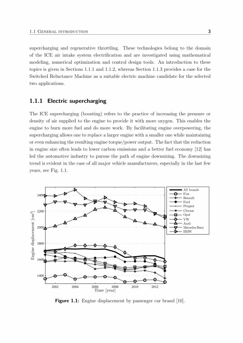
or even enhancing the resulting engine torque/power output. The fact that the reduction
in engine size often leads to lower carbon emissions and a better fuel economy [12] has
led the automotive industry to pursue the path of engine downsizing. The downsizing
trend is evident in the case of all major vehicle manufacturers, especially in the last few
years, see Fig. 1.1.
2002 2004 2006 2008 2010 2012
1400
1600
1800
2000
2200
2400
Time [year]
Enginedisplacement[cm
3]
All brandsFiatRenaultFordPeugeot
CitroenOpel
VWAudiMercedes-BenzBMW
Figure 1.1: Engine displacement by passenger car brand [10].
4 1 Introduction
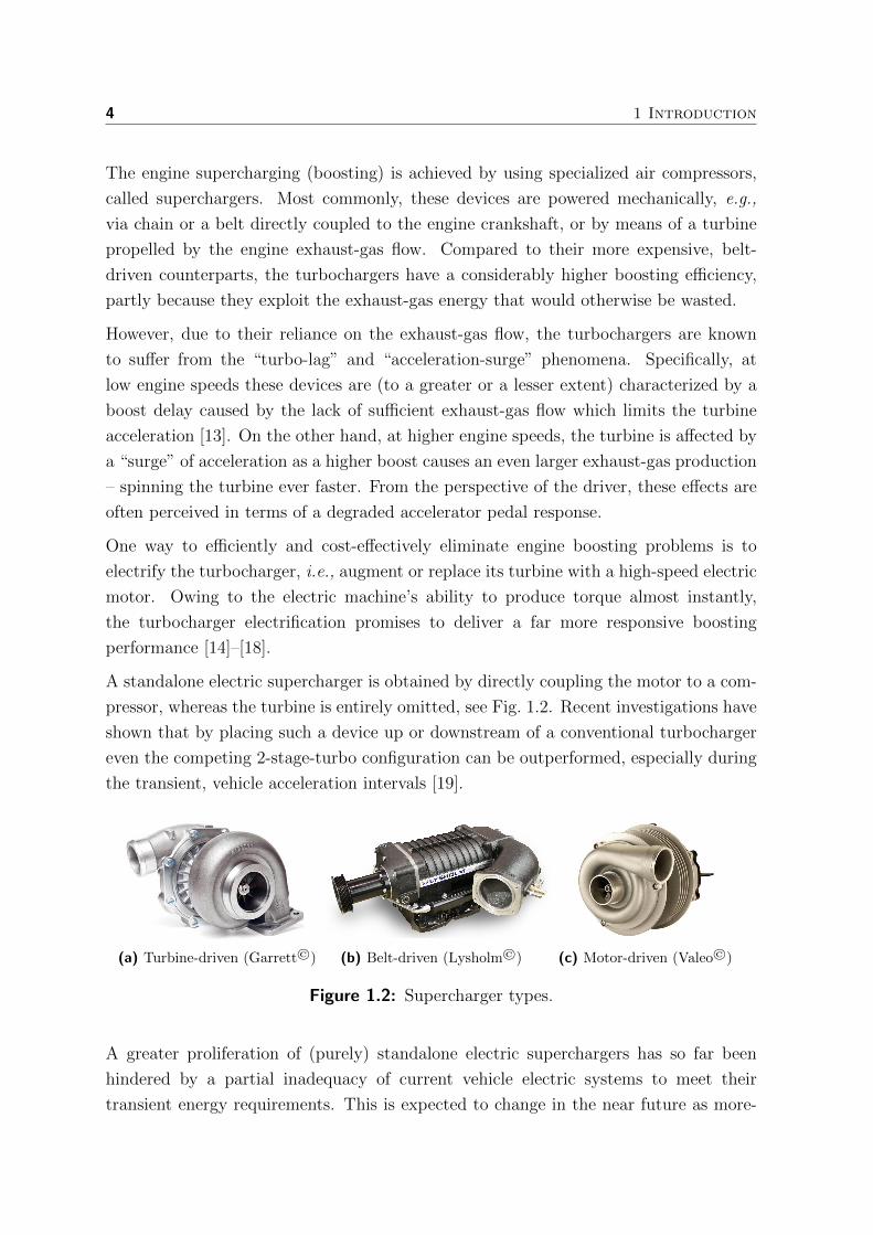
The engine supercharging (boosting) is achieved by using specialized air compressors,
called superchargers. Most commonly, these devices are powered mechanically, e.g.,
via chain or a belt directly coupled to the engine crankshaft, or by means of a turbine
propelled by the engine exhaust-gas flow. Compared to their more expensive, belt-
driven counterparts, the turbochargers have a considerably higher boosting efficiency,
partly because they exploit the exhaust-gas energy that would otherwise be wasted.
However, due to their reliance on the exhaust-gas flow, the turbochargers are known
to suffer from the “turbo-lag” and “acceleration-surge” phenomena. Specifically, at
low engine speeds these devices are (to a greater or a lesser extent) characterized by a
boost delay caused by the lack of sufficient exhaust-gas flow which limits the turbine
acceleration [13]. On the other hand, at higher engine speeds, the turbine is affected by
a “surge” of acceleration as a higher boost causes an even larger exhaust-gas production
– spinning the turbine ever faster. From the perspective of the driver, these effects are
often perceived in terms of a degraded accelerator pedal response.
One way to efficiently and cost-effectively eliminate engine boosting problems is to
electrify the turbocharger, i.e., augment or replace its turbine with a high-speed electric
motor. Owing to the electric machine’s ability to produce torque almost instantly,
the turbocharger electrification promises to deliver a far more responsive boosting
performance [14]–[18].
A standalone electric supercharger is obtained by directly coupling the motor to a com-
pressor, whereas the turbine is entirely omitted, see Fig. 1.2. Recent investigations have
shown that by placing such a device up or downstream of a conventional turbocharger
even the competing 2-stage-turbo configuration can be outperformed, especially during
the transient, vehicle acceleration intervals [19].
(a) Turbine-driven (Garrett©) (b) Belt-driven (Lysholm©) (c) Motor-driven (Valeo©)
Figure 1.2: Supercharger types.
A greater proliferation of (purely) standalone electric superchargers has so far been
hindered by a partial inadequacy of current vehicle electric systems to meet their
transient energy requirements. This is expected to change in the near future as more-
1.1 General introduction 5
efficient, 48V architectures replace conventional, 12V vehicle electrical systems and as
low-cost, high-power-density batteries and (ultra-) capacitors appear on the market.
The prospective advantages of standalone, electric supercharging over its alternatives
can be summarized as:
1. Simplified packaging and installation.
2. Reduced manufacturing costs.
3. Instantaneous throttle response.
4. Programmable and efficient boosting.
The first two are a consequence of the electric supercharger’s lack of the engine
exhaust connection which eliminates the need for materials capable of withstanding
high exhaust-gas pressures and temperatures. The second two reflect its potential to
quickly, precisely and when necessary, deliver the air-mass required for the optimal fuel
combustion [20].
Due to these beneficial properties, electric supercharging is seen as a key enabler of the
engine downsizing in the near future. The main difficulty facing such a prospect lies
in the optimal sizing and utilization of the components constituting the electrically
supercharged ICE powertrain. Unlike the turbocharger, the electric supercharger
introduces both a coupling and a trade-off between the sizes of the ICE and the vehicle
electric components, such as a battery and an alternator. Clearly, the resolution of
this trade-off depends on an envisioned vehicle daily usage, which therefore has to be
accounted for as well when attempting to improve the vehicle fuel economy, via the
described ICE downsizing mechanism. This topic is treated in more detail as a part of
the research presented in this thesis.
1.1.2 Regenerative throttling
A throttle is a valve used to regulate the amount of air entering the gasoline ICE in
response to the driver’s accelerator pedal input. Thus, by assuming that a relatively
constant air-fuel ratio is maintained, the throttle actuation (throttling) also indirectly
determines the amount of fuel burned in each engine cycle. When the throttle is fully
open, the air in the engine intake manifold is at approximately ambient atmospheric
pressure. Otherwise, when it is partially closed, the (intake manifold) air pressure drops
below the ambient value, i.e., a partial vacuum develops.
6 1 Introduction
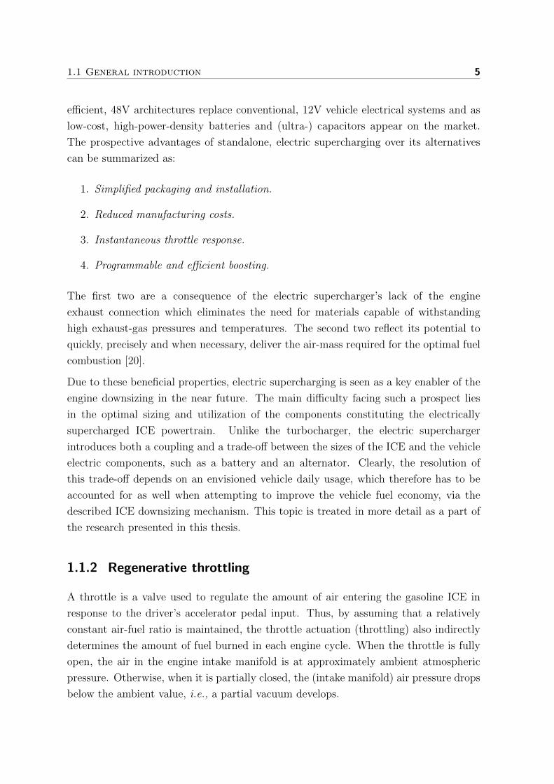
Negative work done by the engine to inhale and exhale gases is known as a pumping
(throttling) loss, which constitutes a significant portion of the total energy losses of
throttled gasoline ICEs, see Fig. 1.3. This is because in such engines, due to the
throttling, the piston is required to counteract the developed pressure differential
between the intake manifold and the engine crankcase in order to draw the air into
the cylinder.
Power loop
Pumping loop
VTDC VBDC
pAM
pIM
Volume
Pressure
Figure 1.3: PV diagram for a throttled gasoline ICE.
To minimize the pumping loss, an increasing number of modern-day drive-by-wire2
gasoline ICEs are designed to operate with a wide open throttle, under various load
conditions. This is made possible by a combination of different engine technologies
such as gasoline direct injection [21], exhaust gas recirculation [22] and variable valve
actuation [23], [24]. However, as in most cases dramatic changes to the engine design
become necessary, this raises concerns regarding the durability and cost-effectiveness of
such solutions.
Regenerative throttling represents an alternative and yet simple way to deal with the
engine pumping loss. Instead of trying to eliminate it, this approach actually exploits
the loss, i.e., the inherent pressure differential associated with it, to do useful work.
Regenerative throttling can be achieved by replacing the throttle valve with a turbo-
expander (turbine) equipped with variable stator vanes [25]. The turbine is used to
extract the potential energy from the intake airflow and convert it into kinetic energy
for driving an electric generator. In this way, electricity needed for powering a growing
number of vehicle electric auxiliary loads can be produced [26]. As an additional benefit,
the cool air mass exiting the turbine can be utilized to assist the vehicle air conditioning
2Refers to the use of an electrical, instead of a traditional, purely mechanical linkage between the
accelerator pedal and the throttle.
1.1 General introduction 7
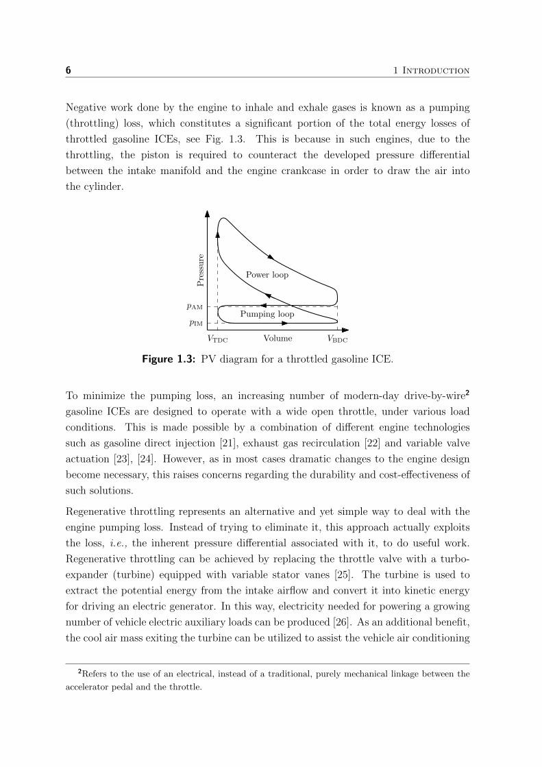
system via a dedicated heat-exchanger, see Fig. 1.4.
Figure 1.4: Regenerative throttling: Waste-Energy Driven Air-Conditioning
System concept [25].
Apart from the added cooling capacity, the advantage of using a regenerative throttling
device instead of, or in addition to, the conventional (Lundell [27], [28]) car alternator
is a potentially more efficient vehicle electricity production. The higher operational
efficiency stems from the fact that, unlike the alternator, a regenerative throttling device
(i.e., a generator-turbine throttle unit) is not connected to the engine’s crankshaft. This
offers the opportunity to independently control its speed such that it maximizes the
generator power output.
However, the computation of the optimal turbine speed is not at all trivial – the optimal
value varies with the conditions present in the ICE air intake system and, in addition,
depends on a range of turbine parameters. This creates a necessity for a specialized
turbine calibration procedure, which adds to the cost and limits the functionality of the
resulting device. Motivated by this problem, a part of this thesis is dedicated to the
research and development of methods for relieving the engineering systems, e.g., the
generator-turbine throttle unit, from excessive calibration requirements. In addition,
this thesis also presents the techniques for investigating the effect of the (calibrated)
regenerative throttling device on the vehicle fuel economy.
1.1.3 Switched Reluctance Machines
One of the prerequisites for a wider adoption of the electric supercharging and regener-
ative throttling technologies is the availability of an electric machine endowed with the
8 1 Introduction
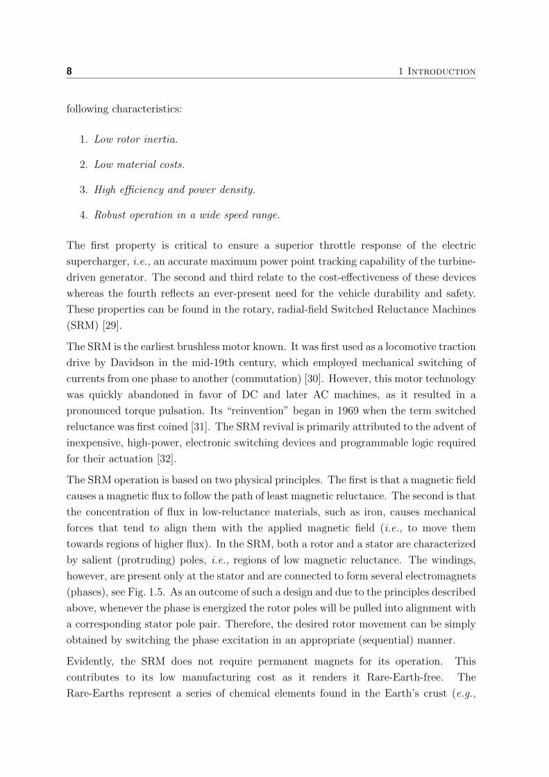
following characteristics:
1. Low rotor inertia.
2. Low material costs.
3. High efficiency and power density.
4. Robust operation in a wide speed range.
The first property is critical to ensure a superior throttle response of the electric
supercharger, i.e., an accurate maximum power point tracking capability of the turbine-
driven generator. The second and third relate to the cost-effectiveness of these devices
whereas the fourth reflects an ever-present need for the vehicle durability and safety.
These properties can be found in the rotary, radial-field Switched Reluctance Machines
(SRM) [29].
The SRM is the earliest brushless motor known. It was first used as a locomotive traction
drive by Davidson in the mid-19th century, which employed mechanical switching of
currents from one phase to another (commutation) [30]. However, this motor technology
was quickly abandoned in favor of DC and later AC machines, as it resulted in a
pronounced torque pulsation. Its “reinvention” began in 1969 when the term switched
reluctance was first coined [31]. The SRM revival is primarily attributed to the advent of
inexpensive, high-power, electronic switching devices and programmable logic required
for their actuation [32].
The SRM operation is based on two physical principles. The first is that a magnetic field
causes a magnetic flux to follow the path of least magnetic reluctance. The second is that
the concentration of flux in low-reluctance materials, such as iron, causes mechanical
forces that tend to align them with the applied magnetic field (i.e., to move them
towards regions of higher flux). In the SRM, both a rotor and a stator are characterized
by salient (protruding) poles, i.e., regions of low magnetic reluctance. The windings,
however, are present only at the stator and are connected to form several electromagnets
(phases), see Fig. 1.5. As an outcome of such a design and due to the principles described
above, whenever the phase is energized the rotor poles will be pulled into alignment with
a corresponding stator pole pair. Therefore, the desired rotor movement can be simply
obtained by switching the phase excitation in an appropriate (sequential) manner.
Evidently, the SRM does not require permanent magnets for its operation. This
contributes to its low manufacturing cost as it renders it Rare-Earth-free. The
Rare-Earths represent a series of chemical elements found in the Earth’s crust (e.g.,

1.1 General introduction 9
1
1
2 2
statorpole
rotorpole
statorwindings
+
Figure 1.5: Cross section of a 2-phase 4/2 SRM.
dysprosium and neodymium), which are vital to many modern technologies such as
consumer electronics, clean energy, health care, national defense and many others [33],
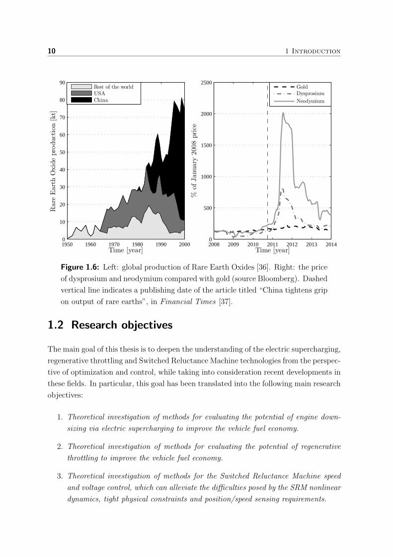
[34]. Since mid-1990s China has emerged as a dominant Rare-Earth supplier and as such
uses its near-monopoly to restrict their availability and dictate the price, see Fig. 1.6.
In the long run, this considerably adds to the attractiveness of the SRM, w.r.t. its
alternatives, e.g., Permanent Magnet Synchronous Machine (PMSM) [35].
Due to its lack of magnets and windings, the SRM rotor is highly mechanically robust,
small in size and has a low moment of inertia. At low speeds (e.g., below 10000rpm) the
power density of the SRM is comparable to that of the induction motor and somewhat
lower than the PMSM, whereas at higher speeds it is equivalent or even larger [29].
These and other favorable characteristics make the SRM well-suited to the vehicle
electrification purposes, including the electric supercharging and regenerative throttling
applications. In an effort to help harvest the full potential of these two technologies a
part of this thesis is devoted to the research on high-speed (low-cost) SRMs.
The “standard” SRM control problems concern the minimization of acoustic noise,
torque ripple, energy losses and the elimination of position/speed sensors. Furthermore,
as a consequence of its simple mechanical design and the switched reluctance principle
of operation, the SRM is also characterized by an inherently nonlinear switched system
dynamics, which renders a treatment of the “standard” issues challenging. For this
reason, a particular emphasis in this thesis has been put on the dynamical modeling,
optimization and control of the SRMs.
10 1 Introduction
1950 1960 1970 1980 1990 20000
10
20
30
40
50
60
70
80
90
Time [year]
Rare
EarthOxideproduction[kt]
Rest of the worldUSAChina
2008 2009 2010 2011 2012 2013 20140
500
1000
1500
2000
2500
Time [year]
%ofJanu
ary
2008price
GoldDysprosium
Neodymium
Figure 1.6: Left: global production of Rare Earth Oxides [36]. Right: the price
of dysprosium and neodymium compared with gold (source Bloomberg). Dashed
vertical line indicates a publishing date of the article titled “China tightens grip
on output of rare earths”, in Financial Times [37].
1.2 Research objectives
The main goal of this thesis is to deepen the understanding of the electric supercharging,
regenerative throttling and Switched Reluctance Machine technologies from the perspec-
tive of optimization and control, while taking into consideration recent developments in
these fields. In particular, this goal has been translated into the following main research
objectives:
1. Theoretical investigation of methods for evaluating the potential of engine down-
sizing via electric supercharging to improve the vehicle fuel economy.
2. Theoretical investigation of methods for evaluating the potential of regenerative
throttling to improve the vehicle fuel economy.
3. Theoretical investigation of methods for the Switched Reluctance Machine speed
and voltage control, which can alleviate the difficulties posed by the SRM nonlinear
dynamics, tight physical constraints and position/speed sensing requirements.
1.3 Contributions and outline 11
4. Theoretical investigation of methods for relieving the engineering systems, such as
the generator-turbine throttle unit, from excessive calibration requirements.
In response to these objectives, a number of research contributions has been made.
They are listed in the following Section.
1.3 Contributions and outline
This thesis contains six research chapters, i.e., Chapters 2-7. The first objective is
addressed in Chapter 2, the second in Chapter 3, the third in Chapters 4 to 6 and
the fourth in Chapter 7. A short summary of the main contributions of each of these
chapters is given below.
In Chapter 2, a method for sizing of an electrically supercharged ICE powertrain is
presented. The main contributions of Chapter 2 are:
• Detailed modeling of the electrically supercharged ICE vehicle powertrain. Apart
from the ICE, the model also includes a standalone electric supercharger used to
help the engine during short-duration high-power demands (and thus allows it to
be downsized), as well as an electric energy buffer which provides the supercharger
with sufficient electric energy/power to operate.
• Development of a computational method for finding the optimal ICE and buffer
size, for the case of the described vehicle powertrain. The sizing of both
components is performed by minimizing the sum of the vehicle operational (fuel)
and component (engine and buffer) costs. In general, the resulting optimization
problem constitutes a non-convex, nonlinear and a mixed-integer dynamic pro-
gram, where the ICE and buffer are optimally sized only when the vehicle is
also optimally controlled (on a studied driving cycle). The problem is handled
by first decoupling the integer decisions, i.e., the gear selection strategy (decided
heuristically), and then by formulating the remaining problem as a convex second-
order cone program, which can be solved efficiently with the help of dedicated
numerical tools.
• A representative, simulation-based case study is performed providing a solution of
the problem defined above, where the optimal engine and the electric buffer sizes
are computed for a specific, electrically supercharged ICE vehicle. The results
show that the (standalone) electric supercharging can support considerable ICE
12 1 Introduction
downsizing – yielding up to 10% savings in fuel costs over a specific driving cycle,
w.r.t. a baseline, naturally-aspirated engine scenario.
In Chapter 3, a regenerative throttling potential to improve the gasoline ICE vehicle
fuel economy is investigated. The main contributions of Chapter 3 are:
• Detailed modeling of the vehicle powertrain equipped with a generator-turbine
throttle unit, which is used to complement the car alternator while powering the
vehicle electric auxiliaries.
• Development of a computational method for finding the optimal buffer size, for
the case of the described vehicle powertrain. In particular, the minimization of the
sum of the vehicle operational (fuel) and component (buffer) costs is considered.
The resulting optimization problem is casted into a semi-definite convex program
using a series of convex (model) relaxation steps, whereas a transmission gear, an
integer variable, is decided outside the convex optimization.
• A representative, simulation-based case study is performed that provides a solu-
tion of the problem defined above for several different driving cycles and engine
sizes. The presented results show that the use of the generator-turbine throttle
unit can reduce the total operational (fuel) and component (buffer) costs by
typically 2-4% or even more than 4% in selected cases, depending on factors such
as the engine size and the choice of a driving cycle.
In Chapter 4, a method for four-quadrant speed control of 4/2 Switched Reluctance
Machines is presented. The main contributions of Chapter 4 are:
• Development of a model-based, open-loop average torque control scheme in the
form of a nonlinear mapping between the 4/2 SRM operating point (defined by
the desired average torque, rotational speed and the applied DC-link voltage) and
a set of low-level current reference parameters.
• Development of a four-quadrant 4/2 SRM speed controller that can cope with the
identified, speed and voltage-dependent, average torque bounds.
• Development of a supervisory control algorithm for supporting the startup and
change of rotational direction of 4/2 SRMs.
In Chapter 5, a method for Model Predictive voltage Control (MPC) of high-speed
Switched Reluctance Generators (SRG) is developed. The main contributions of
Chapter 5 are:

1.3 Contributions and outline 13
• Development of a linear, explicit MPC law that enforces the desired SRG average
DC-link current and voltage bounds and enables tracking of the specified DC-link
voltage reference, in the presence of an unknown electrical load.
• Development of a model-based, parametric SRG commutation strategy based on
its measured electromagnetic characteristics. In this context, the commutation
rules are parametrized by the desired average DC-link current, rotational speed
and the DC-link voltage.
In Chapter 6, a method for speed control of high-speed Switched Reluctance Ma-
chines, using only the DC-link measurements, is presented. The main contribution of
Chapter 6 is:
• Development of a novel position-sensorless speed control strategy for high-speed
Switched Reluctance Machines. Its key component is an algorithm for rotor po-
sition and speed estimation using the DC-link voltage and current measurements
only. This algorithm eliminates a need for a number of hardware components
related to position, speed, phase current and phase voltage sensing. It thus allows
the SRM electric system’s costs to be lowered and its reliability increased.
In Chapter 7, a method for auto-calibration of the generator-turbine throttle unit is
described. The main contributions of Chapter 7 are:
• Development of a novel, parametric Extremum-Seeking Control (ESC) algorithm,
with a disturbance-based optimal input parametrization, which is suitable for
tracking an unknown, time-varying extremum. The proposed ESC scheme is
applicable to situations where the disturbances leading to changes in the optimal
input are known/measurable. Its main advantage over other ESC approaches is
that it identifies a mapping between the disturbances and optimal inputs. Once
found, the constructed mapping can be directly employed in real-time, without
the need for further extremum-seeking.
• Application of the developed ESC algorithm for purposes of the generator-turbine
throttle unit auto-calibration. In this context, the presented solution is used to
find an unknown relationship between the disturbances (turbine pressure ratio
and vanes position) and the optimal input (turbine reference speed), in an initial,
automated calibration step.
Finally, in Chapter 8, conclusions are drawn and recommendations for future research
are presented.
14 1 Introduction
1.4 Interconnections between topics of research
Chapters 2 and 3 employ a similar powertrain modeling and optimization methodology.
Namely, in these chapters, the common vehicle powertrain components, such as wheels,
brakes, gearbox and electric buffer, are modeled in the same way. Also, the formulation
of the underlying optimization problems and related cost functions is, in certain aspects,
shared as well (e.g., the electric buffer and fuel costs are considered in both cases).
However, as these chapters treat the two different air intake system electrification
technologies, the crucial differences between them are in the model and functionality
of the related air intake devices. This also results in distinct fuel-saving mechanisms
(engine downsizing via electric supercharging vs. regenerative throttling) and air intake
manifold conditions (above vs. below ambient pressure). Moreover, even though both
applications implicitly assume the use of high-speed electric machines, Chapter 2
explicitly refers to their motoring and Chapter 3 to their generating operation, i.e.,
discharging and charging of the electric buffer.
The 4/2 SRM four-quadrant controller, proposed in Chapter 4, can be used for both
electric supercharging and regenerative throttling purposes. This is because it allows
the 4/2 SRM to operate in either direction of rotation, both as a motor and as a
generator. Hence, the developed algorithm could be even applied to control the speed
of a hypothetical, hybrid device, which would combine the properties of the standalone
electric supercharger and generator-turbine throttle unit. The practicality of such a
device, however, remains to be researched. In contrast, the SRM controllers, discussed
in Chapters 5 and 6, are intended for unidirectional applications only. These and other
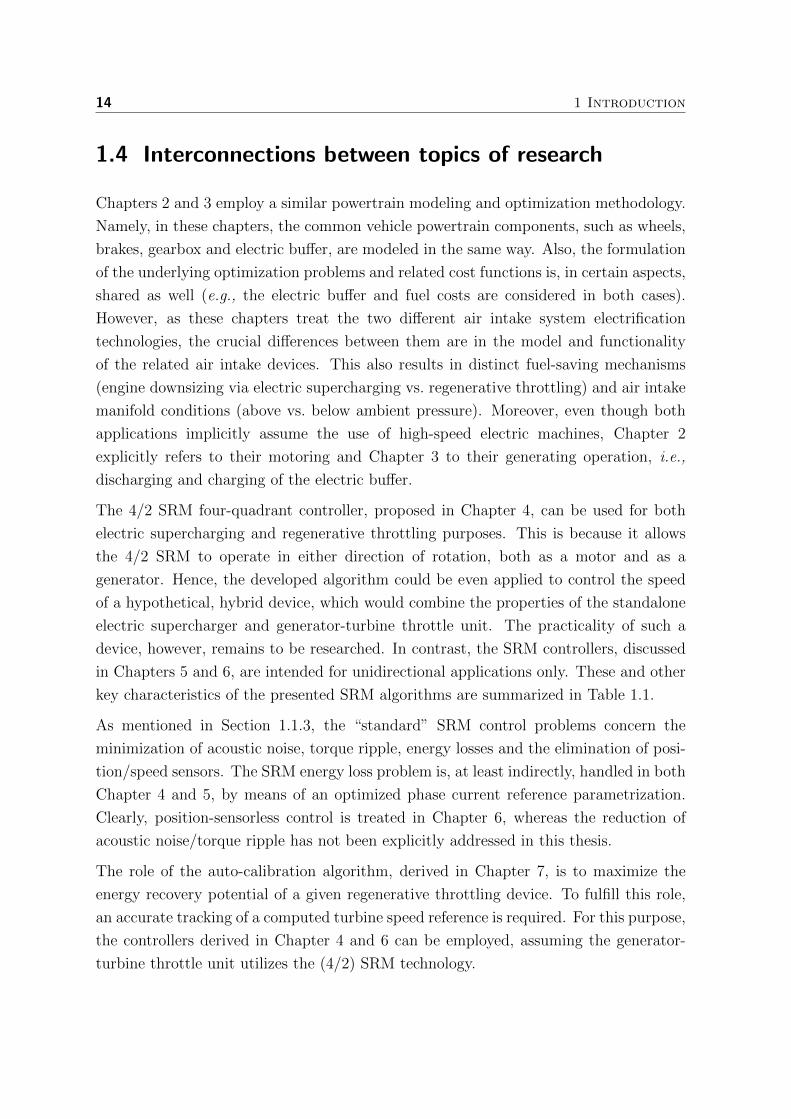
key characteristics of the presented SRM algorithms are summarized in Table 1.1.
As mentioned in Section 1.1.3, the “standard” SRM control problems concern the
minimization of acoustic noise, torque ripple, energy losses and the elimination of posi-
tion/speed sensors. The SRM energy loss problem is, at least indirectly, handled in both
Chapter 4 and 5, by means of an optimized phase current reference parametrization.
Clearly, position-sensorless control is treated in Chapter 6, whereas the reduction of
acoustic noise/torque ripple has not been explicitly addressed in this thesis.
The role of the auto-calibration algorithm, derived in Chapter 7, is to maximize the
energy recovery potential of a given regenerative throttling device. To fulfill this role,
an accurate tracking of a computed turbine speed reference is required. For this purpose,
the controllers derived in Chapter 4 and 6 can be employed, assuming the generator-
turbine throttle unit utilizes the (4/2) SRM technology.
1.5 List of publications 15
Table 1.1: Comparison of proposed SRM controllers
Chapter SRM controller Operation Speed range Sensors
Chapter 4 speed mot/genneg/pos, DC-link voltage,
low/high position, phase currents
Chapter 5 DC-link voltage genpos, DC-link voltage/current
high position, speed
Chapter 6 speed mot/genpos,
DC-link voltage/currenthigh
1.5 List of publications
Journal articles
• S. Marinkov, N. Murgovski and B. de Jager. “Convex modeling and sizing of
electrically supercharged internal combustion engine powertrain.” accepted for
publication, IEEE Transactions on Vehicular Technology. – Chapter 2
• S. Marinkov, N. Murgovski and B. de Jager. “Convex modeling and optimization
of a vehicle powertrain equipped with a generator-turbine throttle unit.” submit-
ted, under review. – Chapter 3
• S. Marinkov and B. de Jager. “Four-Quadrant speed control of 4/2 Switched
Reluctance Machines.” submitted, under review. – Chapter 4
Proceedings & Conference Contributions
• S. Marinkov, B. de Jager, and M. Steinbuch, “Model predictive control of a high
speed switched reluctance generator system,” in European Control Conference,
Zurich, Switzerland, 2013. – Chapter 5
• S. Marinkov, B. de Jager, and M. Steinbuch, “Extremum seeking control with
data-based disturbance feedforward,” in American Control Conference, Portland
OR, USA, 2014. – Chapter 7 (in part)
• S. Marinkov, B. de Jager, and M. Steinbuch, “Extremum seeking control with
adaptive disturbance feedforward,” in The 19th IFAC World Congress, Cape
Town, South Africa, 2014. – Chapter 7 (in part)
16 1 Introduction
• S. Marinkov and B. de Jager, “Control of a high-speed Switched Reluctance
Machine using only the DC-link measurements,” in IEEE International Conference
on Industrial Technology, Seville, Spain, 2015. – Chapter 6
• N. Murgovski, S. Marinkov, D. Hilgersom, B. de Jager, M. Steinbuch, and J.
Sjoberg, “Powertrain Sizing of Electrically Supercharged Internal Combustion
Engine Vehicles,” in The 4th IFAC Workshop on Engine and Powertrain Control,
Simulation and Modeling, Columbus OH, USA, 2015.
Supervised projects
• E. Hoedemaekers, “SRG vehicle charging system: design and implementation of
the test setup”, BSc thesis, Eindhoven University of Technology, February-May
2012.
• E. Stamatopoulos, “Observer-based control of a high-speed Switched Reluctance
Machine”, MSc thesis, Eindhoven University of Technology, January-August 2014.
• N. Strous, “Modeling and measurement of the acoustic noise produced by a
Switched Reluctance Machine”, BSc thesis, Eindhoven University of Technology,
September 2014-January 2015.
• D. Hilgersom, “Potential of an Add-On Electric Supercharger for Internal Combus-
tion Engines”, MSc thesis, Eindhoven University of Technology, February 2014-
August 2015.
• D. Shanbhag, “Extremum Seeking Control tuning of Switched Reluctance Ma-
chines”, research project, Eindhoven University of Technology and University of
Queensland, Australia, March-June 2015.
Chapter 2
Convex modeling and sizing of
electrically supercharged internal
combustion engine powertrains
Abstract This Chapter investigates a concept of an electrically supercharged internal
combustion engine powertrain. A supercharger consists of an electric motor and a compressor.
It draws its power from an electric energy buffer (e.g., a battery) and helps the engine during
short-duration high-power demands. Both the engine and the buffer are sized to reduce the
sum of the vehicle operational (fuel) and component (engine and buffer) costs. For this
purpose, a convex, driving cycle-based vehicle model is derived, enabling the formulation of
an underlying optimization problem as a second-order cone program. Such a program can be
efficiently solved using dedicated numerical tools (for a given gear selection strategy), which
provides not only the optimal engine/buffer sizes but also the optimal vehicle control and state
trajectories (e.g., compressor power and buffer energy). Finally, the results obtained from a
representative, numerical case study are discussed in detail.
2.1 Introduction
Recent years have shown high interest in the reduction of energy consumption and
pollutant emissions of ground transportation. With the goal of improving energy
efficiency and employing renewable energy sources, vehicle manufacturers are currently
introducing several types of electrified vehicles. Nevertheless, internal combustion
engines (ICE) are expected to remain the dominant force in the automotive market
for the next decade [38].
17
182 Convex modeling and sizing of electrically supercharged internal
combustion engine powertrains
To meet the ever-tightening expectations on the vehicle fuel economy, the automotive
industry has pursued the path of engine downsizing [12]. The engine downsizing has
been typically followed by the ICE overpowering, e.g., by means of torque boosting [39],
[40], to improve the vehicle drivability. In general, the application of the ICE downsizing
and overpowering results in lower carbon emissions and a better fuel economy, w.r.t.
the original, large engine situation – due to the reductions in the engine weight, friction
and pumping losses [19]. The ICE overpowering can be also achieved using intake air
boosting, with the help of a turbocharger (driven by hot exhaust gases) or a supercharger
(driven mechanically by a crankshaft via a chain or a belt). In both cases, a compressor
is utilized to increase (boost) the pressure/density of air supplied to the engine and thus
provide it with more oxygen. This allows more fuel to be injected and burned, thereby
rising the ICE maximum torque and power limits.
However, the turbocharged ICEs exhibit a relatively poor torque capability at low engine
speeds, which compromises the vehicle drivability and acceleration performance [41].
Namely, at low speed, the downsized ICEs suffer from insufficient exhaust gas-flow
to adequately propel the turbocharger from the moment the gas pedal is pressed,
resulting in a well-known turbo-lag [12]. The belt-driven supercharger, on the other
hand, does not experience this phenomenon but is less fuel economic, as it increases
the engine parasitic losses. One way to efficiently provide the required low-end torque
and at the same time eliminate the turbo-lag is to electrify the supercharger, i.e., to
replace its mechanical power source (prime mover) with an electric motor [16]–[18]. The
resulting device, an electric supercharger, i.e., a motor-compressor unit (MCU), follows
a popular automotive trend of vehicle electrification – which has already proven capable
of enhancing the efficiency and performance of numerous systems such as steering, water
pump and air conditioning [9].
Historically, a lack of compact, high-power/energy-density electric sources and of light-
weight, high-speed, high-power-density electric motors prohibited the proliferation of
the MCUs throughout the automotive sector. The widely used 12 V battery system is
at the limit of providing sufficient power for the electrical boost [40]. Besides, the high
power surges from the MCU may incur high battery losses.
Today the situation regarding electric storage elements is somewhat different as a
plethora of high-power batteries and high-energy capacitors has appeared on the market.
However, the choice of the electric buffer technology and optimal buffer size, in terms
of its power rating and energy density, is still an open question.
This Chapter presents a method for computing the buffer size that provides sufficient
electric power and energy to run the supercharger. The supercharger is used to help

2.2 The powertrain sizing problem 19
the engine during short-duration high-power demands, which could potentially allow it
to be downsized. Specifically, the sizing of both the ICE and the buffer is performed
by minimizing the sum of the vehicle operational (fuel) and component (engine and
buffer) costs. This optimization problem constitutes a dynamic program, where the
ICE and buffer are optimally sized only when the vehicle is also optimally controlled on
a studied driving cycle. In addition, this problem is also a non-convex, nonlinear and
a mixed-integer dynamic program, where both plant design and control parameters act
as optimization variables.
The plant design and control problem is typically handled by decoupling the plant and
the controller, and then optimizing them sequentially or iteratively [42]–[47]. However,
sequential and iterative strategies generally fail to achieve global optimality [48]. An
alternative is a nested optimization strategy, where an outer loop optimizes the system
objectives over a set of feasible plants, and an inner loop generates optimal controls
for plants chosen by the outer loop [45]. This approach delivers a globally optimal
solution, but may incur heavy computational burden (when, e.g., dynamic programming
is used to optimize the energy management [49]), or may require substantial modeling
approximations [50]–[52].
This Chapter addresses the plant design and control problem by first decoupling the
integer decisions, i.e., the gear selection strategy, and then by formulating the remaining
problem as a convex second-order cone program (SOCP) [53]. The integer signals are
decided outside of the convex program, by means of two simple heuristic strategies –
one designed to promote the ICE downsizing and one that aims to maximize the ICE
efficiency. Finally, a case study is provided where the optimal engine and the electric
buffer sizes are computed for a specific, MCU-equipped vehicle.
This Chapter is organized as follows. Section 2.2 provides background to the electrically
supercharged ICE configuration and states a verbal problem formulation. The math-
ematical modeling is provided in Section 2.3 and the convex optimization problem is
formulated in Section 2.4. Section 2.5 presents a use-case study. Conclusions are drawn
in Section 2.6.
2.2 The powertrain sizing problem
The block diagram of the electrically supercharged ICE is illustrated in Fig. 2.1. The
MCU, which is placed in the ICE air intake along with a bypass valve, enables more
power to be delivered by the ICE, e.g., while overtaking or when starting-off at the

202 Convex modeling and sizing of electrically supercharged internal
combustion engine powertrains
BV TV
A
MC
IM EM
ICEMCU
B
AUe
G
AUm
W
BRE. link
electrical
mechanicalpneumatic
Figure 2.1: Illustration of the components considered in the proposed power-
train sizing problem – arrows indicate a power flow direction. The source of air
flow feeding an internal combustion engine (ICE) intake (IM) and exhaust (EM)
manifolds is determined using a bypass (BV) and a throttle valve (TV). The
ICE is equipped with a stand-alone motor-compressor unit (MCU) consisting of
a compressor (C) and an electric motor (M). The motor, as well as other electric
auxiliary loads (AUe), draws its power from an electric buffer (B). The buffer
is charged by a conventional car-alternator (A) that is mechanically coupled to
the ICE crankshaft along with mechanical auxiliary loads (AUm). A clutch and
a gearbox (G) connect the ICE with wheels (W) and brakes (BR).
traffic lights. The supercharging (SC) refers to a situation when the excess power is
needed, i.e., when the bypass valve is closed. In contrast, during naturally-aspirated
(NA) operation the bypass valve is open.
The bursts of mechanical MCU power have to be matched by the power ratings of
the electric buffer that feeds the MCU. However, deciding the optimal buffer energy
requirement is not trivial since it depends on the typical daily usage of the vehicle. A
common way of representing the vehicle daily usage is by recording the vehicle speed
and acceleration time profiles, and then by constructing a driving cycle that contains
both the vehicle speed and road topography as functions of time. An example of one
such cycle is the Class 3 World Harmonized Light Vehicle Test Procedure1 (WLTP3),
which is used here as a proof of concept for realization of the method being proposed.
The vehicle is required to exactly follow the speed demanded by the driving cycle,
thus ensuring that a possible downsizing of the powertrain does not compromise the
demanded performance. To have a fair comparison, the buffer is required to sustain
its initial charge at the end of the driving cycle, meaning that any energy used for
supercharging has to be put back in the buffer at some point, through the use of a
conventional car alternator driven by the ICE. This may require high utilization of the
electric buffer, making it beneficial to increase its size. However, a larger buffer increases
1http://www.dieselnet.com/standards/cycles, March 2015.

2.3 Quasistatic vehicle model 21
Table 2.1: Optimization problem for powertrain components sizing and energy
management.
Minimize:
Operational + component cost,
Subject to:
Driving cycle constraints,
Energy conversion and balance constraints,
Buffer dynamics,
Physical limits of components,
...
(For all time instances along the driving cycle).
the cost of the vehicle. Then, to keep the cost down, the possibility of downsizing
the ICE is also considered, such that the optimal trade-off is reached between the
components cost and the operational cost within the lifetime of the vehicle.
The resulting optimization problem is verbally stated in Table 2.1, whereas its mathe-
matical description is deferred to Section 2.4.
2.3 Quasistatic vehicle model
In the remainder, a power-based [54], quasistatic model of a 4-stroke ICE is provided.
The ICE is downsized by scaling its displacement volume while keeping its bore-stroke
and compression ratios constant. Specifically, the ICE displacement volume is defined
as VE = sEVE, where VE denotes the baseline volume and sE ∈ (0, 1] the engine scaling
coefficient. The ICE is equipped with the MCU, which provides the possibility to
enhance its torque capacity by means of supercharging. To match the MCU power
requirements the vehicle electric energy buffer is sized as well. For this purpose, the
buffer is considered to be built out of nB = sBnB cells connected in series, where sB > 0
represents the buffer scaling coefficient and nB the baseline cell count. Both sE and sB
are treated as real optimization variables.
222 Convex modeling and sizing of electrically supercharged internal
combustion engine powertrains
PmW
Vehicle
sE sB
ωW
PmG2
ωG
PmG1
ICEωE
PmE
ωA PmA
sE
P cE
Gearbox
sE
P eA
systemAir
ωC PmC
P eC
sBP eB2
EeB
P eAU
derived
optimized
predetermined
sE
g
bufferElectric
Motor
P eB1
Ambient
pAM TAM
Brakes
ωW PmBR
Electricaux.
Mech.aux.
ωE PmAU
ωE
α
aV
vV
Wheels
cycleDrive Alter.
& p.e. & p.e.
ωW
Electriclink
Mech.link
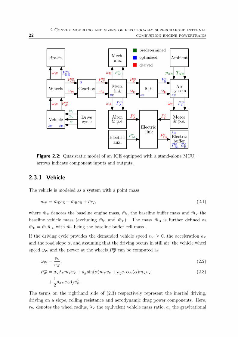
Figure 2.2: Quasistatic model of an ICE equipped with a stand-alone MCU –
arrows indicate component inputs and outputs.
2.3.1 Vehicle
The vehicle is modeled as a system with a point mass
mV = mEsE + mBsB + mV, (2.1)
where mE denotes the baseline engine mass, mB the baseline buffer mass and mV the
baseline vehicle mass (excluding mE and mB). The mass mB is further defined as
mB = mcnB, with mc being the baseline buffer cell mass.
If the driving cycle provides the demanded vehicle speed vV ≥ 0, the acceleration aV
and the road slope α, and assuming that the driving occurs in still air, the vehicle wheel
speed ωW and the power at the wheels PmW can be computed as
ωW =vV
rW
, (2.2)
PmW = aVλVmVvV + ag sin(α)mVvV + agcr cos(α)mVvV (2.3)
+1
2ρAMcdAfv
3V.
The terms on the righthand side of (2.3) respectively represent the inertial driving,
driving on a slope, rolling resistance and aerodynamic drag power components. Here,
rW denotes the wheel radius, λV the equivalent vehicle mass ratio, ag the gravitational

2.3 Quasistatic vehicle model 23
acceleration, cr the rolling resistance coefficient, ρAM the ambient air density, cd the
drag coefficient and Af the vehicle’s frontal area. Due to (2.1) the power PmW is affine
in the optimization variables, i.e.,
PmW = γW0 + γW1sE + γW2sB, (2.4)
where
γW2 = (aVλV + ag sin(α) + agcr cos(α)) mBvV, (2.5)
γW1 = (aVλV + ag sin(α) + agcr cos(α)) mEvV,
γW0 =1
2ρAMcdAfv
3V + (aVλV + ag sin(α) + agcr cos(α)) mVvV.
2.3.2 Wheels & brakes
The required mechanical power at the wheel side of the gearbox is given by
PmG2 = Pm
W + PmBR, (2.6)
where PmBR ≥ 0 is an optimization variable representing the power of the brakes.
2.3.3 Gearbox
The speed and power at the engine side of the gearbox are given by the following
expressions
ωG = λG(g)ωW, (2.7)
PmG1 = γG0 + Pm
G2, (2.8)
where
γG0 = cG0 + cG1ωG + cG2ω2G, (2.9)
with λG(g) denoting the gear ratio corresponding to the gear g ∈ 1, . . . , 5 and γG0 ≥0 the gearbox drag losses. The gear is treated as an optimization variable decided
separately and prior to the rest, see Section 2.4.2.
2.3.4 Mechanical power link
To be able to distinguish between regular and idling engine operation, define
γML =
1, for ωG ≥ ωE,min,
0, otherwise.(2.10)
242 Convex modeling and sizing of electrically supercharged internal
combustion engine powertrains
Then the engine and the alternator speed exiting the mechanical power link follow
ωE = ωGγML + ωE,min(1− γML), (2.11)
ωA = λAωE, (2.12)
while the corresponding engine mechanical power balance reads
PmE = Pm
G1γML + PmA + Pm
AU. (2.13)
Here, λA denotes the alternator speed ratio, ωE and ωE,min the ICE rotational and idle
speed, ωA the alternator speed, and PmE , P
mA , P
mAU ≥ 0 the mechanical power of the
ICE, alternator and the remaining mechanical auxiliary units (assumed constant). The
power PmA is one of the optimization variables.
2.3.5 ICE & air-fuel control
The ICE mechanical behavior can be described with the following relationship [55], [56]:
pE = ηEpφ − pEf − pEg, (2.14)
where ηE denotes the effective ICE efficiency, pE and pφ the engine brake and fuel mean
effective pressures, and pEf and pEg the brake mean effective pressure losses due to engine
friction and pumping work. Assuming that the ratio λec, the ignition/injection timing
angles, the burnt gas fraction and the bore-stroke ratio are kept constant, the effective
efficiency ηE can be treated as a function of the engine speed only [55], i.e.,
ηE = cη0 + cη1ωE + cη2ω2E, (2.15)
where cηi, i ∈ 0, 1, 2 denote constant parameters. The two pressures, pE and pφ,
further read
pE =4πτE
VEsE
(2.16)
pφ =4πP c
E
VEωEsE
, (2.17)
while the related loss components may be modeled2 [55] as
pEf = cf0 + cf2ω2E, (2.18)
pEg = cg0 + cg1τE
τE,max
, (2.19)
2The adopted friction loss model is pessimistic as lower friction losses can be expected in the case
of downsized engines.

2.3 Quasistatic vehicle model 25
with τE,max = τE,max(ωE, sE) denoting the maximum achievable torque τE of a downsized
ICE during its NA operation, cf0, cf2, cg0 and cg1 some constant parameters. The ICE
chemical (fuel) power P cE is given by
P cE = mφHl, (2.20)
with Hl being the fuel lower heating value and mφ the ICE fuel mass flow. Assuming
that the fuel controller maintains a constant, stoichiometric air-fuel ratio λαφ, the flow
mφ is related to the required engine air mass flow as
mφ =mα
λαφ. (2.21)
Since from the air system perspective the engine acts as a volumetric pump, the air
mass flow fulfills
mα = ηvolpAMsEVEωEλΠ
4πcRTIM
, (2.22)
where λΠ represents the ratio between the intake manifold and the ambient air pressures,
pIM and pAM, satisfying 0 ≤ λΠ ≤ λΠ,max > 1, with λΠ,max being its stoichiometric
combustion knock limit value. Furthermore, cR is the specific gas constant of air,
TIM the intake manifold air temperature and ηvol = ηvol(ωE, λΠ) the engine volumetric
efficiency. The efficiency ηvol is frequently modeled as a multilinear function [55] of the
pressure ratio λΠ and the speed ωE, i.e.,
ηvol = ηvol,ωηvol,Π, (2.23)
where
ηvol,ω = cvol0 + cvol1ωE + cvol2ω2E, (2.24)
ηvol,Π = 1 +1
λec
(1−
(pEM
pAM
)1/λκ
λ−1/λκΠ
),
with pEM being the (constant) exhaust manifold pressure, λec the engine compression
ratio, λκ the specific heat ratio of air and cvoli, i ∈ 0, 1, 2 some constant parameters.
Using (2.16) to (2.21) the expression (2.14) can be rewritten in terms of torque, as
follows
τE = ηEmαHl
λαφωE
− VEsE
4π
(pEf + cg0 + cg1
τE
τE,max
). (2.25)
Since during the ICE NA operation at a wide-open throttle it holds τE = τE,max(ωE, sE),
λΠ ≈ 1 and TIM ≈ TAM, where TAM denotes the ambient air temperature – by

262 Convex modeling and sizing of electrically supercharged internal
combustion engine powertrains
substituting these values and the flow given by (2.22) in (2.25), the expression for
torque τE,max can be derived. This yields
τE,max =
(ηEηvol
pAMVEHl
4πcRTAMλαφ− VE(pEf + cg0 + cg1)
4π
)sE, (2.26)
= τE,maxsE. (2.27)
where τE,max = τE,max(ωE) denotes the maximum achievable torque of a baseline (non-
downsized) NA ICE and ηvol = ηvol(ωE, 1). By multiplying both sides of (2.25) with ωE
and using (2.27), one can further obtain the relationship between the ICE mechanical
PmE = τEωE and the fuel power P c
E, i.e.,
P cE =
4πτE,max + cg1VE
4πτE,maxηE
PmE +
VEωE(pEf + cg0)
4πηE
sE, (2.28)
P cE = γE1P
mE + γE,minsE, (2.29)
where γE1 > 1 and γE,min > 0. The power P cE is treated as an optimization variable.
2.3.6 Air system
During the ICE SC operation it holds τE > τE,max(ωE, sE), when pIM ≈ pC > pAM and
TIM ≈ TC > TAM, where pC, TC denote the compressor outlet pressure and temperature.
Thus one may approximate the compressor pressure ratio pC/pAM by the intake manifold
pressure ratio λΠ and express the temperature TC, as
TC = TAM +TAM
ηC
(λλκ−1λκ
Π − 1
), (2.30)
where ηC is the isentropic compressor efficiency (assumed constant). The equa-
tions (2.22) and (2.30) uniquely determine the values of TC and λΠ for each given mα
and ωE. Although the underlying relations are nonlinear in λΠ, in its narrow range of
interest, i.e., for λΠ ∈ [1, λΠ,max], they can be approximated by suitable affine functions.
To achieve this, the expressions (2.22) and (2.30) are first rewritten as
TC = λTTAM, (2.31)
mα = λmγmsE,
where λT = 1 + 1ηC
(λλκ−1λκ
Π − 1
), λm =
ηvol,ΠλΠ
λTand γm =
pAMVEωEηvol,ω
4πcRTAM. Then, the best
affine fits λT ≈ λT and λm ≈ λm (w.r.t. λΠ, in the least-squares sense) are constructed
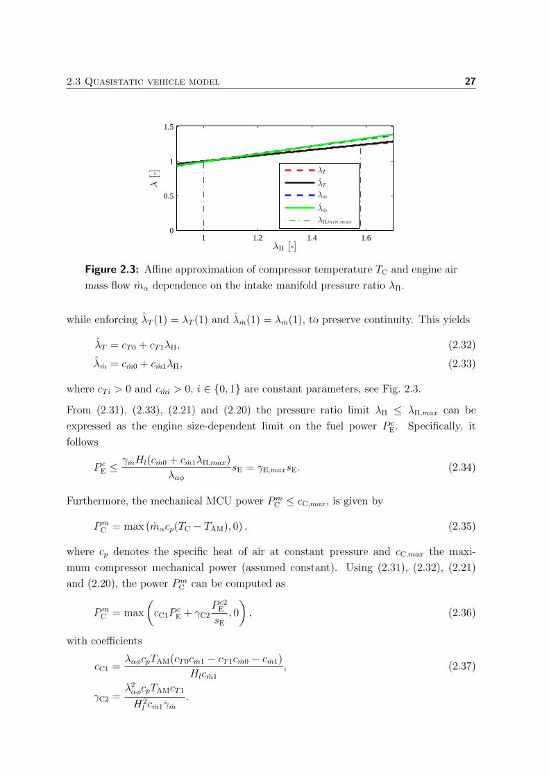
2.3 Quasistatic vehicle model 27
1 1.2 1.4 1.60
0.5
1
1.5
λΠ [-]
λ[-]
λT
λT
λm
λm
λΠ,min,max
Figure 2.3: Affine approximation of compressor temperature TC and engine air
mass flow mα dependence on the intake manifold pressure ratio λΠ.
while enforcing λT (1) = λT (1) and λm(1) = λm(1), to preserve continuity. This yields
λT = cT0 + cT1λΠ, (2.32)
λm = cm0 + cm1λΠ, (2.33)
where cT i > 0 and cmi > 0, i ∈ 0, 1 are constant parameters, see Fig. 2.3.
From (2.31), (2.33), (2.21) and (2.20) the pressure ratio limit λΠ ≤ λΠ,max can be
expressed as the engine size-dependent limit on the fuel power P cE. Specifically, it
follows
P cE ≤
γmHl(cm0 + cm1λΠ,max)
λαφsE = γE,maxsE. (2.34)
Furthermore, the mechanical MCU power PmC ≤ cC,max, is given by
PmC = max (mαcp(TC − TAM), 0) , (2.35)
where cp denotes the specific heat of air at constant pressure and cC,max the maxi-
mum compressor mechanical power (assumed constant). Using (2.31), (2.32), (2.21)
and (2.20), the power PmC can be computed as
PmC = max
(cC1P
cE + γC2
P c2E
sE
, 0
), (2.36)
with coefficients
cC1 =λαφcpTAM(cT0cm1 − cT1cm0 − cm1)
Hlcm1
, (2.37)
γC2 =λ2αφcpTAMcT1
H2l cm1γm
.

282 Convex modeling and sizing of electrically supercharged internal
combustion engine powertrains
Since γC2 > 0, ∀ωE, the expression γC2Pc2E + cC1P
cE is convex in P c
E. Moreover, as
sE > 0, a perspective function [53] corresponding to this expression is given by the
first argument of the maximum function in (2.36), which implies that this argument
is convex in both P cE and sE. Because the maximum of two convex functions is itself
convex, the same also holds for the compressor power PmC .
Furthermore, it is assumed that for the air mass flow/pressure ratio range of interest
the MCU can be always chosen such that the compressor surge/choke phenomena do
not occur. The surge condition can be expressed as [55]:
ωC ≤ ωC,surge ≈ csurge0 + csurge1mα, (2.38)
where ωC denotes the compressor speed, ωC,surge(mα) the compressor surge speed limit
(for a given air mass flow) and csurge0, csurge1 > 0 some constant fitting coefficients.
2.3.7 Alternator and MCU motor
The electric machine electric power can be modeled as a second-order polynomial of its
mechanical power, with a constant term representing a speed-dependent drag loss [56].
In this context, the alternator electric power can be formulated as
P eA = γA0 + cA1P
mA + cA2P
m2A , (2.39)
where
γA0 = cA00 + cA01ωA + cA02ω2A > 0, (2.40)
with cA0i, i ∈ 0, 1, 2, cA02 ≥ 0, −1 < cA1 < 0 and cA2 ≥ 0 being constant coefficients,
see Fig. 2.5. The signs of cA1 and cA2 ensure that the electric alternator power P eA is
non-positive for a non-negative mechanical alternator power PmA . This is in accordance
with a general convention (in the energy management of electrified vehicles) which
states that the electric power should be positive when the electric machine acts to
discharge the electric buffer (i.e., during motoring) and negative when it charges it (i.e.,
during generating). Furthermore, the coefficient cA1 is bounded to reflect the physical
limitations of the alternator. Namely, if one would let cA1 >= 0 this would imply that
the alternator can sometimes operate as a motor, which is not considered in this study.
If, however, cA1 <= −1, then it could happen that the alternator electrical power output
is absolutely larger than its mechanical power input, which is not physically possible.
The mechanical power PmA is constrained both above and below, i.e., 0 ≤ γA,min ≤
PmA ≤ cA,max, where
γA,min =−cA1 −
√c2
A1 − 4γA0cA2
2cA2
(2.41)
2.3 Quasistatic vehicle model 29
2 4 6
0.5
1
1.5
2
2.5
nE [krpm]
Pm C[kW]
BL & NADS & NADS & SCideal
2 4 6
50
60
70
80
90
100
nE [krpm]
τE[N
m]
2 4 60
50
100
nE [krpm]
Pc E[kW]
0 20 400
50
100
1500
4000
4000
6000
6000
P mE [kW]
Pc E[kW]
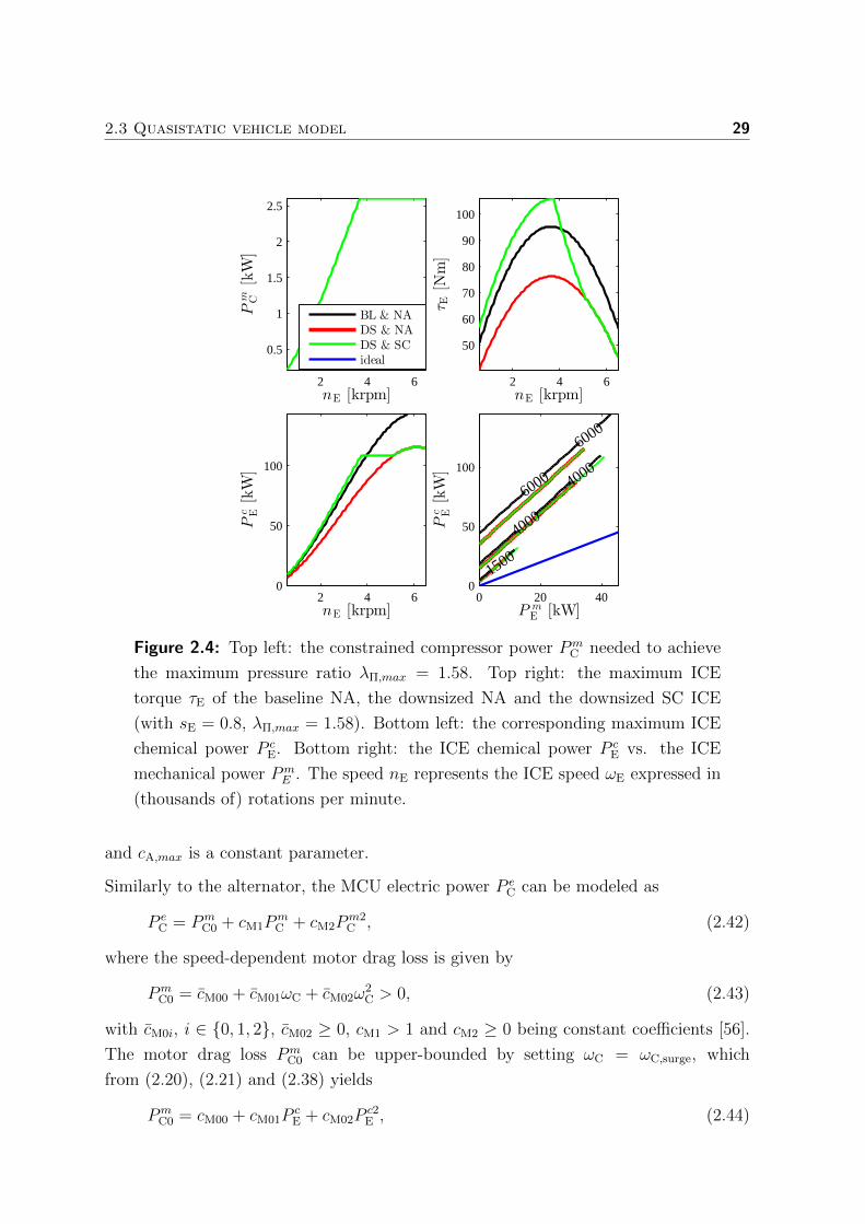
Figure 2.4: Top left: the constrained compressor power PmC needed to achieve
the maximum pressure ratio λΠ,max = 1.58. Top right: the maximum ICE
torque τE of the baseline NA, the downsized NA and the downsized SC ICE
(with sE = 0.8, λΠ,max = 1.58). Bottom left: the corresponding maximum ICE
chemical power P cE. Bottom right: the ICE chemical power P c
E vs. the ICE
mechanical power PmE . The speed nE represents the ICE speed ωE expressed in
(thousands of) rotations per minute.
and cA,max is a constant parameter.
Similarly to the alternator, the MCU electric power P eC can be modeled as
P eC = Pm
C0 + cM1PmC + cM2P
m2C , (2.42)
where the speed-dependent motor drag loss is given by
PmC0 = cM00 + cM01ωC + cM02ω
2C > 0, (2.43)
with cM0i, i ∈ 0, 1, 2, cM02 ≥ 0, cM1 > 1 and cM2 ≥ 0 being constant coefficients [56].
The motor drag loss PmC0 can be upper-bounded by setting ωC = ωC,surge, which
from (2.20), (2.21) and (2.38) yields
PmC0 = cM00 + cM01P
cE + cM02P
c2E , (2.44)

302 Convex modeling and sizing of electrically supercharged internal
combustion engine powertrains
with the coefficients
cM00 = cM00 + cM01csurge0 + cM02c2surge0, (2.45)
cM01 =λαφHl
(cM01csurge1 + 2cM02csurge0csurge1) ,
cM02 =λ2αφ
H2l
cM02c2surge1.
Note that since cM02 ≥ 0 the drag loss PmC0 is convex w.r.t. the fuel power P c
E. In
the same way, the compressor electric power P eC is convex w.r.t. both its mechanical
power PmC and fuel power P c
E, and the alternator electric power P eA is convex w.r.t. its
mechanical power PmA .
0 0.5 1 1.5 2
−1.5
−1
−0.5
0
2250
2250
6000
6000
9000
9000
PmA [kW]
Pe A[kW]
P eA
P eA
ideal
Figure 2.5: Convex approximation of the alternator electric power P eA as a
function of its mechanical power PmA and speed ωA.
2.3.8 Electric power link
The electric buffer terminal power follows from the power balance at the electric power
link, given by
P eB2 = P e
A + P eC + P e
AU, (2.46)
where P eAU ≥ 0 is the power consumed by electric auxiliary devices (assumed constant).
2.3.9 Electric buffer
The electric buffer cells are considered to be either lithium-ion batteries, or supercapac-
itors. Each cell is modeled as a cell open circuit voltage uc with a constant resistance Rc
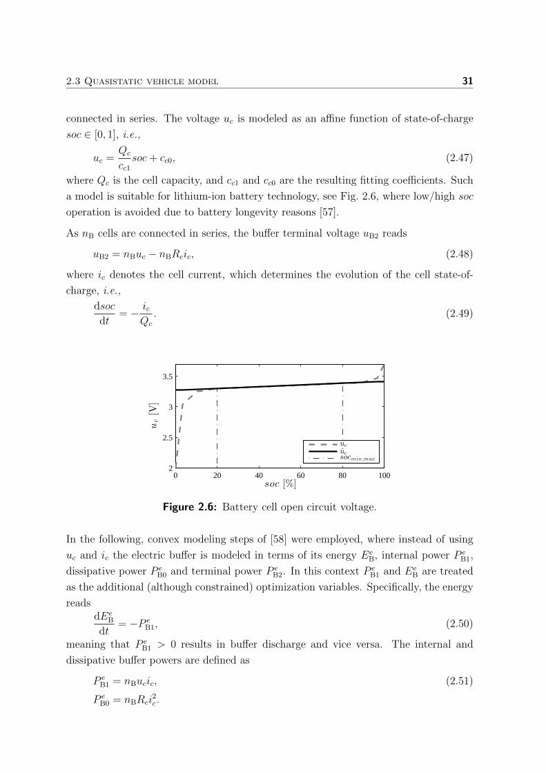
2.3 Quasistatic vehicle model 31
connected in series. The voltage uc is modeled as an affine function of state-of-charge
soc ∈ [0, 1], i.e.,
uc =Qc
cc1soc+ cc0, (2.47)
where Qc is the cell capacity, and cc1 and cc0 are the resulting fitting coefficients. Such
a model is suitable for lithium-ion battery technology, see Fig. 2.6, where low/high soc
operation is avoided due to battery longevity reasons [57].
As nB cells are connected in series, the buffer terminal voltage uB2 reads
uB2 = nBuc − nBRcic, (2.48)
where ic denotes the cell current, which determines the evolution of the cell state-of-
charge, i.e.,
dsoc
dt= − ic
Qc
. (2.49)
0 20 40 60 80 1002
2.5
3
3.5
soc [%]
uc[V
]
uc
ucsocmin,max
Figure 2.6: Battery cell open circuit voltage.
In the following, convex modeling steps of [58] were employed, where instead of using
uc and ic the electric buffer is modeled in terms of its energy EeB, internal power P e
B1,
dissipative power P eB0 and terminal power P e
B2. In this context P eB1 and Ee
B are treated
as the additional (although constrained) optimization variables. Specifically, the energy
readsdEe
B
dt= −P e
B1, (2.50)
meaning that P eB1 > 0 results in buffer discharge and vice versa. The internal and
dissipative buffer powers are defined as
P eB1 = nBucic, (2.51)
P eB0 = nBRci
2c .

322 Convex modeling and sizing of electrically supercharged internal
combustion engine powertrains
This implies
P eB1 = P e
B2 + P eB0. (2.52)
Furthermore, from (2.49), (2.50) and (2.51), it follows
EeB = nBQc
soc∫
0
uc(s)ds =nBcc1
2(u2
c − c2c0). (2.53)
Thus the pack losses may be expressed as
P eB0 =
Rccc1Pe2B1
2EeB + nBcc1c2
c0
, (2.54)
which, as a quadratic-over-linear, with a strictly positive denominator, is a convex
function [53] of P eB1, Ee
B and nB (and therefore also sB). Note that when cc0 = 0 the
adopted model, (2.53) and (2.54), describes a capacitor with a capacitance cc1.
Constraints on the state soc and the current ic can be translated into constraints on
the energy EeB and the power P e
B1, i.e.,
EeB ∈
nBcc12
([u2c(socmin), u2
c(socmax)]− c2
c0
)(2.55)
= [EeB,min, E
eB,max]sB,
P eB1 ∈ [ic,min, ic,max]
√nB
(2Ee
B
cc1+ nBc2
c0
), (2.56)
where socmin and socmax represent the minimum and the maximum state-of-charge,
ic,min < 0 and ic,max > 0 the minimum and the maximum cell current and EeB,min
and EeB,max the baseline minimum and the maximum buffer energy. Notice that the
geometric mean in (2.56) is a concave function [53] of EeB and nB.
2.4 Optimization problem formulation
The optimization problem formulated in Table 2.1 is revisited here by providing
mathematical meaning to constraints and the objective function. In this context, the
optimization goal is defined as finding the minimum of a weighted sum of operational and
component costs. The former is simply represented by the cost of consumed petroleum
while the latter consists of a sum of the ICE and the electric buffer cost. Each specific
cost component is weighted by its respective weighting coefficient, wφ, wE or wB, so

2.4 Optimization problem formulation 33
that its contribution is expressed in currency per distance. Using the approach outlined
in [59] these coefficients can be computed as
wφ = µφ1
Hlρφd, (2.57)
wE = µE
PmE,max
dyear
tyear
tlife
(1 + εE,year
tlife + 1
2
),
wB = µBEe
B,max
dyear
tyear
tlife
(1 + εB,year
tlife + 1
2
).
where µφ, µE and µB are fuel, engine and buffer price expressed respectively in currency
per volume, power and energy. Furthermore, d =∫ tend
0vVdt is the total drive cycle
length, dyear the average distance a vehicle travels during one year tyear, ρφ the fuel
density, PmE,max = maxωE
τE,maxωE the maximum baseline NA ICE mechanical power,
tlife the duration of the expected vehicle life-cycle, and εE,year and εB,year the yearly engine
and buffer interest rates.
2.4.1 Convex optimization problem
Based on the equations derived in the previous section the related optimization problem
is summarized as follows
min J = wφ
tend∫
0
P cEdt+ wEsE + wBsB, (2.58)
s.t. (2.55), (2.56),
0 < sB, 0 < sE ≤ 1, 0 ≤ PmBR, Pm
C ≤ cC,max,
γA,min ≤ PmA ≤ cA,max, γE,minsE ≤ P c
E ≤ γE,maxsE,
EeB = −P e
B1,
EeB(0) = Ee
B(tend),
P cE = γE,minsE + (Pm
A + PmAU
+ (γG0 + PmBR + γW0 + γW1sE + γW2sB) γML) γE1,
PmC = max
(γC2
P c2E
sE
+ cC1PcE, 0
),
P eB1 =
Rccc1Pe2B1
2EeB + sBnBcc1c2
c0
+ γA0 + cA1PmA + cA2P
m2A
+ cM00 + cM01PcE + cM02P
c2E + cM1P
mC + cM2P
m2C + P e
AU,
with the constraints imposed ∀t ∈ [0, tend], where tend is the time when the trip ends.
Note that the values of all the varying coefficients γ can be pre-computed for the entire
342 Convex modeling and sizing of electrically supercharged internal
combustion engine powertrains
range of the driving cycle. This is because the variations originate from the changes in
vehicle speed vV, acceleration aV or slope α that are given, or from one of the rotational
speeds ωG, ωE or ωA, which can be computed using the knowledge of vV and of the gear
ratio trajectory λG(t). The λG(t) trajectory is thus assumed fixed prior to solving the
convex optimization problem.
In (2.58) the last two equality constraints can be relaxed with inequalities by replacing
“=” with “≥” sign. The relaxation changes the original formulation by creating a
convex superset of the non-convex set. However, it can be logically reasoned that
the resulting two constraints hold with equality at the optimum – otherwise energy
would be unnecessarily wasted. Hence, the solutions of the relaxed and the non-relaxed
problem are the same. For a detailed proof see [60]. This implies that the compressor
power PmC may be treated as an additional optimization variable, yielding in total six
time dependent, P cE, P
mBR, P
mA , P
mC , P
eB1, E
eB, and two scalar ones, sE and sB. Also strict
inequalities describing lower bounds of sizing parameters can be relaxed by means of a
small constant ε > 0. In other words, (2.58) may be rewritten as
min J = wφ
tend∫
0
P cEdt+ wEsE + wBsB, (2.59)
s.t. (2.55), (2.56),
ε ≤ sB, ε ≤ sE ≤ 1, 0 ≤ PmBR,
γA,min ≤ PmA ≤ cA,max, γE,minsE ≤ P c
E ≤ γE,maxsE,
EeB = −P e
B1,
EeB(0) = Ee
B(tend),
P cE = γE,minsE + (Pm
A + PmAU
+ (γG0 + PmBR + γW0 + γW1sE + γW2sB) γML) γE1,
max
(γC2
P c2E
sE
+ cC1PcE, 0
)≤ Pm
C ≤ cC,max
P eB1 ≥
Rccc1Pe2B1
2EeB + sBnBcc1c2
c0
+ γA0 + cA1PmA + cA2P
m2A
+ cM00 + cM01PcE + cM02P
c2E + cM1P
mC + cM2P
m2C + P e
AU.
All the optimization variables in (2.59) are further scaled with their expected maximal
values, the resulting problem is discretized using a zero-order hold with a sample time
δt and then casted into a standard convex second-order cone program (SOCP) form.
2.4 Optimization problem formulation 35
The SOCP is given by
min J = fTx (2.60)
s.t. ||Aix+ ei||2 ≤ cTi x+ di, i = 1, .., .m,
Fx = g
where x ∈ Rn are optimization variables, Ai ∈ Rni×n, F ∈ Rp×n, and || · ||2 is Euclidean
norm. Constraints of the type z ≥ x2/y are written as∣∣∣∣∣
∣∣∣∣∣
(2x
y − z
)∣∣∣∣∣
∣∣∣∣∣2
≤ y + z. (2.61)
The SOCP (2.60) is specified and solved using the CVX optimization modeling lan-
guage [61], [62], in combination with the SDPT3 solver [63].
2.4.2 Gear selection strategy
The discrete-time gear trajectory g(tk), with tk = kδt and k ≥ 0, is decided prior to and
outside of the convex optimization. In particular, two different gear selection strategies
have been implemented. The first searches for a gear that results in the largest difference
between the approximate and the maximum operating torque of a baseline NA ICE,
at every time instant. This is expected to promote the ICE downsizing. The second
however, at every time instant finds a gear that maximizes the estimated ICE efficiency,
so that a lower vehicle fuel consumption can be achieved.
These two gear selection strategies are implemented using the functions
g(1)(tk) = arg maxg∈1,...5
(τE,max(tk)− ˆτE(tk)), (2.62)
g(2)(tk) = arg maxg∈1,...5
ηE(tk),
where ˆτE and ηE denote the baseline NA ICE operating torque and efficiency estimates,
computed as
ˆτE =Pm
E
ωE
, (2.63)
ηE =Pm
E
γE1PmE + γE,min
.
with PmE being the estimated baseline NA ICE mechanical power, given by
PmE = max
(Pm
A + PmAU + γG0 + γW0 + γW1 + γW2, 0
)(2.64)

362 Convex modeling and sizing of electrically supercharged internal
combustion engine powertrains
and PmA the estimated alternator mechanical power, i.e.,
PmA = Re
(−cA1 −
√c2
A1 − 4 (γA0 + P eAU) cA2
2cA2
). (2.65)
The use of torque ˆτE, efficiency ηE, power PmE and Pm
A estimates, instead of their optimal
values, is required since the computation of gear selection strategy precedes the convex
optimization – which renders the optimal values unavailable. However, an alternative,
more sophisticated gear selection strategies, employing iterative solutions of a convex
problem (2.59), could be applied here as well. For details, see [47], [64], [65].
2.5 Case study results
This section provides the case study results related to the sizing of electrically su-
percharged ICE powertrain. The purpose of the study is mainly to demonstrate the
proposed modeling and optimization methodology. For this reason, the standard
WLTP3 driving cycle has been used. Note that cycles, such as the WLTP3, are
more often employed for evaluating the vehicle fuel consumption than for component
sizing. Thus, for purposes a specific, real-world powertrain sizing application, one should
consider replacing the WLTP3 with a different (more demanding) cycle, which would
better suit the intended vehicle driving scenario. The values of the relevant model
parameters, used in this particular study, are listed in Appendix A.
2.5.1 Optimal component sizes
Table 2.2 summarizes the results of 6 different optimization runs. They correspond to
3 distinct engine scenarios: baseline NA ICE, downsized NA ICE and downsized SC
ICE, each for 2 defined gear selection strategies: g(1) and g(2). From the presented data
it is apparent that the electric supercharging has led to a substantial decrease in both
the engine size (1 − sE) and the dominant fuel cost (Jφ). As expected, the engine size
reduction is more prominent in the case of g(1) strategy, where gears are chosen such
that they maximize the distance between the engine operating torque and its maximum
torque line. In this case, the use of the MCU has resulted in 41.57% of engine volume
decrease, when the downsized SC ICE is compared to the baseline NA ICE. On the other
hand, more fuel is saved with g(2) strategy, which is reflected in the downsized SC ICE
fuel cost of 6.53 ¢/km vs. the baseline NA ICE fuel cost of 7.22 ¢/km. This is expected
since g(2) strategy maximizes the ICE efficiency, instead of the torque difference, thereby
also promoting a lower ICE fuel consumption.
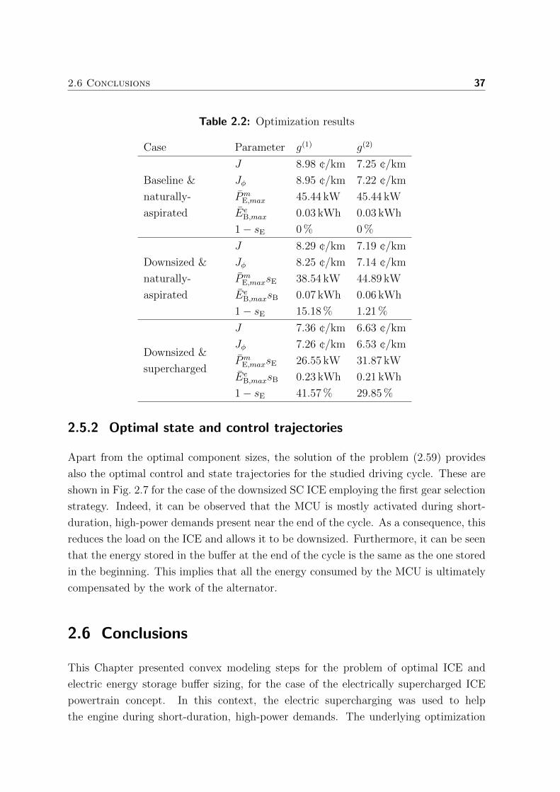
2.6 Conclusions 37
Table 2.2: Optimization results
Case Parameter g(1) g(2)
Baseline &
naturally-
aspirated
J 8.98 ¢/km 7.25 ¢/km
Jφ 8.95 ¢/km 7.22 ¢/km
PmE,max 45.44 kW 45.44 kW
EeB,max 0.03 kWh 0.03 kWh
1− sE 0 % 0 %
Downsized &
naturally-
aspirated
J 8.29 ¢/km 7.19 ¢/km
Jφ 8.25 ¢/km 7.14 ¢/km
PmE,maxsE 38.54 kW 44.89 kW
EeB,maxsB 0.07 kWh 0.06 kWh
1− sE 15.18 % 1.21 %
Downsized &
supercharged
J 7.36 ¢/km 6.63 ¢/km
Jφ 7.26 ¢/km 6.53 ¢/km
PmE,maxsE 26.55 kW 31.87 kW
EeB,maxsB 0.23 kWh 0.21 kWh
1− sE 41.57 % 29.85 %
2.5.2 Optimal state and control trajectories
Apart from the optimal component sizes, the solution of the problem (2.59) provides
also the optimal control and state trajectories for the studied driving cycle. These are
shown in Fig. 2.7 for the case of the downsized SC ICE employing the first gear selection
strategy. Indeed, it can be observed that the MCU is mostly activated during short-
duration, high-power demands present near the end of the cycle. As a consequence, this
reduces the load on the ICE and allows it to be downsized. Furthermore, it can be seen
that the energy stored in the buffer at the end of the cycle is the same as the one stored
in the beginning. This implies that all the energy consumed by the MCU is ultimately
compensated by the work of the alternator.
2.6 Conclusions
This Chapter presented convex modeling steps for the problem of optimal ICE and
electric energy storage buffer sizing, for the case of the electrically supercharged ICE
powertrain concept. In this context, the electric supercharging was used to help
the engine during short-duration, high-power demands. The underlying optimization
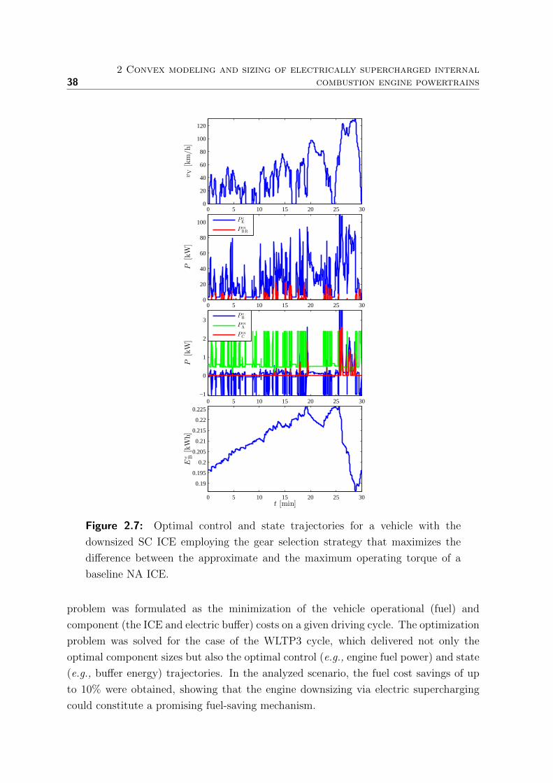
382 Convex modeling and sizing of electrically supercharged internal
combustion engine powertrains
0 5 10 15 20 25 300
20
40
60
80
100
120
vV[km/h]
0 5 10 15 20 25 300
20
40
60
80
100
P[kW]
P cE
PmBR
0 5 10 15 20 25 30−1
0
1
2
3
P[kW]
P eB
PmA
PmC
0 5 10 15 20 25 30
0.19
0.195
0.2
0.205
0.21
0.215
0.22
0.225
t [min]
Ee B[kWh]
Figure 2.7: Optimal control and state trajectories for a vehicle with the
downsized SC ICE employing the gear selection strategy that maximizes the
difference between the approximate and the maximum operating torque of a
baseline NA ICE.
problem was formulated as the minimization of the vehicle operational (fuel) and
component (the ICE and electric buffer) costs on a given driving cycle. The optimization
problem was solved for the case of the WLTP3 cycle, which delivered not only the
optimal component sizes but also the optimal control (e.g., engine fuel power) and state
(e.g., buffer energy) trajectories. In the analyzed scenario, the fuel cost savings of up
to 10% were obtained, showing that the engine downsizing via electric supercharging
could constitute a promising fuel-saving mechanism.
Chapter 3
Convex modeling and optimization of
a vehicle powertrain equipped with a
generator-turbine throttle unit
Abstract This Chapter investigates an internal combustion (gasoline) engine throttled by a
generator-turbine unit. Apart from throttling, the purpose of this device is to complement
the operation of a conventional car alternator by introducing an additional source of energy
for the electric auxiliaries. Its energy recovery potential is examined by employing a novel,
convex approach to modeling and optimization of the resulting vehicle powertrain. For a
given gear-shifting strategy, the proposed method allows the computation of optimal control
trajectories, e.g., the optimal engine fuel, alternator and turbine power, as well as of optimal
design parameters, e.g., the optimal battery size. The conducted numerical case study shows
that the use of a generator-turbine throttle unit has a potential to reduce the total operational
(fuel) and component (battery) costs by typically 2-4% or even more than 4% in selected cases
– depending on factors such as the engine size and the choice of a driving cycle.
3.1 Introduction
Although recent years have brought significant advances in electric vehicle technology,
the internal combustion engine (ICE) is still seen as a key enabler of ground trans-
portation for the foreseeable future. This can be primarily attributed to the superior
energy density and storage properties of carbon-based fuels, compared to the alternative
energy carriers (e.g., electric batteries). The ICE, however, suffers from high energy
losses, whereas the loss reduction remains a considerable challenge for the automotive
39

403 Convex modeling and optimization of a vehicle powertrain equipped with a
generator-turbine throttle unit
industry.
In [66]–[69] the authors have attempted to address the ICE energy loss problem by
introducing an exhaust heat recovery device as a substitute for a poorly-performing,
conventional car alternator. The device consists of a high-speed radial turbo-expander
which captures the energy from the exhaust air and uses it to (directly) drive a
permanent magnet or a switched reluctance electric generator. Compared to the
alternator such a device offers substantially more efficient vehicle electricity production
and a greater power density – at the cost of potentially increased exhaust back-pressure
and the need for water-cooling.
The energy recovery devices of this type can be also applied to the ICE air intake
system with the added benefit of easier installation due to a lack of external cooling
requirements. For instance, in the case of a spark-ignited (SI) gasoline engine a similar
generator-turbine unit (GTU) has been used to recover otherwise wasted intake throt-
tling losses [25], [26]. Here, the authors have proposed to replace a throttle valve with
the electric generator directly coupled to a variable geometry turbine (with adjustable
stator vanes), so that the intake airflow can be controlled while simultaneously producing
electricity. In [25], it has been also noted that in such a configuration the cool air after
the turbine can have both a negative (poor evaporation) and a positive (reduced risk of
knock) effect on the ensuing combustion phase. For this reason, the authors have argued
that the resulting lower intake air temperatures can be in addition used to assist the
air conditioning system, by cooling the working fluid via a dedicated heat exchanger.
In this Chapter, a numerical study is performed to evaluate a fuel-saving potential of
the GTU-based gasoline engine throttle. The main contributions of this research are:
1. Detailed modeling of the GTU assisted powertrain.
2. Convex relaxation steps that allow the combined optimal control and buffer sizing
problem to be formulated as a semi-definite convex program, where transmission
gear is considered as an input signal decided outside the convex optimization.
Moreover, a case study is performed providing a solution of the problem defined above
for several different driving cycles and engine sizes. The presented results show that the
use of the GTU-based throttle can potentially reduce the total operational (fuel) and
component (battery) costs by typically 2-4% or even more than 4% in selected cases,
depending on factors such as the engine size and the choice of a driving cycle.
This Chapter is organized as follows. The mathematical modeling is presented in
Section 3.2 and the optimization problem is formulated in Section 3.3. Section 3.4
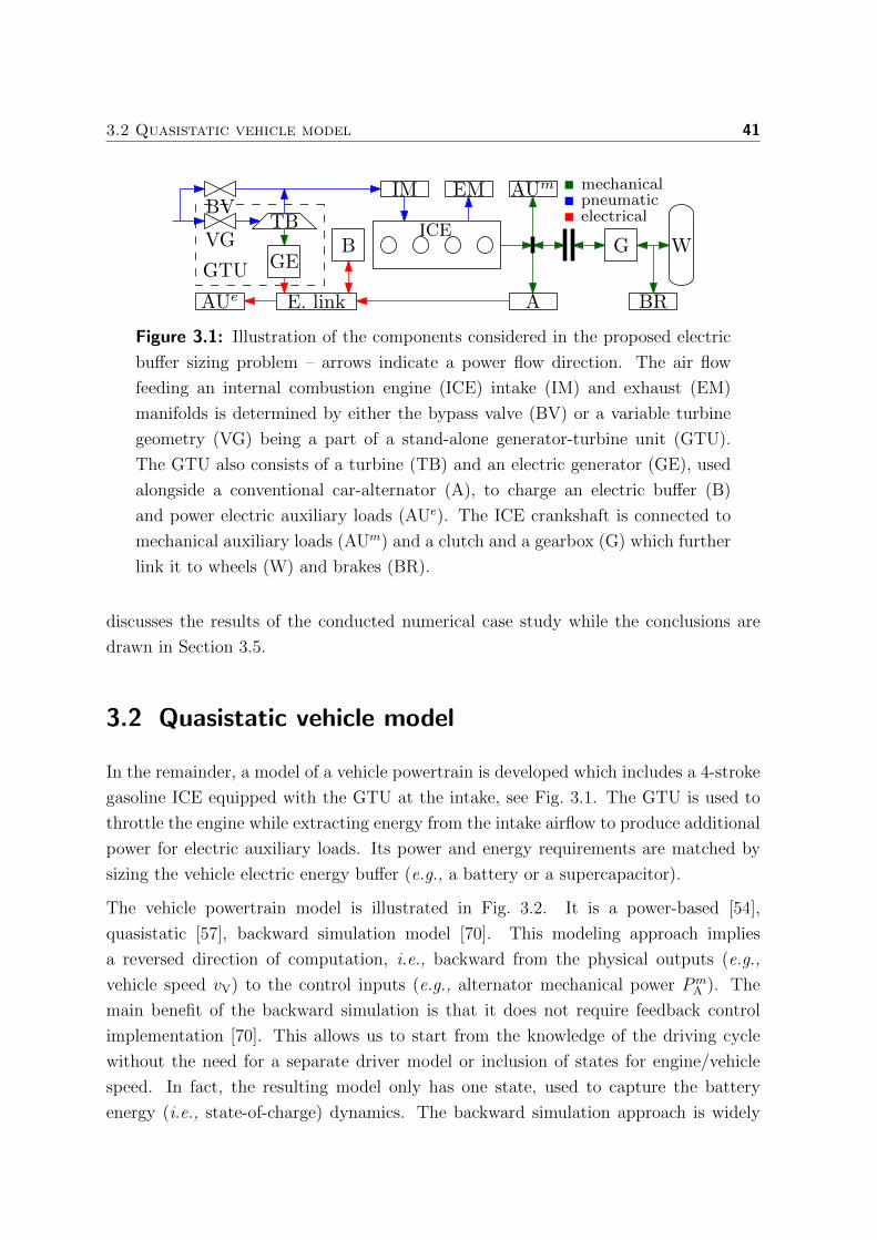
3.2 Quasistatic vehicle model 41
BV
A
GE
TB
IM EM
ICE
GTUB
AUe
G
AUm
W
BRE. link
electrical
mechanicalpneumatic
VG
Figure 3.1: Illustration of the components considered in the proposed electric
buffer sizing problem – arrows indicate a power flow direction. The air flow
feeding an internal combustion engine (ICE) intake (IM) and exhaust (EM)
manifolds is determined by either the bypass valve (BV) or a variable turbine
geometry (VG) being a part of a stand-alone generator-turbine unit (GTU).
The GTU also consists of a turbine (TB) and an electric generator (GE), used
alongside a conventional car-alternator (A), to charge an electric buffer (B)
and power electric auxiliary loads (AUe). The ICE crankshaft is connected to
mechanical auxiliary loads (AUm) and a clutch and a gearbox (G) which further
link it to wheels (W) and brakes (BR).
discusses the results of the conducted numerical case study while the conclusions are
drawn in Section 3.5.
3.2 Quasistatic vehicle model
In the remainder, a model of a vehicle powertrain is developed which includes a 4-stroke
gasoline ICE equipped with the GTU at the intake, see Fig. 3.1. The GTU is used to
throttle the engine while extracting energy from the intake airflow to produce additional
power for electric auxiliary loads. Its power and energy requirements are matched by
sizing the vehicle electric energy buffer (e.g., a battery or a supercapacitor).
The vehicle powertrain model is illustrated in Fig. 3.2. It is a power-based [54],
quasistatic [57], backward simulation model [70]. This modeling approach implies
a reversed direction of computation, i.e., backward from the physical outputs (e.g.,
vehicle speed vV) to the control inputs (e.g., alternator mechanical power PmA ). The
main benefit of the backward simulation is that it does not require feedback control
implementation [70]. This allows us to start from the knowledge of the driving cycle
without the need for a separate driver model or inclusion of states for engine/vehicle
speed. In fact, the resulting model only has one state, used to capture the battery
energy (i.e., state-of-charge) dynamics. The backward simulation approach is widely
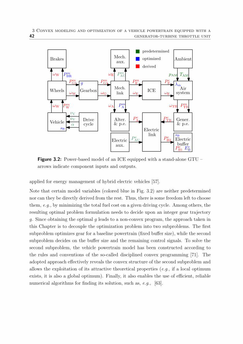
423 Convex modeling and optimization of a vehicle powertrain equipped with a
generator-turbine throttle unit
PmW
Vehicle
sB
ωW
PmG2
ωG
PmG1
ICEωE
PmE
ωA PmA
P cE
P eA
systemAir
ωTB PmTB
P eTB
sBP eB2
EeB
P eAU
derived
optimized
predetermined
g
bufferElectric
Gener.
P eB1
Ambient
pAM TAM
Brakes
ωW PmBR
Electricaux.
Mech.aux.
ωE PmAU
ωE
α
aV
vV
Wheels
cycleDrive Alter.
& p.e. & p.e.
ωW
Electriclink
λmMech.link
Gearbox
Figure 3.2: Power-based model of an ICE equipped with a stand-alone GTU –
arrows indicate component inputs and outputs.
applied for energy management of hybrid electric vehicles [57].
Note that certain model variables (colored blue in Fig. 3.2) are neither predetermined
nor can they be directly derived from the rest. Thus, there is some freedom left to choose
them, e.g., by minimizing the total fuel cost on a given driving cycle. Among others, the
resulting optimal problem formulation needs to decide upon an integer gear trajectory
g. Since obtaining the optimal g leads to a non-convex program, the approach taken in
this Chapter is to decouple the optimization problem into two subproblems. The first
subproblem optimizes gear for a baseline powertrain (fixed buffer size), while the second
subproblem decides on the buffer size and the remaining control signals. To solve the
second subproblem, the vehicle powertrain model has been constructed according to
the rules and conventions of the so-called disciplined convex programming [71]. The
adopted approach effectively reveals the convex structure of the second subproblem and
allows the exploitation of its attractive theoretical properties (e.g., if a local optimum
exists, it is also a global optimum). Finally, it also enables the use of efficient, reliable
numerical algorithms for finding its solution, such as, e.g., [63].
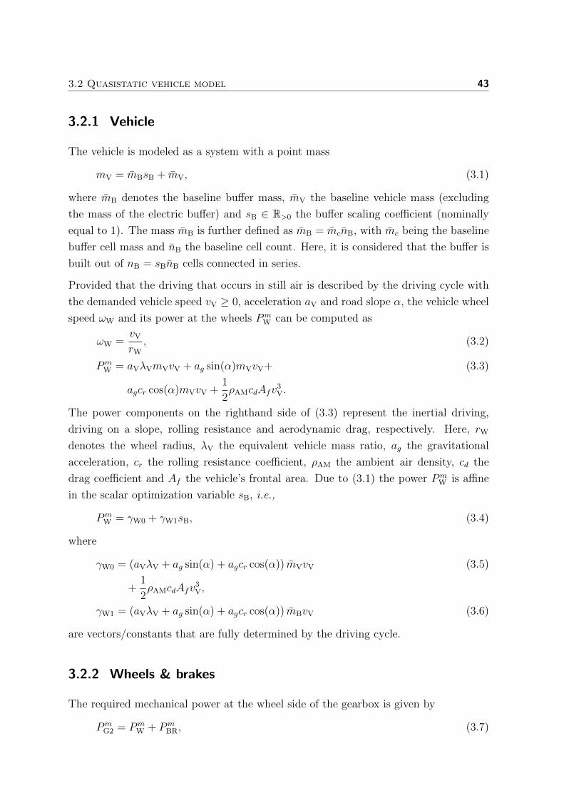
3.2 Quasistatic vehicle model 43
3.2.1 Vehicle
The vehicle is modeled as a system with a point mass
mV = mBsB + mV, (3.1)
where mB denotes the baseline buffer mass, mV the baseline vehicle mass (excluding
the mass of the electric buffer) and sB ∈ R>0 the buffer scaling coefficient (nominally
equal to 1). The mass mB is further defined as mB = mcnB, with mc being the baseline
buffer cell mass and nB the baseline cell count. Here, it is considered that the buffer is
built out of nB = sBnB cells connected in series.
Provided that the driving that occurs in still air is described by the driving cycle with
the demanded vehicle speed vV ≥ 0, acceleration aV and road slope α, the vehicle wheel
speed ωW and its power at the wheels PmW can be computed as
ωW =vV
rW
, (3.2)
PmW = aVλVmVvV + ag sin(α)mVvV+ (3.3)
agcr cos(α)mVvV +1
2ρAMcdAfv
3V.
The power components on the righthand side of (3.3) represent the inertial driving,
driving on a slope, rolling resistance and aerodynamic drag, respectively. Here, rW
denotes the wheel radius, λV the equivalent vehicle mass ratio, ag the gravitational
acceleration, cr the rolling resistance coefficient, ρAM the ambient air density, cd the
drag coefficient and Af the vehicle’s frontal area. Due to (3.1) the power PmW is affine
in the scalar optimization variable sB, i.e.,
PmW = γW0 + γW1sB, (3.4)
where
γW0 = (aVλV + ag sin(α) + agcr cos(α)) mVvV (3.5)
+1
2ρAMcdAfv
3V,
γW1 = (aVλV + ag sin(α) + agcr cos(α)) mBvV (3.6)
are vectors/constants that are fully determined by the driving cycle.
3.2.2 Wheels & brakes
The required mechanical power at the wheel side of the gearbox is given by
PmG2 = Pm
W + PmBR, (3.7)
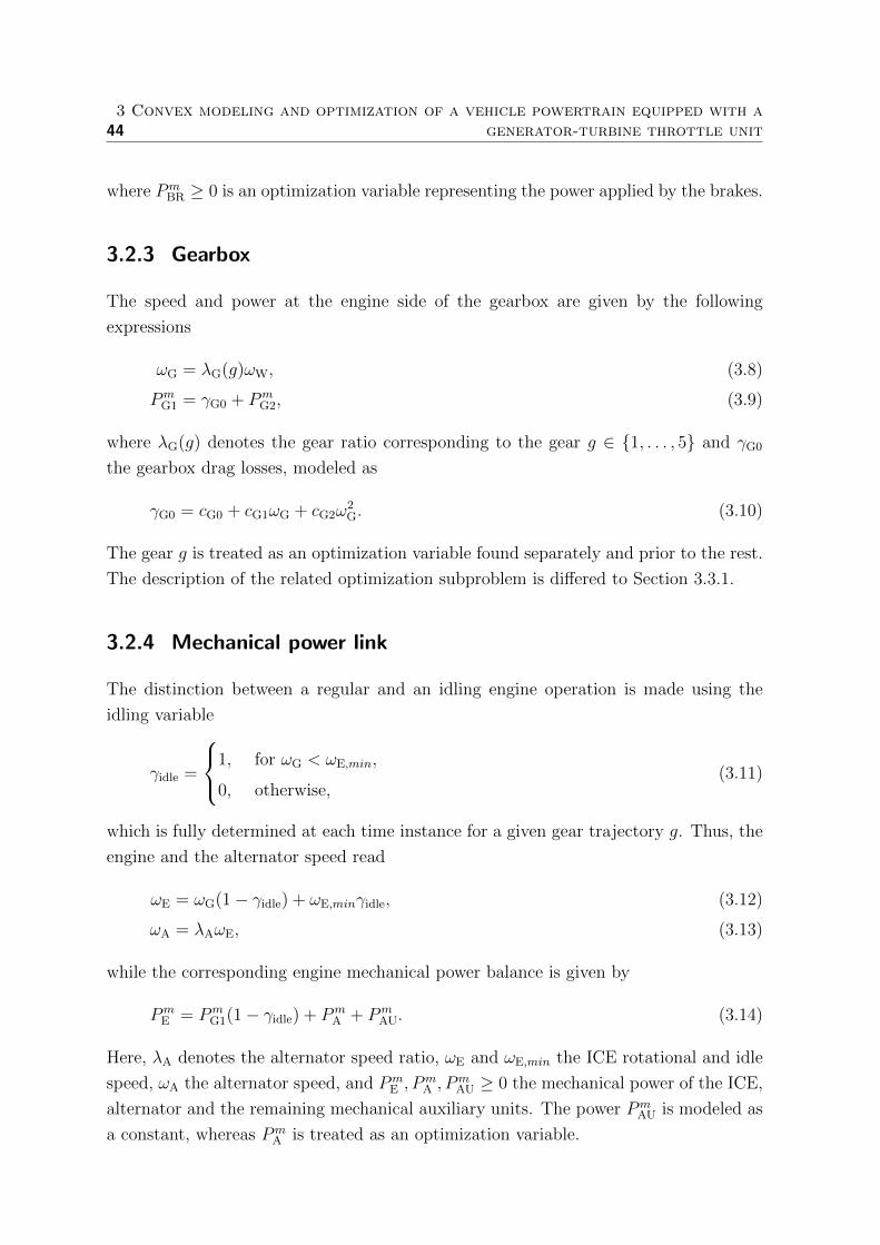
443 Convex modeling and optimization of a vehicle powertrain equipped with a
generator-turbine throttle unit
where PmBR ≥ 0 is an optimization variable representing the power applied by the brakes.
3.2.3 Gearbox
The speed and power at the engine side of the gearbox are given by the following
expressions
ωG = λG(g)ωW, (3.8)
PmG1 = γG0 + Pm
G2, (3.9)
where λG(g) denotes the gear ratio corresponding to the gear g ∈ 1, . . . , 5 and γG0
the gearbox drag losses, modeled as
γG0 = cG0 + cG1ωG + cG2ω2G. (3.10)
The gear g is treated as an optimization variable found separately and prior to the rest.
The description of the related optimization subproblem is differed to Section 3.3.1.
3.2.4 Mechanical power link
The distinction between a regular and an idling engine operation is made using the
idling variable
γidle =
1, for ωG < ωE,min,
0, otherwise,(3.11)
which is fully determined at each time instance for a given gear trajectory g. Thus, the
engine and the alternator speed read
ωE = ωG(1− γidle) + ωE,minγidle, (3.12)
ωA = λAωE, (3.13)
while the corresponding engine mechanical power balance is given by
PmE = Pm
G1(1− γidle) + PmA + Pm
AU. (3.14)
Here, λA denotes the alternator speed ratio, ωE and ωE,min the ICE rotational and idle
speed, ωA the alternator speed, and PmE , P
mA , P
mAU ≥ 0 the mechanical power of the ICE,
alternator and the remaining mechanical auxiliary units. The power PmAU is modeled as
a constant, whereas PmA is treated as an optimization variable.
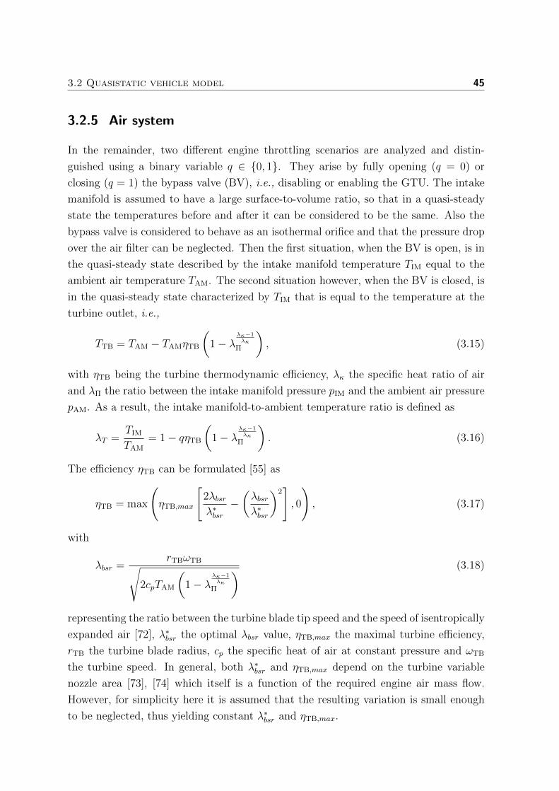
3.2 Quasistatic vehicle model 45
3.2.5 Air system
In the remainder, two different engine throttling scenarios are analyzed and distin-
guished using a binary variable q ∈ 0, 1. They arise by fully opening (q = 0) or
closing (q = 1) the bypass valve (BV), i.e., disabling or enabling the GTU. The intake
manifold is assumed to have a large surface-to-volume ratio, so that in a quasi-steady
state the temperatures before and after it can be considered to be the same. Also the
bypass valve is considered to behave as an isothermal orifice and that the pressure drop
over the air filter can be neglected. Then the first situation, when the BV is open, is in
the quasi-steady state described by the intake manifold temperature TIM equal to the
ambient air temperature TAM. The second situation however, when the BV is closed, is
in the quasi-steady state characterized by TIM that is equal to the temperature at the
turbine outlet, i.e.,
TTB = TAM − TAMηTB
(1− λ
λκ−1λκ
Π
), (3.15)
with ηTB being the turbine thermodynamic efficiency, λκ the specific heat ratio of air
and λΠ the ratio between the intake manifold pressure pIM and the ambient air pressure
pAM. As a result, the intake manifold-to-ambient temperature ratio is defined as
λT =TIM
TAM
= 1− qηTB
(1− λ
λκ−1λκ
Π
). (3.16)
The efficiency ηTB can be formulated [55] as
ηTB = max
(ηTB,max
[2λbsrλ∗bsr
−(λbsrλ∗bsr
)2], 0
), (3.17)
with
λbsr =rTBωTB√
2cpTAM
(1− λ
λκ−1λκ
Π
) (3.18)
representing the ratio between the turbine blade tip speed and the speed of isentropically
expanded air [72], λ∗bsr the optimal λbsr value, ηTB,max the maximal turbine efficiency,
rTB the turbine blade radius, cp the specific heat of air at constant pressure and ωTB
the turbine speed. In general, both λ∗bsr and ηTB,max depend on the turbine variable
nozzle area [73], [74] which itself is a function of the required engine air mass flow.
However, for simplicity here it is assumed that the resulting variation is small enough
to be neglected, thus yielding constant λ∗bsr and ηTB,max.
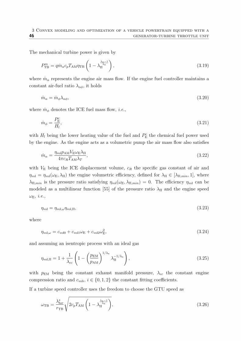
463 Convex modeling and optimization of a vehicle powertrain equipped with a
generator-turbine throttle unit
The mechanical turbine power is given by
PmTB = qmαcpTAMηTB
(1− λ
λκ−1λκ
Π
), (3.19)
where mα represents the engine air mass flow. If the engine fuel controller maintains a
constant air-fuel ratio λαφ, it holds
mα = mφλαφ, (3.20)
where mφ denotes the ICE fuel mass flow, i.e.,
mφ =P c
E
Hl
, (3.21)
with Hl being the lower heating value of the fuel and P cE the chemical fuel power used
by the engine. As the engine acts as a volumetric pump the air mass flow also satisfies
mα =ηvolpAMVEωEλΠ
4πcRTAMλT, (3.22)
with VE being the ICE displacement volume, cR the specific gas constant of air and
ηvol = ηvol(ωE, λΠ) the engine volumetric efficiency, defined for λΠ ∈ [λΠ,min, 1], where
λΠ,min is the pressure ratio satisfying ηvol(ωE, λΠ,min) = 0. The efficiency ηvol can be
modeled as a multilinear function [55] of the pressure ratio λΠ and the engine speed
ωE, i.e.,
ηvol = ηvol,ωηvol,Π, (3.23)
where
ηvol,ω = cvol0 + cvol1ωE + cvol2ω2E, (3.24)
and assuming an isentropic process with an ideal gas
ηvol,Π = 1 +1
λec
(1−
(pEM
pAM
)1/λκ
λ−1/λκΠ
), (3.25)
with pEM being the constant exhaust manifold pressure, λec the constant engine
compression ratio and cvoli, i ∈ 0, 1, 2 the constant fitting coefficients.
If a turbine speed controller uses the freedom to choose the GTU speed as
ωTB =λ∗bsrrTB
√2cpTAM
(1− λ
λκ−1λκ
Π
), (3.26)

3.2 Quasistatic vehicle model 47
then from (3.17) and (3.18) it follows that the turbine will be operated on the optimal
efficiency line, i.e., ηTB = ηTB,max while the turbine power may be written as
PmTB = qηTB,maxcpTAMγmγTB, (3.27)
where
γTB = λm
(1− λ
λκ−1λκ
Π
), (3.28)
λm =ηvol,ΠλΠ
1− qηTB,max
(1− λ
λκ−1λκ
Π
) , (3.29)
γm =pAMVEωEηvol,ω
4πcRTAM
. (3.30)
Note that the air mass flow coefficient γm and the ratio λm satisfy
mα = γmλm. (3.31)
Now, λm is treated as an optimization variable while, e.g., the ratio λΠ is derived from
it. For this purpose, let the function λΠ = λΠ(λm, q) denote the inverse of (3.29) for
λm ∈ [0, ηvol,Π] and q ∈ 0, 1, where ηvol,Π = ηvol,Π(λΠ = 1). Then, the function γTB =
γTB(λΠ(λm, 1)) can be accurately approximated by a concave 4th-order polynomial with
constant coefficients cTBi, i ∈ 1, . . . , 4, i.e.,
γTB = cTB1λm + cTB2λ2m + cTB3λ
3m + cTB4λ
4m, (3.32)
such that it passes through the end points (λm, γTB) ∈ (0, 0), (ηvol,Π, 0). The function
γTB and the resulting fit γTB are shown in Fig. 3.3.
Finally, to simplify the derivations that follow consider a polynomial approximation of
λΠ = λΠ(λm, q), given by
λΠ = cΠ0 + cΠ1λm + cΠ2λ2m, (3.33)
where cΠi = cΠi(q), i ∈ 0, 1, 2 are the resulting fitting coefficients. The functions λΠ
and λΠ are illustrated in Fig. 3.4.
3.2.6 ICE
The ICE mechanical behaviour can be described with the following relationship [55],
[56]:
pE = ηE1pφ − ηE2p2φ − pEf − pEg, (3.34)
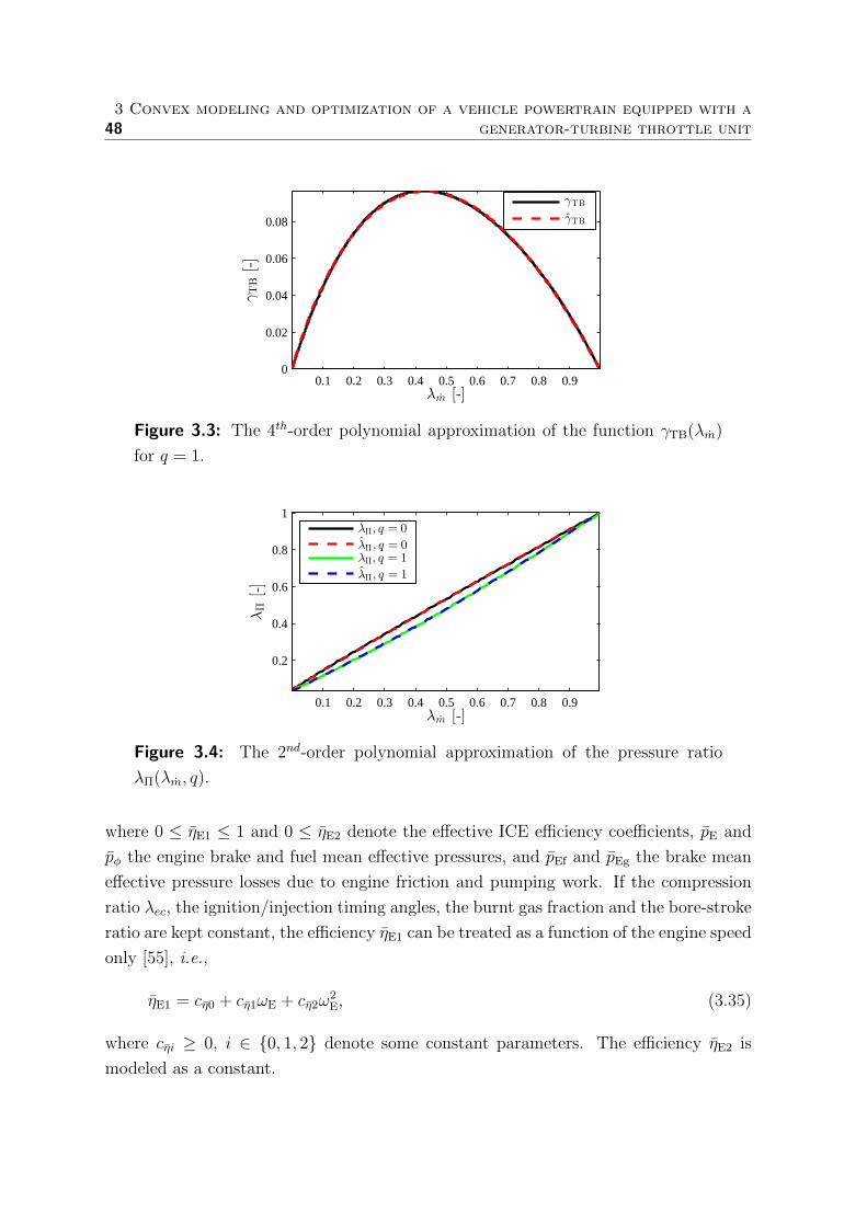
483 Convex modeling and optimization of a vehicle powertrain equipped with a
generator-turbine throttle unit
0.1 0.2 0.3 0.4 0.5 0.6 0.7 0.8 0.90
0.02
0.04
0.06
0.08
λm [-]
γTB[-]
γTB
γTB
Figure 3.3: The 4th-order polynomial approximation of the function γTB(λm)
for q = 1.
0.1 0.2 0.3 0.4 0.5 0.6 0.7 0.8 0.9
0.2
0.4
0.6
0.8
1
λm [-]
λΠ[-]
λΠ, q = 0
λΠ, q = 0λΠ, q = 1
λΠ, q = 1
Figure 3.4: The 2nd-order polynomial approximation of the pressure ratio
λΠ(λm, q).
where 0 ≤ ηE1 ≤ 1 and 0 ≤ ηE2 denote the effective ICE efficiency coefficients, pE and
pφ the engine brake and fuel mean effective pressures, and pEf and pEg the brake mean
effective pressure losses due to engine friction and pumping work. If the compression
ratio λec, the ignition/injection timing angles, the burnt gas fraction and the bore-stroke
ratio are kept constant, the efficiency ηE1 can be treated as a function of the engine speed
only [55], i.e.,
ηE1 = cη0 + cη1ωE + cη2ω2E, (3.35)
where cηi ≥ 0, i ∈ 0, 1, 2 denote some constant parameters. The efficiency ηE2 is
modeled as a constant.

3.2 Quasistatic vehicle model 49
The two pressures, pE and pφ, read
pE =4πτE
VE
(3.36)
pφ =4πP c
E
VEωE
, (3.37)
with τE being the ICE torque. The related loss components are modeled [55], [75] as
pEf = cf0 + cf1ωE + cf2ω2E, (3.38)
pEg = pEM − pAMλΠ,
where cf0i ≥ 0, i ∈ 0, 1, 2 are some constant parameters. Using (3.33) the ICE
pumping loss becomes
pEg = pEM − pAMcΠ0 − pAMcΠ1λm − pAMcΠ2λ2m. (3.39)
By inserting the expressions for pressures in (3.34) and by multiplying both sides withVEωE
4π, it follows
PmE = γE0 + γE1λm + γE2λ
2m, (3.40)
with PmE = τEωE the mechanical ICE power and
γE0 =VEωE(−cf0 − cf1ωE − cf2ω
2E − pEM + pAMcΠ0)
4π, (3.41)
γE1 =VEωEpAMcΠ1
4π+ηE1Hlγmλαφ
,
γE2 =VEωEpAMcΠ2
4π− ηE2H
2l γ
2m
λ2αφ
.
Note that only if γE2 ≤ 0, the expression (3.40) has physical sense, as it results in a
convex relationship between the mechanical PmE and the chemical power P c
E, as shown
in Figure 3.5. Thus, under this condition (3.40) is a concave function of the λm ratio.
3.2.7 Alternator and GTU generator
The electric machine electric power can be modeled as a second-order polynomial of its
mechanical power, with a constant term representing a speed-dependent drag loss [56].
In this context, the alternator electric power can be formulated as
P eA = γA0 + cA1P
mA + cA2P
m2A , (3.42)
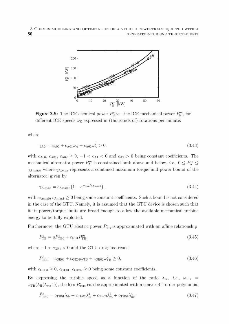
503 Convex modeling and optimization of a vehicle powertrain equipped with a
generator-turbine throttle unit
1000
2000
2000
3000
3000
3000
4000
4000
4000
4000
5000
5000
5000
5000
PmE [kW]
Pc E[kW]
0 10 20 30 40 50 600
50
100
150
200
Figure 3.5: The ICE chemical power P cE vs. the ICE mechanical power Pm
E , for
different ICE speeds ωE expressed in (thousands of) rotations per minute.
where
γA0 = cA00 + cA01ωA + cA02ω2A > 0, (3.43)
with cA00, cA01, cA02 ≥ 0, −1 < cA1 < 0 and cA2 > 0 being constant coefficients. The
mechanical alternator power PmA is constrained both above and below, i.e., 0 ≤ Pm
A ≤γA,max, where γA,max represents a combined maximum torque and power bound of the
alternator, given by
γA,max = cAmax0
(1− e−ωA/cAmax1
), (3.44)
with cAmax0, cAmax1 ≥ 0 being some constant coefficients. Such a bound is not considered
in the case of the GTU. Namely, it is assumed that the GTU device is chosen such that
it its power/torque limits are broad enough to allow the available mechanical turbine
energy to be fully exploited.
Furthermore, the GTU electric power P eTB is approximated with an affine relationship
P eTB = qP e
TB0 + cGE1PmTB, (3.45)
where −1 < cGE1 < 0 and the GTU drag loss reads
P eTB0 = cGE00 + cGE01ωTB + cGE02ω
2TB ≥ 0, (3.46)
with cGE00 ≥ 0, cGE01, cGE02 ≥ 0 being some constant coefficients.
By expressing the turbine speed as a function of the ratio λm, i.e., ωTB =
ωTB(λΠ(λm, 1)), the loss P eTB0 can be approximated with a convex 4th-order polynomial
P eTB0 = cTB01λm + cTB02λ
2m + cTB03λ
3m + cTB04λ
4m, (3.47)
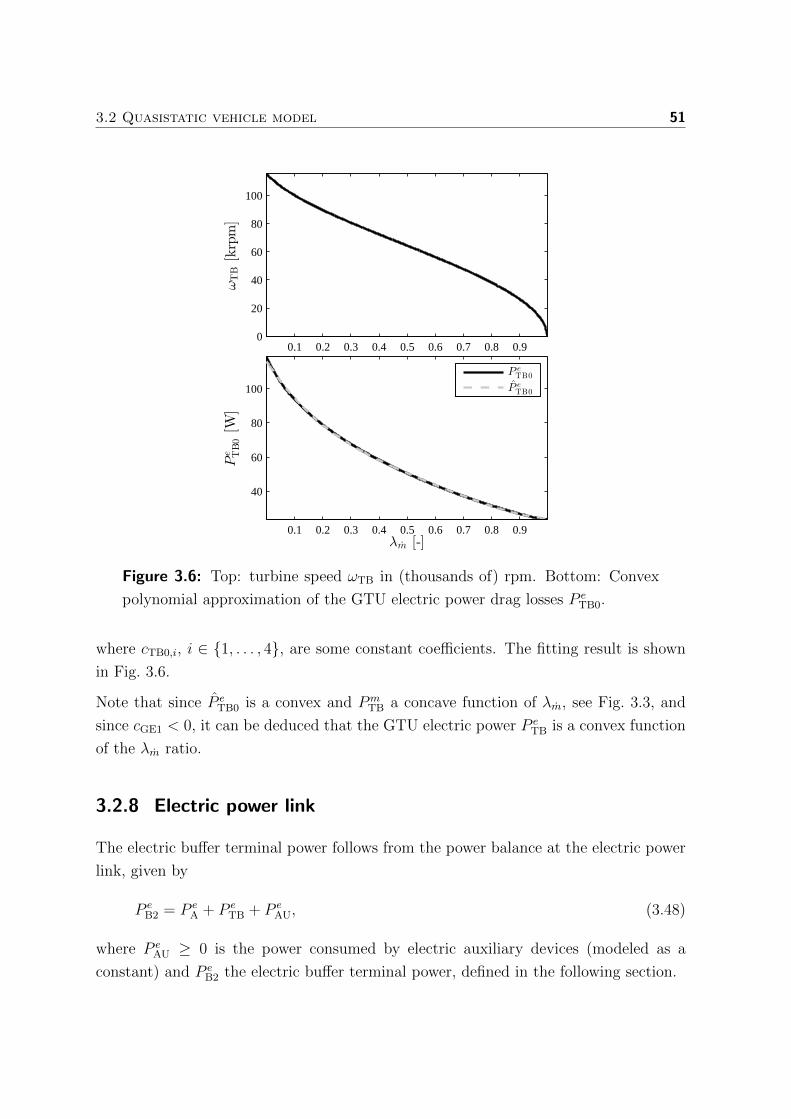
3.2 Quasistatic vehicle model 51
0.1 0.2 0.3 0.4 0.5 0.6 0.7 0.8 0.90
20
40
60
80
100
ωTB[krpm]
0.1 0.2 0.3 0.4 0.5 0.6 0.7 0.8 0.9
40
60
80
100
λm [-]
Pe TB0[W
]
P eTB0
P eTB0
Figure 3.6: Top: turbine speed ωTB in (thousands of) rpm. Bottom: Convex
polynomial approximation of the GTU electric power drag losses P eTB0.
where cTB0,i, i ∈ 1, . . . , 4, are some constant coefficients. The fitting result is shown
in Fig. 3.6.
Note that since P eTB0 is a convex and Pm
TB a concave function of λm, see Fig. 3.3, and
since cGE1 < 0, it can be deduced that the GTU electric power P eTB is a convex function
of the λm ratio.
3.2.8 Electric power link
The electric buffer terminal power follows from the power balance at the electric power
link, given by
P eB2 = P e
A + P eTB + P e
AU, (3.48)
where P eAU ≥ 0 is the power consumed by electric auxiliary devices (modeled as a
constant) and P eB2 the electric buffer terminal power, defined in the following section.
523 Convex modeling and optimization of a vehicle powertrain equipped with a
generator-turbine throttle unit
3.2.9 Electric buffer
The electric buffer cells are considered to be either lithium-ion batteries, or supercapac-
itors. Each cell is modeled as a cell open circuit voltage uc with a constant resistance
Rc connected in series. The battery voltage uc is modeled as an affine function of
state-of-charge soc, i.e.,
uc =Qc
cc1soc+ cc0, (3.49)
where Qc is the cell capacity, and cc1 and cc0 are the resulting fitting coefficients. Such
a model is suitable for lithium-ion battery technology where low/high soc operation is
avoided due to battery longevity reasons [57], as well as for supercapacitors.
As nB cells are connected in series, the buffer terminal voltage uB2 reads
uB2 = nBuc − nBRcic, (3.50)
where ic denotes the cell current, which determines the evolution of the cell state-of-
charge, i.e.,
dsoc
dt= − ic
Qc
. (3.51)
In the following, convex modeling steps of [58] are employed, where instead of using uc
and ic the electric buffer is modeled in terms of its energy EeB, internal power P e
B1 and
dissipative power P eB0. Specifically, the following holds
dEeB
dt= −P e
B1, (3.52)
implying that P eB1 > 0 results in the buffer discharge and vice versa. The internal and
dissipative buffer powers are defined as
P eB1 = nBucic, (3.53)
P eB0 = nBRci
2c .
This implies
P eB1 = P e
B2 + P eB0. (3.54)
Furthermore, from (3.51), (3.52) and (3.53), the following derives
EeB = nBQc
soc∫
0
uc(s)ds =nBcc1
2(u2
c − c2c0). (3.55)
3.3 Optimization problem formulation 53
Thus the pack losses may be expressed as
P eB0 =
Rccc1 (P eB1)2
2EeB + nBcc1c2
c0
, (3.56)
which as a quadratic-over-linear with a strictly positive denominator is a convex
function [53] of P eB1, Ee
B and nB (and therefore convex in sB as well). Note that when
cc0 = 0 the adopted model, (3.55) and (3.56), describes a capacitor with a capacitance
cc1.
Constraints on the state-of-charge soc ∈ [socmin, socmax] and the current ic ∈[ic,min, ic,max] can be translated into constraints on the energy Ee
B and the power P eB1,
i.e.,
EeB ∈ sB
( nBcc12
([u2c(socmin), u2
c(socmax)]− c2
c0
))(3.57)
= sB[EeB,min, E
eB,max],
P eB1 ∈[ic,min, ic,max]
√sBnB
(2Ee
B
cc1+ sBnBc2
c0
), (3.58)
where 0 ≤ socmin < socmax ≤ 1 represent the minimum and the maximum state-of-
charge, ic,min < 0 and ic,max > 0 the minimum and the maximum cell current and
EeB,min and Ee
B,max the baseline minimum and maximum buffer energy. Notice that the
geometric mean in (3.58) is a concave function [53] of EeB and nB. In this context Ee
B is
treated as an optimization variable, although it can also be treated as a state variable
that depends on the control variable P eB1.
3.3 Optimization problem formulation
The optimization goal is to find a minimum of a weighted sum of operational and
component costs. The operational costs are simply represented by the cost of consumed
gasoline while the component costs are given by the cost of the electric buffer. Each
cost component is weighted by its respective weighting coefficient, wφ or wB, so that its
contribution is expressed in currency per distance. Using the approach outlined in [59]
these coefficients are computed as
wφ = µφ1
Hlρφd, (3.59)
wB = µBEe
B,max
dyear
tyear
tlife
(1 + εB,year
tlife + 1
2
),

543 Convex modeling and optimization of a vehicle powertrain equipped with a
generator-turbine throttle unit
where µφ and µB are fuel and buffer price expressed respectively in currency per volume
and usable energy content (i.e., at a specified maximum state-of-charge). Furthermore,
d =∫ tend
0vVdt is the total drive cycle length, dyear the average distance a vehicle travels
during one year tyear, ρφ the fuel density, tlife the duration of the expected vehicle life-
cycle and εB,year the yearly buffer interest rate.
3.3.1 Gear selection strategy
For a driving cycle specified by the vehicle speed vV, the acceleration aV and the slope α,
a feasible gear trajectory g is found by minimizing the fuel power of a baseline powertrain
(fixed buffer size), i.e., when the ICE is throttled using a bypass valve (q = 0).
First, the expressions (3.2), (3.5), (3.6), (3.8) and (3.10)-(3.13) are evaluated at each
time instant tk = kδt, k ≥ 0 for all gears g(tk) ∈ 1, . . . , 5, where δt denotes the driving
cycle sample time. Second, the obtained values are used to estimate the powers PmA ,
PmE and P c
E, and the ratio λm, according to
PmA =
−cA1 −√c2
A1 − 4 (γA0 + P eAU) cA2
2cA2
, (3.60)
PmE = max
(Pm
A + PmAU + (γG0 + γW0 + γW1) (1− γidle), 0
),
P cE = λm
Hlγmλαφ
,
λm =
−γE1 +
√γ2
E1 − 4(γE0 − Pm
E
)γE2
2γE2
.
Third, at each time instant tk, the gear g(tk) ∈ F(tk) yielding the lowest fuel power P cE
is selected. Here F(tk) ⊂ 1, . . . , 5 denotes a feasible set of gears at the moment tk, i.e.,
the gears resulting in a feasible ratio λm ∈ [0, ηvol,Π] ⊂ R and power PmA ⊂ R. Finally,
to limit the maximum number of consecutive gear up-shifts gup,max, the computed gear
trajectory g is processed as follows
g(tk) =
g(tk), if F(tk) = ∅,ming∈F(tk)
g, otherwise,(3.61)
where F(tk) = g ∈ F(tk)|g(tk−1) < g ≤ g(tk−1)+gup,max denotes a set of feasible gears
at the moment tk satisfying the imposed gear shifting criterion. The gear trajectory
obtained using the described procedure is shown in Fig. 3.7, for the case of the US
Environmental Protection Agency Federal Test Procedure driving cycle (FTP75).
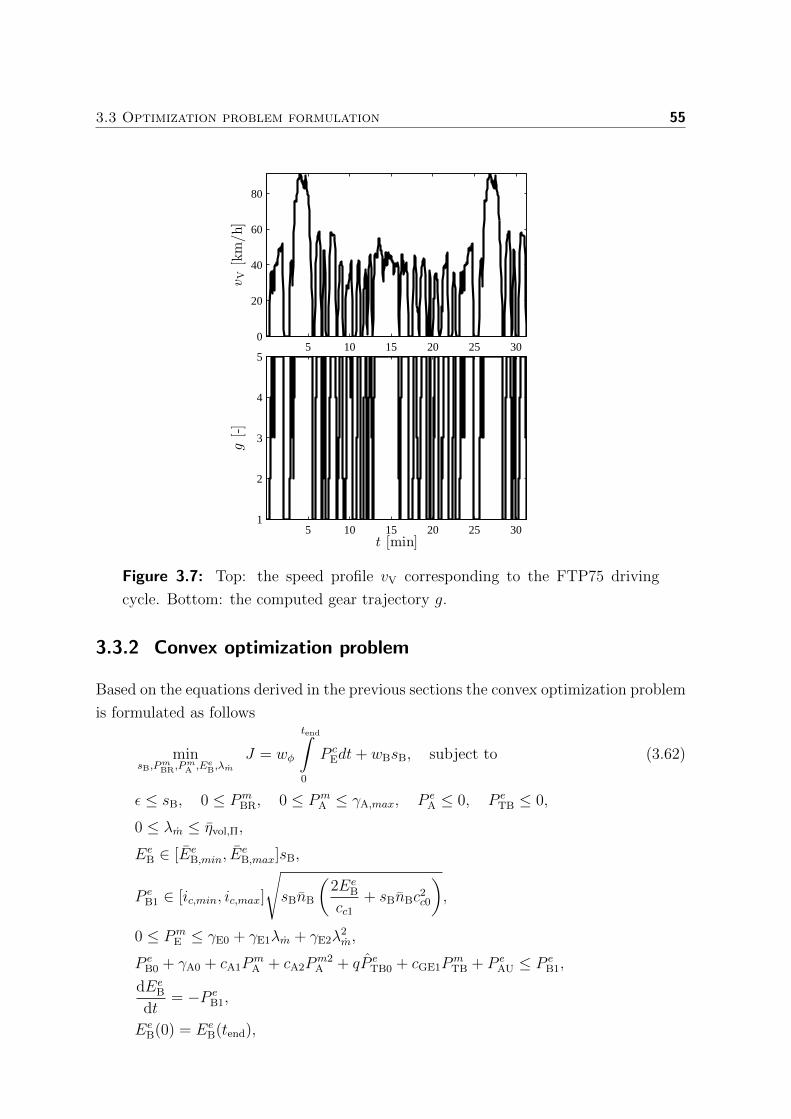
3.3 Optimization problem formulation 55
5 10 15 20 25 300
20
40
60
80
vV[km/h]
5 10 15 20 25 301
2
3
4
5
g[-]
t [min]
Figure 3.7: Top: the speed profile vV corresponding to the FTP75 driving
cycle. Bottom: the computed gear trajectory g.
3.3.2 Convex optimization problem
Based on the equations derived in the previous sections the convex optimization problem
is formulated as follows
minsB,P
mBR,P
mA ,EeB,λm
J = wφ
tend∫
0
P cEdt+ wBsB, subject to (3.62)
ε ≤ sB, 0 ≤ PmBR, 0 ≤ Pm
A ≤ γA,max, P eA ≤ 0, P e
TB ≤ 0,
0 ≤ λm ≤ ηvol,Π,
EeB ∈ [Ee
B,min, EeB,max]sB,
P eB1 ∈ [ic,min, ic,max]
√sBnB
(2Ee
B
cc1+ sBnBc2
c0
),
0 ≤ PmE ≤ γE0 + γE1λm + γE2λ
2m,
P eB0 + γA0 + cA1P
mA + cA2P
m2A + qP e
TB0 + cGE1PmTB + P e
AU ≤ P eB1,
dEeB
dt= −P e
B1,
EeB(0) = Ee
B(tend),
563 Convex modeling and optimization of a vehicle powertrain equipped with a
generator-turbine throttle unit
where
P eB0 =
Rccc1 (P eB1)2
2EeB + sBnBcc1c2
c0
, (3.63)
P eTB0 = cTB01λm + cTB02λ
2m + cTB03λ
3m + cTB04λ
4m,
PmTB = qηTB,maxcpTAMγm
(cTB1λm + cTB2λ
2m + cTB3λ
3m + cTB4λ
4m
),
PmE = Pm
A + PmAU + (γG0 + Pm
BR + γW0 + γW1sB) (1− γidle),
P cE =
Hlγmλαφ
λm,
with the constraints imposed ∀t ∈ [0, tend], where tend is the time when the trip ends
and ε > 0 is some small constant. Note that the values of all the varying coefficients
γ can be pre-computed for the entire range of the driving cycle. This is because they
only depend on the vehicle speed vV, acceleration aV and/or slope α or the rotational
speeds ωG, ωE and ωA, i.e., on the gear trajectory g.
In (3.62) the electrical and mechanical power balance equalities are relaxed with an
inequality. The relaxation changes the original model formulation by creating a convex
superset of a non-convex set. However, it can be logically reasoned that the resulting two
constraints hold with equality at the optimum – otherwise energy would be unnecessarily
wasted. Hence, the solutions of the relaxed and of the non-relaxed problem are the same.
For a more detailed discussion, see [60].
The problem (3.62) has in total four time dependent, λm, PmBR, P
mA , E
eB, and one scalar
optimization variable, sB. Before the problem is solved all the optimization variables are
scaled with their expected maximal values. Then (3.62) is discretized using a zero-order
hold (with a sample time δt) and casted into a standard convex semi-definite program
(SDP) form [76]. The SDP is implemented and solved using the CVX optimization
modeling language [61], [62], in combination with the SDPT3 solver [63].
3.4 Case study results
In this Section the solution of (3.62) is discussed for the case of 4 different driving cycles,
i.e.,
• the US Environmental Protection Agency Federal Test Procedure driving cycle
(FTP75),
• the Worldwide harmonized Light vehicles Test Procedure Class 3 driving cycle
(WLTP3),
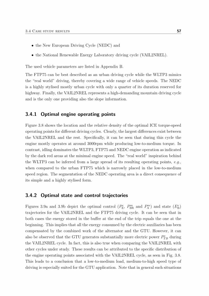
3.4 Case study results 57
• the New European Driving Cycle (NEDC) and
• the National Renewable Energy Laboratory driving cycle (VAIL2NREL).
The used vehicle parameters are listed in Appendix B.
The FTP75 can be best described as an urban driving cycle while the WLTP3 mimics
the “real world” driving, thereby covering a wide range of vehicle speeds. The NEDC
is a highly stylised mostly urban cycle with only a quarter of its duration reserved for
highway. Finally, the VAIL2NREL represents a high-demanding mountain driving cycle
and is the only one providing also the slope information.
3.4.1 Optimal engine operating points
Figure 3.8 shows the location and the relative density of the optimal ICE torque-speed
operating points for different driving cycles. Clearly, the largest differences exist between
the VAIL2NREL and the rest. Specifically, it can be seen that during this cycle the
engine mostly operates at around 3000rpm while producing low-to-medium torque. In
contrast, idling dominates the WLTP3, FTP75 and NEDC engine operation as indicated
by the dark red areas at the minimal engine speed. The “real world” inspiration behind
the WLTP3 can be inferred from a large spread of its resulting operating points, e.g.,
when compared to the urban FTP75 which is narrowly placed in the low-to-medium
speed region. The segmentation of the NEDC operating area is a direct consequence of
its simple and a highly stylised form.
3.4.2 Optimal state and control trajectories
Figures 3.9a and 3.9b depict the optimal control (P cE, Pm
BR and PmA ) and state (Ee
B)
trajectories for the VAIL2NREL and the FTP75 driving cycle. It can be seen that in
both cases the energy stored in the buffer at the end of the trip equals the one at the
beginning. This implies that all the energy consumed by the electric auxiliaries has been
compensated by the combined work of the alternator and the GTU. However, it can
also be observed that the GTU generates substantially more electric power P eTB during
the VAIL2NREL cycle. In fact, this is also true when comparing the VAIL2NREL with
other cycles under study. These results can be attributed to the specific distribution of
the engine operating points associated with the VAIL2NREL cycle, as seen in Fig. 3.8.
This leads to a conclusion that a low-to-medium load, medium-to-high speed type of
driving is especially suited for the GTU application. Note that in general such situations

583 Convex modeling and optimization of a vehicle powertrain equipped with a
generator-turbine throttle unit
are also characterized by increased engine throttling (pumping) losses as they necessarily
imply partially closed engine air-path.
Table 3.1 summarizes the optimization results while Fig. 3.10 provides an illustration.
Here, the total vehicle operational and component costs J are presented for all driving
cycles, both when the GTU is disabled (q = 0) and when it is enabled (q = 1).
Specifically for a baseline, 1.6 liter engine, the GTU use delivered cost reductions ranging
from 0.17 ¢/km (FTP75) to 0.28 ¢/km (VAIL2NREL), i.e., 2.24% to 3.86% respectively.
1000 1500 2000 2500 3000 3500 4000 4500 5000
20
40
60
80
100
120
140
FTP75
ωE [rpm]
τE[N
m]
1000 1500 2000 2500 3000 3500 4000 4500 5000
20
40
60
80
100
120
140
NEDC
ωE [rpm]
τE[N
m]
1000 1500 2000 2500 3000 3500 4000 4500 5000
20
40
60
80
100
120
140
VAIL2NREL
ωE [rpm]
τE[N
m]
1000 1500 2000 2500 3000 3500 4000 4500 5000
20
40
60
80
100
120
140
WLTP3
ωE [rpm]
τE[N
m]
Figure 3.8: The ICE torque-speed diagram showing the relative density of the
optimal engine operating points for different driving cycles. To emphasize the
active driving w.r.t. engine idling operation, a logarithmic color scale is used
with the high density areas colored in red.
The data also shows that in all cases the addition of the GTU led to an increase in
the battery size, e.g., from 6.57 Wh to 15.82 Wh for the case of the FTP75 driving
cycle. The location of its battery operating points is presented in Fig. 3.11. Notice that
some of them are located on the buffer power P eB1 and energy Ee
B bounds. The activity
of one or more of these constraints is expected as this is what ultimately determines
the required buffer size. Nevertheless, it can be seen that the entire battery energy
content was not actually used. Namely, it appears that a battery with the same power
capability but half of the energy content could have been employed just as well. As
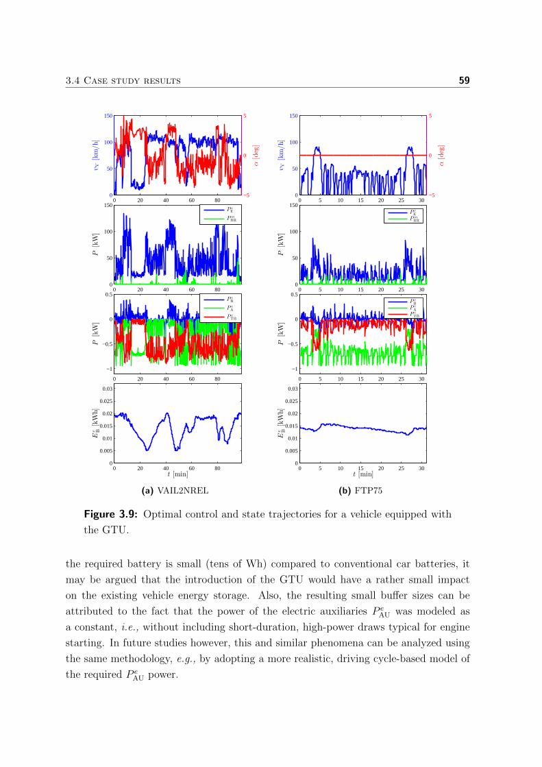
3.4 Case study results 59
0 20 40 60 800
50
100
150
vV[km/h]
−5
0
5
α[deg]
0 20 40 60 800
50
100
150
P[kW]
P cE
PmBR
0 20 40 60 80
−1
−0.5
0
0.5
P[kW]
P eB
P eA
P eTB
0 20 40 60 800
0.005
0.01
0.015
0.02
0.025
0.03
t [min]
Ee B[kWh]
(a) VAIL2NREL
0 5 10 15 20 25 300
50
100
150
vV[km/h]
−5
0
5
α[deg]
0 5 10 15 20 25 300
50
100
150
P[kW]
P cE
PmBR
0 5 10 15 20 25 30
−1
−0.5
0
0.5
P[kW]
P eB
P eA
P eTB
0 5 10 15 20 25 300
0.005
0.01
0.015
0.02
0.025
0.03
t [min]
Ee B[kWh]
(b) FTP75
Figure 3.9: Optimal control and state trajectories for a vehicle equipped with
the GTU.
the required battery is small (tens of Wh) compared to conventional car batteries, it
may be argued that the introduction of the GTU would have a rather small impact
on the existing vehicle energy storage. Also, the resulting small buffer sizes can be
attributed to the fact that the power of the electric auxiliaries P eAU was modeled as
a constant, i.e., without including short-duration, high-power draws typical for engine
starting. In future studies however, this and similar phenomena can be analyzed using
the same methodology, e.g., by adopting a more realistic, driving cycle-based model of
the required P eAU power.

603 Convex modeling and optimization of a vehicle powertrain equipped with a
generator-turbine throttle unit
VAIL2NREL FTP75 WLTP3 NEDC0
2
4
6
8
10
12
J[cent/km]
3.86%2.24% 2.96% 2.47%
GTU enabled
reduction
Figure 3.10: The effect of using the GTU at the place of a throttle valve in
terms of the total operational and component costs J for different driving cycles.
Table 3.1: Optimization results
Driving cycle Parameter disabled GTU enabled GTU
VAIL2NRELJ 7.19 ¢/km 6.91 ¢/km
sBEeB,max 5.83 Wh 20.22 Wh
FTP75J 7.77 ¢/km 7.59 ¢/km
sBEeB,max 6.57 Wh 15.82 Wh
WLTP3J 8.10 ¢/km 7.86 ¢/km
sBEeB,max 6.72 Wh 20.16 Wh
NEDCJ 8.26 ¢/km 8.05 ¢/km
sBEeB,max 6.57 Wh 18.05 Wh
3.4.3 The effect of varying the ICE displacement volume on the
GTU performance
The effect of varying the ICE displacement volume on the total cost J associated with
the VAIL2NREL driving cycle, is shown in Fig. 3.12. The cost reduction caused by the
GTU use ranges from 3.6% for a 1.5 liter to 4.5% for a 2 liter engine. Thus, although
larger engines induce greater driving costs they also yield greater benefits from the
GTU-based throttle technology, w.r.t. their smaller counterparts. This relates to the
fact that engine throttling losses become more prominent when the engine is oversized.

3.5 Conclusions 61
−0.3 −0.2 −0.1 0 0.1 0.2 0.30
0.005
0.01
0.015
8888
9090
90 9090
909292
92 9292
929494
94 9494
949696
96 9696
969898
9898
9898
P eB [kW]
Ee B[kWh]
Figure 3.11: The electric buffer power P eB vs. energy Ee
B, for the case
of the FTP75 driving cycle. The contour lines represent the buffer charg-
ing/discharging efficiency.
1.5 1.6 1.7 1.8 1.9 26.8
7
7.2
7.4
7.6
7.8
Cost
[cent/km]
VE [liter]
disabled GTUenabled GTU
Figure 3.12: The effect of varying the ICE displacement volume on the total
operational and component costs for the case of the VAIL2NREL driving cycle.
3.5 Conclusions
This Chapter provided a method for numerical evaluation of the fuel-saving potential of
the generator-turbine throttle unit. For this purpose, the disciplined convex modeling
and optimization methodology was employed to derive a convex model of the underlying
vehicle powertrain. The derived model was used to formulate a convex optimization
problem considering the minimization of the total vehicle operational (fuel) and com-
ponent (electric buffer) costs. The analysis of the optimal problem solution has shown
that the GTU-based throttle can yield major fuel benefits during the high-demand
highway driving and for vehicles equipped with oversized ICEs. In such circumstances,
the GTU use was capable of reducing the total costs by more then 4%.

623 Convex modeling and optimization of a vehicle powertrain equipped with a
generator-turbine throttle unit
The optimal problem solution also provided the optimal control and state trajectories
which minimize the vehicle operational costs, on a given driving cycle. Thus, due to its
convex properties, the proposed optimization algorithm (excluding the electric buffer
sizing part) could also be applied for online vehicle state/control prediction purposes.
However, as this inherently implies the use of driving cycle estimates, the fuel-economy
improvements might be lower.

Chapter 4
Four-Quadrant speed control of 4/2
Switched Reluctance Machines
Abstract The main challenge in designing a 4Q speed control algorithm for a 4/2 SRM lies
in the existence of “dead” torque zones where the machine’s capability to produce torque is
considerably reduced. This makes its startup challenging and has so far hindered its four-
quadrant control. This Chapter provides a solution for the 4/2 SRM startup problem and
uses it to enable its four-quadrant operation. The proposed control algorithm respects the
varying average torque bounds and explicitly enforces the maximum phase current limit.
A parametric, open-loop, average torque control scheme is derived and employed to ensure
efficient production of torque required to track the desired speed reference. The effectiveness
of the proposed solution is verified experimentally on a high-speed hardware setup.
4.1 Introduction
The Switched Reluctance Machine (SRM) is an electric machine often attributed with
high reliability, fault tolerance and power density, as well as the ability to operate in
harsh environments. It has salient (protruding) poles both on a rotor and a stator while
its windings consist exclusively of coils wound around the stator poles [77]. Due to its
lack of brushes and permanent magnets the SRM is a machine of a simple design and low
manufacturing costs, capable to operate in a wide speed range. Since most of its losses
arise on the stator it is also easy to cool and maintain. This places it in a favorable
position for many industrial applications, especially within the automotive [17], [67],
[78] and aerospace industries [79], [80].
63
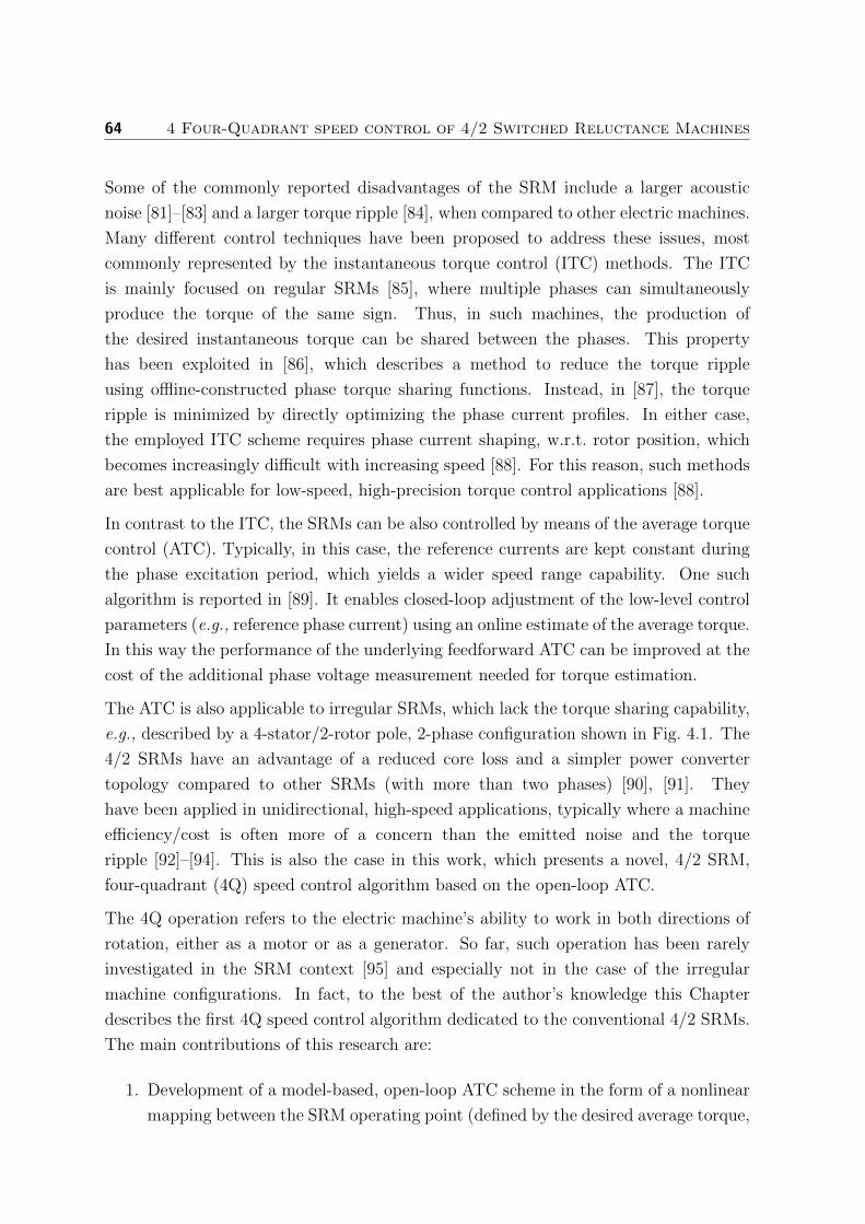
64 4 Four-Quadrant speed control of 4/2 Switched Reluctance Machines
Some of the commonly reported disadvantages of the SRM include a larger acoustic
noise [81]–[83] and a larger torque ripple [84], when compared to other electric machines.
Many different control techniques have been proposed to address these issues, most
commonly represented by the instantaneous torque control (ITC) methods. The ITC
is mainly focused on regular SRMs [85], where multiple phases can simultaneously
produce the torque of the same sign. Thus, in such machines, the production of
the desired instantaneous torque can be shared between the phases. This property
has been exploited in [86], which describes a method to reduce the torque ripple
using offline-constructed phase torque sharing functions. Instead, in [87], the torque
ripple is minimized by directly optimizing the phase current profiles. In either case,
the employed ITC scheme requires phase current shaping, w.r.t. rotor position, which
becomes increasingly difficult with increasing speed [88]. For this reason, such methods
are best applicable for low-speed, high-precision torque control applications [88].
In contrast to the ITC, the SRMs can be also controlled by means of the average torque
control (ATC). Typically, in this case, the reference currents are kept constant during
the phase excitation period, which yields a wider speed range capability. One such
algorithm is reported in [89]. It enables closed-loop adjustment of the low-level control
parameters (e.g., reference phase current) using an online estimate of the average torque.
In this way the performance of the underlying feedforward ATC can be improved at the
cost of the additional phase voltage measurement needed for torque estimation.
The ATC is also applicable to irregular SRMs, which lack the torque sharing capability,
e.g., described by a 4-stator/2-rotor pole, 2-phase configuration shown in Fig. 4.1. The
4/2 SRMs have an advantage of a reduced core loss and a simpler power converter
topology compared to other SRMs (with more than two phases) [90], [91]. They
have been applied in unidirectional, high-speed applications, typically where a machine
efficiency/cost is often more of a concern than the emitted noise and the torque
ripple [92]–[94]. This is also the case in this work, which presents a novel, 4/2 SRM,
four-quadrant (4Q) speed control algorithm based on the open-loop ATC.
The 4Q operation refers to the electric machine’s ability to work in both directions of
rotation, either as a motor or as a generator. So far, such operation has been rarely
investigated in the SRM context [95] and especially not in the case of the irregular
machine configurations. In fact, to the best of the author’s knowledge this Chapter
describes the first 4Q speed control algorithm dedicated to the conventional 4/2 SRMs.
The main contributions of this research are:
1. Development of a model-based, open-loop ATC scheme in the form of a nonlinear
mapping between the SRM operating point (defined by the desired average torque,
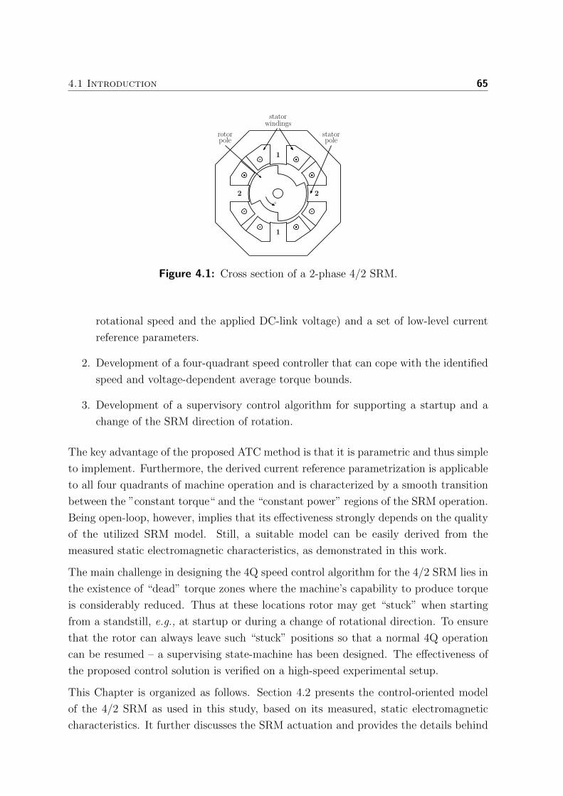
4.1 Introduction 65
1
1
2 2
statorpole
rotorpole
statorwindings
+
Figure 4.1: Cross section of a 2-phase 4/2 SRM.
rotational speed and the applied DC-link voltage) and a set of low-level current
reference parameters.
2. Development of a four-quadrant speed controller that can cope with the identified
speed and voltage-dependent average torque bounds.
3. Development of a supervisory control algorithm for supporting a startup and a
change of the SRM direction of rotation.
The key advantage of the proposed ATC method is that it is parametric and thus simple
to implement. Furthermore, the derived current reference parametrization is applicable
to all four quadrants of machine operation and is characterized by a smooth transition
between the ”constant torque“ and the “constant power” regions of the SRM operation.
Being open-loop, however, implies that its effectiveness strongly depends on the quality
of the utilized SRM model. Still, a suitable model can be easily derived from the
measured static electromagnetic characteristics, as demonstrated in this work.
The main challenge in designing the 4Q speed control algorithm for the 4/2 SRM lies in
the existence of “dead” torque zones where the machine’s capability to produce torque
is considerably reduced. Thus at these locations rotor may get “stuck” when starting
from a standstill, e.g., at startup or during a change of rotational direction. To ensure
that the rotor can always leave such “stuck” positions so that a normal 4Q operation
can be resumed – a supervising state-machine has been designed. The effectiveness of
the proposed control solution is verified on a high-speed experimental setup.
This Chapter is organized as follows. Section 4.2 presents the control-oriented model
of the 4/2 SRM as used in this study, based on its measured, static electromagnetic
characteristics. It further discusses the SRM actuation and provides the details behind
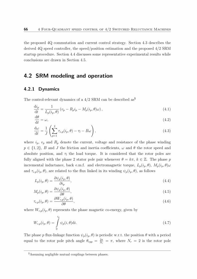
66 4 Four-Quadrant speed control of 4/2 Switched Reluctance Machines
the proposed 4Q commutation and current control strategy. Section 4.3 describes the
derived 4Q speed controller, the speed/position estimation and the proposed 4/2 SRM
startup procedure. Section 4.4 discusses some representative experimental results while
conclusions are drawn in Section 4.5.
4.2 SRM modeling and operation
4.2.1 Dynamics
The control-relevant dynamics of a 4/2 SRM can be described as1
dipdt
=1
Lp(ip, θ)(vp −Rpip −Mp(ip, θ)ω) , (4.1)
dθ
dt= ω, (4.2)
dω
dt=
1
J
(2∑
p=1
τe,p(ip, θ)− τl −Bω), (4.3)
where ip, vp and Rp denote the current, voltage and resistance of the phase winding
p ∈ 1, 2, B and J the friction and inertia coefficients, ω and θ the rotor speed and
absolute position, and τl the load torque. It is considered that the rotor poles are
fully aligned with the phase 2 stator pole pair whenever θ = kπ, k ∈ Z. The phase p
incremental inductance, back e.m.f. and electromagnetic torque, Lp(ip, θ), Mp(ip, θ)ω
and τe,p(ip, θ), are related to the flux linked in its winding ψp(ip, θ), as follows
Lp(ip, θ) =∂ψp(ip, θ)
∂ip, (4.4)
Mp(ip, θ) =∂ψp(ip, θ)
∂θ, (4.5)
τe,p(ip, θ) =∂Wc,p(ip, θ)
∂θ, (4.6)
where Wc,p(ip, θ) represents the phase magnetic co-energy, given by
Wc,p(ip, θ) =
ip∫
0
ψp(i, θ)di. (4.7)
The phase p flux-linkage function ψp(ip, θ) is periodic w.r.t. the position θ with a period
equal to the rotor pole pitch angle θrpp = 2πNr
= π, where Nr = 2 is the rotor pole
1Assuming negligible mutual couplings between phases.
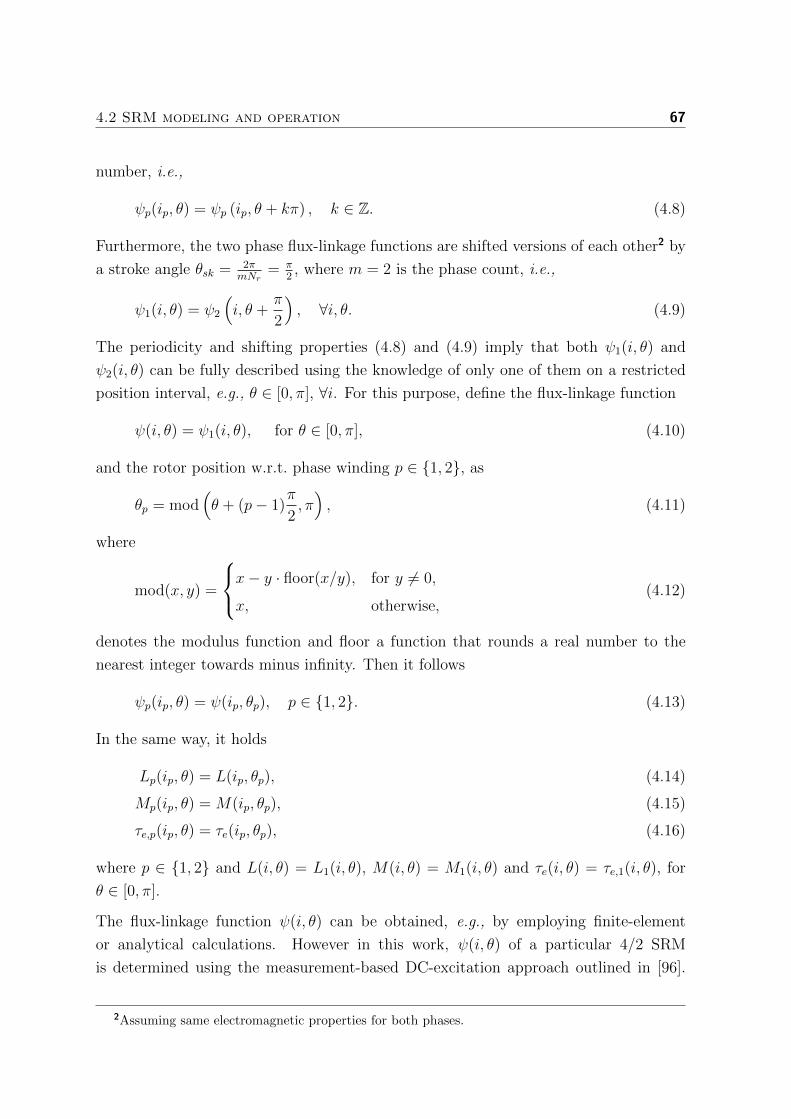
4.2 SRM modeling and operation 67
number, i.e.,
ψp(ip, θ) = ψp (ip, θ + kπ) , k ∈ Z. (4.8)
Furthermore, the two phase flux-linkage functions are shifted versions of each other2 by
a stroke angle θsk = 2πmNr
= π2, where m = 2 is the phase count, i.e.,
ψ1(i, θ) = ψ2
(i, θ +
π
2
), ∀i, θ. (4.9)
The periodicity and shifting properties (4.8) and (4.9) imply that both ψ1(i, θ) and
ψ2(i, θ) can be fully described using the knowledge of only one of them on a restricted
position interval, e.g., θ ∈ [0, π], ∀i. For this purpose, define the flux-linkage function
ψ(i, θ) = ψ1(i, θ), for θ ∈ [0, π], (4.10)
and the rotor position w.r.t. phase winding p ∈ 1, 2, as
θp = mod(θ + (p− 1)
π
2, π), (4.11)
where
mod(x, y) =
x− y · floor(x/y), for y 6= 0,
x, otherwise,(4.12)
denotes the modulus function and floor a function that rounds a real number to the
nearest integer towards minus infinity. Then it follows
ψp(ip, θ) = ψ(ip, θp), p ∈ 1, 2. (4.13)
In the same way, it holds
Lp(ip, θ) = L(ip, θp), (4.14)
Mp(ip, θ) = M(ip, θp), (4.15)
τe,p(ip, θ) = τe(ip, θp), (4.16)
where p ∈ 1, 2 and L(i, θ) = L1(i, θ), M(i, θ) = M1(i, θ) and τe(i, θ) = τe,1(i, θ), for
θ ∈ [0, π].
The flux-linkage function ψ(i, θ) can be obtained, e.g., by employing finite-element
or analytical calculations. However in this work, ψ(i, θ) of a particular 4/2 SRM
is determined using the measurement-based DC-excitation approach outlined in [96].
2Assuming same electromagnetic properties for both phases.

68 4 Four-Quadrant speed control of 4/2 Switched Reluctance Machines
Specifically, the SRM phase 1 was energized with a DC voltage while the rotor was
mechanically locked at a desired position θ ∈ [0, π]. The instantaneous phase voltage
v1 and current i1 were measured and the difference v1 − R1i1 was integrated (and
filtered) to obtain ψ1(i1, θ) = ψ(i1, θ). Subsequently, the functions L(i, θ), M(i, θ)
and τe(i, θ), θ ∈ [0, π], were obtained by numerically evaluating the expressions (4.4)
to (4.7). Figure 4.2 shows the resulting flux-linkage ψ(i, θ) and torque τe(i, θ) functions.
0.010.01
0.01
0.02
0.020.02
0.02
0.03
0.03
0.03
0.04
0.04
Flux-linkage ψ(i, θ) [Vs]
Currenti[A
]
0 45 90 135 1800
5
10
15
20
−0.3−0.2
−0.2
−0.1
−0.1
00
0.1
0.1
0.2
0.2 0.3
0.4Electromagnetic torque τe(i, θ) [Nm]
Position θ [deg]
Currenti[A
]
0 45 90 135 1800
5
10
15
20
Figure 4.2: 4/2 SRM flux-linkage ψ(i, θ) and electromagnetic torque τe(i, θ)
functions obtained using the DC-excitation method [96].
4.2.2 Actuation
The 4/2 SRM is actuated using the Asymmetric Half Bridge Converter (AHBC)
equipped with two switches, Sup and Slp, per phase p ∈ 1, 2, see Fig. 4.3. The AHBC
converter allows application of different voltages to each phase winding. Its functionality
is described in Table 4.1, where 0 is used to denote an open and 1 a closed switch, and vdc
the applied DC-link voltage. The switch states are manipulated in accordance with their
PWM duty cycles dup ∈ [0, 1] for Sup and dlp ∈ [0, 1] for Slp, to allow the exploitation of a
full DC link voltage range [−vdc, vdc]. Here, the duty cycle value d implies that during
each PWM period 1/fpwm a switch is closed d · 100% of the time, where fpwm = 60kHz
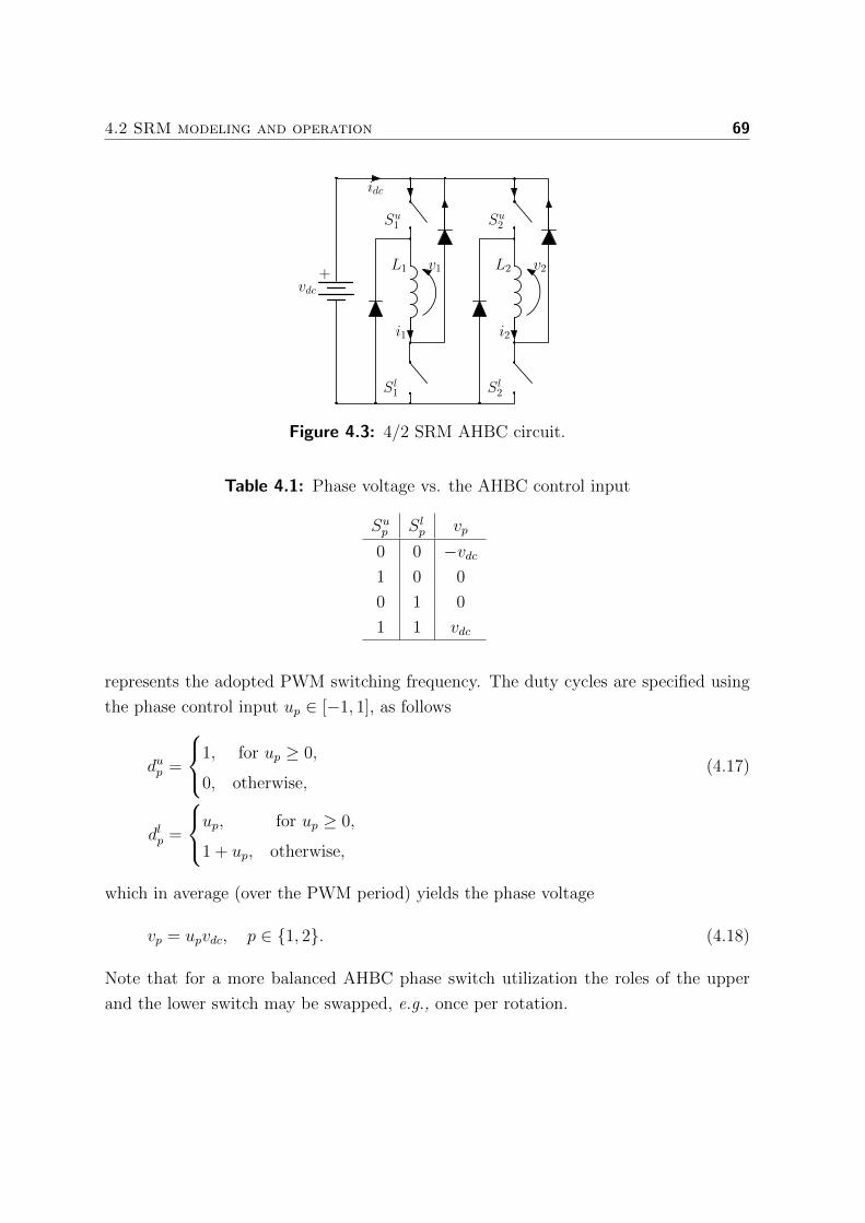
4.2 SRM modeling and operation 69
v1 v2
Su1 Su
2
Sl1 Sl
2
i1 i2
L1 L2+vdc
idc
Figure 4.3: 4/2 SRM AHBC circuit.
Table 4.1: Phase voltage vs. the AHBC control input
Sup Slp vp
0 0 −vdc1 0 0
0 1 0
1 1 vdc
represents the adopted PWM switching frequency. The duty cycles are specified using
the phase control input up ∈ [−1, 1], as follows
dup =
1, for up ≥ 0,
0, otherwise,(4.17)
dlp =
up, for up ≥ 0,
1 + up, otherwise,
which in average (over the PWM period) yields the phase voltage
vp = upvdc, p ∈ 1, 2. (4.18)
Note that for a more balanced AHBC phase switch utilization the roles of the upper
and the lower switch may be swapped, e.g., once per rotation.
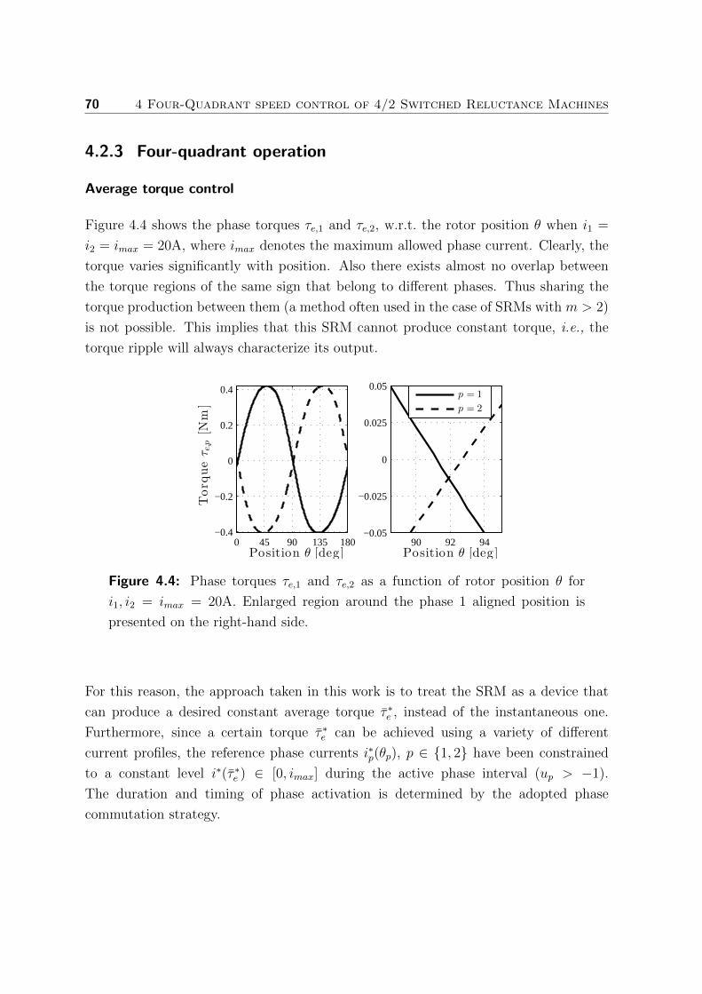
70 4 Four-Quadrant speed control of 4/2 Switched Reluctance Machines
4.2.3 Four-quadrant operation
Average torque control
Figure 4.4 shows the phase torques τe,1 and τe,2, w.r.t. the rotor position θ when i1 =
i2 = imax = 20A, where imax denotes the maximum allowed phase current. Clearly, the
torque varies significantly with position. Also there exists almost no overlap between
the torque regions of the same sign that belong to different phases. Thus sharing the
torque production between them (a method often used in the case of SRMs with m > 2)
is not possible. This implies that this SRM cannot produce constant torque, i.e., the
torque ripple will always characterize its output.
0 45 90 135 180−0.4
−0.2
0
0.2
0.4
Position θ [deg]
Torq
ueτe,p[N
m]
90 92 94−0.05
−0.025
0
0.025
0.05
Position θ [deg]
p = 1
p = 2
Figure 4.4: Phase torques τe,1 and τe,2 as a function of rotor position θ for
i1, i2 = imax = 20A. Enlarged region around the phase 1 aligned position is
presented on the right-hand side.
For this reason, the approach taken in this work is to treat the SRM as a device that
can produce a desired constant average torque τ ∗e , instead of the instantaneous one.
Furthermore, since a certain torque τ ∗e can be achieved using a variety of different
current profiles, the reference phase currents i∗p(θp), p ∈ 1, 2 have been constrained
to a constant level i∗(τ ∗e ) ∈ [0, imax] during the active phase interval (up > −1).
The duration and timing of phase activation is determined by the adopted phase
commutation strategy.

4.2 SRM modeling and operation 71
Fixed commutation strategy
Each phase activation cycle begins by setting up = 1 to magnetize the windings and
ends with up = −1 to demagnetize them. The phase positions where the magnetization
and demagnetization start are denoted with θon(Q) and θoff(Q), where Q ∈ 1, . . . , 4represents the machine operating quadrant. The quadrants are defined in Table 4.2,
along with the nominal phase activation/deactivation position values, θon(Q) and
θoff(Q), which are listed in the last column. The θon(Q) and θoff(Q) positions directly
follow from the 4/2 SRM torque characteristics shown in a lower part of Fig. 4.2,
and together describe a nominal, fixed four-quadrant phase commutation strategy.
Figure 4.5 illustrates the phase torque τe,p, in the case when ip > 0 within the θp
interval delimited by θon(Q) and θoff(Q).
Table 4.2: Quadrant specification
Q Operation Direction Condition (θon, θoff)
1 motoring positive τ ∗e ≥ 0 ∧ ω ≥ 0 (0, π/2)
2 generating negative τ ∗e ≥ 0 ∧ ω < 0 (π/2, 0)
3 motoring negative τ ∗e < 0 ∧ ω < 0 (π, π/2)
4 generating positive τ ∗e < 0 ∧ ω ≥ 0 (π/2, π)
θp
τe,p
0
θp
τe,p
0
θp
τe,p
0 ππ2
θp
τe,p
0
τ∗e
ω0
Q = 1Q = 2
Q = 3 Q = 4
ππ2
ππ2
ππ2
Figure 4.5: Phase torque τe,p as a function of the phase position θp for the case
of a nominal phase commutation strategy.
Based on this commutation scheme the nominal (constant) phase current level i∗(τ ∗e )
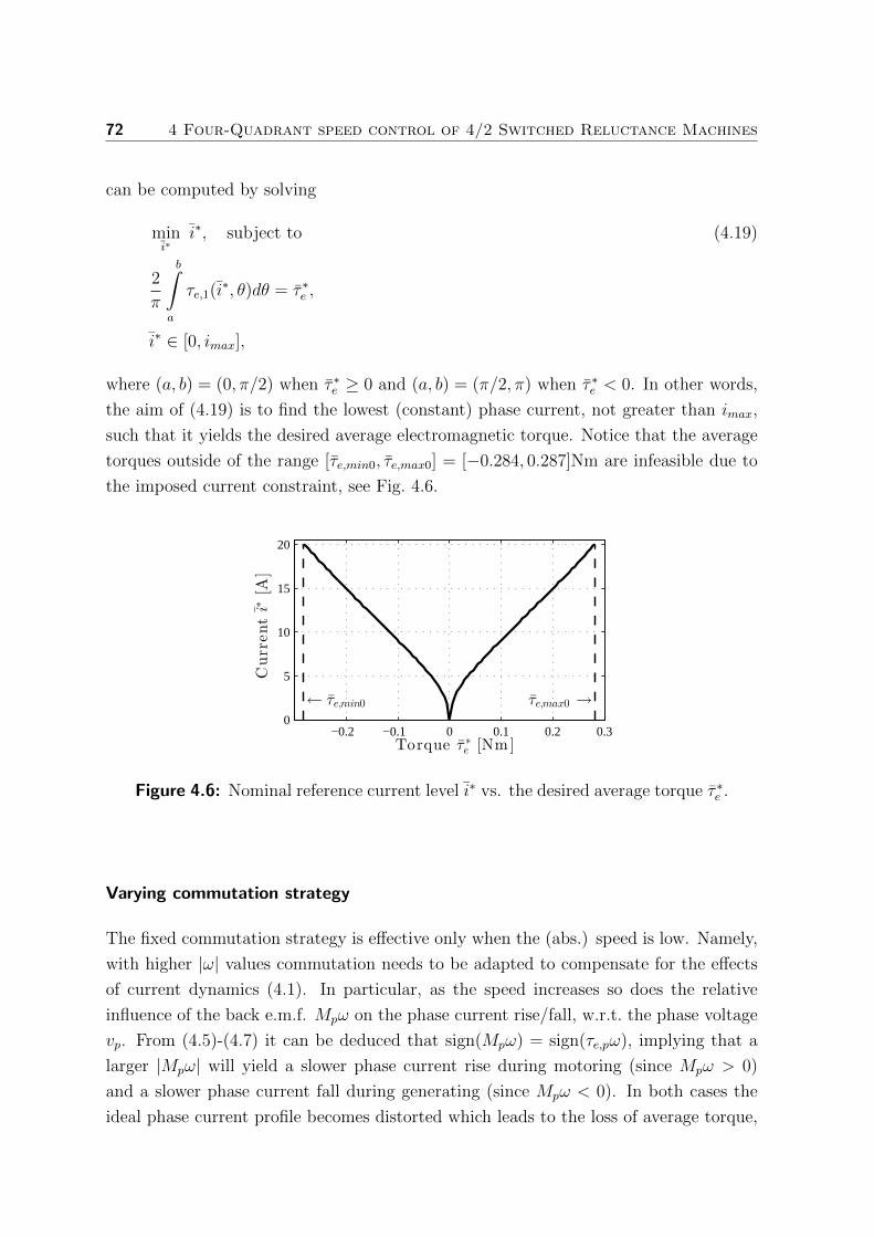
72 4 Four-Quadrant speed control of 4/2 Switched Reluctance Machines
can be computed by solving
mini∗
i∗, subject to (4.19)
2
π
b∫
a
τe,1(i∗, θ)dθ = τ ∗e ,
i∗ ∈ [0, imax],
where (a, b) = (0, π/2) when τ ∗e ≥ 0 and (a, b) = (π/2, π) when τ ∗e < 0. In other words,
the aim of (4.19) is to find the lowest (constant) phase current, not greater than imax,
such that it yields the desired average electromagnetic torque. Notice that the average
torques outside of the range [τe,min0, τe,max0] = [−0.284, 0.287]Nm are infeasible due to
the imposed current constraint, see Fig. 4.6.
−0.2 −0.1 0 0.1 0.2 0.30
5
10
15
20
τe,max0 →← τe,min0
Currenti∗
[A]
Torque τ∗
e [Nm]
Figure 4.6: Nominal reference current level i∗ vs. the desired average torque τ ∗e .
Varying commutation strategy
The fixed commutation strategy is effective only when the (abs.) speed is low. Namely,
with higher |ω| values commutation needs to be adapted to compensate for the effects
of current dynamics (4.1). In particular, as the speed increases so does the relative
influence of the back e.m.f. Mpω on the phase current rise/fall, w.r.t. the phase voltage
vp. From (4.5)-(4.7) it can be deduced that sign(Mpω) = sign(τe,pω), implying that a
larger |Mpω| will yield a slower phase current rise during motoring (since Mpω > 0)
and a slower phase current fall during generating (since Mpω < 0). In both cases the
ideal phase current profile becomes distorted which leads to the loss of average torque,

4.2 SRM modeling and operation 73
either because the desired current level is reached too late or because the current does
not extinguish on time.
To address these issues, the phase activation/deactivation positions, θon(Q) and θoff(Q),
are advanced3 w.r.t. their nominal values θon(Q) and θoff(Q). The effect of the
commutation angle advance on the phase current/torque is shown in Fig. 4.7. Clearly,
the current/torque profiles become less distorted and the average torque is higher in the
case of commutation advancement.
0 90 180 2700
10
Current[A
]
i1 nom.
i∗1 nom.
i1 adv.
i∗1 adv.
0 90 180 270−0.1
0
0.1
0.2
Torque[N
m]
Position θ [deg]
τe,1 nom.
τe nom.
τe,1 adv.
τe adv.
Figure 4.7: The effect of commutation angle advance on the phase 1 cur-
rent/torque production at vdc = 50V and ω = 15000rpm.
Since the resulting θon(Q) and θoff(Q) can lie outside of the admissible θp interval [0, π],
their ”wrapped“ versions are defined as
[θ′, θ′′]T
=
mod([θon, θoff ]T , π), for ω ≥ 0,
mod([θoff , θon]T , π), otherwise.(4.20)
3Shifted in the direction opposite to that of rotation.
74 4 Four-Quadrant speed control of 4/2 Switched Reluctance Machines
They are used to compute the phase commutation (activation) signal
σp =
1, for (θ′ < θ′′ AND θp ∈ [θ′, θ′′]) OR
(θ′′ < θ′ AND θp /∈ [θ′′, θ′]),
0, otherwise,
(4.21)
which further defines the phase reference current
i∗p = σpi∗. (4.22)
Optimal commutation angles
The optimal θon and θoff commutation angles and the optimal current level i∗ are found
for a set of SRM operating points given by the triplets (τ ∗e , ω, vdc), τ∗e ∈ [τe,min0, τe,max0],
ω ∈ [−ωmax, ωmax], vdc ∈ [vdc,min, vdc,max], by solving
minθon,θoff ,i∗
i∗, subject to (4.23)
τe(θon, θoff , i∗, ω, vdc) = τ ∗e ,
θon, θoff ∈ [−π, 3π],
|θoff − θon| ∈ [π/2, π],
i∗ ∈ [0, imax],
where ωmax = 40000rpm is the maximal considered SRM speed, vdc,min = 50V and
vdc,max = 100V the minimal and the maximal DC-link voltage and τe the steady-
state average of the total electromagnetic torque2∑p=1
τe,p(ip, θ), produced by the SRM
during a time period T = π/|ω|. The total torque is computed by simulating the phase
current (4.1) and position (4.2) dynamics at a specified speed ω and voltage vdc, while
the phase currents ip are forced to track the reference (4.22) defined by θon, θoff and
i∗. The currents are controlled using a proportional controller with output saturation,
given by
up = sat(κcc[i∗p − ip
],−1, 1
), (4.24)
where κcc = 5 represents a proportional tuning gain and
sat(x, xmin, xmax) =
xmin, for x ≤ xmin,
xmax, for x ≥ xmax,
x, otherwise,
(4.25)
4.2 SRM modeling and operation 75
the classical linear saturation function. The closed-loop simulation was conducted
with the help of Simulinkr while Matlabr (global) optimization toolbox was used to
implement and solve the constrained nonlinear programming problem (4.23). Notice
that by minimizing current i∗ in (4.23), for each specific speed ω, voltage vdc and torque
τ ∗e , the proposed approach puts an emphasis on high-efficiency operation of the SRM.
To support easier real-time implementation the optimal θon, θoff and i∗ have been
parameterized by the variables defining the SRM operating point. In particular, the
optimal current level i∗ is represented as
i∗(Q, τ ∗e , ω, vdc) = i∗(τ ∗e e
(ω/ωb(Q,vdc))2), (4.26)
where ωb(Q, vdc) denotes the quadrant-dependent base speed which separates the
constant torque (|ω| ≤ ωb) and constant power (|ω| > ωb) regions of the SRM operation.
The base speed is related to the DC-link voltage, i.e.,
ωb = κb(Q)vdc, (4.27)
where κb(Q) is a constant coefficient. Furthermore, the commutation angles are
described as
θon(Q, q) = θon(Q)− αon(Q, q), (4.28)
θoff(Q, q) = θoff(Q)− αoff(Q, q),
where αon(Q, q) and αoff(Q, q) denote the optimal advance angles parameterized using
the scheduling signal4
q =i∗
imax
|ω|ωmax
vdc,minvdc
, (4.29)
where ωmax = 40000rpm is the maximum considered SRM speed and vdc,min = 50V
the minimal expected DC-link voltage. Moreover, because of similarity between the
positive and negative phase torque characteristics (in the absolute sense, see the lower
plot in Fig. 4.2), similar optimization results were obtained in both directions of rotation.
In other words, the following identities hold
i∗(3, τ ∗e , ω, vdc) ≈ i∗(1, τ ∗e , ω, vdc), (4.30)
i∗(2, τ ∗e , ω, vdc) ≈ i∗(4, τ ∗e , ω, vdc),
αon(3, q) ≈ −αon(1, q),
αon(2, q) ≈ −αon(4, q),
ωb(3, vdc) ≈ −ωb(1, vdc),ωb(2, vdc) ≈ −ωb(4, vdc).
4Motivation behind this choice is explained in the Appendix C.
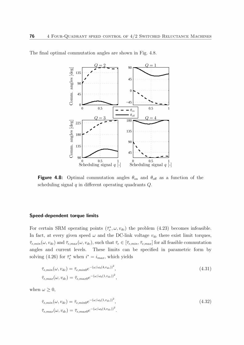
76 4 Four-Quadrant speed control of 4/2 Switched Reluctance Machines
The final optimal commutation angles are shown in Fig. 4.8.
0 0.5 1
−45
0
45
90Q = 1
0 0.5 10
45
90
135
Q = 2Comm.angles[deg]
0 0.5 190
135
180
225Q = 3
Scheduling signal q [-]
Comm.angles[deg]
0 0.5 1
45
90
135
180Q = 4
Scheduling signal q [-]
θon
θoff
Figure 4.8: Optimal commutation angles θon and θoff as a function of the
scheduling signal q in different operating quadrants Q.
Speed-dependent torque limits
For certain SRM operating points (τ ∗e , ω, vdc) the problem (4.23) becomes infeasible.
In fact, at every given speed ω and the DC-link voltage vdc there exist limit torques,
τe,min(ω, vdc) and τe,max(ω, vdc), such that τe ∈ [τe,min, τe,max] for all feasible commutation
angles and current levels. These limits can be specified in parametric form by
solving (4.26) for τ ∗e when i∗ = imax, which yields
τe,min(ω, vdc) = τe,min0e−(ω/ωb(4,vdc))
2
, (4.31)
τe,max(ω, vdc) = τe,max0e−(ω/ωb(1,vdc))
2
,
when ω ≥ 0,
τe,min(ω, vdc) = τe,min0e−(ω/ωb(1,vdc))
2
, (4.32)
τe,max(ω, vdc) = τe,max0e−(ω/ωb(4,vdc))
2
.
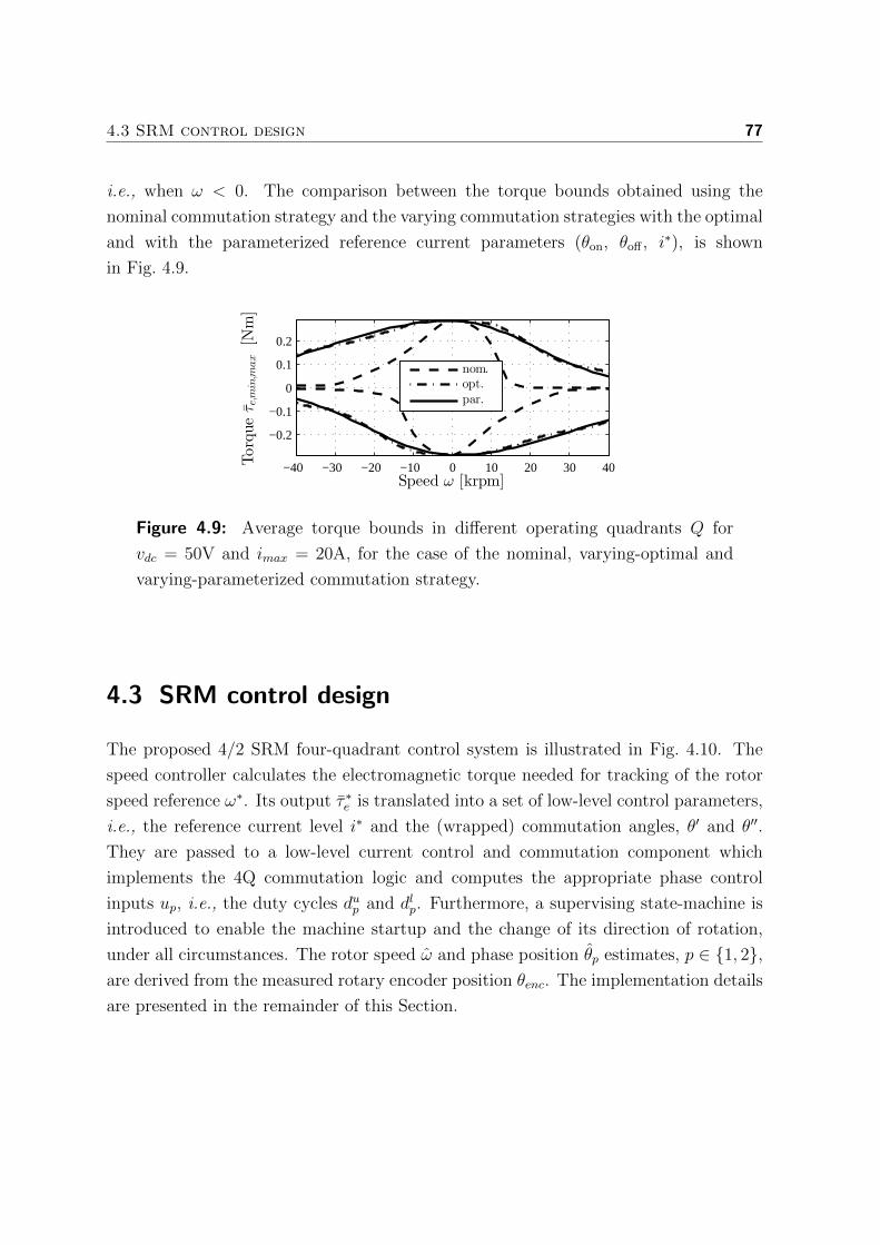
4.3 SRM control design 77
i.e., when ω < 0. The comparison between the torque bounds obtained using the
nominal commutation strategy and the varying commutation strategies with the optimal
and with the parameterized reference current parameters (θon, θoff , i∗), is shown
in Fig. 4.9.
−40 −30 −20 −10 0 10 20 30 40
−0.2
−0.1
0
0.1
0.2
Speed ω [krpm]
Torqueτe,min,m
ax[N
m]
nom.opt.par.
Figure 4.9: Average torque bounds in different operating quadrants Q for
vdc = 50V and imax = 20A, for the case of the nominal, varying-optimal and
varying-parameterized commutation strategy.
4.3 SRM control design
The proposed 4/2 SRM four-quadrant control system is illustrated in Fig. 4.10. The
speed controller calculates the electromagnetic torque needed for tracking of the rotor
speed reference ω∗. Its output τ ∗e is translated into a set of low-level control parameters,
i.e., the reference current level i∗ and the (wrapped) commutation angles, θ′ and θ′′.
They are passed to a low-level current control and commutation component which
implements the 4Q commutation logic and computes the appropriate phase control
inputs up, i.e., the duty cycles dup and dlp. Furthermore, a supervising state-machine is
introduced to enable the machine startup and the change of its direction of rotation,
under all circumstances. The rotor speed ω and phase position θp estimates, p ∈ 1, 2,are derived from the measured rotary encoder position θenc. The implementation details
are presented in the remainder of this Section.

78 4 Four-Quadrant speed control of 4/2 Switched Reluctance Machines
ip
dup , dlp
mode
vdc
θp
controlSpeed
ω Speed &position
ω∗ SRMθ′, θ′′
i∗
Param.
Supervisor
τ∗e
tsc tcc
θenc
Currentcontrol &
commutation
Figure 4.10: Structure of the proposed four-quadrant SRM control system.
4.3.1 Speed and position estimation
The position θ is measured using an incremental rotary encoder with a resolution θres =0.25π180
rad, which yields the encoder position θenc. The encoder is mounted on the SRM
shaft such that its index (absolute reference) position coincides with the phase 2 aligned
position, i.e., θ2 = π2
and θ1 = 0. Absolute position measurement is achieved by applying
a hardware-reset of θenc to 0 whenever the index pulse is detected. This yields θenc in
the range [−2π, 2π]. The phase position θp estimates are found as
θp = mod(θenc + (p− 1)
π
2, π), p = 1, 2. (4.33)
Furthermore, at the time instant k ∈ Z≥0 with the sampling time tcc = 5 · 10−5s, the
rotor speed estimate ω(k) is computed from the difference δ(k) = θenc(k)− θenc(k − 1).
First, δ(k) is processed to remove its erroneous values (spikes of ±2π, see Fig. 4.11)
occurring when θenc transits from −2π or 2π to 0 due to index reset. This yields
δ(k) =
δ(k)− 2πsign
(δ(k)
), for |δ(k)| ≥ δmax,
δ(k), otherwise,(4.34)
where δmax = ωmaxtcc denotes the maximum position difference. Then, the result δ(k)
is filtered using a discretized version of a low-pass filter Glp(s) = 1tcc
1κlps+1
with the filter
time constant κlp = 1/10π. This provides the speed estimate
ω(z) = Glp(z)δ(z). (4.35)
4.3.2 Supervisor for startup and change of rotational direction
In a 4/2 SRM, the ability of each phase to produce torque is considerably reduced when
the rotor is (nearly) aligned to a pair of stator poles, see the right-hand side of Fig. 4.4.
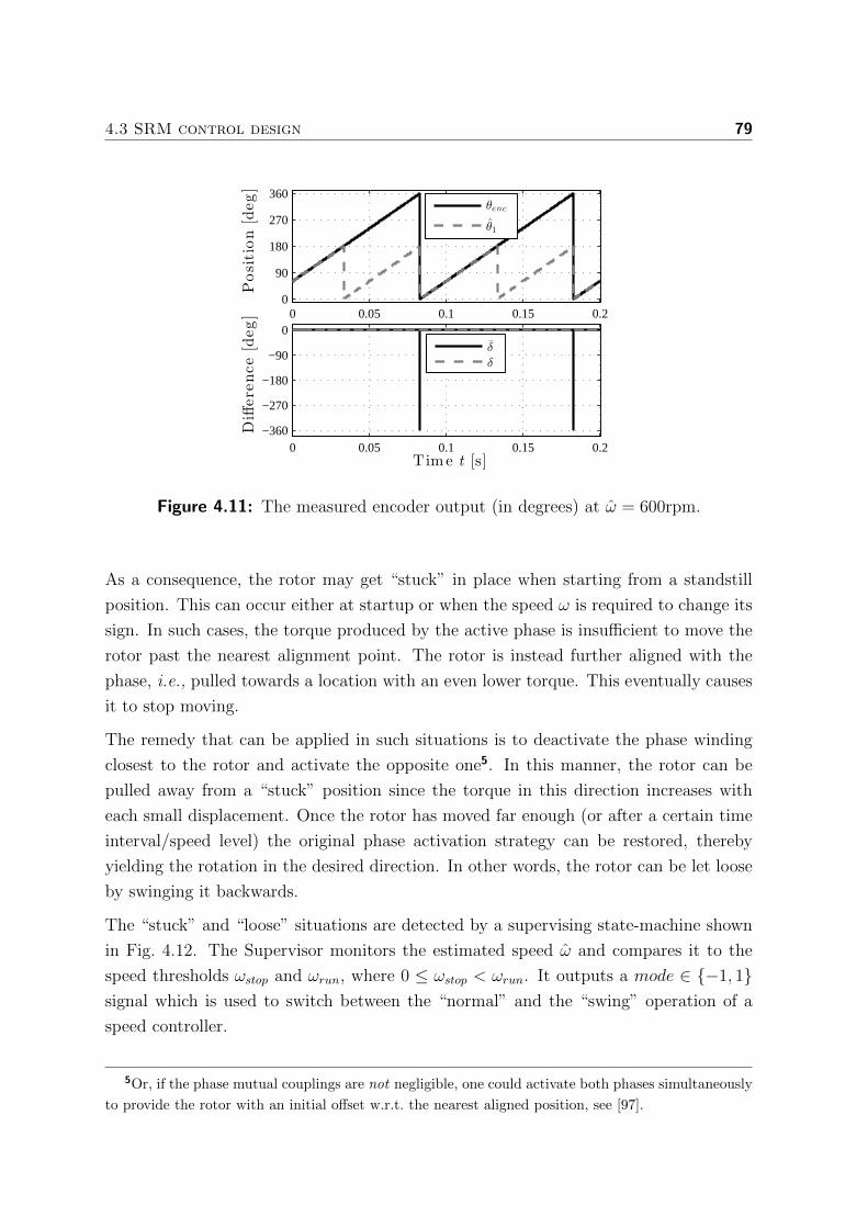
4.3 SRM control design 79
0 0.05 0.1 0.15 0.20
90
180
270
360
Position[deg]
θenc
θ1
0 0.05 0.1 0.15 0.2−360
−270
−180
−90
0
Difference[deg]
T ime t [s]
δ
δ
Figure 4.11: The measured encoder output (in degrees) at ω = 600rpm.
As a consequence, the rotor may get “stuck” in place when starting from a standstill
position. This can occur either at startup or when the speed ω is required to change its
sign. In such cases, the torque produced by the active phase is insufficient to move the
rotor past the nearest alignment point. The rotor is instead further aligned with the
phase, i.e., pulled towards a location with an even lower torque. This eventually causes
it to stop moving.
The remedy that can be applied in such situations is to deactivate the phase winding
closest to the rotor and activate the opposite one5. In this manner, the rotor can be
pulled away from a “stuck” position since the torque in this direction increases with
each small displacement. Once the rotor has moved far enough (or after a certain time
interval/speed level) the original phase activation strategy can be restored, thereby
yielding the rotation in the desired direction. In other words, the rotor can be let loose
by swinging it backwards.
The “stuck” and “loose” situations are detected by a supervising state-machine shown
in Fig. 4.12. The Supervisor monitors the estimated speed ω and compares it to the
speed thresholds ωstop and ωrun, where 0 ≤ ωstop < ωrun. It outputs a mode ∈ −1, 1signal which is used to switch between the “normal” and the “swing” operation of a
speed controller.
5Or, if the phase mutual couplings are not negligible, one could activate both phases simultaneously
to provide the rotor with an initial offset w.r.t. the nearest aligned position, see [97].
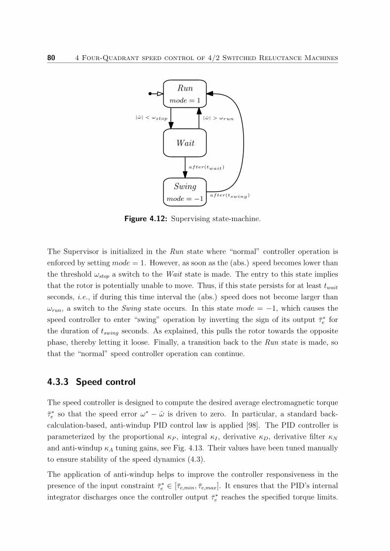
80 4 Four-Quadrant speed control of 4/2 Switched Reluctance Machines
|ω| > ωrun|ω| < ωstop
mode = 1
Run
Wait
after(twait)
after(tswing)
Swing
mode = −1
Figure 4.12: Supervising state-machine.
The Supervisor is initialized in the Run state where “normal” controller operation is
enforced by setting mode = 1. However, as soon as the (abs.) speed becomes lower than
the threshold ωstop a switch to the Wait state is made. The entry to this state implies
that the rotor is potentially unable to move. Thus, if this state persists for at least twait
seconds, i.e., if during this time interval the (abs.) speed does not become larger than
ωrun, a switch to the Swing state occurs. In this state mode = −1, which causes the
speed controller to enter “swing” operation by inverting the sign of its output τ ∗e for
the duration of tswing seconds. As explained, this pulls the rotor towards the opposite
phase, thereby letting it loose. Finally, a transition back to the Run state is made, so
that the “normal” speed controller operation can continue.
4.3.3 Speed control
The speed controller is designed to compute the desired average electromagnetic torque
τ ∗e so that the speed error ω∗ − ω is driven to zero. In particular, a standard back-
calculation-based, anti-windup PID control law is applied [98]. The PID controller is
parameterized by the proportional κP , integral κI , derivative κD, derivative filter κN
and anti-windup κA tuning gains, see Fig. 4.13. Their values have been tuned manually
to ensure stability of the speed dynamics (4.3).
The application of anti-windup helps to improve the controller responsiveness in the
presence of the input constraint τ ∗e ∈ [τe,min, τe,max]. It ensures that the PID’s internal
integrator discharges once the controller output τ ∗e reaches the specified torque limits.

4.3 SRM control design 81
At the given speed and the DC-link voltage, the torque limits τe,min and τe,max are
computed using (4.31) and (4.32).
The output of the saturation block shown in Fig. 4.13 is multiplied with the mode signal
produced by the Supervisor. This changes its sign during the “swing” operation so that
the rotor can be temporarily pulled in the direction opposite to the one of the reference
speed ω∗. In this way, the rotor can get loose from a “stuck” position as explained in
the previous section.
The speed controller (as well as the Supervisor and the Parametrization block) is
implemented at the discrete sampling time tsc = 5 · 10−4s.
1s sat(·)+
κP
κI
κN
κA
1s
−+
+
+
−
−+
ω∗
ωτe,min(·)
τe,min, τe,max
vdc
×
mode
κD
τ∗e
τe,max(·)
Figure 4.13: PID speed controller with a back-calculation integrator anti-
windup.
4.3.4 Current reference parametrization
Based on the desired speed controller torque τ ∗e , speed estimate ω and the DC-link
voltage vdc, the desired SRM operating quadrant Q is determined as in Table 4.2, the
phase current reference level i∗ as in (4.26), the scheduling signal q as in (4.29), the
commutation angles, θon and θoff , as in (4.28) and the wrapped commutation angles, θ′
and θ′′ as in (4.20). The current reference parameters i∗, θ′ and θ′′ are then passed to
the low-level current controller and commutation component.
82 4 Four-Quadrant speed control of 4/2 Switched Reluctance Machines
4.3.5 Current control and commutation
The control parameters θ′, θ′′ are used to compute the binary signal σp, as in (4.21).
The signal σp defines the active phase region, w.r.t. the estimated phase position θp, and
is multiplied with i∗ to produce the phase current reference i∗p, as in (4.22). The phase
current is controlled using a simple proportional control law (4.24), which produces the
phase input up. Finally, up is translated into a set of AHBC switch duty cycles dup and
dlp according to (4.17).
The current control and commutation (as well as the speed and position estimation) is
implemented at the discrete sampling time tcc = 5 · 10−5s. Thus, due to the difference
between the speed and the current controller sampling rates, the signals ω, θ′, θ′′ and
i∗ are passed through rate transition blocks when transiting between the two domains.
4.4 Hardware and software implementation
4.4.1 Hardware configuration
Figures 4.14 and 4.15 show the experimental hardware arrangement and the SRM test-
bed used in this project. The test-bed consists of two identical 4/2 SRMs (manufactured
by Dyson Ltd.), coupled via a Magtrol TMHS-304 torque sensor. Speed ω is controlled
using SRM1 while the load torque τl is controlled using SRM2. For this purpose,
the proposed 4Q controller is used to control the SRM1, whereas its simplified version,
without the Speed Control and the Supervisor components, is used to control the SRM2.
A custom-made measurement board enabled the measurement of the phase and the
DC-link currents and voltages. The currents ip, p ∈ 1, 2 were measured using
galvanically isolated LEM LA 55-P current transducers with a bandwidth of approx.
200kHz while the voltage vdc was measured using a galvanically isolated LEM LV 25-P
voltage transducer with a bandwidth of approx. 200kHz. The voltage measurement
is subsequently low-passed using an analog low-pass filter with a bandwidth of 5Hz.
Furthermore, a custom-made power board implemented the AHBC shown in Fig. 4.3.
The phase switches were realized using insulated-gate bipolar transistors (IGBTs).
The data acquisition and real-time control implementation was performed using a
dSPACE DS1103 PPC controller board with MATLABr/Simulinkr installed on a
standard personal computer (PC) running a 64-bit Windows 7 operating system. The
real-time hardware input/output (IO) access was obtained through the use of Simulinkr
CoderTM blocks.
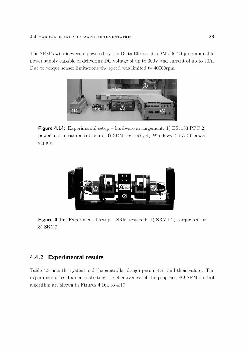
4.4 Hardware and software implementation 83
The SRM’s windings were powered by the Delta Elektronika SM 300-20 programmable
power supply capable of delivering DC voltage of up to 300V and current of up to 20A.
Due to torque sensor limitations the speed was limited to 40000rpm.
1 5
4
32
Figure 4.14: Experimental setup – hardware arrangement: 1) DS1103 PPC 2)
power and measurement board 3) SRM test-bed, 4) Windows 7 PC 5) power
supply.
2
1 3
Figure 4.15: Experimental setup – SRM test-bed: 1) SRM1 2) torque sensor
3) SRM2.
4.4.2 Experimental results
Table 4.3 lists the system and the controller design parameters and their values. The
experimental results demonstrating the effectiveness of the proposed 4Q SRM control
algorithm are shown in Figures 4.16a to 4.17.
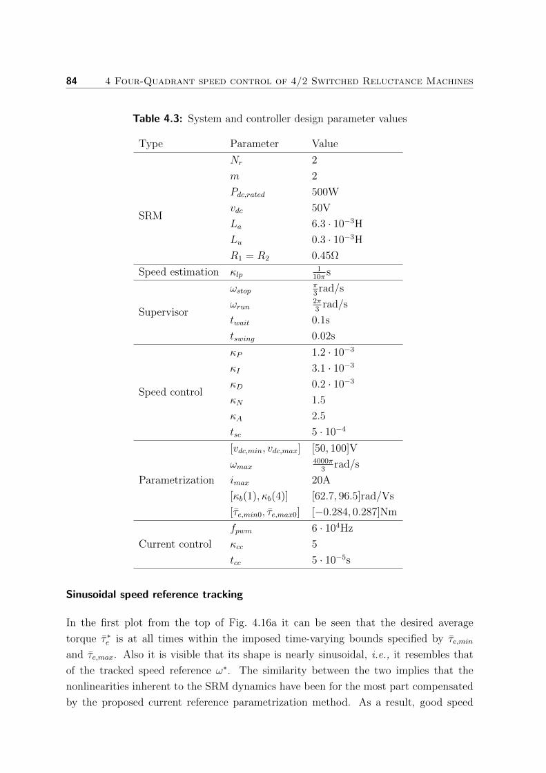
84 4 Four-Quadrant speed control of 4/2 Switched Reluctance Machines
Table 4.3: System and controller design parameter values
Type Parameter Value
SRM
Nr 2
m 2
Pdc,rated 500W
vdc 50V
La 6.3 · 10−3H
Lu 0.3 · 10−3H
R1 = R2 0.45Ω
Speed estimation κlp1
10πs
Supervisor
ωstopπ3rad/s
ωrun2π3
rad/s
twait 0.1s
tswing 0.02s
Speed control
κP 1.2 · 10−3
κI 3.1 · 10−3
κD 0.2 · 10−3
κN 1.5
κA 2.5
tsc 5 · 10−4
Parametrization
[vdc,min, vdc,max] [50, 100]V
ωmax4000π
3rad/s
imax 20A
[κb(1), κb(4)] [62.7, 96.5]rad/Vs
[τe,min0, τe,max0] [−0.284, 0.287]Nm
Current control
fpwm 6 · 104Hz
κcc 5
tcc 5 · 10−5s
Sinusoidal speed reference tracking
In the first plot from the top of Fig. 4.16a it can be seen that the desired average
torque τ ∗e is at all times within the imposed time-varying bounds specified by τe,min
and τe,max. Also it is visible that its shape is nearly sinusoidal, i.e., it resembles that
of the tracked speed reference ω∗. The similarity between the two implies that the
nonlinearities inherent to the SRM dynamics have been for the most part compensated
by the proposed current reference parametrization method. As a result, good speed
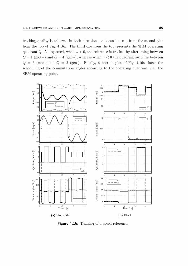
4.4 Hardware and software implementation 85
tracking quality is achieved in both directions as it can be seen from the second plot
from the top of Fig. 4.16a. The third one from the top, presents the SRM operating
quadrant Q. As expected, when ω > 0, the reference is tracked by alternating between
Q = 1 (mot+) and Q = 4 (gen+), whereas when ω < 0 the quadrant switches between
Q = 3 (mot-) and Q = 2 (gen-). Finally, a bottom plot of Fig. 4.16a shows the
scheduling of the commutation angles according to the operating quadrant, i.e., the
SRM operating point.
0 5 10 15 20
−0.2
−0.1
0
0.1
0.2
0.3
Torque[N
m]
τ∗
e
τe,min,max
0 5 10 15 20−15
−10
−5
0
5
10
15
Speed[krpm]
ω∗
ω
0 5 10 15 20
−1
0
1
2
3
4
Quadrant/mode[-]
Qmode
0 5 10 15 20
0
45
90
135
180
Comm.angles[deg]
Time t [s]
θonθoff
(a) Sinusoidal
0 5 10 15 20
−0.2
−0.1
−0.05
0
0.06
0.1
Torque[N
m]
τ∗
eτl
0 5 10 15 20
8
11.5
15
Speed[krpm]
ω∗
ω
0 5 10 15 20
1
2
3
4
Quadrant/mode[-]
Q
mode
0 5 10 15 20
0
45
90
135
180
Comm.angles[deg]
Time t [s]
θon
θoff
(b) Block
Figure 4.16: Tracking of a speed reference.
86 4 Four-Quadrant speed control of 4/2 Switched Reluctance Machines
Block speed reference tracking under load
Figure 4.16b shows the tracking of a block (step) speed reference in the presence of load
torque τl 6= 0. In the top plot it can be seen that the adopted algorithm is successful in
rejecting the load torque disturbance irrespective of its sign. In particular, when the load
changes from 0.06Nm to −0.05Nm the controller quickly compensates for the change by
switching the machine operating quadrant Q from 1 (mot+) to 4 (gen+). At t ≈ 12s
the speed reference is abruptly reduced from 15krpm to 8krpm while τl = 0.06Nm.
However, it can be seen that accurate tracking is still maintained, even under load.
Supervised startup
Figure 4.17 zooms on the beginning of the first (sinusoidal reference tracking) exper-
iment where the rotor was initially placed at a position θ1 ≈ 90deg. As initially the
reference speed was positive and the speed was zero, the controller started operation
in the quadrant Q = 1 (mot+). Since θ1 < 90deg the adopted commutation strategy
resulted in phase 1 activation. However, due to the inability of the phase 1 to produce
sufficient torque and thus move the rotor past its alignment point – the rotor got “stuck”.
This caused it to vibrate in place, with its speed alternating between positive and
negative (which eventually caused a switch to Q = 2, gen-). However, after twait = 0.1s
had elapsed with ω < ωstop condition true, the “stuck” situation was detected by the
Supervisor and the Swing state was activated. This can be seen from the change in the
mode signal from 1 to −1, i.e., the resulting change in the sign of the desired torque
τ ∗e . The negative torque request was fulfilled by switching the quadrant to Q = 3
(mot-), i.e., by engaging the phase 2. As a consequence, during twait = 0.02s the rotor
was pulled away from the “stuck” position after which the regular operation had been
resumed.
4.5 Conclusions
In this Chapter, a novel four-quadrant control scheme for the 4/2 SRM was proposed.
The control algorithm was designed to explicitly handle the physical torque and current
constraints and to allow the SRM to start/resume operation even when the rotor gets
“stuck” near or at one of the aligned positions. A dedicated commutation strategy
was also derived, which supports the compensation of the inherent torque loss in a
wide range of the SRM operating conditions. Experimental results were provided to
demonstrate the feasibility of the presented solution.

4.5 Conclusions 87
0.65 0.7 0.75 0.8 0.85
−0.2
−0.1
0
0.1
0.2
0.3Torq
ue[N
m]
τ∗
eτe,min,max
0.65 0.7 0.75 0.8 0.8575
90
105
120
Position[deg]
θ1
0.65 0.7 0.75 0.8 0.85
−50
0
50
Speed[rpm]
ω
0.65 0.7 0.75 0.8 0.85
−1
0
1
2
3
Quadra
nt/
mode[-]
T ime t [s]
Qmode
Figure 4.17: 4/2 SRM startup from the “stuck” position.

88

Chapter 5
Model predictive voltage control of
high-speed Switched Reluctance
Generators 1
Abstract This Chapter presents a predictive voltage control strategy for high-speed Switched
Reluctance Generators, derived using an average model of the SRG electrical system. The
controller computes an average DC-link current needed to track a desired DC-link voltage
reference, in the presence of an unknown electrical load. The production of the required DC-
link current is ensured by means of single-pulse commutation and control. For this purpose,
the turn-on and turn-off commutation angles are chosen such that the resulting peak phase
flux-linkage and, indirectly, the machine iron loss, are minimized. The proposed control scheme
explicitly enforces the average DC-link current and voltage bounds. This is also verified in
closed-loop simulations.
5.1 Introduction
The Switched Reluctance Generator (SRG) is an electric machine characterized by high
reliability, fault tolerance and power density [99]–[101]. It has salient poles both on a
rotor and a stator whereas it lacks brushes, rotor windings and permanent magnets.
Due to its simple and rugged structure the SRG is easy to cool and maintain, and can
be operated in a wide range of speeds.
Specifically, at speeds higher than the base speed the SRG is often controlled in a Single-
1This chapter is based on [94].
89

905 Model predictive voltage control of high-speed Switched Reluctance
Generators
Pulse (SP) mode where the turn-on and turn-off commutation angles are the only control
parameters used to adjust the amount of produced DC-link current. This approach is
mainly motivated by a large phase back-emf which in such cases prevents an effective use
of phase current regulation and/or by the need to eliminate the hardware costs related
to current sensing. When compared to the actual rotor position, the commutation
angles provide information when the phase current pulses should occur. The generating
operation is achieved when these pulses are synchronized with a decreasing phase
inductance [102].
So far, numerous approaches for computation of optimal commutation angles have been
reported. In general, one can distinguish between online and offline methods, depending
on whether the angles are adapted during the SRG operation or determined and stored
prior to it. In either case, various optimality criteria have been employed. For instance,
in [78], [102] the optimal turn-on and turn-off commutation angles were found through
a series of steady-state experiments by minimizing the RMS phase current. A similar
approach was used in [99] where instead experiments were conducted to maximize the
ratio of the average output and input power. The extensive experimentation required
by these methods is however often impractical, especially when one considers variable
speed/voltage applications. Thus an alternative, offline solution, based on the SRG
Finite Element Model (FEM), was proposed in [103]. Here, the optimal commutation
angles were derived directly from FEM data by maximizing the SRG electro-mechanical
efficiency, i.e., its average produced torque. In contrast, an analytic approach was
pursued in [104]. Based on simplified SRG electromagnetic characteristics, this work
establishes a relationship between the commutation angles, peak phase flux-linkage,
applied DC-link voltage and rotational speed for the SRG with a regular machine
geometry [85]. In contrast, an online, search-based algorithm was proposed in [101]
that focuses on minimization of the DC-link current ripple. The reported algorithm
however does not take into account the changes in the SRM operating point (DC-link
voltage, speed), which limits its application.
Irrespective of the adopted commutation angle selection strategy, the SRM output
voltage is most commonly regulated using a PI control law [78], [102]–[104]. Thus
typically, the bounds on the DC-link voltage/current are not directly enforced. This
is in spite of the fact that the SRG loses its self-excitation capacity as soon as the
DC-link voltage drops to zero [105]–[108]. Recently several papers have described the
use of Model Predictive Control (MPC) for purposes of Switched Reluctance Motor
(SRM) torque control [109]–[111]. One of the main advantages of using the MPC over
conventional motor control techniques, such as the PID, is the possibility to enforce
current and voltage limits [112].
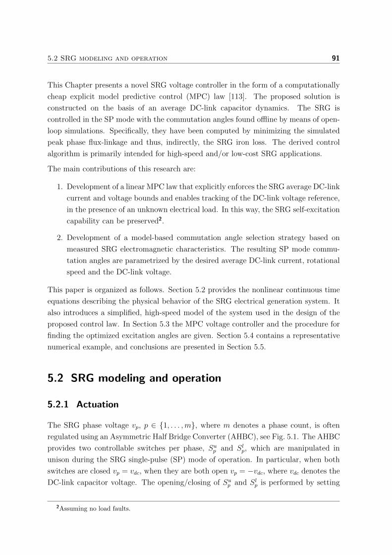
5.2 SRG modeling and operation 91
This Chapter presents a novel SRG voltage controller in the form of a computationally
cheap explicit model predictive control (MPC) law [113]. The proposed solution is
constructed on the basis of an average DC-link capacitor dynamics. The SRG is
controlled in the SP mode with the commutation angles found offline by means of open-
loop simulations. Specifically, they have been computed by minimizing the simulated
peak phase flux-linkage and thus, indirectly, the SRG iron loss. The derived control
algorithm is primarily intended for high-speed and/or low-cost SRG applications.
The main contributions of this research are:
1. Development of a linear MPC law that explicitly enforces the SRG average DC-link
current and voltage bounds and enables tracking of the DC-link voltage reference,
in the presence of an unknown electrical load. In this way, the SRG self-excitation
capability can be preserved2.
2. Development of a model-based commutation angle selection strategy based on
measured SRG electromagnetic characteristics. The resulting SP mode commu-
tation angles are parametrized by the desired average DC-link current, rotational
speed and the DC-link voltage.
This paper is organized as follows. Section 5.2 provides the nonlinear continuous time
equations describing the physical behavior of the SRG electrical generation system. It
also introduces a simplified, high-speed model of the system used in the design of the
proposed control law. In Section 5.3 the MPC voltage controller and the procedure for
finding the optimized excitation angles are given. Section 5.4 contains a representative
numerical example, and conclusions are presented in Section 5.5.
5.2 SRG modeling and operation
5.2.1 Actuation
The SRG phase voltage vp, p ∈ 1, . . . ,m, where m denotes a phase count, is often
regulated using an Asymmetric Half Bridge Converter (AHBC), see Fig. 5.1. The AHBC
provides two controllable switches per phase, Sup and Slp, which are manipulated in
unison during the SRG single-pulse (SP) mode of operation. In particular, when both
switches are closed vp = vdc, when they are both open vp = −vdc, where vdc denotes the
DC-link capacitor voltage. The opening/closing of Sup and Slp is performed by setting
2Assuming no load faults.
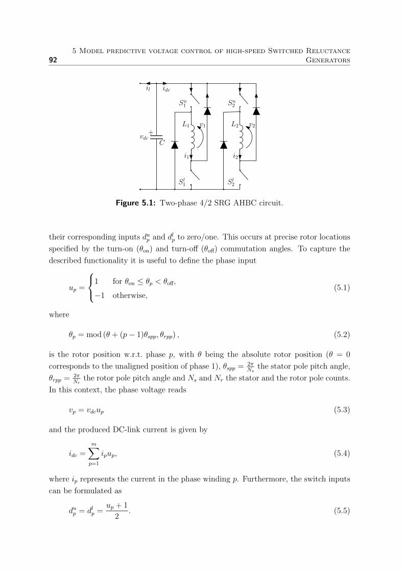
925 Model predictive voltage control of high-speed Switched Reluctance
Generators
C
idcil
+v1 v2
Su1 Su
2
Sl1 Sl
2
i1 i2
L1 L2
vdc
Figure 5.1: Two-phase 4/2 SRG AHBC circuit.
their corresponding inputs dup and dlp to zero/one. This occurs at precise rotor locations
specified by the turn-on (θon) and turn-off (θoff) commutation angles. To capture the
described functionality it is useful to define the phase input
up =
1 for θon ≤ θp < θoff,
−1 otherwise,(5.1)
where
θp = mod (θ + (p− 1)θspp, θrpp) , (5.2)
is the rotor position w.r.t. phase p, with θ being the absolute rotor position (θ = 0
corresponds to the unaligned position of phase 1), θspp = 2πNs
the stator pole pitch angle,
θrpp = 2πNr
the rotor pole pitch angle and Ns and Nr the stator and the rotor pole counts.
In this context, the phase voltage reads
vp = vdcup (5.3)
and the produced DC-link current is given by
idc =m∑
p=1
ipup, (5.4)
where ip represents the current in the phase winding p. Furthermore, the switch inputs
can be formulated as
dup = dlp =up + 1
2. (5.5)
5.2 SRG modeling and operation 93
5.2.2 Dynamics
The voltage equation for the SRG phase p reads
dψpdt
= upvdc −Rpip (5.6)
and the DC-link capacitor dynamics can be formulated as
dvdcdt
= − 1
C(idc + il), (5.7)
with ψp denoting the phase flux-linkage, Rp the phase winding resistance, il the unknown
electrical load current and C the DC-link capacitor capacitance. Note that due to a
presence of diodes in the AHBC circuit it holds ψp ≥ 0 and ip = ip(ψp, θ) ≥ 0. The
expressions (5.6) and (5.7) capture the SRG electrical system dynamics. Its mechanical
part, is described by
dθ
dt= ω, (5.8)
where ω is the rotor speed.
Equation 5.7 implies that an instantaneous DC-link voltage vdc can be controlled using
an instantaneous DC-link current idc as a control input. However, this would require
precise idc control which is impossible in the single-pulse mode, where only the beginning
and the end of phase excitation can be specified (and not the shape of the current in
between). Instead, an average DC-link current idc can be used to design a controller
for an average DC-link voltage vdc. For this purpose, an average model of capacitor
dynamics is introduced by replacing idc with idc, vdc with vdc and il with an average
load current il in (5.7), i.e.,
dvdcdt
= − 1
C(idc + il). (5.9)
5.2.3 Analytic commutation angles
To gain insight into the relationship between the DC-link current, voltage, speed and
the commutation angles, an analytic expression for idc has been derived by averaging idc
during one electrical period of length θrpp, see Appendix D. For this purpose, a number
of simplifying assumptions has been made, i.e.,
• All SRG phases have the same electromagnetic properties (such as inductance,
resistance, etc.).
945 Model predictive voltage control of high-speed Switched Reluctance
Generators
• During one electrical period the voltage vdc and speed ω vary slowly enough that
they can be considered constant.
• The phase ohmic voltage drop Rpip in (5.6) can be neglected since |Rpip| vdc.
• The SRG operates under non-saturating conditions yielding Lp(ip, θ) = Lp(θ), i.e.,
ip = ψpLp(θ)
, where Lp > 0 represents the phase inductance.
• In its decreasing region, given by θ ∈[θrpp
2, θrpp
], the phase inductance L1(θ) can
be approximated by an affine function, i.e., L1(θ) ≈ kLθ + nL.
• The commutation angles satisfy θon ≥ θrpp2
and θe = 2θoff − θon ≤ θrpp.
These simplifications give rise to Lp, ψp, up and idc profiles (w.r.t. position θ) illustrated
in Fig. 5.2, i.e., to the average DC-link current
idc ≈mvdcθrppωk2
L
[2∆kL − Lon ln
(Loff
Lon
)+ Le ln
(Loff
Le
)], (5.10)
where kL < 0 is the slope of Lp when it is decreasing, ∆ = θoff− θon the dwell angle and
Lon, Loff and Le the inductance Lp values at the angles θon, θoff and θe, respectively.
LonLoffLe
vdcω
∆
1
−1
Lp
ψp
up
idc
θon
θoffθe θ
0
0
θ
θ
θ
Figure 5.2: Simplified phase inductance Lp, flux-linkage ψp, input up and the
DC-link current idc profiles, w.r.t. rotor position θ.
Equation (5.10) can be rewritten as
q ≈ mvdc,minθrppidc,minωmaxk2
L
(5.11)
·[2∆kL − Lon(θoff ,∆) ln
(Loff(θoff)
Lon(θoff ,∆)
)+ Le(θoff ,∆) ln
(Loff(θoff)
Le(θoff ,∆)
)],
≈ f(∆, θoff),
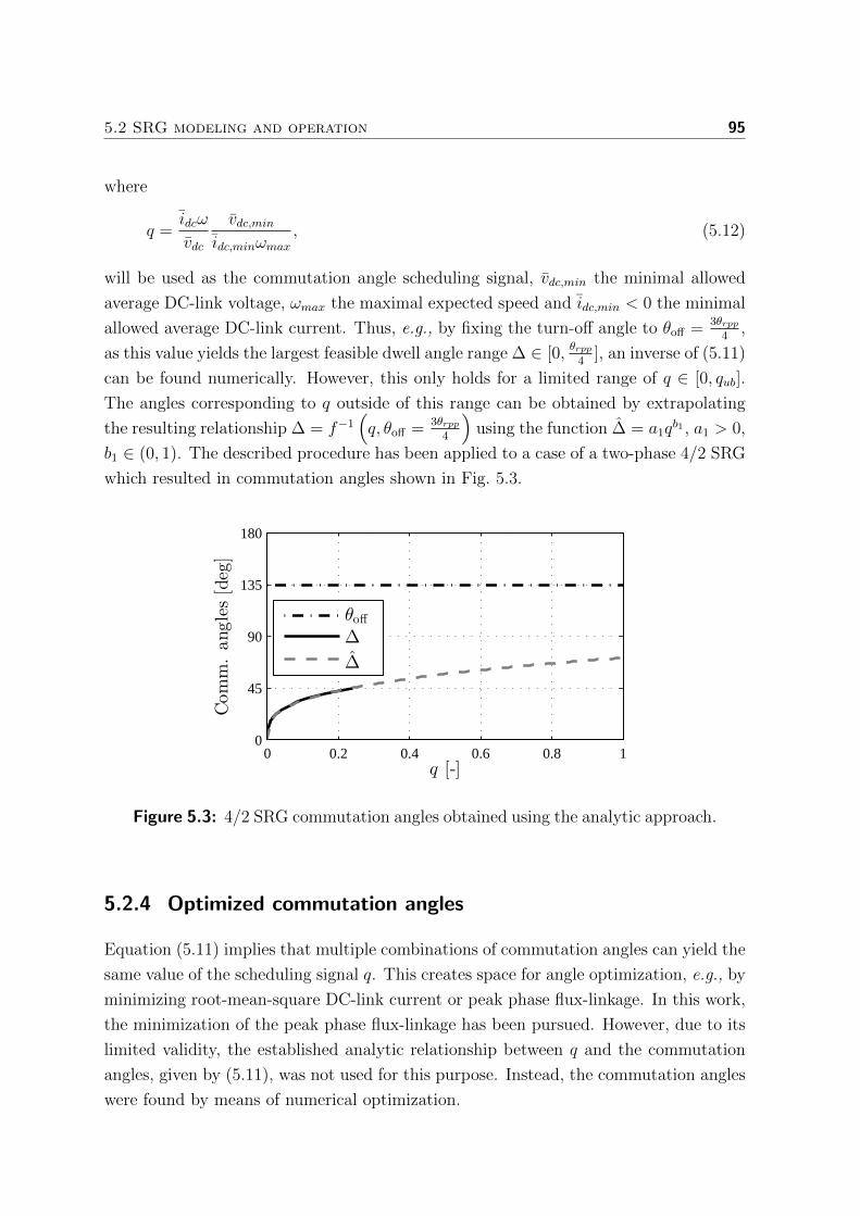
5.2 SRG modeling and operation 95
where
q =idcω
vdc
vdc,minidc,minωmax
, (5.12)
will be used as the commutation angle scheduling signal, vdc,min the minimal allowed
average DC-link voltage, ωmax the maximal expected speed and idc,min < 0 the minimal
allowed average DC-link current. Thus, e.g., by fixing the turn-off angle to θoff = 3θrpp4
,
as this value yields the largest feasible dwell angle range ∆ ∈ [0, θrpp4
], an inverse of (5.11)
can be found numerically. However, this only holds for a limited range of q ∈ [0, qub].
The angles corresponding to q outside of this range can be obtained by extrapolating
the resulting relationship ∆ = f−1(q, θoff = 3θrpp
4
)using the function ∆ = a1q
b1 , a1 > 0,
b1 ∈ (0, 1). The described procedure has been applied to a case of a two-phase 4/2 SRG
which resulted in commutation angles shown in Fig. 5.3.
0 0.2 0.4 0.6 0.8 10
45
90
135
180
q [-]
Comm.angles[deg]
θoff
∆
∆
Figure 5.3: 4/2 SRG commutation angles obtained using the analytic approach.
5.2.4 Optimized commutation angles
Equation (5.11) implies that multiple combinations of commutation angles can yield the
same value of the scheduling signal q. This creates space for angle optimization, e.g., by
minimizing root-mean-square DC-link current or peak phase flux-linkage. In this work,
the minimization of the peak phase flux-linkage has been pursued. However, due to its
limited validity, the established analytic relationship between q and the commutation
angles, given by (5.11), was not used for this purpose. Instead, the commutation angles
were found by means of numerical optimization.

965 Model predictive voltage control of high-speed Switched Reluctance
Generators
Specifically, the optimal ∆∗ and θ∗off were computed for a range of desired average DC-
link current values i∗dc ∈ [idc,min, 0], at the DC-link voltage vdc = vdc,min and the SRG
rotor speed ω = ωmax, by solving
min∆∗,θ∗off
ψ1,max, subject to (5.13)
idc(∆∗, θ∗off , ω, vdc) = i∗dc,
∆∗ ∈ [0, θ∗rpp],
θ∗off ∈ [θrpp/2, θrpp],
where idc denotes the steady-state average of the DC-link current idc produced by
the SRG and ψ1,max the steady-state maximum of the phase 1 flux-linkage ψ1, within
one electrical period of length θrpp. The current idc was computed by simulating the
phase flux-linkage (5.6) and position (5.8) dynamics, i.e., by evaluating (5.4), for each
particular ∆∗ and θ∗off. For this purpose, the phase current functions ip = ip(ψp, θ) have
been numerically derived from measured phase flux-linkage characteristics.
Subsequently, by inserting i∗dc, vdc = idc,min and ω = ωmax in (5.12) the desired scheduling
signal q∗ was calculated for each optimized operating point. The result was used to
parametrize ∆∗ and θ∗off, yielding
∆ = a2qb2 , (5.14)
θoff = c0 + c1q + c2q2,
with a2 > 0, b2 ∈ (0, 1), c0 > 0, c1 ∈ R and c2 ≥ 0 being some fitting coefficients,
and ∆ the nominal (optimized) dwell angle value. The outcome of the optimization is
illustrated in Fig. 5.4.
Remark: The main SRG losses are the copper and the iron (core) losses, PCu and
PFe, with the iron loss PFe being the dominant loss component at high speeds [114].
The iron loss consists of hysteresis Phy and eddy current losses Ped, which can be
approximated [115] by
Phy = k1fψk2 , (5.15)
Ped = k3f2ψ,
where f is the flux-linkage excitation frequency and k1, k2, k3 > 0 are some unknown
empirical constants. Equation (5.15) implies that the iron loss can be reduced by
minimizing the (phase) flux-linkage ψ. This motivates the choice of objective function
in (5.13).
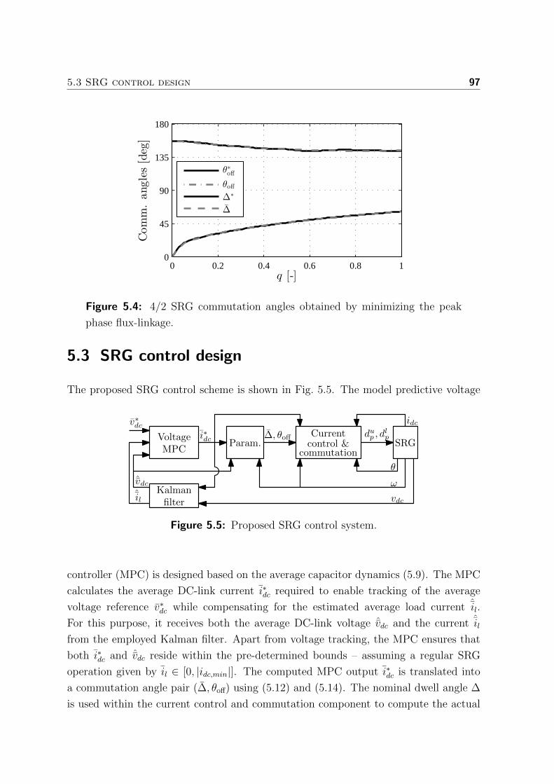
5.3 SRG control design 97
0 0.2 0.4 0.6 0.8 10
45
90
135
180
q [-]
Comm.angles[deg]
θ∗
off
θoff
∆∗
∆
Figure 5.4: 4/2 SRG commutation angles obtained by minimizing the peak
phase flux-linkage.
5.3 SRG control design
The proposed SRG control scheme is shown in Fig. 5.5. The model predictive voltage
dup , dlp
vdc
ω
v∗dc
SRG∆, θoff
Param.i∗dc
idcCurrent
control &commutation
filterKalman
ˆvdcˆil
θ
MPCVoltage
Figure 5.5: Proposed SRG control system.
controller (MPC) is designed based on the average capacitor dynamics (5.9). The MPC
calculates the average DC-link current i∗dc required to enable tracking of the average
voltage reference v∗dc while compensating for the estimated average load current ˆil.
For this purpose, it receives both the average DC-link voltage ˆvdc and the current ˆil
from the employed Kalman filter. Apart from voltage tracking, the MPC ensures that
both i∗dc and ˆvdc reside within the pre-determined bounds – assuming a regular SRG
operation given by il ∈ [0, |idc,min|]. The computed MPC output i∗dc is translated into
a commutation angle pair (∆, θoff) using (5.12) and (5.14). The nominal dwell angle ∆
is used within the current control and commutation component to compute the actual

985 Model predictive voltage control of high-speed Switched Reluctance
Generators
dwell angle ∆ such that the difference between the desired i∗dc and the estimated average
DC-link current ˆidc is reduced. Finally, the resulting commutation angles are compared
with the rotor position θ to obtain the AHBC phase switch inputs dup and dlp.
5.3.1 Model predictive voltage control
Due to a time-discrete character of the MPC the dynamics (5.9) is first discretized
(using exact discretization). If x = [vdc, il]T denotes the state, u = i∗dc the input and
y = vdc the output of such a system, its time-discrete state-space representation then
reads
x(k + 1) =
[1 −T
C
0 1
]
︸ ︷︷ ︸Ac
x(k) +
[−TC
0
]
︸ ︷︷ ︸Bc
u(k) + ρ(k), (5.16)
y(k) =[1 0
]
︸ ︷︷ ︸Cc
x(k) + η(k),
where k ∈ N0 is used to represent the discrete time instant tk = kT , with T being
the adopted MPC sampling time. The signals ρ and η denote white zero-mean state
and measurement noise described by their covariance matrices W1 and W2, respectively.
Since (5.16) is observable a Kalman filter was employed for estimation of the state x
from the measured output y and the input u. It was designed using MATLABr kalman
routine, where the matrices W1 and W2 were treated as tuning parameters. For more
information regarding Kalman filter design, see, e.g., [116].
Remark: Equation (5.16) includes a load current disturbance il as a part of the state.
The augmentation of the plant with a disturbance model is a standard practice in the
MPC, inspired by the Internal Model Principle (IMC) [117]. This particular choice
of the disturbance model is commonly used to remove a steady-state offset due to a
persistent disturbance [118].
By representing the predicted state and the output at time instant k + j, j ≥ 1, given
the state and the output at time k, as xk+j|k and yk+j|k, the MPC optimization problem
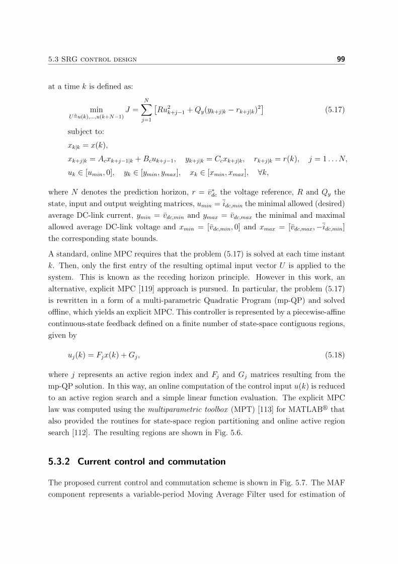
5.3 SRG control design 99
at a time k is defined as:
minU,u(k),...,u(k+N−1)
J =N∑
j=1
[Ru2
k+j−1 +Qy(yk+j|k − rk+j|k)2]
(5.17)
subject to:
xk|k = x(k),
xk+j|k = Acxk+j−1|k +Bcuk+j−1, yk+j|k = Ccxk+j|k, rk+j|k = r(k), j = 1 . . . N,
uk ∈ [umin, 0], yk ∈ [ymin, ymax], xk ∈ [xmin, xmax], ∀k,
where N denotes the prediction horizon, r = v∗dc the voltage reference, R and Qy the
state, input and output weighting matrices, umin = idc,min the minimal allowed (desired)
average DC-link current, ymin = vdc,min and ymax = vdc,max the minimal and maximal
allowed average DC-link voltage and xmin = [vdc,min, 0] and xmax = [vdc,max,−idc,min]
the corresponding state bounds.
A standard, online MPC requires that the problem (5.17) is solved at each time instant
k. Then, only the first entry of the resulting optimal input vector U is applied to the
system. This is known as the receding horizon principle. However in this work, an
alternative, explicit MPC [119] approach is pursued. In particular, the problem (5.17)
is rewritten in a form of a multi-parametric Quadratic Program (mp-QP) and solved
offline, which yields an explicit MPC. This controller is represented by a piecewise-affine
continuous-state feedback defined on a finite number of state-space contiguous regions,
given by
uj(k) = Fjx(k) +Gj, (5.18)
where j represents an active region index and Fj and Gj matrices resulting from the
mp-QP solution. In this way, an online computation of the control input u(k) is reduced
to an active region search and a simple linear function evaluation. The explicit MPC
law was computed using the multiparametric toolbox (MPT) [113] for MATLABr that
also provided the routines for state-space region partitioning and online active region
search [112]. The resulting regions are shown in Fig. 5.6.
5.3.2 Current control and commutation
The proposed current control and commutation scheme is shown in Fig. 5.7. The MAF
component represents a variable-period Moving Average Filter used for estimation of
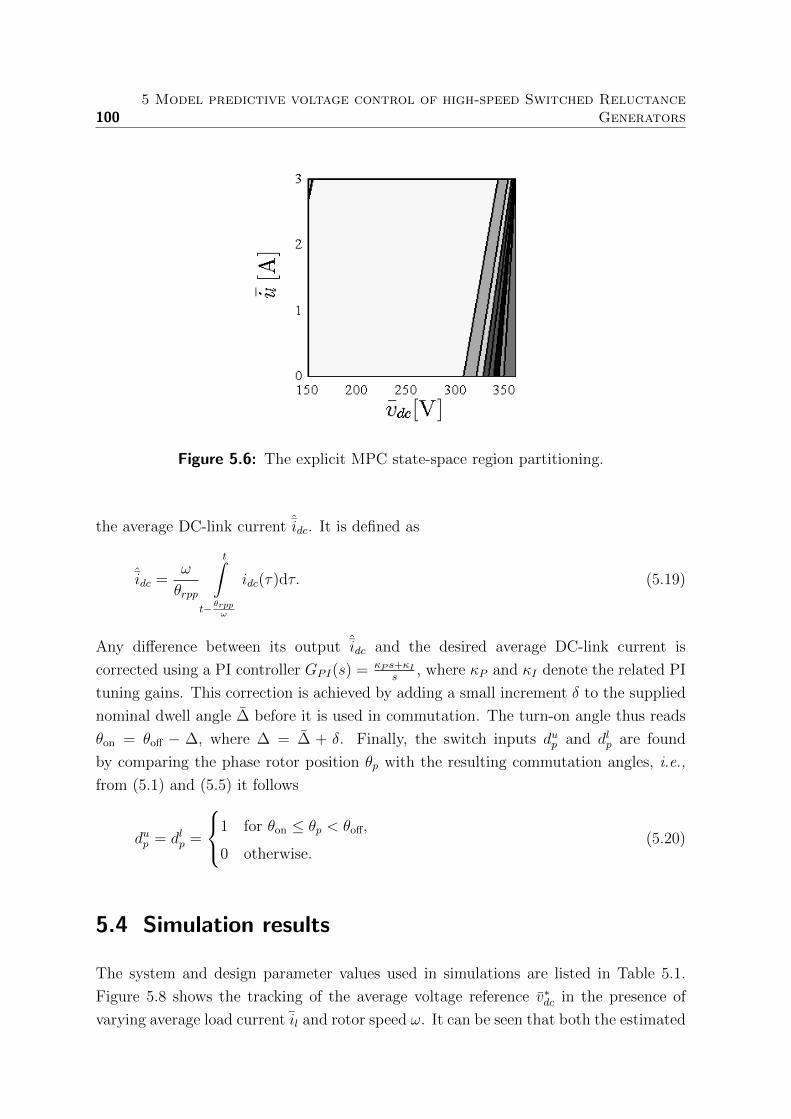
1005 Model predictive voltage control of high-speed Switched Reluctance
Generators
|
Figure 5.6: The explicit MPC state-space region partitioning.
the average DC-link current ˆidc. It is defined as
ˆidc =ω
θrpp
t∫
t− θrppω
idc(τ)dτ. (5.19)
Any difference between its output ˆidc and the desired average DC-link current is
corrected using a PI controller GPI(s) = κP s+κIs
, where κP and κI denote the related PI
tuning gains. This correction is achieved by adding a small increment δ to the supplied
nominal dwell angle ∆ before it is used in commutation. The turn-on angle thus reads
θon = θoff − ∆, where ∆ = ∆ + δ. Finally, the switch inputs dup and dlp are found
by comparing the phase rotor position θp with the resulting commutation angles, i.e.,
from (5.1) and (5.5) it follows
dup = dlp =
1 for θon ≤ θp < θoff,
0 otherwise.(5.20)
5.4 Simulation results
The system and design parameter values used in simulations are listed in Table 5.1.
Figure 5.8 shows the tracking of the average voltage reference v∗dc in the presence of
varying average load current il and rotor speed ω. It can be seen that both the estimated
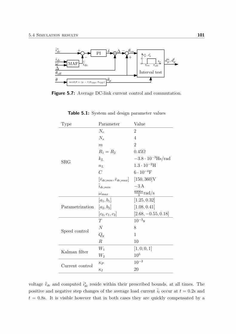
5.4 Simulation results 101
dup , dlpω
∆
i∗dc
idc
θ
PI+
−MAF ˆidc
θoff
+∆ −+
θon
Interval test
mod(θ + (p − 1)θspp, θrpp)θp
0
1
θon θoff
θp
dup , dlp
δ
Figure 5.7: Average DC-link current control and commutation.
Table 5.1: System and design parameter values
Type Parameter Value
SRG
Nr 2
Ns 4
m 2
R1 = R2 0.45Ω
kL −3.8 · 10−3Hs/rad
nL 1.3 · 10−2H
C 6 · 10−4F
[vdc,min, vdc,max] [150, 360]V
idc,min −3 A
ωmax6000π
3rad/s
Parametrization
[a1, b1] [1.25, 0.32]
[a2, b2] [1.08, 0.41]
[c0, c1, c2] [2.68,−0.55, 0.18]
Speed control
T 10−3s
N 8
Qy 1
R 10
Kalman filterW1 [1, 0; 0, 1]
W2 105
Current controlκP 10−2
κI 20
voltage ˆvdc and computed i∗dc reside within their prescribed bounds, at all times. The
positive and negative step changes of the average load current il occur at t = 0.2s and
t = 0.8s. It is visible however that in both cases they are quickly compensated by a
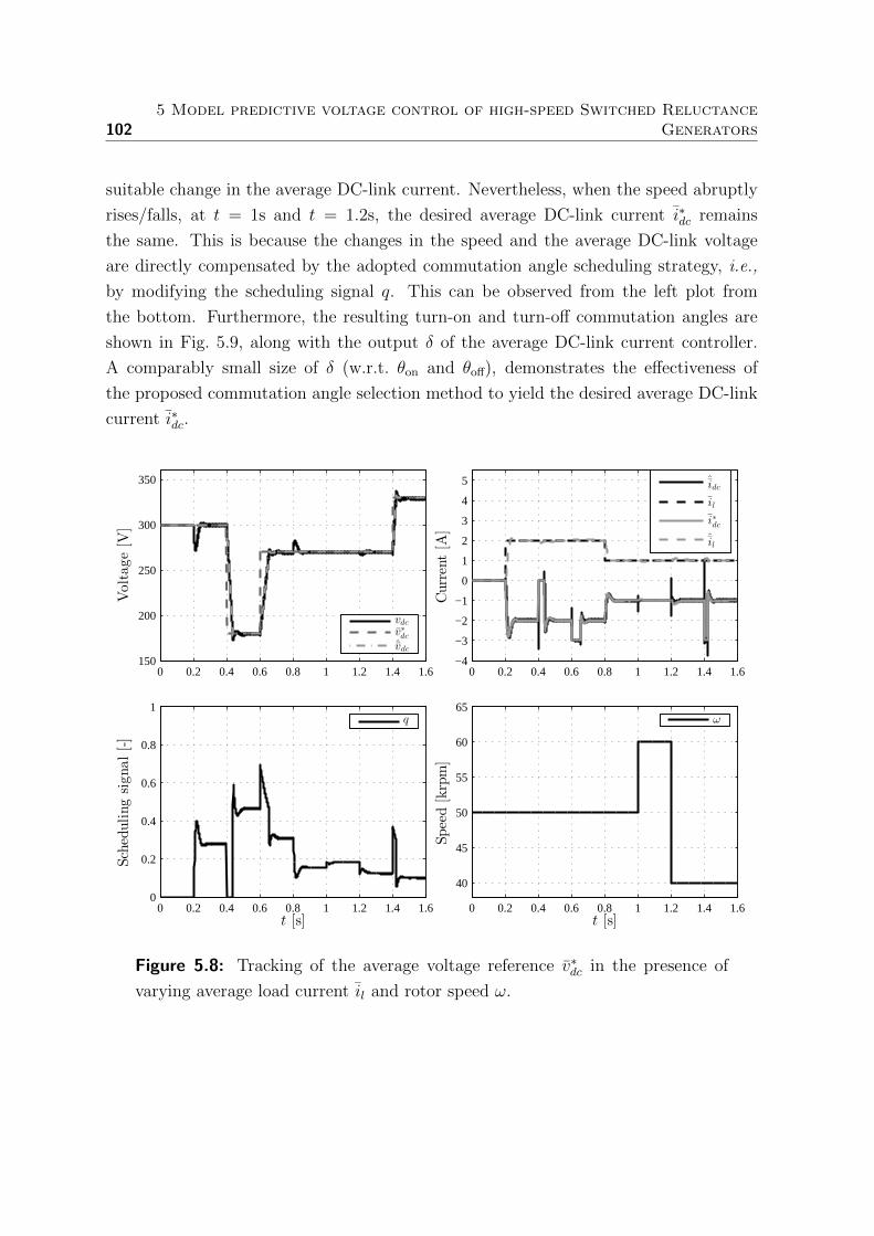
1025 Model predictive voltage control of high-speed Switched Reluctance
Generators
suitable change in the average DC-link current. Nevertheless, when the speed abruptly
rises/falls, at t = 1s and t = 1.2s, the desired average DC-link current i∗dc remains
the same. This is because the changes in the speed and the average DC-link voltage
are directly compensated by the adopted commutation angle scheduling strategy, i.e.,
by modifying the scheduling signal q. This can be observed from the left plot from
the bottom. Furthermore, the resulting turn-on and turn-off commutation angles are
shown in Fig. 5.9, along with the output δ of the average DC-link current controller.
A comparably small size of δ (w.r.t. θon and θoff), demonstrates the effectiveness of
the proposed commutation angle selection method to yield the desired average DC-link
current i∗dc.
0 0.2 0.4 0.6 0.8 1 1.2 1.4 1.6150
200
250
300
350
Voltage[V
]
vdcv∗dcˆvdc
0 0.2 0.4 0.6 0.8 1 1.2 1.4 1.6−4
−3
−2
−1
0
1
2
3
4
5
Current[A
]
ˆidc
il
i∗dc
ˆil
0 0.2 0.4 0.6 0.8 1 1.2 1.4 1.60
0.2
0.4
0.6
0.8
1
t [s]
Schedulingsignal[-]
q
0 0.2 0.4 0.6 0.8 1 1.2 1.4 1.6
40
45
50
55
60
65
t [s]
Speed[krpm]
ω
Figure 5.8: Tracking of the average voltage reference v∗dc in the presence of
varying average load current il and rotor speed ω.
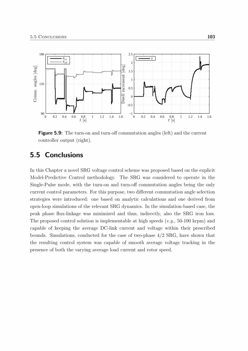
5.5 Conclusions 103
0 0.2 0.4 0.6 0.8 1 1.2 1.4 1.690
135
180
t [s]
Comm.angles[deg]
θonθoff
0 0.2 0.4 0.6 0.8 1 1.2 1.4 1.6−1
−0.5
0
0.5
1
1.5
2
2.5
t [s]Dwellincrem
ent[deg]
δ
Figure 5.9: The turn-on and turn-off commutation angles (left) and the current
controller output (right).
5.5 Conclusions
In this Chapter a novel SRG voltage control scheme was proposed based on the explicit
Model-Predictive Control methodology. The SRG was considered to operate in the
Single-Pulse mode, with the turn-on and turn-off commutation angles being the only
current control parameters. For this purpose, two different commutation angle selection
strategies were introduced: one based on analytic calculations and one derived from
open-loop simulations of the relevant SRG dynamics. In the simulation-based case, the
peak phase flux-linkage was minimized and thus, indirectly, also the SRG iron loss.
The proposed control solution is implementable at high speeds (e.g., 50-100 krpm) and
capable of keeping the average DC-link current and voltage within their prescribed
bounds. Simulations, conducted for the case of two-phase 4/2 SRG, have shown that
the resulting control system was capable of smooth average voltage tracking in the
presence of both the varying average load current and rotor speed.

104
Chapter 6
Speed control of high-speed Switched
Reluctance Machines using only the
DC-link measurements 1
Abstract This Chapter presents a novel position-sensorless speed control strategy for high-
speed Switched Reluctance Machines. The main contribution of this work is an algorithm
for rotor position and speed estimation using the DC-link voltage and current measurements
only. This eliminates a number of hardware components related to position, speed, phase
current and phase voltage sensing. In this way, the electrical system’s costs can be further
lowered and its reliability increased. The effectivness of the derived solution is demonstrated
in closed-loop simulations.
6.1 Introduction
The Switched Reluctance electrical Machine (SRM) is characterized by the absence of
permanent magnets, rotor windings and brushes. It is robust and cheap to produce,
achieves high efficiency and is capable of operating in a wide speed range. This makes
it suitable for applications in automotive [121], aircraft [80], wind power [122] and home
appliance industry [123].
Due to its lack of brushes the SRM is electronically commutated which requires
accurate knowledge of either phase inductance or rotor position. The inductance-based
1This chapter is based on [120].
105
1066 Speed control of high-speed Switched Reluctance Machines using only the
DC-link measurements
commutation [122], [124] is achieved by comparing the instantaneous phase inductance
(measured or estimated) with its computed turn-on and turn-off values. This determines
the moments when each phase should be magnetized/demagnetized. However, as
inductance sensing is often difficult to perform the SRMs are more commonly position-
commutated. This is achieved by energizing each SRM phase in a rotor position interval
specified by turn-on and turn-off angles. Typically, an absolute rotary encoder is used
to measure the rotor position. This not only adds to the cost and complexity of the
system but also reduces its reliability. As a consequence, a lot of interest has emerged
for position-sensorless commutation, both in industry [123] and academia [125]. The
related control methods can be divided into hardware and software-based.
A hardware-based method is proposed in [126]. Here, an analog circuit is designed for
detecting a change in a phase current gradient that occurs when rotor and stator poles
begin or cease to overlap. The resulting gradient detection signal is used to obtain high
frequency position pulses by feeding it to a Phase-Locked Loop (PLL). However, apart
from a need for the additional hardware, this method is not suitable for applications
involving large load torque transients.
Software-based methods typically require knowledge of the relationship between phase
flux-linkage, current and position. These methods do not require any extra hardware
such as analog differentiators, inductance sensors, PLLs, etc. They can be further
split into open- and closed-loop methods. In an open-loop case [127]–[129], the
measured phase current and the computed flux-linkage are directly mapped to the
rotor position. Popular mapping choices constitute either look-up tables or certain
neural network/fuzzy logic-based approximators. As the map is constructed (trained)
off-line, these methods bear low real-time computational requirements at the cost of
increased sensitivity to modeling and measurement errors. The closed-loop, observer-
based methods [130]–[133], utilize a dynamic model of the SRM to estimate its position
and speed. This practically implies the use of (sliding-mode) observers based on either
phase flux-linkage or current error. When compared to others, observer-based methods
provide superior estimation accuracy and as a result are becoming a preferred choice in
many sensorless applications [134]. Their main drawback is an increased computational
burden and a reliance on both phase voltage and current measurements.
The contribution of this Chapter is a derivation of a position-sensorless SRM control
algorithm which does not require phase voltage/current sensing. Specifically, a novel
SRM speed control strategy is presented using the measurements of DC-link voltage and
current only. In this context, rotor position and speed are estimated using a nonlinear
observer. The proposed method is intended for high-speed SRM applications.
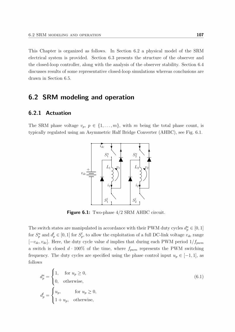
6.2 SRM modeling and operation 107
This Chapter is organized as follows. In Section 6.2 a physical model of the SRM
electrical system is provided. Section 6.3 presents the structure of the observer and
the closed-loop controller, along with the analysis of the observer stability. Section 6.4
discusses results of some representative closed-loop simulations whereas conclusions are
drawn in Section 6.5.
6.2 SRM modeling and operation
6.2.1 Actuation
The SRM phase voltage vp, p ∈ 1, . . . ,m, with m being the total phase count, is
typically regulated using an Asymmetric Half Bridge Converter (AHBC), see Fig. 6.1.
v1 v2
Su1 Su
2
Sl1 Sl
2
i1 i2
L1 L2+vdc
idc
Figure 6.1: Two-phase 4/2 SRM AHBC circuit.
The switch states are manipulated in accordance with their PWM duty cycles dup ∈ [0, 1]
for Sup and dlp ∈ [0, 1] for Slp, to allow the exploitation of a full DC-link voltage vdc range
[−vdc, vdc]. Here, the duty cycle value d implies that during each PWM period 1/fpwm
a switch is closed d · 100% of the time, where fpwm represents the PWM switching
frequency. The duty cycles are specified using the phase control input up ∈ [−1, 1], as
follows
dup =
1, for up ≥ 0,
0, otherwise,(6.1)
dlp =
up, for up ≥ 0,
1 + up, otherwise,
1086 Speed control of high-speed Switched Reluctance Machines using only the
DC-link measurements
which in average (over the PWM period) yields the phase voltage
vp = upvdc, p ∈ 1, 2. (6.2)
and a DC-link current
idc =m∑
p=1
upip, (6.3)
where ip denotes a phase current in a phase winding p.
6.2.2 Electromagnetic properties
The SRM is typically described by its phase flux-linkage characteristics ψp = ψp(ip, θ),
where θ denotes an absolute rotor position defined w.r.t. a fully unaligned position of
phase 1. A time-derivative of ψp reads
dψpdt
(ip, θ) = Lp(ip, θ)dipdt
+Mp(ip, θ)dθ
dt, (6.4)
where Lp(ip, θ) = ∂ψp∂ip
(ip, θ) and Mp(ip, θ) = ∂ψp∂θ
(ip, θ). In general, both Lp and Mp
are bounded. Since an incremental phase inductance Lp is strictly positive, ψp(ip) is
strictly monotonic and there exists an inverse mapping ip = ip(ψp, θ). Then, from (6.4),
it follows
dipdt
=1
Lp
dψpdt− Mp
Lp
dθ
dt, (6.5)
i.e.,
dipdψp
(ψp, θ) =1
Lp(ip(ψp, θ), θ)= Np(ψp, θ), (6.6)
dipdθ
(ψp, θ) = −Mp(ip(ψp, θ), θ)
Lp(ip(ψp, θ), θ)= Kp(ψp, θ). (6.7)
Both ip and ψp are periodic in θ with a period equal to the rotor pole pitch angle
θrpp = 2πNr
, with Nr denoting the rotor pole count, i.e.,
ip(ψp, θ) = ip(ψp, θk), (6.8)
where
θk = θ + kθrpp, k ∈ Z. (6.9)
Thus, from the perspective of phase commutation and/or speed control the positions
θk, k ∈ Z, are mutually equivalent.
6.3 SRM position-sensorless control design 109
6.2.3 Dynamics
The following set of equations can be used to describe the SRM electrical system
dynamics:
dψpdt
= zpvp, (6.10)
vp = upvdc −Rpip,
where Rp represents the phase winding resistance. The logic function zp = zp(ψp, vp)
models the fact that both ip and ψp must be nonnegative (≥ 0) due to the presence of
diodes in the AHBC circuit. It is defined as
zp = (ψp > 0) ∨ (vp > 0). (6.11)
Furthermore, the SRM mechanical system dynamics may be formulated as
dθ
dt= ω, (6.12)
dω
dt=
1
J
(m∑
p=1
τe,p − τl −Bω), (6.13)
where
τe,p(ip, θ) =∂
∂θ
ip∫
0
ψp(i, θ)di, (6.14)
is the phase torque, τl the load torque, B the viscous friction coefficient and ω the
rotor speed. Note that in non-saturating conditions, i.e., when Lp(ip, θ) = Lp(θ) and
ψp(ip, θ) = Lp(θ)ip, one can simplify (6.14) to obtain
τe,p(ip, θ) =1
2
dLp(θ)
dθi2p. (6.15)
6.3 SRM position-sensorless control design
6.3.1 Open-loop phase flux-linkage and current estimation
As a consequence of phase commutation and the fact that ψp ≥ 0, the SRM phase
flux-linkage is characterized by alternating intervals of positive and zero values. The

1106 Speed control of high-speed Switched Reluctance Machines using only the
DC-link measurements
interval when ψp > 0 is referred to as a phase p cycle, see Fig. 6.2. The cyclic reset of
ψp motivates its estimation using an open-loop estimator, given by
dψpdt
= zp ˆvp, (6.16)
ˆvp = upvdc −Rpip,
zp = zp(ψp, ˆvp)
where ψp denotes the phase flux-linkage estimate, ip = ip(ψp, θ) the phase current
estimate and θ the rotor position estimate. It can be assumed that the adopted phase
flux-linkage estimation law results in eψp = 0 at the beginning of every cycle. This is
because both (6.10) and (6.16) are dominated by a common upvdc voltage term (w.r.t.
to the Ohmic voltage drop Rpip), which ensures that both ψp and ψp are reset almost
simultaneously.
2 4 6 8 10
0
0.01
0.02
0.03
0.04
0.05
Fluxlinka
ge[W
b]
Position θ [rad]
ψp
ψp
eψp
cycle
Figure 6.2: Typical ψp, ψp and eψp waveforms as a function of θ.
Define phase current, position and speed estimation errors, respectively as
eψp = ψp − ψp, (6.17)
eip = ip − ip,eθj = θj − θ,eω = ω − ω,
with j ∈ Z such that
|θj − θ| ≤ |θk − θ|, ∀k ∈ Z, (6.18)
where ω is the rotor speed estimate. It can be reasoned that during each phase cycle
the largest |eψp | is reached when zp = zp = 1. This is because if (zp, zp) = (0, 1) then
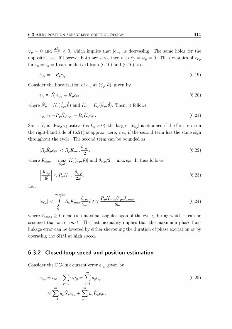
6.3 SRM position-sensorless control design 111
ψp = 0 and dψpdt
< 0, which implies that |eψp | is decreasing. The same holds for the
opposite case. If however both are zero, then also ψp = ψp = 0. The dynamics of eψpfor zp = zp = 1 can be derived from (6.10) and (6.16), i.e.,
eψp = −Rpeip . (6.19)
Consider the linearization of eip at (ψp, θ), given by
eip ≈ Npeψp + Kpeθj , (6.20)
where Np = Np(ψp, θ) and Kp = Kp(ψp, θ). Then, it follows
eψp ≈ −RpNpeψp −RpKpeθj . (6.21)
Since Np is always positive (as Lp > 0), the largest |eψp | is obtained if the first term on
the right-hand side of (6.21) is approx. zero, i.e., if the second term has the same sign
throughout the cycle. The second term can be bounded as
|RpKpeθj | < RpKmaxθrpp2, (6.22)
where Kmax = maxψp,θ|Kp(ψp, θ)| and θrpp/2 = max eθj . It thus follows
∣∣∣∣deψpdθ
∣∣∣∣ < RpKmaxθrpp2ω
, (6.23)
i.e.,
|eψp | <θc,max∫
0
RpKmaxθrpp2ω
dθ ≈ RpKmaxθrppθc,max2ω
, (6.24)
where θc,max ≥ 0 denotes a maximal angular span of the cycle, during which it can be
assumed that ω ≈ const. The last inequality implies that the maximum phase flux-
linkage error can be lowered by either shortening the duration of phase excitation or by
operating the SRM at high speed.
6.3.2 Closed-loop speed and position estimation
Consider the DC-link current error eidc given by
eidc = idc −m∑
p=1
upip =m∑
p=1
upeip , (6.25)
≈m∑
p=1
upNpeψp +m∑
p=1
upKpeθj .
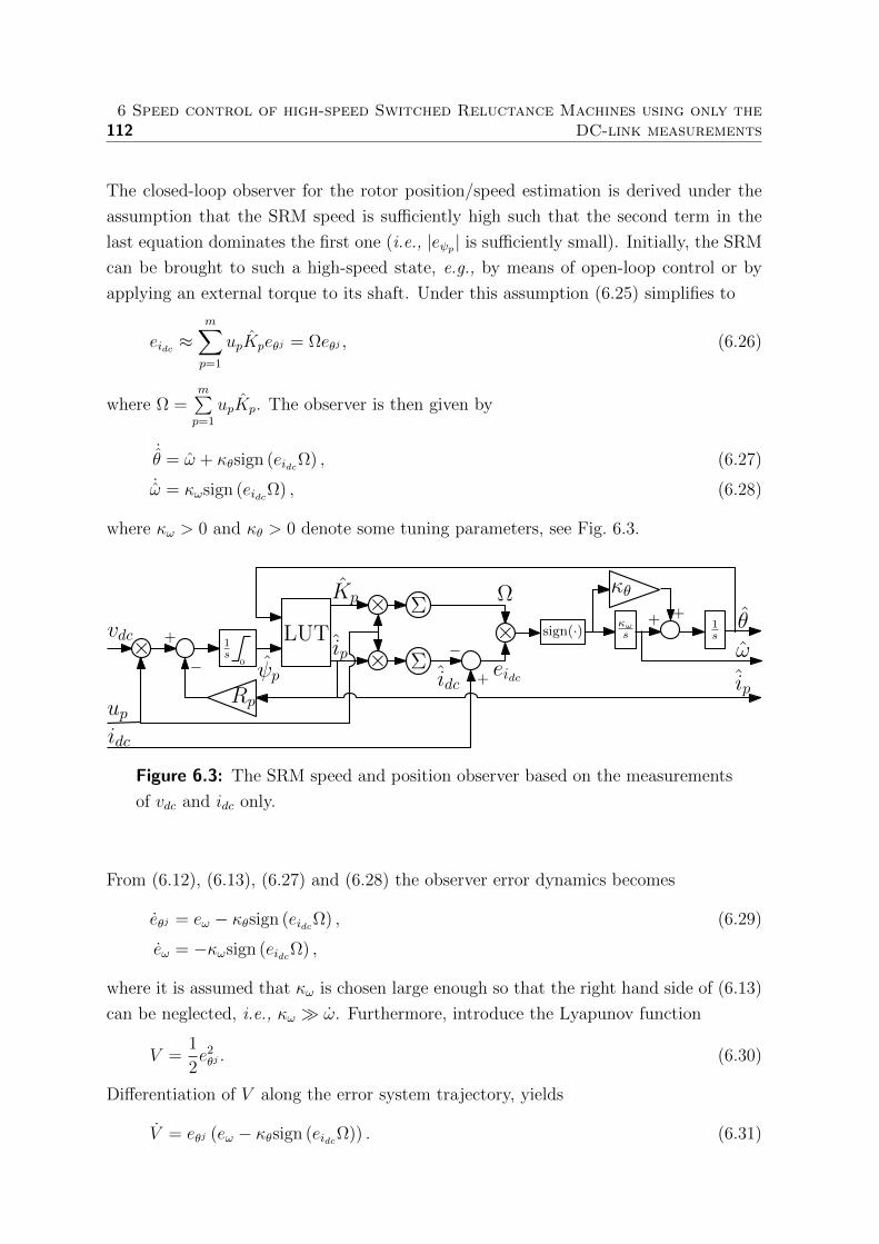
1126 Speed control of high-speed Switched Reluctance Machines using only the
DC-link measurements
The closed-loop observer for the rotor position/speed estimation is derived under the
assumption that the SRM speed is sufficiently high such that the second term in the
last equation dominates the first one (i.e., |eψp | is sufficiently small). Initially, the SRM
can be brought to such a high-speed state, e.g., by means of open-loop control or by
applying an external torque to its shaft. Under this assumption (6.25) simplifies to
eidc ≈m∑
p=1
upKpeθj = Ωeθj , (6.26)
where Ω =m∑p=1
upKp. The observer is then given by
˙θ = ω + κθsign (eidcΩ) , (6.27)
˙ω = κωsign (eidcΩ) , (6.28)
where κω > 0 and κθ > 0 denote some tuning parameters, see Fig. 6.3.
vdc1s
up
θ
ωψp
Rp
×0
ip
Kp
×
Σ×
idcΣ
+
−+
−
idc
×eidc
κωs
1s
++
κθΩ
ip
LUT sign(·)
Figure 6.3: The SRM speed and position observer based on the measurements
of vdc and idc only.
From (6.12), (6.13), (6.27) and (6.28) the observer error dynamics becomes
eθj = eω − κθsign (eidcΩ) , (6.29)
eω = −κωsign (eidcΩ) ,
where it is assumed that κω is chosen large enough so that the right hand side of (6.13)
can be neglected, i.e., κω ω. Furthermore, introduce the Lyapunov function
V =1
2e2θj . (6.30)
Differentiation of V along the error system trajectory, yields
V = eθj (eω − κθsign (eidcΩ)) . (6.31)

6.3 SRM position-sensorless control design 113
Assuming that we choose κθ such that
|eω| < κθ, (6.32)
then it holds
sign(V ) = −sign(eθj)sign (eidcΩ) . (6.33)
Since (6.26) implies that sign(eidcΩ) ≈ sign(eθj), it follows
sign(V ) ≈ −1 (6.34)
i.e., eθj → 0. Once eθj = 0, the error dynamics becomes
eθj = 0, (6.35)
eω = −κωκθeω,
i.e., ω → ω at the rate given by the ratio of κω and κθ.
Remark: Typically, the applied SRM speed control law yields up > 0 in the phase
motoring region (Mp > 0) and up < 0 in the phase generating region (Mp < 0).
This implies that sign(upMp) ≈ 1, i.e., sign(upKp) ≈ −1, and as a result sign(Ω) ≈−1. In such control cases, the resulting property may be used to further simplify the
observer (6.27), at the cost of slightly degraded speed/position estimation performance.
6.3.3 Speed control, current control and commutation
Figure 6.4 illustrates the structure of the proposed SRM control system. The speed is
controlled using a PI controller C(s) = κP1 +κI1s
with a speed tracking error ω∗−ω as its
input and a desired average electromagnetic torque τ ∗e as its output. Here ω∗ represents
the speed reference and κP1 and κI1 the PI controller gains. In a subsequent current
reference parametrization step the torque τ ∗e is converted into a set of phase current
references i∗p, p ∈ 1, . . . ,m. Specifically, for each phase p a rectangular reference
i∗p ∈ 0, i∗ is used, with i∗p = σpi∗, where σp ∈ 0, 1 represents the phase commutation
signal. The level i∗ is computed as
i∗ = imax
√|τ ∗e |τe,max
, (6.36)
with imax denoting the maximum expected phase current and τe,max the maximum
average phase electromagnetic torque. The introduced torque-to-current mapping is
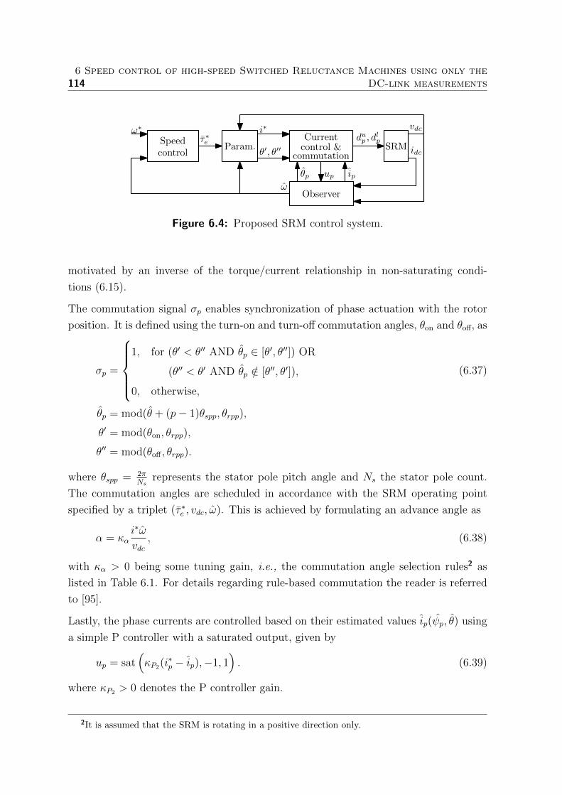
1146 Speed control of high-speed Switched Reluctance Machines using only the
DC-link measurements
dup , dlp
vdc
θp
controlSpeed
ωObserver
ω∗
SRMθ′, θ′′
i∗
Param.τ∗e
idc
Currentcontrol &
commutation
ipup
Figure 6.4: Proposed SRM control system.
motivated by an inverse of the torque/current relationship in non-saturating condi-
tions (6.15).
The commutation signal σp enables synchronization of phase actuation with the rotor
position. It is defined using the turn-on and turn-off commutation angles, θon and θoff, as
σp =
1, for (θ′ < θ′′ AND θp ∈ [θ′, θ′′]) OR
(θ′′ < θ′ AND θp /∈ [θ′′, θ′]),
0, otherwise,
(6.37)
θp = mod(θ + (p− 1)θspp, θrpp),
θ′ = mod(θon, θrpp),
θ′′ = mod(θoff , θrpp).
where θspp = 2πNs
represents the stator pole pitch angle and Ns the stator pole count.
The commutation angles are scheduled in accordance with the SRM operating point
specified by a triplet (τ ∗e , vdc, ω). This is achieved by formulating an advance angle as
α = καi∗ω
vdc, (6.38)
with κα > 0 being some tuning gain, i.e., the commutation angle selection rules2 as
listed in Table 6.1. For details regarding rule-based commutation the reader is referred
to [95].
Lastly, the phase currents are controlled based on their estimated values ip(ψp, θ) using
a simple P controller with a saturated output, given by
up = sat(κP2(i∗p − ip),−1, 1
). (6.39)
where κP2 > 0 denotes the P controller gain.
2It is assumed that the SRM is rotating in a positive direction only.
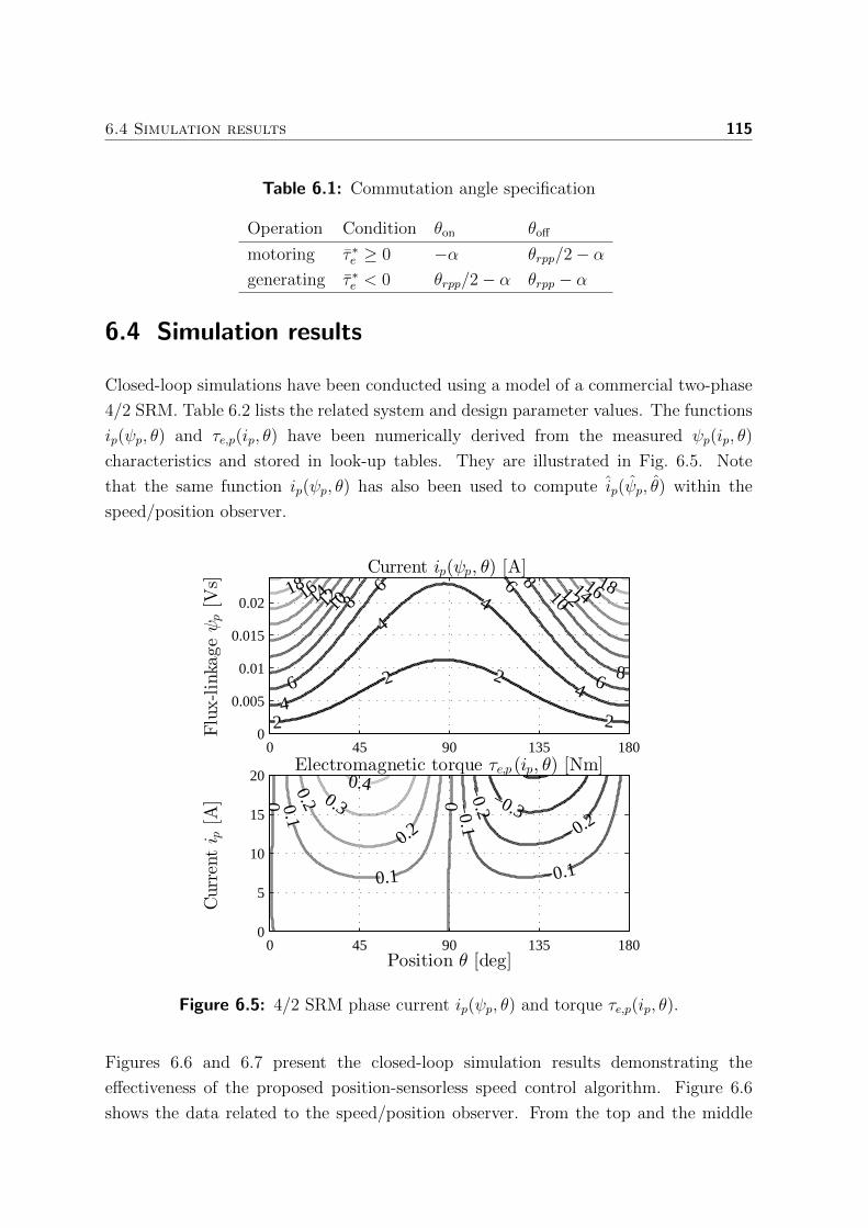
6.4 Simulation results 115
Table 6.1: Commutation angle specification
Operation Condition θon θoff
motoring τ ∗e ≥ 0 −α θrpp/2− αgenerating τ ∗e < 0 θrpp/2− α θrpp − α
6.4 Simulation results
Closed-loop simulations have been conducted using a model of a commercial two-phase
4/2 SRM. Table 6.2 lists the related system and design parameter values. The functions
ip(ψp, θ) and τe,p(ip, θ) have been numerically derived from the measured ψp(ip, θ)
characteristics and stored in look-up tables. They are illustrated in Fig. 6.5. Note
that the same function ip(ψp, θ) has also been used to compute ip(ψp, θ) within the
speed/position observer.
2
22
2
4
4
4
46
6
6
6
8
88
1010
12121414 1616 1818
Current ip(ψp, θ) [A]
Flux-linkageψp[V
s]
0 45 90 135 1800
0.005
0.01
0.015
0.02
−0.3−0.2
−0.2
−0.1
−0.1
00
0.1
0.1
0.2
0.2 0.30.4
Electromagnetic torque τe,p (ip, θ) [Nm]
Position θ [deg]
Currenti p
[A]
0 45 90 135 1800
5
10
15
20
Figure 6.5: 4/2 SRM phase current ip(ψp, θ) and torque τe,p(ip, θ).
Figures 6.6 and 6.7 present the closed-loop simulation results demonstrating the
effectiveness of the proposed position-sensorless speed control algorithm. Figure 6.6
shows the data related to the speed/position observer. From the top and the middle
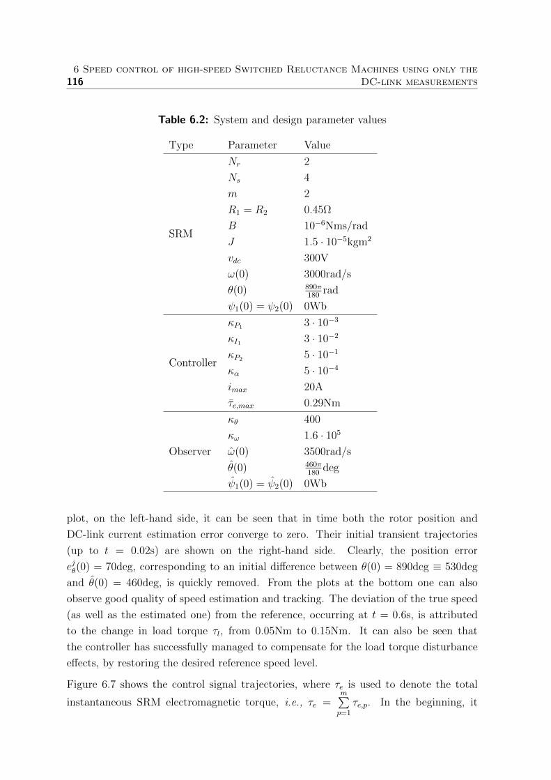
1166 Speed control of high-speed Switched Reluctance Machines using only the
DC-link measurements
Table 6.2: System and design parameter values
Type Parameter Value
SRM
Nr 2
Ns 4
m 2
R1 = R2 0.45Ω
B 10−6Nms/rad
J 1.5 · 10−5kgm2
vdc 300V
ω(0) 3000rad/s
θ(0) 890π180
rad
ψ1(0) = ψ2(0) 0Wb
Controller
κP1 3 · 10−3
κI1 3 · 10−2
κP2 5 · 10−1
κα 5 · 10−4
imax 20A
τe,max 0.29Nm
Observer
κθ 400
κω 1.6 · 105
ω(0) 3500rad/s
θ(0) 460π180
deg
ψ1(0) = ψ2(0) 0Wb
plot, on the left-hand side, it can be seen that in time both the rotor position and
DC-link current estimation error converge to zero. Their initial transient trajectories
(up to t = 0.02s) are shown on the right-hand side. Clearly, the position error
ejθ(0) = 70deg, corresponding to an initial difference between θ(0) = 890deg ≡ 530deg
and θ(0) = 460deg, is quickly removed. From the plots at the bottom one can also
observe good quality of speed estimation and tracking. The deviation of the true speed
(as well as the estimated one) from the reference, occurring at t = 0.6s, is attributed
to the change in load torque τl, from 0.05Nm to 0.15Nm. It can also be seen that
the controller has successfully managed to compensate for the load torque disturbance
effects, by restoring the desired reference speed level.
Figure 6.7 shows the control signal trajectories, where τe is used to denote the total
instantaneous SRM electromagnetic torque, i.e., τe =m∑p=1
τe,p. In the beginning, it
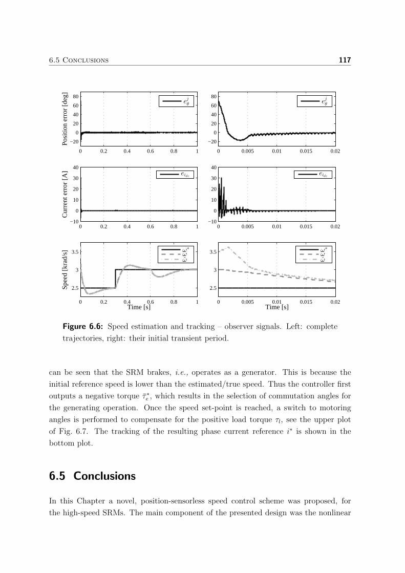
6.5 Conclusions 117
0 0.2 0.4 0.6 0.8 1
−20
0
20
40
60
80
Pos
ition
err
or [d
eg]
ej
θ
0 0.005 0.01 0.015 0.02
−20
0
20
40
60
80
ej
θ
0 0.2 0.4 0.6 0.8 1−10
0
10
20
30
40
Cur
rent
err
or [A
]
eidc
0 0.005 0.01 0.015 0.02−10
0
10
20
30
40
eidc
0 0.2 0.4 0.6 0.8 1
2.5
3
3.5
Time [s]
Spe
ed [k
rad/
s]
ω∗
ωω
0 0.005 0.01 0.015 0.02
2.5
3
3.5
Time [s]
ω∗
ωω
Figure 6.6: Speed estimation and tracking – observer signals. Left: complete
trajectories, right: their initial transient period.
can be seen that the SRM brakes, i.e., operates as a generator. This is because the
initial reference speed is lower than the estimated/true speed. Thus the controller first
outputs a negative torque τ ∗e , which results in the selection of commutation angles for
the generating operation. Once the speed set-point is reached, a switch to motoring
angles is performed to compensate for the positive load torque τl, see the upper plot
of Fig. 6.7. The tracking of the resulting phase current reference i∗ is shown in the
bottom plot.
6.5 Conclusions
In this Chapter a novel, position-sensorless speed control scheme was proposed, for
the high-speed SRMs. The main component of the presented design was the nonlinear
1186 Speed control of high-speed Switched Reluctance Machines using only the
DC-link measurements
0 0.2 0.4 0.6 0.8 1−0.5
0
0.5T
orqu
e [N
m]
τe
τ∗
e
τl
0 0.2 0.4 0.6 0.8 1
0
90
180
Com
m. a
ngle
s [d
eg]
θonθoff
0 0.2 0.4 0.6 0.8 10
10
20
30
Time [s]
Cur
rent
[A]
i1i∗
Figure 6.7: Speed estimation and tracking – controller signals.
speed/position observer that relies solely on the DC-link voltage and current measure-
ments. The developed algorithm has shown good speed tracking performance, even in
the presence of the load torque disturbances. This was demonstrated in closed-loop
simulations.
Chapter 7
Auto-calibration of a generator-turbine
throttle unit1
Abstract This Chapter presents a method for auto-calibration of a generator-turbine throttle
unit (GTU). The GTU is a device consisting of a variable geometry turbine with adjustable
stator vanes and a high-speed electric generator. It is used to throttle the engine while
simultaneously producing electricity. To maximize its energy-recovery the turbine speed needs
to be suitably matched to the conditions present in the engine air-intake system, at all times.
However, often the exact dependency of the optimal turbine speed on its pressure ratio and
vanes position is either unknown or difficult to derive. This research proposes a non-model-
based solution to this problem using Extremum-Seeking Control with a disturbance-based
input parametrization. The presented algorithm enables the identification of the unknown
relationship between the disturbances (pressure ratio, vanes position) and the optimal input
(turbine reference speed) in an initial, automated calibration step. Once identified, the
resulting mapping can be employed for optimal, real-time reference speed generation. The
effectiveness of the proposed auto-calibration approach is demonstrated in simulations.
7.1 Introduction
Extremum-Seeking Control
In a wide variety of control applications the aim is to operate a physical system
or a process in the vicinity of an extremum of some performance function. The
1This chapter is based on [135], [136].
119

120 7 Auto-calibration of a generator-turbine throttle unit
performance function is often measurable but unknown to the designer, in terms of its
exact analytic dependency on the optimizing inputs. In such cases Extremum-Seeking
Control (ESC) techniques [137]–[140] can be used to achieve and maintain operation
of a dynamical system under optimal conditions. Numerous reports of successful ESC
implementation can be found in literature, e.g., for improving continuously variable
transmission efficiency [141] or Maximum Power Point Tracking (MPPT) in photovoltaic
(PV) [142], fuel cell [143] and wind energy systems [144].
The Extremum-Seeking Control was first investigated in the 1950s and 1960s as a
control framework for finding a minimum/maximum of a static map [140]. However, a
rigorous stability proof for the classical derivative-based ESC with a general nonlinear
dynamical plant arrived only at the beginning of the past decade [145]. Since then
there has been a revival of interest and a steady development in the field. Figure 7.1
shows the classification of various ESC schemes described in literature so far. On a
top level, a distinction between non-parametric (“black box”) and parametric (“gray
box”) ESC is made, based on whether the optimized system is assumed entirely or only
partially unknown. The non-parametric ESC can be further divided into derivative-
based, e.g., classical [145]–[147] and numerical [148], [149], and derivative-free, e.g.,
sliding-mode [150], [151] and direct-search [152], [153] methods, depending on the need
for performance function derivatives during optimization. In the parametric ESC the
knowledge of the structure of the performance function is typically assumed [138], [154]–
[156]. Specifically, the performance function is often parametrized by the optimizing
inputs and a set of unknown parameters that are estimated online, using the available
measurement data. The benefit of the parametric approach is that the optimal input
values can be computed analytically once the related parameters are identified.
ESC
Non-parametric
Parametric
Derivative-based
Derivative-free
Performance output(input)
Optimal input(disturbance)
- Classical- Numerical- etc.
- Sliding-mode- Direct-search- etc.
- Gradient- Least-Squares- etc.
- Gradient- Least-Squares- etc.
Figure 7.1: Classification of different ESC schemes. The path corresponding
to the proposed ESC algorithm is italicized.
In general, most of the reported ESC algorithms consider that the optimal input value
is constant. The tracking of an unknown, time-varying extremum is rarely investigated.

7.1 Introduction 121
However, in [157] this issue has been addressed for the case when the optimal input
variations can be represented as an output of a known, linear time-invariant system.
An alternative approach was presented in [158]. Instead of explicitly modeling the
optimal input time-dependency, in [158], the authors have treated the optimal input
variations as an uncertainty. As a result, they have shown that using robust tracking
techniques [159] the extremum of a static plant can be successfully followed.
This Chapter introduces a novel, parametric ESC algorithm, with a disturbance-
based optimal input parametrization, for tracking of the time-varying extremum. The
proposed ESC scheme is applicable to situations where the disturbances leading to
changes in the optimal input are known/measurable. Its main advantage over the
previously mentioned ESC approaches is that it allows one to identify the mapping
between the disturbances and the optimal inputs. Once found, the constructed mapping
can be directly employed in real-time, without the need for further extremum-seeking.
Generator-turbine throttle unit
The proposed ESC method is developed for purposes of auto-calibration of a generator-
turbine throttle unit (GTU). The GTU is a device consisting of a variable geometry
turbine with adjustable stator vanes and a high-speed electrical generator. It replaces a
throttle valve of a gasoline internal combustion engine (ICE) so that the intake airflow
can be controlled while simultaneously producing electricity [25], [26].
To maximize the GTU energy-recovery the turbine speed needs to be suitably matched
with the conditions present in the engine air-intake system, at all times. In this work,
the derived ESC scheme is employed to adaptively reconstruct the unknown relationship
between the optimal turbine speed, pressure ratio and vanes position. This results in a
disturbance-based optimal input mapping that can be used for real-time reference speed
generation, leading to an improved energy recovery. The effectiveness of the proposed
approach is demonstrated in simulations.
This Chapter is organized as follows. Section 7.2 introduces the proposed ESC scheme
whereas Section 7.3 describes its application for the GTU auto-calibration. Section 7.4
provides simulation results related to the proposed auto-calibration approach. The
conclusions are drawn in Section 7.5.
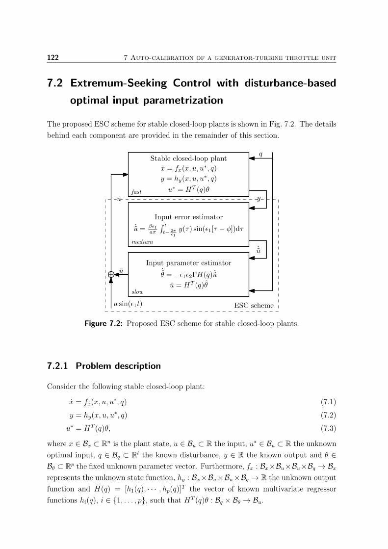
122 7 Auto-calibration of a generator-turbine throttle unit
7.2 Extremum-Seeking Control with disturbance-based
optimal input parametrization
The proposed ESC scheme for stable closed-loop plants is shown in Fig. 7.2. The details
behind each component are provided in the remainder of this section.
y
ˆu
q
+
a sin(ε1t)
u
u
ESC scheme
ˆu = βε1aπ
∫ tt− 2π
ε1
y(τ) sin(ε1[τ − φ])dτ
Input error estimator
u = HT (q)θ
Input parameter estimator˙θ = −ε1ε2ΓH(q)ˆu
fast
medium
slow
Stable closed-loop plant
x = fx(x, u, u∗, q)
y = hy(x, u, u∗, q)
u∗ = HT (q)θ
Figure 7.2: Proposed ESC scheme for stable closed-loop plants.
7.2.1 Problem description
Consider the following stable closed-loop plant:
x = fx(x, u, u∗, q) (7.1)
y = hy(x, u, u∗, q) (7.2)
u∗ = HT (q)θ, (7.3)
where x ∈ Bx ⊂ Rn is the plant state, u ∈ Bu ⊂ R the input, u∗ ∈ Bu ⊂ R the unknown
optimal input, q ∈ Bq ⊂ Rl the known disturbance, y ∈ R the known output and θ ∈Bθ ⊂ Rp the fixed unknown parameter vector. Furthermore, fx : Bx×Bu×Bu×Bq → Bxrepresents the unknown state function, hy : Bx×Bu×Bu×Bq → R the unknown output
function and H(q) = [h1(q), · · · , hp(q)]T the vector of known multivariate regressor
functions hi(q), i ∈ 1, . . . , p, such that HT (q)θ : Bq × Bθ → Bu.

7.2 Extremum-Seeking Control with disturbance-based optimal inputparametrization 123
Assuming the equation
0 = fx(x, u, u∗, q) (7.4)
has a unique solution x = l(u, u∗, q), define the equilibrium input-output map
Q(u, u∗, q) := hy(l(u, u∗, q), u∗, q). (7.5)
Furthermore, assume that the map Q(u, ·, ·) is smoothly differentiable sufficiently many
times and that for any q there exists an extremum2 at u = u∗. Moreover, assume that
the disturbance derivative exists and that it holds
|q| < ε1ε2, (7.6)
with 0 < ε1, 0 < ε2 ≤ 1 being some user-assignable (Lipschitz) constants. In the follow-
ing, the i-th derivative of Q(·, ·, ·), w.r.t. u, is denoted as DiQ(u, u∗, q) := ∂iQ∂ui
(u, u∗, q).
The aim of the proposed ESC scheme is to identify the unknown input parameters θ
which define the optimal input u∗, given by (7.3). The benefit of this ESC approach
is that, once identified, the parameters θ can be used to directly compute the input
u which maximizes the input-output map Q(u, u∗, q), for any value of the measured,
time-varying disturbance q and without the need for further extremum-seeking.
The proposed ESC algorithm contains two estimators: one for the unknown input error
u = u − u∗ and one for the unknown input parameters θ. As the input parameter
estimator relies on the estimated input error, it is designed to run on the slowest
timescale, whereas the input error estimator runs on the medium and the plant on
the fastest timescale. Note that for this purpose the disturbance is required to operate
(vary) at the slowest timescale, to allow the input error estimator to perceive the closed-
loop plant dynamics in terms of its equilibrium map Q(u, u∗, q).
Note that apart from the adopted optimal input structure (7.3), other model structures
may be also used. The advantage of the chosen one is that a plethora of suitable param-
eter estimators exists [161]. In the case of an alternative (nonlinear) parametrization the
input parameter estimation rule should be changed accordingly. The implementations
details related to the ESC scheme shown in Fig. 7.2 are in the following.
2Without loss of generality only maxima are considered; minima can easily treated in the same
manner by defining Q = −Q and then applying the theory to Q.
124 7 Auto-calibration of a generator-turbine throttle unit
7.2.2 Input error estimation
Consider the following plant input:
u = u+ a sin(ε1t), (7.7)
and a moving-average filter:
D1Q =ε1aπ
t∫
t− 2πε1
y(τ) sin(ε1[τ − φ])dτ, (7.8)
where a > 0 denotes the tunable dither signal amplitude, u ∈ Bu the nominal plant
input and φ ≥ 0 an additional tuning parameter.
The expression (7.8) implies that by decreasing ε1 the dynamics of the moving-average
filter can be made arbitrarily slower than that of the plant. Thus from a perspective
of the moving-average filter, for a sufficiently small ε1, the plant (7.4) input-output
relationship will appear as the static mapping Q(u, u∗, q). As a consequence, the filter
output D1Q will become approximately equal to the gradient D1Q(u, u∗, q) (for details,
see [160]), i.e.,
D1Q ≈ D1Q(u, u∗, q). (7.9)
Consider a Taylor expansion of D1Q(u, u∗, q), w.r.t. u, in the vicinity of u∗:
D1Q(u, u∗, q) ≈ D1Q(u∗, u∗, q) +D2Q(u∗, u∗, q)u. (7.10)
As the first term on the right-hand side of (7.10) is zero at the extremum, it follows
u ≈ ˆu = βD1Q(u, u∗, q), (7.11)
with ˆu being the input error estimate and β < 0 the tuning parameter representing the
inverse of the Hessian3 of Q(u, ·, ·), at u = u∗.
7.2.3 Input parameter estimation
Based on (7.3), consider the following nominal input parametrization
u = HT (q)θ. (7.12)
3The Hessian and other higher-order derivatives of Q(u, ·, ·) can be also estimated automatically,
e.g., see [137], [154], [155].
7.3 Application of proposed ESC scheme to generator-turbine throttle unitauto-calibration 125
The estimate θ of the unknown parameter vector θ can be obtained, e.g., via the gradient
algorithm [161], given by
˙θ = −ε1ε2ΓH(q)u, (7.13)
where Γ = ΓT > 0 is a diagonal matrix of gains. Here it is assumed that H(q) is
persistently exciting [161], i.e., for any t ≥ 0 there exist µ, T such that
t+T∫
t
H(q(τ))HT (q(τ))dτ ≥ µI. (7.14)
From (7.13) it follows that by decreasing ε2 the parameter estimator dynamics can be
made arbitrarily slower compared to that of the moving-average filter. The resulting
timescale separation allows one to use the input error estimate ˆu, given by (7.11), at
the place of the true input error u, in (7.13). Note that a smaller ε2 also implies the
need for a slower disturbance q, due to the assumption on its derivative.
7.3 Application of proposed ESC scheme to generator-
turbine throttle unit auto-calibration
The generator-turbine throttle unit (GTU) is a device consisting of a variable geometry
turbine with adjustable stator vanes and a high-speed electrical generator. It replaces a
throttle valve of a gasoline internal combustion engine (ICE), so that the intake airflow
can be controlled while simultaneously producing electricity [25], [26]. To maximize
the GTU energy-recovery the turbine speed needs to be suitably matched with the
conditions present in the engine air-intake system, at all times.
In the context of the GTU auto-calibration, the stable closed-loop plant refers to the
speed-controlled GTU with the input u being the turbine reference rotational speed ωr,
the output y the mechanical turbine power estimate Pt and the disturbance q the vector
[ut, λΠ]T , where ut ∈ [0, 1] is the turbine vanes position control signal and λΠ ∈ (0, 1)
the ratio of the pressure after and before the turbine. The goal of calibration is to
find the relationship between the speed ωr, which maximizes the power Pt, and the
disturbance pair [ut, λΠ]T . For this purpose, it is assumed that both λΠ and ut are
known (measurable).

126 7 Auto-calibration of a generator-turbine throttle unit
ESC GTU
×
λΠ, ut
Pt
ωr ω
τt
Speedcontrol
Kalmanfilter
τe
Stable closed-loop plantProposed ESC
Figure 7.3: Proposed GTU auto-calibration control scheme.
7.3.1 GTU modeling and optimal operation
This section describes a model of the GTU used to evaluate the designed auto-calibration
procedure. Note that an analytic derivation and a subsequent parameter estimation
of variable-geometry turbine models is in general challenging [75], which justifies the
presented non-model based approach to its calibration.
The dynamics of the turbine speed ω reads
ω =1
J(τt(ω, ut, λΠ) + τe) , (7.15)
where J is the rotor inertia, τe the electric generator torque and τt(ω, ut, λΠ) ≥ 0 the
unknown turbine torque. For simplicity, the electric torque is treated as a control input
whereas the turbine torque is given by
τt =Pt(ω, ut, λΠ)
ω, (7.16)
where Pt denotes the turbine mechanical power after the friction loss, modeled as [55]:
Pt(ω, ut, λΠ) = mα(ut, λΠ)cpTAMηt(ω, λΠ)
(1− λ
λκ−1λκ
Π
)−Bω2, (7.17)
with mα being the turbine air mass flow, cp the specific heat of air at constant pressure,
TAM the ambient air temperature, ηt the turbine efficiency, λκ the specific heat ratio of
air and B the viscous friction coefficient. Furthermore, the turbine mass-flow can be
formulated as [75]:
mα(ut, λΠ) = At(ut)pAM√cRTAM
√1− λKtΠ (7.18)
where cR is the specific gas constant of air, pAM the ambient air pressure, Kt > 0 an
empirical fitting coefficient and
At(ut) = −c2u2t + c1ut + c0 (7.19)
7.3 Application of proposed ESC scheme to generator-turbine throttle unitauto-calibration 127
the turbine effective flow area with the fitting coefficients c0, c1, c2 > 0. The efficiency
ηt reads [55]:
ηt(ω, λΠ) = ηt,max
[2λbsr(ω, λΠ)
λ∗bsr−(λbsr(ω, λΠ)
λ∗bsr
)2], (7.20)
with
λbsr(ω, λΠ) =rtω√
2cpTAM
(1− λ
λκ−1λκ
Π
) = kbsr(λΠ)ω (7.21)
representing the ratio between the turbine blade tip speed and the speed of isentropically
expanded air [72], λ∗bsr the optimal λbsr value, ηt,max the maximal turbine efficiency, rt
the turbine blade radius, and ωt the turbine speed. In general, both λ∗bsr and ηt,max
depend on the At area [73], [74] and thus on the vanes control signal ut. However, here
it is assumed that this dependency is negligible to simplify the exposition.
Define
a1 = mα(ut, λΠ)cpTAMηt,max2kbsr(λΠ)
λ∗bsr
(1− λ
λκ−1λκ
Π
), (7.22)
a2 = mα(ut, λΠ)cpTAMηt,max
(kbsr(λΠ)
λ∗bsr
)2(1− λ
λκ−1λκ
Π
)+B. (7.23)
Then
Pt(ω, ut, λΠ) = −a2(ut, λΠ)ω2 + a1(ut, λΠ)ω, (7.24)
i.e.,
τt(ω, ut, λΠ) = −a2(ut, λΠ)ω + a1(ut, λΠ). (7.25)
From (7.24) it follows that the optimal speed ω∗r , which maximizes the power Pt, is
given by
ω∗r(ut, λΠ) =a1(ut, λΠ)
2a2(ut, λΠ), (7.26)
whereas the corresponding power maximum reads
P ∗t (ut, λΠ) =a2
1(ut, λΠ)
4a2(ut, λΠ), (7.27)
The optimal speed and power are illustrated in Fig. 7.4 for parameter values listed
in Table 7.1. Specifically, in this study, the values of typically uncertain parameters B,
Kt, λ∗bsr, rTB, ηTB,max, c0, c1 and c2 have been obtained by reformulating the turbine
model, identified in [75], such that it admits the structure given by (7.17)-(7.21).
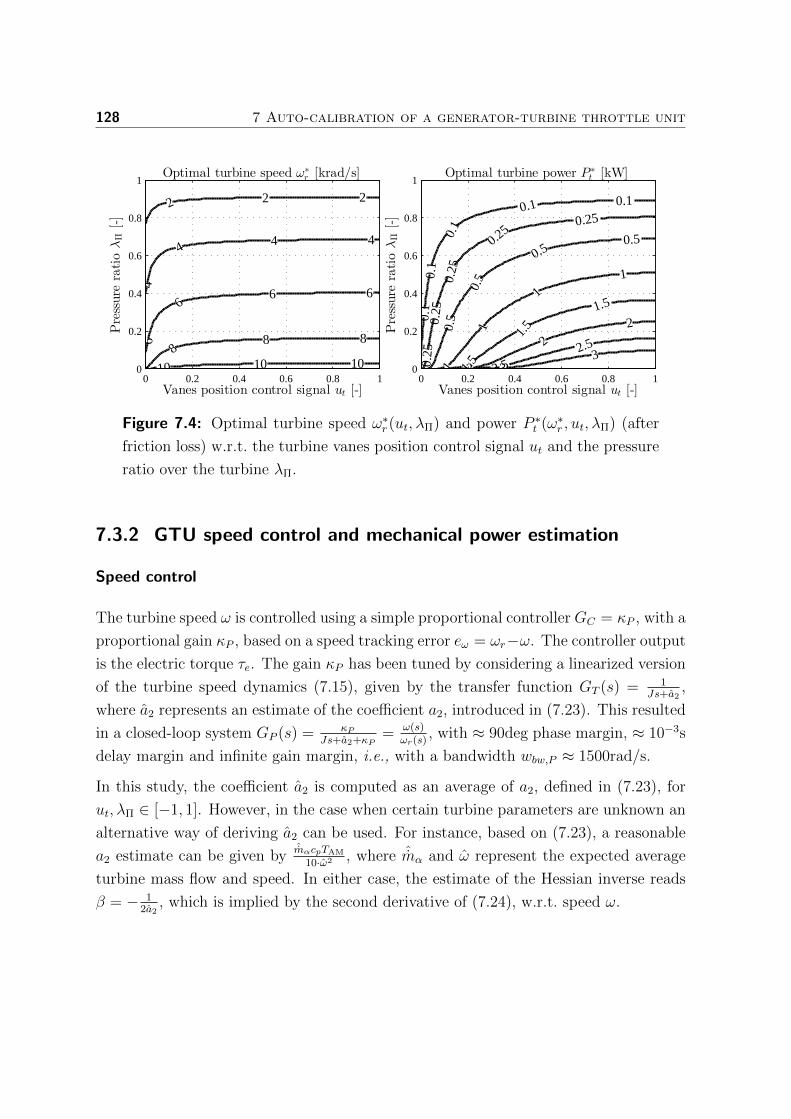
128 7 Auto-calibration of a generator-turbine throttle unit
2 2 2
4
4 4 4
6
66 6
88 8
101010
Vanes position control signal ut [-]
Pressure
ratioλΠ[-]
Optimal turbine speed ω∗
r [krad/s]
0 0.2 0.4 0.6 0.8 10
0.2
0.4
0.6
0.8
1
0.1
0.1
0.1
0.1 0.1
0.25
0.25
0.25
0.25
0.25
0.50.5
0.5
0.5
11
1
1
1.5
1.5
1.5
2
2
2
2.5
2.53
3
Vanes position control signal ut [-]Pressure
ratioλΠ[-]
Optimal turbine power P∗
t [kW]
0 0.2 0.4 0.6 0.8 10
0.2
0.4
0.6
0.8
1
Figure 7.4: Optimal turbine speed ω∗r(ut, λΠ) and power P ∗t (ω∗r , ut, λΠ) (after
friction loss) w.r.t. the turbine vanes position control signal ut and the pressure
ratio over the turbine λΠ.
7.3.2 GTU speed control and mechanical power estimation
Speed control
The turbine speed ω is controlled using a simple proportional controller GC = κP , with a
proportional gain κP , based on a speed tracking error eω = ωr−ω. The controller output
is the electric torque τe. The gain κP has been tuned by considering a linearized version
of the turbine speed dynamics (7.15), given by the transfer function GT (s) = 1Js+a2
,
where a2 represents an estimate of the coefficient a2, introduced in (7.23). This resulted
in a closed-loop system GP (s) = κPJs+a2+κP
= ω(s)ωr(s)
, with ≈ 90deg phase margin, ≈ 10−3s
delay margin and infinite gain margin, i.e., with a bandwidth wbw,P ≈ 1500rad/s.
In this study, the coefficient a2 is computed as an average of a2, defined in (7.23), for
ut, λΠ ∈ [−1, 1]. However, in the case when certain turbine parameters are unknown an
alternative way of deriving a2 can be used. For instance, based on (7.23), a reasonable
a2 estimate can be given byˆmαcpTAM
10·ω2 , where ˆmα and ω represent the expected average
turbine mass flow and speed. In either case, the estimate of the Hessian inverse reads
β = − 12a2
, which is implied by the second derivative of (7.24), w.r.t. speed ω.
7.3 Application of proposed ESC scheme to generator-turbine throttle unitauto-calibration 129
Power estimation
The turbine mechanical power Pt is not measured directly but instead estimated as a
product between the speed ω and the estimated turbine torque τt, which yields
Pt = τtω. (7.28)
The torque τt is obtained by filtering the controller output τe and the speed ω with a
Kalman filter. For this purpose, the following state-space representation of the turbine
speed dynamics (7.15) is used
d
dt
[ω
τt
]=
[0 1
J
0 0
]
︸ ︷︷ ︸Ac
[ω
τt
]+
[1J
0
]
︸︷︷︸Bc
τe + ρ1, (7.29)
ωm =[1 0
]
︸ ︷︷ ︸Cc
[ω
τt
]+ ρ2,
where the signals ρ1 and ρ2 denote white zero-mean state and measurement noise. The
properties of the noise signals, ρ1 and ρ2, are described by their respective covariance
matrices, W1 and W2, which are in this context treated as tuning parameters. The
Kalman filter is implemented using MATLABr kalman routine. This resulted in a
transfer function GK(s) = τt(s)ωr(s)
, from the reference speed ωr to the estimated turbine
torque τt, with a bandwidth of wbw,K ≈ 1530rad/s.
7.3.3 ESC implementation
Optimal input model
The proposed ESC scheme requires that the adopted disturbance-based optimal input
parametrization admits a linear regressor form (7.3). This requirement is fulfilled by
assuming that the optimal turbine speed ω∗r can be sufficiently well approximated by
a multivariate polynomial in q = 2q − 1, of order c and with unknown coefficients θ.
Here q denotes the “normalized” disturbance vector obtained by linearly mapping the
entries of q = [ut, λΠ]T to the interval [−1, 1]. Note that the disturbance normalization
is not strictly necessary. However, it has been observed that such practice improves
the quality of parameter estimation when the regressor functions hi(q), i ∈ 1, . . . , p,p = (l+c)!
l!c!, are chosen as monomial terms of the corresponding multivariate polynomial.
Specifically, for c = 4 and l = 2, they are given by
hi(q) = qD1,i
1 qD2,i
2 , i ∈ 1, . . . , 15, (7.30)
130 7 Auto-calibration of a generator-turbine throttle unit
where the “degree” matrix D reads
D =
[0 0 0 0 0 1 1 1 1 2 2 2 3 3 4
0 1 2 3 4 0 1 2 3 0 1 2 0 1 0
]T. (7.31)
Accordingly, the nominal input u is computed as
u = HT (q)θ. (7.32)
Disturbances
To satisfy both the disturbance derivative (7.6) and the persistence of excitation
condition (7.14) w.r.t. the normalized disturbance q, the signals ut and λΠ are each
specified by filtering a uniform random noise defined on the interval [0, 1], using a low-
pass filter
Gq(s) =ω2q
s2 +√
2ωqs+ ω2q
, (7.33)
with ωq = 12ε1ε2.
To facilitate the necessary timescale separation between the input error estimator and
closed-loop system dynamics, ε1 has been set an order of magnitude smaller than the
lowest bandwidth of GP (s) and GK(s), i.e., ε1 = 115
min(wbw,P , wbw,K) = 100rad/s.
Accordingly, the ε2 was set to 1/15, enforcing further timescale separation between the
disturbances (as well as the parameter estimator) and the error estimator.
7.4 Simulation results
Based on the model (7.15)-(7.21) closed-loop simulations have been conducted to verify
the feasibility of the proposed GTU auto-calibration scheme. Table 7.1 lists the related
system and design parameter values.
Figure 7.5 shows the tracking of the optimal turbine power P ∗t and reference speed ω∗r .
The corresponding turbine vanes position control signal ut and the pressure ratio λΠ are
shown in the plot at the bottom. It can be seen that after an initial transient period,
of approximately 5s, both the power Pt and the reference speed ωr have converged to
their optimal values. This is even more apparent in Fig. 7.6 which depicts the power
and speed errors, P ∗t −Pt and ω∗r − ωr, as both approach zero quickly upon the start of
auto-calibration. By looking at the estimated input parameters θ, shown at the bottom
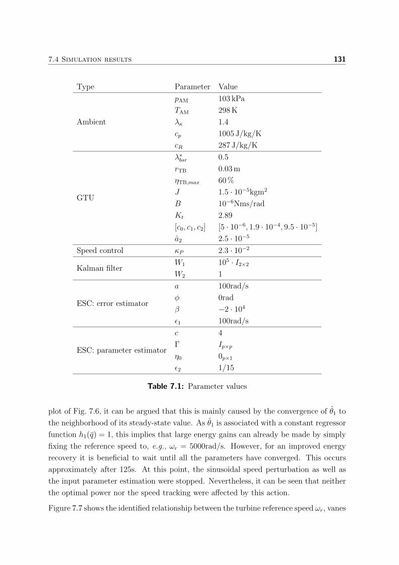
7.4 Simulation results 131
Type Parameter Value
Ambient
pAM 103 kPa
TAM 298 K
λκ 1.4
cp 1005 J/kg/K
cR 287 J/kg/K
GTU
λ∗bsr 0.5
rTB 0.03 m
ηTB,max 60 %
J 1.5 · 10−5kgm2
B 10−6Nms/rad
Kt 2.89
[c0, c1, c2] [5 · 10−6, 1.9 · 10−4, 9.5 · 10−5]
a2 2.5 · 10−5
Speed control κP 2.3 · 10−2
Kalman filterW1 105 · I2×2
W2 1
ESC: error estimator
a 100rad/s
φ 0rad
β −2 · 104
ε1 100rad/s
ESC: parameter estimator
c 4
Γ Ip×p
η0 0p×1
ε2 1/15
Table 7.1: Parameter values
plot of Fig. 7.6, it can be argued that this is mainly caused by the convergence of θ1 to
the neighborhood of its steady-state value. As θ1 is associated with a constant regressor
function h1(q) = 1, this implies that large energy gains can already be made by simply
fixing the reference speed to, e.g., ωr = 5000rad/s. However, for an improved energy
recovery it is beneficial to wait until all the parameters have converged. This occurs
approximately after 125s. At this point, the sinusoidal speed perturbation as well as
the input parameter estimation were stopped. Nevertheless, it can be seen that neither
the optimal power nor the speed tracking were affected by this action.
Figure 7.7 shows the identified relationship between the turbine reference speed ωr, vanes

132 7 Auto-calibration of a generator-turbine throttle unit
0 125 2500
0.2
0.4
0.6
0.8
1
1.2
1.4
1.6Power
[kW]
P ∗
t
Pt
0 125 250
1
2
3
4
5
6
7
8
9
Speed[krad/s]
ω∗
rωr
0 125 2500
0.2
0.4
0.6
0.8
1
Time [s]
Disturbance
[-]
ut
λΠ
Figure 7.5: Tracking of the optimal turbine power P ∗t and reference speed ω∗r .
position control signal ut and pressure ratio λΠ. By comparing Fig. 7.4 and Fig. 7.7 one
can observe that the contour lines corresponding to speeds ωr(ut, λΠ) and ω∗r(ut, λΠ)
follow the same trend but do not match exactly. The discrepancy between the two
can be explained by the following: the adopted optimal speed model (7.32) is different
than the true one (7.26); only the estimate of the input error (7.11) is known; the
performance function Hessian D2Q is approximated by a tunable constant β, whereas
in fact it varies with the disturbance q; the HessianD2Q is relatively small and as a result
the performance function is rather flat near the extremum. This has a negative effect
on the speed and accuracy of the parameter convergence as it renders the performance
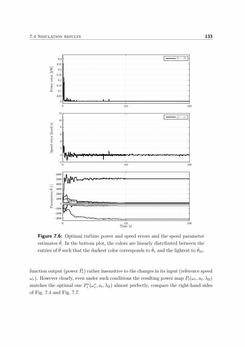
7.4 Simulation results 133
0 125 250
0
0.05
0.1
0.15
0.2
0.25
0.3
0.35
0.4
Pow
ererror[kW]
P ∗
t − Pt
0 125 250−2
0
2
4
6
8
10
12
Speederror[krad/s]
ω∗
r − ωr
0 125 250
−3000
−2000
−1000
0
1000
2000
3000
4000
5000
6000
Time [s]
Parametersθ[-]
Figure 7.6: Optimal turbine power and speed errors and the speed parameter
estimates θ. In the bottom plot, the colors are linearly distributed between the
entries of θ such that the darkest color corresponds to θ1 and the lightest to θ15.
function output (power Pt) rather insensitive to the changes in its input (reference speed
ωr). However clearly, even under such conditions the resulting power map Pt(ωr, ut, λΠ)
matches the optimal one P ∗t (ω∗r , ut, λΠ) almost perfectly, compare the right-hand sides
of Fig. 7.4 and Fig. 7.7.
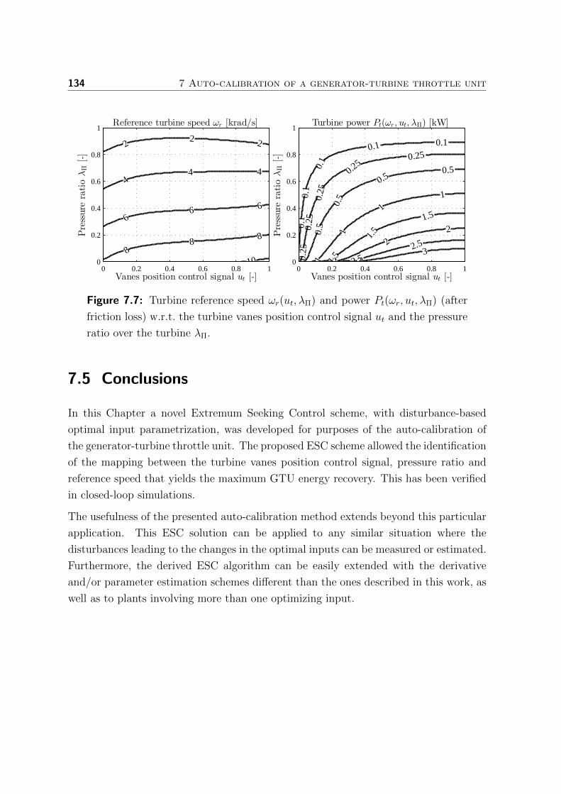
134 7 Auto-calibration of a generator-turbine throttle unit
22 2
44 4
66 6
88
8
10
Vanes position control signal ut [-]
Pressure
ratioλΠ[-]
Reference turbine speed ωr [krad/s]
0 0.2 0.4 0.6 0.8 10
0.2
0.4
0.6
0.8
1
0.1
0.1
0.1
0.1 0.1
0.25
0.25
0.25
0.25
0.25
0.50.5
0.5
0.5
11
1
1
1.5
1.5
1.5
22
2
2.5
2.53
3
Vanes position control signal ut [-]Pressure
ratioλΠ[-]
Turbine power Pt(ωr, ut, λΠ) [kW]
0 0.2 0.4 0.6 0.8 10
0.2
0.4
0.6
0.8
1
Figure 7.7: Turbine reference speed ωr(ut, λΠ) and power Pt(ωr, ut, λΠ) (after
friction loss) w.r.t. the turbine vanes position control signal ut and the pressure
ratio over the turbine λΠ.
7.5 Conclusions
In this Chapter a novel Extremum Seeking Control scheme, with disturbance-based
optimal input parametrization, was developed for purposes of the auto-calibration of
the generator-turbine throttle unit. The proposed ESC scheme allowed the identification
of the mapping between the turbine vanes position control signal, pressure ratio and
reference speed that yields the maximum GTU energy recovery. This has been verified
in closed-loop simulations.
The usefulness of the presented auto-calibration method extends beyond this particular
application. This ESC solution can be applied to any similar situation where the
disturbances leading to the changes in the optimal inputs can be measured or estimated.
Furthermore, the derived ESC algorithm can be easily extended with the derivative
and/or parameter estimation schemes different than the ones described in this work, as
well as to plants involving more than one optimizing input.
Chapter 8
Conclusions and recommendations
Abstract This Chapter dicusses the main conclusions of this thesis and presents certain
recommendations for future directions of research.
8.1 Conclusions
This thesis was set out to obtain deeper understanding of the electric supercharg-
ing, regenerative throttling and Switched Reluctance Machine technologies, from the
perspective of optimization and control. In this context, the following main research
objectives were formulated:
1. Theoretical investigation of methods for evaluating the potential of engine down-
sizing via electric supercharging to improve the vehicle fuel economy.
2. Theoretical investigation of methods for evaluating the potential of regenerative
throttling to improve the vehicle fuel economy.
3. Theoretical investigation of methods for the Switched Reluctance Machine speed
and voltage control, which can alleviate the difficulties posed by the SRM nonlinear
dynamics, tight physical constraints and position/speed sensing requirements.
4. Theoretical investigation of methods for relieving the engineering systems, such as
the generator-turbine throttle unit, from excessive calibration requirements.
The first objective was addressed in Chapter 2, the second in Chapter 3, the third in
Chapters 4 to 6 and the fourth in Chapter 7. The conclusions of each of these chapters
are summarized in the following.
135
136 8 Conclusions and recommendations
The capacity of the electric supercharging to improve the vehicle fuel economy was
investigated in Chapter 2. For this purpose, a detailed model of the electrically
supercharged ICE was derived. The model was used to define a convex optimization
problem considering the minimization of the vehicle operational (fuel) and component
(ICE and electric energy storage buffer) costs. The optimal solution of this problem was
found using state-of-the-art numerical tools, for the case of the WLTP3 driving cycle.
The provided case study has shown that during short-duration high-power demands the
(standalone) electric supercharger can effectively increase the pressure of air supplied to
the engine and thereby considerably rise its maximum torque bound – especially at low
engine speeds. This helps facilitate engine downsizing and reduce the fuel consumption.
Specifically, in the analyzed case, fuel cost savings of up to 10% were obtained.
Chapter 3 addressed the regenerative throttling technology. To this end, a mathematical
model of the gasoline engine powertrain equipped with the generator-turbine throttle
unit was developed. The model was constructed in accordance with the disciplined
convex modeling methodology, for purposes of the convex optimization. In particular,
the considered optimization problem was formulated as the minimization of the total
vehicle operational (fuel) and component (electric buffer) costs. The analysis of the
results, obtained for several different driving cycles (FTP75, WLTP3, NEDC and
VAIL2NREL), has shown that regenerative throttling was the most beneficial for the
case of the VAIL2NREL cycle, which corresponds to high-demand highway driving,
as well as for vehicles equipped with oversized ICEs. In such circumstances, the
regenerative throttling technology offered the possibility to reduce the total costs by
more then 4%.
In Chapter 4, a novel Four-Quadrant (4Q) speed control scheme was developed for
the 4/2 SRM. The proposed algorithm adopted a cascade structure: the outer closed-
loop speed controller computed the desired torque reference and passed it to the inner
open-loop average torque controller (ATC), which then translated the torque command
into the suitable phase current reference pair – for the innermost closed-loop current
controller. For this purpose, a parametric, model-based, open-loop ATC was derived on
the basis of the measured, static electromagnetic SRM characteristics. The 4Q controller
was designed to explicitly handle the identified, speed and voltage-dependent, average
torque bounds, as well as to impose the desired phase current limit. Since the 4/2 SRM
is prone to getting “stuck” near or at one of the phase aligned positions – a supervising
state-machine was also constructed to enable the machine to start/resume operation
in “stuck” situations. The effectiveness of the proposed approach was demonstrated
experimentally, in terms of sinusoidal and block speed reference tracking (under load).
Due to the employed parametrization with the machine operating point, the proposed

8.1 Conclusions 137
4/2 SRM 4Q control scheme can be applied in a wide range of applications, including
electric supercharging and regenerative throttling.
Chapter 5 presented the Switched Reluctance Generator (SRG) voltage control scheme
utilizing the explicit Model-Predictive Control (MPC) methodology. The proposed
voltage controller was intended for high-speed (e.g., 50-100 krpm), low-cost applications,
such as regenerative throttling. Due to these requirements, the SRG was considered to
operate in the Single-Pulse mode, where the turn-on and turn-off commutation angles
were the only current control parameters. Two different commutation angle selection
strategies were derived: the first based on analytic calculations and the second on open-
loop simulations of the relevant SRG dynamics. In the case of the second, the angles were
found by minimizing the peak phase flux-linkage and thus also, indirectly, the SRG iron
loss. Furthermore, the voltage MPC was developed such to keep the average DC-link
current and voltage within their prescribed bounds. This was demonstrated in closed-
loop simulations, which are conducted for the case of the 4/2 SRG. The simulations
have also shown that the designed controller can ensure smooth voltage tracking, in the
presence of both varying load current and rotor speed.
In Chapter 6, a novel position-sensorless speed control scheme was proposed for the
high-speed SRMs. The main component of the presented design was the nonlinear
speed/position observer which relied solely on the DC-link voltage and current measure-
ments, whereas the measurements of phase voltage, current, rotor position and speed
were not used. Due to fewer sensors required, the derived speed control algorithm
can help reduce the associated hardware costs and increase the reliability of the SRM
electrical system. The developed control algorithm has shown good speed tracking
performance, even in the presence of load torque disturbances. This was demonstrated
in closed-loop simulations.
Finally, Chapter 7 treated the development of a real-time optimization and control
method for the auto-calibration of the turbine-driven generator, used for regenerative
throttling purposes. The proposed method utilized a novel Extremum Seeking Control
(ESC) scheme with a disturbance-based optimal input parametrization. The ESC was
designed to enable tracking of a varying, unknown extremum of a dynamical plant,
under the assumption that the disturbances leading to changes in the optimal input are
known/measurable. In the considered application, the derived ESC scheme allowed
the identification of the mapping between the disturbances, i.e., the turbine vanes
position signal and pressure ratio, and the optimal input, i.e., the turbine reference
speed which maximizes the turbine-driven generator power output. Simulation results
were presented to verify the effectiveness of the derived auto-calibration scheme.
138 8 Conclusions and recommendations
8.2 Recommendations for future research
In control engineering, especially when dealing with real physical systems, it is fairly
common to adopt a series of modeling approximations, as well as simplifying assump-
tions, to arrive with a practically useful control solution. Furthermore, while performing
state-of-the-art research on a certain topic, some questions might remain partly or
even completely unanswered. However, this often represents a good starting point for
further scientific investigations. In this context, the remainder of this section provides
an overview of the recommended directions for future research, based on the insights
obtained during the work conducted on this thesis.
In Chapter 2 it was shown how to scale the electric energy storage buffer as well as the
engine displacement volume, in the case of the electrically supercharged ICE vehicle
powertrain. This research could be extended in at least two different directions. The
first would be to consider also the sizing of the vehicle alternator and gearbox, so
that they match the downsized engine and electric supercharger more precisely. The
second would be to evaluate the investigated powertrain concept on a more-demanding
driving cycle, or a few of them, consisting of prolonged high-load intervals. To this end,
it could be beneficial to also adapt the developed convex modeling and optimization
method towards an electrified turbocharger powertrain topology.
The regenerative throttling study, described in Chapter 3, could also be extended
to include the alternator sizing. Potentially, this could bring further fuel economy
benefits, as a consequence of the reduced alternator weight/cost. Moreover, due to its
convex properties, the proposed optimization algorithm (excluding the electric buffer
sizing part) could also be applied for online vehicle state/control prediction purposes.
However, as this inherently implies the use of driving cycle estimates, the fuel-economy
improvements might be lower. The analysis of the cooling potential of the regenerative
throttling, within the same, convex framework, constitutes yet another topic for future
research.
In Chapter 4, the cascaded 4/2 SRM 4Q speed control scheme was proposed, which
employed a novel open-loop average torque controller (ATC). The ATC was derived
using the measured, static SRM electromagnetic characteristics. To compensate for the
inevitable modeling errors, the first direction of research could be to extend the proposed
ATC towards parametric, closed-loop ATC. Second, the performance of the innermost
current control loop could be improved by means of a model-based feedforward control.
The feedforward controller could be derived based on the knowledge of the SRM phase
current dynamics and the employed commutation strategy. The third direction of
8.2 Recommendations for future research 139
research could be to replace the expensive, high-resolution encoder, with a cheap, low-
resolution one (1-2 pulses per rotation), e.g., to enable event-triggered 4/2 SRM 4Q
speed control.
Chapter 5 concerned the development of the SRG explicit voltage MPC. The controller
choice was motivated by its straightforward ability to enforce the constant, average DC-
link voltage and current bounds. However, to increase the control system performance
and extend the machine operating range, one could consider identifying and imposing
varying DC-link current constraints instead. This could be achieved, e.g., via an online
Nonlinear Model Predictive Control. Furthermore, the PWM current control could also
be employed to allow the SRG to operate at low rotor speeds. Naturally, experimental
validation of the proposed solution is of interest as well.
In Chapter 6, the position-sensorless SRM speed controller was described. The
developed closed-loop controller required that the SRM is brought to a sufficiently high
speed before being engaged. In the absence of an external rotor torque, this implies
the need for a dedicated SRM startup procedure. Its development, as well as the
experimental verification of the complete solution, could be a topic for future research.
Chapter 7 considered the auto-calibration of the generator-turbine throttle unit. For this
purpose, the optimal turbine reference speed was modeled as a multivariate polynomial
in the turbine vanes position signal and pressure ratio. Although simple to implement,
this model/basis choice is almost certainly not optimal. Therefore, the first extension
of this work could be to improve the parametrization of the turbine optimal reference
speed (e.g., using the obtained analytical insights), yielding a more accurate/faster
parameter convergence. The second extension could treat the design of the auto-
calibration experiment, i.e., of the mechanism for generation of suitable disturbance
inputs (such as the turbine pressure ratio). The third extension could focus on the
analysis and generalization of the underlying ESC scheme, e.g., by considering other
parameter/derivative estimators, neural networks, etc.
Finally, as a step towards further integration of the presented research topics, the
developed ESC algorithm could also be utilized for the SRM real-time tuning purposes,
e.g., to minimize the acoustic noise, torque ripple and/or energy losses. In such cases, the
ESC disturbances could be interpreted as the signals defining the SRM operating point,
whereas the commutation angles, or any other suitable low-level controller parameters,
could be selected as the ESC optimizing inputs.

140
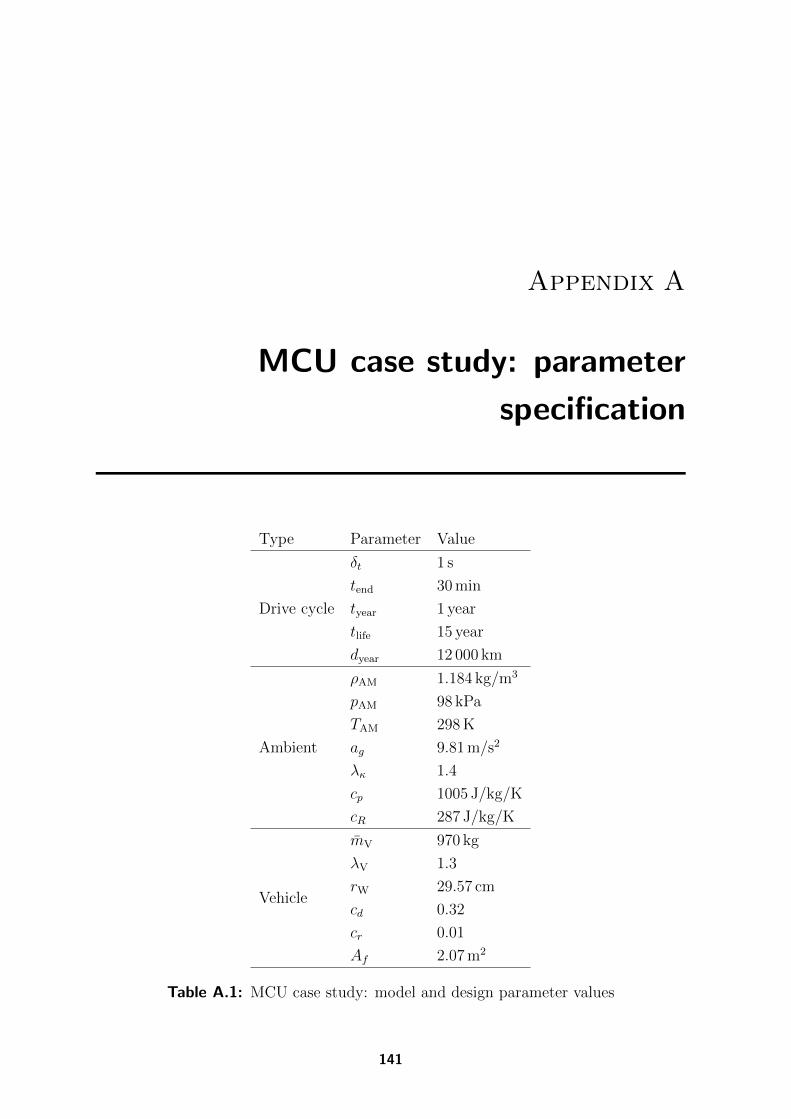
Appendix A
MCU case study: parameter
specification
Type Parameter Value
Drive cycle
δt 1 s
tend 30 min
tyear 1 year
tlife 15 year
dyear 12 000 km
Ambient
ρAM 1.184 kg/m3
pAM 98 kPa
TAM 298 K
ag 9.81 m/s2
λκ 1.4
cp 1005 J/kg/K
cR 287 J/kg/K
Vehicle
mV 970 kg
λV 1.3
rW 29.57 cm
cd 0.32
cr 0.01
Af 2.07 m2
Table A.1: MCU case study: model and design parameter values
141
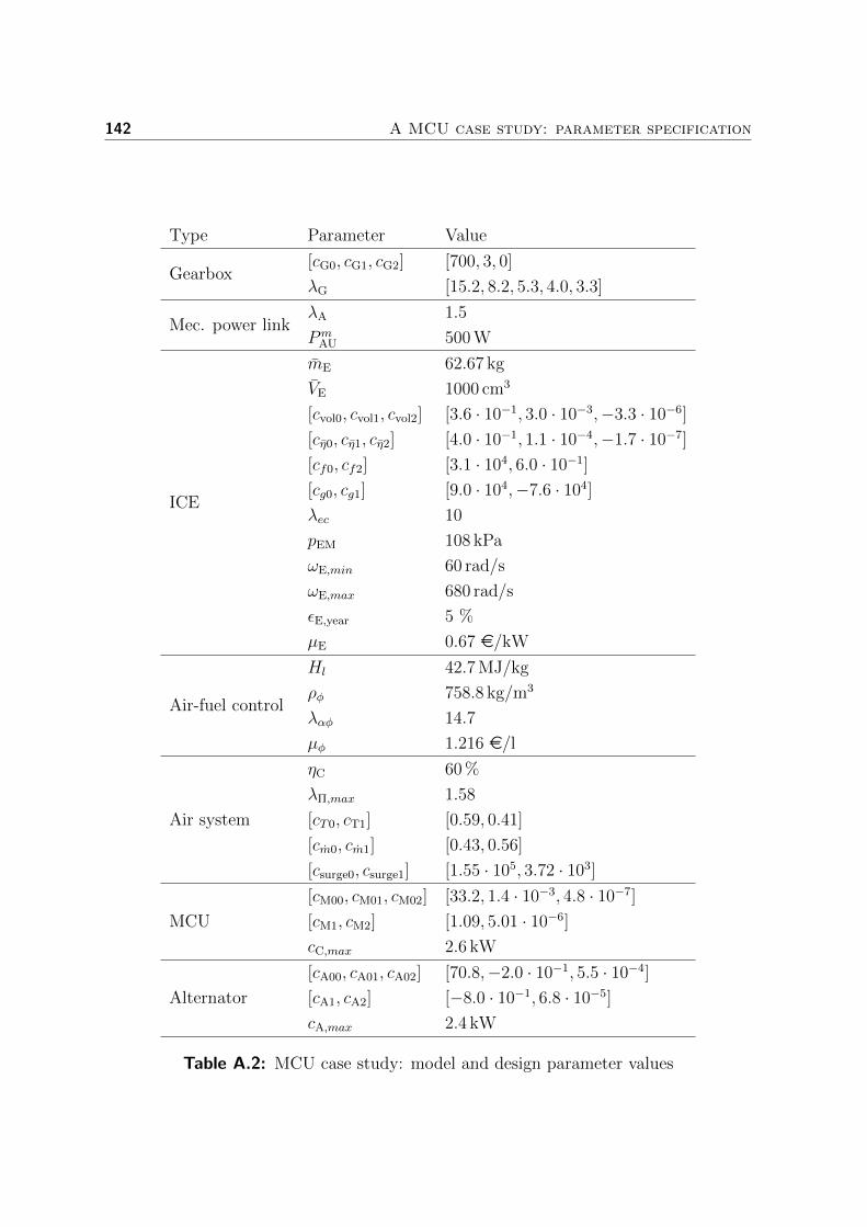
142 A MCU case study: parameter specification
Type Parameter Value
Gearbox[cG0, cG1, cG2] [700, 3, 0]
λG [15.2, 8.2, 5.3, 4.0, 3.3]
Mec. power linkλA 1.5
PmAU 500 W
ICE
mE 62.67 kg
VE 1000 cm3
[cvol0, cvol1, cvol2] [3.6 · 10−1, 3.0 · 10−3,−3.3 · 10−6]
[cη0, cη1, cη2] [4.0 · 10−1, 1.1 · 10−4,−1.7 · 10−7]
[cf0, cf2] [3.1 · 104, 6.0 · 10−1]
[cg0, cg1] [9.0 · 104,−7.6 · 104]
λec 10
pEM 108 kPa
ωE,min 60 rad/s
ωE,max 680 rad/s
εE,year 5 %
µE 0.67 e/kW
Air-fuel control
Hl 42.7 MJ/kg
ρφ 758.8 kg/m3
λαφ 14.7
µφ 1.216 e/l
Air system
ηC 60 %
λΠ,max 1.58
[cT0, cT1] [0.59, 0.41]
[cm0, cm1] [0.43, 0.56]
[csurge0, csurge1] [1.55 · 105, 3.72 · 103]
MCU
[cM00, cM01, cM02] [33.2, 1.4 · 10−3, 4.8 · 10−7]
[cM1, cM2] [1.09, 5.01 · 10−6]
cC,max 2.6 kW
Alternator
[cA00, cA01, cA02] [70.8,−2.0 · 10−1, 5.5 · 10−4]
[cA1, cA2] [−8.0 · 10−1, 6.8 · 10−5]
cA,max 2.4 kW
Table A.2: MCU case study: model and design parameter values

143
Type Parameter Value
El. power link P eAU 300 W
Battery
nB 4
mc 80 g
Qc 2.3 Ah
cc0 3.27 V
cc1 58 kF
Rc 11.5 mΩ
ic,min/max ∓35 A
socmin/max 20, 80%
εB,year 5 %
µB 500 e/kWh
Table A.3: MCU case study: model and design parameter values

144

Appendix B
GTU case study: parameter
specification
Type Parameter Value
Drive cycle
δt 2 s
tyear 1 year
tlife 8 year
dyear 12 000 km
Ambient
ρAM 1.184 kg/m3
pAM 103 kPa
TAM 298 K
ag 9.81 m/s2
λκ 1.4
cp 1005 J/kg/K
cR 287 J/kg/K
Vehicle
mV 970 kg
λV 1.3
rW 29.57 cm
cd 0.32
cr 0.01
Af 2.07 m2
Table B.1: GTU case study: model and design parameter values
145
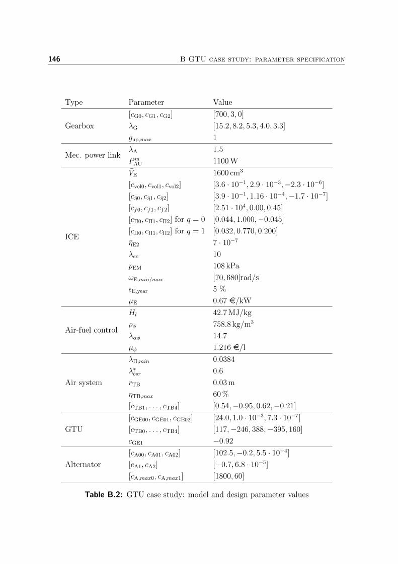
146 B GTU case study: parameter specification
Type Parameter Value
Gearbox
[cG0, cG1, cG2] [700, 3, 0]
λG [15.2, 8.2, 5.3, 4.0, 3.3]
gup,max 1
Mec. power linkλA 1.5
PmAU 1100 W
ICE
VE 1600 cm3
[cvol0, cvol1, cvol2] [3.6 · 10−1, 2.9 · 10−3,−2.3 · 10−6]
[cη0, cη1, cη2] [3.9 · 10−1, 1.16 · 10−4,−1.7 · 10−7]
[cf0, cf1, cf2] [2.51 · 104, 0.00, 0.45]
[cΠ0, cΠ1, cΠ2] for q = 0 [0.044, 1.000,−0.045]
[cΠ0, cΠ1, cΠ2] for q = 1 [0.032, 0.770, 0.200]
ηE2 7 · 10−7
λec 10
pEM 108 kPa
ωE,min/max [70, 680]rad/s
εE,year 5 %
µE 0.67 e/kW
Air-fuel control
Hl 42.7 MJ/kg
ρφ 758.8 kg/m3
λαφ 14.7
µφ 1.216 e/l
Air system
λΠ,min 0.0384
λ∗bsr 0.6
rTB 0.03 m
ηTB,max 60 %
[cTB1, . . . , cTB4] [0.54,−0.95, 0.62,−0.21]
GTU
[cGE00, cGE01, cGE02] [24.0, 1.0 · 10−3, 7.3 · 10−7]
[cTB0, . . . , cTB4] [117,−246, 388,−395, 160]
cGE1 −0.92
Alternator
[cA00, cA01, cA02] [102.5,−0.2, 5.5 · 10−4]
[cA1, cA2] [−0.7, 6.8 · 10−5]
[cA,max0, cA,max1] [1800, 60]
Table B.2: GTU case study: model and design parameter values
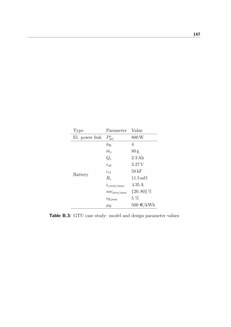
147
Type Parameter Value
El. power link P eAU 800 W
Battery
nB 4
mc 80 g
Qc 2.3 Ah
cc0 3.27 V
cc1 58 kF
Rc 11.5 mΩ
ic,min/max ∓35 A
socmin/max 20, 80%
εB,year 5 %
µB 500 e/kWh
Table B.3: GTU case study: model and design parameter values

148

Appendix C
SRM advance angle scheduling signal
The finite difference approximation of (4.1) and (4.2) yields
∆ip ≈∆t
Lp(ip, θ)(vp −Rpip −Mp(ip, θ)ω), (C.1)
∆θ ≈ ω∆t.
By neglecting the Ohmic losses and the back e.m.f. term, it follows
∆ip ≈vp∆θ
ωLp(ip, θ). (C.2)
Then by setting |vp| = vdc and |∆ip| = i∗,
∆θ ∼ i∗ω
vdc∼ i∗
imax
ω
ωmax
vdc,minvdc
=: q. (C.3)
In the context of commutation, ∆θ can be interpreted as the required change in
duration/start of the active phase interval (by means of commutation angle advance)
needed to compensate for the change in the variable q. This motivates the use of q as
the advance angle scheduling signal.
149

150
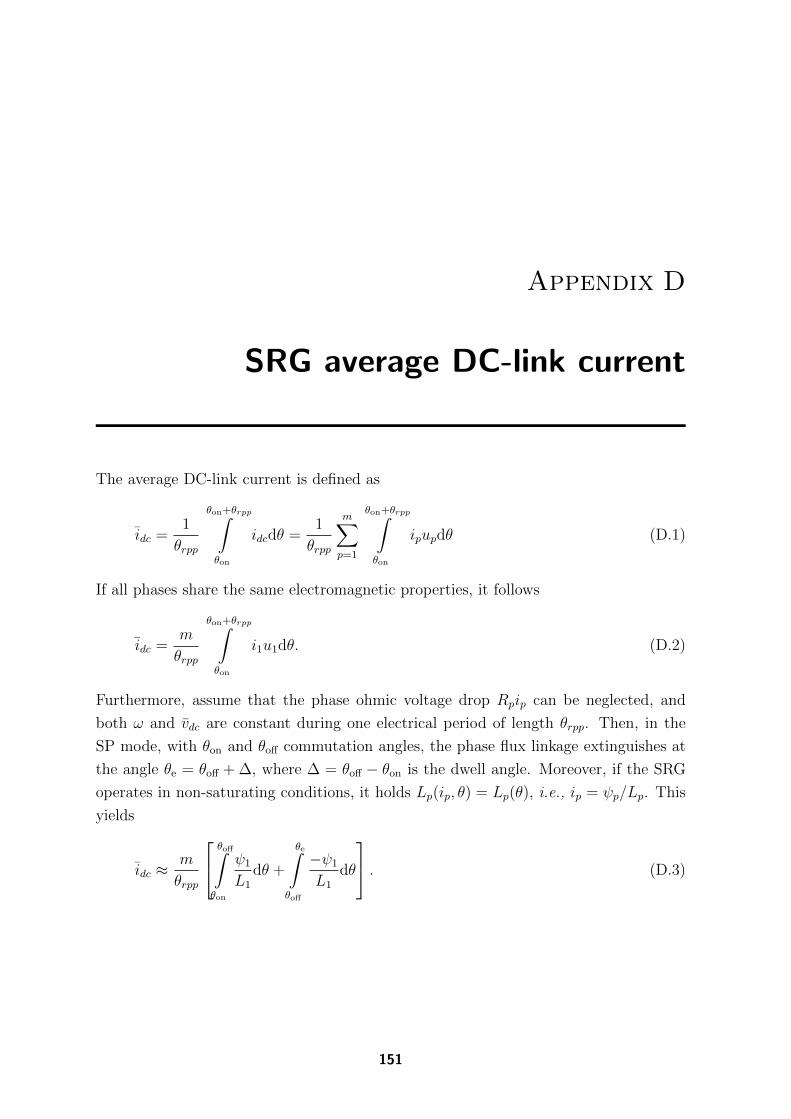
Appendix D
SRG average DC-link current
The average DC-link current is defined as
idc =1
θrpp
θon+θrpp∫
θon
idcdθ =1
θrpp
m∑
p=1
θon+θrpp∫
θon
ipupdθ (D.1)
If all phases share the same electromagnetic properties, it follows
idc =m
θrpp
θon+θrpp∫
θon
i1u1dθ. (D.2)
Furthermore, assume that the phase ohmic voltage drop Rpip can be neglected, and
both ω and vdc are constant during one electrical period of length θrpp. Then, in the
SP mode, with θon and θoff commutation angles, the phase flux linkage extinguishes at
the angle θe = θoff + ∆, where ∆ = θoff − θon is the dwell angle. Moreover, if the SRG
operates in non-saturating conditions, it holds Lp(ip, θ) = Lp(θ), i.e., ip = ψp/Lp. This
yields
idc ≈m
θrpp
θoff∫
θon
ψ1
L1
dθ +
θe∫
θoff
−ψ1
L1
dθ
. (D.3)
151
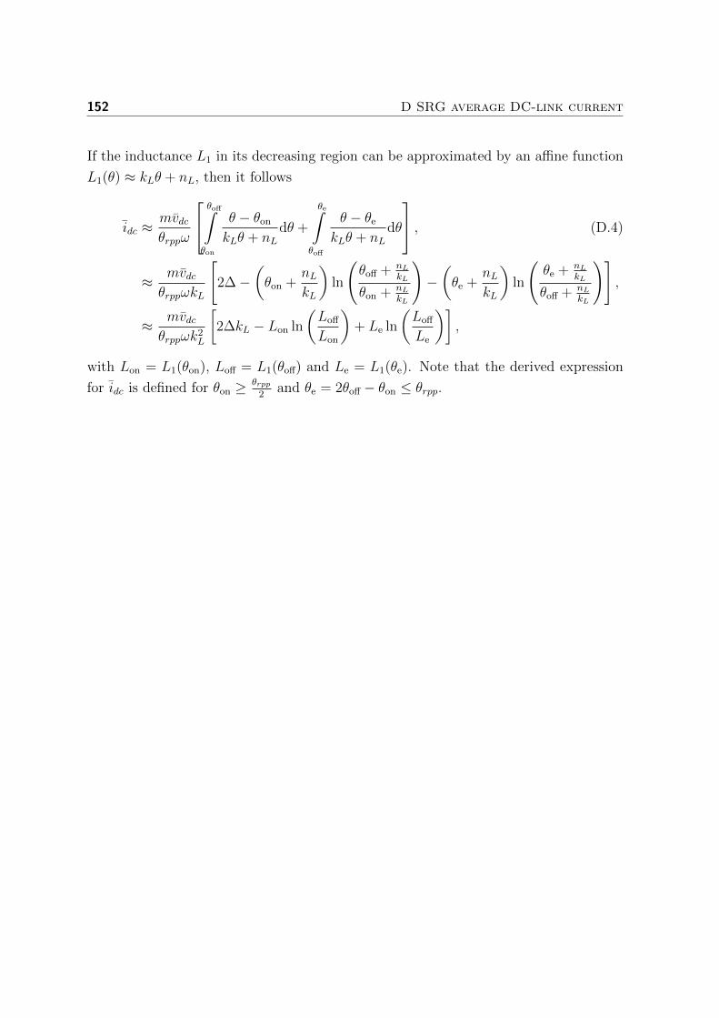
152 D SRG average DC-link current
If the inductance L1 in its decreasing region can be approximated by an affine function
L1(θ) ≈ kLθ + nL, then it follows
idc ≈mvdcθrppω
θoff∫
θon
θ − θon
kLθ + nLdθ +
θe∫
θoff
θ − θe
kLθ + nLdθ
, (D.4)
≈ mvdcθrppωkL
[2∆−
(θon +
nLkL
)ln
(θoff + nL
kL
θon + nLkL
)−(θe +
nLkL
)ln
(θe + nL
kL
θoff + nLkL
)],
≈ mvdcθrppωk2
L
[2∆kL − Lon ln
(Loff
Lon
)+ Le ln
(Loff
Le
)],
with Lon = L1(θon), Loff = L1(θoff) and Le = L1(θe). Note that the derived expression
for idc is defined for θon ≥ θrpp2
and θe = 2θoff − θon ≤ θrpp.
Bibliography
[1] “World population prospects: the 2012 revision,” United Nations: Department
of Economic and Social Affairs, Tech. Rep., 2013.
[2] D. Pimentel and M. Pimentel, “Global environmental resources versus world
population growth,” Ecological Economics, vol. 59, no. 2, pp. 195–198, 2006.
[3] B. Raj and O. Singh, “Global trends of fossil fuel reserves and climate change in
the 21st century,” in Fossil Fuel and the Environment, InTech, 2012, pp. 167–192.
[4] “Climate change 2014: impacts, adaptation, and vulnerability,” Intergovernmen-
tal Panel on Climate Change, Tech. Rep., 2014.
[5] M. H. Huesemann, “Can pollution problems be effectively solved by environ-
mental science and technology? An analysis of critical limitations,” Ecological
Economics, vol. 37, no. 2, pp. 271–287, 2001.
[6] P. Moriarty and D. Honnery, “Mitigating greenhouse: limited time, limited
options,” Energy Policy, vol. 36, no. 4, pp. 1251–1256, 2008.
[7] “Energy = future: think efficiency,” American Physical Society, Tech. Rep., 2008.
[8] “European Union emission inventory report 1990-2013 under the UNECE con-
vention on long-range transboundary air pollution (LRTAP),” European Envi-
ronment Agency, Tech. Rep., 2014.
[9] B. Lequesne, “Automotive electrification: the nonhybrid story,” IEEE Transac-
tions on Transportation Electrification, vol. 1, no. 1, pp. 40–53, 2015.
[10] “European vehicle market statistics: pocketbook 2014,” The International Coun-
cil on Clean Transportation, Tech. Rep., 2014.
[11] M. Broy, I. H. Kruger, A. Pretschner, and C. Salzmann, “Engineering automotive
software,” Proceedings of the IEEE, vol. 95, no. 2, pp. 356–373, 2007.
153
154 Bibliography
[12] P. Leduc, B. Dubar, A. Ranini, and G. Monnier, “Downsizing of gasoline engine:
an efficient way to reduce CO2 emissions,” Oil & Gas Science and Technology,
vol. 58, no. 1, pp. 115–127, 2003.
[13] B. An, S. Hiroshi, M. Ebisu, and H. Tanaka, “Development of two-stage tur-
bocharger system with electric supercharger,” in Proceedings of the FISITA
2012 World Automotive Congress, ser. Lecture Notes in Electrical Engineering,
vol. 192, Springer Berlin Heidelberg, 2013, pp. 147–155.
[14] T. Noguchi and M. Kano, “Development of 150000 r/min, 1.5 kW permanent-
magnet motor for automotive supercharger,” in 2007 7th International Confer-
ence on Power Electronics and Drive Systems, IEEE, 2007, pp. 183–188.
[15] Y. Niwa, T. Naruta, and Y. Akiyama, “Research and development of the elec-
tric supercharger for minivehicles,” 2008 International Conference on Electrical
Machines and Systems, pp. 3518–3521, 2008.
[16] J. Villegas, B. Gao, K. Svancara, W. Thornton, and J. Parra, “Real-time
simulation and control of an electric supercharger for engine downsizing,” in
2011 IEEE Vehicle Power and Propulsion Conference, IEEE, 2011, pp. 1–6.
[17] N. Chayopitak, R. Pupadubsin, S. Karukanan, and P. Champa, “Design of a
1.5 kW high speed switched reluctance motor for electric supercharger with
optimal performance assessment,” in 15th International Conference on Electrical
Machines and Systems, Sapporo: IEEE, 2012, pp. 1 –5.
[18] S. Kachapornkul, P. Somsiri, R. Pupadubsin, and N. Nulek, “Low cost high
speed switched reluctance motor drive for supercharger applications,” in 15th
International Conference on Electrical Machines and Systems, Sapporo: IEEE,
2012, pp. 1 –6.
[19] N. Fraser, H. Blaxill, G. Lumsden, and M. Bassett, “Challenges for increased
efficiency through gasoline engine downsizing,” SAE International Journal of
Engines, vol. 2, no. 1, pp. 2009–01–1053, 2009.
[20] L. Eriksson, T. Lindell, O. Leufven, and A. Thomasson, “Scalable component-
based modeling for optimizing engines with supercharging, e-boost and tur-
bocompound concepts,” SAE International Journal of Engines, vol. 5, no. 2,
pp. 2012–01–0713, 2012.
[21] H. Zhao, “Overview of gasoline direct injection engines,” in Advanced Direct
Injection Combustion Engine Technologies and Development, Elsevier, 2010,
pp. 1–19.
Bibliography 155
[22] P. G. Szymkowicz, Using exhaust gas recirculation (EGR) in spark-ignition
engines to lower NOx emissions and improve fuel consumption. University of
Michigan–Dearborn, 1988.
[23] T. Ahmad and M. A. Theobald, A survey of variable-valve-actuation technology.
Society of Automotive Engineers, 1989.
[24] S. Hara, S. Suga, S. Watanabe, and M. Nakamura, “Variable valve actuation
systems for environmentally friendly engines,” Hitachi Review, vol. 58, no. 7,
pp. 319–324, 2009.
[25] R. Eichhorn, M. Boot, and C. Luijten, “Waste energy driven air conditioning
system (WEDACS),” SAE International Journal of Engines, vol. 2, no. 2,
pp. 477–492, 2009.
[26] L. Guzzella, M. Betschart, T. Fluri, R. De Santis, C. Onder, and T. Auckenthaler,
“Recuperative throttling of SI engines for improved fuel economy,” in SAE 2004
World Congress & Exhibition, 2004.
[27] D. Whaley, W. Soong, and N. Ertugrul, “Extracting more power from the Lundell
car alternator,” in Australasian Universities Power Engineering Conference,
Brisbane, Queensland: IEEE, 2004, pp. 1–6.
[28] R. Ivankovic, J. Cros, M. Taghizadeh, C. A., and P. Viarouge, “Power electronic
solutions to improve the performance of Lundell automotive alternators,” in New
Advances in Vehicular Technology and Automotive Engineering, InTech, 2012,
ch. 6.
[29] R. Krishnan, “Application considerations and applications,” in Switched Reluc-
tance Motor Drives - Modeling, Simulation, Analysis, Design, and Applications,
CRC Press, 2001.
[30] L. Day and I. McNeil, Biographical Dictionary of the History of Technology.
Taylor & Francis, 2003, p. 864.
[31] S. Nasar, “D.C.-switched reluctance motor,” Proceedings of the Institution of
Electrical Engineers, vol. 116, no. 6, pp. 1048–1049, 1969.
[32] R. Krishnan, “Principle of operation of the switched reluctance motor,” in
Switched Reluctance Motor Drives - Modeling, Simulation, Analysis, Design, and
Applications, CRC Press, 2001.
[33] “The rare-earth elements – vital to modern technologies and lifestyles,” U.S.
Geological Survey, Tech. Rep., 2004.

156 Bibliography
[34] N. Haque, A. Hughes, S. Lim, and C. Vernon, “Rare earth elements: overview of
mining, mineralogy, uses, sustainability and environmental impact,” Resources,
vol. 3, no. 4, pp. 614–635, 2014.
[35] A. Borisavljevic, Limits, Modeling and Design of High-Speed Permanent Magnet
Machines, ser. Springer Theses. Springer Berlin Heidelberg, 2013.
[36] “Rare earth elements: critical resources for high technology,” U.S. Geological
Survey, Tech. Rep., 2002, p. 4.
[37] L. Hook, “China tightens grip on output of rare earths,” Financial Times, 2010.
[38] S. M. Shahed and K.-H. Bauer, “Parametric studies of the impact of turbocharg-
ing on gasoline engine downsizing,” SAE International Journal of Engines, vol.
2, no. 1, pp. 2009–01–1472, 2009.
[39] J. Wang, Z. Xia, and D. Howe, “Three-phase modular permanent magnet
brushless machine for torque boosting on a downsized ICE vehicle,” IEEE
Transactions on Vehicular Technology, vol. 54, no. 3, pp. 809–816, 2005.
[40] Jiabin Wang, B. Taylor, Zhigang Sun, and D. Howe, “Experimental character-
ization of a supercapacitor-based electrical torque-boost system for downsized
ICE vehicles,” IEEE Transactions on Vehicular Technology, vol. 56, no. 6,
pp. 3674–3681, 2007.
[41] A. Lefebvre and S. Guilain, “Modelling and measurement of the transient
response of a turbocharged SI engine,” SAE Technical Paper 2005-01-0691, 2005.
[42] D. Assanis, G. Delagrammatikas, R. Fellini, Z. Filipi, J. Liedtke, N. Michelena,
P. Papalambros, D. Reyes, D. Rosenbaum, A. Sales, and M. Sasena, “An
optimization approach to hybrid electric propulsion system design,” Journal
of Mechanics of Structures and Machines, Automotive Research Center Special
Edition, vol. 27, no. 4, pp. 393–421, 1999.
[43] V. Galdi, L. Ippolito, A. Piccolo, and A. Vaccaro, “A genetic-based methodology
for hybrid electric vehicle sizing,” Soft Computing - A Fusion of Foundations,
Methodologies and Applications, vol. 5, no. 6, pp. 451–457, 2001.
[44] L. Wu, Y. Wang, X. Yuan, and Z. Chen, “Multiobjective optimization of
HEV fuel economy and emissions using the self-adaptive differential evolution
algorithm,” IEEE Transactions on Vehicular Technology, vol. 60, no. 6, pp. 2458–
2470, 2011.
[45] H. Fathy, P. Papalambros, and A. Ulsoy, “On combined plant and control
optimization,” in 8th Cairo University International Conference on Mechanical
Design and Production, Cairo University, 2004.
Bibliography 157
[46] D. L. Peters, P. Y. Papalambros, and A. G. Ulsoy, “Sequential co-design of an
artifact and its controller via control proxy functions,” Mechatronics, vol. 23, no.
4, pp. 409–418, 2013.
[47] T. Nuesch, P. Elbert, M. Flankl, C. Onder, and L. Guzzella, “Convex optimiza-
tion for the energy management of hybrid electric vehicles considering engine
start and gearshift costs,” Energies, vol. 7, no. 2, pp. 834–856, 2014.
[48] J. A. Reyer and P. Y. Papalambros, “Combined optimal design and control with
application to an electric DC motor,” Journal of Mechanical Design, vol. 142,
no. 2, pp. 183–191, 2002.
[49] E. Tara, S. Shahidinejad, S. Filizadeh, and E. Bibeau, “Battery storage sizing
in a retrofitted plug-in hybrid electric vehicle,” IEEE Transactions on Vehicular
Technology, vol. 59, no. 6, pp. 2786–2794, 2010.
[50] Z. Filipi, L. Louca, B. Daran, C.-C. Lin, U. Yildir, B. Wu, M. Kokkolaras,
D. Assanis, H. Peng, P. Papalambros, J. Stein, D. Szkubiel, and R. Chapp,
“Combined optimisation of design and power management of the hydraulic
hybrid propulsion systems for the 6 x 6 medium truck,” International Journal of
Heavy Vehicle Systems, vol. 11, no. 3, pp. 372–402, 2004.
[51] M. Kim and H. Peng, “Power management and design optimization of fuel
cell/battery hybrid vehicles,” Journal of Power Sources, vol. 165, no. 2, pp. 819–
832, 2007.
[52] O. Sundstrom, L. Guzzella, and P. Soltic, “Torque-assist hybrid electric power-
train sizing: from optimal control towards a sizing law,” IEEE Transactions on
Control Systems Technology, vol. 18, no. 4, pp. 837–849, 2010.
[53] S. Boyd and L. Vandenberghe, Convex Optimization. Cambridge University
Press, 2004.
[54] B. de Jager, “Predictive storage control for a class of power conversion systems,”
in Proceedings of European Control Conference, Cambridge, UK, 2003.
[55] L. Guzzella and C. H. Onder, Introduction to Modeling and Control of Internal
Combustion Engine Systems. Springer-Verlag Berlin Heidelberg, 2010.
[56] B. de Jager, T. van Keulen, and J. Kessels, Optimal Control of Hybrid Vehicles.
Springer London, 2013, p. 142.
[57] L. Guzzella and A. Sciarretta, Vehicle Propulsion Systems. Springer-Verlag
Berlin Heidelberg, 2013.

158 Bibliography
[58] B. Egardt, N. Murgovski, M. Pourabdollah, and L. Johannesson, “Electromo-
bility studies based on convex optimization: Design and control issues regarding
vehicle electrification,” IEEE Control Systems Magazine, vol. 34, no. 2, pp. 32–49,
2014.
[59] M. Pourabdollah, N. Murgovski, A. Grauers, and B. Egardt, “Optimal sizing of
a parallel PHEV powertrain,” IEEE Transactions on Vehicular Technology, vol.
62, no. 6, pp. 2469–2480, 2013.
[60] N. Murgovski, L. Johannesson, X. Hu, B. Egardt, and J. Sjoberg, “Convex
relaxations in the optimal control of electrified vehicles,” in American Control
Conference, Chicago, USA, 2015.
[61] M. Grant and S. Boyd, CVX: Matlab software for disciplined convex program-
ming, version 2.1, 2014.
[62] ——, “Graph implementations for nonsmooth convex programs,” in Recent
Advances in Learning and Control, London: Springer London, 2008, pp. 95–110.
[63] K. C. Toh, M. J. Todd, and R. H. Tutuncu, “SDPT3 – a matlab software
package for semidefinite programming,” Optimization Methods and Software, vol.
11, pp. 545–581, 1999.
[64] M. Pourabdollah, N. Murgovski, A. Grauers, and B. Egardt, “An iterative
dynamic programming/convex optimization procedure for optimal sizing and
energy management of PHEVs,” in IFAC World Congress, Cape Town, South
Africa, 2014, pp. 6606–6611.
[65] V. Ngo, T. Hofman, M. Steinbuch, and A. Serrarens, “Optimal control of the
gearshift command for hybrid electric vehicles,” IEEE Transactions on Vehicular
Technology, vol. 61, no. 8, pp. 3531–3543, 2012.
[66] M. Michon, S. Calverley, R. Clark, D. Howe, J. Chambers, P. Sykes, P. Dickinson,
M. Clelland, G. Johnstone, R. Quinn, and G. Morris, “Modelling and testing of a
turbo-generator system for exhaust gas energy recovery,” in 2007 IEEE Vehicle
Power and Propulsion Conference, IEEE, 2007, pp. 544–550.
[67] M. Michon, S. D. Calverley, and K. Atallah, “Operating strategies of switched re-
luctance machines for exhaust gas energy recovery systems,” IEEE Transactions
on Industry Applications, vol. 48, no. 5, pp. 1478–1486, 2012.
[68] I. Briggs, G. McCullough, S. Spence, R. Douglas, R. O’Shaughnessy, A. Hanna,
C. Rouaud, and R. Seaman, “Waste heat recovery on a diesel-electric hybrid bus
using a turbogenerator,” in SAE 2012 Commercial Vehicle Engineering Congress,
2012.
Bibliography 159
[69] F. Crescimbini, A. Lidozzi, G. Lo Calzo, and L. Solero, “High-speed electric drive
for exhaust gas energy recovery applications,” IEEE Transactions on Industrial
Electronics, vol. 61, no. 6, pp. 2998–3011, 2014.
[70] M. Liermann, “Backward simulation - a tool for designing more efficient mecha-
tronic systems,” in Proceedings of the 9th International MODELICA Conference,
Munich, 2012, pp. 867–876.
[71] M. Grant, S. Boyd, and Y. Ye, “Disciplined convex programming,” in Global
Optimization, ser. Nonconvex Optimization and Its Applications, L. Liberti and
N. Maculan, Eds., vol. 84, Boston: Kluwer Academic Publishers, 2006, pp. 155–
210.
[72] P. Moraal and I. Kolmanovsky, “Turbocharger modeling for automotive control
applications,” in SAE Technical Paper 1999-01-0908, 1999.
[73] J. Serrano, F. Arnau, V. Dolz, A. Tiseira, and C. Cervello, “A model of tur-
bocharger radial turbines appropriate to be used in zero- and one-dimensional gas
dynamics codes for internal combustion engines modelling,” Energy Conversion
and Management, vol. 49, no. 12, pp. 3729–3745, 2008.
[74] D. C. Dinescu and M. Tazerout, “Mean value modeling of a variable nozzle tur-
bocharger (VNT),” UPB Scientific Bulletin, Series D: Mechanical Engineering,
vol. 72, no. 1, pp. 109–116, 2010.
[75] J. Wahlstrom and L. Eriksson, “Modelling diesel engines with a variable-
geometry turbocharger and exhaust gas recirculation by optimization of model
parameters for capturing non-linear system dynamics,” Proceedings of the Insti-
tution of Mechanical Engineers, Part D: Journal of Automobile Engineering, vol.
225, no. 7, pp. 960–986, 2011.
[76] L. Vandenberghe and S. Boyd, “Semidefinite programming,” SIAM Review, vol.
38, no. 1, pp. 49–95, 1996.
[77] T. J. E. Miller, “Optimal design of switched reluctance motors,” IEEE Transac-
tions on Industrial Electronics, vol. 49, no. 1, pp. 15–27, 2002.
[78] D. A. Torrey, “Switched reluctance generators and their control,” IEEE Trans-
actions on Industrial Electronics, vol. 49, no. 1, pp. 3–14, 2002.
[79] W. Ding and D. Liang, “A fast analytical model for an integrated switched
reluctance starter/generator,” IEEE Transactions on Energy Conversion, vol.
25, no. 4, pp. 948–956, 2010.
160 Bibliography
[80] S. Shoujun, L. Weiguo, D. Peitsch, and U. Schaefer, “Detailed design of a
high speed switched reluctance starter/generator for more/all electric aircraft,”
Chinese Journal of Aeronautics, vol. 23, no. 2, pp. 216–226, 2010.
[81] W. Cai and P. Pillay, “Resonant frequencies and mode shapes of switched
reluctance motors,” IEEE Transactions on Energy Conversion, vol. 16, no. 1,
pp. 43–48, 2001.
[82] C. Lin and B. Fahimi, “Prediction of acoustic noise in switched reluctance motor
drives,” IEEE Transactions on Energy Conversion, vol. 29, no. 1, pp. 250–258,
2014.
[83] T. Sattel and M. Dahlmann, “Continuous control for reduced vibration exci-
tation in reluctance machines,” in 7th IET International Conference on Power
Electronics, Machines and Drives (PEMD 2014), Manchester, 2014, pp. 1–5.
[84] V. P. Vujicic, “Minimization of torque ripple and copper losses in switched
reluctance drive,” IEEE Transactions on Power Electronics, vol. 27, no. 1,
pp. 388–399, 2012.
[85] T. Miller, Electronic Control of Switched Reluctance Machines. Elsevier, 2001,
pp. 34–61.
[86] J. Ye, B. Bilgin, and A. Emadi, “An offline torque sharing function for torque
ripple reduction in switched reluctance motor drives,” IEEE Transactions on
Energy Conversion, vol. 30, no. 2, pp. 726–735, 2015.
[87] R. Mikail, I. Husain, Y. Sozer, M. S. Islam, and T. Sebastian, “Torque-ripple
minimization of switched reluctance machines through current profiling,” IEEE
Transactions on Industry Applications, vol. 49, no. 3, pp. 1258–1267, 2013.
[88] H. Chen, Z. Yang, and H. Cheng, “Average torque control of switched reluctance
machine drives for electric vehicles,” IET Electric Power Applications, vol. 9, no.
7, pp. 459–468, 2015.
[89] R. Inderka and R. De Doncker, “High-dynamic direct average torque control for
switched reluctance drives,” IEEE Transactions on Industry Applications, vol.
39, no. 4, pp. 1040–1045, 2003.
[90] D. H. Lee and J. W. Ahn, “Performance of high-speed 4/2 switched reluctance
motor,” Journal of Electrical Engineering and Technology, vol. 6, no. 5, pp. 640–
646, 2011.
[91] M. M. Khater, W. A. Afifi, and M. A. EI-Khazendar, “Operating performances of
a two-phase switched reluctance motor,” in Eleventh International Middle East
Power Systems Conference, vol. 2, El-Minia: IEEE, 2006, pp. 636 –642.
Bibliography 161
[92] T. Genda and H. Dohmeki, “Characteristics of 4/2 switched reluctance motor
for a high speed drive by the excitation angle,” in Proceedings - The 12th
International Conference on Electrical Machines and Systems, ICEMS 2009,
2009.
[93] Y. Kano, T. Kosaka, and N. Matsui, “Optimum design approach for a two-
phase switched reluctance compressor drive,” in IEEE Transactions on Industry
Applications, vol. 46, 2010, pp. 955–964.
[94] S. Marinkov, B. de Jager, and M. Steinbuch, “Model predictive control of a high
speed switched reluctance generator system,” in European Control Conference,
IEEE, 2013, pp. 4592–4597.
[95] I. Kioskeridis and C. Mademlis, “A unified approach for four-quadrant optimal
controlled switched reluctance machine drives with smooth transition between
control operations,” IEEE Transactions on Power Electronics, vol. 24, no. 1,
pp. 301–306, 2009.
[96] R. Gobbi, N. C. Sahoo, and R. Vejian, “Experimental investigations on computer-
based methods for determination of static electromagnetic characteristics of
switched reluctance motors,” IEEE Transactions on Instrumentation and Mea-
surement, vol. 57, no. 10, pp. 2196–2211, 2008.
[97] R. Hamdy, J. Fletcher, and B. W. Williams, “Bidirectional starting of a sym-
metrical two-phase switched reluctance machine,” IEEE Transactions on Energy
Conversion, vol. 15, no. 2, pp. 211–217, 2000.
[98] K. J. Astrom and T. Hagglund, Advanced PID Control. ISA – The Instrumen-
tation, Systems, and Automation Society; Research Triangle Park, NC 27709,
2006.
[99] Y. Sozer and D. Torrey, “Closed loop control of excitation parameters for high
speed switched-reluctance generators,” IEEE Transactions on Power Electronics,
vol. 19, no. 2, pp. 355–362, 2004.
[100] M. Michon, S. Calverley, and K. Atallah, “Operating strategies for switched
reluctance generators in exhaust gas energy recovery systems,” in 2011 IEEE
International Electric Machines & Drives Conference (IEMDC), IEEE, 2011,
pp. 1609–1614.
[101] S. Narla, Y. Sozer, and I. Husain, “Switched reluctance generator controls
for optimal power generation and battery charging,” in 2011 IEEE Energy
Conversion Congress and Exposition, IEEE, 2011, pp. 3575–3581.

162 Bibliography
[102] E. Kennedy, A. Murphy, M. Condon, and J. Dowling, “Closed-loop control
of switched reluctance generators,” COMPEL: The International Journal for
Computation and Mathematics in Electrical and Electronic Engineering, vol. 24,
no. 2, pp. 662–681, 2005.
[103] C. S. Dragu and R. J. M. Belmans, “Optimal firing angles control for four-
quadrant operation of an 8/6 SRM,” in Proceedings of 10th European Conference
on Power Electronics and Applications, Toulouse, 2003, pp. 1–10.
[104] C. Mademlis and I. Kioskeridis, “Optimizing performance in current-controlled
switched reluctance generators,” IEEE Transactions on Energy Conversion, vol.
20, no. 3, pp. 556–565, 2005.
[105] V. R. Bernardeli, D. A. Andrade, A. W. F. V. Silveira, L. C. Gomes, G. P.
Viajante, and L. Cabral, “Self-excited switched reluctance generator,” in XI
Brazilian Power Electronics Conference, IEEE, 2011, pp. 55–60.
[106] M. Toulabi, H. Torkaman, and E. Afjei, “Experimental comparison between the
electric efficiencies of two different types of switched reluctance generators,” in
2011 2nd Power Electronics, Drive Systems and Technologies Conference, IEEE,
2011, pp. 157–162.
[107] M. Nassereddine, J. Rizk, and M. Nagrial, “Study on excitation control of
switched reluctance generator for wind energy conversion,” in Power Engineering
Conference, 2008. AUPEC ’08. Australasian Universities, Sydney, 2008, pp. 1–5.
[108] S. Mendez, A. Martinez, W. Millan, C. E. Montano, and F. Perez-Cebolla,
“Design, characterization, and validation of a 1-kW AC self-excited switched
reluctance generator,” IEEE Transactions on Industrial Electronics, vol. 61, no.
2, pp. 846–855, 2014.
[109] A. Sadeghzadeh and B. Araabi, “Auto-tune predictive control of switched reluc-
tance motor,” in 2006 IEEE International Symposium on Industrial Electronics,
IEEE, 2006, pp. 335–340.
[110] H. Peyrl, G. Papafotiou, and M. Morari, “Model predictive torque control
of a switched reluctance motor,” in 2009 IEEE International Conference on
Industrial Technology, IEEE, 2009, pp. 1–6.
[111] J. Villegas, S. Vazquez, J. Carrasco, and I. Gil, “Model predictive control of
a switched reluctance machine using discrete space vector modulation,” in 2010
IEEE International Symposium on Industrial Electronics, IEEE, 2010, pp. 3139–
3144.

Bibliography 163
[112] S. Bolognani, L. Peretti, and M. Zigliotto, “Design and implementation of model
predictive control for electrical motor drives,” IEEE Transactions on Industrial
Electronics, vol. 56, no. 6, pp. 1925–1936, 2009.
[113] M. Kvasnica, P. Grieder, M. Baotic, and M. Morari, “Multi-parametric toolbox
(MPT),” in Hybrid Systems: Computation and Control, R. Alur and G. Pappas,
Eds., Springer Berlin / Heidelberg, 2004, pp. 121–124.
[114] P. Materu and R. Krishnan, “Estimation of switched reluctance motor losses,”
IEEE Transactions on Industry Applications, vol. 28, no. 3, pp. 668–679, 1992.
[115] P. Kjaer, P. Nielsen, L. Andersen, and F. Blaabjerg, “A new energy optimizing
control strategy for switched reluctance motors,” IEEE Transactions on Industry
Applications, vol. 31, no. 5, pp. 1088–1095, 1995.
[116] M. S. Grewal and A. P. Andrews, Kalman Filtering: Theory and Practice.
Prentice Hall, 1993, p. 368.
[117] B. Francis and W. Wonham, “The internal model principle of control theory,”
Automatica, vol. 12, no. 5, pp. 457–465, 1976.
[118] G. Pannocchia and J. B. Rawlings, “Disturbance models for offset-free model-
predictive control,” AIChE Journal, vol. 49, no. 2, pp. 426–437, 2003.
[119] A. Bemporad, M. Morari, V. Dua, and E. Pistikopoulos, “The explicit solution
of model predictive control via multiparametric quadratic programming,” in
Proceedings of the 2000 American Control Conference, vol. 2, 2000, pp. 872–876.
[120] S. Marinkov and B. de Jager, “Control of a high-speed switched reluctance
machine using only the DC-link measurements,” in 2015 IEEE International
Conference on Industrial Technology (ICIT), IEEE, 2015, pp. 677–682.
[121] M. Krishnamurthy, C. Edrington, A. Emadi, P. Asadi, M. Ehsani, and B. Fahimi,
“Making the case for applications of switched reluctance motor technology in
automotive products,” IEEE Transactions on Power Electronics, vol. 21, no. 3,
pp. 659–675, 2006.
[122] E. Echenique, J. Dixon, R. Cardenas, and R. Pena, “Sensorless control for a
switched reluctance wind generator, based on current slopes and neural net-
works,” IEEE Transactions on Industrial Electronics, vol. 56, no. 3, pp. 817–825,
2009.
[123] T.-H. Liu, C.-G. Chen, and C.-Y. Lu, “Implementation of a sensorless switched
reluctance drive system for a washing machine with reduced vibration and acous-
tic noise,” Electric Power Components and Systems, vol. 39, no. 7, pp. 605–620,
2011.
164 Bibliography
[124] M. Ehsani and K. Ramani, “Direct control strategies based on sensing inductance
in switched reluctance motors,” IEEE Transactions on Power Electronics, vol.
11, no. 1, pp. 74–82, 1996.
[125] I. Al-Bahadly, “Examination of a sensorless rotor-position-measurement method
for switched reluctance drive,” IEEE Transactions on Industrial Electronics, vol.
55, no. 1, pp. 288–295, 2008.
[126] G. Gallegos-Lopez, P. Kjaer, and T. Miller, “A new sensorless method for
switched reluctance motor drives,” IEEE Transactions on Industry Applications,
vol. 34, no. 4, pp. 832–840, 1998.
[127] G. Tan, G. Li, Y. Zhao, S. Kuai, and X. Zhang, “Sensorless control of switched
reluctance generator drive based on neural networks,” in The 2010 IEEE Interna-
tional Conference on Information and Automation, IEEE, 2010, pp. 2126–2130.
[128] S. Paramasivam, R. Arumugain, B. Umarnaheswari, S. Vijayan, S. Balamurugan,
and G. Venkatesan, “Accurate rotor position estimation for switched reluctance
motor using ANFIS,” in TENCON 2003. Conference on Convergent Technologies
for Asia-Pacific Region, vol. 4, Allied Publishers Pvt. Ltd, 2003, pp. 1493–1497.
[129] C. Yu and Z. Jingyuan, “Sensorless method research for SRM based on ANFIS,”
in 2010 International Conference on Intelligent System Design and Engineering
Application, IEEE, 2010, pp. 361–365.
[130] M. Islam and J. Husain, “Torque-ripple minimization with indirect position and
speed sensing for switched reluctance motors,” IEEE Transactions on Industrial
Electronics, vol. 47, no. 5, pp. 1126–1133, 2000.
[131] I.-W. Yang and Y.-S. Kim, “Rotor speed and position sensorless control of a
switched reluctance motor using the binary observer,” IEE Proceedings - Electric
Power Applications, vol. 147, no. 3, p. 220, 2000.
[132] Y. J. Zhan, “A novel sliding-mode observer for indirect position sensing of
switched reluctance motor drives,” IEEE Transactions on Industrial Electronics,
vol. 46, no. 2, pp. 390–397, 1999.
[133] C. Elmas and H. Zelaya-De La Parra, “Application of a full-order extended
Luenberger observer for a position sensorless operation of a switched reluctance
motor drive,” IEE Proceedings - Control Theory and Applications, vol. 143, no.
5, pp. 401–408, 1996.
[134] M. Ehsani and B. Fahimi, “Elimination of position sensors in switched reluc-
tance motor drives: state of the art and future trends,” IEEE Transactions on
Industrial Electronics, vol. 49, no. 1, pp. 40–47, 2002.

Bibliography 165
[135] S. Marinkov, B. de Jager, and M. Steinbuch, “Extremum seeking control with
data-based disturbance feedforward,” in 2014 American Control Conference,
IEEE, 2014, pp. 3627–3632.
[136] ——, “Extremum seeking control with adaptive disturbance feedforward,” in The
19th IFAC World Congress, Cape Town, South Africa, 2014.
[137] A. Ghaffari, M. Krstic, and D. Nesic, “Multivariable Newton-based extremum
seeking,” Automatica, vol. 48, no. 8, pp. 1759–1767, 2012.
[138] W. H. Moase, C. Manzie, and M. J. Brear, “Newton-like extremum-seeking
for the control of thermoacoustic instability,” IEEE Transactions on Automatic
Control, vol. 55, no. 9, pp. 2094–2105, 2010.
[139] W. Moase and C. Manzie, “Fast extremum-seeking for Wiener-Hammerstein
plants,” Automatica, vol. 48, no. 10, pp. 2433–2443, 2012.
[140] Y. Tan, D. Nesic, and I. Mareels, “On non-local stability properties of extremum
seeking control,” Automatica, vol. 42, no. 6, pp. 889–903, 2006.
[141] S. van der Meulen, B. de Jager, F. Veldpaus, E. van der Noll, F. van der Sluis,
and M. Steinbuch, “Improving continuously variable transmission efficiency with
extremum seeking control,” IEEE Transactions on Control Systems Technology,
vol. 20, no. 5, pp. 1376–1383, 2012.
[142] H. Zazo, E. del Castillo, J. F. Reynaud, and R. Leyva, “MPPT for photovoltaic
modules via Newton-like extremum seeking control,” Energies, vol. 5, no. 12,
pp. 2652–2666, 2012.
[143] N. Bizon, “On tracking robustness in adaptive extremum seeking control of the
fuel cell power plants,” Applied Energy, vol. 87, no. 10, pp. 3115–3130, 2010.
[144] J. Singh and M. Ouhrouche, “MPPT control methods in wind energy conversion
systems,” in Fundamental and Advanced Topics in Wind Power, 1, D. R. Car-
riveau, Ed., InTech, 2011.
[145] M. Krstic and H.-H. Wang, “Stability of extremum seeking feedback for general
nonlinear dynamic systems,” Automatica, vol. 36, no. 4, pp. 595–601, 2000.
[146] S. J. Moura and Y. A. Chang, “Asymptotic convergence through Lyapunov-based
switching in extremum seeking with application to photovoltaic systems,” in
American Control Conference 2010, Baltimore, MD, USA: IEEE, 2010, pp. 3542–
3548.
[147] N. van de Wouw, M. Haring, and D. Nesic, “Extremum-seeking control for
periodic steady-state response optimization,” in Proceedings of the 51st IEEE
Conference on Decision and Control (CDC), IEEE, 2012, pp. 1603–1608.
166 Bibliography
[148] R. Ordonez, “Numerical optimization-based extremum seeking control of LTI
systems,” in Proceedings of the 44th IEEE Conference on Decision and Control,
IEEE, 2005, pp. 4428–4433.
[149] ——, “Numerical optimization-based extremum seeking control with application
to ABS design,” IEEE Transactions on Automatic Control, vol. 52, no. 3,
pp. 454–467, 2007.
[150] S. Korovin and V. Utkin, “Using sliding modes in static optimization and
nonlinear programming,” Automatica, vol. 10, no. 5, pp. 525–532, 1974.
[151] Y. Pan, U. Ozguner, and T. Acarman, “Stability and performance improvement
of extremum seeking control with sliding mode,” International Journal of Con-
trol, vol. 76, no. 9-10, pp. 968–985, 2003.
[152] Z. Yinghua and N. Gans, “Simplex guided extremum seeking control for real-time
optimization,” in 2012 American Control Conference (ACC), vol. 2, Montreal:
IEEE, 2012, pp. 3377–3382.
[153] S. Z. Khong, D. Nesic, C. Manzie, and Y. Tan, “Multidimensional global
extremum seeking via the DIRECT optimisation algorithm,” Automatica, vol.
49, no. 7, pp. 1970–1978, 2013.
[154] J. J. Ryan and J. L. Speyer, “Peak-seeking control using gradient and Hessian
estimates,” in American Control Conference (ACC), Baltimore, MD, USA, 2010,
pp. 611–616.
[155] D. Nesic, Ying Tan, C. Manzie, A. Mohammadi, and W. Moase, “A unifying
framework for analysis and design of extremum seeking controllers,” in 2012 24th
Chinese Control and Decision Conference (CCDC), IEEE, 2012, pp. 4274–4285.
[156] C. Manzie, W. Moase, R. Shekhar, A. Mohammadi, D. Nesic, and Y. Tan,
Optimization and Optimal Control in Automotive Systems, H. Waschl, I. Kol-
manovsky, M. Steinbuch, and L. del Re, Eds., ser. Lecture Notes in Control and
Information Sciences. Cham: Springer International Publishing, 2014, vol. 455.
[157] M. Krstic, “Performance improvement and limitations in extremum seeking
control,” Systems & Control Letters, vol. 39, no. 5, pp. 313–326, 2000.
[158] F. D. Sahneh, G. Hu, and L. Xie, “Extremum seeking control for systems with
time-varying extremum,” in 2012 31st Chinese Control Conference (CCC), Hefei:
IEEE, 2012, pp. 225–231.
[159] P. Patre, W. MacKunis, C. Makkar, and W. Dixon, “Asymptotic tracking for
systems with structured and unstructured uncertainties,” IEEE Transactions on
Control Systems Technology, vol. 16, no. 2, pp. 373–379, 2008.

Bibliography 167
[160] M. Haring, N. van de Wouw, and D. Nesic, “Extremum-seeking control for
nonlinear systems with periodic steady-state outputs,” Automatica, vol. 49, no.
6, pp. 1883–1891, 2013.
[161] P. Ioannou and B. Fidan, Adaptive Control Tutorial. Philadelphia, PA: SIAM,
2006.

168

Summary
Electrified engine air intake system: modeling, optimization and control
Despite recent advances in electric and fuel cell vehicle technology, the internal com-
bustion engine is still seen as a key facilitator of ground transportation for the next
decade. This is mainly due to superior energy density and storage properties of carbon-
based liquid fuels compared to, e.g., electric batteries. However, increasing societal
concerns for natural resource depletion and environmental pollution put ever-tightening
constraints on the vehicle fuel economy. This thesis addresses the improvement of the
vehicle fuel economy using two novel engine technologies: electric supercharging and
regenerative throttling. The research conducted within this domain resulted in the
following main developments.
The first new development is a theoretical investigation of a downsized engine concept,
where short-duration, high-power demands are delivered by means of a standalone
electric supercharger. In this context, the supercharger consists of a compressor and a
high-speed electric motor, which is powered from a car battery. This research presents
a novel, convex method for the battery and engine sizing such that they match the
supercharger energy requirements and power-enhancing capabilities. A simulation-
based case study is also provided, showing that, over a specific driving cycle, the
investigated powertrain configuration can yield up to 10% savings in fuel costs, w.r.t. a
naturally-aspirated engine powertrain scenario.
The second new development concerns a theoretical investigation of regenerative throt-
tling for gasoline engines. Namely, by replacing a throttle valve with a high-speed
generator-turbine throttle unit (GTU), the engine intake airflow can be controlled while
simultaneously producing electricity. In this development a new computational method
is proposed for studying the effect of such a device on the vehicle fuel consumption.
169

170 Summary
The analysis has shown that regenerative throttling has a potential to deliver 2-4% fuel
cost savings compared to a conventional throttle valve situation.
The third new development relates to Switched Reluctance Machine (SRM) control.
The SRM is an electric machine free of brushes, rotor windings and permanent magnets.
Its simple, low-cost design and high-speed capability make it suitable for both electric
supercharging and regenerative throttling applications. However, the same design also
imposes a considerable challenge for control, as it results in inherently nonlinear switched
system dynamics. This issue has been addressed by means of three novel control
strategies. The first introduces a four-quadrant speed tracking controller for 4-stator/2-
rotor pole SRMs. The second provides an Explicit Model Predictive Controller for
the SRM output voltage tracking. The third, however, explores the possibility of the
SRM speed control using only the DC-link voltage and current measurements, i.e.,
without speed, position, and phase voltage and current sensors. The effectiveness of all
presented control algorithms has been verified in simulations, whereas the first has also
been validated experimentally.
Finally, the fourth new development is a method for the GTU auto-calibration. To
maximize the GTU fuel-saving potential the turbine speed needs to be suitably matched
to the conditions present in the engine air-intake system, at all times. However, often the
exact optimal speed value, which yields maximal energy recovery, is unknown or difficult
to derive. This research proposes a non-model-based solution to the problem of finding
the optimal turbine rotational speed. The algorithm is based on a novel Extremum
Seeking Control (ESC) law, with a disturbance-based optimal input parametrization.
The proposed method allows adaptive reconstruction of the unknown relationship
between the measured disturbance signals, i.e., the turbine pressure ratio and its vanes
position, and the optimal turbine speed – in an initial, automated calibration step.
The usefulness of the presented auto-calibration scheme, however, extends beyond this
particular application. It can be applied to any similar ESC situation, where the
disturbances leading to the changes in the optimal inputs can be measured or estimated.

Acknowledgements
Over the past four years I have faced many challenges while working on this PhD thesis.
Overcoming them often required reaching beyond my original abilities and venturing
into the unknown. This lengthy endeavour would’ve been surely far more difficult for
me if it wasn’t for the help and support of many people, some of which I wish to thank
in particular.
First of all, I would like to state my sincere appreciation to my promotor Maarten
Steinbuch. Dear Maarten, thank you for giving me the opportunity to do this PhD
research, for supporting my attendance at numerous conferences and for many efficient
and stimulating conversations we had. Talking with you helped me keep the stress low
and focus sharp, for which I thank you the most.
I would also like to thank my co-promotor Bram de Jager. Dear Bram, I am grateful
for having the opportunity to work with you. Thank you for your thoughtful guidance
and support, for always being open for discussion, for your critical reading of all my
manuscripts and for providing me with an abundance of valuable suggestions on how
to improve my work. You have taught me the art of conducting a consistent and a
productive research process while keeping an eye on the detail. For this and for many
other things, I am immensely thankful.
I also want to express my gratitude to my other committee members: Christopher
Onder, Jonas Sjoberg, Nathan van de Wouw and Michael Boot, for taking the time
to read my thesis and for their constructive comments. I owe my special thanks to
Michael, for our regular discussions which helped me engage with new ideas and see the
big picture more clearly.
I would further like to thank Nikolce Murgovski for his help on convex modeling and
optimization, and for all the technical and non-technical discussions we had. Nikolce,
you have considerably contributed to my PhD thesis, both in a direct and an indirect
way. Thank you for being not only a fellow researcher but a friend as well.
171

172 Acknowledgements
I also wish to thank my BSc and MSc students: Erik Hoedemaekers, Noud Strous,
Evangelos Stamatopoulos, Devavrat Shanbhag and Daniel Hilgersom, for their efforts
and contributions. My special thanks goes to Daniel for helping me resolve many
practical issues I’ve encountered while performing the lab experiments, for our casual
discussions and for embarking on the whole startup adventure with me. Moreover, I
would like to thank Wietse Loor for helping me with the specification and the assembly
of the experimental setup, and for explaining me all the details behind the accompanying
electronics.
Thanks to my office mates Tom Gommans, Niek Borgers and Benjamin Biemond for all
the fun talks we had, in and out of our office, and especially for tolerating my annoying
lack of coffee/tea drinking habits. In addition, I want to thank all my colleagues from the
-1 floor: Nick Bauer, Menno Lauret, Behnam Assadi, Masoud Dorosti, Xi Luo, Victor
Dolk, Elise Moers, Dennis Heck, Thijs Vromen, Bert Maljaars, Robbert van Herpen,
Eelco van Horssen, Nikolaos Kontaras, Alejandro Morales Medina, Isaac Castanedo
Guerra and many others, for making my stay at the TU/e very enjoyable. Special
thanks to Emilia Silvas, Cesar Lopez Martinez and Emanuel Feru for all the laughs we
had and for all those lengthy conversations about life and the meaning of everything.
Furthermore, I wish to thank Frank Boeren, Michiel Beijen, Bas van Loon and Niek
Borgers for an amazing US road trip that I will never forget. I would also like to thank
Petra Aspers, Geertje Janssen-Dols and all the women from the ME HR Services for
solving my administrative problems in a smooth and friendly manner.
Furthermore, I want to thank my closest friends: Nenad, Boris, Ivan, Brano, Nikola,
Mita, Branko, Saja, Zarko, Tijana, Durda, Maarten, Guido, Daniel and others not
explicitly mentioned, for supporting me and for being there for me.
Finally, I would like to express my deepest gratitude to my parents Dimitrije and Ruzica,
sister Milana, girlfriend Nevena and my extended family: cousins Milica, Ljubica,
Verica, Dragana, Boba, Branislav, aunt Ruzica, uncle Zika and others. Their limitless
love, caring advices and constant encouragement helped me endure through the toughest
of times.
Mama, tata, Milana i Nevena, bezgranicno vam hvala na vasoj ljubavi, podrsci i
strpljenju. Moj uspeh je i vas uspeh, jer vi ste moje najvece blago..
Sava Marinkov,
Eindhoven, November 2015.
Curriculum Vitae
Sava Marinkov was born in Novi Sad, Serbia in 1986. He received
his B.Sc. degree (best in class) from the department of Electrical
and Computer Engineering at the University of Novi Sad, Serbia,
in 2009. He continued his education at the Eindhoven University of
Technology, The Netherlands, where he obtained his M.Sc. degree
(cum laude) in Systems and Control from the department of Me-
chanical Engineering, in 2011. His master thesis concerned motion
control of an anthropomorphic robotic arm. During his Master studies he also joined
ASML, The Netherlands, for a three-month internship on wafer stage motion control.
In January 2012, Sava started his PhD research within the Control Systems Technology
group of the department of Mechanical Engineering at the Eindhoven University of
Technology, under the guidance of prof.dr.ir. M. Steinbuch and dr.ir. A.G. de Jager.
His research was financially supported by the EUREKA program, project WETREN,
focusing on a reduction of vehicle fuel consumption using high-speed electric turbine
and compressor devices. The main results of his research are presented in this thesis.
173

174
![TRANSITION MODELING FOR HYPERSONIC AIR INTAKE FLOWS … · 2014. 2. 26. · Figure 1: CAD model of the intake [9]. The geometry of the considered scramjet intake is shown in Figure](https://img.pdfslide.net/doc/110x75/611a5d6346651c41600ea77c/transition-modeling-for-hypersonic-air-intake-flows-2014-2-26-figure-1-cad.jpg)