ELECTROCARDIOGRAM ABNORMALITY DETECTION BASED ON MULTIPLE MODELS

Gangyi Zhu, Congrong Guan, Ke Tan, Peidong Wang

Department of Computer Science and EngineeringThe Ohio State University, Columbus, OH 43210

1. ABSTRACT

This paper introduces a study of applying three indepen-dent machine learning approaches to detect abnormal elec-trocardiogram (ECG) beats from the MIT-BIH arrhythmiadatabase [1]. The ECG signals are classified into two differ-ent classes - normal and abnormal - based on the statisticalanalysis of the features extracted by discrete wavelet trans-form (DWT). The models we utilize are Support VectorMachine (SVM), Feedforward Neural Network (FNN) andElman Recurrent Neural Network (Elman RNN). In this pa-per, we explain the frameworks of these three models and testtheir performance on our DWT features.

Index Terms— ECG Abnormity, Discrete Wavelet Trans-form, Support Vector Machine, Feedforward Neural Network,Elman Recurrent Neural Network

2. INTRODUCTION

Electrocardiogram (ECG) records the electrical activity of theheart which shows the regular contraction and relaxation ofheart muscle. The information provided by electrocardiog-raphy is significantly valuable to assess the functionalities ofthe heart and cardiovascular system. The patient can receiveappropriate treatment if heart abnormalities can be detectedin the early stage. Therefore, numerous works and methodsare proposed to detect heart diseases [2, 3]. Here we adoptthree models in our paper as well as a discrete wavelet trans-form method to decompose the ECG signals from MIT-BITarrhythmia database containing 48 files each of which records30 minutes of ECG signals. The process can be generally di-vided into three procedures: 1) beat detection; 2) feature ex-traction; 3) classification.

The wavelet transform (WT) has been widely applied tomany signal processing tasks [2, 3]. Since it can manipu-late data in compressed parameters named features instead ofthe huge volume of the raw data, we can represent the ECGsignals as a few parameters. Therefore, WT can significantlyenhance the efficiency of the following classification step.

The first classification model is support vector machines(SVM) [4]. The second approach is Feedforward Neural Net-work (FNN) [5]. And Elman Recurrent Neural Networks (El-

man RNN) [6] is the third classification approach adopted inour paper.

The result shows we are able to detect heart beat abnor-malities with good accuracy.

The following paper is organized as follows. In section 3,we discuss the approach of the discrete wavelet transform torepresent the ECG signals. From section 4 - 6, three adoptedmodels are introduced. In section 7 and 8 , the experimentresults are presented and the conclusion is drawn.

3. FEATURE EXTRACTION USING DISCRETEWAVELET TRANSFORM

Given that ECG signals can be viewed as an overlap of mul-tiple structures occurring on different time scales at differenttime spots, we adopt wavelet analysis to isolate these struc-tures of different time scales because of its ability to processnon-stationary signals. According to the work of Guler etal. [7], the number of decomposition levels is set as 4. There-fore, the original ECG signals are decomposed into four sub-bands D1-D4, and one approximation A4. And the waveletcoefficients are computed using the Daubechies wavelet of or-der 2. The wavelet coefficients were calculated by a Pythonpackage called PyDev [8].

After the features are calculated, the following statisticanalysis are performed on all subbands D1-D4 and A4 [7]:1. Mean of the absolute values of the coefficients in eachsubband;2. Average power of the wavelet coefficients in each subband;3. Standard deviation of the coefficients in each subband;4. Ratio of the absolute mean values of adjacent subbands.

All these statistical features for D1-D4 and A4 serve asinput to all the following three classifiers.

4. CLASSIFICATION OF SVM

4.1. Support Vector Machine

The SVM is designed for binary classification for linear di-vision of feature space but can be extended to multiple classusing methods like one-against-one, one-against-all and fuzzydecision and non-linear separation using kernel trick to map-ping inputs to high-dimensional feature space. The SVM

classifier is defined as following:

f(x) = sgn(wTφ(x) + b) (1)

where φ(x) is the kernel function and wT is the vector offeature space, and b is a scalar. sgn(x) is the decision functionseparate the results into -1 and +1. Thus creating linearlyhyperplanes. The optimal one can be calculated as follows:

minJ(w, b, ξi) =1

2wTw + γ

1

2

n∑i=1

ξi (2)

subject to:

yi(minJ(w, b) =1

2wTw) ≥ 1 − ξi (3)

ξi ≥ 0 (4)

parameter ξi is slack variables if the training data are nonlin-early separable and γ is the tradeoff between maximum mar-gin and the minimum classification error. The optimizationproblem of (2) is a convex quadratic program. The quadraticprogramming problem of soft margin SVM can be expressedin the dual form as follows:

max

n∑i=1

αi −1

2

n∑i=1

n∑j=1

yiyj(φ(xi)Tφ(xj))αiαj (5)

subject to:0 ≤ αi ≤ γ (6)n∑i=1

yiαi = 0 (7)

By solving the equation above, we can find the αi coefficients.And by substituting these coefficients to the following equa-tion we can obtain the parameters of the classifier:

w =

n∑i=1

αiyiφ(xi) (8)

4.2. Sequential Minimal Optimization

To solve the quadratic programming problem, Sequentialminimal optimization (SMO) method is introduced in thispaper. SMO is an iterative algorithm that breaks this prob-lem into a series of smallest possible sub-problems. For theSVM constraints the smallest possible problem involves twoLagrange multipliers as follows:

0 ≤ α1, α2 ≤ γ (9)

y1α1 + y2α2 = 0 (10)

The algorithm proceeds as follows:1. Find a Lagrange multiplier that satisfies the Karush-Kuhn-Tucher (KKT) conditions.2. Pick a second multiplier and optimize the pair .3. Repeat steps 1 and 2 until convergence.When all Lagrange multiplier found, the problem has beensolved.

5. CLASSIFICATION USING FEEDFORWARDNEURAL NETWORK

Backpropagation (BP) Neural Network [9] is a multi-layerfeedforward network trained by error backpropagation algo-rithm. Due to its good generalization performance againstmany machine learning problems, it has been popular in pat-tern classification and other related areas.

5.1. The Architecture of Feedforward Neural Network

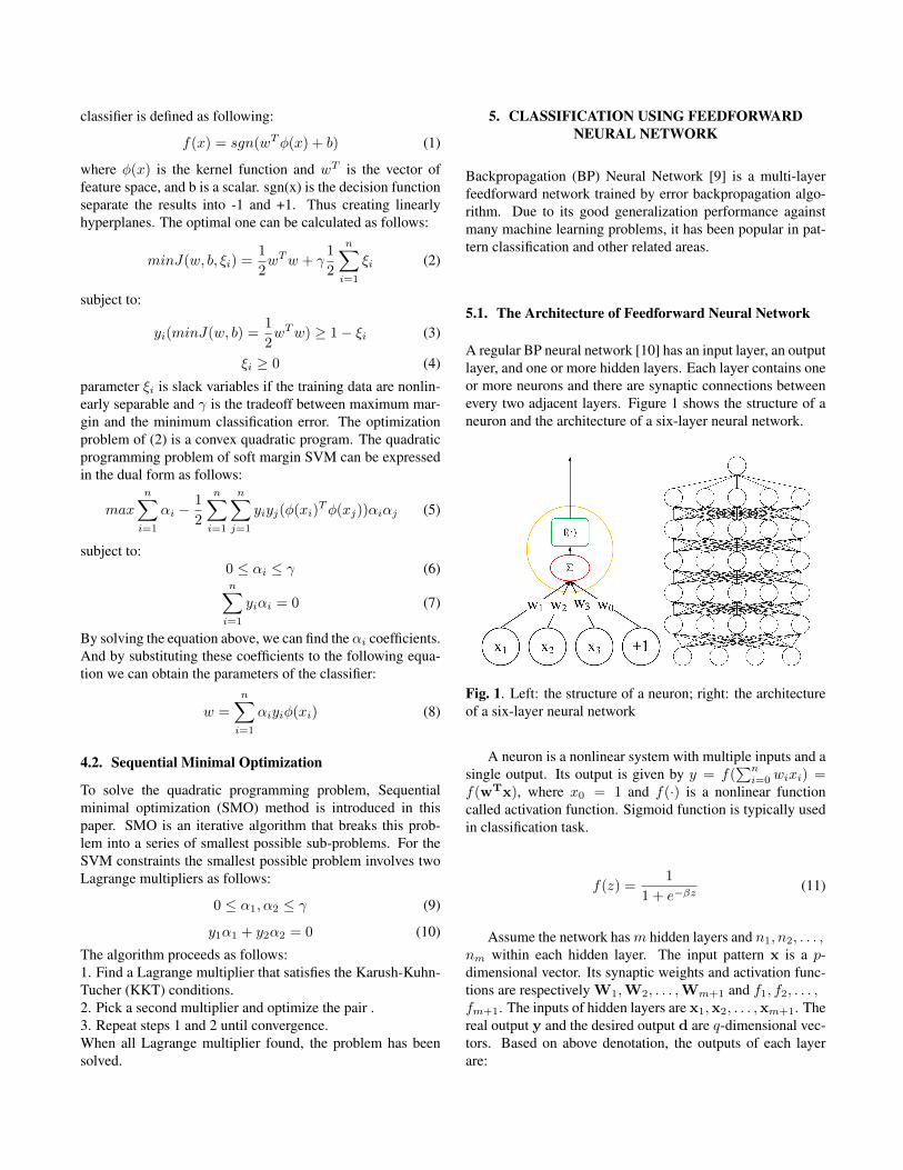
A regular BP neural network [10] has an input layer, an outputlayer, and one or more hidden layers. Each layer contains oneor more neurons and there are synaptic connections betweenevery two adjacent layers. Figure 1 shows the structure of aneuron and the architecture of a six-layer neural network.

Fig. 1. Left: the structure of a neuron; right: the architectureof a six-layer neural network

A neuron is a nonlinear system with multiple inputs and asingle output. Its output is given by y = f(

∑ni=0 wixi) =

f(wTx), where x0 = 1 and f(·) is a nonlinear functioncalled activation function. Sigmoid function is typically usedin classification task.

f(z) =1

1 + e−βz(11)

Assume the network hasm hidden layers and n1, n2, . . . ,nm within each hidden layer. The input pattern x is a p-dimensional vector. Its synaptic weights and activation func-tions are respectively W1,W2, . . . ,Wm+1 and f1, f2, . . . ,fm+1. The inputs of hidden layers are x1,x2, . . . ,xm+1. Thereal output y and the desired output d are q-dimensional vec-tors. Based on above denotation, the outputs of each layerare:

x1(j) = f1(

p∑i=0

W1(i, j)x(i)), j = 1, 2, . . . , p

x2(j) = f2(

n1∑i=0

W2(i, j)x1(i)), j = 1, 2, . . . , n1

. . .

xm(j) = fm(

nm−1∑i=0

Wm(i, j)xm−1(i)), j = 1, 2, . . . , nm−1

y(j) = fm+1(

nm∑i=0

Wm+1(i, j)xm(i)), j = 1, 2, . . . , nm

(12)

5.2. Error Backpropagation Algorithm

The object of error backpropagation algorithm is to minimizethe cost function:

J(W, θ) =1

2

q∑i=1

(d(i) − y(i))2 (13)

According to the gradiend descent method and the chainrule, weight update for the output layer is as follows:

∆Wm+1(i, j) = ηδm+1(j)xm(i) (14)

where

δm+1(j) = (d(j) − y(j))f ′m+1 (15)

We can easily obtain the weight update for other layersfollowing the same rules. As we can see, the order of weightupdate computation is from higher layers through lower lay-ers. That is why the learning algorithm is called error back-propagation [10].

6. CLASSIFICATION USING ELMAN RECURRENTNEURAL NETWORKS (ELMAN RNNS)

There are many forms of Recurrent Neural Networks (RNNs).One of the simplest ones is the Elman RNN [11].

6.1. The Framework of Elman RNN

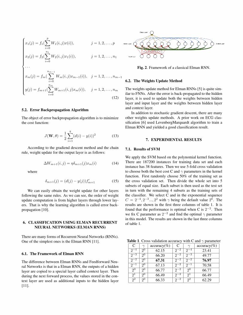
The difference between Elman RNNs and Feedforward Neu-ral Networks is that in a Elman RNN, the outputs of a hiddenlayer are copied to a special layer called context layer. Thenduring the next forward process, the values stored in the con-text layer are used as additional inputs to the hidden layer[11].

Fig. 2. Framework of a classical Elman RNN.

6.2. The Weights Update Method

The weights update method for Elman RNNs [5] is quite sim-ilar to FNNs. After the error is back-propagated to the hiddenlayer, it is used to update both the weights between hiddenlayer and input layer and the weights between hidden layerand context layer.

In addition to stochastic gradient descent, there are manyother weights update methods. A prior work on ECG clas-sification [6] used LevenbergMarquardt algorithm to train aElman RNN and yielded a good classification result.

7. EXPERIMENTAL RESULTS

7.1. Results of SVM

We apply the SVM based on the polynomial kernel function.There are 187200 instances for training data set and eachinstance has 38 features. Then we use 5-fold cross validationto choose both the best cost C and γ parameters in the kernelfunction. First randomly choose 50% of the training set asthe cross validation set. Then divide the whole set into 5subsets of equal size. Each subset is then used as the test setin turn with the remaining 4 subsets as the training sets ofthe classifier. We select C and in the exponential sequenceC = 2−4, 2−3..., 22 with γ being the default value 20. Theresults are shown in the first three columns of table 1. It isfound that the performance is optimal when C is 2−2. Thenwe fix C parameter as 2−2 and find the optimal γ parameterin this model. The results are shown in the last three columnsof table 1.

Table 1. Cross validation accuracy with C and γ parameterC γ accuracy(%) C γ accuracy(%)

2−4 20 62.15 2−2 2−4 23.412−3 20 66.20 2−2 2−3 49.772−2 20 67.31 2−2 2−2 76.972−1 20 67.13 2−2 2−1 70.5820 20 66.77 2−2 20 66.7721 20 66.49 2−2 21 66.4922 20 66.33 2−2 22 62.29

Then we use the optimal parameters found above to testthe accuracy in the test set. The test set has 62400 instancesand the accuracy of the model is 66.67%.

7.2. Results of FNN

We use a four-layer BP neural network including two hid-den layers with 16 neurons in each hidden layer to handlethis classification task. The inputs of the model are 38-dimensional feature vectors and the output layer has onesingle neuron. The classification threshold of the output neu-ron is 0.5, which means the input pattern is classified to Class“N” (Normal) if y > 0.5 and Class “A” (Abnormal) other-wise. We use sigmoid function with β = 1 as the activationfunction for all neurons. The whole model was implementedin C++ and no machine learning toolkit was used.

To make sure the convergence of the training process, aself-adaptive learning rate is set up. The initial value of learn-ing rate η is 0.0005, and we reset η = η × 0.8 if the value ofthe cost function increases in the process.

The classification accuracy on training set with differentepochs is shown in figure 3.

Fig. 3. The classification accuracy on training set with differ-ent epochs

The classification accuracy is 83.64% (after 2000 epochs)on training set and on test set is 69.45%.

7.3. Results of Elman RNN

The experimental settings of Elman RNN are similar to theFNN. There are four layers in the network. Input layer isconsisted of 38 nodes. The numbers of nodes in the hiddenlayer and the context layer are both 32. There is only onenode in the output layer. The classification threshold of theoutput neuron is also 0.5 and the same sigmoid function isused. The whole model was implemented in Python and nomachine learning toolkit was used.

An adaptive training method is also used in the trainingprocess of the Elman RNN. The initial learning rate is 0.02.For each epoch, the training accuracies of both current state

and the previous state are stored. If the accuracy of currentstate is lower than the previous state, the training process willroll back to the previous state and the learning rate will bedivided by 2.

The training process will stop if the accuracy improve-ment between current state and the previous state is not largerthan 0.001% or the learning rate becomes smaller than 10−20.

The accuracies at different epochs are shown in figure 4.

Fig. 4. The accuracies at different epochs on training set.

The figures show that with the increase of epochs, the per-formance on both the training set and the test set increase.The final accuracy is 72.98% on the training set and 63.98%on test set. Multiple experiments with the same settings areconducted and we get similar results.

One thing worths noticing is that as the accuracies on thetraining set increases, the accuracies on the test set may notincrease correspondingly. This phenomenon is common be-cause the accuracies on the training set and the test set areusually not linearly correlated.

8. CONCLUSION

In this paper, we proposed three different models for classify-ing ECG signal segmentations: SVM, FNN, Elman RNN. Theexperimental results in figure 5 show that SVM and FNN havehigher classification accuracy on test set than Elman RNN.In addition, all three models outperform the baseline model.However, further research on the models is demanded sincethe classification performance can be impacted by model con-figuration, such as parameter setting, selection of activationfunction, etc.

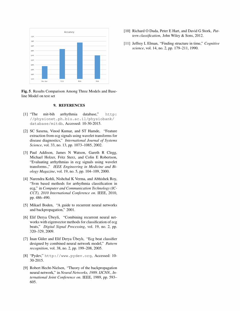
Fig. 5. Results Comparison Among Three Models and Base-line Model on test set

9. REFERENCES

[1] “The mit-bih arrhythmia database,” http://physionet.ph.biu.ac.il/physiobank/database/mitdb, Accessed: 10-30-2015.

[2] SC Saxena, Vinod Kumar, and ST Hamde, “Featureextraction from ecg signals using wavelet transforms fordisease diagnostics,” International Journal of SystemsScience, vol. 33, no. 13, pp. 1073–1085, 2002.

[3] Paul Addison, James N Watson, Gareth R Clegg,Michael Holzer, Fritz Sterz, and Colin E Robertson,“Evaluating arrhythmias in ecg signals using wavelettransforms.,” IEEE Engineering in Medicine and Bi-ology Magazine, vol. 19, no. 5, pp. 104–109, 2000.

[4] Narendra Kohli, Nishchal K Verma, and Abhishek Roy,“Svm based methods for arrhythmia classification inecg,” in Computer and Communication Technology (IC-CCT), 2010 International Conference on. IEEE, 2010,pp. 486–490.

[5] Mikael Boden, “A guide to recurrent neural networksand backpropagation,” 2001.

[6] Elif Derya Ubeyli, “Combining recurrent neural net-works with eigenvector methods for classification of ecgbeats,” Digital Signal Processing, vol. 19, no. 2, pp.320–329, 2009.

[7] Inan Guler and Elif Derya Ubeylı, “Ecg beat classifierdesigned by combined neural network model,” Patternrecognition, vol. 38, no. 2, pp. 199–208, 2005.

[8] “Pydev,” http://www.pydev.org, Accessed: 10-30-2015.

[9] Robert Hecht-Nielsen, “Theory of the backpropagationneural network,” in Neural Networks, 1989. IJCNN., In-ternational Joint Conference on. IEEE, 1989, pp. 593–605.

[10] Richard O Duda, Peter E Hart, and David G Stork, Pat-tern classification, John Wiley & Sons, 2012.

[11] Jeffrey L Elman, “Finding structure in time,” Cognitivescience, vol. 14, no. 2, pp. 179–211, 1990.