Embed Size (px)
Citation preview

Electromagnetic Noise Generated in the
Electrified Railway Propulsion System
Kelin Jia
Licentiate Thesis
Electromagnetic Engineering
Royal Institute of Technology (KTH)
School of Electrical Engineering
Stockholm, Sweden 2011

Division of Electromagnetic Engineering
KTH School of Electrical Engineering
SE 100-44, Stockholm, Sweden
TRITA-EE 2011:011
ISSN 1653-5146
ISBN 978-91-7415-873-1
Akademisk avhandling som med tillstånd av Kungliga Tekniska Högskolan
framlägges till offentlig granskning för avläggande av teknologie licentiatexamen
måndagen den 28 marsch 2011 kl. 10:00 i rummet V3, Kungliga Tekniska
Högskolan, Teknikringen 72, Stockholm.
© Kelin Jia, 2011
Tryck: Universitetsservice US-AB
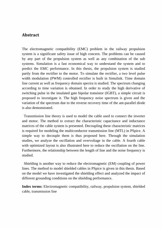
Abstract
The electromagnetic compatibility (EMC) problem in the railway propulsion
system is a significant safety issue of high concern. The problems can be caused
by any part of the propulsion system as well as any combination of the sub
systems. Simulation is a fast economical way to understand the system and to
predict the EMC performance. In this thesis, the propulsion system is studied
partly from the rectifier to the motor. To simulate the rectifier, a two level pulse
width modulation (PWM) controlled rectifier is built in Simulink. Time domain
line current as well as frequency domain spectra is studied. The spectrum changing
according to time variation is obtained. In order to study the high derivative of
switching pulse in the insulated gate bipolar transistor (IGBT), a simple circuit is
proposed to investigate it. The high frequency noise spectrum is given and the
variation of the spectrum due to the reverse recovery time of the ant-parallel diode
is also demonstrated.
Transmission line theory is used to model the cable used to connect the inverter
and motor. The method to extract the characteristic capacitance and inductance
matrices of the cable system is presented. Decoupling these characteristic matrices
is required for modeling the multiconductor transmission line (MTL) in PSpice. A
simple way to decouple them is thus proposed here. Through the simulation
studies, we analyze the oscillation and overvoltage in the cable. A fourth cable
with optimized layout is also illustrated here to reduce the oscillation on the line.
Furthermore, the relationship between the length of line and the noise frequency is
studied.
Shielding is another way to reduce the electromagnetic (EM) coupling of power
lines. The method to model shielded cables in PSpice is given in this thesis. Based
on the model we have investigated the shielding effect and analyzed the impact of
different grounding conditions on the shielding performance.
Index terms: Electromagnetic compatibility, railway, propulsion system, shielded
cable, transmission line


Acknowledgements
I would like to thank my supervisor professor Rajeev Thottappillil for his guidance
in my studies. His knowledge and way of guidance frees all of my study
capabilities.
Mr. Georg Bohlin, I highly appreciate his extremely valuable participation in my
studies and tremendous help. The fruitful discussion with him inspires me always.
I thank my former colleagues Dr. Surajit Midya, and Dr. Ziya Mazloom; fellow
Ph.D students Mr. Helin Zhou, Mr. Pu Zhang, Ms. Xiaolei Wang and Ms. Siti
Fatimah Jainal for all the good time and discussions together.
My thanks also go to all members in ETK.
Finally, I wish to thank my family and friends for supporting me.


List of papers This thesis is based on the following papers; they are referred to the text by the
authors’ names and the year of publication.
I. Kelin Jia, Rajeev Thottappillil, "PSpice Modeling of Electrified Railway
Propulsion Drive Rectifiers for Harmonic Analysis" The 9th International
Conference on Intelligent Transport Systems Telecommunications, 2009,
Page(s): 113 – 116.
II. Kelin Jia, Rajeev Thottappillil, "EMC assessment of the railway traction
system by using PSpice" Asia-Pacific Symposium on Electromagnetic
Compatibility (APEMC), 2010, Page(s): 598 – 601.
III. Kelin Jia, Georg Bohlin, and Rajeev Thottappillil. "Optimal Cable
Assembly for reducing Electromagnetic Interference in Traction System"
IET Electrical System in Transportation 2010. (Under review)
IV. Kelin Jia, Georg Bohlin, and Rajeev Thottappillil. "Modeling the traction
system in PSpice for electromagnetic noise analysis" Electronic
Environment 2011, Stockholm. (Accepted)


Contents
Chapter 1 Introduction ............................................................................................. 1
1.1 Propulsion system in the high speed electrical multiple unit .................... 1
1.2 Electromagnetic Compatibility challenges in EMU .................................. 3
1.3 Outline of the thesis ................................................................................... 5
Chapter 2 Rectifier simulation................................................................................. 7
2.1 PWM controlled rectifier ........................................................................... 7
2.2 Simulation results and discussions .......................................................... 10
Chapter 3 IGBT simulation ................................................................................... 13
3.1 The structure of IGBT and Modeling in PSpice ...................................... 13
3.2 High frequency disturbance caused by the operation of IGBTs .............. 16
3.3 Simulation results and discussions .......................................................... 17
Chapter 4 Motor converter module ....................................................................... 19
4.1 System description of MCM and multiconductor transmission line theory
....................................................................................................................... 19
4.2 Decoupling method ................................................................................. 22
4.3 Decoupling method verification .............................................................. 23
4.4 MCM modeling in PSpice ....................................................................... 25
4.5 Oscillation in MCM ................................................................................. 27
4.6 Optimal cable assembly for reducing EM noise and discussions ............ 31
Chapter 5 Shielded cable ....................................................................................... 35
5.1 Introduction to shielded cable ................................................................. 35
5.2 Modeling shielded cable in PSpice .......................................................... 36
5.3 Simulation results and discussions .......................................................... 37
Chapter 6 Summary of papers ............................................................................... 41
Chapter 7 Conclusion and future work .................................................................. 43

List of Abbreviations ............................................................................................. 45
References ............................................................................................................. 47

1
Chapter 1 Introduction
1.1 Propulsion system in the high speed electrical multiple unit
The development of railway has been significant since the beginning of 20th
century. Railway transportation is playing a significant role not only in peoples’
daily life but also in global economic growth. In 1897, Siemens displayed the first
electrically powered locomotive at the Berlin Commerce Fair. The maximum
speed of this train was 13 km/h, and the output energy came to about 2.2 kW [1].
Since then, electrified railways have been improved dramatically due to the rapid
development of power electronics and manufacturing industries. Nowadays, the
highest wheel-rail speed, which is kept by TGV (French: Train à Grande Vitesse,
meaning high-speed train), is 574.8 km/h [2], and the transportation capability of a
single locomotive has been increased to thousands of tons.
Except locomotive, electrical multiple unit (EMU) is another strategy to propel
the train. The term EMU is referred to a self driving train unit capable of coupling
with other similar units and can be controlled from one cabin. The EMU possesses
the merits such as speed, safety, comfort, and high efficiency [3]. The max service
speed of an EMU can reach 300 km/h and the design of a new EMU with speed
500km/h is carried out in China. Figure 1.1 shows an example of an EMU train
which consist of eight coaches where eight or ten axles are driven.
T1c T2cM2 M1 T2 T1 M2 M1
Train Base Unit Train Base Unit
T: Trailer coachM: Motor coachc: cabin
Figure 1.1 Example of an EMU train
The EMU shown above has two base units which consist of 2M and 2T with the
sequence: T1+M2+M1+T2. The two parts with four cars are identical with respect
to the high voltage, propulsion and auxiliary power supply systems. This means
that each train base unit has independent propulsion system and can be operated

2
individually. Both ends of the train are equipped with a driver’s cab so that driver
easily can control the train in the front cab.
There are two types of railway electrical supply networks in Europe i.e. direct
current (DC), single-phase alternating current (AC). Tramways and metro systems
are usually operating on DC supply systems due to the simple vehicle structure, i.e.
no rectifier is required in the trains. However for long distance railways like
intercity or international lines, AC voltage of 15kV/16.67 Hz or 25kV/50 Hz is the
preferable choice. The AC voltage of 15kV/16.67 Hz system has been utilized
since 1912 and is the system followed in Sweden, Norway, Germany, Austria and
Switzerland [1]. The EMU mentioned in this thesis is electrified by AC system of
either 15kV/16.67 Hz or 25kV/50 Hz. All the discussion here is based on this
prerequisite.
The EMU applies AC propulsion systems which are mainly composed of the
pantograph, main transformers, rectifiers, DC-link, inverters, AC motors, gear
boxes, and wheels. AC electrical power is fed through pantograph and then
transformed in the listed stages; finally mechanical output force of wheels propels
the train. The overview graph of a railway propulsion system is shown in figure
1.2.
Rail
Transformer
AC Motor
Contact wire AC
~
=
Rectifier
=
DC Link Inverter
Gear
Wheel
Pantograph
~~~
M
Wheel
Figure 1.2 Block diagram of the propulsion system
The pantograph is connected to a propulsion transformer distributing the
electricity to several secondary coils. After regulated to a certain level of voltage
by the transformer, the AC is converted to DC by the rectifier controlled by the
PWM signal. A DC-link filter, which is composed of DC-link capacitor, second-
harmonic filter, and midpoint earthing unit, is added between the rectifier and
inverter [4]. This filter is able to smooth the DC-link voltage and keep the system
voltage at a certain level reference to the ground. The DC filter is composed of

3
resistances, capacitors and inductors. After passing the filter, the DC power is
inverted to the 3-phase power by the inverter. In this conversion stage, the PWM
control strategy is also applied but generated by a separate set of auxiliary control
circuits which is different from that in the rectifier.
Contact Wire Pantograph Transformer Rectifier DC-Link Inverter AC Motor Gear Wheel
E~ E~ E~ E- E- M M
E~:1AC E-:DC
E~~~
E~~~:3AC M :Mechanical power
Figure 1.3 Energy flowchart of the propulsion system
When the train is operating the electric power is converted to mechanical power
as the energy flow illustrated by the solid arrows in figure 1.3; when the train
braking the mechanical power is reversely converted to electric power as the dash
arrows indicate in figure 1.3.
There are two ways to conduct the reversal energy away:
The old way is to burn the reversal energy in so-called brake resistors.
There is a rather new concept, “energy saving”, where the reversal energy
is feed back to the contact wire, and can be used by other trains on the
same supply section or in some cases can be stored in the substation and
even be feed back to the high voltage supply line, depending on the design
of the infrastructure.
Due to the energy saving consideration the propulsion system is designed as a
bidirectional system so that when train is braking the mechanical energy will
transmit back to the substation. In the reverse conversion the AC motor works in
generator mode, propulsion inverter works in rectifier mode, and the rectifier
works as a single phase inverter. Finally the mechanical to electric conversion is
implemented therefore the energy can be stored in the substation.
1.2 Electromagnetic Compatibility challenges in EMU
As mentioned earlier, between the propulsion supply and electric motor there are
several stages for power collection and conversion. Unwanted electromagnetic
disturbance can be generated at any of these stages and distributed in the cables as
well as radiated through different loop circuits formed by the complex cable
systems. The disturbance which is caused by discontinuous working of the
converters and inverters can extend up to dozens of MHz thereby rail cars fail

4
passing EMC requirements. A common method to mitigate this EM noise is to
introduce a passive filter at the inverter output. However sometimes conventional
filter is not a practical way to reduce the EM noise because of cost, weight, and
space restrictions in railway vehicles. Better understanding of the generation
mechanism of EM noise from propulsion systems may provide solutions to
mitigate the EM noise at the beginning stage of design.
~
~~~
M
Car body
Rail
Clc
Clg
Iinput
Ilm
Ilg
Ilc Ilc
Inverter
Figure 1.4 CM current flow paths in the propulsion system
Common mode (CM) current is one source of emission. The use of PWM
essentially produces CM voltage therefore cause CM current on the motor cable
between the inverter and the motor. The spreading of CM current through different
paths leads to many EMC problems such as bearing current (especially high
frequency CM current), track circuit failure. Figure 1.4 illustrates the CM current
paths in the railway propulsion system. The CM current flows through feeding
cables, the motor winding, the stray capacitor of the motor, and the motor frame.
In practical installation, there is a return cable connecting the inverter and motor
frame which provides a significant return path for most CM current. However due
to the long distance between the inverter and motor frame a large loop circuit is
formed acting as a big loop antenna [5]. Small part of the CM current returns
through the car bodies and rails [6]. We should notice that the CM current
propagates along the rails can return to other car bodies and even to substations
thereby causing serious EMC problems. DC interference currents generated by an
EMU can interfere with DC track circuits.

5
System simulation of the propulsion system from the EMC point of view can
benefit railway system R&D. This simulation requires the accurate modeling of
insulated gate bipolar transistor (IGBT) modules in MCM [7], coupling effects
between power cables [8], and the motor equivalent circuit [9]. If possible, the
ground system and interconnections should have special models rather than simple
lossless lines. Furthermore, in order to represent the system with higher accuracy
the environmental condition should be considered when modeling, proper
simulation software is significant as well. Hybrid simulation software may provide
better solution to efficient and accurate modeling of the railway system.
1.3 Outline of the thesis
This thesis is organized as follows.
Chapter two gives the details of simulating a propulsion rectifier in Simulink and
corresponding waveform at input port as well as the harmonics in the frequency
domain.
Chapter three shows the details of how to implement an IGBT in PSpice. An
efficient way to predict the worst EMC performance is proposed, especially for
high frequency EM noises. The impact of the reverse-recovery time of a free-
wheeling diode on high frequency EM noise generation is also studied.
Chapter four presents the method of modeling a propulsion system in PSpice
with the consideration about optimal cable arrangements for reducing conducted
EM noise. The cable model is implemented in different software and results are
compared.
Chapter five deals with the shielded cable. The details of modeling a shielded
cable in PSpice are presented. The shielding effect is demonstrated by a two line
sample case.
Lastly, Chapter six gives the conclusion and plan for the future work.

6

7
Chapter 2 Rectifier simulation
2.1 PWM controlled rectifier
The rectifier is conversion stage after the secondary winding of the main
transformer for converting the 15 kV 16.67Hz or 25 kV 50 Hz AC to 1500 V AC
(or other suitable voltage). At this conversion stage the 1500 V AC was rectified
by the diode bridge to DC in the old railway technology. The diode rectifier has
some advantage e.g. very simple structure, high reliability, cheap. However since
diodes are a single directional device, the power can only conduct through the
rectifier from supply to load. Thus the braking energy fails to be reused. Due to the
invention of the IGBT and the emergence of PWM control strategy, the rectifier
composed of IGBTs with anti-parallel diode is widely used in electrified railway
propulsion system. This four-quadrant converter can implement bidirectional
energy transmission during different train movements. When the train is
accelerating or stead steady running the energy flows from the supply to the motor.
On the contrary, when the train is braking the energy flows in opposite direction
from motor to supply i.e. regenerative energy.
C
Rf
Lf
Cf
S11
S14
S21
S24
Load
LTRT
i
+
-
+
-
uin uab
+
-
Vdc
Figure 2.1 Schematic of a single-phase PWM rectifier for propulsion systems
The two-level PWM rectifier is shown in figure 2.1. It contains four IGBTs anti-
parallel with four free-wheel diodes. The switching frequency of IGBTs is much
higher than the line frequency so that the diodes are considered steady-state when
analyzing the behaviors of IGBTs. The rectifier works in the boost condition i.e.
the Vdc is higher than the peak value of the secondary transformer voltage. The
leakage inductance LT of the secondary transformer will take care of the voltage
difference between them. In order to control the power factor, the PWM strategy is

8
applied to control the four IGBTs. Thus the voltage drop uab for the two converter
arms is notch rather than a pure sinusoidal waveform. The schematic figure 2.1
can be redrawn as an equivalent circuit shown in figure 2.2 for energy analysis.
RT LT
+
-
+
-
uin uabi
Figure 2.2 The equivalent circuit for the rectifier
uin
uab
i∙RT
i∙jωLTi
φ
uin
uabi∙RT
i∙jωLT
i
(a) (b)
Figure 2.3 Phasor diagram for the rectifier
From figure 2.2 it is known the voltage and current relationship is described as
(2-1)
where all the vectors in the equation are fundamental components. By
investigating the equation, we can notice that for a specific transformer winding
the leakage inductance LT and resistance RT are fixed so that i is in relation to the
difference between uin and uab. Figure 2.3 (a) shows the phasor diagram for the
vectors. φ is the phase angle between input voltage and current, the active power
drawn from supply is therefore
(2-2)
If the phase angle is not zero the power factor is not unit. This means that the
working efficiency is relatively low. In order to make the rectifier working in the
condition having unit power factor, four IGBTs are controlled to alter the
magnitude and phase with respect to current loop circuit [10]. Finally the rectifier

9
works in the condition shown in figure 2.3 (b), where i and uin are in phase, which
is called unit power factor.
As mentioned above, the PWM controller is applied to help achieving unit power
factor. However the line current is no longer sinusoidal because notches are
introduced to the system. These notches are containing harmonics and high
frequencies which is the drawback of this technique. With different fundamental
frequencies, these harmonics can be dozens of kHz and even extend to dozens of
MHz which can lead to malfunction of the electric equipments and contamination
of the power supply networks. Thus, it is extremely important for system designers
to explore the harmonic spectra generated in power equipments. For any time
varying function f(t), Fourier transform can be applied to expand it into a sum of
frequency components.
In PWM waveform analysis, double Fourier series expansion is applied because
this expansion can provide clearer spectrum information than Fourier transform
can do. The procedure of the double Fourier series expansion is shown in [11].
The PWM waveform f(t) can be represented as
000 0 0 0 0 0
1
( ) cos sin2
n nn
Af t A n t B n t
cos sin0 0
1A m t B m tc c c cm m
m
0 0 0 01
cos sinmn c c mn c cm n
A m t n t B m t n t
(2-3)
where m is carrier modulation index, n is the baseband index, ωC is the carrier
frequency, and ω0 is the fundamental frequency. By examining the equation
carefully, the first term is the DC component of the waveform, the second term
represents the baseband harmonics of the modulation form, the third term contains
the carrier harmonics components, and the last term shows the sideband harmonics.
The carrier index m and baseband index n define the frequency of each harmonics
of the output voltage. That means, for example, values of m=1 and n=2 define the
second sideband harmonic in the group of harmonics which exist around the first
carrier harmonic. Furthermore, the absolute frequency of this sideband harmonic is
(1 ωC +2 ω0).

10
2.2 Simulation results and discussions
In order to investigate the harmonics generated in the rectifier, a two-level PWM
controlled rectifier is constructed in Simulink with the system parameters listed in
table 2.1. In the paper [12] the EM performance of a three-level PWM controlled
rectifier is discussed. The simulation model in this chapter applies the similar
procedure to deal with the rectifier. For the sake of simplification, only load
capacitor implemented at output end and the load is considered as pure resistive.
The secondary winding of the main transformer is replaced by an AC voltage
source with wanted magnitude and phase. Because this model is for evaluating the
converter from the EMC point of view, so open-loop control circuit is adopted.
The IGBT control pulse is generated from a carrier-based PWM block. The carrier
frequency is 500 Hz. The simulation time is set to 0.5 second with variable time
step.
Parameter Value
Rectifier’s AC-side voltage (uin) 1500V Rectified voltage (Vdc) 2500V
AC line frequency 50Hz Transformer leakage inductance (RT) 1.7mH Transformer winding resistance(LT) 0.33Ω
Load resistor(Load) 41 Ω
Table 2.1 Parameters for the rectifier model in Simulink
Figure 2.4 DC-link voltage

11
The DC-link voltage is shown in figure 2.4. It is presented that the voltage level
is 2500 V coinciding with our specification well. If we study the waveform
carefully, the voltage will appear modulated with a sinusoidal wave having 100 Hz.
This is the reason why sometimes second harmonic filters are required after DC-
link capacitors in real propulsion systems.
Figure 2.5 presents the input voltage uab and line current. The modulated pulse is
+2500 V and -2500 V i.e. +Vdc and –Vdc. The fundamental component of line
current wave is sinusoidal as illustrating in figure 2.5(a). The peak value of current
is 500 A when steady state. However at the very beginning of the simulation the
current rockets up to 2.5 kA, five times bigger than the steady value. From the
expanded view figure 2.5(b), it can be observed that the current waveform is not
perfect due to pulse modulation, some higher frequency components exist in this
waveform. These disturbances may interfere with other circuit thus reduce the
reliability of the whole system. Transformer can provide some filter effect but
distortion is not avoidable. Every time the IGBT is switching the current will
charge or discharge the inductance. From 0.44 sec to 0.45 sec, when the IGBT is
turning on, the current goes up and therefore charge the inductance. After time
moving beyond 0.45 sec, when the IGBT is turning on, the current charges the
inductance but in opposite direction.
Figure 2.5 Line voltage, uab and line current, i
Figure 2.6 gives the current spectra for different harmonic orders with respect to
the time variation. In figure 2.6(a), we can note that the fundamental component
(first order) is very high, up to 2000 A in the time range from 0 to 0.05 sec. This is
mentioned above, when we are analyzing in the time domain, that the current has
very big value at beginning of the operation. By studying all the graphs in figure
2.6, we can conclude that the current spectra are far more different with that in

12
steady state operation, even DC component can be found at the starting time. So
the likelihood of system fault is higher when the system is starting to work. Figure
2.7 shows the line current spectra in steady state working condition, the
fundamental component is 488 A. The first group sideband harmonics can reach
90 A, 18% of the fundamental component.
Figure 2.6 Line current spectra
Figure 2.7 Line current spectra when steady state

13
Chapter 3 IGBT simulation
3.1 The structure of IGBT and Modeling in PSpice
The insulated gate bipolar transistor (IGBT) is a replacement of the power bipolar
junction transistor (BJT), metal oxide semiconductor field effect transistor
(MOSFET), and GTO thyristor in various electric applications [13]. The IGBT,
which commercially emerged in 1983, possess following advantages [14]:
No snubber circuit required so that lighter weight, less complexity of the
circuit.
IGBT is a voltage controlled semiconductor, so only simple gate drive is
needed.
Lower switching losses and relatively high switching frequency
Good power rating, high current and high voltage is possible ( > 3.3 kV/
1.2 kA)
Owning to such advantages listed above, the IGBT is widely used in power
application especially high energy consuming devices including the railway
propulsion system. The biggest EMC problem of the IGBT is attributed to the di/dt
and dv/dt. In order to achieve high efficient and due to the improvement of
fabrication processes, high voltage and fast switching are realized in new
generation IGBTs. In some applications the dv/dt can reach 5 kV/µs which may
lead to serious EMC problems both conducted and radiated [15]. Proper IGBT
circuit model is essential for circuit designer to understand its behavior and predict
EMC performance.
The cross-section view of an N-Channel IGBT is shown in figure 3.1. We
basically can consider the generic IGBT is a power MOSFET (M) in series with a
PNP transistor (Q) in a Darlington configuration. When positive voltage is applied
from the Gate to Emitter electrons are to be drawn towards the gate terminal in the
body region. If the gate-emitter voltage exceeds the threshold voltage, enough
electrons are drawn from the Base of the transistor to the Drain of the MOSFET so
as to allow the current flows from the collector to the emitter.

14
The parasitic capacitor and stray inductance existing between the different
layers affect the performance of the IGBT model. The main parasitic capacitors
are Cgc, Cge, and Cce. Cgc is the gate to collector capacitance which is expressed as
gc gd cdC C C (3-1)
gd oxC C when gd thV V (3-2)
/(1 / )gd ox ox depC C C C when gd thV V (3-3)
where Cgd is the gate-drain capacitor which is constituted by the gate-drain overlap
oxide capacitor Cox and the depletion layer capacitor Cdep. The gate-drain overlap
depletion layer capacitor is replaced by a PSpice diode model. The collector-drain
capacitor Ccd can also be represented by a PSpice diode model in this simulation.
n+
p body regin
n- Drift regin
p+ Substrate
Emitter Gate
Collector
M
Q
Figure 3.1 Cross-section of an NPT IGBT
The collector-emitter capacitor Cce is determined by the anode cathode junction
of the intrinsic free-wheeling diode
1
m
cece jo
j
VC C
V (3-4)
where Cjo is the PN junction capacitance, Vj is the junction potential and m is the
junction grading coefficient [16].The stray inductances are related to the terminal
internal connections and the typical value of them is from 10 to 100nH [17].
15
During the simulation in this thesis, the stray inductances at the gates are set to 50
nH.
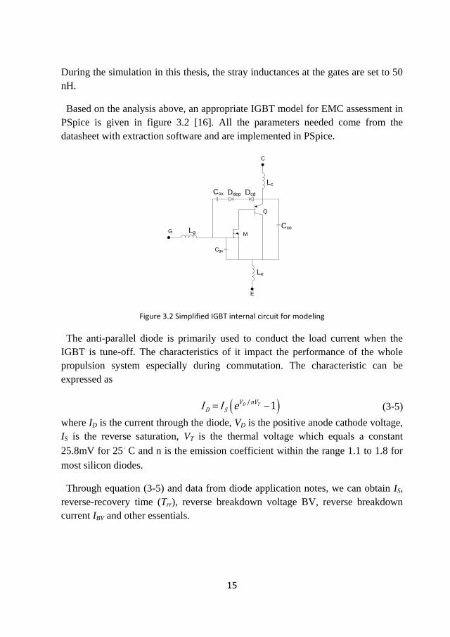
Based on the analysis above, an appropriate IGBT model for EMC assessment in
PSpice is given in figure 3.2 [16]. All the parameters needed come from the
datasheet with extraction software and are implemented in PSpice.
G
E
C
Cox Ddep Dcd
Lg
Le
Lc
Cce
Cge
Q
M
Figure 3.2 Simplified IGBT internal circuit for modeling
The anti-parallel diode is primarily used to conduct the load current when the
IGBT is tune-off. The characteristics of it impact the performance of the whole
propulsion system especially during commutation. The characteristic can be
expressed as
/ 1D TV nVD SI I e (3-5)
where ID is the current through the diode, VD is the positive anode cathode voltage,
IS is the reverse saturation, VT is the thermal voltage which equals a constant
25.8mV for 25。
C and n is the emission coefficient within the range 1.1 to 1.8 for
most silicon diodes.
Through equation (3-5) and data from diode application notes, we can obtain IS,
reverse-recovery time (Trr), reverse breakdown voltage BV, reverse breakdown
current IBV and other essentials.

16
3.2 High frequency disturbance caused by the operation of IGBTs
From system simulation, only the characteristic harmonics are obtained. The high
frequency EM noise due to gradients of voltage and current can be studied through
a chopper circuit shown in figure 3.3 [18].
Control Signal
L
R
IGBT
D
Ifw Isurge
Vd
C
EG
Figure 3.3 Chopper circuit
When the IGBT is turned on for a time duration ton, the switch conducts the
inductor current and the free-wheeling diode becomes reverse biased. This leads to
a negative voltage –Vd across the diode and positive voltage +Vd across the LR
series. Therefore
L
L d
di tL i t R V
dt (3-6)
Solution to this equation for iL(0)=I0 is as follows:
0ln dVR
t Id L R
L
Vi t e
R (3-7)
The energy stored in the inductor at the end of the turn-on period is
21
2L L onE Li t (3-8)
When the IGBT tunes off for a duration time TS-ton, the free-wheeling diode
conducts the current. Thus, the collector-emitter voltage of the IGBT is

17
,,( ) L
ce d L
di tu t V i t R L
dt (3-9)
The free-wheeling loop satisfies the voltage-current relationship as follows:
,, 0L
L
di tL i t R
dt (3-10)
with the initial value i’L(0) = iL(ton) . Therefore, the solution for inductor current in
the switch off time is
, ( )R
tL
L L oni t i t e (3-11)
If the circuit works in the continuous-conduction mode, before the instant that the
control signal initiates the IGBT turn-on action, the diode is conducting the current.
After this moment, the IGBT begins to conduct the current and voltage across the
diode is –Vd. Since the voltage drop is negative, the diode should be tuned off
immediately, but unfortunately, the diode is still conducting during the reverse
recovery time. In this short interval, the positive voltage V is applying to the IGBT
emitter terminal and the reverse current flows until the diode reverts to blocking
state. The series of actions produce a pike current in the IGBT collector containing
high frequency interference. Besides, the diode is enduring the enormous reverse
current that may damage the diode.
In order to make sure the chopper circuit works in the continuous-conduction
mode, i’L(Ts) > 90%·iL(ton) should be satisfied. The values of these components and
sources should be set properly according to the propulsion system so that the most
possible EM noise can be analyzed.
3.3 Simulation results and discussions
The IGBT collector currents with different Trr are recorded to illustrate the high
frequency disturbance changes in relation to Trr. The time domain waveform and
spectrum are presented in figure 3.4 and figure 3.5, respectively for various values
of the diode Trr. As seen in figure 3.4, with the increasing Trr, the duration of the
spike is prolonged and the peak value goes up. However, the downward slopes are
not same, as the blue and red lines are sharper than the rest two ones. This

18
phenomenon is not only resulted from the Trr but also due to the system impact
introduced by other components.
From figure 3.5, it is showing that along the increasing Trr the magnitude of the
spectrum below 5MHz is increasing. And at 5 MHz, the spectra are higher than 85
dBuA, which is relatively high. Before 5 MHz, the changes are nonlinear because
the spectrum for 700 ns is lower than that for 600 ns. These spectrum information
can be used to evaluated the possible interference at high frequency and provide
details about how the diode impacts the system.
Figure 3.4 IGBT Collector current for different values of diode reverse-recovery time Trr
Figure 3.5 Spectrum of collector currents for different Trr

19
Chapter 4 Motor converter module
4.1 System description of MCM and multiconductor transmission line
theory
Conventionally a motor converter module (MCM) in the propulsion system mainly
consists of the 3-phase motor inverter, one part of the DC-link capacitance, and the
drive control unit in the MCM (DCU/M) [4]. Here for EMC analysis we would
like to extend the notion of MCM to encompass feeding cables. The circuit
diagram is demonstrated in figure 4.1. Long 3-phase feeding cables are always
with two problems: overvoltage at the motor terminals and high frequency
common-mode (CM) voltage [19]. The magnitude of overvoltage and CM voltage
depends on the pulse edge derivatives and on the characteristics of cables [20].
DC-link
Capacitor
=
~~~
DC+
DC-
M
MCM
Motor converterFeeding
cable
Figure 4.1 Circuit diagram of an MCM
The most common method to mitigate this EM noise is to introduce a passive
filter at the inverter output or motor terminal. However, due to the cost, weight and
volume restriction, filter is not a preferable solution sometimes. Moreover,
coupling effects between the cables connecting to induction motors and mitigation
methods haven’t been studied in detail especially at high frequencies. In order to
investigate the crosstalk in propulsion systems from the EMC point of view in an
efficient and economical way, a sophisticated model including the accurate cable
model has been constructed in the simulation software [21]. This model can help
engineers to study and evaluate EM performance of the propulsion system in the
early design stages.
The cables in the MCM refer to conductors that have circular cylindrical cross
sections. All the cables are assumed to have the same cross section, therefore have

20
the same characteristic properties. This cable system can be considered as the
lossless transmission line system. The voltages and currents on a lossless cable
system are described by the transmission line equations [8]
1
1
1 2
1 2
1
, , ,
, , , , ,
i n
i in
ni n i
i i in im
m
V z t I z t I z tl l
z t t
I z t V z t V z t V z t V z tc c c c
z t t t t
(4-1)
By using matrix notation
(4-2)
If this is a three cable system, , and
,
. is the per-unit-
length inductance matrix which comprises individual per-unit-length self
inductance and per-unit-length mutual inductance between different cables. is
the per-unit-length capacitance matrix indicates the displacement current flowing
between the conductors in the transverse plane. The capacitance and inductance of
multiconductor transmission line (MTL) affects the behavior of the wave
propagating along the lines. The per-unit-length parameters are determined by the
given cross sectional cable configuration as well as the media between the wires.
For determining these parameters, analytical and numerical methods are
previously investigated a lot. In this thesis, the finite-element method (FEM) with
COMSOL multiphysics is used to obtain the capacitance and inductance matrices
[22].
Another issue is skin effect. Due to the undesired effect the conductor loss
increases proportional to frequency and hence the propagating signal is attenuated.
A four ladder compact circuit model is used to represent the skin effect for round
cables [23]. In this modeling method, DC resistance of the cable RDC and internal
inductance Llf of the wire are required to calculate the inductance and resistance

21
values. The specification of the cable is given in figure 4.2 and table 4.1. The
compact circuit model including skin effect is shown in figure 4.3.
Figure 4.2 Cable transverse diagram
Conductor Exterior layers Cable
diameter
(mm) diameter
(mm)
area (mm2) insulation
(mm)
sheath (mm)
7.8 35 0.65 0.85 11.7
Table 4.1 Cable diameters
Figure 4.3 Four ladder circuit model of the cable to include skin-effect
A five meter cable is considered as an example case to illustrate the skin effect.
400 V square pulse is applied at the front end of the cable and corresponding
voltage response is obtained with or without skin effect. As observed in figure 4.4,
the signal is delayed by the cable no matter whether skin effect is considered.
From the expanded view of the terminal response we can conclude that the skin
effect only slightly affects the performance of the cable in this relatively short
1 2 31 2 33

22
cable application. The difference between two responses is less than one volt so
that we do not take into account skin effect in our following studies. The cables
are dealt with by lossless MTL system.
Figure 4.4 Input pulse and terminal responses
4.2 Decoupling method
In the PSpice implementation of MTL procedure, n coupled line system should be
decoupled to n single transmission lines. Decoupling method for inductance and
capacitance matrices are required. [24] and [25] gave methods to decouple the
characteristic matrices. A simplified way to tackle this problem is introduced here.
If there exists a nonsingular matrix P, let us introduce P-1AP=B, the n×n matrices,
where A and B are recognized to be similar. The product P-1AP is called a
similarity transformation. When A is similar to a diagonal matrix, A is
diagonalizable.
Assuming a three cable system both of the inductance and capacitance matrices
are 3×3 matrices. We need to diagonalize the two characteristic matrices by means
of similarity transformation. This process transforms (4-2) into three single
transmission lines.
Rewrite (4-2) in a compact form
(4-3)
Because is a positive definite matrix possessing a complete set of eigenvectors, a
matrix P which is constituted by 3 linearly independent eigenvectors can be used
to diagonalize it

23
(4-4)
Where l1, l2, l3 are the eigenvalues of , is a diagonal matrix whose diagonal
entries are the corresponding eigenvalues. We premultiply on both
sides of (4-3)
(4-5)
then
on the right side of
yields
(4-6)
For transmission lines in homogeneous media, and satisfies
(4-7)
where is the wave speed. Expand (4-6) in the form
(4-8)
Observe most right part of the equation, must be a diagonal matrix so that
can equal 1/v2. Inductance and capacitance matrices are therefore
decoupled to and . The MTL system can be represented in n single
transmission line.
4.3 Decoupling method verification
In order to verify our decoupling method, voltage response in three cable system
is calculated by both PSpice and finite difference time domain (FDTD) method.
Comparison of these two responses blow shows that the decoupling method
mentioned above is correct.
The MTL and terminal configuration are shown in figure 4.5. It is a three
conductor system in the arrangement of one supply cable and two victim cables.

24
All cables at far end are equipped with 50 Ω terminal load. For two victim cables
50 Ω RNE resistors are used to determine the near-end response. At the near-end
of the source wire a 50 Ω time-domain source produce a trapezoidal periodic pulse
with a 0.1 µs rise and fall time, 50% duty cycle, 500 V pulse and 3 µs period time.
The near-end responses for both victim cables are obtained through PSpice and
FDTD method respectively as shown in figure 4.6.
Source wire 1
Victim wire 2
Victim wire 3
RL
RL
RL
RS
RNE
RNE
Figure 4.5 Diagram of MTL
From figure 4.6 it can be observed that the results from PSpice and FDTD
method show excellent agreement. Two methods show the same responses in each
cable. According to the expanded view about the peak values of induced voltage in
wire 2, PSpice gives 35.3 V while FDTD method gives 35.5 V (see inset figure
4.6). There is only a difference less than 1%. The induced voltage in wire 2 is
bigger than that in wire 3 because of shorter distance between source wire and
victim wire 2. The above comparison illustrates the accuracy of the MTL model in
PSpice as well as the reliability of our decoupling transformation method for
characteristic inductance and capacitance matrices.

25
Figure 4.6 Near-end coupling voltage for wire 2 and 3 for PSpice and FDTD
4.4 MCM modeling in PSpice
The procedure of implementing MCM model in PSpice is shown in the following
stages. Firstly, the spacing and length of the cables are determined. The
geometrical and physical information including radius of the cable, interval
between different cables, and permittivity of the material will then be used in the
COMSOL to calculate the inductance and capacitance matrices. More accurate
geometrical information can help to increase the reliability of the outcomes. After
knowing the per-unit-length (PUL) properties of cables, the coupled MTL model
is decoupled into single transmission lines by means of methods illustrated in last
section. Usually these lines have different PUL capacitance and inductance, i.e.
different characteristic impedance and wave propagation speed. These parameters
are used to model the lossless transmission line in PSpice. For the transmission
line model in PSpice, the characteristic impedance and time delay of the cable are
required.
Since the main objective of our work is to solve the problems caused by the long
feeding cables in MCM so that for the sake of simplification, the PWM generator
and induction motor (IM) equivalent circuit are applied in this work. By using this
model we can easily analyze the near end and far end response of the power
transmission line, the common mode current of the system, spectrum of the
conducted EM noise in the line and other interesting properties of the system. If
the cables are rearranged, the parameters for transmission line model can be

26
obtained again by repeating characteristic inductance and capacitance calculation
in COMSOL.
The PSpice model circuit for the MCM is shown in figure 4.7. It consists of the
three phase PWM source, transmission lines and IM equivalent circuits. The
voltage controlled voltage source and current controlled current source are used to
decouple the MTL and they obey the relation:
,1
i
i i n nn
E P e
' ',
1
i
i i n nn
E P e
1
,1
i
i i n nn
F P I
,
' ' '
1i n
i
i nn
F P I
(4-9)
E1
V1
F1 F4 E4
GND
E2
V2
F2 F5 E5
GND
E3
V3
F3 F6 E6
GND
T1
T2
T3
E: Voltage Controlled Voltage Source
F: Current Controlled Current Source
T: Transmission Line
M
M
M
I1
I2
I3
e1
e2
e3
I’1
I’2
I’3
e'1
e'2
e'3
Figure 4.7 PSpice model for the propulsion system
In our simulation we use a smaller scale model, the voltage level and power
rating for IM is smaller than that used in real trains. The supply source here is a

27
two level 3-phase carrier based sinusoidal PWM. The specifications for the PWM
inverter are: DC-link voltage: 440 V, Fundamental frequency: 50 Hz, Modulation
index: 1, Pulse number: 11.
The equivalent circuit of an induction motor for PSpice simulation is shown in
figure 4.8 [26]. Parameters in this equivalent circuit obtained from locked-rotor
and no-load tests. When different type of motors is in applications, these
parameters are varied accordingly. Both of the tests are easily carried out in
experiments, so this equivalent circuit is easy to be obtained and reliable to
simulate different types of induction motors. The parameters for the equivalent
circuit used in this section are:
Stator resistance: Rs=1.51 Ω, Magnetizing inductance: Lm=0.29 H, Stator
inductance: Ls=7.9 mH, Rotor inductance: Lr=5.9 mH, Rotor resistance: Rr=1.05 Ω,
Slip (steady-state operation): =0.0397
Rs Ls LrRr
Rr(1-s)/s
LmU
+
-
Figure 4.8 Induction motor equivalent circuit
4.5 Oscillation in MCM
Three cables are used to connect inverter and IM in order to deliver the electric
power. In railway propulsion applications these cables are several meter long and
mounted underneath the car bodies. In the simulation we use COMSOL to extract
the PUL for the cable system according to the geometrical information. The cross
section for it is shown in figure 4.9.
2 31
GND
20cm
5cm 5cm
Figure 4.9 Cross-section of the cables connecting the inverter and motor

28
The height of the cable above the ground plane is 20 cm and interval of the cables
is 5 cm. Ground here is metal and considered as perfect electric conductor. Despite
of the geometrical information, the property of the cable itself is required in the
PUL extract procedures. The diameter for different layers of the cable is illustrated
in the figure 4.2. The relative permittivity of layer 2 and layer 3 are 3.5 and 5.5
respectively.
In the simulation capacitance matrix can be obtained from COMSOL directly
however the inductance matrix must be calculated from capacitance matrix when
relative permeability and permittivity are set to one. The PUL inductance and
capacitance of MTL is in relation of
(4-10)
The geometry is enclosed by a 1.5×2 m frame. The simulation is done twice first
time to compute [C0] when ε=1 for both layers to calculate the inductance [L]
according to (4-10) and another one to get [C] when ε is not equal to 1. Figure
4.10 shows potential distribution in contour plot while figure 4.11 gives the 2-D
surface potential distribution of cables using port one as input.
Figure 4.10 Contour plot of Electric potential Length (m)
Len
gth
(m
)

29
Figure 4.11 2-D Surface potential distribution
The characteristic inductance and capacitance matrices for MTL shown above are
as follows:
(4-11)
(4-12)
Through decoupling those matrices by the method introduced in Section 4.2, we
obtain the parameters for the linear dependent sources in PSpice MTL model. The
MCM circuit model is then constructed in PSpice. A system with 14 meter long
feeding cables is studied as an example. Figure 4.12 shows the motor side voltage
response in phase A and corresponding spectrum for high frequency EM noise,
figure 4.13. It can be observed from figure 4.12 that a lot of oscillation exists in
the phase voltage. This phenomenon is due to the oscillating circuit comprised by
the inductance and capacitance in the transmission line and the inductance in the
motor. By further investigation some spikes can be also found at specific times.
These spikes results from the crosstalk between different cables. Each switching
behavior can cause voltage spikes in the other two cables. The short period
oscillation described above results in high frequency conducted EM noise in
propulsion system as shown in figure 4.13. The frequency where EM noise is the
highest is 5.245 MHz and the magnitude is 19.48V.
Length (m)
Len
gth
(m
)

30
Figure 4.12 Phase voltage at motor end
Figure 4.13 High frequency components in phase voltage
Frequency
5.160MHz 5.200MHz 5.240MHz 5.280MHz 5.320MHz 0V
10V
20V
Time
0s 4ms 8ms 12ms 16ms 20ms -400V
-200V
0V
200V
400V
Vo
ltag
e (
V)
Vo
ltag
e (
V)

31
Figure 4.14 Noise frequency vs. cable length for the cable configuration of figure 4.9
The relationship between the frequency of the EM noise and the length of cables
is also studied. We varied the length of cable in the model from 10 to 20 meters
with 1 meter interval. Figure 8 gives the EM noise frequency vs. length of the
cable. From this graph, it is noted that the frequency of the EM noise is decreasing
when the length is increasing. The highest noise around 7.4 MHz is found when
the cable is 10 meters while the lowest noise around 3.8 MHz is found when the
cable is 20 meter long. The noise in long cable has lower frequency than the short
cable has. In above observation, it is concluded that specific frequency
corresponds certain length of cable. So we can adjust the cable to improve the
EMC performance of the propulsion system by means of avoiding generating
noise at the frequency used by other signaling system.
4.6 Optimal cable assembly for reducing EM noise and discussions
From figure 4.12 we can see that the overvoltage is up to more than 50 Volts.
Because this is a reduced scale model so that if in the real railway propulsion
system the overvoltage will reach hundred volts. This is really a big problem.
There are some ways to mitigate the overvoltage such as adding filters, shielding
the cable which will be studied in the next chapter. However in some occasions,
filter and shielded cable are not the proper solutions to this problem due to the
economic or volume restrictions. Here we proposed a way in terms of the cable

32
arrangement to solve this problem. Figure 4.15 shows the delta cable spacing with
a parallel earth conductor (PEC) to reduce the crosstalk between the cables.
2 3
1
1.5cm
The fourth ground
cable
Figure4.15 Four cable configuration
This structure can be considered as a four cable MTL thus the characteristic
inductance and capacitance are 4×4 matrices as shown in (4-13) and (4-14)
respectively.
(4-13)
(4-14)
As same in the previous case study, a system with 14 meter long cables is
simulated. The corresponding phase voltage response as well as high frequency
EM noise in phase A are given. Oscillation is also found in figure 4.16. From
investigating figure 4.17 we can know that the largest magnitude of the high
frequency harmonics caused by the oscillation is 2.13 V located at 4.609 MHz.
Compared with previous case, the magnitude of the EM noise is reduced
dramatically to nearly one tenth.

33
Figure 4.16 Four cable assembly phase voltage
Figure 4.17 High frequency components in phase voltage
Figure 4.18 shows the noise frequency variation in accordance with the length of
feeding cables. The frequency change trend is same with three cable system that
longer cable leads to lower frequency of EM noise. What is more, the noise
frequency varies from 2.75 to 6 MHz following increase in the length of cable
from 10 to 20 meters. For pervious three cable arrangement (figure 4.9) the noise
increases from 3.75 to 7.5 MHz, which is within a higher average frequency
domain, when the cable length changes from 10 to 20 meters.
There is a possibility of losing good grounding for PEC. High frequency EM
noise can be found in frequency domain (6.5-3.5 MHz) and (2.5-1.25 MHz), as
can be seen from figure 4.19. The disturbances showed in line 2 are the product of
poor grounding [27].
Frequency
4.520MHz 4.560MHz 4.600MHz 4.640MHz 4.680MHz 0V
1.0V
2.0V
Time
0s 4ms 8ms 12ms 16ms 20ms -400V
-200V
0V
200V
400V
Vo
ltag
e (
V)
Vo
ltag
e (
V)

34
Figure 4.18 Noise frequency vs. cable length for the cable configuration of figure 4.15
Figure 4.19 Noise frequency vs. cable length when one end of the parallel earth conductor is
imperfectly grounded. Line 1) higher frequency, Line 2) lower frequency

35
Chapter 5 Shielded cable
5.1 Introduction to shielded cable
Shielded cables are frequently used to protect signals from being interfered. For
low power application, e.g. telecommunication, multi cores are enclosed in one
shield. However single core cable is preferable for high power applications.
Shielded cable with single core can be defined into two distinct transmission lines:
the external wire (shielding) having current flows on the exterior of the contour
with the possible ground return, and an internal line protected by the outer
shielding. A simple transverse view of the coaxial cable is given in figure 5.1.
The core wire is for power transmission and the shield is for protective purpose.
The main two types of shield tape are solid and braided. Solid shields have better
shielding effect but braided shields are also widely used due to the flexibility and
economic reason.
Core
InsulatorShield
Sheath
Figure 5.1 Transverse structure of the coaxial cable
When the coaxial cable is applied in the electrical system both ends are bonded
well with the ground, keeping it at a constant potential. The current occurring in
the loop consisting of shield and ground cancels the magnetic fields generated by
the inner current, figure 5.2. Thus the immunity and susceptibility of the inner
conductor is improved.
GND
Inner current
External current
Figure 5.2 Shielding effect demonstration

36
The most common coaxial cable impedance is 50 Ω or 75 Ω. However
manufacturers can produce any coaxial cable with impedance from 35 Ω to 185 Ω.
The characteristic impedance is determined by the ratio of internal conductor
diameter to outer shield interior diameter [28]:
(5-1)
where Z is the characteristic impedance, ε is the dielectric constant for the
insulator, d1 is the inside diameter of the shielding, d2 is the diameter of the inner
conductor.
Recently a lot of work has been addressed to build circuit models for coaxial
cable for the analysis of the conducted and radiated susceptibilities and immunities
[29] [30]. However the complex models given in these papers are partly for
radiated analysis, beyond our scope. A simple PSpice model for coaxial cables in
propulsion applications is proposed and moreover grounding condition studies are
demonstrated in following content.
5.2 Modeling shielded cable in PSpice
Here we consider the cable having solid shielding so that the model is simpler than
the braided shield. The isolation mechanism is shown in figure 5.3 [8]. It is
assumed that several lines are enclosed by a metallic thick foil. Each line is
considered as a single transmission line. The foil is usually made of aluminum or
copper. The electric fields of internal conductors terminate on the interior of the
shield while the electric fields of external conductors terminate on the exterior of
the shield. So the shield cuts off the electric field coupling path for two groups of
transmission lines. For the mathematical expression, the mutual capacitances
between internal and external lines, as well as the internal lines’ self capacitance
are zero, as shown in dashed lines. However the shielding itself cannot eliminate
the magneto static coupling unless a negative current is conducted with the
resulting counter directional magnetic flux, the principle of which is illustrated in
last section.
The modeling procedure is similar to the unshielded cable in previous chapter.
Firstly we extract the characteristic inductance and capacitance matrices from the
cable structure mentioned above. Then we construct the corresponding PSpice
model for MTL. Both ends of the transmission line which represents the shield
should be connected to tiny value of resistors, simulating a direct connection to

37
good electrical grounding. If poor grounding is simulated, the end should be
connected to a huge value of resistor. So the terminal resistor represents the
grounding condition.
GND
Shielding
Figure 5.3 Sketch for shielding effect showing parasitic capacitances
In order to illustrate the shielding effect, we compare the near end coupling of the
victim line in terms of with or without shielding. The structure for this sample is
given in figure 5.4. The height from center of the cables to ground is 10 cm and
the distance between cables is 20 cm.
GND
Source Victim
20 cm
10
cm
GND
Source Victim
20 cm
10
cm
Adding shield
Figure 5.4 Cable structure for sample case. a) without shield b) with shield
5.3 Simulation results and discussions
The input source has a magnitude of 1500 V, 0.5 µs rising and falling time, 20 µs
cycle time with 50% duty ratio, shown in figure 5.5. Figure 5.6 gives the
comparison of the induced voltages in the victim line with or without shielding the

38
victim wire. To represent the good grounding, shields are grounded in low
resistance (0.001 Ω) at both ends. The left y axis is for the induced voltage when
the cable is not shielded and the right y axis is for the voltage when shielding
grounded at both sides is applied. From the figure, it is observed that the peak
value of coupling on unshielded victim line is more than 20 volts however the
peak value is reduced dramatically to less than one volt when shielded cable is
employed. Furthermore, the trend of the induced voltage is not changed due to the
shielding; both cases have the same start and stop time for the pulses. This means
the spectra for them are identical merely with different magnitudes.
Figure 5.5 Input source
Figure 5.6 Comparison of induced voltage on victim cable with and without grounded shield
There is a possibility of failing perfect grounding for the outer shield. We study
the different kinds of imperfect grounding by means of changing the resistors at

39
both ends of the shield. At first beginning, we set one end of terminal resistor of
the shield to be 10 MΩ then we measure the induced voltage on the inner
conductor. Followed with one end failing perfect grounding, both ends of the
shield are connected to 10 MΩ resistor and corresponding induced response on the
victim line is obtained.
Figure 5.7 illustrates the different responses on the victim line including
unshielded case, one end open case, and two ends open case. We can simply
divide the three responses into two groups: the first group is unshielded and two
ends open case (the dashed red line), the second group is shielded but one end
open case (the solid blue line). The two lines in the first group have almost the
same peak value and waveform, which means that a shielded cable acts like an
unshielded cable when both ends of the shield are not grounded well. When the
blue line (one end of the shield open) is studied, it is noted that it owns the highest
peak value among the three responses and negative polarity voltage exists in
certain time, which is a distinguishing feature from the other two. The reason for
this phenomenon is that the impedance mismatching and the resonant circuit
formed by the inner conductor and shield. What is more, by studying the expanded
figure carefully, we can observe that the rising time and falling time of the three
pulses are same. Because owning the biggest peak value, the shielded cable with
one open end thus produces the greater dv/dt resulting in EMC problems.
Figure 5.7 Induced voltage on victim line in terms of different grounding situation

40

41
Chapter 6 Summary of papers All the papers focus on modeling the electrified railway propulsion system in
PSpice. Based on the modeling, we can analyze the EM noise generated in the
propulsion system and study the methods to mitigate them as well. According to
the electrical functions, the propulsion system can be considered as two
subsystems: the rectifier and motor inverter.
Paper I deals with the rectifier which is the first conversion stage after main
transformer in the propulsion system. The working mechanisms of a three level
PWM rectifier and its logical signal generator are elaborated. Besides that, the
convergence problem of PSpice is explained and the proper parametric settings for
simulation in this paper are given.
First author developed the model, carried out the simulation, wrote the paper and
presented it in the conference. First author’s contribution to this paper was about
90%.
Paper II gave the analysis method as well as the modeling details of power
devices, i.e. IGBT and power diodes. A chopper circuit to predict the worst EMC
performance of the IGBT is proposed. The impact of the reverse-recovery time of
a free-wheeling diode on high frequency EM noise generation is discussed in this
paper.
First author designed the chopper circuit, carried out the simulation, wrote the
paper and presented it in the conference. First author’s contribution to this paper
was about 90%.
Paper III presented a method of modeling a propulsion system in PSpice with
the consideration for optimal cable arrangements for reducing conducted
electromagnetic interference. MTL theory is adopted to model the cable
connecting the PWM source inverter and the motor. In order to mitigate the high
frequency noise, a cable system with a fourth parallel earth conductor is proposed
and the noise level is indeed reduced by this technique.

42
First author finished the modeling work, made the analysis, and wrote the paper.
First author’s contribution to this paper was about 85%.
Paper IV simulated the motor inverter system based on the modeling method
given in paper III. The oscillation in the cable is observed and the conducted EM
noise in the system is studied. The relationship about frequency of EM noise
against the length of cables is also demonstrated in this paper.
First author made calculation work as well as the data analysis. Composition of
the paper was also done by me. First author’s contribution to this paper was about
85%.

43
Chapter 7 Conclusion and future work The possible EMC issues related to electrified railway propulsion system are
presented at the beginning of this thesis. A lot of failure is resulted from the
disturbance generated by the propulsion system. However, as the railway
propulsion system is an extremely complex electric system, it is hard to figure out
which part contributes more to the interference than other parts do. Conventional
way to evaluate the EMC performance of the system is field test after the
propulsion system is assembled on the train. This is a must but not enough because
the most right chance to fix EMC problems is lost. Higher cost and more technical
efforts are needed at this stage. The better way to avoid EMC problems is to
predict the whole system at the beginning of the design by means of simulations.
Another advantage of simulation is that we can study the sub system individually.
From the rectifier simulation, it is shown that the noise spectra are changing with
time especially in the starting period, conventionally only the steady-state
operations get enough investigations. Some DC voltage can also be found in this
period. When the rectifier is working stable, the noise spectra are also coming to
certain levels. However different working conditions, namely different load
conditions, can lead to different noise level. The IGBT also affects the whole
system on EMC performance. Faster switching gives higher di/dt and dv/dt thus
causes higher amplitude of EM noise. Faster IGBT is a trend but EMC problems
should be not ignored.
The long feeding cable connecting the inverter and motor is important from the
EMC point of view although some engineers do not pay enough attention on it. In
most previous motor cable studies the load is simply considered as impedance
rather than an induction motor equivalent circuit, which is actually affecting the
simulation results. The long cable may cause overvoltage and oscillation in the
system. Cables with different length produce noise at different frequencies.
Shorter cable leads to higher noise frequency. A forth cable in specific spacing is
proposed to reduce the conducted EM noise whereas good grounding is required.
Despite of the forth cable in optimal layout, the shielded cable is a good practice
for dealing with crosstalk between feeding cables. A simple method to simulate
the shielded cable is given in this thesis. The simulation studies show shielding

44
gives perfect results but bad grounding of the shielding may cause more EMC
problems.
Until now the shielded cable is not applied in the entire feeding system between
the inverter and motor so how far it can improve the system is not known. In the
continued studies, the shielded cables will be included instead of unshielded cables.
The system EMC performance will be simulated again. Until then, the main
electrical parts of the propulsion system is modeled and studied in PSpice.
Another interesting issue is bearing current. Some studies indicate that 30%
failure operations of AC motors are due to bearing current [31]. The fast rising
pulses and high switching frequencies of motor drivers may lead to current pulses
through bearings and these current pulses can gradually damage the bearings [32].
The model for bearing current should be constructed followed by investigations
and suggestions to reduce the bearing current.

45
List of Abbreviations Notation Description
CM Common mode
EM Electromagnetic
EMC Electromagnetic compatibility
EMU Electrical multiple unit
FDTD Finite-difference time-domain
IGBT Insulated-gate bipolar transistor
IM Induction motor
MCM Motor converter module
MTL Multiconductor transmission line
PEC Parallel earth conductor
PUL Per-unit-length
PWM Pulse width modulation
TGV Train à Grande Vitesse

46

47
References [1]. Andreas Steimel. Electric Traction- Motive Power and Energy Supply. Munich :
Oldenbourg Industrieverlag GmbH, 2008.
[2]. Wikipedia. [Online] [Cited: October 20, 2010.]
http://en.wikipedia.org/wiki/TGV.
[3]. Shuguang Zhang. CRH2 Electrical Multiple Unit. Beijing : 2008, China Railway
Publishing House.
[4]. Håkan Pettersson. High voltage, propulsion and auxiliary power supply
systems CHE (China High Speed EMU).: Bombardier transportation, 2005. System
description.
[5]. Satoru Hatsukade and Nagata Minoru.Reduction of EMI from Traction
Circuits Using Shielded Cable. 2005, Quarterly Report of RTRI, Vol. 49, pp. 20-25.
[6]. Gary L. Skibinski, Russel J. Kerkman, and Dave Schlegel.EMI Emissions of
Modern PWM ac Drives. November/December 1999, IEEE Industry Applications
Magazine, pp. 47-81.
[7]. Vinod Kumar Khanna. The Insulated Gate Bipolar Transistor (IGBT): theory
and design.: 2003, A John Wiley & Sons, Inc., Publication.
[8]. Clayton R. Paul. Analysis of Multiconductor Transmission Lines. New York :
1994, John Wiley & Sons. Inc..
[9]. Behrooz Mirafza, Gary L. Skibinski, Rangarajan M. Tallam, David W. Schlege,
and Richard A. Lukaszewski. Universal Induction Motor Model With Low-to-High
Frequency-Response Characteristics., September/October 2007, IEEE Trans. on
Industry Applications, Vol. 43, pp. 1233-1246.
[10]. P.Paku and R.Marschalko.Matlab/Simulink/Sim-Power-Systems Model for a
PWM AC to DC Converter with Line Conditioning Capabilities.: Mediamira Science
Publisher, 2010, ACTA Electrotehnica, Vol. 51, pp. 152-159.

48
[11]. Gary W. Chang, Hsin-Wei Lin, and Shin-Kuan Chen. Modeling
Characteristics of Harmonic Currents Generated by High-Speed Railway Traction
Drive Converters. April 2004, IEEE Trans .Power Delivery., Vol. 19, pp. 766–773.
[12]. Kelin Jia and Rajeev Thottappillil.PSpice Modeling of Electrified Railway
Propulsion Drive Rectifiers for Harmonics Analysis. Lille : 2009, IEEE The 9th
International Conference on Intelligent Transport Systems Telecommunications.
pp. 113-116.
[13]. Kuang Sheng, Barry W. Williams, and Stephen J. Finney.A Review of IGBT
Models. 2000, IEEE Trans. on Power Electronics, Vol. 15, pp. 1250-1266.
[14]. H. G. Eckel, M. M. Bakran, E. U. krafft, and A. Nagel.A new Familiy of
Modular IGBT Converters for Traction Applications. Dresden, 2005. EPE. pp. 1-10.
[15]. C. Abbate, G. Busatto, L. Fratelli, and L. Iannuzzo.The High Frequency
Behaviour of High Voltage and Current IGBT Modules.: Elsevier Ltd, 2006,
Microelectronics Reliability, Vol. 46, pp. 1848-1853.
[16]. Masahiro Kimata, Masato Koyama, Royouhei Uchida, Mikio Ikeda, Toshimi
Kawamura, and Takeo Okada.Smart IGBT model and its application for power
converter design. Denver : 1994. IEEE Industry Applications Society Annual
Meeting. Vol. 2, pp. 1168 - 1173.
[17]. S. Igarashi, H. Takubo, Y. Kobayashi, M. Otsuki, T. Miyasaka, and T. Heinzel
Low EMI Techniques for New Generation IGBT Modules. 2008, Power Electronics
Europe, pp. 13-17.
[18]. Kelin Jia and Rajeev Thottappillil.EMC Assessment of Railway Traction
System by Using PSpice. Beijing : 2010, IEEE, EMC assessment of the railway
traction system by using PSpice. pp. 598-601.
[19]. Helder De Paula, Darizon Alves de Andrade, Marcelo Lynce Ribeiro Chaves,
Jose Luis Domingos, and Marcos Antonio Arantes de Freitas.Methodology for
Cable Modeling and Simulation for High-Frequency Phenomena Studies in PWM
Motor Drives.March 2008, IEEE Trans. on Power Electronics, Vol. 23, pp. 744-752.

49
[20]. Alessandro F. Moreira, Thomas A. Lipo, Giri Venkataramanan, and Steffen
Bernet.High-Frequency Modeling for Cable and Induction Motor Overvoltage
Studies in Long Cable Drives. IEEE, September/October 2002, IEEE Trans. on
Industry Applications, Vol. 38, pp. 1297-1306.
[21]. Kelin Jia, Georg Bohlin, and Rajeev Thottappillil.Modeling the traction
system in PSpice for electromagnetic noise analysis. Stockholm , April 2011.
Electronic Environment 2011.
[22]. COMSOL. Comsol Multiphysics AC/DC Module User's Guide. s.l. : COMSOL AB,
2008.
[23]. S. Kim and D. P. Neikirk Compact equivalent circuit model for the skin effect..
San Francisco : 1996, IEEE. Microwave Symposium Digest. Vol. 3, pp. 1815 - 1818.
[24]. Clayton R.Paul.Decoupling the Multiconductor Transmission Line Equations.
August 1996, IEEE Trans. on Microwave Theory and Techniques, Vol. 44, pp.
1429-1440.
[25]. Guang-Tsai Lei, Guang-Wan (George) Pan, and Barry K. Gilbert.Examination,
Clarification, and Simplification of Modal Decoupling Method for Multiconductor
Transmission Lines. September 1995, IEEE Trans. on Microwave Theory and
Techniques, Vol. 43, pp. 2090-2099.
[26]. Austin Hughes. Electric Motors and Drives.: Elsevier, 2006. pp. 252-257.
[27]. Kelin Jia, Georg Bohlin, and Rajeev Thottappillil.Optimal Cable Assembly for
reducing Electromagnetic Interference in Traction System. 2010, IET Electrical
System in Transportation (under review).
[28]. John Magnusson. The national association for Amateur Radio. www.arrl.org.
[Online] November 1984. [Cited: November 25, 2010.]
www.arrl.org/files/file/Technology/tis/info/pdf/8411019.pdf.
[29]. Antonio Orland. Circuit Model for Bulk Current Injection Test on shielded
Coaxial Cables. November 2003, IEEE Trans. on Electromagnetic Compatibility,
Vol. 45, pp. 602-615.

50
[30]. Haiyan Xie, Jianguo Wang, Ruyu Fan, and Yinong Liu.Spice models to
Analyze Radiated and Conducted Susceptibilities of Shielded Coaxial Cables.
February 2010, IEEE Trans. on Electromagnetic Compatibility, Vol. 52, pp. 215-222.
[31]. H. Prashad, Theoretical Analysis of Capacitive Effect of Roller Bearings on
Repeated Starts and Stops of a Machine Under the Influence of Shaft Voltages.
January 1991, Journal of Tribology.
[32]. ABB. Bearing Currents in Modern AC Drive Systems. Helsinki : ABB
Automation Group Ltd, 1999. Technical Guide.