Electromagnetic Problems Solving by Conformal … Problems Solving by Conformal Mapping: A Mathematical Operator for Optimization Wesley Pacheco Calixto,1,2,3 Bernardo Alvarenga,1,3

Hindawi Publishing CorporationMathematical Problems in EngineeringVolume 2010, Article ID 742039, 19 pagesdoi:10.1155/2010/742039

Research ArticleElectromagnetic Problems Solving byConformal Mapping: A Mathematical Operatorfor Optimization

Wesley Pacheco Calixto,1, 2, 3 Bernardo Alvarenga,1, 3

Jesus Carlos da Mota,4 Leonardo da Cunha Brito,1Marcel Wu,3 Aylton Jose Alves,3 Luciano Martins Neto,3and Carlos F. R. Lemos Antunes2, 3

1 Electrical & Computer Engineering School, Federal University of Goias (UFG),Avenda Universitaria, 1488 Qd. 86 Bl., 74605-010 Goiania, GO, Brazil

2 Electrical Engineering and Computers Department of the Faculty of Sciences and Technology,University of Coimbra, 3030-290 Coimbra, Portugal

3 Electromagnetism and Electric Grounding Systems Nucleus Research and Development,Department Electrical Engineering, Federal University of Uberlandia, 38400-902 Uberlandia, MG, Brazil

4 Institute of Mathematics & Statistics (IME), Federal University of Goias, Campus II,74001-970 Goiania, GO, Brazil

Correspondence should be addressed to Wesley Pacheco Calixto, [email protected]

Received 22 September 2010; Accepted 10 December 2010

Academic Editor: Piermarco Cannarsa

Copyright q 2010 Wesley Pacheco Calixto et al. This is an open access article distributed underthe Creative Commons Attribution License, which permits unrestricted use, distribution, andreproduction in any medium, provided the original work is properly cited.

Having the property to modify only the geometry of a polygonal structure, preserving its physicalmagnitudes, the Conformal Mapping is an exceptional tool to solve electromagnetism problemswith known boundary conditions. This work aims to introduce a new developed mathematicaloperator, based on polynomial extrapolation. This operator has the capacity to accelerate anoptimization method applied in conformal mappings, to determinate the equipotential lines, thefield lines, the capacitance, and the permeance of some polygonal geometry electrical devices withan inner dielectric of permittivity ε. The results obtained in this work are compared with othersimulations performed by the software of finite elements method, Flux 2D.

1. Introduction

The conformal mapping simplifies some solving processes of problems, mapping complexpolygonal geometries and transforming them into simple geometries, easily to be studied.This transformations became possible, due to the conformal mapping property to modifyonly the polygon geometry, preserving the physical magnitudes in each point of it [1].

2 Mathematical Problems in Engineering

In this work, the selected problems have only continuous second-order derivatives, uand v with respect to x and y in a region of the complex plane �.

Under these conditions, the real and the imaginary parts of an analytical functionsatisfies the Laplace equations, that is, functions such as u(x, y) and v(x, y). These are knownas harmonic functions [2].

All the electrical devices, work based on the action of electrical fields produced byelectrical charges, and magnetic fields produced by electrical currents. To understand theworking principle of these electrical devices, its fields lines must be evaluated inside andaround then, allowing a spatial visualization of the phenomena [3].

In another words, field mapping must be produced, describing the behavior of theelectric and magnetic phenomena. These maps typically represents flux and fields lines,equipotential surfaces and densities distributions, having information about field intensity,potential difference, energy storage, charges, current densities, and so forth. Getting the fieldmapping is possible by solving the Laplace equation. However, these differential equationsare rather complex solution, and in most practical cases, only have a numerical solution.

Some works have been produced, using optimized processes applied in conformalmappings, intending to simplify certain electromagnetic problems [4]. This paper aimsto show that some difficult electromagnetic problems can be easily solved, using simplecomputational and mathematical tools.

For a better comprehension of the process, the analytical calculation of thedirect Schwarz-Christoffel Transformation is defined in Section 2. Section 3 presented thecalculation of the inverse Schwarz-Christoffel Transformation, within the employment of anelliptic integral of first kind, whose inverse is known as the Jacobi function. In Section 4 theGenetic Algorithm employed in this work is described and a new mathematical operator isdeveloped, introducing a newmethod to be used in optimization techniques. In Section 5 theproposed methodology to solve electromagnetic problems is described and in Section 6 theresults are exposed.

2. Direct Schwarz-Christoffel Transformation

The Schwarz-Christoffel Transformation is a conformal mapping of the complex plane � in� that maps the real axis onto the boundary of a polygon and the upper half plane of thecomplex plane into the interior of this polygon [1].

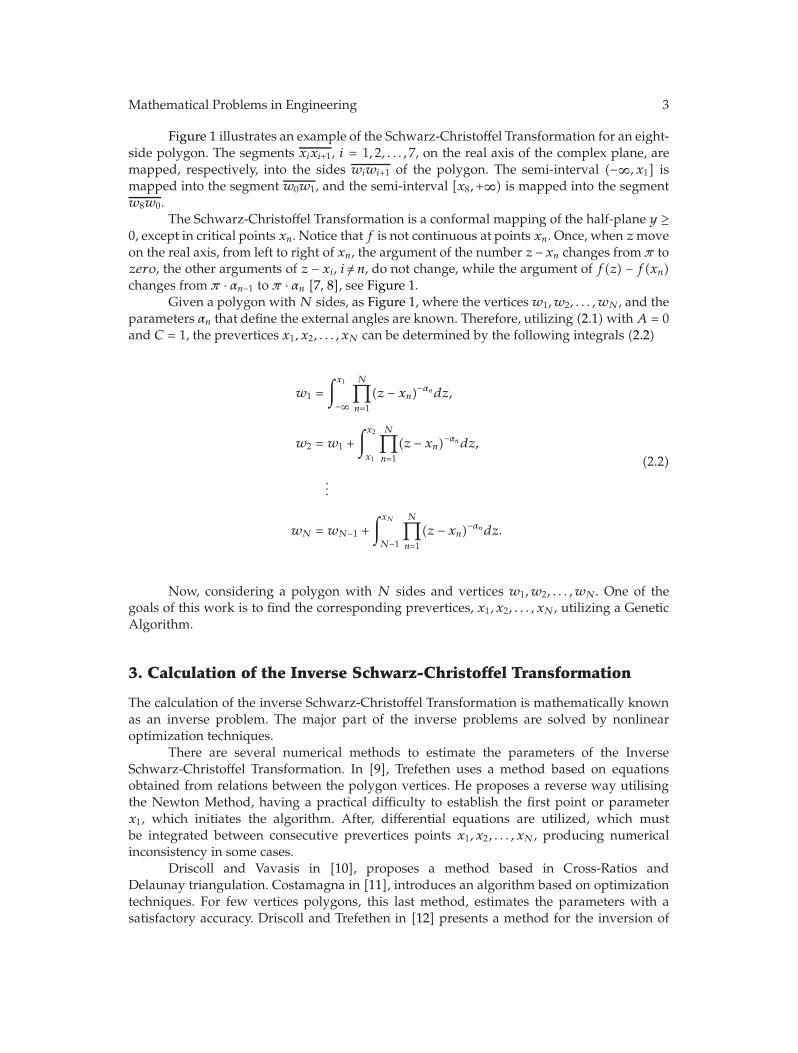
Consider a polygon in �, ofN sides, with its vertices inw1, w2, . . . , wN , ordered in thecounterclockwise, with corresponding internal angles denoted by β1, β2, . . . , βN and externalangles denoted by π · αn, n = 1, 2, . . . ,N. The Schwarz-Christoffel Transformation in theintegral form is defined by [2, 5]

w = f(z) = A + C∫ N∏

n=1

1(z − xn)αn

dz, (2.1)

where A and C are complex constants. The points x1, x2, . . . , xN over the real axis, calledprevertices, are mapped into the verticesw1, w2, . . . , wN. It is convenient to assume that z0 =f−1(w0) = ∞, because if infinity is not a prevertex, its image will be a new vertex with thecorresponding internal angle equal to π [6].

The complex constants A and C and the prevertices x1, x2, . . . , xN , are referred asparameters of the Schwarz-Christoffel Transformation.

Mathematical Problems in Engineering 3

Figure 1 illustrates an example of the Schwarz-Christoffel Transformation for an eight-side polygon. The segments xixi+1, i = 1, 2, . . . , 7, on the real axis of the complex plane, aremapped, respectively, into the sides wiwi+1 of the polygon. The semi-interval (−∞, x1] ismapped into the segment w0w1, and the semi-interval [x8,+∞) is mapped into the segmentw8w0.

The Schwarz-Christoffel Transformation is a conformal mapping of the half-plane y ≥0, except in critical points xn. Notice that f is not continuous at points xn. Once, when zmoveon the real axis, from left to right of xn, the argument of the number z − xn changes from π tozero, the other arguments of z − xi, i /=n, do not change, while the argument of f(z) − f(xn)changes from π · αn−1 to π · αn [7, 8], see Figure 1.

Given a polygon withN sides, as Figure 1, where the verticesw1, w2, . . . , wN , and theparameters αn that define the external angles are known. Therefore, utilizing (2.1)withA = 0and C = 1, the prevertices x1, x2, . . . , xN can be determined by the following integrals (2.2)

w1 =∫x1

−∞

N∏n=1

(z − xn)−αndz,

w2 = w1 +∫x2

x1

N∏n=1

(z − xn)−αndz,

...

wN = wN−1 +∫xN

N−1

N∏n=1

(z − xn)−αndz.

(2.2)

Now, considering a polygon with N sides and vertices w1, w2, . . . , wN. One of thegoals of this work is to find the corresponding prevertices, x1, x2, . . . , xN , utilizing a GeneticAlgorithm.

3. Calculation of the Inverse Schwarz-Christoffel Transformation

The calculation of the inverse Schwarz-Christoffel Transformation is mathematically knownas an inverse problem. The major part of the inverse problems are solved by nonlinearoptimization techniques.

There are several numerical methods to estimate the parameters of the InverseSchwarz-Christoffel Transformation. In [9], Trefethen uses a method based on equationsobtained from relations between the polygon vertices. He proposes a reverse way utilisingthe Newton Method, having a practical difficulty to establish the first point or parameterx1, which initiates the algorithm. After, differential equations are utilized, which mustbe integrated between consecutive prevertices points x1, x2, . . . , xN , producing numericalinconsistency in some cases.

Driscoll and Vavasis in [10], proposes a method based in Cross-Ratios andDelaunay triangulation. Costamagna in [11], introduces an algorithm based on optimizationtechniques. For few vertices polygons, this last method, estimates the parameters with asatisfactory accuracy. Driscoll and Trefethen in [12] presents a method for the inversion of


−∞

y

x

+∞x1 x2 x3 x4 x5 x6 x7 x8

z plane

z

(a)

π · αS

π · α7

π · α6

π · α2

π · α4

π · α5

π · α1

w w1 wS

w0

w2

w3

w4

w7

w5

w6

u

β1βS

β2

w planeν

π · α3

(b)

Figure 1:Mapping of a polygon through the direct Schwarz-Christoffel transformation.

the Schwarz-Christoffel Transformation, based on algebraic computation, which maps thepolygon onto a disc, an infinite strip or a rectangle.

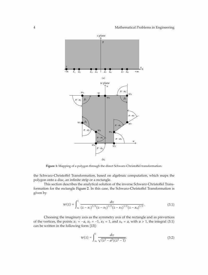
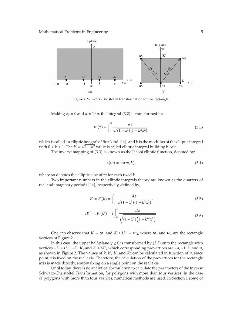
This section describes the analytical solution of the inverse Schwarz-Christoffel Trans-formation for the rectangle Figure 2. In this case, the Schwarz-Christoffel Transformation isgiven by

w(z) =∫z

z0

dz

(z − x1)1/2(z − x2)1/2(z − x3)1/2(z − x4)1/2. (3.1)

Choosing the imaginary axis as the symmetry axis of the rectangle and as preverticesof the vertices, the points x1 = −a, x2 = −1, x3 = 1, and x4 = a, with a > 1, the integral (3.1)can be written in the following form [13]:

w(z) =∫z

z0

dz√(z2 − a2)(z2 − 1)

. (3.2)


−αz0

z plane

α

x1 x2 x3 x4

y

−∞ +∞x

1−1

(a)

w plane

−K+iK ′ K

+iK

′

w2 w0 w3

w1w4

iK′

u

v

K

(b)

Figure 2: Schwarz-Christoffel transformation for the rectangle.

Making z0 = 0 and k = 1/a, the integral (3.2) is transformed in:

w(z) =∫z

0

dz√(1 − z2)(1 − k2z2) (3.3)

which is called an elliptic integral of first kind [14], and k is themodulus of the elliptic integralwith 0 < k < 1. The k′ =

√1 − k2 value is called elliptic integral building block.

The inverse mapping of (3.3) is known as the Jacobi elliptic function, denoted by:

z(w) = sn(w, k), (3.4)

where sn denotes the elliptic sine of w for each fixed k.Two important numbers in the elliptic integrals theory are known as the quarters of

real and imaginary periods [14], respectively, defined by,

K = K(k) =∫1

0

dz√(1 − z2)(1 − k2z2)

, (3.5)

iK′ = iK(k′)= i

∫1

0

dz√(1 − z2)

(1 − k′2z2

) , (3.6)

One can observe that K = w3 and K + iK′ = w4, where w3 and w4 are the rectanglevertices of Figure 2.

In this case, the upper half-plane y ≥ 0 is transformed by (3.3) onto the rectangle withvertices −K + iK′, −K, K, and K + iK′, which corresponding prevertices are −a, −1, 1, and a,as shown in Figure 2. The values of k, k′, K, and K′ can be calculated in function of a, sincepoint a is fixed on the real axis. Therefore, the calculation of the prevertices for the rectangleaxis is made directly, simply fixing on a single point on the real axis.

Until today, there is no analytical formulation to calculate the parameters of the InverseSchwarz-Christoffel Transformation, for polygons with more than four vertices. In the caseof polygons with more than four vertices, numerical methods are used. In Section 1 some of


0.3348 0.1554 0.2594 0.1911

0 0.325 0.1805 0.2538 0 0.101

0.3232 0.1997 0 00.26 0.0908

0.3199 0.2015 0.2678 0.0908

0.3155 0.2001 0 0.275 0.0792

0.3105 0.2107 0.2792 0.0792

0.3087 0.2394 0.2801 0.0554

0.3087 0 0.239 0 0.282 0.0422

0.3077 0.2492 0.2849 0.0422

Optimized individual

19.35

16.24

10.52

9.47

8.82

8.01

7.54

6.65

1.72

Evaluation function value

1st generation

2nd generation

3rd generation

4th generation

7th generation

10th generation

12th generation

14th generation

Individuals generated by theguided evolution operator

Figure 3: Guided Evolution operator.

these methods are cited. In this work, a Genetic Algorithm is utilized [15], to perform theparameters calculation.

4. Genetic Algorithm

Amongst the four paragons of the Evolutionary Computing, the Genetic Algorithm ownsmain position, once they constitute the most complete paradigm, gathering naturally allthe fundamental ideas of evolutionary computing [15]. Genetic algorithms are stochasticmethods with random search of optimal solutions. In the method, a population of individualsis maintained (chromosomes) representing possible solutions, being this populationsubjected to certain transformations (mutations and crossover), generating new and bettercandidates, which tend to improve the performance of the algorithm towards an optimalpoint or some optimized points [16].

In the genetic algorithm structure, the following operators are employed: DirectedCrossover operator [15], Tournament Selection operator [17], Elitism [18], CrossoverOperator with Multiple Descendants [19], Variable Mutation operator [17] and GuidedEvolution operator.

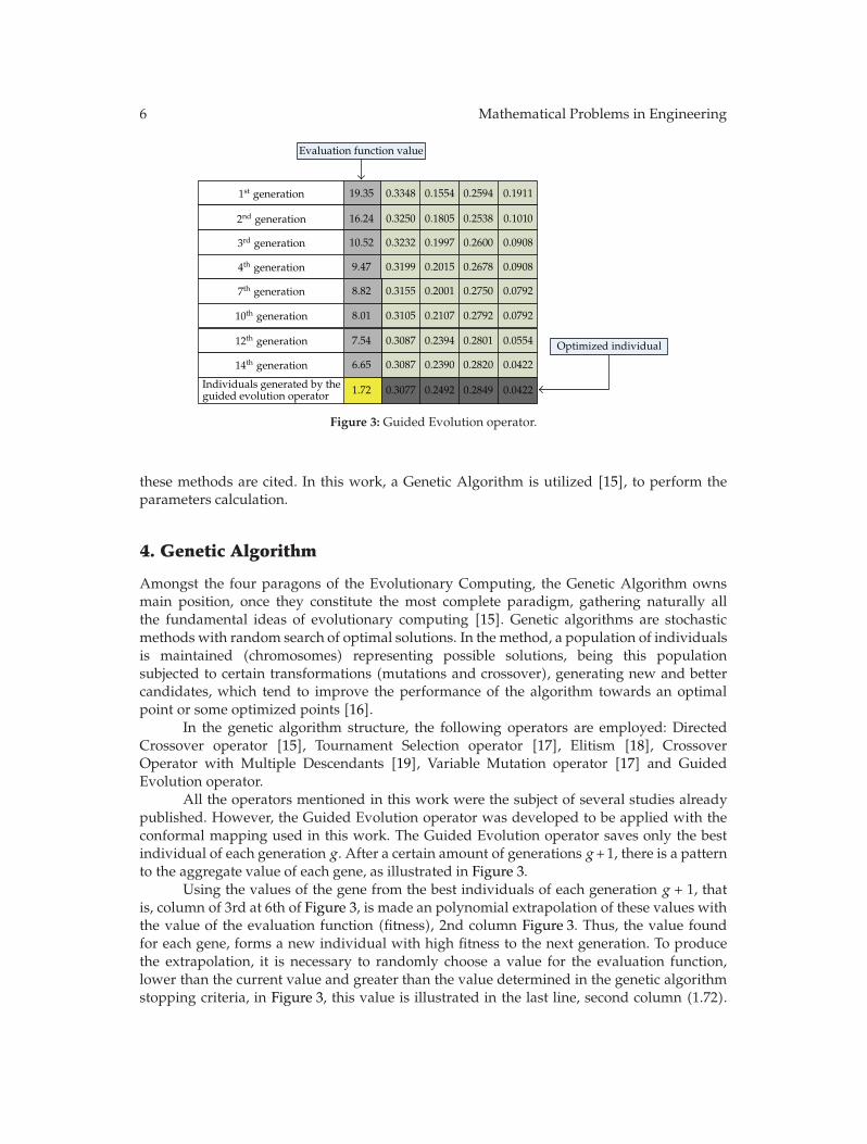
All the operators mentioned in this work were the subject of several studies alreadypublished. However, the Guided Evolution operator was developed to be applied with theconformal mapping used in this work. The Guided Evolution operator saves only the bestindividual of each generation g. After a certain amount of generations g +1, there is a patternto the aggregate value of each gene, as illustrated in Figure 3.

Using the values of the gene from the best individuals of each generation g + 1, thatis, column of 3rd at 6th of Figure 3, is made an polynomial extrapolation of these values withthe value of the evaluation function (fitness), 2nd column Figure 3. Thus, the value foundfor each gene, forms a new individual with high fitness to the next generation. To producethe extrapolation, it is necessary to randomly choose a value for the evaluation function,lower than the current value and greater than the value determined in the genetic algorithmstopping criteria, in Figure 3, this value is illustrated in the last line, second column (1.72).


0.305

0.31

0.315

0.32

0.325

0.33

0.335

Gen

e

Cubic spline extrapolationStorage geneFound gene

0 2 4 6 8 10 12 14 16 18 20

Guided evolution operation

Evaluation function f(x)

Figure 4: Extrapolation example for one column of genes.

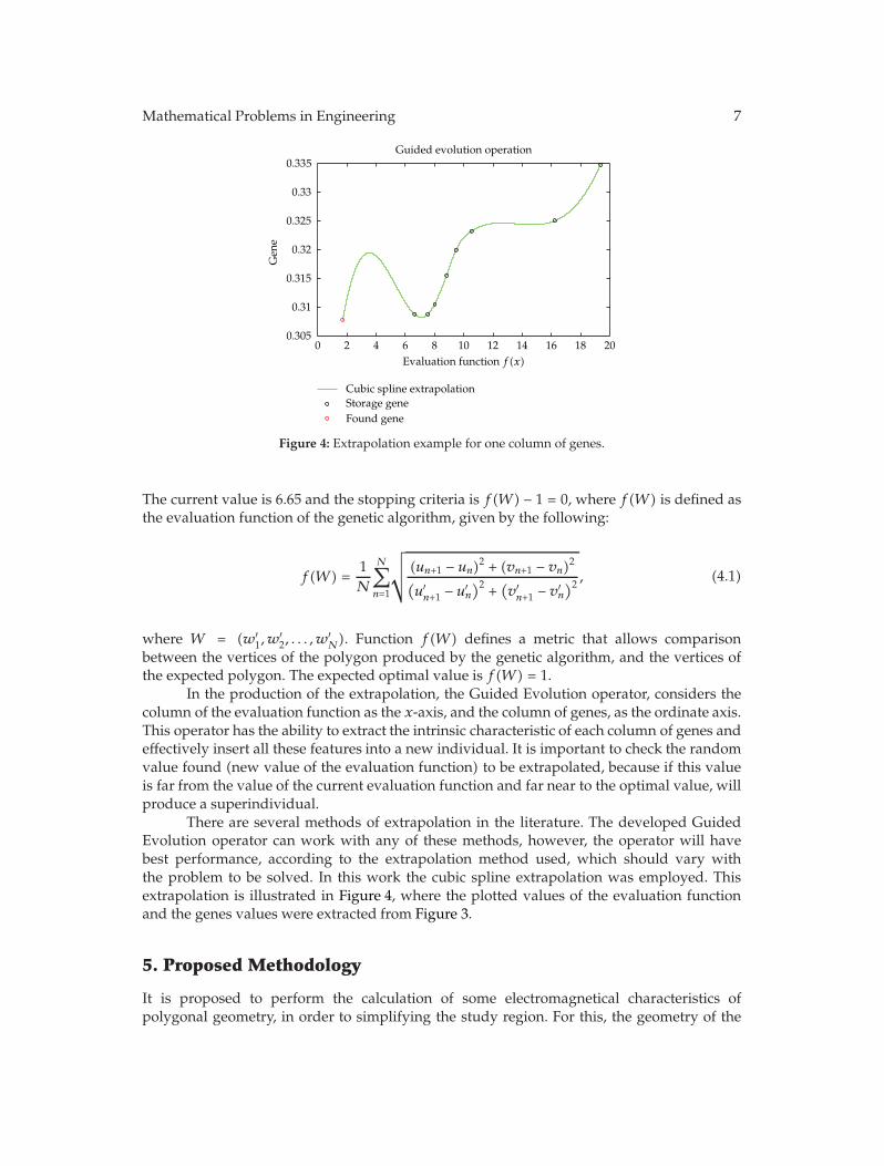
The current value is 6.65 and the stopping criteria is f(W) − 1 = 0, where f(W) is defined asthe evaluation function of the genetic algorithm, given by the following:

f(W) =1N

N∑n=1

√√√√ (un+1 − un)2 + (vn+1 − vn)2(u′n+1 − u′n

)2 + (v′n+1 − v′n

)2 , (4.1)

where W = (w′1, w

′2, . . . , w

′N). Function f(W) defines a metric that allows comparison

between the vertices of the polygon produced by the genetic algorithm, and the vertices ofthe expected polygon. The expected optimal value is f(W) = 1.

In the production of the extrapolation, the Guided Evolution operator, considers thecolumn of the evaluation function as the x-axis, and the column of genes, as the ordinate axis.This operator has the ability to extract the intrinsic characteristic of each column of genes andeffectively insert all these features into a new individual. It is important to check the randomvalue found (new value of the evaluation function) to be extrapolated, because if this valueis far from the value of the current evaluation function and far near to the optimal value, willproduce a superindividual.

There are several methods of extrapolation in the literature. The developed GuidedEvolution operator can work with any of these methods, however, the operator will havebest performance, according to the extrapolation method used, which should vary withthe problem to be solved. In this work the cubic spline extrapolation was employed. Thisextrapolation is illustrated in Figure 4, where the plotted values of the evaluation functionand the genes values were extracted from Figure 3.

5. Proposed Methodology

It is proposed to perform the calculation of some electromagnetical characteristics ofpolygonal geometry, in order to simplifying the study region. For this, the geometry of the


w1

w2w3

w4 w5

w6w7

w8

v

Plate 1Plate 2

u

w plane

(a)

y

xx1 x2 x3 x4 x5 x6 x7 x8

Plate 1 Plate 2

z plane

(b)

Figure 5: Inverse Schwarz-Christoffel transformation.

s

r

t4 t5

t3 t6

Plate 1 Plate 2

Figure 6: Equipotential and field lines in the auxiliary complex plane, t plane.

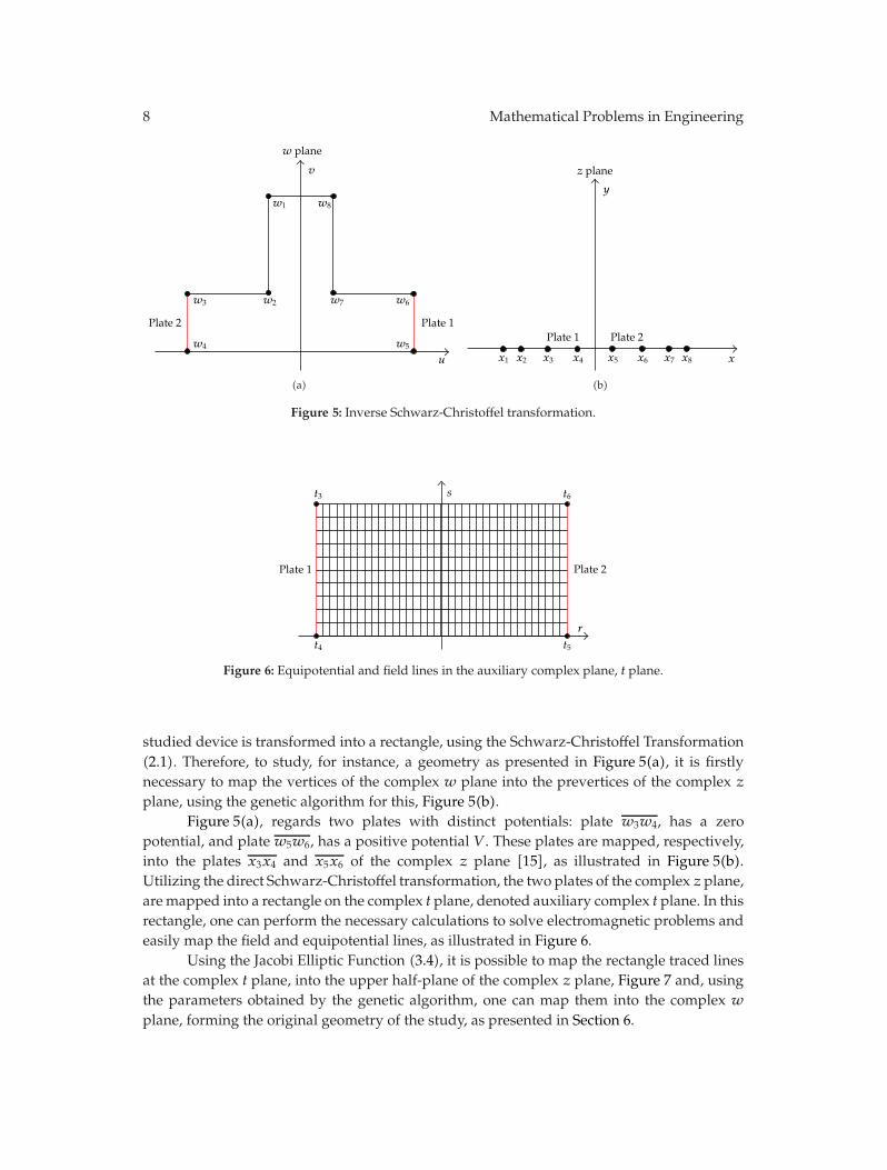
studied device is transformed into a rectangle, using the Schwarz-Christoffel Transformation(2.1). Therefore, to study, for instance, a geometry as presented in Figure 5(a), it is firstlynecessary to map the vertices of the complex w plane into the prevertices of the complex zplane, using the genetic algorithm for this, Figure 5(b).

Figure 5(a), regards two plates with distinct potentials: plate w3w4, has a zeropotential, and plate w5w6, has a positive potential V . These plates are mapped, respectively,into the plates x3x4 and x5x6 of the complex z plane [15], as illustrated in Figure 5(b).Utilizing the direct Schwarz-Christoffel transformation, the two plates of the complex z plane,aremapped into a rectangle on the complex t plane, denoted auxiliary complex t plane. In thisrectangle, one can perform the necessary calculations to solve electromagnetic problems andeasily map the field and equipotential lines, as illustrated in Figure 6.

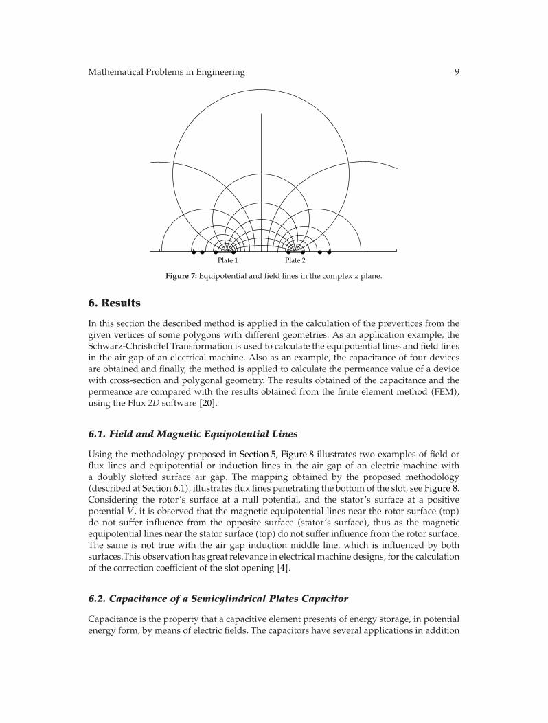
Using the Jacobi Elliptic Function (3.4), it is possible to map the rectangle traced linesat the complex t plane, into the upper half-plane of the complex z plane, Figure 7 and, usingthe parameters obtained by the genetic algorithm, one can map them into the complex wplane, forming the original geometry of the study, as presented in Section 6.


Plate 1 Plate 2

Figure 7: Equipotential and field lines in the complex z plane.

6. Results

In this section the described method is applied in the calculation of the prevertices from thegiven vertices of some polygons with different geometries. As an application example, theSchwarz-Christoffel Transformation is used to calculate the equipotential lines and field linesin the air gap of an electrical machine. Also as an example, the capacitance of four devicesare obtained and finally, the method is applied to calculate the permeance value of a devicewith cross-section and polygonal geometry. The results obtained of the capacitance and thepermeance are compared with the results obtained from the finite element method (FEM),using the Flux 2D software [20].

6.1. Field and Magnetic Equipotential Lines

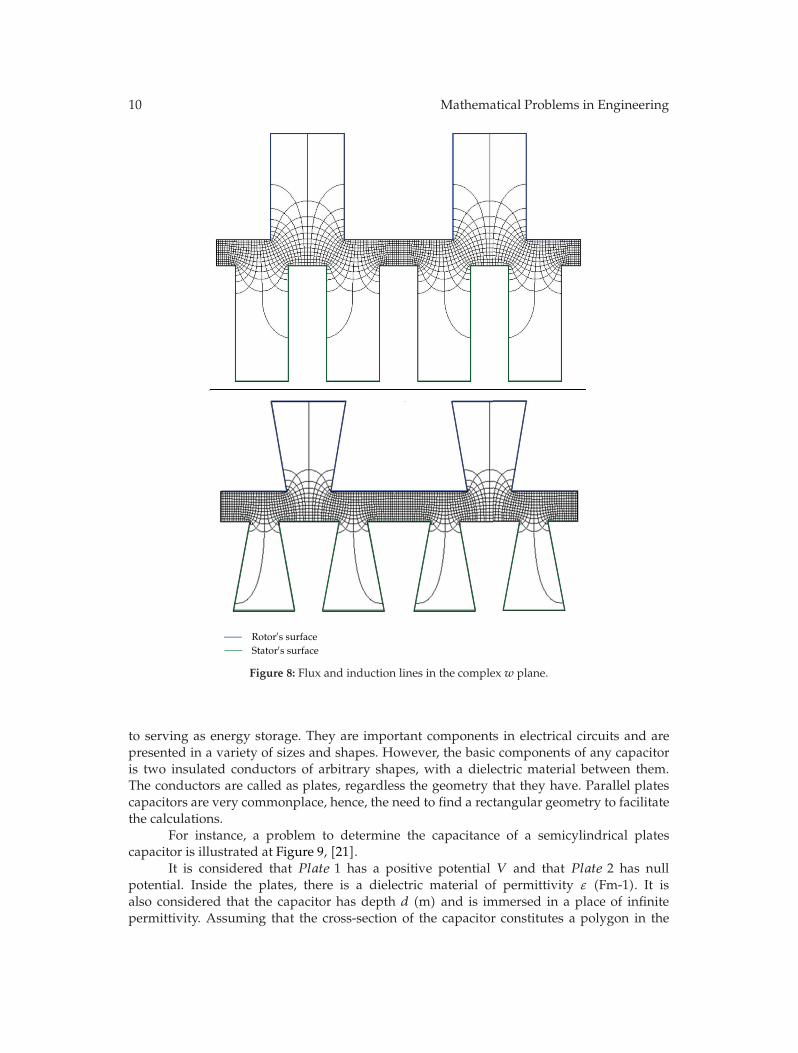
Using the methodology proposed in Section 5, Figure 8 illustrates two examples of field orflux lines and equipotential or induction lines in the air gap of an electric machine witha doubly slotted surface air gap. The mapping obtained by the proposed methodology(described at Section 6.1), illustrates flux lines penetrating the bottom of the slot, see Figure 8.Considering the rotor’s surface at a null potential, and the stator’s surface at a positivepotential V , it is observed that the magnetic equipotential lines near the rotor surface (top)do not suffer influence from the opposite surface (stator’s surface), thus as the magneticequipotential lines near the stator surface (top) do not suffer influence from the rotor surface.The same is not true with the air gap induction middle line, which is influenced by bothsurfaces.This observation has great relevance in electrical machine designs, for the calculationof the correction coefficient of the slot opening [4].

6.2. Capacitance of a Semicylindrical Plates Capacitor

Capacitance is the property that a capacitive element presents of energy storage, in potentialenergy form, by means of electric fields. The capacitors have several applications in addition


Rotor′s surfaceStator′s surface

Figure 8: Flux and induction lines in the complexw plane.

to serving as energy storage. They are important components in electrical circuits and arepresented in a variety of sizes and shapes. However, the basic components of any capacitoris two insulated conductors of arbitrary shapes, with a dielectric material between them.The conductors are called as plates, regardless the geometry that they have. Parallel platescapacitors are very commonplace, hence, the need to find a rectangular geometry to facilitatethe calculations.

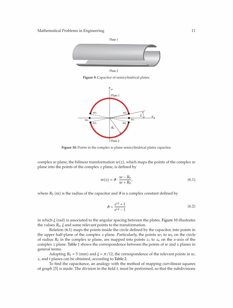
For instance, a problem to determine the capacitance of a semicylindrical platescapacitor is illustrated at Figure 9, [21].

It is considered that Plate 1 has a positive potential V and that Plate 2 has nullpotential. Inside the plates, there is a dielectric material of permittivity ε (Fm-1). It isalso considered that the capacitor has depth d (m) and is immersed in a place of infinitepermittivity. Assuming that the cross-section of the capacitor constitutes a polygon in the


Plate 1

Plate 2

Figure 9: Capacitor of semicylindrical plates.

w1

w2w3

w4w6

Plate 1

Plate 2

uξ

ν

R0

w5

Figure 10: Points in the complexw plane semicylindrical plates capacitor.

complex w plane, the bilinear transformationw(z), which maps the points of the complex wplane into the points of the complex z plane, is defined by

w(z) = ϑ · w − R0

w + R0, (6.1)

where R0 (m) is the radius of the capacitor and ϑ is a complex constant defined by

ϑ =ei·ξ + 1ei·ξ − 1

(6.2)

in which ξ (rad) is associated to the angular spacing between the plates. Figure 10 illustratesthe values R0, ξ and some relevant points to the transformation.

Relation (6.1) maps the points inside the circle defined by the capacitor, into points inthe upper half-plane of the complex z plane. Particularly, the points w1 to w6 on the circleof radius R0 in the complex w plane, are mapped into points z1 to z6 on the x-axis of thecomplex z plane. Table 1 shows the correspondence between the points of w and z planes ingeneral terms.

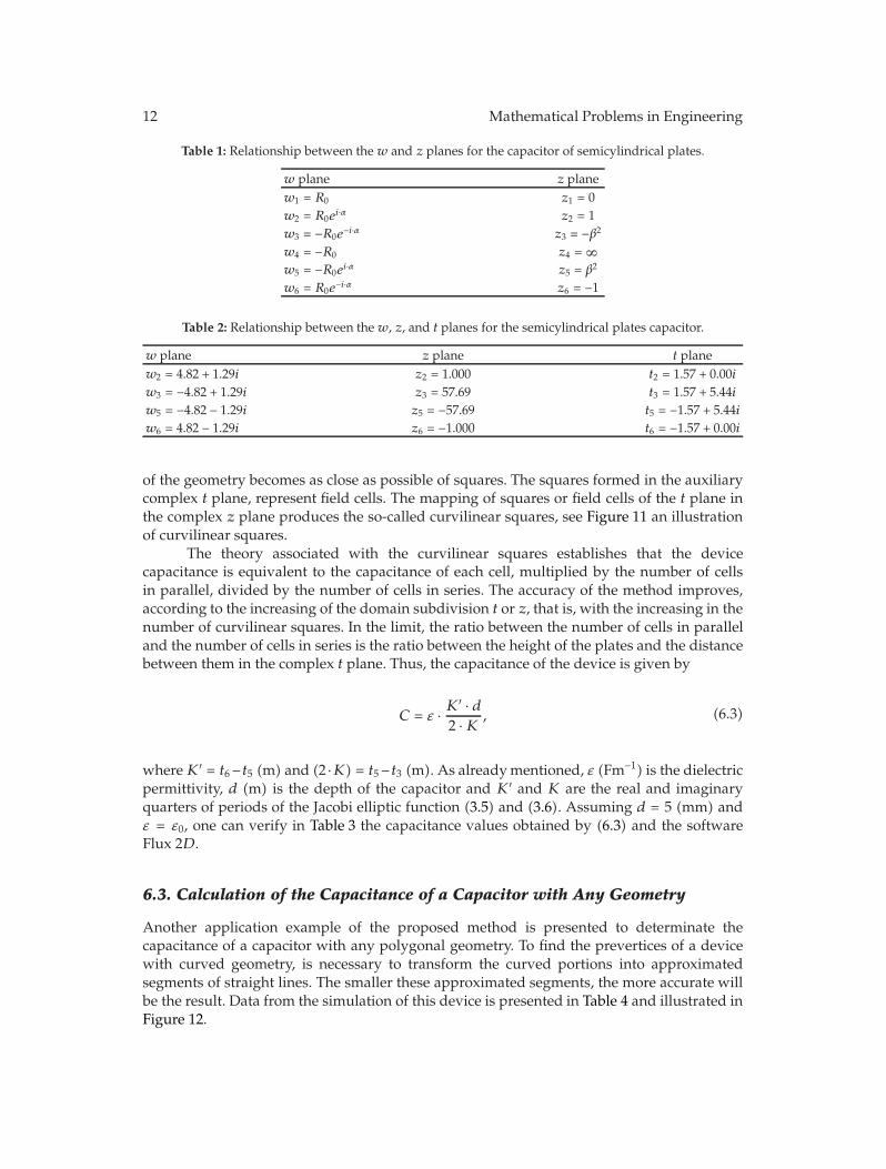
Adopting R0 = 5 (mm) and ξ = π/12, the correspondence of the relevant points in w,z, and t planes can be obtained, according to Table 2.

To find the capacitance, an analogy with the method of mapping curvilinear squaresof graph [3] is made. The division in the field t, must be performed, so that the subdivisions


Table 1: Relationship between the w and z planes for the capacitor of semicylindrical plates.

w plane z planew1 = R0 z1 = 0w2 = R0ei·α z2 = 1w3 = −R0e−i·α z3 = −β2w4 = −R0 z4 = ∞w5 = −R0ei·α z5 = β2

w6 = R0e−i·α z6 = −1

Table 2: Relationship between the w, z, and t planes for the semicylindrical plates capacitor.

w plane z plane t planew2 = 4.82 + 1.29i z2 = 1.000 t2 = 1.57 + 0.00iw3 = −4.82 + 1.29i z3 = 57.69 t3 = 1.57 + 5.44iw5 = −4.82 − 1.29i z5 = −57.69 t5 = −1.57 + 5.44iw6 = 4.82 − 1.29i z6 = −1.000 t6 = −1.57 + 0.00i

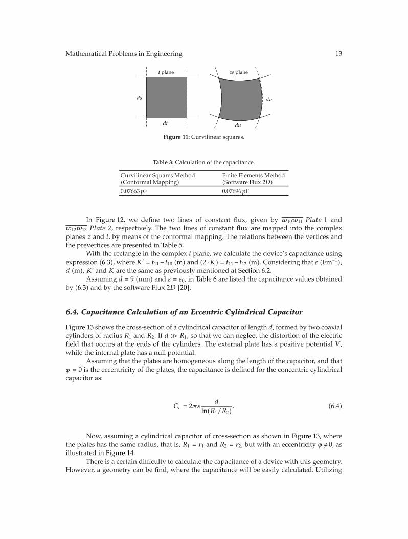
of the geometry becomes as close as possible of squares. The squares formed in the auxiliarycomplex t plane, represent field cells. The mapping of squares or field cells of the t plane inthe complex z plane produces the so-called curvilinear squares, see Figure 11 an illustrationof curvilinear squares.

The theory associated with the curvilinear squares establishes that the devicecapacitance is equivalent to the capacitance of each cell, multiplied by the number of cellsin parallel, divided by the number of cells in series. The accuracy of the method improves,according to the increasing of the domain subdivision t or z, that is, with the increasing in thenumber of curvilinear squares. In the limit, the ratio between the number of cells in paralleland the number of cells in series is the ratio between the height of the plates and the distancebetween them in the complex t plane. Thus, the capacitance of the device is given by

C = ε · K′ · d

2 ·K , (6.3)

whereK′ = t6− t5 (m) and (2 ·K) = t5− t3 (m). As alreadymentioned, ε (Fm−1) is the dielectricpermittivity, d (m) is the depth of the capacitor and K′ and K are the real and imaginaryquarters of periods of the Jacobi elliptic function (3.5) and (3.6). Assuming d = 5 (mm) andε = ε0, one can verify in Table 3 the capacitance values obtained by (6.3) and the softwareFlux 2D.

6.3. Calculation of the Capacitance of a Capacitor with Any Geometry

Another application example of the proposed method is presented to determinate thecapacitance of a capacitor with any polygonal geometry. To find the prevertices of a devicewith curved geometry, is necessary to transform the curved portions into approximatedsegments of straight lines. The smaller these approximated segments, the more accurate willbe the result. Data from the simulation of this device is presented in Table 4 and illustrated inFigure 12.


t plane w plane

dv

du

ds

dr

Figure 11: Curvilinear squares.

Table 3: Calculation of the capacitance.

Curvilinear Squares Method(Conformal Mapping)

Finite Elements Method(Software Flux 2D)

0.07663pF 0.07696pF

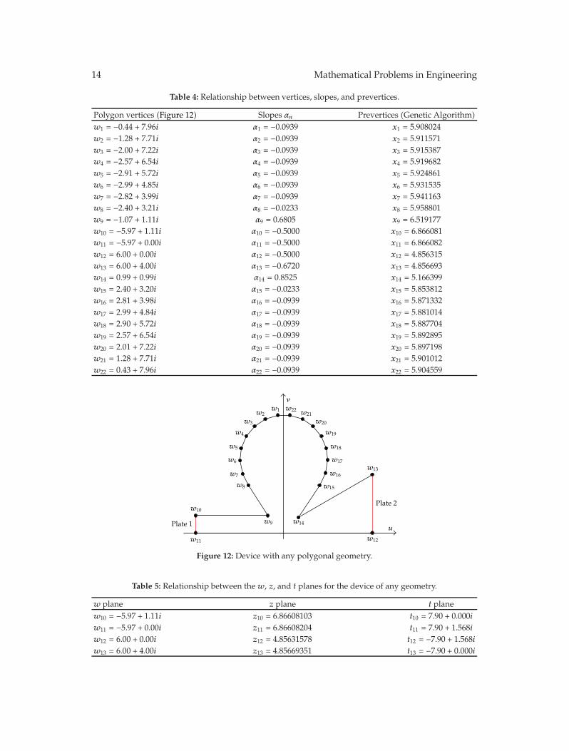
In Figure 12, we define two lines of constant flux, given by w10w11 Plate 1 andw12w13 Plate 2, respectively. The two lines of constant flux are mapped into the complexplanes z and t, by means of the conformal mapping. The relations between the vertices andthe prevertices are presented in Table 5.

With the rectangle in the complex t plane, we calculate the device’s capacitance usingexpression (6.3), whereK′ = t11 − t10 (m) and (2 ·K) = t11 − t12 (m). Considering that ε (Fm−1),d (m), K′ and K are the same as previously mentioned at Section 6.2.

Assuming d = 9 (mm) and ε = ε0, in Table 6 are listed the capacitance values obtainedby (6.3) and by the software Flux 2D [20].

6.4. Capacitance Calculation of an Eccentric Cylindrical Capacitor

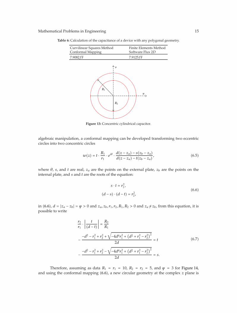
Figure 13 shows the cross-section of a cylindrical capacitor of length d, formed by two coaxialcylinders of radius R1 and R2. If d � R1, so that we can neglect the distortion of the electricfield that occurs at the ends of the cylinders. The external plate has a positive potential V ,while the internal plate has a null potential.

Assuming that the plates are homogeneous along the length of the capacitor, and thatψ = 0 is the eccentricity of the plates, the capacitance is defined for the concentric cylindricalcapacitor as:

Cc = 2πεd

ln(R1/R2). (6.4)

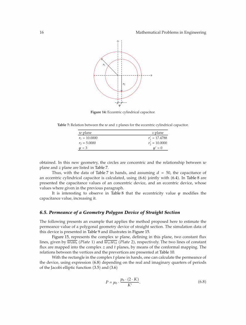
Now, assuming a cylindrical capacitor of cross-section as shown in Figure 13, wherethe plates has the same radius, that is, R1 = r1 and R2 = r2, but with an eccentricity ψ /= 0, asillustrated in Figure 14.

There is a certain difficulty to calculate the capacitance of a device with this geometry.However, a geometry can be find, where the capacitance will be easily calculated. Utilizing


Table 4: Relationship between vertices, slopes, and prevertices.

Polygon vertices (Figure 12) Slopes αn Prevertices (Genetic Algorithm)w1 = −0.44 + 7.96i α1 = −0.0939 x1 = 5.908024w2 = −1.28 + 7.71i α2 = −0.0939 x2 = 5.911571w3 = −2.00 + 7.22i α3 = −0.0939 x3 = 5.915387w4 = −2.57 + 6.54i α4 = −0.0939 x4 = 5.919682w5 = −2.91 + 5.72i α5 = −0.0939 x5 = 5.924861w6 = −2.99 + 4.85i α6 = −0.0939 x6 = 5.931535w7 = −2.82 + 3.99i α7 = −0.0939 x7 = 5.941163w8 = −2.40 + 3.21i α8 = −0.0233 x8 = 5.958801w9 = −1.07 + 1.11i α9 = 0.6805 x9 = 6.519177w10 = −5.97 + 1.11i α10 = −0.5000 x10 = 6.866081w11 = −5.97 + 0.00i α11 = −0.5000 x11 = 6.866082w12 = 6.00 + 0.00i α12 = −0.5000 x12 = 4.856315w13 = 6.00 + 4.00i α13 = −0.6720 x13 = 4.856693w14 = 0.99 + 0.99i α14 = 0.8525 x14 = 5.166399w15 = 2.40 + 3.20i α15 = −0.0233 x15 = 5.853812w16 = 2.81 + 3.98i α16 = −0.0939 x16 = 5.871332w17 = 2.99 + 4.84i α17 = −0.0939 x17 = 5.881014w18 = 2.90 + 5.72i α18 = −0.0939 x18 = 5.887704w19 = 2.57 + 6.54i α19 = −0.0939 x19 = 5.892895w20 = 2.01 + 7.22i α20 = −0.0939 x20 = 5.897198w21 = 1.28 + 7.71i α21 = −0.0939 x21 = 5.901012w22 = 0.43 + 7.96i α22 = −0.0939 x22 = 5.904559

w15

w16

w17

w18

w19

w20

w21w22

w14

w13

w12

w1w2

w3

w4

w5

w6

w7

w8

w9

w10

w11

u

ν

Plate 1

Plate 2

Figure 12: Device with any polygonal geometry.

Table 5: Relationship between the w, z, and t planes for the device of any geometry.

w plane z plane t planew10 = −5.97 + 1.11i z10 = 6.86608103 t10 = 7.90 + 0.000iw11 = −5.97 + 0.00i z11 = 6.86608204 t11 = 7.90 + 1.568iw12 = 6.00 + 0.00i z12 = 4.85631578 t12 = −7.90 + 1.568iw13 = 6.00 + 4.00i z13 = 4.85669351 t13 = −7.90 + 0.000i


Table 6: Calculation of the capacitance of a device with any polygonal geometry.

Curvilinear Squares MethodConformal Mapping

Finite Elements MethodSoftware Flux 2D

7.9082fF 7.9125fF

R1

R2

u

ν

Figure 13: Concentric cylindrical capacitor.

algebraic manipulation, a conformal mapping can be developed transforming two eccentriccircles into two concentric circles

w(z) = t · R1

r1· eiθ · d(z − za) − s(zb − za)

d(z − za) − t(zb − za) , (6.5)

where θ, s, and t are real, za are the points on the external plate, zb are the points on theinternal plate, and s and t are the roots of the equation:

s · t = r21 ,

(d − s) · (d − t) = r22 ,(6.6)

in (6.6), d = |za − zb| = ψ > 0 and za, zb, r1, r2, R1, R2 > 0 and za /= zb, from this equation, it ispossible to write

r2r1

·∣∣∣∣ t

(d − t)∣∣∣∣ = R2

R1

−−d2 − r21 + r22 +

√−4d4r21 +

(d2 + r21 − r22

)22d

= t

−−d2 − r21 + r22 −

√−4d4r21 +

(d2 + r21 − r22

)22d

= s.

(6.7)

Therefore, assuming as data R1 = r1 = 10, R2 = r2 = 5, and ψ = 3 for Figure 14,and using the conformal mapping (6.6), a new circular geometry at the complex z plane is


r1

r2

ψ

Figure 14: Eccentric cylindrical capacitor.

Table 7: Relation between the w and z planes for the eccentric cylindrical capacitor.

w plane z planer1 = 10.0000 r ′1 = 17.4788r2 = 5.0000 r ′2 = 10.0000ψ = 3 ψ ′ = 0

obtained. In this new geometry, the circles are concentric and the relationship between wplane and z plane are listed in Table 7.

Thus, with the data of Table 7 in hands, and assuming d = 50, the capacitance ofan eccentric cylindrical capacitor is calculated, using (6.6) jointly with (6.4). In Table 8 arepresented the capacitance values of an concentric device, and an eccentric device, whosevalues where given in the previous paragraph.

It is interesting to observe in Table 8 that the eccentricity value ψ modifies thecapacitance value, increasing it.

6.5. Permeance of a Geometry Polygon Device of Straight Section

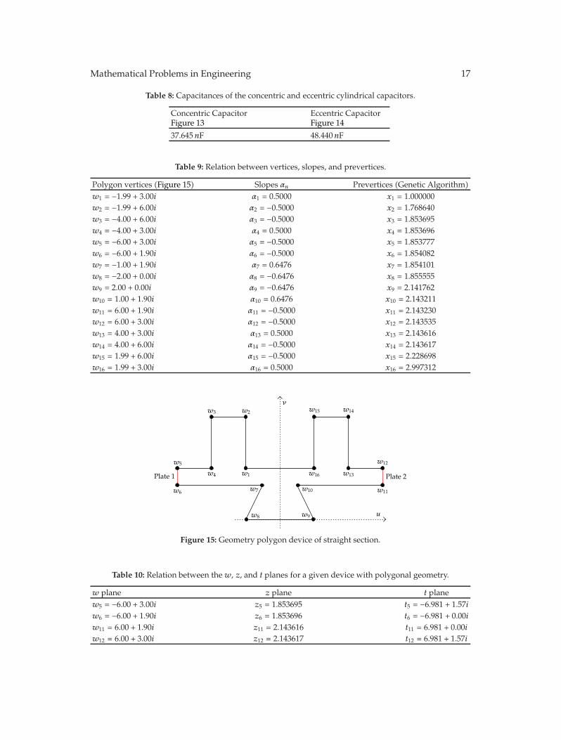
The following presents an example that applies the method proposed here to estimate thepermeance value of a polygonal geometry device of straight section. The simulation data ofthis device is presented in Table 9 and illustrates in Figure 15.

Figure 15, represents the complex w plane, defining in this plane, two constant fluxlines, given by w5w6 (Plate 1) and w11w12 (Plate 2), respectively. The two lines of constantflux are mapped into the complex z and t planes, by means of the conformal mapping. Therelations between the vertices and the prevertices are presented at Table 10.

With the rectangle in the complex t plane in hands, one can calculate the permeance ofthe device, using expression (6.8) depending on the real and imaginary quarters of periodsof the Jacobi elliptic function (3.5) and (3.6)

P = μ0 ·pb · (2 ·K)

K′ . (6.8)


Table 8: Capacitances of the concentric and eccentric cylindrical capacitors.

Concentric CapacitorFigure 13

Eccentric CapacitorFigure 14

37.645nF 48.440nF

Table 9: Relation between vertices, slopes, and prevertices.

Polygon vertices (Figure 15) Slopes αn Prevertices (Genetic Algorithm)w1 = −1.99 + 3.00i α1 = 0.5000 x1 = 1.000000w2 = −1.99 + 6.00i α2 = −0.5000 x2 = 1.768640w3 = −4.00 + 6.00i α3 = −0.5000 x3 = 1.853695w4 = −4.00 + 3.00i α4 = 0.5000 x4 = 1.853696w5 = −6.00 + 3.00i α5 = −0.5000 x5 = 1.853777w6 = −6.00 + 1.90i α6 = −0.5000 x6 = 1.854082w7 = −1.00 + 1.90i α7 = 0.6476 x7 = 1.854101w8 = −2.00 + 0.00i α8 = −0.6476 x8 = 1.855555w9 = 2.00 + 0.00i α9 = −0.6476 x9 = 2.141762w10 = 1.00 + 1.90i α10 = 0.6476 x10 = 2.143211w11 = 6.00 + 1.90i α11 = −0.5000 x11 = 2.143230w12 = 6.00 + 3.00i α12 = −0.5000 x12 = 2.143535w13 = 4.00 + 3.00i α13 = 0.5000 x13 = 2.143616w14 = 4.00 + 6.00i α14 = −0.5000 x14 = 2.143617w15 = 1.99 + 6.00i α15 = −0.5000 x15 = 2.228698w16 = 1.99 + 3.00i α16 = 0.5000 x16 = 2.997312

w15

w16

w14

w13

w12

w1

w2w3

w4

w5

w6 w7

w8 w9

w10 w11

ν

Plate 1 Plate 2

u

Figure 15: Geometry polygon device of straight section.

Table 10: Relation between thew, z, and t planes for a given device with polygonal geometry.

w plane z plane t planew5 = −6.00 + 3.00i z5 = 1.853695 t5 = −6.981 + 1.57iw6 = −6.00 + 1.90i z6 = 1.853696 t6 = −6.981 + 0.00iw11 = 6.00 + 1.90i z11 = 2.143616 t11 = 6.981 + 0.00iw12 = 6.00 + 3.00i z12 = 2.143617 t12 = 6.981 + 1.57i


In which (2 ·K) = t11 − t6 (m), K′ = t12 − t11 (m) and pb (m) is the depth of the device,in this case, pb = 1. The permeance value found for the device shown at Figure 15, using theproposed methodology in (6.8), is 11.17nH.

7. Conclusion

The results presented in Sections 6.1, 6.2, 6.3, 6.4, and 6.5 showed that the solution ofelectromagnetic problems related to geometry, can be simplified, using the conformalmapping. Also, the Schwarz-Christoffel Transformation appears to be a suitable and effectivetool to solve problems involving complicated geometries forms, considering the conformalmapping property of modifying only the geometry of a polygonal structure, preserving thephysical magnitude corresponding to each point at the plane. Regarding the mathematicaloperator developed to help the optimization method, there was a reduction of approximately38% on average in the number of generations g to be achieved, when compared with thegenetic algorithm without the operator. Therefore, the guided evolution operator, promoteda stimulus in the used optimization method, reducing the time spent in the search ofoptimized parameters. In Sections 6.2 and 6.4, the capacitance calculation performed by theproposed method was compared with results obtained by Flux 2D software, validating theproposed method. The computational processes were reduced comparing with sophisticatedsoftwares used to produce electromagnetic fields, leading an improvement in the calculationperformance of some devices with odd geometry. As a suggestion for future studies, themethodology using conformal mapping allied to the developed mathematical operator,could be applied in the design of optimized electric devices, of any desired geometry. Thecalculations presented here are useful as a theoretical framework to guide experiments oncapacitors from different geometry and introduce a new concept in the permeance estimationof electrical devices.

Acknowledgments

The authors acknowledge the Capes Foundation, Ministry of Education of Brazil, for thefinancial support scholarship Proc. no. BEX 3873/10-2. This work was supported in partby the brazilian agencies Coordenacao de Aperfeicoamento de Pessoal de Nıvel Superior(CAPES/MEC) and Conselho Nacional de Desenvolvimento Cientıfico e Tecnologico(CNPq) under Grant 479186/2006-5/Universal.

References

[1] P. Henrici, Applied and Computational Complex Analysis, vol. 3 of Pure and Applied Mathematics, JohnWiley & Sons, New York, NY, USA, 1986.

[2] M. R. Spiegel, Complex Variable, McGraw-Hill, New York, NY, USA, 1967.[3] J. D. Kraus and K. R. Carver, Electromagnetics, McGraw-Hill, New York, NY, USA, 1973.[4] W. P. Calixto, E. G. Marra, L. C. Brito, and B. P. Alvarenga, “A new methodology to calculate

carter factor using geneticalgorithms,” International Journal of Numerical Modelling: Electronic Networks,Devices and Fields. In press.

[5] Z. Nehari, Conformal Mapping, McGraw-Hill, New York, NY, USA, 1952.[6] H. Cohn, Conformal Mapping on Riemann Surfaces, Dover, New York, NY, USA, 1967.[7] W. J. Gibbs, Conformal Transformations in Electrical Engineering, Chapman and Hall, London, UK, 1958.[8] G. C. Wen, Conformal Mappings and Boundary Value Problems, vol. 106 of Translations of Mathematical

Monographs, American Mathematical Society, Providence, RI, USA, 1992.


[9] L. N. Trefethen, “Numerical computation of the Schwarz-Christoffel transformation,” Society forIndustrial and Applied Mathematics, vol. 1, no. 1, pp. 82–102, 1980.

[10] T. A. Driscoll and S. A. Vavasis, “Numerical conformal mapping using cross-ratios and Delaunaytriangulation,” SIAM Journal on Scientific Computing, vol. 19, no. 6, pp. 1783–1803, 1998.

[11] E. Costamagna, “On the numerical inversion of the schwarz-christoffel conformal transformation,”IEEE Transactions on Microwave Theory and Techniques, vol. 35, no. 1, pp. 35–40, 1987.

[12] T. A. Driscoll and L. N. Trefethen, Schwarz-Christoffel Mapping, vol. 8 of Cambridge Monographs onApplied and Computational Mathematics, Cambridge University Press, Cambridge, UK, 2002.

[13] M. Abramowitz and I. A. Stegun, Handbook of Mathematical Functions: with Formulas, Graphs, andMathematical Tables, Dover, New York, NY, USA, 1968.

[14] S. C. Milne, Infinite Families of Exact Sums of Squares Formulas, Jacobi Elliptic Functions, ContinuedFractions, and Schur Functions, vol. 5 of Developments in Mathematics, Kluwer Academic Publishers,Boston, Mass, USA, 2002.

[15] W. P. Calixto, Application of conformal mapping to the calculus of Carter’s factor, M.S. thesis, Electrical &Computer Engineering School, Federal University of Goias, Goiania, Brazil, 2008.

[16] Z. Michalewicz, Genetic Algorithms + Data Structures = Evolution Programs, Artificial Intelligence,Springer, Berlin, Germany, 1992.

[17] Z. Michalewicz and D. B. Fogel, How to Solve it: Modern Heuristics, Springer, Berlin, Germany, 2000.[18] J. H. Holland, Adaptation in Natural and Artificial Systems: an Introductory Analysis with Applications to

Biology, Control, and Artificial Intelligence, University of Michigan Press, Ann Arbor, Mich, USA, 1975.[19] F. Herrera, M. Lozano, and J. L. Verdegay, “Crossover operators and offspring selection for real

coded genetic algorithms,” Tech. Rep., Department of Intelligence of the Computation and Artificialintelligence, University of Granada, Granada, Spain, 1994.

[20] Cedrat, Flux 2D User’s Guide, Cedrat, Grenoble, France, 2000.[21] R. E. Collins, Mathematical Methods for Physicists and Engineers, Dover, New York, NY, USA, 2nd

edition, 1999.

Documents

Electromagnetic Problems Solving by Conformal … Problems Solving by Conformal Mapping: A Mathematical Operator for Optimization Wesley Pacheco Calixto,1,2,3 Bernardo Alvarenga,1,3