Embed Size (px)
Citation preview

UNIVERSITÀ DEGLI STUDI DI TRIESTE
Sede amministrativa del Dottorato di Ricerca
DIPARTIMENTO DI FISICA
XXVI CICLO DEL
DOTTORATO DI RICERCA IN FISICA
Electromagnetic Radiation Emission and
Flavour Oscillations in Collapse Models
Settore scientifico-disciplinare FIS/02
DOTTORANDO: COORDINATORE DEL DOTTORATO DI RICERCA:
Sandro Donadi Prof. Paolo Camerini
Firma:
SUPERVISORE DI TESI:
Dr. Angelo Bassi
Firma:
ANNO ACCADEMICO 2012/2013

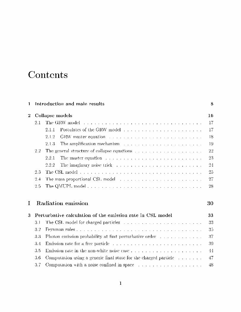
Contents
1 Introduction and main results 8
2 Collapse models 16
2.1 The GRW model . . . . . . . . . . . . . . . . . . . . . . . . . . . . . . . . . 17
2.1.1 Postulates of the GRW model . . . . . . . . . . . . . . . . . . . . . . 17
2.1.2 GRW master equation . . . . . . . . . . . . . . . . . . . . . . . . . . 18
2.1.3 The amplication mechanism . . . . . . . . . . . . . . . . . . . . . . 19
2.2 The general structure of collapse equations . . . . . . . . . . . . . . . . . . . 22
2.2.1 The master equation . . . . . . . . . . . . . . . . . . . . . . . . . . . 23
2.2.2 The imaginary noise trick . . . . . . . . . . . . . . . . . . . . . . . . 24
2.3 The CSL model . . . . . . . . . . . . . . . . . . . . . . . . . . . . . . . . . . 25
2.4 The mass proportional CSL model . . . . . . . . . . . . . . . . . . . . . . . 27
2.5 The QMUPL model . . . . . . . . . . . . . . . . . . . . . . . . . . . . . . . . 28
I Radiation emission 30
3 Perturbative calculation of the emission rate in CSL model 33
3.1 The CSL model for charged particles . . . . . . . . . . . . . . . . . . . . . . 33
3.2 Feynman rules . . . . . . . . . . . . . . . . . . . . . . . . . . . . . . . . . . . 35
3.3 Photon emission probability at rst perturbative order . . . . . . . . . . . . 37
3.4 Emission rate for a free particle . . . . . . . . . . . . . . . . . . . . . . . . . 39
3.5 Emission rate in the non-white noise case . . . . . . . . . . . . . . . . . . . . 44
3.6 Computation using a generic nal state for the charged particle . . . . . . . 47
3.7 Computation with a noise conned in space . . . . . . . . . . . . . . . . . . 48
1

CONTENTS 2
4 Radiation emission in QMUPL model 52
4.1 The model and the solutions of the Heisenberg equations . . . . . . . . . . . 53
4.2 The formula for the emission rate . . . . . . . . . . . . . . . . . . . . . . . . 56
4.3 Free particle . . . . . . . . . . . . . . . . . . . . . . . . . . . . . . . . . . . . 57
4.4 Harmonic oscillator . . . . . . . . . . . . . . . . . . . . . . . . . . . . . . . . 59
4.5 First order perturbation analysis . . . . . . . . . . . . . . . . . . . . . . . . . 61
4.6 Semiclassical derivation of the emission rate . . . . . . . . . . . . . . . . . . 62
5 The emission rate in the CSL model 66
5.1 The formula for the emission rate . . . . . . . . . . . . . . . . . . . . . . . . 66
5.2 Computation of the emission rate . . . . . . . . . . . . . . . . . . . . . . . . 68
5.2.1 The formula for the photon's number operator . . . . . . . . . . . . . 69
5.2.2 Time evolution of the relevant operators . . . . . . . . . . . . . . . . 70
5.2.3 Analytic expression of C (t, t1) . . . . . . . . . . . . . . . . . . . . . . 73
5.2.4 Analytic expression of D (t, t1, t2) . . . . . . . . . . . . . . . . . . . . 76
5.2.5 Computation of the average photon number . . . . . . . . . . . . . . 77
5.2.6 Time integrals . . . . . . . . . . . . . . . . . . . . . . . . . . . . . . . 80
5.2.7 Final Result . . . . . . . . . . . . . . . . . . . . . . . . . . . . . . . . 84
6 The emission rate for a generic system 85
6.1 The non resonant terms and their connection with the unphysical term . . . 86
6.1.1 Adiabatic switch on of the potential and other approaches . . . . . . 88
6.1.2 Decay of propagator . . . . . . . . . . . . . . . . . . . . . . . . . . . 89
6.2 The model . . . . . . . . . . . . . . . . . . . . . . . . . . . . . . . . . . . . . 91
6.3 Computation of the generic emission rate formula . . . . . . . . . . . . . . . 92
6.4 Contribution to the emission rate from the amplitudes A1 and A2 . . . . . . 93
6.4.1 Computation of R11 . . . . . . . . . . . . . . . . . . . . . . . . . . . 94
6.4.2 Computation of R12 . . . . . . . . . . . . . . . . . . . . . . . . . . . 96
6.4.3 Computation of R22 . . . . . . . . . . . . . . . . . . . . . . . . . . . 97
6.5 Contribution due to the mixed terms . . . . . . . . . . . . . . . . . . . . . . 99
6.5.1 Computation of B∗C1 . . . . . . . . . . . . . . . . . . . . . . . . . . 99
6.6 Final result . . . . . . . . . . . . . . . . . . . . . . . . . . . . . . . . . . . . 101

CONTENTS 3
II Flavour oscillations 106
7 Neutrino oscillations 109
7.1 Derivation of the oscillation formula . . . . . . . . . . . . . . . . . . . . . . . 110
7.1.1 The transition amplitude . . . . . . . . . . . . . . . . . . . . . . . . . 112
7.1.2 The matrix elements . . . . . . . . . . . . . . . . . . . . . . . . . . . 113
7.1.3 The transition probability . . . . . . . . . . . . . . . . . . . . . . . . 117
7.2 The CSL prediction for neutrino oscillation . . . . . . . . . . . . . . . . . . . 122
7.3 Comparison with the Diosi-Penrose collapse model . . . . . . . . . . . . . . . 124
7.4 Decoherence eects . . . . . . . . . . . . . . . . . . . . . . . . . . . . . . . . 125
8 Neutral meson oscillations 127
8.1 The oscillation formula for a single meson . . . . . . . . . . . . . . . . . . . 127
8.2 The Collapse Model for Two Particle States . . . . . . . . . . . . . . . . . . 131
8.3 Conclusions . . . . . . . . . . . . . . . . . . . . . . . . . . . . . . . . . . . . 134
9 Acknowledgements 135
10 APPENDICES 137

4
CONTENTS 5
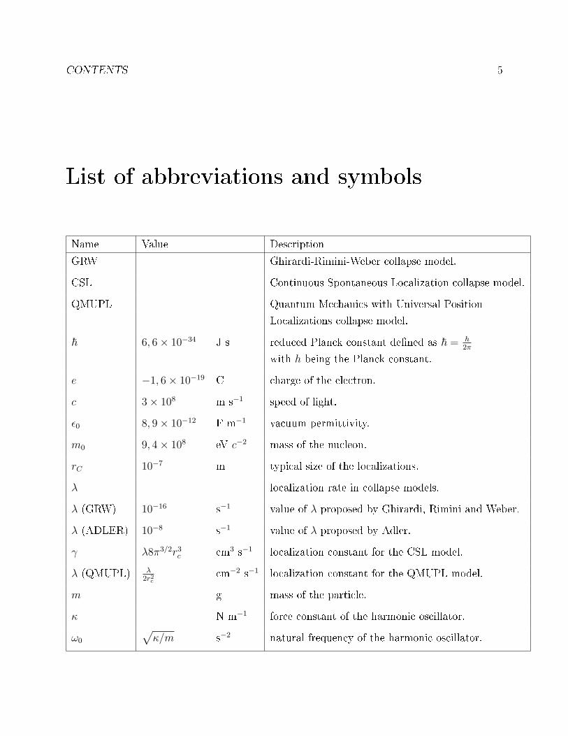
List of abbreviations and symbols
Name Value Description
GRW Ghirardi-Rimini-Weber collapse model.
CSL Continuous Spontaneous Localization collapse model.
QMUPL Quantum Mechanics with Universal Position
Localizations collapse model.
~ 6, 6× 10⁻³⁴ J s reduced Planck constant dened as ~ = h2π
with h being the Planck constant.
e −1, 6× 10⁻¹⁹ C charge of the electron.
c 3× 10⁸ m s−1 speed of light.
ǫ0 8, 9× 10⁻¹² F m−1 vacuum permittivity.
m0 9, 4× 10⁸ eV c−2 mass of the nucleon.
rC 10−7 m typical size of the localizations.
λ localization rate in collapse models.
λ (GRW) 10−16 s−1 value of λ proposed by Ghirardi, Rimini and Weber.
λ (ADLER) 10−8 s−1 value of λ proposed by Adler.
γ λ8π3/2r3c cm3 s−1 localization constant for the CSL model.
λ (QMUPL) λ2r2c
cm−2 s−1 localization constant for the QMUPL model.
m g mass of the particle.
κ N m−1 force constant of the harmonic oscillator.
ω0
√
κ/m s−2 natural frequency of the harmonic oscillator.

List of publications directly related to
this thesis
1. S. L. Adler, A. Bassi, S. Donadi. On spontaneous photon emission in collapse models;
Journ. Phys. A: Math. Theor. 46, 245-304 (2013).
Link to Arxiv: http://arxiv.org/abs/1011.3941.
The most important contents of this article are reported in CHAPTER 3.
2. A. Bassi, S. Donadi. Spontaneous photon emission from a non-relativistic free charged
particle in collapse models: A case study; Phys. Lett. A 378, 761-765 (2014).
Link to Arxiv: http://arxiv.org/abs/1307.0560.
The most important contents of this article are reported in CHAPTER 4.
3. S. Donadi, A. Bassi, D.-A. Deckert. On the spontaneous emission of electromagnetic
radiation in the CSL model; Annals of Physics 340, Issue 1, 70-86 (2014).
Link to Arxiv: http://arxiv.org/abs/1307.1021.
The most important contents of this article are reported in CHAPTER 5.
4. S. Donadi, A. Bassi, C. Curceanu, L. Ferialdi. The eect of spontaneous collapses on
neutrino oscillations; Found. Phys. 43, 1066-1089 (2013).
Link to Arxiv: http://arxiv.org/abs/1207.5997.
The most important contents of this article are reported in CHAPTER 7.
5. S. Donadi, A. Bassi, C. Curceanu, A. Di Domenico, B. C. Hiesmayr. Are Collapse
Models Testable via Flavor Oscillations?; Found. Phys. 43, 813-844 (2013).
6
CONTENTS 7
Link to Arxiv:http://arxiv.org/abs/1207.6000.
The most important contents of this article are reported in CHAPTER 8.
6. M. Bahrami, S. Donadi, L. Ferialdi, A. Bassi, C. Curceanu, A. Di Domenico, B. C.
Hiesmayr. Are collapse models testable with quantum oscillating systems? The case of
neutrinos, kaons, chiral molecules; Sci. Rep.3, 1952 (2013).
Link to Arxiv: http://arxiv.org/abs/1305.6168.
The most important contents of this article are reported in CHAPTER 7 and 8.

Chapter 1
Introduction and main results
In the last decades the interest of the scientic community in better understanding the limits
of validity of quantum mechanics has increased. Indeed, many scientist (among them, e.g.,
the Nobel laureates A. Leggett and S. Weinberg [1, 2]) now believe quantum mechanics, as
it is now, is a phenomenological theory and not a fundamental one.
Among the reasons why quantum mechanics should be modied, perhaps the most impor-
tant is the so called measurement problem. The problem can be stated as follow: it is well
known that, for microscopic systems, the quantum superposition principle holds. This has
been veried in many experiments during the last century, e.g., diraction and interference
experiments [3, 4, 5, 6, 7, 8]). However, when we move toward the macroscopic scale, the
superposition principle seems to break down: we never see macro-objects in superposition of
dierent position states in our daily life. In order to explain this behavior, the wave packet
reduction postulate (or collapse postulate) has been introduced in quantum mechanics. This
poses a problem: since measurement instruments and observers are made of the same atoms
that are supposed to follow quantum mechanical rules, it is not clear why for these systems
the Schrödinger equation does not hold and one has to use the wave packet reduction postu-
late. Moreover, even accepting the presence of two completely dierent dynamics the rst
one, given by the Schrödinger equation which is linear and deterministic while the other one,
described by the wave packet reduction postulate, is non linear and stochastic the theory
does not explain clearly which systems should be considered as measurement instrument and
which should not. To quote Bell [9]: What exactly qualies some physical systems to play
the role of measurer. Was the wave function of the world waiting to jump for thousands of
millions of years until a single-celled living creature appeared? Or did it have to wait a little
8

CHAPTER 1. INTRODUCTION AND MAIN RESULTS 9
longer for some better qualied system...with a PhD?. Therefore in quantum mechanics,
the limit between micro systems, obeying a linear dynamics and macro systems, obeying a
non linear collapse dynamics, is ambiguous.
In the last century dierent solutions for this problem were proposed. Some of them
change the interpretation of the theory keeping the same physical predictions of quantum
mechanics. This is the case, for example, of Bohmian Mechanics [10, 11, 12, 13]. A dierent
way out of the problem is given by collapse models [14, 15, 16, 17]. The idea underlying
these models is the following: each physical system interacts with a noise eld which induces
the collapse of the wave function in space. These models are engineered in a such way
that the eect of the noise is almost negligible for microscopic systems but, because of an
amplication mechanism, this interaction becomes predominant for macro systems. As such,
within a unique dynamics, collapse models provide an explanation of why micro systems have
a quantum behavior while macro systems behave classically.
Collapse models make predictions dierent from quantum mechanics, hence they can be
tested. Many dierent phenomena and experimental data have been studied so far and for all
of them the predictions of quantum mechanics and of collapse models were compared. The
dierence between these predictions is too small to be detected with the current technology
and so there is not yet a decisive test of collapse models. However, these experiments set
quite interesting bounds on collapse models' parameters. The state of the art of this research
and the related bounds on the parameters of collapse models can be found in [18, 19].
In this thesis we focus two phenomena where the predictions of quantum mechanics and
collapse models are dierent: (i) electromagnetic radiation emission from charged systems
and (ii) avour oscillations. We analyzed both of them and obtained a quantitative prediction
of the deviations from standard quantum behavior.
In the rst part of the thesis we study the electromagnetic radiation emission in collapse
models. The interest in this phenomenon is due to the fact that so far it sets the strongest
bound on the parameters of collapse models [18, 19]. Since in collapse models any system
always interacts with a noise (that induces the collapse of the wave function), if the system
is charged this interaction induces the emission of radiation. To give an intuitive semi-
classical picture, one can think of a system being accelerated by the noise and, because of
this acceleration, it emits radiation.
In the literature there are several computations of the radiation emission rate. In [20,
21] the calculation was carried out to the rst perturbative order using the Continuous

CHAPTER 1. INTRODUCTION AND MAIN RESULTS 10
Spontaneous Localization (CSL) model. In [22] the formula for emission rate was found
doing exact computations using the simpler QMUPL (Quantum Mechanics with Universal
Position Localizations) model. The results of these calculations were not the same, as they
were supposed to be. In order to clarify this issue, in the rst part of chapter 3 we repeat
the computations performed in [20, 21]. We study the radiation emission in the Continuous
Spontaneous Localization (CSL) model for a free particle, taking a white noise. Treating both
the electromagnetic and the noise interactions as perturbations, we nd that the formula for
the emission rate is:d
dkΓk
∣∣∣∣white
=λ~e2
2π2ε0c3m20r
2Ck, (1.1)
where ~, c and ε0 have the usual meaning, λ and rC are two parameters introduced in collapse
models, m0 the mass of a nucleon, k is the photon wave vector. Eq. (1.1) diers from the
result found in [20, 21] but it agrees with the result found in [22]. We show that the origin
of the discrepancy is that in [20, 21] some relevant contributions to the emission rate were
neglected [23]. The next step is to generalize the perturbative calculations using a colored
noise. We present this computation in the second part of chapter 3 and we show that the
emission rate formula is:
d
dkΓk =
1
2
d
dkΓk
∣∣∣∣white
· [f(0) + f(ωk)], (1.2)
where
f(ω) :=
∫ +∞
−∞f(s)eiωsds, (1.3)
is the noise spectral density where f(s) is the noise eld time correlation. The second term
inside the square bracket on the right side of Eq. (1.2) is the expected one: the probability
of emitting a photon with momentum k is proportional to the spectral density of the noise
correlation at the frequency ωk = kc. On the other hand, the rst term is related to the
spectral density of the noise at zero energy. Due to the presence of this term, even a noise
with very low energy can induce an emission of high energetic photons. This is unexpected as
the typical picture is that the noise gives energy to the particle, and such energy is converted
into that of the emitted photon. Understanding the origin of this term and how to avoid it
is one of the main task of this thesis. In the third and fourth part of chapter 3 we study a
prescription to avoid the presence of the unphysical term f(0). We show that, if one takes
wave packets instead of plane waves as nal states and if one connes the noise in space,

CHAPTER 1. INTRODUCTION AND MAIN RESULTS 11
then the unphysical term is not present anymore. However, this procedure seems an ad-hoc
solution and it is not clear if it is valid also for systems dierent from the free particle.
Moreover, it forces us to change the model by imposing a noise connement.
A deeper insight into the problem is obtained working with the QMUPL model, where
an exact treatment of the problem is possible. Indeed, in chapter 4 we show that, in the case
of the free particle, the unphysical term is still present. However, for a harmonic oscillator,
the rate is1:dΓ
dk≃ 1
2
d
dkΓk
∣∣∣∣white
·[
e−γtf(0) + f(ωk)]
, (1.4)
where γ =ω20β
2mand β = e2
6πǫ0c3. We see that the unphysical term, for large times, is suppressed
by the exponential damping factor e−γt. However, it is important to note that treating
electromagnetic interaction at the lowest order, which is equivalent of setting β = 0, implies
γ = 0 and so the unphysical term f(0) is not suppressed anymore. The same problem arises if
we set ω0 = 0, which is the free particle case. Therefore, from this analysis we proved that in
order to get a physically meaningful result, rst the particle cannot be treated as completely
free, and second the electromagnetic interaction cannot be treated at the lowest perturbative
order. In chapter 5 we use the above results to compute the emission rate with the CSL
model. Here an exact treatment of the problem is not possible. However, from the previous
analysis with the QMUPL model, we see that the damping factor e−γt responsible for the
decay of the unphysical term f(0), does not depend on the noise. This means that the noise
can be treated perturbatively, but the higher orders terms of the electromagnetic interaction
must be considered. This is exactly what we do in chapter 5: we nd the emission rate for
a harmonic oscillator in the CSL model treating the electromagnetic interaction exactly and
the noise interaction perturbatively. The emission rate, in the free particle limit, is the one
given in Eq. (1.2) without the unphysical term f(0).
The method used in chapter 5 gives a meaningful result, but it requires treating the
electromagnetic interaction exactly when solving the Heisenberg equations. This can be done
only for simple systems. For more complicated systems, one has to resort to perturbation
theory. Therefore, we look for a way to include the decay behavior due to the electromagnetic
interaction into the perturbative approach. In chapter 6 we show that this can be done by
1In this formula we used the symbol ≃ instead of = because this is not the exact result of ourcomputation, that is given by the much more complicated formula in Eq. (4.24). However, in order to avoiduseless complication, here we can refer to this simplied version of that equation, which catches all theimportant points.
CHAPTER 1. INTRODUCTION AND MAIN RESULTS 12
taking into account the possibility that, because of the electromagnetic self interaction, the
propagator decays. Indeed, as discussed for example in [24], the presence of any external
perturbation makes the eigenstates of the unperturbed Hamiltonian unstable so that they
can decay. We computed the emission rate for a generic system taking into account this eect
and nally we found a general formula where the unphysical term is not present.
To conclude, we briey discuss the experimental bounds on the collapse parameter coming
from the emission of radiation. Following the analysis of [20], it is show that a mass propor-
tional coupling between the noise and the particle is required for the model to be consistent
with experimental data.

CHAPTER 1. INTRODUCTION AND MAIN RESULTS 13
PART I: RADIATION EMISSION IN COLLAPSE MODELS
Main results
- We nd a formula for the radiation emission rate in collapse models.
- We show that, in order to get a correct emission rate, the electromagnetic interaction
cannot be treated at the lowest perturbative order.
Main steps of our analysis and relative results
Step 1 We compute the emission rate from a free particle to the lowest perturbative order using the CSL
model .
The rate is given by Eq. (1.1): it is in agreement with the result found in [22] and twice of the result
found in [20, 21]. We claried this discrepancy showing that in [20, 21] some relevant
contributions were neglected.
Step 2 We extend the calculation to a colored noise, obtaining the result in Eq. (1.2).
A problem arises: the emission rate contains an unphysical term, proportional to f(0), which
implies emission of high energy photons also in presence of weak noises.
Step 3 The calculation of the emission rate is repeated by taking wave packets as nal states and
conning the noise. The unphysical factor disappears.
Problem: this procedure seems an ad-hoc solution and requires to modify the model conning the
noise.
Step 4 To better understand the origin of the unphysical factor we compute the emission rate from a free
particle and a harmonic oscillator using the QMUPL model. Besides the dipole approximation,
the calculation is carried out treating the interactions with the electromagnetic eld and the noise exactly.
The formula for the rate of a harmonic oscillator has the structure given in Eq. (1.4).
The unphysical term is not present when:
1) The particle is not completely free (ω0 6= 0);
2) The electromagnetic interaction is not treated at the lowest order (β 6= 0).
Step 5 We check if the results found with the QMUPL model are true also for the CSL model.
In order to do that, we solve the Heisenberg equations, treating exactly the electromagnetic
interaction and perturbatively the interaction with the noise.
We compute the emission rate for a harmonic oscillator and we show that the unphysical
term is not present.
Step 6 We introduce the eect of higher order terms of the electromagnetic interaction in the
lowest order perturbative calculations by taking into account the decay of the the propagator.
The result we nd is a formula for the emission rate from a generic system and a generic collapse model
which does not contains unphysical terms anymore.
Table 1.1: Summary of the main results and the most important steps of the rst part of the
thesis

CHAPTER 1. INTRODUCTION AND MAIN RESULTS 14
In the second part of the thesis we study the phenomenon of avour oscillations in collapse
models. Flavour oscillations arise whenever avour eigenstates of a particle are dierent
from its mass eigenstates. Then avour eigenstates are supposed to be linear superposition
of mass eigenstates. According to quantum mechanics, during the time evolution the mass
eigenstates of a free particle change by acquiring dierent phase factors, depending on their
mass. Therefore, a particle that is initially in some avour eigenstates (which are the ones
that are measured in practice), after some time has a non zero probability to be in another
avour eigenstate. This probability shows an oscillatory behavior in the course of time.
Collapse models describe a dierent evolution for the mass eigenstates due to the constant
interaction with the noise. As a consequence, the formula for the evolution of the oscillations
changes. In fact, by treating the noise as perturbation, we show that in collapse models the
oscillation probability is damped by an exponential factor. We performed this computation
for two dierent types of particles: neutrinos in chapter 7 and mesons in chapter 8. The
decay rate ξjk in the case of neutrinos is:
ξjk =γ
16π3/2r3Cm20c
4
(
m2jc
4
E(j)i
− m2kc
4
E(k)i
)2
, (1.5)
where γ = λ8π3/2r3c and the label j(k) refers to the mass eigenstate with mass mj(mk) and
energy E(j)i (E
(k)i ), with E
(j)i =
√
p2i c
2 +m2jc
4 and pi the momentum of the particle. Using
available experimental data, we quantify the damping factors for these particles. The result
for cosmogenic, solar and laboratory neutrinos are summarized in the following table:
cosmogenic solar laboratory
E(eV) 1019 106 1010
t(s) 3.15× 10¹⁸ 5× 10² 2, 13× 10−2
ξijt 2.31× 10−55 3.66× 10−45 1.56× 10−57
For each type of neutrinos, in the rst line we report the typical order of magnitude
of their energies, in the second line their typical times of ight and in the third line the
damping factor obtained using Eq. (1.5). We see that, on the contrary to what was claimed
in a previous work in the literature [25], the eect is very small.
CHAPTER 1. INTRODUCTION AND MAIN RESULTS 15
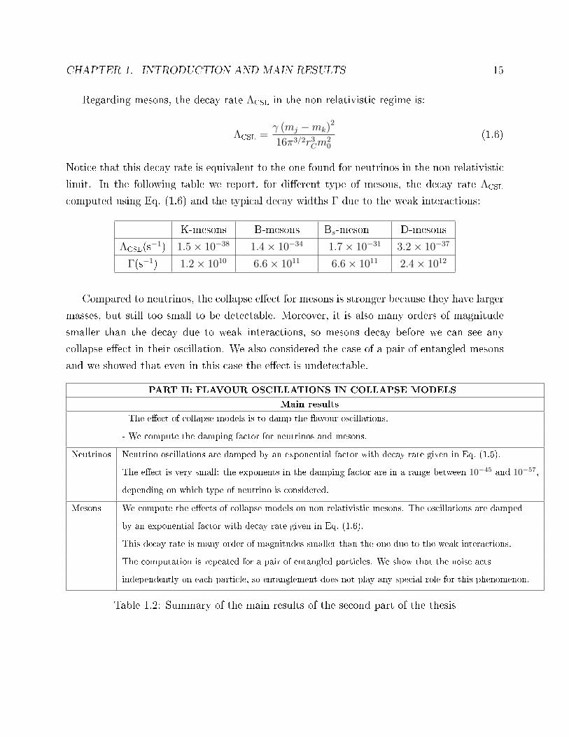
Regarding mesons, the decay rate ΛCSL in the non relativistic regime is:
ΛCSL =γ (mj −mk)
2
16π3/2r3Cm20
(1.6)
Notice that this decay rate is equivalent to the one found for neutrinos in the non relativistic
limit. In the following table we report, for dierent type of mesons, the decay rate ΛCSL
computed using Eq. (1.6) and the typical decay widths Γ due to the weak interactions:
K-mesons B-mesons Bs-meson D-mesons
ΛCSL(s−1) 1.5× 10−38 1.4× 10⁻³⁴ 1.7× 10⁻³¹ 3.2× 10−37
Γ(s−1) 1.2× 10¹⁰ 6.6× 10¹¹ 6.6× 10¹¹ 2.4× 10¹²
Compared to neutrinos, the collapse eect for mesons is stronger because they have larger
masses, but still too small to be detectable. Moreover, it is also many orders of magnitude
smaller than the decay due to weak interactions, so mesons decay before we can see any
collapse eect in their oscillation. We also considered the case of a pair of entangled mesons
and we showed that even in this case the eect is undetectable.
PART II: FLAVOUR OSCILLATIONS IN COLLAPSE MODELS
Main results
- The eect of collapse models is to damp the avour oscillations.
- We compute the damping factor for neutrinos and mesons.
Neutrinos Neutrino oscillations are damped by an exponential factor with decay rate given in Eq. (1.5).
The eect is very small: the exponents in the damping factor are in a range between 10−45 and 10−57,
depending on which type of neutrino is considered.
Mesons We compute the eects of collapse models on non relativistic mesons. The oscillations are damped
by an exponential factor with decay rate given in Eq. (1.6).
This decay rate is many order of magnitudes smaller than the one due to the weak interactions.
The computation is repeated for a pair of entangled particles. We show that the noise acts
independently on each particle, so entanglement does not play any special role for this phenomenon.
Table 1.2: Summary of the main results of the second part of the thesis

Chapter 2
Collapse models
In this chapter we introduce collapse models, explain their most important features and how
they resolve the measurement problem. Collapse models modify the Schrödinger dynamics
in a non linear way to include the collapse of the state vector. To avoid the possibility
of having faster than light signaling (for example by manipulating entangled systems) the
new dynamics must be also stochastic. Indeed, it has been proved that a non linear and
deterministic time evolution allows faster than light signaling [26, 27]. The deviations of
this new dynamics from the Schrödinger dynamics should be small for microscopic systems,
in order to avoid contradictions with experiments. On the other hand, when a macroscopic
system is considered, in order to solve the measurement problem the new dynamics should
assure a well dened position to the center of mass of the system. Collapse models fulll
all of these requirements [16, 17]. Therefore, within an unique dynamics, collapse models
describe the typical quantum behavior of the microscopic systems and explain the collapse
of the wave function for a macro system.
In the rst section of this chapter we introduce and explain the main properties of the
rst collapse model proposed in the literature: the Ghirardi-Rimini-Weber (GRW) model [14].
In the second section we introduce the dynamical equation of collapse models in the most
general way, and we study its main features. Then, in the third section, we introduce the
Continuous Spontaneous Localization (CSL) model [15] and the Quantum Mechanics with
Universal Position Localization (QMUPL) model [28]. The CSL and the QMUPL models
are the ones that we will use in this thesis.
16

CHAPTER 2. COLLAPSE MODELS 17
2.1 The GRW model
The GRW model was proposed in 1986 by Ghirardi, Rimini and Weber. In the GRW model
each elementary constituent of matter is subject to random and spontaneous localizations.
The localizations amount to the collapse of the wave function in space. The important
point is that these localizations processes are supposed to be part of the laws of nature, not
something that happens only when an observer performs a measurement on the system.
2.1.1 Postulates of the GRW model
The postulates of the GRW model are the following:
1. Each particle is subject to spontaneous and random localizations, described by a Pois-
sonian process with the mean rate λi (where "i" labels the i-th particle of the system).
2. The localization process for the i-th particle changes the state vector as follow:
|Ψ〉 −→ Lia |Ψ〉
‖Lia |Ψ〉‖ ,
with
Lia =
(πr2c)−3/4
e− (qi−a)2
2r2c ,
where qi is the position operator of the i-th particle, a is the point around which the
particle is localized, and rc is the typical size of the localization.
3. The probability of having a localization around the point a is:
P i (a) =∥∥Li
a |Ψ〉∥∥2.
4. When there is no localization, the system evolves according to the Schrödinger equation:
i~d
dt|Ψ(t)〉 = H |Ψ(t)〉 ,
where H is the standard quantum Hamiltonian.
The rst postulate describes the probability of having a localization at a certain time. The
localization rates λi are chosen to be equal for all particles to λ = 10−16 s−1 and this is a new

CHAPTER 2. COLLAPSE MODELS 18
parameter of the model. Such a choice implies that the probability of having a localization
(and therefore a deviation from the behavior predicted by the Schrödinger equation) for a
single particle is very small. However, because of an amplication mechanism that we will
describe later, the rate of localization for a macroscopic object turns out to be much larger,
making the localization more eective. The second postulate describes in a precise way what
is meant by localization: the wave function of the system is coarse-grained with the spatial
resolution rC . The parameter rC is the second new parameter introduced by the model and
is chosen to be equal to 10−7 m. The coarse-graining is precisely expressed by multiplying
the wave function with a gaussian centered at a with width rC . The third postulate sets
the probability of having a localization around a given point a. This is the GRW model
counterpart of the Born rule in quantum mechanics. It has been recently proven that this
choice of probability is the only way to avoid the possibility of having faster than light
signaling [27].
2.1.2 GRW master equation
Here we derive the equation for the density matrix in the GRW model. The dynamics of
the GRW model evolves pure states into statistical mixtures. Indeed, when a localization
happens, the state of the system |ψ (t)〉 evolves into one of the states Lia|Ψ(t)〉
‖Lia|Ψ(t)〉‖ :=
|Ψia(t)〉
‖|Ψia(t)〉‖
with probability P i (a, t) = ‖|Ψia (t)〉‖
2. This means that before a localization occurs the
density matrix of the system is given by the pure state |Ψ(t)〉 〈Ψ(t)|, while after it is given
by a statistical mixture of pure states|Ψi
a(t)〉〈Ψia(t)|
‖|Ψia(t)〉‖2
, each one weighted with the probability
P i (a, t). Therefore, a localization of the i-th particle of the system corresponds to the
following change of the density matrix ρ(t):
ρ (t) = |Ψ(t)〉 〈Ψ(t)| −→localization
ρ (t) =
∫
da|Ψi
a (t)〉 〈Ψia (t)|
‖|Ψia (t)〉‖2
P i (a, t) =
=
∫
da∣∣Ψi
a (t)⟩ ⟨
Ψia (t)
∣∣ =
∫
daLia |Ψ(t)〉 〈Ψ(t)|Li
a . (2.1)
If we introduce the map:
Ti [ρ(t)] :=
∫
daLia ρ(t)L
ia (2.2)

CHAPTER 2. COLLAPSE MODELS 19
then the localization process can be described as:
ρ (t) −→ Ti [ρ (t)] . (2.3)
Now we have all what we need to derive the master equation for the GRW model. Since the
localizations follow a Poissonian statistic, in the innitesimal time dt there is a probability
λidt to have a collapse whose dynamics is given by Eq. (2.3) and a probability 1− λidt that
no collapse happens, so the system evolves accordingly to the Schrödinger equation. This
means that the matrix density ρ(t) evolves as:
ρ (t+ dt) = (1− λidt)
[
ρ (t)− i
~[H, ρ (t)] dt
]
+ λidtTi [ρ (t)] , (2.4)
which is equivalent to:
d
dtρ (t) = − i
~[H, ρ (t)]− λi (ρ (t)− Ti [ρ (t)]) . (2.5)
The rst term in the right hand side of above equation gives the standard Schrödinger
evolution while the second term describes the collapse of the wave function. If we focus on
the behavior of the matrix elements in the position basis ρt (x,y) = 〈x |ρ (t)|y〉, Eq. (2.5)becomes:
dρt (x,y)
dt= − i
~[H, ρt (x,y)]− λi
[
1− e− 1
4r2c(x−y)2
]
ρt (x,y) . (2.6)
This equation shows how, as a consequence of the collapse, the o diagonal elements are
suppressed.
Let us introduce the master equation for a system composed by many particles. The
derivation is similar to the one particle case and the nal result is:
d
dtρ (t) = − i
~[H, ρ (t)]−
N∑
i=1
λi (ρ (t)− Ti [ρ (t)]) . (2.7)
2.1.3 The amplication mechanism
As already explained in the introduction, one of the major achievements of collapse models
is to guarantee well dened positions for macroscopic objects. This is possible because of
amplication mechanism, which we describe now for the GRW model. Let us consider a

CHAPTER 2. COLLAPSE MODELS 20
macroscopic object composed of N microscopic constituents. Follwing [29], we focus on the
study of the dynamics of the center of mass of the system. The position operator of the i-th
particle qi can be written in term of the center of mass position operator Q and the relative
coordinates rj (j = 1, 2, .., N − 1) as follows:
qi = Q+∑
j
cijrj (2.8)
where cij are real coecients. Since we are interested in the time evolution of the center of
mass, we want to derive the dynamics for the reduced density matrix ρ CM = Trrel[ρ] (here
Trrel signies the trace over the relative coordinates) starting from Eq. (2.7). The non
trivial part amounts to computing the partial trace of the term containing the maps Ti [ρ]
introduced in Eq. (2.2). In order to do that, it is convenient to rewrite this maps as follows1:
Ti [ρ] =
(1
πr2c
)3/2 ∫
da e− (qi−a)2
2r2c ρ e− (qi−a)2
2r2c
=
(r2cπ~2
)3/2 ∫
dp e−p2r2c2~2 e
i~p·qiρ e−
i~p·qi
=
(r2cπ~2
)3/2 ∫
dp e−p2r2c2~2 e
i~p·(
Q+∑
jcijrj
)
ρ e− i
~p·(
Q+∑
jcijrj
)
. (2.9)
The equivalence between the rst and the second line of Eq. (2.9) can be veried by computing
Ti[ρ] between two generic position eigenstates. The partial trace of Eq. (2.9) can be computed
using the fact that center of mass and relative coordinates commute and the cyclic property
1For sake of clarity we recall that a and p are vectors which components are real numbers while qi, Qand rj are vector operators.

CHAPTER 2. COLLAPSE MODELS 21
of the trace:
Trrel [Ti [ρ]] =
(r2cπ~2
)3/2 ∫
dp e−p2r2c2~2 Trrel
ei~p·(
Q+∑
jcijrj
)
ρ e− i
~p·(
Q+∑
jcijrj
)
=
(r2cπ~2
)3/2 ∫
dp e−p2r2c2~2 Trrel
[
ei~
∑
jcijp·rj
ei~p·Qρ e−
i~p·Qe
− i~
∑
jcijp·rj
]
=
(r2cπ~2
)3/2 ∫
dp e−p2r2c2~2 e
i~p·Qρ e−
i~p·Q := TCM [ρ] (2.10)
The above equation says that the localization of any particle (that is described by the
maps Ti[ρ]) implies the localization of the center of mass of the object. Therefore, taking
the partial trace with respect to the relative coordinates of the master equation given in
Eq. (2.7), we get:
d
dtρCM (t) = − i
~[HCM, ρCM (t)]− λ (ρCM (t)− TCM [ρ (t)]) . (2.11)
with λ =
(N∑
i=1
λi
)
. This means that, even if the localization rate of a single particle is very
small (λi = 10−16 s−1), the localization rate for the center of mass of a macroscopic object
(where the number of particles is of order of Avogadro number 10−23) is of the order 107 s−1.
This implies that in the GRW model any macroscopic superposition is suppressed in a time
scale of order 10−7 s.
Before concluding our discussion about the GRW model, we recall that in literature two
dierent value for λ has been proposed. The rst one is λ = 10−16 s−1 proposed by Ghirardi
Rimini and Weber. This value is, somehow, the smallest possible choice: if one takes a smaller
value, then the eect of the collapse becomes too weak and the localization of macroscopic
systems becomes inecient. The second value for λ has been proposed by Adler [18]. It is
based on the requirement that the process of latent image formation yields to a well localized
position. This process involves a relatively small number of atoms, which implies that the
amplication mechanism is not very eective. Therefore, in order for the latent image to
be well localized, the strength of the noise has to be increased, according to Adler, by eight
orders of magnitude. This implies λ = 10−8 s−1.
The GRW model is the rst important and fully consistent collapse model. Compared to

CHAPTER 2. COLLAPSE MODELS 22
quantum mechanics, the model provides a clear and unambiguous description of the collapse
of the wave function. However, the model as it is cannot be applied to systems containing
identical particles. This is due to the fact that the collapse, as described in this model, does
not preserve the symmetry of the wave function. This problem has been solved in the CSL
model, which we will introduce soon.
2.2 The general structure of collapse equations
In the following we will introduce two other important collapse models: the CSL model and
the QMUPL model. In these models, contrary to what happens in the GRW model where
the collapse is described by discrete jumps, the collapse is described as a continuous process
due to the interaction with an external noise. The dynamics of both models are described
by stochastic dierential equations having the same mathematical structure. Recently it
has been proven that, under quite general assumptions (e.g., no-faster-than-light signaling
and the conservation of probability), any non linear modication of the Schrödinger equation
described by a stochastic dierential equation must have the structure of collapse models [27].
Therefore, although collapse models are phenomenological (in particular the physical origin
of the collapse is still unknown), they are the only possible consistent way to introduce non
linear modications of quantum mechanics [27].
We rst summarize the general features of collapse equations. Their dynamical structure
is:
d|φt〉 =
[
− i
~H dt +
√γ
N∑
i=1
(Ai − 〈Ai〉t) dWi, t − γ
2
N∑
i=1
(Ai − 〈Ai〉t)2 dt]
|φt〉, (2.12)
where H is the standard Hamiltonian of the system, Ai are set of commuting self-adjoint
operators, 〈Ai〉t := 〈φ (t) |Ai|φ (t)〉, γ is a constant which sets the strength of the coupling
with the noise eld and Wi, t are set of independent standard Wiener processes, one for each
operator Ai. Notice that the dynamics is non linear, because of the presence of the terms
〈Ai〉t, and stochastic because of the presence of the Wiener processes Wi, t. The rst term on
the right hand side of the above equation is the standard Schrödinger evolution, and the other
two terms describe the collapse of the state vector. In order to better understand how the
collapse works and how it is related to the operators Ai, let us study Eq. (2.12) by neglecting
the Schrödinger term. In such a case, it can be shown that any initial state evolves to one

CHAPTER 2. COLLAPSE MODELS 23
of the (common) eigenstates of the operators Ai [30]. In fact, for any given operator A that
commutes with each of the operators Ai, its variance VA (t) := 〈A2〉t − 〈A〉2t is given by:
E [VA (t)] = VA (0)− 4γN∑
i=1
∫ t
0
dsE[C2
A,Ai(s)], (2.13)
where E denotes the noise average and CA,Ai(t) := 〈(A−〈A〉t)(Ai−〈Ai〉t)〉t is the correlation
between the operator A and Ai. Taking into account that VA (t) must be positive for any
time t and the second term in the right hand side of Eq. (2.13) is always negative, it must be
that CA,Ai(t) → 0 when t → ∞ for any i. Therefore, if we choose A as one of the operators
Aj, this implies that its variance VAj(t) = CAj ,Aj
(t) goes to zero for large enough times. This
is equivalent to saying that the state has evolved to one of the eigenstates of Aj. As we will
see, in order to guarantee macroscopic objects to have well dened positions, the operators
Ai are chosen to be functions of the position operator.
2.2.1 The master equation
Here we derive the master equation associated to Eq. (2.12). Using the Ito product rule we
have:
d|φt〉〈φt| = (d|φt〉) 〈φt|+ |φt〉 (d〈φt|) + (d|φt〉) (d〈φt|) = (2.14)
=
[
− i
~H dt +
√γ
N∑
i=1
(Ai − 〈Ai〉t) dWi, t − γ
2
N∑
i=1
(Ai − 〈Ai〉t)2 dt]
|φt〉〈φt|
+ |φt〉〈φt|[
i
~H dt +
√γ
N∑
i=1
(Ai − 〈Ai〉t) dWi, t − γ
2
N∑
i=1
(Ai − 〈Ai〉t)2 dt]
+ γN∑
i=1
(Ai − 〈Ai〉t)|φt〉〈φt|(Ai − 〈Ai〉t)dt.
A direct calculation shows that all the terms involving 〈Ai〉t and 〈Ai〉2t multiplied with dt
cancel each other. Moreover, the expectation value of the terms containing dWi, t is zero.
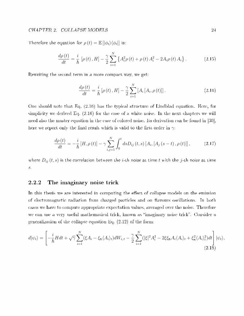
CHAPTER 2. COLLAPSE MODELS 24
Therefore the equation for ρ (t) = E [|φt〉〈φt|] is:
dρ (t)
dt=i
~[ρ (t) , H]− γ
2
N∑
i=1
A2
i ρ (t) + ρ (t)A2i − 2Aiρ (t)Ai
. (2.15)
Rewriting the second term in a more compact way, we get:
dρ (t)
dt=i
~[ρ (t) , H]− γ
2
N∑
i=1
[Ai [Ai, ρ (t)]] . (2.16)
One should note that Eq. (2.16) has the typical structure of Lindblad equation. Here, for
simplicity we derived Eq. (2.16) for the case of a white noise. In the next chapters we will
need also the master equation in the case of colored noise. Its derivation can be found in [30],
here we report only the nal result which is valid to the rst order in γ:
dρ (t)
dt= − i
~[H, ρ (t)]− γ
N∑
i,j=1
∫ t
0
dsDij (t, s) [Ai, [Aj (s− t) , ρ (t)]] , (2.17)
where Dij (t, s) is the correlation between the i-th noise at time t with the j-th noise at time
s.
2.2.2 The imaginary noise trick
In this thesis we are interested in computing the eect of collapse models on the emission
of electromagnetic radiation from charged particles and on avours oscillations. In both
cases we have to compute appropriate expectation values, averaged over the noise. Therefore
we can use a very useful mathematical trick, known as imaginary noise trick. Consider a
generalization of the collapse equation Eq. (2.12) of the form:
d|ψt〉 =[
− i
~Hdt+
√γ
N∑
i=1
(ξAi − ξR〈Ai〉t)dWi, t −γ
2
N∑
i=1
(|ξ|2A2i − 2ξξRAi〈Ai〉t + ξ2
R〈Ai〉2t )dt
]
|ψt〉,
(2.18)

CHAPTER 2. COLLAPSE MODELS 25
where ξ is a generic complex number. When ξ = 1 Eq. (2.18) reduces exactly to the collapse
equation in Eq. (2.12). On the contrary, if one takes ξ = i the equation reduces to:
d|ψt〉 =[
− i
~Hdt+ i
√γ
N∑
i=1
AidWi, t −γ
2
N∑
i=1
A2i dt
]
|ψt〉. (2.19)
This equation is written in the Ito form. The corresponding Stratonovich form, which is the
one we are interested in, is given by the same equation without the third term on the right
hand side term [31]. If we introduce the white noises as wi, t :=dWi, t
dt, then the Stratonovich
form of Eq. (2.19) can be written as:
i~d|ψt〉dt
=
[
H − ~√γ
N∑
i=1
Aiwi, t
]
|ψt〉, (2.20)
which is a Schrödinger equation with random potentials. The dynamics given in Eq. (2.20)
is completely dierent from the one given by Eq. (2.12). In particular Eq. (2.12) describes
an evolution that leads to the collapse of the wave function while in the dynamics given
by Eq. (2.20) there is no collapse at all. However, one can show that the master equation
associated to Eq. (2.18) is:
d
dtρ(t) = − i
~[H, ρ(t)] +
γ
2|ξ|2
N∑
i=1
(2Ai ρ(t)Ai − A2
i , ρ(t)). (2.21)
The important point is that the equation for ρ depends only from the modulus of ξ. This
means that Eq. (2.12) (ξ = 1) and Eq. (2.20) (ξ = i), despite the fact that they describe
a very dierent dynamics for the state vector, turn out to be completely equivalent at the
statistical level. Therefore, as far as we are interested in making physical predictions, we will
work with Eq. (2.20) which is much easier to handle compared to Eq. (2.12).
2.3 The CSL model
Here we introduce the CSL model. The equation that describes the evolution of state vectors
in the CSL model has the form of Eq. (2.12) with a particular choice of the localization
operators Ai. The operators are chosen in order to satisfy the following requirements:

CHAPTER 2. COLLAPSE MODELS 26
1. A macroscopic object must be well localized in space;
2. The model should be able to describe systems of identical particles.
Both conditions lead to the choice of a continuous set of operators N(x), one for each
point of space x:
Ai −→ N (x) =∑
j
∑
s
∫
dyg (y − x)ψ†j (y, s)ψj (y, s) . (2.22)
Here ψ†j (y, s) and ψj (y, s) are respectively the creation and annihilation operator of a particle
of type j in the point y with spin s and
g (y − x) =1
(√2πrc
)3 e− (y−x)2
2r2c (2.23)
is a gaussian smearing function that has the same role as the one introduced for the GRW
model. Accordingly, the CSL dynamics reads:
d|φt〉 =[
− i
~Hdt+
√γ
∫
dx (N(x)− 〈N(x)〉) dWt(x)−γ
2
∫
dx (N(x)− 〈N(x)〉)2 dt]
|φt〉.(2.24)
Since the dynamics in the above equation is written using the second quantization formalism,
the second requirement mentioned above is automatically fullled. In order to understand
the connection with the GRW model, it is useful to study the master equation in the position
representation. For one particle this is given by:
dρt (x,y)
dt= − i
~[H, ρt (x,y)]− λGRW
[
1− e− 1
4r2c(x−y)2
]
ρt (x,y) (2.25)
where λGRW := γ8π3/2r3c
is equivalent to the parameter λ introduced for the GRW model if
one takes γ = 10−30 cm3 s−1. Therefore Eq. (2.25) is exactly the same like Eq. (2.6). This
result is not true anymore in the case of many particles when they are identical. Let us also
mention that also for the CSL model there is an amplication mechanism similar to the one
of the GRW model [15, 16].

CHAPTER 2. COLLAPSE MODELS 27
2.4 The mass proportional CSL model
In the CSL model the noise eld inducing the collapse of the wave function acts in the same
way on dierent types of particles. However, there are both theoretical and experimental
reasons to believe that the eect of the collapse should be mass proportional [16, 20]. On
the experimental side, for example, the data on the spontaneous radiation emission from
Germanium falsify the original CSL model [20]. On the other hand, when a mass proportional
coupling is considered, there is no disagreement between the theoretical prediction and the
experimental data. We will discuss this issue in the conclusion of Part I. On the theoretical
side, one of the main reasons to believe that the strength of the collapse eect should be
mass proportional is the following. Consider two systems, with the same mass but composed
of a dierent number of particles. According to the original CSL model, they are localized
in dierent ways, depending on their number of particles. However, if we consider the total
mass as a measure of macroscopicity, then we would expect both systems to be localized
in the same way. This is exactly what happens using the mass proportional CSL model.
In addition, taking a mass proportional coupling suggests that the noise eld may have a
connection with gravity. This possibility has been proposed by Penrose and Diosi [32, 33, 34]
and recently reconsidered in [35].
The mass proportional CSL dynamics is given by:
d|φt〉 =[
− i
~Hdt+
√γ
m0
∫
dx (M(x)− 〈M(x)〉) dWt(x)−γ
2m20
∫
dx (M(x)− 〈M(x)〉)2 dt]
|φt〉,(2.26)
where m0 is a reference mass, chosen to be equal to the mass of a nucleon, and
M (x) =∑
j
mj
∑
s
∫
dyg (y − x)ψ†j (y, s)ψj (y, s) (2.27)
with mj the mass of the particle type j.
As explained before, in many computations it is convenient to use the imaginary noise
trick introduced in section 2.6; in such a case the dynamics is given by a Schrödinger equation
with the Hamiltonian:
HTOT = H − ~√γ∑
j
mj
m0
∑
s
∫
dyw(y, t)ψ†j(y, s)ψj(y, s). (2.28)

CHAPTER 2. COLLAPSE MODELS 28
Here w(x, t) is a Gaussian noise, with zero mean and the correlation function:
E[w(x, t)w(y, s)] = f(t− s)F (x− y), F (x) =1
(√4πrC)3
e−x2/4r2C . (2.29)
In the case of a white noise in time, the function f(t) is simply a Dirac delta δ(t). From now
on, in order to simplify the writing, we will refer to the mass proportional CSL model simply
as CSL model.
2.5 The QMUPL model
The QMUPL model was introduced for the rst time by Diosi in [28]. The model has a
very simple coupling between the noise and the particles. The localization operators Ai are
chosen to be position operators: Ai = qi with i = 1, 2, 3 labeling the three space directions.
Therefore, for a single particle, the dynamics of the model is:
d|φt〉 =
[
− i
~H dt +
√λ (q− 〈q〉t) · dWt − λ
2(q− 〈q〉t)2 dt
]
|φt〉, (2.30)
where λ is the coupling constant with noise, analogous to the γ introduced for the CSL
model. This model, compared to the CSL, has the disadvantage of not holding for system
of identical particles. However, it has the great advantage of being much easier to handle
compared to the CSL model. Indeed, as we will see in the next chapters, some problems that
with the CSL model can be studied only perturbatively, in the QMUPL model can be solved
exactly. Moreover, this model is not that much dierent from the CSL model as it might
seem. The master equation of the QMUPL model in the position basis is:
dρt (x,y)
dt= − i
~[H, ρt (x,y)]−
λ
2(x− y)2 ρt (x,y) . (2.31)
If we compare Eq. (2.31) with Eq. (2.25) we see that, for any system whose typical size
is smaller than rC , the gaussian in Eq. (2.25) can be expanded in Taylor series and the
relevant term is exactly the one in Eq. (2.31), if one sets λ = λGRW2r2c
. Therefore, for a large
number of systems, the predictions of the QMUPL model are practically equivalent to the
CSL predictions. As in the case of the CSL model, for the calculations we will also use the
imaginary noise trick. Then the dynamics given by Eq. (2.30) is replaced by a Schrödinger

CHAPTER 2. COLLAPSE MODELS 29
equation with Hamiltonian:
HTOT = H − ~
√λ q ·w(t). (2.32)
Our review on collapse models ends here. For the rest of the thesis we will present original
work done by using these models.

Part I
Radiation emission
30

31
In this part of the thesis we present the problem of the electromagnetic radiation emission
in collapse models. In collapse models no system is completely free because of the interaction
with the noise. The direct eect of this interaction is the localization of the center of mass of
the system. However, as an indirect eect, if the system is composed of charged particles the
collapse noise induces the emission of radiation. As a consequence, collapse models predict
the spontaneous radiation emission even for systems, e.g., a free particle or an atom in its
ground state, that should not emit according to quantum mechanics.
The radiation phenomenon provides so far the strongest upper bound on the collapse pa-
rameter λ. Therefore, research on radiation emission in collapse models has been quite
active. After some preliminary results by P. Pearle and collaborators using the GRW
model [36, 37, 38], the rst theoretical calculation using the CSL model has been carried
out by Q. Fu [20], to the rst meaningful perturbative order, for a free particle. The cal-
culation has been conrmed by S.L. Adler and F.M. Ramazanoglu [21], and generalized to
hydrogenic atoms and to non-white noises. More recently A.Bassi and D. Dürr have done a
similar calculation using the QMUPL model [22]. Since the QMUPL model is simpler, from
the mathematical point of view, than the CSL model, it allows an exact analytical treatment
of the problem. Moreover, as discussed in chapter 2, the QMUPL model should reproduce
the same results of the CSL model, as far as the system's size is smaller than rC = 10−7
m. However, the free particle's photon-emission rate in the case of white noise turns out to
be twice larger than the CSL prediction. This discrepancy, which initially seemed of little
importance, revealed many subtleties in the implementation of standard quantum eld per-
turbative methods in the context of stochastic models; in particular, for the case of colored
noises, terms appear in the radiation emission formula, which look unphysical [23].
In the following chapters we study the radiation emission problem in detail. In chapter
3 we recompute the radiation emission from a free particle using the CSL model. We show
that, mathematically speaking, the emission rate found in [20, 21] is wrong, while the correct
result is the one found in [22]. Then we repeat the computation using a non white noise. Here
a problem arise, because an unphysical factor is present in the emission rate. A possible way
out of the problem is discussed in the last section of chapter 3, where we change the model
by conning the noise and performing a more realistic calculation using wave packets instead
of plane waves as nal states. A deeper insight into the problem is given in chapter 4, where
we show that the unphysical terms disappear if higher order contributions are considered,
without having to change the model. Accordingly in chapter 5, using the CSL model and

32
treating the electromagnetic interaction exactly, we give a derivation of the emission rate
formula for a harmonic oscillator which does not contain any unphysical term. In chapter 6
we generalize this result to a generic system, showing that the unphysical term disappears if
the decay of the propagator is taken into account. To conclude, following the analysis done
in [20], we compare the predicted rate with the available data on the spontaneous emission
from Germanium, in order to derive a bound on the collapse parameter λ.

Chapter 3
Perturbative calculation of the emission
rate in CSL model
In this chapter we compute the emission rate from a free particle in the CSL model. We start
by repeating the computation already done in [20, 21], where a white noise was considered.
Then we extend the calculation to a colored noise. In this case a problem arises: the formula
for the emission rate, as we will see, contains an unphysical term. Because of this term, even
a weak noise can induce the emission of photons with high energies. We show that a possible
way to avoid the presence of this term is to carry out the perturbative calculation by taking
wave packets as nal states and conning the noise.
3.1 The CSL model for charged particles
As explained in chapter 2, in order to compute physical predictions such as like the emission
rate, one can use a Schrödinger dynamics given by the Hamiltonian in Eq. (2.28) which is:
HTOT = H − ~√γ∑
j
mj
m0
∑
s
∫
dyw(y, t)ψ†j(y, s)ψj(y, s). (3.1)
We are interested only in one type of particle, so from now on we will drop the sum over
j. We will also neglect the spin degree of freedom since its eect is negligible compared to
the other electromagnetic terms that we are considering.
Following the quantum eld theory approach, we write the Hamiltonian HTOT in terms of
a Hamiltonian density HTOT. For the systems we are studying, we can identify three terms
33

CHAPTER 3. PERTURBATIVE CALCULATIONOF THE EMISSION RATE IN CSLMODEL34
in HTOT:
HTOT = HP +HR +HINT. (3.2)
where HP contains all terms involving the matter eld, namely its kinetic term, possibly the
interaction with an external potential V and the interaction with the collapse noise eld:
HP =~2
2m∇ψ∗ ·∇ψ + V ψ∗ψ − ~
√γm
m0
wψ∗ψ. (3.3)
The term HR contains the kinetic term for the electromagnetic eld:
HR =1
2
(
ε0E2⊥ +
B2
µ0
)
, (3.4)
where E⊥ is the transverse part of the electric component and B is the magnetic component.
Finally HINT contains the standard interaction between the quantized electromagnetic eld
and the non-relativistic Schrödinger eld:
HINT = i~e
mψ∗A ·∇ψ +
e2
2mA2ψ∗ψ. (3.5)
The electromagnetic potential A(x, t) takes the form:
A(x, t) =∑
k,µ
αk
[
ǫk,µ ak,µei(k·x−ωkt) + ǫ
∗k,µ a
†k,µe
−i(k·x−ωkt)]
, (3.6)
with αk =√
~/2ε0ωkL3 and ωk = kc. We quantize elds in a cubical box of the size L (i.e.,
box quantization). We also work in the Coulomb gauge.
To analyze the problem of the emission rate, we will use a perturbative approach. We
identify the unperturbed Hamiltonian as that of the matter eld (interaction with the noise
excluded) plus the kinetic term of the electromagnetic eld:
H0 =~2
2m∇ψ∗ ·∇ψ + V ψ∗ψ +HR. (3.7)
We assume that eigenstates and eigenvalues of this unperturbed Hamiltonian are known. In
particular, we assume that the matter part of H0 is diagonalizable. Then the perturbation

CHAPTER 3. PERTURBATIVE CALCULATIONOF THE EMISSION RATE IN CSLMODEL35
is given by:
H1 = i~e
mψ∗A ·∇ψ +
e2
2mA2ψ∗ψ − ~
√γm
m0
wψ∗ψ. (3.8)
This division of HTOT in H0 + H1 is justied by the fact that the eects of spontaneous
collapses driven by the noise eld are very small at microscopic scales. This is also true for
the electromagnetic eects we are interested in computing.
3.2 Feynman rules
The Feynman diagrams for our model can be derived in a standard way by means of the
Dyson series and Wick theorem. We will present Feynman rules in space-time, instead of
the more familiar Feynman rules in momentum space, because in the following calculation a
crucial role will be played by the integration over space, and by the large-time limit. They
are:
1. External lines (the symbol • denotes the generic space-time vertex (x, t)):
= uk (x) e− i
hEkt
= αp~ǫp,λei(p·x−ωpt)
= w (x, t)
= u∗k (x) eihEkt
= αp~ǫ∗p,λe
−i(p·x−ωpt)p, λ p, λ
k k
The functions un(x) are the eigenstates of− ~2
2m∇
2+V , and En is the associated eigenvalue:
[
− ~2
2m∇
2 + V
]
un(x) = Enun(x).
Since the noise eld w is treated classically, there is no distinction between incoming and
outgoing lines.
2. Internal lines. The propagators for the matter eld and for the photons are:
= F12 = P lm12
11 22

CHAPTER 3. PERTURBATIVE CALCULATIONOF THE EMISSION RATE IN CSLMODEL36
with 1 := (x1, t1), 2 := (x2, t2) and:
F12 := F (x1, t1;x2, t2) = θ (t2 − t1)∑
k
uk (x2) u∗k (x1) e
− i~Ek(t2−t1) (3.9)
P lm12 := P lm(x1, t1;x2, t2) = θ (t1 − t2)
∑
k,µ
α2kǫ
lk,µǫ
∗mk,µe
i[k·(x1−x2)−ωk(t1−t2)]
+ θ (t2 − t1)∑
k,µ
α2kǫ
mk,µǫ
∗lk,µe
i[k·(x2−x1)−ωk(t2−t1)]. (3.10)
3. Vertices. There are three types of vertices, corresponding to the three terms in the
interaction Hamiltonian H1:
= i hem~∇, =
e2m,
= −h√γ mm0.
In the rst vertex, the derivative acts always on the incoming external line. In the
second vertex, e2/m appears in place of e2/2m (as one would naively expect by inspecting at
Eq. (3.8)) in order to take properly into account the multiplicity of the diagrams. The same
rule applies also to the standard scalar QED (without the noise term) [39].
4. One has to integrate over space and time in all vertices
1
(i~)n
n∏
j=1
∫ tf
ti
dtj
∫
L3
dxj
Note that there is no factorial term 1/n! coming from the Dyson's series, because this is
canceled by the multiplicity of the diagram1. Only diagrams containing double photon prop-
agators, like:
do not follow this rule. In such a case, one has to multiply by a factor 1/2 for each such
a loop.
1More precisely, a diagram containing n vertices has a factor 1/n! in front, coming from the Dyson'sexpansion. However, there are n! such identical diagrams, diering only in the way the vertices are numbered.
CHAPTER 3. PERTURBATIVE CALCULATIONOF THE EMISSION RATE IN CSLMODEL37
3.3 Photon emission probability at rst perturbative or-
der
In order to compute the emission rate, we need to know the transition probability from the
initial state |i; Ω〉 = |i〉⊗|Ω〉 to the nal state |f ;k, µ〉 = |f〉⊗|k, µ〉. Here |i〉 and |f〉 denote,respectively, the initial and nal state of the system that are eigenvectors of H0, while |Ω〉and |k, µ〉 denote respectively the vacuum state of the electromagnetic eld and the state
with one photon with the wave vector k and polarization µ. The transition probability is
given by:
Pfi := E[|〈f ;k, µ |U (t, ti)| i; Ω〉|2] = E[|〈f ;k, µ |UI (t, ti)| i; Ω〉|2] (3.11)
where UI (t, ti) = ei~H0tU (t, ti) e
− i~H0ti is the time evolution operator in the interaction picture
which can be expanded by means of the Dyson series [24]:
UI (t, ti) = 1 +∞∑
n=1
(−i~
)n ∫ t
ti
dt1
∫ t1
ti
dt2...
∫ tn−1
ti
dtnH1I (t1)H1I (t2) ...H1I (tn) . (3.12)
Here we focus on computing the transition amplitude Tfi dened as follow:
Tfi := 〈f ;k, µ |UI (t, ti)| i; Ω〉 . (3.13)
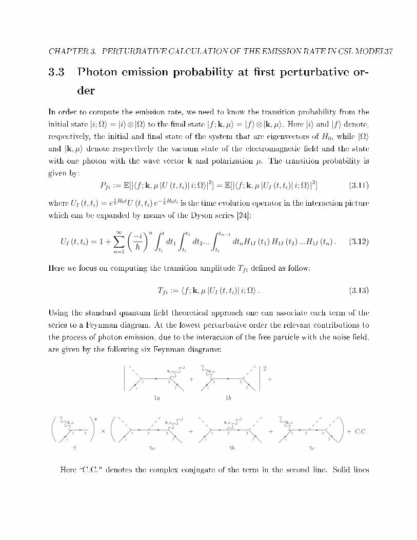
Using the standard quantum eld theoretical approach one can associate each term of the
series to a Feynman diagram. At the lowest perturbative order the relevant contributions to
the process of photon emission, due to the interaction of the free particle with the noise eld,
are given by the following six Feynman diagrams:
×∗
+ C.C.+ +
1a 1b
2
+ +1 2
i f
k, µ
1 2
i f
k, µ
2
1 2
i
k, µ
3a
3
f
k, µ
21
i
3b
3
f
2
k, µ
1
i
3c
1
i
k, µ
f
32
Here C.C." denotes the complex conjugate of the term in the second line. Solid lines

CHAPTER 3. PERTURBATIVE CALCULATIONOF THE EMISSION RATE IN CSLMODEL38
represent the charged fermion, wavy lines the photon, and dashed lines the noise eld. In
the above diagrams each electromagnetic vertex gives a factor proportional to e while each
noise vertex gives a factor proportional to√γ.
When computing the square modulus of the transition amplitude, the lowest order con-
tributions are those proportional to e2γ. These are obtained by taking the square modulus
of the sum of the contributions due to the rst two diagrams 1a and 1b plus the product
between the complex conjugate of the contribution due to the single-vertex diagram 2 with
each one of the contributions corresponding to the three-vertex diagrams 3a, 3b, 3c plus the
complex conjugate of this last contribution.
The diagrams 1a and 1b are the only ones which have been considered in [20, 21]. In
principle one should also take into account the contribution due to the diagrams 2 and 3a, 3b
and 3c. However, here we are interested in computing the rate for a free particle and we can
always choose an initial state with zero momentum. In such a case, both contributions due
to diagrams 1b and 2 vanish. Therefore the only non-zero contribution comes from diagram
1a. According to the rules previously outlined, the contribution due to this diagram is:
Tfi = − 1
~2αk
(
i~e
m
)(
−~√γm
m0
)∑
n
∫ tf
ti
dt1
∫ t1
ti
dt2 eiωkt1e−
i~Eit2e
i~Ef t1e−
i~En(t1−t2)
×∫
L3
dx1
∫
L3
dx2 ui(x2)e−ik·x1
ǫ∗k,µ · [∇un(x1)]u
∗n (x2) u
∗f (x1)w(x2, t2), (3.14)
or introducing the position operator x:
Tfi = − 1
~2αk
(
i~e
m
)(
−~√γm
m0
)∑
n
∫ tf
ti
dt1
∫ t1
ti
dt2 ei~(Ef+~ωk−En)t1e
i~(En−Ei)t2
×[〈f | e−ik·x
ǫ∗k,µ ·∇ |n〉 〈n|w(x, t2) |i〉
]. (3.15)
It is convenient to rewrite the above expression in a more compact form. Since the correlation
function of the noise given in Eq. (2.29) is a product of its time and space components, as
far as the average values are concerned we can replace w(x, t) with ξtN(x), where ξt is a
gaussian noise in time, while N(x) is a Gaussian noise in space, with zero mean and the
correlation F (x − y). In this section we focus on the case where the noise ξt is white, i.e.

CHAPTER 3. PERTURBATIVE CALCULATIONOF THE EMISSION RATE IN CSLMODEL39
E[ξt ξs] = δ(t− s). We also introduce the following two operators:
Rk := αk
(
i~e
m
)
e−ik·xǫk,µ ·∇, N := −~
√γm
m0
N(x). (3.16)
The rst operator refers to the radiative contribution (hence the symbol R), and the second
one to the interaction with the noise (hence the symbol N ). Dening the matrix elements
Rkfn := 〈f |Rk|n〉 and Nni := 〈n|N |i〉 and also considering photons with linear polarization
(ǫ∗k,µ = ǫk,µ), we can write Eq. (3.15) in the following way:
Tfi = − 1
~2
∑
n
∫ tf
ti
dt1
∫ t1
ti
dt2 ei~(Ef+~ωk−En)t1e
i~(En−Ei)t2ξt2Rk
fnNni (3.17)
This is a useful compact expression of the rst-order transition amplitude for emission of a
photon due to the interaction with the noise eld.
3.4 Emission rate for a free particle
In the case of a free charged particle, the initial and nal states and the generic eigenstate
of HP are:
ui(x) =1√L3, uf (x) =
eiq·x√L3, un(x) =
ein·x√L3, (3.18)
and we have chosen the reference frame where the particle is initially at rest. In order to
avoid divergences typical of the plane waves, we used the standard prescription of conning
the system in a box with the side L. At the very end of the computation we will take the
limit L→ ∞ and the nal result will be independent from L. The eigenvalue corresponding
to the eigenstate un is En = ~2n2/2m2, and similarly for Ei and Ef . The matrix elements
2Since the system is conned in a box with side L and we are assuming the periodic boundary conditions,here n = 2π
Ljn where jn is a vector which components are integers.

CHAPTER 3. PERTURBATIVE CALCULATIONOF THE EMISSION RATE IN CSLMODEL40
for the radiative part can now be easily computed:
Rkfn = 〈f |Rk|n〉 = 1
L3
∫
L3
dx e−iq·x[
αk
(
i~e
m
)
e−ik·xǫk,µ ·∇
]
ein·x
= αk
(
−~e
m
)
(ǫk,µ · q) δn,q+k, (3.19)
Nni = −~
√λm
m0
1
L3
∫
dxN(x)e−in·x (3.20)
Squaring Eq. (3.17) and taking the average with respect to the noise, we obtain:
Pfi =1
~4
∑
n
∑
j
Rk∗fjRk
fnE[N ∗jiNni] (3.21)
×∫ t
0
dt1
∫ t1
0
dt2
∫ t
0
dt3
∫ t3
0
dt4eiat1eibt2eict3eidt4δ (t2 − t4) ,
where we have set ti = 0 and tf = t, and also we have dened following constants:
a :=1
~(Ef + ~ωk − En) , b :=
1
~(En − Ei) , c := −1
~(Ef + ~ωk − Ej) , d := −1
~(Ej − Ei) ,
(3.22)
Focusing on the temporal part we have:
T =
∫ t
0
dt1
∫ t1
0
dt2
∫ t
0
dt3
∫ t3
0
dt4eiat1eibt2eict3eidt4δ (t2 − t4)
=
∫ t
0
dt1
∫ t
0
dt2
∫ t
0
dt3
∫ t
0
dt4eiat1eibt2eict3eidt4δ (t2 − t4) θ (t1 − t2) θ (t3 − t4)
=
∫ t
0
dt2
∫ t
t2
dt1
∫ t
t2
dt3eiat1ei(b+d)t2eict3
=1
ca
[
ei(c+a)t1− eigt
ig+ eiat
ei(g+c)t − 1
i (g + c)+ eict
ei(g+a)t − 1
i (g + a)+
1− ei(g+c+a)t
i (g + c+ a)
]
, (3.23)
with
g := b+ d =1
~(En − Ej) . (3.24)
Because of the relation a+ b+ c+ d = a+ c+ g = 0, Eq. (3.23) simplies to:
T =1
ac
[e−igt − 1
ig+eiat − 1
ia+eict − 1
ic− t
]
, (3.25)

CHAPTER 3. PERTURBATIVE CALCULATIONOF THE EMISSION RATE IN CSLMODEL41
We are now ready to replace the matrix elementsRk∗fj andRk
fn with the explicit expressions
in Eq. (3.19) for the free particle. The indices n, j become vector indices n, j labeling the
wave number, and the constraints given by the deltas in theR terms (see Eq. (3.19)) suppress
the two sums in Eq. (3.21). They also imply:
g = 0 , (3.26)
a = −c =1
~(Ef + ~ωk − Eq+k) =
(
kc− ~k2
2m− ~q · k
m
)
. (3.27)
Then Eq. (3.25) for T simplies to:
T =2
a3[at− sin (at)] . (3.28)
We now focus on the remaining part of Eq. (3.21):
1
~4
∑
n
∑
j
Rk∗fjRk
fnE[N ∗jiNni] =
1
~4α2k
(~e
m
)2
(ǫk,µ · q)2 E[N ∗(k+q)iN(k+q)i], (3.29)
where we have taken into account the constraints coming from the Kronecker delta in
Eq. (3.19). The stochastic average gives:
E[N ∗(k+q)iN(k+q)i] = ~
2γ
(m
m0
)21
L6
∫
L3
dx1
∫
L3
dx2 ei(k+q)·(x1−x2)F (x1 − x2) . (3.30)
We make the change of variable: x = x1 − x2 and y = x1 + x2 and we use the rule:
∫ +L2
−L2
dx1
∫ +L2
−L2
dx2f (x1, x2) =1
2
∫ +L
0
dx
∫ +(L−x)
−(L−x)
dy [f (x, y) + f (−x, y)] , (3.31)
thus obtaining:
E[N ∗(k+q)iN(k+q)i] =
= ~2γ
(m
m0
)21
8L6
3∏
i=1
∫ +L
0
dxi
∫ +(L−xi)
−(L−xi)
dyi1√4πrc
[ei(k+q)ixi + e−i(k+q)ixi
]e−x2
i /4r2C .(3.32)

CHAPTER 3. PERTURBATIVE CALCULATIONOF THE EMISSION RATE IN CSLMODEL42
The integral over yi gives:1
2L
∫ +(L−xi)
−(L−xi)
dyi = 1− xiL. (3.33)
The second term vanishes in the large L limit, so we can ignore it. We are left with:
E[N ∗(k+q)iN(k+q)i] = ~
2γ
(m
m0
)21
L3
∫ +L
−L
dxei(k+q)·xF (x) . (3.34)
In the large L limit, the integral gives the Fourier transform of the correlation function F .
Taking into account the form of F given in Eq. (2.29), and collecting all pieces, we get:
E|Tfi|2 = Λ(ǫk,µ · q)2e−(q+k)2r2Cat− sin(at)
a3, (3.35)
where:
Λ = 21
~4α2k
(~e
m
)2
~2γ
(m
m0
)21
L3=
1
L6
γ~e2
ε0cm20k
(3.36)
collects all constant terms.
The emission rate Γ(k) can be computed from the transition probability by dierentiating
over time and by summing over the momentum q of the outgoing particle and the polarization
µ of the emitted photon, as follows:
dΓ
d3k=
(L
2π
)6 ∫
dq∑
µ
∂
∂tE|Tfi|2. (3.37)
Let us choose the axes so that k = (0, 0, k); in this way a, as given in Eq. (3.27), becomes
a function of only k and qz. The sum over polarizations then gives∑
µ(ǫk,µ · q)2 = q2x + q2y .
All factors L cancel with each other, so we can take safely the limit L→ +∞. The sum over
q then becomes a triple integral. The two integrals over qx and qy can be easily computed,
being Gaussian, and we obtain:
dΓ
d3k= 2Λ
(√π
rC
)(√π
2r3C
)∫
dqz e−(qz+k)2r2C
1− cos(at)
a2. (3.38)
The above integral can be rewritten in the following way:
∫
dqz e−(qz+k)2r2C
1− cos(at)
a2=
m
~k
∫
dz e−z2B2 1− cos[(D − z)t]
(D − z)2, (3.39)
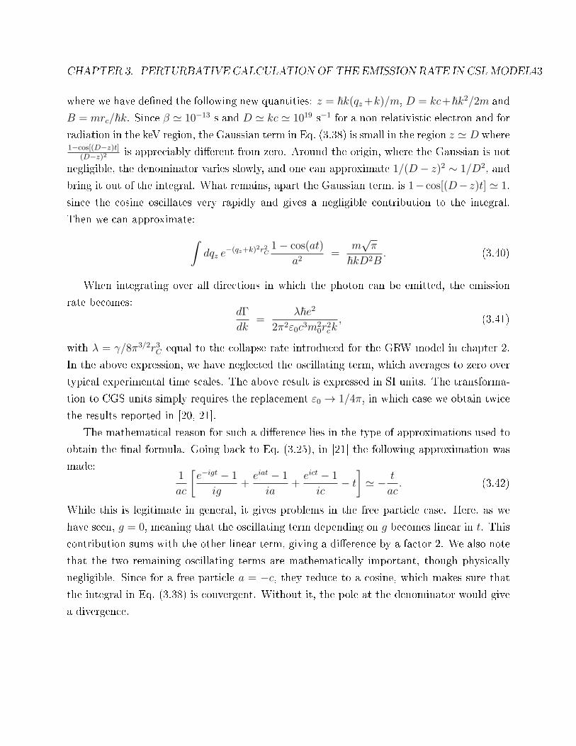
CHAPTER 3. PERTURBATIVE CALCULATIONOF THE EMISSION RATE IN CSLMODEL43
where we have dened the following new quantities: z = ~k(qz+k)/m, D = kc+~k2/2m and
B = mrc/~k. Since β ≃ 10−13 s and D ≃ kc ≃ 1019 s−1 for a non relativistic electron and for
radiation in the keV region, the Gaussian term in Eq. (3.38) is small in the region z ≃ D where1−cos[(D−z)t]
(D−z)2is appreciably dierent from zero. Around the origin, where the Gaussian is not
negligible, the denominator varies slowly, and one can approximate 1/(D− z)2 ∼ 1/D2, and
bring it out of the integral. What remains, apart the Gaussian term, is 1− cos[(D− z)t] ≃ 1,
since the cosine oscillates very rapidly and gives a negligible contribution to the integral.
Then we can approximate:
∫
dqz e−(qz+k)2r2C
1− cos(at)
a2=
m√π
~kD2B. (3.40)
When integrating over all directions in which the photon can be emitted, the emission
rate becomes:dΓ
dk=
λ~e2
2π2ε0c3m20r
2ck, (3.41)
with λ = γ/8π3/2r3C equal to the collapse rate introduced for the GRW model in chapter 2.
In the above expression, we have neglected the oscillating term, which averages to zero over
typical experimental time scales. The above result is expressed in SI units. The transforma-
tion to CGS units simply requires the replacement ε0 → 1/4π, in which case we obtain twice
the results reported in [20, 21].
The mathematical reason for such a dierence lies in the type of approximations used to
obtain the nal formula. Going back to Eq. (3.25), in [21] the following approximation was
made:1
ac
[e−igt − 1
ig+eiat − 1
ia+eict − 1
ic− t
]
≃ − t
ac. (3.42)
While this is legitimate in general, it gives problems in the free particle case. Here, as we
have seen, g = 0, meaning that the oscillating term depending on g becomes linear in t. This
contribution sums with the other linear term, giving a dierence by a factor 2. We also note
that the two remaining oscillating terms are mathematically important, though physically
negligible. Since for a free particle a = −c, they reduce to a cosine, which makes sure that
the integral in Eq. (3.38) is convergent. Without it, the pole at the denominator would give
a divergence.

CHAPTER 3. PERTURBATIVE CALCULATIONOF THE EMISSION RATE IN CSLMODEL44
3.5 Emission rate in the non-white noise case
To better understand the origin of the factor-2 dierence, we now generalize the computation
to include colored noises. In such a case, we will nd that the extra term that doubles the
answer of [20, 21] has a suspicious energy non-conserving form3, which is not related to the
steady increase of the particle's kinetic energy due to the energy transfer from the noise to
the particle during the collapse, that is a well-known feature of collapse models [16]. To see
this, we now generalize Eq. (3.41) to the case where the collapsing noise has a correlation
function which is not white in time:
E[w(x, t)w(y, s)] = f(t− s)F (x− y). (3.43)
We can start from Eq. (3.21) for the average transition probability:
E|Tfi|2 =1
~4
∑
n
∑
j
∫
L3
dz RkfnNni(z)Rk∗
fjN ∗ji(z) (3.44)
×∫ t
0
dt1
∫ t1
0
dt2
∫ t
0
dt3
∫ t3
0
dt4eiat1eibt2eict3eidt4f (t2 − t4) ,
where now f replaces the Dirac delta. The coecients a, b, c and d are the same as in
Eq. (3.22). The only eect of the non-white noise is to modify the time dependent part of
the transition probability, which we consider separately:
T =
∫ t
0
dt1
∫ t1
0
dt2
∫ t
0
dt3
∫ t3
0
dt4 eiat1eibt2eict3eidt4f(t2 − t4). (3.45)
This can be rewritten as follows:
T =
∫ t
0
dt2
∫ t
t2
dt1
∫ t
0
dt4
∫ t
t4
dt3 eiat1eibt2eict3eidt4f (t2 − t4)
= − 1
ac
∫ t
0
dt2
∫ t
0
dt4(eiat − eiat2
) (eict − eict4
)eibt2eidt4f (t2 − t4) . (3.46)
3Moreover, an unpublished calculation by S. L. Adler shows that for an electron bound in a hydrogenatom, the extra term leads to a suspicious orders of magnitude increase in the radiation rate, rather thanjust the doubling found in the free particle case.

CHAPTER 3. PERTURBATIVE CALCULATIONOF THE EMISSION RATE IN CSLMODEL45
There are four terms with the same structure given by:
I :=
∫ t
0
du
∫ t
0
dv eiαueiβvF (u− v) =
∫ t
0
du
∫ t
0
dv ei2[(α+β)(u+v)+(α−β)(u−v)]f (u− v) . (3.47)
We perform the change of variable x = u − v and y = u + v. In these new variables, the
integral changes as follows:
∫ t
0
du
∫ t
0
dv f(u, v) =1
2
∫ t
0
dx
∫ 2t−x
x
dy [f(−x, y) + f(x, y)] . (3.48)
In our case, the integrand is separable, so the integral over y can be easily performed, giving:
∫ 2t−x
x
dy ei2(α+β)y = 4
ei2(α+β)t
(α + β)sin
1
2(α + β)(t− x). (3.49)
Then, taking into account that f(u− v) = f(x) = f(−x), the double integral I reduces to:
I = 4e
i2(α+β)t
(α + β)
∫ t
0
dx f(x) sin1
2(α + β)(t− x) cos
1
2(α− β)x. (3.50)
Going back to Eq. (3.46) and taking into account the relation a + b + c + d = 0, we can
write:
T = − 4
ac
e−i2gt
g
∫ t
0
dx f(x) sin
[1
2g(t− x)
]
cos
[1
2(b− d)x
]
−ei2at
a
∫ t
0
dx f(x) sin
[1
2a(t− x)
]
cos
[1
2ax
]
−ei2ct
c
∫ t
0
dx f(x) sin
[1
2c(t− x)
]
cos
[1
2cx
]
+1
2
∫ t
0
dx f(x)(t− x) cos [(a+ b)x]
. (3.51)
For white noise (f(x) = δ(x)) the above equation reduces to Eq. (3.25).4 In computing
the matrix elements Rkij and Nij for the free particle, a further constraint comes from the
Kronecker delta of Eq. (3.19), which implies a = −c and g = 0. Accordingly, the expression
4Note that∫ t
0dxδ(x)g(x) = 1
2g(0), for a general function g(x), must be used in the reduction to the whitenoise case.
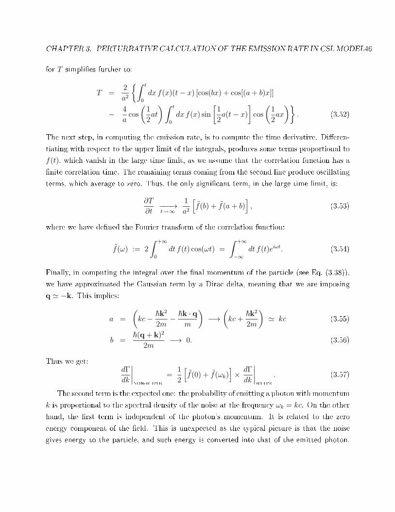
CHAPTER 3. PERTURBATIVE CALCULATIONOF THE EMISSION RATE IN CSLMODEL46
for T simplies further to:
T =2
a2
∫ t
0
dx f(x)(t− x) [cos(bx) + cos[(a+ b)x]]
− 4
acos
(1
2at
)∫ t
0
dx f(x) sin
[1
2a(t− x)
]
cos
(1
2ax
)
. (3.52)
The next step, in computing the emission rate, is to compute the time derivative. Dieren-
tiating with respect to the upper limit of the integrals, produces some terms proportional to
f(t), which vanish in the large time limit, as we assume that the correlation function has a
nite correlation time. The remaining terms coming from the second line produce oscillating
terms, which average to zero. Thus, the only signicant term, in the large time limit, is:
∂T
∂t−−−→t ∞
1
a2
[
f(b) + f(a+ b)]
, (3.53)
where we have dened the Fourier transform of the correlation function:
f(ω) := 2
∫ +∞
0
dt f(t) cos(ωt) =
∫ +∞
−∞dt f(t)eiωt. (3.54)
Finally, in computing the integral over the nal momentum of the particle (see Eq. (3.38)),
we have approximated the Gaussian term by a Dirac delta, meaning that we are imposing
q ≃ −k. This implies:
a =
(
kc− ~k2
2m− ~k · q
m
)
−→(
kc+~k2
2m
)
≃ kc (3.55)
b =~(q+ k)2
2m−→ 0. (3.56)
Thus we get:dΓ
dk
∣∣∣∣NON-WHITE
=1
2
[
f(0) + f(ωk)]
× dΓ
dk
∣∣∣∣WHITE
. (3.57)
The second term is the expected one: the probability of emitting a photon with momentum
k is proportional to the spectral density of the noise at the frequency ωk = kc. On the other
hand, the rst term is independent of the photon's momentum. It is related to the zero
energy component of the eld. This is unexpected as the typical picture is that the noise
gives energy to the particle, and such energy is converted into that of the emitted photon.

CHAPTER 3. PERTURBATIVE CALCULATIONOF THE EMISSION RATE IN CSLMODEL47
Therefore, the zero energy component of the eld should not allow a photon emission with
an arbitrarily high energy 5. Precisely this term, in the white-noise limit, is responsible for
the factor-2 dierence, as one can easily check.
3.6 Computation using a generic nal state for the charged
particle
At the end of Section 3.4 we discussed that the factor-2 dierence arises because g as dened
in Eq. (3.24) becomes 0, due to the deltas in the R terms (see Eq. (3.19)) that make En to be
equal to Ej. One could then expect that by considering a generic nal state for the outgoing
particleinstead of more articial plane wavesuch a constraint is removed. So, instead of
a nal state with a denite momentum for the particle, let us now take a normalized wave
packet:
ui (x) =1√L3, uf (x) =
∑
∆
h (∆)ei(q+∆)·x√L3
, un (x) =ein·x√L3, (3.58)
where h (∆) normalizes the wave function:
1 =
∫
L3
dx |ψf |2 =1
L3
∑
∆′
∑
∆
h∗ (∆′)h (∆)
∫
L3
dxe−i(q+∆′)·xei(q+∆)·x =∑
∆
|h (∆)|2 . (3.59)
The matrix elements in Eq. (3.19) and Eq.(3.20) now become:
Rkfn =
⟨f∣∣Rk
∣∣n⟩=∑
∆
h∗ (∆)⟨f∆∣∣Rk
∣∣n⟩= αk
(
−e~m
)∑
∆
h∗ (∆) [ǫk,µ · (q+∆)] δn,q+∆+k.(3.60)
Nni = −~
√λm
m0
1
L3
∫
dxN(x)e−in·x (3.61)
The formula of E|Tfi|2 is still given by Eq. (3.21):
E|Tfi|2 =1
~4
∑
n
∑
j
Rk∗fjRk
fn E[N ∗jiNni] T, (3.62)
5One can object that this is a peculiar feature of the CSL model which diers from the standard quantumpicture. This criticism can be easily rejected by remembering that, in order to perform the computation inan easier way, one has eectively considered a standard quantum Hamiltonian with a random term.

CHAPTER 3. PERTURBATIVE CALCULATIONOF THE EMISSION RATE IN CSLMODEL48
with T given in Eq. (3.25). The two Kronecker deltas coming from Eq. (4.27) set:
n = q+∆+ k and j = q+∆′ + k. Accordingly, the coecients a, c and g, dened in (3.22)
and (3.24), become:
a =(Ef + ~ωk − Eq+∆+k)
~, c = −(Ef + ~ωk − Eq+∆′+k)
~, g =
Eq+∆+k − Eq+∆′+k
~.
(3.63)
Moreover, we have:
E[N ∗jiNni] = ~
2γ
(m
m0
)21
L6
∫
L3
dx1
∫
L3
dx2e−i(k+q)·(x1−x2)e−i(∆·x1−∆′·x2)F (x1−x2). (3.64)
The two exponents can be rewritten as: −i(k+ q) · (x1 − x2)− (i/2)(∆−∆′) · (x1 − x2)−(i/2)(∆+∆′) · (x1+x2). We now make the change of variables: x = x1−x2, y = x1+x2, as
we did after Eq. (3.30). The integral over y produces L3δ∆,∆′ plus extra terms which vanish
in the large L limit. Thus, as in the previous section, a, c and g take the values:
a = −c =(Ef + ~ωk − Eq+∆+k)
~, g = 0. (3.65)
The integral over x gives the Fourier transform of the correlation F ; accordingly, the transi-
tion probability reduces to:
E|Tfi|2 = Λ∑
∆
|h (∆)|2 [ǫk,µ · (q+∆)]2e−(q+∆+k)2r2C
[at− sin(at)
a3
]
, (3.66)
with Λ dened as in Eq. (3.36). As we see, the structure is minimally modied from that
of Eq. (3.35). In particular, in the non white noise case the condition g = 0 implies the
presence of the unphysical factor f(0).
3.7 Computation with a noise conned in space
The calculation of the previous section shows that the reason why we have g = 0 for an
outgoing wave packet is because a delta δ∆,∆′ appears, which arises from the integral over
space with respect to the variable y = x1+x2. This suggests that the problem can be avoided
by considering a noise which is conned to a nite region of space. We analyze this case here.

CHAPTER 3. PERTURBATIVE CALCULATIONOF THE EMISSION RATE IN CSLMODEL49
Let us suppose that the correlation function of the noise is:
E[w(x, t)w(y, s)] = f(t− s)F (x− y)e−(x+y)2/ℓ2 , (3.67)
where ℓ is an appropriate cut o. We start from Eq. (3.62)
E|Tfi|2 =1
~4
∑
n
∑
j
Rk∗fjRk
fn E[N ∗jiNni]T, (3.68)
where the temporal part T is given by Eq. (3.51). The two Kronecker deltas coming from
Eq. (4.27) set: n = q+∆+ k and j = q+∆′ + k. In this case, Eq. (3.64) is replaced by:
E[N ∗jiNni] = ~
2γ
(m
m0
)21
L6
∫
L3
dx1
∫
L3
dx2e−i(k+q)·(x1−x2)e−i(∆·x1−∆′·x2)F (x1−x2)e
−(x+y)2/ℓ2 .
(3.69)
As before, we perform the change of variables: x = x1−x2, y = x1+x2. In integrating over
the new variables, we use the rule:
∫ +L2
−L2
dx1
∫ +L2
−L2
dx2f (x1, x2) =1
2
∫ L
0
dx
∫ +(L−x)
−(L−x)
dy [f (x, y) + f (−x, y)] . (3.70)
In our case:
f(x1,x2) = ei(q+∆′+k)·x1e−i(q+∆+k)·x2F (x1 − x2)e−(x1+x2)2/l2 (3.71)
= ei(
q+∆′+∆2
+k)
·xe
i2(∆′−∆)·yF (x)e−y2/l2 =
3∏
i=1
fi(xi, yi), (3.72)
fi(xi, yi) = ei2(j+n)ixie
i2(∆′−∆)iyi
1√4πrC
e−x2i /4r
2Ce−y2i /l
2
, (3.73)
where we have used the Kronecker delta constraints to replace q+ k+12(∆+∆′) by 1
2(j+ n).
Thus we arrive at the following expression:
E[N ∗jiNni] = ~
2γ
(m
m0
)21
8L6
3∏
i=1
∫ L
0
dxi
∫ +(L−xi)
−(L−xi)
dyi 2 cos
[1
2(j + n)ixi
]
× ei2(∆′−∆)iyi
1√4πrC
e−x2i /4r
2Ce−y2i /l
2
.
(3.74)
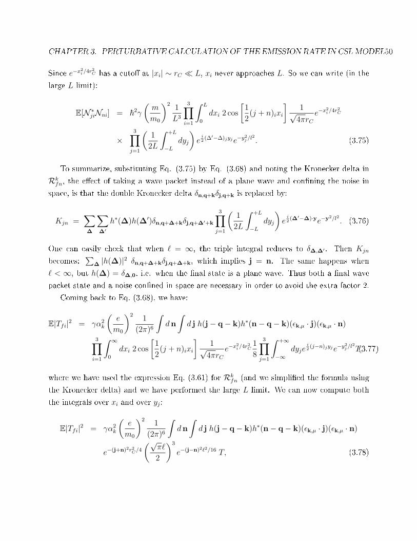
CHAPTER 3. PERTURBATIVE CALCULATIONOF THE EMISSION RATE IN CSLMODEL50
Since e−x2i /4r
2C has a cuto at |xi| ∼ rC ≪ L, xi never approaches L. So we can write (in the
large L limit):
E[N ∗jiNni] = ~
2γ
(m
m0
)21
L3
3∏
i=1
∫ L
0
dxi 2 cos
[1
2(j + n)ixi
]1√4πrC
e−x2i /4r
2C
×3∏
j=1
(1
2L
∫ +L
−L
dyj
)
ei2(∆′−∆)jyje−y2j /l
2
. (3.75)
To summarize, substituting Eq. (3.75) by Eq. (3.68) and noting the Kronecker delta in
Rkfn, the eect of taking a wave packet instead of a plane wave and conning the noise in
space, is that the double Kronecker delta δn,q+kδj,q+k is replaced by:
Kjn =∑
∆
∑
∆′
h∗(∆)h(∆′)δn,q+∆+kδj,q+∆′+k
3∏
j=1
(1
2L
∫ +L
−L
dyj
)
ei2(∆′−∆)·ye−y2/l2 . (3.76)
One can easily check that when ℓ = ∞, the triple integral reduces to δ∆,∆′ . Then Kjn
becomes:∑
∆ |h(∆)|2 δn,q+∆+kδj,q+∆+k, which implies j = n. The same happens when
ℓ < ∞, but h(∆) = δ∆,0, i.e. when the nal state is a plane wave. Thus both a nal wave
packet state and a noise conned in space are necessary in order to avoid the extra factor 2.
Coming back to Eq. (3.68), we have:
E|Tfi|2 = γα2k
(e
m0
)21
(2π)6
∫
dn
∫
d j h(j− q− k)h∗(n− q− k)(ǫk,µ · j)(ǫk,µ · n)3∏
i=1
∫ ∞
0
dxi 2 cos
[1
2(j + n)ixi
]1√4πrC
e−x2i /4r
2C1
8
3∏
j=1
∫ +∞
−∞dyje
i2(j−n)jyje−y2j /l
2
T,(3.77)
where we have used the expression Eq. (3.61) for Rkfn (and we simplied the formula using
the Kronecker delta) and we have performed the large L limit. We can now compute both
the integrals over xi and over yj:
E|Tfi|2 = γα2k
(e
m0
)21
(2π)6
∫
dn
∫
d j h(j− q− k)h∗(n− q− k)(ǫk,µ · j)(ǫk,µ · n)
e−(j+n)2r2C/4
(√πℓ
2
)3
e−(j−n)2ℓ2/16 T, (3.78)

CHAPTER 3. PERTURBATIVE CALCULATIONOF THE EMISSION RATE IN CSLMODEL51
Since we can take ℓ arbitrarily large, according to the second Gaussian term, only those
elements with j ≃ n are relevant. We can therefore simplify the above expression as follows:
E|Tfi|2 = γα2k
(e
m0
)21
(2π)6
∫
dn|h(n−q−k)|2(ǫk,µ·n)2e−n2r2C
(√πℓ
2
)3 ∫
d j e−(j−n)2ℓ2/16 T .
(3.79)
Here we have used the wave packet assumption that h is a smooth function of its arguments,
and not a delta function.
We now focus on the last integral containing the time dependence, which generates the
factor 2 problem when ℓ = ∞. We now show that the undesired term has a vanishing contri-
bution, for large times. For simplicity, we focus our attention to the white-noise expression
for T (see Eq. (3.25)), but the calculation can immediately be generalized to the non-white-
noise case of Eq. (3.51) as well. Taking into account only the undesired term, the integral to
compute becomes:
J =
(√πℓ
2
)3 ∫
dj e−(j−n)2ℓ2/16 1
ac
e−igt − 1
ig. (3.80)
According to Eq. (3.22), when j = n, then c = −a, and the dependence of c over j drops out.
According to Eq. (3.24), g = ~(n2 − j2)/2m ≃ ~n · (n− j)/m. Moreover we can re-write the
exponential term in integral form. We arrive at the following formula:
J =
(√πℓ
2
)31
a2
∫ t
0
ds
∫
dj e−(j−n)2ℓ2/16−i~n·(n−j)s/m
=(2π)3
a2
∫ t
0
dse−4~2n2s2/m2ℓ2 . (3.81)
As we see, if we take the limit ℓ→ ∞, the above integral gives a linear increase in time, and
therefore contributes to the total rate, giving rise to the extra factor 2. On the other hand, if
we keep ℓ nite, we compute the rate (which corresponds to dierentiating in time) and we
take the large time limit, such a term decays exponentially and does not contribute to the
asymptotic rate. All above conditions are consistent with typical experimental situations. In
this regime, the extra term found in [22] is negligible, and the Golden Rule formula used as
the basis for the calculations of [20, 21] gives the entire answer.
Chapter 4
Radiation emission in QMUPL model
In the previous chapter we studied the emission of radiation in the CSL model. We found
that, when the computation is done by using perturbation theory naively, an extra term
containing an unphysical factor appears. We gave a prescription to solve such a problem, for
a free particle. However, this is not a satisfactory solution for two reasons: (i) it is not clear
whether such a prescription works for systems dierent from the free particle; (ii) the idea of
conning the noise when using perturbation theory seems reasonable but it is only an ad-hoc
solution.
In order to better understand the origin of the unphysical term, we repeat the computation
using the QMUPL model. The advantage of using this model is that, only with the dipole
approximation, the emission rate can be computed exactly. Moreover, as discussed in chapter
2, for systems whose typical size is smaller than rC , the QMUPL model approximates the
CSL model. Such a computation has already been done in [22] for the white noise case.
Here we generalize it using a colored noise, in order to better identify when unphysical terms
appears.
52

CHAPTER 4. RADIATION EMISSION IN QMUPL MODEL 53
4.1 The model and the solutions of the Heisenberg equa-
tions
We start by using the imaginary noise trick in the QMUPL model. The corresponding
dynamics is determined by the Hamiltonian:
HTOT = H − ~
√λ q ·w(t), (4.1)
where the quantum Hamiltonian H reads:
H =1
2m0
(p− eA)2 +1
2κq2 +
1
2ǫ0
∫
d3x[E2 + c2B2
](4.2)
and where all the symbols are dened in the previous chapter, apart for κ which is the force
constant of the harmonic term. As before, we work in Coulomb gauge where ∇ ·A = 0 and
V = 0, with V the electromagnetic scalar potential. Under only the dipole approximation,
the equations of motions have been exactly solved [22]. In this section we recall these results
and generalize them to the case of a non white noise. The plane waves decomposition of the
vector potential A, in the dipole approximation, reads:
A(x) :=
√
~
ǫ0
∑
µ
∫
d3kg(k)√2ωk
ǫkµ
[
akµ + a†kµ
]
; (4.3)
where the linear polarization vectors ǫkµ are taken as real and the form factor g(k) is the
Fourier transform of the charge distribution and it reduces to 1/(2π)3/2 for a point like
particle.
The second term on the right hand side of Eq. (4.1) is a random potential depending
on the position q of the particle and on the noise w(t). This noise has zero mean and the
generic (scalar) correlation function:
E[wi(s)wj(s′)] = δijf(s− s′), (4.4)
where the subscripts i, j = 1, 2, 3 label the three directions in the space. This means that,
contrary to what was done in [22], here we consider the more generic situation of a (isotropic)
colored noise. However, since the solutions of the Heisenberg equations for the operators are

CHAPTER 4. RADIATION EMISSION IN QMUPL MODEL 54
formally equivalent both in the white and in the colored noise cases, we can take the solutions
found in [22], without any further calculation.
The Heisenberg equations of motion for the position of the particle q(t), its conjugate
momentum p(t) and the electromagnetic-eld operators a†kµ(t) are:
dp
dt= −κq +
√λ~w(t), (4.5)
dq
dt=
p
m0
− e
m0
A, (4.6)
da†kµdt
= iωka†kµ −
ie√~ǫ0m0
g(k)√2ωk
ǫkµ · p
+ie2
ǫ0m0
g(k)√2ωk
ǫkµ ·∑
µ′
∫
d3k′g(k′)√2ωk′
ǫk′µ′
[
ak′µ′ + a†k′µ′
]
. (4.7)
The equation for akµ(t) can be obtained from the previous one by taking the hermitian
conjugate.

CHAPTER 4. RADIATION EMISSION IN QMUPL MODEL 55
By solving the above set of coupled linear dierential equations, one obtains:
q(t) = [1− κF1(t)]q(0) + F0(t)p(0)
−e√
~
ǫ0
∑
µ
∫
d3kg(k)√2ωk
ǫkµ
[
G+1 (k, t) akµ(0) +G−
1 (k, t) a†kµ(0)
]
+√λ~
∫ t
0
dsF0(t− s)w(s), (4.8)
p(t) = −κ [t− κF2(t)]q(0) + [1− κF1(t)]p(0)
+κ e
√
~
ǫ0
∑
µ
∫
d3kg(k)√2ωk
ǫkµ
[
G+0 (k, t) akµ(0) +G−
0 (k, t) a†kµ(0)
]
+√λ~
∫ t
0
ds [1− κF1(t− s)]w(s) (4.9)
a†kµ(t) = eiωkta†kµ(0) − ie√~ǫ0
g(k)√2ωk
ǫkµ ·[G−
1 (k, t)p(0)− κG−0 (k, t)q(0)
]
+ie2
ǫ0
g(k)√2ωk
ǫkµ ·∑
µ′
∫
d3k′g(k′)√2ωk′
ǫk′µ′
[
G−+(k, k
′, t) ak′µ′(0) +G−−(k, k
′, t) a†k′µ′(0)]
−ie√
~λ
ǫ0
g(k)√2ωk
ǫkµ ·∫ t
0
dsG−1 (k, t− s)w(s), (4.10)
akµ(t) = e−iωktakµ(0) +ie√~ǫ0
g(k)√2ωk
ǫkµ ·[G+
1 (k, t)p(0)− κG+0 (k, t)q(0)
]
− ie2
ǫ0
g(k)√2ωk
ǫkµ ·∑
µ′
∫
d3k′g(k′)√2ωk′
ǫk′µ′
[
G++(k, k
′, t) ak′µ′(0) +G+−(k, k
′, t) a†k′µ′(0)]
+ie
√
~λ
ǫ0
g(k)√2ωk
ǫkµ ·∫ t
0
dsG+1 (k, t− s)w(s), (4.11)
where the following functions have been introduced:
Fn(t) :=
∫
Γ
dz
2πi
ezt
znH(z), n = 0, 1, 2, (4.12)
G±n (k, t) :=
∫
Γ
dz
2πi
znezt
(z ± iωk)H(z), n = 0, 1, (4.13)
G±±(k, k
′t) :=
∫
Γ
dz
2πi
z2ezt
(z ± iωk)(z ± iωk′)H(z). (4.14)

CHAPTER 4. RADIATION EMISSION IN QMUPL MODEL 56
In Eq. (4.14) the upper ± refers to the rst parenthesis, while the lower one refers to the
second parenthesis. In all the above formulas, according to the theory of Laplace transform,
the contour Γmust be a line parallel to the imaginary axis, lying to the right of all singularities
of the integrand. The function H(z), after the renormalization procedure, is:
H(z) = κ+ z2 [m− β z] , β =e2
6πǫ0c3≃ 5.71× 10−54 Kg s. (4.15)
Since Fn(t), G±n (k, t) and G
±±(k, k
′t) are dened by contour integrals of functions containing
H(z) at the denominator, it is fundamental to know the zeros of H(z). Their approximated
values are (see Appendix A in [22]):
z1 ≃ m
β+ o(ω0), z2,3 ≃ −ω
20β
2m± iω0 + o(ω3
0), (4.16)
where we introduced the natural frequency of the harmonic oscillator ω0 :=√
κ/m.
4.2 The formula for the emission rate
We now focus our attention on the emission rate, dened as follows:
d
dkΓk(t) = 8πk2
d
dtE[〈φ|a†kµ(t)akµ(t)|φ〉] (4.17)
where |φ〉 is the initial state and a†kµ(t), akµ(t) are the creation and annihilation operators
of a photon of momentum k and polarization µ, in the Heisenberg picture. The factor 8πk2
arises because a sum over the polarization states and directions of the photon momentum is
taken. In what follows, we take |φ〉 := |ψ〉 ⊗ |Ω〉, where |ψ〉 is the initial state of the particle
and |Ω〉 is the vacuum state for the electromagnetic eld.
Before going on, let us explain why this denition of the emission rate is equivalent to the
one given before in Eq. (3.37). This can be seen by inserting a completeness in Eq. (4.17):
d
dkΓk(t) = 8πk2
d
dtE[〈φ|a†kµ(t)akµ(t)|φ〉] = 8πk2
d
dtE[〈φ|U †(t)a†kµakµU(t)|φ〉] ≃
≃ 8πk2d
dt
∑
f
E[|〈f,Ω|akµU(t)|φ〉|2] = 8πk2d
dt
∑
f
E[|〈f,k, µ|U(t)|φ〉|2],(4.18)

CHAPTER 4. RADIATION EMISSION IN QMUPL MODEL 57
where we used akµ(t) = U †(t) akµ U(t), with U(t) the unitary time evolution operator. In the
above formula f denotes a state of the particle and the sum is taken over a complete set
of states. Therefore E[|〈f,k, µ|U(t)|φ〉|2] is exactly the transition probability Pfi dened in
Eq. (3.11), we see that Eq. (4.18) is equivalent to Eq. (3.37). Notice that in the second step
we made an approximation: we inserted only the vacuum state of the electromagnetic eld,
instead of the sum over all the possible states with dierent number of photons. However,
this is not a problem since the neglected terms correspond to processes involving the creation
of many photons, that are contributions of terms whose orders are bigger than e2. Therefore,
at the lowest order, the two denitions are equivalent.
Looking at Eq. (4.10) for a†kµ(t) and Eq. (4.11) for akµ(t), we see that the only non zero
contribution due to the noise, the one proportional to λ, is given by the product of the last
terms. The reason why the terms proportional to√λ do not contribute is that they contain
only one noise, which has zero average. Using Eq. (4.4), one can easily see that the rate of
emitted radiation from a point like particle (g(k) = 1/(2π)3/2) due to the interaction with
the noise eld is:
d
dkΓk(t) =
λ~e2
2π2ε0c2ωk
d
dt
∫ t
0
ds
∫ t
0
ds′G−1 (k, t− s)G+
1 (k, t− s′) f (s− s′) , (4.19)
where ωk = ck (k = |k|). The functions G+1 and G−
1 are dened in Eq. (4.13). Now we have
all the ingredients to compute the emission rate both for a free particle and for a harmonic
oscillator.
4.3 Free particle
When the particle is free (κ = 0), the integral in Eq. (4.13) is easy to solve and the functions
G±1 (k, t) take the form [40]:
G±1 (k, t) = ∓ i
mωk
± ie∓iωkt
ωk (m± iβωk)+
emt/β
(m/β) [m± iβωk]. (4.20)
The last term gives rise to the runaway behavior, which is expected after the renormaliza-
tion procedure; we pragmatically dismiss it by ignoring its contribution. The second term
oscillates in time, while the rst term is constant. When computing the product between G−1
and G+1 , some terms arise, which oscillate with a rate much bigger than typical experimental
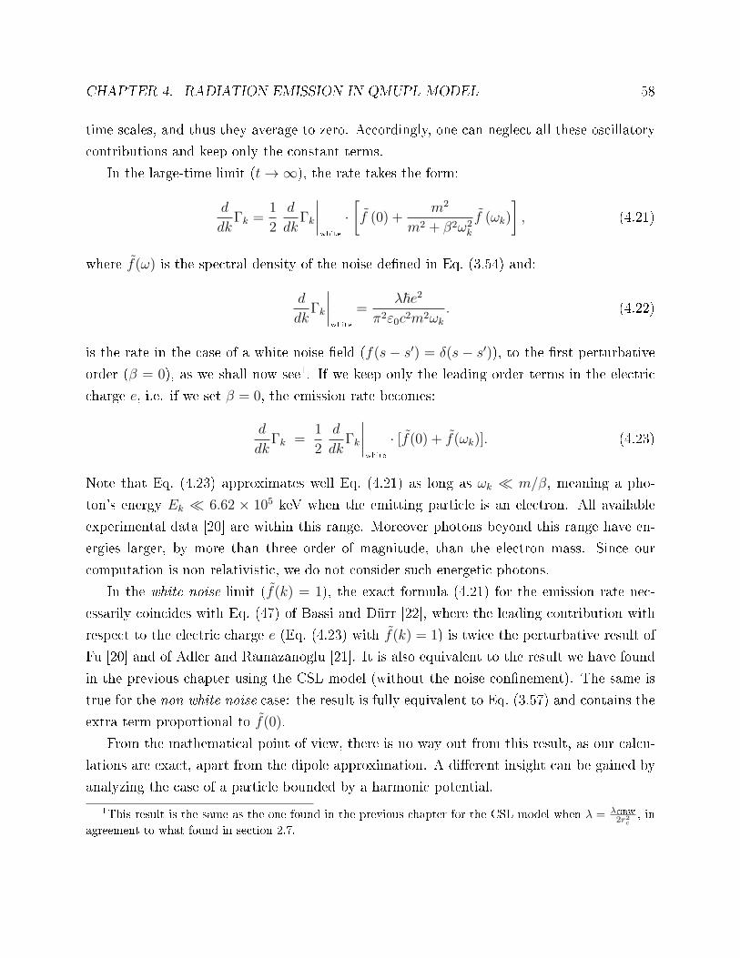
CHAPTER 4. RADIATION EMISSION IN QMUPL MODEL 58
time scales, and thus they average to zero. Accordingly, one can neglect all these oscillatory
contributions and keep only the constant terms.
In the large-time limit (t→ ∞), the rate takes the form:
d
dkΓk =
1
2
d
dkΓk
∣∣∣∣white
·[
f (0) +m2
m2 + β2ω2k
f (ωk)
]
, (4.21)
where f(ω) is the spectral density of the noise dened in Eq. (3.54) and:
d
dkΓk
∣∣∣∣white
=λ~e2
π2ε0c2m2ωk
. (4.22)
is the rate in the case of a white noise eld (f(s − s′) = δ(s − s′)), to the rst perturbative
order (β = 0), as we shall now see1. If we keep only the leading order terms in the electric
charge e, i.e. if we set β = 0, the emission rate becomes:
d
dkΓk =
1
2
d
dkΓk
∣∣∣∣white
· [f(0) + f(ωk)]. (4.23)
Note that Eq. (4.23) approximates well Eq. (4.21) as long as ωk ≪ m/β, meaning a pho-
ton's energy Ek ≪ 6.62 × 10⁵ keV when the emitting particle is an electron. All available
experimental data [20] are within this range. Moreover photons beyond this range have en-
ergies larger, by more than three order of magnitude, than the electron mass. Since our
computation is non relativistic, we do not consider such energetic photons.
In the white noise limit (f(k) = 1), the exact formula (4.21) for the emission rate nec-
essarily coincides with Eq. (47) of Bassi and Dürr [22], where the leading contribution with
respect to the electric charge e (Eq. (4.23) with f(k) = 1) is twice the perturbative result of
Fu [20] and of Adler and Ramazanoglu [21]. It is also equivalent to the result we have found
in the previous chapter using the CSL model (without the noise connement). The same is
true for the non white noise case: the result is fully equivalent to Eq. (3.57) and contains the
extra term proportional to f(0).
From the mathematical point of view, there is no way out from this result, as our calcu-
lations are exact, apart from the dipole approximation. A dierent insight can be gained by
analyzing the case of a particle bounded by a harmonic potential.
1This result is the same as the one found in the previous chapter for the CSL model when λ = λGRW2r2c
, in
agreement to what found in section 2.7.

CHAPTER 4. RADIATION EMISSION IN QMUPL MODEL 59
4.4 Harmonic oscillator
The dierent behavior of a harmonic oscillator, mathematically speaking, lies in the fact that
the function H(z) dened in Eq. (4.15) has a dierent dependence on z compared to a free
particle. The functions G±1 (k, t) entering Eq. (4.19) are again the ones dened in Eq. (4.13),
that is a sum of terms whose time dependence is given by ezℓt, where zℓ are the three zeros
of H(z). The dierence with respect to the free particle case is that the zeros of H(z) are
not zfree1 = m/β and zfree2 = 0 but the ones dened in Eq. (4.16). Writing the functions
G±1 (k, t) in Eq. (5.24) in a more explicit form, one gets (the terms containing ez1t gives the
usual runaway contribution, therefore we dismiss them):
d
dkΓk =
λ~e2
2π2ε0c2ωk · (4.24)
·
3∑
ℓ,ℓ′=2
zℓzℓ′
(zℓ − iωk) (zℓ′ + iωk)
1
β
3∏
j=1j 6=ℓ
1
zℓ − zj
1
β
3∏
j=1j 6=ℓ′
1
zℓ′ − zj
e(zℓ+zℓ′ )t[Ft(−zℓ′) + Ft(−zℓ)]
−i3∑
ℓ=2
ωkzℓH (−iωk) (zℓ − iωk)
1
β
3∏
j=1j 6=ℓ
1
zℓ − zj
e
(zℓ−iωk)t[Ft(iωk) + Ft(−zℓ)] +
+i3∑
ℓ=2
ωkzℓH (+iωk) (zℓ + iωk)
1
β
3∏
j=1j 6=ℓ
1
zℓ − zj
e
(zℓ+iωk)t[Ft(−zℓ) + Ft(−iωk)] +
+ω2k
H (+iωk)H (−iωk)[Ft(iωk) + Ft(−iωk)]
,
where Ft(z) is dened as:
Ft(α) =
∫ t
0
dxf(x)eαx. (4.25)
The major dierence from the free particle case is the presence of exponentially damped
terms, originating from the solutions z2 and z3. These exponential contributions become
1 in the free particle limit (ω0 = 0), but vanish asymptotically in the case of a harmonic
oscillator. Moreover they vanish very rapidly: In fact, taking ω0 = E/~ ≃ 3.29 × 10¹⁵Hz
for E = 13.6 eV which is the energy of the ground state of the hydrogen atom, one gets
ω20β/2m ≃ 3.39 × 10⁷s−1, while typical experiments last years [20]. The large time limit is

CHAPTER 4. RADIATION EMISSION IN QMUPL MODEL 60
easy to understand. Since z2,3 = −ω20β
2m± iω0, the rst three lines contain terms that vanish
exponentially. Then the only term that survives is the one in the fourth line, which for t→ ∞gives:
d
dkΓk =
λ~e2
2π2ε0c2ω3k
m2 (ω20 − ω2
k)2+ β2ω6
k
f (ωk) , (4.26)
where f(ωk) is the one dened in Eq. (3.54).
This formulain the free particle limitreduces to:
d
dkΓk =
1
2
d
dkΓk
∣∣∣∣white
· m2
m2 + β2ω2k
f (ωk) . (4.27)
When compared with Eq. (4.21), we see that the unphysical term associated to f (0) has
disappeared, and with it also the factor of 2 dierence with respect to the CSL perturbative
calculation of Fu [20] (β = 0, f (ωk) = 1) and of Adler et all [21, 23] (β = 0, f (ωk) generic).
Since in our case the whole calculation has been done non perturbatively, the mathe-
matical reason behind such a dierence is easy to nd: the order of performing the large
time limit and the free particle limit is very important since the two limits do not commute.
The reason for this, as previously noted, is that the free particle limit ω0 → 0 implies also
z2,3 → 0. Accordingly, if one takes the large time limit before the free particle limit, then
the terms in the formula for the emission rate depending on z2,3 vanish exponentially and
do not contribute to the asymptotic rate. On the other hand, if one takes the free particle
limit before the large time limit, then those terms do not vanish exponentially anymore, and
do contribute to the nal rate. In particular, the third and the fourth line of Eq. (4.24) give
contributions that oscillate in time, due to the presence of e±iωkt. In the large time limit such
contributions average to zero. However, the same is not true for the term in the second line:
this term now is constant and gives rise to the term proportional to f (0) in Eq. (4.21).
With the mathematical clarication comes also the physical explanation. To introduce the
free particle limit before the large time limit, one is assuming that the particle is perfectly free
at all times, forever. Vice-versa, by computing the large time limit before the free particle
limit, one is assuming that the particle feelssooner or laterthe edges of a (harmonic)
potential. Therefore the two dierent orders of limits imply two dierent physical situations,
hence two dierent behaviors.
Since particles, which are forever free, do not exist in nature, we come to the following
conclusion. Eq. (4.21), and the result of Bassi and Dürr [22], is mathematically correct for

CHAPTER 4. RADIATION EMISSION IN QMUPL MODEL 61
a perfectly free particle, with the unphysical term included. However, at the practical level
such a term is irrelevant, since real particles are never truly free. Then, the physically relevant
formula is that of Eq. (4.27), without the unphysical term: this equation, in the white noise
limit, and to rst perturbative order (β = 0), coincides with the CSL calculation of Fu [20]
and of Adler et al. [21, 23].
4.5 First order perturbation analysis
A deeper insight into the problem can be obtained by considering a perturbative approach
with respect to the electromagnetic coupling constant e. The lowest-order analysis is equiva-
lent to taking rst the limit β → 0, and then the limit t→ ∞ in the formula for the emission
rate in Eq. (4.19). Indeed, since there is a factor e2 in front of all the terms in Eq. (4.24) and
since all other e's are contained in β = e2
6πǫ0c3, performing the computation at the lowest order
(that is e2) is equivalent to taking the solution of Eq. (4.24) and setting β = 0. For a free
particle, the nal result (i.e. Eq. (4.23) with the unphysical term included) does not change.
Therefore, in this case the exact and perturbative calculations match. However, in the case
of a harmonic oscillator the perturbative result is completely dierent. Setting β = 0 implies
that z2,3 = ± iω0. Since the real negative part of z2,3, responsible of the decay behavior, has
reduced to zero, once again the decaying terms become oscillating terms (third and fourth
lines of Eq. (4.24)) or constant terms (rst line of Eq. (4.24)). In particular, the rst line is
proportional to Ft(ω0). It is straightforward to see that, in the large time limit t → ∞, one
gets:d
dkΓk =
e2~λ
4π2ε0c2m2ωk
(ω2k + ω2
0) f (ω0) + 2ω2kf (ωk)
(ω2k − ω2
0)2 ; (4.28)
which should be compared with Eq. (4.26). Moreover, by taking the free-particle limit, one
obtains:d
dkΓk =
1
2
d
dkΓk
∣∣∣∣white
·[
f (0)
2+ f (ωk)
]
, (4.29)
which diers from both Eq. (4.23) and Eq. (4.27) in the limit β → 0. We have checked the
result also by solving the problem from the scratch, to rst perturbative order [41].
From the mathematical point of view the reason for such a discrepancy is simple. In
the exact calculation, some terms appear which are proportional to e−(ω20β/2m)t and therefore
vanish in the large time limit. On the other hand, if one takes the limit β → 0 before the

CHAPTER 4. RADIATION EMISSION IN QMUPL MODEL 62
large time limit, the decaying exponential is approximated by 1, and the associated terms
contribute to the nal result. From the physical point of view, what happens is that, by
stopping the computation at the rst perturbative order in the electromagnetic constant e,
one does not take into account all processes where virtual photons are emitted and reabsorbed.
Actually, as we will discuss later in chapter 6, this is one way to look at the physical meaning
of the exponential e−(ω20β/2m)t.
We have shown that for a particle bounded by a harmonic potential (no matter how
weakly bounded) when the emission rate is computed exactly the unphysical term is not
present anymore, even without introducing any noise connement. More precisely, we have
seen that, when the emission rate is computed exactly, new contributions appear that, in the
large time limit, suppress the terms containing the unphysical factor. Therefore the root of
the problem lies in how the electromagnetic eld reacts to the particle being accelerated by
the noise. Constraining the eect of the noise by conning it in space/time allows to use the
rst order perturbation theory. In the other cases, also higher orders become relevant.
This analysis has been carried out using the QMUPL model. Now we want to check
if the same results apply also to the CSL model. However, for such a model, solving the
Heisenberg equations for the operators, treating all the interactions exactly, is not possible.
A rst attempt might be to treat perturbatively both the electromagnetic and the noise
interactions and carry the calculation up to the second order, instead of stopping at the rst
order. However, this poses a problem: the number of Feynman diagrams to compute is huge,
as an easy inspection to the perturbative series shows. A more promising idea is to perform
the computation by treating the electromagnetic interaction exactly and the noise interaction
perturbatively. This is suggested by the fact that the exponential damping factor e−(ω20β/2m)t,
the one that suppresses the term proportional to the unphysical factor, does not depend by
λ but only on e. This calculation will be carry out in the next chapter.
4.6 Semiclassical derivation of the emission rate
As a double check, in this section we derive the emission rate for a free particle and for a
harmonic oscillator using a semiclassical method. Such an approach has been used in [18]
(see the appendix of the article) to compute the radiation emission in the CSL model. The

CHAPTER 4. RADIATION EMISSION IN QMUPL MODEL 63
starting point is the Larmor formula:
P (t) =e2
6πǫ0c3a2 (t) , (4.30)
where a (t) is the (modulus of the) acceleration of the charged particle and P (t) is the total
radiated power. Since the emission rate computed in the previous sections gives the number
of photons emitted with energy ωk = kc, the total emitted power is related to the emission
rate by the relation:
P (t) =
∫
dk~ωkdΓ (t)
dk=
∫
dωk~ωk
c
dΓ (t)
dk. (4.31)
In order to nd the emission rate starting from Eq. (4.30), we rewrite it in terms of the
Fourier transform of the acceleration:
P (t) =e2
6πǫ0c3
3∑
j=1
1
(2π)2
∫
dνdωei(ν+ω)taj (ν) aj (ω) , (4.32)
where aj is the j-th cartesian component of the acceleration. This formula, together with
the relation
E [wj (ν)wj′ (ω)] = δj,j′4πδ (ω + ν) f (ω) , (4.33)
where wj (ν) is the Fourier transform of the noise wj (t) and f (ω) is dened in Eq. (3.54), is
all we need to nd the emission rate.
For a free particle under the inuence of the noise, the acceleration is given by:
a (t) =
√λ~
mw (t) . (4.34)
Note that ~ appears in this semi-classical calculation simply in order to keep the strength of
the noise the same as in the quantum case. Inserting Eq. (4.34) into Eq. (4.32) and taking
the noise average, one gets:
P (t) =
∫
dωe2λ~2
2π2ǫ0m2c3f (ω) , (4.35)
where we used the relation given in Eq. (4.33). By a comparison between this equation and

CHAPTER 4. RADIATION EMISSION IN QMUPL MODEL 64
Eq. (4.31) the emission rate becomes:
dΓ (t)
dk=
e2λ~
2π2ǫ0m2c2ωk
f (ωk) , (4.36)
that it is exactly the emission rate given in Eq. (4.23) without the unphysical factor f (0).
It is remarkable that using this semiclassical method the factor f (0) does not appear. The
reason for this behavior is not clear and will be subject to future research.
For a harmonic oscillator, the acceleration is:
aj(t) =
√λ~
m[wj(t) + ω0 cos (ω0t) fs(t)− ω0 sin (ω0t) fc(t)]
+ terms not depending on the noise, (4.37)
where fs (t) :=∫ t
0dx sin (ω0x)wj (x) and fc (t) :=
∫ t
0dx cos (ω0x)wj (x). By using the con-
volution theorem, we can write the Fourier transform of the second and the third terms as
follows:
Fω cos (ω0t) fs (t) =1
2Fω−ω0 (fs (t)) +
1
2Fω+ω0 (fs (t)) , (4.38)
Fω sin (ω0t) fc (t) =i
2Fω+ω0 (fc (t))−
i
2Fω−ω0 (fc (t)) , (4.39)
where Fω f (t) denotes the Fourier transform of f (t). The Fourier transform of the accel-
eration becomes:
aj (ω) =
√λ~
m
wj (ω) + iω0
2
[
Fω−ω0
(∫ t
0
dxe−iω0xwj (x)
)
− Fω+ω0
(∫ t
0
dxeiω0xwj (x)
)]
+ terms not depending on the noise. (4.40)
The two Fourier transforms in the above equation can be computed using integration by
parts:
Fω−ω0
(∫ t
0
dxe−iω0xwj (x)
)
=wj (ω)
i (ω − ω0), (4.41)
Fω+ω0
(∫ t
0
dxeiω0xwj (x)
)
=wj (ω)
i (ω + ω0). (4.42)

CHAPTER 4. RADIATION EMISSION IN QMUPL MODEL 65
Here we have neglected the terms that oscillate innitely fast with respect to ω. This is
justied by the fact that, in the formula for the total emitted power, an integral over ω
appears, which is zero for these terms. Using Eq. (4.41) and Eq. (4.42) the expression for
aj (ω) becomes:
aj (ω) =
√λ~
mwj (ω)
[ω2
(ω2 − ω20)
]
. (4.43)
Using Eq. (4.32) and taking the average over the noise we get:
P (t) =e2λ~2
2π2ǫ0m2c3
∫
dωω4
(ω2 − ω20)
2 f (ω) , (4.44)
which means that the emission rate is:
dΓ (t)
dk=
e2λ~
2π2ǫ0m2c2ω3k
(ω2k − ω2
0)2 f (ωk) . (4.45)
This is equivalent to the quantum formula of Eq. (4.26) in the lowest order limit β → 0.

Chapter 5
The emission rate in the CSL model
In chapter 4 we showed that, in order to get the correct formula for the rate emission,
two conditions must be fullled: the system cannot be taken as completely free (i.e. it
must be bounded by some potential) and the electromagnetic interaction cannot be treated
perturbatively at the lowest order. We now come back to the CSL model and apply what we
learned through the analysis done with the QMUPL model. In particular we derive a formula
for the emission rate from a charged harmonic oscillator interacting with the CSL noise. We
show that, in agreement to what we showed in the previous section, if the electromagnetic
interaction is not treated at the lowest order the unphysical term f(0) is not present.
5.1 The formula for the emission rate
In this section we wish to summarize the main results about the calculation of the emission
rate using the CSL model, where we treat the electromagnetic interaction exactly. Since the
computation is very long, all the technical details are reproduced in the following sections.
Contrary to what we did in section 3.1, here we will not use the whole Fock space: we
will work directly with the one-particle Hilbert space. Then Eq. (3.1) becomes:
HTOT = H − ~√γ
m0
∫
M(x)w(t,x) d3x, (5.1)
where M (x) simply becomes M (x) = mg (x− q) with g (x) dened in Eq. (2.23) and
w(t,x) = dWt(x)/dt is a noise eld with correlation E[w(t,x)w(s,y)] = f(t − s)δ(x− y).
As anticipated, we study a system of a single non-relativistic charged particle coupled to
66

CHAPTER 5. THE EMISSION RATE IN THE CSL MODEL 67
a harmonic potential and a second-quantized electrodynamic eld. The standard quantum
Hamiltonian it is:
H =1
2m(p− eA)2 +
1
2mω2
0 q2 +
1
2ǫ0
∫
d3x[E2
⊥ + c2B2]. (5.2)
Since we wish to treat the electromagnetic interaction exactly, we dene the unperturbed
and perturbed Hamiltonian as follows:
H0 =p2
2m+
1
2mω2
0 q2 +
1
2ǫ0
∫
d3x[E2
⊥ + c2B2]− e
mA · p+
e2
2mA2, (5.3)
H1 = −~
√γ
m0
∫
d3xM(x)w(t,x). (5.4)
Under only the dipole approximation, we will solve the Heisenberg equations of motion exactly
for the free kinetic term of the particle and the full electromagnetic term. In this way we
automatically include higher order terms of the electromagnetic eld in our analysis. This
step will prove to be crucial. The noise terms will be analyzed only to the rst perturbative
order. In contrast to [23] and what we have done in section 3.1, we will not conne the noise
and our result will be independent of the initial and nal state of the particle.
Most integrals can be solved exactly. We identify those terms that at lowest order in e
give a nite contribution to the asymptotic emission rate, while they decay exponentially in
time when higher order corrections are included, as in our case. Such terms are precisely
responsible for the appearance of the term proportional to f(0) in Eq. (3.57). When such
terms are appropriately taken into account the formula for the emission rate turns out to be:
dΓ
dk=
e2~λc
4π2ǫ0m20r
2C
k3
(ω2k − ω2
0)2 f (ωk) , (5.5)
where only terms proportional to f (ωk) survive. This formula, in the free particle limit
ω0 → 0, reduces to:dΓ
dk=
e2~λ
4π2ǫ0m20r
2Cc
3kf (ωk) , (5.6)
which is the expected result.
This result shows that, as anticipated in the previous chapter with the QMUPL model,
the suspicious term in Eq. (3.57) arises because calculations were limited to the lowest per-

CHAPTER 5. THE EMISSION RATE IN THE CSL MODEL 68
turbative order.
In order to derive the correct result it is necessary to bound the particle with a (harmonic)
potential, no matter how weakly it is coupled. Indeed, in agreement with the analysis done
in chapter 4 for the QMUPL model, it can be showed that for a perfectly free particle,
even when higher order terms are included in the perturbative analysis, the undesired term
remains. However, if we bound the particle with a harmonic oscillator and only at the
very end of calculations we take the free particle limit, we get the correct result where the
unphysical term f(0) is not present. The logic of this orderly computation is consistent with
the picture of physical reality where particles being perfectly free forever do not exist.
5.2 Computation of the emission rate
In this section we explain the mathematical details of computing the emission rate. We
show how to derive the emission rate formula given in Eq. (5.5). The relevant steps are the
following.
• In subsection 5.2.1 we consider the master equation for the density matrix ρ(t), and we
use it to compute the expectation value of a generic observable, to the rst perturbative
order in γ, while the electromagnetic term is treated exactly. Then we obtain the time
evolution of the expectation value of the photon number operator a†k,µak,µ (t) in terms
of two quantities, C(t, t1) and D(t, t1, t2) dened in Eqs. (5.17) and (5.18) respectively.
• In subsection 5.2.2 we consider the explicit time dependence of those operators which
are relevant for computing C(t, t1) and D(t, t1, t2).
• In subsection 5.2.3 and 5.2.4 we nd the analytic expression for C(t, t1) and D(t, t1, t2).
• In subsection 5.2.5 we compute the expectation value of the photon's number operator
a†k,µak,µ (t).
• In subsection 5.2.6 we perform all remaining time integrals, and show which terms
vanish, which rapidly oscillate, and which in turn give a nite contribution in the large
time limit.
• In subsection 5.2.7 we put all pieces together and draw the conclusion.

CHAPTER 5. THE EMISSION RATE IN THE CSL MODEL 69
5.2.1 The formula for the photon's number operator
We start recalling the master equation of a generic collapse model in the case of colored noise,
i.e., Eq. (2.17) of chapter 2:
dρ (t)
dt= − i
~[H, ρ (t)] + γ
N∑
i,j=1
∫ t
0
dsDij (t, s) [Ai, [Aj (s− t) , ρ (t)]] , (5.7)
In our case, the discrete sum becomes an integral over space, the collapse operators are
M (x), and the correlation function becomes: Dij (t, s) = δijf (t− s) → δ (x− x′) f (t− s).
Therefore we get:
dρ (t)
dt= − i
~[H, ρ (t)]− γ
(m
m0
)2 ∫
dx
∫ t
0
dsf (t− s) [g (x− q) , [g (x− q (s− t)) , ρ (t)]]
(5.8)
This equation is given in the Schrödinger picture. We switch to the interaction picture:
|ψ (t)〉I = U † (t) |ψ (t)〉S , OI (t) = U † (t)OS (t)U (t) , (5.9)
where U (t) is the time evolution operator generated by the Hamiltonian H0 dened in
Eq. (5.3). Eq. (5.8) becomes (from now on we will omit the subscript I"):
dρ (t)
dt= −γ
(m
m0
)2 ∫
dx
∫ t
0
dsf (t− s) [g (x− q (t)) , [g (x− q (s)) , ρ (t)]] . (5.10)
The solution, to the rst order in γ, is:
ρ (t) = ρ (0)− γ
(m
m0
)2 ∫ t
0
dt1
∫ t1
0
dt2f (t1 − t2)
∫
dx [g (x− q (t1)) , [g (x− q (t2)) , ρ (0)]] .
(5.11)
In general, to compute the expectation of the observable O at time t, one needs to
compute:
〈O (t)〉 := Tr [ρ (t)O (t)] . (5.12)
Using the relation
Tr ([A1, [A2, [A3, [... [An, ρ (ti)]]]]]O) = 〈ψ (ti) |[[[O,A1] , A2] , .., An]|ψ (ti)〉 , (5.13)

CHAPTER 5. THE EMISSION RATE IN THE CSL MODEL 70
one can write:
〈O (t)〉 = 〈ψ (0) |O (t)|ψ (0)〉 − γ
(m
m0
)2 ∫ t
0
dt1
∫ t1
0
dt2f (t1 − t2)×
×∫
dx 〈ψ (0) |[[O (t) , g (x− q (t1))] , g (x− q (t2))]|ψ (0)〉 (5.14)
In the case of the emission rate the operator O, whose average we want to compute, is the
photon's number operator a†k,µak,µ. We will focus only on the second term in Eq. (5.14)
because we are only interested in the emission rate due to the interaction with the noise eld.
We then have:
〈a†k,µak,µ (t)〉noise = −γ(m
m0
)2 ∫ t
0
dt1
∫ t1
0
dt2f (t1 − t2)×
×∫
dx〈ψ (0) |[[a†k,µ (t) ak,µ (t) , g (x− q (t1))], g (x− q (t2))]|ψ (0)〉.(5.15)
The double commutator can be rewritten as the sum of four terms:
[[a†k,µ (t) ak,µ (t) , g (x− q (t1))], g (x− q (t2))] = a†k,µ (t) [[ak,µ (t) , g (x− q (t1))] , g (x− q (t2))]
+ [a†k,µ (t) , g (y − q (t2))] [ak,µ (t) , g (x− q (t1))]
+ [a†k,µ (t) , g (y − q (t1))] [ak,µ (t) , g (x− q (t2))]
+ [[a†k,µ (t) , g (x− q (t1))], g (x− q (t2))]ak,µ (t) .
(5.16)
As we will show later it suces to compute only two dierent terms:
C (t, t1) := [ak,µ (t) , g (x− q (t1))] , (5.17)
D (t, t1, t2) := [[ak,µ (t) , g (x− q (t1))] , g (x− q (t2))] , (5.18)
all the other terms are directly connected to above terms.
5.2.2 Time evolution of the relevant operators
In order to compute the commutators dened in Eq. (5.17) and Eq. (5.18) we need to know
the time evolution of the operators ak,µ (t) and q (t). They are the same as those computed

CHAPTER 5. THE EMISSION RATE IN THE CSL MODEL 71
in the previous section, if one sets λ = 0:
akµ (t) = e−iωktakµ +ie√~ǫ0
g (k)√2ωk
ǫjkµ[G+
1 (k, t) pj − κG+0 (k, t) qj
]
+ie2
ǫ0
g (k)√2ωk
ǫjkµ∑
µ′
∫
dk′ g (k′)√
2ωk′ǫjk′µ′
[
G++ (k, k′, t) ak′µ′ +G+
− (k, k′, t) a†k′µ′
]
,(5.19)
qi (t) = [1− κF1 (t)] qi + F0 (t) pi
− e
√
~
ǫ0
∑
µ′
∫
dk′ g (k′)√
2ωk′ǫik′µ′
[
G+1 (k′, t) ak′µ′ +G−
1 (k′, t) a†k′µ′
]
. (5.20)
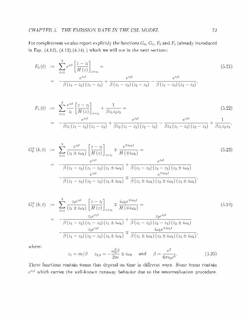
CHAPTER 5. THE EMISSION RATE IN THE CSL MODEL 72
For completeness we also report explicitly the functionsG0, G1, F0 and F1 (already introduced
in Eqs. (4.12), (4.13),(4.14) ) which we will use in the next sections:
F0 (t) :=3∑
l=1
ezlt[z − zlH (z)
]
z=zl
= (5.21)
= − ez1t
β (z1 − z2) (z1 − z3)+
ez2t
β (z1 − z2) (z2 − z3)− ez3t
β (z1 − z3) (z2 − z3),
F1 (t) :=3∑
l=1
ezlt
zl
[z − zlH (z)
]
z=zl
+1
βz1z2z3= (5.22)
= − ez1t
βz1 (z1 − z2) (z1 − z3)+
ez2t
βz2 (z1 − z2) (z2 − z3)− ez3t
βz3 (z1 − z3) (z2 − z3)+
1
βz1z2z3,
G±0 (k, t) :=
3∑
l=1
ezlt
(zl ± iωk)
[z − zlH (z)
]
z=zl
∓ e∓iωkt
H (∓iωk)= (5.23)
= − ez1t
β (z1 − z2) (z1 − z3) (z1 ± iωk)+
ez2t
β (z1 − z2) (z2 − z3) (z2 ± iωk)
− ez3t
β (z1 − z3) (z2 − z3) (z3 ± iωk)∓ e∓iωkt
β (z1 ± iωk) (z2 ± iωk) (z3 ± iωk),
G±1 (k, t) :=
3∑
l=1
zlezlt
(zl ± iωk)
[z − zlH (z)
]
z=zl
∓ iωke∓iωkt
H (∓iωk)= (5.24)
= − z1ez1t
β (z1 − z2) (z1 − z3) (z1 ± iωk)+
z2ez2t
β (z1 − z2) (z2 − z3) (z2 ± iωk)
− z3ez3t
β (z1 − z3) (z2 − z3) (z3 ± iωk)∓ iωke
∓iωkt
β (z1 ± iωk) (z2 ± iωk) (z3 ± iωk),
where:
z1 = m/β z2,3 = −ω20β
2m± iω0 and β =
e2
6πǫ0c3. (5.25)
These functions contain terms that depend on time in dierent ways. Some terms contain
ez1t which carries the well-known runaway behavior due to the renormalization procedure.

CHAPTER 5. THE EMISSION RATE IN THE CSL MODEL 73
We pragmatically dismiss them according to standard practice. There are constant and
oscillating terms which can potentially give important contributions to the emission rate.
More importantly, there are terms containing ez2t or ez3t which vanish for large times. These
are the crucial terms. Performing the computation to the lowest order in the electromagnetic
interaction is equivalent to setting β = 0. In such a case the decaying behavior of the
exponential functions containing z2 and z3 is lost and the associated terms give a nite
contribution to the emission rate. This contribution turns out to be, in the case of a free
particle, proportional to f(0). However, if one performs the computation to higher orders,
their contribution vanishes. This shows that in order to get the correct result for the radiation
emission it is important not to treat the electromagnetic interaction only at the rst order.
5.2.3 Analytic expression of C (t, t1)
In order to compute explicitly the commutators entering Eq. (5.17) it is worthwhile to nd
some general computational rule. Consider a family of operators A, B, C1, ...,Cn where every
pair commutes except [A,B] = ǫ. Let us dene
O := aA+ bB +n∑
j=1
cjCj (5.26)
where a, b and cj are constants or functions of the time (the discrete sum could also be an
integral over some continuous parameter as in the case of integrals containing a†kµ and akµ).
Then[
A, eαO2]
=∞∑
k=0
αk
k!
[A,O2k
], (5.27)
and one can show that:[A,O2k
]= 2bǫkO2k−1 (5.28)
so that the commutator becomes:
[
A, eαO2]
=∞∑
k=1
αk
k!2bǫkO2k−1 = 2bǫαO
∞∑
k=1
αk−1
(k − 1)!O2k−2 = [A,O] 2αOeαO
2
. (5.29)

CHAPTER 5. THE EMISSION RATE IN THE CSL MODEL 74
Using Eq. (5.29) we have:
C (t, t1) = [ak,µ (t) , g (x− q (t1))] =1
(√2πrC
)3
[
ak,µ (t) ,3∏
i=1
exp
[
−(xi − qi (t1))2
2r2C
]]
=
(5.30)
=1
(√2πrC
)3 exp
[
−(x1 − q1 (t1))2
2r2C
]
exp
[
−(x2 − q2 (t1))2
2r2C
][
ak,µ (t) , exp
[
−(x3 − q3 (t1))2
2r2C
]]
+1
(√2πrC
)3 exp
[
−(x1 − q1 (t1))2
2r2C
][
ak,µ (t) , exp
[
−(x2 − q2 (t1))2
2r2C
]]
exp
[
−(x3 − q3 (t1))2
2r2C
]
+1
(√2πrC
)3
[
ak,µ (t) , exp
[
−(x1 − q1 (t1))2
2r2C
]]
exp
[
−(x2 − q2 (t1))2
2r2C
]
exp
[
−(x3 − q3 (t1))2
2r2C
]
.
This means that we just have to focus on:
Ci (t, t1) :=
[
ak,µ (t) , exp
[
−(xi − qi (t1))2
2r2C
]]
. (5.31)
Using Eq. (5.29) it is easy to see that the term proportional to e2 in akµ (t) (see the second
line of Eq. (5.19)), when commuted with exp[
− (xi−qi(t1))2
2r2C
]
, gives a term of order e3. Since
at the end we want a result at the lowest order e2 we can neglect this contribution. Thus,
we can write Ci (t, t1) as the sum of two terms:
Ci (t, t1) = C1i (t, t1) + C2i (t, t1) . (5.32)
Using Eq. (5.29) we compute:
C1i (t, t1) := e−iωkt
[
akµ, exp
[
−(xi − qi (t1))2
2r2C
]]
= (5.33)
= − e~g (k)√~ǫ02ωkr2C
ǫikµe−iωktG−
1 (k, t1) (xi − qi (t1)) exp
[
−(xi − qi (t1))2
2r2C
]
,

CHAPTER 5. THE EMISSION RATE IN THE CSL MODEL 75
C2i (t, t1) :=ie√~ǫ0
g (k)√2ωk
ǫjkµ
[
G+1 (k, t) pj − κG+
0 (k, t) qj, exp
[
−(xi − qi (t1))2
2r2C
]]
=e~g (k)√~ǫ02ωkr2C
ǫikµG+
1 (k, t) [1− κF1 (t1)] + κG+0 (k, t)F0 (t1)
×
× (xi − qi (t1)) exp
[
−(xi − qi (t1))2
2r2C
]
. (5.34)
Hence, we get:
Ci (t, t1) =e~g (k)√~ǫ02ωkr2C
−e−iωktG−
1 (k, t1) +G+1 (k, t) [1− κF1 (t1)] + κG+
0 (k, t)F0 (t1)×
× ǫikµ (xi − qi (t1)) exp
[
−(xi − qi (t1))2
2r2C
]
. (5.35)
Inserting this in Eq. (5.30) one nds:
C (t, t1) =e~g (k)√~ǫ02ωkr2C
−e−iωktG−
1 (k, t1) +G+1 (k, t) [1− κF1 (t1)] + κG+
0 (k, t)F0 (t1)×
× ǫjkµ (xj − qj (t1)) g (x− q (t1)) , (5.36)
where we used the fact that [f (qj (t1)) , g (qk (t1))] = U † (t1) [f (qj) , g (qk)]U (t1) = 0.
The commutator [a†k,µ (t) , g (x− q (t1))] is related to the one here above. In fact, since:
g† (x− q (t1)) = g (x− q (t1)) and (ak,µ (t))† = a†k,µ (t) (5.37)
it follows that:
[a†k,µ (t) , g (x− q (t1))] = − [ak,µ (t) , g (x− q (t1))]† = −C† (t, t1) . (5.38)

CHAPTER 5. THE EMISSION RATE IN THE CSL MODEL 76
5.2.4 Analytic expression of D (t, t1, t2)
We can use the previous result to compute:
D (t, t1, t2) = [[ak,µ (t) , g (x− q (t1))] , g (x− q (t2))] =
=e~g (k)√~ǫ02ωkr2C
−e−iωktG−
1 (k, t1) +G+1 (k, t) [1− κF1 (t1)] + κG+
0 (k, t)F0 (t1)×
× ǫjkµ [(xj − qj (t1)) g (x− q (t1)) , g (x− q (t2))] . (5.39)
Because of the complicated time evolution of q (t) given by Eq. (5.20), the commutator in
Eq. (5.39) is hard to evaluate. However, by looking at Eq. (5.15) we can see that we only
need to compute the expectation value of the commutator D (t, t1, t2) on the initial state and
integrate over x, i.e., we only need to compute:
I :=
∫
dx 〈ψ (0) |(xj − qj (t1)) g (x− q (t1)) g (x− q (t2))|ψ (0)〉 . (5.40)
The other term of the commutator in Eq. (5.39) involves an integral over x that is equal to
I∗. Let us rewrite I in the following way:
I =
∫
dx 〈ψ (0) |(xj − qj (t1)) g (x− q (t1)) g (x− q (t2))|ψ (0)〉 =
=
∫
dx〈ψ (0) |U † (t1) (xj − qj) g (x− q)U (t1)U† (t2) g (x− q)U (t2) |ψ (0)〉 =
=
∫
dq
∫
dq′∫
dx (xj − qj) g (x− q) g (x− q′)×
× 〈ψ (0) |U † (t1) |q〉〈q|U (t1)U† (t2) |q′〉〈q′|U (t2) |ψ (0)〉. (5.41)
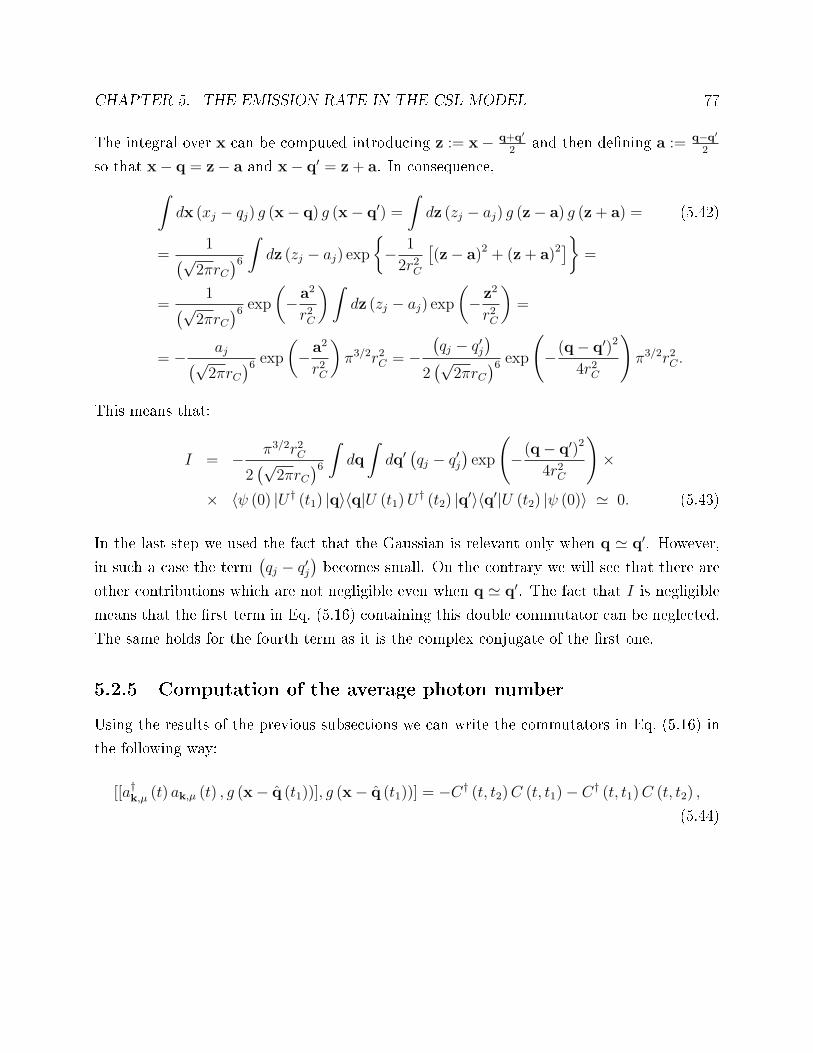
CHAPTER 5. THE EMISSION RATE IN THE CSL MODEL 77
The integral over x can be computed introducing z := x− q+q′
2and then dening a := q−q′
2
so that x− q = z− a and x− q′ = z+ a. In consequence,
∫
dx (xj − qj) g (x− q) g (x− q′) =
∫
dz (zj − aj) g (z− a) g (z+ a) = (5.42)
=1
(√2πrC
)6
∫
dz (zj − aj) exp
− 1
2r2C
[(z− a)2 + (z+ a)2
]
=
=1
(√2πrC
)6 exp
(
−a2
r2C
)∫
dz (zj − aj) exp
(
− z2
r2C
)
=
= − aj(√
2πrC)6 exp
(
−a2
r2C
)
π3/2r2C = −(qj − q′j
)
2(√
2πrC)6 exp
(
−(q− q′)2
4r2C
)
π3/2r2C .
This means that:
I = − π3/2r2C
2(√
2πrC)6
∫
dq
∫
dq′ (qj − q′j)exp
(
−(q− q′)2
4r2C
)
×
× 〈ψ (0) |U † (t1) |q〉〈q|U (t1)U† (t2) |q′〉〈q′|U (t2) |ψ (0)〉 ≃ 0. (5.43)
In the last step we used the fact that the Gaussian is relevant only when q ≃ q′. However,
in such a case the term(qj − q′j
)becomes small. On the contrary we will see that there are
other contributions which are not negligible even when q ≃ q′. The fact that I is negligible
means that the rst term in Eq. (5.16) containing this double commutator can be neglected.
The same holds for the fourth term as it is the complex conjugate of the rst one.
5.2.5 Computation of the average photon number
Using the results of the previous subsections we can write the commutators in Eq. (5.16) in
the following way:
[[a†k,µ (t) ak,µ (t) , g (x− q (t1))], g (x− q (t1))] = −C† (t, t2)C (t, t1)− C† (t, t1)C (t, t2) ,
(5.44)

CHAPTER 5. THE EMISSION RATE IN THE CSL MODEL 78
with C (t, t′) dened in Eq. (5.36). Accordingly, Eq. (5.15) becomes:
〈a†k,µak,µ (t)〉noise = γ
(m
m0
)2 ∫ t
0
dt1
∫ t1
0
dt2f (t1 − t2)× (5.45)
×∫
dx 〈ψ (0) |C† (t, t2)C (t, t1) + C† (t, t1)C (t, t2) |ψ (0)〉
= γ
(m
m0
)2 ∫ t
0
dt1
∫ t
0
dt2f (t1 − t2)
∫
dx 〈ψ (0) |C† (t, t2)C (t, t1) |ψ (0)〉,
where in the second line we used the fact that we consider a noise eld with symmetric
correlation function f (t1 − t2) = f (|t1 − t2|). By substituting Eq. (5.36) in Eq. (5.45) one
gets:
〈a†k,µak,µ (t)〉noise = γ
(m
m0
)2e2~ |g (k)|2ǫ02ωkr4C
ǫi∗kµǫjkµ
∫ t
0
dt1
∫ t
0
dt2f (t1 − t2)× (5.46)
×−eiωktG−∗
1 (k, t2) +G+∗1 (k, t) [1− κF ∗
1 (t2)] + κG+∗0 (k, t)F ∗
0 (t2)×
×−e−iωktG−
1 (k, t1) +G+1 (k, t) [1− κF1 (t1)] + κG+
0 (k, t)F0 (t1)Iij ,
where:
Iij :=
∫
dx 〈ψ (0) |g (x− q (t1)) (xi − qi (t1)) (xj − qj (t2)) g (x− q (t2))|ψ (0)〉 . (5.47)
As before we can rewrite Iij by inserting the identity∫dq |q〉 〈q| = 1:
Iij =
∫
dq
∫
dq′∫
dx g (x− q) (xi − qi)(xj − q′j
)g (x− q′)×
× 〈ψ (0) |U † (t1) |q〉〈q|U (t1)U† (t2) |q′〉〈q′|U (t2) |ψ (0)〉. (5.48)

CHAPTER 5. THE EMISSION RATE IN THE CSL MODEL 79
We compute the integral over x by performing the change of variable: z := x − q+q′
2and
introducing a := q−q′
2; we get:
Xij :=
∫
dxg (x− q) (xi − qi)(xj − q′j
)g (x− q′) =
∫
dzg (z− a) (zi − ai) (zj + aj) g (z+ a) =
=1
(√2πrC
)6
∫
dz exp
− 1
2r2C
[(z− a)2 + (z+ a)2
]
(zi − ai) (zj + aj) =
=1
(√2πrC
)6 exp
(
−a2
r2C
)∫
dz exp
(
− z2
r2C
)
(zi − ai) (zj + aj) . (5.49)
Let us focus on the quantity:
Zij :=
∫
dz exp
(
− z2
r2C
)
(zi − ai) (zj + aj) . (5.50)
If i 6= j the only non zero term is:
Zij = −aiaj∫
dz exp
(
− z2
r2C
)
= −aiajr3Cπ3/2. (5.51)
On the contrary, if i = j we have:
Zii =
∫
dz exp
(
− z2
r2C
)(z2i − a2i
)= π3/2 r
5C
2− a2i r
3Cπ
3/2. (5.52)
Therefore,
Xij =1
(√2πrC
)6 exp
(
−a2
r2C
)[
δijπ3/2 r
5C
2− aiajr
3Cπ
3/2
]
=1
8π3/2r3Cexp
(
−(q− q′)2
4r2C
)[
δijr2C2
−(qi − q′i
2
)(qj − q′j
2
)]
. (5.53)
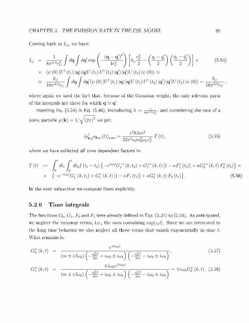
CHAPTER 5. THE EMISSION RATE IN THE CSL MODEL 80
Coming back to Iij, we have:
Iij =1
8π3/2r3C
∫
dq
∫
dq′ exp
(
−(q− q′)2
4r2C
)[
δijr2C2
−(qi − q′i
2
)(qj − q′j
2
)]
× (5.54)
× 〈ψ (0) |U † (t1) |q〉〈q|U (t1)U† (t2) |q′〉〈q′|U (t2) |ψ (0)〉 ≃
≃ δij16π3/2rC
∫
dq
∫
dq′〈ψ (0) |U † (t1) |q〉〈q|U (t1)U† (t2) |q′〉〈q′|U (t2) |ψ (0)〉 = δij
16π3/2rC,
where again we used the fact that, because of the Gaussian weight, the only relevant parts
of the integrals are those for which q ≃ q′.
Inserting Eq. (5.54) in Eq. (5.46), introducing λ := γ8π3/2r3C
, and considering the case of a
point particle g (k) = 1/√
(2π)3 we get:
〈a†k,µak,µ (t)〉noise =e2~λm2
32π3ǫ0m20ωkr2C
T (t) , (5.55)
where we have collected all time dependent factors in:
T (t) :=
∫ t
0
dt1
∫ t
0
dt2f (t1 − t2)−eiωktG−∗
1 (k, t2) +G+∗1 (k, t) [1− κF ∗
1 (t2)] + κG+∗0 (k, t)F ∗
0 (t2)×
×−e−iωktG−
1 (k, t1) +G+1 (k, t) [1− κF1 (t1)] + κG+
0 (k, t)F0 (t1). (5.56)
In the next subsection we compute them explicitly.
5.2.6 Time integrals
The functions G0, G1, F0 and F1 were already dened in Eqs. (5.21) to (5.24). As anticipated,
we neglect the runaway terms, i.e., the ones containing exp[z1t]. Since we are interested in
the long time behavior we also neglect all those terms that vanish exponentially in time t.
What remains is:
G±0 (k, t) =
e∓iωkt
(m± iβωk)(
−ω20β
2m+ iω0 ± iωk
)(
−ω20β
2m− iω0 ± iωk
) , (5.57)
G±1 (k, t) =
∓iωke∓iωkt
(m± iβωk)(
−ω20β
2m+ iω0 ± iωk
)(
−ω20β
2m− iω0 ± iωk
) = ∓iωkG±0 (k, t) . (5.58)

CHAPTER 5. THE EMISSION RATE IN THE CSL MODEL 81
One can safely use this approximation for terms that depend only on t while for terms under
time integrals one has to be more careful and use the full expression which was given in
subsection 5.2.2. This simplies the expression for T (t) in the following way:
T (t) :=
∫ t
0
dt1
∫ t
0
dt2f (t1 − t2)−eiωktG−∗
1 (k, t2) +G+∗0 (k, t) [iωk − iωkκF
∗1 (t2) + κF ∗
0 (t2)]×
×−e−iωktG−
1 (k, t1) +G+0 (k, t) [−iωk + iωkκF1 (t1) + κF0 (t1)]
= TA (t) + TB (t) + TC (t) + TD (t) , (5.59)
where these four terms in the last line are given by:
TA (t) :=
∫ t
0
dt1
∫ t
0
dt2f (t1 − t2)−eiωktG−∗
1 (k, t2)
−e−iωktG−1 (k, t1)
, (5.60)
TB (t) :=
∫ t
0
dt1
∫ t
0
dt2f (t1 − t2)−eiωktG−∗
1 (k, t2)×
×G+
0 (k, t) [−iωk + iωkκF1 (t1) + κF0 (t1)],(5.61)
TC (t) :=
∫ t
0
dt1
∫ t
0
dt2f (t1 − t2)−e−iωktG−
1 (k, t1)×
×G+∗
0 (k, t) [iωk − iωkκF∗1 (t2) + κF ∗
0 (t2)], (5.62)
TD (t) :=
∫ t
0
dt1
∫ t
0
dt2f (t1 − t2)G+∗
0 (k, t) [iωk − iωkκF∗1 (t2) + κF ∗
0 (t2)]×
×G+
0 (k, t) [−iωk + iωkκF1 (t1) + κF0 (t1)].(5.63)
In the following we will elaborate each of these terms.
1. Expression for TA (t). We start by plugging in the explicit expression of G−1 (k, t) given by
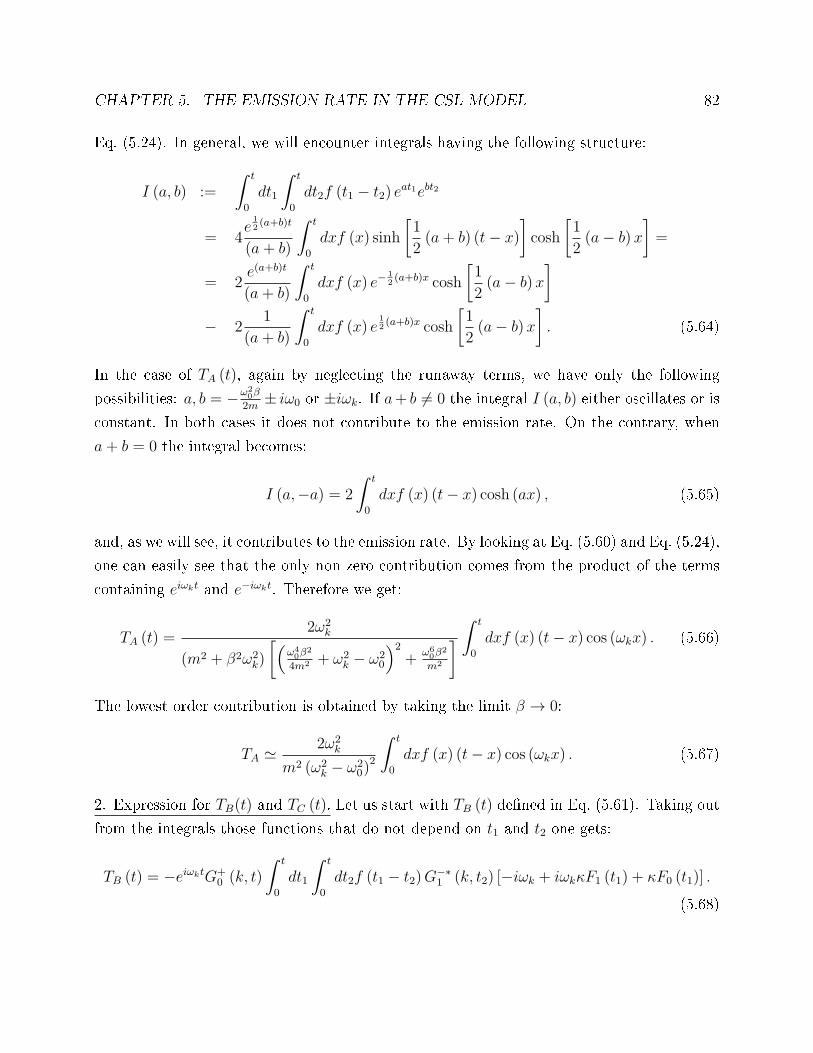
CHAPTER 5. THE EMISSION RATE IN THE CSL MODEL 82
Eq. (5.24). In general, we will encounter integrals having the following structure:
I (a, b) :=
∫ t
0
dt1
∫ t
0
dt2f (t1 − t2) eat1ebt2
= 4e
12(a+b)t
(a+ b)
∫ t
0
dxf (x) sinh
[1
2(a+ b) (t− x)
]
cosh
[1
2(a− b) x
]
=
= 2e(a+b)t
(a+ b)
∫ t
0
dxf (x) e−12(a+b)x cosh
[1
2(a− b) x
]
− 21
(a+ b)
∫ t
0
dxf (x) e12(a+b)x cosh
[1
2(a− b) x
]
. (5.64)
In the case of TA (t), again by neglecting the runaway terms, we have only the following
possibilities: a, b = −ω20β
2m± iω0 or ±iωk. If a+ b 6= 0 the integral I (a, b) either oscillates or is
constant. In both cases it does not contribute to the emission rate. On the contrary, when
a+ b = 0 the integral becomes:
I (a,−a) = 2
∫ t
0
dxf (x) (t− x) cosh (ax) , (5.65)
and, as we will see, it contributes to the emission rate. By looking at Eq. (5.60) and Eq. (5.24),
one can easily see that the only non zero contribution comes from the product of the terms
containing eiωkt and e−iωkt. Therefore we get:
TA (t) =2ω2
k
(m2 + β2ω2k)
[(ω40β
2
4m2 + ω2k − ω2
0
)2
+ω60β
2
m2
]
∫ t
0
dxf (x) (t− x) cos (ωkx) . (5.66)
The lowest order contribution is obtained by taking the limit β → 0:
TA ≃ 2ω2k
m2 (ω2k − ω2
0)2
∫ t
0
dxf (x) (t− x) cos (ωkx) . (5.67)
2. Expression for TB(t) and TC (t). Let us start with TB (t) dened in Eq. (5.61). Taking out
from the integrals those functions that do not depend on t1 and t2 one gets:
TB (t) = −eiωktG+0 (k, t)
∫ t
0
dt1
∫ t
0
dt2f (t1 − t2)G−∗1 (k, t2) [−iωk + iωkκF1 (t1) + κF0 (t1)] .
(5.68)

CHAPTER 5. THE EMISSION RATE IN THE CSL MODEL 83
The integrals contain the functions F0 (t), F1 (t) and G−1 (k, t) dened in Eq. (5.21), Eq. (5.22)
and Eq. (5.24), respectively. As before we will neglect the runaway terms proportional to
ez1t. We are left only with integrals having the same structure as that of I (a, b) dened in
Eq. (5.64). Every term which involves ez2t or ez3t does not contribute to the asymptotic rate.
This means that when we substitute the functions F0 (t), F1 (t) and G−1 (k, t) in Eq. (5.68)
we can set:
F0 (t1) = 0 , F1 (t1) =1
βz1z2z3and G−∗
1 (k, t2) =
(iωke
iωkt2
β (z1 − iωk) (z2 − iωk) (z3 − iωk)
)∗.
(5.69)
So we have:
TB (t) = −eiωktG+0 (k, t)
[κ
βz1z2z3− 1
]ω2k
β (z1 + iωk) (z2 + iωk) (z3 + iωk)×
×∫ t
0
dt1
∫ t
0
dt2f (t1 − t2) e−iωkt2 . (5.70)
This term gives no contribution at the lowest order. In fact, if we replace the values of z1, z2
and z3 in the above expression the contribution of the term in the square brackets becomes:
[κ
βz1z2z3− 1
]
=mω2
0
m(
ω40β
2
4m2 + ω20
) − 1 = −ω40β
2
4m2
ω40β
2
4m2 + ω20
. (5.71)
Hence, again by taking the limit β → 0 this term vanishes (the function G+0 (k, t) and the
fraction in front of the integrals give a nite contribution in this limit). Since TC (t) = T ∗B (t),
also TC = 0 at the lowest order.
3. Expression for TD (t). Let us rewrite Eq. (5.63) by carrying out of the double integral the
functions that do not depend by t1 and t2:
TD (t) =∣∣G+
0 (k, t)∣∣2∫ t
0
dt1
∫ t
0
dt2f (t1 − t2) [iωk − iωkκF∗1 (t2) + κF ∗
0 (t2)]×
× [−iωk + iωkκF1 (t1) + κF0 (t1)] . (5.72)
The functions F0 (t) and F1 (t) are dened in Eq. (5.21) and Eq. (5.22). Once again we have
only integrals with the same structure as that of I (a, b) in Eq. (5.64), and therefore, the only
terms that survive are those for which F0 (t) = 0 and F1 (t) = 1βz1z2z3
. In such a case the

CHAPTER 5. THE EMISSION RATE IN THE CSL MODEL 84
above expression becomes:
TD (t) =∣∣G+
0 (k, t)∣∣2ω2k
∣∣∣∣1− κ
βz1z2z3
∣∣∣∣
2 ∫ t
0
dt1
∫ t
0
dt2f (t1 − t2) . (5.73)
This term vanishes in the limit β → 0. In fact the term inside the square modulus is
proportional to β2 (see Eq. (5.71)) while all the others terms remain nite in such a limit.
5.2.7 Final Result
In summary, we have obtained that at the lowest order T (t) = TA (t) with TA (t) given by
Eq. (5.67). Thus, Eq. (5.55) simplies as follows:
〈a†k,µak,µ (t)〉noise =e2~λ
32π3ǫ0m20r
2C
2ωk
(ω2k − ω2
0)2
∫ t
0
dxf (x) (t− x) cos (ωkx) . (5.74)
The emission rate is obtained by taking the time derivative of the above expression. Moreover,
since 〈a†k,µak,µ (t)〉noise does not depend on the direction and the polarization of the photon
we can sum over these degrees of freedom multiplying by a factor 8πk2. Using
d
dt
∫ t
0
dxf (x) (t− x) cos (ωkx) =1
2f (ωk) , (5.75)
where the function f (ωk) is the one dened in Eq. (3.54) we get
dΓ
dk=
e2~λc
4π2ǫ0m20r
2C
k3
(ω2k − ω2
0)2 f (ωk) . (5.76)
In the free particle limit ω0 → 0 Eq. (5.76) becomes:
dΓ
dk=
λ~e2
4π2ǫ0c3m20r
2ckf (ωk) , (5.77)
which is the desired result.

Chapter 6
The emission rate for a generic system
Let us summarize all the results of the previous chapters. We have seen that when perturba-
tion theory is limited to the lowest meaningful order, unphysical terms appear in the formula
for the emission rate. We found two ways to avoid this problem. The rst one, discussed in
chapter 3, includes conning the noise eld and performing the computation by taking wave
packets as nal states. We were not satised with this procedure, mainly for two reasons:
it is not clear if it works for systems dierent from the free particle; it requires to modify
the model by conning the noise in space. The second way to avoid the presence of the
unphysical term is discussed in chapters 4 and 5. We showed that, if the electromagnetic
interaction is treated exactly, for a harmonic oscillator, no matter how weak the potential,
the formula for the emission rate does not contain any unphysical term. However, this anal-
ysis lacks of generality: we need to solve the Heisenberg equations, while treating exactly the
electromagnetic interaction, and this can be done only for simple systems. Nevertheless, the
fact that the presence of the unphysical term can be avoided when higher order contributions
are considered, put us in the right direction. Indeed, one can try to use perturbation theory,
considering the higher order contributions. A rst attempt could be to consider all the dia-
grams at the next relevant order. However, the number of diagrams that should be taken into
account is huge (of order of seventy). A clever selection over which higher order contributions
should be considered is suggested by the fact that the unphysical term is exactly what in
standard perturbation theory is called non resonant term. There are dierent possibilities
to show that this non resonant terms are negligible and we discuss some of them in the rst
section. We show that the most general and elegant way for avoiding the presence of the non
resonant terms is to take into account the decay of the propagator. Indeed, because of the
85

CHAPTER 6. THE EMISSION RATE FOR A GENERIC SYSTEM 86
electromagnetic interaction, the propagator is not stable and can decay1 [42, 43]. In the rest
of the chapter we focus on taking this eect into account and we repeat and generalized the
perturbative computations done in chapter 3. As result, we nd the formula for the emission
rate from a generic system using a generic collapse model.
6.1 The non resonant terms and their connection with
the unphysical term
In this section we show that the unphysical term encountered in the previous chapters is due
to the presence of non resonant terms in the transition amplitude. We also discuss about the
possible methods to avoid the presence of this term.
In order to focus our analysis, we study the contribution due to the diagram:
i f
k, µ
We showed in chapter 3 that the transition amplitude for this diagram is given by Eq. (3.17):
Tfi = − 1
~2
∑
n
∫ tf
ti
dt1
∫ t1
ti
dt2 ei~(Ef+~ωk−En)t1e
i~(En−Ei)t2ξt2Rk
fnNni, (6.1)
where we recall that the sum is over the eigenstates |n〉 of the unperturbed Hamiltonian H0
and the matrix elements are dened as Rkfn := 〈f |Rk|n〉 and Nni := 〈n|N |i〉 with R and N
dened in Eq. (3.16). For the following analysis it is convenient to expand the noise ξt using
the Fourier transform:
ξt =1
2π
∫ +∞
−∞dν e−iνtξν , (6.2)
so that
Tfi = − 1
2π~2
∑
n
RkfnNni
∫ +∞
−∞dν ξνT. (6.3)
1In principle there is also a similar eect due to the noise, but here we are not interested in computing it.

CHAPTER 6. THE EMISSION RATE FOR A GENERIC SYSTEM 87
In the above equation we introduced:
T :=
∫ tf
ti
dt1
∫ t1
ti
dt2 ei(∆fn+ωk)t1ei(∆ni−ν)t2 , (6.4)
with∆fn :=Ef−En
~. The emission rate is proportional to the time derivative of the probability
transition Pfi = E |Tfi|2 (see Eq. (3.37)). Using the relation:
E [ξ∗ν ξω] = 2πδ (ν − ω) f (ν) , (6.5)
with f (ν) dened in Eq. (3.54), we can write Pfi as:
Pfi =1
4π2~4E
∣∣∣∣∣
∑
n
RkfnNni
∫ +∞
−∞dν ξνT
∣∣∣∣∣
2
=1
2π~4
∫ +∞
−∞dνf (ν)
∣∣∣∣∣
∑
n
RkfnNniT
∣∣∣∣∣
2
. (6.6)
Let us focus on T, which contains the time dependence of Pfi. Taking ti = 0 and tf = t,
we get:
T =−1
i(∆fn + ωk)
[ei(∆fi+ωk−ν)t − 1
i(∆fi + ωk − ν)− ei(∆fn+ωk)t
ei(∆ni−ν)t − 1
i(∆ni − ν)
]
(6.7)
where, for better enlightening the connection with the unphysical term found in the previous
chapters, we computed T changing the order of the integrals in t1 and t2. When taking the
square modulus, in the large time limit the crossed terms oscillates and do not contribute
to the emission rate. On the contrary the square modulus of each term in Eq. (6.7) has the
form: ∣∣∣∣
eixt − 1
ix
∣∣∣∣
2
=sin2
(xt2
)
(x2
)2 −→t→∞
2πtδ (x) , (6.8)
where we used the Dirac delta representation δ (x) = π−1 limt→∞1t
(sin(xt)
x
)2
. The rst term
in Eq. (6.7), called resonant term, gives relevant contributions when the energy is conserved,
i.e. when ν = ∆fi + ωk. On the contrary the second term in Eq. (6.7), called non resonant
term, becomes relevant when ν = ∆ni. It is because of this term that, in the case of the free
particle, we get the unphysical contribution to the rate proportional to f(0). Notice that the
presence of this non resonant terms is not related to the fact that our interaction is a noise:
they are present also with a generic potential [24]. In the next subsection we briey discuss
about some methods commonly used to show that the non resonant terms are negligible. We

CHAPTER 6. THE EMISSION RATE FOR A GENERIC SYSTEM 88
will point out why this methods does not work in our case. Then, we will introduce the decay
of the propagator and we will show why, taking this eect into account, the non resonant
terms can be neglected.
6.1.1 Adiabatic switch on of the potential and other approaches
A possible argument to show why the non resonant terms should be neglected is based on
introducing a slowly switching on the potential [24]. Mathematically speaking this is done
taking as initial time ti = −∞ and changing the potential using V → V eǫt, with ǫ real
positive parameter which will be sent to zero at the end of the calculation. Since we have
two dierent potentials, the electromagnetic interaction and the noise eld, this correspond
on taking
Rk → Rkeǫt and N → N eηt. (6.9)
Taking ti = −∞ and tf = t, Eq. (6.4) becomes:
T =
∫ t
−∞dt1
∫ t1
−∞dt2 e
[i(∆fn+ωk)+ǫ]t1e[i(∆ni−ν)+η]t2 = (6.10)
=e[i(∆fi+ωk−ν)+(ǫ+η)]t
[i(∆fi + ωk − ν) + (ǫ+ η)][i(∆ni − ν) + η]. (6.11)
Then Eq. (6.6) becomes:
Pfi =1
2π~4
∫ +∞
−∞dνf (ν)
∣∣∣∣∣
∑
n
RkfnNni
[i(∆ni − ν) + η]
∣∣∣∣∣
2e2(ǫ+η)t
[(∆fi + ωk − ν)2 + (ǫ+ η)2]. (6.12)
Using the following representation of the Dirac delta function:
limǫ→0
ǫ
x2 + ǫ2= πδ (x) , (6.13)
we obtain:
d
dtPfi =
1
2π~4
∫ +∞
−∞dνf (ν)
∣∣∣∣∣limη→0
∑
n
RkfnNni
[i(∆ni − ν) + η]
∣∣∣∣∣
2
2πδ(∆fi + ωk − ν). (6.14)

CHAPTER 6. THE EMISSION RATE FOR A GENERIC SYSTEM 89
We see that, apparently, everything seems to be solved, since there is only the delta function
typical of the resonant term. However, Eq. (6.14) this is not true in general, in particular
when the matrix elements involve delta functions. As example, if we consider a free particle,
then Rkfn ∼ δn(f+k) (see Eq. (3.20)), and:
Pfi ∝∫ +∞
−∞dνf (ν)
∣∣N(f+k)i
∣∣2 e2(ǫ+η)t
[(∆fi + ωk − ν)2 + (ǫ+ η)2][(∆(f+k)i − ν)2 + η2]. (6.15)
In this case there are relevant contributions not only for ν = ∆fi + ωk but also for ν =
∆(f+k)i. This second contribution is the one who gives the unphysical factor f(0). Let us
remark that the same argument is true also for a harmonic oscillator: in such case, in dipole
approximation, the matrix element Rkfn is proportional to the sum of two delta functions.
Therefore, in general, the adiabatic switching on of the potential does not avoid the presence
of the non resonant terms and hence of the unphysical term.
To conclude, let us also mention a dierent analysis of the role of the non resonant terms
in perturbations theory given in [44], where Eq. (6.14) is obtained without introducing any
articial switch on of the potential. In particular it is showed that the role of the non-
resonant term is to avoid divergences when ∆fn + ωk = 0. However, in the analysis done
in [44] a crucial role is played by the fact that the eigenstates are a continuum set and that
the matrix elements are smooth functions. Therefore, in the case they are delta functions,
their argument is not valid. In [45] a similar argument is reported. However, once again, the
result is not true for generic matrix elements.
6.1.2 Decay of propagator
In order to nd a more general way to show why the non resonant terms must be neglected,
we start from the analysis done in chapter 4 and chapter 5. We showed that the higher
order contributions of the electromagnetic interaction play a fundamental role in avoiding
the presence of the unphysical term. This suggest that we have to nd a way to introduce
their eect in the perturbative calculations. In particular we showed that the role of the
higher orders contributions of the electromagnetic interaction is to exponentially damp the
unphysical term. This exponential decay suggest that a crucial role may be played by the fact
that the eigenstates of the unperturbed Hamiltonian H0 decay because of the electromagnetic
interaction. This eect is related to the self interaction of the system by means of the

CHAPTER 6. THE EMISSION RATE FOR A GENERIC SYSTEM 90
electromagnetic interaction [42, 43]. In particular, it can be shown that the higher order
contributions of the electromagnetic interaction give a complex shift in the energy of the
eigenstates ∆E = ∆Er + i∆Ei [24, 42]. The real part ∆Er is a shift of the energy levels (the
Lamb shift) while the imaginary part ∆Ei described the decay rate (or natural linewidth)
of the state. As a check that this decay is related to the exponential damping factors found
in chapters 4 and 5, in appendix A we computed ∆Ei for a harmonic oscillator and the
decay turns out to be proportional to the decay rate found in chapter 4 and 5 responsible for
suppressing the terms proportional to f(0). This strongly suggest that the decay of the state
due to the electromagnetic self interaction play a fundamental role in avoiding the presence
of the unphysical terms2.
Therefore, we compute again T in Eq. (6.4) taking into account the possibility that
the propagator decay. This is equivalent of the replacement in the integral ei~En(t1−t2) →
ei~(En+i~Γn)(t1−t2). In such a case:
T =
∫ t
0
dt1
∫ t1
0
dt2 e[i(∆fn+ωk)]t1e[i(∆ni−ν)]t2e−Γn(t1−t2) = (6.16)
=−1
[i(∆fn + ωk)− Γn]
ei(∆fi+ωk−ν)t − 1
i(∆fi + ωk − ν)− e[i(∆fn+ωk)−Γn]t
e[i(∆ni−ν)+Γn]t − 1
[i(∆ni − ν) + Γn]
.
The rst term is the same as in Eq. (6.7). Therefore we still have contribution in the
large time limit when ν = ∆fi + ωk. However, because of the damping e−Γnt, the second
term does not contribute anymore to the emission rate for large times. Therefore we see that,
taking into account the decay of propagator, we avoid the presence of the non resonant term
and therefore the unphysical factorf(0). The great advantage of this method is that is quite
general and does not depend by the form of the matrix elements R and N .
In the rest of this chapter we apply this method to all the Feynman diagram relevant for
the process of photon emission that we are considering. We will prove that, when the decay
of propagator is taken into account, the unphysical term is not present anymore.
2Moreover, this is also discussed in [43].
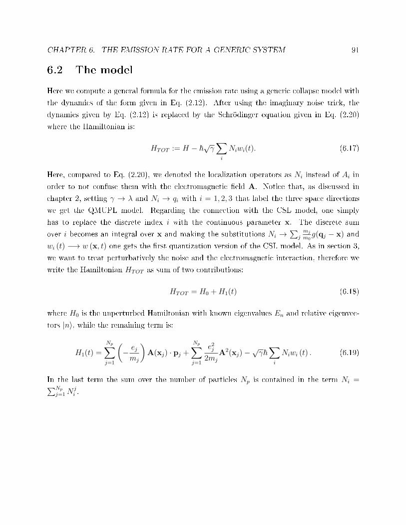
CHAPTER 6. THE EMISSION RATE FOR A GENERIC SYSTEM 91
6.2 The model
Here we compute a general formula for the emission rate using a generic collapse model with
the dynamics of the form given in Eq. (2.12). After using the imaginary noise trick, the
dynamics given by Eq. (2.12) is replaced by the Schrödinger equation given in Eq. (2.20)
where the Hamiltonian is:
HTOT := H − ~√γ∑
i
Niwi(t). (6.17)
Here, compared to Eq. (2.20), we denoted the localization operators as Ni instead of Ai in
order to not confuse them with the electromagnetic eld A. Notice that, as discussed in
chapter 2, setting γ → λ and Ni → qi with i = 1, 2, 3 that label the three space directions
we get the QMUPL model. Regarding the connection with the CSL model, one simply
has to replace the discrete index i with the continuous parameter x. The discrete sum
over i becomes an integral over x and making the substitutions Ni →∑
jmj
m0g(qj − x) and
wi (t) −→ w (x, t) one gets the rst quantization version of the CSL model. As in section 3,
we want to treat perturbatively the noise and the electromagnetic interaction, therefore we
write the Hamiltonian HTOT as sum of two contributions:
HTOT = H0 +H1(t) (6.18)
where H0 is the unperturbed Hamiltonian with known eigenvalues En and relative eigenvec-
tors |n〉, while the remaining term is:
H1(t) =
Np∑
j=1
(
− ejmj
)
A(xj) · pj +
Np∑
j=1
e2j2mj
A2(xj)−√γ~∑
i
Niwi (t) . (6.19)
In the last term the sum over the number of particles Np is contained in the term Ni =∑Np
j=1Nji .
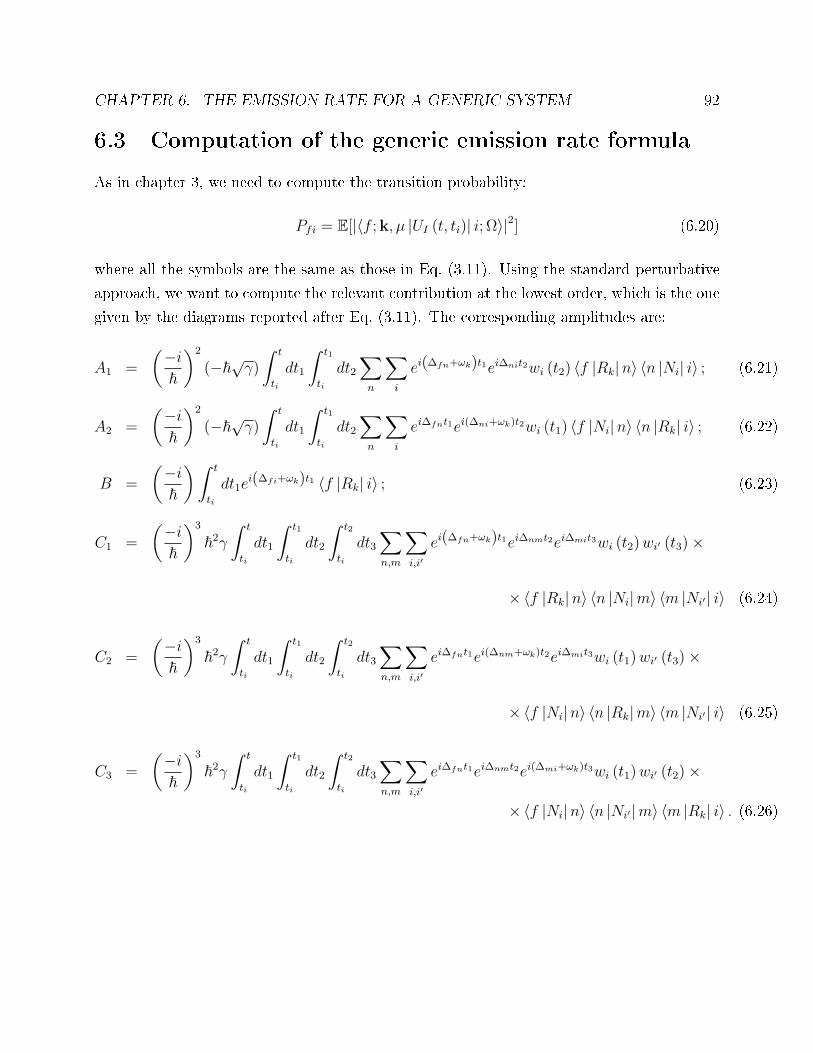
CHAPTER 6. THE EMISSION RATE FOR A GENERIC SYSTEM 92
6.3 Computation of the generic emission rate formula
As in chapter 3, we need to compute the transition probability:
Pfi = E[|〈f ;k, µ |UI (t, ti)| i; Ω〉|2] (6.20)
where all the symbols are the same as those in Eq. (3.11). Using the standard perturbative
approach, we want to compute the relevant contribution at the lowest order, which is the one
given by the diagrams reported after Eq. (3.11). The corresponding amplitudes are:
A1 =
(−i~
)2
(−~√γ)
∫ t
ti
dt1
∫ t1
ti
dt2∑
n
∑
i
ei(∆fn+ωk)t1ei∆nit2wi (t2) 〈f |Rk|n〉 〈n |Ni| i〉 ; (6.21)
A2 =
(−i~
)2
(−~√γ)
∫ t
ti
dt1
∫ t1
ti
dt2∑
n
∑
i
ei∆fnt1ei(∆ni+ωk)t2wi (t1) 〈f |Ni|n〉 〈n |Rk| i〉 ; (6.22)
B =
(−i~
)∫ t
ti
dt1ei(∆fi+ωk)t1 〈f |Rk| i〉 ; (6.23)
C1 =
(−i~
)3
~2γ
∫ t
ti
dt1
∫ t1
ti
dt2
∫ t2
ti
dt3∑
n,m
∑
i,i′
ei(∆fn+ωk)t1ei∆nmt2ei∆mit3wi (t2)wi′ (t3)×
×〈f |Rk|n〉 〈n |Ni|m〉 〈m |Ni′ | i〉 (6.24)
C2 =
(−i~
)3
~2γ
∫ t
ti
dt1
∫ t1
ti
dt2
∫ t2
ti
dt3∑
n,m
∑
i,i′
ei∆fnt1ei(∆nm+ωk)t2ei∆mit3wi (t1)wi′ (t3)×
×〈f |Ni|n〉 〈n |Rk|m〉 〈m |Ni′ | i〉 (6.25)
C3 =
(−i~
)3
~2γ
∫ t
ti
dt1
∫ t1
ti
dt2
∫ t2
ti
dt3∑
n,m
∑
i,i′
ei∆fnt1ei∆nmt2ei(∆mi+ωk)t3wi (t1)wi′ (t2)×
×〈f |Ni|n〉 〈n |Ni′ |m〉 〈m |Rk| i〉 . (6.26)

CHAPTER 6. THE EMISSION RATE FOR A GENERIC SYSTEM 93
Here, similarly to what we did in chapter 2, we have introduced the radiation matrix element:
Rk := αk
Np∑
j=1
(
− ejmj
)
e−ik·xjǫk,µ · pj, with αk ≡
√
~
2ε0ωk (2π)3 . (6.27)
The formula for the transition probability becomes:
Pfi = E|A1 + A2|2 + 2Re [(B∗C1 +B∗C2 +B∗C3)]
(6.28)
The emission rate is again given by Eq. (3.37), therefore it can be written as function of
the transition amplitudes dened above:
dΓ
dk=∑
µ
∫
dΩkd
dt
∑
f
E|A1 + A2|2 + 2Re [(B∗C1 +B∗C2 +B∗C3)]
(6.29)
In the next sections we will focus on computing the terms introduced in Eqs. (6.21)-(6.26)
taking into account the decay of the propagator.
6.4 Contribution to the emission rate from the ampli-
tudes A1 and A2
The contribution due to the amplitudes A1 and A2 can be written as the sum of three terms
because of the relation:
∑
µ
∫
dΩkd
dt
∑
f
E |A1 + A2|2 =∑
µ
∫
dΩk
(1
~4
)
(−~√γ)2 [R11 + 2Re (R12) +R22]

CHAPTER 6. THE EMISSION RATE FOR A GENERIC SYSTEM 94
where we have introduced:
R11 =d
dt
∑
f
E
∣∣∣∣∣
∑
n
∑
i
∫ t
ti
dt1
∫ t1
ti
dt2ei(fn+ωk)t1einit2wi (t2) 〈f |Rk|n〉 〈n |Ni| i〉
∣∣∣∣∣
2
; (6.30)
R12 =d
dt
∑
f
E
(∑
n
∑
i
∫ t
ti
dt1
∫ t1
ti
dt2ei(fn+ωk)t1einit2wi (t2) 〈f |Rk|n〉 〈n |Ni| i〉
)
×
×(∑
n′
∑
i′
∫ t
ti
dt1
∫ t1
ti
dt2eifn′ t1ei(n′i+ωk)t2wi′ (t1) 〈f |Ni′ |n′〉 〈n′ |Rk| i〉
)∗
; (6.31)
R22 =d
dt
∑
f
E
∣∣∣∣∣
∑
n
∑
i
∫ t
ti
dt1
∫ t1
ti
dt2eifnt1ei(ni+ωk)t2wi (t1) 〈f |Ni|n〉 〈n |Rk| i〉
∣∣∣∣∣
2
. (6.32)
6.4.1 Computation of R11
Since we will focus on the time dependent part, it is convenient to write R11 in this way:
R11 =∑
f
∑
n,m
∑
i,i′
〈f |Rk|n〉 〈n |Ni| i〉 〈f |Rk|m〉∗ 〈m |Ni′ | i〉∗d
dtT1 (6.33)
where we have introduced:
T1 :=
∫ t
ti
dt1
∫ t1
ti
dt2
∫ t
ti
dt3
∫ t3
ti
dt4ei(fn+ωk)t1einit2e−i(fm+ωk)t3e−imit4E [wi (t2)wi′ (t4)] .
(6.34)
Until now we never introduced the decay of the propagator. If one simply computes T1
(as dened in Eq. (6.34)) and then performs the usual lowest order computation, then the
unphysical term is present. On the contrary, taking into account the decay of the propagator,
i.e., the fact that the intermediate states |m〉 and |n〉 may decay respectively with rate Γm
and Γn, is equivalent to introducing the exponentials e−Γm(t3−t4) and e−Γn(t1−t2) in Eq. (6.34).
Then, setting ti = 0 and using E [wi (t2)wi′ (t4)] = δi,i′f(t2 − t4), Eq. (6.34) becomes:
T1 = δi,i′
∫ t
0
dt1
∫ t1
0
dt2
∫ t
0
dt3
∫ t1
0
dt4ei(fn+ωk)t1einit2e−i(fm+ωk)t3e−imit4f (t2 − t4)×
×e−Γn(t1−t2)e−Γm(t3−t4) =
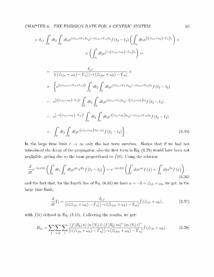
CHAPTER 6. THE EMISSION RATE FOR A GENERIC SYSTEM 95
= δi,i′
∫ t
0
dt2
∫ t
0
dt4e(ini+Γn)t2e(−imi+Γm)t4f (t2 − t4)
(∫ t
t2
dt1e[i(fn+ωk)−Γn]t1
)
×
×(∫ t
t4
dt3e[−i(fm+ωk)−Γm]t3
)
=
=δi,i′
[i (fn + ωk)− Γn] [−i (fm + ωk)− Γm]×
×
e[i(mn)−(Γn+Γm)]t
∫ t
0
dt2
∫ t
0
dt4e(ini+Γn)t2e(−imi+Γm)t4f (t2 − t4)
− e[i(fn+ωk)−Γn]t∫ t
0
dt2
∫ t
0
dt4e(ini+Γn)t2e−i(fi+ωk)t4f (t2 − t4)
− e[−i(fm+ωk)−Γm]t∫ t
0
dt2
∫ t
0
dt4ei(fi+ωk)t2e(−imi+Γm)t4f (t2 − t4)
+
∫ t
0
dt2
∫ t
0
dt4ei(fi+ωk)(t2−t4)f (t2 − t4)
. (6.35)
In the large time limit t → ∞ only the last term survives. Notice that if we had not
introduced the decay of the propagator, also the rst term in Eq. (6.35) would have been not
negligible, giving rise to the term proportional to f(0). Using the relation:
d
dte−(a+b)t
(∫ t
0
dt1
∫ t
0
dt2eat1ebt2f (t1 − t2)
)
= e−(a+b)t
(∫ t
0
dxeaxf (x) +
∫ t
0
dxebxf (x)
)
.
(6.36)
and the fact that, for the fourth line of Eq. (6.35) we have a = −b = fi+ωk, we get, in the
large time limit,
d
dtT1 =
δi,i′
[i (fn + ωk)− Γn] [−i (fm + ωk)− Γm]f (fi + ωk) , (6.37)
with f(k) dened in Eq. (3.54). Collecting the results, we get:
R11 =∑
f
∑
n,m
∑
i
〈f |Rk|n〉 〈n |Ni| i〉 〈f |Rk|m〉∗ 〈m |Ni| i〉∗[i (fn + ωk)− Γn] [−i (fm + ωk)− Γm]
f (fi + ωk) . (6.38)
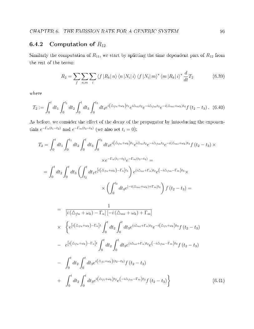
CHAPTER 6. THE EMISSION RATE FOR A GENERIC SYSTEM 96
6.4.2 Computation of R12
Similarly the computation of R11, we start by splitting the time dependent part of R12 from
the rest of the terms:
R2 =∑
f
∑
n,m
∑
i
〈f |Rk|n〉 〈n |Ni| i〉 〈f |Ni|m〉∗ 〈m |Rk| i〉∗d
dtT2 (6.39)
where
T2 :=
∫ t
0
dt1
∫ t1
0
dt2
∫ t
0
dt3
∫ t3
0
dt4ei(fn+ωk)t1einit2e−ifmt3e−i(mi+ωk)t4f (t2 − t3) . (6.40)
As before, we consider the eect of the decay of the propagator by introducing the exponen-
tials e−Γn(t1−t2) and e−Γm(t3−t4) (we also set ti = 0):
T2 =
∫ t
0
dt1
∫ t1
0
dt2
∫ t
0
dt3
∫ t3
0
dt4ei(fn+ωk)t1einit2e−ifmt3e−i(mi+ωk)t4f (t2 − t3)×
×e−Γn(t1−t2)e−Γm(t3−t4) =
=
∫ t
0
dt2
∫ t
0
dt3
(∫ t
t2
dt1e[i(fn+ωk)−Γn]t1
)
e(ini+Γn)t2e(−ifm−Γm)t3×
×(∫ t3
0
dt4e[−i(mi+ωk)+Γm]t4
)
f (t2 − t3) =
=1
[i (fn + ωk)− Γn] [−i (mi + ωk) + Γm]
×
e[i(fn+ωk)−Γn]t∫ t
0
dt2
∫ t
0
dt3e(ini+Γn)t2e−i(fi+ωk)t3f (t2 − t3)
− e[i(fn+ωk)−Γn]t∫ t
0
dt2
∫ t
0
dt3e(ini+Γn)t2e(−ifm−Γm)t3f (t2 − t3)
−∫ t
0
dt2
∫ t
0
dt3ei(fi+ωk)(t2−t3)f (t2 − t3)
+
∫ t
0
dt2
∫ t
0
dt3ei(fi+ωk)t2e(−ifm−Γm)t3f (t2 − t3)
(6.41)

CHAPTER 6. THE EMISSION RATE FOR A GENERIC SYSTEM 97
The rst two lines of Eq. (6.41) have the same structure as in Eq. (6.35) and it is clear that,
in the large time limit t → ∞, they go to zero. In order to understand if the third or the
fourth term in Eq. (6.41) are relevant, let us consider the generic integrals:
I(a, b, t) : =
∫ t
0
dt1
∫ t
0
dt2eat1ebt2f (t1 − t2) (6.42)
=1
a+ b
(
e(a+b)t
∫ t
0
dxe−bxf (x)−∫ t
0
dxeaxf (x) + e(a+b)t
∫ t
0
dxe−axf (x)−∫ t
0
dxebxf (x)
)
.
Since the rate is essentially proportional to the above quantity divided by t, in the large times
limit the only integral that survive is the one with a = −b, since they increase linearly with
the time. Indeed:
I(a,−a, t) =∫ t
0
dxeax (t− x) f (x) +
∫ t
0
dx (t− x) e−axf (x) −→t→∞
t
∫ t
−t
dxeaxf (x) .
(6.43)
This means that only the third term in Eq. (6.41) survives and then
d
dtT2 −→
t→∞
f (fi + ωk)
[i (fn + ωk)− Γn] [−i (mi + ωk) + Γm](6.44)
and therefore:
R12 =∑
f
∑
n,m
∑
i
〈f |Rk|n〉 〈n |Ni| i〉 〈f |Ni|m〉∗ 〈m |Rk| i〉∗[i (fn + ωk)− Γn] [−i (mi + ωk) + Γm]
f (fi + ωk) . (6.45)
6.4.3 Computation of R22
As already done for R11 and R12, we write R22 in this way:
R22 =∑
f
∑
m,n
∑
i
〈f |Ni|n〉 〈n |Rk| i〉 〈f |Ni′ |m〉∗ 〈m |Rk| i〉∗d
dtT3 (6.46)
where
T3 :=
∫ t
ti
dt1
∫ t1
ti
dt2
∫ t
ti
dt3
∫ t3
ti
dt4eifnt1ei(ni+ωk)t2f (t1 − t3) e
−ifmt3e−i(mi+ωk)t4 (6.47)

CHAPTER 6. THE EMISSION RATE FOR A GENERIC SYSTEM 98
Adding the decay of the propagator and setting ti = 0 we have:
T3 =
∫ t
0
dt1
∫ t1
0
dt2
∫ t
0
dt3
∫ t3
0
dt4eifnt1ei(ni+ωk)t2f (t1 − t3) e
−ifmt3e−i(mi+ωk)t4×
×e−Γn(t1−t2)e−Γm(t3−t4) =
=
∫ t
0
dt1
∫ t
0
dt3e(ifn−Γn)t1
(∫ t1
0
dt2e[i(ni+ωk)+Γn]t2
)
f (t1 − t3) e(−ifm−Γm)t3×
×(∫ t3
0
dt4e[−i(mi+ωk)+Γm]t4
)
=
=1
[i (ni + ωk) + Γn] [−i (mi + ωk) + Γm]
∫ t
0
dt1
∫ t
0
dt3ei(fi+ωk)(t1−t3)f (t1 − t3)
−∫ t
0
dt1
∫ t
0
dt3ei(fi+ωk)t1e(−ifm−Γm)t3f (t1 − t3)
−∫ t
0
dt1
∫ t
0
dt3e(ifn−Γn)t1
(
e−i(fi+ωk)t3)
f (t1 − t3)
+
∫ t
0
dt1
∫ t
0
dt3e(ifn−Γn)t1e(−ifm−Γm)t3f (t1 − t3)
. (6.48)
All the four terms in Eq. (6.48) contains integrals with the same structure of I(a, b, t) given
in Eq. (6.42). As already discussed, the only relevant terms in the large time limit t → ∞are the ones with a = −b, which in this case correspond to the rst line. Therefore we have:
d
dtT3 −→
t→∞
f (fi + ωk)
[i (ni + ωk) + Γn] [−i (mi + ωk) + Γm](6.49)
and thus:
R22 =∑
f
∑
m,n
∑
i
〈f |Ni|n〉 〈n |Rk| i〉 〈f |Ni′ |m〉∗ 〈m |Rk| i〉∗[i (ni + ωk) + Γn] [−i (mi + ωk) + Γm]
f (fi + ωk) . (6.50)
CHAPTER 6. THE EMISSION RATE FOR A GENERIC SYSTEM 99
6.5 Contribution due to the mixed terms
In this section we will compute the contribution to the rate due to the mixed terms B∗C1,
B∗C2 and B∗C3.
6.5.1 Computation of B∗C1
Here we want to study the contributions due to the terms B and C1 given in Eqs. (6.23) and
(6.24). The B term is simply:
B =
(−i~
)
〈f |Rk| i〉TB (6.51)
where, setting ti = 0,
TB =
∫ t
0
dt1ei(fi+ωk)t1 =
ei(fi+ωk)t − 1
i (fi + ωk). (6.52)
The term C1 can be written as:
C1 =
(−i~
)3
~2γ∑
n,m
∑
i,i′
〈f |Rk|n〉 〈n |Ni|m〉 〈m |Ni′ | i〉TC1. (6.53)
After taking the noise average, we have:
TC1 = δi,i′
∫ t
0
dt1
∫ t1
0
dt2
∫ t2
0
dt3ei(Ef+ωk−En)t1ei(En−Em)t2ei(Em−Ei)t3f (t2 − t3) e
−Γn(t1−t2)e−Γm(t2−t3) =
=
∫ t
0
dt1ei(fn+ωk)t1e−Γnt1
∫ t1
0
dt2
∫ t1
0
dt3θ (t2 − t3) einmt2eΓnt2eimit3f (t2 − t3) e
−Γm(t2−t3)(6.54)

CHAPTER 6. THE EMISSION RATE FOR A GENERIC SYSTEM 100
The integral can be computed using the same techniques introduced here above and in chapter
3; the result is:
TC1 =δi,i′
(ini + Γn) i (fi + ωk)
(
ei(fi+ωk)t∫ t
0
dxe(iim−Γm)xf (x)−∫ t
0
dxf (x) e[i(fm+ωk)−Γm]x)
−
− δi,i′
(ini + Γn) [i (fn + ωk)− Γn]×
×(
e[i(fn+ωk)−Γn]t∫ t
0
dxe[inm+(Γn−Γm)]xf (x)−∫ t
0
dxf (x) e[i(fm+ωk)−Γm]x)
(6.55)
Since in the end we need to compute∑
µ
∫dΩk
ddt
∑
f E 2Re (B∗C1), we have to focus on
TBC1 =TC1 − TC1e
−i(fi+ωk)t
i (fi + ωk)(6.56)
and in particular on its time derivative:
d
dtTBC1 =
ddtTC1 − d
dt
[
TC1e−i(fi+ωk)t
]
i (fi + ωk). (6.57)
It is straightforward to see that, in the large time limit, one gets:
dTC1
dt−→t→∞
δi,i′ei(fi+ωk)t
(ini + Γn)
∫ t
0
dxe(iim−Γm)xf (x)
d
dt
[
TC1e−i(fi+ωk)t
]
−→t→∞
δi,i′
[
1− i (fi + ωk)
[i (fn + ωk)− Γn]
]e−i(fi+ωk)t
(ini + Γn)×
×∫ t
0
dxf (x) e[i(fm+ωk)−Γm]x

CHAPTER 6. THE EMISSION RATE FOR A GENERIC SYSTEM 101
So in the large time limit:
d
dtTBC1 = δi,i′
1
i (fi + ωk)×
ei(fi+ωk)t
(ini + Γn)
∫ t
0
dxe(iim−Γm)xf (x)− (6.58)
−[
1− i (fi + ωk)
[i (fn + ωk)− Γn]
]e−i(fi+ωk)t
(ini + Γn)
∫ t
0
dxf (x) e[i(fm+ωk)−Γm]x
The important point is that this term oscillates, therefore when we compute the average rate
it gives zero contribution. The only exception is when fi + ωk = 0. However, as far as we
study systems which initial state is the ground state, the condition fi + ωk = 0 is never
fullled and therefore we do not need to consider this term. The reason why we can consider
only systems which are in the ground state is that, when this is not the case, the eect of
the spontaneous emission due only to the vacuum uctuation of the electromagnetic eld is
expected to be bigger than the one due to the presence of the noise. This can be qualitatively
understood considering the fact that the eect due to the vacuum uctuations is of order e2
while the eect we are considering is of order e2γ. The same conclusions are true also for the
contributions B∗C2 and B∗C3, since they behave in a similar way to B∗C1.
6.6 Final result
We have seen that the terms B∗Cn with n = 1, 2, 3 give zero contribution while A1 and A2
give:dΓ
dt=∑
µ
∫
dΩk
( γ
~2
)
[R11 + 2Re (R12) +R22] (6.59)
with R11, R12 and R22 given respectively in Eqs. (6.38), (6.45) and (6.50). Therefore we have:
R11 + 2Re (R12) +R22 = R11 +R12 +R∗12 +R22 =

CHAPTER 6. THE EMISSION RATE FOR A GENERIC SYSTEM 102
=∑
f
∑
i
∑
n,m
〈f |Rk|n〉 〈n |Ni| i〉 〈f |Rk|m〉∗ 〈m |Ni| i〉∗[i (fn + ωk)− Γn] [−i (fm + ωk)− Γm]
+
+〈f |Rk|n〉 〈n |Ni| i〉 〈f |Ni|m〉∗ 〈m |Rk| i〉∗[i (fn + ωk)− Γn] [−i (mi + ωk) + Γm]
+
+〈f |Rk|n〉∗ 〈n |Ni| i〉∗ 〈f |Ni|m〉 〈m |Rk| i〉[−i (fn + ωk)− Γn] [i (mi + ωk) + Γm]
+
+〈f |Ni|n〉 〈n |Rk| i〉 〈f |Ni′ |m〉∗ 〈m |Rk| i〉∗[i (ni + ωk) + Γn] [−i (mi + ωk) + Γm]
f (fi + ωk) (6.60)
=∑
f
∑
i
∣∣∣∣∣
∑
n
〈f |Rk|n〉 〈n |Ni| i〉[i (fn + ωk)− Γn]
− 〈f |Ni|n〉 〈n |Rk| i〉[i (ni + ωk) + Γn]
∣∣∣∣∣
2
f (fi + ωk)
So the formula for the emission rate becomes:
dΓ
dt=∑
µ
∫
dΩk
( γ
~2
)∑
f
∑
i
∣∣∣∣∣
∑
n
〈f |Rk|n〉 〈n |Ni| i〉[i (fn + ωk)− Γn]
− 〈f |Ni|n〉 〈n |Rk| i〉[i (ni + ωk) + Γn]
∣∣∣∣∣
2
f (fi + ωk)
(6.61)
Notice that the unphysical terms proportional to f(0) has disappeared. The great importance
of the result found in this chapter is that it is true for generic systems, the only assumptions
that we included is that the system is initially in its ground state and that the propagator
may decay (this assumption, apart for a free particle, is usually always true). Such a formula
is therefore suitable to be applied to more realistic systems than the free particle or the
harmonic oscillator. This will be the subject of further research.

Conclusion of Part I
In this part of the thesis we studied the electromagnetic radiation emission in collapse models.
In particular, we focused in understanding the origin of an unphysical term present in the
emission rate when the calculation is carried out to the lowest perturbative order. The main
result we achieved is to show that this term is not present when the higher order contributions
of the electromagnetic interaction are taken into account. Indeed, we compute the emission
rate for a harmonic oscillator treating exactly the electromagnetic interaction for the QMUPL
model (chapter 4) and for the CSL model (chapter 5), and in both cases the unphysical term
is not present. Then, in chapter 6, we showed that the eect of the higher order contributions
coming from the electromagnetic interaction can be properly taking into account also in the
lowest order perturbative calculations, introducing the decay of the propagator.
Now that we have the correct formula for the emission rate, we wish to compare the CSL
predictions with available experimental data.
We report the analysis done in [20]. The author took available data on photon's emission
from Germanium (Ge) and compared them with the prediction given by the CSL model. To
obtain the emission rate from Ge, he considered the four external electrons of this element
as free particles, and then he computed the emission rate from a Ge atom as four time of the
emission rate of one free electron, using Eq. (5.6) in the white noise case (f(ω) = 1)3. Even
though this analysis is quite rough, the results are quite interesting. They are listed in the
following table:
3To be more precise, Eq. (5.6) is used to compute the rate in the mass proportional CSL model (thirdcolumn of Table 6.1). The rate in the original CSL model (second column of Table 6.1) is given by the sameformula taking the electron mass instead of the nucleon mass m0.
103

CHAPTER 6. THE EMISSION RATE FOR A GENERIC SYSTEM 104
Energy experimental data CSL mass proportional CSL
(KeV) (counts/(KeV*Kg*day)) (counts/(KeV*Kg*day)) (counts/(KeV*Kg*day))
11 0.049 0.071 2.1× 10⁻⁸
101 0.031 0.0073 2.2× 10⁻⁹
201 0.030 0.0037 1.1× 10⁻⁹
301 0.024 0.0028 8.4× 10⁻¹⁰
401 0.017 0.0019 5.7× 10⁻¹⁰
501 0.014 0.0015 4.5× 10⁻¹⁰
Table 6.1: The CSL predictions vs experimental data for the radiation emitted from Germa-
nium, for dierent energies. The second column shows the number of photons counted in one
day from one Kg of material at the energy considered. The same quantity has been computed
using the original CSL model (second column) and the mass proportional CSL model (third
column). The values are obtained using the λ proposed by Ghirardi Rimini and Weber. If
the λ value proposed by Adler is considered, then the prediction given in the second and the
third line must be increased by a factor 108.
We see that the original CSL model, with the λ value proposed by Ghirardi Rimini and
Weber, is disproved: indeed, the emission rate of photons with energy 13 KeV predicted by
this model is bigger than the one experimentally observed. However, if one considers the
mass proportional CSL model, then the theoretical predictions are reduced by a factor4 106,
and there is no disagreement between the model and experimetal data. Regarding the value
of λ proposed by Adler, the situation is dierent: in this case, even considering the mass
proportional CSL model, there is no agreement with the experimental data. However, till
now, we only considered the predictions given when the noise is white. A white noise is a
noise where each energy component has the same weight. Therefore, it cannot be considered
realistic; then the interesting issue is to compute the predictions given by a non white noise.
They are given by Eq. (5.6). We see that the emission rate is the one predicted in the white
noise case multiplied by the spectral density of the noise f(ωk). As discuss in [16, 21], it
is reasonable to assume that the spectral density of the noise has a cuto at the frequency
c/rC ≃ 1015 s−1, which correspond to photons with energy Ek = ~ωk ≃ 1 eV. Therefore, since
4This is a consequence of the fact that, as discussed in chapter 2, going from the original CSL model to
the mass proportional CSL model, in the case of the electrons, is equivalent to the replacement λ → λ(
mm0
)2
where m is the mass of the electron and m0 the one of a nucleon.

CHAPTER 6. THE EMISSION RATE FOR A GENERIC SYSTEM 105
the range of energies we are considering is in the region of keV, all the theoretical predictions
are suppressed and the value of λ proposed by Adler becomes compatible with experimental
data.

Part II
Flavour oscillations
106

107
In this second part of the thesis we study the eects of collapse models on a dierent type
of quantum phenomenon: avour oscillations.
Flavour oscillations arises when avour eigenstates of a particle are dierent from its mass
eigenstates. Flavour eigenstates are supposed to be linear superposition of mass eigenstates.
In the course of time, the mass eigenstates acquire dierent phase factors, depending on their
mass. The phenomenon of avour oscillation arises because what we measure are not the
mass eigenstates, but the avour eigenstates, which are superpositions of mass eigenstates.
The dierent phase factors in front of the mass eigenstates change the relative weights in the
superposition, making it possible that a particle initially in a avour eigenstate ends up in
another avour eigenstate. Let us shows explicitly how this happens, by studying the simple
case of a particle with only two dierent avour and mass eigenstates. We will denote with
|α〉 and |β〉 the avour eigenstates and with |m1〉 and |m2〉 the mass eigenstates. The two
basis are related by a unitary transformation U, so we have:
(
|α〉|β〉
)
=
(
Uα1 Uα2
Uβ1 Uβ2
)(
|m1〉|m2〉
)
(6.62)
The probability Pα→β (t) for a particle with the initial state |α〉 to be found in the state |β〉at the time t is given by:
Pα→β (t) =∣∣∣
⟨
β∣∣∣e−
i~Ht∣∣∣α⟩∣∣∣
2
=
∣∣∣∣∣
2∑
k,j=1
U∗βjUαk
⟨
mj
∣∣∣e−
i~Ht∣∣∣mk
⟩∣∣∣∣∣
2
=
∣∣∣∣∣
2∑
k=1
U∗βkUαke
− i~Ekt
∣∣∣∣∣
2
=
= |Uα1|2 |Uβ1|2 + |Uα2|2 |Uβ2|2 + 2 Re[
U∗β1Uα1Uβ2U
∗α2e
i~(E2−E1)t
]
(6.63)
withH the Hamiltonian of the system and Ek the eigenvalue associated to the mass eigenstate
|mk〉. In Eq. (6.63) we used the fact that 〈mj |mk〉 = δjk. In the two dimensional case the
matrix U is usually taken as a rotation, which is parametrized by the mixing angle φ, that
is to say: Uα1 = Uβ2 = cosφ and Uα2 = −Uβ1 = sinφ. Therefore the transition probability
becomes:
Pα→β (t) =sin2 (2φ)
2
1− cos
[1
~(E2 − E1) t
]
(6.64)
This is the formula describing the avour oscillation in quantum mechanics. It tells that
the transition probability |α〉 −→ |β〉 oscillates in time with a frequency proportional to the

108
energy dierence between the two mass eigenstate. An analogous formula can be found in
the more general case where n avour and mass eigenstates are considered.
In the following, we compute how collapse models modify Eq. (6.63). As discuss in chapter
2 the eect of the collapse is to localize the wave function in space. So, at rst sight, it may
seem strange that a collapse in real space induces a change in the transition probability
in avour space. However, in collapse models the free time evolution of mass eigenstates is
dierent from that of standard quantum mechanics. This implies, as an indirect consequence,
that also avour eigenstates evolve dierently, and therefore particles are expected to oscillate
in a dierent manner.
In the next two chapters we will study avour oscillations for neutrinos and mesons using
the CSL model. We will study the general case of a particle with n dierent mass and avour
eigenstates. Performing the calculations to the second order in perturbation theory, we will
derive the modied probability for avour oscillations.

Chapter 7
Neutrino oscillations
In this chapter we compute the eect of collapse models on neutrino oscillations. The eect
of the collapse is to modify the evolution of the spatial part of the wave function and we will
show that this indirectly amounts to a change on the avour components. In some sense,
it is as if neutrinos were traveling through a random medium, instead of free space. It is
well known that neutrino oscillations are aected by a random medium [46, 47]. However,
we stress that this is more a mathematical analogy because in our case the origin of the
randomness is dierent, and it is due to the spontaneous collapse of the wave function. As
we will show, the CSL dynamics changes the avour oscillation, introducing a damping factor
in front of the oscillation term. The eect is very smallmainly due to the very small mass
of neutrinosand practically undetectable.
A previous analysis of this kind was proposed in [25], based on the Penrose model of
gravity-induced collapse [32, 33]. This model however lacks a fully consistent dynamical
equation, and previous attempts to ll this gap, e.g. [34], have been criticized [48]. Moreover
the model fails when applied to single constituents (e.g., protons and electrons), since in
this case its predictions are in conict with known experimental data [48]. Therefore, the
application of gravity-induced collapse models to neutrino oscillations is rather delicate.
In the next section we compute the avour oscillation formula for neutrinos. In section
3.2 we discuss this result, in section 3.3 we compare it with the one found in [25] and in
section 3.4 with decoherence eects.
109

CHAPTER 7. NEUTRINO OSCILLATIONS 110
7.1 Derivation of the oscillation formula
Since the collapse mechanism acts on the spatial part of the wave function implies that we
have to consider the whole Hilbert space of the system, not just the part related to the avour
degrees of freedom. As discussed in chapter 2, the time evolution of the states in the CSL
model is described by Eq. (2.26). However, as also discussed in chaper 2, as far as we are
concerned in computing physical predictions, the non linear dynamics given by Eq. (2.26)
can be always replaced by the Schrödinger equation given in Eq. (2.28), that is:
HTOT = H − ~√γ∑
j
mj
m0
∑
s
∫
dyw(y, t)ψ†j(y, s)ψj(y, s). (7.1)
Here we focus on the white noise case, i.e., w(x, t) is a Gaussian noises eld, with zero mean
and the correlation function:
E[w(x, t)w(y, s)] = δ(t− s)F (x− y), F (x) =1
(√4πrC)3
e−x2/4r2C . (7.2)
We are interested in the relativistic generalization of the Hamiltonian (7.1). The most natural
choice is: HTOT = HD +N(t) where (in the case of just one type of particle):
HD =
∫
dxHD (x) =
∫
dxψ† (x)[−i~cα ·∇+mc2β
]ψ (x) (7.3)
is the standard Dirac Hamiltonian. Here we have introduced the four-vector notation where
x := (ct,x), ψ (x) is the Dirac spinor eld, c the speed of light, m the mass of the particle
associated to this eld, α := (α1, α2, α3) with αi = γ0γi and β = γ0 where the γµ are the
Dirac matrices, which we take in their standard representation:
γ0 =
(
1 0
0 −1
)
, γi =
(
0 σi
−σi 0
)
with i = 1, 2, 3. (7.4)
where 1 is the identity matrix in two dimensions and σi are the Pauli matrices. The noise
term N(t) is given by:
N(t) =
∫
dxN (x) = −~√γm
∫
dxw (x)ψ (x)ψ (x) , γm = γ
(m
m0
)2
(7.5)

CHAPTER 7. NEUTRINO OSCILLATIONS 111
It can be shown1 that the Hamiltonian HTOT = HD+N(t) dened in this way reduces to the
Hamiltonian of Eq. (7.1) in the non relativistic limit.
We chose to treat neutrinos as Dirac particles, although it is not yet known if they are
Dirac or Majorana particles. We expect that the strenght of the collapse eect does not
change signicantly if Majorana elds are used instead of Dirac elds. As a matter of fact,
in the next chapter and in [50], the eect of the CSL model on kaon oscillations formula
are studied. Although kaons are dierent from neutrinos and we study them in the non-
relativistic regime, the result is the same as that of neutrinos: a damping factor in front of
the oscillating term, with a decay rate equivalent to the one found for neutrinos, when the
non-relativistic limit is taken.
Working with plane waves gives rise to unphysical divergences, since they are not normal-
izable. To avoid potential problems, we use the box normalization, i.e. we conne our elds
in a box of length L, and we impose periodic boundary conditions: ψ (t,x) = ψ (t,x+ L),
where L is a vector with all the components equal to L. In turn, the momentum is discretized:
p = 2π~Lk with ki ∈ Z and i = 1, 2, 3 labels the spatial components. Then the Dirac eld,
in the interaction picture where we choose HD as the unperturbed Hamiltonian and N (t) as
the perturbation (the noise coupling√γm is very small), takes the usual expression2:
ψI (x) =2∑
s=1
+∞∑
k=−∞
1√L3
√
mc2
Ep
[
b (p, s) u (p, s) e−i~Ept+i 2π
Lk·x + d† (p, s) v (p, s) e
i~Ept−i 2π
Lk·x]
,
(7.6)
where u and v are the usual Dirac spinors, Ep =√
p2c2 +m2c4 is the energy and b and d
are operators satisfying the standard anti-commutation relations. We also recall the relation
between the evolution operator U(t) in the Schrödinger picture and UI (t) in the interaction
picture [24]:
U (t) = e−i~HDtUI (t) , (7.7)
and we set the initial time to zero.
One can question why we use a relativistic Hamiltonian in a model which is not relativistic,
since the correlation function of the noise is not Lorentz-invariant. Our approach to this issue,
is that collapse models are phenomenological models emerging from a pre-quantum theory
1A proof of this can be found in section 2.3 of [49]. There, the proof is worked out for the Dirac equationcoupled with an electromagnetic eld. This is the same case as ours, if one sets A (x) = 0 and eA0 (x) =−~
√γmw (x).
2Here and in the following we use the notation of [49].

CHAPTER 7. NEUTRINO OSCILLATIONS 112
yet to be discovered. The noise eld is a real cosmological eld (whose nature is yet to be
investigated) which naturally denes a privileged frame, most likely corresponding to the
co-moving frame of the universe. Hence we see no contradiction in analyzing relativistic
phenomena with the CSL model. For attempts towards a fully relativistic formulation of
collapse models, one can refer to [51, 52].
7.1.1 The transition amplitude
In the more general approach to the problem of neutrino oscillations, we consider n avour
eigenstates, which will be labeled by greek subscripts |να〉 and each of them is a linear
combination of n mass eigenstates that will be labeled by latin subscripts |νj〉:
|να〉 =n∑
j=1
Uαj |νj〉 . (7.8)
Here, U is the n × n mixing matrix, which relates the two dierent bases; since the avour
eigenstates are supposed to be orthonormal, as well as the mass eigenstates, U must be
unitary.
We take a neutrino in an initial avour eigenstate, and compute the probability of nding
it in another avour eigenstate, after some time t, assuming that the dynamics is governed
by the Hamiltonian HTOT = HD + N(t), with HD dened in Eq. (7.3) and N(t)
dened in Eq. (7.5). We assume that the neutrino has denite initial and nal momenta.
This means that its initial and nal states are plane waves and that both mass eigenstates
have the same momentum3.
As discussed in [53], in order to have a more consistent description, one should use wave
packets instead of plane waves. However, a wave packet analysis goes beyond the scope
of this thesis: it would make the calculations much more dicult, and the expected result
should not be much dierent from the one here derived. Moreover, in the standard treatment
of neutrino oscillations, the plane wave analysis already gives a satisfactory description, to
some degree, both in vacuum and in matter. Mathematically, we will compute the following
3Sometimes a dierent choice is done, where the neutrino mass eigenstates has the same energy butdierent momenta. However, this choice lead to the same oscillation formula [53].
CHAPTER 7. NEUTRINO OSCILLATIONS 113
quantity:
Tα→β(t) := 〈νβ;pf , sf |U (t)| να;pi, si〉 =n∑
i,j=1
UαjU∗βi 〈νi;pf , sf |U (t)| νj;pi, si〉 (7.9)
where U (t) is the time-evolution operator given in Eq. (7.7) while |να;pi, si〉 is the avour
eigenstate α with initial momentum pi and spin si and |νβ;pf , sf〉 is the nal state with
momentum pf and spin sf . Since the Hamiltonian is the sum of Hamiltonians associated to
dierent mass eigenstates (H =∑n
j=1Hj), it is convenient to expand the avour eigenstates
into the mass eigenstates, as we did in Eq. (7.9). The form of the Hamiltonian also implies
that U(t) factorizes: U (t) =∏n
k=1 Uk (t). Here Uk (t) is the time evolution operator related
to the Fock space of a neutrino having a denite mass mk. This is an important property,
because it implies that if i 6= j:
〈νi;pf , sf |U(t)|νj;pi, si〉 = 〈Ω1 |U1 (t)|Ω1〉 ... 〈νi;pf , sf |Ui (t)|Ωi〉 ... 〈Ωj |Uj (t)| νj;pi, si〉 ...... 〈Ωn |Un (t)|Ωn〉 = 0, (7.10)
where |Ωk〉 is the vacuum state of the space associated to the neutrino mass eigenstate νk.
The relation in Eq. (7.10) is due to the fact that 〈νi;pf , sf |Ui (t)|Ωi〉 = 0, as one can check
with a direct calculation. Therefore we can write:
Tα→β(t) =n∑
j=1
UαjU∗βj [〈Ω1 |U1 (t)|Ω1〉 ... 〈νj;pf , sf |Uj (t)| νj;pi, si〉 .... 〈Ωn |Un (t)|Ωn〉] ,
(7.11)
which reduces the entire calculation to a 1-particle computation. In the next section we will
focus our attention on the matrix element 〈νj;pf , sf |Uj (t)| νj;pi, si〉 since, as we will show,
the remaining terms contribute with an unimportant global phase factor.
7.1.2 The matrix elements
We now focus on the main part of this work. What we need is to compute the 1-particle
matrix element:
T (pf , sf ;pi, si; t) := 〈pf , sf |U (t)|pi, si〉 = e−i~Ef t 〈pf , sf |UI (t)|pi, si〉 . (7.12)

CHAPTER 7. NEUTRINO OSCILLATIONS 114
Since this part of the computation is the same for every mass eigenstate, we drop the label
j. We expand the evolution operator using Dyson series up to the second order:
UI (t, 0) ≃ 1− i
~
∫ t
0
dt1 : NI (t1) : −1
~2
∫ t
0
dt1
∫ t1
0
dt2 : NI (t1) :: NI (t2) :, (7.13)
where NI (t) is the interaction picture representation of Eq. (7.5) and : ... :" denotes the
normal ordering4. Accordingly, the transition probability is the sum of three terms:
T (pf , sf ;pi, si; t) = e−i~Ef t[T (0) (pf , sf ;pi, si; t) + T (1) (pf , sf ;pi, si; t) + T (2) (pf , sf ;pi, si; t)
],
(7.14)
which correspond to the rst three terms of the Dyson series. We now represent each term
by means of Feynman diagram and then we compute them. The rst term corresponds to
the free propagation:
T (0) (pf , sf ;pi, si; t) = ikFkfwhere the solid line represent the particle. This term is trivial:
T (0) (pf , sf ;pi, si; t) := 〈pf , sf |pi, si〉 = δsf siδpf ,pi. (7.15)
The second term correspond to the diagram:
T (1) (pf , sf ;pi, si; t) = iF1i`Df
where the dashed line represents the noise eld. This term is:
T (1) (pf , sf ;pi, si; t) := i√γm
∫ t
0
dt1
∫
dx1w (x1) 〈pf , sf | : ψI (x1)ψI (x1) : |pi, si〉. (7.16)
In order to compute the matrix element in Eq. (7.16), we use the series expansion of the elds
as given in Eq. (7.6). The non-null terms are those containing two b and two b† operators.
4As well know in Quantum Field Theory, the reason why we used : NI (t) : in place of NI (t) is that, withthis prescription, we can remove all divergent contributions coming from tadpole diagrams. This type ofdivergences can be absorbed through a renormalization procedure, without giving any physically observableconsequence [39, 54].
CHAPTER 7. NEUTRINO OSCILLATIONS 115
After some calculations, one nds that:
〈Ω|b (pf , sf ) : ψI (x1)ψI (x1) : b† (pi, si) |Ω〉 =
=2∑
s,s′=1
+∞∑
p,p′=−∞
1
L3
mc2√EpEp′
ei~(p′µ−pµ)x1µu (p′, s′) u (p, s) 〈Ω|b (pf , sf ) b† (p′, s′) b (p, s) b† (pi, si) |Ω〉
=1
L3
mc2√EiEf
ei~(pµf−pµi )x1µu (pf , sf ) u (pi, si) . (7.17)
Here we introduced the four momentum pµ = (Ep/c,p). If we substitute Eq. (7.17) in the
denition of T (1), we get:
T (1) (pf , sf ;pi, si; t) = i√γm
mc2√EiEf
u (pf , sf ) u (pi, si)1
L3
∫ t
0
dt1
∫
dx1w (x1) ei~(pµf−pµi )x1µ .
(7.18)
The last term in Eq. (7.14) is more complicated to compute, since it involves the product
of four elds. It gives the following contribution:
T (2) (pf , sf ;pi, si; t) := − 1
~2〈pf , sf |
[∫ t
0
dt1
∫ t1
0
dt2 : NI (t1) :: NI (t2) :
]
|pi, si〉 = (7.19)
= −γm2
∫ t
0
dt1dt2
∫
dx1dx2w (x1)w (x2) 〈pf , sf |T[: ψI (x1)ψI (x1) :: ψI (x2)ψI (x2) :
]|pi, si〉,
where T is the time-ordering product. Using Wick's theorem, and discarding all tadpole
terms, which involve a contraction between two elds at the same spacetime point, we get:
T[ψ1aψ1aψ2bψ2b
]= : ψ1aψ1aψ2bψ2b : −Sab (x1 − x2)Sba (x2 − x1)
+iSab (x1 − x2) : ψ1aψ2b : −iSba (x2 − x1) : ψ1aψ2b :, (7.20)
where a and b label the spinor components and the Dirac propagator is: iSab (x1 − x2) :=
〈Ω|T[ψ1aψ2b
]|Ω〉. Here, Einstein's summation convention is used for the spinor indices. We
momentarily drop the pedex I related to the interaction picture and we write the dependence
on x1 and x2 simply as 1 and 2. The diagramatic representation of the dierent terms in

CHAPTER 7. NEUTRINO OSCILLATIONS 116
Eq. (7.20) is:
iF1i`Df
iF2i`Df
= : ψ1aψ1aψ2bψ2b : , h1L
2h = −Sab (x1 − x2)Sba (x2 − x1) ,
ij
2F
1iE`Df
= iSab (x1 − x2) : ψ1aψ2b : ,ij
1F
2iE`Df
= −iSba (x2 − x1) : ψ1aψ2b : .
We can easily see that the rst term is zero, since we are studying the case with only one
particle in the initial and nal states. Regarding the second diagram, an important issue
arises here. This diagam represents a vacuum uctuation term, which is divergent. As
well known [39], all vacuum uctuations diagrams of any order sum up to a phase factor
〈Ω |UI (t, 0)|Ω〉, and all divergences cancel with each other. Therefore we can write:
〈pf , sf |UI (t, 0)|pi, si〉 = 〈Ω |UI (t, 0)|Ω〉 · 〈pf , sf |UI (t, 0)|pi, si〉ext , (7.21)
where 〈pf , sf |UI (t, 0)|pi, si〉ext denotes the contribution from diagrams with external fermionic
legs. This vacuum uctuation term is important because, together with those of Eq. (7.11),
it gives a global phase∏n
k=1 〈Ωk |UkI (t, 0)|Ωk〉 independent of j, which factorizes out of
the sum. Therefore, such terms are physically unimportant, and the only relevant part is
〈pf , sf |UI (t, 0)|pi, si〉ext. From now on, we will work only with diagrams with external
fermionic legs, and we drop the pedex ext.
Coming back to Eq. (7.20), we can now focus our attention on the third and the fourth
term, that correspond to the last two diagrams. Since : ψ2bψ1a : = − : ψ1aψ2b : for fermions,
these two terms give the same contribution. The Dirac propagator reads:
iSab (x1 − x2) =2∑
s=1
+∞∑
p=−∞
1
L3
mc2
Ep
θ (t1 − t2) e− i
~pµ(x1µ−x2µ)ua (p, s) ub (p, s)
−θ (t2 − t1) e− i
~pµ(x2µ−x1µ)vb (p, s) va (p, s)
, (7.22)
while the matrix element gives:
〈pf , sf | : ψ1aψ2b : |pi, si〉 =1
L3
mc2√EfEi
ei~pµfx1µe−
i~pµi x2µua (pf , sf ) ub (pi, si) . (7.23)
CHAPTER 7. NEUTRINO OSCILLATIONS 117
In the following we will need only the case pf = pi and sf = si. In this case, we have:
T (2) (pi, si;pi, si; t) = −γm1
L3
mc2
Ei
2∑
s=1
+∞∑
p=−∞
1
L3
mc2
Ep
·∫ t
0
dt1
∫ t1
0
dt2
∫
dx1
∫
dx2w(x1)w(x2)ei~(pµi −pµ)(x1µ−x2µ)
· ua(pi, si)ua(p,s)ub(p,s)ub(pi, si)
−∫ t
0
dt2
∫ t2
0
dt1
∫
dx1
∫
dx2w (x1)w (x2) ei~(pµi −pµ)(x1µ−x2µ)
· ua(pi, si)va(p, s)vb(p, s)ub(pi, si)
. (7.24)
Using the standard relations [49]:
2∑
s=1
ua(p, s)ub(p, s) =
(pµγµ +mc
2mc
)
ab
,2∑
s=1
va(p, s)vb(p, s) =
(pµγµ −mc
2mc
)
ab
, (7.25)
we can see that the terms containing pµγµ cancel each other, while those containing the mass
give δab. Thus, if we also use: u(pi, sf )u(pi, si) = δsf ,si , we obtain:
T (2) (pi, si;pi, si; t) = −γm1
L3
mc2
Ei
+∞∑
p=−∞
1
L3
mc2
Ep
∫ t
0
dt1
∫ t1
0
dt2
∫
dx1
∫
dx2w (x1)w (x2)
×e i~(pµi −pµ)(x1µ−x2µ). (7.26)
Now we have all the elements we need, in order to compute the transition probability. We
will do this in the next section.
7.1.3 The transition probability
The physical quantity we are interested in is the transition probability, which corresponds to
|Tα→β|2, averaged over the noise, and integrated over the nal momentum and polarization
states:
Pα→β(t) :=∑
sf
+∞∑
pf=−∞E |Tα→β(t)|2 =
n∑
k=1
n∑
j=1
U∗αkUβkUαjU
∗βjPkj (pi, si; t) , (7.27)
CHAPTER 7. NEUTRINO OSCILLATIONS 118
where:
Pkj (pi, si; t) :=∑
sf
+∞∑
pf=−∞e
i~(E
(k)f −E
(j)f )t
E [T ∗k (pf , sf ;pi, si; t)Tj (pf , sf ;pi, si; t)] , (7.28)
and Tj (pf , sf ;pi, si; t) is given by Eq. (7.14), where now we have explicitly indicated the
label j associated to the mass eigenstate mj and E(j)f =
√
p2fc
2 +m2jc
4. When averaging,
one has to remember that only terms containing an even number of noises survive (in the
Feynman representation, all products of diagrams containing an even number of dotted legs).
Using this fact, and exploiting the Kronecher deltas of T (0) (pf , sf ;pi, si; t) (see Eq. (7.15)),
we can write:
Pkj (pi, si; t) = ei~(E
(k)i −E
(j)i )t
[
1 + I(1)jk (pi, si; t) + I
(2)j (pi, si; t) + I
(2)∗k (pi, si; t)
]
, (7.29)
where we have dened:
I(1)jk (pi, si; t) :=
∑
sf
+∞∑
pf=−∞e
i~(E
(k)f −E
(k)i −E
(j)f +E
(j)i )t
E
[
T(1)∗k (pf , sf ;pi, si; t)T
(1)j (pf , sf ;pi, si; t)
]
,
I(2)j (pi, si; t) := E
[
T(2)j (pi, si;pi, si; t)
]
. (7.30)
We focus our attention on I(1)jk (pi, si; t). Using Eq. (7.18), keeping in mind the spinor relation
(ufui)∗ = uiuf , and performing the average over the noise, which brings in a Dirac delta in
time that cancels one of the two time-integrals, one obtains:
E
[
T(1)∗k (pf , sf ;pi, si; t)T
(1)j (pf , sf ;pi, si; t)
]
=
=√γmj
γmk
mjmkc4
√
E(j)i E
(j)f E
(k)i E
(k)f
u(p(j)f , sf )u(p
(j)i , si)u(p
(k)i , si)u(p
(k)f , sf )
·∫ t
0
dt1ei~(E
(j)f −E
(j)i −E
(k)f +E
(k)i )t1S (pi,pf ) (7.31)
where p(j)f := (E
(j)f /c,pf ) and similarly for p
(j)i . Moreover:
S (pi,pf ) :=1
L6
∫ +L2
−L2
dx1
∫ +L2
−L2
dx2e−(x1−x2)
2/4r2C
(√4πrC
)3 e−i~[(pf−pi)·(x1−x2)] (7.32)
CHAPTER 7. NEUTRINO OSCILLATIONS 119
where here we have explicitly indicated the integration volume. In order to compute S (pi,pf ),
we change integration variables as follows:
y = (x1 + x2) and x = (x1 − x2) , (7.33)
and we use the relation:
∫ +L2
−L2
dx1
∫ +L2
−L2
dx2f (x1, x2) =1
2
∫ +L
0
dx
∫ +(L−x)
−(L−x)
dy [f (x, y) + f (−x, y)] . (7.34)
Accordingly, we have:
S (pi,pf ) =1
L3
∫ L
0
dxe−x2/4r2C
(√4πrC
)32 cos
[1
~(pf − pi) · x
]1
23
3∏
i=1
2(
1− xiL
)
(7.35)
Let us now take the limit L→ ∞, which amounts to making the replacement:
+∞∑
pf=−∞−→
∫
dpf and1
L3−→ 1
(2π~)3. (7.36)
In this limit, the term xi/L gives a vanishingly small contribution. Therefore we can write:
S (pi,pf ) =1
(2π~)3
∫ +∞
−∞dx
e−x2/4r2C
(√4πrC
)3 ei~(pf−pi)·x =
1
(2π~)3e−
(pf−pi)2r2C
~2 . (7.37)
The time integral in Eq. (7.31) is trivial, and one arrives easily at the formula:
I(1)jk (pi, si; t) =
∑
sf
∫
dpf√γmj
γmk
mjmkc4
√
E(j)i E
(j)f E
(k)i E
(k)f
u(p(j)f , sf )u(p
(j)i , si)u(p
(k)i , si)u(p
(k)f , sf )
·(
1− ei~(E
(k)f −E
(k)i −E
(j)f +E
(j)i )t
i~(E
(j)f − E
(j)i − E
(k)f + E
(k)i )
)(1
(2π~)3
)
e−(pf−pi)
2r2C~2 . (7.38)
As it is shown in the Appendix D, the integrand (except for the Gaussian term) changes slowly
within the region where the Gaussian term is appreciably dierent from zero. Therefore we
can approximate it with the value it takes in the center of the Gaussian (where pf = pi) and
bring it out of the integral. Taking into account that u (p, si) u (p, sf ) = δsisf and performing
CHAPTER 7. NEUTRINO OSCILLATIONS 120
the integration of the Gaussian part, Eq. (7.38) takes the very simple expression:
I(1)jk (pi, si; t) =
√γmj
γmk
(
mjmkc4
E(j)i E
(k)i
)(t
(2π)3
)(π3/2
r3C
)
. (7.39)
We now turn our attention to the term I(2)j (pi, si; t) in Eq. (7.30). Substituting Eq. (7.26)
in Eq. (7.30), we get:
I(2)j (pi, si; t) = −γmj
mjc2
E(j)i
+∞∑
p=−∞
mjc2
E(j)p
t
2
1
L6
∫
dx1
∫
dx2e−(x1−x2)
2/4r2C
(√4πrC
)3 e−i~(pi−p)(x1−x2).
(7.40)
The spatial integrals are equal to S (p,pi) dened in Eq. (7.32). Performing the same type
of calculation as before, and taking the limit L→ ∞, one arrives at the result:
I(2)j (pi, si; t) = −γmj
mjc2
E(j)i
∫
dp
(
mjc2
E(j)p
)(t
2
)(1
(2π~)3
)
e−(p−pi)
2r2C
~2 . (7.41)
Once again, one can show that the integrand (Gaussian term apart) varies slowly within the
region where the Gaussian term is appreciably dierent from zero. Therefore one can bring
this function out of the integral, xing its value at the center of the Gaussian (p = pi), and
perform the Gaussian integration. The nal expression is:
I(2)j (pi, si; t) = −
(γmj
2
)(
m2jc
4
E2(j)i
)(t
(2π)3
)(π3/2
r3C
)
. (7.42)
Having computed explicitly all the terms of Eq. (7.29), we can turn our attention to
Eq. (7.27). It is convenient to split the sum of Eq. (7.27) in one part with k = j and the
another part with k 6= j:
Pα→β(t) =n∑
k=1
U∗αkUβkUαkU
∗βkPkk (pi, si; t)
+n∑
k=2j<k
[U∗
αkUβkUαjU∗βjPkj (pi, si; t) + U∗
αjUβjUαkU∗βkPjk (pi, si; t)
]. (7.43)
Using the symmetry relation I(1)jk = I
(1)∗kj , which implies that Pkj (pi, si; t) = P ∗
jk (pi, si; t), one

CHAPTER 7. NEUTRINO OSCILLATIONS 121
can rewrite Eq. (7.43) as follows :
Pα→β(t) =n∑
k=1
U∗αkUβkUαkU
∗βk +
n∑
k=2j<k
2Re[U∗
αkUβkUαjU∗βjPkj (pi, si; t)
], (7.44)
where we have exploited the identity: Pkk (pi, si; t) = 1. In the physically interesting cases
where the mixing elements Uαk are real, Eq. (7.44) takes a very simple form:
Pα→β(t) =n∑
k=1
UαkUβkUαkUβk+n∑
k 6=j
UαkUβkUαjUβj [1− ξjkt] cos
[1
~(E
(k)i − E
(j)i )t
]
, (7.45)
with:
ξjk :=1
16π3/2r3C
(
√γmj
mjc2
E(j)i
−√γmk
mkc2
E(k)i
)2
=γ
16π3/2r3Cm20c
4
(
m2jc
4
E(j)i
− m2kc
4
E(k)i
)2
. (7.46)
As a check, one can easily see that the probability is conserved, i.e.:
∑
β
Pα→β(t) = 1. (7.47)
This is the expected result. It shows that, also in collapse models, the number of particles
is conserved, but the oscillations are damped according to Eq. (7.45), by a factor equal to
[1− ξjkt]. This is in perfect agreement5 with well established results concerning the eect of
decoherence on oscillatory systems like those here considered [55, 56]. Our calculation gives
an analytical expression for the damping rate ξjk, as predicted by the mass-proportional CSL
model. Note that the calculation has been carried out to the second perturbative order, which
means ξjkt ≪ 1. Therefore, the fact that the probability in Eq. (7.45) becomes negative for
ξjkt > 1 is of no concern because it goes beyond the validity limits of the present result.
Actually, one can try to extend the above result beyond the second perturbative order, and
guess the following expression for the transition probability:
Pα→β(t) =n∑
k=1
UαkUβkUαkUβk +n∑
k 6=j
UαkUβkUαjUβj e−ξjkt cos
[1
~(E
(k)i − E
(j)i )t
]
. (7.48)
5In general, spontaneous collapses and decoherence are described by similar master equations.
CHAPTER 7. NEUTRINO OSCILLATIONS 122
In the next section we discuss the physical implications of Eq. (7.48) and we compute the
value of the damping factor ξjk for dierent types of neutrinos.
7.2 The CSL prediction for neutrino oscillation
In the previous section we have shown that, according to the CSL model, the transition
probability of nding a neutrino in a avour eigenstate β at time t, when it was initially in
the avour state α, is given by Eq. (7.48). Note that the frequency of the oscillations is the
same as the one predicted by quantum mechanics6. The prediction of the CSL model diers
from the standard formula only for a damping factor in front of the oscillating term, with a
decay rate given by Eq. (7.46). Since collapse master equations have the same structure as
decoherence master equations for open quantum systems, it does not come as a surprise that
Eq. (7.48) is in agreement with general arguments, giving the same form of damping terms
for decoherence eect [57, 58, 59].
Having the above equations at hand, we now give a quantitative estimate of the CSL
eect on neutrino oscillations, by computing the damping factor ξjk given in Eq. (7.46). We
consider the stronger value γ ≃ 10−22 cm3s−1 for the collapse parameter, suggested in [18].
Substituting the numeric values of the constants in Eq. (7.46), one nds that:
ξijt ≃ (7.33× 10−36s−1eV2)t
E2. (7.49)
Here we have taken the largest possible squared mass dierence m21c
4 − m22c
4 = 7.59 ×10⁻⁵eV2 [60], where m1 and m2 are respectively the rst and the second mass eigenstate and
we have considered the ultra-relativistic approximation E(j)i =
√
p2i c
2 +m2jc
4 ≃ pic := E,
and the same approximation for E(k)i . The energy E and the time t depend on the nature of
the neutrinos under the study. Neutrinos detected in laboratories have mainly three origins:
cosmogenic, solar and those produced in labs. Table 7.1 displays the typical values for the
energy and time of ight (for simplicity, we assume that neutrinos travel at the speed of
light) for these three types of neutrinos. The magnitude of the damping of the oscillations,
as predicted by the CSL model, has been evaluated using Eq. (7.49). As we can see, in all
three cases the CSL damping eect on neutrino oscillations is very small. The main reason
6Eq. (7.48) diers from those one typically reported in the literature only because the latter are written
in the ultra-relativistic approximation E =√
p2c2 +m2c4 ≃ pc(
1 + m2c4
2p2c2
)
.

CHAPTER 7. NEUTRINO OSCILLATIONS 123
cosmogenic solar laboratoryE(eV) 1019 106 1010
t(s) 3.15× 10¹⁸ 5× 10² 2, 13× 10−2
ξijt 2.31× 10−55 3.66× 10−45 1.56× 10−57
Table 7.1: We consider three types of neutrinos: cosmogenic, solar and laboratory neutrinos.For each type, the table shows: the typical order of magnitude of the energies (rst line),the time of ight (second line) and the damping factor as predicted by the CSL model (thirdline).
is that the masses here involvedthose of neutrinosare very small, thus hampering the
collapse mechanism.
To conclude we compare the eect of the CSL model for the oscillation formula with the
error embodied in the ultra-relativistic approximation. This approximation is usually done
in the literature since the error introduced is very small. In order to estimate the error due to
the ultra-relativistic approximation, we expand in series the energies Ei of Eq. (7.48) in the
ultra-relativistic regime (pc≫ mc2). The energy dierence, at the second order, becomes:
E(k)i − E
(j)i ≃ m2
kc4 −m2
jc4
2pic− 1
8
(m4
kc8 −m4
jc8
p3i c3
)
≃ m2
2E− m2
8E3
(m2
kc4 +m2
jc4)
(7.50)
where we introduced m2 = m2kc
4 −m2jc
4 and we approximated, only for the denominator,
E(k)i ≃ E
(j)i ≃ pic := E. The rst term is the oscillation frequency usually considered in the
literature [58]. The other one is the most relevant correction. Even taking the upper value for
neutrinos masses of order of 2.2 eV [61] and considering the case of solar neutrinos, that have
a lower energy (E = 106 eV), the second term on the right hand side of the above equation
is 12 order of magnitude smaller than the rst term. This shows that the ultra-relativistic
approximation is very good in general.
The error in the oscillation formula due to the ultra-relativistic approximation is:
m2
8E3
(m2
kc4 +m2
jc4) t
~=(1.01× 10¹⁰ s−1eV3
) t
E3. (7.51)
Using the data in Table 7.1, the error is ∼ 10−29 for cosmogenic neutrinos, ∼ 10−6 for solar
neutrinos and ∼ 10−22 for laboratory neutrinos. Compared with the eect due to the collapse,
reported in the last line of Table 7.1, the error due to the ultra-relativistic approximation is
bigger. This is the reason why we did not make such an approximation.

CHAPTER 7. NEUTRINO OSCILLATIONS 124
7.3 Comparison with the Diosi-Penrose collapse model
As mentioned in the introduction, the damping of neutrino oscillations due to the gravita-
tional collapse, as described by the Diosi-Penrose model, was rst studied in [25]. In this
work, the author argued that the decaying factor (the analog of ξjkt in Eq. (7.48) for the
CSL model) has the form (here we follow the computation done in [25] keeping all constants
explicit):
Λj,kG ≃ 8π
G
~c
[3 (mj +mk) ~
2
5GF
− mjmkE
2π~cln
(6 (mj +mk) π~
3c
5mjmkGFE
)]
L (7.52)
where G is the gravitational constant, GF is the Fermi constant and mj,mk and E are,
respectively, the neutrino masses and energy; and L is the distance traveled by the neutrino.
In the case of cosmogenic neutrinos which have an energy of about E = 1019eV and travel
a distance L ≃ 1025m, the magnitude of the damping factor Λj,kG lies between 1 and 10−2,
depending on the mass of the neutrino. Therefore, for the Diosi-Penrose model the damping
eect is by far stronger than the one computed with the CSL model. This does not come as a
surprise, becauseas we stated in the introductionit is well known that the Diosi-Penrose
model predicts, for single elementary constituents, a too-strong collapse of the wave function,
which is incompatible with known experimental data [48]. The reason is the following. The
model gives rise to divergences in the limit where the particle is taken as a point-like particle,
therefore one has to introduce a cuto [62]. One way of doing it, is to consider elementary
particles as spherical mass-distributions with a nite radius R. In [34] it was proposed to
take R ∼ 10−15m, i.e. the nuclear size. However in [48] it was shown that also in this case
the model is inconsistent with known facts (the energy increase of isolated systems, due to
the collapse, is too large), and proposed a much larger radius, namely R ∼ 10−7m, in order
to restore compatibility. On the contrary, in [25] the radius (aj, according to the paper's
notation) R ∼ GFm/~2 ∼ 10−31±1m (where the uncertainty depends on the chosen value for
the neutrino's mass) was considered. This radius is far beyond the suggested cutos, and
therefore the result cannot be trusted.

CHAPTER 7. NEUTRINO OSCILLATIONS 125
7.4 Decoherence eects
While traveling through outer space and in particular through the atmosphere, neutrinos
interact with the surrounding environment and scatter with other particles, mainly protons,
electrons and other neutrinos. These interactions give rise to decoherence eects which also
modify neutrino oscillations. Since protons interact with neutrinos only via the neutral weak
current, both neutrino families7 are aected in the same way by this kind of interaction
and thus neutrino oscillations are not modied. Unlike protons, electrons and neutrinos
interact with the incoming neutrino both via neutral and charged weak currents: since these
scatterings have dierent cross sections depending on the neutrino avour, they contribute
to decoherence [63].
A natural phenomenological estimate for the order of the decoherence rate is: ΛDEC ∼ n v σ
with v the relative velocity of the incoming neutrinos, n the density of the environmental
leptons, and σ the relevant scattering cross section whose values are known in the litera-
ture [64, 65]:
σνe,e ≃ 7× 10−42(Eν/GeV)cm2 , (7.53)
σνµ,e ≃ 10−42(Eν/GeV)cm2 , (7.54)
σνe,νe ≃ 2, 8× 10−47(Eν/GeV)cm2 , (7.55)
σνe,νµ ≃ 4× 10−48(Eν/GeV)cm2 . (7.56)
The average density of electrons in the outer space and in the atmosphere are respectively
nOUTe ∼ 1/m3 and nATMe ∼ 2 × 1026/m3, while the average density of neutrinos is about
nν ∼ 108/m3 everywhere. Assuming v to be the velocity of light in vacuum, then one nds:
ΛOUT
DEC∼ 10−43(E/eV)Hz , ΛATM
DEC∼ 10−20(E/eV)Hz. (7.57)
with ΛOUT[ATM]
DEC the decoherence rate in the outer space [atmosphere]. Neutrinos travel through
the atmosphere within ∼ 10−4 s. Using this data with the time-of-ights and energies in
Table 7.1, for the decoherence damping factor of the cosmogenic neutrinos, one nds: ∼ 10−5.
For solar neutrinos instead, one gets: ∼ 10−18, thus the damping of solar neutrino oscillations
is hardly detectable, in agreement with experimental results [66, 67].
7In the following, we will consider decoherence eects only on electronic and muonic neutrinos.

CHAPTER 7. NEUTRINO OSCILLATIONS 126
This estimate shows that, since environmental decoherence on neutrino oscillations is
much stronger than the CSL collapse eect, these spontaneous collapse eects cannot be
observed experimentally, even if the technology were sophisticated enough to reach such
sensitivities. They would anyhow be masked by decoherence eects.

Chapter 8
Neutral meson oscillations
In this chapter we derive the eect of the mass-proportional CSL model on the dynamics
of neutral mesons. Contrary to neutrinos that have to be treated relativistically, we limit
our analysis to non-relativistic mesons. The non-relativistic regime is in accordance with the
experimental situation at some acceleration facilities. Compared to the calculation we have
done in the previous chapter, here we study the more general case of non white noises and
we include also the possibility of decay. We will see that, compared to the neutrino's case,
the eects of the noise on meson oscillations are stronger. This is mainly due to the fact
that meson masses are bigger compared to neutrinos'. However, the eect is still too small
to be observed in the current experiments. Finally we also study the eect of the collapse on
a bipartite system of entagled kaons. We show that the presence of entanglement does not
signicantly change the eect of the collapse on the oscillation formula.
8.1 The oscillation formula for a single meson
Flavored neutral mesons, those with a non-zero net strangeness, charm, or beauty content, are
among the most fascinating systems in elementary particle physics. Particle and antiparticle
are distinguished only by the avour quantum number, exhibiting the phenomenon of avour
oscillations in their time evolution [68, 69] (see also [70, 71]). Here we derive the avour
oscillation formula (the one analogous of Eq. (7.48) for neutrinos) for neutral mesons. A
brief introduction about neutral mesons and their phenomenology is given in Appendix E.
In the following we will focus on kaons, but our conclusions can be easily generalized to the
other avored meson systems. For kaons, there are two mass eigenstates, the short state |KS〉
127
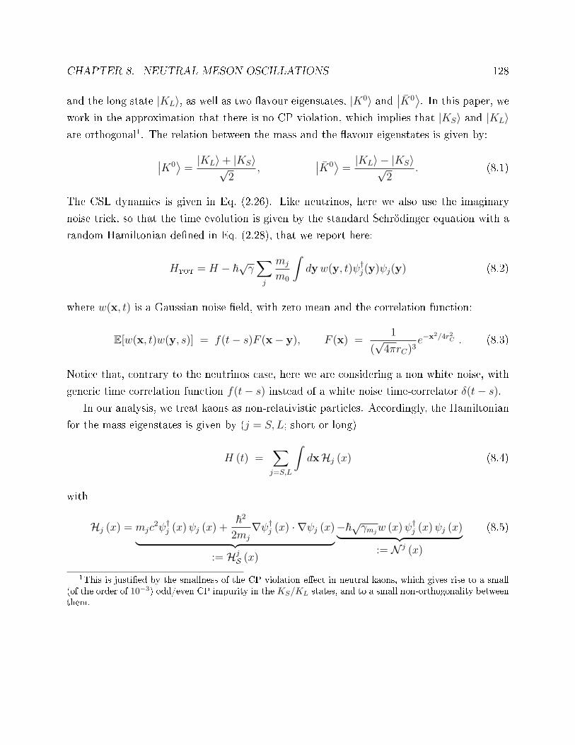
CHAPTER 8. NEUTRAL MESON OSCILLATIONS 128
and the long state |KL〉, as well as two avour eigenstates, |K0〉 and∣∣K0
⟩. In this paper, we
work in the approximation that there is no CP violation, which implies that |KS〉 and |KL〉are orthogonal1. The relation between the mass and the avour eigenstates is given by:
∣∣K0
⟩=
|KL〉+ |KS〉√2
,∣∣K0
⟩=
|KL〉 − |KS〉√2
. (8.1)
The CSL dynamics is given in Eq. (2.26). Like neutrinos, here we also use the imaginary
noise trick, so that the time evolution is given by the standard Schrödinger equation with a
random Hamiltonian dened in Eq. (2.28), that we report here:
HTOT = H − ~√γ∑
j
mj
m0
∫
dyw(y, t)ψ†j(y)ψj(y) (8.2)
where w(x, t) is a Gaussian noise eld, with zero mean and the correlation function:
E[w(x, t)w(y, s)] = f(t− s)F (x− y), F (x) =1
(√4πrC)3
e−x2/4r2C . (8.3)
Notice that, contrary to the neutrinos case, here we are considering a non white noise, with
generic time correlation function f(t− s) instead of a white noise time-correlator δ(t− s).
In our analysis, we treat kaons as non-relativistic particles. Accordingly, the Hamiltonian
for the mass eigenstates is given by (j = S, L; short or long)
H (t) =∑
j=S,L
∫
dxHj (x) (8.4)
with
Hj (x) = mjc2ψ†
j (x)ψj (x) +~2
2mj
∇ψ†j (x) · ∇ψj (x)
︸ ︷︷ ︸
:= HjS (x)
−~√γmj
w (x)ψ†j (x)ψj (x)
︸ ︷︷ ︸
:= N j (x)
(8.5)
1This is justied by the smallness of the CP violation eect in neutral kaons, which gives rise to a small(of the order of 10−3) odd/even CP impurity in the KS/KL states, and to a small non-orthogonality betweenthem.

CHAPTER 8. NEUTRAL MESON OSCILLATIONS 129
and
γmj:= γ
(mj
m0
)2
. (8.6)
The Hamiltonian includes two terms: the standard Schrödinger term HS (x) = HSS (x) +
HLS (x) and the term N (x) = N S (x) + N L (x) which accounts for the collapse. Note that
in HS (x) we have included also the mass terms. These terms are usually ignored, since they
lead only to a constant shift of the energy, which implies no observable eect. For kaons,
where we have a superposition of two dierent mass eigenstates, it is fundamental to keep
those terms.2
In the following, we focus our attention on computing the probability of starting from
a |K0〉 state at time t = 0 and ending up in a∣∣K0
⟩state at a later time t. The other
possible transition probabilities (|K0〉 −→ |K0〉,∣∣K0
⟩−→
∣∣K0
⟩and
∣∣K0
⟩−→ |K0〉) can
be computed in a very similar way. In order to keep the computation as simple as possible,
we assume that the initial state is a plane wave with denite momentum pi. Therefore, the
quantity we wish to compute is:
PK0→K0 (t) =∑
pf
E∣∣⟨K0,pf |U (t)|K0,pi
⟩∣∣2
(8.7)
where we assumed that also the nal state is a momentum eigenstate, and we sum over all
the possible nal states. Here, as usual, E denotes the stochastic average with respect to the
noise of the background eld.
The computation is done in the same way as it has been done in the previous chapter
with neutrinos. We write avour eigenstates as superposition of mass eigenstates, compute
perturbatively the transition amplitude up to the second order and nally compute the
probability PK0→K0 (t) dened in Eq. (8.7). We do not report here this long calculation, since
it is very similar to the one done for neutrinos. However, all the details of this computation
can be found in [50]. The nal result is:
PK0→K0 (t) =1
2
1− cos
[1
~
(
E(L)i − E
(S)i
)
t
] [
1− γ (mS −mL)2
8π3/2r3Cm20
(∫ t
0
dsf (s) (t− s)
)]
,
(8.8)
2Indeed, for most investigations of the kaon phenomenology the kinetic part is not relevant and oneintroduces an eective Hamiltonian with two dierent mass eigenstates [70, 71]

CHAPTER 8. NEUTRAL MESON OSCILLATIONS 130
Similarly we can nd the probability that a K0 remains K0 during the time evolution:
PK0→K0 (t) =1
2
1 + cos
[1
~
(
E(L)i − E
(S)i
)
t
] [
1− γ (mS −mL)2
8π3/2r3Cm20
(∫ t
0
dsf (s) (t− s)
)]
.
(8.9)
The computations starting from an anti-kaon are completely analogous, since we neglected
CP violation. Let us list here two important features:
(1) The probabilities PK0→K0 (t) and PK0→K0 (t) sum up to 1, which means that there are
no particle losses.
(2) The factor after the cosine is due to the CSL noise, i.e. if there is no noise (γ = 0) the
square bracket gives 1 and arrive at the standard oscillations formula3.
Since the eect of the noise is usually very similar to the decoherence [72, 73], and it is
well known from the literature that in such cases decoherence damps the oscillation with an
exponential function, we can consider the term inside the curely bracket as the rst term of
the series of an exponential function. Therefore, we can guess that the transition probability
from a kaon to an anti-kaon could be reasonably given by:
PK0→K0 (pi) =1
2
1− cos
[1
~
(
E(L)i − E
(S)i
)
t
]
· e−
γ(mj−mk)2
8π3/2r3C
m20[∫ t0 dsf(s)(t−s)]
.
(8.10)
To conclude the computation on a single particle, we can include the decay of the particle
adding to the free Hamiltonian HS an imaginary term:
HjS −→ HjS − i
2Γj. (8.11)
This changes the previous computation by sending E(j)i −→ E
(j)i − i
2Γj and one can easily
notice that the only change consists in multiplying each Pkj (pi; t) with the exponential
function e−Γk+Γj
2~t in order to take the decay into account. Thus we obtain the nal result:
PK0→K0 (pi) =1
4
e−ΓL~
t + e−ΓS~
t − 2 cos
[1
~
(
E(L)i − E
(S)i
)
t
]
· e−ΓL+ΓS
2~t · e−ΛCSLt
(8.12)
3In some of these works, inside the cosine, only the mass dierence appears. This is the same result as
ours, if one makes the approximation (good at the non-relativistic level) E(j)i = mjc
2 +p
2
i
2mj≃ mjc
2.

CHAPTER 8. NEUTRAL MESON OSCILLATIONS 131
K-mesons B-mesons Bs-meson D-mesonsΛCSL (s−1) 1.5× 10−38 1.4× 10⁻³⁴ 1.7× 10⁻³¹ 3.2× 10−37
Γ (s−1) 1.2× 10¹⁰ 6.6× 10¹¹ 6.6× 10¹¹ 2.4× 10¹²
Table 8.1: We consider four dierent types of mesons: K-mesons, B-mesons, Bs-meson andD-mesons. For each type, the table shows in the rst line the decay factor as predicted bythe CSL model while in the second line the typical decay widths of these mesons is reported.
where now we have assumed that the noise is white in time, i.e. f(s) = δ(s) and we have
introduced the decay rate:
ΛCSL :=γ (mS −mL)
2
16π3/2r3Cm20
. (8.13)
Notice that the neutrino damping factor ξjk dened in Eq. (7.46) reduces, in the non rela-
tivistic limit, to ΛCSL. The same result holds for the other type of mesons.
Using the stronger value suggested by Adler for γ, namely γ = 10−22cm3s−1 [18], and
recalling that rC = 10−5cm and m0 ≃ 9.4 ·102MeV/c2 [74], we can compute ΛCSL for dierent
types of mesons. The results are reported in Table 8.1: for dierent type of mesons, the
decay factor ΛCSL predicted by the CSL model (rst line) and the observed decay rate Γ
(second line) are shown. Compared to the neutrinos case, we can see that the decay factor
ΛCSL is bigger. This is due to the fact that the typical masses of the mesons are bigger than
neutrinos'. However, the eect is yet too small to be observed, especially when compared to
the typical decay widths of mesons Γ, which are more than forty orders of magnitude bigger
than ΛCSL.
8.2 The Collapse Model for Two Particle States
At the DAΦNE collider [75, 76, 77, 78] neutral kaons are copiously produced in an entangled
antisymmetric state:
|I〉 = |KSKL〉 − |KLKS〉√2
=
∣∣K0K0
⟩−∣∣K0K0
⟩
√2
. (8.14)
We want here to investigate how the mass-proportional CSL model changes the time evolution
of entangled states. In order to obtain a more general result, we performed the computation
for an arbitrary two-particle state. One particle evolves to the left hand side and the other

CHAPTER 8. NEUTRAL MESON OSCILLATIONS 132
particle evolves to the right hand side, for which they need the time tl, tr, respectively. It is
convenient to use the mass basis |KSKS〉, |KSKL〉, |KLKS〉 and |KLKL〉, where the state onthe left hand side is a plane wave with momentum −pi and the one on the right hand side
is a plane wave with momentum pi. In the Fock space framework, this means for example
|KSKL〉 = a†S (−pi) a†K (pi) |Ω〉 with |Ω〉 the vacuum state. Since we are considering only
states with two particles with denite momenta ±pi, the four states above form a complete
basis. So the generic initial state can be decomposed as:
|I〉 =∑
j,k=S,L
αjk |KjKk〉 with∑
j,k=S,L
|αjk|2 = 1 . (8.15)
Let us assume that we want to know the probability of nding the left particle at time
tl in the state |Fl,pl〉 =∑
m=S,L βm |Km,pl〉 and the right particle at time tr in the state
|Fr,pr〉 =∑
n=S,L γn |Kn,pr〉. Here |Fl〉 and |Fr〉 can be mass or avour eigenstates. In
the end we have to sum over all pl and all pr since we are interested in a result which is
independent from a particular nal momentum of the particles. We start by computing the
amplitude:
A (Fl,pl;Fr,pr) = 〈Fl,pl;Fr,pr |ULEFT (tl)⊗ URIGHT (tr)| I〉 ==
∑
j,k=S,L
αjk 〈Fl,pl |Uj (tl)|Kj,−pi〉 〈Fr,pr |Uk (tr)|Kk,pi〉 =
=∑
j,k,m,n=S,L
αjkβ∗mγ
∗n 〈Km,pl |Uj (tl)|Kj,−pi〉 〈Kn,pr |Uk (tr)|Kk,pi〉 =
=∑
j,k=S,L
αjkβ∗j γ
∗k 〈Kj,pl |Uj (tl)|Kj,−pi〉 〈Kk,pr |Uk (tr)|Kk,pi〉 , (8.16)
because it gives the probability we are interested in, as follows:
P (Fl;Fr) :=∑
pl,pr
E |A (Fl,pl;Fr,pr)|2 =∑
j,k,j′,k′=S,L
αjkβ∗j γ
∗kα
∗j′k′βj′γk′
× E
[∑
pl
〈Kj′ ,pl |Uj′ (tl)|Kj′ ,−pi〉∗ 〈Kj,pl |Uj (tl)|Kj,−pi〉]
×[∑
pr
〈Kk′ ,pr |Uk′ (tr)|Kk′ ,pi〉∗ 〈Kk,pr |Uk (tr)|Kk,pi〉]
. (8.17)
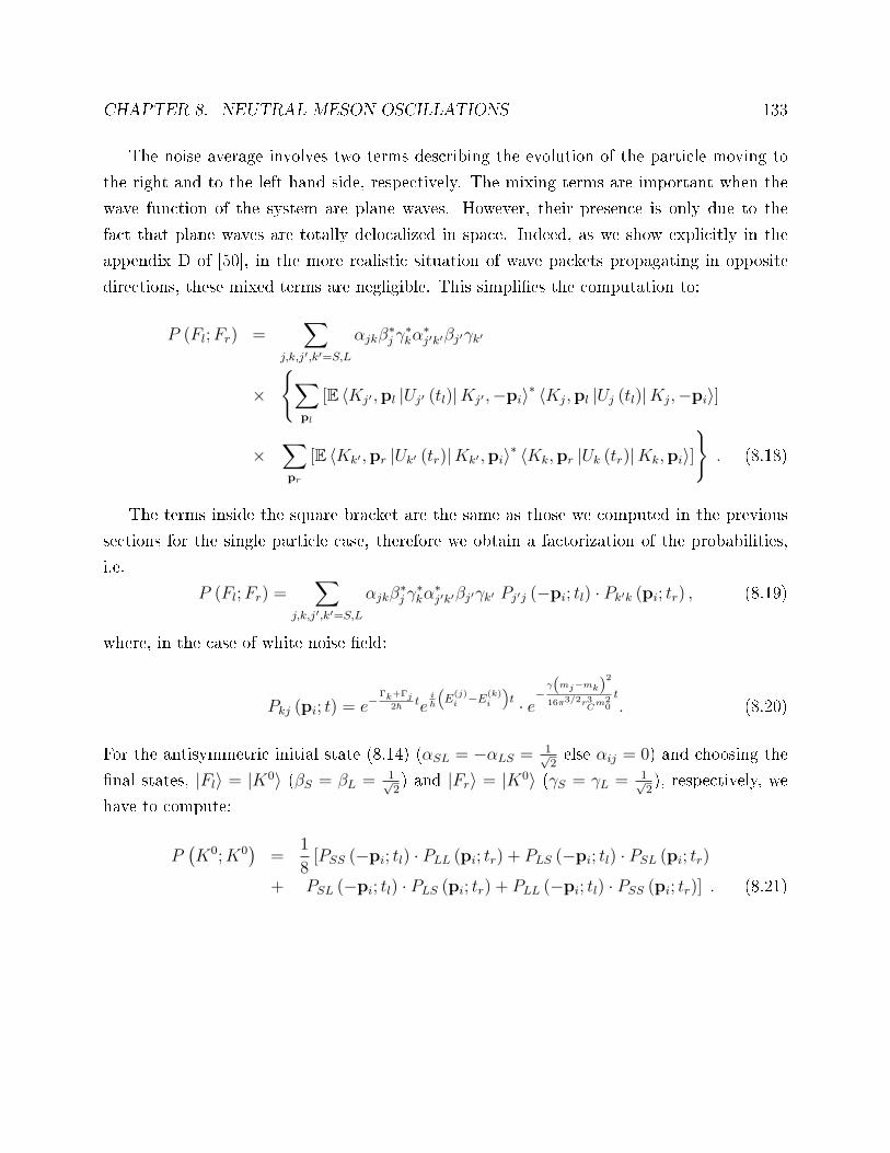
CHAPTER 8. NEUTRAL MESON OSCILLATIONS 133
The noise average involves two terms describing the evolution of the particle moving to
the right and to the left hand side, respectively. The mixing terms are important when the
wave function of the system are plane waves. However, their presence is only due to the
fact that plane waves are totally delocalized in space. Indeed, as we show explicitly in the
appendix D of [50], in the more realistic situation of wave packets propagating in opposite
directions, these mixed terms are negligible. This simplies the computation to:
P (Fl;Fr) =∑
j,k,j′,k′=S,L
αjkβ∗j γ
∗kα
∗j′k′βj′γk′
×∑
pl
[E 〈Kj′ ,pl |Uj′ (tl)|Kj′ ,−pi〉∗ 〈Kj,pl |Uj (tl)|Kj,−pi〉]
×∑
pr
[E 〈Kk′ ,pr |Uk′ (tr)|Kk′ ,pi〉∗ 〈Kk,pr |Uk (tr)|Kk,pi〉]
. (8.18)
The terms inside the square bracket are the same as those we computed in the previous
sections for the single particle case, therefore we obtain a factorization of the probabilities,
i.e.
P (Fl;Fr) =∑
j,k,j′,k′=S,L
αjkβ∗j γ
∗kα
∗j′k′βj′γk′ Pj′j (−pi; tl) · Pk′k (pi; tr) , (8.19)
where, in the case of white noise eld:
Pkj (pi; t) = e−Γk+Γj
2~te
i~
(
E(j)i −E
(k)i
)
t · e−
γ(mj−mk)2
16π3/2r3C
m20
t. (8.20)
For the antisymmetric initial state (8.14) (αSL = −αLS = 1√2else αij = 0) and choosing the
nal states, |Fl〉 = |K0〉 (βS = βL = 1√2) and |Fr〉 = |K0〉 (γS = γL = 1√
2), respectively, we
have to compute:
P(K0;K0
)=
1
8[PSS (−pi; tl) · PLL (pi; tr) + PLS (−pi; tl) · PSL (pi; tr)
+ PSL (−pi; tl) · PLS (pi; tr) + PLL (−pi; tl) · PSS (pi; tr)] . (8.21)

CHAPTER 8. NEUTRAL MESON OSCILLATIONS 134
with Pkj (pi; t) (j, k = S or L) given in Eq. (8.20). Collecting all pieces, we get:
P(K0;K0
)=
1
8
e−ΓS~
tl−ΓL~
tr + e−ΓL~
tl−ΓS~
tr
+ 2 · cos[1
~
(
E(S)i − E
(L)i
)
(tr − tl)
]
· e−ΓL+ΓS
2~(tl+tr) e
− γ(mS−mL)2
16π3/2r3C
m20
(tl+tr)
︸ ︷︷ ︸
The CLS eect
.(8.22)
We can see that the eect of the collapse is the same as the one found for one particle, with
the only dierence that in the exponenzial there is the sum of the two detection times tl and
tr. The same result can be found using separable states. The reason why entaglement does
not play any special role in this phenomena is that the noise acts independently on each mass
eigenstates.
8.3 Conclusions
Our computations show that the oscillation terms are aected by an exponential damping
due to the interaction with the CSL noise eld. The value of this damping is larger than the
one found for neutrinos, but yet too small to be observed in experiments. Moreover, contrary
to neutrinos, mesons decay and the typical time scale of the decay is smaller than the one
necessary to see any CSL eect. We computed also the case of bipartite entangled systems
where we found that the eect of CSL factorizes, i.e. each meson is aected separately and
independently of the initial state they share.

Chapter 9
Acknowledgements
I wish to thank Dr. A. Bassi for having read the thesis manuscript, but even more for having
been a great supervisor from the scientic and the human points of view. Besides having
helped me in doing research in these three years, Angelo gave me the opportunity of having
a lot of interesting experiences. In the future, when I will look back at this period, I will
have for sure a good memory.
I wish to thank Dr. M. Bahrami for having patiently read and corrected many times the
draft of my thesis. Dealing with my drafts in English, especially the rst ones, is not an easy
task.
I wish to thank Prof. S. L. Adler and Dr. D.-A. Deckert for sharing the work experience
on the radiation emission in collapse models. I also wish to thank Dirk for the great time we
had together in Davis.
I wish to thank Dr. L. Ferialdi, Dr. C. Curceanu, Prof. A. Di Domenico and Dr. B. C.
Hiesmayr for the useful conversations and the work we did together on avour oscillations
in collapse models. In particular I wish to thank Luca for all the nice experiences we had
together in the last three years and Catalina for having invited me and Angelo many times
in Frascati, where we always had very good times.
I wish to thank Prof. T. P. Singh, Dr. K. Lochan and Dr. S. Das for having taught
me more about cosmological implications of collapse models and for having given me the
opportunity of visiting India.
I wish to thank Prof. A. Buchleitner for having invited me to visit his group in Freiburg,
where I learned more about quantum optics.
I wish to thank G. Gasbarri, Dr. A. Smirne, M. Carlesso, M. Schiulaz and Dr. K.
135

CHAPTER 9. ACKNOWLEDGEMENTS 136
Piscicchia, for the many useful conversations we had about physics and for the good free
time we had together.
Desidero ringraziare la mia famiglia, in particolare i miei genitori Antonella ed Eros, mia
sorella Lisa, mio zio Patrizio e mia nonna Rina per avermi supportato e per essermi stati
sempre vicini nella vita.
To conclude, I wish to thank all the friends (no names here, you are too much!) and the
good people who I had the luck to meet in my life. Hope to see you soon and have a beer
together!

Chapter 10
APPENDICES
Appendix A: Calculation of the natural linewidth for a
harmonic oscillator
The starting point is the equation for the imaginary part of the energy shift which, in case
of the non relativistic electromagnetic interaction is given in [42]:
Ei = −π∑
λ
∫
dk∑
n
|〈k, λ;n |Hint|Ω; i〉|2 δ (Ei − En − ~ωk) . (10.1)
We work in dipole approximation, so that Hint is:
Hint = − e
mA · p = − e
m
∑
λ
∫
dkαk
(
ak,λ + a†k,λ
)
(ǫk,λ · p) . (10.2)
Then Eq. (10.1) becomes:
Ei = −( e
m
)2
π∑
λ
∫
dkα2k
∑
n
|〈n |ǫk,λ · p| i〉|2 δ (Ei − En − ~ωk) (10.3)
= −( e
m
)2
π∑
λ
∫
dkα2k
∑
n
〈i |ǫk,λ · p|n〉 〈n |δ (Ei −H0 − ~ωk) ǫk,λ · p| i〉
= −( e
m
)2
π∑
λ
∫
dkα2k 〈i |ǫk,λ · pδ (Ei −H0 − ~ωk) ǫk,λ · p| i〉
where in the third line we used the completeness over the states n.
137

CHAPTER 10. APPENDICES 138
It is now convenient to write the momentum operator p in terms of the raise and lower
operators b†j and bj, where j labels the three spatial components. Then we get:
ǫk,λ · p =∑
j
ǫjk,λi
√
mω0~
2
[
b†j − bj
]
(10.4)
Substituting in the above equation and using the relation:
∑
λ
∫
dΩkǫjkλǫ
j′
kλ =8
3πδjj′ , (10.5)
we obtain
Ei = −( e
m
)2
π
(
−mω0~
2
)(8
3π
)∫
dk k2α2k
∑
j
⟨
i∣∣∣
(
b†j − bj
)
δ (Ei −H0 − ~ωk)(
b†j − bj
)∣∣∣ i⟩
.
(10.6)
It is straightforward to show that the matrix element is:
⟨
i∣∣∣
(
b†j − bj
)
δ (Ei −H0 − ~ωk)(
b†j − bj
)∣∣∣ i⟩
= − (ij + 1) δ (~ω0 + ~ωk)− ijδ (~ω0 − ~ωk) ,
(10.7)
where ij with j = 1, 2, 3 is one of the three quantum numbers which identify the initial state
energy, i.e. Ei = ~ω0
(32+ i1 + i2 + i3
). Therefore Eq. (10.6) becomes:
Ei = −( e
m
)2
π
(
−mω0~
2
)(8
3π
)1
c3
∫
dωk ω2k
(~
2ε0ωk (2π)3
)
× (10.8)
×∑
j
[− (ij + 1) δ (~ω0 + ~ωk)− ijδ (~ω0 − ~ωk)] ,
where we used α2k =
~
2ε0ωk(2π)3 and we did the change of variable k → ωk = kc. The rst delta
function never contributes, then Eq. (10.8) becomes:
Ei = −( e
m
)2
π(mω0
2
)(8
3π
)1
c3
(~
2ε0 (2π)3
)
ω0
[∑
j
ij
]
= −~
(βω2
0
2m
)∑
j
ij (10.9)
where we introduced β = e2
6c3πε0. The decay is proportional to −Ei
~=(
βω20
2m
)∑
j ij, therefore
it is proportional to the decay encountered in chapters 4 and 5, see Eq. (4.16) and Eq. (4.24).

CHAPTER 10. APPENDICES 139
Appendix B: Estimation of the decay rate by dimensional
analysis.
Here we discuss about the possibility of estimating the predictions of the CSL model in
neutrino oscillations by using dimensional analysis. Collapse models are described by the
same type of master equations as open quantum systems (which experience decoherence due
to interactions with an external environment). It is well known that the eect of decoherence
is to suppress exponentially avour oscillations. So it does not come as a surprise that for
collapse models the eect is also a damping. Then one could try to guess the decay rate
with dimensional analysis, using the relevant constants and parameters of the model. First
of all it is reasonable to assume that the eect is proportional to the strength of the noise γ.
Moreover, since we are using the mass proportional CSL model, for which γ is replaced by
γmj:= γ
(mj
m0
)2
, one expects also a factor m20 in the denominator. Because [γ] = cm3s−1, and
the decay rate must have the dimension s−1, we need to introduce terms with the dimension
cm−3. Since the parameter rC has the dimension of a length, then it is natural to introduce
an r3C in the denominator. Finally, we need to introduce terms with the dimension of a
squared mass. The simplest choices are:
ξ(1)jk ∼ γ
r3Cm20
(mj −mk)2 or ξ
(2)jk ∼ γ
r3Cm20
(m2
j −m2k
). (10.10)
Both formulas are dierent from the correct one given in Eq. (7.46). If we substitute the
values of the constants and the parameters, e.g., for the cosmological neutrinos we get:
ξ(1)jk tcosm ∼ γ
r3Cm20
(mj −mk)2 tcosm ∼ 10−17 (10.11)
ξ(2)jk tcosm ∼ γ
r3Cm20
(m2
j −m2k
)tcosm ∼ 10−11 (10.12)
The formula derived with dimensional analysis shows that the CSL eect on neutrino oscilla-
tions is very small, practically undetectable. However, it diers by many orders of magnitude
from the correct result (which is given in the third line of table 7.1). We performed the lengthy
calculation presented in chapter 7 in order to arrive at a fully trustable result. As we showed
here, dimensional analysis does not allow to reach a trustable conclusion.
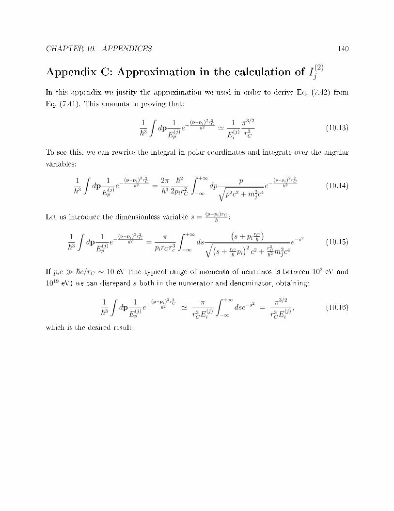
CHAPTER 10. APPENDICES 140
Appendix C: Approximation in the calculation of I(2)j
In this appendix we justify the approximation we used in order to derive Eq. (7.42) from
Eq. (7.41). This amounts to proving that:
1
~3
∫
dp1
E(j)p
e−(p−pi)
2r2C
~2 ≃ 1
E(j)i
π3/2
r3C(10.13)
To see this, we can rewrite the integral in polar coordinates and integrate over the angular
variables:
1
~3
∫
dp1
E(j)p
e−(p−pi)
2r2C
~2 =2π
~3
~2
2pir2C
∫ +∞
−∞dp
p√
p2c2 +m2jc
4e−
(p−pi)2r2C
~2 (10.14)
Let us introduce the dimensionless variable s = (p−pi)rC~
:
1
~3
∫
dp1
E(j)p
e−(p−pi)
2r2C
~2 =π
pirCr3c
∫ +∞
−∞ds
(s+ pi
rC~
)
√(s+ rC
~pi)2c2 +
r2C~2m2
jc4
e−s2 (10.15)
If pic ≫ ~c/rC ∼ 10 eV (the typical range of momenta of neutrinos is between 103 eV and
1019 eV) we can disregard s both in the numerator and denominator, obtaining:
1
~3
∫
dp1
E(j)p
e−(p−pi)
2r2C
~2 ≃ π
r3CE(j)i
∫ +∞
−∞dse−s2 =
π3/2
r3CE(j)i
, (10.16)
which is the desired result.

CHAPTER 10. APPENDICES 141
Appendix D: Approximation in the calculation of I(1)jk
Here we justify the approximation we used to pass from Eq. (7.38) to Eq. (7.39). We start
with Eq. (7.38):
I(1)jk (pi, si; t) =
∑
sf
∫
dpf√γmj
γmk
mjmkc4
√
E(j)i E
(j)f E
(k)i E
(k)f
u(p(j)f , sf )u(p
(j)i , si)u(p
(k)i , si)u(p
(k)f , sf )
× 1− ei~
(
E(k)f −E
(k)i −E
(j)f +E
(j)i
)
t
i~(E
(j)f − E
(j)i − E
(k)f + E
(k)i )
1
(2π~)3e−
(pf−pi)2r2C
~2 (10.17)
where:
E(j)f =
√
p2fc
2 +m2jc
4 , u (p, s) =pµγµc+mc2
√
2mc2 (Ep +mc2)u (0, s) and
√γmj
=√γmj
m0
(10.18)
The rst part of the integrand:
mjmkc4
√
E(j)i E
(j)f E
(k)i E
(k)f
∑
sf
u(p(j)f , sf )u(p
(j)i , si)u(p
(k)i , si)u(p
(k)f , sf ) (10.19)
is a composition of polynomial functions of pf , and we can safely assume that it does not
change too much, in the region where the Gaussian function is appreciably dierent from
zero. Therefore we can then take pf = pi; by using also the relation:
u(p(1)i , sf )u(p
(1)i , si) = δsf ,si , (10.20)
then Eq. (10.17) becomes:
I(1)jk (pi, si; t) ≃ √
γmjγmk
mjmkc4
E(j)i E
(k)i
1
(2π~)3
∫
dpf1− e
i~(E
(k)f −E
(k)i −E
(j)f +E
(j)i )t
i~(E
(j)f − E
(j)i − E
(k)f + E
(k)i )
e−(pf−pi)
2r2C~2
︸ ︷︷ ︸
:=I
(10.21)
Now we have to focus our attention on the integral I, which contains an oscillating term that
needs special care. As before, we write the integral in polar coordinates and perform the
integration over the angular variables; moreover, we introduce once again the a-dimensional

CHAPTER 10. APPENDICES 142
variable s =(pf−pi)rC
~. We have:
I = π~3
pir3Ct
∫ +∞
−∞ds
(~
rCs+ pi
)eig(s) − 1
ig (s)e−s2 , (10.22)
where we have dened:
g (s) :=1
~(E
(k)f − E
(k)i − E
(j)f + E
(j)i )t
=ct
rC
(√
(s+ y)2 + ak −√
(s+ y)2 + aj −√
y2 + ak +√
y2 + aj
)
, (10.23)
with
aj :=r2C~2m2
jc2 =
(10−2eV−2
)m2
jc4 e y :=
rC~pi =
(10−1eV−1
)pic (10.24)
Our goal is to show that g (s) does not vary appreciably, within the range where the Gaussian
term is signicantly dierent from zero, and can be approximated with g (0) = 0; in this way,
the integral can be computed exactly. This kind of approximation is not obvious because the
factor ct/rC in front of Eq. (10.23) can be very large.
In the ultra-relativistic limit, we approximate the particle's velocity with the speed of
light. In this limit, y2 ≫ aj, ak, and so we can expand the square roots in g(s) using the
Taylor series√x+ ǫ =
√x+ ǫ
2√xand we get:
g (s) ≃ ct
rC(aj − ak)
s
(s+ y) y=ct
rC
(aj − ak)(
y + y2
s
) . (10.25)
In order for g(s) to remain small within the interval where the Gaussian term of Eq. (10.22)
is appreciably dierent from zero, we need:
(
y +y2
s
)
≫ ct
rC(aj − ak) (10.26)
In all physically interesting situations, the term on the right hand side of Eq. (10.26) is
bigger than 1; moreover s is of the order of unity, because of the Gaussian in Eq. (10.22).
Inequality (10.26) is veried if the following condition is true:
y ≫√ct
rC(aj − ak). (10.27)

CHAPTER 10. APPENDICES 143
Typically, cosmogenic neutrinos have energies bigger than 1018eV and travel distances of at
most 109 light-years [25]. This means that, in the worst case, ct/rC ∼ 1032 while (aj − ak)
= (10−2eV−2) (m2jc
4 −m2kc
4) ≃ (10−2eV−2)(2× 10⁻³eV2) = 10−5. So we must have y ≫ 1014,
that means pic = y/(10−1eV−1) ≫ 1015eV, which is satised.
For atmospheric neutrinos, ct/rC is in the range 1011 − 1014 while the range of energies is
between 10−1GeV and 104GeV [80]. This means that, even in the worse case, the condition
to check is y ≫ 105, which means pic = y/(10−1eV−1) ≫ 106eV. This is also satised.
Appendix E: Kaon Phenomenology
The phenomenology of oscillation and decay of meson-antimeson systems can be described
by nonrelativistic quantum mechanics eectively, because the dynamics depends on the ob-
servable hadrons rather than on the more fundamental quarks. A quantum eld theoretical
calculation showing negligible corrections that can be found, e.g., in Refs. [53, 79].
A neutral meson M0 is a bound state of quark and antiquark. As numerous experiments
have revealed the particle stateM0 and the antiparticle state M0 can decay into the same nal
states, thus the system has to be handled as a two state system similar to spin 12systems. In
addition to being a decaying system these massive particles show the phenomenon of avour
oscillation, i.e. an oscillation between matter and antimatter occurs. If e.g. a neutral meson
is produced at time t = 0 the probability to nd an antimeson at a later time is nonzero.
The most general time evolution for the two state systemM0−M0 including all its decays
is given by an innitedimensional vector in Hilbert space:
|ψ(t)〉 = a(t)|M0〉+ b(t)|M0〉+ c(t)|f1〉+ d(t)|f2〉+ . . . (10.28)
where fi denote all decay products and the state |ψ(t)〉 is a solution of the Schrödinger
equation (~ := 1):
d
dt|ψ(t)〉 = −iH|ψ(t)〉 (10.29)
where H is an innite-dimensional Hamiltonian operator. There is no known method about
how to solve this innite set of coupled dierential equations aected by strong dynamics.
The usual procedure is based on restricting to the time evolution of the components of the
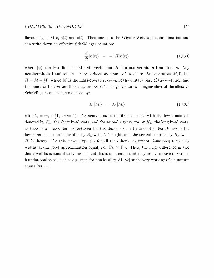
CHAPTER 10. APPENDICES 144
avour eigenstates, a(t) and b(t). Then one uses the Wigner-Weisskopf approximation and
can write down an eective Schrödinger equation:
d
dt|ψ(t)〉 = −i H|ψ(t)〉 (10.30)
where |ψ〉 is a two dimensional state vector and H is a non-hermitian Hamiltonian. Any
non-hermitian Hamiltonian can be written as a sum of two hermitian operators M,Γ, i.e.
H =M + i2Γ, where M is the mass-operator, covering the unitary part of the evolution and
the operator Γ describes the decay property. The eigenvectors and eigenvalues of the eective
Schrödinger equation, we denote by:
H |Mi〉 = λi |Mi〉 (10.31)
with λi = mi +i2Γi (c := 1). For neutral kaons the rst solution (with the lower mass) is
denoted by KS, the short lived state, and the second eigenvector by KL, the long lived state,
as there is a huge dierence between the two decay widths ΓS ≃ 600ΓL. For B-mesons the
lower mass solution is denoted by BL with L for light, and the second solution by BH with
H for heavy. For this meson type (as for all the other ones except K-mesons) the decay
widths are in good approximation equal, i.e. ΓL ≃ ΓH . Thus, the huge dierence in two
decay widths is special to K-mesons and this is one reason that they are attractive to various
foundational tests, such as e.g. tests for non locality [81, 82] or the very working of a quantum
eraser [83, 84].

Bibliography
[1] "I'm inclined to put my money on the idea that if you push quantum mechanics hard
enough it will break down and something else will take over - something we can't envisage
at the moment"A. J. Leggett, in m. Brooks, New Scientist 2766, (2010).
[2] S. Weinberg, Phys. Rev. A 85, 062116 (2012).
[3] C. J. Davisson and L. H. Germer, Nature 119, 558â560 (1927).
[4] H. v. Jr Halban and P. Preiswerk, C.R. Acad. Sci. 203, 73â75 (1936).
[5] W. Schöllkopf and J. P. Toennies, Science 266, 1345â1348 (1994).
[6] M. Arndt, O. Nairz, J. Vos-Andreae, C. Keller, G. van der Zouw and A. Zeilinger, Nature
401, 680 (1999).
[7] L. Hackermüller, K. Hornberger, B. Brezger, A. Zeilinger and M. Arndt, Nature 427,
711 (2004).
[8] S. Gerlich, S. Eibenberger, M. Tomandl, S. Nimmrichter, K. Hornberger, P. J. Fagan, J.
Tüxen, M. Mayor and M. Arndt, Nature Comm. 2, 263 (2011).
[9] J. S. Bell., Against Measurement, Physics World, 33-35 (1990).
[10] D. Bohm, Phys. Rev. 85, 166 (1952a).
[11] D. Bohm, Phys. Rev. 85, 180 (1952b).
[12] D. Dürr and S. Teufel, Bohmian Mechanics, Springer (2009).
[13] D. Dürr and S. Goldstein, Quantum physics without quantum philosophy, Springer
(2012).
145

BIBLIOGRAPHY 146
[14] G.C. Ghirardi, A. Rimini and T. Weber, Phys. Rev. D 34, 470 (1986).
[15] G.C. Ghirardi, P. Pearle and A. Rimini, Phys. Rev. A 42, 78 (1990).
[16] A. Bassi and G.C. Ghirardi, Phys. Rept. 379, 257 (2003).
[17] A. Bassi, K. Lochan, S. Satin, T. P. Singh and H. Ulbricht, Rev. Mod. Phys. 85, 471-527
(2013).
[18] S.L. Adler, J. Phys. A 40, 2935 (2007). Ibid. A 40, 13501 (2007).
[19] S.L. Adler and A. Bassi, Science 325, 275 (2009).
[20] Q. Fu, Phys. Rev. A 56, 1806 (1997).
[21] S.L. Adler and F.M. Ramazanoglu, J. Phys. A 40, 13395 (2007); J. Phys. A 42, 109801
(2009).
[22] A. Bassi and D. Dürr, J. Phys. A 42, 485302 (2009).
[23] S.L. Adler, A. Bassi and S. Donadi, J. Phys. A 46, 245304 (2013).
[24] J.J. Sakurai, S.F. Tuan, Modern Quantum Mechanics, Addison-Wesley Publishing Com-
pany (1994).
[25] J. Christian, Phys. Rev. Lett. 95, 160403 (2005).
[26] N. Gisin, Hel. Phys. Acta 62, 363 (1989).
[27] A. Bassi, D. Duerr and G. Hinrichs, Phys. Rev. Lett. 111, 210401 (2013).
[28] L. Diósi, Phys. Rev. A 40, 1165 (1989); 42, 5086 (1990).
[29] B. Vacchini, J. Phys. A: Math. Theor. 40, 2463-2473 (2007).
[30] S.L. Adler, A. Bassi, J. Phys. A 40, 15083 (2007).
[31] L. Arnold, Stochastic dierential equations: theory and applications, Wiley-Interscience,
New York, (1974).
[32] R. Penrose, Gen. Rel. Grav. 28, 581 (1996).
BIBLIOGRAPHY 147
[33] R. Penrose, in Mathematical Physics 2000, ed. by A. Fokas et al., Imperial College ,
London, (2000).
[34] L. Diósi, Phys. Rev. A 40, 1165 (1989).
[35] M. Bahrami, A. Bassi and H. Ulbricht, arXiv:1309.5889 (2013).
[36] E.J. Squires, Phys. Lett. A 158, 431 (1991).
[37] P. Pearle and E. Squires, Phys. Rev. Lett. 73, 1 (1994).
[38] B. Collett, P. Pearle, F. Avignone and S. Nussinov, Found. Phys. 25, 1399 (1995).
[39] W. Greiner, J. Reinhardt, Field Quantization, Springer (1996).
[40] In this way we also correct a typo in Eq. (41) of [22].
[41] A. Bassi and S. Donadi, unpublished calculations on the spontaneous photon emission
in the QMUPL model computed using perturbative technique.
[42] W. Greiner, Quantum Mechanics: special chapters, Springer (1998).
[43] J.J. Sakurai, Advanced Quantum Mechanics, Hardcover, (1967).
[44] R.P. Feynman, A.R. Hibbs Quantum Mechanics and Path Integrals, Emended Edition,
(1965).
[45] P. Moretti, American Journal of Physics 56, 172-174 (1988).
[46] L. Wolfenstein, Phys. Rev. D 17, 2369 (1978).
[47] S. P. Mikheyev and A. Yu. Smirnov, Sov. J. Nucl. Phys. 42, 913 (1985).
[48] G.C. Ghirardi, R. Grassi, A. Rimini, Phys. Rev. A 42, 1057 (1990).
[49] W. Greiner, Relativistic quantum mechanics - wave equations, Springer (2000).
[50] S. Donadi, A. Bassi, C. Curceanu, A. Di Domenico, B. C. Hiesmayr, Found. Phys. 43,
813-844 (2013).
[51] R. Tumulka, J. Stat. Phys. 125, 821 (2006).

BIBLIOGRAPHY 148
[52] D. J. Bedingham, Found. Phys. 41, 686 (2011).
[53] M. Beuthe, Physics Reports 375, 105 (2003).
[54] W. Greiner, Quantum Electrodynamics 3Ed, Springer (2003).
[55] R.A. Bertlmann, K. Durstberger, B. C. Hiesmayr, Phys. Rev. A 68, 012111 (2003).
[56] S.L. Adler, Phys. Rev. D 62, 117901 (2000).
[57] F. Benatti, R. Floreanini, Phys. Rev. D 71, 013003 (2005).
[58] E. Lisi, A. Marrone, D. Montanino, Phys. Rev. Lett. 85, 1166 (2000).
[59] G.L. Fogli, E. Lisi, A. Marrone, D. Montanino, Phys. Rev. D 67, 093006 (2003).
[60] K. Nakamura et al, J. Phys. G: Nucl. Part. Phys. 37, 075021 (2010).
[61] V. N. Aseev, A. I. Belesev, A. I. Berlev, E. V. Geraskin, A. A. Golubev, N. A. Likhovid,
V. M. Lobashev, A. A. Nozik, V. S. Pantuev, V. I. Parfenov, A. K. Skasyrskaya, F. V.
Tkachov, and S. V. Zadorozhny, Phys. Rev. D 84, 112003 (2011).
[62] L. Diósi, Braz. Journ. Phys. 35, 260 (2005).
[63] L. Stodolsky, Phys. Rev. D 36, 2273 (1987).
[64] W. J. Marciano, Z. Parsa, J. Phys. G 29, 2629 (2003).
[65] E. G. Flowers, P. G. Sutherland, Astrophys. J. 208, L19 (1976).
[66] G. L. Fogli et al., Phys. Rev. D 76, 033006 (2007).
[67] see e.g. R.D. McKeown, P. Vogel, Phys. Rept. 394, 315-356 (2004) and references therein.
[68] M. Gell-Mann and A. Pais, Phys. Rev. 97, 1387 (1955).
[69] A. Pais and O. Piccioni, Phys. Rev. 100, 1487 (1955).
[70] B.C. Hiesmayr, European Physical Journal C 50, 73 (2007).
[71] R.A. Bertlmann, B.C. Hiesmayr, Quantum Information Processing 5, 421 (2006).
BIBLIOGRAPHY 149
[72] F. Benatti, R. Floreanini, R. Romano, Phys. Rev. D 68, 094007 (2003).
[73] R.A. Bertlmann, K. Durstberger and B.C. Hiesmayr, Phys. Rev. A 68, 012111 (2003).
[74] K. Nakamura et al. (Particle Data Group), J. Phys. G 37, 075021 (2010).
[75] F. Ambrosino et al., KLOE collaboration, Phys. Lett. B 642, 315 (2006).
[76] G. Amelino-Camelia et.al., European Physical Journal C 68, Number 3-4, 619 (2010).
[77] A. Di Domenico, J. Phys.: Conf. Ser. 171, 012008 (2009).
[78] Di Domenico, A. & KLOE coll., Found. Phys. 40, 852 (2010).
[79] A. Capolupo, C.-R. Ji, Y. Mishchenko and G. Vitiello, Phys. Lett. B 594, 135 (2004).
[80] C. Giunti and C. W. Kim, Fundamentals of neutrino physics and astrophysics, Oxford
University Press (2007).
[81] B.C. Hiesmayr, A. Di Domenico, C. Curceanu, A. Gabriel, M. Huber, J.-A. Larsson and
P. Moskal, European Physical Journal C 72, 1856 (2012).
[82] M. Genovese, Phys. Rev. A 69, 022103 (2004).
[83] A. Bramon, G. Garbarino and B.C. Hiesmayr, Phys. Rev. A 69, 062111 (2004).
[84] A. Bramon, G. Garbarino and B.C. Hiesmayr, Phys. Rev. A 69, 022112 (2004).