Embed Size (px)
Citation preview

Electromagnetic Techniques for On-line
Inspection of Steel Microstructure
A thesis submitted to The University of Manchester
for the degree of Doctor of Philosophy
in the Faculty of Engineering and Physical Sciences
2013
Wenqian Zhu
School of Electrical and Electronic Engineering

2
List of Contents
LIST OF CONTENTS ............................................................................................................. 2
LIST OF FIGURES ................................................................................................................. 6
LIST OF TABLE ................................................................................................................... 11
ABSTRACT ............................................................................................................................ 12
DECLARATION.................................................................................................................... 13
COPYRIGHT STATEMENT ............................................................................................... 14
ACKNOWLEDGEMENT ..................................................................................................... 15
CHAPTER 1 INTRODUCTION .......................................................................................... 16
1.1. INDUSTRIAL CONTEXT OF THE RESEARCH ..................................................................................... 16
1.1.1. Monitoring the hot transformation of strip steel.................................................... 16
1.1.2. Assessing decarburisation of rail........................................................................... 18
1.2. OBJECTIVES .......................................................................................................................................... 19
1.3. CONTRIBUTIONS .................................................................................................................................. 20
1.4. ORGANISATION OF THIS THESIS ....................................................................................................... 20
1.5. PUBLISHED OUTPUT FROM THIS STUDY TO DATE ......................................................................... 22
CHAPTER 2 STEEL PHASE TRANSFORMATION ....................................................... 24
2.1. STEEL STRIP PROCESSING ................................................................................................................. 24
2.2. PHASE TRANSFORMATION OF PURE IRON: -IRON AND -IRON ............................................ 26
2.3. STEEL PHASE TRANSFORMATION ..................................................................................................... 27
2.3.1. Equilibrium Temperature Analysis ........................................................................ 28
2.3.1.1. Phase diagram for 3Fe C ................................................................................. 28
2.3.1.2. Medium carbon ............................................................................................... 31
2.3.1.3. High carbon ..................................................................................................... 33
2.3.2 Dynamic cooling ..................................................................................................... 34
2.3.2.1. Grain evolution ............................................................................................... 34
2.3.2.2. Typical Transformation of carbon steel .......................................................... 35
2.3.2.3. Pearlitic Transformation ................................................................................. 37
2.3.2.4. Bainitic Transformation .................................................................................. 37
2.3.2.5. Martensitic Transformation ............................................................................ 39

3
2.3.2.6 Relative properties of Bainite/Pearlite/Martensite ........................................... 41
2.3.2.7 Dual-phase (DP) steel and its mechanical property ......................................... 43
2.4. SUMMARY ............................................................................................................................................. 45
CHAPTER 3 MAGNETISM AND MAGNETIC PROPERTIES ..................................... 46
3.1 BULK MAGNETIC EFFECTS ................................................................................................................. 46
3.1.1Paramagnetism ........................................................................................................ 46
3.1.2 Ferromagnetism ...................................................................................................... 47
3.1.2.1 Domain Formation ........................................................................................... 47
3.1.2.2 The influence of applied fields ........................................................................ 51
3.1.2.3 Temperature effects upon magnetic properties ................................................ 54
3.1.2.4 Solute Atom Content........................................................................................ 55
3.2 FUNDAMENTAL EM RELATIONSHIPS ............................................................................................... 57
3.2.1 Maxwell’s Equations ............................................................................................... 57
3.2.2 Harmonic consideration ......................................................................................... 59
3.2.3 Spatial Implication .................................................................................................. 60
3.2.4 Boundary Conditions .............................................................................................. 61
3.3 EDDY CURRENT THEORY .................................................................................................................... 63
3.4 SUMMARY .............................................................................................................................................. 65
CHAPTER 4 INVESTIGATION OF THE EM SENSOR RESPONSE ........................... 66
4.1 TRANSDUCTION CHAIN BETWEEN STEEL MICROSTRUCTURE AND SENSOR OUTPUT ............. 66
4.1.1 The link between steel microstructure and EM properties ..................................... 66
4.1.1.1 Theoretical method to find relationship between fraction transformed and EM
property ........................................................................................................................ 67
4.1.1.2 FEM modeling and the electrostatics and magneto-static analogy .................. 68
4.1.2 Link between fraction transformed and sensor output ........................................... 72
4.1.2.1 Investigation on the relationship between trans-impedance and ferrite fraction
...................................................................................................................................... 72
4.1.2.2 Impedance spectrum ........................................................................................ 80
4.1.2.3 Peak frequency for the imaginary part and zero-crossing frequency for real
inductance .................................................................................................................... 81
4.2 APPLICATION OF EM SENSOR IN NDT ............................................................................................ 91
4.2.1 Thickness measurement of none-magnetic plates using multi-frequency eddy
current sensor. ................................................................................................................. 91

4
4.2.1.1 Analytical solution for an air-cored sensor on a conducting plate and two
limiting cases 0 and . .......................................................................................... 91
4.2.1.2 Simulation and experiment results ................................................................... 92
4.2.2 Off line measurement of decarburization of steels using a multifrequency
electromagnetic sensor .................................................................................................... 95
4.2.2.1 Decarburization processing .............................................................................. 95
4.2.2.2 Sensor output and decarburization depth ......................................................... 97
4.3 SUMMARY .............................................................................................................................................. 99
CHAPTER 5 MFIA PRELIMINARY TRIAL RESULTS FROM TATA STEEL ....... 100
5.1 INDUSTRY TEST SETUP ..................................................................................................................... 100
5.2 DATA ANALYSIS ................................................................................................................................. 101
5.3 SUMMARY ............................................................................................................................................ 104
CHAPTER 6 MODELLING THE RESPONSE OF THE SENSOR SYSTEM ............. 105
6.1 METHODOLOGY .................................................................................................................................. 105
6.2 SENSOR HEAD DESIGN INVESTIGATION USING FEM METHOD ................................................. 108
6.2.1 Inner width variation ............................................................................................ 109
6.2.2 Cross sectional area variation .............................................................................. 111
6.3 MFIA SYSTEM DEVELOPMENTS ...................................................................................................... 113
6.3.1 FEM Model of the MFIA system in situ ................................................................ 113
6.3.2 Miscellaneous Effects on the MFIA performance ................................................. 114
6.3.2.1 Roller Effect ................................................................................................... 114
6.3. 2.2 Industry housing............................................................................................ 116
6.3.2.3 Lift-off effect ................................................................................................. 120
6.3.3 Linkage between sensor output and steel microstructure ................................. 124
6.3.3 Combining FEM Electromagnetic models with Mill Thermodynamic Simulations
........................................................................................................................................ 129
6.3.3.1 The Titan simulation ...................................................................................... 130
6.3.3.2 Methodology .................................................................................................. 131
6.3.3.3 FEM simulation ............................................................................................. 132
6.3.3.4 Result analysis ............................................................................................... 134
6.4. SUMMARY ........................................................................................................................................... 136
CHAPTER 7 COLD EXPERIMENTS ON THE MFIA SYSTEM’S PERFORMANCE
................................................................................................................................................ 138
7.1 HARDWARE OF MFIA SYSTEM ....................................................................................................... 139

5
7.2 MFIA SYSTEM TEST IN THE LABORATORY ................................................................................. 140
7.2.1 Using a Bench Top Impedance Analyser to Simulate MFIA System Process ....... 140
7.2.2 MFIA System Signal Drift Test ............................................................................. 145
7.2.3 Housing Effect Test using an Impedance Analyser............................................... 147
7.2.4 MFIA test for Austenite, 1% Ferrite and 100% Ferrite sample ........................... 148
7.2.5 Impedance analyser test for different thickness samples ...................................... 150
7.2.6 New Sensor Head Working Frequency Investigation ........................................... 153
7.2.7 Housing Effect for New Sensor Head ................................................................... 154
7.2.8 Signal to Noise Ratio Test ..................................................................................... 155
7.2.9 Lift-off Test for the New Sensor ............................................................................ 158
7.2.10 Thickness Test for New Sensor ........................................................................... 163
7.2.11 Working Range Test ............................................................................................ 165
7.3 COMPARING THE TEST RESULTS FOR THE H-SHAPED FERRITE CORE SENSOR WITH AN
EQUIVALENT ANALYTICAL SOLUTION FOR AN AIR CORE COIL ....................................................... 168
7.4 SUMMARY ............................................................................................................................................ 170
CHAPTER 8 EVALUATION OF RAIL DECARBURISATION DEPTH USING A H-
SHAPED ELECTROMAGNETIC SENSOR ................................................................... 171
8.1 DECARBURISATION AND EFFECT ON RAIL .................................................................................... 171
8.2 CURRENT DECARBURISATION MEASUREMENT METHOD ........................................................... 171
8.3 THEORY OF EDDY CURRENT METHOD ............................................................................................ 173
8.4 SAMPLES AND EXPERIMENT SETUP ................................................................................................ 180
8.4 MEASUREMENT RESULTS AND ANALYSIS ................................................................................... 187
8.5 SIMULATION RESULTS AND ANALYSIS ......................................................................................... 192
8.6 SUMMARY ............................................................................................................................................ 194
CHAPTER 9 CONCLUSION ............................................................................................. 195
9.1 SUMMARY ............................................................................................................................................ 195
9.2. FUTURE RESEARCH ........................................................................................................................... 197
REFERENCE ....................................................................................................................... 199
Total words: 29,249

6
List of figures
FIGURE 2.1 (A) STEEL TO DIFFERENT PRODUCTS (B) ROT [12] ................................................. 25
FIGURE 2.2 ROLLING STANDS IN OPERATION (TATA STEEL) [12] ............................................. 26
FIGURE 2.3 TEMPERATURE DEPENDENCE OF THE MEAN VOLUME PER ATOM IN IRON CRYSTALS
[14] ................................................................................................................................... 27
FIGURE 2.4 FE-FE3C DIAGRAM [18] ......................................................................................... 29
FIGURE 2.5 MAGNETIC MOVEMENTS FOR (A) FERROMAGNET (B) PARAMAGNET ....................... 30
FIGURE 2.6 STEEL MICROSTRUCTURE PHASE EVALUATION (0.2 WT% C) [12] ......................... 31
FIGURE 2.7 OPTICAL MICROGRAPH FOR FERRITE MIXED WITH CEMENTITE [20] ........................ 32
FIGURE 2.8 MEDIUM CARBON STEEL COMPOSED BY FERRITE AND PEARLITE [12] ..................... 33
FIGURE 2.9 HIGH CARBON STEEL PROPERTIES VERSUS OTHER STEELS [32] ............................... 34
FIGURE 2.10 CCT-TTT DIAGRAM FOR EUTECTOID CARBON STEEL [36] .................................. 36
FIGURE 2.11 PEARLITE TRANSFORMATION AT CCT COOLING [40] ............................................ 37
FIGURE 2.12 SCHEMATIC OF THE MICROSTRUCTURE OF UPPER AND LOWER BAINITE [41] ......... 38
FIGURE 2.13 LOWER (A) AND UPPER (B) BAINITE STEEL (0.87 WT% C; 0.44 WT% MN, 0.17 WT%
SI, 0.21 WT% CR, 0.39 WT% NI) [41] ............................................................................... 38
FIGURE 2.14 BAINITE AND MARTENSITE TRANSFORMATION AT CTT COOLING [40] ................. 39
FIGURE 2.15 MICROGRAPH OF MARTENSITIC MICROSTRUCTURE [20] ....................................... 40
FIGURE 2.16 POSSIBLE TRANSFORMATION INVOLVING AUSTENITE DECOMPOSING.................... 41
FIGURE 2.17 INFLUENCE OF CARBON CONTENT ON MARTENSITE AND PEARLITE [48] ................ 42
FIGURE 2.18 RELATIONSHIP BETWEEN MECHANICAL PROPERTIES AND TEMPERING FOR A STEEL
(0.3 WT% C, 0.25 WT% SI, 0.6 WT% MN, 0.3 %CR, 3.3 WT% NI AND 0.25 WT% MO),
QUENCHED FROM 850 DEGREE IN OIL. [49] ....................................................................... 43
FIGURE 2.19 FERRITE-MARTENSITE (DP) MICROSTRUCTURE [50] ............................................. 44
FIGURE 3.1 PHOTOMICROGRAPH OF NDFEB [12] ...................................................................... 48
FIGURE 3.2 SPLIT OF RECTANGULAR FERROMAGNETIC DOMAIN INTO PARALLEL DOMAINS. ..... 50
FIGURE 3.3 B-H RELATIONSHIP OF A FERROMAGNETIC MATERIAL [67] .................................... 52
FIGURE 3.4 PERMEABILITY OF A POINT ON A B-H CURVE [67] .................................................. 53
FIGURE 3.5 MAGNETISATION OF A SINGULAR FERROMAGNETIC CRYSTAL [20] ......................... 54
FIGURE 3.6 RELATIONSHIP OF MAGNETISATION TO TEMPERATURES RELATIVE TO CURIE IN A
FERROMAGNETIC MATERIAL [70] ..................................................................................... 55
FIGURE 3.7 RELATIONSHIP BETWEEN CURIE TEMPERATURE AND SOLUTE ATOMS [70] ............. 56
FIGURE 3.8 ILLUSTRATION OF SKIN DEPTH [71] ........................................................................ 63
FIGURE 3.9 TYPICAL EDDY CURRENT INSTRUMENT [72] ........................................................... 64
FIGURE 4.1 ILLUSTRATION OF THE LINKAGE [7] ........................................................................ 66
FIGURE 4.2 THE SKETCH OF TOROIDAL COIL [92] ...................................................................... 69
FIGURE 4.3 FEM MODEL OF PARALLELED CAPACITOR SENSOR WITH VARYING PERCENTAGES OF
HIGH PERMITTIVITY PHASE [7] .......................................................................................... 71

7
FIGURE 4.4 COMPARISON OF PERMEABILITY FROM FEM AND ANALYTICAL FORMULA [7]........ 71
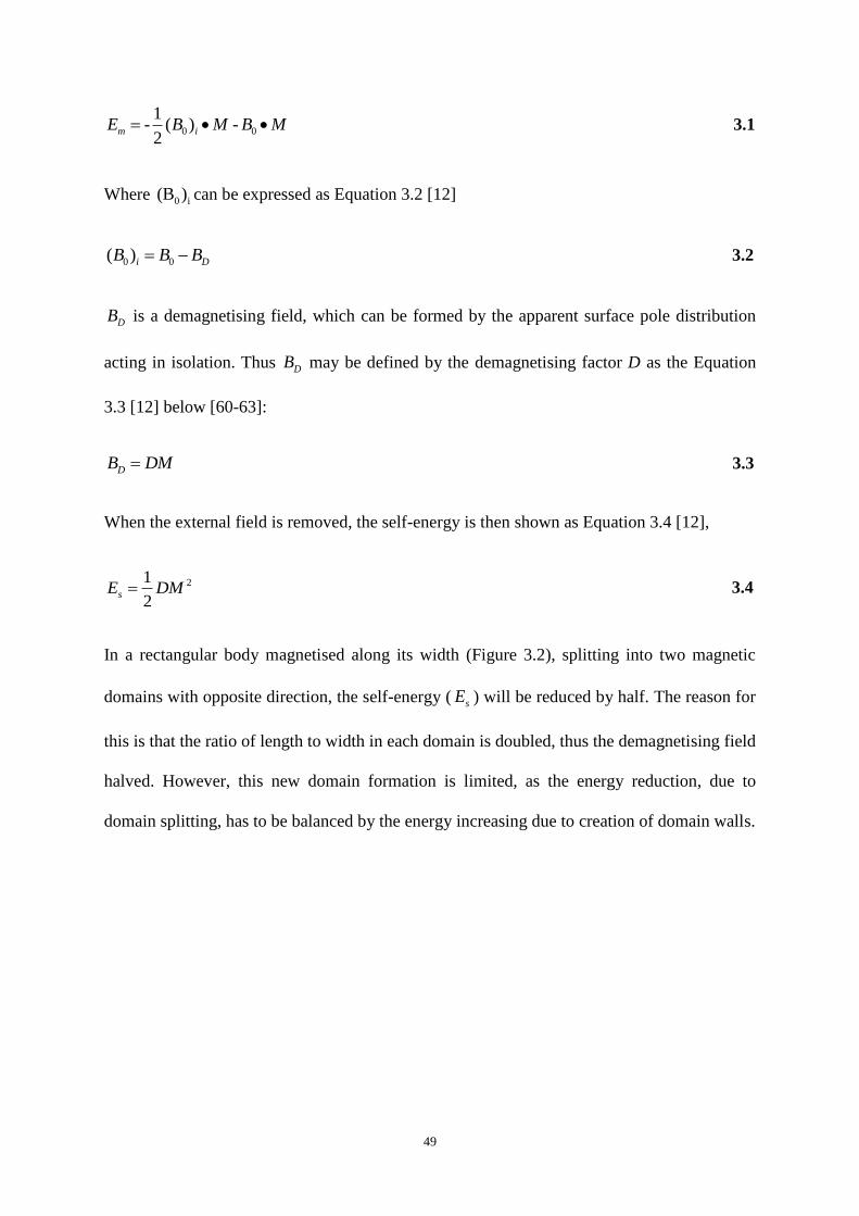
FIGURE 4.5 TRANS-IMPEDANCE VERSUS TEMPERATURE FOR DIFFERENT CARBON CONTENT
SAMPLES (A) LOW CARBON (B) MEDIUM CARBON (C) HIGH CARBON [3] .......................... 74
FIGURE 4.6 TRANS-IMPEDANCE VERSUS TEMPERATURE FOR SMALL GRAINED SAMPLE WITH
OPTICAL MICROGRAPHS SHOWING PERCENTAGE OF FERRITE (WHITE OR LIGHTER) FORMED
AT SPECIFIC POINTS ON THE TEMPERATURE AXIS. [3] ........................................................ 75
FIGURE 4.7 TRANS-IMPEDANCE VERSUS FERRITE FRACTION FOR DIFFERENT GRAIN SIZE [3] ..... 76
FIGURE 4.8 FEM SIMULATION OF STEEL SPECIMEN WITHIN EM SENSOR [3] ............................. 77
FIGURE 4.9 FEM SIMULATION RESULTS FOR GIVEN FERRITE DISTRIBUTION [3] ........................ 78
FIGURE 4.10 TRANS-IMPEDANCE VERSUS FERRITE PERCENTAGE OBTAINED USING FEM [3] .... 79
FIGURE 4.11 TRANS-IMPEDANCE VERSUS FERRITE FRACTION FOR FEM AND EXPERIMENTS FOR
MEDIUM CARBON STEEL [3] ............................................................................................... 80
FIGURE 4.12 (A) THE SCHEMATIC DIAGRAM OF THE MODEL; (B) THE GEOMETRY OF THE COIL [8]
.......................................................................................................................................... 83
FIGURE 4.13 REAL INDUCTANCE VALUE VERSUS FREQUENCY FOR SEVERAL HIPPED SAMPLES [4]
.......................................................................................................................................... 88
FIGURE 4.14 IMPEDANCE VERSUS FERRITE FRACTION FOR FEM AND EXPERIMENTS ON HIPPED
SAMPLES [4] ...................................................................................................................... 89
FIGURE 4.15 ZERO-CROSSING FREQUENCY VERSUS FERRITE FRACTION FOR HIPPED SAMPLE [4]
.......................................................................................................................................... 90
FIGURE 4.16 THE IMAGINARY PART OF THE INDUCTANCE FOR COPPER PLATE WITH THICKNESS
22,44,…..22*6 UM (SIMULATION RESULT) [95] ................................................................ 93
FIGURE 4.17 THE IMAGINARY PART OF THE INDUCTANCE FOR ALUMINUM PLATE WITH
THICKNESS 22,44,…..22*6 UM (SIMULATION RESULT) [95] .............................................. 93
FIGURE 4.18 THE PEAK FREQUENCY FOR IMAGINARY PART OF INDUCTANCE FOR ALUMINUM
PLATE WITH THICKNESS 1-5MM (EXPERIMENT RESULT) [95] ............................................. 94
FIGURE 4.19 THE PEAK FREQUENCY FOR IMAGINARY PART OF INDUCTANCE FOR AN ALUMINUM
PLATE WITH THICKNESS IS 3MM [95] ................................................................................. 95
FIGURE 4.20 MICROSTRUCTURES OF FE-0.8 WT % C AFTER DECARBURIZING AT 1000DEGREE
FOR DIFFERENT TIMES: (A) 10 MINUTES, (B)1 HOUR, (C) 2 HOUR AND (D) 5 HOURS [10] .... 96
FIGURE 4.21 INDUCTANCE VERSUS FREQUENCY FOR DECARBURIZED SAMPLES. [10] ................ 97
FIGURE 4.22 DECARBURIZING DEPTH AND INDUCTANCE CHANGE WITH DECARBURIZING TIME
[10] ................................................................................................................................... 98
FIGURE 4.23 COMPARISON THE MODELED AND MEASURED RESULT [10] .................................. 98
FIGURE 5.1 SENSOR POSITION IN THE STRIP MILL [110] ........................................................... 100
FIGURE 5.2 FERRITE FRACTION AND TEMPERATURE TESTED BY MFIA AT POSITION1 [110] ... 101
FIGURE 5.3 OPTICAL MICROGRAPHS OF HIPPED SAMPLE WITH DIFFERENT FERRITE FRACTION (A)
10% (B) 40% (C) 60% (D) 70% [111] ............................................................................. 102
FIGURE 5.4 PHASE MEASURED BY MFIA AT DIFFERENT POSITION OF THE ROT [110] ............ 103
FIGURE 6.1 FINITE ELEMENT MESH OF A SIMPLE 2D GEOMETRY ............................................ 106
FIGURE 6.2 CONTINUOUS ELEMENTS IN A FINITE ELEMENT MESH [103] ................................ 107
FIGURE 6.3 FEM MODEL OF THE H-SHAPED SENSOR HEAD .................................................... 108
FIGURE 6.4 FEM MODEL OF H-SHAPED SENSOR PLACED UNDER MAGNETIC SAMPLE ............. 109
FIGURE 6.5 H-SHAPED SENSOR WITH (A) 50MM (B) 100MM AND (C) 150MM INNER WIDTH ..... 110

8
FIGURE 6.6 SIGNAL RANGE UNDER SENSORS WITH DIFFERENT WIDTHS ................................... 111
FIGURE 6.7 CROSS SECTIONAL AREA OF THE H-SHAPED SENSOR ............................................. 112
FIGURE 6.8 EFFECTIVE SIGNAL RANGES FOR SENSORS WITH DIFFERENT CROSS SECTION ........ 112
FIGURE 6.9 FEM MODEL OF THE MFIA SYSTEM IN REAL INDUSTRY SITUATION ..................... 114
FIGURE 6.10 THE ROLLER IS DIVIDED INTO SEVERAL LAYERS FOR SIMULATION ...................... 115
FIGURE 6.11 INDUCTANCE DIFFERENCE VERSUS FREQUENCY FOR ROLLERS WITH DIFFERENT
PERMEABILITY ................................................................................................................ 115
FIGURE 6.12 (A) COMPUTER AIDED DESIGN MODEL OF THE HOUSING [106] (B) FEM MODEL OF
INDUSTRY HOUSING WITH SENSOR IN IT. .......................................................................... 117
FIGURE 6.13 INDUCTANCE DIFFERENCE VERSUS FREQUENCY FOR ROLLER INFLUENCE (A)
WITHOUT HOUSING (B) WITH HOUSING ............................................................................ 118
FIGURE 6.14 STEEL SHEET EFFECTS (A) WITHOUT HOUSING (B) WITH HOUSING ...................... 119
FIGURE 6.15 LIFT-OFF INDICATION ......................................................................................... 120
FIGURE 6.16 INDUCTANCE DIFFERENCE SPECTRA FOR DIFFERENT LIFT-OFF (A) 35MM (B) 45MM
........................................................................................................................................ 122
FIGURE 6.17 SIMPLIFIED LIFT-OFF MODEL .............................................................................. 123
FIGURE 6.18 IMPEDANCE PHASE ANGLE VERSUS FREQUENCY AT DIFFERENT LIFT-OFF (A)
RELATIVE PERMEABILITY IS 150 (B) RELATIVE PERMEABILITY IS 200 ............................. 124
FIGURE 6.19 FREQUENCY RESPONSE OF THE EM SENSOR FOR STEEL STRIPS WITH DIFFERENT
PERMEABILITIES (A) REAL INDUCTANCE (B) IMAGINARY INDUCTANCE ........................... 125
FIGURE 6.20 RELATIONSHIP BETWEEN (A) ZERO-CROSSING FREQUENCY FOR REAL INDUCTANCE
AND RELATIVE PERMEABILITY OF STEEL SHEET (B) PEAK FREQUENCY FOR IMAGINARY
INDUCTANCE AND RELATIVE PERMEABILITY ................................................................... 126
FIGURE 6.21 FEM RESULTS FOR DIFFERENT RELATIVE PERMEABILITY VERSUS ANALYTICAL
MODEL (A) RELATIVE PERMEABILITY IS 50; (B) RELATIVE PERMEABILITY IS 100; (C)
RELATIVE PERMEABILITY IS 150; (D) RELATIVE PERMEABILITY IS 200. ........................... 129
FIGURE 6.22 SCREEN SHOT FROM THE TITAN SIMULATION SOFTWARE [107] .......................... 130
FIGURE 6.23 MODELLED PHASE DISTRIBUTION OVER THICKNESS [107] .................................. 131
FIGURE 6.24 SIX POSITIONS ALONG ROT ................................................................................ 132
FIGURE 6.25 FEM MODEL FOR MULTI-LAYER STEEL PLATE .................................................... 133
FIGURE 6.26 INDUCTANCE DIFFERENCE AT DIFFERENT POSITION ............................................ 134
FIGURE 6.27 PHASE DIAGRAM ................................................................................................. 135
FIGURE 6.28 POLAR DIAGRAM OF PHASE RESPONSE ................................................................ 136
FIGURE 7.1 BLOCK DIAGRAM OF THE SYSTEM HARDWARE [109] ............................................ 139
FIGURE 7.2 HARDWARE OF THE MFIA SYSTEM ...................................................................... 140
FIGURE 7.3 SENSOR HEAD WORKING BETWEEN 800 HZ TO 100 KHZ ....................................... 141
FIGURE 7.4 TRANS-IMPEDANCE VERSUS FREQUENCY FOR THE H-SHAPED FERRITE SENSOR IN
FREE SPACE ..................................................................................................................... 141
FIGURE 7.5 PROCESS OF NORMALISATION (A) PURE FERRITE SIGNAL BEFORE NORMALISATION (B)
AFTER NORMALIZATION .................................................................................................. 143
FIGURE 7.6 PHASE DIAGRAM AFTER NORMALISATION (A) AUSTENITE (B) 100% FERRITE ...... 144
FIGURE 7.7 VARIATION OF IMPEDANCE MAGNITUDE (A) IMPEDANCE MAGNITUDE VARIATION IN
20 MINS WITH NO SAMPLE (B) IMPEDANCE VARIATION IN 1 MINUTE WITH 100% FERRITE (C)
PHASE VARIATION IN 1 MINUTE WITH 100% FERRITE ...................................................... 146

9
FIGURE 7.8 INDUSTRY HOUSING .............................................................................................. 147
FIGURE 7.9 HOUSING EFFECT TO ACTIVE AND BACKING-OFF COILS ......................................... 147
FIGURE 7.10 BACKING-OFF COIL RESPONSE WITH DIFFERENT SAMPLES .................................. 148
FIGURE 7.11 MFIA TEST RESULTS (A) IMAGINARY INDUCTANCE (B) REAL INDUCTANCE ....... 149
FIGURE 7.12 IMPEDANCE ANALYSER THICKNESS TEST (A) REAL INDUCTANCE FOR FERRITE
SAMPLES (B) IMAGINARY INDUCTANCE FOR FERRITE SAMPLES (C) REAL INDUCTANCE FOR
AUSTENITE SAMPLES (D) IMAGINARY INDUCTANCE FOR FERRITE SAMPLES .................... 152
FIGURE 7.13 RE-WOUND SENSOR HEAD FOR THE 200 HZ TO 24 KHZ FREQUENCY RANGE. ..... 153
FIGURE 7.14 FREQUENCY RESPONSE OF THE NEW SENSOR HEAD ............................................. 154
FIGURE 7.15 HOUSING EFFECT ON THE ACTIVE COIL AND BACKING-OFF COILS ....................... 155
FIGURE 7.16 BACKGROUND SIGNAL DRIFT OFF IN 10 MINUTES ............................................... 156
FIGURE 7.17 SIGNAL DRIFT OFF IN 10 MINUTES FOR 100% FERRITE SAMPLE (A) IMPEDANCE
MAGNITUDE (B) PHASE ................................................................................................... 157
FIGURE 7.18 2 MM THICK STAINLESS STEEL SIGNAL VARIATION IN TEN MINUTES (A) IMPEDANCE
MAGNITUDE (B) PHASE ................................................................................................... 158
FIGURE 7.19 LIFT-OFF TEST SET-UP ......................................................................................... 159
FIGURE 7.20 LIFT-OFF EFFECT TO 100% FERRITE SAMPLE (A) REAL INDUCTANCE (B)
IMAGINARY INDUCTANCE (C) PHASE............................................................................... 160
FIGURE 7.21 LIFT-OFF EFFECT TO AUSTENITE SAMPLE (A) REAL INDUCTANCE (B) IMAGINARY
INDUCTANCE (C) PHASE .................................................................................................. 162
FIGURE 7.22 LIFT-OFF 35 MM (A) FERRITE REAL INDUCTANCE (B) FERRITE IMAGINARY (C)
AUSTENITE REAL INDUCTANCE (D) AUSTENITE IMAGINARY ............................................ 164
FIGURE 7.23 SKETCH AND SETUP FOR THE POSITION TEST IN THE HORIZONTAL DIRECTION .... 166
FIGURE 7.24 IMPEDANCE VERSUS D3 ...................................................................................... 166
FIGURE 7.25 SETUP FOR THE POSITION TEST IN THE VERTICAL DIRECTION .............................. 167
FIGURE 7.26 IMPEDANCE VERSUS DISTANCE ........................................................................... 168
FIGURE 7.27 MEASUREMENT SETUP INCLUDING THE IMPEDANCE ANALYSER AND THE METALLIC
HOUSING ......................................................................................................................... 169
FIGURE 7.28 COMPARISON BETWEEN EXPERIMENTAL RESULTS AND THE ANALYTICAL MODEL
........................................................................................................................................ 170
FIGURE 8.1 (A) ELECTRICAL RESISTIVITY VERSUS CARBON CONTENT [122] (B) VARIATION IN
INITIAL RELATIVE PERMEABILITY OF CARBON STEEL WITH CARBON CONTENT AND FERRITE
FRACTION [123] .............................................................................................................. 174
FIGURE 8.2 SCHEMATIC DIAGRAM OF THE MODEL [124] ......................................................... 175
FIGURE 8.3 INDUCTANCE DIFFERENCE VALUE VERSUS FREQUENCY FOR THE DIFFERENT
SIMULATED DECARBURISATION LAYERS ......................................................................... 178
FIGURE 8.4 INDUCTANCE DIFFERENCE VALUE VERSUS DECARBURISATION LAYER THICKNESS AT
1 KHZ .............................................................................................................................. 179
FIGURE 8.5 CROWN POSITION OF RAIL SAMPLE ....................................................................... 181
FIGURE 8.6 OPTICAL MICROGRAPH SHOWING HOW THE VISUAL DECARBURISATION DEPTH WAS
ESTABLISHED (RAIL SURFACE ON LEFT SIDE OF MICROGRAPH) ........................................ 182
FIGURE 8.7 OPTICAL MICROGRAPH SHOWING (A) 610 µM DECARBURISATION LAYER (B)
MINIMUM DECARBURISATION LAYER (NONE) .................................................................. 183
FIGURE 8.8 THE H-SHAPED SENSOR HEAD............................................................................... 185

10
FIGURE 8.9 (A) WHOLE TEST SET UP (B) SENSOR HOLDER ....................................................... 186
FIGURE 8.10 INDUCTANCE DIFFERENCE VERSUS FREQUENCY FOR THE FOUR RAIL SAMPLES AT
THE CROWN POSITION. ..................................................................................................... 187
FIGURE 8.11 RELATIONSHIP BETWEEN THE SQUARE ROOT OF DWELL TIME AND SENSOR
INDUCTANCE IN CROWN POSITION ................................................................................... 188
FIGURE 8.12 RELATIONSHIP BETWEEN THE DECARBURISATION DEPTHS DETERMINED FROM THE
HARDNESS TESTS AND SENSOR INDUCTANCE DIFFERENCE AT THE CROWN POSITION ....... 190
FIGURE 8.13 RELATIONSHIP BETWEEN THE DECARBURISATION DEPTHS DETERMINED FROM THE
MICROGRAPHS AND THE SENSOR INDUCTANCE DIFFERENCE AT THE CROWN POSITION .... 190
FIGURE 8.14 LIFT-OFF EFFECTS TO SENSOR RESPONSE FOR THE 195 MINS AND 613 MINS DWELL
TIME RAIL SAMPLE .......................................................................................................... 191
FIGURE 8.15 MAXWELL MODEL FOR THE H-SHAPED SENSOR UPON RAIL SAMPLE ................... 192
FIGURE 8.16 INDUCTANCE DIFFERENCE VERSUS FREQUENCY FOR DIFFERENT DECARBURISATION
THICKNESS LAYERS USING THE FEM MODEL .................................................................. 193
FIGURE 8.17 COMPARISON BETWEEN THE MODELLED AND MEASURED RESULTS FOR TESTING AT
1 KHZ .............................................................................................................................. 194

11
List of table
TABLE 4.1 CORRESPONDING PARAMETERS IN ELECTROSTATICS AND MAGNETOSTATICS [7] ..... 69
TABLE 4.2 COMPOSITIONS OF STEEL ROBS, WT-% [3] ............................................................... 72
TABLE 4.3 HIPPED SAMPLE CHARACTERISTICS IN TERMS OF WT.% FERRITE STAINLESS STEEL
(434L) POWDER USED AND THE MEASURED MICROSTRUCTURE OBTAINED [4] .................. 87
TABLE 6.1 TITAN SIMULATION DATA FOR R4272170 (C: 0.04WT%, MN: 0.209WT%, THICKNESS:
5.13MM) .......................................................................................................................... 133
TABLE 8.1 COMPOSITION (WT %) OF BRITISH 260 GRADE RAIL STEEL. ................................... 180
TABLE 8.2 DWELL TIMES FOR RAIL SAMPLES 1- 4 ................................................................... 180
TABLE 8.3 OPTICAL MICROSCOPY (OM) MEASURED, PREDICTED AND HARDNESS MEASURED
DECARBURISATION DEPTHS IN THE SAMPLES WITH DIFFERENT DWELL TIMES. ................. 184
12
Abstract
This thesis covers two main topics- the development of Electromagnetic (EM) on-line
microstructure inspection system for steel under controlled cooling and the investigation of
using EM sensor to measure rail decarburisation depth off-line.
First, through extensive Finite Element Modelling (FEM) the link between EM sensor output
and steel microstructure has been found. Both zero-crossing frequency for real inductance
and the peak- frequency for imaginary inductance are linearly proportional to magnetic
permeability of steel which is an indicative for microstructure. Furthermore, the response of
the complex H-shaped ferrite core sensor is found can be described by a simple analytical
model of an air core sensor after normalization. In addition, the factors that might affect
sensor performance are been investigated, including lift-off, rollers and industrial housing.
Second, experiments were carried out both in the lab and at the service line of Tata Steel to
check the sensor performance. Test results show the Multi-frequency Impedance Analyser
(MFIA) system works very stable in real industrial setup with good performance in signal to
noise ratio. It can successfully distinguish samples with different magnetic properties
(paramagnetic and ferromagnetic).
After that, the possibility to apply EM sensor in off-line rail decarburisation depth test is
investigated. Both FEM simulation and experiment results show the decarburisation depth
has a linear relationship with inductance. Also the EM sensor output has a good agreement
with the predicted decarburisation depth (Fick’s law) and measured results from other
methods (micro-hardness and visual test).

13
Declaration
No portion of the work referred to in this dissertation has been submitted in support of an
application for another degree or qualification of this University or any other institution of
learning.

14
Copyright Statement
(1)Copyright in text of this dissertation rests with the author. Copies (by any process) either
in full, or of extracts, may be made only in accordance with instructions given by the author.
Details may be obtained from the appropriate Graduate Office. This page must from part of
any such copies made. Further copies (by any process) of copies made in accordance with
such instructions may not be made without the permission (in writing) of the author.
(2)The ownership of any intellectual property rights which may be described in this
dissertation is vested in the University of Manchester, subject to any prior agreement to the
contrary, and may not be made available for use by third parties without the written
permission of the University, which will prescribe the terms and conditions of any such
agreement.
(3)Further information on the conditions under which disclosures and exploitation may take
place is available from the Head of the School of Electrical and Electronic Engineering.

15
Acknowledgement
First and foremost, I wish to thank my supervisor, Prof.A.J.Peyton, for his patient guidance,
advice and support throughout my Ph.D studies in the last three years. He has not only shared
his academic expertise with me, to more important he demonstrated me the rigorous attitude
in research and work with passion. Without his valuable help, this thesis would not happen to
be possible.
I am also grateful to Dr.W.Yin for his guidance in my research. Furthermore, I would like to
thank all my colleagues for their help in my study; they are Dr.C.Ktistis, Dr.L.Marsh,
Dr.B.Dekdouk, Dr.X.Li and Miss Y.Tan. I also want to express my thanks to Prof. C.L.Davis
from University of Birmingham, Dr.S.Dickinson from Organised Technology Ltd., Mr H.
Ploegaert, Dr.F.van den Berg and Dr.H.Yang from Tata Steel for their valuable comments
and suggestions, which greatly improved my work.
In addition, I must thank my parents for their continuous support, encourage, and never lose
confidence to me through all my life. I also want to thank my wife for the happiness she
brings to my life and unconditional support in every decision I have made.
Last but not least, I am grateful to Miss M.Wang, Miss L.Suematsu and Mr W.Huang for the
time we spend together in Manchester.

16
Chapter 1 Introduction
This thesis places an emphasis on the research of EM methods to the steel microstructure
variation. Two different applications using EM techniques have been introduced. The first
application is the development of MFIA system for on-line inspection of steel microstructure
transformation during controlled cooling. In the second area, the possibility of using EM
method in off-line rail sample decarburisation depth detection is investigated. These will be
described in more detail in the following section.
1.1 Industrial context of the research
1.1.1. Monitoring the hot transformation of strip steel
Monitoring steel microstructure is directly relevant to the hot operation of a hot strip mill.
Before passing through the hot strip mill, steel is in the form of slab, which has been
produced by continuous casting. There is a limited market for slab and this form is of little
use to product manufacturers. Therefore, strip mill is used to convert slab into steel sheet.
Rolling not only produces the necessary physical dimension, but also the microstructure
required by end-users. The strip mill is usually composed of two parts: mill rolling stands and
run out table (ROT). The mill rolling stands convert slab into the mechanical dimension
required by customers as well as a fine grained microstructure. After that, steel strip is cooled
by water on the ROT to ensure the steel transforms to the desired microstructure. The
physical properties such as strength and toughness of the final steel products can be strongly
dependent on its microstructure. Thus the cooling process should be tightly controlled.
17
At present, there is no established method for monitoring the steel microstructure
transformation on-line, however several techniques such as electromagnetic, X-ray
(attenuation and diffraction) and ultrasonic, have been investigated for this purpose [1] [2].
Compared to these techniques, the EM method has particular virtues, for instance being non-
contact, having a fast response, being unaffected by water and dust, and offering the potential
of a relatively low cost solution.
The main strategy of using the EM methodology on steel microstructure transformation
monitoring is to link the microstructure directly to the sensor output. This link is usually
divided into two parts: first to find the connection between microstructure of steel and the
electromagnetic properties, and then link the electromagnetic properties variation with EM
sensor output change. A lot of efforts have been spent on finding the relationship between the
microstructure and EM properties [3-10]. The aim of the research in this thesis is to study the
latter problem and to formulate a modelling methodology using 3D FEM to describe the link
between EM properties of steel and the EM sensor output.
The EM sensors used in this project consist of an arrangement of transmitter and receiver
coils configured on a ferrite core. The EM sensor is interrogated using MFIA techniques.
The MFIA system will be used in the real industry situation; therefore the sensor head size
and working frequency should be carefully chosen to satisfy the industrial requirements; and
numerous factors should be taken into consideration, such as housing, roller and lift-off
effects. Therefore the second aim of the project is using the FEM method to develop a system
to meet the industry requirements.
Tests to present the performance were undertaken by both the University of Manchester and
Tata Steel. Experiments carried out in the University of Manchester were concerned on the
MFIA system’s stability, sensitivity, signal to noise ratio and the effects of the housing

18
containing the EM sensor. The MFIA system has been installed at the service line of Tata
Steel. Results from the system at present of samples with different properties have been
compared to show the process of microstructure variation. Furthermore ferrite fraction is
deduced using MFIA output.
1.1.2. Assessing decarburisation of rail
To expand the application of EM technology, an investigation on surface decarburisation of
rail was undertaken in co-operation with University of Birmingham With the aim of finding a
non-destructive off-line rail decarburisation measurement method.
Surface decarburisation whereby carbon atoms at the surface of the sample react with the
oxygen around occurs at high temperature, typically above 1150 °C. Previous research
indicated that as the depth of the decarburisation layer increases, the total wear and the wear
rate both increase, which affects the lifetime of rail. Therefore, rail decarburisation has
potential safety implications and it is necessary to determine the decarburisation depth. At
present the decarburisation depth is measured by destructive method, including
metallographic observation, hardness tests and chemical analysis on a sample cross-section
after processing. EM technology provides a potential non-destructive way to monitor the rail
decarburisation depth.
To investigate the relationship between decarburisation layer and the sensor output, both
analytical solution and FEM simulation were used. Analytical and FEM results show that the
decarburisation depths for samples with different reheat time can clearly be distinguished by
inductance output under certain frequency. Eventually, the decarburisation depths, measured
using micro-hardness tests and visual evaluation, and the predicted amount (based on Fick’s

19
law) by Birmingham University, were compared with the H-shaped EM sensor measurement
results, where a reasonable agreement can be found.
1.2 Objectives
This thesis focuses on the development of MFIA system and investigation in applying EM
technology in off-line rail decarburization depth measurement.
The first objective was using FEM method to investigate the relationship between EM sensor
output and steel microstructure. It has been known that electromagnetic permeability of steel
is strongly related to its ferrite fraction. Thus the key of this research lies in finding the
relationship between electromagnetic permeability variation and EM sensor response change.
The second objective focused on designing MFIA system. The dimension of the sensor head
needed to be decided by carefully considering both its size effect to magnitude of signal and
industrial requirements. In addition, the influence from real industrial setup has to be
investigated.
The third objective was to measure the MFIA performance both in the lab and in real
industrial setup. The goal was to test the reliability and sensitivity of MFIA in both lab and
industrial situation.
The last objective was to investigate the possibility of using EM technology in off-line rail
decarburization depth measurement both by FEM method and lab experiments. The key point
of this research was to find the relationship between the EM sensor output and the rail
decarburization depth.

20
1.3 Contributions
The main contributions of this thesis are summarized as follows:
Both the zero-crossing frequency of real inductance and the peak frequency of
imaginary inductance were found to be linearly proportional to steel electromagnetic
permeability. This finding linked the EM sensor response to steel microstructure.
The complex H-shaped ferrite core sensor was found to be approximately described
by an equivalent simple air-cored sensor after normalization, which means the whole
inductance spectrum of H-shaped sensor can be predicted using limited test points.
The inductance response of H-shaped ferrite core sensor is proved to have a linear
relationship with rail decarburisation depth by both FEM method and experiments.
This finding gives confidence in using EM technology in non-destructive test of rail
decarburisation.
1.4. Organisation of this thesis
This thesis consists of nine chapters. Prior to the consideration of the work accomplished
within this thesis, necessary background is introduced in Chapter 2, Chapter 3 and Chapter 4.
Chapter 2 gives the background information of steel processing parameters. After that, the
phase transformation of steel in pure iron and heat treatment is discussed under both
equilibrium and dynamic conditions. This chapter reveals that the steel’s electromagnetic
property, especially magnetic permeability, is influenced by the microstructure of steel,
which gives a potential link between microstructure and EM sensor output.

21
In Chapter 3, the EM properties of steel are investigated firstly; the basic electromagnetism
and eddy current principles are presented after that. The principle of employing EM
technology in steel microstructure detection is that the difference of signal due to steel’s
microstructure variation can be detected by the eddy current instrument.
The linkage between steel microstructure and sensor output is presented at the beginning of
Chapter 4. Great deals of findings of EM application have been published in the recent years.
Then two examples of EM sensor application in metal sample testing are introduced in the
following part of Chapter 4.
Chapter 5 gives the preliminary MFIA test results in ROT at Tata Steel. The MFIA system is
installed in the ROT and results is compared with Magtran response at different position of
ROT. The investigation of zero-crossing frequency for samples with different grade has been
carried out. In addition, the transferred ferrite fraction is deduced by MFIA output.
Chapter 6 introduces the FEM modelling methodology of this research. At the beginning of
this chapter the theory of FEM will be presented. After that, FEM results in developing
MFIA system are presented and analysed, including effect of sensor dimension, roller and
housing influence and lift-off. In addition, zero-crossing frequency of real inductance and
peak frequency of imaginary inductance have been found linearly proportional to the ferrite
percentage of steel. The output of a H-shaped sensor is also found, which can be predicted by
an equivalent simple air-cored sensor. At the end of this chapter, FEM is used to simulate the
MFIA response using the data from thermodynamic models of the mill.
In Chapter 7, the hardware of MFIA system is presented at the first part. The initial design
allows the working frequency up to 100 kHz. Based on the thickness of the products in Tata
Steel, the new MFIA’s working frequency is adjusted below 24 kHz. Both the original and

22
newly designed MFIA are tested in the lab including stability, signal to noise ratio, sensitivity
and housing effect.
Moreover, besides the MFIA system development in strip mill, the application of using the
EM sensor to monitor rail sample decarburisation depth is given in Chapter 8. In this chapter,
analytical and Maxwell simulation results have been compared with the experiments results.
This research shows the possibility of using an EM sensor to detect different decarburisation
depth in rail sample off-line.
The overall discussion and conclusion from the content provided in the above chapters are
shown in Chapter 9, along with further improvement of the MFIA system and future work.
1.5. Published output from this study to date
Published papers, concerning all aspects of this work that have either been authored or co-
authored are listed below:
1. W. Zhu, W. Yin, A. J. Peyton, Henk Ploegaert. Analytical and FEM modelling of an
electromagnetic sensor with an H-shaped ferrite core used for monitoring the hot
transformation steel. in IEEE Instrumentation and Measurement Technology
Conference (I2MTC), Austin, USA, p986-989, 2010.
2. W. Zhu; W. Yin, A. J. Peyton, Henk Ploegaert. (2011) Modelling and experimental
study of an electromagnetic sensor with a H-shaped ferrite core used for monitoring
the hot transformation of steel in an industrial environment. NDT&E International.
44(7), p547-552.

23
3. W.Zhu; S.Cruchley; W.Yin; X.J.Hao, C.L.Davis; A.J.Peyton. (2012) Evaluation of
rail decarburisation depth using a H-shaped electromagnetic sensor. NDT&E
International 46(3), p63-69

24
Chapter 2 Steel Phase Transformation
Steels are known to be one of the most widely used metallic materials, comprising over 80%
by weight of the alloys in industrial usage, as they can be manufactured cheaply in large
quantities to achieve different demands. Steels also give an extensive range of mechanical
and physical properties by changing their alloy content and the conditions during their
manufacturing process for specific industrial use, making the study of steel very important
[11].
This chapter will present steel processing parameters, and introduce ROT problem in more
detail. After that, the phase transformation in pure iron and heat treatment under equilibrium
and dynamic conditions will be discussed.
2.1. Steel Strip Processing
Prior to passing through the strip mill, steel is in the form of slab, which has been produced
by continuous casting. There is very limited market for slab and this form is of little use to
product manufacturers, which require thinner gauges. Therefore, the strip mill is used to
convert slab into thinner steel sheet. The rolling produces not only the necessary physical
dimensions, but also the microstructure required by the end-users. Figure 2.1 shows the
process of steel to product and cooling process upon the ROT within the hot strip mill.

25
(a)
(b)
Figure 2.1 (a) Steel to different products (b) ROT [12]
The strip mill is usually composed by two parts: (i) mill rolling and (ii) ROT. The rolling
stands convert the slab into the mechanical dimension required by customers as well as a
fine-grained microstructure. The mechanical properties of steel sheets are then finally formed
by controlled cooling upon the ROT. According to the specific microstructure, the
temperature of the steel on the ROT is between 1000 C and 400 C . The resulting strip sheet
is stored in coil form. The steel quality monitoring is currently achieved by destructive

26
methods, on samples cut from the final strip. This is an off-line method, which, although
effective, is known to be wasteful of time and money [12] [13].
Figure 2.2 shows the scale of the strip manufacturing processes, where six rolling stands are
pictured.
Figure 2.2 Rolling Stands in Operation (Tata steel) [12]
2.2. Phase transformation of pure iron: -iron and -iron
To study steel, an easy way is to start from pure iron first, before moving onto the more
complex group of steels. At normal pressure, pure iron has two crystal forms -iron (ferrite)
and -iron (austenite). When the temperature goes up to 910 C , -iron will be transformed
to -iron. If the pressure is higher than 130 kbar, another -iron could be obtained. With the
temperature increasing to 1536 C , the -iron reverts to -iron [11]. Figure 2.3 illustrates

27
the phase change with temperature variation, which also reveals the variation in the atomic
volume together with the phase transformation.
Figure 2.3 Temperature dependence of the mean volume per atom in iron crystals [14]
2.3. Steel phase transformation
Pure iron converts to steel by adding carbon, as such even a small presence of carbon [15],
has a significant influence on the property of iron, e.g. strength [16][17]. Steel phase
conversion can be discussed under two conditions, namely equilibrium and dynamic
conditions.
Under equilibrium conditions, the cooling rate effect is ignored; the steel state is analysed at
constant temperatures. Dynamic transformation, on the other hand, takes the cooling rate
effect into account, which is more consistent with the realistic situation [11].

28
2.3.1. Equilibrium Temperature Analysis
At Equilibrium transformation, the cooling regime is ignored, in contrast both temperature
and composition are under 3Fe C consideration as they determine steel phase. Carbon is the
most important solute atom, thus the iron-iron carbide (Fe- 3Fe C ) phase diagram will be
presented in the following section.
2.3.1.1. Phase diagram for 3Fe C
Carbon which is the most significant solute atom in steel, influences the atomic structure and
also the relationship between temperature and phase. Figure 2.4 is the Fe- 3Fe C phase diagram,
showing the steel phase transformation together with temperature and carbon content. In this
figure, stands for ferrite and austenite is presented by .

29
Figure 2.4 Fe-Fe3C diagram [18]
The Fe- 3Fe C phase diagram, shown above, illustrates that for steel with 0 wt% carbon
content, the -ferrite state remains stable until the temperature rises to 910 C where -
ferrite to -austenite transformation occurs.
The consequence of increasing carbon content in iron lowers the ferrite -austenite
transformation temperature (along the GS line) with the formation of 3Fe C . Another
important point in Figure 2.4 is the Curie point, which is the transformation temperature
when ferrite changes from the ferromagnetic condition to paramagnetic condition. Magnetism
will be lost if a magnet is heated above the Curie temperature, due to the change of magnetic
moments. Figure 2.5 shows that below the Curie temperature the neighbouring magnetic
spins from Fe atoms align in a ferromagnet, even without an external magnetic field. As the
Curie Temperature
for Pure Iron

30
temperature increasing near to the Curie temperature, the alignment in each domain decreases.
When the temperature rises above the Curie point, the magnetic movement is in completely
random, i.e. paramagnetic. For pure iron the Cure point is 769 C .
(a)
(b)
Figure 2.5 Magnetic movements for (a) ferromagnet (b) paramagnet
Figure 2.4 also indicates that in equilibrium cooling that there are two main transformations
for steel with different carbon content. For pure iron, with the equilibrium cooling, austenite

31
to ferrite transformation happens at 910 C (Point G in Figure 2.4). With the increasing of
carbon content the austenite-ferrite transformation temperature decreases along the GS line
until 0.8 wt% carbon content. However, for steel with 0.8 wt% carbon content, pearlite ( +
3Fe C ) forms at the temperature 723 C , which is also called eutectic temperature. Figure 2.4
shows the microstructure transformation under equilibrium cooling, if under dynamic cooling,
the situation will be more complex.
2.3.1.2. Medium carbon
Medium carbon steel is the type of steel with carbon content from 0.3 – 0.6 wt%. Due to its
balanced ductility and strength and excellent wear resistance, medium carbon steel is widely
used for large parts, forging and automotive components [19].
Figure 2.6 Steel Microstructure Phase Evaluation (0.2 wt% C) [12]
0.3 0.6

32
Figure 2.6 shows that there is another significant temperature called the eutectoid temperature
(Te). Eutectoid conversion transfers the austenite into ferrite and cementite ( 3Fe C ). For steel
with 0.8 wt% carbon content, the eutectoid temperature is about 723 C . When eutectoid
transformation occurs, austenite converts to two phases: ferrite and cementite, to form
pearlite. Pearlite has a layered structure of ferrite and cementite, shown in Figure 2.7. The
mechanical properties for pearlite are between the soft, ductile ferrite and hard, brittle
cementite. From 910 C to the eutectoid temperature, hypo-eutectoid ferrite formed during
steel with less than 0.8 wt% together with the residual austenite. At the eutectoid temperature
the remaining austenite transforms to pearlite. An optical micrograph is illustrated in Figure
2.7, indicating the process of pearlite formation. Figure 2.8 presents the final microstructure
of pearlite steel. The pre-eutectoid ferrite region is in black, the pearlite region is in light
colour [20-28].
Figure 2.7 Optical micrograph for ferrite mixed with cementite [20]

33
Figure 2.8 Medium Carbon steel composed by ferrite and pearlite [12]
2.3.1.3. High carbon
High carbon steel contains 0.8 wt% to 2.11 wt% carbon. For high carbon steel, cementite
formed with the decreasing of carbon in austenite from 1147 C to 723 C (along with ES
line in Figure 2.4.). At 723 C , pearlite is also formed when the austenite contains 0.8 wt% C
[29-31]. High carbon steel is characterized by its hardness, especially after heat treatment. It
also presents high strength ratings property, including fatigue resistance. Figure 2.9 illustrates
the comparison between high carbon steel properties and other steels.

34
Figure 2.9 High carbon steel properties versus other steels [32]
High carbon steels can be cold rolled or heat treated (annealing, quenching and tempering), to
adapt to different applications. It is commonly used for manufacturing mechanical parts,
including clutches, springs, saws etc. However, due to the high carbon content, high carbon
steel is more brittle than other types of steel, which leads to fracture when misused [33].
2.3.2 Dynamic cooling
In the steel industry, steels may be cooled up to 400 C /s. The effect of the cooling rate on
steel microstructure transformation will be discussed in the following section, which is the
main difference between dynamic cooling and equilibrium cooling.
2.3.2.1. Grain evolution
When steel falls into the zone, ferrite grains nucleate at the intersections of austenite
grains. The factors that affect the ferrite grain size and distribution are listed below:

35
Residual stress within the steel
Cooling rate
Chemical composition of the transformation steel
Grain nucleation will be promoted by an increase in stress levels within increases of localised
energy maxima. In the heating and cooling process of the steel industry, stress levels are
increased to form finer grain structure, thus improving the mechanical properties of the steel
[12].
Ferrite grains will nucleate at austenite grain boundaries due to the microstructure instability
in the cooling process. Higher strains are induced in steel by carbon diffusion and phase
variation, thus more grains are created at high cooling rates than at slow cooling rates. A
grain grows until it reaches the boundary of the neighbouring grain. Thus steel is processed to
reach the final use requirement, i.e. steels with large grains may have good electrical
properties, but are mechanically ductile, and in contrast finer grained steels have better
mechanical characteristics.
2.3.2.2. Typical Transformation of carbon steel
Cooling rate affects the steel microstructure transformation in two aspects: grain formation
and specific grain structure upon cooling rate [35]. At equilibrium cooling, the cooling rate is
not taken into account, thus equilibrium is not suitable for real steel industry processes,
dynamic cooling has to be introduced. The phase transformation is more complex compared
with equilibrium transformation due to influence of the cooling rate.

36
Figure 2.10 shows the comparison between isothermal Time-Transformation-Temperature
(TTT) diagrams and Continuously Cooled Temperature (CCT) diagrams. The TTT diagram
illustrates the rate of transformation at a constant temperature. The transformation starting
time and finish time can be shown by the TTT diagram, whereas CCT diagrams represent the
effects of the actual cooling rate. The transformation period and the temperature at which the
transformation occurs are lengthened and lowered in continuous cooling. Both TTT and CCT
diagrams are phase transformation with time diagrams. Microstructure can be predicted
through TTT or CCT diagrams in a period time at constant temperature or continuous cooling
condition [36-38].
Figure 2.10 CCT-TTT diagram for Eutectoid Carbon Steel [36]
Normally, at continuous cooling bainite will not be created since all the austenite would
transform to pearlite at the time when bainite transformation started. Thus, the austenite-
pearlite transformation zone terminated below the nose in Figure 2.10.

37
2.3.2.3. Pearlitic Transformation
Figure 2.11 indicates the pearlitic transformation schedules upon a CCT diagram for eutectic
carbon steel. It can be clearly seen that cooling rate not only influences the grain size, but it
also has a significant effect on the temperature at which transformation occurs. Thus, pearlite
formation is more complex in dynamic cooling [38][39].
Figure 2.11 Pearlite transformation at CCT cooling [40]
2.3.2.4. Bainitic Transformation
Bainite is composed by two phases: -ferrite and cementite. Figure 2.12 reveals that Bainite
has two transformations, upper and lower. Upper bainite transformation occurs at the upper
end of Bainatic formation zone. Bainite formed by upper transformation has relatively coarse,
irregular shaped cementite particles between -ferrite plates. If transformation occurs at

38
lower temperature range, -ferrite starts nucleation between austenite grain boundaries, this
process is similar to pearlite formation and cementite has a regular needle like shape within
fine ferrite plate. The schematics of upper bainite and lower bainite have been compared in
Figure 2.13.
Figure 2.12 Schematic of the microstructure of upper and lower bainite [41]
Figure 2.13 Lower (a) and upper (b) bainite steel (0.87 wt% C; 0.44 wt% Mn, 0.17 wt% Si,
0.21 wt% Cr, 0.39 wt% Ni) [41]
It can be found that the cooling rate required for bainite formation is slower than martensitic
formation.

39
Figure 2.14 Bainite and martensite transformation at CTT cooling [40]
2.3.2.5. Martensitic Transformation
Figure 2.14 indicates that, in order to obtain martensite, a high cooling rate is needed to attain
a low temperature very rapidly. Martensite grain nucleation occurs in this rapid cooling
process, and the resulting ferrite structure is lengthened to a body centered structure as the
carbon cannot diffuse from the austenitic matrix. Carbon content has a significant effect on
martensite transformation.
Figure 2.15 shows that plate martensite is formed into needle formation for high carbon steels.
The white areas stand for the untransformed austenite.

40
Figure 2.15 Micrograph of martensitic microstructure [20]
Martensite is hard to obtain due to its high cooling rate. However, by adding alloying
elements, the ferrite transformation temperature can be lowered [42-44].
By the analysis of phase transformation at dynamic cooling, a schematic of possible
transformation is shown in Figure 2.16, which shows that cooling rate has a significant effect
to the steel microstructure.
Martensite
Untransformed austenite

41
Figure 2.16 Possible transformation involving austenite decomposing
2.3.2.6 Relative properties of Bainite/Pearlite/Martensite
Martensite is the hardest and most brittle material in all steel phases; in addition it has
virtually no ductility at all. The hardness of martensite increases with increasing of carbon
content, there is a rapid increase of hardness until 0.4 wt% C, and after that the hardness
reaches its maximum at 1 wt% C with a slower speed. Figure 2.17 illustrates the influence of
carbon content of pearlite and martensite [45-47].

42
Figure 2.17 Influence of carbon content on martensite and pearlite [48]
In the quenched state, martensite is not suitable for most applications since it is too hard,
brittle and crack sensitive. However, by tempering between 250 C and 650 C , the
martensite’s brittleness could be reduces and its toughness improved. The microstructure of
martensite after tempering is similar to lower bainite which is shown in Figure 2.13.
The properties of hardened steel can be improved for most different applications, by varying
the tempering time and temperature. Figure 2.18 shows the possibilities of adapting steel
properties by tempering.

43
Figure 2.18 Relationship between mechanical properties and tempering for a steel (0.3 wt% C,
0.25 wt% Si, 0.6 wt% Mn, 0.3 %Cr, 3.3 wt% Ni and 0.25 wt% Mo), quenched from 850
degree in oil. [49]
As the resemblance to tempered martensite in microstructure, bainitic steels shows good
combinations of hardness, strength and toughness.
2.3.2.7 Dual-phase (DP) steel and its mechanical property
In order to meet the increasing demand of automotive industry for high strength steels, which
needs a significant reduction in weight and improvement in crush resistance, dual-phase (DP)
steels were developed in 1970s. DP steels consist of a continuous, soft, ductile ferrite matrix
containing a second phase, fine dispersion of hard martensite islands. The strength of DP
steels increase as the increasing fraction of the hard second phase.

44
Figure 2.19 Ferrite-martensite (DP) microstructure [50]
Figure 2.19 is the schematic microstructure for DP steel, which is composed by continuous
ferrite and isolated martensite particle. The continuous soft ferrite phase provides the DP
steels with good ductility. Strain is concentrated in the lower-strength ferrite phase
surrounding the particles of martensite, which makes the DP steels show high work-
hardening rate, when DP steels are being crashed,
Ignoring the chemical composition of the alloy, the simplest process to obtain DP steel is
intercritical annealing of a ferritic-pearlitic microstructure into the ferrite and austenite two
phases zone, then using rapid cooling process to make austenite transform to martensite.
Three industry approaches for DP steels manufacturing are:
Continuous annealing approach
Batch annealing
Conventional hot rolling
Carbon enables the creation of martensite by increasing the hardenability of DP steels. Other
additions, like Manganese, chromium, and nickel, can also make DP steels show unique
mechanical properties as below:
Ferrite
Martensite

45
Low yield strength
Low yield to tensile strength ratio
High initial strain hardening rates
Good uniform elongation
Good fatigue resistance
Due to these properties DP steels are often used for automotive body panels, wheels and
bumpers [51].
2.4. Summary
The required microstructure of steel product is formed during cooling process on ROT. The
steel phase transformation is normally discussed under two different conditions: equilibrium
condition and dynamic condition. Under equilibrium conditions, the steel state is analyzed at
constant temperature. The iron-iron carbide phase diagram focuses on the effect of the most
important solute atom (Carbon). The increasing of carbon content in iron has two
consequences: the decreasing of ferrite-austenite transformation temperature and the
formation of . By contrast, the dynamic transformation is more realistic as taking the
cooling rate effect into account. Austenite transforms to different phase under different
cooling rate. Fast cooling leads to the formation of martensite. Bainite forms at moderate
cooling. However, under slow cooling pearlite is created. Thus cooling process is very
important in steel manufacturing. The cooling parameters directly influence the steel
microstructure, in hence present different mechanical and physical properties.

46
Chapter 3 Magnetism and Magnetic Properties
As it was previously discussed in Chapter 2, when steels are cooled at the Curie point, ferrite
transforms from a paramagnetic to a ferromagnetic condition. This transformation reveals
that the steel’s electromagnetic property, especially magnetic permeability, is influenced by
the microstructure of steel.
In this chapter, the EM properties of steel will be discussed, followed by fundamental
electromagnetism and basic eddy current principles.
3.1 Bulk Magnetic effects
The previous discussion in Chapter 2 shows that iron has two magnetic states: paramagnetic
and ferromagnetic. When temperature is above the Curie temperature, (i.e. around 770 0C for
pure iron) iron is paramagnetic; in contrast iron is in a ferromagnetic state when temperature
is below the Curie temperature [52]. The magnetic state is also influenced by the solute atom
content, i.e. addition of a sufficient amount of chromium results in paramagnetic stainless
steel [53].
3.1.1Paramagnetism
Paramagnetism is the occurrence of a magnetic susceptibility due to the presence of an
external magnetic field. The electron spin leads to a magnetic dipole moment and creates a
small magnetic field. However, within an atom, in a full filled electron shell material, the
total magnetic dipole moment is zero; since the spins are in up/down pairs. In materials, with

47
partially filled outer shells, a small fraction of the spin moments become aligned due to the
incident magnetic field, hence resulting in an increase of field intensity, the fraction is
proportional to the incident field strength.
Paramagnetic materials have a small relative magnetic permeability, greater or equal to unity
and are attracted by a magnetic field. However, paramagnets do not show any magnetic
properties when the external magnetic field is removed, as thermal motion lead to
randomisation of the spin orientations [54-56].
3.1.2 Ferromagnetism
A ferromagnetic material can similarly be magnetised by an external magnetic field and the
material magnetisation increases with increasing of the incident magnetic field. Unlike
paramagnetism, ferromagnetic materials retain magnetic properties when the external
magnetic field is removed. In ferromagnetic materials, large local magnetic moments exist
before the presence of a applied field, however with no prior external field, their random
alignment of the local moments results in zero overall magnetisation. These small domain
magnetic moments will be aligned into larger domains due to the presence of external field,
which makes the material produce a greater magnetisation than the vector sum of the random
individual domain moments. Common ferromagnetic materials are iron, nickel, cobalt and
their alloys [56-59].
3.1.2.1 Domain Formation
48
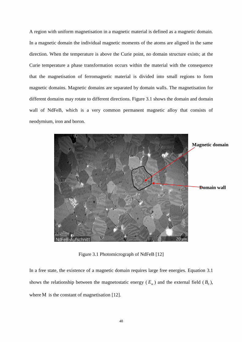
A region with uniform magnetisation in a magnetic material is defined as a magnetic domain.
In a magnetic domain the individual magnetic moments of the atoms are aligned in the same
direction. When the temperature is above the Curie point, no domain structure exists; at the
Curie temperature a phase transformation occurs within the material with the consequence
that the magnetisation of ferromagnetic material is divided into small regions to form
magnetic domains. Magnetic domains are separated by domain walls. The magnetisation for
different domains may rotate to different directions. Figure 3.1 shows the domain and domain
wall of NdFeB, which is a very common permanent magnetic alloy that consists of
neodymium, iron and boron.
Figure 3.1 Photomicrograph of NdFeB [12]
In a free state, the existence of a magnetic domain requires large free energies. Equation 3.1
shows the relationship between the magnetostatic energy ( mE ) and the external field ( 0B ),
where M is the constant of magnetisation [12].
Magnetic domain
Domain wall
49
0 0
1- ( ) -
2m iE B M B M 3.1
Where 0 i(B ) can be expressed as Equation 3.2 [12]
0 0( )i DB B B 3.2
DB is a demagnetising field, which can be formed by the apparent surface pole distribution
acting in isolation. Thus DB may be defined by the demagnetising factor D as the Equation
3.3 [12] below [60-63]:
DB DM 3.3
When the external field is removed, the self-energy is then shown as Equation 3.4 [12],
21
2sE DM 3.4
In a rectangular body magnetised along its width (Figure 3.2), splitting into two magnetic
domains with opposite direction, the self-energy ( sE ) will be reduced by half. The reason for
this is that the ratio of length to width in each domain is doubled, thus the demagnetising field
halved. However, this new domain formation is limited, as the energy reduction, due to
domain splitting, has to be balanced by the energy increasing due to creation of domain walls.

50
Figure 3.2 Split of rectangular ferromagnetic domain into parallel domains.
Figure 3.2 illustrates the process of one rectangular ferromagnetic domain divided into four
parallel domains. The length of the arrow indicates the magnitude of the demagnetising field.
In the neighbouring domain, the angular displacement is commonly 180or90 . The variation
in spin direction occurs gradually over several planes. The exchange energy ( exE ) between
two spins with the angle displacement can be described in Equation 3.5 [12]:
2 2 /exE JS N 3.5
Where J is the angular momentum, S is the spin momentum, and N stands for the number
of atom be consisted in a ‘wall’. Equation 3.5 indicates that the exchange energy is inversely
Domain Wall
Magnitude of the
demagnetising field

51
proportional to the number of atoms, thus increasing the number of atoms in a wall will
improve the creation of the wall.
It is sufficient to state that magnetisation is not only dependent upon domain formation and
evolution, but also the internal strains within the material [64-66].
3.1.2.2 The influence of applied fields
The relationship between magnetic flux density (B) and field strength (H) is given in
Equation 3.6.
0 0 0 0( )B H M H H 3.6
In Equation 3.6, 0 is the magnetic permeability for free space, and M represents the
magnetisation, which denotes how strongly a region is magnetised. represents the
magnetic susceptibility, which is a parameter to describe the degree of magnetisation of a
material in response to an applied field. The above equation indicates that the flux density is
influenced by the field strength, via permeability in vacuum and by the magnetic
susceptibility of the material.
Equation 3.6 can be simplified and written as Equation 3.7:
0 0(1 ) rB H H 3.7
r is the relative permeability for the material. This equation reveals that, in some cases, the
flux density is proportional to the field strength.

52
Figure 3.3 B-H relationship of a ferromagnetic material [67]
Figure 3.3 is a hysteresis loop illustrates the relationship between the induced magnetic flux
density (B) and the magnetising force (H) in a ferromagnetic material. The magnetic flux in a
ferromagnetic material without previous magnetising history changes along the curve Oa as
magnetising force increases. The dashed line Oa reveals the stronger current applied (H+),
the higher magnetic field in the material (B+). Point ‘a’ is the magnetic saturation point for
this material, at where most of the magnetic domains are aligned and the increasing external
field has little effect to the magnetic flux in the component. When the magnetising force is
reduced to zero following the line ab, the component retains some magnetic flux even there is
no applied field. As applying the reverse magnetising force, the magnetic flux reduces to
zero at point ‘c’, this process is called ‘demagnetisation’ and point ‘c’ is referred as
‘Coercivity point’. The amount of reverse force which required removing the residual
magnetism from the material is the ‘Coercive Force’.
As the reverse magnetising force increases, the component then goes to the negative
saturation point‘d’. If then the negative magnetising force gradually reduces to zero, the
B Flux Density
Saturation
H -H
Magnetising Force
-B Saturation in
Opposite Direction
Retentivity
Coercivity
O

53
residual magnetism in the material at Point ‘e’ would be the same level as at Point ‘b’, but
with opposite direction. When the positive magnetising force increased to ‘f’, the residual
magnetism from the material can be removed. Continuing to increase the positive
magnetising force, the material will reach its positive magnetic saturation ‘a’ again along
curve f-a.
Magnetic permeability ( r ) represents the ease a magnetic flux can be established in a
material. Permeability can be expressed by Equation 3.8 with magnetic flux density (B) and
magnetising force (H).
/r B H 3.8
Equation 3.8 indicates that the magnetic permeability is the slope at any point of B-H curve
(Figure 3.3). Figure 3.4 shows the permeability at a point in the hysteresis loop [67-69].
Figure 3.4 Permeability of a point on a B-H Curve [67]
B
H
The slope of the line that is
tangent to the B-H curve at this
point is used to determine the
permeability

54
Figure 3.5 Magnetisation of a singular ferromagnetic crystal [20]
Figure 3.5 shows the process of magnetisation of a singular ferromagnetic crystal. At the
initial point (Point O in Figure 3.3), the un-magnetised ferromagnetic material consists of
domains with a random pattern of magnetic moments. After applying a weak external field,
the magnetic dipoles start to rotate to align with the external field; shown in Figure 3.5 A.
With increasing of the field strength, domains become aligned with their neighbouring
domain, accompanied by the disappearance of domain walls and the appearance of domain
growth, which is indicated in Figure 3.5 B, C.
3.1.2.3 Temperature effects upon magnetic properties
When ferromagnetic material is heated above Curie temperature, the thermal energy
overcomes the exchange energy and results in a randomising effect, thus the aligned magnetic
moments are destroyed. Figure 3.6 shows the relationship between magnetisation and
temperature for iron. Below the Curie temperature, the iron falls into the ferromagnetic zone,

55
as temperature increases magnetisation decreases to zero at Curie point. When the
temperature goes up to the Curie temperature, the iron is in paramagnetic state, however the
susceptibility ( ) is inversely proportional to temperature due to the random electrons.
Figure 3.6 Relationship of Magnetisation to Temperatures Relative to Curie in a
Ferromagnetic Material [70]
Equation 3.9 below shows the relationship between susceptibility ( ) and temperature. C
stands for Curie temperature [70-75].
C
T
3.9
3.1.2.4 Solute Atom Content
Addition of solute atoms influences the Curie temperature, which is related to material
magnetic properties, due to the interactions between electrons and the effects of atoms upon a

56
crystal lattice [25]. Figure 3.7 shows the relationship between Curie temperature and solute
atom content in Fe.
Figure 3.7 Relationship between Curie temperature and solute atoms [70]
For Mn, Si, Al and Cr, the Curie temperature decreases as the solute atom content increases.
However, for Gold (Au) and Tin (Sn), the effect of solute atom content to Curie temperature
is not that significant. For Vanadium (V), the Curie temperature increases with the increase of
content until it reaches 6 wt %, and then decreases, when the content is higher than 21 wt%,
the Curie temperature will be independent of the solute atom content.

57
3.2 Fundamental EM relationships
Four areas, including basic electromagnetic Maxwell’s equations, quasi-static fields,
harmonic fields and spatial condition, will be discussed in the following sections to
understand the influence of the external magnetic field on ferromagnetic material.
3.2.1 Maxwell’s Equations
Maxwell’s equations are a set of four concise equations to state the relations between
electricity and magnetism. The four equations illustrate how electric charges and electric
currents create electric and magnetic fields, furthermore the relationship between time
varying electric field and magnetic field has been revealed. Maxwell’s equations consist of
Gauss’s law, Gauss’s law for magnetism, Faraday’s law of induction and Ampere’s circuital
law. Gauss’s law shows that electric charges are the source for the electric field; by contrast
Gauss’s law for magnetism indicates that there is no magnetic charge for magnetic field.
Faraday’ law illustrates how an electric field is formed by a time changing magnetic field,
and Ampere’s law indicates the reverse process. The differential forms of Maxwell’s
equations are shown as below [77-82]:
0
E
Gauss’ Law 3.10
0B Gauss’ Law for magnetism 3.11
BE
t
Faraday’s Law of induction 3 .12

58
0 0 0
EB J
t
Ampere’s circuital Law 3.13
Where E stands for electric field intensity, B is the magnetic flux density, is the free
charge density, and J stands for current density.
The relationship between magnetic flux ( B ), electric field intensity ( E ), magnetic field
intensity ( H ), electric field displacement ( D ) and charge density ( J ) are revealed by
constitutive equations below:
0 rB H 3.14
J E 3.15
D E 3.16
, and stand for the electromagnetic constant permittivity, permeability and
conductivity respectively.
In order to calculate fields from symmetric distributions of charges and currents simply and
directly, Maxwell’s equations can be presented in integral forms as below:
0
( )
V
Q VE dA
Gauss’ law 3.17
0V
B dA
Gauss’ law for magnetism 3.18
( )S
S
BE dl
t
Faraday’s law of induction 3.19
0 0 0
( )SS
S
EB dl I
t
Ampere’s circuital Law 3.20

59
The integral Faraday’s law (Ampere’s law) illustrates the creation of a line integral of the
electric (magnetic) field over the closed boundary S of surface S. The integral in Gauss’ law
(Gauss’ law for magnetism) stands for the electric (magnetic) flux through the closed surface
V .
3.2.2 Harmonic consideration
The previous equations (Equation 3.10 - 3.13) are for quasi-static field. Considering a
sinusoidal time changing field, the Maxwell Equations could be re-written in the following
form:
E j B 3.21
H J j D 3.22
D 3.23
0B 3.24
Helmholtz decomposition describes that a smooth and rapidly decaying vector field can be
separated into the sum of an irrotational and a solenoidal vector field, i.e. one of curl-free and
divergency-free respectively.
In the Curl-free (irrotational) field, 0F ,but 0F , thus the scalar potential can be
derived as:
2F V 3.25

60
The scalar potential V is represented as Equation 3.25. By contrast, in a divergency-free
(solenoidal) field, 0F , the relationship between magnetic flux and vector potential ( A )
is shown as [70] :
B A 3.26
Equation 3.25 and Equation 3.26 demonstrate the superposition of vector and scalar
potentials for magnetostatic and electrostatic problem respectively in Helmholtz form.
2 2A A J 3.27
2 2 /V V 3.28
3.2.3 Spatial Implication
Solutions to Maxwell’s equations can be derived through the imposition of boundary
conditions, which lead to Poissons, Laplace and diffusion equations by considering frequency
and material properties.
For Equation 3.27 and Equation 3.28, when at very low frequency, fields may be stated as
quasi-static as its dimensions are much smaller than the wavelength (2
2
). In addition
as tends to be zero, Poisson’s equation formed from Equation 3.29 and Equation 3.30 [20]:
2E J 3.29
2 /V 3.30

61
Laplacian equations are derived from Poisson’s equation under the condition of a medium
without source. Under boundary conditions, in a magnetostatic source free zone, the
Laplacian equations are given below, which states the field under investigation:
2 0V 3.31
Equation 3.32 illustrates the relationship between a low frequency field and a conducting
material without free charges.
( )B E j E E 3.32
The relationship E j A can be derived from Equation 3.21 and 3.26. Diffusion equation
(Equation 3.34) can be created by applying Equation 3.33 to E j A .
2( )F F F 3.33
2 0A j A 3.34
3.2.4 Boundary Conditions
When magnetic field is induced to a conducting material, the field, shown as Equation 3.33,
is affected. In an electromagnetic medium, the following statements can be made [67]:
1. The tangential component of E across the boundary is continuous, i.e.
1 2t tE E 3.35
2. B , which is normal to the interface, is continuous.
3. Tangential components of E across the boundary resulted by the induced current ( sJ )
is presented by Equation 3.36, where n̂ is the unit vector normal to the interface.

62
1 1 2ˆ ( ) sn H H J 3.36
4. The normal components of D is discontinuous because of the charge imbalances at
the medias surface, thus:
2 1 2ˆ ( ) sn D D 3.37
Considering the time and Cartesian co-ordinate variables, the diffusion equation can be
reformatted as Equation 3.38. The solution of the reformatted diffusion equation is given in
Equation 3.39, which shows the relationship between the incident field and material
penetration.
22
2
1( ) x
B BB j B
x t
3.38
( )
0
y yj t
B B e e
3.39
Symbol ‘y’ represents the displacement between the material and source, is the skin depth.
For the case of simple planar geometry, the skin depth is the distance from the surface of the
material to where the magnitude of the field is 1e compared to the value at the surface, shown
as Figure 3.8.

63
Figure 3.8 Illustration of Skin depth [71]
The skin depth is calculated as Equation 3.40:
0
1
rf
3.40
The equation above indicates that the skin depth is influenced by the properties of the
material and the frequency of the field.
3.3 Eddy Current theory
Eddy Current theory is based on the fundamental EM theories provided in section 3.2. The
basic principle for all eddy-current instruments is Faraday’s law which illustrates that a time
changing magnetic field will induce a voltage in a conductor loop. When a time varying
magnetic field is applied to a large conducting object, voltages are induced in this object,
which drive currents flowing in appropriate paths. These currents are referred as eddy current.
Figure 3.9 below shows a typical Eddy Current instrument [83-86].
Magnetic Strength
Pen
etra
tion
dep
th
Skin depth

64
Figure 3.9 Typical eddy current instrument [72]
The AC signal generator in the eddy current device creates a time varying electrical signal in
the eddy current coil. Based on Ampere’s law, a magnetic field is formed due to the time
varying electrical current flowing in the coil. When the conductive object exposed in the
induced magnetic field, eddy currents are generated and start to flow. Physical properties of
the conductive object will influence the flow of the eddy current.
At the same time the eddy current in the conductive material drives its induced magnetic field,
which will be received by the same eddy current coil and generate an electrical signal. The
eddy current instrument will analyse the current signal and compare it with a reference signal
[86].
Material in the magnetic field created by excitation coil of eddy current instrument, leads to
the distortion of the magnetic flux. Several factors could influence the distribution of
magnetic field, e.g. electrical conductivity, magnetic permeability, dimension and position of
Coil
Eddy Currents
Eddy Current Instrument
Coil’s Magnetic Field
Eddy Current’s Magnetic Field
Conductive Material

65
the component. The previous discussion in Chapter 2 illustrates that temperature has a
significant effect on material’s physical property, mainly the magnetic permeability, via steel
microstructure. Thus the difference in the signal detected by the eddy current instrument
could reflect the variation of steel microstructure under controlled cooling. These provide a
rough idea on how to apply EM technology into steel microstructure detection.
3.4 Summary
Ferrite transforms from paramagnetic to ferromagnetic when cooled below Curie temperature,
due to the formation of magnetic domains. The small domain magnetic moments in
ferromagnetic material will be aligned into larger domains and produce a strong
magnetisation, if applied an external field. The magnetic permeability has a significant
increasing at paramagnetic to ferromagnetic transformation. The change of the magnetic
permeability will influence the magnetic flux created by excitation coil of an eddy current
instrument, if the material is placed in that magnetic field. The signal difference caused by
steel phase transformation provides the possibility of using EM method to monitor steel
microstructure variation.

66
Chapter 4 Investigation of the EM Sensor Response
In the previous chapters, the different types of steel microstructure and basic EM principle
have been discussed separately. In order to apply successfully EM technology into steel
microstructure monitoring, the link between steel microstructure and EM sensor output will
be presented in this chapter. Two examples of EM sensor application in metallurgy testing
will also be introduced at the end of this chapter.
4.1 Transduction chain between steel microstructure and sensor
output
The main strategy of using the EM sensor to monitor the evolution of microstructure of steel
during thermal processing, such as controlled cooling, is to link the steel microstructure
directly to the sensor output. The link is shown as Figure 4.1 below.
Figure 4.1 Illustration of the linkage [7]
4.1.1 The link between steel microstructure and EM properties

67
The relationship between steel microstructure and the EM properties of the material is
complex, depending on both phase fraction and morphology. In [7], the relationship between
phase fraction and EM properties is investigated using both theoretical and 3D FEM methods.
4.1.1.1 Theoretical method to find relationship between fraction transformed and EM
property
Effective medium theory can be used to predict the EM properties for a two phase mixture.
Effective medium theory states that the electrical / magnetic potential due to a mixture placed
in an external electrical / magnetic field is equal to the potential created by a object with the
same geometry having an equivalent effective conductivity / permeability / permittivity. The
Laplace equation is the governing relationship for these three cases and consequently results
can be generalised [4-6][87].
Maxwell’s equation can be employed to predict the effective conductivity of a cell
suspension in a dilute solution [88], shown as Equation 4.1.
1 1
3
effective e
i e e
f
f
4.1
where effective is the effective conductivity, e and i is the solution conductivity and
conductivity of particles in suspension respectively, f is the particle volume fraction.
The Bruggeman’s formula is an extension of Maxwell’s equation for concentrated
suspensions by a mathematical procedure [88] [89], presented as Equation 4.2 below.
1/3
1effective i e
e i effective
f
. 4.2
The Maxwell and Bruggeman equations are not suitable for all particle volume fractions (f of
0 to 1). The suitable range depends on the difference between the particles and solutions.

68
Power-law models are employed to predict effective permittivity, presented as Equation 4.3
below.
(1 )effective e if f , 4.3
Where is a dimensionless parameter. Known examples are Birchak formula [90] with
1/ 2 and Looyenga formula [91] 1/ 3 .
The Maxwell, Bruggemen and Power-law relationships are used to predict effective
conductivity and permittivity. Cases for predicting permeability are rare although the
relationships for permeability can be obtained by analogy with their conductivity and
permittivity counterparts as described in the following section.
4.1.1.2 FEM modeling and the electrostatics and magneto-static analogy
A simple structured sensor is used to derive permeability from the sensor output directly. The
toroidal structure is a good choice due to its simple analytical solution link between
permeability to sensor output.
2
0
2
2ln
2
r
L
R wN h
R w
, 4.4
Where r and 0 is relative permeability and permeability in air respectively. L stands for the
inductance and N denotes the number of turns. Figure 4.2 denotes the geometry of the
toroidal coil [7].

69
Figure 4.2 The sketch of toroidal coil [92]
However it is hard to thread coils around toroidal structure and magnetic linkage should be
minimized. The possible way is using the analogy between electrostatics and magnetostatics
to simplify the toroidal coil model into a parallel plate capacitor geometry whose permittivity
can be easily calculated [7]. Table 4.1 below shows the corresponding quantities in
electrostatics and magnetostatics respectively.
Table 4.1 Corresponding parameters in electrostatics and magnetostatics [7]
Electrostatic Magnetostatic
Permittivity Permeability
Relative permittivity Relative permeability
Electrical potential Magnetic scalar potential
Electric flux Magnetic flux
Capacitance Inductance
The FEM model of a parallel plate capacitor sensor is used to derive effective permittivity of
mixtures. The mixture is comprised of isolated spheres with one phase mixed into the other
h
R
l
w
l

70
randomly; the two phases have contrasting permittivity, which corresponds to permeability in
magnetostatics [7].
The effective permittivity of mixture in a paralleled capacitor sensor is illustrated as Equation
4.5.
0
r
Cd
A
4.5
Where C stands for the capacitance value, A and d is the area and separation between two
plates respectively. Figure 4.3 indicates the FEM models of a paralleled capacitor sensor with
varying permittivity as 5, 10 and 20% specimens in it.
(a) (b)
(c)

71
Figure 4.3 FEM model of paralleled capacitor sensor with varying percentages of high
permittivity phase [7]
Figure 4.4 shows the comparison of relative permeability value from FEM and formula.
Figure 4.4 Comparison of permeability from FEM and analytical formula [7]
The poor match between the Maxwell and Bruggeman and the FEM result is possibly due to
the reason that the equations are created for models with different conductivities and their
application for models of different permeabilities is limited. This is due to the analogy
between conductivity and permeability is not valid for some specific materials. In particular
insulators have zero conductivity, but there are no practical materials with zero permittivity.
For random austenite / ferrite distributions, Birchak’s formula [90] provides the best
prediction of permeability compared to FEM and other formulas [7].
Ferrite Percentage
Per
mea
bil
ity

72
4.1.2 Link between fraction transformed and sensor output
4.1.2.1 Investigation on the relationship between trans-impedance and ferrite fraction
In [3], three samples were employed to represent different composition cases: 100% fully
transformed steel, below the Curie temperature (high C steel); majority transformation
happens above Curie temperature (low C steel); transformation occurs for a range above and
below Curie temperature (medium C steel). The atomic compositions of the three cases
samples are shown in Table 4.2.
Table 4.2 Compositions of steel robs, wt-% [3]
Steel Sample C Si Mn P S Fe
Low C 0.03 0.05 0.23 0.009 0.0013 Bal.
Medium C 0.45 0.21 0.85 0.0013 0.026 Bal.
High C 0.83 0.23 0.64 0.012 0.01 Bal.
A cylindrical AC EM sensor which had one excitation coil and one sensing coil was used for
the experiment. The excitation coil was driven at 3 V and 2 Hz. The sensing coil recorded the
induced voltage due to the electromagnetic field created by the excitation coil.
The equation for trans-impedance is given as Equation 4.6:
* 1VZ
I , 4.6

73
where I stands for current in the excitation coil and 1V is the quadratic component of the
induced voltage at the sensing coil.
(a)
(b)
(c)
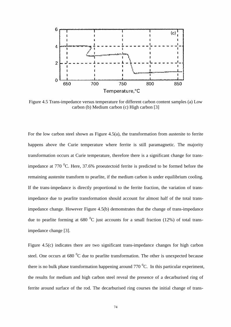
74
Figure 4.5 Trans-impedance versus temperature for different carbon content samples (a) Low
carbon (b) Medium carbon (c) High carbon [3]
For the low carbon steel shown as Figure 4.5(a), the transformation from austenite to ferrite
happens above the Curie temperature where ferrite is still paramagnetic. The majority
transformation occurs at Curie temperature, therefore there is a significant change for trans-
impedance at 770 0C. Here, 37.6% proeutectoid ferrite is predicted to be formed before the
remaining austenite transform to pearlite, if the medium carbon is under equilibrium cooling.
If the trans-impedance is directly proportional to the ferrite fraction, the variation of trans-
impedance due to pearlite transformation should account for almost half of the total trans-
impedance change. However Figure 4.5(b) demonstrates that the change of trans-impedance
due to pearlite forming at 680 0C just accounts for a small fraction (12%) of total trans-
impedance change [3].
Figure 4.5(c) indicates there are two significant trans-impedance changes for high carbon
steel. One occurs at 680 0C due to pearlite transformation. The other is unexpected because
there is no bulk phase transformation happening around 770 0C. In this particular experiment,
the results for medium and high carbon steel reveal the presence of a decarburised ring of
ferrite around surface of the rod. The decarburised ring courses the initial change of trans-

75
impedance at the Curie temperature. Additionally, the distribution of ferrite is also very
important. The continuous ferrite ring around the rod has a more significant effect on the
trans-impedance than the isolated ferrite region [3].
Interrupted quench tests between 740 0C and 680
0C were employed to determine the
relationship between trans-impedance and ferrite fraction. Figure 4.6 demonstrates the
amount of ferrite at different points in the trans-impedance and temperature trace line for
small grained (15 m ) medium carbon steel. At Position 1, where the temperature was 740
0C, there is no bulk ferrite formed. From Position 2 to Position 4, temperature decreased from
7200C to 690
0C, however the percentage of ferrite increased from 1% to 18%. At Position 5,
the temperature was 6810C and the specimen was consisted by 28% bulk ferrite and 6%
pearlite [3].
Figure 4.6 Trans-impedance versus temperature for small grained sample with optical
micrographs showing percentage of ferrite (white or lighter) formed at specific points on the
temperature axis. [3]
Position 1
Position 2
Position 3
Position 4
Position 5

76
Figure 4.6 indicates that pearlite accounts for 72% of total microstructure area fraction, at the
same time it only contributes 12% of the trans-impedance change.
Figure 4.7 Trans-impedance versus ferrite fraction for different grain size [3]
Figure 4.7 shows the ferrite fraction versus trans-impedance for small grain size (15 m ) and
large grain size (500 m ). It can clearly be seen that the relationship between ferrite fraction
and trans-impedance is also influenced by grain size. Therefore, for the EM sensor used to
detect microstructure transformation online in a hot strip mill, the prior grain size should be
determined or taken into account with calibration [3].
The finite element setup within the model of the EM sensor is shown in Figure 4.8.

77
Figure 4.8 FEM simulation of steel specimen within EM sensor [3]
The 20*20 cells stand for different distribution of ferrite within the austenite matrix. FEM
results are given in Figure 4.9.
20*20 Cell ‘Sample’
Paramagnetic Cell
Ferromagnetic Cell
Magnetic Flux
Sample
Electromagnetic Sensor

78
Figure 4.9 FEM simulation results for given ferrite distribution [3]
(a) 100% austenite (b) 100% ferrite (c) 10% ferrite in random distribution (d) 5% ferrite
distribute in a connected line horizontal through the center (e) 5% ferrite distribute in a
connected line perpendicular through the center (f) 15% ferrite represents decarburized ferrite
layer at surface and 5% ferrite distribute randomly within the specimen
Figure 4.9(a) indicates that a fully paramagnetic specimen (100% austenite) has no effect on
the magnetic flux through the EM sensor in the magnetostatic case. Figure 4.9(b) shows if the
fully ferromagnetic specimen is placed within the sensor, the magnetic flux would be drawn
into the specimen and penetrates to full thickness. Figure 4.9(c) reveals the sample with 10%
ferrite in random distribution, the magnetic flux path varied compared with Figure 4.9(a) due
to the presence of ferrite phase. The small path deviation occurs to the areas close to ferrite
cells. Figure 4.9(d) and Figure 4.9(e) represent 5% ferrite distributed as a connected line

79
running horizontal and perpendicular to the centre of specimen respectively. In Figure 4.9(d)
the magnetic flux line deviate and concentrate at ferrite cells. However, the effect of the
presence of ferrite to the magnetic path is very small. In Figure 4.9(f) the horizontal
connected ferrite line at the top and bottom of the sample represent the decarburised ferrite
region and ferrite distributed randomly throughout the specimen. The magnetic flux lines are
almost fully concentrated in the top and bottom of the specimen [3].
Figure 4.10 shows the trans-impedance versus ferrite fraction under different ferrite
distribution cases.
Figure 4.10 Trans-impedance versus ferrite percentage obtained using FEM [3]
It can clearly be seen that trans-impedance value is linearly proportional to the ferrite fraction
if the ferrite is distributed randomly in austenite.
Figure 4.11 plots the trans-impedance values obtained by FEM for the EM sensor output on
for different distributions of ferrite grains. These are also plotted against the equivalent
curves measured from medium carbon steel, but with significantly different grain sizes.

80
Figure 4.11 Trans-impedance versus ferrite fraction for FEM and experiments for medium
carbon steel [3]
Figure 4.11 reveals that the change of trans-impedance is strongly affected by prior grain size
of the steel and related to the contiguity of the bulk ferrite phase. However, if distribution of
the ferrite is determined, EM sensor can be used to measure ferrite volume fraction [3].
4.1.2.2 Impedance spectrum
Impedance stands for the ability to oppose alternating current (AC). The complex quantity of
impedance can be represented by two parts: one is the real part resistance R, the other is the
imaginary part, i.e. the reactance X, as Equation 4.7.
Z R jX 4.7
Imaginary impedance is defined as the impedance 90 out of phase (leading) with the driving
current. In electromagnetic circuits, imaginary impedance relates the induced voltage in a

81
sensing coil to the source. Real impedance represents in phase with the source. In respect to
electromagnetic impedance, real impedance describes the losses in the electromagnetic circuit.
The impedance of an ideal resistor is purely real as Equation 4.8:
RZ R . 4.8
Ideal inductors and capacitors have purely imaginary impedance shown as Equation 4.9 and
4.10:
LZ j L , 4.9
1cZ
j C . 4.10
Inductance can be calculated as Equation 4.11:
LZL
j . 4.11
Z R jX X Rj
j j
, 4.12
Where 2 f ,X
is called the real inductance, and
R
is the imaginary inductance.
4.1.2.3 Peak frequency for the imaginary part and zero-crossing frequency for real
inductance
The zero-crossing frequency can be explained in terms of basic electromagnetic principles as
below: The magnetic field created by the EM sensor affects the magnetic object in two ways.
On the one hand, it magnetizes the steel which would increase the inductance of the coil.
However, on the other hand, the magnetic field also induced eddy currents in the magnetic

82
object, which tends to oppose the driven current and therefore reduce the inductance of the
coil. At lower excitation frequencies, the magnetization dominates and change in inductance
caused by the target steel is positive. As the excitation frequency increases, eddy current
effects become dominant and inductance change decrease to negative. At high frequencies,
the inductance reaches a constant negative value. The zero–crossing frequency is the
frequency at which the change of inductance due to the steel is zero [93].
The analytical solution for peak frequency and zero-crossing frequency is given below,
following the formulation developed by Dodd and Deeds [94].
The difference of inductance due to presence of steel plate is )()()( ALLL , where
)(L is the coil inductance above a target steel plate, and )(AL is the inductance in air.
Figure 4.12 is the geometry of the model.

83
(a)
(b)
Figure 4.12 (a) The schematic diagram of the model; (b) the geometry of the coil [8]
Dodd and Deeds [94] provided the solution to calculate the difference of inductance due the
presence of sample which is shown as Equation 4.13:
2
6
0
( )( ) ( ) ( )
PL K A d
4.13
where ( )L is the coil inductance change due to the presence of the conduction plate.

84
1
1
2
1 1 1 1
2
1 1 1 1
( )( ) ( )( )( )
( )( ) ( )( )
c
r r r r
c
r r r r
e
e
4.14
2
1 rj 4.15
2
0
2 2
1 2 1 2( ) ( )
NK
l l r r
4.16
2
1
1( ) ( )
r
r
P xJ x dx
4.17
1 2 2( ) ( )l l
A e e
4.18
Where K is the integration variable and is the angular frequency of the excitation signal.
The relative permeability and conductivity of the sample are provided as r and . N denotes
the number of turns of the coil. 1r And 2r stands for the inner and outer radii of the coil
respectively, 1l and 2l denote the height of the bottom and top of the coil, c is the thickness of
the plate. 0 is the permeability in air and 1( )J x is a first-order Bessel function.
( ) in Equation 4.14 varies slower with than other components in Equation 4.13. At a
characteristic spatial frequency 0 , which is defined as the reciprocal of the smallest
dimension of the coil, when ( ) is maximum. Thus, the formulas above can be simplified.
If we take ( ) at 0 outside of the integral, Equation 4.13 can be simplified to
0 0( ) ( )L L , 4.19
Where2
0 6
( )( )
PL K A d
could be regarded as the inductance in the limit of an
arbitrary large frequency, 0L L .

85
The skin depth is smaller compared to the thickness c of the specimen, as the thickness is
assumed to be infinity. Equation 4.14 can be simplified to
2
0 0 0
02
0 0 0
( )r r
r r
j
j
. 4.20
For the magnetic sample, the relative permeability r is assumed to be much larger than 1,
Equation 4.20 can be further simplified as:
0
2
0
0
0
2
0
1
( )
1
r
r
j
j
4.21
Assuming 0
2
0r
x
, Equation 4.21 can be expressed as:
0
1( )
1
jx
jx
4.22
Then the real part of 1
1
jx
jx
2
2
1
1
x
x
is zero, only when x=1, i.e., 0
2
0
1r
the real part of
Equation 4.21 equals 0.
So for the real inductance equals zero, the relationship between the excitation frequency and
relative permeability is shown as below:
2
00
0
r
. 4.23
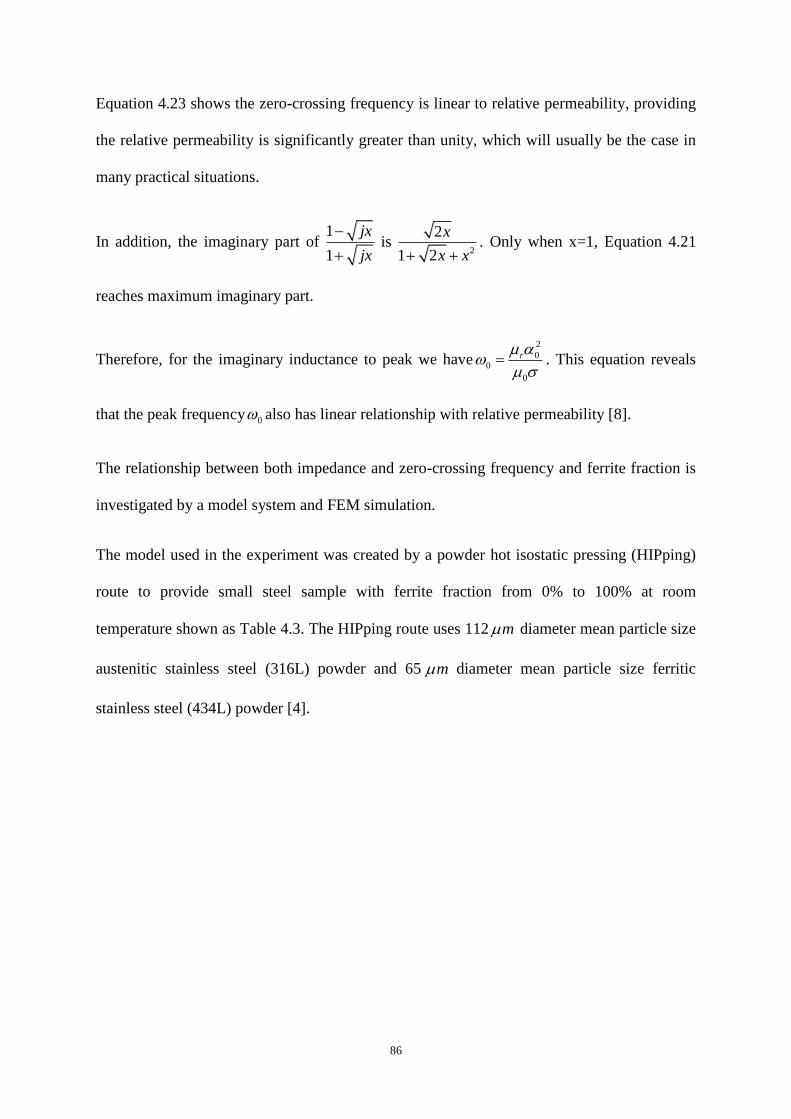
86
Equation 4.23 shows the zero-crossing frequency is linear to relative permeability, providing
the relative permeability is significantly greater than unity, which will usually be the case in
many practical situations.
In addition, the imaginary part of 1
1
jx
jx
is
2
2
1 2
x
x x . Only when x=1, Equation 4.21
reaches maximum imaginary part.
Therefore, for the imaginary inductance to peak we have2
00
0
r
. This equation reveals
that the peak frequency 0 also has linear relationship with relative permeability [8].
The relationship between both impedance and zero-crossing frequency and ferrite fraction is
investigated by a model system and FEM simulation.
The model used in the experiment was created by a powder hot isostatic pressing (HIPping)
route to provide small steel sample with ferrite fraction from 0% to 100% at room
temperature shown as Table 4.3. The HIPping route uses 112 m diameter mean particle size
austenitic stainless steel (316L) powder and 65 m diameter mean particle size ferritic
stainless steel (434L) powder [4].

87
Table 4.3 HIPped sample characteristics in terms of wt.% ferrite stainless steel (434L)
powder used and the measured microstructure obtained [4]
wt.% 434L Powder Measured ferrite
percentage (%)
Measured oxide/voids
(%)
5 6.9 1.2 0.7 0.03
10 11.2 1.0 0.8 0.06
20 26.3 1.6 1.2 0.35
30 36.8 3.6 1.8 0.28
40 40.3 2.5 1.8 0.25
60 54.5 0.9 1.8 0.14
70 69.9 1.4 2.3 0.30
100 96.4 0.3 3.6 0.30
The samples were machined into the shape of a disc with 43 mm diameter and 10 mm
thickness. The EM sensor has air cored excitation and sensing coils. The excitation
frequency is from 100 Hz to 1 MHz, tests for inductance and impedance were carried out for
all samples.
Figure 4.13 shows the EM sensor output of real inductance versus excitation frequency for
different ferrite fractions.

88
Figure 4.13 Real inductance value versus frequency for several HIPped samples [4]
As mentioned above, the magnetic field generated by the EM sensor affects the magnetic
target in two ways. At lower frequencies, the inductance difference for sensing coil should be
positive as magnetization dominates. As frequency increases, eddy current become
dominating so inductance would decrease and eventually reach constant at high frequency.
Figure 4.13 denotes that zero-crossing frequency to be related to ferrite fraction.
FEM software (Comsol Ltd.) was employed in [4] for the 3D FEM simulation. The cylinder
with 6 mm diameter and 3 mm high is used to represent the target object. The relative
permeability is set as 200 and 1 to ferromagnetic regions and paramagnetic regions
respectively. By adding 1 mm diameter austenite spheres into ferrite sequentially to 100
spheres, the increase of paramagnetic material is represented. If the amount of austenite is
increased beyond 100 spheres, the diameter of austenite sphere can be increased to maximum
2.2 mm. The simulation was carried out at 50 Hz, where the effects of eddy currents can be
neglected for the size of sample.
The inductance is given by Equation 4.24:

89
22 mW
LI
, 4.24
where mW is the magnetic energy and I is excitation current. The impedance Z is given by
Equation 4.25:
2 2 0.5(( ) ( ) )Z L R , 4.25
Where is the angular velocity (in rad/s) and R stands for the effect of energy losses due to
hysteresis and eddy currents in target object.
Figure 4.14 Impedance versus ferrite fraction for FEM and experiments on HIPped samples
[4]
Figure 4.14 shows a comparison of FEM simulation results and experimental HIPped sample
results for impedance versus ferrite fraction. The difference between FEM results and
experiment results may be due to the difference in size and geometry of the experiment and
the simulated sample. Figure 4.14 denotes a linear relationship between the imaginary
impedance and ferrite fraction from 0% to 40% ferrite. Above 40% ferrite, the increase of
impedance is relatively small when compared to the increase of ferrite fraction. The linear
Impedance (Ohms)
% F
erri
te

90
relationship between imaginary impedance and ferrite fraction, when ferrite percentage is
lower than 40%, is of little use in practical steel manufacture industry because normally
ferrite fraction is required to 80% [4]. Unfortunately, we note from Figure 4.14 that
impedance is insensitive to ferrite fraction above 40% ferrite.
Figure 4.15 Zero-crossing frequency versus ferrite fraction for HIPped sample [4]
Figure 4.15 presents a plot of the zero-crossing frequency, which is approximately linearly
proportional to ferrite fraction for ferrite percentage above 35-40%.
Comparing Fgures 4.14 and 4.15, it is found that impedance value can be used to measure
ferrite transformation when ferrite fraction is below 40% [6] [9] , for ferrite fraction above
40%, zero-crossing frequency can be employed for monitoring phase transformation which is
linearly proportional to ferrite fraction over this range. Therefore, EM sensor can be used to
detect the whole ferrite range during cooling.
Ferrite Fraction (%)
Zer
o C
ross
ing F
req
uen
cy (
Hz)

91
4.2 Application of EM sensor in NDT
4.2.1 Thickness measurement of none-magnetic plates using multi-
frequency eddy current sensor.
In [95], an inversely proportional relationship between the peak frequency of the imaginary
inductance and the thickness of a given material is reported. This suggests that the multi-
frequency eddy current method has possibility to carry real-time thickness measurement.
Simulation and experiment results also show that thickness measurement using a multi-
frequency approach through the relationship between peak frequency and thickness is almost
immune to lift-off variation for particular sensor geometries.
4.2.1.1 Analytical solution for an air-cored sensor on a conducting plate and two limiting
cases 0 and .
The analytical solution for an air-cored sensor on a conducting plate was detailed discussed in
Section 4.1.2.3. earlier
When 0 , the real part of the inductance is zero which means that the magnetic flux
penetrates into the plate as in free space. The magnetic field didn’t induce eddy current when
the excitation frequency is zero; therefore the imaginary part of the inductance is zero as well.
At very large frequency, the inductance change is given as Equation 4.26:
0L L , 4.26
where2
60
( )( ) ( )P
L K A d
, in this situation the inductance change is immune to the
thickness and conductivity variation of the conducting plate. The incident magnetic flux is

92
totally excluded from the plate. At both of the two limiting cases, the imaginary inductance
is zero which means the energy loss due to eddy current does not exist in the conducting plate
at these frequencies. However, eddy current effect does exist between these two frequencies.
From this discussion, it may be reasonable to deduce that there must be a peak frequency at
which the energy loss due to eddy current effect reaches its maximum value.
From the analytical solution of air-cored sensor upon a conducting plate, a simple relation
between thickness of a conducting plate c and peak frequency p can be presented as
Equation 4.27:
pc const . 4.27
The constant in the previous equation depends on the geometry of the sensor, if the constant
is determined; it is easy to calculate the thickness. This equation indicates that the peak
frequency decreases as thickness increases for a conducting, non-magnetic plate [95].
4.2.1.2 Simulation and experiment results
Figure 4.16 and Figure 4.17 show the relationship between peak frequency of imaginary
inductance and thickness of conducting plate. Apparently, the peak frequency of imaginary
inductance increases as the thickness decreases as expected from the previous section.

93
Figure 4.16 The imaginary part of the inductance for copper plate with thickness
22,44,…..22*6 um (simulation result) [95]
Figure 4.17 The imaginary part of the inductance for aluminum plate with thickness
22,44,…..22*6 um (simulation result) [95]

94
Figure 4.18 The peak frequency for imaginary part of inductance for aluminum plate with
thickness 1-5mm (experiment result) [95]
The experiment result shows as Figure 4.18 agrees with simulation result that peak frequency
for imaginary part of inductance increase as thickness decrease. A ferrite core U-shaped
sensor is employed for the test.

95
Figure 4.19 The peak frequency for imaginary part of inductance for an aluminum plate with
thickness is 3mm [95]
Figure 4.19 gives the conclusion that with increase of lift-off, the magnitude of inductance
decreases. However peak frequency holds the same under different lift-off.
The peak frequency parameter of the sensor response provides a real-time thickness
measurement method and it is also lift-off independent.
4.2.2 Off line measurement of decarburization of steels using a
multifrequency electromagnetic sensor
The possibility of using an electromagnetic sensor to measure the depth of decarburization
off-line through the difference in permeability between surface ferrite and bulk pearlite was
reported [10].
4.2.2.1 Decarburization processing

96
The decarburization phenomenon describes the reduction of carbon at the surface of metal,
especially steel.Steel was heated up to 800 0C during heat treatment and heat processing; at
this temperature the material was in austenite phase field. Carbon at the surface can be moved
away by reaction with oxygen in air, this process is called decarburization. Loss of carbon at
the surface is harmful to the mechanical properties of steel, such as hardness, strength and
fatigue resistance. The depth and extent of decarburization zone need accurate measurement.
In [10] decarburized samples were produced by heat treatment of a Fe-0.8 % C steel bar in
an air furnace for different dwell times and then cooled in air. Figure 4.20 is the
microstructure for different decarburization sample.
Figure 4.20 Microstructures of Fe-0.8 wt % C after decarburizing at 1000degree for different
times: (a) 10 minutes, (b)1 hour, (c) 2 hour and (d) 5 hours [10]

97
In Figure 4.20 the white part is of the surface is the ferrite zone which is fully decarburized.
Ferrite and pearlite mixed zone which is partially decarburised is represented by dark. Full
pearlite region is extended to the core. With increasing of the decarburizing time, the depth of
decarburizing zone increases [10].
4.2.2.2 Sensor output and decarburization depth
The decarburization samples were placed in an air-cored cylindrical sensor and the excitation
frequency was in the range 10 to 100 Hz.
Figure 4.21 Inductance versus frequency for decarburized samples. [10]
Figure 4.21 indicates that inductance of the sensor increases as the decarburizing time
increase at all frequencies. At 10 Hz the sensor cannot readily distinguish the sample with
decarburizing times of 10mins and 1 hour as the skin depth is too large compared to the
decarburization depth. The frequency 100 Hz shows the larger difference for different
samples.
The decarburizing process is related to carbon atom diffusion in austenite region according
to Fick’s law. Measurement from direct microstructure images shows the decarburizing depth
is proportional to the square root of diffusion time as figure 4.22.
Frequency (Hz)
Ind
uct
an
ce (
H)

98
Figure 4.22 Decarburizing depth and inductance change with decarburizing time [10]
Figure 4.22 also indicates the inductance under 100Hz is almost linear to the square root of
decarburizing time.
Also the result of the modelling is compared with the measurement in Figure 4.23.
Figure 4.23 Comparison the modeled and measured result [10]
Figure 4.23 shows that the modelled result and measured result have a good agreement. Both
of the results are approximately linear to the full decarburizing depth.

99
The modelling and test work indicate that the air-cored cylindrical sensor can be employed to
measure the off-line decarburizing depth of pearlite based steel bar [10].
4.3 Summary
Previous investigation indicates that there are strong connection between steel microstructure
and EM sensor output via steel physical properties especially electrical conductivity and
magnetic permeability. It is found that when ferrite percentage is below 40% the impedance
has a linearly relationship with ferrite fraction. However, when ferrite fraction is higher than
40%, both theoretical and measurement results presented that the zero-crossing frequency is
linearly proportional to ferrite percentage. The two application examples of eddy current
methods on thickness test for non-magnetic plates and off-line decarburisation depth
measurement for rail also provide confidence to use EM technology in steel microstructure
evaluation, more investigations on EM method are presented elsewhere[96- 101].

100
Chapter 5 MFIA Preliminary Trial Results from
Tata Steel
The MFIA system has been installed in the strip mill in Tata steel at Ijmuiden. This chapter
will present the initial test results carried out by Tata Steel and also the early stage of
calibration investigation.
5.1 Industry Test Setup
Figure 5.1 shows the test setup in a real strip mill.
Figure 5.1 Sensor position in the strip mill [110]
Position 1 Position2

101
The image at the top of Figure 5.1 is the sketch of the strip mill in Titan simulation, where
strip rolls from the left side to right side. There are two positions in the sketch Position 1 and
Position 2. The MFIA system is planted at ET1. The bottom image of Figure 5.1 shows the
MFIA system in the housing is installed between two rollers. The response of MFIA will be
presented to indicate the process of steel microstructure transformation.
5.2 Data Analysis
Steel samples in four different categories are tested, including High Stress Low Alloy (HSLA)
steel, DP steel and steels with different carbon content (0.04% and 0.14%). Figure 5.2
indicates the ferrite fraction and temperature for the four samples measured.
Figure 5.2 Ferrite fraction and temperature tested by MFIA at position1 [110]
0 50 100 150 200 250 3000
10
20
30
40
50
60
70
80
90
100
Time (s)
Fra
ction o
f tr
ansfo
rmation
0 50 100 150 200 250 300550
575
600
625
650
675
700
725
750
775
800
Measure
d T
em
pera
ture
(oC
)0.04% C
0.14% C
HSLA
DP

102
Figure 5.2 shows the plot of the transformation fraction over time, which also indicated the
length of the ROT for four different grades samples. The transformation fraction in Figure 5.2
is deduced from the power-law model in [111]. Effective medium theory is used to predict
the conductivity/permittivity/permeability for a multi-phase mixture. In [111], the two phase
(austenite/ferrite) mixture is created HIPping of ferritic and austenitic stainless steel powders.
Figure 5.3 shows the microstructure of HIPping mixture with different ferrite fraction. In
Figure 5.3 the dark part represents ferrite; on the other hand the bright part expressed
austenite.
Figure 5.3 Optical micrographs of HIPped sample with different ferrite fraction (a) 10% (b)
40% (c) 60% (d) 70% [111]
Power lower models uses Equation 5.1 to explain the relationship between effective
permeability ( e ) and the fraction of the two compositions.

103
(1 )e A Ff f 5.1
In Equation 5.1, A and F stands for the permeability of austenite and ferrite respectively. f
is the ferrite percentage. is the dimensionless parameter, which is related to the
morphology and distribution of particles. In most conditions, the mixture is random, where
the value of is 1/2 and 1/3 in Birchak formula [90] and Looyenga formula [91].
Equation 4.23 indicates the relationship between zero-crossing frequency and permeability.
Thus combining Equation 5.1 and Equation 4.23, the relationship between austenite/ferrite
fraction and the two phase mixture zero-crossing frequency can be found as:
(1 )e A Ff f 5.2
Where A and F is the zero-crossing frequency for austenite and ferrite respectively and f is
ferrite fraction.
e can be deduced from data measured by MFIA. Figure 5.4 is the plot of the phase against
ROT length and frequency respectively, which is measured by MFIA.
Figure 5.4 Phase measured by MFIA at different position of the ROT [110]
Frequency (Hz) Zero-crossing line
P1 P2 P3 P4

104
In Figure 5.4 the phase data are measured at four positions, which are 80m, 90m, 120m and
400m. The working frequency range for the existence MFIA system is under 24 kHz. Thus
for the sample, at 120m (red curve) and 400m (light blue curve), the zero-crossing frequency
is out of the MFIA’s working range. The zero-crossing frequencies at 120m and 400m are
obtained by curve fitting. Using Equation 5.2 the transformation fraction can be deduced as
20%, 37%, 63% and 87%.
5.3 Summary
The measurement result in Tata Steel indicates that MFIA system has a good performance in
the real ROT; MFIA produced continual and stable data. In addition, the MFIA data clearly
present the ferrite transformation process from 20% to 87% at four different positions along
the ROT. Furthermore, power law model provides a possibility to transfer MFIA output to the
transformation fraction through zero-crossing frequency. However there are still some
problems need to be solved, when using the power law model, these problems are as follows:
Increase the accuracy of the measure of zero-crossing frequency
Establish the zero-crossing frequency for fully transformed steel and un-transformed
steel
Increase in the MFIA frequency coverage

105
Chapter 6 Modelling the Response of the Sensor
System
The previous chapter discussed the link between steel microstructure and the EM sensor
output, which gives confidence to apply EM technology in steel microstructure evaluation.
Research and development of the MFIA system for the purposes of steel microstructure
monitoring start from FEM.
6.1 Methodology
FEM, which is also known as finite element analysis (FEA), is a numerical solution for a
partial differential equation (PDE). The FEM method reduces the problem into a set of
simultaneous linear equations, which saves solution time [102-104].
The basic concept of FEM is dividing the complex geometry system into small elements, the
behaviour of which can be readily analysed. Thus all FEM involves following steps [103]:
Problem domain should be divided into small sub-regions
Imposing boundary conditions to each element
Simultaneous solution of individual area equations
Summation of element solutions to the whole problem region

106
Figure 6.1 Finite Element Mesh of a simple 2D geometry
Figure 6.1 shows a simple 2D geometry that can be presented by several small triangular
shaped sub-regions. The error between the FEM method and real solution is closely linked
with the size of the elements. Smaller element size results in minimal errors, however leads to
longer processing time as there are more simultaneous equations to solve.
A 2D Laplacian problem can be used to explain the methodology of FEM. The Laplace
equation is given as Equation 3.29, which indicates that the potential has to be found. To
solve a Laplacian problem, the two boundary conditions for each element, known as the
Dirichlet (Equation 6.1) and Neumann (Equation 6.2) boundaries, should be fulfilled.
0v v 6.1
0v
n
6.2
A special potential ( v ) is imposed at each elements boundary in Equation 6.1 and 6.2. The
energy which is related to the potential (Equation 6.3), can be formulated, as the special
potential tends to a minimum. A Laplace solution ( v ) can be found, if the value of the
potential which is related to the minimum energy can be solved.

107
1( )
2W v v v dS 6.3
The potential with in an element can be expressed in Equation 6.4, in which is the scalar
error and ( , )h x y is the differential function at each boundary.
( , ) ( , ) ( , )v x y v x y h x y 6.4
If the potential with error shown as Equation 6.4 was introduced to Equation 5.3, the energy –
potential relationship can be expressed as Equation 6.5.
2( ) ( ) ( )W v h W v W h 6.5
Here, presents the difference between the Laplacian solution and FEM method which is the
solver accuracy.
Figure 6.2 Continuous elements in a Finite Element Mesh [103]
Figure 6.2 reveals the solution of ( , )v x y in element A is the basis for element B, because of
the continuous nature of the elements. Based on the Dirichlet boundary condition shown as
Equation 6.1, then 0v is the potential at the 1-2 boundary in element B, thus a solution can be
found in element B depending on this initial value. If ( , )v x y is solved in each sub-region, the
problem domain is solved for ( , )v x y .

108
ANSYS Maxwell is employed in the FEM investigation in this research. This software is a
premier EM field simulation package, which uses the FEM method to solve the
electromagnetic and electric field problems [105].
6.2 Sensor head design investigation using FEM method
Figure 6.3 FEM Model of the H-shaped sensor head
The H-shaped sensor can be treated as a two U-shaped sensors place back to back. The upper
U-shape directs half the magnetic field towards the target, which helps to make the magnetic
flux more concentrated to the target object and increase the strength of the response signal.
The lower U-shape is used to provide a cancellation or reference signal. The sensing head
consists of five coils: one excitation coil and four sensing coils. Adjacent pairs of sensing
coils are wired in series, therefore maximising the signal of interest while helping to reduce
the common mode interference caused by ambient magnetic fields. The material for the H-
shaped core is non-conductive ferrite (Mn-Zn) and for the coils is non-magnetic copper.
In order to understand how the geometry would affect the sensor performance, the size of the
width and cross section of the sensor have been changed into different values. Different FEM
models of the sensor size effects were then investigated as described in the following sections.

109
Figure 6.4 FEM Model of H-shaped sensor placed under magnetic sample
Figure 6.4 illustrates that the H-shaped sensor is placed under a steel plate. Here, the lift-off
is 30 mm, which is the distance from the top of the sensor to the bottom of the steel object.
The dimension of the steel sheet is 700 mm wide and 700 mm long with the thickness is 3
mm. In simulation, to optimise the meshing operation of Maxwell v.12 and considering the
skin depth, the steel sheet is divided into six layers with the thicknesses from the bottom to
the top layer are 0.1 mm, 0.2 mm, 0.4 mm, 0.5 mm, 0.8 mm, 1 mm respectively. The
electrical conductivity of the steel sheet is set as 61 10 /S m with its magnetic permeability
varies from 10 to 200. Based on Equation 3.40 at 10 kHz the skin depth for steel sample with
200r is around 0.3 mm, which is suitable for the thickness of sample layers, thus all the
simulations were carried out at 10 kHz.
6.2.1 Inner width variation
Figure 6.5 shows the sensor with different inner widths. Three sensors with different inner
width are used in the FEM simulations, from 50 mm to 150 mm.
Lift-off

110
Figure 6.5 H-shaped sensor with (a) 50mm (b) 100mm and (c) 150mm inner width
Figure 6.6 reveals signal ranges for different steel samples ( r from 10 to 200) responding to
different sensor width.
100mm
100mm 50mm
150mm
115mm
115mm
150mm
200mm

111
Figure 6.6 Signal range under sensors with different widths
Figure 6.6 shows the effective signal range when relative permeability of the steel sheet
changes from 10 to 200 is 63.6 10 mH, 64.8 10 mH and 64.95 10 mH respectively as the
width of the sensor is 50 mm, 100 mm and 150 mm. The simulation results reveal the signal
range increases with the increase of sensor width; therefore larger pole separations (inner
widths) are preferable.
6.2.2 Cross sectional area variation
Ind
uct
an
ce d
iffe
ren
ce (
mH
)

112
Figure 6.7 Cross sectional area of the H-shaped sensor
Figure 6.7 shows the cross section of the H-shaped sensor. In this simulation, the geometry of
the cross section has been changed from 25 mm by 25 mm to 40 mm by 40 mm and 50 mm
by 50 mm and the sensor width remains at 100 mm. Figure 5.8.indicates the effective signal
range as the relative permeability of steel sheet changes from 10 to 200 under different cross
section.
Figure 6.8 Effective signal ranges for sensors with different cross section
Cross Section
Ind
uct
an
ce d
iffe
ren
ce (
mH
)

113
Figure 6.8 reveals that as the relative permeability of steel sheet changes from 10 to 200, the
effective signal range is 64.7 10 mH, 69.6 10 mH and 51.39 10 mH respectively when the
cross-section of the H-shaped sensor is 25 mm by 25 mm, 40 mm by 40 mm and 50 mm by
50 mm, which means the larger cross section is, the larger signal range will be obtained.
Investigation on the effective signal range for different sensor sizes shows that large signal
range can be achieved by increasing sensor size such as width and cross section. However,
under real circumstance, the size of sensor should decided by other factors such as the size of
gap between the two rollers and the size of housing, which contains the sensor. By discussion
with our industrial partner (Tata Steel) the sensor geometry is decided as 115 mm high and
100 mm wide with a 25 mm*25 mm cross section as the largest permissible device using
commercially available ferrite U and I ferrite cores.
6.3 MFIA system developments
The FEM method is used to determine the relationship between the multi-frequency output of
the sensor and phase fraction of the steel microstructure. In addition, some other factors
influence the performance of the sensor system, especially the effects of nearby metalwork.
6.3.1 FEM Model of the MFIA system in situ
Figure 6.9 illustrates the real industry setup for the system.

114
Figure 6.9 FEM model of the MFIA system in real industry situation
Figure 6.9 shows that in a real controlled cooling zone, the sensor head is encapsulated in an
industry housing and placed between two rollers. Thus the effects of rollers, lift-off and
housing were investigated as part of this study.
6.3.2 Miscellaneous Effects on the MFIA performance
6.3.2.1 Roller Effect
In the model, the rollers are represented as being 1 m long with a 30 mm diameter.
Considering skin depth, the roller was divided into four layers with thickness is 0.5 mm, 1.5
mm, 4 mm and 24 mm respectively from surface to interior, shown as Figure 6.10.
Roller
Hot Strip
H-shaped Sensor
Housing

115
Figure 6.10 The roller is divided into several layers for simulation
The material for the rollers is stainless steel with high conductivity and permeability. The
electro-conductivity is set as 71.03 10 /S m with its permeability varies from 500 to 4000.
The excitation frequency range is from 100 Hz to 10 kHz. In this simulation the steel plates
upon the sensor is set as vacuum which has no effect to the sensor output. Figure 6.11
illustrates the sensor output inductance difference versus excitation frequency for rollers with
different physical properties (mainly magnetic permeability).
Figure 6.11 Inductance difference versus frequency for rollers with different permeability
Frequency (kHz)
Ind
uct
an
ce
dif
feren
ce(m
H)

116
Figure 6.11 shows that at low frequency when the frequency is lower than 2 kHz, the
inductance difference decreases rapidly as the frequency increases; which means that the
roller has a significant effect to the sensor performance. However, when the frequency is
higher than 2 kHz, the curve of inductance difference becomes flat, that is because as
frequency is very high the skin depth is small and the flux cannot penetrate into rollers. This
investigation indicates that if the excitation frequency is above 2 kHz then the roller has
negligible effect on the sensor performance.
6.3. 2.2 Industry housing
The industry housing was built for the sensor head in real industry setup. The housing is used
to protect the sensor head from water, dust and collision. In the other hand, it can shield the
magnetic field.
The housing has a ferrite base and ceramic window on the top. The bottom of the housing is
open. The model and geometry of the housing are given in Figure 6.12 shows the design and
FEM housing model.
(a)

117
(b)
Figure 6.12 (a) Computer Aided Design model of the housing [106] (b) FEM model of
industry housing with sensor in it.
The housing has a wider top (70 mm) and a narrower bottom (40 mm) with a height of 150
mm.
The effects of industry housing on the response of the sensor, in particular the ability of the
sensor to reject interference from the rollers has, been investigated. Figure 6.13 shows the
roller effect to the sensor performance with and without housing. The material for the rollers
is iron with relative permeability varies from 10 to 4000 and the housing is made with ferrite
with low conductivity (0.01 S/m) and high relative permeability (1000).

118
(a)
(b)
Figure 6.13 Inductance difference versus frequency for roller influence (a) without housing (b)
with housing
Both the above two figures show that at high frequency the curves become flat, which the
effect of the rollers is constant and therefore can be removed as an offset above 100 kHz
when there is no industrial housing and above 1 kHz when the housing is present. As the
Ind
uct
an
ce d
iffe
ren
ce (
mH
) In
du
cta
nce
dif
feren
ce (
mH
)

119
operating frequency range is a maximum100 kHz, the benefit of the housing is clear. In
addition, comparing with the two figures, it is easily to see that the industrial housing
minimises roller effect from values in the order of 610 mH (no housing) to 710 mH (with
housing) at low frequency, which means the housing effectively shields the magnetic flux
away from the roller direction.
(a)
(b)
Figure 6.14 Steel sheet effects (a) without housing (b) with housing
Ind
uct
an
ce d
iffe
ren
ce (
mH
) In
du
cta
nce
dif
feren
ce (
mH
)

120
The next simulation shown in Figure 6.14 assesses the effect of the industrial housing on the
sensitivity of the sensor. Here, the spectral response for the sensor is plotted for a steel plate,
1 mm thick placed over the sensor. The relative permeability of the plate is varied from 1 to
200 (values of 1, 5, 10, 50, 100, 150, and 200). Clearly the signal change in response to the
steel has been reduced by the housing. Simulation results reveal that the industry housing not
only shields the magnetic field flux (from 6 x 610
mH to 1.4 x 710
mH) to the roller
direction, it also reduces the sensitivity of the sensor (from 8 x 610 mH to 2.5 x 610 mH).
However, the rejection of the roller effect is much greater than the loss of sensitivity.
6.3.2.3 Lift-off effect
Lift-off is the distance from the top of sensor to the bottom of steel sheet, which is given in
Figure 6.15
Figure 6.15 Lift-off indication
Lift-off

121
To get accurate results, it is important to use the same mesh then the deviations that are
caused by interpolating between mesh elements can be avoided. The way to generate the
same mesh in different simulation is creating all the different geometries needed and then
creating the mesh. Then, the material properties of all the geometries can be changed without
changing the mesh.
In the model, all the steel sheets are built at different lift-offs (35 mm and 45 mm). The total
thickness for each steel sheet is 1 mm and has been divided into three layers of thickness 0.1
mm, 0.3 mm and 0.6 mm. The conductivity for the steel is 1.1 Ms/m and relative
permeability changes from 3 to 200. The results of the simulations are shown in Figure 6.16.
(a)
(b)
Ind
uct
an
ce d
iffe
ren
ce (
mH
)

122
Figure 6.16 Inductance difference spectra for different lift-off (a) 35mm (b) 45mm
Figure 6.16 indicates that for both lift-offs the sensor outputs have smooth inductance
difference spectra over the whole frequency range. The trend of the inductance difference
spectra can be explained as eddy current affects the object in two ways; at a low frequency,
the strip will be magnetised, which will increase the inductance difference for this coil
geometry, however at high frequencies the eddy current will tend to decrease the inductance
difference.
The phase angle of the transimpedance was also investigated. In this case, a simplified model,
as shown in Figure 6.17, was used in order to reduce the computational load.
Ind
uct
an
ce d
iffe
ren
ce (
mH
)

123
Figure 6.17 Simplified lift-off model
The lift-off varied as 35 mm, 40 mm and 45 mm.(a)
(b)

124
Figure 6.18 Impedance phase angle versus frequency at different lift-off (a) relative
permeability is 150 (b) relative permeability is 200
Figure 6.18 reveals that the phase angle spectra are almost overlapped at very low and very
high frequency and under different lift-offs. Therefore the effect of aviations in lift-off effect
will be minimised if phase angle can be used as a parameter to monitor the microstructure of
steel.
6.3.3 Linkage between sensor output and steel microstructure
Figure 6.19 shows the real and imaginary mutual induction spectral for the sensor response to
a series of steel strips with different relative permeabilities; the thickness of the steel strip is
3mm. It may be noted that in both the zero-crossing frequency of the real inductance and the
peak frequency for the imaginary inductance both increase in proportion to the relative
permeability of steel sheet increases.
(a)

125
(b)
Figure 6.19 Frequency response of the EM sensor for steel strips with different permeabilities
(a) real inductance (b) imaginary inductance
(a)
Ind
uct
ance
dif
fere
nce
(m
H)
Ind
uct
ance
dif
fere
nce
(m
H)

126
(b)
Figure 6.20 Relationship between (a) zero-crossing frequency for real inductance and relative
permeability of steel sheet (b) peak frequency for imaginary inductance and relative
permeability
Figure 6.20 indicates that both the zero-crossing frequency and peak frequency are linearly
proportional to the permeability prompted further investigation. This finding agrees with the
previous discussion in Chapter 4, where Equation 4.23 reveals both zero-crossing frequency

127
for real inductance and peak-frequency for imaginary inductance are linearly proportional to
magnetic permeability for circular air cored coils. This result can be extended to the case of
the H-shaped used here.
Due to the complex geometry of the H-shaped sensor, it is hard to find an analytical solution
for this H-shaped sensor. Fortunately the analytical solution for the simple air-cored sensor
has been discussed in Chapter 4. Combining these two results, the response of the H–shaped
ferrite cored EM sensor can be approximated by that of an equivalent air-cored sensor with
appropriate choice of parameters.
Figure 6.21 shows the comparison of FEM results for different relative permeabilities of the
steel sheet and for the analytical model. All of these figures show that the two results have a
good agreement, particularly near the zero-crossing frequency.
(a)
(b)
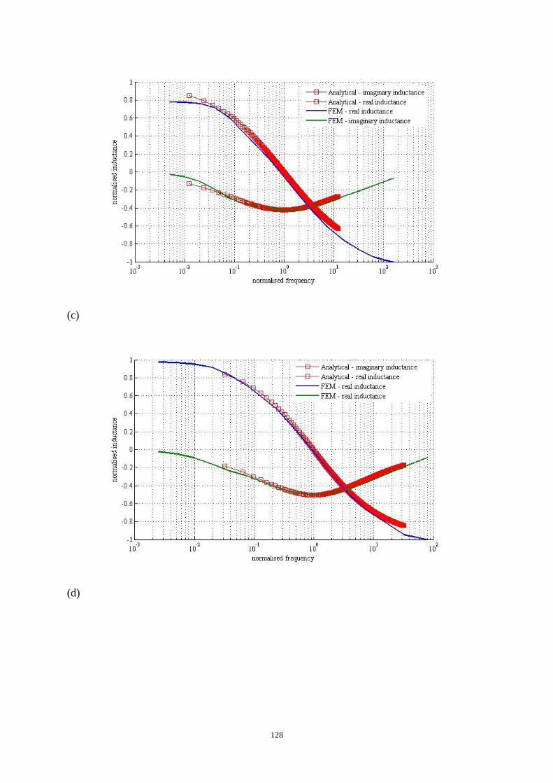
128
(c)
(d)

129
Figure 6.21 FEM results for different relative permeability versus analytical model (a)
relative permeability is 50; (b) relative permeability is 100; (c) relative permeability is 150; (d)
relative permeability is 200.
The fact that the response of the H – shaped ferrite core EM sensor in a complex industrial
setup can be approximated by that of an air-cored sensor has significance.
1. The zero-crossing frequency and the peak frequency can be expressed analytically
and can be inferred more easily.
2. The whole spectra can be deduced from discrete points means we can improve the
speed of the measurement process by taking less measurement and there is less
demand on the instruments to provide wide frequency measurement data. Therefore,
it may be possible to predict the complex sensor output using an analytical solution of
the air-cored coil, which will help the sensor calibration.
6.3.3 Combining FEM Electromagnetic models with Mill Thermodynamic
Simulations

130
6.3.3.1 The Titan simulation
Titan simulations were carried out by Tata Steel. The Titan software calculates the thermal
distribution from the surface to interior of steel at different place along the ROT and together
with the level of transformation, shown as Figure 6.22.
Figure 6.22 Screen shot from the Titan simulation software [107]
Temperature and transformation along ROT
Position in ROT
Tem
per
atu
re

131
Figure 6.23 Modelled phase distribution over thickness [107]
Figure 6.23 illustrates the transformed phase distribution level for the surface and interior of
the steel sample at different positions on the ROT. During controlled cooling the surface
temperature is lower than the interior temperature, which results in a quicker ferrite creation
at surface than interior at the same ROT position thus the ferrite percentage at A1 and A2 are
higher than B in Figure 6.23. On the other hand, the untransformed austenite percentage is
lower at surface than interior part.
6.3.3.2 Methodology
In Chapter 4, the relationship between the magnetic permeability and ferrite percentage has
been discussed. Figure 4.4 also provides the permeability – ferrite fraction curves from
different methods. As the Titan simulation gives the ferrite percentage at different thickness
depths of the sample, the magnetic permeability can then be easily derived.
In addition, from Titan simulation, temperature data can also be abstracted for different
thickness positions of the sample. Equation 6.6 below shows the connection between
electrical resistivity and temperature together with carbon content [108]:

132
1
2 41 2 3( , )T C bT b T b C 6.6
Where, ( , )T C is electrical resistivity, C is carbon content, T is temperature, is constant,
1b , 2b , 3b is the regression coefficients of predictors respectively. In this equation, 0.0651 ,
3
1 0474 10b , 6
2 0.889 10b and 3 0.122b . Based on Equation 5.6 electrical
conductivity can be calculated.
Thus, in the FEM model the steel sample is divided into several layers from top to bottom
and each layer will be assigned permeability and conductivity based on previous discussions.
6.3.3.3 FEM simulation
In order to illustrate the response from an array of sensors, six different positions were
selected along the ROT (shown as Figure 6.24) and together the corresponding data were
derived from Titan simulation (shown in Table 6.1)
Figure 6.24 Six positions along ROT

133
Table 6.1 Titan simulation data for R4272170 (C: 0.04wt%, Mn: 0.209wt%, Thickness:
5.13mm)
Figure 6.25 shows the FEM model of the simulation.
Figure 6.25 FEM model for multi-layer steel plate

134
FEM model shows the steel sample has been divided into several layers assigned with
different physical parameters.
6.3.3.4 Result analysis
Figure 6.26 presents the inductance difference spectrum of the EM sensor for steel sample at
different positions of the ROT. Excitation frequency range is from 10 Hz to 100 kHz.
Figure 6.26 Inductance difference at different position
In Figure 6.26, it can be found that at position 1, the inductance difference is only in the
negative region which means the eddy current effect minimises the induced signal,
combining with the theory in the previous section. At this point the steel is non-magnetic
which agrees with the state in Table 5.1 that there is no transformation happening at this point.
For the following points, the inductance difference values increases and the curves shift from
bottom to top, this means with the steel moving on the ROT the transformation is continuous
Ind
uct
an
ce d
iffe
ren
ce (
mH
)

135
and the ferrite percentage increases. Also the zero-crossing frequency increases with
formation of ferrite.
Figure 6.27 is the phase response of the simulation.
Figure 6.27 Phase diagram
Figure 6.27 reveals that for the non-magnetic steel, the phase is only in one quadrant,
however with the creation of ferrite the phase response shifts into two quadrants.
The polar diagram in Figure 6.28 gives a clear illustration of the transformation process of
steel along ROT.
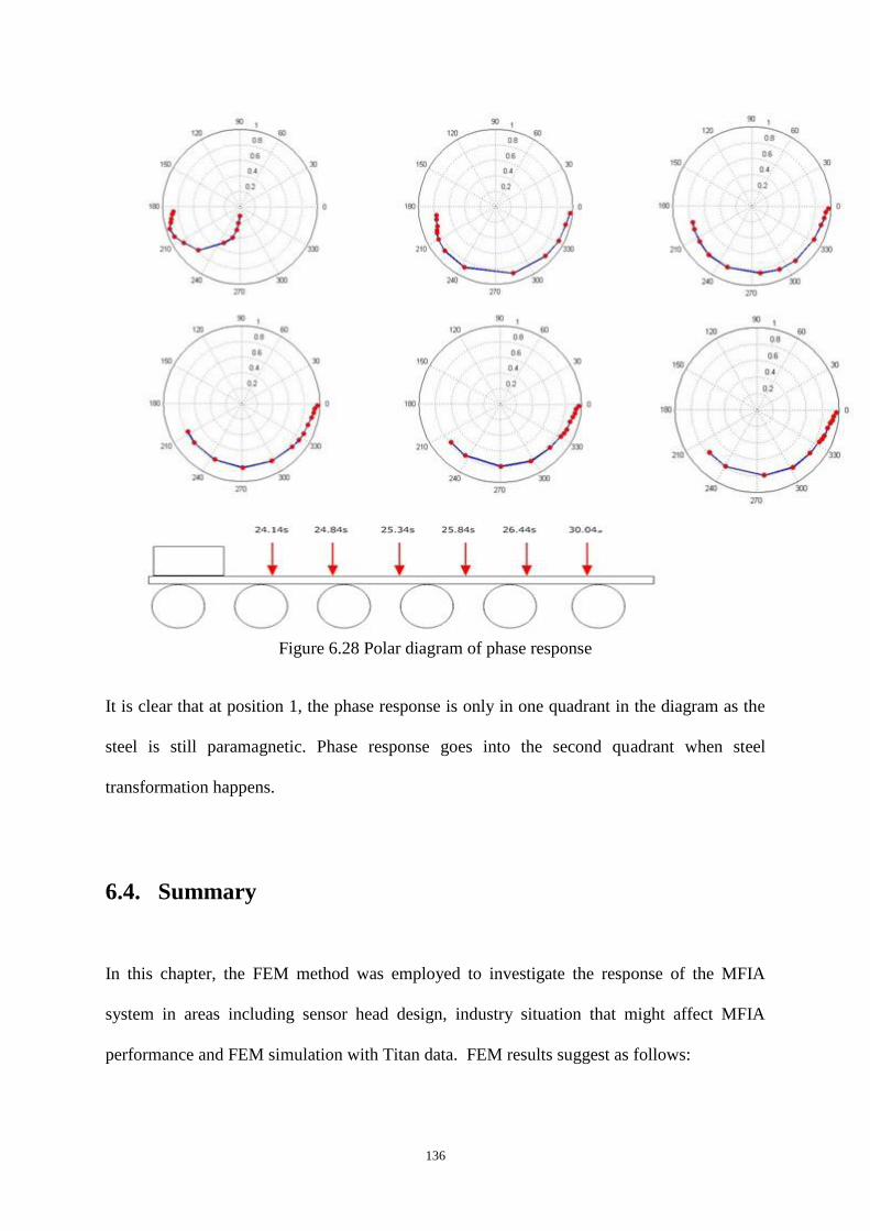
136
Figure 6.28 Polar diagram of phase response
It is clear that at position 1, the phase response is only in one quadrant in the diagram as the
steel is still paramagnetic. Phase response goes into the second quadrant when steel
transformation happens.
6.4. Summary
In this chapter, the FEM method was employed to investigate the response of the MFIA
system in areas including sensor head design, industry situation that might affect MFIA
performance and FEM simulation with Titan data. FEM results suggest as follows:

137
The larger sensor size, the larger signal will be obtained. The largest practical H-core
is preferred.
The industrial housing can effectively shield the magnetic flux, however it also
reduces sensor sensitivity. There is a considerable net benefit from using a ferrous
housing.
The lift-off has a significant effect to inductance difference, but phase is almost
independent of lift-off effect for the idealised situation where no rollers or industrial
housing is present.
Both the zero-crossing frequency for real inductance and peak frequency for
imaginary inductance are linearly proportional with magnetic permeability
The response of the H-shaped sensor can be described using the analytical solution of
simple air cored sensor
The phase response can be clearly used to describe the transformation process of steel
moving along the run out table.

138
Chapter 7 Cold Experiments on the MFIA System’s
Performance
In chapter 6, the relationship between steel microstructure and the sensor output has been
evaluated using the FEM method. In addition, factors that may affect MFIA system’s
performance have been investigated. In this chapter, the hardware of MFIA system, will be
introduced followed by the measurements which have been carried out in the laboratory with
cold steel samples to illustrate the stability and sensitivity of the system.

139
7.1 Hardware of MFIA system
Figure 7.1 Block diagram of the system hardware [109]
Figure 7.1 is an overview of the whole MFIA system. The system is composed of a sensing
head, a digital signal processing (DSP) unit and impedance measuring circuitry. Commands
are send to the DSP unit from a host computer via a serial link. The DSP controls the
measurement process and can create an excitation waveform containing up to eight
frequencies, where the value of the frequencies follow a binary sequence. The excitation
waveform is send to the sensing head by a digital-to-analogue converter (DAC) and a buffer
amplifier. Two analogue-to-digital convertors (ADC) are employed for the impedance

140
measurement. One ADC is used for excitation current measurement and the other is for the
detected voltage from the receiver coils [109].
Figure 7.2 Hardware of the MFIA system
Figure 7.2 shows the whole MFIA system, which includes the power supply, electronics,
communication components and sensor head.
7.2 MFIA System Test in the Laboratory
7.2.1 Using a Bench Top Impedance Analyser to Simulate MFIA System
Process
Electronic box
Sensor Head
RS232/USB converter
RS422/RS232 converter
Power supply

141
Figure 7.3 Sensor head working between 800 Hz to 100 kHz
The sensor head shown in Figure 7.3 was designed for the working frequency range up to 100
kHz. This sensor has a 100 turn excitation coil, two 50 turn active coils wired in series and an
additional two 50 turn backing-off coils.
The resonant frequency of this sensor head was measured using a Solartron 1260 bench top
Impedance Analyser.
Figure 7.4 Trans-impedance versus frequency for the H-shaped ferrite sensor in free space
50mm
Imp
ed
an
ce M
ag
nit
ud
e (O
hm
)

142
Figure 7.4 shows the impedance magnitude has a dramatic increase at 200 kHz and then
followed by a sharp drop, which indicates that the resonant frequency for this sensor head is
approximately 200 kHz. The required working frequency from 10 Hz to 100 kHz located in
the acceptable range.
The data from the Solartron impedance analyser was both compensated and normalised in a
similar manner to the actual sensor system. Compensation is used to balance the signal
difference between the active and backing-off coil in their housing when no sample is present.
This ensures that the output is zero without a steel target. Normalisation is used to rotate and
scale the phasor response so that a pure magnetic reference sample gives unity magnitude and
zero phase.

143
(a)
(b)
Figure 7.5 Process of normalisation (a) pure ferrite signal before normalisation (b) after
normalization
Figure 7.5 indicates the pure ferrite signal before and after normalisation. Figure 7.5 (b)
shows for pure ferrite the signal is in phase with the back ground signal, which is consistent
with Figure 6.24.

144
(a)
(b)
Figure 7.6 Phase diagram after normalisation (a) Austenite (b) 100% Ferrite
Figure 7.6 shows the phase spectrum for austenite and ferrite sample. The frequency range
here is 10 Hz to 100 kHz. Figure 7.5 and Figure 7.6 indicate that for purely magnetic sample
with conductivity is 0, the response is in phase with background. For Austenite, at low

145
frequency there is virtually no response, as the frequency increases the phasors rotate in one
quadrant. The response of ferritic steel sample combines both the purely magnetic sample and
the austenitic; now the phasor rotates across two quadrants from in-phase at zero frequency to
1800 at a very high frequency.
7.2.2 MFIA System Signal Drift Test
(a)
(b)
Imp
ed
an
ce M
ag
nit
ud
e (O
hm
)

146
(c)
Figure 7.7 Variation of impedance magnitude (a) Impedance magnitude variation in 20 mins
with no sample (b) Impedance variation in 1 minute with 100% ferrite (c) phase variation in 1
minute with 100% ferrite
Figure 7.7 shows the signal variation in over 20 minutes under laboratory conditions. The
variation is less than 1% compared with the response for 100% ferrite with 12.5mm lift-off
(Impedance magnitude is 0.413 for 0.8 kHz). This investigation shows the MFIA is quite
stable during work.
Imp
ed
an
ce M
ag
nit
ud
e (O
hm
)

147
7.2.3 Housing Effect Test using an Impedance Analyser
To protect the sensor head and shield the sensor from extraneous electromagnetic fields, the
sensor is placed in a ferritic steel housing. The housing is shown as Figure 7.8. The effect of
housing on the balance between the active coil and the backing-off coils is also investigated.
Figure 7.8 Industry housing
Figure 7.9 Housing effect to active and backing-off coils
Ind
uct
an
ce d
iffe
ren
ce (
H)

148
Figure 7.9 indicates that housing has a significant effect on the backing-off coil compared
with the active coil, due the asymmetric geometry of the housing which is wider at the top
than the body.
Figure 7.10 Backing-off coil response with different samples
Figure 7.10 shows that the responses of backing-off coil almost the same when different
samples are applied. This result indicates that although housing affected the backing-off coil,
the backing-off coil still provides a stable reference after compensation.
7.2.4 MFIA test for Austenite, 1% Ferrite and 100% Ferrite sample
(a)
Ind
uct
an
ce d
iffe
ren
ce (
H)

149
(b)
Figure 7.11 MFIA test results (a) Imaginary inductance (b) Real inductance
Figure 7.11 shows that MFIA system can clearly distinguish between an entirely
paramagnetic material and a slightly ferromagnetic material with only 1% ferrite fraction.
The eight excitation frequencies are: 0.78 kHz, 1.56 kHz, 3.1 kHz, 6.3 kHz, 12.5 kHz, 25 kHz,
50 kHz and 100 kHz. Figure 7.11 (b) indicates that the 100% ferrite sample has a zero
Ind
uct
an
ce d
iffe
ren
ce (
H)
Ind
uct
an
ce d
iffe
ren
ce (
H)

150
crossing frequency at around 8 kHz, however there is no crossing point for 1% ferrite sample
and austenite sample.
7.2.5 Impedance analyser test for different thickness samples
The aim of this investigation is to detect the sensitivity of the MFIA system to the samples’
thickness. Different thicknesses have been made using sample sets available in the laboratory,
as shown as Table 7.1. The frequency range is from 10 Hz to 100 kHz.
Table 7.1 Sample set summary
Name Dimension (Length *Width*Thickness
mm)
Quantity
Austenite 340 * 109 * 2 1
1% Ferrite 281 * 107 * 1.5 1
100% Ferrite 198 * 149 * 1.5 1
Ferrite 300 * 210 * 1
300 * 210 * 2.5
300 * 210 * 4
300 * 210 * 8
1
2
2
1
Stainless
Steel
300 * 210 * 1
300 * 210 * 2
300 * 210 * 4
300 * 210 * 8
1
2
2
1
(a)

151
(b)
(c)
Ind
uct
an
ce d
iffe
ren
ce (
H)
Ind
uct
an
ce d
iffe
ren
ce (
H)

152
(d)
Figure 7.12 Impedance analyser thickness test (a) Real inductance for ferrite samples (b)
Imaginary inductance for ferrite samples (c) Real inductance for Austenite samples (d)
Imaginary inductance for ferrite samples
Figure 7.12 (a) shows that at low frequencies, the real inductance can distinguish the ferrite
sample with different thickness, however for austenite samples the response below 100 Hz
are almost overlapped as shown in Figure 7.12 (c). For the ferrite samples, when the
frequency is higher than 50 kHz, the real inductances seem no different for different
Frequency (Hz)
Ind
uct
an
ce d
iffe
ren
ce (
H)
Ind
uct
an
ce d
iffe
ren
ce (
H)

153
thickness. Figure 7.12 (b) shows for the ferrite sample, that the peak frequencies are almost
the same, however for the austenite sample, the peak frequencies decreases as the thickness
increases. For the austenite samples with thickness 14 mm, 16 mm, 20 mm, the response is
quite close to each other.
7.2.6 New Sensor Head Working Frequency Investigation
In order to make the MFIA system suitable to the thickness of steel sheet in the rolling mill, a
new sensor with a lover working frequency between 200 Hz to 24 kHz was wound as
illustrated in Figure 7.13 The new sensor head has a 400 turn excitation coil, two 200 turn
active coils and two 200 turn backing-off coils.
Figure 7.13 Re-wound Sensor Head for the 200 Hz to 24 kHz frequency range.
The working frequency of the new sensor head was measured using a Solartron1260
Impedance analyzer. Figure 7.14 indicates the relationship between the magnitude of transi-
impedance and the excitation frequency.
50mm

154
Figure 7.14 Frequency response of the new sensor head
Figure 7.14 reveals that the resonant frequency for this sensor head is around 50 kHz, which
is close, but above our highest working frequency (24 kHz).
7.2.7 Housing Effect for New Sensor Head
The housing effect on both the active coil and backing-off coils has also been investigated for
the new sensor. Figure 7.15 shows a comparison between the two coils in free space and in
the housing.

155
Figure 7.15 Housing effect on the active coil and backing-off coils
Figure 7.15 displays the same relationship as Figure 7.9 that the housing has an obvious
effect on the backing-off coil than to the active coil.
7.2.8 Signal to Noise Ratio Test
Figure 7.16 shows the back ground signal drift off over a 10 minute period.
Ind
uct
ance
dif
fere
nce
(H
)

156
Figure 7.16 Background signal drift off in 10 minutes
Figure 7.16 shows that high frequency (24 kHz) is more stable than the low frequency (0.2
kHz) signal. However the signals are all in the range below 0.005 which is less than 5%
compared to the signal with presence of test a samples (Figure 7.17 and Figure 7.18).
(a)
(b)

157
Figure 7.17 Signal drift off in 10 minutes for 100% ferrite sample (a) Impedance magnitude
(b) Phase
(a)
(b)

158
Figure 7.18 2 mm thick stainless steel signal variation in ten minutes (a) Impedance
magnitude (b) Phase
7.2.9 Lift-off Test for the New Sensor
In this measurement, the lift-off is changed between 35 mm to 70 mm with 5 mm steps. The
sample is 1mm thick. The test setup is given in Figure 7.19.

159
Figure 7.19 Lift-off test set-up
(a)
(b)
Lift-off

160
(c)
Figure 7.20 Lift-off effect to 100% ferrite sample (a) Real inductance (b) Imaginary
inductance (c) Phase
(a)

161
(b)
(c)

162
Figure 7.21 Lift-off effect to austenite sample (a) Real inductance (b) Imaginary inductance
(c) Phase
Figure 7.20 and Figure 7.21 indicate that the largest lift-off in this investigation (70 mm) is
still in the system’s working lift-off range.
Figure 7.20 (a) shows crossing frequency of inductance difference changes with the lift-off,
this agrees with the simulation results. At low frequency (200 Hz), the inductance difference
for ferrite sample is much more significant compared with austenite sample, this can be
explained by the skin depth concept. The austenite sample has a much lower magnetic
permeability compared with ferrite sample, which leads to a large skin depth of the austenite
sample, thus the magnetic flux can easily penetrate the sample and the air gap contributes
most of the inductance difference that makes smaller difference due to sample lift off. The
positive imaginary part at 24 kHz in Figure 7.21 (b) is mainly due to 24 kHz is close to the
resonant frequency of the sensor. These two figures also reveal that the influence of lift-off is
not that obvious to phase response compared with magnitude.

163
7.2.10 Thickness Test for New Sensor
This test is repeating the previous thickness test for the new sensor head.
(a)
(b)

164
(c)
(d)
Figure 7.22 Lift-off 35 mm (a) ferrite real inductance (b) ferrite imaginary (c) austenite real
inductance (d) austenite imaginary
Figure 7.22 (a) and (b) show for ferrite sample there is a clear difference for the samples
thinner than 4 mm and thicker than 4 mm. Figure 7.22 (c) indicates for the austenite samples

165
which are thicker than 4 mm, it is hard to distinguish them using real inductance. However,
figure 7.22 (d) shows the peak frequency of imaginary inductance decrease with the thickness
increase.
7.2.11 Working Range Test
This investigation is used to measure the effective working area of the MFIA system. Figure
7.23 shows the sketch for the distance test and its setup.
(a)
(b)

166
Figure 7.23 Sketch and setup for the position test in the horizontal direction
Figure 7.24 shows the impedance magnitude changes with different positions in the
horizontal direction to the sensor. The sample used in this experiment is 100% ferrite sample.
Here, the lift-off is 20 mm.
Figure 7.24 Impedance versus d3
d3
Direction
0 Im
ped
ance
Mag
nit
ud
e (O
hm
)

167
Figure 7.24 shows that the MFIA system can detect the presence of the steel sample when the
sample is 30 cm away from it in horizontal direction.
The working range in transversal direction also been tested, the setup is shown as Figure 7.25.
Figure 7.25 Setup for the position test in the vertical direction
The impedance magnitude versus distance is shown as Figure 7.26.
d3

168
Figure 7.26 Impedance versus distance
7.3 Comparing the test results for the H-shaped ferrite core
sensor with an equivalent analytical solution for an air core coil
The analytical solution of the air core sensor and the comparison of simulation results have
been provided in Chapter 6. Experimental verification has also been carried out using the
sensor and housing, as shown in Figure 7.27. The test results are in good agreement with the
analytical solution for different lift-offs as shown in Figure 7.28.
Imp
edan
ce M
agn
itud
e (O
hm
)

169
Figure 7.27 Measurement setup including the impedance analyser and the metallic housing
(a)
(b)

170
Figure 7.28 Comparison between experimental results and the analytical model
(a) 12.5 mm liftoff (b) 25 mm liftoff
Figure 7.28 illustrates that the response of the H – shaped ferrite core EM sensor in a
complex industrial setup can be approximated by that of an air-cored sensor.
7.4 Summary
In this chapter, the stability and sensitivity of the MFIA system has been checked. The
influence of the industrial housing on the sensor output has also been investigated. The MFIA
system worked stably over a long time running with a good signal to noise ratio. The MFIA
system also has a good performance to distinguish samples with different thickness and
physical properties. Also the industry housing influence to the sensor has been checked. In
addition, as work continues, the test results have been compared with the analytical model,
which also shows a good agreement.

171
Chapter 8 Evaluation of rail decarburisation depth
using a H-shaped electromagnetic sensor
8.1 Decarburisation and effect on rail
Hot processing of steel typically involves heating the material into the austenite phase field
prior to rolling and controlled cooling. The heating process is conducted in an air atmosphere
at temperatures typically between 1150-1250 °C. At such high temperatures, decarburisation
can occur whereby the carbon atoms at the surface react with oxygen in the surrounding
atmosphere. Over a period of time carbon atoms near the surface diffuse outwards and react
with the atmosphere leaving a partial or continuous decarburised surface layer.
Decarburisation is more severe at higher temperatures and longer exposure times in an air
atmosphere. Decarburisation can be a problem in the production of rail especially if the billet
feed stock has received a long furnace dwell-time, which can occur during delays in
production. The carbon loss at the surface of the steel can cause a significant decrease in the
mechanical properties, such as hardness, fatigue resistance and wear properties. A recent
study has shown that as the depth of decarburisation increases, the total wear and the wear-
rate both increase affecting the lifetime of rail [112]. Therefore, rail decarburisation has
potential safety implications and it is necessary to determine the decarburisation depth.
8.2 Current decarburisation measurement method
Currently, evaluation of decarburisation is usually achieved by destructive methods, such as
metallographic observation, hardness tests and chemical analysis on a sample cross-section

172
after processing. The optical metallography method monitors the decarburisation depth by
measuring the ferrite fraction due to carbon loss. A 10 mm steel ball bearing is pushed into
the surface of the rail in the Brinell hardness test. The chemical analysis measures the carbon
content directly by using a chemical agent. All these methods are known to be destructive,
time consuming, and not suitable for on-line use. Non-destructive methods such as Magnetic
Barkhausen Noise (MBN) emission [112][113] and eddy current [114-120] measurements
have previously been attempted for steel samples.
The principle of MBN phenomena is by monitoring a signal from ferromagnetic materials
subjected to an external magnetic field. The externally imposed magnetic field moves the
magnetic domain wall, also referred to as the Bloch wall, back and forth. The change in the
magnetic field is resisted by dissipative barriers to the motion of the Bloch walls, so when a
group of domain walls is finally relocated, it is abrupt and irreversible, overcoming the inter-
atomic interactions within the crystal lattice. The internal energy of domain wall reaches then
a high level, causing the emission of sudden peaks or pulses of magnetic field, generating
voltage pulses in a sensor coil placed in the surface of the sample. By the improvement in
electronic instrumentation, MBN method has been widely used for non-destructive testing of
materials structure [121].
Previously, the evaluation of decarburisation thickness for a cylindrical sample using an air-
cored eddy current sensor have been reported [10], however, for rail samples, due to its
different geometry this previous method was not suitable as it relied on a circular coil, which
enclosed the sample. This paper considers an alternative, H-shaped sensor configuration that
can be deployed close to the rail surface.

173
The EM sensor has the potential to be able to detect the decarburised ferrite, by the
differences in the effective permeability (dominant effect) and resistivity between ferrite and
pearlite. This gives the possibility of using this method for decarburisation measurement.
8.3 Theory of eddy current method
An important point to the successful application of EM sensors for decarburised ferrite
detection is to link the microstructure of steel to the EM properties, and hence to the sensor
output. The electromagnetic field created by the EM sensor is sensitive to the difference in
magnetic permeability and electrical resistivity, which will result in changes to the trans-
impedance, which is measured by the sensor. Both magnetic permeability and electrical
resistivity are affected by decarburisation due to the loss of carbon from the surface region
resulting in a change in microstructure. Figure 8.1 illustrates the changes in the magnetic
permeability and the electrical resistivity with increase of carbon content.

174
(a)
(b)
Figure 0.1 (a) Electrical resistivity versus carbon content [122] (b) Variation in initial relative
permeability of carbon steel with carbon content and ferrite fraction [123]
To exploit the relationship between magnetic permeability and carbon content, the response
of the sensor to magnetic permeability should be known. Unfortunately, the sensor contains a
H shaped magnetic core, which does not allow easy access to a direct analytic solution.
However, the response of the sensor can be approximated by considering that of an

175
equivalent air cored device of similar dimensions, for which an analytical solution does exist.
The response of the actual H shaped sensor will be considered later using the FEM.
The analytical solution of an air-cored sensor is presented in Chapter 4. Here it is placed
above a layered conductor with smoothly varying conductivity and permeability has been
proposed in [124].
Figure 0.2 Schematic diagram of the model [124]
Figure 8.2 shows the schematic diagram of the model for which the base of the coil is at a
height 1h above the surface and the top of the coil is at 2h . The coil parameters of importance
are the number of turns N, inner and outer radii 1r and 2r and coil length 2 1L h h . In
practice, the change in inductance induced by the layered conductor is compared with a
reference conductor with known and constant conductivity. The thickness of the reference
conductor is set to be that of the layered conductor. Note that the space below layer 1 is free
space. In the forward model, layer 0 is treated as a layer with infinite thickness.
The coil inductance difference for cases I, the layered conductor and II, a reference conductor
is:

176
2
12 12
6
22 220
= -W UP
L A dW U
( )( )K ( ) 8.1
Equations 8.2 to 8.8 will further explain each term presented in Equation 8.1.
1 2 0n n nU H H H H 8.2
0rW H H 8.3
1 1
1 1
( ) ( )1 1
1 1
( ) ( )1 1
1 1
(1 ) (1 )1
2(1 ) (1 )
k k k k k k
k k k k k k
z zk k k k
k k k k
k
z zk k k k
k k k k
e e
H
e e
8.4
1 2 2( ) ( )l lA e e 8.5
1
21( ) ( )
r
rP xJ x dx
8.6
2
0
2 2
1 2 1 2( ) ( )
NK
l l r r
8.7
2
k k kj 8.8
The above equations are obtained by solving differential equations describing a coil above a
stratified conductor. The term is referred to as the spatial frequency; U, H and W are the
transfer matrices; K is a pre-factor and 1( )J x is a first-order Bessel function of the first kind.
The interface between layers k and k+1 occurs at a depth kz . Also k and k denote the
permeability and conductivity of layer k respectively. The layers are numbered starting from
the base of the material; that is base material is layer number 0; making the total of n + 1
layers [124].

177
The multi-layer analytical model can be used to gain insight between the response of a sensor
coil to the thickness of a decarburised layer. Here, the sample is divided into four layers, then
the relative permeability for all the four layers was set as 50 to represent a sample without
any decarburisation layer, after that the relative permeability of layer 1 which is 0.1 mm thick
was set as 200 and the other three layers as 50 to represent a sample with a 0.1 mm
decarburisation layer. Later, the thickness of layer 1 was varied as 0.3 mm, 0.5 mm and 0.6
mm to represent 0.3 mm, 0.5 mm and 0.6 mm decarburisation layers respectively. The values
of relative permeability of 50 and 200, to represent pearlite and ferrite, are based on previous
work [123]. The thickness of the non-decarburisation layer was set as infinite compared with
the sensor size, and the conductivity was set as 1.1 x 10⁶ S/m. The inductance value in Figure
8.3 is the difference of the inductance response for the air-cored coil in free space and with
the present of the layered conductor. The five curves represent the inductance difference
response for model without decarburisation layer, with 0.1 mm decarburisation layer, with
0.3 mm decarburisation layer, 0.5 mm decarburisation layer and 0.6 mm decarburisation layer,
as surface decarburisation layer increases, the curves move from bottom to top. Figure 8.3
indicates the decarburisation layers from 0.1 mm to 0.6 mm, the biggest difference of
inductance can be observed at frequency range from 1 kHz to 10 kHz.

178
Figure 0.3 Inductance difference value versus frequency for the different simulated
decarburisation layers
Figure 8.3 shows at low frequency (< 100 Hz) that there is only a small difference in
inductance for different decarburisation layer models. This can be described in terms of basic
electromagnetic concepts.At low frequency (i.e. << 100 Hz, where the skin depth is larger
compared to dimension of the coil and the air gap between the sensor and layered sample)
then the magnetic flux can easily flow through the bulk of the steel and the steel offers a low
reluctance path. Here the inductance difference of the coil is dominated by the effect of the
air path and the steel has little effect once the value of permeability become much greater
than unity. So the curves for the relative permeabilities of 50 to 200 show little difference
here.
As frequency increases, the skin depth reduces. For example the skin depth at 1 kHz is
around 1 mm for ferrite ( 200r ) and around 2 mm for pearlite ( 50r ). Consequently
Ind
uct
an
ce d
iffe
ren
ce (
H)

179
the magnetic flux is confined to a narrow strip near the surface of the steel and the higher the
permeability of this skin depth region, the higher is the inductance difference. Also Figure 8.3
reveals the maximum sensitivity for decarburisation layers around 0.1 mm to 0.6 mm, which
is typical of rail sample shown later in section 3, occurs when the frequency is round 1 kHz,
which support this as the optimum choice of frequency.
Therefore, the frequency at which the curves (excluding the sample without decarburisation),
separate can be used to determine the decarburised layer thickness. Alternatively, for the
decarburisation layer thickness values considered here, the inductance difference at a single
frequency, i.e. 1 kHz in this case, can be used to distinguish between the samples. Figure 8.4
illustrates this relationship between inductance difference at 1 kHz and the thickness of the
decarburised layer based on the analytic model, which suggests an approximately linear
relationship between the decarburisation depths and the inductance difference values.
Figure 0.4 Inductance difference value versus decarburisation layer thickness at 1 kHz
Ind
uct
an
ce d
iffe
ren
ce (
H)

180
8.4 Samples and experiment setup
Rail samples, supplied by Tata Steel Scunthorpe Medium Section Mill, were produced from
billets that had received different dwell times in the reheat furnace. The composition of the
rail steel is given in Table 1.
Table 0.1 Composition (wt %) of British 260 grade rail steel.
Type of rail
steel
C Si Mn P S
British 260
grade
0.65 - 0.85 0.10 - 0.50 0.80 - 1.30 0.040 - Max. 0.040 - Max.
Dwell time and sample number are provided in Table 2.
Table 0.2 Dwell times for rail samples 1- 4
Rail samples Dwell Time (mins)
1 195
2 220
3 330
4 613
For each sample, the decarburisation depth at the centre crown position, shown in Figure 8.5,
was estimated from micrographs taken from sectioned samples, predicted by the Fick’s law
approximation and micro-hardness method.

181
Figure 0.5 Crown position of rail sample
According to an equation derived from Fick’s law, which describes diffusion and can be used
to solve for the diffusion coefficient, decarburisation depths can be approximately predicted
as Equation 8.9 [125-130].
2X Dt 8.9
Where:
X = Distance below surface to half bulk carbon content (m)
D = Diffusivity of carbon at a given temperature (m2s
-1)
t = Time (s)
The visual decarburisation depth was established from micrographs (prepared from samples
ground, polished and etched in 2% Nital) based on the depth to a connected ferrite network,
as shown in Figure 8.6, as defined in the Rail Standard BS EN 13674 (2003). Figure 8.7
Crown position

182
shows how the optical micrograph methods distinguished the samples with different
decarburisation layers.
Figure 0.6 Optical micrograph showing how the visual decarburisation depth was established
(rail surface on left side of micrograph)
(a)

183
(b)
Figure 0.7 Optical Micrograph showing (a) 610 µm decarburisation layer (b) minimum
decarburisation layer (none)
Rail
Rail

184
Micro indentation hardness tests, using a 100g load, were carried out on sectioned samples
removed from the rail at 50 µm intervals from the surface until a depth of 600 µm and then
every 100 µm to a depth of 800 µm. A final bulk hardness measurement was taken at 3 mm
below the surface. Average Vickers hardness (Hv) values, from three values, were calculated
and plotted for each depth. Decarburisation depth was worked out from the micro-hardness
values by taking 7Hv, (equivalent to 7 Brinell hardness points at the rail hardness values,
determined from hardness conversion tables) as defined by BS EN 13674 (2003), from the
bulk hardness value and recording which depth this correlates to.
Decarburisation depths at the centre crown position for the different samples using the
various methods described are listed in Table 3.
Table 0.3 Optical Microscopy (OM) measured, predicted and hardness measured
decarburisation depths in the samples with different dwell times.
Rail Dwell Time (mins) OM
decarburisation
depth ( m )
Predicted
decarburisation
depth ( m )
Decarburisation
depth from
micro-hardness
( m )
1 195 230 ± 50 340 350
2 220 290 ±5 0 360 300
3 330 300 ± 50 440 400
4 613 610 ± 50 610 600
A H-shaped EM sensor was employed to determine variations in inductance difference values
as a function of decarburisation depth. The sensor has five coils, one primary coil and four

185
secondary flux sensing coils. The H-shaped arrangement can be treated as two U-shaped
placed back to back together with a common excitation coil (100 turns). Two of the
secondary picking up coils (100 turns) are used as test coils and the other two as reference.
The adjacent pairs of secondary sensing coils are wired in series to maximise the sensor
output signal and reduce the common mode interference due to ambient magnetic fields [109].
The height of the sensor is 18 mm and 10 mm wide. The separation between the poles of the
sensor is 5 mm and the cross section is 3 mm by 6 mm, as shown in Figure 8.8.
Figure 0.8 The H-shaped sensor head
An impedance analyser (Solartron 1260) was connected to the sensor and used to record its
inductance difference values, set up of which is show in Figure 8.9.
(a)
Excitation coil
Picking up coil

186
(b)
Figure 0.9 (a) Whole test set up (b) Sensor holder

187
8.4 Measurement Results and Analysis
Five points along the crown position were picked out for each rail sample and the lift-off (the
distance between the surface of the rail and the near face of the sensor) was set at 1 mm.
Figure 0.10 Inductance difference versus frequency for the four rail samples at the crown
position.
Figure 8.10 illustrates the rail samples with longer dwell times (>220 minutes) can be
distinguished by their different inductance values over a range of frequencies. The rail
samples having experienced dwell times of 195 min and 220 min sample cannot be clearly
distinguished, probably due to the similar dwell times and predicted decarburisation depths
presented in Table 8.3. It should be noted that for these samples there is variation in
decarburisation depth measured by optical and hardness techniques. Figure 8.10 also reveals
that the inductance difference increases with the increase in dwell time and this is in general
Ind
uct
an
ce d
iffe
ren
ce (
H)

188
agreement with the simulation and analytic graphs from Section 8.3 earlier. At 1 kHz, for
ferritic steel ( r of 200 and of 61.1 10 /S m ) the skin depth is around 1 mm, which is
suitable compared with the maximum decarburisation layer of 0.61 mm shown in Table 8.3.
Hence inductance difference values at 1 kHz are shown in the following plots. The choice of
1 kHz as an appropriate excitation frequency is also in accordance to the value suggested in
Section 8.3 based on the analytical model.
According to equation 10, the decarburisation thickness should be linearly proportional to the
square root of the furnace dwell time. Figure 8.11 shows the relationship between the changes
of inductance difference for the crown position at a frequency of 1 kHz. As can be seen, there
is an approximately linear relation between the inductance difference value of the sensor and
the dwell time.
Figure 0.11 Relationship between the square root of dwell time and sensor inductance in
crown position
Ind
uct
an
ce d
iffe
ren
ce (
H)

189
The error bars depicted in figure 8.11 indicate the degree of scatter in inductance difference
measurement values for each rail sample over the 5 separate readings. This is possibly due to
microstructural variation along the length of the rail even for one sample and small variations
in lift-off because of the curved surface.
Figure 8.11 shows that the inductance difference values generally increase as the furnace
dwell time increases, which is consistent with the increase in relative permeability of the
surface region caused by decarburisation. The partial decarburisation zone has a mixed ferrite
and pearlite microstructure. Previous work [121] has shown that for a mixed microstructure
the effective permeability is related to the amounts of the different phases present. As the
furnace dwell time increases, the decarburisation depth increases, and the partial decarburised
zone contains more ferrite that has a higher relative permeability than pearlite. Consequently,
it makes a larger contribution to the inductance difference change.

190
Figure 0.12 Relationship between the decarburisation depths determined from the hardness
tests and sensor inductance difference at the crown position
Figure 0.13 Relationship between the decarburisation depths determined from the
Ind
uct
an
ce d
iffe
ren
ce (
H)
Ind
uct
an
ce d
iffe
ren
ce (
H)

191
micrographs and the sensor inductance difference at the crown position
From Figures 8.12 and 8.13, it can be seen that the inductance difference values show a better
linear relationship with the decarburisation depth determined from the hardness tests than that
determined from the optical micrographs.
Finally the effect of the sensor response due to the separation between the sensor head and
the rail (lift-off) also has been investigated. Inductance difference values versus frequency at
different lift-offs for the 195 mins rail sample and 613 mins rail sample have been shown in
Figure 8.14.
Figure 0.14 Lift-off effects to sensor response for the 195 mins and 613 mins dwell time rail
sample
Ind
uct
an
ce d
iffe
ren
ce (
H)

192
Figure 8.14 indicates that lift-off has a significant effect on the output of the sensor. As lift-
off increase the inductance difference value drops dramatically. However, the 195 min and
613min samples can still be easily distinguished at 3 mm lift-off.
8.5 Simulation Results and Analysis
EM solver (Ansoft MAXWELL) was employed for the finite element simulation. The model
is shown in Figure 8.15. It is worth noting that the geometry of the H-shaped sensor in the
simulation is the same as the one used during the experiments and the lift-off is set as 1 mm.
Figure 0.15 Maxwell model for the H-shaped sensor upon rail sample
The inductance values versus frequency for the different decarburisation layers are presented
in Figure 8.16. The general shape of the graphs have a similarity to those obtained by the
analytical model, but with an air cored coil rather than the H-shape shown here.

193
Figure 0.16 Inductance difference versus frequency for different decarburisation thickness
layers using the FEM model
Figure 8.16 shows the same trend for the inductance difference curve versus frequency
compared with the Dodd and Deeds model presented in Figure 8.3. All of the five different
decarburisation layers can be distinguished at 1 kHz, however when the frequency is higher
than 100 kHz, the curves for the samples with decarburisation overlap.
The inductance difference values of the modelled results have a near-linear relationship with
decarburisation depth and shows reasonable agreement with the experimental test results,
shown in figure 8.17.
Ind
uct
an
ce d
iffe
ren
ce (
H)

194
Figure 0.17 Comparison between the modelled and measured results for testing at 1 kHz
8.6 Summary
This research work has shown the possibility of using an EM sensor to detect the different
decarburisation depths in rail samples during off-line testing when the rails are inspected at
room temperature having previously been hot rolled following different reheat times. This is
a non-destructive test that does not require elaborate sample surface preparation and therefore
the measurement process can be carried out quickly. The sensor exploits the increase in
relative permeability in the surface layers of the steel due to decarburisation.
Simulation
Measurement
Ind
uct
an
ce d
iffe
ren
ce (
H)

195
Chapter 9 Conclusion
9.1 Summary
The major work carried out in this Ph.D research can be divided into two parts. The first part
is MFIA system development for an on-line inspection of steel microstructure. Through
extensive FEM simulation and practical experiments, a MFIA system is now successfully
installed upon the ROT on the Ijmuiden hot strip mill in Tata Steel. This provides a non-
destructive method to monitor the steel microstructure variation online.
Separately from the realisation of the MFIA system, an investigation of using EM techniques
in detecting rail decarburisation was undertaken. All the analytical modelling, FEM
simulation and experiments have demonstrated that the EM method can be used to detect rail
decarburisation depth; hence this investigation gives the possibility of using an EM sensor to
measure rail decarburisation depth off-line.
The main research tasks include:
Extensive FEM simulations have been carried for the MFIA development and rail
decarburisation depth measurement:
a) Influence of rolling conditions to MFIA performance
b) Link between EM sensor output and steel microstructure
c) Relationship between rail decarburisation depth and EM sensor output
d) Temperature distribution model using Titan simulation data
e) Comparison of H-shaped sensor response with air-cored analytical model
Cold experiments carried out in the lab to test the MFIA performance and rail
decarburisation measurement.

196
a) MFIA system stability and sensitivity test
b) Housing influence on the MFIA
c) Rail samples inductance difference response test
Manufacture of the MFIA system
a) Sensor head
b) Power unit
c) Communication part
In the development of MFIA system and the investigation of using the EM method to
measure rail decarburisation depth, several findings and observations were recorded, a list of
which is as below:
FEM simulation results indicate the larger the H-shaped sensor pole separation and
cross section, the larger signal could be obtained. However, sensor dimension design
must be based on the industry real situation.
To permit the use of EM techniques, in detecting steel parameters during
transformation, the majority of rolling conditions, such as roller and housing
influence, have to be rejected. By FEM simulation, the roller influenced the sensor
output when excitation frequency is lower than 2 kHz, however when the frequency
increased more than 2 kHz, the roller effect is negligible. FEM results also indicate
that the housing can shield the magnetic flux efficiently; on the other hand it reduces
the sensitivity. Experiments show that housing has a more significant effect to on
dummy coils of the sensor than to the active coils; this is due to its non-symmetrical
shape.

197
The phase spectra was shown to be lift-off independent. Thus the EM sensor could be
utilised in rejection the lift-off effect, from microstructure monitoring.
Experiments carried out both in the lab and on a real ROT show the MFIA system is
sufficiently stable and sensitive to respond to steel with different microstructure.
Both theory and FEM investigation proved that the zero-crossing frequency for real
inductance and peak- frequency for imaginary inductance are linearly proportional to
the magnetic permeability, which directly related to the steel microstructure. This
finding gives a direct link between EM sensor outputs to the steel microstructure.
In both the MFIA development and rail decarburisation depth measurement, the
outputs of the H-shaped sensor were compared with the analytical results for air-cored
sensors. The consistency of the two results indicate that the response of the complex
H-shaped ferrite core EM sensor can be approximated by that of an equivalent air-
cored sensor. This finding allows the relevant part of the inductance difference spectra
be deduced from discrete points, which will improve the speed of measurement
process by taking fewer measurement data.
The discovery that the inductance difference has an approximately linear relationship
with decarburisation depth provides the possibility of using an EM sensor to measure
decarburisation in rail post production.
9.2. Future research
To accomplish the MFIA system development and EM technology for off-line rail
decarburisation depth measurement, further areas of research are required, these are:

198
Inversion algorithms: make sense of the response of an array of sensors along the
ROT. Some initial investigation has been carried to quantify the relationship, which
includes all the parameters such as lift-off, permeability and conductivity, based on
the inductance difference spectra. Ultimately, the fraction transformed should be
calculated.
Adjust MFIA frequency coverage to suit the industrial requirements, such as the
thickness of the target
For the off-line rail decarburisation depth measurement, the next step is to try to reject
the lift-off influence. One potential way is checking phase parameters; also at the
present stage, the measurement is in a single frequency, thus it is worth trying using
the multi-frequency approach.

199
Reference
[1] A.G. Astill, J.H. Tweed, K. Stacey, B.C. Moss; Proc IoM Conf; London, 1999, p27-28
[2] S. Johnstone, R. Binns, A.J. Peyton, W.D.N. Pritchard; Using electromagnetic methods to
monitor the transformation of steel samples; Transactions of the institute of
measurement and control; Vol 23, part1, 2001, p21-29
[3] C.L. Davis, M.P. Papaelias, M. Strangwood, A.J. Peyton; Measurement of phase
transformation in steels using electromagnetic sensors; Iron making and steel making;
Vol 29, part6, 2002, p469-476
[4] R.J. Haldane, W. Yin, M. Strangwood, A.J. Peyton, C.L. Davis; Multi-frequency
electromagnetic sensor measurement of ferrite/austenite phase fraction-experiment
and theory; Scripta Materialia; Vol 54, part10, 2006, p1761-1765
[5] M.P. Papaelias, M. Strangwood, A.J. Peyton, C.L. Davis; Effect of microstructural
variations on smart inductive sensor measurements of phase transformation in steel;
Scripta Materialia; Vol 51, part5, 2004, p379-393
[6] K.H. Lee, H.J. Kim, Y. Song; Electromagnetic method for analyzing the property of steel
casing; Lawrence Berkeley National Lab; 1998
[7] W. Yin, A.J. Peyton, M. Strangwood, C.L. Davis; Exploring the relationship between
ferrite fraction and morphology and the electromagnetic properties of steel; Material
Science; Vol 51. part5, 2004, p379-383
[8] W. Yin, X.J. Hao, A.J. Peyton, M. Strangwood, C.L. Davis; Measurement of permeability
and ferrite / austenite phase fraction using a multi-frequency electromagnetic sensor;
NDT&E International, Vol 42, part1, 2009, p64-68
[9] M.P. Papaelias, M. Strangwood, C.L. Davis, A.J. Peyton; Measurement and modelling of
the electromagnetic response to phase transformation in steels; Metallurgical and
materials transactions A; Vol 35, part3, 2004, p965-972
[10] X.J. Hao, W. Yin, M. Strongwood, A.J. Peyton, C,L, Davis; Off-line measurement of
decarburization of steels using a multifrequency electromagnetic sensor; Scripta
Materialia; Vol 58, part11, 2008, p1033-1036
[11] R.W.K. Honeycombe, H.K.D.H. Bhadeshia; Microstructure and properties; Edward
Arnold; 1986; ISBN 0-340-58946-9
[12] R. Binns; Smart inductive sensors for the steel industry; Ph.D Thesis, 2002
[13] K. Yamasawa, H. Houjou; A new thermomagnetic proximity sensor using a temperature
sensitive planar cell; IEEE transaction on magnetic; Vol 23, part5, 1987, p2209-2211
[14] W. Hune-Rothery; The structure of alloys of iron; Pergamon Press, 1966, ISBN 0-080-
11250-1
[15] N.J. van der Merwe, D.H. Avery; Path way to steel; American Scientist, Vol 70, part3,
1982, p146-155
200
[16] G. Lagerberg, Å. Josefsson; Influence of grain boundaries on the behaviour of carbon
and nitrogen in α-iron; Acta Metallurgica, Vol 3, part3, 1995, p236-244.
[17] I.A. EI-Sesy, Z.M. EI-Baradie; Influence carbon and / or iron carbide on the structure
and properties of dual-phase steels; Materials Letters, Vol 57, part3, 2002, p580-585
[18] M. Hansen; Constitution of binary alloys; McGraw-Hill, 1958,
[19] B.P. Bardes; Metals Handbook: irons and steels; American Society for Metals, 1978
[20] J.C. Anderson, K.D. Leaver, R.D. Rawlings, J.M. Alexander; Materials science;
Chapman & Hall; 1997; ISBN 0-412-34150-6
[21] R. Bengochea, B. Lopez, Z. Guiterrez; Microstructureal evolution during austenite to
ferrite transformation from deformed austenite; Metallurgical and materials
transactions A-Physical and materials science; Vol 29, part2, 1998, p417-426
[22] Z. Wang, S. Jiang, J. Gao, W. Gao; Mechanical properties of 16 Mn steel control-rolled
in the two phase region; Conference proceedings on HSLA steels metallurgy and
applications; 1985, p173-180
[23] A. Jacot, M. Rappaz, R.C. Read; Modelling of reaustenitissation from pearlite strcucture
in steel; Acta Materialia; Vol 46, part11, 1998, p3949-3962
[24] A. Belyakov, R. Kaibyshev, T. Sakai; New grain formation during warm deformation of
ferritic stainless steel; Metallurgical and materials transactions A-Physical metallurgy
and materials science; Vol 29, part1, 1998, p 161-167
[25] S.B. Singh, H.K.D.H. Bhadeshia; Materials science and technology; Vol 14, part8, 1998,
p832-834
[26] M. Militzer, R. Pandi, E.B. Hawbolt; Ferrite nucleation and growth during continuous
cooling; Metallurgical and materials transactions A-Physical metallurgy and materials
science; Vol 27, part6, 1996, p1547-1556
[27] J. Miettinen; Calculation of solidification related thermophysical properties for steels;
Metallurgical and materials transactios B; Vol 28, 1997, p281-297
[28] F.H. Samuel, S. Jue, J.J. Jonas, K. Baignes; Effect of dynamic recrystallisation on
microstructural evaluations during strip rolling; ISIJ international; Vol 30, part3,1990,
p216-225
[29] R. Kuziak, T. Bold, Y.W. Cheng; Microstructure control of ferrite-pearlite high strength
low alloy steels utilizing microalloying additions; Journal of materials processing
technology; Vol 53, 1995, p 255-262
[30] G. Krauss, S.W. Thompson; Ferritic microstructure in continuously cooled low carbon
and ultra low carbon steels; ISIJ international; Vol 35, part8, 1995, p937-945
[31] L. Fang, W.E. Wood, D.G. Acteridge; Metallurgical and materials transactions A-
physical metallurgy and materials science; Vol 28, part1, 1997, p5-14
[32] High carbon and case hardening steels: Reliable hot rolled steels for high quality
products; ArcelorMittal report

201
[33] T. Tarui, N. Maruyama, J. Takahashi, S. Nishida, H. Tashiro; Microstructure control and
strengthening of high-carbon steel wires; Nippon Steel Technical Report, Vol 1, 2005,
p56-61
[34] V. Izoto, L. Utevsky; Structure of the martensite crystals of high-carbon steel; Phys
metals metallogr; Vol 25, part1, 1968, p86-96
[35] D.C. Collinson, P.D. Hodgson, C.H.J. Davies; Effect of carbon on hot deformation and
recrystallisation of austenite; International conference on thermomechanical
processing of steels and other materials; Vol 1, 1997, p483-489
[36] E.B. Hawbolt, B. Chau, J.K. Brimacombe; Kinetics of austenite- pearlite transformation
in eutectoid carbon steel; Metallgugical and materials transaction A; Vol 14, part9,
1983, p1803-1815
[37] R. Abbaschian, L. Abbaschian, R.E. Reed-Hill; Physical metallurgy principles; PWS-
Kent, 1992, ISBN 0-534-92173-6
[38] H.K.D.H. Bhadeshia; Effects of stress and strain on formation of bainite in steels;
International symposium on hot workability of steels and light alloys-composites 35th
annual conference of metallurgists; 1996, p543-555
[39] A. Bodin, P.D. Marchal; The use of thermal analysis techniques for the validation of
phase transformation models; Steel research; Vol 65,part3, 1994, p103-109
[40] W.D. Callister; Materials science and engineering; Wiley; 1999; ISBN 0-471-32013-7
[41] H.K.D.H. Bhadeshia; The bainite transformation: unresolved issues; Materials science
and engineering: A; Vol 273, 1999, p 58-66
[42] G. Krauss; Martensite in steel: strength and structure; Materials science and engineering:
A; Vol 273, 1999, p40-57
[43] J.A. Venables; The martensite transformation in stainless steel; Philosophical Magazine;
Vol 7, part73, 1962, p35-44
[44] Y. Murata, S. Ohashi, Y. Uematsu; Recent trends in the production and use of high
strength stainless steels; ISIJ International; Vol 33,part7, 1993,p711-720
[45] M. Sarwar, R. Priestner; Influence of ferrite-martensite microstructure morphology on
tensile properties of dual-phase steel; Material science; Vol 31. Part8, 1996, p 2091-
2095
[46] A.H.Cottrell; An introduction to metallurgy; Edward Arnold, 1968, ISBN 0-713-12044-
4
[47] H.K.D.H. BHADESHIA, D.V. Edmonds; Analysis of mechanical properties and
microstructure of high-silicon dual-phase steel; Metal science; Vol 14,part
2,1980,p41-49
[48] E.C. Bain; Functions of the alloying elements in steels; ASM, 1961, ISBN 0-442-30624-
5
[49] Sandvikens Handbok; Sandvikens Jernverks Aktiebolag; 1964

202
[50] The advanced high-strength steel application guidelines version 4.0; World Auto Steel;
2009
[51] R.A. Kot, J.W. Morris; Structure and properties of dual-phase steels; TMS-AIME; 1979
[52] P. Lorrain, D.R. Corson; Electromagnetism; W.H Freeman and company; 1979; ISBN 0-
7161-0064-6
[53] J. Friedel; On some electrical and magnetic properties of metallic solid solutions;
Canadian Journal of Physics; Vol 34, part12, 1956, p56-134
[54] G.L. Miessler, D.A. Tarr; Inorganic Chemistry; 2003; ISBN 0-13-035471-6
[55] F. Moon; Magneto-solid mechanics; Wiley; 1984; ISBN 0-471-88536-3
[56] N.W. Ashcroft, N. Davis; Solid State Physics; Holt, Rinehart and Winston; 1977; ISBN
978-0-03-083993-1
[57] Chikazumi, Sõshin; Physics of ferromagnetism. English edition prepared with the
assistance of C.D.Graham; Oxford University Press; 2009; ISBN 978-0-19-956481-1
[58] Kittel, Charles; Introduction to solid state physics; John Wiley and Sons; 1986; ISBN 0-
471-87474-4
[59] Aharoni, Amikam; Introduction to the theory of derromagnetism; Clarendon; 1996;
ISBN 0-19-851791-2
[60] J. Crangle; Solid state magnetism; Edward Arnold; 1991; ISBN 0-340-545526
[61] R. Carey, E.D. Isaac; Magnetic domains and techniques for their observation; English
universities press; 1966;
[62] Hubert, Alex, Rudolf; Magnetic domains; Springer; 1998; ISBN 978-3-540-64108-7
[63] F.N.H. Robinson; Macroscopic Electromagnetism; Pergamon press;1973; ISBN 0-08-
017647-X
[64] H. Masui, Y. Matsuo, M. Mizokami, H. Mogi; Relation between magnetostriction and
magnetic domains in changing direction of grain oriented silicon steel sheet; ISIJ
international; Vol 36, part1, 1996, p101-110
[65] J.M. Makar, B.K. Tanner; The in-situ measurement of the effect of plastic deformation
on the magnetic properties of steel: part 2-permeability curves; Journal of magnetism
and magnetic materials; Vol 187, 1998, p 352-365
[66] J.T. Park, S.J. Pwoo, S.K. Chang; Effect of soaking temperature and annealing
atmosphere on magnetic properties of semi processed non orientated electrical steel
containing 0.4% silicon; Steel research; Vol 69, part2, 1998, p60-64
[67] Bertotti, Giorgio; Hysteresis in magnetism: For physicists, materials scientists, and
engineers; Academic press; 1998; ISBN 978-0-12-093270-2
[68] D.C. Jiles, D.L. Atherton; Theory of ferromagnetic hysteresis; Journal of Magnetism and
Magnetic Materials; Vol 61, part1, 1986, p48-60

203
[69] Mayergoyz, D. Isaak; Mathematical Models of Hysteresis and their Applications;
Academic press; 2003; ISBN 978-0-12-480873-7
[70] R.M. Bozorth; Ferromagnetism; Van Nostrand; 1965
[71] S.K. Chang, J.S. Joo, S.Y. Cha, Z.B. Chudakov; Stabilisation and destabilisation of
domain wall positions in Fe-Si Polycrystals using magnetic annealing techniques;
Journal of magnetism and magnetic materials; Vol 177, part1, 1998, p217-219
[72] T. Nelligan, C. Calderwood; Eddy current testing; Olympus
[73] A.S. Alexandrov, A.M. Bratovsky; Theory of ferromagnetism and colossal
magnetoresistance in doped manganites; Journal of applied physics; Vol 85, part
8,1999, p4349-4351
[74] W. Nolting, A. Vega; Temperature dependent electronic structure and ferromagnetism of
BBC iron; Journal of applied physics; Vol 76, part10, 1994, p6691-6694
[75] D. Craik; Magnetics-Principles and applications; Wiley; 1995; ISBN 0-471-95417-9
[76] V.A. Sandovskii, L.D. Kurmaeva, E.A. Fokina; Effect of doping elements on
electromagnetic properties of iron and low carbon steel; Russian journal of non
destructive testing; Vol 36, part7, 2000, p471-474
[77] J.D. Kraus; Electromagnetism; McGraw-Hill; 1992; ISBN 0-07-112666-X
[78] S. Ramo, J.R. Whinney, T. Van Duzer; Fields and waves in communication electronics;
Wiley; 1984; ISBN 0-471-81103-3
[79] P. Lorrain, D.R. Corson; Electromagnetism; W.H Freeman and company; 1979; ISBN 0-
7167-0064-6
[80] L. Solymar; Lectures on electromagnetic theory; Oxford science publications; 1984;
ISBN 0-19-856169-5
[81] R. Plonsey, R.E. Collin; Principles and applications of electromagnetic fields; McGraw-
Hill; 1961
[82] H.G. Booker; Energy in electromagnetism; Peter Peregrinus Ltd; 1982; ISBN 0-906048-
59-1
[83] R.A. Williams, M.S. Beck; Process Tomography: Principles, Techniques and
Applications; Butterworth Heinemann; 1995; ISBN 0-7506-0744-0
[84] F. Fiorillo; Measurement and characterisation of magnetic materials; Elsevier Academic
press; 2004; ISBN 0-12-257251-3
[85] D.G. Fink, D. Christiansen; Electronic engineers’ handbook; McGraw- Hill; 1989; ISBN
0-07-020982-0
[86] W. Boyes; Instrumentation Reference Book; Butterworth Heinemann;2010; ISBN 978-
0-7506-8308-1
[87] J.C. Maxwell, A treatise on electricity and magnetism; Oxford University press; 1873

204
[88] E. Matijevic; Surface and colloid science: in dielectric properties of disperse system;
Wiley-Interscience; 1971; ISBN 0-306-46456-X
[89] P. Sherman; Emulsion Science; Academic press; 1968
[90] J.R. Birchak, L.G. Gardner, J.W. Hipp, J.M. Victor; High dielectric constant microwave
probes for sensing soil moisture; Proceedings of The IEEE; Vol 62, part1, 1974, p93-
98
[91] H. Looyenga; Dielectric constants of mixtures; Physica; Vol 31; 1965; p401-406
[92] P. Lorrain, D. Corson; Electromagnetic fields and waves; W.H.Freeman and Company;
1970, ISBN 0-7167-1823-5
[93] W. Zhu, W. Yin, A.J. Peyton, H. Ploegaert; Modelling and experimental study of an
electromagnetic sensor with an H-shaped ferrite core used for monitoring the hot
transformation of steel in an industrial environment; NDT&E International; Vol 44,
part7, 2011, p547-552
[94] C.V. Dodd, W.E. Deeds; Analytical solutions to eddy-current probe coil problems;
J.Appl.Phys; Vol 39, 1968, p2829-2839
[95] W. Yin, A.J. Peyton; Thickness measurement of non-magnetic plates using multi-
frequency eddy currents sensors; NDT&E International, Vol 40, part1, 2007, p43-48
[96] X. Ma, A.J. Peyton, Y.Y. Zhao; Eddy current measurement of electrical conductivity and
magnetic permeability of porous metals; NDT&E International; Vol 39, part7,2006,
p562-568
[97] S.M. Nair, J.H. Rose; Reconstruction of three- dimensional conductivity variations from
eddy current(electromagnetic induction) data; Inverse problem, Vol 6,1990, p1007-
1030
[98] A.J. Bahr, B.A. Auld; An electromagnetic model for eddy current imaging; Journal of
non-destructive evaluation; Vol 7, part1, 1988, p71-77
[99] J. Cox; Eddy current testing near surface flaw detection; Insight; Vol 42, part2, 2000, p
822-823
[100] W. Yin, S. Dickinson, A.J. Peyton; ‘Evaluation the permeability distribution of a
layered conductor by inductance spectroscopy’; IEEE transactions on Magnetics; Vol
42, part11, 2006, p3645-3651
[101] M.W. Coffey; Theory for coils impedance of conducting half space: analytic results for
eddy current analysis; Journal of applied physics; Vol 89, part4, 2001, p2473-2481
[102] R.T. Fenner; Finite element methods for engineering; Imperial college press; 1996;
ISBN 1-86094-016-1
[103] P.P. Silver, R.L. Ferrari; Finite elements for electrical engineers; Cambridge university
press; 1996; ISBN 0-521-449537

205
[104] H. Ammari, A. Buffa, J.C. Medelec; A justification of eddy currents model for
Maxwell equations; Siam Journal of applied mathematics, Vol 6, part5, 2000, p1805-
1823
[105] Ansoft Maxwell V.12 User Manual; ANSYS; 2010
[106] Tata steel Industry housing design report; Tata Steel; 2010
[107] Titan simulation report from Tata steel; Tata Steel; 2011
[108] Y. Sun, D. Niu, J. Sun; Temperature and carbon content dependence of electrical
resistivity of carbon steel; 4th Industrial electronics and applications, 2009, p368-372
[109] S.J. Dickinson, R. Binns, W. Yin, C.L. Davis, A.J. Peyton; The development of a
multifrequency electromagnetic instrument for monitoring the phase transformation of
hot strip steel; IEEE transaction on instrumentation and measurement; Vol 56, part3,
2007, p879-886
[110] H. Yang; Tata Steel Internal Report; 2012
[111] X.J. Hao, W. Yin, M. Strangwood, A.J. Peyton, P.F. Morris, C.L. Davis; Modelling the
electromagnetic response of two phase steel microstructures; NDT&E International;
Vol 43, part4, 2010, p305-315
[112] R.I. Carroll, J.H. Beynon; Decarburisation and rolling contact fatigue of a rail steel;
Wear; Vol 260, part4, 2006, p523-537
[113] M. Blaow, J.T. Evans, B.A. Shaw; Surface decarburisation of steel detected by
magnetic barkhausen emission; Journal of materials science; Vol 40, part20, 2005,
p5517-5520
[114] E. Shariff, C. Bell, P. Morris, A.J. Peyton; Imaging the transformation of hot strip steel
using magnetic techniques; Journal of electronic imaging; Vol 10, part3, 2008, p669-
678
[115] B.A. Auld, J.C. Moulder, S. Jefferies, P.J. Shull, S. Ayter, J. Kenney; Eddy-current
reflection probes: Theory and experiment; Research in non-destructive evaluation;
Vol 1, part1, 1989, p1-11
[116] D. Mercier,J. Lesagea, X. Decoopmana, D. Chicota; Eddy currents and hardness
testing for evaluation of steel decarburizing ; NDT & E International; Vol 39 ,
part8,2006, p652-660.
[117] J.C. Moulder, E. Uzal, J.H. Rose; Thickness and conductivity of metallic layers from
eddy current measurements; Review of Scientific Instruments; Vol 63, part6,1992,
p1-11.
[118] T. Uchimoto, T. Takagia, S. Konoplyuka, T. Abeb, H. Huanga, M. Kurosawaa. ; Eddy
current evaluation of cast irons for material characterization; Journal of Magnetism
and Magnetic Materials; Vol 258, part2,2003, p493-496.
[119] S. Konoplyuk, T. Abe, T. Uchimoto, T. Takagi, M. Kurosawa; Characterization of
ductile cast iron by eddy current method; NDT & E International; Vol 38, part8,2005,
p623-626.

206
[120] K.J. Stevens, A. Parbhu, J. Soltis; Magnetic force microscopy and cross-sectional
transmission electron microscopy of carburised surfaces; Current Applied Physics;
Vol 4, part2,2004, p304-307.
[121] E.A. Huallpa, P.F.S. Farina, J. Capo, L.R. Padovese; The Use of Barkhausen Noise to
Study the Martensitic Phase Transformation; Solid State Phenomeno; Vol 172,
part1,2011, p 184-189
[122] R. Steiner; ASM Handbook Properties and selection: iron and steels;ASM
International;1990; ISBN 978-0-87170-377-4.
[123] X.J. Hao, W. Yin, M. Strangwood, A.J. Peyton, P.F. Morris, C.L. Davis;
Characterization of decarburization of steels using a multifrequency electromagnetic
sensor: Experiment and modelling; Metallurgical and Materials Transactions A; Vol
40, part4, 2009, p745-757.
[124] W. Yin, S.J. Dickinson, A.J. Peyton; Imaging the continuous conductivity profile
within layered metal structures using inductance spectroscopy; Sensors Journal; Vol 5,
part2,2005, p161-166.
[125] S.S. Babu, H.K.D.H. Bhadeshia; Diffusion of carbon in substitutionally alloyed
austenite; Journal of Materials Science Letters; Vol 15, part5,1995, p314-316.
[126] Tibbetts, G. Gary; Diffusivity of carbon in iron and steels at high temperatures; Journal
of Applied Physics; Vol 51, part9,1980, p4813-4816.
[127] R.P. Smith; The diffusivity of carbon in iron by the steady state method; Acta
Metallurgica; Vol 1, part5, 1953, p578-587.
[128] O. Bouaziz, T. Lung, M. Kandel, C. Lecomte; Physical modelling of microstructure
and mechanical properties of dual-phase steel; Journal de physique archives; Vol 11,
part4,2001, p223-231.
[129] M.J. Gildersleeve; Relationship between decarburisation and fatigue strength of
through hardened and carburising steels; Materials Science and Technology; Vol 7,
part4,1991, p307-310.
[130] R.G. Baggerly, R.A.Drollinger; Determination of decarburization in steel; Journal of
Materials Engineering and Performance; Vol2, part1,1993, p47-50.