Electromagnetic Theory 2 notes - uCoz

Dr. Naser Abu-Zaid; Lecture notes in electromagnetic theory 1; Referenced to Engineering electromagnetics by Hayt, 8th

edition 2012;

Dr. Naser Abu-Zaid Page 1 9/19/2012

Chapter 10

Transmission lines


edition 2012;


TRANSMISSION LINES AND THEIR TIME DOMAIN WAVE EQUATIONS

Most common types include:

Coaxial cable

Cross-section of microstrip geometry. Conductor (A) is separated from ground plane

(D) by dielectric substrate (C). Upper dielectric (B) is typically air

Cross-section diagram of stripline geometry. Central conductor (A) is sandwiched

between ground planes (B and D). Structure is supported by dielectric (C

http://en.wikipedia.org/wiki/Dielectric

http://en.wikipedia.org/wiki/File:Coaxial_cable_cutaway.svg

http://en.wikipedia.org/wiki/File:Microstrip_geometry.svg

http://en.wikipedia.org/wiki/File:Stripline_geometry.svg


edition 2012;


Unshielded twisted pair cable with different twist rates

Two or more conductors surrounded by a dielectric. Used to transmit electric energy and information bearing signals form one

point to another. Lossless TL implies perfect conductors and perfect dielectrics. Distributed parameter network. Voltages and currents vary spatially besides time variation. TEM: Transverse ElectroMagnetic. Divide the line into small segments, and consider a differential length z of the line:

CandGLR ,,, are per unit length parameters.

http://en.wikipedia.org/wiki/File:UTP_cable.jpg


edition 2012;


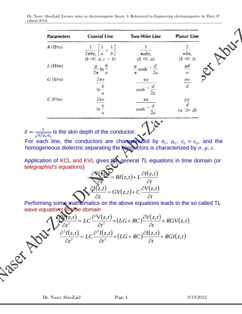
is the skin depth of the conductor.

For each line, the conductors are characterized by , , , and the homogeneous dielectric separating the conductors is characterized by , , . Application of KCL and KVL gives the general TL equations in time domain (or telegraphist's equations)

t

tzILtzRI

z

tzV

,,

,

t

tzVCtzGV

z

tzI

,,

,

Performing some mathematics on the above equations leads to the so called TL wave equations in time domain

tzRGV

t

tzVRCLG

t

tzVLC

z

tzV,

,,,2

2

2

2

tzRGI

t

tzIRCLG

t

tzILC

z

tzI,

,,,2

2

2

2


edition 2012;


LOSSLESS PROPAGATION 0GR

Lossless Line, perfect conductors and perfect dielectrics surrounding. All power input to the line reaches the output. Voltage wave equation reduces to:

2

2

2

2 ,,

t

tzVLC

z

tzV

A general solution to the above equation is assumed to be of the form:

VV

v

ztf

v

ztftzV 21,

Substituting the forward propagating part of the solution into the wave equation gives the condition:

s

mLC

v1

This is also clear from a dimensional check of the voltage wave equation.


edition 2012;


HOW VOLTAGE IS RELATED TO CURRENT?

Using telegraphist equations 0GR , and the assumed solution for tzV , ,

then performing differentiation w.r.t then integration w.r.t time, one may obtain:

II

v

ztf

v

ztf

LvtzI 21

1,

Identifying

v

ztf

LvI 1

1

v

ztf

LvI 2

1

I

V

I

V

C

LLvZo

The characteristic impedance of the line is the ratio of positively traveling voltage wave to current wave at any point on the line.

SINUSOIDAL VOLTAGES

Assigning for forward and backward propagating voltages a sinusoid of the form

tVo cos

Then replacing t with pv

zt for forward wave and t with

pv

zt for backward

wave:


edition 2012;


z

vtVtzV

p

o cos,

With (assuming 0 )

z

vtVtzV

p

of

cos,

z

vtVtzV

p

ob

cos,

Define the phase constant as:

m

radv p

It represents the change in phase per metre along the path travelled by the wave at any instant

Remind yourself;

radss

radt

radmm

radz

frequencyspatial

ztVtzV of cos,

ztVtzV ob cos,

zVzVzV obf cos0,0,


edition 2012;


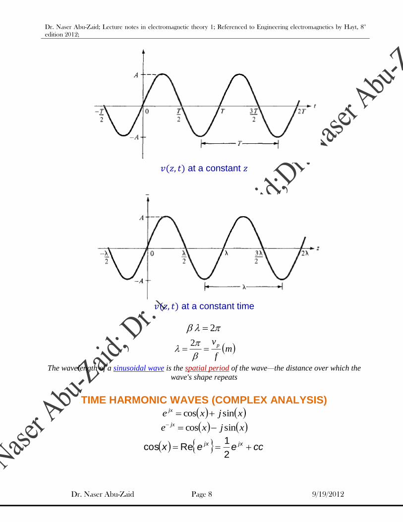
at a constant

at a constant time

2

mf

vp

2

The wavelength of a sinusoidal wave is the spatial period of the wave—the distance over which the

wave's shape repeats

TIME HARMONIC WAVES (COMPLEX ANALYSIS)

xjxe jx sincos

xjxe jx sincos

cceex jxjx 2

1Recos

http://en.wikipedia.org/wiki/Sinusoidal_wave


edition 2012;


ccej

ex jxjx 2

1Imsin

Consider:

cceeeV

eeV

ztVtzV

tjzjj

o

ztjztjo

of

2

1

2

cos,

Define: Instantanous complex voltage

tjzj

oc eeVtzV ,

And the phasor voltage (droppingtje )

zj

os eVzV

Or

tj

zV

zj

o

ztj

o

of

eeV

eV

ztVtzV

s

)(

Re

Re

cos,

To obtain time domain representation from frequency domain representation:

1. Multiply zj

os eVzV by tje .

2. Take the real part of the result. Q: How to obtain frequency domain representation from time domain representation?


edition 2012;


TL WAVE EQUATIONS AND THEIR SOLUTIONS IN PHASOR FORM

Recall:

t

tzILtzRI

z

tzV

,,

,

t

tzVCtzGV

z

tzI

,,

,

Rewriting voltages and currents in terms of their phasor representations, then

performing the indicated differentiations and dropping the tje term, one can

obtain:

1 zILjRdz

zdVs

s

2 zVCjG

dz

zdIs

s

To obtain the wave equations in frequency domain, differentiate (1) w.r.t. then substitute (2) into the result.

zVCjGLjR

dz

zVds

s 2

2

zICjGLjR

dz

zIds

s 2

2


edition 2012;


The propagation constant is defined as:

j

ZYCjGLjR

And the solution to the voltage wave equation is given by:

zz

s eVeVzV 00

zz

s eIeIzI 00

The relation between voltage and current in frequency domain is found from telegraphist equations namely:

1 zILjR

dz

zdVs

s

2 zVCjG

dz

zdIs

s

Substituting the expressions for zVs and zI s , then matching exponents, one

may obtain:

jeZCjG

LjR

Y

Z

ZY

ZZ

I

V

I

VZ

0

0

0

0

00


edition 2012;


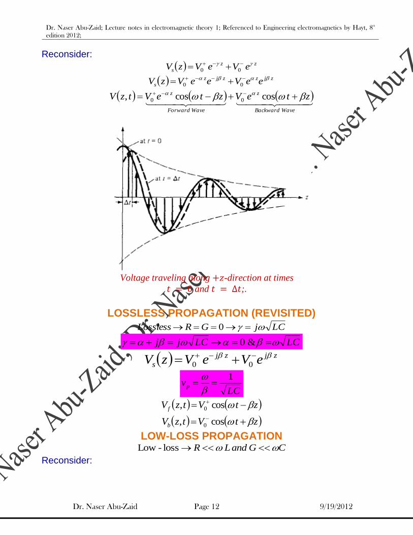
Reconsider:

zz

s eVeVzV 00

zjzzjz

s eeVeeVzV 00

WaveBackward

z

WaveForward

z zteVzteVtzV coscos, 00

Voltage traveling along -direction at times

and ;.

LOSSLESS PROPAGATION (REVISITED)

LCjGRLossless 0

LCLCjj &0

zjzj

s eVeVzV 00

LCvp

1

ztVtzV f cos, 0

ztVtzVb cos, 0

LOW-LOSS PROPAGATION CGandLR loss-Low

Reconsider:


edition 2012;


2

1

2

1

11

Cj

G

Lj

RLCj

CjGLjRj

Using the first three terms in the binomial series expansion, namely:

1........82

112

2

1

xforxx

x

Then, the attenuation and propagation constants may be approximated by:

C

LG

L

CR

2

1Re

2

8

11Im

L

R

C

GLC

Similar argument may be applied to the characteristic impedance:

L

R

C

Gj

C

G

C

G

L

R

C

L

CjG

LjRZ

24

1

2

11

2

22

2

0

Note that:

GandR .

is a non-linear function of frequency , then

pv is frequency

dependent.

The group velocity

d

dv g also depends on frequency Signal distortion.

A constant phase and group velocities may be obtained, even when

00 GandR . This occurs when:

C

G

L

R

(Distortionless line)


edition 2012;


L

CR Re

LCL

R

C

GLC

2

1

8

11

LCv p

1

LCd

dd

dv g

11

C

LZ 0

POWER TRANSMISSION AND LOSS

zjzzjz

s eeVeeVzV 00

zjzjzjzj

s eeeVeeeVzV 00


edition 2012;


zjzjzjzj

s eeeIeeeIzI 00

And since

oZjj

o

oeZe

I

V

I

V

I

VZ

0

0

0

0

00

Then

zjz

o

zjz

o

s eeZ

Vee

Z

VzI

00

Considering the forward waves

zjzj

sf eeeVzV

0

zjzj

o

sf eeeZ

VzI

0

The Instantaneous power tzp , is defined as:

tzItzVtzp ff ,,,

Is evaluated to give

ztzteZ

Vtzp z

o

ocoscos, 2

2

And the time-averaged power is given by:

T

dttzpT

p ,1

This may be evaluated to give:

oZ

z

o

oe

Z

Vp cos

2

2

2

The same result may be obtained more easily if the average power is defined as:

zIzVp ss

*Re2

1

This may be evaluated to give:

zjzj

o

zjzj eeeZ

VeeeVp 0

0Re2

1


edition 2012;


oZ

z

o

oe

Z

Vp cos

2

2

2

As a measure of power drop along a lossy line, consider:

oZ

o

o

Z

Vp cos

20

2

So

zepzp 20

Then

ze

zp

p2

0

In dB

z

zp

p69.8

0

1010LogdB inLossPower

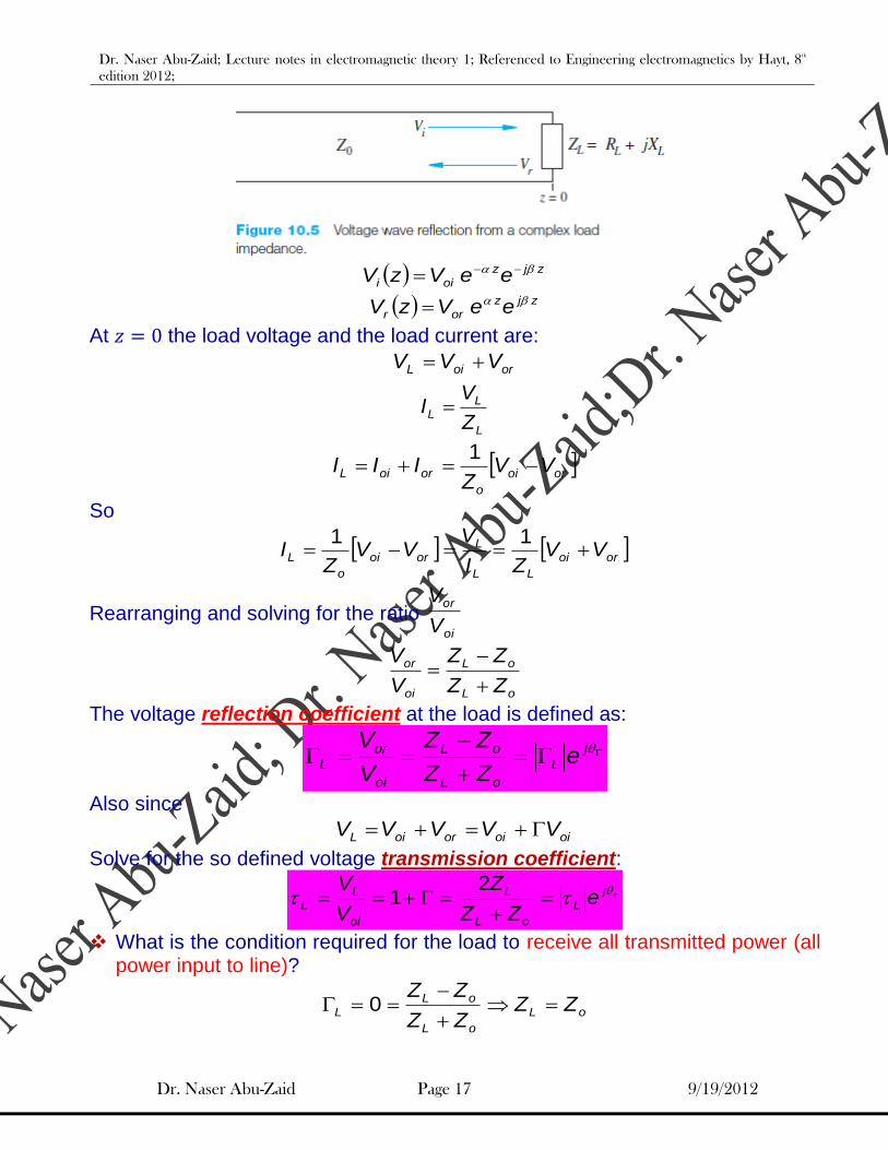
WAVE REFLECTIONS @ DISCONTINUITIES


edition 2012;


zjz

oii eeVzV

zjz

orr eeVzV

At the load voltage and the load current are:

oroiL VVV

L

LL

Z

VI

oroi

o

oroiL VVZ

III 1

So

oroi

LL

Loroi

o

L VVZI

VVV

ZI

11

Rearranging and solving for the ratio oi

or

V

V

oL

oL

oi

or

ZZ

ZZ

V

V

The voltage reflection coefficient at the load is defined as:

j

L

oL

oL

oi

or

L eZZ

ZZ

V

V

Also since

oioioroiL VVVVV

Solve for the so defined voltage transmission coefficient:

j

L

oL

L

oi

L

L eZZ

Z

V

V

21

What is the condition required for the load to receive all transmitted power (all power input to line)?

oL

oL

oL

L ZZZZ

ZZ

0


edition 2012;


Load matched to line when

oL ZZ

What fractions of incident power are reflected and dissipated by the load? The load in this case is assumed to be located at .

o

o

Z

L

o

o

Lz

Z

z

o

o

Lzi

eZ

V

eZ

Vzp

cos2

cos2

2

2

2

2

Also the power reflected from the load is:

oZ

L

o

o

Lzr eZ

Vp cos

2

2

22

(It would be a good exercise for you to derive the above result)

So, from the above we have:

*2

i

r

p

p

And

21

i

t

p

p

For a wave incident from a semi-infinite TL to a second semi-infinite TL, the second may be treated as a load

0102

0102

ZZ

ZZ


edition 2012;


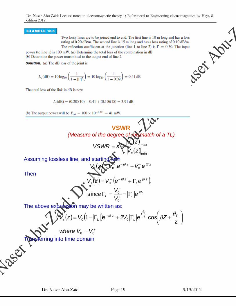
VSWR

(Measure of the degree of mismatch of a TL)

min

max

zV

zVsVSWR

s

s

Assuming lossless line, and starting with

zjzj

s eVeVzV 00

Then

j

LL

zj

L

zj

s

eV

Vce

eeVzV

0

0

0

sin

,

The above expression may be written as:

00

200

2cos21

VVwhere

ZeVeVzVj

L

zj

Ls

Transferring into time domain


edition 2012;


partStanding

2cos

2cos2

partTraveling

cos1,

0

0

tZV

ztVtzV

L

L

Portion of the first incident wave reflects back and propagates in the line, and interferes with an equivalent portion of the 2nd incident wave to form a standing wave, the rest of the incident wave (which does not interfere) is the traveling wave part.

WHAT IS THE VOLTAGE MAXIMUM AND MINIMUM AND WHERE DO THEY OCCUR?

zj

L

zj

zj

L

zj

zj

L

zj

s

eeV

eeV

eeVzV

2

0

0

0

1

Maximum’s occur when:

,....2,1,0,22 mmz

Hence;

mz 22

1max

Then

L

zz

zj

L

zj

s

V

eeVzV

1

1

0

2

0maxmax


edition 2012;


Minimum's occur when:

,....2,1,0,122 mmz

So;

122

1min mz

Then

L

zz

zjL

zjs

V

eeVzV

1

1

0

2

0minmin

And the VSWR is obtained easily as:

1

1

min

max

zV

zVsVSWR

s

s

1

1

s

s

Plot of the magnitude of as found from

zj

L

zj

sT eeVzV 0 as a function of

position, , in front of the load (at z = 0). The reflection coefficient phase is , which

leads to the indicated locations of maximum and minimum voltage amplitude, as found

from

122

1min mz and

mz 2

2

1max

.


edition 2012;


Implication: maybe found from measured s , and may be found from

measured locations of maximum’s and minimum’s. Then the load impedance is known.


edition 2012;


FINITE LENGTH TL’S (TL CIRCUITS)

?inZ and ? z

zjzj

s eVeVzV 00

zjzj

s eIeIzI 00

0

00

0

00

0

0 ,,Z

VI

Z

VIe

V

V j

LL

Define the wave impedance zZw at any as:

zI

zVzZ

s

sw

zjzj

zjzj

weIeI

eVeVzZ

00

00

)(@ Hzf

gV

gZ

LZoZ

Lossless

+

-

LI

inVLV+

-

+

-

0z lz

inZ

inI


edition 2012;


zj

L

zj

zj

L

zj

w

eeZ

V

eeVzZ

0

0

0

zj

L

zj

zj

L

zj

wee

eeZzZ

0

Using Euler’s identity and the fact that oL

oLL

ZZ

ZZ

. Then If evaluated at lz

zjZzZ

zjZzZZzZ

L

L

w

sincos

sincos

0

00

ljZlZ

ljZlZZZ

L

Lin

sincos

sincos

0

00

Also a generalized reflection coefficient may be defined as follows:

zj

L

zj

L

zj

zj

zj

ee

eV

V

eV

eVz

22

2

0

0

0

0

zj

L ez 2

L

j

L

j

L ee 020

lj

L el 2

Also, note that the wave impedance may be obtained as:

z

zZ

e

eZ

ee

eeZzZ

zj

L

zj

L

zj

L

zj

zj

L

zj

w

1

1

1

1

0

2

2

0

0


edition 2012;


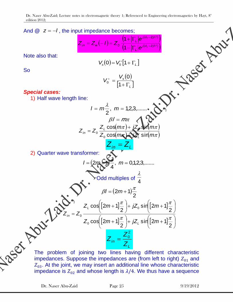
And @ lz , the input impedance becomes;

lj

L

lj

L

wine

eZlZZ

2

2

01

1

Note also that:

Ls VV 10 0

So

L

sVV

1

00

Special cases: 1) Half wave length line:

,.......3,2,1,2

mml

ml

mjZmZ

mjZmZZZ

L

L

insincos

sincos

0

00

Lin ZZ

2) Quarter wave transformer:

,.......3,2,1,0,4

12 mml

Odd multiples of 4

2

12

ml

212sin

212cos

212sin

212cos

0

0

0

mjZmZ

mjZmZ

ZZ

L

L

in

L

inZ

ZZ

2

0

The problem of joining two lines having different characteristic impedances. Suppose the impedances are (from left to right) and . At the joint, we may insert an additional line whose characteristic impedance is and whose length is . We thus have a sequence


edition 2012;


of joined lines whose impedances progress as , , and , in that order. A voltage wave is now incident from line 1 onto the joint between and . Now the effective load at the far end of line 2 is . The input impedance to line 2 at any frequency is now

Reflections at the – interface will not occur if . Therefore, we can match the junction (allowing complete transmission through the three-line sequence) if is chosen so that

This technique is called quarter-wave matching.

3) Short Circuit termination:

0LZ

ljlZ

ljZlZZ in

sin0cos

sincos0

0

00

ljZZscin tan0

4) Open circuit termination:

LZ

lj

Z

lZ

Z

lZjl

ZZ

L

L

Zin

L

sincos

sincos

0

0

0lim

ljZZocin cot0

Note also that 0Z may be found from measurements of short and open circuit

terminations

scin

ocin ZZZ 0


edition 2012;


1) The line is matched; The reflection coefficient is zero; The standing wave ratio is unity;

300

300oZ

s

mv 8105.2

+

-

inI

LI

inV LV+

-

+

-

0z mz 2

inZ

300LZ

)(100@

60

MHz

V

Example:

1) Calculate the load reflection coefficient, the standing wave ratio, the wavelength

on the line, the phase constant, the attenuation constant, the electrical length of

the line, the input impedance offered to the source, the voltage at the input to

the line, the time domain input voltage, the time domain load voltage, the time

domain input current, the time domain load current, the average power

delivered to the input of the line, the average power delivered to the load by

the line.

2) If a 300 load is connected in parallel with the first load then calculate: the

reflection coefficient, the standing wave ratio, the input impedance offered to

the source, the phasor input current, the average power supplied to the line by

the source, the average power received by each load, the phasor voltage across

each load, where is the voltage maximums and minimums and what are those

values, the phasor load voltage.


edition 2012;


or

offered to the voltage source

The source is matched to the line and delivers the maximum available power to the line.

A transmission line that is matched at both ends produces no reflections and thus delivers maximum power to the load.

No reflection and no attenuation;

30

0

00

ljlj

sin eVeVlVV

6.130300 ljeV

The average power delivered to the input of the line by the source must all be delivered to the load by the line,

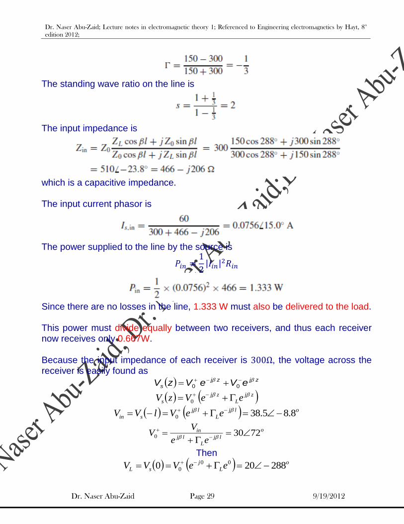
2) across the line in parallel with the first receiver. The load impedance is

. The reflection coefficient is


edition 2012;


The standing wave ratio on the line is

The input impedance is

which is a capacitive impedance. The input current phasor is

The power supplied to the line by the source is

Since there are no losses in the line, 1.333 W must also be delivered to the load. This power must divide equally between two receivers, and thus each receiver now receives only 0.667W. Because the input impedance of each receiver is , the voltage across the receiver is easily found as

zjzj

s eVeVzV 00

zj

L

zj

s eeVzV

0

olj

L

lj

sin eeVlVV 8.85.380

o

lj

L

lj

in

ee

VV 72300

Then

o

L

j

sL eeVVV 288200 00

0


edition 2012;


The magnitude alone can be found from the power as

The voltage maxima is located at:

with and ,

The minima are distant from the maxima;

The load voltage (at z = 0) is a voltage minimum. a voltage minimum occurs at the load if , and a voltage maximum occurs if

, where both impedances are pure resistances.


edition 2012;



edition 2012;


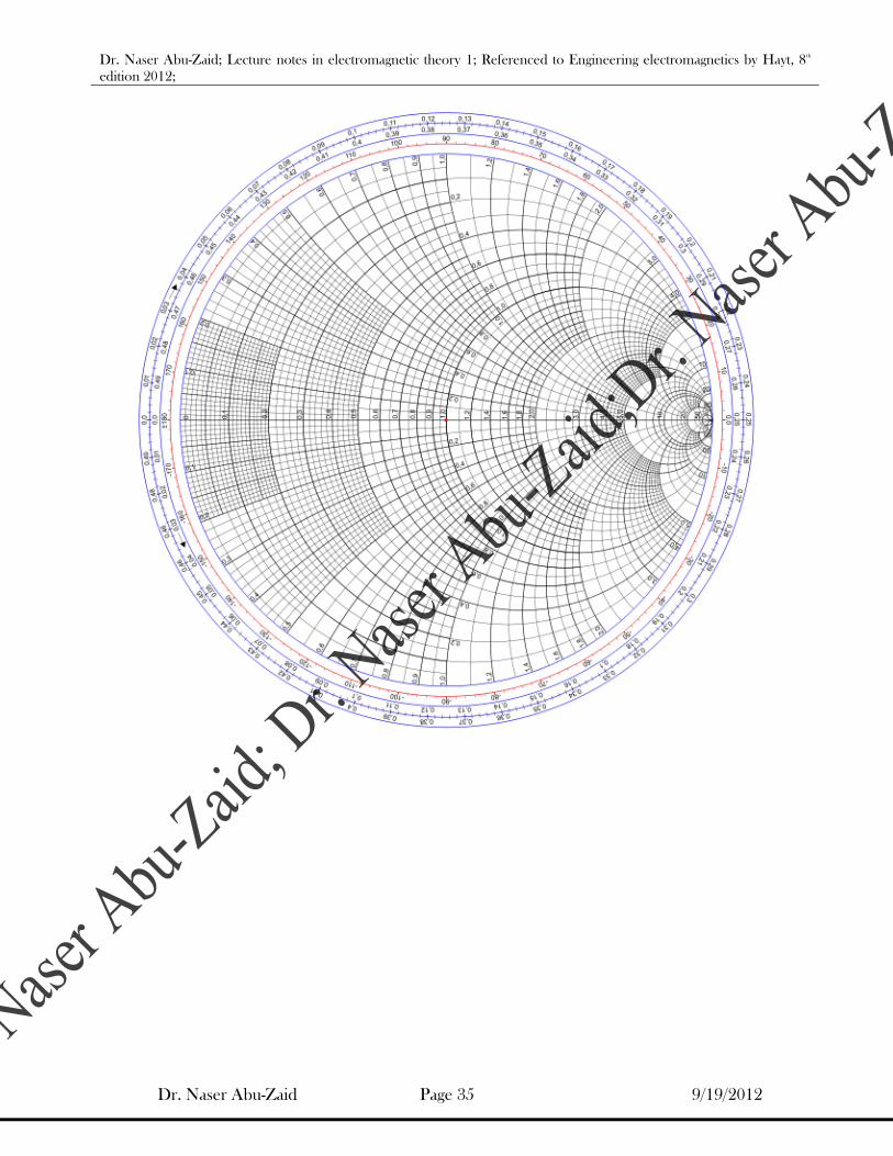
SMITH CHART The Smith chart is a graphical tool for high frequency circuit

applications.

The domain of definition of the reflection coefficient for a loss-less line is a circle of unitary radius in the complex plane. This is also the domain of the Smith chart.

The goal of the Smith chart is to identify all possible impedances on the domain of existence of the reflection coefficient. To do so, we start from the general definition of line impedance (which is equally applicable to a load impedance when d=0)

In order to obtain universal curves, we introduce the concept of normalized impedance

The normalized impedance is represented on the Smith chart by using families of curves that identify the normalized resistance r

(real part) and the normalized reactance x (imaginary part)


edition 2012;


Let’s represent the reflection coefficient in terms of its coordinates

After some lengthy mathematicl manipulations (follow your text book), it may by shown that the result for the real part indicates that on the complex plane with coordinates all the possible impedances with a given normalized resistance r are found on a circle with

As the normalized resistance varies from to , we obtain a family of circles completely contained inside the domain of the reflection coefficient .

Also the result for the imaginary part indicates that on the complex plane with coordinates all the possible impedances with a given normalized reactance are found on a circle with


edition 2012;


As the normalized reactance varies from to , we obtain a family of arcs contained inside the domain of the reflection coefficient .

Basic Smith Chart techniques for loss-less transmission lines

Given Find Given Find

Given or Find and @ a specified d.

Given or ⇒ Find and

Find and (maximum and minimum locations for the voltage standing wave pattern)

Find the Voltage Standing Wave Ratio s (VSWR)

Given Find Given Find


edition 2012;


http://upload.wikimedia.org/wikipedia/commons/7/7a/Smith_chart_gen.svg


edition 2012;


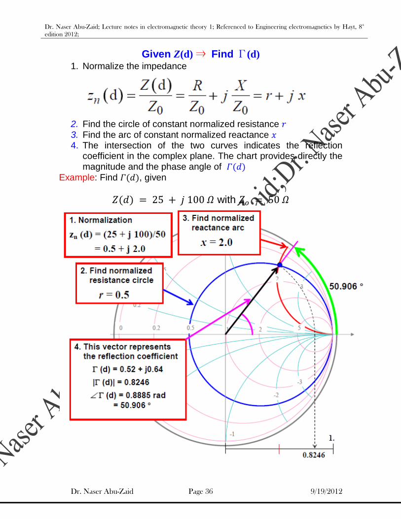
Given Z(d) ⇒ Find Γ(d) 1. Normalize the impedance

2. Find the circle of constant normalized resistance

3. Find the arc of constant normalized reactance 4. The intersection of the two curves indicates the reflection

coefficient in the complex plane. The chart provides directly the magnitude and the phase angle of

Example: Find , given

with


edition 2012;


Given Γ(d) ⇒ Find Z(d) 1. Determine the complex point representing the given reflection

coefficient on the chart. 2. Read the values of the normalized resistance and of the

normalized reactance that corresponds to the reflection coefficient point.

3. The normalized impedance is and the actual impedance is

Given and/or Find and

NOTE: the magnitude of the reflection coefficient is constant along a loss-less transmission line terminated by a specified

load, since

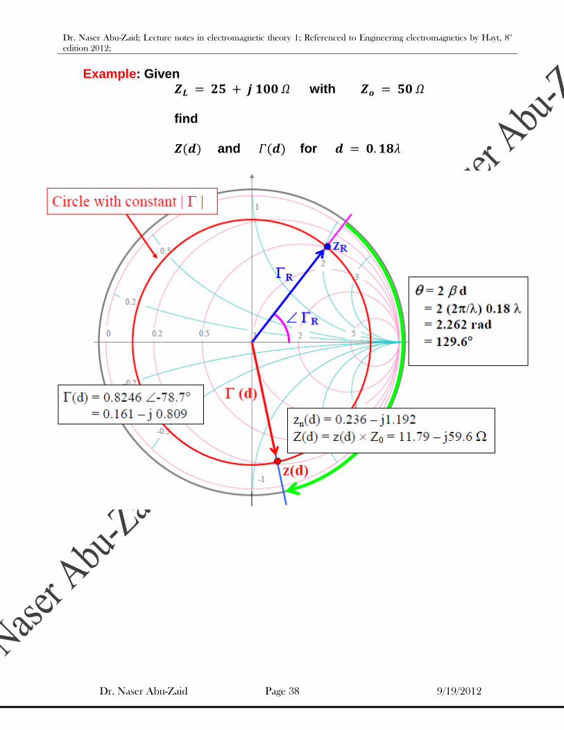
Therefore, on the complex plane, a circle with center at the origin and radius represents all possible reflection coefficients found along the transmission line. When the circle of constant magnitude of the reflection coefficient is drawn on the Smith chart, one can determine the values of the line impedance at any location. The graphical step-by-step procedure is:

1. Identify the load reflection coefficient and the normalized load impedance on the Smith chart.

2. Draw the circle of constant reflection coefficient amplitude .

3. Starting from the point representing the load, travel on the circle in the clockwise direction (wavelengths toward generator), by an angle

4. The new location on the chart corresponds to location on the

transmission line. Here, the values of and can be read from the chart as before.


edition 2012;


Example: Given with find and for


edition 2012;


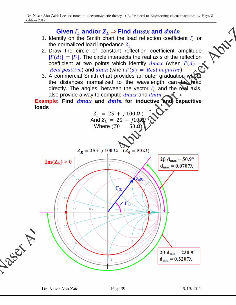
Given and/or Find and 1. Identify on the Smith chart the load reflection coefficient or

the normalized load impedance . 2. Draw the circle of constant reflection coefficient amplitude

. The circle intersects the real axis of the reflection coefficient at two points which identify (when ) and (when )

3. A commercial Smith chart provides an outer graduation where the distances normalized to the wavelength can be read directly. The angles, between the vector and the real axis, also provide a way to compute and .

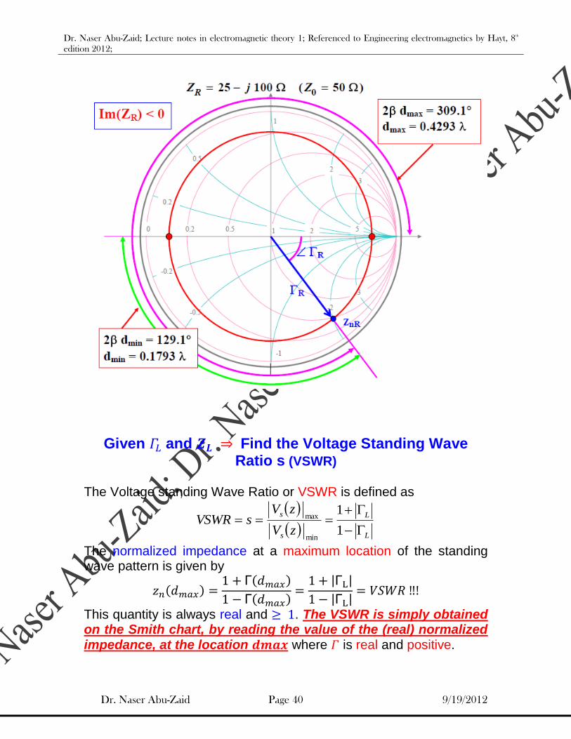
Example: Find and for inductive and capacitive loads

; And

Where


edition 2012;


Given and Find the Voltage Standing Wave Ratio s (VSWR)

The Voltage standing Wave Ratio or VSWR is defined as

L

L

s

s

zV

zVsVSWR

1

1

min

max

The normalized impedance at a maximum location of the standing wave pattern is given by

This quantity is always real and . The VSWR is simply obtained on the Smith chart, by reading the value of the (real) normalized impedance, at the location where is real and positive.


edition 2012;


The graphical step-by-step procedure is:

1. Identify the load reflection coefficient and the normalized load impedance on the Smith chart.

2. Draw the circle of constant reflection coefficient amplitude .

3. Find the intersection of this circle with the real positive axis for the reflection coefficient (corresponding to the transmission line location ).

4. A circle of constant normalized resistance will also intersect this point. Read or interpolate the value of the normalized resistance to determine the VSWR.

Example: Find the VSWR for two different loads

; And

Where


edition 2012;


Given Find Review the impedance-admittance terminology:

Impedance = Resistance + j Reactance

Admittance = Conductance + j Susceptance

Note: The normalized impedance and admittance are defined as

Keep in mind that the equality

is only valid for normalized impedance and admittance. The actual values are given by

where

is the characteristic admittance of the transmission line.

The graphical step-by-step procedure is: 1. Identify the load reflection coefficient and the normalized load

impedance on the Smith chart. 2. Draw the circle of constant reflection coefficient amplitude

. 3. The normalized admittance is located at a point on the circle of

constant which is diametrically opposite to the normalized impedance.


edition 2012;


Example: Given with find .

Documents

Electromagnetic Theory 2 notes - uCoz