Embed Size (px)
Citation preview

Jay R. Yablon, September 26, 2016
Electromagnetic Time Dilation and Contraction, and a Geometrodynamic Foundation of Classical and Quantum
Electrodynamics
Jay R. Yablon 910 Northumberland Drive
Schenectady, New York 12309-2814 [email protected]
September 26, 2016
Abstract: We summarize how the Lorentz Force motion observed in classical electrodynamics may be understood as geodesic motion derived by minimizing the variation of the proper time along the worldlines of test charges in external potentials, while the spacetime metric remains invariant under, and all other fields in spacetime remain independent of, any rescaling, i.e., re-gauging of the charge-to-mass ratio q/m. In order for this to occur, time is dilated or contracted due to repulsive and attractive electromagnetic interactions respectively, in very much the same way that time is dilated due to relative motion in special relativity and due to gravitational fields in general relativity, without contradicting the well-corroborated experimental content of standard electrodynamic theory and both special and general relativity. As such, it becomes possible to lay an entirely geometrodynamic foundation for classical electrodynamics in four spacetime dimensions, in which mechanical motions and objects are merely promoted into canonical motions and objects in accordance with well-established local symmetry principles. Further, when we consider the self-interactions of individual leptons understood to be responsible for the magnetic moment anomalies, and upon identifying a universal relation between time and energy whereby all forms of energy dilate (or contract) time regardless of their kinetic or interaction origin, it is shown how these magnetic moment anomalies which are quintessential hallmarks of quantum field theory, both measure and empirically validate electromagnetic time dilation, and are a direct and immediate consequence of local abelian and non-abelian gauge symmetries. PACS: 03.50.De; 11.15.-q; 13.40.Em; 04.20.Cv
Jay R. Yablon, September 26, 2016
Contents 1. Motivation, Purpose and Historical Background .................................................................... 1
2. A Brief Note about Signs and Sign Conventions .................................................................... 3
PART I: CLASSICAL GEOMETRO-ELECTRODYNAMICS .................................................... 5
3. Geometro-Electrodynamics and Time Dilation and Contraction: An Overview .................... 5
4. Derivation of Lorentz Force Geodesic Motion from Variation Minimization ...................... 15
5. The Lagrangian Gauge and the Geodesic Gauge, and Canonically-Inertial Motion ............. 18
6. The Electrodynamic Action in Lagrangian Gauge ................................................................ 22
7. The Electro-Gravitational Power Equation ........................................................................... 23
8. The Electro-Gravitational Energy Flux Field Equation ........................................................ 26
PART II: DERIVATION OF ELECTRODYNAMIC TIME DILATION ................................... 29
9. Review of Time Dilation in Special and General Relativity ................................................. 29
10. Electrodynamic Time Dilation and Contraction, and Time-Energy Relations in Special and General Relativity and Electrodynamics ................................................................................ 33
PART III: QUANTUM GEOMETRO-ELECTRODYNAMICS AND THE LEPTON MAGNETIC MOMENT ANOMALIES ...................................................................................... 41
11. Electrodynamic Time Dilation and the Magnetic Moment Anomalies: Introduction ....... 41
12. The Canonical-to-Mechanical Ratio and the Lepton Magnetic Moment Anomalies ........ 44
13. “Canonical Co-Scaling” Directly Connecting Electromagnetic Time Dilation, Lepton Self-Interaction Energies, and Lepton Magnetic Moment Anomalies ......................................... 46
14. Time “Sees” all Energy: Why the Magnetic Moment Anomalies are an Exact Consequence of Local Abelian and non-Abelian Gauge Symmetries .......................................... 59
15. Lepton Bare Masses and Probability Density Standard Deviations for Possible Experimental Validation, and the Observable Physical Meaning of Lepton Compton Wavelengths .................................................................................................................................. 62
16. Electromagnetic Time Dilation and DeVries’ Formula for the Fine Structure Constant .. 64
17. Conclusion ......................................................................................................................... 69
References ..................................................................................................................................... 71

Jay R. Yablon, September 26, 2016
1
1. Motivation, Purpose and Historical Background The equation of motion for a test particle along a geodesic line in curved spacetime
specified by the metric interval 2 2c d g dx dxµ νµντ = with metric tensor gµν was first obtained by
Albert Einstein in §9 of his landmark 1915 paper [1] introducing the General Theory of Relativity. The infinitesimal linear element /d ds cτ = for the proper time is a scalar invariant which is
independent of the chosen system of coordinates. Likewise the finite proper time B
Adτ τ= ∫
measured along the worldline of the test particle between two spacetime events A and B has an invariant meaning independent of the choice of coordinates. Specifically, the geodesic of motion is stationary, and results from a minimization of the variational equation
0B
Adδ τ= ∫ . (1.1)
After carrying out the well-known calculation originally given by Einstein in [1], the particle’s equation of geodesic motion is found to be:
2
2
d x du du u
x dx
d d d dβ β µ ν
µν
β µ
µ
β ν
ντ τ τ τ= −Γ= = −Γ , (1.2)
with Christoffel connection defined (denoted “≡ ” ) by ( )12 g g ggβ
µν α µβα
µ να ν αµν−Γ ≡ − ∂∂ − ∂
and the relativistic four-velocity by /dx du µµ τ≡ .
The geodesic (1.2) can also be viewed in alternative, yet equivalent way. In curved spacetime, ( ) ;/ /DB D x Bβ ν β
ντ τ≡ ∂ ∂ ∂ defines the “derivative along the curve” for any
contravariant vector Bβ , using gravitationally-covariant derivatives ; B B Bβ β β σν ν σν∂ = ∂ + Γ and
the chain rule. So when B uβ β= , then, in view of (1.2), we may also write:
( ); 0Du x x x dx du
u u u u u uD x d d
β α α α β ββ β β σ β σ β µ ν
α α σα σα µνατ τ τ τ τ τ ∂ ∂ ∂ ∂= ∂ = ∂ + Γ = + Γ = + Γ = ∂ ∂ ∂ ∂
. (1.3)
This has exactly the same content as the geodesic equation (1.2). But given that / 0du dβ τ = describes Newtonian inertial motion when the gravitational connection 0β
µνΓ = , we may think of
/ 0Du Dβ τ = above as describing covariantly-inertial motion in the presence of gravitation. This is what gives gravitational geodesics their colloquial characterization as “straight lines,” or more precisely, “inertial lines” in curved spacetime. Just as ordinary derivatives ( )/ ,tα∂ = ∂ ∂ ∇ are replaced by gravitationally-covariant
derivatives ;α∂ in curved spacetime, so too in gauge theory ordinary derivatives α∂ are replaced
by gauge-covariant or “canonical” derivatives iqAα α α≡ ∂ −D , where q is the electric charge

Jay R. Yablon, September 26, 2016
2
strength and Aα is the gauge field / vector potential, and where we use αD rather than the often-
employed Dα to distinguish symbolically from the D of gravitational motion in (1.3). Motivated
by the geodesic nature of gravitationally-covariant motion for which / 0Du Dβ τ = rather than / 0du dβ τ = and how this motion stems directly from the replacement of ordinary with
gravitationally-covariant derivatives, the purpose of this paper is to summarize how electrodynamic Lorentz Force motion is likewise geodesic motion which is canonically-inertial described by / 0uβ τ =D D , which stems directly from the canonical derivatives of gauge theory. As will be shown, this comes about as a consequence of heretofore unrecognized time dilations and contractions which occur any time two material bodies are electromagnetically interacting. It will also be shown how in quantum electrodynamics, these time dilations directly give rise to the observed lepton magnetic moment anomalies. Finding a geometrodynamic foundation for electrodynamics limited to four spacetime dimensions has been of great interest yet defied solution for almost a century. The Special Theory of Relativity [2] together with Minkowski’s famous proclamation [3] that “from now onwards space by itself and time by itself will recede completely to become mere shadows and only a type of union of the two will still stand independently on its own,” first established the geometric unification of space and time that now underlies all of physics. With the General Theory [1], Einstein soon thereafter applied Riemannian geometry to introduce curvature to spacetime and found that gravitation including motion in a gravitational field could be fully explained on this entirely geometric foundation, giving birth to what Wheeler would later coin as “geometrodynamics.” [4]
After the General Theory established that the Riemann curvature was simply a measurement ; ;,R B Bα
βµν α ν µ β = ∂ ∂ of degree to which derivatives at any given spacetime event
in are non-commuting when operating on any four-vector Bβ , it was natural to try to explain
electrodynamics in a similar way based on spacetime curvature. Hermann Weyl’s gauge theory – which will be central to this paper – is perhaps the most important of these efforts, and has become the foundation for our modern understanding not only of electrodynamics, but also of the weak and strong interactions which are non-abelian extensions of electrodynamics. Although “gauge” is a historical misnomer from when Weyl first tried unsuccessfully in [5], [6] to explain electrodynamics by imposing a symmetry under local gauge transformations ( , )teψ ψ ψΛ′→ = x rescaling the magnitude of a wavefunction, Weyl did eventually find, correctly in [7], that electrodynamics is indeed the natural consequence of imposing a local phase symmetry under a magnitude-preserving redirection ( , )i tU eψ ψ ψ ψΛ′→ = = x of the wavefunction in a complex two-
dimensional phase space established by the parameter cos sinie iΛ = Λ + Λ . Apropos to curvature, this “gauge” theory established that the electromagnetic field strength bivector F µν – like Rα
βµν
– measures the degree to which gauge-covariant derivatives iqAα α α≡ ∂ −D were non-commuting.
This is why F µν is often referred to as the “curvature” tensor. However, the field strength only
bears an imaginary relation ,qF iµν µ νφ φ = D D to the gauge-covariant derivatives, and so this is
not a real curvature as is that of Rαβµν . Indeed, it was because the incorrect re-gauging of the
wavefunction allowed this curvature to be real like the curvature of Riemann, that Weyl adhered

Jay R. Yablon, September 26, 2016
3
so long to a “gauge” rather than a “phase” transformation. But this was not in accord with observed natural reality.
During the same era when Weyl was developing gauge theory, Kaluza [8] and Klein [9]
did succeed in explaining the Lorentz force law as a type of geodesic motion owing to spacetime curvature that remained real, and even gave a geometric explanation for the electric charge itself. But this came at the cost of adding a fifth dimension to spacetime and curling that dimension into a very tiny cylinder. While theoretically-attractive as a geometrodynamic theory, Kaluza-Klein has not become universally accepted because it relies on a fifth dimension which does not appear to have been observed and likely never could be observed. For his part, Einstein also pursued a geometrodynamic theory of electrodynamics until the end of his life, but he too was never fully satisfied with his or anybody else’s results.
To date, a century later, finding a geometrodynamic foundation for even classical – much
less quantum – electrodynamics remains elusive, and there certainly is no theory of electromagnetism which rises to the level of pure geometry embodied in either the Special or the General Theories of Relativity. Using settled and accepted gauge theory as a foundation, the goal of this paper is to bring a century of work pursuing a geometrodynamic foundation for electrodynamics to a successful conclusion, by achieving for electrodynamics, the pure geometrization that the Special Theory of Relativity achieved for relative motion and the General Theory of Relativity achieved for gravitation. 2. A Brief Note about Signs and Sign Conventions
The dilation and contraction of time whenever a charged body is placed into an electromagnetic potential and the connection of this to electromagnetic interaction energies and to the lepton magnetic moment anomalies will be a fundamental finding of this paper. But because electromagnetic interactions can be attractive or repulsive unlike gravitation which is always attractive, a fundamental question will arise whether for Coulomb interactions between two charges, electrodynamic time dilation occurs between like and therefore repelling charges, or between opposite and therefore attracting charges. Note that one or the other but not both of these possibilities could be true, because two like-electrical-charges repel while two like-gravitational-charges (masses) attract. While one may have a preconception about which of these possibilities is true (we will find that time dilates from the interaction of two like-thus-repelling charges and so contracts for electrical attraction between unlike charges), the answer to this question depends upon, and can only be answered definitively by, whether certain interaction and energy signs are positive or negative, and by how these signs enter into the overall theoretical development. So before we begin, it is important to take a moment to review certain sign conventions and requirements.
In natural units 1c = , the Lorentz force law which we shall study here at length, is
( )/ /du d q m F uβ β σστ = + . Specifically, if one adopts a sign convention in which a test charge q
in the mixed electromagnetic field F g Fβ βασ σα= is taken to be positive and the proper potential
0φ of the gauge field ( ),Aα φ= A in the field strength F A Aβα β α α β= ∂ − ∂ is also taken to be

Jay R. Yablon, September 26, 2016
4
positive, then when using a timelike metric signature ( ) ( )diag 1, 1, 1, 1µνη = + − − − in the flat
spacetime limit gµν µνη= this Lorentz force law requires a positive overall sign. We may see this
using a Coulomb interaction at rest, as follows: Combining all of the foregoing we may write ( ) ( )/ /du d q m A A uβ βτ α β σ
σα τ στ η η= + ∂ − ∂
for the Lorentz force. At rest we may set 0ku = and ( ) ( )0, ,Aα φ φ= =A 0 , so for the space
components we obtain ( ) 000 0/ /k kdu d q m uτ
ττ η η φ= + ∂ . Then we take 0 /ek Q rφ = + to be a
positive proper Coulomb potential for a positive source charge Q, where 02
01/ 4 / 4ek c πµπε= =
is Coulomb’s constant. So if we place the positive q into this potential the electrostatic interaction energy will be 0 /eq k Qq rφ = + , which grows smaller as the separation r between the two positive
charges is increased. Because the test charge will naturally tend toward a lower energy over a higher energy, this tells us that this interaction is repulsive. Consequently, commensurately, we must have a positively-signed / 0kdu dτ > for the acceleration, with a vector direction pointing toward greater space separation, emerge from the Lorentz force law. So let us make sure it does.
If, for example, we align the radial separation along the z axis so that ( ) ( ), , 0,0,x y z r= ,
then along this radius the Lorentz force law will yield
( ) ( ) ( )3 33 0 33 0 200 3 0 00/ / 1/ /edu d q m u m u k Qq rτ η η φ η η= + ∂ = − , via ( ) 2
3 1/ 1/r r∂ = − . Now, at this
juncture, we will have 3300 1η η = − irrespective of whether we choose a timelike signature
( ) ( )diag 1, 1, 1, 1µνη = + − − − or a spacelike signature ( ) ( )diag 1, 1, 1, 1µνη = − + + + for the
Minkowski metric tensor, because 3300 1η η = − either way. So in either case, the Lorenz force law
will reduce to ( )( )3 2 0/ 1/ /edu d m k Qq r uτ = , with the sign now boiling down to that of 0 /u dt dτ= . With this ( ) ( ), , 0,0,x y z r= alignment, the required repulsive result now becomes
3 / 0du dτ > . Now we must choose our metric tensor signature and use that consistently throughout. In
all cases, the flat spacetime line element is 2 2 2 uds c d dx dxνµντ η= = . For a timelike signature
with 2 2 2 2j kjkdx dx dx dy dz drδ = + + = , the time interval ( )2 2 2 2 2 2ds c d c dt drτ= = − . If we are
studying the time evolution of material bodies moving within the light cone, then it is generally preferable to use a timelike signature, because at rest, with 0kdx = , the metric reduces to
2 2d dtτ = . Then, while we still have the choice of setting / 1d dtτ = ± upon taking the square root, it makes no sense to align dτ other than with dt so that these both measure the same time progression, and we therefore set / 1d dtτ = . On the other hand, if we are studying two spacelike-separated events outside the light cone at the same coordinate time, then it is preferable to use a spacelike signature, because at the same time coordinate, with 0dt = , the metric reduces to
2 2ds dr= . Then, although we may choose either of ds dr= ± when taking the square root, we likewise align the coordinate length with the proper length so / 1dr ds= and these both measure the same length in the same direction. But it will also be seen that were we to choose a spacelike

Jay R. Yablon, September 26, 2016
5
signature, then at rest the metric would reduce to 2 2d dtτ = − , and that one would then have d idtτ = ± , requiring the Lorenz force to have an imaginary ( )/q m F uβ σ
σ term. So though
optional, it is preferred to choose a timelike signature. Once we do so, all else must be done consistently with this.
So to keep all terms real in the Lorentz force, we choose a timelike signature, which means
that after alignment / 1d dtτ = , so that the Lorentz acceleration given all of the conventions recited
here finally becomes ( )( )3 2/ 1 / /edu d m k Qq rτ = . For the ( ) ( ), , 0,0,x y z r= alignment, this is a
radial acceleration ( ) ( )2 2 2/ 1/ /ed r d m k Qq rτ = . Given that Q and q are both positive, this yields
the required repulsive motion 2 2/ 0d r dτ > , properly corresponding with the repulsive interaction energy 0 /eq k Qq rφ = + that lessens with increased separation between two positive (like-signed)
charges Q and q. Obviously, if either Q or q but not both is a negative charge, then the interaction energy will go over to 0 /eq k Qq rφ → − , growing smaller with reduced charge separation, while
the motion becomes the attractive 2 2/ 0d r dτ < . Both of these are consistent with electrical attraction between unlike charges. Finally, because this will become important in the development to follow, we again note the widely-known and deeply fundamental empirical fact that for gravitation like charges attract, while for electromagnetism like charges repel. PART I: CLASSICAL GEOMETRO-ELECTRODYNAMICS
3. Geometro-Electrodynamics and Time Dilation and Contraction: An Overview To begin development, if a test particle, to which we now ascribe a mass 0m> , also has a non-zero net electrical charge 0q ≠ and the region of spacetime in which it subsists also has a
nonzero electromagnetic field strength 0F βα ≠ , then the equation of motion is no longer given by (1.2), but is supplemented by an additional term which contains the Lorentz Force law, namely, with a positive sign for the reasons and with the sign conventions already discussed:
2
2
d x du dx dx q dx q ug F g F
d d du
d m cd m cu
β β µ ν σ σβα βα
σβ β µ ν
µν α µν σατ τ τ τ τ= −Γ = −Γ= + + . (3.1)
In the above, the field strength F βα containing the electric and magnetic field bivectors E and B is defined as usual by F A Aβα β α α β≡ ∂ − ∂ in relation to the gauge potential four-vector Aα . The above force law is of course a well-known, well-corroborated, well-established law of physics. Given that the gravitational geodesic (1.2) is derived from the variational equation (1.1), the question arises whether there is a way to obtain (3.1) from the same variation as in (1.1), thus revealing electrodynamic motion to also entail particles moving along geodesic paths in four spacetime dimensions. Conceptually, it cannot be argued other than that this would be a desirable state of affairs. But physically the difficulty rests in how to accomplish this without ruining the integrity of the metric and the background fields in spacetime by making them a function of the

Jay R. Yablon, September 26, 2016
6
charge-to-mass ratio /q m. This ratio is and must remain a characteristic of the test particle alone.
It is not and cannot be a characteristic of the line element dτ , or the metric tensor gµν , or the
gauge field Aα , or the field strength F βα which define the field-theoretical spacetime background through which the test particle is moving. And, at bottom, this difficulty springs from the inequivalence of the “electrical mass” (a.k.a. charge) q and the inertial mass m, versus the Newtonian equivalence of gravitational and inertial mass. In (3.1), this is captured by the fact that m does not appear in the gravitational term u uβ µ ν
µν−Γ , while the /q m ratio does appear in the
electrodynamic Lorentz Force term that we rewrite as ( )/q m F uβ σσ in natural units with 1c = .
This difficulty may also be seen very simply if we compare Newton’s law with Coulomb’s
law. In the former case we start with a force 2/F GMm r= − (with the minus sign indicating that gravitation is attractive) and in the latter 2/eF k Qq r= − (for which we choose an attractive
interaction to provide a direct comparison to gravitation), where G is Newton’s gravitational constant and the analogous ek is Coulomb’s constant. If the gravitational field is taken to stem
from mass M and the electrical field from charge Q, then the test particle in those fields has gravitational mass m and electrical mass q. But the Newtonian force F ma= always contains the inertial mass m. So in the former case, because the gravitational and inertial mass are equivalent, the acceleration 2 2/ / /a F m GMm mr GM r= = − = − and these two masses cancel, giving
u uβ µ νµν−Γ without any mass in (3.1). But in the latter case the acceleration
( )2 2/ / / /e ea F m k Qq mr q m k Q r= = − = − because the electrical and inertial masses are not
equivalent, hence ( )/q m F uβ σσ containing this same ratio in (3.1). Here, the motion is distinctly
dependent on the electrical and inertial masses q and m of the test particle. And as a result, different charges q with different masses m starting with the exact same initial velocity at the exact same position may all be moving through the exact same background fields and yet have different observable motions.
So, were we to pursue the conceptually-attractive goal of understanding electrodynamic
motion as the result of particles moving through spacetime along geodesic paths, with the variational equation (1.1) applying to electrodynamic motion just as it does to gravitational motion, the line element dτ would inescapably have to be a function ( )/d q mτ of /q m. This in turn
would appear to violate the integrity of the line element dτ as well as the metric tensor gµν in 2 2c d g dx dxµ ν
µντ = , because these would all seem to be dependent upon the attributes q and m of
the test particles that are moving through the spacetime background. Were this to be reality and not just seeming appearance, this would be physically impermissible.
Consequently, despite there being many known derivations of the Lorentz Force law, there
does not, to date, appear to be an acceptable rooting of the Lorentz Force law in the variational
equation 0B
Adδ τ= ∫ which would reveal electrodynamic motion to be geodesic motion just like
the familiar gravitational motion. And this is because it has not been understood how to obtain electrodynamic motion from a minimized variation while simultaneously maintaining the integrity

Jay R. Yablon, September 26, 2016
7
of the field theory such that the metric and the background fields do not depend upon the attributes of the test particles which may move through these fields. This, in turn, is because electrical mass is not equivalent to the inertial mass, which causes different test particles to move differently even when they start out with the exact same positions and motions in the exact same background fields, in contrast to the Newtonian equivalence of gravitational and inertial mass from which all particles respond identically in the same gravitational background.
So, when a first test particle with electrical mass q and inertial mass m is placed in a field
F βα , and a second test particle with electrical mass q′ and inertial mass m′ of a different ratio
/ /q m q m′ ′ ≠ is placed at equipotential in the same field F βα with the same initial conditions for each, there are observably-different Lorentz Force motions for these two different test charges even though they are at equipotential. Were we to try to derive this motion from (1.1) the line element dτ would have to be a mathematical function ( )/d q mτ of /q m, yet to maintain the
integrity of the field theory the line element dτ would also have to be physically independent of /q m, which may seem paradoxical. Nevertheless, it is possible to have a line which is a function
of /q m, from which the variational equation 0B
Adδ τ= ∫ does yield the combined gravitational
and electrodynamic equation of motion (3.1), yet for which the line element dτ , the metric tensor gµν , the gauge field Aα , and the electromagnetic field strength F βα are all independent of this
/q m ratio. Specifically, close study reveals that this paradox may be resolved by recognizing that as measured by periodic signals emitted by the test charges acting as geometrodynamic clocks, time does not flow at the same rate for these two test charges in very much the same way that time does not flow at the same rate for two reference frames in special relativity which are in motion relative to one another.
In particular, in the absence of gravitation with gµν µνη= and 0βµνΓ = , the first test
particle will have a Lorentz motion given by:
2
2
d x q dxF
d m cd
β σβα
σαητ τ
= , (3.2)
which also contains a set of coordinates xσ . Now usually it is assumed that for the second test particle the motion is given by this same equation (3.2), merely with the substitution of q q′→ and m m′→ ; that is, by:
2
2
d x q dxF
d m cd
β σβα
σαητ τ
′′
= . (3.3)
The particular assumption here is that there is no change in the measurement of time, i.e., the periodicity of emitted signals, when (3.2) is replaced with (3.3); and more generally the assumption is that the coordinate interval dxσ in (3.3) is identical to the dxσ in (3.2). Yet, it is impossible to
have both (3.2) and (3.3) emerge through the variation 0B
Adδ τ= ∫ from the same metric element

Jay R. Yablon, September 26, 2016
8
dτ , and simultaneously maintain the integrity of the field theory, unless the coordinates are different, wherein dxσ in (3.2) is not identical to what must now be dx dx dxσ σ σ′→ ≠ in (3.3).
In fact, the very physics of having electric charges in electromagnetic fields induces a change in coordinates as between these two test charges with different / /q m q m′ ′ ≠ , very similar to the coordinate change via Lorentz transformations induced by relative motion. As a result, the electrodynamic motion of the second test charge is given, not by (3.3), but by:
2
2
d x q dxF
d m cd
β σβα
σαητ τ
′ ′′
=′
. (3.4)
Here, xσ in (3.2) and x xσ σ′ ≠ in (3.4), respectively, are two different sets of coordinates. Yet, they are interrelated by a definite transformation. Most importantly, this results in time itself being measured differently as between these two sets of coordinates, making time dilation and contraction as fundamental an aspect of electrodynamics, as it already is of the special relativistic theory of motion and the general relativistic theory of gravitation. In fact, what is really happening – physically – is that the placement of a charge in an electromagnetic field is inducing a physically-observable change of coordinates ( / ) ( / )x q m x q mσ σ′ ′ ′→ in the very same way that relative
motion between the coordinate systems ( )x vσ and ( )x vσ′ ′ of two different inertial reference
frames with velocities v and ν ′ induces a Lorentz transformation ( ) ( )x v x vσ σ′ ′→ that relates the
two coordinate systems to one another via 2 2 ( ) ( ) ( ) ( )c d dx v dx v dx v dx vµ ν µ νµν µντ η η ′ ′ ′ ′= = , with an
invariant line element 2 2d dτ τ ′= and the same metric tensor µν µνη η′= in either reference frame.
As it turns out, the line element that yields (3.1) from (1.1), including electrodynamic motion, which element is quadratic in dτ , is:
2 2 q qc d g dx d A dx d A g x x
mc mcµ µ ν ν µ ν
µν µντ τ τ = + + =
D D . (3.5)
Above, we have defined a gauge-covariant coordinate interval ( )/x dx q mc d Aµ µ µτ≡ +D , again
with a canonical D to distinguish from the gravitational D in (1.3). And it will be seen that upon multiplying through by 2 2/m dτ this becomes:
2 2 dx q dx q q qm c g m A m A g p A p A g
d c d c c c
µ νµ ν µ µ ν ν µ ν
µν µν µνπ πτ τ
= + + = + + =
. (3.6)
This, it will be recognized, is the usual relationship 2 2m c g µ ν
µνπ π= between the rest mass m and
canonical energy-momentum /p qA cµ µ µπ ≡ + , with the ordinary mechanical / kinetic energy-
momentum continuing to be denoted by /p mdx dµ µ τ= . To make certain there is no confusion,
it is to be noted that some authors continue to use pµ to denote the canonical momentum when

Jay R. Yablon, September 26, 2016
9
there are charges and gauge fields present. We find it preferable to employ the different symbol µπ to avert confusion. Insofar as terminology, we shall consistently refer to /p mdx dµ µ τ= as
the mechanical momentum, and to /p qA cµ µ µπ ≡ + as the canonical momentum. The gauge
interval ( )/x dx q mc d Aµ µ µτ≡ +D defined in (3.5) is then seen to be merely a restatement of the
gauge-covariant derivatives iqAσ σ σ≡ ∂ −D and canonical momenta /p qA cµ µ µπ ≡ + which
emerge from gauge theory and relate to one another via i pσ σ∂ ⇔ and i σ σπ⇔D , and in
particular, which emerge from the mandate for local gauge (really, phase) symmetry.
Now, the line element (3.5) is clearly a function of /q m and so has the appearance of depending on the ratio /q m. But this is only appearance. For, when we now place the second test charge with the second ratio / /q m q m′ ′ ≠ in the exact same metric measured by the invariant
line element dτ and moving through the exact same fields gµν and Aµ , this metric gives:
2 2 q qc d g dx d A dx d A g x x
m c m cµ µ ν ν µ ν
µν µντ τ τ′ ′ ′ ′ ′ ′= + + = ′ ′ D D , (3.7)
with ( )/x dx q m c d Aµ µ µτ′ ′ ′ ′= +D . Most importantly, with d dτ τ′ = and g gµν µν′ = and A Aµ µ′ =
the metric and the background fields remain completely independent of the mass and charge of the test particle. So despite dτ being a function of the /q m ratio, this d dτ τ ′= as a measured proper time element is actually invariant with respect to the /q m ratio. To ensure this, the differences between different /q m and /q m′ ′ are entirely absorbed into the coordinate transformation
x xµ µ′→ , which as we shall see is quite analogous to the Lorentz transformation of special relativity. So the counterpart to (3.6) now becomes:
2 2 dx q dx qm c g m A m A g
d c d c
µ νµ ν µ ν
µν µνπ πτ τ′ ′ ′ ′ ′ ′ ′ ′ ′= + + =
, (3.8)
with an invariant dτ and unchanged background fields gµν and Aµ in the face of different m and
different q and different /q m.
In fact, this transformation x xµ µ′→ is defined so as to keep d dτ τ ′= invariant, and g gµν µν′= and A Aµ µ′= and by implication the field strength bivector F Fβα βα′= all unchanged,
just as Lorentz transformations are defined so as to maintain a constant speed of light for all inertial reference frames independently of their state of motion. That is, combining (3.5) and (3.7), this transformation x xµ µ′→ which results in time dilations and contractions, is defined by:
2 2 q q q qc d g dx d A dx d A g dx d A dx d A
mc mc m c m cµ µ ν ν µ µ ν ν
µν µντ τ τ τ τ′ ′ ′ ′= + + ≡ + + ′ ′ . (3.9)

Jay R. Yablon, September 26, 2016
10
Consequently, d dτ τ ′= is a function of charge q and mass m yet is invariant with respect to the same, and there is no inconsistency. Likewise, the fields g gµν µν′= and A Aµ µ′= are
independent of the charge and the mass of the test particle, because again, everything stemming from the different /q m ratios is absorbed into a coordinate transformation x xµ µ′→ . Thus, while “gauge” is a historical misnomer for what is really invariance under local phase transformations
( , )i tU eψ ψ ψ ψΛ′→ = = x applied to a wavefunction ψ , we see in (3.9) that the line element dτ truly is invariant under what can be genuinely called a re-gauging of the /q m ratio. And from (3.6) and (3.8), we see that this symmetry is really not new. It is merely a restatement of the usual relationship 2 2m c g µ ν
µνπ π= between rest mass and canonical momentum. This this way, “gauge”
theory really is a “gauge” theory, but it is the /q m ratio not the wavefunction that is re-gauged.
As a result, each and every different test particle carries its own coordinates, all interrelated so as to keep dτ invariant, and gµν , Aµ and F βα unchanged. The coordinate transformation
interrelating all the test particles causes time 0x t= to dilate for electrical repulsion between like-charges and to contract for electrical attraction between opposite charges. For a test particle placed at rest into a background potential ( ) ( )0, ,Aµ φ φ= =A 0 where 0φ is the proper potential,
this time dilation or contraction is measured by a dimensionless ratio / emdt dτ γ≡ that integrally
depends upon the magnitude of the likewise-dimensionless ratio 20 /q mcφ of proper
electromagnetic interaction energy 0qφ to the test particle’s rest energy 2mc . This in turn
supplements the ratio 2 2/ 1 / 1 /vdt d v cτ γ= = − for motion in special relativity and
00/ 1/gdt d gτ γ= = for a clock at rest in a gravitational field, and assembles them into the overall
product combination / em g vdt dτ γ γ γ= governing time dilation and contraction when all of motion
and gravitational and electromagnetic interactions are present. For 2
0 / 1q mcφ << , and for a repulsive Coulomb force 2/eF k Qq r= , the interaction
energies /em em erE F dr k Qq r
∞= ⋅ = +∫ (see (10.14) infra) which diminish with increased separation
between the charges are related to these electromagnetic time dilations in a manner identical to
how the kinetic energy 212vE mv= is contained in 2 2 2 2 2 21
2/ 1 /vmc mc v c mc mvγ = − ≅ + for
nonrelativistic velocities v c<< in special relativity (“≅ ” symbol denotes approximate equality). In fact, the actual expression for the electromagnetic contribution to the time dilation is
202
0
11 /
1 /em
dtq mc
d q mcγ φ
τ φ= = ≅ +
−. (3.10)
also shown in the 2
0 / 1q mcφ << “weak” interaction approximation. This will be explicitly derived
in (10.11) infra, from the transformation defined in (3.9). And for a Coulomb proper potential
0 /ek Q rφ = + for a repulsive electrical interaction, this is ( )21/ 1 /em ek Qq mc rγ = − , see (10.12)

Jay R. Yablon, September 26, 2016
11
infra. So the combined time dilation factor / em g vdt dτ γ γ γ= mentioned earlier, employing the
Schwarzschild metric with 200 1 2 /g GM c r= − thus the gravitational factor
2001/ ( ) 1 /g g r GM c rγ = ≅ + in the weak field Newtonian limit (where the Reissner–Nordström
metric term 2 24/eG Q c rk may clearly be neglected), produces an overall energy which, in the low
velocity, weak-gravitational and weak-electromagnetic interaction limit, is derived at (10.23) infra, namely:
22 2 2
2 2 2
2 2 2 2 22 2 2 2 2
11 1 1
2
1 1 1 1
2 2 2 2
eem g v
e e e e
k Qdt q GM vE mc mc mc
d m c r c r c
k Qq k Qq k Qq k QqGMm GMm GM GMmc mv v v v
r c r r c r r c r c r c r
γ γ γτ
= = ≅ + + +
= + + + + + + +
. (3.11)
What we see here, in succession, are 1) the rest energy 2mc , 2) the kinetic energy of the mass m, 3) the Coulomb interaction energy of the charged mass, 4) the kinetic energy of the Coulomb energy, 5) the gravitational interaction energy of the mass, 6) the kinetic energy of the gravitational energy, 7) the gravitational energy of the Coulomb energy and 8) the kinetic energy of the gravitational energy of the Coulomb energy. It is clear that this accords entirely with empirical observations of the linear limits of these same energies.
Importantly, unlike gravitational redshifts or blueshifts which are a consequence of
spacetime curvature, these electromagnetic time dilations do not stem directly from curvature. They only affect curvature indirectly through any changes in energy to which they give rise, because gravitation still “sees” all energy. Hermann Weyl’s ill-fated attempt from 1918 until 1929 in [5], [6], [7] to base electrodynamics on real gravitational curvature in the same way as
gravitation is via ; ;,R B Bαβµν α ν µ β = ∂ ∂ made clear that electrodynamics did not originate from
real spacetime curvature in four dimensions. This is because Weyl’s initial attempt was rooted in invariance under a non-unitary local transformation ( , )teψ ψ ψΛ′→ = x which re-gauges the magnitude of a wavefunction, rather than under the correct transformation
( , )i tU eψ ψ ψ ψΛ′→ = = x with an imaginary exponent that simply redirects the phase. Specifically, the latter correct phase transformation is associated with an imaginary, not real, curvature that
places a factor 1i = − into the geodesic deviation 2 2/D Dµξ τ when expressed in terms of the
commutativity of spacetime derivatives via ,qF iµν µ νφ φ = D D . So at best, electrodynamics
can be understood on the basis of a mathematically-imaginary spacetime curvature. Kaluza [8] and Klein [9] do of course provide an explanation based on real curvature, but at the cost of adding a fifth dimension. And so the time dilation and contraction that we suggest here to provide a four-dimensional geometrodynamic understanding of electrodynamics, is much more akin to the time dilation of special relativity than it is to the gravitational redshifts and blueshifts of general relativity. It may transpire entirely in flat spacetime, and real spacetime curvature only becomes implicated indirectly, when the energies added to 2mc reach sufficient magnitude beyond their linear limits shown in (3.11) to curve the nearby spacetime.

Jay R. Yablon, September 26, 2016
12
Also importantly, the similarity of the ratios 20 /q mcφ and 2 2/v c as the driving number in
( )201/ 1 /em q mcγ φ= − and 2 21/ 1 /v v cγ = − , respectively, is more than just an analogy. Just as
v c< (a.k.a. 2 2mv mc< ) is a fundamental limit on the motion of material subluminal particles, so too, it turns out that 2
0q mcφ < is a material limit on the strength of the interaction energy between
a test charge q with mass m interacting with the sources of the proper potential 0φ . This transpires
by requiring particle and antiparticle energies to always be positive and time to always flow forward in accordance with Feynman-Stueckelberg. Further, it turns out that when 0 /ek Q rφ = is
the Coulomb potential whereby this limit becomes 2/ek Qq r mc< (a.k.a. 2/er k Qq mc> ), we find
that there is a lower physical limit on how close two interacting charges can get to one another, thereby solving the long-standing problem of how to circumvent the 0r = singularity in Coulomb’s law.
To be sure, these electromagnetic time dilations are miniscule for everyday
electromagnetic interactions, as are special relativistic time dilations for everyday motion. So testing of /dt dτ changes for electrodynamics at the classical macroscopic level may perhaps be best pursued with experimental approaches similar to those used to test relativistic time dilations. As a very simple example to establish a numeric benchmark, consider two bodies with charges
1 CQ q= = (Coulomb) separated by 1 mr = (meter). In this event, the Coulomb interaction
energy has a magnitude 90/ 1/ 4 8.897 10 Je ek Qq r k πε= = = × (Joules). Yet, if the test particle
which we take to have the charge q has a rest mass 1 kgm = (kilogram), then the electrodynamic
time dilation factor contained in (3.11) is 2 701 / 1 / 4 1 10 1.0000001em ek cγ µ π −≅ + = + = + = . This
is a very tiny time dilation for a tremendously energetic interaction. The release of this much energy per second would yield a power of approximately 8.897 GW (gigawatts), which roughly approximates seven or eight nuclear power plants, or roughly four times the power of the Hoover Dam, or the power output of a single space shuttle launch, or the power of about seventy five jet engines, or that of a single lightning bolt. For a special relativistic comparison, consider an airplane flying one mile in six seconds, versus light which travels a bit over one million miles in
six seconds. Here, 6/ 10v c −≅ and the time dilation is 2 21/ 1 / 1.0000000000005v v cγ = − ≅ .
So in fact the exemplary electrodynamic time dilation is substantially less miniscule than this exemplary special relativistic dilation. However in daily experience where one encounters watts and kilowatts not gigawatts, these time dilations would be of similar magnitude.
Experimentally, to test for these electromagnetic time dilations ( )21/ 1 /em ek Qq mc rγ = −
embedded in (3.11), one would compare the detected periodicity of otherwise identical, synchronized geometrodynamic clocks or oscillators which are then electrically charged with different /q m ratios, and then placed at rest into the proper potential 0φ . Or more generally, these
would be measured by electrically charging otherwise identical clocks and then placing them into the potential to have differing dimensionless 2
0 /q mcφ ratios, then measuring their relative
oscillatory periods. Given that 2/ek Qq mc r is a ratio of the electromagnetic interaction energy
/ek Qq r , to the total rest energy 2mc of the test particle which is dominated by nuclear energy,
Jay R. Yablon, September 26, 2016
13
the time dilation or contraction is seen to be driven by what may qualitatively be thought of as the ratio of the electromagnetic energy to nuclear energy of the test charge. This is why, for example, the benchmark ratio reviewed in the last paragraph is so very small even for such a large electromagnetic interaction of billions of Joules.
While such macroscopic experiments to detect this electromagnetic time dilation are
certainly of interest, the question also arises whether there are microscopic experiments which can be performed upon individual test charges, such as the charged leptons, to detect this time dilation. As we shall study in depth in Part III of this paper, this time dilation is directly responsible for the lepton magnetic moment anomalies a which are well-known to arise from repulsive QED self-interactions internal to an individual lepton as characterized by Feynman loop diagrams. Moreover, those anomalies in provide direct, already-available empirical validation that time is dilated as a result of repulsive electromagnetic interactions. And, as to the question whether time dilates for repulsive interactions or for attractive ones which was introduced with the note about signs and sign conventions in section 2, the fact that the observed lepton g-factors 2 2 2g a= + > as opposed to 2 2 2g a= − < is a direct consequence of electromagnetic time dilation occurring for repulsive interactions between like charges, not attractive interactions between unlike charges.
One may erroneously conclude that the foregoing theoretical approach, if it is to have any observable consequences, must be a proposal for an alternative to standard electromagnetism, which of course has passed many experimental tests to very high precision (e.g., the magnetic moments of the electron and muon). But it is not an alternative; it is a non-contradictory supplement which, when applied to individual leptons, actually explains the lepton magnetic moment anomalies as a consequence of the time dilation that occurs because of repulsive lepton self-interactions in QED. These result do not contradict known observations in any way. Rather, all of the usual results of classical and quantum electrodynamics including the observed anomalies may be expressed in relation to the measurement of time as observed by comparing the periods of charged geometrodynamic clocks in a variety of circumstances, to which the energies are related by ( )2 /E mc dt dτ= in (3.11). So what becomes new – but is not contradictory to known
observations in any way – is this generalized classical linkage between time and energy for what turns out to be all type of energy from all sources and origins, and the connection of the time dilation to the lepton magnetic moment anomalies. In sum, to be able to obtain equation (3.1) for gravitational and electrodynamic motion from the minimized proper time variation (1.1) in a way that preserves the integrity of the metric and the background fields independently of the /q m ratio for a given test charge and thereby achieves the conceptually-attractive goal of understanding electrodynamic motion to be geodesic motion just like gravitational motion all in four spacetime dimensions, we are required to recognize that repulsive electrodynamic interactions inherently dilate and attractive electrodynamic interactions inherently contract time itself, as an observable physical effect. This is identical to how relative motion dilates time, and to how gravitational fields dilate (redshift) or contract (blueshift) time. In this way, it becomes possible to have a spacetime metric which – although a function of the electrical charge and inertial mass of test particles – also remains invariant with respect to those charges and masses and particularly with respect to a re-gauging of the charge-to-mass ratio. This preserves the integrity of the field theory, and establishes that electrodynamic

Jay R. Yablon, September 26, 2016
14
motion is in fact geodesic motion which satisfies the minimized proper time variation 0B
Adδ τ= ∫
from (1.1). Moreover, this connects observed energies of motion, and of gravitational and electrodynamic interactions, as well as the magnetic moment anomalies, all to the geometrodynamic measurement of time. As a result, it becomes possible to lay an entirely geometrodynamic foundation for classical and quantum electrodynamics in four spacetime dimensions. In the next section we shall review in detail exactly how (3.1), which includes gravitational and electrodynamic motion, is deductively derived from minimizing the action (1.1) using the line element (3.5) and the related equation (3.6) for the canonical energy-momentum. As we shall see in (4.4), this derivation produces an additional term in the Lorentz force that is not gauge-invariant, and thus leaves an unobservable ambiguity in the physical motion. To address this, as reviewed in section 5, it is necessary to impose two conditions on the gauge field. The first condition fixes the gauge field to the Maxwell Lagrangian in lieu of the often-imposed Lorenz gauge, but still leaves some residual ambiguity in the gauge field. The second condition fixes the additional Lorentz force term to zero, thereby removing the remaining gauge ambiguity. Then, in section 6, we reformulate the former Lagrangian-based gauge condition in terms of the Maxwell action. In sections 7 and 8, respectively, we use these gauge conditions to uncover a covariant scalar equation for power, and a scalar field equation for energy flux, in the presence of both gravitational and electrodynamic interactions and sources. In essence, sections 4 through 8 directly explicate the derivation of the Lorentz force (3.1) from the minimized variation (1.1) and the immediate consequences of this in terms of required gauge fixing conditions and resulting power and energy flux equations. Section 9 then reviews how time dilation is derived in Special and General relativity, as the basis for showing in section 10 precisely how the time dilation and contraction summarized above, as well as the time / energy relation (3.11), are derived by simply requiring the metric line element must to invariant and the background fields in spacetime to remain unchanged, under a re-gauging of the electrodynamic charge-to-mass ratio /q m. In Part III, starting with an introduction in section 11, we turn to Quantum Electrodynamics and the lepton magnetic moment anomalies. In Section 12 we first derive several ratio relationships between canonical and mechanical objects such as the canonical momentum
/p qA cµ µ µπ = + and the mechanical momentum pµ . We then show how when applied to the repulsive Coulomb interaction between two bodies with charges equal to that of the charged leptons, separated by the Compton wavelength of the body taken to be the test charge, the electromagnetic time dilation factor / 1 / 2em dt dγ τ α π= ≅ + comes to depend upon Schwinger’s
one-loop contribution 2/Sa πα= to the lepton magnetic moment anomalies, see (12.7) infra. This
raises the question whether these are in fact connected. Recognizing that because of Heisenberg uncertainty one may not really talk about the “separation” between two individual leptons or the position of a single lepton in other than a statistical way, section 13 carefully and systematically demonstrates leading to (13.16) infra, how the electrodynamic self-interaction contributions QEDa
to the lepton magnetic moment anomalies really are an exact measure of the electromagnetic time dilation, such that QED QED/ 1 / 2em dt d a gγ τ= = + = for each lepton type.

Jay R. Yablon, September 26, 2016
15
But the complete observed anomaly QED EW Hada a a a= + + also contains comparatively-
small contributions from electroweak and hadronic self-interactions. Given that 2 /E mc dt dτ= by this point has been shown to apply to energies of motion and of gravitational interaction and of electromagnetic interaction, we surmise in section 14 that this must really be a generalized, universal connection between time and energy whereby times “sees” all energy just as gravitation “sees” all energy. In other words, any change in the total energy of a material body, irrespective of the nature or origin of that energy change, must have a commensurate effect on the rate at which periodic signals used to measure time are emitted when that body is used as a geometrodynamic clock. As a result, we are then able to account for the electroweak and hadronic contributions, leading in (14.1) infra to the relation / 1 / 2em dt d a gγ τ= = + = between the time dilation and the
complete magnetic moment anomalies from all contributing self-interactions. In section 15 we use the foregoing to calculate the bare masses of each of the thee charged leptons, and review how the Compton wavelengths of the leptons establish “statistical diameters” for the lepton probability densities which may well be empirically measurable as a means for providing experimental validation of these results. Section 16 casts the electromagnetic time dilation into a recursive form, and shows that this leads to a direct connection to the 2004 DeVries formula for the fine structure constant, which formula remains valid to date within experimental errors but has heretofore never been afforded a physical explanation. Finally, section 17 contains concluding remarks. 4. Derivation of Lorentz Force Geodesic Motion from Variation Minimization The foundational calculation to derive (3.1) including the Lorentz force from the minimized variation (1.1) begins with the spacetime metric 2 2c d g dx dxµ ν
µντ = which is multiplied
through by 2m and turned into the free particle energy-momentum relation 2 2m c g p pµ νµν=
containing the mechanical momentum /p mdx dµ µ τ= . This in turn is readily turned into Dirac’s
( ) 0i mµµγ ψ∂ − = for a free electron in flat spacetime making use of { }1
2 ,µν µ νη γ γ= . Then, we
simply use Weyl’s well-known gauge prescription [7] which transforms the mechanical momentum to the canonical momentum /p p qA cµ µ µ µπ→ ≡ + thus the energy-momentum
relation to 2 2m c g µ νµνπ π= in (3.6), and the ordinary derivatives to gauge-covariant derivatives
iqAσ σ σ σ∂ → ≡ ∂ −D and thus Dirac’s equation to ( ) 0i mµµγ ψ− =D for interacting particles. All
of this emerges by requiring “gauge” symmetry under the local phase transformation ( , )i tU eϕ ϕ ϕ ϕΛ′→ = = x acting generally on the scalar fields ϕ φ= of the Klein-Gordon equation
and the fermion fields ϕ ψ= of Dirac’s equation, redirecting phase but preserving magnitude. This is all well-known, so it is not necessary to detail this further. The point is that the relation
2 2m c g µ νµνπ π= in (3.6) is easily derived from the metric 2 2c d g dx dxµ ν
µντ = using local gauge
symmetry, and that nothing more is needed to furnish the starting point to minimize the variation and arrive at the combined gravitational and electrodynamic motion (3.1). Starting with (3.6) and dividing through by 2 2m c , we form the number 1 as such:

Jay R. Yablon, September 26, 2016
16
2 2 2 21
dx q dx q u q u q U Ug A A g A A g
cd mc cd mc c mc c mc c c
µ ν µ ν µ νµ ν µ ν
µν µν µντ τ
= + + = + + =
, (4.1)
which “1” will be useful in a variety of circumstances. The above includes the mechanical four-velocity /u dx dµ µ τ≡ and a canonical four-velocity defined by /U u qA mcµ µ µ≡ + . From here, we work in natural units 1c = and use dimensional rebalancing to restore c only after a final result. The first place that “1” above will be useful is in (1.1), where, distributing the expression after the first equality while absorbing gµν into the electrodynamic term indices, we write:
( ).52
20 1 2
B B
A A
dx dx q dx qd d g A A A
d d m d m
µ ν σσ
µν σ σδ τ δ ττ τ τ
= = + +
∫ ∫ . (4.2)
From here, we carry out the variational calculation, which deductively culminates in:
( )
( ) ( )
2
2
2
2
1
201
2
B B
A A
d x dx dxg g g
d d dd dq dx q
A A A Am d
gx
m
ν µ ν
αν µ να ν αµ
σσ
α
α µνα
ασ σ α σ
τ τ ττ τ
τ
δδ∂
− + − ∂ − ∂ = =
+ ∂ − ∂ +
∂∫ ∫ . (4.3)
Going from (4.2) to (4.3) is straightforward. The top line contains the same result usually obtained for gravitational geodesics, and is the result of setting 0q = in (4.2). This is the calculation Einstein first presented in §9 of [1], and does not need to be reviewed further. The terms on the bottom line emerge as a direct and immediate consequence of starting with the canonical energy-momentum relation 2 2m c g µ ν
µνπ π= rather than the ordinary mechanical 2 2m c g p pµ νµν= , which
is to say, the bottom line is a result merely of mandating local gauge symmetry. Some specific guides to note when performing the detailed calculation include: a) we assume no variation in the charge-to-mass ratio, i.e., that ( )/ 0q mδ = , over the path from A to B; b) applied to gauge field
terms, the variations obtained using the chain rule are xA Aαασ σδ δ= ∂ and
( ) ( )xA A A Aαα
σ σσ σδ δ= ∂ ; c) we also use / /dA d A dx dα
σ α στ τ=∂ ; and d) there is an integration-
by-parts in the calculation. This integration-by-parts produces a boundary term
( ) ( ) 0BB
A Ad A x A xσ σ
σ σδ δ= =∫ that can be eliminated, and for the remaining term causes the sign
reversal appearing in A Aα σ σ α∂ − ∂ .
Now, for material worldlines, the proper time 0dτ ≠ . And between the boundaries at A and B the variation 0xσδ ≠ . So the large parenthetical expression in (4.3) must be zero. The connection is of course given by ( )1
2 g g ggβµν α µ
αβµ να ν αµν−Γ = − ∂∂ − ∂ and field strength by
; ;F A A A Aασ α σ σ α α σ σ α= ∂ − ∂ = ∂ − ∂ . So with c restored, this enables us to extract:

Jay R. Yablon, September 26, 2016
17
( )2 2
2 2 2
1
2
d x dx dx q dx qF A A
d d d m cd m cβ β
µ
β µ ν σβ
νσ
σ στ τ τ τ= − ∂+Γ + . (4.4)
This clearly reproduces (3.1) and includes the Lorentz force motion alongside the gravitational geodesic, all obtained from the minimized variation (4.2). Therefore, (4.4) does represent geodesic
motion, although when contrasted to the Lorentz motion it contains an additional term ( )A Aσβσ∂
that we shall shortly review in depth.
As with (1.3), we may view (4.4) in an alternative albeit equivalent way that highlights how Lorentz motion plus the extra term is now merely a consequence of local gauge symmetry: It is well-known how imposing gauge symmetry spawns the heuristic rules iqAσ σ σ σ∂ → ≡ ∂ −D
and /p p qA cµ µ µ µπ→ ≡ + for gauge-covariant derivatives and canonical momenta, and 2 2 2 2m c g p p m c gµ ν µ ν
µν µνπ π= → = for the energy momentum relation. Here, referring to (1.3),
we see another heuristic rule which emerges in lockstep with these others, namely:
( )2
2 220
1Du du u Du q qF u A A
D d D mu u
c m c
β β β βββ µ ν β
µνβ σ σ
σ στ τ τ τ+Γ →= Α ≡ ≡ − ∂− =D
D. (4.5)
In the absence of gravitation we may write this as:
( )2
2 220
1du u du q qF u A A
d d mc m c
β β ββ σ
σβσ
στ τ τ∂ =≡→ − −D
D. (4.6)
In the above, /uβ τD D symbolizes the gauge-covariant or canonical acceleration, which
is rooted in the further heuristic ( )/dx x dx q mc d Aµ µ µ µτ→ ≡ +D defined at (3.5). And more
generally, using the boldface D notation whenever there are both gravitational and electrodynamic fields, we have used / 0uβ β τΑ ≡ =D D to denote the gravitationally- and gauge-covariant acceleration, which we shall refer to collectively as the “canonical acceleration.” The canonical equation / 0uβ τ =D D in (4.5) states that the canonical acceleration is gravitationally-covariant and gauge-covariant, which we shall refer to generally as “canonical covariance.” Yet, when shown in terms of mechanical four-velocities /u dx dµ µ τ= , the mechanical acceleration contains the geodesic motion of gravitation and the Lorentz force motion of electrodynamics. In the absence of any charge or electromagnetic potential / field (4.5) reverts back to
/ / 0Du D du d u uβ β β µ νµντ τ + Γ= = for gravitationally-covariant motion (1.3). In the absence of
gravitation (4.5) reduces to (4.6) for the canonically-covariant Lorentz force alone. And in the absence of both gravitation and electromagnetism what remains is merely / 0du dβ τ = for the Newtonian inertial motion governed by special relativity alone. From this view, all classical physical motion is inertial and geodesic because / 0uβ τ ≡D D ; the motion is simply canonically-
inertial with regard to any gravitational curvature ; ;,R B Bαβµν α ν µ β = ∂ ∂ and any (imaginary)
gauge curvature ,qF iµν µ νφ φ = D D . What we observe physically are canonical motions

Jay R. Yablon, September 26, 2016
18
growing out of the application of local symmetry principles to the Newtonian equation / 0du dβ τ = for mechanical inertial motion.
All of the above provides a conceptually-compelling view of classical physical motion.
However, (4.4) yields a term ( )A Aσβσ∂ which is not ordinarily a part of the Lorentz force law.
And in fact, this term needs to be removed for one empirical reason and two theoretical reasons: The empirical reason is that this term is not part of the well-established, well-corroborated. universally-observed Lorentz Force law (3.1). The first theoretical reason is that the motion cannot
depend upon a term ( )A Aσβ σ∂ which in turn depends upon and changes as a function of the
unobservable local phase ( , )tΛ x . Specifically, the gauge transformation qA qA qAσ σ σ σ′→ = − ∂ Λ
would introduce the phase into (4.4) and thus leave the observable motion ambiguous and in violation of gauge symmetry. The second theoretical reason is that by removing this term, (4.4) now does fully describe the Lorentz motion as geodesic motion, which is conceptually attractive. So the question arises whether there is some clear natural basis upon which this term does in fact get removed in the physical world.
A simple fix would be to modify the metric (3.5) by subtracting out the second-order term
with A Aσσ , and to then start the variation of (4.2) on the basis of:
2 2
2 2 2 22 2 2 2
q q q qc d x x d A A dx d A dx d A d A A
m c mc mc m cσ σ σ σ σ
σ σ σ σ στ τ τ τ τ = − = + + −
D D . (4.7)
When turned into the number “1” as in (4.1) and then used in the variation as in (4.2), it is clear
that this will result in (4.4) but without the extra term ( )A Aσβσ∂ because the source of that term
is subtracted out of (4.7). So the result is the Lorentz force plus gravitational motion, precisely, as desired. However, this approach loses some conceptual strength, because the Lorentz force does not emerge simply from applying local gauge symmetry and the heuristic rules which emerge from this symmetry as reviewed in equations (4.5) and (4.6). Now the rule becomes: apply gauge symmetry, and then take the extra step of subtracting off the A Aσ
σ term to get a desired result.
Occam's razor would in this circumstance compel us to see if this second step can be eliminated,
and whether the term ( )A Aσβσ∂ can be removed from (4.4) in some other, more natural way.
As we shall now see in sections 5 through 8, this extra term in (4.4), and the process for its
prospective removal from (4.4), is intimately connected with gauge fixing, Maxwell’s electric charge equation, the electrodynamic Lagrangian and action, electrodynamic and gravitational power, and the sources T µν in Einstein’s field equation for gravitation. 5. The Lagrangian Gauge and the Geodesic Gauge, and Canonically-Inertial Motion

Jay R. Yablon, September 26, 2016
19
To study the extra term ( )A Aσβσ∂ in (4.4), we start with Maxwell’s equation ;J Fβ αβ
α= ∂
for the electric charge density. Via the usual expression ; ;F A A A Aαβ α β β α α β β α= ∂ − ∂ = ∂ − ∂ for the field strength we write this in terms of the gauge fields as ; ; 0J A Aβ α β β α
α α− ∂ ∂ + ∂ ∂ = . But
we do not use the Lorenz condition ; 0Aαα∂ = to fix the gauge; rather for now we leave this term
as is. We then multiply this Maxwell equation through by Aβ , thus writing the scalar equation:
; ; 0A J A A A Aβ α β β αβ β α β α− ∂ ∂ + ∂ ∂ = . (5.1)
For the second term above we have ( ); ; ;A A A A A Aα β α β α ββ α α β α β− ∂ ∂ = ∂ ∂ − ∂ ∂ , using the product
rule. We may also form the identity ( )12A A A Aα β α β
β β∂ = ∂ . Using both of these in (5.1) yields:
( )1; ; ;2 0A J A A A A A Aβ α β α β β α
β α β α β β α+ ∂ ∂ − ∂ ∂ + ∂ ∂ = . (5.2)
The second term 1
; 4A A A A F Fα β α β αβα β α β αβ∂ ∂ = ∂ ∂ = , and with this, the first two terms are
equivalent to minus the electrodynamic Lagrangian density, 14 emA J F Fβ αβ
β αβ+ = −L . Therefore,
(5.2) is simply:
( )1; ;2 emA A A Aα β β αα β β α− ∂ ∂ + ∂ ∂ = L . (5.3)
Again, this is an alternative way of saying that ;A J A Fβ αβ
β β α= ∂ , which is a four-dimensional
scalar product of Maxwell’s charge equation with the gauge field. Note that ; ; ;A Aα αβ α β α∂ ∂ = ∂ ∂
because the gravitationally-covariant derivative of any scalar is equal to the ordinary derivative of
the same. As is easily seen, within ( ); A Aα βα β∂ ∂ the first term above contains the extra term
( )A Aσβσ∂ that appeared in (4.4). And the second term contains ; Aα
α∂ which in the Lorenz gauge
is fixed to ; 0Aαα∂ = . The latter is a covariant scalar condition which removes one degree of
freedom from the gauge field Aα .
Now, because photons which comprise the gauge field are massless, we are not required to use ; 0Aα
α∂ = as we would be if photons were massive. Instead, we are permitted to fix the
gauge directly to the physical Maxwell Lagrangian by setting:
; emA Aβ αβ α∂ ∂ ≡ L . (5.4)
This is also a covariant scalar gauge condition which removes one degree of freedom, so it would be a suitable replacement for the Lorenz gauge. For obvious reasons we shall refer to this as the “Lagrangian gauge.” If we were to impose this condition, then as a consequence of combining (5.4) with Maxwell’s equation represented via (5.3), we would also find that:
Jay R. Yablon, September 26, 2016
20
( ); 0A Aβ αβ α∂ ∂ = . (5.5)
Therefore, at the very least, the four-gradient ( ); A Aβ σβ σ∂ ∂ of the term ( )A Aσβ
σ∂ would become
zero. The question now is: may we and should we adopt the Lagrangian gauge (5.4), and also, the
stronger condition that ( ) 0A Aβ σσ∂ = itself?
Were we to impose the condition ( ) 0A Aβ σσ∂ = and thus add further constraint beyond
(5.4), then (5.5) would still remain true and thus be compatible with the Lagrangian gauge condition (5.4). And all of this would remain compatible with the scalar representation (5.3) of Maxwell’s equation in ;A J A Fβ αβ
β β α= ∂ . So there is no apparent conflict or contradiction with
any standard electrodynamics that arises from setting ( ) 0A Aβ σσ∂ = . But it is also well-known
that a covariant scalar gauge condition such as the Lorenz gauge ; 0Aαα∂ = or the Lagrangian
gauge of (5.4) still leaves some residual ambiguity in the gauge field, which ambiguity still needs
to be removed. The question is how we do so. Setting ( ) 0A Aβ σσ∂ = would be an even stronger
constraint than (5.5), because this would clearly squeeze out some further ambiguity. The question now is whether this would remove just enough ambiguity to eliminate all residual ambiguity, while simultaneously not over-determining the results by imposing too much constraint. This brings us back to (4.4). As noted in the paragraph prior to (4.7), a gauge transformation qA qA qAσ σ σ σ′→ = − ∂ Λ applied to (4.4) would leave the physical motion
ambiguous because of the extra term ( )A Aσβσ∂ . Further, there is no way to completely remove
this ambiguity without removing this term entirely. The weaker condition (5.5) which via (5.3) is a proxy for the Lagrangian gauge (5.4), which in turn is a substitute for the Lorenz gauge, would remove all traces of this extra term from the third-derivative expression that would result were we to take 2 2
; /d x dββ τ∂ by applying ;β∂ to (4.4). But there would still remain some ambiguity at the
second derivative which is (4.4) because of what happens when we apply the transformation qA qA qAσ σ σ σ′→ = −∂ Λ . Therefore, to remove all ambiguity from the physical motion, we do
need to apply the stronger condition ( ) 0A Aβ σσ∂ = . Once we do so, all of the remaining ambiguity
is removed from the physical motion of (4.4), and the result is no more and no less than the Lorentz force law. And because the Lorentz force law thereafter is entirely symmetric under the gauge transformation qA qA qAσ σ σ σ′→ = − ∂ Λ , we are assured that not only have we removed all physical
ambiguity by setting ( ) 0A Aβ σσ∂ = , but also that we have not removed too much ambiguity so as
to over-determine the physical result. Rather, we have precisely determined the physical result with no residual ambiguity and nothing over-determined and no inconsistency with standard electrodynamics. This includes assurance from the derivation (5.1) through (5.5) that there is no contradiction whatsoever with Maxwell’s equation ;J Fβ αβ
α= ∂ . And, this ensures that the

Jay R. Yablon, September 26, 2016
21
Lorentz motion must be locally gauge invariant, which even standing alone with no other
considerations is sufficient justification for imposing ( ) 0A Aβ σσ∂ = as a gauge condition.
Therefore, we shall now formally take the following two steps: First, to covariantly remove one degree of freedom from the gauge field, we shall fix the gauge using the Lagrangian gauge condition ; emA Aβ α
β α∂ ∂ =L of (5.4). This is in lieu of applying the Lorenz gauge condition
; 0Aαα∂ = . Second, to remove any additional ambiguity from the gauge field, we shall impose the
condition:
( ) 0A Aβ αα∂ ≡ (5.6)
on the four-gradient of the scalar quantityA Aα
α . The d'Alembertian of this scalar will then also
be zero as shown in (5.5), which is fully compatible with Maxwell’s electric charge equation
;J Fβ αβα= ∂ . By imposing both conditions (5.4) and (5.6), the result in (4.4) now reduces to:
2
2
d x dx dx q dxF
d d d m cd
ββ
µν
µ ν σβ
στ τ τ τ+−Γ= . (5.7)
Now we arrive at is the Lorentz force law together with the gravitational geodesic equation of motion, precisely. Note, because we now have ; emA Aβ α
β α∂ ∂ = L , that the additional use of the
Lorenz gauge ; 0Aαα∂ = is not permitted: imposing this condition would cause 0em =L and
thereby over-determine the physical results.
Now, the Lorentz force law has been derived from the minimized variation 0B
Adδ τ= ∫ of
(1.1) starting at (4.2) by merely requiring local gauge symmetry and, true to Occam's razor, nothing
more. The extra term ( )A Aβ αα∂ has been removed not by the unnatural fix of (4.7), but rather by
the natural solution of fixing the gauge to entirely remove any ambiguity from the physical motion without over-determination. Following all of this, (4.5) reduces to:
0u Du q du q
F u F uD m d
um
uβ µ νµ
β β ββ β σ β σ
σ σντ τ τΑ = ≡ − −+Γ= =D
D, (5.8)
and the combined Lorentz and gravitational acceleration truly is geodesic motion.
Specifically, the motion (5.8) is inertial in both a gravitationally- and canonically-covariant manner. As a shorthand, we shall refer to this as “canonically-inertial motion.” This is a generalization of Newtonian inertial motion / 0du dβ τ = to the circumstance where gravitational and electromagnetic fields are present and the test particle has a charge q that interacts with the electromagnetic fields F β
σ . Now, instead of a mechanical motion / 0du dβ τ = , we have a
canonical motion / 0uβ τ =D D , while the mechanical motion / 0du dβ τ ≠ . Given that (5.6)
Jay R. Yablon, September 26, 2016
22
produces / 0uβ τ =D D in (5.8) which is an equation of gravitational and Lorentz geodesic motion, we shall refer to (5.6) as the “geodesic gauge” condition. Note also that the two gauge conditions (5.4) and (5.6) are necessary and sufficient to yield (5.7) a.k.a. (5.8). But, by starting with (5.6) alone, one immediately deduces (5.7) as well as (5.5). And (5.5) via (5.3) which embeds Maxwell’s equation, yields (5.4). So from a simpler view, the Lagrangian gauge (5.4) is a corollary of the geodesic gauge (5.6) combined with Maxwell’s equation ;J Fβ αβ
α= ∂ . So by imposing the
geodesic gauge (5.6), and by simply having Maxwell’s equation ;J Fβ αβα= ∂ , we also have the
Lagrangian gauge. Finally, note again that the Lagrangian gauge (5.4) precludes the Lorentz gauge because that would force 0em =L and so over-determine the physical results.
The foregoing (5.8) is yet another example of the general heuristic rule that when gauge fields and charges are present, mechanical motions and objects are promoted to canonical motions and objects, with the canonical motions and objects behaving in the same way as their counterpart mechanical motions and objects do in the absence of the gauge fields and charges. Thus, for
example, the mechanical ( ) 0i mµµγ ψ∂ − = is inherited by Dirac’s canonical ( ) 0i mµ
µγ ψ− =D ;
while the mechanical energy relation 2 2m c g p pµ νµν= is inherited by the canonical
2 2m c g µ νµνπ π= of (3.6). Here, in the absence of gravitation, the mechanical / 0du dβ τ = is
inherited by the canonical / 0uβ τ =D D for the Lorentz force, which is to say, from (4.6) in geodesic gauge:
0du u du q
F ud d mc
β β ββ σ
στ τ τ−→ =≡D
D. (5.9)
This is simply (5.8) without gravitational fields. Now, let us explore some further significant results which arise from the Lagrangian gauge (5.4) and the geodesic gauge (5.6). As noted at the end of the previous section, these results relate to the electrodynamic Lagrangian and action [the former already seen in the Lagrangian gauge
; emA Aβ αβ α∂ ∂ =L of (5.4)], electrodynamic and gravitational power, and the sources T µν in
Einstein’s equation. 6. The Electrodynamic Action in Lagrangian Gauge It is very illustrative to rewrite the Lagrangian gauge (5.4) using the product rule as
( ); ; ;em A A A A A Aβ α β α β αβ α β α β α= ∂ ∂ = ∂ ∂ − ∂ ∂L , (6.1)
and then obtain the electrodynamic action 4em emS d x= ∫ L . Once inside the action integral, we may
set ( )4; 0d x A Aβ α
β α∂ ∂ =∫ via the boundary condition ( , ) 0A tβ =x at the extremum ,t = ±∞x .
What we then end up with is an action:

Jay R. Yablon, September 26, 2016
23
( )4 4 4;em emS d x d x A A d x A A A Aβ α β α α σ β
β α β α σα β= = − ∂ ∂ = − ∂ ∂ + Γ ∂∫ ∫ ∫L , (6.2)
noting also that g gασα σΓ = ∂ − − where g is the metric tensor determinant. In flat spacetime,
with 0gσ∂ − = , this becomes the very simple action:
( )24 4em emS d x d x Aαα= = − ∂∫ ∫L . (6.3)
It will be seen that (6.3), containing a ( )2Aα
α− ∂ , is analogous to the Rξ gauge conditions, which
are ordinarily written as ( )2/ 2Aα
αδ ξ= − ∂L . However, (6.2) and (6.3) are not local conditions;
they are global because they represent an integral over the entire volume of the four-dimensional spacetime.
Once working with the action, we are but a step away from Quantum Electrodynamics,
which is generated through the path integration ( )exp /em emZ DA iSα= ∫ ℏ . As usual, we may
obtain the electrodynamic action ( )( )4 12emS d x A g A J Aµν σ µ ν µ
µ σ ν µ= ∂ ∂ − ∂ ∂ −∫ starting with
14 emA J F Fβ αβ
β αβ+ = −L . Note that this has no expressly-appearing gravitationally-covariant
derivatives, because of the cancellations that occur via ; ;F A A A Aαβ α β β α α β β α= ∂ − ∂ = ∂ − ∂ . However, there is an implicit gravitational term, because ;J Fβ αβ
α= ∂ . This is the exact origin
starting at (5.1) of the ;α∂ appearing in (6.1) and (6.2). Then we use Gaussian integration to path
integrate as usual. But the upshot of (6.2) is to tell us that:
( )( ) ( )( )24 412emS d x A g A J A d x A A Aµν α µ ν α α α σ β
µ α ν α α σα β= ∂ ∂ − ∂ ∂ − = − ∂ + Γ ∂∫ ∫ . (6.4)
This provides a second expression for the action based on employing the Lagrangian gauge (5.4), which as pointed out after (5.8) is a corollary of the geodesic gauge plus Maxwell’s equation. So (6.4) above is a direct consequence of the Lagrangian gauge (5.4). But the more general
condition of which (5.4) thus (6.4) is a corollary, is the geodesic gauge condition ( ) 0A Aβ αα∂ =
of (5.6) to which we now turn. This condition leads to a relation for electrodynamic and gravitational power, and to a direct connection with the sources T µν in Einstein’s equation. 7. The Electro-Gravitational Power Equation
We now study the effect of the geodesic gauge condition (5.6) on the canonical energy-momentum relation (3.6). We first return to (3.6), which, with indices summed and with 1c = , we expand without commuting the left-right ordering of the momenta and the gauge fields, to obtain 2 2m p p qA p qp A q A Aσ σ σ σ
σ σ σ σ= + + + . The reason we refrain from commuting is to

Jay R. Yablon, September 26, 2016
24
highlight that were we to combine the two middle terms into 2qA p qp A qA pσ σ σσ σ σ+ = we would
need to commute pσ and Aσ which needs to be done with care given the Heisenberg commutation
relation ,j jp B i B = − ∂ ℏ for any field ( , )B t x which is a function of the spacetime coordinates.
And as to the time component, we would also want to be mindful of the Heisenberg equation of motion [ ]0 0,H O i O= − ∂ℏ for an operator O with no explicit time dependence, together with
relationship 0 0H pψ ψ= between the Hamiltonian 0H operator and the observable energy
0p E= which contains its eigenvalues. Thus, even if we were to commute the energy with the
time component of the potential 0A φ= thus setting 00, 0p A = , we would still have to recognize
that j j jj j jp A A p i A= − ∂ℏ and thus include a term of the form j
ji A− ∂ℏ , if not i Aσσ− ∂ℏ , if it was
our desire to move beyond classical physics and account for the quantum mechanical non-commutativity.
For present purposes, to be completely general, let us use the relationship
,p A i Aσ σσ σ = − ∂ ℏ a.k.a. p A A p i Aσ σ σ
σ σ σ= − ∂ℏ covariantly extended into the time dimension,
recognizing that we may always restrict this to its space components by setting 00, 0p A = , thus
00 0A∂ = , and may additionally ignore quantum effects entirely by setting , 0j
jp A = , thus the
space divergence 0jj A∂ = ⋅ =A∇ . Therefore, we start by writing (3.6), with 1c= =ℏ , as:
2 22m p p qA p q A A iq Aσ σ σ σ
σ σ σ σ= + + − ∂ . (7.1)
The final term Aσ
σ∂ arises from the commutativity just discussed, and may be removed or ignored
under the circumstances just discussed. Now, let us take the covariant spacetime gradient ;β∂ of the above. The rest mass is
invariant, so its four-gradient ; 0m mβ β∂ = ∂ = . Therefore, after reduction we obtain:
( )21 1; ; ; ; ;2 20 p p q A p qA p q A A iq Aσ σ σ σ σ
σ β β σ σ β β σ β σ= ∂ + ∂ + ∂ + ∂ − ∂ ∂ . (7.2)
Now we apply the geodesic gauge (5.6), so the term ( ) ( ); 0A A A Aσ σβ σ β σ∂ = ∂ = is removed. We
may also use the field strength to replace ; ;A F Aβ σ βσ σ β∂ = + ∂ . Additionally, p muσ σ= is the
ordinary mechanical momentum, so we can divide out m, whereby p uσ σ→ throughout the contravariant momentum terms in the above. Thus, segregating the field strength term on the left, (7.2) becomes:
( )1; ; ; ;2 /qF u p u qA u q A u i q m Aσ σ σ σ σ
βσ σ β σ β σ β β σ= − ∂ − ∂ − ∂ + ∂ ∂ . (7.3)

Jay R. Yablon, September 26, 2016
25
We of course recognize qF uσβσ as a variant of the Lorentz force term in (3.1). The net effect of
the geodesic gauge (5.6), is to have removed the terms A Aσσ of second order in the gauge field.
Now, we wish to express the terms on the right in relation to the passage of proper time, that is, as derivatives along the curve, see (4.5) and (4.7). For the next-to-last term in (7.3) we may substitute ; /A u dA d A uσ τ σ
σ β β σβ ττ∂ = − Γ derived using the gravitationally-covariant
derivative and the chain rule. So also with ; A Aσ σβ σ β σ∂ ∂ = ∂ ∂ , (7.3) advances to:
( ); ;
1/
2
dAqF u p u qA u q q A u i q m A
dβσ σ σ τ σ σ
βσ σ β σ β σβ τ β στ= − ∂ − ∂ − + Γ + ∂ ∂ . (7.4)
As to the remaining terms, we now multiply by /u dx dβ β τ= throughout, giving us a ;u uβ σ
β∂ in
the first two terms after the equality. Then we may similarly derive and then substitute
; /u u du d u uβ σ σ σ β τβ βττ∂ = + Γ . Also writing p muσ σ= for the remaining mechanical momentum,
and seeing that the terms with A u uτ β σσβ τΓ cancel identically, and using the chain rule in the final
term ( )/ / /u A d d A dA dβ σ σ σβ σ σ στ τ∂ ∂ = ∂ = ∂ , with renamed indices and 1c= =ℏ restored, we
now have:
1
2
dAq q du q q dAF u u mu A u m u u u i
c c d c d mc d
σ σµ ν σ σ µ νσ
µν σ σ µν σ στ τ τ = − + − − Γ + ∂
ℏ . (7.5)
This ( )/q c F u uµ ν
µν term on the left is a scalar number, and it has dimensions of power.
So this is an expression for electrodynamic and gravitational power. However, because Fµν is an
antisymmetric tensor, this term vanishes identically. Therefore, moving all of the mechanical and gravitational terms to the left and keeping the electrodynamic terms on the right, we may consolidate to:
( ) 1
2
du q d q dAmu u u A u i
d c d mc d
σ σσ µ ν σ
σ µν σ στ τ τ
+ Γ = − + ∂
ℏ . (7.6)
It is easily seen that when the right hand side becomes zero in the absence of electrodynamics, the left hand side contains the gravitational geodesic motion (1.1). The final term may also be vanished by setting 0=ℏ , i.e., in the classical limit. In terms of spacetime coordinates with all terms expanded, and isolating all the acceleration terms on the left, another way to express this is:
2
2
1
2
dx dxq d x dx dx q dA q dAm A m i
d c d d d c d d mc d
σ µ ν σ σσσ σ
σ µν στ τ τ τ τ τ τ + = − Γ − + ∂
ℏ . (7.7)

Jay R. Yablon, September 26, 2016
26
In the absence of gravitation, we merely set 0σµνΓ = . And if we neglect the non-commutativity
discussed in the first paragraph of this section, then we may set 0=ℏ to vanish the final term. Now let us see how the Lagrangian gauge (5.4) connects to Einstein’s equation and gravitational curvature. 8. The Electro-Gravitational Energy Flux Field Equation As already reviewed, by fixing to the Lagrangian gauge ; emA Aβ α
β α∂ ∂ ≡ L of (5.4) in lieu
of the Lorenz gauge ; 0Aαα∂ = , Maxwell’s equation ;J Fβ αβ
α= ∂ also constrains us to require the
relation ( ); 0A Aβ αβ α∂ ∂ = of (5.5). The stronger geodesic gauge ( ) 0A Aβ α
α∂ ≡ of (5.6) was used
to remove the remaining gauge ambiguity from the equation of motion (4.4), or (4.5), thereby producing the combined gravitational and Lorentz force law of motion (5.7). This raises an interesting question: if we want to explore the impact on the equation of motion of the weaker
condition ( ); 0A Aβ αβ α∂ ∂ = which is required for compatibility with Maxwell’s equation, then it
is clear that this can be done by taking the covariant gradient ;β∂ of the original equation of motion
(4.4) from before we imposed the stronger condition of (5.6). What makes this interesting is that this ties together the sources in both the Einstein equation for gravitation and Maxwell’s equation for electric charges, as we shall now see. Mindful that 1
4 emA J F Fβ αββ αβ+ = −L , we start by taking the covariant gradient ;β∂ of
(4.5), and then applying (5.3) which stems from Maxwell’s charge equation, to obtain:
( ) ( )2
; ; ; ; ;20em
u Du q qF u A A
D m m
β ββ β σ β α
β β β β σ β ατ τ∂ Α = ∂ = ∂ − ∂ + − ∂ ∂ =D
DL . (8.1)
To be clear, the above, via the development laid out from (4.2) to (4.5), is a direct deductive
consequence of taking the variation 0B
Adδ τ= ∫ based on the canonical mass-energy-momentum
relation 2 2m c g µ νµνπ π= of (3.6) in combination with Maxwell’s charge equation ;J Fβ αβ
α= ∂ .
No additional assumptions are used to obtain (8.1), and in particular, no gauge conditions have yet been imposed on (8.1).
First, let us focus on the term ; /Du Dββ τ∂ . Using the expression ; ;,R B Bα
βµν α ν µ β = ∂ ∂
which relates the Riemann tensor to the degree to which gravitationally-covariant derivatives do not commute when operating on an arbitrary vector Bα , from which we deduce
; ;,R u R u uα αβ βν α βν α ν β = = ∂ ∂ for the velocity four-vector uβ , it is easily seen that:
; ; ; ; ; ; ; ; ; ; ;
Du x x xu u u u u u u R u u
D
β ν ν νβ β β ν β ν β µ ν
β β ν β ν β ν β ν ν β µντ τ τ τ ∂ ∂ ∂∂ = ∂ ∂ = ∂ ∂ + ∂ ∂ = ∂ ∂ + ∂ ∂ − ∂ ∂ ∂
. (8.2)

Jay R. Yablon, September 26, 2016
27
So the Ricci tensor which is part of the Einstein equation 1
2T R g Rµν µν µνκ− = − and thus related
to the energy tensor Tµν which is the source of gravitation, is seen to be contained in (8.1). This
is especially direct using the inverse form ( )12R T g Tµν µν µνκ= − − .
Next let us insert (8.2) into (8.1) and also expand terms while applying Maxwell’s
;J Fβσ β σ= ∂ . With some index renaming, this now yields a scalar equation:
( )
; ; ; ; ; ; ;
2
;20em
u q qR u u J u u u u u F u
m m
qA A
m
ββ µ ν β σ ν β ν β β σ
β β µν σ β ν ν β σ β
β αβ α
τ∂ Α = ∂ = − − + ∂ ∂ + ∂ ∂ − ∂
+ − ∂ ∂ =
D
D
L
. (8.3)
Here, we find both gravitational sources in ( )12R T g Tµν µν µνκ= − − and electric charge sources
0 ;J Fβσ β σµ = ∂ (with 2
0 01/ cµ ε= balancing dimensionality) all as part of the same dynamical
equation. Now, to eliminate the entire second line of (8.3), we impose the Lagrangian gauge condition ; emA Aβ α
β α∂ ∂ ≡ L of (5.4) which covariantly removes just as much freedom from this
equation as does the Lorenz gauge ; 0Aαα∂ = . Again, the Lagrangian gauge is a corollary of the
geodesic gauge and Maxwell’s charge equation. We may also write ; ; ;u uν νµ ν µ ν∂ ∂ = ∂ ∂ because
; uνν∂ is a scalar. We also multiply the above through by m, while noting that mR u uµ ν
µν has
dimensions of energy per area i.e. energy flux. We then restore c so as to give all terms this same dimensionality, while mindful that 48 /G cκ π= and 2
0 0 1cµ ε = . And, we make explicit use of
( )12R T g Tµν µν µνκ= − − while isolating all sources on the left. With all of this, these sources are
now seen to bring about motion via the differential equation:
( )10 ; ; ; ;2 /T mu u Tmu u qJ u m u u mu u q c F uµ ν σ σ µ ν µ ν τ σ
µν σ σ ν µ µ ν σ τκ κ µ− + + = ∂ ∂ + ∂ ∂ − ∂ . (8.4)
This is a combined differential equation for the gravitational and electrodynamic motion of material bodies with a four-velocity uν . Because all terms have dimensions of energy per area, i.e. energy flux, we recognize this to be a scalar energy flux equation.
In general one may find it helpful to keep this equation in the form of (8.4). To the extent one wishes to be more explicit about the derivatives involved in (8.4), we may expand using
; u u uµ µ µ σν ν σν∂ = ∂ + Γ and the like. So the first term after the equality is:
; ; 2m u u m u u mu u mu uµ ν µ ν µ σ ν ν µ σ τν µ ν µ σν µ τµ σν∂ ∂ = ∂ ∂ + Γ ∂ + Γ Γ . (8.5)

Jay R. Yablon, September 26, 2016
28
For the next term, 0uνν∂ = by the chain rule, so we have ; u uν ν σ
ν σν∂ = Γ . Noting as well that
( )12/ 1/g g g gν
σν σ σΓ = ∂ − − = ∂ , this next term in (8.4) is:
( );
2 2 2
2 2 2
1 1
2
1 1 1 1
2
dx g dxmu u mu u m
d x g x d
dg d g g d xm
g d g d g x d
µ σµ ν µ ν σ
µ ν µ σν µ σ
σ
σ
τ τ
τ τ τ
∂ ∂∂ ∂ = ∂ Γ = ∂ ∂
∂ = − + + ∂
. (8.6)
Placing (8.5) and (8.6) into (8.4) and also expanding the ;F uτ σ
σ τ∂ term, we then obtain the final
expanded form of the energy flux equation:
102
2 2 2
2 2 2
2
1 1 1 1 1 1
2 2 2
T mu u Tmu u qJ u
m u u mu u mu u
dg d g g d x q qm m m F u F u
g d g d g x d c c
µ ν σ σµν σ σ
µ ν µ σ ν α β µ νν µ σν µ µβ να
στ σ σ τ α
σ τ ατ σσ
κ κ µ
τ τ τ
− + +
= ∂ ∂ + Γ ∂ + Γ Γ
∂ − + + − ∂ − Γ ∂
. (8.7)
In regions of spacetime where there is no gravitating matter, i.e., in vacuo, we set 0Tµν = and
0T = above, and then solve for the motion, given only the probability density contained in the
time component of 0J uσ σ σρ ψγ ψ= = . In the further absence of electrodynamic sources we set
0Jσ = so the entire top line of the above equation becomes zero.
One interesting way to use (8.7) is to remove all energy sources except for the Maxwell-
Poynting electromagnetic field energy tensor which is 2 10 44 c T F F g F Fσ αβ
µν σµ ν µν αβπµ = − + with
dimensional balancing, with 20 0 1cµ ε = . This tensor of course has no trace, which is related to
why electromagnetic fields travel at the speed of light and photons are massless. So when this is the only energy present – and recognizing that this energy still gravitates and thus affects the metric and the spacetime curvature – then, with the source term 0cqJ uσ
σµ isolated on the left, and with
the constants reorganized via 2 40/ 4 / 2 ec G c kκ πµ π= to display the embedded ratio / eG k of
Newton’s to Coulomb’s constant, (8.7) becomes:
0
4 4
2 2 2
2 2 2
22 8
1 1 1 1 1 1
2 2 2
e e
qJ u
G Gm u u mu u F F mu u F F mu u
c k c k
dg d g g d x q qm m m F u F u
g d g d g x d c c
σσ
µ ν µ σ ν α β σ µ ν αβ σν µ σν µ µβ να σµ ν αβ σ
στ σ σ τ α
σ τ ατ σσ
µ
π π
τ τ τ
= ∂ ∂ + Γ ∂ + Γ Γ − +
∂ − + + − ∂ − Γ ∂
.(8.8)
An equation free of electrodynamic source charges then results from setting 0Jσ = in the above.
Jay R. Yablon, September 26, 2016
29
It is important to keep in mind that (8.7) may be derived directly from the known Lorentz force law (3.1) as represented in (5.8), even had we not obtained this from the minimization of the action (1.1). This is because (8.7) is simply the spacetime gradient ;β∂ applied to (5.8) as starting
at (8.1), and because (5.8) is true whether or not we obtain it from a variation. But the motivation to operate on the Lorentz force law in this way comes from the fact that when we do obtain the Lorentz force from a variation, Maxwell’s equation ;J Fβ αβ
α= ∂ together with the Lagrangian
gauge ; emA Aβ αβ α∂ ∂ = L of (5.4) mandate the gauge condition ( ); 0A Aβ α
β α∂ ∂ = , which is a
corollary of the geodesic gauge ( ) 0A Aβ αα∂ ≡ of (5.6). So when we study the impact of this
weaker corollary ( ); 0A Aβ αβ α∂ ∂ = on the Lorentz force, the result is the energy flux field equation
(8.7). When we impose the stronger condition ( ) 0A Aβ αα∂ ≡ , the result is the Lorentz force itself.
What is important about (8.7) and (8.8) is that they put the energy source tensor Tµν or the
spacetime curvature Rµν (as chosen for best convenience in any given calculation), directly into
the dynamical equation for energy flux right alongside of the electrodynamic sources Jσ .
Having now reviewed how the combined gravitational and Lorentz motion (3.1) is derived
from the variational equation (1.1), and the required gauge conditions and the immediately-consequent power and energy flux equations, we now show how to derive the electrodynamic time dilation and contraction summarized in section 3, including how the time dilation (3.10) and the key energy relation (3.11) are derived. Again, as a reminder, this is all premised on requiring the line element to remain invariant and the background fields in spacetime to remain unchanged, under a re-gauging of the electrodynamic charge-to-mass ratio /q m. PART II: DERIVATION OF ELECTRODYNAMIC TIME DILATION 9. Review of Time Dilation in Special and General Relativity As a comparative baseline for deducing the effects of electromagnetic time dilation and contraction, we begin in this section by briefly reviewing the connection between time dilation and kinetic and potential energies in the Special and General Theories of Relativity, paying close attention to the signs of various terms. In the next section we then extend this known development to demonstrate a heretofore unknown electrodynamic connection to time dilation and contraction.
In Special Relativity, where the metric tensor is that of flat spacetime, gµν µνη= , we begin
with the metric 2 2c d dx dxµ νµντ η= . Using a timelike signature ( )1,µνη = 1− consistent with the
conventions reviewed in section 2, and given ( ),dx cdt dµ = x and the squared velocity
( )( )2 / /k kv dx dt dx dt= , this is easily restructured using the chain rule into:

Jay R. Yablon, September 26, 2016
30
2 20 0 22
2 2 2 2
1 1 11 1
k k k kdx dx dx dx dx dx dt dx dx dt vc
c d d c d d d d c d dt dt d c
µ ν
µνητ τ τ τ τ τ τ τ
= = − = − = −
. (9.1)
Then, selecting the positive square root whereby / 1dt dτ = at rest in accord with the conventions reviewed in section 2, this yields the time dilation factor:
2
22 2
1 11 1
21 /v
dt v
d cv cγ
τ≡ = ≅ + ≥
−, (9.2)
also shown in the v c<< non-relativistic limit. Physically, we associate t with the time coordinate measured by an observer in her or her own reference frame, and we associate τ with the proper time of an observed reference frame moving at velocity v relative to the observer. Operationally, the observer will measure the time coordinate t using a geometrodynamic clock at rest in his or her “laboratory” which clock “ticks” at some periodic rate, and also will measure by τ , a second set of “ticks” coming from an identical clock situated in the frame that is moving at relative velocity v. Because the successive ticks of any clock may occur with great rapidity in the case of a very accurate clock but will never be infinitesimally-separated, for all practical purposes (9.2) will be
measured by 2 2/ 1/ 1 / 1t v cτ∆ ∆ = − > , which will always be greater than 1 for any relative velocity 0v > . Because the elapsed t∆ of the observer’s clock at rest will always exceed the observed elapsed τ∆ coming from the identical albeit moving clock, there will be more ticks tolled by the rest clock than from the moving clock over any given interval. Therefore, time in the moving frame will be observed to be in “slow motion,” i.e., dilated, i.e., redshifted, in relation to time measured in the rest frame. As to energy, we multiply (9.2) through by 2mc to obtain the total energy:
22 2 2 2 2
02 2
1
21 /v v v
dt mcE mc mc mc E E E mc mv
d v cγ
τ= = = = + = + ≅ +
−. (9.3)
In a central result of the Special Theory of Relativity [2] by which the rest energy 2
0E mc= of any
material body with mass m was first discovered in [10], this is equal at low velocities to the rest energy 2
0E mc= plus the Newtonian kinetic energy 212vE mv≅ . It is important to note that
although any periodic signals emitted by objects in the moving frame will be observed via (9.2) to have redshifted toward lower energies, the objects in that frame will likewise increase their total energy by supplementing their rest energy with a kinetic energy via (9.3). One may understand this somewhat counterintuitive result by thinking of the moving body as having “stolen” energy from the signals it emits and plowed that into its own increased kinetic energy. One may also understand this more mundanely by the simple experiential fact that a faster-moving body can do more work with its kinetic energy than a slower-moving body or a body at rest. Turning to the General Theory of Relativity, one starts with the line element
2 2c d g dx dxµ νµντ = , with the gravitational field represented by the metric tensor gµν . At any
infinitesimal location in spacetime the Minkowski tangent space is of course ( )1,µνη = 1− , using

Jay R. Yablon, September 26, 2016
31
the sign conventions previously reviewed. To isolate the effect of gravitation from that of motion upon the measurement of time, we place a geometrodynamic clock at rest in the gravitational field,
0kdx = , so the line element becomes 2 2 0 0 2 200 00c d g dx dx g c dtτ = = , which easily rearranges to
2 200/ 1/dt d gτ = . When taking the square root we continue to use the positive root, so that
00/ 1/ 1dt d gτ = → in the limit where gµν µνη→ , again consistent with sign conventions
previously reviewed. Then, we make use of the Schwarzschild solution for a static, spherically-symmetric gravitational field, for which 2
00 1 2 /g GM c r= − in the vicinity of a gravitating mass
M. Showing also the weak-field limit for which the Newtonian potential
( )2 200/ 1 / 2 /c g GM c rΦ = − = − , the gravitational time dilation factor gγ for 0M > is:
2 2200
1 11 1 1
1 2 /g
dt GM
d c r cg GM c rγ
τΦ≡ = = ≅ + = − >
−. (9.4)
As in (9.2) t is measured in the frame of an observer outside the gravitational field (or in a field that is negligible in comparison to the field of M), and τ originates from a clock under observation (e.g., from a geometrodynamic body that emits a periodic light signal) which is situated in the gravitational field of M. Once again, now with 2/ 1 / 1t GM c rτ∆ ∆ = + > , over any finite interval there will be more ticks emitted from the observer’s clock than from the clock in the gravitational field of M. This is why spectral lines of oscillators near the sun or near distant stars are redshifted. As to energy, starting now with (9.4), we again multiply through by 2mc , where m is the mass of a test particle placed into the field of M. This yields a total energy:
2 22 2 2 2
0 2200
2 20
11 2 /
g g g
dt mc mc GME mc mc mc E E E mc
d c rg GM c r
GMmmc mc m E
r
γτ
= = = = = − = − ≅ + −
= + = − Φ >. (9.5)
In the top line above, we have a similar result as we do in the case of motion. Although the body in the gravitational field emits redshifted light with reduced energy via (9.4), that energy is again “stolen” and plowed into what is now an increased gravitational potential energy of that body. However, the Newtonian gravitational potential ( )2
00 1 / 2 /c g GM rΦ = − = − is a negative
number, with opposite sign from the kinetic energy. This means that a test particle of mass m placed into this potential, naturally moving toward a state of lower energy, will seek to get closer to M, consistent with gravitation always being attractive. This results in an interaction energy
/m GMm rΦ = − which does diminish as the separation r grows smaller. So even though the mass in (9.5) gains energy in the gravitational field, the negatively-signed gravitational potential energy
/gE m GMm r≅ Φ = − is subtracted from the rest energy in (9.3), yielding an overall increase in
the actual observed, usable energy of the test particle. To make sense of this, consider for example that a body near the surface of the sun weighs about 27 times as much as it does near the surface of the earth. Therefore, it carries 27 times as much gravitational potential energy at a given

Jay R. Yablon, September 26, 2016
32
separation from the sun’s surface as it does at the same separation from the earth’s surface. So, notwithstanding that any light signals from the body near the sun are redshifted, this is a real, measurable, increase in the energy available for that body to do work. An important point of distinction between gravitation and electromagnetism already previewed in the various signs in (9.5), is that gravitational interactions are always attractive, which attractive interaction occurs between like charges. In contrast, electromagnetism can be attractive or repulsive, with attraction between unlike charges and repulsion between like charges. So it is also helpful in preparation for examining electrodynamic time dilation and contraction, to express all of the above in terms of the attractive radial Newtonian gravitational “force”
2/gF GMm r= − , in which the minus sign is responsible for the vector direction of gravitational
attraction. This is consistent with the positive sign used in the section 2 discussion of sign conventions to express that the Coulomb repulsion between two like-charges must yield a positively signed 2 2/ 0d r dτ > for the Lorentz acceleration. Relating the definite integral over r of this attractive force to the term /GMm r+ appearing in (9.5) yields:
2
r rr r
g g grr
GMm GMm GMmF dr dr m E F dr
r r r
=∞
∞ ∞=∞
⋅ = − = = + = −Φ = − = − ⋅∫ ∫ ∫ . (9.6)
Note the offsetting reversal of the integration boundaries and sign in the final expression above. Finally, before proceeding to study electrodynamic time dilation and contraction, when the test charge is in a gravitational field and is also in motion, we may simply multiply the two time dilation factors vγ and gγ together, whereby from (9.2) and (9.4), we obtain:
2 2 2
2 2 2 2 2 22 200
1 1 1 11 1 1
2 2 21 /v g
dt v GM v GM v GM
d c c r c c r c c rv c gγ γ
τ = = ≅ + + = + + +
− . (9.7)
If we again multiply through by the rest energy 2mc of the test particle, we obtain:
22 2 2 2 2 2
02 22 200
1 1 1
2 2 21 /
gv g kin g
Edt mc GMm GMmE mc mc mc mv v E E E v
d r c r cv c gγ γ
τ= = = ≅ + + + = + − −
−. (9.8)
In successive terms above, in the linear limit. we see: 1) the rest energy of the test mass, 2) the kinetic energy of the test mass, 3) the potential energy gained by the test mass because it is in the gravitational field, which is equal to minus the negative gravitational potential energy, and 4) the kinetic energy of this gravitational interaction energy. It will be seen that these are the first, second, fifth and sixth terms of (3.11). Because this accords with what is empirically observed, and in particular yields the kinetic energy of the gravitational energy which is required to completely account for all energy when there is both motion and gravitation, this validates the technique of multiplying these two time dilations together to obtain a combined time dilation, and of then multiplying through by 2mc to obtain the overall energy and the various types of energy that

Jay R. Yablon, September 26, 2016
33
contribute to this overall energy. This also establishes a direct connection between time and energy whether kinetic or potential, which will become very important in the development to follow. Now we turn to deducing the electrodynamic time dilation and contraction reviewed in section 3, and to deriving the relationship (3.11) between time dilation and energy. To begin, we return to (3.9) which states that the line element dτ must be invariant, and the metric tensor gµν
and the gauge field Aµ [the latter now subject to the Lagrangian and geodesic gauge conditions (5.4) and (5.6)] must be unchanged, under a rescaling i.e., re-gauging of / /q m q m′ ′→ . Thus, it
is (3.9) which defines the coordinate transformation x xµ µ′→ which leads to electrodynamic time dilation and contraction. Now we show exactly how this occurs. 10. Electrodynamic Time Dilation and Contraction, and Time-Energy Relations in Special and General Relativity and Electrodynamics As noted earlier, the number “1” constructed in (4.1) is useful in a variety of circumstances. One of those circumstances was to derive the Lorentz force from a variation starting at (4.2). Another such circumstance is for the derivation of electrodynamic time dilation and contraction. The starting point for this derivation is (3.9) which maintains the invariance of d dτ τ ′= and leaves the background fields gµν , Aµ and F µν unchanged under a re-gauging / / /q m q m q m′ ′→ ≠ of
the charge-to-mass ratio. We then turn (3.9) into the same “1” which appears in (4.1) by dividing through 2 2c dτ thus obtaining:
2 2 2 2
2 2 2 2
1dx q dx q dx q dx q
g A A g A Acd mc cd mc cd m c cd m c
u q u q u q u qg A A g A A
c mc c mc c m c c m c
U U U Ug g
c c c c
µ ν µ νµ ν µ ν
µν µν
µ ν µ νµ ν µ ν
µν µν
µ ν µ ν
µν µν
τ τ τ τ′ ′ ′ ′
= + + = + + ′ ′
′ ′ ′ ′ = + + = + + ′ ′
′ ′= =
. (10.1)
This shows how the invariant number “1” in (4.1) transforms under a / /q m q m′ ′→ re-gauging,
and also includes both the mechanical four-velocity /u dx dµ µ τ= and the canonical four-velocity
( )/U u q mc Aµ µ µ= + and their “primed” counterparts. Note that we may infer U Uµ µ′= from
the final line, which means the canonical velocity is invariant under a / /q m q m′ ′→ rescaling. Only the mechanical velocity is changed.
Now, let us turn to the Lorentz contraction factor 2 21/ 1 /v v cγ = − and the ordinary four-
velocity ( )/ 1, /v c cµ = v used to describe motion in special relativity. With gµν µνη= and
( ) ( )diag 1,µνη = 1− in accord with sign conventions review in section 2, it is easily shown and
well-known that ( )( ) 2/ 1v vv v cµ νµνη γ γ = by mathematical identity, which is another “1.” In

Jay R. Yablon, September 26, 2016
34
special relativity without any electromagnetic interactions, the mechanical relativistic four-velocity vu vµ µγ= so that this “1” in natural units is given by the familiar 2 1u u u u cµ ν σ
µν ση = = =
using 1c = units. But as we see in (10.1), when there are electromagnetic interactions, the “1” in flat spacetime is instead formed by the scalar product 2 1U U U U cµ ν σ
µν ση = = = which employs
the canonical four-velocity U µ . Comparing the identity ( )( ) 2v vv v cµ ν
µνη γ γ = with 2U U cµ ν
µνη = contained within (10.1), we are able to infer:
vU vµ µγ= . (10.2)
And if we make use of the fact that ( )/U u q mc Aµ µ µ= + and /u dx dµ µ τ= then this may be
extended to:
v
q dx qU u A A v
mc d mc
µµ µ µ µ µγ
τ= + = + = , (10.3)
which may be conversely rewritten in terms of the ordinary mechanical velocity as:
v
dx q qu U A v A
d mc mc
µµ µ µ µ µγ
τ= = − = − . (10.4)
Now we turn to the gauge potential ( ),Aµ φ= A . Ordinarily, with vu vµ µγ= , this is written
in terms of the proper (rest) potential 0φ as 0 0/ /vA u c v cµ µ µφ φ γ= = , employing the mechanical
four-velocity uµ , because at rest with 1vγ = and ( )/ 1,v cµ = 0 this will produce ( )0,Aµ φ= 0 .
However, as we see in (10.2), in the presence of electromagnetism, vU vµ µγ= , and from (10.4)
( )/vu v q mc Aµ µ µγ= − . So to ensure that we continue to have ( )0,Aµ φ= 0 at rest in the potential,
we must now relate the gauge potential to the proper potential and to the motion using the canonical four-velocity, such that :
0 0/ /vA U c v cµ µ µφ φ γ= = . (10.5)
Were we to continue to use 0 /A u cµ µφ= , then we would have ( )20 0/ /vA v c q mc Aµ µ µφ γ φ= −
which is a recursive expression in Aµ and which becomes ( ) ( )20 0, /A q mc Aµ µφ φ= −0 at rest,
rather than simply ( )0,Aµ φ= 0 . Note also that 0 0/ /A U c A U cµ µ µ µφ φ′ ′= = = because U Uµ µ′=
as pointed out at (10.1). So 0 /A U cµ µφ= in (10.5) must be the relation between Aµ and motion
relative to the proper potential, to enforce the essential requirement that the background field A Aµ µ′= must be unchanged under a / /q m q m′ ′→ rescaling. This would not occur were we to
have 0 /A u cµ µφ= . So using (10.5) and U Uµ µ′= , we arrive from the middle line of (10.1) at:

Jay R. Yablon, September 26, 2016
35
0 0 0 02 2 2 2
1U U U Uu q u q u q u q
g gc mc c c mc c c m c c c m c c
µ ν µ νµ ν µ ν
µν µνφ φ φ φ′ ′ ′ ′
= + + = + + ′ ′ . (10.6)
So when q q′→ and m m′→ , the only other object that changes is dx dxµ µ′→ in the mechanical
four velocity / /u dx d u dx dµ µ µ µτ τ′ ′= → = . Everything else is unchanged including the line element dτ , the gravitational field gµν , and the gauge field 0 /A U cµ µφ= . With these
preliminaries, we are now ready to derive the electromagnetic time dilation and contraction. Generally, we will wish to compare periodic signals emitted by a geometrodynamic clock which has a net charge of zero and so is neutral, in relation to signals from a geometrodynamic clock with a nonzero net charge. So working from (10.6), we shall set 0q = to represent electrical neutrality, and leave q′ as it is to maintain a charged body, and thereby obtain:
0 02 2
1U Uu u U U u q u q
g g gc c c c c m c c c m c c
µ νµ ν µ ν µ ν
µν µν µνφ φ′ ′ ′ ′
= = = + + ′ ′ . (10.7)
The relationship g u u g U Uµ ν µ ν
µν µν= is true, because ( )/U u q mc Aµ µ µ= + , so that when we
have a neutral body 0q = , the mechanical and canonical velocities are synonymous, U uµ µ= .
From the final equality in (10.7) we may infer that ( )20/U u q m c Uµ µ µφ′ ′ ′= + . Rearranged to
isolate U µ and also using U uµ µ= for the neutral body as well as /u dx dµ µ τ= and likewise /u dx dµ µ τ′ ′= for the “primed” body, we deduce:
2 20 0
1 1
1 / 1 /
dx dxu U u
d q m c q m c d
µ µµ µ µ
τ φ φ τ′′= = = =
′ ′ ′ ′− −. (10.8)
The time component with ( ),x ctµ = x and c divided out of the above is then seen to be:
20
1
1 /
dt dt
d q m c d
µ
τ φ τ′
=′ ′−
. (10.9)
Now, as with (9.2) for special relativistic motion and (9.4) for general relativistic gravitation, we associate t with temporal oscillations from a neutral clock used to measure the time coordinate for the observer. We also associate τ with oscillations such as the spectra of periodic light signals coming from an observed test particle with mass m′ and charge 0q′ ≠ and time
element dt′ , in the potential 0 0φ ≠ . So as a consequence of the latter association we may set
d dt µτ ′= , that is, / 1dt dτ′ = . This is an extremely important step, and the reader should carefully review (9.2) and (9.4) to become convinced that it is in fact correct and consistent in (10.9) to associate periodic signals from the neutral body and periodic signals from the charged body with dt and d dt µτ ′= respectively. We also posit for the moment that the charged body with m′ and

Jay R. Yablon, September 26, 2016
36
charge q′ is not in any gravitational fields, because /dt dµ τ′ would then deviate from 1 as a result of the gravitational fields. Later, we shall remove this restriction.
As a result of the foregoing, also with the weak field 20q m cφ′ ′<< limit, (10.9) becomes:
02 2
0
11
1 /em
qdt
d q m c m c
φγτ φ
′≡ = ≅ +
′ ′ ′−. (10.10)
This is how we derive /dt dτ and then define the factor emγ , first introduced prior to (3.11), to be
the rate at which time ticks from a positively-signed charge q′ placed in a positively-signed
potential 0φ and emitting periodic signals, in relation to how time ticks from a neutral clock of an
observer, in accordance with the sign conventions reviewed in section 2. As a notational convenience, since /dt dτ specifies time measurements taken using signals from the neutral body with 0q = , we drop the primes from the mass and charge, and re-denote the above simply as:
02 2
0
11
1 /em
qdt
d q mc mc
φγτ φ
≡ = ≅ +−
. (10.11)
This now specifies how a neutral geometrodynamic clock used by an observer to measure a time coordinate t, will “tick” in relation to an otherwise-identical oscillator with charge q and mass m in a proper potential 0φ . As with (9.2) and (9.4), time measurements can never be infinitesimally
small, so ( )20/ 1/ 1 /t q mcτ φ∆ ∆ = − is the practical operational representation of (10.11).
Now, let us consider the special case of a Coulomb proper potential 0 /ek Q rφ = , thus an
electromagnetic potential energy 0 /em eE q k Qq rφ= = . As noted when we reviewed sign
conventions in the introduction, this describes an electrically-repulsive interaction because the energy of the test charge will diminish as the separation r grows larger. Employing this in (10.11) for 0Q > and 0q > now yields:
2 2
11 1
1 /e
eme
k Qqdt
d k Qq mc r mc rγ
τ≡ = ≅ + >
−. (10.12)
Following the analysis at (9.2) and (9.4) for special and general relativistic time dilation, the above predicts that time will dilate and signals will redshift for electrically-repulsive interactions between like-charges, which will become detectable when the electromagnetic potential energy
/em eE k Qq r= grows sufficiently large in relation to the rest energy 2mc of the test charge. If we
flip the sign of Q or q but not both to represent electrical attraction, then we will have 1emγ < ,
which means that time will contract and that light emitted from q will blueshift for electrically-attractive interactions between like charges.

Jay R. Yablon, September 26, 2016
37
Very consequentially, although it is well-known that time dilates for gravitational attraction as reviewed at (9.4), in a striking contrast that will be explored at length in the development to follow, (10.12) reveals that time contracts for electrical attraction. Another way of saying the same thing is that time dilates for interactions between like-charges, for both gravitation and electromagnetism, but because like-gravitational-charges (masses) attract and like-electrical-charges repel, the time effects are opposite as between attractive gravitation and
attractive electromagnetism. This all is a result of the positive sign of 2/ek Qq mc r+ in the linear
limit of (10.12), and this is the main reason why we have been so carefully-attentive to signs and sign conventions from the start of this paper. A very important consequence of this result, will be a connection to and empirical confirmation by the “anomalous” lepton magnetic moments, to be developed in part III of this paper.
Also of significance, if we apply Feynman-Stueckelberg to require that proper time for the
test particle always flows forward for particles and antiparticles alike such that 0dτ > , and we require that the measurement of time in any other frame flows in the same direction whereby we require / 0d dtτ > , then from (10.11) this means that ( )2
01/ 1 / 0q mcφ− > . Because if any real
number 0x > its reciprocal 1/ 0x > also, this also means that 201 / 0q mcφ− > a.k.a. 2
0 / 1q mcφ <
a.k.a. 20q mcφ < . This now becomes a material limit on the strength of electromagnetic
interactions and particularly states that the interaction energy of a test charge in an electromagnetic potential is always less than the rest energy of the test charge itself. And for a Coulomb interaction, this becomes 21 / 0ek Qq mc r− > which algebraically restructures into 2/ 1ek Qq mc r< a.k.a.
2/ek Qq r mc< and then into 2/er k Qq mc> , thereby establishing a lower physical limit on how
close two interacting charges can come to one another. As mentioned in the section 3 overview, this solves the long-standing problem of how the 0r = singularity in Coulomb’s law is circumvented in the physical world. This limit also bars 2/ 1 /em edt d k Qq mc rγ τ= = − < ∞ from
ever growing to infinity for material particle electromagnetic interactions, which is highly analogous to the limitation v c< for the motion of material particles.
As we did at (9.3) and (9.5), let us now multiply (10.12) through by the rest energy
20E mc= of the test charge to obtain the total energy:
2
2 2 2 2 202 2
11 /
e eem em em
e
k Qq k Qqdt mcE mc mc mc E E E mc mc
d k Qq mc r mc r rγ
τ = = = = + = + ≅ + = + −
.(10.13)
In the lowest order 2/ 1ek Qq mc r<< limit this reveals the Coulomb interaction energy
/em eE k Qq r≅ . Also, similarly to what we did at (9.6), we start with a repulsive electrostatic radial
force 2/r eF k Qq r= + , and relate this to /em eE k Qq r≅ via:
2
rr
e e eem em emr r
r r
k Qq k Qq k QqF dr dr q E F dr
r r rφ
=∞∞ ∞
∞=
⋅ = + = − = + = + = + = − ⋅∫ ∫ ∫ . (10.14)

Jay R. Yablon, September 26, 2016
38
This likewise expresses the lowest order interaction energy /em eE k Qq r≅ as an integral of the
Coulomb force. Note the reversal of the integration boundaries and sign in the final expression.
Very importantly, (10.13) reveals heretofore unrecognized non-linear behaviors in classical electrodynamic interactions which parallel the non-linear behaviors already well-known in special relativity for motion and general relativity for gravitation: In special relativity, as seen in (9.3), the Newtonian kinetic energy 21
2vE mv= is merely the lowest-order term added to the rest
energy 2mc in the low-velocity v c<< limit where 2 2 2 2 212/ 1 /E mc v c mc mv= − ≅ + . In
general relativity, as seen in (9.5) for the Schwarzschild metric, the (negative) Newtonian gravitational interaction energy /gE GMm r− = is merely the lowest-order term added to 2mc in
the weak field 22 /GMm r mc<< limit where 2 2 2/ 1 2 / /mc GM c r mc GMm r− ≅ + . And in (10.14) for electrodynamics, we now similarly reveal that the Coulomb interaction energy
/em eE k Qq r= is merely the lowest-order term added to 2mc in the weak field 2/ek Qq r mc<<
limit where ( )2 2 2/ 1 / /e emc k Qq mc r mc k Qq r− ≅ + . But as the interactions grow stronger, even
in classical electrodynamics, we have non-linear behaviors also. Let us review these more closely: Mathematically, the linear Coulomb interaction energy arises from the fact most directly
seen in (10.11) and (10.12), that ( )1/ 1 1em x xγ = − ≅ + for 1x << with 2/ex k Qq mc r= . So when
we multiply by 2mc in (10.13) we find ( )2 2 2 2/ 1 /em em emc mc x mc E mc k Qq rγ = − = + ≅ + . But
this is just the lowest order limit. With the complete series ( ) 2 3 41/ 1 1 ...x x x x x− ≅ + + + + +
which converges for 1 1x− < < , we now deduce from (10.13) that:
2 2 2 02 2
0
2 3 4
2 2 2 2 20
/1
1 / 1
1 ...
e emem
e em
n
e e e e e e e
n
k Qq r Edt xE mc mc mc
d k Qq mc r x mc E
k Qq k Qq k Qq k Qq k Qq k Qq k Qq
r mc r mc r mc r mc r r mc r
τ
∞
=
= − = = = − − −
= + + + + + = ∑
, (10.15)
where 2
0 /em eE mc x k Qq r≡ = denotes the first order linear term in the 20emE mc<< “weak”
interaction limit. Again this is a form of non-linear classical electrodynamic behavior that appears to have heretofore been unrecognized. At present, the only non-linear electrodynamic behaviors which are known, are those arising in quantum electrodynamics as a result of Feynman “loop” diagram calculations which cause the abelian dimensionless interaction strength 2
0/ 4e cα πε= ℏ
(which approaches the numerical value of 1/137.035999139α = [11] at low probe energies) to “run” toward increased magnitude as two charges move closer together. These loop diagram calculations are also used to explain the “anomalous” lepton magnetic moments. It will be helpful for when we begin to consider these anomalies in part III to represent (10.15) wholly in terms of dimensionless energy ratios, using the relation:

Jay R. Yablon, September 26, 2016
39
20 0
2 2 2 20 0 0
/ 11
1 / 1 /em em em
em em em
E E E mc
mc mc E E mc E mc= = = −
− − − (10.16)
between the lowest order, linear interaction energy 0emE and the total nonlinear energy emE .
We also note as pointed out before (10.13) that 2/ek Qq r mc< is a material limit on
electromagnetic interaction strength, and is analogous to the limit v c< a.k.a. 2 2mv mc< for material particle motion in special relativity. As such, the non-linear series obtained from
( )2 2 / 1emmc mc xγ = − with 2/ex k Qq mc r= is naturally convergent because of the natural limit
1x < just reviewed for repulsion, while for attraction which merely flips the sign, it is 1x > − . As we shall show in Part III of this paper, the non-linear behaviors in (10.15), (10.16) may also be used to explain, and are confirmed by, the lepton magnetic moment anomalies. Next, similarly to what we did at (9.7), let us multiply together the special relativistic time dilation factor reviewed at (9.2) with the electrodynamic factor found at (10.12) and also show the low-velocity limit to obtain the combined time dilation factor for a test charge in relative motion:
2
2 2 22 2
1 1 11 1
1 / 21 /e
v eme
k Qqdt v
d k Qq mc r c mc rv cγ γ
τ = = ≅ + + − −
. (10.17)
Then, multiplying through by 2mc , we obtain the total energy of motion and electrodynamic interaction:
22 2 2 2
2 2 22 2
2 2 22
1 1 11 1
1 / 21 /1 1
2 2
ev em
e
e e
k Qqdt vE mc mc mc mc
d k Qq mc r c mc rv c
k Qq k Qqmc mv v
r c r
γ γτ
= = = ≅ + + − −
= + + +
. (10.18)
Here, in succession, we see 1) the rest energy 2mc , 2) the kinetic energy of the mass m, 3) the electrical interaction energy of the charged mass, and 4) the kinetic energy of the electrical energy, which are precisely the first four terms of the key energy relationship (3.11). Now let’s turn to gravitation. One would surmise based on (9.7) that all we need to do to include gravitation is extend the time dilation factor to be / em g vdt dτ γ γ γ= , which is in fact correct.
But because the gravitational dilation (9.4) starts with a metric 2 2c d g dx dxµ νµντ = while the metric
used for electrodynamics is (3.5) in the form 2 2c d g x xµ νµντ = D D with the gauge-coordinate
interval ( )/x dx q mc d Aµ µ µτ≡ +D , we need to be careful. Because the charged mass has the
associated coordinates x µ′ , we write the metric as 2 2c d g x xµ νµντ ′ ′= D D , with
( )/x dx q m c d Aµ µ µτ′ ′ ′ ′≡ +D . So using 0A φ= and dividing out c the canonical time interval is

Jay R. Yablon, September 26, 2016
40
( )2/t dt q m c dτφ′ ′ ′ ′≡ +D . Then, taking the charged mass to be at rest in the gravitational field, the
metric becomes 2 2 0 000c d g x xτ ′ ′= D D , a.k.a. 00/ 1/t d gτ′ =D . And, inverting the general-case
relation (10.9) prior to the specific-case imposing of / 1dt dτ′ = , we have:
0 02 2
1q qdt dt dt dt
d m c d d m c d
φ φτ τ τ τ
′ ′′ = − = − ′ ′ . (10.19)
Therefore, using (10.19) in 00/ 1/t d gτ′ =D just obtained yields:
0 0 02 2 2 2 2
00
1g
q q qt dt q dt dt q dt dt dt dt
d d m c d m c d m c d m c d m c d dg
φ φ φφ φ γτ τ τ τ τ τ τ τ
′ ′ ′′ ′ ′ ′= = + = − + = − + = ≡
′ ′ ′ ′ ′D
. (10.20)
In the above, because U uµ µ= in the neutral frame, we have also used the fact that
0 0/ /A U c u cµ µ µφ φ= = for which the time component is 0 0 00 0 0/ / /A U c u c dt dφ φ φ φ τ= = = = .
So the electrodynamic terms offset and cancel, leaving the usual time dilation relationship
00/ 1/ gdt d gτ γ= ≡ for a particle at rest in a gravitational field.
So now, combining (10.20) for gravitational interactions together with (10.11) for electromagnetic interactions and (9.3) for motion, the complete time dilation for all three is given most generally by:
2 2 20 00
1 1 1
1 / 1 /em g v
dt
d q mc gv cγ γ γ
τ φ= =
− −. (10.21)
For the special case of the Schwarzschild metric 2
00 1 2 /g GM c r= − and a Coulomb proper
potential 0 /ek Q rφ = , and in the weak-field 22 / 1GM c r << and 2( / ) / 1eq m k Q c r<< , low
velocity 1v << linear limits, this becomes:
2
2 2 2 22 2 2
1 1 1 11 1 1
1 / 21 / 1 2 /e
em g ve
k Qdt q GM v
d k Qq mc r m c r c r cv c GM c rγ γ γ
τ = = ≅ + + + − − −
.(10.22)
If we then multiply through by the rest energy 2
0E mc= of the test charge, we find a total energy:
2
2 2 22 2 2
2 2 2 2 22 2 2 2 2
11 1 1
2
1 1 1 1
2 2 2 2
eem g v
e e e e
k Qdt q GM vE mc mc mc
d m c r c r c
k Qq k Qq k Qq k QqGMm GMm GM GMmc mv v v v
r c r r c r r c r c r c r
γ γ γτ
= = ≅ + + +
= + + + + + + +
. (10.23)

Jay R. Yablon, September 26, 2016
41
This precisely reproduces, and is how we derive, the central energy relation (3.11) presented in the overview of section 3. Keeping in mind that the electrostatic interaction in (10.23) is a repulsive interaction between like-charges, we further represent the linear limit in terms of the potentials /GM rΦ = − and /ek Q rφ = and the potential energies gE m= Φ and emE qφ= as well as the kinetic energy
212vE mv= , also using the definite integrals in (9.6) and (10.14), as follows:
2
2 2 22 2 2
22 2
2 2 2 2 2 2
22 2
11 1 1
2
11 1 1 1 1 1
2
1 11 1 1
eem g v
gem v
r r
em g
k Qdt q GM vE mc mc mc
d m c r c r c
EE Eq vmc mc
m c c c mc mc mc
mc F dr F drmc mc
γ γ γτ
φ
∞ ∞
= = ≅ + + +
Φ = + − + = + − +
= − ⋅ + ⋅ +
∫ ∫ 2vE
mc
. (10.24)
These expressions (10.23) and (10.24) – and in particular the combination of signs in these expressions – are of fundamental interest, for reasons that we shall now review in depth. Most importantly, these lead upon close study to a direct connection with the lepton magnetic moment anomalies, and a showing of how these anomalies constitute direct empirical evidence of electromagnetic time dilation. PART III: QUANTUM GEOMETRO-ELECTRODYNAMICS AND THE LEPTON MAGNETIC MOMENT ANOMALIES 11. Electrodynamic Time Dilation and the Magnetic Moment Anomalies: Introduction It has been known since 1784 and thoroughly validated over the more than two centuries since, that Coulomb’s inverse-square law for electrostatic interaction between two “electrical masses” a.k.a. charges is entirely analogous to Newton’s inverse-square law for the interaction between two gravitational masses, with one important difference in sign: As between two like-signed gravitational masses the Newtonian force 2/gF GMm r= − is attractive while as between
two like-signed electrical masses the Coulomb force 2/em eF k Qq r= + is repulsive. Likewise, it
has now been known for a full century that both motion and gravitation dilate time, but also with one important difference in sign: Referring to (10.24) in the nonrelativistic limit of low velocity and the Newtonian limit of weak gravitational fields, although the time dilations
2 212/ 1 / 1dt d v cτ = + > for motion and 2/ 1 / 1dt d GM c rτ = + > for gravitation both contain a
positive sign when expressed in terms of velocity and mass-over-distance respectively, they have opposite signs when expressed in terms of kinetic and potential energies as 2/ 1 /vdt d E mcτ = +
in the former case and as 2/ 1 /gdt d E mcτ = − in the latter. This of course is because kinetic

Jay R. Yablon, September 26, 2016
42
energy 212vE mv= always has a positive sign, but gravitational potential energy
/gE m GMm r= Φ = − always has a negative sign so that lower energy states result from two
relatively-static masses moving toward one another, i.e., attracting, rather than moving apart, i.e., repelling. Simply put: kinetic energy is positive energy, but masses in a gravitational field fall down not up and so the gravitational interaction energy is negative. Given the foregoing, even without deriving the Lorentz force law from the variational minimization (1.1) as has been done here, one might extrapolate on general principle from special and general relativity that perhaps there is time dilation occurring when two electrical masses interact, which dilation follows the form of gravitational time dilation that we now write as
2/ 1 /dt d GMm mc rτ = + , where the m in the numerator is the same as the m in the denominator due to the equivalence of gravitational and inertial mass. So in the same way that Coulomb’s law follows Newton’s law, up to a sign we extrapolate this to 2/ 1 /edt d k Qq mc rτ = ± , which includes
the inequivalence of electrical and inertial mass. But, were we to extrapolate this, there would still be an important question to answer as indicated by the ± sign in the latter relation: Does time dilate for the electromagnetic interaction between two like-charges as it does for gravitation? Or, does time dilate for the electromagnetic interaction between two attracting-charges as is does for gravitation? This is a critical question, because the answer can only be one or the other but not
both. And this question may be reframed simply by asking whether 2/ 1 /edt d k Qq mc rτ = + with
a positive sign that dilates time, applies to electrical attraction, or to electrical repulsion. Now, one might have the preconception – as did the author at first – that this time dilation should occur in the presence of electrical attraction just it does for gravitational attraction. But this is a bias, and the question raised above can only be properly answered by following the mathematics carefully from start to finish. And in fact, a very careful and deliberate study (which is why we have paid great attention to signs throughout) reveals that this preconception is incorrect. In fact, for electromagnetism, as deduced at (10.12), time is dilated for interactions between two like-charges as it is for gravitation, which means time is dilated for electromagnetic repulsion and contracted for electromagnetic attraction. This is not a trivial result: to incorrectly answer this question about the vector direction of the time-dilating interaction, even if everything else is correct as to vector magnitude, would be akin to predicting that mass will fall up rather than down in a gravitational field. Even if one could predict the correct magnitude of the acceleration, predicting that objects fall up would still be a wrong answer. This is a sign that must be gotten right. So let us review:
The prediction in (10.12) that time dilates for electrostatic repulsion is rooted directly in the derivation of the Lorentz force from the variation (1.1): by starting with the metric (3.5) which easily becomes (3.6) and (4.1), we derive a Lorentz force ( )2 2/ / /d x d q m F dx cdβ β σ
στ τ= +
contained in (4.4) which becomes (5.7) once the geodesic gauge of (5.6) is applied. As reviewed in section 2, for an electrostatic Coulomb interaction this will describe electrical repulsion when Q and q both have the same sign. But as was also shown starting at (10.1) which uses the same metric (3.5), and working to (10.12), this repulsive interaction will dilate time. The bridge between
these two results – repulsive Coulomb force and dilated time – is the variation 0B
Adδ τ= ∫ of (1.1).
Jay R. Yablon, September 26, 2016
43
So this time dilation for electrical repulsion, not attraction, becomes an important prediction of the present theory, and one should look for ways in which it can be verified, such as were discussed at the macroscopic level following (3.11). But even better, one should look for ways in which this electromagnetic time dilation between repelling charges might already be validated by what is well-known. And this brings us to the magnetic moments of the leptons, i.e., the electron, and the mu and tau leptons.
Specifically, as it turns out, these questions about interaction sign and time dilation are directly tied to quantum field theory because gravitational interactions between like-charges are attractive as a result of the propagators for spin-2 gravitons, while electromagnetic interactions between like-charges are repulsive as a result of the propagators for spin-1 photons, see, e.g., section 1.5 of [12]. And, as it also turns out, and as we shall demonstrate in the development to follow, the reason the charged leptons in one-loop Schwinger order [13] have a magnetic moment g-factor ( )2 1 / 2 2g α π= + > rather than a g-factor ( )2 1 / 2 2g α π= − < is precisely because the
time dilation 2/ 1 / 1edt d k Qq mc rτ = + > applies to electrical repulsion rather than electrical
attraction. If the time dilation occurred for electrical attraction as it does for gravitational interactions, then the first-order g-factor would be ( )2 1 / 2g α π= − and therefore less than 2.
(Again, 204/e cα πε= ℏ is the running fine structure coupling which approaches the numerical
value of 1/137.035999139α = [11] at low probe energies.) As now embark upon proving this connection, we start with the well-established
understanding that the magnetic moment “anomaly” arises from lepton self-interaction, and that when a lepton self-interacts whether one considers the problem classically or in quantum field theory, this self-interaction is necessarily repulsive. To this understanding we add (10.12), which tells us that two repelling charges dilate time. This means that lepton self-interactions will dilate time, so that this time dilation should be able to be used in some way to measure the lepton self-interaction which in turn gives rise to the magnetic moment anomalies.
Classically, one would view a lepton as a negative charge and consider different parts of
the charge interacting with one another, and of course each part will repel every other part. In Quantum Electrodynamics, one extracts terms from the path integral and associates each term with a Feynman diagram which includes one or more self-interaction “loops.” In the process the magnetic moment anomaly is explained, yet one can only do an exact calculation up to the loop orders that can be enumerated then calculated. Beyond three or at most four loops, exact analytical calculations become intractable. So if a direct mapping can be developed between the quantum approach and the classical approach, then the classical approach yields an advantage, because one can use ordinary calculus to do exact analytical calculations that cannot be done exactly in quantum field theory.
With all of this in mind, because lepton self-interaction is inherently repulsive and so based
on (10.12) should cause time dilation, and because lepton self-interaction is also intimately and inextricably intertwined with magnetic moment anomalies, the task upon which we now embark is to show that having a g-factor 2g > rather than a 2g < is also directly and inextricably tied to time dilation being a result of electrically-repulsive rather than attractive interactions. This is the

Jay R. Yablon, September 26, 2016
44
electrodynamic equivalent of making certain we theoretically predict that masses will fall down not up, and it ties together classical and quantum electrodynamics and reveals a universal relation between time dilation and energy of all types and origins in a way that has not heretofore been recognized. 12. The Canonical-to-Mechanical Ratio and the Lepton Magnetic Moment Anomalies We begin by combining (10.3) with (10.5) and rearranging ( )2
0 /U u q mc Uµ µ µφ= + to
isolate U µ , also using the definition of /em dt dγ τ= in (10.11), to write the canonical velocity in
terms of the mechanical velocity as:
02 2
0
1
1 / em
qqU u A u U u u
mc mc q mcµ µ µ µ µ µ µφ γ
φ= + = + = =
−, (12.1)
most importantly, emU uµ µγ= . Likewise, multiplying through by m we may relate the canonical
momentum mUµ µπ = to the mechanical momentum p muµ µ= by:
20
1
1 / em
q qmU mu A p A p p
c c q mcµ µ µ µ µ µ µ µπ γ
φ= = + = + = =
−, (12.2)
most importantly, empµ µπ γ= . This in turn means that the relativistic energy-momentum relation
(3.6) may be written in terms of the time dilation factor emγ and the scalar product p pσσ of the
mechanical momentum as:
2 2 2em
q qm c g p A p A g p p
c cµ µ ν ν µ ν σ σ
µν µν σ σπ π π π γ = + + = = =
. (12.3)
Now, in natural 1c = units, the relation p qAµ µ µπ = + between the canonical momentum µπ and
mechanical momentum pµ in (12.2) is well-known, wherein an extra term qAµ is added to pµ to
arrive at µπ . What is important about (12.1) through (12.3) is that this relation can also be expressed by taking the mechanical objects uµ and pµ and simply multiplying through by the
single time dilation factor emγ to obtain emU uµ µγ= and empµ µπ γ= .
In fact, we can summarize the ratio of the canonical to the mechanical objects in both (12.1)
and (12.2), and also the ratio 2/E mc of total energy to rest energy from (10.13), also showing the 2
0q mcφ << limit and the special case of Coulomb interactions, by the chain of ratio relations:
02 2 2 2 2
0
canonical 1 11 1
mechanical 1 / 1 /e
eme
q k Qqdt U E
d p u mc q mc k Qq mc r mc mc r
µ µ µ
µ µ µφπγ
τ φ= = = = = = = = ≅ + = +
∂ − −D .(12.4)

Jay R. Yablon, September 26, 2016
45
In the above we have also used the heuristic relations iµ µπ ⇔ D and p iµ µ⇔ ∂ . So from this
view, the electromagnetic time dilation factor /em dt dγ τ= is seen to equal the ratio of the
canonical objects U µ , µπ and 2emE mc E= + , to the respective mechanical objects uµ , pµ and
20E mc= . And it is seen that these ratios are spawned simply by applying a local gauge
transformation which causes µ µ∂ →D , which are also shown in a similar ratio /µ µ∂D . It is also important to see that the term 2/ek Qq mc r+ for the Coulomb energy contained after the final
equality above is the lowest order term in emγ , for the limiting case where the Coulomb energy 2/ek Qq r mc<< . Keep in mind also from after (10.12), that 2
0q mcφ < and for Coulomb
interactions 2/ek Qq r mc< imposes a natural material limit on the strength of electromagnetic
interactions between two charges, which is analogous to the upper limit established by the speed of light for material motion.
The possibility of a connection to lepton magnetic moments first comes into view when we ask how these time dilations manifest for individual charge quanta with the charge e∓ of an electron or a proton and related quanta such as the mu and tau leptons, where 2
04/e cα πε= ℏ is
the running fine structure coupling. Of course, as soon as we start to talk about individual charge quanta, e.g., electrons, it is not possible even in principle to specify an exact position or momentum owing to Heisenberg uncertainty, which will be subjected to deep examination in the next section. Specifically, if we set Q q e= = − in (12.4) so each of the Coulomb charges has the charge of an
electron and they are thereby repelling, and using 01/ 4ek πε= and / 2h π=ℏ and the standard
Compton wavelength /h mcλ = of the test particle, we first find that the key dimensionless ratio:
202 2 2
0
2
4 2 2 2e
S
q k Qq e ga a
mc mc r mc r mcr mcr r r
h
r r
φ α απε π π
α λ λ λ λ− = = = = = = ≅ =
ℏ. (12.5)
In particular, an appearance is made by 2 .00116140/ 973242Sa α π= = which is Schwinger’s
(subscript S) one-loop contribution to the anomalous magnetic moment of the electron, mu and tau leptons [13]. And we then also make use of the approximate fact that ( )2 / 2Sa a g≅ = − ,
where g is the lepton g-factor and a is the empirically-observed anomaly, whether , ,ea a a aµ τ= is
for the electron or for the mu and tau leptons.
Then, if we insert (12.5) into (12.4) we obtain:
2
canonical 1 1 21 1 1 1
mechanical 2 2112
em Se
dt ga a
k Qqd r r r rrmc r
λαγ ατ ππ
λ λ λλ
− = = = = ≅ + = + ≅ + = + −−
.(12.6)

Jay R. Yablon, September 26, 2016
46
Then, in the circumstance (to be reviewed in detail in the next section) where the Coulomb separation between the two lepton charges (which again raises uncertainty issues that we shall also need to consider) is equal to the Compton wavelength, i.e., when r λ= , this simplifies to
0
canonical 11 1 1
mechanical 1 / 2 2 2em S
dt g ga a
d g
αγτ α π π
= = = ≅ + = + ≅ + = =−
, (12.7)
where 0 2g = is the Dirac g-factor. So for an individual charge quantum, the electromagnetic time
dilation – which is also the canonical-to-mechanical ratio in (12.4) – turns out when we set r λ=, to be approximately equal to one-half of the g-factor of all of the leptons, / / 2em dt d gγ τ= ≅ ,
up to the Schwinger one-loop order. The means that for each of the electron and the mu and tau leptons (subscript l), there exists a set of l lr λ≅ very close to the Compton wavelength which will
make / / 2em dt d gγ τ= = for each lepton, exactly. This observation that / / 2em dt d gγ τ= ≅
when the separation of two, e.g., electrons is equal to the Compton wavelength of the electron (again which separation is subject to uncertainty as we shall review), raises the question whether there might be a fundamental relation among the observed lepton magnetic moments, electromagnetic time dilation, the canonical-to-mechanical ratio, and lepton self-interaction.
So the question we shall now study in depth, is whether the observed lepton magnetic moment anomalies can in fact be understood as arising directly from electromagnetic time dilation which is equal to the canonical-to-mechanical ratio. In particular, we ask whether the ratio of the observed g-factors 2 2l lg a= + which contain the non-zero lepton anomalies , ,l ea a a aµ τ= , to the
Dirac g-factor 0 2g = , with the former regarded as canonical and the latter as mechanical objects,
is in fact a direct measure and empirical confirmation of a time dilation factor /dt dτ intrinsic to the repulsive self-interactions of the electron and the mu and tau leptons. As we shall now show, the answer to this question appears to be affirmative. 13. “Canonical Co-Scaling” Directly Connecting Electromagnetic Time Dilation, Lepton Self-Interaction Energies, and Lepton Magnetic Moment Anomalies The Particle Data Group at [14] provides a very thorough review of the muon anomalous magnetic moment. Although the numeric data developed in this review applies specifically to the muon, the exposited theoretical principles for analysis apply equally to the electron and the tau lepton. In the standard model, for a given lepton, the complete anomaly denoted in [14] as SMa
which we simply denote as ( )2 / 2a g= − is generally divided into three parts, namely, QED
contributions, electroweak contributions, and hadronic contributions. These are then summed whereby QED EW Hada a a a= + + , see equation 4 and Figure 1 in [14]. This may also be written in
terms of the g-factor as QED EW Had/ 2 1 1g a a a a= + = + + + . Additionally, although a has these
three contributions, it is QEDa which dominates the other two contributions by five or six orders of
magnitude. So for the muon, as reviewed in equations 6, 9, 11 and 13 which are added to arrive

Jay R. Yablon, September 26, 2016
47
at equation 15 of [14], without showing the error bars, we have 11QED 116584718.95 10a −= × , while
11EW 153.6 10a −= × and 11
Had[LO NLO] 7022 10a −+ = × are very much smaller. So up to parts per
105, one may use the very close approximation QEDa a≅ . In the regard, we may denote component
electromagnetic contribution to the g-factor as QED QED/ 2 1g a≡ + . The same qualitative
considerations – though not the exact same numbers – apply to the electron and the tau lepton.
Now, three quark and lepton generations are of course empirically observed in nature, as are the mediating bosons W µ± and Z µ of electroweak interactions, as are protons and neutrons and other hadrons. All of these are required ingredients in the anomaly calculations. But from a theoretical standpoint, these ingredients only arise following three developments: First, while electrodynamics which is being studied in this paper is an abelian interaction, the weak and strong interactions are non-abelian. So before we can even talk about electroweak interactions or hadrons or their effects upon lepton self-interaction theoretically, we must introduce non-abelian interactions generally. This is ordinarily done by way of Yang-Mills gauge theory [15]. Second, once we have introduced non-abelian interactions, we must know the specific non-abelian GUT gauge group and the manner of its symmetry breaking that leads to the specific ensemble of quarks and leptons and hadrons that are empirically observed in nature. Finally, relatedly, in deference to Isadore Rabi’s famous quip “who ordered that?” following the discovery of the muon, we must also answer the still-unanswered question as to why nature replicates quarks and leptons into three fermion generations distinguishable only by rest mass. These latter two questions have been studied, for example, in [16] by this author.
Because this paper has focused on electrodynamics to the exclusion of weak and strong or
hadronic interactions, in this section we will connect seek to connect the dominant electrodynamics-based anomaly component QEDa to the canonical-to-mechanical time dilation
ratio /em dt dγ τ= in the manner shown in (12.7). Based on what has just been reviewed, this
result then would apply very closely because QEDa a≅ up to our neglect of the further terms
EW Hada a+ . In the following section we shall review how these electroweak and hadronic
contributions may be likewise included in this connection to the time dilation /em dt dγ τ= .
The electron, and the mu and tau leptons, are all observed and understood to be indivisible
elementary “point” particles without internal substructure. More precisely, insofar as we have been able to discern to date using experimental equipment capable of resolving lengths on the order of 1 Fermi and smaller, the leptons are indeed “point” particles, and there is no empirical evidence that they have any substructure. This is important, because in the early days of quantum theory the notion was entertained that an electron might be distributed with a charge density ρ
just like the classical charge distribution contained in the current four-vector ( ),Jµ ρ= J sourcing
Maxwell’s charge equation J Fµ σµσ= ∂ . But it has long since been recognized that electrons and
other leptons are observed as structureless point particles, and that ρ is a probability density for finding the structureless lepton at a given spatial position when an experiment is performed to detect the lepton. This ρ is the time component of a conserved (continuous) Dirac current

Jay R. Yablon, September 26, 2016
48
( ),J µ µψγ ψ ρ= = J with ; 0J µµ∂ = , and specifically, as is well-known, is 0 †J ρ ψ ψ= = , given
† 0ψ ψ γ= and 00 0 0 1η γ γ= = . It is often said for linguistic communication, that the lepton
wavefunction ψ has an associated probability density †ρ ψ ψ= , but that by the very act of observing the lepton, we “collapse” the wavefunction so as to be found at a specific point position observed somewhere in that density region. So in the discussion to follow, we must regard ρ as the probability density of the lepton, rather than as a classical charge density, with the foregoing understanding in mind.
The important point for the discussion to follow, is that even though ρ is a probability
density and not a charge density, we can still use ordinary calculus to analyze self-interactions between various “pieces” of the probability distribution prior to collapse in exactly the same way we would analyze self-interactions between various “pieces” of a classical charge density. And, by doing so, we are able to arrive at results that are entirely consistent with the QED understanding of magnetic moment anomalies reviewed in [14], but which can be calculated to infinite order using the limit-taking techniques of ordinary calculus.
Specifically, in classical theory, the self-interaction of a given charge density ρ may be studied by calculating the electromagnetic interactions between and among different “portions” of that density, and by using ordinary calculus to ascertain the limit as each portion grows infinitesimally small and the combinatorial number of pairwise interactions approaches infinity. But for a quantum particle, such as an electron or the other leptons, we do not have a charge density, we have a probability density. Yet, for a probability distribution that has not yet been collapsed by an observation, we can treat the distribution no differently than we would treat a classical charge density: we simply use ordinary calculus to calculate the self-interaction energy between and among different parts of the probability distribution, rather than different parts of the charge density. Thus, in the same way as is done for the classical density, we use ordinary calculus to take the limit as each element of the distribution approaches infinitesimal volume while the number of pairwise interaction combinations among these elements grows infinitely large. So let us begin this calculation.
Classically, the Coulomb energy is 0 0 /em eE q k Qq rφ= = between two like-signed charges
separated by a distance r. But as (10.15) and (10.16) makes clear, this is only the lowest order term in the non-linear energy ( )2 2
0/ 1/ 1 /em emE mc E mc= − . For the moment, let us neglect these
non-linear behaviors and use the lowest-order interaction energy 0 /em eE k Qq r= which arises from
the internal self-repulsion of a lepton with a charge e− , where e is a positive number given by the running coupling 2 /ek e cα = ℏ with asymptotic value 1/137.035999139α = at low energies.
To start, as a crude estimate of 0emE , we assume a spherically-symmetric lepton probability
density, and we divide this density into two halves A and B each with 12Q q e= = − , so that
( )( ) 21 1 10 2 2 4/ /em e eE k e e r k e r= − − = were we to treat this classically. But we need to proceed with
care because the leptons do not have a position in the classical sense, but rather, have a probability density 0 †J ρ ψ ψ= = , and at rest, 0 †
0J ρ ψ ψ= = . So rather than view this classically as a charge

Jay R. Yablon, September 26, 2016
49
density divided into two halves, we engage in a series of observations whereby we “collapse” the wavefunction, and then record where we have observed the electron each time. Suppose that in one of our observations the lepton is detected in the A half, and in another one of our observations it is detected in the B half. We may then talk about the distance r between the observation that lands in A and the one that lands in B. This employs a form of conditional probability: if 1 | Ax
designates a first position 1x where a lepton is observed in one trial to be in the A half of the
density, and if 2 | Bx designates a second position 2x where a lepton is observed in a second trial
to be in the B half of the density, then the magnitude ( )1 2| |r A B= −x x tells us the radial distance
between 1x found in A and 2x found in B. But this conditional separation distance is a statistical
number, and it will not be the same from one trial to the next. Rather, after repeating many trials we will ascertain an expected value r representing the average distance between observations
“found to land in A” (denoted | A ) and those “found to land in B” (denoted | B ). Statistically, r
is the “average independent draw” separation for the detectable positions of a lepton when detected one time in half A and another time in half B. Equivalently, r is the weighted average separation
between the two halves of the probability distribution ρ , and is mathematically (but not physically) the same as the average weighted separation between two equal halves of a classical charge density ρ .
So as a consequence, given the position uncertainty of the lepton, for any two random
draws which land in different halves, we cannot talk directly about 210 4 /em eE k e r= , but – taking
the expected value of each side of the foregoing – only about the expectation value 2 21 1
0 4 4/ 1 /em e eE k e r k e r= = of the interaction energy of that draw pair, which is dependent
upon this positon uncertainty. However, following a very large number of draws, or, for a probability density which is not collapsed and is teeming with huge numbers of self-interactions such as those shown by the loops diagrams in Figure 1 of [14] and higher orders thereof, we may remove the expectation value brackets from the energy and simply write 21
0 4 1/em eE k e r= . This
is because although 1/ r is obtained from probabilistic events, it is still a number with a definite
value just as is the standard deviation of a probability distribution. Let us discuss why this is so from both a statistical and a physical viewpoint.
Statistically, a probability distribution has a standard deviation, and the standard deviation
is a fixed number which has a definite relation to the average weighted separation between two randomly-selected points in that distribution. But it makes no sense to speak of the expected value of the standard deviation for a given distribution. It is just a standard deviation. In fact, the variance (squared standard deviation) of a distribution is defined as the average of the squared
spread about the expected value, ( )2 22 2x x x x xσ ≡ − = − . And for a mean 0x = the
standard deviation is simply 2x xσ = , which is a Pythagorean relationship with a
dimensionality akin to the very large number of samples that comprise 2x . For example, for a

Jay R. Yablon, September 26, 2016
50
Gaussian distribution represented along a single dimension labelled x, it is well-known that
2 / 1.128379x xx σ π σ= ≅ is the weighted average draw separation, and is directly related to
xσ as such. Consequently, 210 4 1/em eE k e r= – just like 2
x xσ = when centered about zero
– will also be a direct function of xσ and so be a definite number defined by an expectation value.
Another way to see this – physically rather than statistically – is to keep in mind that in
QED the observed rest energy 2E mc= of a lepton is equal to the lepton’s bare energy denoted 2
0 0E m c= plus its electromagnetic self-interaction energy emE (neglecting electroweak and
hadronic contributions). That is, 2 20 emmc m c E= + with emE arising from tremendous numbers of
self-interaction events such as those shown in Figure 1 of [14] (the very large number of samples that comprise 2x in the discussion of the prior paragraph). One does not add emE to 2
0m c to
obtain what would then be an expected value of the mass in 2 20 emm c m c E= + . Rather, the
observed rest mass m is a definite number observed with high precision to be unchanged from one observation to the next, not a number with an expected m that varies from one observation to
the next and so has some standard deviation mσ about the mean. The electron rest mass
51099892 M0. 8 eVem = [17] is not an average or expected detected mass of the electron; it is the
always-detected mass of the electron. For a physical rest mass 2 20 emmc m c E= + such as that of a
lepton, 0mσ = , and emE is a fixed number connected to an expected draw separation connected
to a standard deviation all of which are fixed numbers. So 210 4 1/em eE k e r= says that the first
order self-interaction energy 0emE itself – not the expected value of that energy – between two
halves of a lepton probability density which has not been collapsed by an observation is equal to the numeric coefficient 21 1
4 4ek e cα= ℏ times the expected value of the inverse separation, 1/ r .
It is also important to note that in general, 1/ 1/r r≠ are not the same. This is because
for a probability distribution ( )rρ , the expectation value ( )r r r drρ∞
−∞= ∫ thus
( )1/ 1/r r r drρ∞
−∞= ∫ , while the expectation value of the inverse is ( ) ( )1/ 1/r r r drρ
∞
−∞= ∫
which is not equal to 1/ r . Also, in general, as is well known in statistics, 1/ 1/r r> for
positive r. The only distribution for which 1/ 1/r r= is a Dirac delta ( ) ( )r rρ δ= ; as soon as
there is any finite spread in the distribution, that is, a standard deviation greater than zero, we will always have 1/ 1/r r> . As a result, 2 21 1
0 4 41/ /em e eE k e r k e r= > , which is to say that the
self-interaction energy 0emE between the two halves of the density will always be greater than
214 /ek e r , where ( )r r r drρ
∞
−∞= ∫ and ( ) ( )1/ 1/r r r drρ
∞
−∞= ∫ are both determined by the
precise nature of the probability distribution, with the latter 1/ r determining the precise value
of the self-interaction energy via 210 4 1/em eE k e r= .

Jay R. Yablon, September 26, 2016
51
With all of the foregoing in mind, having split the probability density into two halves, as a
second step, let us now split the probability density into three equal thirds, with the same average draw separation r relative to one another. Now, we will have three pairwise interactions that all
need to be summed, so ( ) ( ) 2 21 1 1 10 3 3 3 33 1/ 1/ /em e e eE k e e r k e r k e r= = > is the self-interaction
energy. This is still approximate, but less so than the split into halves. For a third step, we split the distribution into four equal quarters, still with r separating the quarters one from another.
There are now ( )4,2 4 3 / 2 6C = ⋅ = pairwise interactions, so the self-interaction energy is now
( )( ) 2 23 31 10 4 4 8 86 1/ 1/ /em e e eE k e e r k e r k e r= = > . One can visualize this relationship via a
pyramid with its center at the center of the (spherically-symmetric) distribution and one quarter of the distribution centered at each vertex of the pyramid. This is closer still to the exact energy, than were the two- or three-part divisions. But to really be exact, we now need to keep going with more and more splits, and we now need calculus. Specifically:
We may generalize the above to any number of “pieces” but for the following matter: The
physical space is three dimensional, so were we to split the distribution into 5 or more equally-charged, equally-spaced portions, we would need to visualize this using a hyper-pyramid to locate the vertices. Let us momentarily ignore this matter, and split the distribution into N equal parts, each separated by r , in an 1N − -dimensional space. Now the number of pairwise interactions
is ( ) ( ) ( )2, 2 1 / 2 2C N N N N N= ⋅ − = − , and so the overall expected interaction energy will be
( ) ( )( ) ( )( ) ( )( )2 2 2 2 2 21 1 1 10 2 2, 2 1/ / 1/ / /em e e eN NE C N k e e r N N N k e r N N N k e r= = − > − .
Finally, we may take the calculus limit as N → ∞ , to find that:
( ) ( ) ( )22
2 21 10 2
1 1 1 1 1 1lim ,2 lim
2 2 2e
em e e eN NN N
k eN NE C N k e e k e k e
r N r r r→∞ →∞
−= = = >
.(13.1)
Although this is derived in what has become an abstract infinite-dimensional space, the
fact that we are using a statistical average inverse separation 1/ r allows us to regard (13.1) in
the calculus limit as an exact expression in three space dimensions for the (lowest order, per (10.15)) interaction energy arising from an infinite number of pairwise interactions between infinitesimally-small charge elements, on one condition: We must now regard 1/ r to be the
weighted expected value of the inverse separation of any two independent “draws” of a lepton from anywhere in the undivided distribution, without the conditional probabilities required when we artificially subdivide the lepton into two or three or four etc. discrete and not-infinitesimal charges /e N as was used to construct the calculus limit in (13.1). Put differently, once we no longer subdivide a lepton into N parts, we longer need to think about an 1N − dimensional space, because that space is built upon the artificial partitioning of the lepton probability density into N pieces and the measurement of the expected separation between any two pieces conditioned on a draw from those two pieces. Now, we just think about the average separation between two independent draws taken from anywhere in the lepton probability density, unconditionally. And

Jay R. Yablon, September 26, 2016
52
as earlier noted, 1/ 1/r r> a.k.a. 1/ 1/r r> for other than a Dirac delta. So with r
representing the unconditional expected draw separation, which is now also the mean average separation between any two randomly-selected points of the probability density ρ , this r will
bear a direct relation to the statistical standard deviation σ of the probability density, again, with the exact relation dependent upon the exact type of distribution. Again, as noted, for example,
2 /xx σ π= for a one-dimensional Gaussian. So (13.1) tells us the result that the lowest order
Coulomb self-energy of the lepton 210 2 1/em eE k e r= , exactly. The inverse 1/ r is a definite
number; so too therefore is 0emE .
Next, turning to higher orders, referring to (10.16), we emphasize that (13.1) was calculated using the linear Coulomb interaction energy 2
0 0 / /em e eE q k Qq r k e rφ= = = for two charge quanta
Q q e= = − . An important finding in (10.15) which is represented in terms of energy by (10.16)
is that 0emE is merely the lowest order energy just as 212vE mv≅ in (9.3) is the lowest order term
in the special relativistic energy of motion and /gE GMm r≅ − in (9.5) is the lowest-order term in
the gravitational energy for the Schwarzschild solution of general relativity. In this sense, (10.15) and (10.16) are very important results, because they introduce heretofore-unrecognized non-linear behaviors into classical electrodynamics when the interaction energy grows large in relation to the test particle rest energy, and they also introduce a material limit 2
0 / 1q mcφ < in the strength of
electromagnetic interactions which becomes 2/ 1ek Qq mc r< for Coulomb interactions and 2 2/ 1ek e mc r< for Coulomb interactions with Q q e= = − . So if we now use the first order self-
energy (13.1) in the full expression of (10.16) we may obtain the complete self-interaction energy of the lepton probability density including all of the non-linear terms, namely:
2
2 22
2 22 2 20
2 2
11 1 12
11 1 2 2
1 12 2
en
em e e
ne e
k eE k e k emc r
k e k emc mc r mc rmc r mc r
∞
=
= − = =
− −∑ . (13.2)
Then, given 01/ 4ek πε= , we may multiply the third and sixth expressions in (12.5) through
by r to obtain the relation ( )2 2/ / 2ek e mc α π λ= . Using this in (13.2) and adding 1 throughout,
we obtain the selected terms:
2
2 2 2 0
1 1 canonical1
1 2 2 mechanical12 2
n
em emem n
mc E Edt E
d mc mc mc rr
αγ λατ πλπ
∞
=
+ = = = = + = = = −
∑ ,(13.3)
where 2
emE mc E= + is the total rest energy of the lepton, and where we have also made use of 2/ /em dt d E mcγ τ= = from (12.4) to relate everything to the electromagnetic time dilation as well
as the canonical-to-mechanical ratio.
Jay R. Yablon, September 26, 2016
53
Now, given the context of the lepton self-energy 2
emE mc E= + contained in the above, let
us focus on the meaning of the rest energy 2mc in (13.3). In general, classically, when a test particle is placed into an electromagnetic field, 2mc is the rest energy of the test particle when there is no electromagnetic interaction (formally, prior to imposing local gauge symmetry). Once that test particle is given a charge q and placed into a proper electromagnetic potential 0φ , the
interaction energy becomes 0emE qφ= (formally, after imposing gauge symmetry). And in the
special case of a Coulomb potential, this energy is /em eE k Qq r= + for two like-charges, which
signifies a repulsive interaction for which the energy diminishes as the two charges are separated. Therefore, 2mc is the “starting energy” neglecting electrodynamics and 2
emE mc E= + is the total
energy including the energy of electrodynamic interaction. In (13.3) for an individual lepton self-interacting, 2mc is likewise the “starting energy” neglecting electrodynamics, while emE is the self-interaction energy. Therefore, 2
emE mc E= + is
the total energy of the lepton including self-interactions. But the only lepton energy we ever observe in an experiment is the so called “dressed” energy 2mc with the self-interaction energy already “baked in.” This is central to the use of the Ward –Takahashi identities in QED. Specifically, the “dressed” energy 2mc of a lepton is equal to its “bare” energy denoted 20m c plus
its self-interaction energy emE , that is, 2 20 emmc E m c E= = + (neglecting comparatively-small
electroweak and hadronic loop contributions). So given that 2emmc E+ in (13.3) is the sum of a
“starting” energy plus self-interaction energy, we must reinterpret 2mc in (13.3) as the unobserved bare energy, and therefore replace 2 2
0mc m c→ in (13.3). Likewise, we must reinterpret 2
0 emE m c E= + as the observed rest energy 2mc , and so also replace the total 2E mc→ . With
these replacements (13.3) becomes:
20
2 00 0
1 1 canonical1 2 2 mechanical1
2 2
n
emem n
m c Edt m
d m m c rr
αγ λατ πλπ
∞
=
+ = = = = = = −
∑ . (13.4)
Now, the canonical-to-mechanical time dilation ratio first seen in (12.4) and then (12.6) and (12.7) also represents the ratio of the total dressed mass to the bare mass, in the form of
0/ /em dt d m mγ τ= = .
Next we consider the special case where 1/ 2 1rλ = , which because 1/ 1/r r> from
basis statistics, implies that 1/ 2 1 / 2r rλ λ= > a.k.a. 2r λ> with the exact r dependent
on the precise form of the density ρ . In this special case, (13.4) will reduce to:
QEDQED0
0
1 canonical1 ... 1 1
1 / 2 2 2 mechanical 2 2
n
em n
gdt m ga a
d m
α αγτ α π π π
∞
=
= = = = = + + = ≅ + = ≅ + = − ∑ .(13.5)

Jay R. Yablon, September 26, 2016
54
So in this special case where 1/ 2 1rλ = , the canonical-to-mechanical ratio of 0/m m of the
dressed mass to the bare mass is approximately equal to QED / 2 / 2g g≅ , as is /em dt dγ τ= .
This approximation of 0/ /em dt d m mγ τ= = to / 2g comes about in the special case where
1/ 2 1rλ = , exactly. This means, in turn, that there exists some dimensionless ratio 1Ρ ≅ defined
for each lepton by the approximation 1/ 1/ 2 1rλΡ ≡ ≅ such that 0 QED/ / 2m m g= exactly. In
other words, if 1/ 2 1rλ = leads to 0 QED/ / / 2em dt d m m gγ τ= = ≅ , then there is some
approximate 1Ρ ≅ such that the canonical-to-mechanical 0 QED/ / / 2em dt d m m gγ τ= = = exactly.
And it also means that there is a slightly different ratio 1/ 1/ 2 1rλ′ ′Ρ ≡ ≅ which may be defined
for each lepton such that 0/ / / 2em dt d m m gγ τ= = = . Given QED EW Had/ 2 1 1g a a a a= + = + + +
and EW Had QEDa a a+ << , the very slight difference between each lepton’s Ρ and ′Ρ will be driven
directly by the very slight difference between a and QEDa based on the electroweak and hadronic
contributions to a, as will be reviewed in the next section. So defining 1/ 2 1/ 1rλ ≡ Ρ ≅ such
that 0 QED/ / / 2em dt d m m gγ τ= = = exactly, and using this in (13.4), yields:
2
QED0QED2 0
0 0
1 canonical1
1 / 2 2 mechanical 2
n
emem n
gm c Edt ma
d m m c
αγτ α π π
∞
=
+= = = = = = ≡ = + − Ρ Ρ ∑ . (13.6)
This 1/Ρ may be calculated by algebraically rearranging the relation between the fifth and eighth expressions above and by using QED QED/ 2 1g a= + ,and using 1/ 1/r r> , into:
QED QED QED
QED QED QED
21 1 2 4 2
2 1 2
g a a
r g g a r
π π π λλα α α
−≡ = = = >
Ρ +. (13.7)
This relationship applies independently to each of the three leptons; that is, just as there are three distinct , ,e µ τλ λ λ and , ,eg g gµ τ and related anomalies, so too there are three distinct , ,e µ τΡ Ρ Ρ
and three distinct , ,er r rµ τ .
Given that 1/ 1/ 2 / 2r rλ λΡ ≡ > , this also means that 2r λ> Ρ establishes a lower
bound on the expected draw separation r . For example, using the five-loop magnitude for the
muon anomaly ( ) 1QED
1116584718.95 0.08 10a µ−×= from equation 6 of [14] which is also based on
using 1/137.035999049α = , we may use (13.7) to deduce that 0.9973552022323µΡ = and:
QED
QED
0.9973552021
2 23232
ar
aµ µ µ µ µαλ λ λπ
+> Ρ = = ⋅ , (13.8)
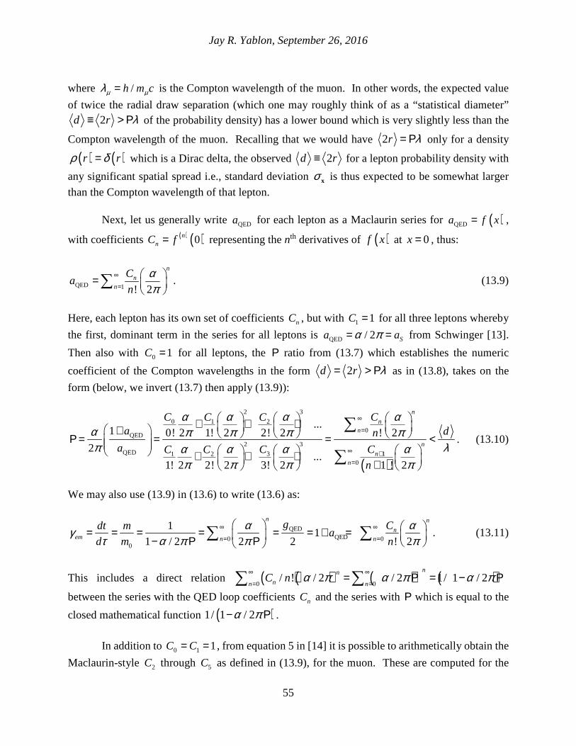
Jay R. Yablon, September 26, 2016
55
where /h m cµ µλ = is the Compton wavelength of the muon. In other words, the expected value
of twice the radial draw separation (which one may roughly think of as a “statistical diameter” 2d r λ≡ > Ρ of the probability density) has a lower bound which is very slightly less than the
Compton wavelength of the muon. Recalling that we would have 2r λ= Ρ only for a density
( ) ( )r rρ δ= which is a Dirac delta, the observed 2d r≡ for a lepton probability density with
any significant spatial spread i.e., standard deviation σ x is thus expected to be somewhat larger
than the Compton wavelength of that lepton. Next, let us generally write QEDa for each lepton as a Maclaurin series for ( )QEDa f x= ,
with coefficients ( ) ( )0nnC f= representing the nth derivatives of ( )f x at 0x = , thus:
QED 1 ! 2
n
n
n
Ca
n
απ
∞
=
=
∑ . (13.9)
Here, each lepton has its own set of coefficients nC , but with 1 1C = for all three leptons whereby
the first, dominant term in the series for all leptons is QED / 2 Sa aα π= = from Schwinger [13].
Then also with 0 1C = for all leptons, the Ρ ratio from (13.7) which establishes the numeric
coefficient of the Compton wavelengths in the form 2d r λ= > Ρ as in (13.8), takes on the
form (below, we invert (13.7) then apply (13.9)):
( )
2 3
0 1 20
QED2 3
QED 3 11 20
...1 0! 2 1! 2 2! 2 ! 2
2...
1! 2 2! 2 3! 2 1 ! 2
n
nn
n
nn
C CC Ca dn
a C CC C
n
α α α αα π π π ππ λα α α α
π π π π
∞
=
∞ +=
+ + + + Ρ = = = < + + + +
∑
∑. (13.10)
We may also use (13.9) in (13.6) to write (13.6) as:
QEDQED0 0
0
11
1 / 2 2 2 ! 2
n n
nem n n
g Cdt ma
d m n
α αγτ α π π π
∞ ∞
= =
= = = = = = + = − Ρ Ρ ∑ ∑ . (13.11)
This includes a direct relation ( ) ( ) ( ) ( )0 0
/ ! / 2 / 2 1/ 1 / 2nn
nn nC n α π α π α π∞ ∞
= == Ρ = − Ρ∑ ∑
between the series with the QED loop coefficients nC and the series with Ρ which is equal to the
closed mathematical function ( )1/ 1 / 2α π− Ρ .
In addition to 0 1 1C C= = , from equation 5 in [14] it is possible to arithmetically obtain the
Maclaurin-style 2C through 5C as defined in (13.9), for the muon. These are computed for the

Jay R. Yablon, September 26, 2016
56
muon to be 22 2! 2 .765857 6.12685940425C = ⋅ ⋅ = , and likewise, without showing the detailed
computation, 3 1154.424478C = , 4 50,257.77C = , and 5 2,892,672C = . From the leading terms
in (13.10) this means that:
2 2
2 2
2 3.0634
... ...2 2 2 2
... ...2 2!
22
702
92
d
Cµ
α α α απ π π π
λα α α απ π π π
+ + + + Ρ = = < + + + +
. (13.12)
Here, it will be noticed that the ratio Ρ from (13.10) which sets the lower bound 2r λ> Ρ
on the weighted expected separation between independent draws from the lepton probability density (and because of the proportionality r rσ ∝ , also on the standard deviation of the density),
will change as the abelian running electromagnetic coupling α increases for deeper probes of the lepton probability density. For example, from (13.8) this ratio has the numeric value
0.9973552022323µΡ = for the muon, but only for the asymptotic 1/137.035999049α = . From
(13.12) it is clear that as one probes more deeply into the muon density with the abelian coupling α becoming larger, the denominator will grow faster than the numerator, so µΡ will be detected
to grow smaller, and therefore, the lower bound 2r rσ λ∝ > Ρ will also grow smaller. Thus, the
lower bound on the standard deviation of the muon probability density will diminish. And it is clear that it is the two-loop (current density 4J ) coefficient 2 / 2!C which determines this behavior.
Given the above, we may also study how eΡ behaves for the electron. The coefficients of
(13.9) for the electron have been calculated by many authors, and are well-summarized in equations 3, 5 and 6 of [18]. These are computed in the Maclaurin-style of (13.9) to be
2 2.62783172463354C = − , 3 56.69958989C = , 4 733.6704C −= and 5 35174.4C = . We may first
use these in (13.9) along with 1/137.035999049α = to calculate that
2 3 4 5
3 52 4QED 2 2! 2 3! 2 4!
0.00115965217 2! 2
75
32
C CC Ca
α α α α απ π π π π
= + + + + =
. (13.13)
This should also be contrasted to the empirical ( )QED EW Had 0.00115965218076 27a a a a= + + =
that includes electroweak and hadronic contributions and is slightly different starting at the 1110− position. We may then use (13.13) and 1/137.035999049α = in (13.10) to calculate that:
QED
QED
1.00267699854081
29e
a d
a
απ λ +
Ρ = = <
. (13.14)
Further, using (13.13) in the leading terms of (13.10), contrast (13.12) for the muon, we find that:

Jay R. Yablon, September 26, 2016
57
2 2
2 2
2
... ...2 2 2 2
... 1.3139 ...2 2! 2 2 2
1586231677e
d
C
α α α απ π π π
λα α α απ π π π
+ + + + Ρ = = < + + +
−
. (13.15)
From (13.14) we learn that the lower bound 1.00267699854089 eed λ> ⋅ for the electron
density spread is actually slightly larger than the electron Compton wavelength, in contrast to (13.8) which shows that for the muon this is smaller than the Compton wavelength. And from (13.15) we learn that unlike the muon, the electron lower bound 2r λ> Ρ will grow larger as the
running α grows larger. This means that for a deeper probe of the electron the standard deviation
r rσ ∝ of the probability density will therefore also be detected to grow larger. Contrasting the
electron with the muon, it will be understood that the behaviors of both (13.14) and (13.15) emanate from the fact that for the electron the empirical / 2e Sa aα π< = , while for the muon the
behaviors of (13.8) and (13.12) stem from the empirical / 2 Sa aµ α π> = . And from this we may
infer that because / 2aτ α π> for the tau lepton just like for the muon, the expected draw
separation from the tau density will have a minimum value that is smaller than the tau Compton wavelength, and will be seen to decrease its standard deviation as it is probed more deeply.
In sum, as a result of defining the ratio 1Ρ ≅ in (13.6) such that 0 QED/ / 2m m g= exactly,
which ratio is deduced in (13.7) and used in (13.8) for the muon and (13.14) for the electron, we may now combine (13.11) with (12.4) and use 2 /ek e cα = ℏ to write, for the electromagnetic self-
interaction of leptons:
2QED QED0
QED2 20 0 0 D
2 0 0
canonical1 1
2 mechanical
1 1
1 / 2 1 / 2 ! 2
em emem
n n
n
n ne
g gm c E Edt U ma
d p u m m c m c g
C
k e hc n
µ µ µ
µ µ µπγ
τ
α αα π π π
∞ ∞
= =
+= = = = = = = + = + = = =∂
= = = = − Ρ − Ρ Ρ ∑ ∑
D
.(13.16)
This very important ratio chain describes the repulsive self-interaction of a single lepton, where
2 20 emmc m c E= + , where m is the dressed mass and 0m is the bare mass and emE is the
electromagnetic self-interaction energy of the lepton. And it must be emphasized that (13.16) applies to the particular circumstance where we are considering lepton self-interaction separately from any external potential, so that emE is the internal electromagnetic interaction energy which
contributes to the dressed mass 2 20 emmc m c E= + . This means that in particular, / pµ µπ above
must be understood as a ratio 0 0 0/ / / /p p p mu m u m mµ µ µ µ µ µπ → = = of the dressed mechanical
momentum to the bare mechanical momentum. Or, to put a point on it, as the ratio of the canonical-mechanical momentum to the mechanical-mechanical momentum.

Jay R. Yablon, September 26, 2016
58
So as we surmised might be the case in (12.7) – at least to the degree that we neglect the electroweak and hadronic contributions to QED EW Hada a a a= + + – (13.16) teaches that the ratio
QED / 2g is indeed a direct measure of a time dilation factor /em dt dγ τ= intrinsic to the self-
interaction of each of the leptons, and in turn is also a direct measure of the canonical-to-mechanical ratio first uncovered at (12.4). Conversely, obtaining the anomalous magnetic moment from theoretical first principles boils down to ascertaining the ratio of canonical objects to mechanical objects, and equivalently, to ascertaining a time dilation factor /dt dτ intrinsic to the electromagnetic self-interactions within the lepton which give rise to the self-interaction energy
emE . The result within (13.17) that 0 QED/ 1m m a= + , is as direct a statement as can be made that
the anomalous magnetic moments arise from and directly measure the electromagnetic energy of lepton self-interactions, and provide a simple way to calculate the unobserved bare masses directly from the observed masses and the associated anomalies.
We shall use the term “canonical co-scaling” to describe this very significant result
whereby the lepton g-factors QED D canonical :mechan a: ic lg g = co-scale in direct proportion to the
ratio of all of the other canonical-to-mechanical quantities in (13.16), and most importantly, in direct proportion to the electromagnetic time dilation factor /em dt dγ τ= . Very importantly, as
has been demonstrated throughout this paper, these canonical quantities all arise from their mechanical counterparts simply from the requirement for local gauge symmetry which spawns the ratio /µ µ∂D of gauge-covariant to ordinary derivatives. Simply put: the anomalous magnetic
2g > (or so far, at least QED 2g > ) themselves arise out of the Dirac0 2g = , also simply from
applying local gauge symmetry. So these are just another consequence of how ordinary derivatives become gauge-covariant derivatives, iqAσ σ σ σ∂ → ≡ ∂ −D , as a consequence of requiring local
gauge symmetry. No more, and no less. Also, in (13.16) the magnetic moment anomalies provide direct empirical validation of the
time dilation predicted in (10.12), and establish that in the physical world, time is in fact dilated for interactions between repelling like-charges, rather than between attracting thus unlike-charges. Referring back to the discussion at the start of section 11, this is because if
2/ 1 /edt d k Qq mc rτ = + in lowest order was for electrical attraction and not repulsion, which was
the author’s own initial misconception due to using the analogous 2/ 1 /dt d GMm mc rτ = + from gravitational theory, then between two repelling charges time would contract as
2/ 1 /edt d k Qq mc rτ = − in lowest order, and the same analysis which then led to (13.5) would
have instead yielded QED QED/ 1 / 2 1 / 2dt d a gτ α π≅ − ≅ − ≅ . So given that QEDa a≅ up to the
comparatively-minor EW Hada a+ contributions, this would have meant that 2 / 2g α π≅ − < which
is contradicted by observation, versus 2 / 2g α π≅ + > which is observed. Consequently (13.16),
which contains what is now an exact connection 0 QED/ / 1em dt d m m aγ τ= = = + between the
electromagnetic contribution to time dilation and the lepton magnetic moment anomaly by way of the self-interaction energy contained in 2 2
0 emmc m c E= + , provides direct empirical evidence that
repulsive electromagnetic interactions between like-electrostatic charges dilate time just as do attractive gravitational interactions between (what always are) like-gravitational charges a.k.a.

Jay R. Yablon, September 26, 2016
59
masses. And as earlier noted, this is a quantum field theory consequence of the reversed propagator sign for spin-1 photons versus spin-2 gravitons which causes like-gravitational-masses to attract but like-electrical-masses to repel. This, again, is why we have paid such close attention to signs and sign conventions throughout.
To this point, however, we have only used QEDa a= , neglecting the relatively tiny, albeit
still detectable, electroweak and hadronic contributions through which QED EW Hada a a a= + + . As
stated at the start of this section, this is because this paper has thus far developed electrodynamics to the exclusion of weak and strong or hadronic interactions. Now, we turn to these electroweak and hadronic contributions, which as we shall show, are most simply accounted for by a very profound and universal connection between time and energy. 14. Time “Sees” all Energy: Why the Magnetic Moment Anomalies are an Exact Consequence of Local Abelian and non-Abelian Gauge Symmetries It is often said that gravitation “sees” all energy. What is meant by this statement is that any two masses / energies in proximity to one another will attract one another, no matter what the source of those energies. And the quantum mediator of these interactions, of course, is the spin-2 graviton. A good example of this is (10.24), in which not only do the rest masses gravitate, but so too do the energies of motion and the energies of electromagnetic interaction and even, in a self-feeding non-linear way governed by Einstein’s equation, the energies of gravitation. In this respect, gravitation is unique among all interactions: For electromagnetism, the spin-1 photon mediators will only “see” particles with electrical charges. And so, for example, they will miss the neutrinos. For electroweak interactions, the spin-1 W bosons will only “see” particles with weak isospin such as left-chiral quarks and leptons, and so will miss the right handed fermions. And the spin-1 Z boson will miss right-chiral neutrinos which carry neither charge nor isospin. For strong interactions, gluons will only “see” quarks, not leptons. And for hadronic interactions which employ spin-0 Yukawa mesons to mediate attractive short-range interactions between baryons such as protons and neutrons which are composite entities comprising confined quarks and the gluon-mediated interactions among those quarks, the mesons will only “see” baryons but not leptons. A fundamental finding of this paper is that time “sees” all energy, just as does gravitation: In (9.3) we reviewed how time “sees” the kinetic energy vE of motion because
2 2 2/v vE mc mc dt d mc Eγ τ= = = + . In (9.5) we reviewed how time “sees” gravitational
interaction energy gE because 2 2 2/g gE mc mc dt d mc Eγ τ= = = − . In (10.13) we discovered that
time “sees” electromagnetic interaction energy emE via 2 2 2/em emE mc mc dt d mc Eγ τ= = = + .
And in (10.24) we saw how when all of kinetic and gravitational and electromagnetic energies are present simultaneously, because of the compound relation 2 2 /em g vE mc mc dt dγ γ γ τ= = , time
“sees” all of these energies and all of the nonlinear compositions of these energies. So it is natural to believe that this pattern will continue, whereby when an energy EWE is produced as a result of
electroweak interactions mediated by W and Z bosons, or an energy QCDE is produced as a result
of strong interactions between quarks within a baryon which are mediated by gluons, or an energy

Jay R. Yablon, September 26, 2016
60
HadE is produced as a result of hadronic interactions between baryons mediated by Yukawa
mesons, time will “see” all of these energies as well, just as we already know that that gravitation does “see” all of these energies. Specifically, time should be expected to dilate or contract in proportion with these other energies as well, just as gravitation will act on all of these energies. Any time there is some motion or interaction which gives rise to measurable energy that is “seen” by gravitation, the very same motion or interaction simultaneously gives rise to a dilation or contraction seen in the measurement of time.
In fact, from this viewpoint, if one were create a field map for any region of the universe – whether macroscopic or microscopic – in terms of the energies E that exist at each event point in that region, one could equivalently map out that very same region in terms of the 2/ /dt d E mcτ = ratio at each event point with the total energy E having a variety of origins from a variety of interactions and motions. The coordinates for measuring all events in this “ /dt dτ field” are then established by a laboratory clock of the observer observing this field, for which clock / 1dt dτ = exactly, by definition. And all other observed events (except for extremely-large motions or extremely-strong interactions) will have a / 1dt dτ ≅ differing from 1 only by parts per million or billion or trillion or higher. But there will still be a difference from 1 that establishes a measurable
2/ /dt d E mcτ = field which serves a proxy for the energy field. We shall refer to this as the “time dilation field,” recognizing that in some instances time will dilate negatively, i.e., contract.
So from the person running at six miles per hour to the car driving at 60 miles per hour to
the plane flying at 600 miles per hour to the rocket travelling at 6 miles per second, to a mass in a gravitational field, to an electron in the electromagnetic field of a nucleus, to a proton or neutron bound into an atomic nucleus, to a quark interacting inside a proton or a neutron, to a lepton or a quark or a baryon that is weakly interacting, each will have its own unique total /dt dτ to go along with its unique total energy 2/ /E mc dt dτ= from whatever origin or origins. In short, from this viewpoint, 2/ /dt d E mcτ = is a universal relation between the total energy of a material body from all sources and origins of its energy. In this relation, dτ for all practical purposes is a tick interval τ∆ at which periodic signals are emitted by that body acting as a geometrodynamic clock, while dt is the tick interval t∆ at which periodic signals are emitted by a like-clock in the observer’s laboratory. It is with this understanding, that we now turn to the electroweak and hadronic contributions to the lepton magnetic moments contained in the standard model relation
QED EW Hada a a a= + + .
Using the generalized energy/time relation 2/ /dt d E mcτ = to consider the contributions
to QED EW Hada a a a= + + , the key relation within (13.16) is 20 QED1 / 1emE m c a+ = + . From this we
see that the QED contribution to the anomaly 2QED 0/ema E m c= directly measures the ratio of the
electromagnetic self-interaction energy emE to the bare energy 20m c . This suggests that
2EW EW 0/a E m c= will measure the electroweak self-interaction energy and 2
Had Had 0/a E m c= will
measure the hadronic contribution to the self-interaction energy. We summarize each distinct contribution (subscript C QED, EM, Had= ) to the magnetic anomaly by 2
C C 0/a E m c= . So with
a total self-interaction (SI) energy SI EW HademE E E E= + + from all sources, and given

Jay R. Yablon, September 26, 2016
61
QED EW Hada a a a= + + , and taking the total dressed energy to be 2 20 SImc m c E= + , and – most
importantly – taking 2/ /dt d E mcτ = to be universally-true for all energies irrespective of source or origin whereby time “sees” all energy, we may immediately advance (13.16) to:
2
0 SI2
0 0
SI EW HadQED EW Had2 2
0 0 D
2 0 0
canonical
mechanical
1 1 1 12
1 1
1 / 2 1 / 2 ! 2
em
em
n n
nn n
e
m c Edt U m
d p u m m c
E E E E g ga a a a
m c m c g
C
k e hc n
µ µ µ
µ µ µπγ
τ
α αα π π π
∞ ∞
= =
+= = = = = = =∂+ += + = + = + + + = + = =
≅ = = = − Ρ − Ρ Ρ ∑ ∑
D
. (14.1)
The middle line in (14.1) shows the result of time “seeing” all energy contributions, which,
when applied to lepton self-interactions, takes the form 2 20 0/ / /dt d E E mc m cτ = = of a dressed-
to-bare ratio. The only expressions in (13.16) which will now become approximate in relation to all other expressions by virtue of QEDa a≅ are the those shown on the bottom lines of both (13.16)
and (14.1). This is because although ( ) ( )( )QED 01 1/ 1 / 2 / ! / 2
n
nna C nα π α π∞
=+ = − Ρ =∑ by itself
is related exactly to the electromagnetic running coupling 2 /ek e cα = ℏ , one must expect EWa to
be related to the electroweak charges Wg and Zg . And further, as stated on page 3 of [14], Hada ,
the “hadronic (quark and gluon) loop contributions to SMaµ give rise to the main theoretical
uncertainties. At present, those effects are not calculable from first principles, but such an approach, at least partially, may become possible as lattice QCD matures.” In all events, however, neither can one expect these hadronic contributions to be an exclusive function of the electromagnetic 2 /ek e cα = ℏ , because these will involve the strong charges QCDg and possibly
short-range Yukawa couplings between hadrons as well. But what is critically important, via time “seeing” all energy, is the result in (14.1) that the
time dilation 0/ / 1 / 2dt d m m a gτ = = + = is now a direct, exact measurement of the lepton
magnetic moment anomaly, including the electroweak and the hadronic and any other possible contributions not part of the standard model that may go into the observed anomaly a. The only requirement for some self-interaction to contribute to the magnetic moment anomaly is that it contribute some energy to the total energy 2mc in 2 2
0/ 1mc m c a= + . That QED EW Hada a a a= + +
with QEDa a≅ in the standard model, is a statement that the only self-interactions which
measurably-contribute to the dressed lepton energy are those involving electrodynamic interaction loops which are dominant, and electroweak and hadronic loops which offer small corrections. Now, given that for lepton self-interactions, the complete / 2 /g µ µ= ∂D is exactly equal to the canonical-to-mechanical ratio of the gauge-covariant to the ordinary spacetime derivatives, with the canonical co-scaling of (13.6) carrying through with exactitude to (14.1), we see how the anomalous lepton magnetic moments are all a direct and immediate theoretical consequence of local gauge symmetry, and that no other theoretical basis is necessary. Of course, the gauge

Jay R. Yablon, September 26, 2016
62
symmetry we must now speak of in (14.1), includes the non-abelian symmetries of Yang-Mills theory [15] which underlies the theories of weak and strong interactions. But what is so powerful about the principle that time “sees” all energy, is that even without going into the details of electroweak and strong and hadronic interaction theory, it is possible to precisely account via (14.1) for the electroweak and hadronic and any other possible contributions to the lepton magnetic moment anomalies. 15. Lepton Bare Masses and Probability Density Standard Deviations for Possible Experimental Validation, and the Observable Physical Meaning of Lepton Compton Wavelengths As a direct result of (14.1) it becomes possible to calculate an exact value for the bare masses of each of the three leptons, via the simple relation 0 2 /m m g= . Using the empirical values
2.00231930436152eg = and 2.0023318418gµ = deduced from [17] and 2.00235442gτ = from
[19], together with the rest energies 2 0.5109989280 MeVem c = ; 2 105.6583715 MeVm cµ = and 2 1776.86 MeVm cτ = from [17], we compute that the bare masses (note GeV units for tau):
2 2 2
0 0 00.5104070334 MeV; 105.5353257 MeV; 1.77477 GeVem c m c m cµ τ= = = . (15.1)
Consequently, the total self-energy of each lepton, from all contributions, is easily calculated via
2 2SI 0E mc m c= − to be (note KeV units for the first two leptons):
SI SI SI0.5918946 KeV; 123.0458 KeV; 2.09 MeVeE E Eµ τ= = = . (15.2)
As to the ratio Ρ first deduced in (13.7) to which the expected draw separation is related by 2r d λ= > Ρ , (14.1) makes clear as discussed that this is now only an approximate
relationship, up to the contributions from electroweak and hadronic loops, and their dependency on couplings other than 2 /ek e cα = ℏ . So restructuring (13.7) to include this approximation,
including QEDg g≅ , we may write:
22 2
gd r
g
αλ λπ
= > Ρ ≅−
. (15.3)
Then using the successive signs “>≅ ” to mean “greater than approximately,” we find that the approximate lower bounds on the expected draw separations, i.e., on the average weighted separations between spatial points within each lepton probability density, using
1/137.035999049α = and the foregoing g-factors, are computed to be:
1.002676995571 ; 0.9972922220 ; 0.98773962e ed d dµ µ τ τλ λ λ>≅ >≅ ≅⋅ ⋅>⋅ . (15.4)

Jay R. Yablon, September 26, 2016
63
Because these are proportional to the standard deviation of each probability density, dσ ∝ , (15.4) provides us with approximate relative ratios for the standard deviations of each of
the lepton probability densities, on the assumption that the form (e.g., Gaussian) of each lepton density is the same. So what we learn from (15.4) – which might be accessible to experimental testing – is that in relation to the Compton wavelength of each lepton, the probability densities are more densely packed for each successive higher generation. If the statistical standard deviation for the tau lepton probability density is scaled to 1, then the ratios of these standard deviations is easily computed to be 1.00967118 :: : 1: 1.01512279eτ µσ σ σ = . In other words, in relation to the
Compton wavelength of each lepton, the standard deviation of the muon probability density is about 1% larger than that of the tau lepton, while the standard deviation of the electron probability density is about 1.5% larger than that of the tau lepton, assuming their underlying distribution types are all the same and differ only by their standard deviations. Again, it may perhaps be possible to experimentally test the approximate “spread” ratios contained in (15.4).
The foregoing also gives us a very direct physical explanation of the Compton wavelengths
/h mcλ = of the three leptons. Often, it is pointed out that the Compton wavelength of a lepton (or other particle) is the wavelength of a photon with an energy equal to the rest energy of that lepton. And this in turn makes this a scale at which the uncertainty difficulties of localizing the position of a lepton come into play, whereby the Compton wavelength is a sort of qualitative boundary between circumstances under which one may or may not use classical physics. But these are all roundabout understandings, because leptons are structureless point particles as has been discussed early in section 13, and so the Compton wavelength most certainly cannot be not the “size” of a lepton in any classical sense. However, because leptons prior to “collapse” do have an associated probability density 0 †J ρ ψ ψ= = with an associated standard deviation σ (or standard deviations about each axis and / or in radial and angular directions), there is a “size” of the spatial region within which it is most likely to detect a lepton when its wavefunction is “collapsed.” So if the average separation between any two independent draws from the probability density is r ,
then one may readily think of 2d r= as a sort of “statistical diameter” for the lepton probability
density. Therefore, what (15.4) teaches is that the minimum statistical diameter of a lepton is very close to the Compton wavelength of the lepton, with the exact relation dependent on the specific nature of ρ . Further, because the standard deviation is also proportional to the average draw
separation (again, 2 / 1.128379x xx σ π σ= ≅ for a one-dimensional Gaussian), 2d r= will
also establish a minimum value for the standard deviations , ,e µ τσ σ σ of the lepton probability
distributions, again with the exact σ value(s) dependent upon the particulars of the distribution. So the Compton wavelength now has a very clear and direct and satisfying and most
importantly, empirically-verifiable meaning, at least for the leptons: One-half of the Compton wavelength of a lepton sets an approximate lower bound on the expected separation of any two independent draws obtained by detecting the lepton at some position within the probability density, with the exact expected independent draw separation determined by the specific character of the probability density. Because by basic statistics the standard deviation of a probability distribution is directly related to the expected independent draw separation, the Compton wavelengths also establish the standard deviations of the lepton probability densities. In short: the Compton
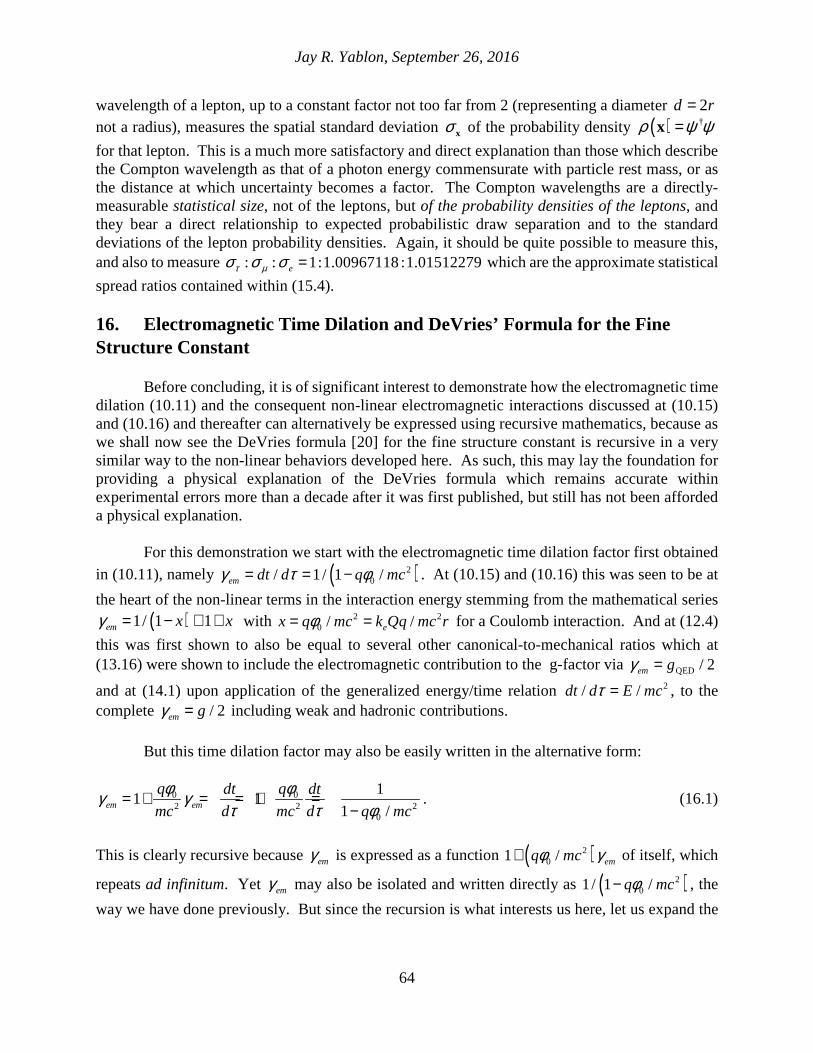
Jay R. Yablon, September 26, 2016
64
wavelength of a lepton, up to a constant factor not too far from 2 (representing a diameter 2d r= not a radius), measures the spatial standard deviation σ x of the probability density ( ) †ρ ψ ψ=x
for that lepton. This is a much more satisfactory and direct explanation than those which describe the Compton wavelength as that of a photon energy commensurate with particle rest mass, or as the distance at which uncertainty becomes a factor. The Compton wavelengths are a directly-measurable statistical size, not of the leptons, but of the probability densities of the leptons, and they bear a direct relationship to expected probabilistic draw separation and to the standard deviations of the lepton probability densities. Again, it should be quite possible to measure this, and also to measure 1.00967118 :: : 1: 1.01512279eτ µσ σ σ = which are the approximate statistical
spread ratios contained within (15.4). 16. Electromagnetic Time Dilation and DeVries’ Formula for the Fine Structure Constant Before concluding, it is of significant interest to demonstrate how the electromagnetic time dilation (10.11) and the consequent non-linear electromagnetic interactions discussed at (10.15) and (10.16) and thereafter can alternatively be expressed using recursive mathematics, because as we shall now see the DeVries formula [20] for the fine structure constant is recursive in a very similar way to the non-linear behaviors developed here. As such, this may lay the foundation for providing a physical explanation of the DeVries formula which remains accurate within experimental errors more than a decade after it was first published, but still has not been afforded a physical explanation. For this demonstration we start with the electromagnetic time dilation factor first obtained
in (10.11), namely ( )20/ 1 / 1 /em dt d q mcγ τ φ= = − . At (10.15) and (10.16) this was seen to be at
the heart of the non-linear terms in the interaction energy stemming from the mathematical series
( )1/ 1 1em x xγ = − ≅ + with 2 20 / /ex q mc k Qq mc rφ= = for a Coulomb interaction. And at (12.4)
this was first shown to also be equal to several other canonical-to-mechanical ratios which at (13.16) were shown to include the electromagnetic contribution to the g-factor via QED / 2em gγ =
and at (14.1) upon application of the generalized energy/time relation 2/ /dt d E mcτ = , to the complete / 2em gγ = including weak and hadronic contributions.
But this time dilation factor may also be easily written in the alternative form:
0 02 2 2
0
11 1
1 /em em
q qdt dt
mc d mc d q mc
φ φγ γτ τ φ
= + = = + =−
. (16.1)
This is clearly recursive because emγ is expressed as a function ( )201 / emq mcφ γ+ of itself, which
repeats ad infinitum. Yet emγ may also be isolated and written directly as ( )201/ 1 /q mcφ− , the
way we have done previously. But since the recursion is what interests us here, let us expand the

Jay R. Yablon, September 26, 2016
65
recursion by simply placing emγ from (16.1) into itself several times to identify and solve for the
infinite series, as such:
( )
( )
0 0 0 0 0 02 2 2 2 2 2
2 3 4 5
0 0 0 0 02 2 2 2 2
02 2
0 0
1 1 1 1 1 1 1 ...
1 ...
1
1 /
em em
n
emn
q q q q q q
mc mc mc mc mc mc
q q q q q
mc mc mc mc mc
q
mc q mc
φ φ φ φ φ φγ γ
φ φ φ φ φ
φ γφ
∞
=
= + = + + + + + +
= + + + + + +
= = = − ∑
. (16.2)
This is the same series that underlies the non-linear energy (10.15), but recursively expressed.
What makes this of special interest is that the DeVries formula [20] for the fine structure constant, namely:
( ) ( ) ( ) ( ) ( )( )
22
0 1 2 3 4exp ; 1 1 1 1 1 1 ...2 2 2 2 2 2
π α α α α ααπ π π π π
= Γ − Γ = + + + + + +
, (16.3)
has a the parameter Γ which is structurally very similar to the top line of (16.2). Given that
( )2exp / 2 1/139.0456366606...π− = , it is clear that 2 1Γ > for which 2 1Γ ≅ is a dimensionless
number that turns out to be slightly larger than 1 such that ( )2 2exp / 2α π= Γ − equals the
empirically-observed fine structure constant with the value 1/137.035999139(31)α = reported in [11] or the value 1/137.035999049(90)α = used in [14], to within present-day experimental errors. It is for this reason that even though it has not yet been afforded a physical interpretation, the DeVries relationship must be regarded very seriously. Note also that the only two independent numbers in (16.3) are α and π . So while the fine structure constant ( )α π is a function of only
the number π , we can also say that ( )π α is a function only of α , which suggests and extremely
close connection between the physics of electromagnetism and the pure mathematics of circles, spheres, etc. All of this motivates us to see if some connection can be established between (16.2) and (16.3). Starting with (16.2), let us now consider a Coulomb potential 0 /ek Q rφ = for which the
linear interaction energy ratio 2 2 20 0/ / /em eE mc q mc k Qq mc rφ= = , see (10.15). Then as we did
to arrive at (13.1), let us consider a single charged self-interacting lepton probability density prior to wavefunction “collapse,” and divide this into two halves each with 1
2Q q e= = − . Thus, 21
0 4 1/em eE k e r= , with 1/ 1/r r> being the expected value of the inverse draw separation on
the condition that the two draws come from different halves of the probability density. What we then learned leading up to (13.1) is that as we subdivide the lepton further and further ad infinitum

Jay R. Yablon, September 26, 2016
66
then take the ordinary calculus limit, the linear self-interaction energy ends up being given by 2
0 0 1/ 2em eE q k e rφ= = , which is (13.1). Then using the relation ( )2 2/ / 2ek e mc α π λ= as we
did at (13.3), and also using the statistical diameter 2d r= , from (13.1) we obtain:
2
0 02 2 2
1 1 1
2 2 2 2em eE q k e
mc mc mc r r d
φ α αλ λπ π
= = = = . (16.4)
Although this is the linear expression for the electromagnetic self-interaction energy, we see from (13.3) that the complete non-linear energy is obtained by setting ( )/ 2 1/ 2x rαλ π= in the
mathematical function ( )1/ 1em xγ = − . But the recursive (16.2) is just an alternative way of
representing this function. So to obtain a recursive expression for emγ which contains all of the
non-linear terms of (10.15) built in, we may substitute (16.4) into the top line of (16.2) to obtain:
( )1 1 1 1 11 1 1 1 1 1 ...
2 2 2 2 2em d d d d d
α α α α αγ λ λ λ λ λπ π π π π
= + + + + + + . (16.5)
This is simply an equivalent, albeit recursive way to write (13.3). This may also be written in terms of the dimensionless ratio parameter 1/ 1/dλΡ = defined in (13.7).
Contrasting this with (16.3) we now see an extremely close resemblance with the
dimensionless DeVries number Γ . This resemblance is not just structural; now it is directly physically-substantive because the driving number in each is α . In fact, the only difference between emγ in (16.5) and Γ in (16.3) is that in (16.5) the denominator of α is 2π at all recursive
orders, while in (16.3) the denominator at nth order is ( )2nπ . Yet, (16.5) also has the term 1/ dλ
multiplying / 2α π at each order, while in (16.3) a ( )1/ 2nπ multiplies α at each order. Thus, it
seems there is a link to be found between 1/ dλ and ( )1/ 2nπ , which we now explore.
In 1/ dλ , λ is the Compton wavelength of the lepton, and thus a single, definite number
just like the mass /m h cλ= . But treating the inverse statistical dimeter 1/ d as a free variable
at each order, let us now define an infinite sequence of statistical diameters that we denote by nd
with 0 n≤ ≤ ∞ where each such diameter is associated with each recursive order in (16.5). So changing nd d→ in (16.5) and setting n at each order to be the number of that order, (16.5)
becomes:
( )0 1 2 3 4
1 1 1 1 11 1 1 1 1 1 ...
2 2 2 2 2em d d d d d
α α α α αγ λ λ λ λ λπ π π π π
′ = + + + + + +
.(16.6)
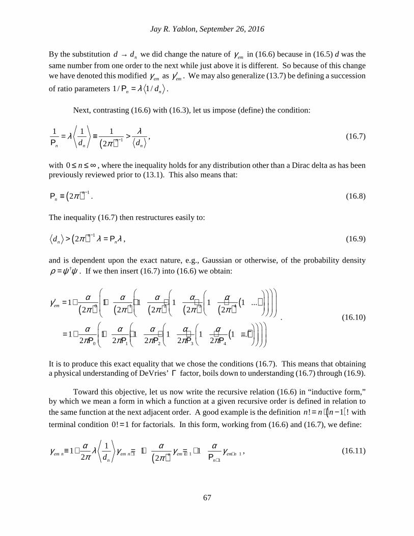
Jay R. Yablon, September 26, 2016
67
By the substitution nd d→ we did change the nature of emγ in (16.6) because in (16.5) d was the
same number from one order to the next while just above it is different. So because of this change we have denoted this modified emγ as emγ ′ . We may also generalize (13.7) be defining a succession
of ratio parameters 1/ 1/n ndλΡ = .
Next, contrasting (16.6) with (16.3), let us impose (define) the condition:
( ) 1
1 1 1
2n
n n nd d
λλπ −= ≡ >
Ρ, (16.7)
with 0 n≤ ≤ ∞ , where the inequality holds for any distribution other than a Dirac delta as has been previously reviewed prior to (13.1). This also means that:
( ) 12
n
n π −Ρ ≡ . (16.8)
The inequality (16.7) then restructures easily to:
( ) 12
n
n nd π λ λ−> = Ρ , (16.9)
and is dependent upon the exact nature, e.g., Gaussian or otherwise, of the probability density
†ρ ψ ψ= . If we then insert (16.7) into (16.6) we obtain:
( ) ( ) ( ) ( ) ( )( )
( )
0 1 2 3 4
0 1 2 3 4
1 1 1 1 1 1 ...2 2 2 2 2
1 1 1 1 1 1 ...2 2 2 2 2
em
α α α α αγπ π π π π
α α α α απ π π π π
′ = + + + + + +
= + + + + + + = Γ Ρ Ρ Ρ Ρ Ρ
. (16.10)
It is to produce this exact equality that we chose the conditions (16.7). This means that obtaining a physical understanding of DeVries’ Γ factor, boils down to understanding (16.7) through (16.9). Toward this objective, let us now write the recursive relation (16.6) in “inductive form,” by which we mean a form in which a function at a given recursive order is defined in relation to the same function at the next adjacent order. A good example is the definition ( )! 1 !n n n= ⋅ − with
terminal condition 0! 1= for factorials. In this form, working from (16.6) and (16.7), we define:
( )1 1 11
11 1 1
2 2em n em n em n em nn
n nd
α α αγ λ γ γ γπ π+ + +
+
≡ + = + = +Ρ
, (16.11)

Jay R. Yablon, September 26, 2016
68
where 0 n≤ ≤ ∞ . Then, it is clear that (16.6) is compactly written as 0em emγ γ′ = , and that with the
condition (16.7) the DeVries number is actually 0emγΓ = . So with the foregoing, the DeVries
relationship (16.3) simplifies to the trilogy:
( )( )
22
0 0 1exp ; ; 12 2
em em em n em nn
π αα γ γ γ γπ +
= − Γ = = +
. (16.12)
Here, 0emγΓ = is the terminal relation analogous to 0! 1= , while ( )( ) 11 / 2n
em n em nγ α π γ += + is the
inductive form of the recursion analogous to ( )! 1 !n n n= ⋅ − .
So, what might one make of (16.7) through (16.9), physically? To gain some clues, it is
probably simplest to work from (16.9), which we write as the equality ( ) 1
min2
n
nd π λ−= of a set
of minimum statistical diameters in relation to the Compton wavelength. For the first several orders, using the reduced Compton wavelength / 2λ π=Ż , these statistical diameter minima are:
( ) ( )2 3
0 1 2 3 4min min min min min; ; 2 ; 2 ; 2d d d d dλ πλ π λ π λ= = = = =Ż . (16.13)
Another way to write this is as the recursive kernel and terminal condition:
1 0min min min2 ;n nd d dπ −= = Ż . (16.14)
In this vein, 2 /C rπ = is of course the ratio of the circumference of a circle to its radius, so at each order, the statistical diameter is promoted from a radial length to a circumferential length.
Further, while each of the minnd arise from a different order of the recursion, it is perfectly
reasonable to think of the n in minnd as some type of quantum number. Additionally, because
/em dt dγ τ= is the electromagnetic contribution to time dilation, and because dt t→ ∆ measures
the “tick” interval of a clock in a laboratory, the existence of a succession of em nγ in (16.12) is
suggestive of a relation /em n ndt dγ τ= containing a collection of proper time “tick” rates
n ndτ τ→ ∆ emanating from the lepton. At the same time, the “tick” rate of a signal is related to
its frequency by 1/f τ= ∆ , so that a collection of tick rates is related to a collection 1/n nf τ= ∆
of frequencies. And this in turn means that there is some collection of time dilation factors:
em n em n nn n
dt tt f
dγ γ
τ τ∆= → = = ∆
∆ (16.15)
which are equal to nf multiplied by the t∆ ticks of the laboratory clock.

Jay R. Yablon, September 26, 2016
69
So in this vein, the intuitive sense that one may gain by studying (16.13) and how it interrelates to the DeVries formula is not unlike how one might think about the quantum number that Planck first found in E nhf= to describe the energy oscillations in a blackbody radiation spectrum. Or with /h pλ = , this is not unlike the Bohr / deBroglie relation 2n rλ π= first used
to model the hydrogen atom. In fact, the deBroglie relation may be rewritten as / / 2nr nλ π= and
then likened to ( ) 1
min/ 2
n
nd λ π −= , keeping in mind that the former is for electron orbits in
(hydrogen) atoms while the latter is for the self-interaction of electrons standing alone. So in the
same way that / / 2nr nλ π= was the point of entry to modelling atoms, ( ) 1
min/ 2
n
nd λ π −=
would seem to be the point of entry for modelling individual electrons. Likewise, (16.15) contains an infinite collection of frequencies, and we know that any time we have such a collection of frequencies, these may be approached using Fourier analysis. Further, it is well-known that Heisenberg’s matrix mechanics arose from considering the Fourier analysis of an infinite collection of frequencies. So one can envision that (16.15), properly advanced, could perhaps lead to an even deeper understanding matrix mechanics. And most certainly, the relations ascertained in the forgoing do seem to be rife with quantum mechanical information that needs to be closely studied and deciphered. 17. Conclusion From ancient times, through those of Galileo, Huygens, Newton, Bernoulli, du Châtelet, Joule, Carnot and Einstein, the principle of energy conservation and the understanding that energy is a universal form of currency or liquidity of the natural world out of which everything is made and which can be transformed from one form to another but can never be created or destroyed, has evolved into perhaps the most universal, overarching, unifying principle of theoretical physics. Likewise, the manipulation of material objects to convert energy from one form to another, be it chemical, solar, nuclear, mechanical, electromagnetic, heat or other types of energy, has been the foundation of humanity’s technological advancement insofar as being able to perform important and necessary work without the use of human or animal physical labor. The Special and General theories of Relativity gave the first inkling of a similarly-deep and universal connection between energy and time. Not only was energy understood to be time component 0E p= of an energy-momentum vector in spacetime, but more importantly it was understood that for an object in relative motion time dilates in relation to the total energy by
2 2 2 212/vE mc mc dt d mc mvγ τ= = ≅ + which includes a rest energy 2mc plus to lowest order the
Newtonian kinetic energy 212 mv as in (9.3). And it was understood that a mass in a gravitational
field also dilates time in relation to the total energy for the Schwarzschild solution in the Newtonian limit according to 2 2 2/ /gE mc mc dt d mc GMm rγ τ= = ≅ + where /gE GMm r= − is the
gravitational interaction energy as in (9.5). Moreover, when there is both motion and gravitation, the total energy continues to be related to the overall time dilation by 2 /E mc dt dτ= , but with a compounded effect whereby / v gdt dτ γ γ= as shown in (9.8). The present paper similarly
establishes, consistent with the well-validated Lorentz force law at (5.7) as obtained from the metric (3.5) via the variation minimization (1.1), that when an electromagnetic charge q with mass

Jay R. Yablon, September 26, 2016
70
m is placed into a proper potential 0φ , there is also a time dilation given by
( )20/ 1/ 1 /em dt d q mcγ τ φ≡ = − at (10.11) which likewise obeys the relation 2 /E mc dt dτ= as
seen in (10.13). And this likewise compounds with gravitational and kinetic energy according to 2
em g vE mcγ γ γ= as seen in (10.23) a.k.a. (3.11).
So if there is any single result of paramount importance here, it is the finding at (14.1) of a universal relation between time and energy whereby all forms of energy dilate (or contract) time regardless of their origin, and that this is not only a classical feature of nature, but that this carries through to the lepton magnetic moment anomalies which are the quintessential hallmarks of the success of quantum field theory. In short, just as gravitation “sees” all energy, so too does time “see” all energy, not just macroscopically, but even at the microscopic level of individual quantum particles, via the universal relation 2/ /dt d E mcτ = . Any time a material body of whatever character gains or loses energy of whatever form from whatever origin, the rate at which a geometrodynamic clock associated with that body will tick is altered, and therefore, so too is the measurement of time when that body is used as a clock. One cannot change the energy of a particle or a system without simultaneously changing how time is measured when that particle or system is used as a geometrodynamic clock. So, as a simple example from Special Relativity, when a person is stuck by a ball moving at, say, 60 miles per hour, one can and does say that the impact is the result of the kinetic energy of motion of that ball relative to the person. But one can equally say that the impact is the result of time being different for the ball than for the person, albeit with a miniscule difference of parts per quadrillion (1015). And when lightning strikes, one can say that it is nature trying to bring a large potential difference into equipotential, or one can say that nature is trying to bring different rates of time into equilibrium. Any talk of energy, has a parallel and equivalent talk of time. The other present result of underlying, unifying importance, is that the motions of material bodies in nature and many of the observed numeric objects observed in nature, are fundamentally “canonical” motions and objects growing from “mechanical” motions and objects as a result of local symmetry principles. Thus, gravitational motion has been known for a century to simply be the canonical motion / / 0du d Du Dβ βτ τ→ = of (1.3) obtained by promoting ordinary spacetime derivatives to gravitationally-covariant derivative ;aα∂ → ∂ governing parallel transport in curved
spacetime with ; ;,R A Aαβµν α ν µ β = ∂ ∂ . And based on this present work, the Lorenz force motion
of classical electrodynamics is seen to be simply the canonical motion / / 0du d uβ βτ τ→ =D D of (5.9) obtained via the variation (1.1) and using the geodesic gauge (5.6), of promoting spacetime derivatives to gauge-covariant derivatives iqAα α α α∂ → = ∂ −D governing parallel transport in an
abstract space first developed by Hermann Weyl in [5], [6], [7] in which the field strength
,qF iµν µ νφ φ = D D defines an imaginary form of curvature.
Then, at the same time mechanical motion is promoted to canonical motion / 0uβ τ =D D
as a consequence of the derivative promotion α α∂ →D of gauge symmetry, so too a number of
mechanical objects are simultaneously promoted into canonical objects as shown in (12.4), such as the four-velocity u Uµ µ→ , the four-momentum pµ µπ→ and the energy 2mc E→ ,

Jay R. Yablon, September 26, 2016
71
canonically co-scaling directly with the electromagnetic contribution /em dt dγ τ= to the time
dilation. And although (12.4) applies to classical objects, when we study the behavior of individual charged lepton quanta, we find at (13.16) that this carries through to the quantum level, whereby the “mechanical” Dirac g-factor Dg also co-scales via D QEDg g→ into the canonical
QED QED2 2g a= + which includes the electromagnetic contribution to the lepton magnetic moment
anomalies QEDa that are a hallmark of Quantum Electrodynamics. At the same time, the bare
lepton masses co-scale into dressed masses via 0m m→ also in step with the time dilation
/em dt dγ τ= . This ties the electromagnetic time dilation together to the modern understanding
that the magnetic moment anomalies arise from the same lepton self-interactions that turn the bare masses into dressed masses in accordance with the Ward-Takahashi identities.
Then, when we turn again to the universal relation 2/ /dt d E mcτ = between time and
energy whereby the time “sees” all energy, we find at (14.1) that even the electroweak and hadronic anomaly contributions may be accounted for. Now, D 2g = co-scales into 2 2g a= +
containing the complete, observed anomaly with all contributions, because electroweak and hadronic interactions also produce energies which directly affect time. So the physics of all interactions – gravitational, electromagnetic, weak and strong – and the hadronic interactions which this author has studied in depth at [21], [22], [16], [23] and [24], all enjoy the unifying thread whereby mechanical motions and objects grow into canonical motions and objects, and measurements of time are affected by any and all energies of whatever form from whatever origin. In this way it becomes possible to establish a geometrodynamic foundation for classical and quantum electrodynamics centered about time dilation and contraction and a universal time-energy relation, and lay out the path by which this is extended via non-abelian gauge theories to weak and strong and hadronic interactions. The author wishes to acknowledge and thank Joy Christian for his encouragement and his input throughout the conduct of this research. References
[1] A. Einstein, The Foundation of the General Theory of Relativity, Annalen der Physik (ser. 4), 49, 769–822 (1915) [2] A. Einstein, On the Electrodynamics of Moving Bodies, Annalen der Physik 17: 891 (1905) [3] H. Minkowski, Space and Time, Physikalische Zeitschrift 10, 104-111 (1909) [4] J. A. Wheeler, Geometrodynamics. New York: Academic Press (1963) [5] H. Weyl, Gravitation and Electricity, Sitzungsber. Preuss. Akad.Wiss., 465-480. (1918). [6] H. Weyl, Space-Time-Matter (1918) [7] H. Weyl, Electron und Gravitation, Zeit. f. Physik, 56, 330 (1929) [8] T. Kaluza, Zum Unitätsproblem in der Physik, Sitzungsber. Preuss. Akad. Wiss. Berlin. (Math. Phys.): 966–972 (1921) [9] O. Klein, Quantentheorie und fünfdimensionale Relativitätstheorie, Zeitschrift für Physik A 37 (12): 895–906 (1926) [10] A. Einstein, Does the inertia of a body depend upon its energy-content?, Annalen der Physik, 18:639 (1905) [11] http://pdg.lbl.gov/2015/reviews/rpp2015-rev-phys-constants.pdf [12] A. Zee, Quantum Field Theory in a Nutshell, Princeton University Press (2003) [13] J. Schwinger, On Quantum-Electrodynamics and the Magnetic Moment of the Electron, Physical Review 73 (4): 416 (1948)

Jay R. Yablon, September 26, 2016
72
[14] http://pdg.lbl.gov/2015/reviews/rpp2015-rev-g-2-muon-anom-mag-moment.pdf [15] C.N. Yang, R. Mills, R., Conservation of Isotopic Spin and Isotopic Gauge Invariance, Physical Review. 96 (1): 191–195 (1954) [16] J. Yablon, Grand Unified SU(8) Gauge Theory Based on Baryons which Are Yang-Mills Magnetic Monopoles, Journal of Modern Physics, Vol. 4 No. 4A, pp. 94-120 (2013). doi: 10.4236/jmp.2013.44A011, http://www.scirp.org/Journal/PaperDownload.aspx?paperID=30822 [17] http://pdg.lbl.gov/2015/tables/rpp2015-sum-leptons.pdf [18] T. Aoyama, M. Hayakawa, T. Kinoshita, M. Nio, Tenth-Order QED Contribution to the Electron g−2 and an Improved Value of the Fine Structure Constant. Physical Review Letters. 109 (11): 111807. arXiv:1205.5368 (2012) [19] http://pdg.lbl.gov/2015/listings/rpp2015-list-tau.pdf [20] H. DeVries, An exact formula for the Electro Magnetic coupling constant, http://www.chip-architect.com/news/2004_10_04_The_Electro_Magnetic_coupling_constant.html (2004) [21] J. R. Yablon, Why Baryons Are Yang-Mills Magnetic Monopoles, Hadronic Journal, Volume 35, Number 4, 399-467 https://jayryablon.files.wordpress.com/2013/03/hadronic-journal-volume-35-number-4-399-467-20121.pdf (2012) [22] J. R. Yablon. , Predicting the Binding Energies of the 1s Nuclides with High Precision, Based on Baryons which are Yang-Mills Magnetic Monopoles, Journal of Modern Physics Vol.4 No.4A, pp. 70-93. doi: 10.4236/jmp.2013.44A010, http://www.scirp.org/journal/PaperDownload.aspx?paperID=30817 (2013) [23] J. R. Yablon, Predicting the Neutron and Proton Masses Based on Baryons which Are Yang-Mills Magnetic Monopoles and Koide Mass Triplets, Journal of Modern Physics, Vol. 4 No. 4A, 2013, pp. 127-150. doi: 10.4236/jmp.2013.44A013 http://www.scirp.org/journal/PaperDownload.aspx?paperID=30830 (2013) [24] J. R. Yablon, System, Apparatus, Method and Energy Product-By-Process for Resonantly-Catalyzing Nuclear Fusion Energy Release, and the Underlying Scientific Foundation,http://patentscope.wipo.int/search/docservicepdf_pct/id00000025517277.pdf?download (2014)