1

Electromagnetic Time-Reversal Source Localization in Changing Media: Experiment and Analysis

Dehong Liu, Sathya Vasudevan, Jeffrey Krolik, 1Guillaume Bal and Lawrence Carin

Department of Electrical and Computer Engineering Duke University

Durham, NC 27708-0291 lcarin@ee.duke.edu

1 Department of Applied Physics & Applied Mathematics

Columbia University New York, New York

Abstract – An experimental study is performed on electromagnetic time reversal in

highly scattering environments, with a particular focus on performance when

environmental conditions change. In particular, we consider the case for which there is a

mismatch between the Green’s function used on the forward measurement and that used

for time-reversal inversion. We examine the degradation in the time-reversal image with

increasing media mismatch, and consider techniques that mitigate such degradation. The

experimental results are also compared with theoretical predictions for time reversal in

changing media, with good agreement observed.

I. Introduction

Time reversal is a technique that is based on the principle of reciprocity [1]. In particular,

assume a source emits radiation that propagates through a complex media to a set of

receiving antennas. The data that arrives early in time at a given receiver implicitly

travels a shorter distance than data that arrives later in time. By reversing the received

waveforms in time, and emitting them from their respective reception points, the data that

traveled a longer distance is emitted early, and the data that traveled a shorter distance is

emitted later, and all of the energy arrives at the original source in unison, approximately

recreating the original excitation. In the above discussion we have assumed that the

medium is lossless. Further, the original source is not recreated exactly after time

reversal, because in practice a finite set of receiver/source antennas are used.

2

While the concept of time reversal is simple, a direct result of reciprocity, it has

important implications. For example, in conventional imaging the focusing resolution is

limited by the size of the antenna aperture (for an antenna array) [2]. However, in a

complex propagation medium, characterized by multiple paths from the original source to

the receiving elements, time reversal may have an effective aperture [3,4] that is much

larger than that of the physical array aperture, acting as a filter that increases with the

number of available paths [5,6]. This phenomenon has been termed “superresolution” [4].

Interestingly, the more complex the media the more paths are manifested from a source to

the multiple receivers, thereby enhancing superresolution refocusing quality (see Fig. 1).

However, while resolution quality may be enhanced by increased media complexity, one

also typically observes a reduction in the energy refocused at the original source [4,5,6]

(the complex media yields highly scattered waves, most of which are not observed by the

antennas).

Time reversal has been demonstrated experimentally in an extensive set of ultrasonic and

acoustic measurements [7-13], as well as in recent electromagnetic studies [14,15]. Time

reversal examined in this previous work consists of two steps: (i) a source emits a pulse

of radiation from a given point in a complex propagation environment, with the data

observed at a set of receiving antennas; and (ii) the time-domain data at each of the

receiver elements are reversed and synchronously re-radiated from the respective source-

receiver antennas. A question arises as to focusing quality when there is a mismatch

between the environments considered in steps (i) and (ii). This issue has been examined

experimentally in acoustics [8,16,17] and ultrasonics [10], as well as in theoretical studies

[6]. Theory predicts that the strength of the refocused signal is a function of the

correlation of the two underlying media between the forward and backward stages of the

time reversal experiment.

We may seek to generalize time reversal, particularly when there is uncertainty in the

medium associated with step (i). Addressing the imaging problem, rather than

numerically implementing step (ii) through a single (fixed) media, which may be

different from that actually used in step (i), we may perform this step using an ensemble

3

of media (i.e., a media subspace, with the idea that the actual media from step (i) may be

in the subspace, but without requiring knowledge of the exact/precise media associated

with step (i)). For example, we may use an average Green’s function for step (ii), with

averaging performed over an ensemble of Green’s functions corresponding to a set of

(distinct) media related to the particular media for which step (i) was performed.

Alternatively, one may perform an eigen-based principal components analysis (PCA)

[18] on an ensemble of Green’s functions for different media in step (ii), with use of the

principal eigenvector(s) when imaging. We examine these techniques for electromagnetic

source localization in changing and uncertain media.

II. Theory of Time Reversal in Fixed and Changing Media

A. Superresolution

A key property of time reversal

sensing is that multiple scattering

manifested by a complex (cluttered)

environment may be used to constitute

an effective aperture that is larger than

the actual physical aperture [4]. In Fig.

1 we consider a two-dimensional

problem with a line-source radiator,

with the fields observed along a linear

aperture. In Fig. 1(a) the source

radiates in a homogeneous medium,

while in Fig. 1(b) the source radiates in

a medium characterized by multi-path

(clutter). Because of the homogeneous

medium in which the fields radiate, in Fig. 1(a) the range of observed angle-dependent

wavefronts is dictated by the size of the linear aperture and the distance of the source to

the aperture [2]. By contrast, in Fig. 1(b) a richer set of waves emitted from the source

(a)

(b)

Figure 1. Wavefronts emitted from a source, observed at a linear antenna array (at left). (a) Source in a homogeneous medium, (b) in a highly multi-pathed environment.

4

make their way to the linear receiver aperture, as a result of multi-path. From Fig. 1 we

therefore note that the number of different source wavefronts (emitted at different angles)

observed by the receiver increases with increasing multi-path. When the data observed on

the linear aperture is time reversed and synchronously reradiated, the multiple angle-

dependent wavefronts emitted from the source are back-propagated, coalescing at the

original source. Since the diversity of different angle-dependent waves arriving at the

focus point increases with increasing clutter, the resolution (tightness) of the focus

increases commensurately [1,4,7-14]; this has been referred to as “superresolution”,

because in a cluttered environment the focusing is tighter than would be expected in a

homogeneous medium for the same physical aperture size.

B. Rayleigh scattering

In addition to examining the focusing tightness as a function of aperture size and clutter,

we may examine the focusing energy strength as a function of frequency f. In the limit of

small scatterer diameters with respect to the wavelength, it is known that scattering

strength is proportional to 4f for three-dimensional problems and to 3f in two

dimensions. This is Rayleigh scattering modeling light propagation in the atmosphere.

We briefly recall how the scaling arises. Amplitude fluctuations in the wave speed caused

by the presence of rods generates scatterers in the time harmonic representation

(Lippman-Schwinger equation [19]) whose strength is proportional to the square of

frequency [5]. Their power spectrum is therefore proportional to the fourth power of

frequency. The homogeneous Green’s function for observation point r and source point

r′ may be expressed as

rrrr

rrk

′−=′−

′−

π4)(D3

ieG

in three dimensions for wavenumber cfπ2=k , and therefore it has intensity

independent of frequency, explaining the Rayleigh scaling in that setting (scattering

proportional to 4f , and a Green’s function with frequency-independent scaling). In two

space dimensions, the Green’s function is inversely proportional to the square root of

frequency in the high frequency limit:

5

x

rrrr iki ee

kiG 4/

D2 π2

4)( π−

′−≈′− , 1>>′− rrk .

The resulting intensity is thus inversely proportional to frequency. The power spectrum is

proportional to 4f and the energy free propagator is proportional to 1−f , and the product

of these two provides the 3f Rayleigh scaling in two space dimensions.

C. Correlations

Time reversal as viewed in the frequency domain is the product of two Green’s function

propagators: the first one sends the signal from the source to the array of detectors, and

the second one backpropagates the signal from the detector array. In the above discussion

we assumed that the media associated with the forward and inverse phases were the

same, and therefore that the respective Green’s functions were identical; this represents

the conditions under which time reversal is typically implemented [1]. It is of interest to

examine the time-reversal image quality when the forward and inverse media are

different (e.g., because the media conditions have changed, or because an approximate

numerical Green’s function is used in the inverse problem for representation of the actual

Green’s function associated with a forward measurement).

For the case of different Green’s functions in the forward and inverse phases, the product

of operators has a kernel represented by the correlation function of the two corresponding

Green’s function. In the Lippman-Schwinger representation of the wave equation [19],

the correlation of the two Green’s functions turns out to be proportional to the power

spectrum of the random heterogeneities of the underlying heterogeneous media. If we

denote by )(xδc the fluctuations in the propagation speed of the underling medium,

relative to a reference homogeneous medium, the correlation function as a function of

position x is defined by

)()()( yxyx += δcδcR ,

which is independent of y when the fluctuations are statistically independent by

translation. The power spectrum )(ˆ kR is defined as the Fourier transform of the above

correlation.

6

When the underlying medium does not change between the two phases of the time

reversal experiment, it is well known that the correlation of the two Green’s function

solves a radiative transfer equation in the phase space [19]. When the two media are

different, then the radiative transfer equation needs to be modified. The salient feature of

this modification is the following: the scattering coefficient in the radiative transfer

equation, which was proportional to the power spectrum of the heterogeneities, is now

proportional to the cross-correlation of the two sets of heterogeneous fluctuations; see

[6]. When )(xjδc are the speed fluctuations during states 1=j (forward stage) and

2=j (backward stage) of the time reversal experiment, the cross-correlation is given by

)()()( 2112 yxyx += δcδcR .

The analysis in [5] shows that the intensity of the time reversed signal is all the more

important when the medium is scattering, i.e., heterogeneous. Consequently, when the

two random media become less and less correlated, the scattering term in the radiative

transfer equations decreases and so does the intensity of the time reversed signal. Such

decay was validated by numerical studies in [5].

D. Shifted media

The above discussion considered the general case of changing media in the forward and

inverse phases. We now consider the special case for which the media in the inverse

phase is shifted by the vector τ with respect to the media considered in the forward

measurement. As media separate from one another, the power spectrum appearing in the

radiative transfer equations is multiplied by a plane wave (complex exponential) in the

direction of the shift. Indeed we observe that

)()(δ)(δ)(δ)(δ)( 112112 τxyτxyyxyx +=++=+= RccccR .

This shift by τ in the physical domain translates to multiplication by kτ ⋅ie for the power

spectrum in the Fourier domain: )(ˆ)(ˆ12 kk kτ ReR i ⋅= .

7

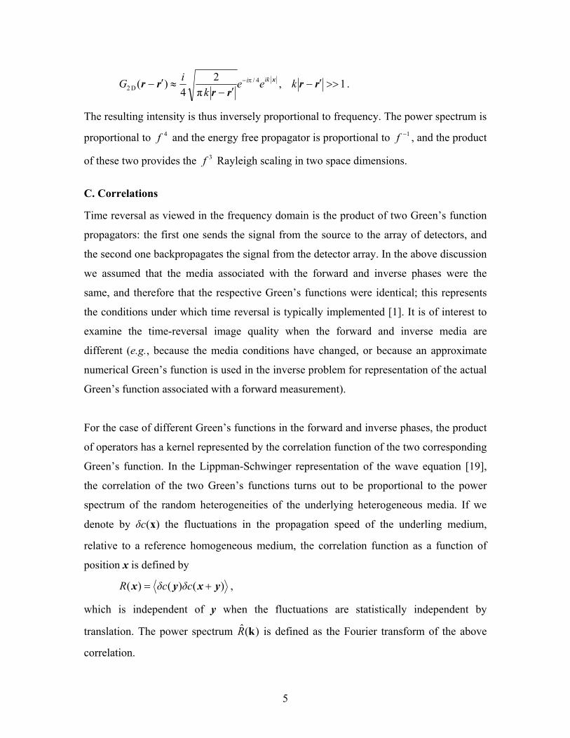
In the diffusive regime of wave propagation, where the energy of waves propagating in

all directions is equipartitioned, this complex exponential is averaged over all directions

of propagation [5]. The integral of plane waves over the space of directions

kτkτde

S

ik )sin(ˆ41

2

ˆ =∫ ⋅ kτk

π, )(ˆ

21

0ˆ

1kτJde

S

ik =∫ ⋅ kτk

π

provides a sinc function in three dimensions and a Bessel function in two dimensions,

where τ=τ . In either case, it can be identified with the imaginary part of the Green’s

function in homogeneous media.

The strength of scattering is multiplied by the Bessel function )(0 kτJ in the case of two-

dimensional shifted media considered below. In the diffusive regime, we thus obtain that

the refocused signal vanishes for those frequencies such that kτ is a zero of the Bessel

function; see [5] for more details.

E. Accounting for mismatched media

The discussion in Secs. IIC and IID

demonstrates that the time-reversal

imaging quality is expected to deteriorate

with diminished correlation between the

Green’s functions used in the forward and

inverse measurements. However, this was

based on the assumption that we only had

access to a single (mismatched) Green’s

function for the inverse phase. In Sec. V

we extend these ideas by considering the

case for which we assume access to an

ensemble of Green’s functions, and it is

assumed that this ensemble captures the general properties for which the actual

Antenna 1

Antenna 2

Antenna 1

Antenna 2

Figure 2. Dielectric rod experimental setup used in experimental time-reversal studies. The two antennas are moved using precision stepper motors. The length of the domain in the horizontal direction is 1.2 m, and it is 2.4 m in the vertical direction (of this photo).

8

(unknown) forward-phase Green’s function is a special case. Simple ideas from the

signal-processing community are employed to improve time-reversal imaging quality

under these assumptions.

III. Experimental Configuration and Matched Media

A. Details of measurements

Electromagnetic time reversal (ETR) measurements are performed using a vector

network analyzer. The measurements are performed with Vivaldi antennas, over the 0.5-

10.5 GHz band. The electric fields are polarized vertically. Low-loss dielectric rods of

1.25 cm diameter, 0.6 m length, and with approximate dielectric constant 5.2=rε are

situated with axes parallel to the direction of the electric fields. As indicated in Fig. 2, a

total of 750 rods are considered, configured randomly, with an average inter-rod spacing

of 6.5 cm (between rod axes). The rods are situated in a domain 1.2 m long and 2.4 m

wide, with the rods embedded at the bottom in styrofoam ( 1≈rε ); the 2.4 m width is

employed to minimize edge effects in the measurements, as detailed below. A top view of

the geometry is shown in Fig. 3. The

1.2×2.4 m2 rod domain is composed of six

distinct and contiguous rod sections (see

Fig. 3), each 2.4 m wide and 20 cm long.

Multiple rod-placement realizations may be

manifested by interchanging the positions of

the six styrofoam-supported subsections.

The antennas are situated in a plane

bisecting the midpoint of the rods.

The measurements are performed with two

antennas, one used for transmission and the

other for reception. Multiple antenna

Imaging domain

x

y

x

y

Source location

Linear array

meters

met

ers

1 2 3 4 5 6

Figure 3. Top schematic view of the rods in Fig. 2. The rods are decomposed into six regions, with the rods in each region held together at the bottom via styrofoam. Different media instantiations are implemented by interchanging the positions of the six rod regions.

9

positions are realized using precision stepper motors. The transmitting antenna, on one

side of the domain (see Fig. 3), is placed at M×M positions, with inter-grid spacing

cm5.2=∆=∆ yx . On the other side of the domain the receiver antenna is moved to N

positions along a linear aperture, with inter-element spacing cm5.2=∆ .

Let the transmitting-antenna location be represented as rm, for m=1, 2, …, M2, and the

receiving antenna is placed at rn, for n=1, 2, …, N. These NM2 measurements constitute

the data ),,( mnkG rrω , where ω represents the angular frequency. As indicated above the

positions of the six contiguous styrofoam sections are interchanged to constitute different

media realizations, the kth of which defining ),,( mnkG rrω .

The center of the M×M domain is defined as the source position rs, and the fields

measured on the linear aperture due to this source are ),,(),( smnknk GS rrrr == ωω . An

electromagnetic time-reversal (ETR) space-time image is computed using the measured

Green’s functions as

)exp(),,(),()(),(1

** tiGSWdtI mnk

N

nnjmjk

BW

ω−ωωωω=∑ ∫= ω

rrrr (1)

where the Fourier integral is performed over the system bandwidth BWω , the symbol *

denotes complex conjugate, and )(ωW is the window function used to weight (shape) the

source excitation. While ),( njS rω and ),,( mnkG rrω are both measured, the final image

defined by (1) is synthesized; we typically consider the image manifested at t=0. We may

observe ETR quality when the forward and inverse measurements are matched (j=k) and

when there is a mismatch ( kj ≠ ).

We note that the signals ),( njS rω and ),,( mnkG rrω contain not only the Green’s

function of the medium, but also the responses of the antennas. The same two antennas

are used for all transmission and reception measurements, and therefore the antenna

response does not change the basic time-reversal principal. In addition, the transmitting

10

and receiving antennas are on opposite ends of a highly cluttered media (the 750

dielectric rods) and therefore there is little if any direct coupling of the antennas.

B. Time-reversal imaging for matched media: effective aperture

In the first set of results we consider j=k

(matched media), and address image

quality as a function of the bandwidth

and aperture size. All images are shown

at the M×M imaging points, at t=0, i.e.,

we plot ),0( mjk tI r= . Ideally we expect

spatial focusing at the center source

location. In these examples M=13, and

in the initial case N=5. A representative

example image is presented in Fig. 4, for

which tight spatial focusing is observed

at the source location.

The multi-path manifested from the rods yields “superresolution”. It is of interest to

examine this phenomenon in the context of the present measurements. Using the full-

band data (0.5-10.5 GHz) the measured cross-range resolution is approximately 7.5 cm,

with approximately 10 cm resolution in down-range. For a homogeneous medium, the

cm

cm

t= 0.0000 ns

-15 -10 -5 0 5 10 15

-15

-10

-5

0

5

10

15

-20

-18

-16

-14

-12

-10

-8

-6

-4

-2

0

x

ycm

cmcm

cm

t= 0.0000 ns

-15 -10 -5 0 5 10 15

-15

-10

-5

0

5

10

15

-20

-18

-16

-14

-12

-10

-8

-6

-4

-2

0

x

ycm

cm

Figure 4. Time reversal focusing of a single antenna source via an N=5 element linear array. The color scale is in dB. The results use the full 0.5-10.5 GHz bandwidth.

cm

cm

t= 0.0000 ns

-15 -10 -5 0 5 10 15

-15

-10

-5

0

5

10

15

-20

-18

-16

-14

-12

-10

-8

-6

-4

-2

0

cm

cm

cm

cm

t= 0.0000 ns

-15 -10 -5 0 5 10 15

-15

-10

-5

0

5

10

15

-20

-18

-16

-14

-12

-10

-8

-6

-4

-2

0

cm

cm

(a)

cm

cm

t= 0.0000 ns

-15 -10 -5 0 5 10 15

-15

-10

-5

0

5

10

15

-20

-18

-16

-14

-12

-10

-8

-6

-4

-2

0

cm

cm

cm

cm

t= 0.0000 ns

-15 -10 -5 0 5 10 15

-15

-10

-5

0

5

10

15

-20

-18

-16

-14

-12

-10

-8

-6

-4

-2

0

cm

cm

(b)

cm

cm

t= 0.0000 ns

-15 -10 -5 0 5 10 15

-15

-10

-5

0

5

10

15

-20

-18

-16

-14

-12

-10

-8

-6

-4

-2

0

cm

cm

cm

cm

t= 0.0000 ns

-15 -10 -5 0 5 10 15

-15

-10

-5

0

5

10

15

-20

-18

-16

-14

-12

-10

-8

-6

-4

-2

0

cm

cm

(c) Figure 5. As in Fig. 4, but for N=9, N=3 and N=1 linear elements. (a) N=9, (b) N=3, (c) N=1

11

anticipated cross-range resolution is Rc= aL /λ , where λ is the wavelength, a is the real

linear aperture length, and L is the distance from the aperture center to the imaging point.

If we consider a free-space medium, and center frequency 5.5 GHz, a real aperture a=10

cm (for N=5), and length L=1.5 m, the optimal free-space cross-range resolution is

Rc=81.75 cm; Fig. 4 demonstrates the significant improvement in cross-range resolution

manifested by the rod-induced multipath.

To further assess the superresolution phenomenon, in Fig. 5 we present example time-

reversal imaging results (at t=0) for N=9, N=3 and N=1 receiver elements. The results for

N=5 and N=9 elements are comparable, with only a slight degradation for the case of

N=3.

C. Time-reversal imaging for matched media: effect of bandwidth

An important observation from our measurements is the dependence of the ETR image

quality on the system bandwidth and the absolute frequencies employed, as was the case

for acoustic waves [1,7]. For example, in Fig. 6 we consider N=5 linear elements and a

fixed bandwidth of 2.5 GHz. However, the absolute frequencies considered in Figs. 6(a)-

(c) are respectively 0.5-3 GHz, 2.5-5 GHz and 5-7.5 GHz. The 5-7.5 GHz results in Fig.

6(c) are only slightly less well focused than the full-band results in Fig. 4. However,

much weaker focusing is observed for the bandwidth considered in Fig. 6(a). This is

attributed to the fact that, at 3 GHz, the wavelength is relatively large relative to the inter-

cm

cm

t= 0.0000 ns

-15 -10 -5 0 5 10 15

-15

-10

-5

0

5

10

15

-20

-18

-16

-14

-12

-10

-8

-6

-4

-2

0

cm

cm

t= 0.0000 ns

-15 -10 -5 0 5 10 15

-15

-10

-5

0

5

10

15

-20

-18

-16

-14

-12

-10

-8

-6

-4

-2

0

cm

cm

t= 0.0000 ns

-15 -10 -5 0 5 10 15

-15

-10

-5

0

5

10

15

-20

-18

-16

-14

-12

-10

-8

-6

-4

-2

0

cm

cm

cm

cm

cm

cm

(a) (b) (c)

Figure 6. Time reversal focusing of a single antenna source via an N=5 element linear array. The color scale is in dB. Results are shown using a constant bandwidth of 2.5 GHz, but with absolute bandwidths of 0.5-3 GHz, 2.5-5 GHz and 5-7.5 GHz. (a) 0.5-3 GHz, (b) 2.5-5 GHz, (c) 5-7.5 GHz.

12

rod spacing and to the overall

distance of propagation, and

therefore the rods act as an

effective mixture medium, rather

than a highly multi-scattering

environment. This lack of multi-

path undermines the

aforementioned effective increase

in the aperture size. However, the

multipath increases for the 5-7.5

GHz data, yielding multi-path-

induced superresolution.

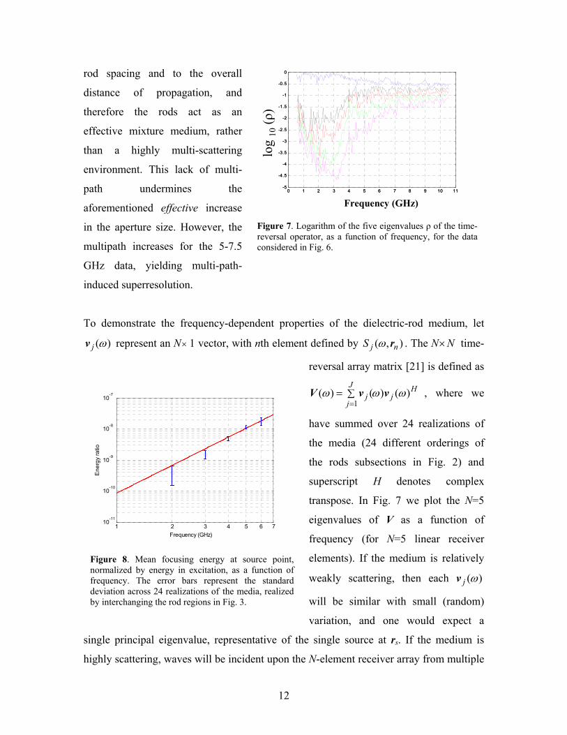
To demonstrate the frequency-dependent properties of the dielectric-rod medium, let

)(ωjv represent an N× 1 vector, with nth element defined by ),( njS rω . The N×N time-

reversal array matrix [21] is defined as

Hj

J

jj )()()(

1ωωω vvV ∑

== , where we

have summed over 24 realizations of

the media (24 different orderings of

the rods subsections in Fig. 2) and

superscript H denotes complex

transpose. In Fig. 7 we plot the N=5

eigenvalues of V as a function of

frequency (for N=5 linear receiver

elements). If the medium is relatively

weakly scattering, then each )(ωjv

will be similar with small (random)

variation, and one would expect a

single principal eigenvalue, representative of the single source at rs. If the medium is

highly scattering, waves will be incident upon the N-element receiver array from multiple

1 2 3 4 5 6 710

-11

10-10

10-9

10-8

10-7

Frequency (GHz)

Ene

rgy

ratio

Figure 8. Mean focusing energy at source point, normalized by energy in excitation, as a function of frequency. The error bars represent the standard deviation across 24 realizations of the media, realized by interchanging the rod regions in Fig. 3.

0 1 2 3 4 5 6 7 8 9 10 11-5

-4.5

-4

-3.5

-3

-2.5

-2

-1.5

-1

-0.5

0Spec trum of eigen value

Frequency (GHz)

log1

0(la

mda

)

0 1 2 3 4 5 6 7 8 9 10 11-5

-4.5

-4

-3.5

-3

-2.5

-2

-1.5

-1

-0.5

0Spec trum of eigen value

Frequency (GHz)

log1

0(la

mda

)

Frequency (GHz)

log

10(ρ

)

Figure 7. Logarithm of the five eigenvalues ρ of the time-reversal operator, as a function of frequency, for the data considered in Fig. 6.

13

angles, and the rank of V will increase. One notices two distinct regions in Fig. 7. Up to

approximately 4 GHz there is one principal mode, implying that in this frequency range

the waves realize relatively weak multipath, and the rods constitute a relatively weak-

scattering random media. Above 4 GHz the five eigenvalues are similar in magnitude,

implying that V is full rank, and that the medium is highly scattering. As indicated in the

previous paragraph, the highly-scattering character of the waves above 4 GHz is

beneficial to time reversal, in that it yields an increased effective aperture and

superresolved imaging resolution.

D. Frequency dependence of focusing energy, and image stability

Theoretical studies in the Rayleigh scattering regime (scatterers of small diameter

compared to wavelength) predicts that the ETR focusing intensity should increase as the

third power of frequency in two space dimensions and as the fourth power of frequency

in three dimensions [6] (as discussed in Sec. IIB). To consider this issue, we considered

the ratio of energy focused at the original source location, normalized by the source

energy, as a function of frequency. The experimental results in Fig. 8 confirm the

theoretical predictions (for this approximately two-dimensional system), demonstrating a

frequency dependence of 3f . The error bars in Fig. 8 correspond to different realizations

of the media (as discussed in Sec. IIIA), manifested by interchanging the six rod regions,

as reflected in Fig. 3). To compute the results in Fig. 8, full-band ETR imaging was

performed, yielding a time-dependent signal for the data imaged via time reversal to the

original source location. A Fourier transform was performed of this waveform, and the

energy was normalized to the strength of the excitation energy, as a function of

frequency.

We also note that the error bars reflected in Fig. 8, corresponding to variation in

),0( mjj tI r= for 24 distinct manifestations of the intervening rod media, are relatively

tight (little variation across different media realizations). This observation is consistent

with previous studies that predict a high degree of stability [4,20,21] in the time-reversal

image quality, for different media realizations (assuming the media used in the forward

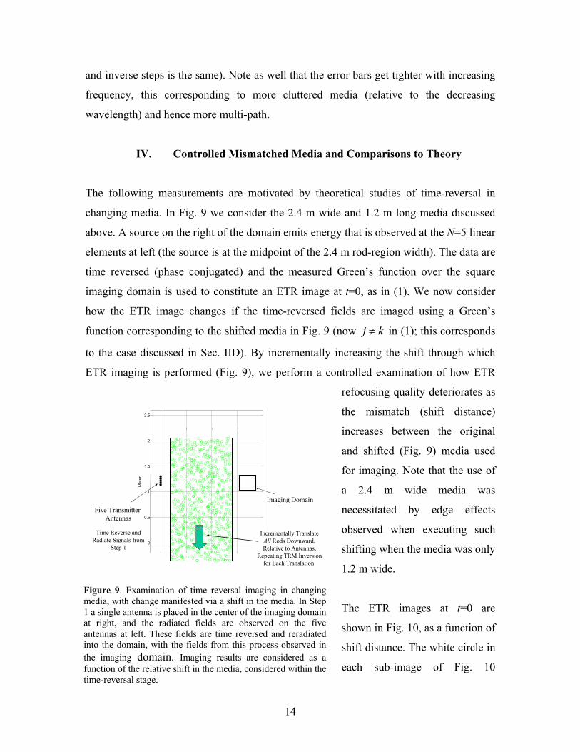
14

and inverse steps is the same). Note as well that the error bars get tighter with increasing

frequency, this corresponding to more cluttered media (relative to the decreasing

wavelength) and hence more multi-path.

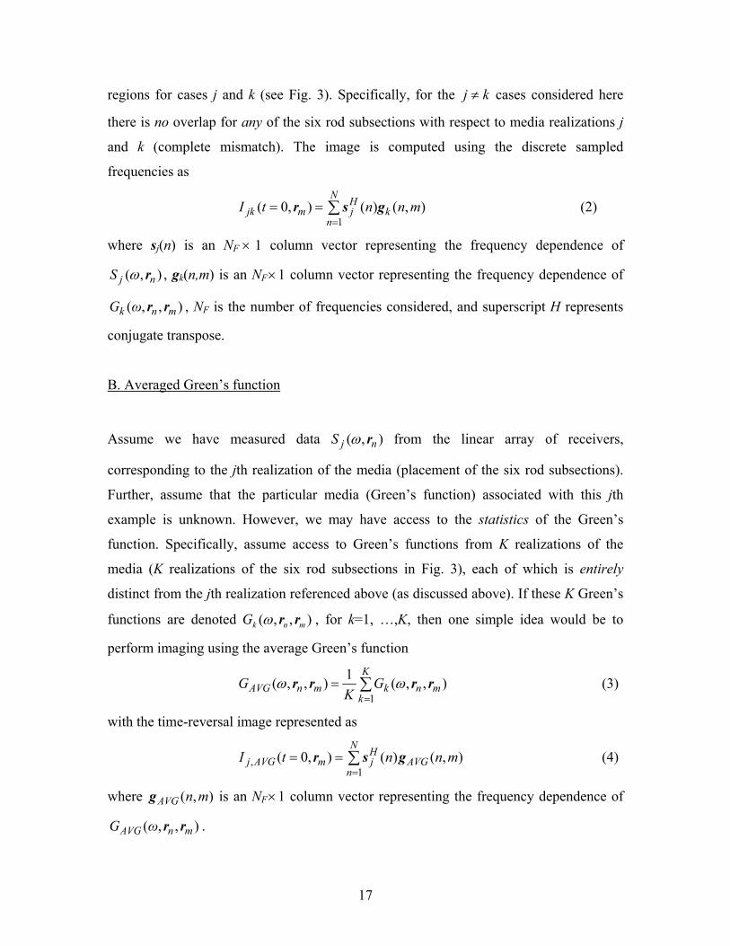
IV. Controlled Mismatched Media and Comparisons to Theory

The following measurements are motivated by theoretical studies of time-reversal in

changing media. In Fig. 9 we consider the 2.4 m wide and 1.2 m long media discussed

above. A source on the right of the domain emits energy that is observed at the N=5 linear

elements at left (the source is at the midpoint of the 2.4 m rod-region width). The data are

time reversed (phase conjugated) and the measured Green’s function over the square

imaging domain is used to constitute an ETR image at t=0, as in (1). We now consider

how the ETR image changes if the time-reversed fields are imaged using a Green’s

function corresponding to the shifted media in Fig. 9 (now kj ≠ in (1); this corresponds

to the case discussed in Sec. IID). By incrementally increasing the shift through which

ETR imaging is performed (Fig. 9), we perform a controlled examination of how ETR

refocusing quality deteriorates as

the mismatch (shift distance)

increases between the original

and shifted (Fig. 9) media used

for imaging. Note that the use of

a 2.4 m wide media was

necessitated by edge effects

observed when executing such

shifting when the media was only

1.2 m wide.

The ETR images at t=0 are

shown in Fig. 10, as a function of

shift distance. The white circle in

each sub-image of Fig. 10

2

0

0.5

1

1.5

2

2.5

Met

er

Imaging DomainFive Transmitter

Antennas

Time Reverse andRadiate Signals from

Step 1

Incrementally TranslateAll Rods Downward,Relative to Antennas,

Repeating TRM Inversionfor Each Translation

Figure 9. Examination of time reversal imaging in changing media, with change manifested via a shift in the media. In Step 1 a single antenna is placed in the center of the imaging domain at right, and the radiated fields are observed on the five antennas at left. These fields are time reversed and reradiated into the domain, with the fields from this process observed in the imaging domain. Imaging results are considered as a function of the relative shift in the media, considered within the time-reversal stage.

15

corresponds to the physical location of the actual original source, with respect to which

the imaging domain is shifted (see Fig. 9). Considering Fig. 10, we note that the down-

range resolution (along the horizontal direction of the figures) is preserved as the media is

shifted; however, with increasing shift distance the cross-range localization (vertical

direction) is lost.

As reviewed in Sec. IID, in the diffusion regime, it has been predicted that the amplitude

at the center of the imagery domain, for shifts of the type considered in Fig. 10, should

vary as ( )τkJo where τ is the spatial shift and k is the wavenumber. A qualitatively

similar result is predicted in the radiative transfer regime. In Fig. 11 we plot the energy

observed at the center of each image, as a function of the shift between the media

considered in step (i) and step (ii) of the time-reversal process. In addition, the results in

Fig. 11 are presented as a function of the bandwidth used when performing time reversal.

In Fig. 12 we plot the magnitude of the excitation window used in (1), )(ωW .

Considering )(ωW , the strongest energy in one of the subbands considered in Fig. 12

occurs at the respective peak energy (e.g., for the 0.5-1 GHz subband, the greatest energy

cm

cm

(g)-10 -5 0 5 10

-25-20-15-10-505

10152025

cm

cm

(h)-10 -5 0 5 10

-25-20-15-10-505

10152025

cm

cm

(f)-10 -5 0 5 10

-25-20-15-10-505

10152025

cm

cm

(i)-10 -5 0 5 10

-25-20-15-10-50510152025

cm

cm

-10 -5 0 5 10-25-20-15-10-505

10152025

cm

cm

-10 -5 0 5 10-25-20-15-10-50510152025

cm

cm

-10 -5 0 5 10-25-20-15-10-50510152025

cm

cm

-10 -5 0 5 10-25-20-15-10-50510152025

cm

cm

-10 -5 0 5 10-25-20-15-10-50510152025

cm

cm

(j)-10 -5 0 5 10

-25-20-15-10-50510152025

(a) (b) (c) (d) (e)

cm

cm

(g)-10 -5 0 5 10

-25-20-15-10-505

10152025

cm

cm

(h)-10 -5 0 5 10

-25-20-15-10-505

10152025

cm

cm

(f)-10 -5 0 5 10

-25-20-15-10-505

10152025

cm

cm

(i)-10 -5 0 5 10

-25-20-15-10-50510152025

cm

cm

-10 -5 0 5 10-25-20-15-10-505

10152025

cm

cm

-10 -5 0 5 10-25-20-15-10-50510152025

cm

cm

-10 -5 0 5 10-25-20-15-10-50510152025

cm

cm

-10 -5 0 5 10-25-20-15-10-50510152025

cm

cm

-10 -5 0 5 10-25-20-15-10-50510152025

cm

cm

(j)-10 -5 0 5 10

-25-20-15-10-50510152025

(a) (b) (c) (d) (e)

Figure 10. Time reversal image as a function of shift in the media (see Fig. 9). The position of the original source is shown with the white circle. (a) -8 cm shift, (b) -6 cm, (c) -4 cm, (d) – 2 cm, (e) 0 cm, (f) 2 cm, (g) 4 cm, (h) 6 cm, (i) 8 cm, (j) 10 cm

16

is at 1 GHz).

Using ( )τkJo , the first null in the

predicted energy at the center of the

imaging domain should occur at

shifts of 12 cm, 8 cm, 6 cm and 4.8

cm, for respective (peak) frequencies

of 1 GHz, 1.5 GHz, 2 GHz and 2.5

GHz. By considering Fig. 12, we

note excellent agreement between

our measured results and the predictions based on the theory in [6]. A qualitative

behavior of the refocused intensity proportional to ( )τkJo is not only a characteristic of

the diffusion regime; for instance it

approximately holds in the less scattering

radiative transfer regime [6]. We have also

stressed that frequencies below 4 GHz

were weakly scattering. However it does

demonstrate that multiple scattering is

responsible for the refocused signal, for in

homogeneous medium, the refocused

energy would not depend on the shiftτ .

Moreover it indicates that loss of

correlation between the two media (see Sec. IIC) of the two stages of the time reversal

experiment induces reduction in refocused signal strength.

V. Imaging in Changing Media

A. Imaging with mismatched Green’s function

We consider image quality ),,(),(),0(1

*mnk

N

nnjmjk GSdtI

BW

rrrr ωωωω

∑ ∫=

== for kj ≠ ,

addressing the problem for which there is a completely distinct arrangement of the six

0 5 10 15 20 25 300

0.1

0.2

0.3

0.4

0.5

0.6

0.7

0.8

0.9

1

Shift (cm)

Nor

mal

ized

Ene

rgy

0.5 ~1 GHz1 ~1.5 GHz1.5 ~2 GHz2 ~ 2.5GHz

Theory First null should be located at following shifts:

1 GHz – Shift of 12 cm1.5 GHz – Shift of 9 cm2 GHz – Shift of 6 cm2.5 GHz – Shift of 4.8 cm

0 5 10 15 20 25 300

0.1

0.2

0.3

0.4

0.5

0.6

0.7

0.8

0.9

1

Shift (cm)

Nor

mal

ized

Ene

rgy

0.5 ~1 GHz1 ~1.5 GHz1.5 ~2 GHz2 ~ 2.5GHz

Theory First null should be located at following shifts:

1 GHz – Shift of 12 cm1.5 GHz – Shift of 9 cm2 GHz – Shift of 6 cm2.5 GHz – Shift of 4.8 cm

Figure 11. Normalized energy at the center of each subimage in Fig. 10, as a function of sensor bandwidth. The theoretical predictions for the position of the first null are tabulated in the inset.

0 2 4 6 8 10 12 14 16 18 200

0.005

0.01

0.015

0.02

0.025

0.03

0.035

0.04

Frequency (GHz)

Mag

nitu

de

Figure 12. Spectrum of the waveform used in the time-reversal experiments.

17

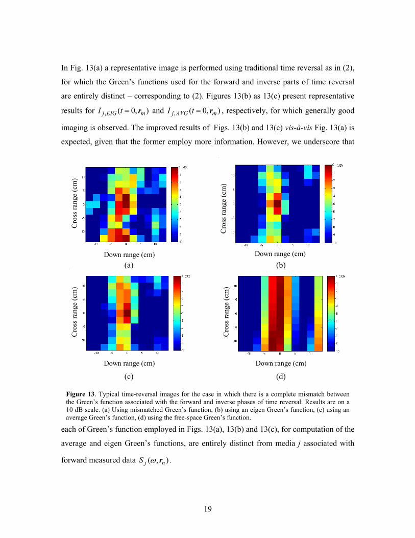
regions for cases j and k (see Fig. 3). Specifically, for the kj ≠ cases considered here

there is no overlap for any of the six rod subsections with respect to media realizations j

and k (complete mismatch). The image is computed using the discrete sampled

frequencies as

),()(),0(1

mnntI kN

n

Hjmjk gsr ∑

=== (2)

where sj(n) is an NF × 1 column vector representing the frequency dependence of

),( njS rω , gk(n,m) is an NF×1 column vector representing the frequency dependence of

),,( mnkG rrω , NF is the number of frequencies considered, and superscript H represents

conjugate transpose.

B. Averaged Green’s function

Assume we have measured data ),( njS rω from the linear array of receivers,

corresponding to the jth realization of the media (placement of the six rod subsections).

Further, assume that the particular media (Green’s function) associated with this jth

example is unknown. However, we may have access to the statistics of the Green’s

function. Specifically, assume access to Green’s functions from K realizations of the

media (K realizations of the six rod subsections in Fig. 3), each of which is entirely

distinct from the jth realization referenced above (as discussed above). If these K Green’s

functions are denoted ),,( mnkG rrω , for k=1, …,K, then one simple idea would be to

perform imaging using the average Green’s function

∑=

=K

kmnkmnAVG G

KG

1),,(1),,( rrrr ωω (3)

with the time-reversal image represented as

),()(),0(1

, mnntI AVGN

n

HjmAVGj gsr ∑

=== (4)

where ),( mnAVGg is an NF×1 column vector representing the frequency dependence of

),,( mnAVGG rrω .

18

C. Subspace imaging

For a given source and receiver point, again assume access to K examples of the Green’s

function, denoted ),,( mnkG rrω , for k=1, …, K. Rather than taking the average of these K

Green’s functions (for K realizations of the media), we may perform a principal

components analysis (PCA) [18], and project the measured data onto the principal

Green’s function eigenvectors. We perform an eigen decomposition of the NF×NF matrix

Hk

K

kk mnmnmn ),(),(),(

1ggG ∑

== (5)

Let ),( mnle represent the lth eigenvector of (5). A PCA-based imaging result is

represented as

∑ ∑= =

==N

n

L

ll

HjmEIGj mnntI

P

1 1, ),()(),0( esr (6)

In the example results we have considered Lp=1 principal component.

D. Example imaging results

The measurements were performed as follows. The Green’s function ),,( mnG rrω was

measured for Nmedia=24 realizations of the six rod subsections depicted in Fig. 3. For the

jth of these realizations, there was a set jΩ of Nj < Nmedia other rod arrangements

considered for which there was a complete mismatch in the order of the six rod regions.

When considering the technique in Sec. IVA for media j, Ijk was calculated separately for

all media jk Ω∈ ; consequently, for each media j we compute Nj distinct images Ijk. For

the techniques in Secs. IVB and IVC, a single image is computed for each of the Nmedia

media arrangements. Specifically, for AVGjI , the average Green’s function ),( mnAVGg

was computed using the Nj media in jΩ ; for EIGjI , the principal component ),(1 mne

was also computed using the Nj media in jΩ . In these examples a total of Nmedia=24

media were considered, and for each media j on average Nj=10 (the minimum was Nj=6).

19

In Fig. 13(a) a representative image is performed using traditional time reversal as in (2),

for which the Green’s functions used for the forward and inverse parts of time reversal

are entirely distinct – corresponding to (2). Figures 13(b) as 13(c) present representative

results for ),0(, mEIGj tI r= and ),0(, mAVGj tI r= , respectively, for which generally good

imaging is observed. The improved results of Figs. 13(b) and 13(c) vis-à-vis Fig. 13(a) is

expected, given that the former employ more information. However, we underscore that

each of Green’s function employed in Figs. 13(a), 13(b) and 13(c), for computation of the

average and eigen Green’s functions, are entirely distinct from media j associated with

forward measured data ),( njS rω .

(a)Down range (cm)

Cro

ss ra

nge

(cm

)

(b)Down range (cm)

Cro

ss ra

nge

(cm

)

(c)Down range (cm)

Cro

ss ra

nge

(cm

)

(d)Down range (cm)

Cro

ss ra

nge

(cm

)

Figure 13. Typical time-reversal images for the case in which there is a complete mismatch between the Green’s function associated with the forward and inverse phases of time reversal. Results are on a 10 dB scale. (a) Using mismatched Green’s function, (b) using an eigen Green’s function, (c) using an average Green’s function, (d) using the free-space Green’s function.

20

F. Quantitative analysis of imaging results

It is of interest to perform a quantitative analysis of all analyzed images of the form in

Fig. 13. Toward this end, a square region is defined corresponding to a

contiguous 33× pixel region in image space, with pixels defined as in Fig. 13. The test

statistic l used in this analysis is the peak pixel amplitude within the 33× pixel box. We

compute this test statistic l for all possible 33× boxes within the image. For a general

threshold T, if Tl > a target is declared as being within the corresponding 33× inner

region, and if Tl < no target is

declared (the actual target position is

in the center of the image, as in Fig.

13). By varying the threshold T, from

zero to maxlT > (the largest value of

l within a given image), we yield the

receiver operating characteristic

(ROC) [22], representing the

probability of detection as a function

of the probability of false alarm (a

false alarm is defined by declaring

the presence of a source at a location

for which there is in reality none). In Fig. 14 we plot the ROC curves for the imaging

techniques considered in Fig. 13. We note that the techniques based on the average and

eigen Green’s functions (equations (4) and (6), respectively) yield comparable

performance, while performance deteriorates precipitously when considering a single

mismatched Green’s function or the free-space Green’s function (the latter yielding the

worst results).

VI. Conclusions

Time-reversal imaging has been examined experimentally for electromagnetic source

localization in highly scattering media. We initially addressed the well-known time-

Probability of False Alarm

Prob

abili

ty o

f Det

ectio

n

Probability of False Alarm

Prob

abili

ty o

f Det

ectio

n

Figure 14. Receiver operating characteristic (ROC) averaged across multiple realizations of mismatched media, using the four imaging techniques reflected in Fig. 13.

21

reversal behavior for the case in which the media employed in the forward and inverse

steps are matched. These experiments confirmed theoretical predictions concerning time-

reversal imaging stability, for the case in which the forward and inverse media are

matched, but for different media realizations [6]. The experiments also confirmed the

anticipated 3f frequency dependence of the imaging amplitude in the Rayleigh regime

[6], for the case of matched media.

In our first analysis of time-reversal imaging in changing media, we considered the

special case for which the two media are shifted with respect to each other. While this is a

special case, it is of particular interest because it allows us to address the accuracy of

previous theoretical predictions [6]. In particular, in the diffusive regime it is predicted

that the imaged amplitude should vary as )( τkJo , where k represents the wavenumber

and τ the spatial shift [6]; the experimental results considered here are in excellent

agreement with theoretical predictions.

While the theory and experimental results indicate time-reversal imaging deterioration as

media mismatch increases between the forward and inverse phases, we have also

considered alternative techniques for the case in which the media employed in the

forward phase is either unknown or may not be modeled precisely. Specifically, we have

performed time-reversal imaging based on an average Green’s function, computed using

an ensemble of Green’s functions; each Green’s function in the ensemble corresponds to

a media completely distinct from that used in the forward step, but with similar statistics.

A similar use of the ensemble of Green’s functions was considered via an eigen analysis,

analogous to principal components analysis (PCA) [18]. It was demonstrated that we

often observe significantly improved time-reversal imaging quality based on either the

average or eigen Green’s function (quantified in terms of the receiver operating

characteristic, or ROC).

While the ensemble of Green’s functions were employed to improve imaging

performance, there remains a question of how this could be utilized in practice. If one is

performing the inverse phase using computed Green’s functions, there may be

22

uncertainty as to which specific propagation media should be used within the

computational model. The results presented here suggest that one may consider an

ensemble of computed Green’s functions within the inverse phase, with this ensemble

designed to capture the range of different media deemed representative of the forward

measurement. In the results presented here, the Green’s functions were measured, for

different realizations of the intervening media. If one wished to perform time-reversal

imaging in a multi-path environment, such as an urban setting, the Green’s functions

could be measured, analogous to wireless measurements. The variable properties of such

a propagation environment may be captured by an ensemble of Green’s functions,

measured at different times, as the propagation media changes.

References

[1] M. Fink, “Time-reversal of ultrasonic fields - Part I: Basic Principles,” IEEE Trans.

Ultrason., Ferroelectr., and Freq. Control, vol 39, pp. 555-566, 1992

[2] B. Steinberg, Microwave Imaging Techniques, New York: J. Wiley, 1991

[3] D.R. Jackson and D.R. Dowling, “Phase conjugation in underwater acoustics,” J.

Acoust. Soc. of Amer., vol. 89, pp. 171-181,1990

[4] P. Blomberg, G. Papanicolaou, and H.K. Zhao, “Super-resolution in time-reversal

acoustics,” J. Acoust. Soc. of Amer., vol. 111, pp. 230-248, 2002

[5] G. Bal and L. Ryzhik, “Time reversal and refocusing in random media,” SIAM Appl.

Math., vol. 63 (5), pp. 1375-1498, 2003

[6] G. Bal and R. Verastegui, “Time reversal in changing environment,” Multiscale

Model. Simul. , vol. 2, pp. 639-661, 2004

[7] M. Fink, “Time reversed acoustics,” Physics Today, 50, pp. 34-40, 1997

[8] A. Derode, P. Roux, and M. Fink, “Robust acoustic time reversal with high-order

multiple scattering,” Phys. Rev. Lett., vol. 75, pp. 4206–4209, 1995

[9] P. Roux, B. Roman and M. Fink, “Time-reversal in an ultrasonic waveguide,” Appl.

Phys. Letts., vol. 70, 1997

23

[10] J. de Rosny, A. Tourin, A. Derode, B. van Tiggelen and M. Fink, “The relation

between time reversal focusing and coherent backscattering in multiple scattering

media: a diagrammatic approach,” Phys. Rev. E, vol. 70, 046601, 2004

[11] W.A. Kuperman, W.S. Hodgkiss, H.C. Song, T. Akal, C. Ferla, and D.R. Jackson,

“Phase conjugation in the ocean: Experimental demonstration of an acoustic time-

reversal mirror,” J. Acoust. Soc. Am., vol. 103, pp. 25-40, 1998.

[12] H.C. Song, W.A. Kuperman, W.S. Hodgkiss, T. Akial and C. Ferla, “Iterative time

reversal in the ocean,” J. Acoust. Soc. Am., vol. 105, pp. 3176-3184, 1999.

[13] S. Kim, G.F. Edelmann, W.A. Kuperman, W.S. Hodgkiss, H.C. Song and T. Akal,

“Spatial resolution of time-reversal arrays in shallow water,” J. Acoust. Soc. Am.,

vol. 110, pp. 820-829, 2001.

[14] G. Lerosey, J. de Rosny, A. Tourin, A. Derode, G. Montaldo and M. Fink, “Time

reversal of electromagnetic waves,” Phys. Rev. Letts., vol. 92(19), 2004

[15] D. Liu, G. Kang, L. Li, Y. Chen, S. Vasudevan, W. Joines, Q. H. Liu, J. Krolik and

L. Carin, “Electromagnetic time-reversal imaging of a target in a cluttered

environment,” IEEE Trans. Antenna Propag., vol. 53, pp. 3058-3066, 2005

[16] J.L. Krolik, “The performance of matched-field beamformers with Mediterranean

vertical array data,” IEEE Trans. Signal Process., vol. 44, pp. 2605-2611, 1996

[17] J.L. Krolik, “Matched-field minimum variance beamformaing in a random ocean

channel,” J. Acoust. Soc. Amer., vol. 92, pp.1408-1419, 1992

[18] A. Basilevsky, Statistical Factor Analysis and Related Methods, Theory and

Application. New York: J. Wiley, 1994

[19] A. Ishimaru, Waves Propagation in Scattering and Random Media, Wiley-IEEE

Press, 1999.

[20] G. Bal, “On the self-averaging of wave energy in random media,” SIAM Multiscale

Model. Simul. , vol. 2, pp. 398-420, 2004

[21] L. Borcea, G. Papanicolaou, C. Tsogka and J. Berryman, “Imaging and time reversal

in random media,” Inverse Problems, vol. 18, pp. 1247–1279, 2002

[22] T.D. Wickens, Elementary Signal Detection Theory. New York: Oxford University

Press, 2002.