Electron and Ion Dynamics of the Solar Wind Interactionwith a Weakly Outgassing Comet

Jan Deca,1,2,* Andrey Divin,3,4 Pierre Henri,5 Anders Eriksson,4 Stefano Markidis,6

Vyacheslav Olshevsky,7 and Mihály Horányi1,21Laboratory for Atmospheric and Space Physics (LASP), University of Colorado Boulder, Boulder, Colorado 80303, USA

2Institute for Modeling Plasma, Atmospheres and Cosmic Dust, NASA/SSERVI, Moffett Field, California 94035, USA3Physics Department, St. Petersburg State University, St. Petersburg 198504, Russia

4Swedish Institute of Space Physics (IRF), Uppsala 751 21, Sweden5LPC2E, CNRS, Orléans 45071, France

6KTH Royal Institute of Technology, Stockholm 100 44, Sweden7Centre for mathematical Plasma Astrophysics (CmPA), KU Leuven, Leuven 3001, Belgium(Received 8 February 2017; published 15 May 2017; publisher error corrected 5 June 2017)

Using a 3D fully kinetic approach, we disentangle and explain the ion and electron dynamics of the solarwind interaction with a weakly outgassing comet. We show that, to first order, the dynamical interaction isrepresentative of a four-fluid coupled system. We self-consistently simulate and identify the origin ofthe warm and suprathermal electron distributions observed by ESA’s Rosetta mission to comet67P/Churyumov-Gerasimenko and conclude that a detailed kinetic treatment of the electron dynamicsis critical to fully capture the complex physics of mass-loading plasmas.

DOI: 10.1103/PhysRevLett.118.205101

Cometary nuclei are small, irregularly shaped “icy dirtballs” left over from the dawn of our Solar System 4.6billion years ago and are composed of a mixture of ices,refractory materials, and large organic molecules [1–4].When a comet is sufficiently close to the Sun, thesublimation of ice leads to an outgassing atmosphereand the formation of a coma, and a dust and plasma tail.Historically, this process revealed the existence of the solarwind and the interplanetary magnetic field [5–8]. Cometsare critical to decipher the physics of gas release processesin space. The latter result in mass-loaded plasmas [9,10],which more than three decades after the ActiveMagnetospheric Particle Tracer Explorers (AMPTE) spacerelease experiments [11] are still not fully understood.First observed in 1969, comet 67P/Churyumov-

Gerasimenko was escorted for almost two years alongits 6.45-yr elliptical orbit by ESA’s Rosetta orbiter space-craft. During the mission, the comet transitioned from itsweakly outgassing phase into a more active object as itapproached the Sun, and back again to quieter phases whentraveling outward in the Solar System. This first evermission to do more than a simple cometary fly-by revealedin unprecedented detail the fascinating evolution of a comet[12] and the building up of its induced magnetosphere [13].To date, the focus of modeling studies to predict and

explain the complex cometary plasma observations hasbeen on magnetohydrodynamic (MHD) or multifluid[14–19] and hybrid (using a kinetic description for theions but describing the electrons as a massless fluid)[20–26] simulations, leading to comprehensive modelsfor the ion dynamics. A satisfactory explanation for theobserved electron dynamics, however, is not yet available.

For instance, the Ion and Electron Sensor (IES) instrumentonboard the Rosetta orbiter shows the presence of non-thermal electron distributions inside the inhomogeneousexpanding cometary ionosphere, including both a warm(∼5 eV) and suprathermal (10–20 eV) component [27–29].The origin and physical mechanism behind the variouscomponents of the observed electron distributions isunclear, but must be understood to disentangle the com-etary plasma dynamics.We develop and analyze a detailed model of the

cometary plasma dynamics, including fine-scale electronkinetic physics, and discuss the relative accelerationmechanisms decoupling the plasma populations. Usingthe collisionless semi-implicit, fully kinetic, electromag-netic particle-in-cell code iPIC3D [30], which solves theVlasov-Maxwell system of equations for both ions andelectrons using the implicit moment method [31–33], wefocus on the interaction between the solar wind and aweakly outgassing comet such as encountered by Rosettaat approximately 3 astronomical units (A.U.). from theSun. At such large distances from the Sun, the collision-less approximation is valid everywhere except in theinnermost coma [34,35]. We model self-consistently thekinetic dynamics of both cometary water ions and elec-trons, produced by the ionization of the radially expandingand outgassing cometary atmosphere, together with theincoming solar wind proton and electron plasma flow. Toaccommodate a flowing plasma in the computationaldomain, we use open boundary conditions as imple-mented by Deca et al. [36].Maxwellian distributions of solar wind protons and

electrons are injected at the inflow boundary of the

PRL 118, 205101 (2017)Selected for a Viewpoint in Physics

PHY S I CA L R EV I EW LE T T ER Sweek ending19 MAY 2017

0031-9007=17=118(20)=205101(6) 205101-1 © 2017 American Physical Society

computational domain (at x ¼ −1540 km) with densitiesnp;sw ¼ ne;sw ¼ 1 cm−3 and temperatures Tp;sw ¼ 7 eV,Te;sw ¼ 10 eV, respectively, approximating the free-stream-ing solar wind plasma distributions [29,37]. The solar windflows along X at vsw ¼ ð400; 0; 0Þ km s−1. We use a reducedmass ratiomp;sw=me;sw ¼ 100 to meet our numerical restric-tions, a common practice in fully kinetic simulations thatensures scale separation between electron and ion dynamics[38]. The interplanetary magnetic field is directed along Y atBIMF ¼ ð0; 6; 0Þ nT, resulting in a solar wind proton andelectron Larmor radius of rp;sw¼142km and re;sw ¼ 12 km,respectively. The nucleus of the comet is represented by anabsorbing sphere placed 110 km upstream of the center of thecomputational domain (at ðx; y; zÞ ¼ ð−110; 0; 0Þ km). Thecomputational domain measures 3300 × 2200 × 2200 km3

witha resolutionof10kminall threeCartesiandirections.Thesimulation time step is Δt ¼ 4.5 × 10−5 s, which is wellbelow the electron gyroperiod (5.95 ms for 6 nT) and, hence,resolves the electron gyromotion.The solar wind is mass loaded by cold cometary ions as a

consequence of the outgassing cometary neutral atmospherethat is ionized as it expands [39]. In order to inject cometaryion-electron pairs, we do not implement the neutral gasdistribution. Instead, we use an analytical profile for theplasma production rate that results from the ionization of anexpanding neutral gas with a 1=r2 radial density profile. Weassume a gas production rate of Q ¼ 1026 s−1 [40]. Theresulting cometary density profile then mimics the 1=rplasma density profile observed close to the cometarynucleus [41]. We radially inject Maxwell-distributed com-etary electrons (Te;c ¼ 10 eV) and cold cometary watergroup ions (mi;c=mp;sw ¼ 20) accordingly. The thermalvelocity of the implanted water ions is set 2 orders ofmagnitude smaller than the solar wind protons, which

translates to a cometary ion temperature of Ti;c ¼ 0.5 eV.Although Ti;c is somewhat higher than observed by Rosetta(see, e.g., Nilsson et al. [13]), cometary ions are born in thesimulation with energies 2000 times less than the solar windenergy, ensuring sufficient separation of scales.Figure 1 shows the density profiles in the XY (terminator)

and XZ (cross magnetic field) planes for the solar wind[Figs. 1(a)–1(d)] and cometary [Figs. 1(e)–1(h)] ion andelectron species. The simulated global structure of the solarwind-weak comet interaction confirms the results reportedby hybrid simulations on the induced cometary magneto-sphere [23–25]. In particular, we observe a magnetic pileup(a direct consequence of the ionization of outflowing gasfrom the nucleus) up to more than 3 times the interplanetarymagnetic field magnitude [42], together with a compressionof the incoming, mass-loaded, solar wind [Fig. 1(a)]. Themagnetic field lines drape around the nucleus. No bow shockdevelops, as expected for a weakly outgassing comet [22].The heavy cometary ions are accelerated by the convectiveelectric field, to be eventually picked up far downstream,whereas solar wind protons deflect in the opposite directionin accordancewith momentum conservation. Downstream ofthe nucleus, Figs. 1(d) and 1(g) show a fanlike structure [15]and density fluctuations or filamentation [43] that can beassociated with the so-called “singing comet” waves [25].Focusing on the electron dynamics next [Figs. 1(b), 1(d),

1(f), and 1(h)], we find that, to first order, the electronsbehave as two separate fluids: a solar wind and a cometaryelectron fluid. We observe a spatial separation of thecometary electrons with respect to the cometary ions,and of the solar wind electrons with respect to the solarwind protons. Cometary electrons eventually end upneutralizing the solar wind protons, and solar wind elec-trons eventually neutralize the cometary ions.

FIG. 1. Density profiles in the XY=XZ planes for the solar wind (left-hand panels) and cometary (right-hand panels) ions andelectrons. The Y axis is directed along the solar wind magnetic field. Field lines are plotted in black. The red arrow in (c) indicates thedeflected solar wind proton flow in the XZ plane.

PRL 118, 205101 (2017) P HY S I CA L R EV I EW LE T T ER S week ending19 MAY 2017

205101-2

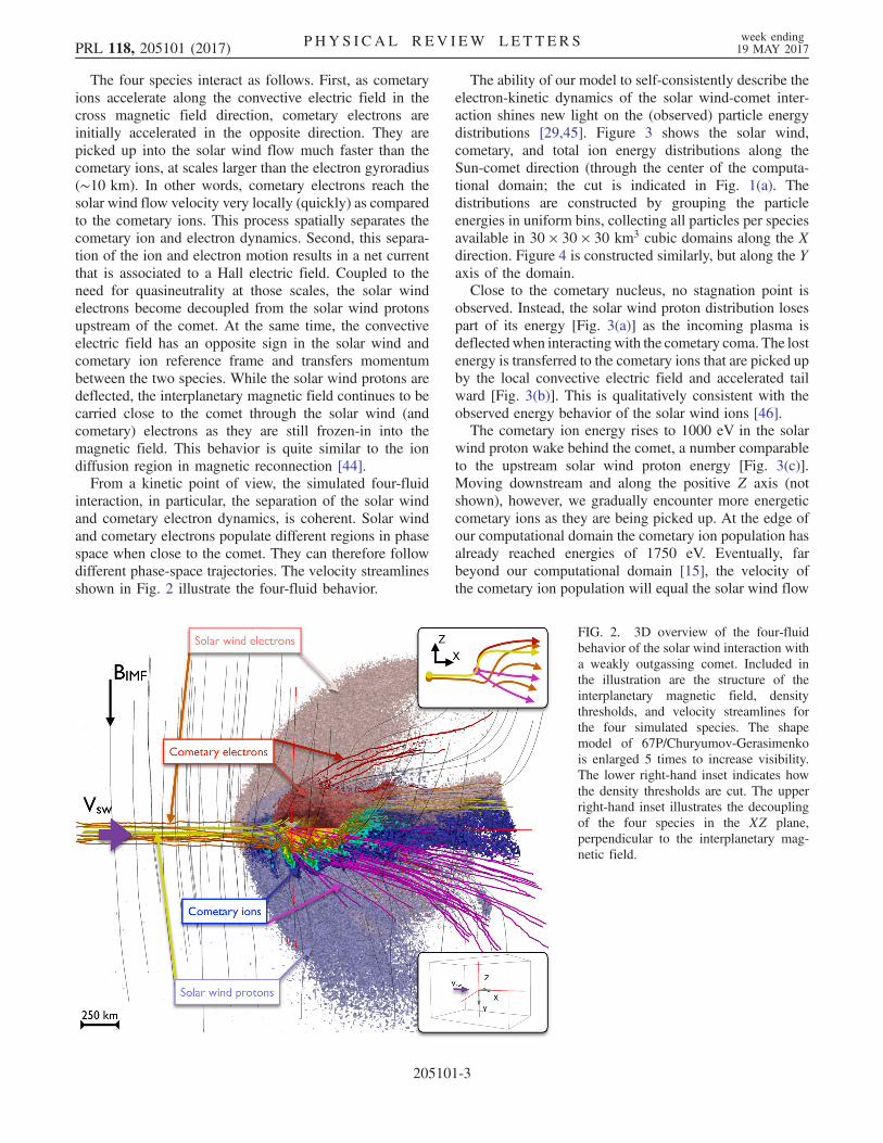
The four species interact as follows. First, as cometaryions accelerate along the convective electric field in thecross magnetic field direction, cometary electrons areinitially accelerated in the opposite direction. They arepicked up into the solar wind flow much faster than thecometary ions, at scales larger than the electron gyroradius(∼10 km). In other words, cometary electrons reach thesolar wind flow velocity very locally (quickly) as comparedto the cometary ions. This process spatially separates thecometary ion and electron dynamics. Second, this separa-tion of the ion and electron motion results in a net currentthat is associated to a Hall electric field. Coupled to theneed for quasineutrality at those scales, the solar windelectrons become decoupled from the solar wind protonsupstream of the comet. At the same time, the convectiveelectric field has an opposite sign in the solar wind andcometary ion reference frame and transfers momentumbetween the two species. While the solar wind protons aredeflected, the interplanetary magnetic field continues to becarried close to the comet through the solar wind (andcometary) electrons as they are still frozen-in into themagnetic field. This behavior is quite similar to the iondiffusion region in magnetic reconnection [44].From a kinetic point of view, the simulated four-fluid

interaction, in particular, the separation of the solar windand cometary electron dynamics, is coherent. Solar windand cometary electrons populate different regions in phasespace when close to the comet. They can therefore followdifferent phase-space trajectories. The velocity streamlinesshown in Fig. 2 illustrate the four-fluid behavior.

The ability of our model to self-consistently describe theelectron-kinetic dynamics of the solar wind-comet inter-action shines new light on the (observed) particle energydistributions [29,45]. Figure 3 shows the solar wind,cometary, and total ion energy distributions along theSun-comet direction (through the center of the computa-tional domain; the cut is indicated in Fig. 1(a). Thedistributions are constructed by grouping the particleenergies in uniform bins, collecting all particles per speciesavailable in 30 × 30 × 30 km3 cubic domains along the Xdirection. Figure 4 is constructed similarly, but along the Yaxis of the domain.Close to the cometary nucleus, no stagnation point is

observed. Instead, the solar wind proton distribution losespart of its energy [Fig. 3(a)] as the incoming plasma isdeflectedwhen interactingwith the cometary coma. The lostenergy is transferred to the cometary ions that are picked upby the local convective electric field and accelerated tailward [Fig. 3(b)]. This is qualitatively consistent with theobserved energy behavior of the solar wind ions [46].The cometary ion energy rises to 1000 eV in the solar

wind proton wake behind the comet, a number comparableto the upstream solar wind proton energy [Fig. 3(c)].Moving downstream and along the positive Z axis (notshown), however, we gradually encounter more energeticcometary ions as they are being picked up. At the edge ofour computational domain the cometary ion population hasalready reached energies of 1750 eV. Eventually, farbeyond our computational domain [15], the velocity ofthe cometary ion population will equal the solar wind flow

FIG. 2. 3D overview of the four-fluidbehavior of the solar wind interaction witha weakly outgassing comet. Included inthe illustration are the structure of theinterplanetary magnetic field, densitythresholds, and velocity streamlines forthe four simulated species. The shapemodel of 67P/Churyumov-Gerasimenkois enlarged 5 times to increase visibility.The lower right-hand inset indicates howthe density thresholds are cut. The upperright-hand inset illustrates the decouplingof the four species in the XZ plane,perpendicular to the interplanetary mag-netic field.

PRL 118, 205101 (2017) P HY S I CA L R EV I EW LE T T ER S week ending19 MAY 2017

205101-3

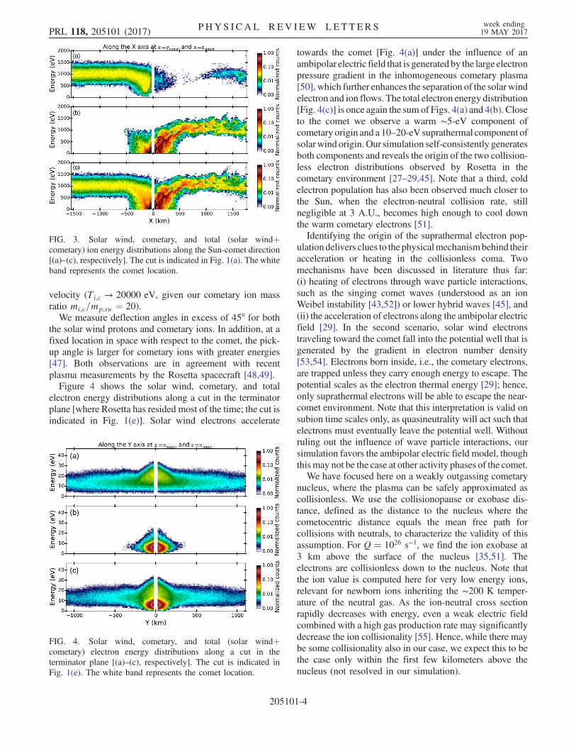
velocity (Ti;c → 20000 eV, given our cometary ion massratio mi;c=mp;sw ¼ 20).We measure deflection angles in excess of 45° for both

the solar wind protons and cometary ions. In addition, at afixed location in space with respect to the comet, the pick-up angle is larger for cometary ions with greater energies[47]. Both observations are in agreement with recentplasma measurements by the Rosetta spacecraft [48,49].Figure 4 shows the solar wind, cometary, and total

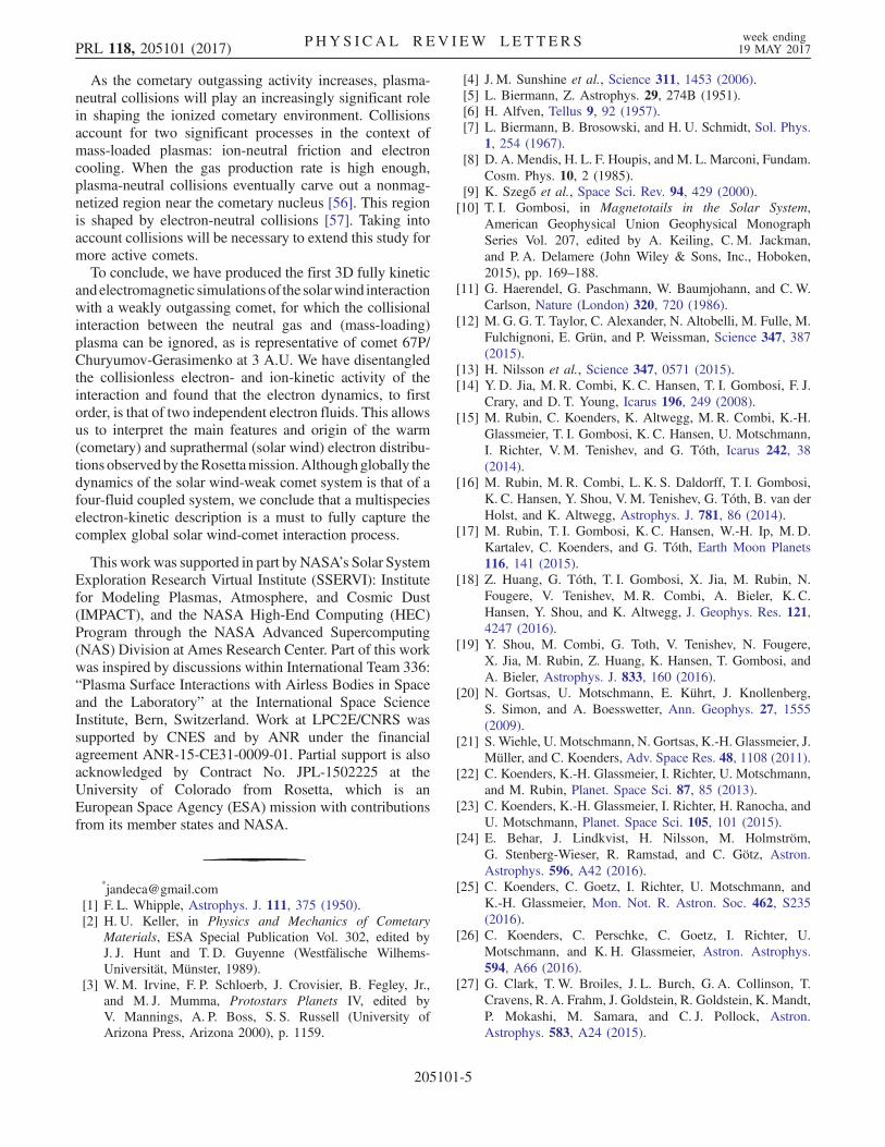
electron energy distributions along a cut in the terminatorplane [where Rosetta has resided most of the time; the cut isindicated in Fig. 1(e)]. Solar wind electrons accelerate

towards the comet [Fig. 4(a)] under the influence of anambipolar electric field that is generated by the large electronpressure gradient in the inhomogeneous cometary plasma[50], which further enhances the separation of the solar windelectron and ion flows. The total electron energy distribution[Fig. 4(c)] is once again the sum of Figs. 4(a) and 4(b). Closeto the comet we observe a warm ∼5-eV component ofcometary origin and a 10–20-eV suprathermal component ofsolarwind origin.Our simulation self-consistently generatesboth components and reveals the origin of the two collision-less electron distributions observed by Rosetta in thecometary environment [27–29,45]. Note that a third, coldelectron population has also been observed much closer tothe Sun, when the electron-neutral collision rate, stillnegligible at 3 A.U., becomes high enough to cool downthe warm cometary electrons [51].Identifying the origin of the suprathermal electron pop-

ulation delivers clues to the physicalmechanismbehind theiracceleration or heating in the collisionless coma. Twomechanisms have been discussed in literature thus far:(i) heating of electrons through wave particle interactions,such as the singing comet waves (understood as an ionWeibel instability [43,52]) or lower hybrid waves [45], and(ii) the acceleration of electrons along the ambipolar electricfield [29]. In the second scenario, solar wind electronstraveling toward the comet fall into the potential well that isgenerated by the gradient in electron number density[53,54]. Electrons born inside, i.e., the cometary electrons,are trapped unless they carry enough energy to escape. Thepotential scales as the electron thermal energy [29]; hence,only suprathermal electrons will be able to escape the near-comet environment. Note that this interpretation is valid onsubion time scales only, as quasineutrality will act such thatelectrons must eventually leave the potential well. Withoutruling out the influence of wave particle interactions, oursimulation favors the ambipolar electric field model, thoughthis may not be the case at other activity phases of the comet.We have focused here on a weakly outgassing cometary

nucleus, where the plasma can be safely approximated ascollisionless. We use the collisionopause or exobase dis-tance, defined as the distance to the nucleus where thecometocentric distance equals the mean free path forcollisions with neutrals, to characterize the validity of thisassumption. For Q ¼ 1026 s−1, we find the ion exobase at3 km above the surface of the nucleus [35,51]. Theelectrons are collisionless down to the nucleus. Note thatthe ion value is computed here for very low energy ions,relevant for newborn ions inheriting the ∼200 K temper-ature of the neutral gas. As the ion-neutral cross sectionrapidly decreases with energy, even a weak electric fieldcombined with a high gas production rate may significantlydecrease the ion collisionality [55]. Hence, while there maybe some collisionality also in our case, we expect this to bethe case only within the first few kilometers above thenucleus (not resolved in our simulation).

FIG. 3. Solar wind, cometary, and total (solar windþcometary) ion energy distributions along the Sun-comet direction[(a)–(c), respectively]. The cut is indicated in Fig. 1(a). The whiteband represents the comet location.

FIG. 4. Solar wind, cometary, and total (solar windþcometary) electron energy distributions along a cut in theterminator plane [(a)–(c), respectively]. The cut is indicated inFig. 1(e). The white band represents the comet location.

PRL 118, 205101 (2017) P HY S I CA L R EV I EW LE T T ER S week ending19 MAY 2017

205101-4

As the cometary outgassing activity increases, plasma-neutral collisions will play an increasingly significant rolein shaping the ionized cometary environment. Collisionsaccount for two significant processes in the context ofmass-loaded plasmas: ion-neutral friction and electroncooling. When the gas production rate is high enough,plasma-neutral collisions eventually carve out a nonmag-netized region near the cometary nucleus [56]. This regionis shaped by electron-neutral collisions [57]. Taking intoaccount collisions will be necessary to extend this study formore active comets.To conclude, we have produced the first 3D fully kinetic

andelectromagnetic simulationsof the solarwind interactionwith a weakly outgassing comet, for which the collisionalinteraction between the neutral gas and (mass-loading)plasma can be ignored, as is representative of comet 67P/Churyumov-Gerasimenko at 3 A.U. We have disentangledthe collisionless electron- and ion-kinetic activity of theinteraction and found that the electron dynamics, to firstorder, is that of two independent electron fluids. This allowsus to interpret the main features and origin of the warm(cometary) and suprathermal (solar wind) electron distribu-tions observedby theRosettamission.Althoughglobally thedynamics of the solar wind-weak comet system is that of afour-fluid coupled system, we conclude that a multispecieselectron-kinetic description is a must to fully capture thecomplex global solar wind-comet interaction process.

This workwas supported in part byNASA’s Solar SystemExploration Research Virtual Institute (SSERVI): Institutefor Modeling Plasmas, Atmosphere, and Cosmic Dust(IMPACT), and the NASA High-End Computing (HEC)Program through the NASA Advanced Supercomputing(NAS) Division at Ames Research Center. Part of this workwas inspired by discussions within International Team 336:“Plasma Surface Interactions with Airless Bodies in Spaceand the Laboratory” at the International Space ScienceInstitute, Bern, Switzerland. Work at LPC2E/CNRS wassupported by CNES and by ANR under the financialagreement ANR-15-CE31-0009-01. Partial support is alsoacknowledged by Contract No. JPL-1502225 at theUniversity of Colorado from Rosetta, which is anEuropean Space Agency (ESA) mission with contributionsfrom its member states and NASA.

*jandeca@gmail.com[1] F. L. Whipple, Astrophys. J. 111, 375 (1950).[2] H. U. Keller, in Physics and Mechanics of Cometary

Materials, ESA Special Publication Vol. 302, edited byJ. J. Hunt and T. D. Guyenne (Westfälische Wilhems-Universität, Münster, 1989).

[3] W.M. Irvine, F. P. Schloerb, J. Crovisier, B. Fegley, Jr.,and M. J. Mumma, Protostars Planets IV, edited byV. Mannings, A. P. Boss, S. S. Russell (University ofArizona Press, Arizona 2000), p. 1159.

[4] J. M. Sunshine et al., Science 311, 1453 (2006).[5] L. Biermann, Z. Astrophys. 29, 274B (1951).[6] H. Alfven, Tellus 9, 92 (1957).[7] L. Biermann, B. Brosowski, and H. U. Schmidt, Sol. Phys.

1, 254 (1967).[8] D. A. Mendis, H. L. F. Houpis, and M. L. Marconi, Fundam.

Cosm. Phys. 10, 2 (1985).[9] K. Szegő et al., Space Sci. Rev. 94, 429 (2000).

[10] T. I. Gombosi, in Magnetotails in the Solar System,American Geophysical Union Geophysical MonographSeries Vol. 207, edited by A. Keiling, C. M. Jackman,and P. A. Delamere (John Wiley & Sons, Inc., Hoboken,2015), pp. 169–188.

[11] G. Haerendel, G. Paschmann, W. Baumjohann, and C.W.Carlson, Nature (London) 320, 720 (1986).

[12] M. G. G. T. Taylor, C. Alexander, N. Altobelli, M. Fulle, M.Fulchignoni, E. Grün, and P. Weissman, Science 347, 387(2015).

[13] H. Nilsson et al., Science 347, 0571 (2015).[14] Y. D. Jia, M. R. Combi, K. C. Hansen, T. I. Gombosi, F. J.

Crary, and D. T. Young, Icarus 196, 249 (2008).[15] M. Rubin, C. Koenders, K. Altwegg, M. R. Combi, K.-H.

Glassmeier, T. I. Gombosi, K. C. Hansen, U. Motschmann,I. Richter, V. M. Tenishev, and G. Tóth, Icarus 242, 38(2014).

[16] M. Rubin, M. R. Combi, L. K. S. Daldorff, T. I. Gombosi,K. C. Hansen, Y. Shou, V. M. Tenishev, G. Tóth, B. van derHolst, and K. Altwegg, Astrophys. J. 781, 86 (2014).

[17] M. Rubin, T. I. Gombosi, K. C. Hansen, W.-H. Ip, M. D.Kartalev, C. Koenders, and G. Tóth, Earth Moon Planets116, 141 (2015).

[18] Z. Huang, G. Tóth, T. I. Gombosi, X. Jia, M. Rubin, N.Fougere, V. Tenishev, M. R. Combi, A. Bieler, K. C.Hansen, Y. Shou, and K. Altwegg, J. Geophys. Res. 121,4247 (2016).

[19] Y. Shou, M. Combi, G. Toth, V. Tenishev, N. Fougere,X. Jia, M. Rubin, Z. Huang, K. Hansen, T. Gombosi, andA. Bieler, Astrophys. J. 833, 160 (2016).

[20] N. Gortsas, U. Motschmann, E. Kührt, J. Knollenberg,S. Simon, and A. Boesswetter, Ann. Geophys. 27, 1555(2009).

[21] S. Wiehle, U. Motschmann, N. Gortsas, K.-H. Glassmeier, J.Müller, and C. Koenders, Adv. Space Res. 48, 1108 (2011).

[22] C. Koenders, K.-H. Glassmeier, I. Richter, U. Motschmann,and M. Rubin, Planet. Space Sci. 87, 85 (2013).

[23] C. Koenders, K.-H. Glassmeier, I. Richter, H. Ranocha, andU. Motschmann, Planet. Space Sci. 105, 101 (2015).

[24] E. Behar, J. Lindkvist, H. Nilsson, M. Holmström,G. Stenberg-Wieser, R. Ramstad, and C. Götz, Astron.Astrophys. 596, A42 (2016).

[25] C. Koenders, C. Goetz, I. Richter, U. Motschmann, andK.-H. Glassmeier, Mon. Not. R. Astron. Soc. 462, S235(2016).

[26] C. Koenders, C. Perschke, C. Goetz, I. Richter, U.Motschmann, and K. H. Glassmeier, Astron. Astrophys.594, A66 (2016).

[27] G. Clark, T. W. Broiles, J. L. Burch, G. A. Collinson, T.Cravens, R. A. Frahm, J. Goldstein, R. Goldstein, K. Mandt,P. Mokashi, M. Samara, and C. J. Pollock, Astron.Astrophys. 583, A24 (2015).

PRL 118, 205101 (2017) P HY S I CA L R EV I EW LE T T ER S week ending19 MAY 2017

205101-5

[28] T. W. Broiles et al., J. Geophys. Res. 121, 7407 (2016).[29] H. Madanian, T. E. Cravens, A. Rahmati, R. Goldstein, J.

Burch, A. I. Eriksson, N. J. T. Edberg, P. Henri, K. Mandt,G. Clark, M. Rubin, T. Broiles, and N. L. Reedy, J.Geophys. Res. 121, 5815 (2016).

[30] S. Markidis, G. Lapenta, and Rizwan-uddin, Math. Comput.Simul. 80, 1509 (2010).

[31] R. J. Mason, J. Comput. Phys. 41, 233 (1981).[32] J. U. Brackbill and D.W. Forslund, J. Comput. Phys. 46,

271 (1982).[33] G. Lapenta, J. U. Brackbill, and P. Ricci, Phys. Plasmas 13,

055904 (2006).[34] T. E. Cravens, Am. Geophys. Union Geophys. Monograph

Ser. 61, 27C (1991).[35] K. E. Mandt et al. Mon. Not. R. Astron. Soc. 462, S9

(2016).[36] J. Deca, A. Divin, B. Lembège, M. Horányi, S. Markidis,

and G. Lapenta, J. Geophys. Res. 120, 6443 (2015).[37] K. C. Hansen, T. Bagdonat, U. Motschmann, C. Alexander,

M. R. Combi, T. E. Cravens, T. I. Gombosi, Y.-D. Jia, and I.P. Robertson, Space Sci. Rev. 128, 133 (2007).

[38] A. Bret and M. E. Dieckmann, Phys. Plasmas 17, 032109(2010).

[39] T. I. Gombosi, M. Horanyi, K. Kecskemety, T. E. Cravens,and A. F. Nagy, Astrophys. J. 268, 889 (1983).

[40] A. Bieler et al., Astron. Astrophys. 583, A7 (2015).[41] N. J. T. Edberg et al., Geophys. Res. Lett. 42, 4263 (2015).[42] M. Volwerk et al., Ann. Geophys. 34, 1 (2016).[43] I. Richter et al., Ann. Geophys. 33, 1031 (2015).[44] B. U. Ö. Sonnerup, in Solar System Plasma Physics, edited

by L. J. Lanzerotti, C. F. Kennel, and E. N. Parker (North-Holland Publishing Co., Amsterdam, 1979), pp. 45–108.

[45] T. W. Broiles, J. Burch, K. Chae, G. Clark, T. Cravens,A. Eriksson, S. Fuselier, R. Frahm, S. Gasc, R. Goldstein,P. Henri, C. Koenders, G. Livadiotis, K. Mandt, P. Mokashi,

Z. Nemeth, E. Odelstad, M. Rubin, and M. Samara, Mon.Not. R. Astron. Soc. 462, S311 (2016).

[46] H. Nilsson et al., Astron. Astrophys. 583, A20 (2015).[47] A. Divin, J. Deca, P. Henri, A. Eriksson, S. Markidis, and M.

Horányi, in Proceedings of the American GeophysicalSociety (AGU) Fall Meeting (2016).

[48] T. W. Broiles, J. L. Burch, G. Clark, C. Koenders, E. Behar,R. Goldstein, S. A. Fuselier, K. E. Mandt, P. Mokashi, andM. Samara, Astron. Astrophys. 583, A21 (2015).

[49] E. Behar, H. Nilsson, G. S. Wieser, Z. Nemeth, T. W.Broiles, and I. Richter, Geophys. Res. Lett. 43, 1411 (2016).

[50] A. Divin, J. Deca, P. Henri, A. Eriksson, S. Markidis, and M.Horányi, Mon. Not. R. Astron. Soc. (to be published)

[51] A. I. Eriksson et al., Astron. Astrophys. (to be published).[52] P. Meier, K.-H. Glassmeier, and U. Motschmann, Ann.

Geophys. 34, 691 (2016).[53] E. Vigren, M. Galand, A. I. Eriksson, N. J. T. Edberg,

E. Odelstad, and S. J. Schwartz, Astrophys. J. 812, 54(2015).

[54] T. E. Cravens, T. I. Gombosi, B. E. Gribov, M. Horanyi, K.Kecskemety, A. Korosmezey, M. L. Marconi, D. A. Mendis,A. F. Nagy, R. Z. Sagdeev, V. I. Shevchenko, V. D. Shapiro,and K. Szego, Role of Electric Fields in the CometaryEnvironment (Hungarian Academy of Science, Budapest1984).

[55] E. Vigren and A. I. Eriksson, Astron. J. 153, 150 (2017).[56] C. Goetz, C. Koenders, I. Richter, K. Altwegg, J. Burch, C.

Carr, E. Cupido, A. Eriksson, C. Güttler, P. Henri, P.Mokashi, Z. Nemeth, H. Nilsson, M. Rubin, H. Sierks,B. Tsurutani, C. Vallat, M. Volwerk, and K.-H. Glassmeier,Astron. Astrophys. 588, A24 (2016).

[57] P. Henri, X. Vallières, C. Goetz, I. Richter, K.-H. Glassmeier,M. Galand, M. Rubin, A. Eriksson, Z. Nemeth, E. Vigren, A.Beth, J. Burch, C. Carr, H. Nilsson, B. Tsurutani, and G.Wattieaux (to be published).

PRL 118, 205101 (2017) P HY S I CA L R EV I EW LE T T ER S week ending19 MAY 2017

205101-6