Ocean Circulation

Andrew F. Thompson

Department of Applied Mathematics and Theoretical Physics, University of Cambridge, Cambridge, UK

Stefan Rahmstorf

Potsdam Institute for Climate Impact Research, Potsdam, Germany

The ocean moderates the Earth's climate due to its vast capacity to store and transport heat; the influence of the large-scale ocean circulation on changes in climate is considered in this chapter. The ocean experiences both buoyancy forcing (through heating/cooling and evaporation/precipitation) and wind forcing. Almost all ocean forcing occurs at the surface, but these changes are communicated throughout the entire depth of the ocean through the meridional overturning circulation (MOC). In a few localized regions, water become sufficiently dense to penetrate thousands of meters deep, where it spreads, providing a continuous source of deep dense water to the entire ocean. Dense water returns to the surface and thus closes the MOC, either through density modification due to diapycnal mixing or by upwelling along sloping isopycnals across the Southern Ocean. Determination of the relative contributions of these two processes in the MOC remains an active area of research. Observations obtained primarily from isotopic compositions in ocean sediments provide substantial evidence that the structure of the MOC has changed significantly in the past. Indeed, large and abrupt changes to the Earth's climate during the past 120,000 years can be linked to either a reorganization or a complete collapse of the MOC. Two of the more dramatic instances of abrupt change include Dansgaard-Oeschger events, abrupt warmings that could exceed I ooc over a period as short as a few decades, and Heinrich events, which are associated with massive freshwater fluxes due to rapid iceberg discharges into the North Atlantic. Numerical models of varying complexity that have captured these abrupt transitions all underscore that the MOC is a highly nonlinear system with feedback loops, multiple equilibria, and hysteresis effects. Prediction of future abrupt shifts in the MOC or "tipping points" remains uncertain. However, the inferred behavior of the MOC during glacial climates suggests that significant modifications to the present circulation are possible and that any change is likely to have a large effect on the Earth's climate.

Surface Ocean-Lower Atmosphere Processes Geophysical Research Series 187 Copyright 2009 by the American Geophysical Union. I 0.1 029/2008GM000842

99

100 OCEAN CIRCULATION

1. INTRODUCTION

Flows in the atmosphere and ocean are fundamentally controlled by the effects of rotation and stratification. Ocean currents and atmospheric winds that have large spatial scales, on the order of tens of kilometers in the ocean and hundreds of kilometers in the atmosphere, "feel" the Earth's rotation. This gives rise to the Corio lis effect that generates horizontal motion perpendicular to large-scale pressure gradients; this is known as geostrophic flow and should be familiar from the flow around low and high pressure systems on a weather map. Stratification refers to the vertical layering of fluid masses such that less dense water masses are found above denser water masses. This characteristic, in particular, has important implications for how the ocean exchanges heat and salt between the sea surface and the deep sea.

The dominance of rotation and stratification means that the dynamics of atmospheric and oceanic flows share many similarities. However, one need only spend a leisurely day at the seaside to view some of the important differences between air and sea, which in part, determine the ocean's unique role in the Earth's climate. The differing densities of air and seawater is the most obvious and fundamental differ­ence. This point may seem trivial, but this density difference is responsible for the sharp interface between the two envi­ronments, which governs how heat and gases are exchanged between air and sea. The large difference in mass between a given volume of air and water also means that much more heat is required to raise the temperature of sea water by one degree than is required to raise air temperatures by the same amount. This explains why the sea remains cooler than the air on a warm day. Another key point is that the combination of the ocean's opacity to light and electromagnetic radiation, even at relatively shallow depths, significantly limits obser­vations of the ocean. A final, more subtle issue related to differences in air and seawater properties is that mesoscale eddies, the oceanic equivalent of atmospheric lows and highs, are roughly a tenth of the size of their atmospheric counter­parts, such that the ocean is populated by many small-scale oceanic "weather systems" that complicate numerical simu­lations of the global circulation.

At the most basic level, the ocean reflects, absorbs, stores, transports, and exchanges heat in the climate system. The ocean also plays similar storage and transport roles in the cli­mate's budgets of freshwater and carbon. Some of the earli­est climate models treated the ocean as a source of moisture, but little else. In reality the ocean is a massive reservoir of water and heat, with a heat capacity 1100 times larger than the atmosphere. It is now appreciated that the slow move­ment of warm and cold patches of water allows the ocean to be an equal partner with the atmosphere in carrying heat

from the equator to the poles. Heat transport by the ocean can affect weather patterns over periods of months and years, such as El Nino and La Nina events, and climate patterns over centuries and millennia. In this chapter, we consider the general features of the large-scale ocean circulation. We further discuss how the ocean's circulation may have varied in previous climates and what implications this may have for circulation variability in a future changing climate. We begin, though, with a brief discussion of the important pro­cesses occurring at the air-sea interface, which accounts for 71% ofthe Earth's surface.

2. PHYSICAL PROCESSES IN THE PRESENT CLIMATE

2.1. Air-Sea Interactions

2.1.1. Surface fluxes. The ocean surface is the primary lo­cation for the ocean's gain and loss of heat, freshwater, and momentum. Transfers of these properties typically involve an exchange with the atmosphere, although other sources are possible such as freshwater runoff from rivers or melting glaciers. In this section, we provide a brief summary of sur­face transfer processes; a more complete discussion of the physics that govern these transfers can be found in the text­books by Gill [ 1982] and Csanady [200 1 ], among others.

The ultimate energy provider for the climate system is ra­diative heating from the sun. A portion of this solar radiation is reflected back into the atmosphere at the ocean surface. This reflection is known as the ocean's albedo, which in­creases with latitude due to the changing angle of incidence between the sun's rays and the ocean surface. The penetra­tion of solar radiation that is not reflected at the surface de­cays exponentially with depth such that 80% of the energy the ocean obtains from the sun is absorbed in the upper 10m. The opacity of the ocean to incoming sunlight means that the large-scale circulation of the ocean is almost completely driven by surface forcing as discussed in section 2.2.

Besides having much more mass than the atmosphere (the upper 10 m of the ocean has the same mass as the entire atmosphere), the ocean's specific heat is also four times greater than the atmosphere's. Thus, the amount of heat re­quired to raise the atmosphere by 1 oc would only be suf­ficient to raise the upper 2.5 m of the ocean by the same amount. A consequence of this is the relative constancy of sea surface temperatures and, consequently, of atmospheric temperatures over the ocean compared to over land. Figure 1 shows a global map of the annual range of surface air tem­peratures. Although continental boundaries are not indicated in the figure, it is easy to distinguish areas of land (large temperature range) and sea (small temperature range). This

THOMPSON AND RAHMSTORF 101

Figure 1. Annual range of monthly mean temperatures at the Earth's surface. Areas of large and small temperature ranges correspond to areas of land and sea, respectively.

gives one indication of the ocean's important role in mod­erating Earth's climate. The ocean loses heat through the emission of longwave radiation into the atmosphere. Most of this radiation is trapped by greenhouse gases and clouds and is absorbed in the atmosphere, although a small part es­capes into space. Other important heat losses in the ocean occur through cooling by evaporation (latent heat loss) and through direct thermal transfer (sensible heat loss).

The cooling of the ocean surface due to evaporation rep­resents the main loss of heat to the atmosphere required to balance the radiative gain. Water vapor that enters the atmo­sphere through evaporation may travel large distances before condensing and precipitating. Thus, at a given location, there does not need to be a balance between evaporation and pre­cipitation. Indeed, in the inner tropics and at high latitudes the precipitation rate minus the evaporation rate (P ~ E) is positive, producing a positive freshwater flux, while in the subtropics the sign of P ~ E is reversed. The main effect of these processes is to modifY the salinity of seawater. This is of dynamical importance because it produces density gradi­ents that generate ocean flows. Although spatial variations in P ~ E caused by atmospheric exchange are crucial for driving large-scale flows, the actual amount of water in the atmo­sphere at any time is relatively small. In fact, if all the mois-

ture in the atmosphere condensed and fell into the ocean, it would raise the mean sea level by only 3 em. The other main repository of water on Earth is the ice sheets, which could raise sea level by 65 m if melted completely. Ice sheets are glaciers of considerable thickness that cover an area more than 50,000 km2

; they are confined to polar regions, such as Antarctica and Greenland, in the present climate. Other sources offreshwater fluxes include melting sea ice (although this does not contribute to sea level rise), glacial meltwater and river runoff. The role of sea ice is especially important because it also impacts the climate's heat budget due to the sea ice's high albedo and its ability to inhibit heat exchange between the ocean and atmosphere. Sea ice may also inhibit air-sea exchange of gases such as carbon dioxide.

Heat and freshwater fluxes at the air-sea interface modifY the density of seawater, which depends on both temperature and salinity in a complicated, nonlinear manner. For small variations in density, the temperature and salinity dependence is often approximated by linear relationships such that

p(T,S)= Po[l~a(T~To)+~(S~So)], (I)

where Tand S are temperature and salinity, p0 = p(T0,S0) is a reference density, and a and~ are constant, positive expansion

102 OCEAN CIRCULATION

coefficients for temperature and salinity, respectively. Hori­zontal gradients of density, or buoyancy gp, where g is grav­ity, give rise to ocean currents. The gradients are controlled at the sea surface by the surface buoyancy flux B (positive upward), which is given by Gill [ 1982] as:

B = gaQ!cw- g(j(P- E)S,

buoyancy flux = heat flux- freshwater flux (2)

where Q is the upward heat flux and cw the specific heat of water. Positive values of B act to increase surface density. Note that evaporation acts to change buoyancy both by cool­ing through latent heat exchange and by increasing salinity. The fluid motion driven by buoyancy fluxes is an impor­tant component of the general large-scale ocean circulation [Rahmstorf, 2003].

A different mechanism for driving ocean currents comes from the transfer of momentum from atmospheric winds at the ocean surface. In the atmosphere, radiative forcing gives rise to horizontal density gradients that produce winds. Bal­anced motion requires that the momentum carried by atmo­spheric winds and ocean surface currents must be equal at the air-sea interface. Since the ocean is much denser than the air above, slower ocean flows can carry the same mo­mentum as the winds, and consequently a strong vertical shear in wind speed develops above the ocean surface. This vertical shear is unstable and can produce turbulent motion. Ultimately, momentum is transferred downward by the ex­change of fast moving particles downward and slow moving particles upward, which can be represented in a temporal or spatially averaged sense by a stress on the ocean surface. The magnitude of the stress has a complicated dependence on the wind speed, which is discussed in more detail by Gill [1982]. Wind stress is responsible for the ocean's strongest current circling Antarctica in the Southern Ocean, as well as the gyre circulations of the ocean basins.

The bulk of this chapter will focus on the meridional overturning circulation, which largely describes meridional (north-south) and vertical variations in ocean flows; how­ever, important horizontal circulation patterns in the upper ocean, known as gyres, are set up by the wind stress ap­plied at the ocean surface. Because of the Earth's rotation, the ocean response to a wind stress is a thin near-surface flow perpendicular to the wind motion (to the right of the wind in the northern hemisphere and to the left in the south­em hemisphere). Thus, variations in easterly and westerly wind velocities with latitude create areas of surface conver­gence and divergence that "pump down" or "suck up" on the water column, respectively. This surface forcing gives rise to slow equatorward flow in the subtropical gyres and slow poleward flow in the subpolar gyres. The gyres are closed

by narrow rapid currents on the western side of the basin know as western boundary currents (e.g., the Gulf Stream, the Kuroshio). Both western boundary currents and the in­terior circulation are balanced by a zonal (east-west) pres­sure gradient related to slopes in sea surface height-steep across the western boundary currents and gradual across the remainder of the basin. A more quantitative description of gyre circulations, including a discussion of boundary cur­rents, is given by Salmon [ 1998].

While this section has focused on surface fluxes of heat, freshwater, and momentum, an accurate description of ex­changes at the air-sea interface is also required to close global budgets of many gases that play a key role in the cli­mate, such as carbon dioxide and oxygen.

2.1.2. Deep-water formation. Over most of the ocean, the direct influence of surface buoyancy fluxes on ocean density is confined to the oceanic mixed layer (roughly the upper 100m). Yet there are a few localized regions where surface forcing, along with other factors, sufficiently modifies the buoyancy of water masses such that they penetrate to much greater depths and interact with deeper water masses. These locations are limited to the Nordic Seas, the Labrador Sea, the Weddell Sea and the Ross Sea (see the yellow circles in Plate I). These deep-water formation sites, which have very different characteristics in the northern and southern hemi­spheres, determine the structure of the large-scale ocean circulation.

Open-ocean deep-water convection is the dominant pro­cess contributing to the formation and sinking of North Atlantic Deep Water (NADW) in the Labrador Sea and to a lesser extent in the Greenland Sea [Marshall and Schott, 1999]. Cyclonic (counterclockwise in the northern hemi­sphere) winds are first needed to precondition convection sites. These winds induce a flow that pushes surface wa­ter outward due to the Coriolis effect. Dense water rises to replace the surface waters, which causes a "doming" of isopycnals and a reduction of the stratification. Finally, an individual weather system is required to generate a strong heat loss that eliminates the remaining weak stratification and initiates vigorous mixing. This mixing allows cold sur­face waters to penetrate to depths of2000 min the Labrador Sea and 3000 m in the Greenland Sea. An open-ocean deep convection site is typically composed of many 1-km-sized plumes, which make up a "chimney" that covers an area of 50-I 00 km. A chimney may be active for only a few days.

An additional contribution to deep-water formation in the northern hemisphere occurs as relatively shallow, but dense water passes over sills in either Denmark Strait (sill depth 630 m) or the Faroe Bank Channel (sill depth 840 m) upon exiting the Nordic Seas. As the dense water flows over the

THOMPSON AND RAHMSTORF I 03

-surface -Deep

.U Salinity > 36 %o Salinity < 34 %o

-Bottom 0 Deep Water Formation

Plate 1. Simplified schematic of the global overturning circulation. Deep-water formation sites are indicated by the yel­low dots and labeled; no deep-water formation occurs in the Pacific basin. Warm and saline waters travel northward in the Atlantic and are returned at depth in western boundary currents after sinking at high latitudes. Deep water formed in the Southern Ocean is denser than its North Atlantic counterpart and therefore spreads at deeper levels. The small, localized deep-water formation sites are balanced by widespread mixing-driven upwelling as well as wind-driven upwelling within the Antarctic Circumpolar Current (ACC) in the Southern Ocean.

sill and sinks, it behaves as a turbulent plume whose motion draws surrounding water into the plume in a process known as entrainment. Mixing in the plume modifies the density of the entrained water, which makes a substantial contribution to the total formation of NADW. Estimates of NADW for­mation rates vary between 15 and 18 Sv ( 1 Sv = 1 Sverdrup = 1 x 106 m3 s- 1

) [Ganachaud and Wunsch, 2000; Talley et al., 2003].

In the Southern Ocean, deep water is predominantly formed over the continental shelf or slope rather than in the open ocean. During sea ice formation, freshwater solidifies preferentially, leaving excess salt dissolved in the underlying seawater. This process, known as brine rejection, increases the density of already very cold seawater on the continen­tal shelf. As the shelf fills with dense water, a portion spills over the shelf break and flows down the continental slope. Its subsequent path is strongly controlled by topographical features, such as submarine canyons and ridges, as well as by the Corio lis force, which deflects the outflow to the left in the southern hemisphere. Similar to the overflows discussed above, dense flows along the continental slope increase their volume and create more bottom water through turbulent en­trainment. Estimates of Antarctic Bottom Water (AABW) formation rates depend critically on the exact definition of

AABW, but a rough estimate after entrainment processes is another 15 Sv [Orsi et al., 2001]. This gives a global deep­water formation rate of 30 Sv, which must eventually be returned to the surface to maintain the ocean's meridional overturning circulation.

2.2. The Meridional Overturning Circulation

The first insight into the ocean's large-scale circulation structure came from early deep-ocean temperature measure­ments taken in the 1750s. Seawater samples taken almost 2 km below the surface in tropical waters were found to be extremely cold, which implied that this water originated from polar latitudes and had spread to its present location at depth. This deep spreading of dense water is one of the four branches that constitute the meridional overturning circulation (MOC). The others include upwelling processes that transport water to the ocean surface, surface currents that transport light water to high latitudes, and regions of deep-water formation where water becomes dense and sinks. These features of the MOC are shown in a simplified man­ner in Plate 1. The four branches are most prominent in the Atlantic Ocean, where the major deep-water formation sites (with the exception of the Ross Sea) are located. Therefore,

I 04 OCEAN CIRCULATION

our discussion of the MOC will focus on this region, some­times called the Atlantic MOC (AMOC), although in gen­eral, the MOC is a global phenomenon.

The MOC spans both hemispheres and consists of two main overturning cells, one related to the formation of NADW and a second deeper cell related to the spreading of AABW. The MOC must have a volume transport of roughly 30 Sv to balance the deep-water formation at high latitudes described in section 2.1. The MOC is also responsible for transporting up to 1 PW (10 15 W or roughly 1012 hair dry­ers) of heat. Changes in the strength of the MOC may have important impacts on current climate variability, such as the El Nifio-Southern Oscillation phenomenon, on ecosystem dynamics and on sea level rise (see section 4.2). In section 4.1, we discuss how global warming could cause a reorgani­zation or even a shut down of the MOC.

Note that the term "meridional overturning circulation" is not the same as the "thermohaline circulation" (THC), al­though the two are often used interchangeably. The MOC refers to the large-scale meridional flow that is usually inte­grated in the zonal direction across an ocean basin or around the globe. The MOC is easily determined from numerical ocean circulation models and is typically represented by streamlines plotted as a function of latitude and depth with flow moving generally northward near the surface, sinking at high latitudes, and being returned at depth. The THC, on the other hand, in its purest sense, defines a circulation driven only by buoyancy (temperature and salinity) fluxes. How­ever, in the literature, the THC has come to include many different and inconsistent definitions (see Wunsch (2003), for a more complete discussion). The key point is that, in general, it is not possible to separate the thermohaline­driven flow from the other major source of ocean flow, the wind-driven circulation. This is largely because the ocean is nonlinear, and forcing mechanisms for both the wind-driven circulation and the buoyancy-driven circulation feedback on each other. A more subtle point is that winds provide an im­portant source of energy that supports the mixing needed to maintain a "purely thermohaline" circulation. Thus, buoy­ancy and wind forcing are intrinsically linked, and we use the term MOC here so as not to imply a particular forcing mechanism.

The most crucial element needed to enable the MOC is high-latitude cooling. This process allows near-surface wa­ters to become sufficiently dense to sink to the bottom and initiate overturning. In this simplified view, temperature makes the dominant contribution to the density of seawater. It turns out that this is a reasonable assumption, although salinity plays an important role by introducing a nonlinear feedback as discussed in section 4.1. If the ocean interior lacked a mechanism for altering density, dense water would

continue to sink and displace less dense water upward until the entire ocean filled with dense water. Under these "fill­ing box" dynamics, the ocean would eventually become uniformly dense, except for a thin surface layer, and deep­water formation would cease.

Of course, this view of a homogeneous ocean contradicts every ocean observation from the first deep temperature measurements of the 1750s to the present day. Therefore, unless the dense source water associated with deep-water formation is becoming increasingly colder to replace the deepest waters, which violates the notion of a steady circula­tion, other mechanisms must exist to reduce the ocean inte­rior's density such that the dense source water continues to sink to the bottom. In other words, the ocean, which is forced primarily at the surface (see section 2.1 ), requires another source of energy that either mixes near-surface heat down into the ocean interior, or alternatively, lifts dense water up toward the surface.

Ultimately, then, an understanding of the MOC requires insight into where and how deep water returns to the sur­face. Because deep-water formation sites are limited to spe­cific, geographically small regions, they are quantifiable to a certain extent. Upwelling, on the other hand, occurs over a much broader spatial extent, and for this reason, entails extremely small vertical velocities. Vertical velocities in the ocean are difficult to detect and measure accurately with cur­rent technology, and therefore, the upwelling branch is the most poorly understood component of the MOC. There are two distinct mechanisms that enable the upwelling of dense water: ( 1) mixing, which allows the transport of heat down through the water column, and (2) wind-driven upwelling in the Southern Ocean.

2.2.1. Diapycnal mixing. The first mechanism for upwell­ing deep water involves diapycnal mixing, which transports heat from the ocean surface to deeper water. Diapycnal means across levels of constant density or isopycnals. Throughout most of the ocean, isopycnals are predominantly horizontal such that the terms diapycnal and vertical are sometimes used synonymously; at high latitudes, though, isopycnals may acquire a significant tilt (in the Southern Ocean, isopycnals may rise a few thousand meters over as little as 1000 km). The mixing of heat downward makes deep-water masses more buoyant so that they are displaced upward when new dense water sinks and spreads equatorward. This results in a basic advection-diffusion balance whereby the turbulent mixing ofheat, parameterized as a vertical diffusion, is bal­anced by the upward advection of cold water.

The first estimates of diapycnal mixing in the ocean as­sumed (I) that upwelling was uniform throughout the ocean, and (2) this upwelling could be represented by a constant tur-

bulent diffusivity coefficient K. The advection-diffusion bal­ance for a passive tracer of concentration C then becomes:

(3)

where w is the vertical velocity, and z is the depth. Consider­ing this equation, Munk [ 1966] first estimated w by balancing observations of deep-water formation rates with a spatially uniform upwelling throughout the ocean. Munk then com­pared hydrographic profiles of temperature and other tracers in the South Pacific to determine the vertical structure of C and arrived at a turbulent diffusivity K = l X lQ-4 m2 S-l

(roughly three orders of magnitude larger than the molecular diffusivity). This value was believed to be the level of mix-

(a) Case 1

p2 l pl

s EQ

THOMPSON AND RAHMSTORF 105

ing required to return deep waters to the surface and main­tain the MOC as shown schematically in Figure 2a.

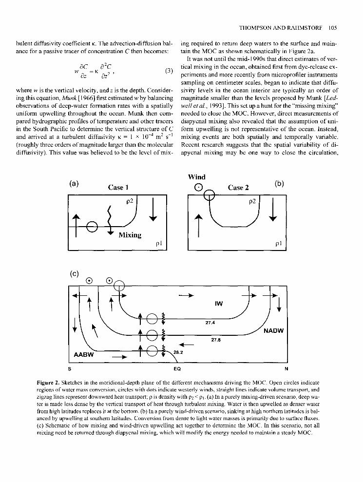
It was not until the mid-1990s that direct estimates of ver­tical mixing in the ocean, obtained first from dye-release ex­periments and more recently from microprofiler instruments sampling on centimeter scales, began to indicate that diffu­sivity levels in the ocean interior are typically an order of magnitude smaller than the levels proposed by Munk [Led­well et al., 1993]. This set up a hunt for the "missing mixing" needed to close the MOC. However, direct measurements of diapycnal mixing also revealed that the assumption of uni­form upwelling is not representative of the ocean. Instead, mixing events are both spatially and temporally variable. Recent research suggests that the spatial variability of di­apycnal mixing may be one way to close the circulation,

Wind

0 Case2 (b)

l p2

i pl

IW

27.4

27.8

N

Figure 2. Sketches in the meridional-depth plane of the different mechanisms driving the MOC. Open circles indicate regions of water mass conversion, circles with dots indicate westerly winds, straight lines indicate volume transport, and zigzag lines represent downward heat transport; pis density with P2 < p1• (a) In a purely mixing-driven scenario, deep wa­ter is made less dense by the vertical transport of heat through turbulent mixing. Water is then upwelled as denser water from high latitudes replaces it at the bottom. (b) In a purely wind-driven scenario, sinking at high northern latitudes is bal­anced by upwelling at southern latitudes. Conversion from dense to light water masses is primarily due to surface fluxes. (c) Schematic of how mixing and wind-driven upwelling act together to determine the MOC. In this scenario, not all mixing need be returned through diapycnal mixing, which will modify the energy needed to maintain a steady MOC.

106 OCEAN CIRCULATION

whereby elevated mixing over rough topography and along continental slopes with turbulent diffusion coefficients up to K = 100 x 10-4 m2 s- 1 compensate for the weak interior mix­ing [Polzin eta!., 1997]. Munk and Wunsch [ 1998] revisited the turbulent diffusivity estimate needed to close the MOC in view of the spatial heterogeneity of mixing, but found that the canonical value K = 10-4 m2 s-1 should still hold in an averaged sense, assuming that 30 Sv of water upwells at low latitudes between I 000 and 4000 m depth. Much work has gone into accounting for all the diapycnal mixing in the ocean. A number of "mixing hotspots" have been found­most involving the breaking of internal waves (oscillations of density surfaces in the ocean interior) generated by tidal motion over topographical ridges. It remains uncertain, however, whether these sites taken together are sufficient to close the MOC.

The energy needed to maintain this mixing is input from the action of winds and tides. These both generate internal waves that dissipate into small-scale motions that give rise to turbulent mixing. Estimating the ocean's energy budget involves a great deal of uncertainty and remains an area of active research. However, assuming an upwelling of 30 Sv in low latitudes, Munk and Wunsch [ 1998] estimated that an energy input of 0.4 TW would be required to maintain the observed stratification. The surface winds contribute to the ocean's energy budget in a number of ways including work on the large-scale flow and work on the surface waves; however, a rough estimate is that I TW of wind energy input is available for turbulent mixing in the deep ocean. Tides input a total of about 3.5 TW, but much of this is dissipated on continental shelves, such that only I TW may be avail­able for deep mixing. Perhaps the most uncertain part of the energy budget is the conversion rate of turbulent kinetic en­ergy to potential energy or, in other words, how much of the energy available for mixing actually goes into raising the potential energy of the ocean. A common value for this mix­ing efficiency is 20%, such that a rough estimate of the en­ergy directly available for diapycnal mixing (0.2 x [I TW + I TW] = 0.4 TW) is exactly that needed to maintain the MOC through diapycnal mixing alone. Implicit in these es­timates are a great number of assumptions and approxima­tions, which are summarized in the review by Wunsch and Ferrari [2004].

2.2.2. Southern Ocean upwelling. The second important mechanism for bringing deep water to the surface is wind­driven upwelling in the Southern Ocean [Toggweiler and Samuels, 1995, 1998], shown schematically in Figure 2b. The Southern Ocean is a key component of the MOC because of its unique characteristic that at the latitudes spanning Drake Passage, there are no continental boundaries. An immedi-

ate consequence is that the dominant current in the South­ern Ocean is a circumpolar flow, the Antarctic Circumpolar Current (ACC), which is the strongest current on Earth (approximately 130 Sv) and enables exchange between the different ocean basins. A further result, though, is that no geostrophically balanced meridional flows are allowed above the level of the highest topographical feature (roughly 2500 m), since there are no boundaries available to support an east-west pressure gradient. This is known as the "Drake Passage effect."

Strong westerly winds blow over the Southern Ocean, which result in a northward flow at the surface, known as an Ekman flow. This flow is in the meridional direction, perpendicular to the ACC. Surface divergence in this Ek­man flow induces an upwelling, as deeper waters rise to replace the northward moving surface water. Since a south­ward flow can only be supported at depths greater than 2500 m, upwelling in the Southern Ocean must come from these deeper waters. Furthermore, since the density of the ACC's northward-flowing surface waters are so different from southward-flowing deep waters, it is argued that these water masses can only be connected in the North Atlantic. In other words, in this purely wind-driven view, NADW formation represents a passive mechanism to close the MOC, and the location of this sinking is largely due to high-latitude cool­ing, which contributes favorably to buoyancy loss. A final consequence of this mechanism is that the strength of the MOC is determined largely by the wind stress in the South­ern Ocean. Note that the deep upwelling described here may occur along isopycnals that tilt toward the surface across the ACC, and is thus a very different process from wind-induced mixing related to small-scale turbulent motions described in the previous section. Indeed, deep upwelling in the Southern Ocean essentially short-circuits the turbulent mixing needed to raise dense water at low latitudes in the diapycnal mix­ing scenario. Therefore, in this upwelling scenario, a much smaller value of the spatially averaged diapycnal diffusivity is needed to close the MOC, and similarly, a smaller energy input is needed to maintain the required mixing. Thus, wind­driven upwelling offers a potential solution to the "missing mixing" problem as well.

A number of studies have attempted to resolve which of these two mechanism has dominant control of the ocean's MOC. The conclusion is that both mechanisms are likely active in the ocean (Figure 2c ). Models that either reduce interior mixing or eliminate wind forcing are still capable of producing an overturning circulation, even if somewhat weakened. A key point is that not all 30 Sv of the MOC need upwell to the surface through diapycnal mixing if some upwelling in the Southern Ocean is also active. A major problem in resolving this issue is the difficulty in obtaining

observations of the different mechanisms, especially in the case of small-scale diapycnal mixing. A more complete re­view of these two mechanisms and their relative importance in numerical simulations of the ocean circulation is given by Kuhlbrodt et al. [2004].

2.3. Past and Present Observations of the MDC

The MOC is a global current system, yet it remains cru­cially dependent on processes occurring at scales as small as centimeters, as in the case of diapycnal mixing. There­fore, it is perhaps not surprising that observing the MOC, and more importantly its variability, is a complicated task, both because of the logistical demands of collecting data and because of the inevitable assumptions that are required to in­terpret these data. For this reason, it is generally as important to document the limitations of observing the MOC, both in present and past climates, as it is to quantify the behavior of the MOC itself.

Modem oceanographic techniques have only been moni­toring the ocean for the past I 00 years, and until recently, observations have been confined to sparse occupations of hydrographic stations-individual locations where full depth temperature and salinity profiles have been obtained from ships. Immense progress on improving the coverage of ocean observations was made during the 1990s through the World Ocean Circulation Experiment, which involved de­tailed ship-based surveys, satellite observations, and many thousand in situ measurements [Siedler et al., 2001]. How­ever, inferring recent interdecadal changes in the MOC has unavoidably relied on the comparison of historical hydro­graphic data with more recent observations.

One of the first studies that attempted to constrain recent decadal changes in the MOC focused on a set of five hydro­graphic sections (occupied in 1957, 1981, 1992, 1998, and 2004) along a transect spanning the Atlantic Basin near 25°N with a goal of monitoring the transport of warm upper waters northward and cold deep-water southward [Bryden et al., 2005]. Profiles of temperature and salinity are suffi­cient to determine profiles of vertical shear, or the change in velocity with depth, but a velocity observation from at least one depth is needed to compute the absolute velocity profile. In the absence of such an observation, a depth where the velocity vanishes is typically selected as a reference, known as the level of no motion. Using a level of no motion at 3200 m, Bryden et al. [2005] reported a weakening ofthe MOC by as much as 30% between 1957 and 2004. While the structure of the MOC was largely unchanged over this period, more southward transport was detected at depths shallower than 1000 m and a large reduction in transport (from 15 to 7 Sv) of lower NADW was found at depths greater than 3000 m.

THOMPSON AND RAHMSTORF 107

The authors interpreted these results as evidence that less of the northward-moving warm water was being converted to NADW at high latitudes. An associated reduction in north­ward heat transport of0.2 PW was also found.

Shortly after this study, however, numerical models be­gan to highlight some of the complications in interpreting changes in the MOC from temporally sparse hydrographic sections. In particular, Wunsch and Heimbach [2006] con­sidered a general circulation model of the North Atlantic MOC constrained by billions of observational data points ranging from satellite measures of sea surface height and wind stress to data from scientific floats and drifters. While this study also detected a statistically significant reduction in the strength of the MOC, although with a trend consider­ably weaker than Bryden et al. [2005], the most remarkable result was that monthly averages of the overturning showed significant fluctuations, ranging from 8 to 21 Sv between 1993 and 2004. This high frequency variability of the MOC was confirmed following deployment of the Rapid Climate Change (RAPID) mooring array along 26.5°N across the Atlantic basin. These instruments allowed estimates of the zonally integrated profile of meridional velocities on a daily basis over a period of a year. In the period from March 2004 to March 2005, the overturning rate was determined to be 18.7 ± 5.6 Sv, but daily overturning values ranged from 4.0 to 34.9 Sv [Cunningham et al., 2007]. This range includes all the transport values from the hydrographic sections used by Bryden et al. [2005].

This example points to the difficulties in observing changes in the MOC. "Snapshot" estimates of mid-ocean circulation from hydrographic sections are unlikely to pro­vide conclusive evidence of past changes because of the pos­sibility of aliasing high frequency variability. However, the ability to monitor the MOC on a daily basis is a significant achievement. Furthermore, from the year-long time series, it has been determined that if the ocean were to undergo a rapid change (as discussed in section 3 .I), this could be de­tected accurately to within 1.5 Sv from the RAPID mooring array.

Observational data has also been useful in indicating that the structure of the MOC has changed significantly in the past. A key motivation for understanding these past circula­tions is that they may provide insight into how the MOC might change in the future. Most observational reconstruc­tions of past circulations have focused on the deep Atlantic during the Last Glacial Maximum (LGM), the height of the last ice age (approximately 20,000 years ago). Inferences about these paleocirculations are largely based on distribu­tions of tracers that do not contribute to the density of sea water, and are measured in sediment cores collected from the seafloor. The fact that ocean circulation patterns of mass,

108 OCEAN CIRCULATION

temperature, salinity, and tracers need not be the same, as well as the possibility that production and consumption rates of tracers may have varied over time both contribute to the complexity of inferring past states of the MOC.

One of the most promising tools for inferring the circula­tion during the LGM is the reconstruction of carbon isotopic compositions 13C/12C of fossil shells ofbenthic foraminifera, single-celled protists with shells, buried in sediments. Varia­tions in the ratio 13C/12C arise because primary producers near the sea surface preferentially take up the lighter iso­tope (' 2C) along with nutrients. Thus, high 13C/12C ratios are found in low-nutrient waters such as NADW, while AABW, which spends little time near the surface, has high nutrient content and low 13C/12C ratios. In the present-day ocean, NADW is easily identified as a tongue of low-nutrient water that extends to nearly all depths in the North Atlantic and spreads southward to the Southern Ocean around a depth of3000 m. However, 13C/12C ratios from the LGM indicate that a low-nutrient water mass with a northern source only extended to a depth of 2000 m. This water mass, likely a modification of present-day NADW, is often referred to as Glacial North Atlantic Intermediate Water (GNAIW). Also, a strong vertical gradient in 13C/12C below 2000 m marks the boundary between GNAIW and a deep southern water mass that fills the bottom of the Atlantic basin [Curry and Oppo, 2005]. This sharp gradient suggests that the MOC was not sluggish during this period, as a significant circulation would be required to maintain this gradient against strong vertical mixing [Wunsch, 2003]. Apart from this inference, however, 13C/12C ratios largely provide a view of water mass distribu­tions without providing information about the strength of the MOC.

The chemical behavior of uranium (U), on the other hand, does provide some insight into deep circulation rates. Highly soluble in water, U has a residence time (several hundred thousand years) that greatly exceeds the mixing time of the ocean (roughly a thousand years), which allows U to be evenly distributed throughout the ocean. In con­trast, the U isotopes, protactinium 231 Pa and thorium 230Th, produced from radioactive decay ofU, have relatively short residence times because they are absorbed by settling par­ticles and buried in the seafloor. In the present day, nearly all 230Th is removed in the North Atlantic because its resi­dence time (20-40 years) is shorter than the transit time of deep water, whereas only about half of 231 Pa is removed because of its longer residence time (I 00-200 years). Thus, present-day 231 Pa!230Th ratios are less than the production ratio 0.093. Assuming scavenging rates have remained con­stant since the LGM, a reduction in the strength of the MOC should be reflected in higher sedimentary 231 Pa/230Th ratios. Observations show that there is no significant difference

between the 231 Pa!230Th ratios during the LGM compared to the Holocene [ Yu eta!., 1996], which again suggests that the MOC remained active during the LGM. New sediment cores have resolved the transition between the LGM and the Holocene and revealed that 231 Pa/230Th ratios varied substantially during this period. A rapid rise in 231 Pa!230Th ratios occurred about 17,500 years ago suggesting that the MOC was all but eliminated, but roughly 5,000 years later, the MOC was rapidly accelerated concurrent with strong warming events during deglaciation [McManus et a!., 2004]. These abrupt climate changes are discussed further in section 3.1.

Two key observations of the MOC during the LGM are (I) a water mass distribution characterized by a shallower export of GNAIW/NADW and more nutrient-rich waters below 2000 m and (2) unchanged ratios of 231 Pa!230Th that argue against a greatly reduced MOC. Observations of the past MOC necessarily have sparser coverage and larger er­rors than present-day measurements. Problems also remain in the interpretation of proxy data, such as the isotopic com­positions described here. Still, paleoceanography is a rela­tively new science, and improvements to existing techniques as well as the development of new methods to study past ocean states [Lynch-Stieglitz eta!., 2007] are sure to enhance our understanding of the physical processes that cause ocean circulation and climate changes.

3. ABRUPT CLIMATE CHANGE IN PAST CLIMATES

3.1. Circulation Modes

One of the most profound ways in which the ocean could alter the climate would involve a reorganization or complete collapse of the MOC. The possibility of an abrupt shift in the MOC in response to increased greenhouse-gas concen­trations and global warming has been realized in a number of coupled ocean-atmosphere numerical models [Clark et al., 2002, and references therein]. However, assessing the likelihood of such a change has proven extremely diffi­cult, mainly because the many parameterizations included in models to account for unresolveable physical processes are poorly constrained. Furthermore, obtaining observations of variability in a system as extensive as the MOC requires long data time series spread over a large spatial extent.

Thus, much of our understanding of the variability of the MOC and its role in influencing the climate comes from analyses of historical instances of abrupt climate change. The best evidence for abrupt climate change comes from the last ice age, which occurred between 120,000 and 12,000 years ago. The observational evidence of these changes is primarily inferred from ice cores, sediment cores, and cor-

als. Reconstruction of ocean temperatures has been carried out from species abundance of fossil plankton, from organic chemistry, and from trace metal ratios in corals or calcite shells. These data are crucial for validating numerical simu­lations of previous climates. Both observational and numeri­cal evidence suggest that abrupt climate changes during the last glaciation were largely caused by shifts in the MOC trig­gered by changes in the hydrological cycle.

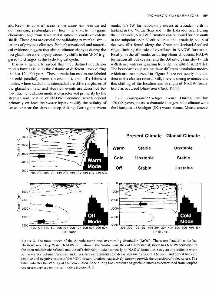
It is now generally agreed that three distinct circulation modes have existed in the Atlantic at different times during the last 120,000 years. These circulation modes are labeled the cold (stadia!), warm (interstadial), and off (Heinrich) modes, where stadia! and interstadial are different phases of the glacial climate, and Heinrich events are described be­low. Each circulation mode is characterized primarily by the strength and location of NADW formation, which depend primarily on how freshwater inputs modify the salinity of seawater near the sites of deep sinking. During the warm

1000 •. --·········· ~-:-. -- ... E

-.._... 2000

0.

~ .3000 ·--·-·-·---····- ... ___ _

4000 .......

·::::.~:::::.·:::< ........ ....

Latitude

THOMPSON AND RAHMSTORF 109

mode, NADW formation only occurs at latitudes north of Iceland in the Nordic Seas and in the Labrador Sea. During the cold mode, NADW formation can be found further south in the subpolar open North Atlantic and, crucially, south of the two sills found along the Greenland-Iceland-Scotland ridge, limiting the role of overflows in NADW formation. Finally, in the off mode, or during Heinrich events, NADW formation all but ceases, and the Atlantic basin slowly fills with dense water originating from the margins of Antarctica. The boundaries separating these different circulation modes, which are summarized in Figure 3, are not nearly this dis­tinct in the climate record. Still, there is strong evidence that this shifting of the location and strength of NADW forma­tion has occurred [Alley and Clark, 1999].

3.1.1. Dansgaard-Oeschger events. During the last 120,000 years, the most dramatic changes in the climate were the Dansgaard-Oeschger (DO) warm events. Measurements

Warm

Cold

Off

1000

Present Climate Glacial Climate

Stable Unstable

Unstable Stable

Stable Unstable

tON 20N 30N 40N 50N 60N 70N BON Latitude

Figure 3. The three modes of the Atlantic meridional overturning circulation (MOC). The warm (stadia!) mode has North Atlantic Deep Water (NADW) formation in the Nordic Seas, the cold (interstadial) mode has NADW formation in the open midlatitude Atlantic and the off(Heinrich) mode has nearly no NADW formation. Gray arrows indicate warm saline surface volume transport, and black arrows represent cold dense volume transport. The solid and dotted lines are positive and negative values of the MOC stream function, respectively (arrows provide the direction of trajectories). The table indicates the stability of each circulation mode during both present and glacial climates as determined from coupled ocean-atmosphere numerical models (section 4.1).

110 OCEAN CIRCULATION

taken from Greenland ice cores indicate that DO events were abrupt occurrences involving warming that could exceed 1 ooc over a period as short as a couple of decades [Bond et al., 1993]. Following the abrupt warming, temperatures un­derwent a slow cooling over several centuries. A more rapid decrease in temperature back to cold (stadia!) conditions completed the cycle. The amplitudes of DO events in the climate record are largest in the North Atlantic, however, the effects of DO events were felt globally. Proxy data show that the South Atlantic cooled, while the North Atlantic warmed. This hemispheric "see-saw" effect, whereby the northern and the southern hemisphere experience opposite trends in a

Dansgaard-Oeschger event

22

16 • H6?

60 55 50 45

property, is a common feature in the climate record [Stocker, 1998].

One of the most fascinating aspects of DO events is the regularity of their occurrences [Rahmstorf, 2003]. The time elapsed between two consecutive DO events is typically around 1500 years, although periods of 3000 and 4500 years are also common. The vertical lines in the lower panel of Plate 2 are spaced at intervals of 14 70 years to illustrate this regular tendency.

The earliest hypotheses about the physical mechanism responsible for DO events typically invoked the role of the ocean circulation in the North Atlantic. It was initially

Heinrich event

36

7 6 5 4 38 ~

0

"' 40 ~

42

35 30 25 20 15 10 Time (kyr ago)

Plate 2. (top) Sketches of the circulation modes during the last glacial climate. (middle) Stable cold circulation mode with deep-water formation occurring in the midlatitude Atlantic. During Dansgaard-Oeschger (DO) events (left) warm saline water extended into high latitudes increasing sea surface temperatures (SST), while during Heinrich events (right) deep-water convection all but ceased. Thin lines in the left and right panels indicate model-derived SST anomalies from the stable cold mode in the middle panel. (bottom) Reconstructed sea surface temperature from proxy subtropical At­lantic Ocean sediment data (green) and Greenland ice core data (blue). DO events are numbered, and Heinrich events are marked by red boxes. Vertical lines are drawn at intervals of 14 70 years to indicate the regularity of DO events. The Bolling-Allerod and Younger Dryas (YO) events are warm and cold events, respectively, which occurred following the end of the last glacial maximum. Adapted from Rahmstorf[2002]; see references therein for discussion of proxy data.

thought that the warm and cold phases of the glacial cli­mate corresponded to active and inactive periods ofNADW formation. However, sediment evidence has indicated that NADW formation only became inactive during extreme Hei­nrich events [Elliot et al., 2002]. Internal oscillations of the ocean circulation have been suggested as a possible mecha­nism for producing the warming and cooling cycle associ­ated with DO events. In this scenario, a change to the climate system that modifies the ocean circulation pattern also in­duces a compensating change that will eventually return the circulation to its original state. A simple example of such an internal oscillation would begin with excessive warming in the North Atlantic due to a strong MOC that produces higher melting rates of sea ice. This meltwater reduces the salinity of the high-latitude surface water and limits deep-water for­mation, slowing the MOC. Once in the reduced MOC state, salinity builds up in the Atlantic over time until eventually the surface water is sufficiently dense to drive deep-water formation again and return the circulation to its strong MOC state. The frequency of DO events in this scenario would be related to the time lag between the two competing changes to the climate system. It is unlikely, however, that internal oscillations of this sort are capable of describing the regular frequency of DO events observed in the climate record.

Ganopolski and Rahmstorf [200 I] have used numerical models to show that a shift in latitude of NADW formation sites from the Nordic Seas to the midlatitude open Atlantic gives rise to a three-phase evolution and a hemispheric see­saw effect that are both characteristic of DO events. In this mechanism, the rapid warming phase of a DO event arises from a switch between the cold circulation mode to the warm circulation mode, which allows warm Atlantic water to penetrate into the Nordic Seas. The period of relatively stable, warm temperatures is the persistence of the warm circulation mode. As this mode weakens, temperatures de­crease, and the final rapid temperature decline of a DO event marks the end of deep-water formation in the Nordic Seas. The life-cycle of DO events has been represented accurately in numerical climate models, yet the trigger that initiates an event is still unknown. It has been argued that random cli­mate variability and a weak external cycle in the freshwa­ter forcing (for example, a solar cycle with the appropriate 1500-year period) would be sufficient to overcome the criti­cal threshold allowing NADW formation in the Nordic Seas, thus initiating the DO events.

There is also a possibility that DO events are not related to the ocean circulation at all. One such theory is that DO events are caused by shifts in the atmospheric planetary wave pattern, controlled remotely from the tropics [Clement and Cane, 1999]. Support for this mechanism comes from the strong control that tropical sea surface temperatures exert

THOMPSON AND RAHMSTORF Ill

on global atmospheric heat-transport patterns in the present climate. However, it is difficult to explain the hundreds of years persistence of DO events with an atmospheric mecha­nism. Furthermore, oceanic changes during DO events are well documented in sediment cores.

3.1. 2. Heinrich events. Heinrich events are the other in­stances of abrupt climate change that occurred during the last glacial climate. Heinrich events were first identified in North Atlantic seafloor sediments, where layers of rock frag­ments were found between layers rich in carbonate fossils [Heinrich, 1988]. The rock-fragment-rich layers, known as ice rafted detritus or IRD layers, are thought to have been deposited by massive discharges of icebergs into the North Atlantic. Discharges of this nature may have occurred when the ice sheet reached a critical height after which small per­turbations led to massive surges. These discharges provided a large forcing to the ocean, whereas with DO events, no associated ocean forcing is known. Heinrich events induced rapid change; the onset occurred over a decade or less with the total event spanning a period of roughly 750 years. Six Heinrich events are indicated in the lower panel of Plate 2, plus the Younger Dryas is sometimes labeled a Heinrich event (HO).

The discharge of icebergs into the North Atlantic would have provided an enormous freshwater flux. For example, during Heinrich event 4, the freshwater flux has been esti­mated at 0.29 ± 0.05 Sv over a duration of 250 ± 150 years [Roche et al., 2004], equivalent to a freshwater volume of about 2.3 million krn3

. For this reason, it is believed that Heinrich events were associated with a large reduction or even a complete cessation ofNADW formation.

An interesting feature of Heinrich events is that despite a reduction in the strength of the MOC, they did not lead to anomalously cold stadials in Greenland. Because of the abruptness of the events, it was previously thought that Hei­nrich events were responsible for cooling Greenland, while it is now believed that Heinrich events only occurred when Greenland was already cool. There is, however, a strong cooling signal observed in the midlatitude Atlantic during Heinrich events [Bard eta!., 2000]. This behavior is con­sistent with the view that a Heinrich event represents a flip between the cold circulation mode and the off mode. The lack of further cooling in Greenland is then explained, since in the cold circulation mode, warm Atlantic water already sinks south of Greenland. A response to the shutdown of NADW formation is only found south of the original deep­water formation location.

The see-saw effect discussed earlier also occurred dur­ing Heinrich events with southern hemisphere warming ac­companying northern hemisphere cooling. The response in

112 OCEAN CIRCULATION

the southern hemisphere is stronger during a Heimich event than during a typical DO event [Blunier eta!., 1998]. This is because once NADW formation ceases, heat transport between the hemispheres is strongly curbed. During a DO event, it is primarily the location of NADW formation that changes, and as such, interhemisphere heat transport is not as strongly affected.

Finally, a key point is that although Heimich events did not occur regularly like DO events, they always occurred during cold stadials (Plate 2) and thus were not purely ran­dom events. The leading theory for the onset of Heimich events is an ice-sheet instability that provides the strong freshwater flux needed to modify NADW formation. This mechanism has been shown to induce Heinrich events in nu­merical models without any other external climatic trigger. It is worth noting that any trigger that may have led to the onset of either DO or Heimich events during glacial climates may be very different from triggers that could produce simi­lar reorganizations of the MOC in our present climate.

4. FUTURE CHANGES IN THE TWENTY-FIRST CENTURY AND BEYOND

4.1. Positive Feedback and Multiple Equilibria

In the previous section, we described three different modes of the MOC (warm, cold, off) that are believed to have been active during the past 120,000 years. Here we describe how nonlinearities in the circulation system enable transitions between these multiple equilibrium states. In particular, we consider the stability of past climates to provide some insight into how changes in the present-day MOC might arise.

The main contribution to increasing surface densities at high latitudes comes from cooling; in other words, the buoy­ancy flux is dominated by temperature. Salinity, though, plays a crucial role by introducing a nonlinearity into the system that allows for positive feedback, by which small changes in forcing can result in large modifications to the circula­tion. The role of this "advective feedback" in the ocean cir­culation was first reported by Stommel [ 1961] in the context of a simple two-box model representing flow between high and midlatitudes. The mechanics of the advective feedback can be understood as follows. The MOC transports saline waters northward toward the deep-water formation regions, and as this water cools, the salinity provides an additional contribution to increasing surface densities and enhancing deep-water formation. This strengthens the MOC and brings even more salt up to high latitudes producing a positive feed­back. Similarly, since deep-water formation sites are found in regions of net precipitation in the present climate, if the MOC weakens or stops, it may be difficult to overcome the

freshwater forcing in order to re-start the process of deep­water formation.

"Convective feedback" is another nonlinearity of the ocean circulation that primarily influences individual convection sites, at least in numerical models [Rahmstorf, 1994]. Deep­water formation sites in the North Atlantic are regions of net precipitation and thus have a net freshwater input. If convec­tion occurs regularly, the surface freshwater remains well­mixed with deeper saline waters; this helps maintain a high surface density so that convection occurs the following win­ter. If, however, convection is inactive over a period of years because of natural variability in the surface buoyancy fluxes, then freshwater accumulates at the convection site, decreases the surface density, and limits the possibility of future con­vection events. In this manner, local convection sites can be "switched off." Similarly, if a previously inactive site under­goes convection because of an anomalously large buoyancy flux, this brings saline water to the surface and encourages future convection at the same site. Convective feedback of­fers a mechanism for specific deep-water formation sites to "flip" on and off, giving rise to the possibility of multiple stable patterns of an MOC with active NADW formation.

Figure 4a shows a schematic stability diagram of the upper cell of the MOC, where the strength of NADW formation is plotted as a function of freshwater input into the North At­lantic. The upper two black lines represent stable equilibria where NADW formation is active. These two lines may rep­resent circulation modes with different NADW formation sites, for instance. The horizontal black line with no NADW formation is another stable equilibrium representing the off mode of the MOC (note that a lower AABW cell may still be present, see Figure 3).

The vertical lines in Figure 4a indicate various transi­tions between the different equilibrium states. A transition between the two upper equilibrium states (line c) may oc­cur through a local convective instability which involves the rapid spin-up or shutdown of a convection site. It is believed that DO events are transitions ofthis type. A complete col­lapse of NADW formation, perhaps through an advective feedback, is illustrated by the dotted curve labeled (b). A steady increase in the freshwater forcing will eventually ex­ceed the bifurcation point, labeled S, in which case, water simply becomes too fresh to sustain an overturning circu­lation and the system transitions to the off mode (line a). Finally, line (d) indicates the initiation of convection in the North Atlantic from the MOC off mode. This line also im­plies that when freshwater forcing is absent, NADW forma­tion will tend to approach an MOC-active equilibrium state due to advective feedback, i.e., accumulation of salt in the North Atlantic will lead to a density increase allowing the MOC to resume. The dotted line connecting the two circles

> ~ s: 0

u::: 3: Cl <( z

o (a)

-0.2

b: s

• : • : ' v

a

0 0.2 Freshwater Forcing [Sv]

30

25

~ 20

3: 15 0 <( z

10

5

0

-0.2 -0.1 0

THOMPSON AND RAHMSTORF 113

0.1 0.2

UVic MOMiso MOM hor

- C-GOLDSTEIN -Bremen - ECBilt-CLIO

0.3 0.4 Freshwater Flux (Sv)

0.5

Figure 4. (a) Schematic stability diagram for the rate of NADW formation as a function of freshwater forcing from a modified version of the box model by Stommel [ 1961] (see details in Rahmstor/[2000]). Solid black lines indicate stable equilibrium states. while dotted lines are unstable. The circle labeled S is a bifurcation point; NADW formation cannot be sustained for freshwater forcing past this point. The vertical lines indicate transitions between different circulation modes; line a is a spin down of the NADW cell due to steadily increasing freshwater forcing, while line b represents a rapid shutdown of the cell through advective feedback. Line c indicates a change in NADW formation sites, while lined is a restart of the NADW overturning cell. (b) Hysteresis curves from a suite of intermediate-complexity climate models. The present-day initial state is marked by the open circle.

roughly indicates the amount of freshwater forcing needed to shut down NADW formation of a given magnitude. A complicating factor in relating stability analyses based on numerical models to the real ocean is that the MOC takes thousands of years to equilibrate to these "stable modes." Thus, the immediate response to a change in forcing may be significantly different from equilibrium solutions.

A key feature of the stability diagram in Figure 4a is the existence of a hysteresis loop. Hysteresis occurs if follow­ing a small change in forcing and the associated adjustment of the circulation, reversing the forcing does not return the circulation to its original state. For example, if the climate resides close to the bifurcation point S in Figure 4a, a small increase in freshwater forcing may shut down NADW for­mation. Once the stable "MOC off" mode has equilibrated, though, a much greater change in freshwater forcing is re­quired to re-start the MOC. Hysteresis appears to be a robust feature found in many climate models (Figure 4b). While most numerical models do show multiple equilibria and hys­teresis loops, only some indicate that the present-day climate exists in a bistable parameter regime; thus, it is unclear if the real climate is bistable.

Most of the insight into abrupt changes between different stable modes of ocean circulation have come from simula­tions of glacial climates. As freshwater forcing is increased in the present-day climate, a clear bifurcation occurs result­ing in the abrupt loss of NADW formation (point S, Figure

4a). In contradistinction, simulations from a coupled climate model of intermediate complexity (CLIMBER-2) show that increasing freshwater forcing in a glacial climate results in a gradual reduction of NADW formation [Ganopolski and Rahrnstorf, 2001]. Furthermore, when the strength of the freshwater forcing is reversed, in this scenario, the hysteresis effect is much smaller than in simulations of the present-day climate. This difference arises because, in the present cli­mate, NADW formation can only occur north of Iceland in the Nordic Seas, temperatures are too warm for deep-water formation sites to migrate south into the midlatitude Atlan­tic. In the glacial climate, though, the colder temperatures allow deep-water formation in the open Atlantic, such that the response to freshwater forcing is a gradual retreat south­ward of the NADW formation sites, rather than a rapid shut­down of the MOC. Thus, the glacial climate does not have a well-defined stable off mode. Instead, it transitions between a marginally stable warm mode and a stable cold mode.

The transition from a marginally stable warm mode to a stable cold mode can be understood as the life cycle of a DO event. Here it is assumed that a small amplitude fresh­water forcing cycle exists in the climate system that triggers the DO event, but after the initiation, the forcing cycle does not subsequently influence the behavior of the MOC (sec­tion 3.1 ). Heinrich events involve much greater forcing of freshwater that completely shuts down NADW formation. However, since this mode is unstable in a glacial climate, the

114 OCEAN CIRCULATION

MOC rapidly returns to its cold mode, once again initiating NADW formation. In this framework, both Heinrich and DO events are transient because both the MOC's warm mode and off mode are unstable in a glacial climate.

Results from numerical simulations (e.g., CLIMBER-2) indicate that the stability of modes in the present-day climate is opposite to the glacial climate. The MOC's warm and off modes are stable equilibrium circulation modes, and the cold mode is either unstable, or perhaps, altogether unattainable (Figure 3). In other words, a warm climate favors the warm mode of circulation, while a glacial climate prefers the cold mode of circulation [Ganopolski and Rahmstorf, 2001]. During glacial climates, transitions between warm and cold circulation modes are easily triggered, although it appears that it becomes more difficult to achieve the warm mode as the background climate becomes colder (DO events are ob­served less regularly during the coldest periods of the last glacial). It has been suggested that the climate variability responsible for triggering DO events during the last glacial climate remains active in the present climate, and it may simply be the case that, in the present climate, the MOC is insensitive to this forcing.

This brief section intends to provide some insight into how the circulation structure could change in the future. One of the greatest challenges in climate science is finding observ­able characteristics of the present-day ocean circulation that can be used to detect a shift in the MOC. While inferred shifts in the MOC during a glacial climate do not necessarily give us an indication of future events, they provide evidence that abrupt and significant modification to the MOC can occur in the Earth's climate system. Most changes in the MOC will have a large effect on the climate. In particular, a collapse of NADW formation could potentially lead to significant cooling over large parts of Europe. However, predicting this response is complicated; for instance, MOC-induced cooling may be compensated in part by anthropogenic warming that originally caused the circulation changes [Rahmstorf, 1999]. Changes in the MOC may also lead to local changes in sea level, as discussed further in section 4.2.

4. 2. Sea Level Rise

Sea level rise is one of the most studied and publicly dis­cussed aspects of climate change because of its implications for island and coastal regions worldwide. An accurate under­standing of how sea level responds to changes in the climate is made difficult because the physical processes that contrib­ute to sea level variability involve several coupled nonlinear systems that act over a number of different timescales. Over decadal and longer timescales, the two chief contributors to sea level variability in the past two centuries have been

( 1) thermal expansion, an increase in volume due to increased heat content in the ocean, and (2) the input of water into the ocean from land-based ice sheets and glaciers. On shorter timescales, changes in atmospheric pressure or in regional ocean circulations may lead to local sea level variability, but these typically make a small contribution to changes in the global mean. Finally, land processes (e.g., tectonics, sedi­mentation) that alter the shape of the ocean basins may also influence mean sea level.

Ice sheets have, by far, the greatest potential to change sea surface height. Complete melting ofthe ice sheets would lead to a global sea level rise of approximately 65 m [Cazenave, 2006]. Of this, 57 m of sea level resides in the ice sheets of Antarctica, where estimates of ice sheet melting are most poorly constrained. Evidence from various observations in­dicate glaciers, ice caps, and ice sheets around Greenland and Antarctica are losing mass [Rignot and Thomas, 2002; Thomas et al., 2004]. However, a key uncertainty about how ice sheet melting will behave in the future is related to a pro­cess known as meltwater basal lubrication. As ice sheets melt, meltwater does not remain on the surface of the ice sheet, but rather migrates downward under the force of gravity through narrow holes or crevasses known as moulins. Moulins typi­cally extend to the base of the glacier where meltwater reaches bedrock. Here, the relatively warm meltwater can reduce friction at the glacier bed and act like a lubricant to ice flow. The development of moulins and the positive feedback they provide for glacial melting occur on scales far too small to be resolved in numerical models. Physical parameterizations of these processes are poor at best and are often not included at all. If the contribution of meltwater basal lubrication and other dynamic processes is significant, it implies that the re­sponse of ice sheets to changes in the climate could occur on the order of centuries rather than millennia.

Throughout most of the nineteenth and twentieth centu­ries, estimates of global sea level rise were limited to averages of a few high-quality tide gauge records, typically located in coastal regions. Satellite altimeters such as TOPEX/Po­seidon and Jason-1 have provided measurements of sea sur­face height since 1993. This has led to much more accurate monitoring of sea level rise in the last 15 years. Correlation between satellite altimetry and tide gauge records during this period have also been used to reconstruct sea level variabil­ity throughout the twentieth century.

Sea level indicators suggest that following the end of the last ice age, sea level rose more than 100 m over a long pe­riod ending between 3000 and 2000 years ago [Bindoff et al., 2007]. Since that time, there is no indication of further sea level rise until the mid-nineteenth century. However, during the 20th century, global mean sea level has risen at a rate of I. 7 mm a -I, and during the period 1993-2006, the sea level

has risen at a substantially larger rate of 3.3 ± 0.4 mm a- 1

[Church and White, 2006]. Over this period, it is believed that thermal expansion and the melting of land ice have contrib­uted roughly equal amounts to sea level rise, although these estimates are not well constrained [Domingues et al., 2008].

While sea level has steadily increased, the estimated lin­ear trends quoted above are not meant to imply that the sea level rate of rise has been constant. Instead, the rate of rise shows significant decadal variability. Furthermore, sea level rise exhibits large spatial variability with certain local re­gions increasing by more than five times the global mean with other regions experiencing a fall in sea level. Thus, it is uncertain whether the recent rapid rate of sea level rise will persist. Still, the rate of sea level rise between 1993 and 2006 is 25% faster than any previous period in the last 115 years. The rate of rise is also significantly larger than the best estimate rise of less than 2 mm a -I in the Third Assessment Report of the Intergovernmental Panel on Climate Change (IPCC) [Houghton et al., 2001]. In fact, the current rate of rise already lies close to the upper limit in the IPCC report, obtained from assuming the highest emission scenario com­bined with the highest climate sensitivity as well as an addi­tional sea level rise representative of"land ice uncertainty." This suggests that new or improved numerical models may be required to accurately capture the dominant processes contributing to sea level rise.

Global sea level changes are either a result of glacial and ice sheet melt, i.e., an increase in ocean mass, or of thermal expansion of sea water caused by diabatic heating. A source of regional sea level variability is changes in the ocean cir­culation. Changes in sea level resulting from this mechanism necessarily have a near-zero global mean, since no mass is added to the oceans. However, the redistribution of mass due to the reorganization of the MOC, for example, can cause certain regions to experience large and very rapid changes in sea level. Circulation changes are communicated throughout the ocean by internal waves (timescale of years to decades) and by gravity waves at the surface (timescale of days), thus sea level changes through this mechanism are much more rapid than either thermal expansion or land ice melting.

The topography of the ocean surface is determined locally by the surface currents and winds-gradients of sea surface height are largely balanced by geostrophic flows. Some of the clearest signals of the spatial variability of sea level in the current climate are found at open-ocean deep convection sites. These sites appear as regions oflocal sea surface height minima, primarily because of their temperature signature. This characteristic is responsible for the large difference in sea surface height between the high-latitude Atlantic, where deep convection is active, and the high-latitude Pacific, where only intermediate water masses are formed. This 50- to

THOMPSON AND RAHMSTORF 115

60-cm drop in sea surface height leads to a flow through the Bering Strait from the Pacific to the Arctic Ocean. Thus, changes to NADW formation rates are likely to cause sig­nificant sea level changes, especially in the North Atlantic.

The sea level response to a reorganization of the ocean circulation has been investigated by Levermann et al. [2005] using a coupled ocean-atmosphere model that includes sea ice and allows for a nonlinear explicit free surface repre­sentation. The sea level response was tested by introduc­ing a negative salt flux to the North Atlantic to weaken the overturning circulation without adding mass to the ocean (as would an equivalent freshwater flux). As expected, a suffi­ciently large salt flux (the equivalent of a 0.35 Sv freshwater flux) basically eliminates the difference in sea surface height between the Atlantic and the Pacific. The initial rapid rise in sea level occurs within a decade or so following the collapse of the thermohaline circulation.

The largest sea level changes are found along the coasts of Europe and North America and are largely due to the cessation of the upper cell of the MOC. In particular, the elimination of the North Atlantic Current (characterized by a negative meridional sea surface height gradient in the pres­ent climate) and the subsequent flattening of the sea surface produces a rise in sea level that becomes more pronounced moving poleward into the North Atlantic as well as mov­ing onshore along the east coast ofNorth America. Northern convection sites are clear locations of sea level rise due to the elimination of deep sinking. Sea level rise in the north­em hemisphere is balanced by a reduction in sea level in the Southern Ocean. The ACC experiences a strengthening as­sociated with sea level decline along its southern boundary, which enhances the sea surface gradient across the ACC. While the magnitude of these sea level changes depends on the initial strength of the MOC, the spatial pattern is a robust feature in several different climate models.

It is important to note that changes in sea level due to re­organization of the MOC are in addition to any further sea level rise caused by thermal expansion and glacial/ice sheet melting in a warmed climate. For example, cessation of NADW would have the effect of warming the deep ocean diffusively, leading to nearly another meter of sea level rise over a long period. As it is difficult to distinguish long-term trends from decadal variability in observational data, the rapid sea level response to changes in the ocean's circula­tion structure may provide the first observable signals of a major change in the MOC.

5. CONCLUSIONS

The ocean plays a key role in moderating the Earth's cli­mate due to its vast capacity to store and transport heat. Any

116 OCEAN CIRCULATION

realistic model of the climate's variability, whether in past, present, or future climates, must capture the intricacies of the ocean circulation. The fundamental challenge in accurately modeling the ocean, and subsequently its role in the climate, is accounting for the broad range of spatial and temporal scales that are responsible for governing the circulation. As has been discussed in this chapter, the large-scale currents that comprise the MOC stretch across ocean basins and even circle the globe in the case of the ACC, but ultimately, this massive overturning is closed by small-scale mixing events occurring right down to scales as small as millimeters. Com­puters will be unable to capture all of these processes in a comprehensive simulation in the foreseeable future. Some of the most exciting and important research being carried out today is examining alternative means of incorporating small-scale and mesoscale processes into coupled ocean-at­mosphere models in order to generate more accurate climate predictions. The success of this endeavor relies crucially on the exchange of ideas and data between researchers special­izing in theory, observations, and models of physical pro­cesses in the ocean.

A fundamental goal of the oceanographic community is to better understand the variability of the present-day MOC in order to distinguish between natural fluctuations and long-term trends. A major obstacle in achieving this goal is that the ocean remains severely undersampled, especially concerning properties below the surface that cannot be detected by satellite. Novel observing programs are start­ing to expand into some of the more remote regions of the ocean, e.g., the ACC and other polar regions, which have historically been sparsely sampled. An example of one such program is the Argo float array, which in 2007 completed its goal of globally distributing 3000 autonomous floats that sample the upper 2000 m of the ocean; the program's goal of maintaining the array at this level requires a commitment of 800 new floats every year. A more direct attempt to measure the variability of the MOC is the RAPID Climate Change program, which has introduced a monitoring array across the Atlantic at 26.5°N to provide daily measurements of the strength and structure of the MOC across this line (section 2.3) [Cunningham et al., 2007]. A challenge will be to main­tain these or similar programs over time periods (potentially many decades) long enough to capture signatures of climate change.

There is ample evidence from both numerical simulations and observations, obtained from ice cores, sediment cores, and corals, that the Earth's climate has undergone abrupt shifts in the past. Most theories suggest that these shifts were related to significant reorganizations of the ocean's global overturning circulation. With all this historical evidence, a fundamental question arises: How can our understanding of

changes to the ocean circulation in previous climates be ap­plied to the present-day climate? The answer lies not through any analogy of past and future situations, which will always be different, but rather through an understanding of physi­cal processes, which should be the same regardless of time period. This chapter has stressed that abrupt shifts in any cli­mate are largely a result of complex nonlinearities, feedback loops, and hysteresis effects in the physics governing the ocean circulation. Any one of these many processes may be sufficient to produce large changes in the climate that could be difficult to reverse. All this points to the importance of improving our understanding of the response of the present­day MOC to various changes in the climate system.

It is unclear how close the ocean circulation or the cli­mate, as a whole, is to a threshold for a "tipping point" [for a review of tipping points and a wider context of abrupt ocean changes, see Lenton et al., 2008]. Predictions are made difficult due to uncertainties in the freshwater budget (balance between evaporation, precipitation, and meltwater runoff) and the stability of the ocean circulation. However, what is unquestioned is that at present, the Earth's climate has entered a state that has never previously been realized. Atmospheric carbon dioxide concentrations prior to the industrial revolution were 270 parts per million (ppm). In 2008, these concentrations were 383 ppm with an aggre­gate greenhouse gas concentration around 430 ppm C02

equivalent. Thus, there is really no past precedent for how the ocean will respond to increased warming over the next century. Rise in sea level has been one focus of this chapter because of its direct relation to the physics of the ocean and its circulation, and because of its importance to human society. However, any major shift in the ocean circulation will have global effects that influence hydrological cycles, atmospheric temperatures, and weather patterns. It will be crucial in the coming years to monitor trends in the over­turning circulation as well as to continue improving numer­ical models. It will take time to decipher decadal variability from long-term trends, but it is only from the combined insight of observational data and numerical modeling that accurate predictions of the ocean circulation's behavior can be achieved.

REFERENCES

Alley, R. 8., and P. U. Clark (1999), The deglaciation of the north­em hemisphere: A global perspective, Annu. Rev. Earth Planet. Sci., 27, 149~182.

Bard, E., F. Rostek, J.-L. Turon, and S. Gendreau (2000), Hydro­logical impact of Heinrich events in the subtropical Northeast Atlantic, Science, 289, 1321 ~ 1324.

Bindoff, N. L., et al. (2007) Observations: Oceanic climate change and sea level, in Climate Change 2007: The Physical Science Ba­sis, edited by S. Solomon et al., pp. 385-432, Cambridge Univ. Press, Cambridge.

Blunier, T., et al. (1998), Asynchrony of Antarctic and Greenland cli­mate change during the last glacial period, Nature, 394, 739-743.

Bond, G., W. Broecker, S. Johnsen, J. McManus, L. Labeyrie, J. Jouzel, and G. Bonani (1993), Correlations between climate rec­ords from North Atlantic sediments and Greenland ice, Nature, 365, 143-147.

Bryden, H. L., H. R. Longworth, and S. A. Cunningham (2005), Slowing of the Atlantic meridional overturning circulation at 25°N, Nature, 438, 655-657.

Cazenave, A. (2006), How fast are the ice sheets melting?, Science, 314, 1250-1252.

Church, J. A., and N. J. White (2006), A 20th century accelera­tion in global sea-level rise, Geophys. Res. Lett., 33, LOI602, doi:IO.I029/2005GL024826.

Clark, P. U., N. G. Pisias, T. F. Stocker, and A. J. Weaver (2002), The role of the thermohaline circulation in abrupt climate change, Nature, 415, 863-869.

Clement, A. C., and M. A. Cane ( 1999), A role for the tropical Pacific coupled ocean-atmosphere system on Milankovitch and millennia! timescales. Part I: A modeling study of tropical Pa­cific variability, in Mechanisms of Global Climate Change at Millennia! Time Scales, edited by P. U. Clark, R. S. Webb, and L. D. Keigwin, pp. 363-371, AGU, Washington, D. C.

Csanady, G. T. (2001), Air-Sea Interactions: Laws and Mecha­nisms, Cambridge Univ. Press, Cambridge.

Cunningham, S. A., et al. (2007), Temporal variability of the Atlan­tic Meridional Overturning Circulation at 26.5N, Science, 317, 935-938.

Curry, W. B., and D. W. Oppo (2005), Glacial water mass geometry and the distribution of 813C ofLC02 in the western Atlantic Ocean, Paleoceanography, 20, PAI017, doi: 10.1029/2004PAOOI021.

Domingues, C. M., J. A. Church, N.J. White, P. J. Gleckler, S. E. Wijffels, P. M. Barker, and J. R. Dunn (2008), Improved esti­mates of upper-ocean warming and multi-decadal sea-level rise, Nature, 453, 1090-1094.

Elliot, M., L. Labeyrie, and J.-C. Duplessy (2002), Changes in North Atlantic deep-water formation associated with the Dans­gaard-Oeschger temperature oscillations (60-10 ka), Quat. Sci. Rev., 21, 1153-1165.

Ganachaud, A., and C. Wunsch (2000), Improved estimates of global ocean circulation, heat transport and mixing from hydro­graphic data, Nature, 408, 453-457.

Ganopolski, A., and S. Rahmstorf(200 I), Rapid changes of glacial cli­mate simulated in a coupled climate model, Nature, 409, 153-158.

Gill, A. E. ( 1982), Atmosphere-Ocean Dynamics, Elsevier. Heinrich, H. ( 1988), Origin and consequences of cyclic ice rafting

in the northeast Atlantic during the past 130,000 years, Quat. Res., 29, 143-152.

Houghton, J. T., Y. Ding, D. J. Griggs, M. Noguer, P. J. van der Linden, X. Dai, K. Maskell, and C. A. Johnson (Eds.) (2001), Climate Change 2001: The Scientific Basis, Cambridge Univ. Press, Cambridge.

THOMPSON AND RAHMSTORF 117

Kuhlbrodt, T., A. Griese!, M. Montoya, A. Levermann, M. Hof­mann, and S. Rahmstorf (2004 ), On the driving processes of the Atlantic meridional overturning circulation, Rev. Geophys., 45, RG200 I, doi: I 0.1 029/2004RGOOO 166.

Ledwell, J. R., A. J. Watson, and C. S. Law (1993), Evidence for slow mixing across the pycnocline from an open-ocean tracer­release experiment, Nature, 364, 701-703.

Lenton, T., H. Held, E. Kriegler, J. Hall, W. Lucht, S. Rahmstorf, and H. J. Schellnhuber (2008), Tipping elements in the Earth's climate system, Proc. Nat!. Acad. Sci. US. A., 105, 1786-1793.

Levermann, A., A. Griese!, M. Hofmann, M. Montoya, and S. Rahmstorf(2005), Dynamic sea level changes following changes in the thermohaline circulation, Clim. Dyn., 24, 347-354.

Lynch-Stieglitz, J., et al. (2007), Atlantic meridional overturning circulation during the Last Glacial Maximum, Science, 316, 66-69.

Marshall, J., and F. Schott (1999), Open-ocean convection: Obser­vations, theory and models, Rev. Geophys., 37, 1-64.

McManus, J. F., R. Francois, J.-M. Gherardi, L. D. Keigwin, and S. Brown-Leger (2004), Collapse and rapid resumption of Atlantic meridional circulation linked to deglacial climate changes, Na­ture, 428, 834-837.

Munk, W. (1966), Abyssal recipes, Deep Sea Res. Oceanogr. Ab­str., 13, 707-730.

Munk, W., and C. Wunsch (1998), Abyssal recipes II: Energetics of tidal and wind mixing, Deep Sea Res., Part I, 45, 1977-20 I 0.

Orsi, A. H., S. S. Jacobs, A. L. Gordon, and M. Visbeck (2001), Cooling and ventilating the abyssal ocean, Geophys. Res. Lett., 20,2923-2926.

Polzin, K. L., J. M. Toole, J. R. Ledwell, and R. W. Schmitt (1997), Spatial variability of turbulent mixing in the abyssal ocean, Sci­ence, 276, 93-96.

Rahmstorf, S. (1994), Rapid climate transitions in a coupled ocean­atmosphere model, Nature, 372, 82-85.

Rahmstorf, S. (1999), Shifting seas in the greenhouse?, Nature, 399, 523-524.

Rahmstorf, S. (2000), The thermohaline ocean circulation: A sys­tem with dangerous thresholds?, Clim. Change, 46, 247-256.

Rahmstorf, S. (2002), Ocean circulation and climate during the past 120,000 years, Nature, 419,207-214.

Rahmstorf, S. (2003), The current climate, Nature, 421, 699. Rignot, E., and R. H. Thomas (2002), Mass balance of polar ice

sheets, Science, 297, 1502-1506. Roche, D., D. Paillard, and E. Cortijo (2004), Duration and iceberg

volume of Heinrich event 4 from isotope modelling study, Na­ture, 432, 379-382.

Salmon, R. ( 1998), Lectures on Geophysical Fluid Dynamics, Ox­ford Univ. Press.

Siedler, G., J. Church, and J. Gould (Eds.) (2001), Ocean Circulation and Climate: Observing and Modelling the Global Ocean, Esevier.

Stocker, T. F. (1998), The seesaw effect, Science, 282, 61-62. Stommel, H. ( 1961 ), Thermohaline convection with two stable re­

gimes offiow, Tel/us, 13,224-230. Talley, L. D., J. L. Reid, and P. E. Robbins (2003), Data-based

meridional overturning stream functions for the global ocean, J. Clim., 16,3213-3226.

I 18 OCEAN CIRCULATION

Thomas, R., et a!. (2004), Accelerated sea-level rise from West Antarctica, Science, 306, 255-258.

Toggweiler, J. R., and B. Samuels (1995), Effect of Drake Passage on the global thermohaline circulation, Deep Sea Res., Part I, 42,477-500.

Toggweiler, J. R., and B. Samuels (1998), On the ocean's large­scale circulation near the limit of no vertical mixing, J Phys. Oceanogr., 28, 1832-1852.

Wunsch, C. (2003), Determining paleoceanographic circulations, with emphasis on the Last Glacial Maximum, Quat. Sci. Rev., 22, 371-385.

Wunsch, C., and R. Ferrari (2004), Vertical mixing, energy and the general circulation of the oceans, Annu. Rev. Fluid Mech., 36,281-314.

Wunsch, C. and P. Heimbach (2006), Estimated decadal changes in the North Atlantic meridional overturning circulation and heat flux 1993-2004, J Phys. Oceano gr., 36, 2012-2024.

Yu, E.-F., R. Francois, and M.P. Bacon (1996), Similar rates of modem and last-glacial ocean thermohaline circulation inferred from radiochemical data, Nature, 689--694.

S. Rahmstorf, Potsdam Institute for Climate Impact Research, P.O. Box 60 12 03, D-14412 Potsdam, Germany.

A. F. Thompson, Department of Applied Mathematics and Theo­retical Physics, University of Cambridge, Wilberforce Road, Cam­bridge CB3 OWA, UK. (andrew.f.thompson@damtp.cam.ac.uk)