Electronic Design Handbook - Alion System Reliability Center

NOT MEASUREMENTSENSITIVE

MIL-HDBK-338B1 October 1998SUPERSEDINGMIL-HDBK-338A12 October 1988

MILITARY HANDBOOK

ELECTRONIC RELIABILITY DESIGN HANDBOOK

This handbook is for guidance only. Do not cite this documentas a requirement

AMSC N/A AREA RELIDISTRIBUTION STATEMENT A. Approved for public release; distribution is unlimited.

MIL-HDBK-338B

TABLE OF CONTENTS

iii

TABLE OF CONTENTS

Section Page1.0 SCOPE.......................................................................................................................1-11.1 Introduction................................................................................................................1-11.2 Application.................................................................................................................1-11.3 Organization............................................................................................................... 1-1

2 .0 REFERENCED DOCUMENTS................................................................................ 2-12.1 Government Documents ............................................................................................ 2-1

2.1.1 Specifications, Standards and Handbooks ................................................. 2-12.2 Other Referenced Documents.................................................................................... 2-3

3.0 DEFINITIONS OF TERMS AND ACRONYMS AND ABBREVIATIONS.......... 3-13.1 Introduction ............................................................................................................... 3-13.2 Definitions ................................................................................................................ 3-13.3 List of Abbreviations and Acronyms......................................................................... 3-21

4.0 GENERAL STATEMENTS ..................................................................................... 4-14.1 Introduction and Background ................................................................................... 4-14.2 The System Engineering Process .............................................................................. 4-2

4.2.1 Systems Engineering and IPTs .................................................................. 4-34.2.2 The Four Steps of Systems Engineering ................................................... 4-3

4.3 System Effectiveness ................................................................................................ 4-74.3.1 R/M Considerations in System Effectiveness ........................................... 4-8

4.4 Factors Influencing System Effectiveness ................................................................ 4-84.4.1 Equipment of New Design ........................................................................ 4-84.4.2 Interrelationships Among Various System Properties .............................. 4-9

4.5 Optimization of System Effectiveness ...................................................................... 4-11

5 .0 RELIABILITY/MAINTAINABILITY/AVAILABILITY THEORY ..................... 5-15.1 Introduction ............................................................................................................... 5-15.2 Reliability Theory ..................................................................................................... 5-1

5.2.1 Basic Concepts .......................................................................................... 5-25.3 Statistical Distributions Used in Reliability Models ................................................. 5-8

5.3.1 Continuous Distributions .......................................................................... 5-85.3.1.1 Normal (or Gaussian) Distribution ........................................... 5-8

5.3.2 Examples of Reliability Calculations Using the Normal Distribution....... 5-145.3.2.1 Microwave Tube Example ....................................................... 5-145.3.2.2 Mechanical Equipment Example .............................................. 5-15

5.3.3 Lognormal Distribution ............................................................................. 5-165.3.3.1 Fatigue Failure Example .......................................................... 5-17

MIL-HDBK-338B

TABLE OF CONTENTS

iv

TABLE OF CONTENTS

Section Page5.3.4 Exponential Distribution ........................................................................... 5-17

5.3.4.1 Airborne Fire Control System Example ................................... 5-185.3.4.2 Computer Example ................................................................... 5-18

5.3.5 Gamma Distribution .................................................................................. 5-195.3.5.1 Missile System Example .......................................................... 5-21

5.3.6 Weibull Distribution .................................................................................. 5-225.3.6.1 Example of Use of Weibull Distribution .................................. 5-23

5.3.7 Discrete Distributions ................................................................................ 5-245.3.7.1 Binomial Distribution ............................................................... 5-245.3.7.1.1 Quality Control Example ......................................................... 5-245.3.7.1.2 Reliability Example ................................................................. 5-25

5.3.8 Poisson Distribution .................................................................................. 5-265.3.8.1 Example With Permissible Number of Failures ....................... 5-27

5.4 Failure Modeling ....................................................................................................... 5-285.4.1 Typical Failure Rate Curve ....................................................................... 5-285.4.2 Reliability Modeling of Simple Structures ................................................ 5-30

5.4.2.1 Series Configuration ................................................................. 5-315.4.2.2 Parallel Configuration .............................................................. 5-325.4.2.3 K-Out-Of-N Configuration ....................................................... 5-35

5.5 Bayesian Statistics in Reliability Analysis ............................................................... 5-375.5.1 Bayes’ Theorem ........................................................................................ 5-38

5.5.1.1 Bayes’ Example (Discrete Distribution) .................................. 5-395.5.1.2 Bayes’ Example (Continuous Distribution) ............................. 5-42

5.6 Maintainability Theory ............................................................................................. 5-445.6.1 Basic Concepts .......................................................................................... 5-455.6.2 Statistical Distributions Used in Maintainability Models ......................... 5-48

5.6.2.1 Lognormal Distribution ............................................................ 5-495.6.2.1.1 Ground Electronic System Maintainability

Analysis Example ........................................................... 5-515.6.2.2 Normal Distribution ................................................................. 5-63

5.6.2.2.1 Equipment Example .............................................. 5-655.6.2.3 Exponential Distribution .......................................................... 5-67

5.6.2.3.1 Computer Example ................................................ 5-685.6.2.4 Exponential Approximation ..................................................... 5-70

5.7 Availability Theory ................................................................................................... 5-705.7.1 Basic Concepts .......................................................................................... 5-725.7.2 Availability Modeling (Markov Process Approach) ................................. 5-73

5.7.2.1 Single Unit Availability Analysis(Markov Process Approach) ..................................................... 5-75

MIL-HDBK-338B

TABLE OF CONTENTS

v

TABLE OF CONTENTS

Section Page5.8 R&M Trade-Off Techniques .................................................................................... 5-83

5.8.1 Reliability vs Maintainability..................................................................... 5-835.9 References For Section 5 .......................................................................................... 5-88

6 .0 RELIABILITY SPECIFICATION, ALLOCATION, MODELING ANDPREDICTION ........................................................................................................... 6-1

6.1 Introduction ............................................................................................................... 6-16.2 Reliability Specification ........................................................................................... 6-1

6.2.1 Methods of Specifying the Reliability Requirement.................................. 6-16.2.2 Description of Environment and/or Use Conditions ................................. 6-36.2.3 Time Measure or Mission Profile ............................................................. 6-56.2.4 Clear Definition of Failure ........................................................................ 6-66.2.5 Description of Method(s) for Reliability Demonstration .......................... 6-7

6.3 Reliability Apportionment/Allocation ...................................................................... 6-76.3.1 Introduction ............................................................................................... 6-76.3.2 Equal Apportionment Technique .............................................................. 6-106.3.3 ARINC Apportionment Technique (Ref. [6]) ........................................... 6-116.3.4 Feasibility-Of-Objectives Technique (Ref. [7]) ........................................ 6-136.3.5 Minimization of Effort Algorithm ............................................................ 6-16

6.4 Reliability Modeling and Prediction ......................................................................... 6-196.4.1 Introduction ............................................................................................... 6-196.4.2 General Procedure ..................................................................................... 6-21

6.4.2.1 Item Definition ......................................................................... 6-226.4.2.2 Service Use Profile ................................................................... 6-226.4.2.3 Reliability Block Diagrams ...................................................... 6-246.4.2.4 Mathematical/Simulation Models ............................................ 6-246.4.2.5 Part Description ........................................................................ 6-246.4.2.6 Environmental Data .................................................................. 6-246.4.2.7 Stress Analysis ......................................................................... 6-246.4.2.8 Failure Distributions ................................................................. 6-256.4.2.9 Failure Rates ............................................................................. 6-256.4.2.10 Item Reliability ......................................................................... 6-25

6.4.3 Tailoring Reliability Models and Predictions ........................................... 6-256.4.4 Reliability Modeling ................................................................................. 6-26

6.4.4.1 Reliability Block Diagrams ...................................................... 6-266.4.4.2 Reliability Modeling Methods .................................................. 6-29

6.4.4.2.1 Conventional Probability Modeling Method ......... 6-296.4.4.2.1.1 Series Model ................................................... 6-296.4.4.2.1.2 Parallel Models ............................................... 6-306.4.4.2.1.3 Series-Parallel Models ................................... 6-32

6.4.4.2.2 Boolean Truth Table Modeling Method ................ 6-33

MIL-HDBK-338B

TABLE OF CONTENTS

vi

TABLE OF CONTENTS

Section Page6.4.4.2.3 Logic Diagram Modeling Method ......................... 6-386.4.4.2.4 Complex System Modeling Methods .................... 6-41

6.4.4.2.4.1 Markov Modeling (Ref. [9]) .......................... 6-416.4.4.2.4.2 Monte Carlo Simulation Method ................... 6-42

6.4.5 Reliability Prediction ................................................................................ 6-446.4.5.1 General ..................................................................................... 6-466.4.5.2 Mathematical Models for Reliability Prediction ...................... 6-486.4.5.3 Reliability Prediction Methods ................................................. 6-50

6.4.5.3.1 Similar Item Prediction Method ............................ 6-506.4.5.3.2 Parts Count Prediction Method ............................. 6-526.4.5.3.3 Parts Stress Analysis Prediction Method .............. 6-54

6.4.5.3.3.1 Stress Analysis Techniques ............................ 6-576.4.5.3.3.2 Sample Calculation ........................................ 6-596.4.5.3.3.3 Modification for Non-Exponential Failure

Densities (General Case) ....................................... 6-636.4.5.3.3.4 Nonoperating Failure Rates ............................ 6-66

6.4.5.3.4 Reliability Physics Analysis (Ref. [17] and [18]) .... 6-686.4.5.4 Computer Aided Reliability Prediction .................................... 6-71

6.5 Step-By-Step Procedure for Performing Reliability Prediction and Allocation ....... 6-716.6 References for Section 6 ........................................................................................... 6-72

7.0 RELIABILITY ENGINEERING DESIGN GUIDELINES ..................................... 7-17.1 Introduction ............................................................................................................... 7-17.2 Parts Management ..................................................................................................... 7-2

7.2.1 Establishing a Preferred Parts List (PPL) .................................................. 7-37.2.2 Vendor and Device Selection .................................................................... 7-5

7.2.2.1 Critical Devices/Technology/Vendors ..................................... 7-87.2.2.1.1 ASIC Devices ........................................................ 7-97.2.2.1.2 GaAs and MMIC Devices ..................................... 7-9

7.2.2.2 Plastic Encapsulated Microcircuits (PEMs) ............................. 7-107.2.2.3 Hidden Hybrids ........................................................................ 7-107.2.2.4 Device Specifications ............................................................... 7-117.2.2.5 Screening .................................................................................. 7-127.2.2.6 Part Obsolescence and Diminishing Manufacturer

Sources (DMS) ......................................................................... 7-127.2.2.7 Failure Reporting, Analysis, And Corrective Action

System (FRACAS) ................................................................... 7-157.2.3 Design for Reliability ................................................................................ 7-15

7.2.3.1 Electronic Part Reliability Assessment / Life Analysis ............ 7-167.2.4 Design for Manufacturability .................................................................... 7-19

MIL-HDBK-338B

TABLE OF CONTENTS

vii

TABLE OF CONTENTS

Section Page7.2.5 Parts Management Plan Evaluation Criteria ............................................. 7-20

7.2.5.1 Quality Improvement Program ................................................. 7-207.2.5.2 Quality Assurance .................................................................... 7-20

7.2.5.2.1 Part Qualification .................................................. 7-217.2.5.2.2 Production Quality Assurance ............................... 7-24

7.2.5.3 Assembly Processes ................................................................. 7-267.2.5.4 Design Criteria ......................................................................... 7-28

7.3 Derating ....................................................................................................................7-307.3.1 Electronic Part Derating ............................................................................ 7-307.3.2 Derating of Mechanical and Structural Components ................................ 7-32

7.4 Reliable Circuit Design ............................................................................................. 7-387.4.1 Transient and Overstress Protection .......................................................... 7-38

7.4.1.1 On-Chip Protection Networks .................................................. 7-407.4.1.2 Metal Oxide Varistors (MOVs) ................................................ 7-427.4.1.3 Protective Diodes ..................................................................... 7-437.4.1.4 Silicon Controlled Rectifier Protection .................................... 7-437.4.1.5 Passive Component Protection ................................................. 7-447.4.1.6 Protective Devices Summary ................................................... 7-477.4.1.7 Protection Design For Parts, Assemblies and Equipment ........ 7-487.4.1.8 Printed Wiring Board Layout ................................................... 7-497.4.1.9 Shielding ................................................................................... 7-507.4.1.10 Grounding ................................................................................. 7-527.4.1.11 Protection With MOVs ............................................................. 7-547.4.1.12 Protection With Diodes ............................................................ 7-57

7.4.2 Parameter Degradation and Circuit Tolerance Analysis ........................... 7-627.4.3 Computer Aided Circuit Analysis ............................................................. 7-70

7.4.3.1 Advantages of Computer Aided Circuit Analysis/Simulation . 7-717.4.3.2 Limitations of Computer-Aided Circuit Analysis/Simulation

Programs ................................................................................... 7-717.4.3.3 The Personal Computer (PC) as a Circuit Analysis Tool ......... 7-71

7.4.4 Fundamental Design Limitations .............................................................. 7-747.4.4.1 The Voltage Gain Limitation ................................................... 7-757.4.4.2 Current Gain Limitation Considerations .................................. 7-787.4.4.3 Thermal Factors ........................................................................ 7-79

7.5 Fault Tolerant Design ............................................................................................... 7-807.5.1 Redundancy Techniques ........................................................................... 7-81

7.5.1.1 Impact on Testability ................................................................ 7-817.5.2 Reliability Role in the Fault Tolerant Design Process .............................. 7-84

7.5.2.1 Fault Tolerant Design Analysis ................................................ 7-86

MIL-HDBK-338B

TABLE OF CONTENTS

viii

TABLE OF CONTENTS

Section Page7.5.3 Redundancy as a Design Technique .......................................................... 7-88

7.5.3.1 Levels of Redundancy .............................................................. 7-927.5.3.2 Probability Notation for Redundancy Computations ............... 7-937.5.3.3 Redundancy Combinations ....................................................... 7-94

7.5.4 Redundancy in Time Dependent Situations .............................................. 7-967.5.5 Redundancy Considerations in Design ..................................................... 7-98

7.5.5.1 Partial Redundancy ................................................................... 7-1057.5.5.2 Operating Standby Redundancy ............................................... 7-109

7.5.5.2.1 Two Parallel Elements .......................................... 7-1097.5.5.2.2 Three Parallel Elements ........................................ 7-1117.5.5.2.3 Voting Redundancy ............................................... 7-112

7.5.5.3 Inactive Standby Redundancy .................................................. 7-1137.5.5.4 Dependent Failure Probabilities ............................................... 7-1177.5.5.5 Optimum Allocation of Redundancy ....................................... 7-118

7.5.6 Reliability Analysis Using Markov Modeling .......................................... 7-1197.5.6.1 Introduction .............................................................................. 7-1197.5.6.2 Markov Theory ......................................................................... 7-1217.5.6.3 Development of the Markov Model Equation .......................... 7-1237.5.6.4 Markov Model Reduction Techniques ..................................... 7-1257.5.6.5 Application of Coverage to Markov Modeling ........................ 7-1277.5.6.6 Markov Conclusions ................................................................. 7-128

7.6 Environmental Design .............................................................................................. 7-1287.6.1 Environmental Strength ............................................................................. 7-1287.6.2 Designing for the Environment ................................................................. 7-1297.6.3 Temperature Protection ............................................................................. 7-1407.6.4 Shock and Vibration Protection ................................................................ 7-1427.6.5 Moisture Protection ................................................................................... 7-1447.6.6 Sand and Dust Protection .......................................................................... 7-1457.6.7 Explosion Proofing .................................................................................... 7-1467.6.8 Electromagnetic Radiation Protection ....................................................... 7-1477.6.9 Nuclear Radiation ...................................................................................... 7-1497.6.10 Avionics Integrity Program (AVIP) .......................................................... 7-151

7.6.10.1 MIL-STD-1670: Environmental Criteria and Guidelinesfor Air Launched Weapons ...................................................... 7-153

7.7 Human Performance Reliability ............................................................................... 7-1597.7.1 Introduction ............................................................................................... 7-1597.7.2 Reliability, Maintainability, and Availability Parameters for

Human - Machine Systems ....................................................................... 7-1617.7.3 Allocating System Reliability to Human Elements ................................. 7-165

7.7.3.1 Qualitative Allocation ............................................................. 7-1657.7.3.2 Quantitative Allocation ........................................................... 7-167

MIL-HDBK-338B

TABLE OF CONTENTS

ix

TABLE OF CONTENTS

Section Page7.7.4 Sources of Human Performance Reliability Data ..................................... 7-1697.7.5 Tools for Designing Man-Machine Systems ............................................. 7-172

7.7.5.1 Task Analysis ........................................................................... 7-1737.7.5.2 General Design Tools ............................................................... 7-1737.7.5.3 Computer-Based Design Tools ............................................... 7-175

7.7.5.3.1 Parametric Design Tools ....................................... 7-1767.7.5.3.2 Interface Design Tools .......................................... 7-1767.7.5.3.3 Work Space Design Tools ..................................... 7-176

7.7.6 Reliability Prediction for Human-Machine Systems ................................ 7-1777.7.6.1 Probability Compounding ........................................................ 7-1787.7.6.2 Stochastic Models ..................................................................... 7-1837.7.6.3 Digital Simulation .................................................................... 7-1847.7.6.4 Expert Judgment Techniques ................................................... 7-186

7.7.7 Verification of Human Performance Reliability ....................................... 7-1877.8 Failure Mode and Effects Analysis (FMEA) ............................................................ 7-187

7.8.1 Introduction ............................................................................................... 7-1877.8.2 Phase 1 ...................................................................................................... 7-1907.8.3 Phase 2 ...................................................................................................... 7-2017.8.4 Example ..................................................................................................... 7-2037.8.5 Risk Priority Number ................................................................................ 7-206

7.8.5.1 Instituting Corrective Action .................................................... 7-2097.8.6 Computer Aided FMEA ............................................................................ 7-2097.8.7 FMEA Summary ....................................................................................... 7-210

7.9 Fault Tree Analysis ................................................................................................... 7-2107.9.1 Discussions of FTA Methods .................................................................... 7-221

7.10 Sneak Circuit Analysis (SCA) .................................................................................. 7-2227.10.1 Definition of Sneak Circuit ........................................................................ 7-2227.10.2 SCA: Definition and Traditional Techniques ........................................... 7-2237.10.3 New SCA Techniques ............................................................................... 7-2247.10.4 Examples of Categories of SNEAK Circuits ............................................ 7-2257.10.5 SCA Methodology ..................................................................................... 7-229

7.10.5.1 Network Tree Production ......................................................... 7-2297.10.5.2 Topological Pattern Identification ............................................ 7-2297.10.5.3 Clue Application ....................................................................... 7-231

7.10.6 Software Sneak Analysis ........................................................................... 7-2317.10.7 Integration of Hardware/Software Analysis .............................................. 7-2347.10.8 Summary ................................................................................................... 7-235

7.11 Design Reviews ........................................................................................................ 7-2367.11.1 Introduction and General Information ....................................................... 7-2367.11.2 Informal Reliability Design Review ......................................................... 7-2397.11.3 Formal Design Reviews ............................................................................ 7-240

MIL-HDBK-338B

TABLE OF CONTENTS

x

TABLE OF CONTENTS

Section Page7.11.4 Design Review Checklists ......................................................................... 7-246

7.12 Design for Testability ............................................................................................... 7-2507.12.1 Definition of Testability and Related Terms ............................................. 7-2517.12.2 Distinction between Testability and Diagnostics ...................................... 7-2517.12.3 Designing for Testability ........................................................................... 7-2517.12.4 Developing a Diagnostic Capability ......................................................... 7-2557.12.5 Designing BIT ........................................................................................... 7-2567.12.6 Testability Analysis ................................................................................... 7-257

7.12.6.1 Dependency Analysis ............................................................... 7-2587.12.6.1.1 Dependency Analysis Tools ................................. 7-260

7.12.6.2 Other Types of Testability Analyses ........................................ 7-2607.13 System Safety Program ............................................................................................. 7-262

7.13.1 Introduction ............................................................................................... 7-2627.13.2 Definition of Safety Terms and Acronyms ............................................... 7-2677.13.3 Program Management and Control Elements ........................................... 7-268

7.13.3.1 System Safety Program ............................................................ 7-2687.13.3.2 System Safety Program Plan .................................................... 7-2687.13.3.3 Integration/Management of Associate Contractors,

Subcontractors, and Architect and Engineering Firms ............ 7-2697.13.3.4 System Safety Program Reviews/Audits .................................. 7-2697.13.3.5 System Safety Group/System Safety Working Group

Support ..................................................................................... 7-2697.13.3.6 Hazard Tracking and Risk Resolution ...................................... 7-2697.13.3.7 System Safety Progress Summary ............................................ 7-269

7.13.4 Design and Integration Elements .............................................................. 7-2697.13.4.1 Preliminary Hazard List ........................................................... 7-2697.13.4.2 Preliminary Hazard Analysis .................................................... 7-2707.13.4.3 Safety Requirements/Criteria Analysis .................................... 7-2707.13.4.4 Subsystem Hazard Analysis ..................................................... 7-2707.13.4.5 System Hazard Analysis ........................................................... 7-2707.13.4.6 Operating and Support Hazard Analysis .................................. 7-2707.13.4.7 Occupational Health Hazard Assessment ................................. 7-270

7.13.5 Design Evaluation Elements ..................................................................... 7-2707.13.5.1 Safety Assessment .................................................................... 7-2707.13.5.2 Test and Evaluation Safety ....................................................... 7-2717.13.5.3 Safety Review of Engineering Change Proposals and

Requests for Deviation/Waiver ................................................ 7-271

MIL-HDBK-338B

TABLE OF CONTENTS

xi

TABLE OF CONTENTS

Section Page7.13.6 Compliance and Verification .................................................................... 7-271

7.13.6.1 Safety Verification ................................................................... 7-2717.13.6.2 Safety Compliance Assessment ................................................ 7-2717.13.6.3 Explosive Hazard Classification and Characteristics Data ...... 7-2717.13.6.4 Explosive Ordinance Disposal Source Data ............................. 7-271

7.13.7 Tailoring Guidelines .................................................................................. 7-2727.14 Finite Element Analysis ............................................................................................ 7-272

7.14.1 Introduction and General Information ....................................................... 7-2727.14.2 Finite Element Analysis Application ........................................................ 7-2727.14.3 Finite Element Analysis Procedure ........................................................... 7-2767.14.4 Applications .............................................................................................. 7-2787.14.5 Limitations ................................................................................................. 7-278

7.15 References for Section 7............................................................................................ 7-279

8.0 RELIABILITY DATA COLLECTION AND ANALYSIS, DEMONSTRATIONAND GROWTH ....................................................................................................... 8-1

8.1 Introduction ............................................................................................................... 8-18.2 Failure Reporting, Analysis, and Corrective Action System (FRACAS) and

Failure Review Board (FRB) .................................................................................... 8-28.2.1 Failure Reporting, Analysis and Corrective Action System (FRACAS) .. 8-2

8.2.1.1 Closed Loop Failure Reporting/Corrective Actions System .... 8-38.2.1.2 Failure Reporting Systems ....................................................... 8-78.2.1.3 Failure Reporting Forms .......................................................... 8-78.2.1.4 Data Collection and Retention ................................................. 8-7

8.2.2 Failure Review Board ................................................................................ 8-98.3 Reliability Data Analysis .......................................................................................... 8-10

8.3.1 Graphical Methods .................................................................................... 8-108.3.1.1 Examples of Graphical Methods .............................................. 8-13

8.3.2 Statistical Analysis .................................................................................... 8-218.3.2.1 Introduction .............................................................................. 8-218.3.2.2 Treatment of Failure Data ........................................................ 8-228.3.2.3 Reliability Function (Survival Curves) .................................... 8-29

8.3.2.3.1 Computation of Theoretical ExponentialReliability Function ............................................... 8-31

8.3.2.3.2 Computation For Normal Reliability Function ..... 8-338.3.2.4 Censored Data .......................................................................... 8-368.3.2.5 Confidence Limits and Intervals .............................................. 8-37

8.3.2.5.1 Confidence Limits - Normal Distribution ............. 8-398.3.2.5.2 Confidence Limits - Exponential Distribution ...... 8-438.3.2.5.3 Confidence-Interval Estimates for the

Binomial Distribution ............................................ 8-50

MIL-HDBK-338B

TABLE OF CONTENTS

xii

TABLE OF CONTENTS

Section Page8.3.2.6 Tests for Validity of the Assumption Of A Theoretical

Reliability Parameter Distribution ............................................ 8-528.3.2.6.1 Kolmogorov-Smirnov (K-S) Goodness-of-Fit

Test (also called “d” test) ...................................... 8-538.3.2.6.2 Chi-Square Goodness-of-Fit Test ......................... 8-608.3.2.6.3 Comparison of K-S and Chi-Square

Goodness-of-Fit Tests ........................................... 8-678.4 Reliability Demonstration ......................................................................................... 8-68

8.4.1 Introduction ............................................................................................... 8-688.4.2 Attributes and Variables ............................................................................ 8-758.4.3 Fixed Sample and Sequential Tests ........................................................... 8-758.4.4 Determinants of Sample Size .................................................................... 8-758.4.5 Tests Designed Around Sample Size ........................................................ 8-768.4.6 Parameterization of Reliability .................................................................. 8-768.4.7 Instructions on the Use of Reliability Demonstration Test Plans ............. 8-76

8.4.7.1 Attributes Demonstration Tests ................................................ 8-778.4.7.1.1 Attributes Plans for Small Lots ............................. 8-778.4.7.1.2 Attributes Plans for Large Lots ............................. 8-81

8.4.7.2 Attributes Demonstration Test Plans for Large Lots,Using the Poisson Approximation Method .............................. 8-84

8.4.7.3 Attributes Sampling Using ANSI/ASQC Z1.4-1993 ............... 8-878.4.7.4 Sequential Binomial Test Plans ............................................... 8-898.4.7.5 Variables Demonstration Tests ................................................ 8-93

8.4.7.5.1 Time Truncated Demonstration Test Plans ........... 8-938.4.7.5.1.1 Exponential Distribution (H-108) .................. 8-938.4.7.5.1.2 Normal Distribution ....................................... 8-958.4.7.5.1.3 Weibull Distribution (TR-3, TR-4, TR-6) ...... 8-100

8.4.7.5.2 Failure Truncated Tests ......................................... 8-1038.4.7.5.2.1 Exponential Distribution

(MIL-HDBK-H108) ........................................................ 8-1038.4.7.5.2.2 Normal Distribution,σ Known ...................... 8-1058.4.7.5.2.3 Normal Distribution,σ Unknown

(MIL-STD-414) .............................................................. 8-1108.4.7.5.2.4 Weibull Distribution ....................................... 8-113

8.4.7.5.3 Sequential Tests .................................................... 8-1168.4.7.5.3.1 Exponential Distribution

(MIL-HDBK-781) ................................................. 8-1168.4.7.5.3.2 Normal Distribution ....................................... 8-119

8.4.7.6 Interference Demonstration Tests ............................................ 8-1238.4.7.7 Bayes Sequential Tests ............................................................. 8-127

8.4.8 Reliability Demonstration Summary ......................................................... 8-131

MIL-HDBK-338B

TABLE OF CONTENTS

xiii

TABLE OF CONTENTS

Section Page8.5 Reliability Growth .................................................................................................... 8-132

8.5.1 Reliability Growth Concept ...................................................................... 8-1328.5.2 Reliability Growth Modeling .................................................................... 8-135

8.5.2.1 Application Example ................................................................ 8-1428.5.3 Comparison of the Duane and AMSAA Growth Models ......................... 8-144

8.5.3.1 Other Growth Models ............................................................... 8-1478.5.4 Reliability Growth Testing ........................................................................ 8-147

8.5.4.1 When Reliability Growth Testing is Performed ....................... 8-1478.5.4.2 Reliability Growth Approach ................................................... 8-1488.5.4.3 Economics of Reliability Growth Testing ................................ 8-153

8.5.5 Reliability Growth Management ............................................................... 8-1548.5.5.1 Management of the Reliability Growth Process ....................... 8-1548.5.5.2 Information Sources That Initiate Reliability Growth ............. 8-1568.5.5.3 Relationships Among Growth Information Sources ................ 8-157

8.6 Summary of the Differences Between Reliability Growth Testing andReliability Demonstration Testing ........................................................................... 8-159

8.7 Accelerated Testing .................................................................................................. 8-1608.7.1 Accelerated Life Testing ........................................................................... 8-1628.7.2 Accelerated Stress Testing ........................................................................ 8-1628.7.3 Equipment Level Accelerated Tests .......................................................... 8-1628.7.4 Component Level Accelerated Test .......................................................... 8-1638.7.5 Accelerated Test Models ........................................................................... 8-163

8.7.5.1 The Inverse Power Law Acceleration Model ........................... 8-1648.7.5.2 The Arrhenius Acceleration Model .......................................... 8-1658.7.5.3 Miner’s Rule - Fatigue Damage ............................................... 8-167

8.7.6 Advanced Concepts In Accelerated Testing ............................................. 8-1698.7.6.1 Step Stress Profile Testing ....................................................... 8-1708.7.6.2 Progressive Stress Profile Testing ............................................ 8-1718.7.6.3 HALT Testing .......................................................................... 8-1718.7.6.4 HASS Testing ........................................................................... 8-1738.7.6.5 HAST (Highly Accelerated Temperature and Humidity -

Stress Test) ............................................................................... 8-1748.7.7 Accelerated Testing Data Analysis and Corrective Action Caveats ......... 8-174

8.8 References for Section 8 ........................................................................................... 8-176

9.0 SOFTWARE RELIABILITY ................................................................................... 9-19.1 Introduction ............................................................................................................... 9-19.2 Software Issues ......................................................................................................... 9-4

MIL-HDBK-338B

TABLE OF CONTENTS

xiv

TABLE OF CONTENTS

Section Page9.3 Software Design ........................................................................................................ 9-12

9.3.1 Preliminary Design .................................................................................... 9-129.3.1.1 Develop the Architecture .......................................................... 9-139.3.1.2 Physical Solutions .................................................................... 9-139.3.1.3 External Characteristics ............................................................ 9-149.3.1.4 System Functional Decomposition ........................................... 9-15

9.3.2 Detailed Design ......................................................................................... 9-159.3.2.1 Design Examples ...................................................................... 9-159.3.2.2 Detailed Design Tools .............................................................. 9-169.3.2.3 Software Design and Coding Techniques ................................ 9-16

9.4 Software Design and Development Process Model .................................................. 9-179.4.1 Ad Hoc Software Development ................................................................ 9-199.4.2 Waterfall Model ........................................................................................ 9-199.4.3 Classic Development Model ..................................................................... 9-209.4.4 Prototyping Approach ............................................................................... 9-229.4.5 Spiral Model .............................................................................................. 9-249.4.6 Incremental Development Model .............................................................. 9-269.4.7 Cleanroom Model ...................................................................................... 9-28

9.5 Software Reliability Prediction and Estimation Models ........................................... 9-309.5.1 Prediction Models ..................................................................................... 9-31

9.5.1.1 In-house Historical Data Collection Model .............................. 9-319.5.1.2 Musa’s Execution Time Model ................................................ 9-329.5.1.3 Putnam’s Model ....................................................................... 9-339.5.1.4 Rome Laboratory Prediction Model: RL-TR-92-52

(Ref. [16]) ................................................................................. 9-359.5.1.5 Rome Laboratory Prediction Model: RL-TR-92-15

(Ref. [17]) ................................................................................. 9-389.5.2 Estimation Models .................................................................................... 9-40

9.5.2.1 Exponential Distribution Models .............................................. 9-409.5.2.2 Weibull Distribution Model (Ref. [19]) ................................... 9-469.5.2.3 Bayesian Fault Rate Estimation Model .................................... 9-469.5.2.4 Test Coverage Reliability Metrics ............................................ 9-48

9.5.3 Estimating Total Number of Faults Using Tagging .................................. 9-499.6 Software Reliability Allocation ................................................................................ 9-51

9.6.1 Equal Apportionment Applied to Sequential Software CSCIs ................. 9-539.6.2 Equal Apportionment Applied to Concurrent Software CSCIs ................ 9-549.6.3 Allocation Based on Operational Criticality Factors ................................ 9-549.6.4 Allocation Based on Complexity Factors .................................................. 9-56

MIL-HDBK-338B

TABLE OF CONTENTS

xv

TABL E OF CONTENTS

Section Page9.7 Software Testing ....................................................................................................... 9-58

9.7.1 Module Testing ......................................................................................... 9-589.7.2 Integration Testing .................................................................................... 9-599.7.3 System Testing .......................................................................................... 9-619.7.4 General Methodology for Software Failure Data Analysis ....................... 9-61

9.8 Software Analyses .................................................................................................... 9-629.8.1 Failure Modes ............................................................................................ 9-649.8.2 Failure Effects ........................................................................................... 9-649.8.3 Failure Criticality ...................................................................................... 9-659.8.4 Fault Tree Analysis ................................................................................... 9-669.8.5 Failure Modes and Effects Analysis .......................................................... 9-67

9.9 References f o r Section 9 ..................................................................................... 9-69

10.0 SYSTEMS RELIABILITY ENGINEERING .......................................................... 10-110.1 Introduction ............................................................................................................... 10-1

10.1.1 Commercial-Off-The-Shelf (COTS) and Nondevelopmental Item(NDI) Considerations ................................................................................ 10-2

10.1.2 COTS/NDI as the End Product ................................................................. 10-810.1.3 COTS/NDI Integrated with Other Items ................................................... 10-810.1.4 Related COTS/NDI Issues ........................................................................ 10-9

10.2 System Effectiveness Concepts ................................................................................ 10-910.2.1 The ARINC Concept of System Effectiveness (Ref. [1]) ......................... 10-910.2.2 The Air Force (WSEIAC) Concept (Ref. [2]) .......................................... 10-1010.2.3 The Navy Concept of System Effectiveness (Ref. [4]) ............................. 10-1410.2.4 An Illustrative Model of a System Effectiveness Calculation .................. 10-16

10.3 System R&M Parameters .......................................................................................... 10-2010.3.1 Parameter Translation Models .................................................................. 10-21

10.3.1.1 Reliability Adjustment Factors ................................................. 10-2110.3.1.2 Reliability Prediction of Dormant Products ............................. 10-24

10.3.2 Operational Parameter Translation ............................................................ 10-2510.3.2.1 Parameter Definitions ............................................................... 10-2710.3.2.2 Equipment Operating Hour to Flight Hour Conversion ........... 10-27

10.3.3 Availability, Operational Readiness, Mission Reliability, andDependability - Similarities and Differences ............................................ 10-28

10.4 System, R&M Modeling Techniques ....................................................................... 10-3010.4.1 Availability Models ................................................................................... 10-33

10.4.1.1 Model A - Single Unit System (Point Availability) ................. 10-3310.4.1.2 Model B - Average or Interval Availability ........................... 10-3810.4.1.3 Model C - Series System with Repairable/Replaceable

Units ......................................................................................... 10-4010.4.1.4 Model D - Redundant Systems ............................................... 10-43

MIL-HDBK-338B

TABLE OF CONTENTS

xvi

TABLE OF CONTENTS

Section Page10.4.1.5 Model E - R&M Parameters Not Defined in Terms

of Time ..................................................................................... 10-5510.4.2 Mission Reliability and Dependability Models ......................................... 10-5810.4.3 Operational Readiness Models .................................................................. 10-60

10.4.3.1 Model A - Based Upon Probability of Failure DuringPrevious Mission and Probability of Repair Before NextMission Demand ....................................................................... 10-61

10.4.3.2 Model B - Same As Model A Except Mission DurationTime, t is Probabilistic .............................................................. 10-63

10.4.3.3 Model C - Similar To Model A But Includes CheckoutEquipment Detectability ........................................................... 10-64

10.4.3.4 Model D - For a Population of N Systems ............................. 10-6610.5 Complex Models ....................................................................................................... 10-7310.6 Trade-off Techniques ................................................................................................ 10-74

10.6.1 General ...................................................................................................... 10-7410.6.2 Reliability - Availability - Maintainability Trade-offs .............................. 10-75

10.7 Allocation of Availability, Failure and Repair Rates ............................................... 10-8610.7.1 Availability Failure Rate and Repair Rate Allocation for Series

Systems ..................................................................................................... 10-8710.7.1.1 Case (1) ..................................................................................... 10-8710.7.1.2 Case (2) ..................................................................................... 10-88

10.7.2 Failure and Repair Rate Allocations For Parallel Redundant Systems ..... 10-9310.7.3 Allocation Under State-of-the-Art Constraints ......................................... 10-99

10.8 System Reliability Specification, Prediction and Demonstration ............................. 10-10010.8.1 Availability Demonstration Plans ............................................................. 10-100

10.8.1.1 Fixed Sample Size Plans .......................................................... 10-10110.8.1.2 Fixed-Time Sample Plans ........................................................ 10-104

10.9 System Design Considerations ................................................................................. 10-10610.10 Cost Considerations .................................................................................................. 10-109

10.10.1 Life Cycle Cost (LCC) Concepts .............................................................. 10-10910.11 References for Section 10 ......................................................................................... 10-117

11.0 PRODUCTION AND USE (DEPLOYMENT) R&M ............................................. 11-111.1 Introduction ...............................................................................................................11-111.2 Production Reliability Control .................................................................................. 11-3

11.2.1 Quality Engineering (QE) and Quality Control (QC) ............................... 11-411.2.1.1 Quality System Requirements .................................................. 11-6

11.2.1.1.1 ISO 9000 .............................................................. 11-611.2.1.1.1.1 Comparing ISO 9000 to MIL-Q-9858 ......... 11-811.2.1.1.1.2 Why ISO 9000? ............................................ 11-9

11.2.1.2 Quality Control ......................................................................... 11-10

MIL-HDBK-338B

TABLE OF CONTENTS

xvii

TABLE OF CONTENTS

Section Page11.2.2 Production Reliability Degradation Assessment & Control ..................... 11-14

11.2.2.1 Factors Contributing to Reliability Degradation DuringProduction: Infant Mortality ..................................................... 11-15

11.2.2.2 Process Reliability Analysis ..................................................... 11-1911.2.3 Application of Environmental Stress Screening (ESS) During

Production to Reduce Degradation and Promote Growth ......................... 11-2611.2.3.1 Part Level Screening ................................................................ 11-2811.2.3.2 Screening at Higher Levels of Assembly ................................. 11-3011.2.3.3 Screen Test Planning and Effectiveness ................................... 11-32

11.2.3.3.1 Environmental Stress Screening perMIL-HDBK-344 ............................................................. 11-32

11.2.3.3.2 Tri-Service ESS Guidelines .................................. 11-3611.2.3.3.2.1 Types of Flaws to be Precipitated ................ 11-3711.2.3.3.2.2 Levels of Assembly at which ESSMay be Performed ....................... ................................... 11-37

11.2.3.3.2.3 Types and Severities of Stresses .................. 11-4011.2.3.3.2.4 Failure Detection Measurements DuringThermal Cycling and Random Vibration ........................ 11-41

11.2.3.3.2.5 Baseline ESS Profiles ................................... 11-4111.2.3.3.2.6 Optimizing/Tailoring of ESS ....................... 11-44

11.2.4 Production Reliability Acceptance Testing (MIL-HDBK-781) ................ 11-4511.2.5 Data Collection and Analysis (During Production) .................................. 11-5211.2.6 Monitor/Control of Subcontractors and Suppliers .................................... 11-54

11.2.6.1 Major Subcontractor and Manufacturer Monitoring ................ 11-5411.2.6.2 Establishing Vendor Capability and Program Reviews ........... 11-5411.2.6.3 Supplier Monitoring ................................................................. 11-55

11.3 Production Maintainability Control .......................................................................... 11-5511.4 Reliability and Quality During Shipment and Storage ............................................. 11-55

11.4.1 Factors Contributing to Reliability Degradation DuringShipment & Storage .................................................................................. 11-56

11.4.2 Protection Methods ................................................................................... 11-5811.4.3 Shipment and Storage Degradation Control (Storage Serviceability

Standards) .................................................................................................. 11-6211.4.3.1 Application of Cyclic Inspection During Storage

to Assure Reliability and Material Readiness .......................... 11-7211.4.4 Data Collection and Analysis (During Storage) ........................................ 11-72

11.5 Operational R&M Assessment and Improvement .................................................... 11-7411.5.1 Factors Contributing to R&M Degradation During Field Operation ........ 11-7511.5.2 Maintenance Degradation Control (During Depot Storage) ..................... 11-7611.5.3 Maintenance Documentation Requirements ............................................. 11-7911.5.4 Data Collection and Analysis (During Field Deployment) ....................... 11-80

MIL-HDBK-338B

TABLE OF CONTENTS

xviii

TABLE OF CONTENTS

Section Page11.5.5 System R&M Assessment ......................................................................... 11-8211.5.6 System R&M Improvement ...................................................................... 11-85

11.6 References For Section 11 ........................................................................................ 11-87

12.0 RELIABILITY MANAGEMENT CONSIDERATIONS ........................................ 12-112.1 Impacts of Acquisition Reform ................................................................................. 12-1

12.1.1 Acquisition Reform History ...................................................................... 12-112.1.1.1 Performance-based Specifications ........................................... 12-112.1.1.2 Other Standardization Documents ............................................ 12-312.1.1.3 Overall Acquisition Policy and Procedures .............................. 12-412.1.1.4 Impacts on Reliability Management ......................................... 12-4

12.2 Reliability Program Management Issues .................................................................. 12-512.3 Reliability Specification Requirements .................................................................... 12-6

12.3.1 Template for Preparing Reliability Section of Solicitation ....................... 12-712.3.2 Guidance for Selecting Sources ................................................................ 12-15

12.4 Reliability Program Elements ................................................................................... 12-1712.5 Phasing of Reliability Program Activities ................................................................ 12-19

12.5.1 Reliability Activities by Life Cycle Phase ................................................ 12-2012.5.1.1 Phase 0 - Concept Exploration ................................................. 12-2212.5.1.2 Phase I - Program Definition and Risk Reduction ................... 12-2212.5.1.3 Phase II - Engineering and Manufacturing Development ........ 12-2312.5.1.4 Phase III - Production, Deployment, and Operational

Support ..................................................................................... 12-2412.6 R&M Planning and Budgeting ................................................................................. 12-25

12.6.1 Conceptual Exploration Phase Planning ................................................... 12-2612.6.2 Program Definition and Risk Reduction ................................................... 12-2612.6.3 Engineering and Manufacturing Development (EMD) Phase Planning ... 12-2712.6.4 Production, Deployment, and Operational Support Phase Planning ......... 12-28

12.7 Trade-offs .................................................................................................................. 12-2812.7.1 Concept Exploration Phase Trade-off Studies .......................................... 12-2912.7.2 Program Definition and Risk Reduction Phase Trade-off Studies ............ 12-3012.7.3 Trade-offs During Engineering Manufacturing Development

(EMD), Production, Deployment and Operational Support Phases .......... 12-3112.8 Other Considerations ................................................................................................ 12-32

12.8.1 Software Reliability ................................................................................... 12-3212.8.1.1 Requirements Definition .......................................................... 12-3512.8.1.2 System Analysis ....................................................................... 12-3512.8.1.3 Package Design ........................................................................ 12-3712.8.1.4 Unit Design, Code and Debug .................................................. 12-3712.8.1.5 Module Integration and Test .................................................... 12-3712.8.1.6 System Integration and Test ..................................................... 12-38

MIL-HDBK-338B

TABLE OF CONTENTS

xix

TABLE OF CONTENTS

Section Page12.8.1.7 Acceptance Test ....................................................................... 12-3812.8.1.8 Program Plan ............................................................................ 12-3812.8.1.9 Specifications ........................................................................... 12-3812.8.1.10 Data System .............................................................................. 12-3912.8.1.11 Program Review ....................................................................... 12-3912.8.1.12 Test Plan ................................................................................... 12-4012.8.1.13 Technical Manuals ................................................................... 12-40

12.8.2 Cost Factors and Guidelines ...................................................................... 12-4012.8.2.1 Design-To-Cost Procedures ..................................................... 12-4312.8.2.2 Life Cycle Cost (LCC) Concepts ............................................. 12-45

12.8.3 Product Performance Agreements ............................................................. 12-4512.8.3.1 Types of Product Performance Agreements ............................. 12-4712.8.3.2 Warranty/Guarantee Plans ........................................................ 12-51

12.8.4 Reliability Program Requirements, Evaluation and Surveillance ............. 12-5312.8.4.1 Reliability Program Requirements Based Upon

the Type of Procurement .......................................................... 12-5312.8.4.2 Reliability Program Evaluation and Surveillance .................... 12-55

12.9 References for Section 12 ......................................................................................... 12-56

MIL-HDBK-338B

TABLE OF CONTENTS

xx

LIST OF FIGURES

PageFIGURE 3-1: INTERVALS OF TIME ......................................................................... 3-19FIGURE 4.2-1: SYSTEM MANAGEMENT ACTIVITIES ............................................ 4-4FIGURE 4.2-2: FUNDAMENTAL SYSTEM PROCESS CYCLE.................................. 4-6FIGURE 4.5-1: FLOW DIAGRAM FOR A GENERAL OPTIMIZATION

PROCESS ............................................................................................... 4-12FIGURE 5.2-1: SUMMARY OF BASIC RELIABILITY CONCEPTS ......................... 5-7FIGURE 5.3-1: SHAPES OF FAILURE DENSITY, RELIABILITY AND HAZARD

RATE FUNCTIONS FOR COMMONLY USED CONTINUOUSDISTRIBUTIONS .................................................................................. 5-9

FIGURE 5.3-2: SHAPES OF FAILURE DENSITY AND RELIABILITY FUNCTIONSOF COMMONLY USED DISCRETE DISTRIBUTIONS .................... 5-10

FIGURE 5.3-3: FIVE CHANNEL RECEIVER WITH TWO FAILURES ALLOWED 5-25FIGURE 5.4-1: HAZARD RATE AS A FUNCTION OF AGE....................................... 5-28FIGURE 5.4-2: STABILIZATION OF FAILURE FREQUENCY ................................. 5-30FIGURE 5.4-3: SERIES CONFIGURATION ................................................................. 5-31FIGURE 5.4-4: PARALLEL CONFIGURATION .......................................................... 5-33FIGURE 5.4-5: COMBINED CONFIGURATION NETWORK .................................... 5-33FIGURE 5.5-1: SIMPLE PRIOR DISTRIBUTION ........................................................ 5-40FIGURE 5.5-2: SIMPLE POSTERIOR DISTRIBUTION .............................................. 5-41FIGURE 5.5-3: TREE DIAGRAM EXAMPLE .............................................................. 5-42FIGURE 5.6-1: BASIC METHODS OF MAINTAINABILITY MEASUREMENT ...... 5-47FIGURE 5.6-2: EXAMPLE MAINTAINABILITY FUNCTION DERIVED FROM

TIME-TO-REPAIR DISTRIBUTION ................................................... 5-47FIGURE 5.6-3: PLOT OF THE LOGNORMAL OF THE TIMES-TO-RESTORE

DATA GIVEN IN TABLE 5.6-5 IN TERMS OF THESTRAIGHT t’S ....................................................................................... 5-56

FIGURE 5.6-4: PLOT OF THE LOGNORMAL PDF OF THE TIMES-TO-RESTOREDATA GIVEN IN TABLE 5.6-5 IN TERMS OF THE LOGARITHMSOF T, ORln t’ ........................................................................................ 5-58

FIGURE 5.6-5: PLOT OF THE MAINTAINABILITY FUNCTION FOR THETIMES-TO-REPAIR DATA OF EXAMPLE 2 ..................................... 5-61

FIGURE 5.6-6: EXPONENTIAL APPROXIMATION OF LOGNORMALMAINTAINABILITY FUNCTIONS ..................................................... 5-71

FIGURE 5.7-1: THE RELATIONSHIP BETWEEN INSTANTANEOUS, MISSION,AND STEADY STATE AVAILABILITIES AS A FUNCTION OFOPERATING TIME ............................................................................... 5-74

FIGURE 5.7-2: MARKOV GRAPH FOR SINGLE UNIT .............................................. 5-75FIGURE 5.7-3: SINGLE UNIT AVAILABILITY WITH REPAIR................................. 5-81FIGURE 5.8-1: BLOCK DIAGRAM OF A SERIES SYSTEM ...................................... 5-84FIGURE 5.8-2 RELIABILITY-MAINTAINABILITY TRADE-OFFS ......................... 5-87

MIL-HDBK-338B

TABLE OF CONTENTS

xxi

LIST OF FIGURES

PageFIGURE 6.2-1: SATISFACTORY PERFORMANCE LIMITS FOR EXAMPLE

RADAR .................................................................................................. 6-4FIGURE 6.2-2: TEMPERATURE PROFILE .................................................................. 6-5FIGURE 6.2-3: TYPICAL OPERATIONAL SEQUENCE FOR AIRBORNE

FIRE CONTROL SYSTEM ................................................................... 6-6FIGURE 6.2-4: EXAMPLE DEFINITION OF RELIABILITY DESIGN

REQUIREMENTS IN A SYSTEM SPECIFICATION FOR(1) AVIONICS, (2) MISSILE SYSTEM AND (3) AIRCRAFT ............ 6-8

FIGURE 6.4-1: SERVICE USE EVENTS IN THE LOGISTIC AND OPERATIONALCYCLES ................................................................................................. 6-23

FIGURE 6.4-2: PROGRESSIVE EXPANSION OF RELIABILITY BLOCKDIAGRAM AS DESIGN DETAIL BECOMES KNOWN .................... 6-27

FIGURE 6.4-3: RADAR SYSTEM HIERARCHY (PARTIAL LISTING) .................... 6-45FIGURE 6.4-4: SAMPLE RELIABILITY CALCULATION ......................................... 6-56FIGURE 7.2-1: VENDOR SELECTION METHODOLOGIES....................................... 7-6FIGURE 7.2-2: PART OBSOLESCENCE AND DMS PROCESS FLOW ..................... 7-14FIGURE 7.2-3: REDUCED SCREEN FLOW.................................................................. 7-25FIGURE 7.3-1: STRESS-STRENGTH DISTRIBUTIONS AND UNRELIABILITY IN

DESIGN................................................................................................... 7-35FIGURE 7.3-2: NORMAL (GAUSSIAN) STRESS-STRENGTH DISTRIBUTIONS

AND UNRELIABILITY IN DESIGN .................................................... 7-36FIGURE 7.3-3: FACTORS AFFECTING UNRELIABILITY......................................... 7-37FIGURE 7.4-1: ON-CHIP DIODE PROTECTION CIRCUIT......................................... 7-41FIGURE 7.4-2: (A) FOUR-LAYER STRUCTURE OF AN SCR

(B) CURRENT - VOLTAGE CHARACTERISTIC............................... 7-44FIGURE 7.4-3: GROUNDING PRACTICE AT A SINGLE PHASE

SERVICE ENTRANCE .......................................................................... 7-52FIGURE 7.4-4: CIRCUIT SUBSYSTEMS WITH GROUND CONNECTIONS

“DAISY-CHAINED” INVITES PROBLEMS........................................ 7-53FIGURE 7.4-5: GROUND TRACES RETURNED TO A COMMON POINT ............... 7-54FIGURE 7.4-6: DIODE PROTECTION OF A BIPOLAR TRANSISTOR ..................... 7-58FIGURE 7.4-7: DIODE PROTECTION FOR A DISCRETE MOSFET

TRANSISTOR......................................................................................... 7-58FIGURE 7.4-8: DIODE PROTECTION FOR SILICON CONTROLLED

RECTIFIERS........................................................................................... 7-59FIGURE 7.4-9: TRANSIENT PROTECTION FOR A TTL CIRCUIT USING

DIODES................................................................................................... 7-59FIGURE 7.4-10: TRANSIENT PROTECTION FOR A CMOS CIRCUIT ....................... 7-60FIGURE 7.4-11: INPUT PROTECTION FOR POWER SUPPLIES................................. 7-60FIGURE 7.4-12: PROTECTION OF DATA LINES OR POWER BUSES USING

A DIODE ARRAY .................................................................................. 7-61

MIL-HDBK-338B

TABLE OF CONTENTS

xxii

LIST OF FIGURES

PageFIGURE 7.4-13: FUSE PROTECTION FOR A TRANSIENT VOLTAGE

SUPPRESSOR DIODE ........................................................................... 7-62FIGURE 7.4-14: RESISTOR PARAMETER VARIATION WITH TIME (TYPICAL) ... 7-64FIGURE 7.4-15: CAPACITOR PARAMETER VARIATION WITH TIME

(TYPICAL).............................................................................................. 7-65FIGURE 7.4-16: RESISTOR PARAMETER CHANGE WITH STRESS AND TIME

(TYPICAL).............................................................................................. 7-66FIGURE 7.4-17: OUTPUT VOLTAGE VERSUS TRANSISTOR GAIN BASED ON A

FIGURE APPEARING IN TAGUCHI TECHNIQUES FOR QUALITYENGINEERING (REFERENCE [21]) .................................................... 7-69

FIGURE 7.4-18: RATIO OF ICO OVER TEMPERATURE T TO ICO AT T = 25°C ... 7-79

FIGURE 7.5-1: HARDWARE REDUNDANCY TECHNIQUES ................................... 7-82FIGURE 7.5-2: EFFECT OF MAINTENANCE CONCEPT ON LEVEL OF FAULT

TOLERANCE.......................................................................................... 7-85FIGURE 7.5-3: PARALLEL NETWORK........................................................................ 7-88FIGURE 7.5-4: SIMPLE PARALLEL REDUNDANCY: SUMMARY.......................... 7-91FIGURE 7.5-5: SERIES-PARALLEL REDUNDANCY NETWORK ............................ 7-92FIGURE 7.5-6: RELIABILITY BLOCK DIAGRAM DEPICTING REDUNDANCY

AT THE SYSTEM, SUBSYSTEM, AND COMPONENT LEVELS..... 7-93FIGURE 7.5-7: SERIES-PARALLEL CONFIGURATION ............................................ 7-94FIGURE 7.5-8: PARALLEL-SERIES CONFIGURATION ............................................ 7-95FIGURE 7.5-9: DECREASING GAIN IN RELIABILITY AS NUMBER OF ACTIVE

ELEMENTS INCREASES...................................................................... 7-103FIGURE 7.5-10: RELIABILITY GAIN FOR REPAIR OF SIMPLE PARALLEL

ELEMENT AT FAILURE....................................................................... 7-104FIGURE 7.5-11: PARTIAL REDUNDANT ARRAY........................................................ 7-106FIGURE 7.5-12: RELIABILITY FUNCTIONS FOR PARTIAL REDUNDANT

ARRAY OF FIGURE 7.5-11................................................................... 7-108FIGURE 7.5-13: REDUNDANCY WITH SWITCHING................................................... 7-109FIGURE 7.5-14: THREE-ELEMENT REDUNDANT CONFIGURATIONS WITH

SWITCHING........................................................................................... 7-111FIGURE 7.5-15: THREE-ELEMENT VOTING REDUNDANCY ................................... 7-112FIGURE 7.5-16: MAJORITY VOTING REDUNDANCY................................................ 7-115FIGURE 7.5-17: SYSTEM RELIABILITY FOR N STANDBY REDUNDANT

ELEMENTS............................................................................................. 7-116FIGURE 7.5-18: LOAD SHARING REDUNDANT CONFIGURATION........................ 7-117FIGURE 7.5-19: SUCCESS COMBINATIONS IN TWO-ELEMENT

LOAD-SHARING CASE........................................................................ 7-118FIGURE 7.5-20: POSSIBLE REDUNDANT CONFIGURATIONS RESULTING

FROM ALLOCATION STUDY............................................................. 7-120FIGURE 7.5-21: MARKOV MODELING PROCESS....................................................... 7-122

MIL-HDBK-338B

TABLE OF CONTENTS

xxiii

LIST OF FIGURES

PageFIGURE 7.5-22: MARKOV FLOW DIAGRAM ............................................................... 7-124FIGURE 7.5-23: TWO CHANNEL EXAMPLE ................................................................ 7-126FIGURE 7.5-24: COVERAGE EXAMPLE........................................................................ 7-127FIGURE 7.6-1: EFFECTS OF COMBINED ENVIRONMENTS.................................... 7-130FIGURE 7.7-1: THE HUMAN IN SYSTEM RELIABILITY AND

MAINTAINABILITY [44]...................................................................... 7-162FIGURE 7.7-2: THE COGNITIVE HUMAN MODEL.................................................... 7-163FIGURE 7.7-3: FACTORS THAT AFFECT HUMAN FUNCTION RELIABILITY..... 7-163FIGURE 7.7-4: ZONES OF HUMAN PERFORMANCE FOR LONGITUDINAL

VIBRATION (ADAPTED FROM MIL-STD-1472) .............................. 7-164FIGURE 7.7-5: HIERARCHICAL STRUCTURE OF FUNCTIONAL ANALYSIS

(EXAMPLE)............................................................................................ 7-166FIGURE 7.7-6: SIMPLIFIED DYNAMIC PROGRAMMING........................................ 7-170FIGURE 7.7-7: TOOLS FOR DESIGNING HUMAN-MACHINE SYSTEMS.............. 7-172FIGURE 7.7-8: GOAL-SUCCESS TREE......................................................................... 7-175FIGURE 7.7-9: CATEGORIES OF HUMAN PERFORMANCE RELIABILITY

PREDICTION METHODS ..................................................................... 7-177FIGURE 7.7-10: THERP PROBABILITY TREE [62]....................................................... 7-180FIGURE 7.8-1: TYPICAL SYSTEM SYMBOLIC LOGIC BLOCK DIAGRAM .......... 7-191FIGURE 7.8-2: TYPICAL UNIT SYMBOLIC LOGIC BLOCK DIAGRAM ................ 7-192FIGURE 7.8-3: FAILURE EFFECTS ANALYSIS FORM.............................................. 7-200FIGURE 7.8-4: SYMBOLIC LOGIC DIAGRAM OF RADAR EXAMPLE .................. 7-203FIGURE 7.8-5: DETERMINATION OF PREAMPLIFIER CRITICALITY................... 7-205FIGURE 7.9-1: FAULT TREE ANALYSIS SYMBOLS................................................. 7-213FIGURE 7.9-2: TRANSFORMATION OF TWO-ELEMENT SERIES RELIABILITY

BLOCK DIAGRAM TO “FAULT TREE” LOGIC DIAGRAMS ......... 7-214FIGURE 7.9-3: TRANSFORMATION OF SERIES/PARALLEL BLOCK DIAGRAM

TO EQUIVALENT FAULT TREE LOGIC DIAGRAM ....................... 7-215FIGURE 7.9-4: RELIABILITY BLOCK DIAGRAM OF HYPOTHETICAL ROCKET

MOTOR FIRING CIRCUIT.................................................................... 7-216FIGURE 7.9-5: FAULT TREE FOR SIMPLIFIED ROCKET MOTOR FIRING

CIRCUIT ................................................................................................. 7-217FIGURE 7.10-1: AUTOMOTIVE SNEAK CIRCUIT ....................................................... 7-223FIGURE 7.10-2: SNEAK PATH ENABLE........................................................................ 7-226FIGURE 7.10-3: REDUNDANT CIRCUIT SWITCHED GROUND................................ 7-226FIGURE 7.10-4: EXAMPLES OF CATEGORIES OF SNEAK CIRCUITS..................... 7-228FIGURE 7.10-5: BASIC TOPOGRAPHS .......................................................................... 7-230FIGURE 7.10-6: SOFTWARE TOPOGRAPHS................................................................. 7-232FIGURE 7.10-7: SOFTWARE SNEAK EXAMPLE.......................................................... 7-234FIGURE 7.11-1: DESIGN REVIEW AS A CHECK VALVE IN THE SYSTEM

ENGINEERING CYCLE ........................................................................ 7-237

MIL-HDBK-338B

TABLE OF CONTENTS

xxiv

LIST OF FIGURES

PageFIGURE 7.11-2: BASIC STEPS IN THE PRELIMINARY DESIGN REVIEW

(PDR) CYCLE......................................................................................... 7-242FIGURE 7.11-3: DESIGN RELIABILITY TASKS FOR THE PDR................................. 7-243FIGURE 7.11-4: BASIC STEPS IN THE CDR CYCLE.................................................... 7-244FIGURE 7.11-5: DESIGN RELIABILITY TASKS FOR THE CRITICAL DESIGN

REVIEW (CDR)...................................................................................... 7-245FIGURE 7.11-6: TYPICAL AREAS TO BE COVERED IN A DESIGN REVIEW......... 7-246FIGURE 7.11-7: TYPICAL QUESTIONS CHECKLIST FOR THE DESIGN

REVIEW ................................................................................................. 7-249FIGURE 7.12-1: SIMPLE SYSTEM SHOWING TEST DEPENDENCIES ..................... 7-258FIGURE 7.12-2: REDUNDANCY BIT (SOURCE: RADC-TR-89-209, VOL. II) ........... 7-261FIGURE 7.12-3: WRAP-AROUND BIT (SOURCE: RADC-TR-89-209, VOL II) .......... 7-261FIGURE 7.14-1: NODAL ANALYSIS............................................................................... 7-276FIGURE 7.14-2: DISPLACEMENT/STRESS INTERPRETATION................................. 7-277FIGURE 7.14-3: DETERMINISTIC ANALYSIS.............................................................. 7-277FIGURE 7.14-4: LIFETIME ESTIMATE .......................................................................... 7-278FIGURE 8.2-1: CLOSED LOOP FAILURE REPORTING AND CORRECTIVE

ACTION SYSTEM ................................................................................. 8-4FIGURE 8.2-2: EXAMPLE OF FAILURE REPORT FORM ......................................... 8-8FIGURE 8.2-3: CLOSED LOOP FAILURE REPORTING AND CORRECTIVE

ACTION SYSTEM WITH FAILURE REVIEW BOARD .................... 8-9FIGURE 8.3-1: GRAPHICAL POINT ESTIMATION FOR THE NORMAL

DISTRIBUTION .................................................................................... 8-14FIGURE 8.3-2: GRAPHICAL POINT ESTIMATION FOR THE WEIBULL

DISTRIBUTION .................................................................................... 8-20FIGURE 8.3-3: DISTRIBUTION GRAPHICAL EVALUATION .................................. 8-21FIGURE 8.3-4: HAZARD AND DENSITY FUNCTIONS FOR TABLE 8.3-3 ............. 8-25FIGURE 8.3-5: RELIABILITY FUNCTIONS FOR THE EXAMPLE GIVEN IN

TABLE 8.3-4 .......................................................................................... 8-28FIGURE 8.3-6: NORMAL DISTRIBUTION OF FAILURE IN TIME .......................... 8-30FIGURE 8.3-7: CALCULATION AND PRESENTATION OF A NORMAL

SURVIVAL CURVE .............................................................................. 8-30FIGURE 8.3-8: EXPONENTIAL DISTRIBUTION OF FAILURES IN TIME ............. 8-30FIGURE 8.3-9: CALCULATION AND PRESENTATION OF AN EXPONENTIAL

CURVE ................................................................................................... 8-30FIGURE 8.3-10: OBSERVED AND THEORETICAL EXPONENTIAL SURVIVAL

CURVES ................................................................................................. 8-32FIGURE 8.3-11: OBSERVED AND THEORETICAL NORMAL SURVIVAL

CURVES ................................................................................................. 8-32FIGURE 8.3-12: ACTUAL RELIABILITY FUNCTION AND THEORETICAL

EXPONENTIAL RELIABILITY FUNCTION ...................................... 8-34

MIL-HDBK-338B

TABLE OF CONTENTS

xxv

LIST OF FIGURES

PageFIGURE 8.3-13: NON-PARAMETRIC AND THEORETICAL NORMAL

RELIABILITY FUNCTIONS ................................................................ 8-36FIGURE 8.3-14: GEOMETRICAL INTERPRETATION OF THE CONCEPT OF A

CONFIDENCE INTERVAL .................................................................. 8-39FIGURE 8.3-15: TWO-SIDED CONFIDENCE INTERVAL AND LIMITS ................... 8-41FIGURE 8.3-16: MULTIPLICATION RATIOS FOR DETERMINING UPPER AND

LOWER CONFIDENCE LIMITS VS. NUMBER OF FAILURES FORTEST TRUNCATED AT A FIXED TIME ............................................ 8-49

FIGURE 8.3-17: CHART FOR 95% CONFIDENCE LIMITS ON THE PROBABILITYS/N .......................................................................................................... 8-51

FIGURE 8.3-18: EXAMPLE OF THE APPLICATION OF THE "d" TEST .................... 8-57FIGURE 8.3-19: FUEL SYSTEM FAILURE TIMES ....................................................... 8-62FIGURE 8.3-20: COMPUTATION ................................................................................... 8-63FIGURE 8.4-1: NORMAL DISTRIBUTION .................................................................. 8-69FIGURE 8.4-2A: HYPOTHESIS TEST A .......................................................................... 8-70FIGURE 8.4-2B: HYPOTHESIS TEST B .......................................................................... 8-70FIGURE 8.4-3A: IDEAL OPERATING CHARACTERISTIC (OC) CURVE .................. 8-71FIGURE 8.4-3B: TYPICAL OPERATING CHARACTERISTIC CURVE ...................... 8-71FIGURE 8.4-4: ACTUAL OPERATING CHARACTERISTIC CURVE........................ 8-72FIGURE 8.4-5: OC CURVE CHARACTERISTICS ....................................................... 8-73FIGURE 8.4-6: GRAPHICAL SOLUTION OF SEQUENTIAL BINOMIAL TEST ..... 8-92FIGURE 8.5-1: RELIABILITY GROWTH PROCESS.................................................... 8-134FIGURE 8.5-2: RELIABILITY GROWTH PLOTS......................................................... 8-136FIGURE 8.5-3: UP-IS-GOOD DUANE CHART WITH PLOT OF CURRENT

MTBF ...................................................................................................... 8-138FIGURE 8.5-4: FAILURE RATE VS. DEVELOPMENT TIME FOR WEIBULL

FAILURE RATE .................................................................................... 8-141FIGURE 8.5-5: FAILURE RATE VS. DEVELOPMENT TEST TIME FOR WEIBULL

FAILURE RATE .................................................................................... 8-144FIGURE 8.5-6: RELIABILITY GROWTH ANALYSIS (AMSAA MODEL) ............... 8-146FIGURE 8.5-7: RELIABILITY GROWTH PLOTS......................................................... 8-150FIGURE 8.5-8: COMPARISON OF CUMULATIVE LIFE CYCLE COSTS WITH

AND WITHOUT SPECIFIED RELIABILITY GROWTH TESTREQUIREMENTS .................................................................................. 8-153

FIGURE 8.5-9: RELIABILITY GROWTH MANAGEMENT MODEL(ASSESSMENT) .................................................................................... 8-155

FIGURE 8.5-10: EXAMPLE OF A RELIABILITY GROWTH CURVE ......................... 8-156FIGURE 8.5-11: INFORMATION SOURCES THAT INITIATE RELIABILITY

GROWTH ............................................................................................... 8-157FIGURE 8.6-1: RELIABILITY TESTING OPTIONS .................................................... 8-160FIGURE 8.7-1: ARRHENIUS ACCELERATION MODEL ........................................... 8-167

MIL-HDBK-338B

TABLE OF CONTENTS

xxvi

LIST OF FIGURES

PageFIGURE 8.7-2: STEP STRESS PROFILE ....................................................................... 8-170FIGURE 8.7-3: PROGRESSIVE STRESS PROFILE ..................................................... 8-171FIGURE 9.1-1: SOFTWARE ENVIRONMENT TIMELINE ......................................... 9-2FIGURE 9.1-2: HARDWARE/SOFTWARE SYSTEM LIFE CYCLE

RELATIONSHIP (REF. [2]) .................................................................. 9-4FIGURE 9.2-1: BATHTUB CURVE FOR HARDWARE RELIABILITY .................... 9-9FIGURE 9.2-2: REVISED BATHTUB CURVE FOR SOFTWARE RELIABILITY .... 9-11FIGURE 9.3-1: HIGH-LEVEL SOFTWARE ARCHITECTURE EXAMPLE ............... 9-14FIGURE 9.4-1: WATERFALL MODEL (REF. [6]) ....................................................... 9-20FIGURE 9.4-2: THE CLASSIC DEVELOPMENT MODEL (REF. [7]) ........................ 9-21FIGURE 9.4-3: STEPS IN THE PROTOTYPING APPROACH .................................... 9-23FIGURE 9.4-4: SPIRAL MODEL (REF. [7]) .................................................................. 9-25FIGURE 9.4-5: INCREMENTAL DEVELOPMENT MODEL (REF. [7]) .................... 9-27FIGURE 9.4-6: THE CLEANROOM DEVELOPMENT PROCESS (REF. [10]) .......... 9-29FIGURE 9.5-1: EXPECTED PROPORTION OF THE TOTAL NUMBER OF

DEFECTS ............................................................................................... 9-35FIGURE 9.5-2: EXPONENTIAL MODEL BASIS ......................................................... 9-41FIGURE 9.6-1: RELIABILITY ALLOCATION PROCESS (REF. [2]) ......................... 9-52FIGURE 9.7-1: STRUCTURAL REPRESENTATION OF A SOFTWARE

SYSTEM ................................................................................................. 9-60FIGURE 9.7-2: FLOWCHART FOR SOFTWARE FAILURE DATA ANALYSIS

AND DECISION-MAKING .................................................................. 9-63FIGURE 9.8-1: EXAMPLE OF SOFTWARE FMECA .................................................. 9-68FIGURE 10.1-1: THE COMMERCIAL/NDI DECISION PROCESS .............................. 10-7FIGURE 10.2-1: SYSTEM EFFECTIVENESS MODELS ............................................... 10-15FIGURE 10.3-1: PART DATABASE DISTRIBUTION ................................................... 10-22FIGURE 10.4-1: PRINCIPAL STEPS REQUIRED FOR EVALUATION OF SYSTEM

EFFECTIVENESS .................................................................................. 10-32FIGURE 10.4-2: THE AVAILABILITY OF A SINGLE UNIT ....................................... 10-35FIGURE 10.4-3: AVERAGE AND POINTWISE AVAILABILITY ................................ 10-39FIGURE 10.4-4: BLOCK DIAGRAM OF A SERIES SYSTEM ...................................... 10-42FIGURE 10.4-5: HYPOTHETICAL HISTORY OF MACHINE GUN USAGE .............. 10-56FIGURE 10.4-6: RENEWAL PROCESS IN TERMS OF ROUNDS FIRED ................... 10-57FIGURE 10.4-7: OPERATIONAL READINESS PROBABILITY VERSUS QUEUING

FACTORρ. FOR POPULATION SIZE N = 15; NUMBER OF REPAIRCHANNELS k ........................................................................................ 10-72

FIGURE 10.4-8: OPERATIONAL READINESS PROBABILITY VERSUS QUEUINGFACTORρ. FOR POPULATION SIZE N = 20; NUMBER OF REPAIRCHANNELS k ........................................................................................ 10-73

FIGURE 10.6-1: RELIABILITY - MAINTAINABILITY - AVAILABILITYRELATIONSHIPS .................................................................................. 10-77

MIL-HDBK-338B

TABLE OF CONTENTS

xxvii

LIST OF FIGURES

PageFIGURE 10.6-2: AVAILABILITY AS A FUNCTION OF λ/µ ........................................ 10-78FIGURE 10.6-3: AVAILABILITY AS A FUNCTION OF MTBF AND 1/MTTR .......... 10-78FIGURE 10.6-4: AVAILABILITY NOMOGRAPH ......................................................... 10-79FIGURE 10.6-5: RELIABILITY-MAINTAINABILITY TRADE-OFFS ......................... 10-82FIGURE 10.6-6: BLOCK DIAGRAM OF A SERIES SYSTEM ...................................... 10-84FIGURE 10.7-1: PERMISSIBLE EQUIPMENT FAILURE AND REPAIR RATES

FOR=λ/µ = .25 ......................................................................................... 10-97FIGURE 10.7-2: UNAVAILABILITY CURVES ............................................................. 10-98FIGURE 10.10-1: LCC CATEGORIES VS. LIFE CYCLE ............................................... 10-111FIGURE 10.10-2: R&M AND COST METHODS ............................................................. 10-114FIGURE 10.10-3: LIFE CYCLE COSTS VS. RELIABILITY ........................................... 10-116FIGURE 11.1-1: RELIABILITY LIFE CYCLE DEGRADATION & GROWTH

CONTROL .............................................................................................. 11-2FIGURE 11.2-1: QUALITY ENGINEERING AND CONTROL OVER TIME ............... 11-5FIGURE 11.2-2: ISO 9000 FAMILY OF STANDARDS .................................................. 11-7FIGURE 11.2-3: LIFE CHARACTERISTIC CURVE ...................................................... 11-16FIGURE 11.2-4: IMPACT OF DESIGN AND PRODUCTION ACTIVITIES ON

EQUIPMENT RELIABILITY ............................................................... 11-18FIGURE 11.2-5: “STEP” MTBF APPROXIMATION ...................................................... 11-19FIGURE 11.2-6: MTBF (OUTGOING FROM PRODUCTION) ESTIMATING

PROCESS ............................................................................................... 11-23FIGURE 11.2-7: SAMPLE PROCESS FLOW DIAGRAM .............................................. 11-24FIGURE 11.2-8: A TYPICAL PRODUCTION PROCESS, FINDING DEFECTS AT

THE LOWEST LEVEL OF MANUFACTURE IS THE MOST COST-EFFECTIVE ........................................................................................... 11-28

FIGURE 11.2-9: APPLICATION OF SCREENING WITHIN THEMANUFACTURING PROCESS ........................................................... 11-29

FIGURE 11.2-10: EFFECTIVENESS OF ENVIRONMENTAL SCREENS ..................... 11-31FIGURE 11.2-11: MIL-HDBK-344 ESS PROCESS .......................................................... 11-35FIGURE 11.2-12: SAMPLE ENVIRONMENTAL TEST CYCLE ................................... 11-49FIGURE 11.2-13: REJECT-ACCEPT CRITERIA FOR TEST PLAN XVIIIC ................. 11-50FIGURE 11.4-1: PROTECTIVE CONTROL DURING SHIPMENT AND STORAGE . 11-60FIGURE 11.4-2: TECHNICAL APPROACH TO STORAGE SERVICEABILITY

STANDARDS (SSS) ............................................................................... 11-64FIGURE 11.4-3: STORAGE SERVICEABILITY STANDARD PREPARATION

PROCESS................................................................................................ 11-68FIGURE 11.4-4: DETERIORATION CLASSIFICATION OF MATERIAL ................... 11-69FIGURE 11.4-5: INSPECTION FREQUENCY MATRIX ................................................ 11-71FIGURE 11.4-6: CODED QUALITY INSPECTION LEVELS ........................................ 11-73FIGURE 12.3-1: CHECKLIST FOR EVALUATING RELIABILITY PORTION OF A

PROPOSAL ............................................................................................ 12-16

MIL-HDBK-338B

TABLE OF CONTENTS

xxviii

LIST OF FIGURES

PageFIGURE 12.5-1: LIFE CYCLE PHASES OF A PRODUCT ............................................ 12-21FIGURE 12.8-1: CONCURRENT SYSTEM DEVELOPMENT PROCESS FOR BOTH

HARDWARE AND SOFTWARE (REF. [6]) ....................................... 12-33FIGURE 12.8-2: SOFTWARE RELIABILITY PROGRAM ELEMENTS BY

PROGRAM PHASE ............................................................................... 12-36FIGURE 12.8-3: BALANCED DESIGN APPROACH ..................................................... 12-41FIGURE 12.8-4: EXPENDITURES DURING LIFE CYCLE ........................................... 12-42FIGURE 12.8-5: EFFECT OF EARLY DECISION ON LIFE CYCLE COST ................ 12-42FIGURE 12.8-6: LIFE CYCLE COST ACTIVITIES ........................................................ 12-46

MIL-HDBK-338B

TABLE OF CONTENTS

xxix

LIST OF TABLES

PageTABLE 4.5-1: PARTIAL LIST OF OPTIMIZATION TECHNIQUES ........................ 4-13TABLE 5.3-1: VALUES OF THE STANDARD NORMAL DISTRIBUTION

FUNCTION ............................................................................................ 5-12TABLE 5.3-2: ORDINATES F(z) OF THE STANDARD NORMAL CURVE AT z .. 5-13TABLE 5.3-3: GAMMA FUNCTION Γ(n) .................................................................. 5-20TABLE 5.6-1: COMPARISON OF BASIC RELIABILITY AND

MAINTAINABILITY FUNCTIONS ..................................................... 5-46TABLE 5.6-2: VALUES OF φ OR Z(T’(1-α)) MOST COMMONLY USED IN

MAINTAINABILITY ANALYSIS ....................................................... 5-51TABLE 5.6-3: TIME-TO-REPAIR DATA ON A GROUND ELECTRONIC

SYSTEM ................................................................................................. 5-52TABLE 5.6-4: CALCULATIONS TO DETERMINEt' AND σΤ=FOR THE DATA

IN TABLE 5.6-3 .................................................................................... 5-54TABLE 5.6-5: THE PROBABILITY DENSITY OF TIME-TO-REPAIR DATA

(FROM TABLE 5.6.2.1.1-1 BASED ON THE STRAIGHT TIMES TOREPAIR AND THE NATURAL LOGARITHM OF THE TIMES TOREPAIR USED TO PLOT FIGURES 5.6-3 AND 5.6-4,RESPECTIVELY.*) ............................................................................... 5-57

TABLE 5.6-6: VALUES OFφ FOR SPECIFIEDα ...................................................... 5-65TABLE 5.6-7: VALUES OF kE FOR SPECIFIEDα ..................................................... 5-68TABLE 5.7-1: THE AVAILABILITY OF A SINGLE SYSTEM OR UNIT ................ 5-82TABLE 6.3-1: MECHANICAL-ELECTRICAL SYSTEM ........................................... 6-16TABLE 6.4-1: USES OF RELIABILITY MODELS AND PREDICTIONS ................. 6-21TABLE 6.4-2: TRUTH TABLE CALCULATION FOR THE SYSTEM

RELIABILITY DIAGRAM ................................................................... 6-35TABLE 6.4-3: REDUCTION TABULATION ............................................................... 6-37TABLE 6.4-4: LOGIC DIAGRAM EXAMPLES .......................................................... 6-39TABLE 6.4-5: PROS AND CONS OF PHYSICS-OF-FAILURE PREDICTION

MODELS ................................................................................................ 6-46TABLE 6.4-6: ENVIRONMENTAL SYMBOL IDENTIFICATION AND

DESCRIPTION ...................................................................................... 6-47TABLE 6.4-7: RELIABILITY ANALYSIS SIMILAR ITEM ....................................... 6-52TABLE 6.4-8: GENERIC FAILURE RATE -λG (FAILURES PER 106 HOURS)

FOR DISCRETE SEMICONDUCTORS................................................ 6-55TABLE 6.4-9: DISCRETE SEMICONDUCTOR QUALITY FACTORS -πQ ............. 6-56TABLE 6.4-10: MAJOR INFLUENCE FACTORS ON PART RELIABILITY ............. 6-57TABLE 6.4-11: FORMULAS FOR CALCULATING MICROCIRCUIT

RELIABILITY ........................................................................................ 6-58TABLE 6.4-12: BIPOLAR COMPLEXITY FAILURE RATE C1 .................................. 6-60TABLE 6.4-13: ENVIRONMENTAL FACTOR -πE ...................................................... 6-61

MIL-HDBK-338B

TABLE OF CONTENTS

xxx

LIST OF TABLES

PageTABLE 6.4-14: QUALITY FACTORS -πQ .................................................................... 6-61TABLE 6.4-15: BASIC APPROACH TO RELIABILITY PHYSICS ANALYSIS ........ 6-69TABLE 6.4-16: EXAMPLE OF A PINION RELIABILITY ANALYSIS ...................... 6-70TABLE 7.2-1: QUESTIONS FOR PART SUPPLIERS.................................................. 7-7TABLE 7.2-2: HIDDEN HYBRID CHECKLIST........................................................... 7-11TABLE 7.2-3: GENERIC PART APPLICATION FACTORS....................................... 7-17TABLE 7.3-1: PRINCIPLE RELIABILITY DEPENDENT STRESS

FACTORS/DERATING FACTORS....................................................... 7-31TABLE 7.3-2: DERATING VALUES FOR TRANSISTORS........................................ 7-32TABLE 7.4-1: COMPARISON OF PROTECTION DEVICES ..................................... 7-48TABLE 7.4-2: 0.5µS - 100 KHZ RING WAVE.............................................................. 7-56TABLE 7.4-3: 8/20µS, 1.2/50µS COMBINATION WAVE........................................... 7-57TABLE 7.4-4: COMPARISON OF VARIABILITY ANALYSIS METHODS ............. 7-68TABLE 7.5-1: DIAGNOSTIC IMPLICATIONS OF FAULT TOLERANT DESIGN

APPROACHES ....................................................................................... 7-83TABLE 7.5-2: REDUNDANCY TECHNIQUES ........................................................... 7-100TABLE 7.5-3: RELIABILITY CALCULATIONS FOR EXAMPLE 2 ......................... 7-107TABLE 7.6-1: ENVIRONMENTAL COVERAGE CHECKLIST (TYPICAL) ............ 7-129TABLE 7.6-2: VARIOUS ENVIRONMENTAL PAIRS................................................ 7-131TABLE 7.6-3: ENVIRONMENTAL EFFECTS ............................................................. 7-135TABLE 7.6-4: LOW TEMPERATURE PROTECTION METHODS............................ 7-142TABLE 7.6-5: ENVIRONMENTAL STRESSES IMPROVEMENT TECHNIQUES

IN ELECTRONIC EQUIPMENT ........................................................... 7-150TABLE 7.6-6: SYSTEM USE CONDITIONS CHECKLIST (TYPICAL) .................... 7-154TABLE 7.6-7: ENVIRONMENTAL ANALYSIS (INDUCED ENVIRONMENT) ...... 7-156TABLE 7.6-8: ASSOCIATION OF FACTOR IMPORTANCE WITH REGION OF

ENVIRONMENT ................................................................................... 7-158TABLE 7.7-1: COMPARISON BETWEEN HARDWARE AND HUMAN

RELIABILITY [39]................................................................................. 7-160TABLE 7.7-2: HUMAN-MACHINE COMPARATIVE CAPABILITIES..................... 7-167TABLE 7.7-3: DATA BANKS AND THEIR AFFILIATIONS [55] ............................. 7-171TABLE 7.7-4: DATA CATEGORIES OF NATIONAL DATA BANKS [55] .............. 7-172TABLE 7.7-5: MAPPS SCOPE....................................................................................... 7-185TABLE 7.8-1: FAILURE MODE DISTRIBUTION OF PARTS ................................... 7-193TABLE 7.8-2: COLUMN DESCRIPTIONS FOR FIGURE 7.8-3 ................................. 7-200TABLE 7.8-3: SEVERITY CLASSIFICATION............................................................. 7-207TABLE 7.8-4: OCCURRENCE RANKING ................................................................... 7-207TABLE 7.8-5: DETECTION RANKING........................................................................ 7-209TABLE 7.11-1: DESIGN REVIEW GROUP, RESPONSIBILITIES AND

MEMBERSHIP SCHEDULE.................................................................. 7-241TABLE 7.11-2: RELIABILITY ACTIONS CHECKLIST ............................................... 7-247

MIL-HDBK-338B

TABLE OF CONTENTS

xxxi

LIST OF TABLES

PageTABLE 7.12-1: RISKS AND CONSEQUENCES OF NOT MAKING BIT PART OF

PRODUCT DESIGN ............................................................................... 7-257TABLE 7.12-2: FIRST ORDER DEPENDENCY MODEL FOR SIMPLE SYSTEM .... 7-258TABLE 7.12-3: INHERENT TESTABILITY CHECKLIST............................................ 7-263TABLE 7.13-1: APPLICATION MATRIX FOR SYSTEM PROGRAM

DEVELOPMENT.................................................................................... 7-273TABLE 7.13-2: APPLICATION MATRIX FOR FACILITIES ACQUISITION............. 7-274TABLE 8.3-1: DATA ON TIMES TO FAILURE OF 20 ITEMS ................................. 8-12TABLE 8.3-2: MEDIAN RANKS .................................................................................. 8-15TABLE 8.3-3: FAILURE DATA FOR TEN HYPOTHETICAL ELECTRONIC

COMPONENTS ..................................................................................... 8-23TABLE 8.3-4: COMPUTATION OF DATA FAILURE DENSITY AND DATA

HAZARD RATE .................................................................................... 8-24TABLE 8.3-5: FAILURE DATA FOR 1,000 B-52 AIRCRAFT ................................... 8-26TABLE 8.3-6: TIME-TO-FAILURE DATA FOR S = 1000 MISSION HOURS ......... 8-27TABLE 8.3-7: COMPUTATION OF THEORETICAL EXPONENTIAL

RELIABILITY FUNCTION FOR MTBF = 1546 HOURS ................... 8-34TABLE 8.3-8: OBSERVED FAILURE DATA ............................................................. 8-35TABLE 8.3-9: CONFIDENCE LIMITS - NORMAL DISTRIBUTION ....................... 8-40TABLE 8.3-10: CONFIDENCE INTERVAL .................................................................. 8-42TABLE 8.3-11: DISTRIBUTION OFχ2 (CHI-SQUARE)............................................... 8-44TABLE 8.3-12: FACTORS FOR CALCULATION OF MEAN LIFE

CONFIDENCE INTERVALS FROM TEST DATA(FACTORS = 2/χ2

P,D) ............................................................................. 8-48TABLE 8.3-13: CRITICAL VALUES dα;n OF THE MAXIMUM ABSOLUTE

DIFFERENCE BETWEEN SAMPLE AND POPULATIONRELIABILITY FUNCTIONS ................................................................ 8-54

TABLE 8.7-1: ACTIVATION ENERGIES ASSOCIATED WITH VARIOUSSILICON SEMICONDUCTOR FAILURE MECHANISMS ................ 8-166

TABLE 9.2-1: ASSESSING THE ORGANIZATIONAL COMMUNICATIONSGAP ........................................................................................................ 9-7

TABLE 9.2-2: SUMMARY: LIFE CYCLE DIFFERENCES ....................................... 9-12TABLE 9.3-1: SOFTWARE DESIGN TECHNIQUES ................................................. 9-17TABLE 9.3-2: SOFTWARE CODING TECHNIQUES ................................................ 9-17TABLE 9.4-1: SOFTWARE DEVELOPMENT PROCESS SELECTION ................... 9-18TABLE 9.4-2: CLEANROOM PERFORMANCE MEASURES (REF. [11]) .............. 9-30TABLE 9.5-1: COMPARING PREDICTION AND ESTIMATION MODELS ........... 9-31TABLE 9.5-2: SOFTWARE RELIABILITY PREDICTION TECHNIQUES .............. 9-32TABLE 9.5-3: TERMS IN MUSA’S EXECUTION TIME MODEL ............................ 9-33TABLE 9.5-4: PUTNAM’S TIME AXIS MILESTONES ............................................. 9-34TABLE 9.5-5: RL-TR-92-52 TERMINOLOGY ............................................................ 9-36

MIL-HDBK-338B

TABLE OF CONTENTS

xxxii

LIST OF TABLES

PageTABLE 9.5-6: AMOUNT OF HISTORICAL DATA INCLUDED .............................. 9-36TABLE 9.5-7: SUMMARY OF THE RL-TR-92-52 MODEL ...................................... 9-37TABLE 9.5-8: REGRESSION EQUATION COEFFICIENTS ..................................... 9-39TABLE 9.5-9: NOTATIONS FOR THE EXPONENTIAL DISTRIBUTION

MODEL .................................................................................................. 9-41TABLE 9.5-10: VARIOUS EXPONENTIAL MODELS ................................................ 9-42TABLE 9.6-1: SOFTWARE RELIABILITY ALLOCATION TECHNIQUES

(REF. [2]) ................................................................................................ 9-52TABLE 9.6-2: SOFTWARE FUNCTIONS BY SYSTEM MODE - EXAMPLE ......... 9-51TABLE 9.6-3: COMPLEXITY PROCEDURES ............................................................ 9-56TABLE 9.8-1: HARDWARE FAILURE SEVERITY LEVELS (REF. [26]) ................ 9-65TABLE 9.8-2: SOFTWARE FAILURE SEVERITY LEVELS (REF. [5]) ................... 9-66TABLE 9.8-3: SOFTWARE FAILURE MODES AND CRITICALITY ANALYSIS

CATEGORIES ........................................................................................ 9-67TABLE 10.1-1: CONCEPT OF SYSTEM EFFECTIVENESS ....................................... 10-1TABLE 10.1-2: ADVANTAGES AND DISADVANTAGES OF COTS/NDI ............... 10-5TABLE 10.1-3: R&M ACTIVITIES FOR NEW DEVELOPMENT ITEMS AND

FOR COTS ............................................................................................. 10-6TABLE 10.3-1: SYSTEM R&M PARAMETERS ........................................................... 10-20TABLE 10.3-2: PART QUALITY FACTORS (MULTIPLY SERIES MTBF BY) ........ 10-22TABLE 10.3-3: ENVIRONMENTAL CONVERSION FACTORS

(MULTIPLY SERIES MTBF BY) ......................................................... 10-23TABLE 10.3-4: TEMPERATURE CONVERSION FACTORS

(MULTIPLY SERIES MTBF BY) ......................................................... 10-24TABLE 10.3-5: AIRCRAFT RECEIVER CONVERSION: AIRBORNE

OPERATING TO GROUND DORMANT FAILURE RATE(EXAMPLE) ........................................................................................... 10-25

TABLE 10.3-6: RELIABILITY TRANSLATION MODELS ......................................... 10-26TABLE 10.3-7: DEFINITIONS OF KEY R&M SYSTEM PARAMETERS .................. 10-29TABLE 10.4-1: AVAILABILITY OF SOME REDUNDANT SYSTEMS BASED

ON EXPONENTIAL FAILURE AND REPAIR DISTRIBUTIONS .... 10-48TABLE 10.6-1: ALTERNATIVE DESIGN TRADE-OFF CONFIGURATIONS .......... 10-83TABLE 10.6-2: COST COMPARISON OF ALTERNATIVE

DESIGN CONFIGURATIONS .............................................................. 10-83TABLE 10.7-1: PRELIMINARY SYSTEM AND SUBSYSTEM RELIABILITY

SPECIFICATIONS ................................................................................. 10-95TABLE 10.10-1: LIFE CYCLE COST BREAKDOWN ..................................................... 10-115TABLE 11.2-1: MIL-Q-9858 QUALITY PROGRAM ELEMENTS .............................. 11-9TABLE 11.2-2: QUALITY ENGINEERING TASKS ..................................................... 11-12TABLE 11.2-3: FOUR TYPES OF FAILURES .............................................................. 11-15

MIL-HDBK-338B

TABLE OF CONTENTS

xxxiii

LIST OF TABLES

PageTABLE 11.2-4: SCREENING ENVIRONMENTS VERSUS TYPICAL FAILURE

MECHANICS ......................................................................................... 11-37TABLE 11.2-5: RISKS AND RESULTS OF ESS AT VARIOUS LEVELS .................. 11-39TABLE 11.2-6: BASELINE VIBRATION PROFILE ..................................................... 11-42TABLE 11.2-7: BASELINE THERMAL CYCLE PROFILE ......................................... 11-43TABLE 11.2-8: TEST CONDITIONS MATRIX (TAKEN FROM MIL-HDBK-781) ... 11-48TABLE 11.4-1: FAILURE MODES ENCOUNTERED WITH ELECTRONIC

COMPONENTS DURING STORAGE ................................................. 11-59TABLE 11.4-2: STORAGE-INDUCED QUALITY DEFECTS ...................................... 11-65TABLE 11.5-1: DEPOT MAINTENANCE REQUIREMENT AREAS ......................... 11-79TABLE 12.4-1: COMMON RELIABILITY PROGRAM ELEMENTS ......................... 12-18TABLE 12.5-1: RELIABILITY PROGRAM ACTIVITIES TO BE CONSIDERED

IN THE CONCEPT EXPLORATION PHASE....................................... 12-22TABLE 12.5-2. RELIABILITY PROGRAM ACTIVITIES TO BE CONSIDERED

IN THE PROGRAM DEFINITION AND RISK REDUCTIONPHASE .................................................................................................... 12-23

TABLE 12.5-3: RELIABILITY PROGRAM ACTIVITIES TO BE CONSIDEREDIN THE ENGINEERING AND MANUFACTURINGDEVELOPMENT PHASE ..................................................................... 12-24

TABLE 12.5-4: RELIABILITY PROGRAM ACTIVITIES TO BE CONSIDEREDIN THE PRODUCTION, DEPLOYMENT, AND OPERATIONALSUPPORT PHASE ................................................................................. 12-25

TABLE 12.8-1: TYPES OF DESIGN-TO-COST PROGRAMS ..................................... 12-44TABLE 12.8-2: FEATURES OF CURRENT WARRANTY-GUARANTEE PLANS ... 12-52

MIL-HDBK-338B

TABLE OF CONTENTS

xxxiv

THIS PAGE HAS BEEN LEFT BLANK INTENTIONALLY

MIL-HDBK-338B

SECTION 1: INTRODUCTION

1-1

1.0 SCOPE

1.1 Introduction

This Handbook provides procuring activities and development contractors with an understandingof the concepts, principles, and methodologies covering all aspects of electronic systemsreliability engineering and cost analysis as they relate to the design, acquisition, and deploymentof DoD equipment/systems.

1.2 Application

This Handbook is intended for use by both contractor and government personnel during theconceptual, validation, full scale development, production phases of an equipment/system lifecycle.

1.3 Organization

The Handbook is organized as follows:

SECTION 2 Referenced DocumentsSECTION 3 DefinitionsSECTION 4 General StatementsSECTION 5 Reliability/Maintainability/Availability TheorySECTION 6 Reliability Specification, Allocation and PredictionSECTION 7 Reliability Engineering Design GuidelinesSECTION 8 Reliability Data Collection and Analysis, Demonstration and

GrowthSECTION 9 Software ReliabilitySECTION 10 Systems Reliability EngineeringSECTION 11 Production and Use (Deployment) R&MSECTION 12 R&M Management Considerations

MIL-HDBK-338B

SECTION 1: INTRODUCTION

1-2


MIL-HDBK-338B

SECTION 2: REFERENCED DOCUMENTS

2-1

2 .0 REFERENCED DOCUMENTS

The documents cited in this section are for guidance and information.

2.1 Government Documents

2.1.1 Specifications, Standards and Handbooks

The following specifications, standards, and handbooks form a part of this document to theextent specified herein. Unless otherwise specified, the issues of these documents are thoselisted in the issue of the Department of Defense Index of Specifications and Standards (DODISS)and applicable supplement thereto.

SPECIFICATIONS

Military

MIL-E-4158 General Specification For Ground Electronic Equipment

MIL-E-5400 General Specifications For Aerospace Electronic Equipment

MIL-E-16400 General Specification For Naval Ship and Shore: Electronic, InteriorCommunication and Navigation Equipment

MIL-E-17555 Packaging of Electronic and Electrical Equipment, Accessories, andProvisioned Items (Repair Parts)

MIL-M-28787 General Specification For Standard Electronic Modules

MIL-H-38534 General Specification For Hybrid Microcircuits

MIL-I-38535 General Specification For Manufacturing Integrated Circuits

MIL-H-46855 Human Engineering Requirements For Military Systems, Equipmentand Facilities

MIL-PRF-19500K General Specification For Semiconductor Devices

MIL-PRF-3853C General Specification For Microcircuits

MIL-S-52779 Software Quality Assurance Program Requirements

MIL-HDBK-338B


2-2

STANDARDS

Military

MIL-STD-210 Climatic Extremes For Military Equipment

MIL-STD-414 Sampling Procedures and Tables For Inspection by Variables ForPercent

MIL-STD-701 Lists of Standard Semiconductor Devices

MIL-STD-721 Definitions of Terms For Reliability, and Maintainability

MIL-STD-750 Tests Methods For Semiconductor Devices

MIL-STD-756 Reliability Modeling and Prediction

MIL-STD-790 Reliability Assurance Program For Electronic Part Specifications

MIL-STD-810 Environmental Test Methods and Engineering Guidelines

MIL-STD-882 System Safety Program Requirements

MIL-STD-883 Test Methods and Procedures For Microelectronics

MIL-STD-975 Standard Parts Derating Guidelines

MIL-STD-1472 Human Engineering Design Criteria For Military Systems, Equipmentand Facilities

MIL-STD-1562 Lists of Standard Microcircuits

MIL-STD-1670 Environmental Criteria and Guidelines for Air Launched Weapons

MIL-STD-1686 Electrostatic Discharge Control Program For Protection of Electricaland Electronic Parts, Assemblies and Equipment (ExcludingElectrically Initiated Explosive Devices)

MIL-STD-1772 Certification Requirements For Hybrid Microcircuit Facility and Lines

MIL-STD-2155 Failure Reporting, Analysis and Corrective Action System

MIL-STD-2167 Defense System Software Development

MIL-HDBK-338B


2-3

HANDBOOKS

Military

MIL-HDBK-454 Standard General Requirements For Electronic Equipment

MIL-HDBK-470 Maintainability Program Requirements For Systems and Equipment

MIL-HDBK-471 Maintainability Verification/Demonstration/Evaluation

MIL-HDBK-781 Reliability Testing For Engineering Development, Qualification andProduction

MIL-HDBK-965 Parts Control Program

MIL-HDBK-1547 Technical Requirements For Parts, Materials, and Processes for Spaceand Launch Vehicles

MIL-HDBK-2084 General Requirements For Maintainability

MIL-HDBK-2164 Environmental Stress Screening Process For Electronic Equipment

MIL-HDBK-2165 Testability Program For Electronic Systems and Equipment

Unless otherwise indicated, copies of federal and military specification, standards, handbooksand bulletins are available from:

Standardization Documents Order DeskBldg. 4D700 Robbins AvenuePhiladelphia, PA 19110-5094For Assistance: (215) 697-2667 or 2179Telephone Order Entry System (Touch-Tone Access Only): (215) 697-1187FAX: (215) 697-2978

Copies of the DODISS's are also available on a yearly subscription basis from theStandardization Documents Order Desk.

2.2 Other Referenced Documents

Other referenced documents, government and non-government are listed in other sections of thishandbook under “REFERENCES.”

MIL-HDBK-338B


2-4


MIL-HDBK-338B

SECTION 3: DEFINITIONS OF TERMS, ACRONYMS AND ABBREVIATIONS

3-1

3.0 DEFINITIONS OF TERMS AND ACRONYMS AND ABBREVIATIONS

3.1 Introduction

The information contained herein is intended for reference only. Many definitions, acronyms,and abbreviations are used in the field of reliability, and no attempt has been made to list them allhere. Instead, a compilation of terms from historical documents (such as MIL-STD-721) and keyterms from this handbook is provided. In addition, a list of acronyms and abbreviations used inthis handbook or commonly associated with reliability and related disciplines, together with theirmeanings, is provided for the convenience of the reader.

For additional terms and definitions, the reader is referred to the Product Assurance Dictionaryby Richard R. Landers, 1996 and those references listed in RL-TR-97-27, “A Primer of US andNon-US Commercial and Government Documents,” March 1997.

3.2 Definitions

-A-

ACCESSIBILITY: A measure of the relative ease of admission to the various areas of an itemfor the purpose of operation or maintenance.

ACCEPTANCE TEST: A test conducted under specified conditions by or on behalf of thecustomer, using delivered or deliverable items, to determine whether or not the item satisfiesspecified requirements. Includes acceptance of first production units.

ACHIEVED: Obtained as verified by measurement, as in "achieved reliability performance."

ACTIVE TIME: That time during which an item is in an operational inventory.

ADMINISTRATIVE TIME: That element of delay time, not included in the supply delay time.

AFFORDABILITY: Affordability is a measure of how well customers can afford to purchase,operate, and maintain a product over its planned service life. Affordability is a function ofproduct value and product costs. It is the result of a balanced design in which long-term supportcosts are considered equally with near-term development and manufacturing costs.

ALERT TIME: That time during which a product is immediately ready to perform its function ormission if required. No maintenance or other activities that would impede or slow the start of thefunction or mission is permitted.

ALIGNMENT: Performing the adjustments necessary to return an item to specified operation.

MIL-HDBK-338B


3-2

AMBIGUITY: The inability to distinguish which of two or more subunits of a product or itemhas failed.

AMBIGUITY GROUP: The number of possible subunits of a product or item identified by BIT,ETE, or manual test procedures, which might contain the failed hardware or software component.

ANTHROPOMETRICS: Quantitative descriptions and measurements of the physical bodyvariations in people. These are useful in human factors design.

AUTOMATIC TEST EQUIPMENT (ATE): Equipment that is designed to automaticallyconduct analysis of functional or static parameters and to evaluate the degree of UUT (UnitUnder Test) performance degradation; and may be used to perform fault isolation of UUTmalfunctions. The decision making, control, or evaluative functions are conducted withminimum reliance on human intervention and usually done under computer control.

AVAILABILITY: A measure of the degree to which an item is in an operable and committablestate at the start of a mission when the mission is called for at an unknown (random) time. (Itemstate at start of a mission includes the combined effects of the readiness-related system R & Mparameters, but excludes mission time.)

-B-

BUILT-IN-TEST (BIT): An integral capability of the mission equipment which provides an on-board, automated test capability, consisting of software or hardware (or both) components, todetect, diagnose, or isolate product (system) failures. The fault detection and, possibly, isolationcapability is used for periodic or continuous monitoring of a system's operational health, and forobservation and, possibly, diagnosis as a prelude to maintenance action.

BUILT-IN TEST EQUIPMENT (BITE): Any device permanently mounted in the prime productor item and used for the express purpose of testing the product or item, either independently or inassociation with external test equipment.

BURN-IN: Also known as preconditioning, burn-in is the operation of an item under stress tostabilize its characteristics. Not to be confused with debugging.

-C-

CALIBRATION: A comparison of a measuring device with a known standard and a subsequentadjustment to eliminate any differences. Not to be confused with alignment.

CHARGEABLE: Within the responsibility of a given organizational entity. Used with termssuch as failures, maintenance time, etc.

MIL-HDBK-338B


3-3

CHECKOUT TIME: That element of maintenance time during which performance of an item isverified to be a specified condition.

CHECKOUT: Tests or observations of an item to determine its condition or status.

COMMERCIAL ITEM: Any item, other than real property, that is of a type customarily used fornongovernmental purposes and that has been sold, leased, or licensed to the general public, orhas been offered for sale, lease, or license to the general public; items evolved from these itemsthat are not yet available in the commercial market but will be in time to meet the deliveryrequirements of a solicitation. (See “Buying Commercial and Non-Developmental Items: AHandbook [SD-2, Apr 1996, OUSD/A&T]” or the Federal Acquisition Regulation, Parts 6, 10,11, 12 and 14, for a complete definition and criteria.)

COMMERCIAL-OFF-THE-SHELF (COTS): Items available in a domestic or foreigncommercial marketplace and usually ordered by part number.

COMPONENT: Within a product, system, subsystem, or equipment, a component is aconstituent module, part, or item.

COMPUTER-AIDED DESIGN (CAD): A process which uses a computer system to assist in thecreation, modification, verification, and display of a design.

CONFIGURATION ITEM (CI): A collection of hardware and software which satisfies a definedend-use function. The CI is designated for separate as-designed, as-built and as-shipped contentmakeup management control.

CONTRACT DELIVERABLES REQUIREMENTS LIST (CDRL): A listing of all technicaldata and information which the contractor must deliver to the Customer.

CORRECTIVE ACTION: A documented design, process, procedure, or materials changeimplemented and validated to correct the cause of failure or design deficiency.

CORRECTIVE MAINTENANCE (CM): All actions performed as a result of failure, to restorean item to a specified condition. Corrective maintenance can include any or all of the followingsteps: Localization, Isolation, Disassembly, Interchange, Reassembly, Alignment and Checkout.

CRITICAL DESIGN REVIEW (CDR): The comparative evaluation of an item and programparameters. It is usually held just prior to production release after the item has reached a degreeof completion permitting a comprehensive examination and analysis.

CRITICALITY: A relative measure of the consequence and frequency of occurrence of a failuremode.

MIL-HDBK-338B


3-4

-D-

DATA ITEM DESCRIPTION (DID): A Government form used to define and describe thewritten outputs required from a contractor.

DEBUGGING: A process to detect and remedy inadequacies in an item. Not to be confusedwith burn-in, fault-isolation, or screening.

DEGRADATION: A gradual decrease in an item's characteristic or ability to perform.

DELAY TIME: That element of downtime during which no maintenance is being accomplishedon the item because of either supply or administrative delay.

DEMONSTRATED: That which has been measured using objective evidence gathered underspecified and predetermined conditions.

DEMONSTRATION TEST: A test conducted under specified conditions, by or on behalf of thecustomer, using items representative of the production configuration, in order to determinecompliance with item design requirements as a basis for production approval (also known as aQualification Test).

DEPENDABILITY: A measure of the degree to which an item is operable and capable ofperforming its required function at any (random) time during a specified mission profile, giventhat the item is available at mission start. (Item state during a mission includes the combinedeffects of the mission-related system R&M parameters but excludes non-mission time; seeavailability.)

DERATING: (a) Using an item in such a way that applied stresses are below rated values. (b)The lowering of the rating of an item in one stress field to allow an increase in another stressfield.

DETECTABLE FAILURE: Failures at the component, equipment, subsystem, or system(product) level that can be identified through periodic testing or revealed by an alarm or anindication of an anomaly.

DEVELOPMENT TEST: Testing performed during development and integration to ensurecritical design parameters are met, verify the performance of an item's design, and produce datasupporting design improvements. Development test, sometimes called engineering test, alsodiscloses deficiencies and verifies that corrective action effectively prevents recurrence of thesedeficiencies. Properly done, development test reduces the risk of redesign being necessaryfollowing demonstration testing or delivery to the customer.

MIL-HDBK-338B


3-5

DEVELOPMENT TEST AND EVALUATION (DT&E): Test and evaluation focused on thetechnological and engineering aspects of the product (system, subsystem, or equipment).

DIAGNOSTICS: The hardware, software, or other documented means used to determine that amalfunction has occurred and to isolate the cause of the malfunction. Also refers to "the actionof detecting and isolating failures or faults."

DIRECT MAINTENANCE MANHOURS PER MAINTENANCE ACTION (DMMH/MA): Ameasure of the maintainability parameter related to item demand for maintenance labor. Thesum of direct maintenance labor hours divided by the total number of preventive and correctivemaintenance actions during a stated period of time.

DIRECT MAINTENANCE MANHOURS PER MAINTENANCE EVENT (DMMH/ME): Ameasure of the maintainability parameter related to item demand for maintenance labor. Thesum of direct maintenance labor hours, divided by the total number of preventive and correctivemaintenance events during a stated period of time.

DISASSEMBLE: Opening an item and removing a number of parts or subassemblies to makethe item that is to be replaced accessible for removal. This does not include the actual removalof the item to be replaced.

DORMANT: A state in which an item is able to but is not required to function. Most oftenassociated with long-term storage and "wooden" rounds. Not to be confused with downtime.

DOWNING EVENT: An event which causes an item to become unavailable to begin a mission(i.e., the transition from up-time to down-time).

DOWNTIME: That element of time during which an item is in an operational inventory but isnot in condition to perform its required function.

DURABILITY: A measure of an item's useful life (a special case of reliability). Often referredto as ruggedness.

-E-

ENVIRONMENT: The aggregate of all external and internal conditions (such as temperature,humidity, radiation, magnetic and electrical fields, shock, vibration, etc.), whether natural, man-made, or self-induced, that influences the form, fit, or function of an item.

ENVIRONMENTAL STRESS SCREENING (ESS): A series of tests conducted underenvironmental stresses to disclose weak parts and workmanship defects so that corrective actioncan be taken.

MIL-HDBK-338B


3-6

EQUIPMENT: A general term designating an item or group of items capable of performing acomplete function.

-F-

FAILURE: The event, or inoperable state, in which any item or part of an item does not, orwould not, perform as previously specified.

FAILURE ANALYSIS: Subsequent to a failure, the logical systematic examination of an item,its construction, application, and documentation to identify the failure mode and determine thefailure mechanism and its basic course.

FAILURE, CATASTROPHIC: A failure that causes loss of the item, human life, or seriouscollateral damage to property.

FAILURE, CRITICAL: A failure or combination of failures that prevents an item fromperforming a specified mission.

FAILURE, DEPENDENT: A failure of one item caused by the failure of an associated item(s).A failure that is not independent.

FAILURE EFFECT: The consequence(s) a failure mode has on the operation, function, or statusof an item. Failure effects are typically classified as local, next higher level, and end.

FAILURE, INDEPENDENT: A failure of an item that is not caused by the failure of any otheritem. A failure that is not dependent.

FAILURE, INTERMITTENT: Failure for a limited period of time, followed by the item'srecovery of its ability to perform within specified limits without any remedial action.

FAILURE MECHANISM: The physical, chemical, electrical, thermal or other process whichresults in failure.

FAILURE MODE: The consequence of the mechanism through which the failure occurs, i.e.,short, open, fracture, excessive wear.

FAILURE MODE AND EFFECTS ANALYSIS (FMEA): A procedure for analyzing eachpotential failure mode in a product to determine the results or effects thereof on the product.When the analysis is extended to classify each potential failure mode according to its severity andprobability of occurrence, it is called a Failure Mode, Effects, and Criticality Analysis (FMECA).

MIL-HDBK-338B


3-7

FAILURE, NON-CHARGEABLE: (a) A non-relevant failure. (b) A relevant failure caused bya condition previously not specified as being the responsibility of a given organizational entity.All relevant failures are chargeable to one organizational entity or another.

FAILURE, NON-RELEVANT: (a) A failure verified as having been caused by a condition notpresent in the operational environment. (b) A failure verified as peculiar to an item design thatwill not enter the operational, or active, inventory.

FAILURE, RANDOM: A failure, the occurrence of which cannot be predicted except in aprobabilistic or statistical sense.

FAILURE RATE: The total number of failures within an item population, divided by the totalnumber of life units expended by that population, during a particular measurement period understated conditions.

FALSE ALARM RATE (FAR): The frequency of occurrence of false alarms over a definedperiod of measure (e.g., time, cycles, etc.).

FALSE ALARM: A fault indicated by BIT or other monitoring circuitry where no fault can befound or confirmed.FAULT: Immediate cause of failure (e.g., maladjustment, misalignment, defect, etc.).

FAULT DETECTION (FD): A process which discovers the existence of faults.

FAULT ISOLATION (FI): The process of determining the location of a fault to the extentnecessary to effect repair.

FAULT ISOLATION TIME: The time spent arriving at a decision as to which items caused thesystem to malfunction. This includes time spent working on (replacing, attempting to repair, andadjusting) portions of the system shown by subsequent interim tests not to have been the cause ofthe malfunction.

FAULT LOCALIZATION: The process of determining the approximate location of a fault.

FRACTION OF FAULTS DETECTABLE (FFD): That fraction of all failures that occur overoperating time, t, that can be correctly identified through direct observation or other specifiedmeans by an operator or by maintenance personnel under stated conditions.

FRACTION OF FAULTS ISOLATABLE (FFI): That fraction of all failures that occur overoperating time, t, that can be correctly isolated to n or fewer units at a given maintenance levelthrough the use of specified means by maintenance personnel under stated conditions.

MIL-HDBK-338B


3-8

FUNCTIONAL TEST: An evaluation of a product or item while it is being operated andchecked under limited conditions without the aid of its associated equipment in order todetermine its fitness for use.

-G-

GOVERNMENT-FURNISHED EQUIPMENT (GFE): An item provided for inclusion in or usewith a product or service being procured by the Government.

GUIDE SPECIFICATION: This is a type of performance specification prepared by theGovernment. It identifies standard, recurring requirements that must be addressed whendeveloping new systems, subsystems, equipments, and assemblies. Its structure forcesappropriate tailoring to meet user needs.

-H-

HUMAN ENGINEERING (HE): The application of scientific knowledge to the design of itemsto achieve effective user-system integration (man-machine interface).

HUMAN FACTORS: A body of scientific facts about human characteristics. The term coversall biomedical and psychosocial considerations; it includes, but is not limited to, principles andapplications in the areas of human engineering, personnel selection, training, life support, jobperformance aids, work loads, and human performance evaluation.

-I-

INACTIVE TIME: That time during which an item is in reserve. (In an inactive inventory).

INHERENT AVAILABILITY(Ai): A measure of availability that includes only the effects of anitem design and its application, and does not account for effects of the operational and supportenvironment. Sometimes referred to as "intrinsic" availability.

INHERENT R&M VALUE: A measure of reliability or maintainability that includes only theeffects of an item's design and application, and assumes an ideal operating and supportenvironment.

INITIAL ISOLATION LEVEL OF AMBIGUITY: The initial number of possible productsubunits, identified by the built-in-test, built-in-test equipment, external test equipment, ormanual test procedure, which might contain the failed component.

INITIAL ISOLATION: Isolation to the product subunit which must be replaced on line to returnthe product to operation. A subunit can be a modular assembly, or a component such as a crystal

MIL-HDBK-338B


3-9

or antenna subsection. In the event that the maintenance concept requires a subunit to beremoved, repaired and then replaced in the product, initial isolation includes both isolation to thefailed subunit and isolation to the failed and removable portion of the subunit.

INTEGRATED DIAGNOSTICS: A structured process which maximizes the effectiveness ofdiagnostics by integrating pertinent elements, such as testability, automatic and manual testing,training, maintenance aiding, and technical information as a means for providing a cost effectivecapability to unambiguously detect and isolate all faults known or expected in items and tosatisfy system mission requirements. Products of this process are hardware, software,documentation, and trained personnel.

INTEGRATED PRODUCT TEAM: A concurrent engineering team made up of individualsrepresenting all relevant disciplines associated with a product's design, manufacturing, andmarketing. All members work together using shared knowledge and capabilities to develop andmanufacture a product in which requirements are balanced. The individuals must be committedto a common purpose, work to a unified set of requirements, and hold themselves accountable fordecisions made and actions taken.

INTERCHANGE: Removing the item that is to be replaced, and installing the replacement item.

INTERCHANGEABILITY: The ability to interchange, without restriction, like equipments orportions thereof in manufacture, maintenance, or operation. Like products are two or more itemsthat possess such functional and physical characteristics as to be equivalent in performance anddurability, and are capable of being exchanged one for the other without alteration of the itemsthemselves or of adjoining items, except for adjustment, and without selection for fit andperformance.

INTERFACE DEVICE: An item which provides mechanical and electrical connections and anysignal conditioning required between the automatic test equipment (ATE) and the unit under test(UUT); also known as an interface test adapter or interface adapter unit.

INVENTORY, ACTIVE: The group of items assigned to an operational status.

INVENTORY, INACTIVE: The group of items being held in reserve for possible futureassignment to an operational status.

ISOLATION: Determining the location of a failure to the extent possible.

ITEM: A general term used to denote any product, system, material, part, subassembly, set,accessory, shop replaceable assembly (SRA), Shop Replaceable Unit (SRU), WeaponReplaceable Assembly (WRA), Line Replaceable Unit (LRU), etc.

MIL-HDBK-338B


3-10

-L-

LEVELS OF MAINTENANCE: The division of maintenance, based on different and requisitetechnical skill, which jobs are allocated to organizations in accordance with the availability ofpersonnel, tools, supplies, and the time within the organization. Within the DoD, typicalmaintenance levels are organizational, intermediate and depot.

LIFE CYCLE COST (LCC): The sum of acquisition, logistics support, operating, and retirementand phase-out expenses.

LIFE CYCLE PHASES: Identifiable stages in the life of a product from the development of thefirst concept to removing the product from service and disposing of it. Within the Department ofDefense, four phases are formally defined: Concept Exploration; Program Definition and RiskReduction; Engineering and Manufacturing Development; and Production, Deployment, andOperational Support. Although not defined as a phase, demilitarization and disposal is definedas those activities conducted at the end of a product's useful life. Within the commercial sector,various ways of dividing the life cycle into phases are used. One way is: Customer NeedAnalysis, Design and Development, Production and Construction, Operation and Maintenance,and Retirement and Phase-out.

LIFE PROFILE: A time-phased description of the events and environments experienced by anitem throughout its life. Life begins with manufacture, continues during operational use (duringwhich the item has one or more mission profiles), and ends with final expenditure or removalfrom the operational inventory.

LINE REPLACEABLE UNIT (LRU): A unit designed to be removed upon failure from a largerentity (product or item) in the operational environment, normally at the organizational level.

LIFE UNITS: A measure of use duration applicable to the item. Measures include time, cycles,distance, rounds fired, attempts to operate, etc.

LOCALIZATION: Determining the location of a failure to the extent possible, without usingaccessory test equipment.

MIL-HDBK-338B


3-11

-M-

MAINTAINABILITY: The relative ease and economy of time and resources with which an itemcan be retained in, or restored to, a specified condition when maintenance is performed bypersonnel having specified skill levels, using prescribed procedures and resources, at eachprescribed level of maintenance and repair. Also, the probability that an item can be retained in,or restored to, a specified condition when maintenance is performed by personnel havingspecified skill levels, using prescribed procedures and resources, at each prescribed level ofmaintenance and repair.

MAINTAINABILITY, MISSION: Maintainability as measured when maintenance is performedduring the course of a specified mission profile. A mission-related system maintainabilityparameter.

MAINTENANCE: All actions necessary for retaining an item in or restoring it to a specifiedcondition.

MAINTENANCE ACTION: An element of a maintenance event. One or more tasks (i.e., faultlocalization, fault isolation, servicing and inspection) necessary to retain an item in or restore it toa specified condition.

MAINTENANCE, CORRECTIVE: See Corrective Maintenance.

MAINTENANCE EVENT: One or more maintenance actions required to effect corrective andpreventive maintenance due to any type of failure or malfunction, false alarm or scheduledmaintenance plan.

MAINTENANCE, MANNING LEVEL: The total number of authorized or assigned personnelto support a given system at specified levels of maintenance.

MAINTENANCE, PREVENTIVE: See Preventive Maintenance.

MAINTENANCE RATIO: A measure of the total maintenance manpower burden required tomaintain an item. It is expressed as the cumulative number of labor hours of maintenanceexpended in direct labor during a given period of the life units divided by the cumulative numberof end item life units during the same period.

MAINTENANCE, SCHEDULED: See Scheduled Maintenance

MAINTENANCE, UNSCHEDULED: See Unscheduled Maintenance

MIL-HDBK-338B


3-12

MAINTENANCE TASK: The maintenance effort necessary for retaining an item in, orchanging/restoring it to a specified condition.

MAINTENANCE TIME: An element of downtime which excludes modification and delay time.

MEAN DOWNTIME (MDT): The average time a system is unavailable for use due to a failure.Time includes the actual repair time plus all delay time associated with a repair person arrivingwith the appropriate replacement parts.

MEAN MAINTENANCE TIME: A basic measure of maintainability taking into accountmaintenance policy. The sum of preventive and corrective maintenance times, divided by thesum of scheduled and unscheduled maintenance events, during a stated period of time.

MEAN TIME BETWEEN DEMAND (MTBD): A measure of system reliability related todemand for logistic support. The total number of system life units divided by the total number ofsystem demands on the supply system during a stated period of time.

MEAN TIME BETWEEN DOWNING EVENTS: A measure of system reliability related toreadiness and availability. The total number of system life units divided by the total number ofevents which cause the system to be unavailable to initiate its mission(s), over a stated period oftime.

MEAN TIME BETWEEN CRITICAL FAILURE (MTBCF): A measure of mission orfunctional reliability. The mean number of life units during which the item performs its missionor function within specified limits, during a particular measurement interval under statedconditions.

MEAN TIME BETWEEN FAILURE (MTBF): A basic measure of reliability for repairableitems. The mean number of life units during which all parts of the item perform within theirspecified limits, during a particular measurement interval under stated conditions.

MEAN TIME BETWEEN MAINTENANCE (MTBM): A measure of the reliability taking intoaccount maintenance policy. The total number of life units expended by a given time, divided bythe total number of maintenance events (scheduled and unscheduled) due to that item.

MEAN TIME BETWEEN MAINTENANCE ACTIONS (MTBMA): A measure of the productreliability parameter related to demand for maintenance labor. The total number of product lifeunits, divided by the total number of maintenance actions (preventive and corrective) during astated period of time.

MEAN TIME BETWEEN REMOVALS (MTBR): A measure of the product reliabilityparameter related to demand for logistic support: The total number of system life units dividedby the total number of items removed from that product during a stated period of time. This term

MIL-HDBK-338B


3-13

is defined to exclude removals performed to facilitate other maintenance and removals forproduct improvement.

MEAN TIME TO FAILURE (MTTF): A basic measure of reliability for non-repairable items.The total number of life units of an item population divided by the number of failures within thatpopulation, during a particular measurement interval under stated conditions.

MEAN TIME TO REPAIR (MTTR): A basic measure of maintainability. The sum of correctivemaintenance times at any specific level of repair, divided by the total number of failures withinan item repaired at that level, during a particular interval under stated conditions.

MEAN TIME TO RESTORE SYSTEM (MTTRS): A measure of the product maintainabilityparameter, related to availability and readiness: The total corrective maintenance time,associated with downing events, divided by the total number of downing events, during a statedperiod of time. (Excludes time for off-product maintenance and repair of detached components.)

MEAN TIME TO SERVICE (MTTS): A measure of an on-product maintainability characteristicrelated to servicing that is calculated by dividing the total scheduled crew/operator/driverservicing time by the number of times the item was serviced.

MISSION RELIABILITY: The measure of the ability of an item to perform its required functionfor the duration of a specified mission profile. Mission reliability defines the probability that thesystem will not fail to complete the mission, considering all possible redundant modes ofoperation.

MISSION PROFILE: A time-phased description of the events and environments experienced byan item during a given mission. The description includes the criteria for mission success andcritical failures.

MISSION TIME: That element of up time required to perform a stated mission profile.

MISSION-TIME-TO-RESTORE-FUNCTIONS (MTTRF): A measure of missionmaintainability: The total corrective critical failure maintenance time, divided by the totalnumber of critical failures, during the course of a specified mission profile.

MODIFICATION TIME: That time during which a product is being modified to enhance orexpand functionality, correct a design deficiency, improve safety or reliability through designchanges, or to bring the product up to the latest configuration.

MIL-HDBK-338B


3-14

-N-

NON-DEVELOPMENTAL ITEM (NDI): Any previously developed item used exclusively forgovernmental purposes by a Federal agency, a State or local government, or a foreigngovernment with which the U.S. has a mutual defense cooperation agreement; any such item withminor modifications; and any item fully developed and in production but not yet in use. (See“Buying Commercial and Non-Developmental Items: A Handbook [SD-2, Apr 1996,OUSD/A&T]” or the Federal Acquisition Regulation Parts 6, 10, 11, 12 and 14, for a completedefinition and criteria.)

NON-DESTRUCTIVE INSPECTION (NDI): Any method used for inspecting an item withoutphysically, chemically, or otherwise destroying or changing the design characteristics of the item.However, it may be necessary to remove paint or other external coatings to use the NDI method.A wide range of technology is usually described as nondestructive inspection, evaluation, ortesting (collectively referred to as non-destructive evaluation or NDE). The core of NDE iscommonly thought to contain ultrasonic, visual, radiographic, eddy current, liquid penetrant, andmagnetic particle inspection methods. Other methodologies, include acoustic emission, use oflaser interference, microwaves, magnetic resonance imaging, thermal imaging, and so forth.

NON-DETECTABLE FAILURE: Failures at the component, equipment, subsystem, or system(product) level that are identifiable by analysis but cannot be identified through periodic testingor revealed by an alarm or an indication of an anomaly.

NOT-OPERATING TIME: That time during which the product is operable according to allindications or the last functional test, but is not being operated.

-O-

OPERABLE: The state in which an item is able to perform its intended function(s).

OPERATIONAL ENVIRONMENT: The aggregate of all external and internal conditions (suchas temperature, humidity, radiation, magnetic and electric fields, shock vibration, etc.) eithernatural or man made, or self-induced, that influences the form, operational performance,reliability or survival of an item.

OPERATIONAL R&M: A measure of reliability and maintainability that includes the combinedeffects of design, installation, quality, environment, operation, maintenance, etc. on an item.

OPERATIONAL READINESS: The ability of a military unit to respond to its operation plan(s)upon receipt of an operations order. (A function of assigned strength, item availability, status, orsupply, training, etc.).

MIL-HDBK-338B


3-15

OPERATIONAL TEST AND EVALUATION (OT&E): Test and evaluation which focuses onthe development of optimum tactics, techniques, procedures, and concepts for products anditems, evaluation of reliability, maintainability and operational effectiveness, and suitability ofproducts and items under realistic operational conditions.

-P-

PERCENT ISOLATION TO A GROUP OF RIs: The percent of time that detected failures canbe fault isolated to a specified ambiguity group of size n or less, where n is the number ofreplaceable items (RIs).

PERCENT ISOLATION TO A SINGLE RI: The percent of time that detected failures can befault isolated to exactly one replaceable item (RI).

PERFORMANCE SPECIFICATION (PS): A design document stating the functionalrequirements for an item.

PERFORMANCE-BASED REQUIREMENTS (SPECIFICATION): Requirements that describewhat the product should do, how it should perform, the environment in which it should operate,and interface and interchangeability characteristics. They should not specify how the productshould be designed or manufactured.

PREDICTED: That which is expected at some future time, postulated on analysis of pastexperience and tests.

PROCESS ACTION TEAM (PAT): A group of individuals with complementary skills,committed to a common purpose, set of performance goals, and approach for which they holdthemselves accountable, who work together using shared knowledge and capabilities to improvebusiness processes.

PROGRAM-UNIQUE SPECIFICATION. This type of Government specification, also called asystem specification, establishes requirements for items used for a particular weapon system orprogram. Little potential exists for the use of the document in other programs or applications. Itis written as a performance specification, but it may include a blend of performance and detaildesign type requirements.

PREPARATION TIME: The time spent obtaining, setting up, and calibrating maintenance aids;warming up equipment; etc.

PREVENTIVE MAINTENANCE (PM): All actions performed to retain an item in specifiedcondition by providing systematic inspection, detection, and prevention of incipient failures.

MIL-HDBK-338B


3-16

-Q-

QUALIFICATION TEST: A test conducted under specified conditions, by or on behalf of thecustomer, using items representative of the production configuration, to determine if item designrequirements have been satisfied. Serves as a basis for production approval. Also known as aDemonstration Test.

-R-

REACTION TIME: The time between the instant a product is required to perform a function ormission and the time it is ready to perform that function or mission. It is the time needed for aproduct to be transitioned from a non-operating state to an operating state.

REASSEMBLY: Assembling the items that were removed during disassembly and closing thereassembled items.

RECONDITIONING: See Burn-In.

REDUNDANCY: The existence of more than one means for accomplishing a given function.Each means of accomplishing the function need not necessarily be identical. The two basic typesof redundancy are active and standby.

Active Redundancy - Redundancy in which all redundant items operatesimultaneously.

Standby Redundancy - Redundancy in which some or all of the redundant itemsare not operating continuously but are activated only upon failure of the primaryitem performing the function(s).

RELEVANT: That which can occur or recur during the life of an item.

RELIABILITY: (1) The duration or probability of failure-free performance under statedconditions. (2) The probability that an item can perform its intended function for a specifiedinterval under stated conditions. (For non-redundant items this is equivalent to definition (1).For redundant items this is equivalent to definition of mission reliability.)

RELIABILITY-CENTERED MAINTENANCE (RCM): A disciplined logic or methodologyused to identify preventive and corrective maintenance tasks to realize the inherent reliability ofequipment at a minimum expenditure of resources.

RELIABILITY GROWTH: The improvement in reliability that results when design, material, orpart deficiencies are revealed by testing and eliminated or mitigated through corrective action.

MIL-HDBK-338B


3-17

REPAIR TIME: The time spent replacing, repairing, or adjusting all items suspected to havebeen the cause of the malfunction, except those subsequently shown by interim test of the systemnot to have been the cause.

REPAIRABILITY: The probability that a failed item will be restored to operable conditionwithin a specified time of active repair.REPAIRABLE ITEM: An item which, when failed, can be restored by corrective maintenance toan operable state in which it can perform all required functions

REPLACEABLE ITEM (RI) or REPLACEABLE UNIT (RU): An item, unit, subassembly, orpart which is normally intended to be replaced during corrective maintenance after its failure.

REQUEST FOR PROPOSAL (RFP): A letter or document sent to suppliers asking to show howa problem or situation can be addressed. Normally the supplier's response proposes a solutionand quotes a price. Similar to a Request for Quote (RFQ), although the RFQ is usually used forproducts already developed.

-S-

SCHEDULED MAINTENANCE: Periodic prescribed inspection and servicing of products oritems accomplished on the basis of calendar, mileage or hours of operation. Included inPreventive Maintenance.

SCREENING: A process for inspecting items to remove those that are unsatisfactory or likely toexhibit early failure. Inspection methods includes visual examination, physical dimensionmeasurement, and functional performance measurement under specified environmentalconditions.

SERVICEABILITY: The relative ease with which an item can be serviced (i.e., kept in operatingcondition).

SERVICING: The performance of any act needed to keep an item in operating condition, (i.e.lubricating, fueling, oiling, cleaning, etc.), but not including preventive maintenance of parts orcorrective maintenance tasks.

SINGLE-POINT FAILURE: A failure of an item that causes the system to fail and for which noredundancy or alternative operational procedure exists.

SNEAK CIRCUIT ANALYSIS: An analytical procedure for identifying latent paths that causeoccurrence of unwanted functions or inhibit desired functions, assuming all components areoperating properly.

MIL-HDBK-338B


3-18

STANDARD PERFORMANCE SPECIFICATION (SPS): A type of specification thatestablishes requirements for military-unique items used in multiple programs or applications.

STORAGE LIFE: The length of time an item can be stored under specified conditions and stillmeet specified operating requirements. Also called shelf life.

SUBSYSTEM: A combination of sets, groups, etc. which performs an operational functionwithin a product (system) and is a major subdivision of the product. (Example: Data processingsubsystem, guidance subsystem).

SUPPLY DELAY TIME: The time between the demand on the supply system for a part or itemto repair a product, or for a new product to replace a failed product, and the time when it isavailable.

SYSTEM: A composite of equipment and skills, and techniques capable of performing orsupporting an operational role, or both. A complete system includes all equipment, relatedfacilities, material, software, services, and personnel required for its operation and support to thedegree that it can be considered self-sufficient in its intended operational environment.

SYSTEM DOWNTIME: The time interval between the commencement of work on a system(product) malfunction and the time when the system has been repaired and/or checked by themaintenance person, and no further maintenance activity is executed.

SYSTEM EFFECTIVENESS: (a) For repairable systems and items: the probability that asystem can successfully meet an operational demand within a given time when operated underspecified conditions. (b) For "one-shot" devices and non-repairable items: the probability thatthe system will operate successfully when called upon to do so under specified conditions.

SYSTEM FINAL TEST TIME: The time spent confirming that a system is in satisfactoryoperating condition (as determined by the maintenance person) following maintenance. It ispossible for a system final test to be performed after each correction of a malfunction.

SYSTEM R&M PARAMETER: A measure of reliability or maintainability in which the units ofmeasurement are directly related to operational readiness, mission success, maintenance laborcosts, or logistics support costs.

-T-

TESTABILITY: A design characteristic which allows an item's status (operable, inoperable, ordegraded) be determined and faults within the item to be isolated in a timely manner.

MIL-HDBK-338B


3-19

TEST, ANALYZE, AND FIX (TAAF): A synonym for reliability growth in which the threemain elements (test, analyze deficiencies, and take corrective action) for achieving reliabilitygrowth are identified.

TEST, MEASUREMENT, AND DIAGNOSTIC EQUIPMENT (TMDE): Any product or itemused to evaluate the condition of another product or item to identify or isolate any actual orpotential failures.TEST POINT: A jack or similar fitting to which a test probe is attached for measuring a circuitparameter or wave form.

TIME: Time is a fundamental element used in developing the concept of reliability and is usedin many of the measures of reliability. Determining the applicable interval of time for a specificmeasurement is a prerequisite to accurate measurement.. In general, the interval of interest iscalendar time, but this can be broken down into other intervals as shown in Figure 3-1.

Inactive Time

Includes time instorage or supply

pipeline

Calendar Time

Active Time

NotOperating

Time

AlertTime

ReactionTime

MissionTime

MaintenanceTime

DelayTime

Downtime

PMTime

SupplyDelayTime

AdminTime

Up Time

ModificationTime

Time to RestoreFunctions

During Mission

CMTime

FIGURE 3-1: INTERVALS OF TIME

TIME, TURN AROUND: That element of maintenance time needed to replenish consumablesand check out an item for recommitment.

TOTAL SYSTEM DOWNTIME: The time interval between the reporting of a system (product)malfunction and the time when the system has been repaired and/or checked by the maintenanceperson, and no further maintenance activity is executed.

MIL-HDBK-338B


3-20

-U-

UNIT UNDER TEST (UUT): A UUT is any product or item (system, set, subsystem, assemblyor subassembly, etc.) undergoing testing or otherwise being evaluated by technical means.

UNSCHEDULED MAINTENANCE: Corrective maintenance performed in response to asuspected failure.

UPTIME: That element of ACTIVE TIME during which an item is in condition to perform itsrequired functions. (Increases availability and dependability).

UPTIME RATIO: A composite measure of operational availability and dependability thatincludes the combined effects of item design, installation, quality, environment, operation,maintenance, repair and logistic support: The quotient of uptime divided by the sum of uptimeand downtime.)

USEFUL LIFE: The number of life units from manufacture to when the item has an unrepairablefailure or unacceptable failure rate. Also, the period of time before the failure rate increases dueto wearout.

UTILIZATION RATE: The planned or actual number of life units expended, or missionsattempted during a stated interval of calendar time.

-V-

VERIFICATION: The contractor effort to: (1) determine the accuracy of and update theanalytical (predicted) data; (2) identify design deficiencies; and (3) gain progressive assurancethat the required performance of the item can be achieved and demonstrated in subsequentphases. This effort is monitored by the procuring activity from date of award of the contract,through hardware development from components to the configuration item (CI).

-W-

WEAROUT: The process that results in an increase of the failure rate or probability of failure asthe of number of life units increases.

MIL-HDBK-338B


3-21

3.3 List of Abbreviations and Acronyms

-A-

Ai - Availability, Inherent (or intrinsic)Ao - Availability, OperationalACAT - Acquisition CategoryAGREE - Advisory Group on Reliability of Electronic EquipmentANSI - American National Standards InstituteARINC - Aeronautical Radio IncorporatedASIC - Application Specific Integrated CircuitATE - Automatic Test EquipmentAVIP - Avionics Integrity Program

-B-

BIT - Built-In TestBITE - Built-In Test EquipmentBOL - Beginning of Life

-C-

CAD - Computer Aided DesignCAM - Computer Aided ManufacturingCDR - Critical Design ReviewCDRL - Contract Data Requirements ListCI - Configuration ItemCID - Commercial Item DescriptionCM - Corrective MaintenanceCND - Cannot DuplicateCOTS - Commercial-Off-The-ShelfCUT - Circuit Under Test

-D-

DAR - Defense Acquisition ReformDARPA - Defense Advanced Research Project AgencyDESC - Defense Electronic Supply CenterDLA - Defense Logistics AgencyDoD - Department of DefenseDoDISS - Department of Defense Index of Standards and SpecificationsDOE - Design of Experiments

MIL-HDBK-338B


3-22

DT - Development TestDTIC - Defense Technical Information CenterDMH/MA - Direct Manhours per Maintenance ActionDT&E - Development Test and Evaluation

-E-

ECP - Engineering Change ProposalEDIF - Electronic Data Interchange FormatEHC - Explosive Hazard ClassificationEMC - Electromagnetic CompatibilityEMD - Engineering and Manufacturing DevelopmentEMI - Electromagnetic InterferenceEMP - Electromagnetic PulseEOL - End of LifeESD - Electrostatic DischargeESS - Environmental Stress ScreeningETE - External Test Equipment

-F-

FA - False AlarmFAR - False Alarm RateFEA - Finite Element AnalysisFMEA - Failure Modes and Effects AnalysisFMECA - Failure Modes, Effects, and Criticality AnalysisFD - Fault DetectionFD&I - Fault Detection and IsolationFEA - Finite Element AnalysisFFD - Fraction of Faults DetectableFFI - Fraction of Faults IsolatableFI - Fault IsolationFL - Fault LocalizationFFD - Fraction of Faults DetectedFFI - Fraction of Faults IsolatedFH - Flying HoursF3I - Form, Fit, Function, and InterfaceFPGA - Field Programmable Gate ArraysFRACAS - Failure Reporting and Corrective Action SystemFTA - Fault Tree Analysis

MIL-HDBK-338B


3-23

-G-

GaAs - Gallium ArsenideGEM - Generalized Emulation of MicrocircuitsGIDEP - Government-Industry Data Exchange ProgramGPTE - General Purpose Test EquipmentGS - Guide Specification

-H-

HALT - Highly Accelerated Life TestHAST - Highly Accelerated Stress TestHCR - Human Cognitive ReliabilityHE - Human Engineering

-I-

IC - Integrated CircuitIEC - International Electrotechnical CommissionIEEE - Institute of Electrical and Electronic EngineersILS - Integrated Logistics SupportIOT&E - Initial Operational Test and EvaluationIPD - Integrated Product TeamIPDT - Integrated Product Development Team

-L-

LCC - Life Cycle CostLRM - Line Replaceable ModuleLRU - Line Replaceable UnitLSA - Logistics Support Analysis

-M-

MA - Maintenance ActionMCM - Multichip ModuleMDT - Mean DowntimeMIMIC - Monolithic Microwave Millimeter Wave Integrated CircuitMOS - Metal Oxide SemiconductorMOV - Metal Oxide VaristorMPCAG - Military Parts Control Advisory GroupMR - Mission Reliability or Maintenance Rate

MIL-HDBK-338B


3-24

MTBF - Mean Time Between FailureMTBCF - Mean Time Between Critical FailureMTBD - Mean Time Between DemandMTBDE - Mean Time Between Downing EventsMTBF - Mean Time Between FailureMTBM - Mean Time Between MaintenanceMTTF - Mean Time To FailureMTTR - Mean Time To RepairMTTRS - Mean Time To Restore SystemMTTS - Mean Time To ServiceMVT - Majority Vote Comparator

-N-

NDI - Non-Developmental Item or Non-Destructive Inspection

-O-

O&M - Operation and MaintenanceO&SHA - Operating and Support Hazard AnalysisOHHA - Occupational Health Hazard AssessmentOT&E - Operational Test and Evaluation

-P-

PAT - Process Action TeamPCB - Printed Circuit BoardPDR - Preliminary Design ReviewPEM - Plastic Encapsulated MicrocircuitPHA - Preliminary Hazard AnalysisPHL - Preliminary Hazard ListPLD - Programmable Logic DevicePM - Preventive MaintenancePMP - Parts Management ProgramPPL - Preferred Parts ListPPSL - Program Parts Selection ListPRDR - Preproduction Reliability Design ReviewPSP - Performance Shaping FactorP&V - Power and Voltage

MIL-HDBK-338B


3-25

-Q-

QFD - Quality Function DeploymentQML - Qualified Manufacturers List

-R-

RAM - Reliability, Availability, MaintainabilityR&D - Research and DevelopmentR/R - Remove and ReplaceRAC - Reliability Analysis CenterRADC - Rome Air Development CenterRCM - Reliability Centered MaintenanceRF - Radio FrequencyRFP - Request for ProposalRGA - Residual Gas AnalysisRGT - Reliability Growth TestRISC - Reduced Instruction Set ComputerRIW - Reliability Improvement WarrantyRL - Rome LaboratoryRMS - Reliability, Maintainability, SupportabilityRPN - Risk Priority NumberRTOK - Retest OKR&M - Reliability and Maintainability

-S-

SAE - Society of Automotive EngineersSCA - Sneak Circuit AnalysisSCR - Silicon Controlled RectifierSHA - System Hazard AnalysisSLI - Success Likelihood IndexSMD - Surface Mount DeviceSOO - Statement of ObjectivesSOW - Statement of WorkSPC - Statistical Process ControlSPS - Standard Performance SpecificationSRA - Shop Replaceable AssemblySRU - Shop Replaceable UnitSSHA - Subsystem Hazard AnalysisSSG - System Safety GroupSSWG - System Safety Working Group

MIL-HDBK-338B


3-26

-T-

TAAF - Test, Analyze, and FixTMDE - Test, Measurement, and Diagnostic EquipmentTQM - Total Quality ManagementTRB - Technology Review BoardTTF - Time to Failure

-U-

UR - Uptime Ratio or Utilization RateUUT - Unit Under Test

-V-

VHDL - VHSIC Hardware Description LanguageVHSIC - Very High Speed Integrated Circuit

-W-

WSEIAC - Weapon System Effectiveness Industry Advisory CommitteeWCA - Worst Case AnalysisWCCA - Worst Case Circuit AnalysisWRA - Weapon Replaceable AssemblyWUC - Work Unit Code

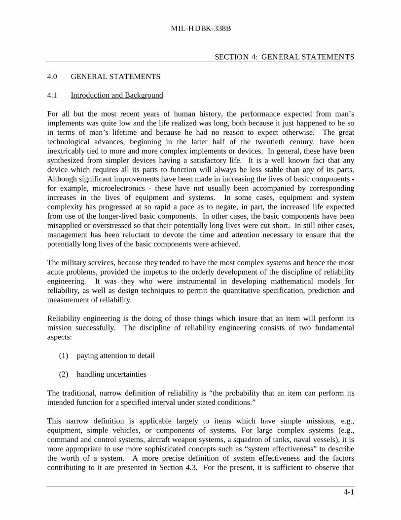
MIL-HDBK-338B

SECTION 4: GENERAL STATEMENTS

4-1

4.0 GENERAL STATEMENTS

4.1 Introduction and Background

For all but the most recent years of human history, the performance expected from man’simplements was quite low and the life realized was long, both because it just happened to be soin terms of man’s lifetime and because he had no reason to expect otherwise. The greattechnological advances, beginning in the latter half of the twentieth century, have beeninextricably tied to more and more complex implements or devices. In general, these have beensynthesized from simpler devices having a satisfactory life. It is a well known fact that anydevice which requires all its parts to function will always be less stable than any of its parts.Although significant improvements have been made in increasing the lives of basic components -for example, microelectronics - these have not usually been accompanied by correspondingincreases in the lives of equipment and systems. In some cases, equipment and systemcomplexity has progressed at so rapid a pace as to negate, in part, the increased life expectedfrom use of the longer-lived basic components. In other cases, the basic components have beenmisapplied or overstressed so that their potentially long lives were cut short. In still other cases,management has been reluctant to devote the time and attention necessary to ensure that thepotentially long lives of the basic components were achieved.

The military services, because they tended to have the most complex systems and hence the mostacute problems, provided the impetus to the orderly development of the discipline of reliabilityengineering. It was they who were instrumental in developing mathematical models forreliability, as well as design techniques to permit the quantitative specification, prediction andmeasurement of reliability.

Reliability engineering is the doing of those things which insure that an item will perform itsmission successfully. The discipline of reliability engineering consists of two fundamentalaspects:

(1) paying attention to detail

(2) handling uncertainties

The traditional, narrow definition of reliability is “the probability that an item can perform itsintended function for a specified interval under stated conditions.”

This narrow definition is applicable largely to items which have simple missions, e.g.,equipment, simple vehicles, or components of systems. For large complex systems (e.g.,command and control systems, aircraft weapon systems, a squadron of tanks, naval vessels), it ismore appropriate to use more sophisticated concepts such as “system effectiveness” to describethe worth of a system. A more precise definition of system effectiveness and the factorscontributing to it are presented in Section 4.3. For the present, it is sufficient to observe that

MIL-HDBK-338B


4-2

system effectiveness relates to that property of a system output which was the real reason forbuying the system in the first place - namely, the carrying out of some intended function. If thesystem is effective, it carries out this function well. If it is not effective, attention must befocused on those system attributes which are deficient.

4.2 The System Engineering Process

In recent years, the word “system” has come to include:

(1) The prime mission equipment

(2) The facilities required for operation and maintenance

(3) The selection and training of personnel

(4) Operational and maintenance procedures

(5) Instrumentation and data reduction for test and evaluation

(6) Special activation and acceptance programs

(7) Logistic support programs

System engineering is the application of scientific, engineering, and management effort to:

(1) Transform an operational need into a description of system performance parameters anda system configuration through the use of an iterative process of definition, synthesis,analysis, design, test, and evaluation.

(2) Integrate related technical parameters and assure compatibility of all physical,functional, and program interfaces in a manner that optimizes the total system design.

(3) Integrate reliability, maintainability, safety, survivability (including electronic warfareconsiderations), human factors, and other factors into the total engineering effort.

From the system management viewpoint, system engineering is but one of five major activitiesrequired to develop a system from Conceptual Exploration through the subsequent phases ofProgram Definition and Risk Reduction; Engineering and Manufacturing Development (EMD);and Production, Fielding/Deployment, and Operational Support. (These are the major phasesdefined in DoD 5000.2-R). These five activities (procurement and production, program control,configuration management, system engineering, and test and deployment management), must

MIL-HDBK-338B


4-3

perform their general functions within each of the system evolutionary phases, and theirrelationships to one another are summarized in Figure 4.2-1.

4.2.1 Systems Engineering and IPTs

Integrated Product Teams (IPTs) are a pragmatic means of implementing a true systemsengineering approach. As part of Defense Acquisition Reform (see Section 12), then Secretaryof Defense William Perry instituted the Integrated Product/Process Development (IPPD)approach to system acquisition. It is a systematic approach to the integrated, concurrent designof products and their related processes, including manufacturing and life cycle support. Essentialto the IPPD approach is the use of IPTs. These teams are multi-functional groups of individualswho manage and integrate critical processes.

All too often in the past, each phase of system acquisition was dominated by one functionalgroup. For example, during design, the design engineers were the primary “players.” Althoughsome interaction between the designers and other functional groups occurred, it did so in aniterative, serial fashion. Sometime prior to the beginning of production, the design was ìhandedoffî to the manufacturing organization which was supposed to design the processes needed toproduce the system. Also, after the design was “frozen,” the support community was given thetask of planning for the support of the system. This essentially sequential approach led toproblems of poor producibility, high manufacturing costs, slipped schedules, high supportrequirements, and so forth.

Efforts were made to solve this “stovepiping” of functions. In the late 1970’s, IntegratedLogistics Support Offices (ILSOs) were co-located with and as part of major system programoffices. One objective of these co-located ILSOs was to influence the design to enhance inherentsupportability. In the 1970’s and 1980’s, computer-aided design (CAD) and computer-aidedmanufacturing (CAM) were introduced as tools for linking the various functional disciplinestogether. With the advent of IPTs, however, came a multi-disciplined approach todecision-making. By empowering these IPTs to make decisions in a collaborative manner, many of theproblems of stovepiping are being overcome. Together with tools such as CAD/CAM, IPTs areproving to be an effective way of implementing the systems engineering concept and finding theoptimal balance among competing requirements under the constraints of cost and schedule.

4.2.2 The Four Steps of Systems Engineering

System engineering consists of four steps in an interacting cycle (Figure 4.2-2). Step 1 considersthreat forecast studies, doctrinal studies, probable military service tasks, and similar sources ofdesired materiel and system objectives; then it translates them into basic functional requirementsor statements of operation. The usual result of Step 1 is a set of block diagrams showing basicfunctional operations and their relative sequences and relationships. Even though hardware may

MIL-HDBK-338B


4-4

Tes

t&D

eplo

ymen

tP

lan

Tes

t&D

eplo

ymen

tM

anag

emen

t

Dev

elop

men

tal

and

Op

erat

iona

l

Det

aile

dD

esig

n

FAC

I*&

Det

ail

Spec

sfo

rC

EI*

*(S

yste

mC

on-

figu

rati

onB

asel

ine)

Syst

emP

rogr

amSc

hed

ule

s&

Allo

cati

ons

Dev

elop

men

tC

onst

ruct

ion

&P

rod

uct

ion

Con

trac

t

Des

ign

Req

uir

emen

tsB

asel

ine

Def

ined

Syst

emE

ngin

eeri

ngM

anag

emen

t

Gen

eral

Syst

emSp

ecs

for

Con

trac

tE

ndIt

ems

(CE

I)

Con

figu

rati

onM

anag

emen

t

Pre

limin

ary

Syst

emP

rogr

amP

lan

Pro

gram

Con

trol

Man

agem

ent

Pro

cure

men

tP

lan

Def

ine

Pro

gram

Bas

elin

es

Req

uir

emen

ts

Syst

emP

lann

ing

Tec

hnol

ogy

Det

erm

ine

Gen

eral

Obj

ecti

ves,

Feas

ibili

ty

Pro

cure

men

t&

Pro

du

ctio

nM

anag

emen

t

CO

NC

EP

TE

XP

LO

RA

TIO

N

Pro

du

ctio

n

Up

grad

eSy

stem

Eng

inee

ring

Pro

gram

Cha

nge

Req

ues

ts&

Mod

ific

atio

ns

Tra

nsit

ion

Agr

eem

ents

Follo

w-u

pP

rod

uct

ion

Syst

emin

Ope

rati

on

Dis

pos

itio

nof

Syst

em

PR

OG

RA

MD

EFI

NIT

ION

AN

DR

ISK

RE

DU

CT

ION

EN

GIN

EE

RIN

GA

ND

MA

NU

FAC

TU

RIN

GD

EV

EL

OP

ME

NT

PR

OD

UC

TIO

ND

EP

LO

YM

EN

T

*FA

CI=

Func

tion

alan

dC

onfi

gura

tion

Item

**C

EI=

Con

figu

rati

onE

ndIt

em

FIGURE 4.2-1: SYSTEM MANAGEMENT ACTIVITIES

MIL-HDBK-338B


4-5

help shape the basic system design, it is not specifically included in Step 1. Step 1 is intended toform a first hypothesis as a start toward the eventual solution.

In Step 2, the first hypothesis is evaluated against constraints such as design, cost, and time andagainst specific mission objectives to create criteria for designing equipment, definingintersystem interfaces, defining facilities, and determining requirements for personnel, training,training equipment and procedures.

Step 3 consists of system design studies that are performed concurrently with Steps 2 and 4 to:

(1) Determine alternate functions and functional sequences

(2) Establish design personnel, training and procedural data requirements imposed by thefunctions

(3) Find the best way to satisfy the mission requirements

(4) Select the best design approach for integrating mission requirements into the actualhardware and related support activities

Normally, the studies in Step 3 involve tradeoffs where data are in the form of schematic blockdiagrams, outline drawings, intersystem and intrasystem interface requirements, comparativematrices, and data supporting the selection of each approach. Some of the scientific tools used inthe system design studies in Step 3 are: probability theory, statistical inference, simulation,computer analysis, information theory, queuing theory, servomechanism theory, cybernetics,mathematics, chemistry, and physics.

Step 4 uses the design approach selected in Step 3 to integrate the design requirements from Step2 into the Contract End Items (CEI’s). The result of Step 4 provides the criteria for detaileddesign, development, and test of the CEI based upon defined engineering information andassociated tolerances. Outputs from Step 4 are used to:

(1) Determine intersystem interfaces

(2) Formulate additional requirements and functions that evolve from the selected devicesor techniques

(3) Provide feedback to modify or verify the system requirements and functional flowdiagrams prepared in Step 1

MIL-HDBK-338B


4-6

Ste

p1

Tra

nsl

ate

Sys

tem

Req

uir

eme

nts

into

Fu

nct

ion

alR

equi

rem

ents

Ste

p2

An

aly

zeF

un

ctio

ns

&T

ran

sla

tein

toR

eq

uri

em

en

tsfo

rD

esi

gn

,F

aci

litie

s,P

ers

on

ne

l,T

rain

ing

,&

Prc

edu

res

Ste

p4

Inte

gra

teR

equ

irem

ents

into

Co

ntra

ctE

ndite

ms,

trai

ning

&T

ech

nic

alP

roce

dur

es

Ste

p3

Sys

tem

/De

sig

nE

ng

ine

eri

ng

Tra

deo

ffS

tudi

esto

Det

erm

ine

Re

qu

irem

en

ts&

De

sig

nA

ppr

oach

FIGURE 4.2-2: FUNDAMENTAL SYSTEM PROCESS CYCLE

MIL-HDBK-338B


4-7

When the first cycle of the system engineering process is completed, the modifications,alternatives, imposed constraints, additional requirements, and technological problems that havebeen identified are recycled through the process with the original hypothesis (initial design) tomake the design more practical. This cycling is continued until a satisfactory design is produced,or until available resources (time, money, etc.) are expended and the existing design is accepted,or until the objectives are found to be unattainable.

Other factors that are part of the system engineering process - such as reliability, maintainability,safety, and human factors - exist as separate but interacting engineering disciplines and providespecific inputs to each other and to the overall system program. Pertinent questions at this pointmight be: “How do we know when the design is adequate?” or “How is the effectiveness of asystem measured?” The answers to these questions lead to the concept of system effectiveness.

4.3 System Effectiveness

System effectiveness is a measure of the ability of a system to achieve a set of specific missionrequirements. It is a function of readiness (or availability), and mission success (ordependability).

Cost and time are also critical in the evaluation of the merits of a system or its components, andmust eventually be included in making administrative decisions regarding the purchase, use,maintenance, or discard of any equipment or system.

The operational effectiveness of a system obviously is influenced by the way the equipment wasdesigned and built. It is, however, just as influenced by the way the equipment is used andmaintained; i.e., system effectiveness is influenced by the designer, production engineer,maintenance man, and user/operator. The concepts of availability and dependability illustratethese influences and their relationships to system operational effectiveness. The following are thedefinitions of these concepts:

(1) Availability - A measure of the degree to which an item is in an operable andcommittable state at the start of a mission, when the mission is called for at an unknown(random) time.

(2) Dependability - A measure of the degree to which an item is operable and capable ofperforming its required function at any (random) time during a specified missionprofile, given item availability at the start of the mission. (This definition issignificantly different than the definition of dependability used by most other US andinternational organizations dealing with reliability e.g., the InternationalElectrotechnical Commission (IEC) and the Society of Automotive Engineers (SAE).The IEC defines Dependability in publication IEC 50 Chapter 191 as: “The collectiveterm used to describe the availability performance and its influencing factors: reliability

MIL-HDBK-338B


4-8

performance, maintaintability performance and maintenance support performance.” Assuch, its use is restricted to general descriptions in non-quantitative terms).

Dependability is related to reliability; the intention was that dependability would be a moregeneral concept then reliability.

4.3.1 R/M Considerations in System Effectiveness

From a system effectiveness viewpoint, reliability and maintainability jointly provide systemavailability and dependability. Increased reliability directly contributes to system uptime, whileimproved maintainability reduces downtime. If reliability and maintainability are not jointlyconsidered and continually reviewed, serious consequences may result. With military equipment,failures or excessive downtime can jeopardize a mission and possibly cause a loss of lives.Excessive repair time and failures also impose burdens on logistic support and maintenanceactivities, causing high costs for repair parts and personnel training, expenditure of many man-hours for actual repair and service, obligation of facilities and equipment to test and service, andto movement and storage of repair parts.

From the cost viewpoint, reliability and maintainability must be evaluated over the system lifecycle, rather than merely from the standpoint of initial acquisition. An effective design approachto reliability and maintainability can reduce the cost of upkeep.

Both reliability and maintainability are important considerations for the user of the system,although maintainability is probably more important from the point of view of most users.Although frequent system failures may be an annoyance, if each failure can be repaired in a veryshort time so that the system has a high availability, and the maintenance costs are reasonable,then the poor reliability may be acceptable. For example, if failures occur on the average ofevery fifteen minutes but can be repaired in a microsecond, at acceptable cost, the user will notbe too concerned. On the other hand, if repair of a failure takes hours or days, the user has a non-available weapon system which may have a significant effect on the operational commander’sreadiness posture.

4.4 Factors Influencing System Effectiveness

4.4.1 Equipment of New Design

A typical history of the development of a new equipment would reveal a number of interestingsteps in the progression from original concept to acceptable production model. These steps areparticularly marked if the equipment represents a technical innovation, i.e., if it “pushes the stateof the art” by introducing entirely new functions or by performing established functions in anentirely new way. Starting with a well- defined operational need, the research scientist, designer,reliability engineer, statistician, and production engineer all combine their talents to execute amultitude of operations leading to one ultimate objective: the production of an equipment that

MIL-HDBK-338B


4-9

will perform as intended, with minimum breakdowns and maximum speed of repair. All thismust be done at minimum cost and usually within an accelerated time schedule.

These program requirements are severe, to say the least. In order to meet them, manycompromises are required. One of the first of these compromises is often a sharp curtailment inthe basic research time allotted to the job of proving the feasibility of the new design. After onlybrief preliminary study, a pilot model of the equipment is built. With luck, it will work; but it islikely to be somewhat crude in appearance, too big and too heavy, not well-designed for massproduction, subject to frequent failure, and difficult to repair. Indeed, at this early stage in theprogram, it is quite possible that the first model might be incapable of working if it were takenout of the laboratory and subjected to the more severe stresses of field operation, whether this bemilitary or civilian. By the time this situation is corrected, the development program will haveincluded many design changes, part substitutions, reliability tests, and field trials, eventuallyculminating in a successful operational acceptance test.

Usually, it is not until the equipment appears to have some chance of reaching this ultimate goalof acceptance that attention is focused on reduction of the frequency of failure, thus providing theimpetus for a serious reliability effort. Experience has shown that this is unfortunate. Ideally,such an effort should begin immediately after the feasibility study, because some problems canbe eliminated before they arise, and others can be solved at an early development stage, whendesign modifications can be effected most easily and economically. Even with this early start,reliability will continue to be a primary problem in new equipment, especially when it is of noveldesign. Early neglect of reliability must be compensated for by extraordinary efforts at a laterperiod, because an equipment simply is not usable if it fails too frequently to permit suitablereliance on the likelihood of its operation when needed. Since such early neglect has beencommon in the past, reliability has received strong emphasis in the research designed to bringequipment performance characteristics up to satisfactory levels.

The description just given is generally applicable to the development of radically new equipment.However, when attention is directed to equipment in everyday use or to new equipment builtpredominantly on standard design principles and from well-tested parts, it becomes evident thateffectiveness is dependent not only on performance capabilities and reliability but also on anumber of other factors, including operational readiness, availability, maintainability, andrepairability. Definitions for these concepts are given in Section 3. From the definitions it canbe seen that they are all so interrelated that they must be viewed together and discussed, not asseparate concepts but within the framework of the overall system to which they contribute.

4.4.2 Interrelationships Among Various System Properties

The discussion above implies that it is probably not practicable to maximize all of the desirableproperties of a system simultaneously. Clearly, there are “tradeoff” relationships betweenreliability and system cost, between maintainability and system cost, between reliability andmaintainability, and between many other properties. It would be most helpful to have a

MIL-HDBK-338B


4-10

numerical scale of values for each of the several properties, and to have a multi-dimensional plotor chart showing the interrelationship among those values. Before such relationships can beobtained, it is first necessary to define in a precise and quantitative manner the properties withwhich we are concerned. The following outline is intended to show some of the factors whichmust be considered:

A. SYSTEM PERFORMANCE (DESIGN ADEQUACY)(1) Technical Capabilities

(a) Accuracy(b) Range(c) Invulnerability to countermeasures(d) Operational simplicity

(2) Possible Limitations on Performance(a) Space and weight requirements(b) Input power requirements(c) Input information requirements(d) Requirements for special protection against shock, vibration, low pressure,

and other environmental influences

B. OPERATIONAL READINESS(1) Reliability

(a) Failure-free operation(b) Redundancy or provision for alternative modes of operation

(2) Maintainability(a) Time to restore failed system to satisfactory operating status(b) Technical manpower requirements for maintenance(c) Effects of use-cycle on maintenance. (Can some maintenance be performed

when operational use of the system is not required?)(3) Logistic Supportability(4) Availability

C. SYSTEM COST(1) Development cost, and particularly development time, from inception to operational

capability(2) Production cost(3) Operating and operational support costs

MIL-HDBK-338B


4-11

4.5 Optimization of System Effectiveness

The optimization of system effectiveness is important throughout the system life cycle, fromconcept through the operation. Optimization is the balancing of available resources (time,money, personnel, etc.) against resulting effectiveness parameters (performance, operationalreadiness, etc.), until a combination is found that provides the most effectiveness for the desiredexpenditure of resources. Thus, the optimum system might be one that:

(1) Meets or exceeds a particular level of effectiveness for minimum cost, and/or

(2) Provides a maximum effectiveness for a given total cost

Optimization is illustrated by the flow diagram of Figure 4.5-1 which shows the optimizationprocess as a feedback loop consisting of the following three steps:

(1) Designing many systems that satisfy the operational requirements and constraints

(2) Computing resultant values for effectiveness and resources used

(3) Evaluating these results and making generalizations concerning appropriatecombinations of design and support factors, which are then fed back into the modelthrough the feedback loops

Optimization also can be illustrated by the purchase of a new car or, more specifically, by puttinginto precise, quantifiable terms the rule, or criteria, that will be followed in the automobileselection process. Although automobiles do have quantifiable characteristics, such ashorsepower, cost, and seating capacity, they are basically similar in most cars of a particular class(low-price sedans, sports models, etc.). Thus the selection criteria essentially reduces to estheticappeal, prior experience with particular models, and similar intangibles. In the same sense, thechoice of best design for the weapon system is greatly influenced by experience with goodengineering practices, knowledge assimilated from similar systems, and economics. Despite thisfuzziness, the selection criteria must be adjusted so that:

(1) The problem size can be reduced to ease the choice of approaches

(2) All possible alternatives can be examined more readily and objectively for adaptation tomathematical representation and analysis

(3) Ideas and experiences from other disciplines can be more easily incorporated into thesolution

(4) The final choice of design approaches can be based on more precise, quantifiable terms,permitting more effective review and revision, and better inputs for future optimizationproblems

MIL-HDBK-338B


4-12

NO

TE

EFF

EC

TA

TH

IGH

ER

EC

HE

LO

NS

MA

TH

EM

AT

ICS/

PRO

BA

BIL

ITY

STA

TIS

TIC

S/O

PER

AT

ION

SR

ESE

AR

CH

/E

CO

NO

MIC

SE

NG

INE

ER

ING

/C

OM

PUT

AT

ION

MA

KE

FIN

AL

DE

CIS

ION

MO

DIF

YFO

RN

ON

-QU

AN

TIF

IAB

LE

FAC

TO

RS

&E

FFE

CT

SA

TH

IGH

ER

EC

HE

LO

NS

GE

NE

RA

LIZ

ER

ESU

LT

S

APP

LY

MO

DE

L

OB

TA

INA

PPR

OPR

IAT

ED

AT

A

SEL

EC

TA

PPR

OPR

IAT

EO

PTIM

IZA

TIO

NT

EC

HN

IQU

E

TE

STM

OD

EL

&R

EV

ISE

IDE

NT

IFY

RE

QU

IRE

DD

AT

AIN

PUT

S

CO

NST

RU

CT

OV

ER

AL

LE

FFE

CT

IVE

NE

SS&

CO

STM

OD

EL

S

ASS

UM

PTIO

NSC

ON

STR

UC

TO

PTIM

IZA

TIO

NC

RIT

ER

ION

GE

NE

RA

TE

AN

OV

ER

AL

LD

ESI

GN

AL

TE

RN

AT

IVE

DO

ES

DE

SIG

NM

EE

TO

PER

AT

ION

AL

RE

QU

IRE

ME

NT

S&

CO

NST

RA

INT

S?

IDE

NT

IFY

NO

N-Q

UA

NT

IFIA

BL

EFA

CT

OR

SID

EN

TIF

YU

NC

ER

TA

INT

IES

CO

NST

RU

CT

SUB

-MO

DE

LS

QU

AN

TIF

YC

ON

STR

AIN

TS

SEL

EC

TSU

ITA

BL

EM

EA

SUR

ES

OF

CO

ST&

EFF

EC

TIV

EN

ESS

TR

AN

SLA

TE

INT

OO

PER

AT

ION

AL

RE

QU

IRE

ME

NT

SPL

AC

ED

ON

SYST

EM

&SU

PPO

RT

FAC

TO

RS

DE

TE

RM

INE

SYST

EM

/R

ESO

UR

CE

INT

ER

FAC

E

DE

FIN

EG

EN

ER

AL

MIS

SIO

NPR

OFI

LE

DE

FIN

EO

PER

AT

ION

AL

&R

ESO

UR

CE

BO

UN

DS

DE

FIN

ESY

STE

MB

OU

ND

S

DE

FIN

EO

BJE

CT

IVE

S/SY

STE

MR

EQ

UIR

EM

EN

TS

STE

P1

NO

YE

S

STE

P2

STE

P3

IDE

NT

IFY

FIX

ED

&V

AR

IAB

LE

FAC

TO

RS

FIGURE 4.5-1: FLOW DIAGRAM FOR A GENERAL OPTIMIZATION PROCESS

MIL-HDBK-338B


4-13

The choice of parameters in the optimization model also is influenced by system definition. Theautomobile purchaser, for example, may not consider the manufacturer’s and dealer’s servicepolicies. If these policies are considered, the system becomes the automobile plus the servicepolicies. If service policies are not considered, the system consists only of the automobile.

The optimization of system effectiveness is a highly complex problem; there is a degree ofinteraction among the factors which enter into consideration of this problem. The actualtechniques used to optimize system effectiveness will be described in greater detail in Section 10of this handbook. Table 4.5-1, for example, lists only some of the more commonly-usedtechniques. These techniques are not peculiar to system effectiveness optimization, nor are theylimited to system engineering.

This section is an introduction to the Handbook from a top level, or system, viewpoint. Theremaining sections of this Handbook will expand upon the concepts introduced in this chapter.They will cover: (1) the basic reliability/maintainability/ availability theory, (2) practicalapplication of the theory in terms of the design methodology and procedures of reliabilityengineering at the equipment and system level, (3) procedures for insuring that inherentreliability is not degraded during production and field deployment of systems, and (4) steps thatmanagement must take to insure the acquisition and deployment of reliable systems at minimumlife cycle cost.

TABLE 4.5-1: PARTIAL LIST OF OPTIMIZATION TECHNIQUES

I. Mathematical Techniques II. Statistical TechniquesBirth and death processes Bayesian analysisCalculus of finite differences Decision theoryCalculus of variations Experimental designGradient theory Information theoryNumerical approximation Method of steepest ascentSymbolic logic Stochastic processesTheory of linear integralsTheory of maxima and minima

III. Programming Techniques IV. OtherDynamic programming Gaming theoryLinear programming Monte Carlo techniquesNonlinear programming Queuing theory

Renewal theorySearch theorySignal flow graphsValue theory

MIL-HDBK-338B


4-14


MIL-HDBK-338B

SECTION 5: RELIABILITY/MAINTAINABILITY/AVAILABILITY THEORY

5-1

5.0 RELIABILITY/MAINTAINABILITY/AVAILABILITY THEORY

5.1 Introduction

The language of engineering is mathematics. The theories behind each engineering specialty areconcisely stated in a set of mathematical procedures. For the engineering specialties ofreliability, availability and maintainability (RAM), the theories are stated in the mathematics ofprobability and statistics.

The underlying reason for the use of these concepts is the inherent uncertainty in predicting afailure. Even given a failure model based on physical or chemical reactions, the results will notbe the time a part will fail, but rather the time a given percentage of the parts will fail or theprobability that a given part will fail in a specified time. Individual parts will fail according totheir individual strengths, which will vary from part to part and are practically unknowable.Similarly, the time to repair a failure will also vary dependent on many factors whose values inindividual cases are practically unknowable.

Since RAM parameters must be defined in probabilistic terms, probabilistic parameters such asrandom variables, density functions, and distribution functions are utilized in the development ofRAM theory.

This section describes some of the basic concepts, formulas, and simple examples of applicationof RAM theory which are required for better understanding of the underlying principles anddesign techniques presented in later sections. Practicality rather than rigorous theoreticalexposition is emphasized. Many excellent texts are available (see references) for the reader whois interested in delving into the rigorous theoretical foundations of these disciplines.

5.2 Reliability Theory

Because, as was mentioned previously, reliability is defined in terms of probability, probabilisticparameters such as random variables, density functions, and distribution functions are utilized inthe development of reliability theory. Reliability studies are concerned with both discrete andcontinuous random variables. An example of a discrete variable is the number of failures in agiven interval of time. Examples of continuous random variables are the time from partinstallation to failure and the time between successive equipment failures.

The distinction between discrete and continuous variables (or functions) depends upon how theproblem is treated and not necessarily on the basic physical or chemical processes involved. Forexample, in analyzing “one shot” systems such as missiles, one usually utilizes discrete functionssuch as the number of successes in “n” launches. However, whether or not a missile issuccessfully launched could be a function of its age, including time in storage, and could,therefore, be treated as a continuous function.

MIL-HDBK-338B


5-2

5.2.1 Basic Concepts

The cumulative distribution function F(t) is defined as the probability in a random trial that therandom variable is not greater than t (see note), or

F(t) = −∞

t

∫ f(t) dt (5.1)

where f(t) is the probability density function of the random variable, time to failure. F(t) istermed the “unreliability function” when speaking of failure. It can be thought of as representingthe probability of failure prior to some time t. If the random variable is discrete, the integral isreplaced by a summation. Since F(t) is zero until t=0, the integration in Equation 5.1 can be fromzero to t.

NOTE: Pure mathematicians object to the use of the same letter in the integral and also inthe limits of the integral. This is done here, and in the rest of this section in spite of theobjection in order to simplify the reference to time as the variable in such functions as F(t),R(t), M(t), f(t), etc.

The reliability function, R(t), or the probability of a device not failing prior to some time t, isgiven by

R(t) = 1 - F(t) = t

∞

∫ f(t) dt (5.2)

By differentiating Equation (5.2) it can be shown that

-dR(t)dt = f(t) (5.3)

The probability of failure in a given time interval between t1 and t2 can be expressed by the

reliability function

t 1

∞

∫ f(t) dt -

t 2

∞

∫ f(t) dt = R(t1 ) - R(t2 ) (5.4)

The rate at which failures occur in the interval t1 to t2 , the failure rate, λ(t), is defined as the

ratio of probability that failure occurs in the interval, given that it has not occurred prior to t1, thestart of the interval, divided by the interval length. Thus,

MIL-HDBK-338B


5-3

λ(t) = R(t1) - R(t2)

(t2 - t1) R(t1) (5.5)

or the alternative form

λ(t) = )(

)()(ttR

ttRtR∆

∆+− (5.6)

where t = t1 and t2 = t + ∆t. The hazard rate, h(t), or instantaneous failure rate, is defined as

the limit of the failure rate as the interval length approaches zero, or

h(t) =

∆

∆+−→∆ )(

)()(lim

ttRttRtR

t 0

= -1

R(t)

dR(t)dt =

1R(t)

-dR(t)dt (5.7)

But it was previously shown, Eq. (5.3), that

f(t) = -dR(t)

dt

Substituting this into Eq. (5.7) we get h(t) = f(t)R(t) (5.8)

This is one of the fundamental relationships in reliability analysis. For example, if one knowsthe density function of the time to failure, f(t), and the reliability function, R(t), the hazard ratefunction for any time, t, can be found. The relationship is fundamental and important because itis independent of the statistical distribution under consideration.

The differential equation of Eq. (5.7) tells us, then, that the hazard rate is nothing more than ameasure of the change in survivor rate per unit change in time.

Perhaps some of these concepts can be seen more clearly by use of a more concrete example.

Suppose that we start a test at time, t0 , with NO devices. After some time t, Nf of the original

devices will have failed, and NS will have survived (NO = Nf + Ns ). The reliability, R(t), is

given at any time t, by:

MIL-HDBK-338B


5-4

R(t) = NSNO

(5.9)

= NO - Nf

NO = 1 -

NfNO

(5.10)

From Eq. (5.3)

f(t) = - dR(t)

dt = 1

NO dNfdt (5.11)

Thus, the failure density function represents the proportion of the original population, (NO),which fails in the interval (t, t + ∆t).

On the other hand, from Eqs. (5.8), (5.9) and (5.11)

h(t) =

f(t)R(t)

=

1NO

dNfdt

NS/NO = 1

NS dNfdt (5.12)

Thus, h(t) is inversely proportional to the number of devices that survive to time t, (Ns ), which

fail in the interval (t, t + ∆t).

Although, as can be seen by comparing Eqs. (5.6) and (5.7), failure rate, λ(t), and hazard rate,h(t), are mathematically somewhat different, they are usually used synonymously in conventionalreliability engineering practice. It is not likely that this handbook will change firmly entrenchedconventional practice, so the reader should be aware of this common deviation from exactmathematical accuracy.

Perhaps the simplest explanation of hazard and failure rate is made by analogy. Suppose a familytakes an automobile trip of 200 miles and completes the trip in 4 hours. Their average rate was50 mph, although they drove faster at some times and slower at other times. The rate at anygiven instant could have been determined by reading the speed indicated on the speedometer atthat instant. The 50 mph is analogous to the failure rate and the speed at any point is analogousto the hazard rate.

In Eq. (5.8), a general expression was derived for hazard (failure) rate. This can also be done forthe reliability function, R(t). From Eq. (5.7)

MIL-HDBK-338B


5-5

h(t) = - 1

R(t)

dR(t)dt (5.13)

dR(t)R(t) = - h(t) dt

Integrating both sides of Eq. (5.13)

0

t

∫dR(t)R(t)

= -

0

t

∫ h(t) dt

ln R(t) - ln R(0) = - 0

t

∫ h(t) dt

but R(0) = 1, ln R(0) = 0, and

R(t) = exp

−0

t

∫ h(t)dt

(5.14)

Eq. (5.14) is the general expression for the reliability function. If h(t) can be considered aconstant failure rate (λ), which is true for many cases for electronicequipment, Eq. (5.14) becomes

R(t) = e tλ− (5.15)

Eq. (5.15) is used quite frequently in reliability analysis, particularly for electronic equipment.However, the reliability analyst should assure himself that the constant failure rate assumption isvalid for the item being analyzed by performing goodness of fit tests on the data. These arediscussed in Section 8.

In addition to the concepts of f(t), h(t), λ(t), and R(t), previously developed, several other basic,commonly-used reliability concepts require development. They are: mean-time-to-failure(MTTF), mean life (θ), and mean-time-between-failure (MTBF).

MIL-HDBK-338B


5-6

Mean-Time-To-Failure (MTTF)

MTTF is nothing more than the expected value of time to failure and is derived from basicstatistical theory as follows:

MTTF = 0

∞

∫ t f(t) dt

= 0

∞

∫ t

-

dR(t)dt dt (5.16)

Integrating by parts and applying “Hopital's rule,” we arrive at the expression

MTTF = 0

∞

∫ R(t) dt (5.17)

Eq. (5.17), in many cases, permits the simplification of MTTF calculations. If one knows (or canmodel from the data) the reliability function, R(t), the MTTF can be obtained by directintegration of R(t) (if mathematically tractable), by graphical approximation, or by Monte Carlosimulation. For repairable equipment MTTF is defined as the mean time to first failure.

Mean Life (θ)

The mean life (θ) refers to the total population of items being considered. For example, given aninitial population of n items, if all are operated until they fail, the mean life (θ) is merely thearithmetic mean time to failure of the total population given by:

θ = i=1

n∑ t i

n(5.18)

where:ti = time to failure of the ith item in the population

n = total number of items in the population

Mean-Time-Between-Failure (MTBF)

This concept appears quite frequently in reliability literature; it applies to repairable items inwhich failed elements are replaced upon failure. The expression for MTBF is:

MIL-HDBK-338B


5-7

MTBF = T(t)

r (5.19)

where:T(t) = total operating timer = number of failures

It is important to remember that MTBF only has meaning for repairable items, and, for that case,MTBF represents exactly the same parameter as mean life (θ). More important is the fact that aconstant failure rate is assumed. Thus, given the two assumptions of replacement upon failureand constant failure rate, the reliability function is:

R(t) = e tλ− = e t /− = e-t/MTBF (5.20)

and (for this case)

λ =1

MTBF (5.21)

Figure 5.2-1 provides a convenient summary of the basic concepts developed in this section.

Failure Density Function(time to failure) f(t)

Reliability Function R(t) =

t

∞

∫ f(t) dt = exp

−0

t

∫ h(t)dt

Hazard Rate

(Failure Rate)

h(t) = f(t)/R(t)

λ(t) = 0

t

∫ h(t) dt

Mean Time to Failure (MTTF)(no repair)

MTTF = 0

∞

∫ R(t) dt

Mean Time Between Failure(constant failure rate, λ, with repair)

MTBF =

T(t)r

= 1/λ

FIGURE 5.2-1: SUMMARY OF BASIC RELIABILITY CONCEPTS

MIL-HDBK-338B


5-8

5.3 Statistical Distributions Used in Reliability Models

There are many standard statistical distributions which may be used to model the variousreliability parameters. It has been found that a relatively small number of statistical distributionssatisfies most needs in reliability work. The particular distribution used depends upon the natureof the data, in each case. The following is a short summary of some of the distributions mostcommonly used in reliability analysis, criteria for their use, and examples of application. Figures5.3-1 and 5.3-2 are summaries of the shape of common failure density, reliability, and hazard ratefunctions for the distributions described. Each distribution will be described in more detail, withreliability examples, in the following sections.

5.3.1 Continuous Distributions

5.3.1.1 Normal (or Gaussian) Distribution

There are two principal applications of the normal distribution to reliability. One applicationdeals with the analysis of items which exhibit failure due to wear, such as mechanical devices.Frequently the wear-out failure distribution is sufficiently close to normal that the use of thisdistribution for predicting or assessing reliability is valid.

Another application is in the analysis of manufactured items and their ability to meetspecifications. No two parts made to the same specification are exactly alike. The variability ofparts leads to a variability in systems composed of those parts. The design must take this partvariability into account, otherwise the system may not meet the specification requirement due tothe combined effect of part variability. Another aspect of this application is in quality controlprocedures.

The basis for the use of normal distribution in this application is the central limit theorem whichstates that the sum of a large number of identically distributed random variables, each with finitemean and variance, is normally distributed.

Thus, the variations in value of electronic component parts, for example, due to manufacturingare considered normally distributed.

The failure density function for the normal distribution is

f(t) = 1

s 2p e

−

12

(t − µ

σ)

2

, where − ∞ < t < ∞ (5.22)

MIL-HDBK-338B


5-9

t

f(t)

2e

1

σ 2š√f(t) =

NORMAL

EXPONENTIAL

GAMMA

WEIBULL

LOGNORMAL

TYPE OFDISTRIBUTION

PROBABILITY DENSITY FUNCTION, f(t)

RELIABILITY FUNCTION R(t) = 1 - f(t)

HAZARD FUNCTION

f(t) = λ e−λt

t

R(t) = e−λt

t

h(t) = λ = θ

t

-1

t

R(t) = 1 - φ lnσ

(t) - µ( )

t

h(t) = f(t)

1 - φ lnσ

(t) - µ( )

t

t

R(t) = 1 - φ t - µσ( )

lnσ

(t) - µ( )2e

1

σ t (2š)f(t) =

t

f(t)

f(t)

f(t) = (λt) e-λtΓ(α)

α -1λ

t

α = 2α = 1

α = 0.5

f(t)

t

α = 0.5α = 1

α = 2

R(t) = e-λt dtα-1tα

Γ(α)λ

h(t) =tα-1e-λt

tα-1e-λtdt∞∫

t

α = 1

α = 0.5

α = 2

t

h(t)

t

t

t

β = 3β = 1

β = 0.5

f(t)

R(t

)R

(t)

R(t

)R

(t)

R(t

)

h(t)

h(t)

h(t)

h(t)

h(t) =f(t)R(t)

f(t) =βη

t- γ

ηβ -1

e

t- γβ

η

-R(t) = e

(t- )

ηγ β

- h(t) =

βη

t-

ηγ β−1

β = 1

β = 0.5

β = 3β = 3

β = 0.5β = 1

- 12

t

∞∫

See Note

h(t) = f(t)

1 - φσ

t - µ( )See Note

t - µσ( )- 1

2

Note: φ

σµ-t ln

(lognormal) and φ

σµ-t

(normal) is the standardized form of these distributions and is equal to the integral of the pdfs

for those distributions (i.e., the cumulative distribution function).

FIGURE 5.3-1: SHAPES OF FAILURE DENSITY, RELIABILITY AND HAZARD RATEFUNCTIONS FOR COMMONLY USED CONTINUOUS DISTRIBUTIONS

MIL-HDBK-338B


5-10

0 2 4 6 8

0.2

0.4

0.6

0.8

1.0

UNITS OF X10 12

TYPE OFDISTRIBUTION

PARAMETERSPROBABILITY DENSITY

FUNCTIONf(x)

RELIABILITY FUNCTIONR(x) = 1 - F(t)

BINOMIAL

POISSON

MEAN, µ = np

Standard Deviation,

σ = npq

n

x =n!

(n-x)!x!

MEAN, µ = a,

Standard Deviation,

σ = a = λt

R(x) = ∑i=x

n

n

i pi qn-i

n=8

p=2/3

f(x) =

n

x px

qn-x

n=8

p=2/3

f(x) =axe -a

x!

= (λt)xe -λt

x!

a = λt = 4

R(x) = ∑i=x

aie -a

i!

= ∑i=x

∞(λt)xe -λt

x!

a = λt = 4

0 2 4 6 8

0.2

0.4

0.6

0.8

1.0

UNITS OF X

f(x)

0 2 4 6 8

0.2

0.4

0.6

0.8

1.0

UNITS OF X

R(x)

0 2 4 6 8

0.2

0.4

0.6

0.8

1.0

UNITS OF X1210

R(x)f(x)

q = 1 - p

Sample data usedto plot charts shown

Sample data used toplot charts shown

∞

FIGURE 5.3-2: SHAPES OF FAILURE DENSITY AND RELIABILITY FUNCTIONS OFCOMMONLY USED DISCRETE DISTRIBUTIONS

MIL-HDBK-338B


5-11

where:µ = the population meanσ = the population standard deviation, which is the square root of the

variance

For most practical applications, probability tables for the standard normal distribution are used(See Table 5.3-1). The standard normal distribution density function is given by

f(z) = 12p

exp

- z2

2 (5.23)

where:µ = 0

σ2 = 1

One converts from the normal to standard normal distribution by using the transformations

z = σ

µ−t(5.24)

f(t) = σ

)(zf(5.25)

F(t) = P[t ≤ t] = −∞

t

∫1

σ 2πexp[−

12

(t − µ

σ)2]dt (5.26)

R(t) = 1 - F(t) (5.27)

where:F(t) is the cumulative distribution functionR(t) is the reliability function

This integral cannot be evaluated in closed form; however, using the transformations in equations5.24 and 5.25 along with Table 5.3-2, the probabilities for any normal distribution can bedetermined.

MIL-HDBK-338B


5-12

TABLE 5.3-1: VALUES OF THE STANDARD NORMAL DISTRIBUTION FUNCTION

φ(t) =

−∞

z

∫12π

e - 12 z

2

dz = P(Z ≤ z)

z 0 1 2 3 4 5 6 7 8 9

-3.0 .0013 .0010 .0007 .0005 .0003 .0002 .0002 .0001 .0001 .0000

-2.9 .0019 .0018 .0017 .0017 .0016 .0016 .0015 .0015 .0014 .0014

-2.8 .0026 .0025 .0024 .0023 .0023 .0022 .0021 .0021 .0020 .0019

-2.7 .0035 .0034 .0033 .0032 .0031 .0030 .0029 .0028 .0027 .0026

-2.6 .0047 .0045 .0044 .0043 .0041 .0040 .0039 .0038 .0037 .0036

-2.5 .0062 .0060 .0059 .0057 .0055 .0054 .0052 .0051 .0049 .0048

-2.4 .0082 .0080 .0078 .0075 .0073 .0071 .0069 .0068 .0066 .0064

-2.3 .0107 .0104 .0102 .0099 .0096 .0094 .0091 .0089 .0087 .0084

-2.2 .0139 .0136 .0132 .0129 .0126 .0122 .0119 .0116 .0113 .0110

-2.1 .0179 .0174 .0170 .0166 .0162 .0158 .0154 .0150 .0146 .0143

-2.0 .0228 .0222 .0217 .0212 .0207 .0202 .0197 .0192 .0188 .0183

-1.9 .0287 .0281 .0274 .0268 .0262 .0256 .0250 .0244 .0238 .0233

-1.8 .0359 .0352 .0344 .0336 .0329 .0322 .0314 .0307 .0300 .0294

-1.7 .0446 .0436 .0427 .0418 .0409 .0401 .0392 .0384 .0375 .0367

-1.6 .0548 .0537 .0526 .0516 .0505 .0495 .0485 .0475 .0465 .0455

-1.5 .0668 .0655 .0643 .0630 .0618 .0606 .0594 .0582 .0570 .0559

-1.4 .0808 .0793 .0778 .0764 .0749 .0735 .0722 .0708 .0694 .0681

-1.3 .0968 .0951 .0934 .0918 .0901 .0885 .0869 .0853 .0838 .0823

-1.2 .1151 .1131 .1112 .1093 .1075 .1056 .1038 .1020 .1003 .0985

-1.1 .1357 .1335 .1314 .1292 .1271 .1251 .1230 .1210 .1190 .1170

-1.0 .1587 .1562 .1539 .1515 .1492 .1469 .1446 .1423 .1401 .1379

-.9 .1841 .1814 .1788 .1762 .1736 .1711 .1685 .1660 .1635 .1611

-.8 .2119 .2090 .2061 .2033 .2005 .1977 .1949 .1922 .1894 .1867

-.7 .2420 .2389 .2358 .2327 .2297 .2266 .2236 .2206 .2177 .2148

-.6 .2743 .2709 .2676 .2643 .2611 .2578 .2546 .2514 .2483 .2451

-.5 .3085 .3050 .3015 .2981 .2946 .2912 .2877 .2843 .2810 .2776

-.4 .3446 .3409 .3372 .3336 .3300 .3264 .3228 .3192 .3156 .3121

-.3 .3821 .3783 .3745 .3707 .3669 .3632 .3594 .3557 .3520 .3483

-.2 .4207 .4168 .4129 .4090 .4052 .4013 .3974 .3936 .3897 .3859

-.1 .4602 .4562 .4522 .4483 .4443 .4404 .4364 .4325 .4286 .4247

-.0 .5000 .4960 .4920 .4880 .4840 .4801 .4761 .4721 .4681 .4641

MIL-HDBK-338B


5-13

TABLE 5.3-2: ORDINATES F(z) OF THE STANDARD NORMAL CURVE AT z

z 0 1 2 3 4 5 6 7 8 90.0 .3989 .3989 .3989 .3988 .3986 .3984 .3982 .3980 .3977 .39730.1 .3970 .3965 .3961 .3956 .3951 .3945 .3939 .3932 .3925 .39180.2 .3910 .3902 .3894 .3885 .3876 .3867 .3857 .3847 .3836 .38250.3 .3814 .3802 .3790 .3778 .3765 .3752 .3739 .3725 .3712 .36970.4 .3683 .3668 .3653 .3637 .3621 .3605 .3589 .3572 .3555 .3538

0.5 .3521 .3503 .3485 .3467 .3448 .3429 .3410 .3391 .3372 .33520.6 .3332 .3312 .3292 .3271 .3251 .3230 .3209 .3187 .3166 .31440.7 .3123 .3101 .3079 .3056 .3034 .3011 .2989 .2966 .2943 .29200.8 .2897 .2874 .2850 .2827 .2803 .2780 .2756 .2732 .2709 .26850.9 .2661 .2637 .2613 .2589 .2565 .2541 .2516 .2492 .2468 .2444

1.0 .2420 .2396 .2371 .2347 .2323 .2299 .2275 .2251 .2227 .22031.1 .2179 .2155 .2131 .2107 .2083 .2059 .2036 .2012 .1989 .19651.2 .1942 .1919 .1895 .1872 .1849 .1826 .1804 .1781 .1758 .17361.3 .1714 .1691 .1669 .1647 .1626 .1604 .1582 .1561 .1539 .15181.4 .1497 .1476 .1456 .1435 .1415 .1394 .1374 .1354 .1334 .1315

1.5 .1295 .1276 .1257 .1238 .1219 .1200 .1182 .1163 .1145 .11271.6 .1109 .1092 .1074 .1057 .1040 .1023 .1006 .0989 .0973 .09571.7 .0940 .0925 .0909 .0893 .0878 .0863 .0848 .0833 .0818 .08041.8 .0790 .0775 .0761 .0748 .0734 .0721 .0707 .0694 .0681 .06691.9 .0656 .0644 .0632 .0620 .0608 .0596 .0584 .0573 .0562 .0551

2.0 .0540 .0529 .0519 .0508 .0498 .0488 .0478 .0468 .0459 .04492.1 .0440 .0431 .0422 .0413 .0404 .0396 .0387 .0379 .0371 .03632.2 .0355 .0347 .0339 .0332 .0325 .0317 .0310 .0303 .0297 .02902.3 .0283 .0277 .0270 .0264 .0258 .0252 .0246 .0241 .0235 .02292.4 .0224 .0219 .0213 .0208 .0203 .0198 .0194 .0189 .0184 .0180

2.5 .0175 .0171 .0167 .0163 .0158 .0154 .0151 .0147 .0143 .01392.6 .0136 .0132 .0129 .0126 .0122 .0119 .0116 .0113 .0110 .01072.7 .0104 .0101 .0099 .0096 .0093 .0091 .0088 .0086 .0084 .00812.8 .0079 .0077 .0075 .0073 .0071 .0069 .0067 .0065 .0063 .00612.9 .0060 .0058 .0056 .0055 .0053 .0051 .0050 .0048 .0047 .0046

3.0 .0044 .0043 .0042 .0040 .0039 .0038 .0037 .0036 .0035 .00343.1 .0033 .0032 .0031 .0030 .0029 .0028 .0027 .0026 .0025 .00253.2 .0024 .0023 .0022 .0022 .0021 .0020 .0020 .0019 .0018 .00183.3 .0017 .0017 .0016 .0016 .0015 .0015 .0014 .0014 .0013 .00133.4 .0012 .0012 .0012 .0011 .0011 .0010 .0010 .0010 .0009 .0009

3.5 .0009 .0008 .0008 .0008 .0008 .0007 .0007 .0007 .0007 .00063.6 .0006 .0006 .0006 .0005 .0005 .0005 .0005 .0005 .0005 .00043.7 .0004 .0004 .0004 .0004 .0004 .0004 .0003 .0003 .0003 .00033.8 .0003 .0003 .0003 .0003 .0003 .0002 .0002 .0002 .0002 .00023.9 .0002 .0002 .0002 .0002 .0002 .0002 .0002 .0002 .0001 .0001

MIL-HDBK-338B


5-14

The standardized cumulative distribution function is,

φ(t) = −∞

z

∫1

2πexp(−

z2

2)dz (5.28)

then for a normally distributed variable t, with mean µ and standard deviation σ

P(t ≤ t) = P (Z ≤

t − µσ

) = Φ (

t − µσ

) (5.29)

The hazard function for a normal distribution is a monotonically increasing function of t. Thiscan be shown by proving h’(t) ≥ 0 for all t.

5.3.2 Examples of Reliability Calculations Using the Normal Distribution

5.3.2.1 Microwave Tube Example

A microwave transmitting tube has been observed to follow a normal distribution with µ = 5000hours and σ = 1500 hours. Find the reliability of such a tube for a mission time of 4100 hoursand the hazard rate of one of these tubes at age 4400 hours.

R(t) = P

>

σu-t

z

R(4100) = P

z >

4100 - 50001500

= P ( z > -0.6 ) = 1 - P ( z < -0.6 )

= 1 - 0.27 = 0.73

as found in Table 5.3-1. Remember P ( z > -zi) = P ( z < zi) by symmetry of the normaldistribution.

h(t) = f(t)R(t) =

)(/)(tR

zf σ

f(t = 4400) = f

z =

4400 - 50001500

1500 = 1

1500 f (z = -0.4)

MIL-HDBK-338B


5-15

= (0.00067)(0.37) = 0.00025

where f(z = 0.4) was obtained from Table 5.3-2. Remember f(z)=f(-z) because of the symmetryof the normal distribution.

R(4400) = P

z >

4400 - 50001500 = P ( z > -0.4 ) = 1 - P ( z < -0.4 ) = 0.65

h(4400) =f(4400)R(4400) =

0.000250.65 = 0.00038 failures/hour

5.3.2.2 Mechanical Equipment Example

A motor generator has been observed to follow a normal distribution with µ = 300 hours and σ =40 hours. Find the reliability of the motor generator for a mission time (or time beforemaintenance) of 250 hours and the hazard rate at 200 hours.

R(250) = P

z >

250 - 30040 = P ( z > -1.25 )

= 1 - P ( z < -1.25 ) = 1 - 0.11 = 0.89

where P(z < -1.25) was interpolated from Table 5.3-1.

h(t) = f(t)R(t) =

)(/)(tR

zf σ

f (t = 200) = f

z =

200 - 30040

40 = 140 f (z= -2.5)

f ( z = -2.5 ) = (0.025)(0.0175) = 0.00044

where f (z = 2.5) was found in Table 5.3-2.

R(200) = P

z >

200 - 30040 = P (z > -2.5) = 1 - P (z < -2.5) = 0.994

h(200) = f(200)

R(200) = 0.00044

0.994 = 0.00044 failures/hour

MIL-HDBK-338B


5-16

5.3.3 Lognormal Distribution

The lognormal distribution is the distribution of a random variable whose natural logarithm isdistributed normally; in other words, it is the normal distribution with ln t as the variate. Thedensity function is

f(t) =

1σt 2π

exp

−−

2

2

1

σµ)(tln

for t ≥ 0 (5.30)

where the mean = exp

+

2

2σµ (5.31)

and the standard deviation = [ ] 2122 222/

)exp()exp( σµσµ +−+ (5.32)

where µ and σ are the mean and standard deviation (SD) of ln (t).

The lognormal distribution is used in reliability analysis of semiconductors and fatigue life ofcertain types of mechanical components. This distribution is also commonly used inmaintainability analysis and will be further discussed in Section 5.6.2.1.

The cumulative distribution function for the lognormal is,

F(t) = dtt

t

t

−−∫

2

0 2

1

2

1

σµ

πσ)(

expln

(5.33)

this can be related to the standard normal variant Z by

F(t) = [ ]

−≤=≤

σµt

ZPtPln

t (5.34)

the reliability function is 1-F(t) or

R(t) = ( )

−>=−

σµ)(

)(t

ZPtFln

1 (5.35)

MIL-HDBK-338B


5-17

the hazard function, h(t), is given as follows

h(t) = )(

)(

)()(

tRt

t

tRtf

σσ

µ

−∅

=

ln

(5.36)

where ∅ is the standard normal probability function and µ and σ are the mean and t standarddeviation of the natural logarithm of the random variable t.

5.3.3.1 Fatigue Failure Example

Suppose it has been observed that gun tube failures occur according to the lognormal distributionwith µ = 7 and σ = 2 (remember µ and σ are the mean and SD of the ln (t) data). Find thereliability for a 1000 round mission and the hazard rate at 800 rounds. For this case, the variablet is the number of rounds.

R(t) = P

−>

σµ)(t

zln

R(1000) = P

−>

02

071000

..)(ln

z = P ( z > -0.045 ) = 0.52

h(t) = f(t)R(t) =

)(/)(tR

tzf σ The numerator represents the trans-formation in the lognormal case.

h(800) = )(

)(800

800

tRf

σ=

)())((

)((

80080022

7800

R

zf−= ln

= f

z =

ln 800 - 72

(2)(800) P

z >

ln 800 - 72

= f ( z = -0.16)

1600 P (z > -0.16) = 0.3939

(1600)(0.5636) = 0.0004 failures/round

where P ( z > -0.16 ) was interpolated from Table 5.3-1 and f ( z = -0.16 ) was obtained fromTable 5.3-2.

5.3.4 Exponential Distribution

This is probably the most important distribution in reliability work and is used almost exclusivelyfor reliability prediction of electronic equipment (Ref. MIL-HDBK-217). It describes thesituation wherein the hazard rate is constant which can be shown to be generated by a Poisson

MIL-HDBK-338B


5-18

process. This distribution is valuable if properly used. It has the advantages of

(1) A single, easily estimated parameter ( λ)

(2) Is mathematically very tractable

(3) Has fairly wide applicability

(4) Is additive - that is, the sum of a number of independent exponentially distributedvariables is exponentially distributed

Some particular applications of this model include

(1) Items whose failure rate does not change significantly with age

(2) Complex and repairable equipment without excessive amounts of redundancy

(3) Equipment for which the early failures or "infant mortalities" have been eliminated by"burning in" the equipment for some reasonable time period

The failure density function is

f(t) = λe tλ− for t > 0, (5.37)

where λ is the hazard (failure) rate, and the reliability function is

R(t) = e tλ− (5.38)

the mean life (θ) = 1/λ, and, for repairable equipment, the MTBF = θ = 1/λ.

5.3.4.1 Airborne Fire Control System Example

The mean time to failure (MTTF = θ, for this case) of an airborne fire control system is 10 hours.What is the probability that it will not fail during a 3 hour mission?

R(3) = e tλ− = e θ/t− = e 103 /− = e 30.− = 0.74

5.3.4.2 Computer Example

A computer has a constant error rate of one error every 17 days of continuous operation. What isthe reliability associated with the computer to correctly solve a problem that requires 5 hourstime? Find the hazard rate after 5 hours of operation.

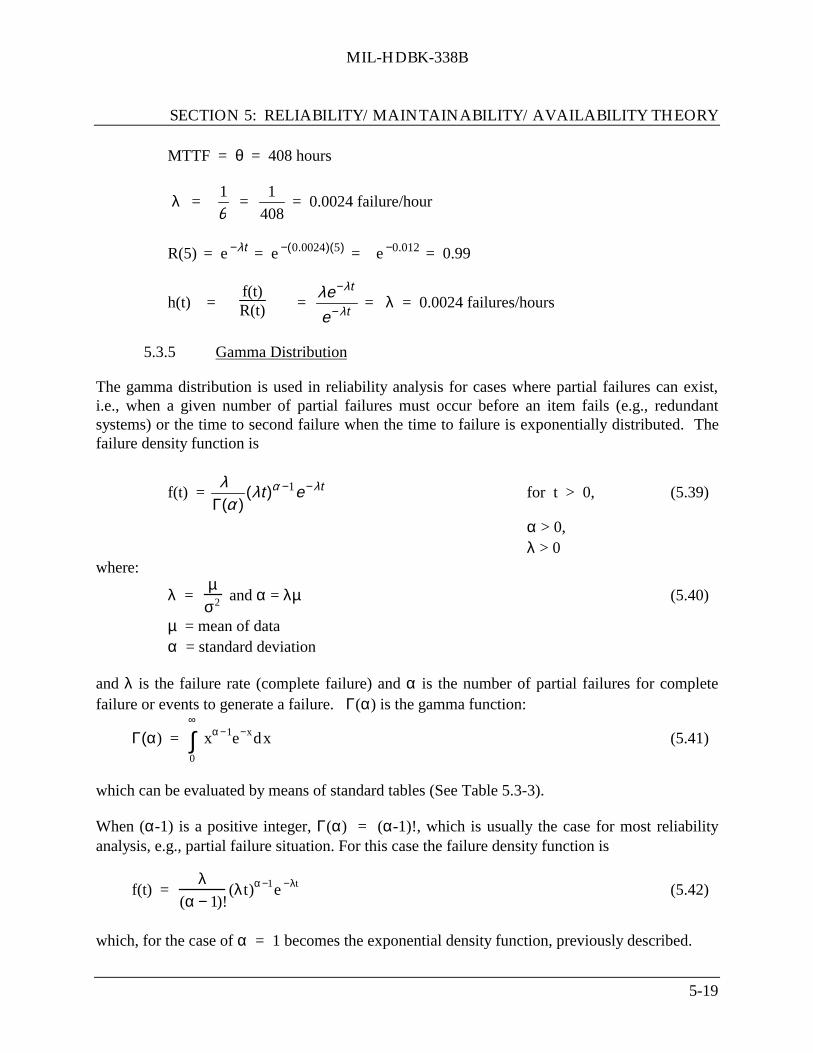
MIL-HDBK-338B


5-19

MTTF = θ = 408 hours

λ = θ1

= 408

1 = 0.0024 failure/hour

R(5) = e tλ− = e ))(.( 500240− = e 0120.− = 0.99

h(t) =f(t)R(t) =

t

t

e

eλ

λλ−

− = λ = 0.0024 failures/hours

5.3.5 Gamma Distribution

The gamma distribution is used in reliability analysis for cases where partial failures can exist,i.e., when a given number of partial failures must occur before an item fails (e.g., redundantsystems) or the time to second failure when the time to failure is exponentially distributed. Thefailure density function is

f(t) = tet λαλα

λ −−Γ

1)()(

for t > 0, (5.39)

α > 0,λ > 0

where:

λ =

µσ2 and α = λµ (5.40)

µ = mean of dataα = standard deviation

and λ is the failure rate (complete failure) and α is the number of partial failures for completefailure or events to generate a failure. Γ(α) is the gamma function:

Γ(α) = 0

∞

∫ xα−1e−xdx (5.41)

which can be evaluated by means of standard tables (See Table 5.3-3).

When (α-1) is a positive integer, Γ(α) = (α-1)!, which is usually the case for most reliabilityanalysis, e.g., partial failure situation. For this case the failure density function is

f(t) =

λ(α − 1)!

(λt)α−1e −λt (5.42)

which, for the case of α = 1 becomes the exponential density function, previously described.

MIL-HDBK-338B


5-20

TABLE 5.3-3: GAMMA FUNCTION Γ(n)

Γ(n) =

0

∞

∫ e-x Xn-1 dx

n Γ(n) n Γ(n) n Γ(n) n Γ(n)1.00 1.00000 1.25 .90640 1.50 .88623 1.75 .91961.01 .99433 1.26 .90440 1.51 .88659 1.76 .921371.02 .98884 1.27 .90250 1.52 .88704 1.77 .923761.03 .98355 1.28 .99072 1.53 .88757 1.78 .926231.04 .97844 1.29 .89904 1.54 .88818 1.79 .928771.05 .97350 1.30 .89747 1.55 .88887 1.80 .931381.06 .96874 1.31 .89600 1.56 .88964 1.81 .934081.07 .96415 1.32 .89464 1.57 .89049 1.82 .936851.08 .95973 1.33 .89338 1.58 .89142 1.83 .939691.09 .95546 1.34 .89222 1.59 .89243 1.84 .942611.10 .95135 1.35 1.89115 1.60 .89352 1.85 .945611.11 .94739 1.36 .89018 1.61 .89468 1.86 .948691.12 .94359 1.37 .88931 1.62 .89592 1.87 .951841.13 .93993 1.38 .88854 1.63 .89724 1.88 .955071.14 .93642 1.39 .88785 1.64 .89864 1.89 .958381.15 .93304 1.40 .88726 1.65 .90012 1.90 .961771.16 .92980 1.41 .88676 1.66 .90167 1.91 .965231.17 .92670 1.42 .88636 1.67 .90330 1.92 .968781.18 .92373 1.43 .88604 1.68 .90500 1.93 .972401.19 .92088 1.44 .88580 1.69 .90678 1.94 .976101.20 .91817 1.45 .88565 1.70 .90864 1.95 .979881.21 .91558 1.46 .88560 1.71 .91057 1.96 .983741.22 .91311 1.47 .88563 1.72 .91258 1.97 .987681.23 .91075 1.48 .88575 1.73 .91466 1.98 .991711.24 .90852 1.49 .88595 1.74 .91683 1.99 .99527

2.00 1.00000

Note: Γ(n+x) = (n - 1+x)(n - 2+x) . . . (1 + x) Γ(1 + x)e.g., Γ(3.15) = (2.15)(1.15) Γ(1.15)

MIL-HDBK-338B


5-21

F(t) = 0

t

∫λα

Γ(α)tα−1e −λtdt (5.43)

If α is an integer, it can be shown by integration by parts that

F(t) = k =α

∞

∑ (λt)k exp[−λt]K!

(5.44)

Then R(t) = 1 - F(t) = K =0

n −1

∑ (λt)k exp[−λt]K!

(5.45)

and h(t) =

f(t)R(t)

=

λα

Γ(α)tα−1e−λt

K =0

n −1

∑ (λt)K exp[−λt]K!

(5.46)

The gamma distribution can also be used to describe an increasing or decreasing hazard (failure)rate. When α > 1, h(t) increases; when α < 1, h(t) decreases. This is shown in Figure 5.3-1.

5.3.5.1 Missile System Example

An antiaircraft missile system has demonstrated a gamma failure distribution with α = 3 andλ = 0.05 (failures/hour). Determine the reliability for a 24 hour mission time and the hazard rateat the end of 24 hours.

R(t) =

λαΓ(α)

t

∞

∫ tα−1e −λtdt

Ordinarily, special tables of the Incomplete Gamma Function are required to evaluate the aboveintegral. However, it can be shown that if α is an integer

R(t) = k =0

α−1

∑ (λt)k e−λt

k!(5.47)

which later in the section will be shown to be a Poisson distribution. Using Eq. (5.47)

R(24) =

k=0

2∑ [(0.05)(24)]k e−(0.05)(24)

k! =

k=0

2∑ (1.2)k(0.3)

k!

MIL-HDBK-338B


5-22

= (0.3) + (1.2)(0.3) + (1.2)2 (0.3)

2 = 0.3 + 0.36 + 0.216 = 0.88

h(t) = f(t)R(t)

f(t) =

λ(α − 1)!

(λt)α−1e −λt

f(24) =

0.052

(1.2)2e −1.2 = (0.025)(0.434) = 0.011

h(24) =

f(24)R(24)

=

0.0110.88

= 0.012 failures/hour

5.3.6 Weibull Distribution

The Weibull distribution is particularly useful in reliability work since it is a general distributionwhich, by adjustment of the distribution parameters, can be made to model a wide range of lifedistribution characteristics of different classes of engineered items.

One of the versions of the failure density function is

f(t) =

βη

t − γη

β−1exp −

t − γη

β

(5.48)

where:β is the shape parameterη is the scale parameter or characteristic life

(life at which 63.2% of the population will have failed)γ is the minimum life

In most practical reliability situations, γ is often zero (failure assumed to start at t = 0) and thefailure density function becomes

f(t) =

βη

tη

β−1

exp −tη

β

(5.49)

MIL-HDBK-338B


5-23

and the reliability and hazard functions become

R(t) = exp

-

t

h b

(5.50)

h(t) =

b

h

t

h b-1

(5.51)

Depending upon the value of β, the Weibull distribution function can take the form of thefollowing distributions as follows,

β < 1 Gamma β = 1 Exponential

β = 2 Lognormal β = 3.5 Normal (approximately)

Thus, it may be used to help identify other distributions from life data (backed up by goodness offit tests) as well as being a distribution in its own right. Graphical methods are used to analyzeWeibull failure data and are described in Section 8.

5.3.6.1 Example of Use of Weibull Distribution

The failure times of a particular transmitting tube are found to be Weibull distributed with β = 2and η = 1000 hours. Find the reliability of one of these tubes for a mission time of 100 hours,and the hazard rate after a tube has operated successfully for 100 hours.

R(t) = exp

−

β

ηt

R(100) = exp

-

100

1000

2 = e

-(0.1)2 ≈ 0.99

h(100) =

βη

tη

β−1

=2

1000

1001000

2 −1

= 0.0002 failures/hour

MIL-HDBK-338B


5-24

5.3.7 Discrete Distributions

5.3.7.1 Binomial Distribution

The binomial distribution is used for those situations in which there are only two outcomes, suchas success or failure, and the probability remains the same for all trials. It is very useful inreliability and quality assurance work. The probability density function (pdf) of the binomialdistribution is

f(x) =

nx

pxq n−x( ) (5.52)

where

n

x = n!

(n-x)!x! and q = 1 - p (5.53)

f(x) is the probability of obtaining exactly x good items and (n-x) bad items in a sample of nitems where p is the probability of obtaining a good item (success) and q (or 1-p) is theprobability of obtaining a bad item (failure).

The cumulative distribution function (cdf), i.e., the probability of obtaining r or fewer successesin n trials, is given by

F(x; r) =

x=0

r∑

nx

pxqn−x (5.54)

5.3.7.1.1 Quality Control Example

In a large lot of component parts, past experience has shown that the probability of a defectivepart is 0.05. The acceptance sampling plan for lots of these parts is to randomly select 30 partsfor inspection and accept the lot if 2 or less defectives are found. What is the probability, P(a), ofaccepting the lot?

P(a) =

x=0

2∑

30x

(0.05)

x (0.95)

30-x

= 30!

0! 30! (0.05)0(0.95)30 + 30!

1! 29! (0.05)(0.95)29 + 30!

2! 28! (0.05)2(0.95)28

= 0.812

MIL-HDBK-338B


5-25

Note that in this example, the probability of success was the probability of obtaining a defectivepart.

5.3.7.1.2 Reliability Example

The binomial is useful for computing the probability of system success when the system employspartial redundancy. Assume a five channel VHF receiver as shown in Figure 5.3-3.

FIGURE 5.3-3: FIVE CHANNEL RECEIVER WITH TWO FAILURES ALLOWED

As long as three channels are operational, the system is classified as satisfactory. Thus, twochannel failures are allowed. Each channel has a probability of 0.9 of surviving a 24 houroperation period without failure. What is the probability that the receiver will survive a 24 hourmission without loss of more than two channels?

Letn = 5 = number of channelsr = 2 = number of allowable channel failuresp = 0.9 = probability of individual channel successq = 0.1 = probability of individual channel failurex = number of successful channelsP(S) = probability of system success

Then

P(S) =

x=3

n∑ n!

x!(n − x)!px qn-x

MIL-HDBK-338B


5-26

= 5!

3!2! (0.9)3 (0.1)2 + 5!

4!1! (0.9)4 (0.1)1 + 5!

5!0! (0.9)5 (0.1)0 = 0.99144

This is the probability that three or more of the five channels will survive the 24 hour operatingperiod.

The problem can be solved another way, by subtracting the probability of three or more failuresfrom one, e.g.:

P(S) = 1 - P(F)

= 1 - x=(r+1)

n

∑

n!n!(n − x)!

qx pn-x

= 1 -

5!

3!2! (0.1)3 (0.9)2 + 5!

4!1! (0.1)4 (0.9)1 + 5!

5!0! (0.1)5 (0.9)0

= 1 - 0.00856 = 0.99144 as before

Note the change in notation (only) that x now represents the number of failures and qx is the

probability of x failures whereas before x represented the number of successes and px was theprobability of x successes.

Computations involving the binomial distribution become rather unwieldy for even small samplesizes; however, complete tables of the binomial pdf and cdf are available in many statistics texts.

5.3.8 Poisson Distribution

This distribution is used quite frequently in reliability analysis. It can be considered an extensionof the binomial distribution when n is infinite. In fact, it is used to approximate the binomialdistribution when n ≥ 20 and p ≤ 0.05.

If events are Poisson distributed, they occur at a constant average rate and the number of eventsoccurring in any time interval are independent of the number of events occurring in any othertime interval. For example, the number of failures in a given time would be given by

f(x) = ax e-a

x! (5.55)

where x is the number of failures and a is the expected number of failures.

MIL-HDBK-338B


5-27

For the purpose of reliability analysis, this becomes

f(x; λ, t) = !

)(xet tx λλ −

(5.56)

where:λ = failure ratet = length of time being consideredx = number of failures

The reliability function, R(t), or the probability of zero failures in time t is given by:

R(t) =

(λt)0e−λt

0! = e tλ− (5.57)

or our old friend, the exponential distribution.

In the case of redundant equipments, the R(t) might be desired in terms of the probability of r orfewer failures in time t. For that case

R(t) =

x=0

r∑ (λt)x e−λt

x!(5.58)

5.3.8.1 Example With Permissible Number of Failures

A slide projector is needed for 500 hours of operation. Replacement of failed lamps is permitted,but there are only two spare bulbs on hand. If the lamp failure rate is 0.001 failures per hour,what is the reliability for the mission (i.e., the probability that no more than two lamp failureswill occur)?

λ = 0.001 t = 500 λt = 0.5 r ≤ 2

R(500) =

r=0

2∑ (0.5)re−0.5

r!

= e −0.5 + 0.5 e-0.5 + (0.5)2 e-0.5

2 = 0.986

MIL-HDBK-338B


5-28

5.4 Failure Modeling

Failure modeling is a key to reliability engineering. Validated failure rate models are essential tothe development of prediction techniques, allocation procedures, design and analysismethodologies, test and demonstration procedures/control procedures, etc. In other words, all ofthe elements needed as inputs for sound decisions to insure that an item can be designed andmanufactured so that it will perform satisfactorily and economically over its useful life.

Inputs to failure rate models are operational field data, test data, engineering judgment, andphysical failure information. These inputs are used by the reliability engineer to construct andvalidate statistical failure rate models (usually having one of the distributional forms describedpreviously) and to estimate their parameters.

5.4.1 Typical Failure Rate Curve

Figure 5.4-1 shows a typical time versus failure rate curve for equipment. This is the "bathtubcurve," which, over the years, has become widely accepted by the reliability community. It hasproven to be particularly appropriate for electronic equipment and systems. The characteristicpattern is a period of decreasing failure rate (DFR) followed by a period of constant failure rate(CFR), followed by a period of increasing failure rate (IFR).

TB = possible burn-in time TW = wear begins

FIGURE 5.4-1: HAZARD RATE AS A FUNCTION OF AGE

MIL-HDBK-338B


5-29

Zone I is the infant mortality (DFR) period characterized by an initially high failure rate. This isnormally the result of poor design, the use of substandard components, or lack of adequatecontrols in the manufacturing process. When these mistakes are not caught by quality controlinspections, an early failure is likely to result. Early failures can be eliminated from the customerby “burn in” during which time the equipment is operated at stress levels equal to the intendedactual operating conditions. The equipment is then released for actual use only when it haspassed through the “burn-in” period.

Zone II, the useful life period, is characterized by an essentially constant failure rate (CFR). Thisis the period dominated by chance failures. Chance failures are those failures that result fromstrictly random or chance causes. They cannot be eliminated by either lengthy burn-in periods orgood preventive maintenance practices. Equipment is designed to operate under certainconditions and up to certain stress levels. When these stress levels are exceeded due to randomunforeseen or unknown events, a chance failure will occur. While reliability theory and practiceis concerned with all three types of failures, its primary concern is with chance failures, sincethey occur during the useful life period of the equipment. Figure 5.4-1 is somewhat deceiving,since Zone II is usually of much greater length than Zones I or III. The time when a chancefailure will occur cannot be predicted; however, the likelihood or probability that one will occurduring a given period of time within the useful life can be determined by analyzing theequipment design. If the probability of chance failure is too great, either design changes must beintroduced or the operating environment made less severe.

This CFR period is the basis for application of most reliability engineering design methods.Since it is constant, the exponential distribution of time to failure is applicable and is the basisfor the design and prediction procedures spelled out in documents such as MIL- HDBK-217.

The simplicity of the approach utilizing the exponential distribution, as previously indicated,makes it extremely attractive. Fortunately, it is widely applicable for complex equipments andsystems. If complex equipment consists of many components, each having a different mean lifeand variance which are randomly distributed, then the system malfunction rate becomesessentially constant as failed parts are replaced.

Thus, even though the failures might be wearout failures, the mixed population causes them tooccur at random time intervals with a constant failure rate and exponential behavior. Figure 5.4-2 indicates this for a population of incandescent lamps in a factory. This has been verified formany equipments from electronic systems to bus motor overhaul rates.

MIL-HDBK-338B


5-30

10

100

50

M 2M 3M 4M 5M 6M 7M

NU

MB

ER

FA

ILIN

G

TOTAL NUMBER OF LAMPSFAILING PER DAY

Nλ = CONSTANT

M (MULTIPLES OF MTBF)

FIGURE 5.4-2: STABILIZATION OF FAILURE FREQUENCY

Zone III, the wearout period, is characterized by an IFR as a result of equipment deterioration dueto age or use. For example, mechanical components such as transmission bearings willeventually wear out and fail, regardless of how well they are made. Early failures can bepostponed and the useful life of equipment extended by good design and maintenance practices.The only way to prevent failure due to wearout is to replace or repair the deteriorating componentbefore it fails.

Since modern electronic equipment is almost completely composed of semi-conductor deviceswhich really have no short term wearout mechanism, except for perhaps electromigration, onemight question whether predominantly electronic equipment will even reach Zone III of thebathtub curve.

From Figure 5.4-1, it can be seen that different statistical distributions might be used tocharacterize each zone. For example, the infant mortality period might be represented by gammaor Weibull, the useful life period by the exponential, and the wearout period by gamma or normaldistributions.

The rest of this section will be devoted to models using the exponential distribution since it isapplicable during the useful life period, which is the longest period of an equipment’s life.

5.4.2 Reliability Modeling of Simple Structures

In this section, the reliability functions of some simple, structures will be derived. Thesefunctions are based upon the exponential distribution of time to failure.

MIL-HDBK-338B


5-31

5.4.2.1 Series Configuration

The simplest and perhaps most commonly occurring configuration in reliability mathematicalmodeling is the series configuration. The successful operation of the system depends on theproper functioning of all the system components. A component failure represents total systemfailure. A series reliability configuration is represented by the block diagram as shown in Figure5.4-3 with n components. Further, assume that the failure of any one component is statisticallyindependent of the failure or success of any other. This is usually the case for most practicalpurposes. If this is not the case, then conditional probabilities must be used, which only increasethe complexity of the calculations.

R (t)1 R (t)4R (t)2 R (t)3 R (t)n

FIGURE 5.4-3: SERIES CONFIGURATION

Thus, for the configuration of Figure 5.4-3, under the assumptions made, the series reliability isgiven by

RS(t) = R1(t) • R2(t) • R3(t) • . . . • Rn(t) =

i=1

n∏ Ri(t) (5.59)

If, as we said before, a constant failure rate, λ, is assumed for each component, which means theexponential distribution for the reliability function, then, is

RS(t) = e t1λ− • e t2λ− • . . . • e tnλ− = exp

−i =1

n∑ λit

= exp −λt[ ] (5.60)

where:

λ = λ1 + λ2 + . . . + λn = θ1

Thus, the system failure rate, λ, is the sum of the individual component failure rates and thesystem mean life, θ = 1/λ.

Consider a system composed of 400 component parts each having an exponential time to failuredensity function. Let us further assume that each component part has a reliability of 0.99 forsome time t. The system reliability for the same time t is

R(t) = 0.99400 = 0.018

Out of 1,000 such systems, 982 will be expected to fail by time t.

MIL-HDBK-338B


5-32

Remember for the case of component replacement upon failure,

MTBF = θ = λ1 , and, R = e-t/MTBF

The reader should keep in mind that, for the exponential distribution, the probability of survivingone MTBF without failure is

R = e-1 = 0.368 or 37%

5.4.2.2 Parallel Configuration

The next most commonly occurring configuration encountered in reliability mathematicalmodeling is the parallel configuration as shown in the reliability block diagram of Figure 5.4-4.

For this case, assuming all the components are operating “on-line,” for the system to fail, all of

the components would have to fail. Letting Qi = 1 - Ri = 1 - eλ it , the probability of failure

(or unreliability) of each component, the unreliability of the system would be given by

QS = Q1 • Q2 • . . . • Qn =

i=1

n∏ Qi (5.61)

And the reliability of the system would be

RS = 1 - QS (5.62)

since R + Q = 1

Consider such a system composed of five parallel components, each with a reliability of 0.99.Then

Qi = 1 - Ri = 1 - 0.99 = 0.01

QS = (0.01)5 = 10-10 = 0.0000000001

RS = 1 - QS = 0.9999999999

MIL-HDBK-338B


5-33

R1

R2

R3

Rn

FIGURE 5.4-4: PARALLEL CONFIGURATION

Thus, parallel configurations, or the use of redundancy, is one of the design procedures used toachieve extremely high system reliability, greater than the individual component reliabilities. Ofcourse, this is a very simple concept, which becomes more complicated in actual practice.Redundant equipment can be active (“on-line”) or turned off (“standby”), some redundant unitscan repaired without shutting down the system, others can not, and the number of repair crewscan vary. All these factors must be considered in formulating appropriate reliability models.Redundancy design techniques will be described in more detail in Section 7.

Most practical equipments and systems are combinations of series and parallel components asshown in Figure 5.4-5.

R = 0.82

A C

a

b

c

d

R = 0.77

R = 0.96R = 0.83 R = 0.84 R = 0.95

R = 0.91

FIGURE 5.4-5: COMBINED CONFIGURATION NETWORK

MIL-HDBK-338B


5-34

To solve this network, one merely uses the previously given series and parallel relationships todecompose and recombine the network step by step. For example,

Rad = R1 • R2 = (0.9)(0.8) = 0.72

Rbd = R3 • R4 • R5 = (0.8)(0.8)(0.9) = 0.576

but Rad and Rbd are in parallel; thus, the unreliability of this parallel subsystem (S1 ) is

QS1 = Qad • Qbd = (1 - Rad ) • (1 - Rbd )

= (1 - 0.72)(1 - 0.576) = (0.28)(0.424) = 0.119

and its reliability is

RS1 = 1 - QS1

= 1 - 0.119 = 0.88

Now the network has been decomposed to

.

R = 0.96

C

R = 0.77

R = 0.881S

A

Letting RS2 equal the combined reliability of RS1

and R6 in series

RS2 = RS1

• R6 = (0.88)(0.9) = 0.792

QS2 = 1 - RS2

= 1 - 0.792 = 0.208

Q7 = 1 - R7 = 1 - 0.7 = 0.3

MIL-HDBK-338B


5-35

Since QS2 and Q7 are in parallel, the total system unreliability is

QAC = QS2 • Q7 = (0.208)(0.3) = 0.06

and the total network reliability is

RAC = 1 - QAC = 1 - 0.06 = 0.94

thus, the reliability of the combined network is 0.94.

As the system network increases in complexity, the mathematics of system analysis becomesmore laborious and are best handled by computerized techniques.

5.4.2.3 K-Out-Of-N Configuration

A system consisting of n components or subsystems, of which only k need to be functioning forsystem success, is called a k-out-of-n configuration. For such a system, k is less than n. Anexample of such a system might be an air traffic control system with n displays of which k mustoperate to meet the system reliability requirement.

For the sake of simplicity, let us assume that the units are identical, they are all operatingsimultaneously, and failures are statistically independent.

Then,

R = reliability of one unit for a specified time periodQ = unreliability of one unit for a specified time period

and R + Q = 1

For n units

(R + Q)n = 1

(R + Q)n = Rn + nRn-1 Q + n(n-1)

2! Rn-2 Q2 + n(n-1)(n-2)Rn-3Q3

3!

+ . . . + Qn = 1

MIL-HDBK-338B


5-36

This is nothing more than the binomial expansion of (R + Q)n

Thus,

P [at least (n-1) surviving ] = Rn + nRn-1 Q

P [at least (n-2) surviving ] = Rn + nRn-1 Q + n(n-1)Rn-2Q2

2!

P [at least 1 surviving ] = 1 - Qn

Let us look at the specific case of four display equipments which meet the previously mentionedassumptions.

(R + Q)4 = R4 + 4R3 Q + 6R2 Q2 + 4RQ3 + Q4 = 1

from which

R4 = P(all four will survive)

4R3 Q = P(exactly 3 will survive)

6R2 Q2 = P(exactly 2 will survive)

4RQ3 = P(exactly 1 will survive)

Q4 = P(all will fail)

We are usually interested in k out of n surviving.

R4 + 4R3 Q = 1 - 6R2 Q2 - 4RQ3 - Q4 = P(at least 3 survive)

R4 + 4R3 Q + 6R2 Q2 = 1 - 4RQ3 - Q4 = P(at least 2 survive)

R4 + 4R3 Q + 6R2 Q2 + 4RQ3 = 1 - Q4 = P(at least 1 survives)

If the reliability of each display for some time t is 0.9, what is the system reliability for time t if 3out of 4 displays must be working?

RS = R4 + 4R3Q = (0.9)4 + 4(0.9)3(0.1) = 0.6561 + 0.2916 = 0.9477

MIL-HDBK-338B


5-37

A similar example would be the case of launching 4 missiles, each of which had a probability of0.9 of successfully hitting its target. What is the probability that at least 3 missiles will be ontarget? The procedure and result would be the same as the previous example.

For the case where all units have different reliabilities (or probabilities of success) the analysisbecomes more difficult for the same assumptions. Let us look at the case of three units withreliabilities of R1, R2, and R3, respectively. Then,

(R1 + Q1 )(R2 + Q2 )(R3 + Q3 ) = 1 (5.63)

The above equation can be expanded to permit analysis as was done for the previous case ofequal reliabilities. An easy way of bookkeeping is to set up Boolean truth tables where Ri = 1,Qi = 0, as follows:

1 2 30 0 0 Q1 Q2 Q3 = all three fail

0 0 1 Q1 Q2 R3 = 1 & 2 fail, 3 survives

0 1 0 Q1 R2 Q3 = 1 & 3 fail, 2 survives

0 1 1 Q1 R2 R3 = 1 fails, 2 & 3 survive

1 0 0 R1 Q2 Q3 = 2 & 3 fail, 1 survives

1 0 1 R1 Q2 R3 = 2 fails, 1 & 3 survive

1 1 0 R1 R2 Q3 = 3 fails, 1 & 2 survive

1 1 1 R1 R2 R3 = all three survive

For the previous example, if we are not interested in which particular unit fails, we can set upexpressions for at least 1, 2 or 3 units surviving. For example,

P(at least 2 units surviving) = R1 R2 R3 + R1 R2 Q3 + R1 Q2 R3 + Q1 R2 R3

The simple combinational reliability models developed in this section were, primarily, forillustrative purposes to demonstrate the basic theory involved. More complex examples areaddressed in the references at the end of this section and in Section 7.

5.5 Bayesian Statistics in Reliability Analysis

Bayesian statistics have been increasingly used in reliability analysis. The advantage to the useof Bayesian statistics is that it allows prior information (e.g., predictions, test results, engineeringjudgment) to be combined with more recent information, such as test or field data, in order toarrive at a prediction/assessment of reliability based upon a combination of all available data. Italso permits the reliability prediction/assessment to be continually updated as more and more test

MIL-HDBK-338B


5-38

data are accumulated. The Bayesian approach is intuitively appealing to design engineers becauseit permits them to use engineering judgment, based upon prior experience with similar equipmentdesigns, to arrive at an initial estimate of the reliability of a new design. It is particularly usefulfor assessing the reliability of new systems where only limited field data exists. For example, itcan be argued that the result of a reliability test is not only information available on a product,but that information which is available prior to the start of the test, from component andsubassembly tests, previous tests on the product, and even intuition based upon experience. Whyshould this information not be used to supplement the formal test result? Bayes’ Theorem can beused to combine these results.

Thus, the basic difference between Bayesian and non-Bayesian (classical) approaches is that theformer uses both current and prior data, whereas the latter uses current data only.

One of the main disadvantages to the use of the Bayesian approach is that one must be extremelycareful in choosing the prior probabilities based upon part experience or judgment. If these arecapriciously or arbitrarily chosen for Bayesian analysis, the end results of Bayesian analysis maybe inaccurate and misleading. Thus, the key to the successful use of the Bayesian method residesin the appropriate choice of prior probability distributions. An objective prior such as existingtest data is much better than a subjective prior based on opinion.

Bayes’ analysis begins by assigning an initial reliability on the basis of whatever evidence iscurrently available. The initial prediction may be based solely on engineering judgment or it maybe based on data from other similar types of items. Then, when additional test data issubsequently obtained, the initial reliabilities are revised on the basis of this data by means ofBayes’ Theorem. The initial reliabilities are known as prior reliabilities in that they are assignedbefore the acquisition of the additional data. The reliabilities which result from the revisionprocess are known as posterior reliabilities.

5.5.1 Bayes’ Theorem

From basic probability theory, Bayes’ Theorem is given by

Pr [A|B] = Pr [A] Pr [B|A]Pr [B] (5.64)

In the specific framework and context of reliability, the various terms in the equation may bemotivated and defined as follows:

A An hypothesis or statement of belief. (“The reliability of thiscomponent is 0.90.”)

B A piece of evidence, such as a reliability test result that has bearingupon the truth or credibility of the hypothesis. (“The component

MIL-HDBK-338B


5-39

failed on a single mission trial.”)

Pr [A] The prior probability: the probability we assign to the hypothesis Abefore evidence B becomes available. (“We believe, based onengineering experience, that there is a 50-50 chance that the reliabilityof this component is about 0.90, as opposed to some-thing drasticallylower, e.g., Pr [A] = 0.5.”)

Pr [B|A] The likelihood: the probability of the evidence assuming the truth ofthe hypothesis. (“The probability of the observed failure, given thatthe true component reliability is indeed 0.90, is obviously 0.10.”)

Pr [B] The probability of the evidence B, evaluated over the entire weightedensemble of hypotheses Ai

Pr [A|B] The posterior probability of A, given the evidence B

The posterior probability is the end result of the application of Bayes' Equation. The followingexamples illustrate the use of Bayesian statistics in reliability analysis.

5.5.1.1 Bayes' Example (Discrete Distribution)

To demonstrate the use of Bayes' Equation within the framework of the binomial estimation ofreliability, consider the following simplistic (but illustrative) example.

We wish to estimate the reliability of a simple pyrotechnic device which, upon being tested,either fires (success) or doesn't fire (failure). We have in the warehouse two lots of thiscomponent, one of which we have been assured has a reliability of R = 0.9 (that is, in the longterm, 9 of 10 randomly selected components will work). The other lot supposedly contains only50% good items. Unfortunately, we have lost the identity of which lot is which.

After randomly selecting one of the lots (such that the probability for each lot is 0.50), we thenrandomly select a single item from it (each item has equal chance of being chosen), which fails intest. What can be said about all this in the context of Bayesian analysis?

First, terms must be defined (see Figure 5.5-1).

A1 “Lot chosen has R = 0.50”

A2 “Lot chosen has R = 0.90”

MIL-HDBK-338B


5-40

Then, from above,

Pr [A1] = 0.5, Pr [A2] = 0.5.

P(A )1

1.0

0.5

0.50 0.90 1.0000

LOT FRACTION GOOD (=R)

FIGURE 5.5-1: SIMPLE PRIOR DISTRIBUTION

Next, the test evidence must be considered. Therefore

B “One unit was tested and it failed.”

The likelihoods required for Bayes' Equation are obviously

Pr[B|A1 ] = Pr[single test failure|R = 0.5] = (1 - 0.5) = 0.5

Pr[B|A2 ] = Pr[single test failure|R = 0.9] = (1 - 0.9) = 0.1

If A is partitioned into a set of states [A1 , ..., An ] and if Pr[Ai ] and Pr[B|Ai ] are known for

each i; then Eq. (5.64) becomes

Pr[Ai | B] = Pr[Ai ] ]Pr[]|Pr[

]|Pr[

ii

iAAB

AB•Σ

= Pr [Ai ] Pr[B|Ai]

Pr[B]

where the sum is over all n values of i. For this example, we have

Pr[B] = Pr[B|A1 ] Pr[A1 ] + Pr[B|A2 ] Pr[A2 ] = 0.5(0.5) + 0.1(0.5) = 0.30.

MIL-HDBK-338B


5-41

Finally, all necessary inputs having been obtained, Bayes’ Equation now yields

Pr[A1|B] = Pr[A1] Pr[B|A1]

Pr[B] = 0.5(0.5)

0.30 = 0.833,

Pr[A2|B] = Pr[A2] Pr[B|A2]

Pr[B] = 0.5(0.1)

0.30 = 0.167

The prior distribution in Figure 5.5-1 has been transformed, under the impact of a single trialresulting in failure, to the posterior distribution shown in Figure 5.5-2. The analyst may already besomewhat dubious that he has picked the lot with R = 0.9.

The process is usually a sequential one, i.e., as successive packets of new information (B1, B2,B3, ...) become available, the posterior degree of belief in proposition Ai is successively modifiedby each new increment of information.

1.0

0.5

0.50 0.90 1.0000

0.833

0.167

LOT FRACTION GOOD (=R)

P[A1|B]

P[A2|B]

FIGURE 5.5-2: SIMPLE POSTERIOR DISTRIBUTION

Another way of visualizing this situation is by constructing a tree diagram like the one shown inFigure 5.5-3, where the probability of the final outcome “B” is given by the products of theprobabilities corresponding to each individual branch.

MIL-HDBK-338B


5-42

.

B B

BB

P(A2 )

P(B|A )1

2P(B|A )

A1

A2

0.1

0.5

0.5

0.5

P(A 1)

FIGURE 5.5-3: TREE DIAGRAM EXAMPLE

P[B] = (0.5)(0.5) + (0.5)(0.1) = 0.3

P[A1|B] =

P[A1]P[B|A1]P[B]

= (0.5)(0.5)

(0.3) = 0.8333

P[A2|B] =

P[A2]P[B|A2]P[B]

= (0.5)(0.1)

(0.3) = 0.167

5.5.1.2 Bayes’ Example (Continuous Distribution)

As with the discrete example, the basic equation can be extended to cover continuous probabilitydistributions. For example, assume that based upon prior test results, engineering judgment, etc.it has been observed that r failures occur in time t. The probability density function of t is agamma distribution given by

f(λ) = )(

)(ret tr

Γ

−− λλ 1(5.65)

where:t is the amount of testing time (scale parameter)r is the number of failures (shape parameter)

From Section 5.3.5, we know that (note changes in notation)

0µ (mean failure rate) = shape parameter scale parameter =

rt (5.66)

and

20σ =

r

t2 (5.67)

MIL-HDBK-338B


5-43

Eqs. (5.64 and 5.65) represent the prior failure rate and the prior variance. Let us assume that

these are given by 0.02 and (0.01)2 , respectively. Assume that we then run a reliability test for500 hours (t’) and observe 14 failures (r’). What is the posterior estimate of failure rate?

The basic expression for the continuous posterior distribution is given by

f(λ|t) = f(l) f(t|l)

f(t) (5.68)

where:f(λ) is the prior distribution of λ, Eq. (5.65)

f(t|λ) is the sampling distribution of t based upon the new data

f(t) is

0

∞

∫ f(λ) f(t|λ) dλ

f(λ|t) is the posterior distribution of combining the prior distribution and the new data.

It can be shown that the posterior distribution resulting from performing the operations indicatedin Eq. (5.68) is

f(λ|t) = )’(

)]’(exp[)’( ’

rrtttt rr

+Γ+−+ −+ λλ 1

(5.69)

which is another gamma distribution with

shape parameter = (r + r’)

scale parameter = (t + t’)

Using Eqs. (5.66) and (5.67) to solve for r and t, we obtain

r = 0µ t = 20σ t

2

MIL-HDBK-338B


5-44

Therefore,

t =

^µ0^σ0

2 =

0.02

(0.01)2 =

2 x 10-2

1 x 10-4 = 200

r = ^µ0 t = (2 x 10-2 ) (200) = 4

Returning to the posterior gamma distribution, Eq. (5.69) we know that the posterior failure rateis

^µ1 =

shape parameter scale parameter =

(r+r’)(t+t’)

From the test data r’ = 14, t’ = 500, and we found that r = 4, and t = 200; thus

^µ1 =

4 + 14200 + 500 =

18700 = 0.0257

This compares with the traditional estimate of failure rate from the test result, 14/500 = 0.028.Thus, the use of prior information resulted in a failure rate estimate lower than that given by thetest results.

5.6 Maintainability Theory

In reliability, one is concerned with designing an item to last as long as possible without failure;in maintainability, the emphasis is on designing an item so that a failure can be repaired asquickly as possible. The combination of high reliability and high maintainability results in highsystem availability; the theory of which is developed in Section 5.7.

Maintainability, then, is a measure of the ease and rapidity with which a system or equipment canbe restored to operational status following a failure. It is a function of the equipment design andinstallation, personnel availability in the required skill levels, adequacy of maintenanceprocedures and test equipment, and the physical environment under which maintenance isperformed.

As with reliability, maintainability parameters are also probabilistic and are analyzed by the useof continuous and discrete random variables, probabilistic parameters, and statisticaldistributions. An example of a discrete maintainability parameter is the number of maintenanceactions completed in some time t, whereas an example of a continuous maintainability parameteris the time to complete a maintenance action.

MIL-HDBK-338B


5-45


A good way to look at basic maintainability concepts is in terms of functions which areanalogous to those in reliability. They may be derived in a way identical to that done forreliability in the previous section by merely substituting t (time-to-restore) for t (time-to-failure),µ (repair rate) for λ (failure rate), and M(t) (probability of successfully completing a repair actionin time t, or P(T ≤ t)) for F(t) (probability of failing by age t, or P(T ≤ t)). In other words, thefollowing correspondences prevail in maintainability and reliability engineering functions.

(1) The time-to-failure probability density function (pdf) in reliability corresponds to thetime-to-maintain pdf in maintainability.

(2) The failure rate function in reliability corresponds to the repair rate function inmaintainability. Repair rate is the rate with which a repair action is performed and isexpressed in terms of the number of repair actions performed and successfullycompleted per hour.

(3) The probability of system failure, or system unreliability, corresponds to the probabilityof successful system maintenance, or system maintainability. These and otheranalogous functions are summarized in Table 5.6-1.

Thus, as illustrated in Figure 5.6-1, maintainability can be expressed either as a measure of thetime (T) required to repair a given percentage (P%) of all system failures, or as a probability (P)of restoring the system to operational status within a period of time (T) following a failure.

Some of the commonly used maintainability engineering terms are portrayed graphically inFigure 5.6-2 as a maintainability “function” derived as illustrated for the case where the pdf has alognormal distribution. Points (1), (2), and (3) shown in the figure identify the mean, median,and maximum corrective time-to-repair, respectively.

MIL-HDBK-338B


5-46

TABLE 5.6-1: COMPARISON OF BASIC RELIABILITYAND MAINTAINABILITY FUNCTIONS

RELIABILITY MAINTAINABILITY

Time to Failure (pdf)

f(t)

Time to Repair (pdf)

g(t) (5.70)

Reliability

R(t) =

t

∞

∫ f(t) dt

Maintainability

M(t) =

0

t

∫ g(t) dt (5.71)

Failure Rate

λ(t) = f(t)R(t)

Repair Rate

µ(t) =

g(t)1− M(t)

(5.72)

Mean-Time-to-Failure

MTTF = −∞

∞

∫ tf(t) dt

=

0

∞

∫ R(t) dt

Mean Time to Repair

MTTR = −∞

∞

∫ t g(t) dt (5.73)

Pdf of Time to Failure

f(t) = λ(t) • R(t)

= λ(t) exp

−0

t

∫ λ(t)dt

Pdf of Time to Repair

g(t) = µ(t) ( )1 - M(t) (5.74)

= µ(t) exp

−0

t

∫ µ(t)dt

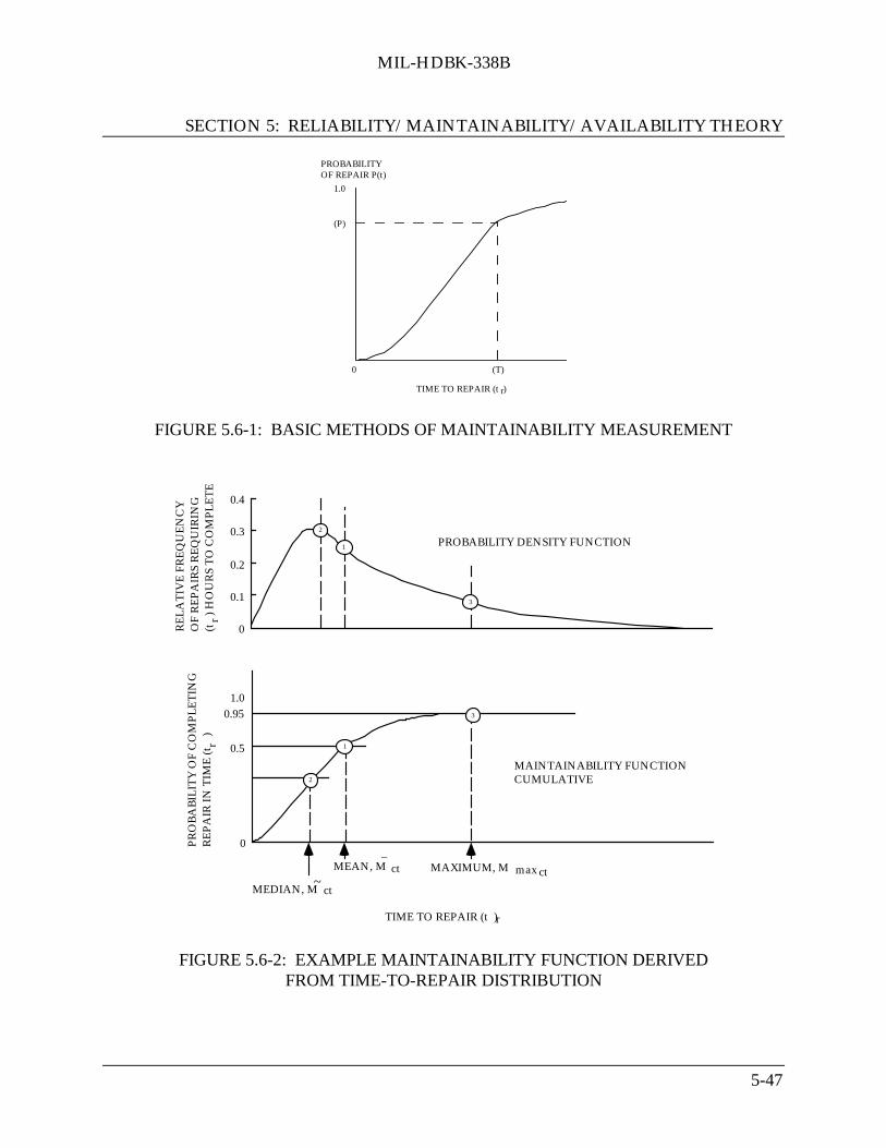
MIL-HDBK-338B


5-47

PROBABILITY OF REPAIR P(t)

TIME TO REPAIR (t )r

(P)

(T)0

1.0

FIGURE 5.6-1: BASIC METHODS OF MAINTAINABILITY MEASUREMENT

0

0.5

0.951.0

MAINTAINABILITY FUNCTION CUMULATIVE

TIME TO REPAIR (t )r

PR

OB

AB

ILIT

Y O

F C

OM

PL

ET

ING

R

EP

AIR

IN T

IME

(t

)r 1

2

3

MEDIAN, M ct~

ctMEAN, M ctMAXIMUM, M max_

0.4

0.3

0.2

0.1

0

PROBABILITY DENSITY FUNCTION

RE

LA

TIV

E F

RE

QU

EN

CY

O

F R

EP

AIR

S R

EQ

UIR

ING

(t

) H

OU

RS

TO

CO

MP

LE

TE

r

3

2

1

FIGURE 5.6-2: EXAMPLE MAINTAINABILITY FUNCTION DERIVEDFROM TIME-TO-REPAIR DISTRIBUTION

MIL-HDBK-338B


5-48

Points (1), (2), and (3) are defined as follows:

(1) Mean Time to Repair, M ct : The mean time required to complete a maintenance

action, i.e., total maintenance downtime divided by total maintenance actions for agiven period of time, given as

Mct = Σ(λi M cti

)

Σλi (5.75)

where: λi = failure rate for the ith repairable element of the item for which

maintainability is to be determined, adjusted for duty cycle,catastrophic failures, tolerance and inter-action failures, etc., whichwill result in deterioration of item performance to the point that amaintenance action will be initiated.

iM ct = average corrective time required to repair the ith repairable element

in the event of its failure.

(2) Median Time to Repair, ~Mct : The downtime within which 50% of all maintenance

actions can be completed.

(3) Maximum Time to Repair: The maximum time required to complete a specified, e.g.,95%, percentage of all maintenance actions.

These terms will be described in more detail in the following sections, in terms of the form thatthey take, given the statistical distribution of time-to-repair.

5.6.2 Statistical Distributions Used in Maintainability Models

A smaller number of statistical distributions is used for maintainability analysis than forreliability analysis. This may be due to the fact that maintainability has traditionally laggedreliability theory in development.

The most commonly used distributions for maintainability analysis have been the normal,lognormal, and exponential. Just as the exponential distribution has been the one most widelyused in reliability analysis of equipment/systems, the lognormal distribution is the mostcommonly used for equipment/system maintainability analysis. A number of studies havevalidated the lognormal as being the most appropriate for maintainability analysis (Ref. [25]).

MIL-HDBK-338B


5-49

However, use of other distributions such as the Weibull and gamma is also possible, dependingupon the analysis of the data and the use of “goodness of fit” tests.

Since the form and expressions for the more commonly used distributions were previously givenin Section 5.2.2, this section will concentrate on the use of the normal, exponential, andlognormal distribution, and give examples of their use in maintainability analysis.

5.6.2.1 Lognormal Distribution

This is the most commonly used distribution in maintainability analysis. It applies to mostmaintenance tasks and repair actions comprised of several subsidiary tasks of unequal frequencyand time duration.

The probability density function is given by

g(t = Mcti ) =

1Mcti

Sln Mct 2π exp

- 12

ln Mcti

- ln Mct

Sln Mct

2

(5.76)

= 1

tσt' 2π exp

- 12

t' - t'

σt' 2 (5.77)

where:t = Mcti

= repair time from each failure

ln Mct =

Σ ln MctiN

Sln Mct = σt' =

Σ ln Mcti

2 - (Σln Mcti

)2/N

N-1 (5.78)

Sln Mct =

Σti'

2 - (Σti')2/N

N-1 = standard deviation of ln of repair times.

t' = ln Mcti = ln t

MIL-HDBK-338B


5-50

t ’ = ln Mct = Σti’

N

N = number of repair actions (5.79)

The mean time to repair is given by

MTTR = Mct = t =

0

∞

∫ t g(t = Mcti ) dt (5.80)

(also see Eq. (5.76))

= exp ( )

+ 2

2

1ctct MSM lnln (5.81)

= exp t’ +

12

(σt’)2

(5.82)

The median time to repair is given by

~M

ct = t

( = antiln

Σλi ln Mct

Σλi (5.83)

= exp ( ln Mcti ) (5.84)

= exp ( t’ ) (5.85)

The maximum time to repair is given by

Mmaxct = tmax = antiln ( )ctct MSM lnln φ+ (5.86)

= antiln

t’ + z(t’1−α )σt ’[ ] (5.87)

MIL-HDBK-338B


5-51

where φ = z(t’1-α ) = value from normal distribution function corresponding to the percentage

point (1-α) on the maintainability function for which Mmaxct is defined.

Most commonly used values of φ or z(t’1-α ) are shown in Table 5.6-2.

TABLE 5.6-2: VALUES OF φ OR Z(T’(1-α)) MOST COMMONLY USED INMAINTAINABILITY ANALYSIS

1-α φ or Z(t’(1-α))

0.80 0.84160.85 1.0360.90 1.2820.95 1.6450.99 2.326

Following is an example of maintainability analysis of a system which has a lognormaldistribution of repair times.

5.6.2.1.1 Ground Electronic System Maintainability Analysis Example

Given the active repair times data of Table 5.6-3 on a ground electronic system find thefollowing:

(1) The probability density function, g(t)

(2) The MTTR of the system

(3) The median time to repair the system

(4) The maintainability function

(5) The maintainability for a 20 hour mission

(6) The time within which 90% and 95% of the maintenance actions are completed

(7) The repair rate, u(t), at 20 hours

MIL-HDBK-338B


5-52

TABLE 5.6-3: TIME-TO-REPAIR DATA ON A GROUND ELECTRONIC SYSTEM

Group No.j

Times to Repairtj (hr.)

Frequency of Observationnj

1 0.2 12 0.3 13 0.5 44 0.6 25 0.7 36 0.8 27 1.0 48 1.1 19 1.3 110 1.5 411 2.0 212 2.2 113 2.5 114 2.7 115 3.0 216 3.3 217 4.0 218 4.5 119 4.7 120 5.0 121 5.4 122 5.5 123 7.0 124 7.5 125 8.8 126 9.0 127 10.3 128 22.0 1

N’ = 29 24.5 1

MIL-HDBK-338B


5-53

1. Probability Density Function of g(t)

To determine the lognormal pdf of the times-to-repair given in Table 5.6-3, the values of t ’ and

σt’ should be calculated from

t ’=

nj t’jj =1

N’

∑

j =1

N’

∑ nj

(5.88)

where nj is the number of identical observations given in the third column of Table 5.6-3, N’ is

the number of different-in-value observed times-to-repair, or number of data groups, which forthis problem is N’ = 29, given in the second column of Table 5.6-3, and N is the total number ofobserved times-to-repair,

N = i=1

N’

∑ nj

which, for this example, is 46,

and

σt’ =

∑i=1

N (t’i)

2 - N( t ’)

2

N-1

12

=

∑j=1

N’ nj(t’j )

2 - N( t ’)

2

N-1

12

(5.89)

To facilitate the calculations, Table 5.6-4 was prepared. From Table 5.6-4, t ’ and σt’ , are

obtained as follows:

t’ =

j =1

N’

∑ njt’j

j=1

N ’

∑ nj

= 30.330439

46 = 0.65879

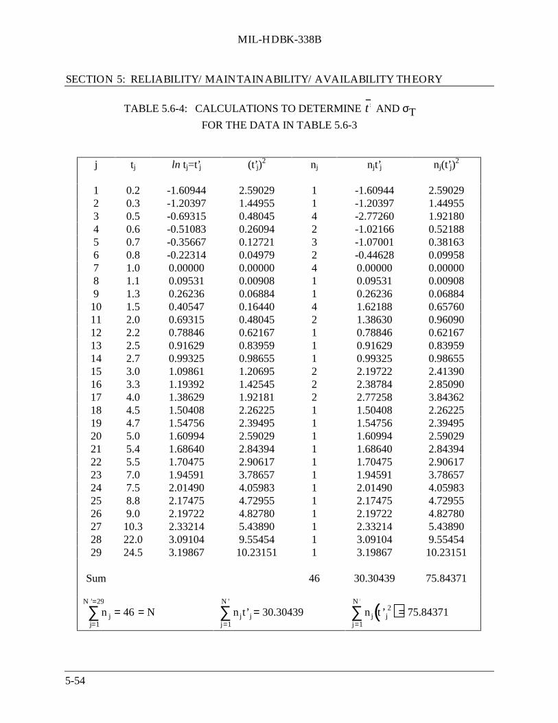
MIL-HDBK-338B


5-54

TABLE 5.6-4: CALCULATIONS TO DETERMINE t’ AND σT FOR THE DATA IN TABLE 5.6-3

j tj ln tj=t’j (t’j)2 nj njt’j nj(t’j)

2

1 0.2 -1.60944 2.59029 1 -1.60944 2.590292 0.3 -1.20397 1.44955 1 -1.20397 1.449553 0.5 -0.69315 0.48045 4 -2.77260 1.921804 0.6 -0.51083 0.26094 2 -1.02166 0.521885 0.7 -0.35667 0.12721 3 -1.07001 0.381636 0.8 -0.22314 0.04979 2 -0.44628 0.099587 1.0 0.00000 0.00000 4 0.00000 0.000008 1.1 0.09531 0.00908 1 0.09531 0.009089 1.3 0.26236 0.06884 1 0.26236 0.0688410 1.5 0.40547 0.16440 4 1.62188 0.6576011 2.0 0.69315 0.48045 2 1.38630 0.9609012 2.2 0.78846 0.62167 1 0.78846 0.6216713 2.5 0.91629 0.83959 1 0.91629 0.8395914 2.7 0.99325 0.98655 1 0.99325 0.9865515 3.0 1.09861 1.20695 2 2.19722 2.4139016 3.3 1.19392 1.42545 2 2.38784 2.8509017 4.0 1.38629 1.92181 2 2.77258 3.8436218 4.5 1.50408 2.26225 1 1.50408 2.2622519 4.7 1.54756 2.39495 1 1.54756 2.3949520 5.0 1.60994 2.59029 1 1.60994 2.5902921 5.4 1.68640 2.84394 1 1.68640 2.8439422 5.5 1.70475 2.90617 1 1.70475 2.9061723 7.0 1.94591 3.78657 1 1.94591 3.7865724 7.5 2.01490 4.05983 1 2.01490 4.0598325 8.8 2.17475 4.72955 1 2.17475 4.7295526 9.0 2.19722 4.82780 1 2.19722 4.8278027 10.3 2.33214 5.43890 1 2.33214 5.4389028 22.0 3.09104 9.55454 1 3.09104 9.5545429 24.5 3.19867 10.23151 1 3.19867 10.23151

Sum 46 30.30439 75.84371

n j = 46 = N

j=1

N ’=29

∑

nj t’j = 30.30439j =1

N’

∑

nj t ’j2( )= 75.84371

j =1

N’

∑

MIL-HDBK-338B


5-55

and from Eq. (5.89)

σt’ = 2

12

146

658790468437175

−

− ).(.= 1.11435

Consequently, the lognormal pdf representing the data in Table 5.6-3 is

g(t) = pts 2∋τ

1 exp

−−2

2

1

’

’’

t

ttσ

or

g(t) = pt 2).( 114351

1 exp

−−

2

114351

658790

2

1

..’t

where t’ = ln t. The plot of this pdf is given in Figure 5.6-3 in terms of the straight times inhours. See Table 5.6-5 for the g(t) values used.

The pdf of the ln t or of the t’ is

g(t’) = t

tσt’ 2π exp

−−2

2

1

’

’’

t

ttσ

= t g(t)

or

g(t’) = 1

(1.11435) 2π exp

−−

2

114351

658790

2

1

..’t

This pdf is that of a normal distribution which is what one should expect since if t follows alognormal distribution, ln t should be normally distributed. This is shown plotted in Figure5.6-3, the values of g(t’) were obtained from Table 5.6-5.

MIL-HDBK-338B


5-56

0

0.1

0.2

0.3

0.4

01

23

45

67

89

Probability Density, g(t)

Mod

e =

t =

0.5

584

Med

ian

= t

= 1

.932

Mea

n =

t =

3.5

95

Tim

e to

Res

tore

, t, H

ours

ˆ×

-

FIGURE 5.6-3: PLOT OF THE LOGNORMAL OF THE TIMES-TO-RESTORE DATAGIVEN IN TABLE 5.6-5 IN TERMS OF THE STRAIGHT t’s

MIL-HDBK-338B


5-57

TABLE 5.6-5: THE PROBABILITY DENSITY OF TIME-TO-REPAIR DATA(FROM TABLE 5.6.2.1.1-1 BASED ON THE STRAIGHT TIMES TO REPAIR AND

THE NATURAL LOGARITHM OF THE TIMES TO REPAIR USED TO PLOTFIGURES 5.6-3 AND 5.6-4, RESPECTIVELY.*)

Time to Probability Probabilityrestore, density, densityt hours g(t) g(t’) = g(ln t)

0.02 0.00398 7.95 x 10-50.1 0.10480 0.010480.2 0.22552 0.045100.3 0.29510 0.088530.5 0.34300 0.171500.7 0.33770 0.236361.0 0.30060 0.300601.4 0.24524 0.343341.8 0.19849 0.357282.0 0.17892 0.357842.4 0.14638 0.351303.0 0.11039 0.331183.4 0.09260 0.314834.0 0.07232 0.289294.4 0.06195 0.272585.0 0.04976 0.248806.0 0.03559 0.213517.0 0.02625 0.183738.0 0.01985 0.158849.0 0.01534 0.1380410.0 0.01206 0.1206120.0 0.00199 0.0397130.0 0.00058 0.0173340.0 --- 0.0088880.0 --- 0.00135

*At the mode, t = 0.5584, g(t ) = 0.34470 and g(t ') = 0.19247.

At the median, Ùt = 1.932, g(Ùt ) = 0.18530 and g(Ùt ') = 0.35800.

MIL-HDBK-338B


5-58

0

0.1

0.2

0.3

0.4

0.5

0.6

0.7

0.01 0.1 1 10 100

Time to Restore, t, hours

FIGURE 5.6-4: PLOT OF THE LOGNORMAL PDF OF THE TIMES-TO-RESTOREDATA GIVEN IN TABLE 5.6-5 IN TERMS OF THE

LOGARITHMS OF T, OR ln t’

MIL-HDBK-338B


5-59

2. MTTR (Mean Time to Repair) of the System

The mean time to repair of the system, t , is obtained from Eq. (5.83).

t = exp t’ +

12

(σt’)2

= exp

0.65879 +

12

(1.11435)2

= 3.595 hr.

3. Median Time to Repair

The median of the times-to-repair the system, Ùt , is obtained from Eq. (5.85)

Ùt = exp ( t ’) = e0.65879 = 1.932 hr.

This means that in a large sample of t’s, half of the t’s will have values smaller than Ùt , and the

other half will have values greater than Ùt . In other words, 50% of the repair times will be ≤ Ùt .

4. Maintainability Function M(t)

The maintainability of a unit can be evaluated as follows, using Eq. (5.71):

M(t1 ) =

0

t1

∫ g(t) dt =

−∞

t’1

∫ g(t’) dt’ =

−∞

z(t’1)

∫ φ(z) dz (5.90)

where t’ = ln t, (5.90a)

z(t’1 ) = t’1 - t ’

σt’ (5.90b)

and t ’ and σt’ are given by Eq. (5.88) and (5.91), respectively.

By means of the transformations shown in Eqs. (5.90a) and (5.90b), the lognormal distribution ofthe pdf of repair times, g(t), is transformed to the standard normal distribution φ(z) which enablesthe use of standard normal distribution tables (Table 5.3-3).

MIL-HDBK-338B


5-60

The maintainability function for the system, M(t), from (5.90) is:

M(t) =

−∞

z(t’)

∫ φ(z) dz

where:

z(t’) = t’ - t ’

σt’

t’ = ln t

From the data in Table 5.6-3 we previously calculated

t ’ = 0.65879

σt’ = 1.11435

The quantified M(t) is shown in Figure 5.6-5. The values were obtained by inserting values for t’= ln t into the expression,

z(t’) = t’ - 0.65879

1.11435

solving for z(t’), and reading the value of M(t) directly from the standard normal tables in Table5.3-3.

5. Maintainability for a 20 Hour Mission

M(20) =

−∞

z(ln20)

∫ φ(z) dz

where ln 20 = 2.9957

and

z(ln 20) = 2.9957 - 0.65879

1.111435 = 2.0972

MIL-HDBK-338B


5-61

0

0.2

0.4

0.6

0.81

01

23

45

67

89

Tim

e to

Res

tore

, t, h

ours

Maintainability, M(t)

FIGURE 5.6-5: PLOT OF THE MAINTAINABILITY FUNCTION FOR THETIMES-TO-REPAIR DATA OF EXAMPLE 2

MIL-HDBK-338B


5-62

From Table 5.3-3 we find that for z = 2.0972

M(20) =

−∞

2.0972

∫ φ(z) dz = 1 - 0.018 = 0.982 or 98.2%

6. The time within which 90% and 95% of the Maintenance Actions are Completed (Mmaxct)

This is the time t1-α for which the maintainability is 1-α , or

M(t1-α ) = P(t W1-α ) =

0

t1−α

∫ g(t) dt =

−∞

t ’1−α

∫ g(t’) dt’ =

−∞

z(t’1−α )

∫ φ(z) dz (5.91)

and

z(t’1-α ) = ’

’

t

t

σα ’t −−1 (5.92)

The commonly used maintainability, or (1- α), values are 0.80, 0.85, 0.90, 0.95, and 0.99.Consequently, the z(t’

1-α ) values which would be used most commonly would be those

previously given in Table 5.6-2. Using Eq. (5.92) the time t’1-α would then be calculated from

t’1-α = t ’ + z(t’

1-α ) • σt'

ort'

1-α = antiln (t'1-α ) = antiln [ ]’’(’ ttzt σα )+ −1 (5.93)

Thus, for 90% Mmaxct , from the previously obtained value of t ’ and σt'

t0.90 = antiln [ ]’. )’(’ ttzt σ900+ = antiln

+ ).(.. 1143512821658790

= antiln (2.08737) = 8.06 hrs.

MIL-HDBK-338B


5-63

For 95% Mmaxct

t0.95 = antiln

0.65879 + 1.645(1.11435)

= antiln (2.491896) = 12.08 hrs.

7. Repair Rate at t = 20 hours

Using Eq. (5.60) and substituting the values for g(20) from Table 5.6-5 and the previouslycalculated value for M(20)

µ(20) = g(20)

1 - M(20) = 0.001991 - 0.982 =

0.001990.018 = 0.11 repairs/hr.

5.6.2.2 Normal Distribution

The normal distribution has been adequately treated in Section 5.3.2.1 in the discussion onreliability theory. The same procedures and methodology apply for maintainability if one merelyuses repair time for t, mean repair time for µ, and standard deviation of repair times for σ.

In maintainability, the normal distribution applies to relatively straightforward maintenance tasksand repair actions (e.g., simple removal and replacement tasks) which consistently require a fixedamount of time to complete. Maintenance task times of this nature are usually normallydistributed, producing a probability density function given by

g(t = Mct ) = 1

SMct 2π exp

-(Mcti

- M ct)2

2(SMct)2 (5.94)

where:Mcti

= repair time for an individual maintenance action

M ct = Σ(Mcti

)

N = average repair time for N observations

SMct = Σ(Mcti - M ct)

2

N-1 = standard deviation of the distribution

of repair times, based on Nobservations

MIL-HDBK-338B


5-64

N = number of observations

The mean time to repair ( M ct ) is given by

M ct = ΣMcti

N (5.95)

The median time to repair (~Mct ) is given by

~Mct =

ΣMctiN (5.96)

which is equal to the mean time to repair because of the symmetry of the normal distribution (seeFig. 5.3-1).


Mmaxct = M ct + φ SMct (5.97)

where:φ = z(t1-α )

= value from normal distribution function corresponding to thepercentage point (1-α) on the maintainability function for whichMmaxct

is defined. Values of φ as a function of (1-α) are shown in

Table 5.6-6. Note that this is the same as Table 5.6-2 withrounded-off values.

MIL-HDBK-338B


5-65

TABLE 5.6-6: VALUES OF φ FOR SPECIFIED α

1-α φ or z(t1-α)

95% 1.6590% 1.2885% 1.0480% 0.84

5.6.2.2.1 Equipment Example

An equipment whose repair times are assumed to be normally distributed was monitored and thefollowing repair times were observed (in minutes):

6.5, 13.25, 17.25, 17.25, 19.75, 23, 23, 24.75, 27.5, 27.5, 27.5, 32, 34.75, 34.75,37.5, 37.5, 40.25, 42.5, 44.75, 52

Find the following parameters.

(1) The pdf of g(t) and its value at 30 minutes

(2) The MTTR and median times to repair

(3) The maintainability for 30 minutes

(4) The time within which 90% of the maintenance actions are completed

(5) The repair rate, u(t), at 30 minutes

(1) Pdf of g(t)

M ct = ΣMcti

N = 583.25

20 = 29.16 minutes

SMct = Σ(Mcti

- M ct)2

N-1

MIL-HDBK-338B


5-66

= Σ(Mcti

)2 - N( M ct)

2

N-1

=

19527 - 1700619

= 11.5 minutes

g(t) = p2511

1

. exp

−−

2

2

5112

1629

).(

).( ictM

g(30) = 8228

1

. exp

−−2

2

5112

162930

).(

).( =

128.82 e -0.0032

= (0.035)(0.9973) = 0.035

(2) MTTR and Median Time to Repair

These are the same for the normal distribution because of its symmetry, and are given by

M

ct = Σ Mcti

N = 58320 = 29.16 minutes

(3) Maintainability for 30 Minutes

M(30) =

−∞

30

∫ g(t) dt =

−∞

z(30)

∫ φ(z) dz

z(30) = Mcti

- M ct

SMct =

30 - 29.1611.5 =

0.8411.5 = 0.07

From the standard normal table (Table 5.3-3).

φ(0.07) = 1 - .4721 = 0.5279 = 0.53

∴ M(30) = 0.53 or 53% probability of making a repair in 30 minutes.

MIL-HDBK-338B


5-67

(4) Time within which 90% of the Maintenance Actions are completed

M0.9 = M ct + φSMct φ = 1.28 from Table 5.6-6

= 29.16 + (1.28)(11.5) = 43.88 minutes

(5) Repair Rate at 30 Minutes

µ(30) = g(30)

1 - M(30) = 0.035

1 - 0.53 = 0.0350.47 = 0.074 repairs/minute

5.6.2.3 Exponential Distribution

In maintainability analysis, the exponential distribution applies to maintenance tasks andmaintenance actions whose completion times are independent of previous maintenanceexperience (e.g., substitution methods of failure isolation where several equally likelyalternatives are available and each alternative is exercised, one at a time, until the one whichcaused the failure is isolated), producing a probability density function given by

g t = Mct( )= 1

M ct exp

−

MctiMct

(5.98)

The method used in evaluating the maintainability parameters is similar to that previously shownin Section 5.3.4 for analyzing reliability with exponential times-to-failure. The fundamental

maintainability parameter is repair rate, µ(t), which is the reciprocal of M ct , the mean-time-to-

repair (MTTR). Thus, another expression for g(t) in terms of µ(t), the repair rate, is

g(t) = µ e-µt (5.99)

where µ is the repair rate (which is constant for the exponential case).

The maintainability function is given by

M(t) =

0

t

∫ g(t) dt =

0

t

∫ µe -µt dt = 1 - e-µt (5.100)

MIL-HDBK-338B


5-68

The MTTR is given by

M ct = 1µ =

Σ MctiN (5.101)

If the maintainability function, M(t), is known, the MTTR can also be obtained from

MTTR = M ct = -t

ln[1 - M(t)] (5.102)

The median time to repair ~Mct is given by

~Mct = 0.69 M ct (5.103)


Mmaxct = ke M ct (5.104)

where:

ke = value of Mcti / M ct at the specified percentage point α

on the exponential function at which Mmaxct is defined.

Values of ke are shown in Table 5.6-7.

TABLE 5.6-7: VALUES OF ke FOR SPECIFIED α

α ke

95% 3.0090% 2.3185% 1.9080% 1.61

5.6.2.3.1 Computer Example

For a large computer installation, the maintenance crew logbook shows that over a period of amonth there were 15 unscheduled maintenance actions or downtimes, and 1200 minutes in

MIL-HDBK-338B


5-69

emergency maintenance status. Based upon prior data on this equipment, the maintainabilityanalyst knew that the repair times were exponentially distributed. A warranty contract betweenthe computer company and the government calls for a penalty payment of any downtimeexceeding 100 minutes.

Find the following:

1. The MTTR and repair rate

2. The maintainability function M(t) for 100 minutes, or the probability that the warrantyrequirement is being met

3. The median time to repair

4. The time within which 95% of the maintenance actions can be completed

1. MTTR and Repair Rate

MTTR = M ct = 120015 = 80 minutes

µ(repair rate) = 1

M ct = 1/80 = 0.0125 repairs/minute

2. Maintainability Function for 100 Minutes

M(100) = 1 - e-µt = 1 - e-(0.0125)(100) = 1 - e-1.25 = 1 - 0.286 = 0.714

or a 71% probability of meeting the warranty requirement.

3. Median Time to Repair

~Mct = 0.69 M ct = (0.69)(80) = 55.2 minutes

4. Time within which 95% of the Maintenance Actions can be Completed

Mmaxct = M0.95 = 3 M ct = 3(80) = 240 minutes

MIL-HDBK-338B


5-70

5.6.2.4 Exponential Approximation

In general, the repair time density function is lognormally distributed. In practice, however, the

standard deviation of the logarithms of repair times (σlnMct) is not usually known and must beestimated in order to compute the probability of repair for any value of repair time. A value ofσ = 0.55 has been suggested by some prediction procedures, based on maintenance experiencedata accumulated on equipment. In the absence of justifiable estimates of σ, it is practicable touse the exponential distribution as an approximation of the lognormal.

Figure 5.6-6 compares the exponential function with several lognormal functions of differentstandard deviations. All functions in the figure are normalized to a common ctM at M ict / ctM

= 1.0. The exponential approximation is, in general, conservative over the region shown.Probability of repair in time t in the exponential case is given by

M(t) ≈ 1 - e-t/ M ct = 1 - e-µt

where:M(t) = probability of repair in a specified time t

M ct = known mean corrective maintenance time

This approximation will be used in the next section on availability theory because it allows for arelatively simple description of the basic concepts without becoming overwhelmed by themathematics involved.

5.7 Availability Theory

The concept of availability was originally developed for repairable systems that are required tooperate continuously, i.e., round the clock, and are at any random point in time either operatingor “down” because of failure and are being worked upon so as to restore their operation inminimum time. In this original concept a system is considered to be in only two possible states -operating or in repair - and availability is defined as the probability that a system is operatingsatisfactorily at any random point in time t, when subject to a sequence of “up” and “down”cycles which constitute an alternating renewal process (Ref. [35]). In other words, availability isa combination of reliability and maintainability parameters.

MIL-HDBK-338B


5-71

.

0.0

0.1

0.2

0.3

0.4

0.5

0.6

0.7

0.8

0.9

1.0

0.0 0.5 1.0 1.5 2.0 2.5 3.0 3.5

PR

OB

AB

ILIT

Y O

F R

EP

AIR

NORMALIZED TIME, t /Mr ct

σ = 0.55

σ = 0.80

σ = 20

σ = 40

EXPONENTIAL APPROXIMATIONNORMALIZED AT t /M = 1.0r ct

FIGURE 5.6-6: EXPONENTIAL APPROXIMATION OFLOGNORMAL MAINTAINABILITY FUNCTIONS

MIL-HDBK-338B


5-72

For simplicity, consider a single equipment which is to be operated continuously. If a record iskept on when the equipment is operating or down over a period of time, it is possible to describeits availability as a random variable defined by a distribution function H(A) as illustrated.

Time

0

1

H(A)

The expected value availability is simply the average value of the function over all possiblevalues of the variable. When we discuss a system’s steady state availability, we are referring, onthe other hand, to the behavior of an ensemble of equipments. If we had a large number ofequipments that have been operating for some time, then at any particular time we would expectthe number of equipments that are in state 0 (available) to be NP0 . Thus, the ratio of the number

of equipments available to the total number of equipments is simply NP0 /N = P0, where N =

total number of equipments and P0 is fraction of total equipment (N) in state 0 (available).


System availability can be defined in the following ways:

(1) Instantaneous Availability: A(t) Probability that a system will be available for use atany random time t after the start of operation.

(2) Mission Availability: Am(t2 - t1) The proportion of time in an interval (t2 - t1), during amission, that a system is available for use, or

Am(t2 - t1), =

1t2 − t1 t1

t2

∫ A(t) dt (5.105)

This is also called average availability, AAV

(3) Steady State of Availability: AS Probability a system will be available for use at a

point in time t after the start of system operation as t becomes very large, or as t → ∞,or

As =

Limit A(t)t → ∞

MIL-HDBK-338B


5-73

These three availabilities are illustrated in Figure 5.7-1.

(4) Achieved Availability: AA

AA = 1 - Downtime Total Time =

Uptime Total Time (5.106)

Downtime includes all repair time (corrective and preventive maintenance time), administrativetime and logistic time.

(5) Intrinsic Availability: Ai

Ai = MTBF

MTBF + MTTR (5.107)

This does not include administrative time and logistic time; in fact, it usually does not includepreventive maintenance time. Ai is primarily a function of the basic equipment/system design.

5.7.2 Availability Modeling (Markov Process Approach)

A Markov process (Ref. [2]) is a mathematical model that is useful in the study of the availabilityof complex systems. The basic concepts of the Markov process are those of “state” of the system(e.g., operating, nonoperating) and state “transition” (from operating to nonoperating due tofailure, or from nonoperating to operating due to repair).

A graphic example of a Markov process is presented by a frog in a lily pond. As time goes by,the frog jumps from one lily pad to another according to his whim of the moment. The state ofthe system is the number of the pad currently occupied by the frog; the state transition is, ofcourse, his leap.

Any Markov process is defined by a set of probabilities pij which define the probability oftransition from any state i to any state j. One of the most important features of any Markov

model is that the transition probability pij depends only on states i and j and is completely

independent of all past states except the last one, state i; also pij does not change with time.

MIL-HDBK-338B


5-74

0

1.0

t

Operating time, t

Ava

ilabi

lity

0.9

Instantaneous Availability, A(t)

Mission Availability, A (t - t )m 2 1

Steady State Availability, As

As

A (t - t )m 2 1

t1 2

0

FIGURE 5.7-1: THE RELATIONSHIP BETWEEN INSTANTANEOUS,MISSION, AND STEADY STATE AVAILABILITIES AS A

FUNCTION OF OPERATING TIME

MIL-HDBK-338B


5-75

In system availability modeling utilizing the Markov process approach, the following additionalassumptions are made:

(1) The conditional probability of a failure occurring in time (t, t + dt) is λ dt.

(2) The conditional probability of a repair occurring in time (t, t + dt) is µ dt.

(3) The probability of two or more failures or repairs occurring simultaneously is zero.

(4) Each failure or repair occurrence is independent of all other occurrences.

(5) λ (failure rate) and µ (repair rate) are constant (e.g., exponentially distributed).

Let us now apply the Markov process approach to the availability analysis of a single unit withfailure rate λ and repair rate µ.

5.7.2.1 Single Unit Availability Analysis (Markov Process Approach)

The Markov graph for a single unit is shown in Figure 5.7-2.

S0 S1

1 - λ 1 - µ

µ

λ

FIGURE 5.7-2: MARKOV GRAPH FOR SINGLE UNIT

where:S0 = State 0 = the unit is operating and available for use

S1 = State 1 = the unit has failed and is being repaired

λ = failure rate

µ = repair rate

Now since the conditional probability of failure in (t, t + dt) is λ dt, and the conditionalprobability of completing a repair in (t, t + dt) is u dt, we have the following transition matrix

MIL-HDBK-338B


5-76

P =

01

01− λ

µ

1λ

1 − µ

For example, the probability that the unit was in state 0 (operating) at time t and remained in state0 at time t + dt is the probability that it did not fail in time dt, or (1 - λ) dt. On the other hand,the probability that the unit transitioned from state 0 (operating) to state 1 (failed) in time t + dt isthe probability of systems failure in time dt, or λ dt. Similarly, the probability that it was in state1 (failed) at time t and transitioned to state 0 (operating) in time dt is the probability that it wasrepaired in dt, or µ dt. Also, the probability that it was in state 1 (failed) at time t and remainedin state 1 at time t + dt is the probability that it was not repaired in dt, or (1 - µ) dt.

The single unit’s availability is

A(t) = P0(t) (probability that it is operating at time t)

and

P0(t) + P1(t) = 1 (it is either operating or failed at time t)

The differential equations describing the stochastic behavior of this system can be formed byconsidering the following: the probability that the system is in state 0 at time t + dt is derivedfrom the probability that it was in state 0 at time t and did not fail in (t, t + dt), or that it was instate 1 at the time t and (was repaired) returned to state 0 in (t, t + dt). Thus, we have

P0(t + dt) = P0(t) (1 - λ dt) + P1(t) µ dt

Similarly the probability of being in state 1 at time t + dt is derived from the probability that thesystem was in state 0 at time t and failed in (t, t + dt); or it was in state 1 at time t, and the repairwas not completed in (t, t + dt). Therefore

P1(t + dt) = P0(t) λ dt + P1(t) (1 - µ dt)

It should be noted that the coefficients of these equations represent the columns of the transitionmatrix. We find the differential equations by defining the limit of the ratio

Pi(t + dt) - Pi(t)

dt

MIL-HDBK-338B


5-77

which yields

P0 ’(t) = - λ P0(t) + µ P1(t) (5.108)

P1 ’(t) = λ P0(t) - µ P1(t)

The above equations are called differential - difference equations.

If we say that at time t = 0 the system was in operation, the initial conditions are P0(0) = 1,P1(0) = 0. It is also of interest to consider the case where we begin when the system is down and

under repair. In this case, the initial conditions are P0(0) = 0, P1(0) = 1.

Transforming Equation [5.108] into LaPlace transforms under the initial conditions that

P0(0) = 1, P1(0) = 0 we have

sP0(s) - 1 + λ P0(s) - µ P1(s) = 0

sP1(s) - λ P0(s) + µ P1(s) = 0

and simplifying

(s + λ) P0(s) - µ P1(s) = 1

(5.100)-λ P0(s) + (s + µ) P1(s) = 0 (5.109)

Solving these simultaneously for P0(s) yields

P0(s) =

1− µ

0 s + µ

s + λ−λ

-µ

s + µ

= s + µ

s(s + λ + µ) =

ss(s + λ + µ)

+ µ

s(s + λ + µ)

or

P0(s) = 1

s + λ + µ + µ

s1 - s2

1

s - s1 -

1s - s2

where:

s1 = 0 and s2 = -( λ + µ).

MIL-HDBK-338B


5-78

Therefore,

P0(s) = 1

s + λ + µ + µ

λ + µ

1s -

1 s - [ - (λ + µ)]

or, taking the inverse Laplace transform

P0(t) = L-1[ ]P0(s)

The use of LaPlace transform, L[f(t)] and inverse LaPlace transform, L-1 [f(t)], for availabilityanalysis is described in a number of texts (see Refs. [35], [36]).

Therefore,

P0(t) = e-(λ +µ)t + µ

λ + µ

1 - e -(λ + µ)t

and

A(t) = P0(t) = µ

λ + µ +λ

λ + µ e -(λ + µ)t (5.110)

↑↑ ↑↑ Steady state Transient component component

1 - A(t) = P1(t) = λ

λ + µ -λ

λ + µ e-(λ + µ)t

↑↑ ↑−−−↑Steady state Transient componentcomponent

If the system was initially failed, the initial conditions are P0(0) = 0, P1(0) = 1, and the solutionsare

A(t) = P0(t) = µ

λ + µ - λ

λ + µ e -(λ + µ)t (5.111)

and

1 - A(t) = P1(t) = λ

λ + µ + λ

λ + µ e -(λ + µ)t (5.111a)

MIL-HDBK-338B


5-79

We note that as t becomes very large, Eqs. (5.110) and (5.111) become equivalent. Thisindicates that after the system has been operating for some time its behavior becomesindependent of its starting state.

We will show later that the transient term becomes negligible when

t = 4

λ + µ (5.112)

For a mission of (t1 - t2 ) duration, the mission availability is

Am(t2 - t1) =

1t2 − t1 t1

t2

∫ A(t) dt =

1t2 − t1 t1

t2

∫ P0(t) dt

= µ

λ + µ - λ

(λ + µ)2T exp [ ]-(λ + µ)T) (5.113)

The steady state availability, As , is

As = ∞→t

tLimitA )( = A(∞),

Therefore Eq. (5.111) becomes

As = µ

λ + µ = 1

1 + λµ

As λ = 1

MTBF and µ = 1

MTTR the steady state availability becomes

As = MTBF

MTBF + MTTR

Usually µ is much larger in value than λ, and As may be written as

MIL-HDBK-338B


5-80

As = 1

1 + λµ

= 1 - λµ +

2

µ2 - . . . ≅ 1 - λµ

As was previously stated, the transient part decays relatively fast and becomes negligible before

t = 4

λ + µ

If µ is substantially greater than λ, then the transient part becomes negligible before

t = 4µ

Figure 5.7-3 gives the availability of a single unit with repairs, showing how it approaches thesteady state availability, as a function of

iλ + µ where i = 1, 2, . . .

The instantaneous and steady state availabilities for a single exponential unit are tabulated as afunction of operating time in Table 5.7-1.

The same technique described for a single unit can be applied to different equipment/systemreliability configurations, e.g., combinations of series and parallel units. As the systems becomemore complex, the mathematical manipulations can be quite laborious. The important trick is toset up the Markov graph and the transition matrix properly; the rest is just mechanical.Reference [5] contains an extensive list of solutions for different system configurations.

For example, for the most general case of n equipments and r repairmen where r = n, the steadystate availability, As , is

As =

−+

−

−

=

−

=∑∑

11

0

kr

n

rk

kn

k rrknn

kknn ρρρ

!)!(!

!)!(!

(5.114)

where ρ = λµ

More details on availability modeling and applications are presented in Section 10.

MIL-HDBK-338B


5-81

STEADY COMPONENT

TRANSIENT COMPONENT

0 1 2 3 4 5

1

λ + µλ + µλ + µλ + µλ + µt

λ + µ

µ

A(t)

Operating time, t

Ava

ilabi

lity,

A(t

)

FIGURE 5.7-3: SINGLE UNIT AVAILABILITY WITH REPAIR

MIL-HDBK-338B


5-82

TABLE 5.7-1: THE AVAILABILITY OF A SINGLE SYSTEM OR UNIT

(a) instantaneous or point availability (b) steady state availability or inherent uptime ratio.

λ = 0.01 failures/hr (fr/hr);µ = 1.0 repairs/hr (rp/hr).

(a) (b)Operating Time (Hrs.) Point Availability Steady State

A(t) Availability As

= µ

λ + µ

0.25 0.9977910.50 0.996074

0.75 0.994741 = 1

0.01 + 1

1.00 0.9937051.50 0.992275

2.00 0.991412 = 1

1.01

2.50 0.9908923.00 0.9905773.50 0.990388 = 0.9900994.00 0.9902735.00 0.9901626.00 0.9901227.00 0.9901078.00 0.9901029.00 0.99010010.00 0.990099∞ 0.990099

MIL-HDBK-338B


5-83

5.8 R&M Trade-Off Techniques

System effectiveness and cost/effectiveness models provide the best tools for performing trade-off studies on the system level. Because of the complexities involved, most of these models arecomputerized. Through the computerized models any changes in any of the multitude ofreliability, maintainability, performance, mission profile, logistic support, and other parameterscan be immediately evaluated as to their effect on the effectiveness and total cost of a system.Thus cost effectiveness modeling and evaluation, besides being used for selecting a specificsystem design approach from among several competing alternatives, is a very powerful tool forperforming parametric sensitivity studies and tradeoffs down to component level whenoptimizing designs to provide the most effective system for a given budgetary and life cycle costconstraint or the least costly system for a desired effectiveness level.

At times, however, especially in the case of the more simple systems, tradeoffs may be limited toachieving a required system availability while meeting the specified reliability andmaintainability requirements. Comparatively simple trade-off techniques can then be used asshown in the paragraphs below. The maintainability design trade-off aspects and the costoriented trade-offs are discussed further in Sections 10 and 12.

5.8.1 Reliability vs. Maintainability

As stated earlier in this section, reliability and maintainability jointly determine the inherentavailability of a system. Thus, when an availability requirement is specified, there is a distinctpossibility of trading-off between reliability and maintainability since, in the steady state,availability depends only on the ratio or ratios of MTTR/MTBF that is referred to as maintenancetime ratio (MTR) and uses the symbol α, i.e.,

α = MTTR/MTBF (5.115)

so that the inherent availability equation assumes the form

Ai = 1/(1+α ) = (1 + α)−1 (5.116)

Now, obviously innumerable combinations of MTTR and MTBF will yield the same α and,therefore, the same availability Ai. However, there is usually also a mission reliabilityrequirement specified and also a maintainability requirement. Both of these requirements mustalso be met in addition to the availability requirement. Following is a tradeoff example. Figure5.8-1 represents a system consisting of five major subsystems in a series arrangement. TheMTBF of this system is

MTBF = (∑ λi ) -1 = (0.0775)-1 = 12.9 hour

MIL-HDBK-338B


5-84

SUB

SYST

EM

1SU

BSY

STE

M 2

SUB

SYST

EM

3

SUB

SYST

EM

4SU

BSY

STE

M 5

MT

BF

= 4

00

λ =

0.0

025

MT

TR

= 2

MT

BF

= 5

0

λ =

0.0

20M

TT

R =

5

MT

BF

= 1

00

λ =

0.0

10M

TT

R =

2

MT

BF

= 2

00

λ =

0.0

05M

TT

R =

1

MT

BF

= 2

5 λ

= 0

.040

MT

TR

= 5

FIGURE 5.8-1: BLOCK DIAGRAM OF A SERIES SYSTEM

MIL-HDBK-338B


5-85

and its MTTR is

MTTR = ∑ λi (MTTR)i /∑ λi = 0.33(0.0775)-1 = 4.26 hr

Since the maintenance time ratio equals

α = 4.26(12.9)-1 = 0.33 (5.117)

which is the sum of the maintenance ratios of the five serial subsystems

α = ∑ αi = 2/100 + 1/200 + 5/25 + 5/50 + 2/400 = 0.33 (5.118)

then

Ai = [(1 + (4.26/12.9)]-1 = .752

By inspection of Eq. (5.118) we see that Subsystems 3 and 4 have the highest maintenance timeratios, i.e., 0.2 and 0.1, and therefore are the “culprits” in limiting system availability to 0.752which may be completely unacceptable.

If, because of state-of-the-art limitations it is not possible to increase the MTBFs of these twosubsystems and their MTTRs cannot be reduced by repackaging, the first recourse could be theadding of a parallel redundant subsystem to Subsystem 3. Now two cases may have to beconsidered: (a) the case where no repair of a failed redundant unit is possible until both fail andthe system stops operating, or (b) repair is possible while the system is operating.

In the first case the MTBF of Subsystem 3, which now consists of two parallel units, becomes1.5 times that of a single unit, i.e., 1.5 x 25 = 37.5 hr. With both units failed, both must berepaired. If a single crew repairs both in sequence, the new MTTR becomes 2 hr and availabilityactually drops. If two repair crews simultaneously repair both failed units, and repair time isassumed exponentially distributed, the MTTR of both units is again 1.5 times that of a singleunit, or 1.5 hr., and system availability remains the same as before, with nothing gained. But ifrepair of a failed redundant unit is possible while the system operates, the steady-state availabilityof Subsystem 3 becomes

A3 = (µ2 + 2λµ)/(µ2 + 2λµ + 2λ2 )

for a single repair crew. Since, for a single unit in this subsystem the failure rate λ = 0.04 andthe repair rate µ = 1/5 = 0.2, we get

A3 = (0.04 + 2 • 0.04 • 0.2)(0.04 + 2 • 0.04 • 0.02 + 2 • 0.0016)-1

MIL-HDBK-338B


5-86

= 0.056(0.0592)-1 = 0.946

as compared to 0.883 (e.g., 25/30) when no redundancy was used. The value of A1 = 0.946 of

the redundant configuration corresponds to a maintenance time ratio of

αs = (1 - A3 )A3-1 = 0.054(0.946)-1 = 0.057

The whole system maintenance time ratio now becomes

α = ∑ αi = 0.02 + 0.005 + 0.057 + 0.1 + 0.005 = 0.187

and system availability A is

A = (1 + 0.187)-1 = (1.187)-1 = 0.842

as compared with 0.752 without redundancy in Subsystem 3. If this new value of availability isstill not acceptable, redundancy would also have to be applied to Subsystem 4. But to achievethese gains in availability, repair of failed redundant units must be possible while the system isoperating. This is called availability with repair. Otherwise, redundancy will not increaseavailability and may even reduce it, even though it increases system reliability.

A different method of straightforward trade-off between reliability and maintainability is shownin Figure 5.8-2. The specific trade-off example shown in this figure is based on a requirementthat the inherent availability of the system must be at least A = 0.99, the MTBF must not fallbelow 200 hr, and the MTTR must not exceed 4 hr. The trade-off limits are within the shadedarea of the graph, resulting from the equation for inherent availability

Ai = MTBF/(MTBF + MTTR)

The straight line A = 0.99 goes through the points (200,2) and (400,4), the first number being theMTBF and the second number being the MTTR. Any system with an MTBF larger than 200 hrand an MTTR smaller than 2 hr will meet or exceed the minimum availability requirement of A= 0.99. If there are several system design alternatives that comply with the specificationrequirements, the design decision is made by computing the life cycle costs of each alternativeand usually selecting the least expensive system, unless substantial gains in system effectivenessare achieved which would warrant increasing the expenditures.

More examples of R&M tradeoffs are given in Section 10.

MIL-HDBK-338B


5-87

.

2018161412108642

MEAN-TIME-TO-REPAIR (MTTR), HR

0

100

200

300

400

500

600

700

800

900

1000

ME

AN

-TIM

E-B

ET

WE

EN

-FA

ILU

RE

(MT

BF)

, HR

A = .99

A = .98

A = .96

A = .995

TRADE-OFF AREA WITHIN SPECIFICATION

OUT OF SPECIFICATION

REQUIREMENTA = 99%MTBF = 200 HR MINMTTR = 4 HR MAX

A = .97

FIGURE 5.8-2 RELIABILITY-MAINTAINABILITY TRADE-OFFS

MIL-HDBK-338B


5-88

5.9 References For Section 5

1. Amstader, B. Reliability Mathematics. New York, NY: McGraw-Hill, 1971.

2. ARINC Research Corporation, Reliability Engineering, Englewood Cliffs, NJ: Prentice-Hall, 1963.

3. Arsenault, J.E. and J.A. Roberts, “Reliability and Maintainability of Electronic Systems.”Computer Science Press, Potomac, MD, 1980.

4. Ascher, H. and H. Feingold, Repairable Systems Reliability. New York, NY, MarcelDekker, 1984

5. Barlow, R.E. and F. Proschan, Mathematical Theory of Reliability. New York, NY: JohnWiley & Sons, Inc., 1965.

6. Bazovsky, I., Reliability Theory and Practice. Englewood Cliffs, NY: Prentice-Hall, 1961.

7. Blanchard, B.S., Jr., and E. Lowery, Maintainability, Principles and Practice. New York,NY: McGraw-Hill, 1969.

8. Bourne, A.J. and A.E. Greene, Reliability Technology. London, UK: Wiley, 1972.

9. Calabro, S.R., Reliability Principles and Practice. New York, NY: McGraw-Hill, 1962.

10. Cox, D.R., Renewal Theory. New York, NY: John Wiley & Sons, 1962.

11. Cunningham, C.E. and Cox, W., Applied Maintainability Engineering. New York, NY:Wiley, 1972.

12. Dummer, G.W., and N.B. Griffin, Electronic Reliability: Calculation and Design. Elmsford,NY: Pergamon, 1966.

13. Enrick, N.L., Quality Control and Reliability. New York, NY: Industrial Press, 1972.

14. Fuqua, N., Reliability Engineering for Electronic Design. New York, NY: Marcel Dekker,1987.

15. Gnedenko, B.J. Belyayev and A.D. Solovyev, Mathematical Methods of Reliability.(translation edited by Richard E. Barlow), New York, NY: Wiley, 1969.

MIL-HDBK-338B


5-89

16. Goldberg, M., et al., “Comprehensive Failure Mechanism Theory - Metal Film ResistorBehavior,” Proceedings of Second Annual Symposium on the Physics of Failure inElectronics, RADC, Griffiss Air Force Base, NY, 1963.

17. Goldman, A.S. and T.B. Slattery, Maintainability: A Major Element of SystemEffectiveness, New York, NY: Wiley, 1964.

18. Ireson, W.G., Reliability Handbook. NewYork, NY: McGraw-Hill, 1966.

19. Ireson, W.G. and C.F. Coombs, Handbook of Reliability Engineering and Management.New York, NY: McGraw-Hill, 1988.

20. Kececioglu, D., Reliability Engineering Handbook. Englewood Cliffs, NJ: Prentice-Hall,1991.

21. Klion, J., Practical Electronic Reliability Engineering. New York, NY: Van Nostrand,1992.

22. Krishnamoorthi, K.S., “Reliability Methods for Engineers,” Milwaukee, WI, ASQC, 1992.

23. Kozlov, B.A. and I.A. Ushakov, Reliability Handbook. Winston, NY: Holt, Rinehart,1970.

24. Landers, R.R., Reliability and Product Assurance. Englewood Cliffs, NJ: Prentice-Hall,1963.

25. Lloyd, D.K. and M. Lipow, Reliability Management, Methods, and Mathematics. (secondedition published by the authors), TRW, Inc., Redondo Beach, CA, 1977.

26. Locks, M.O., Reliability, Maintainability, and Availability Assessment. Rochelle Park, NJ:Hayden Book Co., 1973.

27. Mann, N.R., R.E. Schafer and N.D. Singpurwallar, Methods for Statistical Analysis ofReliability and Life Data. New York, NY: Wiley, 1974.

28. Myers, R.H. (ed.), Reliability Engineering for Electronic Systems. New York, NY: Wiley,1964.

29. O'Connor, P. and D.T. O'Connor, Practical Reliability Engineering. Philadelphia, PA:Heyden & Son, 1981.

30. Pieruschka, E., Principles of Reliability. Englewood Cliffs, NJ: Prentice-Hall, 1963.

MIL-HDBK-338B


5-90

31. Polovko, A.M., Fundamentals of Reliability Theory. (translation edited by William H.Pierce), New York, NY: Academic Press, 1968.

32. Rau, J.G., Optimization and Probability in Systems Engineering. New York, NY: VanNostrand-Reinhold, 1970.

33. Reheja, D.E., Assurance Technologies: Principles and Practices. New York, NY: McGraw-Hill, 1991.

34. Roberts, N.H., Mathematical Methods in Reliability Engineering. New York, NY:McGraw-Hill, 1964.

35. Sandler, G.W., System Reliability Engineering. Englewood Cliffs, NJ: Prentice-Hall, 1963.

36. Shooman, M., Probabilistic Reliability: An Engineering Approach. New York, NY:McGraw-Hill, 1968.

37. Smith, D.J., Reliability Engineering. New York, NY: Barnes and Noble, 1972.

MIL-HDBK-338B

SECTION 6: RELIABILITY SPECIFICATION, ALLOCATION, MODELINGAND PREDICTION

6-1

6.0 RELIABILITY SPECIFICATION, ALLOCATION, MODELING AND PREDICTION

6.1 Introduction

Section 5 of this handbook laid the theoretical, mathematical foundation for the reliabilityengineering discipline; this section emphasizes the practical approaches to specifying, allocatingand predicting equipment/system reliability.

Section 6.2 discusses methods for specifying reliability, quantitatively; Section 6.3 describesprocedures for allocating reliability to each of the elements of an equipment or system so as tomeet the overall equipment/system reliability requirement; Section 6.4 provides details onmethods for modeling equipment/system reliability and describes the techniques for predictingequipment/system reliability; and Section 6.5 ties it all together in a step-by-step procedure forperforming reliability allocation and prediction.

6.2 Reliability Specification

The first step in the reliability engineering process is to specify the required reliability that theequipment/system must be designed to achieve. The essential elements of a reliabilityspecification are:

(1) A quantitative statement of the reliability requirement

(2) A full description of the environment in which the equipment/system will be stored,transported, operated and maintained

(3) Clear identification of the time measure (operating hours, flying hours, cycles, etc.) andmission profile

(4) A clear definition of what constitutes failure

(5) A description of the test procedure with accept/reject criteria that will be used todemonstrate the specified reliability

6.2.1 Methods of Specifying the Reliability Requirement

To be meaningful, a reliability requirement must be specified quantitatively. Three basic ways inwhich a reliability requirement may be defined are:

(1) As a “mean life” or mean-time-between-failure, MTBF. This definition is useful forlong life systems in which the form of the reliability distribution is not too critical orwhere the planned mission lengths are always short relative to the specified mean life.Although this definition is adequate for specifying life, it gives no positive assurance of

MIL-HDBK-338B


6-2

a specified level of reliability in early life, except as the assumption of an exponentialdistribution can be proven to be valid.

(2) As a probability of survival for a specified period of time, t. This definition is usefulfor defining reliability when a high reliability is required during the mission period butmean-time-to-failure beyond the mission period is of little tactical consequence, exceptas it influences availability.

(3) As a probability of success, independent of time. This definition is useful forspecifying the reliability of one-shot devices, such as the flight reliability of missiles. Itis also useful for items that are cyclic, such as the reliability of launch equipment.

The reliability requirement may be specified in either of two ways as: a NOMINAL or designvalue with which the customer would be satisfied, on the average; or a MINIMUM acceptablevalue below which the customer would find the system totally unacceptable and which could notbe tolerated in the operational environment -- a value based upon the operational requirements.

Whichever value is chosen as the specified requirement, there are two rules that should beapplied; (a) when a nominal value is specified as a requirement, always specify a minimumacceptable value which the system must exceed, (b) when a minimum value alone is used tospecify the requirement, always insure that it is clearly defined as minimum. In MIL-HDBK-781, “Reliability Test Methods, Plans and Environments for Engineering Development,Qualification and Production,” (Ref. [1]), the nominal value is termed the “upper test MTBF”and the minimum acceptable value is the “lower test MTBF.”

Of the two methods, the first is by far the best, since it automatically establishes the design goalat or above a known minimum.

MIL-HDBK-338B


6-3

Example 1:

A complex radar has both search and track functions. It is also possible to operate the searchfunction in both a low and high power mode. The reliability requirement for this system could beexpressed as:

“The reliability of the system shall be at least:

Case I - High power search: 28 hours MTBF

Case II - Low power search: 40 hours MTBF

Case III - Track: 0.98 probability of satisfactory performance for 1/2 hour”

The definition of satisfactory performance must include limits for each case. These are necessarysince if the radar falls below the specified limits for each case, it is considered to have failed thereliability requirement. A portion of the Satisfactory Performance Table for the radar is shown inFigure 6.2-1.

An important consideration in developing the reliability requirement is that it be realistic in termsof real need, yet consistent with current design state-of-the-art. Otherwise, the requirement maybe unattainable or attainable only at a significant expenditure of time and money.

6.2.2 Description of Environment and/or Use Conditions

The reliability specification must cover all aspects of the use environment to which the item willbe exposed and which can influence the probability of failure. The specification should establishin standard terminology the “use” conditions under which the item must provide the requiredperformances. “Use” conditions refer to all known use conditions under which the specifiedreliability is to be obtained, including the following:

Temperature Penetration/AbrasionHumidity Ambient LightShock Mounting PositionVibration Weather (wind, rain, snow)Pressure Operator Skills

MIL-HDBK-338B


6-4

System Performance LimitsCharacteristic Units Case 1 Case 2 Case 3

Range Yards 300,000 120,000 120,000

Resolution - Range Yards ±50 ±50 ± 10- Bearing Degrees ±0.1 ±0.1 ±0.1- Velocity Ft./Sec. ±100 ±100 ±25

FIGURE 6.2-1: SATISFACTORY PERFORMANCE LIMITS FOR EXAMPLE RADAR

The “Use” conditions are presented in two ways:

(1) Narrative: Brief description of the anticipated operational conditions under which thesystem will be used.

Example 2:

(a) The MK 000 Computer will be installed in a 15 to 30°C temperature-controlledspace aboard the aircraft.

(b) The TOY missile must be capable of withstanding exposed airborne environmentsencountered while suspended from the launcher for periods up to three hours.This includes possible ice-loading conditions, subzero weather, etc.

(2) Specific: Itemized list of known or anticipated ranges of environments and conditions.When changes of environment are expected throughout an operating period, as in anaircraft flight, an environmental profile should be included.

Example 3:

(a) MK 000 Computer shall operate as specified under the following environments,either singly or combined:

Vibration: Vehicle Motion 10-25 Hz at 2.5gRoll: 47°Pitch: 10°Yaw: 20°Temperature: 45°F to 80°FHumidity: to 95%Input Power: Nominal 440 Hz 110V ± 20%

(b) The AN/ARC-000 shall meet its performance requirements when subjected to themission temperature profile, as illustrated in Figure 6.2-2.

MIL-HDBK-338B


6-5

TEMPERATURE, °C

+80°C

0

-65°C

t t t t t

TIME1 2 3 4 5

FIGURE 6.2-2: TEMPERATURE PROFILE

Many individual specifications for specific categories of systems provide environmentalclassifications which may be referenced, providing the standard environments adequately coverthe specified system’s planned use. The practice of stating extreme environmental ranges forsystems which will be used under controlled or limited conditions leads to undue costs.

6.2.3 Time Measure or Mission Profile

Time is vital to the quantitative description of reliability. It is the independent variable in thereliability function. The system usage from a time standpoint, in large measure, determines theform of the reliability expression of which time is an integral part. The types of mission timescommonly encountered are given in Figure 6.2-3. For those cases where a system is not designedfor continuous operation, a total anticipated time profile or time sequences of operation should bedefined, either in terms of duty cycles or profile charts.

Example 4:

The mission reliability for an airborne fire control system shall be at least 0.9 for a six-hourmission having the typical operational sequence illustrated in Figure 6.2-3.

MIL-HDBK-338B


6-6

0 1 2 3 4 5 6

.2 .32.5

.252.5

.25

PRE

FLIG

HT

CH

EC

K

AU

X. P

OW

ER

ST

AN

DB

Y

STA

ND

BY

TIM

E(W

ITH

2 M

INU

TE

RE

AD

INE

SS C

HE

CK

SE

VE

RY

30

MIN

UT

ES)

EN

GA

GE

ME

NT

PE

RIO

D

STA

ND

BY

TIM

E

POST

-FL

IGH

T C

HE

CK

TOTAL TIME IN HOURS

FIGURE 6.2-3: TYPICAL OPERATIONAL SEQUENCE FORAIRBORNE FIRE CONTROL SYSTEM

From the example it can be seen that a large portion of time is standby time rather than fullpower-on time.

6.2.4 Clear Definition of Failure

A clear, unequivocal definition of "failure" must be established for the equipment or system inrelation to its important performance parameters. Successful system (or equipment) performancemust be defined. It must also be expressed in terms which will be measurable during thedemonstration test.

Parameter measurements will usually include both go/no-go performance attributes and variableperformance characteristics. Failure of go/no-go performance attributes such as channelswitching, target acquisition, motor ignition, warhead detonation, etc., are relatively easy todefine and measure to provide a yes/no decision boundary. Failure of a variable performancecharacteristic, on the other hand, is more difficult to define in relation to the specific limitsoutside of which system performance is considered unsatisfactory. The limits of acceptableperformance are those beyond which a mission may be degraded to an unacceptable level. Thesuccess/failure boundary must be determined for each essential system performance characteristicto be measured. They must be defined in clear, unequivocal terms. This will minimize thechance for subjective interpretation of failure definition, and post-test rationalization (other thanlegitimate diagnosis) of observed failures.

MIL-HDBK-338B


6-7

6.2.5 Description of Method(s) for Reliability Demonstration

It is not enough to merely specify the reliability requirement. One must also delineate the test(s)that will be performed to verify whether the specified requirement has been met. In essence, theelement of reliability specification should answer the following questions:

(1) How the equipment/system will be tested.

• The specified test conditions, e.g., environmental conditions, test measures, lengthof test, equipment operating conditions, accept/reject criteria, test reportingrequirements, etc.

(2) Who will perform the tests.

• Contractor, Government, independent organization.

(3) When the tests will be performed.

• Development, production, field operation.

(4) Where the tests will be performed.

• Contractor's plant, Government facility.

Examples of several forms of reliability specifications are given in Figure 6.2-4.

6.3 Reliability Apportionment/Allocation

6.3.1 Introduction

System-level requirements are not usually sufficient to scope the design effort. For example, arequirement that a truck have an MTBF of 1000 hours doesn’t help the designers of thetransmission, engine, and other components. How reliable must these components be?Consequently, the requirement process for “complex” products usually involves allocating thereliability requirements to lower levels. When a product contains “few” parts, the allocation ofproduct requirements may not be necessary or cost-effective. Functional complexity, partscounts, and challenge to the state-of-the-art are some considerations in a typical allocationprocess. In some cases, the process is iterative, requiring several attempts to satisfy allrequirements. In other cases, the requirements can't be satisfied (components are needed withunattainable levels of reliability) and trade-off discussions with the customer may be required.

MIL-HDBK-338B


6-8

3.2.3 Reliability

(1) Avionics

3.2.3.1 Operational Stability. The equipment shall operate with satisfactory performance, continuously orintermittently, for a period of at least hours or year (whichever occurs first)without the necessity for readjustment of any controls which are inaccessible to the operator during normal use.

3.2.3.2 Operating Life. The equipment shall have a minimum total operating life of hours with reasonable

servicing and replacement of subassemblies. Complete information on parts requiring scheduled replacement due to wear duringthe life of the equipment, and the wearout life of such subassemblies, shall be determined by the contractor and submitted to theprocuring agency for approval.

3.2.3.3 Reliability in Mean Time Between Failures (MTBF). The equipment shall be designed to meet ahour specified mean (operating) time between failure demonstration as outlined under the requirements of paragraph

(2) Missile System

3.2.3.1 System Reliability. The system (excluding ) shall have a mission reliability of as a designobjective and a minimum acceptable value of . A mission is defined as one catapult launch and recovery cycle consisting ofcaptive flight and missile free flight, with total system performance within specifications.

3.2.3.3 Aircraft Equipment Subsystem Reliability. The avionics equipment/aircraft installation shall have a designobjective mean time between failure (MTBF) of hours and a minimum acceptable MTBF of hours. Thelauncher minimum acceptable reliability shall be .

3.2.3.2 Missile Free Flight Reliability. The missile shall have a free flight reliability of as a designobjective and as a minimum acceptable value. Free flight is defined as the mission profile from launch to targetincluding motor action, guidance to target with terminal fuze and warhead actions within specifications.

3.2.3.3 Missile Captive Flight Reliability. The missile shall have a captive flight MTBF of hours as a designobjective and hours as a minimum acceptable value. Captive flight includes catapult launch or take-off and recovery,

accrued flight time, and missile component operation within specifications up to missile launch. The missile shall have apercent probability of surviving successive captive-flight cycles of hours each without checkout or maintenance as adesign objective, and a percent probability of surviving successive captive-flight cycles without checkout or

(3) Aircraft

3.2.3.1 Mission Reliability. The mission reliability expressed as the probability that the Airplane Weapon System canperform all the mission functions successfully, shall equal or exceed based on a mission duration, with

as a goal.

3.2.3.2 Refly Reliability. The refly reliability, expressed as the probability that the Airplane Weapon System can bereturned to full operating capability without corrective maintenance between missions, shall equal or exceed basedon a mission duration, with as a goal .

maintenance as the minimum acceptable value.

.

FIGURE 6.2-4: EXAMPLE DEFINITION OF RELIABILITY DESIGN REQUIREMENTS INA SYSTEM SPECIFICATION FOR (1) AVIONICS, (2) MISSILE SYSTEM

AND (3) AIRCRAFT

MIL-HDBK-338B


6-9

The allocation of system reliability involves solving the basic inequality:

f(^R1 ,

^R2 , ... ,

^Rn ) ≥ R* (6.1)

where:^Ri is the allocation reliability parameter for the ith subsystem

R* is the system reliability requirement parameter

f is the functional relationship between subsystem and system reliability

For a simple series system in which the ^R ’s represent probability of survival for t hours, Eq. (6.1)

becomes:

^R1(t) •

^R2(t) ... •

^Rn(t) ≥ R*(t) (6.2)

Theoretically, Eq. (6.2) has an infinite number of solutions, assuming no restrictions on theallocation. The problem is to establish a procedure that yields a unique or limited number ofsolutions by which consistent and reasonable reliabilities may be allocated. For example, theallocated reliability for a simple subsystem of demonstrated high reliability should be greaterthan for a complex subsystem whose observed reliability has always been low.

The allocation process is approximate. The reliability parameters apportioned to the subsystemsare used as guidelines to determine design feasibility. If the allocated reliability for a specificsubsystem cannot be achieved at the current state of technology, then the system design must bemodified and the allocations reassigned. This procedure is repeated until an allocation isachieved that satisfies the system level requirement, within all constraints, and results insubsystems that can be designed within the state of the art.

In the event that it is found that, even with reallocation, some of the individual subsystemrequirements cannot be met within the current state of the art, the designer must use one or anynumber of the following approaches (assuming that they are not mutually exclusive) in order toachieve the desired reliability:

(1) Find more reliable component parts to use.

(2) Simplify the design by using fewer component parts, if this is possible withoutdegrading performance.

(3) Apply component derating techniques to reduce the failure rates below the averages.

MIL-HDBK-338B


6-10

(4) Use redundancy for those cases where (1), (2) and (3) do not apply.

It should be noted that the allocation process can, in turn, be performed at each of the lowerlevels of the system hierarchy, e.g., equipment, module, component.

This section will discuss six different approaches to reliability allocation. These approachesdiffer in complexity, depending upon the amount of subsystem definition available and thedegree of rigor desired to be employed. References [2] through [5] contain a more detailedtreatment of allocation methods, as well as a number of more complex examples.

6.3.2 Equal Apportionment Technique

In the absence of definitive information on the system, other than the fact that “n” subsystems areto be used in series, equal apportionment to each subsystem would seem reasonable. In this case,the nth root of the system reliability requirement would be apportioned to each of the “n”subsystems.

The equal apportionment technique assumes a series of “n” subsystems, each of which is to beassigned the same reliability goal. A prime weakness of the method is that the subsystem goalsare not assigned in accordance with the degree of difficulty associated with achievement of thesegoals. For this technique, the model is:

R* = ∏i=1

n R

*i (6.3)

or

R*i = (R*)1/n for i = 1, 2, ..., n (6.4)

where:R* is the required system reliability

R*i is the reliability requirement apportioned to subsystem “i,” and each

subsystem has the same reliability requirement

Example 5:

Consider a proposed communication system which consists of three subsystems (transmitter,receiver, and coder), each of which must function if the system is to function. Each of thesesubsystems is to be developed independently. Assuming each to be equally expensive todevelop, what reliability requirement should be assigned to each subsystem in order to meet asystem requirement of 0.729?

MIL-HDBK-338B


6-11

The apportioned subsystem requirements are found as:

R*T = R

*R = R

*C = (R*)1/n = (0.729)1/3 = 0.90

Then a reliability requirement of 0.90 should be assigned to each subsystem.

6.3.3 ARINC Apportionment Technique (Ref. [6])

This method assumes series subsystems with constant failure rates, such that any subsystemfailure causes system failure and that subsystem mission time is equal to system mission time.This apportionment technique requires expression of reliability requirements in terms of failurerate.

The following steps apply:

(1) The objective is to choose λ*i such that:

∑i=1

n λ*

i ≤ λ* (6.5)

where:

λ*i is the failure rate allocated to subsystem “i”

λ* is the maximum allowable failure rate

(2) Determine the subsystem failure rates (λi) from past observation or estimation

(3) Assign a weighting factor (wi) to each subsystem according to the failure ratesdetermined in (2) above

wi =

λi

i=1

n

∑ λi

(6.6)

(4) Allocate subsystem failure rate requirements

λ*i = wi λ* (6.7)

MIL-HDBK-338B


6-12

Example 6:

To illustrate this method, consider a system composed of three subsystems with predicted failure

rates of λ1 = 0.003, λ2 = 0.001, and λ3 = 0.004 failures per hour, respectively. The system has amission time of 20 hours and 0.90 reliability is required. Find the subsystem requirements.

The apportioned failure rates and reliability goals are found as follows:

(1) R*(20) = exp −λ * (20)[ ]= 0.90

Solving (1) for λ* gives

λ* = 0.005 failures per hour

(2) λ1 = 0.003, λ2 = 0.001, λ3 = 0.004

(3) w1 = 0.003

0.003 + 0.001 + 0.004 = 0.375

w2 = 0.001

0.003 + 0.001 + 0.004 = 0.125

w3 = 0.004

0.003 + 0.001 + 0.004 = 0.5

(4) λ*1 = 0.375(0.005) = 0.001875

λ*2 = 0.125(0.005) = 0.000625

λ*3 = 0.5(0.005) = 0.0025

(5) The corresponding allocated subsystem reliability requirements are

R*1(20) = exp [ ]-20 (0.001875) = 0.96

R*2(20) = exp [ ]-20 (0.000625) = 0.99

R*3(20) = exp [ ]-20 (0.0025) = 0.95

MIL-HDBK-338B


6-13

6.3.4 Feasibility-Of-Objectives Technique (Ref. [7])

This technique was developed primarily as a method of allocating reliability without repair formechanical-electrical systems. In this method, subsystem allocation factors are computed as afunction of numerical ratings of system intricacy, state of the art, performance time, andenvironmental conditions. These ratings are estimated by the engineer on the basis of hisexperience. Each rating is on a scale from 1 to 10, with values assigned as discussed:

(1) System Intricacy. Intricacy is evaluated by considering the probable number of parts orcomponents making up the system and also is judged by the assembled intricacy ofthese parts or components. The least intricate system is rated at 1, and a highly intricatesystem is rated at 10.

(2) State-of-the-Art. The state of present engineering progress in all fields is considered.The least developed design or method is a value of 10, and the most highly developed isassigned a value of 1.

(3) Performance Time. The element that operates for the entire mission time is rated 10,and the element that operates the least time during the mission is rated at 1.

(4) Environment. Environmental conditions are also rated from 10 through 1. Elementsexpected to experience harsh and very severe environments during their operation arerated as 10, and those expected to encounter the least severe environments are rated as1.

The ratings are assigned by the design engineer based upon his engineering know- how andexperience. They may also be determined by a group of engineers using a voting method such asthe Delphi technique.

An estimate is made of the types of parts and components likely to be used in the new system andwhat effect their expected use has on their reliability. If particular components had proven to beunreliable in a particular environment, the environmental rating is raised.

The four ratings for each subsystem are multiplied together to give an overall rating for thesubsystem. Each subsystem rating will be between 1 and 10. The subsystem ratings are thennormalized so that their sum is 1.

The basic equations are:

λs T = λkT∑ (6.8)

λ k = C’k λs (6.9)

MIL-HDBK-338B


6-14

where:λs = system failure rate

T = mission duration

λ k = failure rate allocated to each subsystem

C’k = complexity of subsystem “k”

Further:

C'k =

w'k

W' (6.10)

w'k = r

'1k r

'2k r

'3k r

'4k (6.11)

W' = ∑k=1

N w

'k (6.12)

where:

w'k = rating for subsystem k

W’ = sum of the rated products

r'

ik = rating for each of the four factors for each subsystem

N = number of subsystems

Example 7:

A mechanical-electrical system consists of the following subsystems: propulsion, ordnance,guidance, flight control, structures, and auxiliary power. A system reliability of 0.90 in 120hours is required. Engineering estimates of intricacy, state-of-the-art, performance time, andenvironments can be made. The subsystems and their ratings are described in Table 6.3-1,Columns 1-5. Compute the allocated failure rate for each subsystem.

MIL-HDBK-338B


6-15

Procedure Example

(1) Compute the product of the w’1 = 5 • 6 • 5 • 5 = 750

rating r'i for each subsystem . .

and their sums, i.e., fill . .in column 6, Table 6.3-1 . .

by Eq. (6.11) and (6.12). w'6 = 6 • 5 • 5 • 5 = 750

W' = 750 + 840 + 2500 + 2240+ 640 + 750 = 7720

(2) Compute the complexity C'1 = 750/7720 = 0.097

factors C'k for each . .

subsystem, i.e., fill in . .Column 7, Table 6.3-1 by . .

Eq. (6.10). C'6 = 750/7720 = 0.097

(3) Compute system failure rate λs = -ln (0.90)/120 hr

λs from system specifications; λs = 878.0 per 106 hr R= 0.90 and T = 120 hr.

(4) Compute the allocated sub- λ1 = 0.097 • (878.0 per 106 hr)

system failure rate λk , λ1 = 85.17 per 106 hr

i.e., fill in Column 8, . .Table 6.3-1 by Eq. (6.9). . .

. .

λ 6 = 0.097 x (878.0 per 106 hr)

λ 6 = 85.17 per 106 hr

(5) Round-off failure rates, λ k , so that too k=1

k =6

∑ λk = 85+96+284+255+73+85

much accuracy will not be implied; sumand compare with λs, Step (3).

λk∑ = 878

λk∑ compare to λs

878 ≤ 878

MIL-HDBK-338B


6-16

TABLE 6.3-1: MECHANICAL-ELECTRICAL SYSTEM

(1)

Subsystem

(2)

Intricacyr’ 1

(3)

State-of-the-art

r’ 2

(4)

Performancetimer’ 3

(5)

Environmentr’ 4

(6)

OverallRating

w’ k

(7)

ComplexityC’k

(8)Allocated

Failure Rate(per 106

hours)1. Propulsion 5 6 5 5 750 .097 852. Ordnance 7 6 10 2 840 .109 963. Guidance 10 10 5 5 2500 .324 2844. Flight

Control8 8 5 7 2240 .290 255

5. Structure 4 2 10 8 640 .083 736. Auxiliary

Power6 5 5 5 750 .097 85

Total 7720 1.000 878

System reliability = 0.90Mission time = 120 hoursλs = 878 failures per 106 hours

6.3.5 Minimization of Effort Algorithm

This algorithm considers minimization of total effort expended to meet system reliabilityrequirements. It assumes a system comprised of n subsystems in series. Certain assumptions aremade concerning the effort function. It assumes that the reliability of each subsystem ismeasured at the present stage of development, or is estimated, and apportions reliability such thatgreater reliability improvement is demanded of the lower reliability subsystems.

Let R1, R2, . . ., Rn denote subsystem reliabilities, and the system reliability R would be given by:

R = ∏i=1

n Ri (6.13)

Let R* be the required reliability of the system, where R* > R. It is then required to increase atleast one of the values of the Ri to the point that the required reliability R* will be met. Toaccomplish such an increase takes a certain effort, which is to be allocated in some way amongthe subsystems. The amount of effort would be some function of the number of tests, amount ofengineering manpower applied to the task, etc.

The algorithm assumes that each subsystem has associated with it the same effort function,G(Ri,Ri*), which measures the amount of effort needed to increase the reliability of the ith

subsystem from Ri to R*i .

MIL-HDBK-338B


6-17

The problem, then, is to determine R*i such that:

i=1

n

∑ G (Ri , R*i ) (6.14)

is minimized subject to the condition:

∏i=1

n R

*i = R* (6.15)

With the preceding assumptions, it can be shown that the unique solution is:

R*i =

Ro * if i ≤ Ko

Ri if i > Ko

where the subsystem reliabilities R1, R2, ..., Rn are ordered in an increasing fashion (assumingsuch an ordering is implicit in the notation).

R1 ≤ R2 ≤ ... ≤ Rn

and the number Ko is determined as:

Ko = maximum value of j such that

Rj <

j

i

n

jiR

R

/

*

1

1

1

∏+

+=

= rj (6.16)

where Rn+1 = 1 by definition.

The number R*o is determined as

(6.17)

R*o =

o

o

K

j

n

KjR

R

/

*

1

1

1

∏+

+=

MIL-HDBK-338B


6-18

It is evident that the system reliability will then be R*, since the new reliability is:

Ro

*( )

K o R Ko+1( ) . . . R n+1( )= Ro*( )K o

R jj=K o +1

n +1

∏

= R * (6.18)

when the relationship for R*o is substituted.

Example 8:

As an example, consider a system that consists of three subsystems (A, B, and C), all of whichmust function without failure in order to achieve system success. The system reliabilityrequirement has been set at 0.70. We have predicted subsystem reliabilities as RA = 0.90, RB =0.80, and RC = 0.85. How should we apportion reliability to the subsystem in order that the totaleffort be minimized and that the system reliability requirement be satisfied? Assume identicaleffort functions for the three subsystems.

The resulting minimum effort apportionment goals are found as follows:

(1) Arrange subsystem reliability values in ascending order:

R1 = RB = 0.80, R2 = RC = 0.85, R3 = RA = 0.90

(2) Determine Ko , the maximum value of j, such that:

Rj <

R *

R ji= j+1

n +1

∏

1/ j

= rj

(3) When j = 1,

R1 = 0.80 < r1 = 0.7

R2R3(1.0) = 0.7

(0.85)(0.9)(1.0) = 0.7

0.765 = 0.915

MIL-HDBK-338B


6-19

Note that Rn+1 was previously defined as 1 (Eq. 6.16).

(4) When j = 2,

R2 = 0.85 < r2 =

0.7(0.9)(1.0)

1/ 2

=

0.70.9

1/ 2= 0.882

(5) When j = 3,

R3 = 0.90 > r3 =

0.7

1.01/3

= 0.888

(6) Since R1 < r1 , R2 < r2 , but R3 > r3 , then Ko = 2 because 2 is the largest subscript

j such that Rj < rj . Thus,

R*o =

0.7

0.91/2

= 0.882

which means that the effort is to be allotted so that subsystem B increases in reliability from 0.80to 0.882, and subsystem C increases in reliability from 0.85 to 0.882, whereas subsystem A is leftalone with a reliability of 0.90. The resulting reliability of the entire system is, as required,

0.70 = (0.882)2(0.90) . This means that effort should be expended on subsystems C and B toraise their respective reliabilities to 0.882 with no developmental effort spent on subsystem A.This policy would minimize the total expended effort required to meet system reliabilityrequirements. The minimization, however, is dependent upon the effort in meeting the initialassumptions, which may not be possible.

6.4 Reliability Modeling and Prediction

6.4.1 Introduction

Reliability modeling and prediction are essential functions in evaluating a design. The real worthof the quantitative expression lies in the information conveyed with the numerical value and theuse which is made of that information. Reliability models and predictions do not, in themselves,contribute significantly to system reliability.

Predictions do, however, provide a rational basis for design decisions such as the choice betweenalternative concepts, choice of part quality levels, derating factors to be applied, use of provenversus state-of-the-art techniques, and other factors. Some of the important uses of reliabilitymodels and predictions are summarized in Table 6.4-1.

MIL-HDBK-338B


6-20

Reliability models and predictions are not used as a basis for determining the attainment ofreliability requirements. Attainment of these requirements is based on representative test resultssuch as those obtained by using tests plans from MIL-HDBK-781 (see Section 8 and Ref. [1]).However, predictions are used as the basis against which reliability performance is measured.Therefore, all ground rules and assumptions used in the prediction process must be thoroughlyunderstood and carefully documented.

Reliability modeling and prediction is a methodology for estimating an item’s ability to meetspecified reliability requirements. A Mission Reliability prediction estimates the probability thatan item will perform its required functions during the mission. A Basic Reliability predictionestimates the demand for maintenance and logistic support caused by an item’s unreliability.When used in combination, the two predictions provide a basis for identifying areas whereinspecial emphasis or attention is needed, and for comparing the ownership cost-effectiveness ofvarious design configurations. The two predictions may also be used as a basis for theapportionment (allocation) of ownership cost and operational effectiveness requirements tovarious subdivisions.

Reliability modeling and prediction should be initiated early in the configuration definition stageto aid in the evaluation of the design and to provide a basis for item reliability allocation(apportionment) and establishing corrective action priorities. Reliability models and predictionsare updated when there is a significant change in the item design, availability of design details,environmental requirements, stress data, failure rate data, or service use profile.

MIL-HDBK-338B


6-21

TABLE 6.4-1: USES OF RELIABILITY MODELS AND PREDICTIONS

(1) Evaluate reliability requirements in planning documents, preliminary designspecifications and requests for proposals, and determination of the feasibility ofproposed reliability requirements.

(2) Compare established reliability requirements with state-of- the-art feasibility, andprovide guidance in budget and schedule decisions.

(3) Provide a basis for uniform proposal preparation, evaluation and contractor selection.

(4) Evaluate potential reliability through predictions submitted in technical proposals andreports in pre-contract transactions.

(5) Identify and rank potential problem areas and suggest possible solutions.

(6) Allocate reliability requirements among the subsystems and lower-level items.

(7) Evaluate the choice of proposed parts, materials, and processes.

(8) Conditionally evaluate the design before prototype fabrication.

(9) Provide a basis for trade-off analysis and evaluate design alternatives.

6.4.2 General Procedure

The steps set forth below define the procedure for developing a reliability model and performinga reliability prediction. Effort to develop the information, for the steps below, should be closelycoordinated with related program activities (such as design engineering, system engineering,maintainability, and logistics) to minimize duplications and to assure consistency andcorrectness. Comprehensive documentation of all the following definitions, their sources,ground rules and assumptions, and limitations of data is essential for the success of follow-onactivities (Sections 7 and 8).

(1) Define the item for which the prediction is applicable.

(2) Define the service use (life cycle) for which item reliability will be modeled andpredicted.

(3) Define the item reliability block diagrams.

MIL-HDBK-338B


6-22

(4) Define the mathematical or simulation models for computing item reliability.

(5) Define the parts of the item.

(6) Define the environmental profile and expected conditions.

(7) Define the stress conditions.

(8) Define the failure distribution.

(9) Define the failure rates.

(10) Compute the item reliability.

6.4.2.1 Item Definition

Item definition includes performance requirements and hardware concept to the extent known atthe time the model and prediction are prepared. Characteristics of the item are stated in terms ofrange, altitude, speed, maneuverability, environmental conditions, power, or such otherparameters as may be applicable. The manner in which the item and its subdivision operate isusually expressed by means of functional diagrams which become the basis for the reliabilityblock diagrams. Normally, the initial item definition used for the feasibility prediction will belacking several details and will require certain assumptions as to environmental conditions,design configuration, etc. The item definition is defined and updated as more informationbecomes available to support the preliminary design prediction, and subsequently, the detaileddesign prediction. As the item description is progressively updated, higher levels of accuracywill be attained for prediction results.

6.4.2.2 Service Use Profile

The service use (life cycle) profile is a thorough description of all events and environmentsassociated with an item from final factory acceptance through its terminal expenditure or removalfrom inventory. Each significant service use event, such as transportation, storage, test andcheckout, operational deployment, etc., is addressed. Figure 6-4-1 illustrates the major serviceuse events to be considered in the logistic and operational cycles. The profile depicts expectedtime spans, environments, operating modes (including standby and ready modes), etc., for eachevent. Information from logistic cycles, operational cycles, mission profiles, and environmentalprofiles is used to develop the service use profile.

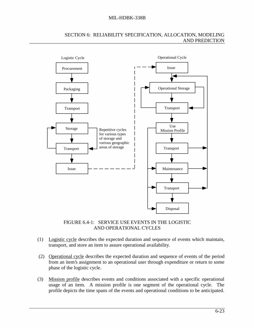
MIL-HDBK-338B


6-23

Procurement

Packaging

Transport

Storage

Transport

Issue

Repetitive cyclesfor various typesof storage andvarious geographicareas of storage

Issue

Operational Storage

Transport

UseMission Profile

Transport

Maintenance

Transport

Disposal

Operational CycleLogistic Cycle

FIGURE 6.4-1: SERVICE USE EVENTS IN THE LOGISTICAND OPERATIONAL CYCLES

(1) Logistic cycle describes the expected duration and sequence of events which maintain,transport, and store an item to assure operational availability.

(2) Operational cycle describes the expected duration and sequence of events of the periodfrom an item’s assignment to an operational user through expenditure or return to somephase of the logistic cycle.

(3) Mission profile describes events and conditions associated with a specific operationalusage of an item. A mission profile is one segment of the operational cycle. Theprofile depicts the time spans of the events and operational conditions to be anticipated.

MIL-HDBK-338B


6-24

Multiple mission profiles may be required to adequately describe an item’s multimissioncapabilities.

(4) Environmental profile describes the specific natural and induced environments(nominal and worst case) with the operations, events, and functions described by thelogistic and operational cycles. Each mission profile has an associated environmentalprofile.

6.4.2.3 Reliability Block Diagrams

Reliability block diagrams are prepared to show interdependencies among all elements(subsystems, equipments, etc.) or functional groups of the item for item success in each serviceuse event. The purpose of the reliability block diagram is to show by concise visual shorthandthe various series-parallel block combinations (paths) that result in item success. A completeunderstanding of the item’s mission definition, and service use profile is required to produce thereliability diagram.

6.4.2.4 Mathematical/Simulation Models

Models need to be derived to relate reliability block diagrams to time-event relationships andfailure rate data. This can be done through purely mathematical means or computer generatedsimulation models. The solution of the models will be the item predicted reliability. Themathematical model shall be capable of being readily updated with information resulting fromreliability and other relevant tests as well as changes in item configuration, mission parametersand operational constraints.

6.4.2.5 Part Description

Part and application descriptions needs to be provided for any prediction based upon part failurerates. The part identification number from the schematic diagram, the applicable specificationand the specification type number needs to be included.

6.4.2.6 Environmental Data

Environmental data affecting part failure rates must be defined. These data include the specificnatural and induced environments (nominal and worst case) associated with the operations,events, and functions described by the logistic and operational cycles.

6.4.2.7 Stress Analysis

Analyses will be performed to determine the operating stresses to be experienced by each partcommensurate with the prediction classification and the design detail available. Failure rates canbe modified by appropriate factors to account for the effect of applied stress. Stress ratios cited

MIL-HDBK-338B


6-25

in the prediction report shall be individually identified as Estimated (E), Calculated (C), orMeasured (M).

6.4.2.8 Failure Distributions

The failure distribution appropriate to the specific electronic, electrical, electromechanical,mechanical, and ordnance item will be in used in computation. In instances where the failuredistribution for the item is not known, the Weibull failure distribution may be assumed. Thefailure distribution utilized needs to be cited and any assumptions substantiated in the predictionreport.

6.4.2.9 Failure Rates

Failure rates for all electronic, electrical, electromechanical, mechanical, and ordnance items arerequired for each significant event and environment defined by the service use profile. Allsources of failure data shall be approved by the procuring activity prior to use. Basic failure ratesfrom most data sources must be modified with appropriate factors to account for the specific itemapplication under consideration. Factors used shall be cited and substantiated in the predictionreport.

6.4.2.10 Item Reliability

Item reliability will be computed using mathematical or simulation based models and applicablefailure rate data. The prediction results should be expressed in terms consistent with thespecified reliability requirements.

6.4.3 Tailoring Reliability Models and Predictions

Since the reliability prediction process is iterative in nature, tailoring of the reliability model andprediction is based primarily upon the program procurement phase. As the design progresses, thehardware relationships become better defined, thus the model of the system depicting therelationship between basic reliability and mission reliability is refined and it must be exercisediteratively to provide reliability predictions up through the system level.

Tailoring of these tasks involves, primarily, the selection of the prediction method utilized andthe rigor with which it is applied. For relatively simple systems (i.e., those containing noredundant elements and without alternate modes of operation or degraded modes of operation)the basic reliability model and the mission reliability model will be identical and a singlereliability prediction will suffice.

An example of tailoring based upon the procurement phase may be as follows: in the conceptualdesign phase reliability predictions are based primarily upon comparison with similar equipment,in the preliminary design phase, a simple part count prediction is used, in the final design phase,as more detailed design information becomes available, a detailed stress reliability prediction

MIL-HDBK-338B


6-26

would be made, and in the test phase, test or field data would be integrated in the predictionmodel.

Reliability modeling and prediction is only as accurate as the assumptions and data sources usedin its preparation, and to the extent all pertinent influences are considered. The primary value ofthe reliability prediction is as a design tool for comparison of alternative approaches. Althoughthe absolute value of item reliability derived by the prediction may be used in the determinationof expected field use reliability, it must be used with great caution and with full disclosure of thedata sources and assumptions used. As an example, when field experience data for similar itemsin a like environment are utilized, the prediction reflects anticipated field performance afterdesign maturity has been achieved. Conversely, when laboratory data are utilized, the predictionreflects expected performance under laboratory conditions.

6.4.4 Reliability Modeling

The reliability model consists of a reliability block diagram and an associated mathematical orsimulation model (Ref. [8]). Elements of the item intended for redundancy or alternate modes ofoperation are modeled in a parallel configuration or similar construct appropriate to the missionphase and mission application.

6.4.4.1 Reliability Block Diagrams

A reliability block diagram shows the interdependencies among all elements (subsystems,equipments, etc.) or functional groups of the item for item success in each service use event. Aprogressive example of a reliability block diagram is illustrated in Figure 6.4-2. The purpose isto show, by concise visual shorthand, the various series-parallel block combinations (paths) thatresult in item success. A complete understanding of the item’s mission definition, and serviceuse profile is required.

Each reliability block diagram will have a title including identification of the item, the missionidentification or portion of the service use profile addressed, and a description of the mode ofoperation for which the prediction is to be performed.

Each reliability block diagram should include a statement of conditions listing all constraintswhich influence the choice of block presentation, the reliability parameters or reliability variablesutilized in the analysis, and the assumptions or simplifications utilized to develop the diagram.Once established, these conditions are observed throughout the analysis.

MIL-HDBK-338B


6-27

STRESSλ λ λ0 1 2

vii ii

iiivi

vi

iv

v

5

4321

MAJOR SYSTEM

LEVEL I

LEVEL II

LEVEL III

LEVEL IV

LEVEL V

edcba

SYSTEM

D

DX

XC

C

D

D

SUBSYSTEM

UNIT

PART STRESS ANALYSIS ANDFAILURE MODE DIAGRAM

X L C R

FIGURE 6.4-2: PROGRESSIVE EXPANSION OF RELIABILITY BLOCKDIAGRAM AS DESIGN DETAIL BECOMES KNOWN

MIL-HDBK-338B


6-28

The blocks in the diagram follow a logical order which relates the sequence of events during theprescribed operation of the item. The reliability block diagram is drawn so that each element orfunction employed in the item can be identified. Each block of the reliability block diagramrepresents one element of function contained in the item. All blocks are configured in series,parallel, standby, or combinations thereof as appropriate.

(1) Identification of blocks. The coding system should be based upon a uniformidentification system that will permit unambiguous traceability of the reliability block toits hardware (or functional) equivalent as defined in program documentation. Hardwareor functional elements of the item which are not included in the reliability model areidentified in a separate listing.

(2) Reliability variable. For each block include the units of the reliability or mean lifevalue. Examples include; time, cycles, events, etc.

(3) Block diagram assumptions. The following general assumptions apply to reliabilityblock diagrams:

(a) Blocks denote elements or functions of the items that are considered whenevaluating reliability and which have reliability values associated with them.

(b) Lines connecting blocks have no reliability values. The lines serve only to giveorder to the diagram. Cabling and connectors are incorporated into a single blockor included as part of the block for an element or function.

(c) All inputs to the item are within specification limits.

(d) Failure of any element or function denoted by a block in the diagram will causefailure of the entire item, except where alternative modes of operation may bepresent; i.e., redundant units or paths.

(e) Each element or function denoted by a block in the diagram is independent, withregard to probability of failure, from all other blocks.

(4) Software reliability and human reliability assumptions. The impact of software andhuman reliability needs to be stated and considered in the reliability model.

MIL-HDBK-338B


6-29

6.4.4.2 Reliability Modeling Methods

Four reliability modeling methods presented are: the conventional probability model, the BooleanTruth table model, the logic diagram model and the simulation model. These models aredescribed as follows:

6.4.4.2.1 Conventional Probability Modeling Method

The conventional probability method may be used to prepare a reliability mathematical modelfrom a reliability block diagram. The conventional probability method makes use of theequations developed for redundancy to handle series, parallel, and series-parallel combinations ofequipments. For non-series parallel or complex configurations, use or repeated use of thefollowing equation is required.

PS = PS (if X is good) RX + PS (if X is bad) QX (6.19)

where:PS = reliability of mission

PS (if X is good) = reliability of mission if X is good

PS (if X is bad) = reliability of mission if X is bad

RX = reliability of X

QX = unreliability of X = 1 - RX

In other words, the reliability of the mission is equal to the reliability of the mission given aspecific portion of the system works times the probability that the portion of the system will workplus the reliability of the mission given that the specific portion of the system fails times theprobability that the portion fails.

The above formula can also be used to generate probability of success equations for series-parallel configurations.

Formulas for probability of success, PS, for various system configurations are derived as followsfor various success diagrams. Each formula shown can be used as a building block to evaluate amore complex success diagram.

6.4.4.2.1.1 Series Model

If there is only one equipment in the system and it is required, then the reliability diagram is:

A Success

MIL-HDBK-338B


6-30

The probability of success for the system is obviously the probability of success of equipment A,or

PS = PA (6.20)

The probability of A failing would be 1 - PA.

For a two equipment serial system the reliability diagram is:

A B

The probability of success for the system is the probability of success of equipment A and B, or

PS = PAPB (6.21)

If A and B are identical, then

PS = (PA)2 (6.22)

For a three equipment serial system the reliability diagram is:

A B C

The probability of success for the system is the probability of success of equipment A, B and C,or

PS = PA PB PC (6.23)

6.4.4.2.1.2 Parallel Models

For a two equipment active parallel system the reliability diagram is:

A

B

PS = P(mission success with A working) PA +

P (mission success with A failed) (1 - PA )

MIL-HDBK-338B


6-31

PS = (1) PA + PB (1 - PA)

PS = PA + PB - PA PB (6.24)

If A and B are identical, then

PS = 2PA - (PA )2 (6.25)

For a three equipment active parallel system the reliability diagram is:

A

B

C

PS = PA + PB + PC - PA PB - PA PC - PB PC + PA PB PC (6.26)

If A, B, and C are identical, then

PS = 3PA - 3(PA )2 + (PA )3 (6.27)

For a two equipment standby parallel system with a switch, the reliability diagram is:

S

A

B

The switch, “S,” detects a failure of the operative element and instantaneously switches from thefailed element to a standby element.

The switch may fail in two ways: (1) the switch may fail to operate when required, Q1 and (2)the switch may operate without command (i.e., prematurely), Q2. Q1 and Q2 can be representedas (1-P1) and (1-P2) as the probability of failure (Q) plus the probability of success (P) equalsone.

PS = P(mission success with A working) PA +

P(mission success with A failed) (1 - PA )

PS = P2 PA + (1 - P2 ) PB PA + P1 PB (1 - PA)

PS = PA PB (1 - P1 - P2) + PA P2 + PB P1 (6.28)

MIL-HDBK-338B


6-32

The equivalent series reliability mathematical model for this system is:

PS = PA PB P1 P2 (6.29)

6.4.4.2.1.3 Series-Parallel Models

As one example of a complex series-parallel combination of equipments the reliability diagramis:

A

B 1

B2

C1

C2

The system requirement would be that equipment A and either equipment C1 or C2 work, or

that equipments B1 and C1 work, or that B2 and C2 work for success. Equipments with the

same letter are identical, i.e., C1 = C2 and B1 = B2 .

PS = P(mission success with A working) PA

+ P(mission success with A failed) (1 - PA )

PS = (2PC - PC2 ) PA + [2PB PC - (PB PC )2 ] (1 - PA ) (6.30)

An example involving the above diagram is as follows:

Given that,

PA = 0.3

PB1 = PB2 = 0.1

PC1 = PC2 = 0.2

Evaluating the probability of success for a given mission using equation 6.30 is:

PS = (.4 - .04) .3 + [.04 - .0004] (.7)

PS = 0.13572

MIL-HDBK-338B


6-33


PS = PA PB2 PC

2 (6.31)

and the reliability is 0.00012.

6.4.4.2.2 Boolean Truth Table Modeling Method

A Boolean Truth Table may also be used to prepare a reliability mathematical model from areliability block diagram. This method is applicable to single functioned and malfunctionedsystems. The method is more tedious than the conventional probability method but is usefulwhen there is familiarity with Boolean algebra. The procedure for the Boolean Truth Tableapproach for a single function system is illustrated by the following example. The systemreliability diagram is given as:

B1

A

B2

C1

C2

where:PA = 0.3 1 - PA = 0.7

PB1 = PB2 = 0.1 and therefore 1 - PB = 0.9

PC1 = PC2 = 0.2 1 - PC = 0.8

The Boolean algebra approach lists all equipments in a truth table form (See Table 6.4-2). Thetruth table has 2n entries where n is the number of equipments in the system. The table has a 1or 0 entry in each column indicating success or failure respectively on each equipment. Allpossible combinations of all equipments working and failing are thus listed. The procedure is toexamine each row of the truth table and decide whether the combination of equipments workingand failed yields system success (S) or failure (F). Insert an S or F respectively in the nextcolumn in the table. For each S entry, multiply the respective probabilities for the indicated stateof each equipment to yield a PS for that entry.

Entry number 4 is the entry with a success indicated and .03888 is obtained by multiplying

(1 - PB1 ) (1 - PB2 ) (1 - PC1 ) PC2 PA or

(.9) (.9) (.8) (.2) (.3) = .03888

MIL-HDBK-338B


6-34

All figures in the PS column are then added for a system reliability probability of .13572 in this

example.


PS = PA PB1 PB2 PC1 PC2 (6.32)

and the probability is 0.00012.

A Boolean algebra reliability equation can be written from the truth table (Table 6.4-2) if it isdesired. In this case it would look like the following:

PS = B1B2C1C2A + B1B2C1C2A + B1B2C1C2A + B1B2C1C2A + B1B2C1C2A + B1B2C1C2A +

B1B2C1C2 A + B1B2C1C2A + B1B2C1C2A + B1B2C1C2A + B1B2C1C2A + B1B2C1C2A +

B1B2C1C2A + B1B2C1C2 A + B1B2C1C2A + B1B2C1C2A + B1B2C1C2A + B1B2C1C2A + B1B2C1C2A

(6.33)

MIL-HDBK-338B


6-35

TABLE 6.4-2: TRUTH TABLE CALCULATION FOR THESYSTEM RELIABILITY DIAGRAM

Entry No. B1 B2 C1 C2 ASuccess

OR FAILURE PS

1234567891011121314151617181920212223242526272829303132

00000000000000001111111111111111

00000000111111110000000011111111

00001111000011110000111100001111

00110011001100110011001100110011

01010101010101010101010101010101

FFFSFSFSFFSSFSSSFFFSSSSSFFSSSSSS

---

.03888-

.03888-

.00972--

.01008

.00432-

.00432

.00252

.00108---

.00432

.01008

.00432

.00252

.00108--

.00112

.00048

.00112

.00048

.00028

.00012Σ All success paths = .13572

MIL-HDBK-338B


6-36

A bar above a letter indicates the complement or unreliability, e.g., A = (1 - A).

With the aid of a reduction technique the nineteen terms of (6.33) can be reduced as follows:

(1) A reduction table (Table 6.4-3) is constructed which allows the reduction of the 19Boolean success terms to a simplified expression for the given mission reliabilitymodel. All 19 success paths are first listed in Column 1 of Table 6.4-3.

(2) By a comparative process, product pairs are formed for those terms in Column 1 ofTable 6.4-3 which differ only by a letter inverse, thus forming a new product term

which has this letter missing. For example, in Column 1 the two terms B1B2C1C2 A

and B1B2C1 C2 A differ only in the letter C1 and therefore can be combined to form

the product term B1B2C 2 A entered in Column 2. Again, this process is repeated bycomparing product terms in Column 2 which differ only by a letter inverse, thusforming a new product term which is then entered in Column 3. It should be noted thatonce a term is used in a comparison, it is eliminated from all further comparisons, thusensuring that all remaining terms are still mutually exclusive. The order of termsselected for the comparison process in Table 6.4-3 is not a necessary consideration; theresulting disjoint group of Boolean terms can always be interpreted, on a one-for-onebasis, as the simplified probability of success (reliability) expression. For the givenmodel, the probability of success has been reduced to the following terms:

(3) Substituting the reliabilities and unreliabilities used previously into (equation 6.34), weobtain:

PS = (.1) (.2) + (.9) (.1) (.2) + (.9) (.9) (.2) (.3) + (.9) (.2) (.8) (.3) + (.1) (.1) (.8) (.2) +

(.1) (.9) (.8) (.2) (.3) = .13572

which is the same probability of success shown in the summation for Table 6.4-2.

MIL-HDBK-338B


6-37

TABLE 6.4-3: REDUCTION TABULATION

B1B2C1C2A

B1B2C1C2A

B1B2C1C2A

B1B2C1C2A

B1B2C1C2A

B1B2C1C2A

B1B2C1C2A

B1B2C1C2A

B1B2C1C2A

B1B2C1C2A

B1B2C1C2A

B1B2C1C2A

B1B2C1C2A

B1B2C1C2A

B1B2C1C2A

B1B2C1C2A

B1B2C1C2A

B1B2C1C2A

B1B2C1C2A

B1B2C2A

B1C1C2A

B1B2C1C2

B1B2C1C2

B1B2C1A

B1B2C1A

B1B2C1C2

B1B2C1C2

B1B2C1C2

Column 1 Column 2 Column 3 Column 4

B1B2C2

B1B2C1

B1B2C1

B1C1

PS = B1 C1 + B1B2 C2 + B1B2C 2 A + B1C 1C2 A + B1 B 2 C1C2

+ B 1B2C1C2 A (6.34)

MIL-HDBK-338B


6-38

6.4.4.2.3 Logic Diagram Modeling Method

Logic diagrams may also be used to prepare a reliability mathematical model from a reliabilityblock diagram. This method is applicable to single functioned and multifunctioned systems.This method is more tedious than the conventional probability method but is a short cut methodfor the Boolean truth table approach in combining terms to simplify the reliability equation.

The logic diagram procedure for a single function system is to translate the reliability blockdiagram into a switching network. A closed contact represents equipment success, an opencontact equipment failure. Each complete path of contacts represents an alternate mode ofoperation. Each equipment that is required for each alternative mode of operation is identified bya contact along a path. All paths terminate at the same point (success). The logic diagram isdeveloped so that all paths are mutually exclusive; by use of a few simple manipulations, theamount of effort involved over the Boolean truth table method can be shortened.

Logic diagrams for series, parallel, and series-parallel diagrams are easy to draw as shown inTable 6.4-4.

For complex configurations the procedure is to reduce the reliability diagram to a series-parallelconfiguration by successively splitting the diagram into subdiagrams by removing one equipmentand replacing it with a short circuit and an open circuit. An example will clarify the procedure.

B1

A

B2

C1

C2

MIL-HDBK-338B


6-39

TABLE 6.4-4: LOGIC DIAGRAM EXAMPLES

Mission Reliability Diagram Logic Diagram

A BA B

B

ABA

A B

A B

OR

,

OR

A BA

,

B

B

A ,

B

A

C

A B C

A B C

BA C

A B C

A B C

A B C

A B C

,

ABA

B C

OR

B

A

A

C

B

C

BA C

A B C

A B C

A B C

,

A

B COR

BA C

B

Other series parallel combinationscan be quite simply drawn.NOTE:When one logic switch A is open, all must be open and all A must be closed andsimilarly for B and C logic switches.

MIL-HDBK-338B


6-40

Remove equipment A by splitting the diagram as follows:

(In the diagrams which follow, the term "Short" indicates a circuit which is always operative; theterm "open" indicates a circuit which is never operative).

B1

B2

C1

C2

Short

B1

B2

C1

C2

Open

X Y

start the logic diagram

A

A

X

Y

X and Y are now in series parallel form and can be drawn directly, therefore, the logic diagramwould appear as follows:

B1 C1C1B1 B2 C2C1B1 B2 C2C1B1 B2 C2

C1 C2

C1A

A

If removing one equipment by replacing it by an open and short circuit will not reduce the systemto two series parallel diagrams, two equipments must be removed. The logic diagram would thenlook as follows:

MIL-HDBK-338B


6-41

EQ 2

EQ 2

1 and 2Shorted

1 Shorted2 Open

EQ 1

EQ 2

EQ 2

1 Open2 Shorted

1 and 2Open

EQ 1

After the logic diagram is drawn, two approaches are possible for a numerical answer. The firstinvolves writing an equation for the probability of success, PS, by writing down every path withan addition sign joining all paths. The second approach is to insert values for the variousprobabilities directly into the logic diagram and multiply series terms and add parallel terms untiljust one series term remains. This result is the answer. For the above example:

PS = A [C1 + C2 C2 ] + A [B1 C1 + B1C1 B2 C2 +

B1C1B2 C2 + B 1C1B2 C 2 ] (6.35)

6.4.4.2.4 Complex System Modeling Methods

The closed form techniques for modeling, as described in paragraph 6.4.4.2.1 through 6.4.4.2.3,are difficult to use on complex configurations that include high levels of fault-tolerance, standbyspares and complex repair methods. Markov modeling is one method that can assist in providingneeded performance and dependability prediction. Simulation tools are another method whichmay be more attractive as they are even more flexible.

6.4.4.2.4.1 Markov Modeling (Ref. [9])

Markov modeling processes are stochastic processes using random variables to describe thestates of the process, transition probabilities for changes of state and time or event parameters formeasuring the process. A stochastic process is said to be a Markov property if the conditionalprobability of any future event, given any past events and the present state, is independent of thepast events and depends only on the present state of the process (Ref. [10]).

The advantages for using Markov modeling methods include the flexibility in expressingdynamic system behavior. These types of behavior include:

(1) Complex repair. Situations consisting of repairs of either individual components orgroups of components or partial repair of components.

MIL-HDBK-338B


6-42

(2) Standby spares. Standby conditions include hot, warm and cold spares. Hot spares arepower-on units with identical stresses as apply to the active units, where warm spareshave power-on but have lower stresses. Cold spares are power-off units.

(3) Sequence dependent. This behavior includes: functional dependency in which thefailure of one component can cause the unavailability of other components; prioritydependency in which behavior will differ depending on whether an event occurs beforeor after another; and sequence enforcement in which it is impossible for certain eventsto occur before others have occurred.

(4) Imperfect fault coverage. Imperfect fault coverage conditions arise when a dynamicreconfiguration process that is invoked in response to a fault or component failure has achance of not being successful leading to system failure.

The disadvantages of using Markov modeling techniques include state size and modelconstruction. Solving models with thousands of states can challenge the computer resourcesavailable. Also, the problem of identifying all the states and transitions correctly can be adifficult assignment.

Software tools for performing dependability analysis, such as Markov modeling include (see theRAC Web Site; the URL is http://rac.iitri.org/DATA/RMST):

(1) HARP, Hybrid-Automated Reliability Predictor was developed to input systemconditions directly in the form of a Markov model or in the form of a dynamic faulttree.

(2) SHARPE, Symbolic Hierarchical Automated Reliability and Performance Evaluation, isan integrated tool that allows models to be solved either individually or combinedhierarchically. In addition to Markov models, SHARPE can solve reliability blockdiagrams, fault trees and generalized stochastic Petri nets.

(3) CARMS, Computer-Aided Rate Modeling and Simulation, is an interactive Markovmodeling tool designed for reliability analysis of redundant systems.

(4) CARSA, Computer-Aided Redundant System Reliability Analysis, utilizes Markovmodeling for failure effect coverage. CARSA by-passes disadvantages of Markovmodeling (larger number of states) by partitioning the system so that the model is alower dimension.

6.4.4.2.4.2 Monte Carlo Simulation Method

Monte Carlo simulation may be used to synthesize a system reliability prediction from areliability block diagram by means of random sampling. Monte Carlo simulation is employed ininstances where individual equipment probabilities (or equivalent reliability parameter) are

MIL-HDBK-338B


6-43

known but the mission reliability model is exceedingly complex to derive a general equation forsolution. The method does not result in a general probability of success equation but computesthe system probability of success from the individual equipment probabilities and the reliabilityblock diagram. Monte Carlo simulation is performed by computer due to the large number ofrepetitive trials and calculations required to obtain a significant result. Monte Carlo simulation isapplicable to single functioned and multifunctioned systems.

Monte Carlo simulation determines the distribution of a function of one or more variables fromthe distribution of the individual variables. The method involves random sampling from thedistributions of all variables and inserting the values so obtained in the equation for the functionof interest. Suppose the function whose probability of success distribution is to be estimated is,P(x1 . . . , xn ) and that the x1 , x2 . . . , xn are independent random variables whose

distributions are presumed to be known. The procedure is to pick a set of x’s randomly from thedistributions of the x’s, calculate P for that set, and store that value of P. This is repeated manytimes until enough values of P are obtained. From this sample of P values, its distribution andparameters can be estimated.

Monte Carlo simulation is based on several principles of probability and on the techniques ofprobability transformation. One underlying principle is the law of large numbers, which statesthat the larger the sample the more certainly the sample mean will be a good estimate of thepopulation mean.

Software tools for simulation modeling include (see the RAC Web Site; the URL ishttp://rac.iitri.org/DATA/RMST):

(1) AvSim, Availability Simulator allows the user to predict and optimize system andcomponent performance. Uses Monte Carlo simulation techniques.

(2) CARE, Computer-Aided Reliability Estimation helps estimate the reliability ofcomplex, redundant, or fault-tolerant systems. Capable of modeling very large systemsthat incorporate some form of system management strategy which controlshardware/software resources in the presence of multiple faults or errors.

(3) ETARA, Event Time Availability, Reliability Analysis is an interactive event drivensimulation program. The program simulates the behavior of a system over a specifiedperiod of time using Monte Carlo methods to generate block failure and repair times asa function of exponential or Weibull distributions.

(4) REST, (RADC Reliability Simulation Tool, is a Monte Carlo simulation used toevaluate reliability figures of merit for fault tolerant systems. Given a fault tolerantsystem configuration component MTBF’s and repair rates, the program calculates thesystem MTBCF, MTTR, reliability and availability. REST also synthesizes reliabilitydemonstration plans for fault tolerant systems. Can be used to model systems with full,standby, or partial standby redundancy.

MIL-HDBK-338B


6-44

(5) RAPTOR, The Rapid Availability Prototyping for Testing Operational Readiness(RAPTOR) software tool was developed by Headquarters Air Force Operational Testand Evaluation Center, Logistics Studies and Analysis Team (HQ AFOTEC/SAL). Itsprimary purpose is Reliability, Maintainability & Availability (RM&A) analysis ofsystems undergoing Operational Test and Evaluation (OT&E). Other applicationsinclude test planning, requirements definition, reliability prediction and sensitivityanalysis. It can be downloaded over the Internet

(URL: http://www.afotec.af.mil/sa/safrmset.htm).

6.4.5 Reliability Prediction

Predictions are a means of determining the feasibility of requirements and of assessing progresstoward achieving those requirements. In general, there is a hierarchy of reliability predictiontechniques available to the designer depending upon (1) the depth of knowledge of the designand (2) the availability of historical data on equipment and component part reliabilities. As thesystem design proceeds from conceptual, through detailed design, data describing the systemevolves from a qualitative description of systems functions to detailed specifications anddrawings suitable for hardware production. Therefore, a hierarchy of reliability predictiontechniques have been developed to accommodate the different reliability study and analysisrequirements and the availability of detailed data as the system design progresses as shown inFigure 6.4-3. These techniques can be roughly classified in four categories, depending on thetype of data or information availability for the analysis. The categories are:

(1) Similar Item Analysis. Each item under consideration is compared with similar itemsof known reliability in estimating the probable level of achievable reliability, thencombined for higher level analyses.

(2) Part Count Analysis. Item reliability is estimated as a function of the number of partsand interconnections included. Items are combined for higher level analysis.

(3) Stress Analyses. The item failure rate is determined as a function of all the individualpart failure rates as influenced by operational stress levels and derating characteristicsfor each part.

(4) Physics-of-Failure Analysis. Using detailed fabrication and materials data, each item orpart reliability is determined using failure mechanisms and probability density functionsto find the time to failure for each part. The physics-of-failure (PoF) approach is mostapplicable to the wearout period of an electronic product’s life cycle and is not suited topredicting the reliability during the majority of its useful life. In addition, at the timethis handbook was being revised, a practical and economic method for applying a PoFprediction method was not available. The pros and cons of PoF prediction models areshown in Table 6.4-5.

MIL-HDBK-338B


6-45

.

Tra

nsis

tors

Tra

velin

gW

ave

Tu

beC

apac

itor

sR

esis

tors

Par

t

Rad

arSy

stem

Rec

eive

rSt

alo

Low

Pow

erA

mpl

ifie

rPo

wer

Sup

plie

s

Early TradeStudies

ConceptualDesign

PreliminaryDesign

DetailedDesign

Tec

hniq

ues:

• Si

mila

r It

em A

naly

sis

Tec

hniq

ues:

• Si

mila

r It

em A

naly

sis

• Pa

rt C

ount

Ana

lysi

s

Tec

hniq

ues:

• Pa

rt C

ount

Ana

lysi

s•

Stre

ss A

naly

sis

Tec

hniq

ues:

• St

ress

Ana

lysi

s

Subs

yste

m

Syst

em

Ass

embl

y

Pow

er O

utp

utA

mpl

ifie

r

Tra

nsm

itte

r

FIGURE 6.4-3: RADAR SYSTEM HIERARCHY (PARTIAL LISTING)

MIL-HDBK-338B


6-46

TABLE 6.4-5: PROS AND CONS OF PHYSICS-OF-FAILURE PREDICTION MODELS

Advantages DisadvantagesMore accurate than generic models for wearoutmechanisms

Can only be used by those having access todetailed fabrication and materials data

Based on fundamental reliability parameters Relatively complex and difficult to useCan be developed sooner since they requireonly fabrication & materials data

Do not address early and mid-life failure

6.4.5.1 General

To perform a satisfactory reliability analysis of a system, basic information is needed and shouldinclude:

(1) Description. Part or component descriptions should be provided for any predictionbased upon part failure rates. The identification numbers from the schematic diagram,the applicable specification and the specification type number should be included.

(2) Environmental Data. Environmental data affecting part failure rates must be defined.These data include the specific natural and induced environments (nominal and worstcase) associated with the operations, events, and functions described by the logistic andoperational cycles. Environmental categories should be defined for each service useevent using Table 6.4-6 as a guide of typical categories. Data sources, such as MIL-HDBK-217 (Ref. [11]) and NPRD-95 (Ref. [12]) which utilize environmental factors toadjust failure rates, should apply the environmental factor which most closely matchesthe intended environment. Factors utilized should be cited and substantiated.

(3) Operating Temperature. Part or component temperatures used for prediction purposesshould include the item internal temperature rise as determined by thermal analysis ortest data.

(4) Stress Analysis. Analyses should be performed to determine the operating stressesexperienced by each part commensurate with the prediction classification and thedesign detail available. Failure rates are modified by appropriate factors to account forthe effect of applied stress.

(5) Failure Distributions. The failure distribution appropriate to the specific electronic,electrical, electromechanical, mechanical, and ordnance item should be used incomputation. In instances where the failure distribution for the item is not known, theexponential, binomial, Weibull, or other failure distribution may be assumed. Thefailure distributions utilized should be cited and any assumptions substantiated in theprediction report.

MIL-HDBK-338B


6-47

(6) Failure Rates. Failure rates for all electronic, electrical, electromechanical, mechanical,and ordnance items are needed for each significant event and environment defined bythe service use profile. Basic failure rates from most data sources must be modifiedwith appropriate factors to account for the specific item application underconsideration. Factors used should be cited and substantiated in the prediction report.These include:

(a) Functional group failure rates may be derived from failure rate data forfunctionally similar groups or items. The GIDEP Failure Rate Summaries are anavailable source for locating group and item failure rates.

TABLE 6.4-6: ENVIRONMENTAL SYMBOL IDENTIFICATIONAND DESCRIPTION

Environment Symbol Nominal Environmental ConditionsGround, Benign GB Nonmobile, temperature and humidity controlled

environments.Space, Flight SF Earth orbital. Approaches Ground Benign conditions. Vehicle

neither under powered flight nor in atmospheric reentry.Ground, Fixed GF Conditions less than ideal to include installation in permanent

racks with adequate cooling air and possible installation inunheated buildings.

Ground, Mobile GM Conditions more severe mostly for vibration and shock.Equipment installed on wheeled or tracked vehicles.

Naval, Sheltered NS Sheltered or below deck conditions on surface ships andsubmarines.

Naval, Unsheltered NU Unprotected surface shipborne equipments exposed to weatherconditions and salt water.

Airborne,Inhabited, Cargo

AIC Typical conditions in cargo compartments occupied by aircrewwithout environmental extremes of pressure, temperature,shock and vibration.

Airborne,Inhabited, Fighter

AIF Same as AIC but installed on high performance aircraft such asfighters and interceptors.

Airborne,Uninhabited, Cargo

AUC Uncontrolled areas with environmental extremes of pressure,temperature and shock.

Airborne,Uninhabited, Fighter

AUF Same as AUC but installed on high performance aircraft such asfighters and interceptors.

Airborne,Rotary Winged

ARW Equipment installed on helicopters, internally and externally.

Missile, Launch ML Severe conditions of noise, vibration, and other environmentsrelated to missile launch, and space vehicle boost into orbit,vehicle re-entry and landing by parachute. Conditions mayalso apply to installation near main rocket engines duringlaunch operations.

Missile, Flight MF Typical conditions of pressure, vibration and temperatureexperienced in atmospheric flight to target.

MIL-HDBK-338B


6-48

(b) Operating failure rates for electronic and electromechanical parts may be found inMIL-HDBK-217 (Ref. [11]) and Bellcore TR-NWT-00332 (Ref. [13]). Failuresrates for other parts may be found in NPRD-95 (Ref. [12]), Electronic PartsReliability Data, 1997 (Ref. [14]), the GIDEP Failure Rate Summaries, and othersources.

(c) Nonoperating failure rates take into consideration pertinent environmentalinfluences or other stresses of the application. Data sources such as RADC-TR-85-91 (Ref. [15]) and NONOP-1 (Ref. [16]), provide nonoperating failure rates.

6.4.5.2 Mathematical Models for Reliability Prediction

For the simplest case of equipment or system configurations consisting of N independentelements or subsystems in series, the reliability equation is:

Rs = ∏i=1

N Ri (6.36)

where:Rs is the equipment or system reliabilityRi is the reliability of each of the elements or subsystems

For the case where time is a factor

Rs(t) = ∏i=1

N Ri(t) (6.37)

where:Rs(t) = The probability that the system will not fail before time t. (In this case a

“system” is considered to be any device consisting of n elements, none ofwhich can fail without system failure).

Ri(t) = The probability that the ith element of the system will not fail beforetime t.

Finally, if one assumes that each of the Ri(t) 's is exponentially distributed with constant failure

rate of λi, then

Ri(t) = exp −λit( ) (6.38)

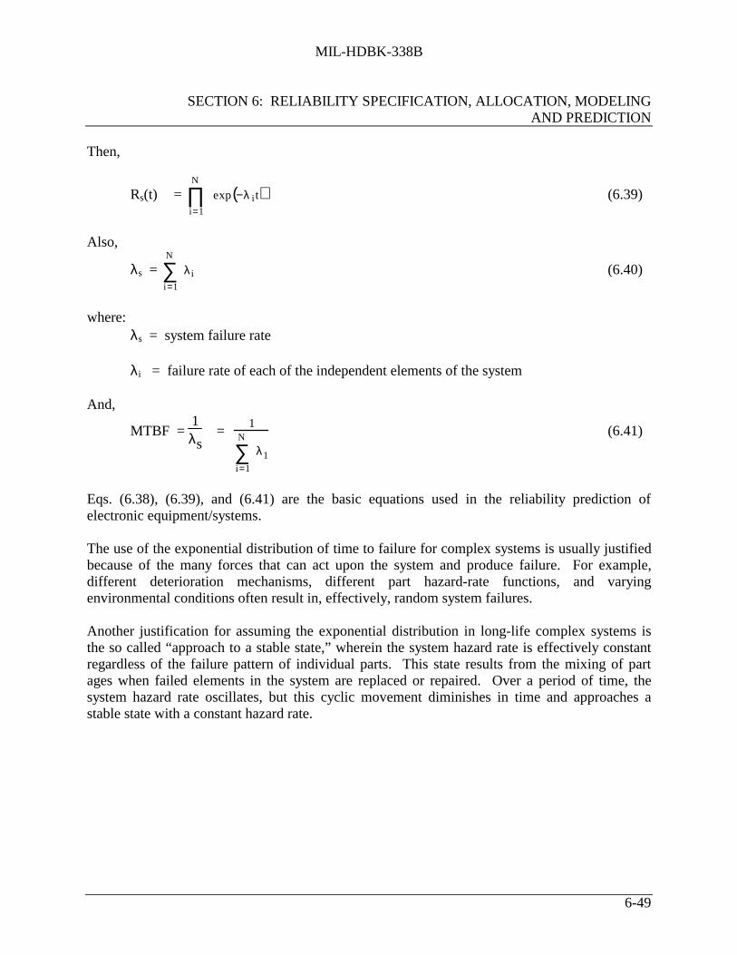
MIL-HDBK-338B


6-49

Then,

Rs(t) = i=1

N

∏ exp −λ it( ) (6.39)

Also,

λs = i=1

N

∑ λi (6.40)

where:λs = system failure rate

λi = failure rate of each of the independent elements of the system

And,

MTBF = 1λs

=

1

i=1

N

∑ λ1

(6.41)

Eqs. (6.38), (6.39), and (6.41) are the basic equations used in the reliability prediction ofelectronic equipment/systems.

The use of the exponential distribution of time to failure for complex systems is usually justifiedbecause of the many forces that can act upon the system and produce failure. For example,different deterioration mechanisms, different part hazard-rate functions, and varyingenvironmental conditions often result in, effectively, random system failures.

Another justification for assuming the exponential distribution in long-life complex systems isthe so called “approach to a stable state,” wherein the system hazard rate is effectively constantregardless of the failure pattern of individual parts. This state results from the mixing of partages when failed elements in the system are replaced or repaired. Over a period of time, thesystem hazard rate oscillates, but this cyclic movement diminishes in time and approaches astable state with a constant hazard rate.

MIL-HDBK-338B


6-50

6.4.5.3 Reliability Prediction Methods

Four prediction methods are described as follows:

6.4.5.3.1 Similar Item Prediction Method

Several techniques have been developed and used in performing very early predictions of itemreliability before any characteristics of the system design have been established. The most basicof these techniques involves a simple estimate of item reliability in terms of MTBF, failure rate,or similar parameters, based on experience gained from operational items of similar function.

In general, these similar item prediction techniques involve the following steps:

(1) Defining the new item in terms such as general equipment type (e.g., radar), operationaluse (e.g., ground based) and other known characteristics.

(2) Identifying an existing item or class of equipment that most nearly compares with thenew item.

(3) Obtaining and analyzing historical data generated during operation of the existingequipment to determine as nearly as possible the reliability of the items under the statedoperating environment.

(4) Drawing conclusions concerning the level of reliability that will be demonstrated by thenew items. Such conclusions assume that similar equipment will exhibit similarreliability and that reliability achievement evolves in an orderly manner from onegeneration of equipments to the next. These reliability prediction techniques permitvery early estimation of the failure rate of a new item based on experience gained fromoperational items of similar function. The accuracy of the estimates, however, dependson the quality of historical data and the similarity between the existing and newequipments. If the technology of the new items is too advanced, then the operationaldata for the old items will not be relevant and another technique will have to beconsidered.

The similar item prediction method utilizes specific experience on similar items. The more rapidway of estimating reliability is to compare the item under consideration with a similar itemwhose reliability has previously been determined by some means and has undergone fieldevaluation. The method has a continuing and meaningful application for items undergoingorderly evolution. Not only is the contemplated new design similar to the old design, but smalldifferences can be easily isolated and evaluated. In addition, difficulties encountered in the olddesign are signposts to improvements in the new design.

MIL-HDBK-338B


6-51

Major factors for a direct comparison of similar items should include:

(1) Item physical and performance comparison

(2) Design similarity

(3) Manufacturing similarity

(4) Similarity of the service use profile (logistic, operational, and environmental)

(5) Program and project similarity

(6) Proof of reliability achievement

The validity of the similar item method is dependent upon the degree of equivalence between theitems and not simply the generic term used to describe the items. For example, although both arepower supplies (generic type), the achieved reliability of a ten watt power supply should notnormally be used as a prediction method for a proposed one kilowatt power supply as the muchhigher power level of the proposed power supply may result in much lower reliabilityachievement due to significant design differences and stresses. A comparison may be made ifthere are scale factors to realistically relate reliability with item parameters such as power levels.

An example of this technique is: a new computer product which is composed of a processor, adisplay, a modem and a keyboard is expected to operate in a 20°C environment. Data on similaritems indicates mean-time-between-failure (MTBF) values as shown in the second column ofTable 6.4-7. The similar item data is for a computer operating in a 30°C environment. If a 30%reliability improvement factor (as a result of improved technology) is expected, what MTBF canwe expect?

MIL-HDBK-338B


6-52

TABLE 6.4-7: RELIABILITY ANALYSIS SIMILAR ITEM

Item Similar DataMTBF (hrs.)

TemperatureFactor*

ImprovementFactor

New ProductMTBF (Hrs.)

Processor 5,000 1.1 1.3 7,150

Display 15,000 1.1 1.3 21,450

Modem 30,000 1.1 1.3 42,900

Keyboard 60,000 1.1 1.3 85,800System 3,158 4,516

*Each item MTBF is corrected using temperature conversion factors from the “ReliabilityToolkit: Commercial Practices Edition,” page 176 (Ref. [8]).

Each item MTBF is corrected for the change in temperature of 30°C to 20°C. Technologyimprovement factors are also included and the system MTBF is calculated using the expression:

MTBFs = i

n

∑ 1λi

where:MTBFs = mean-time-between-failure of the systemλi = failure rate of the i component which equals 1/MTBFi

6.4.5.3.2 Parts Count Prediction Method

This technique is used when one has a “feel” for the number of component parts (actual orestimated) by class or type that will be used in an equipment/system but does not have enoughdata as to the stresses to which each part will be subjected in the final design. It involvescounting the number of parts of each class or type, multiplying this number by the generic failurerate for each part class or type, and summing these products to obtain the failure rate for theequipment. The procedure distinguishes a part class as being all parts of a given function (e.g.,resistors, capacitors, transformers). Part types are used to further define parts within a class (e.g.,fixed composition resistors, fixed wire wound resistors).

This method is used in the preliminary design stage when the number of parts in each generictype class such as capacitors, resistors, etc., are reasonably fixed and the overall designcomplexity is not expected to change appreciably during later stages of development andproduction. The parts count method assumes the time to failure of the parts is exponentiallydistributed (i.e., a constant failure rate).

MIL-HDBK-338B


6-53

The item failure rate can be determined directly by the summation of part failure rates if allelements of the item reliability model are in series or can be assumed in series for purposes of anapproximation. In the event the item reliability model consists of non-series elements (e.g.,redundancies, alternate modes of operation), item reliability can be determined either byconsidering only the series elements of the model as an approximation or by summing partfailure rates for the individual elements and calculating an equivalent series failure rate for thenon-series elements of the model.

The information needed to support the parts count method includes:

(1) Generic part types (including complexity for microelectronics),

(2) Part quantity,

(3) Part quality levels (when known or can be assumed), and

(4) Item environment.

The general expression for item failure rate with this method is:

λ ITEM =

i=1

n

∑ Ni λ GiπQi( ) (6.42)

where:λITEM = total failure rate

λGi = generic failure rate for the ith generic partπQi = quality factor for the ith generic partNi = quantity of ith generic partn = number of different generic part categories

Equation 6.42 applies to an entire item being used in one environment. If the item comprisesseveral units operating in different environments (such as avionics with units in airborne,inhabited, fighter (AIF) and uninhabited, fighter (AUF) environment), then equation 6.42 should beapplied to the portions of the item in each environment. These “environment-item” failure ratesshould be added to determine total item failure rate.

Quality factors are to be applied to each part type where quality level data exists or can bereasonably assumed. Multi-quality levels and data exist for parts, such as microelectronics,discrete semiconductors, and for established reliability (ER) resistors and capacitors. For otherparts such as nonelectronics, πQ = 1 providing that parts are procured in accordance withapplicable parts specifications.

MIL-HDBK-338B


6-54

The generic (average) failure rate (λGi) and the quality factor (πQi) can be obtained from the latestversion of MIL-HDBK-217 (Ref. [11]) or manufacturer’s data. MIL-HDBK-217 contains anumber of tables of generic failure rates for various classes and types of parts, as well as theassociated quality factors. Tables 6.4-8 and 6.4-9 (taken from MIL-HDBK-217F, Notice 2), arespecific examples of generic failure rates and quality factors for diodes and transistors.

An example of how this technique might be applied to predict the MTBF and reliability of amobile electronic receiver is shown in Figure 6.4-4. The part failure rates for a ground mobileenvironmental condition are presented from MIL-HDBK-217 for the various part types.

6.4.5.3.3 Parts Stress Analysis Prediction Method

The previous method described was based upon average failure rates for each component parttype. It is well known that part failure rates vary significantly with applied stresses, sometimesby several orders of magnitude. For example, a 110 volt light bulb does not operate very longwhen subjected to 220 volts. It is this interaction between strength of the component and thestress level at which the component operates which determines the failure rate of a component ina given situation. Thus, at different stress levels component parts assume different failure rates.This is the rationale for the stress analysis prediction technique. This technique is based upon aknowledge of the stress to which the part will be subjected, e.g., temperature, humidity,vibration, etc., and the effect of those stresses on the part's failure rate. Some of the factors thatinfluence part reliability, for a sample of part types, are shown in Table 6.4-10.

MIL-HDBK-338B


6-55

MIL-HDBK-338B


6-56

TABLE 6.4-9: DISCRETE SEMICONDUCTOR QUALITY FACTORS - πQ

Section Number Part Types JANTXV

JANTX JAN Lower Plastic

6.1, 6.3, 6.4, 6.5, 6.10,6.11, 6.12

Non-RF Devices/Opto-Electronics*

.70 1.0 2.4 5.5 8.0

6.2 High Freq Diodes .50 1.0 5.0 25 50

6.2 Schottky Diodes .50 1.0 1.8 2.5 - - - -

6.6, 6.7, 6.8, 6.9 RF Transistors .50 1.0 2.0 5.0 - - - -

6.13 *Laser Diodes πQ = 1.0 Hermetic Package

= 1.0 Nonhermetic with Facet Coating= 3.3 Nonhermetic without Facet Coating

Part Type

Failure Rate(λG) per106 Hrs.)

QuantityUsed(N)

QualityFactor(πQ)

Total Failurerate per 106 Hrs.

(λG x N x πQ)MicrocircuitLinear 0.18 20 2 7.20Memory 0.07 5 2 0.70DiodeGeneral Purpose 0.05 30 1 1.50Regulator 0.04 20 1 0.80TransistorPower 0.07 20 1 1.40FET 0.16 5 1 0.80ResistorComposition 0.05 80 .3 1.20Variable 0.07 20 .3 0.42CapacitorCeramic 0.06 60 .3 1.08Tantalum 0.04 40 .3 0.48SwitchRocker 0.41 5 2 4.10Rotary 2.00 5 2 20.00TransformerPower 0.80 2 1 1.60ConnectorEdge 0.45 2 1 0.90Circular 0.10 10 1 1.00Circuit BoardTwo Layer 0.16 2 1 0.32Total 326 43.50

MTBFTOTAL = 1/λT = 1/43.5 x 10-6 = 22,989 hoursFIGURE 6.4-4: SAMPLE RELIABILITY CALCULATION

MIL-HDBK-338B


6-57

TABLE 6.4-10: MAJOR INFLUENCE FACTORS ON PART RELIABILITY

Part Type Influence FactorsIntegrated Circuits • Temperature

• Complexity• Supply Voltage

Semiconductors • Temperature• Power Dissipation• Voltage Breakdown

Capacitors • Temperature• Voltage• Type

Resistors • Temperature• Power Dissipation• Type

Inductors • Temperature• Current• Voltage• Insulation

6.4.5.3.3.1 Stress Analysis Techniques

A number of empirical stress analysis prediction techniques exist to estimate the reliability in theoperating domain. The best known are:

(1) MIL-HDBK-217F, “Reliability Prediction of Electronic Equipment”

(2) Bellcore Reliability Prediction Procedures for Electronic Equipment (Bellcore RPP)

(3) Nippon Telegraph and Telephone Cooperation Standard Reliability Tables forSemiconductor Devices (NTT Procedure)

(4) British Telecom Handbook of Reliability Data for Components in TelecommunicationsSystems (British Telecom HRD-4)

(5) French National Center for Telecommunications Study (CNET Procedure)

(6) Siemens Reliability and Quality Specification Failure Rates of Components (SiemensProcedure)

MIL-HDBK-338B


6-58

Examples of the models used in each technique are shown in Table 6.4-11 for microcircuit parts.

TABLE 6.4-11: FORMULAS FOR CALCULATING MICROCIRCUIT RELIABILITY

Technique Microcircuit ModelMIL-HDBK-217 λ = πQ (C1 πTπV + C2πE)πL

Bellcore λ = λGπQπSπΤ

British HRD-4 λ = λbπTπQπE

NTT Procedure λ = λbπQ(πE + πTπV)

CNET Procedure λ = (C1πTπtπV + C2πBπσπE)πLπQ

Siemens Procedure λ = λbπUπT

The factors cited for each of the models are the stress parameters and base part failure ratevalues. The factors for failure rate calculation are as follows:

(1) πQ equals the quality factor based on test and inspection

(2) C1 and C2 equal the complexity and technology factors

(3) πT equals the temperature acceleration factor

(4) πV, πS and πU equals the voltage acceleration factors

(5) πE equals the environment that the part is expected to operate

(6) πL equals the part manufacturing or process learning factor

(7) λG equals the generic or average failure rate assuming average operating conditions

(8) λb equals the base failure rate depending on part complexity and technology

(9) πt equals the technology function factor

(10) πB equals the packaging factor

MIL-HDBK-338B


6-59

(11) πσ equals the package factor based on the number of pins

6.4.5.3.3.2 Sample Calculation

The best way to illustrate the stress analysis prediction technique is to perform a samplecalculation. The example is; a 60,000 gate dual-in-line 64 pin digital bipolar microcircuit whichwill be operated in a ground fixed environment. General commercial practices apply to themanufacturing which has been on-going for two years. The formula for determining the failurerate of the microcircuit is from MIL-HDBK-217 (Ref. [11]):

λp = (C1πT + C2πE)πQπL

where:λp = bipolar failure rate in failure per 106 hours

C1 = complexity factor for 60,000 gates

πT = temperature factor based on junction temperature

C2 = complexity factor for the package type

πE = operating environment factor

πQ = quality inspection and test factor

πL = the learning factor based on years in production

STEP 1: Given: 60,000 gate bipolar microcircuit, with 64 pin non-hermetic dual-in-linepackage, to be operated in a ground fixed condition. The manufacturing has been on-going for 2years and is considered good commercial practices. The case temperature is expected to be nogreater than 45°C, and the thermal resistance factor is 11 degrees centigrade per watt. Themicrocircuit maximum power dissipation is 200 milliwatts.

STEP 2: Determine C1: From MIL-HDBK-217, the complexity factor for a 60,000 gate digitalmicrocircuit is 0.08 as shown in Table 6.4-12.

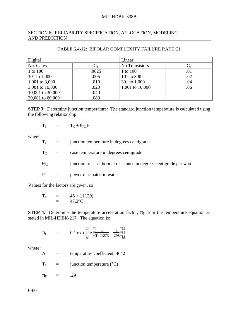
MIL-HDBK-338B


6-60

TABLE 6.4-12: BIPOLAR COMPLEXITY FAILURE RATE C1

Digital LinearNo. Gates C1 No Transistors C1

1 to 100 .0025 1 to 100 .01101 to 1,000 .005 101 to 300 .021,001 to 3,000 .010 301 to 1,000 .043,001 to 10,000 .020 1,001 to 10,000 .0610,001 to 30,000 .04030,001 to 60,000 .080

STEP 3: Determine junction temperature: The standard junction temperature is calculated usingthe following relationship:

TJ = TC + θJC P

where:TJ = junction temperature in degrees centigrade

TC = case temperature in degrees centigrade

θJC = junction to case thermal resistance in degrees centigrade per watt

P = power dissipated in watts

Values for the factors are given, so

TJ = 45 + 11(.20)= 47.2°C

STEP 4: Determine the temperature acceleration factor, πT from the temperature equation asstated in MIL-HDBK-217. The equation is:

πT = 0.1 exp

−A1

TJ + 273−

1298

where:A = temperature coefficient, 4642

TJ = junction temperature (°C)

πT = .29

MIL-HDBK-338B


6-61

STEP 5: Determine the packaging factor C2 given a 64 pin non-hermetic dual-in-line packagefrom the equation in MIL-HDBK-217. The equation is:

C2 = 3.6 x 10-4 (Np)1.08

where:C2 = 3.6 x 10-4 (64)1.08

= .032

STEP 6: Find the environmental factor from MIL-HDBK-217 which is shown in Table 6.4-13.For ground fixed conditions, the value is 2.0.

TABLE 6.4-13: ENVIRONMENTAL FACTOR - πE

Environment πE

GB (Ground Benign) 0.5

GF (Ground Fixed) 2.0

GM (Ground Mobile) 4.0

STEP 7: Select the quality value from MIL-HDBK-217. Since the product is a commercialdevice with an unknown screening level, the quality factor has a value of 10.0 as shown in Table6.4-14. When the screening level is known, MIL-HDBK-217 has a table that relates πQ values(lower than 10.0) to the specific screening level.

TABLE 6.4-14: QUALITY FACTORS - πQ

Description πQ Description πQ

Class S 0.25 Class B-1 2.00

Class B 1.00 Commercial 10.00

STEP 8: Using the equation for manufacturing learning from MIL-HDBK-217 which is:

πL = 0.1 exp (5.35 - .354/Y)

πL = 1 for production lines in operation longer than 2 years

MIL-HDBK-338B


6-62

where:Y = years, which is 2

πL = .01 exp (5.35 - .35(2))

= 1.05, which is rounded to 1.

STEP 9: Perform the calculation.

λp = [C1πT + C2πE] πQπL

= [ (0.08)(.29) + (.032)(2.0)] (10) (1.0)

= 0.87 failures per 106 hours

After one has calculated the failure rate for each component, the equipment failure rate isdetermined by summing the failure rates of the individual components as shown in equation 6.43.

λEQUIP = i=1

n

∑ λi (6.43)

and the MTBF is

MTBF = 1

λEQUIP (6.44)

Stress analysis failure rate predictions such as this permit extremely detailed analyses ofequipment or system reliability. However, since details of the system design are required indetermining stress ratios, temperature and other application and environmental data, thesetechniques are only applicable during the later stages of design. Because of the high level ofcomplexity of modern systems, the application of the procedure is time consuming.

MIL-HDBK-338B


6-63

6.4.5.3.3.3 Modification for Non-Exponential Failure Densities (General Case)

Although the exponential technique indicated in the previous sections can be used in mostapplications with little error, it must be modified (1) if the system contains parts for which thedensity function of failure times cannot be approximated by an exponential distribution over thetime period of interest; or (2) if the parts which are the dominant factor in overall systemunreliability do not follow an exponential density function of times to failure. Mechanical partssuch as gears, motors, and bearings usually fall into this category.

In these cases, one cannot add the failure rates of all parts because there are some parts whosefailure rates vary significantly with time. The method used is to consider separately within eachblock diagram the portion of the block containing parts with constant failure rates, and theportion containing parts with time varying failure rates. If the former portion contains n parts,then the reliability of this portion is

R1(t) = exp − λ1

i =1

n∑

t

(6.45)

The reliability of the second portion at time t is formed by using the appropriate failure densityfunction for each part whose parameters have been determined through field experience ortesting. If this portion contains B parts, then

R2(t) = ∏i=1

B Ri(t) (6.46)

where:

Ri(t) =

fi(t)dt

t

∞

∫ (6.47)

and fi(t) is the probability density function, general expression, of each of the B parts.

As discussed in 5.3.6, the Weibull distribution can be used to describe the distribution of times tofailure in a wide variety of cases. If we use the Weibull to describe the portion of the blockdiagram containing parts with varying failure rate, equation 6.47 becomes:

R2(t) =

∏=

θθβ

∫∏

ββ

θ

=

θ−β∞

=

tB

i

t

t

B

iee

t

1

1

1(6.48)

MIL-HDBK-338B


6-64

where:B = numbered partst = timeθi = Weibull scale parameter for part iβi = Weibull shape parameter for part i

The reliability for the block diagram, under the assumption of independence between the twoportions, is

R(t) = R1(t) R2(t) (6.49)

For example, consider the failure rates of two elements, x and y, that make up a system. Let x bea microprocessor controller with a constant failure of 2 failures per million hours. Let y be aroller bearing operating at 1000 revolutions per minute for which 90% of the population willoperate without failure for 3.6 x 109 revolutions. Bearing life test results have been fitted to theWeibull distribution with a shape parameter, β, of 1.5.

STEP 1: The microcircuit reliability is found by using equation 6.38.

R1(t) = exp(-λt)

= exp [ - (2 x 10-6)(50,000) ]

R1(t) = 0.905

STEP 2: The bearing reliability is determined by converting the revolutions into hours giventhat the speed is 60,000 revolutions per hour. This is 3.6 x 109 revolutions divided by 60,000revolutions per hours which equals 60,000 hours.

Then scale parameter θ, is determined from the standard Weibull equation shown as 6.48.

R(t) = exp -

tθ

β

MIL-HDBK-338B


6-65

where:R(t) = 0.9 at 60,000 hours (given)t = 60,000 hoursβ = Weibull shape of 1.5 for product characteristic of early wearoutθ = mean-time-to-failure

R(t) = 0.9 = exp -

60,000θ

1.5

θ = 60,000/(-ln 0.9)1/1.5

θ = 268,967 hours

This scale parameter is used to determine the reliability at the 50,000-hour point using equation6.48.

R(t) = exp -(

tθ

)B

R(t) = 0.9 = exp -51

976268

00050.

,,

= 0.923

STEP 3: The system reliability is found using equation 6.49 where

R(t) = R1(t) R2(t)

= (0.905) (0.923)

= 0.835

STEP 4: Calculate the system MTBF as follows:

MTBF =

( )

( )

−

∫

=−

∫

β

θ−

λ−

θ−

λ−

Tt

tT

tT

ee

dtee

)T(R

dt)t(R

1

1

00

MIL-HDBK-338B


6-66

where T is the time period of interest (T = 50,000 hours in this case).

MTBF =

R(t)dt0

50,000

∫1− R(50, 000)

= 279,795 hours

6.4.5.3.3.4 Nonoperating Failure Rates

The component failure rates in MIL-HDBK-217 (Ref. [11]) and in the Nonelectronic PartsReliability Data (Ref. [12]) are based upon operating time. There are, however, equipment andsystems in which nonoperating time represents a significant portion of the useful life, e.g.,missiles, fuses, projectiles, etc.

Nonoperating component failure rate prediction models have been developed in the technicalreport, RADC-TR-85-91, Impact of Nonoperating Periods on Equipment Reliability (Ref. [15]).These models are patterned after those found in MIL-HDBK-217 and are applicable toequipment/systems subjected to nonoperating conditions.

Nonoperating failure rates are computed in a manner similar to operating failure rates only usingsomewhat different models and different multiplying factors. A typical nonoperating failure ratemodel is as shown in the following equation for discrete semiconductors.

λp = λnb πNT π NQ π NE πcyc failures/106 nonoperating hours (6.50)

where:λp = predicted transistor or diode nonoperating failure rate

λnb = nonoperating base failure rate

πNT = nonoperating temperature factor, based on device style

πNE = nonoperating environmental factor

πNQ = nonoperating quality factor

πcyc = equipment power on-off cycling factor

The nonoperating failure rate prediction models can be used separately to predict nonoperatingfailure rate and reliability, or they can be used to complement the operating failure rate predictionmodels in the other sections of the Handbook. The following equations illustrate the methods for

MIL-HDBK-338B


6-67

predicting equipment (or system) level nonoperating reliability (Rn), service life failure rate (λsl)and combined operating/nonoperating reliability (Ro/n).

Rni

= exp (- λnitni) Rn =

Rnii=1

n

∏

λ(sl)i

= Doi λo

i + Dn

iλn

i λsl = i=1

n

∑ λ sl( )i

R(o/n)i

= exp ( - (λnitn

i + λo

ito

i) ) R(o/n)

i =

R(o /n)i

i=1

n

∏

where:Rn

i= nonoperating reliability of the ith item

λni = nonoperating failure rate in the ith nonoperating environment

tni = nonoperating time in the ith nonoperating environment

λ(sl)i

= service life failure rate of the ith item, equal to the number of

failures per unit time regardless of operational mode

Doi

= duty cycle in the ith operating environment, equal to the time in the

ith operating environment divided by total operating time plus totalnonoperating time

λoi = operating failure rate in the ith operating environment

Dni = duty cycle in the nonoperating environment, equal to the time inthe ith nonoperating environment divided by total operating timeplus total nonoperating time

λni = nonoperating failure rate in the ith nonoperating environment

R(o/n)i

= reliability of the ith item for the mission duration plus nonoperating

time between missions

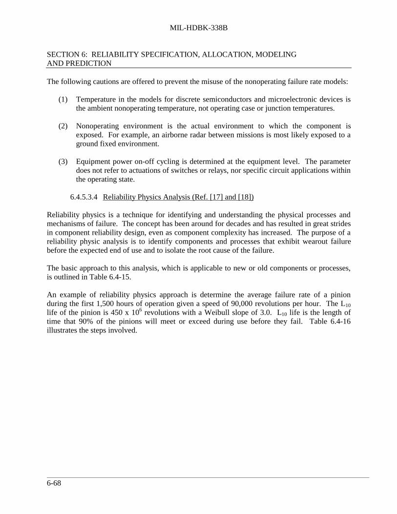
MIL-HDBK-338B


6-68

The following cautions are offered to prevent the misuse of the nonoperating failure rate models:

(1) Temperature in the models for discrete semiconductors and microelectronic devices isthe ambient nonoperating temperature, not operating case or junction temperatures.

(2) Nonoperating environment is the actual environment to which the component isexposed. For example, an airborne radar between missions is most likely exposed to aground fixed environment.

(3) Equipment power on-off cycling is determined at the equipment level. The parameterdoes not refer to actuations of switches or relays, nor specific circuit applications withinthe operating state.

6.4.5.3.4 Reliability Physics Analysis (Ref. [17] and [18])

Reliability physics is a technique for identifying and understanding the physical processes andmechanisms of failure. The concept has been around for decades and has resulted in great stridesin component reliability design, even as component complexity has increased. The purpose of areliability physic analysis is to identify components and processes that exhibit wearout failurebefore the expected end of use and to isolate the root cause of the failure.

The basic approach to this analysis, which is applicable to new or old components or processes,is outlined in Table 6.4-15.

An example of reliability physics approach is determine the average failure rate of a pinionduring the first 1,500 hours of operation given a speed of 90,000 revolutions per hour. The L10

life of the pinion is 450 x 106 revolutions with a Weibull slope of 3.0. L10 life is the length oftime that 90% of the pinions will meet or exceed during use before they fail. Table 6.4-16illustrates the steps involved.

MIL-HDBK-338B


6-69

TABLE 6.4-15: BASIC APPROACH TO RELIABILITY PHYSICS ANALYSIS

Step Discussion1. Define the operating and

nonoperating liferequirements

Length of time or number of cycles expected or needed forboth operating and nonoperating periods should bedetermined.

2. Define the life environment Temperature, humidity, vibration and other parametersshould be determined so that the load environment can bequantified and the cycle rates determined. For example, abusiness computer might expect a temperature cycle onceeach day from 60°F to 75°F ambient. This would quantifythe maximum and minimum temperatures and a rate of onecycle per day.

3. Identify the materialproperties

Usually this involves determining material characteristicsfrom a published handbook. If unique materials are beingconsidered, then special test programs will be necessary.

4. Identify potential failuresites

Failure areas are usually assumed to fall into categories ofnew materials, products or technologies. Considerationsshould include high deflection regions, high temperaturecycling regions, high thermal expansion materials,corrosion sensitive items, and test failures.

5. Determine if a failure willoccur within the time ornumber of cycles expected

A detailed stress analysis using either a closed form orfinite element simulation method should be performed.Either analysis will result in a quantifiable mechanicalstress for each potential failure site.

6. Calculate the component orprocess life

Using fatigue cycle curves from material handbooks,estimate the number of cycles to failure. The followingfigure shows a typical fatigue curve for stress versus cyclesto failure. Specific material fatigue data can be obtainedfrom databases maintained by the Center for Informationand Numerical Data Analysis and Synthesis.

nonferrousalloys

ferrousalloys

predictedcycles tofailure

calculatedstress

Cycles to Failure

Stre

ss

STRESS VERSUS CYCLES TO FAILURE

MIL-HDBK-338B


6-70

TABLE 6.4-16: EXAMPLE OF A PINION RELIABILITY ANALYSIS

Step Parameters and Calculations1. Identify the pinion life characteristics • L10 = 450 x 10

6 revolutions• Weibull slope (β ) = 3.0• Speed = 90,000 revolutions/hour

2. Convert L10 revolutions to hours L10 (Hours) =

L10 Revolutions

Revolutions/Hour

450 x 106

90, 000 = 5, 000

3. Determine the characteristic life usingthe Weibull reliability function R(t) = exp

−

tθ

β

θ =

t

−R(t)[ ]1/ β

where: t = time in hours θ = mean-time-to-failureβ = Weibull slope of 3.0R(t) = 0.9 at 5,000 hours

θ =

5, 000

−ln(.9)[ ]1/ 3 = 10,586 hours

4. Compute the failure rate for 1,500hours

λ (t) = H(t) =

tβ-1

θβ

where: λ (t) = instantaneous failure ratet = time in hours θ = mean time between failureβ = Weibull slope of 3.0

λ (t) =

1, 500( )3−1

10, 586( )3 = 1.9 failures/ 106 hours

MIL-HDBK-338B


6-71

6.4.5.4 Computer Aided Reliability Prediction

Reliability prediction for a modern complex system requires a tremendous amount ofcomputation. To overcome this obstacle, various commercial software packages have beendeveloped to automate MIL-HDBK-217 (Ref. [11]) and other reliability predictions. In fact,some of the more elaborate commercial software packages also handle intricate missionreliability modeling of complex systems.

An ever-growing abundance of reliability prediction software packages are available in a varietyof price ranges, each offering an assortment of common attributes and various unique features.Due to the changes occurring daily in this field it is not possible to include a detailed discussionof each such program. A comprehensive listing of the various commercial packages currentlyavailable is beyond the scope of this handbook, but may be found at the RAC world wide website at (http://rome.iitri.com/RAC/DATA/RMST/).

6.5 Step-By-Step Procedure for Performing Reliability Prediction and Allocation

In summary, the following basic steps apply to the prediction and allocation of reliabilityrequirements:

Step (1) Definition of equipment

Step (2) Definition of failure

Step (3) Definition of operational and maintenance conditions

Step (4) Develop the reliability block diagram(s)

Step (5) Establish mathematical model(s)

Step (6) Compilation of equipment, component or part lists

Step (7) Performance of “similar item,” “parts count,” “parts stress analysis,”“reliability physics analysis predictions”

Step (8) Assignment of failure rates or reliability

Step (9) Combination of failure rates or reliability

Step (10) Computation of equipment reliability

Step (11) Allocate failure rates and reliability

Step (12) Allocate among redundant configurations

MIL-HDBK-338B


6-72

Step (13) Evaluate feasibility of allocated requirements

The procedures for making pre-design or interim reliability predictions are basically the same asfor final design predictions except that the difference lies in the degree of precision (and details)with which the basic steps are implemented.

For predictions made at any stage of development, each of the steps will be carried out to themaximum extent possible. The system failure and operating and maintenance conditions shouldbe defined as explicitly as possible. Reliability block diagrams are constructed to the lowestidentifiable function, and appropriate system reliability formulas are established.

Precise parts lists, of course, cannot be compiled prior to design of an equipment. It is necessary,however, to make the best possible estimate of the parts complements of the various itemsubdivisions (blocks on the reliability diagram).

Stress analyses obviously cannot be made prior to design. However, for portions of theequipment that have not been designed, gross stress analyses can be accomplished. Stress levelsmay be assumed and failure rate estimates can be made by applying failure rate vs. stresstradeoffs to the assumed failure rate data. The process of combining part failure rates to obtainpreliminary block failure rates or reliabilities, of adjusting block rates or probabilities, and ofcomputing equipment reliability is the same for pre-design and interim predictions as for finalpredictions.

6.6 References for Section 6

1. MIL-HDBK-781, “Reliability Test Methods, Plans and Environments for EngineeringDevelopment, Qualification and Production,” 1987.

2. Arsenault, J.E., et al., “Reliability of Electronic Systems,” Computer Science Press, Inc.,1980.

3. Fuqua, N.B., “Reliability Engineering for Electronic Design,” Marcel Dekker, Inc., NewYork, NY, 1987.

4. Klion, J., “Practical Electronic Reliability Engineering,” Van Norstrand Reinhold, 1992.

5. Shooman, M.L., “Probabilistic Reliability, An Engineering Approach,” McGraw Hill,1968.

6. Von Alven, W.H., “Reliability Engineering,” Prentice Hall, Inc., Englewood Cliff, NJ,1964.

7. “Engineering Design Handbook: Design for Reliability,” AMCP 706-196, ADA 027370,1976.

MIL-HDBK-338B


6-73

8. “Reliability Toolkit: Commercial Practices Edition,” Reliability Analysis Center and RomeLaboratory, 1995.

9. Boyd, M.A., “What Markov Modeling Can Do For You,” Annual Reliability andMaintainability Symposium - Tutorial Notes, 1996.

10. Regulinski, T.L., “Availability Function for Communicating Computer Net,” ProceedingsReliability and Maintainability Symposium, 1980.

11. “Reliability Prediction of Electronic Equipment,” MIL-HDBK-217F, 1995.

12. “Nonelectronic Parts Reliability Data,” (NPRD), Reliability Analysis Center, 1995.

13. Bellcore, TR-332, “Reliability Prediction Procedure,” Issue 5, December 1995.

14. “Electronic Parts Reliability Data,” (EPRD), Reliability Analysis Center, 1997.

15. “Impact of Nonoperating Periods on Equipment Reliability,” RADC-TR-85-91, 1985.

16. “Nonoperating Reliability Data Book,” (NONOP-1), Reliability Analysis Center, 1987.

17. “Reliability Assessment Using Finite Element Techniques,” RADC-TR-89-281, RomeLaboratory, 1989.

18. “Computer-Aided Assessment of Reliability Using Finite Element Methods,” RADC-TR-91-155, Rome Laboratory, 1991.

MIL-HDBK-338B


6-74


MIL-HDBK-338B

SECTION 7: RELIABILITY ENGINEERING DESIGN GUIDELINES

7-1

7.0 RELIABILITY ENGINEERING DESIGN GUIDELINES

7.1 Introduction

Reliability engineering is the technical discipline of estimating, controlling, and managing theprobability of failure in devices, equipment and systems. In a sense, it is engineering in its mostpractical form, since it consists of two fundamental aspects:

(1) Paying attention to detail

(2) Handling uncertainties

However, merely to specify, allocate, and predict reliability is not enough. One has to dosomething about it in terms of having available a family of design guidelines which the designercan use to achieve a desired reliability. These guidelines are provided in this section.

During a product development program, a design is developed to meet previously definedquantitative reliability requirements. The importance of designing in the required degree ofreliability initially cannot be overemphasized, for once the design is approved, inherent reliabilityis fixed.

There are a host of design principles and tools of which the designer should be aware and shoulduse as required to achieve a reliable electronic equipment/system design. They include:

(1) Parts Management(2) Part derating(3) Reliable circuit design(4) Redundancy(5) Environmental design(6) Human factors design(7) Failure modes and effects analysis (FMEA)(8) Fault tree analysis (FTA)(9) Sneak circuit analysis(10) Design reviews(11) Design for testability(12) System safety program(13) Finite element analysis

Each of these will be briefly discussed in this section in terms of its role in the design of reliableequipment/systems.

MIL-HDBK-338B


7-2

7.2 Parts Management

Many factors affect the ultimate levels of quality and reliability of parts. Possibly the mostimportant factor is the degree to which the manufacturer is able to fabricate them in a defect-freemanner. This factor is a strong function of the volume and continuity of part production.Additional factors affecting part reliability are the levels to which the part is screened, theapplication, and the manner in which the part is integrated into the system.

The volume of parts produced usually impacts field reliability, since manufacturers producinglarge numbers of parts on a continuous basis can easily benefit from Statistical Process Control(SPC). When used wisely, SPC has proven to be an effective tool for improving processes,thereby increasing the quality and reliability levels of manufactured parts. Manufacturing linesintermittently producing small numbers of parts on a line with non-standard manufacturingprocesses typically do not exhibit the reliability levels of fully loaded manufacturing lines usingwell-controlled manufacturing processes.

Critical parts are often highly reliable, simply due to the attention given to them by both the partmanufacturers and by the users. As an example, consider integrated circuits. When first usedextensively twenty years ago, they often were the predominant device type limiting systemreliability. Since then, due to their critical nature, part manufacturers have improved theirreliability by orders of magnitude and part users are learning how to apply them in a mannerwhich results in a robust design. These efforts have resulted in integrated circuits that are muchmore reliable than many other part types used in systems.

Therefore, high usage, highly critical and high volume parts often show rapid technologymaturation, whereas low usage, noncritical or low volume parts can exhibit slower reliabilityimprovement and result in lower levels of field reliability. As an example, consider the itemsidentified by field data as being high failure rate parts: fasteners, actuators, connectors,transducers and switches. These are ordinary and necessary parts which are not considered state-of-the-art, but yet can significantly impact field reliability.

The general elements of an effective Parts Management Plan (PMP) are (MIL-HDBK-965,“Acquisition Practices for Parts Management” provides guidance in selecting tasks to include ina PMP):

(1) Preferred Parts List (2) Vendor and Device Selection (3) Critical Devices/Technologies/Vendors (4) Device Specifications (5) Screening (6) Part Obsolescence (7) Failure Reporting, Analysis and Corrective Action (FRACAS)

MIL-HDBK-338B


7-3

Each of these elements can be tailored to meet the specific needs of each system. Reference [1]“Parts Selection, Application and Control” provides generic guidance in the development of thisprocess.

Each of these elements are discussed in the following subsections.

A comprehensive PMP defines the manner in which each of the aforementioned elements will beaddressed. It should identify the responsible personnel and include a milestone schedule. Thisplan can also be tailored in accordance with specific requirements of the system for each of thePMP elements. Tailoring should be accomplished considering:

(1) Development Cycle Time (6) Budget(2) Warranty Period (7) Screenability(3) Maintainability (8) Preventive Maintenance(4) Cost of Failure (9) Customer Requirements(5) System Characteristics (10) Severity (or Criticality) of Failure

(a) volume(b) weight(c) performance(d) operating environment

Understanding, defining and then implementing all the tasks involved in a PMP program is thekey to its success. The representation and active participation of the following disciplines, as aminimum, are necessary to enable, in a concurrent engineering fashion, an effective PMP:

(1) Parts (components) engineering (3) Design engineering(2) Reliability engineering (4) Manufacturing engineering

Successful implementation of a PMP requires a disciplined approach, and must havemanagement participation and support to ensure cooperation among disciplines and resolve anydifferences based on the ultimate impacts on cost, schedule and performance.

7.2.1 Establishing a Preferred Parts List (PPL)

In the course of a design effort, equipment designers need to select the parts and materials to beused to meet specified equipment requirements for performance, reliability, quality, producibilityand cost. This selection task is greatly enhanced if the designer has a list of preferred partsavailable to help in this selection process.

Preferred parts are those whose quality and reliability are well-known to the industry, and areprobably parts that the company is already using in other equipments. Without a preferred partslist (PPL), designers may tend to choose parts in haphazardly. The result is the uncontrolledproliferation of parts throughout a manufacturer's product line, all varying in performance andreliability. All potential candidate parts should undergo an independent assessment before being

MIL-HDBK-338B


7-4

placed on the preferred parts list. Information sheets or data sheets from part suppliers may paintan optimistic picture of the part’s capabilities, but may omit information regarding the part’sinherent characteristics that are critical to proper operation of the final product.

The absence of a PPL may have wide-ranging consequences for manufacturing, purchasing, andlogistics. Manufacturing engineers may have to cope with parts that require a variety ofassembly methods and unique tooling. More inventory may be needed and, as a result, inventorycosts can mushroom out of control. Manufacturing automation may also be adversely affected.Purchasing representatives may have to deal with many different suppliers, making it hard forthem to monitor quality and timely delivery, and to obtain volume cost discounts. Logisticsspecialists must now provide spares for many different parts, enter them into the supply system,and find storage space for all of them.

Some consequences of designing equipment without a PPL are:

(1) Proliferation of non-preferred parts and materials with identical functions(2) Increased need for development and preparation of engineering justification for

new parts and materials(3) Increased need for monitoring suppliers and inspecting/screening parts and materials(4) Selection of obsolete (or potentially obsolete) and sole-sourced parts and materials(5) Possibility of diminishing sources(6) Use of unproven or exotic technology ("beyond" state-of-the-art)(7) Incompatibility with the manufacturing process(8) Inventory volume expansion and cost increases(9) Increasing supplier base and audit requirements(10) Loss of "ship-to-stock" or "just-in-time" purchase opportunities(11) Limited ability to benefit from volume buys(12) Increased cost and schedule delays(13) Nonavailability of reliability data(14) Additional tooling and assembly methods may be required to account for the added

variation in part characteristics(15) Decreased part reliability due to the uncertainty and lack of experience with new parts(16) Impeded automation efforts due to the added variability of part types(17) Difficulty in monitoring vendor quality due to the added number of suppliers(18) More difficult and expensive logistics support due to the increased number of part

types that must be spared.

When a PPL is available at the beginning of the design process, designers avoid using non-approved parts and the laborious task of having to supply engineering justification for their use.

MIL-HDBK-338B


7-5

Preferred parts databases help to flag obsolete parts and also indicate a part’s long termavailability (i.e., how long a given part may actually be available in the market).

The PMP must provide some level of standardization to minimize the number of new partsentering the system/equipment, or the logistic support and supply system, and yet still be flexibleenough to effectively capitalize on the advantages offered by alternative technologies. To betruly effective, the PMP must first ensure that the parts selected will provide the necessary levelof performance and reliability over the projected life of the system/equipment. It must also betailored to the expected life of the equipment to ensure, among other things, that replacementspares will continue to be available throughout the effective life of the system/equipment. ThePPL should be updated periodically to ensure a proactive approach to minimizing the impact ofpart obsolescence.

7.2.2 Vendor and Device Selection

Major factors to consider when implementing a PMP is the evaluation of vendors and theselection of components. It is imperative that engineers select and use components frommanufacturers in which they have confidence. This confidence can be attained either empiricallythrough adequate past performance of the part manufacturer, or from verification that themanufacturer is indeed producing high quality parts. The latter can be achieved via evaluation ofthe part manufacturing processes through testing and subsequent data analysis.

To ensure the supply of adequate parts, both vendors and subcontractors must be effectivelymanaged. A procedure is needed in which each vendor/technology is evaluated, certified andqualified in a cost-effective manner. Traditionally, this procedure was to test all devices andaudit all vendors. Due to the increased emphasis on quality (especially in microcircuits), a moregeneric approach to vendor certification/qualification of processes is recommended. Then,existing data from technology families can be used for qualification by similarity. Ongoingvendor/customer testing programs on representative products may be used to determineacceptability. Procedures for performing and monitoring vendor/product testing and incominginspection are still necessary, but should be tailored to allow each vendor to be handled on acase-by-case basis. For example, outgoing vendor quality and user incoming inspection andboard level testing can be monitored to determine device quality and productdesign/manufacturing process compatibility. Data analysis can then determine the need forvendor testing, incoming inspection and increased vendor surveillance. These data can also formthe basis for determining whether a "ship to stock" program (i.e., acceptance of a product withoutincoming inspection) is feasible.

Parts must be selected based on a knowledge of both the application environment in which thepart is to operate and the conditions it is exposed to during part manufacturing, assembly,handling and shipping. It is equally important to understand how the failure rate during the part’suseful life, and its wearout characteristics (lifetime), are impacted by the specific applicationconditions. Only with this understanding are robust designs possible.

MIL-HDBK-338B


7-6

One specific area of importance is the continuity of production. As mentioned earlier,facilities/production lines that manufacture parts on a continuous basis often produce higherquality parts than those manufactured on an intermittent basis. Intermittent production can be acharacteristic of custom, low usage parts. High volume, continuous production is usuallycontrolled in a statistical manner, whereas intermittent production may not be able to implementSPC. Additionally, intermittent lines often run into unanticipated problems associated with start-up which can adversely affect the quality, availability, and reliability of the part.

Many successful organizations have developed a qualified manufacturers list (QML) on whichprocurement decisions are based. A QML lists manufacturers who have proven that they cansupply good parts with a high degree of confidence. The DoD is also using this methodology inthe procurement of microcircuit devices, via the QML program (i.e. MIL-PRF-38535).

Part manufacturers can be evaluated in many ways. For suppliers of parts that have beenmanufactured for some time, analysis of historical reliability/quality data is usually the optimummethod. In many cases, these data are readily available from the manufacturer and, in somecases, are published in their data catalogs. To be meaningful, historical data must berepresentative of the same, or a similar, part with few changes, and must be for a similarapplication under similar operational stresses.

Vendor evaluation can be accomplished by analyzing design, manufacturing, quality, andreliability practices. Figure 7.2-1 illustrates a methodology to evaluate potential vendors.

Add to PotentialList of Vendors

MultipleManufacturers

InvestigateManufacturer’s

Quality Practices(Audits?)

Are Good Designand QC Practices

in Place?

Select AnotherManufacturer

Identify Needfor Part

SingleManufacturer

High VolumePart

Low VolumePart

Has Part DemonstratedReliability (from TestData, SPC Data, etc.)?

Are Good Designand Quality Practices

in Place?

Add to PotentialList of Vendors

Consider Redesign,Establish Alternate

Source or Workwith Manufacturerfor Improvement

Keep Lines ofCommunication

Open withManufacturer

Yes No

YesYesNo

No

FIGURE 7.2-1: VENDOR SELECTION METHODOLOGIES

An audit/validation should focus on whether a documented baseline system exists and is beingused. Additionally, required demonstration of generic product manufacturability, verified by

MIL-HDBK-338B


7-7

reliability testing, is necessary. Representative questions such as those in Table 7.2-1 should beasked.

TABLE 7.2-1: QUESTIONS FOR PART SUPPLIERS

• Is a quality program defined and implemented?• Have potential failure mechanisms been identified?• Are the manufacturing materials and processes documented?• Are there process controls in place?• Are parts manufactured continuously or is there intermittent production?• What defect levels are present?• Is there a goal in place for continuous improvement?• Have life limiting failure mechanisms been designed out?• If it is not practical to design or screen out life limiting mechanisms, have they

been modeled such that the user can quantify the part's lifetime in a specificapplication?

• Are efforts being taken to identify the causes of part failure and to improve themanufacturing process to alleviate their occurrence?

• Is the part screening and qualification process effective?• Are design rules used and adhered to that result in high quality and reliability?• Are design changes made only after analyzing and quantifying possible

reliability impact?• What is the on-time delivery success rate?

Recent improvements in customer/supplier relationships have resulted in alliances orpartnerships where both parties work together to improve the quality and reliability of deliveredproducts. However, to achieve these alliances, it is necessary to understand that:

(1) Effective preferred parts selection is a dynamic process which minimizes the number ofdifferent parts used, while providing designers an adequate choice of components tomeet equipment performance requirements.

(2) Vendor selection certification and qualification criteria based on technical expertise areused to minimize the number of vendors.

(3) Good production suppliers are willing to support problem analysis and correctiveactions.

A process based on these considerations should be formalized to assess and validate potentialsuppliers' quality, reliability and manufacturing systems, and delivery, cost and serviceperformance. The resulting data, when reviewed by cognizant personnel (i.e., purchasing, design

MIL-HDBK-338B


7-8

engineering and manufacturing), can be used to select the appropriate suppliers. Once this step isaccomplished, alliances or partnerships can be established that can result in a win-win situation,where the procurement process changes from an adversarial to a cooperative relationship. Toestablish the continuous improvement process and manage the supplier, a reassessment andinformation exchange program can be put in place. The validation/audit plan results that wereused to select a vendor can now be the reference from which progress is measured.

7.2.2.1 Critical Devices/Technology/Vendors

Critical part types are considered to be those that require additional attention due to potentialreliability, safety or availability problems. Many parts programs focus too much attention onstandard or non-controversial part types. It is imperative that special attention be given to criticalparts, since they are often the parts driving the system reliability. The establishment of a listingof critical devices, technology and vendors, and a monitoring/action plan, should be part of everyPMP, and should address components exhibiting the following characteristics:

(1) Performance Limitations: due to stringent environmental conditions or non-robustdesign practice.

(2) Reliability Limitations: component/materials with life limitations or use of unrealisticderating requirements.

(3) Vendors: those with a past history of delivery, cost performance or reliability problems(4) Old Technology: those with availability problems(5) New Technology: parts fabricated using immature design and manufacturing

technology

The first three categories require historical data to track and define actions to minimize theiroccurrence or provide alternate solutions. In addition, sound component engineering judgmentand the combined efforts of design, reliability, and manufacturing engineering, and vendors, areneeded to ensure the identification and management of critical components.

The subject of old and new technology can involve the generation of different procurementprocedures for tracking technology maturity, obsolescence and hidden hybrids (i.e., those devicesthat fall between generic device categories and, as a result, are incorrectly specified and tested,see 7.2.2.3).

The PMP should address the identification and control of limited or critical parts and off-the-shelf equipment. Also, the PMP must ensure that parts engineering, design, manufacturing andreliability personnel are notified of potential risks in using critical parts/technology. As statedpreviously, a PMP program must be tailored to account for the unique failure mechanismsassociated with the parts being used. For example, if plastic packaged microcircuits are used,their expected lifetime must be determined as a function of the use environment (temperature,humidity, dissipated power, etc.) and then compared to the design life of the equipment in whichthe component operates. As another example, consider off-the-shelf equipment. In this case, the

MIL-HDBK-338B


7-9

equipment must be analyzed to assess its suitability for use in its intended application. This isespecially true for commercial equipment designed for benign environments that are to be used inmore severe environments. A determination should be made of its reliability and performance,since it would be neither cost-effective nor practical for the vendor to change the design orproduction procedures. The task becomes one of evaluating subcontractor procedures, reliabilitydesign analyses and past performance.

7.2.2.1.1 ASIC Devices

The rapid technology changes in the field of microelectronics, both hybrid and monolithic, haveto be monitored closely. Application Specific Integrated Circuits (ASICs) are one part typeusually considered to be critical. The advent of ASICs requires a change in the device selectionprocedure. The term "ASIC" describes a wide variety of different types of devices which caninclude custom and semicustom standard cells, gate arrays, Programmable Logic Devices (PLD)and Field Programmable Gate Arrays (FPGA) typically designed for a specific application.Advantages include a relatively short development cycle and customized performance andfunctionality. Disadvantages are that the equipment schedule may be impacted because systemdesigners are involved in the device design cycle, and unproven vendors and technologies may beused for the first time.

Typically, ASIC devices are designed for a very specific application and then produced and soldin very limited quantities. Thus, there is no market for marginal devices. Historically, genericICs have been produced in a tiered market environment. Parts not meeting the highest level ofperformance could usually be sold to a less demanding customer at a reduced price. This issimply not the case with ASICs. Either they are 100% perfect or they are scrap. Given this fact,there is a very strong incentive to reduce or eliminate all possible variation in the partmanufacturing processes to attain a very high yield of good parts. Thus, Total QualityManagement (TQM) and SPC become imperative to the manufacture of these types of parts. Touse ASICs, a supplier must select and certify a silicon foundry and design the device usingfoundry design rules. Performance would be demonstrated through simulation tools. Thefoundry would then fabricate wafers and packaged devices for test. The planning andmanagement of ASIC design requires a very rigorous and controlled procedure to achieve desireddevice functionality, reliability, cost and delivery schedules.

7.2.2.1.2 GaAs and MMIC Devices

Gallium arsenide (GaAs) devices are now being used in military and commercial systems. GaAsoffers some significant advantages over silicon that can result in improved device performance.It has unique qualities which allow the fabrication of devices that can operate at frequencieswhich outperform their silicon counterparts. In addition, GaAs offers inherent radiation hardnessand improved power efficiency for high frequency digital and analog circuitry.

Monolithic Microwave Integrated Circuits (MMIC) are replacing hybrid microwave devicesthroughout the industry as a result of the Defense Advanced Research Project Agency (DARPA)

MIL-HDBK-338B


7-10

sponsored Monolithic Microwave Millimeter Wave Integrated Circuit (MIMIC) program. Beforethe development of GaAs MMIC technology, discrete packaged devices and multifunctionassemblies were commonly utilized in microwave applications. MMIC technology, however,offers several advantages including weight/size reduction, process tolerance and uniformperformance with a reduced need of tuning circuits. These advantages, combined with GaAs’sinherent performance advantages, have led to significant interest in the technology.

To date, information concerning the reliability of GaAs and MMIC components has shownvarying results and inconsistent activation energies for a specific failure mechanism. Thus, theabsolute reliability of GaAs devices is not easy to predict with accuracy, though anapproximation can be made based on government/industry reliability studies.

7.2.2.2 Plastic Encapsulated Microcircuits (PEMs)

Plastic packaging is a leading factor in the growth of microelectronics companies and has had asignificant positive effect in the telecommunications, computer and automotive industries. PEMshave demonstrated cost effectiveness while providing improved performance and reliability inthese applications environments. Now, acquisition reform initiatives and continuedimprovements in plastic packaging and die protection (i.e., silicon nitride passivation) have led totheir consideration and limited use in military environments. The RAC publication PEM2 (Ref.2) provides additional information.

7.2.2.3 Hidden Hybrids

Quality and reliability efforts for microcircuits have been more intense than for any othercommodity items, resulting in orders of magnitude improvement in their performance since the1960’s. However, the procurement of complementary devices/modules sometimes ignores thelessons learned in this area. We have chosen to call these devices "hidden hybrids," indicating amix or composite of technologies.

Examples include the following:

(1) Crystal Oscillators (4) Solid State Relays(2) Multichip and Microwave Modules (5) Transformers(3) Power Regulators (Supplies)

In many cases, these items have escaped the traditional testing and technology/vendor evaluationthat has led to the successes achieved for microelectronics devices. Crystal oscillators evolvedfrom a combination of discrete components mounted on a printed wiring board to hybridmicrocircuits made up of chip components (including the crystal), all contained in a singlehermetic package. Solid state relays are essentially a hybrid device containing discretesemiconductor components which should be individually tested and controlled.

MIL-HDBK-338B


7-11

The problem is presently being compounded by the various types of multichip and highfrequency (i.e., R.F. and microwave) modules being introduced. Multichip modules (MCM) aretaking advantage of integrated circuit, hybrid and printed wiring board (PWB) technologies, andare being used to fabricate state-of-the-art high performance products.

It is specifically recommended that packaged items be reviewed to uncover potential "hiddenhybrids" as shown in Table 7.2-2. Once located, the appropriate component procurementapproach (such as MIL-PRF-38534) should be used to ensure reliable and quality products.Incorporation of appropriate evaluation, audit and testing requirements could eliminate costlytesting and corrective action procedures at a later date, while ensuring customer satisfaction.

TABLE 7.2-2: HIDDEN HYBRID CHECKLIST

Analyze:• Fabrication Process - uses hybrid microcircuit assembly

techniques• Technology - contains microcircuits and/or semiconductors• Packaging - potted/encapsulated modules

Take Action:• Testing Requirements - per applicable test procedure

7.2.2.4 Device Specifications

Part electrical, mechanical and physical characteristics should be defined in a devicespecification to be used for design and procurement. Applicable device electrical performanceparameters that ensure product performance objectives are met for all operating conditionsshould be specified, including reliability parameters. This information may be available invendor catalogs/data sheets. Special care should be taken for electrical parameters that are"guaranteed but not tested," or other special features which should be discussed and agreed towith each vendor. The part specification should be based on several factors, including operatingenvironments, worst case stress levels, and quality requirements.

The Defense Electronic Supply Center (DESC) Standard Microcircuit Drawing format is anexample of how to prepare a company specification for microcircuits and other applicablecomponents. This format has been reviewed and coordinated with industry and can be used todevelop a specification that provides realistic, clearly stated requirements. Details are providedin MIL-HDBK-780 "Standardized Microcircuit Drawings." Reference [3] “Analog TestingHandbook (ATH)” provides information for the specification for analog and mixed mode(analog/digital) devices.

MIL-HDBK-338B


7-12

7.2.2.5 Screening

Screening, or 100% testing similar to that included in MIL-PRF-38534 and -38535, isrecommended, pending vendor validation and use experience. Data from appropriate in-processand reliability testing can be used to justify deletion of end-of-line tests. Vendor/customer trustand alliances can result in practical cost-effective testing.

7.2.2.6 Part Obsolescence and Diminishing Manufacturer Sources (DMS)

Obsolescence occurs when parts that are required for system support are no longer manufactured(usually due to insufficient market demand). It is a common occurrence within the DoD forsystems to have lifetimes greater than the life cycle of their supporting part technologies. Hence,part obsolescence is typically more of a problem for military systems than for commercialsystems. Also, parts qualified for military use have historically represented more maturetechnologies relative to those used in non-military applications. The potential for diminishingmanufacturing sources, causing parts that are not yet obsolete to become unavailable, must alsobe considered. This unavailability can be the result of the manufacturer experiencing limitedorders, downsizing, market instability, or the result of other business decisions to exit the marketfor a particular technology or device. Regardless of the reason, the part is unavailable, and theeffect is essentially the same as if the part had become obsolete.

Part and vendor obsolescence management should be a basic part of a company’s operating,design, and manufacturing procedures (i.e., best commercial practices) and be substantiallyproduct independent, evolve around needed components, operating environments and packagestyles. Implementation of an effective PMP requires diligent management in maintaining partavailability for system support, including taking the actions necessary to maintain availability ofparts that are, or will be, obsolete during the equipment life cycle. Such actions can be groupedinto two categories: management and technical.

Management solutions to part availability problems include preventive measures to alleviate theuse of potentially obsolete parts, detection of the use of potentially unavailable parts, andidentification of the need to procure an adequate quantity of parts to support the equipmentthroughout its life cycle. Management solutions include the use of a PPL and the lifetimepurchase of parts to ensure part availability in the event that they become obsolete. This lattersolution carries its own risks and burdens (for example, provisions for storing the parts in asufficiently benign environment that precludes the occurrence of storage-related failuremechanisms).

Technical solutions include replacement of the unavailable part with an equivalent part, deviceemulation, and system redesign. If there is a direct replacement available, substitution is usuallythe easiest and least costly solution. There are several semiconductor information sources thatcan assist in the identification of equivalent parts. These include the IC Master and Part Master(available from International Handling Services), and Computer Aided Product Selection (CAPS)(available from Cahners Publishing).

MIL-HDBK-338B


7-13

Early notification of part/vendor end-of-life status provides time to select an acceptable solutionthat will minimize the identified problem’s impact on manufacturing. External sources such asthe Defense Logistics Agency/Defense Supply Center Columbus (DLA/DSCC), GovernmentIndustry Data Exchange Program (GIDEP) and vendors, as well as management of the company’sinternal PPL, can be used to provide early notification. Figure 7.2-2 illustrates a process flow forshort and long term solutions that takes place when obsolete part notification is received. Themajor difference between short and long term solutions is that, in the long term solution, evenwhen a part or vendor exists or another solution is found, the effort does not stop. As mentioned,it is critical that the solution is not just a stop gap and that long term support issues are addressed.Therefore, a trade study using the factors indicated in Figure 7.2-2 is performed to ensure a longterm solution is not required in the future. (This concept is further described in reference [4]"767 AWACS Strategies For Reducing DMS Risk").

When a device has been identified as needed but unprocurable, the most practical solution isemulation. Device emulation is a process by which a direct replacement is designed andfabricated for an unavailable part. The design task may include reverse engineering, simulation,or direct design and fabrication (if original schematics and drawings are available). The DefenseLogistics Agency (DLA) currently leads such an emulation program, referred to as theGeneralized Emulation of Microcircuits (GEM).

System redesign is also a possible technical solution to alleviate the dependence on unavailableparts. Device emulation and system redesign can be very costly solutions to the unavailabilityproblem. Implementation of preventive measures early in the part selection process can providesignificant cost savings as the system reaches end-of-life.

The VHSIC Hardware Description Language (VHDL) is a valuable tool that can assist in theemulation or redesign of devices. VHDL is fast becoming the hardware description language ofchoice because it is an IEEE standard and has technology process and vendor independence,CAD tool support, and top-down design methodology capability. What is required is a VHDLbehavioral description of the obsolete device or printed wiring assembly. The next step is toproduce a structural VHDL description of the design to be emulated, which can then beprocessed by logic and layout synthesis tools of choice. This emulated design can then beprocessed by a compatible wafer foundry processing capability and packaged appropriately forinsertion.

MIL-HDBK-338B


7-14

Trade Study Factors

• Current product/customer

• Future needs

• Storage facilities

• Part/vendor sustainment

• Funding

Part/VendorStill

Available

NoPerform LifeBuy

Part/VendorStill

Available

No

Part/VendorNotification of

End of Life (EOL)

Short TermSolution Yes Part/Vendor

Still NeededYes

Long TermSolution

Check forAlternate• Source• F3

AlternatePart/VendorAcceptable

Change DrawingBuy Parts

PerformLong TermUse Trade

Study

Assess Replacement Options• Wafer Bank• Remanufacture/Emulate• New Off-the-Shelf Part• Custom Device• Redesign Function

No

Change Drawingand Implement

Track inDatabase

Track inData Base

FIGURE 7.2-2: PART OBSOLESCENCE AND DMS PROCESS FLOW

MIL-HDBK-338B


7-15

7.2.2.7 Failure Reporting, Analysis, And Corrective Action System (FRACAS)

FRACAS is a management tool established to identify and correct deficiencies in equipment andthus prevent further occurrence of these deficiencies. It is based upon the systematic reportingand analysis of failures during manufacturing, inspection, test and use. The closed-loop featureof FRACAS requires that the information obtained during the failure analysis be disseminated toall of the decision making engineers and managers in the program. See Section 8 for moreinformation on FRACAS.

7.2.3 Design for Reliability

In Section 7.2, the elements of a traditional Parts Management Program were discussed. Thissection discusses some of the methodologies that can be used to ensure that systems are designedand parts are applied in a robust manner. It presents an overview of the analytical tools that canbe used to ensure a robust design and discusses several considerations for ensuring amanufacturable product. Although this material is not part of a traditional parts managementprogram, it is relevant since the manner in which a part is used is as important as ensuring anadequate part is obtained. This observation illustrates the inseparability of part selection andapplication in the design and manufacture of a reliable system, and illustrates the necessity ofusing a concurrent engineering approach.

In the course of developing a system or equipment, suppliers must determine the market theproduct will serve and the need they will fulfill (i.e., environment to be used in, quality/reliabilityto satisfy customer, guarantee/warranty, and performance when compared to competition andcost). Once this is determined, requirements for part quality levels, design guidelines,temperature range and packaging can be defined. Assembly procedures must be defined todetermine the appropriate component packaging (i.e., surface mount, through-hole, etc.). Designguidelines for manufacturing producibility must be available to determine package lead pitch vs.printed wiring board capability, specification of component drift parameters and the many otherfactors leading to robust design. Once they are determined, the PMP function can attempt toprovide the components and materials necessary to satisfy them. The output of this functionshould be company-specific procedures containing:

(1) Guidelines for choosing component quality levels(2) Design guidelines

(a) Performance(b) Environmental/temperature(c) Assembly procedures

(3) Manufacturing/assembly procedures(4) Performance/reliability demonstration plan

Correct application of parts means "using the best part for the job in an optimum/cost effectivemanner." Hence, electrical and electronic parts must be selected with the proper temperature,performance, reliability, testability, and environmental characteristics to operate correctly and

MIL-HDBK-338B


7-16

reliably when used in a specific application. Parts and materials should be selected based ontheir ability to meet functional requirements for a given period of time under the expectedextremes of operating stresses, including shock/vibration, temperature, temperature cycling,humidity, contamination, mechanical stress, electrical stress, radiation and electromagneticinterference. Factors to be considered in optimum parts application are both numerous andcomplex, and should address each of the factors included in Table 7.2-3. Many of these partapplication factors can be specifically addressed by performing a reliability assessment.

Design for reliability is the process of selecting a part or material and applying it in such amanner that results in high reliability under the worst case actual use conditions. Such an effortrequires a structured approach during the part selection and design process. This process shouldinclude:

(1) Definition of operating environments(2) Establishment of lifetime requirements(3) Use of reliability models to estimate lifetime under use conditions(4) Estimates of reliability during the useful life(5) Stress derating(6) Analysis and design modifications to ensure robustness

Several analytical techniques are useful in robust design. These include derating, failure modeand effects analysis (FMEA) (with or without criticality analysis), fault tree analysis (FTA,) andfinite element analysis (FEA) (see 7.3, 7.8, 7.9, and 7.14, respectively).

7.2.3.1 Electronic Part Reliability Assessment / Life Analysis

A reliable product requires that the applicable part reliability and life requirements be adequatelydefined. This effort requires accurate quantification of the environmental and operationalstresses that the part will experience during use and an assessment of part reliability and lifeunder these conditions. Typical stress profiles are frequently used, but worst case stress valuesmay often be better suited for this assessment.

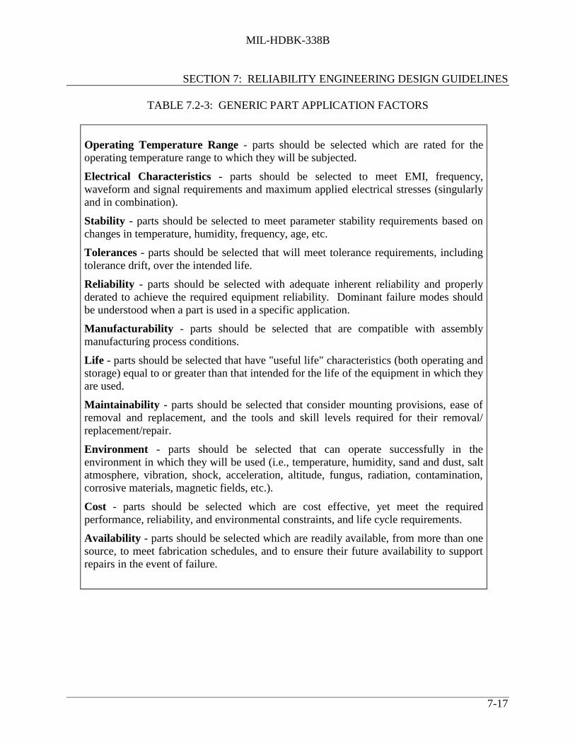
MIL-HDBK-338B


7-17

TABLE 7.2-3: GENERIC PART APPLICATION FACTORS

Operating Temperature Range - parts should be selected which are rated for theoperating temperature range to which they will be subjected.

Electrical Characteristics - parts should be selected to meet EMI, frequency,waveform and signal requirements and maximum applied electrical stresses (singularlyand in combination).

Stability - parts should be selected to meet parameter stability requirements based onchanges in temperature, humidity, frequency, age, etc.

Tolerances - parts should be selected that will meet tolerance requirements, includingtolerance drift, over the intended life.

Reliability - parts should be selected with adequate inherent reliability and properlyderated to achieve the required equipment reliability. Dominant failure modes shouldbe understood when a part is used in a specific application.

Manufacturability - parts should be selected that are compatible with assemblymanufacturing process conditions.

Life - parts should be selected that have "useful life" characteristics (both operating andstorage) equal to or greater than that intended for the life of the equipment in which theyare used.

Maintainability - parts should be selected that consider mounting provisions, ease ofremoval and replacement, and the tools and skill levels required for their removal/replacement/repair.

Environment - parts should be selected that can operate successfully in theenvironment in which they will be used (i.e., temperature, humidity, sand and dust, saltatmosphere, vibration, shock, acceleration, altitude, fungus, radiation, contamination,corrosive materials, magnetic fields, etc.).

Cost - parts should be selected which are cost effective, yet meet the requiredperformance, reliability, and environmental constraints, and life cycle requirements.

Availability - parts should be selected which are readily available, from more than onesource, to meet fabrication schedules, and to ensure their future availability to supportrepairs in the event of failure.

MIL-HDBK-338B


7-18

Part test data is generally used to assess part reliability under specific operating stresses. Suchdata can take many different forms. Useful reliability assessment data are often gleaned from theanalysis of life tests, performed either by the part manufacturer or by the user of the part. Helpfulpart reliability and life information may also be found in the literature. In any case, the data usedfor this assessment must address the specific predominant failure mechanisms applicable to thatparticular part and the specific materials used in the construction of that part. The use ofappropriate data can help in ensuring adequate part life in a specific application, as well as inprojecting anticipated part reliability. On the other hand, using inappropriate part life andreliability assessment data can give a false degree of confidence in the life estimate and thusprovide a potential for early field failures or poor long term reliability.

Part failure mechanisms can generally be grouped into two categories: common cause and specialcause. These two types of mechanisms have very different failure characteristics. Thisdifference must be recognized, and properly addressed, in the data collection, analysis andassessment effort.

Common cause failures are due to inherent failure mechanisms; they have the potential ofaffecting the entire population of parts. These mechanisms are typically addressed through thedesign of the part itself and the part’s fabrication process controls. These contributions help toensure that the device is sufficiently robust to operate reliably for a given period of time. Forthese types of mechanisms, a physics-of-failure based reliability assessment is appropriate, sinceit is possible to gain a good understanding of the failure mechanisms. Such an assessmentrequires a fundamental knowledge of the device fabrication process, the appropriate processcontrols, and applicable materials data.

Special cause failure mechanisms result from defects or from specific events. An example ofsuch a mechanism might be: capacitor failures resulting from a defective dielectric or fromelectrical overstress. Since special cause failure mechanisms are defect or event related, ratherthan process related, they tend to occur randomly. For such mechanisms, a purely physics-basedassessment may not be appropriate, due to the random nature of failure occurrence. For thesefailure mechanisms, statistical analysis of the data is usually the more appropriate assessmentapproach.

Clearly, it is important that a combination of both a physics-based approach and a statisticalanalysis approach be used in any part reliability and life assessment. Because of the differencesin the potential failure mechanisms involved, either approach used alone is unlikely to yieldcorrect conclusions regarding part reliability or life assessment.

MIL-HDBK-338B


7-19

7.2.4 Design for Manufacturability

Of equal importance to the selection and application of parts is the manufacturing process to beused for their implementation. The best part used in a good design is useless, unless it can beprocessed in a reliable and reproducible manner. Manufacturing process evaluation is especiallyimportant for new or immature technologies, or for technologies for which the manufacturer haslittle or no experience. Therefore, the manufacturability of equipment designs should be givenequal weight with the part selection and application efforts. Reference [5] “Best Practices - Howto Avoid Surprises in the World’s Most Complicated Technical Process” is a good referencesource for this task.

Procedures are required today to not only procure acceptable parts and materials, but also toensure that the process steps from shipping to assembly do not destroy good components. It isnot enough to qualify components to a standard qualification procedure, because some currentassembly processes impose greater stress than those used in the past. A classic example issurface mount technology, which uses soldering processes (i.e., vapor phase, infrared heating)that provide a very fast temperature transition to 220°C, creating a thermal shock which is greaterthan that used for component verification testing. This is exemplified by the use of plasticsurface mount packages which, in some cases, have resulted in the "popcorn effect." This refersto a phenomena in which moisture is absorbed by the plastic encapsulant material and, uponexposure to the soldering thermal shock, the moisture vaporizes, causing the package todelaminate or crack due to the resulting high internal pressures.

In order to determine if components will perform reliably after exposure to handling andassembly stresses, a preconditioning procedure emulating these processes should be developedand applied. Reference [6] describes a procedure generated to ensure that surface mountcomponents can withstand severe printed wiring board assembly conditions and still meetexpected reliability requirements. It can be used as a guide to define eachtest/procedure/operation/ material that is used in component handling and fabrication/assemblyfor establishing a process requirements procedure. This procedure should emulate all steps, fromreceipt of material through manufacturing. Additional or different preconditioning may benecessary for a specific process. After exposure, these devices should be subjected to appropriatetesting to determine if performance degradation has occurred. Common tests for a moldedplastic package include “85°C/85RH,” Highly Accelerated Stress Testing (HAST), Autoclave,and Dye Penetrant. For a hermetic device, seal testing should be part of the test procedure.Residual Gas Analysis (RGA) is also sometimes performed.

MIL-HDBK-338B


7-20

7.2.5 Parts Management Plan Evaluation Criteria

The following paragraphs provide guidelines which customers can use to evaluate a supplier’sPMP. This evaluation includes an assessment of the quality improvement program, qualityassurance, assembly processes, and design criteria. These guidelines are based on industry-accepted quality standards and are practiced by world-class organizations. These paragraphs areprovided to express the level of detail desired, highlight the subjects of interest, and provideconcrete guidelines. It is intended that suppliers clearly describe their own processes and explainhow these processes develop, maintain and improve the reliability of equipment.

7.2.5.1 Quality Improvement Program

Quality is defined as providing customers with products and services that consistently meet theirneeds and expectations. But quality goes beyond that of the product to include quality of work,service, information, processes, people, and management. Control of quality in every aspect ofthe contractor’s operation is the basic approach to total quality management.

A quality improvement program should be instituted to apply quantitative methods and humanresources to control processes. The objective is to achieve continuous improvement in theselection and application of components, their installation in subassemblies, and in end usersatisfaction. Each supplier should document their plan for achieving the goal of continuousimprovement in the development, manufacture, reliability, administration, and distribution ofproducts and services that meet the customer’s needs and expectations.

7.2.5.2 Quality Assurance

Quality assurance is the corporate effort that is specifically aimed at reducing process variationby improving process controls during product development and manufacture, and by takingmeasures to prevent recurrence of detected problems. Quality assurance also addresses thosetechniques that will give the customer confidence that future components and assembly processeswill have equivalent or better reliability than current components and assembly processes.

Assurance of component and assembly quality should be established before the part andassembly process is approved for use. Suppliers should have procedures for verifying thatselected components will operate reliably in the intended environment for the life of theequipment. Component qualification processes should be documented or referenced in the PMP.Testing should be conducted to verify that the proposed components will satisfactorily operate inthe intended environment with acceptable reliability. This verification usually takes the form ofa qualification test and screening. However, other methods may be proposed, such as extensivefield experience of the proposed parts in similar applications or previous contractor qualificationdata which is valid for the intended application. Furthermore, evidence of quality assemblyprocesses should be demonstrated and documented to ensure reliability at higher levels ofintegration. The supplier should ensure that the component quality is maintained during the

MIL-HDBK-338B


7-21

manufacture of equipment. The component reliability should not be compromised by equipmentmanufacturing processes such as handling or assembly.

7.2.5.2.1 Part Qualification

Qualification is used to verify that components are able to function for the specified life in theintended environment. The goal of qualification should be to ensure long term mechanical andelectrical integrity. Qualification requirements may be satisfied by similarity to existing qualifieddevices of similar packaging and technology. The process for the disposition of failures duringthe qualification procedures should be at the discretion of the supplier, but should be identified inthe PMP. The following items should be accounted for during component qualification:

(1) Hermetic and hygroscopic nature of unique package types(2) Operating characteristics over entire temperature range(3) Packaging capability for handling thermal shock(4) Internal circuitry and connection resistance to contamination and corrosion

(passivation)(5) Internal connection fatigue life(6) Levels of inherent contamination in packaging(7) Solderability of leads

Detailed qualification processes should be documented or referenced in PMP and should address,as a minimum:

(1) Goals/objectives(2) Procedures(3) Test reports(4) Pass/fail criteria(5) Failure detection and analysis(6) Requalification criteria(7) Failure resolution/corrective action procedures

Qualification Testing - Accelerated environmental qualification testing may be proposed for allcomponents if adequate field data does not exist to indicate long term reliability has beenachieved. The environmental testing is to verify that reliability performance is withinspecification. Electrical characteristics for all potential environmental conditions should beverified through qualification testing if it is not already verified by the manufacturer.

Field Data - Component field data can be used in lieu of qualification testing when the dataverify an acceptable failure rate. Component failure rates are generated by dividing totalaccumulated component failures by total accumulated hours. Component failure rates may alsobe calculated using industry-accepted prediction methodologies, such as those presentedpreviously. Component types used for failure rate calculations should be of similar families,

MIL-HDBK-338B


7-22

technologies or package types. The sample size should be statistically significant, with adequatefield experience per component.

Component Manufacturer Data - Component manufacturer qualification data may also be used inlieu of field data, provided the data are adequately documented, statistically significant, andindicates that the components should function in the environment for the specified time. Thesedata demonstrate that processes are in statistical process control and accelerated componenttesting data can be correlated to the intended application environment.

Component Reliability Assessment - Suppliers should have a plan for performing componentreliability assessment. The formulas, data and assumptions used to generate the reliabilityassessments should be documented or referenced in the PMP. When required by contract, thesupplier should explain to the customer how part reliability will allow the resulting product tomeet or exceed the reliability requirements of the respective equipment performancespecification.

When components are selected for use in an intended environment, a component quality andreliability assessment is necessary. The assessment technique and source of reliability datashould be clearly defined or referenced in the PMP. The following reliability sections addressonly component reliability, and not assembly, LRU or system reliability assessments.

Reliability Analysis - A preliminary reliability analysis for each component should be performedprior to the preliminary design review and, as a minimum, should consist of a clear example ofthe content and format of the reliability analyses being proposed. The supplier is encouraged tobase component reliability predictions on field data or other acceptable technical evaluations.Further, suppliers are encouraged to modify component reliability assessments based on methodsused to improve the quality of components, such as component manufacturing process control,screening, qualification or other provisions. Failure rates based on the supplier’s experience andmodifications based on quality provisions should be available for customer review when requiredby contract.

A final reliability analysis for each component should be required at the critical design review.This analysis should be completed as early as possible, so that potential problems with partsselection or system architecture can be uncovered in time for a cost-effective correction.

Reliability Tracking - In order to perform root cause failure analysis and provide a basis forquality improvement, the component reliability and quality assessments should be verified on acontinual basis. A verification should be made to show that the measured reliability exceeds thepredicted reliability. This may include tracking field reliability measurements and analysis,tracking screen yield, and/or monitoring manufacturing floor rejects. Failure rate assessmentsshould be updated for future reliability predictions, particularly when part reliability is measuredto be less than predicted.

MIL-HDBK-338B


7-23

When field data are used to perform a part reliability assessment, the following informationshould be provided:

(1) Component MTBF formulas correlating field performance to MTBF should beavailable to the customer. Details of operating hours should be included, as well ascomponent part numbers, equipment part numbers, and failure analysis results.

(2) Data submittals, if required, should include a summary of part types and failuremechanisms, and should include or reference the raw data used to arrive at theseconclusions.

(3) Component failure rates should be generated by dividing total accumulated componentfailures by total accumulated hours. Component types used for failure rate calculationsshould be of similar families, technologies or package types.

(4) Accumulated operating hours and failures should be statistically significant to provideaccurate failure rates. Suppliers should establish confidence intervals for the calculatedfailure rates using statistical techniques similar to the chi-square method.

(5) Continue to track component in-service data on an ongoing basis until equipmentproduction is completed.

Requalification - Requalification of the component should be performed when significantchanges (i.e., form, fit or function) are made to the package or internal circuitry. The followingare examples of significant changes that would require requalification, but do not constitute acomplete list.

(1) Changing the package material or component size.(2) Changing the component fabrication process.(3) Changing component materials.(4) Changing lead finish/material.(5) Internal circuit redesign.(6) Changing the assembly plant.(7) Substantial rejections from the field or infant mortality during testing.

The extent of the requalification should correspond to the changes made to the component.Partial qualification testing should be allowed, provided changed features are tested thoroughly.It is the purchaser’s responsibility to establish the means of communication with componentmanufacturers such that major changes are identified to the purchaser in a timely fashion. Thedetermination to requalify may be difficult if parts are procured through distributors, wheredesign or material changes to the part may be unknown.

MIL-HDBK-338B


7-24

7.2.5.2.2 Production Quality Assurance

Components should perform initially with minimal infant mortality and latent defect rates.Verification should be provided that current and future component reliability is not compromisedby unpredictable variations in the manufacturing process. Suppliers should strive to continuouslydetect and eliminate component flaws that result in infant mortality failures, or changes whichmay unpredictably degrade future lot quality.

Screening - Product assurance can be accomplished by 100% part screening, but alternativeprocesses may be proposed, such as analyzing key process measurements of the componentduring manufacture or sample screening. The screening procedures, if applicable, can beperformed by either the purchaser, the part vendor or a qualified screening house. Periodicscreening failure reports should be available to customers.

Reduced Screening - Reduced screening may be considered when screening, factory and in-service rejections are measured and are found to consistently exhibit an acceptable defectdensity. Available data, including those from the device manufacturer, should be provided toindicate that the current level of screening is not required. Reduced screening may consist ofsample screening, or a reduction of electrical testing and/or burn-in. However, to eliminatescreening, some kind of quantitative measure of lot quality should be offered to ensurecontinuing quality. Approval of an alternate assurance method should be based upon scientifictechniques and statistical analysis.

Historically, screening data indicates that part quality may change over time. Future part qualitycan be adequately assessed by measuring past part quality performance. The reduced screencriteria is aimed at measuring the level of part defects over a period of time, and then making adetermination as to whether the level of defects is acceptable. The criteria stated in this sectionrepresents one possible baseline. Changes to the criteria can occur based upon experience and apartnership with vendors that would allow other innovative approaches to be considered. Ageneralized process flow appears in Figure 7.2-3.

At the start, parts should be qualified and screened. All failures before, during, and afterscreening should be recorded. These failures can be used to determine the level of defects in thetested parts.

MIL-HDBK-338B


7-25

Proposed Methodology forScreening Reduction

Submit in accordance with the PMPEvaluation and Approval

Enhanced Failure Awarenessand Recording During:

1) LRU Manufacture2) Aircraft Integration3) In-Service Operation

Resume 100% screening if:

1) Increase in Part Quality defects to > 500 PPM2) Increased Rejection Rates3) Increased In-Service Infant Mortality

Re-evaluation Criteria:

1) 100% Screening2) 3 Date Codes3) 1000 Parts Screened4) Defects < 500 PPM

100% Screenfor Minimumof 18 Months

Minimum ofFour UniqueDate Codes

Minimum of4000 PartsScreened

Less Than500 PPM

FIGURE 7.2-3: REDUCED SCREEN FLOW

In order to identify whether the part manufacturer consistently produces low defect levels in alllots (including future lots) and maintains configuration control of part specifications, thefollowing data can be collected:

(1) Parts being screened should come from a minimum of four separate lots (date codes).(2) 100% screening should be performed for at least 18 months.(3) 4,000 parts, minimum, should have been screened.

The defects measured should be below 500 parts per million (500 PPM = 1 failure in 2,000parts). If the sample of parts tested has more than 500 PPM, then the reduction or elimination ofscreening should not be allowed. Failing this criteria indicates a possibility that future parts mayalso have more flaws than are acceptable.

As part of the original PMP, a failure recording system should be developed and implementedthat will record failures during sample screening, equipment/item assembly, environmental stressscreening, and field operation. If these measurements indicate a decline in part quality, 100%screening can be reinstituted until 500 PPM quality is re-established.

Screening Documentation - Detailed screening processes should be documented in the supplier’sprogram plan and should address, as a minimum:

(1) Goals and objectives(2) Test methods(3) Data collection techniques(4) Test reports(5) Pass/fail criteria(6) Failure detection and analysis(7) Failure resolution and corrective action procedures

MIL-HDBK-338B


7-26

Data Retention - Results of all screening, qualification, tests, inspections, field history and failureanalysis should be recorded and maintained on file. It is recognized that some yield, qualificationor screening data may be proprietary to the component manufacturer. Suppliers should stillcollect and retain some evidence of component quality.

7.2.5.3 Assembly Processes

Equipment manufacturing processes contribute to equipment reliability. Thus, when reviewingthe process for selecting components, an assessment of the ability to manufacture the assemblyusing the proposed technology should be accomplished. The overall goal is to ensure thatmanufacturing processes are mature.

Processes In Manufacturing - A verification should be made that all manufacturing processesinvolving electronic components are mature. Further, the supplier should implement continuousimprovement goals and quality assurance requirements.This portion of the parts management plan should include a definition of the manufacturingprocesses used, how the piece parts flow through these processes, and where process controls areused. The use of statistical process control, design of experiments, and other methods of processcontrol should be documented.

Process Maturity - Suppliers should document their ability to use the proposed processessuccessfully. If the proposed manufacturing techniques have been used on other products,identification of these existing processes, and a simple statement that these processes are incontrol and capable, should be adequate. If new techniques are being proposed (such as a changeto surface mount technology), demonstration of process control and capability should berequired. Suppliers should list the activities performed to identify all of the key processparameters, measurement criteria, and manufacturing procedures needed to minimize the learningcurve during production. Examples of these activities include:

(1) Development of manufacturing procedures(2) Personnel training(3) Identification of process measurements(4) Development of pass/fail criteria(5) Design of experiments(6) Product life testing after assembly

Process Control and Capability - The next item that should be demonstrated is a supplier’s abilityto keep their processes in statistical control and capable. Guidelines are provided in Reference[7].

Component Packaging - Maintainability of equipment can be enhanced through the use ofstandard part package types. Therefore, suppliers are encouraged to procure components withstandard package outlines. Standard package outlines are contained in Reference [8].

MIL-HDBK-338B


7-27

Component Marking - Components which undergo screening should be permanently marked toindicate the individual component has received quality assurance testing. Markings should bevisible when components are mounted on the PC board. This helps prevent components withoutquality assurance from being accidentally installed at the factory or at a remote repair facility.

Components should also be permanently and legibly marked by the manufacturer with thefollowing information, where space allows:

(1) Manufacturers name, trademark or logo(2) Manufacturers part number(3) Inspection lot identification or date code(4) Pin 1 locator or orientation designator

Components without adequate space for marking should have provisions to preclude accidentalreplacement with a different part. All component marking should be able to withstand normaluse in the planned environment. For military products, marking should be able to pass theresistance-to-solvents test of MIL-STD-883, Method 2015.

Component Handling - Component quality assurance measures can be easily compromised byimproper handling. Thus, the contractor PMP plan should reflect practical and proven handlingprocedures to maintain component quality. Considerations may include ESD prevention, leadformation maintenance and automated handling practices for standard and non-standard packagesand humidity control (i.e., PEMs).

All components should be shipped in appropriate packing material. The program plan shouldaddress component handling issues, such as ESD, installation orientation, mounting techniques(tube, reel, etc.), contamination and humidity.

Procurement and Shipping Procedures - Component quality should not be degraded duringhandling or screening. Handling or screening provisions placed in effect with third partyparticipants, such as manufacturers, distributors or screening facilities, should be identified orreferenced. Suppliers should be encouraged to eliminate unnecessary processing which maydegrade component quality.

The component manufacturer or screening house should obtain and keep on file writtencertification of specified shipments of components. The shipment certificate should include:

(1) Manufacturer name and address(2) Customer or distributor name and address(3) Component type(4) Date code and latest re-inspection date, if applicable(5) Quantity of components in the shipment(6) Level of screen and specification reference

MIL-HDBK-338B


7-28

To maintain quality as shipped from the part manufacturer, date codes should be no older than 12months from receiving date of the purchase order by the manufacturer.

The supplier should ensure that the components are the correct type, date code, screening level,and package type prior to stocking. Incoming inspection is one way to ensure that thecomponents are received with the proper information. This procedure should be properlyidentified in the PMP.

Discrepancy controls for non-conforming materials should be implemented. These controlsshould include flow charts describing corrective actions, actions taken to prevent recurrence ofdiscrepancies, etc.

Storage Procedures - The PMP should also address relevant storage and stocking procedures.For instance, plastic packages absorb moisture over time, which may cause package crackingduring the solder process. Dry storage may be necessary up until the time of soldering. Analternative process would involve a thermal pre-bake to drive out excessive moisture.

References [9] and [10] can be used in determining the sensitivity of particular ICs to moisture-induced package cracking.

Rotation of stock is also an important function of the storage process. The supplier’s plan shouldidentify how their process controls stock flow (i.e., First In/First Out, Last In/First Out, etc.).

Modification and Repair of PCBs and Assemblies - Repair and modification techniques forsurface mounted components can be complicated, and may require special tooling and processes.Thus, the program plan should identify the governing documents and procedures for themodification and repair of PC boards.

7.2.5.4 Design Criteria

A reliability program should provide Line Replaceable Unit/Line Replaceable Module(LRU/LRM) design guidance and control early in an equipment design program. Misapplicationof any part can affect the reliability and performance of that part. Many parts have uniquepackaging and performance characteristics that should be accounted for in the design of theequipment.

LRU/LRM design guidance should address such issues as thermal stresses, contamination andelectrical derating. Appropriate industry standards or proven "in-house" standards should befollowed rigorously. The parts management plan should reference these design standards andanalytical methods. Design criteria should embody lessons learned by the supplier.

The reliability of components can be greatly improved by using the best equipment designstandards and techniques available. Early equipment design analyses not only gives the customerconfidence in the product, but gives the supplier time to implement design changes in an orderly

MIL-HDBK-338B


7-29

and cost-effective manner. This early analysis is an essential practice with the use of newtechnology parts.

Many of the design requirements are already defined by the equipment specification or otherdesign guidelines. The objective is to have the existing design standards referenced, rather thanbeing detailed in the contractor’s PMP.

Electronic Parts Selection List - The contractor should prepare a parts selection list. The listshould be initially submitted at the preliminary design review. This list is considered preliminaryand should be updated as the design matures. The parts list should specify whether “preferred”or “non-preferred” parts (definitions follow) are being used.

Preferred Parts Selection - Preferred parts are those parts for which the contractor hasdemonstrated a successful history of use.

Non-Preferred Parts (NPPs) - Many component manufacturers are now producing high qualitynew technology components. If the reliability of these new technology parts can be shown to beacceptable in the intended environment, adequate quality assurance provisions exist which willensure future production, and application of these NPPs will meet or exceed current reliabilityperformance requirements, then these parts can be considered.

Component Descriptions - Components can be procured under a variety of product descriptionswhich include commercial item descriptions (CIDs), program-specific documents, and defensedetail specifications (MIL-DTL). The selected component description should provideconfiguration (and interchangability) control such that the manufacturer, supplier or distributorguarantees the electrical operating characteristics and package specifications.

Components should be tested to supplier requirements under control of the componentspecification. Lot tolerance percent defective, or other quality and performance guarantees, canbe specified in the component description, and should be contracted with the screening house orvendor. The PMP plan should also identify the disposition of failed lots. Tips for selecting anddeveloping product descriptions are presented in reference [11] “Buying Commercial andNondevelopmental items: A Handbook.”

Notification of Change - The component should be controlled to the greatest extent possiblethrough a system of change control. Requalification may be necessary based on the significanceof the change. Part specifications should be documented and performance to those specificationsguaranteed.

The program plan should define the supplier's "notice of change" agreement. The agreementshould ensure that the component is under configuration control at all times, and that quality isnot compromised by manufacturer process changes. The component description should requirethe component vendor or distributor to notify the supplier of component process or designchanges.

MIL-HDBK-338B


7-30

Thermal/Fatigue Analysis and Measurements - The equipment contractor should provide anengineering analysis of the component thermal operating characteristics early in the equipmentdesign process, followed by a thermal test to verify the analysis accuracy. Equipment thermalrequirements may necessitate a thermal management program, a thermal analysis, and a coolingevaluation. Thermal cycling fatigue analysis should also be accounted for in the design. Thisanalysis may account for lead compliance during thermal cycling and identify coefficient ofexpansion mismatches.

7.3 Derating

Derating can be defined as the operation of an item at less severe stresses than those for which itis rated. In practice, derating can be accomplished by either reducing stresses or by increasingthe strength of the part. Selecting a part of greater strength is usually the most practicalapproach.

Derating is effective because the failure rate of most parts tends to decrease as the applied stresslevels are decreased below the rated value. The reverse is also true. The failure rate increaseswhen a part is subjected to higher stresses and temperature. The failure rate model of most partsis stress and temperature dependent.

7.3.1 Electronic Part Derating

Achieving high equipment reliability requires that each electronic part be both properly appliedand capable of withstanding all of the stresses to which it will be subjected. Thus proper deratingof electronic parts is a powerful tool for enhancing equipment reliability.

Electronic part derating is done with reference to the “Absolute Maximum Ratings.” Theseratings are defined in the manufacturer's specification or data sheet as those values which:“should not be exceeded under any service or test condition.” There are various "absolutemaximum ratings" for each part: voltage, current and power, etc. Each absolute maximumratings is unique. It is applied individually, not in combination with other absolute maximumrating. Absolute maximum ratings include both operating and storage temperatures, e.g., themaximum junction or hot spot temperature. The “absolute maximum ratings” are typically basedupon “DC power conditions measured in free air at 25°C.”

Electronic part reliability is a function of both electrical and thermal stresses. Increased thermalstresses generate higher junction temperatures. The result is increased chemical activity withinthe part as described by the Arrhenius Reaction Rate Model and thus in an increased failure rate.Electronic part reliability is largely determined by the thermal stress.

The specific parameters to be derated vary with different types of parts as shown in Table 7.3-1.Capacitors are derated by reducing the applied voltage to a stated percentage of the absolutemaximum rated. Transistors are derated by reducing applied voltage to avoid voltage

MIL-HDBK-338B


7-31

breakdown, reducing output current, power dissipation and maximum junction temperature. Asample set of derating values for transistors is shown in Table 7.3-2.

TABLE 7.3-1: PRINCIPLE RELIABILITY DEPENDENT STRESSFACTORS/DERATING FACTORS

COMPONENTFAMILY

TEMPERATURE°C VOLTAGE CURRENT POWER OTHER

Capacitors Ambient Ripple &Transient

Circuit Breakers Ambient Contact Load type

Connectors Insert Dielectricwithstanding

Contact

Crystals Input

Diodes Junction Reverse & PeakInverseVoltage

Surge, Forward, Zener

Dissipation

EMI & RF Filters Ambient MaximumOperating

Maximum Operating

Fuses Ambient MaximumOperating

Surge

Inductive Devices,Transformers

Hotspot Dielectricwithstanding

Maximum Operating

Microcircuits Junction Supply & InputSignal

Output & Load

Dissipation Frequency Fanout

Relays Ambient Contact Load type Cycle Rate

Resistors Hotspot MaximumOperating

Dissipation

Switches Ambient Contact Load typeCycle Rate

Thermistors Maximum Operating

Dissipation

Transistors Junction Breakdown,VCB, VCE, VBE

Output Dissipation Safe operatingarea

MIL-HDBK-338B


7-32

TABLE 7.3-2: DERATING VALUES FOR TRANSISTORS1

DERATING LEVEL

PART TYPE DERATING PARAMETERI

(Space)II

(Airborne)III

(Ground)

TRANSISTORS• Thyristors

(SCR/TRIAC)

On-State Current (It - % Rated)Off-State Voltage (VDM - % Rated)Max T (°C)

50%70%95°

70%70%105°

70%70%125°

• Field Effect Power Dissipation (% Rated)Breakdown Voltage (% Rated)Max T (°C)

50%60%95°

60%70%105°

70%70%125°

• Bipolar Power Dissipation (% Rated)Breakdown Voltage (% Rated)Max T (°C)

50%60%95°

60%70%105°

70%70%125°

It is imperative that derating be cost effective. If derating is excessively conservative (e.g., lowerthan necessary part stresses are applied) part costs rise severely. At optimum derating, a rapidincrease in failure rate is usually noted for a small increase in temperature or stress. However,there is usually a practical minimum derating value. Below this minimum stress level, circuitcomplexity increases drastically, offsetting any reliability gain achieved by further derating.

Derating helps to compensate for many of the variables inherent in any design. Electronic partsproduced on an assembly line are not all identical. There are subtle differences and variationsfrom one part to the next. Proper part derating helps to compensate for part-to-part variationsand alleviate their impact upon equipment reliability. Electronic parts with identical partnumbers may be purchased from a variety of suppliers. While these items are “electricallyinterchangeable” there may be significant design, material and manufacturing differencesbetween them. Derating also compensates for these differences. Furthermore, critical partparameters are not necessarily stable over their entire life. Proper derating will help assureproper circuit operation in spite of these part parameter changes.

Data on failure rates vs. stress is available for a number of electronic parts. This data can be usedto determine the reliability improvement through derating. The same is not true of mechanicaland structural parts, as can be seen in the following subsection.

7.3.2 Derating of Mechanical and Structural Components

For mechanical and structural components, such failure rate versus stress data may be obtainablefrom the manufacturer or users, but time rate data may not be available. In using amanufacturer's rating and single design stress values, the design engineer must keep in mind thatthey are really distributions, not single values. Either the worst case “tolerances” for both stress

1 Rome Laboratory, Part Derating Guide

MIL-HDBK-338B


7-33

and strength or a plot of the distributions must be utilized. When there is time dependency forthe distributions (e.g., degradation, wear out), the stress and strength distributions must be relatedin the appropriate manner to the cyclic or time operation in the intended environment.

The classical approach to mechanical and structural design is to give every part enough strengthto handle the worst stress it will encounter. Several references, such as MIL-HDBK-5 areavailable, providing data on the strength of materials. Some of these provide limited data onstrength degradation with time, resulting from fatigue. Effective design procedures shouldprovide for evaluating alternative configurations with respect to reliability. Since failure is notalways related to time, the designer needs techniques for comparing stress vs. strength, anddetermining the quantitative reliability measure of the design. The traditional use of safetyfactors and safety margins is inadequate for providing a reliability measure of design integrity.The concept of stress strength in design recognizes the reality that loads or stresses and strengthsof particular items subjected to these stresses cannot be identified as a specific value but haveranges of values with a probability of occurrence associated with each value in the range. Theranges of values (variables) may be described with appropriate statistical distributions for theitem. Stress/strength design requires knowledge of these distributions. After the strength andstress distributions are determined, a probabilistic approach can be used to calculate thequantitative reliability measure of the design, including confidence limits.

To illustrate the concept of stress and strength distributions related to reliable design, assume thata large number of tests of the strength of a given manufactured item have been run, with each testbeing run to failure. A relationship (frequency distribution) between the number failing at anyparticular value of strength (or band of values) and the value can be determined. Figure 7.3-1(a)shows a generalized frequency distribution of the results. If the exact relationship were known,the probability of a randomly selected specimen failing at a particular value of stress F’ could bepredicted. It would be that fraction of the population, whose strength was equal to or less than astress F’. Similarly if a large number of experiments were conducted, and the stress was recordedon each experiment, a relationship between the relative frequency of stresses and the stress canbe established. This relationship is shown in Figure 7.3-1(b). If the exact relationship wereknown, the probability that on any randomly selected trial the stress would exceed a strength S’could be predicted. This would be the fraction of the population (of possible trials) in which thestress exceeded the strength S’. With both of these distributions defined, unreliability isdetermined as the probability that the stress is greater than the strength. Unreliability can bedetermined analytically, graphically, by numerical integration or by probabilistic techniques suchas "Monte Carlo" provided the form or shape of the two probability distribution functions areknown. The curves from Figure 7.3-1(a) and 7.3-1(b) are combined in Figure 7.3-1(c) toillustrate the region of the unreliability given by the shaded area where stress exceeds strength.Figure 7.3-2 illustrates normal (gaussian) stress and strength distributions, where the stress andstrength variables are identified as Kips (a thousand pounds).

Looking at Figure 7.3-2, two things may happen with time and repeated stress. The variance ofthe strength distribution may change; for example the curve may extend from 13 to 23 Kipsrather than the original 16 to 20 Kips. This would result in an increased unreliability since the

MIL-HDBK-338B


7-34

shaded area would now extend from 13 to 20 Kips. This is shown in Figure 7.3-3(a). The otherfactor that could change with time and stress is that the mean of the strength distribution mightbe lowered, to say 15 Kips. This, in turn, would result in a decreased reliability as shown by theshaded area of Figure 7.3-3(b).

The purpose of stress strength analysis is to improve the reliability of the design. That is, to findthe optimum comparison of stress and strength that will have an acceptable probability of successand compete favorably with other constraints such as weight, cost, and availability of material.

There are four basic procedures the designer may use to increase reliability.

(1) Increase Average Strength: This approach is tolerable if size, weight, and cost increasescan be accepted or if a stronger material is available.

(2) Decrease Average Stress: Occasionally the average allowable stress on a componentcan be reduced without greatly affecting its performance.

(3) Decrease Stress Variation: The variation in stress is usually hard to control. However,the stress distribution can be effectively truncated by putting limitations on useconditions.

(4) Decrease Strength Variation: The inherent part-to-part variation in strength can bereduced by improving the basic process, holding tighter control over the process, or byutilizing tests to eliminate the less desirable parts.

References [12], [13] and [14] provide more details on this procedure and its application tomechanical and structural components.

MIL-HDBK-338B


7-35

b) Stress Frequency Distribution

STRESS DISTRIBUTION

UNRELIABILITY (SHADED AREA)

STRENGTH DISTRIBUTION

FRE

QU

EN

CY

STRESS AND STRENGTHS F

c) Probability of Stress Exceeding Strength

F ’STRENGTHS

NU

MB

ER

OF

TE

STS

a) Strength Frequency Distribution

S’STRESSES

NU

MB

ER

OF

EX

PER

IME

NT

S

FIGURE 7.3-1: STRESS-STRENGTH DISTRIBUTIONS ANDUNRELIABILITY IN DESIGN

MIL-HDBK-338B


7-36

5 10 15 20 250

21201918

171615

13

11

9

7

Kip

s

Test Number

Stre

ssSt

reng

thNumber of tests

Unreliability

FIGURE 7.3-2: NORMAL (GAUSSIAN) STRESS-STRENGTH DISTRIBUTIONSAND UNRELIABILITY IN DESIGN

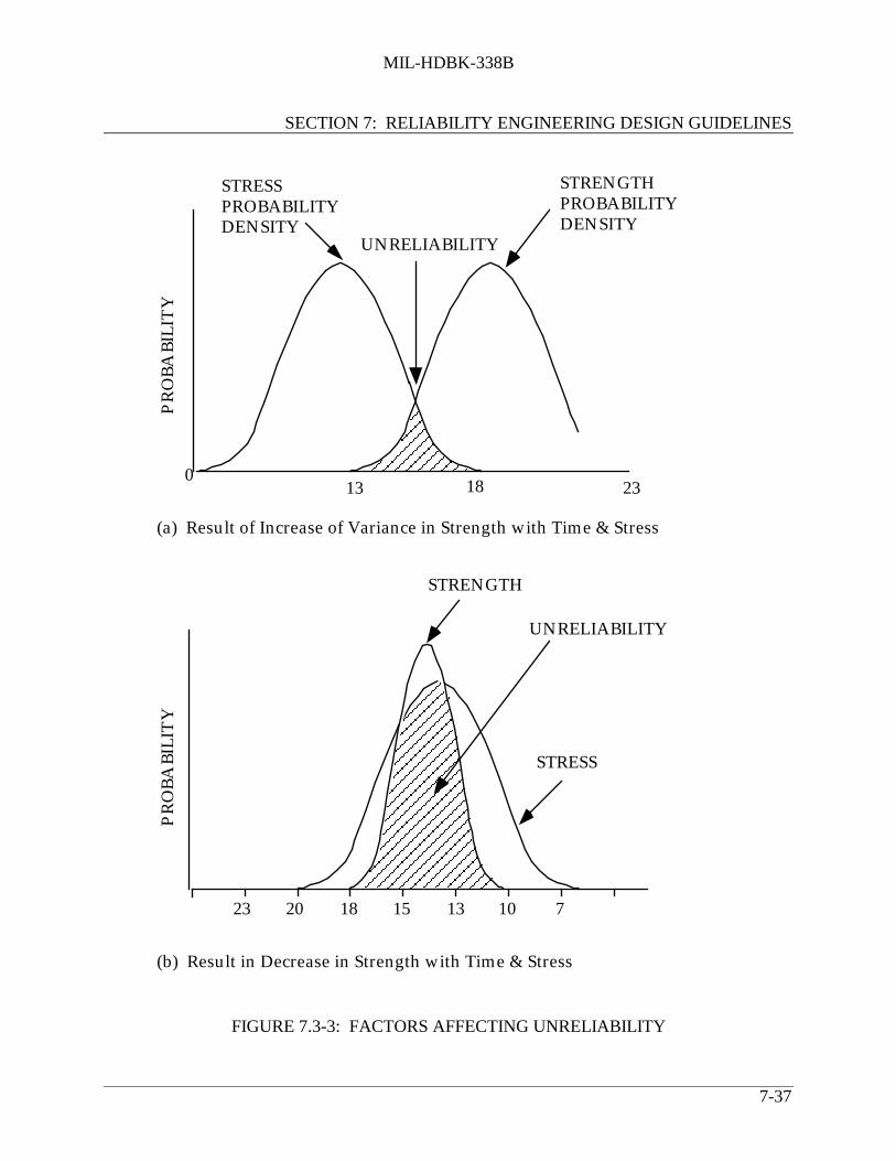
MIL-HDBK-338B


7-37

STRESS PROBABILITY DENSITY

UNRELIABILITY

STRENGTH PROBABILITY DENSITY

013 18 23

(a) Result of Increase of Variance in Strength with Time & Stress

23 20 18 15 13 10 7

STRENGTH

UNRELIABILITY

STRESS

(b) Result in Decrease in Strength with Time & Stress

PR

OBA

BILI

TY

PR

OBA

BILI

TY

FIGURE 7.3-3: FACTORS AFFECTING UNRELIABILITY

MIL-HDBK-338B


7-38

7.4 Reliable Circuit Design

This section cannot possibly cover all of the aspects of circuit design. In addition to a number ofdesign textbooks, there are handbooks available (e.g., References [15] and [16]) which can beused to solve almost any circuit design problem.

The only thing that this section can accomplish in the limited space available is to outline someof the circuit design methods available to ensure high reliability. They are by no meanscomprehensive; circuit designers should consult their own organizations’ design rules,component application notes, the cited references and other relevant sources. The methodsoutlined in this section are intended as a guide to the points which reliability engineers andcircuit designers need to consider.

In order to produce a reliable circuit design, the designer must consider the following reliabilitydesign criteria:

(1) Component derating (discussed in the previous section)

(2) Proper use of parts (discussed in 7.2)

(3) Transient and overstress protection

(4) Parameter degradation and analysis

(5) Fundamental design limitations

Except for component derating, which was discussed in the previous section and parts use, whichwas discussed in 7.2, the following paragraphs discuss each of the listed criteria.

7.4.1 Transient and Overstress Protection

Electronic components are often prone to damage by short-duration voltage transients, caused byswitching of loads, capacitive or inductive effects, static electricity, power supply ripple, testing,etc. Small semiconductor components are particularly vulnerable, owing to the very low thermalinertia of their wire bonds. MOS devices are very vulnerable to static electricity, and requirespecial protection.

The subject of electrostatic discharge (ESD) is treated very thoroughly in other sources, and willonly be summarized here. It is becoming an increasingly important and recognizable problemwith the trend toward the development of integrated circuits of greater complexity and highercomponent densities. Some of today’s microcircuits can be damaged by ESD voltages as low as20 volts. The smaller the part, the less power it can dissipate or the lower the breakdownvoltage, and the more likely it is to be damaged by an electrostatic discharge (ESD). Certainparts are considered highly susceptible and their chances for damage are great. These include

MIL-HDBK-338B


7-39

metal oxide semiconductor (MOS) parts with a direct access to the MOS junction, highfrequency parts produced by the Schottky barrier process, many bipolar and field-effectmicrocircuits like RAMs, ROMs, and PROMs utilizing small active area junctions, thindielectrics, metallization crossovers, and N+ guard ring structures, precision film resistors andsimilar parts. A detailed list of electrostatic discharge sensitive (ESDS) parts and their voltagesensitivity ranges are provided in MIL-STD-1686 and MIL-HDBK-263. They also describecontrol programs that can be applied to minimize component failures due to ESD.

In addition to ESD, the designer must cope with the other causes of transient generationdescribed in the first paragraph.

Semiconductor device circuit malfunctions can arise from two general sources: (1) transientcircuit disturbances and (2) component burnout. Generally, transient upsets are the controllingfactors, because they can occur at much lower energy levels.

Transients in circuits can prove troublesome in many ways. Flip-flop and Schmitt triggers can beinadvertently triggered, counters can change count, memory can be altered due to driving currentor direct magnetic field effect, one-shot multivibrators can pulse, the transient can be amplifiedand interpreted as a control signal, switches can change state, semiconductors can latch-up,requiring reset, etc. The effect can be caused by transients at the input terminals, outputterminals, on the supply terminals, or on combinations of these. Transient upset effects can begenerally characterized as follows:

(1) Circuit threshold regions for upset are very narrow. That is, there is a very smallvoltage amplitude difference between signals which have no probability of causingupset and signals which will certainly cause upset.

(2) The dc threshold for response to a very slow input swing is calculable from the basiccircuit schematic. This can establish an accurate bound for transients that exceed the dcthreshold for times longer than the circuit propagation delay (a manufacturer’sspecification).

(3) Transient upsets are remarkably independent of the exact waveshape, and dependlargely on the peak value of the transient and the time duration over which the transientexceeds the dc threshold. This waveform independence allows relatively easyexperimental determination of circuit behavior with simple waveforms (square pulse).

(4) The input leads (or signal reference leads) are generally the ones most susceptible totransient upset.

Logic devices which interface with inductive or capacitive loads, or which "see" test connections,require transient voltage protection. This can be provided by a capacitor between the voltage lineto be protected and ground to absorb high frequency transients, by diode protection to prevent

MIL-HDBK-338B


7-40

voltages from rising beyond a fixed value (clamping), or by series resistances to limit currentvalues.

The transient voltage levels which can cause failure of semiconductor devices are referred to asVZAP. VZAP values depend upon transient duration. Passive devices can also be damaged bytransient voltages, but the energy levels required are much higher than for small semiconductordevices. Therefore, passive devices do not normally need individual protection.

7.4.1.1 On-Chip Protection Networks

On-chip protection networks for integrated circuits incorporate many of the principles that applyto equipment protection. It is appropriate therefore to discuss some of these principles beforedescribing discrete devices that are used for protection from transients. The basic approach is toutilize clamps and attenuators that reduce current and voltage transients and protect internalcomponents from excessive thermal dissipation or voltage levels capable of rupturing insulatinglayers.

A simple yet very effective protection network consists of a diode connected between an inputterminal and ground. The diode is designed to clamp the input voltage to the gate to a level belowthe breakdown voltage for any input less than the design goal. Figure 7.4-1 shows the diagramand illustrates the voltage transfer function between the voltage source Vs and the internal gatebeing protected.

For negative values of input voltage Vs the voltage surge or ESD transient is conducted to groundwith the gate voltage VG increasing to one forward diode voltage drop. For positive voltages lessthan the diode breakdown voltage VBR the protection diode is transparent and the gate voltageresponds as it would to any signal voltage (note that any noise could be interpreted as a signal).If the transient exceeds VBR, the diode goes into the reverse breakdown region, and furtherincreases in the input voltage are attenuated by the voltage divider consisting of the diodeincremental resistance and the source resistance RS. The object is to prevent VG from reachingthe destructive level BVoxide for any anticipated value of the input voltage VS.

On-chip protection is the least expensive and best way to improve device and system levelhardness and provide maximum customer satisfaction. Nevertheless, sensitive parts do exist, andtheir use compels the equipment designer to employ effective techniques for best performanceand reliability.

MIL-HDBK-338B


7-41

PAD Protected GateBVoxide

RS

CS VS

VBR

rd

VG

BVoxide

VG

VBR

VBR VSVS max

Ideal rd = 0

Slope =rd + RS

rd

PAD

FIGURE 7.4-1: ON-CHIP DIODE PROTECTION CIRCUIT

MIL-HDBK-338B


7-42

7.4.1.2 Metal Oxide Varistors (MOVs)

A varistor is a variable resistor whose value depends on the voltage (or current). It is, in otherwords, a non-linear resistive element that serves the dual function of clamping and energyabsorption. Invented in Japan, it is a widely used, effective, and low cost solution to the problemof controlling voltage surges, especially on power lines.

The metal oxide varistor, or MOV, consists mostly of ZnO with a small amount of other oxideadditives. The powdered material is pressed and sintered to form various shapes and sizesaccording to the intended application. ZnO is conductive, and the individual grains are separatedby an insulating layer that produces a p-n junction-like characteristic. At about 3 volts across theinsulating layer a tunneling mechanism provides electrons for carrying the current. The nominal“clamping” voltage is determined by the number of grain boundaries between the electrodes.

The conduction is highly non-linear and the current and voltage are related by the equation:

I = CVα

where C depends on the cross section area and thickness and α is a constant between 20 and 50.A plot of this equation on a linear scale resembles the characteristics of a back-to-back diodeconfiguration.

The current rating of an MOV depends on its area, and the energy absorbed depends on thevolume. Since energy is absorbed uniformly throughout its volume, the energy rating can besubstantial. The speed of these devices is excellent, limited primarily by the lead inductance.There is a small aging effect. MOVs generally have low leakage current, even at elevatedtemperatures, and good tolerance to radiation environments.

MOVs are available in many sizes, shapes, and ratings, for applications in both ac and dc systemsranging from several volts to several thousand volts. Peak current ratings range from a few tensof amperes to several tens of kiloamperes, with energy capabilities from fractions of a joule to 10kilojoules. When one compares these energies with the millijoules in an ESD pulse capable ofdestroying an integrated circuit, it becomes clear that MOVs are not a good choice for protectingthe inputs of integrated circuits from ESD. In addition, the capacitance of even the smallestMOVs is fractions of a nanofarad and would degrade the high frequency performance.Nevertheless, protection of power ICs or of circuit boards is a possible application, and MOVsare available as coaxial inserts for connector pins.

The largest application for MOV surge suppressors is protection against power line surges.Many computers, appliances, power cord extensions, etc., are equipped with MOVs forprotection from routine power line transients.

MIL-HDBK-338B


7-43

7.4.1.3 Protective Diodes

Discrete diodes and diode networks can be used in a multitude of applications for protection inpower lines, signal lines, and equipment from transients caused by lightning or lightning inducedeffects, power line surges, inductive switching, ESD, or EMP. The sophisticated processingtechnology of the silicon semiconductor industry makes possible such a wide variety ofapplications.

Turn-on time for silicon pn junctions is extremely short, claimed to be a picosecond or so intheory, with actual response time limited by lead inductance. The series resistance is very small,leading to a minimal increase in clamping voltage with current. Clamping voltage ranges fromseveral volts to several hundred volts. Pulse power rating at 100 ns ranges from a few kilowattsto over 10 megawatts. From 100 ns to 10 ms the power rating follows the classical Wunsch-Bell

model, decreasing as t-1/2 . Power is derated linearly above 25°C to zero at 175°C. Since theseries resistance is so small virtually all of the power is dissipated in the depletion layer of the pnjunction, which ranges from small fractions of a micron at lower voltage ratings to several tensof microns at 500 volts. Diode capacitance can be as low as several tens of picofarads for highvoltage diodes, and an order of magnitude larger at lower voltages. Many different packagingstyles are available, including arrays in ceramic dual-in-line packages, hermetically sealed.

7.4.1.4 Silicon Controlled Rectifier Protection

A silicon controlled rectifier (SCR) is a four-layer silicon device employing regenerativefeedback to achieve a snap-back characteristic that offers excellent circuit protection and lowpower dissipation. High power devices have been in use for many years as a control device forlighting, motors, and voltage control. Their use in protection networks for integrated circuits ismore recent.

The four-layer structure of an SCR is shown in Figure 7.4-2 together with its current-voltagecharacteristic. For positive values of voltage a very small leakage current flows until the forwardbreakdown voltage VBF is reached, whereupon the device switches into a low-voltage, high-current conduction state. It remains in this state until the transient surge decreases to a low valuewhere the SCR current falls below the holding current IH. The SCR then reverts to its normalblocking state.

In the blocking state the np junction is reverse biased and sustains the large voltage. Oncetriggering occurs the junction voltage collapses, and both transistors saturate. This leads to asmall voltage across the device in the conducting state. By adjusting the doping levels thebreakdown voltage can be varied over a wide range. In integrated circuit form there are largeparasitic resistors that complicate the design; nevertheless the basic ideas are the same.

The holding current is a very important parameter in any SCR. The device cannot resume itsnon-conducting state unless the current falls below IH. In an ac circuit this is accomplished bythe normal reversal of voltage every half cycle. In surge suppression this requires that the

MIL-HDBK-338B


7-44

transient be reduced to a level where the source resistance or other resistance be sufficient tolimit the current to less than IH when the transient has subsided, otherwise the continueddissipation may destroy the device (as in latch-up).

p

n

p

n

I+

V

- VBF

V

IH

I

(a) (b)

FIGURE 7.4-2: (A) FOUR-LAYER STRUCTURE OF AN SCR(B) CURRENT - VOLTAGE CHARACTERISTIC

The key that makes the SCR such an effective clamping device is its very low voltage in theconducting state, together with its very low incremental resistance. As a result it can conductlarge currents with very little power dissipation. In effect, it is a “crowbar” device oncetriggered.

Besides its use in on-chip protection, discrete devices and arrays are available for a large varietyof applications, from protecting integrated circuits and circuit boards to surge protection andcontrol in high-voltage, high-current environments.

7.4.1.5 Passive Component Protection

Discrete components can also be useful in reducing susceptibility to transient electricaloverstress. To be effective, they must function in concert with other impedances. For example, aresistor in series with the input impedance to an integrated circuit can form a voltage dividernetwork to attenuate the transient and absorb part of the energy. Similarly, a resistor across theline could act with the source resistance to attenuate a surge. On the other hand, if the sourcewere a true voltage source, then shunt elements would have no effect. Furthermore, since alinear device affects desired signals as well as transients, it may not be feasible to use a purelylinear network, especially if the frequency spectrum of the signals overlaps the spectrum of the

MIL-HDBK-338B


7-45

disturbance. Nevertheless, resistors, capacitors, and inductors can be an inexpensive means toachieve the desired result.

There are several types of resistors, the common ones being carbon composition resistors, filmresistors, and wirewound resistors. The conducting element in a carbon composition resistor ismade of a silica-loaded resin with dispersed carbon particles that is formed into a slug or pellet.Because the thermal mass of the slug is relatively large, it can absorb a considerable amount ofenergy. Experimental data show that a 100 Ω, 1/8 W carbon composition resistor can dissipate 1Mw of power for 1 ms before exhibiting a resistance change greater than 5%. The damage

threshold follows a t-1 dependence to 100 ms, where the threshold is about 10 watts. Theenergy absorbed in this range is several orders of magnitude greater than the threshold forintegrated circuits.

Note that the power level in the preceding paragraph corresponds to a voltage of 10 kV across the100 W resistor, far in excess of the rated value of 150 volts. Nevertheless, unless the powerdissipation results in catastrophic thermal failure or flashover, the resistor will remain functionaland continue to offer protection.

At high frequencies the capacitance and inductance of the resistor must be considered. A typicalvalue for the parasitic capacitance is 1.6 pF. For a low value resistor, less than 100 ohms, thecapacitive reactance is negligible below several hundred MHz. For higher values the uppercutoff frequency can be as low as 10 MHz. If the resistor is used in a shunt arrangement thecapacitance would aid in transient suppression by blunting very fast wavefronts; on the otherhand, in a series arrangement the capacitance would be deleterious, exposing a sensitiveintegrated circuit to the full leading edge spike.

The parasitic inductance of a carbon composition resistor depends on the size of the conductingslug and the length of the leads. In a practical sense the larger the conductor the lower theinductance, with hollow or square conductors the best shape. A typical measured value ofinductance for carbon composition resistors is 20 nH, with leads adding to this by about 20 nHper inch. However, with short leads and except for very low values of resistance the capacitivereactance from the lead terminations and the capacitance between conducting particles dominatesthe high frequency performance and total impedance decreases at high frequencies faster thanwith film resistors.

Film resistors consist of evaporated films of thickness from 0.005 to 1 mm, or thicker films up to100 mm deposited from a resistive ink, or, in the case of carbon film resistors, deposited from thepyrolitic decomposition of an organic gas. Sheet resistances for the different types vary from 10to 10,000 ohms per square. The films are spiral-cut to trim the resistors to final value. Thespiraling increases the total inductance; nevertheless, the high frequency performance isdominated by capacitance.

The ability to absorb energy from a transient pulse depends on the thermal mass of the resistiveelement and on the maximum temperature that can be tolerated before permanent damage occurs.

MIL-HDBK-338B


7-46

Film-type resistors, especially carbon film, have a much higher critical temperature than carboncomposition resistors. However their much smaller thermal mass makes them inferior to carboncomposition resistors for this application. In fact, ESD pulses are known to cause permanentdamage to film resistors. The spiraling causes a non-uniform power dissipation in the film thatcan lead to thermal damage at the ends of the spiral cut, and high voltages can cause an arc acrossthe spiral cuts. Both types of damage have been observed.

Wirewound resistors are made by winding a resistance wire on a substrate or bobbin. Althoughthe thermal mass is large, and, in fact, pulse-handling capabilities compare to those of carboncomposition resistors in some cases, the very large inductive property limits their suitability forfast transient suppression.

There are two main classes of capacitors, electrolytic and electrostatic. Electrolytic capacitorsinclude aluminum and tantalum types, characterized by large capacitance values, up to 1 F, butlimited to voltages below 600 volts. They are made of high purity aluminum foil or tantalum,anodized to form the dielectric layer. This layer has unidirectional properties similar to those ofa diode. Unless both electrodes are anodized the capacitor is unipolar and the instantaneousvoltage must always remain of one polarity. At voltages roughly 50% higher than the ratedvoltage additional electrode material is anodized and a substantial current can flow.

One of the principal applications of electrolytic capacitors is in power supply filtering, wherethey also perform the useful function of suppressing surges that are coupled through from powerlines. They are also used on printed circuit boards to decouple circuits connected to powerbusses, or to shield sensitive ICs from noise generated on the board.

Electrolytic capacitors are limited by their poor frequency response. They have a large inductivecomponent that limits the self resonant frequency to 10 kHz or so. For this reason electrolyticsare often paralleled with a 0.1 or 0.01 mF electrostatic capacitor that acts as a low impedance tohigh- frequency signals.

The main electrostatic capacitor types include plastic, ceramic disk, ceramic multilayer chipcapacitors, and glass and mica capacitors. Plastic capacitors are made by evaporating a thin layerof aluminum onto a thin plastic film of polyester, polystyrene, polycarbonate, or other plastic.They exhibit the interesting property of self-healing, whereby voltage breakdown at a site iscleared by the evaporation of the aluminum around that site, restoring operation to an equal orhigher voltage capability.

Ceramic capacitors make use of the high dielectric constant of ferroelectric materials to achievelarge capacitance values in a small package. For disk capacitors the appropriate combination ofpowders is mixed and pressed into the desired form. These are sintered at high temperature, thenelectrodes are screened on, and the device encapsulated. By forming a very thick disk, highvoltage ratings can be achieved. Multilayer chip capacitors are made from a slurry containing themix of dielectric powders, and cast onto a stainless steel or plastic belt. After drying, electrodesare screen printed, the layers are stacked, then cut apart into individual units. The capacitors are

MIL-HDBK-338B


7-47

then sintered, contacts attached, and encapsulated. Because of their extremely small size, thesecapacitors are especially useful in hybrid circuits or on printed circuit boards.

Glass and mica capacitors are used in tuned circuits and high frequency applications where theirstability and accuracy are needed. They are made from alternate layers of the dielectric and metalfoils, brought out at either end, where leads are attached. They are available in high voltageratings but relatively low capacitance values.

Electrostatic capacitors are capable of withstanding surges several times their rated values. Insmaller values, especially, the dielectric thickness may be increased to keep the area amanageable size, even though the voltage rating is listed the same as other capacitors of the samestyle. This makes them good candidates for transient suppression.

Inductors can serve useful purposes in filters or attenuators for transient electrical overstress. Onthe other hand, inductors can be the source of high voltage transients when high di/dt values areencountered, and the main design task then becomes one of minimizing parasitic inductance. Thefact that inductance is a magnetic field phenomenon means that coupling from magnetic fieldsproduced by arcs or conductors carrying discharge current needs to be minimized by good layoutpractices and shielding.

Inductors are not as widely used as resistors and capacitors because of their size, weight, cost,and dissipative property. Because discrete inductors are wound with wire of non-zero resistivityparasitic resistance is unavoidable and can limit the performance, especially at high frequencieswhere skin effect becomes important.

Ferrite beads are an interesting form of inductance often used to reduce high frequency noise.They consist of a ferrite material of high µ that is lossless to a high frequency, even up to thegigahertz range. They are designed to be slipped over a wire, or multiple turns can be threadedthrough a single bead. They are transparent to dc or low frequencies, but introduce inductivereactance and then resistance at selected high frequencies. In combination with other circuitimpedances they are widely used to reduce noise and system transients as a low-cost andconvenient measure.

7.4.1.6 Protective Devices Summary

Surge suppressors such as gas tubes and air-gap arrestors for lightning protection have beenomitted because they are used mainly in exterior locations or service entrances but seldom inelectronic equipment. The characteristics of the protection devices discussed are summarized inTable 7.4-1, but the entries are for only those devices that are appropriate for use on printedcircuit boards or within equipment enclosures. Very large diodes and SCRs are available butseldom used for circuit board applications. The following material illustrates how theseprotection devices can be used.

MIL-HDBK-338B


7-48

7.4.1.7 Protection Design For Parts, Assemblies and Equipment

The best way to build robust equipment is to use parts that are themselves robust. This is themost efficient, cost-effective, and practical approach. It protects integrated circuits duringfabrication, testing, shipping, assembly, and equipment operation and repair. It requires no extracomponents or board space and imposes no degradation in frequency response. Nonetheless,sensitive parts do exist and at times must be used; in any event no matter how well a systemperforms it can always be improved by good design.

If an item of equipment were battery operated, shielded from electrical and magnetic fields andradiation, and had no input or output ports it might be impervious to anything except perhaps adirect lightning stroke. Realistically, equipment has a direct connection to power lines, signalports, output ports, switches and other controls, apertures for cooling air, etc. The equipmentwill encounter transients at the inputs, radiated fields, both direct and indirect ESD discharges,handling by inexperienced personnel and repair persons, etc.

TABLE 7.4-1: COMPARISON OF PROTECTION DEVICES

ADVANTAGES DISADVANTAGESRANGE OFMAXIMUMVALUES*

COMMENTS

MOV low costhigh energy capabilitylow leakage currentradiation hard

high capacitanceaging effect

E = 0.06J - 10kJIpeak = 25A - 100kA

VDC = 3.5V = 6kV

C = 11pF - 11nF

especially usefulfor power linetransients, boardprotection

Diode low series resistancelow capacitance

higher cost P = 400 - 6500WV = 5 - 270VIpeak = 2 - 600A

C = 3 - 500pF

fail short or open

SCR nearly ideal characteristicslow leakage current

higher costlimited availabilityturn-off requirementsneed to be addressed

V = 30 - 270VIpeak = 2 - 600A

C = 3 - 90pF

fail short

R, L, C low costreadily available

linear devicesoften not transparentto signals

V = 100V - 10kVp = 0.1 - 1mW

often used inconjunction withother transientsuppressor

*Values in this column apply to specific transient waveforms or other special conditions. Consult specificationsheets for details.

There are many anecdotes about computer malfunctions on cold winter days when the humidityis low: sensitive keyboards; equipment that is “dead on arrival;” costly repairs and retrofits;latent failures; etc. One expert in the discipline claims that computer upset can be caused byshaking coins in a plastic bag nearby. Upsets and failures are not only annoying, they can be verycostly. Unless one is prepared to condition power and signal lines, prohibit static-prone materials

MIL-HDBK-338B


7-49

and furnishings, and thoroughly train all staff members in proper procedures, the best approach isto make the equipment fool-proof.

To protect against direct-discharge ESD, it is necessary either to insulate the equipment or toprovide a safe alternative path for the discharge current. If the discharge is indirect, then theequipment must be properly shielded to prevent magnetic or electrostatic coupling to interiorcircuitry. Protection must also be provided for maintenance, upgrading, or repair operations.This requires on-board protection and good layout.

There are four categories of techniques for system hardening.

(1) Board layout

(2) Shielding and grounding

(3) Use of transient protective devices

(4) Use of passive components and filters

Because of the wide overlap between these categories it is not possible to treat them as entirelyseparate areas; however all of them will be covered in what follows.

7.4.1.8 Printed Wiring Board Layout

Arrangement of parts on a printed wiring board should give priority to sensitive ICs. Theseshould be placed near the center of the board where they are less likely to be contacted duringhandling. To further protect the components a guard ring should be in place around theperiphery. The guard ring should be connected to the pull-out lever or board latch and to frameground, but not directly to circuit ground. To prevent arc-over after the board has been installedthe guard ring should be connected to circuit ground through a high resistance to bleed off staticcharges that might accumulate. To avoid electromagnetic interference (EMI), noisy circuitryshould be segregated from sensitive circuits, and analog circuits segregated from digital. Edge-triggered logic should be avoided where possible. In extreme cases Faraday shields might beneeded. To avoid coupling between an ESD discharge path (such as the guard ring) and sensitiveinputs, parallel traces should be avoided. It is best to remember that any circuit that is a goodradiator is also a good receiver for EMI. Whenever a trace becomes a significant fraction of awavelength it has the potential of becoming a good antenna. Since light travels a foot per ns infree space (slower in materials), fast risetime transients can be efficiently radiated from shortlines; therefore leads should be kept short, or shielded where necessary.

Inductive coupling is minimized by small loop areas. For example, power and ground tracesshould be close together. This can be accomplished by running multiple power and ground lines,on different layers, and transposing them at intervals. It is preferable to run each set of thesemultiple feeders back to a common point near the connector rather than form one long,continuous run. To maximize the capacitance between power and ground, a ground plane, and

MIL-HDBK-338B


7-50

ground fill, should be utilized - no area should be left unused. To minimize coupling betweensignal lines it is preferable to alternate them with ground or power buses, but this may not befeasible from a real estate and frequency performance point of view.

Power supply filtering and decoupling is such an important concern that many boards use severalcapacitors to reduce noise and glitches on the power bus caused by digital circuits. Clearly evena low magnitude transient is capable of causing upset. Even though the power supply itself has avery low output impedance, cabling within the cabinet and the impedance of interconnectsprovide opportunities for EMI. One recommendation is that each board use an electrolyticcapacitor (> 50 µF), a 0.01 µF capacitor for high frequency suppression, and a ferrite bead on thepower lead, all as close as possible to the connector. Also recommended is a 0.01µF capacitor foreach IC. Such filtering will also help to attenuate surges on the power lines that couple throughthe power supply. At high frequencies the power supply busses are a significant fraction of awavelength, and the characteristic impedance of the transmission line formed by the powersupply trace and ground can contribute significantly to the noise. One way to lower thecharacteristic impedance is to use a power supply trace that is separated from the ground plane bya thin insulator. In lieu of this the inductance of the supply trace should be minimized by makingthe buss as wide as possible, and by providing multiple paths for the supply current.

7.4.1.9 Shielding

Equipment enclosures rely on the reflection of incident electromagnetic waves or their absorption

by I2R losses in the material to prevent the transmission of electromagnetic energy, either intothe equipment, or from the equipment. In the first case we wish to protect the interior circuitsfrom radiation caused by indirect ESD, lightning, or EMI. In the second case we wish to preventemission from the equipment itself in order to avoid adding to the EMI background, and tocomply with regulatory requirements.

An electromagnetic wave incident on a conducting surface generates currents in the material thatproduce electromagnetic fields opposing the incident wave. The stimulated wave is observed asa reflection of the incident wave, and the stimulated current produces losses in the body of thematerial that represent an attenuation of the wave as it progresses through the conductor. If theilluminated body is a perfect conductor the wave is totally reflected; there is no penetration of theshield, which acts like a Faraday cage. When the conductor is less than ideal only a portion ofthe wave is reflected, and non-uniform conduction currents flow in a layer near the surface. Thisis the so-called skin effect. The skin depth is the distance in which the induced currents or fieldsdecrease by a factor of 1/e, to 37% of their original amplitude.

The shielding effectiveness due to absorption depends on the thickness of the material, and thedecibel loss in any given material increases with the square root of frequency. (Ref. [101],RADC-TR-78-156, “Electromagnetic Properties and Effects of Advanced Composite Materials:Measurement and Modeling” and Ref. [102], RADC-TR-81-162, “Electromagnetic ShieldingEffectiveness for Isotropic and Anisotropic Materials.”)

MIL-HDBK-338B


7-51

The other component of shielding refers to the reflection of the electromagnetic wave at front andback surfaces of the shield. A plane wave or an electric field is reflected very effectively fromthe surface of a good conductor. A magnetic field tends to be reflected from the back surface ofa shield as it re-enters the atmosphere. The magnetic field that is reflected is virtually 100% ofthe incident wave, but is reflected in phase, and adds to the incident wave, again producing astanding wave.

Shielding effectiveness must be re-examined when the incident wave is not a plane wave (far-field condition). When the source is close to the shield (near-field region) the wave impedance isnot 377 ohms and important differences exist.

The transition between near-field and far-field regions occurs at a distance d = λ/2π. At greaterdistances the fields are plane waves, the wave impedance is 377 ohms, and both the E field and Hfield decrease with distance as 1/r.

In the near-field region the reflection conditions are different because the wave impedance isdifferent. For electric field sources the reflection losses are even greater than those with a planewave. Consequently, shielding is not a problem. Even a thin, evaporated coating on a plasticlayer is effective, although making a good electrical contact to ground the shield is problematic.(Grounding of any shield or conducting surface within the enclosure is necessary to preventsecondary arcs within the equipment.) When the source generates a primarily magnetic field,shielding is more of a challenge. Reflection losses are smaller than those of a plane wave, anddecrease as the frequency decreases. Since absorption losses are small at low frequencies, itbecomes a challenge to design shielding against low-frequency, near-field, magnetic sources.

The common methods of shielding against low-frequency magnetic fields are the use offerromagnetic shields, such as “mumetal“ and the use of the “shorted turn”. Some ferromagneticmaterials have very high permeabilities below 1 kHz and are particularly effective in confiningmagnetic fields. The “shorted turn” method uses a closed, conducting loop perpendicular to themagnetic field to generate an opposing magnetic field within its area. It is useful in subduingemissions from motors, transformers, etc.

Indirect ESD sparks and other arcing sources are usually high impedance, high E field sources.Magnetic sources are those that involve large currents as in power lines, ground return wires,conductors carrying a discharge current, transformers, etc.

Once appropriate shielding material has been selected, any apertures must be given properattention. These are required for input and output signals, power, switches and controls,ventilation, and access. The general rule is that the largest dimension of an aperture must be asmall fraction of a wavelength at the highest harmonics present. Some experts recommend λ/10,others as small as λ/50. With digital clock frequencies at 100 MHz and harmonics approaching 1GHz the appropriate size of apertures to limit emissions would be of the order of 3 cm. To shieldfrom ESD arcs of 10 ns duration would likewise require on aperture of 3 cm. With microwave

MIL-HDBK-338B


7-52

equipment even these dimensions are too large. Note that any apenture with a wire through itacts like a section of coaxial cable with good transmission.

The 3 cm limit refers to the largest dimension of the aperture. If an opening is long and narrow itacts as a slot antenna, receiving or emitting frequencies corresponding to its length. When alarger opening must be used it can be subdivided into smaller openings or covered with a wiremesh. Access panels and doors must have closure seams protected by gaskets or interrupted byscrews at least every 3 cm.

All conductive surfaces within the equipment should be grounded. Otherwise a secondary arcbetween the surface and another part of the cabinet could occur, or, worse yet, to a sensitive partor a trace on the printed wiring board. An arc occurring within the cabinet is itself a source ofclose range EMI confined to the cabinet enclosure. Direct ESD injection to internal circuitrymust be prevented. No parts of the internal circuitry should be accessible to hands or fingers, andany direct discharge must be confined to the cabinet or shielding only. There should be noaccessibility through apertures; switches and other controls should have grounded cases or shouldbe insulated and sufficiently separated from circuits to preclude the possibility of arcing.

7.4.1.10 Grounding

Grounding refers literally to the electrical connection between equipment and a conducting roddriven into the earth. Figure 7.4-3 shows how grounding is accomplished at the service entranceto a building.

Red (hot)

Green (Ground)

White (Neutral)

Black (Hot)

EquipmentService Entrance

Ground Rod

FIGURE 7.4-3: GROUNDING PRACTICE AT A SINGLE PHASESERVICE ENTRANCE

If the “ground” for every circuit in every piece of equipment were at the same potential as thebuilding earth ground, as intended, the circuit and systems designers’ jobs would be much easier.The reason this is not the case is because all ground conductors have impedance associated with

MIL-HDBK-338B


7-53

them that renders different parts of the ground system at different potentials whenever groundcurrents are present.

An extreme case is associated with a nearby lightning stroke. Even if the stroke is conductedharmlessly to “ground”, the flow of the extremely large currents through the finite resistance ofthe earth would cause one building ground to be at a different potential from another. If twoitems of equipment were located in two different buildings, connected by a shielded cable“grounded” at each end, a large current would flow through the shield and through theequipment.

One can immediately sense that grounding may be as much an art as a science; nevertheless thereare important general principles that are effective in minimizing grounding problems. Theoverriding concern is to prevent large ground currents from flowing through impedances(especially inductive impedances) that raise parts of the system ground to higher voltages, the so-called “ground bounce” problem.

In Figure 7.4-4 several subsystems have their ground returns “daisy-chained”. This invitesproblems. The noisy currents from the block of digital circuits flow through ZG2 and ZG1 andtogether with the large and erratic currents from the power electronics block that flow throughZG1 raise the potential of the ground bus of the low level and sensitive analog block, raising thenoise level in that system. It is far better to keep the grounds from each block separate, andconnect them all at a common point. Figure 7.4-5 shows separate grounds returned to a commonpoint.

PowerElectronics

DigitalCircuits

AnalogCircuits

ZG1 ZG2 ZG3

FIGURE 7.4-4: CIRCUIT SUBSYSTEMS WITH GROUNDCONNECTIONS “DAISY-CHAINED” INVITES PROBLEMS

MIL-HDBK-338B


7-54

PowerElectronics

DigitalCircuits

AnalogCircuits

GuardRing

Supply Voltage

PowerSupplyGround

FIGURE 7.4-5: GROUND TRACES RETURNED TO A COMMON POINT

The question often arises, should the cabinet also be connected to the common ground point?Generally no. If the green safety wire enters the cabinet it is usually the best place for thecommon ground point, and the enclosure should be grounded there. This raises the possibilitythat a direct ESD discharge could cause an arc from the cabinet to a point on a printed wiringboard. If the cabinet has a low impedance from the discharge site to the ground point this isunlikely. It may be necessary to keep the boards a sufficient distance from the cabinet, but toconnect the ground of each board to the nearest cabinet point is not a good solution.

On the printed wiring board itself ground traces should be low impedance, with particularattention given to keep the inductance low. Ground planes, ground fill, and ground grids areeffective ways to accomplish this. Several ground traces from the connector can be interspersedwith signal lines to reduce crosstalk, and power supply filtering at the connector can besupplemented by running power and ground traces in such a manner as to maximize thecapacitance between them.

Shielded cables should have their shields grounded at the point of entry with a 360° contact tothe socket, rather than with a pigtail. Although shielded cables are usually grounded at bothends, this is not necessarily advisable, especially if the equipment is spaced some distance apart.The shield may be a better “ground” than the green safety wire between outlets, thus raising thepossibility of large current flow in the shield. At high frequencies the stray capacitance of theshield negates the advantages of shielding connected at one end only, and both ends are usuallygrounded. Also, grounding the cable at both ends can produce a ground loop. Any nearby sourceof flux may introduce considerable current into this loop.

7.4.1.11 Protection With MOVs

Metal oxide varistors, or MOVs, can be used in several ways to protect electronic equipment.They are not especially useful in protecting individual inputs to integrated circuits. The prospectof populating a printed circuit board with large numbers of extra devices is not appealing, and thecapacitance of the low voltage types is excessive and would seriously degrade the speed of a

MIL-HDBK-338B


7-55

digital system. They are intended to absorb energy far in excess of the threshold energy for atypical IC. Because they are low cost and high speed they have proved to be useful in otherways.

In principle an MOV could be used to suppress transients on power supply buses. They are notappropriate for clamping supply voltages because the MOV tolerance is greater than that of manydc supply requirements. Nevertheless, they would be appropriate for suppressing large amplitudetransients.

Transient protection on input and output signal lines is a possible application, especially if thelines are long and subjected to a noisy environment. Telephone lines are susceptible to powercontact (when the line makes accidental contact with a power line), induction from power lines,and transients from lightning strokes. EMI and direct or indirect ESD are other sources. In anycase the use of an MOV can limit the transients and is a viable option. MOVs are available asconnector pin inserts for cable connectors. They are an integral part of the connector, cylindricalin shape, with a hollow core so that the pins of a standard connector can be inserted. Theyprovide transient surge protection in voltage ratings from 6 to 150 volts dc with energyabsorption from 0.5 to 1.5 joules. The capacitance ranges from 350 to 2750 pF, with the largervalues in the lower voltages.

The main advantage of connector pin inserts over board-mounted suppressors is that they do nottake up valuable board space. A second important advantage is that surge currents are diverteddirectly to ground through the connector itself rather than being conducted onto board traces.This concept has extended to other schemes that employ voltage-variable material as an add-onto standard connectors. The material has a clamping voltage of 100 volts, typical, whensubjected to a 15 kV ESD transient, yet adds only 3 pF of shunt capacitance.

The most popular application of MOVs is in power line protection. Typically, an MOV isconnected across the line at a point where the power line enters the equipment cabinet. A 0.01 to0.1 µF capacitor is placed in parallel to act as a low impedance shunt element for high frequencynoise. The MOV has a good high frequency response as well, but the capacitor is effective atamplitudes below the clamping level of the MOV. Without the capacitor the high frequencytransients would couple through the power supply and hence into the interior circuits.

The first step in selecting an MOV is to determine the steady-state working voltage. This isusually taken to be 10-25% above the nominal voltage of the circuit. For 120 volt ac applicationthis implies an MOV with a maximum voltage rating of 132-150 volts rms.

The energy or surge power rating of the MOV is more difficult to specify. Clearly the larger theMOV the better, but this is unrealistic. Attempts to calculate power and energy absorption for aspecific location are also unrealistic because the characteristics of the surge source are unknown,the impedance seen by the suppressor is unknown, and the presence of other equipment withnon-linear loading is unknown. Rather than design to meet some proposed situation it is better to

MIL-HDBK-338B


7-56

design to meet a particular standard, especially if that standard has been drafted on statistics froma large amount of credible data.

In IEEE Standard C62.41-1991 (Reference [17]), the importance of location of the equipment isemphasized. Location Category C is defined as being outside the building and service entrance;Category B includes distribution panels, heavy appliance outlets with “short” connections toservice entrances, etc.; and Category A includes outlets and branch circuits more than 10 metersfrom Category B locations and more than 20 meters from Category C locations.

Information on standard waveforms for voltage and current surges in an ac distribution systemfor varying exposure to system transients is shown in Tables 7.4-2 and 7.4-3. This information isbased on IEEE Standard C62.41-1991. Exposure levels are categorized as low, medium or high.These categories are described as follows:

(1) Low Exposure. Systems in geographical areas known for low lightning activity, withlittle load or capacitor switching activity.

(2) Medium Exposure. Systems in geographical areas known for medium to high lightningactivity, or with significant switching transients. Both or only one of these causes maybe present, as it is difficult to separate them in reviewing the results of monitoringdisturbances.

(3) High Exposure. Those rare installations that have greater surge exposures than thosedefined by Low Exposure and Medium Exposure. The more severe conditions resultfrom extensive exposure to lightning or unusually severe switching surges.

Location Category C is rarely of concern. In location Categories B and A the peak voltageexcursion is considered to be limited to 6 kV by flashover in outlets and insulation. Location Ais assumed to be controlled by reactances that filter the surge into an oscillatory waveform. The“effective impedance” of the surge is simply the ratio of the peak voltage and peak current; it hasthe dimension of ohms, but is not a pure resistance.

TABLE 7.4-2: 0.5µS - 100 KHZ RING WAVE

LOCATIONCATEGORY

SYSTEMEXPOSURE VOLTAGE KV CURRENT A

EFFECTIVEIMPEDANCE

Low 2 70 30A Medium 4 130 30

High 6 200 30Low 2 170 12

B Medium 4 330 12High 6 500 12

MIL-HDBK-338B


7-57

TABLE 7.4-3: 8/20µS, 1.2/50µS COMBINATION WAVE

LOCATIONCATEGORY

SYSTEMEXPOSURE VOLTAGE KV CURRENT A

EFFECTIVEIMPEDANCE

Low 2 1 2B Medium 4 2 2

High 6 3 2Low 6 3 2

C Medium 10 5 2High 20 10 2

The philosophy of IEEE Standard C62.41-1991 is that it is unnecessary to duplicate field-measured surges, since these occurrences are dependent on the site, time of year, etc. Rather, afew representative waveforms should be selected that are realistic and readily reproducible, andwill allow researchers to compare the vulnerability of various equipment. The 0.5 µs - 100 kHzring wave and the 1.2/50 ms waveform are intended to be open-circuit voltages to test insulation,whereas the 8/20 µs waveform is a current surge into a short circuit. When a test generator isconnected to an MOV the voltage and current are not the same as the open-circuit and short-circuit standard waveforms due to the loading by the MOV; the effective source impedance, theratio of Vpeak/Ipeak, is given in Tables 7.4-2 and 7.4-3.

7.4.1.12 Protection With Diodes

PN junction diodes are commonly used for transient protection because of their fast turn-on timeand low series resistance. Diodes intended for transient suppression are especially designed tohave low resistance. With their small size, low capacitance, wide range of clamping voltage, andsomewhat modest ratings they are especially suited for on-board protection of integrated circuitsand other semiconductor devices.

Figure 7.4-6 illustrates how diodes would be used to protect a discrete bipolar transistor. In part(a) of the figure diode D1 in conjunction with RB limits the base voltage to the range of onediode drop negative to one reverse breakdown voltage positive. D2 prevents the output line fromgoing negative, while the capacitor filters noise from the power supply bus.

In part (b) of Figure 7.4-6 a more elaborate arrangement of diodes and resistors limits thepositive excursion of the base to two forward diode drops.

MIL-HDBK-338B


7-58

0.1µF

D2RB

VCC

D1

(a)

0.1µF

(b)

D1D3

D2

R1R2

D4

VCC

FIGURE 7.4-6: DIODE PROTECTION OF A BIPOLAR TRANSISTOR

Figure 7.4-7 shows the analogous protection scheme for a discrete MOSFET transistor. Somemanufacturers suggest that D2 be connected between the gate and drain, however thearrangement shown in the figure is preferred.

Large SCRs require transient protection for the gate circuit only. The peak inverse voltage ratingshould provide adequate protection for anode to cathode surges. Figure 7.4-8 shows twoschemes for incorporating diode protection of the gate. Part (a) of the figure shows a simpleresistor diode arrangement, whereas in part (b) the resistor and inductor form an integratingcircuit to reduce the noise level at the gate.

0.1µF

D2RG

VDD

D1

FIGURE 7.4-7: DIODE PROTECTION FOR A DISCRETEMOSFET TRANSISTOR

MIL-HDBK-338B


7-59

R

D

(a)

SCR

R D

(b)

SCRL

FIGURE 7.4-8: DIODE PROTECTION FOR SILICONCONTROLLED RECTIFIERS

Figure 7.4-9 illustrates diode protection for a TTL circuit. Diode D1 clamps the negativetransient to ground (using the output impedance of the driving circuit), and D2 prevents the inputfrom going more positive than VCC . D3 clips any negative surges on the output bus and thecapacitor filters the VCC bus.

D3

D2

D1

TTL Block

0.1µF

VCC

FIGURE 7.4-9: TRANSIENT PROTECTION FOR A TTLCIRCUIT USING DIODES

In Figure 7.4-10 a simple scheme for protecting CMOS circuits is shown. In part (a) the diodeclamps positive pulses to VDD and limits negative voltages to VDD minus the diode reversebreakdown voltage. In part (b) the protection circuit is more elaborate, patterned after acommonly used on-chip protection scheme. D1 is selected to have a larger reverse breakdownvoltage than D2 or D3 . Resistor R2 in conjunction with the on-chip protection network at theinput of the CMOS circuit provides a third stage of protection. Each of the three stages wouldturn on sequentially as the input transient becomes larger and larger.

MIL-HDBK-338B


7-60

CMOSCircuit

VDD

D2

CMOSCircuit

0.1µF

VDD

D1

R2R1D3

(a) (b)

FIGURE 7.4-10: TRANSIENT PROTECTION FOR A CMOS CIRCUIT

Line transients are one of the causes of failures in switching mode power supplies. A majorfailure mode is shorting of the switching power transistors caused by power line surges. Theinrush of current in conjunction with the equivalent series resistance and inductance of the filtercapacitors produces an overstress of the power switches that leads to failure. The best remedy isto suppress the transients at the input to the power supply.

Figure 7.4-11 shows an effective method of suppressing line transients that uses a hybrid schemeemploying both an MOV and clamping diodes. The MOV is a high energy absorbing device thatprovides the main protection. The clamping diodes provide a more precise limit to the voltageexcursion. Suitable values of L and R are of the order of 100µH and 1 ohm, respectively.

R

Diodes

L

MOVPowerSupply

ACLine

FIGURE 7.4-11: INPUT PROTECTION FOR POWER SUPPLIES

Diodes are compatible with on-board protection of components, and diode arrays can beeffectively utilized to provide protection for data lines and power buses. Figure 7.4-12 shows anarrangement where the diode array is located adjacent to the edge connector. Some designersprefer to place the protection devices close to the components being protected; others try to avoidsurge currents being propagated around the circuit board where they become sources of rf fields,and high voltage transients can cause arcs to nearby components or traces. For the latter case, thediodes are located at the connector as shown in the figure.

MIL-HDBK-338B


7-61

Transient voltage suppressor diodes usually fail short, but may also fail open. If they fail openthere is no longer protection of susceptible components against subsequent transients. For themore common case of failing short, a significant surge current can occur unless limited by seriesimpedances. This condition is much more serious for power buses than for data lines. The short-circuit current will eventually cause the protection diode to open-circuit. The relationshipbetween the amplitude (squared) of the short-circuit current and the time to fail open is describedfairly well by the classical Wunsch-Bell model; in other words the current is proportional tot-1/4 .

Figure 7.4-13 shows a fuse in a power bus protected by a diode. The fuse must be carefullyselected to conduct the expected transient current, but to open when the diode fails short. Theserequirements are especially difficult to meet for low voltage diodes.

GND

DiodeArray

FIGURE 7.4-12: PROTECTION OF DATA LINES OR POWER BUSESUSING A DIODE ARRAY

MIL-HDBK-338B


7-62

Fuse

DiodePowerBus

FIGURE 7.4-13: FUSE PROTECTION FOR A TRANSIENTVOLTAGE SUPPRESSOR DIODE

Since the threat from ESD comes mainly during handling of the boards, CRO-BAR devices that

connect all traces together at the edge connector pads would eliminate ESD pulses that are

applied at the connector. CRO-BAR devices automatically disengage when the board is

inserted into a slot or when a cable is attached. CRO-BAR devices on the cable itself alsoremove any static charges that may accumulate when the cable is left unconnected or unrolledfrom a spool.

Most of the techniques mentioned are common sense to those with some design experience inEMI, electromagnetic compatibility (EMC), ESD, or transient suppression. A few are stillsomewhat controversial. The importance of good design becomes increasingly relevant aselectronic equipment and appliances proliferate and as devices become smaller and moresensitive. The battle is never finished, and as the electronics industry evolves, design engineersmust realize that old remedies may no longer be applicable and new, innovative solutions mustbe thought of. Once a solution has been found, funding is often discontinued, those who makesuch decisions not realizing that like the mythical multiheaded dragon, new crises continuallyarise to frustrate those caught unawares.

7.4.2 Parameter Degradation and Circuit Tolerance Analysis

The values of part parameters, physical and electrical characteristics, are known to vary with timeunder the effects of aging and stress. Variations in part parameter values, if not considered in thedesign, can have undesirable effects on circuit performance and are a significant cause of systemfailure. Even when the variations in the value of a single parameter for a single part have noeffect on system performance, the cumulative effect of such changes can degrade systemperformance to a point where it is no longer acceptable.

In addition to the variations caused by aging and stresses, the values of part parameters vary dueto the manufacturing processes used in the manufacture of the parts. These variations can differby manufacturing lot and can be affected by procedures in which parts are individually selected,using for example, “screens”. Whatever the causes, the variations in a given part parameter canbe described by a statistical distribution. The expected value and standard deviation of thisdistribution represent the nominal or “average” value of the parameter and the variation aroundthis nominal value, respectively. As already indicated, the nature of the distribution is a functionof the manufacturing process, aging, and stress. Stress includes elements of the operating

MIL-HDBK-338B


7-63

environment, such as temperature, vibration, pressure, and so forth. Examples of part parametervariations are shown in Figures 7.4-14, 7.4-15, and 7.4-16. Figure 7.4-14 shows the averagevariation from the initial value and the standard deviation of the variation plotted over time forthe resistance of a particular type of resistor and Figure 7.4-15 shows the same information forthe capacitance of a particular type of capacitor. Figure 7.4-16 shows how the variability in thenominal resistance increases under a specified stress and temperature condition for a period oftime, for two different levels of power dissipation.

In designing a system, these variations in the values of part parameters must be specificallyaddressed to ensure that the design is robust. A robust design is one in which substantialvariations in the values of part parameters have little or no effect on system performance. Indesigning for robustness, designers must have a knowledge of the variations expected due tomanufacturing, aging, and stress and the expected ranges of those variations. With thisknowledge to guide them, designers can work to eliminate or mitigate the effects of variations inparameter values.

Two approaches that can be used to eliminate or mitigate the effects of variations in parametervalues are:

(1) Control the device and material parameter variations through process design and controlto hold them within specified limits for a specified time under specified conditions.This will be referred to as Parts Control.

(2) Design circuits and systems to be sufficiently tolerant of variations in device andmaterial parameters so that anticipated variations over time and stress do not degradesystem performance. This will be referred to as Design Control.

The first approach requires that the parameter value be controlled. Burn-in, preconditioning, andother screening methods, can be used to eliminate or reduce variation in a specific parameter.This screening results in parts having more stable parameters. Controlling the parameters of apart requires detailed testing and control of materials used in the parts. It requires strict controlof manufacturing processes, the use of proven designs, and parts testing to collect data onparameter variation over time.

The second approach is to design circuits that are tolerant or insensitive to variations in partsparameters. Three different techniques for designing tolerant circuits are: (1) use feedback toelectrically compensate for variations and thereby provide stable performance, (2) ensure that thecircuitry provides the minimum required performance even under expected or worst caseconditions (i.e., maximum variation), and (3) design the circuit to be insensitive to variations.

MIL-HDBK-338B


7-64

Average Variation from Initial (% of initial average value)

.35

.30

.25

.20

.15

.10

.05 0

00.

51.

01.

52.

02.

5

Stan

dar

d D

evia

tion

of V

aria

tion

from

Init

ial R

esis

tanc

e fo

r M

IL-R

-11

Car

bon

Com

posi

tion

Res

isto

r at

70°

C A

mbi

ent a

nd V

ario

us E

lect

rica

l Str

esse

s

00.

51.

01.

52.

02.

5

+1.

5

+1.

0

+0.

5 0

-0.5

-1.0

-1.5

-2.0

wat

tage

rat

io

0.5

1.0

Standard Deviation of Variation from Initial (% of initial average value)

wat

tage

rat

io

1.0

0.5

Ope

rati

ng W

atta

geR

ated

Wat

tage

Wat

tage

rat

io =

Ope

rati

ng W

atta

geR

ated

Wat

tage

Wat

tage

rat

io =

The

deg

rad

atio

n ch

arac

teri

stic

s sh

own

here

wer

e d

eter

min

ed fr

om li

fe te

st d

ata

repr

esen

ting

a to

tal o

f 1,5

20 te

sted

par

ts fr

om 3

man

ufac

ture

rs.

Ave

rage

Var

iati

on fr

om In

itia

l Res

ista

nce

for

MIL

-R-1

1 C

arbo

n C

ompo

siti

onR

esis

tors

at 7

0°C

Am

bien

t and

Var

ious

Ele

ctri

cal S

tres

ses

Tim

e (H

ours

x 1

03)

Tim

e (H

ours

x 1

03)

FIGURE 7.4-14: RESISTOR PARAMETER VARIATION WITH TIME (TYPICAL)

MIL-HDBK-338B


7-65

.

Average Variation from Initial (% of initial average value)

.0.6

0.5

0.4

0.3

0.2

0.1 0

00.

51.

01.

52.

02.

50

0.5

1.0

1.5

2.0

2.5

+0.6

+0.4

+0.2 0

-0.2

-0.4

-0.6

-0.8

Standard Deviation of Variation from Initial (% of initial average value)

The

deg

rad

atio

n ch

arac

teri

stic

s sh

own

here

wer

e d

eter

min

ed fr

om th

e lif

e te

st d

ata

repr

esen

ting

a to

tal o

f34

0 te

sted

par

ts fr

om 2

man

ufac

ture

rs.

0.7

Ave

rage

Var

iati

on fr

om In

itia

l Cap

acit

ance

for

MIL

-C-2

0 T

empe

ratu

reC

ompe

nsat

ing

Cer

amic

Cap

acit

ors

at R

ated

Vol

tage

and

85°

C A

mbi

ent

Stan

dar

d D

evia

tion

of V

aria

tion

from

Init

ial C

apac

itan

ce fo

r M

IL-C

-20

Tem

pera

ture

Com

pens

atin

g C

eram

ic C

apac

itor

s at

Rat

ed V

olta

ge a

nd 8

5°C

Am

bien

t

Tim

e (H

ours

x 1

03)

Tim

e (H

ours

x 1

03)

FIGURE 7.4-15: CAPACITOR PARAMETER VARIATION WITH TIME (TYPICAL)

MIL-HDBK-338B


7-66

0 .2 .4 .6 .8 1.0 1.2 1.4 1.6 1.8 2.0 2.2

.04

0

-.04

-.08

-.12

-.16

Hours x 103

N = 60T = 125°C

0 .2 .4 .6 .8 1.0 1.2 1.4 1.6 1.8 2.0 2.2

Hours x 103

.20

.10

0

-.10

N = 60T = 125°C

Data shown for 60 resistors of fixed metal film type rated at 1/8 watt during 2000 hoursof operation at 125 degrees C and two different levels of power dissipation (stress levels).

Upper Limit

% Variationfrom NominalValue of R(1/32 wattdissipation)

% Variationfrom NominalValue of R(1/16 wattdissipation)

Upper Limit

Average

Lower Limit

Average

Lower Limit

FIGURE 7.4-16: RESISTOR PARAMETER CHANGEWITH STRESS AND TIME (TYPICAL)

MIL-HDBK-338B


7-67

In designing tolerant or insensitive circuits, the procedures for analyzing variability include:

(1) Worst Case Circuit Analysis (WCCA)

(2) Parameter Variation

(3) Monte Carlo

(4) Design of Experiments (DOE)

(5) Taguchi robust design methodology

These methods are presented in Table 7.4-4 and are described in detail in References [18], [19],[20], and [21]. The ultimate objective of these analytical methods can be one of the following.

(1) To select parts based on a determination of the allowable limits of variation for eachpart parameter and the anticipated operational environment. (Parts Control.)

(2) To design the circuit to produce the minimum performance under worst case orstatistically expected conditions of environment and parameter variation. (DesignControl.)

(3) To determine the parameter(s) most critical to proper operation of the part and then todesign the circuit in such a way that variations in that parameter(s) do not affectperformance. (Design Control.)

The first objective is to match the part to the application. It is seldom possible to find an exactmatch, so the parts usually have less parameter variability than could be tolerated. The secondobjective is to design the circuit to operate properly under the worst possible conditions. In sodoing, the cost of the design could offset the advantages gained or make the design unaffordable.The last objective is to design a circuit in which the variation in critical part parameters isovercome by the nature of the design. Consider the following example from Reference [21].

MIL-HDBK-338B


7-68

TABLE 7.4-4: COMPARISON OF VARIABILITY ANALYSIS METHODS

AnalyticalMethod

Type of AnalysisStatistical? Output Objectives

WCCA Mathematical No Worst-case values forinputs with allparameters atcumulative worst-caselimits

Determine if failureis possible and, if so,under whatconditions

ParameterVariation

Mathematical No Range of variabilitydata for Schmoo plots

Establish realistictolerance limits forparameters

Monte Carlo Mathematical Yes Output histograms Reliability estimatesDOE Mathematical No Significant (critical)

parameters andoptimal values

Minimize number ofexperiments neededto establishrelationship betweenparameters andperformance

Robustdesign

Mathematical Yes Component values Less variability(better quality)

A circuit is required to provide a specified output voltage, Vo, that is primarily determined by thegain of a transistor and the value of a resistor. As shown by the graphs of output voltage versustransistor gain for resistance values R1 and R2 in Figure 7.4-17, the transistor is a non-lineardevice. Assume the prototype circuit achieves the required voltage, indicated by the diamond,with resistance R1 and transistor gain G1. The inherent variability in the gain of transistor 1 isdepicted by the bell-shaped curve centered on G1. The amount of variability in R1 causes a largevariation in Vo as shown by the bell-shaped curve marked a.

Trying to reduce the variation in Vo by reducing the variability of G1 may be very difficult orexpensive. An alternative to selecting a higher quality (i.e., less variability) transistor is todevelop a more robust design. We can do this in the following manner. First, operate thetransistor at a higher gain, G2. Note that the variance of G2 is now larger as indicated by the bell-shaped curve centered on G2. However, the non-linear relationship between gain and Vo resultsin a smaller variation of Vo as indicated by curve b. Vo, however, is now too large. By choosing

resistance R2, we reduce the voltage to the proper level, as indicated by curve c. Vo is againequal to the target value but with a much smaller variability. Since transistor gain is somewhataffected by ambient temperature and Vo is now less sensitive to gain, an added benefit of thisdesign is that Vo now is less sensitive to ambient temperature.

MIL-HDBK-338B


7-69

OutputVoltage

TransistorGain

G2G1

b

c

a

Target

R1

R2

FIGURE 7.4-17: OUTPUT VOLTAGE VERSUS TRANSISTOR GAINBASED ON A FIGURE APPEARING IN TAGUCHI TECHNIQUES

FOR QUALITY ENGINEERING (REFERENCE [21])

MIL-HDBK-338B


7-70

7.4.3 Computer Aided Circuit Analysis

All of the following material in which computer analysis software packages are identified ispresented for information only. The DoD does not endorse their specific use or attest to theirquality.

Circuit Simulation: A Brief History

In the early 1960’s military requirements led to the development of mathematical simulation ofcomponents (capacitors, semiconductors, etc.) to determine their response to pulsed x-ray andgamma radiation. These simulation studies were subsequently extended to small circuits to studytheir response to the same radiation conditions. This work resulted in the early circuit analysisprograms (ECAP, SCEPTRE, CIRCUS, etc.).

Later program capabilities included AC, DC and transient performance simulation - with andwithout radiation effects. RF and microwave circuit simulation capabilities, sensitivity analysis,Monte Carlo, worst-case analysis and optimization analysis capabilities were also eventuallyadded.

Early simulations were run overnight, in batch mode, on large mainframe computers; it wascumbersome to input the data and the graphics outputs were poor.

These simulation programs quickly migrated to engineering workstations and their capabilitieswere significantly enhanced by such features as simulation integration and schematic capture.They became more user friendly, included high resolution graphics and gave quick turn-around.These circuit analysis and simulation tools eventually became available for the ubiquitous PCs.

Hardware design and analysis is typically performed on workstations today. At the same time,however, the capabilities of PCs continue to improve. Thus, even the distinctions between PCsand workstations continues to blur with improvements in the state-of-the-art.

The current trends in design and in analysis software are toward portability and standardization,especially the increased use of higher level languages. The trend is to a fully integrated design-analysis environment including:

(1) Schematic Capture(2) Circuit Simulation(3) Manufacturing Considerations(4) Test Vector Generation(5) Configuration Control

At present, analog circuit analysis and digital circuit analysis usually require different softwarepackages. However, efforts are underway to unify analog and digital simulation software.Several commercial packages are available with mixed analog/ digital simulation capability.

MIL-HDBK-338B


7-71

7.4.3.1 Advantages of Computer Aided Circuit Analysis/Simulation

Computer-aided analysis is the standard for large (multi-node), sophisticated circuits, thoserequiring special analysis techniques (transient, Monte Carlo, etc.) and iterative type analyses(e.g., frequency response). It is very cost effective for programs where the schedule imposessignificant time restraints and where an insufficient number of skilled circuit analysts areavailable for the task. Computer-aided analysis is the only way to handle highly complex circuitsaccurately.

Computer simulation of circuit performance is a universally accepted technique. It’s features arerelatively easy to learn, including the ability to adjust (i.e., "tweak") parameter values for re-analysis (temperature changes, BOL (Beginning-of-Life) vs. EOL (End-of-Life) values, etc.).Furthermore, it can provide automatic documentation of the analytical results including: topologylistings; calculations of voltage, current, and power; and plots of the variables.

7.4.3.2 Limitations of Computer-Aided Circuit Analysis/Simulation Programs

In general, a single computer program does not provide performance simulation of all classes ortypes of circuits, i.e., RF and microwave, analog (AC, DC, and transient analysis) and digital(logic and timing analyses). Also, because of the variety of computer platforms, computerprograms are typically prepared for use by only one (or a few) computer families.

The accuracy of the circuit simulation results is no better than the accuracy of the modelrepresenting the circuit. This, of course, is also true for manual analysis. For each circuit type,special data are required. The accuracy of these data can also affect simulation results. In casesof extreme complexity, even the task of generating the circuit models needed for the computeranalysis may be difficult to deal with.

7.4.3.3 The Personal Computer (PC) as a Circuit Analysis Tool

The PC has emerged as a powerful, economical engineering tool with a wealth of applicationsoftware, particularly for MS-DOS/Windows-based systems. PC software packages typicallyused in circuit analysis include:

(1) Spreadsheets(2) Data Base Management Programs(3) Mathematics packages(4) Circuit analysis and simulation programs

MIL-HDBK-338B


7-72

Spreadsheets

Spreadsheet programs are useful for performing stress analysis and simple calculations. Variousdifferent spreadsheet are available. User interfaces for most spreadsheets are similar, thusmaking it is relatively easy to switch between different spreadsheet packages.

Data Base Management Programs

Data base management programs are very helpful for dealing with large parts data bases. Thesesoftware packages usually include a built-in command language to facilitate data manipulationand report generation.

Mathematical Software Packages

A variety of general purpose mathematical software packages are currently available. Typicalpackage capabilities include:

(1) Simultaneous equations(2) Complex variables(3) Derivatives and integrals(4) Iterations(5) Trigonometric and exponential functions(6) Equations entered in their normal form can generate output plots(7) Statistical functions(8) Cubic spline curve fitting(9) Fast Fourier transforms and inverse vectors and matrices(10) User-definable functions,(11) 3-dimensional plotting.

Additional features might include:

(1) A scientific word processor, complete with mathematical function symbols.

(2) Ability to solve both linear/non-linear simultaneous equations with constraints andconditions.

(3) A "root" function which can solve for the zeros of linear and non-linear functions andcombinations thereof.

(4) Support for complex arithmetic and matrix data.

(5) Ability to read and write scalar and matrix/vector data to standard ASCII files; orformatted files for matrix or vector data.

MIL-HDBK-338B


7-73

(6) Matrix operators: addition, subtraction, multiplication, inversion and powers, (wherenegative powers of the matrix are powers of the inverse), determinant, transpose, andcomplex conjugate along with numerous matrix functions.

(7) Vector operators including: scalar multiplication, dot product, scalar division, addition,subtraction, scalar subtraction, magnitude, and complex conjugate along with numerousother vector functions.

(8) Support for various mathematical functions including; trigonometric, hyperbolic, log,exponential, Bessel, complex variables, interpolation, statistical, linear regression andFourier transform.

Circuit Analysis and Simulation Programs

Analog Circuit Simulation

The different analog simulation programs available typically perform similar circuit analysisfunctions and program enhancements are implemented regularly. Typical features include :

(1) DC (bias point) and AC (frequency response) steady state analysis(2) AC and DC Transient (time response) analysis(3) Noise Analysis(4) AC and Transient analyses at fixed temperatures(5) FOURIER Analysis(6) Worst-Case Analysis(7) MONTE CARLO Analysis(8) Component sweeps(9) Initial condition documentation(10) MACRO Models(11) Continuous and piece-wise nonlinearities(12) Graphic plot or tabular output

A MONTE CARLO analysis option allows multiple repetitive runs to be performed with arandom selection of part values (within the tolerance band) for each run. This option can usuallybe applied to all types of circuit analyses. Data reduction capability then allows deviations fromthe nominal to be determined and tabulated to determine the probability of proper circuitperformance.

Schematic capture interfaces may be included or they are available for most popular packages.Using one of these packages then allows you to go directly from the schematic to the circuitsimulation.

MIL-HDBK-338B


7-74

Device Models and Parts Data

Device model libraries are usually supplied with the simulation program. Typically they mightinclude: Diodes and Rectifiers, Bipolar Transistors, Power MOSFETs (with Enhanced Curticeand Raytheon models), GaAs MESFETS, Operational Amplifiers, Transformers and PowerInductors (with Jiles-Atherton nonlinear ferromagnetic equations), Voltage Comparators,Switches and miscellaneous parts such as; Voltage-controlled - capacitance, - inductance, -resistance, - conductance. More extensive integrated circuit libraries are also frequently availablewhen needed from the part manufacturers themselves.

Semi-automated processes for creating model libraries may also be included. The parameters aretypically estimated from the manufacturers’ data sheet parameters. The process is interactive,prompts are provided for the input data, device curves can be presented for verification and theresults can be saved in a library file.

Once they are developed, the circuit model libraries provide a repeatable, accurate, basis foranalysis. Upon completion of the analysis, the results can easily be integrated into a final report.

Digital Circuit Simulation

Typical program features include:

(1) Schematic capture interface(2) Extensive model libraries for specific ICs(3) Logic simulation(4) Multi-state simulator(5) Timing analysis(6) Nominal and worst-case timing(7) Race, spike, hazard and pulse width analyses(8) Fault simulation(9) Grading of test vectors(10) ATE tester interfaces are available(11) Ethernet link to workstations and/or mainframes

Digital circuit simulators are very convenient for performing critical timing analyses. Graphicdisplay of the circuit nodes simplifies the analysis of timing relationships. Advanced programfeatures, such as load-dependent delays improve the accuracy of the analysis and eliminate overlyconservative delay estimates.

7.4.4 Fundamental Design Limitations

Probably the first and prime step in the establishment of reliability criteria is the establishment ofthe boundaries which represent the limitations on the controlled characteristics for the componentor device in question. Some of the limitations are commonly known: breakdown voltage, power

MIL-HDBK-338B


7-75

dissipation limitation, current density limitations, and similar factors. Many, however, are eitherpoorly known, or possibly not known at all. Often it is these factor which cause difficulties incircuits.

If one examines the behavior of components in systems, one finds that there normally is a regionof operation in which failures are rare or unlikely, but when operating conditions reach a possiblyundefinable level, the probability of failure rises substantially. Conversely, with any givenconfiguration, improvements in reliability as a result of redesign may be easy to obtain to acertain level of improvement, and then become progressively more difficult to obtain.

Improvement of reliability in terms of these criteria generally makes more sense than eitherattempting to attain an excessively high value for all components or being satisfied with anexcessively small value based on the poor reliability of the few components. Limiting thecollector supply voltage to the minimum provides a very economical way of improving thereliability of a given circuit.

The optimization of the reliability of a system on a circuit-by-circuit basis might appear to be anexcessively time consuming and difficult problem. Actually, however, such need not be the case,since it is entirely practical to test at the design state (on paper) the effects of voltage reductionon circuit performance. Since it is necessary to limit voltage gain for reasons of circuit stability,proceeding in this manner might lead to an occasional additional amplifier circuit but it should atthe same time lead to substantially reduced power consumption and substantially reduced coolingproblems. Both of these are important criteria for reliability.

The following paragraphs discuss some fundamental design limitations which are important todesigners of military electronic equipment.

7.4.4.1 The Voltage Gain Limitation

The development of radar brought with it the need to be able to amplify very weak signals in thepresence of strong ones, and for the first time made the question of stability and freedom fromringing a prime consideration in tuned amplifiers. These tuned amplifiers frequently wererequired to have voltage amplifications as great as a million overall, with no change in operatingfrequency permitted.

The basic criterion which must be satisfied, both for each individual amplifier stage and for theamplifier as a whole, is that the loop amplification of individual elements as well as of theassembled groups of elements must be rigidly limited to assure that stability will not be impaired.This stability problem is essentially a phase-sum problem. If an input voltage is applied to theamplifier or stage in question, then the voltage returned through feedback to be summed into theinput voltage is the product of this voltage by the amplification "around the loop" from inputback to input

KL = Kυ • Kf (7.3)

MIL-HDBK-338B


7-76

where Kυ is the forward voltage amplification to the output, and Kf is the feedback"amplification" from the output back to the input on an open-loop basis.

The modified forward amplification, K’υ, then takes the form:

K’υ = Kυ /(1 - Kυ Kf ) (7.4)

and the phasor term (1 - Kυ Kf ) determines both the variation of the signal amplitude and the

signal phase.

Clearly, one of the requirements of any amplifier to which Eq. (7.3) applies is that |Kυ KF | must

be small compared to unity, or a potentially unstable situation can develop. In addition,significant phase shift in the output circuit compared to the input can occur even with relativelysmall values of |Kυ KF | values as small as 0.1 or 0.2, for example. In such a situation, as much

as 5 to 10 degree phase discrepancy per stage can be encountered.

Where phase stability is of prime importance, it is evident that values of |Kυ KF | should be less

than 0.01 if at all possible, as then there is reasonable chance that the cumulative phase anglediscrepancy in a system may be limited to a fraction of a radian. The design of an amplifiermeeting this limitation can be both difficult and painstaking, and the mechanical realization ofthe calculated design can be even more difficult. The design techniques described in Reference[35] offer possibly one of the best ways of achieving the required results.

Early radar experience quickly showed that the limit on per stage gain Kυ for achieving

amplitude and phase stability with minimum to modest ringing proved to be approximately 10.(It is possible to get device gains of 100 with common grid or common base circuits, but therequired impedance transformation required to match the input circuit for the succeedingamplifier typically reduces the overall stage gain back to approximately 10.) This means that themaximum permitted value for Kf is approximately 0.01 to 0.02, for a power isolation possibly as

much as 40 dB. Where phase stability is of primary importance, the maximum permitted valuefor Kf is nearer 0.001 than 0.01.

It is very important to control and restrain the circulation of carrier frequency currents throughoutany multistage amplifier, since if five stages overall are involved, the isolation from output back

to input must be about 0.015 or 10-10 . This is the reason that radar IF amplifiers were designedto receive power in the vicinity of the middle stage, and R-C decoupling was used in bothdirections for supply voltages, and L-C decoupling for heater currents. All voltage feed pointswere in addition individually bypassed, and grounds grouped within the channel in such a way asto prevent circulation of carrier frequency currents in the channel.

MIL-HDBK-338B


7-77

Clearly, there is really nothing magic about the value of Kυ of 10. The magic number, if one

exists, is in fact the "invariant" Kυ • Kf whose value must be sufficiently small to limit the

phase and amplitude excursions in the signal. This is the basic stability criterion. But theredefinitely is an upper limit on the value of Kυ , at least in a practical way, since there is a lowerpractical limit on how small Kf can be made successfully in production type equipment. The

internal stage voltage gain from input to output on control separation amplifiers can besignificantly higher, since the input admittances for these devices are sufficiently high that thereturn feedback gain is severely reduced.

This limitation on voltage gain has very interesting consequences, particularly in design forreliable operation. The voltage gain of a bipolar transistor is given by Eq. (7.5).

Kυ = κΛIC ZL (7.5)

where:Kυ = forward voltage amplification

IC = collector current

ZL = load impedance

κ = efficiency factor ≅ 1Λ = q/kT = 40V-1 at 25°Cq = electron chargek = Boltzmann's constantT = absolute temperature

In this equation, it is evident that IC ZL is the maximum signal voltage for Class A operation.

It is possible to relate the voltage IC ZL to the minimum possible supply voltage VCC , which

can be used with the ideal device in question to produce the required operating characteristics.The minimum supply voltage may then be defined in terms of the equation

IC ZL = κη (VCC - VSAT) (7.6)

where κη is a parameter which relates the output load voltage to the supply voltage and VSAT is

the maximum saturation voltage. κη usually has a value between 0.2 and 1.0. Substituting Eq.

(7.6) in Eq. (7.5) gives the result:

Kυ = κ κη Λ(VCC - VSAT) (7.7)

MIL-HDBK-338B


7-78

This equation may be solved for the minimum supply voltage VCC for a device in a circuit to

give

| VCC | = | Kυ | (κ κηΛ)-1 + VSAT (7.8)

In Eq. (7.8), the value of κυ is about 10, typical values of κ κη are less than unity, and Vsat is a

few tenths of a volt. As a result, with κ κη = .5, for example, the minimum value of supplyvoltage required for a circuit can be expected to be roughly a twentieth of the voltage gain. Thismeans that the range of required supply voltage is between 0.5 and 10V, the lower voltage limitapplying to the common emitter configuration, and the higher to the common base configuration.

The significance of this relation cannot be overemphasized. The properties of the device and itsassociated circuitry are controlled largely by the current level selected for operation, and there islittle point to selecting a supply voltage for the output circuit which is more than marginallygreater than calculated by Eq. (7.8). Selection of a higher voltage leads either to excessivepower dissipation, excessive gain with its inherent instability, or combinations of theseconditions. In short, the selected supply voltage should be as small as possible consistent withthe demands on the circuits.

This discussion should not be construed to mean that the base supply voltage provided for basebias current and voltage necessarily can be as small as that for the collector. Since crudestabilization of circuits is frequently obtained by controlling the base current in a transistor, thesupply voltage provided for this function must be sufficiently large to assure that an adequateconstancy of current level can be achieved. This and this alone is the justification for use of alarge voltage, yet the current requirement for these circuits is sufficiently small that a substantialdecrease in power dissipation and a substantial improvement in reliability could be achievedthrough the use of separate power sources for these two functions. In comparison, then, onesource of high current and low voltage is required, and one of higher voltage but substantiallysmaller current also is required. Using a common source for both clearly leads to the worstfailures of each! Also, use of two power sources allows a better matching of total power andcurrent to the demand resulting in a smaller, lighter, and less expensive solution than with asingle power supply.

7.4.4.2 Current Gain Limitation Considerations

The voltage gain limitation is electrostatic, or charge control, in nature. It is particularlyimportant with transadmittance2 devices, which tend to have a relatively high input impedanceand tend to become regenerative by passing through a zero admittance (infinite impedance)condition.

2 Transadmittance for a bipolar transistor is y’f = ΛIC

MIL-HDBK-338B


7-79

The network dual of the voltage gain limitation is the current gain limitation. It is technicallypossible for this also to be critical, but at present its consequences are much less severe than itsdual. Probably the principal reason for this is the rapidity of decay of magnetic fields associatedwith currents due to mutual cancellation of opposing components. Additional reasons are thedependence on rate-of-change of current (since only changing fields create voltage and currents),and the nonexistence of true transimpedance devices.

The control of magnetic fields proves to be one of control of fluctuating currents. The more thatcan be done to keep current fluctuations isolated and out of wires and shielding structures, themore freedom there is from coupling currents and fields. Size of loops carrying fluctuatingcurrents should be kept to an absolute minimum unless the inductive properties of the loop areessential to the operation at hand. Even then the loop or coil should be so designed and soinstalled that it generates its field efficiently, so that an adequate quality factor, or Q, is obtained,and so that coupled fields and circulating currents induced and generated by the field are limitedto regions where they are required and otherwise kept to a practical minimum.

7.4.4.3 Thermal Factors

One of the major problems in the use of transistor circuits is the stabilization of operatingconditions so that the circuit can give the required performance over an adequate range ofenvironmental conditions.

There are two principal thermal factors that affect the stability of transistor circuits. The firstfactor is the reverse leakage current of the collector base junction, the so-called I, and the secondfactor is the variation of V with temperature. The leakage current increases rapidly as thetemperature of the transistor is increased. This effect limits the conditions under which thetransistor can provide effective operation (Figure 7.4-18). This current, in conjunction with thecurrent gain of the transistor, limits the minimum usable current through the common emitteramplifier, thereby restricting the available range of operation.

1000

100

10

20 40 60 80 100T(°C)

1

I CO

TI C

O 2

5°

FIGURE 7.4-18: RATIO OF ICO OVER TEMPERATURE T TO ICO AT T = 25°C

MIL-HDBK-338B


7-80

Even though it is possible to use the transistor in the common emitter circuit with very smallvalues of currents, the nonlinearity of the device when the base current has a reverse polarity isso pronounced that it is not practical to attempt to do so.

The variation of the base-to-emitter voltage with temperature for fixed values of base and emittercurrent is the second important thermal property of a transistor requiring compensation. Thevoltage between base and emitter affects the static operation of the transistor, and it also affectsthe small signal operation. Because the static, or Q-point for the transistor varies rapidly withtemperature if the base voltage is fixed, it is necessary to fix the Q-point in a way to assure that afull range of operating conditions is available over the required range of operating temperature.The static stability must be determined in terms of the practical circuit in use, and the circuitmust be designed to provide the required stability.

Reference [6] provides detailed design procedures for thermal stabilization of circuits, as well asdesign procedures to prevent thermal runaway.

7.5 Fault Tolerant Design

Simply stated, fault tolerant design means providing a system with the ability to operate, perhapsat a degraded but acceptable level, in the presence of faults. The goal of fault tolerance is tointercept the propagation of faults so that failure does not occur, usually by substitutingredundant functions affected by a particular fault. Depending on the system operationalrequirements, and the fault tolerant design techniques being implemented, a fault tolerant systemmay have to detect, diagnose, confine, mask, compensate and recover from faults. Systems arestill being built today where real time reconfiguration, in the presence of a fault, is not required.

These system still need to have the capability to detect and isolate a failure, but may only requiremanual intervention to reconfigure the system to compensate. Other systems, such as thosedesigned for space applications, may require built-in capabilities to detect, isolate, confine, mask,compensate and recover from faults in the system.

Each of the preceding concepts (i.e., fault detection, isolation, confinement, etc.) are typicallyrelated to what is known as redundancy management. Redundancy is typically necessary toachieve fault tolerance, but is not in itself sufficient for fault tolerance. For example, a systemmay contain redundant elements performing the same function such that in the presence of afault, at least one of the outputs or results is correct. However, if the user must determine whichresult is correct, then only the user is performing the fault tolerant function. Only when thesystem is designed to determine which redundant result or output is correct for the user can wesay that the system is fault tolerant. Using this example, redundancy management controls thenon-faulty resources to provide the correct result. In this context then, each of the referencedconcepts above can now be defined.

MIL-HDBK-338B


7-81

(1) Fault Detection: The process of determining that a fault has occurred.

(2) Fault Isolation: The process of determining what caused the fault, or exactly whichsubsystem or component is faulty.

(3) Fault Containment: The process that prevents the propagation of faults from their originat one point in a system to a point where it can have an effect on the service to the user.

(4) Fault Masking: The process of insuring that only correct values get passed to the systemboundary in spite of a failed component.

(5) Fault Compensation: If a fault occurs and is confined to a subsystem, it may benecessary for the system to provide a response to compensate for output of the faultysubsystem.

7.5.1 Redundancy Techniques

There are essentially two kinds of redundancy techniques employed in fault tolerant designs,space redundancy and time redundancy. Space redundancy provides separate physical copies of aresource, function, or data item. Time redundancy, used primarily in digital systems, involvesthe process of storing information to handle transients, or encoding information that is shifted intime to check for unwanted changes. Space, or hardware redundancy is the approach mostcommonly associated with fault tolerant design. Figure 7.5-1 provides a simplified tree-structureof hardware redundancy techniques that have been used or considered in the past.

A detailed discussion of each of the techniques can be found in Section 7.5.3 through 7.5.5.

7.5.1.1 Impact on Testability

As discussed previously, many of today’s more sophisticated systems require the ability to notonly detect faults, but to diagnose or isolate faults, and to reconfigure the system to avoid systemfailure. Automated fault detection and isolation has therefore become an essential means ofobtaining highly fault tolerant systems. Because of this, the design of the diagnostic system,including any built-in-test (BIT) features and the overall testability of the design are importanttradeoffs that need to be made as part of the fault tolerant design process. Table 7.5-1 presents asample list of hardware fault tolerant design approaches and their impact on diagnosticapproaches and BIT.

MIL-HDBK-338B


7-82

ColdSpares

Hardware Redundancy Techniques

Active Standby

GracefulDegradation

Voting Dynamic

Hybrid

Pooled Spares

Parallel

SimpleK of N

Non-Operating Operating

MajorityVote Simple

BimodalSeries/Parallel

Duplex Adaptive

HotSpares

FIGURE 7.5-1: HARDWARE REDUNDANCY TECHNIQUES

MIL-HDBK-338B


7-83

TABLE 7.5-1: DIAGNOSTIC IMPLICATIONS OF FAULTTOLERANT DESIGN APPROACHES

FAULT TOLERANT DESIGNTECHNIQUE

DIAGNOSTIC DESIGNIMPLICATIONS BIT IMPLICATIONS

Active Redundancy Hardware/Software is more readilyavailable to perform multiplefunctions.

N/A

Active Redundancy with voting logic Performance/status-monitoringfunction assures the operator that theequipment is working properly;failure is more easily isolated to thelocked-out branch by the votinglogic.

N/A

Stand-by Redundancy Test capability and diagnosticfunctions must be designed into eachredundant or substitute functionalpath (on-line AND off-line) todetermine their status.

Passive, periodic, or initiated BIT.

Active Redundancy N/A Limited to passive BIT (i.e.,continuous monitoring)supplemented with periodic BIT.

No matter what technique is chosen to implement fault tolerance in a design, the ability toachieve fault tolerance is increasingly dependent on the ability to detect, isolate, and repairmalfunctions as they occur, or are anticipated to occur. This mandates that alternatemaintainability diagnostic concepts be carefully reviewed for effectiveness before committing toa final design approach. In particular, BIT design has become very important to achieving a faulttolerant system. When using BIT in fault tolerant system design, the BIT system must:

(1) Maintain a real-time status of the system’s assets (both on-line and off-line equipment)

(2) Provide the operator with the status of available system assets

(3) Maintain a record of hardware faults and reconfiguration events required for systemrecovery during the mission for post-mission evaluation and corrective maintenance.

For fault tolerant systems, it is important that the design’s inherent testability provisions includethe ability to detect, identify, recover, and if necessary reconfigure, and report equipmentmalfunctions to operational personnel. Fault tolerant systems often are characterized bycomplex, non-serial reliability block diagrams, a multitude of backups with non-zero switch-overtime, and imperfect fault detection, isolation, and recovery. Therefore it is imperative thateffective testability provisions be incorporated in the system design concept. If not, the design,when fielded, will exhibit long troubleshooting times, high false alarm rates, and low levels ofsystem readiness.

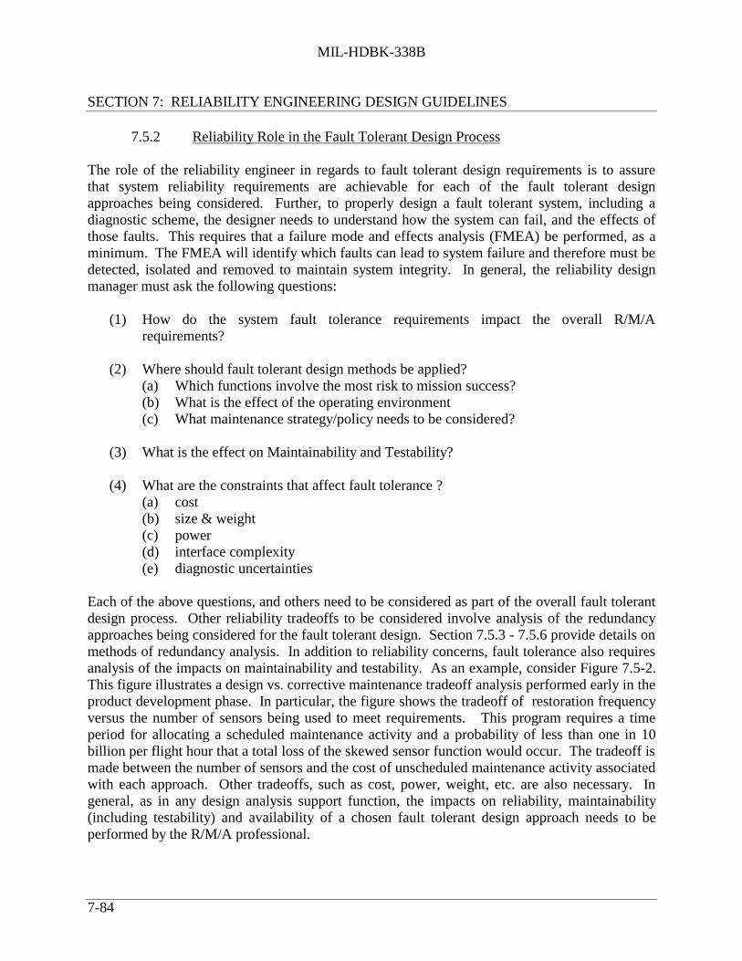
MIL-HDBK-338B


7-84

7.5.2 Reliability Role in the Fault Tolerant Design Process

The role of the reliability engineer in regards to fault tolerant design requirements is to assurethat system reliability requirements are achievable for each of the fault tolerant designapproaches being considered. Further, to properly design a fault tolerant system, including adiagnostic scheme, the designer needs to understand how the system can fail, and the effects ofthose faults. This requires that a failure mode and effects analysis (FMEA) be performed, as aminimum. The FMEA will identify which faults can lead to system failure and therefore must bedetected, isolated and removed to maintain system integrity. In general, the reliability designmanager must ask the following questions:

(1) How do the system fault tolerance requirements impact the overall R/M/Arequirements?

(2) Where should fault tolerant design methods be applied?(a) Which functions involve the most risk to mission success?(b) What is the effect of the operating environment(c) What maintenance strategy/policy needs to be considered?

(3) What is the effect on Maintainability and Testability?

(4) What are the constraints that affect fault tolerance ?(a) cost(b) size & weight(c) power(d) interface complexity(e) diagnostic uncertainties

Each of the above questions, and others need to be considered as part of the overall fault tolerantdesign process. Other reliability tradeoffs to be considered involve analysis of the redundancyapproaches being considered for the fault tolerant design. Section 7.5.3 - 7.5.6 provide details onmethods of redundancy analysis. In addition to reliability concerns, fault tolerance also requiresanalysis of the impacts on maintainability and testability. As an example, consider Figure 7.5-2.This figure illustrates a design vs. corrective maintenance tradeoff analysis performed early in theproduct development phase. In particular, the figure shows the tradeoff of restoration frequencyversus the number of sensors being used to meet requirements. This program requires a timeperiod for allocating a scheduled maintenance activity and a probability of less than one in 10billion per flight hour that a total loss of the skewed sensor function would occur. The tradeoff ismade between the number of sensors and the cost of unscheduled maintenance activity associatedwith each approach. Other tradeoffs, such as cost, power, weight, etc. are also necessary. Ingeneral, as in any design analysis support function, the impacts on reliability, maintainability(including testability) and availability of a chosen fault tolerant design approach needs to beperformed by the R/M/A professional.

MIL-HDBK-338B


7-85

.

10-18

10-14

10-10

ScheduledMaintenance

Interval Note: Failed components willnot be repaired during thisinterval unless critical.

6 Skewed Sensors(Unscheduled Maintenanceas Required BetweenMissions)

12 Skewed Sensors(No UnscheduledMaintenance)

10 Skewed Sensors(Unscheduled Maintenance Onlywhen 6 Sensors Remain)

System Goal

Time (t)

Los

s Pr

obab

ility

/Flt

Hr.

Note: More Frequent Restoration of Redundancy Lowers Fault Tolerance Requirements, But Results in Higher Maintenance Manhours

FIGURE 7.5-2: EFFECT OF MAINTENANCE CONCEPT ONLEVEL OF FAULT TOLERANCE

MIL-HDBK-338B


7-86

As a final note on the role of the reliability engineer, consider the following reliability inputs tothe development of the specification for a fault tolerant design

(1) Critical mission definition

(2) Quantitative mission reliability

(3) Quantitative maintenance frequency reliability

(4) Description of the storage, transportation, operation, and maintenance environments

(5) Time measure or mission profile

(6) Definition of satisfactory and acceptable degraded system performance

(7) Tolerable failure policy (fail-safe, fail-operational, etc.)

(8) Failure independence

These and other inputs are necessary to ensure that the system specifications are well defined andthat they support the ability to clearly define the best approach that also meets R/M/Arequirements.

7.5.2.1 Fault Tolerant Design Analysis

The FMEA is a primary reliability analysis, critical to the fault tolerant design process. Thereliability engineer will also utilize additional techniques for analyzing the fault tolerant design toverify that it meets reliability requirements. However, many of the evaluation tools used in thepast are no longer adequate to deal with more sophisticated fault tolerant designs that includemore complex fault handling capabilities. Because fault handling methods include the use offault detection and fault recovery approaches, any evaluation tool must include the ability toproperly account for the effects of imperfect fault coverage (or fault detection) and fault recovery.

Monte Carlo simulation and Markov analysis techniques continue to be used as the primarymeans of analyzing highly sophisticated fault tolerant designs. These approaches have beenmodified to incorporate situations where the sequence of failure is important, where the failure istransient or intermittent, or where the response to failure (i.e., detection, isolation, recovery,reconfiguration) is imperfect. In these situations, Markov methods continue to lead the way inevaluation methods. Markov analysis is described in more detail in Section 7.5.6 and will not bediscussed in detail here. In general, the Markov approach, which is used to define the specificstates that a system can occupy, has been used to incorporate fault handling and recovery. Amajor limitation to the Markov approach is that the number of system states that must be definedto comprehensively describe a large system and model the behavior of complex fault

MIL-HDBK-338B


7-87

management schemes can become very large (approaching 105 for highly complex systems). Acommon solution to this problem is to partition the system into smaller systems, evaluate eachpartition separately, and then combine the results at the system level. However, such anapproach is only exact when each partitioned subsystem’s fault tolerant behavior is mutuallyindependent of each other. If subsystem dependencies do exist, then an assumption ofindependence will result in only an approximate solution.

Other approaches that are now becoming more common involve decomposing the system intoseparate fault-occurrence and fault handling submodels. However, the inputs for this type ofapproach require knowledge of the distribution and parameter values of: detection, isolation,recovery, rates, etc. The following is a list of assumptions, limitations and sources of error foundin existing reliability models:

(1) Solving a fault-handling model in isolation and then reflecting its results in anaggregate model is, itself, an approximation technique. The assumptions necessary todetermine a solution typically result in a lower bound (conservative) approximation ofthe system reliability.

(2) Separate fault-handling models have been assumed to be independent of system state.This requires that the same fault-handling model and choice of parameters be usedirrespective of the system’s level of degradation. This ignores the fact that for manysystems the recovery process is faster if the number of active units is smaller or that therecovery process may be different, depending on the sequence of events in differentsubsystems.

(3) The common technique of partitioning the system into independent functionalsubgroups for computational ease is a potential source of error. The magnitude anddirection of the error is a function of how truly independent/dependent the subgroupsare of each other. If subgroups are assumed independent when in fact they are not, theeffect is an overstatement of system reliability/availability. If subgroups are assumedcompletely dependent when some degree of independence exists, the effect is anunderstatement of the system’s reliability/availability.

(4) Some models assume a constant instantaneous fault-protection coverage factor in lieuof a separate fault handling model. These fail to recognize that during time spent in theintermediate fault-handling states to detect, isolate, and recover/reconfigure, a seconditem failure could result in system failure. Further, as with fault handling models, thesetimes are generally not constant, but depend on the current state of the system.

(5) Most models require the assumption that the system is perfect at the mission start.Therefore, they cannot evaluate the effects of latent defects (e.g., handling,manufacturing, transportation, prior mission), nor assist in determining the testabilitypayoff or requirements for detection and removing them before the start of the mission.

MIL-HDBK-338B


7-88

Models with this limitation cannot be used to evaluate alternate maintenance conceptsthat include degradation between missions as an acceptable strategy.

(6) Some models require that spares be treated exactly like active units, irrespective of theiractual utilization in the system mechanization. This requires that spares are assumed tobe “hot” and have the same failure rates and failure modes as the active units. Thisassumption will cause the model to understate the system reliability in those situationswhere spares are “cold” or in “stand-by” and/or where their failure rates may be lessthat those of the active units.

(7) As indicated previously, some models require the assumption that item failure rates areconstant throughout time. This will result in an overstatement of system reliability ifthe items have failure rates that increase with mission time. Some models remove thisrestriction and permit time-varying failure rates. However, the solution the algorithmsemploy requires the use of global time (as opposed to local time of entry into a state),thus precluding the use of the model for repairable systems and availability analysis.

7.5.3 Redundancy as a Design Technique

In reliability engineering, redundancy can be defined as the existence of more than one means foraccomplishing a given task. In general, all means must fail before there is a system failure.

Thus, if we have a simple system consisting of two parallel elements as shown in Figure 7.5-3with A1 having a probability of failure q1 and A2 having a probability of failure q2 , the

probability of total system failure is

Q = q1 q2

A 2

INPUT OUTPUT

A1

FIGURE 7.5-3: PARALLEL NETWORK

MIL-HDBK-338B


7-89

Hence the reliability or probability of no failure is

R = 1 - Q = 1 - q1 q2

For example, assume that A1 has a reliability r1 of 0.9 and A2 a reliability r2 of 0.8. Then

their unreliabilities q1 and q2 would be

q1 = 1 - r1 = 0.1

q2 = 1 - r2 = 0.2

and the probability of system failure would be

Q = (0.1)(0.2) = 0.02

Hence the system reliability would be

R = 1 - Q = 0.98

which is a higher reliability than either of the elements acting singly. Parallel redundancy istherefore a design tool for increasing system reliability when other approaches have failed. Itshould be pointed out that while redundancy reduces mission failures, it increases logisticsfailures.

In general, with n elements in parallel, the overall probability of failure at time t is

Q(t) = q1(t) • q2(t) • . . . • q (t) n (7.9)

and the probability of operating without failure is

R(t) = 1 - Q(t) = 1 - q1(t) q2(t) . . . qm(t) (7.10)

which, because qi(t) = 1 - ri(t) for each component, can also be given as

R(t) = 1 - [ 1 - r1(t) ] [ 1 - r2(t) ] . . . [ 1 - rm(t) ] (7.11)

When each of the component reliabilities is equal, the above equations reduce to

Q(t) = [ q(t) ] m (7.12)

R(t) = 1 - [q(t)]m = 1 - [ 1 - r(t) ]m (7.13)

MIL-HDBK-338B


7-90

Figure 7.5-4 summarizes the characteristics of simple parallel active redundancy.

So far it has been assumed that parallel components do not interact and that they may beactivated when required by ideal failure sensing and switching devices. Needless to say, thelatter assumption, in particular, is difficult to meet in practice. Therefore, the potential benefitsof redundancy cannot be realized fully. The reader is referred to the cited references, e.g.,References [22] and [23], for detailed treatment of redundancy with sensing and switchingdevices which are most ideal.

Most cases of redundancy encountered will consist of various groupings of series and parallelelements. Figure 7.5-5 typifies such a network. The basic formulas previously given can be usedto solve the overall network reliability RAC .

MIL-HDBK-338B


7-91

All Blocks

Are AssumedTo BeIdentical

M0.0

0.2

0.4

0.6

0.8

2M

Rel

iabi

lity

Time

M = MTBF = 1/λ

1.0

0 1 2

Single Element

n=5n=4

n=3

n=2

RELIABILITY FUNCTION FOR SIMPLEPARALLEL RELIABILITY

APPLICATION

Provides protection against irreversible hardwarefailures for continuously operating equipments.

MATHEMATICAL MODEL

R = 1 - (1 - e −λt )n

APPROXIMATE MODEL

R = 1 - (λt)n

for small λt ≤ 0.1

where:n = number of parallel

elementsλ = failure rateR = reliability

ADVANTAGES OF PARALLELREDUNDACY

• Simplicity• Significant gain in Reliability

from nonredundant element• Applicable to both analog and

digital circuitry

DISADVANTAGES OF PARALLELREDUNDACY

• Load sharing must be considered• Sensitive to voltage division across the

elements• Difficult to prevent failure propagation• May present circuit design problems

FIGURE 7.5-4: SIMPLE PARALLEL REDUNDANCY: SUMMARY

MIL-HDBK-338B


7-92

a

b

c

A B C

ra = 0.9 rb = 0.8

rc = 0.8 rd = 0.8 re = 0.9 rf = 0.9

rg = 0.7

FIGURE 7.5-5: SERIES-PARALLEL REDUNDANCY NETWORK

7.5.3.1 Levels of Redundancy

Redundancy may be applied at the system level (essentially two systems in parallel) or at thesubsystem, component, or part level within a system. Figure 7.5-6 is a simplified reliabilityblock diagram drawn to illustrate the several levels at which redundancy can be applied. SystemD is shown with its redundant alternative D’, at the system level. D’ is in turn built up ofredundant subsystems or components (C1 and C2) and redundant parts within components (b1 andb2 within Component B). From the reliability block diagram and a definition of block or systemsuccess, the paths which result in successful system operation can be determined. For example,the possible paths from Input to Output are:

(1) A, a, b1 , C1

(2) A, a, b1 , C2

(3) A, a, b2 , C1

(4) A, a, b2 , C2

(5) D

MIL-HDBK-338B


7-93

b2

a

D

b1

C2

C1

A

BD’

Input Output

FIGURE 7.5-6: RELIABILITY BLOCK DIAGRAM DEPICTING REDUNDANCY AT THESYSTEM, SUBSYSTEM, AND COMPONENT LEVELS

The success of each path may be computed by determining an assignable reliability value foreach term and applying the multiplicative theorem. The computation of system success (all pathscombined) requires a knowledge of the type of redundancy to be used in each case and anestimate of individual element reliability (or unreliability).

7.5.3.2 Probability Notation for Redundancy Computations

Reliability of redundancy combinations is expressed in probabilistic terms of success or failure --for a given mission period, a given number of operating cycles, or a given number of timeindependent "events," as appropriate. The "MTBF" measure of reliability is not readily usablebecause of the nonexponentiality of the reliability function produced by redundancy. Reliabilityof redundancy combinations which are "time dependent" is therefore computed at a discrete pointin time, as a probability of success for this discrete time period. The following notation isapplicable to all cases and is used throughout this section:

R = probability of success or reliability of a unit or block

Q = R = probability of failure or unreliability of a unit or block

p = probability of success or reliability of an element

q = probability of failure or unreliability of an element

MIL-HDBK-338B


7-94

For probability statements concerning an event:

P(A) = probability that A occurs

P( A ) = probability that A does not occur

For the above probabilities:

R + Q = 1

p + q = 1

P(A) + P( A ) = 1

7.5.3.3 Redundancy Combinations

The method of handling redundancy combinations can be generalized as follows:

(1) If the elements are in parallel and the units in series (Figure 7.5-7), first evaluatethe redundant elements to get the unit reliability. Then find the product of all unitreliabilities to obtain the block reliability.

(2) If the elements are in series and the units or paths are in parallel (Figure 7.5-8), firstobtain the path reliability by calculating the product of the reliabilities of allelements in each path. Then consider each path as a redundant unit to obtain theblock reliability.

C

UNIT A UNIT B UNIT C

A1

A2

B1

B2

B3

FIGURE 7.5-7: SERIES-PARALLEL CONFIGURATION

MIL-HDBK-338B


7-95

A

B

(a) (b)

B1

A1 A2

B2 B3

FIGURE 7.5-8: PARALLEL-SERIES CONFIGURATION

In the redundancy combination shown in Figure 7.5-7, Unit A has two parallel redundantelements, Unit B has three parallel redundant elements, and Unit C has only one element.Assume that all elements are independent. For Unit A to be successful, A1 or A2 must operate;

for Unit B success, B1 , B2 or B3 must operate; and C must always be operating for block

success. Translated into probability terms, the reliability of Figure 7.5-7 becomes:

R =

1 - P( A 1) • P( A 2) • [1 - P( B1 ) • P( B 2 ) • P( B 3 )] • P(C)

If the probability of success, p, is the same for each element in a unit,

R =

1 - (1 - pA)2] • [1 - (1 - pB)3 • pc

= (1 - qA2 ) • (1 - qB

3 ) • pc

where:qi = 1 - pi

Often there is a combination of series and parallel redundancy in a block as shown in Figure7.5-8. This arrangement can be converted into the simple parallel form shown in Figure 7.5-8 byfirst evaluating the series reliability of each path:

pA = pa1 pa2

MIL-HDBK-338B


7-96

pB = pb1 pb2

pb3

where the terms on the right hand side represent element reliability. Then block reliability can befound from:

R = 1 - (1 - pA ) • (1 - pB )

= 1 - qA qB

7.5.4 Redundancy in Time Dependent Situations

The reliability of elements used in redundant configurations is usually time dependent. If therelation between element reliability and time is known, inclusion of the time factor does notchange the basic notation and approach to redundancy computation outlined above. As anexample, assume two active independent elements in parallel. System reliability is given by:

R = pa + pb - pa pb

This equation is applicable for one time interval. To express reliability over a segment of time,the reliability of each element must be expressed as a function of time.

Hence,R(t) = pa(t) + pb(t) - pa(t) pb(t)

where:R(t) = system reliability for time t, t > 0

andpa(t) , pb(t) = element reliabilities for time t

The failure pattern of most components is described by the exponential distribution, i.e.:

R(t) = e −λt = e −t /θ

where λ is the constant failure rate; t is the time interval over which reliability, R, is measured;and θ is the mean-time-between-failure.

For two elements in series with constant failure rates λa and λb, using the product rule ofreliability gives:

MIL-HDBK-338B


7-97

R(t) = pa(t) pb(t)

= e −λ at e −λ bt = e −(λa +λb )t

The system reliability, R(t), function is also exponential. With redundant elements present in thesystem, however, the system reliability function is not itself exponential. This is illustrated bytwo operative parallel elements whose failure rates are constant. From:

R(t) = pa + pb - pa pb

R(t) = e −(λa)t + e −(λb )t - e −(λa +λb )t

which is not of the simple exponential form e −λt . Element failure rates cannot, therefore, becombined in the usual manner to obtain the system failure rate if considerable redundancy isinherent in the design.

Although a single failure rate cannot be used for redundant systems, the mean-time-to-failure of

such systems can be evaluated. The mean life of a redundant "pair" whose failure rates are λa

and λb, respectively, can be determined from:

MTBF =

o

∞

∫ R(t)dt =

1λa

+

1λb

-

1λa + λ b

If the failure rates of both elements are equal, then,

R(t) = 2e −λt - e −2λt

and

MTBF =

32λ

= 32 θ

For three independent elements in parallel, the reliability function is:

R(t) = 1 -

(1− e−λat )(1− e−λbt )(1− e−λct )[ ]

and

MTBF =

1λa

+

1λb

+

1λc

-

1λa + λ b

-

1λa + λc

-

1λb + λc

+

1λa + λ b + λc

MIL-HDBK-338B


7-98

Ifλa = λb = λc = λ

then

R(t) = 3e −λt - 3e −2λt + e −3λt

and

MTBF =

3λ

-

32λ

+

13λ

=

1λ

+

12λ

+

13λ

=

116λ

= 116 θ

In general, for n active parallel elements, each element having the same constant failure rate, λ,

R(t) = 1 - 1− e−λt( )n

and

MTBF = 1

i

i=1

n

∑ λ=

i=1

n

∑ θi

7.5.5 Redundancy Considerations in Design

The two basic types of redundancy are:

(1) Active Redundancy: External components are not required to perform the function ofdetection, decision and switching when an element or path in the structure fails. Theredundant units are always operating and automatically pick up the load for a failedunit. An example is a multi-engined aircraft. The aircraft can continue to fly with oneor more engines out of operation.

(2) Standby Redundancy: External elements are required to detect, make a decision andswitch to another element or path as a replacement for a failed element or path.Standby units can be operating (e.g., a redundant radar transmitter feeding a dummyload is switched into the antenna when the main transmitter fails) or inactive (e.g., aspare radio is turned on when the primary radio fails).

Table 7.5-2 summarizes a variety of redundancy techniques. The most important of these arediscussed further later in this section.

The application of redundancy is not without penalties. It will increase weight, spacerequirements, complexity, cost, and time to design. The increase in complexity results in anincrease in unscheduled maintenance. Thus, safety and mission reliability is gained at theexpense of adding an item(s) in the unscheduled maintenance chain. The increase in

MIL-HDBK-338B


7-99

unscheduled maintenance may be counteracted by reliability improvement techniques such asdesign simplification, derating, and the use of more reliable components, as discussed elsewherein this Handbook.

The decision to use redundant design techniques must be based on analysis of the tradeoffsinvolved. Redundancy may prove to be the only available method, when other techniques ofimproving reliability, e.g., derating, simplification, better components, have been exhausted, orwhen methods of item improvement are shown to be more costly than duplications. Whenpreventive maintenance is planned, the use of redundant equipment can allow for repair with nosystem downtime. Occasionally, situations exist in which equipments cannot be maintained, e.g.,satellites; then redundant elements may be the best way to significantly prolong operating time.

MIL-HDBK-338B


7-100

TABLE 7.5-2: REDUNDANCY TECHNIQUES

Simple Parallel Redundancy (Active Redundancy)

In its simplest form, redundancy consists of a simpleparallel combination of elements. If any element failsopen, identical paths exist through parallel redundantelements.

(a) Bimodal Parallel/Series Redundancy

(b) Bimodal Series/Parallel Redundancy

A series connection of parallel redundant elementsprovides protection against shorts and opens. Directshort across the network due to a single element shortingis prevented by a redundant element in series. An openacross the network is prevented by the parallel element.Network (a) is useful when the primary element failuremode is open. Network (b) is useful when the primaryelement failure mode is short.

Majority Voting Redundancy

MVT

A1

A2

A3

An

Decision can be built into the basic parallel redundantmodel by inputting signals from parallel elements into avoter to compare each element’s signal with the signalsof the other elements. Valid decisions are made only ifthe number of useful elements exceeds the failedelements.

MIL-HDBK-338B


7-101

TABLE 7.5-2: REDUNDANCY TECHNIQUES (CONT’D)

Adaptive Majority Logic

MVT

A1

A2

A3

An

Comp

This technique exemplifies the majority logicconfiguration discussed previously with a comparatorand switching network to switch out or inhibit failedredundant elements.

Standby Redundancy

A 1

A 2

Output Power

PowerOutput

A 1

A 2

A particular redundant element of a parallelconfiguration can be switched into an active circuit byconnecting outputs of each element to switch poles.Two switching configurations are possible.

1) The elements may be isolated by the switch untilswitching is completed and power applied to theelement in the switching operation.

2) All redundant elements are continuouslyconnected to the circuit and a single redundantelement activated by switching power to it.

Operating Standby Redundancy

S 1

A

A

A

A

D

D

D

D

1

2

3

n n

3

2

1

In this application, all redundant units operatesimultaneously. A sensor on each unit detects failures.When a unit fails, a switch at the output transfers to thenext unit and remains there until failure.

MIL-HDBK-338B


7-102

In general, the reliability gain for additional redundant elements decreases rapidly for additionsbeyond a few parallel elements. As illustrated by Figure 7.5-9 for simple parallel redundancy,there is a diminishing gain in reliability and MTBF as the number of redundant elements isincreased. As shown for the simple parallel case, the greatest gain achieved through addition ofthe first redundant element is equivalent to a 50% increase in the system MTBF. Optimization ofthe number of parallel elements is discussed in Section 7.5.5.5.

In addition to maintenance cost increases due to repair of the additional elements, reliability ofcertain redundant configurations may actually be less than that of a single element. This is due tothe serial reliability of switching or other peripheral devices needed to implement the particularredundancy configuration. Care must be exercised to insure that reliability gains are not offset byincreased failure rates due to switching devices, error detectors and other peripheral devicesneeded to implement the redundancy configurations. One case where the reliability of switchingdevices must be considered is that of switching redundancy. This occurs when redundantelements are energized but do not become part of the circuit until switched in after the primaryelement fails. See Section 7.5.5.2.6 for further discussion.

The effectiveness of certain redundancy techniques (especially standby) can be enhanced byrepair. Standby redundancy allows repair of the failed unit (while operation of the good unitcontinues uninterrupted) by virtue of the switching function built into the standby redundantconfiguration. Through continuous or interval monitoring, the switchover function can providean indication that failure has occurred and operation is continuing on the alternate channel. Witha positive failure indication, delays in repair are minimized. A further advantage of switching isrelated to built-in test (BIT) objectives. Built-in test can be readily incorporated into a sensingand switchover network for ease of maintenance purposes.

An illustration of the enhancement of redundancy with repair is shown in Figure 7.5-10. Theincreased reliability brought about by incorporation of redundancy is dependent on effectiveisolation of redundant elements. Isolation is necessary to prevent failure effects from adverselyaffecting other parts of the redundant network. In some cases, fuses or circuit breakers, overloadrelays, etc., may be used to protect the redundant configuration. These items protect aconfiguration from secondary effects of an item’s failure so that system operation continues afterthe element failure. The susceptibility of a particular redundant design to failure propagationmay be assessed by application of failure mode and effects analysis as discussed in Section 7.8.The particular techniques addressed there offer an effective method of identifying likely faultpropagation paths.

MIL-HDBK-338B


7-103

M

0.2

0.4

0.6

0.8

1

2

Rel

iab

ility

Time

M = MTBF = 1/ λ

1 of 10RedundantElements

1 of 5

1 of 4

1 of 3

1 of 2

SingleElement

(a) Simple Active Redundancy for One of n Element Required

n M ∆M 1 1.00 0 2 1.50 .50 3 1.83 .33 4 2.08 .25 5 2.28 .20

(n) (n)

2 3 4 5Degree of Redundancy (n)

2.4

2.2

2.0

1.8

1.6

1.4

1.2

1.0

∆M = .502

∆M = .333

∆M = .254

∆M = .205

Incr

emen

tal I

ncre

ase

in S

yste

m M

TB

F, M

n

(b) Incremental Increase in System MTBF for n Active Elements

FIGURE 7.5-9: DECREASING GAIN IN RELIABILITY AS NUMBEROF ACTIVE ELEMENTS INCREASES

MIL-HDBK-338B


7-104

Redundant Elements With Repair

Single Element

Time

Rel

iabi

lity

Redundant Elements

FIGURE 7.5-10: RELIABILITY GAIN FOR REPAIR OFSIMPLE PARALLEL ELEMENT AT FAILURE

Redundancy may be incorporated into protective circuits3 as well as the functional circuit whichit protects. Operative redundancy configurations of protection devices (e.g., fuse, circuit breaker)can be used to reduce the possibility that the "protected" circuit is not completely disabled shouldthe protective circuit device open prematurely or fail to open due to overcurrent.

The incorporation of redundancy into a design must take into account "checkability." Someitems may not be checkable prior to mission start. Such items must then be assumed to befunctional at the beginning of the mission. In reality, pre-mission failures of redundant itemscould be masked. If it is not known that redundant elements are operational prior to missionstart, then the purpose of redundancy can be defeated because the possibility exists of starting amission without the designed redundancy (a reliability loss). The designer must take this intoaccount for built-in test planning, inclusion of test points, packaging, etc., when redundancy isused in system design.

3 It should be noted that the need for or usefulness of modeling reliability at the circuit level is not universally accepted. Inparticular, many engineers question the value of such modeling for modern technologies. Discussion of circuit-level modeling isincluded here since it may be of value in some instances.

MIL-HDBK-338B


7-105

7.5.5.1 Partial Redundancy

Instances in which the system is successful if at least one of n parallel paths is successful hasbeen discussed. In other instances, at least k out of n elements must be successful. In such cases,the reliability of the redundant group (each with the same Probability of Success, p) is given by aseries of additive binomial terms in the form of

P(k, np) =

n

k pk (1 - p)n-k

Two examples of partial redundancy follow.

Example 1:

A receiver has three channels. The receiver will operate if at least two channels are successful,that is, if k = 2 or k = 3. The probability of each channel being successful is equal to p; then

R = P (2, 3p) + P (3, 3p)

R =

3

2 p2 (1 - p) +

3

3 p3 (1 - p)0

R = 3p2 (1 - p) + p3

R = 3p2 - 2p3

Use of the binomial formula becomes impractical for hand calculation in multi-element partialredundant configurations when the values of n and k become large.4 In these cases, the normalapproximation to the binomial may be used. The approach can be best illustrated by an example.

Example 2:

A new transmitting array is to be designed using 1000 RF elements to achieve design goalperformance for power output and beam width. A design margin has been provided, however, topermit a 10% loss of RF elements before system performance becomes degraded below theacceptable minimum level. Each element is known to have a failure rate of 1000 x 10-6 failuresper hour. The proposed design is illustrated in Figure 7.5-11, where the total number of elementsis n = 1000; the number of elements required for system success is k = 900; and, the number ofelement failures permitted is r = 100. It is desired to compute and plot the reliability function forthe array.

4 See any good textbook on probability and statistics.

MIL-HDBK-338B


7-106

1

2

3

998

999

1000

FIGURE 7.5-11: PARTIAL REDUNDANT ARRAY

For each discrete point of time, t, the system reliability function, Rs(t) is given by the binomial

summation as:

Rs(t) = n

x

x=0

r

∑

p n −x q x

= x=0

100

∑ 1000

x

e−λ t( )n-x

(1 - e-λ t )x

where:

q = 1 - e −λt

p = e −λt

x = number of failures

λ = element failure rate

MIL-HDBK-338B


7-107

This binomial summation can be approximated by the standard normal distribution functionusing Table 7.5-3 to compute reliability for the normalized statistic z.

TABLE 7.5-3: RELIABILITY CALCULATIONS FOR EXAMPLE 2

Time, t z F(z) = Rs(t)

90 1.57 .94295 .989 .8389105 0.0 .500110 -.42 .337120 -1.30 .097130 -2.03 .021

Note that Rs(t) = F(z)

where:

z =

x − µσ

= x - nq

npq =

x − n(1 − e−λt )

n(1 − e−λt)e−λt

By observation, it can be reasoned that system MTBF will be approximately 100 hours, since 100element failures are permitted and one element fails each hour of system operation. Apreliminary selection of discrete points at which to compute reliability might then fall in the 80-to 100-hour bracket.

At 80 hours:

q = 1 - e −λt = 1 - e-(1000 • 10-6 • 80) = .077

p = e-1000 • 10-6 • 80 = .923

µ = nq = 1000 (1 - e-1000 • 10-6 • 80) = 77

σ = npq = 1000 (.077) (.923) = 71.07 = 8.4

x = 100

z80 = 100 - 77

8.4 = 2.74

MIL-HDBK-338B


7-108

Rs(80) = F(z80 ) = F(+2.74) = .997, from standard normal tables

At 100 hours:

µ = nq = 1000

1 - e-1000 • 10-6• 100 = 95

p = e-1000 • 10-6 • 100 = .905

σ = npq = 86 = 9.3

x = 100

z100 =100 - 95

9.3 = 0.54

Rs(100) = F(z100 ) = F(+.54) = .705

These points are then used to plot the reliability function for the array, shown in Figure 7.5-12.Also shown in the figure are curves for r=0, 50, and 150.

r = 0 50 100 150

0 50 100 150 2000

.5

1.0

SYSTEM OPERATING TIME IN HOURS, t

Rs(t)

FIGURE 7.5-12: RELIABILITY FUNCTIONS FOR PARTIAL REDUNDANTARRAY OF FIGURE 7.5-11

MIL-HDBK-338B


7-109

7.5.5.2 Operating Standby Redundancy

Until now we have dealt with circuits where it was assumed that switching devices were eitherabsent or failure free. We now deal with circuits whose redundant elements are continuouslyenergized but do not become part of the circuit until switched in after a primary element fails.We will consider two modes of failure that can be associated with the switching mechanism:

a. Type (1). The switch may fail to operate when it is supposed to.

b. Type (2). The switch may operate without command (prematurely).

In the following discussion

qs = probability of a Type (1) failure

q’s = probability of a Type (2) failure

7.5.5.2.1 Two Parallel Elements

Consider the system in Figure 7.5-13. There are three possible states that could lead to systemfailure:

a. A succeeds, B fails, switch fails (Type 2).

b. A fails, B succeeds, switch fails (Type 1).

c. A fails, B fails.

B

A

S

FIGURE 7.5-13: REDUNDANCY WITH SWITCHING

MIL-HDBK-338B


7-110

The unreliability of the system, Q, is found from

Q = pa qb q’s + qa pb qs + qa qb

As an example, assume

qa = qb = 0.2

andqs = q’s = 0.1

ThenQ = pa qb q’s + qa pb qs + qa qb

= (0.8)(0.2)(0.1) + (0.2)(0.8)(0.1) + (0.2)(0.2)

= 0.072

R = 1 - Q

= 1 - 0.072

= 0.928

If we are not concerned with Type (2) failures,

q’s = 0

and the unreliability is

Q = qa pb qs + qa qb

= (0.2)(0.8)(0.1) + (0.2)(0.2)

= 0.056

R = 1 - 0.056 = 0.944

MIL-HDBK-338B


7-111

7.5.5.2.2 Three Parallel Elements

Figure 7.5-14 illustrates this type circuit. It operates as follows: If A fails, S switches to B. If Bthen fails, S switches to C. Enumerating all possible switching failures shows two kinds of Type(1) failure and four kinds of Type (2) failure:

a. Type (1) Switching Failures:

1. qs1 - A fails, S does not switch to B.

2. qs2 - A fails, S switches to B, B fails, S fails to switch to C.

B

A

C

S

FIGURE 7.5-14: THREE-ELEMENT REDUNDANT CONFIGURATIONSWITH SWITCHING

b. Type (2) Switching Failures:

1. q’s3 - A succeeds, but S switches to B.

2. q’s4 - A succeeds, S switches to B, B fails, S does not switch to C.

3. q’s5 - A succeeds, S switches to B, B succeeds, S switches to C.

4. q’s6 - A fails, S switches to B, B succeeds, S switches to C.

The probability of switching failures must be considered in modeling redundancy with switching.The consideration of such failures can be complex. If the switching reliability is high incomparison with element reliability (i.e., switch failure rate is one-tenth that of the elementfailure rate), it is often possible to simplify the model with an acceptable loss of accuracy by

MIL-HDBK-338B


7-112

ignoring switch failures. For more detailed information, the reader is referred to textbooks on thesubject and Refs. [22] and [24].

7.5.5.2.3 Voting Redundancy

Figure 7.5-15 shows three elements, A, B, and C, and the associated switching and comparatorcircuit which make up a voting redundant system. The circuit function will always be performedby an element whose output agrees with the output of at least one of the other elements. At leasttwo good elements are required for successful operation of the circuit. Two switches areprovided so that a comparison of any two outputs of the three elements can be made. Acomparator circuit is required that will operate the two switches so that a position is locatedwhere the outputs again agree after one element fails.

B

A

C

COMPARATOR

FIGURE 7.5-15: THREE-ELEMENT VOTING REDUNDANCY

If comparison and switching are failure free, the system will be successful as long as two or threeelements are successful. In this case,

R = pa pb + pa pc + pb pc - 2pa pb pc

If failure free switching cannot be assumed, conditional probabilities of switching operation haveto be considered. To simplify the discussion, consider the probability of the comparator andswitches failing in such a manner that the switches remain in their original positions. If thisprobability is qs , then

R = pa pb + (pa pc + pb pc - 2pa pb pc ) (1 - qs )

MIL-HDBK-338B


7-113

Example of a Voting Redundant System

Let all three elements have the same probability of success, 0.9, i.e., pa = pb = pc = 0.9.

Assume that the comparator switch has a probability of failing (qs ) of 0.01:

R = .92 +

.92 + .92 - 2(.9)3 [1 - .01]

R = .970

Information and expressions for the general majority voting case are given in Figure 7.5-16.

7.5.5.3 Inactive Standby Redundancy

In a system with redundant elements on an inactive standby basis (not energized), no time isaccumulated on a secondary element until a primary element fails. For a two-element system(see Figure 7.5-13) the reliability function can be found directly as follows. The system will besuccessful at time t if either of the following two conditions hold (let A be the primary element):

a. A is successful up to time t.

b. A fails at time t1 < t, and B operates from t1 to t.

For the exponential case where the element failure rates are λa and λb , reliability of the standby

pair is given by

R(t) =

λbλb − λa

e −λ at -

λaλb − λa

e −λ bt

This is a form of the mixed exponential and it does not matter whether the more reliable elementis used as the primary or as the standby element.

The mean-time-to-failure of the system is

MTBF =

λa + λ bλaλ b

= θa + θb

= 2θ when θa = θb = θ

MIL-HDBK-338B


7-114

For n elements of equal reliability, it can be shown that,

R(t) = e t)

r! - t

r =0

n-1 rλ λ∑ (

where:r is the number of failures

MTBF =

nλ

= nθ

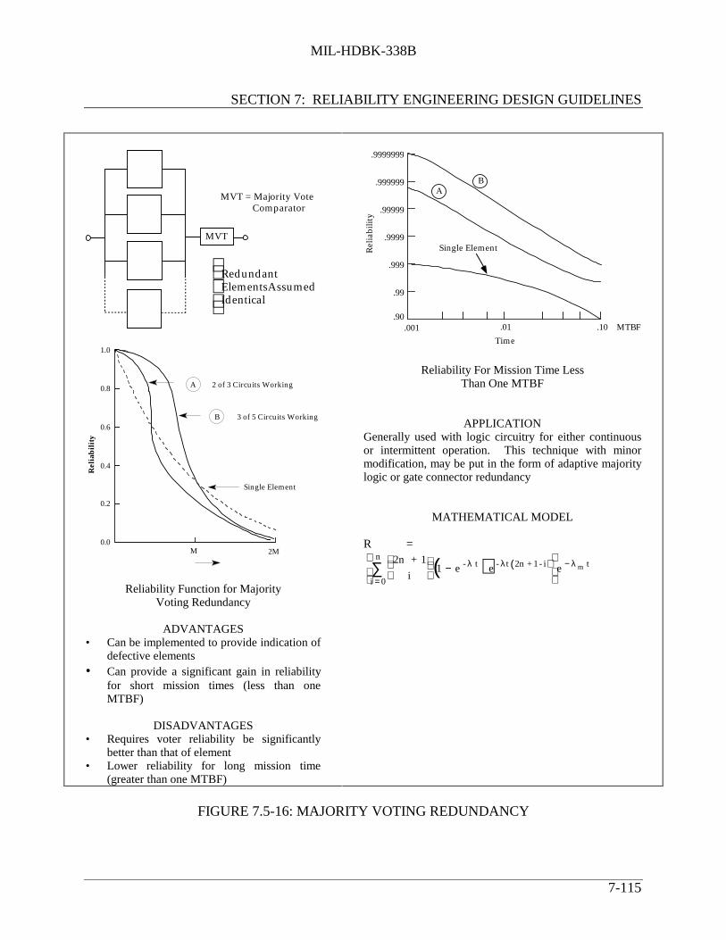
MIL-HDBK-338B


7-115

MVT

Redundant

ElementsAssumedIdentical

MVT = Majority Vote Comparator

0.0

0.2

0.4

0.6

0.8

1.0

M 2M

Rel

iab

ilit

y

Single Element

A 2 of 3 Circuits Working

B 3 of 5 Circuits Working

Reliability Function for MajorityVoting Redundancy

ADVANTAGES• Can be implemented to provide indication of

defective elements• Can provide a significant gain in reliability

for short mission times (less than oneMTBF)

DISADVANTAGES• Requires voter reliability be significantly

better than that of element• Lower reliability for long mission time

(greater than one MTBF)

BA

.9999999

.999999

.99999

.9999

.999

.99

.90.001 .01 .10 MTBF

Single Element

Time

Rel

iabi

lity

Reliability For Mission Time LessThan One MTBF

APPLICATIONGenerally used with logic circuitry for either continuousor intermittent operation. This technique with minormodification, may be put in the form of adaptive majoritylogic or gate connector redundancy

MATHEMATICAL MODEL

R =

2n + 1i

1 − e - λ t( ) e - λt 2n + 1- i( )

i = 0

n

∑

e

− λ m t

FIGURE 7.5-16: MAJORITY VOTING REDUNDANCY

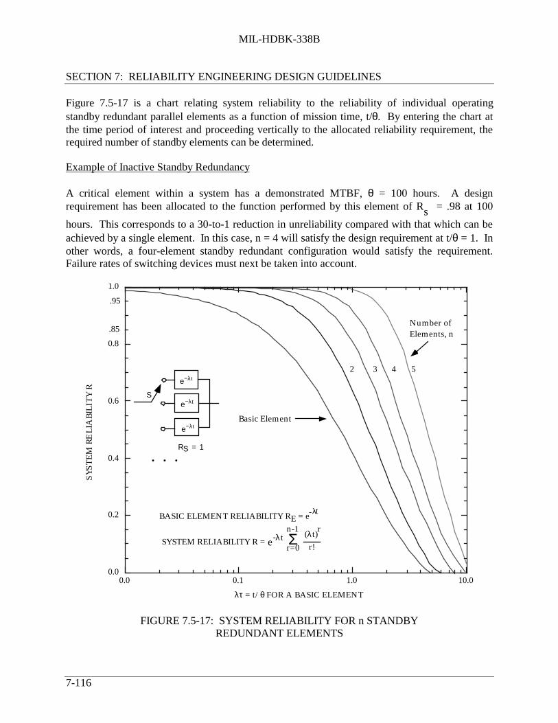
MIL-HDBK-338B


7-116

Figure 7.5-17 is a chart relating system reliability to the reliability of individual operatingstandby redundant parallel elements as a function of mission time, t/θ. By entering the chart atthe time period of interest and proceeding vertically to the allocated reliability requirement, therequired number of standby elements can be determined.

Example of Inactive Standby Redundancy

A critical element within a system has a demonstrated MTBF, θ = 100 hours. A designrequirement has been allocated to the function performed by this element of Rs = .98 at 100

hours. This corresponds to a 30-to-1 reduction in unreliability compared with that which can beachieved by a single element. In this case, n = 4 will satisfy the design requirement at t/θ = 1. Inother words, a four-element standby redundant configuration would satisfy the requirement.Failure rates of switching devices must next be taken into account.

Number ofElements, n

−λte

−λte

−λte

RS = 1

S

0.0

0.2

0.4

0.6

0.8

1.0

0.0 0.1 1.0 10.0

Basic Element

2 3 4 5

λτ = t/θ FOR A BASIC ELEMENT

SYST

EM R

ELI

ABI

LITY

R

BASIC ELEMENT RELIABILITY R = e-λtE

SYSTEM RELIABILITY R =

• • •

.95

.85

e-λtn-1

r=0Σ (λt)r

r!

FIGURE 7.5-17: SYSTEM RELIABILITY FOR n STANDBYREDUNDANT ELEMENTS

MIL-HDBK-338B


7-117

7.5.5.4 Dependent Failure Probabilities

Up to this point, it has been assumed that the failure of an operative redundant element has noeffect on the failure rates of the remaining elements. Dependent failures might occur, forexample, with a system having two elements in parallel where both elements share the full load.

An example of conditional or dependent events is illustrated by Figure 7.5-18. Assume elementsA and B are both fully energized, and normally share or carry half the load, L/2. If either A or Bfails, the survivor must carry the full load, L. Hence, the probability that one fails is dependenton the state of the other, if failure probability is related to load or stress. The system is operatingsatisfactorily at time t if either A or B or both are operating successfully.

A

B

FIGURE 7.5-18: LOAD SHARING REDUNDANT CONFIGURATION

Figure 7.5-19 illustrates the three possible ways the system can be successful. The bar above aletter represents a failure of that element. A primed letter represents operation of that elementunder full load; absence of a prime represents operation under half load. If the elements’ failuretimes are exponentially distributed and each has a mean life of θ under load L/2 and θ’ = θ/kunder load L where k ≥ 0, block reliability is given below without derivation:

R(t) =

2θ’2θ’−θ

e −t /θ’-

θ2θ’−θ

e −2t /θ

System mean life is equal to

θs = θ/k + θ/2

When k = 1, the system is one in which load sharing is not present or an increased load does notaffect the element failure probability. Thus, for this case, θs is equal to 3θ/2.

MIL-HDBK-338B


7-118

TIME AXIS

CONDITION

AB

AB

A B’

B A’

(1)

(2)

(3)

AB

0 tt1

FIGURE 7.5-19: SUCCESS COMBINATIONS IN TWO-ELEMENTLOAD-SHARING CASE

7.5.5.5 Optimum Allocation of Redundancy

Decision and switching devices may fail to switch when required or may operate inadvertently.However, these devices are usually necessary for redundancy, and increasing the number ofredundant elements increases the number of switching devices. If such devices are completelyreliable, redundancy is most effective at lower system levels. If switching devices are not failurefree, the problem of increasing system reliability through redundancy becomes one of choosingan optimum level at which to replicate elements.

Since cost, weight, and complexity factors are always involved, the minimum amount ofredundancy that will produce the desired reliability should be used. Thus efforts should beconcentrated on those parts of the system which are the major causes of system unreliability.

As an example, assume that we have two elements, A and B, with reliabilities over a certain timeperiod of 0.95 and 0.50, respectively. If A and B are joined to form a series nonredundant circuit,its reliability is

R = (0.95)(0.50) = 0.475

If we duplicate each element, as in Figure 7.5-20a,

R1 = [1 - (0.50)2 ] [1 - (0.05)2 ] = 0.748

MIL-HDBK-338B


7-119

Duplicating Element B only, as in Figure 7.5-20b,

R2 = 0.95 [1 - (0.50)2 ] = 0.712

Obviously, duplicating Element A contributes little to increasing reliability.

Triplication of B gives the configuration shown in Figure 7.5-20c and

R3 = 0.95 [1 - (0.5)3 ] = 0.831

R3 gives a 75% increase in original circuit reliability as compared to the 58% increase of R1 .

If complexity is the limiting factor, duplicating systems is generally preferred to duplicatingelements, especially if switching devices are necessary. If another series path is added in parallel,we have the configuration in Figure 7.5-20d, and

R4 = 1 - (1 - .475)2 = 0.724

R4 is only slightly less than R1 . If switches are necessary for each redundant element, R4 may

be the best configuration. A careful analysis of the effect of each element and switch on systemreliability is a necessary prerequisite for proper redundancy application.

7.5.6 Reliability Analysis Using Markov Modeling

7.5.6.1 Introduction

Markov Modeling is a reliability analysis tool which in the past few years has become the mostprominent method of computing the reliability (or unreliability) of fault tolerant systems. It is anextremely flexible tool which can be used to predict the reliability of in-flight critical digitalelectronic systems. It has been used on a number of digital electronic engine controls to computethe probability of events such as aircraft loss due to control system failures, mission aborts, in-flight shut-down of engines, overspeeding of engines and inadvertent thrust reversal. Markovmodeling offers many advantages over other reliability modeling techniques, some of which are:

(1) Simplistic modeling approach: The models are simple to generate although they requirea more complicated mathematical approach. This is not a problem, however, becausethe mathematics are well suited for the digital computer.

MIL-HDBK-338B


7-120

B

BA

A

(a)

B

B

B

A

(c)

A

(b)

B

B

B

BA

A

(d)

FIGURE 7.5-20: POSSIBLE REDUNDANT CONFIGURATIONS RESULTINGFROM ALLOCATION STUDY

(2) Redundancy management techniques: System reconfiguration required by failures iseasily incorporated in the model.

(3) Coverage: Covered and uncovered failures of components are mutually exclusiveevent. These are not easily modeled using classical techniques, but are readily handledby the Markov mathematics.

(4) Complex systems: Many simplifying techniques exist which allow the modeling ofcomplex systems.

(5) Sequenced events: Many times the analyst is interested in computing the probability ofan event which is the result of a certain sequence of sub-events. As an example, theprobability of an engine overspeed might be desired. This is usually the result of twoevents, these being loss of overspeed protection and an uncommanded high fuel flow.These must necessarily occur in that order. For if the uncommanded high fuel flow

MIL-HDBK-338B


7-121

precedes the overspeed protection failure, an engine shutdown occurs rather than anoverspeed. While these types of problems do not lend themselves well to classicaltechniques, they are easily handled using Markov modeling.

7.5.6.2 Markov Theory

Markov modeling can be applied to systems which vary discretely or continuously with respect totime and space. In reliability we are generally concerned with continuous time, discrete statemodels. These systems are characterized by randomly varying stochastic processes. Stochasticprocesses must have two important properties in order to model them with the Markovapproach.5

These are:

(1) The process must be memoryless

(2) The process must be stationary

A memoryless system is characterized by the fact that the future state of the system depends onlyon its present state. A stationary system is one in which the probabilities which govern thetransitions from state to state remain constant with time. In other words, the probability oftransitioning from some state i to another state j is the same regardless of the point in time thetransition occurs. The states of the model are defined by system element failures. Thetransitional probabilities between states are a function of the failure rates of the various systemelements. A set of first-order differential equations are developed by describing the probabilityof being in each state in terms of the transitional probabilities from and to each state. Thenumber of first-order differential equations will equal the number of states of the model. Themathematical problem becomes one of solving the following equation:

•P = [A]P

where •P and P are n x 1 column vectors, [A] is an n x n matrix and n is the number of states in

the system. The solution of this equation is:

P = exp[A]t • P(0)

where exp[A]t is an n x n matrix and P(0) is the initial probability vector describing the initialstate of the system. Two methods which are particularly well suited for the digital computer forcomputing the matrix exp[A]t are the infinite series method and the eigenvalue/eigenvectormethod. Figure 7.5-21 presents a flow chart which illustrates the procedure used to develop aMarkov model.

5 Extensions of the theory to other processes exist but are beyond the scope of this handbook.

MIL-HDBK-338B


7-122

Define Event forWhichProbability is Desired

PR(Subevent)

Define Critical HardwareAssociated with the Event

Divide Hardware intoSeparate Pieces whose

Failures are Defined asSubevents

Define Markov ModelElements

Develop Markov Model

Element Failure Rates

Compute Markov Model

Coverages Based on BIT

Define Markov Model StateTransitions based on

Redundancy ManagementStrategies

Define Initial StateProbabilities

Input Data and RunMarkov Program

Combine Hardwarewith Equivalent

Failure Effects

ApplySimplifyingTechnqiues to Reduce

the Number of States

Number ofSubevents > 1

PR(EVENT)

All Models

Performed

PR(Event) = f [PR(Subevent)]

YES

YES NO

NO

FIGURE 7.5-21: MARKOV MODELING PROCESS

MIL-HDBK-338B


7-123

7.5.6.3 Development of the Markov Model Equation

In order to illustrate how the Markov model equations are developed, assume we have a systemwhich is made up of two elements. Each element has two mutually exclusive states - a good andfailed. The states of the model are generated based on the elements being in one of these twostates. The probabilities that cause transition from state to state are a function of the elementfailure rates. An element with constant failure rate (1) has a transitional probability which isapproximated by λ • ∆t. The probability of more than one element failure in ∆t is considerednegligible. A flow diagram of the two element problem mentioned above is presented in Figure7.5-22.

We develop the Markov differential equation by describing the probability of being in each of thestates at time t + ∆t as a function of the state of the system at time t. The probability of being instate one at some time t + ∆t is equal to the probability of being in state on at time t and nottransitioning out during ∆t. This can be written as:

P1(t + ∆t) = P1(t) • [1 - (λ1 + λ2) • ∆t]

The probability of being in state two at time t + ∆t is equal to the probability of being in state oneat time t and transitioning to state two in ∆t plus the probability of being in state two at time t andnot transitioning out during ∆t. This can be written as:

P2(t + ∆t) = P1(t) • λ1 • ∆t + P2(t)(1 - λ2 • ∆t)

The other state probabilities are generated in the same manner resulting in the followingequations:

P1(t + ∆t) = P1(t) • [1 - (λ1 + λ2) • ∆t]

P2(t + ∆t) = P1(t) • λ1 • ∆t + P2(t)(1 - λ2 • ∆t)

P3(t + ∆t) = P1(t) • λ2 • ∆t + P3(t)(1 - λ1 • ∆t)

P4(t + ∆t) = P2(t) • λ2 • ∆t + P3(t) • λ1 • ∆t + P4(t)

MIL-HDBK-338B


7-124

STATE 3

ELEMENT 1 GOOD ELEMENT 2 FAILED

STATE 2

ELEMENT 1 FAILED ELEMENT 2 GOOD

STATE 4

ELEMENT 1 FAILED ELEMENT 2 FAILED

1

λ2 • ∆t

STATE 1

ELEMENT 1 GOOD ELEMENT 2 GOOD

1 - λ2 • ∆t

λ1 • ∆t

1 - (λ 1 + λ2) • ∆t

λ2 • ∆t

1 - λ1 • ∆t

λ1 • ∆t

FIGURE 7.5-22: MARKOV FLOW DIAGRAM

Rearranging:

[P1(t + ∆t) - P1(t)]/∆t = - (λ1 + λ2) • P1(t)

[P2(t + ∆t) - P2(t)]/∆t = λ1 • P1(t) - λ2 • P2(t)

[P3(t + ∆t) - P3(t)]/∆t = λ2 •P1(t) - λ1 •P3(t)

[P4(t + ∆t) - P4(t)]/∆t = λ2 • P2(t) + λ1 • P3(t)

Taking the limit as ∆t → 0:

dP1(t)/dt = -(λ1 + λ2) • P1(t)

dP2(t)/dt = λ1 • P1(t) - λ2 • P2(t)

dP3(t)/dt = λ2 • P1(t) - λ1 • P3(t)

dP4(t)/dt = λ2 • P2(t) + λ1 • P3(t)

MIL-HDBK-338B


7-125

In matrix form this becomes:

dP1(t)/dt -(λ1 + λ2) 0 0 0 P1(t)

dP2(t)/dt λ1 -λ20 0 P2(t)

dP3(t)/dt = λ20 -λ1

0 • P3(t)

dP4(t)/dt 0 λ2 λ10 P4(t)

or P•

= [A] • P where [A] is defined as the state transition matrix. The important thing to notehere is that the analyst need only generate the states and the transitions between states as definedby the element failure rates. This information can then be inputted to the computer in a formwhich allows it to set up the state transition matrix and compute the state probabilities usingmatrix mathematics.

7.5.6.4 Markov Model Reduction Techniques

Since the Markov modeling approach can generate all the possible states of a system, the numberof states can be extremely large even for a relatively small number of Markov elements.Therefore it become imperative for the analyst using the Markov modeling approach to becomefamiliar with the reduction techniques that can be applied to reduce the number of statessignificantly while maintaining the accuracy of the model. As an example, if we assume asystem contains 10 elements, each of which have two states (good and failed), the total numberof possible states becomes:

# STATES = 2N = 210 = 1024

Furthermore, a system containing only 10 elements would be considered small when modelingdigital electronic engine controls, for instance. Fortunately many simplification techniques existwhich can be used alone, or in combination, to reduce the amount of states in the model.

One approach is to use the principle that states which represent multiple levels of failurecontribute insignificantly to the overall probability of failure of the system. The model can betruncated at a certain failure level, combining all states below that level into one failed state. Iffor instance it is desired to truncate at the nth level, all state transitions from n-1 level stateswould be directed to one nth order failed state. Care should be taken, however, to make sure thatthis truncation does not have an overly conservative impact on the system.

Many elements have the same, or nearly the same, impact on system operation when failed. Inthis case the states which are the result of failure of these elements can be combined. As anexample, assume we have a two channel engine control in dual active mode. By dual activemode we mean both channels are simultaneously in control. Let each channel have a failure rateλ. If one channel fails we have the ability to control with the other good channel. Because lossof either channel leads to the same effect (i.e., single channel control), the corresponding states

MIL-HDBK-338B


7-126

can be combined. Figure 7.5-23 shows the Markov model for this system using no reductiontechnique and the equivalent model by combining States 2 and 3. Because the system impactwas the same independent of what channel failed first, and because the channel failure rates werethe same, we are able to reduce the number of states with no loss of accuracy. If this is not thecase, assumptions have to be made as to what element failure caused transition to the new stateso that a conservative approximation to the transitions out of the state can be made.

STATE 11G AND 2G

STATE 11G AND 2G

STATE 21F AND 2G

OR1G AND 2F

STATE 31F AND 2F

2 • λ

λ

STATE 21F AND 2G

STATE 31G AND 2F

STATE 41F AND 2F

λ λ

λ λ

FIGURE 7.5-23: TWO CHANNEL EXAMPLE

Many times failure of a certain element causes loss of other elements in a system. An examplewould be loss of a power supply. In this case the analyst need not define transitions for the otherlost element(s) because by definition they are also no longer part of the functioning system.

Another reduction technique involves dividing the top level event for which the probability offailure is desired into n sub-events, each of which is modeled separately. The probabilities foreach sub-event are then combined to yield the probability of the top level event. If for instancethe system being modeled has ten elements, we have a possible of 1024 total states. If the toplevel event containing these ten elements can be broken down into two sub-events, eachcontaining five elements, the system can be described with two models each with a possiblethirty-two states. If the top level event has probability P and the two sub-events haveprobabilities P1 and P2 respectively, the top level probability can be computed as P = f(P1,P2).

MIL-HDBK-338B


7-127

7.5.6.5 Application of Coverage to Markov Modeling

In redundant system modeling we generally consider three Markov element states - good, failedcovered, and failed uncovered. Covered and uncovered markov element states are mutuallyexclusive meaning that an element cannot fail both covered and uncovered. System coverage isgenerally defined in terms of the conditional probability.

P[detect, isolate, reconfigurefailure]

When computing a coverage for Markov model elements we are concerned with that portion ofthe Markov element failure rate that is detectable and isolatable. Reconfiguration becomes afunction of what resources are available at the time the failure occurs.

As an example of how coverage is used in the Markov model, we will return to the two channeldual active engineer control discussed previously. In this case if either channel fails covered, theother channel has the ability to take over full control. However, if either channel failsuncovered, system failure occurs. The Markov model for this example appears in Figure 7.5-24.Note that once state two is entered, no resources are available and both the covered anduncovered portions of the remaining channels failure rate are routed to system failure.

STATE 11G AND 2G

STATE 21COV AND 2G

OR1G AND 2COV

STATE 3SYSTEM FAILURE

2 • λ cov

λ

2 • λ unc

FIGURE 7.5-24: COVERAGE EXAMPLE

MIL-HDBK-338B


7-128

7.5.6.6 Markov Conclusions

Markov modeling is a powerful reliability analysis tool which allows the analyst to modelcomplex fault tolerant systems that would otherwise be difficult to model with classicaltechniques. The Markov technique decreases the analysts task by reducing the problem from oneof mathematical computation to one of state modeling. Many model reduction techniques existwhich yield relatively simple models with insignificant impact on model accuracy.

An excellent resource document dealing with the Markov methodology is IEC 1165, Reference[25].

7.6 Environmental Design

7.6.1 Environmental Strength

A series of Engineering Design Handbooks deals explicitly, and in great detail, withenvironmental design problems (References [26] - [30]). Those handbooks should be consultedfor specific information. This section will concentrate on some general environmental designconsiderations against specific environments. Many of the details on environmental predictionand specific design methods are in the previously mentioned documents.

To design inherently reliable equipment, the design engineer must take into account theenvironment in which the equipment is to operate, with relation to the ideal operating conditionsfor the elements which make up the equipment. Each item in a system has its own failure ratebased upon the conditions under which it operates.

MIL-STD-210 (Climatic Extremes for Military Equipment) establishes climatic design criteriafor material intended for worldwide usage. It provides design conditions for land, sea, and air inwhich equipment will be required to operate (or be stored). The standard breaks down climateextremes into three categories - ground, naval surface and air, and worldwide air. For these threecategories, the climatic conditions for which values and factors are presented includetemperature, humidity, precipitation, atmospheric pressure, and many others. MIL- STD-210 isthe baseline document from which climatic environmental conditions can be derived. Operatingconditions may vary considerably from climatic conditions due to changes caused by systemoperation, e.g., equipment heating. The designer may have to address climatic problems usingspecial parts. Such parts may need to operate at low temperature, incorporate pre-heatingarrangements, utilize temperature-tolerant lubricants, or incorporate other methods of adjustingfor climatic conditions.

MIL-HDBK-338B


7-129

7.6.2 Designing for the Environment

Since the reliability achieved in actual use depends on the operating conditions that areencountered during the entire life of the equipment, it is important that such conditions areaccurately identified at the beginning of the design process. Environmental factors which exert astrong influence on equipment reliability are included in Table 7.6-1, which is a checklist forenvironmental coverage.

TABLE 7.6-1: ENVIRONMENTAL COVERAGE CHECKLIST (TYPICAL)

NATURAL INDUCED

Clouds Rain AccelerationFog Salt Spray Electromagnetic, LaserFreezing Rain Sand and Dust Electrostatic, LightningFrost Sleet ExplosionFungus Snow IcingGeomagnetism Hail Radiation, ElectromagneticGravity, Low Ice Radiation, NuclearTemperature, High Wind ShockTemperature, Low Temperature, High, Aero. HeatingHumidity, High Temperature, Low, Aero. CoolingHumidity, Low TurbulenceIonized Gases Vapor TrailsLightning Vibration, MechanicalMeteoroids Vibration, AcousticPollution, AirPressure, HighPressure, LowRadiation, Cosmic, SolarRadiation, Electromagnetic

Concurrent (combined) environments are usually more detrimental to reliability than the effectsof any single environment. Design and test criteria must consider both single and combinedenvironments. Figure 7.6-1 illustrates the effects of combined environments (typical) in a matrixrelationship. It shows the combinations where the total effect is more damaging than thecumulative effect of each environment acting independently. Concurrent environments mayinclude a combination such as temperature, humidity, altitude, shock, and vibration. Table 7.6-2provides reliability considerations for pairs of environmental factors.

The impact of each of the environmental factors anticipated during the life cycle of equipment onthe operational and reliability characteristics of the materials and parts comprising the equipmentbeing designed must be determined. Packaging techniques that afford the necessary protectionagainst such degrading factors must also be identified.

MIL-HDBK-338B


7-130

→←

N a tI n d

↑ ↓ ↑ ↓

Clo

uds

Fog

5Fr

eezi

ng R

ain

3Fr

ost

5Fu

ngus

Geo

mag

neti

smH

ail

2,1

6H

umid

ity

33

33

3L

ight

ning

36

2-2,

1Po

lluti

on, A

ir4

11

Rai

n3

26

36

1,2

34

4Sa

lt S

pray

1-5

55

Sand

and

Dus

t1-

1-1-

1-Sl

eet

37

63

6Sn

ow3

73

62-

Rad

iati

on, S

olar

55

51-

61

1-T

empe

ratu

re, H

igh

55

66

31

15

66

1T

empe

ratu

re, L

ow3

33

51

1-5

1-3

35

6W

ind

2-5

71,

27

1,2

31,

21

1,2

1,2

1,2

11-

2,1

Gra

vity

, Low

44

4Io

nize

d G

lass

51

11

54

Met

eoro

ids

Pres

sure

, Low

71

1-1

15

43

Rad

iati

on, C

osm

ic3

37

1-R

adia

tion

, Ele

ctro

mag

.3

71-

3R

adia

tion

, Van

Alle

n3

34

3A

ccel

erat

ion

77

1E

xplo

sion

1-7

77

1-Ic

ing

31-

2,1

1-5

56

32-

Rad

iati

on, N

ucle

ar1-

1-1

77

77

77

Shoc

k1

1-7

Tem

p., H

igh

Aer

o. H

eat

66

71

Tem

p., L

ow, C

ryog

enic

67

16

Tur

bule

nce

2-6

2,1

2,1

22,

12,

17

Vap

or T

rails

56

63

67

66

64

63

5V

ibra

tion

, Mec

hani

cal

1,2

1,2

1,2

11

11-

15

11

1V

ibra

tion

, Aco

usti

c7

11-

E a r t h a

H y p e r

1*C

ombi

ne to

inte

nsif

y m

echa

nica

l det

erio

rati

on2

*Com

bine

to in

tens

ify

oper

atio

nal d

eter

iora

tion

3In

terd

epen

den

t (on

e en

viro

nmen

t dep

end

ent o

n ot

her

4C

oexi

st w

ith

no s

igni

fica

nt c

ombi

ned

eff

ect

5W

eake

ned

eff

ect (

one

envi

ronm

ent w

eake

ns e

ffec

ts o

f oth

ers)

6In

com

pati

ble

7U

nkno

wn

(unl

ikel

y co

mbi

natt

ion

or in

det

erm

inat

e co

mbi

ned

eff

ect)

(Bla

nk)

Com

bina

tion

not

con

sid

ered

(ind

epen

den

t env

iron

men

ts)

* A

min

us s

ign

(-) f

ollo

win

g nu

mbe

r in

dic

ates

th

at in

tens

ific

atio

n th

roug

h co

mbi

nata

ion

is

wea

k or

dou

btfu

l

←→

FIGURE 7.6-1: EFFECTS OF COMBINED ENVIRONMENTS

MIL-HDBK-338B


7-131

TABLE 7.6-2: VARIOUS ENVIRONMENTAL PAIRS

HIGH TEMPERATUREAND HUMIDITY

HIGH TEMPERATURE ANDLOW PRESSURE

HIGH TEMPERATUREAND SALT SPRAY

High temperature tends to increasethe rate of moisture penetration.The general deterioration effectsof humidity are increased by hightemperatures.

Each of these environments depends onthe other. For example, as pressuredecreases, outgassing of constituents ofmaterials increases, and as temperatureincreases, the rate of outgassing increases.Hence, each tends to intensify the effectsof the other.

High temperature tends to increasethe rate of corrosion caused by saltspray.

HIGH TEMPERATUREAND SOLAR RADIATION

HIGH TEMPERATUREAND FUNGUS

HIGH TEMPERATUREAND SAND AND DUST

This is a man-independentcombination that causes increasingeffects on organic materials.

A certain degree of high temperature isnecessary to permit fungus and

microorganisms to grow. But, above 160o

F (71o C) fungus and micro-organismscannot develop.

The erosion rate of sand may beaccelerated by high temperature.However, high temperaturesreduce sand and dust penetration.

HIGH TEMPERATURE ANDSHOCK AND VIBRATION

HIGH TEMPERATUREAND ACCELERATION

HIGH TEMPERATURE ANDEXPLOSIVE ATMOSPHERE

Both of these environments affectcommon material properties, andwill intensify each other’s effects.The degree of intensificationdepends on the magnitude of eachenvironment in the combination.Plastics and polymers are moresusceptible to this combinationthan metals, unless extremely hightemperatures are involved.

This combination produces the same effectas high temperature and shock andvibration.

Temperature has little effect on theignition of an explosiveatmosphere, but it does affect theair-vapor ratio which is animportant consideration.

LOW TEMPERATURE ANDHUMIDITY

HIGH TEMPERATURE AND OZONE

Humidity decreases withtemperature, but low temperatureinduces moisture condensation,and, if the temperature is lowenough, frost or ice.

Starting at about 300o F (150o C),temperature starts to reduce ozone. Above

about 520o F (270o C) ozone cannotexist at pressures normally encountered.

LOW TEMPERATURE ANDSOLAR RADIATION

LOW TEMPERATURE ANDLOW PRESSURE

LOW TEMPERATURE ANDSALT SPRAY

Low temperature tends to reducethe effects of solar radiation, andvice versa.

This combination can accelerate leakagethrough seals, etc.

Low temperature reduces thecorrosion rate of salt spray.

Low temperature increases dustpenetration.

Low temperature reduces fungusgrowth. At sub-zero temperatures,fungi remain in suspendedanimation.

MIL-HDBK-338B


7-132

TABLE 7.6-2: VARIOUS ENVIRONMENTAL PAIRS (CONT’D)

LOW TEMPERATURE ANDSAND AND DUST

LOW TEMPERATURE ANDFUNGUS

LOW TEMPERATURE ANDSHOCK AND VIBRATION

LOW TEMPERATURE ANDACCELERATION

LOW TEMPERATURE ANDEXPLOSIVE ATMOSPHERE

Low temperature tends to intensifythe effects of shock and vibration.It is, however, a considerationonly at very low temperatures.

This combination produces the same effectas low temperature and shock andvibration.

Temperature has very little effecton the ignition of an explosiveatmosphere. It does however, affectthe air-vapor ratio which is animportant consideration.

LOW TEMPERATURE ANDOZONE

HUMIDITY AND LOW PRESSURE HUMIDITY AND SALT SPRAY

Ozone effects are reduced at lowertemperatures, but ozone concentra-tion increases with lower tempera-tures.

Humidity increases the effects of lowpressure, particularly in relation toelectronic or electrical equipment.However, the actual effectiveness of thiscombination is determined largely by thetemperature.

High humidity may dilute the saltconcentration, but it has no bearingon the corrosive action of the salt.

HUMIDITY AND FUNGUS HUMIDITY AND SAND AND DUST HUMIDITY AND SOLARRADIATION

Humidity helps the growth offungus and microorganisms butadds nothing to their effects.

Sand and dust have a natural affinity forwater and this combination increasesdeterioration.

Humidity intensifies thedeteriorating effects of solarradiation on organic materials.

HUMIDITY AND VIBRATION HUMIDITY AND SHOCK ANDACCELERATION

HUMIDITY AND EXPLOSIVEATMOSPHERE

This combination tends to increasethe rate of breakdown of electricalmaterial.

The periods of shock and acceleration areconsidered too short for theseenvironments to be affected by humidity.

Humidity has no effect on theignition of an explosiveatmosphere, but a high humiditywill reduce the pressure of anexplosion.

HUMIDITY AND OZONE LOW PRESSURE AND SALT SPRAY LOW PRESSURE AND SOLARRADIATION

Ozone meets with moisture toform hydrogen peroxide, whichhas a greater deteriorating effecton plastics and elastomers than theadditive effects of moisture andozone.

This combination is not expected to occur. This combination adds nothing tothe overall effects.

LOW PRESSURE AND FUNGUSThis combination adds nothing to theoverall effects.

MIL-HDBK-338B


7-133

TABLE 7.6-2: VARIOUS ENVIRONMENTAL PAIRS (CONT’D)

LOW PRESSURE ANDSAND AND DUST

LOW PRESSURE AND VIBRATION LOW PRESSURE AND SHOCKOR ACCELERATION

This combination only occurs inextreme storms during which smalldust particles are carried to highaltitudes.

This combination intensifies effects in allequipment categories but mostly withelectronic and electrical equipment.

These combinations only becomeimportant at the hyper-environmentallevels, in combination with hightemperature.

LOW PRESSURE ANDEXPLOSIVE ATMOSPHERE

SALT SPRAY AND FUNGUS SALT SPRAY AND DUST

At low pressures, an electricaldischarge is easier to develop, butthe explosive atmosphere is harderto ignite.

This is considered an incompatiblecombination.

This will have a more corrosive effectthan humidity and sand and dust.

SALT SPRAY ANDVIBRATION

SALT SPRAY AND SHOCKOR ACCELERATION

SALT SPRAY AND EXPLOSIVEATMOSPHERE

This will have a more corrosiveeffect than humidity and vibration.

These combinations will produce no addedeffects.

This is considered an incompatiblecombination.

SALT SPRAY AND OZONE SOLAR RADIATION AND FUNGUS SOLAR RADIATION ANDSAND AND DUST

These environments have a morecorrosive effect than humidity andozone.

Because of the resulting heat from solarradiation, this combination probablyproduces the same combined effect as hightemperature and fungus. Further, theultraviolet in unfiltered radiation is aneffective fungicide.

It is suspected that this combinationwill produce high temperatures.

SOLAR RADIATION ANDOZONE

FUNGUS AND OZONE SOLAR RADIATION ANDSHOCK OR ACCELERATION

This combination increases therate of oxidation of materials.

Fungus is destroyed by ozone. These combinations produce noadditional effects.

SOLAR RADIATION ANDVIBRATION

SAND AND DUST ANDVIBRATION

Under vibration conditions, solarradiation deteriorates plastics,elastomers, oils, etc., at a higherrate.

Vibration might possibly increase thewearing effects of sand and dust.

SHOCK AND VIBRATION VIBRATION AND ACCELERATIONThis combination produces noadded effects.

This combination produces increasedeffects when encountered with hightemperatures and low pressures in thehyper-environmental ranges.

SOLAR RADIATION ANDEXPLOSIVE ATMOSPHEREThis combination produces noadded effects.

MIL-HDBK-338B


7-134

In the environmental stress identification process that precedes the selection of environmentalstrength techniques, it is essential that the environments associated with all life intervals of theequipment be considered. These include not only the operational and maintenance environments,but also the pre-operational environments, when stresses imposed on the parts duringmanufacturing assembly, inspection, testing, shipping, and installation may have a significantimpact on the eventual reliability of the equipment. Stresses imposed during the pre-operationalphase are often overlooked. They may, however, represent a particularly harsh environmentwhich the equipment must withstand. Often, the environments to which a system is exposedduring shipping and installation are more severe than those it will encounter under normaloperating conditions. It is also probable that some of the environmental strength features of asystem design address conditions that are encountered in the pre-operational phase, not in theoperational phases.

Environmental stresses affect parts in different ways. Table 7.6-3 illustrates the principal effectsof typical environments on system parts and materials.

High temperatures impose a severe stress on most electronic items since they can cause not onlycatastrophic failure (such as melting of solder joints and burnout of solid-state devices), but alsoslow, progressive deterioration of performance levels due primarily to chemical degradationeffects. It is often stated that excessive temperature is the primary cause of poor reliability inelectronic equipment.

In electronic systems design, great emphasis is placed on small size and high part densities. Thisdesign philosophy generally requires a cooling system to provide a path of low thermal resistancefrom heat-producing elements to an ultimate heat sink of reasonably low temperature.

Solid-state parts are generally rated in terms of maximum junction temperatures. The thermalresistance from a junction to either the case or to free air is usually specified. The specificationof maximum ambient temperature for which a part is suitable is generally not a sufficient methodfor part selection, since the surface temperatures of a particular part can be greatly influenced byheat radiation or heat conduction effects from nearby parts. These effects can lead tooverheating, even though an ambient temperature rating appears not to be exceeded. It ispreferable to specify thermal environment ratings such as equipment surface temperatures,thermal resistance paths associated with conduction, convection and radiation effects, andcooling provisions such as air temperature, pressure and velocity. In this manner, the truethermal state of the temperature-sensitive internal elements can be determined. Reliabilityimprovement techniques for high temperature stress include the use of heat dissipation devices,cooling systems, thermal insulation, and heat withstanding materials.

MIL-HDBK-338B


7-135

TABLE 7.6-3: ENVIRONMENTAL EFFECTS

ENVIRONMENT PRINCIPAL EFFECTS TYPICAL FAILURES INDUCED

High temperature Thermal aging: Oxidation Structural change Chemical reactionSoftening, melting, and subliminationViscosity reduction and evaporationPhysical expansion

Insulation failure;Alteration of electrical properties

Loss of lubrication properties.

Structural failure; Increased mechanicalstress; Increased wear on moving parts

Low temperature Increased viscosity and solidification

Ice formation

Embrittlement

Physical Contraction

Loss of lubrication properties.Alteration of electrical properties.Loss of mechanical strength;

cracking, fracture structural failure; increased wear on moving parts.

High relative humidity Moisture absorption

Chemical reaction Corrosion Electrolysis

Swelling, rupture of container; physicalbreakdown; loss of electrical strength.Loss of mechanical strength;interference with function; loss ofelectrical properties; increasedconductivity of insulators.

Low relative humidity Desiccation Embrittlement Granulation

Loss of mechanical strength;Structural collapse; Alteration ofelectrical properties, "dusting".

High pressure Compression Structural collapse; Penetration ofsealing; Interference with function.

MIL-HDBK-338B


7-136

TABLE 7.6-3: ENVIRONMENTAL EFFECTS (CONT’D)


Low pressure Expansion

Outgassing

Reduced dielectricstrength of air

Fracture of container; Explosiveexpansion. Alteration of electricalproperties; Loss of mechanical strength.Insulation breakdown and arc-over;Corona and ozone formation.

Solar radiation Actinic and physio-chemical reactions:Embrittlement

Surface deterioration; Alteration ofelectrical properties; Discoloration ofmaterials; Ozone formation.

Sand and dust AbrasionClogging

Increased wear; Interference withfunction; Alteration of electricalproperties.

Salt Spray Chemical reactions:Corrosion

Electrolysis

Increased wear. Loss of mechanicalstrength; Alteration of electricalproperties;Interference with function. Surfacedeterioration; Structural weakening;Increased conductivity.

Wind Force application

Deposition of materials

Heat loss (low velocity)

Heat gain (high velocity)

Structural collapse; Interference withfunction; Loss of mechanical strength;Mechanical interference and clogging;Abrasion accelerated.Accelerates low-temperature effects.Accelerates high temperature effects.

Rain Physical stressWater absorption and immersion

Erosion

Corrosion

Structural collapse. Increase in weight;Aids heat removal;Electrical failure; Structural weakening.Removes protective coatings; Structuralweakening;Surface deterioration. Enhances chemicalreactions.

MIL-HDBK-338B


7-137

TABLE 7.6-3: ENVIRONMENTAL EFFECTS (CONT’D)


Temperature Shock Mechanical stress Structural collapse or weakening; Sealdamage

High-speed particles (nuclear irradiation)

Heating

Transmutation and ionization

Thermal aging; Oxidation. Alteration ofchemical physical, and electricalproperties; Production of gases andsecondary particles.

Zero gravity Mechanical stress

Absence of convection cooling

Interruption of gravity-dependentfunctions. Aggravation of high-temperature effects.

Ozone Chemical reactions: Crazing. cracking Embrittlement Granulation

Reduced dielectric strength of air

Rapid oxidation;Alteration of electrical properties; Loss ofmechanicalstrength; Interference with function.Insulation breakdown and arc-over.

Explosive decompression Severe mechanical stress Rupture and cracking; Structuralcollapse.

Dissociated gases Chemical reactions: Contamination

Reduced dielectric strength

Alteration of physical and electricalproperties.

Insulation breakdown and arc-over.

Acceleration Mechanical stress Structural collapse.

Vibration Mechanical stress

Fatigue

Loss of mechanical strength;Interference with function;Increased wear.Structural collapse.

Magnetic fields Induced magnetization Interference with function;Alteration of electrical properties;Induced heating.

MIL-HDBK-338B


7-138

Low temperatures experienced by electronic equipment can also cause reliability problems.These problems are usually associated with mechanical elements of the system. They includemechanical stresses produced by differences in the coefficients of expansion (contraction) ofmetallic and nonmetallic materials, embrittlement of nonmetallic components, mechanical forcescaused by freezing of entrapped moisture, stiffening of liquid constituents, etc. Typical examplesinclude cracking of seams, binding of mechanical linkages, and excessive viscosity of lubricants.Reliability improvement techniques for low temperature stress include the use of heating devices,thermal insulation and cold-withstanding materials.

Additional stresses are produced when electronic equipment is exposed to sudden changes oftemperature or rapidly changing temperature cycling conditions. These conditions generate largeinternal mechanical stresses in structural elements, particularly when dissimilar materials areinvolved. Effects of the thermal shock- induced stresses include cracking of seams,delamination, loss of hermeticity, leakage of fill gases, separation of encapsulating componentsfrom components and enclosure surface leading to the creation of voids, and distortion of supportmembers.

A thermal shock test is generally specified to determine the integrity of solder joints since such atest creates large internal forces due to differential expansion effects. Such a test has also beenfound to be instrumental in creating segregation effects in solder alloys leading to the formulationof lead-rich zones which are susceptible to cracking effects.

Electronic equipment is often subjected to environmental shock and vibration both during normaluse and testing. Such environments can cause physical damage to parts and structural memberswhen resulting deflections produce mechanical stresses which exceed the allowable workingstress of the constituent parts.

The natural frequencies of items are important parameters which must be considered in thedesign process since a resonant condition can be produced if a natural frequency is within thevibration frequency range. The resonance condition will greatly amplify the deflection of thenext higher level of assembly and may increase stresses beyond the safe limit.

The vibration environment can be particularly severe for electrical connectors, since it may causerelative motion between members of the connector. This motion, in combination with otherenvironmental stresses, can produce fret corrosion. This generates wear debris and causes largevariations in contact resistance. Reliability improvement techniques for vibration stress includethe use of stiffening, control of resonance, and reduced freedom of movement.

Humidity and salt-air environments degrade equipment performance since they promotecorrosion effects in metallic components. They can also foster the creation of galvanic cells,particularly when dissimilar metals are in contact. Another deleterious effect of humidity andsalt air atmospheres is the formation of surface films on nonmetallic parts. These films causeleakage paths and degrade the insulation and dielectric properties of these materials. Absorptionof moisture by insulating materials can also cause a significant increase in volume conductivity

MIL-HDBK-338B


7-139

and the dissipation factor of materials so affected. Reliability improvement techniques forhumidity and salt environments include the usage of hermetic sealing, moisture-resistantmaterial, dehumidifiers, protective coatings, protective covers, and reduced use of dissimilarmetals.

Electromagnetic and nuclear radiation can disrupt performance and, in some cases, causepermanent damage to exposed equipment. It is important, therefore, that such effects beconsidered in determining the required environmental strength required to achieve a specifiedreliability goal.

Electromagnetic radiation often produces interference and noise effects within electroniccircuitry which can impair the functional performance of the system. Sources of these effectsinclude corona discharges, lightning discharges, sparking, and arcing phenomena. These may beassociated with high voltage transmission lines, ignition systems, brush-type motors, and eventhe equipment itself. Generally, the reduction of interference effects requires incorporation offiltering and shielding features, or the specification of less susceptible components and circuitry.

Nuclear radiation can cause permanent damage by alteration of the atomic or molecular structureof dielectric and semiconductor materials. High energy radiation can also cause ionizationeffects which degrade the insulation levels of dielectric materials. The mitigation of nuclearradiation effects typically involves the use of materials and parts possessing a higher degree ofradiation resistance, and the incorporation of shielding and hardening techniques.

Each of the environmental factors experienced by an item during its life cycle must be consideredin the design process. This ensures that the design will have adequate environmental strength.

Equipment failures have three convenient classifications:

(1) Poor design or incorrect choice of materials or components.

(2) Inadequate quality control which permits deviations from design specifications.

(3) Deterioration caused by environmental effects or influences.

Obviously, the first and third classes are related. Specifically, the careful selection of design andmaterials can extend item reliability by reducing or eliminating adverse environmental effects.The environment is neither forgiving nor understanding; it methodically surrounds and attacksevery component of a system, and when a weak point exists, equipment reliability suffers.Design and reliability engineers, therefore, must understand the environment and its potentialeffects, and then must select designs or materials that counteract these effects or must providemethods to alter or control the environment within acceptable limits. Selecting designs ormaterials that withstand the environment has the advantage of not requiring extra componentsthat also require environmental protection and add weight and cost.

MIL-HDBK-338B


7-140

In addition to the obvious environments of temperature, humidity, shock, and vibration, thedesign engineer will create environments by his choice of designs and materials. A gasket orseal, for example, under elevated temperatures or reduced pressures may release corrosive ordegrading volatiles into the system. Teflon may release fluorine, and polyvinylchloride (PVC)may release chlorine. Certain solid rocket fuels are degraded into a jelly-like mass when exposedto aldehydes or ammonia, either of which come from a phenolic nozzle cone. These examplesillustrate that internal environments designed into the system can seriously affect reliability.

7.6.3 Temperature Protection

Heat and cold are powerful agents of chemical and physical deterioration for two very simple,basic reasons

(1) The physical properties of almost all known materials are greatly modified by changesin temperature.

(2) The rate of almost all chemical reactions is markedly influenced by the temperature ofthe reactants. A familiar rule-of-thumb for chemical reactions (Reference [31]) is thatthe rate of many reactions doubles for every rise in temperature of 10°C; this isequivalent to an activation energy of about 0.6 eV.

High temperature degradation can be minimized by passive or active techniques. Passivetechniques use natural heat sinks to remove heat, while active techniques use devices such asheat pumps or refrigeration units to create heat sinks. Such design measures ascompartmentation, insulation of compartment walls, and intercompartment and intrawall air flowcan be applied independently or in combination. Every system component should be studiedfrom two viewpoints:

(1) Is a substitute available that will generate less heat?

(2) Can the component be located and positioned so that its heat has minimum effect onother components?

For a steady temperature, heat must be removed at the same rate at which it is generated.Thermal systems such as conduction cooling, forced convection, blowers, direct or indirect liquidcooling, direct vaporization or evaporation cooling, and radiation cooling must be capable ofhandling natural and induced heat sources. Passive sinks require some means of progressive heattransfer from intermediate sinks to ultimate sinks until the desired heat extraction has beenachieved. Thus, when heat sources have been identified, and heat removal elements selected,they must be integrated into an overall heat removal system, so that heat is not merelyredistributed within the system. Efficiently integrated heat removal techniques can significantlyimprove item reliability.

MIL-HDBK-338B


7-141

Besides the out-gassing of corrosive volatiles when subjected to heat, almost all known materialswill expand or contract when their temperature is changed. This expansion and contractioncauses problems with fit and sealing, and produces internal stresses. Local stress concentrationsdue to nonuniform temperature are especially damaging, because they can be so high. A familiarexample is a hot water glass that shatters when immersed in cold water. Metal structures, whensubjected to cyclic heating and cooling, may ultimately collapse due to the induced stresses andfatigue caused by flexing. The thermocouple effect between the junction of two dissimilarmetals causes an electric current that may induce electrolytic corrosion. Plastics, natural fibers,leather, and both natural and synthetic rubber are all particularly sensitive to temperatureextremes as evidenced by their brittleness at low temperatures and high degradation rates at hightemperatures. Table 7.6-4 summarizes some of the basic precautions for achieving reliability atlow temperatures. An always-present danger is that in compensating for one failure mode, thechange will aggravate another failure mode.

The preferred method for evaluating the thermal performance of electronic equipment (withrespect to reliability) is a parts stress analysis method. It can be used to determine the maximumsafe temperatures for constituent parts. The parts stress analysis method for evaluating systemthermal performance is based on a determination of the maximum allowable temperature for eachpart. This determination is to be consistent with the equipment reliability and the failure rateallocated to that part.

A reduction in the operating temperature of components is a primary method for improvingreliability. Reduction in temperature generally can be achieved by providing a thermal designwhich reduces heat input to minimally achievable levels and provides low thermal resistancepaths from heat producing elements to an ultimate heat sink of reasonably low temperature. Thethermal design is often as important as the circuit design in obtaining the necessary performanceand reliability characteristics of electronic equipment. Adequate thermal design maintainsequipment and parts within their permissible operating temperature limits under operatingconditions. Thermal design is an engineering discipline in itself, and will not be addressed in thissection. An excellent document on thermal design is MIL-HDBK-251. It provides a verycomprehensive review of the aspects of thermal design. Also, Chapter 9 of Reference [32]discusses the subject in some detail.

MIL-HDBK-338B


7-142

TABLE 7.6-4: LOW TEMPERATURE PROTECTION METHODS

EFFECT PREVENTIVE MEASURES

Differential contraction Careful selection of materialsProvision of proper clearance between moving partsUse of spring tensioners and deeper pulleys for control cablesUse of heavier material for skins

Lubrication stiffening Proper choice of lubricants:• Use greases compounded from silicones, diesters or silicone

diesters thickened with lithium stearate• Eliminate liquid lubricants wherever possible

Leaks in hydraulic systems Use of low temperature sealing and packing compounds, such as silicone rubbers

Stiffening of hydraulic system Use of proper low temperature hydraulic fluids

Ice Damage caused by freezing ofcollected water

Elimination of moisture by:

• Provision of vents• Ample draining facilities• Eliminating moisture pockets• Suitable heating• Sealing• Desiccation of air

Degradation of material properties andcomponent reliability

Careful selection of materials and components with satisfactory lowtemperature capabilities

7.6.4 Shock and Vibration Protection

Protection against mechanical abuse is generally achieved by using suitable packaging,mounting, and structural techniques. The reliability impact of mechanical protection techniquesis generally singular in that these measures do or do not afford the required protection against theidentified mechanical abuse stresses. In most cases, tradeoff situations between the level ofprotection and reliability improvements are not as pronounced as in the case of thermalprotection. The one exception may be the case of fatigue damage, where the level of protectionwould have a significant impact on reliability if, in fact, fatigue were a primary failuremechanism in the normal life of the equipment.

Basic structural design techniques, such as proper component location and selection of suitablematerials, can aid in protecting an item against failure caused by severe environmental stressesfrom shock or vibration.

There are two approaches that may be taken when shock or vibration are present; either isolatethe equipment or build it to withstand the shock or vibration. The problem with isolation is thateffective, simultaneous control of both shock and vibration is difficult. When only one or the

MIL-HDBK-338B


7-143

other is present, special mountings are often used. Protective measures against shock andvibration stresses are generally determined by an analysis of the deflections and mechanicalstresses produced by these environment factors. This generally involves the determination ofnatural frequencies and evaluation of the mechanical stresses within component and materialsproduced by the shock and vibration environment. If the mechanical stresses so produced arebelow the allowable safe working stress of the materials involved, no direct protection methodsare required. If, on the other hand, the stresses exceed the safe levels, corrective measures suchas stiffening, reduction of inertia and bending moment effects, and incorporation of furthersupport members are indicated. If such approaches do not reduce the stresses below the safelevels, further reduction is usually possible by the use of shock absorbing mounts.

One factor, however, which is not often considered, is that the vibration of two adjacentcomponents, or separately insulated subsystems, can cause a collision between them if maximumexcursions and sympathetically induced vibrations are not evaluated by the designer. Anotherfailure mode, fatigue (the tendency for a metal to break under cyclic stressing loads considerablybelow its tensile strength) is an area of reliability concern due to shock or vibration. Fatigueincludes low cycle fatigue, acoustic fatigue, and fatigue under combined stresses. The interactionbetween multiaxial fatigue and other environmental factors such as temperature extremes,temperature fluctuations, and corrosion requires careful study. Stress-strength analysis ofcomponents and parameter variation analysis are particularly suited to these effects. Destructiontesting methods are also very useful in this area. For one shot devices, several efficientnondestructive evaluation (NDE) methods are available - such as X-ray, neutron radiography, anddye penetrant - which can be used to locate fatigue cracks. Developing a simple design that isreliable is much better than elaborate fixes and subsequent testing to redesign for reliability.

In some cases, even though an item is properly isolated against shock and vibration damage,repetitive forces may loosen the fastening devices. Obviously, if the fastening devices loosenenough to permit additional movement, the device will be subjected to increased forces and mayfail. Many specialized self-locking fasteners are commercially available, and fastenermanufacturers usually will provide valuable assistance in selecting the best fastening methods.

An isolation system can be used at the source of the shock or vibration, in addition to isolatingthe protected component. The best results are obtained by using both methods. Dampingdevices are used to reduce peak oscillations, and special stabilizers employed when unstableconfigurations are involved. Typical examples of dampeners are viscous hysteresis, friction, andair damping. Vibration isolators commonly are identified by their construction and material usedfor the resilient elements (rubber, coil spring, woven metal mesh, etc.). Shock isolators differfrom vibration isolators in that shock requires stiffer springs and a higher natural frequency forthe resilient element. Some of the types of isolation mounting systems are underneath, over-and-under, and inclined isolators.

A specific component may initially appear to be sufficiently durable to withstand the anticipatedshock or vibration forces without requiring isolation or insulation. However, this observationcan be misleading since the attitude in which a part is mounted, its location relative to other

MIL-HDBK-338B


7-144

parts, its position within the system, and the possibility of its fasteners or another componentfasteners coming loose can alter significantly the imposed forces. Another component, forexample, could come loose and strike it, or alter the forces acting on it to the extent that failureresults.

The following basic considerations must be included in designing for shock and vibration:

(1) The location of the component relative to the supporting structure (i.e., at the edge,corner, or center of the supporting structure).

(2) The orientation of the part with respect to the anticipated direction of the shock orvibration forces.

(3) The method used to mount the part.

7.6.5 Moisture Protection

Moisture is a chemical (HO plus impurities) and, considering its abundance and availability inalmost all environments, is probably the most important chemical deteriorative factor of all. It isthe impurities in moisture that cause many of chemical problems. In addition to its chemicaleffects, such as the corrosion of many metals, condensed moisture also acts as a physical agent.An example of the physical effects of moisture is the damage done in the locking together ofmating parts when moisture condenses on them and then freezes. Similarly, many materials thatare normally pliable at low temperatures will become hard and perhaps brittle if moisture hasbeen absorbed and subsequently freezes. Condensed moisture acts as a medium for theinteraction between many otherwise-relatively-inert materials. Most gases readily dissolve inmoisture. The chlorine released by PVC plastic, for example, forms hydrochloric acid whencombined with moisture.

While the presence of moisture may cause deterioration, the absence of moisture also may causereliability problems. The useful properties of many nonmetallic materials, for example, dependupon an optimum level of moisture. Leather and paper become brittle and crack when they arevery dry. Similarly, fabrics wear out at an increasing rate as moisture levels are lowered andfibers become dry and brittle. Dust is encountered in environments and can cause increasedwear, friction, and clogged filters due to lack of moisture.

Moisture, in conjunction with other environmental factors, creates difficulties that may not becharacteristic of the factors acting alone. For example, abrasive dust and grit, which wouldotherwise escape, are trapped by moisture. The permeability (to water vapor) of some plastics(PVC, polystyrene, polyethylene, etc.) is related directly to their temperature. The growth offungus is enhanced by moisture, as is the galvanic corrosion between dissimilar metals.Some design techniques that can be used singly or combined to counteract the effects of moistureare: (1) eliminating moisture traps by providing drainage or air circulation; (2) using desiccantdevices to remove moisture when air circulation or drainage is not possible; (3) applying

MIL-HDBK-338B


7-145

protective coatings; (4) providing rounded edges to allow uniform coating of protective material;(5) using materials resistant to moisture effects, fungus, corrosion, etc.; (6) hermetically sealingcomponents, gaskets and other sealing devices; (7) impregnating or encapsulating materials withmoisture resistant waxes, plastics, or varnishes; and (8) separating dissimilar metals, or materialsthat might combine or react in the presence of moisture, or of components that might damageprotective coatings. The designer also must consider possible adverse effects caused by specificmethods of protection. Hermetic sealing, gaskets, protective coatings, etc., may, for example,aggravate moisture difficulties by sealing moisture inside or contributing to condensation. Thegasket materials must be evaluated carefully for out-gassing of corrosive volatiles or forincompatibility with adjoining surfaces or protective coatings.

MIL-HDBK-454 provides common requirements for electronic equipment related to corrosionprotection (Guideline 15), dissimilar metals (Guideline 16), and moisture pockets (Guideline 31).

7.6.6 Sand and Dust Protection

Sand and dust primarily degrade equipment by:

(1) Abrasion leading to increased wear.

(2) Friction causing both increased wear and heat.

(3) Clogging of filters, small apertures, and delicate equipment.

Thus, equipment having moving parts requires particular care when designing for sand and dustprotection. Sand and dust will abrade optical surfaces, either by impact when being carried byair, or by physical abrasion when the surfaces are improperly wiped during cleaning. Dustaccumulations have an affinity for moisture and, when combined, may lead to corrosion or thegrowth of fungus.

In relatively dry regions, such as deserts, fine particles of dust and sand are readily agitated intosuspension in the air, where they may persist for many hours, sometimes reaching heights ofseveral thousand feet. Thus, even though there is virtually no wind present, the speeds ofvehicles or vehicle-transported equipment through these dust clouds can cause surface abrasionby impact, in addition to the other adverse effects of the sand or dust.

Although dust commonly is considered to be fine, dry particles of earth, it also may includeminute particles of metals, combustion products, solid chemical contaminants, etc. These otherforms may provide direct corrosion or fungicidal effects on equipment, since this dust may bealkaline, acidic, or microbiological.

Since most equipment requires air circulation for cooling, removing moisture, or simplyfunctioning, the question is not whether to allow dust to enter, but, rather, how much or what sizedust can be tolerated. The problem becomes one of filtering the air to remove dust particles

MIL-HDBK-338B


7-146

above a specific nominal size. The nature of filters, however, is such that (for a given workingfilter area), as the ability of the filter to stop increasingly smaller dust particles is increased, theflow of air or other fluid through the filter is decreased. Therefore, the filter surface area eithermust be increased, the flow of fluid through the filter decreased, or the allowable particle sizeincreased. Interestingly enough, a study by R.V. Pavia (Reference [33]) showed that, for aircraftengines, the amount of wear was proportional to the weight of ingested dust, but that the wearproduced by 100m dust is approximately half that caused by 15m dust. The 15m dust was themost destructive of all sizes tried.

Sand and dust protection, therefore, must be planned in conjunction with protective measuresagainst other environmental factors. It is not practical, for example, to specify a protectivecoating against moisture if sand and dust will be present, unless the coating is carefully chosen toresist abrasion and erosion, or is self-healing.

7.6.7 Explosion Proofing

Protection against explosion is both a safety and reliability problem. An item that randomlyexhibits explosive tendencies is one that has undesirable design characteristics and spectacularfailure modes. Preventing this type of functional termination, therefore, requires extreme care indesign and reliability analyses.

Explosion protection planning must be directed to three categories (not necessarily mutuallyexclusive) of equipment:

(1) Items containing materials susceptible to explosion.

(2) Components located near enough to cause the explosive items to explode.

(3) Equipment that might be damaged or rendered temporarily inoperative by overpressure,flying debris, or heat from an explosion.

The first category includes devices containing flammable gases or liquids, suspensions of dust inthe air, hypergolic materials, compounds which spontaneously decompose in certainenvironments, equipment containing or subjected to high or low extremes of pressure (includesimplosions), or any other systems capable of creating an explosive reaction. The second categoryis fairly obvious and includes many variations on methods for providing an energy pulse, acatalyst, or a specific condition that might trigger an explosion. A nonexplosive component, forexample, could create a corrosive atmosphere, mechanical puncture, or frictional wear on theside of a vessel containing high pressure air and thereby cause the air container to explode. Thethird category encompasses practically everything, including items in the first two categories,since a potentially explosive device (such as a high pressure air tank) can be damaged or made toexplode by the overpressure from another explosion. Thus, some reasoning must be appliedwhen considering devices not defined by the first two categories. From a practical standpoint,explosion protection for items in the third category ought to be directed to equipment that might

MIL-HDBK-338B


7-147

possibly be near explosions. The sides of an electronic maintenance van, for example, will besubjected to overpressures from exploding enemy artillery rounds. If designed for protectionagainst anything but a direct hit, the van would be extremely difficult to transport. Thus,mobility (and size) and protections against blast are traded off. On the other end of thecompromise scale, however, is the bad effect on the reliability of internal equipment whenexplosion protection is minimal or nonexistent.

The possibility of an explosive atmosphere leaking or circulating into other equipmentcompartments must be recognized. Lead acid batteries, for example, create hydrogen gas that, ifconfined or leaked into a small enclosure, could be exploded by electrical arcing from motorbrushes, by sparks from metallic impacts, or by exhaust gases. Explosive environments, such asdust-laden air, might be circulated by air distribution systems.

Explosion protection and safety are very important for design and reliability evaluations, andmust be closely coordinated and controlled. Just as safe equipment is not necessarily reliable,neither is reliable equipment necessarily safe.

7.6.8 Electromagnetic Radiation Protection

The electromagnetic spectrum is divided conveniently into several categories ranging fromgamma rays at the short wavelength end through X-rays, ultraviolet, visible, infrared, and radio,to the long wavelength radiation from power lines. Solar radiation is the principal reliabilityconcern. Damage near the surface of the earth is caused by the electromagnetic radiation in thewavelength range from approximately 0.15 to 5m. This range includes the longer ultravioletrays, visible light, and up to about midpoint in the infrared band. Visible light accounts forroughly one-third of the solar energy falling on the earth, with the rest being in the invisibleultraviolet and infrared ranges. The solar constant (the quantity of radiant solar heat receivednormally at the outer layer of the atmosphere of the earth) is, very roughly, about 1 kilowatt persquare meter. In some parts of the world, almost this much can fall on a horizontal surface on theground at noon.

Solar radiation principally causes physical or chemical deterioration of materials. Examples arethe effects due to the increased temperature and deterioration of natural and synthetic rubber.These are mechanical effects. Radiation also can cause functional effects, such as the temporaryelectrical breakdown of semiconductor devices exposed to ionizing radiation. Considerations toinclude in a radiation protection analysis are the type of irradiated material and its characteristicsof absorption and sensitivity to specific wavelengths and energy levels, ambient temperature, andproximity of reactive substances such as moisture, ozone, and oxygen. Some specific protectiontechniques are shielding, exterior surface finishes that will absorb less heat and are less reactiveto radiation effects of deterioration, minimizing exposure time to radiation, and removingpossibly reactive materials by circulation of air or other fluids or by careful location of systemcomponents. More extensive information is given in Reference [27].

MIL-HDBK-338B


7-148

Another form of natural electromagnetic radiation is that associated with lightning. It isestimated that lightning strikes the earth about 100 times each second, each stroke releasing largebursts of electromagnetic energy which encircle the globe. Most of this energy is concentrated atthe low frequency end of the electromagnetic spectrum with the maximum power level beingconcentrated at about 3 kHz.

Man-made electromagnetic energy is second in importance only to solar energy. Artificialelectromagnetic radiators include those in power distribution systems, a multitude of uses incommunications, and specialized detection and analytical applications. The development oflasers has introduced another intense source of electromagnetic radiation and, in militaryapplication, the electromagnetic pulse (EMP) associated with nuclear weapon detonations is ofconsiderable importance.

The EMP spectrum is similar to that created by lightning with a maximum energy appearing atabout 10 kHz but distributed with smaller amplitudes throughout a broad region of the frequencyspectrum. EMP energy is of considerably greater magnitude than that observed in lightning andextends over a much larger area of the earth. Despite the similarities among EMP and lightningand other strong sources of electromagnetic energy, it cannot be assumed that protectivemeasures consistent with these other electromagnetic radiation sources will protect material fromthe effects of EMP. The rapid rise time of the pulse associated with a nuclear detonation and thestrength of the resulting pulse are unique.

A variety of effects of electromagnetic radiation on material are known, probably a number ofeffects are still unrecognized, and some of the effects on humans are poorly understood. Ofcourse, one of the most important effects of electromagnetic radiation in the environment is theelectromagnetic interference (EMI) it produces in the electromagnetic spectrum. Well knownexamples are called radio interference and radar clutter. Another important effect in the militaryis the interaction of electromagnetic radiation with electroexplosive devices used as detonators.Military as well as civilian explosives are provided with detonators that often depend on heatinga small bridge wire to initiate the explosion. Absorbed electromagnetic radiation canaccidentally activate such fuzes.

Protection against the effects of electromagnetic radiation has become a sophisticatedengineering field of electromagnetic compatibility (EMC) design. The most direct approach toprotection is, in most cases, to avoid the limited region in which high radiation levels are found.When exposure cannot be avoided, shielding and filtering are important protective measures. Inother cases material design changes or operating procedural changes must be instituted in orderto provide protection.

MIL-HDBK-338B


7-149

7.6.9 Nuclear Radiation

Although a natural background level of nuclear radiation exists, the only nuclear radiation that isof interest to design engineers is that associated with manmade sources such as reactors, isotopepower sources, and nuclear weapons. The most important of these sources is nuclear weapons,the effects of which can produce both transient and permanent damaging effects in a variety ofmaterial.

X-rays, gamma rays, and neutrons are the types of nuclear radiation of most concern. Asopposed to charged nuclear particles, which also emanate from nuclear reactions, those forms ofradiation listed have long ranges in the atmosphere; thus, they can irradiate and damage a varietyof military material.

Among the nuclear effects that are of most concern are those called "transient radiation effects onelectronics," often referred to as TREE. These transient effects are due primarily to the non-equilibrium free charged condition induced in material primarily by the ionization effects ofgamma rays and X-rays. The separation of transient and permanent effects is made on the basisof the primary importance of the radiation effects. For example, a large current pulse may beproduced by ionizing radiation, and this current pulse may result in permanent damage to adevice by overheating. This effect is considered transient because the permanent damage resultsfrom overheating due to excess current rather than to direct radiation-induced material propertychange.

It is impossible to completely protect material items from nuclear radiation. The variety of effectsproduced by nuclear radiation for different materials and components makes protective designdifficult. The procedure employed is to define a radiation hardness level in a given material itemand to design and test the item to that level.

Nuclear radiation hardening is a large and complex field with a variety of specialists required todeal with different aspects of the problem. This subject is treated extensively in the DesignEngineers’ Nuclear Effects Manual (References [34] - [37]).

Table 7.6-5 represents a summary of environmental effects and design techniques to overcomethem.

MIL-HDBK-338B


7-150

TABLE 7.6-5: ENVIRONMENTAL STRESSES IMPROVEMENTTECHNIQUES IN ELECTRONIC EQUIPMENT

ENVIRONMENTALSTRESS EFFECTS

RELIABILITY IMPROVEMENTTECHNIQUES

High Temperature Parameters of resistance, inductance,capacitance, power factor, dielectric constant,etc. will vary; insulation may soften; movingparts may jam due to expansion; finishes mayblister; devices suffer thermal aging; oxidationand other chemical reactions are enhanced;viscosity reduction and evaporation oflubricants are problems; structural overloadsmay occur due to physical expansions.

Heat dissipation devices, coolingsystems, thermal insulation, heat-withstanding materials.

Low Temperature Plastics and rubber lose flexibility and becomebrittle; electrical constants vary; ice formationoccurs when moisture is present; lubricants geland increase viscosity; high heat losses;finishes may crack; structures may beoverloaded due to physical contraction.

Heating devices, thermal insulation,cold-withstanding materials.

Thermal Shock Materials may be instantaneously overstressedcausing cracks and mechanical failure;electrical properties may be permanentlyaltered. Crazing, delamination, ruptured seals.

Combination of techniques for highand low temperatures.

Shock Mechanical structures may be overloadedcausing weakening or collapse; items may beripped from their mounts; mechanical functionsmay be impaired.

Strengthened members, reducedinertia and moments, shockabsorbing mounts.

Vibration Mechanical strength may deteriorate due tofatigue or overstress; electrical signals may bemechanically and erroneously modulated;materials and structures may be cracked,displaced, or shaken loose from mounts;mechanical functions may be impaired; finishesmay be scoured by other surfaces; wear may beincreased.

Stiffening, control of resonance.

Humidity Penetrates porous substances and causesleakage paths between electrical conductors;causes oxidation which leads to corrosion;moisture causes swelling in materials such asgaskets; excessive loss of humidity causesembrittlement and granulation.

Hermetic sealing, moisture-resistantmaterial, dehumidifiers, protectivecoatings.

Salt Atmosphere and Spray Salt combined with water is a good conductorwhich can lower insulation resistance; causesgalvanic corrosion of metals; chemicalcorrosion of metals is accelerated.

Nonmetal protective covers,reduced use of dissimilar metals incontact, hermetic sealing,dehumidifiers.

MIL-HDBK-338B


7-151

TABLE 7.6-5: ENVIRONMENTAL STRESSES IMPROVEMENTTECHNIQUES IN ELECTRONIC EQUIPMENT (CONT’D)

ENVIRONMENTALSTRESS EFFECTS

RELIABILITY IMPROVEMENTTECHNIQUES

Electromagnetic Radiation Causes spurious and erroneous signals fromelectrical and electronic equipment andcomponents; may cause complete disruption ofnormal electrical and electronic equipmentsuch as communication and measuring systems.

Shielding, material selection, parttype selection.

Nuclear/Cosmic Radiation Causes heating and thermal aging; can alterchemical, physical and electrical properties ofmaterials; can produce gases and secondaryradiation; can cause oxidation anddiscoloration of surfaces; damages electricaland electronic components especiallysemiconductors.

Shielding, component selection,nuclear hardening.

Sand and Dust Finely finished surfaces are scratched andabraded; friction between surfaces may beincreased; lubricants can be contaminated;clogging of orifices, etc.; materials may beworn, cracked, or chipped; abrasion,contaminates insulations, corona paths.

Air-filtering, hermetic sealing.

Low Pressure (High Altitude) Structures such as containers, tanks, etc. areoverstressed and can be exploded or fractured;seals may leak; air bubbles in materials mayexplode causing damage; internal heating mayincrease due to lack of cooling medium;insulations may suffer arcing and breakdown;ozone may be formed, outgasing is more likely.

Increased mechanical strength ofcontainers, pressurization, alternateliquids (low volatility), improvedinsulation, improved heat transfermethods.

7.6.10 Avionics Integrity Program (AVIP)

Attention is increasingly being given to potential wear-out mechanisms associated withelectronic equipments used in modern aircraft. Fatigue induced failures are recognized as amajor portion of complex aircraft electronics system failures. Both vibration and temperaturecycling are major contributors to the fatigue phenomenon. Of these two factors, temperaturecycling by itself usually makes the more significant contribution, but the combined effect of thetwo factors acting in concert can be much greater than either one in isolation. Many of themetals and plastics used in complex avionics electronic systems have a high thermal coefficientof expansion (TCE) and also a high modulus of elasticity.

This combination of TCE mismatch and high modulus of elasticity can lead to high localizedstress within various circuit elements which is exacerbated by any vibration contribution as theequipment is exposed to the full range of operational temperatures, and the shock and vibrationeffects incident to high performance aircraft operation. Some of the greatest thermal-expansionproblem areas are in the electronic-component lead wires, solder joints, and printed-circuit-boardmaterials. A great deal of attention is also being focused on the field of leadless chip carriercomponents and other surface-mounted devices with respect to preventing thermal-creep strain in

MIL-HDBK-338B


7-152

the solder joints. A large number of different materials, with various different TCE’s, areinvolved in the manufacture and assembly of these types of devices.

The Air Force Avionics Integrity Program (AVIP) as detailed in MIL-HDBK-87244, "AvionicsIntegrity Program," is specifically designed to address these types of problems. MIL-HDBK-87244 is a guidance handbook that emphasizes reliability by design including linkages to relatedsystems engineering areas and experience from recent programs, program studies, relatedinitiatives, and the latest concepts in integrated product development (IPD). AVIP is a logicaland disciplined systems engineering approach to requirements definition, development, andproduction of avionics and other electronics products. It defines life, usage, environment andsupportability requirements and process tasks to achieve required performance over the life of theelectronics. AVIP employs basic physics, chemistry, and engineering principles to ensure anunderstanding of the influence of the usage and environments on materials and parts. It focuseson key production and process characteristics and control of variability of materials, parts andprocesses.

Incorporation of the AVIP philosophy into an integrated engineering and manufacturing processsupports the following:

a. Understanding and defining:- product life requirements- how and where the equipment will be operated and maintained and the

associated environments- user supportability and constraints

b. Understanding:- materials, processes and technologies to include properties, life limits and

variabilities- the stresses imposed by the life cycle usage and environments

c. Establishing product and process design criteria tailored for the specific application

d. Identifying key product characteristics, design parameters, and production processcharacteristics and controlling their impact on cost, performance and supportability

e. Performing iterative analyses, simulations and trade studies to facilitate a balanceddesign solution

f. Conducting incremental developmental and qualification testing to verify analyses anddesign solutions

While all TCE and vibration induced stress concentrations cannot be eliminated in a typicalelectronic box, they can be minimized by the proper selection of parts and materials, and by theoptimization of fabrication techniques, and geometrics. It is virtually impossible to analyze every

MIL-HDBK-338B


7-153

material interface, every notch, hole, rivet, bend and screw in every section of an electronic box.Time and money will usually permit the examination and analysis of only major structuralmembers in the system. Therefore, it is necessary to recognize and identify the most probableprimary and secondary stress points during the preliminary design phase and to adequatelyaddress at least these concerns before the design effort culminates in the final manufacturedproduct.

Each event and situation in the life cycle of an item can be related to environmental factors.These events and situations in the pre-operational, operational, and maintenance environmentscan be related to stresses, which the equipment must withstand to perform reliably.

7.6.10.1 MIL-STD-1670: Environmental Criteria and Guidelines for Air LaunchedWeapons

This standard:

(1) provides guidelines for determining the environmental conditions to which air-launched weapons will be subjected during the factory-to-target sequence (acceptance-to-end-of-useful-life profile).

(2) describes the tasks involved in applying the essential environmental design criteriain all phases of weapon development.

(3) provides the developer with background data on which to base environmental designand test requirements.

Table 7.6-6 provides a checklist for typical system use conditions. This checklist helps thedesigner or analyst to determine if environments have been adequately considered in the designfor events and situations of an item’s life cycle.

Table 7.6-7 shows somes effects of natural and induced environments during the various phasesof the lifetime of an item. Table 7.6-8 rates the importance of the environmental factors for thevarious regions of the environment.

Starting with program initiation, the standard defines the requirements necessary for thedevelopment of information leading to full-scale development. Usage information needed fordelineation and examination of all probable environments that could affect reliability oroperational capability of an air-launched weapon includes the aircraft profile (launch-to-landingsubphases), combat use tactics, store mix, etc., of the same nature as items shown in Table 7.6-6.For reference, Figure 1 through 28 of MIL-STD-1670 demonstrate a method of presenting

MIL-HDBK-338B


7-154

TABLE 7.6-6: SYSTEM USE CONDITIONS CHECKLIST (TYPICAL)

HANDLING/TRANSFER TRANSPORTATION

- CONUS - CONUS- Oversea Global Locality - Oversea Global Locality- Shore Station - Truck Transport- NWS Flatbed truck, exposed- Depot Van, Truck- Commercial Rework Trailer- Truck Transport Containerized- Rail Transport - Rail Transport- Air Transport Boxcar- Marine Transport Flatcar- Carrier Onboard Delivery (COD) Containerized

Aviation spares airlift - Air Transport- Underway Replenishment (UNREP) Turboprop

Vertical (Rotary Wing Aircraft) PropellerCargo aircraft JetRam tensioned highline (RTHL) - Marine TransportHigh line transfer Ammunition Ship (AE)UNREP Ship Fast Combat Support Ship (AOE)

- Launch Platform Cargo Ship (AK)Aircraft carrier Other auxiliary ship (AKL,...)Expeditionary airlift Ship Hold

Ship deck exposureShort Airfield for Tactical Support (SATS)

- NWS- Shore station

Non-aviation ship - Depot(AGC, AK, CA, DE, DLGN,...) - Commercial rework

- Operational - PackagingA/C handling, weapons handlingShipboard tie-downLand based tie-downLand based apron tie downTowing, SpottingHandling equipmentMaintenance testMaintenance shopAvionics maintenance vanA/C elevator vertical transitA/C cyclic turnaroundHangar/flight deckMobile maintenance facilityFlight deck-to-storage, storage-to-flight deck

MIL-HDBK-338B


7-155

TABLE 7.6-6: SYSTEM USE CONDITIONS CHECKLIST (TYPICAL) (CONT’D)

STORAGE OPERATIONAL

- CONUS - Natural environment- Oversea global locality - Induced environment- Shore station - Combined environment- NWS - Catapult launch- Depot - Arrested landing- Commercial rework - Store separation- Igloo magazine - Weapon release- Uninsulated building - Weapon delivery- Roofed Structure - no sidewalls - Weapon exhaust impingement- Dump storage, exposed - Weapon to weapon- Dump storage, revetment - Weapon to A/C- Railroad siding - A/C to weapon- Store item - A/C taxi- Weapons item - Jet exhaust backflow- Explosives item - Helicopter in-flight refueling (HIFR)- Aircraft carrier - Probe/drogue refueling- Expeditionary airfield - Buddy tanker- SATS - Jet blast (other aircraft)- Non-aviation ship - Jet blast (VTOL)- Long term - Mission mix- Short term - Store mix- Interim - Combat tactics- Maintenance shop - Operational deployment- Avionics maintenance van - A/C/Weapons maneuvers- Mobile maintenance facility - Equipment location- Containerization - Flight line operations- Packaging - Chance of environment encounter

- Launch platform

MIL-HDBK-338B


7-156

TABLE 7.6-7: ENVIRONMENTAL ANALYSIS(INDUCED ENVIRONMENT)

Mission Regime Stor

age

Tra

nspo

rt-

atio

n

Stan

dby

(Idl

e)

Stan

dby

Use

Mai

nten

-an

ce

Acceleration NA NA NA xo xo NAAcoustic Vibration NA NA xo xo xo NACountermeasures NA NA NA NA xo NAEnemy Action x x x xo xo NAExplosive Atmosphere NA NA NA NA NA NAFlutter NA NA NA NA xo NAIonized Gases NA NA NA NA x NAMagnetic Fields NA NA NA o o oMoisture x NA x xo xo xo Nuclear Radiation NA NA NA x xo xo Pressure NA NA NA NA xo NAShock NA x NA x xo xTemperature NA NA xo xo xo NATemperature Shock NA NA xo xo xo NAVibration NA x NA x x x

Effects Operational Effects Mechanical/Physical Effectso - Operationalx - Mechanical/Physicalxo - Either or bothNA - Not Applicable

Function, mission, etc. influencedrather than direct physical alternationof item. Example: reduced visibilitycaused by fog

Direct physical alteration of item.Examples: corrosion, fracture,puncture, melting

MIL-HDBK-338B


7-157

TABLE 7.6-7: ENVIRONMENTAL ANALYSIS (NATURAL ENVIRONMENT) (CONT’D)

Mission Regime Stor

age

Tra

nspo

r-ta

tion

Stan

dby

(Idl

e)

Stan

dby

Use

Mai

nten

-an

ce

Aridity x x x x x xAsteroids NA NA NA NA NA NABirds o NA NA NA xo xo Clouds NA NA NA o o NACosmic Radiation NA NA NA NA x NADensity, Air NA NA NA NA o NADust, Interplanetary NA NA NA NA NA NADust, Lunar NA NA NA NA NA NADust, Terrestrial xo x x o NA xElectricity, Atmospheric NA NA NA NA xo NAFog x NA x o NA oFrost x NA x o NA xFungi x NA NA NA NA xGeomagnetism NA NA NA NA o NAGravity NA NA NA NA o NAHeat x x x xo xo xHumidity x x x xo xo xIcing x x xo xo xo xo Ionized Gases NA NA NA NA xo NAInsects xo xo xo xo xo xo Lightning x x x xo xo xo Meteoroids NA NA NA NA NA NAOzone NA NA NA NA x NAPollution, Air x x x NA xo NAPressure, Air NA NA NA o xo oRain x x x x x x

MIL-HDBK-338B


7-158

MIL-HDBK-338B


7-159

environmental criteria. The standard illustrates the major events, corresponding environments,and weapon status in a factory-to-target sequence. The air-launched weapon must perform asrequired in this sequence subsequent to, or while being subjected to, the establishedenvironments.

For more detailed information on environments, see References [26] - [30].

7.7 Human Performance Reliability

This section contains copyright-protected material for which permission has been granted forpublication in this handbook.

7.7.1 Introduction

A short, but informative history of human performance reliability is given by Dougherty andFragola [38]. Lee et. al. [39] developed an extensive, useful literature survey on the subject. Thesurvey is sorted into the following categories:

(1) Human-Operator Reliability Prediction(2) Human Reliability in Maintenance Work(3) Data on Human Reliability Estimates(4) Human-Machine System Effectiveness(5) Allocation of Human-Machine Reliability(6) Human Operator Models in Control Loop Systems(7) Literature Survey and Overview(8) Miscellany

The survey includes a convenient comparison of hardware and human reliability, see Table 7.7-1.

Another major comparative work is the survey of human reliability models performed by Meister[40]. Although somewhat dated now, the work provides excellent detailed narratives of themodels extant in 1971 and, to a large extent, still applicable. Each of the many models aredescribed and then evaluated with respect to comprehensiveness, applicability, and timing.Model characteristics are described in terms of objectivity and structure. Ten analytic methodsfor operability prediction, six simulation methods for operability prediction, and threemaintainability prediction methods are described.

In a profile of the state of the art almost 20 years after Meister’s work, Apostolakis et al. [41]reviewed human performance reliability analysis techniques, primarily with respect to those usedin the nuclear power industry. Some of the evaluations tend to be pessimistic regarding theutility and validity of the available models. The reader certainly is advised to consider the viewsthey provide when considering a specific prediction technique.

MIL-HDBK-338B


7-160

TABLE 7.7-1: COMPARISON BETWEEN HARDWARE ANDHUMAN RELIABILITY [39]

HARDWARERELIABILITY

HUMAN RELIABILITY HUMAN RELIABILITY

Function Hardware Reliability Discrete Task Continuous TaskSystem Definition A set of components which

perform their intendedfunctions.

A task which consists ofseveral human behavioralunits.

Continuous control tasksuch as vigilance, tracking,and stabilizing

System Configuration Functional relationships ofcomponents

Relationships of behaviorunits for a given task (tasktaxonomy)

Not necessary to definefunctional relationshipsbetween task units.

System failure analysis Fault-tree analysis Human error categorization;derivation of mutuallyexclusive and exhaustive setof human errors for a giventask.

Binary error logic forcontinuous system response.

Nature of failure - Mostly binary failure logic- Multi-dimensionality offailure- Common-cause failure

- Sometimes hard to applybinary error logic to humanaction- Multi-dimensionality oferror- Common cause error- Error correction

Same as discrete task

Cause of failure Most hardware failures areexplained by the laws ofphysics and chemistry.

No well-codified laws whichare generally accepted asexplanations of humanerrors.

Same as discrete task

System reliability evaluation - With probabilistictreatments of failure logicand statistical independenceassumption betweencomponents, mathematicalmodels are derived.- In cases of networkreliability and phasedmission reliability, whichrequire statisticaldependency betweencomponents, it is hard toevaluate exact systemreliability.

Very difficult because ofproblems in depicting thefunctional relationshipsbetween human behavioralunits.

With probabilistictreatments of binary errorlogic for system responsestochastic models arederived.

Data The data for most types ofmachines is relatively largeand robust compared tohuman reliability.

- No trustworthy and usefuldata base exists for humanbehavior units.- Largely depends on thejudgment of experts.

Same as discrete task.

A brief survey of current industrial practices was conducted by LaSala [42]. In the survey,aerospace industries were queried with regard to the techniques used in human reliabilityprediction, design approaches, design validation approaches, allocation approaches, and neededtools. The survey revealed that the greatest need was for front-end tools.

MIL-HDBK-338B


7-161

The facts that up to 70% of operational failures, Reference [43], and 40% of in-plant rework aredue to human error demand aggressive consideration of operator and maintainer reliability foroperational systems and aggressive consideration of assembler and maintenance technicianreliability in in-plant operations.

7.7.2 Reliability, Maintainability, and Availability Parameters for Human - MachineSystems

A careful analysis of human-machine systems recognizes that both humans and machineelements can fail, and that human errors can have varying effects on a system. In some cases,human errors result from an individual’s action during operation, while others are a consequenceof system design or manner of use. Some human errors cause system failure or increase the riskof such failure while others merely create delays in reaching objectives. Thus, as with othersystem elements, the human elements exert a strong influence on the design and ultimatereliability of all human-machine systems.

The human interacts in a complicated manner with the non-human portions of the system. Atendency that must be resisted is to segregate human and machine functions. Watson andHebenstreit [44] effectively characterized the interplay of human and machine in complexsystems, as shown in Figure 7.7-1. In reality, effective system design recognizes that the"human-in-the-loop" cannot be segregated from other system functions.

Human errors take many forms and are due to many causes. There are types of human errors thatare not caused specifically by design, although good design practices can reduce the occurrenceof these errors. These are Reference [45]:

(1) Slips - attentional failures(a) Intrusion(b) Omission(c) Reversal(d) Misordering(e) Mistiming

(2) Lapses - memory failures(a) Omission of planned items(b) Place-losing(c) Forgetting intentions

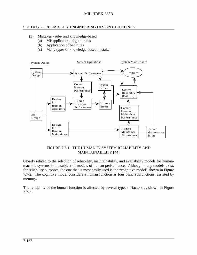
MIL-HDBK-338B


7-162

(3) Mistakes - rule- and knowledge-based(a) Misapplication of good rules(b) Application of bad rules(c) Many types of knowledge-based mistake

SystemDesign

System Performance Readiness

CorrectHumanPerformance

DesignforHumanOperators

JobDesign

DesignforHumanMaintainers

HumanOperatorPerformance

SystemErrors

HumanErrors

SystemReliability(Failures)

CorrectHumanMaintainerPerformance

HumanMaintainerPerformance

HumanMaintenanceErrors

System Design System Operations System Maintenance

FIGURE 7.7-1: THE HUMAN IN SYSTEM RELIABILITY ANDMAINTAINABILITY [44]

Closely related to the selection of reliability, maintainability, and availability models for human-machine systems is the subject of models of human performance. Although many models exist,for reliability purposes, the one that is most easily used is the “cognitive model” shown in Figure7.7-2. The cognitive model considers a human function as four basic subfunctions, assisted bymemory.

The reliability of the human function is affected by several types of factors as shown in Figure7.7-3.

MIL-HDBK-338B


7-163

Memory

SensingInformationProcessing

Decision Response

Examples: Radar operator, electric power monitor

FIGURE 7.7-2: THE COGNITIVE HUMAN MODEL

PerformanceShapingFactors

OperatingEnvironments

HumanAbilities

ExternallyImposedFactors

Time Durationand Fatigue

FIGURE 7.7-3: FACTORS THAT AFFECT HUMAN FUNCTION RELIABILITY

Of the factors shown in Figure 7.7-3, operating environments are, perhaps the easiest tounderstand. Some of the more commonly known environmental factors or combinations offactors are:

(1) Temperature-humidity(2) Pressure-oxygen concentration(3) Longitudinal and transverse vibration(4) Ambient noise

MIL-HDBK-338B


7-164

For each of these, there is a region where human performance is not degraded, a region wherehuman performance ceases, and a region of transition between the previous two (see Figure7.7-4). Sources such as MIL-STD-1472E, “Human Engineering Design Criteria for MilitarySystems, Equipment, and Facilities” provide this information Although specific reliability datahave not been published for these regions, inferences can be made regarding the impact on thehuman performance reliability. In the case of ambient noise, message complexity, vocabularycontent, distance between speaker and listener, and background noise levels and frequenciesaffect human performance reliability.

Human abilities pertain to the ability of the human to detect input signals, analyze their meaning,make decisions, and then perform the proper response. Typically, inputs consist of visual, sound,or touch-related signals. There are minimum levels for the detectability of each and levels atwhich damage is done to the human. There also are transition zones from the threshold ofdetection to physical damage.

0 2 4 6

Longitudinal Acceleration (rms) (m/sec2)

0

100

200

300

400

DegradingHuman

Performance

50 HzDanger Zone

UnaffectedPerformance

50 Hz

Un

imp

aire

d P

erfo

rman

ceD

ura

tion

(in

min

ute

s)

8

FIGURE 7.7-4: ZONES OF HUMAN PERFORMANCE FOR LONGITUDINALVIBRATION (ADAPTED FROM MIL-STD-1472)

Externally imposed factors consist of workplace layout, assignments, group interactions andsimilar factors. Specific, reliability oriented data for these have not been tabulated, althoughstudies have suggested changes in performance due to these factors.

Time duration and fatigue are important factors that frequently are neglected. For most tasks,performing 30 minutes without a break is the recommended limit because longer durations result

MIL-HDBK-338B


7-165

in degradation of human performance. Also, there must be a balance between the allowed timeto perform a task and the actual time to perform the task, otherwise human errors will occur.

Much of the system development process depends on quantitative measures. Consequently, forhuman-machine systems, it is necessary to define a set of parameters that includes the human aswell as the hardware. Fortunately, it is possible to construct a set of analogues to conventionalreliability, maintainability, and availability measures [46]. Two examples follow.

Human Performance Reliability =

No. Human Task SuccessNo. Human Task Attempt

Human Availability = 1 -

Unmanned Station HoursTotal Hours

These parameters can be used in simulations and can be used in probability compounding modelsas well. Like all reliability and maintainability parameters, they should not be construed as endsin themselves but rather vehicles for obtaining good system designs.

7.7.3 Allocating System Reliability to Human Elements

The allocation of reliability and maintainability requirements is the first step in the man-machinesystem development process beyond the receipt of the customer requirements. This sectiondiscusses qualitative allocation and two forms of quantitative allocation: an application of theAGREE method and dynamic programming. Qualitative allocation pertains to the earliest stagesof system functional analysis and the evaluation of potential design solutions. Although, inpractice, quantitative allocation rarely is performed, the consequence of not performing aquantitative allocation is the inadequate design of human tasks and an increase in the likelihoodof human error - in some cases to very significant and dangerous levels.

7.7.3.1 Qualitative Allocation

One of the early stages of system engineering is the identification and non-quantitative allocationof system functions. This step commonly is known as "functional analysis." "Functions" arediscrete actions for the attainment of specific objectives. Generally, the products of functionalanalysis are functional flow diagrams that are structured in a hierarchical manner [47]. A simpleexample is shown in Figure 7.7-5.

MIL-HDBK-338B


7-166

SYSTEM

Sensor

Processor

Human

Dish Base

Computer

MonitorKeyboard

Human Model(e.g. Cognitive)

FIGURE 7.7-5: HIERARCHICAL STRUCTURE OF FUNCTIONAL ANALYSIS(EXAMPLE)

At an appropriate level in the functional analysis, it must be decided whether a function will beperformed by human or machine. This can be a relatively high level, e.g. first tier, or at a detailedlevel such as the third or lower tier. For man-machine systems, the functional analysis caninclude operation and maintenance functions presented as separate flows or as a combined flow.Examples are given in reference [47].

Qualitative allocation is simply the selection of which functions are best performed by the humanand which are best performed by the machine. Table 7.7-2 identifies the functions at whichhumans and machines excel. In general, the human is better at handling a variety of differentinformation-processing tasks, adapting to new tasks and environments, devising new procedures,and resolving unexpected contingencies. The greatest limitations of the human are the rate ofdata processing and the amount of immediate retention.

MIL-HDBK-338B


7-167

TABLE 7.7-2: HUMAN-MACHINE COMPARATIVE CAPABILITIES

HUMAN SUPERIORITY MACHINE SUPERIORITY1. Originality (ability to arrive at new, different

problem solutions)1. Precise, repetitive operations

2. Reprogramming rapidly (as in acquiring newprocedures)

2. Reacting with minimum lag (in microseconds,not milliseconds)

3. Recognizing certain types of impendingfailures quickly (by sensing changes inmechanical and acoustic vibrations)

3. Storing and recalling large amounts of data

4. Detecting signals (as radar scope returns) inhigh-noise environments

4. Being sensitive to stimuli (machines senseenergy in bands beyond human’s sensitivityspectrum)

5. Performing and operating though task-overloaded

5. Monitoring functions (even under stressconditions)

6. Providing a logical description of events (toamplify, clarify, negate other data)

6. Exerting large amounts of force

7. Reasoning inductively (in diagnosing a generalcondition from specific symptoms)

7. Reasoning deductively (in identifying aspecific item as belonging to a larger class)

8. Handling unexpected occurrences (as inevaluating alternate risks and selecting theoptimal alternate or corrective action)

___

9. Utilizing equipment beyond its limits asnecessary (i.e. advantageously usingequipment factors for safety)

___

From An Introduction to the Assurance of Human Performance in Space Systems, SP-6506, NASA, 1968.

7.7.3.2 Quantitative Allocation

The first of the quantitative methods, and the simplest, for allocating man-machine reliability isan adaptation of the AGREE allocation method. This method, described in Reference [48], wasdeveloped for electronic equipments and was based on unit complexity and importance.

Unit complexity is described in terms of modules, where a module is a single functional unit.Unit importance is defined as the probability that the system will fall if the unit fails. Aimportance value of one implies that the unit is essential for successful system operation. A valueof zero means that the unit has no impact on system performance.

The AGREE allocation is expressed in terms of allocated reliability R(tj).

R(

jt ) = 1 -1- [ *R (T) nj /N]

jEwhere:

R*(T) = system reliability requirementnj = number of modules in unit j,Ej = importance factor of unit j,tj = number of hours unit j will be required to operate in T system hours

MIL-HDBK-338B


7-168

N = total number of modules in the system.

Although the AGREE report discusses the allocation for redundant situations, the quality of theapproximations for those cases is inadequate. Hence, serial system configurations should beconsidered the primary application of the AGREE allocation method.

To apply the AGREE method to man-machine systems, the system must be broken down intodiscrete functions and be depicted in a serial reliability block manner. The first order assignmentof functions to man or machine can be made using the qualitative approach described in Section7.7.3.1. In a similar manner to the machine portions, the human functions must be decomposedinto discrete elements, e.g. the portions of the cognitive model. These elements determinefunction complexity. Function operating hours and importance then are determined. Anexample of a non-unity importance factor that is applicable to a man or a machine in a target (ormalfunction) detection function might be that if the man or machine fails to perform properly,25% of the targets (or malfunctions) may be lost. Hence Ej would be 0.25. The allocationformulas are used to determine the allocated failure rate or reliability as required.

In most practical situations, the problem is to design a man-machine system with the highestachievable reliability subject to practical considerations such as competing mission requirements,limitations on personnel, and limitations on cost. In an analytic sense, the problem is representedas a function (reliability) to be maximized subject to a set of constraints. Allocations withassigned constraints generally are solvable by means of dynamic programming because theybecome very complicated very quickly.

Dynamic programming is a mathematical technique for optimizing a sequence of decisions bybreaking the sequence into a sequence of simpler problems. For each simpler problem, or stage,an optimal feasible solution is determined. The selected set of solutions is the optimal solutionfor the entire problem. It is used frequently in capital allocation and transportation problems.Blanchard and Fabricky [49] and Taha [50] have excellent treatments of the subject.

Mission reliability and operational readiness are common parameters for optimization. Otherparameters could be used. For example, availability may be used in place of operationalreadiness depending on the planned use of the system. Bazovski [51] provided an excellentdiscussion for distinguishing between readiness and availability. The parameters provide a directlink between high level effectiveness requirements and component oriented design parameterssuch as MTBF, MTTR, and both numbers and skill levels of personnel.

To apply mission reliability and operational readiness to the allocation process, first identifycritical functions and their reliability and maintainability design parameters and use theparameters to write expressions for the mission reliability and operational readiness of theman-machine system. One mission reliability constraint and one operational readiness equationmust be written for each mission.

MIL-HDBK-338B


7-169

Cost and personnel constraints must also be constructed. Personnel can be specified in manyways. The most convenient way is to specify numbers of men at a discrete skill level.Acquisition cost, support cost and life cycle cost can all be used as constraints. Regardless of thetype of cost selected, the system cost must be defined in terms of human and hardwarecontributions and in terms of basic design parameters.

Example

A multi-mission equipment in which each mission, i, has a probability pi of being required. Thereliability function associated with each mission is ri. The r functions are constructed to includethe human element. For example, an operational sequence diagram, which is roughly equivalentto a reliability block diagram, can be merged with a functional reliability block diagram toprovide a mission reliability function. Human functions are constructed in terms of reliability andmaintainability parameters.

With the above preparation, the allocation problem can be written as the following optimizationproblem:

Maximize Rop (operational reliability):

Rop =

i=1

n

∑ piri

subject to:

Rm Pm

Pm ≥ Xm

N v≤C c≤

where:Rm = mission reliabilityP = availabilityN = number of personnelC = costm = a specific mission

There will be one set of constraint equations for each mission. This leads to exactly the form ofoptimization problem that is solved by dynamic programming. A simplified flow of dynamicprogramming is shown in Figure 7.7-6.

7.7.4 Sources of Human Performance Reliability Data

One of the major issues in man-machine reliability is the location and availability of humanperformance reliability data. The tabulated data take the form of time measurements, including

MIL-HDBK-338B


7-170

reaction time and task performance time, error and error frequency data. The most commonlyused data are error data. Task performance data play an important role where task performancewithin a specified time is a criterion for mission success: e.g., restoration of full power within 30minutes. Most of the data come from controlled laboratory studies; an increasing amount comefrom simulators; very little come from field use. The laboratory data have the liability of beingderived from artificial situations that do not represent the real world. Consequently, althoughthey have the requisite degree of precision, they have limited utility. Simulator data are betterbecause they represent the real world more accurately, especially as simulators improve.However, they are collected generally for special applications and, hence, have limitedapplication. Laboratory and simulator data vary from what would be expected in the real worldbecause of the subjects’ awareness that they are being tested. The most realistic data, field data,generally are not collected in a systematic way. Consequently, the physical and psychologicalenvironment in which the data were generated usually are not recorded or analyzed.

WithinConstraints

No

SelectParameters

ImprovedSolution?

ComputeObjectiveFunction

OptimizedSolution

SelectInitial

Parameters

Yes

Yes

No

FIGURE 7.7-6: SIMPLIFIED DYNAMIC PROGRAMMING

An alternative to the use of "hard data" is the use of expert opinion. Techniques such as Delphimethods or paired comparison are used. The primary use of expert opinion occurs when hard dataare modified special situations.

Early data sources consisted primarily of human factors data collections; e.g. Human EngineeringGuide to Equipment Design [52], MIL-STD-1472E, “Human Engineering Design Criteria forMilitary System, Equipment, and Facilities.” More recent data sources are the following:“Handbook Of Perception and Human Performance” [53], “Engineering Data Compendium:

MIL-HDBK-338B


7-171

Human Perception and Performance” [54], the Compendium on a compact disc, and the CrewSystem Ergonomics Information Analysis Center.

The second vehicle for obtaining human performance reliability data is the "data bank." Table7.7-3 shows the current major data banks [55]. Table 7.7-4 summarizes the data incorporatedinto each of the data banks.

Other sources of human performance reliability are described by references [56] and [57]. Moredetailed descriptions of many of the data sources and data banks described herein are given byBooher [55].

TABLE 7.7-3: DATA BANKS AND THEIR AFFILIATIONS [55]

DATA BANK ORGANIZATIONMICRO Human Performance Evaluation System (HPES) Nuclear Power

Nuclear Computerized Library for Assessing ReactorReliability (NUCLARR)

Nuclear Power

Crew Station Ergonomics Information Analysis Center(CSERIAC)

Department of Defense

MACRO Training and Performance Data Center (TPDC) Department of DefenseMateriel Readiness Support Activity (MRSA)MANPRINT Data Base

Department of the Army

Project "A" Data Base Department of the Army

MIL-HDBK-338B


7-172

TABLE 7.7-4: DATA CATEGORIES OF NATIONAL DATA BANKS [55]

Data Categories HPES NUCLARR CSERIAC TPDC MRSAMANPRINT

PROJECT"A"

Human Performance X X X X XHuman Performance(Error)

X X X

Hardware Reliability X XHuman FactorsEngineering

X

Manpower X X XPersonnel X X X XTraining X X XSystem Safety X XHealth Hazards X X

There is a recognized need for a human performance data bank that applies to both the militaryand commercial sectors. Until a broadly supported effort such as this is implemented, there willbe both considerable subjectivity and many limitations in the use of available humanperformance reliability data.

7.7.5 Tools for Designing Man-Machine Systems

This section explores the various tools that are used to design reliable man-machine systems.The tools are many and varied in their approaches. An overview of them is provided by Figure7.7-7.

Computer-BasedDesign Tools

General DesignTools

TaskAnalysis

Design Tools

Graphics-Based

Analytical

Parameter-Based

Human-InterfaceLayout

Work SpaceLayout

FIGURE 7.7-7: TOOLS FOR DESIGNING HUMAN-MACHINE SYSTEMS

MIL-HDBK-338B


7-173

7.7.5.1 Task Analysis

Task analysis is a critical part of a human factors program. However, it is usually not done aspart of reliability program. Maintenance task analysis is usually done in a maintainabilityprogram. Task analysis focuses on the following:

(1) Input information to human(2) Evaluation processes(3) Action to be taken(4) Environments and constraints(5) Tools and job aids(6) Manpower(7) Communications

7.7.5.2 General Design Tools

There are many general design tools that apply to the design of human-machine interfaces. Oneof the most useful is the Operational Sequence Diagram (OSD). The features of the OSD are:

(1) Shows all participants(2) Displays functional flow - all functions(3) Represents types of operations with standard symbols(4) Represents approximate time line(5) Employs rules for representing flows(6) Represents a certain level of system or process indenture

Goal, success, and fault trees are other useful tools. The general format of these is shown inFigure 7.7-8. Operator action trees and event trees are horizontally-oriented trees that showpossible branches in action and the consequences. The Failure Mode, Effects, and CriticalityAnalysis can be adapted for use in the analysis of human-machine reliability by incorporatinghuman error modes and evaluating their consequences.

The treatment of the role of traditional human factors is brief. The brevity should not beconstrued as a reflection of the importance of the subject. Many excellent volumes, some ofwhich are referenced, have been written on the subject and any attempt to replicate even portionsof them here would serve little purpose. Human factors provides many of the basic designdisciplines that enable reliable systems to be designed. Too often, this fact is not appreciated andthe human factors experts are given a secondary priority in system development (unless safety isa critical factor). Human factors experts need to be involved in the earliest stages of systemdevelopment, especially in the function allocations. The role of human factors in theachievement of system reliability often is clouded by the lack of sensitivity to the human byreliability engineers. The key to understanding that role is the recognition that functionally,human behavior can be modeled as stimulus-input chain: internal-response: output- response.Complex behavior is a combination of many of these chains. Human errors occur when:

MIL-HDBK-338B


7-174

(1) A physical change in the environment is not perceived as a stimulus.

(2) Several stimuli cannot be discriminated by an operator.

(3) A stimulus is perceived, but its meaning is not understood.

(4) The stimulus is correctly understood, but the correct output-response is unknown.

(5) The correct output-response is known, but it is beyond the operator’s physicalcapabilities.

(6) The correct output-response is within the operator’s capabilities, but the response isperformed incorrectly or out of sequence.

The implications for equipment design are: in order for an operator to respond adequately, thestimulus must be perceivable and it must demand a response which the operator is capable ofproducing. Hence equipment and task characteristics must be tailored to the capabilities andlimitations of the operator. To accomplish this, the design of equipment must take into accountlimitations on body size, body weight, and reaction times to environmental stimuli. The operatormust receive some verification or feedback from his actions.

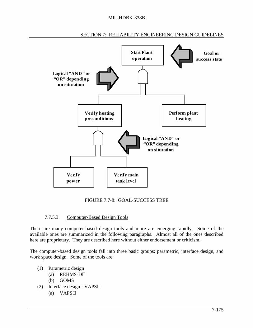
MIL-HDBK-338B


7-175

Start Plantoperation

Verify heatingpreconditions

Perform plantheating

Logical “AND” or“OR” depending

on situtation

Logical “AND” or“OR” depending

on situtation

Goal orsuccess state

Verifypower

Verify maintank level

FIGURE 7.7-8: GOAL-SUCCESS TREE

7.7.5.3 Computer-Based Design Tools

There are many computer-based design tools and more are emerging rapidly. Some of theavailable ones are summarized in the following paragraphs. Almost all of the ones describedhere are proprietary. They are described here without either endorsement or criticism.

The computer-based design tools fall into three basic groups: parametric, interface design, andwork space design. Some of the tools are:

(1) Parametric design(a) REHMS-D(b) GOMS

(2) Interface design - VAPS(a) VAPS

MIL-HDBK-338B


7-176

(b) Computer Interface Toolkits (e.g. Visual Basic)(3) Work space design

(a) SAMMIE(b) CREW CHIEF(c) JACK(d) SAFEWORK

7.7.5.3.1 Parametric Design Tools

REHMS-D uses reliability as a metric for selection of human interface and task parameters. Itincludes two levels of parameter sensitivity analysis, provides on-line help and safety warnings,and derives plans for testing human interfaces. REHMS-D is based on the cognitive model andoffers options for configuring inputs to the human and responses by the human. It addresses theeffects of the following environmental factors: illumination, atmospheric conditions,temperature-humidity, pressure-oxygen, ambient noise, and vibration. GOMS develops fouraspects of human tasks: goals, operators, methods, and selection. The "goals" are a user definedset of things to do or obtain to achieve a task. The "operators" are the actions available toachieve the goals. The methods are the sequence of operations and subgoals for achieving thetask - the "how to." Finally, the "selection" is a means for choosing a method when more thanone method applies - usually rule-based. GOMS uses time-to-perform for its metric.

7.7.5.3.2 Interface Design Tools

VAPS is a work station-based tools that draws objects, specifies data-driven animation, connectsobjects to application data and specifies response behavior, and communicates with externalsources to interact.

7.7.5.3.3 Work Space Design Tools

CREW CHIEF is a 3-dimensional modeling system developed by the US Air Force HumanResources Laboratory, Wright-Patterson AFB, OH. It is oriented toward the computer graphicsimulation of an aircraft maintenance technician and interfaces readily with existing commercialCAD systems. CREW CHIEF reduces the incidence of design problems by allowing thedesigner to perform maintainability analyses and correct design defects while the system is in theearly design stage. It does this by providing a 3-dimensional modeling system that creates acomputerized man-model.

SAMMIE (System for Aiding Man/Machine Interaction Evaluation) is a human factors, 3-Ddesign system that includes a sophisticated, computerized man-model with built-in reach andsight capabilities. The man-model is constructed from logically related links or joint. Virtuallyany size or shape person can be represented through specific dimensional changes or statisticalprofiles of population groups.

MIL-HDBK-338B


7-177

SAFEWORK creates virtual humans of various percentiles. It contains access to populationstatistics. SAFEWORK mannequin movement includes fully articulated hand and spine models,virtual viewing, collision detection, and scene animation.

JACK includes 3D interactive environment for controlling articulated figures, a detailed humanmodel, realistic behavior controls, anthropomorphic scaling, task animation and evaluation, viewanalysis, automatic reach and grasp, and collision detection and avoidance.

Design Evaluation for Personnel, Training, and Human Factors (DEPTH) analyzes maintenanceactivity using Transom Technologies Transom Jack human models; controls human modelmovements through standard mouse, body tracking equipment, or automatic simulation; handlesa variety of populations, dress modes, and tools; and reports on accessibility, visibility, andstrength.

7.7.6 Reliability Prediction for Human-Machine Systems

A great majority of the work published on human reliability has been concerned with humanperformance reliability prediction. Earlier work focused on probability compounding techniques.Some of these were linked with available data sources (never in really great abundance); othercompounding techniques used specially collected data. With the proliferation of computers,digital simulation models were developed and used. More recently, stochastic models have beenproposed. An excellent comparison of prediction techniques is given in reference [58]. Figure7.7-9 shows the categories of the many human performance reliability prediction techniques thathave been published.

PredictionMethods

ProbabilityCompounding

DigitalSimulation

StochasticModels

ExpertJudgement

FIGURE 7.7-9: CATEGORIES OF HUMAN PERFORMANCE RELIABILITYPREDICTION METHODS

MIL-HDBK-338B


7-178

Although there are a great many models for prediction - over 20 years worth of work - there is noconsensus on human reliability prediction technology or a human reliability parameter database[59]. Dougherty [60] noted much the same situation. His expectation is that there will be arecognition that there is a need for a second generation of human reliability models.

Swain [61] notes the following inadequacies in human reliability analysis:

(1) Inadequate data

(2) Stop-gap models and expert judgment are used in place of "hard" data

(3) Lack of agreement on expert judgment methods

(4) Inadequate calibration of simulator data

(5) Inadequate proof of accuracy in human reliability analyses

Increased use of higher mental functions is required by inadequate design of displays, controls,and their interactions.

The emphasis here is on the lack of data to support the human reliability analysis rather than themethodology itself. Swain does identify inadequate implementation of human factors disciplinesas a root cause of the lack of data on favorable human performance situations.

7.7.6.1 Probability Compounding

There are a considerable number of probability compounding models for estimating humanperformance reliability in man-machine systems. Meister [40] provides excellent summaries ofthem. Selected techniques are summarized below.

Technique for Human Error Rate Prediction (THERP) [62], [63] has been the best known andmost frequently applied technique for human reliability prediction. It is a method for predictinghuman error rates and for evaluating the degradation to a man-machine system likely to becaused by human errors in association with factors such as equipment reliability, procedures, andother factors. The THERP technique has been influenced strongly by hardware reliabilitytechniques.

THERP involves five steps:

(1) Define the system or subsystem failure which is to be evaluated. This involvesdescribing the system goals and functions and the consequences of not achieving them.It also requires identifying mission, personnel, and hardware/software characteristics.

MIL-HDBK-338B


7-179

(2) Identify and list all the human operations performed and their relationships to thesystem tasks and functions. This requires an analysis of all operator and maintainertasks.

(3) Predict error rates for each human operation or group of operations. Errors likely to bemade in each task or subtask must be identified. Errors that are not important in termsof system operation are ignored. This step includes estimating the likelihood of eacherror occurring and the likelihood of an error not being detected.

(4) Determine the effect of human errors on the system, including the consequences of theerror not being detected. This requires the development of event trees. The left limbsof the event trees are success paths; the right limbs are failure paths. Probabilities areassigned to each path. The tree reflects the effects of task dependence. The relativeeffects of performance-shaping factors, e.g. stress and experience, are estimated.

(5) Recommend changes as necessary to reduce the system or subsystem failure rate as aconsequence of the estimated effects of the recommended changes. Therecommendations can be developed through the use of sensitivity analyses, in whichfactors and values are varied and effects monitored. THERP makes no assumptionsabout the dependence or independence of personnel behaviors. The data are taken fromavailable sources.

One of the key aspects of THERP is the determination of the probability that an error or class oferrors will result in a system failure. This probability is assigned a value Fi. Branching trees areconstructed to determine the paths to system success and failure (Figure 7.7-10). The probabilitythat an error will occur is given by Pi. FiPi is the joint probability that an error will occur and thatthe error will lead to system failure. 1-FiPi is the probability that an operation will be performedwhich does not lead to system failure. The probability that a class of errors will lead to systemfailure is given by:

Qi = 1 − FiPi( )n i

where ni is the number of independent operations. The total system or subsystem failure rate isgiven by:

QT = 1−

k=1

n

∏ 1 − Qk( )

where QT is the probability that one or more failure conditions will result from errors in at leastone of the n failure classes.

MIL-HDBK-338B


7-180

FIGURE 7.7-10: THERP PROBABILITY TREE [62]

THERP can be used for design analysis, manpower selection, prediction of system effectiveness,and determination of training requirements. For design analysis, it allows the comparison ofalternative system configurations in terms of effect on operator capability. It also allowscomparative analysis of initial system configuration options and reconfiguration if deficienciesare identified. For manpower selection, THERP allows the determination of the types, numbers,and skill levels of the personnel required to operate the system. For system effectiveness,THERP allows an assessment of whether quantitative requirements will be met. Thedetermination of training requirements is more implicit than explicit. Unacceptable taskperformance error rates suggest the need for training to improve proficiency. Hence, THERP cansuggest the need for training rather than specific training topics.

THERP can be applied to all types of equipments, tasks, and behaviors. With the aid of standardhuman engineering techniques, it can be used for design analysis. Finally, THERP can beapplied to the early stages of system design as well as the later stages.

Constraints on its application are that it is applicable to situations where discrete taskdescriptions can be developed, error probability data must be available, the effects ofperformance-shaping factors must be known, and that time must be available to analyze andcategorize all potential errors in a task. THERP is regarded as the standard tool for estimatinghuman error probabilities in routine tasks. It uses performance shaping factors (PSFs) to makejudgments about particular situations. However, experience has shown that in some cases, it wasdifficult to accommodate all of the PSFs that were considered important [64]. In many cases,THERP gave lower error probabilities than other methods. One evaluation of THERP [65] notesthat THERP has the advantage of simplicity but does not account for the influence of time.Fragola [38] describes extensions to THERP, particularly with respect to nuclear powerapplications. Another evaluation [66] notes that when applied to severe accident applications,several problems were noted. In this case, the task information provided in NRC data formstypically is more detailed than required by THERP. Matching the NRC task data to THERP

MIL-HDBK-338B


7-181

operator actions was found to be subjective and a source of error. Also the THERP error datareceived criticism with respect to its being an adaptation of non-nuclear data to nuclearapplications. Krois et. al. note that other data bases are available to be used in THERP andobviate this last criticism.

Dougherty and Fragola [38] have introduced the time-reliability correlation (TRC) system. Thisapproach uses simulator training results to create a family of time-reliability correlations, whichare adjusted with either the Success Likelihood Index or other expert judgment methods toaccount for special conditions. TRC is the relationship between human performance reliabilityand time. Data from simulators suggest that the lognormal distribution is sufficient for modelingTRCs. Interpolation between the s-confidence bounds can be accomplished through the use of aSuccess Likelihood Index (SLI). The SLI is derived in the following manner:

(1) Choose the influences appropriate to the event and the situation.

(2) Rank the influences as multiples of the least important for a given situation, which is setat "10."

(3) Sum the rankings of all influences and normalize the rankings to this sum.

(4) Assess the impact of each influence from best (1) to worst (10).

(5) Compute the "dot product" of the ranking and the quality vectors. This is the SLI.

(6) Apply the SLI. Mathematically, the SLI is expressed by:

SLI = 1

N

∑ riR

qi

where:

R = 1

N

∑ ri

and ri is the rank of the influence i and qi is the quality of the influence i.

Dougherty and Fragola focus on a lognormal TRC based on simulator data. This is inconsonance with the modified Human Cognitive Reliability.

Human Cognitive Reliability (HCR) was developed by Hannaman et al. [67] for calculating theoperator probability of non-response to a cognitive processing task as a function of time. Thetype of cognitive processing may be rule based, skill based, or knowledge based. For task j, theprobability of non-response P(t) is given by:

MIL-HDBK-338B


7-182

P(t) = exp-(Xj)bj

where:

Xj =

(t/Tmed) − Cgj

Cnj

and Tmed = median time to perform the task corrected by a shaping factor Kj

bj = shape parameter

Cgj = time delay factor as a fraction of Tmed for type j cognitive processing

Cnj = scale parameter as a fraction of Tmed for type j cognitive processing

The dependency between tasks was not considered. The model was derived from a threeparameter Weibull distribution. The model was used to develop normalized curvescorresponding to rule based, skill based, and knowledge based cognitive processing. In applyingthe HCR approach to operator task analysis, a table records the following for each subtask:

(1) Dominant human behavior(2) Stress level(3) Operator experience(4) Quality of operator/system interface(5) Median time assumed

The HCR approach has been modified [68] to use the log-normal distribution instead of theWeibull. The modified approach has the acronym HCR/ORE and is supported by simulator data.Guassardo [65] notes that the HCR must be used carefully because variations in applications canlead to very different results. The model does allow some accounting for time effects on errorprobability but is complicated by the fact that the correlation only can be used once whensubtasks have the same influence parameters. In this case, there is an ambiguity regardingwhether or not to cluster subtasks or to convolve individual subtask correlations. Whenexamining consistency among teams using HCR, Poucet [64] noted that the results have greatervariability than THERP methods. The method was very sensitive to assumptions about mediantime and the behavior type of the action Very good median response time data must be availablein order to apply HCR. Poucet also notes that some of the teams in his comparative studycombined the use of THERP and HCR. THERP was used for manual or routine tasks; HCR wasused for cognitive tasks.

MIL-HDBK-338B


7-183

7.7.6.2 Stochastic Models

This approach to modeling the impact of the human in man-machine systems employs Markovmodels to analyze parallel, k-of-n, and standby redundant configurations with human errors andcommon failures. The human error is defined as a failure to perform a prescribed task (or theperformance of a prohibited action), which could result in damage to equipment and property ordisruption of scheduled operations. The errors are categorized as being "critical" or "non-critical." A critical error causes system failure. Common cause failures are cases where multipleunits fail due to a single cause.

Five models are described by Dhillon [69] [70]. Each addresses a different redundantconfiguration. The models assume that:

(1) Units fail independently

(2) Failure rates for hardware, human error, and common cause failures are constant

(3) Repair rates are constant

(4) A repaired system is as good as new

(5) Switchover mechanisms are perfect for standby configurations

(6) System units are statistically identical

The first model represents a two independent and identical unit parallel system, which can failbecause of human error or hardware failure. A Markov model is constructed and an expressionfor system availability A and mean-time-to-repair (MTTR) is obtained. An expression for mean-time-to-failure (MTTF) also is derived. All the expressions are complicated functions of thestate transition probabilities (failure rates, error rates, and repair rates).

The second model is a special case of the first when the non-critical human error rate is zero.The non-critical human errors are omitted from the system transition diagram, which becomesmuch simplified. Expressions are derived for A, MTTR, MTTF, and variance of time to failure(TTF).

The third model represents a 2-out-of-3 unit system with critical human errors and commoncause failures. All system units are identical. A system reliability function and an expression forMTTF are derived. It is noted that repair helps to increase MTTF and human errors decrease it,as expected.

The fourth model is a 3-out-of-four system with critical human errors and common causefailures. MTTF and TTF variance expressions are derived.

MIL-HDBK-338B


7-184

The fifth model represents a standby system with critical human errors and common causefailures. Again, MTTF and TTF variance are calculated.

7.7.6.3 Digital Simulation

Digital simulation provides an inexpensive means for evaluating the impact of operator andmaintainer performance in man-machine systems without the cost or complexity of physicalexperiments. It allows for the identification of problem areas before the actual system has beenconstructed. It can provide the answers to the following questions [71]:

(1) What are the quantitative personnel requirements?

(2) What are the qualitative personnel requirements? Where, during the system utilization,are the operators most overloaded? Underloaded?

(3) How will cross-training improve system effectiveness?

(4) Are the system operators able to complete all of their required tasks within the timeallotted?

(5) Where in the task sequence are operators or teams likely to fail most often? Leastoften?

(6) In which states of the system is the human subsystem and its components least reliableand why?

(7) How will task restructuring or task allocation affect system effectiveness?

(8) How much will performance degrade when the systems operators are fatigued orstressed?

(9) How will various environmental factors (e.g. heat, light, terrain) affect total man-machine system performance?

(10) To what extent will system effectiveness improve or degrade if more or less proficientoperators are assigned?

(11) How do group factors such as morale and cohesion affect system performance?

Simulations can be used in the conceptual as well as developmental stages of system evolution.They provide vehicles for tradeoff analyses.

MIL-HDBK-338B


7-185

At the time this section was written, the Maintenance Personnel Performance Simulation(MAPPS) [72] is the only supported member of the family of Siegel-Wolf simulation models.The basic features of the model are shown in Table 7.7-5.

TABLE 7.7-5: MAPPS SCOPE

FEATURE MODEL LIMITMaximum number of tasks 200Number of maintainers 2-8Types of maintainers 5Number of subtasks 100Types of subtasks 28Maximum task duration (days) 2Number of shifts 1-10Protective clothing types 3Types of ability 2

The model establishes a team of up to eight members who begin a maintenance task at time t=0under a set of initial conditions established by the user. For each maintenance task, subtasks areidentified with data and shift termination information. Subtasks may be repeated because ofinadequate performance, group decisions and looping back. MAPPS selects the maintainers tobe assigned to each task or subtask and then processes the input data and current system statedata to arrive at estimates of task performance. MAPPS is written in FORTRAN IV H(Enhanced) for the IBM 3033 system. MAPPS output can be characterized in terms of type ofinformation and degree of detail. Output can be provided by subtask(the most detailed), byiteration, and by run. For a subtask, the model will provide results such as: degree of success;probability of success; start and end times; duration; time and communication stresses; effects ofaccessibility, fatigue and heat; and required ability.

The Cognitive Environment Simulation (CES) [73] is an artificial intelligence approach thatsimulates predictions about operator action by simulating the processes by which intentions areformed. It enables the analyst to represent of state of knowledge regarding a particular situationand then observe the consequences in terms of human intended actions. It is an application of theproprietary EAGOL artificial intelligence problem solving system developed by Seer Systems.EAGOL has the ability to reason in multiple fault situations and to reason in situations thatevolve over time. The specific CES application of EAGOL is for emergency situations innuclear power plants. Note that CES is not intended to be a "micro" view of human cognitiveprocessing. Applying CES consists of matching CES resources to those of the power plant understudy. Input data consists of a time series of plant state data that would be available to operatorpersonnel. The data are processed into a virtual display board which reports the status of theplant, recognizes undesirable situations, and generates proposed rectifications to those situations.The output is a series of intentions to act and resolve the undesirable situation. CES containsthree types of activities: monitoring, explanation building, and response management. The CESuser can vary the demands placed on CES and the resources available to solve problems. CES is

MIL-HDBK-338B


7-186

used in association with the Cognitive Reliability Assessment Technique (CREATE) for use inthe probabilistic risk analysis of nuclear power plants.

7.7.6.4 Expert Judgment Techniques

These are a collection of techniques that address the lack of "hard data" or firm interpretations ofdata through the use experts.

The Success-Likelihood Index Methodology (SLIM, SLIM-MAUD) [74] [75] examinesperformance shaping factors (PSFs) and establishes both ratings and weight for each PSF.SLIM-MAUD is a personal computer implementation of SLIM. The MAUD acronym refers to"Multi-Attribute Utility Decomposition." MAUD is a proprietary stand alone software packagethat aids the user in assessing alternatives. PSFs that can be considered are:

(1) Situational characteristics(2) Job and task instructions(3) Task characteristics(4) Equipment characteristics(5) Psychological stressors(6) Physiological stressors(7) Internal factors (training, experience, skill)

SLIM ranks the most important PSFs. The products of the rating and the normalized weight foreach task are added to obtain the SLI (described earlier). The SLI is related to the task successprobability through the following calibration equation:

lnP(success) = a*SLI + b

where a and b are empirical constants. Rosa et al. [76] notes that SLIM-MAUD requires thattasks be sorted into subsets of 4 to 10 tasks that are similarly affected by a proposed set of PSFs.The weighting and ranking of tasks is accomplished by a group of experts, usually four innumber, who are led by a facilitator. Analysis is conducted with the aid of the MAUDcomputer program.

Rosa et al. noted many positive characteristics of SLIM-MAUD, including face validity,practicality, estimates with acceptable levels of reliability, ease of use and understanding, andability to identify which PSFs have the most effect on the SLIs. Guassardo [65] notes that SLIMresults are highly dependent on the boundary conditions used to find the calibration equationcoefficients. Poucet [64] indicates that the SLIM results were highly dependent on thecalibration reference points. The use of SLIM is recommended only if good reference data areavailable. Poucet also notes that SLIM does not address relationships among PSFs when suchexist.

MIL-HDBK-338B


7-187

7.7.7 Verification of Human Performance Reliability

For human-machine systems, the purposes of verification testing can be described as follows[77].

(1) Demonstrate the conformance of the product to human engineering design criteria

(2) Confirm compliance with specific performance requirements

(3) Secure quantitative measures of human-machine performance characteristics that arefunctions of human-machine interaction

(4) Determine whether or not undesirable characteristics have been introduced

The demonstration of human performance reliability (in maintenance situations) may overlapwith maintainability demonstrations or testing. The same set of tasks may be considered but withdifferent criteria. For example, in a maintainability demonstration, the principle concern is thetime required to complete a task. If the same task is employed in a human performancereliability context, the important criteria are not only correct completion of the task but alsocompletion of the task within a time constraint. The references provide additional details onstructuring tests to estimate maintenance technician reliability.

For estimates of reliability in an operator type situation, data must be accumulated either by useof a simulator or by an expanded reliability demonstration that includes the operator as well asthe equipment. In either case, the data will resemble actual field results only to the extent thatthe test scenario and the performance of the test subjects resemble the actual field conditions.

7.8 Failure Mode and Effects Analysis (FMEA)

7.8.1 Introduction

Failure Mode and Effects Analysis is a reliability procedure which documents all possiblefailures in a system design within specified ground rules. It determines, by failure mode analysis,the effect of each failure on system operation and identifies single failure points, that are criticalto mission success or crew safety. It may also rank each failure according to the criticalitycategory of failure effect and probability occurrence. This procedure is the result of two steps:the Failure Mode and Effect Analysis (FMEA) and the Criticality Analysis (CA).

In performing the analysis, each failure studied is considered to be the only failure in the system,i.e., a single failure analysis. The FMEA can be accomplished without a CA, but a CA requiresthat the FMEA has previously identified critical failure modes for items in the system design.When both steps are done, the total process is called a Failure Mode, Effects and CriticalityAnalysis (FMECA). The procedures for performing both the FMEA and the CA are found inReference [78] and Reference [79]. At the time of this update Reference [78], MIL-STD-1629,

MIL-HDBK-338B


7-188

was scheduled to be cancelled and replaced by a non-government standard by June 1997.However, it is not known at this time what that new document will be.

FMEA utilizes inductive logic in a "bottoms up" approach. Beginning at the lowest level of thesystem hierarchy, (e.g., component part), and from a knowledge of the failure modes of each part,the analyst traces up through the system hierarchy to determine the effect that each failure modewill have on system performance. This differs from fault tree analysis (discussed in the nextsection) which utilizes deductive logic in a "top down" approach. In fault tree analysis, theanalyst assumes a system failure and traces down through the system hierarchy to determine theevent, or series of events, that could cause such a failure.

The FMEA provides:

(1) A method of selecting a design with a high probability of operational success and crewsafety.

(2) A documented method of uniform style for assessing failure modes and their effect onoperational success of the system.

(3) Early visibility of system interface problems.

(4) A list of possible failures which can be ranked according to their category of effect andprobability of occurrence.

(5) Identification of single failure points critical to mission success or to crew safety.

(6) Early criteria for test planning.

(7) Quantitative and uniformly formatted data input to the reliability prediction,assessment, and safety models.

(8) A basis for design and location of performance monitoring and fault sensing devicesand other built-in automatic test equipment.

(9) A tool which serves as an aid in the evaluation of proposed design, operational, orprocedural changes and their impact on mission success or crew safety.

Items (5) and (8) are the two most important functions performed by an FMEA.

The FMEA is normally accomplished before a reliability prediction is made to provide basicinformation. It should be initiated as an integral part of the early design process and should beperiodically updated to reflect design changes. Admittedly, during the early stages, one usuallydoes not have detailed knowledge of the component parts to be used in each equipment.However, one usually has knowledge of the "black boxes" which make up the system. Thus, at

MIL-HDBK-338B


7-189

this stage, an FMEA might start at the "black box" level and be expanded as more detailedknowledge becomes available. This analysis may also be used to provide a model for analyzingalready-built systems. An FMEA is a major consideration in design reviews.

The principles of FMEA are straightforward and easy to grasp. The practice of FMEA is tedious,time consuming and very profitable. It is best done in conjunction with Cause-Consequence andFault Tree Analysis. The bookkeeping aspects, namely, the keeping track of each item and itsplace in the hierarchy, are very important because mistakes are easily made.

The Cause-Consequence chart shows the logical relationships between causes (events which areanalyzed in no more detail) and consequences (events which are of concern only in themselves,not as they in turn affect other events). The chart usually is represented with consequences at thetop and causes at the bottom; and the words Top and Bottom have come into common use todescribe those portions of the chart. A Failure Modes and Effects Analysis (FMEA) deals largelywith the bottom part of the chart. A fault tree is a part of a Cause-Consequence chart. It consistsof only one consequence and all its associated branches. The Cause-Consequence chart iscreated by superimposing the separately created fault trees. The Cause-Consequence chart can beused to organize one’s knowledge about any set of causes and their consequences; its use is notlimited to hardware oriented systems.

The FMEA consists of two phases which provide a documented analysis for all criticalcomponents of a system. First, however, definitions of failure at the system, subsystem, andsometimes even part level must be established.

Phase 1 is performed in parallel with the start of detailed design and updated periodicallythroughout the development program as dictated by design changes. Phase 2 is performedbefore, or concurrent with, the release of detail drawings.

The Phase 1 analysis consists of the following steps:

(1) Constructing a symbolic logic block diagram, such as a reliability block diagram or aCause-Consequence chart.

(2) Performing a failure effect analysis, taking into account modes of failure such as:(a) Open circuits(b) Short circuits(c) Dielectric breakdowns(d) Wear(e) Part-parameter shifts

(3) Proper system and item identification.

(4) Preparation of a critical items list.

MIL-HDBK-338B


7-190

During Phase 2, the results of Phase 1 are revised and updated as required by design changes. Inaddition, all items in the system are analyzed to determine their criticality with respect to thesystem.

7.8.2 Phase 1

During this phase the following detailed steps are performed:

(1) A Symbolic Logic Block Diagram is constructed. This diagram is developed for theentire system to indicate the functional dependencies among the elements of the systemand to define and identify its subsystems. It is not a functional schematic or a signalflow diagram, but a model for use in the early analysis to point out weaknesses. Figures7.8-1 and 7.8-2 show typical symbolic logic diagrams. Figure 7.8-1 illustrates thefunctional dependency among the subsystems, sets, groups, and units that make up thesystem. Figure 7.8-2 illustrates the functional dependencies among assemblies,subassemblies, and parts that make up one of the units in Figure 7.8-1.

(2) A failure effect analysis is performed for each block in the symbolic logic blockdiagram, indicating the effect of each item failure on the performance of the next higherlevel on the block diagram. Table 7.8-1 shows a typical group of failure modes forvarious electronic and mechanical parts. The failure mode ratios are estimates andshould be revised on the basis of the user’s experience. However, they can be used as aguide in performing a detailed failure effect analysis.

MIL-HDBK-338B


7-191

S

10 20 30 40

50

11 21 31A

31B

01A 02 03 04

01B

01B1 01B2 01B3

INPUT FROMDIFFERENTSYSTEM

LEVEL

SYSTEM

SUBSYSTEM

SET

GROUP

UNIT

Notes:(1) The system depends on subsystems 10, 20, 30 and 40(2) Subsystem 10 depends on sets 11, 21, 31A, and 31B(3) Set 11 depends on groups 01A, 01B, 02, 03, and 04(4) Group 01B depends on units 01B1, 01B2, and 01B3(5) Sets 31A and 31B are redundant(6) Groups 01A and 01B are redundant(7) Subsystem 40 depends on subsystem 50(8) Set 21 depends upon an input from another system

FIGURE 7.8-1: TYPICAL SYSTEM SYMBOLIC LOGIC BLOCK DIAGRAM

MIL-HDBK-338B


7-192

1A1A1011A1A1021A1A1C11A1A1C21A1A1R11A1A1R21A1A1R3

FROM UNIT01B2

LEVEL

UNIT

ASSEMBLY

SUBASSEMBLY

01B1

1A1 1A2 1A3 1A5

1A4 1A6

1A1A1 1A1A2 1A2A1

Notes:

(1) Unit 01B1 depends on assemblies 1A1, 1A2 AND either ’1A3 and 1A5’ OR ’1A4 and 1A6’

(2) Assembly 1A1 depends on subassemblies 1A1A1 AND 1A1A2(3) Assembly 1A2 depends on subassembly 1A2A1(4) Subassembly 1A1A1 depends on all parts contained therein

FIGURE 7.8-2: TYPICAL UNIT SYMBOLIC LOGIC BLOCK DIAGRAM

MIL-HDBK-338B


7-193

TABLE 7.8-1: FAILURE MODE DISTRIBUTION OF PARTS6

DEVICE TYPE FAILURE MODE MODE PROBABILITY (α)Accumulator Leaking

SeizedWornContaminated

.47

.23

.20

.10Actuator Spurious Position Change

BindingLeakingSeized

.36

.27

.22

.15Alarm False Indication

Failure to OperateSpurious OperationDegraded Alarm

.48

.29

.18

.05Antenna No Transmission

Signal LeakageSpurious Transmission

.54

.21

.25Battery, Lithium Degraded Output

Startup DelayShortOpen

.78

.14

.06

.02Battery, Lead Acid Degraded Output

ShortIntermittent Output

.70

.20

.10Battery, Ni-Cd Degraded Output

No Output.72.28

Bearing Binding/StickingExcessive PlayContaminated

.50

.43

.07Belt Excessive Wear

Broken.75.25

Brake Excessive WearLeakingScoredCorrodedLoose

.56

.23

.11

.05

.05Bushing Excessive Wear

LooseCracked

.85

.11

.04Cable Short

Excessive WearOpen

.45

.36

.19Capacitor, Aluminum,

ElectrolyticShortOpenElectrolyte LeakDecrease in Capacitance

.53

.35

.10

.02

6 Reliability Analysis Center, "Failure Mode/Mechanism Distributions" (FMD-91)

MIL-HDBK-338B


7-194

TABLE 7.8-1: FAILURE MODE DISTRIBUTION OF PARTS (CONT’D)

DEVICE TYPE FAILURE MODE MODE PROBABILITY (α)Capacitor, Ceramic Short

Change in ValueOpen

.49

.29

.22Capacitor, Mica/Glass Short

Change in ValueOpen

.72

.15

.13Capacitor, Paper Short

Open.63.37

Capacitor, Plastic OpenShortChange in Value

.42

.40

.18Capacitor, Tantalum Short

OpenChange in Value

.57

.32

.11Capacitor, Tantalum,

ElectrolyticShortOpenChange in Value

.69

.17

.14Capacitor, Variable, Piston Change in Value

ShortOpen

.60

.30

.10Circuit Breaker Opens Without Stimuli

Does Not Open.51.49

Clutch Binding/StickingSlippageNo Movement

.56

.24

.20Coil Short

OpenChange in Value

.42

.42

.16Connector/Connection Open

Poor Contact/IntermittentShort

.61

.23

.16Counter Assembly Inaccurate Count

Seized.91.09

Diode, General ShortOpenParameter Change

.49

.36

.15Diode, Rectifier Short

OpenParameter Change

.51

.29

.20

MIL-HDBK-338B


7-195


DEVICE TYPE FAILURE MODE MODE PROBABILITY (α)Diode, SCR Short

Open.98.02

Diode, Small Signal Parameter ChangeOpenShort

.58

.24

.18Diode, Thyristor Failed Off

ShortOpenFailed On

.45

.40

.10

.05Diode, Triac Failed Off

Failed On.90.10

Diode, Zener, VoltageReference

Parameter ChangeOpenShort

.69

.18

.13Diode, Zener, Voltage

RegulatorOpenParameter ChangeShort

.45

.35

.20Electric Motor, AC Winding Failure

Bearing FailureFails to Run, After StartFails to Start

.31

.28

.23

.18Fuse Fails to Open

Slow to OpenPremature Open

.49

.43

.08Gear Excessive Wear

Binding/Sticking.54.46

Generator Degraded OutputNo OutputFails to Run, After StartLoss of Control

.60

.22

.09

.09Hybrid Device Open Circuit

Degraded OutputShort CircuitNo Output

.51

.26

.17

.06Injector Corroded

DeformedCracked/Fractured

.87

.08

.05

MIL-HDBK-338B


7-196


DEVICE TYPE FAILURE MODE MODE PROBABILITY (α)Keyboard Assembly Spring Failure

Contact FailureConnection FailureLock-up

.32

.30

.30

.08Lamp/Light No Illumination

Loss of Illumination.67.33

Liquid Crystal Display Dim RowsBlank DisplayFlickering RowsMissing Elements

.39

.22

.20

.19Mechanical Filter Leaking

Clogged.67.33

Meter Faulty IndicationUnable to AdjustOpenNo Indication

.51

.23

.14

.12Microcircuit, Digital,

BipolarOutput Stuck HighOutput Stuck LowInput OpenOutput Open

.28

.28

.22

.22Microcircuit, Digital,

MOSInput OpenOutput OpenSupply OpenOutput Stuck LowOutput Stuck High

.36

.36

.12

.09

.08Microcircuit, Interface Output Stuck Low

Output OpenInput OpenSupply Open

.58

.16

.16

.10Microcircuit, Linear Improper Output

No Output.77.23

Microcircuit, Memory,Bipolar

Slow Transfer of DataData Bit Loss

.79

.21Microcircuit, Memory, MOS Data Bit Loss

ShortOpenSlow Transfer of Data

.34

.26

.23

.17

MIL-HDBK-338B


7-197


DEVICE TYPE FAILURE MODE MODE PROBABILITY (α)Microwave Amplifier No Output

Limited Voltage Gain.90.10

Microwave, Connector High Insertion LossOpen

.80

.20Microwave Detector Power Loss

No Output.90.10

Microwave, Diode OpenParameter ChangeShort

.60

.28

.12Microwave Filter Center Frequency Drift

No Output.80.20

Microwave Mixer Power DecreaseLoss of Intermediate Frequency

.90

.10Microwave Modulator Power Loss

No Output.90.10

Microwave Oscillator No OutputUntuned FrequencyReduced Power

.80

.10

.10Microwave VCO No Output

Untuned FrequencyReduced Power

.80

.15

.05Optoelectronic LED Open

Short.70.30

Optoelectronic Sensor ShortOpen

.50

.50Power Supply No Output

Incorrect Output.52.48

Printed Wiring Assembly OpenShort

.76

.24Pump, Centrifugal No Output

Degraded Output.67.33

Pump, Hydraulic LeakingImproper FlowNo Flow

.82

.12

.06Relay Fails to Trip

Spurious TripShort

.55

.26

.19

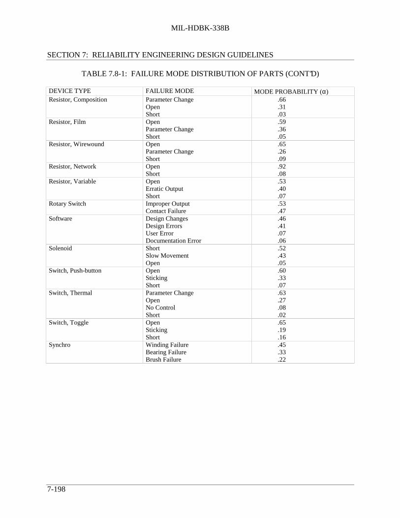
MIL-HDBK-338B


7-198


DEVICE TYPE FAILURE MODE MODE PROBABILITY (α)Resistor, Composition Parameter Change

OpenShort

.66

.31

.03Resistor, Film Open

Parameter ChangeShort

.59

.36

.05Resistor, Wirewound Open

Parameter ChangeShort

.65

.26

.09Resistor, Network Open

Short.92.08

Resistor, Variable OpenErratic OutputShort

.53

.40

.07Rotary Switch Improper Output

Contact Failure.53.47

Software Design ChangesDesign ErrorsUser ErrorDocumentation Error

.46

.41

.07

.06Solenoid Short

Slow MovementOpen

.52

.43

.05Switch, Push-button Open

StickingShort

.60

.33

.07Switch, Thermal Parameter Change

OpenNo ControlShort

.63

.27

.08

.02Switch, Toggle Open

StickingShort

.65

.19

.16Synchro Winding Failure

Bearing FailureBrush Failure

.45

.33

.22

MIL-HDBK-338B


7-199


DEVICE TYPE FAILURE MODE MODE PROBABILITY (α)Transducer Out of Tolerance

False ResponseOpenShort

.68

.15

.12

.05Transformer Open

ShortParameter Change

.42

.42

.16Transistor, Bipolar Short

Open.73.27

Transistor, FET ShortOutput LowParameter ChangeOpenOutput High

.51

.22

.17

.05

.05Transistor, GaAs FET Open

ShortParameter Change

.61

.26

.13Transistor, R.F. Parameter Change

ShortOpen

.50

.40

.10Tube, Traveling Wave Reduced Output Power

High Helix CurrentGun FailureOpen Helix

.71

.11

.09

.09Valve, Hydraulic Leaking

Stuck ClosedStuck Open

.77

.12

.11Valve, Pneumatic Leaking

Stuck OpenStuck ClosedSpurious OpeningSpurious Closing

.28

.20

.20

.16

.16Valve, Relief Premature Open

Leaking.77.23

MIL-HDBK-338B


7-200

In order to accurately address the failure modes of a given LSI microcircuit each of these factorsmust be accounted for. As an example, if the IC chip is packaged in an hermetic cavity packagethere is a possibility that one wire may break and short to an adjacent wire. If this same chip wereencapsulated in a plastic package, this short could not occur, since the wire is constrained by thepotting material. However, the potting material can have other detrimental effects on an IC chip.

Figure 7.8-3 illustrates a useful form for conducting a failure effect analysis. (See also Figure7.8-2 for an example of its use.) For each component in the system, appropriate information isentered in each column. Column descriptions are given in Table 7.8-2.

(1)ITEM

(2)CODE

(3)FUNCTION

(4)FAILUREMODE

(5)FAILUREEFFECT

(6)LOSSPROBABILITY, β

FIGURE 7.8-3: FAILURE EFFECTS ANALYSIS FORM

TABLE 7.8-2: COLUMN DESCRIPTIONS FOR FIGURE 7.8-3

COLUMN NOMENCLATURE DESCRIPTION

1 Item Item name

2 Code Item identification or circuit designation code

3 Function Concise statement of the item’s function

4 Failure Mode Concise statement of the mode(s) of item failure

5 Failure Effect Explanation of the effect of each failure mode on theperformance of the next higher level in the symbolic logic blockdiagram

6 Loss Probability Numerical value indicating the probability of system loss if theitem fails in the mode indicated

MIL-HDBK-338B


7-201

A numerical reference for all items in the symbolic logic block diagram must be provided byusing a standard coding system, such as that specified in MIL-STD-1629. All items below theset and group levels are identified using the scheme illustrated in Table 7.8-2. Items at and abovethe group and set levels are not subject to this standard nomenclature scheme. These items canbe assigned a simple code such as that illustrated in Figure 7.8-1. In this illustration, the systemis assigned a letter; and the subsystems, sets, and groups are assigned numbers in a specificallyordered sequence. As an example, the code S-23-01 designates the first group of the third set inthe second subsystem of system S (Note, this code is limited to subsystems with less than 10sets). The exact coding system used is not as important as making sure that each block in thediagram has its own number. Identical items (same drawing numbers) in different systems, or inthe same system but used in different applications, should not be assigned the same code number.

(1) During the failure effects analysis, a number of changes to the block diagrams may berequired. Therefore, to minimize the number of changes in the coding system, it isrecommended that the failure effects analysis be completed before assignment of codenumbers is finalized.

(2) Based on the failure effects analysis, a list of critical items should be prepared. This listwill contain those items whose failure results in a possible loss, probable loss, or certainloss of the next higher level in the symbolic logic block diagram. All items that cancause system loss should be identified clearly in the list.

7.8.3 Phase 2

This phase is implemented by performing the following steps:

(1) The symbolic logic block diagram, failure effects analysis, coding, and critical items listare reviewed and brought up- to-date.

(2) Criticality is assigned, based on the item applicable failure mode, the system lossprobability, the failure mode frequency ratio, and the item unreliability. The analysis ofcriticality is essentially quantitative, based on a qualitative failure effects analysis.

Criticality CRij defined by the equation

(CR)ij = αij βij λi (7.21)

MIL-HDBK-338B


7-202

where:αij = failure mode frequency ratio of item i for the failure mode j (see Table

7.8-1 for an example), i.e., the ratio of failures of the type being considered toall failures of the item.

βij = loss probability of item i for failure mode j (i.e., the probability of system

failure if the item fails). A suggested scale is Certain Loss = 1.00, ProbableLoss ranges from 0.1 to 1.0, Possible Loss ranges from 0 to 0.10, No Effect -0.0

λi = failure rate of item i

(CR)ij = system failure rate due to item i’s failing in its mode j

The system criticality is given by Eq. (7.22)

(CR)s = ∑ i

∑j

(CR)ij (7.22)

where:(CR)s = system criticality (failure rate)

Σj = sum over all failure modes of item i

Σi = sum over all items

A form useful for conducting the criticality analysis is given in Figure 7.8-5. This form is amodification of Figure 7.8-3 to include the failure mode frequency ratio and the failure rate. Theexample in the next section and Figures 7.8-4 and 7.8-5 illustrate the procedure.

The CR value of the preamplifier unit is 5.739 per 106 hr. This number can be interpreted as thepredicted total number of system failures per hour due to preamplifier failures, e.g., 5.739

x 10-6 . Whether or not this number is excessive, and thus calls for corrective action, dependsupon the requirements for the system and the criticalities for other units in the system. If thenumber is excessive, it can be reduced by any of the following actions:

(1) Lowering the failure rates of parts in the system by derating.

(2) Decreasing the failure mode frequency ratio through selection of other parts.

(3) Decreasing the loss probability by changing the system or preamplifier design.

MIL-HDBK-338B


7-203

(4) Redesign using various techniques such as redundancy, additional cooling, orswitching.

Radar Z

Transmitter

10 20 30 40 60Receiver Antenna Display Power

Supply

Display

50Input fromShip’s Power

Preamplifier20A1

LocalOscillator

20A2

Mixer20A4

IFAmplifier

20A5Detector

20A6Video

20A7

LocalOscillator

20A3

Parts Notes:1. Displays 40 and 50 are redundant (active)2. Local oscillators 20A2 and 20A3 are redundant (standby)

FIGURE 7.8-4: SYMBOLIC LOGIC DIAGRAM OF RADAR EXAMPLE

7.8.4 Example

The detail design of a radar system required the use of FMEA to determine the effect of itemfailures on the system. The FMEA analysis must be performed at this time prior to freezing thedesign. Perform an FMEA analysis as follows:

MIL-HDBK-338B


7-204

PROCEDURE EXAMPLE

(1) Develop a symbolic logic blockdiagram of the radar system. The unitsmaking up the receiver subsystem areshown in detail. In an actual analysis,symbolic diagrams must beconstructed for all other sub-systems.

See Figure 7.8-4

(2) Fill in the work sheets for all units inthe receiver subsystem. Repeat thisprocedure for all subsystems.

See Figure 7.8.-5

(3) Qualitatively estimate the values ofloss probability for each part.

An analysis indicates that for this system thefollowing values of β are applicable: 1.0,0.1, and 0.0.

(4) Determine the failure mode frequencyratio for each failure mode of everypart.

The resistor is fixed, film (Fig. 7.8-5); fromTable 7.8-1, it has two failure modes: open= 0.59 and drift = 0.36.

(5) Tabulate failure rates for eachcomponent.

λ (20A1R1) = 1.5 per 106 hr.

(6) Compute the CR value for each failuremode of each part by Eq. (7.21).

CR(open) = 0.59 x 1.00 x 1.5 per 106 hr

= 0.885 per 106 hr

CR (short) = 0.05 x 1.00 x 1.5 per 106 hr

= 0.075 per 106 hr

CR(parameter change) = 0.36 x 106 hr

x 0.10 x 1.5 per 106 hr

= 0.054 per 106 hr

(7) Compute the total CR for the unit(CR), by Eq. (7.22).

The total CR for the preamplifier unit is

5.739 per 106 hr (See Figure 7.8-5).

MIL-HDBK-338B


7-205

MIL-HDBK-338B


7-206

7.8.5 Risk Priority Number

An alternate evaluation approach to Criticality Analysis is that of the calculation of a RiskPriority Number (RPN). The risk priority number provides a qualitative numerical estimate of thedesign risk. This number is then used to rank order the various concerns and failure modesassociated with a given design as previously identified in the FMEA. RPN is defined as theproduct of three independently assessed factors: Severity (S), Occurrence (O) and Detection (D).

RPN = (S) x (O) x (D)

This technique was originally developed for use by the automotive industry, but it may also beeffectively tailored to many other types of applications. A more detailed description of thistechnique may be found in Reference [80].

A description, and one detailed example, of each of these three independently assessed factors(S), (O), and (D) follows.

SEVERITY (S) is an assessment of the seriousness of the effect of the potential failure mode tothe next higher component, subsystem, system or to the customer if it were to occur. Severity istypically estimated on a scale of “1” to “10”. One such method of ranking is illustrated in Table7.8-3. This table could be appropriately tailored for other non-automotive applications. Severityapplies only to the effect of the failure.

OCCURRENCE (O) is the likelihood that a specific cause/mechanism will occur. Thelikelihood of occurrence ranking number is an index number rather than a probability. Removingor controlling one or more of the causes/mechanisms of the failure mode through a design changeis the only way a reduction in occurrence ranking can be effected.

The likelihood of occurrence of potential failure cause/mechanism is typically estimated on ascale of “1” to “10”. One such method of ranking is illustrated in Table 7.8-4.

MIL-HDBK-338B


7-207

TABLE 7.8-3: SEVERITY CLASSIFICATION

EFFECT CRITERIA: SEVERITY OF EFFECT RANKINGHazardous -withoutwarning

Very high severity ranking when a potential failure mode affects safe vehicleoperation and/or involves noncompliance with government regulation withoutwarning.

10

Hazardous -with warning

Very high severity ranking when a potential failure mode affects safe vehicleoperation and/or involves noncompliance with government regulation withwarning.

9

Very High Vehicle / item inoperable, with loss of primary function. 8High Vehicle / item operable, but at reduced level of performance. Customer

dissatisfied.7

Moderate Vehicle / item operable, but Comfort / Convenience item(s) inoperable. Customerexperiences discomfort.

6

Low Vehicle / item operable, but Comfort / Convenience item(s) operate at a reducedlevel of performance. Customer experiences some dissatisfaction.

5

Very Low Fit & Finish / Squeak & Rattle item does not conform. Defect noticed by mostcustomers.

4

Minor Fit & Finish / Squeak & Rattle item does not conform. Defect noticed by averagecustomer.

3

Very Minor Fit & Finish / Squeak & Rattle item does not conform. Defect noticed bydiscriminating customer.

2

None No Effect 1

TABLE 7.8-4: OCCURRENCE RANKING

PROBABILITY OF FAILURE POSSIBLE FAILURE RATES RANKINGVery High: Failure is almost inevitable ≥ 1 in 2

1 in 3109

High: Repeated failures 1 in 81 in 20

87

Moderate: Occasional failures 1 in 801 in 4001 in 2000

654

Low: Relatively few failures 1 in 15,0001 in 150,000

32

Remote: Failure is unlikely ≤ 1 in 1,500,000 1

In determining this estimate, questions such as the following should be considered:

(1) What is the service history/field experience with similar components or subsystems?

(2) Is this component carried over from, or similar to, a previously used component orsubsystem?

(3) How significant are the changes from a previously used component or subsystem?

(4) Is the component radically different from a previously used component?

MIL-HDBK-338B


7-208

(5) Is the component new?

(6) Has the component application changed?

(7) What, if any, are the environmental changes?

(8) Has an engineering analysis been made to estimate the expected comparable occurrencerate for this application?

A consistent occurrence ranking system should be used to ensure continuity. The “Design LifePossible Failure Rates” shown in Table 7.8-4 are based upon the number of failures which areanticipated during the design life of the component, subsystem, or system. The occurrenceranking number is related to the rating scale and does not reflect the actual likelihood ofoccurrence.

CURRENT DESIGN CONTROLS: This is an additional parameter of concern beyond thosepreviously addressed in the FMEA. Current Design Controls are defined as prevention, designverification/validation, or other activities which will assure the design adequacy for the failuremode and/or cause/mechanism under consideration. Current controls (e.g., road testing, designreviews, fail-safe analysis, mathematical studies, rig/lab testing, feasibility reviews, prototypetests, fleet testing etc.) are those that have been or are being used with the same or similardesigns.

There are three types of Design Controls/Features to consider; those that: (1) Prevent thecause/mechanism or failure mode/effect from occurring, or reduce their rate of occurrence, (2)detect the cause/mechanism and lead to corrective actions, and (3) detect the failure mode.

The preferred approach is to first use type (1) controls if possible; second, use the type (2)controls; and third, use the type (3) controls. The initial detection ranking will be based upon thetype (2) or type (3) current controls, provided the prototypes and models being used arerepresentative of design intent.

DETECTION (D) is an assessment of the ability of the proposed type (2) current designcontrols, to detect a potential cause/mechanism (design weakness), or the ability of the proposedtype (3) current design controls to detect the subsequent failure mode, before the component,subsystem, or system is released for production. In order to achieve a lower detection ranking,generally the planned design control (e.g. preventative, validation, and/or verification activities)has to be improved.

The detection of potential failure cause/mechanism is typically estimated on a scale of “1” to“10”. One such method of ranking is illustrated in Table 7.8-5.

MIL-HDBK-338B


7-209

TABLE 7.8-5: DETECTION RANKING

DETECTION CRITERIA: LIKELIHOOD OF DETECTION BY DESIGN CONTROL RANKINGAbsoluteUncertainty

Design Control will not and/or can not detect a potential cause/ mechanism andsubsequent failure mode; or there is no Design Control.

10

Very Remote Very remote chance the Design Control will detect a potential cause/ mechanismand subsequent failure mode.

9

Remote Remote chance the Design Control will detect a potential cause/ mechanism andsubsequent failure mode.

8

Very Low Very low chance the Design Control will detect a potential cause/ mechanismand subsequent failure mode.

7

Low Low chance the Design Control will detect a potential cause/ mechanism andsubsequent failure mode.

6

Moderate Moderate chance the Design Control will detect a potential cause/ mechanismand subsequent failure mode.

5

ModeratelyHigh

Moderately high chance the Design Control will detect a potentialcause/mechanism and subsequent failure mode.

4

High High chance the Design Control will detect a potential cause/ mechanism andsubsequent failure mode.

3

Very High Very high chance the Design Control will detect a potential cause/ mechanismand subsequent failure mode.

2

Almost Certain Design Control will almost certainly detect a potential cause/ mechanism andsubsequent failure mode.

1

7.8.5.1 Instituting Corrective Action

When the failure modes have been rank ordered by RPN (the product of S, O and D), correctiveaction should be first directed at the highest ranked concerns and critical items. The intent of anyrecommended action is to reduce any one or all of the occurrence, severity and/or detectionrankings. An increase in design validation/verification actions will result in a reduction in thedetection ranking only. A reduction in the occurrence ranking can be effected only by removingor controlling one or more of the causes/mechanisms of the failure mode through a designrevision. Only a design revision can bring about a reduction in the severity ranking. Regardlessof the resultant RPN, special attention should be given when severity is high.

After the corrective action(s) have been identified, estimate and record the resulting severity,occurrence, and detection rankings and recalculate the RPN.

7.8.6 Computer Aided FMEA

As with most other reliability analyses the computer can be quite helpful in performing anFMEA, since a large number of computations and a significant amount of record keeping arerequired for systems of reasonable size.

In the failure effects portion of the analysis the computer is very helpful for functionalevaluation, using performance models. Given that the computer program contains the designequations relating system outputs to various design parameters, each item is allowed to fail ineach of its modes, and the effect on the system is computed.

MIL-HDBK-338B


7-210

Several commercial programs are available for performing an FMECA in accordance with MIL-STD-1629A.

7.8.7 FMEA Summary

The FMEA does not replace the need for sound engineering judgment at the design level. Thissystem analysis is, however, practical in determining many of the significant details which maynot otherwise be determined by separate, individual studies. Like other design tools, the FMEAhas limitations such as those discussed below.

(1) It is not a substitute for good design. If used for its intended purpose it can be an aid tobetter design.

(2) It will not solve item problems which may exist as a limitation to effective systemdesign. It should define and focus attention on such problems and indicate the need fora design solution.

(3) It will not, in itself, guarantee a system design. It is nothing more than a logical way ofestablishing "bookkeeping" which can be systematically analyzed for design reliability.

7.9 Fault Tree Analysis

The "fault tree" analysis (FTA) technique is a method for block diagramming constituent lowerlevel elements. It determines, in a logical way, which failure modes at one level produce criticalfailures at a higher level in the system. The technique is useful in safety analysis where thediscipline of block diagramming helps prevent an oversight in the basic FMEA discussed in theprevious subsection.

As was previously mentioned, FMEA is considered a "bottoms up" analysis, whereas an FTA isconsidered a "top down" analysis. FMEAs and FTAs are compatible methods of risk analysis,with the choice of method dependent on the nature of the risk to be evaluated. There are somedifferences, however, because FTA is a top down analysis there is a higher probability ofmisinterpretation at the lowest level. On the other hand, FMEA starts at the lowest level,therefore will probably result in a better method of risk analysis (assuming lowest level data isavailable). Also, FMEA considers only single failures while FTA considers multiple failures. Ingeneral, FTA requires a greater skill level than FMEA.

Fault tree methods of analysis are particularly useful in functional paths of high complexity inwhich the outcome of one or more combinations of noncritical events may produce anundesirable critical event. Typical candidates for fault tree analysis are functional paths orinterfaces which could have critical impact on flight safety, munitions handling safety, safety ofoperating and maintenance personnel, and probability of error free command in automatedsystems in which a multiplicity of redundant and overlapping outputs may be involved. The faulttree provides a concise and orderly description of the various combinations of possible

MIL-HDBK-338B


7-211

occurrences within the system which can result in a predetermined critical output event.However, performance of the fault tree analysis does require considerable engineering time andeven then the quality of results is only as good as the validity of input data and accuracy of thefault tree logic.

Fault tree methods can be applied beginning in the early design phase, and progressively refinedand updated to track the probability of an undesirable event as the design evolves. Initial faulttree diagrams might represent functional blocks (e.g., units, equipments, etc.), becoming moredefinitive at lower levels as the design materializes in the form of specific parts and materials.Results of the analysis are useful in the following applications:

(1) Allocation of critical failure mode probabilities among lower levels of the systembreakdown.

(2) Comparison of alternative design configurations from a safety point of view.

(3) Identification of critical fault paths and design weaknesses for corrective action.

(4) Evaluation of alternative corrective action approaches.

(5) Development of operational, test, and maintenance procedures to recognize andaccommodate unavoidable critical failure modes.

Symbols commonly used in diagramming a fault tree analysis are shown in Figure 7.9-1. Thebasic relationships between functional reliability (success) block diagrams and the equivalentfault tree diagrams, using some of these symbols, are illustrated in Figures 7.9-2 and 7.9-3.

Success of the simple two element series system comprised of blocks A and B is given by R =

AB; and the probability of system failure (i.e., unsuccessful or unsafe performance) is given by R

= (1 - R) = 1 - AB. When individual element unreliability ( R i ) is less than 0.1, the following

approximations may be used to simplify computations in the fault tree logic diagram, with little(10%) error:

MIL-HDBK-338B


7-212

R = 1 - AB = 1 - (1 - A ) (1 - B )

= A + B - AB § A + B

The two element block diagrams of Figure 7.9-2 is reconfigured as a simple parallel redundantsystem in Figure 7.9-3 to illustrate the treatment of parallel redundant elements in the fault tree

logic diagram. Note that "AND" gates for the combination of successes ( R s ) become "OR"

gates for the combination of failures ( R s ); and "OR" gates for Rs become "AND" gates for

R s . This is illustrated in the series parallel network of Figure 7.9-3.

The fault tree analysis of critical failure modes should proceed as illustrated in the followingsteps.

Step 1: Develop Function Reliability Block Diagram: Develop reliability block diagram forthe system/equipment functional paths in which the critical failure mode is to be circumvented oreliminated. Define the critical failure mode in terms of the system level mal-performancesymptom to be avoided. For example, the hypothetical firing circuit of Figure 7.9-4 is designedto ignite a proposed rocket motor in the following sequence:

(1) Shorting switch S1 is opened to enable launcher release and firing.

(2) Firing switch S2 is closed by the pilot to apply power to relay R1 .

(3) Relay R1 activates the guidance and control (G&C) section.

(4) Relay R2 is activated by signal from the G&C section, closing the igniter firing circuit

which starts the rocket motor.

MIL-HDBK-338B


7-213

A logical "AND" gate - "A" exists if and only ifall of B1, B2 . . . . Bn exist simultaneously.

A logical inclusive "OR" gate - "A" exists if anyB1, B2, . . . Bn or any combination thereof

An event--usually the output of (or input to)and "AND" or an "OR" gate

A failure rate of malfunction event-in terms of aspecific circuit or component, represented bythe symbol X with a numerical subscript

An event not developed further because of lack ofinformation or because of lack of sufficientconsequence. Represented by the symbol W witha numerical subscript

A connecting symbol to another part of the faulttree within the same major branch

An "inhibit" gate, used to describe the relationshipbetween one fault and another. The input faultdirectly produces the output fault if the indicatedconditions is satisfied

Xi

Wi

B1 Bn

"A"

B1 Bn

"A"

FIGURE 7.9-1: FAULT TREE ANALYSIS SYMBOLS

MIL-HDBK-338B


7-214

UNSUCCESSFULEVENT

R = A + B - AB

A B

SUCCESSFULEVENTR = AB

A B

AND OR

A B R = ABR = 1 - AB = A + B - AB

AB A + B - AB

FIGURE 7.9-2: TRANSFORMATION OF TWO-ELEMENT SERIESRELIABILITY BLOCK DIAGRAM TO "FAULT TREE" LOGIC DIAGRAMS

MIL-HDBK-338B


7-215

.

A

B

C DR = CD(1 - AB) = CD(A + B - AB)

R = 1 - CD(1 - AB) = C + D + AB - (CD + ABC + ABD - ABCD)

AND

SUCCESSR = CD(A + B - AB)

C DOR

A B

OR

ANDC D

A B

FAILURER = C + D + AB - (CD + ABC + ABD - ABCD

CD

A + B - AB AB

C + D - CD

FIGURE 7.9-3: TRANSFORMATION OF SERIES/PARALLEL BLOCK DIAGRAM TOEQUIVALENT FAULT TREE LOGIC DIAGRAM

MIL-HDBK-338B


7-216

S 1 S 2 R 1 BATTERY R2 IGNITER MOTOR

ENABLE INITIATE

LAUNCHERRELEASE PILOT

G&CSECTION

(gyro open-up) ACTIVATEEMI EXTERNAL

FACTORS

ROCKET MOTOR IGNITER CIRCUIT

FIGURE 7.9-4: RELIABILITY BLOCK DIAGRAM OF HYPOTHETICAL ROCKET MOTOR FIRING CIRCUIT

The rocket motor can be inadvertently fired by premature ignition due to electronic failure,electromagnetic interference (EMI), or by external factors such as shock, elevated temperature,etc. These are the events to be studied in the fault tree analysis.

Step 2: Construct the Fault Tree: Develop the fault tree logic diagram relating all possiblesequences of events whose occurrence would produce the undesired events identified in Step 1,e.g., inadvertent firing of the missile rocket motor. The fault tree should depict the paths thatlead to each succeeding higher level in the functional configuration. Figure 7.9-5 illustrates theconstruction of one branch of the fault tree for the ignition circuit.

In constructing the fault tree for each functional path or interface within the reliability model,consideration must be given to the time sequencing of events and functions during the specifiedmission profile. Very often the operational sequence involves one or more changes in hardwareconfiguration, functional paths, critical interfaces, or application stresses. When such conditionsare found to apply, it is necessary to develop a separate fault tree for each operating mode,function, or mission event in the mission sequence.

Step 3: Develop Failure Probability Model: Develop the mathematical model of the fault treefor manual (or computer) computation of the probability of critical eventoccurrence on the basis of failure modes identified in the diagram. For example, the undesiredsystem level critical failure mode identified in Figure 7.9-5 is "accidental rocket motor firing,"given by the top level model as follows:

A = B + C - BC

MIL-HDBK-338B


7-217

OR

HARDWAREFAILURE

ACCIDENTALROCKET MOTOR

FIRING

OR OR

OR

XQ

XU

XTQ T

U

OR

TEMPER-ATURE

SHOCK

OTHER

EXTERNALFACTORS

EMI

PREMATUREIGNITION

See SeparateEMI Analysis

AND

BATTERYACTIVATED

FIRING CIRCUITENABLED

XLXK XM

AND

XN

G&CENABLESIGNAL

INHIBITCLOSED

(M)

A

B C

D

EF G

H J

K L MN P

FAILURE MODES (X):XK = Switch S1 shortedXL = Switch S2 shortedXM = Relay R1 failed closedXN = Relay R2 failed closedXQ = High leakage currentXT = Transistor Q-2 openXU = Connector short to B+

FIGURE 7.9-5: FAULT TREE FOR SIMPLIFIED ROCKET MOTOR FIRING CIRCUIT

MIL-HDBK-338B


7-218

As indicated in the figure, C represents the probability of accidental rocket motor firing due topremature ignition via the firing circuit either due to hardware failure (F) or electromagneticinterference (G), i.e.:

C = F + G - FG

Considering hardware failures only, the probability of premature ignition due to hardware failureis given by:

F = HJ

where:

H = KLM

J = N + P - NP

P = Q + T + U = ( QT + QU + TU - QTU )

Step 4: Determine Failure Probabilities or Identified Failure Modes: Determine probabilityof occurrence (i.e., probability of failure) in each event or failure mode identified in the model.Compute safety parameters at the system level by applying the failure data in the models derivedin Step 3.

Assume, for example, the following failure probabilities in the premature ignition branch of thefault tree:

K = 50 x 10-3

L = 100 x 10-3

M = 40 x 10-3

N = 5 x 10-3

Q = 2 x 10-3

T = 1 x 10-3

U = 0.5 x 10-3

MIL-HDBK-338B


7-219

Using the bottom up approach, combine these data in the failure probability models developed inStep 3, and estimate the system level probability as follows:

P = Q + T + U - ( QT + QU + TU - QTU )

= (2 + 1 + 0.5)10-3 - [(2 + 1 + 0.5)10-6 - (1)10-9 ]

≈ 3.5 x 10-3

Higher order (product) terms in the model can be dropped in the P model since the values ofindividual terms are much less than 0.10.

Combining P with N to find J yields:

J = N + P - NP

= 5 x 10-3 + 3.5 x 10-3 - 17.5 x 10-6

≈ 8.5 x 10-3

This is the probability of accidental firing circuit operation conditional on relay R1 having failedin the closed position (i.e., M) in the battery branch of the fault tree. In the battery branch, the

battery can be accidentally activated only if switches S1 and S2 fail in the short mode, and if relay

R1 fails in the closed position, given by:

H = KLM

= (50 x 10-3 ) (100 x 10-3 ) (40 x 10-3 )

= 200 x 10-6

Probability of premature ignition because of hardware failure is then estimated from:

F = HJ = (200 x 10-6 ) (8.5 x 10-3 )

= 1.70 x 10-6

Assume that the EMI analysis discloses a probability of accidental ignition ( G = 5 x 10-6

) due

to exposure to specified level of RF radiation in the operating environment. The probability ofpremature ignition to either cause (hardware failure or EMI exposure) is given by:

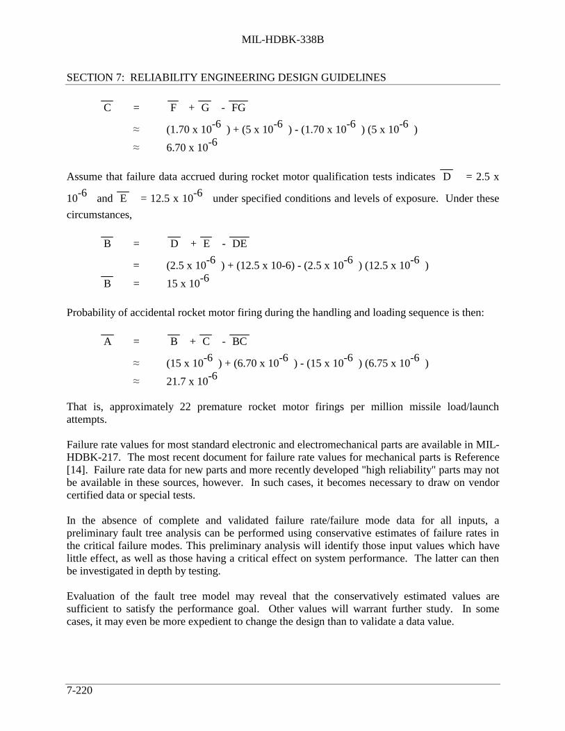
MIL-HDBK-338B


7-220

C = F + G - FG

§ (1.70 x 10-6 ) + (5 x 10-6 ) - (1.70 x 10-6 ) (5 x 10-6 )

§ 6.70 x 10-6

Assume that failure data accrued during rocket motor qualification tests indicates D = 2.5 x

10-6 and E = 12.5 x 10-6 under specified conditions and levels of exposure. Under these

circumstances,

B = D + E - DE

= (2.5 x 10-6 ) + (12.5 x 10-6) - (2.5 x 10-6 ) (12.5 x 10-6 )

B = 15 x 10-6

Probability of accidental rocket motor firing during the handling and loading sequence is then:

A = B + C - BC

§ (15 x 10-6 ) + (6.70 x 10-6 ) - (15 x 10-6 ) (6.75 x 10-6 )

§ 21.7 x 10-6

That is, approximately 22 premature rocket motor firings per million missile load/launchattempts.

Failure rate values for most standard electronic and electromechanical parts are available in MIL-HDBK-217. The most recent document for failure rate values for mechanical parts is Reference[14]. Failure rate data for new parts and more recently developed "high reliability" parts may notbe available in these sources, however. In such cases, it becomes necessary to draw on vendorcertified data or special tests.

In the absence of complete and validated failure rate/failure mode data for all inputs, apreliminary fault tree analysis can be performed using conservative estimates of failure rates inthe critical failure modes. This preliminary analysis will identify those input values which havelittle effect, as well as those having a critical effect on system performance. The latter can thenbe investigated in depth by testing.

Evaluation of the fault tree model may reveal that the conservatively estimated values aresufficient to satisfy the performance goal. Other values will warrant further study. In somecases, it may even be more expedient to change the design than to validate a data value.

MIL-HDBK-338B


7-221

Step 5: Identify Critical Fault Paths: When the probability of an unsafe failure mode at thesystem level exceeds specification tolerances, identify the critical paths which contribute mostsignificantly to the problem. For example, both paths in the preceding analysis contribute aboutequally to the total problem because of environmental sensitivity - ignition circuit to EMI, andpropellant insulation to high ambient temperature.

7.9.1 Discussions of FTA Methods

There are basically three methods for solving fault trees: (1) direct simulation (Reference [81]),(2) Monte Carlo (Reference [82]), and (3) direct analysis (Reference [83]).

Direct simulation basically uses Boolean logic hardware (similar to that in digital computers) in aone-to-one correspondence with the fault tree Boolean logic to form an analog circuit. Thismethod usually is prohibitively expensive. A hybrid method obtains parts of the solution usingthe analog technique and parts from a digital calculation, in an effort to be cost competitive.Because of the expense involved, this method rarely is used.

Monte Carlo methods are perhaps the most simplest in principle but in practice can be expensive.Since Monte Carlo is not practical without the use of a digital computer, it is discussed in thatframework. The most easily understood Monte Carlo technique is called "direct simulation."The term "simulation" frequently is used in conjunction with Monte Carlo methods, becauseMonte Carlo is a form of mathematical simulation. (This simulation should not be confused withdirect analog simulation.) Probability data are provided as input, and the simulation programrepresents the fault tree on a computer to provide quantitative results. In this manner, thousandsor millions of trials can be simulated. A typical simulation program involves the following steps.

(1) Assign failure data to input fault events within the tree and, if desired, repair data.

(2) Represent the fault tree on a computer to provide quantitative results for the overallsystem performance, subsystem performance, and the basic input event performance.

(3) List the failure that leads to the undesired event and identify minimal cut setscontributing to the failure.

(4) Compute and rank basic input failure and availability performance results.

In performing these steps, the computer program simulates the fault tree and, using the inputdata, randomly selects the various parameter data from assigned statistical distributions; and thentests whether or not the TOP event occurred within the specified time period. Each test is a trial,and a sufficient number of trials is run to obtain the desired quantitative resolution. Each timethe TOP event occurs, the contributing effects of input events and the logical gates causing thespecified TOP event are stored and listed as computer output. The output provides a detailedperspective of the system under simulated operating conditions and provides a quantitative basisto support objective decisions.

MIL-HDBK-338B


7-222

A number of computer programs have been developed for fault tree analysis. References [83] -[85] provide additional information on fault tree analysis.

In practice, the methods used for fault tree analysis will depend on which ones are available forthe computer being used. It will rarely, if ever, be worthwhile generating a computer programespecially for a particular problem.

7.10 Sneak Circuit Analysis (SCA)

7.10.1 Definition of Sneak Circuit

A sneak circuit is an unexpected path or logic flow within a system which, under certainconditions, can initiate an undesired function or inhibit a desired function. The path may consistof hardware, software, operator actions, or combinations of these elements. Sneak circuits arenot the result of hardware failure but are latent conditions, inadvertently designed into the systemor coded into the software program, which can cause it to malfunction under certain conditions.Categories of sneak circuits are:

(1) Sneak paths which cause current, energy, or logical sequence to flow along anunexpected path or in an unintended direction.

(2) Sneak timing in which events occur in an unexpected or conflicting sequence.

(3) Sneak indications which cause an ambiguous or false display of system operatingconditions, and thus may result in an undesired action taken by an operator.

(4) Sneak labels which incorrectly or imprecisely label system functions, e.g., systeminputs, controls, displays, buses, etc., and thus may mislead an operator into applying anincorrect stimulus to the system.

Figure 7.10-1 depicts a simple sneak circuit example. With the ignition off, the radio turned tothe on position, the brake pedal depressed, and the hazard switch engaged, the radio will poweron with the flash of the brake lights.

MIL-HDBK-338B


7-223

BRAKE LIGHTS

BATTERY

BRAKE PEDAL

IGNITION SWITCH

SNEAK PATH EXPECTED PATH

HAZARD SWITCH

FLASHER MODULE

RADIO

FIGURE 7.10-1: AUTOMOTIVE SNEAK CIRCUIT

7.10.2 SCA: Definition and Traditional Techniques

Sneak circuit analysis is the term that has been applied to a group of analytical techniques whichare intended to methodically identify sneak circuits in systems. SCA techniques may be eithermanual or computer assisted, depending on system complexity. Current SCA techniques whichhave proven useful in identifying sneak circuits in systems include:

(1) Sneak Path Analysis: A methodical investigation of all possible electrical paths in ahardware system. Sneak path analysis is a technique used for detecting sneak circuits inhardware systems, primarily power distribution, control, switching networks, andanalog circuits. The technique is based on known topological similarities of sneakcircuits in these types of hardware systems.

(2) Digital Sneak Circuit Analysis: An analysis of digital hardware networks for sneakconditions, operating modes, timing races, logical errors, and inconsistencies.Depending on system complexity, digital SCA may involve the use of sneak pathanalysis techniques, manual or graphical analysis, computerized logic simulators orcomputer aided design (CAD) circuit analysis.

MIL-HDBK-338B


7-224

(3) Software Sneak Path Analysis: An adaptation of sneak path analysis to computerprogram logical flows. The technique is used to analyze software logical flows bycomparing their topologies to those with known sneak path conditions in them.

7.10.3 New SCA Techniques

SCA is a powerful analytical tool. Historically, however, SCA has been expensive and performedlate in the design cycle after all of the design documentation was virtually complete. Thus, anysubsequent design changes resulting from the SCA were difficult to make and costly toimplement. Therefore, the use of SCA was usually limited to only items and functions whichwere critical to safety or mission success or where other techniques were not proven to beeffective.

This situation, however, has begun to change. Some Air Force publications shed considerablenew light on SCA techniques. These publications are:

(1) Sneak Circuit Analysis for the Common Man, RADC-TR-89-223, Reference [86]

(2) Integration of Sneak Circuit Analysis with Design, RADC-TR-90-109,Reference [87]

(3) Automated Sneak Circuit Analysis Technique (SCAT), Reference [88]

(4) SCAT: Sneak Circuit Analysis Tool, Version 3.0, RL-TR-95-232, Reference [89]

SCAT is an interactive "Expert System" design tool to assist the designer in identifying andeliminating both sneak circuits and design concerns early in the design phase. In contrast tonormal sneak circuit analyses, SCAT analyses are performed at the assembly level, rather than atthe system level. Thus SCAT is not considered to be a replacement for a complete Sneak CircuitAnalysis. However, since SCAT is used much earlier in the design phase, it may result in theelimination of many (but not all) potential sneak circuits and decrease the later need for acomplete sneak circuit analysis.

Specifically, the referenced publications identify some Sneak Circuit Design Rules, FunctionalGuidelines, and Device Guidelines that can be applied much earlier in the design phase. Thisnew approach helps significantly to demystify the SCA techniques and enables the Sneak CircuitAnalysis to become a much more cost effective reliability design tool.

Because the technology of hardware and software is rapidly evolving, new SCA techniques willundoubtedly evolve as well. SCA will also find applications in non-electrical/electronic systemswhere analogous situations of energy flow, logic timing, etc. are encountered.

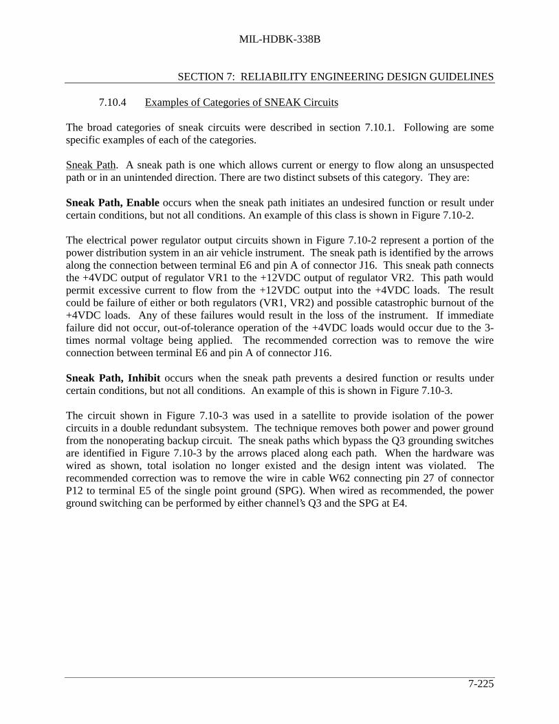
MIL-HDBK-338B


7-225

7.10.4 Examples of Categories of SNEAK Circuits

The broad categories of sneak circuits were described in section 7.10.1. Following are somespecific examples of each of the categories.

Sneak Path. A sneak path is one which allows current or energy to flow along an unsuspectedpath or in an unintended direction. There are two distinct subsets of this category. They are:

Sneak Path, Enable occurs when the sneak path initiates an undesired function or result undercertain conditions, but not all conditions. An example of this class is shown in Figure 7.10-2.

The electrical power regulator output circuits shown in Figure 7.10-2 represent a portion of thepower distribution system in an air vehicle instrument. The sneak path is identified by the arrowsalong the connection between terminal E6 and pin A of connector J16. This sneak path connectsthe +4VDC output of regulator VR1 to the +12VDC output of regulator VR2. This path wouldpermit excessive current to flow from the +12VDC output into the +4VDC loads. The resultcould be failure of either or both regulators (VR1, VR2) and possible catastrophic burnout of the+4VDC loads. Any of these failures would result in the loss of the instrument. If immediatefailure did not occur, out-of-tolerance operation of the +4VDC loads would occur due to the 3-times normal voltage being applied. The recommended correction was to remove the wireconnection between terminal E6 and pin A of connector J16.

Sneak Path, Inhibit occurs when the sneak path prevents a desired function or results undercertain conditions, but not all conditions. An example of this is shown in Figure 7.10-3.

The circuit shown in Figure 7.10-3 was used in a satellite to provide isolation of the powercircuits in a double redundant subsystem. The technique removes both power and power groundfrom the nonoperating backup circuit. The sneak paths which bypass the Q3 grounding switchesare identified in Figure 7.10-3 by the arrows placed along each path. When the hardware waswired as shown, total isolation no longer existed and the design intent was violated. Therecommended correction was to remove the wire in cable W62 connecting pin 27 of connectorP12 to terminal E5 of the single point ground (SPG). When wired as recommended, the powerground switching can be performed by either channel’s Q3 and the SPG at E4.

MIL-HDBK-338B


7-226

VR2 +12 VDC REGULATOR

VR1 +4 VDC REGULATOR

TO OTHER CARDS

TO OTHER CARDS

TO OTHER CARDS

~ ~~

P1-A

E7E6E4

P1-C

J16-A1

1Connection to frequency discriminator SNEAK PATH

FIGURE 7.10-2: SNEAK PATH ENABLE

Q3

64

To Pin 11 (Gnd.) of U1, U2, U3, U16, U19, U42

Q3

64

To Pin 11 (Gnd.) of U1, U2, U3, U16, U19, U42

7

8

41

4083

7

8

35

J16

P16

76

P13

J13

J19 P92

10

10

J18 P92

W17

W16

Y

Z

TB25K

W62

TB27K

Y

Z

E4 E3

SPG

TB12L TE12S

JM

S

M

S

D

YW54

W62

73

79

J12 P12

19

23

27

6767

FIGURE 7.10-3: REDUNDANT CIRCUIT SWITCHED GROUND

MIL-HDBK-338B


7-227

Sneak Timing: A sneak timing condition is one which causes functions to be inhibited or tooccur at an unexpected or undesired time. The example in Figure 7.10-4a illustrates a sneak thatoccurred in the digital control circuitry of a mine. The enable logic for U4 and U5 allows them,briefly, to be enabled simultaneously. Being CMOS devices in a "wired or" configuration, thisallows a potential power-to-ground short through the two devices, damaging or destroying themduring operation.

Sneak Indication: An indication which causes ambiguous or incorrect displays. Figure 7.10-4cillustrates a sneak indication which occurred in a sonar power supply system. The MOP (MotorOperated Potentiometer) OFF and ON indicators do not, in fact, monitor the status of the MOPmotor. Switch S3 could be in the position shown, providing an MOP ON indication eventhrough switches S1 or S2 or relay contacts K1 or K2 could be open, inhibiting the motor.

Sneak Label: A label on a switch or control device which would cause incorrect actions to betaken by operators. The example in Figure 7.10-4b taken from an aircraft radar system, involvesa circuit breaker which provides power to two disparate systems, only one of which is reflected inits label. An operator attempting to remove power from the liquid coolant pump wouldinadvertently deactivate the entire radar.

MIL-HDBK-338B


7-228

~

CLK

U1

O

O

O

S

R

" 1 "

U3

U2

Signifies toOther Circuitry

Output toControl Bus

CP6

~

PICK A

Enable

U4

8 bits

Enable

U5

8 bits

+ 2 8 VDC

CD1Liquid

CoolantPump

RadarControlPanel

LiquidCoolantPump

(a) SNEAK TIMING (b) SNEAK LABEL

M

S 1

65

4

32

1

S3

S2

K2K1

K2

REVFWD

110 VAC

DSP110OFF

DSP110PON

(c) SNEAK INDICATOR

FIGURE 7.10-4: EXAMPLES OF CATEGORIES OF SNEAK CIRCUITS

MIL-HDBK-338B


7-229

7.10.5 SCA Methodology

7.10.5.1 Network Tree Production

The first major consideration that must be satisfied to identify sneak circuit conditions is toensure that the data being used for the analysis represent the actual "as built" circuitry of thesystem. Functional, integrated, and system level schematics do not always represent the actualconstructed hardware. Detailed manufacturing and installation schematics must be used, becausethese drawings specify exactly what was built, contingent on quality control checks, tests, andinspection. However, manufacturing and installation schematics rarely show complete circuits.The schematics are laid out to facilitate hookup by technicians without regard to circuit orsegment function. As a result, analysis from detail schematics is extremely difficult. So manydetails and unapparent continuities exist in these drawings that an analyst becomes entangled andlost in the maze. Yet, these schematics are the data that must be used if analytical results are tobe based on true electrical continuity. The first task of the sneak analyst is, therefore, to convertthis detailed, accurate information into a form usable for analytical work. The magnitude of datamanipulation required for this conversion necessitates the use of computer automation in mostcases.

Automation has been used in sneak circuit analysis since 1970 as the basic method for treeproduction from manufacturing detail data. Computer programs have been developed to allowencoding of simple continuities in discrete "from-to" segments extracted from detail schematicsand wire lists. The encoding can be accomplished without knowledge of circuit function. Thecomputer connects associated points into paths and collects the paths into node sets. The nodesets represent interconnected nodes that make up each circuit. Plotter output of node sets andother reports are generated by the computer to enable the analyst to easily sketch accuratetopological trees. The computer reports also provide complete indexing of every component anddata point to its associated tree. This feature is especially useful in cross indexing functionallyrelated or interdependent trees, in incorporating changes, and in troubleshooting duringoperational support.

7.10.5.2 Topological Pattern Identification

Once the network trees have been produced, the next task of the analyst is to identify the basictopological patterns that appear in each tree. Five basic patterns exist for hardware SCA: (1)single line (no-node) topograph, (2) ground dome, (3) power dome, (4) combination dome, and(5) "H" pattern. These patterns are illustrated in Figure 7.10-5. One of these patterns or severalin combination will characterize the circuitry shown in any given network tree. Although, at firstglance, a given circuit may appear more complex than these basic patterns, closer inspectionreveals that the circuit is actually composed of these basic patterns in combination. In examiningeach node in the network tree, the sneak circuit analyst must identify the topographical pattern orpatterns incorporating the node and apply the basic clues that have been found to typify sneakcircuits involving that particular pattern.

MIL-HDBK-338B


7-230

PwrPwrPwrPwr

S 1S 1 S 1

L1

L2 L3

S 2 S 3

L1 L1 L2

S 2

S 3

L3

S ingle L ine Ground Dome Power Dome

Pwr Pwr Pwr Pwr

L3 L4

S 3 S 4

L1 L2

S 1 S 2

L4 L5

S 5 S 6

S 3 S 4

L3L1 L2

S 1 S 2

Combinat ion Dome " H" Pat tern

FIGURE 7.10-5: BASIC TOPOGRAPHS

MIL-HDBK-338B


7-231

7.10.5.3 Clue Application

Associated with each pattern is a list of clues to help the analyst identify sneak circuit conditions.These lists were first generated during the original study of historical sneak circuits. The listswere updated and revised during the first several years of applied sneak circuit analysis. Now,the list of clues provides a guide to all possible design flaws that can occur in a circuit containingone or more of the five basic topological configurations, subject to the addition of new cluesassociated with new technological developments. The lists consist of a series of questions thatthe analyst must answer about the circuit to ensure that it is sneak free.

As an example, the single line topograph (Figure 7.10-5) would have clues such as:

(a) Is switch S open when load L is desired?

(b) Is switch S closed when load L is not desired?

Obviously, sneak circuits are rarely encountered in this topograph because of its simplicity. Ofcourse, this is an elementary example and is given primarily as the default case which coverscircuitry not included by the other topographs.

With each successive topograph, the clue list becomes longer and more complicated. The cluelist for the "H" pattern includes over 100 clues. This pattern, because of its complexity, isassociated with more sneak circuits than any of the previous patterns. Almost half of the criticalsneak circuits identified to date can be attributed to the "H" patterns. Such a design configurationshould be avoided whenever possible. The possibility of current reversal through the "H"crossbar is the most commonly used clue associated with "H" pattern sneak circuits.

7.10.6 Software Sneak Analysis

In 1975, a feasibility study was performed resulting in the development of a formal technique,involving the use of mathematical graph theory, electrical sneak theory, and computerized searchalgorithms, to identify sneaks in software programs. A software sneak is defined as a logiccontrol path which causes an unwanted operation to occur or which bypasses a desired operation,without regard to failures of the hardware system to respond as programmed.

The feasibility study concluded that:

(1) Software Sneak Analysis is a viable means of identifying certain classes of softwareproblems.

(2) Software Sneak Analysis works equally well on different software languages.

(3) Software Sneak Analysis does not require execution of the software to detect problems.

MIL-HDBK-338B


7-232

The Software Sneak Analysis technique has evolved along lines very similar to hardware SneakCircuit Analysis. Topological network trees are used with electrical symbology representing thesoftware commands to allow easy cross analysis between hardware and software trees and toallow the use of a single standardized analysis procedure.

Since topological pattern recognition is the keystone of both Sneak Circuit Analysis andSoftware Sneak Analysis, the overall methodologies are quite similar. The software package tobe analyzed must be encoded, processed, and reduced to a standardized topographical format, thebasic topological patterns identified and the appropriate problem clues applied to each pattern.For software, it has been found that six basic patterns exist: the Single Line, the Return Dome,the Iteration/Loop Circuit, the Parallel Line, the Entry Dome, and the Trap Circuit, as shown inFigure 7.10-6.

Although at first glance, a given software tree may appear to be more complex than these basicpatterns, closer inspection will reveal that the code is actually composed of these basic structuresin combination. As each node in the tree is examined, the analyst must identify which pattern orpatterns include that node. The analyst then applies the basic clues that have been found to typifythe sneaks involved with that particular structure. These clues are in the form of questions thatthe analyst must answer about the use and interrelationships of the instructions that are elementsof the structure. These questions are designed to aid in the identification of the sneak conditionsin the instruction set which could produce undesired program outputs.

SINGLE LINE

RETURN DOME

PARALLEL LINE

ENTRY DOME

TRAP CIRCUIT

FIGURE 7.10-6: SOFTWARE TOPOGRAPHS

MIL-HDBK-338B


7-233

Software sneaks are classified into four basic types:

(1) Sneak Output: The occurrence of an undesired output.

(2) Sneak Inhibit: The undesired inhibition of an output.

(3) Sneak Timing: The occurrence of an undesired output by virtue of its timing ormismatched input timing

(4) Sneak Message: The program message does not adequately reflect the condition.

Figure 7.10-7 illustrates a software sneak which occurred in the operating software of a militaryaircraft. Figure 7.10-7a illustrates the design intent of the section of software with the sneak.When the actual code was produced, however, the two tests were inadvertently interchanged.The network tree of the actual software code (see Figure 7.10-7b) makes the sneak readilyapparent. This historical problem was uncovered only during the software system integratedtesting when it was found that the instructions represented by LOAD 1 could never be executed.

MIL-HDBK-338B


7-234

ORIGINAL DESIGN INTENT

To Other Code

~

Test 1 VAR1 < 0No

Yes

Test 2 VAR1 = -2

No

Yes

Load 3 Load 2 Load 1

VAR1 = -2VAR1 < 0 VAR1 > -2 VAR1 0

To Other Code

(a)

~~

NETWORK TREE OF ACTUAL CODE

PWR/SMIN

SKMINC/A001

IN2/0002

K00035/D002

SK0001/D002

LSUB/0006

S00006/MOEZ

Is Variable 1 equal to -2

SK0001/D007 S00007/MOLZ

Is Variable 1 less than 0

Yes

YesEQ-2NE-2

No

Load 1

GNDThis branch can never be reached

GND

No

Load 2

Load 3

KSIR/A035

LTZGEZ

FIGURE 7.10-7: SOFTWARE SNEAK EXAMPLE

7.10.7 Integration of Hardware/Software Analysis

After a sneak circuit analysis and a software sneak analysis have been performed on a system, theinteractions of the hardware and software can readily be determined. For this purpose, theanalyst has diagramatic representations of these two elements of the system in a singlestandardized format. The effect of a control operation that is initiated by some hardware elementcan be traced through the hardware trees until it impacts the system software. The logic flow canthen be traced through the software trees to determine its ultimate impact on the system.Similarly, the logic sequence of a software initiated action can be followed through the softwareand electrical network trees until its eventual total system impact can be assessed.

MIL-HDBK-338B


7-235

The joint analysis of a system’s software and hardware circuitry previously described is simplycalled Sneak Analysis. Sneak Analysis helps provide visibility of the interactions of a system’shardware and software and hence will help reduce the difficulties involved in the properintegration of two such diverse, complex system designs. As hardware and software systemsincrease in complexity, the use of interface bridging analysis tools, such as Sneak Analysis,becomes imperative to help ensure the safety of the total system.

7.10.8 Summary

SCA is different from other analyses commonly performed in a reliability program in a numberof important ways. SCA generally concentrates on the interconnections, interrelationships, andinteractions of system components rather than on the components themselves. SCA concentratesmore on what might go wrong in a system rather than on verifying that it works right under someset of test conditions. The SCA technique is based on a comparison with other systems whichhave "gone wrong", not because of part failures, but because of design oversight or because ahuman operator made a mistake. The consequence of this subtly different perspective may bevery important, because it tends to concentrate on and find problems which may be hidden fromthe perspectives of other analytical techniques.

For example FMEA/FMECA differs from SCA in that it predicts and quantifies the response of asystem to failures of individual parts or subsystems. An FMECA is an analysis of all expectedfailure modes and their effect on system performance. FMECA results are often used inmaintainability predictions, in the preparation of maintenance dependency charts, and to establishsparing requirements. SCA, on the other hand, considers possible human error in providingsystem inputs while FMECA does not. In this regard the two types of analysis tend tocomplement one another.

Fault Tree Analysis is a deductive method in which a catastrophic, hazardous end result ispostulated and the possible events, faults, and occurrences which might lead to that end event aredetermined. Thus, FTA overlaps SCA in purpose because the FTA is concerned with all possiblefaults, including component failures as well as operator errors.

Concerning the availability of SCA computer programs, the original SCA computer programsdeveloped under government contract with (NASA), Johnson Spacecraft Center, Houston, Texas,on the Apollo program are available to all industry and government agencies. They can bepurchased from Computer Software Management and Information Center (COSMIC), Universityof Georgia, 112 Barrow Hall, Athens, Georgia 30602. These programs may not be current.However, several companies have purchased these programs and updated them. The improvedprograms and the accompanying analysis techniques are considered proprietary by mostcompanies.

References [86] - [93] provide more details on SCA.

MIL-HDBK-338B


7-236

7.11 Design Reviews

7.11.1 Introduction and General Information

The purpose of a design review is to ensure that each design has been studied to identify possibleproblems, to improve the item where necessary, and to provide assurance that the mostsatisfactory design has been selected to meet the specified requirements. Design reviews arecritical audits of all pertinent aspects of the design and are conducted at critical milestones in anacquisition program. They are essential to reliability engineering.

The formal review (depicted in Figure 7.11-1) of equipment design concepts and designdocumentation for both hardware and software is an essential activity in any developmentprogram. Standard procedures should be established to conduct a review of all drawings,specifications, and other design information by a supplier’s technical groups such as engineering,reliability engineering, and manufacturing engineering. (Ideally, representatives of these andother key groups would comprise one or more integrated product development teams (IPDTs)).This review should be accomplished prior to the release of design information for manufacturingoperations. Such a review is an integral part of the design-checking reviews. Responsiblemembers of each reviewing department meet to consider all design documents, resolve anyproblem areas uncovered, and signify their acceptance of the design documentation by approvingthe documents for their departments.

Reliability engineering, ideally as part of an IPDT, should conduct an intensive review of thesystem during initial design. A design review, from a reliability perspective, includes thefollowing major tasks:

(1) Analysis of environment and specifications

(2) Formal design review of engineering information

(3) Reliability participation in all checking reviews

Prior to the formal review, the requirements defined in applicable specifications are reviewed.The expected environmental extremes of the system are studied to determine suspecteddetrimental effects on equipment performance. Checklists, based on these studies, are preparedto ensure that the objectives of formal design reviews are fulfilled.

MIL-HDBK-338B


7-237

SYST

EM

OPE

RA

TIO

NA

L R

EQU

IREM

ENT D

ESIG

N R

EQU

IREM

ENT

S

DEF

INIT

ION

ALL

OC

AT

ION

DES

IGN

FO

RM

UL

AT

ION

DES

IGN

INFO

RM

AL

DES

IGN

V

ERIF

ICA

TIO

N

FOR

MA

L D

ESIG

N

REV

IEW

DEC

ISIO

N

REV

ERIF

Y

R

EDES

IGN

REA

LLO

CA

TE

R

EDEF

INE

R

E-EV

ALU

AT

E

Con

form

ance

V

erif

ied,

D

esig

n A

ppro

ved

Con

form

ance

N

ot V

erif

ied,

D

esig

n N

ot A

ppro

ved

FIGURE 7.11-1: DESIGN REVIEW AS A CHECK VALVE IN THESYSTEM ENGINEERING CYCLE

MIL-HDBK-338B


7-238

The formal design review, which is instituted prior to the release of drawings, is intended to dothe following in regard to reliability:

(1) Detect any conditions that could degrade equipment reliability

(2) Provide assurance of equipment conformance to applicable specifications

(3) Ensure the use of preferred or standard parts as far as practical

(4) Ensure the use of preferred circuitry as far as possible

(5) Evaluate the electrical, mechanical, and thermal aspects of the design

(6) Review stress analysis to ensure adequate part derating

(7) Ensure accessibility of all parts that are subject to adjustment

(8) Ensure interchangeability of similar subsystems, circuits, modules, andsubassemblies

(9) Ensure that adequate attention is given to all human factors aspects of the design

(10) Ensure that the quality control effort will be effective

Reviews should be made at appropriate stages of the design process. It may be necessary toconduct specific reviews to evaluate achievement of the reliability requirements on a timelybasis. The reviews should include, to the extent applicable but not necessarily limited to: currentreliability estimates and achievements for each mode of operation, as derived from reliabilityanalyses or test(s); potential design or production (derived from reliability analyses) problemareas, and control measures necessary to preserve the inherent reliability; failure mode(s) andeffect(s) and criticality analyses; corrective action on reliability critical items; effects ofengineering decisions, changes and tradeoffs upon reliability achievements, potential and growth,within the functional model framework; status of supplier and vendor reliability programs; andstatus of previously-approved design review actions. The results of reliability reviews should bedocumented.

In order to satisfy the objectives of the design review, the review team must have sufficientbreadth to handle aspects of the items under review, such as performance, reliability, etc., and theinterfaces and interactions with adjacent items. The ultimate objective of the team is to arrive ata balanced and reliable design.

MIL-HDBK-338B


7-239

7.11.2 Informal Reliability Design Review

The informal reliability design review is conducted for the purpose of evaluating and guidingspecified reliability characteristics and maintenance features "in process." That is, it is conductedwhile the design is in the evolutionary or formative stage and still amenable to major conceptualand configuration changes. Reviews are conducted on an unscheduled, "as required," informalbasis. They are usually conducted at the request of the designer or the systems engineer to verifyconformance throughout the team effort, to allocate requirements and design constraints, toverify the solution of problems identified in earlier design iterations, or to provide the basis forselection of design alternatives.

Even though the verification review is an informal working session, usually involving only a fewselected reviewers, results of each review should be documented. The review may result in oneof five alternatives being selected for further design iteration. These alternatives are:

(1) Reverify Design Adequacy to provide additional analytical or empirical proof ofdesign adequacy to facilitate design review approval decision with more confidencethan current data will substantiate

(2) Redesign to correct design discrepancies and marginal characteristics disclosed by thereview

(3) Reallocate Design Requirements to rectify allocation errors identified in the review,or reallocate subsystem requirements on the basis of updated estimates of designfeasibility or changes in relative criticality disclosed during the review

(4) Redefine Design Requirements to restudy previous requirements analyses and tradeoffstudies, and redefine or refine baseline design and configuration requirements morenearly consistent with state-of-art and program constraints revealed during the designreview.

(5) Re-evaluate System Operational Requirements to provide the basis for choosing oneof two alternatives: (a) redefine system operational requirements consistent withcurrent design state-of-art and program constraints; or (b) redefine program constraints,such as delivery schedule and funds, to rectify earlier estimating errors.

The recommended design review team membership, and functions of each member, are brieflysummarized in Table 7.11-1. For these informal design reviews, customer participation isusually optional. The IPDT is the current and preferred approach to forming the design team.

MIL-HDBK-338B


7-240

7.11.3 Formal Design Reviews

Formal design reviews, when the customer is the government, are usually the subject ofcontractual agreement between the government and the supplier. Table 7.11-1 shows therecommended review team composition. Regardless of who the customer is, formal reviewsnormally include the following:

Preliminary Design Review (PDR): The PDR is conducted prior to the detail designprocess to evaluate the progress and technical adequacy of the selected design approach,determine its compatibility with the performance requirements of the specification; andestablish the existence and the physical and functional interfaces between the item andother items of equipment or facilities. The basic design reliability tasks shown in Figure7.11-3 should be accomplished for the PDR.

Eight suggested basic steps pertinent to the PDR are shown in Figure 7.11-2.

Critical Design Review: The CDR is conducted when detail design is essentiallycomplete and fabrication drawings are ready for release. It is conducted to determine thatthe detail design satisfies the design requirements established in the specification, andestablish the exact interface relationships between the item and other items of equipmentand facilities.

Preproduction Reliability Design Review (PRDR): The PRDR is a formal technicalreview conducted to determine if the achieved reliability of a weapon system at aparticular point in time is acceptable to justify commencement of production. For DoDacquisitions, details for the PRDR are usually provided in the individual Servicedocuments or instructions, e.g., NAVAIR INST. 13070.5.

MIL-HDBK-338B


7-241

TABLE 7.11-1: DESIGN REVIEW GROUP, RESPONSIBILITIESAND MEMBERSHIP SCHEDULE

Group Member Responsibilities

Chairman Calls, conducts meetings of group, and issues interim and finalreports

Design Engineer(s)(of product)

Prepares and presents design and substantiates decisions withdata from tests or calculations

*Reliability Manager or Engineer Evaluates design for optimum reliability, consistent with goals

Quality ControlManager or Engineer

Ensures that the functions of inspection, control, and test canbe efficiently carried out

Manufacturing Engineer Ensures that the design is producible at minimum cost andschedule

Field Engineer Ensures that installation, maintenance, and operatorconsiderations were included in the design

Procurement Representative Assures that acceptable parts and materials are available tomeet cost and delivery schedules

Materials Engineer Ensures that materials selected will perform as required

Tooling Engineer Evaluates design in terms of the tooling costs required tosatisfy tolerance and functional requirements

Packaging and Shipping Engineer Assures that the product is capable of being handled withoutdamage, etc.

Design Engineers(not associated with unit under review)

Constructively review adequacy of design to meet allrequirements of customer

Customer Representative (optional) Generally voices opinion to acceptability of design and mayrequest further investigation on specific items

*May have other titles within some companies. Other specialties, such as maintainability, human factors, and valueengineering are also represented.

MIL-HDBK-338B


7-242

The PRDR is conducted just prior to production (and, for DoD programs, after completion ofinitial operational test and evaluation) to ensure the adequacy of the design from a reliabilitystandpoint. The level of achieved reliability and adequacy of design will be evaluated primarilyon initial technical and operational testing, e.g., test results, failure reports, failure analysesreports, reports of corrective action, and other documents which could be used as necessary forback-up or to provide a test history.

Suggested steps for a CDR are shown in Figure 7.11-4. The basic design reliability tasks shownin Figure 7.11-5 should be accomplished for the CDR.

DECISIONASSIGN

ACTION ITEMSFOR FOLLOW-UP

REVIEW

ACQUISITIONMANAGERCONDUCTS

DESIGN REVIEW

REVIEWERPREPARE

FOR REVIEW

NO

GOVERNMENTAPPROVES

DESIGN

COORDINATE

DESIGNERPREPARE

FOR REVIEW

DEFINEDATA

REQUIREMENTS& TASKS

PREPAREDESIGN REVIEW

AGENDA(RELIABILITY)


SCHEDULE

ô

í

÷

û

ø

î

ù

Design review requirements are established.Supplier prepares preliminary design review schedulecompatible with master program milestone schedule.

ô Supplier prepares and distributes agenda inadvance of each review, defining: purpose and scope ofreview; specific items to be reviewed; date, time, andplace for the review.

í Supplier defines applicable data, to assistdesigner and reviewer in preparation for the designreview.

÷ Designer prepares for review, to includeanswers to questions accompanying the agenda,description of design concept, analysis, test results,problems, requirements, etc.

û Review committee (or IPDT) members preparefor review; formulate questions and suggestions.

øùî Review committee members approve ordisapprove preliminary design.

FIGURE 7.11-2: BASIC STEPS IN THE PRELIMINARY DESIGN REVIEW (PDR) CYCLE

MIL-HDBK-338B


7-243

1. Identify the quantitative reliability requirements and compare preliminary predictionswith specified requirements.

2. Review failure rate sources, derating policies, and prediction methods.

3. Identify planned actions when predictions are less than specified requirements.

4. Identify and review parts or items which have a critical life or require specialconsideration, and general plan for handling.

5. Identify applications of redundant elements. Evaluate the basis for their use andprovisions for redundancy with switching.

6. Review critical signal paths to determine that a fail-safe/fail-soft design has beenprovided.

7. Review margins of safety between functional requirements and design provisions forelements, such as: power supplies, transmitter modules, motors, and hydraulic pumps.Similarly, review structural elements, i.e., antenna pedestals, dishes, and radomes todetermine that adequate margins of safety are provided between operational stresses anddesign strengths.

8. Review Reliability Design Guidelines to ensure that design reliability concepts shall beavailable and used by equipment designers. Reliability Design Guidelines shouldinclude, part application guidelines (electrical derating, thermal derating, part parametertolerances), part selection order of preference, prohibited parts/materials, reliabilityallocations/predictions, and management procedures to ensure compliance with theguidelines.

9. Review preliminary reliability demonstration plan: failure counting ground rules,accept-reject criteria, number of test articles, test location and environment, plannedstarting date, and test duration.

10. Review elements of reliability program plan to determine that each task has beeninitiated toward achieving specified requirements.

11. Review vendor reliability controls.

FIGURE 7.11-3: DESIGN RELIABILITY TASKS FOR THE PDR

MIL-HDBK-338B


7-244

DECISIONASSIGN

ACTION ITEMSFOR FOLLOW-UP

REVIEW

ACQUISITIONMANAGERCONDUCTS

DESIGN REVIEW

REVIEWERPREPARES

FOR REVIEW

NO

DESIGNAPPROVED

COORDINATE

û

ø

î

ù

DESIGNERPREPARES

FOR REVIEW

DEFINEDATA

REQUIREMENTS& TASKS


AGENDA(RELIABILITY)


SCHEDULE

ô

í

÷

ô Design review requirements are established.Supplier prepares and distributes agenda in advance ofCritical Design Review (CDR) defining: purpose andscope of review; specific items to be reviewed; date, timeand place for the review.

í Supplier defines applicable data, to assistdesigner and reviewer in preparation for the designreview.

÷ Designer prepares for pre-critical designreview, to include answers to questions accompanyingthe agenda, description of design concept, analyses, testresults, problems, requirements, etc.

û Review committee (or IPDT) members preparefor review; formulate questions and suggestions.

ø Acquisition Manager conducts the criticaldesign review meeting.

ù Decisions made either to approve the design orto withhold approval pending correction of deficiencies.

î Action items for correction of deficienciesassigned and schedule for follow-up review established.

FIGURE 7.11-4: BASIC STEPS IN THE CDR CYCLE

MIL-HDBK-338B


7-245

1. Review the most recent predictions or assessments of quantitative reliability andcompare against specified requirements. Substantiate predictions by review of partsapplication stress data and substantiate assessments by reviewing any test data.

2. Review application of parts or items with minimum life, or those which require specialconsideration to insure their affect on system performance is minimized.

3. Review completed Reliability Design Review Checklist to insure principles have beensatisfactorily reflected in the design.

4. Review applications of redundant elements to establish that expectations havematerialized since the PDR.

5. Review detailed reliability demonstration plan for compatibility with specified testrequirements. Review the number of test articles, schedules, location, test conditions,and personnel involved to insure a mutual understanding of the plan and to provideoverall planning information to activities concerned.

FIGURE 7.11-5: DESIGN RELIABILITY TASKS FOR THECRITICAL DESIGN REVIEW (CDR)

MIL-HDBK-338B


7-246

7.11.4 Design Review Checklists

A design review checklist delineates specific areas to be considered for the item under review. Inorder to ensure that every consideration has been appropriately taken into account, a checklist fordesign should be prepared. Figure 7.11-6 is a typical list of areas to be considered in variousstages of a design review (not to be considered all inclusive). Table 7.11-2 is a typical exampleof a Reliability Actions Checklist.

Technical checklists can be in question format to ensure that critical factors will not beoverlooked. Figure 7.11-7 illustrates typical questions which could be asked at various stages ofthe design review.

1. System concept/alternative approaches2. System performance and stability3. Design documentation4. Design changes5. Tradeoff studies6. Materials and Processes7. Construction, Fabrication, Maintenance and Service8. Analyses (Failure Mode, Effects and Criticality, Tolerance, etc.9. Equipment compatibility10. Environmental effects11. Test data12. Reliability allocation/prediction/assessment13. Redundancy14. Cost and procurement considerations15. Life and controls16. Interchangeability, spares and repair parts17. Weight18. Supplier design19. Safety20. Critical functions

FIGURE 7.11-6: TYPICAL AREAS TO BE COVERED IN A DESIGN REVIEW

MIL-HDBK-338B


7-247

MIL-HDBK-338B


7-248

MIL-HDBK-338B


7-249

1. Is the design simple?

2. Does the design reflect an integrated system approach rather than an accumulation of parts?

3. Is the item compatible with the system in which it is used?

4. Are there adequate indicators to verify critical functions?

5. Has reliability of spares and repair parts been considered?

6. Are reliability requirements established for critical items? For each part?

7. Are there specific reliability design criteria for each item?

8. Have reliability tests been established?

9. Are appropriate parts being used properly?

10. Are unreliable parts identified?

11. Has the failure rate for each part or part class been established?

12. Have parts been selected to meet reliability requirements?

13. Has shelf life been determined?

14. Have limited-life parts been identified, and inspection, and replacement requirements specified?

15. Have critical parts which required special procurement, testing, and handling been identified?

16. Have stress analyses been accomplished?

17. Have derating factors been used in the application of parts?

18. Have safety factors and safety margin been used in the application of parts?

19. Are circuit safety margins ample?

20. Have standard and proven circuits been used?

21. Has the need for the selection of parts (matching) been eliminated?

22. Have circuit studies been made considering variability and degradation of electrical parameters of parts?

23. Is the reliability or MTBF of the item based on actual application of the parts?a. Comparison made with reliability goal?b. Provision for necessary design adjustments?

FIGURE 7.11-7: TYPICAL QUESTIONS CHECKLIST FOR THEDESIGN REVIEW

MIL-HDBK-338B


7-250

24. Are the best available methods for reducing the adverse effects of operational environments on criticalparts being utilized?

25. Has provision been made for forecasting failures, including the use of marginal testing?

26. Is there a process for identifying improvements to eliminate design inadequacies observed in tests?

27. Have normal modes of failure and the magnitude of each mode for each item or critical part beenidentified?

28. Have the following effects been considered?a. External effects on the next higher level in which the item is located.b. Internal effects on the item.c. Common effects, or direct effect of one item on another item, because

of mechanical or electro-mechanical or electro-mechanical linkage.

30. Has redundancy been provided where needed to meet specified reliability?

31. Have failure mode and effects analyses been adequately conducted for the design?

32. Have the risks associated with critical item failures been identified? Accepted? Has design action beentaken?

33. Does the design account for early failure, useful life and wear-out?

FIGURE 7.11-7: TYPICAL QUESTIONS CHECKLIST FOR THEDESIGN REVIEW

7.12 Design for Testability

Testability, an important subset of maintainability, is a product design characteristic reflectingthe ability to determine the status (operable, inoperable or degraded) of an item, and to isolatefaults within the item in a timely and efficient manner. Therefore, a great deal of attention mustbe paid to ensuring that all designs incorporate features that allow testing to occur without a greatdeal of effort. The design must be such that testing is efficient in terms of detecting and isolatingonly failed items, with no removal of good items. The removal of good items continues to be aproblem in many industries, with obvious impacts on troubleshooting times and repair andlogistics costs.

Design guides and analysis tools must be used rigorously to ensure a testable design. Not doingso leads to greater costs in the development of manufacturing and field tests, as well as in thedevelopment of test equipment. Trade-offs must be made up front on the use of built-in-test(BIT) versus other means of fault detection and isolation. Further, the expected percentage offaults that can be detected and isolated to a specified or desired level of ambiguity must bedetermined - it is an important input to the logistics analysis process. The consequences of poortestability are higher manufacturing costs, higher support costs, and lower customer satisfaction.

MIL-HDBK-338B


7-251

7.12.1 Definition of Testability and Related Terms

Testability is a discipline that has many unique terms that may be unfamiliar to some readers.Many of these terms are defined in Section 3. Some additional terms are defined here to help inunderstanding the material that follows. Additional terms and definitions related to testability areprovided (References [94] and [95]).

• Controllability: A design attribute that defines or describes the degree of test controlthat can be realized at internal nodes of interest.

• General Purpose Test Equipment (GPTE): Test equipment used to measure a range ofparameters common to two or more systems of basically different design.

• Observability: A design attribute that describes the extent to which signals of interestcan be observed.

• On-line Test: Testing of a UUT in its normal operating environment.

• Off-line Test: Testing of a UUT removed from its normal operating environment.

• Troubleshooting: A procedure for locating and diagnosing malfunctions or breakdownsin equipment using systematic checking or analysis.

7.12.2 Distinction between Testability and Diagnostics

Whereas testability is related to the physical design characteristics of a product, diagnostics arerelated to the means by which faults are detected and isolated. This includes the actual on-lineand off-line tests themselves, as well as the means (BIT, BIT Equipment, GPTE, External TestEquipment, etc.) by which tests are performed. Achieving good diagnostics involvesdetermining the diagnostic capability required in a product. A diagnostic capability can bedefined as all capabilities associated with detecting, isolating, and reporting faults, includingtesting, technical information, personnel, and training. In comparing testability with diagnostics,we see that testability is an inherent design characteristic, while diagnostics involves factors otherthan those associated with the design itself. Attention paid to both in all design phases willimpact not only the cost of producing a product, but certainly the cost and time associated withtroubleshooting failures of the product once it has been fielded.

7.12.3 Designing for Testability

Although a subset of maintainability, testability has become recognized as a separate designdiscipline in its own right. Because of the impact of poor testability on production andmaintenance costs, it will continue to be treated as a distinct discipline, at least in the foreseeablefuture. Therefore, it is important to develop a testability program plan as an integral part of thesystems engineering process, and to elevate testability to the same level of importance accordedto other product assurance disciplines. Plans must be established that define the need to analyze

MIL-HDBK-338B


7-252

a design to assure it contains characteristics that allow efficient and effective fault detection andisolation.

Ensuring that a product is testable requires adherence to some basic testability design principles.A brief description of the most common testability design principles follows.

• Physical and functional partitioning - The ease or difficulty of fault isolation depends toa large extent upon the size and complexity of the units that are replaceable.Partitioning the design such that components are grouped by function (i.e., eachfunction is implemented on a single replaceable unit), or by technology (e.g., analog,digital) whenever possible will enhance the ability to isolate failures.

• Electrical partitioning - Whenever possible, a block of circuitry being tested should beisolated from circuitry not being tested via blocking gates, tristate devices, relays, etc.

• Initialization - The design should allow an item to be initialized to a known state so itwill respond in a consistent manner for multiple testing of a given failure.

• Controllability - The design should allow external control of internal componentoperation for the purpose of fault detection and isolation. Special attention should begiven to independent control of clock signals, the ability to control and break upfeedback loops, and tri-stating components for isolation.

• Observability - Sufficient access to test points, data paths and internal circuitry shouldbe provided to allow the test system (machine or human) to gather sufficient signaturedata for fault detection and isolation.

• Test System Compatibility - Each item to be tested should be designed to be electricallyand mechanically compatible with selected or available test equipment to eliminate orreduce the need for a large number of interface device (ID) designs.

In addition to the preceding principles, checklists of testability design practices have beendeveloped that are specific to technologies, such as analog, digital, mechanical, and so forth. See7.12.6.1.2 for one such checklist.

Determining the amount of testability necessary in a design will be driven by the requirementsfor fault detection and fault isolation. Fault detection requirements are typically stated as thepercentage of faults that can be detected, using defined means (BIT, semi-automatic/automatictest, etc.), out of all possible faults. For instance, a system may have a requirement of 95% faultdetection, indicating that 95% of all possible failures are to be detectable by the diagnosticcapability of the system. Fault isolation requirements are typically stated as the percentage oftime fault isolation is possible to a specified number of components. As an example, a systemmay have a requirement of 90% isolation to a single replaceable unit (RU), 95% isolation to anambiguity group of 2 or fewer RUs and 100% isolation to an ambiguity group of 3 or fewer RUs.

MIL-HDBK-338B


7-253

Mathematically, fault detection and isolation are defined in the following equations for thefraction of faults detectable (FFD) and the fraction of faults isolatable (FFI).

FFD = FD/FA

where:FA = total number of actual faults occurring over time

FD = no. of actual failures correctly identified using defined means

Equation 1 is used to calculate predicted fault resolution. To use the equation, data are requiredthat correlate each detected failure with the signature, or “error syndrome”, that each failureproduces during testing. The data are most conveniently ordered by signature and by failedmodule within each signature. The signature, then, is the observed test response when aparticular failure occurs. This information typically is generated from an FMEA, or in the caseof electronics design, especially digital, from a fault simulation program. The collection of testresponses, or failure signatures, represents a fault dictionary. In many instances, several failureswill produce the same observed (usually at the system output(s)) signature, creating ambiguity.The fault resolution predicted by equation 1 measures the amount of ambiguity that exists, for agiven level of test capability. As noted, for each signature, a list of suspect modules is created,providing the input data needed to apply the following equation:

FFIL = 100λd

Xi

i=1

N

∑ λijj=1

M i

∑

where:Xi = 1 if Mi ≤ L; 0 otherwiseN = number of unique test responsesL = number of modules isolated to (i.e., ambiguity group size)i = signature indexM i = number of modules listed in signature ij = module index within signatureλij = failure rate for jth module for failures having signature i

λd = overall failure rate of detected failures =

i=1

N

∑ j=1

Mi

∑ λij

Additional quantitative measures of testability may include fault isolation time, which is derivedfrom the Mean Time To Repair (MTTR).

Mean Fault isolation time = Mean [repair time - (operation time + disassembly time +interchange time + reassembly time + alignment time + verification time)]

MIL-HDBK-338B


7-254

Note that the first two measures are interrelated in that before you can isolate a fault, you mustfirst detect it. Therefore, a testability analysis program is designed to analyze the effectiveness ofthe detection scheme, and then to analyze the effectiveness of the isolation scheme. For complexdesigns, the analysis of testability often requires the use of testability design and analysis toolsthat provide information on fault detection and isolation, for a given diagnostic approach, ordiagnostic capability.

False alarms (in which a failure is “detected” even though none occurred) is a problem related toboth testability and a system's diagnostic design. Manifesting themselves in varying degrees inavionics and other types of equipment, false alarms are a drain on maintenance resources andreduce a system’s mission readiness. The two most commonly reported symptoms of falsealarms are CND and RTOK.

False alarms occur for many reasons, including external environmental factors (temperature,humidity, shock, etc.), design of diagnostics, equipment degradation due to age, design tolerancefactors, maintenance-induced factors (e.g., connectors, wire handling, etc.), or combinations ofthese factors. External environmental factors may cause failures of avionics or other equipmentthat do not occur under ambient conditions and are believed to be a leading cause of false alarms.When the environmental condition is removed, the “failure” cannot be found. One solution tothe problem is to use a stress measurement device to record the environmental stresses before,during, and after a system anomaly. Subsequent diagnosis can use this data to determine whatoccurred and whether any action (maintenance, modifications, etc.) is needed.

The Time Stress Measurement Device (TSMD) is a stress measurement device that has beendeveloped over the past few years by the Air Force. TSMDs measure and record selectedenvironmental parameters and fault signatures and record a time stamp, for use in subsequentfailure correlation analysis. TSMD has been adapted to record an image of all of theenvironmental data prior to, during, and after a system anomaly. These recorded events can beused to identify environmental stress-related conditions that may be causing intermittent or hardfailures. The TSMD data aids in reducing RTOK, and CND conditions by correlating the eventwith the conditions that existed when the anomaly was detected.

Several different models of TSMDs have been developed by different manufacturers. Theyfeature both 8 bit (Ref. [96]) and 32 bit (Ref. [97]) internal microprocessors and RS-232 and RS-485 interfaces. Typically they are powered by 5 volts DC drawn from the host system anddissipate 1 watt or less. They may be powered by an external battery for operation under power-off conditions, e.g., shipping or storage, or when host system power is impractical or too costly toprovide.

Many commercial stress measurement devices are also in use or under study. A RAC publication(Ref. [98]) provides a compendium of such commercially available devices, including theirsensing and storing capabilities. This publication is part of an on-going market survey aimed atidentifying sources of stand-alone environmental stress data collection systems.

MIL-HDBK-338B


7-255

7.12.4 Developing a Diagnostic Capability

Defining and developing a product’s diagnostic capability depends on factors such as:

• The product's performance and usage requirements

• Maintenance support requirements (e.g., levels of maintenance)

• Technology available to: improve diagnostics in terms of test effectiveness; reduce theneed for test equipment, test manuals, personnel, training, and skill levels; and reducecost

• The amount of testability designed into the product

• Previously known diagnostic problems on similar systems

Each of these factors will play a role in determining the approach to detecting and isolatingfaults. A typical approach to diagnostics includes the use of BIT. BIT is an integral capability ofthe mission equipment which provides an on-board, automated test capability. This capabilityconsists of software or hardware (or both) components that detect, diagnose, or isolate product(system) failures. The fault detection and isolation capability is used for periodic or continuousmonitoring of a system’s operational health, and for observation and diagnosis as a prelude tomaintenance action. BIT reduces the need for maintenance manpower and External TestEquipment. Other approaches may consider the use of automatic or semi-automatic testequipment, manual testing using benchtop test equipment, or visual inspection procedures. In allcases, tradeoffs are required among system performance, cost, and test effectiveness.

It must be remembered that the effectiveness of the diagnostic capability, and the cost ofdevelopment, is greatly influenced by how well testability has been designed into the system.Should there be a lack of test points available to external test equipment, for example, then theability to isolate failures to smaller ambiguity group sizes may be adversely affected. The resultis higher costs to locate the failure to a single replaceable item. The cost of test developmentmay also increase. BIT design should be supported by the results of a failure modes and effectsanalysis (FMEA). An FMEA should be used to define those failures that are critical to systemperformance, and to identify when the effects of a failure can be detected using BIT. Withoutsuch information, BIT tests will be developed based only on the test engineer’s knowledge ofhow the system works, and not on whether a test needs to be developed for a particular fault.

MIL-HDBK-338B


7-256

7.12.5 Designing BIT

Planning for BIT at all levels within the system design is becoming more important for severalreasons. First, surface mount devices (SMDs) are increasingly being used in circuit cards. Theuse of SMDs, and devices with higher packaging density (including double-sided boards),decreases the accessibility required for guided-probe testing, while increasing the risks of suchtesting. Incorporating BIT in such designs therefore becomes critical to effective diagnostics.Second, many component vendors of integrated circuits (ICs), such as Application Specific ICs(ASICs) are incorporating some form of BIT into their designs. Higher-level designs (i.e., board,module, etc.) that use such devices must take advantage of this fact by planning to integratelower-level BIT capabilities with higher-level BIT designs. Doing this will increase the verticaltestability of an entire system, wherein factory-level test programs can be used in field operationsas well as the factory. Further, tests performed using BIT at higher levels of support (e.g., depotor intermediate) can also be used at lower levels (i.e., intermediate and organizational). Thischaracteristic of the diagnostic system will help to maintain consistency across maintenancelevels and may reduce the high incidences of false alarms. False alarms are often reflected bysuch measures as Retests OK (RTOK) or Can Not Duplicates (CNDs). (Note that not all themilitary services either use these terms or define them the same way).

The most important factor in BIT design is early planning. Without planning for BIT early in thelife cycle, it will be harder to maximize any advantages offered by the use of BIT whileminimizing any negative impacts such as increased design cost, higher hardware overhead, andincreased failure rate. In “Chip-To-System Testability” (Interim Report submitted to RomeLaboratory under Contract No. F30602-94-C0053, 1996, Research Triangle Institute and Self-Test Services), five axioms are given that will allow designers to capitalize on the use of BIT.These axioms are:

• Plan for BIT starting at the earliest stage (e.g., proposal stage) of the program

• Design BIT in conjunction with the functional design, not as an afterthought

• Use the same high degree of engineering cleverness and rigor for BIT that is used forthe functional design

• Take advantage of computer aided design (CAD) tools for the BIT design processwhenever possible

• Incorporate the subject of BIT into peer, design and program reviews

BIT must be a part of the product’s design to avoid the risks and consequences shown in Table7.12-1.

MIL-HDBK-338B


7-257

TABLE 7.12-1: RISKS AND CONSEQUENCES OF NOT MAKINGBIT PART OF PRODUCT DESIGN

Risks ConsequencesBIT is designed independently of theproduct

BIT fails to support operational andmaintenance needs

BIT is designed after the fact BIT’s MTBF is less than that of the productProduction personnel are not consulted onBIT

BIT is not effective in the factory

7.12.6 Testability Analysis

Testability analysis is important at all levels of design and can be accomplished in a variety ofways. For instance, when designing complex integrated circuits (ICs), such as ApplicationSpecific ICs, or ASICs, it is important to develop test vectors that will detect a high percentage of‘stuck at’ faults (i.e., signal stuck at logic ‘1’ or ‘0’). This is almost always determined via logicsimulation wherein a model of the design is developed in an appropriate fault simulationlanguage. Once the model is compiled and ready to be simulated, a set of test vectors are appliedto the model. The fault simulation program then produces a list of faults detected by the testvectors, as well as reporting the percentage (or fraction) of faults detected. Many such programsalso identify specific signals that were not detected such that adjustments can be made either inthe design or in the test vectors themselves in order to increase the fault detection percentage.

For non-digital electronics, fault detection efficiency is typically determined with the aid of anFMEA. The FMEA will identify those faults that result in an observable failure and cantherefore be detected. The test engineer then must develop a test that will verify operation anddetect any malfunctions identified in the FMEA. Fault detection percentages are determined bysumming the number of faults identified in the FMEA that are detected versus the total numberidentified as being detectable. This process can occur at all levels of design. The fault gradingmethods described in the preceding paragraph are primarily applied at the IC and printed circuitcard levels.

In addition to determining fault detection percentage, a testability analysis should be performedto determine the fault isolation effectiveness of designed tests. For digital electronics, many ofthe tools used to grade test vectors also provide statistics on fault isolation percentages. This istypically provided by creating a fault dictionary. During fault simulation, the response of thecircuit is determined in the presence of faults. These responses collectively form the faultdictionary. Isolation is then performed by matching the actual response obtained from the circuitor test item with one of the previously computed responses stored in the fault dictionary. Faultsimulation tools can determine from the fault dictionary the percentage of faults that are uniquelyisolatable to an ambiguity group of size n (n = 1, 2, 3, ...). These tools can be used to verify faultisolation goals or requirements via analysis, prior to actual testing. For non-digital circuits,hybrid circuits or even digital systems above the printed circuit card level, analysis of faultisolation capability can be performed with the aid of a diagnostic model and a software tool thatanalyzes that model. Examples are dependency modeling tools such as the Weapon System

MIL-HDBK-338B


7-258

Testability Analyzer (WSTA), System Testability Analysis Tool (STAT) or the SystemTestability and Maintenance Program (STAMP)7. These tools, and others like them, can be usedto determine the fault isolation capability of a design based on the design topology, order of testperformance, and other factors such as device reliability. Statistics such as percentage of faultsisolatable to an ambiguity of group size n are provided, as is the identification of whichcomponents or modules are in an ambiguity group for a given set of tests. Test effectiveness andmodel accuracy are the responsibility of the test designer, however.

7.12.6.1 Dependency Analysis

Assessing testability via dependency analysis has gained in popularity recently, and it is thereforeprudent to provide some additional information on this technique. Dependency analysis startswith the creation of a dependency model of the item to be analyzed. The model is designed tocapture the relationship between tests or test sites within a system, and those components andfailure modes of components that can affect the test. As an example, consider the simplefunctional block diagram shown in Figure 7.12-1.

FIGURE 7.12-1: SIMPLE SYSTEM SHOWING TEST DEPENDENCIES

The dependency model for the system, in the form of a tabular list of tests and their dependenciesis provided in Table 7.12-2.

TABLE 7.12-2: FIRST ORDER DEPENDENCY MODEL FOR SIMPLE SYSTEM

Test First-Order DependenciesT1 NoneT2 C1, T1T3 C2, T2T4 C3, T2

Figure 7.12-1 has been labeled to identify each potential test site within the system, where in thisexample, exactly one test is being considered at each node. The dependency model shown inTable 7.12-2 is a list of “first-order dependencies” of each test. For example, the first orderdependency of test T3 is C2 and T2. This would indicate that T3 depends upon the health ofcomponent C2 and any inputs to C2, which is T2 in this case. For this simple system, it is also

7 STAT is a registered trademark of DETEX Systems, Inc. and STAMP is a registered trademark of the ARINCResearch Corporation. WSTA is a tool developed by the US Navy and available to most US Governmentcontractors and US Government employees.

T1 T2 T3

T4

C1 C2

C3

MIL-HDBK-338B


7-259

obvious that T3 will also depend on C1 and T1, but these are considered higher-orderdependencies. Each of the tools mentioned previously (i.e., STAT, STAMP and WSTA),determine all higher order dependencies based on a first order dependency input model.

Dependency modeling is attractive due to its applicability to any kind or level of system. Note inthe example that neither the nature nor level of the system is required to process the model.Consequently, this methodology is applicable to most any type of system technology and anylevel (i.e., component to system).

Based on the input model, the analysis tools can determine the percentage of time isolation to anambiguity group of n or fewer components will occur. In addition, each of the tools discussedwill also identify which components or failures will be in the same ambiguity group with othercomponents or failures. Furthermore, any test feedback loops that exist, including thosecomponents contained within the feedback loop, will also be identified. Note that the ambiguitygroup sizes and statistics are based on a binary test outcome (i.e., test is either good or bad), andin most cases the tools assume that the test is 100% effective. This means that if the modelindicates that a particular test depends on a specified set of components, the tools assume thatshould the test pass, all components within the dependency set are good. Conversely, a failedtest makes all of the components within the dependency set suspect. Therefore, the accuracy ofthe model, in terms of what components and component failure modes are actually covered by aparticular test are the responsibility of the model developer. The coverage is very muchdependent upon test design and knowledge of the system’s functional behavior.

Even before intimate knowledge of what tests are to be performed is known, such as in the earlystages of system development, a model can be created that assumes a test at every node, forinstance. The system design can be evaluated as to where feedback loops reside, whichcomponents are likely to be in ambiguity, and where more visibility, in terms of additional testpoints, need to be added to improve the overall testability of the design. Once the design is moredeveloped, and knowledge of each test becomes available, the dependency model can then berefined. Given that the analyst is satisfied with the model results, each of the tools discussed canbe used to develop optimal test strategies based on system topology and one or more weightingfactors such as test cost, test time, component failure rates, time to remove an enclosure to accessa test point, etc.

One of the drawbacks in the past to dependency modeling has been the time it takes to create amodel. However, translation tools exist and are continuously being developed that can translatea design captured in a CAD format, such as the Electronic Data Interchange Format (EDIF), intoa dependency model compatible with the specific dependency analysis tool being used. Theanalyst is still responsible for verifying the accuracy of the model, however, as in some cases, notall dependencies will be 100% correctly translated. Despite this fact, the amount of time that canbe saved in translation out weighs any additional time it may take to verify the model.

MIL-HDBK-338B


7-260

7.12.6.1.1 Dependency Analysis Tools

The three tools mentioned, STAT, STAMP and WSTA, provide the same basic kinds of outputsas just discussed. Each tool has other features that may be attractive depending on the systembeing analyzed, CAD tools being used in the design process, etc. Therefore, more informationshould be gathered on these and other similar tools prior to making a final decision as to whichone to acquire.

The key points to remember about any of these tools is that model accuracy is most important.Therefore, it is important to understand how the system behaves in the presence of a failure, andwhich tests can be developed to detect such behavior. Thus, to gain the most benefit from themodel development process, experts in design and test should be involved.

7.12.6.2 Other Types of Testability Analyses

Other types of analyses that do not require the use of a software tool are ad hoc procedures, suchas reviewing a design against a known set of testability design practices. Grumman, and laterRaytheon, developed such a procedure for the US Air Force Rome Laboratory that rates a designbased on the presence or absence of design features that increase or decrease ease of test. Theresult is a score that is subjectively evaluated as indicating the design is anywhere betweenuntestable without redesign to very testable. Used in conjunction with a design guide, alsodeveloped as part of the process by the mentioned companies, this method can be very effectivein making the test engineer’s job easier and less costly. The report, RL-TR-92-12 (Ref. [99]),VOLUMES I & II - Testability Design Rating System: Testability Handbook (VOL. I) &Analytical Procedure (VOL. II), include testability design.

In addition to specific diagnostics testability and diagnostics guidelines, RL-TR-92-12 providesthe following general guidance regarding testability.

Redundancy - Built-in-Test (BIT) can be implemented by repeating the functional circuitry (theredundancy) to be tested by BIT. The same functional signal(s) is input into the redundantelement and Circuit Under Test (CUT). Therefore, the circuitry of the CUT exists twice in thedesign and the outputs can be compared. If the output values are different and their differenceexceeds a limit (analog circuits), then a fault exists. Due to the expense of this technique,redundant BIT design is usually implemented only in critical functions

An example of a BIT design using redundancy is shown in Figure 7.12-2. In this example, ananalog circuit is repeated and the difference between the output levels is compared. If thedifference exceeds a predefined threshold, then a fault signal is generated and latched.

MIL-HDBK-338B


7-261

reset

CUT

Redundancy

DifferentialAmplifier

WindowComparator

FaultLatch

FIGURE 7.12-2: REDUNDANCY BIT (SOURCE: RADC-TR-89-209, VOL. II)

Wrap-around BIT - Wrap-around BIT requires and tests microprocessors and their input andoutput devices. During test, data leaving output devices is routed to input devices of the module.The BIT routine is stored in on-board read-only memory (ROM). Wrap-around can be done bydirecting output signals from the processor back to the input signals and verifying the inputsignal values. Wrap-around BIT can be applied to both digital and analog signals concurrently.An example of wrap-around BIT testing both analog and digital devices is shown in Figure 7.12-3. In this example, during normal operation processor outputs are converted from digital toanalog outputs and analog inputs are converted to digital input signals. When the BIT isinitiated, the analog outputs are connected to the analog inputs and the signals are verified by theprocessor.

Microprocessor

Memory

D/A

ROM

BITRoutines

AnalogSwitch

•

A/D •

•

FIGURE 7.12-3: WRAP-AROUND BIT (SOURCE: RADC-TR-89-209, VOL II)

MIL-HDBK-338B


7-262

The remainder of RL-TR-92-12, VOL I, provides detailed guidance on testability designtechniques and structured test techniques for various categories of part types and technologies.

In addition to the practical design guide information found in RL-TR-92-12, VOL I, Reference[100], provides an inherent testability checklist. It is reprinted here, in a slightly different format,as Table 7.12-3. Refer to Reference [100] for further guidance on testability program planning.

7.13 System Safety Program

7.13.1 Introduction

Reliability and safety are closely related subjects. Many of the analyses are complementary. Forthese reasons, a discussion of a system safety program is included here.

The principal objective of a system safety program is to ensure that safety, consistent withmission requirements, is designed into systems, subsystems, equipment and facilities, and theirinterfaces.

Within the DoD, MIL-STD-882, "System Safety Program Requirements," provides uniformguidelines for developing and implementing a system safety program of sufficientcomprehensiveness to identify the hazards of a system and to impose design requirements andmanagement controls to prevent mishaps by eliminating hazards or reducing the associated riskto a level acceptable to the managing activity.

Four different types of program elements are addressed: (a) Program Management and ControlElements, (b) Design and Integration Elements, (c) Design Evaluation Elements and (d)Compliance and Verification Elements.

(a) Program Management and Control Elements are those relating primarily tomanagement responsibilities dealing with the safety of the program and less to thetechnical details involved.

(b) Design and Integration Elements focus on the identification, evaluation, prevention,detection, and correction or reduction of the associated risk of safety hazards by the useof specific technical procedures.

(c) Design Evaluation Elements focus on risk assessment and the safety aspects of tests andevaluations of the system and the possible introduction of new safety hazards resultingfrom changes.

(d) Compliance and Verification Elements are those directly related to the actualverification or demonstration that all legal and contractual safety requirements havebeen compiled with.

MIL-HDBK-338B


7-263

TABLE 7.12-3: INHERENT TESTABILITY CHECKLIST

Mechanical Design Checklist (for electronic designs)• Is a standard grid layout used on boards to facilitate

identification of components?• Are the number of I/O pins in an edge connector or

cable connector compatible with the I/O capabilities ofthe selected test equipment?

• Are connector pins arranged such that the shorting ofphysically adjacent pins will cause minimum damage?

• Is the design free of special set-up requirements (specialcooling) which would slow testing?

• Does the item warm up in a reasonable amount of time?• Has provision been made to incorporate a test-header

connector into the design to enhance ATE testing ofsurface-mounted devices?

• Is defeatable keying used on each board so as to reducethe number of unique interface adapters required?

• Is each hardware component clearly labeled?• Are all components oriented in the same direction (pin 1

always in same position)?• Does the board layout support guided-probe testing

techniques?• When possible, are power and ground included in the

I/O connector or test connector?• Have test and repair requirements impacted decisions on

conformal coating?• Is enough spacing provided between components to

allow for clips and test probes?

Partitioning Checklist (for electronic functions)• Is each function to be tested placed wholly upon one

board?• Within a function, is the size of each block of circuitry

to be tested small enough for economical fault detectionand isolation?

• Is the number of power supplies required compatiblewith the test equipment?

• If more than one function is placed on a board, can eachbe tested independently?

• If required, are pull up resistors located on the sameboard as the driving component?

• Is the number and type of stimuli required compatiblewith the test equipment?

• Within a function, can complex digital and analogcircuitry be tested independently?

• Are analog circuits partitioned by frequency to easetester compatibility?

• Are elements which are included in an ambiguity groupplaced in the same package?

Test Control Checklist• Are connector pins not needed for operation used to

provide test stimulus and control from the tester tointernal nodes?

• Is it possible to disable on-board oscillators and drive alllogic using a tester clock?

• Is circuitry provided to by-pass any (unavoidable) one-shot circuitry?

• In microprocessor-based systems, does the tester haveaccess to the data bus, address bus and important controllines?

• Are active components, such as demultiplexers and shiftregisters, used to allow the tester to control necessaryinternal nodes using available input pins?

• Can circuitry be quickly and easily driven to a knowninitial state? (master clear, less than N clocks forinitialization sequence)?

• Can long counter chains be broken into smallersegments in test mode with each segment under testercontrol?

• Can feedback loops be broken under control of thetester?

• Are test control points included at those nodes whichhave high fan-in (test bottlenecks)?

• Are redundant elements in design capable of beingindependently tested?

• Can the tester electrically partition the item into smallerindependent, easy-to-test segments? (placing tri-stateelement in a high impedance state).

• Have provisions been made to test the system bus as astand-alone entity?

• Are input buffers provided for those control pointsignals with high drive capability requirements?

MIL-HDBK-338B


7-264

TABLE 7.12-3: INHERENT TESTABILITY CHECKLIST (CONT’D)

Parts Selection Checklist• Is the number of different part types the minimum

possible?• Is a single logic family being used? If not, is a common

signal level used for interconnections?

• Have parts been selected which are well characterized interms of failure modes?

• Are the parts independent of refresh requirements? Ifnot, are dynamic devices supported by sufficientclocking during testing?

Test Access• Are unused connector pins used to provide additional

internal node data to the tester?• Are test access points placed at those nodes which have

high fan-out?• Are active components, such as multiplexers and shift

registers, used to make necessary internal node test dataavailable to the tester over available output pins?

• Are signal lines and test points designed to drive thecapacitive loading represented by the test equipment?

• Are buffers employed when the test point is a latch andsusceptible to reflections?

• Are all high voltages scaled down within the item priorto providing test point access so as to be consistent withtester capabilities?

• Are test points provided such that the tester can monitorand synchronize to onboard clock circuits?

• Are buffers or divider circuits employed to protect thosetest points which may be damaged by an inadvertentshort circuit?

• Is the measurement accuracy of the test equipmentadequate compared to the tolerance requirement of theitem being tested?

Analog Design Checklist• Is one test point per discrete active stage brought out to

the connector?• Are circuits functionally complete without bias networks

or loads on some other UUT?• Is a minimum number of complex modulation or unique

timing patterns required?• Are response rise time or pulse width measurements

compatible with test capabilities?• Does the design avoid or compensate for temperature

sensitive components?• Is each test point adequately buffered or isolated from

the main signal path?• Is a minimum number of multiple phase-related or

timing-related stimuli required?

• Are stimulus frequencies compatible with testercapabilities?

• Are stimulus amplitude requirements within thecapability of the test equipment?

• Does the design allow testing without heat sinks?• Are multiple, interactive adjustments prohibited for

production items?• Is a minimum number of phase or timing measurements

required?• Do response measurements involve frequencies

compatible with tester capabilities?• Does the design avoid external feedback loops?• Are standard types of connectors used?

Performance Monitoring Checklist• Have critical functions been identified (by FMECA)

which require monitoring for the system operation andusers?

• Have interface standards been established that ensurethe electronic transmission of data from monitoredsystems is compatible with centralized monitors?

• Has the displayed output of the monitoring systemreceived a human engineering analysis to ensure that theuser is supplied with the required information in the bestuseable form?

MIL-HDBK-338B


7-265


RF Design Checklist• Do transmitter outputs have directional couplers or

similar signal sensing/attenuation techniques employedfor BIT or off-line test monitoring purposes, or both?

• Has provision been made in the off-line ATE to provideswitching of all RF stimulus and response signalsrequired to test the subject RF UUT?

• Are the RF test input/output access ports of the UUTmechanically compatible with the off-line ATE I/Oports?

• Have adequate testability (controllability/ observability)provisions for calibrating the UUT been provided?

• If an RF transmitter is to be tested utilizing off-lineATE, has suitable test fixturing (anechoic chamber)been designed to safely test the subject item over itsspecified performance range of frequency and power?

• Have all RF testing parameters and quantitativerequirements for these parameters been explicitly statedat the RF UUT interface for each RF stimulus/ responsesignal to be tested?

• Has the UUT/ATE RF interface been designed so thatthe system operator can quickly and easily connect anddisconnect the UUT without special tooling?

• Have RF compensation procedures and data bases beenestablished to provide calibration of all stimulus signalsto be applied and all response signals to be measured byBIT or off-line ATE to the RF UUT interface?

• Have suitable termination devices been employed in theoff-line ATE or BIT circuitry to accurately emulate theloading requirements for all RF signals to be tested?

• Does the RF UUT employ signal frequencies or powerlevels in excess of the core ATE stimulus/ measurementcapability? If so, are signal converters employed withinthe ATE to render the ATE/UUT compatible?

• Has the RF UUT been designed so that repair orreplacement of any assembly or subassembly can beaccomplished without major disassembly of the unit?

• Does the off-line ATE or BIT diagnostic softwareprovide for compensation of UUT output power andadjustment of input power, so that RF switching andcable errors are compensated for in the measurementdata?

Electro-optical (EO) Design Checklist• Have optical splitters/couplers been incorporated to

provide signal accessibility without major disassembly?• Has temperature stability been incorporated into

fixture/UUT design to assure consistent performanceover a normal range of operating environments?

• Have optical systems been functionally allocated so thatthey and associated drive electronics can beindependently tested?

• Are the ATE system, light sources, and monitoringsystems of sufficient wave-length to allow operationover a wide range of UUTs?

• Does the test fixturing intended for the off-line testpresent the required mechanical stability?

• Is there sufficient mechanical stability andcontrollability to obtain accurate optical registration?

• Can requirements for boresighting be automated oreliminated?

• Do monitors possess sufficient sensitivity toaccommodate a wide range of intensities?

• Can optical elements be accessed without majordisassembly or realignment?

• Do they possess sufficient range of motion to meet avariety of test applications?

• Has adequate filtering been incorporated to providerequired light attenuation?

• Can all modulation models be simulated, stimulated, andmonitored?

• Can targets be automatically controlled for focus andaperture presentation?

• Do light sources provide enough dynamics over theoperating range?

• Do test routines and internal memories test pixels forshades of gray?

• Are optical collimators adjustable over their range ofmotion via automation?

MIL-HDBK-338B


7-266


Digital Design Checklist• Does the design contain only synchronous logic?• Does the design avoid resistance capacitance one-

shots and dependence upon logic delays to generatetiming pulses?

• Is the design free of WIRED-ORs?• Will the selection of an unused address result in a well

defined error state?• Are all clocks of differing phases and frequencies

derived from a single master clock?• Is the number of fan-outs for each board output

limited to a predetermined value? Are latchesprovided at the inputs to a board in those cases wheretester input skew could be a problem?

• For multilayer boards, is the layout of each major bussuch that current probes or other techniques may beused for fault isolation beyond the node?

• If the design incorporates a structured testabilitydesign technique (scan path, signature analysis), areall the design rules satisfied?

• Is the number of fan-outs for each internal circuitlimited to a predetermined value?

• Are all memory elements clocked by a derivative ofthe master clock? (Avoid elements clocked by datafrom other elements.)

• Does the design include data wrap-around circuitry atmajor interfaces?

• Is a known output defined for every word in a readonly memory?

• Are sockets provided for microprocessors and othercomplex components?

• Does the design support testing of “bit slices”?• Do all buses have a default value when unselected?

Diagnostic Capability Integration• Have vertical testability concepts been established,

employed, and documented?• Has the diagnostic strategy (dependency charts, logic

diagrams) been documented?

• Has a means been established to ensure compatibilityof testing resources with other diagnostic resources ateach level of maintenance (technical information,personnel, and training)?

Mechanical Systems Condition Monitoring (MSCM) Checklist• Have MSCM and battle damage monitoring functions

been integrated with other performance monitoringfunctions?

• Are preventive maintenance monitoring functions (oilanalysis, gear box cracks) in place?

• Have scheduled maintenance procedures beenestablished?

Sensors Checklist• Are pressure sensors placed very close to pressure

sensing points to obtain wideband dynamic data?• Has the selection of sensors taken into account the

environmental conditions under which they willoperate?

• Have procedures for calibration of sensing devicesbeen established?

• Has the thermal lag between the test media andsensing elements been considered?

Test Requirements Checklist• Has a “level of repair analysis” been accomplished?• For each maintenance level, has a decision been made

for each item on how BIT, ATE, and General PurposeElectronic Test Equipment (GPETE), will supportfault detection and isolation?

• For each item, does the planned degree of testabilitydesign support the level of repair, test mix, and degreeof automation decisions?

• Is the planned degree of test automation consistentwith the capabilities of the maintenance technician?

MIL-HDBK-338B


7-267


Built-in-Test (BIT) Checklist• Can BIT in each item be exercised under control of

the test equipment?• Does the BIT use a building-block approach (all

inputs to a function are verified before that function istested)?

• Does on-board ROM contain self-test routines?• Does BIT include a method of saving on-line test data

for the analysis of intermittent failures and operationalfailures which are non-repeatable in the maintenanceenvironment?

• Is the additional volume due to BIT within statedconstraints?

• Does the allocation of BIT capability to each itemreflect the relative failure rate of the items and thecriticality of the items’ functions?

• Are the data provided by BIT tailored to the differingneeds of the system operator and the systemmaintainer?

• Is sufficient memory allocated for confidence testsand diagnostic software?

• Are BIT threshold limits for each parameterdetermined as a result of considering each parameter’sdistribution statistics, the BIT measurement error andthe optimum fault detection/false alarmcharacteristics?

• Is BIT optimally allocated in hardware, software, andfirmware?

• Have means been established to identify whetherhardware or software has caused a failure indication?

• Is the failure latency associated with a particularimplementation of BIT consistent with the criticalityof the function being monitored?

• Is the test program set designed to take advantage ofBIT capabilities?

• Does building-block BIT make maximum use ofmission circuitry?

• Is the self-test circuitry designed to be testable?• Is the predicted failure rate contribution of the BIT

circuitry within stated constraints?• Is the additional power consumption due to BIT

within stated constraints?• Are BIT threshold values, which may require

changing as a result of operational experience,incorporated in software or easily-modified firmware?

• Are on-board BIT indicators used for importantfunctions? Are BIT indicators designed such that aBIT failure will give a “fail” indication?

• Is the additional weight due to BIT within statedconstraints?

• Is the additional part count due to BIT within statedconstraints?

• Is processing or filtering of BIT sensor dataperformed to minimize BIT false alarms?

• Does mission software include sufficient hardwareerror detection capability?

Test Data Checklist• Do state diagrams for sequential circuits identify

invalid sequences and indeterminate outputs?• For computer-assisted test generation, is the available

software sufficient in terms of program capacity, faultmodeling, component libraries, and post-processing oftest response data?

• If a computer-aided design system is used for design,does the CAD data base effectively support the testgeneration process and test evaluation process?

• Is the tolerance band known for each signal on theitem?

• Are testability features included by the systemdesigner documented in the Test RequirementDocument (TRD) in terms of purpose and rationalefor the benefit of the test designer?

• For large scale ICs used in the design, are dataavailable to accurately model the circuits and generatehigh-confidence tests?

• Are test diagrams included for each major test? Is thediagram limited to a small number of sheets? Areinter-sheet connections clearly marked?

7.13.2 Definition of Safety Terms and Acronyms

The meanings of some terms and acronyms are unique to this section and are therefore includedhere to aid the reader.

MIL-HDBK-338B


7-268

Fail Safe: A design feature that either ensures that the system remains safe, or, in the event of afailure, forces the system to revert to a state which will not cause a mishap.

Hazard: A condition that is prerequisite to a mishap.

Hazard Probability: The aggregate probability of occurrence of the individual events that create aspecific hazard.

Hazardous Material: Anything that due to its chemical, physical, or biological nature causessafety, public health, or environmental concerns that result in an elevated level of effort tomanage.

Mishap: An unplanned event or series of events that result in death, injury, occupational illness,or damage to or loss of equipment or property or damage to the environment. An accident.

Risk: An expression of the possibility of a mishap in terms of hazard severity and hazardprobability.

Risk Assessment: A comprehensive evaluation of the risk and its associated impact.

Safety: Freedom from those conditions that can cause death, injury, occupational illness, ordamage to or loss of equipment or property or damage to the environment.

Safety Critical: A term applied to a condition, event, operation, process or item of whose properrecognition, control, performance or tolerance is essential to safe operation or use; e.g., safetycritical function, safety critical path or safety critical component.

Safety-Critical Computer Software Components: Those computer software components and unitswhose errors can result in a potential hazard, or loss of predictability or control of a system.

System Safety: The application of engineering and management principles, criteria, andtechniques to optimize safety within the constraints of operational effectiveness, time, and costthroughout all phases of the system life cycle.

7.13.3 Program Management and Control Elements

7.13.3.1 System Safety Program

A basic system safety program consists of the following safety-related elements.

7.13.3.2 System Safety Program Plan

This plan describes in detail those elements and activities of safety system management andsystem safety engineering required to identify, evaluate, and eliminate hazards, or reduce the

MIL-HDBK-338B


7-269

associated risk to a level acceptable to the managing activity throughout the system life cycle. Itnormally includes a description of the planned methods to be used to implement a system safetyprogram plan, including organizational responsibilities, resources, methods of accomplishment,milestones, depth of effort, and integration with other program engineering and managementactivities and related systems.

7.13.3.3 Integration/Management of Associate Contractors, Subcontractors,and Architect and Engineering Firms

This element consists of appropriate management surveillance procedures to ensure uniformsystem safety requirements are developed.

7.13.3.4 System Safety Program Reviews/Audits

This element is a forum for reviewing the system safety program, to periodically report the statusof the system safety program, and, when needed, to support special requirements, such ascertifications and first flight readiness reviews.

7.13.3.5 System Safety Group/System Safety Working Group Support

This element is a forum for suppliers and vendors to support system safety groups (SSGs) andsystem safety working groups (SSWGs) established in accordance with government regulationsor as otherwise defined by the integrating supplier.

7.13.3.6 Hazard Tracking and Risk Resolution

This element is a single closed-loop hazard tracking system to document and track hazards fromidentification until the hazard is eliminated or the associated risk is reduced to an acceptablelevel.

7.13.3.7 System Safety Progress Summary

This element consists of periodic progress reports summarizing the pertinent system safetymanagement and engineering activity that occurred during the reporting period.

7.13.4 Design and Integration Elements

7.13.4.1 Preliminary Hazard List

This element is a preliminary hazard list (PHL) identifying any especially hazardous areas foradded management emphasis. The PHL should be developed very early in the developmentphase of an item.

MIL-HDBK-338B


7-270

7.13.4.2 Preliminary Hazard Analysis

The purpose of the Preliminary Hazard Analysis (PHA) is to identify safety critical areas,evaluate hazards, and identify the safety design criteria to be used.

7.13.4.3 Safety Requirements/Criteria Analysis

The Safety Requirements/Criteria Analysis (SRCA) relates the hazards identified to the systemdesign and identifies or develops design requirements to eliminate or reduce the risk of thehazards to an acceptable level. The SRCA is based on the PHL or PHA, if available. The SRCAis also used to incorporate design requirements that are safety related but not tied to a specifichazard.

7.13.4.4 Subsystem Hazard Analysis

The Subsystem Hazard Analysis (SSHA) identifies hazards associated with design of subsystemsincluding component failure modes, critical human error inputs, and hazards resulting fromfunctional relationships between components and equipments comprising each subsystem.

7.13.4.5 System Hazard Analysis

The System Hazard Analysis (SHA) documents the primary safety problem areas of the totalsystem design including potential safety critical human errors.

7.13.4.6 Operating and Support Hazard Analysis

The Operating and Support Hazard Analysis (O&SHA) identifies associated hazards andrecommends alternatives that may be used during all phases of intended system use.

7.13.4.7 Occupational Health Hazard Assessment

The Occupational Health Hazard Assessment (OHHA) identifies human health hazards andproposes protective measures to reduce the associated risks to levels acceptable to the managingactivity.

7.13.5 Design Evaluation Elements

7.13.5.1 Safety Assessment

This element is a comprehensive evaluation of the mishap risk that is being assumed prior to thetest or operation of a system or at the contract completion.

MIL-HDBK-338B


7-271

7.13.5.2 Test and Evaluation Safety

The purpose of this element is to ensure that safety is considered (and safety responsibilityassigned) in test and evaluation, to provide existing analysis reports and other safety data, and torespond to all safety requirements necessary for testing in-house, at other supplier facilities, andat Government ranges, centers, or laboratories.

7.13.5.3 Safety Review of Engineering Change Proposals and Requests forDeviation/Waiver

This element consists of performing and documenting the analyses of engineering changeproposals (ECPs) and requests for deviation/waiver to determine the safety impact, if any, uponthe system.

7.13.6 Compliance and Verification

7.13.6.1 Safety Verification

Safety Verification is conducted to verify compliance with safety requirements by defining andperforming tests and demonstrations or other verification methods on safety critical hardware,software, and procedures.

7.13.6.2 Safety Compliance Assessment

The element consists of performing and documenting a safety compliance assessment to verifycompliance with all military, federal, national, and industry codes imposed contractually or bylaw. This element is intended to ensure the safe design of a system, and to comprehensivelyevaluate the safety risk that is being assumed prior to any test or operation of a system or at thecompletion of the contract.

7.13.6.3 Explosive Hazard Classification and Characteristics Data

The purpose of this element is to ensure the availability of tests and procedures need to assign anExplosive Hazard Classification (EHC) to new or modified ammunition, explosives (includingsolid propellants), and devices containing explosives, and to develop hazard characteristics datafor these items.

7.13.6.4 Explosive Ordinance Disposal Source Data

The purpose of this element is to ensure that the following resources are available as needed:source data, explosive ordnance disposal procedures, recommended “render safe” procedures,and test items for new or modified weapons systems, explosive ordnance items, and aircraftsystems.

MIL-HDBK-338B


7-272

7.13.7 Tailoring Guidelines

A system safety program needs to be matched to the scope and complexity of the developmentprogram, i.e., tailored to the program requirements. The requirements of MIL-STD-882 aretailored primarily by the selection of the applicable elements. Tables 7.13-1, and 7.13-2 takenfrom MIL-STD-882, Appendix A, are element application matrices used to indicate theapplicable elements for development programs, and for facilities acquisition programs.

7.14 Finite Element Analysis

7.14.1 Introduction and General Information

Finite element analysis (FEA) is an automated technique for determining the effects ofmechanical loads and thermal stress on a structure or device. It is a computer simulation that canpredict the material response or behavior of a model of that device or structure represented as anetwork of simple elements.

FEA is a powerful method for identifying areas of stress concentration that are susceptible tomechanical failure. A device is modeled by decomposing it into a collection of simple shapes,such as plate elements or three dimensional brick elements. The elements are connected togetherat node points. The analysis can provide material temperatures and stresses at each node point bysimulating thermal or dynamic loading situations.

FEA can be used to assess the potential for thermal and mechanical failures before manufactureand testing. It may be used to analyze mechanical systems ranging in size from a portion of amicrocircuit chip to a large space antenna. For this reason, FEA is an important numericalanalysis technique.

7.14.2 Finite Element Analysis Application

FEA is most appropriately applied to structures too large to test economically, to irregularshaped objects or those composed of many different materials, which do not lend themselves todirect analysis, and to microelectronic devices that may exist only as electronic designrepresentations. In each case, it will reveal areas at risk from mechanical or thermal stress.

A realistic test of a tower, large antenna, etc., cannot be done without going through the expenseof constructing the structure. In most cases, this is much too costly, yet it is too risky to committhe design for a large structure to production without assurance of its reliability. FEA canprovide the necessary assurance at a relatively insignificant expense. It can also be used whentests are impossible, such as when the structure is intended for use in outer space.

MIL-HDBK-338B


7-273

MIL-HDBK-338B


7-274

MIL-HDBK-338B


7-275

Conventional mathematical analysis of structures become intractable when they are complex orcomposed of many different materials. These same factors confound the estimation oftemperatures within the structure. Judiciously applied, FEA can reduce the risks of using lessconservative structural designs. Even smaller designs can benefit from using FEA simulatedstructures to reduce the need for prototypes and expensive tests.

Mechanical systems have historically been designed with large safety margins. However, manyapplications preclude this. Airborne structures, for example, must be lightweight, severelylimiting the selection and the amount of material available. To accommodate such constraintswithout courting disaster requires a comprehensive stress analysis. Even when large safetyfactors are possible, the knowledge provided by FEA permits sound design to be achieved withthe minimum amount of materials, thus generating significant cost savings.

The optimum time to detect a structural design flaw is before any construction begins. Changinga design while it is still only a file in a computer is almost trivial. The cost of fixing design errorsafter prototypes or production models are produced can be significant. The most costly fixes arethose required after the system is operational, and the need for these is often revealed by somedisaster. FEA provides the means for the early detection of problems in proposed structures, andhence, economical corrective action.

FEA, however, can be time consuming and analysis candidates must be carefully selected.Candidates for FEA include devices, components, or design concepts that: (a) are unproven andfor which little or no prior experience or test information is available; (b) use advanced or uniquepackaging or design concepts; (c) will encounter severe environmental loads; or (d) have criticalthermal or mechanical performance and behavior constraints. The most difficult and timeconsuming portion of an FEA is creating the model. This aspect of FEA is being addressed bythe development of intelligent modeling software and automated mesh generators.

FEA can take many different forms, some specific types of FEA include:

(1) Linear Static Analysis - Responses of a linear system to statically applied loads

(2) Linear and Modal Dynamic Analyses - Responses to time-dependent loads

(3) Heat Transfer Analysis - Analyses the flow or transfer of heat within a system

(4) FEAP - Analyzes mechanical stress effects on electronic equipment, printed circuitboards (PCB), avionic equipment, etc.

Many commercial general purpose and special purpose software products for FEA are available.

MIL-HDBK-338B


7-276

7.14.3 Finite Element Analysis Procedure

The following is a brief outline of a typical Finite Element Analysis - that of a hypotheticalmicrocircuit/printed circuit board interface application.

First, the entire device (or a symmetrical part of the entire device) is modeled with a coarse meshof relatively large sized elements such as 3-dimensional brick elements. The loading, materialproperty, heat sink temperature, and structural support data are entered into the data file in theproper format and sequence as required by the FEA solver. The deflections and material stressesfor all node point locations, see Figure 7.14-1, on the model are the desired output from the FEA.

Step 1: Perform FEA

(1) Establish FEA mesh

(2) Apply loading and boundary conditions

(3) Perform simulation

Displacement Dueto Vibration Loads

Displacement Dueto Thermal Loads

FIGURE 7.14-1: NODAL ANALYSIS

Step 2: Interpretation of Local Displacements/Stresses

For microelectronic devices, second or third follow-on models of refined regions of interest maybe required because of the geometrically small feature sizes involved. The boundary nodes forthe follow-on model are given initial temperatures and displacements that were acquired from thecircuit board model. Figure 7.14-2 shows a refined region containing a single chip carrier and itsleads. The more refined models provide accurate temperature, deflection, and stress information

MIL-HDBK-338B


7-277

for reliability analyses. For example, the results of Step 2 could be a maximum stress value in acorner lead of a chip carrier caused by temperature or vibration cycling.

Vibration and Thermal DisplacementsComponent Relative to Board

FIGURE 7.14-2: DISPLACEMENT/STRESS INTERPRETATION

Step 3: Perform Life Analysis

A deterministic life analysis is then made by locating the stress value, S1, on a graph of stress

versus cycles-to-failure for the appropriate material, reading cycles to failures, N1, on theabscissa as shown in Figure 7.14-3. Cycles to failure and time to failure are related by thetemperature cycling rate or the natural frequency for thermal or dynamic environments,respectively.

S1

N1

Cycles to Failure

Stress

FIGURE 7.14-3: DETERMINISTIC ANALYSIS

Step 4: Estimate Circuit Board Lifetime

A distribution of stress coupled with a distribution of strength (i.e. scatter in fatigue data) willresult in a probability distribution function and an estimate of the circuit board lifetime as shownin Figure 7.14-4.

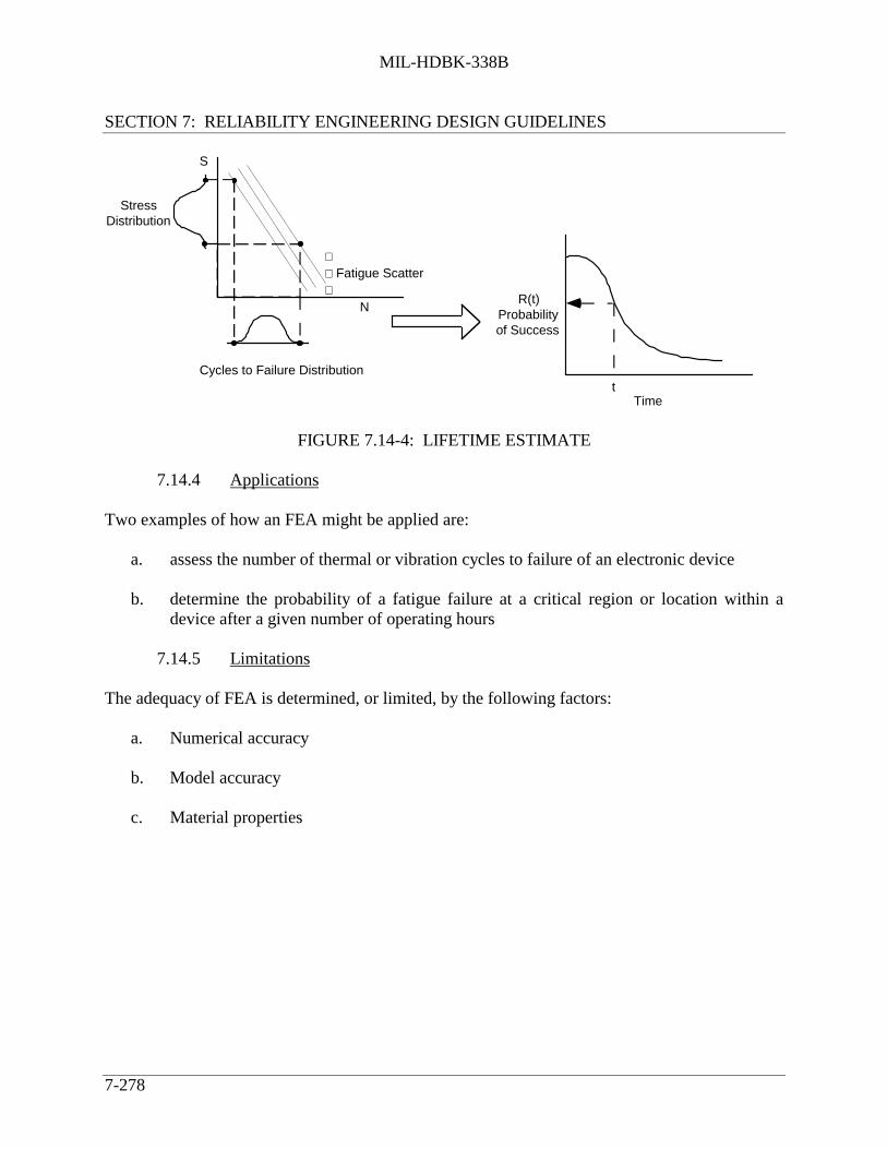
MIL-HDBK-338B


7-278

S

N

Cycles to Failure Distribution

StressDistribution

Fatigue Scatter

R(t)Probabilityof Success

tTime

FIGURE 7.14-4: LIFETIME ESTIMATE

7.14.4 Applications

Two examples of how an FEA might be applied are:

a. assess the number of thermal or vibration cycles to failure of an electronic device

b. determine the probability of a fatigue failure at a critical region or location within adevice after a given number of operating hours

7.14.5 Limitations

The adequacy of FEA is determined, or limited, by the following factors:

a. Numerical accuracy

b. Model accuracy

c. Material properties

MIL-HDBK-338B


7-279


1. Parts Selection, Application, and Control (PASC), Reliability Analysis Center, Rome,NY, 1993.

2. Reliable Application of Plastic Encapsulated Microcircuits, (PEM2), Reliability AnalysisCenter, Rome, NY, 1995.

3. Analog Testing Handbook, (ATH), Reliability Analysis Center, Rome, NY, 1993.

4. 767 AWACS Strategies for Reducing Diminishing Manufacturing Sources (DMS) Risk,DMSMS (Diminishing Manufacturing Sources and Material Shortages) 96 Conference,Montgomery, Texas, 7-9 May 96.

5. Best Practices - How to Avoid Surprises in the World’s Most Complicated TechnicalProcess, NAVSO P6071.

6. Precondition of Plastic Surface Mount Devices Prior to Reliability Testing, JESD 22-A113.

7. General Standard for Statistical Process Control, JEDEC Publication 19.

8. JEDEC Registered and Standard Outlines for Semiconductor Devices, JEDECPublication 95.

9. Impact of Moisture on Plastic IC Package Cracking IPC-SM-786.

10. Test Method, Surface Mount Component Cracking, IPC-TM-650.

11. Buying Commercial and Nondevelopmental Items: A Handbook, SD-2, Office of theUnder Secretary of Defense for Acquisition and Technology, April 1996.

12. Lipson, C., et al., Reliability Prediction -- Mechanical Stress/Strength InterferenceModels, RADC-TR-68-403, March 1967.

13. Lipson, C., et al., Reliability Prediction--Mechanical Stress/Strength Interference(nonferrous), RADC-TR-68-403, December 1968.

14. Nonelectronic Reliability Notebook, RADC-TR-85-194, October 1985.

15. Electronic Engineers' Handbook. Fink, D.G. and D. Christiansen, ed., New York, NY:McGraw Hill Book Co., 1982.

MIL-HDBK-338B


7-280

16. Engineering Design Handbook: Reliable Military Electronics. AMCP 706-124,Headquarters U.S. Army Materiel Command, 5001 Eisenhower Ave, Alexandria, VA22333, AD#A025665.

17. IEEE Recommended Practice on Surge Voltages in Low Voltage AC Power Circuits ,IEEE Standard C62.41-1991.

18. Engineering Design Handbook: Design for Reliability, AMCP 706-196, AD#A027230,January 1976.

19. Lewis, E.E., Introduction to Reliability Engineering, John Wiley & Sons, Inc., New York,1996.

20. Practical Reliability, Vol. 1 - Parameter Variations Analysis, NASA CR-1126, ResearchTriangle Institute, Research Triangle Park, NC, July 1968.

21. Ross, P., Taguchi Techniques for Quality Engineering, McGraw-Hill, New York, 1988.

22. Klion, J., A Redundancy Notebook, RADC-TR-77-287, December 1977, AD#A050837.

23. Shooman, M., Probabilistic Reliability: An Engineering Approach, New York, NY,McGraw-Hill Book Co., 1968.

24. Barrett, L.S., Reliability Design and Application Considerations for Classical and CurrentRedundancy Schemes, Lockheed Missiles and Space Co., Inc., Sunnyvale, CA,September 30,1973.

25. Application of Markov Techniques, IEC 1165, 1995.

26. Engineering Design Handbook: Environmental Series, Part One: Basic EnvironmentalConcepts, AMCP 706-115, AD#784999.

27. Engineering Design Handbook: Environmental Series, Part Two: natural EnvironmentalFactors, AMCP 706-116, AD#012648.

28. Engineering Design Handbook: Environmental Series, Part Three: InducedEnvironmental Factors, AMCP 706-117, AD#023512.

29. Engineering Design Handbook: Environmental Series, Part Four: Life CycleEnvironments, AMCP 706-118, AD#0151799.

30. Engineering Design Handbook: Environmental Series, Part Five: Glossary ofEnvironmental Terms, AMCP 706-119.

MIL-HDBK-338B


7-281

31. Engineering Design Handbook: Design for Reliability. AMCP 706-196, AD#A027370,January 1976.

32. Arsenault, J.E. and J.A. Roberts, “Reliability and Maintainability of Electronic Systems,”Computer Science Press, 9125 Fall River lane, Potomac, MD 20854, 1980.

33. Pavia, R.V., An Investigation into Engine Wear Caused by Dirt, Aeronautical ResearchCommittee Report, ACA-50, July 1950.

34. Engineering Design Handbook: Design Engineer’s Nuclear Effects Manual, Vol. I,Munitions and Weapon Systems (U), AMCP 706-335 (SRD).

35. Engineering Design Handbook: Design Engineer’s Nuclear Effects Manual, Vol. II,Electronic Systems and Logistical Systems (U), AMCP 706-336 (SRD).

36. Engineering Design Handbook: Design Engineer’s Nuclear Effects Manual, Vol. III,Nuclear Environment (U), AMCP 706-337 (SRD).

37. Engineering Design Handbook: Design Engineer’s Nuclear Effects Manual, Vol. IV,Nuclear Effects (U), AMCP 706-338 (SRD).

38. Dougherty, E.M. and J.R. Fragola, Human Reliability Analysis, Wiley, 1988.

39. Lee, K.W., F.A. Tillman, and J.J. Higging, “A Literature search of the Human ReliabilityComponent in a Man-Machine System,” IEEE Transactions on Reliability, Vol. 37, No.1, 1988 Apr, pp. 24-34.

40. Meister, D., “A Comparative Analysis of Human Reliability Models, Final Report,Contract N00024-71-C-1257,” Naval Sea Systems Command, 1971 Nov.

41. Apostolakis, G.E., G. Mancini, R.W. van Otterloo, and F.R. Farmer, eds., “Special Issueon Human Reliability Analysis,” Reliability Engineering & System Safety, Vol. 29, No. 3,ISBN:0951-8320, 1990.

42. LaSala, K.P., “Survey of Industry Human Performance Reliability Practices,” IEEEReliability Society Newsletter, Vol. 36, No. 2, 1990 Apr, pp. 7-8.

43. D.D. Woods, L.J. Johannesen, Richard I Cook, N.B. Sarter, Behind Human Error:Cognitive Systems, Computers, and Hindsight, Crew Systems Ergonomics InformationAnalysis Center, 1994.

44. Watson, P.A. and W. Hebenstreit, “Manpower, Personnel, and Training Workshop GroupReport (IDA Record Document D-35),” Institute of Defense Analysis, 1983.

MIL-HDBK-338B


7-282

45. Reason, J., Human Error, Cambridge University Press, 1992.

46. Siegel, A.I., K.P. LaSala, and C. Sontz, Human Reliability Prediction System User’sManual, Naval Sea Systems Command, 1977 Dec.

47. Blanchard, B.S., System Engineering Management, Wiley, 1991.

48. Advisory Group on Reliability of Electronic Equipment (AGREE), "Reliability ofMilitary Electronic Equipment, “Office of the Assistant Secretary of Defense, 1957 4 Jun,pp. 52-57.

49. Blanchard, B.S. and W.J. Fabricky, System Engineering Analysis, Prentice-Hall, 1990.

50. Taha, H., Operations Research: An Introduction, Macmillan, 1971.

51. Bazovski, I., Sr., “Weapon System Operational Readiness,” Proceedings 1975 R&MSymposium, IEEE, 1975, pp. 174-178.

52. Van Cott, H.P. and R.G. Kinkade, Human Engineering Guide to Equipment Design (2ndEdition), Joint Army-Navy-Air Force Steering Committee, US Government PrintingOffice, 1972.

53. Boff, K.R., L. Kaufman, and J. Thomas, Handbook of Perception and HumanPerformance (Vols. 1 and 2), Wiley, 1986.

54. Boff, K. R. and Lincoln, J. E., Engineering Data Compendium: Perception andPerformance (Vols. 1-3), Wright-Patterson AFB, OH: Armstrong Aerospace MedicalResearch Laboratory, 1988.

55. Booher, H. R., Ed, MANPRINT: An Approach to Systems Integration, Van NostrandReinhold, 1990.

56. Munger, S.J., R.W. Smith, and D. Paynes, “An Index of Electronic EquipmentOperability: Data Store," (Air-C-43-1/62-RP[l]) (DTIC No. AD 607161), Pittsburgh PA,American Institute for Research, 1962 Jan.

57. Topmiller, D.A., J.S. Eckel, and E.J. Kozinsky, "Human Reliability Data Bank forNuclear Power Plant Operations, Volume l: A Review of Existing Human ErrorReliability Data Banks" (NUREG/CR-2744/1 of 2 and SAND82-70571/1 of 2, AN, RX),Dayton OH, General Physics Corp., 1982 Dec .

58. Haney, L.N., H.S. Blackman, B.J. Bell, S.E. Rose, D.J. Hesse, L.A. Minton, and J.P.Jenkins, "Comparison and Application of Quantitative Human Reliability Analysis

MIL-HDBK-338B


7-283

Methods for the Risk Methods Integration and Evaluation Program (RMIEP),"NUREG/CR-4835, Idaho National Engineering Laboratory, Idaho Falls, ID, Jan. 1989.

59. Lydell, B.O.Y., "Human Reliability Methodology. A Discussion of the State of the Art,"Reliability Engineering and System Safety, 36 (1992), pp. 15-21.

60. Dougherty, E.M., "Human Reliability Analysis; Need, Status, Trends, and Limitations,"Reliability Engineering and System Safety, 29(1990), pp. 283-289.

61. Swain, A.D., "Human Reliability Analysis: Need, Status, Trends and Limitations,"Reliability Engineering and Systems Safety, 29(1990), pp. 301-313.

62. Swain, A.D., "THERP", SC-R-64-1338, Sandia National Laboratories, Albuquerque,NM, 1964 Aug.

63. Swain, A. D., and Guttman, H.E., Handbook of Human Reliability Analysis withEmphasis on Nuclear Power Plant Applications (NUREG/CR-1278, SAND800 200, RX,AN), Sandia National Laboratories, Albuquerque, NM, 1983 Aug.

64. Poucet, A., "The European Benchmark Exercise on Human Reliability Analysis,"Proceedings of the International Topical Meeting on Probability, Reliability, and SafetyAssessment, PSA ’89, American Nuclear Society, Inc., La Grange, IL, 1989, pp. 103-110.

65. Guassardo, G., "Comparison of the Results Obtained from the Application of ThreeOperator Action Models," Proceedings of the International Topical Meeting onProbability, Reliability, and Safety Assessment, PSA ’89, American Nuclear Society, Inc.,La Grange , IL, 1989, pp. 111-119.

66. Krois., P.A., P.M. Haas, J.J. Manning, and R. Bovell, "Human Factors Review for SevereAccident Sequence Analysis" NUREG/CR-3887, Oak Ridge National Laboratory, OakRidge TN, 1985 Nov., p. 26.

67. Hannaman, G.W., A.J. Spurgin, and Y.D. Lukic, "Human Cognitive Reliability for PRAAnalysis," NUS-4531, NUS Corp., 1984, Dec.

68. Joksimovich, V., A.J. Spurgin, D.D. Orvis, and P. Moieni, "EPRI Operator ReliabilityExperiments Program: Model Development/Testing," Proceedings of the InternationalTopical Meeting on Probability, Reliability, and Safety Assessment, PSA ’89, AmericanNuclear Society, Inc., La Grange Park IL, 1989 Apr., pp. 120-127.

69. Dhillon, B.S., Human Reliability With Human Factors, Pergamon, 1988.

70. Dhillon, B.S., "Modeling Human Errors in Repairable Systems", Proceedings of the 1989Reliability and Maintainability Symposium, IEEE, New York, NY, pp. 418-423.

MIL-HDBK-338B


7-284

71. Siegel, A.I., and J.J. Wolf, Man-Machine Simulation Models, Wiley, 1969.

72. Siegel, A.I., W.D. Barter, J.J. Wolf, and H.E. Knee, "Maintenance Personnel PerformanceSimulation (MAPPS) Model: Description of Model Content, Structure, and SensitivityTesting," NUREG/CR-3626, Oak Ridge National Laboratory, Oak Ridge, TN, 1984 Dec.

73. Woods, D.D., E.M. Roth, and H. Pople, Jr, "Cognitive Environment Simulation: AnArtificial Intelligence System for Human Performance Assessment," NUREG/CR-4862,Westinghouse Research and Development Center, Pittsburgh, PA, 1987 Nov.

74. Embrey, D.E., "The Use of Performance Shaping Factors and Quantified ExpertJudgement in the Evaluation of Human Reliability: An Initial Appraisal," NUREG/CR-2986, Brookhaven National Laboratory, 1983.

75. Embrey, D.E., P. Humphreys, E.A.Rosa, B. Kirwan, K. Rea, "SLIM-MAUD, AnApproach to Assessing Human Error Probabilities Using Structured Expert Judgement,"NUREG/CR-3518, U.S. Nuclear Regulatory Commission, 1984.

76. Rosa, E.A., P.C. Humphreys, C.M. Spettell, and D.E. Embrey, "Application of SLIM-MAUD: A Test of an Interactive Computer-based Method for Organizing ExpertAssessment of Human Performance and Reliability," NUREG/CR-4016, BrookhavenNational Laboratory, Upton, NY, 1985 Sep.

77. Ireson, W.G., and C.F. Coombs, Handbook of Reliability Engineering and Management,New York, McGraw-Hill, 1988, Ch 12.

78. Procedures for Performing a Failure Mode, Effects, and Criticality Analysis, MIL-STD-1629, 28 Nov 1984.

79. Analysis Techniques for System Reliability - Procedure for Failure Mode and EffectsAnalysis (FMEA) , IEC 812, 1985.

80. Surface Vehicle Recommended Practice: Potential Failure Mode and Effects Analysis inDesign (Design FMEA) and Potential Failure Mode and Effects in Manufacturing(Process FMEA) Reference Manual , SAE J-1739, July 1994.

81. Michels, J.M., "Computer Evaluation of the Safety Fault Tree Model," ProceedingsSystem Safety Symposium, 1965, available from University of Washington Library,Seattle, WA.

82. Henley, E.J., and J.W. Lynn (Eds), Generic Techniques in System Reliability Assessment,Nordhoff, Leyden, Holland, 1976.

MIL-HDBK-338B


7-285

83. Vesely, W.E., "A Time-Dependent Methodology for Fault Tree Evaluation," NuclearEngineering and Design, 13, 2 August 1970.

84. Fault Tree Handbook. NUREG-0492, available from Division of Technical Informationand Document Control, U.S. Nuclear Regulatory Commission, Washington, DC 20555.

85. Fault Tree Analysis , IEC 1025, 1990.

86. Sneak Circuit Analysis for the Common Man, RADC-TR-89-223.

87. Integration of Sneak Circuit Analysis with Design, RADC-TR-90-109.

88. Automated Sneak Circuit Analysis Technique, Rome Air Development Center, GriffissAir Force Base, N.Y., 13441, 1990.

89. SCAT: Sneak Circuit Analysis Tool, Version 3.0, RL-TR-95-232.

90. Clardy, R.C., "Sneak Circuit Analysis Development and Application," 1976 Region V,IEEE Conference Digest, 1976, pp. 112-116.

91. Hill, E.J., and L.J. Bose, "Sneak Circuit Analysis of Military Systems," Proceedings ofthe 2nd International System Safety Conference, July 1975, pp. 351-372.

92. Buratti, D.L., and Goday, S.G., Sneak Analysis Application Guidelines. RADC-TR-82-179, Rome Air Development Center, Griffiss Air Force Base, N.Y., 13441, June 1982.

93. Godoy, S.G., and G.J. Engels, "Sneak Circuit and Software Sneak Analysis," Journal ofAircraft, Vol. 15, August 1978, pp. 509-513.

94. Definition of Terms for Testing Measurement and Diagnostics, MIL-STD-1309,February 1992.

95. Testability Program for Electronic Systems and Equipments, MIL-HDBK-2165, July1995.

96. Skeberdis, P.W., E.G. White, Fault Logging Using a Micro Time Stress MeasurementDevice, RL-TR-95-289, Westinghouse Electronics Systems, January 1996.

97. Havey, G., S. Louis, S. Buska, Micro-Time Stress Measurement Device Development,RL-TR-94-196, Honeywell, Inc., November 1994.

98. Environmental Characterization Device Sourcebook (ECDS), Reliability Analysis Center,PO Box 4700, Rome, NY 13342-4700, September 1995.

MIL-HDBK-338B


7-286

99. Testability Design Rating System: Testability Handbook and Analytical Procedure,(2 Vols.), RL-TR-92-12.

100. Testability Program for Systems and Equipment, MIL-HDBK-2165, January 1985.

101. Electromagnetic Properties and Effects of Advanced Composite Materials: Measurementand Modeling, RADC-TR-78-156.

102. Electromagnetic Shielding Effectiveness for Isotropic and Anisotropic Materials,RADC-TR-81-162.

MIL-HDBK-338B

SECTION 8: RELIABILITY DATA COLLECTION AND ANALYSIS,DEMONSTRATION, AND GROWTH

8-1

8.0 RELIABILITY DATA COLLECTION AND ANALYSIS, DEMONSTRATION,AND GROWTH

8.1 Introduction

Successful or satisfactory operation - the goal of all design efforts - yields little information onwhich to base improvements. Failures, on the other hand, contribute a wealth of data on “what toimprove” or “what to design against” in subsequent efforts. The feedback of informationobtained from the analysis of failures is one of the principal stepping stones of progress.

The prediction or assessment of reliability is actually an evaluation of unreliability, the rate atwhich failures occur. The nature and underlying cause of failures must be identified andcorrected to improve reliability. Reliability data consist of reports of failures and reports ofduration of successful operation of the monitored equipment/system.

Reliability data is used for three main purposes:

(1) To verify that the equipment is meeting its reliability requirements

(2) To discover deficiencies in the equipment to provide the basis for corrective action

(3) To establish failure histories for comparison and for use in prediction

Reliability data can also be useful in providing information about logistics, maintenance, andoperations. The data can provide a good estimate of the degradation and wearout characteristicsof parts and components and how spare parts requirements are affected.

From this information, not only can effective preventive maintenance routines to control frequenttrouble areas be developed, but also an estimate can be obtained of the number of maintenancemanhours required to assure a desired level of reliability.

It is important that the data be factual so that a high degree of credence may be placed in theconclusions derived from it. Incomplete and inaccurate reporting will inevitably lead to eithercomplete loss of confidence in the data or to incorrect conclusions and, hence, incorrect decisionsand actions based on the conclusions.

MIL-HDBK-338B


8-2

Reliability/failure data can be obtained from a number of sources.

(1) An in-house failure analysis and corrective action system (FRACAS)

(2) Reliability test data

(3) Subcontractor or vendor data

(4) Field data

(5) Reliability data banks

The most useful of the above sources are (1) and (2), and possibly (5). The other sources are notas reliable since they are, in most cases, incomplete. For example, the military maintenancecollection systems for collecting field data (e.g., the Army’s TAMMS, the Navy’s 3M, and the AirForce’s REMIS and other maintenance data collection systems) are primarily maintenanceoriented (see Section 11). Thus, field reliability cannot be assessed by using data from thesesystems alone. All of the factors influencing the data need to be clearly understood. Thesefactors include the ground rules for collecting the data, assumptions made during analysis, and soforth. Clearly understanding these factors assures that the data will be properly interpreted andthat conclusions will be credible.

The following section provides more details on a FRACAS system. The sections on ReliabilityTesting and Growth discuss the collection and analysis of reliability test data.

8.2 Failure Reporting, Analysis, and Corrective Action System (FRACAS) andFailure Review Board (FRB)

8.2.1 Failure Reporting, Analysis and Corrective Action System (FRACAS)

The purpose of FRACAS is to collect failure data, provide procedures to determine failure cause,and document corrective action taken. It requires the contractor to have a system that collects,analyzes and records failures that occur for specified levels of assembly prior to acceptance of thehardware by the procuring activity.

Failure reporting and analysis is necessary to ensure that a product’s reliability andmaintainability will be achieved and sustained. The FRACAS program is a key element in“failure recurrence” control for newly developed and production equipment. A FRACASprogram must include provisions to ensure that failures are accurately reported and thoroughlyanalyzed and that corrective actions are taken on a timely basis to reduce or prevent recurrence.

MIL-HDBK-338B


8-3

An in-plant FRACAS determines the basic causes of failures associated with design ormanufacturing, and provides a closed-loop method of implementing corrective action. Thesystem should emphasize the investigation and analysis of all failures, regardless of theirapparent frequency or impact, and classification of failures according to categories of design/partprocurement, manufacture, or assembly and inspection. It is well known that the mosteconomical repair of a failure occurs at the component part level. A conventional rule of thumbis that a repair action at the subassembly level costs an order of magnitude more than at the partlevel, and a repair at the product level costs an order of magnitude more than a repair at thesubassembly level.

Data on electronic equipment malfunctions can be obtained from any or all of the following typesof data sources:

(1) Design verification tests

(2) Pre-production tests

(3) Production tests

(4) Subcontractor tests

(5) Field data

The FRACAS system must provide essential information on:

(1) What failed

(2) How it failed

(3) Why it failed

(4) How future failures can be eliminated

8.2.1.1 Closed Loop Failure Reporting/Corrective Actions System

Figure 8.2-1 indicates the main steps in a closed-loop FRACAS. As shown in Figure 8.2-1, atypical FRACAS consists of fourteen steps.

(1) A failure is observed during some operation or test.

(2) The observed failure is fully documented, including, as a minimum(a) Location of failure(b) Date and time of failure

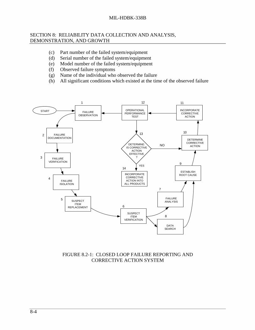
MIL-HDBK-338B


8-4

(c) Part number of the failed system/equipment(d) Serial number of the failed system/equipment(e) Model number of the failed system/equipment(f) Observed failure symptoms(g) Name of the individual who observed the failure(h) All significant conditions which existed at the time of the observed failure

1

OPERATIONALPERFORMANCE

TEST

FAILUREOBSERVATION

FAILUREDOCUMENTATION

START

DATASEARCH

FAILUREVERIFICATION

FAILUREISOLATION

SUSPECTITEM

REPLACEMENT

FAILUREANALYSIS

ESTABLISHROOT CAUSE

DETERMINECORRECTIVE

ACTION

INCORPORATECORRECTIVEACTION INTO

ALL PRODUCTS

14

SUSPECTITEM

VERIFICATION

INCORPORATECORRECTIVE

ACTION

2

3

4

5

6

7

8

9

11

10

12

13

DETERMINE:IS CORRECTIVE

ACTIONEFFECTIVE

?

YES

NO

FIGURE 8.2-1: CLOSED LOOP FAILURE REPORTING ANDCORRECTIVE ACTION SYSTEM

MIL-HDBK-338B


8-5

(3) Failure verification (i.e., reconfirmation of the validity of the initial failure observation).

(4) Failure isolation (i.e., localization of the failure to the lowest replaceable defective itemwithin the system/equipment).

(5) Replacement of the suspected defective item with a known good item and retest of thesystem/equipment to provide assurance that the replacement item does in fact correctthe originally reported failure.

(6) Retest of the suspect item at the system/equipment level or at a lower level to verify thatthe suspect item is defective.

(7) Failure analysis of the defective item to establish the internal failure mechanismresponsible for the observed failure or failure mode.

(8) A search of existing data to uncover similar failure occurrences in this or related items(i.e., establishing the historical perspective of the observed failure mode/failuremechanism).

(9) Utilizing the data derived from Steps 7 and 8, determine the antecedent or root cause ofthe observed failure.

(10) Determine the necessary corrective action, design change, process change, procedurechange, etc. to prevent future failure recurrence. The decision regarding the appropriatecorrective action should be made by an interdisciplinary design team.

(11) Incorporation of the recommended corrective action into the original testsystem/equipment.

(12) Retest of the system/equipment with the proposed corrective action modificationincorporated.

(13) After suitable retest and review of all applicable data, determine if proposed correctiveaction is effective.

(14) After the effectiveness of the proposed corrective action has been proven, the correctiveaction is then incorporated into the deliverable systems/equipment.

MIL-HDBK-338B


8-6

There are several “keys” that make the failure reporting and corrective action cycle effective.These are:

(1) The discipline of the report writing itself must be maintained so that an accuratedescription of failure occurrence and proper identification of the failed items areensured.

(2) The proper assignment of priority and the decision for failure analysis must be madewith the aid of cognizant design engineers and systems engineers.

(3) The status of all failure analyses must be known. It is of prime importance that failureanalyses be expedited as priority demands and that corrective action be implemented assoon as possible.

(4) The root cause of every failure must be understood. Without this understanding, nologically derived corrective actions can follow.

(5) There must be a means of tabulating failure information for determining failure trendsand the mean times between failures of system elements. There should also be a meansfor management visibility into the status of failure report dispositions and correctiveactions.

(6) The system must provide for high level technical management concurrence in theresults of failure analysis, the soundness of corrective action, and the completion offormal actions in the correction and recurrence prevention loop.

(7) An extremely valuable assurance mechanism is to have active Government involvementin surveillance of the adequacy of the failure reporting, analysis, and corrective actioneffort.

The contractor's program plan should clearly describe his proposed FRACAS. Furthermore itshould identify those provisions incorporated therein to ensure that effective corrective actionsare taken on a timely basis. The applicable statement of work (SOW) should identify the extentto which the contractor's FRACAS must be compatible with the procuring agency's data system.It should also identify the levels of assembly and test to be addressed by the FRACAS, givedefinitions for each of the failure cause categories, identify the applicable logistics supportrequirements and identify the data items required for delivery.

MIL-HDBK-338B


8-7

8.2.1.2 Failure Reporting Systems

Normally a manufacturer’s reliability engineering organization is responsible for instituting andmanaging FRACAS. They establish policy, provide direction, and monitor the status ofFRACAS investigations. The cognizant inspection and testing organizations, includingreliability and quality engineering, are responsible for initiating failure reports promptly as theyare observed. The project management office generally reviews recommendations, coordinatesanalyses and test activities with the government, authorizes the implementation of acceptablefixes or corrective measures and provides direction relative to continuation of tests. Often, it isthe quality assurance organization that transmits reports to the government and coordinatesimplementation of corrective actions.

8.2.1.3 Failure Reporting Forms

It is imperative that failure reporting and resultant corrective actions be documented. Therefore,failure reporting and corrective actions forms must be designed to meet the needs of theindividual system development and production program as well as the organizationalresponsibilities, requirements, and constraints of the manufacturer. Figure 8.2-2 is an example ofa typical failure report form used in a FRACAS system.

8.2.1.4 Data Collection and Retention

Maintaining accurate and up-to-date records through the implementation of the data reporting,analysis and corrective action system described in the preceding subsections provides a dynamic,expanding experience base. This experience base, consisting of test failures and correctiveactions, is not only useful in tracking current programs but can also be applied to thedevelopment of subsequent hardware development programs. Furthermore, the experience datacan be used to:

(1) Assess and track reliability

(2) Perform comparative analysis and assessments

(3) Determine the effectiveness of quality and reliability activities

(4) Identify critical components and problem areas

(5) Compute historical part failure rates for new design reliability prediction (in lieu ofusing generic failure rates found in MIL-HDBK-217, for example)

MIL

-HD

BK

-338

B

SE

CT

ION

8:

RE

LIA

BIL

ITY

DA

TA

CO

LL

EC

TIO

N A

ND

AN

AL

YS

IS,

DE

MO

NS

TR

AT

ION

, AN

D G

RO

WT

H

8-8

DO

C. N

O.

SEC

ON

DA

RY

DO

CU

ME

NT

TR

AC

FA

ILU

RE

AN

D D

EFE

CT

RE

POR

TD

AT

E

CO

NT

INU

ED

DO

CU

ME

NT

MFG

. JO

B I

TE

MPT

. NO

. (FA

ILE

D I

TE

M)

NO

ME

NC

LA

TU

RE

SER

.NO

. OR

DA

TE

CO

DE

CO

NT

INU

ED

TO

DO

C. N

O.

IF E

ITH

ER

, E

NT

ER

PR

IMA

RY

DO

C.

NO

. HE

RE

SHO

P O

RD

ER

SUB

MIS

SIO

NN

O.

TE

ST N

O.

TE

STC

OM

PLE

TE

DFA

TP

LO

T S

IZE

SAM

PLE

SIZ

E#

AC

CE

PTE

D#

RE

JEC

TE

DT

EST

UN

ITT

EST

ER

CO

GN

IZA

NT

FO

RE

MA

N

DE

F. #

CH

AR

. #D

EFE

CT

CO

DE

QT

Y.

DE

SCR

IPT

ION

OF

DE

FE

CT

WH

EN

MO

RE

TH

AN

ON

E S

N O

R D

AT

EC

OD

E, L

IST

EA

CH

HE

RE

DIS

P. #

AU

TH

OR

IZA

TIO

N

TR

OU

BL

ESH

OO

TIN

G/R

EP

AIR

PA

RT

VE

RIF

ICA

TIO

NSE

CO

ND

AR

Y

DE

F. #

RE

PAIR

CO

DE

DE

SCR

IPT

ION

FAIL

UR

EC

AU

SEC

IRC

UIT

DE

SIG

NA

TO

RPA

RT

NA

ME

RE

PLA

CE

D I

TE

MPA

RT

NO

.SU

B-A

SSY

S/N

OR

PT. D

AT

E C

OD

EC

ON

NE

CT

ED

BY

INSP

.V

ER

IFIE

D G

OO

DV

ER

IFIC

AT

ION

FIN

DIN

GS

DO

C #

QU

AL

ITY

& C

OM

PO

NE

NT

RE

VIE

WC

LE

AR

ED

BY

DE

F #

DIS

P. #

CO

MM

EN

TC

ON

NE

CT

ED

BY

INSP

.

Q.E

.D

AT

EP&

E/E

T/P

RO

GR

N.

EN

GR

DA

TE

FA

ILU

RE

AN

AL

YSI

S R

EP

OR

TD

EF

#M

AN

UFA

CT

UR

ER

AN

AL

YST

DA

TE

FAIL

UR

E A

NA

LY

SIS

RE

POR

T N

O.

FAIL

UR

EC

AU

SE C

OD

E

TH

IS D

OC

UM

EN

T S

TA

YS

WIT

H O

RIG

INA

L F

AIL

ED

IT

EM

UN

TIL

CL

EA

RE

D.

FO

RE

MA

N S

HO

UL

D M

AK

E C

OP

IES

FOR

EA

CH

SE

PA

RA

TE

D C

OM

PO

NE

NT

PA

RT

.FO

RE

MA

N S

HO

UL

D E

NT

ER

AP

PR

OP

RIA

TE

DE

FEC

T N

UM

BE

R O

N C

OP

IES

IN Q

UA

LIT

Y A

ND

CO

MP

ON

EN

T R

EV

IEW

SE

CT

ION

. A

T C

OM

PL

ET

ION

OF

INIT

IAL

DIS

PO

SIT

ION

FO

R S

EP

AR

AT

ED

CO

MP

ON

EN

T P

AR

TS

A S

EC

ON

DA

RY

DO

CU

ME

NT

SH

OU

LD

BE

FIL

LE

D O

UT

FO

R E

AC

H S

EP

AR

AT

E A

SSE

MB

LY

.

FIG

UR

E 8

.2-2

: E

XA

MPL

E O

F FA

ILU

RE

RE

POR

T F

OR

M

MIL-HDBK-338B


8-9

8.2.2 Failure Review Board

For the acquisition of certain critical (extremely expensive and complex) systems andequipments, a separate Failure Review Board (FRB) may sometimes be established specificallyto oversee the effective functioning of the FRACAS. The Failure Review Board activity isreliability management. A closed loop FRACAS with an FRB is illustrated in Figure 8.2-3.

FAILUREOBSERVATION

INCORPORATECORRECTIVEACTION INTO

DEVELOP EQUIP

YES

NO

DATASEARCH

ESTABLISHROOT

CAUSE

FAILUREDOCUMENTATION

FAILUREVERIFICATION

FAILUREISOLATION

SUSPECTITEM

REPLACEMENT SUSPECTITEM

VERIFICATION

FAILUREANALYSIS

FAILUREREVIEWBOARD

END ITEMTEST

DETERMINECORRECTIVE

ACTIONINCORPORATE

CORRECTIVEACTION INTOPRODUCTION

ISCORRECTIVE

ACTIONEFFECTIVE

?

START

FIGURE 8.2-3: CLOSED LOOP FAILURE REPORTING AND CORRECTIVE ACTIONSYSTEM WITH FAILURE REVIEW BOARD

The purpose of the Failure Review Board is to provide increased management visibility andcontrol of the FRACAS. Its intent is to improve reliability and maintainability of hardware andassociated software by the timely and disciplined utilization of failure and maintenance data. TheFRB consists of a group of representatives from appropriate organizations with sufficient level ofresponsibility to ensure that failure causes are identified with enough detail to generate andimplement effective corrective actions which are intended to prevent failure recurrence and tosimplify or reduce the maintenance tasks.

MIL-HDBK-338B


8-10

The FRB usually consists of higher level management personnel who possess the authority to setpriorities, establish schedules, assign specific responsibility and authorize adequate funding toinsure the implementation of any necessary changes when dealing with complex and difficultproblems. The acquiring activity usually reserves the right to appoint a representative to the FRBas an observer.

8.3 Reliability Data Analysis

From a reliability assessment viewpoint, failure data are used to:

(1) Determine the underlying probability distribution of time to failure and estimate itsparameters (if not already known)

(2) Determine a point estimate of a specific reliability parameter, e.g., MTBF

(3) Determine a confidence interval that is believed to contain the true value of theparameter

Two methods are used to analyze failure data:

(1) Graphical methods

(2) Statistical analysis

In many practical cases, graphical methods are simple to apply and produce adequate results forestimating the underlying distribution. They are virtually always a useful preliminary to moredetailed statistical analysis. The two methods will be discussed in more detail in the followingsubsections.

8.3.1 Graphical Methods

The basic idea of graphical methods is the use of special probability plotting papers in which thecumulative distribution function (cdf) or the cumulative hazard function can be plotted as astraight line for the particular distribution being studied. Since a straight line has two parameters(slope and intercept), two parameters of the distribution can be determined. Thus, reliability datacan be evaluated quickly, without a detailed knowledge of the statistical mathematics beingnecessary. This facilitates analysis and presentation of data.

Graphical curve-fitting techniques and special probability-plotting papers have been developedfor all of the distributions commonly associated with reliability analysis (Refs. [4], [5]).

Ranking of Data

Probability graph papers are based upon plots of the variable of interest against the cumulative

MIL-HDBK-338B


8-11

percentage probability. The data, therefore, need to be ordered, and the cumulative probabilitycalculated. For reliability work, the data are ordered from the smallest to largest; this is referredto as order statistics. For example, consider the data on times-to-failure of 20 items (Table 8.3-1). For the first failure, the cumulative percent failed is 1/20 or 5%. For the second, thecumulative percent failed is 2/20 or 10%, and so on to 20/20 or 100% for the 20th failure.However, for probability plotting, it is better to make an adjustment to allow for the fact that eachfailure represents a point on a distribution. Thus, considering that the whole population of 20items represents a sample, the times by which 5, 10, ..., 100% will have failed in several samplesof 20 will be randomly distributed. However, the data in Table 8.3.1-1 show a bias, in that thefirst failure is shown much further from the zero cumulative percentage point than is the lastfrom 100% (in fact, it coincides). To overcome this, and thus to improve the accuracy of theestimation, mean or median ranking of cumulative percentages is used for probability plotting.Mean ranking is used for symmetrical distributions, e.g., normal; median ranking is used forskewed distributions, e.g., Weibull.

The usual method for mean ranking is to use (n + 1) in the denominator, instead of n, whencalculating the cumulative percentage position. Thus in Table 8.3-1 the cumulative percentages(mean ranks) would be:

120 + 1 = .048 ≅ 5%

220 +1 = .096 ≅ 10%

...

2020 + 1 = .952 ≅ 95%

MIL-HDBK-338B


8-12

TABLE 8.3-1: DATA ON TIMES TO FAILURE OF 20 ITEMS

Time to Cumulative % Mean RankOrder No. Failure (hours) (Cdf) (%) (Cdf)

1 175 5 52 695 10 103 872 15 144 1250 20 195 1291 25 246 1402 30 297 1404 35 338 1713 40 389 1741 45 4310 1893 50 4811 2025 55 5212 2115 60 5713 2172 65 6214 2418 70 6715 2583 75 7116 2725 80 7617 2844 85 8118 2980 90 8619 3268 95 9020 3538 100 95

These data are shown plotted on normal probability paper in Figure 8.3-1 (circles). The plottedpoints show a reasonably close fit to the straight line drawn ’by eye.’ Therefore, we can say thatthe data appear to fit the cumulative normal distribution represented by the line.

Median ranking, as was previously stated, is used for skewed distributions such as the Weibullbecause it provides a better correction. The most common approximation for median ranking(Ref. [4]) is given by:

Median rank (n,i) = ri = i - 0.3n + 0.4

where ri is the ith

order value and n is the sample size. Median ranking is the method most usedin probability plotting, particularly if the data are known not to be normally distributed. Also, tosave calculations, tables of median ranks are available for use. These are included in Table 8.3-2and will be used in the examples to be described later.

MIL-HDBK-338B


8-13

8.3.1.1 Examples of Graphical Methods

Reference [5] provides an excellent discussion of caveats that must be considered in graphicalestimation. Now, let us turn to some examples.

Example 1: Normal Distribution

1. When to Use

This method estimates µ and σ, the mean and standard deviation when failure times are normallydistributed. This method yields a less accurate estimate than statistical analysis but requires veryminimal calculations.

2. Conditions for Use

a. Failure times must be collected, but may be censored; censored data isdiscussed in the next section.

b. Normal probability paper is required.

3. Method Example

a. On normal probability paper plot

the ith

failure time in a sample of nordered failure times on the lower

axis vs. i

n + 1 on the right hand

axis.

a. The sample data used in Table8.3-1 are repeated here, with thenecessary plotting positions (meanranks).

MIL-HDBK-338B


8-14

0 500 1000 1500 2000 2500 3000 3500 4000.01

.1

1

5

10

20

30

50

70

80

90

95

99

99.9

99.99

.1

1

5

10

20

30

50

70

80

90

95

99

99.9

.01PE

RC

EN

T FA

ILE

D

PER

CE

NT

ST

ILL

FU

NC

TIO

NIN

G

L X U

16

1l

HOURS

99.99

FIGURE 8.3-1: GRAPHICAL POINT ESTIMATION FORTHE NORMAL DISTRIBUTION

MIL-HDBK-338B


8-15

TABLE 8.3-2: MEDIAN RANKS

sample size = nfailure rank = i

n

i 1 2 3 4 5 6 7 8 9 101 .5000 .2929 .2063 .1591 .1294 .1091 .0943 .0830 .0741 .06702 .7071 .5000 .3864 .3147 .2655 .2295 .2021 .1806 .16323 .7937 .6136 .5000 .4218 .3648 .3213 .2871 .25944 .8409 .6853 .5782 .5000 .4404 .3935 .35575 .8706 .7345 .6352 .5596 .5000 .45196 .8906 .7705 .6787 .6065 .54817 .9057 .7979 .7129 .64438 .9170 .8194 .74069 .9259 .836810 .9330

n

i 11 12 13 14 15 16 17 18 19 201 .0611 .0561 .0519 .0483 .0452 .0424 .0400 .0378 .0358 .03412 .1489 .1368 .1266 .1788 .1101 .1034 .0975 .0922 .0874 .08313 .2366 .2175 .2013 .1873 .1751 .1644 .1550 .1465 .1390 .13224 .3244 .2982 .2760 .2568 .2401 .2254 .2125 .20099 .1905 .18125 .4122 .3789 .3506 .3263 .3051 .2865 .2700 .2553 .2421 .23026 .5000 .4596 .4253 .3958 .3700 .3475 .3275 .3097 .2937 .27937 .5878 .5404 .5000 .4653 .4350 .4085 .3850 .3641 .3453 .32838 .6756 .6211 .5747 .5347 .5000 .4695 .4425 .4184 .3968 .37749 .7634 .7018 .6494 .6042 .5650 .5305 .5000 .4728 .4484 .426410 .8511 .7825 .7240 .6737 .6300 .5915 .5575 .5272 .5000 .475511 .8389 .8632 .7987 .7432 .6949 .6525 .6150 .5816 .5516 .524512 .9439 .8734 .8127 .7599 .7135 .6725 .6359 .6032 .573613 .9481 .8822 .8249 .7746 .7300 .6903 .6547 .622614 .9517 .8899 .8356 .7875 .7447 .7063 .671715 .9548 .8966 .8450 .7991 .7579 .720716 .9576 .9025 .8535 .8095 .769817 .9600 .9078 .8610 .818818 .9622 .9126 .867819 .9642 .916920 .9659

MIL-HDBK-338B


8-16

3. Method (continued) Example

Failure PlottingTime Position

(Hours) i n+1

175 .05695 .10872 .141250 .191291 .241402 .291404 .331713 .381741 431893 .482025 .522115 .572172 .622418 .672583 .712725 .762844 .812980 .863268 .903538 .95

b. Draw the line of best fit through theplotted points by using the lastpoint plotted as a reference pointfor a straight edge and dividing therest of the points into two equalgroups above and below the line.

b. Figure 8.3-1 is the plot of this data onnormal paper. The normal line hasbeen labeled l1.

c. The mean, µ, is estimated byprojecting the 50% probability offailure point on the right hand axisto the line and then projecting thatintersection point down to thelower axis. The estimate of µ, x , isread there.

c. The value of X is read as 2000

hours.

MIL-HDBK-338B


8-17

3. Method Example

d. The estimate of σ is obtained byfirst projecting the intersection ofthe 84% probability of failure pointon the right hand axis with thenormal line to the lower axis. Callthat point on the lower axis U.

d. U = 2900 hours

e. Repeat step d with the 16% point.Call the point L

e. L = 1100 hours

f. The estimate of σ is

s = U - L

2

f. The sample standard deviation is

s = U - L

2 = 2900 - 1100

2 = 900

hours

g. The 95% confidence limits around

the mean are given by X ± t s/ n

where t is shown below for varioussample sizes, n.

n t5 2.5710 2.2320 2.0930 2.0450 2.00

∞ 1.96

g. 2000 ± (2.09) (900)/ 20 2000 ± 420 hours

MIL-HDBK-338B


8-18

Example 2: Weibull Distribution

1. When to Use. The flexibility of the Weibull distribution makes it useful in describing theprobability density function for a variety of cases. The Weibull cumulative distributionfunction is given by:

( )[ ]F(t) = 1 - e , 0 t1 t /θ β

≤ ≤ ∞

The Weibull distribution is used to describe the distribution of times to failure and of strengths ofbrittle materials, and the weakest link phenomena. It is an appropriate failure law modelwhenever the system consists of a number of components, and failure is essentially due to the“most severe” fault among a large number of faults in the system. By making an appropriatechoice of the shape parameter, β, either an increasing or a decreasing failure rate can be obtained.Estimates of the Weibull shape (β) and scale (θ) parameters may be obtained graphically usingln-ln (or a special Weibull probability) graph paper. Less accurate than statistical methods, thismethod can be done quickly and easily.

2. Steps in Using the Graphical Method

a. Collect failure times for items under test, put in ascending order, and assign an ordernumber to each. The failure times are the values to be plotted on the x-axis. Note thatfailure time may be in hours, cycles, or whatever measure of life is appropriate for theitem in question.

b. Assign the median rank for each order number. The median ranks are the values to beplotted on the y-axis. The median rank is one model used for the cumulativeprobability of failures, F(t). It is usable when the number of failures is greater than 20.The formula is:

Median Rank (n,i) =

i − 0.3n + 0.4

where: n = number of failuresi = order number

c. Plot the pairings of median ranks and failure times on Weibull probability graph paper.Draw a straight line that best fits the data (i.e., roughly an equal number of data pointswill be on either side of the line).

MIL-HDBK-338B


8-19

d. The slope of the line is β. The slope is calculated using the following equation:

β = ( ) ( )

1

12 1

1

1

1

t

tFtF

XY

ln -t ln

lnlnlnln

2

−

−

−

=∆∆

Note 1: This equation assumes that ln-ln paper is used. Log-log paper can also be usedwith the following equation:

β = ( ) ( )

1

12 1

1

1

1

t

tFtF

log -t log

lnlnlog

2

−

−−

−

−log

Note 2: Some special Weibull graph paper allows β to be read directly.

3. Example

The following failure data are collected from a test in which 20 items were tested to failure.

Order Number Failure Time (in hours) Median Rank (%)1 92 3.412 130 8.313 233 13.224 260 18.125 320 23.026 325 27.937 420 32.838 430 37.749 465 42.64

10 518 47.5511 640 52.4512 700 57.3613 710 62.2614 770 67.1715 830 72.0716 1010 76.9817 1020 81.8818 1280 86.7819 1330 91.6920 1690 96.59

MIL-HDBK-338B


8-20

Figure 8.3-2 shows the data plotted on ln-ln graph paper. From the graph, θ is 739.41 hours.β is:

β = 5311

051

1

991

1

... =

−−

−=∆∆

05 ln -2000 ln

lnlnlnln

XY

The reliability at t = 1000 hours is found by drawing a line up vertically from t=1000 on theabscissa to the line. Then, from that point a horizontal line is drawn to the ordinate. It intersectsthe ordinate at F(t) = 80%. The reliability is 1- F(t) = 20% (i.e., 20% percent probability of nofailure).

1

5

2

10

20

30 40

50 60

70 80

90 95

99

10 100 1000 10000

F(t)

%

Time to Failure (Hours)

θ

∆Y

∆X

(t2, F2)

(t1, F1)

θ = 739.41 β = 5311

1

1

1

12 .)()(

=−

−

−

−

=∆∆

12 t lnt ln

lnlnlnlntFtF

XY

FIGURE 8.3-2: GRAPHICAL POINT ESTIMATION FORTHE WEIBULL DISTRIBUTION

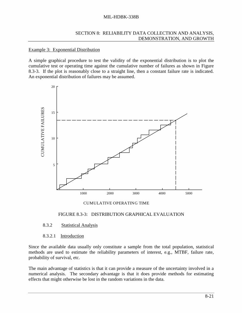
MIL-HDBK-338B


8-21

Example 3: Exponential Distribution

A simple graphical procedure to test the validity of the exponential distribution is to plot thecumulative test or operating time against the cumulative number of failures as shown in Figure8.3-3. If the plot is reasonably close to a straight line, then a constant failure rate is indicated.An exponential distribution of failures may be assumed.

CUMULATIVE OPERATING TIME

CU

MU

LA

TIV

E F

AIL

UR

ES

1000 2000 3000 4000 5000

5

10

15

20

FIGURE 8.3-3: DISTRIBUTION GRAPHICAL EVALUATION

8.3.2 Statistical Analysis

8.3.2.1 Introduction

Since the available data usually only constitute a sample from the total population, statisticalmethods are used to estimate the reliability parameters of interest, e.g., MTBF, failure rate,probability of survival, etc.

The main advantage of statistics is that it can provide a measure of the uncertainty involved in anumerical analysis. The secondary advantage is that it does provide methods for estimatingeffects that might otherwise be lost in the random variations in the data.

MIL-HDBK-338B


8-22

It is important to keep in mind the fact that data constitute a sample from the total population,that random sampling peculiarities must be smoothed out, that population density parametersmust be estimated, that the estimation errors must themselves be estimated, and - what is evenmore difficult - that the very nature of the population density must be estimated. To achievethese ends, it is necessary to learn as much as one can about the possible population densityfunctions, and especially what kind of results we can expect when samples are drawn, the dataare studied, and we attempt to go from data backward to the population itself. It is also importantto know what types of population densities are produced from any given set of engineeringconditions. This implies the necessity for developing probability models, or going from a set ofassumed engineering characteristics to a population density.

It is customary, even necessary, in statistical analysis to develop, from physical engineeringprinciples, the nature of the underlying distribution. The sample of data is then compared againstthe assumed distribution.

The usual parameter of interest in reliability is the distribution of times to failure, called theprobability density function or failure density function. The failure density function may bediscrete, that is, only certain (integer) values may occur, as in tests of an explosive squib.Success or failure will occur on any trial, time not being considered. Or it may be continuous,any value of time to failure being possible.

Typically histograms are plotted (e.g., time-to-failure plots) and statistical techniques used to firsttest the data to determine the applicable form of the probability distribution, and then identifyand evaluate the relationship between the reliability parameter(s), such as failure rate, and thecritical hardware characteristics/attributes which affect reliability (such as technology,complexity, application factors, etc.) as defined by the data.

8.3.2.2 Treatment of Failure Data

Failure data are usually obtained from a) test results or b) field failure reports. Experience hasshown that a good way to present these data is to compute and plot either the failure densityfunction, f(t), or the hazard rate, h(t), as a function of time.

Remember from Section 5 that f(t) is given by the ratio of the number of failures occurring in thetime interval to the size of the original population, divided by the length of the time interval. Thehazard rate, h(t), on the other hand, is given by the ratio of the number of failures occurring in thetime interval to the number of survivors at the beginning of the time interval, divided by thelength of the time interval.

Although f(t) and h(t) are defined as continuous functions, piecewise continuous functions of f(t)and h(t) are computed, graphed results are examined, and a continuous model is chosen whichbest fits the data.

MIL-HDBK-338B


8-23

Once having found f(t) from the data, F(t) (the cumulative distribution of time to failure) andR(t) = 1 - F(t), the reliability function or survival probability, can be readily determined from therelationships.

F(t) =

−∞

t

∫ f(t) dt (8.1)

R(t) = 1 - F(t) (8.2)

Two examples follow.

Example 4:

TABLE 8.3-3: FAILURE DATA FOR TEN HYPOTHETICALELECTRONIC COMPONENTS

Failure Number Operating Time, Hr.1 82 203 344 465 636 867 1118 1419 18610 266

From Table 8.3-4 and Eq. (8.1) and (8.2) one can calculate and plot F(t) and R(t). The dataplots for the various function of interest are shown in Figure 8.3-4.

Note, from the dashed lines of Figure 8.3-4 (a) and (b), that the exponential distribution oftime to failure represents a good approximation to the data.

MIL-HDBK-338B


8-24

TABLE 8.3-4: COMPUTATION OF DATA FAILURE DENSITYAND DATA HAZARD RATE

Time Interval, Hourt

Failure Density per Hour

f(t) x 10-2

Hazard Rate per Hour

h(t) x 10-2 0 - 8 1

10 x 8 = 1.251

10 x 8 = 1.25

8 - 20 110 x 12 = 0.83

19 x 12 = 0.93

20 - 34 110 x 14 = 0.71

18 x 14 = 0.89

34 - 46 110 x 12 = 0.83

17 x 12 = 1.19

46 - 63 110 x 17 = 0.59

16 x 17 = 0.98

63 - 86 110 x 23 = 0.43

15 x 23 = 0.87

86 - 111 110 x 25 = 0.40

14x 25 = 1.00

111 - 141 110 x 30 = 0.33

13 x 30 = 1.11

141 - 186 110 x 45 = 0.22

12 x 45 = 1.11

186 - 266 110 x 80 = 0.13

11 x 80 = 1.25

MIL-HDBK-338B


8-25

0.0

0.2

0.4

0.6

0.8

1.0

1.2

1.4

0 100 200 300

Operating time, hr(a)

f(t)

frac

tion

al f

ailu

res

/ hr

x 1

0-2

0.0

0.20

0.40

0.60

0.80

1.0

0 50 100 150 200 250 300Operating time, hr

(c)

F(t)

failu

re d

istr

ibut

ion

func

ition

.

0.0

0.20

0.40

0.60

0.80

1.00

1.2

1.4

0 100 200 300

Operating time, hr(b)

h(t)

failu

res

/ s

urv

ivor

/ h

r x

10 -2

0.0

0.20

0.40

0.60

0.80

1.0

0 50 100 150 200 250 300

Operating time, hr(d)

(Rel

iabi

lity)

R(t

), su

cces

s fu

ncti

on

FIGURE 8.3-4: HAZARD AND DENSITY FUNCTIONS FOR TABLE 8.3-3

MIL-HDBK-338B


8-26

Example 5:

Data for a single B-52 performing 1000 missions of 2 to 24 hours, or the equivalent of 1000B-52s performing a single mission of 2 to 24 hours, are shown in Tables 8.3-5 and 8.3-6 andFigure 8.3-5 (Ref. [6]). This data shows that the B-52 is most likely to fail in the first twohours of its mission. The exponential distribution of times to failure does not fit well to thedata.

TABLE 8.3-5: FAILURE DATA FOR 1,000 B-52 AIRCRAFT

Time Until

Failure, Hour

Number of Failures inInterval

f(t)

Failure Density/Hr.

h(t)

Hazard Rate/Hr.0 - 2 222 222

1,000 x 2 = 0.1110222

1,000 x 2 = 0.1110

2 - 4 45 451,000 x 2 = 0.0225

45778 x 2 = 0.0289

4 - 6 32 321,000 x 2 = 0.0160

32733 x 2 = 0.0218

6 - 8 27 271,000 x 2 = 0.0135

27701 x 2 = 0.0192

8 - 10 21 211,000 x 2 = 0.0105

21674 x 2 = 0.0156

10 - 12 15 151,000 x 2 = 0.0075

15653 x 2 = 0.0113

12 - 14 17 171,000 x 2 = 0.0085

17638 x 2 = 0.0133

14 - 16 7 71,000 x 2 = 0.0035

7621 x 2 = 0.0056

16 - 18 14 141,000 x 2 = 0.0070

14614 x 2 = 0.0114

18 - 20 9 91,000 x 2 = 0.0045

9600 x 2 = 0.0075

20 - 22 8 81,000 x 2 = 0.0040

8591 x 2 = 0.0068

22 - 24 3 31,000 x 2 = 0.0015

3583 x 2 = 0.0026

TOTAL 420

MIL-HDBK-338B


8-27

TABLE 8.3-6: TIME-TO-FAILURE DATA FOR S = 1000 MISSION HOURS

TIME-TO- FAILURE(HOURS) CUMULATIVE FAILURES = F

R =

1000 − F1000

2 222 .7784 267 .7336 299 .7018 326 .67410 347 .65312 362 .63814 379 .62116 386 .61418 400 .60020 409 .59122 417 .58324 420 .580

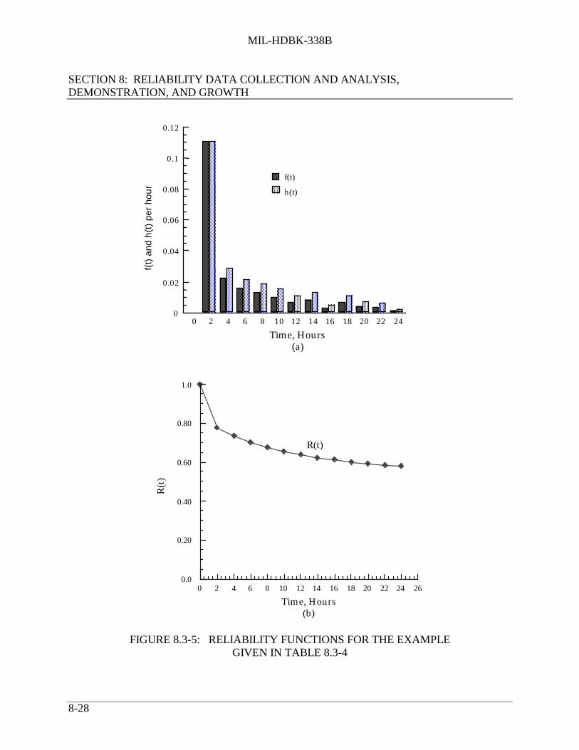
MIL-HDBK-338B


8-28

.

0.0

0.20

0.40

0.60

0.80

1.0

0 2 4 6 8 10 12 14 16 18 20 22 24 26

R(t

)

Time, Hours(b)

R(t)

FIGURE 8.3-5: RELIABILITY FUNCTIONS FOR THE EXAMPLEGIVEN IN TABLE 8.3-4

f(t)

h(t)

0

0.02

0.04

0.06

0.08

0.1

0.12

0 2 4 6 8 10 12 14 16 18 20 22 24

Time, Hours(a)

f(t)

and

h(t

)pe

rho

ur

MIL-HDBK-338B


8-29

8.3.2.3 Reliability Function (Survival Curves)

A survival curve or reliability function, R(t), is a graphic representation of the relationshipbetween the probability of survival and time. Here, probability of survival is synonymous withprobability of nonfailure or probability of satisfactory performance. Three types of survivalcurves are of primary interest. The first is a discrete or point-type curve derived from observeddata by nonparametric or distribution-free methods. The second type is a continuous curve basedon an assumption as to the form of the distribution (Gaussian, exponential, etc.) and on values ofthe distribution parameters estimated from the observed data. The third type of curve is the truereliability function of the population from which the sample observations were drawn. This lastfunction can only be estimated (i.e., not determined precisely), although the limits within whichit will fall a given percentage of the time can be defined.

Figure 8.3-6 presents a frequency distribution of failures in a fixed population of 90 items, over a6-hour period. To obtain a survival curve from these data, the following simplified method isused.

During the first period of observation, from 0 to 1 hour, 4 of the original 90 items failed. Thefailure rate during this period was 4/90, or 0.0444, which is equivalent to a survival rate of1 - 0.0444, or 0.9556. In the second period of observation, 21 of the 86 remaining items failed.The failure rate was 21/86, or 0.244, and the survival rate was 1 - 0.244, or 0.756. The tabulationabove Figure 8.3-7 gives the failure rates and survival rates for the remaining periods ofobservation. It will be noted that the failure rate increases with time.

To obtain a survival curve, which is the cumulative probability of survival with time, theprobability of survival in each time period is multiplied by the survival rate in the succeedingtime period. Thus, 0.9555 x 0.756 = 0.723; 0.723 x 0.538 = 0.388, etc. The probability valuesare plotted versus the centers of the time periods as shown at the bottom of 8.3-7.

Figure 8.3-8 presents a frequency distribution of failures for a population of 90 items in whichthe removal rate is constant with time. The approach described in connection with the normalcurve yields the tabulation and exponential survival curve shown in Figure 8.3-9. (Note in thisexample, only 83 of 90 items failed in six hours).

Survival curves for most electronic equipment/systems are of the exponential form. Survivalcurves for mechanical parts, on the other hand, are frequently of the normal or Weibull form. Asparts wear out, their failure rate increases and their probability of survival decreases. A largenumber of such parts, all having normal or Weibull survival curves but each having a differentmean life and variance, will produce a system malfunction rate which is essentially constant,since the mean lives of the parts will be randomly distributed.

MIL-HDBK-338B


8-30

0

10

20

30

40

1 2 3 4 5 6

HOURS

NU

MB

ER

OF

FAIL

UR

ES

4

FIGURE 8.3-6: NORMAL DISTRIBUTIONOF FAILURE IN TIME

0

10

20

30

40

50

1 2 3 4 5 6

HOURS

NU

MB

ER

OF

FAIL

UR

ES

FIGURE 8.3-8: EXPONENTIALDISTRIBUTION OF FAILURES IN TIME

FAILURE SURVIVAL PROBABILITYTIME RATE RATE OF SURVIVAL0 - 1 0.444 0.9556 0.95551 - 2 0.2442 0.7558 0.72302 - 3 0.4615 0.5385 0.38803 - 4 0.7143 0.2857 0.11104 - 5 0.8000 0.2000 0.02205 - 6 1.0000 0.0000 - - -

FAILURE SURVIVAL PROBABILITYTIME RATE RATE OF SURVIVAL0 - 1 0.333 0.667 0.6671 - 2 0.333 0.667 0.4442 - 3 0.350 0.650 0.2893 - 4 0.346 0.654 0.1894 - 5 0.353 0.647 0.1225 - 6 0.364 0.636 0.078

NOTE: Population is 90 for all figures.

0.0

0.2

0.4

0.6

0.8

1.0

0 1 2 3 4 5 6CALCULATION AND PRESENTATION

OF A NORMAL SURVIVAL CURVE

PR

OB

AB

ILIT

Y O

F SU

RV

IVA

L

FIGURE 8.3-7: CALCULATION ANDPRESENTATION OF A NORMAL

SURVIVAL CURVE

0.0

0.2

0.4

0.6

0.8

1.0

0 1 2 3 4 5 6

HOURS

PRO

BA

ILIT

Y O

F SU

RV

IVA

L

FIGURE 8.3-9: CALCULATION ANDPRESENTATION OF AN EXPONENTIAL

CURVE

HOURS # OFFAILURES

0 - 1 41 - 2 212 - 3 303 - 4 254 - 5 85 - 6 2

HOURS # OF FAILURES

0 - 1 301 - 2 202 - 3 143 - 4 94 - 5 65 - 6 4

MIL-HDBK-338B


8-31

To determine what type of population gives rise to a particular survival curve, the theoreticalreliability function most closely resembling the curve is computed from sample parameters. Thetheoretical function is then matched to the observed curve by statistical techniques. If thisprocedure establishes that there is no significant difference between the observed and theoreticalcurves, the theoretical curve is usually employed for all additional calculations.

Figures 8.3-10 and 8.3-11 portray observed and theoretical probability of survival curves for thecase of exponential and normal distributions of time to failure. Note that the mean life for theexponential case has R(t) = 0.368, whereas for the normal case, R(t) = 0.5. This is due to thesymmetrical characteristic of the normal distribution, versus the skewed characteristic of theexponential.

Thus, if one can develop a mathematical expression for R(t), it can be shown that the mean timeto failure is given by:

MTTF = 0

∞

∫ R(t) dt (8.3)

8.3.2.3.1 Computation of Theoretical Exponential Reliability Function

When the form of the distribution is sufficiently well defined, it is possible to estimate thereliability function in terms of the parameters of the distribution. This method has the advantageof permitting utilization of all the accumulated knowledge concerning the items in thepopulation. In addition, the reliability function can be summarized by specifying the values ofthe parameters, and can be compared with other reliability functions merely by comparing thevalues of the summarized data.

For the case of an equipment/system which is repaired upon failure, the reliability function isgiven by:

R(t) = e-t/MTBF (8.4)

MIL-HDBK-338B


8-32

.

0 1000 2000 3000 4000 5000 6000 7000 8000 9000

PRO

BA

BIL

ITY

OF

SUR

VIV

AL

TIME IN HOURS

MEAN LIFE

SAMPLE MEAN LIFE ≅ 3230 HOURS

95% CONFIDENCE LIMITS = 2395 - 4615 HOURS

_____ OBSERVED

- - - - THEORETICAL

0.0

0.2

0.4

0.6

0.8

1.0

FIGURE 8.3-10: OBSERVED AND THEORETICAL EXPONENTIALSURVIVAL CURVES

.

0.0

0.2

0.4

0.6

0.8

1.0

0 1000 2000 3000 4000 5000 6000 7000 8000 9000

PR

OB

AB

ILIT

Y O

F SU

RV

IVA

L

TIME IN HOURS

SAMPLE MEAN LIFE ≅ 2950 HOURS

STANDARD DEVIATION ≅ 1000 HOURS95% CONFIDENCE LIMITS = 2711 - 3189 HOURS

OBSERVED- - - - - THEORETICAL

MEAN LIFE

FIGURE 8.3-11: OBSERVED AND THEORETICAL NORMALSURVIVAL CURVES

MIL-HDBK-338B


8-33

where:t = time at which R(t) is calculatedMTBF = mean time between failures, given by

MTBF = ntr (8.5)

andn = the number of equipments operated to time tr = the number of failures, with the last failure occurring at time t

For example, assume that in a sample of twenty equipments operated for 773 hours, we observed10 failures (each of which was repaired), with the last failure occurring at 773 hours.

Then

MTBF =ntr =

(20)(773)10 = 1546 hours

R(t) = e-t/1546

Table 8.3-7 shows the computations for R(t) for selected values of t. Figure 8.3-12 shows theactual reliability function (solid line) plotted from the data versus the theoretical exponentialfunction from column 3 of Table 8.3-7. Determination of confidence intervals is discussed brieflyin the next section.

8.3.2.3.2 Computation For Normal Reliability Function

Table 8.3-8 presents some observed failure data for a sample of twenty units tested to failure, andthe failure times observed. The units were known to follow a normal distribution of time tofailure.

The sample mean, X , an estimate of µ, is given by:

X = i=1

20

∑ Xi /n = 39104

20 = 1955.2 hours

MIL-HDBK-338B


8-34

TABLE 8.3-7: COMPUTATION OF THEORETICAL EXPONENTIALRELIABILITY FUNCTION FOR MTBF = 1546 HOURS

(1)t

(2)t/MTBF

(3)

e-t/MTBF 0 0 1.00096 0.0621 0.9389216 0.1397 0.8696312 0.2018 0.8173456 0.2950 0.7445552 0.3571 0.6997696 0.4502 0.6375792 0.5123 0.5991888 0.5744 0.5630960 0.6210 0.53741200 0.7762 0.46021416 0.9159 0.40021546 1.0000 0.36791896 1.2264 0.29332064 1.3351 0.2631

0.0

0.2

0.4

0.6

0.8

1.0

0 400 800 1200 1600 2000 2400

OPERATING TIME, t, IN HOURS

PRO

BA

BIL

ITY

OF

SUR

VIV

AL

R(t

)

BAR DENOTES 95% CONFIDENCEINTERVAL ABOUT SAMPLE MEAN

MTBF = 1546.0 HOURS

Actual Theoretical

FIGURE 8.3-12: ACTUAL RELIABILITY FUNCTION AND THEORETICALEXPONENTIAL RELIABILITY FUNCTION

MIL-HDBK-338B


8-35

TABLE 8.3-8: OBSERVED FAILURE DATA

Probability of Probability ofTime Survival, R Time Survival, R

175 0.95 2025 0.45695 0.90 2115 0.40872 0.85 2172 0.351250 0.80 2418 0.301291 0.75 2583 0.251402 0.70 2725 0.201404 0.65 2844 0.151713 0.60 2980 0.101741 0.55 3268 0.051893 0.50 3538 0.00

The sample standard deviation, s, an estimate of σ, is given by:

52

20

1

1

.

iis

n

)XX(

−

−∑== = 886.6 hours

where:

Xi = ith

failure time

n = sample size

X = sample mean

Figure 8.3-13 shows the actual or nonparametric reliability function plotted from the data versusthe theoretical function calculated using the estimates of µ and σ. The theoretical values wereobtained from the expression

R(x) = P

z > X - µ

σ

where the value of z was obtained from a table of the Standard Normal Distribution (Table 5.3.1of Section 5).

MIL-HDBK-338B


8-36

0.0

0.1

0.2

0.3

0.4

0.5

0.6

0.7

0.8

0.9

1.0

0 500 1000 1500 2000 2500 3000 3500

TIME TO FAILURE, t, IN HOURS

PRO

BA

BIL

ITY

OF

SUR

VIV

AL

R(t

)

FIGURE 8.3-13: NON-PARAMETRIC AND THEORETICALNORMAL RELIABILITY FUNCTIONS

8.3.2.4 Censored Data

If a sample contains both complete and incomplete lifetimes, the incomplete lifetimes arereferred to as “censored” observations. These consist primarily of lifetimes which are too long tobe observed completely (“terminated” observations) and lifetimes in which the item beingobserved is lost before completion of observation (“lost” observation). In the case of terminatedobservations, the length of observation time is controlled; in the case of lost observations, thelength of observation time is not controlled. In either case, the investigator knows that thelifetime of the item exceeds the period of time during which the item was being observed.Terminated observations do not present a problem to the investigator other than to increase thecomplexity of the calculations, but lost observations may constitute a real problem because theymaybe associated with only a portion of the population.

For example, for the case of the exponential distribution in which n items are put on test, r of

them fail at time t1, t2 . . . tr, with the test discontinued at tr when the rth

failure occurs, theMTBF is given by

MTBF = i=1

r

∑ t i + (n − r)tr

n(8.6)

MIL-HDBK-338B


8-37

where ti is the time of each failure and (n - r) represents the number of surviving items at time tr.In this nonreplacement case, the failed items are not repaired or replaced upon failure.

The mathematics become somewhat more difficult when analyzing censored data wheredistributions other than the exponential are involved, or when using nonparametric methods.These cases are treated in detail in References [1], [3], [4] and [5].

8.3.2.5 Confidence Limits and Intervals

Previously, we discussed methods of obtaining point estimates of reliability parameters, e.g.,R(t), λ, MTBF, etc. For most practical applications, we are interested in the accuracy of the pointestimate and the confidence which we can attach to it. We know that statistical estimates aremore likely to be closer to the true value as the sample size increases. Only the impossiblesituation of having an infinitely large number of samples to test could give us 100 percentconfidence or certainty that a measured value of a parameter coincides with the true value. Forany practical situation, therefore, we must establish confidence intervals or ranges of valuesbetween which we know, with a probability determined by the finite sample size, that the truevalue of the parameter lies.

Confidence intervals around point estimates are defined in terms of a lower confidence limit, L,and an upper confidence limit, U. If, for example, we calculate the confidence limits for aprobability of, say, 95 percent, this means that in repeated sampling, 95 percent of the calculatedintervals will contain the true value of the reliability parameter. If we want to be 99 percent surethat the true value lies within certain limits for a given sample size, we must widen the interval ortest a larger number of samples if we wish to maintain the same interval width. The problem,then, is reduced to one of either determining the interval within which the true parametric valuelies with a given probability for a given sample size, or determining the sample size required toassure us with a specified probability that true parametric value lies within a specific interval.

Thus, we would like to be able to make assertions such as

P ( )[ ]UL θθθ ˆˆ << = η (8.8)

where θ is some unknown population parameter, θL and θU are estimators associated with arandom sample and η is a probability value such as 0.99, 0.95, 0.90, etc. If, for instance,η = 0.95 we refer to the interval

( )Uθ<θ<θL (8.9)

for particular values of Lθ and Uθ as a 95% confidence interval. In this case we are willing to

accept a 5% probability (risk) that our assertion is not, in fact, true.

MIL-HDBK-338B


8-38

Or, we may also want to make statements such as

P [ ]Lθθ ˆ> = η (8.10)

in which case we make statements like, “we are 90% confident that the true MTBF is greater thansome lower confidence limit (or measured value).” Eq. (8.10) is the case of the one-sidedconfidence limit, versus Eq. (8.9) which is a two-sided confidence limit, or confidence interval.

To help clarify the concept of a confidence interval we can look at the situation in a geometrical

way. Suppose we draw repeated samples (x1, x2) from a population, one of whose parameterswe desire to bracket with a confidence interval. We construct a three-dimensional space with the

vertical axis corresponding to θ and with the two horizontal axes corresponding to values of X1

and X2 (see Figure 8.3-14). The actual value of the population parameter θ is marked on thevertical axis and a horizontal plane is passed through this point. Now we take a random sample

(X1, X2) from which we calculate the values Uθ and Lθ at, say, the 95% confidence level. The

interval defined by Uθ and Lθ is plotted on the figure.

Next, we take a second sample (X’1 , X’2 ) from which we calculate the value U’θ and L’θ at the

95% level. This interval is plotted on the figure. A third sample (X"1 , X"2 ) yields the values

U"θ and L"θ , etc. In this way we can generate a large family of confidence intervals. The

confidence intervals depend only on the sample values (X1 , X2 ), (X’1 , X’2 ), etc., and hence we

can calculate these intervals without knowledge of the true value of θ. If the confidence intervalsare all calculated on the basis of 95% confidence and if we have a very large family of theseintervals, then 95% of them will cut the horizontal plane through θ (and thus include θ) and 5%of them will not.

The process of taking a random sample and computing from it a confidence interval is equivalentto the process of reaching into a bag containing thousands of confidence intervals and grabbingone at random. If they are all 95% intervals, our chance of choosing one that does indeed includeθ will be 95%. In contrast, 5% of the time we will be unlucky and select one that does not

include θ (like the interval ( U"θ , L"θ ) in Figure 8.3-14. If a risk of 5% is judged too high, we

can go to 99% intervals, for which the risk is only 1%. As we go to higher confidence levels(and lower risks) the lengths of the intervals increase until for 100% confidence levels (and lowerrisks) the interval includes every conceivable value of θ (I am 100% confident that the number ofdefective items in a population of 10,000 is somewhere between 0 and 10,000). For this reason100% confidence intervals are of little interest.

MIL-HDBK-338B


8-39

θθ

θ θ

θ

θ

θ

U

L

U

UL

L

’

"

"

’

X2

X1

FIGURE 8.3-14: GEOMETRICAL INTERPRETATION OF THE CONCEPTOF A CONFIDENCE INTERVAL

Let us now look at some simple examples of how these concepts are applied to analyze reliabilityfor some of the more commonly-used distributions.

8.3.2.5.1 Confidence Limits - Normal Distribution

When the lives of n components are known from a wearout test and we compute their mean, M ,and their standard deviation, s, and when n is large so that we can assume that s ≈ σ, the upperand lower confidence limits can be readily evaluated from Table 8.3-9 for the more commonly-used confidence levels.

Strictly speaking, this procedure of assigning confidence intervals to an estimate is correct onlywhen the true standard deviation, σ, of component wearout is known and used instead of s inTable 8.3-9. However, it can be applied in reliability work as an approximation whenever theestimate s, of σ, was obtained from a large sample, i.e., when the number of failures is at least

25, and preferably, more. In fact, it can be shown for samples of 20, kα/2 (at the 95% confidencelevel) is 2.09 vs. a value of 1.96 for an infinite number of samples. α is equal to100(1 - confidence level)%.

MIL-HDBK-338B


8-40

TABLE 8.3-9: CONFIDENCE LIMITS - NORMAL DISTRIBUTION

Two-sidedConfidence intervals Confidence levels

kα/2 M ± Kα/2 s/ n 100(1 - α)%

0.84 M ± 0.84s/ n 60.0

1.28 M ± 1.28s/ n 80.0

1.64 M ± 1.64s/ n 90.0

1.96 M ± 1.96s/ n 95.0

2.58 M ± 2.58s/ n 99.0

Figure 8.3-15 graphically illustrates what is being done. Since the normal distribution issymmetrical, we are computing the confidence interval as the area (1 - α) under the curve,leaving an area α/2 in each of the left and right hand tails which is outside of the confidence

interval (CI). For example, using the calculated values of ^Μ (or X ) and s obtained from the

data in Table 8.3-10, the CI at the 95% level is

M ± 1.96 s/ n = 1955.2 ± 1.96 (886.6)/ 20

= 1955.2 ± 388.6

= (2343.8, 1566.6)

In other words, we can be 95% confident that the true value of the mean life (M) lies between1566.6 and 2343.8 hours.

Actually, in reliability work, we are usually more interested in the lower confidence limit L of the

mean wearout life than in the upper limit. Given a measured value of M , we would like to makesome statement about our confidence that the true value of M exceeds some minimum value.

When only the lower confidence limit, L, is of interest, we apply the procedure of so-called “one-sided” confidence limits, as opposed to the two-sided CI of the preceding example. The problemis to assure ourselves (or our customer) that the true mean life, M, is equal to or larger than somespecified minimum value with a probability of (1 - α).

MIL-HDBK-338B


8-41

Confidence Interval

Area1 - α

α /2 α /2

-3 -2 -1 0 1 2 3-K α/2 K α/2

- K α/2[M σ(M)] + K α/2[M σ(M)][M]

FIGURE 8.3-15: TWO-SIDED CONFIDENCE INTERVAL AND LIMITS

Whereas in the case of the two-sided confidence limits, we had an area of α/2 under the left tailof the normal curve (Figure 8.3-15), we now have an area α to the left of L and an area (1 - α) tothe right.

Therefore, the estimate of mean life obtained from the data should be:

M ≥ L + Kα σ/ n (8.11)

If this equation is not satisfied, the requirement that the true M must be at least L at the specified100 (1 - α) percent confidence level has not been fulfilled.

Table 8.3-10, in which the assumption s ≈ σ is made, allows a quick check as to whether an

estimate, M , obtained from a sample of size n fulfills the requirement that the true M must notbe smaller than the specified minimum L. Only the more commonly-used confidence levels aregiven.

MIL-HDBK-338B


8-42

TABLE 8.3-10: CONFIDENCE INTERVAL

The estimate M must exceed: Confidence levels

K α/2 L + K α/2 s/ n 100 (1 - α)%

0.25 L + 0.25s/ n 600.52 L + 0.52s/ n 700.84 L + 0.84s/ n 801.28 L + 1.28s/ n 901.64 L + 1.64s/ n 952.33 L + 2.33s/ n 99

Once again, using the data and calculated values of M and s from Table 8.3-10, assume that wewould like to be 95% confident that the true M ≥ 1500 hours. The equation from Table 8.3-10 is

M ≥ L + 1.64 s/ n

1955.2 ≥ 1500 + 1.64 (886.6)/ 20

1955.2 ≥ 1500 + 325

1955.2 ≥ 1825

Since the inequality is satisfied, the requirement has been met.

As previously mentioned, the above procedure can be applied if the sample size n is at least 25.However, similar procedures also apply to smaller sample sizes except that now we cannotassume that s ≈ σ, and we must use another set of equations based on Student’s t distribution.

Actually, all we do is replace the normal percentage points Kα/2 and Kα in the previously

developed equations by the tabulated percentage points tα/2;n-1 and tα;n-1 of the t distribution,where n-1 is called the degrees of freedom and n is the number of failures. Student’s t tables areavailable in most standard statistical texts.

For example, for the two-sided CI example using the data from Table 8.3-10 and calculated

values of M and s,

MIL-HDBK-338B


8-43

M ± tα/2;n-1 s/ n = 1955.2 ± 2.09 (886.6)/ 20

= 1955.2 ± 414.4

= (2370, 1541.2)

which is a slightly wider CI than the case where it was assumed the s ≈ σ.

8.3.2.5.2 Confidence Limits - Exponential Distribution

Two situations have to be considered for estimating confidence intervals: one in which the test isrun until a preassigned number of failures (r*) occurs, and one in which the test is stopped after apreassigned number of test hours (t*) is accumulated. The formula for the confidence interval

employs the X2 (chi-square) distribution. A short table of X2 values is given in Table 8.3-11.

The general notation used is

χ2 p,d

where p and d are two constants used to choose the correct value from the table.

The quantity p is a function of the confidence coefficient; d, known as the degrees of freedom, is

a function of the number of failures. X2

α/2, 2r+2 for example, is the a

2 percentage point of the

chi-square distribution for (2r+2) degrees of freedom.

Equations (8.12) and (8.13) are for one-sided or two-sided 100(1 - α) percent confidenceintervals. For nonreplacement tests with a fixed truncation time, the limits are only approximate.Also, for non-replacement tests, only one sided intervals are possible for r = 0.

MIL-HDBK-338B


8-44

MIL-HDBK-338B


8-45

Equations for Confidence Limits on Mean Life

Type ofConfidence Limits

Fixed Number of

Failures, r*

Fixed Truncation

Time t*

One Sided(Lower Limit)

2Tχ2(α, 2r)

, ∞

2Tχ2(α, 2r + 2)

,∞

(8.12)

Two Sided(Upper and

Lower Limits)

2T

χ2(α2,2r)

, 2T

χ2(1-α2,2r)

2T

χ2(α2,2r+2)

, 2T

χ2(1-α2,2r)

(8.13)

The terms used are identified as follows:n = number of items placed on test at time t = 0t* = time at which the life test is terminatedθ = mean life (or MTBF for the case of replacement or repair upon failure)r = number of failures accumulated at time t*r* = preassigned number of failuresα = acceptable risk of error1 - α = confidence levelT = total test time

Note that T is computed as follows, depending on the type of test procedure.

Replacement Tests (failure replaced or repaired) T = nt* (8.14)

Non-Replacement Tests T = i =1

r

∑ ti + (n - r)t* (8.15)

where ti = time of the ith failure

Censored Items (withdrawal or loss of items which have not failed)

(a) If failures are replaced and censored items are not replaced

T = ∑j=1

c tj + (n - c)t* (8.16)

MIL-HDBK-338B


8-46

where:tj = time of censorship

c = number of censored items

(b) If failures are not replaced

T = i =1

r

∑ ti + j =1

c

∑ tj + (n - r - c)t* (8.17)

Example 6:

Twenty items undergo a replacement test. Testing continues until ten failures are observed. Thetenth failure occurs at 80 hours. Determine (1) the mean life of the items; and (2) the one-sidedand two- sided 95% confidence intervals for the MTBF.

(1) From Equation (8.4)

MTBF = nt*r =

(20)(80)10 = 160 hours

(2) α = 1 - Confidence Level = 1 - 0.95 = 0.05

2r = 2(number of failures) = 2(10) = 20

C( )

∞,2T

22

r

= C

∞

χ,

)(

),.( 200502

16002 = C

∞,31.41

3200 = C [101.88, ∞] = .95

That is, 101.88 hours is the lower (one-sided) 95% confidence limit of θ, the true mean life

where X2(0.05,20) = 31.41 is from Table 8.3-11.

In other words, we are 95% confident that the true MTBF exceeds 101.88 hours.


C

2T

χ2

α

2, 2r

, 2T

χ2

1 - α2, 2r

= C

320034.17 ,

32009.591 = C(93.65, 333.65) = .95

MIL-HDBK-338B


8-47

That is, 93.65 hours is the lower (two-sided) 95% confidence limit for the mean life and333.65 hours is the upper (two-sided) 95% confidence limit for that true mean. We are95% confident that the interval between 93.65 and 333.65 hours contains the true MTBF.

Example 7:

Twenty items undergo a nonreplacement test, which is terminated at 100 hours. Failure timesobserved were 10, 16, 17, 25, 31, 46, and 65 hours. Calculate (1) the one-sided approximate90% confidence interval (α = 0.10), and (2) the two-sided approximate 90% confidence limits ofθ, the mean life.

(1) From Equations (8.12) and (8.15)

C = C

∞χ

−+

∑=

,),(.

))((t ii

1610

1007202

2

7

1

= C

302023.54

, ∞

= C (128.3, ∞) = .90

128.3 hours is the lower single-sided 90% confidence limit for θ, the true mean life.


C

2T

χ2

α2 , 2r + 2

, 2T

χ2

1 - α2 , 2r

= C

302026.30 ,

30206.57

= C (114.83, 459.67) = .90

That is, 114.83 hours is the lower (two-sided) 90% confidence limit for θ, the true mean life, and459.67 hours is the upper (two-sided) 90% confidence limit.

Table 8.3-12 presents the factor 2/χ2p,d for one-sided and two-sided confidence limits, at six

confidence levels for each. Multiplying the appropriate factor by the observed total life T gives aconfidence limit on σ. Figure 8.3-16 presents a graphical technique for determining upper andlower confidence limits for tests truncated at a fixed time, when the number of failures is known.

MIL

-HD

BK

-338

B

SE

CT

ION

8:

RE

LIA

BIL

ITY

DA

TA

CO

LL

EC

TIO

N A

ND

AN

AL

YS

IS,

DE

MO

NS

TR

AT

ION

, AN

D G

RO

WT

H

8-48

TA

BL

E 8

.3-1

2: F

AC

TO

RS

FOR

CA

LC

UL

AT

ION

OF

ME

AN

LIF

EC

ON

FID

EN

CE

IN

TE

RV

AL

S F

RO

M T

ES

T D

AT

A (

FAC

TO

RS

= 2

/χ2 P,

D)

(Ass

umpt

ion

of E

xpon

entia

l Dis

trib

utio

n)99

% T

wo-

Sid

ed

9

9-1/

2% O

ne-S

ided

98%

One

-Sid

ed

99%

One

-Sid

ed95

% T

wo-

Sid

ed

9

7-1/

2% O

ne-S

ided

9

0% T

wo-

Sid

ed

95%

One

-Sid

ed 8

0% T

wo-

Sid

ed

90%

One

-Sid

ed60

% T

wo-

Side

d80

% O

ne-S

ided

dL

ower

Lim

itU

pper

Lim

it2 4 6 8 10 12 14 16 18 20 22 24 26 28 30 32 34 36 38 40

.185

.135

.108

.090

9.0

800

.070

2.0

635

.058

8.0

536

.050

0.0

465

.043

9.0

417

.039

2.0

373

.035

5.0

339

.032

5.0

311

.029

9

.217

.151

.119

.100

.085

7.0

759

.069

0.0

625

.057

1.0

531

.049

5.0

463

.043

8.0

413

.039

3.0

374

.035

7.0

342

.032

7.0

314

.272

.180

.139

.114

.097

6.0

856

.076

5.0

693

.063

3.0

585

.054

3.0

507

.047

6.0

449

.042

5.0

404

.038

5.0

367

.035

1.0

337

.333

.210

.159

.129

.109

.095

2.0

843

.076

0.0

693

.063

5.0

589

.054

8.0

513

.048

3.0

456

.043

3.0

411

.039

2.0

375

.035

9

.433

.257

.188

.150

.125

.107

.094

8.0

848

.076

9.0

703

.064

8.0

601

.056

1.0

527

.049

6.0

469

.044

5.0

423

.040

4.0

386

.619

.334

.234

.181

.149

.126

.109

.097

6.0

878

.079

9.0

732

.067

6.0

629

.058

8.0

551

.051

9.0

491

.046

6.0

443

.042

3

4.47

1.21

.652

.437

.324

.256

.211

.179

.156

.137

.123

.111

.101

.092

7.0

856

.079

5.0

742

.069

6.0

656

.061

9

9.46

21.

882

.909

.573

.411

.317

.257

.215

.184

.158

.142

.128

.116

.106

.097

1.0

899

.083

4.0

781

.073

2.0

689

19.3

882.

826

1.22

10.

733

.508

.383

.305

.251

.213

.184

.162

.144

.130

.118

.108

.099

7.0

925

.089

9.0

804

.075

6

39.5

84.

102

1.61

3.9

21.6

00.4

54.3

55.2

90.2

43.2

08.1

82.1

61.1

44.1

31.1

19.1

09.1

01.0

939

.087

4.0

820

100.

06.

667

2.30

771.

212

.789

.555

.431

.345

.286

.242

.208

.185

.164

.147

.133

.122

.113

.104

.097

1.0

901

200.

010

.00

3.00

71.

481

.909

.645

.500

.385

.322

.270

.232

.200

.178

.161

.145

.131

.122

.111

.103

.096

8

To

Use

: M

ultip

ly v

alue

sho

wn

by to

tal p

art h

ours

to g

et M

TB

F fi

gure

s in

hou

rsN

ote:

d

= 2

r, e

xcep

t for

the

low

er li

mit

on

test

s tr

unca

ted

at a

fix

ed ti

me

and

whe

re r

< n

. In

suc

h ca

ses,

use

d =

2(r

+ 1

)

MIL-HDBK-338B


8-49

0.00

0.50

1.00

1.50

2.00

2.50

3.00

3.50

1.0

10.0

100.

010

00.0

Low

er C

onfi

den

ce L

imit

(In

Per

cent

)

Mu

ltip

licat

ion

Fact

ors

for

Det

erm

inin

gC

onfi

den

ce L

evel

s B

ased

on

Num

ber

of F

ailu

res

Up

per

Con

fid

ence

Lim

it(I

n P

erce

nt)

99

95

90

80

60

50

Num

ber

of F

ailu

res

MultiplyθBy^

50

60

80

90

95

99

FIGURE 8.3-16: MULTIPLICATION RATIOS FOR DETERMINING UPPERAND LOWER CONFIDENCE LIMITS VS. NUMBER OF FAILURES FOR

TEST TRUNCATED AT A FIXED TIME

MIL-HDBK-338B


8-50

Reliability Estimates (Exponential Distribution)

We know the probability of (or proportion of items) surviving t hours is found by:

R(t) = e-t/θ (8.18)

The confidence interval on R(t) is

C

e-t/θL < R(t) < e

-t/θU = 1 - α

where:

θL and θU are the lower and upper confidence limits on θ.

Example 8:

Based on the data of Example 1, (1) what is the probability of an item surviving 100 hours? (2)what are the two-sided 95% confidence limits on this probability?


R(100) = e-100/θ = e-100/160 = 0.535

(2) The two-sided confidence limits on the reliability are

( )653331006593100 ././ e,e −− = (0.344, 0.741) = 95%

8.3.2.5.3 Confidence-Interval Estimates for the Binomial Distribution

For situations where reliability is measured as a ratio of the number of successes to the totalnumber of trials, e.g., one-shot items, missiles, etc., the confidence interval is determined byconsideration of the binomial distribution. Table XI of Hald’s Statistical Tables and Formulas(John Wiley and Sons, Inc., New York, 1952) and Ref. [10] gives 95% and 99% confidencelimits for a wide range of values. Figure 8.3-17 allows a rough estimate to be made when thenumber of successes (S) and the number of trials (N) are known.

MIL-HDBK-338B


8-51

.

0.0

0.1

0.2

0.3

0.4

0.5

0.6

0.7

0.8

0.9

1.0

0.0 0.1 0.2 0.3 0.4 0.5 0.6 0.7 0.8 0.9 1.0

Value of S/N

1015203050100250

1000

1000250100503020151095

% C

onfi

denc

e L

imits

FIGURE 8.3-17: CHART FOR 95% CONFIDENCE LIMITSON THE PROBABILITY S/N1

1 From Clopper, C.J., and Pearson, E.S., “The Use of Confidence or Fiducial Limits Illustrated in the Case of the

Binomial,” BIOMETRIKA, Vol. 26 (1934), p. 410. Reprinted with permission.

MIL-HDBK-338B


8-52

Example 9:

S = 8; N = 10. (a) What is the reliability estimate? (b) What are the two-sided upper and lower95% confidence limits? Answers: (a) 0.80; (b) 0.98 and 0.43.

More detailed analyses of confidence limits and intervals, with many more examples under avariety of circumstances, and for a variety of distributions, e.g., binomial, gamma, Weibull, etc.,are given in Refs. [5], [8], [9] and [10].

8.3.2.6 Tests for Validity of the Assumption Of A Theoretical Reliability ParameterDistribution

The validity of many statistical techniques used in the calculation, analysis, or prediction ofreliability parameters depends on the distribution of the failure times. Many techniques are basedon specific assumptions about the probability distribution and are often sensitive to departuresfrom the assumed distributions. That is, if the actual distribution differs from that assumed, thesemethods sometimes yield seriously wrong results. Therefore, in order to determine whether ornot certain techniques are applicable to a particular situation, some judgment must be made as tothe underlying probability distribution of the failure times.

As was discussed in Section 8.3.1, some theoretical reliability functions, such as those based onthe exponential, normal, lognormal, and Weibull distributions will plot as straight lines onspecial types of graph paper. This is the simplest procedure and should be used as a "first cut" indetermining the underlying distribution. Plot the failure data on the appropriate graph paper forthe assumed underlying distribution; “eyeball” it, and if it quite closely approximates a straightline, you are home free.

If it cannot be determined visually that the reliability function follows a straight line when plottedon special graph paper, then one must resort to the application of analytical “goodness-of-fit”tests.

The two goodness-of-fit tests described in this section assume a null hypothesis, i.e., the sampleis from the assumed distribution. Then a statistic, evaluated from the sample data, is calculatedand looked-up in a table that shows how “lucky” or “unlucky” the sample. The luck isdetermined by the size of the two-sided tail area. If that tail is very small (you were very unluckyif the null hypothesis is true), the null hypothesis (there is no difference between the actual andthe assumed distributions) is rejected. Otherwise, the null hypothesis is accepted, i.e., the actualdistribution could easily have generated that set of data (within the range of the data); the testsays nothing about the behavior of the distribution outside the range of the data.

Goodness-of-fit tests are statistical tests, not engineering tests. No matter what the distribution orwhat the test, it is possible to take a sample small enough so that virtually no distribution will berejected, or large enough so that virtually every distribution will be rejected.

MIL-HDBK-338B


8-53

Thus, while a method for small sample sizes is presented as well as one for large sample sizes, itis a fact of life that must be accepted that tests based on small samples are simply not verypowerful (power is the probability of rejecting the null hypothesis where it, indeed, is incorrect).Therefore, the methodology is presented here for completeness, but very likely a more logicalapproach is to first make an assumption regarding the failure distribution based on engineeringjudgment or on historical data or on knowledge of the failure characteristics of similar parts.Once the failure distribution has been assumed the test can be performed for goodness-of-fit forthat particular distribution. If the hypothesized distribution is shown not to fit, it is quite certainthat the assumed distribution was not the one from which the samples were selected. If,however, the goodness-of-fit test shows that the data could have come from the hypothesizeddistribution, then it is virtually certain that tests for fit to other distributions would yield likeresults.

In summary then, it must be realized that the tests presented in the next two sections havelimitations. The only cure for these limitations is a larger number of observations. If this provesuneconomical or not feasible from the standpoint of the test time required to generate the desirednumber of failures or the cost of testing , or some other practical constraint, then the onlyalternative is to use the results of small sample size analyses with proper discretion.

8.3.2.6.1 Kolmogorov-Smirnov (K-S) Goodness-of-Fit Test (also called “d” test)

This test is based upon the fact that the observed cumulative distribution of a sample is expectedto be fairly close to the true cumulative distribution. The goodness-of-fit is measured by findingthe point at which the sample and the population are farthest apart and comparing this distancewith the entry in a table of critical values, Table 8.3-13, which will then indicate whether such alarge distance is likely to occur. If the distance is too large, the chance that the observationsactually come from a population with the specified distribution is very small. This is evidencethat the specified distribution is not the correct one.

1. When to Use

When failure times from a sample have been observed and it is desired to determine theunderlying distribution of failure times.


(a) Usually historical data or engineering judgment suggest that item failure times ofinterest are from a given statistical failure distribution. This test then follows thestep of assuming a given failure distribution and is useful to determine if empiricaldata disprove this hypothesis.

MIL-HDBK-338B


8-54

(b) The Kolmogorov-Smirnov test for goodness-of-fit is distribution free and cantherefore be used regardless of the failure distribution that the data are assumed tofollow.

(c) The discriminating ability of the statistical test is dependent on sample size; thelarger the sample size, the more reliable the results. When large sample sizes areavailable, the χ2 Test for Goodness-of- Fit is more powerful but requires additionalmanipulation of the data. Where sample sizes are small, the Kolmogorov-Smirnovtest provides limited information but is a better choice than the χ2 alternative.

(d) Strictly speaking, this test method requires prior knowledge of the parameters. Ifthe parameters are estimated from the sample the exact error risks are unknown.

(e) A Kolmogorov-Smirnov table is required (see Table 8.3-13).

TABLE 8.3-13: CRITICAL VALUES dα;n OF THE MAXIMUMABSOLUTE DIFFERENCE BETWEEN SAMPLE AND POPULATION

RELIABILITY FUNCTIONS

SampleSize,

Level of Significance, α

N 0.20 0.15 0.10 0.05 0.01345101520253035404550

0.5650.4940.4460.3220.2660.2310.210.190.180.170.160.15

0.5970.5250.4740.3420.2830.2460.220.200.190.180.170.16

0.6420.5640.4740.3680.3040.2640.240.220.210.190.180.17

0.7080.6240.5650.4100.3380.2940.270.240.230.210.200.19

0.8280.7330.6690.4900.4040.3560.320.290.270.250.240.23

over

50 1.07

N

1.14N

1.22

N

1.36N

1.63

N

MIL-HDBK-338B


8-55

3. Graphic Method (Example Using Exponential Distribution)

Forty-eight samples of an equipment’s time-to-failure are acquired. Based upon the assumption ofan exponential distribution of time-to-failure, the point estimate of MTBF is calculated to be1546 hours.

We would like to test the hypothesis that the sample came from a population where time-to-failure followed an exponential distribution with an MTBF of 1546 hours (see Figure 8.3-18).

(a) Draw the curve (dashed line) for the theoretical distribution of R(t) which is assumed tobe an exponential with an MTBF = 1546 hours.

(b) Find the value, d, using Table 8.3-13 which corresponds to sample size, n = 48, andlevel of significance, α = 0.05: d = (1.36/ 48 = 0.196).

(c) Draw curves at a distance d = 0.196 above and below the theoretical curve drawn instep (a), providing upper and lower boundaries as shown in Figure 8.3-18.

(d) On the same graph draw the observed cumulative function (solid line).

(e) If the observed function falls outside the confidence band drawn in step (c), there wouldbe a five percent chance that the sample came from an exponential population with amean life of 1546 hours.

(f) If the observed function remains inside the band, as it does in the example, this does notprove that the assumed distribution is exactly right, but only that it might be correct andthat it is not unreasonable to assume that it is.

This example could have also been solved analytically by calculating the difference between thetheoretical cumulative distribution function (CDF) and the actual CDF at each data point, findingthe maximum deviation and comparing it with the value derived from Table 8.3-13 (d = 0.196).If the maximum deviation is less than 0.196, we accept the hypothesis (at the .05 significancelevel) that the time to failure is exponentially distributed with an MTBF of 1546 hours.

MIL-HDBK-338B


8-56

4. Analytical Method Example (Weibull Distribution)

a. Observe and record part failuretimes

a. Given the following 20 failure timesin hours

92 640130 700233 710260 770320 830325 1010420 1020430 1280465 1330518 1690

b. Assume a distribution of failuretimes based on historicalinformation or on engineeringjudgment

b. Assume failure times are distributedaccording to the two-parameterWeibull distribution.

c. Estimate the parameters of theassumed distribution from theobserved data.

c. By the graphic method or the methodof least squares, find the Weibullparameters. The Weibull shapeparameter β equals 1.50 and theWeibull scale parameter α equals28400.

MIL-HDBK-338B


8-57

0 400 800 1200 1600 2000 2400 2800

0.1

Operating Time in Hours

Prob

abili

ty o

f Sur

viva

l R, (

T)

Lower Boundary

Upper Boundary

TheoreticalFunction

ObservedFunction

1.0

0.9

0.8

0.7

0.6

0.5

0.4

0.3

0.2

d

FIGURE 8.3-18: EXAMPLE OF THE APPLICATION OF THE "d" TEST

MIL-HDBK-338B


8-58

d. Calculate the probability of failurefor each observation from thecumulative failure function for theassumed distribution.

d. For the Weibull distribution thecumulative failure function is

F(X) = 1 - exp

α

−βx

where X = observed failure time,β = 1.5 = Weibull shape parameter,α = 28400 = Weibull scale

parameter, F(X) = probability offailure at or before time X.

For the 20 observations of thisexample, the probability of failure atthe respective times is:

X F(X)

92 .03130 .05233 .12260 .14320 .18325 .19420 .26430 .27465 .30518 .34640 .43700 .48710 .49770 .53830 .571010 .681020 .681280 .801330 .821690 .91

MIL-HDBK-338B


8-59

e. Calculate the percentile for each of(i) failure times by the relationship

F(i) = i

n + 1 . Subtract those of

Step d. above. Record the absolutevalue of the difference.

e. For n = 20, i

n + 1 gives the

following results:

^F(x) F(i)

^F(x)-F(i)

.03 .05 .02

.05 .10 .05

.12 .14 .02

.14 .19 .05

.18 .24 .06

.19 .29 .10

.26 .33 .07

.27 .38 .11

.30 .43 .13

.34 .48 .14

.43 .52 .09

.48 .57 .09

.49 .62 .13

.53 .67 .14

.57 .71 .14

.68 .76 .08

.68 .81 .13

.80 .86 .06

.82 .90 .08

.91 .95 .04

f. Compare the largest differencefrom step e with a value at thedesired significance level in theKolmogorov-Smirnov tables to testfor goodness-of-fit. If the tabledvalue is not exceeded then it is notpossible to reject the hypothesisthat the failure times are from theassumed distribution.

f. The largest difference in Step e. was.14. From the Kolmogorov-Smirnovtable for a significance of .05 and fora sample of size 20 a difference ofgreater than .294 must be observedbefore it can be said that the datacould not have come from a Weibulldistribution with β = 1.5,α = 28400.

MIL-HDBK-338B


8-60

8.3.2.6.2 Chi-Square Goodness-of-Fit Test

The chi-square goodness-of-fit test may be used to test the validity of any assumed distribution,discrete or continuous. The test may be summarized as follows for a continuous distribution.

(a) Determine the underlying distribution to be tested.

(b) Determine a level of significance, α, which is defined as the risk of rejecting theunderlying distribution if it is, in fact, the real distribution.

(c) Divide the continuous scale into k intervals. For reliability analysis, this scale is usuallytime.

(d) Determine the number of sample observations falling within each interval.

(e) Using the assumed underlying distribution, determine the expected number ofobservations in each interval. Combining of intervals may be required because theexpected number of observations in an interval must be at least 5.0. This determinationmay require an estimation of the distribution parameters from the sample data (w is thenumber of estimated parameters).

(f) Compute

2χ = ∑i=1

k

Oi - Ei2

Ei (8.19)

where:Oi = number of sample observations in the ith interval

Ei = expected number of observations in the ith interval

k = number of intervals

(g) Let w be the number of parameters estimated from the data and let 1-w-k,αχ 2 be thevalue found in Table 8.3-11.

(h) Compare the calculated 2χ statistic with the tabled 2χ value for the discrete level ofthe signature

MIL-HDBK-338B


8-61

If 2χ = ∑i=1

k

Oi - Ei2

Ei > 1-w-k,αχ 2 (8.20)

reject the distribution under test. Otherwise, we do not have sufficient evidence toreject the assumed underlying distribution.

1. When to Use

When failure times are available from a relatively large sample and it is desired to determine theunderlying distribution of failure times.


(a) In the statistical analysis of failure data it is common practice to assume that failuretimes follow a given failure distribution family. This assumption can be based onhistorical data or on engineering judgment. This test for goodness-of-fit is used todetermine if the empirical data disproves the hypothesis of fit to the assumeddistribution.

(b) The 2χ test for goodness-of-fit is “distribution-free” and can therefore be usedregardless of the failure distribution that the data are assumed to follow.

(c) This test is not directly dependent on sample size but on the number of intervalsinto which the scale of failure times is divided with the restriction that no intervalshould be so narrow that there are not at least 5 theoretical failures within theinterval. Therefore, the test is only useful if a relatively large number of failures hasbeen observed.

(d) A table of 2χ percentage points is required (see Table 8.3-12).

MIL-HDBK-338B


8-62

3. Method (Example Using Exponential Distribution)

Consider the data in Figure 8.3-19 indicating the failure times obtained from testing a sample of100 fuel systems. Using a significance level of α = 0.05, test whether the assumption of anexponential distribution is reasonable. The sample mean was found to be 8.9 hours.

(a) Figure 8.3-20 is used as a means of computing

∑i=1

k

( )Oi - Ei2

Ei

(b) The expected frequency, Ei, is found by multiplying the sample size by theprobability of falling within the ith interval if the assumed (exponential) distributionis true.

Ei = n

−

θθ ˆˆii U-

expL-

exp

= 100

exp

-Li8.9 - exp

-Ui

8.9

Interval (Hours) Frequency0 - 5.05 48

5.05 - 10.05 2210.05 - 15.0515.05 - 20.0520.05 - 25.0525.05 - 30.0530.05 - 35.0535.05 - 40.0540.05 - 45.0545.05 - 50.0550.05 - 55.05

1173520101

100

FIGURE 8.3-19: FUEL SYSTEM FAILURE TIMES

MIL-HDBK-338B


8-63

Interval (hours)(Li - Ui )

ObservedFrequency

(Oi )

ExpectedFrequency

(Ei )

Oi - Ei (Oi - Ei )2 (Oi - Ei )

2

Ei

0 - 5.05 48 43 5 25 .585.05 - 10.05 22 24 -2 4 .1710.05 - 15.0515.05 - 20.0520.05 - 25.0525.05 - 30.0530.05 - 35.0535.05 - 40.0540.05 - 45.0545.05 - 50.0550.05 - 55.05

11735

20101

4

14853

3

-3-1-22

1

9144

1

.64

.13

.801.33

.33

3.98

FIGURE 8.3-20: COMPUTATION

where Ui and Li are the upper and lower limits of the ith interval, Ui = Li + 5, andθ = 8.9 hours.

(c) Some of the original intervals were combined to satisfy the requirement that no Eivalue be less than 2.5.

2χ = ∑i=1

7

( )Oi - Ei2

Ei = 3.98

1wk2

−−χ = 11.05,7

2−−χ = 0.5,5

2χ = 11.070

(See Table 8.3-11)

Since 2χ = ∑i=1

7

( )Oi - Ei2

Ei = 3.97 < 0.5,5

2χ = 11.070,

we do not have sufficient evidence to reject the exponential distribution as a model for thesefailure times.

MIL-HDBK-338B


8-64

4. Method Example (Weibull Distribution)

a. Observe and record part failuretimes.

a. The following is the number ofcycles to failure for a group of 50relays on a life test:

1283 6820 163061887 7733 176211888 8025 178072357 8185 207473137 8559 219903606 8843 234493752 9305 289463914 9460 292544394 9595 308224398 10247 383194865 11492 415545147 12913 428705350 12937 626905353 13210 639105410 14833 688885536 14840 734736499 14988

b. Assume a distribution of failuretimes based on historicalinformation or on engineeringjudgment.

b. Assume failure times are distributedaccording to the two-parameterWeibull distribution.

c. Estimate the parameters of theassumed distribution from theobserved data.

c. By the graphical method or methodof least squares find the Weibullparameters. The Weibull shapeparameter β=1.21 and the Weibullscale parameter α =127978.

MIL-HDBK-338B


8-65

d. Divide the spectrum of failuretimes into intervals of such a widththat the theoretical number offailures in each interval will be atleast five. The width of intervalsneed not be equal but extra caremust be used in determining theexpected frequencies in this case.

d. Divide the relay cycles-to-failure intothe following intervals:

0 - 40004001 - 72007201 - 1300013001 - 1800018001 - 2500025001 - above

e. Calculate the theoretical number offailures for each interval.

e. The expected number of failures ineach interval is obtained as follows:

For the Weibull distribution thecumulative failure function is

F(X) = 1 - exp

−

αχ β

where: X = observed failure timesβ = Weibull shape parameterα = Weibull scale parameter

Then F(Xn ) - F(Xn-1 ) = probability

that a failure time falls within theinterval. Then for each interval theprobability of failure in that interval,multiplied by the sample size, equalsthe theoretical number of failures foreach interval.

MIL-HDBK-338B


8-66

(1) (2) (3) (4)Upper Theoretical

Boundary F(X) F(Xn) - Failure

of Interval F(X(n-1)) Frequency (Col. 3x50)

Ei

4000 .16 .16 87200 .30 .14 7

13000 .52 .22 1118000 .66 .14 725000 .80 .14 7∞ 1.00 .20 10

NOTE: The theoretical frequency must notbe less than 5 for any interval.

f. Calculate the 2χ statistic by theformula

2χ = ∑i=1

k

(Oi - Ei)2

Ei

where: k = number of intervalsOi = observed frequency

intervalEi = theoretical

frequency per interval

Upper Ei Oi (Oi - Ei)

2

Ei

Boundaryof Interval

4000 8 8 07200 7 10 1.29

13000 11 12 .0918000 7 7 025000 7 3 2.29

∞ 10 10 0

50 50 2χ = 3.67

MIL-HDBK-338B


8-67

g. Determine if the χ2 statisticindicates that the data could havecome from the hypothesized

distributions using χ2 tables(Table 8.3-11) and (k-1) - p degreesof freedom.

where: k = number of intervalsp = number of parameters

estimated

g. The degrees of freedom for thisexample are calculated as:

d.f. = (k-1) - pd.f. = (6-1) - 2 = 3

The value from the χ2 table for 3degrees of freedom at the 0.05 levelof significance is 7.815. Since 3.69does not exceed the tabled value,then the hypothesis that this datacame from a Weibull distributioncannot be rejected.

8.3.2.6.3 Comparison of K-S and Chi-Square Goodness-of-Fit Tests

The K-S test is superior to χ2 in the following ways:

(1) The K-S Test can be used to test for deviations in a given direction, while Chi-SquareTest can by used only for a two-sided test.

(2) The K-S Test uses ungrouped data so that every observation represents a point ofcomparison, while the Chi-Square Test requires the data to be grouped into cells witharbitrary choice of interval, size, and selection in starting point. Minimum expectedfrequency values are required.

(3) The K-S Test can be used in a sequential test where data become available fromsmallest to largest, computations being continued only up to the point at which rejectionoccurs.

The Chi-Square Test is superior to the K-S Test in the following ways:

(1) Chi-square can be partitioned and added

(2) Chi-square can be applied to discrete populations

MIL-HDBK-338B


8-68

8.4 Reliability Demonstration

8.4.1 Introduction

The single purpose of a reliability demonstration test is to determine conformance to specified,quantitative reliability requirements as a basis for qualification or acceptance; this is to answerthe question, “Does the item meet or exceed (not by how much) the specified minimumreliability requirement?”

Reliability testing involves an empirical measurement of time-to-failure during equipmentoperation for the purpose of determining whether an equipment meets the established reliabilityrequirements. A reliability test is effectively a “sampling” test in the sense that it is a testinvolving a sample of objects selected from a population. In reliability testing, the populationbeing measured encompasses all failures that will occur during the life span of the equipment. Atest sample is drawn from this population by observing those failures occurring during a smallportion of the equipment's life. In reliability testing, as in any sampling test, the sample isassumed to be representative of the population, and the mean value of the various elements of thesample (e.g., times-to-failure) is assumed to be a measure of the true mean (MTBF, etc.) of thepopulation.

A sample in a reliability test consists of a number of times-to-failure, and the population is all thetimes-to-failure that could occur either from the one equipment or the more than one equipmenton test. The “test” equipments (assuming more than one equipment) are considered identicaland, thus, their populations are also identical. Under the assumption of an exponential failuremodel (constant λ), a test of 10 devices for 100 hours each is mathematically equivalent to a testof 1 device for 1000 hours. If all possible samples of the same number of times-to-failure weredrawn from the same or identical equipment, the resulting set of sample means would bedistributed about the true MTBF (θ) of the equipment, following a normal distribution as isshown in Figure 8.4-1.

Since it is not economically feasible to test the complete population, we have to be satisfied witha sample of the population. From the data in the sample we then make some statement about thepopulation parameter.

MIL-HDBK-338B


8-69

θSAMPLE MEAN

FRE

QU

EN

CY

OF

OC

CU

RE

NC

E

FIGURE 8.4-1: NORMAL DISTRIBUTION

What we are doing is testing a statistical hypothesis: For example, we might test

H0: (null hypothesis) θ0 ≥ 200 hours

H1: (alternate hypothesis) θ1 ≤ 100 hours

Based upon the test results, we either accept H0 or reject it. In making our decision we have tokeep several risks in mind.

Producer’s risk (α) is the probability of rejecting H0 when it is true (probability of rejectinggood equipment)

Consumer’s risk (β) is the probability of accepting H0 when it is false (probability of acceptingbad equipment)

Looking at it another way, if θ0 and θ1 represent the hypotheses, then the α and β errors are thehatched areas shown in Figure 8.4-2A. Of course, if we could take enough samples, then thestandard deviation about each of the means would be reduced and the α and β errors would alsobe reduced.

However, this is usually impractical so the sample size is set as low as possible to reduce costs byspecifying the maximum acceptable α and β risks that can be associated with θ0 and the smallestacceptable θ1. Why two values? Let’s look at our decision rule, or accept/reject criteria. Wewould like it to look like Figure 8.4-3A.

MIL-HDBK-338B


8-70

α βθ1 θ0

ACCEPT REJECT

FIGURE 8.4-2A: HYPOTHESIS TEST A

θ1 θ0

ACCEPT REJECT

FIGURE 8.4-2B: HYPOTHESIS TEST B

This relationship between the probability of acceptance and the requirement (e.g. MTBF) iscalled the operating characteristic curve. The ideal curve shown in Figure 8.4-2B would requirean infinite number of samples. In real life we settle for something that gives a small probabilityof acceptance (PA) for MTBF’s below the requirement and high PA for MTBF’s above therequirement, M0.

MIL-HDBK-338B


8-71

REQUIREMENT

PA

1.0

FIGURE 8.4-3A: IDEAL OPERATING CHARACTERISTIC (OC) CURVE

PA

1.0

M0

FIGURE 8.4-3B: TYPICAL OPERATING CHARACTERISTIC CURVE

For example, suppose we had an MTBF requirement of 200 hours, a demonstration test of 1000hours, and the decision rule,

Accept H0 if r ≤ 5

Reject H0 if r > 5

MIL-HDBK-338B


8-72

where r is the number of failures which is Poisson distributed (fixed time test) as

P(r) = PR = (t/m)r e-t/m

r! (8.21)

where m is the MTBF.

We plot PA (r ≤ 5) for various values of m based upon the expected number of failures, as shownin Figure 8.4-4.

MTBF t/m PA(r ≤ 5)100 10 0.067125 8 0.191167 6 0.446200 5 0.616333 3 0.916500 2 0.983

PA (r ≤ s) = r=0

5

∑ t/n( )r e−t /n

r!

P (r ≤ 5)A

100 200 300 400 500

1.0

0.8

0.6

0.4

0.2

0

MTBF

0.304

0.616

FIGURE 8.4-4: ACTUAL OPERATINGCHARACTERISTIC CURVE

The decision rule “tends” to give the right decision, but won't always result in an accept decision

for m > 200 or a reject decision for m < 200. Remember PA + PR = 1. Thus, we can see that wehave almost a fifty-fifty chance of accepting an m of 167 hours (0.446) and a greater than 20%chance of rejecting an m = 250 hours. Neither the producer or consumer would be happy with

this. Each would like a lower risk probability. But since PA = 1 - PR, if we lower PA for

m ≤ 200 to 0.1, we raise PR for m > 200 to 1 - 0.1 = 0.9. What do we do now?

MIL-HDBK-338B


8-73

In order to overcome this difficulty it is necessary to specify the reliability requirements, eitherexplicitly or implicitly, in terms of two MTBF values rather than a single MTBF value. The

lower value is defined as the lower test MTBF (Mm or θ1) and the higher value is defined as the

upper test MTBF (MR or θ0). The test plan can then be designed to give a low probability of an

accept decision for equipment with an MTBF of m < Mm (or θ1) and a low probability of reject

decision when m > MR. PA at m = Mm (or θ1) is the consumers risk (β); PR at m = MR (or θ0)

is the producer’s risk (α). Thus, specifying the two MTBF values Mm(θ1) and MR(θ0) and thetwo risks (α and β) defines two points on the OC curve as shown in Figure 8.4-5.

PA

1.0α

ββ

α

FAILURE RATE

M (θ )m 1 M (θ )r o

λλr m

FIGURE 8.4-5: OC CURVE CHARACTERISTICS

The curve on the right is the OC curve for failure rate (α) rather than for MTBF. λm = 1/Mm is

the maximum acceptable failure rate. λR = 1/MR is the design-required (specified) failure rate

with λR < λm.

The method used to design a fixed time reliability (R) demonstration test is mathematicallyequivalent to the method used to construct confidence limits for MTBF. Therefore, if a fixed

time R demonstration involving a test time T and an accept number r0 provides a consumer risk

MIL-HDBK-338B


8-74

of β with respect to a minimum acceptable MTBF (Mm or θ1), it will be found that if the

maximum allowable number of failures, r0, actually occurs, the lower 100(1 - β)% confidence

limit for MTBF as calculated from the test data is exactly Mm. For this reason, the value (1 - β),or 100(1 - β)% is often called the confidence level of the demonstration test. Thus, a fixed timeR demonstration test providing a 10% consumer risk is called “a demonstration test at a 90%confidence level,” or is said to “demonstrate with 90% confidence that the lower test MTBF isachieved.” This is not really correct since, technically, confidence level is used in the estimationof a parameter while an R demonstration test is testing a hypothesis about the parameter, m,rather than constructing an interval estimate for m.

There are six characteristics of any reliability demonstration test that must be specified:

(1) The reliability deemed to be acceptable, R0, “upper test MTBF”

(2) A value of reliability deemed to be unacceptable, R1, “lower test MTBF”

(3) Producer's risk, or α

(4) Consumer's risk, or β

(5) The probability distribution to be used for number of failures or for time-to-failure

(6) The sampling scheme

Another term frequently used in connection with reliability demonstration tests should be definedhere although it is derived from two of the six characteristics. The discrimination ratio is the

ratio of upper test reliability to the lower test reliability. R0/R1 is an additional method ofspecifying certain test plans.

There are, of course, an infinite number of possible values for the actual reliability. In the

specification of two numerical values, R0 and R1, the experimenter achieves the producer's risk,α, and consumer's risk, β, only for those specific reliabilities.

For other values, the relationship is:

(a) Probability of Acceptance ≥ 1-α for R ≥ R0

(b) Probability of Acceptance ≤ β for R ≤ R1

(c) Probability of Acceptance > β for R1 ≤ R 50

MIL-HDBK-338B


8-75

8.4.2 Attributes and Variables

Demonstration tests are classified according to the method of assessing reliability. If eachcomponent tested is merely classified as acceptable or unacceptable, then the demonstration testis an attributes test. If the service life of the items under test is recorded in time units, andservice life is assumed to have a specific probability distribution such as the normal or Weibull,then the test is a variables test. Attributes tests may be performed even if a probabilitydistribution such as the normal or Weibull is assumed by dichotomizing the life distribution intoacceptable and unacceptable time-to-failure. Attributes tests are usually simpler and cheaper toperform, but require larger sample sizes to achieve the same α and β as variables tests.

8.4.3 Fixed Sample and Sequential Tests

When R0, R1, α, and β have been specified, along with the probability distribution for time tofailure, the test designer often has a choice of sampling schemes. To achieve the desired α and β,statistical theory will dictate the precise number of items which must be tested if a fixed samplesize is desired. Alternatively, a sequential test may be selected, where the conclusion to accept orreject will be reached after an indeterminate number of observations. For reliability at R0 or R1,the average sample size in a sequential test will invariably be lower than in a fixed sample test,but the sample size will be unknown, and could be substantially larger in a specific case.Usually, an upper bound for sample size is known in sequential tests.

8.4.4 Determinants of Sample Size

Whether a fixed sample or sequential test is selected, the number of observations required will berelated to the degree of discrimination asked for. In general,

(a) The closer R1 is to R0, the larger the sample size required

(b) The smaller the α specified, the larger the sample size required

(c) The smaller the β specified, the larger the sample size required

If the test is sequential, substitute “average sample size” for sample size in the above remarks.

MIL-HDBK-338B


8-76

8.4.5 Tests Designed Around Sample Size

It is possible to set the sample size (or average sample size in sequential tests) independently.For example, the sample size, N, may be limited by test facilities, cost, or time. If this is done,

then one cannot specify all of the values R0, R1, α, and β. One of the four will be fixed when the

remaining three and N are specified. The usual practice where N must be fixed is to specify R0

and β and then to include a plot of 1 - β as a function of R1, the corresponding probability of

rejection, 1 - β. If the discriminating power is unacceptable, then R1, α, β, or N must be alteredin the direction noted in Section 8.4.4.

8.4.6 Parameterization of Reliability

In the case of variables tests, the desired reliability will be a function of the parameters ofwhatever probability distribution is selected. For example, if equipment mean life is normallydistributed, then

R = ps

T2

1∫∞

exp

- 12

x - µ

σ2 dx (8.22)

where:T = desired lifeµ = population meanσ = population standard deviation

Suppose that R0 is specified at 0.995 for a service life, T, of 10,000 hours. Clearly, thesespecifications place numerical requirements on µ and σ to make the equation true. Therefore, thedemonstration test may be performed on (µ0, σ0), rather than on R0. Demonstration tests areoften specified in terms of the probability distribution parameters, rather than reliabilities.

8.4.7 Instructions on the Use of Reliability Demonstration Test Plans

Instructions and examples are given for the following test plans:

(1) Attributes Demonstration Tests

(a) Plans for Small Lots(b) Plans for Large Lots(c) Plans for Large Lots (Poisson Approximation Method)(d) Attributes Sampling Using ANSI/ASQC Z1.4-1993(e) Sequential Binomial Test Plans

MIL-HDBK-338B


8-77

(2) Variables Demonstration Tests

(a) Time Truncated Test Plans(1) Exponential Distribution(2) Normal Distribution(3) Weibull Distribution

(b) Failure Truncated Tests(1) Exponential Distribution(2) Normal Distribution (Known)(3) Normal Distribution (Unknown)(4) Weibull Distribution

(c) Sequential Tests(1) Exponential Distribution(2) Normal Distribution

(d) Interference Demonstration Tests

(e) Bayes Sequential Tests

8.4.7.1 Attributes Demonstration Tests

8.4.7.1.1 Attributes Plans for Small Lots

1. When to Use

When testing items from a small lot where the accept/reject decision is based on attributes, thehypergeometric distribution is applicable. Attributes tests should be used when the accept/rejectcriterion is a go-no-go situation, when the probability distribution of times to failure is unknown,or when variables tests are found to be too expensive. The example demonstrating the method isbased on a small lot and small sample size. This situation frequently characterizes thedemonstration test problem associated with large systems. The sample size limits thediscriminatory power of the demonstration test plan but frequently cost and time constraints forceus into-larger-than desired risks.

MIL-HDBK-338B


8-78


The definition of successfully passing the test may be that an item survives the test. Theparameter to be evaluated then is the fraction of the items in the lot that survive. The estimationof the parameter would be based on a fixed sample size and testing without repair. The selectionof the criteria for success (survive, detonate on impact, time) can be derived from a requirementor, if the items being tested are known to follow a particular probability distribution, thespecification of the criteria for success can be based on defining acceptable and unacceptableportions of the range of failures. If the lot size is large, say 30 or more, then the Poissonapproximation may be used to make the calculation simpler.

3. Method Example

a. Define criterion for success/failure. a. A missile that seeks and destroys thetarget. Missiles that fail to destroy thetarget are consideredfailures.

b. Define acceptable lot quality level

(1 - p0).b. Lots in which (1 - p0) = 90% of the

missiles will destroy the target are to beaccepted by this demonstration testplan with high probability.

c. Specify producer’s risk (α), i.e., theprobability that acceptable lots willbe rejected.

c. Let α = .2. This decision is anengineering one based on the con-sequences of allowing good lots to berejected and based on the time anddollar constraints associated withinspecting the lot.

MIL-HDBK-338B


8-79

3. Method Example

d. Define unacceptable quality level

(1 - p1).d. Lots in which only (1 - p1) = 20% of

the missiles destroy the target will beaccepted by the demonstrations testplan with low probability.

e. Specify the consumer’s risk (β), i.e.,the probability that unacceptablequality lots will pass thedemonstration test).

e. Let β = .022 (taken for conveniencein calculations).

f. Now that α, β, 1 - p0, and 1 - p1 havebeen specified the following stepsdescribe the calculations required todetermine the sample size andaccept/reject criteria which willsatisfy the stated risks.

f. Given: lot size N = 10

1 - p0 = .9

1 - p1 = .2

α = .2β = .022

g. The process consists of a trial anderror solution of the hyper-geometric

equation using N, 1 - p0, 1 - p1and various sample sizes until theconditions of α and β are met. Theequation used is

Pr(x) =

r

x

N-r

n-x

N

n

x = 0, 1, 2 . . . min(n,r)

where:x = number of successes in

sample

g. The calculations are as follows: IfN = 10 and it is assumed that thesamples are taken from a lot with

1 - p0 = .9 then that lot contains 9good items and 1 defective item. Asthe first step in the trial and errorprocedure assume a sample size of two.The possible outcomes are either 0, 1or 2 good items.

The probability of each outcome usingthe hypergeometric formula is

Pr(2) =

9

2

1

0

10

2

= .8

MIL-HDBK-338B


8-80

3. Method Example

g. r = number of successes in lotN = lot sizen = sample size

r

x = r!

x! (r-x)!

g. Pr(1) = .2Pr(0) = 0

The same calculations for

1 - p1 = .2 result in

Pr(2) = .022Pr(1) = .356Pr(0) = .622

h. Find the number of successes whichsatisfies α and β in the calculations

involving 1 - p0 and 1 - p1.

h. From these 2 sets of results it can beseen that if a sample size of 2 isspecified, then α and β will be satisfiedif the decision rule is made that if 2successes are observed in the samplethe lot is accepted and for all otheroutcomes the lot is rejected.

If 1 - p0 = .9, then Pr(2) = .8,therefore 1 - .8 = .2 = α.

If 1 - p1 = .2, then Pr(2) = .022= β;

NOTE: A different sample size can betraded off against different α, β, 1 -

p0 and 1 - p1.

i. The demonstration test is thenspecified.

i. The test procedure is as follows:

1. Test a random sample of 2 missiles from a lot of 10 missiles.

2. If both missiles destroy the target, accept the lot.

3. If 0 or 1 successes are observed reject the lot.

MIL-HDBK-338B


8-81

4. For Further Information

There are "Tables of the Hypergeometric Distribution" by G.J. Lieberman and D.B. Owen,Stanford University Press, Stanford, California, 1961 to perform the mathematical calculations ofStep g. Also if N becomes large (say 30) then the binomial or the Poisson distribution can beused as an approximation for the hypergeometric distribution.

8.4.7.1.2 Attributes Plans for Large Lots

1. When to Use

When testing parts from a large lot where the accept/reject decision is based on attributes, thebinomial distribution is applicable. Strictly speaking, all reliability testing should follow thehypergeometric distribution as long as individual items are placed on test and tested to failurewithout repair. However, when the lot size is large, the binomial distribution is a goodapproximation for the hypergeometric and, therefore, the example presented in this sectioncovers the use of the binomial. Attributes tests should be used when the accept/reject criterion isgo/no-go, when the distribution of failure times is unknown, or when variables tests are found tobe too expensive.


The definition of successfully passing the test may be that an item performs as specified. Theparameter to be evaluated then is the fraction of the items in the lot that perform as specified.The estimation of the parameter would be based on a fixed sample size and testing withoutrepair. The selection of the criteria for success can be derived from a requirement, or if the itemsbeing tested are known to follow a particular probability distribution, the specification of thecriteria for success can be based on defining acceptable and unacceptable portions of the range offailure times. If the lot size is large, say 30 or more, then the Poisson approximation may be usedto make the calculation simpler.

3. Method Example

a. Define criterion for success/ failure a. An artillery fuze that detonates onimpact is considered a success. Fuzesthat fail to detonate on impact areconsidered failures.

MIL-HDBK-338B


8-82

3. Method Example


(1 - p0).b. Lots in which 1 - p0 = .9 (i.e., 90% of

the fuzes in the lot will detonate onimpact) are to be accepted by thisdemonstration test plan with highprobability.

c. Specify producer’s risk (α), (i.e.,the probability that acceptable lotswill be rejected).

c. Let α = .01.

d. Define unacceptable lot quality

level (1 - p1).

d. Lots with only a true fraction of

acceptable parts 1 - p1 = .5 are to beaccepted by this demonstration testplan with low probability.

e. Specify consumer’s risk (β), (i.e.,the probability that lots ofunacceptable quality level will beaccepted.)

e. Let β = .12 (selected for ease ofcalculation).

f. Now that α, β, 1 - p0, and 1 - p1have been specified, the followingsteps describe the calculationsrequired to determine the samplesize and accept/reject criteriawhich will satisfy the stated risks.

f. Given: lot size N = large, say, 30

1 - p = .9

1 - p1 = .5α = .01β = .12

g. The process now consists of a trialand error solution of the binomial

equation using 1 - p0, 1 - p1 andvarious sample sizes until at agiven decision point, the conditionsof α and β are satisfied. Thebinomial equation is:

g. Assume a random sample of sizen = 10 is taken from a lot whose truefraction of good parts is .9. Solve thebinomial equation for the total numberof consecutive outcomes whosesummed probabilities equal a startingat 0 successes. The calculations forthis decision point are:

MIL-HDBK-338B


8-83

3. Method Example

Pr(x) = (nx )(1 - p)x(p)n-x

where:n = samplex = observed successes in

samplep = lot fraction defective

Pr(10) = (1010 ) (.9)10(.1)0 = .3486

Pr(9) = .387Pr(8) = .1935Pr(7) = .0574Pr(7 or more) = .9865

Then

Pr(6 or less) = 1 - Pr (7 or more) = 1.0 - .9865 = .0135 ≈ .01 (which satisfies the risk.)Perform the same type of calculationsassuming the true fraction defective is.5. In this instance, sum theprobabilities starting at 10 successesuntil succeeding consecutive prob-abilities sum to the value of β. Thisyields the following results:

Pr(10) = (1010 )(.5)10(.5)0 = .001

Pr(9) = .01Pr(8) = .045Pr(7) = .117Pr(7 or more) ≈ .12 (which satisfies the β risk).

h. The demonstration test is thenspecified.

h. The test procedure is as follows:1. Test a random sample of 10 fuzes.2. If 7 or more fuzes detonate on

impact accept the lot.3. If 6 or less successes are observed,

reject the lot.

MIL-HDBK-338B


8-84


There are several published tables for use in determining binomial probabilities in the event thatthe sample size makes calculations too lengthy. One of these is "Tables of the BinomialProbability Distribution," National Institute of Standards and Technology, US Department ofCommerce. It gives individual terms and the distribution function for p = .01 to p = .50 ingraduations of .01 and n = 2 to n = 49 in graduations of 1. If n is large say ≥ 30, the Poissondistribution can be used as an approximation for the binomial distribution.

8.4.7.2 Attributes Demonstration Test Plans for Large Lots Using the PoissonApproximation Method

1. When to Use

In attributes demonstration test plans, if the lot size gets much above 20, the calculations requiredto generate a demonstration test plan become very time consuming. The Poisson distribution canbe used as an approximation of both the hypergeometric and the binomial distributions if the lotsize is large and if the fraction defective in the lot is small. This method can therefore be used inlieu of the previous two methods in many cases.


If the lot size is large and the fraction defective is small, this method is applicable. Its use isinitiated by specifying a desired producer’s risk, consumer’s risk, acceptable lot fraction defectiveand unacceptable lot fraction defective. As before, it is also necessary to specify thecharacteristics that constitute a defective part since this is an attributes type test.

3. Method Example

a. Define criterion for success/failure. a. An artillery fuze that detonates onimpact is considered a success. Fuzesthat fail to detonate on impact areconsidered failures.


(1 - p0).b. Lots in which 1 - p0 = .9 (90% of the

fuzes in the lot detonate on impact) areto be accepted by this demonstrationtest plan with high-probability.

MIL-HDBK-338B


8-85

3. Method Example

c. Specify the producer’s risk (α), (i.e.,the probability that acceptable lotswill be rejected).

c. Select α = .05.

d. Define unacceptable lot quality level

(1 - p1).

d. Lots with only a true fraction of

acceptable parts 1 - p1 = .75 are to beaccepted by this demonstration testplan with low probability.

e. Specify the consumer’s risk (β),(i.e., the probability that lots ofunacceptable quality level will beaccepted by this plan).

e. Select β = .02.

f. Now that α, β, 1 - p0, 1 - p1 havebeen specified, the Table of theSummation of Terms of Poisson’sExponential Binomial Limit* is usedto determine the accept/rejectcriteria.

f. Given: lot size N = 1000

1 - p0 = .9

1 - p1 = .75

α = .05β = .02

g. The process now consists of a trialand error solution using Poisson

Tables*, 1 - p0, 1 - p1 and variousassumed sample sizes until theconditions of α and β are satisfied.

*See any good statistical text

g. Assume sample size of 100. Now,calculate the expected number of

failures for 1 - p0 and 1 - p1 asfollows:

n(1 - p0) = 100(.9) = 90

n(1 - p1) = 100(.75) = 75

The Poisson Tables are constructed forsmall values of p, so, in this case, tomake calculations easier, it is necessaryto work with the opposite tail of thedistribution. Therefore the numbers toenter the table with are:

MIL-HDBK-338B


8-86

3. Method Example

np0 = 100(.1) = 10

np1 = 100(.25) = 25

The procedure now is to enter thecolumn labeled c’ or np’ with the above

numbers. Beginning with 1 - p0 = .9

and np0 = 10, search across thenp’ = 10 row beginning at c orless = 1.0.

Continue to smaller values of c untilthe probability of c or less = 1 - α .

In this example at c = 15 or less, theprobability of 15 or less is .951 whichis approximately 1 - α.

The same procedure is followed in the

table at 1 - p1 = .75 and np1 = 25.

In the np’ = 25 row at c = 15, thecumulative probability is .022 which isapproximately equal to β.

The decision criteria is now specifiedas c = 15 or less failures.

h. The demonstration is then fullyspecified.

h. The demonstration test procedure is asfollows:

1. Take a random sample of 100 fuzesfrom each lot of size N = 1000and test each part.

2. If 85 or more fuzes (i.e., 15 or lessdefectives) detonate on impact,accept the lot.

3. If less than 85 successes areobserved, reject the lot.

MIL-HDBK-338B


8-87


For additional examples using this method, refer to E. B. Grant "Statistical Quality Control,"McGraw Hill, 1964.

8.4.7.3 Attributes Sampling Using ANSI/ASQC Z1.4-1993

ANSI/ASQC Z1.4-1993 replaced MIL-STD-105, but all applicable tables, table numbers andprocedures used in MIL-STD-105 were retained.

1. When to Use

When the accept/reject criteria for a part is based on attributes decisions ANSI/ASQC Z1.4-1993is a useful tool. These sampling plans are keyed to fixed AQL’s and are expressed in lot size,sample size, AQL and acceptance number. Plans are available for single sampling, doublesampling and multiple sampling. The decision as to which type to use is based on a trade-offbetween the average amount of inspection, the administration cost and the information yieldedregarding lot quality. For example, single sampling usually results in the greatest amount ofinspection, but this can be offset by the fact that it requires less training of personnel, and recordkeeping is simpler, and it gives a greater amount of information regarding the lot being sampled.


The user of a ANSI/ASQC Z1.4-1993 sampling plan must have the following information:

a. Lot Size

b. Acceptable Quality Level (AQL)

c. Sample Size

d. Acceptance Number

e. Criteria for Acceptance or Rejection

The specification of the AQL is an engineering decision based on the fraction defective that auser of parts considers acceptable. Lots with this percent defective will be accepted a highfraction of the time. Operating characteristic curves are supplied with each sampling plan andthese can be used to evaluate the protection afforded by the plan for various quality levels.

ANSI/ASQC Z1.4-1993 also contains plans for normal, tightened and reduced inspection planswhich can be invoked if the fraction defective of lots seems to be varying or trending.

MIL-HDBK-338B


8-88

3. Method Example

a. Determine lot size and specify AQLand type of sampling.

a. Given a lot containing 100 parts, withan AQL of 6.5% and single samplingspecified.

b. Enter the table with lot size andselect the sample size code letter.

b. From Table I Sample Size Code Lettersin ANSI/ASQC Z1.4-1993, find thesample size code letter for a lot of size100. For this example and for normalsampling, the specified code number isF.

c. Enter the single sampling plan tablefor normal inspection with the codenumber from Step b.

c. Enter Table II-A Single SamplingPlans for Normal Inspection page 10with code letter F. Under the columntitled Sample Size, find the number 20in the same row as the letter F. This isthe number of parts to be randomlyselected and inspected.

d. Enter the same table in the propercolumn for the specified AQL.

d. Find the column in Table II-A page 10corresponding to an AQL of 6.5%.

e. Proceed horizontally along theSample Size Code Number row untilit intersects with the AQL column toobtain the acceptance number.

e. At the intersection of row R andcolumn 6.5%, the acceptance numberis 3 and the rejection number is 4.

f. The Single Sampling Plan fromANSI/ASQC Z1.4-1993 is to select arandom sample of size n from a lot ofsize N, inspect it and accept the lot ifthe number of defectives in the lot isequal to or less than the AcceptanceNumber. If the observed number ofdefects is equal to or greater than therejection number, the lot is rejected.

f. For the single sampling plan N = 100,AQL = 6.5%, select a random sampleof size n = 20 and inspect it forattributes criteria. If 3 or less defectivesare found in the sample accept the lot.If 4 or more defectives are found in thesample reject the lot.

MIL-HDBK-338B


8-89


In addition to the example discussed above, ANSI/ASQC Z1.4-1993 contains other plans for anylot size and for selected AQL’s from .01 to 1000. Operating characteristic curves are alsoincluded.

8.4.7.4 Sequential Binomial Test Plans

1. When to Use

When the accept/reject criterion for the parts on test is based on attributes, and when the exacttest time available and sample size to be used are not known or specified then this type of testplan is useful. The test procedure consists of testing parts one at a time and classifying the testedparts as good or defective. After each part is tested, calculations are made based on the test datagenerated to that point and the decision is made either that the test has been passed, failed, or thatanother observation should be made. A sequential test will result in a shorter average number ofparts tested than either failure-truncated or time-truncated tests when the lot tested has a fraction

defective at or close to p0 or p1.


a. The parts subjected to test will be classified as either good or defective. In otherwords, testing will be by attributes.

b. The acceptable fraction defective in the lot p0, the unacceptable fraction defective p1,the producer’s risk α, and consumer’s risk β must be specified.

c. The test procedure will be to test one part at a time. After the part fails or its test timeis sufficient to classify it as a success, the decision to accept, reject or continue testingthe lot will be made.

3. Method Example

a. Specify p0, p1, α, β. a. Given a lot of parts to be tested by

attributes. Lots having only p0 = .04fraction defective parts are to beaccepted by the demonstration test plan95% of the time (i.e., α = .05). Lots

having p1 = .10 fraction defective areto be accepted 10% of the time(i.e., β = .10).

MIL-HDBK-338B


8-90

3. Method Example

b. Calculate decision points from thefollowing formula

1 - βα and

β1 - α

b. The decision points are:

1 - βα =

1 - .10.05 = 18

β1 − α =

.101 - .05 = .105

c. As each part is tested classify it as apart failure or a success and evaluatethe following expression:

c. In this example, if the value of theformula

.10

.04

f

.90

.96

s

p

1p0

f

1 - p

11 - p

0

s

where:f = total number of failuress = total number of successes

1) exceeds 18, reject the lot.2) < .105 accept the lot.3) is between .105 and 18, the test should be continued.

d. A graphical solution for criticalvalues of f and s is possible bysolving the following equations.

1) ln

1 − βα

= (f) ln

p1p0

+

(s) ln

1 − p11 − p0

d. The equations for the graphicalsolution in this example are:

1) ln 18 = f ln 2.5 + s ln .942) ln .105 = f ln 2.5 + s ln .94

Substituting value of f and sin the equations yields thefollowing points.

MIL-HDBK-338B


8-91

3. Method Example

2) ln β

1 - α = (f) ln p1

p0 + g) ln

β1 - α = (f) ln

p1

p0

+

(s)ln

1 − p11 − p0

0 -46.6 -2.44 0 3.16 0 -1.78 10 3.84 10 0 36.4 10 101 10 184

1) f s 2) f s

Figure 8.4-6 shows the graphical solutionfor this test plan. As each good part isobserved a horizontal line is drawn, andeach defective part is recorded by a verticalline. When the line crosses either of thedecision lines, the appropriate action istaken.

e. The Operating Characteristic Curvecalculation is as follows:Four points can be generated byobservation.

e. The OC curve for this test plan yieldsthe following points:

p Probabilityof Acceptance

p Probabilityof Acceptance

p0 1 - α .04 .95

p1 β .10 .10

1 0 1.00 0.000 1 0.00 1.00

One additional point can be calculatedwith the following formula

The 5th point of the OC curve in the example

p =

ln

1 - p

11 - p

0

ln

1 - p

11 - p

0 - ln

p

1p0

Pr(Acc) = ln

1 - βα

ln 1 - β

α - ln β

1 - α

where Pr(Acc) = probability of acceptance

p = ln 0.94

ln 0.94 - ln 2.5 = .063

Pr(Acc) = ln 18

ln 18 - ln 0.105 = .562

MIL-HDBK-338B


8-92

-5

0

5

10

15

- 5 0 0 5 0 1 0 0 1 5 0 2 0 0

REJECT(P1 = 0.10)

CONTINUOUSSAMPLING

ACCEPT(P0 = 0.04)

NUMBER OF GOOD PARTS

NU

MB

ER

OF

DE

FEC

TIV

E P

AR

TS

FIGURE 8.4-6: GRAPHICAL SOLUTION OF SEQUENTIAL BINOMIAL TEST

MIL-HDBK-338B


8-93


A more complete discussion of this demonstration test method is presented in "Introduction toStatistical Analysis" by W.J. Dixon and F.J. Massey, McGraw Hill, New York, 1951. Thetheory of sequential testing is presented in "Sequential Analysis" by A. Wald, John Wiley &Sons, 1947.

8.4.7.5 Variables Demonstration Tests

8.4.7.5.1 Time Truncated Demonstration Test Plans

8.4.7.5.1.1 Exponential Distribution (H-108)

1. When to Use

When a demonstration test program is constrained by time or schedule and testing is by variables(in this case the variable is mean life) and the distribution of failure times is known, a test plan ofthis type can be specified.


a. The failure times of the items under test must be exponentially distributed.

b. The acceptable mean life θ0 , unacceptable mean life θ1 , producer’s risk, (α), and

consumer’s risk, (β), and test time (T) must be specified.

c. The decision of testing with or without replacement must be made.

3. Method Example

a. Specify θ0 , θ1 , α, β. a. Given an item type whosefailure times are distributedexponentially.

Specify θ0 = 1000 hours

θ1 = 500 hours

α = .10β = .10

b. Specify a fixed test time. b. The program plan allows time for a200 hour test.

MIL-HDBK-338B


8-94

3. Method Example

c. Specify whether testing will be withor without replacement.

c. Testing will be carried on withoutreplacement.

d. Calculate T/θ0 .

d. T/θ0 =

15

e. Calculate θ1 /θ

0 .

e. θ1 /θ

0 =

5001000 =

12

f. From the appropriate table inMIL-HDBK-H108 "SamplingProcedures and Tables for Life andReliability Testing (Based onExponential Distribution)" select thesample size and number of failureswhich will cause rejection of the lotfrom which the parts were randomlyselected.

f. Enter Table 2C-3 on page 2.52 ofMIL-HDBK-H108 with α, β, T/θ0 and

θ1/θ0 and select the number of items tobe placed on test (in this case 59) andthe number of failures (in this example15) which will cause failure of thedemonstration test.

g. Summarize test outcome. g. The demonstration test plan specifiedhere has the following characteristics:

1. Lots having an MTBF of 1000hours will be accepted 90% of thetime.

2. Lots having a MTBF of 500 hourswill be accepted 10% of the time.

3. Test 59 items for 200 hours each.Do not replace or repair parts asthey fail.

4. If less than 15 failures occur,terminate the test at 200 hours andaccept the lot.

5. If 15 or more failures occur rejectthe lot at the time of the fifteenthfailure.

MIL-HDBK-338B


8-95


The demonstration test method and example discussed in this section are from "Quality Controland Reliability Handbook,” MIL-HDBK-H108. In addition to the example presented here, thehandbook has tabled sample sizes and reject numbers for testing without replacement withα = .01, .05, .10 and .25, and β = .01, .05, .10 and .25 and for all combinations thereof. Thetables are also constructed for θ1 /θ0 values of 2/3, 1/2, 1/3, 1/5 and 1/10 and T/θ0 values of

1/3, 1/5, 1/10 and 1/20. A like set of tables is presented also for demonstration test plans for thesame values of α, β, θ1 /θ0 and T/θ0 for testing with replacement. Tables are also provided for

time truncated tests in which only α, θ0 and T (test time) are specified (α = .01, .05, .10, .25

and .50) for plans involving testing with and without replacement. Fixed time test plans are alsopresented in MIL-HDBK-781.

8.4.7.5.1.2 Normal Distribution

1. When to Use

When the underlying distribution of failure times is normal and when a fixed calendar time isavailable for a test, this type of test plan can be specified. This test plan essentially becomes abinomial type problem since the survivors at the end of the time truncation are treated assuccesses. The failures regardless of their time of occurrence are utilized in specifying theaccept/reject criteria.


a) The distribution of failure times must be normal.

b) The acceptable mean life (θ0), unacceptable mean life (θ1), the known or desired

standard deviation of the distribution of acceptable mean lives (σ0), the known or

desired standard deviation of the distribution of unacceptable mean life (σ1), thesample size (n), the test truncation time (T), the producer’s risk (α), and theconsumer’s risk (β), must be specified.

c) The test should be run without replacement of failed parts.

MIL-HDBK-338B


8-96

3. Method Example

a. Specify θ0, θ1, α, β, σ0, σ1, n, T. Ifthe requirements are stated in termsof reliability at some time t, it isnecessary to solve the followingequation.

z0 = t - θ0

σ0

where z0 is the standard normaldeviate for the desired probability of

R0, t is the desired mission time,

σ0 is the known standard deviation,

and θ0 is the acceptable mean life.The same procedure is followed to

solve for θ1 and R1 is specified.

z1 = t - θ1

σ1

a. Given an item type whose failure timesare normally distributed with a knownstandard deviation = 50. A reliabilityof .95 is desired that the equipmentwill last 100 hours. A product with areliability of .85 is unacceptable.

The standard normal deviate for

R0 = .95 is z0 = -1.645 and for

R1 = .85 is z1 = -1.04 from a table ofareas under the normal curve (Table5.3.1-1).

z0 = t - θ0

σ

-1.645 = 100 - θ0

50

θ0 = 182 hours

z1 = t - θ1

σ

-1.04 = 100 - θ1

50

θ1 = 152 hours

Therefore, it is possible to specify R0 and

R1 in terms of θ0 and θ1.

MIL-HDBK-338B


8-97

3. Method Example

θ0 = 182 hours

σ0 = 50 hours

θ1 = 152 hours

σ1 = 50 hours

The schedule and cost of testing allows182 hours of test time with 30 samplesto be placed on test. α is specified as.10 and β = .05.

b. Calculate the expected number offailures during the fixed time test if nsamples are tested T hours, forsamples from lots with mean lives of

θ0, σ0 and θ1, σ1.

b. The θ0 = 182, σ0 = 50, n = 30 thenthe expected number of failures in a

test of 182 hours is 15. If θ1 = 152,

σ1 = 50, n = 30, the expected numberfailures in a test of 182 hours is 21.6using a table of areas under the normalcurve.

c. The problem of specifying accept/reject criterion at the end of a fixedtest time, T, is now similar to theexample in Attributes Plans ForLarge Lots. In other words, it is abinomial distribution problem sinceitems that last T hours are listed ashaving successfully passed the test,while items that do not last T hoursare classed as failures regardless oftheir exact failure times.

c. Items that exceed the fixed test timeT = 182 hours are counted assuccesses. The remaining problem tobe solved is specifying theaccept/reject criterion (i.e., r or morefailures out of a sample of 30 items ontest for 182 hours results in failure ofthe demonstration test - regardless ofthe individual part failure times).Additionally, the test may beterminated at less than T = 182 hoursif r failures are observed, in which casethe demonstration test is failed.

MIL-HDBK-338B


8-98

3. Method Example

d. The accept/reject criteria can becalculated using the binomialdistribution or, if the expectednumber of failures ≥ 5 the normaldistribution can be used as anapproximation to the binomial.

d. From Step b the expected number of

failures of θ0 = 182 is 15 and theexpected number of failures when

θ1 = 152 is 21.6. Therefore the normaldistribution as an approximation of thebinomial is used.

e. Calculate the decision point based on

θ0 and α using the normaldistribution.

e. The decision point for θ0 = 182,

α0 = 50, α = .10 is calculated asfollows:

z = 1.28 for α = .10

z = x - npnp(1-p)

1.28 = x - 1515(.5)

x = 18.5 failures

The demonstration test plan procedureis now stated as follows:

Take a random sample of 30 items, testthem for 182 hours. If, 18.5 or lessfailures are observed the test is passed.

f. Adjust the decision point to a wholenumber, thus adjusting α slightly.

f. Either 18 or 19 failures can be set asthe rejection number without affectingα too severely. For this example,assume that 19 failures will be allowedand still accepted. α now becomes

MIL-HDBK-338B


8-99

3. Method Example

z =

19 − 1515(.5)

= 1.46

From a Table of Areas under theNormal Curve the probability ofexceeding z = 1.46 is .09. Therefore,α = .09.

g. Calculate β based on the accept/reject criteria established in Step f.

NOTE: The OC curve for thisdemonstration test plan can beconstructed by assuming differentvalues of θ and performing similarcalculations to those of this step.Note that np and 1 - p will change foreach new value of θ.

g. If θ1 = 152 hours, σ1 = 50, T = 182hours, n = 30, and the decision rule forpassing the test is 19 or less failures,then β is calculated as:

z = x - npnp(1-p)

= 18 - 21.621.6(.28)

z = -1.46

The area under the normal curve notexceeding a z value of -1.46 is .07.Therefore, β = .07.

h. Summarize the characteristics of thedemonstration test plan.

h. Test a random sample of 30 items for182 hours. If 19 or less failures areobserved, the test has been passed. If19 or more failures are observed thetest is failed. If the 19th failure occursbefore 182 hours, stop testing when itoccurs, as the test is failed.

This test plan will reject lots with anaverage mean life of 182 hours andstandard deviation of 50 hoursapproximately 9% of the time. It willaccept lots with an average mean lifeof 152 hours and a standard deviationof 50 hours approximately 7% of thetime.

MIL-HDBK-338B


8-100


Additional examples describing this method are presented in most books on elementary statistics.

8.4.7.5.1.3 Weibull Distribution (TR-3, TR-4, TR-6)

1. When to Use

When the distribution of failure times is Weibull and when only a given calendar time isavailable for a demonstration test, then this type of test plan is useful. Test plans covering thissituation have been generated by Kao and Goode and published as a series of Quality Control andReliability Technical Reports (TR-3, TR-4, TR-6) titled "Sampling Procedures and Tables forLife and Reliability Testing Based on the Weibull Distribution" by the Office of the AssistantSecretary of Defense (Installations and Logistics), September 1961, February 1962 and February1963. (Refs. [13], [14], [15]). The plans are based on the user of the test plans specifying hisreliability parameter of interest in terms of mean life, hazard rate, or reliable life (life at givenfailure %). The plans were generated based on the assumption of a known shape parameter andgive protection against a certain fraction of items in a lot not meeting the acceptance criterion.The test procedure essentially states that a sample of n items should be tested t hours. Thosesurviving the fixed time are classed as successes, while those not surviving are consideredfailures regardless of the exact time of failure. From this definition of failure it can be seen thatthese plans are based on the binomial distribution. Tables of the cumulative binomial distributioncan be used to generate the OC curves for specific test plans. Each set of test plans features a setof conversion factors relating to ANSI/ASQC Z1.4-1993 Sampling Plans. Tabled test plans arepresented for values of the Weibull shape parameter of .33, .5, 1, 1.67, 2.5, 3.33, 4 and 5.


a. The failure times of the items being evaluated follow the Weibull distribution withknown or assumed shape parameter β.

b. The acceptable mean life µ0, unacceptable mean life µ1, producer’s risk α, consumer’srisk β (care must be taken to differentiate this quantity from the Weibull shapeparameter which is also symbolized by β) and the test time t, must be specified.

c. Testing is without replacement.

d. It is also possible to select test plans be specifying the fraction defective allowable ina lot having an acceptable quality level.

MIL-HDBK-338B


8-101

3. Method Example

a. Specify µ0, µ1, α, β (consumer’srisk), β (Weibull shape parameter)and test time t.

a. Given a lot of items whose failuretimes follow the Weibull distribution.Historical failure data on the itemindicates the Weibull shape parameterβ is approximately 2.0. The programschedule allows 2500 hours ofreliability demonstration testing. Lots

having a mean life µ0 of 10,000 hoursare to pass the demonstration test 95%of the time (i.e., α = .05). Lots having

a mean life µ1 of 5,000 hours are to beaccepted by this test plan only 10% ofthe time (i.e., consumer’s riskβ = .10).

b. Determine the sample size andacceptance number for a plan thatwill give the protection specified inStep a.

b. Enter Table 3e on page 32 on TR-3"Sampling Procedures and Tables forLife and Reliability Testing Based onthe Weibull Distribution" which is forsampling plans for the case of theWeibull shape parameter β = 2.0.The quantity that is used to enter thetable is

t/µ1 x 100 = 25005000 x 100 = 50

Search the column headed by 50 forthe parenthesized value in the body ofthe table corresponding to

t/µ0 x 100 = 250010000 x 100 = 25

MIL-HDBK-338B


8-102

3. Method Example

b. The table contains values for t/µ0 x100 of 24 and 26. To assure greaterprotection (i.e., a smaller α) the largervalue should be used.

The t/µ0 x 100 = 26 row specifies asample size of 50 with an acceptancenumber of 5.

c. Summarize the test procedure. c. The test procedure is as follows:

1) Select a random sample of 50 items(from a large lot).

2) Test the items for 2500 hours.3) If the number of failures observed

during the test is 5 or less acceptthe lot.

4) If there are 6 or more failures isreject the lot.

5) If the 6th

failure occurs before 2500hours, the test may be discontinuedat that point and the lot rejected.


Frequently, the exact test desired is not covered in the tabled values in which case it is possible tointerpolate to some degree at the expense of changing the risks slightly. Operating characteristiccurves can be generated using a table of binomial probabilities.

Each of the Technical Reports contains an extensive bibliography describing other publicationsin which the details leading to these sampling plans were presented by Professors Goode andKao.

MIL-HDBK-338B


8-103

8.4.7.5.2 Failure Truncated Tests

8.4.7.5.2.1 Exponential Distribution (MIL-HDBK-H108)

1. When to Use

When tests designed to demonstrate life characteristics of items whose failure times areexponentially distributed are to be performed wherein the test will be terminated after apreassigned number of failures then a test plan of this type can be specified. Plans of this typeare available in MIL-HDBK-H108, “Sampling Procedure and Tables for Life and ReliabilityTesting (Based on Exponential Distribution),” also known as “Quality Control and ReliabilityHandbook.” Plans are presented for testing with and without replacement. Test criteria aretabled for specified values of α and β equal to .01, .05, .1, and .25 and for all combinations

thereof, and for values of θ1/θ0 of 2/3, 1/2, 1/3, 1/5 and 1/10. A set of tables is also presented

for cases in which α and θ0 only are specified for various values of termination number r. Sincea major factor in specifying a demonstration test plan of this type is the expected waiting timebefore a decision is made (i.e., a given number of failures occur) there is also included a set oftables for calculating this statistic for various sample sizes and termination numbers. Operatingcharacteristic curves are presented for many of the demonstration test plans to enable the

assessment of risk for values of mean life other than θ0 and θ1.


a. The failure times of the items placed on test must be exponentially distributed.

b. The acceptable mean life θ0, unacceptable mean life θ1, producer's risk α, andconsumer's risk β should be specified.

c. The decision of whether testing will be with or without replacement must be made.

d. An estimate may be made regarding the time available for the test as this willaffect the number of items placed on test.

MIL-HDBK-338B


8-104

3. Method Example

a. Specify θ0, θ1, α, β. a. Given an item type whose failuretimes are distributed exponentially.

Specify θ0 = 1000 hours

θ1 = 500 hoursα = .10β = .10

b. Specify whether testing will bewith or without replacement.

b. Testing will be withoutreplacement.

c. Calculate θ1/θ0. c. θ1/θ0 = 5001000 =

12

d. Enter the appropriate table inMIL-HDBK-H108 and select atermination number andacceptability constant.

d. Enter Table 2B-5 on page 2.41 ofMIL-HDBK-H108 with α = .10,

β = .10, and θ1/θ0 = 12 . The

termination number is 15 and theacceptability constant is .687.

e. Establish test procedure. e. The specified demonstration testhas the following characteristics:

1) Items with a mean life of 1000hours will be accepted by thistest plan 90% of the time.

2) Items with a mean life of only500 hours will be accepted bythis test plan only 10% of thetime.

3) Select a random sample of 15 ormore items and test until 15failures are observed.

4) Multiply the acceptabilityconstant by θ0 (in this example1000) = .687.

MIL-HDBK-338B


8-105

3. Method Example

e.5) After 15 failures have been

observed stop the test and sumthe hours of operating timeaccumulated on all items thathave been on test (both failedand unfailed). Divide the totalitem operating time by thenumber of failures (15).

6) If this θ is less than 687 hoursreject the item.

7) If θ ≥ 687 the demonstrationtest has been passed.

f. Estimate the expected waiting foran accept/reject decision byentering the appropriate table inMIL-HDBK-H108.

f. Assume that 20 items had beenplaced on test in this example andthe termination number is 15.From Table 2B-2(a) on page 2.34of MIL-HDBK-H108, enter thetable at n = 20 and r = 15. Thisyields an expected waiting timefactor of 1.3144. If this ismultiplied by θ0 (1000 hours in theexample) the expected time for adecision, if the true mean life of theitems on test is 1000 hours, will be1314 hours.


The statistical theory on which the H-108 sampling plans are based is presented in "StatisticalTechniques in Life Testing," Technical Report No. 2, Testing of Hypotheses, by BenjaminEpstein, October 1958, and was prepared under Contract No. 2163(00) (NR-042-18) for theOffice of Naval Research.

8.4.7.5.2.2 Normal Distribution, σ Known

1. When to Use

When the distribution of failure times is normal and when a given number of items are to betested to failure, this type of test plan can be specified. Testing is without replacement.

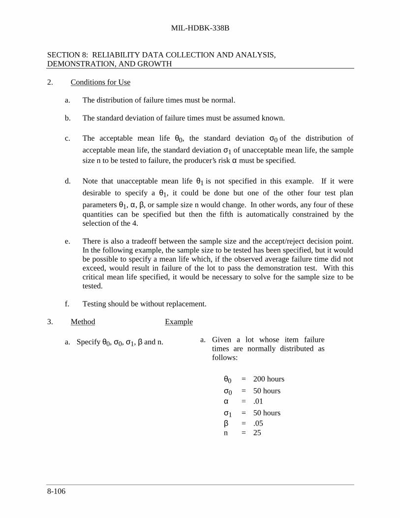
MIL-HDBK-338B


8-106


a. The distribution of failure times must be normal.

b. The standard deviation of failure times must be assumed known.

c. The acceptable mean life θ0, the standard deviation σ0 of the distribution of

acceptable mean life, the standard deviation σ1 of unacceptable mean life, the samplesize n to be tested to failure, the producer’s risk α must be specified.

d. Note that unacceptable mean life θ1 is not specified in this example. If it were

desirable to specify a θ1, it could be done but one of the other four test plan

parameters θ1, α, β, or sample size n would change. In other words, any four of thesequantities can be specified but then the fifth is automatically constrained by theselection of the 4.

e. There is also a tradeoff between the sample size and the accept/reject decision point.In the following example, the sample size to be tested has been specified, but it wouldbe possible to specify a mean life which, if the observed average failure time did notexceed, would result in failure of the lot to pass the demonstration test. With thiscritical mean life specified, it would be necessary to solve for the sample size to betested.

f. Testing should be without replacement.

3. Method Example

a. Specify θ0, σ0, σ1, β and n. a. Given a lot whose item failuretimes are normally distributed asfollows:

θ0 = 200 hours

σ0 = 50 hoursα = .01

σ1 = 50 hoursβ = .05n = 25

MIL-HDBK-338B


8-107

3. Method Example

b. Solve for the accept/rejectdecision point.

b. The accept/reject point iscalculated as follows:

z0 = x - θ0σ0/ n

-2.33 = x - 200

50/ 25

x = 176.7

c. Solve for θ1. c. Using the result from Step (b) andthe specified β = .05

z1 = x - θ1σ1/ n

+

1.645 = 176.7 - θ1

50/ 25

θ1 = 160.25

NOTE: The z values are from a tableof “Areas Under the Normal Curve.”

d. Summarize the characteristics ofthe demonstration test plan.

d. The demonstration test procedure isas follows:

1) Take a random sample of 25items from a population whosedistribution of failure times isnormal.

MIL-HDBK-338B


8-108

3. Method Example

2) Test until all items have failed,recording the exact failure time ofeach.

3) Take the arithmetic mean of the 25failures and compare it with thedecision point 176.7 hours. If theobserved mean equals or exceeds176.7 hours the demonstration testis passed. If it is less than 176.7the demonstration test is failed.

4) The demonstration test shown inthis example will:

• accept lots with a mean life of200 hours and a standarddeviation of 50 hours 99% ofthe time.

• accept lots with a mean life of160.25 hours and standarddeviation of 50 hours 5% of thetime.

e. Construct the operatingcharacteristic curve.

e. This is done by assuming values of

θ other than θ0 and θ1 and solvingfor the probability of acceptance ofa lot with that θ. Assume

θ = 175, σ = 50

z = 176.7 - 175

50/ 25 =

1.710 = .17

From a table of Areas Under the NormalCurve the probability of acceptance of a lotwith a mean life of 175 hours, σ = 50 isapproximately .43.

MIL-HDBK-338B


8-109

3. Method Example

f. Calculate the expected waitingtime for a decision.

f. The expected waiting time for adecision is the expected failuretime of the last order statistic. Inthis ex-ample and sample sizen = 25, α = 50 and µ = 200. Thesevalues are used with Table 10A.1,page 186 of the book"Contributions to Order Statistics"edited by A.E. Sarhan and B.G.Greenberg, published by JohnWiley & Sons, New York, 1962.

Table 10A.1 give a z = 1.965 forthe last order statistic in a sampleof n = 25. Applying the formula

z = x - µ

σ

1.965 = x - 200

50

x = 298 hours

Therefore the expected waiting

time for a decision of θ0 = 200, and25 items are tested to failure, is 298hours.


MIL-STD-414 Section D yields a series of variables demonstration test plans for the normaldistribution with σ known. The tests are constructed to assure protection in the form of percentdefective of the lot from which the sample was drawn, whereas, the example presented here isbased on mean life.

MIL-HDBK-338B


8-110

8.4.7.5.2.3 Normal Distribution, σ Unknown (MIL-STD-414)

1. When to Use

When the distribution of failure times is normal, with unknown standard deviation and thecriterion for acceptance is a variable (in the case, hours of life expectancy) with the protectiondesired stated in terms of percent defective in the lot from which the sample was drawn, then thistype of demonstration test is useful. This procedure basically is an application of MIL-STD-414,“Sampling Procedures and Tables for Inspection by Variables for Percent Defective.” Itcontains plans for both single and double specification limits. The criteria for acceptance caneither be stated in terms of an acceptability constant, k, stated in standard normal deviates or as amaximum allowable percent defective, M. MIL-STD-414 also presents plans based on thecalculation of an estimate of the standard deviation from sample data and also presents the rangemethod. In the range method, the sample is segmented and the range of each sub-sample is usedto estimate variability. It also contains test plans for the case when the standard deviation isknown.


a. The distribution of failure times must be normal.

b. The standard deviation is unknown and must be assumed equal for both acceptableand unacceptable lots (when it is known, see previous example).

c. Failure is measured in hours or cycles of operation.

d. All items in the sample will be tested to failure.

e. The lot size, acceptable quality level AQL, specification limit or limits, andinspection level must be stated.

f. Testing is performed without replacement of failed items.

MIL-HDBK-338B


8-111

3. Method Example

a. Specify the lot size from whichthe sample is to be randomlydrawn, AQL (the percentdefective of accept-able lots), thespecification limit, and themethod to be used (standarddeviation or range method) tomeasure variability.

a. Given an item type whose failuretimes are normally distributed. Thelot to be evaluated contains 100items with an unknown standarddeviation. An AQL of 4%represents an acceptable level ofdefectives in a lot. The normalinspection level in MIL-STD-414is IV. The standard deviationmethod is to be used fordetermining compliance with theaccepability criterion. Theminimum life (L) for items of thistype is 300 hours.

b. Determine the sample size to betested.

b. Enter Table A-2 on page 4 of MIL-STD-414 with the lot size = 100.It is found that for Inspection LevelIV, sample size code letter Fapplies. On page 39 in Table B-1sample size code letter F calls for asample size of 10.

c. Determine the acceptabilityconstant k.

c. From Table B-1 enter Row F andthe column headed byAQL = 4.00. This yields anacceptability constant k = 1.23.

MIL-HDBK-338B


8-112

3. Method Example

d. Draw a random sample from thelot and test until all items failrecording exact failure times.

d. Ten failure times are re-corded asfollows:

Failure Time (Hours)

275310315370400425450515625630

e. Calculate the sample mean andstandard deviation from theobserved test data.

e. Using standard statisticalcalculations

x = 432 hours

s = 119 hours

f. Calculate the quantity

x - L

s

where L = the specified minimumlife.

f.x - L

s = 432 - 300

119 = 1.10

g. Compare x - L

s with k.g. From Step c, the acceptability

constant is k = 1.23. From Step f,x - L

s = 1.10 Since 1.10 < 1.23,

reject the lot.

MIL-HDBK-338B


8-113


MIL-STD-414 also presents test plans for cases where the standard deviation is known.Operating characteristic curves are presented in Section A of MIL-STD-414 to enable assessmentof the risk at all quality levels. All lot sizes can be accommodated, but only certain values ofAQL are covered by test plans. MIL-STD-414 also covers tightened and reduced sampling. Adiscussion of the methodology of the development of this type of sampling plan is presented in"Quality Control and Statistics" by A. J. Duncan, published by Richard D. Irwin, Homewood,Illinois, 1959.

8.4.7.5.2.4 Weibull Distribution

1. When to Use

When the underlying distribution of failure time is Weibull, with the shape parameter, β, knownor assumed, and the test must be truncated after a specified number of failures has occurred. Theordered failure times are required, along with the number of items on test.


a. The two-parameter Weibull distribution must be assumed for failure times.

b. The parameter, β, must be known and be the same under the null and alternativehypothesis concerning the population mean.

c. The acceptable mean life, µ0 , the unacceptable mean life, µ1 , and the producer’s risk

must be specified. If the number of failures at which the test is truncated is specified,then the consumer’s risk will be determined, and cannot be set arbitrarily.

MIL-HDBK-338B


8-114

3. Method Example

a. The method involves replacement

of the original failure times x1,

. . . xr by a new variable definedas yi = xi β

This variable has an exponentialdistribution with mean α. Hence,the previous method developedfor failure-truncated exponentiallife-distributions may be used(See Section ExponentialDistribution (MIL-HDBK-H108).

a. With producer’s risk .05 andconsumer’s risk .10, test thehypothesis that µ0 = 800 hours

against µ1 = 400 hours. Assume aWeibull distribution withparameter β = 1.5. Twentyspecimens were placed on test, andthe test was concluded after thefourth failure, the observed failuretimes being 600, 750, 1000, and1220 hours.

b. To perform a Weibulldemonstration test with

parameters µ0, µ1, β. Solve thefollowing equations:

µ0 = α0 1/β Γ(1β + 1)

µ1 = α1 1/β Γ (1β + 1)

forα0 and α1 .

b. α0 =

µ0

Γ(1β + 1)

β

=

800

Γ(1.67)1.5

=

800

.9031.5

= 24600

α1 =

400

.9031.5

= 9400

MIL-HDBK-338B


8-115

3. Method Example

c. Perform the demonstration test inSection Exponential Distribution(MIL-HDBK-H108) on the

observations y1, y2, . . .yK fromthe exponential distribution with

θ0 = α0 θ1 = α1

The test is described inMIL-HDBK-H108.

On page 2.26 ofMIL-HDBK-H108, the formulafor θ is

^θ =

1r i=1

r

∑ yi + (n − r)yr

This is compared withacceptability constant, C, givenon page 2.28 ofMIL-HDBK-H108. Theacceptance region is

^θ ≥ θ0 /(C/θ0 )

c. y1 = 6001.5 = 14,700

y2 = 7501.5 = 20,500

y3 = 10001.5 = 31620

y4 = 12201.5 = 42,600

^θ =

14 [14,700 + 20500 + 31620

+ 42600 + 16(42600)]

^θ = 197755

θ0 = 26400

C/θ0 = .342 for producer’s risk .05

and 4 failures (Table 2B-1)(MIL-HDBK-H108)

Critical Value = 26400.342

= 77200

Since 197755 > 77200, accept thevalue, µ0 , for the Weibull

population mean

d. The consumer’s risk may beestimated from OC curvesprovided in the referenced

document. Compute θ1/θ0 andread the value of the β error fromTable 2A-2.

d.θ1θ0

= 940026400 = 0.36

β = 0.38 from Table 2A-2(MIL-HDBK-H108)

MIL-HDBK-338B


8-116

3. Method

The larger the value of θ, thesmaller the value of β error. Toachieve a β error of 0.1, forexample, it would be necessary(Table 2-A-2) to continue testinguntil 9 failures had occurred.


Tables of the Gamma Function are presented on page 497 of the "Handbook of Tables forProbability and Statistics" edited by W. H. Beyer, Chemical Rubber Company, 1966.

8.4.7.5.3 Sequential Tests

8.4.7.5.3.1 Exponential Distribution (MIL-HDBK-781)

1. When to Use

When the demonstration test is to be based upon time-to-failure data and the underlyingprobability distribution is exponential, the sequential test is an alternate for the fixed sample sizeor fixed time tests discussed in Sections Time Truncated Demonstration Test Plans and FailureTruncated Tests. The sequential test leads to a shorter average number of part hours of exposure

than either fixed sample or fixed time tests if the lot tested is near θ0 or θ1. Sequential testsshould not be used where the exact length, or cost, of the test must be known before-hand, or isspecified.


a. The failure distribution must be exponential.

b. The upper test MTBF, θ0, lower test MTBF, θ1, producer’s risk, α, and consumer’srisk, β, must be specified.

c. The test may be run either with or without replacement of failed items, since thepertinent statistic is "total item-hours" of test time.

d. The producer’s risk, α, and consumer’s risk, β, are always equal in these test plans.

MIL-HDBK-338B


8-117

3. Method Example

a. Specify θ0 , θ1 , α, β. If the

requirements are stated in termsof reliability at a time T0, thiswill involve solution of theequation.

exp -( )T0/θ = R

a. Given equipment type whosefailure times are distributedexponentially. A reliability of 0.95is desired for 150 hours ofoperation. A product with areliability of 0.9 or lower isunacceptable. We specify thatα = 0.10 for 0.95 reliability andβ = 0.10 for 0.90 reliability.

for θ. The solution is

θ = - T0lnR

We have

θ0 = - 150

ln.95

θ0 = 2924 hours

θ1 = - 150

ln.90

θ1 = 1424 hours

b. Compute θ0 /θ1 b. θ0 /θ1 =

29241424 = 2.05

MIL-HDBK-338B


8-118

3. Method Example

c. Tests in MIL-HDBK-781 areclassified by θ0 /θ1 , α and β.

Find the Test Plan which mostnearly fits the three values, andrecord the acceptance andrejection criteria. These aregiven in terms of θ1 , and must

be multiplied by θ1 to convert to

"equipment hours" criteria.

c. For α = β = .10 the nearest test inMIL-HDBK-781 is Test Plan IIID.The criteria given for acceptanceand rejection are:

No. of Equipment Hours Failures Reject Accept

0 N/A 4.41 N/A 5.792 N/A 7.183 0.7 8.564 2.08 9.94

After multiplying by θ1 , or 1424

hours, we obtain

No. of Equipment HoursFailures Reject Accept

0 - 62661 - 82452 - 102243 997 121894 2962 14155

For example, if 3 failures areencountered prior to 997 equipmenthours, reject the equipment asunsatisfactory.

d. The OC curve of each sequentialtest is given as multiples of θ0

and θ1 . The document supplies

for each Test Plan the expectedlength and the OC curve.

d. The expected number of equipmenthours to reach a decision, when θ0

is the population parameter, and theOC curve are given inMIL-HDBK-781A (Ref. [18]).

MIL-HDBK-338B


8-119


The material presented herein is from MIL-HDBK-781, “Reliability Test Methods, Plans andEnvironments for Engineering Development, Qualification and Production.” The theory ofsequential testing is developed in “Sequential Analysis” by A. Wald, John Wiley and Sons, Inc.,1947. Examples of sequential exponential demonstration tests are given in an article byBenjamin Epstein and Milton Sobel, “Sequential Life Tests in the Exponential Case,” Annals ofMathematical Statistics, Vol. 25, 1955, pp. 82-93.

8.4.7.5.3.2 Normal Distribution

1. When to Use

When the underlying failure distribution is assumed to be normal, and random sampleobservations are gathered sequentially. This method does not apply to ordered sampleobservations such as are usually obtained in life testing. It is useful where the cost of a single testis high, testing is done one unit at a time, and it is desired to minimize expected sample size.

As an example, consider the destructive testing of an aluminum alloy exhaust fan, where thecomponent is rotated in a “whirl pit” at increasing velocity until a tensile failure occurs. In

service, the component will rotate at a maximum velocity v0, and the purpose of thedemonstration test is to assure that the population mean velocity at failure is sufficiently high to

provide satisfactory reliability at v0.


a. The distribution of failures must be normal.

b. The acceptable population mean, µ0, unacceptable mean, µ1, must be specified, along

with the known or assumed population standard deviations, σ0 and σ1, the producer'srisk, α, and consumer's risk, β. If α is unknown, and the test involves a strengthdistribution, α is often assumed to be 5% of the mean, in accordance with thediscussion of normal distribution estimation in Section 5 of this handbook.

MIL-HDBK-338B


8-120

3. Method Example

a. Specify µ0, µ1, σ0, σ1, α, andβ. Compute

A = 1 - β

α

B = β

1 - α

a. µ0 = 1000

µ1 = 800

σ0 = σ1 = 100α = β = .05

A = .95.05 = 19.0

B = .05.95 = .053

b. Compute, as each newobservation is obtained, thecorresponding unit normaldeviates

zoi = xi - µ0

σ0

b. The first sample observation wasfound to be

x1 = 1020, hence

z01 = 1020 - 1000

100 = 0.2

z1i = xi - µ1

σ1 z11 =

1020 - 800100 = 2.2

and the corresponding probabilitydensity from a table of the normaldistribution ordinates (Table5.3.1-2).

Note that it is not the usual areasunder the normal curve but theordinates that are required.

The ordinate in the normal tablecorresponding to 0.2 is 0.3900while the ordinate corresponding to2.2 is 0.0355.

MIL-HDBK-338B


8-121

3. Method Example

c. Form the product of ordinates

L0 = i=1

k

∑ f(zoi )

and

L1 = i=1

k

∑ f(z1i )

c. L0 = .3900

L1 = .0355

L1L0

=

.0355

.3900= .091

Since this is between B and A,continue testing. The secondobservation was

x2 = 904.

Determine, as each new sample isreceived, the ratio,

L1L0

If

B < L1L0

< A

continue testing. If

L1L0

< B, accept µ0

Calculating as before,

z02 = .96

Ordinate = .2516

z12 = 1.04

Ordinate = .2323

L1L0

= .091

.2323

.2516 = .084

Therefore, continue testing.

We observe

L1L0

> A, accept µ1 x3 = 1050

z03 = 0.5

MIL-HDBK-338B


8-122

3. Method Example

Ordinate = .3521

z13 = 2.5

Ordinate = .0175

L1L0

= .084

.0175

.3521 = .004

Since this is less than B, accept µ0

as population mean.

d. The expected sample size(assuming that the true parameteris µ0 ) may be obtained from the

formula

E(N) =

(1 - α) ln B + α ln A1

2σ2 [2(µ1 - µ0)µ0 + µ02 - µ1

2]

d. For this test, the expected numberof observations was

E(N) =

( )( )[ 6 10461011000200220000

10190505395

x.x

..-..

−+−

ln ln

≈ 2(Note: sample size must be aninteger)


See "Sequential Analysis" by Abraham Wald, John Wiley and Sons, N.Y., 1947, p. 77 and p. 53.

MIL-HDBK-338B


8-123

8.4.7.6 Interference Demonstration Tests

1. When to Use

Interference demonstration testing is applicable to mechanical systems where a strengthdistribution and a stress distribution overlap, or interfere. See Section 7 for several detailedexamples. In the case of demonstration testing, both the strength and stress distribution must beassumed to be normal. We distinguish four cases:

Case 1: The mean of the stress distribution is assumed to be known, and the standard deviationof the stress distribution is assumed to be zero. See the discussion in Section 7 for conditionswhere these assumptions are valid. In this case, the interference problem becomes identical tolife testing of the normal distribution described in Section 8.4.7.5.2.2, Normal Distribution σKnown. The specified stress level plays the role of the specified life. The strength distributionplays the role of the life distribution, and the demonstration procedure follows the example inSection 8.4.7.5.2.2.

Case 2: The mean of the stress distribution is assumed to be known, along with its standarddeviation (often assumed to be 5% of the mean). The standard deviation of the strengthdistribution is assumed to be known, and its mean unknown. This may be translated to ademonstration test on strength and solved by the methods of Section 8.4.7.5.2.2. An examplewill be given.

Case 3: The mean of the stress distribution and the mean of the strength distribution areunknown, but their standard deviations are assumed known. In this instance, sampling data willbe required from both stress and strength. It is rare that a sample size for each may be specifiedahead of testing. Therefore, it is unlikely that the consumer’s risk may be set for this test. β willbe a function of N and α. An example will be given.

Case 4: The means and standard deviations of the strength and stress distributions are unknown.This case cannot be subjected to a demonstration test using standard statistical methods.


a. The strength distribution and stress distribution must be stochastically independent.

b. The strength distribution and stress distribution must be normal.

c. A random sample of strength and stress observations must be obtained.

MIL-HDBK-338B


8-124

3. Method Example

a. If the strength distribution hasnormal parameters µx , σx and

the stress distribution has nor-malparameters µy , σy , then the

statistic

w = x - y

is normally distributed withparameters

w = µx - µy

1. Stress has a specified value of 30KSI* with standard deviation 1.5KSI. Strength is expected to be inthe vicinity of 40 KSI but the meanis unknown. The standarddeviation is assumed to be 2.0 KSI.A reliability of 0.99 is acceptablewhile a reliability of 0.90 isunacceptable. The producer’s riskis .05 and the consumer’s risk .10.

σw = σx2 + σy

2

and the reliability is defined as theprobability that w exceeds zero.Clearly, specifying a particularreliability is the equivalent ofrequiring the unit normal deviate

z = (µx - µy) - 0

σx2 + σy

2

to correspond to this reliability in theright tail of the unit normal.

Solution:

σw = 22 + (1.5)2

= 2.5 KSI

The unit normal deviatescorresponding to 0.99 and 0.90reliability are 2.33 and 1.28respectively.

Therefore,

2.33 = (µ0 - 30) - 0

2.5

1.28 = (µ1 - 30) - 0

2.5

* KSI = 1000 lbs/sq. in

MIL-HDBK-338B


8-125

3. Method Example

and the requirements on thestrength distribution are

µ0 = 35.9

µ1 = 33.2

with a known σ = 2.0,α = .05, β = .10. The methods ofSection 8.4.7.5.2.2, may now beused.

2. If we retain the data of example 1,and delete the informationconcerning the mean of the stressdistribution, then,

σx = 2.0 µ0 - µX

= 35.9 - 30 = 5.9

σy = 1.5 µ1 - µX

= 33.2 - 30 = 3.2

α = .05

β = .10

If Nx observations of strength and Ny

observations of stress are obtained, theappropriate statistic is

z = ( x - y ) - 5.9

σx2

Nx +

σx2

Ny

MIL-HDBK-338B


8-126

3. Method Example

Hence, the critical value of

( x - y ) is

zα σx

2

Nx +

σy2

Ny + 5.9

For example, ten observations ofstrength and four observations ofstress are available.

For 0.99 reliability, we have fromthe previous example, µx - µy =5.9, and zα = z.95 = -1.65

-1.65 4.010 +

2.254 + 5.9

= + 4.21

as the critical value of the statistic

( x - y ). Accept if

x - y ≥ 4.21

Otherwise, reject. The β risk forthis example would be

z = 4.21 - 3.2

4.010 +

2.254

= + 1.03

β = 0.15

A larger sample size for eitherstress or strength will reduce β.

MIL-HDBK-338B


8-127

8.4.7.7 Bayes Sequential Tests

1. When to Use

A test plan of this type can be specified if mean life θ is the parameter of interest and if a priordistribution on θ is known. The use of a test plan of this type results in a smaller sample sizethan most other test plans described in this section.

2. Conditions of Use

a. The lot of items being evaluated must have a known prior distribution on the meanlife.

b. The parameters of the prior distribution must be specified as well as θ1, the minimum

acceptable mean life. It is necessary to specify two other terms K2 and K1 as criteria

for terminating the test. K2 is a probability such that if Pr(θ ≥ θ1/θn) ≥ K2 the testis deemed passed. It is usually specified at .90, .95 or .99 and is the probability

associated with a lower bound at θ1. K1 is usually specified as .01, .05, or .10 and

1 - K1 is the probability associated with an upper bound at θ1. K2 + K1 need notequal 1.

c. In this demonstration test procedure it is possible to pass or fail without testing. Iftesting is called for, one item is tested at a time and a decision is made after eachfailure to either accept, reject, or continue testing.

MIL-HDBK-338B


8-128

3. Method Example

a. Specify the prior distributionform, its parameters, and the

quantities θ1, K1 and K2

a. It has been found that a given itemtype has a prior distribution on itsmean life θ that is inverted gammawith a shape parameter λ = 3, ascale parameter α = 100, aminimum acceptable mean life

θ1 = 60, K1 = .10 and K2 = .90.

b. Compute P0 to determine iftesting should be performed:

if P0 ≥ K2, accept and do nottest

if P0 ≤ K1, reject and do not test

if K1 < P0 < K2, place an itemon test

b. To solve for P0 use the Tables of

Percentage Points of the X2 distribution for 2λ degrees offreedom (d.f.). In this case use 6d.f.

Next solve the equation

X2 = 2αθ1

= 2(100)

60 = 3.33

In the X2 Table for 6 d.f.

X2 = 3.33 corresponds to a

percentage point (P0 in thisproblem) of approximately .23.

Therefore, K1 < P0 < K2 = .10< .23 < .90 resulting in theinstruction to begin testing.

MIL-HDBK-338B


8-129

3. Method Example

c. Construct a table of decisionpoints for each failure time. Thisis done by solving for

θn * =

θ1X2K 2,2(n +λ) −2α

2n

where n = # of failures

and

θ n* =

θ1X2K1, 2(n +λ) −2α

2n

c. For 1 failure the following decisionpoints are calculated

θ1 * = 60X2

(.90,8) - 2(100)

2(1)

θ1 * = 60(13.36) - 200

2 = 301

θ1 * = 60X2

(.10, 8) - 2(100)

2(1)

θ1 * = 60(3.49) - 200

2 = 4.7

The following table gives theaccept/reject mean lives for additionalfailures.

θn* θn*n Accept if θn Reject if θn

θn* Š θn*1 301 4.72 190 23.53 152 29.74 133 33.45 - -

^

^

^

^

MIL-HDBK-338B


8-130

3. Method Example

θ n* and θn* eventually terminate

at some n. Therefore, the test couldnot continue indefinitely.

The θn = i=1

n

∑ t i

n

where:t = failure time

n = number of failures

d. Test the first part and make thedecision to accept, reject orcontinue testing.

d. Test the first item. If its failure timeis:

1) 4.7 hours or less, reject theproduct.

2) 301 hours or more, accept theproduct.

3) greater than 4.7 and less than301, test another sample tofailure compare again to theaccept/reject criteria of Step c.


The theoretical development of this method is presented in “A Sequential Bayes Procedure forReliability Demonstration,” by R.E. Schafer and N.D. Singpurwalla, Naval Research LogisticsQuarterly, March 1970.

The methodology of fitting prior distributions is developed in RADC-TR-69-389 “BayesianReliability Demonstration - Phase I - Data for A Prior Distribution.” Further details are providedin RADC-TR-76-296, Vols. I through V, “Reliability Acceptance Sampling Plans Based UponPrior Distribution,” and in RADC-TR-81-106, “Bayesian Reliability Tests Made Practical.”

MIL-HDBK-338B


8-131

8.4.8 Reliability Demonstration Summary

MIL-HDBK-781 covers the detailed requirements for development and production reliabilitytests for equipment that experiences a distribution of time-to-failure that is exponential. MIL-HDBK-781 contain: test conditions, procedures, and various fixed length and sequential testplans with respective accept/reject criteria. Refs. [5] and [12] provide additional guidance anddetails on reliability measurement. The reliability test plan should contain, as a minimum, thefollowing information:

(1) How the equipment/system will be tested

• The specified test conditions, e.g., environmental conditions, testmeasures, length of test, equipment operating conditions, accept/rejectcriteria, test reporting requirements, etc.

(2) Who will perform the tests

• Contractor, Government, independent organization

(3) When the tests will be performed

• Development, production, field operation

(4) Where the tests will be performed

• Contractor's plant, Government organization

Section 8.4.7 presented step-by-step instructions on the use of various types of reliabilitydemonstration test plans. Instructions and examples are given for the following test plans:

(1) Attributes Demonstration Tests(a) Plans for Small Lots(b) Plans for Large Lots(c) Plans for Large Lots (Poisson Approximation Method)(d) Attributes Sampling Using ANSI/ASQC Z1.4-1993(e) Sequential Binomial Test Plans

(2) Variables Demonstration Tests(a) Time Truncated Test Plans

(1) Exponential Distribution(2) Normal Distribution(3) Weibull Distribution

MIL-HDBK-338B


8-132

(b) Failure Truncated Tests(1) Exponential Distribution(2) Normal Distribution (Known)(3) Normal Distribution (Unknown)(4) Weibull Distribution

(c) Sequential Tests(1) Exponential Distribution(2) Normal Distribution

(d) Interference Demonstration Tests

(e) Bayes Sequential Tests

8.5 Reliability Growth

Experience has shown that programs which rely simply on a demonstration test by itself todetermine compliance with the specified reliability requirements generally do not achieve thereliability objectives with the allocated resources. This is particularly true of complex systems.Generally, these systems require new technologies and represent a challenge to the state of theart. Moreover, the requirements for reliability, maintainability and other performance parametersare usually highly demanding. Consequently, striving to meet these requirements represents asignificant portion of the entire acquisition process and, as a result, the setting of priorities andthe allocation and reallocation of resources such as funds, manpower and time are oftenformidable management tasks.

In order to help ensure that the equipment/system will meet the required operational reliabilityrequirement, the concept of reliability growth testing and management has been developed forequipment/system development programs.

8.5.1 Reliability Growth Concept

Reliability growth is defined as the positive improvement of the reliability of an equipmentthrough the systematic and permanent removal of failure mechanisms. Achievement ofreliability growth is dependent upon the extent to which testing and other improvementtechniques have been used during development and production to “force out” design andfabrication flaws, and on the rigor with which these flaws are analyzed and corrected.

MIL-HDBK-338B


8-133

Figure 8.5-1 suggests an ideal growth process. The initial reliability of the prototype starts atsome level that might be considered the state-of-the-art at the beginning of development.Through the development effort, reliability grows up to the pilot production stage. At that time,some loss of growth occurs due to the introduction of manufacturing problems. During the pilotproduction, corrective actions are continuing that cause resumption of growth. At the beginningof full scale production, some loss in the achieved level of reliability occurs because of theeffects of mass production. However, growth will resume as these problems are eliminated. And,at a time when the equipment is released to the field it should have achieved the specified levelor, under ideal conditions, the inherent or predicted level. The slope of this curve is affected bymany variables and these will be discussed later. Thus, reliability growth is the result of aniterative design process. As the design matures, it is investigated to identify actual (via testing)or potential (via analysis) sources of failures. Further design effort is then spent on correctingthese problem areas. The design effort can be applied to either product design or manufacturingprocess design. There are three essential elements involved in achieving reliability growth:

(1) Detection of failure sources (by analysis and test)

(2) Feedback of problems identified

(3) Effective redesign effort based on problems identified

The rate at which reliability grows is therefore dependent on how rapidly activities in thisiterative loop can be accomplished, how real the identified problems are, and how well theredesign effort solves the identified problems. It is important to realize that some activities mayact as a bottleneck. The bottleneck activities may vary from one development program to thenext. Even within a single program they may vary from one stage of development to the next. Inmost cases, however, failure sources are detected through testing, and the testing processeffectively controls the rate of growth. As a consequence, the reliability growth process becomesfamiliarly known as one of test, analyze, and fix (TAAF). However, the reliability achieved as aresult of the growth process only becomes meaningful when the necessary changes developedand proven during TAAF to achieve that reliability are properly and fully incorporated inconfiguration-control documentation for production hardware.

Reliability growth testing (RGT) is only one aspect of a total reliability growth program. It mustbe accompanied by a reliability growth management program. This involves setting interimreliability goals to be met during the development testing program and the necessary allocationand reallocation of resources to attain these goals. A comprehensive approach to reliabilitygrowth management throughout the development program consists of planning, evaluating andcontrolling the growth process.

Note that RGT or TAAF, is intended neither to replace a sound design approach and thoroughanalytical effort nor compensate for a poor design. RGT should never be used or viewed as a“trial and error” approach to designing a reliable product.

MIL-HDBK-338B


8-134

PR

ED

ICT

ED

(IN

HE

RE

NT

)M

TB

F

SPE

CIF

IED

MT

BF

RE

LIA

BIL

ITY

DE

MO

NST

RA

TIO

N

RE

L. O

FIN

ITIA

LP

RO

TO

TY

PE

HA

RD

WA

RE

MT

BF

INH

OU

RS

STA

RT

OR

RE

L.

DE

VE

LO

PT

EST

PIL

OT

PR

OD

UC

TIO

NIN

TR

OD

UC

TIO

N

RE

L. D

EM

OT

EST

CO

MM

EN

CE

ME

NT

FUL

LP

RO

DU

CT

ION

INT

RO

DU

CT

ION

CA

LE

ND

ER

TIM

E IN

MO

NT

HS

RE

LIA

BIL

ITY

GR

OW

TH

DU

RIN

GD

EV

EL

OP

ME

NT

RE

L. O

FIN

ITIA

LP

ILO

TP

RO

DU

CT

ION

HA

RD

WA

RE

RE

LIA

BIL

ITY

GR

OW

TH

DU

RIN

GP

ILO

TP

RO

DU

CT

ION

RE

L. O

FIN

ITIA

LFU

LL

SC

AL

EP

RO

DU

CT

ION

HA

RD

WA

RE

RE

LIA

BIL

ITY

GR

OW

TH

DU

RIN

GFU

LL

SC

AL

EP

RO

DU

CT

ION

FIGURE 8.5-1: RELIABILITY GROWTH PROCESS

MIL-HDBK-338B


8-135

Reliability growth planning addresses program schedules, amount of testing, resources availableand the realism of the test program in achieving the requirements. The planning is qualified andreflected in the construction of a reliability growth program plan curve. This curve establishesinterim reliability goals throughout the program. To achieve these goals it is important that theprogram manager be aware of reliability problems during the conduct of the program so that hecan effect whatever changes are necessary, e.g., increased reliability emphasis. It is, therefore,essential that periodic assessments of reliability be made during the test program (e.g., at the endof a test phase) and compared to the planned reliability growth values. These assessmentsprovide visibility of achievements and focus on deficiencies in time to affect the system design.By making appropriate decisions in regard to the timely incorporation of effective fixes into thesystem commensurately with attaining the milestones and requirements, management can controlthe growth process.

8.5.2 Reliability Growth Modeling

For complex electronic/electro-mechanical avionic systems, the model used most often forreliability growth processes, and in particular reliability growth testing, is one originallypublished by J. T. Duane. (Ref. [16]). Essentially, this model provides a deterministic approachto reliability growth such that the system MTBF versus operating hours falls along a straight linewhen plotted on log-log paper. That is, the change in MTBF during development is proportionalto T where T is the cumulative operating time and α is the rate of growth corresponding to therapidity with which faults are found and changes made to permanently eliminate the basic causesof the faults observed.

The model is shown graphically in Figure 8.5-2, with each of the growth lines having differentslopes, depending upon the emphasis given to the reliability growth program.

Duane’s postulate was that as long as reliability improvement efforts continue, the followingmathematical expression would hold:

λ = FH = K H-α (8.23)

where:λ = cumulative failure rate

H = total test hoursF = number of failures, during time HK = constant determined by circumstancesα = growth rate

MIL-HDBK-338B


8-136

10100

1000

100

1000

1000

010

0000

(4) C

umul

ativ

e O

pera

ting

Tim

e U

nder

Tes

t Con

dit

ions

(Hou

rs)

(2) I

niti

al M

TB

F O

r St

arti

ng P

oint

Min

imum

Gro

wth

Rat

e

(3) R

ate

Of G

row

th O

r Sl

ope

(1)

Pred

icte

d (I

nher

ent)

MT

BF

(1)

Spec

ifie

d (A

ccep

tabl

e) M

TB

F

Max

imum

Gro

wth

Rat

eα

= 0

.6

α =

0.1

α =

0.5

α =

0.4

α =

0.3

α =

0.2

FIG

UR

E 8

.5-2

: R

EL

IAB

ILIT

Y G

RO

WT

H P

LO

TS

MIL-HDBK-338B


8-137

The original mathematical model was expressed in terms of cumulative failure rate; butcurrently, since equipment reliability is generally expressed in terms of MTBF, the followingexpression is used,

MR = MI

Ttti

α (8.24)

where:MR = required MTBF

MI = initial MTBF

ti = time at which initial data point is plotted (preconditioning time)

Tt = time at which the instantaneous MTBF of the equipment under test

will reach the MTBF requirementα = growth rate

Differentiating Eq. (8.23) with respect to time

Since

FH

= KH-α

then F = KH(1-α)

The instantaneous failure rate is found by differentiating with respect to H (i.e., time).

λinstantaneous =

dFdH

=d(KH 1−α1( ))

dH(8.25)

=

Kd(H(1−α))dH

= (1 − α)KH−α

so that the "instantaneous" or current failure rate is (1 - α) times the cumulative failure rate, or

the "instantaneous MTBF" is 1

1 - α times the cumulative MTBF. An adequate interpretation of

"instantaneous MTBF" is: The MTBF that the equipment currently on test would exhibit if westopped the reliability growth and continued testing.

Thus the "instantaneous" or current MTBF curves are straight lines displaced from the

cumulative plot by a factor

11− α

, which shows up as a fixed distance on a logarithmic plot, as

MIL-HDBK-338B


8-138

shown in Figure 8.5-3.

..

10

100

1000

MT

BF

10 100 1000

CUMULATIVE TEST HOURS

CURRENT MTBF

CUMULATIVE MTBF

1

1 - α

40

60

200

400

20

80

600800

FIGURE 8.5-3: UP-IS-GOOD DUANE CHART WITH PLOT OF CURRENT MTBF

Normally, the cumulative MTBF (Mc) is measured in test and converted to instantaneous (orcurrent) MTBF (MI) by dividing by 1 - α, that is,

MI = Mc

1 - α (8.26)

The cumulative MTBF is plotted versus cumulative test time, a straight line is fitted to the dataand its slope, α, is measured. The current MTBF line is then drawn parallel to the cumulative

line but displaced upward by an offset equal to 1

1 - α . The corresponding test time at which this

line reaches the required MTBF is the expected duration of the growth test. Much evidence hasbeen accumulated since Duane’s original report that verifies the adequacy of the Duane Model inrepresenting the real world of reliability growth testing.

MIL-HDBK-338B


8-139

In fact, recently the Duane Model has been successfully applied to software growth modeling(Ref. [18]).

Crow presents a formal mathematical development of the growth model. He showed that thefailure rate during development follows the Weibull failure rate curve. The development whichfollows is similar to that given by Crow (Ref. [17]).

Mathematically, this model may be expressed by the equation

F(t) = λt-α λ∗ > 0; 0 < α < 1 (8.27)

*λ is used here as a parameter of the Weibull distribution - it is not a failure rate.

where F(t) is the cumulative failure rate of the system at time t and λ and α are parameters. Bydefinition, therefore, it follows that the cumulative failure rate is

F(t) =E(t)

t (8.28)

where E(t) is the expected number of failures experienced by the system during t time units ofdevelopment testing. Thus, from the above two equations

E(t) = λt1-α (8.29)

The instantaneous failure rate, r(t), is of the most interest for applications. It is defined as thechange in the expected number of failures per unit time. For a nonexponential system, it varieswith time while for an exponential system the failure rate is constant.

Differentiating E(t) with respect to time gives the instantaneous failure rate r(t) as follows:

r(t) =dE(t)

dt = (1 - α) λ t-α (8.30)

By substituting in the previous equations

β = 1 - α

one gets

r(t) = λβtβ - 1 (8.31)

which is the Weibull failure rate function for a repairable system, i.e., for a non-homogeneous

MIL-HDBK-338B


8-140

Poisson process with a Weibull intensity function.

Thus, if one plans to use the Crow’s Model, called the AMSAA Growth Model, during adevelopment program, the Weibull failure rate function can be used to determine the failure rateat a particular development time t. The values of λ and β are estimated from test data. Since λ isonly a multiplier and β determines how much the failure rate changes with the development time,β is referred to as the growth parameter. For the systems studied by Duane, a β of approximately0.5 was estimated.

To gain further insight into the AMSAA Growth Model, consider Figure 8.5-4 which is a plot ofthe Weibull failure rate versus development time for β = 0.5 and λ = 0.4. In the early stages ofdevelopment the failure rate decreases rather rapidly due to more failures and more rework goingon during this time. As the development progresses, the rate of decrease of the failure rate dropsoff considerably. The AMSAA Model assumes that at some time t0 which corresponds to aboutthe time that development ends and production starts, the failure rate levels off to a fairlyconstant value. When the failure rate becomes constant, the time between failures can bedescribed by the exponential distribution with a mean time between failure of

MTBF(t0 ) =

λβt

β -10

-1

(8.32)

Crow (Ref. [22]) has developed the maximum likelihood estimates (MLE) of β and λ and also agoodness-of-fit test to determine if the AMSAA Model fits a particular set of data. The MLEestimate for β is

^β =

ir

n

ir

k

r XT

)t(N

N

ln∑∑== 11

(8.33)

where:k = number of different subsystems,

T = the operating time for each of the k subsystems,

Nr(T) = number of failures observed for the rth subsystem during T time,

Xir = the age of the rth subsystem at the ith failure (initially at the beginning of

development)

N = ∑i=1

k Nr(t) (Number of failures)

MIL-HDBK-338B


8-141

0 50 100 150 2000

.01

.02

.03

.04

.05

.06

.07

.08

.09

.10

β = 0.5

λ = 0.4

r(t) = λβtβ-1

1/MTBF(t )0

Development Time (t)

r(t)

Fai

lure

Rat

e

FIGURE 8.5-4: FAILURE RATE VS. DEVELOPMENT TIMEFOR WEIBULL FAILURE RATE

MIL-HDBK-338B


8-142

The previous MLE estimate of β is biased. The unbiased estimate is obtained by using

--β =

N - 1N

^β (8.34)

The MLE of λ is

^λ =

N

kT^β

(8.35)

The chi-square goodness-of-fit test can be used to determine if the observed data fits theAMSAA Model. The chi-square statistic is calculated using

χ2c = ∑

i=1

c

Oi - Ei

2

Ei (8.36)

To compute the statistic the development time is divided into c intervals. The observed numberof failures in the i-th interval, Oi, is obtained from the observed data. The expected number offailures in the i-th interval, Ei, is obtained using

Ei =

N

t--βi

- t--βi-1

T

--β

(8.37)

where ti-1 and Ti are the beginning and ending times for the ith interval. The χ2c is compared

with the tabled value of chi-square, χ2T with degrees of freedom equal to c - 1 and the specified

level of significance. If χ2c < χ

2T then it can be concluded that the data fits the AMSAA

Model.

8.5.2.1 Application Example

An engine system was analyzed for reliability growth using the AMSAA Model. The dataavailable for analysis were based on 8063 hours of development testing. During this time therewere 40 failures and the time of each failure was recorded. The average rates for this systemduring each interval of 1000 hours are shown in Figure 8.5-5.Using this data the MLE’s of λ and β, using equations 8.34 and 8.35, respectively, were

MIL-HDBK-338B


8-143

computed to be

λ = 0.1279

β = 0.6387

The unbiased estimate of β, using equation 8.35, is

--β = 0.6227

The chi-square goodness-of-fit statistic was calculated next using equation 8.36 and six intervals.The result was

χ2c = 10.09

Using a 1% level of significance and degrees of freedom of 6 - 1 = 5, the tabled value of chi-square is

χ2T = 15.086

Thus it can be concluded that the AMSAA Model fits the data.

Using the Eq. (8.31), the estimated failure rate for the engine becomes

r(t) = .128(.623) t.623-1

= .08 t-.377

A plot of this failure rate curve is given in Figure 8.5-5. Notice the curve is beginning to flattenout. In fact it would take 100,000 hours of development time to get the failure rate down to .001failures/hour.

MIL-HDBK-338B


8-144

Failure Times:Interval 1 (0 to 1344 hours)Interval 2 (1345 to 2688 hours)Interval 3 (2689 to 4032 hours)Interval 4 (4033 to 5376 hours)Interval 5 (5377 to 6720 hours)Interval 6 (6721 to 8064 hours)

1, 43, 43, 171, 234, 274, 377, 530, 533, 941, 1074 ,1188, 12482298, 2347, 2347, 2381, 2456, 2456, 25002913, 3022, 3038, 3728, 38734724, 5147, 51795587, 5626 6824, 6983, 7106, 7106, 7568, 7568, 7593, 7642, 7928, 8063

.

0 1 2 3 4 5 6 7 8 9 10 10

1

2

3

4

5

6

Development Time Hours (x103)

EstimatedFailureRate(x10-3)

FIGURE 8.5-5: FAILURE RATE VS. DEVELOPMENT TESTTIME FOR WEIBULL FAILURE RATE

8.5.3 Comparison of the Duane and AMSAA Growth Models

The Duane Model and the Army Material Systems Analysis Activity (AMSAA) Model,developed by Dr. L. H. Crow in 1972 are the two most widely-used growth models. The DuaneModel is based on an empirical relationship that holds as long as the MTBF is growing:

MTBFcum = 1K Tα

where:MTBF

cum = Cumulative MTBF

K = Constant determined by the initial MTBFα = Growth rate (the slope of the log-log plot of MTBFcum vs Test Time)

T = Cumulative test time

Typically the log-log plot of cumulative failures vs. test time will result in a linear relationship ifthe system reliability is improving. The test-analyze-and-fix (TAAF) procedure improves systemreliability by the incorporation of design changes. If the slope of the best fit line of such a plot is

MIL-HDBK-338B


8-145

positive, the system is said to be growing in reliability as time progresses.

The Duane Model assumes that the design fixes are 100% effective and that they areimplemented immediately.

The instantaneous MTBF essentially estimates the projected field failure rate by accounting forfixes without purging the failure data.

The Duane Model assumes that growth is a deterministic process, while the AMSAA Modelviews the process of reliability growth as a probabilistic process. The AMSAA Model is basedon the empirical relationship developed by Duane and is equivalent to a non-homogeneousPoisson process model with a Weibull intensity function. A typical AMSAA Model plot isshown in Figure 8.5-6. The AMSAA Model is

rc (t) = λt β-1

where:rc(t) = The cumulative failure rate at time t

t = Total test timeβ = Estimate of the time value of the growth parameterλ = Scale parameter

The instantaneous failure rate, ri(t), at time t is the incremental change in number of failures (F)with respect to the change in time.

Ft = rc(t) = λtβ-1 (8.38)

F = λtβ (8.39)

dFdt = λβtβ-1 = ri(t) (8.40)

Thereforeβ rc(t) = ri(t) (8.41)

It can be seen that the parameter α used in the Duane Model is equivalent to (1 - β) of theAMSAA Model.

MIL-HDBK-338B


8-146

0.001

1

1 10000Cumulative Test Time

Fai

lure

Rat

e (F

ailu

res/

Ho

ur)

Growth Rate (β - 1)

β - 1 = -0.671

Instantaneous Failure Rate & MTBF

λ inst = 0.003 (F/Hr.)MTBF inst = 3,777.164 (Hrs.)

FIGURE 8.5-6: RELIABILITY GROWTH ANALYSIS (AMSAA MODEL)

MIL-HDBK-338B


8-147

The Duane plot uses a least squares estimate of where the plot would fall while the AMSAAModel takes into account the exponential relationship between each data plot. Therefore inreliability growth plotting, the AMSAA Model tends to give a more accurate representation ofthe reduction in failure rate with respect to time. However, the Duane Model is typically used forprogram planning purposes even by proponents of the AMSAA Model because of its inherentsimplicity.

8.5.3.1 Other Growth Models

Parametric models imply that there is a pattern to the growth, while nonparametric models allowthe growth curve to “fall where it will.” Because of this, only the parametric models are usefulfor mathematical descriptions of the generic or budgeted growth. Also, the nonparametricmodels generally do not allow growth projections to be made. However, either parametric ornonparametric models can be effectively used for controlling reliability growth.

Another consideration is the type of failure distribution that the growth model assumes. Many ofthe models treat the failure distribution in a nonparametric fashion. However, some models arebased specifically on the assumption that the failure distribution is exponential.

Finally, although some of the models utilize a continuous time scale, others utilize a discretescale, implying that the testing is performed in stages.

Although the Duane and the AMSAA reliability growth models have been the most widely used,a number of other models, both discrete and continuous, have been proposed in the literature.

8.5.4 Reliability Growth Testing

Reliability growth testing is the formal process of testing an equipment under natural andinduced environmental conditions to discover and identify latent failure modes and mechanismswhose recurrence can be prevented through implementation of corrective action, thus causing thegrowth of equipment reliability.

These tests are conducted during the development phase on samples which have completedenvironmental tests prior to production commitment and do not replace other tests described inthe contract or equipment specification. MIL-HDBK-781 contains the details on reliabilitygrowth test requirements, methods and procedures for application to electronic equipment.

8.5.4.1 When Reliability Growth Testing is Performed

The formal reliability growth test is usually performed near the conclusion of full scaledevelopment, concurrent with or after successful completion of environmental qualificationtesting and prior to reliability qualification (demonstration) testing. Although all testing shouldbe viewed and planned as contributing to reliability growth, the formal test program dedicated to

MIL-HDBK-338B


8-148

reliability growth is normally deferred until after environmental qualification, when the design ofthe equipment reflects the anticipated configuration and manufacturing processes to be used inproduction, but prior to commitment to production. The hardware to be tested should have allsignificant fixes required as a result of environmental qualification testing incorporated beforeinitiating the reliability growth test. The reliability growth test must be successfully concluded,and all significant fixes incorporated in the test hardware prior to initiating the reliabilityqualification (demonstration) test. The reliability growth test is for the purpose of detectingreliability problems after all performance design and environmental problems have beenresolved. The reliability qualification (demonstration) test discussed in Section 8 is for thepurpose of proving reliability.

8.5.4.2 Reliability Growth Approach

The MIL-HDBK-781A (Ref. [18]) approach to reliability growth is patterned after the Duane andthe AMSAA Models. With the Duane Model the change in MTBF during development is

proportional to Tα where T is the cumulative operating time and "α" is the rate of growthcorresponding to the rapidity with which faults are found, and changes are made to permanentlyeliminate the basic causes of the faults observed.

In order to structure a growth test program (based on the Duane Model) for a newly designedsystem, a detailed test plan is necessary. This plan should describe the test-analyze-fix concept,and show how it will be applied to the system under development. The plan should incorporatethe following:

(a) Values for specified and predicted (inherent) reliabilities. Methods for predictingreliability (model, data base, etc.) should also be described.

(b) Criteria for reliability starting points, i.e., criteria for estimating the reliability ofinitially fabricated hardware, should be determined. For avionics systems, the initialreliability for newly fabricated systems has been found to vary between 10% and 30%of their predicted (inherent) values.

(c) The reliability growth rate (or rates) should be defined. To support the selected growthrate, the rigor with which the test-analyze-fix conditions are structured should becompletely defined.

(d) Calendar time efficiency factors, which define the relationship of test time, correctiveaction time and repair time to calendar time, should be determined.

Note that each of the factors listed above impacts the total time (or resources) which should bescheduled to grow reliability to the specified value. Figure 8.5-2 (repeated here as Figure 8.5-7)illustrates the concepts described above.

MIL-HDBK-338B


8-149

In addition, Figure 8.5-7 graphically depicts the four elements needed to structure and plan agrowth test program such as is described above. These four elements are further described asfollows:

(a) Inherent Reliability: Represents the value of design reliability estimated duringprediction studies, which may correspond to the value above that specified inprocurement documents. Ordinarily, the contract specified value of reliability issomewhat less than the inherent value. The relationship of the inherent (or specified)reliability to the starting point greatly influences the total test time.

(b) Starting Point: Represents an initial value of reliability for the newly manufacturedhardware. This usually falls within the range of 10% to 30% of the inherent orpredicted reliability. Estimates of the starting point can be derived from priorexperience or are based on percentages of the estimated inherent reliability. Startingpoints should take into account the amount of reliability control exercised during thedesign program and the relationship of the system under development to the state-of-the-art. Higher starting points, when justified, minimize test time.

Determination of the starting point is often difficult, with little documented guidanceavailable. The following prioritized list provides the recommended procedures forestablishing the starting point.

(1) Use actual data on early design

(2) Use the results of past reliability growth test and reliability prediction results

(3) Compute the default ratio (i.e., 10%) of the initial MTBF divided by the MTBFprediction

The first option is to use actual reliability data (i.e., failures, test time) recorded on thesystem during its early life. The design team necessarily tests the early design as anatural part of the design/development process. This testing is often informal with littlestandardized or documented reliability reports/data. Nevertheless, this type of datatypically exists and it is most indicative of the actual MTBF of the system prior toreliability growth testing. The initial MTBF is computed as the cumulative amount oftest time divided by the cumulative number of failures. To obtain this type of data andapply it to develop a planned reliability growth curve, requires a high degree ofcooperation and sharing of information between the various engineering disciplines atan organization.

In many instances, this first option is not viable because the requisite data simply cannotbe retrieved or the planned growth curve is needed as part of a proposal or early designdocument before any design activities take place.

MIL-HDBK-338B


8-150

10100

1000

100

1000

1000

010

0000

(4) C

umul

ativ

e O

pera

ting

Tim

e U

nder

Tes

t Con

dit

ions

(Hou

rs)

(2) I

niti

al M

TB

F O

r St

arti

ng P

oint

Min

imum

Gro

wth

Rat

e

(3) R

ate

Of G

row

th O

r Sl

ope

(1)

Pre

dic

ted

(Inh

eren

t) M

TB

F(1

) Sp

ecif

ied

(Acc

epta

ble)

MT

BF

Max

imum

Gro

wth

Rat

eα

= 0.

6

α =

0.1

α =

0.5

α =

0.4

α =

0.3

α =

0.2

FIG

UR

E 8

.5-7

: R

EL

IAB

ILIT

Y G

RO

WT

H P

LO

TS

MIL-HDBK-338B


8-151

The second recommended option involves the use of results of prior reliability growthtests. These results must be from the same organization and indicative of the TAAFphilosophy to be enacted. The degree of reliability growth or growth potential is not aninherent design parameter but is dependent on the management philosophy adopted forreliability growth testing. An aggressive management philosophy which is dedicated toseeking out the root-cause of failure and determining effective design fixes will bemuch more successful than testing programs with a less aggressive approach.

The following example indicates how to use this past data on reliability testing. A 250hour pre-conditioning period was assumed to determine the actual starting point. It isimportant to distinguish between the planned and the actual MTBF starting point. Oncethe test has been conducted and the actual data are available, an actual starting point canbe computed, which may differ from what was planned.

MTBF Prediction(MIL-HDBK-217)

Final Test MTBF(MTBFinst at Test

Conclusion)

Initial MTBF(at 250 hours)

Initial MTBF/MTBF Prediction

2,200 2,000 410 .19800 610 84 .11

1,000 1,100 90 .09920 830 220 .24

1,550 1,400 310 .20

It is necessary to compute the ratio of the initial MTBF (at the assumed 250 hour pre-conditioning period) divided by the MTBF prediction per MIL-HDBK-217. In theexample, the ratio ranges from .09 to .24. In practice, it has been found that these ratiostypically range from .10 to .30. In the example, the average ratio is .17.

The next step is to multiply the computed ratio by the MTBF prediction. If theequipment to undergo the reliability growth test has an MTBF prediction of 5,000hours, then the estimated starting point would be,

MTBFstarting point = (.17)(5,000) = 850 hours

The final and least preferred option is to apply a default ratio of .10. It has been foundthat use of this ratio yields a conservative estimate of the starting point. It needs to berecognized that this estimate is not precise; however, it provides a starting point if noother approach is viable. Again, using the 5,000 hour MTBF estimate, the startingpoint would be,

MTBFstarting point = (.10)(5,000) = 500 hours

MIL-HDBK-338B


8-152

(c) Rate of Growth: Is depicted by the slope of the growth curve. This, in turn, is governedby the amount of control, rigor, and efficiency by which failures are discovered,analyzed, and corrected through design and quality action. Test programs which fosterthe discovery of failures, coupled with management supported analysis and timelycorrective action, will result in a faster growth rate and consequently less total test time.

(d) Calendar Time/Test Time: Represents the efficiency factors associated with the growthtest program. Efficiency factors include repair time, and operating/nonoperating time asthey relate to calendar time. Lengthy delays for failure analysis, subsequent designchanges, implementation of corrective action or short operating periods will extend thegrowth test period.

Figure 8.5-7 shows that the value of the parameter “α” can vary between 0.1 and 0.6. A growthrate of 0.1 can be expected in those programs where no specific consideration is given toreliability. In those cases, growth is largely due to solution of problems impacting production,and from corrective action taken as a result of user experience. A growth rate of 0.6 can berealized if an aggressive, hard-hitting reliability program with management support isimplemented. This type of program must include a formal stress-oriented test program designedto aggravate and force defects and vigorous corrective action.

Figure 8.5-7 also shows the requisite hours of operating and/or test time and the continuous effortrequired for reliability growth. It shows the dramatic effect that the rate of growth has on thecumulative operating time required to achieve a predetermined reliability level. For example,Figure 8.5-7 shows, for an item product whose MTBF potential is 100 hours, that 100,000 hoursof cumulative operating time is required to achieve an MTBF of 200 hours when the growth rateis 0.1. And, as previously stated, a 0.1 rate is expected when no specific attention is given toreliability growth. However, if the growth rate can be accelerated to 0.6 (by growth testing andformal failure analysis activities) then only 300 hours of cumulative operating time is required toachieve an MTBF of 200 hours.

Some general guidance on reliability growth test time is as follows:

Fixed-length test times of 10 to 25 multiples of the specified MTBF will generallyprovide a test length sufficient to achieve the desired reliability growth forequipment in the 50 to 2000 hour MTBF range. For equipments with specifiedMTBFs over 2000 hours, test lengths should be based on equipment complexity andthe needs of the program, but as a minimum, should be one multiple of the specifiedMTBF. In any event, the test length should not be less than 2000 hours or morethan 10,000 hours.

Where time is not an appropriate measurement parameter for the particular hardware, the DuaneModel is adaptable to other measurement parameters such as cycles, events, rounds, etc.

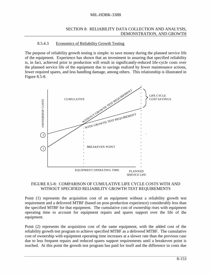
MIL-HDBK-338B


8-153

8.5.4.3 Economics of Reliability Growth Testing

The purpose of reliability growth testing is simple: to save money during the planned service lifeof the equipment. Experience has shown that an investment in assuring that specified reliabilityis, in fact, achieved prior to production will result in significantly-reduced life-cycle costs overthe planned service life of the equipment due to savings realized by fewer maintenance actions,fewer required spares, and less handling damage, among others. This relationship is illustrated inFigure 8.5-8.

2

1

EQUIPMENT OPERATING TIME PLANNEDSERVICE LIFE

BREAKEVEN POINT

LIFE CYCLECOST SAVINGSCUMULATIVE

OW

NE

RSH

IP C

OST

S

WITHOUT GROWTH TEST REQUIREMENT

WITH GROWTH TEST REQUIREMENT

FIGURE 8.5-8: COMPARISON OF CUMULATIVE LIFE CYCLE COSTS WITH ANDWITHOUT SPECIFIED RELIABILITY GROWTH TEST REQUIREMENTS

Point (1) represents the acquisition cost of an equipment without a reliability growth testrequirement and a delivered MTBF (based on post-production experience) considerably less thanthe specified MTBF for that equipment. The cumulative cost of ownership rises with equipmentoperating time to account for equipment repairs and spares support over the life of theequipment.

Point (2) represents the acquisition cost of the same equipment, with the added cost of thereliability growth test program to achieve specified MTBF as a delivered MTBF. The cumulativecost of ownership with equipment operating time increases at a slower rate than the previous casedue to less frequent repairs and reduced spares support requirements until a breakeven point isreached. At this point the growth test program has paid for itself and the difference in costs due

MIL-HDBK-338B


8-154

to the reliability growth program represents a life-cycle cost savings.

8.5.5 Reliability Growth Management

Reliability growth management is the systematic planning for reliability achievement as afunction of time and other resources and is used for controlling the ongoing rate of achievementby reallocation of resources based on comparisons between planned and assessed reliabilityvalues.

Reliability growth management is part of the system engineering process. It does not take theplace of the other basic reliability program activities such as predictions, apportionment, failuremode and effect analysis, and stress analysis. Instead, reliability growth management provides ameans of viewing all the reliability program activities in an integrated manner.

It is imperative to recognize that a total reliability program is needed for effective reliabilitygrowth management. While it is generally recognized that reliability will grow in the presence ofa reliability program, reliability growth planning provides an objective yardstick and an orderlymeans of measuring progress and directing resources so that reliability requirements may beachieved in a timely and cost effective manner. A good reliability growth plan can greatlyimprove the chances of achieving total reliability program objectives. However, it is notintended to be the total reliability program.

MIL-HDBK-189 provides procuring activities and development contractors with anunderstanding of the concepts and principles of reliability growth, advantages of managingreliability growth, and guidelines and procedures to be used in managing reliability growth. Itshould be noted that this Handbook is not intended to serve as a reliability growth plan to beapplied to a program without any tailoring. The Handbook, when used with knowledge of thesystem and its development program, will allow the development of a reliability growthmanagement plan that will aid in developing a final system that meets its requirements andlowers the life cycle cost of the fielded systems.

8.5.5.1 Management of the Reliability Growth Process

There are innumerable ways in which reliability can grow during development. There are, ofcourse, only a finite number of reliability growth models available. Consequently, acquisitionmanagers cannot conduct their development programs in just any fashion, and have an existingreliability growth model available for estimation and prediction purposes. The manner in whichthe development program is managed and the choice of the reliability growth model are,therefore, dependent. Essentially, there are two ways by which acquisition managers can evaluatethe reliability growth process.

(a) They may monitor the various reliability oriented activities (FMEA’s, stress analysis,etc.) in the growth process to assure themselves that the activities are being

MIL-HDBK-338B


8-155

accomplished in a timely manner and that the level of effort and quality of work isappropriate. This is a qualitative approach.

(b) They may utilize assessments (quantitative evaluations of the current reliability status)that are based on information from the detection of failure sources.

The assessment approach is, preferable in that it is results-oriented, in the form of quantitativeestimates of planned and achieved reliability as the program progresses.

Figure 8.5-9 illustrates how assessments may be used in controlling the growth process. One ofthe more important points to emphasize is that assessments have been a way of life in reliabilitywork for many years, as have the resultant decisions.

What, then, is new about reliability growth management? What is new is a formal standardagainst which the assessment may be compared. The fact that managers in the past have madedecisions based on assessments implies that they had at least a subjective standard of acceptablereliability growth against which to make comparison. A formal, objective standard has theadvantage of remaining constant, unless formally changed, rather than bending in the hope that“tomorrow will be better.”

Figure 8.5-10 illustrates an example of a reliability growth curve, showing both the budgeted(planned) reliability growth and assessments. A comparison between the assessment and thebudgeted value will suggest whether the program is progressing as planned, better than planned,or not as well as planned. Based upon the first two data points of assessed growth, the decisionwould probably be made to continue development with no changes. If reliability progress isfalling short, as the two subsequent assessed data points indicate, new strategies should bedeveloped. These strategies will probably involve the reassignment of resources to work onidentified problem areas. They may, as a last resort, result in adjustment of the time frame, orrelaxation of the original requirement.

DECISIONS

RELIABILITY ASSESSMENT PLANNED RELIABILITY

DETECTION OF FAILURE SOURCES(RE) DESIGN

FIGURE 8.5-9: RELIABILITY GROWTH MANAGEMENT MODEL (ASSESSMENT)

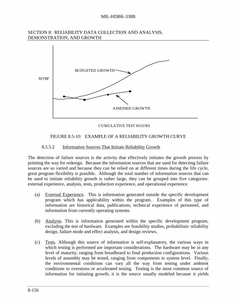
MIL-HDBK-338B


8-156

CUMULATIVE TEST HOURS

MTBF

BUDGETED GROWTH

ASSESSED GROWTH

FIGURE 8.5-10: EXAMPLE OF A RELIABILITY GROWTH CURVE

8.5.5.2 Information Sources That Initiate Reliability Growth

The detection of failure sources is the activity that effectively initiates the growth process bypointing the way for redesign. Because the information sources that are used for detecting failuresources are so varied and because they can be relied on at different times during the life cycle,great program flexibility is possible. Although the total number of information sources that canbe used to initiate reliability growth is rather large, they can be grouped into five categories:external experience, analysis, tests, production experience, and operational experience.

(a) External Experience. This is information generated outside the specific developmentprogram which has applicability within the program. Examples of this type ofinformation are historical data, publications, technical experience of personnel, andinformation from currently operating systems.

(b) Analysis. This is information generated within the specific development program,excluding the test of hardware. Examples are feasibility studies, probabilistic reliabilitydesign, failure mode and effect analysis, and design reviews.

(c) Tests. Although this source of information is self-explanatory, the various ways inwhich testing is performed are important considerations. The hardware may be in anylevel of maturity, ranging from breadboard to final production configurations. Variouslevels of assembly may be tested, ranging from components to system level. Finally,the environmental conditions can vary all the way from testing under ambientconditions to overstress or accelerated testing. Testing is the most common source ofinformation for initiating growth; it is the source usually modeled because it yields

MIL-HDBK-338B


8-157

objective measurements.

(d) Production Experience. The production process itself may identify weak areas in thedesign.

(e) Operational Experience. The use of fielded systems will identify design deficiencieswhich point the way toward reliability growth.

8.5.5.3 Relationships Among Growth Information Sources

The chronological relationship of these information sources is illustrated in Figure 8.5-11. Thisfigure illustrates that growth is at least possible at any point in the life cycle. However, what arethe relative merits of growing reliability at these various points? To a large extent, this questioncan only be answered with respect to a specific development program. But there are twofundamental considerations that must be made. First, changes can be accomplished veryeconomically early in the life cycle. The example usually given is that a change which wouldcost $1 on the drawing board will end up costing about $100 if it is made after the equipment isfielded. Therefore, it is desirable to grow reliability as early as possible. However, theinformation upon which early changes are based tends to contain many unknown factors, such asoperational conditions and component interactions. Second, changes which are made later in thelife cycle tend to be better directed, as there are fewer unknowns in the information as hardwarematurity nears. The two desired characteristics will be referred to as “timeliness” and“credibility.”

BREADBOARDMODEL

MOCK-UP TEST

ENG. DEVEL.HARDWARE

TEST

PROTOTYPEHARDWARE

TEST

EARLY PROD.TOOLED HW

TEST

LATERPRODUCTION

TEST

OPERATIONAL EXPERIENCE

ANALYSIS PRODUCTION EXPERIENCE

EXTERNAL EXPERIENCE

FIGURE 8.5-11: INFORMATION SOURCES THAT INITIATERELIABILITY GROWTH

Depending on the characteristics of the specific program and system, it may be desirable to placeparticular emphasis on certain combinations of these information sources. In effect, we wouldlike to achieve a reasonable combination of timeliness, credibility, and economy. The following

MIL-HDBK-338B


8-158

paragraphs give some suggestions about when it may be desirable to place emphasis on varioustypes of information sources. The rationale that is given here could serve as a basis for a moreformal economic model for specific applications. The suggestions that are given here areintended to point out those information sources which have the strongest potential under varyingsituations. A good program would probably utilize all of the information sources to some degree,but the mix and emphasis will vary from one program to the next.

(a) Reliability Growth Through External Experience. The strongest feature of externalexperience is that it may be available at the very beginning of the life cycle, thusemphasizing timeliness. This, of course, assumes that appropriate external experienceis available.

(b) Reliability Growth Through Analysis. Analysis becomes particularly valuable when thesystem reliability is high, mainly because the next best alternative, testing, will tend tobe time-consuming and, therefore, expensive. However, in order to be able to relyheavily on analysis, much detailed knowledge is necessary. The operation of the systemmust be well understood. This implies that the development must be reasonably withinthe state-of-the-art. There must be good, detailed knowledge of the environment anduse conditions. Finally, appropriate design analysis techniques must either be availableor specially developed and there must be a good information base to support thesetechniques. Many reliability programs put too little emphasis on analysis and theassociated information base. One problem with a reliance on analysis is that the effectscannot be measured objectively.

(c) Reliability Growth Through Testing. Reliability growth models are generally based ontest results. Therefore, testing is a very important information source for initiatingreliability growth. Testing will have the greatest payoff if many failures are encounteredwhich can be thoroughly analyzed. Therefore, a low system reliability and an inabilityto perform failed part analysis suggest strong emphasis be placed on testing. One otherfactor which must be considered is the cost of testing itself. High test costs maydiscourage strong reliance on testing to achieve growth. However, generally there is novalid substitute for a good test program in the reliability growth process.

(d) Reliability Growth Through Production Experience. The production process and itsquality controls are major contributors to reliability. In fact, a drop in reliability duringthe transition from development to production is a common phenomenon. It thenbecomes necessary to grow reliability based on manufacturing process redesign and/orbetter quality controls. Many process and control problems can be eliminated duringthe production phase through the use of process capability studies, worst-case analyses,and similar producibility-related techniques. Moreover, it is unlikely that all processand control problems could be eliminated during pre-production; and almost certainly,the payoff from these techniques, expressed as a function of effort, would show adiminishing-returns pattern. It is almost inevitable that some problems can be more

MIL-HDBK-338B


8-159

cost-effectively eliminated after production starts, particularly when the production runis relatively long and the tooling is relatively inexpensive.

(e) Reliability Growth Through Operational Experience. Although some reliability growththrough operational experience is inevitable, this method is the least desirable of thefive sources listed. Improving reliability through retrofitting of fielded systems oftencosts up to a hundred times as much as the same change made on the drawing board.

8.6 Summary of the Differences Between Reliability Growth Testing and Reliability Demonstration Testing

Reliability growth is the result of an iterative design process. As the design matures, it isinvestigated to identify actual (via testing) or potential (via analysis) sources of failures. Furtherdesign effort is then spent on correcting these problem areas. The design effort can be applied toeither product design or manufacturing process design. There are three essential elementsinvolved in achieving reliability growth:

(1) Detection of failure sources (by analysis and test)

(2) Feedback of problems identified

(3) Effective redesign effort based on problems identified

Reliability demonstration tests, on the other hand, are designed for the purpose of proving, withstatistical confidence, a specific reliability requirement; not specifically to detect problems, or togrow reliability. The test takes place after the design is frozen and its configuration is notallowed to change. However, in practice, some reliability growth may occur because of thedeferred correction of failures observed during the test.

Reliability demonstration is specified in most military system procurement contracts andinvolves, in many instances, formal testing. Demonstration tests are normally conducted afterdevelopment has been completed but before high rate production has been initiated.Demonstration tests are normally conducted after growth tests in the development cycle usinginitial production hardware.

As previously indicated, reliability demonstration testing, carries with it certain statisticalconfidence levels, and the more demonstration testing, the more confidence. The more reliabilitygrowth testing that is performed, the higher the actual reliability. Depending on program fundingand other constraints, system testing may follow one of two options. The first option maximizesgrowth testing and minimizes demonstration testing resulting in a high MTBF at a lowconfidence. Option two minimizes reliability growth testing with a resultant lower MTBF athigher confidence. These concepts are shown graphically in Figure 8.6-1.

MIL-HDBK-338B


8-160

Growth TestTime (Option 1)

TEST TIME

INC

RE

ASI

NG

MT

BF

Growth TestTime (Option 2)

DemonstrationTest Time(Option 2)

DemonstrationTest Time(Option 1)

Option 1 MTBF

Option 2 MTBFGROWTHCURVE

FIGURE 8.6-1: RELIABILITY TESTING OPTIONS

8.7 Accelerated Testing

Although accelerated testing is commonly used today, it frequently means different things todifferent people. There are potentially two main reasons for performing an accelerated test.These are: a) life estimation or b) problem/weakness identification (or confirmation) andcorrection. The difference between these reasons, although subtle, can have a very significantimpact upon the underlying assumptions upon which the test is based, the models utilized inconstructing the test, the test equipment and chambers used, the way in which the test itself isconducted, and the manner in which the resulting data is analyzed and interpreted.

Accelerated Life Testing is the means by which length of life can be determined. Here theprimary focus is on estimating the life of an item under “normal” operating conditions, basedupon data obtained under much more severe conditions. In this case, the failure mechanism isusually well documented and understood; thus, problem identification and correction is ofsecondary importance.

Accelerated Stress Testing is used to identify problems and weaknesses inherent in the design,the parts used, or the manufacturing process so that they can be subsequently fixed. This is doneby changes in: the design itself, the parts used, or the manufacturing processes employed. Athorough understanding, or at least a workable knowledge, of the basic failure mechanisms is thefocus of attention here, estimation of item life may, or may not, be a concern.

MIL-HDBK-338B


8-161

Accelerated testing attempts to get more reliability information from a given test time using a testenvironment that is more severe than that experienced during normal equipment use, however:

Accelerated testing must always be approached with due caution. There are basic limitationsto the technique. Every accelerated test application is unique. Subtle differences in theapplication can totally invalidate the data recorded during the test or the conclusions reachedby the test.

This unfortunate outcome can occur, for example, if the operating range of validity for a givenmodel is exceeded; or if the underlying test/modeling assumptions, while true for mostapplications, are not valid for a given specific application. Therefore, it is frequently necessaryto first perform a preliminary accelerated test to validate the theory for a given application andthen determine the applicable relationship (if not already available in the literature) between theapplied stress and the resulting acceleration of the associated degradation. This preliminaryaccelerated test could also be viewed as a “sanity check.”

Given these caveats, accelerating factors which may be used, either singly or in combination,include:

• More frequent power cycling• Higher temperatures• More severe temperature cycling• Higher vibration levels• Higher humidity

A second very important confounding factor in accelerated testing is the equipment level atwhich the test is performed. Some accelerating techniques are appropriate only for part leveltesting, while others can be used only for higher levels of assembly, and a very few techniquesmay be applicable for both part level and assembly level. The underlying assumptions andmodeling approaches which may be perfectly legitimate at the part level may be totally invalidfor tests performed on higher level equipment and vise-versa.

In addition to the primary purposes of accelerated testing, it also may be useful for:

• Identifying reliability problems in a chosen design• Comparing the reliability of competing designs• Acceptance testing• Environmental Stress Screening• Verifying the elimination of a given problem, etc.

MIL-HDBK-338B


8-162

8.7.1 Accelerated Life Testing

Accelerated life testing requires the use of a model relating the reliability (or life) measuredunder high stress conditions to that which is expected under normal operation. These testsrequire: (a) an understanding of the anticipated failure mechanism(s) and (b) a knowledge of themagnitude of the acceleration of this failure mechanism, as a function of the accelerating stress.In most cases appropriate acceleration factors can be obtained from a study of the literature, butin some cases new models may have to be developed. This will probably involve a significantinvestment of time and money.

It is very important, however, that the range of validity of a given acceleration model not beexceeded and that the accelerating stress change only the rate of failure and not the type of failureexperienced. If an accelerated test introduces a new failure mechanism that will never beexperienced in normal use, it may lead to false conclusions and possibly to unnecessary designchanges. For this reason it is very beneficial to continue the accelerated life test until at least aminimum number of failures have occurred. Post mortem analysis will verify that the anticipatedfailure mechanism is indeed occurring, and that no new, different failure mechanisms have beenintroduced.

8.7.2 Accelerated Stress Testing

The main objective of a stress test is to convert latent defects or design weaknesses into actualfailures, that is, to identify design, part and manufacturing process problems which could causesubsequent failures in the field. Time compression can frequently be realized by accelerating theenvironmental stress applied during the test, just as time compression is obtained duringaccelerated life testing. This same approach may be used both during development tests andduring Environmental Stress Screening (ESS).

8.7.3 Equipment Level Accelerated Tests

Accelerated testing of equipment is usually quite limited. Creating a valid model relating the rateof equipment failures at a high stress - to that at normal operating conditions - is extremelydifficult. Likewise it is very difficult to formulate stress conditions that do not change the failuremechanisms occurring within the equipment.

One example of an accelerated test that can be used effectively on equipment is that of increasingthe duty cycle. Take for example an equipment normally operated at some given duty cycle, e.g.,running only during one shift, or avionics equipment operating only a few hours before andduring a flight. In such cases a higher duty cycle could easily be used during the test. The systemundergoing test could be operated continuously for three shifts a day or the avionics equipmentmight be cycled continuously, with only enough time between simulated flights to permit thetemperature within the equipment to stabilize during non-operating conditions. Although thefailure rate per operating hour does not change, the number of failures accrued per day is

MIL-HDBK-338B


8-163

increased.

This type of accelerated testing is commonly done in reliability qualification test, and although itis not usually recognized as such, this is actually a form of accelerated testing.

Another example of equipment level accelerated testing is ESS. In this case equipment is oftensubjected to higher stresses, particularly thermal cycling and vibration, as part of the ESSprogram. Here the purpose of the stresses are to detect defects induced into the equipment duringthe manufacturing process, e.g., weak solder joints, etc. Assuming that each defect is removedwhen it is discovered, with ESS there is no need of a model to correlate the rate of failure understress to the rate of failure under normal operation.

Given these specific exceptions, accelerated testing is seldom applied at the equipment level.However, accelerated testing is an extremely important concept for component testing.

8.7.4 Component Level Accelerated Test

Components (parts) tend to have many fewer failure modes than equipment. Thus it is far easierto identify a stress which can be effectively accelerate the rate of failure without seriouslychanging the failure mechanism.

There is usually one or more dominant failure mechanisms accelerated by a given stress, e.g.,dielectric breakdown of capacitors as a function of voltage, or corrosion as a function ofhumidity. In this case it is usually relatively easy to find an acceleration model relating failurerate as a function of operating stress. For this reason accelerated life testing is used extensivelyfor components and the technique is highly recommended for most types of parts and for mostpart applications.

8.7.5 Accelerated Test Models

Accelerated test models relate the failure rate or the life of a component to a given stress suchthat measurements taken during accelerated testing can then be related back to the expectedperformance under normal operating conditions. The implicit working assumption here is that thestress will not change the shape of the failure distribution.

Three of the most commonly used acceleration models are:

1. Inverse Power Law2. Arrhenius Acceleration Model3. Miner’s Rule

These are not the only models that exist, there are other models as well. The most importantfactor of concern is the correct choice of the model. The model chosen must be one that

MIL-HDBK-338B


8-164

accurately models the reliability or life under the accelerated conditions to reliability or life undernormal operating conditions. Great care is essential in choosing the most appropriate model andin selecting the appropriate range of validity for the chosen model in a specific application.Documenting the rationale for these choices is important.

8.7.5.1 The Inverse Power Law Acceleration Model

The inverse power law states that component life is inversely related to a power of the dominantstress.

Life at normal stress

Life at accelerated stress=

Accelerated stress

Normal stress

N

(8.42)

where N is the acceleration factor.

Assuming that an application is within the valid operating range of the model and that the shapeof the failure distribution does not change under accelerated conditions, the inverse power lawmodel can be used to solve such problems as the following.

Example: Suppose the mean life of a population of automobile tires was 20,000 miles whendriven at 50 miles per hour. Through testing it has been determined that the mean life of thesetires is 10,000 miles at 70 miles per hour. Thus:

20,000

10,000=

70

50

N

Hence: N = 2.06

From this knowledge, we want to use life data collected at 70 mph to show that there is a 90%probability that a tire will last 10,000 miles at 50 mph.To solve this problem, use the life test data at 70 mph to demonstrate, with a 90% probability,that a tire will last 10,000 miles at 50 mph.

Given:Life at 50 mph

Life at 70 mph=

70

50

2.06

Desired result: 90% probability of no failure before 10,000 miles, i.e., no more than 10% of apopulation fails before 10,000 miles.

The shape of the failure distribution is assumed to be identical at 50 and 70 mph, thus the leftside of the inverse power law equation shown above can be used to represent life at 10% failures,or:

MIL-HDBK-338B


8-165

Life at 10%, failures at 50 mph (10,000 miles desired)Life at 10% failures at 70 mph

=7050

2.06

Thus: Life at 70 mph = 10,000/2 = 5,000

Therefore, if 10% or less of the tires tested at 70 mph fail by 5,000 test miles, we can concludethat 10% or less of tires driven at 50 mph will fail in 10,000 miles. Thus we have a 90%probability that a tire will last 10,000 miles at 50 mph.

8.7.5.2 The Arrhenius Acceleration Model

The Arrhenius acceleration model is widely used to predict life as a function of temperature. Itapplies specifically to those failure mechanisms that are temperature related and which are withinthe range of validity for the model.

It states that : Life = A e( )EkT (8.43)

where:Life = a measure of life e.g., median life of a population of partsA = a constant determined by experiment for the parts involvede = the base of the natural logarithmsE = activation energy (electron volts - a measure of energy) this is a unique value for

each failure mechanism (Examples of the activation energies for some siliconsemiconductor failure mechanisms are shown in Table 8.7-1.)

k = Boltzman’s constant = 8.62 x 10-5 eV/KT = Temperature (Degrees Kelvin)

MIL-HDBK-338B


8-166

TABLE 8.7-1: ACTIVATION ENERGIES ASSOCIATEDWITH VARIOUS SILICON SEMICONDUCTOR FAILURE MECHANISMS

DEVICEASSOCIATION

FAILUREMECHANISM

RELEVANTFACTORS*

ACCELERATINGFACTORS*

ACCELERATION(EA APPARENT

ACTIVATION ENERGY)Silicon Oxide

And

Silicon-SiliconOxide Interface

Surface ChargeAccumulation

DielectricBreakdown

Charge Injection

Mobile IonsV, T

E, T

E, T

T

E

E, T

Bipolar: EA = 1.0-1.05eV

MOS: EA = 1.2-1.35eV

EA = 0.3-2.0 eV

EA =1.3eV(Slow Trapping)

EA =1.2eV "P" Channel

EA =1.05eV "N" Channel

Metallization Electromigration

Corrosion Chemical

Galvanic Electrolytic

Contact Degradation

T, J, AGradients of T andJGrain Size

ContaminationHumidity (H)

V, T

T, MetalsImpurities

T, J

H, V, T

Varied

EA =0.5-1.2eV

J to J4 EA =0.3eV Small Grain Size

0.5eV Typical Al 0.9eV Contact Windows

Strong H EffectEA =0.3-0.6eV (for

V may have thresholds

EA = 0.9eV

Bonds andOtherMechanicalInterfaces

IntermetallicGrowthFatigue

T, ImpuritiesBond Strength

Temperature

Cycling, BondStrength

T

T Extremesin Cycling

Al • Au: EA = 1.0-1.05eV

EA = 0.3-1.0eV

Hermeticity Seal Leaks PressureDifferentialAtmosphere

PressureTemperatureCycling

* V - Voltage E - Electric Field A - AreaT - Temperature J - Current Density H - Humidity

“A” and “E” are typically calculated from test data using graphical methods. Special Arrheniusgraph paper with a logarithmic life vertical scale and an inverse absolute temperature horizontalscale (in degrees Centigrade) is used. A straight line plot on this paper supports the assumptionthat an Arrhenius relationship holds (see Figure 8.7-1).

MIL-HDBK-338B


8-167

.

πT = e

-Ea

K [1T

1To

]-

where: T & To = °K K = "Boltzman's Constant"

= 8.63 x 10-5 ev/°K Ea = ACTIVATION ENERGY

For πT1, Ea = .4000 ev

πT2, Ea = .9000 ev

πT2

πT1

TE

MP

ER

AT

UR

E P

OR

TIO

N O

F F

AIL

UR

E R

AT

E

100

10

1.0

.10

25 50 75 100 125 150 175 200 225

TEMPERATURE °C

FIGURE 8.7-1: ARRHENIUS ACCELERATION MODEL

8.7.5.3 Miner’s Rule - Fatigue Damage

Quantification of metal fatigue under the varying load conditions which an item sees in service isfrequently a major design concern. Fatigue researchers have proposed various cumulativedamage models. The simplest of these models is Miner’s rule. Miner’s rule states thatcumulative damage (CD) is:

CDC

N

s

ii

ki= ≤

=∑ 1

1 (8.44)

where:C Si = number of cycles applied at a given mean stress Si

Ni = the number of cycles to failure under stress Si, (as determined from an S-Ndiagram for that specific material)

k = the number of loads applied

MIL-HDBK-338B


8-168

Thus it is assumed that at the end of life (point of failure) CD = 1.

Miner assumes that every part has a finite useful fatigue life and every cycle uses up a smallportion of that life. Failure is likely to occur when the summation of incremental damage fromeach load equals unity. (Miner’s rule does not extend to infinity, however. It is valid only up tothe yield strength of the material, beyond that point it is no longer valid.)

We can then construct an accelerated fatigue test by combine Miner’s Rule with the previouslydiscussed inverse power law. The inverse power law (equation 8.42) stated that the damage-accumulation rate is proportional to a power of the current stress. Thus:

Life at normal stressLife at accelerated stress

=accelerated stress

normal stress

N

where:N = the acceleration factor derived from the slope of the S-N curve

Accelerated cumulative fatigue damage could therefore be calculated by combining Miner’s rule(equation 8.44) and the power law (equation 8.42). Thus from equation 8.45:

CDC

Nsi

i

= ∑

and from equation 8.42, for accelerated stress causing failure in one cycle:

N S

Si

i11=

α

where:α = N from the inverse power law = material dependent parameter

(slope of the S-N curve)Ni = the number of cycles to failure under stress Si

Si = stress level associated with Ni cyclesS1 = stress level required for failure in 1 stress reversal

Thus: CDC

S

S

CS

Sn

s

S

S

i

i

k

Si

i

k

iii

i=

=

=

= =∑ ∑

11 11 1α

α α(8.45)

MIL-HDBK-338B


8-169

where:ni = the number of applied stress reversals at a single stress level isi = stress level associated with ni

An S-N diagram is commonly used to present the data from equation 8.45. The S-N diagramplots the number of stress cycles required to break an item at a given stress level. The power ofaccelerated fatigue testing can then be demonstrated by simplifying equation 8.45 and assuming amaterial parameter. Since S1 is a constant:

( )CD n si i∝ α(8.46)

The cumulative fatigue damage then becomes proportional to the number of stress cycles andtheir associated stress level. To illustrate, calculate the increase in cumulative fatigue damageduring accelerated testing when the stress level (si) is doubled, assuming (for the sake ofillustration only that) the material parameter α = 10, then:

( ) ( )∆CD n ni i∝ =2 102410

Thus the fatigue damage accumulates 1024 times (210) faster than what it would at the baselinestress. Hence, a 20-second test with the applied stress doubled becomes the equivalent of a 300-minute vibration test at normal stress level! Properly applied, this technique can be a powerfultool. In this example (assuming that the yield strength of the material was not exceeded duringthe test), identifying design problems quickly could be readily achieved using an acceleratedstress test.

8.7.6 Advanced Concepts In Accelerated Testing

The intent here is not to get deeply involved in the mechanics of accelerated testing, especiallynot the advanced concepts, but rather to make the user aware of some of the more commonpractices in the discipline, such as non-constant stress profiles, combined stress profiles and morerecent developments in the field.

Historically, most accelerated testing is done using a single stress and a constant stress profile.This includes cycled stress (e.g. temperature cycling between specified limits) where the cycle(upper and lower temperature limits and rate of change of temperature), rather than thetemperature is fixed. In accelerated testing, however, the stress profile need not be constant and acombination of stresses may also be used. Some common non-constant stress profiles andcombined stress profiles variations include:

• Step Stress Profile Test• Progressive Stress Profile Test• Highly Accelerated Life Test (HALT) (Equipment-level)

MIL-HDBK-338B


8-170

• Highly Accelerated Stress Screens (HASS) (Equipment-level)• Highly Accelerated Temperature and Humidity Stress Test (HAST) (Part-level)

Highly accelerated testing is the systematic application of environmental stimuli at levels wellbeyond those anticipated during product use. Thus, the results need to be carefully interpreted. Itis used to identify relevant faults and to assure that the resulting products have a sufficientmargin of strength above that required to survive the normal operating environments. Highlyaccelerated testing attempts to greatly reduce the time needed to precipitate these defects. Theapproach may be used either for development testing or for screening.

HALT is a development tool and HASS is a screening tool. They are frequently employed inconjunction with one another. They are new, and are in conflict with the classical approach toaccelerated testing; thus, they are controversial. Their specific goal, however, is to improve theproduct design to a point where manufacturing variations and environment effects have minimalimpact on performance and reliability. There is usually no quantitative life or reliabilityprediction associated with highly accelerated testing.

8.7.6.1 Step Stress Profile Testing

Using a step stress profile, test specimens are subjected to a given level of stress for a presetperiod of time, then they are subjected to a higher level of stress for a subsequent period of time.The process continues at ever increasing levels of stress, until either; all specimens fail, or thetime period at the maximum level stress ends, as shown in Figure 8.7-2. This approach providesmore rapid failures for analysis, but with this technique it is very difficult to properly model theacceleration and hence to quantitatively predict the item life under normal usage.

Stress

Time

FIGURE 8.7-2: STEP STRESS PROFILE

MIL-HDBK-338B


8-171

How much to increase the stress in any single step is a function of many variables and is beyondthe scope of this discussion. However, the general rule to follow in the design of such a test is toeventually exceed the expected environments by a comfortable margin so that all members of thepopulation can be expected to survive both the field environment and the screen environments,assuming of course that they are defect free.

8.7.6.2 Progressive Stress Profile Testing

A progressive stress profile or “ramp test” is another frequently used approach (see Figure 8.7-3).With this approach the level of stress is continuously increased with time. The advantages anddisadvantages are the same as those for step stress testing, but with the additional difficulty ofaccurately controlling the rate of increase, of the stress.

FIGURE 8.7-3: PROGRESSIVE STRESS PROFILE

8.7.6.3 HALT Testing

The term HALT was coined in 1988 by Gregg K. Hobbs (Ref. [8]). HALT (also, sometimesreferred to as STRIFE (Stress plus Life) testing) is a development test, an enhanced form of stepstress testing. It is typically used to identify design weaknesses and manufacturing processproblems and to increase the margin of strength of the design rather than to predict quantitativelife or reliability of the product.

HALT testing begins with step stress testing in generic stresses such as temperature, rate ofchange of temperature, vibration, voltage, power cycling and humidity. In addition, productunique stresses such as clock frequency, DC voltage variation and even component valuevariation may be the accelerated stimuli.

Stress

Time

MIL-HDBK-338B


8-172

The type of the vibration stimuli used for HALT (and HASS) testing is unique. It is not basedupon the universally accepted accelerated (power) spectral density concept. Thus it does notutilize classical, single-axis, sinusoidal vibration or a random vibration spectrum, generated byacceleration-controlled electro-dynamic shakers. Instead an unconventional multi-axialpneumatic (six degree of freedom) impact exciter is typically used. This type of equipmentgenerates a highly unique broadband accelerated shock response spectrum (SRS). This iseffectively a repeated shock environment rather than a vibration environment and is, in its self,much more severe than a classical vibration spectrum. Because of the choice of this shock stimulispectrum, the resulting data cannot be easily correlated with either: (a) the normal environmentor with (b) classical vibration testing using classical vibration modeling approaches. Thusquantitative prediction of life or reliability is not usually possible with HALT and HASS.

Using HALT the step stress process continues until stress levels well above those expected in thenormal operational environments are exceeded. Throughout the process continuous evaluation isperformed to determine how to make the unit able to withstand the increasing stress. Generallytemporary fixes are implemented just so that the test can continue. When a group of fixes isidentified, a permanent block change is then implemented.

After one stimuli has been elevated to a level felt to be sufficient, another stimuli is selected forstep stress testing. This progression continues until all stimuli have been applied separately.Then combined stresses are run to exploit the synergism between the stresses, that is, thecombined effect may generate larger stresses than either stress alone would create. After designfixes for the identified problems have been implemented, a second series of step stresses are runto verify the fixes, assure that the fixes themselves have not introduced new problems and to lookfor additional problems which may have been missed due to the limited sample size. This aspectof HALT must be taken into account in selecting the appropriate stress levels since a slightincrease in stress can greatly reduce the number of cycles to failure.

For all of these stimuli, the upper and lower operating limits and the destruct limits should befound or at least understood. Understood means that although the limits are not actually found,they are verified to be well beyond the limits which may be used in any future HASS test andeven farther beyond the normal field environments. For example, a product may be able to

withstand an hour of random vibration at 20 Grms without failure. Although the destruct limitmay not have been found, it is certainly high enough for most commercial equipment intended

for non-military environments where the screen environment may be 10 Grms random vibrationfor 5 minutes and the worst field environment is a truck ride while in an isolation container. Thisexample of the capability far exceeding the field environment is quite common when HALT isproperly applied.

There are several reasons for ascertaining both the operating limits and the destruct limits.Knowledge of the operating limits is necessary in order to assess if suitable design margins existand how large the margins are likely to be as a function of population. It is also necessary toformulate failure detection tests. These can be run during any future HASS test since the

MIL-HDBK-338B


8-173

detection tests run during stimulation are necessary for high detectability of precipitated defects.Knowledge of the destruct limits is required in order to determine the design margins in non-operating environments and to assure that any future HASS environments are well below destructlevels.

8.7.6.4 HASS Testing

HASS is a form of accelerated environmental stress screening. It presents the most intenseenvironment of any seen by the product, but it is typically of a very limited duration. HASS isdesigned to go to “the fundamental limits of the technology.” This is defined as the stress levelat which a small increase in stress causes a large increase in the number of failures. An exampleof such a fundamental limit might be the softening point of plastics.

HASS requires that the product have a sufficient margin of strength above that required tosurvive the normal use environments. Temperature, vibration levels, voltage and other stimuliexceeding the normal levels are used in HASS to force rapid defect precipitation in order to makethe screens more effective and economical. The use of HASS requires a thorough knowledge ofthe product’s ability to function at the extended ranges of simulation and also detailed knowledgeabout the failure mechanisms which limit these stimuli levels. Design and process changes areusually made to extend the functional and destruct levels of the equipment in order to assurelarge design and process margins as well as to allow HASS, with its attendant cost savings, to beperformed. These saving can potentially produce orders of magnitude reduction in screening costas well as significant quality improvements. One risk is that the item may be overdesigned.

Development of screening levels to be used in HASS begins during HALT testing. Operationallevels and destruct levels are used as guidelines to select environmental limits during HASS.Two levels of environmental stimuli are chosen for each accelerated screening environment: theprecipitation level and the detection level. Precipitation is the manifestation of a latent, ordormant, product flaw (i.e., it changes from a latent state to a patent or evident, detectable state).Detection is the observation that an abnormality exists. The observation may be made visually,electronically, audibly, etc.

The precipitation levels are chosen to be well below the destruct level, but beyond theoperational limits. During the precipitation screen, the test item may not operate within therequired limits but functional operation must be maintained and it must be monitored. Theselevels serve as the acceleration factor to minimize the time necessary to precipitate faults. Thedetection stress level is chosen outside of or just below the operational level determined duringHALT testing. During the detection portion of the screen, operational parameters are monitoredfor compliance with the requirements. Once the screening parameters have been set, a proof-of-screen test must be performed to ensure that the accelerated screening levels are not damagingthe product. The proof-of-screen is performed by simply running multiply accelerated screeningprofiles until either the product wears out or assurance is gained that the screen is not devouringappreciable useful life. Typically, repeating the screening environment 10 times is acceptable

MIL-HDBK-338B


8-174

proof, provided there is no evidence of product wear out.

Its is critical that the product be powered up and monitored during HASS. A large portion,typically greater than 50%, of the faults identified during screening are soft or intermittent faults.Not having complete diagnostics and detection these faults can be disastrous. An intermittentfault in the factory is very likely to be an early failure in the field.

HASS is a time compressed environmental stress screen applied at the earliest functional level ofassembly. Complete functional monitoring of the test item is extremely important. Non-detectedfaults correlate with early life failures and dissatisfied customers. A poorly designed screen canbe worse than no screen at all! Thus it is important to perform proof-of-screen evaluations priorto screening in production, to ensure that the screen does not appreciably reduce the useful life ofthe product. One must be receptive to changing the screen if field data indicates that a specificfailure mechanism is escaping the screen. Thus an effective screening process is a dynamicprocess.

8.7.6.5 HAST (Highly Accelerated Temperature and Humidity Stress Test)

With the vast recent improvements in electronics technology and the speed with which thesetechnology improvements are occurring, accelerated tests which were designed just a few yearsago may no longer be adequate and efficient for today’s technology. This is especially true forthose accelerated tests intended specifically for microelectronics. For example, due to theimprovements in plastic IC packages, the previous virtually universally accepted 85°C/85%RHTemperature/Humidity test now typically takes thousand of hours to detect any failures in newintegrated circuits. In most cases the test samples finish the entire test without any failures. Atest without any failures tells us very little. Yet we know that products still fail occasionally inthe field; thus, we need to further improved our accelerated tests.

Without test sample failures we lack the knowledge necessary to make product improvements.Therefore the accelerated test conditions must be redesigned accordingly (e.g., utilize highertemperatures) to shorten the length of time required for the test, to make it more efficient andhence more cost effective. This is the background for today’s focus (at the component level)upon Highly Accelerated Temperature and Humidity Stress Testing.

8.7.7 Accelerated Testing Data Analysis and Corrective Action Caveats

An accelerated test model is derived by testing the item of interest at a normal stress level andalso at one or more accelerated stress levels. Extreme care must be taken when using acceleratedenvironments to recognize and properly identify those failures which will occur in normal fielduse and conversely those that are not typical of normal use. Since an accelerated environmenttypically means applying a stress level well above the anticipated field stress, accelerated stresscan induce false failure mechanisms that are not possible in actual field use. For example,raising the temperature of the test item to a point where the material properties change or where a

MIL-HDBK-338B


8-175

dormant activation threshold is exceeded could identify failures which cannot occur duringnormal field use. In this situation, fixing the failure may only add to the product cost without anassociated increase in reliability. Understanding the true failure mechanism is paramount toelimination of the root cause of the failure.

The key to a successful accelerated testing program is to properly identify the failure mechanismand then eliminate the fault. Accelerating an environment such as temperature or vibration willuncover a multitude of faults. Each of these faults must be analyzed until the failure mechanismis fully understood. Chasing the wrong failure mechanism and implementing corrective actionwhich does not eliminate the true cause of failure adds to the product’s cost but does not improveproduct reliability.

A systematic method of tracking faults identified during accelerated testing ensures that problemsare not forgotten or conveniently ignored. Each fault must then be tracked from the moment it isidentified until either: a) corrective action is verified and documented or, b) a decision is madenot to implement correction action. The failure tracking system must be designed to track theshort term progress of failures over time.

When quantitative estimate of life or reliability is needed, the failure distribution must bedetermined for each stress condition. Next a model is derived to correlate the failuredistributions. This is done to quantitatively predict performance under normal use, based uponthe observed accelerated test data.

Constant stress prediction models frequently employ a least-square fit to the data using graphicalmethods such as those previously described in Section 8.3.1 or statistical methods such as thosedescribed in Section 8.3.2. However, when non-constant stresses are used, correctly plotting thedata is much more complicated. Also, in many cases it may be necessary to use more elaboratetechniques, such as those described in Section 8.3.2.4, to account for censored data. Censored data is defined as data for test specimens which do not have a recorded time to failure.Some of the reasons for censoring data include:

(1) A unit may still be running without failure when the test ends

(2) The failure may be for some reason other than the applied test stress (e.g. mishandling)

(3) The item may have been removed from the test before failure for various reasons.

Complex censored data cases usually require powerful analysis tools, e.g., maximum likelihoodmethods, and cumulative damage models. Such tools can be cumbersome to use, but fortunatelythere are a number of statistically based computer programs to assist in these analyses.

Identifying which corrective action will solve the problem frequently involves multiple

MIL-HDBK-338B


8-176

engineering and production disciplines. Multiple discipline involvement is necessary to preventfinding a “fix” which cannot be economically built in production. Corrective action frequentlyinvolves a pilot build process which confirms that the “fix” does not introduce unanticipated newproblems.

Corrective action verification should be performed in quick steps whenever possible. Theaccelerated testing environment is reapplied to verify that the proposed corrective action doeseliminate the problem. Documenting the action taken is necessary to prevent reoccurrence and toensure that production is modified to conform to the design change. Documentation should beshared throughout the organization to ensure that reoccurrence is indeed prevented. Conversely,a decision might be made not to implement corrective action based upon a monetary riskassessment.

Corrective action is expensive, if the problem affects only a small portion of the productpopulation, the anticipated warranty repair cost will probably also be low. Thus the programmanagement may elect to live with the identified risk. The decision, however, must always bebased upon the root cause of the failure not applying to the intended use of the product, e.g., thefailure mechanism cannot occur in normal field usage. This decision should always be madewith due caution. Historically, some “non-relevant” or “beyond normal use” failures do recur inthe field and become very relevant.


1. Engineering Design Handbook: Reliability Measurement. January 1976, AMCP-706-198,AD#A027371.

2. Horn, R., and G. Shoup, “Determination and Use of Failure Patterns,” Proceedings of theEighth National Symposium on Reliability and Quality Control, January 1962.

3. VanAlvin, W. H., ed., Reliability Engineering. Englewood Cliffs, NJ: Prentice-Hall Inc.,1966.

4. Lloyd, R.K. and M. Lipow, Reliability: Management, Methods, and Mathematics, TRW,Redondo Beach, CA, second edition, 1977.

5. Mann, N., R. Schafer and N. Singpurwalla, Methods of Statistical Analysis of Reliabilityand Life Data. New York, NY: John Wiley and Sons, 1974.

6. Quality Assurance Reliability Handbook. AMCP 702-3, U.S. Army Materiel Command,Washington DC 20315, October, 1968, AD#702936.

7. Turkowsky, W., Nonelectronic Reliability Notebook. RADC-TR-69-458, March 1970.

MIL-HDBK-338B


8-177

8. Hobbs, G. K., Highly Accelerated Life Tests - HALT, unpublished, contained in seminarnotes, “Screening Technology” April 1990.

9. Harris, C.M., Crede, C.E, “Shock and Vibration Handbook,” McGraw-Hill, 1961.

10. Nelson, Dr. Wayne, “Accelerated Testing,” John Wiley & Sons, 1990.

11. “Sampling Procedures and Tables for Life and Reliability Testing Based on the WeibullDistribution (Mean Life Criterion),” Quality Control and Reliability Technical Report,TR3, Office of the Assistant Secretary of Defense (Installations and Logistics), September30, 1961.

12. “Sampling Procedures and Tables for Life and Reliability Testing Based on the WeibullDistribution (Hazard Rate Criterion),” Quality Control and Reliability Technical ReportTR4, Office of the Assistant Secretary of Defense (Installations and Logistics), February28, 1962.

13. “Sampling Procedures and Tables for Life and Reliability Testing Based on the WeibullDistribution (Reliable Life Criterion),” Quality Control and Reliability Technical Report,TR6, Office of the Assistant Secretary of Defense (Installations and Logistics), February15, 1963.

14. Crow, L. H., “On Tracking Reliability Growth,” Proceedings 1975 Annual Reliability &Maintainability Symposium, pp 438-443.

15. Discrete Address Beacon System (DABS) Software System Reliability Modeling andPrediction, Report No. FAA-CT-81-60, prepared for U.S. Department of Transportation,FAA Technical Center, Atlantic City, New Jersey 08405, June 1981.

16. Reliability Growth Study, RADC-TR-75-253, October 1975, ADA023926.

17. Green, J. E., “Reliability Growth Modeling for Avionics,” Proceedings AGARD LectureSeries No 81, Avionics Design for Reliability, April 1976.

18. MIL-HDBK-781A, “Reliability Test Methods, Plans and Environments for Engineering,Development, Qualification and Production,” April 1996.

MIL-HDBK-338B


8-178


MIL-HDBK-338B

SECTION 9: SOFTWARE RELIABILITY

9-1

9.0 SOFTWARE RELIABILITY

9.1 Introduction

Hardware reliability engineering was first introduced as a discipline during World War II toevaluate the probability of success of ballistic rockets. The 1950’s brought more advancedmethods to estimate life expectancies of mechanical, electrical and electronic components usedin the defense and aerospace industry. By the 1960’s, reliability engineering had establisheditself as an integral part of end user product development in commercial products as well asmilitary applications. (Ref. [1]).

The software reliability discipline is much younger, beginning in the mid 1970’s when thesoftware development environment was reasonably stable. Most of software reliability modelswere developed during this time of software stability. However, a surge of new technology, newparadigms, new structured analysis concepts, and new ways of developing software emerged inthe late 1980’s and continues to this date. Figure 9.1-1 provides a chronological reference forsome of the elements which comprise the current software development environment and add toits complexity.

As more and more systems that are a part of everyday life become more and more dependentupon software, perceptions about software reliability have changed. Increasing control bysoftware of items such as dishwashers, ovens and automobiles, along with liability issuesassociated with these products, has led to an increased awareness of the criticality of reducing“hidden” software errors. Additionally, the influx of computers into financial and security-related operations requires a guarantee of data integrity.

Software engineers uniformly do not have an analogous view of reliability. Webster definesreliable as “giving the same result on successive trials.” This definition, when extrapolated toinclude “forever,” more closely resembles the view of reliability imposed on software engineers.In general, the reliability metric for software is used to describe the probability of the softwareoperating in a given environment within the designed range of input without failure. Therefore,software reliability is defined as the probability that software will not cause a system failure overa specified time under specified conditions. This probability is a function of the inputs to and useof the system, as well as the presence of latent software faults. The system inputs determinewhether any latent faults will be encountered during system operation.

MIL-HDBK-338B


9-2

WHEN THESE SOFTWARE ENGINEERING CONCEPTS WERE INTRODUCED

1970 1975 1980 1985 1990 1995

WWW

GUIREUSE

CLS

CEST

SEC

COTS

PC

TQM3GLWFL

CMMRISK

OOD

CASE

PROTO4GL

TIME WHEN MANY RL-TR-92-52SOFTWARE MODELS WERE DEVELOPED DEVELOPED

LABEL TERM LABEL TERM3GL 3rd Generation Languages PC Personal Computers4GL 4th Generation Languages PROTO Rapid PrototypingCASE Computer Assisted Software Engineering Tools REUSE ReuseCEST Software Cost Estimation RISK Software Risk ManagementCLS Client Server Technology RL-TR- 9 Software Reliability,

Measurements and TestingCMM Capability Maturity Model SEC Software Engineering CurriculaCOTS Commercial Off-the-Shelf Software TQM Total Quality ManagementGUI Graphical User Interfaces WFL Waterfall Development ModelOOD Object Oriented Design WWW World Wide Web (Internet)

FIGURE 9.1-1: SOFTWARE ENVIRONMENT TIMELINE

Additional differences between hardware and software reliability include:

(1) The age of the software has nothing to do with its failure rate. If the software hasworked in the past, it will work in the future, everything else remaining the same (i.e.,no hardware, software or interface changes). Software does not rust or exhibit otherhardware wearout mechanisms.

(2) The frequency of software use does not influence software reliability. The samesoftware can be used over and over and, if it did not fail the first time, it will not failany other time in identical usage (same range of inputs with no hardware, software orinterface changes). In contrast, physical parts wear from usage, resulting in failure.

(3) Software does become obsolete as user interface standards evolve and hardware becomeantiquated.

(4) With the exception of documentation and storage/transfer media, software, unlikehardware, cannot be held or touched. Typical methods of judging a hardware iteminclude observing size and material composition, quality of assembly (form, fit andfinish), and compliance with specification. For example, one can observe how well twogears mesh or if a transistor has sufficient current capacity for a circuit application.These physical concepts do not apply to software.

MIL-HDBK-338B


9-3

(5) Software cannot be judged prior to use by the same methods as hardware, i.e., there isno equivalent to incoming inspection.

(6) Software must be matched with hardware before it can ever be tested. If a failureoccurs, the problem could be hardware, software, or some unintended interaction at thehardware/software interface.

(7) In general, hardware will either work or not in a given application. Software, aside fromtotal failure, has varying degrees of success according to its complexity andfunctionality.

(8) Although not executable, documentation usually is considered an integral part of thesoftware. Documentation which does not fully or accurately describe the operation canbe considered to be just as much a failure as a software crash. When a user expects on-line help and does not get it (either because it is not activated or because what wasprovided was incorrect or incomplete), the software does not meet the user’sexpectation and, therefore, is not perfectly reliable. In contrast, documentation isusually not assessed when evaluating hardware reliability.

Admittedly there are differences between hardware and software. Rather than dwelling on thedifferences, we should look at the similarities. Some of these are:

(1) Hardware reliability is a function of equipment complexity; intuitively one wouldexpect the same to be true of software.

(2) Solid state electron devices (e.g., transistors, microcircuits) if fabricated properly, donot have any wearout mechanisms that one can see over a long time period. The defectswhich cause failure (other than obvious misapplication of the device) are built-in duringthe initial fabrication of the device; the same is true of software.

(3) Hardware reliability can be improved by reliability growth testing, e.g., a test-analyze-and-fix program to discover, identify, and correct failure modes and mechanisms whichwould cause early equipment failure. This is similar to finding and eliminating “bugs”in a software program, thus increasing its reliability.

Thus, we should be concentrating on the duality that exists between the successful hardwareapproaches and the emerging software approaches. Once this is accepted, the whole problem issimplified because the hardware and software problems can be approaches together in a totalsystem context.

The duality between hardware and software is graphically portrayed in Figure 9.1-2 whichillustrates the key elements of hardware and software programs during the life cycle phases ofsystem development. The basic difference occurs during full scale engineering development,when hardware is fabricated and tested while software is coded (programmed) and debugged.

MIL-HDBK-338B


9-4

SystemRequirementsAnalysis and

Design

HardwareRequirements

Analysis

HardwarePreliminary

Design

HardwareDetailedDesign

Fabrication HardwareConfiguration

ItemTest

IntegratedSystemTesting

Program Review Board Activity

Hardware/SoftwareGrowth Testing

Reassign Resources

Evaluate GrowthRedesign Activity

Design Correction

Progress Evaluation

Not OK

Hardware/Software

Demo Test

EvaluateResults

AssessmentReport

AssessmentReport

Design Activity

SystemHardware/Software

ReliabilityModel

SystemHardware/Software

ReliabilityAllocations

Hardware/Software

ReliabilityPredictions

SystemReliability

Requirements

Reallocation Needed

SoftwareRequirements

Analysis

SoftwarePreliminary

Design

SoftwareDetailedDesign

Coding andDebugTest

CSC/CSCI*Test

* Computer Software Component/Computer Software Configuration Item

FIGURE 9.1-2: HARDWARE/SOFTWARE SYSTEMLIFE CYCLE RELATIONSHIP (REF. [2])

9.2 Software Issues

Quality Focus. One essential concept for both hardware and software is that the customer’sperception of quality is extremely important. Quality is delivering what the customer wants orexpects. Customers must be considered during the specification and design stages ofdevelopment. Since various customer groups have conflicting interests and view quality andreliability differently, it is important to analyze the customer base.

For example, the organization funding a project is one customer, the user another. If they are

MIL-HDBK-338B


9-5

different organizations, their expectations may be in conflict. Quality for the fundingorganization may be interpreted as “delivering on time and within budget” with “conformance torequirements” viewed as having less priority. In contrast, the customer who depends on thesystem’s functionality to meet organizational needs is probably not as concerned withdevelopment schedule or cost. The pilot of a jet fighter expects the hardware and software towork perfectly regardless of whether the various sub-systems were delivered on time or withinbudget. Any failure, for any reason, may be catastrophic. On the other hand, those accountablefor verifying that the jet will not fail are very much interested in ensuring that both the hardwareand software have been thoroughly tested and that the reliability assessment process is consistentwith what has been used in other systems that have proved to be as reliable as predicted. Theexpectation is that quality consists of evidence that everything possible has been done to ensurefailure-free operation, providing very high reliability.

The Software Engineering Institute (SEI) Capability Maturity Model (CMM) provides aframework for organizing small evolutionary steps into five maturity levels. These levelsprovide successive foundations for continuous improvement. Details of each level are found in“Capability Maturity Model for Software (Version 1.1),” CMU/SEI-93-TR-024, SoftwareEngineering Institute, and are summarized in the following paragraphs.

Level 1. At the initial level, Level 1, the organization typically lacks a stable environment fordeveloping and maintaining software. In this case, the benefits of good software engineeringpractices are undermined by ineffective planning and reactive systems. Since the softwareprocess is not stable, the software process capability is unpredictable. Schedules, budgets,functionality, and product quality also are generally unpredictable.

Level 2. An organization at the repeatable level, Level 2, has developed policies for managingsoftware projects and has procedures for implementing those policies. Experience gained onone software development project is used to plan and manage new, similar projects. Onecriteria for Level 2 is the institutionalization of effective management processes for softwaredevelopment. This institutionalization allows successful practices developed on earlierprojects to be repeated, although specific processes may differ from project to project. Aneffective process has the following characteristics: practiced, documented, enforced,measured and improvable.

A Level 2 organization has basic software management controls in place. Managers ofsoftware projects track costs, schedule, and functionality. They monitor the project toidentify problems in meeting commitments. Software requirements and associated workproducts are baselined and the integrity of the configuration is controlled. Defined projectstandards are available and faithfully followed. A strong customer-supplier relationship isestablished with any subcontractors.

Level 3. Level 2 is called the defined level. At this level, the standard process for developingand maintaining software throughout the organization is documented. Software engineeringand management processes are integrated into a coherent whole. Effective software

MIL-HDBK-338B


9-6

processes are exploited in the development of the organization’s standard software process.Training is conducted across the organization to ensure managers and staff have theknowledge and skills needed to carry out their role in the process. One group is responsiblefor the organization’s software process activities.

The characteristics of a well-defined software process include readiness criteria, inputs, workperformance standards and procedures, verification mechanisms, outputs, and completioncriteria. A well-defined software process gives management good insight into technicalprogress.

Level 4. At the managed level, Level 4, quantitative defect goals for software and the softwareprocess are established. Productivity and defect rates for important software processactivities are measured across all projects as part of an organization-wide measurementprogram. All measurement data is entered into a common data base and used to analyzeprocess performance. Project managers control assigned projects and processes by reducingvariations in performance to fall within acceptable limits. Risks associated with moving upthe learning curve of a new application domain are known, tracked, and managed.

Level 5. The highest level of maturity is aptly called the optimizing level. Here the organizationhas the means and will to continuously improve the process. Weaknesses are identified andprocesses are strengthened proactively, with the prevention of defects being the objective.Data on the effectiveness of the software process are collected and used to conduct cost-benefit analyses of new technologies and proposed process changes. Innovative ideas thatcapitalize on the best software engineering practices are identified and implementedthroughout the organization.

At Level 5, the software process capability is characterized as continuously improving. Thiscontinuous improvement results from constantly striving to improve the range of processcapability, thereby improving process performance of projects. Improvement comes in theform of incremental advancement of existing processes and innovative application of newtechnologies and methods.

Organizational Structure. The typical sequential organizational structure does not supportsignificant cross communication between hardware and software specialists. An organization’sinternal communication gap can be assessed by considering the questions in Table 9.2-1. Theanswers help determine if the organizational structure creates two “separate worlds.” Ifreliability is important and a communication gap exists, then the organization needs to breakdown the communication barriers and get all parts of the technical community to focus on acommon purpose. Activities may involve awareness training, cross training, organizationalrestructuring, implementing/improving a metrics program, reengineering the overall systemdevelopment processes as well as the sub-system (i.e., hardware and software) processes, orinstituting a risk assessment/risk management program.

MIL-HDBK-338B


9-7

Reliability Terminology. While hardware-focused reliability engineers have adopted a commonset of concepts and terms with explicit meaning, the software community has not yet reachedconsensus and, hence, no universally adopted terminology set is in place. Many concepts,fundamental to the discussion and development of software reliability and quality, have severalmeanings. Worse, they are often used interchangeably!

TABLE 9.2-1: ASSESSING THE ORGANIZATIONAL COMMUNICATIONS GAP

• Is the software group a separate entity?

• Does the organization consider software as an engineering discipline?

• What is the career path for hardware/software, or system engineers?

• What forums exist for interaction engineers, and project managers?

• Who heads up system development? Hardware engineers? Software engineers? Others?

• Is there an expressed need for quantifying system reliability?

• Who has defined the system reliability metric?

• Who is responsible for assessing system reliability?

• What metrics are in place for assessing system reliability?

• What program is in place for testing system reliability?

For instance, software engineers often use “defect”, “ error”, “ bug”, “ fault”, and “failure”interchangeably. Capers Jones (Ref. [3]) defined these terms as follows:

(1) Error: A mistake made by a programmer or software team member that caused someproblem to occur.

(2) Bug: An error or defect that finds its way into programs or systems.

(3) Defect: A bug or problem which could cause a program to either fail or to produceincorrect results.

(4) Fault: One of the many nearly synonymous words for a bug or software defect. It isoften defined as the manifestation of an error.

Some software specialists define a “failure” as any inappropriate operation of the softwareprogram while others separate “faults” and “failures” on a time dimension relative to when adefect is detected: “faults” are detected before software delivery while “failures” are detectedafter delivery. To the hardware community this appears to be an artificial distinction; yet it isimportant to be aware of the differentiation since both terms are used in actual practice. Softwarepeople talk about “fault rate” and “failure rate”, with the latter term having a different meaningthan that used with regard to hardware.

MIL-HDBK-338B


9-8

Robert Dunn (Ref. [4]) defines a software defect as “Either a fault or discrepancy between codeand documentation that compromises testing or produces adverse effects in installation,modification, maintenance, or testing”. In contrast, Putnam and Myers (Ref. [5]) define a defectas “A software fault that causes a deviation from the required output by more than a specifiedtolerance. Moreover, the software need produce correct outputs only for inputs within the limitsthat have been specified. It needs to produce correct outputs only within a specified exposureperiod.” Since these definitions differ, a count of the number of defects will yield differentresults, and, hence, a different defect rate, depending on the counter’s definition.

Dunn separates defects into three classes (he feels that it is fairly easy for experiencedprogrammers to relate to each of these):

(1) Requirements Defects: Failure of software requirements to specify theenvironment in which the software will be used, orrequirements documentation that does not reflect thedesign of the system in which the software will beemployed.

(2) Design Defects: Failure of designs to satisfy requirements, or failure ofdesign documentation to correctly describe the design.

(3) Code Defects: Failure of code to conform to software designs.

Typical requirements defects include indifference to the initial system state, incomplete systemerror analysis and allocation, missing functions, and unquantified throughput rates or necessaryresponse times. The many kinds of design defects include misinterpretation of requirementsspecifications, inadequate memory and execution time reserves, incorrect analysis ofcomputational error, and infinite loops. Possible code defects include unreachable statements,undefined variables, inconsistency with design, and mismatched procedure parameters.

Other software experts have different classifications. For example, Putnam and Myers define sixclasses of defects:

(1) Requirements Defects (4) Interface Defects

(2) Design Defects (5) Performance Defects

(3) Algorithmic Defects (6) Documentation Defects

Life Cycle Considerations. Hardware reliability often assumes that the hazard rate (i.e., failurerate per unit time, often shortened to the failure rate) follows the “bathtub” curve, illustrated inFigure 9.2-1. Failures occur throughout the item’s life cycle; the hazard rate initially isdecreasing, then is uniform, and finally is increasing.

MIL-HDBK-338B


9-9

Fai

lure

Rat

ePeriod A

Time

Period CPeriod B

t1 t2t0

FIGURE 9.2-1: BATHTUB CURVE FOR HARDWARE RELIABILITY

The time points on the plot are defined as follows:

(1) Time t0 is the time the population of components is activated or put into service(“fielded” or “distributed”); usually this is after the completion of development andproduction (whose times are not shown on the figure; i.e., design, build and test timesare not included). Failures occurring during Period A, from t0 to t1, are said to be dueto infant mortality.

(2) Time t1 is the time when nearly all items with manufacturing defects have failed andhave been removed from the population. Failures occurring during Period B, from t1 to

t2, are assumed to be random, i.e., not due to any specific factor. The user is confidentthat the component will remain in service during this period. The probability that thecomponent will function until time t2 is expressed as the probability of success or thereliability.

(3) Time t2 is the end of the useful life when components begin to exhibit end-of-lifefailures. Those failures occurring during Period C, after t2, are considered to be due towearout.

In hardware, the number of infant mortality failures observed in the field can be reduced bytesting (screening) the components or assemblies prior to distribution (i.e., in the bathtub curve,the height of the curve in Period A can be reduced; alternatively the length of time attributable toinfant mortality (Period A) can be reduced, causing t1 to be moved closer to t0). In the case ofelectronic components, this screen consists of operating, or burning in, the component for a timeusually less than or equal to t1. In the case of mechanical components, the screen may alsoinclude visual inspection. In addition, a random sample of the items may be tested todemonstrate adherence to specification. These procedures may be performed by the item

MIL-HDBK-338B


9-10

manufacturer prior to distribution to ensure that shipped components have few or no latentfailures. Otherwise, the purchasing organization takes the responsibility for these activities.

When modeling the failure characteristics of a hardware item, the factors which contribute to therandom failures must be investigated. The majority are due to two main sources:

(1) Operating stress is the level of stress applied to the item. The operating stress ratio isthe level of stress applied relative to its rated specification. For example, a resistorrated to dissipate 0.5 watts when actually dissipating 0.4 watts is stressed at 80% ofrated. Operating stresses are well defined and measurable.

(2) Environmental stresses are considered to be those due to the specific environment(temperature, humidity, vibration, etc.) that physically affect the operation of the itembeing observed. For example, an integrated circuit having a rated temperature range of0° to 70°C that is being operated at 50°C is within operational environmentspecification. Environmental stresses also can be well defined and measurable.

When transient stresses occur in hardware, either in the operating stresses or the environmentalstresses, failures may be induced which are observed to be random failures. For this reason,when observing failures and formulating modeling parameters, care must be taken to ensureaccurate monitoring of all of the known stresses.

The same “bathtub” curve for hardware reliability strictly does not apply to software sincesoftware does not typically wearout. However, if the hardware life cycle is likened to thesoftware development through deployment cycle, the curve can be analogous for times up to t2.For software, the time points are defined as follows:

(1) Time t0 is the time when testing begins. Period A, from t0 to t1, is considered to bethe debug phase. Coding errors (more specifically, errors found and corrected) oroperation not in compliance with the requirements specification are identified andresolved. This is one key difference between hardware and software reliability. The“clock” is different. Development/test time is NOT included in the hardware reliabilitycalculation but is included for software.

(2) Time t1 is the initial deployment (distribution) time. Failures occurring during PeriodB, from t1 to t2, are found either by users or through post deployment testing. Forthese errors, work-arounds or subsequent releases typically are issued (but notnecessarily in direct correspondence to each error reported).

(3) Time t2 is the time when the software reaches the end of its useful life. Most errorsreported during Period C, after t2, reflect the inability of the software to meet thechanging needs of the customer. In this frame of reference, although the software isstill functioning to its original specification and is not considered to have failed, that

MIL-HDBK-338B


9-11

specification is no longer adequate to meet current needs. The software has reached theend of its useful life, much like the wearout of a hardware item. Failures reportedduring Period C may be the basis for generating the requirements for a new system.

Usually hardware upgrades occur during Period A, when initial failures often identify requiredchanges. Software upgrades, on the other hand, occur in both Periods A and B. Thus, the PeriodB line is not really “flat” for software but contains many mini-cycles of Periods A and B: anupgrade occurs, most of the errors introduced during the upgrade are detected and removed,another upgrade occurs, etc. Hence, Figure 9.2-2 might be a better representation of the softwarelife cycle. Although the failure rate drops after each upgrade in Period B, it may not reach theinitial level achieved at initial deployment, t1. Since each upgrade represents a minidevelopment cycle, modifications may introduce new defects in other parts of the softwareunrelated to the modification itself. Often an upgrade focuses on new requirements; its testingmay not typically encompass the entire system. Additionally, the implementation of newrequirements may inversely impact (or be in conflict with) the original design. The moreupgrades that occur, the greater the likelihood that the overall system design will becompromised, increasing the potential for increased failure rate, and hence lower reliability. Thisscenario is now occurring in many legacy systems which have recently entered Period C,triggering current reengineering efforts.

Failu

re R

ate

Period A

Time

Period CPeriod B

t1 t2t0

Upgrade

Upgrade

Upgrade

FIGURE 9.2-2: REVISED BATHTUB CURVE FOR SOFTWARE RELIABILITY

In software, the screening concept is not applicable since all copies of the software are identical.Additionally, typically neither operating stresses nor operational environment stresses affectsoftware reliability. The software program steps through the code without regard for thesefactors. Other quality characteristics, such as speed of execution, may be effected, however. Theend user might consider a “slow” program as not meeting requirements.

Table 9.2-2 summarizes the fundamental differences between hardware and software life cycles.

MIL-HDBK-338B


9-12

TABLE 9.2-2: SUMMARY: LIFE CYCLE DIFFERENCES

Life Cycle Pre t0

Period A(t0 to t1)

Period B(t1 to t2)

Period C(Post t2)

HARDWARE ConceptDefinitionDevelopmentBuildTest

DeploymentInfant MortalityUpgrade

Useful Life Wearout

SOFTWARE ConceptDefinitionDevelopmentBuild

TestDebug/Upgrade

DeploymentUseful LifeDebug/Upgrade

Obsolescence

9.3 Software Design

Once the requirements have been detailed and accepted, the design will be established through aprocess of allocating and arranging the functions of the system so that the aggregate meets allcustomer needs. Since several different designs may meet the requirements, alternatives must beassessed based on technical risks, costs, schedule, and other considerations. A design developedbefore there is a clear and concise analysis of the system’s objectives can result in a product thatdoes not satisfy the requirements of its customers and users. In addition, an inferior design canmake it very difficult for those who must later code, test, or maintain the software. During thecourse of a software development effort, analysts may offer and explore many possible designalternatives before choosing the best design.

Frequently, the design of a software system is developed as a gradual progression from a high-level or logical system design to a very specific modular or physical design. Many developmentteams, however, choose to distinguish separate design stages with specific deliverables andreviews upon completion of each stage. Two common review stages are the preliminary designand the detailed design.

9.3.1 Preliminary Design

Preliminary or high-level design is the phase of a software project in which the major softwaresystem alternatives, functions, and requirements are analyzed. From the alternatives, thesoftware system architecture is chosen and all primary functions of the system are allocated to thecomputer hardware, to the software, or to the portions of the system that will continue to beaccomplished manually.

During the preliminary design of a system, the following should be considered:

(1) Develop the architecture• system architecture -- an overall view of system components• hardware architecture -- the system’s hardware components and their interrelations• software architecture -- the system’s software components and their interrelations

MIL-HDBK-338B


9-13

(2) Investigate and analyze the physical alternatives for the system and choose solutions

(3) Define the external characteristics of the system

(4) Refine the internal structure of the system by decomposing the high-level softwarearchitecture

(5) Develop a logical view or model of the system’s data

9.3.1.1 Develop the Architecture

The architecture of a system describes its parts and the ways they interrelate. Like blueprints fora building, there may be various software architectural descriptions, each detailing a differentaspect. Each architecture document usually includes a graphic and narrative about the aspect it isdescribing.

The software architecture for a system describes the internal structure of the software system. Itbreaks high-level functions into subfunctions and processes and establishes relationships andinterconnections among them. It also identifies controlling modules, the scope of control,hierarchies, and the precedence of some processes over others. Areas of concern that are oftenhighlighted during the establishment of the software architecture include: system security, systemadministration, maintenance, and future extensions for the system.

Another aspect of the software architecture may be the allocation of resource budgets for CPUcycles, memory, I/O, and file size. This activity often leads to the identification of constraints onthe design solution such as the number of customer transactions that can be handled within agiven period, the amount of inter-machine communication that can occur, or the amount of datathat must be stored.

The first software architecture model for a system is usually presented at a very high level withonly primary system functions represented. An example of a high-level software architecture ispresented in Figure 9.3-1. As design progresses through detailed design, the architecture iscontinually refined.

9.3.1.2 Physical Solutions

Unless a software system has been given a pre-defined physical solution, an activity calledenvironmental selection occurs during the preliminary design of a system. This is the process ofinvestigating and analyzing various technological alternatives to the system and choosing asolution based upon the system’s requirements, the users’ needs, and the results of the feasibilitystudies. Aspects of a system that are generally selected at this time are: the hardware processingunit; computer storage devices; the operating system; user terminals, scanners, printers and otherinput and output devices; and the computer programming language.

MIL-HDBK-338B


9-14

In some cases, hardware and software items such as communications hardware and software,report writers, screen management systems, or database management systems are available “off-the-shelf.” In other cases, unique requirements of the system may dictate the development ofspecific hardware and software items, specially designed for the system. The additionalresources required to customize the system must be estimated and reviewed.

DatabaseA

DatabaseB

Process 2

Process 1

Process 4

Process 3

Process 5

Process B1

Process B3

Process B2

BULLETIN

BOARD

BULLETIN

BOARD

FIGURE 9.3-1: HIGH-LEVEL SOFTWARE ARCHITECTURE EXAMPLE

9.3.1.3 External Characteristics

Following the software system’s functional allocation and physical environment selection, thedetails of the external or observable characteristics of a system can be developed. Included herewould be terminal screen displays, report formats, error message formats, and interfaces to othersystems.

A human factors engineer may be part of the design team concerned with the observablecharacteristics of a software system. This person specializes in the analysis of the human-machine interface. When a system’s targeted users are novice computer users or when a systemrequires extensive manual data entry, human factors engineering can be a very important aspectof the design.

MIL-HDBK-338B


9-15

9.3.1.4 System Functional Decomposition

The activity of breaking a high-level system architecture into distinct functional modules orentities is called functional decomposition. When preparing to decompose a software system, thedesign team must decide what strategy they will use. Many decomposition strategies have beenwritten about and are advocated; most the variations of the widely used top-down or bottom-upapproaches. (Ref. [13]).

Top-down design is the process of moving from a global functional view of a system to a morespecific view. Stepwise refinement is one technique used in top-down design. With this method,design begins with the statement of a few specific functions that together solve the entireproblem. Successive steps for refining the problem are used, each adding more detail to thefunctions until the system has been completely decomposed.

A bottom-up design strategy for a software system is often used when system performance iscritical. In this method, the design team starts by identifying and optimizing the mostfundamental or primitive parts of the system, and then combining those portions into the moreglobal functions. (Ref. [14] and [15]).

9.3.2 Detailed Design

Detailed design or low-level design determines the specific steps required for each component orprocess of a software system. Responsibility for detailed design may belong to either the systemdesigners (as a continuation of preliminary design activities) or to the system programmers.

Information needed to begin detailed design includes: the software system requirements, thesystem models, the data models, and previously determined functional decompositions. Thespecific design details developed during the detailed design period are divided into threecategories: for the system as a whole (system specifics), for individual processes within thesystem (process specifics), and for the data within the system (data specifics). Examples of thetype of detailed design specifics that are developed for each of these categories are given below.

9.3.2.1 Design Examples

System specifics:

(1) Physical file system structure(2) Interconnection records or protocols between software and hardware components(3) Packaging of units as functions, modules or subroutines(4) Interconnections among software functions and processes(5) Control processing(6) Memory addressing and allocation(7) Structure of compilation units and load modules

MIL-HDBK-338B


9-16

Process specifics:

(1) Required algorithmic details(2) Procedural process logic(3) Function and subroutine calls(4) Error and exception handling logic

Data specifics:

(1) Global data handling and access(2) Physical database structure(3) Internal record layouts(4) Data translation tables(5) Data edit rules(6) Data storage needs

9.3.2.2 Detailed Design Tools

Various tools such as flowcharts, decision tables, and decision trees are common in detailedsoftware design. Frequently, a structured English notation for the logic flow of the system’scomponents is also used. Both formal and informal notations are often lumped under the termpseudocode. This is a tool generally used for the detailed design of individual softwarecomponents. The terminology used in pseudocode is a mix of English and a formalprogramming language. Pseudocode usually has constructs such as “IF ..., THEN ...,” or “DO ...UNTIL ...,” which can often be directly translated into the actual code for that component. Whenusing pseudocode, more attention is paid to the logic of the procedures than to the syntax of thenotation. When pseudocode is later translated into a programming language, the syntacticalrepresentation becomes critical.

9.3.2.3 Software Design and Coding Techniques

Specific design and code techniques are related to error confinement, error detection, errorrecovery and design diversity. A summary of the each technique is included in Table 9.3-1 andTable 9.3-2.

MIL-HDBK-338B


9-17

TABLE 9.3-1: SOFTWARE DESIGN TECHNIQUES

Design Techniques• Recovery designed for hardware failures• Recovery designed for I/O failures• Recovery designed for communication failures• Design for alternate routing of messages• Design for data integrity after an anomaly• Design for replication of critical data• Design for recovery from computational failures• Design to ensure that all required data is available• Design all error recovery to be consistent• Design calling unit to resolve error conditions• Design check on inputs for illegal combinations of data• Design reporting mechanism for detected errors• Design critical subscripts to be range tested before use• Design inputs and outputs within required accuracy

TABLE 9.3-2: SOFTWARE CODING TECHNIQUES

Coding Techniques• All data references documented• Allocate all system functions to a CSCI• Algorithms and paths described for all functions• Calling sequences between units are standardized• External I/O protocol formats standardized• Each unit has a unique name• Data and variable names are standardized• Use of global variables is standardized• All processes within a unit are complete and self

contained• All inputs and outputs to each unit are clearly defined• All arguments in a parameter list are used• Size of unit in SLOC is within standard• McCabe’s complexity of units is within standard• Data is passed through calling parameters• Control returned to calling unit when execution is

complete

• Temporary storage restricted to only one unit - notglobal

• Unit has single processing objective• Unit is independent of source of input or destination

of output• Unit is independent of prior processing• Unit has only one entrance and exit• Flow of control in a unit is from top to bottom• Loops have natural exits• Compounded booleans avoided• Unit is within standard on maximum depth of nesting• Unconditional branches avoided• Global data avoided• Unit outputs range tested• Unit inputs range tested• Unit paths tested

9.4 Software Design and Development Process Model

Software development can occur with no formal process or structure (called “ad hoc”development) or it can follow one of several approaches (i.e., methods or models). Ad hocdevelopment usually is the default used by relatively inexperienced developers or by those whoonly develop software as an aside or on rare occasions. As developers become moreexperienced, they tend to migrate from operating in an ad hoc fashion to using more formalstructured methodologies. These major software development process models have evolvedbased upon actual practice. The selection is based upon several basic concepts, as summarized in

MIL-HDBK-338B


9-18

Table 9.4-1 and described throughout this section.

However, it is important to realize that what is actually being practiced may not fully correspondto the theory of any one model. In reality, developers often customize a model by implementingone or a combination of several elements of the models described. What is important is tounderstand enough about what constitutes the organization’s software development process to beable to identify what characterizes the process used and to determine whether it is stable. Theprocess that is in place will determine not only what data are available but also when they areavailable and whether they are adequate for determining the software reliability and qualityperformance levels as defined by the customer’s contract requirements.

TABLE 9.4-1: SOFTWARE DEVELOPMENT PROCESS SELECTION

Approach When to UseWaterfall Model orClassic Development Model

When the detailed requirements are known, and are very stableWhen the type of application has been developed beforeWhen the type of software class (e.g., compilers or operating systems) has beendemonstrated to be appropriateWhen the project has a low risk in such areas as getting the wrong interface or notmeeting stringent performance requirementsWhen the project has a high risk in budget and schedule predictability and control

Prototyping Approach When the input, processing, or output requirements have not been identifiedTo test concept of design or operationTo test design alternatives and strategiesTo define the form of the man-machine interface

Spiral Model To identify areas of uncertainty that are sources of project riskTo resolve risk factorsTo combine the best features of the classic model and prototyping

Incremental Model When a nucleus of functionality forms the basis for the entire systemWhen it is important to stabilize staffing over the life of the project

Cleanroom Model When a project can be developed in incrementsWhen staff size is sufficient to perform independent testing (staff > 6)When the approach has management support

MIL-HDBK-338B


9-19

9.4.1 Ad Hoc Software Development

The reality in many organizations where software development is not the main focus is that thedevelopment process is ad hoc. This is a polite way of saying that a defined structured processdoes not exist. The development effort is subject to the habits and operating styles of theindividuals who comprise the project team. Responsibility for the project, and for interactionwith the customer, is often in the hands of a non-software engineer. The software is viewed ashaving a supporting role to the project as a whole. Communication regarding requirements isprimarily verbal and seldom documented. It is assumed that requirements are understood by allparties. Additionally, requirements change throughout the development effort. There is seldom afocus on design; design and code become merged into one task. Testing is the responsibility ofthe development team, and is often reduced to a random selection of functionality because thereis no time to do a thorough job. Documentation, including design documents, is often writtenafter the code is completed, and then reflects what was developed rather than serving as a guidefor development. The project schedule is often determined by who is available to work ratherthan who is best qualified, the amount of dollars available, and an arbitrary completion date thattypically is derived from something other than the functionality to be developed. The drivingforce is “having something to show by a specified date.”

9.4.2 Waterfall Model

The Waterfall Model is presented in Figure 9.4-1. In its most simplistic interpretation it suggeststhat the process is strictly sequential, that there is a flow of ideas through the phases, with eachphase having a distinct beginning and end and each phase enhancing the development to result ina software product that is operational when the bottom of the waterfall is reached.

The original intention of this model was that the development process is stable if all reworkrequires going back only one step in the process in order to be rectified. For example, if analysisrevealed that initial requirements were incomplete then further requirements gathering would beimplemented. If a particular design could not be coded correctly in the given environment thenthe design would be revisited. Testing would uncover coding errors which would be fixed beforefinal delivery. The model suggests that the phases follow a time line, but this does not allow forrevisiting previous phases when a problem is discovered.

MIL-HDBK-338B


9-20

SystemFeasibility

Validation

Software Plans &Requirements

Validation

Product Design

Verification

Code

Unit Test

Integration

ProductVerification

Implementation

System Test

Operations andMaintenance

Revalidation

Verification

Detailed Design

FIGURE 9.4-1: WATERFALL MODEL (REF. [6])

9.4.3 Classic Development Model

The Waterfall Model was later augmented to include precise phase ends and continuingactivities, and has come to be known as the Classic Development Model; see Figure 9.4-2. Thismodel provides a systemic approach to software development consisting of consecutive phasesthat begin with system engineering (sometimes called system requirements definition) andprogress through requirements analysis, design, coding, testing, and maintenance. Each phase isdefined in Figure 9.4-2.

MIL-HDBK-338B


9-21

SystemEngineering

Analysis

Design

Code

Testing

Maintenance

SystemDesignReview Software

SpecificationReview Software

DesignReview Test

ReadinessReview

PHASE DESCRIPTION

SystemEngineering(sometimes calledRequirementsDefinition)

When software is part of a larger system, work begins by establishing requirements for all system elementsand then allocating some subset of these requirements to software. This is essential since software mustinterface with other elements such as hardware, people, and databases. Requirements are defined at thesystem level with a small amount of top-level design and analysis. It is during this phase that developersidentify previously developed subsystems that can be reused on the current system.

RequirementsAnalysis

The requirements definition process is now intensified and focused specifically on the software. Thedevelopment team performs functional or object-oriented analysis and resolves ambiguities, discrepancies,and to-be-determined (TBD) specifications. To understand the nature of the software to be built, thedevelopers must understand the information domains for the software, as well as the required functions,performance, and interfaces. Requirements for both the system and the software are documented andreviewed with the sponsor/user.

Design Software design is actually a multi-step process that focuses on four distinct attributes of the software: datastructure, software architecture, procedural detail, and interface characterization. The design processtranslates requirements into a representation of the software that can be assessed for quality before codingbegins. During this step, the developers perform structured, data driven, or object-oriented analysis. Likerequirements, the design is documented and becomes part of the software configuration.

Code The design is translated (coded) into a machine-readable form. If design has been performed in a detailedmanner, coding can be accomplished mechanistically. The developers also reuse existing code (modules orobjects), with or without modification, and integrate it into the evolving system.

Test Once new code has been generated or reused code has been modified, software testing begins. The unit testprocess focuses on the logical internals of the software, ensuring that all statements have been tested. Theintegration and system testing process focuses on the functional externals, testing to uncover errors and toensure that the defined input will produce actual results that agree with required results. During acceptancetesting, a test team that is independent of the software development team examines the completed system todetermine if the original requirements are met. After testing the software is delivered to the customer.

Maintenance Software may undergo change (one possible exception is embedded software) after it is delivered for severalreasons (i.e., errors have been encountered, it must be adapted to accommodate changes in its externalenvironment (e.g., new operating system), and/or customer requires functional or performance enhancements).Software maintenance reapplies each of the preceding phases, but does so in the context of the existingsoftware.

FIGURE 9.4-2: THE CLASSIC DEVELOPMENT MODEL (REF. [7])

MIL-HDBK-338B


9-22

The Classic Development Model includes the notion of validation and verification at each of thephases. Validation is defined as testing and evaluating the integrated system to ensurecompliance with the functional performance and interface requirements. Verification is definedas determining whether or not the product of each phase of the software development processfulfills all the requirements resulting from the previous phase. The purpose of the validationassociated with the analysis and design model phases is to determine if the right product is beingbuilt. In revalidation activity that occurs after the software functionality has been defined, thepurpose is to determine if the right product is still being built. Verification activity, associatedwith product design is to determine if the product is being built right, including the rightcomponents and their inter-combinations. This Classic Model has a definite and important rolein software engineering history. It provides a template into which methods for analysis, design,coding, testing, and maintenance can be placed. It remains the most widely used proceduralmodel for software engineering.

The classic model does have weaknesses. Among the problems that are sometimes encounteredwhen the classic development process model is applied are:

(1) It emphasizes fully elaborated documents as completion criteria for early requirementsand design phases. This does not always work well for many classes of software,particularly interactive end-user applications. Also, in areas supported by fourth-generation languages (such as spreadsheet or small business applications), it isunnecessary to write elaborate specifications for one’s application before implementingit.

(2) Often the customer cannot state all requirements explicitly. The classic model requiresthis and has difficulty accommodating the natural uncertainty that exists at thebeginning of many projects.

(3) The customer must have patience. A working version of the program is not availableuntil late in the project schedule. Errors in requirements, if undetected until theworking program is reviewed, can be costly.

9.4.4 Prototyping Approach

Prototyping is a process that enables the developer to create a model of the software to be built.The steps for prototyping are identified and illustrated in Figure 9.4-3. The model can take oneof three forms:

(1) A model that depicts the human-machine interaction in a form that enables the user tounderstand how such interaction will occur

(2) A working prototype that implements some subset of the functions required of thedesired software

MIL-HDBK-338B


9-23

(3) An existing program that performs part or all of the functions desired, but has otherfeatures that will be improved upon in the new development effort

RequirementsGathering

and Refinement

QuickDesign

BuildingPrototype

CustomerEvaluation of

Prototype

RefiningPrototype

EngineerProduct

Start

Stop

Step DescriptionRequirementsGathering andRefinement

The developer and customer meet and define the overall objectives forthe software, identify whatever requirements are known, and outlineareas where further definition is mandatory.

Quick Design The quick design focuses on a representation of those aspects of thesoftware that will be visible to the user (e.g., user interface and outputformats).

PrototypeConstruction

A prototype is constructed to contain enough capability for it to be usedto establish or refine requirements, or to validate critical designconcepts. If a working prototype is built, the developer should attemptto make use of existing software or apply tools (e.g., report generators,window manager) that enable working programs to be generatedquickly.

CustomerEvaluation

The prototype is evaluated by the customer and is used to refinerequirements or validate concepts.

PrototypeRefinement

The process of iteration occurs as the prototype is “tuned” to satisfy theneeds of the customer, while at the same time enabling the developer tobetter understand what needs to be done.

FIGURE 9.4-3: STEPS IN THE PROTOTYPING APPROACH

Using an iterative rapid prototyping approach, the concept of the software system graduallyunfolds; each iteration continues to explore the functionality that is desired. This process iscomparable to performing “what if” analyses. The developer uses the prototype to generatesuggestions from users, including ideas for innovations and plans for revision of the prototypeitself, or the process it supports.

MIL-HDBK-338B


9-24

Rapid prototyping can significantly improve the quality and reliability of software if themethodology is properly used. However there are severe adverse impacts to quality andreliability when the developer or the customer perceives the prototype to be the completedproject. Adversaries of prototyping claim that prototyping should not replace the traditionaldevelopment cycle for these reasons:

(1) If a system is needed badly the prototype may be accepted in its unfinished state andpressed into service without necessary refinement. Eventually, as deficiencies arerealized, a backlash is likely to develop, requiring maintenance efforts which areextremely costly compared to the cost of doing it right the first time.

(2) It tends to shape the approach to a capability before it is thoroughly understood.

(3) The real costs of supporting prototypes after delivery are not well documented.Therefore there is little evidence to support statements claiming that the cost ofsoftware is less for systems developed under rapid prototyping methods.

(4) Prototyping can be difficult to manage as a project within a larger project.

The key to successful prototyping is to define the rules of the game at the beginning; that is, thecustomer and developer must both agree that the prototype is built to serve as a mechanism fordefining requirements or validating critical design concepts. It is then discarded (at least in part)and the actual software is engineered with an eye toward quality and maintainability.

9.4.5 Spiral Model

The Spiral Model for software development is presented in Figure 9.4-4. This model has beendeveloped to encompass the best features of both the Classic Model and prototyping, while at thesame time adding the element of risk analysis that is missing in both these process models. In thesimplest sense it represents the normalization of a “trial and error” methodology. It is used toexplore the possibilities in situations where a need exists but the exact requirements are not yetknown.

MIL-HDBK-338B


9-25

Risk Analysis (RA)

Risk Analysis (RA)

Risk Analysis (RA)

OperationalPrototype

DetailedDesign

Code

RequirementsValidation

SoftwareProductDesign

SoftwareRqts

Concept ofOperation

RA

Evaluate Alternatives:Identify, Resolve Risks

Process Through Steps

Develop, VerifyNext-Level Product

Requirements Plan,Life Cycle Plan

Integration andTest Plan

DevelopmentPlan

Simulations, Models, Benchmarks

CumulativeCost

Determine Objectives,Alternatives, Constraints

ReviewCommit-mentPartition

Develop,VerifyNext-LevelProcess Plans

Evaluate ProcessAlternatives: Identify,Resolve Process Risks

PlanNext Phases

DetermineProcessObjectives,Alternatives,Constraints

ImplementationIntegration

and Test

Prototype 1 Prototype 2 Prototype 3

AcceptanceTest

UnitTest

Design Validationand Verification

FIGURE 9.4-4: SPIRAL MODEL (REF. [7])

The model defines four major activities represented by the four quadrants (starting at upper leftand progressing clockwise) of the figure:

(1) Planning: Determination of objectives, alternatives and constraints

(2) Risk analysis: Analysis of alternatives and identification/resolution of risks

(3) Engineering: Development of the “next-level” product

(4) Customer evaluation: Assessment of the results of engineering

With each iteration around the spiral (beginning at the center and working outward),progressively more complete versions of the software are built. During the first cycle around thespiral, objectives, alternatives, and constraints are defined and risks are identified and analyzed.If risk analysis indicates that there is uncertainty in requirements, prototyping may be used in theengineering quadrant to assist both the developer and the customer. Simulations and othermodels may be used to further define the problem and refine requirements. The customerevaluates the engineering work and makes suggestions for modification. Based on customer

MIL-HDBK-338B


9-26

input, the next phase of planning and risk analysis occur. At each cycle around the spiral, theculmination of risk analysis results in a “go, no-go” decision. If risk is too great, the project canbe terminated. However, if the flow around the spiral path continues, each path moves thedeveloper outward toward a more complete model of the system, and, ultimately, to theoperational system itself. Every cycle around the spiral requires engineering that can beaccomplished using either the classic or prototyping approaches.

Like the other development process models, the spiral model is not a panacea. The following aresome of the reasons why it is not right for all developments:

(1) It may be difficult to convince the sponsor that the evolutionary approach iscontrollable.

(2) It demands risk assessment expertise, and relies on this expertise for success.

(3) If major risk areas are not uncovered during risk analysis, problems will undoubtedlyoccur.

(4) The model itself is relatively new and has not been used as widely as the Classic orprototyping approaches. It will take a number of years before its effectiveness andefficiency can be determined with certainty.

9.4.6 Incremental Development Model

The Incremental Development Model can be followed using a sequential approach or an iterativeapproach. In a sequential approach, once a step has been completed, a developer never returns tothat step or to any step previous to that step. In an iterative approach, if there is sufficient reasonto do so, the developer may return to a previously completed step, introduce a change, and thenpropagate the effects of that change forward in the development. Projects actually can rarelyfollow the sequential forward flow. Iteration is generally necessary.

The Incremental Development Model is based on developing the software in increments offunctional capability with a series of overlapping developments and a series of staggereddeliveries. As indicated in Figure 9.4-5, each increment is developed under the phased approachdescribed for the Classic Development Model. Each increment undergoes structural, or top-leveldesign, detailed design, code and unit test, integration and test, and delivery. The nucleus of thesoftware, the “cornerstone” functionality that is the foundation for use, must be addressed in thestructural design of the first increment. Additional capability is then added with successiveincrements. Note that all software efforts do not lend themselves to incremental developmentbecause it is often not possible to distinguish a nucleus of functional capability.

MIL-HDBK-338B


9-27

Increment 1

Increment 2

Increment 3

Increment 4

Delivery

Delivery

Delivery

Delivery

CalendarTime

Specification StructuralDesign(S.D.)

DetailedDesign(D.D.)

Code andUnit Test(CAUT)

Integrationand Test(I&T)

S.D. D.D. CAUT I&T

S.D. D.D. CAUT I&T

S.D. D.D. CAUT I&T

FIGURE 9.4-5: INCREMENTAL DEVELOPMENT MODEL (REF. [7])

Incremental development has been used successfully on many large projects. It is frequentlyused when the technical risks make it difficult to predict time scales for development, or whenthere is uncertainty about some aspects of the project. This approach also tends to level out orflatten the project’s labor distribution curve. The design, program, and test teams can remain atrelatively constant strength dealing with each increment in turn. Additionally, increments areeasier to test and the cost of refinements is less expensive than with the single-shot ClassicDevelopment Model.

Incremental development is a useful approach when some functions within the software systemhave more stringent reliability requirements than others. Design efforts for a given increment canfocus on attaining the desired reliability. Another feature of incremental development is thatwhile the timeframe from project start to end may be identical to that of a project developed withthe classic model, this model places operational software in the customer’s hands long beforeproject end.

MIL-HDBK-338B


9-28

9.4.7 Cleanroom Model

Cleanroom Software Engineering (Ref. [8] and [9]) (CSE) or just “Cleanroom” is a metaphorthat comes from the integrated circuit manufacturing process where the environment must be freefrom all contaminants. If one were to rank all software development methodologies according tothe amount of structure inherent in the methodology, the ad hoc development would be the lowerbound (lack of structure) and cleanroom methodology would be the upper bound (verystructured). Figure 9.4-6 illustrates the essential steps of the cleanroom development process.

The uniqueness of this approach is that it has embedded principles of total quality such as the useof teams, use of statistical process control techniques, and the commitment to “Do the rightthings right the first time” into the development process. The approach focuses on the aspects ofthe development that have the greatest impact on quality. Software reliability is specificallydefined and measured as part of the certification process. Cleanroom Certification Test Teamsprovide scientific certification of software reliability -- they do not test it in.

Cleanroom methodology is premised on the notion that the best way to produce softwareapproaching zero defects is to focus on defect prevention by clarifying requirements, developingprecise functional and usage specifications, and then using them as the guide for planning anddesign, and for test development. It further presumes that correctness verification of the designwill detect and eliminate most remaining significant defects before the software is actually built.The design effort entails writing pseudo code which is then subjected to correctness verification.The resulting pseudo code is so thorough and precise that it can be easily translated into thespecified language. The actual coding is considered to be trivial relative to the development ofpseudo code because the complex logic is addressed during pseudo code development.

In this methodology, the focus of testing reflects usage, not the structure of the software. Usageis inherent in the execution behavior of the software. Statistical Usage Testing is a process oftesting software the way users intend to use it. The entire focus is on external system behavior,not on the internals of design and implementation. Test cases are randomly generated based onprobability distributions that model anticipated software use in all possible circumstancesincluding unusual and stressed situations. By definition, testing is designed to detect the moreserious and/or high frequency defects first. Thus this testing method is more effective atimproving software reliability in less time than traditional testing techniques. Data recordedincludes execution time up to the point of each failure in appropriate units (measured in CentralProcessing Unit (CPU) time, clock time, or number of transactions, etc.). After execution of thetest runs, the results are assessed and quality and performance measures computed.

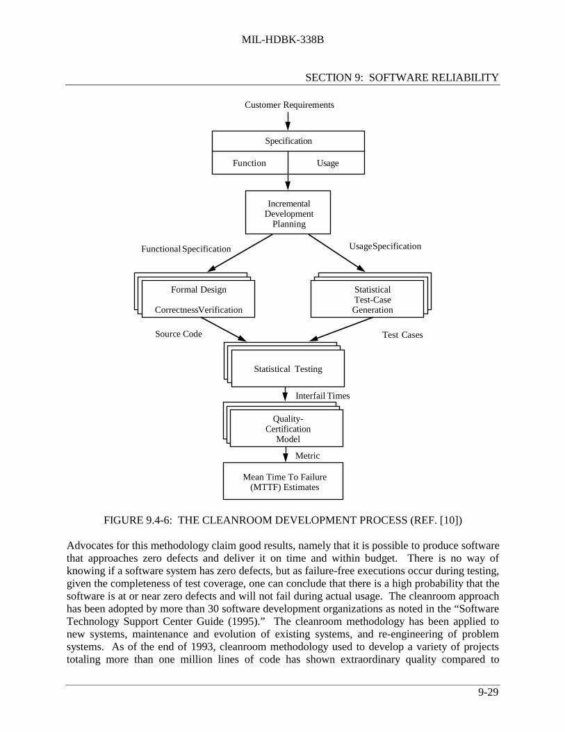
MIL-HDBK-338B


9-29

Quality-Certification

Model

Customer Requirements

Specification

Function Usage

IncrementalDevelopment

Planning

Functional Specification Usage Specification

Interfail Times

Formal Design

Correctness Verification

StatisticalTest-CaseGeneration

Statistical Testing

Source Code Test Cases

Mean Time To Failure(MTTF) Estimates

Metric

FIGURE 9.4-6: THE CLEANROOM DEVELOPMENT PROCESS (REF. [10])

Advocates for this methodology claim good results, namely that it is possible to produce softwarethat approaches zero defects and deliver it on time and within budget. There is no way ofknowing if a software system has zero defects, but as failure-free executions occur during testing,given the completeness of test coverage, one can conclude that there is a high probability that thesoftware is at or near zero defects and will not fail during actual usage. The cleanroom approachhas been adopted by more than 30 software development organizations as noted in the “SoftwareTechnology Support Center Guide (1995).” The cleanroom methodology has been applied tonew systems, maintenance and evolution of existing systems, and re-engineering of problemsystems. As of the end of 1993, cleanroom methodology used to develop a variety of projectstotaling more than one million lines of code has shown extraordinary quality compared to

MIL-HDBK-338B


9-30

traditional results. A summary of cleanroom performance measures is given in Table 9.4-2. Itshould be noted, however, that these results are achieved with cleanroom teams composed ofadequately trained journeyman programmers.

TABLE 9.4-2: CLEANROOM PERFORMANCE MEASURES (REF. [11])

Software DevelopmentPractices

Defects DuringDevelopment(defects per

KLOC*)

OperationalFailures

(failures perKLOC)

ResultantProductivity(LOC*/Staff

Month)Traditional Software-as-art

50 - 60 15 - 18 Unknown

Software Engineering 20 - 40 2 - 4 75 - 475Cleanroom Engineering 0 - 5 < 1 > 750

* KLOC - Thousand Lines of Code * LOC - Lines of Code

Adversaries claim that it is an unrealistic methodology for the following reasons:

(1) The required statistical knowledge is beyond the realm of most software engineers.

(2) The testing strategies are too complicated to expect the average developer to use.

(3) It is too complicated for use on small projects.

(4) The paradigm shift required is so radical that software people will never accept it.

9.5 Software Reliability Prediction and Estimation Models

Software reliability models have been in existence since the early 1970’s; over 200 have beendeveloped. Certainly some of the more recent ones build upon the theory and principles of theolder ones. Some of the older models have been discredited based upon more recent informationabout the assumptions and newer ones have replaced them. This review of software reliability isnot meant to be an exhaustive review of every model ever developed but, rather, a discussion ofsome of the major models in use today, highlighting issues important to the reliability engineer.

Prediction vs. Estimation Models

Software reliability modeling is generally used for one of two purposes: to make predictions andfor estimation. Software reliability prediction models use historical data for similar systemswhile estimation models use data collected during test. Prediction, therefore, is usually lessaccurate than estimation. The objective of software prediction is to predict the potentialreliability (fault rate) early in the development process. Insight into potential reliability allows

MIL-HDBK-338B


9-31

improvements in software management to be considered before coding and testing start. Theobjective of the estimation process is to determine the number of faults remaining in the softwarejust prior to testing so that the length of the test can be determined. Table 9.5-1 provides acomparison of prediction and estimation models.

TABLE 9.5-1: COMPARING PREDICTION AND ESTIMATION MODELS

Issues Prediction Models Estimation Models

Data Reference Uses historical data Uses data from the current softwaredevelopment effort

When Used InDevelopmentCycle

Usually made prior todevelopment or test phases; can beused as early as concept phase

Usually made later in life cycle (aftersome data have been collected); nottypically used in concept ordevelopment phases

Time Frame Predict reliability at some futuretime

Estimate reliability at either presentor some future time

9.5.1 Prediction Models

The most basic prediction model involves the use of an organization’s internal data, based onextensive experience and tracking, to develop predictions. Four other prediction models havebeen developed: Musa’s Execution Time Model, (Ref. [12]), Putnam’s Model, (Ref. [5]), andtwo models developed at Rome Laboratory and denoted by their technical report numbers: theTR-92-52 Model (Ref. [16]) and the TR-92-15 Model (Ref. [17]). Each prediction model, itscapabilities and description of outputs is summarized in Table 9.5-2.

9.5.1.1 In-house Historical Data Collection Model

A few organizations predict software reliability by collecting and using the database ofinformation accumulated on each of their own software projects. Metrics employed includeProduct, Project Management, and Fault indicators. Statistical regression analysis typically isused to develop a prediction equation for each of the important project characteristics.Management uses this information to predict the reliability of the proposed software product aswell as to plan resource allocation.

MIL-HDBK-338B


9-32

TABLE 9.5-2: SOFTWARE RELIABILITY PREDICTION TECHNIQUES

Prediction Model Capabilities Description of OutputsHistorical DataCollection Model

Can be most accurate, if there isorganization wide commitment.

Produces a prediction of the failurerate of delivered software based oncompany wide historical data.

Musa’s Model Predicts failure rate at start of systemtest that can be used later in reliabilitygrowth models.

Produces a prediction of the failurerate at the start of system test.

Putnam’s Model The profile of predicted faults overtime and not just the total number isneeded. Can be used with the otherprediction models.

Produces a prediction in the form ofa predicted fault profile over the lifeof the project.

TR-92-52 Model Allows for tradeoffs. Produces a prediction in terms offault density or estimated number ofinherent faults.

TR-92-15 Model Has default factors for estimatingnumber of faults

Estimates faults during eachdevelopment phase.

9.5.1.2 Musa’s Execution Time Model

Developed by John Musa (Ref. [12]) of Bell Laboratories in the mid 1970s, this was one of theearliest reliability prediction models. It predicts the initial failure rate (intensity) of a softwaresystem at the point when software system testing begins (i.e., when time, t = 0). The initialfailure intensity, λ 0 , (faults per unit time) is a function of the unknown, but estimated, totalnumber of failures expected in infinite time, N. The prediction equation is shown below; termsare explained in Table 9.5-3.

o0 x wpk x = λ

For example, a 100 line (SLOC) FORTRAN program with an average execution rate of 150 linesper second has a predicted failure rate, when system test begins, of λ0 = k x p x w0 = (4.2E-7) x(150/100/3) x (6/1000) = .0126E-7 = 1.26E-9 faults per second (or 1 fault per 7.9365E8 secondswhich is equivalent to 1 fault per 25.17 years).

It is important to note that this time measure is execution time, not calendar time. Sincehardware reliability models typically are in terms of calendar time, it is not feasible to use Musa’sprediction in developing an overall system reliability estimate unless one is willing to assumethat calendar time and execution time are the same (usually not a valid assumption).

MIL-HDBK-338B


9-33

TABLE 9.5-3: TERMS IN MUSA’S EXECUTION TIME MODEL

Symbol Represents Value

k Constant that accounts for the dynamicstructure of the program and the varyingmachines

k = 4.2E-7

p Estimate of the number of executions pertime unit

p = r/SLOC/ER

r Average instruction execution rate,determined from the manufacturer orbenchmarking

Constant

SLOC Source lines of code (not including reusedcode)

ER Expansion ratio, a constant dependent uponprogramming language

Assembler, 1.0; Macro Assembler, 1.5;C, 2.5; COBAL, FORTRAN, 3; Ada,4.5

w0 Estimate of the initial number of faults inthe program

Can be calculated using: w0 = N x Bor a default of 6 faults/1000 SLOC canbe assumed

N Total number of inherent faults Estimated based upon judgment or pastexperience

B Fault to failure conversion rate; proportionof faults that become failures. Proportionof faults not corrected before the product isdelivered.

Assume B = .95; i.e., 95% of the faultsundetected at delivery become failuresafter delivery

9.5.1.3 Putnam’s Model

Trachtenberg (formerly of General Electric) and Gaffney (of then IBM Federal Systems, nowLoral) examined defect histories, by phases of the development process, for many projects ofvarying size and application type. Based on their work, Putnam (Ref. [5]) assigned the generalnormalized Rayleigh distribution to describe the observed reliability, where k and a are constantsfit from the data and t is time, in months:

R(t) = k exp(-at2 )

The corresponding probability density function, f(t), the derivative of R(t) with respect to t, is ofthe general form:

f(t) = 2ak t exp(-at2 )

Putnam further developed an ordinal (i.e., not equally spaced in real time) scale to represent the

MIL-HDBK-338B


9-34

development process milestones; see Table 9.5-4. Of special interest is Milestone 7, denoted by

td, corresponding to the end of the development phases and the beginning of full operationalcapability; this point was defined as occurring at the 95th percentile (i.e., 95% of all defects havebeen detected at this point in the software development). Using td as the reference basis, he thendeveloped the expressions for the model constants, a and k, in terms N and td. The finalequation to predict the expected number of defects per month as a function of the schedule monthand the total number of inherent defects, N, is given by:

f(t) = (6N/td2

) t exp (-3t2/td2

)

TABLE 9.5-4: PUTNAM’S TIME AXIS MILESTONES

Milestone # Milestone0 Feasibility study1 Preliminary design review, function design complete2 Critical design review, detailed design complete3 First code complete4 Start of system integration test5 Start of user systems test6 Initial operational capability; installation7 Full operational capability; reliability about 95% in routine usage8 99% reliability achieved by stress testing9 99.9% reliability, assumed debugged

For example, suppose a FORTRAN program is being developed; the plan is that it will be fully

operational (Milestone 7) in 10 calendar months resulting in td2 to be 102 or 100. The defects

expected per month during development are calculated using the expression:

f(t) = .06 N t exp (-.03t2 )

Calculation results are shown in Figure 9.5-1, where t is the month number, f(t) is the expectedproportion of the total number of defects to be observed in month t, and F(t) represents thecumulative proportion. The Milestone number, based on the planned development schedule isalso shown for comparison; Milestone 7, corresponding to the 95th percentile, is, indeed, inMonth 10, Milestone 8, at the 99th percentile, is expected to occur in scheduled Month 13, andMilestone 9, at .999, is not expected to be reached by the end of scheduled Month 15.

MIL-HDBK-338B


9-35

t f(t) F(t) Mile #

1 0.058 0.058

2 0.106 0.165 1

3 0.137 0.302

4 0.149 0.451 2

5 0.142 0.592

6 0.122 0.715 3

7 0.097 0.811 4

8 0.070 0.881 5

9 0.048 0.929 6

10 0.030 0.959 7

11 0.017 0.976

12 0.010 0.986

13 0.005 0.991 8

14 0.002 0.993

15 0.001 0.994

PROPORTION OF TOTAL N EXPECTED PER MONTH

.00

.05

.10

.15

.20

1 2 3 4 5 6 7 8 9 10 11 12 13 14 15MONTH

PROPORTION

FIGURE 9.5-1: EXPECTED PROPORTION OF THE TOTAL NUMBER OF DEFECTS

One major benefit of this model is that the expected number of faults can be predicted for variouspoints in development process as compared to Musa’s model that provides the prediction whensystem testing begins (i.e., at Milestone 4) only.

Another corollary to this model is that the mean time to the next defect (MTTD) is given by1/f(t). This is only meaningful after Milestone 4 (since prior to that point the system would nothave been developed so defects could not be detected). As the development progresses, (i.e., tincreases), the MTTD increases since defects are being eliminated.

9.5.1.4 Rome Laboratory Prediction Model: RL-TR-92-52 (Ref. [16])

This is a method for predicting fault density at delivery time (i.e., at Putnam’s Milestone 6) andsubsequently using this fault density to predict the total number of inherent faults, N, and thefailure rate. It also provides a mechanism for allocating software reliability as a function of thesoftware characteristics as well as assessing trade-off options. The basic terminology of thismodel is presented in Table 9.5-5. The underlying assumption is that Source Lines of Code(SLOC) is a valid size metric.

MIL-HDBK-338B


9-36

TABLE 9.5-5: RL-TR-92-52 TERMINOLOGY

Terms DescriptionA Factor selected based on Application type; represents the baseline fault densityD Factor selected to reflect the Development environmentS Factor calculated from various “sub-factors” to reflect the Software characteristics

SLOC The number of executable Source Lines Of Code; lines that are blank or containcomments to enhance the readability of the code are excluded

FD Fault density; for the purposes of this model it is defined as the ratio of faults tolines of code (faults/SLOC)

N Estimate of total number of inherent faults in the system; prediction is derived fromthe fault density and the system size

C Factor representing a Conversion ratio associated with each application type; valuesare determined by dividing the average operational failure rate by the average faultdensity in the baseline sample set.

It is recognized as one of a few publicly available prediction models based upon extensivehistorical information. Predictions are based on data collected on various types of softwaresystems developed for the Air Force; see Table 9.5-6.

TABLE 9.5-6: AMOUNT OF HISTORICAL DATA INCLUDED

Application Type # of Systems Total SLOCAirborne 7 540,617Strategic 21 1,793,831Tactical 5 88,252Process Control 2 140,090Production Center 12 2,575,427Developmental 6 193,435TOTAL 53 5,331,652

The basic equations are:

Fault Density = FD = A x D x S (faults/line)Estimated Number of Inherent Faults = N = FD x SLOCFailure Rate = FD x C (faults/time)

The model consists of factors that are used to predict the fault density of the software application.These factors are illustrated in Table 9.5-7.

MIL-HDBK-338B


9-37

TABLE 9.5-7: SUMMARY OF THE RL-TR-92-52 MODEL

Factor Measure Range of Values Phase Used In* Trade-off RangeA - Application Difficulty in developing

various application types2 to 14(defects/KSLOC)

A-T None - Fixed

D - Developmentorganization

Development organization,methods, tools, techniques,documentation

.5 to 2.0 If known at A, D-T

The largest range

SA - Softwareanomaly management

Indication of fault tolerantdesign

.9 to 1.1 Normally, C-T Small

ST - Softwaretraceability

Traceability of design andcode to requirements

.9 to 1.0 Normally, C-T Large

SQ - Software quality Adherence to codingstandards

1.0 to 1.1 Normally, C-T Small

SL - Softwarelanguage

Normalizes fault density bylanguage type

Not applicable C-T N/A

SX - Softwarecomplexity

Unit complexity .8 to 1.5 C-T Large

SM - Softwaremodularity

Unit size .9 to 2.0 C-T Large

SR - Softwarestandards review

Compliance with design rules .75 to 1.5 C-T Large

Key: A - Concept or Analysis Phase

D - Detailed and Top Level DesignC - CodingT - Testing

The following are benefits of using this model:

(1) It can be used as soon as the concept of the software is known

(2) During the concept phase, it allows “what-if” analysis to be performed to determine theimpact of the development environment on fault density

(3) During the design phase, it allows “what-if” analysis to be performed to determine theimpact of software characteristics on fault density

(4) It allows for system software reliability allocation because it can be applied uniquely toeach application type comprising a software system

MIL-HDBK-338B


9-38

(5) The prediction can be customized using unique values for the A, S, and D factors basedupon historical software data from the specific organization’s environment while thefollowing are drawbacks:

(a) Factors and values used were generated based on software developed for the AirForce; if the software in question does not match one of the Air Force-relatedapplication types, then the average value must be selected. The Air Forceapplication types do not map well to software developed outside the militaryenvironment

(b) Use of SLOC as the size metric is becoming more and more irrelevant with recentchanges in software development technology, such as Graphical User Interface(GUI) system development, and the use of Commercial Off-the-Shelf (COTS)software

9.5.1.5 Rome Laboratory Prediction Model: RL-TR-92-15 (Ref. [17])

This technical report, produced by Hughes Aircraft for Rome Laboratory, examined manysoftware systems. It resulted in an average fault rate prediction value of 6 faults/1000 SLOC.(This was the default value for fault rate, w0, used in Musa’s Execution Time Model).In addition, a set of 24 predictor factors, listed in Table 9.5-8, was used to estimate the threemain variables of interest:

(1) Number of faults detected during each development phase (DP)

(2) Man-hours utilized during each phase (UT)

(3) Size of product (S)

The resultant equations were:

(1) f(DP) = 18.04 + .05 x (.009 X1 + .99 X2 + .10 X3 - .0001 X4 + .0005 X5)

(2) f(UT) = 17.90 + .04 x (.007 X1 + .796 X2 + .08 X3 - .0003 X4 + .0003 X5+ .00009 X6 + .0043 X7 + .013 X8 + .6 X9 + .003 X10)

(3) f(S) = 17.88 + .04 x (.0007 X1 + .8 X3 + .01 X8 + .6 X9 + .008 X23 + .03 X25)

where the coefficients and descriptions of the variables of the regression model are listed in thetable.

MIL-HDBK-338B


9-39

TABLE 9.5-8: REGRESSION EQUATION COEFFICIENTS

CoefficientsX Description of Variable EQ 1 EQ 2 EQ 31 Number of faults in software requirements specification .009 .007 .0072 Requirements statement in specification .99 .796 NA3 Pages in specification .10 .08 .804 Man-months spent in requirements analysis .0001 -.0003 NA5 Requirements change after baseline .0005 .0003 NA6 Number of faults in preliminary design document NA .00009 NA7 Number of CSCS NA .0043 NA8 Number of units in design NA .013 .019 Pages in design document NA .6 .6

10 Man-months spent in preliminary design NA .003 NA11 Number of failures in design document NA NA NA12 Man-months spent in detailed design NA NA NA13 Design faults identified after baseline NA NA NA14 Design faults identified after internal review NA NA NA15 Number of executable SLOC NA NA NA16 Faults found in code reviews NA NA NA17 Average years of programmer experience NA NA NA18 Number of units under review NA NA NA19 Average number of SLOC per unit NA NA NA20 Average number branches in unit NA NA NA21 Percentage branches covered NA NA NA22 Nesting depth coverage NA NA NA23 Number of times an unit is unit tested NA NA .00824 Man-months for coding and unit test NA NA NA25 Equals (X13 + X14 + X16) NA NA .03

The results indicate that thirteen of the 24 hypothesized factors had no effect on the threevariables of interest. Further, the most important estimators involved the software requirementsspecification, including the number of requirement statements, number of faults in thesestatements, and the total number of pages in the specification.

The benefits of this model are:

(1) It can be used prior to system testing to estimate reliability

(2) It includes cost and product parameters as well as fault and time

The disadvantages of this model are:

(1) It was based on data collected by one organization in one industry/application type

(2) It does not disclose the unit of measure for specification size

MIL-HDBK-338B


9-40

9.5.2 Estimation Models

The fault count and fault rate models are the most common type of estimation techniques. Eachmakes assumption about how faults arrive (detected) and how they are corrected. The fault countmodels include: Exponential, Weibull and Bayesian techniques. Also, included in theestimation model scenario are the test coverage and fault tagging methods.

9.5.2.1 Exponential Distribution Models

In general, exponential models assume that the software is in an operational state and that allfaults are independent of each other. The time to failure, t, of an individual fault follows theexponential distribution:

t)exp(- = f(t) λλ

with the general form for the reliability given by:

R(t) = exp(-λt)

and the mean time to the next failure (MTTF) expressed as:

MTTF = 1/λ

The notations used in the general case for the exponential distribution model are shown in Table9.5-9 and illustrated in Figure 9.5-2.

MIL-HDBK-338B


9-41

TABLE 9.5-9: NOTATIONS FOR THE EXPONENTIAL DISTRIBUTION MODEL

Notation ExplanationN Total number of defectsn Number of defects to datec Number of defects corrected to date

N-n Defects not yet manifestedN-c Defects yet to be correctednf Fault countλf Fault ratetf Future timenp Fault count at present timeλp Fault rate at present timetp Present time

N

nf

np

0

∆n

∆(n/t)

λf λP λ0

Numberof

Defects

Fault Rate

FIGURE 9.5-2: EXPONENTIAL MODEL BASIS

Advocates of the exponential model note its simplicity and its parallelism to the hardwarereliability framework. The major disadvantage is that it cannot be used early in the softwaredevelopment since the product must be operational before the model can be used. Hence, itcannot be used for early reliability assessment.

Table 9.5-10 summarizes the various exponential models including assumptions and comments.

MIL-HDBK-338B


9-42

TABLE 9.5-10: VARIOUS EXPONENTIAL MODELS*

Model MTTF Dn Dt Assumptions/CommentsGeneralExponential

1/[k(N - c)] k-1 λp / λf k-1 ln (λp / λf) Faults are equal in severity and probability ofdetectionFault rate directly related to number of faultsremaining to be corrected

Lloyd-Lipow 1/[k(N - n)] k-1 λp / λf k-1 ln (λp / λf) Fault rate directly related to number of faultsremaining to be detected

Musa’s Basic N/λ0 (λp - λf) N/λ0 ln (λp - λf) References an initial fault rate at time 0(beginning of system test)

Musa’sLogarithmic

f-1 ln (λp /λf) f-1 (1/λf -1/λp) Some faults are more likely to be foundbefore othersRate of fault detection decreasesexponentially

Shooman’s 1/[kSLOC -((N/SLOC) -(C/SLOC))]

k-1 λp / λf k-1 ln (λp / λf) Adjusts for changing product size; eachparameter is normalized for lines of code

Goel-Okumoto Faults can cause other faultsFaults may not be removed immediately

* where k is a constant of proportionality, N is the number of inherent faults, c is the number of corrected faults andn is the number of detected faults

General Exponential Model

In the general case, the model assumes that all faults are equal in severity and probability ofdetection and that each is immediately corrected upon detection. The fault rate, λ , is assumed tobe directly related to the number of faults remaining in the software. That is, λ is a function ofthe number of corrected faults, c:

c) - (Nk = λ

where k is a constant of proportionality. In actual application, k is typically estimated from theslope of the plot of the observed fault rate vs. number of faults corrected.

The projection of the number of faults needed to be detected to reach a final failure rate λ f isgiven by:

fp / (1/k) =n λλ∆

where k is the same proportionality constant used above.

MIL-HDBK-338B


9-43

The projection of the time necessary to reach a projected fault rate is given by:

[ ]fp /(1/k)ln =t λλ∆

The major disadvantage of this specific approach is that not only must the defects be detected butthey also must be corrected.

Lloyd-Lipow Model (Ref. [18] and [19])

The Lloyd-Lipow Model exponential model also assumes that all faults are equal in severity andprobability of detection. The difference from the previous model is that in this Lloyd-Lipowapproach, the fault rate, λ , is assumed to be directly related to the number of faults remaining tobe detected (not corrected) in the software. That is, λ is a function of the number of detectedfaults, n:

n) - (Nk = λ

The expressions for the mean-time-to-failure (MTTF), ∆n and ∆t are the same as in the generalexponential model.

This form of the exponential model does not require defect correction, just detection. However,the validity of the use of the exponential model in this situation has been questioned.

Musa’s Basic Model (Ref. [12])

Musa’s Basic Model is another form of the general exponential model. It utilizes the initial (i.e.,at the start of software testing) fault rate, λ0, where either λ0 is estimated from the data orcomputed ( λ0 = N/k) based on a guess for N and the estimate for k, the previously referencedslope value.

In this model, the fault rate after n faults have been detected is a fraction of the original fault rate:

λ n = λ0 (1 - n/v)

where:n is usually expressed as µ and v is usually expressed as υ

while the expression for the fault rate at time t is given by:

λ t = λ 0 exp [-(λ 0/υ)τ]

MIL-HDBK-338B


9-44

where:υ = N/B, where N is the number of inherent faults and B is the fault reduction ratio,

usually assumed to be 95% (i.e., 95% of the faults undetected at delivery becomefailures after delivery

τ = System test time


) - ( N/ =n fp0 λλλ∆

The projection of the time necessary to reach a projected failure rate is given by:

) - (ln N/ =t fp0 λλλ∆

The disadvantage is that this model is very sensitive to deviations from the assumptions. Inaddition, as noted with Musa’s previous work, the units are execution time, not calendar time.

Musa’s Logarithmic Model (Ref. [12])

Musa’s Logarithmic Model has different assumptions than the other exponential models:

(1) Some faults are likely to be found before others

(2) The rate of fault detection is not constant, but decreases exponentially

In this model, the fault rate after n faults have been detected is a function of the original faultrate:

exp(-ft) = 0n λλ

while the expression for the fault rate at time t is given by:

1) + t f /( = 00t λλλ

where:f = failure intensity decay parameter, the relative change of n/t over n.

MIL-HDBK-338B


9-45


)/(ln /f1 =n fp λλ∆

The projection of the time necessary to reach a projected failure rate is given by:

)1/ - (1/ 1/f =t pf λλ∆

The major benefit of this model is that it does not require an estimate for N. Since the value for fcan be estimated prior to actual data occurrence, the model can be used earlier in thedevelopment cycle to estimate reliability.

The disadvantage of this model, typical for most exponential models, is that the modelassumptions must be valid for the results to be valid. In particular, the assumption that the rate offault detection decreases exponentially has not been confirmed with many real data sets. Inaddition, as noted with Musa’s previous work, the units are execution time, not calendar time,making direct comparison with hardware reliability difficult.

Shooman’s Model (Ref. [20])

The Shooman’s Model is similar to the general exponential model except that each fault count isnormalized for the lines of code at that point in time. Earlier, λ = k (N - c); here, it is given by:

λ = k SLOC (N/SLOC - c/SLOC)

The equation of MTTF = 1/λ uses Shooman’s expression for λ . The equations for ∆n and ∆tare the same as the general exponential case.

The advantage of Shooman’s model is that it adjusts for the changing size of the softwareproduct. The disadvantages are that it must be used later in development after the LOC havebeen determined and that the general exponential assumptions may not apply.

Goel-Okumoto Model (Ref. [19])

This model is different from other exponential models because it assumes that faults can causeother faults and that they may not be removed immediately. An iterative solution is required.

This model is expressed as:

exp(-bt) ab = tλ

MIL-HDBK-338B


9-46

where a and b are resolved iteratively from the following:

n/a = 1 - exp(-bt) and n/b = a t exp(-bt) + ∑ ti ,

where the summation is over i = 1,..., n,

Use N and k as starting points for solving for these two equations simultaneously.

The major benefit of this model is that it can be used earlier than other exponential models whileits major disadvantage is that it is very sensitive to deviations from the assumptions.

9.5.2.2 Weibull Distribution Model (Ref. [19])

The Weibull Model is one of the earliest models applied to software. It has the same form as thatused for hardware reliability. There are two parameters: a, the scale parameter (a > 0), and b, theshape parameter that reflects the increasing (b > 1), decreasing (b < 1) or constant (b = 1) failurerate.

The mean time to next failure is given by:

(1/a) (b/a) = MTTF Γ

where Γ (c) is the complete Gamma Function = 0

∞

∫ yc −1 e −ydy

The reliability at time t is given by:

R(t) = exp[-(t/b)a ]

The benefits of the Weibull model is its flexibility to take into account increasing and decreasingfailure rates. The disadvantage of this model is more work is required in estimating theparameters over the exponential model.

9.5.2.3 Bayesian Fault Rate Estimation Model

The Bayesian approach does not focus on the estimated inherent fault count, N, but ratherconcentrates on the fault/failure rate. The classical approach assumes that reliability and failurerate are a function of fault detection while the Bayesian approach, on the other hand, assumesthat a software program which has had fault-free operation is more likely to be reliable. TheBayesian approach also differs because it is possible to include an assessment of “priorknowledge” (therefore, it is sometimes called a “subjective” approach).

MIL-HDBK-338B


9-47

The Thompson and Chelson’s model (Ref. [19]) assumes that:

(1) Software is operational

(2) Software faults occur at some unknown rate λ that is assumed to follow a GammaDistribution with parameters Xi and fi + 1

(3) Faults are corrected in between test periods but not during test periods

(4) Total number of faults observed in a single testing period of length ti follows a Poissondistribution with parameter λti

The model assumes that there are i test periods, each with length, ti (not assumed equal); wherethe number of faults detected during that period is represented by fi . The subjective informationis inserted as occurring in period 0, i.e., t0 and f0 represent the prior information. If there is noprior information, these values are set to zero. On the other hand, if there is a great deal ofexperience, t0 might be very large, especially relative to the expected evaluation time; the valuefor the prior number of faults also depends on past experience and is independent from the priorof time.

Let Ti represent the cumulative total of the test period lengths over the entire range, i.e., fromperiod 0 to i and let Fi represent the cumulative total of the faults, fi , over the entire range, i.e.,from period 0 to i.

Then, the reliability at time t (in interval i) is expressed as a function of the values from the

previous (i - 1) interval as well as the current ith interval data:

R(t) = [Ti-1/(Ti-1 + t)]Fi-1

The failure rate estimate at time t (in interval i) is given by:

1-i1-i 1)/T + (F = (t)λ

The benefits of this model are related to its assumptions: N is not assumed fixed, reliability isnot assumed to be directly a function of N, and faults are not assumed to be correctedimmediately. The disadvantage is that Bayesian Models, in general, are not universally acceptedsince they allow for the inclusion of prior information reflecting the analyst’s degree of beliefabout the failure rate.

MIL-HDBK-338B


9-48

9.5.2.4 Test Coverage Reliability Metrics

Test coverage advocates have defined software reliability as a function of the amount of thesoftware product that has been successfully verified or tested. Three such metrics are discussedbelow. The first is a simple ratio based upon the rate of successful testing during the finalacceptance test. The second and third provide a metric based on ways of combining the resultsfrom both white-box and black-box testing.

Advocates of this approach to reliability explain that since the data are (or should be) collectedand tracked during testing, these measures are readily available and require no additionalverification effort. However, to the reliability engineer, these metrics are foreign to anythingused in the hardware environment to describe reliability. Further, none of these metrics can beconverted to failure rate or used to predict or estimate mean time between failures.

Test Success Reliability Metric

In this approach, (Ref. [19]) reliability is simply defined as the ratio of the number of test casesexecuted successfully during acceptance (black-box) testing, defined as s, to the total number oftest cases executed during acceptance testing, defined as r:

R = s/r

The validity of the result is dependent on the size of r as well as the ability for r to represent thetotal operational profile of the software. During the very late stages of testing, immediately priorto delivery, this model may be used for accepting or rejecting the software.

IEEE Test Coverage Reliability Metric

This method (Refs. [21] and [22]) assumes that reliability is dependent upon both the functionsthat are tested (black-box) and the product that is tested (white-box). It assumes that both typesof testing have to be completed for the test coverage to be complete. The reliability value isdefined as the product of two proportions, converted to a percent:

R = p(functions tested) * p(program tested) * 100%

where:p(functions tested) = Number of capabilities tested/total number of capabilities

p(program tested) = Total paths and inputs tested/total number of paths and inputs

Leone’s Test Coverage Reliability Metric

This approach (Ref. [23]) is similar to the IEEE Model except that it assumes that it is possibleto have either white or black box testing and still have some level of reliability. Two white-box

MIL-HDBK-338B


9-49

variables, a and b, and two black-box variables, c and d, are assessed. The reliability is theweighted sum of the four proportions:

R = ((a * w1) + (b * w2) + (c * w3) + (d * w4)) / (w1 + w2 + w3 + w4)

where:a = Number of independent paths tested/total number of pathsb = Number of inputs tested/total number of inputsc = Number of functions verified/total number of functionsd = Number of failure modes addressed/total number of failure modes

The values for w1, w2, w3, w4 represent weights. If all parameters are equally important, theseweights all are set to 1; however, if there are data to support that some parameters are moreimportant than others, then these more important parameters would receive higher weights.This model has two underlying assumptions. First, independent paths are identified usinginformation from testing procedures. Second, failure models (Ref. [24]) are identified usingFault Tree Analysis or Failure Modes, Effects, and Criticality Analysis.

9.5.3 Estimating Total Number of Faults Using Tagging

Tagging (Ref. [23]) is used to estimate the total number of faults in the software, N, based on thenumber observed during testing. It is based on seeding, a method of introducing faults into thesoftware and then determining how many of these faults are found during testing in order toestimate the total number of faults.

To illustrate, suppose the number of fish in a pond, N, is of interest. One way to develop anestimate is to capture and tag some number of the fish, T, and return them to the pond. As fishare caught, the number of tagged fish, t, is recorded as well as the number untagged, u. The totalnumber of untagged fish U, is estimated using the proportion: u/U = t/T. Then, the total numberof fish is estimated as the sum: N = U + T.

The steps used in the basic seeding approach for a software fault estimation are:

(1) A set of faults which represents the faults which would typically be found in operationalusage is identified.

(2) Faults are injected into software without the testers or developers being aware of them.The total number of injected faults is T.

(3) Test software and identify all faults found. Let t = the number of faults detected thatwere injected and let u = the number of faults detected which were not injected.

MIL-HDBK-338B


9-50

(4) The total number of faults which are not injected is estimated by U, where:

u/U = t/T

(5) The total number of faults, N, is estimated by:

N = U + T

(6) The injected faults are removed.

In general, this approach is not recommended based upon the issues identified below:

(1) How can faults which are typical of operational usage be identified and then injected ina completely random manner? (without bias)?

(2) Seeding assumes faults are due to coding mistakes. What about faults due torequirements, design and maintenance errors?

(3) During the course of a typical testing cycle, faults are typically corrected. Do theinjected faults get corrected during this process, or at the very end.

(4) Will seeded faults prevent real faults from being detected?(5) How can injected faults be kept a secret when the maintainer goes to fix them? How

can it be justified to spend resources fixing injected faults?(6) What is the action at the end of testing, go back to the original version with no injected

faults (and no corrected real faults) or remove (hopefully all) the injected faults?

An alternative Dual Test Group Approach is similar to basic seeding except that two groups areused. It assumes that:

(1) Two independent test groups are testing the same software at same time.(2) Groups do not share information on faults detected in testing.(3) Groups create their own test plans, but test the same functionality of the software.(4) Groups are equal in experience and capabilities.

This model predicts N, the total number of faults, based upon three numbers, n1, n2, and n12where n1 and n2 represent the number of faults found by Group 1 and Group 2, respectively,while n12 is the number of faults found by both groups.

The total number of faults, N, is estimated by:

N = R + n1 + n2 + n12

where:R is the estimated total number of remaining faults

MIL-HDBK-338B


9-51

This model assumes that as the number of faults found by both groups increases, the numberremaining decreases. As testing continues, it is assumed that n12 will increase. This means thatwhen there are few faults left in the software (i.e., as R approaches 0), both test groups will beginfinding the same faults. This may not be the case, however, since both test groups may beinefficient. The basic assumptions also may be unrealistic. It is not always possible oreconomical to have two completely independent test groups with equal experience level andcapabilities. It also may not be easy to keep the groups independent and equal in experience.

9.6 Software Reliability Allocation

Software reliability allocation involves the establishment of reliability goals for individualcomputer software configuration items (CSCI) based on top-level reliability requirements for allthe software. It is very important that this activity, allocations, be established early in theprogram so that criteria for evaluating the achieved reliability of each element can be established.Table 9.6-1 describes five allocation techniques. These techniques are based on the type ofexecution expected or the operational profile or the software complexity.

The allocation of a system requirement to software elements makes sense only at the softwaresystem or CSCI level. Once software CSCIs have been allocated reliability requirements, adifferent approach is needed to allocate the software CSCI requirements to lower levels. Thereliability model for software differs significantly from hardware due to its inherent operatingcharacteristics. For each mode in a software system’s (CSCI) operation, different softwaremodules (CSCs) will be executing. Each mode will have a unique time of operation associatedwith it. A model should be developed for the software portion of a system to illustrate themodules which will be operating during each system mode, and indicate the duration of eachsystem mode. An example of this type of model is shown in Table 9.6-2 for a missile system.

TABLE 9.6-1: SOFTWARE RELIABILITY ALLOCATION TECHNIQUES (REF. [2])

Technique Procedure Name Use DescriptionSequential Execution(see 9.6.1)

Equal apportionment applied tosequential software CSCIs

Use early in the SW development process whenthe software components are executedsequentially

Concurrent Execution(see 9.6.2)

Equal apportionment applied toconcurrent software CSCIs

Use early in the SW development process and thesoftware components are executed concurrently

Operational Profile(see Ref. [2])

Mission or Operational ProfileAllocation

Use when the operational profile of the CSCIs areknown

OperationalCriticality (see 9.6.3)

Allocation based on operationalcriticality factors

Use when the operational criticalitycharacteristics of the software is known

Complexity (see9.6.4)

Allocation based on complexityfactors

Use when the complexity factors of the softwarecomponents are known

The software reliability model will include the number of source lines of code (SLOC) expectedfor each module. These data, along with other information pertaining to software developmentresources (personnel, computing facilities, test facilities, etc.) are used to establish initial failureintensity predictions for the software modules.

MIL-HDBK-338B


9-52

To assist in the proper selection of an allocation technique, a flow diagram is provided in Figure9.6-1.

TABLE 9.6-2: SOFTWARE FUNCTIONS BY SYSTEM MODE - EXAMPLE

System Mode Modules SLOCStandby - 2 Hours Built-in Test (BIT)

1760 InterfaceFlight SequencingPrelaunch InitializationTOTAL

4000750

2000900

7650Prelaunch - 20 Minutes BIT

NavigationFlight SequencingPrelaunch InitializationNavigation Kalman FilterTOTAL

400010002000

90020009900

Post-Launch - 10 Minutes BITInterfaceNavigationInfrared Seeker ControlFlight SequencingTerminal ManeuverOther Post-LaunchNavigation Kalman FilterTOTAL

400070001000

50020001000

245002000

42000

Are the CSCIsexecuted

sequentially?

Yes Yes Yes Yes Yes

Are the CSCIsexecuted

concurrently?

Is themission oroperational

profileknown?

Is theoperationalcriticalityavailable?

Is thecomplexity of

each CSCIknown?

Use achievablefailure rateallocation

Equalapportionmentfor sequential

CSCIs

Equalapportionmentfor concurrent

CSCIs

Operationalprofile

allocation

Operationalcriticalityallocation

Complexityallocation

Given:

• Aggregate failure rate goal• Number of software CSCIs*• Total mission time

And any one of these:

• Topology of CSCIs• Profile of CSCIs• Criticality of CSCIs• Complexity of CSCIs• Utilization of CSCIs

No NoNoNoNo

* CSCI - Computer Software Configuration Item

FIGURE 9.6-1: RELIABILITY ALLOCATION PROCESS (REF. [2])

MIL-HDBK-338B


9-53

9.6.1 Equal Apportionment Applied to Sequential Software CSCIs

This technique is used to allocate a failure rate goal to each individual software CSCI when theCSCIs are executed sequentially. This procedure should be used only when the failure rate goalof the software aggregate ( λ s), and the number of software CSCIs in the aggregate (N), areknown. The aggregate’s failure rate goal is either specified in the requirements or is the result ofan allocation performed at a higher level in the system hierarchy.

Steps:

(1) Determine the failure rate goal for the software aggregate; λ s

(2) Determine the number of software CSCIs in the aggregate; N

(3) For each software CSCI, assign the failure rate goal as follows:

hour)per (failures = s(CSCI) i λλ

where:i = 1, 2, ..., N

Example:

A software aggregate is required to have a maximum of 0.05 failures per hour. The aggregateconsists of five software CSCIs that are executed one after another, that is, the five CSCIs runsequentially. All CSCIs must succeed for the system to succeed (this is a series system).

Then, using the equal apportionment technique, the failure rate goal for the ith software CSCI isassigned to be:

λ i = λs = 0.05 failures per hours

where:i = 1, 2, ..., 5

MIL-HDBK-338B


9-54

9.6.2 Equal Apportionment Applied to Concurrent Software CSCIs

This technique is used to allocate the appropriate failure rate goal to each individual softwareCSCI, when the CSCIs are executed concurrently. λ s, the failure rate of the software aggregate,and N, the number of software CSCIs in the aggregate, are needed for this procedure.

Steps:

(1) Determine the failure rate goal for the software aggregate; λ s


(3) For each software CSCI, assign the failure rate goal as follows:

λ i (CSCI) = λs /N (failures per hour)

where:i = 1, 2, ..., N

Example:

A software aggregate has a failure rate goal of 0.05 failures per hour. The aggregate consists offive software CSCIs, which are in series and executed concurrently. Then, the allocated failurerate goal of each of the five software CSCI is:

λ i = λs/N =

0.055

= 0.01 failures per hour

9.6.3 Allocation Based on Operational Criticality Factors

The operational criticality factors method allocates failure rates based on the system impact of asoftware failure. Criticality is a measure of the system’s ability to continue to operate and thesystem’s ability to be fail-safe. For certain modes of operation, the criticality of that mode maycall for a lower failure rate to be allocated. In order to meet very low failure rates, fault-toleranceor other methods may be needed.

The following procedure is used to allocate the appropriate value to the failure rate of eachsoftware CSCI in an aggregate, provided that the criticality factor of each CSCI is known. ACSCI’s criticality refers to the degree to which the reliability and/or safety of the system as awhole is dependent on the proper functioning of the CSCI. Furthermore, gradations of safetyhazards translate into gradations of criticality. The greater the criticality, the lower the failurerate that should be allocated.

MIL-HDBK-338B


9-55

Steps:

(1) Determine the failure rate goal of the software aggregate; λ s


(3) For each ith CSCI, i = 1, 2, ..., N, determine its criticality factor ci. The lower the ci themore critical the CSCI.

(4) Determine i‘τ the total active time of the ith CSCI, i = 1, 2, ..., N. Determine T, the

mission time of the aggregate.

(5) Compute the failure rate adjustment factor K:

K = i =1

N∑ ci i

‘τ

T

(6) Compute the allocated failure rate goal of each CSCI

λi = λs (ci/K)

(Dividing by K makes the allocated CSCI failure rates build up to the aggregate failure rate goal).

Example:

Suppose a software aggregate consisting of three software CSCIs is to be developed. Assume thefailure rate goal of the aggregate is 0.002 failures per hour. Suppose that the mission time is 4hours. Furthermore, the criticality factors and the total active time of the software CSCIs are:

c1 = 4 hours 2 = ’1τ

c2 = 2 hour 1 = ’2τ

c3 = 1 hours 2 = ’3τ

(Note: In this example, since c3 has the smallest value, this indicates that the third CSCI of thissoftware aggregate is the most critical.)

MIL-HDBK-338B


9-56

Compute the adjustment factor K:

3 = 4

(1)(2) + (2)(1) + (4)(2) =

c + c + c =K 332211

T

τττ

Then, the allocated failure rate goals of the software CSCIs are:

/K)(c = 1s1 λλ= 0.002 (4/3) = 0.0027 failures per hour



9.6.4 Allocation Based on Complexity Factors

The following technique is used to allocate a failure rate goal to each software CSCI in anaggregate, based on the complexity of the CSCIs. There are several types of complexity asapplied to software that are listed in Table 9.6-3.

TABLE 9.6-3: COMPLEXITY PROCEDURES

Complexity Type Description When it Can Be UsedMcCabe’s Complexity A measure of the branches in logic in a unit of

code.From the start of detaileddesign on.

Functional Complexity A measure of the number of cohesive functionsperformed by the unit.

From the start of detaileddesign on.

Software ProductResearch Function Points

A measure of problem, code, and data complexity,inputs, outputs, inquiries, data files and interfaces.

From detailed design on.

Software ProductResearch Feature Points

A measure of algorithms, inputs, outputs, inquiries,data files and interfaces.

From detailed design on.

During the design phase, an estimated complexity factor using any one of these techniques isavailable. The greater the complexity, the more effort required to achieve a particular failure rategoal. Thus, CSCIs with higher complexity should be assigned higher failure rate goals.

The complexity measure chosen must be transformed into a measure that is linearly proportionalto failure rate. If the complexity factor doubles, for example, the failure rate goal should be twiceas high.

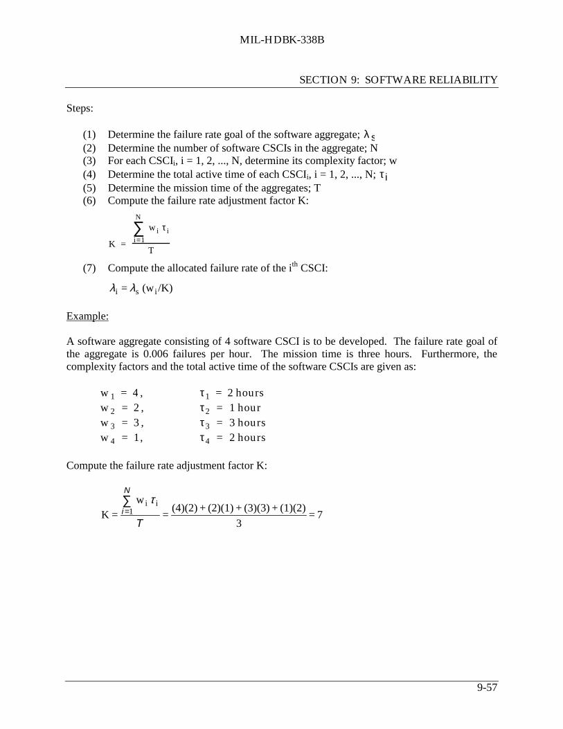
MIL-HDBK-338B


9-57

Steps:

(1) Determine the failure rate goal of the software aggregate; λ s(2) Determine the number of software CSCIs in the aggregate; N(3) For each CSCIi, i = 1, 2, ..., N, determine its complexity factor; w(4) Determine the total active time of each CSCIi, i = 1, 2, ..., N; τ i(5) Determine the mission time of the aggregates; T(6) Compute the failure rate adjustment factor K:

K =

wi τii=1

N

∑T

(7) Compute the allocated failure rate of the ith CSCI:

/K)(w = isi λλ

Example:

A software aggregate consisting of 4 software CSCI is to be developed. The failure rate goal ofthe aggregate is 0.006 failures per hour. The mission time is three hours. Furthermore, thecomplexity factors and the total active time of the software CSCIs are given as:

w1 = 4 , τ1 = 2 hours

w2 = 2 , τ2 = 1 hour

w3 = 3 , τ3 = 3 hours

w4 = 1, τ4 = 2 hours

Compute the failure rate adjustment factor K:

7 = 3

(1)(2) + (3)(3) + (2)(1) + (4)(2) =

w =K 1

ii

T

N

i∑=

τ

MIL-HDBK-338B


9-58

Then, the failure rate goal of each software CSCIs is:

λ1 = λs (w1/K)= 0.006 (4/7) = 0.0034 failures per hour

/K)(w = 2s2 λλ= 0.006 (2/7) = 0.0017 failures per hour

/K)(w = 3s3 λλ= 0.006 (3/7) = 0.00026 failures per hour

λ4 = λs (w4/K)= 0.006 (1/7) = 0.0009 failures per hour

9.7 Software Testing

Most software experts recommend that an independent organization test a software system. Oneoption is to contract with an outside organization for the testing. If this is not possible, thetesting organization should be managerially separate from the design and development groupsassigned to the project.

This recommendation is based more on observations of human nature than on substantiated fact.Effective testing groups need to have somewhat of a “destructive” view of a system, so that theycan flush out errors and “break” the system. The design and development groups who have builtthe software system have a “constructive” view, and may therefore find it too difficult to developthe frame of mind required for testing.

9.7.1 Module Testing

Module testing (also called unit or component testing) is the testing of one individual component(that is, one program module, one functional unit, or one subroutine). The objective of moduletesting is to determine if the module functions according to its specifications.

Module testing is usually conducted by the programmer of the module being tested. It is closelytied to the programmer’s development of the code and often becomes an iterative process oftesting a component, finding a problem, debugging (finding the reason for the problem in thecode), fixing the problem, and then testing again. Module testing is therefore often consideredpart of the implementation rather than part of the testing phase. Module testing shouldnevertheless be recognized as a separate function, and should be disciplined. The tester mustdevelop a test plan for the component and must document test cases and procedures. Too often,this discipline is overlooked and testing of individual components becomes “ad hoc” testing withno records about the actual cases, the procedures, or the results.

MIL-HDBK-338B


9-59

White box testing is frequently used during module testing. White box testing means that thetester is familiar with the internal logic of the component and develops test cases accordingly.

Code coverage (how much of the code is covered by the testing) and logic path coverage (howmany of the logical paths in the code are tested) are two primary considerations when developingtest cases for module testing.

9.7.2 Integration Testing

After module testing, the next step in the software testing phase is integration testing. Thisactivity involves combining components in an orderly progression until the entire system hasbeen built. The emphasis of integration testing is on the interaction of the different componentsand the interfaces between them.

Most often, the programming group performs software integration testing. As with moduletesting, integration testing is very closely linked to the programming activity since the testerneeds to know details of the function of each component to develop a good integration test plan.

Integration Test Techniques. An important decision when planning for integration testing isdetermining the procedure to be used for combining all the individual modules. There are twobasic approaches for doing this: non-incremental testing and incremental testing.

In non-incremental integration testing, all the software components (assuming they have eachbeen individually module tested) are combined at once and then testing begins. Since allmodules are combined at once, a failure could be in any one of the numerous interfaces that havebeen introduced.

The recommended approach for the integration of system components is planned incrementaltesting. With this method, one component is completely module tested and debugged. Anothercomponent is then added to the first and the combination is tested and debugged. This pattern ofadding one new component at a time is repeated until all components have been added to the testand the system is completely integrated.

Incremental testing requires another decision about the order in which the components will beadded to the test. There are no clear-cut rules for doing this. Testers must base a decision ontheir knowledge of what makes the most sense for their system, considering logic and use ofresources. There are two basic strategies: top-down or bottom-up as shown in Figure 9.7-1.

MIL-HDBK-338B


9-60

Top

- D

own

Bot

tom

- U

p

Level 1:

Level 2:

Level 3:

Level 4:

A

B C

D E F

G H

FIGURE 9.7-1: STRUCTURAL REPRESENTATION OF A SOFTWARE SYSTEM

A tester using top-down integration testing on this system begins by module testing anddebugging the A component. The next step is to add a new component to the test. In this case,either B or C is added. If B was chosen and tested, either C or D could be the next choice. Sometesters prefer to follow one path to completion, while others prefer to complete all the moduleson the same level before proceeding to a lower level of the hierarchy.

Bottom-up integration testing reverses top-down testing. With this approach, a tester simplystarts at the bottom-most level of the hierarchy and works up. As shown in Figure 9-16, a testermight start by module testing component G. With bottom-up testing, all the components at thebottom of the hierarchy are usually module tested first and then testing proceeds in turn to eachof their calling components. The primary rule in bottom-up testing is that a component shouldnot be chosen to be the next one added to the test unless all of the components that it calls havealready been tested.

MIL-HDBK-338B


9-61

9.7.3 System Testing

System Testing Techniques. System testing is often referred to as “testing the whole system.”Translated literally, that could mean that every input or output condition in the software needs tobe tested for every possible logical path through the code. Even in a small system this task couldbecome quite lengthy. In a large, complex system, it would be prohibitively time-consuming andexpensive.

The system test organization must develop a strategy for testing a particular system anddetermine the amount of test coverage required. There is no cookbook for doing so. In a smallnoncritical system, a very low degree of test coverage may be acceptable. High coverage isneeded in a critical software system involving human life. The testers must decide the best planbased on system characteristics, the environment in which the software system will operate, andthe testers’ experience.

In general, software system testing is done using black box testing. The tester, viewing thesystem as a black box, is not concerned with the internals, but rather is interested in finding ifand when the system does not behave according to its requirements.

One technique often used for identifying specific test cases is called equivalence partitioning. Inthis method, an equivalence class is identified so that one test case covers a number of otherpossible test cases.

Boundary analysis is another technique used in which testing is performed on all the boundaryconditions. This method tests the upper and lower boundaries of the program. In addition, it isusually wise to test around the boundaries.

A third technique that should always be applied to the testing of a program is called errorguessing. With this method, testers use their intuition and experience to develop specific testcases. A good system tester is usually very effective at doing this.

9.7.4 General Methodology for Software Failure Data Analysis

A step-by-step procedure for software failure data analysis is shown in Figure 9.7-2 anddescribed below:

Step 1: Study the failure data

The models previously described assume that the failure data represent the data collected afterthe system has been integrated and the number of failures per unit time is statistically decreasing.If, however, this is not the case, these models may not yield satisfactory results. Furthermore,adequate amount of data must be available to get a satisfactory model. A rule of thumb would beto have at least thirty data points.

MIL-HDBK-338B


9-62

Step 2: Obtain estimates of parameters of the model

Different methods are generally required depending upon the type of available data. The mostcommonly used ones are the least squares and maximum likelihood methods.

Step 3: Obtain the fitted model

The fitted model is obtained by first substituting the estimated values of the parameters in thepostulated model. At this stage, we have a fitted model based on the available failure data.

Step 4: Perform goodness-of-fit test

Before proceeding further, it is advisable to conduct the Kolmogorov-Smirnov goodness-of-fittest or some other suitable test to check the model fit.

If the model fits, we can move ahead. However, if the model does not fit, we have to collectadditional data or seek a better, more appropriate model. There is no easy answer to either howmuch data to collect or how to look for a better model. Decisions on these issues are very muchproblem dependent.

Step 5: Computer confidence regions

It is generally desirable to obtain 80%, 90%, 95%, and 99% joint confidence regions for theparameters of the model to assess the uncertainty associated with their estimation.

Step 6: Obtain performance measure

At this stage, we can compute various quantitative measures to assess the performance of thesoftware system. Confidence bounds can also be obtained for these measures to evaluate thedegree of uncertainty in the computed values.

9.8 Software Analyses

Two types of analyses will be discussed in this section; the failure modes and effects analysis(FMEA) and the fault tree analysis (FTA). The objective of both analyses is to determine whatthe system or product software may do or not do that is not desirable. This is opposite of mostanalyses which attempt to show that the product performs the intended functions. Safetycriticality is one area for detailed software analysis.

MIL-HDBK-338B


9-63

Failure Data

Postulate aFailure Model

Estimate Parameters

PerformGoodness-of-Fit

Test

reject

accept

Etc.

• cumulative failures• times between failures

Obtain Fitted Model

Software SystemCharacteristics

Estimate FailureModel Parameters

Obtain PerformanceMeasures

CollectMore

Data orChooseAnotherModel

DetectedErrors by tDistribution

UndetectedErrors at t

Distribution

SoftwareReliability

After sFailures

Time ofNext FailureDistribution

Time to kthFailure

Distribution

Decision Making

• systems ready for release?• how much more testing to do?

FIGURE 9.7-2: FLOWCHART FOR SOFTWARE FAILUREDATA ANALYSIS AND DECISION-MAKING

MIL-HDBK-338B


9-64

9.8.1 Failure Modes

The definition of what constitutes a failure in software is often open to debate. When a program“crashes”, it has obviously failed due to an error, either in design, coding, testing, or exceptionhandling.

Software sometimes fails to perform as desired. These failures may be due to errors, ambiguities,oversights or misinterpretation of the specification that the software is supposed to satisfy,carelessness or incompetence in writing code, inadequate testing, incorrect or unexpected usageof the software or other unforeseen problems. (Ref. [25]).

However, the software may not crash and still fail. This can be due to a number of criteria whichare not always well defined before development. Speed of execution, accuracy of thecalculations and other criteria can all be significant factors when identifying lack of successfulsoftware operation. In addition, each of these criteria has a specific level of importance and isassessed on a specific scale.

When first using or evaluating a software program, a significant amount of time can be spentdetermining compliance with specification or applicability of an application. Depending on theperson doing the evaluation, or the evaluation process scope and design, the evaluation may ormay not fully exercise the program or accurately identify functionality that is unacceptable.

Hardware/software interface problems can also occur, including failures in software due tohardware or communications environment modifications. Software errors can be introducedduring software functional upgrades or during either scheduled or unscheduled maintenance.

Software failures are usually considered relative to the application type and the severity of failureas evaluated by the specific end user. Consider the following two examples. One softwareprogram contains complex graphical user interfaces that map exactly to the customer’s layoutrequirements; but this program crashes whenever a specific sequence of user inputs and eventsoccurs. Another software program has layout flaws but it does not fail for any sequence of usertriggered events. Which program is more reliable?

(1) Is an application reliable if it meets all specified requirements? Then the first is better.

(2) If failure is defined as any crash, then the second is more reliable; in fact, some wouldsay it is perfectly reliable because it does not crash.

9.8.2 Failure Effects

When software fails, a dramatic effect, such as a plane crash, can also be observed. Often,however, the effect of a software failure is not immediately seen or may only causeinconvenience. A supermarket checkout system which incorrectly prices selected items maynever be noticed, but a failure has still occurred. An Automatic Teller Machine (ATM) which

MIL-HDBK-338B


9-65

does not allow user access is a nuisance which results in disgruntled customers. Both of thesemay be the result of catastrophic software failures, but, in reference to endangering human life,both are minor system failures.

These examples illustrate that is it important to distinguish between the software failure relativeto the software’s functioning as compared to the software failure relative to the total system’sfunctioning. In the supermarket example, the software may have failed but the checkoutcontinued while in the ATM example, the system did not operate.

9.8.3 Failure Criticality

Both hardware and software fall into two general categories based on the function performed:mission critical and non-mission critical. Mission critical encompasses all failures that are lifethreatening as well as failures that have catastrophic consequences to society. Table 9.8-1identifies hardware failure severity levels with respect to both mission and operator. In hardwarereliability improvement, usually only catastrophic and critical levels of severity are addressed.

TABLE 9.8-1: HARDWARE FAILURE SEVERITY LEVELS (REF. [26])

Term Definition

Catastrophic A failure which may cause death or system loss (i.e., aircraft, tank, missile, ship, etc.).

Critical A failure which may cause severe injury, major property damage, or major system damage whichwill result in mission loss.

Marginal A failure which may cause minor injury, minor property damage, or minor system damage whichwill result in delay or loss of availability or mission degradation.

Minor(Negligible)

A failure not serious enough to cause injury, property damage, or system damage, but which willresult in unscheduled maintenance or repair.

No similar set of criticality classifications has been adopted by the entire software community.Putnam and Myers have defined four classes of software defect severity and identify thecorresponding user response as shown in Table 9.8-2. It is interesting to note that thisclassification is not with respect to operator or mission but views the software as an entity initself. No application reference is included in the descriptions. Another interesting contrast isthat any level of software defect can cause a catastrophic system failure. If the software crashes(“Critical”), mis-computes (“Serious”), provides a partly correct answer (“Moderate”) or mis-displays the answer on the screen (“Cosmetic”), the resultant failure may be catastrophic,resulting in system and/or operator loss.

MIL-HDBK-338B


9-66

TABLE 9.8-2: SOFTWARE FAILURE SEVERITY LEVELS (REF. [5])

Severity Description User Response

Critical Prevents further execution; nonrecoverable. Must be fixed before program is used again.

Serious Subsequent answers grossly wrong orperformance substantially degraded.

User could continue operating only ifallowance is made for the poor results thedefect is causing. Should be fixed soon.

Moderate Execution continues, but behavior onlypartially correct.

Should be fixed in this release.

Cosmetic Tolerable or deferrable, such as errors informat of displays or printouts.

Should be fixed for appearance reasons, butfix may be delayed until convenient.

9.8.4 Fault Tree Analysis

Fault tree analysis is performed on software to determine the areas in the product which couldcause a potential failure and to determine the risk and severity of any such potential failure. Thetiming of this analysis is important and should start during the design phase to identify top-levelhazards. The analysis can continue through code development and testing to identify paths fortesting and verify that safety related hazards will not occur.

The steps for performing a software fault tree are:

(1) Determine failure modes for software starting from top level product and workingdownward.

(2) Make these failure modes the top nodes of the fault tree. Assume that these failuremodes have already occurred and refer to them as events.

(3) When tree completed for top level failure modes, determine risk and severity for each ofthe bottom nodes on the tree.

Risk (Ref. [27])

12-34-67-910-

Remote possibility of happeningLow probability with similar designsModerate probability with similar designsFrequent probability with similar designsHigh probability with similar design

MIL-HDBK-338B


9-67

Severity (Ref. [27])

1-23-56-78-910-

Probably not detected by customerResult in slight customer annoyanceResults in customer dissatisfactionResults in high customer dissatisfactionResults in major customer dissatisfaction, loss of system operation,or non-compliance with government regulations

(4) Using design flows and charts, determine how the failure modes identified in step 1 canoccur. Assume that the failure mode has already occurred and identify what causes it.Bottom nodes of tree will be more specific failure modes.

(5) When the tree is completed for the next level of design, identify failure modesassociated with this level and identify risk and severity.

(6) Repeat steps 4 and 5 until a satisfactory level of abstraction has been reached (normallydetermined by customer).

(7) The tree is pruned when risk and severity are insignificant or when the lowest level ofabstraction is reached. The tree is expanded when risk and probability are significant.

9.8.5 Failure Modes and Effects Analysis

In contrast to the fault tree top down development, the failure modes and effects analysis is abottom up approach. That is, a failure mode is selected in a lower level unit and the failure effectthrough the system is evaluated. The units that will be affected and the probability and criticalityof the failure mode is determined from the failure rates, operating time, and criticality ranking.

The steps for applying failure modes and effects analysis to software are:

(1) Determine product level failure modes using step 1 of the Fault Tree Analysis section.(2) Using a software failure mode chart, work through top level of chart using the top level

failure modes and fill in the form. One unit may have several failure modes or nofailure modes.

(3) Repeat steps 1 and 2 for the next level of design until lowest level is reached.

Table 9.8-3 lists the categories that must be addressed when performing a complete failure modeand criticality analyses.

An example of a software failure modes and effects analysis is shown in Figure 9.8-1. Eachfunction failure mode and end effect are described.

MIL-HDBK-338B


9-68

TABLE 9.8-3: SOFTWARE FAILURE MODES ANDCRITICALITY ANALYSIS CATEGORIES

Software FMECA Categories

(1) Unit - Name of software unit at CSCI, CSC or unit level(2) Function - General function performed by unit(3) Failure mode - the associated failure mode(4) The probable cause of the failure in software terms(5) The effect on the unit, the next level and the top level. Define these effects in terms of

processing, output, etc.(6) Interrupted? If service/mission would be interrupted by this failure mode state so.(7) Crit - Criticality I - catastrophic, II - critical, III - moderate, IV - negligible(8) Predictability - If there is some predictability before the failure occurs state so. Normally

software failure have no predictability so this will probably always be no(9) Action - the type of corrective action required. This will either be restart if the problem can

be circumvented, or remote corrective action if it can only be fixed in an engineeringenvironment.

Effect OnInterrupt

? ActionNo. Unit FunctionFailureMode

ProbableCause

Unit Sub SystemCrit

1 Output Outputsfile into

Output isincorrect

Inputs areinvalidand notdetected

n/a none missiondegraded

no II labrepair


Output isincorrect

Inputs arecorrect butnot storedproperly


no II labrepair


Output isincorrect

Values arenotcomputedto spec


no II labrepair

FIGURE 9.8-1: EXAMPLE OF SOFTWARE FMECA

MIL-HDBK-338B


9-69


1. Coppola, Anthony, “Reliability Engineering of Electronic Equipment - A HistoricalPerspective,” IEEE Transactions on Reliability, April 1984, pp. 29-35.

2. Lakey, P.B., and A.M. Neufelder, “System and Software Reliability Assurance,” RL-TR-97-XX, Rome Laboratory, 1997.

3. Jones, Capers, “Assessment and Control of Software Risks,” Yourdon, 1994.

4. Dunn, Robert, “Software Defect Removal,” McGraw-Hill, 1984.

5. Putnam, Lawrence H., and Myers, Ware, “Measures for Excellence: Reliable Software onTime, Within Budget,“ Prentice-Hill, 1992.

6. Boehm, Barry W., “Software Engineering Economics,“ Prentice-Hall, 1981.

7. Rook, Paul, Editor, “Software Reliability Handbook,” Elsevier, 1990.

8. Dyer, Michael, “The Cleanroom Approach to Quality Software Development,“ Wiley,1992.

9. Mills, Harlan D., “Cleanroom Software Engineering,” Center for Software Engineering,1994.

10. Linger, Richard C., “Cleanroom Process Model,” IEEE Software, March 1994, pp. 50-58.

11. Software Technology Support Center, “Guidelines for Successful Acquisition andManagement of Software Intensive Systems,” Dept. of the Air Force, February 1995.

12. Musa, John, A. Iannino, K. Okumoto, “Software Reliability: Measurement, Prediction,Application,“ McGraw-Hill, 1987.

13. Fairley, .R.E., “Software Engineering Concepts,“ McGraw-Hill, 1985.

14. Booch, Grady, “Object-Oriented Development,” IEEE Transactions of Software(February), 1986.

15. Meyer, Bertrand, “Object-Oriented Construction,” Prentice-Hall, 1988.

16. McCall, J.A., W. Randell, and J. Dunham, “Software Reliability, Measurement, andTesting,” Rome Laboratory, RL-TR-92-52, 1992.

MIL-HDBK-338B


9-70

17. Friedman, M.A., P.K. Tran and P.L. Goddard, “Reliability Techniques for CombinedHardware and Software Systems,” RL-TR-92-15, 1992.

18. Lloyd D.K. and M. Lipow, “Reliability: Management, Methods, and Mathematics,”Second Edition, American Society for Quality Control, 1977.

19. Farr, W.H., “A Survey of Software Reliability Modeling and Estimation,” Naval SurfaceWeapons Center, NSWC-TR-82-171, 1983.

20. Shooman, Martin L., “Software Engineering,” McGraw Hill, 1983.

21. IEEE STD 982.1, “IEEE Standard Dictionary of Measures to Produce Reliable Software,”1989.

22. IEEE STD 982.2, “Guide for the Use of IEEE Standard Dictionary of Measures to ProduceReliable Software,“ 1989.

23. Neufelder, A., “Ensuring Software Reliability,” Marcel Dekker, 1993.

24. Mahar, David, “Fault Tree Analysis,” Reliability Analysis Center (RAC), 1990.

25. Keiller, Peter A. and Douglas R. Miller, “On the Use and the Performance of SoftwareReliability Growth Models,” Software Reliability and Safety, Elsevier, 1991.

26. MIL-STD-1629A, “Procedure for Performing Failure Mode, Effects and CriticalityAnalysis,” Department of Defense, 1980.

27. Texas Instruments, Inc., “Components Sector Training and Organizational Effectiveness,Failure Modes and Effect Analysis,” 1993.

MIL-HDBK-338B

SECTION 10: SYSTEMS RELIABILITY ENGINEERING

10-1

10.0 SYSTEMS RELIABILITY ENGINEERING

10.1 Introduction

The material presented in the previous sections of this handbook in a sense set the stage for thissection. This section combines the R&M theory and engineering practices previously presentedinto a cohesive design methodology which can be applied at the system level to optimize system“worth” for minimum life cycle costs.

The “worth” of a particular equipment/system is determined primarily by the effectiveness withwhich it does its job - its “operational” effectiveness. An acceptable level of effectiveness isrequired for every operational system.

In the final analysis, the effectiveness of a system can only be really measured when the system isperforming its mission in the actual (or accurately simulated) environment for which it wasdesigned. Of critical importance, however, is how system effectiveness can be considered whilesystem design concepts are developed, how it can be ensured during design, and how it can beevaluated during test. Thus, most system effectiveness methodologies address these issues morethan measuring system effectiveness after the system is fielded.

Table 10.1-1 represents the system effectiveness concept and the parameters that have beentraditionally used (with minor variations) for system effectiveness analysis.

TABLE 10.1-1: CONCEPT OF SYSTEM EFFECTIVENESS

System Effectiveness is the Net Result ofAvailability Dependability Capability

Measures: System condition atstart of mission

System conditionduring performance ofmission

Results of mission

Determined by: Reliability

Maintainability

Human Factors

Logistics

Repairability

Safety

Survivability

Vulnerability

Range

Accuracy

Power

Lethality

etc.

MIL-HDBK-338B


10-2

As can be seen from the table, availability (how often), dependability (how long), andperformance capability (how well) are the primary measures of system effectiveness:

(1) Availability is a measure of the degree to which an item is in the operable andcommittable state at the start of the mission, when the mission is called for at anunknown (random) time.

(2) Dependability is a measure of the degree to which an item is operable and capable ofperforming its required function at any (random) time during a specified missionprofile, given item availability at the start of the mission. (This definition is differentthan the definition of dependability as it appears in International ElectrotechnicalCommission documents.)

(3) Capability is a measure of the ability of an item to achieve mission objectives, giventhe conditions during the mission.

System effectiveness assessment fundamentally answers three basic questions:

(1) Is the system working at the start of the mission?

(2) If the system is working at the start of the mission, will it continue to work during themission?

(3) If the system worked throughout the mission, will it achieve mission success?

R&M are important contributions to system effectiveness since they are significant factors inconsideration of the availability and dependability parameters. However, in the total systemdesign context, as shown in Table 10.1-1, they must be integrated with other system parameterssuch as performance, safety, human factors, survivability/vulnerability, logistics, etc., to arrive atthe optimum system configuration.

Just about all of the system effectiveness methodologies which have been developed and/orproposed in the past 20 years are concerned with this fundamental question of combining thepreviously mentioned parameters to achieve optimum system design. In Section 10.2, some ofthe more significant system effectiveness concepts and methodologies are discussed andcompared.

10.1.1 Commercial-Off-The-Shelf (COTS) and Nondevelopmental Item (NDI)Considerations

Under the current military acquisition reform initiatives, the Department of Defense isadvocating the use of Commercial-Off-The-Shelf (COTS) and Nondevelopmental Items (NDI) inthe products it acquires for military applications. Commercial industry has long used NDI inbuilding new products. NDI is any previously developed item used exclusively for governmentpurposes by “federal agency, a state or local government or a foreign government with which the

MIL-HDBK-338B


10-3

US has mutual defense cooperation agreement.”1 COTS are items available in a domestic orforeign commercial marketplace. The increased emphasis on commercial products and practiceshas occurred for a number of reasons. First, the decrease in military spending over the lastdecade has resulted in an erosion in the industrial base that existed to support development ofweapon systems. Second, while technology was driven primarily by the DoD in the past, this isno longer the case. Third, many technologies (e.g., electronics, information, communications)are advancing at such a rapid pace that the government can no longer afford an acquisitionprocess that has historically required at least a 2-3 year cycle to develop, test, and field a system.

The objective of using COTS/NDI is to reduce the development time and risk associated with anew product by reducing or eliminating new design and development, thereby capitalizing onproven designs. Whether it is the government or a private commercial company, usingCOTS/NDI can potentially reduce costs, risks, and acquisition time. However, somecompromises in the required functional performance (including reliability) of the product may benecessary, and other issues, such as logistics support, must also be considered. The decision touse COTS/NDI must be based on a thorough evaluation of its ability to perform the requiredfunction in the intended environment and to be operated and supported over the planned life ofthe product.

A product that is new in every aspect of its design carries with it cost, schedule, and performancerisks. These risks are usually high for such a product because of all the unknowns surrounding atotally new design. A product development involving a completely new design is consideredrevolutionary in nature.

In contrast to a completely new design (revolutionary approach), using a proven product orincorporating proven components and subsystems in a new product is an evolutionary approach.Using COTS/NDI is a way to follow a pattern of new product development in which new designis minimized or eliminated. Some types of NDI include:

• Items available from a domestic or foreign commercial marketplace• Items already developed and in use by the U.S. government• Items already developed by foreign governments

COTS/NDI items may constitute the entire product (e.g., a desktop computer) or they may becomponents or subsystems within the product (e.g., displays, power supplies, etc., used within acontrol system). The advantages and disadvantages of using COTS/NDI are summarized in Table10.1-2.

The use of commercial items in military systems is no longer a question of “yes or no” but aquestion of “to what degree.” A pictorial presentation of the commercial/ NDI decision processis shown in Figure 10.1-1 taken from SD-2. The R&M activities needed for COTS/NDI aredifferent than for new development items, as shown in Table 10.1-3. These considerations are 1 SD-2, Buying Commercial and Nondevelopment Item: A Handbook, Office of the Assistant Secretary ofDefense for Production and Logistics, April 1996.

MIL-HDBK-338B


10-4

discussed in more detail in the following paragraphs.

For new development programs, the customer imposes reliability requirements in the systemspecification and development specifications. (In addition, prior to Acquisition Reform, thecustomer stipulated in the statement of work which tasks the contractor would conduct as part ofthe reliability program and how (by imposing standards) the tasks were to be conducted).

With commercial items and NDI, the basic product is already designed and its reliabilityestablished. Consequently, the reliability assessment should be an operational assessment of themilitary application in the expected military environments. Since the basic design of acommercial or nondevelopmental item cannot be controlled by the buyer, the objective is todetermine whether well-established and sound reliability practices were applied during the item’sdevelopment.

When considering the use of COTS/NDI equipment, much work needs to be done up front interms of market research and development of minimum requirements. This means thatprocurement offices must work closely with the end user to define the minimum acceptableperformance specifications for R&M. Market research then needs to be performed to see whatCOTS/NDI equipment exists that has the potential of meeting defined requirements at anaffordable price.

The challenge for market research is obtaining R&M data on COTS/NDI equipment. COTSvendors may not have the kinds of data that exist in military R&M data collection systems. (Textcontinues after Tables 10.1-1 and 10.1-2 and Figure 10.1-1).

MIL-HDBK-338B


10-5

TABLE 10.1-2: ADVANTAGES AND DISADVANTAGES OF COTS/NDI

AREA OFCOMPARISON ADVANTAGES DISADVANTAGES

Technical,Schedule, andFinancial Risk

Decreased technical, financial,and schedule risks due to lessnew design of components andsubsystems. Ideally no researchand development costs areincurred.

When NDI items are used as thecomponents and subsystems of aproduct, integration of those itemsinto the product can be difficult,expensive, and time-consuming.

Performance There is increased confidence dueto established productperformance and the use ofproven components andsubsystems.

Performance trade-offs may beneeded to gain the advantages ofNDI. Integration may be difficult.

EnvironmentalSuitability

In similar applications, provenability to operate underenvironmental conditions.

In new applications, may requiremodifications external or internal tothe equipment to operate.

Leverage Ability to capitalize oneconomies of scale, state-of-the-art technology, and products withestablished quality.

There may not be a perfect matchbetween requirements and availableproducts.

Responsiveness Quick response to an operationalneed is possible because newdevelopment is eliminated orminimized.

Integration problems may reduce thetime saved.

Manufacturing If already in production,processes are probablyestablished and proven.

Configuration or process may bechanged with no advance notice.

Resupply There is no need for (large)inventory of spares because theycan be ordered from supplier.

The long-term availability of theitem(s), particularly COTS, may bequestionable.

Logistics Support No organic support may berequired (probably not possible).Repair procedures and rates areestablished.

Supplier support or innovativeintegrated logistics support strategiesmay be needed to support theproduct.

MIL-HDBK-338B


10-6

TABLE 10.1-3: R&M ACTIVITIES FOR NEW DEVELOPMENTITEMS AND FOR COTS

TYPE OF ITEMR&M ACTIVITY NEW DEVELOPMENT COTS/NDI

DetermineFeasibility

Develop requirements based onuser needs and technology beingused. Estimate achievable level ofR&M.

Limited to verifying manufacturerclaims.

Understand theDesign

Perform FMEA, FTA, and otheranalyses for entire design. Conductdesign reviews. Develop deratingcriteria. Conduct developmenttesting.

Limited to integration and anymodifications.

Parts Selection Analyze design to determinecorrect parts application for robustdesign. Identify needed screening.

None.

Validate the Design Conduct extensive developmenttesting that addresses all aspects ofthe design. Identify designdeficiencies and take correctiveaction. Establish achieved levels ofR&M.

Limited to what is needed to verifymanufacturer claims and to validateintegration or requiredmodifications based on theintended environment.

Manufacturing Design manufacturing processes toretain inherent R&M. Implementstatistical process control anddevelop good supplierrelationships.

None if the item is already inproduction. Otherwise, design themanufacturing process to retain theinherent design characteristics.

MIL-HDBK-338B


10-7

Conductmarket

investigation

Is amaterial solution

needed?

Identify anoperational

need

Isthere anexistingsystem?

Use or modifythe existing

system

Use anon-material

solution

Evaluate:- Performance- Life cycle cost- Integrated Logistics Support

Issue Requestfor Proposal

orInvitation

for Bid

Is acommercial item

feasible?

Is anNDI feasible?

Go to adevelopment

program

Yes

No

No

YesSelectcommercial

or NDI solution

Consider commercial andnondevelopmental itemsfor subsystems andcomponents.

Yes

Yes*No

No

* In preparation for the market investigation establish objectives and thresholds for cost, schedule, and performancebased on the users’ operational and readiness requirements.

FIGURE 10.1-1: THE COMMERCIAL/NDI DECISION PROCESS

MIL-HDBK-338B


10-8

If design documentation is available, specific R&M tasks, such as prediction and failure modesand effects analysis, may be part of the COTS/NDI evaluation process. Because the primemilitary contractor is not likely to be the COTS/NDI vendor in this case, both the governmentand the prime will need to perform the evaluation i.e., a cooperative effort should exist betweenthe two parties.

The amount of testing required to verify that a commercial item or NDI meets the operationalrequirement is governed by whether the item will be used in the environment for which it wasdesigned and by operators with skills equal to the operators for which it was designed. Whatmay be needed is to require the supplier to furnish operational and environmentalcharacterization data and the results of testing to substantiate reliability and maintainabilityclaims. Also, it may be necessary to require the supplier provide some evidence that themanufacturing processes do not compromise the designed-in reliability and maintainabilitycharacteristics. This evidence may include the results of sampling tests, control charts showingthat critical processes are in control with a high process capability, and so forth.

10.1.2 COTS/NDI as the End Product

When purchasing COTS/NDI as the total product, the best course of action may be to requireonly data that substantiates R&M performance claims and to emphasize the role of themanufacturing processes (for NDI not yet in production) in determining the reliability andmaintainability of the product. In some cases, even that data may not be needed if either thecustomer has already determined (through its own testing of samples, for example) that theproduct has the requisite performance, or if use or independent testing of the product incommercial applications has shown the product’s performance to be satisfactory (for example, apersonal computer in an office environment). In any case, imposing specific R&M tasks onmanufacturers of COTS/NDI, even if they were willing to bid on such a procurement, is usuallycounterproductive and expensive.

The advantage of using COTS/NDI is that the development is complete (with only minorexceptions); the supplier has already done (or omitted) whatever might have been done to designa reliable and maintainable product. What may be need is to require the supplier to furnishoperational and environmental characterization data and the results of testing to substantiatereliability and maintainability claims. Also, it may be necessary to require the supplier providesome evidence that the manufacturing processes do not compromise the designed-in reliabilityand maintainability characteristics. This evidence may include the results of sampling tests,control charts showing that critical processes are in control with a high process capability, and soforth.

10.1.3 COTS/NDI Integrated with Other Items

When COTS/NDI is being integrated with other items, either new development or otherCOTS/NDI, the same attention and level of effort that is characteristic of a new developmentmust be given to the integration. R&M and other performance characteristics may be seriously

MIL-HDBK-338B


10-9

affected by the integration due to feedback, interference and other interactions. The integrationmay require interface devices, which themselves may present new R&M problems. One wouldexpect a supplier to perform Failure Modes and Effects Analysis (FMEA), Fault Tree Analysis(FTA), and other analyses to ensure that the integration does not compromise the R&Mperformance of any of the items being integrated and that the resulting product meets the requiredlevels of R&M performance.

10.1.4 Related COTS/NDI Issues

Three of the most important issues associated with using COTS/NDI are the logistics supportconcept, availability of parts, and performance in the intended military environment. Otherissues include configuration management of the COTS/NDI (important if the customer plans tosupport the product organically), and the availability or development of documentation to supportoperations and organic maintenance.

10.2 System Effectiveness Concepts

The three generally recognized components of system effectiveness previously defined(availability, dependability, capability) will be used as the basis for description and comparisonof the concepts and formulations of system effectiveness. It should be recognized that all ofthese effectiveness components must be derived from an analysis of the operational needs andmission requirements of the system, since it is only in relation to needs and missions that thesebasic components can be meaningfully established.

Many semantic difficulties arise when discussing systems effectiveness and its components.These difficulties result from the fact that some people use the same words to mean differentthings or different words to mean the same things.

Definitions of many of the terms used in the following paragraphs were provided in Section 3and will not be repeated here.

10.2.1 The ARINC Concept of System Effectiveness (Ref. [1])

One of the early attempts to develop concepts of system effectiveness was delineated by ARINC(Aeronautical Radio Inc.) in its book “Reliability Engineering.” It contains some of the earliestpublished concepts of systems effectiveness and represents one of the clearest presentations ofthese concepts from which many of the subsequent descriptions have been derived. Thedefinition of systems effectiveness applied in this early work is: “Systems effectiveness is theprobability that the system can successfully meet an operational demand within a given timewhen operated under specified conditions.” This definition includes the concepts that systemeffectiveness

(1) Can be measured as a probability

MIL-HDBK-338B


10-10

(2) Is related to operation performance

(3) Is a function of time

(4) Is a function of the environment or conditions under which it is used

(5) May vary with the mission to be performed

Although it is not essential to describe system effectiveness in terms of probability as opposed toother quantitative measures, it has often been found convenient to do so. The ARINC modelmay be expressed such that system effectiveness probability, PSE, is the product of threeprobabilities as follows:

PSE = POR • PMR • PDA (10.1)

where:POR = operational readiness probability

PMR = mission reliability probability

PDA = design adequacy probability

This equation states that the effectiveness of the system is the product of three probabilities: (1)the probability that the system is operating satisfactorily or is ready to be placed in operationwhen needed; (2) the probability that the system will continue to operate satisfactorily for theperiod of time required for the mission; and (3) the probability that the system will successfullyaccomplish its mission, given that it is operating within design limits.

10.2.2 The Air Force (WSEIAC) Concept (Ref. [2])

A later definition of system effectiveness resulted from the work of the Weapon SystemEffectiveness Industry Advisory Committee (WSEIAC) established in late 1963 by the Air ForceSystem Command. The WSEIAC definition of system effectiveness is: “System effectiveness isa measure of the extent to which a system may be expected to achieve a set of specific missionrequirements and is a function of availability, dependability, and capability.” The definition maybe expressed as:

SE = ADC (10.2)

MIL-HDBK-338B


10-11

where:A = availabilityD = dependabilityC = capability

See definitions in Section 10.1.

These are usually expressed as probabilities as follows:

(1) “A” is the vector array of various state probabilities of the system at the beginning ofthe mission.

(2) “D” is a matrix of conditional probabilities over a time interval, conditional on theeffective state of the mission during the previous time interval.

(3) “C” is also a delineal probability matrix representing the performance spectrum of thesystem, given the mission and system conditions, that is, the expected figures of meritfor the system.

Basically, the model is a product of three matrices:

• Availability row vector A

• Dependability matrix D

• Capability matrix C

In the most general case, assume that a system can be in different states and at any given point intime is in either one or the other of the states. The availability row vector is then

A = (a1 , a2 , a3 , . . ., ai , . . . an ) (10.3)

where ai is the probability that the system is in State i at a random mission beginning time.

Since the system can be in only one of the n states and n is the number of all possible states it canbe in (including the down states in which the system cannot start a mission), the sum of all theprobabilities ai in the row vector must be unity, i.e.,

∑i=1

n ai = 1 (10.4)

MIL-HDBK-338B


10-12

The dependability matrix D is defined as a square n • n matrix

D =

d11 d12 d13 . . . . d1nd21 d22 d23 . . . . d2n. .. .. .dn1 dn2 dn3 . . . . dnn

(10.5)

where the meaning of the element dij is defined as the expected fraction of mission time during

which the system will be in State j if it were in State i at the beginning of the mission. If systemoutput is not continuous during the mission but is required only at a specific point in the mission(such as over the target area), dij is defined as the probability that the system will be in State j at

the time when output is required if it were in State i at mission start.

When no repairs are possible or permissible during a mission, the system upon failure or partialfailure cannot be restored to its original state during the mission and can at best remain in theState i in which it started the mission or will degrade into lower states or fail completely. In thecase of no repairs during the mission, some of the matrix elements become zero. If we defineState 1 as the highest state (i.e., everything works perfectly) and n the lowest state (i.e., completefailure), the dependability matrix becomes triangular with all entries below the diagonal beingzeros.

D =

d11 d12 d13 . . d1n

0 d22 d23 . . d2n. . . . . .. . . . . .. . . . . .0 0 0 . . dnn

(10.6)

If the matrix is properly formulated the sum of the entries in each row must equal unity. Forexample, for the first row we must have

d11 + d12 + . . . + d1n = 1 (10.7)

and the same must apply to each subsequent row. This provides a good check when formulatinga dependability matrix.

The capability matrix, C, describes system performance or capability to perform while in any of

MIL-HDBK-338B


10-13

the n possible system states. If only a single measure of system effectiveness is of importance orof interest, C will be a one column matrix with n elements, such as

C =

c1c2...

cn

(10.8)

where cj represents system performance when the system is in State j.

System effectiveness, SE, in the WSEIAC model is then defined as

SE = a1, a2, ..., an[ ] •

d11 d12 . . . d1n

d21 d22 . . . d2n. .. .. .

dn1 dn2 . . . dnn

•

C1C2...

Cn

(10.9)

= ∑i=1

n ∑

j=1

n ai • dij • cj (10.10)

Reference [2] contains several numerical examples of how to perform system effectivenesscalculations using the WSEIAC model. Also, Ref. [3], Chapter VII, discusses the model atlength and provides numerical examples.

MIL-HDBK-338B


10-14

10.2.3 The Navy Concept of System Effectiveness (Ref. [4])

In the early 1960’s, the Navy developed a system effectiveness concept which also combinesthree basic system characteristics: performance, availability and utilization. It can be expressedas “a measure of the extent to which a system can be expected to complete its assigned missionwithin an established time frame under stated environmental conditions.” It may also be definedmathematically as “the probability that a system can successfully meet an operational demandthrough a given time period when operated under specified conditions.”

Mathematically it has been formulated as follows:

ES = PAU (10.11)

where:ES = index of system effectiveness

P = index of system performance - a numerical index expressing system capability,assuming a hypothetical 100% availability and utilization of performancecapability in actual operation

A = index of the system availability - a numerical index of the extent to which thesystem is ready and capable of fully performing its assigned mission(s)

U = index of system utilization - a numerical index of the extent to which theperformance capability of the system is utilized during the mission

The components of the Navy model are not as readily computed as are those of the ARINC andWSEIAC models. The Navy has stated that the terms PU and A are similar to the WSEIACterms C and AD (Ref. [5]) and that PAU can be translated into the analytical terms PC and PT

where:PC performance capability - a measure of adequacy of design and system

degradationPT detailed time dependency - a measure of availability with a given

utilization

Thus the Navy model is compatible with the WSEIAC model in the following way:

f(PAU) = f(PC , PT ) = f(A,D,C) (10.12)

The WSEIAC, Navy and ARINC concepts of system effectiveness are depicted in Figure 10.2-1.

MIL-HDBK-338B


10-15

DESIGN ADEQUACY

PROBABILITY THAT ASYSTEM WILL SUCCESS-FULLY ACCOMPLISH ITSMISSION GIVEN THATTHE SYSTEM IS OPERAT-ING WITHIN DESIGNSPECIFICATIONS

MISSION RELIABILITY

PROBABILITY OF ASYSTEM PERFORMINGITS PURPOSEADEQUATELY FORTHE PERIOD OF TIMEINTENDED

OPERATIONAL READINESS

PROBABILITY THAT ATANY POINT IN TIME ASYSTEM IS OPERATINGSATISFACTORILY OR ISREADY TO BE PLACED INOPERATION ON DEMAND

SYSTEM EFFECTIVENESS (SE)

(A) ARINC MODEL

CAPABILITY (C)

MEASURE OF RESULTSOF MISSION

DEPENDABILITY (D)

MEASURE OF SYSTEMCONDITION DURING PER-FORMANCE OF MISSION

AVAILABILITY (A)

MEASURE OF SYSTEMCONDITION AT STARTOF MISSION


(B) WSEIAC MODEL

UTILIZATION (U)

TACTICALENVIRONMENTALFUNCTIONALLOGISTICAL

AVAILABILITY (A)

MAN-MACHINE MODULES

RELIABILITYMAINTAINABILITYOPERABILITYLOGISTICS SUPPORTABILITYSAFETY

PERFORMANCE (P)

ACHIEVED PERFORMANCEDESIRED PERFORMANCE

PRIMARY MISSIONSECONDARY MISSIONNO MISSION

FRACTIONS OF TOTALMISSION TIME


(C) NAVY MODEL

RANGEACCURACYPOWERLETHALITY

REPAIRABILITYSAFETYFLEXIBILITYSURVIVABILITY

RELIABILITYHUMAN FACTORSMAINTAINABILITYLOGISTIC SUPPORT

RELIABILITYHUMAN FACTORSMAINTAINABILITYLOGISTIC SUPPORT

FIGURE 10.2-1: SYSTEM EFFECTIVENESS MODELS

MIL-HDBK-338B


10-16

Although these models are relatively simple to describe, their development and application is arather complex process usually performed by operations research groups and operations analystsutilizing available computerized models (to be discussed later).

10.2.4 An Illustrative Model of a System Effectiveness Calculation

The following simplified example, utilizing the WSEIAC concept, is provided in order to showhow R&M parameters are used in system effectiveness calculations.

Problem Statement

The system to be considered consists of a helicopter and its communication equipment. It is tooperate in a limited warfare environment where rapid movement of supplies upon request isimportant. The mission of the system is that upon random call of transporting supplies from acentral supply to operational activities within a radius of one-half hour flying time and providingvertical underway replenishment of needed spares. Once the helicopter has reached the targetarea, proper functioning of the communication equipment enhances the chances of a successfuldelivery of the supplies in terms of safe delivery, timely delivery, etc. Some major assumptionswhich are inherent in this example are:

(1) A call for supplies is directed to a single helicopter. If this craft is not in flyablecondition (i.e., it is in process of maintenance), the mission will not be started. Aflyable craft is defined as one which is in condition to take off and fly with a standardsupply load.

(2) The flight time required to reach the target area is one-half hour.

(3) The communication equipment cannot be maintained or repaired in flight.

(4) A loaded helicopter which goes down while enroute to, or which does not reach, thetarget area, has no delivery value.

Model Determination

For purposes of model formulation, the system condition is divided into three states:

(1) State 1: Helicopter flyable, communication equipment operable

(2) State 2: Helicopter flyable, communication equipment nonoperable

(3) State 3: Helicopter nonflyable

MIL-HDBK-338B


10-17

The WSEIAC model for effectiveness is given by the following equation:

SE = ADC

where A, D and C are defined as follows:

(1) The availability vector is a three-element, row vector, i.e.,

A = (a1 , a2 , a3 )

where ai is the probability that the helicopter will be in State i at the time of call.

(2) The dependability matrix is a 3x3 square matrix, i.e.,

D =

d11 d12 d13d21 d22 d23d31 d32 d33

where dij is the probability that if the helicopter is in State i at the time of call it will

complete the mission in State j.

(3) The capability vector is a three-element column vector, i.e.,

C =

c1c2c3

where ci is the probability that if the helicopter is in State i at the time of arrival at the

target area the supplies can be successfully delivered. (For multi-capability items, Cwould be a multi-column matrix.)

MIL-HDBK-338B


10-18

Determination of Model Elements

Past records indicate that the average time between maintenance activities (including preventiveand failure initiated maintenance) for this type of helicopter is 100 hours and the averageduration (including such variables as maintenance difficulty, parts availability, manpower, etc.)of a maintenance activity is ten hours. Comparable data for the communication equipment showsan average time between maintenance activities of 500 hours and an average duration of amaintenance activity of five hours.

From the preceding data the elements of A can be determined.

A1 = P(helicopter flyable) • P(communication equipment operable)

=

100

100 + 10

500

500 + 5 = 0.9

A2 = P(helicopter flyable) • P(communication equipment not operable)

=

100

100 + 10

5

500 + 5 = 0.009

A3 = P(helicopter not flyable) =

10

100 + 10 = 0.091

Data from past records indicates that the time between failures of the communication equipmentduring flight is exponentially distributed with a mean of 500 hours. Also, the probability that ahelicopter in flight will not survive the one-half hour flight to its destination is 0.05 (includesprobability of being shot down, mechanical failures, etc.). Then the elements of the D matrixmay be calculated as follows:

(1) If the system begins in State 1:

d11 = P(helicopter will survive flight) • P(communication equipment will

remain operable)

= (1 - 0.05) exp

-

1/2500 = 0.94905

d12 = P(helicopter will survive flight) • P(communication equipment will

fail during flight)

= (1 - 0.05)

1 - exp

-

1/2500 = 0.00095

MIL-HDBK-338B


10-19

d13 = P(helicopter will not survive the flight) = 0.05000


d21 = 0 because the communication equipment cannot be repaired in

flight

d22 = P(helicopter will survive flight) = 0.95000

d23 = P(helicopter will not survive the flight) = 0.05000


d31 = d32 = 0 because the mission will not start

d33 = 1, i.e., if the helicopter is not flyable, it will remain nonflyable with

reference to a particular mission

Experience and technical judgment have determined the probability of successful delivery ofsupplies to be ci if the system is in State i at the time of arrival in the target area, where

c1 = 0.95 c2 = 0.80 c3 = 0

Determination of Effectiveness

The effectiveness of the subject system becomes

E =

0.900 0.009 0.091

0.94905 0.00095 0.050 0.95 0.050 0 1

0.950.80

= 0.82

which means that the system has a probability of 0.82 of successful delivery of supplies uponrandom request.

The effectiveness value attained provides a basis for deciding whether improvement is needed.The model also provides the basis for evaluating the effectiveness of alternative systemsconsidered.

MIL-HDBK-338B


10-20

10.3 System R&M Parameters

In this section we are concerned with those system effectiveness submodels, e.g., availability,dependability, operational readiness, which can be exercised to specify, predict, allocate,optimize, and measure system R&M parameters.

Four types of parameters and examples of specific R&M terms applicable to their specificationand measurement, are shown in Table 10.3-1. Each will be discussed in more detail in thefollowing paragraphs.

TABLE 10.3-1: SYSTEM R&M PARAMETERS

OBJECTIVES EXAMPLE TERMS

• READINESS OR AVAILABILITY R: Mean Time Between Downing EventsM: Mean Time to Restore System

• MISSION SUCCESS R: Mission Time Between Critical FailuresM: Mission Time to Restore Function

• MAINTENANCE MANPOWER COST R: Mean Time Between Maintenance ActionsM: Direct Man-hours per Maintenance Action

• LOGISTIC SUPPORT COST R: Mean Time Between RemovalsM: Total Parts Cost per Removal

Operational Readiness R&M Parameters - These parameters will define the R&M contribution tothe readiness measurement of the system or unit. R&M by itself does not define readiness; thereare many other factors relating to personnel, training, supplies, etc., that are necessarily includedin any real measure of readiness. The context of readiness includes many factors beyond therealm of equipment capability and equipment R&M achievements. R&M parameters of this typeconcern themselves with the likelihood of failures occurring that would make a ready system nolonger ready and with the effort required to restore the system to the ready condition. Examplesof this type of parameter are “mean time between downing events” for reliability and “mean timeto restore system” for maintainability.

Mission Success R&M Parameters - These parameters are similar to the classical reliabilitydiscussion that is found in most reliability text books. They relate to the likelihood of failuresoccurring during a mission that would cause a failure of that mission and the efforts that aredirected at correcting these problems during the mission itself. Examples would be “missiontime between critical failures (MTBCF)” for reliability and “mission time to restore function” formaintainability.

Maintenance Manpower Cost R&M Parameters - Some portion of a system's maintenancemanpower requirement is driven by the system's R&M achievement. This category of systemR&M parameters concerns itself with how frequently maintenance manpower is required and,

MIL-HDBK-338B


10-21

once it is required, how many man-hours are needed. Examples of this type of parameter are“mean time between maintenance actions” for reliability and “direct man-hours to repair” formaintainability. Note that the maintainability example does not address the clock hours tocomplete the repair. Time to restore the system, i.e., the system downtime, is not as significant tothe people concerned with manpower needs as the total man-hours required.

Logistic Support Cost R&M Parameters - In many systems, this type of R&M parameter mightbe properly titled as “material cost” parameters. These parameters address the aspect of R&Machievement that requires the consumption of material. Material demands also relate to thereadiness or availability of the system. Examples are “mean time between removals” forreliability and “total parts cost per removal” for maintainability.

Let us examine some of the techniques for using reliability data, reduced to parameters such asthose just discussed, for making reliability predictions.

10.3.1 Parameter Translation Models

Frequently it is necessary to convert various reliability parameters from one set of environmentalconditions to a different set of environmental conditions. Extensive reliability data may havebeen generated or gathered in a given environment while the equipment may be subsequentlyslated for use in an entirely different environment. In other cases, the customers may define areliability parameter differently than the manufacturer does, or he may use an entirely differentfigure-of-merit as the basis for acceptance. The intent of this section is to address these areas ofconcern.

10.3.1.1 Reliability Adjustment Factors

“What if” questions are often asked regarding reliability figures of merit for different operatingconditions. For example, what reliability could be expected from a product in a ground fixedenvironment that is currently experiencing a 700 hour MTBF in an airborne environment. Tableshave been derived to make estimates of the effects of quality levels, environments andtemperatures enabling rapid conversions between environments. The database upon which thesetables are based was a grouping of approximately 18,000 parts from a number of equipmentreliability predictions performed on various military contracts. Ratios were developed using thisdatabase and the MIL-HDBK-217F algorithms. The relative percentages of each part type in thedatabase are shown in Figure 10.3-1.

MIL-HDBK-338B


10-22

2%

28%

27%

18%

17%

5%3%

Transistors - 2%

Capacitors - 28%

Resistors - 27%

Integrated Circuits - 18%

Inductors - 17%

Diodes - 5%

Miscellaneous - 3%

FIGURE 10.3-1: PART DATABASE DISTRIBUTION

(Source: Reliability Toolkit: Commercial Practices Edition, Rome Laboratory and Reliability Analysis Center, Rome, NY 1995).

The following tables, 10.3-2 through 10.3-4, provide a means of converting a known reliabilityvalue, expressed as an MTBF, from one set of conditions to another.

TABLE 10.3-2: PART QUALITY FACTORS (MULTIPLY SERIES MTBF BY)

To Quality ClassPart Quality Space Military Ruggedized CommercialSpace X 0.8 0.5 0.2

From Full Military 1.3 X 0.6 0.3Quality Ruggedized 2.0 1.7 X 0.4Class Commercial 5.0 3.3 2.5 X

Space - Extra Testing Beyond Full MilitaryMilitary - Standardized 100% Chip TestingRuggedized - Selected 100% Chip TestingCommercial - Vendor Discretion Testing

MIL-HDBK-338B


10-23

TABLE 10.3-3: ENVIRONMENTAL CONVERSION FACTORS (MULTIPLY SERIES MTBF BY)

To EnvironmentGB GF GM NS NU AIC AIF AUC AUF ARW SF

GB X 0.5 0.2 0.3 0.1 0.3 0.2 0.1 0.1 0.1 1.2

GF 1.9 X 0.4 0.6 0.3 0.6 0.4 0.2 0.1 0.2 2.2

GM 4.6 2.5 X 1.4 0.7 1.4 0.9 0.6 0.3 0.5 5.4

FromNS 3.3 1.8 0.7 X 0.5 1.0 0.7 0.4 0.2 0.3 3.8

Environment NU 7.2 3.9 1.6 2.2 X 2.2 1.4 0.9 0.5 0.7 8.3

AIC 3.3 1.8 0.7 1.0 0.5 X 0.7 0.4 0.2 0.3 3.9

AIF 5.0 2.7 1.1 1.5 0.7 1.5 X 0.6 0.4 0.5 5.8

AUC 8.2 4.4 1.8 2.5 1.2 2.5 1.6 X 0.6 0.8 9.5

AUF 14.1 7.6 3.1 4.4 2.0 4.2 2.8 1.7 X 1.4 16.4

ARW 10.2 5.5 2.2 3.2 1.4 3.1 2.1 1.3 0.7 X 11.9

SF 0.9 0.5 0.2 0.3 0.1 0.3 0.2 0.1 0.1 0.1 X

Environmental Factors as Defined in MIL-HDBK-217

GB - Ground Benign; GF - Ground Fixed; GM - Ground Mobile; NS - Naval Sheltered; NU - Naval Unsheltered; AIC -Airborne Inhabited Cargo; AIF - Airborne Inhabited Fighter; AUC - Airborne Uninhabited Cargo; AUF - Airborne UninhabitedFighter; ARW - Airborne Rotary Winged; SF - Space Flight

CAUTION: Do not apply to MTBCF.

MIL-HDBK-338B


10-24

TABLE 10.3-4: TEMPERATURE CONVERSION FACTORS (MULTIPLY SERIES MTBF BY)

To Temperature (°C)Temp. 10 20 30 40 50 60 7010 X 0.9 0.8 0.8 0.7 0.5 0.420 1.1 X 0.9 0.8 0.7 0.6 0.530 1.2 1.1 X 0.9 0.8 0.6 0.5

From Temperature 40 1.3 1.2 1.1 X 0.9 0.7 0.6(°C) 50 1.5 1.4 1.2 1.1 X 0.8 0.7

60 1.9 1.7 1.6 1.5 1.2 X 0.870 2.4 2.2 1.9 1.8 1.5 1.2 X

10.3.1.2 Reliability Prediction of Dormant Products

In the past, analysis techniques for determining reliability estimates for dormant or storageconditions relied on simple rules of thumb such as: “the failure rate will be reduced by a ten toone factor”, or “the expected failure rate is zero.” A more realistic estimate, based on part countfailure results, can be calculated by applying the conversion factors shown for the example inTable 10.3-5. The factors convert operating failure rates by part type to dormant conditions forseven scenarios.

These conversion factors were determined using data from various military contracts andalgorithms from both MIL-HDBK-217F and RADC-TR-85-91, “Impact of Nonoperating Periodson Equipment Reliability” (Ref. [34]). Average values for operating and dormant failure rateswere developed for each scenario. For example, to convert the reliability of an operatingairborne receiver to a ground nonoperating condition, determine the number of components bytype, then multiply each by the respective operating failure rate obtained from handbook data,field data, or vendor estimates. The total operating failure rate for each type is then convertedusing the conversion factors of Table 10.3-5. The dormant estimate of reliability for the examplereceiver is determined by summing the part results.

MIL-HDBK-338B


10-25

TABLE 10.3-5: AIRCRAFT RECEIVER CONVERSION:AIRBORNE OPERATING TO GROUND DORMANT FAILURE RATE (EXAMPLE)

Device Qty λO λTOConversion

Factor λDIntegrated Circuit 25 0.06 1.50 .04 .060Diode 50 0.001 0.05 .01 .001Transistor 25 0.002 0.05 .02 .001Resistor 100 0.002 0.20 .03 .006Capacitor 100 0.008 0.80 .03 .024Switch 25 0.02 0.50 .10 .050Relay 10 0.40 4.00 .04 .160Transformer 2 0.05 0.10 .20 .020Connector 3 1.00 3.00 .003 .009Printed Circuit Board 1 0.70 0.70 .01 .007Totals --- --- 10.9 --- 0.338

λO = Part (Operating) Failure Rate (Failures per Million Hours)

λTO = Total Part (Operating) Failure Rate (Failures per Million Hours)

λD = Total Part Dormant Failure Rate (Failures per Million Hours)

Mean-Time-Between-Failure (Operating) = 92,000 hoursMean-Time-Between-Failure (Dormant) = 2,960,000 hours

10.3.2 Operational Parameter Translation

Field operation typically introduces factors which are beyond the control of designers (e.g.maintenance policy). Thus, “design” reliability may not be the same as “operational” reliability.For this reason, it is often necessary to convert, or translate, from “design” to “operational” termsand vice versa. This translation technique is based on RADC-TR-89-299, “Reliability andMaintainability Operational Parameter Translation II” (Ref. [35]) which developed models forthe two most common environments, ground and airborne. While these models are based onmilitary use, similar differences can be expected for commercial products. The translationmodels are summarized in Table 10.3-6.

MIL-HDBK-338B


10-26

TABLE 10.3-6: RELIABILITY TRANSLATION MODELS

RF Selection

Communication Navigation ComputerCounterMeasure Radar All Other

Dependent Var.Lower Bound (%

of Ind. Var.)*1. Airborne Fighter Models

1A. MTBFF = θP.64RF ( )

CD -.46

2.1 6.5 5.9 4.7 3.6 4.3 48

1B. MTBMF = θP.64 RF ( )

CD

-.571.1 2.7 1.9 2.8 1.7 2.0 24

1C. MTBRF = θP.62 RF ( )

CD -.77

1.8 4.4 3.0 5.9 2.5 3.2 34

1D. MTBFF = θD.76 RF ( )

CD -.34

2.1 5.0 5.3 3.7 5.1 2.2 79

1E. MTBMF = θD.75 RF ( )

CD -.44

1.4 2.2 1.8 2.4 2.8 .90 36

1F. MTBRF = θD.77 RF ( )

CD -.65

1.6 4.0 2.2 3.4 3.0 .83 49

2. Airborne Transport Models RF, Uninhabited Equipment RF, Inhabited Equipment

2A. MTBFF = θP.73 RF ( )

CD -.46 2.7 2.5 50

2B. MTBMF = θP.69 RF ( )

CD -.57 1.6 1.4 26

2C. MTBRF = θP.66 RF ( )

CD -.77 2.1 2.3 35

2D. MTBFF = θD1.0 RF ( )

CD

-.34 .58 .39 91

2E. MTBMF = θD1.1 RF ( )

CD -.44 .13 .09 44

2F. MTBRF = θD.88 RF ( )

CD

-.65 .78 .60 72

3. Ground System Models RF, Fixed Equipment RF, Mobile Equipment

3A. MTBFF = θP.60 RF

27 4.8 90

3B. MTBMF = θP.67 RF

11 1.8 49

3C. MTBRF = θP.50 RF

91 18 80

*The field numeric (i.e., MTBFF, MTBMF or MTBRF) is always taken to be the lesser of (1) the calculated valuefrom Column 1 or, (2) the percentage shown of the independent variable (i.e., θP or θD).

MIL-HDBK-338B


10-27

10.3.2.1 Parameter Definitions

• Mean-time-between-failure-field (MTBFF) includes inherent maintenance events whichare caused by design and manufacturing defects.

MTBFF = Total Operating Hours or Flight Hours

Inherent Maintenance Events

• Mean-time-between-maintenance-field (MTBMF) consists of inherent, induced and nodefect found maintenance actions.

MTBMF = Total Operating Hours or Flight Hours

Total Maintenance Events

• Mean-time-between-removals-field (MTBRF) includes all removals of the equipmentfrom the system.

MTBRF = Total Operating Hours or Flight Hours

Total Equipment Removals

• θP = the predicted MTBF (i.e., estimated by failure rates of the part

population)• θD = the demonstrated MTBF (i.e., controlled testing)

• RF = the equipment type or application constant

• C = the power on-off cycles per mission or operating event• D = the mission duration or operating event

10.3.2.2 Equipment Operating Hour to Flight Hour Conversion

For airborne categories - MTBFF represents the mean-time-between-failure in equipmentoperating hours. To obtain MTBFF in terms of flight hours (for both fighter and transportmodels), divide MTBFF by 1.2 for all categories except countermeasures. Divide by .8 forcountermeasures equipment.

Example 1:

Estimate the MTBM of a fighter radar given a mission length of 1.5 hours, two radar shutdownsper mission and a predicted radar MTBF of 420 hours. Using Model 1B in Table 10.3-6,

MTBMF = θP

.64 R

F

C

D - .57 = (420 hr.).64

1.7

2 cyc. 1.5 hr.

- .57

MTBMF = 69 equipment operating hours between maintenance.

MIL-HDBK-338B


10-28

Since this is below the dependent variable lower bound of (.24)(420) = 101 hours, the calculatedMTBMF is correct. Since this equipment is often turned on for pre- and post-flight checkout,

the number of flight hours between maintenance is somewhat less than the actual equipmentoperating hours. The number of flight hours between maintenance is approximately 69/1.2 = 58hours.

Example 2:

Estimate the MTBF of a commercial airline navigation unit used on an 8 hour flight and shutdown after the flight. The predicted MTBF for the navigation unit is 2,000 hours. Using model2A for inhabited environment,

MTBFF = θP.73 RF

C

D-.46

= (2,000).73 2.5

1 cycle

8 hours-.46

MTBFF = 1,672 hours between failure

The number of flight hours between failure is estimated to be 1,672/1.2 = 1,393 hours. However,in accordance with the footnote of Table 10.3-6, we calculate a value of (.50)(2000) = 1000 hoursusing the dependent variable bound. Since this is less than the previous calculation, this is thevalue to be used.

10.3.3 Availability, Operational Readiness, Mission Reliability, andDependability - Similarities and Differences

As can be seen from their definitions in Table 10.3-7, availability and operational readiness referto the capability of a system to perform its intended function when called upon to do so. Thisemphasis restricts attention to probability “at a point in time” rather than “over an interval oftime.” Thus, they are point concepts rather than interval concepts. To differentiate between thetwo: availability is defined in terms of operating time and downtime, where downtime includesactive repair time, administrative time, and logistic time; whereas, operational readiness includesall of the availability times plus both free time and storage time, i.e., all calendar time.

MIL-HDBK-338B


10-29

TABLE 10.3-7: DEFINITIONS OF KEY R&M SYSTEM PARAMETERS

AVAILABILITY: A measure of the degree to which an item is in an operable and committable state at thestart of a mission when the mission is called for at an unknown (random) time. (Item state at start of amission includes the combined effects of the readiness-related system R&M parameters but excludesmission time.)

OPERATIONAL READINESS: The ability of a military unit to respond to its operation plan(s) uponreceipt of an operations order. (A function of assigned strength, item availability, status or supply, training,etc.)

MISSION RELIABILITY: The ability of an item to perform its required functions for the duration of aspecified "mission profile."

DEPENDABILITY: A measure of the degree to which an item is operable and capable of performing itsrequired function at any (random) time during a specified mission profile, given item availability at the startof the mission. (Item state during a mission includes the combined effects of the mission-related systemR&M parameters but excludes non-mission time.) (This definition is different than the definition ofdependability as it appears in IEC documents.)

MEAN-TIME-BETWEEN-DOWNING-EVENTS (MTBDE): A measure of the system reliabilityparameter related to availability and readiness. The total number of system life units divided by the totalnumber of events in which the system becomes unavailable to initiate its mission(s) during a stated period oftime.

MEAN-TIME-TO-RESTORE-SYSTEM (MTTRS): A measure of the system maintainabilityparameters related to availability and readiness: the total corrective maintenance time associated withdowning events divided by the total number of downing events during a stated period of time. (Excludestime for off-system maintenance and repair of detached components.)

MISSION-TIME-BETWEEN-CRITICAL-FAILURES (MTBCF): A measure of mission reliability:the total amount of mission time divided by the total number of critical failures during a stated series ofmissions.

MISSION-TIME-TO-RESTORE-FUNCTIONS (MTTRF): A measure of mission maintainability: thetotal corrective critical failure maintenance time divided by the total number of critical failures during thecourse of a specified mission profile.

MEAN-TIME-BETWEEN-MAINTENANCE-ACTIONS (MTBMA): A measure of the systemreliability parameter related to demand for maintenance manpower: the total number of system life unitsdivided by the total number of maintenance actions (preventive and corrective) during a stated period oftime.

DIRECT-MAINTENANCE-MAN-HOURS-PER-MAINTENANCE-ACTION (DMMH/MA): Ameasure of the maintainability parameter related to item demand for maintenance manpower: the sum ofdirect maintenance man-hours divided by the total number of maintenance actions (preventive andcorrective) during a stated period of time.

MIL-HDBK-338B


10-30

Also note that the concepts of availability and operational readiness do not include mission time.

Dependability, although it is a point concept like availability and operational readiness, differsfrom those concepts in that it is concerned with the degree (or probability) that an item isoperable at some point (time) during the mission profile, given its (point) availability at the startof the mission.

Mission reliability, on the other hand, is concerned with the ability of a system to continue toperform without failure for the duration of a specified mission time; in other words, theprobability of successful operation over some interval of time rather than at a specific point intime. Thus, mission reliability is an interval concept rather than a point concept. It should bepointed out that mission reliability is also conditional upon the system being operable at thebeginning of the mission or its (point) availability.

Further note that dependability and mission reliability do not include non-mission time.

Hopefully, the mathematical models and examples which follow will help to further clarify theseconcepts.

10.4 System, R&M Modeling Techniques

It was previously pointed out in Section 5 that mathematical models represent an efficient,shorthand method of describing an event and the more significant factors which may cause oraffect the occurrence of the event. Such models are useful to engineers and designers since theyprovide the theoretical foundation for the development of an engineering discipline and a set ofengineering design principles which can be applied to cause or prevent the occurrence of anevent.

At the system level, models such as system effectiveness models (and their R&M parametersubmodels) serve several purposes:

(1) To evaluate the effectiveness of a system of a specific proposed design inaccomplishing various operations (missions) for which it is designed and to calculatethe effectiveness of other competing designs, so that the decision maker can select thatdesign which is most likely to meet specified requirements,

(2) To perform trade-offs among system characteristics, performance, reliability,maintainability, etc., in order to achieve the most desirable balance among those whichresult in highest effectiveness,

(3) To perform parametric sensitivity analyses in which the numerical value of eachparameter is varied in turn and to determine its effect on the numerical outputs of themodel. Parameters that have little or no effect can be treated as constants and the modelsimplified accordingly. Parameters to which the model outputs show large sensitivityare then examined in detail, since small improvements in the highly sensitive

MIL-HDBK-338B


10-31

parameters may result in substantial improvements in system effectiveness at veryacceptable cost,

(4) To “flag” problem areas in the design which seriously limit the ability of the design toachieve the desired level of system R&M or system effectiveness.

The evaluation of system effectiveness and its R&M parameters is an iterative process thatcontinues through all life cycle phases of a system. In each of these phases, system effectivenessis continually being “measured” by exercising the system effectiveness models. In the earlydesign stage, system effectiveness and R&M predictions are made for various possible systemconfigurations. When experimental hardware is initially tested, first real life information isobtained about performance, reliability, and maintainability characteristics, and this informationis fed into the models to update the original prediction and to further exercise the models in anattempt to improve the design. This continues when advanced development hardware is tested togain assurance that the improvements in the system design are effective or to learn what otherimprovements can still be made before the system is fully developed, type classified, anddeployed for operational use. Once in operation, field data starts to flow in and the models arethen used to evaluate the operational effectiveness of the system as affected by the fieldenvironment, including the actual logistic support and maintenance practices provided in thefield. The models again serve to disclose or “flag” problem areas needing improvement.

One may summarize the need for system R&M models as follows:

They provide insight, make an empirical approach to system design and synthesiseconomically feasible, and are a practical method for circumventing a variety of externalconstraints. Furthermore, the models aid in establishing requirements, provide an assessmentof the odds for successful mission completion, isolate problems to definite areas, and rankproblems to their relative seriousness of impact on the mission. They also provide a rationalbasis for evaluation and choice of proposed system configurations and for proposed solutionsto discovered problems.

Thus, system R&M models are an essential tool for the quantitative evaluation of systemeffectiveness and for designing effective weapon systems. Figure 10.4-1 identifies eightprincipal steps involved in system effectiveness evaluation. Step 1 is mission definition, Step 2is system description, Step 3 is selection of figure of merit, and Step 4 is the identification ofaccountable factors that impose boundary conditions and constraints on the analysis to beconducted. After completing these four Steps, it becomes possible to proceed with Step 5, theconstruction of the mathematical models. To obtain numerical answers from the models,numerical values of all parameters included in the models must be established or estimated (Step7). To do this, good and reliable data must first be acquired from data sources, tests, etc. (Step6). In the final Step 8, the models are exercised by feeding in the numerical parametric values toobtain system effectiveness estimates and to perform optimizations. Ref. [7] illustrates in moredetail the whole process of system effectiveness evaluations, beginning with the military

MIL-HDBK-338B


10-32

EXERCISE MODELEstimate EffectivenessComparative AnalysisParameter Variation

Decision Basis

Step 8

CONSTRUCT MODELAssumptions, Definitions

Mission OutcomesSystem StatesSub-Models

Step 5

ESTIMATE MODELPARAMETERS

Data Transformations toModel Requirements

Step 7

ACQUIRE DATAData Sources

Data ElementsTest Method

Report System

Step 6

IDENTIFY ACCOUNTABLE FACTORSLevel of Accountablility

Operate/Maintenance FactorsEnvironment

Data Constraints

Step 4

SPECIFY FIGURESOF MERIT

Step 3

DESCRIBE SYSTEMBlock Diagram

Functional AnalysisOperating Profile

Maintenance Profile

Step 2

DEFINE MISSIONFunctional DescriptionSystem Requirements

Step 1

FIGURE 10.4-1: PRINCIPAL STEPS REQUIRED FOR EVALUATION OFSYSTEM EFFECTIVENESS

MIL-HDBK-338B


10-33

operational requirements and progressing through the exercising of the system effectivenessmodel(s) to the decision-making stage.

In terms of system R&M parameter models, reliability and maintainability define systemavailability and/or operational readiness. Reliability determines the state probabilities of thesystem during the mission, i.e., the system dependability. If repairs can be performed during themission, maintainability also becomes a factor in dependability evaluations; this case is oftenreferred to as “reliability with repair.” Then, there is the impact of logistic support on thedowntime and turnaround time of the system, since shortcomings in the logistic support maycause delays over and above the maintenance time as determined by the system maintainabilitydesign. Finally, there are the performance characteristics of the system that are affected by thestate in which the system may be at any point in time during a mission, i.e., by the systemdependability.

Submodels of availability, operational readiness, downtime distributions, dependability, etc., arerequired to obtain the numerical answers that may be fed into an overall system effectivenessmodel, if such can be constructed. Some of these submodeling techniques will now be discussed.

10.4.1 Availability Models

The concept of availability was originally developed for repairable systems that are required tooperate continuously, i.e., round-the-clock, and are at any random point in time either operatingor “down” because of failure and are being worked upon so as to restore their operation inminimum time. In this original concept, a system is considered to be in only two possible states -- operating or in repair -- and availability is defined as the probability that a system is operatingsatisfactorily at any random point in time, t, when subject to a sequence of “up” and “down”cycles which constitute an alternating renewal process.

Availability theory was treated quite extensively in Section 5; this section will concentrate onfinal results and illustrative examples of the various models.

10.4.1.1 Model A - Single Unit System (Point Availability)

Consider first a single unit system or a strictly serial system that has a reliability, R(t); itsavailability, A(t), that it will be in an “up” state (i.e., will be operating) at time, t, when it startedin an “up” condition at t = 0 is given by:

A(t) = µ

λ + µ +

λλ + µ exp

-(λ + µ)t

(10.13)

where:λ is the failure rate and µ is the repair rate

MIL-HDBK-338B


10-34

If it started in a “down” state at t = 0

A(t) = µ

λ + µ -

λλ + µ exp

-(λ + µ)t (10.14)

This assumes that the probability density functions for failures and repairs are exponentiallydistributed and given by, respectively:

f(t) = λe-λt (10.15)

g(t) = µe-λt (10.16)

We may write Equation 10.13 also in terms of the reciprocal values of the failure and repair rates,i.e., in terms of the MTBF and the MTTR, remembering, however, that both time-to-failure andtime-to-repair must be exponentially distributed for the equation to hold.

A(t) = MTBF

MTBF + MTTR +

MTTR

MTBF + MTTR • exp

-

1

MTBF + 1

MTTR t (10.17)

When we study this equation we see that as t increases the second term on the right diminishesand that availability in the limit becomes a constant, i.e.,

lim A(t)t → ∞

= A s =MTBF

MTBF + MTTR(10.18)

We call this the steady-state availability or inherent uptime ratio of a serial system. It isequivalent to the intrinsic availability, Ai, discussed in Section 5.

Figure 10.4-2 shows plots of A(t), instantaneous availability, and Ai or As (steady stateavailability) for a single system having a failure rate, (λ), of 0.01 failures/hour and a repair rate(µ), of 1 repair/hour.

Note that the transient term decays rather rapidly; it was shown in Section 5 that the transientterm becomes negligible for

t ≥ 4

λ + µ (10.19)

An important point to be made is that Eq. (10.18) holds regardless of the probability distributionof time-to-failure and time-to-repair.

MIL-HDBK-338B


10-35

-

(a)

A(t

) =

µ λ +

µλ

et

+λ

+ µ

- (λ

+ µ

)

(b)

A (t

→ ∞

) =

AS

µ λ +

µ=

= 0

.990

099

1.0

0.01

+ 1

.0

01

23

45

67

89

10

0.99

0

0.99

1

0.99

2

0.99

3

0.99

4

0.99

5

0.99

6

0.99

7

0.99

8

0.99

9

1.00

0

OP

ER

AT

ING

TIM

E, t

, hou

rs

AVAILABILITY

(a) I

NST

AN

TA

NE

OU

S O

R P

OIN

T A

VA

ILA

BIL

ITY

(b)

STE

AD

Y S

TA

TE

AV

AIL

AB

ILIT

Y O

R IN

HE

RE

NT

UPT

IME

RA

TIO

, λ =

0.0

1 fr

/hr

; µ =

1.0

rp/

hr.

FIGURE 10.4-2: THE AVAILABILITY OF A SINGLE UNIT

MIL-HDBK-338B


10-36

Looking again at Eq. (10.18), we may divide the numerator and denominator by the MTBF andwrite the steady state availability as follows:

A = 1/(1 + α) (10.20)

where:α = MTTR/MTBF, the maintenance time ratio (MTR), or alternatively,

α = λ/µ which the reader may recognize from queuing theory as the “utilization” factor.Thus, the availability, A, does not depend upon the actual values of MTBF orMTTR or their reciprocals but only on their ratio.

Since there is a whole range of MTBF (1/λ) and MTTR (1/µ) values which can satisfy a givenavailability requirement, the system designer has the option of trading off MTBF and MTTR toachieve the required system availability within technological and cost constraints. This will bediscussed later.

Another observation to be made from Eq. (10.20) is that if α, which is equal to MTTR/MTBF, orλ/µ, is less than 0.10, then Ai can be approximated by 1 - MTTR/MTBF, or 1 - λ/µ.

Thus far we have discussed inherent or intrinsic availability which is the fundamental parameterused in equipment/system design. However, it does not include preventive maintenance time,logistic delay time, and administrative time. In order to take these factors into account, we needseveral additional definitions of availability.

For example, achieved availability, Aa, includes preventive maintenance and is given by theformula:

Aa = MTBM

MTBM + M (10.21)

where M is the mean active corrective and preventive maintenance time and MTBM is the

mean interval between corrective and preventive maintenance actions equal to the reciprocal ofthe frequency at which these actions occur, which is the sum of the frequency or rate (λ) at whichcorrective maintenance actions occur and the frequency or rate (f) at which preventivemaintenance actions occur.

Therefore,

MTBM = 1/(λ + f)

MIL-HDBK-338B


10-37

Operational availability, Ao, includes, in addition to Aa, logistic time, waiting time, andadministrative time, so that the total mean downtime MDT becomes:

MDT = M + Mean Logistic Time + Mean Administrative Time

and adds to the uptime the ready time, RT, i.e.,

Ao = MTBM + RT

MTBM + RT + MDT (10.22)

It is important to realize that RT is the system average ready time (available but not operating) ina complete operational cycle, the cycle being MTBM + MDT + RT.

Example 3: Illustration of Availability Calculations

The following example is provided to clarify the concepts in the subsection. A ground radar

system was found to have the following R&M parameters. Determine Ai, Aa, and Ao:

MTBF = 100 hours

MTTR = 0.5 hour

Mean active preventive maintenance time = 0.25 hours

Mean logistic time = 0.3 hour

Mean administrative time = 0.4 hours

MTBM = 75 hours for either corrective or preventive maintenance actions

Mean ready time = 20 hours

Intrinsic or Inherent Availability = Ai

Ai = MTBF

MTBF + MTTR = 100

100 + 0.5 = 0.995

Achieved Availability = Aa

Aa = MTBM

MTBM + M =

7575 + 0.5 + 0.25 = 0.99

MIL-HDBK-338B


10-38

Operational Availability = Ao

Ao =

MTBM + RTMTBM + RT + MDT

=

75 + 2075 + 20 + 0.5 + 0.25 + 0.3 + 0.4

= 95

96.45 = 0.985

10.4.1.2 Model B - Average or Interval Availability

What we discussed in the previous section is the concept of point availability which is theprobability that the system is “up” and operating at any point in time. Often, however, one maybe interested in knowing what percent or fraction of a time interval (a,b) a system can beexpected to operate. For example, we may want to determine the availability for some missiontime. This is called the interval or average availability, AAV , of a system and is given by the

time average of the availability function A(t) averaged over the interval (a,b):

AAV(a,b) = [ ]∫−a

bab 1 )/( A(t) dt (10.23)

For instance, if we want to know the fraction of time a system such as shown in Figure 10.4-2will be operating counting from t = 0 to any time, T, we substitute A(t) of Eq. (10.13) into Eq.(10.23) and perform the integration. The result is:

AAV(T) = [ ]

+−

++

+ ∫∫ dtm)t(1expm1

ldt

m1

m

T

1 TT

00

(10.24)

= µ

λ + µ +

λ

T(λ + µ)2 1 - exp [ ] - (λ + µ)T

Figure 10.4-3 shows the relationship of A(t) to AAV(t) for the exponential case. Note that in the

limit in the steady state we again get the availability A of Eq. (10.18), i.e.,

lim AAV(t)t → ∞

= µ/(λ + µ) =MTBF

MTBF + MTTR(10.25)

But in the transient state of the process, as shown in the figure for an interval (0, T), beforeequilibrium is reached AAV(t) is in the exponential case larger than A(t) for an interval (0, t).

This is not true for all distributions, since A(t) and AAV(t) may be subject to very large

fluctuations in the transient state.

From Eq. (10.24) we may also get the average or expected “on” time in an interval (0, t) bymultiplying AAV(t) and t, the length of the time interval of interest. Ref. [8], pp. 74-83,

MIL-HDBK-338B


10-39

contains an excellent mathematical treatment of the pointwise and interval availability andrelated concepts.

Unavailability (U) is simply one minus availability (1-A).

A(t)A

AV(t)

U = 1 - A

A = MTBF

MTBF + MTTR

1.0

A(T)AAV

(T)

T 1

AV

AIL

AB

ILIT

Y

t = 0

FIGURE 10.4-3: AVERAGE AND POINTWISE AVAILABILITY

Example 4: Average Availability Calculation

Using our ground radar example from the previous subsection, calculate AAV for a mission time

of 1 hour.

MTBF = 100 hrs. = 1/λ

MTTR = 0.5 hr. = 1/µ

T = 1 hr.

AAV(T) = µ

λ + µ +

λ

T(λ + µ)2 1 - exp [ ] - (λ + µ)T

= 2

2.01 + 0.01

1(2.01)2 1 - exp [ ] - (2.01)(1)

MIL-HDBK-338B


10-40

= 0.995 + 0.0025 (1 - 0.134)

= 0.9972

and its expected “on” time for a 1-hr. mission would be (0.9972)(60) = 59.8 minutes.

10.4.1.3 Model C - Series System with Repairable/Replaceable Units

When a series system consists of N units (with independent unit availabilities) separatelyrepairable or replaceable whenever the system fails because of any one unit failing, the steadystate availability is given by:

A = i=1

N

∏ Ai (10.26)

=

+∏=

i

i1

MTBF

MTTR1

1N

i(10.27)

= i=1

N

∏ 11+ λ1/µi

(10.28)

= i=1

N

∏ 11+ α i

(10.29)

where:

αi = MTTRiMTBFi

= λiµi

Furthermore, if each

MTTRi

MTBFi is much less than 1, which is usually the case for most practical

systems, Eq. (10.29) can be approximated by:

A = (1 + Σ αi)-1 (10.30)

Caution is necessary in computing αi , since Eq. (10.30) applies to the availability of the whole

system. Thus, when the units are replaceable as line replaceable units or system replaceableunits, the MTTRi is the mean time required to replace the unit with a good one at the system

MIL-HDBK-338B


10-41

maintenance level and is not the mean repair time of the failed removed unit. On the other hand,if failed units are not replaced but are repaired at the system level, MTTRi is the mean-time-to-

repair of the unit, which becomes also the downtime for the system. Thus, when computing the

As of the units and the availability As of the system, all MTTRs must be those repair times that

the system experiences as its own downtime. The MTTRi of the ith

unit is thus the system mean

repair time when the ith

unit fails.

If we compare Eq. (10.30) with Eq. (10.20) in Model A we find that they are identical. Thesystem maintenance time ratio (MTR) is:

α = MTTR/MTBF (10.31)

But the serial system’s MTTR as shown in Section 4 is given by:

MTTR = Σλi (MTTRi)/Σλi (10.32)

while its MTBF is

MTBF = (Σλi)-1

= Σλ i (MTTRi )Σλi/Σλi

= Σλi (MTTRi) = Σαi (10.33)

where:

λi = 1

MTBFi

In other words, the system MTR is the sum of the unit MTRs. The MTR is actually the averagesystem downtime per system operating hour. Conceptually, it is very similar to the maintenanceratio (MR) defined as maintenance man-hours expended per system operating hour. Thedifference is that in the MTR one looks only at system downtime in terms of clock hours ofsystem repair, whereas in the MR one looks at all maintenance man-hours expended at allmaintenance levels to support system operation.

Eq. (10.30) can be still further simplified if i=1

N

∑ λi/µi < 0.1

MIL-HDBK-338B


10-42

In that case

A ≈ 1 - i=1

N

∑ λi/µi (10.34)

or the system availability is equal to 1 - (the sum of the unit MTRs).

Let us work some examples.

Example 5:

Figure 10.4-4 represents a serial system consisting of 5 statistically independent subsystems, eachwith the indicated MTBF and MTTR. Find the steady state availability of the system.

Note that for the system, we cannot use any of the simplifying assumptions since, for example,subsystems 3 and 4 have MTRs of 0.2 and 0.1, respectively, which are not << than 1.

Also i=1

N

∑ λi/ µi = 0.33 which is not < 0.1.

MTBF = 200 λ = 0.005 MTTR = 1 µ = 1

SUBSYSTEM 2

MTBF = 25 λ = 0.040 MTTR = 5 µ = 0.2

SUBSYSTEM 3

MTBF = 50 λ = 0.020 MTTR = 5 µ = 0.2

SUBSYSTEM 4

MTBF = 400 λ = 0.0025 MTTR = 2 µ = 0.5

SUBSYSTEM 5

MTBF = 100 λ = 0.010 MTTR = 2 µ = 0.5

SUBSYSTEM 1


MIL-HDBK-338B


10-43

Therefore, we must use the basic relationship, Eq. (10.27).

A =

+∏=

i

i1

MTBF

MTTR1

1N

i

=

1

1 + 2/100

1

1 + 1/200

1

1 + 5/25

1

1 + 5/50

1

1 + 2/400

= (0.98039) (0.99502) (0.83333) (0.90909) (0.99502) = 0.73534

Example 6:

Now let us look at a similar series system, consisting of 5 statistically independent subsystemshaving the following MTBFs and MTTRs, as shown in the table below.

Subsystem MTBF MTTR α A

1 100 0.5 0.005 0.9952 200 1 0.005 0.9953 300 0.75 0.0025 0.99754 350 1.5 0.0043 0.99575 500 2 0.004 0.996

In this case, each αi is << than 1 and i=1

5

∑ αi < .1, so that we can use the simplified Eq.

(10.34).

A ≈ 1 - i=1

5

∑ λi/µi = 1 - 0.0208 = 0.9792

Of course, the power and speed of modern hand-held calculators and personal computers tend tonegate the benefits of the simplifying assumptions.

10.4.1.4 Model D - Redundant Systems

(See Section 7.5 for a more detailed description of the mathematical models used to calculate thereliability of systems incorporating some form of redundancy). In this model, the availability ofsome redundant systems is considered. First we deal with two equal, independent units in aparallel redundant arrangement with each unit being separately repairable or replaceable whilethe other continues operating. Thus, the system is “up” if both or any one of the two units

MIL-HDBK-338B


10-44

operates. (See Section 7.5 for a more detailed description of the mathematical models used tocalculate the reliability of systems incorporating some form of redundancy).

If we define the unavailability U of a unit as

U = 1 - A = MTTR/(MTBF + MTTR) (10.35)

then the probability that the system is unavailable is the probability that both units are down atthe same time, which is

Usystem = U2 (10.36)

and system availability is

Asystem = 1 - U2 (10.37)

Further, using the binomial expansion

(A + U)2 = A2 + 2AU + U2 = 1 (10.38)

we find that we may write Eq. (10.38) also in the form

Asystem = A2 + 2AU (10.39)

which gives us the probability A2 that both units are operating at any point in time and theprobability 2AU that only one unit is working. Over a period of time T, the system will on the

average be operating for a time TA2 with both units up, while for 2TAU only one unit will be

up. If the performance of the system is P1 when both units are up and P2 when only one unit is

up, the system output or effectiveness, SE, over T2 is expected to be

SE = P1 TA2 + 2P2 TAU (10.40)

Assume a ship has two engines which are subject to on-board repair when they fail. When bothengines work, the ship speed is 30 nmi/hour, and when only one engine works it is 20 nmi/hour.Let an engine MTBF be 90 hr. and let its MTTR be 10 hr., so that the availability of an engine isA = 0.9 and its unavailability is U = 0.1. Over a 24-hour cruise the ship will be expected totravel on the average

SE = 30 • 24 • .81 + 2 • 20 • 24 • 0.9 • 0.1 = 583.2 + 86.4 = 669.6 nmi.

MIL-HDBK-338B


10-45

The expected time for the ship to be found idle with both engines out for a 24-hour cruise is:

Tidle = 24U2 = 24(0.01) = 0.24 hr (10.41)

For three units in parallel we get

(A + U)3 = A3 + 3A2 U + 3AU2 + U3 = 1 (10.42)

If the system goes down only if all three units are down, system availability is:

Asystem = A3 + 3A2 U + 3AU2 = 1 - U3 (10.43)

but if at least two units are needed for system operation since a single unit is not sufficient,system availability becomes

Asystem = A3 + 3A2 U (10.44)

In general, for a system with n equal, redundant units, we expand the binomial term

(A + U)n = 1, or

An + (nA n −1U) + (n(n-1)

2! An-2 U2) + (n(n-1)(n-2)

3! An-3 U3) + . . . + Un = 1

(10.45)

which yields the probabilities of being in any one of the possible states. Then, by adding theprobabilities of the acceptable states, we obtain the availability of the system. As stated earlier,the units must be independent of each other, both in terms of their failures and in terms of theirrepairs or replacements, with no queuing up for repair.

Reference [9] contains, throughout the text, extensive tabulations of availability and relatedmeasures of multiple parallel and standby redundant systems for cases of unrestricted as well asrestricted repair when failed redundant units must queue up and wait until their turn comes to getrepaired.

Returning briefly to Eq. (10.36), when the two redundant units are not equal but have

unavailabilities U1 = 1 - A1 and U2 = 1 - A2, system unavailability becomes:

Usystem = U1 U2 (10.46)

MIL-HDBK-338B


10-46

and availability

Asystem = 1 - U1 U2 (10.47)

Again, we may expand the multinomial

(A1 + U1) (A2 + U2) = A1A2 + A1U2 + A2U1 + U1U2 (10.48)

and may write system availability in the form

Asystem = A1A2 + A1U2 + A2U1 (10.49)

For n unequal units we expand the term

i=1

n

∑ (Ai + Ui ) = 1 (10.50)

and add together the probabilities of acceptable states and other effectiveness measures, asillustrated in the ship engines example.

This approach is analogous to that shown in Section 5 (k out of n configuration) for reliability.

It can be shown that the limiting expression for an n equipment parallel redundant systemreduces to the binomial form if there are as many repairmen as equipments. This is equivalent totreating each equipment as if it had a repairman assigned to it or to saying that a single repairmanis assigned to the system but that the probability of a second failure occurring while the first isbeing repaired is very small. The expression for steady state availability is

A

1/n = 1 - (1 - A)n (10.51)

where n is the number of redundant equipments and l/n indicates that at least 1 equipment mustbe available for the system to be available.

In general where at least m out of n redundant equipments must be available for the system to beavailable:

A

m/n = i= m

n

∑ni

Ai (1 - A)n-i

= i= m

n

∑ n!

(n −1)!i!µ

µ + λ

iλ

µ + λ

n−1

(10.52)

MIL-HDBK-338B


10-47

Table 10.4-1 (Ref. [10]) provides expressions for the instantaneous and steady state availabilityfor 1, 2, and 3 equipments, parallel and standby redundancy, and single and multiple repairmaintenance policies.

Single repair means that failed units can be repaired one at a time. If a unit fails, repairs areimmediately initiated on it. If more than one unit is down, repairs are initiated on a single unituntil it is fully operational; then, repairs are initiated on the second failed unit. For the case ofmultiple repair, all failed units can have repair work initiated on them as soon as failure occurs,and the work continues until each unit is operational. Also, a repair action on one unit isassumed to be independent of any other unit.

One case not yet addressed is the case of redundant units when repairs cannot be made untilcomplete system failure (all redundant units have failed). The steady state availability can beapproximated by (see Ref. [25] for deriving exact expressions):

A = MTTF

MTTF + MTTR (10.53)

where:

MTTF = mean time to failure for redundant system

and

MTTR = mean time to restore all units in the redundant system

In the case of an n-unit parallel system

MTTF = n =1

n

∑ 1iλ

(10.54)

and

MTTR = mµ (10.55)

MIL

-HD

BK

-338

B

SE

CT

ION

10:

SY

ST

EM

S R

EL

IAB

ILIT

Y E

NG

INE

ER

ING

10-4

8

TA

BL

E 1

0.4-

1: A

VA

ILA

BIL

ITY

OF

SOM

E R

ED

UN

DA

NT

SY

STE

MS

BA

SED

ON

EX

PO

NE

NT

IAL

FA

ILU

RE

AN

D R

EP

AIR

DIS

TR

IBU

TIO

NS

Con

ditio

nsS

tead

y S

tate

Ava

ilabi

lity

No.

of

Equ

ipm

ents

Typ

eR

edun

danc

yR

epai

rIn

stan

tane

ous

Ava

ilabi

lity

Mod

elD

efin

ition

s of

Con

stan

ts f

orIn

stan

tane

ous

Ava

ilabi

lity

Mod

elM

odel

Asy

stem

for

λ =

0.0

1µ

= 0

.2

1--

---

-A

(t)

=

te

)(

λµ

λµ

λλ

µµ

+−

++

+__

____

λµ

µ +0.

95

Sin

gle

A(t

) =

)

ss(

ss

es

es(

ts

ts

21

21

12

2

22

22

1

−−λ

−λ

+µλ

+µ

µλ+

µµλ

µλ

−+

−=

)(

1s

µλµ

λ+

+−

=)

(2s

22

2

λµλ

µµλ

µ+

+

+0.

998

2

Stan

dby

Mul

tiple

A(t

) =

)

ss(

ss

es

es(

ts

ts

21

21

12

2

22

22

1

22

22

−−λ

−λ

+µλ

+µ

µλ+

µ(

)

+

++

−=

µλµ

µλ

43

221

21s

()

+−

+−

=µλ

µµ

λ4

32

212

2s

22

2

22

22

λµλ

µµλ

µ+

+

+0.

999

Par

alle

l

Sin

gle

A(t

) =

)

ss(

ss

es

es(

ts

ts

21

21

12

2

22

22

12

22

2

−−λ

−λ

+µλ

+µ

µλ+

µ(

)

+

++

−=

µλλ

µλ

42

321

21s

()

+−

+−

=µλ

λµ

λ4

23

212

2s

22

2

22

2

λµλ

µµλ

µ+

++

0.99

6

Mul

tiple

A(t

) =

)

ss(

ss

es

es(

ts

ts

21

21

12

2

22

22

12

2

2

−−λ

−λ

+µλ

+µ

µλ+

µ)

(λ

µ+

−=

21s

)(

λµ

+−

=2s

22

2

2

2

λµλ

µµλ

µ+

+

+0.

998

Stan

dby

Sin

gle

A(t

) =

)

ss

)(s

s)(

ss(

ss

s]

e)s

s(s

se)

ss(

ss

e)s

s(s

s[t

st

st

s

32

31

21

32

1

21

21

31

31

32

32

3

32

23

22

33

21

−−

−−

+−

−−

λ+

λ+

µλ+

λµ

+µ

µλ+

λµ

+µ

s 1, s

2, a

nd s

3 co

rres

pond

to

the

thre

e ro

ots

of s

3 + s

2 (3λ+

3µ)

+ s(

3λ2 +

4µλ

+ 3

µ2 ) +

(λ3 +

µλ2 +

λµ2 +

µ3 )

32

23

22

3

λµ

λλ

µµ

µλ

λµ

µ+

++

++

0.99

99

3

Mul

tiple

A(t

) =

)

ss

)(s

s)(

ss(

ss

s]

e)s

s(s

se)

ss(

ss

e)s

s(s

s[t

st

st

s

32

31

21

32

1

21

21

31

31

32

32

3

32

23

22

33

21

36

6

36

6

−−

−−

+−

−−

λ+

λ+

µλ+

λµ

+µ

µλ+

λµ

+µ

s 1, s

2, a

nd s

3 co

rres

pond

to

the

thre

e ro

ots

of s

3 +

s2 (3

λ+3µ

) +

s(3λ

2 + 9

µλ +

11µ

2 ) +

(λ3 +

3µλ

2 + 6

µ2 λ +

6µ3 )

32

23

22

3

36

6

36

6

λµλ

λµ

µµλ

λµ

µ+

++

++

0.99

998

Par

alle

l

Sin

gle

A(t

) =

)s

s)(

ss

)(s

s(s

ss

]e)

ss(

ss

e)s

s(s

se)

ss(

ss[

ts

ts

ts

32

31

21

32

1

21

21

31

31

32

32

3

32

23

22

33

21

6

66

3

63

−−

−−

+−

−−

λ+

λ+

µλ+

λµ

+µ

µλ+

λµ

+µ

s 1,

s 2,

and

s 3 c

orre

spon

d to

th

e th

ree

root

s of

s3

+ s

2 (6λ+

3µ)

+

s(11

λ2

+ 9

µλ +

3µ2 )

+ (

6λ3 +

6µλ

2 + 3

µ2 + µ

3 )3

22

3

22

3

66

3

63

λµλ

λµ

µµλ

λµ

µ+

++

++

0.99

93

Mul

tiple

A(t

) =

)

ss

)(s

s)(

ss(

ss

s]

e)s

s(s

se)

ss(

ss

e)s

s(s

s[

)(

ts

ts

ts

32

31

21

32

1

21

21

31

31

32

32

3

3

22

33

21

63

3

−−

−−

+−

−−

λ+

λ+

µµλ

+λ

µ+

µs 1

, s 2

, an

d s 3

cor

resp

ond

to t

he t

hree

roo

ts o

f s3 +

s2 (6

λ +

6µ)

+s[

11(µ

+λ)

2 ] +

6(µ

+λ)

3

32

23

22

3

33

33

λµλ

λµ

µµλ

λµ

µ+

++

++

0.99

99

NO

TE

S:

1.A

(t)

is t

he p

roba

bilit

y of

a s

yste

m b

eing

ava

ilabl

e at

tim

e t:

A(t

) is

a fu

nctio

n of

µ a

nd λ

the

rep

air

and

failu

re r

ates

. Fo

r al

l fun

ctio

ns, t

he p

roba

bilit

y of

a s

yste

m b

eing

ava

ilabl

e at

tim

e ze

ro is

uni

ty.

The

uni

ts o

f µ

and

λ m

ust

be t

he s

ame

as f

or t

.2.

Inst

anta

neou

s av

aila

bilit

y. T

he p

roba

bilit

y th

at t

he s

yste

m w

ill b

e av

aila

ble

at a

ny in

stan

t in

tim

e.

3.M

issi

on a

vaila

bilit

y. E

xpec

ted

avai

labi

lity

for

a gi

ven

mis

sion

per

iod.

Thi

s va

lue

can

be d

eriv

ed fr

om t

he g

ener

al m

odel

by

com

putin

g th

e av

erag

e va

lue

of A

(t)

for

the

mis

sion

per

iod.

Mat

hem

atic

ally

, thi

s is

Am =

A

(t)d

tt

t

12 1

12

∫−

t t.

Usu

ally

t1

is c

onsi

dere

d as

zer

o.

4.S

tead

y st

ate

avai

labi

lity.

The

por

tion

of u

p-tim

e ex

pect

ed fo

r co

ntin

uous

ope

ratio

n.

MIL-HDBK-338B


10-49

where:m = 1, for the multiple repairs case

and

m = n, for the single repair case, or

A (1/n) =

i=1

n

∑ 1iλ

i=1

n

∑ 1iλ

+ mµ

(10.56)

In the case of an n-unit standby system with one active and n-1 standby units

MTTF = nλ (10.57)

and

MTTR = mλ (10.58)

where:m = 1, for the multiple repairs case

and

m = n, for the single repair case.

Then

A = n/λ

n/λ + m/λ (10.59)

Following are some examples utilizing the concepts presented in this section.

MIL-HDBK-338B


10-50

Example 7:

In the case of a 2-unit parallel system with λ = 0.01 fr/hr and µ = 1.0 rp/hr, if the system does notundergo repairs until both units fail, the system’s steady-state availability is by Eq. (10.56).

A[1/2] =

n=1

2

∑ 1nλ

n =1

2

∑ 1nλ

+ mµ

With single repair (Case 1)

A[1/2] =

1λ +

12λ

1λ +

12λ +

2µ

=

10.01 +

12(0.01)

10.01 +

12(0.01) + 2

= 150/152 = 0.9868

With multiple repairs (Case 2)

A(1/2) =

1λ +

12λ

1λ +

12λ +

1µ

or A(1/2) =

10.01 +

12(0.01)

10.01 +

12(0.01) +

11

A(1/2) = 0.9934

If repairs are initiated each time a unit fails, with multiple repairs when both units fail (Case 3)then from Table 10.4-1.

A(1/2) = µ2 + 2λµ

µ2 + 2µλ + λ2 or A(1/2) = (1)2 + 2(0.01)(1)

(1)2 + 2(1)(0.01) + (0.01)2

and

A(1/2) = 0.9999

MIL-HDBK-338B


10-51

Looking at the three cases of this example

Availability Average Downtime in10,000 hours

Case 1 0.9868 132 hrs.Case 2 0.9934 66 hrs.Case 3 0.9999 1 hr.

We can see that the maintenance philosophy plays a significant role. For example, Cases 1 and 2may not be acceptable for a crucial system such as a ballistic missile early warning system.

Example 8:

We have three redundant equipments, each with an availability of 0.9. What is the availability ofthe configuration if two of the three equipments must be available at anytime?

(a) From Eq. (10.45)

A3 + 3A

2U + 3AU

2 + U

3 = 1

A3 + 3A

2U = (0.9)

3 + 3 (0.9)

2(0.1)

= 0.729 + 0.243 = 0.972

(b) From Eq. (10.52)

A( 2/3 ) = 3!

(3-2)! 2! (0.9)2(0.1)3-2 + 3!

(3-3)!3! (0.9)3(0.1)3-3

= 3(0.9)2(0.1) + (0.9)3 = 0.972

MIL-HDBK-338B


10-52

Example 9:

Given three standby equipments with multiple repair capability, the MTBF of each equipment is

1000 hours and the repair rate is 0.02/hr. What is the expected steady state availability (Ass)?

From Table 10.4-1, we see that the appropriate formula is

Ass = 6µ3 + 6µ2λ + 3µλ2

6µ3 + 6µ2λ + 3µλ2 + λ3

λ = 1/1000 = 0.001/hr

µ = 0.02/hr

Substituting these values

Ass = 6(0.02)3 + 6(0.02)2 (0.001) + 3(0.02)(0.001)2

6(0.02)3 + 6(0.02)2 (0.001) + 3(0.02)(0.001)2 + (0.001)3

= 6(0.000008) + 6(0.0004)(0.001) + (0.06)(0.000001)

6(0.000008) + 6(0.0004)(0.001) + (0.06)(0.000001) + (0.001)3

= 0.000048000 + 0.00000240 + 0.00000006

0.000048000 + 0.00000240 + 0.000000060 + 000000001

= 5.046 x 10-5

5.0461 x 10-5 = 0.99998

Example 10:

Given two standby equipments in an early warning ground radar system. The equipments areoperated in parallel and have a single repair capability. The MTBF of each equipment is 100hours and the repair rate is 2/hr. What is the expected steady state availability?

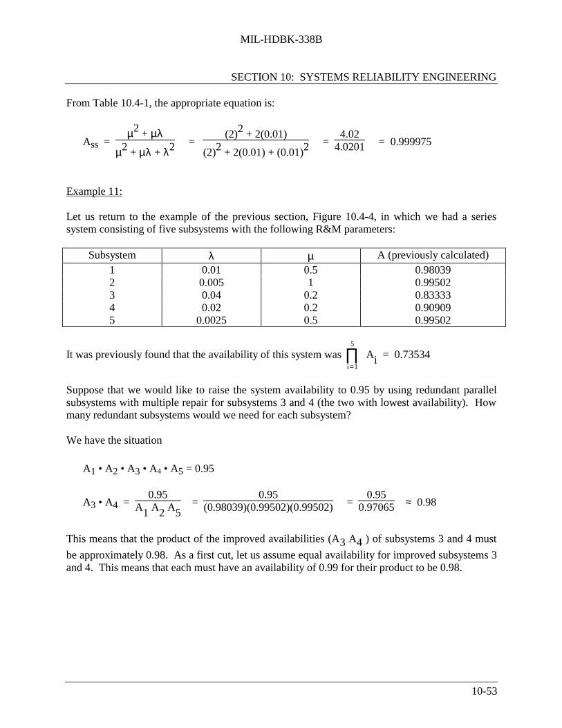
MIL-HDBK-338B


10-53

From Table 10.4-1, the appropriate equation is:

Ass = µ2 + µλ

µ2 + µλ + λ2 = (2)2 + 2(0.01)

(2)2 + 2(0.01) + (0.01)2 =

4.024.0201 = 0.999975

Example 11:

Let us return to the example of the previous section, Figure 10.4-4, in which we had a seriessystem consisting of five subsystems with the following R&M parameters:

Subsystem λ µ A (previously calculated)1 0.01 0.5 0.980392 0.005 1 0.995023 0.04 0.2 0.833334 0.02 0.2 0.909095 0.0025 0.5 0.99502

It was previously found that the availability of this system was i=1

5

∏ Ai = 0.73534

Suppose that we would like to raise the system availability to 0.95 by using redundant parallelsubsystems with multiple repair for subsystems 3 and 4 (the two with lowest availability). Howmany redundant subsystems would we need for each subsystem?

We have the situation

A1 • A2 • A3 • A4 • A5 = 0.95

A3 • A4 = 0.95

A1 A2 A5 =

0.95(0.98039)(0.99502)(0.99502) =

0.950.97065 ≈ 0.98

This means that the product of the improved availabilities (A3 A4 ) of subsystems 3 and 4 must

be approximately 0.98. As a first cut, let us assume equal availability for improved subsystems 3and 4. This means that each must have an availability of 0.99 for their product to be 0.98.

MIL-HDBK-338B


10-54

Eq. (10.51) is the general expression for improvement in availability through redundancy

A(1/n) = 1 - (1 - A)n

where A(1/n) is the improved availability with n redundant units. Let us call this A’. Then,

A’ = 1 - (1 - A)n

and

1 - A’ = (1 - A)n

Taking the natural logarithm of both sides of the equation

ln (1 - A’) = n ln (1 - A)

n = -A)(-A’)(

1

1

ln

ln(10.60)

which is a general expression that can be used to determine the number of redundant subsystemsrequired to achieve a desired subsystem availability (A’).

Let us look at improved subsystem 3:

A’ = 0.99

A = 0.83333

n =).(

).(833301

9901

−−

ln

ln =

).().(

166670

010

ln

ln =

-4.605-1.79

= 2.57, which is rounded up to 3 redundant subsystems (total).

Similarly for subsystem 4:

n =).(

).(9090901

9901

−−

ln

ln =

).().(

090910

010

ln

ln =

-4.605-2.397

= 1.92, which is rounded up to 2 redundant subsystems

Thus, in order for the system availability to be raised to 0.95, we need 3 parallel redundantSubsystems 3, and 2 parallel redundant Subsystems 4.

MIL-HDBK-338B


10-55

Note that we have not discussed the optimum allocation of failure and repair rates to achieve agiven availability; this will be done later in this section.

10.4.1.5 Model E - R&M Parameters Not Defined in Terms of Time

A very different situation in availability modeling is encountered when system “uptime” is notmeasured in hours of operation or any time parameter but rather in terms of number of roundsfired, miles traveled, actuations or cycles performed, etc. The reliability parameter is then nolonger expressed in terms of MTBF but rather in mean-rounds-between-failures (MRBF), mean-miles-between-failures (MMBF), mean-cycles-between-failures (MCBF), etc. The failure ratethen also is expressed in number of failures per round, per mile, or per cycle rather than numberof failures per operating hour.

For straightforward reliability calculations this poses no problem since the same reliabilityequations apply as in the time domain, except that the variable time, t, in hours is replaced by thevariable number of rounds, number of miles, etc. We may then calculate the reliability of suchsystems for one, ten, one hundred, or any number of rounds fired or miles traveled, as we wish.The maintainability calculations remain as before, since downtime will always be measured interms of time and the parameter of main interest remains the MTTR.

However, when it comes to availability, which usually combines two time parameters (i.e., theMTBF and the MTTR into a probability of the system being up at some time, t), a difficultproblem arises when the time, t, is replaced by rounds or miles, since the correlation betweentime and rounds or time and miles is quite variable.

An equation for the steady-state availability of machine guns is given in Reference [11]. This

equation is based on a mission profile that at discrete times, t1, t2, t3, etc., requires the firing of

N1, N2, N3, etc., bursts of rounds. When the gun fails during a firing, for example at time t, it

fires only f rounds instead of N3 rounds and must undergo repair during which time it is not

available to fire; for example, it fails to fire a required N4 rounds at t4, and a further N5 rounds at

t5 before becoming again available (see Figure 10.4-5). Its system availability, A, based on therounds not fired during repair may be expressed, for the described history, as:

A = (N1 + N2 + f)/(N1 + N2 + N3 + N4 + N5) (10.61)

Each sequence of rounds fired followed by rounds missed (not fired) constitutes a renewalprocess in terms of rounds fired, as shown in Figure 10.4-6, where the gun fails after firing xrounds, fails to fire γ(x) rounds in the burst of rounds during which it failed and also misses firingthe required bursts of rounds while in repair for an MTTR = M. Assume that the requirementsfor firing bursts of rounds arrives at random according to a Poisson process with rate r and theaverage number of rounds per burst is N, then the limiting availability of the gun may beexpressed as:

MIL-HDBK-338B


10-56

A = MRBF/(MRBF + N + γMN) (10.62)

where MRBF is the mean number of rounds between failure. The derivation of this formula,developed by R.E. Barlow, is contained in the Appendix of Reference [11]. To calculate A fromEq. (10.62) one must know the MRBF and MTTR of the gun, the average rounds N fired perburst, and the rate γ at which requirements for firing bursts of rounds arrive.

Repair Time

0 t t t t t

N N NN

N

1 2

3

4 5

1 2 3 4 6t

5

f

NU

MB

ER

OF

RO

UN

DS

FIR

ED

N3 - f

FIGURE 10.4-5: HYPOTHETICAL HISTORY OF MACHINE GUN USAGE

MIL-HDBK-338B


10-57

γ (x)

O N

N

N

f

x1

2

3

1

NUMBER OF ROUNDS FIRED

FIGURE 10.4-6: RENEWAL PROCESS IN TERMS OF ROUNDS FIRED

Similar availability equations can be developed for other types of weapons and also for vehicleswhere the renewal process is in terms of miles traveled. Other approaches to calculating theavailability of guns as well as vehicles are found in Reference [12] and are based on calculatingfrom historical field data the maintenance ratios and, via regression analysis, the maintenancetime ratios (called the “maintenance clock hour index”) that are in turn used in the conventionaltime based equation of inherent, achieved, and operational availability.

For example, consider a machine gun system in a tank on which historical data are available,showing that 0.014 corrective maintenance man-hours are expended per round fired and that peryear 4800 rounds are fired while the vehicle travels for 240 hr per yr. The maintenance ratio(MR) for the gun system is then computed as (Ref. [12], pp. 36-38).

MRGun =

MMHRound

• Number of Rounds Fired per AnnumVehicle Operating Hours per Annum

= 0.014 • (4800/240) = 0.28 (10.63)

The dimensions for 0.28 are gun system maintenance man-hours per vehicle operating hour.According to this example, the corrective maintenance time ratio, α (sometimes called themaintenance clock hour index, Ω), is, given by:

αGun = 0.628(0.28)0.952 = 0.187 (10.64)

MIL-HDBK-338B


10-58

The numbers 0.628 and 0.952 are the intercept and the regression coefficients, respectively,obtained by regression analysis as developed in Reference [12], p. 18, Table 1. The dimensionfor αGun is gun system downtime per vehicle operating hour. The inherent availability of the

gun system is then, according to the conventional time equation, Eq. (10.20).

Ai = (1 + αGun)-1 = (1.187)-1 = 0.842 (10.65)

This may be interpreted as the gun system being available for 84.2% of the vehicle operatingtime. Caution is required in using this approach for weapon availability calculations, since in thecase where the vehicle would have to be stationary and the gun would still fire rounds, MR and αwould become infinitely large and the inherent availability of the gun system would become zero.

10.4.2 Mission Reliability and Dependability Models

Although availability is a simple and appealing concept at first glance, it is a point concept, i.e., itrefers to the probability of a system being operable at a random point in time. However, theability of the system to continue to perform reliably for the duration of the desired operating(mission) period is often more significant. Operation over the desired period of time depends,then, on clearly defining system operating profiles. If the system has a number of operatingmodes, then the operating profile for each mode can be considered.

The term mission reliability has been used to denote the system reliability requirement for aparticular interval of time. Thus, if the system has a constant failure rate region so that itsreliability R can be expressed as:

R = exp (-λt) (10.66)

where:λ = failure rate = 1/MTBFt = time for mission

then mission reliability RM for a mission duration of T is expressed as:

RM = exp (-λT) (10.67)

This reliability assessment, however, is conditional upon the system being operable at thebeginning of its mission or its (point) availability.

In order to combine these two concepts, a simplified system effectiveness model may be usedwhere the system effectiveness may be construed simply as the product of the probabilities thatthe system is operationally ready and that it is mission reliable.

MIL-HDBK-338B


10-59

If A is the mean availability of a system at any point in time to when we want to use the system

and if RM is the system reliability during mission time T, then system effectiveness E, not

including performance, may be defined as:

E = ARM (10.68)

Thus, A is a weighting factor, and E represents an assessment of system ability to operate withoutfailure during a randomly chosen mission period.

One concept of dependability used by the Navy (Ref. [13]) takes into account the fact that forsome systems a failure which occurs during an operating period t1 may be acceptable if the

failure can be corrected in a time t2 and the system continues to complete its mission.

According to this concept, dependability may be represented by:

D = RM + (1 - RM)Mo (10.69)

where:D = system dependability - or the probability that the mission will be successfully

completed within the mission time t1, providing a downtime per failure not

exceeding a given time t2 will not adversely affect the overall mission

RM = mission reliability - or the probability that the system will operate without failure for

the mission time t1Mo = operational maintainability - or the probability that when a failure occurs, it will be

repaired in a time not exceeding the allowable downtime t2t2 = specified period of time within which the system must be returned to operation

For this model, the exponential approximation of the lognormal maintainability function is used,or

Mo =

1 - e-µt2 (10.70)

Then, the system effectiveness is:

E = AD = A

RM + (1 - RM) Mo (10.71)

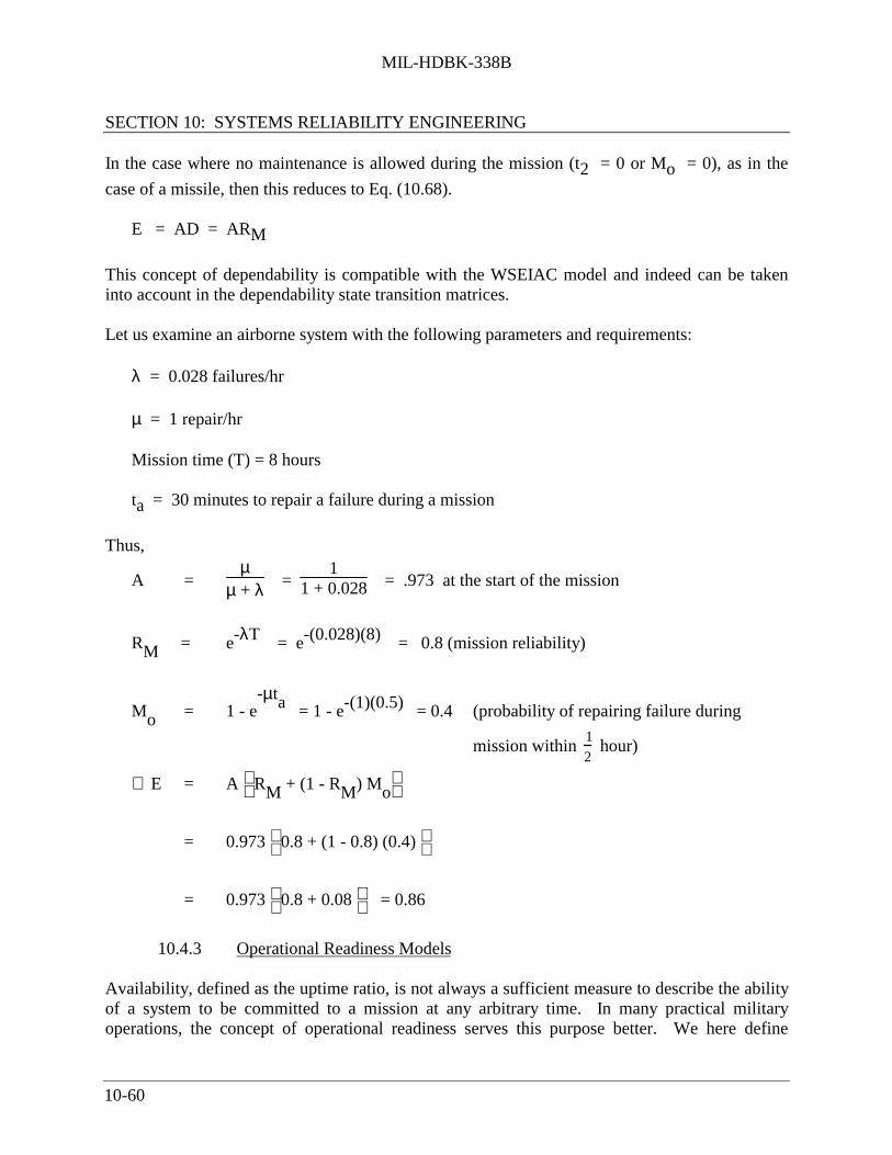
MIL-HDBK-338B


10-60

In the case where no maintenance is allowed during the mission (t2 = 0 or Mo = 0), as in the

case of a missile, then this reduces to Eq. (10.68).

E = AD = ARM

This concept of dependability is compatible with the WSEIAC model and indeed can be takeninto account in the dependability state transition matrices.

Let us examine an airborne system with the following parameters and requirements:

λ = 0.028 failures/hr

µ = 1 repair/hr

Mission time (T) = 8 hours

ta = 30 minutes to repair a failure during a mission

Thus,

A = µ

µ + λ = 1

1 + 0.028 = .973 at the start of the mission

RM = e-λT = e-(0.028)(8) = 0.8 (mission reliability)

Mo = 1 - e-µta = 1 - e-(1)(0.5) = 0.4 (probability of repairing failure during

mission within

12

hour)

∴ E = A

RM + (1 - RM) Mo

= 0.973

0.8 + (1 - 0.8) (0.4)

= 0.973

0.8 + 0.08 = 0.86

10.4.3 Operational Readiness Models

Availability, defined as the uptime ratio, is not always a sufficient measure to describe the abilityof a system to be committed to a mission at any arbitrary time. In many practical militaryoperations, the concept of operational readiness serves this purpose better. We here define

MIL-HDBK-338B


10-61

operational readiness as the probability that a system is in an operable condition, i.e., ready to becommitted to perform a mission when demands for its use arise. The difference as well as thesimilarity between availability and operational readiness will become clear by comparing themodels developed subsequently with the availability models discussed in the preceding section.

In the development of operational readiness models, one has to consider the usage and themaintenance of the system, i.e., its operating, idle, and repair times. When a call arrives for thesystem to engage in a mission, the system at such time may be in a state of perfect repair andready to operate immediately. But it may also be in need of maintenance and not ready. Its statewhen called upon to operate depends on the preceding usage of the system, i.e., on its precedingmission, in what condition it returned from that mission, and how much time has elapsed since itcompleted the last mission. Many models can be developed for specific cases, and some arediscussed in the following paragraphs.

10.4.3.1 Model A - Based Upon Probability of Failure During Previous Mission andProbability of Repair Before Next Mission Demand

In this model, the assumption is made that if no failures needing repair occurred in the precedingmission, the system is immediately ready to be used again; and, if such failures did occur, thesystem will be ready for the next mission only if its maintenance time is shorter than the time bywhich the demand for its use arises. The operational readiness POR may then be expressed as:

POR = R(t) + Q(t) • P(tm < td) (10.72)

where:R(t) = probability of no failures in the preceding missionQ(t) = probability of one or more failures in the preceding missiont = mission duration

P(tm < td) = probability that if failures occur, the system maintenance time, tm, is shorter

than the time, td, at which the next demand or call for mission engagementarrives

The calculations of R(t) and Q(t) = 1 - R(t) are comparatively simple using standard reliabilityequations; however, all possible types of failures that need fixing upon return in order to restorein full the system reliability and combat capability must be considered, including any failures inredundant configurations.

As for P(tm < td), one needs to know the probability distributions of the system maintenance time

and of call arrivals. Denoting by f(tm) the probability density function of maintenance time and

by g(td), the probability density function of time to the arrival of the next call, counted from theinstant the system returned from the preceding mission in a state requiring repair, the probabilitythat the system will be restored to its full operational capability before the next call arrives is:

MIL-HDBK-338B


10-62

P(tm < td) =

t m

∞

∫ f(tm)

∫∞

=dd )dtg(t

md ttdtm (10.73)

The integral in the square brackets on the right side of the equation is the probability that the call

arrives at td after a variable time tm. When this is multiplied by the density function f(tm) of the

duration of maintenance times and integrated over all possible values of tm, we get P(tm< td).

Now assume that maintenance time tm and time to next call arrival td are exponentially

distributed, with M1 being the mean time to maintain the system and M2 the mean time to nextcall arrival. The probability density functions are thus:

f(tm) = exp(−tm/M1)[ ]/M1 (10.74)

f(td) = exp(−td/M2 )[ ]/M2 (10.75)

We then obtain

P(tm < td) =

0

∞

∫ M1-1 exp (-tm/M1) •

−−

∞

∫ d2d1

2 )dt/Mtexp(Mmt

dtm

=

0

∞

∫ (−M1−1)exp −(1/M1 +1/M2)tm[ ]dtm

= M2/(M1 + M2) (10.76)

In this exponential case, system operational readiness becomes

POR = R(t) + Q(t) •

M2 /(M1 + M2)[ ] (10.77)

MIL-HDBK-338B


10-63

As a numerical example let us look at a system with a probability of R = 0.8 of returning from amission of t = 1 hr duration without requiring repair and therefore had a probability of Q = 0.2

that it will require repair. If system mean maintenance time is M1 = 1 hr and the mean time to

next call arrival is M2 = 2 hr., the operational readiness of the system becomes

P = 0.8 + 0.2 (2/3) = 0.933

Comparing this result with the conventional steady-state availability concept and assuming that

the system has a mean maintenance time of M1 = 1 hr and a mean time to failure of M2 = 5 hr(roughly corresponding to the exponential case of R = 0.8 for a one-hour mission), we obtain asystem availability of:

A = M2/(M1 + M2) = 5/6 = 0.833

which is a result quite different from POR = 0.933.

10.4.3.2 Model B - Same As Model A Except Mission Duration Time, t isProbabilistic

The operational readiness model of Eq. (10.72) can be extended to the case when missionduration time t is not the same for each mission but is distributed with a density q(t). We thenget

POR =

R(t)q(t)dt

0

∞

∫ + P(tm < td)

Q(t)q(t)dt

0

∞

∫ (10.78)

Since the integrals in Eq. (10.78) are fixed numbers, we may write:

R =

R(t)q(t)dt

0

∞

∫ , and

Q =

Q(t)q(t)dt

0

∞

∫ (10.79)

and using the symbol P for P(tm < td), i.e., P = P(tm < td), Eq. (10.78) may be written in theform:

POR = R + QP (10.80)

MIL-HDBK-338B


10-64

In this equation R is the probability that the system returns without failures from the last mission;Q = 1 - R is the probability that one or more failures developed in the last mission; and P is theprobability that the system will be repaired before the next call arrives if it developed failures.The mission times are variable here with density q(t).

10.4.3.3 Model C - Similar To Model A But Includes Checkout EquipmentDetectability

The operational readiness of the system at time ta is given by:

POR(ta) = R(tm) + kM(tr)[ ] • 1 − R(tm)[ ] (10.81)

where:

POR(ta) = probability of system being available for turnaround time, e.g., ta of 30 minutes,following completion of preceding mission or initial receipt of alert

R(tm) = probability that the system will survive the specified mission of duration tmwithout failure

tr = specified turnaround time, or maximum downtime for repair required of the

systemk = probability that if a system failure occurs it will be detected during the mission

or during system checkout following the mission

M(tr) = probability that a detected system failure can be repaired in time tr to restore thesystem to operational status

Thus, when mission reliability, mission duration, availability, and turnaround time are specifiedfor the system, the detectability-times-maintainability function for the system is constrained topass through or exceed the point given by:

kM(tr) ≥ POR(ta) - R(tm)

1 - R(tm)

Consider, for example, the following specified operational characteristics for a new weaponssystem:

Mission Reliability, R(tm) = 0.80 for tm of 8 hours

Operational Readiness POR(ta) = 0.95 for turnaround time, ta of 30 minutes, followingcompletion of preceding mission or initial receipt of alert.

MIL-HDBK-338B


10-65

From the requirements, the required detectability-maintainability product (kM) is derived asfollows:

kM(30) = POR(30) - R(8)

1 - R(8) = 0.95 - 0.8

1 - 0.8 = 0.75

Therefore, kM(30) = 0.75 is the joint probability, given that a system failure has occurred, thatthe failure will be detected (either during the mission or during post mission checkout) and willbe repaired within 30 minutes following completion of the mission.

Assume that k is to be 0.9, i.e., built-in test equipment is to be incorporated to detect at least 90%of the system failures and provide go/no-go failure indication.

Then, the maintainability requirement is:

M(30) = 0.75

k = 0.750.9 ≈ 0.83

which means that 83% of all system repair actions detected during the mission or during postmission checkout must be completed within 30 minutes.

Using the exponential approximation, maintainability as a function of repair time is expressed as

the probability of repair in time tr:

M(tr) = 1 - e −µtr = 1 - e −tr /Mct (10.82)

where:

Mct = MTTRµ = repair rate, 1/ Mct

tr = repair time for which M(t) is to be estimated

The required mean time to repair ( Mct ) is found from Eq. (10.82) by taking the natural log ofboth sides:

Mct = - tr

ln

1 - M(tr)

MIL-HDBK-338B


10-66

Substituting tr = 30 minutes, and M(tr), which we previously found to be 0.83,

Mct = - 30

ln (0.17) = -30

-1.77 ≈ 17 minutes

And from M(tmax) = 0.95 we find the maximum time for repair of 95% of detected system

failures (Mmaxct) as follows:

M(tmax) = 0.95 = 1 - e-Mmaxct/ M ct

Mmaxct= - M ct ln (1 - 0.95)

= - (17)(-3) = 51 minutes

Thus, these requirements could be established as design requirements in a system developmentspecification.

Detectability Factor, k = 0.90

Mean Time To Repair, M ct = 17 minutes

Maximum Time To Repair, Mmaxct= 51 minutes

10.4.3.4 Model D - For a Population of N Systems

Let N be the total population of systems, e.g., squadron of aircraft. The service facility itself shallbe considered as having k channels, each servicing systems at a mean rate µ. The analysis isbased on an assumed Poisson distribution of arrivals and on a mean service time which isassumed to be exponentially distributed. This service is performed on a first come, first servedbasis.

The basic equations (derived in Ref. [11]) are as follows:

pn =

N!(N − n)!

ρk

k!

ρk

n−kpo when n > k (10.83)

pn =N!

(N - n)! ρn

n! po when n ≤ k (10.84)

MIL-HDBK-338B


10-67

po =

1knkk

0n

nk

1kn kk!n)!(N

N!

n!n)!(N

N!−−

=+=

−

+−

∑∑ (10.85)

ρ =λµ =

Mean arrival rate (failure)Mean service rate (10.86)

where:pi = probability of i units awaiting service

k = number of repair channels or facilitiesN = total number of systems

POR = N - n

N (10.87)

where: POR = probability that a system is neither awaiting nor undergoing service.

n = average number of systems either awaiting or undergoing service at

a given time and is defined by:

n = n =0

N

∑ npn (10.88)

The specific procedure, which will be illustrated by an example, is as follows:

Step 1: Use Eq. (10.85) to solve for po

Step 2: Use po from Step 1 to help derive pn for all values of n ≤ k by use of

Eq. (10.84)

Step 3: Use po from Step 1 to help derive pn for all values of n > k by use of Eq.

(10.83)

Step 4: For all values of n, from 0 through N, sum the terms npn derived from Steps 1

through 3. This, per Eq. (10.88) gives n , the average number of systems not

ready

Step 5: Use Step 4 results and Eq. (10.87) to obtain the operational readiness probability,POR

MIL-HDBK-338B


10-68

Example 12: POR of Interceptor Squadron

An interceptor squadron contains fifteen planes (N = 15) and has available four flight line repairchannels (k = 4). Each plane averages 50 operating hours per month out of 24 times 30, or 720total available hours. Because of five-day, two-shift maintenance each failure requires anaverage of five clock hours (MTTR) to repair. The plane MTBF is 3.47 operating hours betweenfailures. What is the operational readiness probability for this squadron?

We first compute the utilization factor ρ.

r =

1ρ

• Operating hours per plane per month

Total hours per month

=))(.(

))((720473

505 =

2500

250 = 0.1

Step 1: Use Equation (10.85) to obtain po

po =

1knkN

km

nN

1kn k

r

k!

r

n)!(N

N!

n!

r

n)!(N

N!−−

=+=

−

+− ∑∑

po =

14n415

4m

n4

0m 4

(0.1)

4!

(0.1)

n)!(15

15!

n!

(0.1)

n)!(15

15!−−

==

−

+− ∑∑

MIL-HDBK-338B


10-69

The calculated results are shown in the following table:

n Term (1) Term (2)

0 1.0 - -1 1.5 - -2 1.05 - -3 0.455 - -4 0.1365 0.034125 - - 0.03756 - - 0.037537 - - 0.03378 - - 0.01279 - - 0.018910 - - 0.011311 - - 0.005612 - - 0.002213 - - 0.000614 - - 0.0001315 - - 0.00000

Sum 4.1415 0.19428

po = (4.1415 + 0.19428)-1 = (4.3358)-1 = 0.2306

Step 2: Use Equation (10.84) and obtain pn for n = 1 through 4.

Pn = N!

(N - n)! ρn

n! po

Thus,

p1 = 15!

(15 - 1)! (0.1)1

1! (0.23) = 0.3450

p2 = 15!13!

(0.1)2

2! (0.23) = 0.2415

p3 = 15!12!

(0.1)3

3! (0.23) = 0.10465

p4 = 15!11!

(0.1)4

4! (0.23) = 0.0313

MIL-HDBK-338B


10-70

Step 3: Use Equation (10.83) and obtain pn for n = 5 through 15.

pn = N!

(N - n)!

ρk

k!

ρ

k

n-k po

Thus,

p5 = 15!10!

(0.1)1

4!

0.14

1 (0.23) = 0.0086

p6 = 15!9!

0.14

4!

0.1

4

2 (0.23) = 0.00214

Similarly,p7 = 0.000486

p8 = 0.000097

p9 = 0.000017

p10 through p15 are negligible probabilities.

Step 4: Sum the terms npn for n = 0 through n = 15.

n pn npn

0 0.2300 01 0.3450 0.34502 0.2415 0.48303 0.1047 0.3141004 0.0313 0.125005 0.0086 0.0430006 0.00214 0.0128507 0.000486 0.0034008 0.000097 0.0007769 0.000017 0.00015310 --- ---11 --- ---12 --- ---13 --- ---14 --- ---15 --- ---

Total 1.214779

MIL-HDBK-338B


10-71

Therefore from Equation (10.88):

n = n =0

N

∑ npn

= 1.215 planes which are not ready on the average

Step 5: Using Step 4 results and Equation (5.87), we obtain POR, the operational readinessprobability

POR = N - n

N = 15 - 1.215

15 = 13.785

15 = 0.919

As can be seen, the calculations are rather laborious and best done by a computer. Figures 10.4-7and 10.4-8 (from Ref. [10]) are a series of curves for N = 15 and N = 20 with k values rangingfrom 1 to 10 and 1 to 20, respectively. Note that 0.919 checks out the r = 0.1, k = 4 point onFigure 10.4-7.

MIL-HDBK-338B


10-72

0

0.1

0.2

0.3

0.4

0.5

0.6

0.7

0.8

0.9

1

1.1

0 0.1 0.2 0.3 0.4 0.5 0.6 0.7 0.8 0.9 1 1.1 1.2 1.3 1.4 1.5 1.6 1.7

Op

erat

iona

l Rea

din

ess

Pro

babi

lity

ρ

k=1

k=13, 14, 15k=12k=11k=10k=2

k=3 k=4 k=5 k=6 k=7 k=8 k=9

FIGURE 10.4-7: OPERATIONAL READINESS PROBABILITYVERSUS QUEUING FACTOR ρ. FOR POPULATION SIZE N = 15;

NUMBER OF REPAIR CHANNELS k

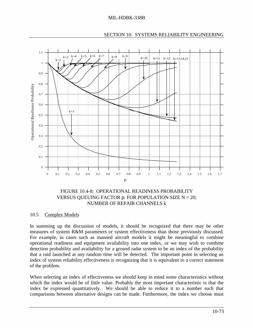
MIL-HDBK-338B


10-73

.

k=9

0

0.1

0.2

0.3

0.4

0.5

0.6

0.7

0.8

0.9

1

1.1

0 0.1 0.2 0.3 0.4 0.5 0.6 0.7 0.8 0.9 1 1.1 1.2 1.3 1.4 1.5 1.6 1.7

Ope

rati

onal

Rea

din

ess

Prob

abili

ty

k=1

k=2k=3 k=4 k=5 k=6 k=7 k=8 k=10 k=11 k=12 k=13,14,15

ρ

FIGURE 10.4-8: OPERATIONAL READINESS PROBABILITYVERSUS QUEUING FACTOR ρ. FOR POPULATION SIZE N = 20;

NUMBER OF REPAIR CHANNELS k

10.5 Complex Models

In summing up the discussion of models, it should be recognized that there may be othermeasures of system R&M parameters or system effectiveness than those previously discussed.For example, in cases such as manned aircraft models it might be meaningful to combineoperational readiness and equipment availability into one index, or we may wish to combinedetection probability and availability for a ground radar system to be an index of the probabilitythat a raid launched at any random time will be detected. The important point in selecting anindex of system reliability effectiveness is recognizing that it is equivalent to a correct statementof the problem.

When selecting an index of effectiveness we should keep in mind some characteristics withoutwhich the index would be of little value. Probably the most important characteristic is that theindex be expressed quantitatively. We should be able to reduce it to a number such thatcomparisons between alternative designs can be made. Furthermore, the index we choose must

MIL-HDBK-338B


10-74

have a basis in physical reality. Thus it should be descriptive of the real problem, not exaggeratedor oversimplified. Yet at the same time the index should be simple enough to allow formathematical manipulation to permit evaluating alternatives.

In complex system effectiveness mathematical models, an attempt is made to relate the impact ofsystem reliability, maintainability, and performance to the mission profiles, scenario, use, andlogistic support. Only in simple situations can a meaningful single model be developed that willrelate all these parameters and yield a single quantitative measure of system effectiveness.Numerous complex computerized models exist and, as a matter of fact, every major company inthe aerospace business has developed a multitude of such models.

10.6 Trade-off Techniques

10.6.1 General

A trade-off is a rational selection among alternatives in order to optimize some system parameterthat is a function of two or more variables which are being compared (traded off). Examples ofsystem trade-offs involve performance, reliability, maintainability, cost, schedule, and risk. Atrade-off may be quantitative or qualitative. Insofar as possible, it is desirable that trade-offs bebased on quantifiable, analytic, or empirical relationships. Where this is not possible, then semi-quantitative methods using ordinal rankings or weighting factors are often used.

The methodology for structuring and performing trade-off analyses is part of the systemengineering process described in Section 4. The basic steps, summarized here are:

(1) Define the trade-off problem and establish the trade-off criteria and constraints

(2) Synthesize alternative design configurations

(3) Analyze these alternative configurations

(4) Evaluate the results of the analyses with respect to the criteria, eliminating those whichviolate constraint boundaries

(5) Select the alternative which best meets criteria and constraint boundaries or iterate thedesign alternatives, repeating Steps 2 through 5 to obtain improved solutions

MIL-HDBK-338B


10-75

System effectiveness and cost effectiveness models provide the best tools for performing trade-off studies on the system level. Through the computerized models, any changes in any of themultitude of reliability, maintainability, performance, mission profile, logistic support, and otherparameters can be immediately evaluated as to their effect on the effectiveness and total cost of asystem. Thus, cost effectiveness modeling and evaluation, besides being used for selecting aspecific system design approach from among several competing alternatives, is a very powerfultool for performing parametric sensitivity studies and trade-offs down to component level whenoptimizing designs to provide the most effective system for a given budgetary and life cycle costconstraint or the least costly system for a desired effectiveness level.

At times, however, especially in the case of the more simple systems, trade-offs may be limitedto achieving a required system availability while meeting the specified reliability andmaintainability requirements. Comparatively simple trade-off techniques can then be used asshown in the following paragraphs.

10.6.2 Reliability - Availability - Maintainability Trade-offs

The reliability-maintainability-availability relationship provides a measure of systemeffectiveness within which considerable trade-off potential usually exists, e.g., betweenreliability, maintainability, and logistic support factors. This potential should be re-evaluated ateach successive stage of system development to optimize the balance between reliability,maintainability, and other system effectiveness parameters with respect to technical risks, lifecycle cost, acquisition schedule, and operating and maintenance requirements. The latter becomeincreasingly more important as complexity of system design increases, dictating the need forintegration of system monitoring and checkout provisions in the basic design.

As stated earlier in this section and in Section 2, reliability and maintainability jointly determinethe inherent availability of a system. Thus, when an availability requirement is specified, there isa distinct possibility of trading-off between reliability and maintainability, since in the steadystate availability depends only on the ratio or ratios of MTTR/MTBF which was previouslyreferred to as maintenance time ratio (MTR), α , i.e.,

α = MTTR/MTBF = λ/µ (10.88)

so that the inherent availability equation assumed the form

Ai = 1/(1 + α) (10.89)

As an example, consider systems I and II with

MTTRI = 0.1 hr.

MTBFI = 2 hr.

MIL-HDBK-338B


10-76

MTTRII = 10 hr.

MTBFII = 200 hr.

Then the steady state availability is

AI = 1/

1 + (0.1/2) = 0.952

AII = 1/

1 + (10/200) = 0.952

Both systems have the same availability, but they are not equally desirable. A 10-hr MTTRmight be too long for some systems, whereas a 2-hr MTBF might be too short for some systems.

Even though reliability and maintainability individually can be increased or decreased incombinations giving the same system availability, care must be taken to insure that reliabilitydoes not fall below its specified minimum or that individually acceptable values of reliability andmaintainability are not combined to produce an unacceptable level of system availability.

A generalized plot of Eq. (10.88) is given in Figure 10.6-1. A plot of A vs. λ/µ, is given inFigure 10.6-2. These equations and graphs show that in order to optimize availability it isdesirable to make the ratio of MTBF/MTTR as high as possible.

Since increasing MTBF and decreasing MTTR is desirable, the equation for availability can beplotted in terms of MTBF and 1/MTTR (or µ) as shown in Figure 10.6-3. Each of the curvesrepresenting the same availability in Figure 10.6-3 just as each of the lines in Figure 10.6-1, iscalled isoavailability contours; corresponding values of MTBF and MTTR give the same value ofA, all other things being equal. Availability nomographs useful for reliability and maintainabilitytrade-offs are given in Reference [13]. Figure 10.6-4 is an example of an availability nomograph.

MIL-HDBK-338B


10-77

1 2 3 4 5 6 7 8 9 10

1

2

3

4

5

6

7

8

9

10

00

A=1 A=0.9

A=0.75

A=0.5

A=0.25

A=0.1

A=0

MTBF

MTTR

(A) AVAILABILITY AS A FUNCTION OF MTBF AND MTTR

1 2 3 4 5 6 7 8 9 10

1

2

3

4

5

6

7

8

9

10

00

A=0 A=0.1

A=0.25

A=0.5

A=0.75

A=0.9

A=1

λ

µ

(B) AVAILABILITY AS A FUNCTION OF λ AND µ

FIGURE 10.6-1: RELIABILITY - MAINTAINABILITY -AVAILABILITY RELATIONSHIPS

MIL-HDBK-338B


10-78

1 2 3 4 5 6 7 8 9 100 11 120

0.1

0.2

0.3

0.4

0.5

0.6

0.7

0.8

0.9

1.0

A

λ/µ

FIGURE 10.6-2: AVAILABILITY AS A FUNCTION OF λ/µ

0 3 6 9 12 15

3

6

9

12

15

MTBF

1/MTTR, µ

A=0.99

0.98

0.960.950.90

0.800.750.50

FIGURE 10.6-3: AVAILABILITY AS A FUNCTION OF MTBF AND 1/MTTR

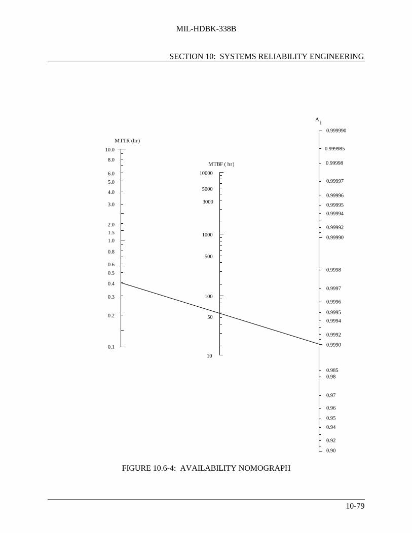
MIL-HDBK-338B


10-79

10.0

8.0

6.0

5.0

4.0

3.0

2.0

0.1

1.0

100

50

1000

500

10000

5000

10

0.8

0.6

0.5

0.4

0.3

0.2

0.90

0.92

0.94

0.95

0.96

0.97

0.98

0.9990

0.9992

0.9994

0.9995

0.9996

0.9997

0.9998

0.99990

0.99992

0.99994

0.99996

0.99995

0.99997

0.999985

0.999990

1.5

3000

0.99998

MTTR (hr)

MTBF ( hr)

Ai

0.985

FIGURE 10.6-4: AVAILABILITY NOMOGRAPH

MIL-HDBK-338B


10-80

There are obvious practical limits which must be considered in trade-off optimization. These arecalled constraints, and all purposeful optimization must be bounded by constraints into feasibleregions. For example, there are practical limits as to how high a value for MTBF can beachieved or how low MTTR can be made. In the one case, the reliability of system componentsor the required redundancy might be so high that the desired reliability could not be realisticallyachieved within the state-of-the-art or would be so expensive as to violate cost constraints.Similarly, MTTRs close to zero would require extreme maintainability design features, such ascompletely built-in test features or automatic test and checkout to allow fault isolation to eachindividual replaceable module, with perhaps automatic switchover from a failed item to astandby item. This also could easily violate state-of-the-art or cost constraints.

It follows, then, that trade-offs not only involve relationships among system parameters andvariables but also that they are bounded by both technical and economic constraints. In a sense,all trade-offs are economic ones, requiring cost-benefit analysis (not necessarily in terms ofdollar costs but rather in terms of the availability and consumption of resources, of which dollarsare often the most convenient measure). Resource constraints may also include manpower andskill levels, schedule or time availability, and the technical state-of-the-art capability. Latersections of this chapter deal with the cost problem.

There are two general classes of trade-offs. In the first, the contributing system variables aretraded-off against one another without increasing the value of the higher level system parameter;for example, trading-off reliability and maintainability along an isoavailability contour (nochange in availability). This might be done for reasons of standardization or safety or foroperational reasons such as the level at which the system and its equipments will be maintained.The other class of trade-off is one in which the system variables are varied in order to obtain thehighest value of the related system parameters within cost or other constraints. For example,reliability and maintainability might be traded-off in order to achieve a higher availability. Thiscould result in moving from one isoavailability curve to another in Figure 10.6-3, perhaps alongan isocline (a line connecting equal slopes).

An example of a reliability - availability - maintainability (RAM) trade-off is given in thefollowing paragraphs. The design problem is as follows: A requirement exists to design a radarreceiver which will meet an inherent availability of 0.99, a minimum MTBF of 200 hours, and anMTTR not to exceed 4 hours. The current design is predicted to have an availability of 0.97, anMTBF of 150 hours, and an MTTR of 4.64 hours.

Using Eq. (10.88) the area within which the allowable trade-off may be made is shown by thecross-hatched portion of Figure 10.6-5. As indicated in the previous paragraph, there are twoapproaches which can be used for trade-off. One is to fix the availability at 0.990. This meansthat any combination of MTBF and MTTR between the two allowable end points on the 0.990isoavailability line may be chosen. These lie between an MTBF of 200 hours with an MTTR of2 hours and an MTBF of 400 hours with an MTTR of 4 hours. The other approach is to allowavailability to be larger than 0.990 and thus allow any combination of MTBF and MTTR withinthe feasible region.

MIL-HDBK-338B


10-81

It is clearly seen that without any additional constraints the designer has a limitless number ofcombinations from which to choose. Assume that the following four alternative designconfigurations have been selected for trade-off as shown in Table 10.6-1.

Design Configuration Nos. 1, 2, and 3 all have the required availability of 0.990. DesignConfiguration No. 1 emphasizes the maintainability aspects in design, while DesignConfiguration No. 3 stresses reliability improvement. Design Configuration No. 2 is betweenNos. 1 and 3 for the same availability. Design Configuration No. 4 is a combination of Nos. 1and 2 and yields a higher availability.

Since all of these alternatives are within the feasible region shown in Figure 10.6-5 some othercriterion must be used for selection of the desired configuration. In this case, we will use theleast cost alternative or the one showing the greatest life cycle cost savings over the presentconfiguration as the basis for trade-off decision. An example cost comparison of the differentalternatives is shown in Table 10.6-2 (such costs would be estimated using various cost andeconomic models).

The cost table shows that Configuration No. 2 is the lowest cost alternative among those withequal availabilities. It also shows that Configuration No. 4, with a higher acquisition cost, has asignificantly better 10-year life cycle support cost and lowest overall cost, as well as a higheravailability. Thus Configuration No. 4 is the optimum trade-off, containing both improvedreliability and maintainability features.

The trade-off example previously shown was a relatively simple example for the case of a singleequipment. Let us now look at a more complex example. Figure 10.6-6 (a repeat of Figure 10.4-4) represents a serial system consisting of five statistically independent subsystems, each with theindicated MTBFi and MTTRi . We found by the use of Eq. (10.27) that the steady state

availability was:

A = i=1

5

∏ Ai = 0.73534

MIL-HDBK-338B


10-82

.

2018161412108642

MEAN-TIME-TO-REPAIR (MTTR), HR

0

100

200

300

400

500

600

700

800

900

1000

ME

AN

-TIM

E-B

ET

WE

EN

-FA

ILU

RE

(MT

BF)

, HR

A = .99

A = .98

A = .96

A = .92

TRADE-OFF AREA WITHIN SPECIFICATION

OUT OF SPECIFICATION

REQUIREMENTA = 99%MTBF = 200 HR MINMTTR = 4 HR MAX

A = .97

FIGURE 10.6-5: RELIABILITY-MAINTAINABILITY TRADE-OFFS

MIL-HDBK-338B


10-83

TABLE 10.6-1: ALTERNATIVE DESIGN TRADE-OFF CONFIGURATIONS

Design Configuration A MTBF, hr MTTR, hr1. R - derating of military standard parts 0.990 200 2.0

M - modularization and automatic testing2. R - design includes high reliability

parts/components0.990 300 3.0

M - limited modularization and semi-automatic testing

3. R - design includes partial redundancy 0.990 350 3.5M - manual testing and limited

modularization4. R - design includes high reliability

parts/components0.993 300 2.0

M - modularization and automatic testing

TABLE 10.6-2: COST COMPARISON OF ALTERNATIVEDESIGN CONFIGURATIONS

ITEM EXISTING 1 2 3 4Acquisition (Thousands of Dollars)

RDT&E 300 325 319 322 330Production 4,500 4,534 4,525 4,530 4,542

Total 4,800 4,859 4,844 4,852 4,87210-Year Support Costs(Thousands of Dollars)

Spares 210 151 105 90 105Repair 1,297 346 382 405 346Training and Manuals 20 14 16 8 14Provisioning & Handling 475 525 503 505 503

Total 2,002 1,036 1,006 1,018 968LIFE CYCLE COST 6,802 5,895 5,850 5,870 5,840

MIL-HDBK-338B


10-84

MTBF = 200 λ = 0.005MTTR = 1 µ = 1

SUBSYSTEM 2

MTBF = 25 λ = 0.040MTTR = 5 µ = 0.2

SUBSYSTEM 3

MTBF = 50 λ = 0.020MTTR = 5 µ = 0.1

SUBSYSTEM 4

MTBF = 400 λ = 0.0025MTTR = 2 µ = 0.5

SUBSYSTEM 5

MTBF = 100 λ = 0.010MTTR = 2 µ = 0.5

SUBSYSTEM 1


By inspection of the maintenance time ratios (MTRs) of each of the subsystems we note thatSubsystems 3 and 4 have the lowest MTRs, given by:

MTTRiMTBFi

= 525 = 0.2

for Subsystem 3 and 5/50 = 0.1 for Subsystem 4. These are, therefore, the “culprits” in limitingsystem availability to 0.73534, which may be unacceptable for the mission at hand. If because ofthe state-of-the-art limitations we are unable to apply any of the design techniques detailed inSection 7 to reduce MTBF, then our first recourse is to add a parallel redundant subsystem toSubsystem 3, the weakest link in the series chain.

We shall consider two cases: (1) the case where no repair of a failed redundant unit is possibleuntil both redundant subsystems fail and the system stops operating; or (2) repair is possible by asingle repair crew while the system is operating.

For case (1) where both units must fail before repair is initiated and a single crew repairs bothfailed units in sequence:

MIL-HDBK-338B


10-85

A(1/2) =

µ+

λ∑

λ∑

=

=n

n

n

n

n

1

1

2

1

2

1 =

1λ +

12λ

1λ +

12λ +

2µ

(from Equation 10.56)

=

10.04

+1

2(0.04)1

0.04+ 1

2(0.04)+ 2

0.2

= 37.547.5 = 0.789

This is a lower availability than the nonredundant case!

ASystem =

1

1+ MTTRSeriesMTBFSeries

= 1

1 + .02 = 0.833 (based on Equation 10.18)

For case (1), where both units must fail before repair is initiated and two repair crewssimultaneously repair both failed units:

A(1/2) =

n=1

2

∑ 1nλ

n=1

2

∑ 1nλ

+ 1µ

=

10.04

+1

2(0.04)1

0.04+ 1

2(0.04)+ 1

0.2

= 37.542.5 = 0.882

which is a slight improvement over the nonredundant case.

For case (2), where a single repair crew initiates repair action on a redundant subsystem as soonas it fails

A =

µ2 + 2µλ

µ2 + 2µλ + λ2 (from Table 10.4-1)

= (0.2)2 + 2(0.2)(0.04)

(0.2)2 + 2(0.2)(0.04) + (0.04)2

=

0.04 + 0.0160.04 + 0.016 + 0.0016

=

0.0560.0576

= 0.972

as compared to 0.833 where no redundancy was used.

MIL-HDBK-338B


10-86

This corresponds to an increased system availability of

A = 0.73534

0.9720.833

= 0.86

If this new value is still not acceptable redundancy might have to be applied to Subsystem 4. Forexample, let us use a 2-unit standby configuration for Subsystem 4 with multiple repairs; then(from Table 10.4-1), the steady state availability would be:

A =

2µ2 + 2µλ2µ2 + 2µλ + λ2 =

2(0.2)2 + 2(0.2)(0.02)

2(0.2)2 + 2(0.2)(0.02) + (0.02)2

=

0.08 + 0.0080.08 + 0.008 + 0.0004

= 0.0880.0884 = 0.995

Thus, the new system availability would be:

A = (0.86)

0.9950.909

= 0.94

where 0.909 was the original availability of Subsystem 4.

Note, however, that to achieve these gains in availability, repair of failed redundant units must bepossible while the system is operating.

Before leaving the subject of trade-offs at the system availability level, it should be pointed outthat design trade-off methodologies can also be used at lower levels of the system hierarchy toincrease MTBF and reduce MTTR. These are discussed in Section 7.

10.7 Allocation of Availability, Failure and Repair Rates

The previous sections discussed how availability can be calculated for various systemconfigurations, e.g., series, parallel, etc., and how R&M can be traded off to achieve a givenavailability. This section discusses methods for allocating availability (and, where appropriate,failure and repair rates) among the system units to achieve a given system availability.

The reader should keep in mind that we are concerned with systems that are maintained uponfailure. For the case of non-maintained systems, e.g., missiles, satellites, etc., the methodspresented in Chapter 3 are appropriate for system reliability design, prediction, and allocation.

During the initial design phase of a program, detailed information is not usually availableregarding the particular equipments to be employed with the system. For example, we may knowthat a transmitter with certain power requirements may be designed, but we do not usually know

MIL-HDBK-338B


10-87

if it is less expensive to design for a low failure rate or a high repair rate. Unless the experienceof similar, previously designed transmitters can guide our decisions, estimation of the best set ofalternatives is necessary. Having developed a system configuration, a range of values ofequipment failure rates and repair rates that would satisfy the system availability requirement canbe initially specified. The state-of-the-art limits for these equipments may not be known or theexpenditures required for improvement, but we can specify their ratio, which would allowconsiderable freedom through the design process.

10.7.1 Availability Failure Rate and Repair Rate Allocation for Series Systems

Several cases can be considered:

(1) A single repairman must repair any one of n identical, statistically independentsubsystems in series. The ratio of failure rate to repair rate is such that there is a strongpossibility that a second subsystem will fail while the first one is being repaired.

(2) Same as (1) except a repairman is assigned to each subsystem and can only work on thatparticular subsystem.

(3) Same as (1) except some intermediate number of repairmen, r, less than the number ofsubsystems is assigned. Any repairman can work on any system.

(4) Repeat cases (1)-(3) with nonidentical subsystems.

10.7.1.1 Case (1)

The steady state availability in Case (1) is from Reference [25]:

As =

(µ/λ)n

n!i =0

n

∑ (µ/λ)i

i!

(10.90)

where:µ = subsystem repair rateλ = subsystem failure raten = number of subsystems in seriesµ/λ = “operability ratio” as opposed to λ/µ (the utilization factor)

MIL-HDBK-338B


10-88

For example, if n = 4 and As = 0.90, the allocation equation becomes

0.90 = ( )

+

+

++

432

4

24

1

6

1

2

1124

or µ/λ = 38.9

The complexities of allocating failure and repair rates for even simple examples are apparent. Ifthe subsystems are not identical, the allocation must be solved using the state matrix approach tocompute availability.

10.7.1.2 Case (2)

This represents the situation in which a repairman is assigned to each subsystem. It is equivalentto the condition in which µ / λ > > 1, i.e., failure rate is much smaller than repair rate. Since thisis true of many practical systems, a wide variety of practical problems can be solved.

It was previously shown that for this case,

As = (Ai)n =

11 + (λ/µ)

n (10.91)

where:Ai = subsystem availability

n = number of subsystems

From Eq. (10.91)

Ai = (As)1/n

(10.92)

Example 13:

Three identical series subsystems must operate so as to give a total system availability of 0.9.What requirement should be specified for the availability of each subsystem? For the ratio ofµ/λ for each subsystem?

Ai = (0.9)1/3 = 0.965

MIL-HDBK-338B


10-89

0.965 = 1

1 + λ/µ

λ/µ =

10.965

- 1 = 0.036

Example 14:

A system consists of three identical, independent subsystems connected in series. Theavailability requirement is 0.99, and the repair rate is limited to 0.3 per hr. What is the minimumfailure rate which must be allocated to each subsystem to satisfy the system requirement? Arepairman is assigned exclusively to each subsystem.

If for Case (2) the series equipments are not identical the relationship

As = i=1

n

∏ Ai (10.93)

can be used to derive the individual subsystem availabilities.

Procedure Example

(1) State the system availability requirement. As = 0.99

(2) Compute the availability of each

subsystem by Ai = (As)1/n Ai = (0.99)13

= 0.99666

(3) For each subsystem compute the ratio λ / µby:

λ / µ =

10.99666

- 1

λµ

=

1Ai

- 1= 0.00336

(4) Compute λ from the previous equationwith µ = 0.3 per hr. The final answer isrounded off to 2 significant figures toavoid implying too much accuracy.

λ = 0.00336 x (0.3 per hr)= 1.0 per 1000 hr

MIL-HDBK-338B


10-90

Example 15: (using Eq. (10.93))

Three subsystems must operate to give a total system availability of 0.9. Subsystem 1 has anavailability of 0.99. What should be specified for the availability of each of the other twosubsystems if: (1) they are equally important, or (2) Subsystem 3 should have twice theavailability of Subsystem 2 (this is interpreted as Subsystem 3 having one-half the unavailabilityof Subsystem 2).

(1) As = 0.99 A2A3

A2 = A3

0.9 = 0.99(2)A2

A2 = 0.91

A2 = A3 = 0.954

(2) (1 - A2) = 2 (1 - A3)

1 - A2 = 2 - 2A3

A3 = A2 + 1

2

0.9 = 0.99 A2A3 = 0.99 A2

+

2

1A2 = 0.99 A2

+2

A

2

2

2A

2

2

0.99

0.9 = A 2

2 + A2

A 22 + A2 - 1.82 = 0

A2 = 0.94

A3 = 0.94 + 1

2 = 0.97

MIL-HDBK-338B


10-91

The failure and repair rate allocations for A2 and A3 would be

λ2/µ2 =

1A2

- 1 = 1

0.94 - 1 = 0.064

λ3/µ3 =

1A2

- 1 =

10.97

- 1 = 0.03

The previous example can be expanded to use weighting factors to derive the required subsystemavailabilities. The choice of weighting factor would depend upon the system being analyzed andthe significant parameters affecting availability. Some examples of weighting factors might berelative cost or equivalent complexity of the subsystem. The latter, for example, should correlatesomewhat with increasing failure and repair rates. Let us examine an example of an allocationusing equivalent complexity.

Example 16:

A ground surveillance series system consists of a radar, a data processor, and display subsystem.A system availability of 0.995 is required. Based upon past experience and engineering analysis,it is estimated that the complexity of each subsystem is as follows:

Display Subsystem § 1000 component partsRadar Subsystem § 2500 component partsData Processor Subsystem § 5500 component parts

What availability requirement should be specified for each of the subsystems to meet the systemrequirement?

The weight assigned to each subsystem is given by:

Wi = Number of parts for subsystem iTotal number of parts in system

W1(Display) = 1000

1000 + 2500 + 5500 = 0.11

W2 (Radar) = 2500

1000 + 2500 + 5500 = 0.28

W3 (Data Processor) = 5500

1000 + 2500 + 5500 = 0.61

MIL-HDBK-338B


10-92

If the system availability requirement is 0.995, then 1 - 0.995 = 0.005 is the unavailability of thesystem. Using the weights previously derived to apportion the system unavailability to each ofthe subsystems, we get:

Display = (0.11)(0.005) = 0.00055Radar = (0.28)(0.005) = 0.00140Data Processor = (0.61)(0.005) = 0.00305

SYSTEM UNAVAILABILITY = 0.005

Thus, the required availabilities for each subsystem would be

A1 (Display) = 1 - 0.00055 = 0.99945

A2 (Radar) = 1 - 0.0014 = 0.9986

A3 (Data Processor) = 1 - 0.00305 = 0.99695

Verifying that the system requirement will be met

As = (0.99945)(0.9986)(0.99695) = 0.995

Also, as was previously shown, failure and repair rate allocation can be derived:

λ1/µ1 =

1A1

- 1 =

10.99945

- 1 = 5.5 • 10-4

λ2/µ2 =

1A2

- 1 =

10.9986

- 1 = 1.4 • 10-3

λ3/µ3 =

1A3

- 1 =

10.99695

- 1 = 3.0 • 10-3

Another slight variation of Case (2) (Section 10.7.1.2) is a series system with nonidenticalsubsystems, in which each subsystem's

λi/µi < 0.1

The availability of such a system with subsystems whose failures and repair are statisticallyindependent is:

As =

1

1+i=1

n

∑ αi

(10.94)

MIL-HDBK-338B


10-93

where:

αi = λi/µi with all αi < 0.1n = number of subsystems in seriesα (system) = α1 + α2 + ... + αn (10.95)

To design such a system, one merely allocates the subsystem αi’s according to some weightingscheme. For example, there may be a requirement to design a new system with higheravailability which is similar in design to the old system, where the relative weighting factors arethe same for each new subsystem.

Wi = αi (new)

αi (old) (10.96)

Example 17:

A system consisting of two statistically independent subsystems has an availability of 0.90.Subsystem 1 has an availability of 0.97, and subsystem 2 has an availability of 0.93. A newsystem, similar in design to this one, must meet a required 0.95 availability. What are the newsubsystem availabilities and ratios of failure-to-repair rate?

Since the allocated ratios are known, additional trade-off studies can be performed to optimize

λi and µi for each subsystem.

10.7.2 Failure and Repair Rate Allocations For Parallel Redundant Systems

A system comprising several stages of redundant subsystems whose λ/µ ratio is less than 0.1 can

be treated as if the stages were statistically independent. The system steady-state availability Asis:

As = A1 • A2 • A3 • ... • An

where:

Ai = the availability of State I

The procedure for allocating the failure and repair rates and the availability is as follows.

MIL-HDBK-338B


10-94

Procedure Example

(1) State the availability requirement As = 0.95

As of the new system

(2) Compute the sum αs of the (Remember αi = λi/µi =

1Ai

- 1)

α = ratios for the old system αs(old) = 0.0309 + 0.0753 = 0.01062

αs(old) = α1 + α2

(3) Compute the relative weights Wi by Eq. (10.96)

W1 =

0.03090.1062

= 0.291

W2 =

0.07530.1062

= 0.709

(4) Compute an overall As for the new system by:

αs’ (new) = 1

As’ - 1 αs’ = 1

0.95 - 1 = 0.0526

(5) Compute the allocated αi’ for each subsystem of the new design by:

α1 = (0.291) (0.0526) = 0.0153

αi’ = Wi αs’ α2’ = (0.709) (0.0526) = 0.0373

(6) Compute the availabilities Ai’ allocated to each subsystem by:

A1’ = 1

1 + 0.0153 = 0.985

Ai’ = 1

1 + αi’ A2’ =

11 + 0.0373 = 0.964

(7) Check the allocated availability As of the new system by:

As = (0.985)(0.964) = 0.95

As’ = A1' • A2'

This is equivalent to treating each stage as if it had a repairman assigned to it. It is alsoequivalent to saying that a single repairman is assigned to the system but that the probability of asecond failure occurring while the first is being repaired is very small. If the stages are notstatistically independent, the system availability must be computed by the state matrix approach.In either case, the system requirement can be obtained with a range of failure and repair rates.Trade-off procedures must be used to determine the best set of these parameters.

MIL-HDBK-338B


10-95

It will be recalled (from Eq. (10.52)) that the steady-state measure of availability for a stagewhere at least m out of n equipments must be available for the stage to be available can beexpressed by the binomial expansion

As = i= m

n

∑ni

Ai (1 - A)n-i (10.97)

and, where m = 1, i.e., only one equipment of n need be available at any one time, Eq. (10.97)simplifies to:

As = 1 - (1 - A)n-1 (10.98)

If Eq. (10.97) can be expressed in terms of the operability ratio µ/λ, the initial allocation may bemade. Eq. (10.97) can be expressed in terms of the operability ratio as:

As = i= m

n

∑nm

µ/λ( )i

(1 + µ/λ)n (10.99)

Now if a value of As is specified and we know the system configuration (at least how manyequipments out of n-equipments must be available within each stage), we can solve for theoperability ratios µ/λ.

For example, consider Table 10.7-1, in which the system availability requirement of 0.992 hasbeen allocated to each of 4 series subsystems (stages) as indicated in column (2). In turn, inorder to achieve the given stage availability, it has been determined that parallel redundantsubsystems are required for each stage (column (3)) in which at least one of the redundantsubsystems per stage must be available for the system availability requirement to be met.

TABLE 10.7-1: PRELIMINARY SYSTEM AND SUBSYSTEMRELIABILITY SPECIFICATIONS

(1) (2) (3) (4) (5)Number of

Number of Subsystems OperabilityStage Subsystems Required Ratio

Stage Availability (n) (m)

1 0.9984 4 1 4.02 0.9976 5 1 2.53 0.9984 4 1 4.04 0.9976 5 1 2.5

MIL-HDBK-338B


10-96

The final column (5) indicates the calculated µ/λ (operability ratio) required of each subsystem inthe redundant configuration of each stage in order to achieve the allocated stage availability.Column (5) results are obtained by the use of Eqs. (10.98) or (10.99). For example, for Stage 1,m = 1, n = 4. Therefore, since m = 1, we may use Eq. (10.98).

As = 1 - (1 - A)n

0.9984 = 1 - 1 −

µλ + µ

4

0.9984 = 1 -

λλ + µ

4

11 + µ/λ = (1 - 0.9984)1/4 = 0.2

0.2 µ/λ = 1 - 0.2

λµ

= .25 This represents an upper bound of the ratio. All solutions for

which the ratio ≤ .25 are acceptable.

Obviously, there are a multitude of combinations that would satisfy this equation as shown inFigure 10.7-1. Until more information becomes available concerning the cost of various failurerates and repair rates of the particular equipments involved, this initial specification allowspreliminary equipment design to start with an availability goal that is consistent with the system’srequirements. To facilitate calculations of operability ratio, solutions to Eq. (10.99) for n fromtwo through five (Ref. [25]) are given in Figures 10.7-2a through 10.7-2d. The abscissa of thegraphs is expressed in terms of unavailability since the plot allows for greater linearity, and, thus,ease of reading. Let us solve an example problem utilizing the graphs.

MIL-HDBK-338B


10-97

21 3 40

.25

.5

.75

1

Repair rate, µ, (repairs per hour)

λ/µ= 0.25

Permissible design region

Failu

re r

ate,

λ (f

ailu

re p

er h

our)

FIGURE 10.7-1: PERMISSIBLE EQUIPMENT FAILUREAND REPAIR RATES FOR λ/µ = .25

MIL-HDBK-338B


10-98

.00001 .0001 .001 .01 .1

Unavailability

Rat

io o

f rep

air

rate

to fa

ilure

rat

e µ

/λ

101

100

102

103

104

105

106

Solution for 1 -

∑m

n

( )nm ( )µ

λ

m

( )1+µλ

n

.00001 .0001 .001 .01 .1

Unavailability

.00001 .0001 .001 .01 .1

Unavailability

.00001 .0001 .001 .01 .1

Unavailability

(a) (b)

(c) (d)

n = 2 n = 3

n = 4 n = 5

m = 2

m = 1

m = 3

m = 2

m = 1

m = 5

m = 4

m = 3

m = 2m = 1

m = 4

m = 3

m = 2

m =1

101

100

102

103

104

106

Rat

io o

f rep

air

rate

to fa

ilure

rat

e µ

/λ

Rat

io o

f rep

air

rate

to fa

ilure

rat

e µ

/λ

101

100

102

103

104

105

106

Rat

io o

f rep

air

rate

to fa

ilure

rat

e µ

/λ

101

100

102

103

104

106

105

105

FIGURE 10.7-2: UNAVAILABILITY CURVES

MIL-HDBK-338B


10-99

Example 18:

A system consists of five identical, statistically independent subsystems connected in a parallelredundant configuration. A system availability of 0.999 is required. Four out of five subsystemsmust be operating for the system availability requirement to be met. What is the required λ/µratio? The procedure for finding this ratio is as follows.

Procedure

(1) State the system availability requirement, As (e.g., As = 0.999)

(2) Compute the system unavailability, Us, by subtracting As from 1(e.g., Us = 1-0.999 = 0.0010)

(3) Enter Figure 10.7.2-2d using m = 2 and Us = 0.0010, and read the required ratio(e.g., λ/µ = .01)

10.7.3 Allocation Under State-of-the-Art Constraints

Following through the example of the previous section, we note that the allocation of anoperability ratio λ/µ to each equipment does not recognize limitations on the range of either ofthese parameters. If R&M predictions indicate what these constraints are and they turn out to bein conflict with the preliminary allocation, revised allocations are warranted. During thereallocation, the cost of reducing the equipment failure rates and repair rates should also beconsidered to provide for a best balance of operability objectives. For example, in the previoussection (see Table 10.7-1) the operability ratio allocated to the subsystems within the first stagewas λ/µ ≤ .25. If reliability predictions indicate that a failure rate of 0.7 failures/hour can beachieved without much difficulty, this would indicate that a repair rate of at least 2.8 repairs/houris required to meet the specifications. If, however, it is expected that repairs cannot be made at arate greater than 2.0/hour, the specification will not be met.

As an example, let it be assumed that it is possible to design the equipment so that it can achievea failure rate of 0.1 failures/hour - however, only at a considerable expenditure over and abovethat which would be required to design for a failure rate of 0.7 failures/hour. Now, it may bepossible that the predicted failure rates and repair rates of the subsystems within the remainingstages are well within the operability ratio. Thus, it may be feasible to tighten the specificationsof the subsystems within the other stages while relaxing the specification of the subsystemswithin the first stage and still achieve the required level of system availability. Again, there maybe many ways of balancing the specifications. It is desirable, therefore, to choose that balancewhich minimizes any additional expenditure involved over that allocated for the systemconfiguration.

MIL-HDBK-338B


10-100

Dynamic programming (Ref. [25]) is a powerful tool for balancing operability ratios indetermining a system configuration at least cost.

Before leaving this subsection on allocation with redundancy, it should be pointed out that if theredundant subsystems in each stage are not identical, state matrix techniques must be used tocompute availability.

10.8 System Reliability Specification, Prediction and Demonstration

Sections 6, 7 and 8 presented in great detail methods for specifying, predicting, anddemonstrating system reliability.

The methods and design procedures presented in Section 7 are directly applicable to systemreliability parameters for the case of non-maintained systems, e.g., missiles, satellites, “one-shot”devices, etc.

For maintained systems, the methods and procedures presented in References [26] and [50] aredirectly applicable to system maintainability parameters. When these are combined with themethods of Section 7 and the appropriate sections of this section, they provide a completecapability for specifying, predicting, and demonstrating most system R&M parameters, as well astrading them off to maximize system availability or some other appropriate effectivenessparameter at minimum cost.

Perhaps the only area that may need some further discussion is availability demonstrationmethods. At the present time no accepted test plans exist for steady state availability; however,MIL-HDBK-781 describes two availability demonstration tests; one for fixed sample size, theother a fixed time test. The tests are based upon a paper presented at the 1979 Annual Reliabilityand Maintainability Symposium (Ref. [26]). The paper also provides a theoretical discussion ofsequential test plans, but no standardized plans are presented. Program managers or R&Mengineers who wish to consider using sequential availability tests should consult the referencedpaper. The proposed demonstration plans are described in the following subsection.

10.8.1 Availability Demonstration Plans

The availability tests are based on the assumption that a system can be treated as being in one(and only one) of two states, “up” or “down.” At t = 0 the system is up (state X) and operates

until the first failure at T = X1; it is down for repairs during the restore cycle Y1. An up/down

cycle is complete by time X1 + Y1. The random variables, Xi and Yi are each assumed to be

independent and identically distributed with means E(X) and E(Y). The sequence of pairs (Xi,

Yi) forms a two dimensional renewal process.

For this system, the availability, A(t), equals the fraction of time the system is up during (0, t).

MIL-HDBK-338B


10-101

The steady state availability is

A =

lim A(t)t → ∞

= E(X)

E(X) + E(Y) (10.100)

Assume that E(X) and E(Y) and, therefore, A are unknown. Hypothesize two values of A.

Ho: A = Ao (10.101)

H1: A = A1 where A1 < Ao

On the basis of test or field data, accept or reject the hypothesis Ho by comparing the computedA to a critical value appropriate to the test type and parameters.

It is assumed that both the up and down times are gamma distributed in order to derive therelationships of each test type. However, extremely useful results can be derived assuming theexponential distribution in both cases; the exponential distribution is used in the followingexamples.

10.8.1.1 Fixed Sample Size Plans

This test plan is based on having the system perform a fixed number of cycles R. The result is R

pairs of times-to-failure and down times (X1, Y1), ......., (XR, YR).

Let AR

= the observed availability of the test

AR

=

i=1

R

∑ Xi

i=1

R

∑ Xi +i=1

R

∑ Yi

= 1

1 + ZR (10.102)

where:

ZR =

i=1

R

∑ Yi

i=1

R

∑ Xi

(10.103)

and

AR

= the maximum likelihood estimate of A

MIL-HDBK-338B


10-102

Let,

ρo = Ao

1 - Ao under the hypothesis Ho (10.104)

and

ρ1 = A1

1 - A1 under the hypothesis H

1 (10.105)

The procedure to be followed is:

If ρo ZR > C reject Ho (10.106)

ρo ZR ≤ C accept Ho

where C will be derived in the following paragraphs.

Assume that the up-times, Xi, are gamma distributed with parameters (m, θ) and the down times,

Yi, are gamma distributed with parameters (n, φ) with n φ = 1.

Then it can be shown that ρZR is F-distributed with parameters (2nR, 2mR)

The critical value, C, and number of up/down cycles, R, are determined so that the significancetest satisfies the consumer and producer risk requirements, α and β, i.e.,

P( ρo ZR > CAo , R) ≤ α (10.107)

P( ρo ZR ≤ CA1 , R) ≤ β (10.108)

which is equivalent to:

C ≥ Fα(2nR, 2mR) (10.109)

ρ1ρo

C ≤ F1-β(2nR, 2mR) (10.110)

MIL-HDBK-338B


10-103

Here Fα(υ1, υ2) denotes the upper α percentile of the F-distribution with parameters υ1 and υ2.

This system of inequalities has two unknowns and is solved numerically by finding the smallestinteger R satisfying

Fα(2nR,2mR) • Fβ(2mR, 2nR) ≤ D

where D is the discrimination ratio,

D = Ao(1 - A1)

A1(1 - Ao) = ρoρ1

(10.112)

The value of R obtained in this way is used to calculate the critical value, C:

C = Fα(2nR, 2mR) (10.113)

The OC function is

OC(A) = Pr ρoZR ≤ C A( ) = F

2nR, 2mR;

A1-A •

Cρo

(10.114)

where F(υ1 , υ2 ; x) is the c.d.f. of the F-distribution with parameters υ1 and υ2.

The expected test duration is:

E(T) = R

1 - A (10.115)

The variance of the total test duration is:

Var(T) = R •

1

n + 1m •

A

1 - A

2 (10.116)

For large sample size, R > 20, the distribution of T is approximately normal.


Let the time-to-failure and downtime distributions be exponentially distributed. Therefore, n = m

= 1. Let Ao = 0.9 and A1 = 0.8 and α = β = 0.2. Calculate the parameters of the test.

MIL-HDBK-338B


10-104

Therefore,

ρo = 0.9

1 - 0.9 = 9

D = 0.9(1 - 0.8)0.8(1 - 0.9) = 2.25

Find the smallest integer R satisfying

F0.2 (2R, 2R) ≤ 2.25 = 1.5 where Fα(2R, 2R) = Fβ(2R, 2R)

From a Table of Percentiles of the F-distribution we find

F0.2(16,16) = 1.536 and F0.2(18,18) = 1.497

Therefore,R = 9 satisfies the inequality

Therefore,C = 1.497

The OC function is

OC(A) = F

18, 18; 0.166 •

A(1 - A)

10.8.1.2 Fixed-Time Sample Plans

In fixed-time sample plans, the system performs consecutive up/down cycles until a fixed-time Thas elapsed. At this point, the test is terminated and the system may be either up or down. In thiscase the test time is fixed and the number of cycles is random.

Let A(T) = the observed availability at the end of the test.

The test procedure is

A(T) < Ac, then reject Ho (10.117)

A(T) ≥ Ac, then accept Ho (10.118)

MIL-HDBK-338B


10-105

where the critical value Ac and test time T are chosen so that the significance test satisfies thefollowing requirements on α and β.

P A(T) < Ac Ao ,T[ ] ≤ α (10.119)

P A(T) ≥ Ac A1, T[ ] ≤ β (10.120)

If λP is the upper P percentile of the standardized normal distribution and time is in mean downtime units, the test time to be used is:

T =

1m +

1n

λα • Ao 1 - Ao + λβ • A1 1 - A1

A0 - A1

2

(10.121)

The critical value Ac is

Ac =

AoA1 λα 1 − Ao + λβ 1− A1[ ]λαAo 1− Ao + λβA1 1 − A1

(10.122)

The operating characteristic function is given by

OC(A) = 1 - φ ( )

−

+

−

T

A1n

1

m

1

•A

AA c (10.123)

where φ is the standardized normal c.d.f.


In this example use the same data as in the previous example. Ao = 0.9, A1 = 0.8, m = n =

1 by the exponential assumption, α = β - 0.2.

Using Eq. (10.121),

T = 58.5 (Mean Down Time Units)

MIL-HDBK-338B


10-106

Using Eq. (10.122),

Ac = 0.856

The OC function is

OC(A) = 1 - φ

0.856 − A

A •1− A)• 2( )

58.5

10.9 System Design Considerations

Many of the design techniques and procedures detailed in Section 7 are directly appropriate tosystem design considerations.

As distinct from equipment design, system design is concerned with the broader aspects oforganization and communication as they relate to the design of the individual equipment/systems.In the design of large scale systems, the need to think in terms of the whole in addition to theoperation of individual equipment has become apparent. Complexity which characterizes largescale systems is at the root of the need for this broad perspective. Complex systems may performmany functions, process many inputs, translate and display many outputs, and cost a great deal ofmoney. Therefore, only a broad perspective will permit a search for the optimum means ofperforming the required operations reliably.

A system R&M goal which is determined by some pertinent measure of system effectivenessstems from the system concept. Preliminary system design determines the types and minimumnumbers of equipments in the network. The configuration of these equipments to achieve thesystem reliability goal is then determined. After a configuration is determined, an allocation offailure and repair rates is made to each equipment consistent with the system R&M goal. Duringthe system development process, continual adjustments and re-evaluations of the means ofachieving the R&M goal at least cost, are made.

The overall system design activity begins with the system concept and culminates with a set ofequipment specifications that are meaningful enough to permit sound planning andcomprehensive enough to present a broad perspective of the system as a single design entity. Abasic philosophy of the system design is sought which allows for the determination of allimportant parameters in such a way that detailed design will not warrant serious redesign and thesystem will be optimized in its total aspect.

Equipment R&M predictions are most valuable in the early stage of a system’s development.Once equipment R&M predictions are available to compare with the allocated operability ratios,discrepancies (if they exist) can be analyzed. It is also desirable to determine the expected state-

MIL-HDBK-338B


10-107

of-the-art limits of failure rate and repair rate for each equipment in the system. Thus, ifpredictions indicate that the operability ratio allocated to certain equipments cannot be metwithout additional expenditures, it may be necessary to reallocate equipment failure and repairrates such that any additional expenditures may be minimized.

Basic to the system design process is the use of comprehensive mathematical models (usuallycomputerized) in order to optimize the system parameters to be achieved at minimum cost.There is a logical sequence to system design, an example of which is presented here for guidance:

(1) Define system R&M parameters in terms of the operational requirements of the system.

(2) Develop an index of system R&M effectiveness.

(3) Rearrange the system into convenient non-interacting stages and equipments withineach stage.

(4) Apply mathematical (and statistical) techniques to evaluate alternate systemconfigurations in terms of reliability and cost.

(5) If necessary, evaluate the consequences in terms of cost and intangible factors of eachalternate configuration.

(6) Specify a system configuration, a maintenance philosophy, and the relationship withother factors (interfaces).

(7) Allocate specifications in terms of failure rate (λ) and/or repair rate (µ) to theequipment within the system as design criteria.

(8) Predict the reliability and maintainability of each equipment and the system usingavailable data either for similar equipments or, if this is not available, from publishedpart failure rates and estimated repair rates.

(9) Compare allocated (goal) and predicted values to determine the next best course ofaction.

(10) Update R&M predictions and compare with goals to allow for continuous informationfeedback to choose the best course of action on the system level.

The procedure is by no means rigid and should vary from system to system. However, what isimportant is that the systematization of objectives and the use of analytic techniques.

Since availability is a system R&M parameter which is a combined measure of reliability andmaintainability, it should be maximized in the most cost effective manner. Following are somedesign guidelines to maximize system availability:

MIL-HDBK-338B


10-108

(1) The designed-in failure rate should be minimized, and the MTBF should be maximized.

(2) The designed-in repair rate should be maximized, and the MTTR should be minimized.

(3) Whenever possible, maintenance actions should be carried out while the equipment isrunning normally, thus minimizing equipment downtime.

(4) If certain functions must be shut down for maintenance, the time required for shuttingdown the equipment should be minimized.

(5) Should certain components require shutdowns for maintenance actions, thesemaintenance actions should be required as rarely as possible.

(6) Should certain maintenance actions require shutdown, the time needed for these actionsshould be minimized.

(7) If certain components or subsystems require shutdowns for maintenance actions, as fewcomponents as possible should be shut down.

(8) The time required for logistics should be minimized.

(9) The time required for administrative actions should be minimized.

(10) Very well written and explicitly illustrated startup and operating manuals should beprepared and made available to the users of the equipment and to the maintenancepersonnel.

(11) Frequent and time-consuming, prescribed, preventive maintenance actions should beminimized.

(12) Special effort should be expended to use qualified and well trained maintenancepersonnel; their training should be updated as required and as design changes and moremodern equipment are introduced.

(13) The Reliability Design Criteria (Section 7) and the Maintainability Design Criteriagiven in MIL-HDBK-470.

(14) Maintenance actions which require the dismantling, moving and assembling of heavycomponents and equipment should be facilitated by the provisioning of special lift-offlugs and accessories.

(15) Frequently inspected, serviced, maintained, and/or replaced components should be solocated in the equipment that they are more accessible and easily visible.

MIL-HDBK-338B


10-109

(16) Servicing media like lubricants, impregnates, detergents, fuels, and other consumablesshould preferably be supplied automatically, and waste media should be removedautomatically.

(17) Whenever possible, automatic diagnostics for fault identification should be provided viafailure-indicating hardware and/or special minicomputers with the associated software.

(18) There should be maximum utilization of designed and built-in automatic test andcheckout equipment.

(19) The distributions of all equipment downtime categories should be determined andstudied, and those maintenance actions which contribute excessively to the overallequipment downtime should be singled out and their downtimes minimized.

(20) The distributions of the equipment downtimes resulting from the failure of keycomponents should be studied; those components contributing significantly to theoverall equipment downtime should be singled out and redesigned with lower failurerates and higher repair rates.

(21) The design should be such as to achieve maximum availability at budgeted cost oracceptable availability at minimum life cycle cost.

The last item in the previous list is what it’s all about - designing for maximum availability atbudgeted cost or acceptable availability at minimum cost. The rest of this section is devoted tothat aspect of system R&M engineering.

10.10 Cost Considerations

The most important constraint that a system designer of today must consider is cost. All of themilitary services face the problem of designing and fielding systems that they can “afford,” i.e.,which have reasonable life cycle costs (LCC). R&M have a significant impact on life cycle costs(LCC) because they determine how frequently a system fails and how rapidly it is repaired whenit fails.

Thus, a vital system design consideration is how to minimize LCC by maximizing R&M withingiven design cost constraints.

10.10.1 Life Cycle Cost (LCC) Concepts

Life cycle cost is the total cost of acquiring and utilizing a system over its entire life span. LCCincludes all costs incurred from the point at which the decision is made to acquire a system,through operational life, to eventual disposal of the system. A variety of approaches can be usedto estimate the cost elements and provide inputs to the establishment of a life cycle cost model.

MIL-HDBK-338B


10-110

The total life cycle cost model is thus composed of subsets of cost models which are thenexercised during trade-off studies. These cost models range from simple informalengineering/cost relationships to complex mathematical statements derived from empirical data.

Total LCC can be considered as generated from two major areas:

(1) system acquisition cost

(2) system utilization cost

In simple mathematical terms, the above can be stated by:

LCC = AC + SUC (10.124)

where:LCC = life cycle costAC = acquisition costSUC = system utilization cost

Figure 10.10-1 identifies the more significant cost categories and shows (conceptually) how LCCmay be distributed in terms of the major cost categories over a system life cycle.

In general, design and development costs include basic engineering, test and systemmanagement; production costs include materials, labor, General and Administrative, overhead,profit, capitalization, handling, and transportation; operational and support (O&S) cost includes asizable number of factors including initial pipeline spares and replacement, equipmentmaintenance (on/off), inventory entry and supply management, support equipment, personneltraining, technical data/ documentation, and logistics management. Disposal costs include allcosts associated with deactivating and preparing the system for disposal through scrap or salvageprograms. Disposal cost may be adjusted by the amount of value received when the disposalprocess is through salvage.

MIL-HDBK-338B


10-111

.

COST OF OWNERSHIP

LIFE-CYCLE

CO

ST

(a)

Production Operation & Support Costs (O&S) Disposal

Design & Development

DISPOSAL

MAINT. & LOGISTICS SUPPORT

OPERATION

R & D

(b)

ACQUISITION COST

SYSTEM LIFE

PRODUCTION

UTILIZATION COST

TOTAL COST OF OWNERSHIP

FIGURE 10.10-1: LCC CATEGORIES VS. LIFE CYCLE

MIL-HDBK-338B


10-112

Life cycle cost elements are influenced by numerous system factors. Among them are:

(1) system performance requirements

(2) reliability/maintainability requirements

(3) technology

(4) system complexity

(5) procurement quantity

(6) procurement type and incentives

(7) production learning curve location

(8) maintenance and logistic support plan

Despite the emphasis on design, development and production cost in contractual requirements,the overriding objective for major DoD systems is to minimize total life cycle cost. TheGovernment requires that life cycle costs are to be estimated during all phases of a major systemacquisition program from design through operations to ensure appropriate trade-offs amonginvestment costs, ownership costs, schedules, and performance. Trade-offs between acquisitionand ownership costs as well as against technical performance and schedule must be performed inselecting from competing system design concept proposals. Life cycle cost factors are used bythe Government in selecting systems for engineering and manufacturing development andproduction.

As shown in Figure 10.10-1, the major components of a system life cycle are its operation andsupport phases and the associated O&S cost. The maintenance and logistic factors that compriseO&S cost should be carefully considered and continually evaluated throughout the entireacquisition process but in particular during the conceptual phase where controllability is thegreatest. These analyses are performed to provide the O&S cost impact of various design anddevelopment decisions and, in general, to guide the overall acquisition process. LCCconsiderations and analyses provide:

(1) A meaningful basis for evaluating alternatives regarding system acquisition and O&Scost

(2) A method for establishing development and production goals

(3) A basis for budgeting

(4) A framework for program management decisions

MIL-HDBK-338B


10-113

The application of R&M disciplines plays a key role in minimizing LCC, since one, (R),determines the frequency of failure and the other, (M), determines the time to fix a failure.System designers must balance performance, reliability, maintainability, and production goalsin order to minimize LCC.

To meet this need, attention is focused on structuring a balanced design approach derived from alife cycle cost model that is comprised of and governed by submodels, which calculate R&M andcost variables. Figure 10.10-2 presents an overview of the R&M and cost methodology withinthis framework. This figure shows the life cycle cost model as the vehicle for which estimatesfor operation, performance, reliability, maintainability, and cost are traded off to obtain “designto” target goals which collectively represent a balanced design. This life cycle cost modelincludes submodels which are representative of acquisition costs and maintenance and logisticssupport costs, subject to the constraints of functional objectives and minimal performancerequirements.

Some of the major controllable factors contributing to system life cycle cost related to these costcategories are shown in Table 10.10-1. In practice, however, all of these cost factors will notappear in each LCC analysis. Only those factors relative to the objective and life cycle phase ofthe analysis are included. For example, a comparison of standard commercial equipment wouldnot include design and development costs but would include procurement and support costs.Similarly, a throwaway part or assembly would result in a simpler decision model than an itemrequiring on-site and off-site maintenance and repair. Thus, a system LCC decision modelshould be established that is flexible and capable of being exercised in various modes in keepingwith the complexity of the system under analysis and the potential cost benefits to be derivedfrom the analysis.

MIL-HDBK-338B


10-114

Initial Values• MTBF• MTTR

Operational Requirements• Mission• Performance• Operational Modes

Design Constraints• Size• Weight• Power

Design BalancingActivities

R & MModels

Life CycleCost Model

"Design To"Targets

R, M & C

R, M & CValues (Status)

ManagementTracking

LogisticsSupport

CostModel

AcquisitionCost Model

Design and Development Cost• Redundancy• Diagnostics• Test & Evaluation

Production Costs• Parts & Material• Fabrication• Quality Control

Maintenance Costs• Spares• Maintenance• Support Equipment

FIGURE 10.10-2: R&M AND COST METHODS

MIL-HDBK-338B


10-115

TABLE 10.10-1: LIFE CYCLE COST BREAKDOWN

Total Life Cycle CostAcquisition Operation & Support

Basic Engineering Recurring Production Costs Logistics & Maintenance Support Operation- Design (Electrical, Mechanical) - Parts & Materials - Pipeline Spares - Supply Management- Reliability, Maintainability- Human Factors Producibility- Component

- Fabrication- Assembly- Manufacturing Support

- Replacement Spares(organization,intermediate, depot)

- Technical Data- Personnel- Operational Facilities

- Software - Inspection & Test - On-Equipment Maintenance - Power- Receiving - Off-Equipment Maintenance - Communications

Test & Evaluation - In-process - Inventory Entry & Supply - Transportation- Development - Screening Management - Materials (excluding

- R Growth - Burn-In - Support Equipment maintenance)

- R&M Demonstration - Acceptance (including maintenance) - General Management

- R Screening - Material Review - Personnel Training & - Modifications

- R Acceptance - Scrap Rate Training Equipment - Disposal

- Rework - Technical Data & DocumentationExperimental Tooling Nonrecurring Production Costs - Logistics Management- System - First Article Tests - Maintenance Facilities

- R Program - Test Equipment & Power

- M Program - Tooling - Transportation (of failed

- Cost - Facilities items to and from depot)- System Integration- Documentation (including

Manufacturing & Quality Engineering maintenance instructions- Process Planning & operating manuals)- Engineering Change Control - Initial spares- Q.A. Planning, Audits, Liaison,

etc.(organizational, intermediateand depot) (pipeline)

MIL-HDBK-338B


10-116

Figure 10.10-3 illustrates (conceptually) the relationships between reliability and cost. The topcurve is the total life cycle cost and is the sum of the acquisition (or investment) and O&S costs.The figure shows that as a system is made more reliable (all other factors held constant) thesupport cost will decrease since there are fewer failures. At the same time, acquisition cost (bothdevelopment and production) is increased to attain the improved reliability. At a given point, theamount of money (investment) spent on increasing reliability will result in exactly that sameamount saved in support cost. This point represents the reliability for which total cost isminimum. Consequently, reliability can be viewed as an investment during acquisition for whichthe return on investment (ROI) is a substantial reduction of maintenance support (the operationalcosts tend to remain constant regardless of reliability investment). An analogous relationshipexists between maintainability and cost.

The implementation of an effective program based on proven LCC principles complete withanalytical models and supporting input cost data will provide early cost visibility and control, i.e.,indicate the logistics and support cost consequences of early research, development, and othersubsequent acquisition decisions, such that timely adjustments can be made as the programprogresses.

• Spares• Repairman Labor Costs• Inventory Entry & Supply Management• Support Equipment• Technical Data & Documentation• Training & Training Equipment• Logistics Management• Operators• Utilities

• Basic Engineering• Test & Evaluation• Program Management & Control• Manufacturing & Quality Engineering• Production Costs - Recurring - Non-Recurring• Experimental ToolingAcquisition

Cost

OperationalSupport

CostOptimum

Reliability, MTBF

Life Cycle Cost

$

FIGURE 10.10-3: LIFE CYCLE COSTS VS. RELIABILITY

MIL-HDBK-338B


10-117


1. Von Alven, W.H., Ed., Reliability Engineering. Englewood Cliffs, NJ: Prentice-Hall, Inc.,1964.

2. AFSC-TR-65-6, Chairman’s Final Report. Weapon System Effectiveness Industry AdvisoryCommittee (WSEIAC), Air Force Systems Command, January 1965, (AD-467816), also

AFSC TR-65-1 “Requirements Methodology,” Final Report of Task Group IAFSC TR-65-2 “Prediction Measurement (Concepts, Task Analysis, Principles of Model

Construction),” Final Report of Task Group IIAFSC TR-65-3 “Data Collection and Management Reports,” Final Report of

Task Group IIIAFSC TR-65-4 “Cost Effectiveness Optimization,” Final Report of Task Group IVAFSC TR-65-5 “Management Systems,” Final Report of Task Group V

3. Elements of Reliability and Maintainability. DoD Joint Course Book, U.S. ArmyManagement Engineering Training Agency, Rock Island, IL, 1967.

4. Systems Effectiveness. System Effectiveness Branch, Office of Naval Material,Washington, DC, 1965, (AD-659520).

5. Navy Systems Performance Effectiveness Manual. NAVMAT P3941, Headquarters NavalMaterial Command, Washington, DC, 1 July 1960.

7. Blanchard, B.S., “Cost Effectiveness, System Effectiveness, Integrated Logistic Support,and Maintainability,” IEEE Transactions in Reliability, R-16, No. 3, December 1967.

8. Barlow, R.E., and F. Proschan, Mathematical Theory of Reliability. New York, NY: JohnWiley & Sons, Inc., 1965.

9. Kozlov, B.A., and I.A. Ushakov, Reliability Handbook. Holt, Rinehart and Winston, Inc.,NY, 1970.

10. Myers, R.H., K.L. Wong and H.M. Gordy, Reliability Engineering for Electronic Systems.New York, NY: John Wiley and Sons, Inc., 1964.

11. Mathematical Models for the Availability of Machine Gun Systems. Technical Report No.3, prepared by Igor Bazovzky and Associates, Inc., for the Small Arms System Laboratory,U.S. Army Weapons Command, February 1970.

12. Availability. PAM 69-8, U.S. Army Combat Development Command MaintenanceAgency, Aberdeen Proving Ground, MD, November 1970.

MIL-HDBK-338B


10-118

13. Maintainability Design Criteria Handbook for Designers of Shipboard ElectronicEquipment. NAVSHIPS 94324, Department of the Navy, Change 2, 1965.

14. Orbach, S., The Generalized Effectiveness Methodology (GEM) Analysis Program. U.S.Naval Applied Science Laboratory, Brooklyn, NY, May 1968.

15. Evaluation of Computer Programs for System Performance Effectiveness, Volume II. RTIProject SU-285, Research Triangle Institute, Research Triangle Park. NC, August 1967.

16. “Computer Tells Launch Vehicle Readiness,” Technology Week, April 1967.

17. Dresner, J., and K.H. Borchers, “Maintenance, Maintainability and System RequirementsEngineering,” Proceedings of the Third Annual Aerospace Reliability and MaintainabilityConference, 1964.

18. Economos, A.M., “A Monte Carlo Simulation for Maintenance and Reliability,”Proceedings of the Third Annual Aerospace Reliability and Maintainability Conference,1964.

19. Faragher, W.E., and H.S. Watson, “Availability Analyses - A Realistic Methodology,”Proceedings of the Tenth National Symposium on Reliability and Quality Control, 1964,pp. 365-378.

20. Horrigan, T.J., Development of Techniques for Prediction of System Effectiveness,RADC-TDR-63-407, Cook Electric Company, February 1964, AD-432844.

21. Maintainability Bulletin No. 8, “Maintainability Trade-Off Techniques,” ElectronicIndustries Association, July 1966.

22. Ruhe, R.K., “Logic Simulation for System Integration and Design Assurance,” Proceedingsof the Third Annual Aerospace Reliability and Maintainability Conference, 1964.

23. Smith, T.C., “The Support Availability Multi-System Operations Model,” Proceedings ofthe Third Annual Aerospace Reliability and Maintainability Conference, 1964.

24. Survey of Studies and Computer Programming Efforts for Reliability, Maintainability, andSystem Effectiveness. Report OEM-1, Office of the Director of Defense Research andEngineering, September 1965, AD-622676.

25. Sandler, G.H., System Reliability Engineering. Englewood Cliffs, NJ: Prentice-Hall, 1963.

26. Rise, J.L., “Compliance Test Plans for Availability,” Proceedings of the 1979 AnnualReliability and Maintainability Symposium, Washington, DC, January 1979.

MIL-HDBK-338B


10-119

27. Arsenault, J.E., and J.A. Roberts, “Reliability and Maintainability of Electronic Systems,”Computer Science Press, 9125 Fall River Lane, Potomac, MD 20854, 1980.

28. SD-2, “Buying Commercial Nondevelopmental Items: A Handbook,” Office of theAssistant Secretary of Defense for Production and Logistics, April 1996.

29. SHARP Notes, SHARP (Standard Hardware Acquisition and Reliability Program) ProgramManager, Naval Warfare Surface Center, Crane Division, Crane, IN, Code PMI.

30. “SHARP Handbook on COTS/MIL Systems,” SHARP (Standard Hardware Acquisitionand Reliability Program) Program Manager, Naval Warfare Surface Center, CraneDivision, Crane, IN, Code PMI, 1994.

31. NAVSO P-3656, Department of the Navy Handbook for the Implementation ofNondevelopmental Acquisition.

32. MAN PRIME Handbook for Nondevelopmental Item (NDI) Acquisition.

33. ARMP-8, “Reliability and Maintainability: Procurement of Off-the-Shelf Equipment,”Ministry of Defense Standard 00-40 (Part 8).

34. RADC-TR-85-91, “Impact of Nonoperating Periods on Equipment Reliability,” RomeLaboratory, 1985.

35. RADC-TR-89-299, “Reliability and Maintainability Operational Parameter Translation II”Rome Laboratory, 1989.

MIL-HDBK-338B


10-120


MIL-HDBK-338B

SECTION 11: PRODUCTION AND USE (DEPLOYMENT) R&M

11-1

11.0 PRODUCTION AND USE (DEPLOYMENT) R&M

11.1 Introduction

An effective system reliability engineering program begins with the recognition that theachievement of a high level of R&M in actual use is a function of design as well as all life cycleactivities. Design establishes the inherent R&M potential of a system or equipment item. Thetransition from the computer-aided-design or paper design to actual hardware, and ultimately tooperation, many times results in an actual R&M that is far below the inherent level. The degreeof degradation from the inherent level is directly related to the inspectability and maintainabilityfeatures designed and built into the system, as well as the effectiveness of the measures that areapplied during production and storage prior to deployment to eliminate potential failures,manufacturing flaws and deterioration factors.

The impact of production, shipment, storage, operation and maintenance degradation factors onthe reliability of a typical system or equipment item and the life cycle growth that can beachieved is conceptually illustrated in Figure 11.1-1. The figure depicts the development of ahardware item as it progresses through its life cycle stages. The figure shows that an upper limitof reliability is established by design, and that, as the item is released to manufacturing, itsreliability will be degraded and as production progresses, with resultant process improvementsand manufacturing learning factors, reliability will “grow.” The figure further shows that whenthe item is released to the field, its reliability will again be degraded. As field operationscontinue and as operational personnel become more familiar with the equipment and acquiremaintenance experience reliability will again “grow.”

As was discussed in Section 7, reliability design efforts include: selecting, specifying andapplying proven high quality, well-derated, long life parts; incorporating adequate designmargins; using carefully considered, cost effective redundancy; and applying tests designed toidentify potential problems. Emphasis is placed on incorporating ease of inspection andmaintenance features, including use of easily replaceable and diagnosable modules (orcomponents) with built-in test, on-line monitoring and fault isolation capabilities. Duringdevelopment, reliability efforts include the application of systematic and highly-disciplinedengineering analyses and tests to stimulate reliability growth and to demonstrate the level ofreliability that has been achieved and the establishment of an effective, formal program foraccurately reporting, analyzing, and correcting failures which would otherwise occur duringoperation.

MIL-HDBK-338B


11-2

FIGURE 11.1-1: RELIABILITY LIFE CYCLE DEGRADATION & GROWTH CONTROL

OP

ER

AT

ION

AL

US

E

MA

INT

EN

AN

CE

PR

OD

UC

TIO

ND

ES

IGN

DE

PO

T S

TO

RA

GE

• R

elia

bilit

y A

ttrib

utes

-

qua

lity

part

s

- d

erat

ing

-

red

unda

ncy

• M

aint

aina

bilit

y

- m

odul

arity

-

dia

gnos

tics

• R

&M

Eng

inee

ring

-

pre

dict

ion

-

FM

EA

-

fai

lure

ana

lysi

s•

R&

M T

ests

-

des

ign

verif

icat

ion

-

gro

wth

-

dem

onst

ratio

n

• In

spec

tion

• R

elia

bilit

y/

Qua

lity

cont

rol

• S

cree

n te

sts

• F

ailu

re A

naly

sis

• D

ata

Col

lect

ion

• R

el A

sses

smen

t•

Acc

epta

nce

Tes

t

Inhe

rent

rel

iabi

lity

esta

blis

hed

by d

esig

n

• F

ailu

re A

naly

sis

• P

rodu

ct Im

prov

emen

t•

Sys

tem

Ass

essm

ent

• D

ata

Col

lect

ion

DIS

PO

SA

L

Tra

nsiti

on to

Mfg

. deg

rada

tion

Rel

iabi

lity

leve

las

initi

ally

Mfg

.T

rans

ition

tode

ploy

men

tde

grad

atio

n

SH

IPM

EN

T

• d

ata

colle

ctio

n•

shi

ppin

g/st

orag

e

str

esse

s•

pre

serv

atio

n,

pac

kagi

ng m

etho

ds•

cyc

lic in

spec

tion

Rel

iabi

lity

leve

l whe

nin

itial

ly d

eplo

yed

Rel

iabi

lity

grow

thdu

ring

prod

uctio

n

Rel

iabi

lity

leve

lfr

om a

mat

ure

proc

ess

Dis

posa

l

MIL-HDBK-338B


11-3

Once the inherent or designed-in R&M is established, engineering efforts focus on the preventionor reduction of degradation. Well-planned and carefully-executed inspections, tests, andreliability/quality control methods are applied during production (as well as during storage andoperation), to eliminate defects and minimize degradation. Manufacturing, transportation, andstorage environmental stresses, as well as inspection methods and operational/maintenanceprocedures are continually assessed to determine the need for better inspection, screening, andcontrol provisions to improve R&M.

This section discusses reliability degradation and growth during production and deployment.Basic procedures and guidelines are described that can be used to plan post-design reliabilitycontrol measures, including the assessment and improvement of reliability during production,shipment, storage and use. Also discussed are maintainability control procedures duringproduction and deployment.

11.2 Production Reliability Control

The need for a reliability program applicable to production becomes evident when consideringthat:

(1) Manufacturing operations introduce unreliability into hardware that is not ordinarilyaccounted for by reliability design engineering efforts.

(2) Inspection and test procedures normally interwoven into fabrication processes areimperfect and allow defects to escape which later result in field failure.

Therefore, if the reliability that is designed and developed into an equipment/system is to beachieved, efforts must also be applied during production to ensure that reliability is built into thehardware. To realistically assess and fully control reliability, the degradation factors resultingfrom production must be quantitatively measured and evaluated. This is particularly importantfor a newly fabricated item, where manufacturing learning is not yet complete and a high initialfailure rate can be expected.

Since the effectiveness of inspection and quality control relates directly to reliabilityachievement, it would be useful to discuss basic quality engineering concepts prior to discussingspecific aspects of production reliability degradation and improvement.

MIL-HDBK-338B


11-4

11.2.1 Quality Engineering (QE) and Quality Control (QC)

The quality of an item is the degree to which it satisfies the user, or it may be stated as a measureof the degree to which it conforms to specified requirements. It can be expressed in terms of agiven set of attributes defined in measurable quantitative terms to meet operational requirements.Quality level can be measured by the number of defects in a given lot or item.

The purpose of a quality control program is to ensure that these attributes are defined andmaintained throughout the production cycle (and continued during storage and operation).Included as part of the quality control program is the verification and implementation ofinspection systems, statistical control methods, and cost control and acceptance criteria. Criticalto the quality control function is the establishment of adequate acceptance criteria for individualitems to assure appropriate quality protection.

Another reason for the importance of a quality control program has to do with continuous qualityimprovement. Measurement systems must be in place to be able to separate special problemsfrom those that can be attributed to common causes such as random variation in the design,development and manufacturing process. Further, as stated in reference 16, “the collection andanalysis of data is the key to identifying specific improvement targets. Data is the raw materialthat we turn into improvement projects. Data must be the basis for making every decision aboutimprovement.” While all data are not necessarily a result of the QC program, having such aprogram is a key element to ensuring that data are produced and collected that can be used toensure quality protection and provide a baseline for quality improvement.

Quality, as with reliability, is a controllable attribute which can be planned during development,measured during production, and sustained during storage and field repair actions. Theachievement of acceptable quality for a given item involves numerous engineering and controlactivities. Figure 11.2-1 depicts some of these activities as they apply to a system over time.These activities represent an approach to a comprehensive and well rounded Quality ControlProgram.

Keys to ensuring the basic quality of a hardware item as depicted in Figure 11.2-1 are: thespecification of cost effective quality provisions and inspections covering the acquisition of newhardware items; the storage of hardware and material; and the repair, reconditioning or overhaulof deployed items. This means that quality requirements should be included in procurementspecifications, in-storage inspection requirements, and in-maintenance work requirements, asapplicable, and that responsive quality programs are to be planned and implemented to meetthese requirements. This section discusses quality control during the acquisition of new systemsand hardware items.

MIL-HDBK-338B


11-5

.

S

YST

EM

ST

OR

AG

E

• P

repa

re &

per

form

i

n-st

orag

e ac

cept

ance

c

yclic

insp

ecti

on

req

uire

men

ts•

Pre

pare

test

&

ins

pect

ion

proc

edur

es•

Rev

iew

dis

crep

ancy

r

epor

ts•

C

ompi

le r

ejec

t rat

e

d

ata

S

YST

EM

DE

PL

OY

ME

NT

• S

truc

ture

mai

nten

ance

/

acc

epta

nce

requ

irem

ents

• C

ompi

le r

ejec

t rat

e d

ata

• E

valu

ate

qual

ity

aspe

cts

o

f pro

duc

t im

prov

emen

ts

SYST

EM

PR

OD

UC

TIO

N

• P

lan

and

impl

emen

t

Q.C

. Sys

tem

-

ins

pect

ion

& te

st

p

roce

dur

es

- t

est d

ata

-

rec

ord

s an

d r

epor

ts

- c

hang

e or

der

s

- w

aive

r re

ques

ts•

Pre

pare

Q.C

. req

uire

men

ts

- p

rod

uct i

mpr

ovem

ents

-

val

ue e

ng. c

hang

es

- e

ngin

eeri

ng c

hang

e

o

rder

s

SYST

EM

DE

VE

LO

PM

EN

T

• P

erfo

rm tr

adeo

ffs-

c

ost q

ualit

y•

Est

ablis

h Q

ualit

y

pro

gram

req

mts

• P

repa

re Q

ualit

y

rqm

ts fo

r pr

ocur

e-

men

t spe

cifi

cati

ons

• P

arti

cipa

te in

s

ourc

e se

lect

ion

QU

AL

ITY

DA

TA

UT

ILIZ

AT

ION

AN

DFE

ED

BA

CK

PR

OD

UC

TIO

N/D

EP

LO

YM

EN

T/

USE

R D

AT

A•

Q.E

. GU

IDE

LIN

ES

• D

AT

A C

LA

SSIF

ICA

TIO

N

FIG

UR

E 1

1.2-

1: Q

UA

LIT

Y E

NG

INE

ER

ING

AN

D C

ON

TR

OL

OV

ER

TIM

E

MIL-HDBK-338B


11-6

11.2.1.1 Quality System Requirements

Until recently, due to acquisition reform (AR) changes, quality requirements applied duringacquisition generally followed Military Specification MIL-Q-9858, Quality ProgramRequirements. MIL-Q-9858 was the basic standard for planning quality programs for DoDdevelopment and production contracts. Under AR, MIL-Q-9858A was cancelled by Notice 2dated October 1996. As with other canceled military documents, there is no barrier to a systemdeveloper, or contractor, using MIL-Q-9858A as a basis for a quality program, or quality system.

Prior to its cancellation, MIL-Q-9858A, Amendment 3, dated 5 September 1995 stated that fornew designs, the International Organization for Standardization (ISO) 9001, ISO 9002 qualitysystem standards, the ANSI/ASQC Q9001, ANSI/ASQC Q9002 quality system standards, or acomparable higher-level non-government quality system should be used. The ANSI/ASQCQ9000 series documents are the technical equivalent to the ISO 9000 series documents.

11.2.1.1.1 ISO 9000

Because the DoD has adopted the ANSI/ASQC Q9000 Standards Series (technical equivalent tothe ISO 9000 Standards Series), it is prudent to provide some information on the ISO 9000quality system. Adoption by the DoD means that the ANSI/ASQC Q9000 documents are listedin the DoD Index of Specifications and Standards (DODISS) and are available to DoD personnelthrough the DODISS publications distribution center. Note, however, that the use of the Q9000standards has not been included within the Federal Acquisition Regulation (FAR) or the DoDFAR Supplement (DFARS). In fact, DFARS paragraph 246.102(4) states that departments andagencies shall: “Provide contractors the maximum flexibility in establishing efficient andeffective quality programs to meet contractual requirements. Contractor quality programs maybe modeled on military, commercial, national, or international quality standards.” The lastsentence allows application of MIL-Q-9858A, ISO 9000 or ANSI/ASQC Q9000 standards forquality planning.

As previously noted, ISO 9000 is a family of standards on quality. These standards have beendeveloped by ISO Technical Committee TC 176. The family of standards is shown in Figure11.2-2.

MIL-HDBK-338B


11-7

ISO 9001, 9002, and9003: Models for Quality

Assurance

ISO 9000: Guidelines forSelection and Use

ISO 9004: QualityManagement and Quality

System Elements

ISO 8402: QualityManagement and QualityAssurance - Vocabulary

ISO 10000 Series:Related Standards

FIGURE 11.2-2: ISO 9000 FAMILY OF STANDARDS

The titles of the five standards are:

• ISO 9001: Quality Systems - Model for quality assurance in design, development,production, installation, and servicing certification system

• ISO 9002: Quality Systems - Model for quality assurance in production, installationand servicing

• ISO 9003: Quality Systems - Model for quality assurance in final inspection and test.

• ISO 9000• Part 1 (9000-1): Guidelines for Selection and Use• Part 2 (9000-2): Quality Management and Quality Assurance Standards

- Generic guidelines for the application of ISO 9001, ISO 9002 and ISO 9003• Part 3 (9000-3): Quality Management and Quality Assurance Standards

- Guidelines for the application of ISO 9001 to the development, supply andmaintenance of software

• Part 4 (9000-4): Quality Management and Quality Systems Elements - Guidelines

MIL-HDBK-338B


11-8

In reviewing the family of ISO 9000 standards, it can be seen that rather than having one, all-encompassing quality standard and relying on the user to tailor it accordingly, some tailoring hasalready been done. Further, there are several guidance documents (i.e., ISO 9000-1 through9000-4) are available to assist in selecting a particular quality system standard.

11.2.1.1.1.1 Comparing ISO 9000 to MIL-Q-9858

The major thrusts behind both MIL-Q-9858 and the ISO 9000 Series Standards are essentially thesame. Table 11.2-1, previously printed in MIL-HDBK-338, shows that MIL-Q-9858 covered 17quality program elements.

As a comparison, ISO 9001 (ANSI/ASQC Q9001-1994) defines the following 20 elements of aquality system:

1. Management responsibility2. Quality system3. Contract review4. Design control5. Document and data control6. Purchasing7. Control of customer - supplied product8. Product identification and traceability9. Process control10. Inspection and testing11. Control of inspection, measuring and test equipment12. Inspection and test status13. Control of nonconforming product14. Corrective and preventive action15. Handling, storage, packaging, preservation and delivery16. Control of quality records17. Internal quality audits18. Training19. Servicing20. Statistical techniques

Many of the subparagraphs within the above 20 elements cover the same subject area as did MIL-Q-9858. The MIL-Q-9858 elements are listed in Table 11.2-1.

Whereas MIL-Q-9858 recommended the use of MIL-I-45208, Inspection System Requirements,when requirements were less stringent, the ISO 9000 family of standards include ISO 9002 andISO 9003 for use in such cases.

MIL-HDBK-338B


11-9

TABLE 11.2-1: MIL-Q-9858 QUALITY PROGRAM ELEMENTS

• Quality Program ManagementOrganizationInitial Quality PlanningWork InstructionsRecordsCorrective Action

• Facilities and StandardsDrawings, Documentation and ChangesMeasuring and Testing EquipmentProduction Tooling Used as Media of InspectionUse of Contractor’s Inspection EquipmentAdvanced Metrology Requirements

• Control of PurchasesResponsibilityPurchasing Data

• Manufacturing ControlMaterials and Material ControlProduction Processing and FabricationCompleted Item Inspection and TestingHandling, Storage and Delivery

• Statistical Quality Control and AnalysisIndication of Inspection Status

11.2.1.1.1.2 Why ISO 9000?

There are varied reasons for recent interest in ISO 9000, and in becoming what is called “ISO9000 Registered,” both within the US and world-wide. A detailing of the reasons and history ofISO 9000 can be found in references 17 - 19. However, a brief explanation is provided here.The development for a worldwide set of quality standards grew as each country’s economybecame a global one, rather than local. To meet this need, and to develop a set of standards thatwould be acceptable to a large number of countries worldwide, ISO, having a globalmembership, created the ISO 9000 series standards in 1987. The US member of ISO is ANSI.

Recently, the European Community (EC), made up primarily of the Western European powers,adopted a policy of buying “regulated products” (e.g., environmental, health, safety related) fromcompanies that were proven to be compliant with the quality system requirements of ISO 9000.

MIL-HDBK-338B


11-10

The concept of registration has quickly spread worldwide, including to the US. Reasons for ISOimplementation include pressure from customers, marketing pressures, as a vehicle for companyimprovement, or simply to become a qualified vendor of regulated products in the EC countries.

To become ISO 9000 registered, a company must create a quality system based on ISO 9001,9002 or 9003, which may be a modification of an existing system. Once this is accomplished, aqualified member of a national Registrar Accreditation Board (RAB) must perform a qualityaudit of a candidate company’s quality system to verify that it is compliant with the chosen ISO9000 standard. See reference 17 for further information on ISO 9000 implementation.

Some final comments regarding ISO 9000 registration have to do with cost. Reference 18 notesthat the cost to implement ISO 9000 for a small company can range from $12,500 to $50,000 andfor a large company from $300,000 to $750,000. Reference 17 states that as of 1995, theminimum charges for a registrar was between $1,500 and $2,500 per person, per day, whenworking on-site. Of course, much depends on the size of the company, facilities, number ofdistinct product lines, and whether or not a quality system is already being used that is similar toISO 9000. The time to implement ISO 9000 and become registered is approximately one year.Of course, ISO 9000 can be used much the same way as MIL-Q-9858 was, without going throughthe process of becoming registered. Note, however, that the customer will still have the right todetermine if your company is compliant with the chosen quality system standard, be it ISO 9000or any other standard.

11.2.1.2 Quality Control

A quality control program is a necessary part of most quality systems. Quality control is theoperational techniques and activities that are used to fulfill the requirements for quality.

The degree of quality control for a given item is determined by considering the benefits derivedfrom and the cost of the provisions. There are numerous examples of the considerations whichapply to quality control in the production environment. These include:

(1) Sampling vs. 100% inspection

(2) Extent of quality controls during design and manufacturing

(3) Defect analysis and rework program

(4) Inspection level and expertise

(5) Special test and inspection equipment, fixtures, gauges, etc., vs. general purposeequipment

(6) Prototype tests and inspection vs. full production control

MIL-HDBK-338B


11-11

(7) Quality of purchased material

(8) Extent of quality control audits and vendor surveillance

(9) Extent of line certification

One of the basic functions of a manufacturer’s quality control organization is to make tradeoffdecisions relative to these considerations and to ensure that quality is adequately planned andcontrolled, consistent with specified requirements and the constraints of the particular system.

Accomplishment of the quality control function, like reliability, requires a comprehensive andhighly detailed program comprising of effective, systematic, and timely management activities,engineering tasks, and controlled tests. The production and acceptance of high quality hardwareitems requires definition and implementation of an effective quality management and controlprogram that includes:

(1) Performance of detailed quality analysis, planning and cost tradeoff analyses duringhardware development.

(2) Application of systematic and highly disciplined quality control tasks during productionwhose purpose is to identify and correct problems during production prior to an item’srelease to storage and field use.

(3) The establishment of a storage/field quality and reliability assurance program. Thisprogram provides controls and procedures which allow a smooth transition fromproduction to storage and field use without degrading the reliability/quality level. It alsoemphasizes nondestructive testing at critical stages in the production/storage/depotmaintenance process.

Once the quality program has been planned, efforts then focus on the performance of engineeringtasks on an ongoing basis to control the quality of the hardware items. Many of themanufacturer’s quality engineering and control tasks are outlined in Table 11.2-2.

MIL-HDBK-338B


11-12

TABLE 11.2-2: QUALITY ENGINEERING TASKS

• Review engineering drawings and specifications, prototype test data, and R&Mengineering data to determine impact on item quality.

• Review purchased material from a quality standpoint. This would include:- Evaluation of purchase requisitions and orders- Selection and certification of vendors- Approval of vendor component part/assembly samples- Review of part/material specifications (in particular, critical

component identification and control)- Evaluation of purchased material through inspection planning,

incoming inspection, and complete test data documentation control- Disposition and allocation of inspected material, discrepant

material, review board provisions• Evaluate material item manufacturing through a review of process inspection

planning, workmanship and acceptance standards, instructions and procedures,production and QA inspection and testing.

• Determine adequacy (accuracy, calibration program, etc.) of inspection tests,production equipment, and instrumentation.

• Provide engineering direction and guidance for the acceptance inspection and testequipment in support of new item procurement production, reconditioning, andmaintenance activities.

• Exercise control over the acquisition, maintenance, modification, rehabilitation, andstock level requirements of final acceptance inspection and test equipment.

• Provide product assurance representation to Configuration Control Boards, and serve asthe control point for evaluation and initiation of all configuration change proposals.

• Advise, survey, and provide staff guidance for special materials and processestechnology, as applied to quality control systems.

• Evaluate the adequacy, effect, and overall quality of process techniques, particularlythose processes which historically have a significant impact on an item's quality.

• Evaluate reliability/quality data stemming from production, storage and use to:- Identify critical items having high failure rates, poor quality or requiring excessive maintenance- Identify significant failure modes, mechanisms, and causes of failure- Reduce and classify data and, in particular, define and classify quality defect codes- Formulate Q.C. guidelines to support preparation of procurement specifications- Prepare failure data and statistical summary reports

• Identify critical material items where cost effective reliability and qualityimprovement can be effectively implemented. Candidates for improvement includethose items which have a history of poor quality, frequent failure, require extensivemaintenance effort, and have excessive support costs.

MIL-HDBK-338B


11-13

TABLE 11.2-2: QUALITY ENGINEERING TASKS (CONT’D)

• Make general reliability/quality improvement recommendations on selectedequipment.

• Provide product assurance engineering impact evaluations for configuration change,product improvement, and value engineering or cost improvement proposals.

• Determine the effectiveness of improvements on item reliability/quality.• Develop calibration procedures and instructions, maintain and recommend changes

to publications, equipment improvement recommendations and new calibrationrequirements, addressing calibration parameters.

An integral part of an effective quality control program is to make available to its engineersdocumented instructions, procedures, or guidance which fully describe the functions and tasksrequired to achieve its objective. Data collected during early production and testing activities, aswell as historical data on similar systems from depot storage, maintenance actions, and fieldoperations, can be compiled, reduced and applied to improve the production quality engineeringand control activities. This data, for example, can be used to:

(1) Track quality

(2) Compare the benefits of various quality programs and activities:• Production quality control techniques• Vendor control and audits• 100% inspection• Sampling inspection• Special quality assurance procedures

(3) Determine the effectiveness of quality control programs related to:• Materials and materials control• Inspection and testing of piece parts and subassemblies• Production processing fabrication• Completed item inspection and testing• Handling, storage and delivery• Corrective action implementation

(4) Determine the effects of depot storage, operation and maintenance factors:• Depot level inspections• Personnel• Logistics• Operational environment• Mission profile

MIL-HDBK-338B


11-14

• Maintenance organization• Quality classification codes• Quality guidelines to support preparation of procurement specifications, storage

inspection requirements and maintenance requirements

11.2.2 Production Reliability Degradation Assessment & Control

As was previously shown, the extent of reliability degradation during production depends on theeffectiveness of the inspection and quality engineering control program. Reliability analysismethods are applied to measure and evaluate its effectiveness and to determine the need forprocess improvement or corrective changes. The accomplishment of the analysis task and, moreimportant, how well subsequent corrective measures are designed and implemented will dictatethe rate at which reliability degrades/grows during production. Specifically, reliabilitydegradation is minimized during manufacturing, and reliability grows as a result ofimprovements or corrective changes that:

(1) Reduce process-induced defects through:• Accelerated manufacturing learning• Incorporation of improved processes

(2) Increase inspection efficiency through:• Accelerated inspector learning• Better inspection procedures• Incorporation of controlled screening and burn-in tests

As process development and test and inspection efforts progress, problem areas become resolved.As corrective actions are instituted, the outgoing reliability approaches the inherent (design-based) value.

The approach to assessing and controlling reliability degradation involves quantifying process-induced defects and determining the effectiveness of the inspections and tests to remove thedefects, i.e., estimating the number of defects induced during assembly and subtracting thenumber estimated to be removed by the quality/reliability inspections and tests. This includesestimating defects attributable to purchased components and materials, as well as those due tofaulty workmanship during assembly.

Process-induced defects can be brought about by inadequate production capability or motivationand from fatigue. Quality control inspections and tests are performed to “weed out” thesedefects. No inspection process, however, can remove all defects. A certain number of defectswill escape the production process, be accepted, and the item released to storage or fieldoperation.

MIL-HDBK-338B


11-15

More important, these quality defects can be overshadowed by an unknown number of latentdefects. These latent defects, which ordinarily pass factory quality inspection, are due to flaws,either inherent to the parts or induced during fabrication, that weaken the fabricated hardwaresuch that it will fail later under the proper condition of stress during field operation. Reliabilityscreen tests (Environmental Stress Screening) are designed to apply a stress duringmanufacturing, at a given magnitude and over a specified duration, to identify these latentdefects. As in the case of conventional quality inspections, screen tests designed to remove latentdefects are not 100% effective.

It must be emphasized that reliability prediction and analysis methods, as discussed in Sections 6,7, and 8, are based primarily on system design characteristics and data emphasizing the attributecharacteristics of the constituent parts. Resulting estimates generally reflect the reliabilitypotential of a system during its useful life period, i.e., during the period after early design whenquality defects are dominant and prior to the time when wearout becomes dominant. Theyrepresent the inherent reliability, or the reliability potential, of the system as defined by its designconfiguration, stress and derating factors, application environment, and gross manufacturing andquality factors. A design-based reliability estimate does not represent the expected early lifeperformance of the system, particularly as it is initially manufactured.

11.2.2.1 Factors Contributing to Reliability Degradation During Production: InfantMortality

In order to assess the reliability of a system or equipment item during its initial life period (aswell as during wearout), it is necessary to evaluate the components of failure that comprise itsoverall life characteristics curve. In general, the total distribution of failure over the life span of alarge population of a hardware item can be separated into quality, reliability, wearout and designfailures as shown in Table 11.2-3. These failure distributions combine to form the infantmortality, useful life, and wearout periods shown in Figure 11.2-3. It should be noted that designand reliability defects normally would exhibit an initially high but decreasing failure rate and thatin an immature design these defects would dominate all other defects.

TABLE 11.2-3: FOUR TYPES OF FAILURES

QUALITY Unrelated to operating stress Eliminated by process control andinspection

RELIABILITY Stress dependent Minimized by screeningWEAROUT Time dependent Eliminated by replacementDESIGN May be stress and/or time

dependentEliminated by proper application,derating, testing and failure dataanalysis

MIL-HDBK-338B


11-16

Fai

lure

Rat

e λ(

t)

FIGURE 11.2-3: LIFE CHARACTERISTIC CURVE

As indicated in earlier sections, the general approach to reliability design for electronicequipment/systems is to address the useful life period, where failure rate is constant. Design isfocused on reducing stress-related failures and generally includes efforts to select high quality,long life parts that are adequately derated.

For new items, this design-based approach in itself is not adequate to ensure reliability.Examination of Figure 11.2-3 shows that the infant mortality period consists of a high but rapidlydecreasing quality-related failure distribution, a relatively high and decreasing latent stress-related (reliability) failure distribution, and a low but slightly increasing wearout-related failuredistribution. Experience has shown that the infant mortality period can vary from a few hours towell over 1000 hours, although for most well designed, complex equipment it is seldom greaterthan 100 hours. The duration of this critical phase in reliability growth depends on the maturityof the hardware and, if not controlled, would dominate the overall mortality behavior, leaving theitem without a significantly high reliability period of useful life. Positive measures must betaken, beginning with design, to achieve a stabilized low level of mortality (failure rate). Thisincludes evaluating the impact of intrinsic part defects and manufacturing process-induceddefects, as well as the efficiency of conventional inspections and the strength of reliabilityscreening tests.

MIL-HDBK-338B


11-17

The intrinsic defects arise from the basic limitation of the parts that constitute the system orequipment and are a function of the supplier’s process maturity, and inspection and test methods.Intrinsic (or inherent) reliability is calculated using design-based reliability prediction techniques(e.g., MIL-HDBK-217 methods described in Section 6).

The process-induced defects, as previously discussed, are those which enter or are built into thehardware as a result of faulty workmanship or design, process stresses, handling damage, or testefforts and lead to degradation of the inherent design-based reliability. Examples of the types offailures which may occur due to manufacturing deficiencies are poor connections, improperpositioning of parts, contamination of surfaces or materials, poor soldering of parts, impropersecuring of component elements, and bending or deformation of materials.

These defects, as mentioned earlier, whether intrinsic to the parts or introduced duringfabrication, can be further isolated into quality and reliability defects. Quality defects are nottime dependent and are readily removed by conventional quality control measures (i.e., processcontrol, inspections and tests). The better the process and the more efficient the inspection andtest the more defects that are avoided or removed. However, since no test or inspection isperfect, some defects will escape to later manufacturing stages and then must be removed at amuch higher cost or, more likely, pass through to field use and thus result in lower actualoperational reliability with higher maintenance cost.

Stress/time dependent reliability defects cannot generally be detected (and then removed) byconventional QC inspections. These defects can only be detected by the careful and controlledapplication of stress screen tests. Screen tests consist of a family of techniques in whichelectrical, thermal, and mechanical stresses are applied to accelerate the occurrence of potentialfailures. By this means, latent failure-producing defects, which are not usually detected duringnormal quality inspection and testing, are removed from the production stream. Included amongthese tests are temperature burn-in, temperature cycling, vibration, on/off cycling, power cycling,and various nondestructive tests. Burn-in is a specific subclass of screens which employs stresscycling for a specified period of time. A discussion of screening and burn-in is presented in thenext section.

As an example of two types of defects, consider a resistor with the leads bent close to its body. Ifthe stress imposed during bending caused the body to chip, this is a quality defect. However, hadthe stress been inadequate to chip the body, the defect would go unnoticed by conventionalinspection. When the body is cycled through a temperature range, small cracks can develop inthe body. This would allow moisture and other gases to contaminate the resistive element,causing resistance changes. This is a reliability defect. Note that this defect can also be a designdefect if the design specifications require a tight bend to fit the component properly in a board.However, if the improper bend is due to poor workmanship or process design, the defect isclassified as a process-induced reliability defect. Consequently, the types of defects to which asystem and its subsystems are susceptible are determined by the parts selected and theirprocessing, while the presence of these defects in the finished item is a function of the quality

MIL-HDBK-338B


11-18

controls, tests and screens that are applied.

Figure 11.2-4 pictorially shows the reliability impact of the part and process defects. As shown,an upper limit of reliability is established by design based on part derating factors, applicationenvironment, quality level, etc. The shaded area indicates that the estimated inherent reliabilitylevel may have a relatively broad range depending on the parts that comprise the system and thevalues for the parameters of the part failure estimating models.

The reliability of initially manufactured units will then be degraded from this upper limit;subsequent improvement and growth is achieved through quality inspections, reliabilityscreening, failure analysis, and corrective action. The extent and rigor with which the tests,failure analysis and corrective actions are performed determine the slope of the reliabilityimprovement curve. As such, process defects, along with the inherent part estimates, must beevaluated in order to accurately estimate reliability, particularly during initial manufacturing.

Includes: • Part DeratingFactors • PartQuality • ApplicationFactors • OperatingEnvironment

Inherent Reliability(R

R(1) Improvement and GrowthBroughtAbout by Screening andTesting

Reliability Level ofInitiallyManufacturedItems

FIGURE 11.2-4: IMPACT OF DESIGN AND PRODUCTION ACTIVITIES ONEQUIPMENT RELIABILITY

MIL-HDBK-338B


11-19

11.2.2.2 Process Reliability Analysis

The infant mortality period (as was shown in Figure 11.2-3) is composed of a high but rapidly-decreasing quality component, a relatively high and decreasing stress component, and a low butslightly increasing wearout component. Because of this non-constant failure rate, this life periodcannot be described simply by the single parameter exponential distribution; computation ofreliability during this period is complex. It would require application of the Weibull distributionor some other multi-parameter distribution to account for the decreasing failure rate. Controlledlife tests would have to be performed or extensive data compiled and statistically evaluated todetermine the parameters of the distributions.

A practical approach, however, that would perhaps be useful during pre-production planning orduring early production is to compute an average constant failure rate (or MTBF). This averageMTBF represents a first approximation of the reliability during this early period. It can beviewed as a form of “step” MTBF, as shown in Figure 11.2-5 where the “step” MTBF includesboth stress and quality failures (defects) at both the part and higher assembly levels, while theinherent MTBF (experienced during the useful life period) includes only stress related failure(defects) at the part level.

MTBF (Step)

IInfant Mortality

IIUseful Life

IIIWearout

Failu

re R

ate λ

(t)

Includes stress andquality related

failures

TIME

Includes only stressrelated failures at

part level (per MIL-HDBK-217)

MTBF

TBTW

SYSTEM LIFE PERIODS

FIGURE 11.2-5: “STEP” MTBF APPROXIMATION

MIL-HDBK-338B


11-20

A production reliability and inspection analysis can be performed to compute this average “step”MTBF. Such an analysis, in its simplest form, will determine where large degrees ofunreliability (defects) are introduced in the manufacturing process and, thus, provides a basis toformulate and implement corrective action in response to the overall improvement process.

This “step” MTBF or outgoing from production MTBF (initial manufacturing) is computed fromthe following expression:

MTBFa = MTBFi Dk (11.1)

where:MTBFa = initial manufacturing MTBF

MTBFi = the inherent MTBF and is computed from part failure rate models as

described in Section 6Dk = overall degradation factor due to effects of process and inspection

efficiencyDk = Di/Dout (11.2)

where:Di = the inherent probability of defects that is computed from MTBFi, i.e,

Di = 1 - e-t/MTBFi

andMTBFi = 1/ λi

λi = (λOP) d + (λNON-OP) (1-d)

λOP = operational failure rate

d = ratio of operational time to total time

NON-OP = failure rate for non-operational time

Nonoperational failure rates (λNON-OP ) have been traditionally calculated by one of two

methods:

(1) Multiplicative “K” factor applied to operating λ

(2) Operating failure rate model extrapolated to zero stress

MIL-HDBK-338B


11-21

To provide a more accurate method for defining the nonoperating failure rate of electronicequipment, Rome Air Development Center published a report (RADC-TR-85-91) entitled"Impact of Nonoperating Periods on Equipment Reliability" (Ref. [15]).

The objective of this study was to develop a procedure to predict the quantitative effects ofnonoperating periods on electronic equipment reliability. A series of nonoperating failure rateprediction models consistent with current MIL-HDBK-217 models were developed at thecomponent level. The models are capable of evaluating component nonoperating failure rate forany anticipated environment with the exception of a satellite environment.

This nonoperating failure rate prediction methodology provides the ability to predict thecomponent nonoperating failure rate and reliability as a function of the characteristics of thedevice, technology employed in producing the device, and external factors such as environmentalstresses which have a significant effect on device nonoperating reliability. An analyticalapproach using observed data was taken for model development where possible. Thus, theproposed models only include variables which can be shown to significantly affect nonoperatingfailure rate. The prediction methodology is presented in a form compatible with MIL-HDBK-217 in Appendix A of the report.

Use of a multiplicative “K” factor has merit under certain circumstances. The “K” factor can beaccurately used to predict nonoperating failure rate if it was based on equipment level data fromthe same contractor on a similar equipment type with similar derating and screening. In anyother circumstances, the use of a “K” factor is very approximate method at best. Additionally, itis intuitively wrong to assume that operating and nonoperating failure rates are directlyproportional. Many application and design variables would be anticipated to have a pronouncedeffect on operating failure rate, yet negligible effect on nonoperating failure rate. Derating is oneexample. It has been observed that derating results in a significant decrease in operating failurerate, but a similar decrease would not be expected with no power applied. Additionally, thestresses on parts are different in the nonoperating state, and therefore, there is no reason tobelieve that the operating factors for temperature, environment, quality and application wouldalso be applicable for nonoperating reliability prediction purposes.

An invalid approach for nonoperating failure rate assessment has been to extrapolate operatingfailure rate relationships to zero electrical stress. All factors in MIL-HDBK-217, whether forelectrical stress, temperature or another factor, represent empirical relationships. An empiricalrelationship is based on observed data, and proposed because of the supposedly good fit to thedata. However, empirical relationships may not be valid beyond the range of parameters found inthe data and this range does not include zero electrical stress for MIL-HDBK-217 operatingreliability relationships. Extrapolation of empirical relationships beyond the range found in thedata can be particularly dangerous when the variable is part of an exponential relationship. Arelatively small error in the exponent can correspond to a large error in the resultant predictedfailure rate. Additionally, there are many intuitive or qualitative reasons why small amounts ofapplied power can be preferable to pure storage conditions. For nonhermetic microcircuits, the

MIL-HDBK-338B


11-22

effect of humidity is the primary failure accelerating stress. A small current will result in atemperature rise, burning off moisture, and probably decreasing device failure rate.Figure 11.2-6 depicts the steps involved in performing a complete reliability analysis leading toan average MTBF (MTBFa) for the early production period of a new hardware item as well as theMTBF (MTBFi) during its useful life period. The analysis involves first evaluating the item’sdesign to determine the inherent (design based) MTBFi. Once the design analysis is completed,the process and inspection analysis is performed, as discussed previously, to determine theoutgoing (from production) defect rate, Dout, and, ultimately, the factor Dk that accounts fordegradation in reliability due to initial manufacturing. The output of these two efforts is thencombined to yield an MTBF estimate that would account for initial manufacturing induceddefects.

The analysis, as depicted in Figure 11.2-6, involves the following steps:

Step 1: Compute the reliability of the system or equipment item as it enters themanufacturing process. The initial estimate of reliability is based upon inherentMTBFi prediction as previously discussed.

Step 2: Construct a process and inspection flow diagram. The construction of such a flowchart involves first the identification of the various processes, inspection, and testswhich take place during manufacturing and second a pictorial presentationdescribing how each process flows into the next process or inspection point.Figure 11.2-7 presents a basic and highly simplified process flow diagram toillustrate the technique. Since the analysis may be performed on new equipmentprior to production or equipment during production, the process diagram maydepict either the planned process or the existing production process.

Step 3: Establish reject rate data associated with each inspection and test. For analysisperformed on planned processes, experience factors are used to estimate the rejectrates. The estimated reject rates must take into account historical part/assemblyfailure modes in light of the characteristics of the test to detect that failure mode.Some of the tests that are used to detect and screen process-induced defects andwhich aid in this evaluation are discussed in the next section. For analysisperformed on existing production processes, actual inspection reject rate data canbe collected and utilized.

MIL-HDBK-338B


11-23

Compute InherentReliability (MTBFi)

STEP 1:

Construct Process &Inspection FlowDiagram

STEP 2:

STEP 3:

STEP 4:

STEP 5:

Compile and/orEstimate RejectRate Data

Establish Inspectionand Test EfficiencyFactors

Compute Outgoing(from Production)Defect Rate, D )out

STEP 6:Compute ReliabilityDegradation, D andinitial Mfg. MTBF (MTBF )

k2

Process & InspectionAnalysis

Reliability Block Diagram

Part FailureRate Models

PartDerating

Part QualityLevel

Environmental Factors

FIGURE 11.2-6: MTBF (OUTGOING FROM PRODUCTION)ESTIMATING PROCESS

MIL-HDBK-338B


11-24

.

PartScreening

IncomingPart

InspectionAssembly Functional

Test

FunctionalTest

Screening &Burn-in

(Remove reliabilitydefects)

To Final Assembly

Defects Added By

Process

PROCESS ADDED DEFECTS

DefectsEnteringFromPriorProcesses

Sum ofDefectsEntering +Defects AddedBy Process

Probabilityof Detection

(E)

DefectsEnteringFrom PriorProcesses

DefectsRemaining

Defects Removed (rejects)

E = defects removed total defects prior to inspection

DEFECTS REMOVED BY INSPECTION

PARTS

FIGURE 11.2-7: SAMPLE PROCESS FLOW DIAGRAM

MIL-HDBK-338B


11-25

Step 4: Establish inspection and test efficiency factors. Efficiency is defined as the ratioof defects removed (or rejects) to the total defects in the fabricated items.Efficiency factors are based on past experience for the same or a similar process,when such data exists. For newly instituted or proposed inspection and screentests having little or no prior history as to how many defects are found, estimatesof inspection and test efficiency must be made. To estimate efficiency, theinspections can be described and characterized relative to such attributes as:

(1) Complexity of part/assembly under test(e.g., simple part, easy access to measurement)

(2) Measurement equipment(e.g., ohmmeter for short/open circuit check, visual for component

alignment check)

(3) Inspector experience(e.g., highly qualified, several years in quality control)

(4) Time for inspection(e.g., production rate allows adequate time for high efficiency)

(5) Sampling plan(e.g., 100% of all parts are inspected)

Weight factors can be applied to each of the inspection attributes and used to estimate percentefficiency.

Step 5: Compute outgoing defect rate based on the reject rates (from Step 3) and theefficiency factors (Step 4) using the process flow diagram developed during Step2. Note that for a given inspection with a predefined efficiency factor, E, thenumber of defects of a fabricated item prior to its inspection can be estimatedfrom the measured or estimated rejects, i.e., E = number rejected/total defects(prior to inspection). The number of outgoing defects is simply the differencebetween the number prior to inspection and that removed by the inspection.

Step 6: Compute reliability degradation based on the ratio of the inherent design basedreliability (Step 1) and the outgoing-from-manufacturing defect rates (Step 5).Note: Not all defects result in an actual hardware failure. Though a defect mayexist, it may not be stressed to the point of failure. Through the reduction of theoutgoing defect rates for a production process, field defect rates are reduced and,thus, reliability is improved.

Hardware reliability can be improved through successive application of the above

MIL-HDBK-338B


11-26

analysis. Those processes, wherein large numbers of defects are being introduced,can be isolated and corrected or changed with an improved process or by applyinga screen test (or sequence of tests) to remove the defects. The inclusion of ascreening test will increase the initial cost of the system, but the cost avoidancedue to increased factory productivity (i.e., lower rework, scrap rate, etc.) and,more important, the lower field maintenance and logistics support cost, shouldmore than offset the initial cost. To be most cost-effective, particularly for largecomplex systems, the application of the production reliability and inspectionanalysis should be first applied to subsystems and equipment designated as criticalby methods such as the failure mode and effects analysis procedures described inSection 6.

11.2.3 Application of Environmental Stress Screening (ESS) during Production toReduce Degradation and Promote Growth

A clear understanding of environmental stress screening (ESS) requires a good definition as abaseline. The following definition addresses the key aspects of ESS:

Environmental stress screening of a product is a process which involves the applicationof one or more specific types of environmental stresses for the purpose of precipitating tohard failure, latent, intermittent, or incipient defects or flaws which would otherwisecause product failure in the use environment. The stresses may be applied either incombination or in sequence on an accelerated basis but within product designcapabilities.

One of the keystones of an effective production reliability/assessment and control program is theproper use of screening procedures. ESS is a procedure, or a series of procedures, specificallydesigned to identify weak parts, workmanship defects and other conformance anomalies so thatthey can be removed from the equipment prior to delivery. It may be applied to parts orcomponents, boards, subassemblies, assemblies, or equipment (as appropriate and cost effective),to remove defects which would otherwise cause failures during higher-level testing or duringearly field operation. ESS is described in detail in the reliability testing specification MIL-HDBK-781, Task 401, "Environmental Stress Screening (ESS)".

Historically the government explicitly specified the screens and screening parameters to be usedat various assembly levels. Failure-free periods were sometimes attached to these screens, as anacceptance requirement, in order to provide assurance that the product is reasonably free ofdefects. This approach is documented in MIL-HDBK-2164A, “Environmental Stress ScreeningProcess for Electronic Equipment.”

Under acquisition reform, the government refrains from telling contractors “how” to do things.With this philosophy, the contractor develops and proposes an environmental stress screeningprogram for the equipment which is tailored to the product. MIL-HDBK-344, “Environmental

MIL-HDBK-338B


11-27

Stress Screening (ESS) of Electronic Equipment,” provides guidelines to assist the contractor inthe development and establishment of an effective ESS program. It establishes a set ofprocedures and ground rules for the selection of the proper type of stress, the amount of stress,and the duration of the stress or stresses to be used in the formulation of a cost-effectiveenvironmental stress screening program for a specific equipment. It also describes generaltechniques for planning and evaluating ESS programs.

Additional guidance on ESS can be found in “Environmental Stress Screening Guidelines forAssemblies,” dated 1990, from the Institute of Environmental Sciences (Ref. [13]) and the Tri-Service Technical Brief 002-93-08, “Environmental Stress Screening (ESS) Guidelines,” datedJuly 1993 (Ref. [11]).

The purpose of ESS is to compress a system’s early mortality period and reduce its failure rate toacceptable levels as quickly as possible. The rigor of the applied stresses and subsequent failureanalysis and corrective action efforts determines the extent of degradation in reliability as well asthe degree of improvement. A thorough knowledge of the hardware to be screened and theeffectiveness and limitations of the various available screenings is necessary to plan andimplement an optimized production screening program.

Screening generally involves the application of stress during hardware production on a 100percent basis for the purpose of revealing inherent, as well as workmanship and process-induced,defects without weakening or destroying the product. The application of stress serves to revealdefects which ordinarily would not be apparent during normal quality inspection and testing.There are a large number of stresses and stress sequences that can be applied to reveal defectsinduced at the various levels of fabricated assembly. Each specific screening program must bedesigned and optimized relative to the individual hardware technology, complexity, and end itemapplication characteristics, as well as the production volume and cost constraints of the productbeing manufactured. Planning a screening program is an iterative process that involves tradeoffanalysis to define the most cost-effective program.

Screening can be applied at the part, assembly, and system levels. In order to detect andeliminate most of the intrinsic part defects, initial screening may be conducted at the part level.Certain defects, however, are more easily detected as part of an assembly test. This isparticularly true of drift measurements and marginal propagation delay problems. Assemblydefects, such as cold solder joints, missing solder joints and connector contact defects can bedetected only at the assembly or subsystem level. At higher assembly levels, the unit’s tolerancefor stress is lower and, thus, the stress that can be safely applied is lower. As a general rule,screens for known latent defects should be performed as early in the assembly process aspossible. They are most cost effective at this stage. A standard rule of thumb used in mostsystem designs is that the cost of fixing a defect (or failure) rises by an order of magnitude witheach assembly level at which it is found. For example, if it costs x dollars to replace a defectivepart, it will cost 10x to replace that part if the defect is found at the printed circuit board level,100x if found at the equipment level, etc.

MIL-HDBK-338B


11-28

Figure 11.2-8 depicts a typical production process where parts and printed circuit boards (PCBs)or wired chassis comprise assemblies; then manufactured assemblies, purchased assemblies andassociated wiring comprise units; and finally the units, other equipment and intercabling make upthe completed system. Latent defects are introduced at each stage in the process and, if noteliminated, propagate through to field use. The cost of repair increases with increasing levels ofassembly, being $6 to $25 at the part level and perhaps as high as $1500 at the system level.Field repair cost estimates have been quoted as high as $20,000. This data would tend to validatethe previously mentioned rule of thumb. Thus, for economic reasons alone, it is desirable toeliminate latent defects at the lowest possible level of assembly, and certainly, prior to field use.

UNITSPARTS ASSEMBLIES SYSTEM FIELDUSE

APPROXCOST PER $1 - $5REPAIR

WIRING

PCBPURCHASEDASSY’S

WIRING

PURCHASEDUNITS

CABLES

$30 - $50 $250 - $500 $500 - $1,000 $5000 - $15000

FIGURE 11.2-8: A TYPICAL PRODUCTION PROCESS, FINDING DEFECTS AT THELOWEST LEVEL OF MANUFACTURE IS THE MOST COST-EFFECTIVE

The idealized manufacturing process, depicted in Figure 11.2-9, starts with screened partsprocured and received to a predetermined level of quality.

Screening is then applied as required at the different levels of assembly. All screening rejects areanalyzed. The results of this analysis are used to identify appropriate product design changes andmodifications to the manufacturing process, and to reduce, if possible, the overall test burden.All screening results, including reject rates, failure modes, and time-to-failure data areincorporated into a dynamic real-time database by which the effectiveness of the screeningprogram is continuously assessed. The database also represents a primary experience pool fordesigning new screening programs as new systems are developed and introduced into themanufacturing stream.

Screening can be applied at the three major levels of assembly: part, intermediate (i.e., PCB),and unit/equipment or system. Initial planning and tradeoff studies should take into account theeffectiveness and the economic choices between part, intermediate, and final equipment/systemlevel screens and their applicable parameters.

11.2.3.1 Part Level Screening

Part level screening is relatively economical and can be incorporated into supplier specificationswhere necessary. It has the potential for maximum cost avoidance, particularly when applied tolow volume parts, such as, complex hybrid microcircuits and other high technology devices

MIL-HDBK-338B


11-29

where reliability is highly dependent upon specific fabrication techniques and very explicitprocess controls. Screen stress levels can be matched to requirements, which, in general, enablethe safe application of higher and more effective stress levels to remove known part defects. Partlevel screens offer procedural simplicity and the ability to pass a great deal of the burden forcorrective action back to the part vendors. Low level screens, however, have no impact on thecontrol of defects introduced during subsequent phases of manufacture and assembly.

FailureAnalysis &Corrective

Action

ReceivingInspection

PartScreening

PCBAssembly

PCBScreening

FinalScreening

FinalAcceptance

Final Assembly

Part Specification(Quality Level

Defined)

High TechnologyDevices

Data Base

- Failure/Reject Rates- Screen Efficiency Factors- Prediction/Test/Field Reliability Correlation

Design/ProductionFeedback

MFGREWORK

REJECTS

Field Operation

FieldExperience Test

Results

Field

FIGURE 11.2-9: APPLICATION OF SCREENING WITHIN THEMANUFACTURING PROCESS

MIL-HDBK-338B


11-30

With the significant growth in the commercial market, accompanied by the decline in the militarymarket, commercial microcircuits are being used more and more frequently in militaryequipments today. These parts are generally not subjected to special manufacturing procedures,inspections, or burn-in but, as a minimum, generally undergo some form of visual and electricalparameter screening. The normal Statistical Process Control (SPC) procedures incorporated inthe continuous high volume production of commercial microcircuits is generally sufficient toassure the quality of these devices. A problem arises, however, when the device volume is notsufficiently large to assure the effectiveness of the manufacturer’s SPC or where SPC is notutilized effectively or not at all. Then part level screening becomes a viable alternative andindeed a necessity for some specific parts.

Screening and inspection tests for resistors, capacitors and other passive components typicallyinclude high temperature conditioning, visual and mechanical inspections, dc resistancemeasurement, low temperature operation, temperature cycling, moisture resistance, short timeoverload, shock, vibration, solderability, and rated power life test.

11.2.3.2 Screening at Higher Levels of Assembly

Among military electronic equipment manufacturers, environmental stress screening at themodule and equipment level has increased significantly in recent years. The general consensus isthat temperature cycling is the most effective stress screen, followed by random vibration (Ref.[2]) as shown in Figure 11.2-10.

The Institute of Environmental Sciences (IES), a professional organization of engineers andscientists, has developed a guidelines document (Ref. [2]) for Environmental Stress Screening ofElectronic Hardware (ESSEH).

Intermediate screening is more expensive but can remove defects introduced at the board level aswell as those intrinsic to the parts. Because of the several part types incorporated into a board,somewhat lower stress levels must be applied. For example, the maximum screeningtemperature depends upon the part with the lowest maximum temperature rating of all the partson the board. Generally, special burn-in/temperature cycling facilities are required as well asspecial automatic test equipment (ATE). In general, some amount of ATE is employed invirtually all large scale screening programs. Automatic testing cannot only perform rapidfunctional testing after screening of complex boards (or other assemblies) but also is effective inthe detection of pervasive faults. The latter consist of marginal performance timing problemsand other defects arising from part interactions during operation. The extent of the facilities andequipment needed is dependent on the test conditions specified. The potential for cost avoidancewith intermediate level screens is not as high as for part level screens, and the necessity toemploy, generally, a lower stress level reduces their effectiveness to some extent.

MIL-HDBK-338B


11-31

0

30

60

90

120

150

180

210

240

270

300

330

360

Ran

dom

Vib

rati

on

Hig

h T

emp

erat

ure

Ele

ctri

cal S

tres

s

Th

erm

al S

hoc

k

Sin

e V

ib.

Fix.

Fre

q.

Low

Tem

p.

Sin

e V

ib.

Sw

eep

Fre

q.

Com

bin

ed

En

v.

Mec

h.

Sh

ock

Hu

mid

ity

Acc

eler

atio

n

Alt

itu

de

ENVIRONMENTAL STRESS

WE

IGH

TE

D R

AN

K

Tem

per

atu

re C

ycli

ng

FIGURE 11.2-10: EFFECTIVENESS OF ENVIRONMENTAL SCREENS

Equipment/system level screening is expensive but it can remove defects introduced at all levelsof fabrication. At this point in the manufacturing stream, the potential for cost avoidance is lowand the permissible stress level may not adequately exercise certain specific parts. However,higher level assembly tests are considered important, even if it is thought that the lower leveltests may have eliminated all defective parts and board defects. The process of assembling theremaining components and the boards into the larger assemblies and into the final item cannot beassumed to be free of failure- producing defects. Good parts may be damaged in final assembly,workmanship errors can occur, and product-level design defects may be present.

Unit/equipment screens are primarily intended to precipitate unit workmanship defects and,secondarily, assembly level defect escapes. Unit level defects vary with construction buttypically include interconnection defects such as:

(1) PWB connector (loose, bent, cracked or contaminated contacts, cracked connector)

(2) Backplane wiring (loose connections, bent pins, damaged wire insulation, debris inwiring)

(3) Unit input/output connectors (loose, cracked pins, damaged connector, excessive,inadequate or no solder on wire terminations, inadequate wire stress relief)

MIL-HDBK-338B


11-32

(4) Intra-unit cabling (improperly assembled coax connectors, damaged insulation)

Units may also contain wired assemblies integral to the unit and not previously screened, such asPower Control and BIT Panels, and purchased assemblies, such as modular power supplies.

11.2.3.3 Screen Test Planning and Effectiveness

An effective reliability screening program requires careful planning that starts during earlydevelopment. Tradeoff studies are performed and a complete test specification is prepared andpossibly verified for its effectiveness on prototype hardware.

A key step in specifying an effective screening program is the identification of the kinds offailure modes that can occur and the assembly level at which they may be induced. Theappropriate screens are those which are most effective in accelerating the identified modes,whether they are intrinsic to the part or induced by the manufacturing process.

Due to the varied nature of military electronics equipments and their associated design,development and production program elements, it is difficult to “standardize” on a particularscreening approach. A tailoring of the screening process to the unique elements of a givenprogram is, therefore, required.

Screens should be selected based upon estimates of cost and effectiveness, early developmentprogram data, equipment design, manufacturing, material and process variables, which at leastnarrow consideration to the most cost effective choices. The screening process then should becontinuously monitored and the results analyzed so that changes in the process can be made asrequired to optimize the cost effectiveness of the screening program.

11.2.3.3.1 Environmental Stress Screening per MIL-HDBK-344

MIL-HDBK-344 is organized according to the general sequence of events for planning,monitoring and controlling a screening program. Five detailed procedures are used to assist theuser in accomplishing ESS planning and evaluation activities. The detailed procedures arebriefly described as follows:

Procedure A - Optimizing Screen Selection and Placement

This procedure is used to plan an ESS program such that the required field reliability is attainedat an optimum combined user-producer cost. Procedures B and C are subsequently used todesign the ESS program, and Procedure D is then used to validate the original estimates of defectdensity and screening strength and to redefine the ESS program as necessary.

Five detailed procedures are contained within Procedure A. Procedure A1 creates the basic ESSmodel for a particular program and determines the incoming defect density, allowable outgoing

MIL-HDBK-338B


11-33

defect density based on a reliability requirement, and factory ESS constraints. Procedure A2optimizes the combined user/producer cost of achieving the specified reliability using the resultsof Procedure A3. Procedure A3 calculates the cost of the ESS program. Procedure A4 is used asa precautionary measure to ensure that the ESS is not too stressful and does not consume toomuch of the useful (fatigue) life. Procedure A5 is then used to refine the program, as designedusing procedures A1 through A4, by determining actual values for incomming defects (DIN),screening strength (SS), detection efficiency (DE), and stress adjustment factor (SAF) fromfactory and field data analyzed using Procedure D.

Procedure B - Estimating Defect Density

This procedure is used to estimate the number of defects resident in the system prior to beginningESS. In this procedure the number of defects is defined relative to a baseline stress level.Appropriate factors are then applied to determine the number of defects for different stress levelsof vibration, temperature and temperature transition rates that occur in the factory and the field.It is important to address these stress adjustment factors when planning an ESS program sincethey affect the economic optimization.

The procedure steps are: 1) estimate defects for each assembly and the total system at baselinestress, 2) proportion the defects into random vibration (RV) and temperature cycling (TC)sensitive populations, and 3) apply stress adjustment factors to determine the defects underdifferent factory stress levels. Two procedures are contained within Procedure B. Procedure B1determines the number of latent defects resident in the equipment at the baseline stress.Procedure B2 determines the stress adjustment factor relating defects at factory (baseline stress)levels to defects at the field application stress levels.

Procedure C - Estimating Screening Strength (SS)

This procedure is used to estimate the number of flaws precipitated and detected (removed) byESS. Screening strength is characterized by a precipitation term and a detection term anddetermines the fraction of existing flaws that are removed by ESS. Precipitation is defined as theconversion of a flaw with some residual strength into a flaw with no strength. The application ofstress precipitates a certain fraction of the existing flaws. This fraction is assumed to be constantfor a specific stress level and duration. The removal of a potential defect or flaw requires theflaw to be precipitated and subsequently detected and removed. Detection efficiency is definedas the capability of detecting, isolating and removing the defect once it has precipitated.Precipitation and detection terms are estimated separately and their product determines thescreening strength.

MIL-HDBK-338B


11-34

Procedure D - Refining Estimates of Defect Density and Screening Strength

This procedure is used to provide revised estimates of the ESS modeling parameters (DIN,precipitation efficiency (PE) and SS, DREMAINING, etc.) using actual factory and field data. Themost important parameter for ESS is the defects remaining at the time of shipment since thisdetermines the field reliability. Other significant parameters are the initial defect density, and thescreening strength of the various screens. The difficulty, however, is that none of theseparameters are directly observable by the producer. Only the defects removed through factoryESS can be measured. This procedure provides the means for determining these other criticalparameters from factory data.

Procedure E - Monitor and Control

This procedure is used to implement a program to monitor and control the ESS program(consistent with TQM philosophy) thereby ensuring that the program remains cost effectiveunder the evolving conditions. It provides a quantitative assessment of whether reliabilityrequirements are being attained and to what extent continuous improvement is being realized.The parameters of interest for monitor and control are those determined in Procedure D.Modified SPC and Pareto charts are prepared to monitor these parameters against therequirements which were established in Procedure A.

Procedure F - Product Reliability Verification Test (PRVT)

This procedure is used in conjunction with Procedure E for monitor and control purposes toprovide confidence that field reliability will be achieved. The objective is to retain a minimumESS program so that field reliability can be projected and out-of-control conditions identified.PRVT is defined as that portion of a minimal ESS retained for the purpose of providing amechanism to indicate when the process is not in control and is an inherent part of the ESSprogram.

The product development phase is used to experiment with stress screens, and to then define andplan a cost effective screening program for production. After the screening program isimplemented during production, stress screening results are used to evaluate the screeningprocess to establish whether program objectives are being achieved.

Quantitative objectives for the screening program must be established early. Appendix A of MIL-HDBK-344 contains the mathematical relations and model descriptions used in the Handbook. Areview of Appendix A will help in gaining a quick understanding of the rationale andmethodology of the Handbook. A typical task sequence in Planning, Monitoring and Controllingan ESS Program in accordance with MIL-HDBK-344 is shown in Figure 11.2-11.

MIL-HDBK-338B


11-35

Collect FieldFailure Data

and PostScreening Test

Data

Establish ESS Planand Procedure

Implement ScreenSelection & Placement

Collect Fallout FailureData and PerformFailure Analysis

Modify Screen Selectionand Placement

Does ScreeningFallout CompareFavorably withPlanned Fallout

Is Field LatentDefect Quality

Unacceptably High

Continue to UsePresent ScreeningPlan and Monitor

No

Yes

Obtain Estimateof Latent Defect Quantity

No

Yes

FIGURE 11.2-11: MIL-HDBK-344 ESS PROCESS

MIL-HDBK-338B


11-36

11.2.3.3.2 Tri-Service ESS Guidelines

A Tri-Service Technical Brief 002-93-08, Environmental Stress Screening Guidelines, wasissued in July 1993. The following excerpts from this document provide examples of itstechnical guidance and flexibility.

A viable ESS program must be actively managed, and tailored to the particular characteristics ofthe equipment being screened. A survey should be conducted to determine the mechanical andthermal characteristics of the equipment and refining the screening profiles as more informationbecomes available and/as designs, processes, and circumstances evolve.

Initially, ESS should be applied to all the units manufactured, including repaired units. By usinga closed loop feedback system, information can be collected to eventually determine if thescreening program should be modified.

The following summarizes the ESS guidance:• Define contractual requirements• Identify a general approach• Identify the nature of anticipated defects for unit design and manufacturing processes• Exercise a cost model considering:

- Assembly level at which to apply ESS- Level of automation versus manual labor- Specific rates of thermal change versus capital investment to achieve it

- Adequacy of available in-house random vibration equipment versus cost of off-site screening or the purchase of new equipment

- Cost considerations of active versus passive screening• Review available government and industry data relative to the design of screening

profiles for comparable equipment• Review product design information to identify any thermal characteristics or

mechanical resonances/weakness which could affect screening profiles• Tailor and finalize the temperature cycling screen, at each level of assembly selected,

for temperature limits, rate of temperature change, number of temperature cycles, andwhether monitored during screen

• Tailor and finalize the random vibration screen, at each level of assembly selected, forspectrum, grms level, number of axes, true random or quasi-random, and whethermonitored during screen

• Optimize or modify the ESS profiles based on data from the screens or from operationaluse

• Consider sampling for the ESS screen based on screening data collected, but only withcustomer concurrence.

MIL-HDBK-338B


11-37

11.2.3.3.2.1 Types of Flaws to be Precipitated

Based on the types of failures expected in the equipment, Table 11.2-4 provides information thatcan be used to help establish the unique equipment profile. Care must be taken that in tailoringthe screening environment to one type of failure, other types of failures do not go undetected.

TABLE 11.2-4: SCREENING ENVIRONMENTS VERSUS TYPICALFAILURE MECHANICS

SCREENING ENVIRONMENT - TYPE OF FAILURE

THERMAL CYCLING VIBRATIONTHERMAL ORVIBRATION

• Componentparameter drift

• Particle contamination • Defective solderjoints

• PCB opens/shorts • Chaffed, pinched wires • Loose hardware• Component

incorrectlyinstalled

• Defective crystals • Defectivecomponents

• Wrongcomponent

• Mixed assemblies • Fasteners

• Hermetic sealfailure

• Adjacent boards rubbing • Broken component

• Chemicalcontamination

• Two componentsshorting

• Improperly etchedPCBs

• Defective harnesstermination

• Improperly seatedconnectors

• Surface mounttechnology flaws

• Improper crimp • Poorly bondedcomponent

• Poor bonding • Inadequately securedparts

• Hairline cracks inparts

• Mechanical flaws

• Out-of-toleranceparts

• Loose wire

11.2.3.3.2.2 Levels of Assembly at which ESS may be Performed

The term piece part, as used here, is defined as a monolithic integrated circuit, resistor, switch,etc., that is the lowest level of assembly. The next level of assembly is a multi-part assembly thathas a defined identity e.g., one that is given a drawing number and, usually, a name. A typicalitem at this level is a printed wiring assembly (PWA), shop replaceable assembly (SRA), or shopreplaceable unit (SRU). The top level is a system. In reality, there is always some aggregate

MIL-HDBK-338B


11-38

that is the largest entity reasonably possible to subject to ESS, and there usually are several levelsof assembly at which ESS can be considered.

It is more cost effective to do ESS at the lowest level possible and at more than one level. Thechoices of how many levels and which levels are made on the basis of an engineering evaluation.

The costs associated with a failure usually appear in connection with a single part orinterconnection and will increase dramatically with the level of assembly. Consider that:

• At higher levels- More assembly work has to be undone and redone when failures occur- More material may need to be scrapped- More impact on production flow and schedule usually occurs

• At lower levels- Corrective action is quicker

In view of the preceding, it is understandable that the tendency is to perform ESS at lower levelsof assembly. However, each step in assembly and integration provides additional opportunitiesfor the introduction of flaws. Obviously, ESS at a particular level cannot uncover flaws that arenot introduced until the next level. Generally, this dilemma is usually controlled by performingESS at each major functioning level in the manufacturing process consistent with an assessmentof the defect population at each level of assembly.

To resolve these conflicting considerations, screening is usually done at multiple (usually 2 or 3)levels of assembly. ESS at lower levels should focus on precipitating and correcting flaws inpiece parts and PWA processing. Most ESS failures at higher levels will reflect flaws introducedlater in the manufacturing sequence that are usually correctable without tear-down to a lowerlevel. Table 11.2-5 provides a summary of the risks and results of doing ESS at various levels.

MIL

-HD

BK

-338

B

SEC

TIO

N 1

1: P

RO

DU

CT

ION

AN

D U

SE (D

EPL

OY

ME

NT

) R&

M

11-3

9

TA

BL

E 1

1.2-

5: R

ISK

S A

ND

RE

SUL

TS

OF

ESS

AT

VA

RIO

US

LE

VE

LS

ESS

CO

ND

ITIO

NS

/ TR

AD

EO

FFS

RIS

KS

/ EFF

EC

TS

Lev

el o

fA

ssem

bly

Pow

erA

pplie

d 1

I/O

2M

onito

red3

ESS

Cos

tT

echn

ical

Com

men

tsY

esN

oY

esN

oY

esN

oR

isk

Res

ults

TE

MP

ER

AT

UR

E C

YC

LIN

GX

XX

Low

Low

Poo

rC

ondu

ct P

re &

Pos

t ESS

fun

ctio

nal t

est

PW

AX

XX

Hig

hL

ower

Bet

ter

scre

en p

rior

to c

onfo

rmal

coa

ting

XX

XH

ighe

stL

owes

tB

est

XX

XH

ighe

stL

owes

tB

est

If c

ircu

mst

ance

s pe

rmit

ESS

at o

nly

one

Uni

t/Box

XX

XL

ower

Hig

her

Goo

dle

vel o

f as

sem

bly

impl

emen

t at u

nit l

evel

XX

XL

owes

tH

ighe

stP

oor

Syst

emX

XX

Hig

hest

See

Com

men

tM

ost

effe

ctiv

e E

SS

at

syst

em

leve

l is

sh

ort

dura

tion

rand

om v

ibra

tion

to l

ocat

e in

ter-

conn

ect

defe

cts

resu

lting

from

sys

tem

inte

grat

ion.

RA

ND

OM

VIB

RA

TIO

NX

XX

Hig

hest

Low

Goo

dR

ando

m v

ibra

tion

can

be e

ffec

tive

at P

CB

leve

l if:

1. S

urfa

ce M

ount

Tec

hnol

ogy

is U

tili

zed

PW

AX

XX

Hig

hH

igh

Fair

2. P

WA

has

larg

e co

mpo

nent

sX

XX

Low

Hig

hest

Poo

r3.

PW

A is

mul

tilay

er4.

PW

A c

anno

t be

effe

ctiv

ely

scre

ened

at

high

eras

sem

blie

sX

XX

Hig

hest

Low

Bes

tR

ando

m v

ibra

tion

mos

t ef

fect

ive

at t

his

leve

l of

ass

embl

y.In

term

itten

t fla

ws

mos

t sus

cept

ible

Uni

t/Box

XX

XL

owH

ighe

rG

ood

to p

ower

-on

with

I/O

ESS

. Pow

er-o

nX

XX

Low

est

Hig

hest

Poo

rw

ithou

t I/

O r

easo

nabl

y ef

fect

ive.

Dec

isio

n re

quir

es c

ost

bene

fit t

rade

off.

Sys

tem

XX

XL

owL

owG

ood

Cos

t is

rel

ativ

ely

low

bec

ause

pow

er a

nd I

/O n

orm

ally

pres

ent d

ue to

nee

d fo

r ac

cept

ance

test

ing.

NO

TE

S to

Tab

le 1

1.2-

5:1.

Pow

er a

pplie

d -

At P

WA

leve

l of

asse

mbl

y, p

ower

on

duri

ng E

SS is

not

alw

ays

cost

eff

ectiv

e.2.

I/O

- E

quip

men

t ful

ly f

unct

iona

l with

nor

mal

inpu

ts a

nd o

utpu

ts3.

Mon

itore

d -

Mon

itori

ng k

ey p

oint

s du

ring

scr

een

to a

ssur

e pr

oper

equ

ipm

ent o

pera

tion

MIL-HDKB-338B


11-40

11.2.3.3.2.3 Types and Severities of Stresses

A variety of environmental stresses have been considered for use in ESS over the years. Ofthese, random vibration and thermal cycling currently are considered to be the most costeffective. Table 11.2-4 identifies some common types of failures and reflects whether randomvibration or thermal cycling is the more likely stress to precipitate that particular failure. Afailure may be precipitated by one stress, but detected under another.

Traditional ESS, consisting of temperature cycling and random vibration, may not be the mosteffective. For example, power cycling is effective in precipitating certain types of latent defects;pressure cycling may be desirable for sealed equipment; and acoustic noise may excitemicroelectronics structures better than structure-borne vibration. Ultimately, ESS environmentsmust be chosen based on the types of flaws that are known or expected to exist.

In the past, fixed-frequency or swept-sine vibration testing was sometimes used. These practiceswere attributable in part to costs and physical limitations of available test equipment at the time.The shortfalls of fixed frequency and swept-sine vibration in comparison with broadband randomvibration were not known at the time. Today, random and quasi-random vibration are usedalmost exclusively for ESS. It is not difficult to visualize that the complex interactions possibleunder random vibration can induce a wider variety of relative motions in an assembly.

Burn-in has been defined many ways by different agencies and companies; however, it is mostfrequently defined as the exposure of powered equipment to either ambient or elevatedtemperature. Burn-in is not adequate for detecting flaws.

Effective screening requires large, rapid temperature changes and broadband random vibration.Such thermal cycling is used for the detection of assembly flaws that involve installation errorsor inadequate chemical or mechanical isolation or bonding. Under rapid thermal cycling,differential thermal expansion takes place without sufficient time for stress relief, and is a majormechanism for precipitating latent defects.

It is important to note that thermal cycling and random vibration are synergistic. For example,thermal cycling following random vibration sometimes leads to detection of vibration-inducedfailures that were not immediately apparent. In reported cases, vibration stressing had caused aflawed conductor to break, but the loss of continuity only became evident with temperaturechange. In other cases, a very small flaw may not propagate to the point of detectability duringrandom vibration but may advance to the point of detectability during subsequent thermalcycling.

MIL-HDBK-338B


11-41

The concurrent application of the vibration and thermal cycling may be desirable, but is oftenavoided because it requires more elaborate facilities and makes it more difficult to provide thedesired capabilities for functional checking during ESS. Also, concurrent application of randomvibration and thermal cycling can make it difficult to determine what caused a defect so thatcorrective action can be taken. If random vibration and thermal cycling are conductedsequentially, random vibration should be done first.

11.2.3.3.2.4 Failure Detection Measurements During Thermal Cycling and RandomVibration

Two approaches are used to monitor equipment during thermal cycling. In the first approach,limited performance measurements are made prior to and at the end of ESS. These performancemeasurements may be made on the first and last cycle. Additional measurements may be taken atother cycles, if desired. Each measurement should be made at the hot and cold operatingextremes.

In the second approach, equipment operation is continuously monitored during the cold-to-hottransition and during the hot dwell portion of each cycle.

The argument for monitoring equipment during vibration screens is that the resulting movementof a marginal component may show up as an equipment failure only during the stress application.Otherwise, the incipient failure will escape detection, only to show up in an operationalenvironment. Some of the initial work in random vibration screening indicated a 2:1 differencein the efficiency of the screen if the equipment were powered and monitored versus not powered.The technical risks and costs are summarized in Table 11.2-5 at each level of assembly forrandom vibration screening.

11.2.3.3.2.5 Baseline ESS Profiles

The baseline profiles (Tables 11.2-6 and 11.2-7) represent the combined agreement of the threemilitary services on minimum levels to ensure effectiveness. The profiles are based onexperimental and analytical stress screening studies and surveys of screens used in industry. Therandom vibration baseline profile given in Table 11.2-6 shows a range of recommendedminimum acceptable values for input levels, frequencies, axes, duration and monitoring. Thethermal cycling baseline profile given in Table 11.2-7 shows a range of recommended values forthe temperature extremes, the temperature rate of change and the number of cycles.

MIL-HDKB-338B


11-42

TABLE 11.2-6: BASELINE VIBRATION PROFILE

LEVEL OF ASSEMBLYCHARACTERISTIC PWA 1 UNIT SYSTEM

Overall Response Level 2 6g RMS 6g RMS 6g RMS

Frequency 3 20 - 2000 Hz 20 - 2000 Hz 20 - 2000 HzAxes 4

(Sequentially or Simultaneous)3 3 3

Duration- Axes Sequentially 10 minutes/axis 10 minutes/axis 10 minutes/axis- Axes Simultaneously 10 minutes 10 minutes 10 minutesProduct Condition Unpowered

(Powered if purchased asan end item deliverable oras a spare)

Powered,Monitored

Powered,Monitored

NOTES: Pure random vibration or Quasi-random vibration are considered acceptable forms of vibration for thepurpose of stress screening. The objective is to achieve a broad-band excitation.

1. When random vibration is applied at the unit level, it may not be cost effective at thePWA level. However, PWAs manufactured as end item deliverables or spares mayrequire screening using random vibration as a stimulus. However, at the system level,when a response survey indicates that the most sensitive PWA is driving the profile ina manner that causes some PWAs to experience a relatively benign screen, that PWAshould be screened individually. Each PWA screened separately should have its ownprofile determined from a vibration response survey.

2. The preferred power spectral density for 6g rms consists of 0.04g2/Hz from 80 to 350Hz with a 3 dB/octave rolloff from 80 to 20 Hz and a 3 dB/octave rolloff from 350 to2000 Hz.

3. Vibration input profile for each specific application should be determined by vibrationresponse surveys which identify the correlation between input and structural responses.Higher frequencies are usually significantly attenuated at higher levels of assembly.

4. Single axis or two axis vibration may be acceptable if data shows minimal flawdetection in the other axes.

MIL-HDBK-338B


11-43

TABLE 11.2-7: BASELINE THERMAL CYCLE PROFILE

LEVEL OF ASSEMBLYCHARACTERISTIC1 PWA 2 UNIT 3 SYSTEM

Temperature Range ofHardware

-50°C to +75°C -40°C to +70°C -40°C to +60°C

Temperature Rate of Changeof Product 4

15°C/minuteto 20°C/minute



Stabilization Criterion Stabilization has occurred when the temperature of theslowest-responding element in the product being screened iswithin ±15% of the specified high and low temperatureextremes. Large magnetic parts should be avoided whendetermining that stabilization has occurred. 5

Soak Time of Hardware at Temperature Extremes after Stabilization- If Unmonitored 5 minutes 5 minutes 5 minutes- If Monitored Long enough to perform functional testing

Number of cycles 20 to 40 12 to 20 12 to 20Product Condition 6 Unpowered Powered,

MonitoredPowered,Monitored

NOTES:1. All temperature parameters pertain to the temperature of the unit being screened and

not the chamber air temperature. The temperature parameters of the unit beingscreened are usually determined by thermocouples placed at various points on the unitbeing screened.

2. PWA guidelines apply to individual PWAs and to modules, such as flow-throughelectronic modules consisting of one or two PWAs bonded to heat exchanger.

3. Unit guidelines apply to electronic boxes and to complex modules consisting of morethan one smaller electronic module.

4. Hardware temperature rate of change is limited to capabilities of ESS chambers. Thechamber temperature rate of change is optimized to approach the hardwaretemperature rate of change. This is best accomplished through a series of thermalsurveys.

5. It is up to the designer of the screening profile to decide which elements of thehardware (parts, solder joints, PWAs, connectors, etc.) must be subjected to theextreme temperatures in the thermal cycle. The temperature histories of the variouselements in the hardware being screened are determined by means of a thermalsurvey.

6. Power is applied during the low to high temperature excursion and remains on untilthe temperature has stabilized at the high temperature. Power is turned off on thehigh to low temperature excursion until stabilization at the low temperature. Power isalso turned on and off a minimum of three times at temperature extremes on eachcycle.

MIL-HDKB-338B


11-44

These minimum acceptable baseline profiles for random vibration and temperature cycling arenot recommended stress levels, but are starting points for developing unique optimum profilesfor a particular configuration.

The most significant conclusion from ten years of random vibration screening is that theexcitation must be tailored to the response experienced by the components of the unit under test.The selection of stress levels must be based on available data and structural design. To avoidpotential fatigue or peak level damage due to resonances, some level reduction of the inputspectrum may be done at points of severe resonant frequencies (i.e., those which result inamplification of the applied stress level by a factor of 3 dB or more.). These resonances wouldbe obtained from data accumulated during development tests, or by conducting a low-level sinesweep. Where warranted, temporary stiffening of the unit should also be considered to preventoverstressing during the stress screen. The stiffening should be done in a manner which achievesthe desired flat response throughout the unit being screened.

The temperature cycling screens also have to be tailored to each specific equipment and areequipment unique. Differences in components, materials and heat dissipation lead to variationsin the thermal stresses throughout the item.

11.2.3.3.2.6 Optimizing/Tailoring of ESS

For any given part or production process, there exists a level of ESS stress that is optimal, i.e.,maximizes the likelihood of flaw detection without significant degradation of the unit undergoingESS. ESS tailoring (modification of ESS parameters to fit specific hardware), if not planned anddone properly, could be a major expense. Experience with similar hardware can be helpful insetting initial tailoring levels leading to a rough approximation of optimal parameters. However,a true optimization is likely to require an extensive, carefully planned effort.

Recommended tailoring techniques are given in Sections 4 and 5 of the tri-service ESSguidelines for vibration screens and thermal cycling screens, respectively. These are not the onlytechniques available but are recognized throughout the industry as starting points for anacceptable profile. The selection and use of one or more of these techniques is usually predicatedon such things as availability of screening equipment or cost of procurement, architecture ofequipment to be tested, type of manufacturing defects expected, and maturity of design andmanufacturing processes. Trade-offs are needed because the payoff between reasonably goodand optimal ESS parameters may not be commensurate with the costs of finding the optimalprofile.

Some specific engineering considerations in determining optimal ESS stress levels and making asound engineering decision that tends to be on the conservative side (i.e., no overstressing) are asfollows:

• Differences in physical characteristics such as thermal inertia, thermal conductivity,

MIL-HDBK-338B


11-45

mechanical coupling, and mechanical resonant frequencies assure that differentlyconfigured assemblies will respond differently to identical thermal and vibrationalinputs.

• Stress profiles should be defined in terms of responses rather than input, especially forvibration. A uniform level of stress may not be achieved throughout the unit, becauseunits are not generally internally homogeneous. The response can be specified andmeasured at only a few points, so it will still differ locally within differently configuredassemblies.

There are various approaches associated with the application of stress screens. Regardless of theapproach used, the fundamental objective of ESS remains the same, i.e., to remove latent defectsfrom the product prior to field delivery. The quantitative methods contained in MIL-HDBK-344and the tri-service ESS guidelines extend this objective by focusing on the defects which remainin the product at delivery and their impact on field reliability.

11.2.4 Production Reliability Acceptance Testing (MIL-HDBK-781)

Reliability acceptance testing is performed on production hardware to determine compliance tospecified reliability requirements. MIL-HDBK-781, “Production Reliability Acceptance Testing”contains all the essential procedures and requirements for designing an acceptance test plan forequipment that experiences a distribution of times-to-failure that is exponential. It defines testconditions, procedures and various test plans, and respective accept/reject criteria.

MIL-HDBK-781 has recently been completely revised to include detailed information for testplanning and evaluation of data. The latest revision has been restructured to make extensive useof appendices to expand and clarify the various sections of the handbook. It clarifies thedefinition of mean-time-between-failures (MTBF) and the use of θ0 (upper test MTBF) and

θ1 (lower test MTBF) , which are test planning parameters, and specifies the use of combined

environmental test conditions (temperature, vibration and moisture)* based on the actual missionprofile environments encountered during the equipment's useful life.

MIL-HDBK-781 is not intended to be used on a blanket basis, but each requirement should beassessed in terms of the need and mission profile. Appendices are designed so that the procuringactivity may reference them along with specific parts of the handbook.

MIL-HDBK-781 covers requirements for preproduction qualification tests as well as productionacceptance tests. Qualification tests are normally conducted after growth tests in the developmentcycle, using initial production hardware to make a production release decision. It should be

* Altitude may be included if the procuring activity determines that it is cost effective, but the cost of

test facilities for combining altitude with the other environments would probably be prohibitive.

MIL-HDKB-338B


11-46

emphasized that qualification testing, conducted per MIL-HDBK-781, is to demonstratereliability with statistical confidence, whereas reliability growth testing is performed to improvereliability. Depending on program requirements, funding, and other constraints, preproductiontesting may maximize growth testing and minimize statistical testing (resulting in a high MTBFat a low confidence) or may minimize growth and maximize demonstration (resulting in a lowerMTBF at a high confidence). Preproduction testing, including both reliability growth andqualification, was discussed in detail in Section 8.

Production reliability acceptance tests per MIL-HDBK-781 are described as “a periodic series oftests to indicate continuing production of acceptable equipment” and are used to indicateindividual item compliance to reliability criteria. The tests are intended to simulate in-serviceevaluation of the delivered item or production lot and to provide verification of the inherentreliability parameters as demonstrated by the preproduction qualification tests. Therefore, anequipment would undergo qualification testing on preproduction hardware.

Once the specified reliability has been demonstrated, and after production begins, the lotsproduced would undergo reliability acceptance testing, usually at a stress less stringent than thedemonstration test level, to indicate continuing fulfillment of reliability requirements.

Production Reliability Acceptance Testing per MIL-HDBK- 781 can be performed based onsampling an equipment from each lot produced as well as on all equipment produced. The testconditions, or stress profile, applied during the test should be measured (preferred) or estimatedby the procuring activity and incorporated into the equipment specification. However, when thestress types and levels are not specified by the procuring activity and when measuredenvironmental stresses for the proposed application or a similar application are not available forestimating, then the stress types and levels given in Table 11.2-8, taken from MIL-HDBK-781,should be applied. Table 11.2-8 provides a summary of combined environmental test conditionrequirements applicable to the following categories of equipment classification:

Category 1: Fixed ground equipment

Category 2: Mobile ground vehicle equipment

Category 3: Shipboard equipment- sheltered- unsheltered

Category 4: Equipment for jet aircraft

Category 5: Turbo-prop aircraft and helicopter equipment

Category 6: Air-launched weapons and assembled external stores

MIL-HDBK-338B


11-47

Figure 11.2-12, also taken from MIL-HDBK-781, illustrates a typical test cycle that shows thetiming of the various conditions. MIL-HDBK-781 describes standard statistical test planscovering:

(1) Fixed length test plans (Test Plans IXC through XVIIC and XIXC through XXIC)

(2) Probability ratio sequential tests (PRST) (Test Plans IC through VIC)

(3) Short run high risk PRST plans (Test Plan VIIC and VIIIC)

(4) All equipment reliability test (Test Plan XVIIIC)

Accept/reject criteria are established on θ1 and θ0 , where θ1 , the lower test MTBF, is an

unacceptable MTBF based on minimum requirements. θ0 is the upper test MTBF, or the

acceptable MTBF. The ratio θ0 /θ1 is defined as the discrimination ratio. Specifying any two of

these three parameters, given the desired producer and consumer decision risks, determines thetest plan to be utilized.

Test Plan XVIIIC, shown in Figure 11.2-13, can be used for 100% production reliabilityacceptance testing. This test plan is to be used when each unit of production (or preproductionequipment if approved by the procuring activity) equipment is to be given a reliability acceptancetest. The plan consists of a reject line and a boundary line. The reject and boundary lines areextended as far as necessary to cover the total test time required for a production run. Theequation of the reject line is fR = 0.72T + 2.50 where T is cumulative test time in multiples of

θ1 and f is cumulative number of failures. The plotting ordinate is failures and the abscissa is in

multiples of θ1 , the lower test MTBF. The boundary line is 5.67 failures below and parallel to

the rejection line. Its equation is fB = 0.72T - 3.17.

The test duration for each equipment shall be specified in the test procedure as approved by theprocuring activity. The maximum duration may be 50 hours and the minimum 20 hours to thenext higher integral number of complete test cycles. If a failure occurs in the last test cycle, theunit shall be repaired and another complete test cycle run to verify repair.

An optional nonstatistical plan can also be used for production reliability acceptance testing. Itspurpose is to verify that production workmanship, manufacturing processes, quality controlprocedures, and the assimilation of production engineering changes do not degrade the reliability,which was found to be acceptable by the reliability qualification test. The test is to be applied toall production items with the item operating (power applied). The required test duration andnumber of consecutive, failure free, thermal test cycles (minimum of two) which each deliverable

MIL-HDKB-338B


11-48

item must exhibit is specified by the procuring activity. The vibration, temperature cycling, andmoisture environments together with any others which are deemed necessary may be appliedsequentially. The equipment duty cycle and the sequence, duration, levels of the environments,and the vibration option to be used in this test require approval of the procuring activity and aresubmitted in accordance with the test program requirements.

TABLE 11.2-8: TEST CONDITIONS MATRIX (TAKEN FROM MIL-HDBK-781)

Summary of Combined Environmental Test Condition RequirementsFIXED GROUND SHIPBOARD

GROUND VEHICLE SHELTERED UNSHELTEREDELECTRICAL STRESS

Input voltageVoltage cycle

Nominal +5%-2%high, nominal and →low

Nominal ± 10%one per test cycle

Nominal ±7%*

Nominal ± 7%*→

VIBRATION STRESSType vibration

AmplitudeFrequency range***Application

sinewavesingle frequency(See APPENDIX B for20 to 60 Hz20 minimum per equipment

swept-sinelog sweepstress levels)5 to 500 Hzsweep rate15 minimum once/hr.

swept-sine **continuous

(See APPENDIX B

swept-sine**continuous

→)

THERMAL STRESS (°C)Storage temperatureOperating temperatureRate off changeMaximum rate of change

A B C ****- - -20 40 60- - -- - -

LOW HIGH-54 85-40 TO555°/min.10°/min.

LOW HIGH-62 710 TO 50 (CONTROLLED)5°/min.10°/min.

LOW HIGH-62 71-28 655°/min.10°/min.

MOISTURE STRESSCondensationFrost/freeze

none 1/test cycle1/test cycle

See APPENDIX B 1/test cycle1/test cycle

AIRCRAFT AIR-LAUNCHED

FIGHTERTRANSPORT,

BOMBER HELICOPTER TURBO-PROP

WEAPONS ANDASSEMBLED

EXTERNAL STORESELECTRICAL STRESS

Input voltage rangeVoltage cycle

nominal ± 10%(nominal, high and

± 10%low voltage, one cycle

± 10%/thermal cycle or per

± 10%APPENDIX B)

± 10%

VIBRATION STRESSType vibrationAmplitudeFrequency rangeApplication

random(200 - 2000 Hzcontinuous

random SEE20 - 2000 Hzcontinuous

swept-sine log-sweepAPPENDIX B 5 - 2000 Hz****sweep rate15 min. one/hr

swept-sine10 - 2000 Hzcontinuous(See APPENDIX B)

swept-sine***→ )20 - 2000 Hzcontinuous(See MIL-STD-1670)

THERMAL STRESS (°C)Storage temperature (non-oper.)Operating temperature rangeRate of change (min.)Duration (nominal)

LOW HIGH-54 +71(←5°/min.3 1/2 hours

LOW HIGH-54 +71 SEE APPENDIX5°/min.3 1/2 hours

LOW HIGH-54 +71B 5°/min.3 1/2 hours

LOW HIGH-54 +715°/min.3 1/2 hours

LOW HIGH-65 +71→)

MOISTURE STRESSCondensationFrost/freeze

(1/test cycle ----------(1/test cycle ----------

--------------------------------------------------

--------------------------------------------------

--------------------------------------------------

---------------------------)---------------------------)

* See MIL-STD-1399** See MIL-STD-167-1*** Frequency tolerance ±2 percent or ±0.5 Hz for frequencies below 25 Hz.**** See 50.1.4 of Appendix B

MIL-HDBK-338B


11-49

DUTY CYCLE

HIGH LOW

ON

OFF

ON

OFF

PRIME VOLTAGE

VIBRATION

EQUIPMENT OPERATION

A B C

Cooling Period

Heating Period Cooling Period

HIGHER TEMPERATURE

TEMPERATURE (°C)

LOWER TEMPERATURE

Time (Hrs.)

Equipment off (can be operated if required) Equipment operated in accordance with duty cycle

Applies to temperature cycle

A. Time for chamber to reach stabilization at higher temperature B. Time of equipment operation at higher temperature C. Optional Hot Soak and hot start-up checkout

FIGURE 11.2-12: SAMPLE ENVIRONMENTAL TEST CYCLE

MIL-HDKB-338B


11-50

5 10 15 20 25

5

10

15

TO

TA

L N

UM

BE

R O

F FA

ILU

RE

S

TEST TIME (IN MULTIPLES OF LOWER TEST TIME, θ )1

REJECT

ACCEPT AND CONTINUE TEST

REJECT LINE

BOUNDARY LINE

f = .72T - 3

.17

B

f= .72T + 2.50

R

Total Test Time*

Number ofFailures

Reject(Equal or less)

BoundaryLine

0 N/A 4.401 N/A 5.792 N/A 7.183 .70 8.564 2.08 9.945 3.48 11.346 4.86 12.727 6.24 14.108 7.63 15.49

Total Test Time*

Number ofFailures

Reject(Equal or less)

BoundaryLine

9 9.02 16.8810 10.40 18.2611 11.79 19.6512 13.18 21.0413 14.56 22.4214 etc. etc.15 . .16 . .. . .

* Total test time is total unit hours of equipment on time and is expressed in multiples of the lower MTBF. Refer to4.5.2.4 for minimum test time per equipment.

FIGURE 11.2-13: REJECT-ACCEPT CRITERIA FOR TEST PLAN XVIIIC

MIL-HDBK-338B


11-51

It must be emphasized that test criteria, including confidence level or decision risk, should becarefully selected and tailored from these documents to avoid driving cost or schedule withoutimproving reliability. Some general guidelines, taken from MIL-HDBK-781 for planning andimplementing production reliability acceptance testing are as follows:

• Production reliability acceptance testing must be operationally realistic, and may berequired to provide estimates of demonstrated reliability.

• The statistical test plan must predefine criteria of compliance ("accept") which limit theprobability that the item tested, and the lot it represents, may have a true reliability lessthan the minimum acceptable reliability. These criteria must be tailored for cost andschedule efficiency.

• Production reliability acceptance testing provide a basis for positive and negativefinancial feedback to the contractor, in lieu of an in-service warranty.

• Production reliability acceptance testing may require expensive test facilities tosimulate the item life profile and operational environment; therefore, all equipmentproduction reliability acceptance testing (100% sampling) is not recommended.

• Because it provides a basis for determining contractual compliance, and applies to theitems actually delivered to operational forces, production reliability acceptance testingmust be independent of the supplier, if at all possible.

• Sampling frequency should be reduced after a production run is well established,however, the protection that it provides for the government (and the motivation itprovides for the contractor's quality control program) argues against complete waiver ofthe production reliability acceptance testing requirement.

Plans for performing production reliability acceptance testing are incorporated into the overallreliability test plan document, and should encompass the following considerations:

(1) Tests to be conducted

(2) Reliability level (i.e., MTBF) to be demonstrated, as well as the associated confidencelevel, and the relationship between demonstrated MTBF, confidence, test time, etc.

(3) Representative mission/environmental profile

(4) The number of units for test, expected test time, calendar time factors, and schedulingof effort

MIL-HDBK-338B


11-52

(5) The kinds of data to be gathered during the test

(6) Definition of failure (relevant, nonrelevant)

(7) Authorized replacement and adjustment actions

(8) Logs/data forms to be maintained that record number of units on test, test timeaccumulated, failures, corrective actions, statistical decision factors, and accept/rejectcriteria

11.2.5 Data Collection and Analysis (During Production)

The production reliability test and control program, once implemented in the factory, shouldcontinually be challenged relative to the effectiveness of the overall program, as well as that ofthe individual tests. Production screening and acceptance testing is a dynamic process whichmust be continually modified in response to experience. Test results and field experience dataare monitored to determine the need to modify individual test criteria and conditions to reducethe sampling frequency of acceptance tests and to identify the possibility of applying earlierscreen tests where the test costs are less and the potential for cost avoidance is higher. It shouldbe emphasized that the production program, as initially planned, represents a baseline forapplying the tests. A production screen test, for example, like any quality inspection, must beadjusted depending on the results of subsequent higher level tests or field performance.However, the extent and nature of any changes should be determined only through careful reviewand analysis of the subsequent failures.

A data system supported by failure analysis and corrective action is established to maintainvisibility over the effectiveness of the production test program as well as all tests includingdevelopment, qualification, and production. The data system is designed to compile test andfailure data and to provide information that would provide a basis to change the test program asnecessary to minimize cost and maximize effectiveness. A failure reporting, analysis andcorrective action system (FRACAS) is an essential element of the production test program aswell as the overall reliability control program. A well designed FRACAS system will provide auniform mechanism for reporting failures, determining causes and remedies, and making thesefindings known to the appropriate engineers and designers to enable them to formulate andimplement corrective action and, specifically, to ascertain whether or not to design andimplement improved inspection, screening and acceptance tests.

Section 8 of the handbook describes failure reporting, analysis, corrective action, and theprovisions necessary to assure that failures are accurately reported, thoroughly analyzed, and thatcorrective actions are taken on a timely basis to reduce or prevent recurrence.

The results of production acceptance test, screening and inspection results, as well as failurereports and analyses from the FRACAS program, are compiled and incorporated into the data

MIL-HDBK-338B


11-53

system. Maintaining accurate and up-to-date records through a formal data recording and analysissystem is particularly essential in tracking and assessing field reliability performance.Comparative evaluation between predicted reliability estimates and actual field reliabilityprovides criteria for improving production acceptance testing (including the screening and burn-in testing procedures) to assure that the most cost effective test program is developed andapplied. This is especially important for new systems where changing performance andreliability characteristics would be expected as a result of design and manufacturingimprovements.

A properly designed and operating data system would provide the following information as itpertains to production testing:

(1) Identification of hardware subjected to production tests

(2) Total cumulative operating time for each hardware item including the last operatingtime interval of failure free operation and acceptance test completion dates

(3) Sampling frequency of reliability acceptance tests

(4) Failure reports of hardware discrepancies including description of failure effects andaccumulated operating hours to time of failure

(5) Failure analysis reports of hardware discrepancies including cause and type of failuremodes

Also, cumulative plots of screening and burn-in failure events versus time can be prepared andmaintained and periodic summary reports submitted to engineering and management activitiesthat provide:

(1) Failure/reject rates by test type and level

(2) Screen test efficiency factors

(3) Responsible failure mechanisms

(4) Recommended or accomplished corrective actions

(5) General product reliability analysis that correlates design predictions with test resultsand field experience of parts, contamination of surfaces or materials, poor soldering ofparts, improper securing of component elements, and bending or deformation ofmaterials

MIL-HDBK-338B


11-54

These defects, as mentioned earlier, whether intrinsic to the parts or introduced during fabricationcan be further isolated into quality and reliability defects. Quality defects are not time dependentand are readily removed by conventional quality control measures (i.e., inspections and tests).The more efficient the inspection and test the more defects that are removed. However, since notest or inspection is perfect, some defects will escape to later manufacturing stages and then mustbe removed at a much higher cost or, more likely, pass through to field use and thus result inlower actual operational reliability with higher maintenance cost.

11.2.6 Monitor/Control of Subcontractors and Suppliers

The monitoring of subcontractors is a critical, but often overlooked function of a successfulreliability program. End product reliability and its life cycle cost can be adversely affected if asub-tier vendor or major subcontractor does not fully comply with the applicable reliabilityprogram requirements.

The requirements for the monitoring of subcontractors and the monitoring of suppliers oftendiffers due to the nature of the product being furnished and may therefore frequently be definedseparately.

11.2.6.1 Major Subcontractor and Manufacturer Monitoring

Development-phase subcontractor monitoring is accomplished by reviewing design data,reliability data, parts selection, non-standard parts requests, failure reports, periodic attendance atdesign reviews and participation in reliability problem resolution. Production-phase monitoringconsists of verifying adherence to the Quality Assurance (QA) standard established between theprime contractor and the subcontractor. It should include the review of process control,production control, personnel qualifications, workmanship and participation in the FRACAS (seesection 8.2).

Normally, except for off-the-shelf procurements, the requirements imposed on the manufacturerof a unit/major assembly is as specified in the prime item/system specification.

Supplier monitoring/control requires detailed inspection of the material being furnished,verification of QA procedures, critique of manufacturing processes, periodic inspection to verifyadherence to the quality standard, identification of problems, incoming inspection, testing andperformance tracking.

Monitoring of Parts Suppliers requires review of vendor performance in addition to the tasksnoted.

11.2.6.2 Establishing Vendor Capability and Program Reviews

The most direct method of determining a vendor capability is to review past performance. If this

MIL-HDBK-338B


11-55

data is not available or is incomplete, a facility survey should be performed.

Program reviews should be conducted on a continuous basis for the life of the contract. It isessential to develop a free exchange of information and data so that the prime contractor hasmaximum program visibility into a vendor’s process methods and performance. These reviewsverify that the manufacturing process is under control, and that: workmanship, personnelcertification training, and testing, as defined in the equipment specification and QA manual, isbeing implemented correctly.

Failure report data from production tests (Burn-in, ESS, PRAT, etc.) received from a vendor oras a result of in-house testing should be reviewed for failure trends and possible correctiveaction.

11.2.6.3 Supplier Monitoring

Monitoring and verification require that the prime contractor and the selected vendors have acomplete and mutual understanding of the standards and quality requirements imposed. Arequirements data package should be supplied to each vendor. These data sets then form thefoundation for mutual agreement regarding the requirements of a purchase. It is also essential toestablish measurement compatibility between the prime contractor’s inspection department andthe vendor’s inspection department should conflicts arise (i.e., a part tests good at vendor finalinspection and fails incoming inspection).

Monitoring requirements may vary with the type of procurement (off-the-shelf purchase, etc.).Therefore it is important to assess and plan for the effort that will be required, to define themonitoring requirement associated with the various types of procurement. For example, ifcomponent parts are procured from a distributor then the monitoring should consist of verifyingthat QA and Reliability requirements are developed, that Certificates of Compliance areavailable, that the Defense Material Administration is monitoring, etc.

11.3 Production Maintainability Control

As was previously indicated for reliability, the inherent design maintainability of anequipment/system can also be degraded during production unless adequate controls are specifiedand applied to prevent this degradation. This topic is addressed in detail in a companiondocument MIL-HDBK-470A, “Military Handbook: Designing and Developing MaintainableProducts and Systems.”

11.4 Reliability and Quality During Shipment and Storage

Electronic components and equipment are subject to change, damage, deterioration andperformance degradation during shipment and while in storage. Consequently, the identification

MIL-HDBK-338B


11-56

of significant defects, the quantification of the rate at which defects occur, and the analysis ofdeterioration influenced by shipment and storage environments, dormancy, storage testing, andenvironmental cycling effects are essential to minimize performance degradation and to assurethe designed hardware reliability. Specific inspections and analyses to predict the effects ofshipment and storage, to assess the in-storage functional status of component and equipmentitems, and to control deterioration mechanisms are performed as part of the overall life-cyclereliability program. Included are efforts applicable to:

(1) New Items - determine the environmental conditions needed for proper storage and theeffects of shipment, storage and handling on reliability.

(2) Items in Storage - generate storage reliability control techniques covering receipt,storage and prior-to-issue phases of material and equipment items.

The control efforts include identifying components and equipment (and their major or criticalcharacteristics) which deteriorate during shipment and with storage and preparing procedures forin-storage cycling inspection to assure reliability and readiness. The inspection procedures are toidentify the number of items for test and the acceptable levels of performance for the parametersunder test. Results of these efforts are used to support long term failure rate predictions, designtrade-offs, definition of allowable test exposures, retest after storage decisions, packaging,handling, or storage requirements, and refurbishment plans.

11.4.1 Factors Contributing to Reliability Degradation During Shipment & Storage

Defects can be induced during shipment because (1) the packing protection was not adequate forthe mode of transportation, (2) the container or other packaging material did not meetspecification requirements, or (3) the equipment was roughly handled or improperly loaded.

Electronic components age and deteriorate over long storage periods due to numerous failuremechanisms. In particular, the electrical contacts of relays, switches, and connectors aresusceptible to the formation of oxide or contaminant films or to the attraction of particulatematter that adheres to the contact surface, even during normal operation. During active use, themechanical sliding or wiping action of the contacts is effective in rupturing the films ordislodging the foreign particles in a manner which produces a generally stable, low resistancecontact closure. However, after long periods of dormant storage, the contaminant films and/orthe diversity of foreign particles may have increased to such an extent that the mechanical wipingforces are insufficient for producing a low resistance contact.

The formation of contaminant films on contact surfaces is dependent on the reactivity of thecontrol material, its history, and the mechanical and chemical properties of the surface regions ofthe material. Gold is normally used whenever maximum reliability is required, primarily becausegold is almost completely free of contaminant oxide films. Even gold, however, is susceptible tothe formation of contaminant films by simple condensation of organic vapors and the deposition

MIL-HDBK-338B


11-57

of particulate matter. Silver is highly susceptible to the sulfide contaminants that abound in theatmosphere, as are alloys of copper and nickel. Shipping and storage of these systems in paperboxes should be avoided because such boxes contain small amounts of sulfur. Particulatecontamination can also lead to corrosive wear of the contact surfaces when the particle ishygroscopic. With this condition, water will be attracted to the contact surface and can lead todeterioration through corrosive solutions or localized galvanic action. The source of suchparticles can be directly deposited airborne dust or wear debris from previous operations.

Another failure mode which may become significant after long term storage is the deteriorationof lubricants used on the bearing surfaces of relays, solenoids, and motors. Lubricants canoxidize and form contamination products. Similarly, lubricants can also attract foreign particles,particularly when exposed to airborne dust, and can lead to lubrication failures and excessivewear.

Over a period of time, many plastics (such as those used in the fabrication of electroniccomponents, i.e., integrated circuits, capacitors, resistors, transistors, etc.) lose plasticizers orother constituents which may evaporate from the plastic, causing it to become brittle, andpossibly, to shrink. This can cause seals to leak, insulation to break down underelectrical/mechanical stress, and other changes conducive to fatigue and failures. Additionally,plastics may continue to polymerize after manufacture. That is, the structure of the moleculesmay change without any accompanying change in chemical composition. This will result inchange in characteristics and physical properties.

Many materials slowly oxidize, combine with sulfur or other chemicals, or break downchemically over a period of time. These changes may affect electrical resistivity, strength, etc. Inaddition, many of these materials when exposed to condensed moisture or high humidityconditions may, through a leaching process, lose essential ingredients such as fire retardantadditives, thereby causing a hazard to slowly develop. Other materials, such as explosives andpropellants, may become unstable over time, posing a safety hazard.

Many component parts and assemblies are sensitive to contaminants and, thus, are sealed duringmanufacture. These seals will often leak, partly as a result of flexing due to changingtemperature and atmospheric pressure, allowing air, moisture or other contaminants to reach theactive portions of the component. This leakage can be so slow that the effects may not bediscernible for years, but ultimately significant changes can occur.

Finally, the methods/materials of preservation, packaging, and packing (PP&P) used in thestorage of components and equipment, i.e., cardboards, plastic bags, polystyrenes, etc.,themselves may react with the items stored and cause decomposition and deterioration when leftdormant for long durations.

Rough handling during shipment and depot operations, aging, and deterioration mechanisms as

MIL-HDBK-338B


11-58

discussed above can, if uncontrolled, lead to a variety of component and equipment failuremodes. A summary of some of the failure modes encountered with electronic components duringstorage is given in Table 11.4-1. Protective measures must be applied to isolate the componentsfrom the deteriorative influences in order to eliminate or reduce failure modes such as thoselisted in Table 11.4-1 and others that can be induced during shipment and storage.

11.4.2 Protection Methods

Proper protection against damage to and deterioration of components and equipment duringshipment and storage involves the evaluation of a large number of interactive factors and the useof tradeoff analysis to arrive at a cost effective combination of protective controls. These factorscan be grouped into four major control parameters: (1) the level of preservation, packaging andpacking (PP&P) applied during the preparation of material items for shipment and storage; (2)the actual storage environment; (3) the need and frequency of in-storage cyclic inspection; and(4) the mode of transportation. These parameters, as depicted in Figure 11.4-1 (circled numbers),must be evaluated and balanced to meet the specific characteristics of the individual equipmentand material items. The significance of each of the three parameters is as follows:

(1) Preservation, packaging and packing (PP&P) is the protection provided in thepreparation of material items for shipment and long term storage. Preservation is theprocess of treating the corrodible surfaces of a material with an unbroken film of oil,grease, or plastic to exclude moisture. Packaging provides physical protection andsafeguards the preservative. In general, sealed packaging should be provided forequipment, spare parts, and replacement units shipped and placed in storage. Packingis the process of using the proper exterior container to ensure safe transportation andstorage.

Various levels of PP&P can be applied, ranging from complete protection against directexposure to all extremes of climatic, terrain, operational, and transportationenvironments (without protection other than that provided by the PP&P) to protectionagainst damage only under favorable conditions of shipment, handling and storage. Amilitary package as defined per MIL-E-17555, “Electronic and Electrical Equipment,Accessories, and Provisioned Items (Repair Parts): Packaging of;” is the degree ofpreservation and packing which will afford adequate protection against corrosion,deterioration, and physical damage during shipment, handling, indeterminate storage,and worldwide redistribution. A minimum military package is the degree ofpreservation and packaging which will afford adequate protection against corrosion,deterioration and physical damage during shipment from supply source to the firstreceiving activity, for immediate use or controlled humidity storage. Many times aminimum military package conforms to the supplier’s commercial practice.

MIL-HDBK-338B


11-59

TABLE 11.4-1: FAILURE MODES ENCOUNTERED WITH ELECTRONICCOMPONENTS DURING STORAGE

COMPONENT FAILURE MODES

Batteries Dry batteries have limited shelf life. They become unusable atlow temperatures and deteriorate rapidly at temperatures above35°C. The output of storage batteries drops as low as 10percent at very low temperatures.

Capacitors Moisture permeates solid dielectrics and increases losseswhich may lead to breakdown. Moisture on plates of an aircapacitor changes the capacitance.

Coils Moisture causes changes in inductance and loss in Q. Moistureswells phenolic forms. Wax coverings soften at hightemperatures.

Connectors Corrosion causes poor electrical contact and seizure of matingmembers. Moisture causes shorting at the ends.

Relays and Solenoids Corrosion of metal parts causes malfunctioning. Dust andsand damage the contacts. Fungi grow on coils.

Resistors The values of composition-type fixed resistors drift, and theseresistors are not suitable at temperatures above 85°C.Enameled and cement-coated resistors have small pinholeswhich bleed moisture, accounting for eventual breakdown.Precision wire-wound fixed resistors fail rapidly when exposedto high humidities and to temperatures at about 125°C.

Semiconductors, Diodes,Transistors, Microcircuits

Plastic encapsulated devices offer poor hermetic seal, resultingin shorts or opens caused by chemical corrosion or moisture.

Motors, Blowers, and Dynamotors Swelling and rupture of plastic parts and corrosion of metalparts. Moisture absorption and fungus growth on coils. Sealedbearings are subject to failure.

Plugs, Jacks, Dial-Lamp Sockets,etc.

Corrosion and dirt produce high resistance contacts. Plasticinsulation absorbs moisture.

Switches Metal parts corrode and plastic bodies and wafers warp due tomoisture absorption.

Transformers Windings corrode, causing short or open circuiting.

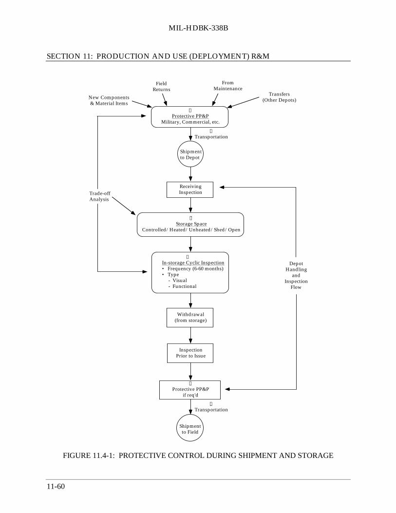
MIL-HDBK-338B


11-60

➀Protective PP&P

Military, Commercial, etc.

New Components& Material Items

FieldReturns

FromMaintenance

Transfers(Other Depots)

Shipmentto Depot

ReceivingInspection

➁Storage Space

Controlled/Heated/Unheated/Shed/Open

➂In-storage Cyclic Inspection• Frequency (6-60 months)• Type - Visual - Functional

Withdrawal(from storage)

InspectionPrior to Issue

Shipmentto Field

➀Protective PP&P

if req'd

DepotHandling

andInspection

Flow

Trade-offAnalysis

④Transportation

④Transportation

FIGURE 11.4-1: PROTECTIVE CONTROL DURING SHIPMENT AND STORAGE

MIL-HDBK-338B


11-61

(2) The storage environment can vary widely in terms of protection afforded. However,whenever possible, electronic hardware should be stored in dry, well ventilatedwarehouses, where the temperature of the air surrounding the equipment can beregulated so that it does not fall to dewpoint values at night. Storage in controlledtemperature/humidity buildings is of course, ideal. If equipment is stored in bins, it isimportant that it be placed above floor level. The military has several types of storageareas. These include warehouse space with complete temperature and humidity control,warehouse space with no humidity and temperature control, sheds, and open groundareas that are simply designated for storage.

(3) In-storage scheduled cyclic inspection is the key to assuring the actual reliability ofcomponents and equipment during storage. In-storage cycling inspections are designedto detect performance degradation, deterioration, and other deficiencies caused byextended periods of storage and improper storage methods. The inspections are toidentify those items which require corrective packaging (or further storage control) orcondition reclassification to a lesser degree of serviceability. The inspections areperformed at intervals derived from shelf life periods and the level of protectivepackaging and storage afforded the material items. It should be noted that all itemswhen originally placed in storage are ready for issue and that all applicablepreservation, packaging and packing (PP&P) requirements have been met. In-storagecycling inspection is part of the depot’s overall inspection system (see Figure 11.4-1)that includes inspection of items at receipt as well as prior to issue.

In general, shipment and storage degradation can be controlled in terms of the above-mentioned three parameters. The planning and specification of shipment and storagerequirements for new component and equipment items (as well as the reestablishmentof requirements for existing items in storage) must take into account economic choicesbetween the various factors within these parameters to arrive at the most cost effectivebalance that meets reliability and readiness objectives.

(4) The Mode of Transportation greatly influences the level of PP&P needed for an item.The modes of transportation used for military systems are primarily:

• aircraft• surface ship• rail• truck

Each mode is characterized by a unique set of environmental factors. Truck andtransport rail, for example, pose a certain temperature and vibration spectrum than doaircraft or surface ships. Exposure times also vary; item shipped by air are exposed tothe environmental stresses of transport for a much shorter time than items transported

MIL-HDBK-338B


11-62

by rail or surface ship. Items shipped by rail may sit in switching yards or sidings fordays under all kinds of climatic conditions. Similarily, an item shipped by air may sitcrated on the tarmac under extremes of heat or cold. Items aboard ships may beexposed to highly corrosive salt water spray.

Complicating matters is the fact that most items are not transported from origin todelivery point via a single mode of transportation. An item may, for example, bepicked up at its point of origin by truck, driven to a rail loading dock, taken by train to aseaport, sent by ship to another port, downloaded to a truck, and then delivered to itsfinal destination. Such multi-modal transportation imposes a greater variety ofenvironmental stresses. In addition, the handling involved in switching between modesimposes its own set of stresses. The level of PP&P must be sufficient to protect theitem against the most severe stresses to which it will be subjected throughout thetransportation process.

11.4.3 Shipment and Storage Degradation Control (Storage Serviceability Standards)

Since electronic components and equipment are subject to damage, deterioration andperformance degradation if unprotected during shipment and left uncontrolled for long periods ofdormant storage, organizations have established programs to control the parameters definedabove. The Army, for example, has established the Care of Supplies in Storage (COSIS)program (Ref. [4]). The program assures that material is maintained in a condition to meetsupply demands at a minimum cost in funds, manpower, facilities, equipment, and materials.COSIS by definition is “a Department of the Army (DA) program to perform specific tasks toassure that the true condition of material in storage is known, properly recorded, and the materialis provided adequate protection to prevent deterioration. The distinction between COSIS-relatedactions and actions that might otherwise fall into the broad category of care given material instorage is that COSIS concerns itself with the in-storage inspection, minor repair, testing,exercising of material and the preservation, packaging and packing (PP&P) aspects of theefforts.”

A major and most significant element within the COSIS program is the Storage ServiceabilityStandards (SSS) documents controlled by participating Army commodity commands as requiredby DARCOM-R 702-23, “Product Assurance - Storage Serviceability Standards (SSSs),” (Ref.[5]). The SSS documents consolidate and establish the depot quality control and reliabilitymanagement procedure for inspection, testing, and/or restoration of items in storage. Theyencompass preservation, packaging, packing (PP&P) requirements, storage environment criteria,as well as inspection requirements during the storage cycle to determine material serviceabilityand the degree of degradation that has occurred. They are applicable to shelf life items as well asall items that are considered sensitive to shipment and storage deterioration. In the case of shelflife items, specifically those items whose shelf life is considered extendible, the standards areused to determine if the items have retained their original characteristics and are of a quality levelwhich warrants extension of their assigned time period.

MIL-HDBK-338B


11-63

Figure 11.4-2 illustrates conceptually the basic technical approach in the preparation of thestandards. The figure shows that the storage serviceability standards are formatted into twodocuments (per Ref. [5]). The first, which is based on Appendix A of Ref. [5], specifies PP&Plevels, storage type and those tests, criteria and other provisions that can be coded easily into acomputerized format. The second, which is based on Appendix B of Ref. [7], specifiesapplicable supplementary tests including functional performance, detailed visual and otherspecial tests that cannot be coded easily into a computerized format but are necessary to assessthe readiness of the stored items.

The form for the storage serviceability standards (see Figure 11.4-2 and Appendix A ofDARCOM-R 702-23) contains in coded format the following data:

Federal Stock Number (FSN) - the federally assigned stock number for the item.

Item Name - provides a brief description of the item.

Quality Defect Code for Inspection (QDC) - defines potential storage-induced defects. Theassigned defect codes cover preservation, packaging, marking, and storage as well as materialdeficiencies. Cyclic inspections are performed to accept or reject material relative to the defectsidentified by this code. A three-digit code is used, where the first digit identifies the severity ofthe defect (critical 0, major 1, or minor 2), and the second and third digits (see Table 11.4-2)identify a specific class of defects. For example, the code 113 would indicate a major defect (1)due to (13): container damaged or deteriorated. Complete definitions for quality defect codesapplicable to the acceptance/rejection of material items inspected during the various depotinspection and testing phases (i.e., on receipt, audit, scheduled cyclic, special, etc.) are providedin AMCR 702-7 (Ref. [6]).

Inspection Level (IL) - determines the relationship between item lot or batch size and sample sizefor inspection. The inspection level is used in conjunction with the acceptable quality level(AQL) to form the sampling plan. (The sampling plan provides accept/reject criteria forindividual item inspections).

Acceptable Quality Level (AQL) - the maximum percent defective (or the maximum number ofdefects per hundred units) that for purposes of sampling inspection can be consideredsatisfactory.

MIL-HDBK-338B


11-64

Pro

tect

ive

Pac

kagi

ng•

Max

Mili

tary

• M

in M

ilita

ry•

Com

mer

cial

In

spec

tion

F

requ

ency

• 6

mon

ths

• 1

2 m

onth

s•

24

mon

ths

• 3

0 m

onth

s•

60

mon

ths

N

o te

st

APP

EN

DIX

A

SSS

RE

QU

IRE

ME

NT

S

Fed

eral

Stoc

kN

o. (F

SN)

Item

Nam

e

Qu

alit

yD

efec

ts(Q

DC

)

Insp

.L

evel

(IL

)

Acc

epta

ble

Qu

alit

y(A

QL

)

Maj

orM

inor

Shel

fL

ife

(SL

C)

Insp

.Fr

eq.

(IFC

)

Tes

tR

eq'd

(TR

C)

Pres

er-

vati

onP

acka

ging

(PP

C)

Typ

eSt

orag

e(T

SC)

Con

trol

Par

amet

ers

➁➀

➂

•

T

est R

eq’d

(Met

hod

s)•

Cod

ed V

isua

l Ins

pect

ions

(

com

plet

ely

des

crib

ed b

y th

e

qu

alit

y d

efec

t cod

es -

QD

C)

• S

uppl

emen

tary

Fun

ctio

nal/

Vis

ual

App

end

ix B

- S

SS R

equi

rem

ents

• C

ompo

nent

/E

quip

men

t Des

igna

tion

• T

est C

rite

ria

• In

stru

ctio

ns/s

lash

she

ets

• D

ata

shee

ts

••

Typ

e St

orag

e•

Con

trol

led

• H

eate

d•

Unh

eate

d•

She

d•

Ope

n

•

FIG

UR

E 1

1.4-

2: T

EC

HN

ICA

L A

PPR

OA

CH

TO

ST

OR

AG

E S

ER

VIC

EA

BIL

ITY

ST

AN

DA

RD

S (S

SS)

MIL-HDBK-338B


11-65

TABLE 11.4-2: STORAGE-INDUCED QUALITY DEFECTS

Category Second & Third Digit (QDC)

Preservation Inadequate 02Container Damaged or Deteriorated 13Containers, Boxes, Crates, or Pallets Damaged orDeteriorated

23

Markings Illegible 33Loose or Frozen Parts (out of adjustment) 40Damaged Parts (cracked, chipped, torn) 41Leakage (liquid) 45Bonding Deterioration (soldering, welding, etc.) 48Contamination (dirt, sludge, moisture, foreign matter) 50Excessive Moisture (fungus, mildew, rot) 51Shelf-life Data Exceeded 55Failed Test Requirements (failed supplementary testsfunctional/visual)

62

Improper Storage Space 86Corrosion, Stage 1 (or more) 90

Shelf Life (SLC) - describes deterioration characteristics versus time. Shelf life periods fordeteriorative material range from 1 month to 60 months. The condition of a shelf-life item isevaluated during cyclic inspection in terms of time remaining and downgraded if necessary.

Inspection Frequency (IFC) - defines the elapsed time between cyclic inspections. Inspectionperiods range from 6 months to 60 months.

Test Required (TRC) - describes the method by which an item is to be inspected or tested.

Preservation Packaging (PPC) - describes the preferred level and/or most cost effective level ofprotection for each item. After an item has been inspected and accepted, thepackaging/preservation is to be restored to its pre-inspection level. Further, the date ofrepackaging as well as the date of original packaging is stamped on the package.

Type Storage (TSC) - indicates the preferred or most cost effective storage condition.

In order to prepare standards for new or existing material items, criteria for specifying costeffective tests and control provisions are first established. The criteria (and the subsequentstandards) should provide for the inspections to be performed frequently enough to detect

MIL-HDBK-338B


11-66

potential problems but not so often as to dilute the total depot inspection effort and compromiseother items in storage which may be more critical and require higher inspection frequencies. Tobe effective, the criteria must take into account:

(1) Material deterioration

(2) Application risk and criticality

(3) Cost

(4) Material complexity

(5) Preservation/packing and packaging (PP&P)

(6) Storage environment

The Army has developed general criteria and a material weighting factor technique as part of acomplete standard preparation process that takes into account these factors (Ref. [7]). Theprocess, which is illustrated in Figure 11.4-3, focuses on the three major control parameters: (1)protective packaging level, (2) storage type, and (3) cyclic inspection (frequency and method).The process involves first defining the level of packaging and storage (preferred) from a reviewof material deterioration properties and then determining inspection frequency by evaluatingdeterioration, application risk, criticality and other factors in light of the defined packaging andstorage environment levels. It is an iterative process that involves tradeoff analysis to define anoptimum set of requirements. It emphasizes and uses to the maximum extent the visual codedinspection criteria, i.e., QDC, to detect material failure and/or defects due to corrosion, erosion,and other deficiencies resulting from improper storage methods, extended periods of storage, andthe inherent deterioration characteristics of the material item. The technique is sufficientlyflexible to make allowances for available storage facilities if they differ from the preferredthrough the adjustment of inspection frequency.

In the initial preparation of the standards, the type and level of storage space and packagingmethods are considered as fixed parameters (although iterative) where the preferred levels aredefined based on material deterioration properties. Therefore, the element which provides theoverall stimulus for the control and assurance of the readiness of stored components andequipment is the type and frequency of inspection. A ranking is assigned to each item thataccounts for material deterioration and the other factors depicted in Figure 11.4-3 and is used asthe basis to determine first the need for inspection and then, if needed, the frequency and type ofinspection.

To effectively manage the depot cyclic inspection program, priorities are established as indicatedin Figure 11.4-3. Items classified as definite shelf-life are given priority and subjected to cyclicinspection. Other indefinite shelf-life items that are considered particularly sensitive to

MIL-HDBK-338B


11-67

deterioration are also subject to cyclic inspection. Definite shelf-life items are those possessingintrinsic deterioration characteristics that cannot be eliminated (or minimized) by storage andpackaging controls. They are further classified into nonextendible (Type I) and extendible (TypeII) materials. Indefinite shelf-life items, on the other hand, include items that do not deterioratewith storage time, as well as items that are sensitive to deterioration as a result of inducedexternal failure mechanisms. The relationship between these types of material item classificationand their relative deterioration level is illustrated in Figure 11.4-3. Figure 11.4-4 shows thenonextendible life characteristic of Type I material, the extendible shelf-life characteristic ofType II material, and the relative indefinite shelf-life characteristic of all other stored material.

Figure 11.4-5 presents a matrix that can be used to determine inspection frequency (IFC) and tooptimize in-storage inspection coverage. The matrix includes:

(1) The most deteriorative items to the least deteriorative in terms of a total ranking factorthat accounts for deterioration, complexity, cost, accessibility and criticality

(2) All combinations of depot storage and packaging conditions ranging from the mostprotective (containerized package and a controlled humidity environment) to the leastprotective (commercial package and an open area)

Application of the matrix to a given material item involves assigning appropriate values to eachof the weight factors depicted in Figure 11.4-5 in order to arrive at a total ranking. This rankingrepresents a rough measure of the overall deterioration/cost sensitivity of the item to the storageenvironment. The ranking is then entered in the proper weight column of the matrix to determineinspection frequency for any desired combination of packaging and depot storage protectionlevel.

MIL-HDBK-338B


11-68

Def

ine

Prot

ecti

vePa

ckag

ing

Lev

el

Def

ine

Stor

age

Typ

e

Det

erm

ine

Freq

uenc

y &

Typ

e of

Inst

orag

e C

yclic

Insp

ecti

on

Con

trol

led

Hea

ted

War

ehou

se

Unh

eata

ed W

areh

ouse

Shed

Ope

n A

rea

Cla

ssif

y &

P

rior

itiz

e M

ater

ial

Incl

ude:

• D

efin

ite

shel

f lif

eit

ems,

i.e.

, ite

ms

poss

essi

ng in

trin

sic

det

erio

rati

onch

arac

teri

stic

sin

clu

din

gno

n-ex

tend

ible

as

wel

las

ext

end

ible

• In

def

init

e sh

elf l

ife

item

s th

at a

re s

ensi

tive

to d

eter

iora

tion

as

are

sult

of i

nduc

ed e

xter

nal

failu

re m

echa

nism

s.(D

epen

den

t on

stor

age

cont

rol a

nd p

acka

ging

leve

l)

I

nspe

ctio

n Fr

eque

ncy

IFC

App

ly w

eigh

t fac

tor

mat

rix

to d

eter

min

e ne

ed a

ndfr

eque

ncy

of in

spec

tion

;m

atri

x ac

coun

ts fo

r:

• M

ater

ial d

eter

iora

tion

• It

em c

ompl

exit

y•

Cos

t•

Acc

essi

bilit

y•

Cri

tica

lity

ITE

RA

TE

AS

NE

CE

SSA

RY

Tes

t Req

'd(T

RC

)

Vis

ual I

nspe

ctio

n

(App

end

ix A

)•

Min

imum

kno

wle

dge

o

f ite

m r

equi

red

• C

ompl

ete,

des

crib

ed

by

Cod

es•

App

lied

to a

ll

ite

ms

test

ed

Sup

plem

enta

ry T

ests

(App

end

ix B

)•

Req

uire

s w

orki

ng

kno

wle

dge

of i

tem

• D

etai

led

inst

ruct

ion

a

nd/o

r pr

oced

ure

• A

pplie

d to

item

s no

t

ad

equa

tely

cov

ered

by

A

ppen

dix

A C

odes

To

Det

ect M

ater

ial:

• C

ond

itio

n D

egra

dat

ion

• D

eter

iora

tion

• C

orro

sion

& O

ther

Def

icie

ncie

sC

ause

d b

y: •

Im

prop

er S

tora

ge M

etho

d •

Ext

end

ed P

erio

ds

of S

tora

ge •

Inh

eren

t Det

erio

rati

on

c

hara

cter

isti

cs o

f the

mat

eria

lM

ust R

efle

ct:

• D

epot

ski

ll le

vel

• T

est e

quip

men

t ava

ilabi

lity

• C

ost e

ffec

tive

ness

Mat

eria

l Sub

ject

toC

yclic

Insp

ecti

on

Max

Mili

tary

Non

Mili

tary

Com

mer

cial

FIG

UR

E 1

1.4-

3: S

TO

RA

GE

SE

RV

ICE

AB

ILIT

Y S

TA

ND

AR

D P

RE

PAR

AT

ION

PR

OC

ESS

MIL-HDBK-338B


11-69

MATERIAL READINESS LEVEL (VS)

STORAGE TIME

T = Time of Material Cyclic Inspection T = Time of Material Restoration (Shelf Life Extended) T = Time of Material Retirement (Shelf Life Completed)

I

E

R

Storage Time

Type I Definite Shelf Life Material (Parachute)

Retirement Level

Type II Definite Shelf Life Material (Fuel Cells, Survival Kits

∅ - Indefinite Shelf Life Material (Engines, Transmissions)

TI TI TE TR TE TITI

FIGURE 11.4-4: DETERIORATION CLASSIFICATION OF MATERIAL

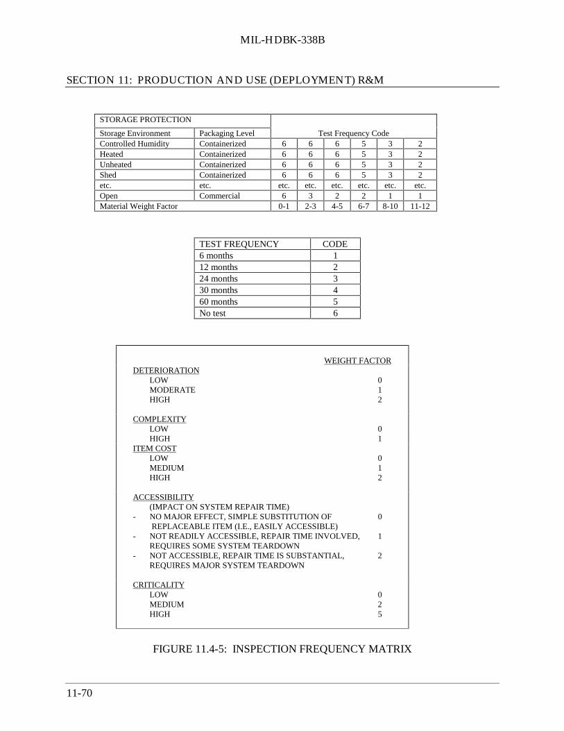
MIL-HDBK-338B


11-70

STORAGE PROTECTION

Storage Environment Packaging Level Test Frequency CodeControlled Humidity Containerized 6 6 6 5 3 2Heated Containerized 6 6 6 5 3 2Unheated Containerized 6 6 6 5 3 2Shed Containerized 6 6 6 5 3 2etc. etc. etc. etc. etc. etc. etc. etc.Open Commercial 6 3 2 2 1 1Material Weight Factor 0-1 2-3 4-5 6-7 8-10 11-12

TEST FREQUENCY CODE6 months 112 months 224 months 330 months 460 months 5No test 6

WEIGHT FACTORDETERIORATION

LOW 0MODERATE 1HIGH 2

COMPLEXITYLOW 0HIGH 1

ITEM COSTLOW 0MEDIUM 1HIGH 2

ACCESSIBILITY(IMPACT ON SYSTEM REPAIR TIME)

- NO MAJOR EFFECT, SIMPLE SUBSTITUTION OF 0 REPLACEABLE ITEM (I.E., EASILY ACCESSIBLE)

- NOT READILY ACCESSIBLE, REPAIR TIME INVOLVED, 1REQUIRES SOME SYSTEM TEARDOWN

- NOT ACCESSIBLE, REPAIR TIME IS SUBSTANTIAL, 2REQUIRES MAJOR SYSTEM TEARDOWN

CRITICALITYLOW 0MEDIUM 2HIGH 5

FIGURE 11.4-5: INSPECTION FREQUENCY MATRIX

MIL-HDBK-338B


11-71

For new items, the matrix allows broad tradeoffs to be made to arrive at the optimum balance ofpackaging, storage, and inspection requirements. Also, the combining of deterioration with costand the other weight factors via the matrix approach allows the specification of cost effectiveinspection periods. This cost effectiveness is illustrated by considering two items one of whichexhibits low deterioration properties but the cost and other factors are high, and the other whichexhibits high deterioration properties but the total of the other factors is low. A relatively lowcost or nominal test inspection frequency may be computed for both items that reflects aneffective balance of all factors; whereas, if only deterioration was considered in computing thetest periods, over-inspection (excessive cost) of the high deterioration item and under-inspection(low readiness assurance) of the low deterioration items would most likely result. Of course, forthose items where all factors including deterioration and cost are high, frequent inspection wouldbe required to ensure the readiness of material and for those items where deterioration and theother factors are low, less frequent inspections would be required.

The matrix approach also provides flexibility for regulating the number and type of itemssubjected to cyclic inspections by adjustment of the weight assigned to the factors that relate thematerial to the storage environment.

As previously indicated, an inspection time period is originally set based upon preferred storageenvironment and packaging methods specified in the TSC and PPC columns of Figure 11.4-2.However, many times an item will be stored and packaged at a different level. In that case anadjustment is made to its inspection time periods to maintain the same state of readiness based onthe data provided in the inspection frequency matrix.

11.4.3.1 Application of Cyclic Inspection During Storage to Assure Reliability andMaterial Readiness

Critical to the control of reliability during storage is the proper application of cyclic inspectionsand tests. The purpose of in-storage cyclic inspection is to assess component/equipmentreliability and readiness for use, to detect deterioration while in storage, and to furnish data forany necessary condition reclassification action. A knowledge of the component or equipmentitem, particularly its deterioration properties and risk attributes, is necessary to plan and specifyoptimum in-storage cyclic inspection requirements. The inspections must be practical andmaintain an overall cost effective posture that reflects readily available depot test equipment andskills.

MIL-HDBK-338B


11-72

In-storage cyclic inspection generally includes two basic types as indicated in the previoussubsection. The first type is based on subjective visual inspections where material acceptance iscompletely described by codes covering quality defects (and included in the QDC column of theStorage Serviceability Standard). A minimum knowledge of the items is required to specify thecriteria and perform the inspections. These coded requirements apply to all items tested. Figure11.4-6 illustrates some of the quality defect codes and shows that the assigned codes coverpreservation, packing, marking and storage, as well as material deficiencies. The figure indicatesthat there are basically three levels of inspection corresponding to (1) the outer package orcontainer, (2) the inner packing, and (3) the item itself. If a defect is not considered critical,major, or minor at the time of inspection but (due to inspector experience) is expected to becomecritical, major or minor prior to the next cyclic inspection, it is identified as such, considered as acause for rejection, and counted relative to the item’s sampling plan criteria. Defects of a trivialnature are not considered as cause for rejection of a lot, unless some reduction in usability orfunction of items is expected prior to the next scheduled inspection. For example, nicks, dents, orscratches that do not break coatings or paint films are considered trivial deficiencies.

INSPECT OUTER PACKAGEOR CONTAINER ANDSTORAGE METHODS

INSPECT INNER PACKAGING

INSPECT MATERIAL ITEMS

ACCEPT

ACCEPT

REJECT

REJECT

REJECT

MATERIAL ACCEPTED

RECLASSIFIEDTO APPROPRIATECONDITIONCODE

• CONTAINERS, BOXES, CRATES OR PALLETS DAMAGED OR DETERIORATED (CODE 23)• MARKINGS ILLEGIBLE (CODE 33)• SHELF LIFE EXCEEDED (CODE 55)• IMPROPER STORAGE SPACE (CODE 86)

• PRESERVATION INADEQUATE (CODE 02)• INNER CONTAINER OR PACKAGING DAMAGED OR DETERIORATED (CODE 13)

• LOOSE OR FROZEN PARTS, OUT OF ADJUSTMENT (CODE 40)• DAMAGED PARTS (CODE 41)• BONDING DETERIORATION (CODE 48)• CONTAMINATION (CODE 50)• EXCESSIVE MOISTURE (CODE 51)• FAILED TEST REQUIREMENTS (SUPPLEMENTARY FUNCTIONAL/ VISUAL (CODE 62)• CORROSION (CODE 90)• LEAKAGE (CODE 45)

FIGURE 11.4-6: CODED QUALITY INSPECTION LEVELS

MIL-HDBK-338B


11-73

The second type of in-storage inspection involves supplementary requirements that are applied toitems that cannot adequately be inspected by the visual coded requirements. They generallyinclude functional tests (derived from technical manuals) and/or special, more-detailed visualinspections. Special test and/or inspection procedures complete with acceptance criteria areprepared for these items and included in Appendix B to the SSS. Emphasis is placed on definingviable test or checkout procedures that can be applied simply and quickly to the stored materialitems to assure that they perform satisfactorily with only a minimal level of evaluation, support,and guidance. These supplementary tests can be applicable to parts, material, equipment, orcomplete systems, including shelf-life items as well as other items that are storage sensitive.

The supplementary tests are not intended to represent a complete and detailed inspection orcheckout of the item to determine compliance to specified requirements. The tests are designedto verify operability and are to be based on a “go/no-go” concept, fully utilizing end itemfunctions to indicate functional readiness for service and issuance.

The functional tests are designed such that they do not require external and specialized testequipment except common and readily available equipment found at the depots and otherinstallations (power supplies, volt-ohmmeters, etc.). The functional tests in general involve firstchecking the operational mode of all indicators such as dial lamps, power lights, meters, and faultlights as applicable and then applying a simple procedure that exercises some or all of itsfunctions to verify operational status. Many times the equipment can be tested as part of asystem. For example, two radio (receiver/transmitter) sets could be tested as a system pair bypositioning the sets a certain distance apart (e.g., 25 feet). One is placed in the receive mode andthe other in the transmit mode, and all associated hardware and interconnecting cables areattached. An audio (spoken word) input is applied to the set in the transmitting mode, and the setin the receive mode is checked for reception. The process is repeated with the transmitter/receivemodes reversed.

The functional test procedures for a given equipment item can be derived from a review of theequipment's maintenance and/or operating manuals. These manuals describe the operationalsequence, the turn-on and shut-down procedure, and the equipment operational test and checkoutprocedure necessary for complete verification of equipment operational status. Consequently,they provide a sound basis for deriving a simplified and cost effective functional test that issuitable for assessing reliability during storage.

MIL-HDBK-338B


11-74

11.4.4 Data Collection and Analysis (During Storage)

The shipment/storage test and control program, like the production test program, must becontinually challenged relative to the effectiveness of the overall program as well as theindividual tests. In-storage cyclic inspection must also be considered as a dynamic test where thetest methods, frequencies, and criteria are adjusted to reflect actual depot and field experience.In-storage data (reject rate, quality discrepancy reports, causal data, etc.) generated during theimplementation of the cyclic inspections should be compiled, reduced, thoroughly analyzed, andfed back to item management and engineering activities in a form that will provide a basis to:

(1) Determine the effectiveness of the shipment/storage degradation control program tomeet reliability and readiness objectives

(2) Eliminate the causes for deficiencies

(3) Revise item inspection or protective packaging and storage level requirements, ifnecessary

11.5 Operational R&M Assessment and Improvement

Electronic systems are also subject to damage and performance degradation during operation andmaintenance. Consequently, operational systems are continually assessed to ensure that they areperforming in accordance with expectation and to identify areas where improvements can beincorporated to minimize degradation, improve R&M, and reduce life cycle costs. This timeperiod is most significant because it is here that the true cost effectiveness of the system and itslogistic support are demonstrated and historical R&M data are gathered and recorded for use onfuture products. The effort includes:

(1) Assessing R&M performance from an analysis of operation/failure data, identifyingoperation/maintenance degradation factors, and comparing actual R&M with thatpredicted and demonstrated during acquisition

(2) Identifying systems, equipment and other hardware items that exhibit poor reliability,require extensive maintenance and are prime candidates for cost effectiveimprovements

(3) Evaluating the impact on R&M of system changes and corrective action implemented inresponse to operational failures

MIL-HDBK-338B


11-75

11.5.1 Factors Contributing to R&M Degradation During Field Operation

Degradation in reliability can occur as a result of wearout, with aging as the dominant failuremechanism. Defects can also be induced into a system during field operation and maintenance.Operators will often stress a system beyond its design limit either to meet a current operationalneed or constraint or inadvertently through neglect, unfamiliarity with the equipment, orcarelessness. Situations occur in which a military system may be called upon to operate beyondits design capabilities because of an unusual mission requirement. These situations can causedegradation in inherent R&M parameters. Operational abuses due to rough handling, extendedduty cycles, or neglected maintenance can contribute materially to R&M degradation during fieldoperation. The degradation is usually the result of the interaction of man, machine andenvironment. The translation of the factors which influence operational R&M degradation intocorrective procedures requires a complete analysis of functions performed by man and machineplus environmental and/or other stress conditions which degrade operator and/or systemperformance.

Degradation in inherent R&M can also occur as a result of poor maintenance practices. Studieshave shown that excessive handling brought about by frequent preventive maintenance or poorlyexecuted corrective maintenance (e.g., installation errors) have resulted in defects introduced intothe system, with resultant degradation of R&M. Some examples of defects resulting from fieldmaintenance, depot overhaul, or reconditioning are due to:

(1) Foreign objects left in an assembly

(2) Bolts not tightened sufficiently or overtightened

(3) Dirt injection

(4) Parts replaced improperly

(5) Improper lubricant installed

Also, during unscheduled maintenance, good parts are replaced in an effort to locate the faultyparts. In many cases, the good parts are written up as defective instead of being reinstalled.These parts often are returned to the depot for repair or discarded, resulting in a reported fieldfailure rate that is higher than is actually occurring.

Several trends in system design have reduced the need to perform adjustments or make continualmeasurements to verify peak performance. Extensive replacement of analog with digitalcircuitry, inclusion of more built-in test equipment, and use of fault-tolerant circuitry areindicative of these trends. These factors, along with greater awareness of the cost ofmaintenance, have brought changes for ease of maintenance whose by-product has increased

MIL-HDBK-338B


11-76

system R&M. In spite of these trends, the maintenance technician remains a primary cause ofR&M degradation. The effects of poorly trained, poorly supported or poorly motivatedmaintenance technicians on R&M degradation require careful assessment and quantification.

The operation and maintenance induced defects are factors that must be carefully considered andtaken into account in the assessment and control of operational R&M. In general, theenvironmental factors considered in prediction techniques account for the added stress providedby operation within that environment. However, the environmental stresses imposed during fieldmaintenance may be other than what was anticipated during the original prediction. For instance,a subassembly removed for repair in a desert area may be placed in direct sunlight while awaitingtransfer. Component temperatures may exceed those experienced during normal operation for anextended period, thus reducing their life expectancy. Mechanical stresses imposed oncomponents during removal, repair, and reinsertion may exceed that designed for a givenenvironment. Therefore, field and depot requirements and procedures must include criteria forcontrolling the reliability and quality of the repair/overhaul action to minimize potentialmaintenance induced defects in order to achieve an actual field R&M that approaches thatpredicted and demonstrated during acquisition.

11.5.2 Maintenance Degradation Control (During Depot Storage)

Depot maintenance activities include complete overhauling, partial rebuilding, productimprovement and retrofit, calibration, and the performance of highly complex repair actions. Inaddition, the depot normally stores and maintains the supply inventory. Physically, depots arespecialized fixed installations that contain complex and bulky production and test equipment, andlarge quantities of spares under environmental storage control. Depot facilities maintain highvolume potential and use assembly line techniques with relatively unskilled specialists in keyareas such as condition evaluation, fault diagnosis, and quality control and inspection.

Since the R&M of hardware items can be materially degraded during maintenance and depotoperations, engineering plans and analyses are performed and R&M controls implemented toassure performance and to eliminate defects due to workmanship and the various other factorsthat would, if uncontrolled, lead to poor quality and R&M degradation.

Control efforts for a given hardware item start with the preparation of a Maintenance Plan duringdevelopment as part of logistic support analysis (LSA); they continue into the operational andmaintenance phase with the establishment of specific criteria and special maintenance andrestoration procedures which must be followed to avoid R&M degradation and to retain theinherent R&M of the item. Possible deviations from the Maintenance Plan are described andrelated to their potential effect on operational R&M. Specifications are prepared andincorporated into a maintenance/depot requirement document including provisions covering:

(1) Life cycle reconditioning performance/quality parameters and acceptance criteria

MIL-HDBK-338B


11-77

(2) Types and kinds of material approved for use during overhaul, repair, andreconditioning

(3) Acceptable workmanship standards and techniques

(4) Quality and reliability assurance inspection, tests, analysis methods, and controls

The intent of the maintenance requirement document is to ensure that quality and R&M measuresreflect adequate, viable, and practical acceptance criteria and procedures that can be implementedmost cost effectively by depot personnel during the repair, overhaul, or reconditioning of thehardware items.

Some of the areas that are evaluated, controlled and reflected into the maintenancedocumentation from a reliability and quality standpoint are listed in Table 11.5-1. These includereviewing the technical accuracy and adequacy of instructions covering equipment checkout,calibration, alignment, and scheduled removal and replacement. In addition, all disassembly,cleaning, inspection, testing, repair, replacement, re-assembly, troubleshooting, preventivemaintenance checks and services, and maintenance processes and procedures are evaluated.

Criteria are also established that recognize the fact that hardware in field use (as well as duringstorage) deteriorates due to age, environment, and storage conditions. When deterioration beginsto take effect, the quality level of the material will decline below that which was initiallyspecified during procurement. Although the effectiveness and adequacy of the reconditioningoperations and controls will minimize the decline, the resultant quality level of the reconditionedmaterial will usually be lower than that initially specified. The depot requirements includemaintenance quality level requirements that reflect:

(1) Minimum deterioration, which is lower than the initially specified value

(2) Criteria that indicate the quality limits beyond which repair is not economicallyachievable

(3) Acceptance criteria for reconditioning cycles(s) at predetermined storage and usemilestones

MIL-HDBK-338B


11-78

TABLE 11.5-1: DEPOT MAINTENANCE REQUIREMENT AREAS

Inspection and Test Equipment - Test equipment used to determine performance of depotmaintenance specifications and requirements

Material Quality - Quality level of parts and material used for replacement, repair ormodification

Pre-shop Analysis - Extent of overhaul required. Included in the analysis would beprocedural instructions as well as a detailed checklist to aid in the evaluation of the items fordetermining extent of cleaning, repair, modification or replacement

In-Process Inspection - In-process inspection requirements, including procedural as well asaccept/reject criteria associated with each overhaul operation such as disassembly, cleaning,repair, replacement and modification, as applicable

Diagnostic and Automated Test Equipment - Diagnostic and automated test equipment (suchas NDT, magnetic particle, dye penetration, etc.) used to determine the adequacy of repair,overhaul or reconditioning

Repair - Total sequential, step-by-step instructions and specifications used for repair,replacement, reclamation, rework or adjustment for hardware items

Assembly/Disassembly - Total step-by-step instructions used to assemble/disassemble thehardware item

Calibration - Level and method of calibration for all equipment and instrumentation

Final Performance Check - Techniques and methods to assure total satisfactory performanceof the hardware item in accordance with the established criteria

In addition, a process analysis similar to that described in Sections 11.2 and 11.3 to determineand control R&M degradation introduced by manufacturing can also be applied to determine andcontrol degradation introduced by the reconditioning and overhaul process. This analysis wouldidentify processing and inspection steps that can be improved to reduce R&M degradation anddetermine the need to incorporate controlled screening and burn-in tests as described in Section11.2.

MIL-HDBK-338B


11-79

11.5.3 Maintenance Documentation Requirements

An important factor in controlling R&M degradation during deployment is the availability ofadequate maintenance documentation for the equipment/system. System maintenancedocumentation includes the written, graphical, and pictorial data which should be supplied withthe system for use by operators and maintenance personnel to accomplish both the routinepreventive maintenance tasks and the corrective repair procedures identified in the MaintenancePlan for the system. This documentation should reflect the maintenance concept and repairpolicies established for the system. In general, system operation and maintenance documentationshould be a completely integrated package providing clear-cut direction leading from failuredetection to fault isolation and repair procedures and should be presented in a format and styledesigned for ready access and updating as changes are introduced.

Four types of data represent the minimum package which should be provided with an operatingsystem if it is to be successfully operated and maintained in accordance with the MaintenancePlan. These working documents should be instructional and factual. The four categories ofmaintenance documentation required to successfully implement the Maintenance Plan aredescribed as follows:

(1) Functional Description and Operating Instructions for Each System - Data in thiscategory includes: a description of the capabilities and limitations of the installedsystem; a technical description of system operation, including its operating modes andalternate modes; step-by-step turn-on and manual operating procedures; “confidence”checks normally employed to verify that equipment is performing satisfactorily.

(2) Equipment and Installation Description - Data in this category must provide anaccurate, up-to-date description of the hardware as it is installed in the weapons system.Minimally, it should consist of: A complete set of functional flow or logic diagrams; acomplete set of schematic diagrams for electrical layout, electronics, hydraulics,pneumatics, etc.; parts data containing reference information in sufficient detail topermit reordering or fabrication of the individual parts within the system; and thenecessary instructions for installing and checking out installed/retrofitted equipment.

(3) Maintenance Aids (Troubleshooting) - This category presents the specific data requiredby the technician for localizing a fault to a replaceable item and for checking out thesystem after repair. Included are:

(a) Methods for system-level fault isolation when the system is “up” butoperating in a degraded mode; use and interpretation of system readiness testresults

MIL-HDBK-338B


11-80

(b) Method of system level fault isolation when the system is totally down; useand interpretation of fault isolation tests and monitoring of console displays

(c) Procedures for functional equipment level fault isolation; based on faultsensing indicators supplemented, as required, by test point measurementsusing built-in test equipment

(d) Equipment-level isolation techniques the use of which will permitidentification of the problem area to a single module or replaceable part

(e) Routine tests, adjustments, alignment, and other “preventive” procedureswhich are performed at periodic intervals

(4) Ready Reference Documentation - This documentation is limited to that informationroutinely required by the technician in a given equipment repair area. Thedocumentation should be easily usable in the work area - i.e., capable of being held withone hand, remaining open to a given section, permitting easy replacement or additions,and suitable for storage in the work area. It should contain only routine checkout,alignment, and preventive maintenance procedures; fault monitoring interpretation andreplacement data; supplemental troubleshooting techniques required to complement theautomatic fault detection and isolation system; and item and unit spare parts orderingdata keyed to system identity codes.

11.5.4 Data Collection and Analysis (During Field Deployment)

A new system or equipment begins to accrue valuable experience data with its initial introductioninto the field. These data, accurately recorded and consistently reported, provide the final basisfor judging suitability of the system for continuing deployment. Thereafter, the reporting systemcan become the essential basis for an effective R&M feedback loop if provisions are made forcontinuous reporting and periodic analysis of maintenance experience data throughout thedeployment phase and if formal procedures are established for progressive correction ofdiscrepancies revealed by the analysis. On the other hand, if the reporting system is not fullyexploited analytically and applied dynamically in a formal corrective action program, the R&Mfeedback loop is short circuited and serves no purpose other than logistic surveillance.

Data required to effectively assess, monitor, control and improve the R&M of fielded systemsand equipment items include hours of operation (and appropriate data on operatingcharacteristics), performance measures and assessments, application environmental factors, and,most important, failure and maintenance data. The feedback of information obtained from theanalysis of failure during actual use is essential to reliability growth. The focus of the datacollection should be on tracking failure modes, not symptoms.

Development of a formal and well-documented field data recovery, analysis and feedback system

MIL-HDBK-338B


11-81

is a key element in an effective R&M program. The data recovery and feedback program isdesigned to be compatible with and incorporate data from other data collection efforts duringacquisition and storage. An effective data system provides output information that can be usedfor:

(1) R&M assessments

(2) R&M tracking

(3) Comparative analysis and assessments

(4) Determination of the effectiveness of R&M tasks and management concepts

(5) Identification of critical equipment, components and problem areas

(6) Compilation of historical component failure rates for design predictions

Plans are prepared that describe the specific mechanisms for collecting operation, maintenanceand installation data at field sites, depots, and disposal areas as well as during factory test forfeedback. Included are detailed instructions, document forms, and the delineation ofresponsibilities for implementation. Furthermore, the system must be planned such that it iscompatible with standard military data systems. It should be noted that during acquisition thedata system is primarily the responsibility of the system equipment developer where control bythe military is established through reporting of summary data and deliverable data items.

During operation, military maintenance data collection systems are used to record andaccumulate ongoing data. These programs, including the Army’s TAMMS (The ArmyMaintenance Management System), the Navy’s 3M and the Air Force’s REMIS and othermaintenance data collection systems, are primarily maintenance oriented. Maintenance actionsare reported and processed in a computer data bank at three levels: equipment, assembly board,and piece-part. For each entry, the failure indicator is reported along with codes identifying suchthings as the base command and the equipment nomenclature. They do not, however, reportoperating time. Moreover, the field use environment and the field maintenance environment arenot adequately quantified to ensure consistent interpretation of field data. Thus, field reliabilitycannot be assessed using data from only the military systems. In order to assess reliability and tocompare the attained field reliability with that specified and estimated during acquisition, bothequipment/system failure (or maintenance) data and their associated operating time(s) arerequired. The associated equipment/system operating time must be estimated or obtained directlyfrom the operational units themselves. Operating times are recorded in station logs and theequipment inventory, with associated records of uptime, storage time and maintenance times, bymonth.

MIL-HDBK-338B


11-82

In addition to the previously mentioned maintenance data collection systems, the Department ofDefense instituted the Reliability Analysis Center (RAC), a DoD Information Analysis Center,which functions as a focal point for the recovery of reliability test data and experienceinformation on electronic, electrical, and electromechanical components, and R&M data on theequipments/systems in which these components are used. Reliability experience information isdisseminated by the RAC through reliability data compilations, handbooks and appropriatespecial publications to upgrade and support system reliability and maintainability.

These publications cover the following:

(1) Nonelectronic Parts Reliability Data (NPRD)

(2) Nonoperating Reliability Databook (NONOP-1)

(3) Failure Mode/Mechanism Distributions (FMD)

The publications are updated and reissued periodically, deleting outdated data entries andincorporating new acquisitions from the latest technologies and applications. For additionalinformation on the RAC, as well as other specialized DoD Information Analysis Centers, seeReference 9.

11.5.5 System R&M Assessment

Once an equipment/system is deployed, its R&M performance is periodically assessed based onthe analysis of collected field operational/failure data as described in the previous section, as wellas information derived from other sources. Programs have been established to assess R&M in amanner so as to yield consistent and accurate data and information that can be fed back into theproduct improvement process as well as to provide a “lessons learned” information base forsubsequent acquisitions. The programs are designed to provide data and information that can beused to:

(1) Uncover problem areas, effect timely corrective action, and provide a solid basis forsystem R&M improvement programs.

(2) Determine the effectiveness of design, test and program concepts applied during systemacquisition.

(3) Track the performance and, in particular, the R&M of the fielded system.

MIL-HDBK-338B


11-83

Application of the feedback loop to service evaluation of R&M and correction of R&M problemsis accomplished in five major steps, the last of which becomes the first step in a repetition of thecycle:

(1) Acquisition of Required Data - Use the data collection and reporting system to acquirethe basic service use experience data, supplemented as necessary by systemconfiguration and engineering data, and operational information to ensure correlationbetween reported maintainability experience and the conditions under which theexperience data was accrued.

(2) R&M Assessment - Analyze the reported experience data to derive a measure of theR&M parameters (e.g., failure rate, MTBF, mean corrective maintenance time ( Mct ),maximum corrective maintenance time (Mmaxct

), maintenance manhours per operating

hour, logistics delay time, etc.) at system, subsystem, equipment, major component, andlower levels, corresponding to the levels to which R&M was allocated, specified, anddemonstrated during the development phase.

(3) Problem Definition - Identify, investigate, and describe the underlying problems whichaccount for major discrepancies or deficiencies noted in the analysis of (2) above interms amenable to translation into corrective action as design changes, documentationchanges, maintenance or logistics procedural changes, etc., as appropriate. Introduce ona limited sampling basis such supplementary data recording forms, time clocks,instrumentation, and reporting instructions as required for the assessment of R&Mwhere the field values greatly exceed predicted or demonstrated values.

(4) Corrective Action Assignment - Formally assign corrective action responsibilityaccompanied by problem descriptions developed under (3) above with specified criteriafor verifying achievement of corrective action objectives.

(5) Follow-Through - Reassess R&M as in (2) above to evaluate effectiveness ofcorrective actions, to compare R&M trends relative to established improvementobjectives, and to reevaluate problems identified in earlier assessments. This stepbegins the assessment cycle all over again.

Department of the Army, Readiness Command (DARCOM) Regulation 702-9 (Ref. [10]) definesthe policies and procedures of a formal R&M System Assessment Program established by theArmy. This regulation requires that assessments be performed in order to determine whether thefielded system has satisfied user needs for mission performance and logistic support. They areconducted in order to identify and take corrective action on problems which are degrading usersatisfaction, operational readiness, and life cycle cost. Through the performance of suchassessments the Army determines how a system is operating, uncovers and corrects problems insystem operation and support, and thus helps achieve complete user satisfaction.

MIL-HDBK-338B


11-84

As presently structured, the System Assessment Program includes the assessment of all aspectsof fielded system operations including:

(1) Technical - A narrative description of the system and its support equipment- Original design objectives- The results of development and operational tests- Corrective action results

(2) Operational - Initial field performance parameter values- Changes incorporated into the fielded system (e.g., payload,

accuracy, reliability, availability, and maintainability)- Present field performance parameter values

(3) Environmental - Individual component shelf-life values- The reliability of components which require storage stockpile

testing- The effect stored components are having on overall system

reliability

(4) Human Factors - The user’s opinion of the adequacy of the system- The quantity of personnel, by military occupational specialty- The quality of personnel, by military occupational specialty

(5) Support - Current problems- Development initiatives for replacement- Effectiveness of the present logistic support system- Improvement actions required- System improvement plans

DARCOM Regulation 702-9 states that maximum use will be made of existing field data toassess these areas. Other data sources include

(1) Sample data collection programs

(2) Field visits and surveys

(3) User questionnaires

(4) User conferences

(5) Logistic personnel and field maintenance technicians

MIL-HDBK-338B


11-85

11.5.6 System R&M Improvement

In addition to optimizing R&M during acquisition through aggressive design, development, andproduction programs, substantial R&M growth potential exists during deployment. Some of thisgrowth occurs naturally as the operations and maintenance personnel become more familiar withthe equipment. However, to accelerate the growth rate and achieve significant increases inoperational R&M requires the application of a closed-loop process of positive corrective actionbased on analysis and assessment of field R&M data. For newly deployed equipment, thisclosed-loop process can achieve significant reliability improvement, especially when used withinthe context of a total, disciplined system assessment program as discussed in the previoussubsection. Reliability growth is based upon the iterative process of monitoring system operationto identify actual or potential sources of failures, to redesign out the failure source, and tofabricate and apply changes which improve system reliability. As such, reliability growth can beapplied during development, production, or during operation. For fielded systems, the reliabilitygrowth process is a valuable tool to attain reliability improvements and achieve savings thatcould more than offset the cost of the reliability improvement program. The process is alsoperformed during field deployment to eliminate problem areas not evident during thedevelopment phase.

The R&M improvement program must work in conjunction with the data collection andassessment programs (as discussed in the previous section) in a total integrated processconsisting of data collection, system assessment and improvement selection, development, andimplementation to achieve reliability growth in the field.

As described in more detail in the previous section, the program is an iterative feedback processconsisting of the following steps:

(1) Acquisition of required data

(2) R&M assessment

(3) Problem definition

(4) Corrective action assignment

(5) Follow through to evaluate effectiveness of corrective action(s)

MIL-HDBK-338B


11-86

The action of improving system reliability involves a systematic review of several conceptswhich appear from the backup data to be most useful for reliability cost tradeoff considerations,among which are:

(1) The reduction of failure rates by operating components at reduced (derated) stresslevels, accomplished by selecting components which have ratings well in excess ofthose required for their system application.

(2) The use of improved components for which reliability has been significantly increasedthrough special manufacturing techniques, quality control procedures, and testingmethods.

(3) Design simplification to eliminate parts or components.

(4) The substitution of functionally equivalent items with higher reliability.

(5) The overall reduction of failure rate through increased control of the internal systemenvironment, e.g., through reduction of ambient temperature, isolation from handlingeffects, and protection from dust.

(6) The provision of design features which enable prediction of incipient failures andpermit remedial action to be taken before an operational failure occurs.

(7) The provision of design features which reduce the probability of human-initiated errors.

(8) The provision of multiple identical parts, paths or higher functional levels (redundancy)in order to prevent a system failure in the event that one element fails.

(9) The reduction of failure rate through increased control of the environment external tothe equipment, as through reduction of ambient temperature, isolation from handlingeffects, isolation of operator from ambient noise, and protection of equipment fromdust.

(10) The implementation of controlled screening and burn-in tests for the purpose ofsignificantly reducing incipient failures due to undetected defects in workmanship orcomponents.

Similarly, maintainability (MTTR) can be improved by incorporating improved use ofmaintenance practices, providing higher quality technical manuals and maintenance aids orpossibly better training to improve the skill level of the technicians.

Computing the impact of the improvement recommendations which appear most useful for costtradeoff consideration on MTBF, MTTR, overall downtime and system performance, using the

MIL-HDBK-338B


11-87

methods and techniques previously described, and determining the total cost for theirimplementation is an essential step in evaluating the effectiveness of the improvement.

Critical to the analysis process is the ability to assess quantitatively the cost effects of reliabilityand maintainability. The cost of each recommended change must take into account total costthroughout the life cycle of the system and accordingly must include cost elements associatedwith design, manufacture, procurement, installation, and field use (i.e., operation, maintenance,and logistics).

The final step is to compute cost/benefit factors, i.e., develop a numeric for each R&Mrecommendation which reflects the total cost of the change, its impact on system performance,and the cost avoidance to be realized over a given time period by their implementation. This willallow the determination of those change recommendations which have maximum costeffectiveness. (See Section 8.1 for a discussion on reliability data collection and analysis). Therecommended changes can then be presented in an improvement plan in prioritized order of costeffectiveness, as defined by the computed cost/benefit factors.

11.6 References For Section 11

1. Schafer, R.E., A.E. Sari and S.J. Van DenBerg, Stress Screening of Electronic Hardware.RADC-TR-82-87, May 1982, (AD-A118261).

2. Environmental Stress Screening Guidelines. The Institute of Environmental Sciences,Library of Congress Catalog Card No. 62- 38584, 1981.

3. Navy Manufacturing Screening Program. NAVMAT P-9492, Naval Material Command,May 1979.

4. Care of Supplies in Storage (COSIS). Army Regulation AR 740-3, 1993.

5. Product Assurance - Storage Serviceability Standards (SSS). Army Regulation DARCOM-R 702-23.

6. Product Assurance Depot Quality Assurance System. Army Regulation AMC-R 702-7.

7. Army Supply Bulletin SB740-99-1, Storage Serviceability Standard for TSARCOMMaterial.

8. Maintenance of Supplies and Equipment, AMC Guide to Logistics Support Analysis.AMCP 750-16, Headquarters, Army Materiel Command, January 1978.

MIL-HDBK-338B


11-88

9. Directory of the Department of Defense Information Analysis Centers. Defense TechnicalInformation Center, Defense Logistics Agency, Cameron Station, Alexandria, VA 22304-6145, April 1995.

10. DARCOM Regulation 702-9, Department of the Army, September 1977.

11. Environmental Stress Screening Guidelines. Tri-Service Technical Brief, 002-93-08.

12. Environmental Stress Screening Guidelines for Assemblies. 1984 & 1988, The Institute ofEnvironmental Sciences.

13. Environmental Stress Screening Guidelines for Assemblies. 1990, The Institute ofEnvironmental Sciences.

14. Environmental Stress Screening Guidelines for Parts. 1985, The Institute of EnvironmentalSciences.

15. Impact of Nonoperating Periods on Equipment Reliability, RADC-TR-85-91.

16. Kinlaw, Dennis C., Continuous Improvement and Measurement for Total Quality: A Team-Based Approach, Pfeiffer & Company/Business One Irwin, 1992.

17. Wilson, Lawrence, H., Eight-Step Process to Successful ISO 9000 Implementation: AQuality Management System Approach, ASQC Quality Press, Milwaukee, WI, 1996.

18. Prescott, Jon, “What the $75 Books Don’t Tell you about ISO 9000 Documentation,”Reliability Review, Volume 15, Number 2, June 1995.

19. Breitenberg, Maureen, “Questions and Answers on Quality, the ISO 9000 Standard Series,Quality System Registration and Related Issues,” NISTIR 4721, National Institute ofStandards and Technology, April 1993.

MIL-HDBK-338

SECTION 12: RELIABILITY MANAGEMENT CONSIDERATIONS

12-1

12.0 RELIABILITY MANAGEMENT CONSIDERATIONS

12.1 Impacts of Acquisition Reform

As discussed in Section 4.0, recent Acquisition Reform policies have resulted in the eliminationof many historical reliability standards from the DoD procurement process. Past versions of thishandbook heavily relied on MIL-STD-785 (canceled 30 July 1998),Reliability Program forSystems and Equipment Development and Production,to explain and provide guidance on themakeup, planning and management of a reliability program. However, under new reforms inacquisition, such standards can no longer be levied as a requirement on the system developmentcontractor. In the past, the procuring agency was able to develop a statement of work (SOW) thatspecifically stated the contractor was to develop a Reliability Program Plan, and further, whichreliability tasks from MIL-STD-785 (canceled 30 July 1998) were targeted to be performed tomeet stated quantitative reliability requirements for the system to be procured. Now, as part ofthe cited reform policies, MIL-STD-785 has been canceled as of 30 July 1998, and militarystandard documents, with some exceptions, may not be imposed without a waiver. On the otherhand, there is nothing in the latest acquisition reform language that prevents the system developerfrom proposing to use any current or previously existing military standard or handbook as thebasis for implementing a design approach or program as part of an overall developmentapproach.

12.1.1 Acquisition Reform History

On June 29, 1994, Secretary of Defense William Perry issued a five-page memorandum,“Specifications & Standards - A New Way of Doing Business.” The intent of the memorandumcan be summarized as three "overarching” objectives:

(1) Establish a performance-oriented solicitation process

(2) Implement a document improvement process

(3) Create irreversible cultural change in the way DoD does business

The DoD is working to streamline the way in which procurement is managed and to adoptcommercial practices whenever possible. It is reassessing and trying to improve the way it doesbusiness to decrease costs and increase customer satisfaction.

As will be explained, military standards and specifications may be cited for guidance in aDepartment of Defense solicitation butshall not be cited as requirements unless a waiver isgranted. Commercial standards may be cited for guidance. Although not specifically prohibitedby policy at the time this handbook was written, commercial standards should not be mandatedas requirements. Given the spirit of the new acquisition policy, mandating a commercialstandard is no different than mandating a military standard. In either case, the procuring agencywould be telling the bidding contractor what to do and how to do it, at least to the extent that the

MIL-HDBK-338


12-2

cited standard provides suggestions on the tasks and activities needed for reliability.The mainobjective of the new policy is to use performance specifications.Only when performancespecifications are inadequate for fully describing what the government wants should commercialspecifications and standards be considered. And only when commercial specifications andstandards are inadequate should a waiver to use a military specification or standard beconsidered.

12.1.1.1 Performance-based Specifications

(1) A performance specification states requirements in terms of the required resultsand provides criteria for verifying whether or not the requirements have beenmet. Performance specifications do not state the methods for achieving therequired results. They have the following characteristics:

(a) Requirements should be stated quantitatively

(b) Requirements should be verifiable

(c) Interfaces should be stated in sufficient detail to allow interchangeabilitywith parts of a different design

(d) Requirements should be material and process independent

(2) There are four types of performance specifications: commercial itemdescriptions (CIDs), guide specifications (GSs), standard performancespecifications (SPSs), and program-unique specifications.

(a) Commercial Item Descriptions. An indexed, simplified productdescription prepared by the government that describes, by performancecharacteristics, an available, acceptable commercial product that willsatisfy the Government’s needs. Guidance for CIDs is given in theGeneral Services Administration Federal Standardization Manual (Chapter6), in the Defense Standardization Manual, DoD 4120.3-M, and in DoD5000.37-H. By definition, CIDs are only to describe requirements in termsof function, performance, and essential form and fit requirements. CIDsare listed in the DoD Index of Specifications and Standards (DoDISS).

(b) Guide Specifications. Guide specifications identify standard, recurringrequirements that are common for like systems, subsystems, equipments,and assemblies. The format of a GS forces the user to tailor the documentto the specific application. Guidance for GSs is in DoD 4120.3-M. GSsare listed in the DoD Index of Specifications and Standards (DoDISS).

(c) Standard Performance Specifications. A specification that establishes

MIL-HDBK-338


12-3

requirements for military-unique items used in multiple programs orapplications. MIL-STD-961 includes guidance on the format and contentof SPSs.

(d) Program-Unique Specifications. This type of specification, also called asystem specification, establishes requirements for items used for aparticular program or weapon system. Little potential exists for usingthese specifications in other programs or applications. They should beperformance-based but may include a blend of performance and detaildesign requirements. They are restricted to items for which the precedingcategories of performance specifications are not applicable.

(3) Performance specifications are also categorized by the type of item beingacquired. Those used to acquire materials are called material specifications, toacquire components are called component specifications, and to acquire systemsare called system specifications. The Department of Defense has issued a guideto performance specifications, SD-15 (Ref. [1]). Issued under the DefenseStandardization Program, the guide covers the writing of performancerequirements, standard performance specifications, guide specifications, andprogram-unique specifications. The discussions under a and b above are basedon SD-15.

12.1.1.2 Other Standardization Documents

(1) Standards. There are four types of standards: interface, test method,manufacturing process, and practices.

(a) Interface Standards. An interface standard is one that specifies thephysical or functional interface characteristics of systems, subsystems,equipments, assemblies, components, items, or parts to permitinterchangeability, compatibility, or communications. Waiversare notrequired to use military interface standards as requirements in Departmentof Defense solicitations.

(b) Test Method Standard. A test method standard is one that specifiesprocedures or criteria for measuring, identifying, or evaluating qualities,characteristics, and properties of a product or process. Military testmethod standardsshall not be cited as requirements in a Department ofDefense solicitation unless a waiver is granted.

(c) Manufacturing Process Standard. This type of standard states the desiredoutcome of manufacturing processes or specifies procedures or criteria onhow to perform manufacturing processes. Military manufacturing processstandardsmay not be cited as requirements in a Department of Defense

MIL-HDBK-338


12-4

solicitation unless a waiver is granted.(d) Standard Practice Standard. A standard practice standard is one that

specifies procedures on how to conduct certain functions or operations.These procedures are not related to manufacturing processes. It has not yetbeen decided if standard practice standards may be cited as requirementsin a Department of Defense solicitation without a waiver.

(2) Handbooks. A handbook is a guidance document that provides engineering ortechnical information, lessons learned, possible options to resolve technicalissues, classification of similar items, interpretive direction and techniques, andother types of guidance or information. The purpose is to help the customer orthe seller to design, construct, select, manage, support, or operate systems,products, processes, or services. Military handbooksshall not be cited as arequirement in a Department of Defense solicitation, contract, specification,standard, drawing, or any other document.

12.1.1.3 Overall Acquisition Policy and Procedures

The primary documents governing defense acquisition are DoD Directive 5000.1 and DoDRegulation 5000.2-R. Both documents were revised as a result of Defense Acquisition Reform.A third document, DoD 5000.2-M has been canceled. The revisions of 5000.1 and 5000.2-Rincorporate new laws and policies, separate mandatory policies and procedures fromdiscretionary practices, and integrate acquisition policies and procedures for weapon systems andautomated information systems. In addition to the two documents, an Acquisition Deskbook isavailable to DoD procuring activities. The Deskbook is an automated repository of informationconsisting of a Desk Reference Set, a Tool Catalog, and a forum for information exchange. TheReference Set consists of mandatory Guiding Principles, discretionary InstitutionalizedKnowledge, and Sage Information (expert wisdom and lessons learned). Information about theAcquisition Deskbook can be obtained using the Internet:

<http://deskbook.osd.mil/deskbook.html>.

The major themes of the new acquisition documents are teamwork, tailoring, empowerment,cost, commercial products, and best practices. These themes can be summarized as follows:acquisition should be a team effort among all concerned in the process, the acquisition approachfor a specific system should be tailored based on risk and complexity, acquisition will beconducted with a customer focus, cost will be an independent variable in programmaticdecisions, commercial products should be used when practical, and acquisition is now moreclosely modeled on best commercial business practices.

12.1.1.4 Impacts on Reliability Management

Despite the recent changes in Acquisition Reform policy, reliability management methods andconcerns have not changed dramatically. The major change is in how the reliability programtasking is defined, and the greater emphasis on the use of Commercial-Off-The-Shelf (COTS)

MIL-HDBK-338


12-5

and Nondevelopmental Item (NDI) equipment. It is now the contractor or supplier who has todecide what needs to be done to cost effectively achieve a stated reliability capability. Further,the government or other customer must evaluate which, of potentially many different approachesprovides the best value. As will be discussed in this section, it is still important to the contractorto develop a reliability program plan and manage reliability as an integral part of the productdesign and development effort. For the customer, greater emphasis must be put on defining therequired levels of reliability, availability and maintainability that are needed to meet performanceexpectations. This will include defining product usage profiles, the maintenance concept,operating and maintenance environments, and other life cycle factors such as storage andhandling conditions. This information is essential if the contractor is to define a reliabilityprogram that meets stated requirements within cost and schedule constraints.

12.2 Reliability Program Management Issues

In managing a reliability effort, whether as a customer or as a supplier, there are several keyissues that must be addressed. For any product or system, the key issues from any customer’sperspective are:

(1) What measures of reliability are important?(2) What levels of reliability are necessary to meet my needs?(3) How will it be ensured that the required levels of reliability have been achieved?(4) What reliability activities are the most effective for the product or system, such that

the reliability program objective is achieved? Note: Even when the contractor selectsthe reliability activities, program offices must be able to judge which activities areapplicable to their particular acquisition. Such judgement allows the acquisition staffto determine the risks associated with a contractor’s proposed effort and, if necessary,negotiate changes.

From a supplier’s perspective, the key issues are:

(5) What reliability activities are the most effective for the product or system, such thatthe reliability program objective is achieved?

(6) What reliability design goals are appropriate to ensure that customer’s needs are met?(7) What design approaches will be most effective in achieving the required reliability in

the expected environmental and usage profiles?(8) What tasks can be effectively used to assess progress towards reliability goals and

requirements?(9) What are the most appropriate means to determine if the reliability objective has been

achieved?(10) How can the designed-in reliability be retained during manufacturing and operational

use, thereby ensuring reliable performance?

MIL-HDBK-338


12-6

Each of the above issues must be addressed as part of meeting the basic objectives of productreliability which are: understanding the customer’s requirements, meeting the requirements anddemonstrating the requirements have been met.

In a commercial world, the customer is not usually concerned with the second set of issues - theyare left to the seller to confront. If the seller does a poor job, the customer will go elsewhere forthe product. Thus, competition in the marketplace provides a strong incentive to “do it right.” Inthe military world, the level of competition is often much lower than in the commercial world. Ifdictated by the nature of the product (e.g., used only by the military), the risks (e.g., very highwith unproved technologies being used), and the type of acquisition (e.g., totally newdevelopment), it will be necessary for the government customer to take more of an active role inaddressing the second set of issues. (Some industrial customers also may be involved with thesecond set of issues, especially those dealing with measuring progress and determining theachieved level of design reliability). The form that this role takes, however, has changed.

Previously, by imposing standards and specifications, the military customer could forcecontractors to use certain analytical tools and methods, perform certain tests in a prescribedmanner, use parts from an approved list, and so forth. The objective under Defense AcquisitionReform is not to tell contractors how best to design and manufacture a product. Theresponsibility for making such decisions has shifted from the government to the contractor.None-the-less, military customers are still more likely to be aware of the second set of issues thanare commercial customers. Consequently, specifications issued by the government will probablycontinue to be more detailed than those issued by commercial organizations. Of course, whenCOTS products or non-developmental items (NDI) (Ref. [2]) are being procured, a morecommercial approach to acquisition by the government is appropriate.

12.3 Reliability Specification Requirements

It is through the solicitation that a customer describes a needed product and solicits bids fromcompeting sources to develop the product. Typically, a solicitation consists of a specificationand a statement of objectives (SOO) or statement of work (SOW). (Note: Military solicitationsmust be issued in accordance with the Federal Acquisition Regulations).

(1) The specification should be a performance specification, one that states requirementsin terms of the required results with criteria for verifying compliance but does notstate the methods for achieving the required results.

Traditionally, a military or commercial acquisition has only one specification. Some customers,however, have adopted a new approach to specifications. They issue an initial specification andthen work with each prospective bidder to develop a specification unique to that bidder. In thatway, multiple specifications are developed. The specifications reflect the technical capability ofeach bidder, and one bidder’s specification may be more demanding than others, although allmust meet the customer’s needs. The bidder whose specification and price represents a best-value is awarded the contract.

MIL-HDBK-338


12-7

In some cases, the customer does not provide a specification. For example, the general publicdoes not provide automobile manufacturers with specifications for a vehicle. Instead, theautomobile manufacturers must develop their own specifications based on such considerationsas: federal, state, and other government laws and regulations, benchmarking of competitors’products or market surveys and opinion polls.

(2) The SOW normally includes constraints, assumptions, and other criteria that thebidders must consider in developing and manufacturing the product. For example, thecustomer should identify how the product will be used (operating concept) andsupported (support concept).

The SOW may also include specific activities or tasks required by the customer. In the past, theSOW included with a military solicitation almost always identified specific tasks, such as“perform a Failure Modes and Effects Analysis.” As stated earlier, the approach under DefenseAcquisition Reform is to allow the bidders to identify planned activities and to explain why,how, and when these activities will be performed. Commercial customers seldom specifyspecific tasks but are, of course, free to do so.

Instead of the traditional SOW, some procuring agencies use a statement of objective (SOO).Considered more in keeping with the spirit of acquisition reform, the SOO is concise and writtento allow the contractor as much flexibility as possible in responding to the solicitation. A typicalSOO has five sections: Objective of the Program (Solicitation), Objective (Purpose) of theContract, Scope of the Contract, Work to be Accomplished under the Contract, and ProgramControl. The SOO is included as an attachment to an RFP, typically appended to Section L.Normally, the government will ask offerors in response to the SOO to prepare and provide aSOW in their proposals. Specific efforts defined in an offerors SOW shall be traceable to theSOO.

12.3.1 Template for Preparing Reliability Section of Solicitation

In developing the reliability portion of a procurement package, two distinct areas must becovered. These areas are performance-based requirements and programmatic and reportingrequirements.

Performance-based requirements for reliability that may be placed in a specification include but

are not limited to: Probability of Success P(S), Mission Reliability R(tm) or MTBF. In the caseof programmatic and reporting requirements, the customer may require the seller to prepare andsubmit reports describing the results of analyses, tests, and other activities conducted by thecontractor and described in the reliability program plan to design and manufacture a reliableproduct.

For NDI and COTS items the customer may require the seller to furnish operational data and theresults of testing to substantiate reliability claims. In addition, the customer may require theseller to propose a method for verifying that reliability requirements have been met.

MIL-HDBK-338


12-8

It should be the supplier’s responsibility to select the tasks and other activities that will achievethese objectives and to describe the tasks and activities in the reliability program plan. When thecustomer mandates specific activities, previously referred to as tasks, the contractor is, to someextent, relieved of the responsibility to ensure each activity is value-added and preferable to otheractivities.

The following Template provides an outline for developing the reliability portion of aprocurement package. The following conventions are used.

Words within pertain only to new development efforts; words within [ ]pertain only to procurement of NDI or COTS. Procurement packages forprograms involving both NDI/COTS and new development items should addresseach type of item separately but require that the reliability efforts be integrated.

Blanks indicate where the user of the template must provide a value or otherinformation.

Italicized wordsare optional instructions that may or may not be used dependingon the desires of the user and the needs of the procurement.

Notes to the reader are in parentheses with NOTE printed all in caps.

The reader is reminded that when purchasing NDI or COTS, the best course of action may be torequire only data that substantiates any claims for performance and to emphasize the role ofmanufacturing processes (for NDI not yet in production) in determining the reliability of theproduct. In some cases, even that data may not be needed if either the customer has alreadydetermined (through its own testing of samples, for example) that the product has the requisiteperformance or if use or independent testing of the product in actual applications has shown theproduct’s performance to be satisfactory (for example, a personal computer in an officeenvironment).

As previously discussed, in lieu of issuing a SOW with a specification, some customers nowissue a SOO and require the offerors to include a SOW as part of their proposals. The SOOcould include reliability objectives for the acquisition program, such as those listed in Section 3of this Handbook. The best manner to respond to the solicitation would be left entirely to thebidders (for example, whether or not to have a reliability program plan).

A draft solicitation can be released by a customer for comment and suggestions for a statement ofwork by potential bidders. Based on the comments and suggestions received, a “negotiated”statement of work reflecting the bidders’ best ideas on achieving the required level of reliabilitywould be included in the formal solicitation (assuming a SOO is not being used instead).

MIL-HDBK-338


12-9

TEMPLATE FOR DEVELOPING RELIABILITY PORTIONOF A PROCUREMENT PACKAGE

SECTION L

(NOTE: Not all possible requirements are listed, and not all listedrequirements are necessarily applicable to all procurements).

1. The bidder shall describe how the reliability requirements of the solicitation will be met. If abidder elects to submit a reliability program plan, the plan may become part of the contract uponcontract award. In any event, the bidders’ responses will be evaluated using the following criteria.

1.1 The bidder shall describe all activities considered to be necessary for ensuringthe development of a [have contributed to designing and manufacturing a] reliableproduct. For each activity, the bidder shall describe the objective, rationale for selection,method of implementation, methods of assessing results, and any associateddocumentation.

1.2 The bidder shall explicitly address how the included activities will be [were]integrated into the product and manufacturing design processes.

1.3 The bidder shall show how the results of the included activities will be [were]used to support other activities, such as logistics planning, safety analyses, etc.

1.4 The bidder shall explicitly show a clear understanding of:a. the importance of designing in reliability and the relationship of reliability toother system performance characteristics.

b. reliability design techniques, methodologies, and concepts

c. the importance of integrating reliability activities into the overall systemsengineering process

1.5 The bidder shall show how the following objectives will be [were] met:a. thoroughly understand the design

b. validate the design and manufacturing processes

c. ensure proper parts application

d. address all portions of the product including those provided by suppliers andvendors

e. evaluate the achieved reliability

f. determine feasibility

MIL-HDBK-338


12-10


STATEMENT OF WORK

1. The bidder shall identify all work activities to be conducted to meet the reliabilityperformance requirements cited in . In so doing, the bidder shall:

• identify the specific objective of each work activity• identify each work activity is to be [was] conducted• identify specific product or outcome expected [achieved]• explain how these work activities fit into the overall design effort• identify any standards (commercial, military or company) that will be [were] used in

performing the work activities

1.1 The bidder will identify special reliability risks or issues associated with thechosen design approach and describe which work activities[ed] address these risks orissues and how.

1.2 The bidder will identify work activities that are new to the company or arebeing used for the first time and explain what steps will be taken to minimize any riskassociated with first use).

NOTE: Regarding the next section, the reader is reminded that mandating tasks, even fornew development, is somewhat risky because it relieves the bidders of the responsibilityfor selecting the best means to accomplish the desired ends (in this case, meet thereliability performance requirements). Mandating tasks should be done only after carefulconsideration of the advantages and disadvantages of doing so.Even then, biddersshould not be told how to accomplish the required task. And, unless a waiver isobtained, processes may not be contractually mandated (reference OUSD (A&T)memorandum dated 18 September 1997, “Requiring Processes on Contract.”)

2. The following activities will be conducted by the bidder and reflected in the technical approach.

2.1 Implement a Failure Reporting and Corrective Action System (FRACAS).

2.2 Conduct either a Fault Tree Analysis (FTA) or Failure Modes and EffectsAnalysis (FMEA). Rationale for selecting one over the other will be given.

2.3 Institute an Environmental Stress Screening program. The bidder should indicate howthe stresses and stress levels will be determined.

2.4 Develop a reliability model and make initial reliability predictions using thatmodel. All predictions should be made at a stated level of confidence.

2.5 Implement a parts control program. Parts will be derated; the bidder willindicate how derating criteria will be developed.

MIL-HDBK-338


12-11


STATEMENT OF WORK

2.6 Conduct thermal analyses to ensure parts and components are not subjected tothermal stresses that exceed design tolerances.

2.7 Conduct formal reliability growth testing for the purpose of uncovering designdeficiencies and other failure mechanisms.

2.8 Conduct a reliability demonstration. The bidder shall explain how the demonstrationwill be implemented and the underlying statistical basis of the demonstration.

2.9 Conduct a (NOTE: Others as determined by buyer).

(NOTE: All reports, data requirements, and deliverable documents should be identified in the ContractDeliverables Requirements List (CDRL). Data items can include FMEA results, results of trade studies,thermal analyses results, and so forth. Data items should be selected based on the nature of thedevelopment, the level of risk, intended use of the item [benefit], and cost. The CDRL should providedata format and content preparation instructions and data delivery requirements. Although the text of theSOW should not include these items, a data item description number listed in the CDRL may be cross-referenced in the SOW. This cross reference should usually be made in the paragraph describing the taskthat will lead to the development of the data or document).

MIL-HDBK-338


12-12


THE SPECIFICATION

(NOTE: User should select the life units most appropriate for each product. For example, operatinghours might be the best measure for an engine, miles traveled for a truck, cycles for a starter, and soforth).

1. The bidder shall carry out the activities described in the Statement of Work to achieve thefollowing levels of reliability. Note: All values are the minimum acceptable values at a

confidence level.

1.1 The product shall exceed life units between any failure that requires amaintenance action

1.2 The product shall exceed life units between any failure that preventsthe product from performing its mission

2. The service life of the product will be life units. Service life is defined as the periodover which the product can be operated and maintained in accordance with the contractor’sprescribed maintenance and operating procedures before continued use becomes prohibitivelyexpensive or risky without major structural repair or replacement, system modifications orreplacement, or other actions not considered normal day-to-day maintenance and upkeep.

3. The product will be designed so that its reliability and service life will not be reduced due to theeffects of being shipped by land, sea, or air or by periods of storage up to life units.

4. All reliability requirements apply to the product as it will be used in the environment defined inSection of the Specification and in accordance with the operating and supportconcepts defined in Section of the . (Customer must indicate where thisinformation is provided in the solicitation).

5. Other. (Customer should indicate other requirements or information pertinent to the requiredlevel of reliability).

MIL-HDBK-338


12-13


STATEMENT OF OBJECTIVES

1.0 Program Objectives

a. The program is: (here the customer defines the program as: (1) multi-phased, (2) single-phase, or (c)one program with multiple contractors).

b. The objective of the program is to design, test, and manufacture (*) to satisfy the performancerequirements of the specification to meet a need date of [date].

2.0 Contract Objectives. The contractor shall meet the following objectives.

2.1 Design, Analysis, and Test

Design the [*] to satisfy performance requirements as defined in [cite applicable section of RFP]. Perform suchanalysis and tests necessary to design the [*], to reduce risk, and to verify that the product meets all performancerequirements.

2.2 Configuration Management

Establish a product baseline to define the configuration of the [*] with a verified capability to satisfy allperformance requirements. Establish and maintain a management process to thereafter control the product’sconfiguration for the life of the contract. Document the design of the product baseline through the use ofengineering data.

2.3 Quality Control

Institute a quality program to ensure the [*] is produced in accordance with engineering data, measuring and testequipment are properly maintained, and that appropriate actions are taken for nonconforming materials.

2.4 Logistics

Develop and deliver all data necessary to support the [*] (including provisioning, installation, andreprocurement data and operating and repair manuals) consistent with the maintenance concept as stated in [citeapplicable section of RFP]. All data shall be in a form and format compatible with existing government datasystems.

*Name of the product

MIL-HDBK-338


12-14

TEMPLATE FOR DEVELOPING RELIABILITY PARTIONOF A PROCUREMENT PACKAGE

STATEMENT OF OBJECTIVES

3.0 Scope of the Contract

The scope of this effort includes all activities and work associated with the:

- design, development, and manufacturing of the [*]- design, development, and manufacturing of all new support equipment required for the [*] consistent with

the maintenance concept- development and delivery of all documentation required for the installation, operation and support of the

[*] consistent with the maintenance concept

4.0 Work to be Accomplished under the Contract

Analyses, testing, documentation, modeling and simulation, process development, and management activitiesassociated with developing the [*] and associated support equipment and documentation.

5.0 Program Control

The contractor shall institute those controls necessary to manage the program performance, schedule, and riskand to allow the government clear visibility into these factors.

6.0 Management Objectives

The management objective is to allow the offeror the maximum flexibility in managing the development andmanufacture of the [*]. Also, it is the government’s objective to encourage innovation in the management ofthe effort while maintaining clear government visibility into program performance, schedule, and risk.

*Name of the product

MIL-HDBK-338


12-15

12.3.2. Guidance for Selecting Sources

The reliability portion of a bidder’s proposal can be evaluated using the criteria in Figure 12.3-1.In addition to the criteria listed in the figure, the customer should encourage and look forinnovative approaches that achieve the reliability performance requirements in the most effectiveway. Also, the proposal should emphasize the following objectives:

(1) Understand the Customer’s Reliability Needs - if the customer has not explicitly doneso, determine the required level of reliability as measured by the user during actual useof the product. No matter the source of the requirement, determine the feasibility ofachieving the required reliability and track progress toward that achievement.

(2) Thoroughly Understand the Design - understand the reliability of the design and themanufacturing processes involved.

(3) Integrate Reliability with the Systems Engineering Process - make the reliabilityactivities conducted during design and manufacturing an integral part of the product andprocesses design effort. Ensure all sources (i.e., suppliers, vendors, etc.) ofcomponents, materials, etc. used in the product, design and manufacture those items inaccordance with the reliability requirements.

(4) Design for Desired Level of Reliability - use proven design approaches to make it safe,economical, and easy to maintain.

(5) Validate the Reliability Through Analysis and Development Test - conduct analyses,simulation, and testing to uncover reliability problems, revise the design, and validatethe effectiveness of the redesign.

(6) Monitor and Analyze Operational Performance - assess the operational reliability of theproduct in actual use to uncover problems, identify needed improvements, and provide“Lessons Learned” for incorporation in handbooks and for refining modeling andanalysis methods.

MIL-HDBK-338


12-16

NOTE: The following list is not all-inclusive and not all itemsnecessarily apply to every program

Understanding. Does the proposal show a clear understanding of:• the importance of designing in reliability?

• reliability techniques, methodology and concepts?

• the importance of integrating reliability activities into the overall systems engineering process?

Approach• Management. Does the proposal identify:

- who is responsible for reliability and his/her experience and qualifications?- the number and experience of reliability personnel assigned to the program and the level of effort

allocated to reliability activities?- how reliability personnel fit in the program’s organizational framework?- an effective means of communication and sharing of information among reliability engineers and analysts,

design engineers, manufacturing engineers, and higher management?- the suppliers’ system for controlling the reliability of items from other suppliers and vendors?- how the supplier implements concurrent engineering practices and integrates reliability into the overall

engineering and manufacturing effort?

• Design. Does the proposal explain:- if and how design standards, derating guidelines, and other criteria will be used?- if and how trade-off studies will be used for critical design areas?- the time-phasing of reliability activities in relation to key program milestones?- any areas of reliability risk?- if and how software reliability will be addressed?

• Analysis/Test. Does the proposal identify and describe:- methods of analysis and math models to be used?- reliability modeling, prediction, and allocation procedures?- the time phasing of any proposed reliability testing in relation to the overall program schedule?- the time available for the test type required (such as maximum time for reliability demonstration ) and

how that time was determined?- if and how the supplier will predict the reliability (in whatever parameters are specified) prior to the start of

testing?- the resources (test chambers, special equipment, etc.) needed to perform all required testing, how they were

determined, and their availability?- how the results of all testing will be used to evaluate reliability and identify reliability problems?

FIGURE 12.3-1: CHECKLIST FOR EVALUATING RELIABILITYPORTION OF A PROPOSAL

MIL-HDBK-338


12-17

Compliance• Design. The proposal should include:

- evidence of compliance with military and commercial specifications and standards, when required, andgood engineering practices for reliability.

- justification (models, preliminary estimates, data sources, etc.) to back-up the claims of meeting reliabilityrequirements

• Analysis/Test. The proposal should indicate:- an explicit commitment to perform all reliability analyses cited in the proposal or required by contract.- an explicit commitment to perform all reliability testing cited in the proposal or required by contract.- that the supplier complies with all product-level reliability test requirements and that the reliability figures-

of-merit will be demonstrated by test using specified accept/reject criteria or by analysis.- if and how the contractor will perform verification and demonstration testing, the type of testing planned,

and the specific purpose of the testing.

• Data. The proposal should show an explicit commitment to deliver all required reliability data items in theformat specified.

FIGURE 12.3-1: CHECKLIST FOR EVALUATING RELIABILITYPORTION OF A PROPOSAL (CONT’D)

12.4 Reliability Program Elements

Once reliability has been quantitatively specified, a major challenge confronting Government andindustry organizations is the selection of reliability engineering and management activities thatcan materially aid in attaining program reliability requirements. Each activity must be judiciallyselected to reflect funding and schedule constraints and tailored to the specific needs of theprogram.

Although the activities may vary among programs, someelements(i.e., categories of activities)have become common to most programs and companies. Consequently, they form a good basisfrom which to begin the selection of individual activities. Table 12.4-1 lists these commonelements. For each element, the table lists some of the related activities. Note that many of theactivities selected for a reliability program may be performed for other purposes (e.g., safety) orrequire inputs from other related activities (e.g., testability analysis). Accordingly, goodcommunication and coordination among disciplines are essential. Integrated Product Teams isone way to ensure good communication and coordination.

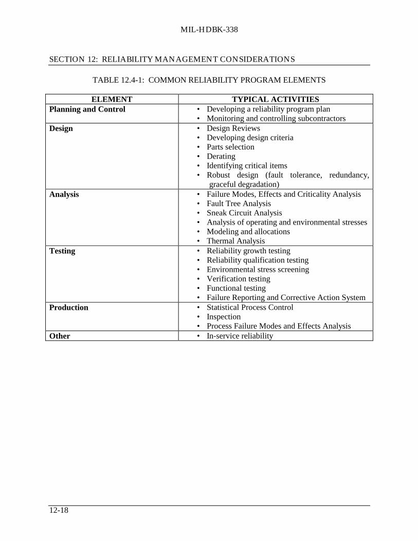
MIL-HDBK-338


12-18

TABLE 12.4-1: COMMON RELIABILITY PROGRAM ELEMENTS

ELEMENT TYPICAL ACTIVITIESPlanning and Control • Developing a reliability program plan

• Monitoring and controlling subcontractorsDesign • Design Reviews

• Developing design criteria• Parts selection• Derating• Identifying critical items• Robust design (fault tolerance, redundancy,

graceful degradation)Analysis • Failure Modes, Effects and Criticality Analysis

• Fault Tree Analysis• Sneak Circuit Analysis• Analysis of operating and environmental stresses• Modeling and allocations• Thermal Analysis

Testing • Reliability growth testing• Reliability qualification testing• Environmental stress screening• Verification testing• Functional testing• Failure Reporting and Corrective Action System

Production • Statistical Process Control• Inspection• Process Failure Modes and Effects Analysis

Other • In-service reliability

MIL-HDBK-338


12-19

12.5 Phasing of Reliability Program Activities

The previous section identified individual reliability program elements. The management,selection and control of activities within those elements must be based on recognition of thesystem’s life cycle. Appropriate reliability management and engineering tasks must beperformed during all life cycle phases.

The successful management of reliability during the system life cycle assumes the followingpremises:

(1) As defined by DoD Regulation 5000.2-R, there are four definable life cycleacquisition phases in the creation of any system, namely: Phase 0, ConceptExploration (CONCEPT); Phase I, Program Definition And Risk Reduction (DEF);Phase II, Engineering And Manufacturing Development (EMD); and Phase III,Production, Fielding/Deployment And Operational Support (PF/DOP). Each of thesephases are defined as follows:

(a) Concept Exploration Phase: is the period where feasibility ofalternative concepts are defined and evaluated and a basis for evaluatingthe relative merits of these alternatives at the next decision milestone areprovided.

(b) Program Definition and Risk Reduction Phase: is the period when one ormore candidate solutions are defined and design approaches andtechnologies are pursued as warranted. Risk reduction activities are alsoperformed including prototyping, demonstrations, and early operationalassessments.

(c) Engineering and Manufacturing Development Phase: is the period whenfor the most promising design approach, detailed design is developed,integration testing conducted, and a manufacturing capabilityestablished.

(d) Production, Fielding/Deployment and Operational Support Phase: is theperiod when systems are produced, operational tests and demonstrationsare conducted, additional support provided, and modifications areincorporated as needed.

(2) There is a special role for reliability in each of these phases. To achieve the goals inthe deployment phase requires planned actions in all previous phases. Each phase hasspecific objectives and the activities conducted during the phase must support theseobjectives. Milestone decision points mark the beginning and end of the acquisitionphases. The milestone decision points are:

MIL-HDBK-338


12-20

(a) Milestone 0 - Approval to Conduct Concept Studies (beginning of phase 0)

(b) Milestone I - Approval to Begin a New Acquisition Program (end of Phase 0,beginning of Phase I)

(c) Milestone II - Approval to Enter EMD (end of Phase I, beginning of Phase II)

(d) Milestone III - Production or Deployment Approval (end of Phase II, beginningof Phase III)

For some products, a phase may be “abbreviated” or even “skipped.” For example, the researchand development phase for a new product that is simply an updated or moderately improvedversion of an older, mature product will likely be very short, concentrating only on thedifferences between the two. Figure 12.5-1 shows the life cycle phases, milestone decisionpoints, the objectives of each phase, and a summary of the activities associated with each phase.

12.5.1 Reliability Activities by Life Cycle Phase

The reliability activities conducted during each of the life cycle phases of a product must beconsistent with and support the overall objectives for the phases. In the following discussion,reliability activities will be discussed in the context of the phase(s) in which they are mostapplicable. It is not practical to try and address all possible types of products, so the discussionassumes that a major product, such as an aircraft, tank, turbine engine, or similar item, is beingdeveloped. It should be obvious that the level of effort and types and scope of activities thatwould be necessary for a smaller system, such as a radar altimeter, will not be the same as for anew tactical fighter or other large system.

MIL-HDBK-338


12-21

FIGURE 12.5-1: LIFE CYCLE PHASES OF A PRODUCT

0Concept

Exploration

IProgram Definition and

Risk Reduction

IIEngineering andManufacturingDevelopment

IIIProduction,

Fielding/Deployment, andOperational Support

ACQUISITION PHASES

Objectives

Act

K ie vy i

ties

1. Define program asone or more concepts

2. Pursue designapproaches andparallel technologies

1. Produce andmanufacture theproduct

2. Deploy theproduct

3. Operate andmaintain the product

1. Validateassessment of need

2. Conduct conceptstudies

3. Develop productrequirements interms ofeffectiveness andperformancemeasures

1. Achieve designstability

2. Verify adequateresources have beenprogrammed forproduction,deployment, andsupport

3. Conduct InitialOperational Test andEvaluation (IOT&E)

ManufacturingUse of the productin the intendedenvironment,scheduled andunscheduledmaintenance,improvementsthrough updatesand modifications,performancetracking

1. Translate mostpromising designapproach into stable,producible, supportable,and cost effective design

2. Validatemanufacturing andproduction processes

3. Demonstrate productcapabilities throughtesting

1. Define andevaluate thefeasibility ofalternative conceptsto meet deficiencies

2. Provide the basisfor assessing relativemerits of alternativeconcepts at nextdecision milestone

1. Conductprototyping,demonstrations, andearly operationalassessments to reducerisk

2. Update productrequirements

3. Identifyaccomplishments to becompleted in Phase 2

Milestone 0Decision Point

Milestone IDecision Point

Milestone IIDecision Point

Milestone IIIDecision Point

MILESTONE DECISION POINTS

MIL-HDBK-338


12-22

12.5.1.1 Phase 0 - Concept Exploration

During the concept exploration phase, reliability activities are necessarily intended to prepare forPhase I. The reliability program plan begins with broadly stating the goals and objectives for thenew product. Some analysis may be made of prior similar products to help establish ranges ofrealistic reliability goals. Very general modeling may also be used to complement the analysis inderiving ranges of goals. Also, new approaches and technologies related to reliability design,analysis, and validation can be identified during this phase. It is important to remember that thereliability program plan should be developed as part of the overall systems engineering effort.The interrelationship (inputs, outputs, etc.) between reliability tasking and other program tasksmust be clearly stated and coordinated throughout the development life cycle.

The reliability activities to be considered in this phase are listed in Table 12.5-1. The specificactivities implemented will depend on the specific requirements of any individual program.Therefore, Table 12.5-1 should be viewed as a guide only, and does not necessarily represent any“typical” program.

TABLE 12.5-1: RELIABILITY PROGRAM ACTIVITIES TO BE CONSIDEREDIN THE CONCEPT EXPLORATION PHASE

Reliability Program PlanningReliability Trade-off StudiesParts and Materials ProgramsDesign ReviewsSupplier ControlLife Cycle PlanningCritical Item Control

Reliability Modeling and PreliminaryAllocations

Test StrategyBenchmarkingQuality Function DevelopmentMarket SurveyAnalysis of operational environment

12.5.1.2 Phase I - Program Definition and Risk Reduction

For the alternative concepts that are carried into this phase, the reliability effort becomes moreintense and focused and additional detail is added to the program plan. Additional analysis isrequired to begin refining requirements for the next phase of acquisition. Reliability engineersshould be participating in and supporting trade studies in which the various alternatives arecompared, different design approaches are evaluated, and overall system requirements areoptimized. Some program and design reviews are usually held during this phase, and the issue ofreliability must be considered during these reviews. The emphasis during these early reviewswill be to choose among the alternative concepts. Preliminary modeling, using high-levelreliability block diagrams of the various concepts for each design, may be needed. In addition,the reliability concept must be evaluated to ensure that the necessary and proper general designattributes are assigned to each product element. Data from whatever prototyping, proof-of-concept demonstrations, and similar “testing” is conducted should be analyzed and the results

MIL-HDBK-338


12-23

used in evaluating the relative reliability of each concept and in determining realistic reliabilitycharacteristics for the product. The reliability activities to be considered in this phase arepresented in Table 12.5-2.

TABLE 12.5-2. RELIABILITY PROGRAM ACTIVITIES TO BE CONSIDERED IN THEPROGRAM DEFINITION AND RISK REDUCTION PHASE

Reliability Program PlanningEnvironmental CharacterizationFault TolerancePart and Material ProgramReliability Modeling and AllocationsDurability AssessmentLife Cycle Planning

Reliability PredictionsThermal AnalysisUser Requirement TranslationBenchmarkingMarket SurveySoftware Reliability

The emphasis on each chosen activity in this phase is as a means to evaluate one designconcept/approach against a competing concept/approach. Information is still not as detailed asfollowing phases, but will have more input than previous phases. For instance, reliabilitypredictions may still be based on the parts count methods or on similar equipments/designs.Likewise, reliability modeling and allocations will be done at higher levels of abstraction. Inchoosing which specific tasks are to be performed, critical requirements or factors must beconsidered. If one approach favors more redundancy over another, for example, then a fault treeanalysis may be a task chosen as a means to evaluate the reliability impact of this approach. Ifinterfacing problems are a key issue, then some level of tolerance analysis may be warranted. Inall cases, the reliability program manager must work in conjunction with all other members ofthe systems engineering team to clearly define the key issues such that reliability tasking can bejudiciously and economically chosen. Further, close coordination with related functions such asmaintainability, logistics and quality is necessary to avoid duplication of effort and to optimizeresources.

12.5.1.3 Phase II - Engineering and Manufacturing Development

Usually only one concept is carried into Phase II. As indicated in Figure 12.5-1, the objectives ofthis phase are to:

(1) translate the most promising design approach into a stable, producible, supportable,and cost effective design

(2) validate the manufacturing and production processes to be implemented in Phase III

(3) demonstrate product capabilities through testing