Electronic Supplementary Material (ESI) for Lab on a Chip ... · This journal is The Royal Society of Chemistry 2011 Supplementary Information ... measured 0.28 mm (ID) and 0.61 mm

Electronic Supplementary Material (ESI) for Lab on a Chip

This journal is The Royal Society of Chemistry 2011

Supplementary Information

Fluidic low pass filter for hydrodynamic flow stabilization

in microfluidic environments

Yang Jun kang1 and Sung Yang*1,2,3

1 School of Mechatronics, Gwangju Institute of Science and Technology (GIST), Gwangju, Republic of Korea 2 Department of Nanobio Materials and Electronics, Institute of Science and Technology (GIST), Gwangju, Republic of Korea 3 Department of Medical System Engineering, Institute of Science and Technology (GIST), Gwangju, Republic of Korea

.

* Corresponding author E-mail: [email protected] Fax: +82-62-715-2384; Tel: +82-62-715-2407; E-mail:[email protected]

Electronic Supplementary Material (ESI) for Lab on a ChipThis journal is © The Royal Society of Chemistry 2012

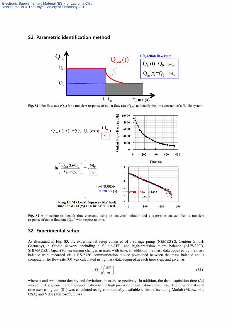
S1. Parametric identification method

Fig. S1 Inlet flow rate (Qin) for a transient response of outlet flow rate (Qout) to identify the time constant of a fluidic system.

Fig. S2 A procedure to identify time constants using an analytical solution and a regression analysis from a transient response of outlet flow rate (Qout) with respect to time.

S2. Experimental setup

As illustrated in Fig. S3, the experimental setup consisted of a syringe pump (NEMESYS, Centoni GmbH, Germany), a fluidic network including a fluidic-LPF, and high-precision micro balance (AUW220D, SHIMADZU, Japan) for measuring changes in mass with time. In addition, the mass data acquired by the mass balance were recorded via a RS-232C communication device positioned between the mass balance and a computer. The flow rate (Q) was calculated using mass data acquired at each time step, and given as

1 ΔmQ=

ρ Δt

(S1)

where and m denote density and deviations in mass, respectively. In addition, the data acquisition time (t) was set to 1 s, according to the specification of the high precision micro balance used here. The flow rate at each time step using eqn (S1) was calculated using commercially available software including Matlab (Mathworks, USA) and VBA (Microsoft, USA).


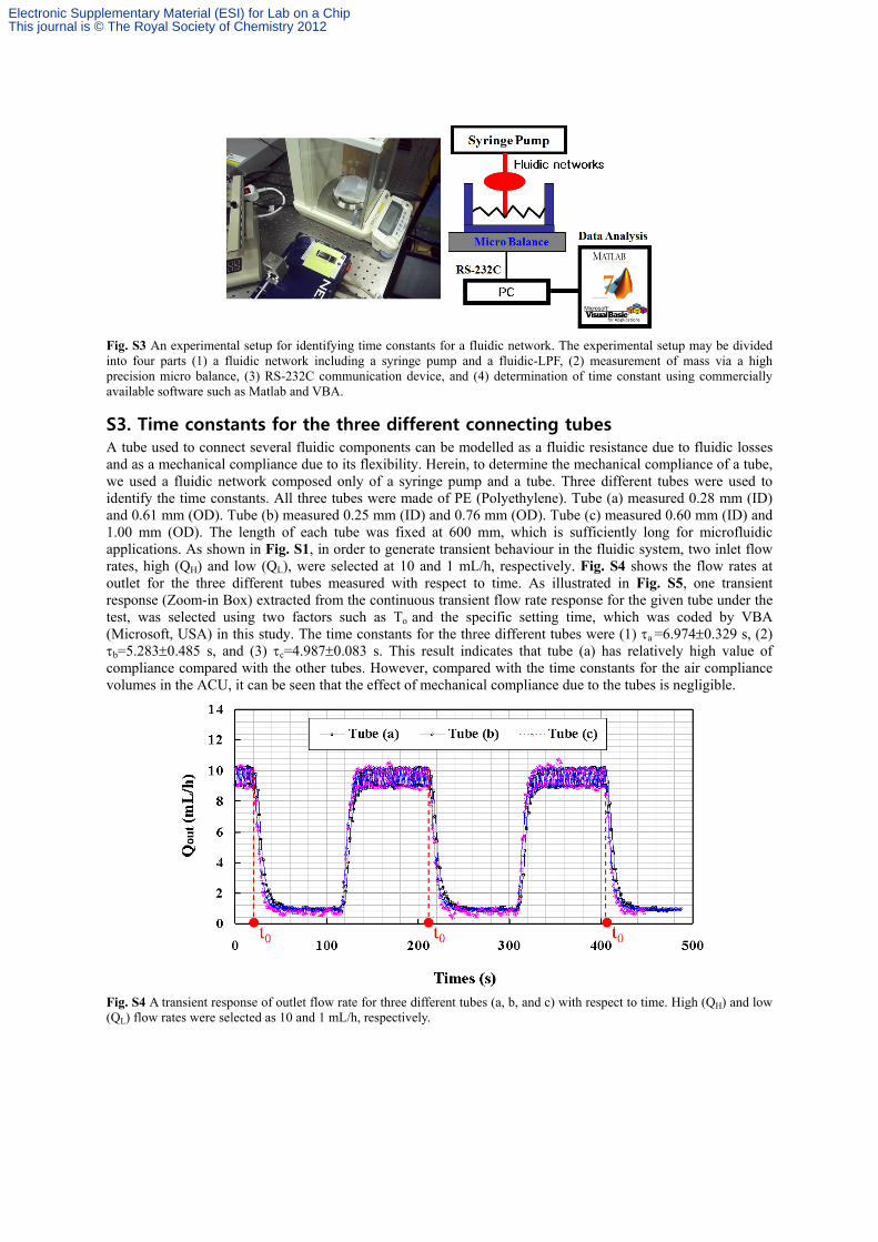
Fig. S3 An experimental setup for identifying time constants for a fluidic network. The experimental setup may be divided into four parts (1) a fluidic network including a syringe pump and a fluidic-LPF, (2) measurement of mass via a high precision micro balance, (3) RS-232C communication device, and (4) determination of time constant using commercially available software such as Matlab and VBA.

S3. Time constants for the three different connecting tubes A tube used to connect several fluidic components can be modelled as a fluidic resistance due to fluidic losses and as a mechanical compliance due to its flexibility. Herein, to determine the mechanical compliance of a tube, we used a fluidic network composed only of a syringe pump and a tube. Three different tubes were used to identify the time constants. All three tubes were made of PE (Polyethylene). Tube (a) measured 0.28 mm (ID) and 0.61 mm (OD). Tube (b) measured 0.25 mm (ID) and 0.76 mm (OD). Tube (c) measured 0.60 mm (ID) and 1.00 mm (OD). The length of each tube was fixed at 600 mm, which is sufficiently long for microfluidic applications. As shown in Fig. S1, in order to generate transient behaviour in the fluidic system, two inlet flow rates, high (QH) and low (QL), were selected at 10 and 1 mL/h, respectively. Fig. S4 shows the flow rates at outlet for the three different tubes measured with respect to time. As illustrated in Fig. S5, one transient response (Zoom-in Box) extracted from the continuous transient flow rate response for the given tube under the test, was selected using two factors such as To and the specific setting time, which was coded by VBA (Microsoft, USA) in this study. The time constants for the three different tubes were (1) a =6.9740.329 s, (2) b=5.2830.485 s, and (3) c=4.9870.083 s. This result indicates that tube (a) has relatively high value of compliance compared with the other tubes. However, compared with the time constants for the air compliance volumes in the ACU, it can be seen that the effect of mechanical compliance due to the tubes is negligible.

Fig. S4 A transient response of outlet flow rate for three different tubes (a, b, and c) with respect to time. High (QH) and low (QL) flow rates were selected as 10 and 1 mL/h, respectively.


Fig. S5 (A) A transient response of outlet flow rate for a tube. (B) A selected transient response of continuous outlet flow rates via To and the specific setting time.

S4. Pulsation Index

Fig. S6 A definition of pulsation index (PI) for quantifying fluctuations in flow by means of Qmax, Qmin, and Qave of flow rate at outlet.


S5. Curve fitting technique via LSM As previously discussed, the PI depends on average (Q) and alternating flow (Q) rates and the time constant. A curve fitting technique is required to obtain Q and Q from the outlet flow rates measured by experiment. Because the outlet flow rates can be approximated using a fundamental harmonic component, the flow rate may be expressed mathematically as

out 0 1 22π 2π

Q (t)=a +a cos t +a sin tT T

(S2)

The unknown variables (a0, a1, and a2) can be identified using the LSM (Least Squares Method). According to this method, the sum of the squares (E2) is

2m

2out n 0 1 n 2 n

n=1

2π 2πE = Q (t )-a -a cos t -a sin t

T T

(S3)

The minimum value of E2 is found by setting the gradient to zero with respect to a0, a1, and a2, respectively. This LSM gives a linear equation,

[A] x = b (S4)

The unknown parameters (a0, a1, and a2) can be expressed as a column vector,

0

1

2

a

x a

a

(S5)

. Additionally, [A] and {b} become

n nn=1 n=1 n=1

2n n n n

n=1 n=1 n=1

2n n n n

n=1 n=1 n=1

2π 2π1 cos t sin t

T T

2π 2π 2π 2πA = cos t cos t cos t sin t

T T T T

2π 2π 2π 2πsin t cos t sin t sin t

T T T T

(S6)

out nn=1

n out nn=1

n out nn=1

Q (t )

2πb = cos t Q (t )

T

2πsin t Q (t )

T

(S7)

The unknown variables (a0, a1, and a2) are identified by solving a linear equation as eqn (S3), and are given as

0

-11

2

a

a = A b

a

x

(S8)

This curve fitting calculation was coded using VBA (Microsoft, USA) as shown in Fig. S7. The program contained two parts. In the first part we selected some parts of all the data, and in the second we calculated the


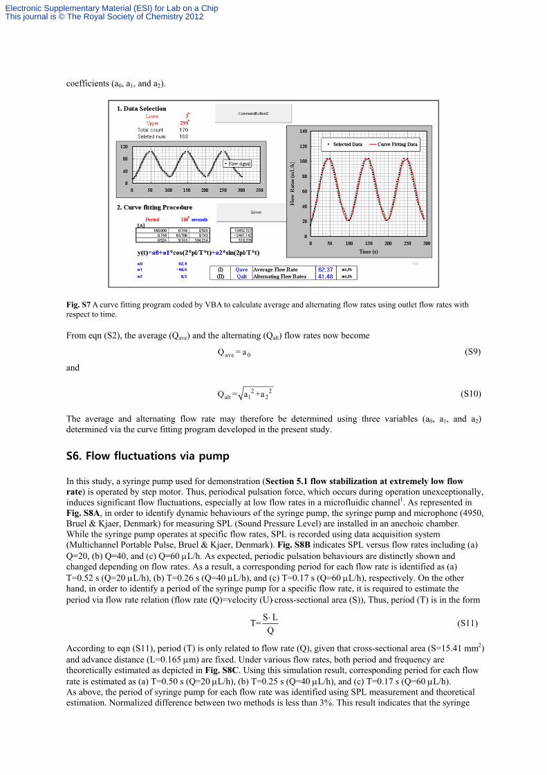
coefficients (a0, a1, and a2).

Fig. S7 A curve fitting program coded by VBA to calculate average and alternating flow rates using outlet flow rates with respect to time.

From eqn (S2), the average (Qave) and the alternating (Qalt) flow rates now become

ave 0Q = a (S9)

and

2 2alt 1 2Q = a +a (S10)

The average and alternating flow rate may therefore be determined using three variables (a0, a1, and a2) determined via the curve fitting program developed in the present study.

S6. Flow fluctuations via pump

In this study, a syringe pump used for demonstration (Section 5.1 flow stabilization at extremely low flow rate) is operated by step motor. Thus, periodical pulsation force, which occurs during operation unexceptionally, induces significant flow fluctuations, especially at low flow rates in a microfluidic channel1. As represented in Fig. S8A, in order to identify dynamic behaviours of the syringe pump, the syringe pump and microphone (4950, Bruel & Kjaer, Denmark) for measuring SPL (Sound Pressure Level) are installed in an anechoic chamber. While the syringe pump operates at specific flow rates, SPL is recorded using data acquisition system (Multichannel Portable Pulse, Bruel & Kjaer, Denmark). Fig. S8B indicates SPL versus flow rates including (a) Q=20, (b) Q=40, and (c) Q=60 L/h. As expected, periodic pulsation behaviours are distinctly shown and changed depending on flow rates. As a result, a corresponding period for each flow rate is identified as (a) T=0.52 s (Q=20 L/h), (b) T=0.26 s (Q=40 L/h), and (c) T=0.17 s (Q=60 L/h), respectively. On the other hand, in order to identify a period of the syringe pump for a specific flow rate, it is required to estimate the period via flow rate relation (flow rate (Q)=velocity (U)cross-sectional area (S)), Thus, period (T) is in the form

S LT=

Q

(S11)

According to eqn (S11), period (T) is only related to flow rate (Q), given that cross-sectional area (S=15.41 mm2) and advance distance (L=0.165 m) are fixed. Under various flow rates, both period and frequency are theoretically estimated as depicted in Fig. S8C. Using this simulation result, corresponding period for each flow rate is estimated as (a) T=0.50 s (Q=20 L/h), (b) T=0.25 s (Q=40 L/h), and (c) T=0.17 s (Q=60 L/h). As above, the period of syringe pump for each flow rate was identified using SPL measurement and theoretical estimation. Normalized difference between two methods is less than 3%. This result indicates that the syringe


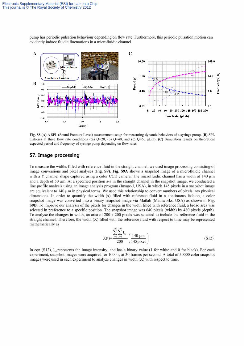
pump has periodic pulsation behaviour depending on flow rate. Furthermore, this periodic pulsation motion can evidently induce fluidic fluctuations in a microfluidic channel.

Fig. S8 (A) A SPL (Sound Pressure Level) measurement setup for measuring dynamic behaviors of a syringe pump. (B) SPL histories at three flow rate conditions ((a) Q=20, (b) Q=40, and (c) Q=60 L/h). (C) Simulation results on theoretical expected period and frequency of syringe pump depending on flow rates.

S7. Image processing

To measure the widths filled with reference fluid in the straight channel, we used image processing consisting of image conversions and pixel analyses (Fig. S9). Fig. S9A shows a snapshot image of a microfluidic channel with a Y channel shape captured using a color CCD camera. The microfluidic channel has a width of 140 m and a depth of 50 m. At a specified position a-a in the straight channel in the snapshot image, we conducted a line profile analysis using an image analysis program (Image-J, USA), in which 145 pixels in a snapshot image are equivalent to 140 m in physical terms. We used this relationship to convert numbers of pixels into physical dimensions. In order to quantify the width (x) filled with reference fluid in a continuous fashion, a color snapshot image was converted into a binary snapshot image via Matlab (Mathworks, USA) as shown in Fig. S9B. To improve our analysis of the pixels for changes in the width filled with reference fluid, a broad area was selected in preference to a specific position. The snapshot image was 640 pixels (width) by 480 pixels (depth). To analyse the changes in width, an area of 200 x 200 pixels was selected to include the reference fluid in the straight channel. Therefore, the width (X) filled with the reference fluid with respect to time may be represented mathematically as

200 200

i,ji=1 j=1

I140 μm

X(t)=200 145pixel

(S12)

In eqn (S12), Ii,j represents the image intensity, and has a binary value (1 for white and 0 for black). For each experiment, snapshot images were acquired for 1000 s, at 30 frames per second. A total of 30000 color snapshot images were used in each experiment to analyze changes in width (X) with respect to time.


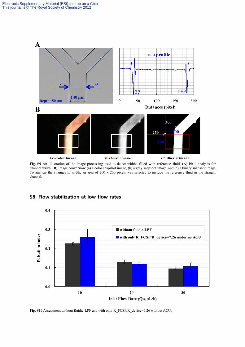
Fig. S9 An illustration of the image processing used to detect widths filled with reference fluid. (A) Pixel analysis for channel width. (B) Image conversion: (a) a color snapshot image, (b) a gray snapshot image, and (c) a binary snapshot image. To analyze the changes in width, an area of 200 x 200 pixels was selected to include the reference fluid in the straight channel.

S8. Flow stabilization at low flow rates

Fig. S10 Assessment without fluidic-LPF and with only R_FCSP/R_device=7.26 without ACU.

0.0

0.1

0.2

0.3

0.4

10 20 30

Inlet Flow Rate (Qin, μL/h)

Pu

lsat

ion

In

dex

without fluidic-LPF

with only R_FCSP/R_device=7.26 under no ACU


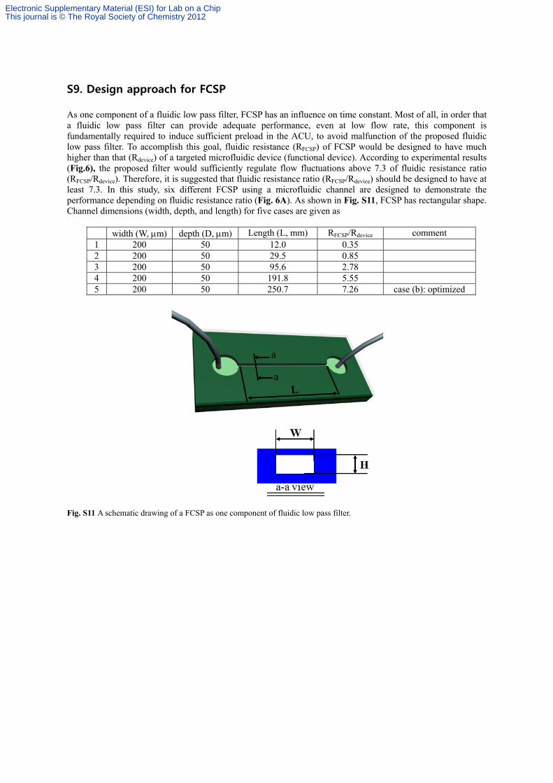
S9. Design approach for FCSP

As one component of a fluidic low pass filter, FCSP has an influence on time constant. Most of all, in order that a fluidic low pass filter can provide adequate performance, even at low flow rate, this component is fundamentally required to induce sufficient preload in the ACU, to avoid malfunction of the proposed fluidic low pass filter. To accomplish this goal, fluidic resistance (RFCSP) of FCSP would be designed to have much higher than that (Rdevice) of a targeted microfluidic device (functional device). According to experimental results (Fig.6), the proposed filter would sufficiently regulate flow fluctuations above 7.3 of fluidic resistance ratio (RFCSP/Rdevice). Therefore, it is suggested that fluidic resistance ratio (RFCSP/Rdevice) should be designed to have at least 7.3. In this study, six different FCSP using a microfluidic channel are designed to demonstrate the performance depending on fluidic resistance ratio (Fig. 6A). As shown in Fig. S11, FCSP has rectangular shape. Channel dimensions (width, depth, and length) for five cases are given as

width (W, m) depth (D, m) Length (L, mm) RFCSP/Rdevice comment 1 200 50 12.0 0.35 2 200 50 29.5 0.85 3 200 50 95.6 2.78 4 200 50 191.8 5.55 5 200 50 250.7 7.26 case (b): optimized

Fig. S11 A schematic drawing of a FCSP as one component of fluidic low pass filter.


Documents

Electronic Supplementary Material (ESI) for Lab on a Chip ... · This journal is The Royal Society of Chemistry 2011 Supplementary Information ... measured 0.28 mm (ID) and 0.61 mm