Embed Size (px)
Citation preview
Elementary Statistics
Larson Farber
5 Normal Probability Distributions
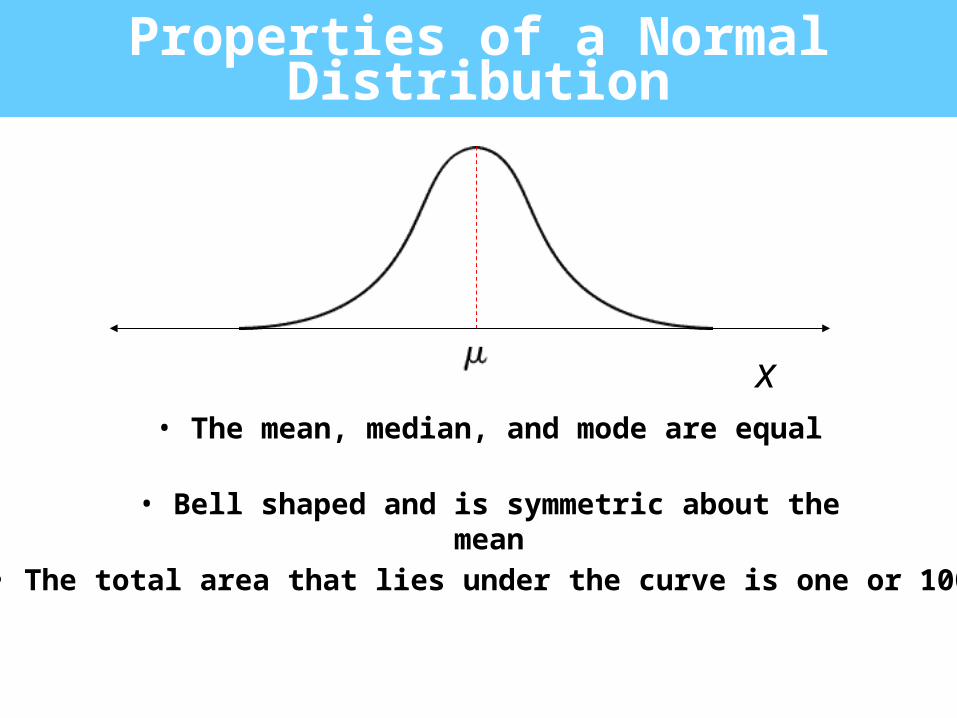
Properties of a Normal Distribution
• The mean, median, and mode are equal
• Bell shaped and is symmetric about the mean
• The total area that lies under the curve is one or 100%
x
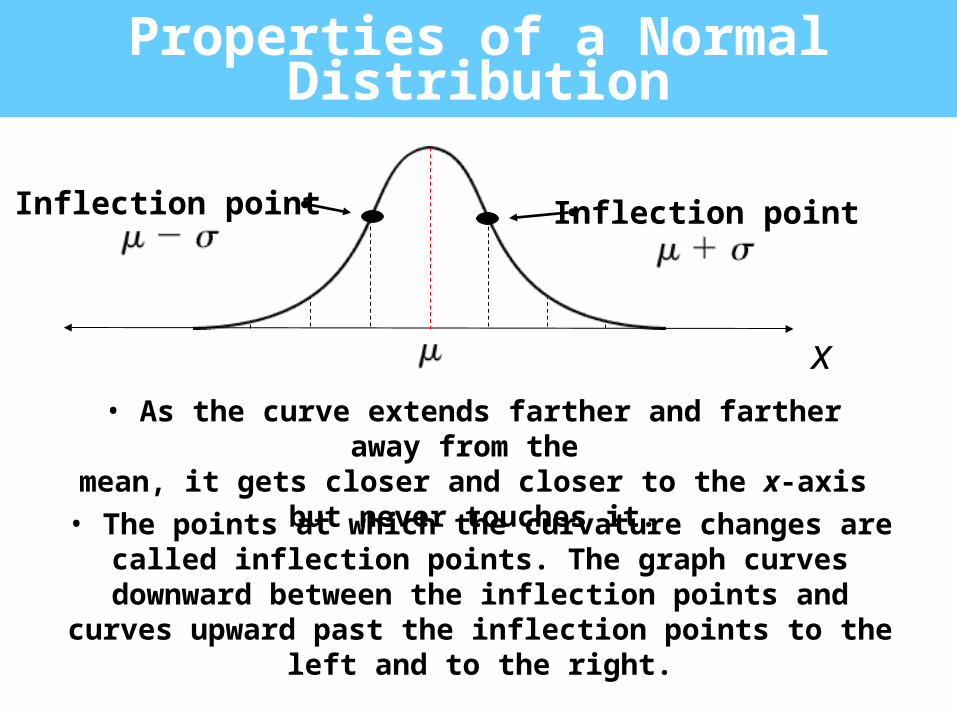
• As the curve extends farther and farther away from the mean, it gets closer and closer to the x-axis but never
touches it.
• The points at which the curvature changes are called inflection points. The graph curves downward between the
inflection points and curves upward past the inflection points to the left and to the right.
x
Inflection pointInflection point
Properties of a Normal Distribution
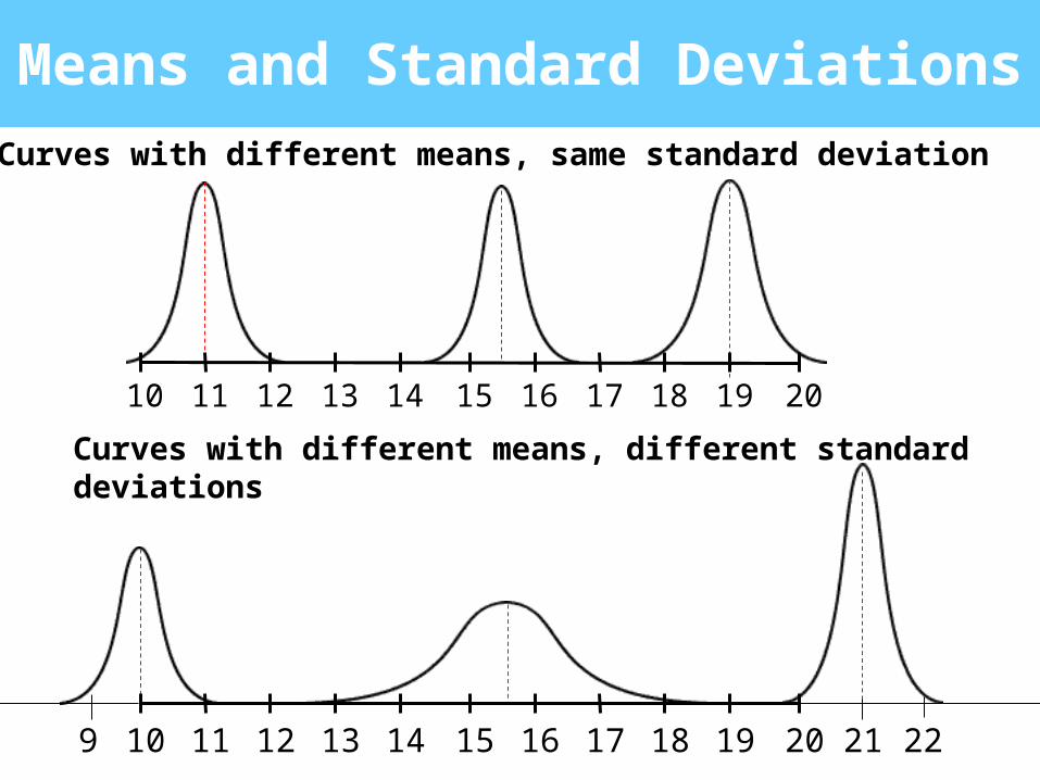
Means and Standard Deviations
2012 15 1810 11 13 14 16 17 19 21 229
12 15 1810 11 13 14 16 17 19 20
Curves with different means, different standard deviations
Curves with different means, same standard deviation
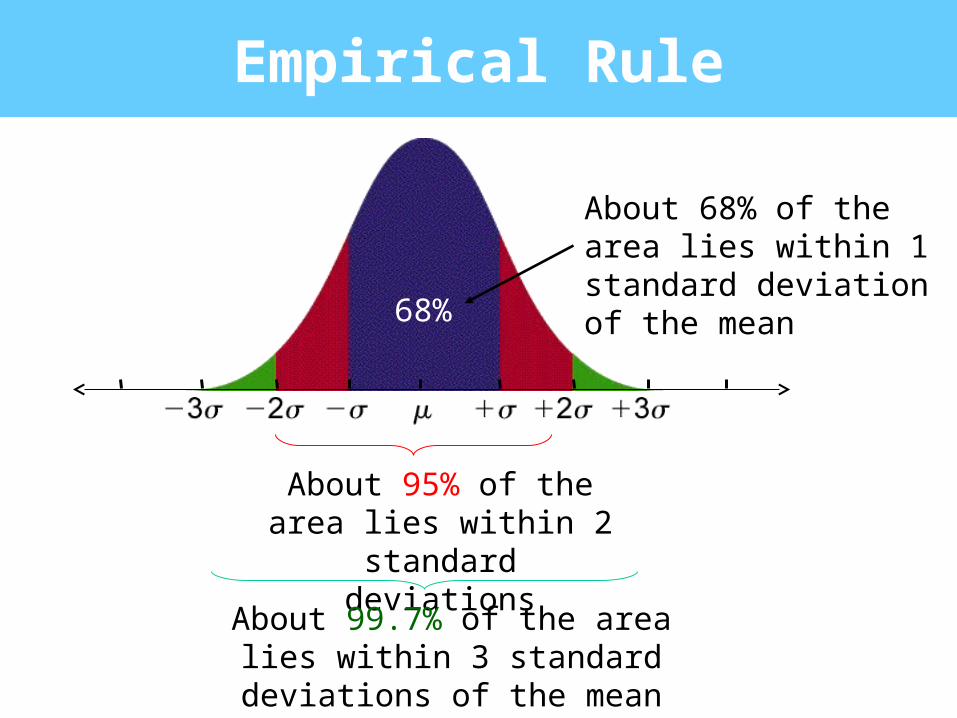
Empirical Rule
About 95% of the area lies within 2 standard
deviations
About 99.7% of the area lies within 3 standard deviations of the mean
About 68% of the area lies within 1 standard deviation of the mean
68%
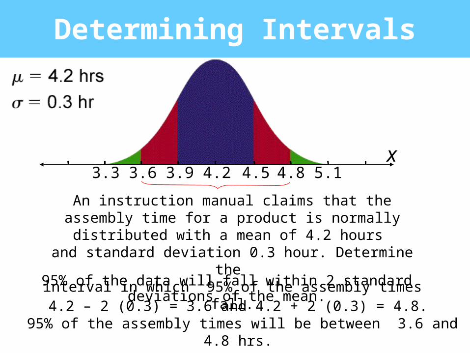
4.2 4.5 4.8 5.13.93.63.3
Determining Intervals
An instruction manual claims that the assembly time for a product is normally distributed with a mean of 4.2 hours
and standard deviation 0.3 hour. Determine the interval in which 95% of the assembly times fall.
x
4.2 – 2 (0.3) = 3.6 and 4.2 + 2 (0.3) = 4.8. 95% of the assembly times will be between 3.6 and 4.8 hrs.
95% of the data will fall within 2 standard deviations of the mean.
The Standard Normal
Distribution
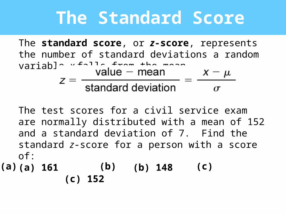
The Standard ScoreThe standard score, or z-score, represents the number of standard deviations a random variable x falls from the mean.
The test scores for a civil service exam are normally distributed with a mean of 152 and a standard deviation of 7. Find the standard z-score for a person with a score of:(a) 161 (b) 148 (c) 152
(a) (b) (c)
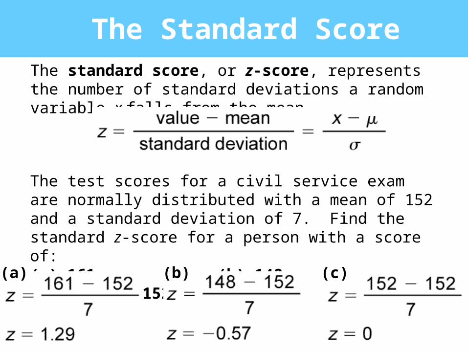
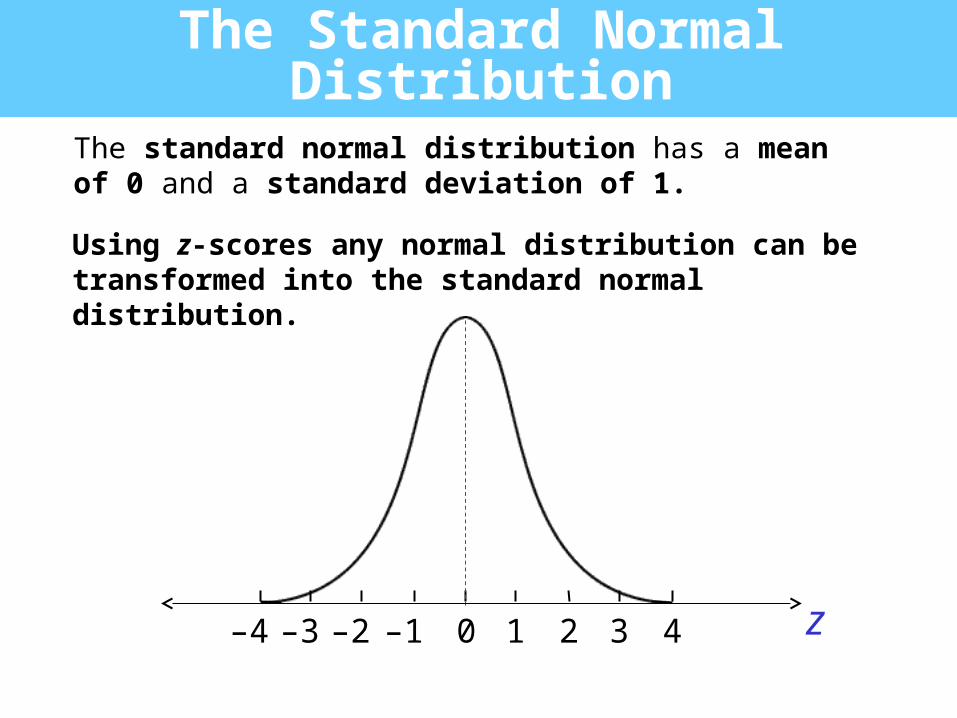
The Standard Normal Distribution
The standard normal distribution has a mean of 0 and a standard deviation of 1.
Using z-scores any normal distribution can be transformed into the standard normal distribution.
–4 –3 –2 –1 0 1 2 3 4 z
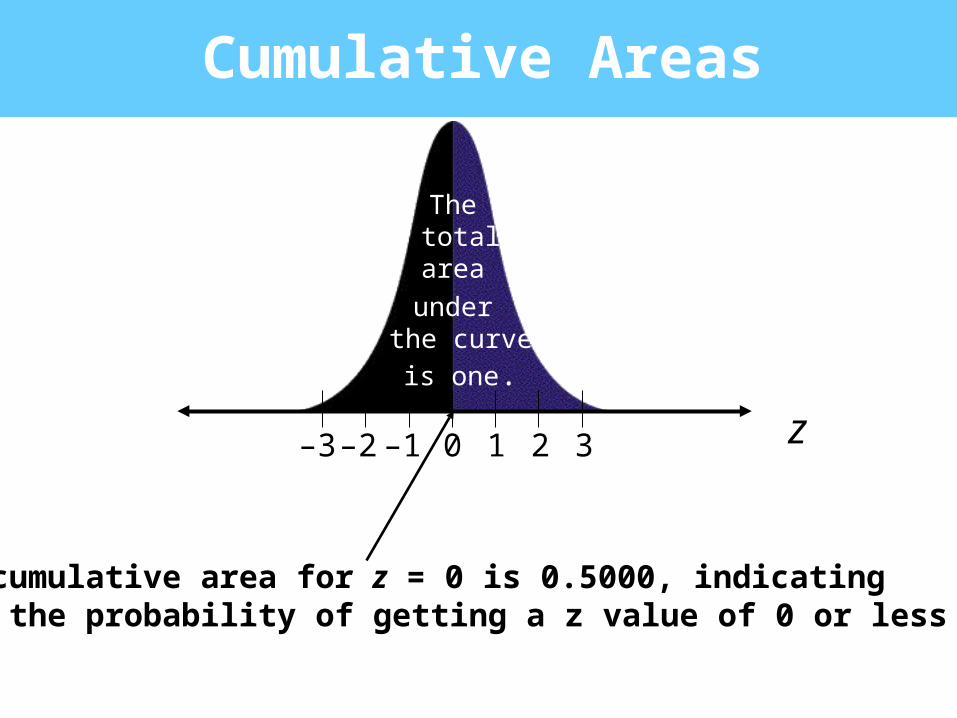
Cumulative Areas
0 1 2 3–1–2–3 z
The total area
under the curve
is one.
The cumulative area for z = 0 is 0.5000, indicating that the probability of getting a z value of 0 or less is .5
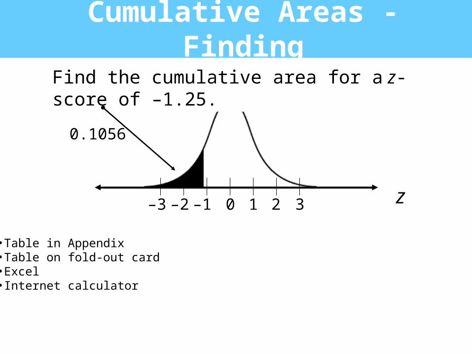
Find the cumulative area for a z-score of –1.25.
0 1 2 3–1–2–3 z
Cumulative Areas - Finding
0.1056
•Table in Appendix•Table on fold-out card•Excel•Internet calculator
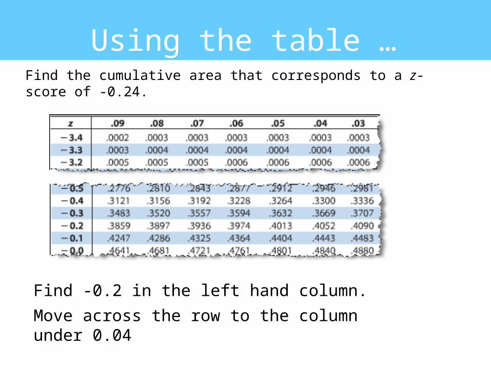
Using the table …Find the cumulative area that corresponds to a z-score of -0.24.
Solution:Find -0.2 in the left hand column.
Move across the row to the column under 0.04
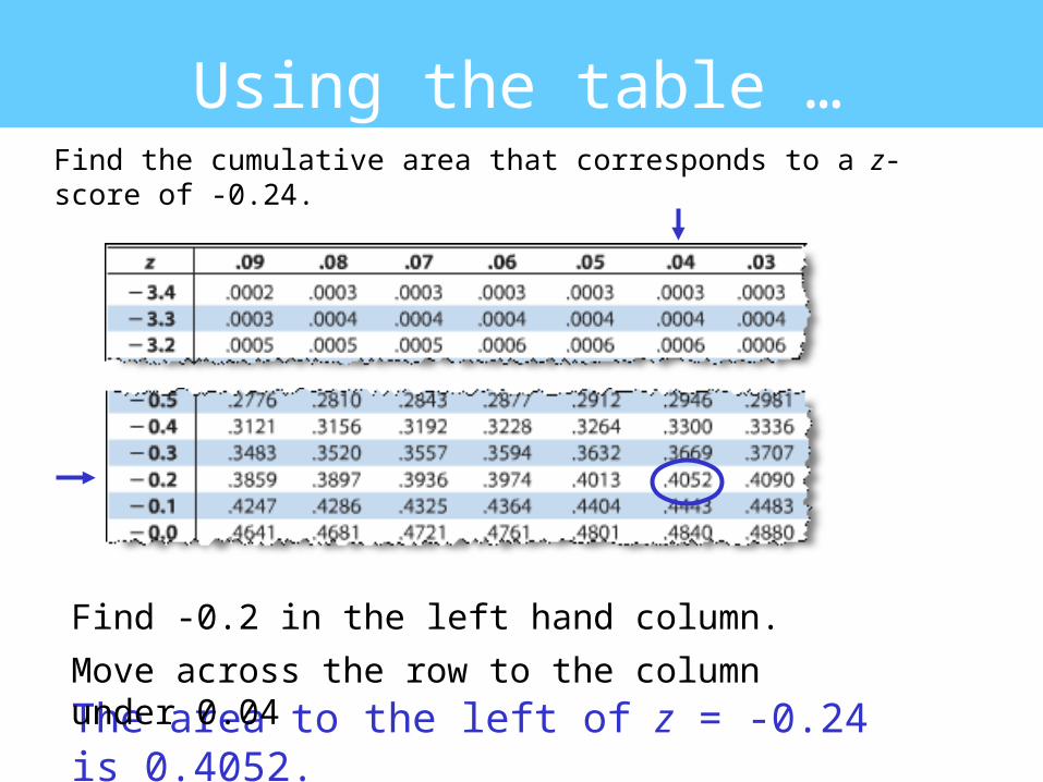
Using the table …Find the cumulative area that corresponds to a z-score of -0.24.
Solution:Find -0.2 in the left hand column.
The area to the left of z = -0.24 is 0.4052.Move across the row to the column under 0.04
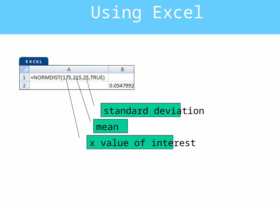
Using Excel
x value of interest
mean
standard deviation
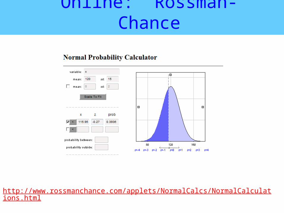
Online: Rossman-Chance
http://www.rossmanchance.com/applets/NormalCalcs/NormalCalculations.html
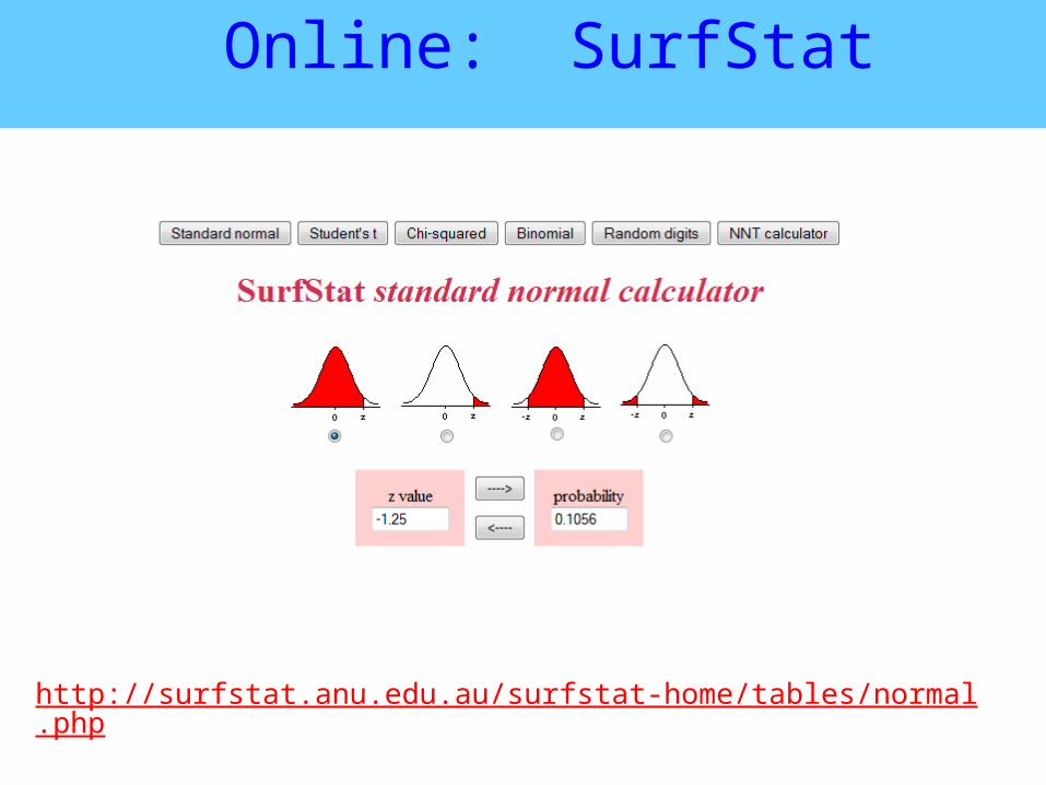
Online: SurfStat
http://surfstat.anu.edu.au/surfstat-home/tables/normal.php
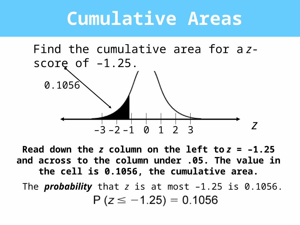
Find the cumulative area for a z-score of –1.25.
0 1 2 3–1–2–3 z
Cumulative Areas
0.1056
Read down the z column on the left to z = –1.25 and across to the column under .05. The value in the cell is 0.1056, the
cumulative area.
The probability that z is at most –1.25 is 0.1056.
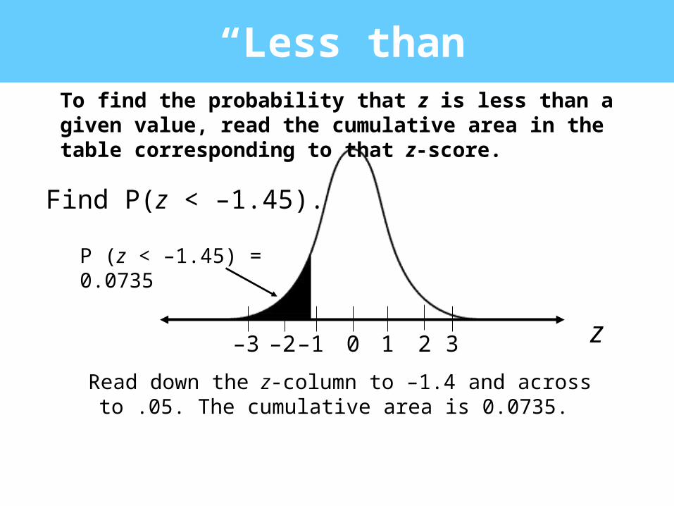
“Less than”To find the probability that z is less than a given value, read the cumulative area in the table corresponding to that z-score.
0 1 2 3–1–2–3 z
Read down the z-column to –1.4 and across to .05. The cumulative area is 0.0735.
Find P(z < –1.45).
P (z < –1.45) = 0.0735
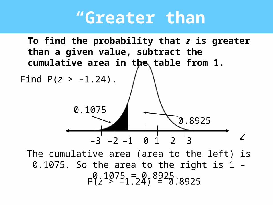
“Greater than”To find the probability that z is greater than a given value, subtract the cumulative area in the table from 1.
0 1 2 3–1–2–3 z
P(z > –1.24) = 0.8925
Find P(z > –1.24).
The cumulative area (area to the left) is 0.1075. So the area to the right is 1 – 0.1075 = 0.8925.
0.10750.8925
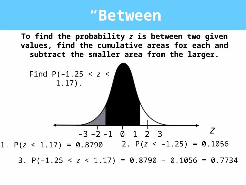
“Between”To find the probability z is between two given values, find the cumulative areas for each and subtract the smaller area from
the larger.
Find P(–1.25 < z < 1.17).
1. P(z < 1.17) = 0.8790 2. P(z < –1.25) = 0.1056
3. P(–1.25 < z < 1.17) = 0.8790 – 0.1056 = 0.7734
0 1 2 3–1–2–3 z
0 1 2 3-1 -2-3 z
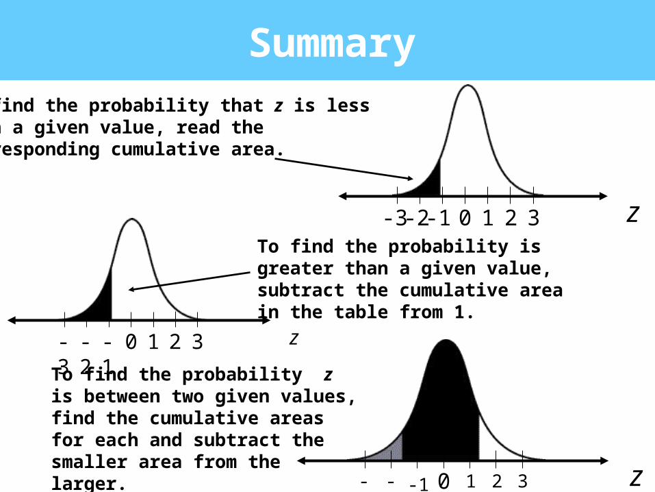
Summary
0 1 2 3-1-2-3 zTo find the probability is greater than a given value, subtract the cumulative area in the table from 1.
0 1 2 3-1-2-3 z
To find the probability z is between two given values, find the cumulative areas for each and subtract the smaller area from the larger.
To find the probability that z is lessthan a given value, read thecorresponding cumulative area.
Normal Distributions
Finding Probabilities
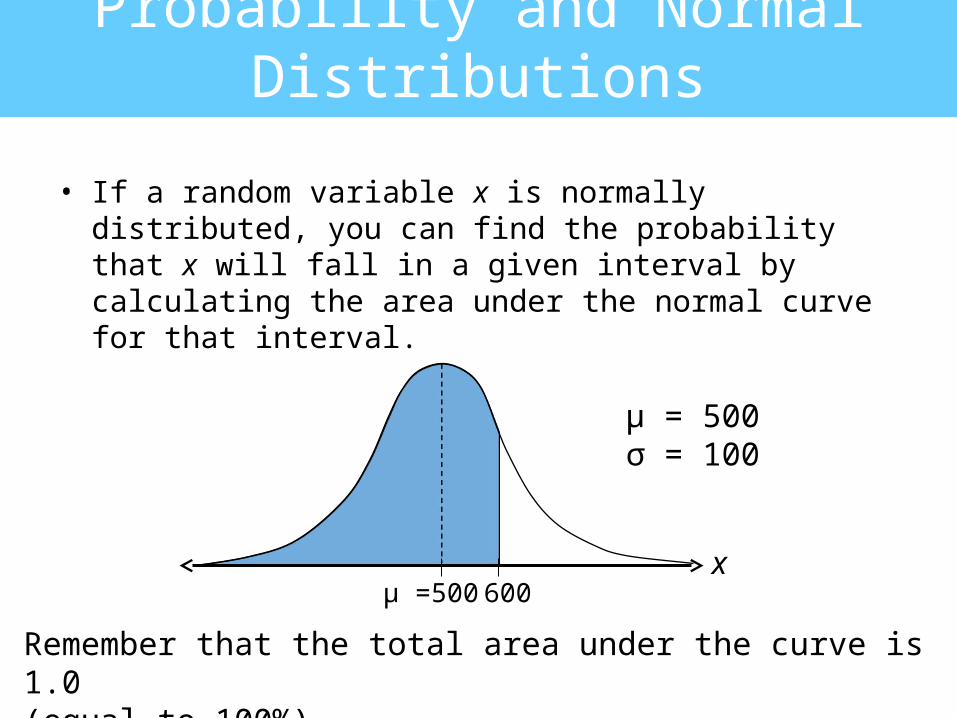
Probability and Normal Distributions
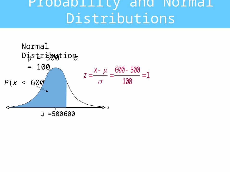
• If a random variable x is normally distributed, you can find the probability that x will fall in a given interval by calculating the area under the normal curve for that interval.
μ = 500σ = 100
600μ =500x
Remember that the total area under the curve is 1.0 (equal to 100%).
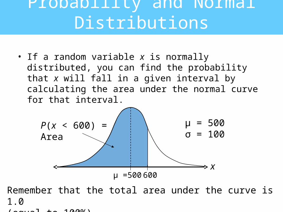
Probability and Normal Distributions
• If a random variable x is normally distributed, you can find the probability that x will fall in a given interval by calculating the area under the normal curve for that interval.
P(x < 600) = Area μ = 500σ = 100
600μ =500x
Remember that the total area under the curve is 1.0 (equal to 100%).
Probability and Normal Distributions
Normal Distribution
600μ =500
P(x < 600)
μ = 500 σ = 100
x
600 5001
100
xz
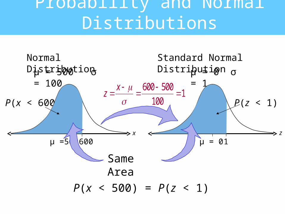
Probability and Normal Distributions
P(x < 500) = P(z < 1)
Normal Distribution
600μ =500
P(x < 600)
μ = 500 σ = 100
x
Standard Normal Distribution
600 5001
100
xz
1μ = 0
μ = 0 σ = 1
z
P(z < 1)
Same Area
Example
A survey indicates that people use their computers an average of 2.4 years before upgrading to a new machine. The standard deviation is 0.5 year. A computer owner is selected at random. Find the probability that he or she will use it for fewer than 2 years before upgrading. Assume that the variable x is normally distributed.
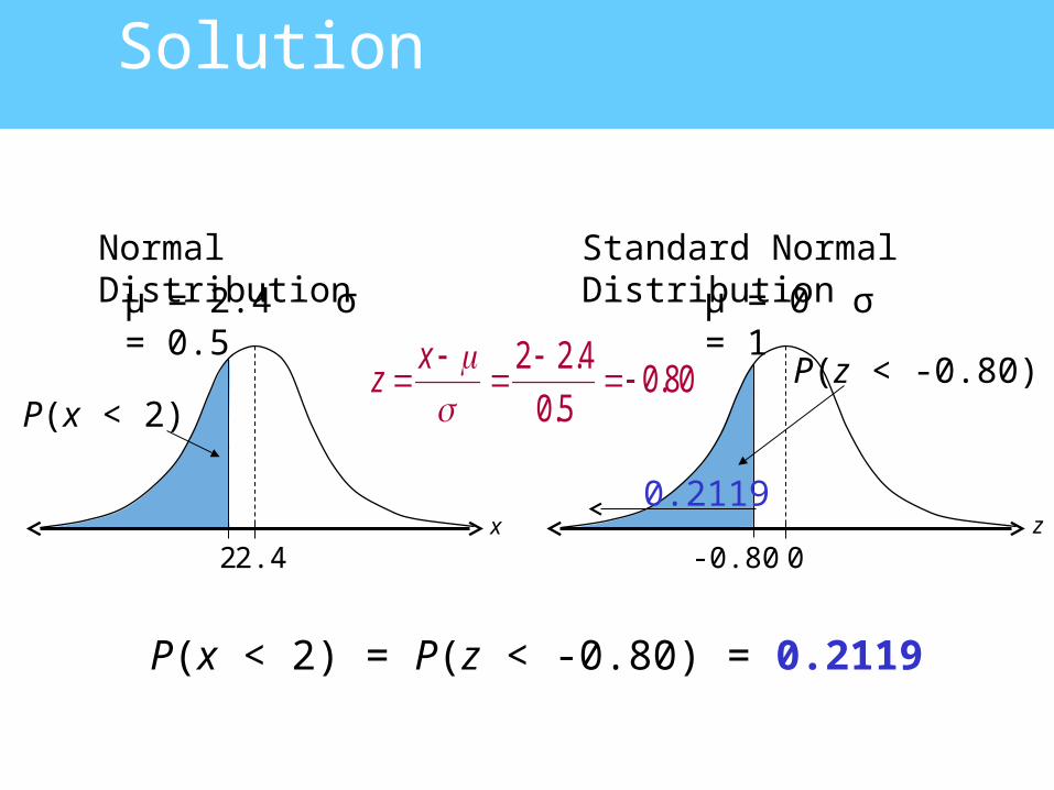
Solution
P(x < 2) = P(z < -0.80) = 0.2119
Normal Distribution
2 2.4
P(x < 2)
μ = 2.4 σ = 0.5
x
2 2.40.80
0.5
xz
Standard Normal Distribution
-0.80 0
μ = 0 σ = 1
z
P(z < -0.80)
0.2119
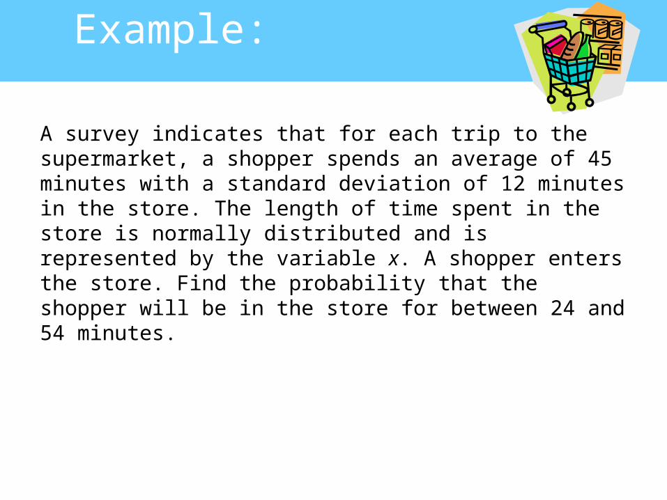
Example:
A survey indicates that for each trip to the supermarket, a shopper spends an average of 45 minutes with a standard deviation of 12 minutes in the store. The length of time spent in the store is normally distributed and is represented by the variable x. A shopper enters the store. Find the probability that the shopper will be in the store for between 24 and 54 minutes.
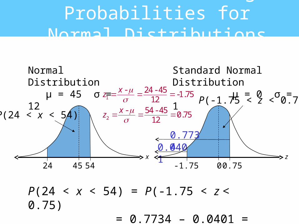
Solution: Finding Probabilities for Normal Distributions
P(24 < x < 54) = P(-1.75 < z < 0.75) = 0.7734 – 0.0401 = 0.7333
1
24 45 1 7512
xz - - - .
24 45
P(24 < x < 54)
x
Normal Distribution μ = 45 σ = 12
0.0401
54
2
54 45 0 7512
xz - - .
-1.75z
Standard Normal Distribution μ = 0 σ = 1
0
P(-1.75 < z < 0.75)
0.75
0.7734
Example:
Find the probability that the shopper will be in the store more than 39 minutes. (Recall μ = 45 minutes and σ = 12 minutes)
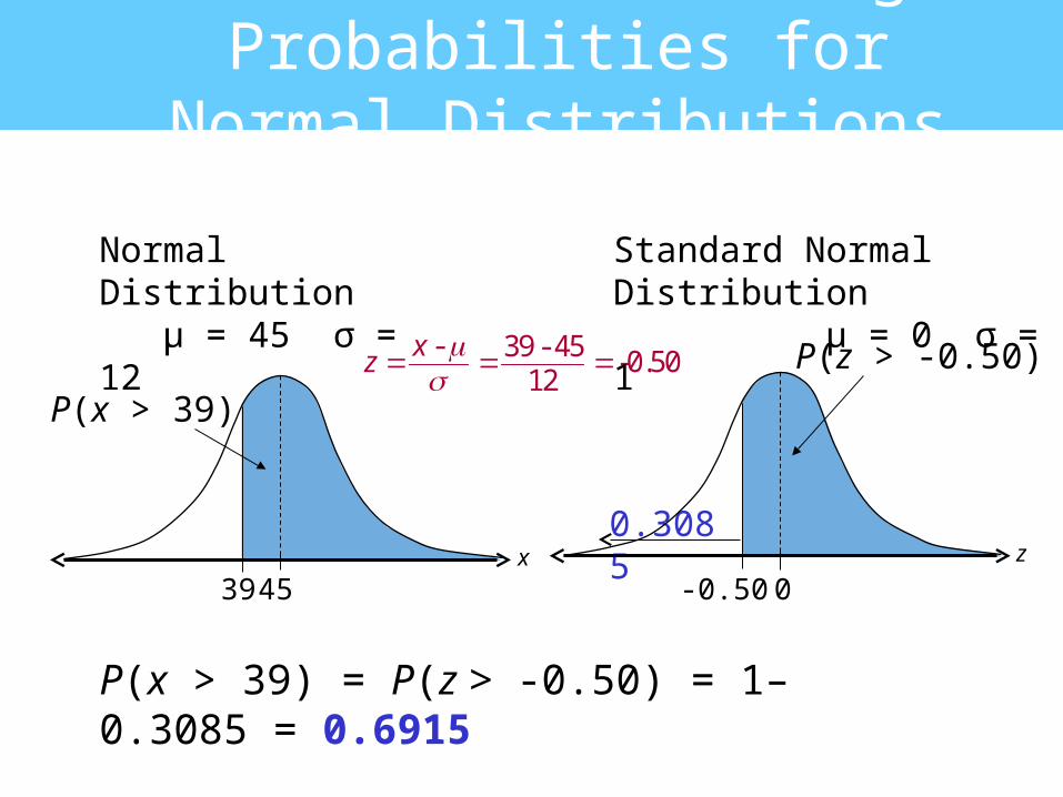
Solution: Finding Probabilities for Normal Distributions
P(x > 39) = P(z > -0.50) = 1– 0.3085 = 0.6915
39 45 0 5012
- - - .xz
39 45
P(x > 39)
x
Normal Distribution μ = 45 σ = 12
Standard Normal Distribution μ = 0 σ = 1
0.3085
0
P(z > -0.50)
z
-0.50
Normal Distributions
Finding Values
Section 5.4
z
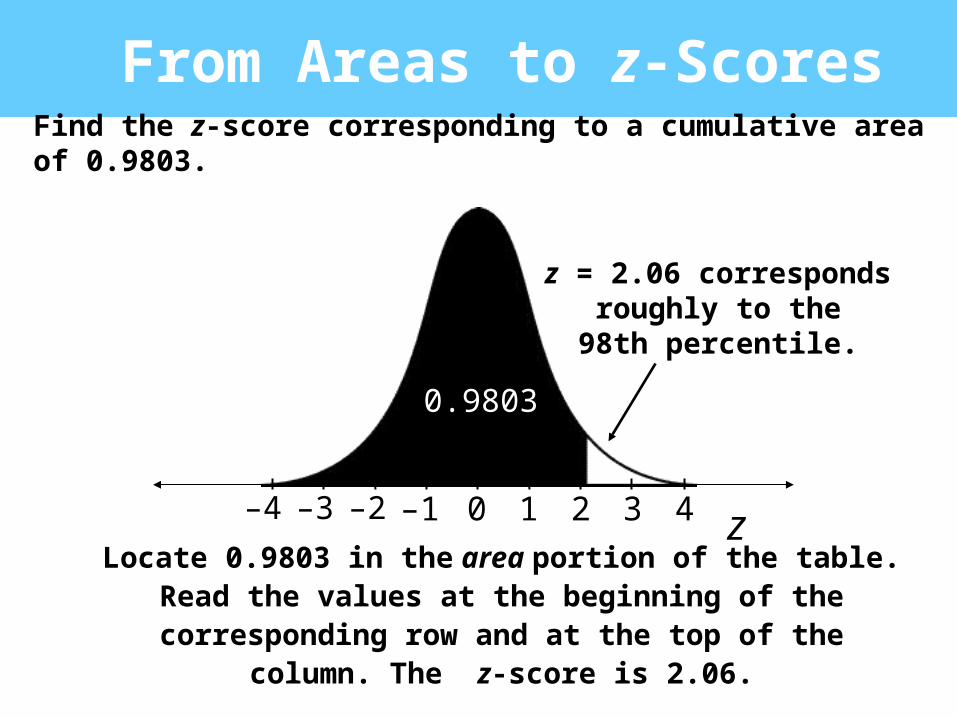
From Areas to z-Scores
Locate 0.9803 in the area portion of the table. Read the values at the beginning of the corresponding row and at
the top of the column. The z-score is 2.06.
Find the z-score corresponding to a cumulative area of 0.9803.
z = 2.06 correspondsroughly to the
98th percentile.
–4 –3 –2 –1 0 1 2 3 4
0.9803
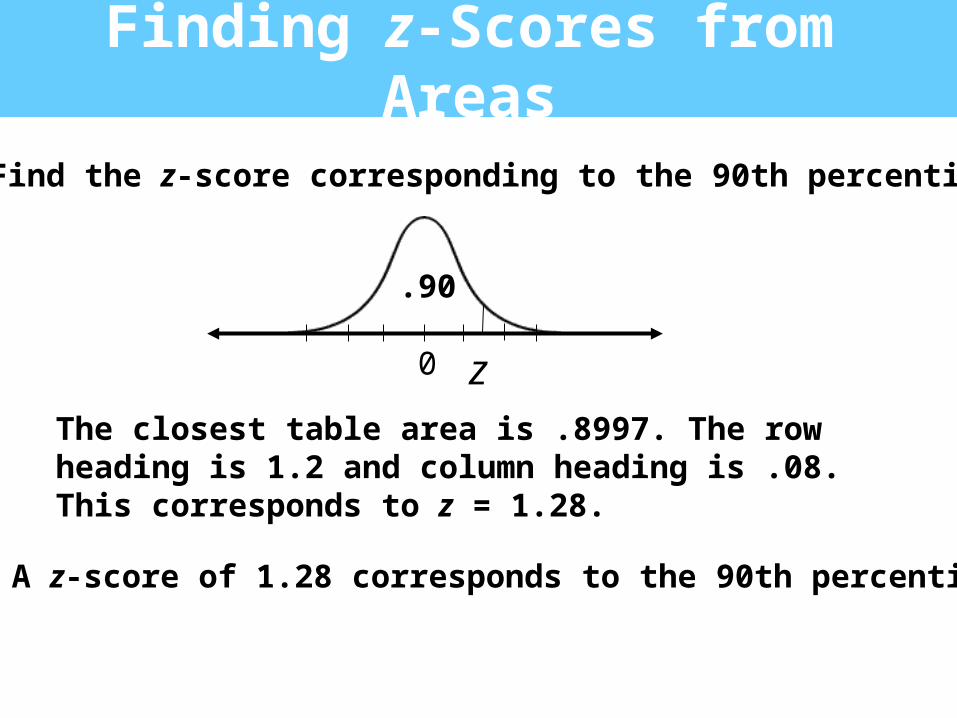
Finding z-Scores from Areas
Find the z-score corresponding to the 90th percentile.
z0
.90
The closest table area is .8997. The row heading is 1.2 and column heading is .08. This corresponds to z = 1.28.
A z-score of 1.28 corresponds to the 90th percentile.
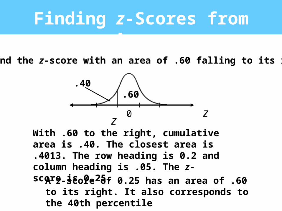
Find the z-score with an area of .60 falling to its right.
.60.40
0 zz
With .60 to the right, cumulative area is .40. The closest area is .4013. The row heading is 0.2 and column heading is .05. The z-score is 0.25.
A z-score of 0.25 has an area of .60 to its right. It also corresponds to the 40th percentile
Finding z-Scores from Areas
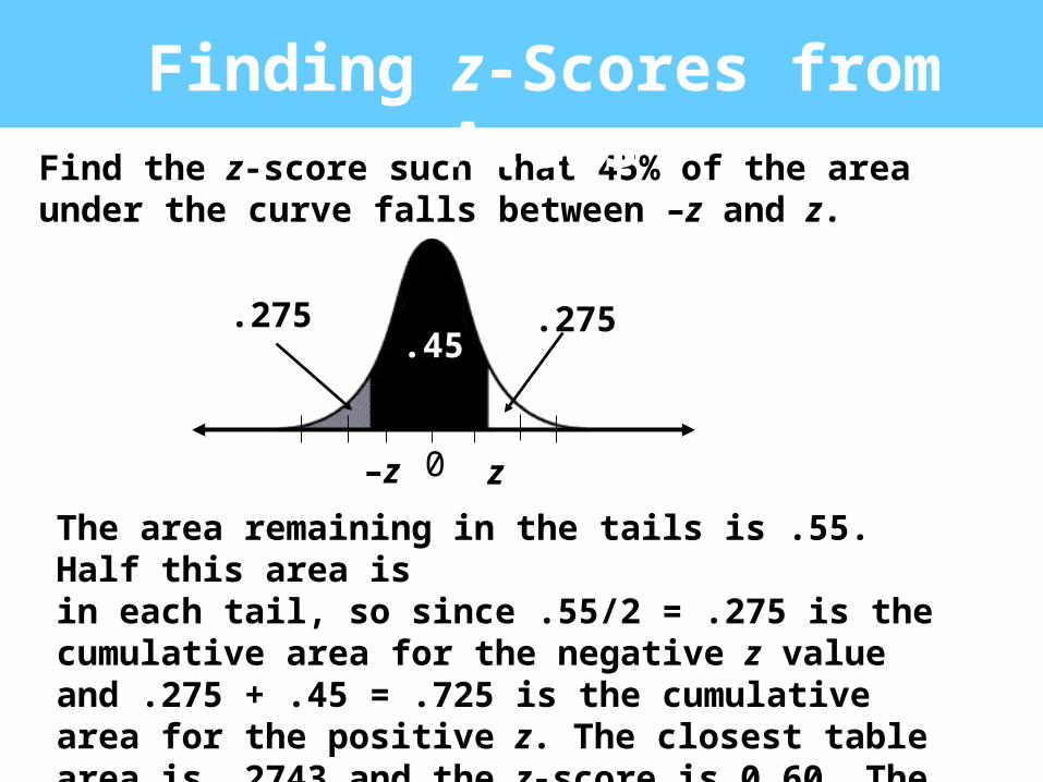
Find the z-score such that 45% of the area under the curve falls between –z and z.
0 z–z
The area remaining in the tails is .55. Half this area isin each tail, so since .55/2 = .275 is the cumulative area for the negative z value and .275 + .45 = .725 is the cumulative area for the positive z. The closest table area is .2743 and the z-score is 0.60. The positive z score is 0.60.
.45.275.275
Finding z-Scores from Areas
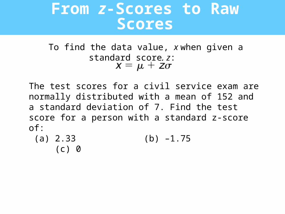
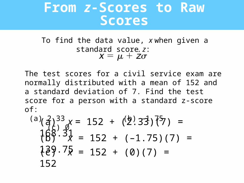
From z-Scores to Raw Scores
The test scores for a civil service exam are normally distributed with a mean of 152 and a standard deviation of 7. Find the test score for a person with a standard z-score of: (a) 2.33 (b) –1.75 (c) 0
To find the data value, x when given a standard score, z:
From z-Scores to Raw Scores
The test scores for a civil service exam are normally distributed with a mean of 152 and a standard deviation of 7. Find the test score for a person with a standard z-score of: (a) 2.33 (b) –1.75 (c) 0
(a) x = 152 + (2.33)(7) = 168.31
(b) x = 152 + (–1.75)(7) = 139.75
(c) x = 152 + (0)(7) = 152
To find the data value, x when given a standard score, z:
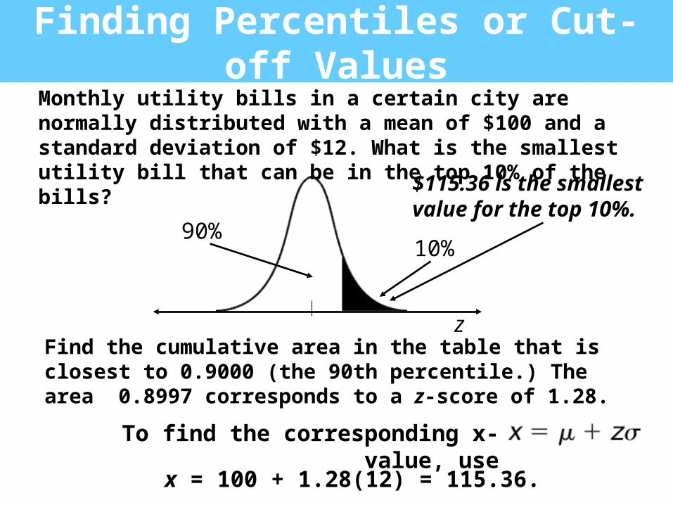
Finding Percentiles or Cut-off ValuesMonthly utility bills in a certain city are normally distributed with a mean of $100 and a standard deviation of $12. What is the smallest utility bill that can be in the top 10% of the bills?
10%90%
Find the cumulative area in the table that is closest to 0.9000 (the 90th percentile.) The area 0.8997 corresponds to a z-score of 1.28.
x = 100 + 1.28(12) = 115.36.
$115.36 is the smallestvalue for the top 10%.
z
To find the corresponding x-value, use

Sampling Distributions & The Central Limit Theorem
Sample
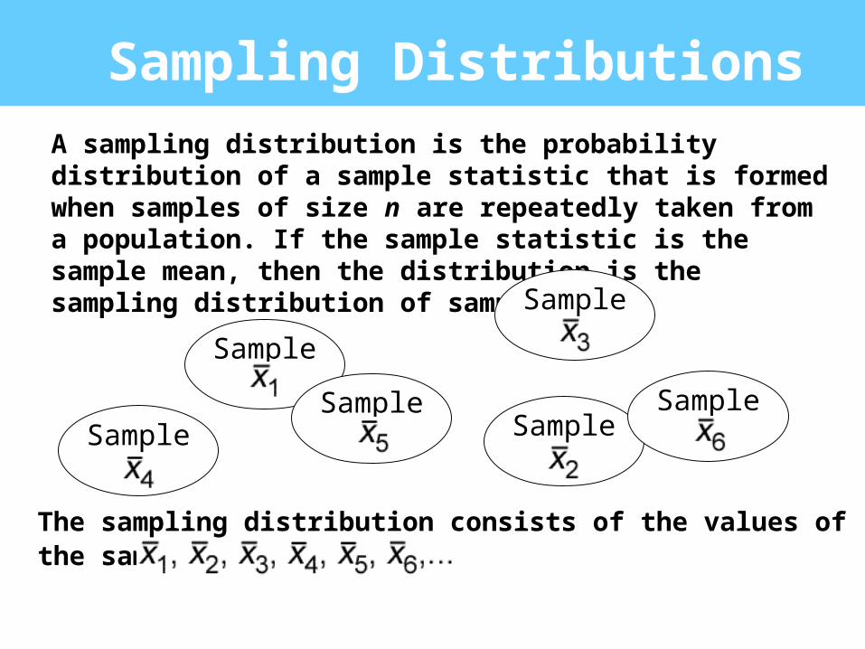
Sampling DistributionsA sampling distribution is the probability distribution of a sample statistic that is formed when samples of size n are repeatedly taken from a population. If the sample statistic is the sample mean, then the distribution is the sampling distribution of sample means.
Sample
The sampling distribution consists of the values of the sample means,
SampleSample
Sample
Sample
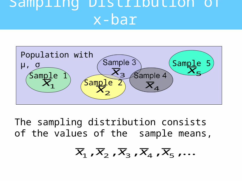
Sampling Distribution of x-bar
Sample 11x
Sample 55x
Sample 22x
3x
4x
Population with μ, σ
The sampling distribution consists of the values of the sample means,
1 2 3 4 5, , , , ,...x x x x x
x
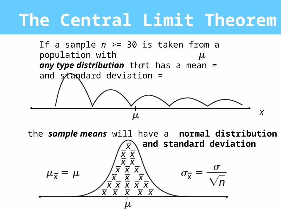
the sample means will have a normal distribution
The Central Limit Theorem
and standard deviation
If a sample n >= 30 is taken from a population withany type distribution that has a mean =and standard deviation =
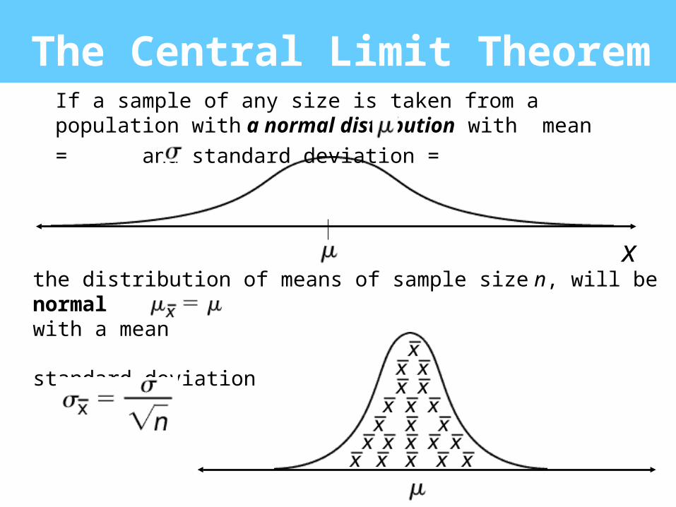
the distribution of means of sample size n, will be normal with a mean
standard deviation
The Central Limit Theorem
x
If a sample of any size is taken from a population with a normal distribution with mean = and standard
deviation =
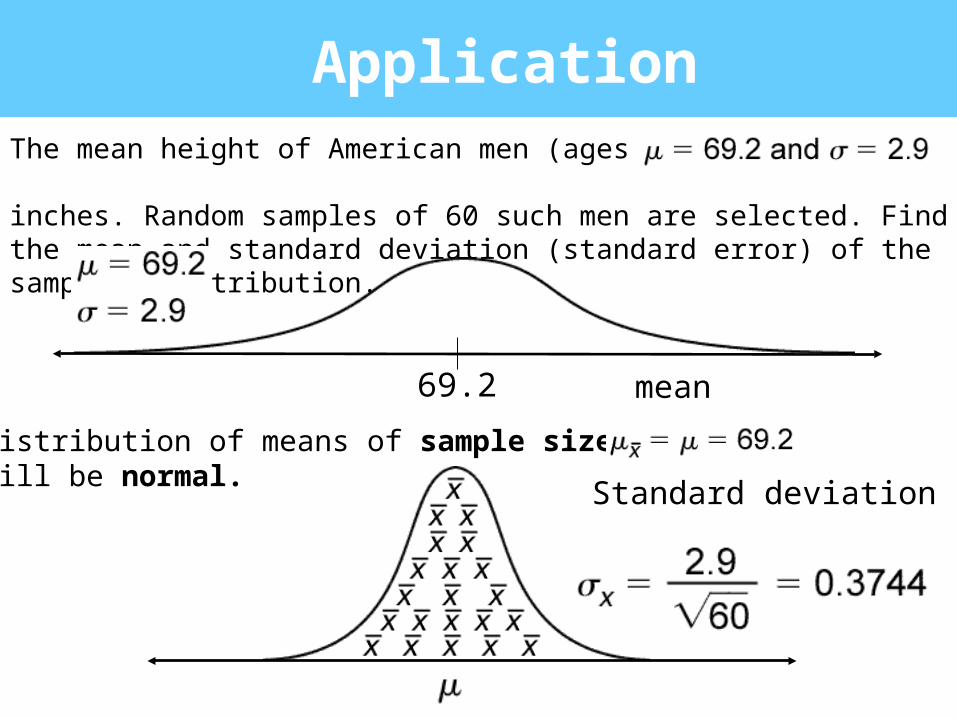
Application
Distribution of means of sample size 60, will be normal.
The mean height of American men (ages 20-29) is inches. Random samples of 60 such men are selected. Find the mean and standard deviation (standard error) of the sampling distribution.
mean
Standard deviation
69.2
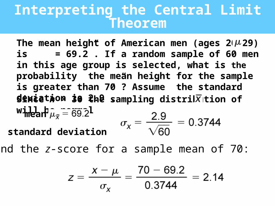
Interpreting the Central Limit Theorem
The mean height of American men (ages 20-29) is = 69.2”. If a random sample of 60 men in this age group is selected, what is the probability the mean height for the sample is greater than 70”? Assume the standard deviation is 2.9”.
Find the z-score for a sample mean of 70:
standard deviation
mean
Since n > 30 the sampling distribution of will be normal
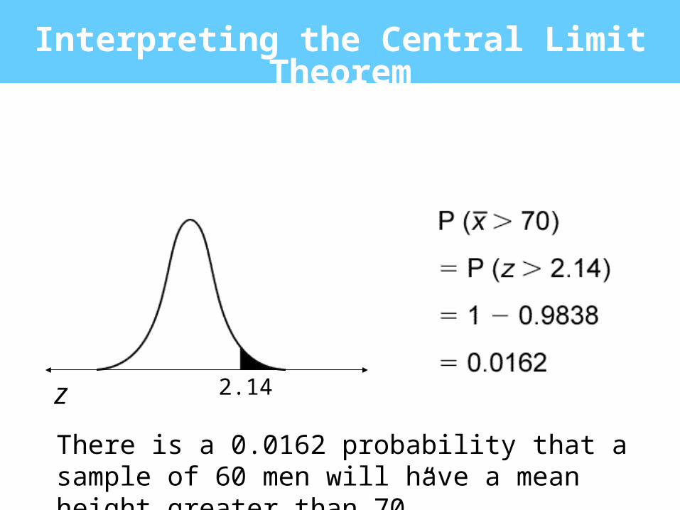
2.14z
There is a 0.0162 probability that a sample of 60 men will have a mean height greater than 70”.
Interpreting the Central Limit Theorem
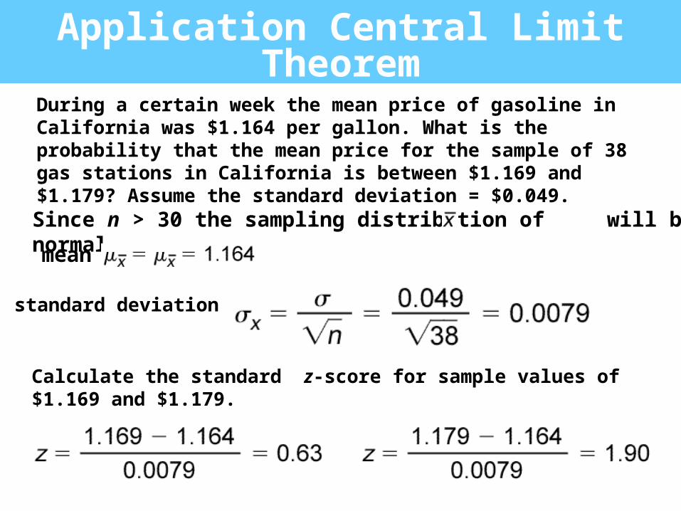
Application Central Limit Theorem
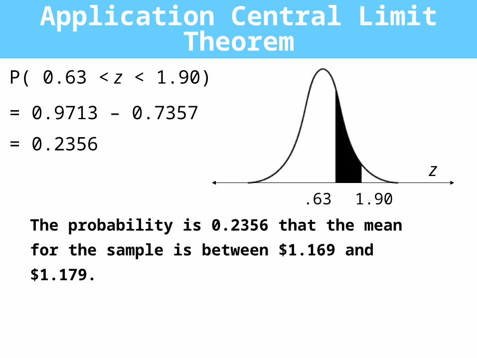
During a certain week the mean price of gasoline in California was $1.164 per gallon. What is the probability that the mean price for the sample of 38 gas stations in California is between $1.169 and $1.179? Assume the standard deviation = $0.049.
standard deviation
mean
Calculate the standard z-score for sample values of $1.169 and $1.179.
Since n > 30 the sampling distribution of will be normal
.63 1.90
z
Application Central Limit Theorem
P( 0.63 < z < 1.90)
= 0.9713 – 0.7357
= 0.2356
The probability is 0.2356 that the mean for the
sample is between $1.169 and $1.179.