Embed Size (px)
Citation preview

Lecture Notes in Physics 908
Elena Tobisch Editor
New Approaches to Nonlinear Waves
Lecture Notes in Physics
Volume 908
Founding Editors
W. BeiglböckJ. EhlersK. HeppH. Weidenmüller
Editorial Board
M. Bartelmann, Heidelberg, GermanyB.-G. Englert, Singapore, SingaporeP. Hänggi, Augsburg, GermanyM. Hjorth-Jensen, Oslo, NorwayR.A.L. Jones, Sheffield, UKM. Lewenstein, Barcelona, SpainH. von Löhneysen, Karlsruhe, GermanyJ.-M. Raimond, Paris, FranceA. Rubio, Donostia, San Sebastian, SpainS. Theisen, Potsdam, GermanyD. Vollhardt, Augsburg, GermanyJ.D. Wells, Ann Arbor, USAG.P. Zank, Huntsville, USA
The Lecture Notes in Physics
The series Lecture Notes in Physics (LNP), founded in 1969, reports new devel-opments in physics research and teaching-quickly and informally, but with a highquality and the explicit aim to summarize and communicate current knowledge inan accessible way. Books published in this series are conceived as bridging materialbetween advanced graduate textbooks and the forefront of research and to servethree purposes:
• to be a compact and modern up-to-date source of reference on a well-definedtopic
• to serve as an accessible introduction to the field to postgraduate students andnonspecialist researchers from related areas
• to be a source of advanced teaching material for specialized seminars, coursesand schools
Both monographs and multi-author volumes will be considered for publication.Edited volumes should, however, consist of a very limited number of contributionsonly. Proceedings will not be considered for LNP.
Volumes published in LNP are disseminated both in print and in electronic for-mats, the electronic archive being available at springerlink.com. The series contentis indexed, abstracted and referenced by many abstracting and information services,bibliographic networks, subscription agencies, library networks, and consortia.
Proposals should be sent to a member of the Editorial Board, or directly to themanaging editor at Springer:
Christian CaronSpringer HeidelbergPhysics Editorial Department ITiergartenstrasse 1769121 Heidelberg/[email protected]
More information about this series athttp://www.springer.com/series/5304
EditorElena TobischInstitute for AnalysisJohannes Kepler UniversityLinz, Austria
ISSN 0075-8450 ISSN 1616-6361 (electronic)Lecture Notes in PhysicsISBN 978-3-319-20689-9 ISBN 978-3-319-20690-5 (eBook)DOI 10.1007/978-3-319-20690-5
Library of Congress Control Number: 2015947251
Springer Cham Heidelberg New York Dordrecht London© Springer International Publishing Switzerland 2016This work is subject to copyright. All rights are reserved by the Publisher, whether the whole or part ofthe material is concerned, specifically the rights of translation, reprinting, reuse of illustrations, recitation,broadcasting, reproduction on microfilms or in any other physical way, and transmission or informationstorage and retrieval, electronic adaptation, computer software, or by similar or dissimilar methodologynow known or hereafter developed.The use of general descriptive names, registered names, trademarks, service marks, etc. in this publicationdoes not imply, even in the absence of a specific statement, that such names are exempt from the relevantprotective laws and regulations and therefore free for general use.The publisher, the authors and the editors are safe to assume that the advice and information in this bookare believed to be true and accurate at the date of publication. Neither the publisher nor the authors orthe editors give a warranty, express or implied, with respect to the material contained herein or for anyerrors or omissions that may have been made.
Printed on acid-free paper
Springer International Publishing AG Switzerland is part of Springer Science+Business Media(www.springer.com)
Preface
The theory of nonlinear waves is located right at the intersection of the linear wavetheory, the theory of nonlinear oscillations, and the theory of nonlinear partialdifferential equations (PDEs), radiating into numerous fields of applied science,including studies in oceanography, nonlinear optics, plasma physics, weather andclimate prediction.
It is hard to imagine that just a few decades ago the same equations arisingin different fields of science were studied independently of each other, and thephenomena which they describe were called by different names. Probably one ofthe most illustrative examples of this kind is the phenomenon discovered in early1960s, which is named modulational instability in purely mathematical texts, whileknown as modulation instability in nonlinear optics, as Benjamin-Feir instability intheory of water waves, as Oraevsky instability in plasma physics, etc. etc.
Only in the late 1980s gradually began to crystallize the idea of creating a newnonlinear science that would synthesize all known results into a single overallscheme and would allow to describe them all in one and the same language. Iremember the annual meeting of the physical branch of the Russian Academyof Sciences, traditionally held at the Institute of Oceanology in Moscow, whereVladimir Eugenievich Zakharov very emotionally expounded the idea of creatingsuch a language and writing an encyclopedia on nonlinear science, in which all ofthe most important results would be collected in one place. The late V.I. Arnold,who was in the audience, said that such language has long been there and it’s calledmathematics. Roars of laughter drowned out the answer of V.E. Zakharov.
Every physicist knows how long the road is from the physical level of accuracy,which is sufficient for solving many theoretical and practical problems in physics, toa rigorous mathematical definition and proof. The simplest example, as very often inphysics, gives us the study of the physical pendulum. Galileo studied its movementand discovered the phenomenon of resonance in 1637. The rigorous mathematicaldefinition of resonance was given by Poincaré 250 years later. And without anaccurate notion of resonance, most of the chapters in this book principally couldnot have been written. In fact, much of the modern theory of nonlinear waves couldnot have been developed.
v
vi Preface
Since then many years have flown, and the notion of nonlinear science hasbecome an integral part of our scientific language, and the first encyclopedia ofnonlinear science saw the light of day in 2002 already, thanks to the invaluableeffort of the late Alwyn Scott, who edited this great work of more than 1000 pages,written by scholars from all over the world.
However, the science does not halt, and new questions are coming forth, to whichthere is no answer in this encyclopedia. How to describe both discrete and kineticregimes of wave turbulence resting on a unified strict mathematical approach?What new physical phenomena can be described if Phillips’ definition of resonanceis generalized to the case of moderate nonlinearity? Why does generalized NLSdescribe weakly nonlinear processes in water waves and strong nonlinear processesin optics? Etc. etc.
Answers to these and some other questions are given in this volume. A briefoverview of individual chapters of the book is provided in the introductory Chap. 1.I also tried to position all the subjects in a logical consequence, i.e., scientific results,yielding new questions and then new results and again new questions ad infinitum.The choice of topics, of course, is biased and reflects my research interests andexpertise. The last and longest Chap. 8 in the book has been written by Lev Shemer,one of the best modern experimentalists with water waves. The main goal of thischapter is to demonstrate why direct comparison of theoretical and numerical resultswith experimental measurements is often challenging; the author discusses in detailexperiments devised to provide a basis for evaluation of the domain of validity of atheoretical model.
Understanding came to me already in 2011 that time is ripe again for gatheringstones in the theory of nonlinear waves. At first, it was transformed into the idea oforganizing a series of regular bi-annual conferences called Wave Interaction (WIN)to discuss new and promising topics in the area. The idea of writing a book wasalready discussed at WIN-2012. The format and content of the present volume wasfinalized during several meetings being held in 2012–2014:
• (2012) Wave Interaction (WIN-2012), 23–26 April (Johannes Kepler UniversityLinz, Austria)
• (2013) Thematic Program on the Mathematics of Oceans, April 29–June 28(Fields Institute for Research in Mathematical Sciences, Toronto, Canada)
• (2014) Weak Chaos and Weak Turbulence, 3–7 February (Max Planck Institutefor the Physics of Complex Systems, Dresden, Germany)
• (2014) Wave Interaction (WIN-2014), 23–26 April (Johannes Kepler UniversityLinz, Austria)
• (2014) Theory of Water Waves, 14 July–8 August (Isaac Newton Institute,Cambridge, UK)
All chapters are based on talks delivered at these conferences by selectedinvited speakers. I am very grateful to all attendants of these conferences whoactively helped me to make a choice of topics. I would like to mention particularlyN. Akhmediev, T. Bridges, W. Craig, A. Degasperis, K. Dysthe, R. Grimshaw,
Preface vii
P. Janssen, C.C. Mei, M. Onorato, D. Pelinovsky, E. Pelinovsky, A. Pikovsky,D. Shepelyansky, V. Shrira, and S.K. Turitsyn.
My aim was to create a book accessible to graduate students, engineers andresearchers working in various fields of physics and applied mathematics. Con-sequently, the authors tried to make their exposition as clear as possible withoutharming scientific rigor. All theoretical chapters contain not only a conceptualbackground, but also illustrative examples of how these new techniques andapproaches can be applied to specific problems. I am very much obliged to all theauthors of this volume for their contributions and their patience when handling myremarks and making revisions.
I am also greatly indebted to all reviewers of the individual chapters which tookover the hard and unremunerated work that resulted in tangible improvement of thequality of this book.
I am specially grateful to Shalva Amiranashvili, whose invaluable remarks andsuggestions allowed me to improve the text of the introductory chapter.
I also would like to thank Dr. Aldo Rampioni and Kirsten Theunissen, Editors ofthe Springer Series Lecture Notes in Physics, who constantly assisted me during thepreparation of the manuscript.
Linz, Austria Elena TobischApril 2015
Chapter 8Quantitative Analysis of NonlinearWater-Waves: A Perspectiveof an Experimentalist
Lev Shemer
Abstract In the present review the emphasis is put on laboratory studies ofpropagating water waves where experiments were designed with the purpose toenable juxtaposing the measurement results with the theoretical predictions, thusproviding a basis for evaluation of the domain of validity of various nonlineartheoretical model of different complexity. In particular, evolution of deterministicwave groups of different shapes and several values of characteristic nonlinearity isstudied in deep and intermediate-depth water. Experiments attempting to generateextremely steep (rogue) waves are reviewed in greater detail. Relation betweenthe kinematics of steep nonlinear waves and incipient breaking is considered.Discussion of deterministic wave systems is followed by review of laboratoryexperiments on propagation of numerous realizations of random wave groupswith different initial spectra. The experimental results are compared with thecorresponding Monte-Carlo numerical simulations based on different models.
8.1 Introduction
Ocean wave forecasting is indispensable for navigation and coastal activities,however accurate predictions critically depend on detailed understanding of theprocesses that govern dynamics of water waves. Gaining such an understandingrepresents a non-trivial intellectual challenge since waves are both nonlinear andstochastic in nature. In recent years the extremely steep (rogue, or freak) wavesattract particular attention [23] due to their potential to cause significant damageto marine traffic as well as to off-shore and coastal structures. The complexityof ocean water-waves in general, and of rogue waves in particular, makes itimperative to investigate much simpler nonlinear gravity wave fields in order toidentify the dominant mechanisms that govern their behavior. For example, waveenergy dissipation by various mechanisms, or energy input due to wind, may
L. Shemer (�)School of Mechanical Engineering, Tel-Aviv University, Tel-Aviv 69978, Israele-mail: [email protected]
© Springer International Publishing Switzerland 2016E. Tobisch (ed.), New Approaches to Nonlinear Waves, Lecture Notesin Physics 908, DOI 10.1007/978-3-319-20690-5_8
211

212 L. Shemer
play an important role in wave evolution. These effects are sometimes accountedfor in the numerical solutions by invoking phenomenological models [24]. Ofparticular interest, however, is wave train transformation as a result of the action ofenergy-conserving factors, like nonlinear interactions and dispersion. In laboratoryexperiments there is no energy input by wind; moreover, for sufficiently long wavesin absence of breaking dissipation may play only a minor role and can thus can oftenbe neglected. This leaves the nonlinearity and dispersion as factors that dominate theevolution process in wave tank experiments.
The theoretical analysis of the effect of nonlinearity on water-waves utilizesthe fact that the most important non-trivial interactions in deep-water waves occuramong four waves (wave quartets) [51, 52], and consequently are limited to thethird order in the wave steepness [86]. In nature, these nonlinear interactions areusually stochastic in nature. Hasselmann [17] was the first to apply statisticalapproach and the kinetic theory to describe random ocean waves. As a result ofnonlinearity, a large number of harmonics with various frequencies exchange energyand transfer it to shorter scales where the wave energy is dissipated by breaking orotherwise. The so-called resonance interactions among four waves are considered.The resonance wave quartets satisfy the following conditions on their wave vectorski and frequencies !i, i being the number of the wave:
k0 C k1 D k2 C k3I !0 C !1 D !2 C !3 (8.1)
This phenomenon is sometimes called wave, or weak, turbulence, to acknowledgesimilarity to Kolmogorov energy cascade in fluid turbulence. Recently water waveturbulence theory was advanced considerably by Zakharov and his colleagues (see,e.g. Zakharov [87], Nazarenko [42] and references therein). The kinetic wavetheory that serves as a basis for modern wave climate prediction is based on twofundamental assumptions: that the wave nonlinearity is weak, and that and thephases of different harmonics are random. The random phase approximation is anessential assumption used for turbulent closures for all stochastic wave systems andeven for a much broader range of turbulent systems.
One major simplification in water waves studies is decoupling of randomnessand nonlinearity. One can thus concentrate first on deterministic, as opposed tostochastic, wave fields. The problem of evolution of a deterministic nonlinear wavesystem still remains extremely complex, and additional simplifications are required.Ocean waves exhibit considerable directional spreading; yet accounting for theangular distribution of the wave propagation directions complicates significantlythe theoretical analysis. While measurements of evolution of short-crested 2D wavefields are possible in laboratory wave basins, see i.e. [22, 48], most experimentson nonlinear wave propagation were performed in long wave flumes where onlyunidirectional (1D) waves can be generated.
Numerous attempts have been made to explore the possibility to use deterministicnonlinear wave theories to forecast the evolution of a random wave field, as analternative to application of the kinetic equation [2, 3, 47, 75]. These studies revealthe crucial role of non-resonant interactions (among wave quartets for which the
8 Analysis of Nonlinear Water-Waves 213
second condition in Eq. (8.1) is not satisfied exactly) in evolution of nonlinearrandom water waves. Shemer [55] demonstrated that nonlinear interactions canbe quite significant for non-resonating deterministic wave quartets as well. Forunidirectional waves, no exact resonances exist among wave quartets that containthree or four different waves and only near-resonant interactions between such wavequartets are possible. The crucial role of near resonant interactions for wave fieldevolution make experiments in a wave tank a very convenient vehicle to study non-linear random waves in laboratory conditions. Some experiments in a long wavetank have been performed on deep narrow-banded waves with random phases (see[41] and references therein). Results of these experiments indicate that in spite oflack of exact resonances in a unidirectional wave field, nonlinear effects are essentialand they strongly affect the statistical properties of the wave field.
A number of fully nonlinear solvers for studying the evolution of unidirec-tional nonlinear waves were developed in recent decades. Nevertheless, simplifiedtheoretical models often offer significant advantages and are widely used. Thesimplifications in the models may also include assumptions of either vanishingor very narrow spectral width. The effects of wave energy dissipation by variousmechanisms, or energy input due to wind, are sometimes accounted for in thenumerical solutions by invoking phenomenological models.
It should be stressed that linear water-wave theory is well developed; it accountsfor dispersion and in many occasions provides satisfactory solutions, in particularfor deep and intermediate-depth water. Involving nonlinearity may be justified inoccasions when it modifies the linear solutions considerably. Different nonlineartheoretical models, as well as fully nonlinear computations contain numeroussimplifying assumptions. To justify application of these advanced methods ofsolution of water-waves problems, the validity of the results has to be verifiedby carrying out controlled experiments that allow estimate of the importanceof essentially nonlinear mechanisms and enable quantitative comparison of thetheoretical predictions with the measurements.
The structure of this chapter is as following. The description of experimentalfacilities used is presented first in Sect. 8.2. Comparison between theoretical resultsand measurements is then carried out for nonlinear wave models with increasingcomplexity. Deterministic water wave groups are considered first. The limitedvalidity of the results based on the nonlinear Schrödinger (NLS) equation isdemonstrated in Sect. 8.3. In order to improve the accuracy of the theoretical results,the modified nonlinear Schrödinger (mNLS, or Dysthe) equation, is employed inSect. 8.4. Part of this section is devoted to presentation of the essential differencesbetween the analysis of the wave field evolution in time that is customarily carriedout in theoretical studies, and the spatial variation observed in wave tanks. Differentaspects of application of the spatial version of the Zakharov equation that is the mostgeneral third order theoretical model, to the analysis of evolution of unidirectionalwave trains are examined in Sect. 8.5. Experiments on random unidirectional waveswith different spectra and comparison with Monte-Carlo simulations based ondifferent models are described in Sect. 8.6. In analysis of both deterministic andrandom waves an emphasis is put on possible mechanisms leading to generation
214 L. Shemer
of extremely large (the so-called freak, or rogue) waves. Such waves, often dubbedkiller-waves, appear and disappear fast and unexpectedly, and have the potential ofcausing substantial damage to marine traffic. Finally, the presented results will bediscussed and the conclusions presented in Sect. 8.7.
8.2 The Experimental Facilities
The majority of the experiments discussed here in detail were carried out in the Tel-Aviv University (TAU) wave tank which is 18 m long, 1.2 m wide and has a constantdepth of 0.6 m. A paddle-type wavemaker hinged near the floor is located at one endof the tank. The wavemaker consists of four modules, which in all experimentsdiscussed here were adjusted to move in phase with identical amplitudes andfrequencies. The wavemaker is driven by a computer-generated signal. At the far endof the tank a wave energy-absorbing sloping beach is installed. The beach starts atthe distance of about 14 m from the wavemaker; no measurements were performedin the beach region. The instantaneous surface elevation is measured simultaneouslyby resistance-type wave gauges. The probes are mounted on a bar parallel to the sidewalls of the tank and fixed to a carriage which can be moved along the tank. In mostexperiments the carriage was placed manually at the desired measuring location.More recently, the capability to control the location of the carriage by computer wasadded. Measurements of the surface elevation are performed at numerous carriagelocations along the center line of the tank. The distance between the adjacent gaugeson the bar is adjustable, in most cases four wave gauges with a constant spacingnot exceeding 0.4 m between the adjacent probes was used. Probes are calibratedusing a stepping motor and a computerized static calibration procedure describedin detail in Shemer et al. [63]. The calibration is performed at the beginning ofeach experimental run. The probe response is essentially linear for the range ofsurface elevations under consideration. The voltages of the four wave gauges, thewavemaker-driving signal and the outputs of position potentiometers of the fourwavemaker paddles are sampled using an A/D converter and stored at the computerhard disk for further processing. The sampling frequency is adjusted in eachexperiment to be by two orders of magnitude higher that the carrier wave frequency.To enable measurements for various water depths, a false bottom made of a numberof 1.18 m by 1.25 m marine plywood plates 1.8 cm thick can be installed in the tank.Each plywood plate is independently suspended on stainless steel rods from the steelframe of the tank, so that any desirable effective water depth can be attained.
Some experiments reported here were carried out in the Large Wave Channel(GWK) in Hanover, Germany. The tank has a length of 300 m, width of 5 m anddepth of 7 m. Water depth in all experiments was set to be 5 m. At the end of thewave tank, there is a sand beach starting at the distance of 270 m with slope of30ı. The computer-controlled piston-type wavemaker is equipped with the reflectedwave energy absorption system. The instantaneous water height is measured using25 wave gauges of resistance type placed along the tank wall; the distribution of
8 Analysis of Nonlinear Water-Waves 215
the wave gauges along the tank was adjusted to the goal of each experiment. Thestatic probe calibration was performed by filling the tank first to the maximumpossible depth and then reducing the depth in steps adjusted to the range of surfaceelevations relative to the undisturbed value. The calibration curve for each wavegauge was obtained by best fit to linear dependence. Due to the size of the facility,the calibration procedure usually takes a whole working day. The wave gauges weretherefore calibrated only once in a week. It is estimated that the absolute error in themeasured instantaneous surface elevation in most cases did not exceed about 1 cm.
In all experiments the wave train of finite duration was generated by a wave-maker. In the GWK experiments, a single wave group was excited in eachexperimental run, while in a smaller TAU facility the number of groups in eachwave train did not exceed four. In both wave tanks each experimental run startedonly after a sufficient interval from the previous experiment when the watersurface was quiescent and all remaining disturbances decayed totally. In the GWKmeasurements the reflected wave energy absorption system effectively eliminatedthe existence of very long waves in the tank and enabled relatively short (about15 min) intervals between consecutive experimental runs. The output voltages of allwave gauges, as well as of the wavemaker driving signal and of the output of thewavemaker position potentiometer that provides information on the instantaneouswavemaker displacement, were sampled at sufficiently high rate adjusted to thedominant frequency with the total sampling duration of 350 s.
8.3 The Nonlinear Schrödinger Equation
Sea waves can be described quite faithfully by JONSWAP spectrum [18]. One of theimportant features of this spectrum is its relatively narrow frequency band, whichresults in a notable wave groupiness. The simplest nonlinear theoretical modelwhich is capable of describing the evolution of propagating wave packet with asufficiently narrow spectrum in the range of water depths from deep to intermediateis the nonlinear Schrödinger (NLS) equation (see, e.g. Mei [39]). This equation wasderived by Zakharov [86] and Hasimoto and Ono [16] and has been extensivelyapplied for description of wave group evolution in deep water. An agreementbetween the experimentally found growth rates of the unstable sidebands with thetheoretical predictions based on the NLS equations was obtained [31]. Zakharovand Shabat [88] demonstrated analytically using the NLS equation that an arbitrarilyshaped envelope disintegrates eventually into a finite number of envelope solitons.Wave train disintegration was indeed observed in deep water by Yuen and Lake[84, 85], and by Su [76].
In an attempt to determine the domain of applicability of the NLS equation,Shemer et al. [64] investigated transformation of deterministic wave groups inintermediate water depth in a laboratory wave tank. The measurements werecompared with the results of numerical solution based on the NLS equation. Wavegroup propagation was studied for a number of values of constant water depth
216 L. Shemer
h with q D k0h D O.1/, k0 D 2�=�0 being the carrier wave number and �0the carrier wave length, covering the range from a nearly shallow water to thevalues of q approaching deep water conditions. Simplest possible initial shapes ofthe wavemaker driving signal which satisfy the narrow spectrum condition wereselected:
s.t/ D s0cos.˝t/cos.!0t/I ˝ D !0=20I (8.2)
s.t/ D s0jcos.˝t/jcos.!0t/I ˝ D !0=20I (8.3)
s.t/ D s0exp.�.t=mT0/2/cos.!0t/I 16T0 < t < 16T0: (8.4)
Here s0 is the forcing wavemaker amplitude, !0 D 2�=T0 is the radian carrier wavefrequency and ˝ is the modulation frequency. The spectrum given by Eq. (8.2) isbimodal, with two distinct peaks of identical height at !0 ˙˝ . The envelope givenby Eq. (8.3) is identical to that given by Eq. (8.2), but the symmetric spectrum of thissignal with the period of 2�=˝ is considerably more complicated; it has a maximumat the carrier frequency !0 and consists of a set of discrete frequencies spaced by!0=10. The Gaussian driving signal given by Eq. (8.4) generates widely separatedwave groups. The parameter m determines the width of the envelope; the larger is thevalue of m, the wider is the group. The discrete frequency spectrum of the surfaceelevation in the wave group defined by Eq. (8.4) also has a Gaussian shape with themaximum at !0 and resolution of !0=32; the value of m D 5 was selected in thoseexperiments, so that the initial spectrum was quite narrow.
Three values of the maximum driving amplitude s0 were used for each shapeof the forcing signal. The maximum driving amplitudes were selected so that closeto the wavemaker, the resulting carrier wave had the maximum wave amplitudesa0 corresponding to the steepness � D k0a0 of about � D 0:07 (low amplitude),� D 0:14 (intermediate amplitude), and � D 0:21 (high amplitude). Two values ofthe carrier wave periods, T0 D 0:7 s and T0 D 0:9 s, were employed. Experimentswere carried out for two positions of the false bottom in the tank, correspondingto the water depths of h D 11:8 cm and h D 17:0 cm, as well as with the falsebottom removed, thus yielding the maximum possible in the facility water depthh D 60 cm. The surface elevation for a modulated unidirectional narrow-bandedwave can be presented at the leading order as
� D Re�a.x; t/ei.k0x�!0t/
�; (8.5)
where a.x; t/ is the slowly varying in time and space complex amplitude of thecarrier wave with the frequency !0 and the wave number k0. The dispersion relationfor intermediate water depth is
!20 D kg � tanh.q/; (8.6)
where g is the acceleration due to gravity.
8 Analysis of Nonlinear Water-Waves 217
In order to perform the comparison of the model results with the experiment,the NLS equation has to be written in a form describing the evolution of the wavegroup along the tank (i.e. in space); thus the enabling determination of the surfaceelevation variation in time, as measured by wave gauges at fixed measuring stations,�.t/. Following Mei [39], the dimensionless scaled variables were introduced as
a D a0A; � D �!0.x=cg � t/; X D �2k0x (8.7)
where A is the complex dimensionless wave group envelope, a0 is the characteristicwave amplitude, x is the coordinate along the tank and t is the time. The groupvelocity cg D @!=@k. The NLS equation can be written as
� i@A
@XC ˛
@2A
@�2C ˇjAj2A D 0: (8.8)
The coefficients in the NLS are defined in the dimensionless form by
˛ D � !02
2k0cg3
@cg
@k(8.9)
ˇ D 1
n
"cosh.4q/C 8 � 2tanh2.q/
16sinh4.q/� 1
2sinh2.2q/
.2cosh2.q/C n2/
qtanh.q/ � n2
#; (8.10)
where the parameter n D cg=cp represents the ratio of group and phase velocitiesand is given by
n D 1
2
�1C 2q
sinh.2q/
: (8.11)
Equation (8.8) was solved numerically using an implicit finite difference schemewith periodic in � boundary conditions. Initial conditions at X D 0 are in accordancewith the shapes defined by Eqs. (8.2)–(8.4). The variation of the surface elevation �is obtained from the solution of Eq. (8.8) using the computed complex amplitudesA.X; �/ and the relations between the scaled dimensionless .X; �/ and the physical.x; t/ variables, given by Eq. (8.7).
As long as characteristic wave lengths are relatively short compared to the waterdepth, the deep water dispersion relation holds and waves are strongly dispersive.For shallower water, wave dispersion becomes weaker and depth-dependent. Wavepropagation in coastal region and in shallow water thus constitutes a separateproblem and is not considered in detail here.
Measurements of instantaneous surface elevation at multiple locations alongthe tank were performed by Shemer et al. [64] for three shapes of wave groups,three values of the dimensional water depth h and for three maximum waveamplitudes a0. For each condition, wave groups with two carrier wave periods T0were investigated. The total number of experimental conditions in this study is thus
218 L. Shemer
0 1 2 3 4 5 6 7 8 9 10−2
−1.5
−1
−0.5
0
0.5
1
k0h
β
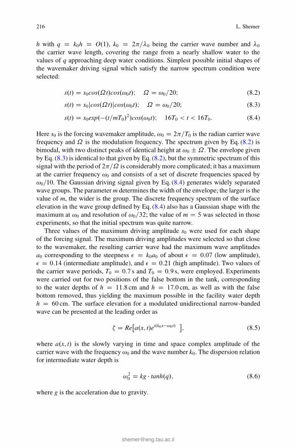
Fig. 8.1 Variation of the nonlinear term coefficient in the NLS equation ˇ with the dimensionlessdepth k0h. Symbols denote the experimental conditions
was 54. For the sake of brevity, the following discussion is limited to three values ofˇ corresponding to the defocusing regime at h D 0:118m; T0 D 0:9 s (ˇ D �1:17),approximately linear regime (h D 0:17m, T0 D 0:7 s, ˇ D 0:19 � 1), and nearlydeep-water case with h D 0:60m, T0 D 0:7 s, ˇ D 0:79. The coefficients ˛ and ˇ inthe NLS equation (8.8), as well as the parameter n are functions of the dimensionlesswater depth q. Note that for q ! 1, ˛ ! 1, ˇ ! 1, and n ! 0:5. The variation ofthe coefficient of the nonlinear term ˇ with the dimensionless depth k0h is plottedin Fig. 8.1. The conditions at which the experiments are performed are marked inthe figure. In view of the dispersion relation (9), the range of intermediate waterdepth is usually defined as �=10 < q < � . The ratio of group to phase velocity nat q > � indeed is very close to 0.5. The coefficient of the nonlinear term in theNLS equation, ˇ, though, still differs notably from their asymptotic values for deepwater even for q D 10. The NLS thus allows to redefine the effective limits of theintermediate water depth range for studying evolution of nonlinear wave groups.
It follows from Fig. 8.1 that as far as the nonlinear effects are concerned, the wavegroups with the selected carrier wave periods and water depths in the experimentspropagate in water of intermediate depth. For the sake of brevity, only characteristicselected results are presented in the following figures. Additional results can befound in [64] and in [21]. Each one of the following figures in this section consistsof six panels, marked (a)–(f). The measured variations of the surface elevation withtime in the vicinity of the wavemaker (at x D 0:24m) are presented in the panel(a), while the corresponding amplitude spectra are given in panel (b). Similarly, theresults of the measurements performed away from the wavemaker, typically aroundx D 9m, are presented in panels (c) and (d). Note that only a fraction of the durationof actual records is shown in these frames. The directly measured surface elevationis given in the bottom curves in panels (a) and (c). These records, however, can not
8 Analysis of Nonlinear Water-Waves 219
be immediately compared with the computations based on the NLS equation. Themodel equation describes the variation of the envelope of the carrier wave at theleading order. The second order (�2) bound second and low frequency harmonicsmay be deduced from carrier wave amplitude using expressions given for finitewater depth in [6]. The experimentally obtained spectra presented in some of thepanels (b) and (d) clearly demonstrate the presence of higher order harmonics. Thepresence of these harmonics in the spectrum is a manifestation of non-negligiblecontribution of bound waves to the surface elevation. The bound waves are mostprominent at the second order, but can be identified at higher orders as well.The second order bound waves cause significant asymmetry of surface elevation� relative to the mean water level, with crests heights exceeding the troughs.
In order to provide a basis for comparison of the experimental results with themodel predictions, the raw signals were band-pass filtered in the range 0:4f0 <f < 1:6f0, where f0 D 1=T0 D !0=2� is the carrier frequency, thus leavingfree waves only. The envelope of the filtered signal is then computed using theHilbert transform, as applied for water wave analysis by Melville [40] (for extensiveintroduction to the Hilbert transform see, e.g. Hahn [15]). Both the band-pass filteredsurface elevation and the absolute value of the envelope are also presented (a verticalshift is introduced for convenience) in panels (a) and (c). The computed usingEq. (8.8) shapes of the envelope at the identical locations along the tank are depictedin panel (e) for qualitative comparison with the experiments.
To eliminate the contribution of the second order bound waves, the maximumamplitudes of the waves in the group for each set of experimental conditions and forall distances from the wavemaker can be calculated either as a half of the maximumwave height obtained in the raw signal Amax D 1
2Hmax D 1
2.�max � �min), where
�max and �min are the maximum and the minimum surface elevations measured ineach group and averaged over all groups in the record. Alternatively, the amplitudeAmax may be calculated as the maximum value of the filtered group envelope,averaged overall groups in the record. As demonstrated in [64], both methods lead tosimilar results. The variation of the maximum wave group amplitudes along the tankcalculated as half difference between crests and troughs is presented in panel (f). Themaximum wave amplitudes in these figures are normalized by their correspondingvalues in the vicinity of the wavemaker. The experimentally determined values ofAmax are compared in panel (f) with computations based on the NLS equation.
The nearly shallow water case (h D 11:8 cm; T0 D 0:9 s, k0h D 0:847; ˇ D�1:17) is described first. The results for the bichromatic forcing by the wavemakergiven by Eq. (8.2) are presented in Fig. 8.2 for the low forcing amplitude, � D 0:07,and in Fig. 8.3 for the high forcing amplitude, � D 0:21. Close to the wavemaker(x D 0:24m, x=�0 D 0:28), the measured wave group envelopes in Figs. 8.2a and8.3a are quite similar to the shape of the driving signal. At high amplitude, however,some distortion of the shape of the carrier wave in Fig. 8.3a can be noticed even atthis close proximity to the wavemaker. The reason for this distortion is clearly seenfrom comparison of the corresponding amplitude spectra in Figs. 8.2b and 8.3b. Incontrast to Fig. 8.2b with a nearly bimodal spectrum, at high amplitude in Fig. 8.3bthe spectrum is characterized by prominent peaks related to the second harmonic
220 L. Shemer
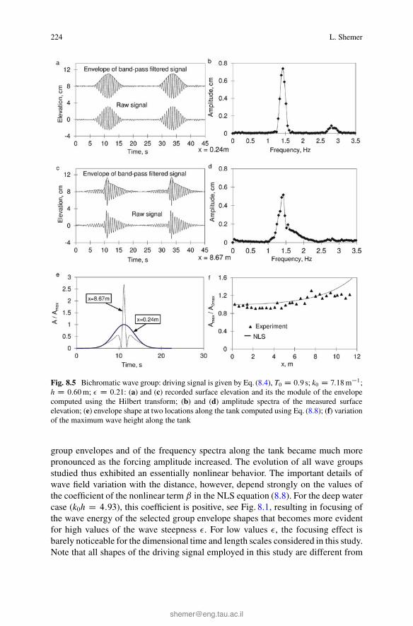
Fig. 8.2 Bichromatic wave group: driving signal is given by Eq. (8.2), T0 D 0:9 s; k0 D 7:18m�1;h D 0:0118m; � D 0:07: (a) and (c) recorded surface elevation and its the module of the envelopecomputed using the Hilbert transform; (b) and (d) amplitude spectra of the measured surfaceelevation; (e) envelope shape at two locations along the tank computed using Eq. (8.8); (f) variationof the maximum wave height along the tank
of the carrier wave. Far from the wavemaker, the generation of free waves at thesecond harmonics of the carrier may be identified, in particular between the wavegroups, in the unfiltered signals of Fig. 8.2c (x D 7:62m, x=�0 D 8:71) and Fig. 8.3c(x D 9:47m, x=�0 D 9:63). The low frequency peaks are also clearly visible inthese spectra. The generation of free second order harmonics that is more prominentfor wavemaker-excited wave fields in shallower water was discussed in detail byKit et al. [28]. Only relatively minor changes occur in the spectrum around thedominant frequency at the remote location in Fig. 8.2d as compared to the initialspectrum at this relatively weak forcing amplitude. At stronger forcing, wideningof the spectrum with the distance becomes essential, and the spectrum becomesmore complicated with numerous harmonics both in the vicinity of the carrier wavefrequency and its second harmonic, see Fig. 8.3b, d. The shape of the envelope in
8 Analysis of Nonlinear Water-Waves 221
Fig. 8.3 Bichromatic wave group: driving signal is given by Eq. (8.2), T0 D 0:9 s; k0 D 7:18m�1;h D 0:0118m; � D 0:21: (a) and (c) recorded surface elevation and its the module of the envelopecomputed using the Hilbert transform; (b) and (d) amplitude spectra of the measured surfaceelevation; (e) envelope shape at two locations along the tank computed using Eq. (8.8); (f) variationof the maximum wave height along the tank
Fig. 8.2c is only slightly distorted, while at the high amplitude, Fig. 8.3c, this shapechanges drastically and becomes notably asymmetric.
The model computations presented in Figs. 8.2e and 8.3e are only in a qualitativeagreement with the experimental observations. At low forcing amplitudes, thecalculated shape of the group in Fig. 8.2e remains virtually unchanged, while at highamplitude, Fig. 8.3e, notable distortion of the group shape accompanied by decreasein the maximum amplitude is obtained. In the simulations, however, the enveloperetains symmetric shape in the process of evolution along the tank, contrary to theexperimental results. For both forcing amplitudes, the decay of the maximum waveamplitude along the tank is observed experimentally, although the slope in Fig. 8.2fis more moderate than that in Fig. 8.3f. The model computations indicate the same
222 L. Shemer
Fig. 8.4 Bichromatic wave group: driving signal is given by Eq. (8.3), T0 D 0:9 s; k0 D 7:18m�1;h D 0:17m; � D 0:21: (a) and (c) recorded surface elevation and its the module of the envelopecomputed using the Hilbert transform; (b) and (d) amplitude spectra of the measured surfaceelevation; (e) envelope shape at two locations along the tank computed using Eq. (8.8); (f) variationof the maximum wave height along the tank
trend, with the decrease in the maximum amplitude much more pronounced for thehigh amplitude case.
The wave group excited by the driving signal given by Eq. (8.3) for the interme-diate depth h D 0:17m that corresponds to very small nonlinearity coefficient ˇ D0:19 is presented in Fig. 8.4 for high forcing amplitude � D 0:21. In the vicinity ofthe wavemaker, x D 0:24m, x=�0 D 0:39, the shape of the wave group in Fig. 8.4aresembles that of the driving signal and does not look very different from that inFig. 8.3a. The spectrum in Fig. 8.4b, however, is very different from that in Fig. 8.3b;it exhibits a dominant peak at the carrier frequency and is not bimodal. The higher
8 Analysis of Nonlinear Water-Waves 223
harmonics are quite visible, similarly to the cases presented above. At the remotelocation, x D 8:67m, x=�0 D 13:73, Fig. 8.4c, the waves are distributed somewhatmore uniformly along the group. Since in this case the wave field is essentially linearwhen analyzed in the framework of the NLS equation, the frequency spectrum odthe surface elevation is supposed to remain practically unchanged along the tank.The spectrum plotted in Fig. 8.4d is however, somewhat different from that at thewavemaker. The theoretically computed wave group shapes in Fig. 8.4e resembleclosely those obtained in the experiments. In contrast to the results obtained forthe shallower water case, the measured maximum wave amplitude in Fig. 8.4e doesnot change notably along the tank. This experimental result is confirmed by thenumerical solution of the model equation for a considerable part of the tank, up to xof about 8 m.
Comparison of Figs. 8.3 and 8.4 reveals that wave groups having identical initialenvelope shapes but different spectral contents may undergo completely differentevolution processes. Specifically, in Fig. 8.3 groups having a bimodal spectrumretain their clear identity in the process of propagation, and their envelope peri-odically attains zero. For wave groups with the same shape and more complicatedspectra, Fig. 8.4, the wave energy tends to become more uniformly distributed alongthe group, so that the clear distinction between the groups vanishes.
The behavior of wave groups generated using the Gaussian driving signal givenby Eq. (8.4) is presented in Fig. 8.5 for nearly deep water with h D 0:60m,T0 D 0:7 s, k0h D 4:93, ˇ D 0:78 and high amplitude of forcing, � D 0:21. Thefrequency spectrum of the driving signal in this case also has a Gaussian shape. Asin previous figures for strongly nonlinear cases, the higher harmonics are clearlyvisible already in the spectrum of the signal measured close to the wavemaker(Fig. 8.5b, x D 0:24m, x=� D 0:32). The unfiltered signal therefore exhibits aclear asymmetry with respect to the mean value. As the wave group propagatesalong the tank, the shape of the wave group envelope changes notably, it becomesquite complicated and strongly asymmetric with respect to its maximum Fig. 8.5c.Correspondingly, the surface elevation frequency spectrum at the remote locationFig. 8.5d now deviates strongly from its initial nearly Gaussian shape and exhibitsconsiderable spreading over a wide frequency range. The substantial distortion ofthe initial group shape along the tank in this case is also obtained in the numericalsimulations, Fig. 8.5e, but the calculated shape is symmetric and has only a weakresemblance to that measured in the tank, Fig. 8.5c. Probably the most strikingdifference between this case and the previously considered sets of parameters is inthe variation of the maximum wave amplitude in the group along the tank, Fig. 8.5f.In contrast to the results of Figs. 8.2f–8.4f, the maximum amplitude in Fig. 8.5fincreases notably with the distance from the wavemaker. This result obtained inthe numerical solutions of the NLS equation is confirmed by experiments. Similarresults were observed for this water depth when the driving signals given byEq. (8.2) or Eq. (8.3) were applied.
The following discussion is based on Figs. 8.2, 8.3, 8.4, and 8.5, as well ason additional results of measurements and simulations presented in [21, 64]. Forall wave group shapes and for all effective water depths, variation of the wave
224 L. Shemer
Fig. 8.5 Bichromatic wave group: driving signal is given by Eq. (8.4), T0 D 0:9 s; k0 D 7:18m�1;h D 0:60m; � D 0:21: (a) and (c) recorded surface elevation and its the module of the envelopecomputed using the Hilbert transform; (b) and (d) amplitude spectra of the measured surfaceelevation; (e) envelope shape at two locations along the tank computed using Eq. (8.8); (f) variationof the maximum wave height along the tank
group envelopes and of the frequency spectra along the tank became much morepronounced as the forcing amplitude increased. The evolution of all wave groupsstudied thus exhibited an essentially nonlinear behavior. The important details ofwave field variation with the distance, however, depend strongly on the values ofthe coefficient of the nonlinear term ˇ in the NLS equation (8.8). For the deep watercase (k0h D 4:93), this coefficient is positive, see Fig. 8.1, resulting in focusing ofthe wave energy of the selected group envelope shapes that becomes more evidentfor high values of the wave steepness �. For low values �, the focusing effect isbarely noticeable for the dimensional time and length scales considered in this study.Note that all shapes of the driving signal employed in this study are different from
8 Analysis of Nonlinear Water-Waves 225
that of an equilibrium envelope soliton (cf. [39]), thus resulting in wave energyfocusing for ˇ > 0. For the experimental conditions of point Fig. 8.4, which areclose to the critical water depth q D 1:36, both the experiments and the numericalsimulations indicate that the maximum amplitude does not change notably along thetank.
At the conditions of Figs. 8.2 and 8.3, the coefficient of the nonlinear term isnegative, resulting in defocusing and a more uniform wave energy distributionalong the group. Thus both the experimental and the numerical results seem tosupport the conjecture that strongly nonlinear wave groups undergo a demodulationprocess while propagating over shallow water. Barnes and Peregrine [5] computednumerically evolution of a deterministic wave group envelope over a sloping bottomusing a full irrotational flow solver. They, too, report on a somewhat surprisingresult that the maximum wave height in the group becomes decreases relative toits initial value. Kit et al. [27] studied a similar problem of wave group shapemodification in shallow water when approaching a beach using the Korteweg-deVries (KdV) equation. They have also observed certain demodulation effects intheir numerical solutions. The tendency of the ratio of the maximum possible waveheight and the significant wave height to decrease with approaching the coastalzone was also observed in field measurements, see [44, 54]. This process can beseen as nonlinear wave amplitude demodulation in the group with decrease inwater depth. Comparison of the experimental results on wave group propagationin shallow water with model predictions based on the KdV equation was performedin [28].
While the theoretical model employed here is non-dissipative, dissipation isapparently present in all experiments. The net effect of dissipation is the gradualdecrease of wave height along the tank. The experimentally observed increaseof the maximum wave amplitude in deep water at high initial wave steepnessindicates that the nonlinear effects in this case dominate over those due to dissipationas well as dispersion. On the other hand, in more shallow water, the relativecontribution of dissipation is more pronounced, and the measured wave amplitudedecay along the tank may exceed significantly the prediction based on a non-dissipative theoretical model. Detailed analysis of the relative importance of variousdissipation mechanisms in a laboratory wave tank was carried out by Kit and Shemer[25].
The free waves frequency spectrum in the initially symmetric wave groupsis initially symmetric around the carrier frequency. The NLS equation conservesthe symmetry of the initial conditions. The wave envelopes and the spectra inintermediate and in particular in deep water conditions, however, develop significantasymmetry, in clear contradiction to the experimental findings. The reason for thisdiscrepancy between the model and the experiment is related to the finite width ofthe wave amplitude spectrum in the vicinity of the carrier, which is supposed to bevanishing in the derivation of the NLS equation.
226 L. Shemer
8.4 The Modified Nonlinear Schrödinger (Dysthe) Equation
8.4.1 Formulation of Temporal and Spatial EvolutionProblems
The results of Sect. 8.3 demonstrate that the NLS equation is adequate for qualitativedescription of the global properties of the envelope evolution of unidirectionalnonlinear wave groups, such as focusing of water waves in sufficiently deep water.This model, however, is incapable of capturing more subtle features, for examplethe emerging front-tail asymmetry observed in experiments due to the asymmetricspectral widening. Such widening of the initially narrow spectrum can occur dueto nonlinear interactions, violating the spectrum width assumptions of the NLSequation. More advanced models that account for non-negligible width of spectraevolving from an initially narrow spectrum are therefore required for accuratedescription of nonlinear wave group evolution. The mNLS equation derived byDysthe [11] is a higher (fourth) order extension of the NLS equation, where thehigher order terms account for finite spectrum width, see [73]. Further modificationof the NLS equation appropriate for wider wave spectra was presented by Trulsenand Dysthe [80] and Trulsen et al. [82]. Kit and Shemer [26] have demonstratedthat this modification can be easily derived by expanding the dispersion term in theZakharov equation into the Taylor series.
The theoretical model derived by Dysthe [11] describes the evolution of thewave field in time. Complete information on the wave field along the tank at aprescribed instant constitutes the initial condition required for the solution of theproblem. In laboratory experiments, however, waves are generated by a wavemakerusually placed at one end of the experimental facility. The experimental data arecommonly accumulated using sensors placed at fixed locations within the tank.Hence, to perform quantitative comparison of model predictions with results gainedin those experiments, the governing equations have to be modified to a spatial form,to describe the evolution of the temporally varying wave field along the experimentalfacility. Such a modification of the Dysthe model was carried out by Lo and Mei[32] who obtained a version of the equation that describes the spatial evolution ofthe group envelope. Gramstad and Trulsen [14] modified the version of the Dystheequation for finite depth originally derived by Brinch-Nielsen and Jonsson [6],starting from the version of the Hamiltonian-conserving version of the Zakharov[86] equation offered by Krasitskii [29].
Numerical computations based on the Dysthe model for unidirectional wavegroups propagating in a long wave tank indeed provided good agreement withexperiments and exhibit front-tail asymmetry, see Shemer et al. [66]. The spatialversion of the Dysthe equation was also derived by Kit and Shemer [26] from thespatial form of the Zakharov equation [65, 67] that is free of any restrictions on thespectrum width.
For a narrow-banded unidirectional deep-water wave group with the dominantfrequency !0and wave number k0 that are related by the deep-water dispersion
8 Analysis of Nonlinear Water-Waves 227
relation for gravity waves !20 D k0g. In the Dysthe equation, in addition to variationin time and space of the surface elevation �.x; t/, the velocity potential � at thefree surface, .x; t/ D �.x; z D �; t/ is also considered. For a narrow-banded wavegroup it is convenient to express the variation of � and at the leading order interms of their complex envelope amplitudes:
�.x; t/ D Re�a�.x; t/e
i.k0x�!0t/�; (8.12)
.x; t/ D Re�a .x; t/e
i.k0x�!0 t/�: (8.13)
The mNLS coupled system of equations, which describes the evolution of thecomplex envelope a.x; t/ and of the potential of the induced mean current �.x; z; t/was in fact derived by Dysthe for the surface velocity potential amplitude, a . Itwas demonstrated by Hogan [19], see also [26], that while at the third order thegoverning equation for both amplitudes, that of the surface elevation, a� , and of thefree surface velocity potential, a , are identical, and thus there is no difference inthe NLS equation for either of those amplitudes, at the fourth order the governingequations differ somewhat. For quantitative comparison of the model predictionswith the experiment that directly provides data on the surface elevation variation,the equation describing the variation of a� is applied in sequel, with the index �omitted. In fixed coordinates, the governing system of equations has the followingform:
@a
@tC !0
2k0
@a
@xC i
!0
8k20
@2a
@x2C i
2!0k
20jaj2a � 1
16
!0
k30
@3a
@x3
C!0k04
a2@a�
@xC 3
2!0k0jaj2 @a
@xC ik0a
�@�
@x
�
zD0D 0 (8.14)
@2�
@x2C @2�
@z2D 0 z � 0: (8.15)
These equations are subject to the boundary conditions at the free surface
@�
@zD !0
2
@jaj2@x
D 0I .z D 0/ (8.16)
and at the bottom
@�
@zD 0I .z ! �1/ (8.17)
The first four terms in Eq. (8.14) constitute the cubic Schrödinger equation fordeep water in the fixed frame of reference. The Dysthe model is of the third order inthe wave steepness � and can be derived from the third order Zakharov integralequation by adding the narrow-band assumption with spectral width O.�/ [73].
228 L. Shemer
Incorporation of the narrow-band assumption results in the overall fourth order ofthe Dysthe equation.
The sign of the term !0k04
a2 @a�
@x in Eq. (8.14) is positive, while in the velocitypotential version used in Dysthe [11] and Lo and Mei [32] it is negative. Theopposite signs of this term constitute the only difference between the two versionsof the fourth order envelope evolution equation.
Two different formulations of the problem of wave field evolution in a tank wereconsidered in Shemer and Dorfman [59]. In the so-called temporal formulation,the spatial distribution of the complex envelope a.x/ is presumed to be known ata prescribed instant t0, and its variation in time is obtained by numerical solutionof the model equation. Alternatively, the variation of the complex envelope in time,a.t/, can be specified at a prescribed location x D x0, and the variation of a.t/ alongthe tank is then studied in the spatial formulation using the appropriately modifiedmodel equations. It should be stressed that the spatial formulation is routinelyapplied in the experiment-related studies [32, 66], since the wave gauges provideinformation on the temporal variation of the surface elevation at fixed locations.The experimental approach in [59] made it possible to measure the variation withtime of the instantaneous complex group envelope along the tank, as well as thevariation of the surface elevation with time at any location within the tank. Bothtemporal and spatial formulations of the Dysthe equation were therefore employed.
Consider first the temporal model. In analogy to Lo and Mei [32], in a coordinatesystem moving at the group velocity cg D !0=2k0 , the following dimensionlessscaled variables are introduced:
� D �2!0tI � D �k0.x � cgt/I A D a=a0I ˚ D !0a20�I Z D �k0z: (8.18)
In these variables, the equations for A and ˚ are:
@A
@�C i
8
@2A
@�2C i
2jAj2A � � 1
16
@3A
@�3C �
1
4A2@A�
@�
C� 32
jAj2 @A
@�C �iA
�@˚
@�
�
ZD0D 0 (8.19)
@2˚
@�2C @2˚
@Z2D 0 .Z < 0/; (8.20)
with ˚ satisfying the following boundary conditions:
@˚
@ZD 1
2
@jAj2@�
; Z D 0;@˚
@ZD 0; Z ! �1: (8.21)
Equations (8.18)–(8.21) and the appropriate initial conditions constitute the tempo-ral version of the Dysthe model.
8 Analysis of Nonlinear Water-Waves 229
The corresponding spatial version can be obtained either from Eq. (8.14) as inLo and Mei [32], or from the spatial version of the Zakharov equation [66]. Insteadof Eq. (8.18), the scaled dimensionless space and time variables now are identicalto those in the spatial NLS equation given by Eq. (8.7). The governing equationsassume the following form
@A
@XC i
@2A
@�2C ijAj2A C 8�jAj2 @A
@�C 2�A2
@A�
@�C 4i�A
�@˚
@�
�
ZD0D 0: (8.22)
4@2˚
@�2C @2˚
@Z2D 0 .Z < 0/; (8.23)
@˚
@ZD @jAj2
@�; Z D 0;
@˚
@ZD 0; Z ! �1: (8.24)
The formulation of the spatial model given by Eq. (8.18) and Eqs. (8.22)–(8.25) iscompleted by specifying the temporal variation of the envelope at the prescribedlocation A.X0; �/. In both temporal and spatial formulations, the normalized enve-lope shape A.X; �/ determines the surface elevation at the leading order. WithA.X; �/ known, application of Eq. (8.12) yields free waves only. The second orderbound, or locked, waves can be determined using:
B.A/ D 1
2�A2 � ik0
!0A@A
@�; (8.25)
see [68]. The surface elevation that contains the second order bound waves withfrequencies and wave numbers that are respectively twice higher than those of thefree waves are thus obtained for both temporal and spatial formulation as
�.x; t/=a0 D Re�Aei.k0x�!0t/ C B.A/e2i.k0x�!0t/
�: (8.26)
The effect of each one of the fourth order terms in the Dysthe model wasstudied in Shemer et al. [66]. The spatial version of the Dysthe model is given byEqs. (8.22)–(8.24); they were solved using pseudo-spectral method and split-stepFourier method as described in [32]. The numerical results obtained for the stronglynonlinear case with � D 0:24 and the initial condition given by Eq. (8.4) with m D 4,are presented in Fig. 8.6. The numerical solution of the deep-water NLS equation[the first 3 terms in Eq. (8.22)] is plotted in Fig. 8.6a. At this high forcing amplitude,the model yields considerable energy focusing along the tank, while retaining thesymmetric shape of the envelope. At the next stage, the effect of the induced currentonly is considered in Fig. 8.6b by adding to the NLS equation the last term in (8.22).In this case, the simultaneous solution of the coupled Eqs. (8.22)–(8.24) is required.This modification retains the symmetry of the NLS solution, but leads to an essentialmodification of the envelope shape as compared to the NLS solution in Fig. 8.6a.Further, in Fig. 8.6c all fourth order terms expect for the last one in Eq. (8.22)
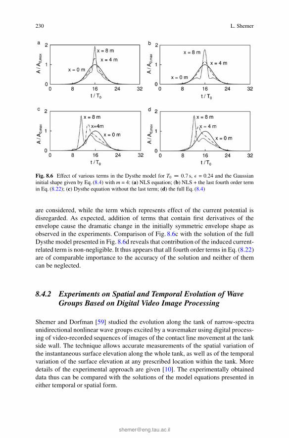
230 L. Shemer
Fig. 8.6 Effect of various terms in the Dysthe model for T0 D 0:7 s, � = 0.24 and the Gaussianinitial shape given by Eq. (8.4) with m = 4: (a) NLS equation; (b) NLS + the last fourth order termin Eq. (8.22); (c) Dysthe equation without the last term; (d) the full Eq. (8.4)
are considered, while the term which represents effect of the current potential isdisregarded. As expected, addition of terms that contain first derivatives of theenvelope cause the dramatic change in the initially symmetric envelope shape asobserved in the experiments. Comparison of Fig. 8.6c with the solution of the fullDysthe model presented in Fig. 8.6d reveals that contribution of the induced current-related term is non-negligible. It thus appears that all fourth order terms in Eq. (8.22)are of comparable importance to the accuracy of the solution and neither of themcan be neglected.
8.4.2 Experiments on Spatial and Temporal Evolution of WaveGroups Based on Digital Video Image Processing
Shemer and Dorfman [59] studied the evolution along the tank of narrow-spectraunidirectional nonlinear wave groups excited by a wavemaker using digital process-ing of video-recorded sequences of images of the contact line movement at the tankside wall. The technique allows accurate measurements of the spatial variation ofthe instantaneous surface elevation along the whole tank, as well as of the temporalvariation of the surface elevation at any prescribed location within the tank. Moredetails of the experimental approach are given [10]. The experimentally obtaineddata thus can be compared with the solutions of the model equations presented ineither temporal or spatial form.
8 Analysis of Nonlinear Water-Waves 231
The wave gauges in this study were applied mainly for validation of the accuracyof surface elevation measurements by digital processing of video clips that recordthe contact line movement at the tank’s wall. The instantaneous contact line shapeswere recorded by a single monochrome CCD video camera at a rate of 30 fps. Thefield of view of the camera spanned 50 cm along the tank. The spatial resolutionwas about 0.8 mm/pixel. Advantage was taken of extremely high repeatability ofthe wave field emanating from the prescribed wavemaker driving signal. The camerawas placed on the instrument carriage to enable imaging of different regions of thetank. Each camera recording session was synchronized with the wavemaker drivingsignal using a common reference signal. A single wave group was generated foreach recording session. For consecutive recording session, the carriage was shiftedalong the tank, so that slightly overlapping images of the contact line movementalong the whole experimental facility were obtained. Every frame of the recordedvideo clip at each camera location was processed separately.
Experiments were performed for a wave group with Gaussian envelope givenby Eq. (8.4) generated by the wavemaker. The selected dominant wave periodT0 D 0:7 s corresponds to the wave length �0 D 0:76m. The value of m D 3:5
in Eq. (8.4) corresponds to the spectral width that is sufficient to satisfy the narrowspectrum constraint for the applicability of the Dysthe equation. On the other hand,the spatial extent of the group is short enough to enable studying of the temporalevolution of the group within the tank. To determine the instantaneous spatialenvelope shape of the wave group and to study its nonlinear temporal evolution, theentire group has to be present in the tank. Hence, on one hand, the group generationby the wavemaker has to be completed before initiation of the study of the temporalvariation of the envelope shape, and on the other hand, measurements of spatialwave group structure remain meaningful as long as the front of the group doesnot reach the beach. The group propagates along the tank with the group velocitycg D 0:54m=s. The length of the group for the adopted parameters does not exceed6–7 m. When the generation of the group by the wavemaker is completed, the groupfront is about 5 m from the beach, leaving the duration that does not exceed 10 sto study the wave group evolution before its front reaches the far end of the tank.According to Eq. (8.7), the time scale of the nonlinear effects is O.�2/. Hence, for theduration of the process prescribed by the group shape, the dominant frequency andthe length of the tank, higher wave steepness increases the effective evolution timeat the slow scale � . To eliminate breaking not accounted for by the Dysthe model,the wave steepness must not exceed the value that can lead to wave breaking. Themaximum adopted initial wave steepness of � D 0:18 (a0 D 22mm) was selectedon the basis of visual observations of wave group propagation along the tank withdifferent values of a0. For this value of �; � D1 corresponds to dimensional durationt D 3:44 s, or 4.9 dominant wave periods. This is well below the experiment durationlimit of about 7 s imposed by the effective length of the tank.
In the spatial evolution formulation the initial condition emerges naturally fromthe water surface elevation variation in time excited by a wavemaker located atx D 0. In the temporal evolution case the initial conditions defining the wave field inthe whole tank are to be prescribed at a certain instant. One possibility to define the
232 L. Shemer
initial conditions for the temporal formulation of the problem is to use the actuallymeasured instantaneous wave field when the whole group emerges in the tank. Fora relatively short wave tank used in the present study this option, however, severelyrestricts the duration of the wave group evolution and thus the role of nonlinearitythat is in the center of the study. An alternative approach was therefore employed.Since nonlinear effects become prominent at slow scales, it can be assumed thatthe initial evolution of the wave group is mainly governed by linear dispersioneffects, while nonlinearity can be neglected. This assumption enables linearizationof Eq. (8.12), yielding
@A
@XC i
@2A
@�2D 0: (8.27)
Following [49], the solution of Eq. (8.27) for a Gaussian envelope at the wavemakergiven by Eq. (8.4) can be written in the physical variables .x; t/ as
A.x; t/ D jA.x; t/jexp.i�/I (8.28)
where the amplitude jA.x; t/j and the phase � of the envelope are given by
jA.x; t/j D m�
4
qm4�4 C 4k20x
2
exp �
m2�2
4.m4�4 C 4k20x2/.!0t � 2k0x/
2
�(8.29)
� D k0x.!0t � 2k0x/2
2.m4�4 C 4k20x2/
� 1
2tan�1.
2k0x
m2�2/: (8.30)
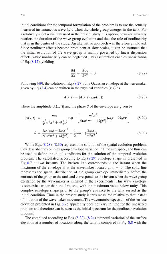
While Eqs. (8.28)–(8.30) represent the solution of the spatial evolution problem;they describe the complex group envelope variation in time and space, and thus canbe used to define the initial conditions for the solution of the temporal evolutionproblem. The calculated according to Eq. (8.29) envelope shape is presented inFig. 8.7 at two instants. The broken line corresponds to the instant when themaximum of the envelope is at the wavemaker located at x D 0. The solid linerepresents the spatial distribution of the group envelope immediately before theentrance of the group to the tank and corresponds to the instant when the wave groupexcitation by the wavemaker is initiated in the experiments. This wave envelopeis somewhat wider than the first one, with the maximum value below unity. Thiscomplex envelope shape prior to the group’s entrance to the tank served as theinitial condition. Time in the present study is thus measured relative to that instantof initiation of the wavemaker movement. The wavenumber spectrum of the surfaceelevation presented in Fig. 8.7b apparently does not vary in time for the linearizedproblem and therefore can be seen as the initial spectrum for the nonlinear evolutionproblem.
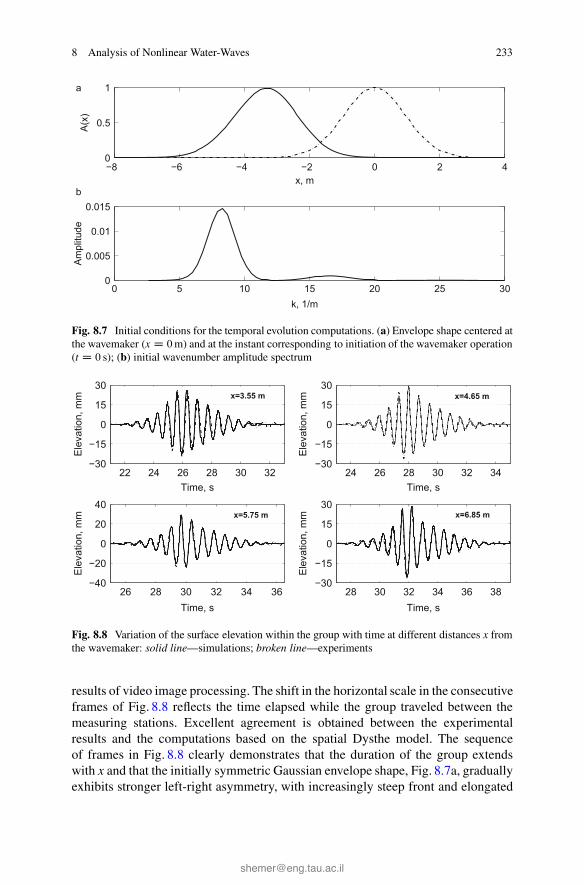
The computed according to Eqs. (8.22)–(8.24) temporal variation of the surfaceelevation at a number of locations along the tank is compared in Fig. 8.8 with the
8 Analysis of Nonlinear Water-Waves 233
−8 −6 −4 −2 0 2 40
0.5
1
x, m
A(x
)
0 5 10 15 20 25 300
0.005
0.01
0.015
k, 1/m
Am
plitu
de
b
a
Fig. 8.7 Initial conditions for the temporal evolution computations. (a) Envelope shape centered atthe wavemaker (x D 0m) and at the instant corresponding to initiation of the wavemaker operation(t D 0 s); (b) initial wavenumber amplitude spectrum
22 24 26 28 30 32−30
−15
0
15
30
Time, s
Ele
vatio
n, m
m
24 26 28 30 32 34−30
−15
0
15
30
Time, s
Ele
vatio
n, m
m
26 28 30 32 34 36−40
−20
0
20
40
Time, s
Ele
vatio
n, m
m
28 30 32 34 36 38−30
−15
0
15
30
Time, s
Ele
vatio
n, m
m x=6.85 mx=5.75 m
x=3.55 m x=4.65 m
Fig. 8.8 Variation of the surface elevation within the group with time at different distances x fromthe wavemaker: solid line—simulations; broken line—experiments
results of video image processing. The shift in the horizontal scale in the consecutiveframes of Fig. 8.8 reflects the time elapsed while the group traveled between themeasuring stations. Excellent agreement is obtained between the experimentalresults and the computations based on the spatial Dysthe model. The sequenceof frames in Fig. 8.8 clearly demonstrates that the duration of the group extendswith x and that the initially symmetric Gaussian envelope shape, Fig. 8.7a, graduallyexhibits stronger left-right asymmetry, with increasingly steep front and elongated
234 L. Shemer
0 0.5 1 1.5 2 2.5 3 3.50
4
8
Frequency, Hz
Am
plitu
de, m
m
0 0.5 1 1.5 2 2.5 3 3.50
4
8
Frequency, Hz
Am
plitu
de, m
m
0 0.5 1 1.5 2 2.5 3 3.50
4
8
Frequency, Hz
Am
plitu
de, m
m
0 0.5 1 1.5 2 2.5 3 3.50
4
8
Frequency, Hz
Am
plitu
de, m
m
x=3.55 m
x=5.75 m x=6.85 m
x=4.65 m
Fig. 8.9 Variation of the frequency spectra along the tank: symbols—experiments, line—simulations
tail. This behavior is consistent with that plotted in Fig. 8.5. The maximum surfaceelevation within the group may exceed significantly the nominal value of a0. Thisincrease of the maximum amplitude is associated in part with the focusing propertiesof the NLS equation as discussed in Sect. 8.3. An apparent additional reason forhigher maximum values of the surface elevation in Fig. 8.8, as well as for the crest-trough asymmetry, is the contribution of the second order bound (locked) waves.
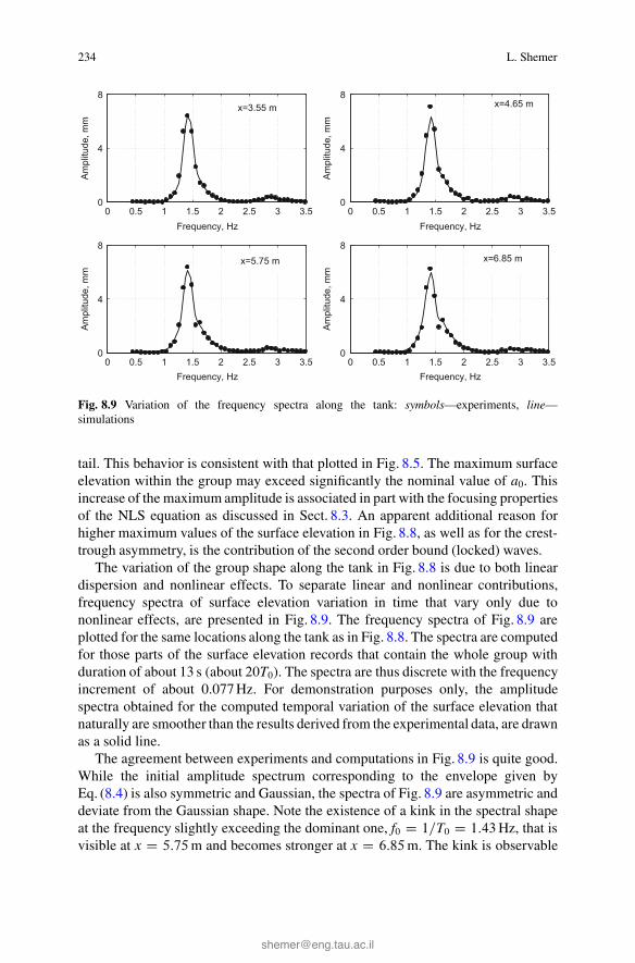
The variation of the group shape along the tank in Fig. 8.8 is due to both lineardispersion and nonlinear effects. To separate linear and nonlinear contributions,frequency spectra of surface elevation variation in time that vary only due tononlinear effects, are presented in Fig. 8.9. The frequency spectra of Fig. 8.9 areplotted for the same locations along the tank as in Fig. 8.8. The spectra are computedfor those parts of the surface elevation records that contain the whole group withduration of about 13 s (about 20T0). The spectra are thus discrete with the frequencyincrement of about 0.077 Hz. For demonstration purposes only, the amplitudespectra obtained for the computed temporal variation of the surface elevation thatnaturally are smoother than the results derived from the experimental data, are drawnas a solid line.
The agreement between experiments and computations in Fig. 8.9 is quite good.While the initial amplitude spectrum corresponding to the envelope given byEq. (8.4) is also symmetric and Gaussian, the spectra of Fig. 8.9 are asymmetric anddeviate from the Gaussian shape. Note the existence of a kink in the spectral shapeat the frequency slightly exceeding the dominant one, f0 D 1=T0 D 1:43Hz, that isvisible at x D 5:75m and becomes stronger at x D 6:85m. The kink is observable

8 Analysis of Nonlinear Water-Waves 235
both in the measured and in the computed spectra. Even for a relatively short extentof the spatial evolution, widening of the spectrum is visible in Fig. 8.9. This spectralwidening and non-Gaussian spectral shape indicate that nonlinearity is essential inthe wave group evolution along the tank.
The contribution of the second order bound waves to the amplitude spectrum isquite significant at all locations. The measured using the digital processing of thevideo images spectrum of bound waves around the second harmonic of the dominantfrequency f0 is in excellent agreement with the model predictions. The bound waves’spectrum also becomes wider with the distance from the wavemaker, in agreementwith the variation of the free wave spectrum around the dominant frequency f0.
As stressed above, the main motivation for developing the data acquisitionmethod based on the processing of sequences of video images is in its capabilityto measure instantaneous spatial distribution of the surface elevation. Applicationof this method enables following the temporal evolution of the whole wave group aswell. This information can be compared with the numerical solution of the systemof Eqs. (8.18)–(8.21) that constitute the Dysthe model in its temporal formulation.The initial conditions for the temporal evolution case A.x; 0/ are obtained usingEqs.(8.28)–(8.30), as presented in Fig. 8.7.
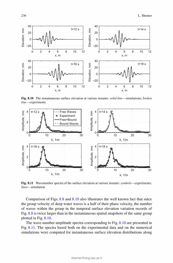
It should be stressed that direct juxtaposing of the theoretical and the experimen-tal results on the temporal evolution of a wave field is quite challenging since it islimited to the time interval when the whole group is physically present within thewave tank boundaries. The numerical solution of Eqs. (8.18)–(8.21) indicates thatat the dimensional time t D 12 s (relative to the instant depicted in Fig. 8.7) theadvancement of the group along the tank is sufficient for the tail of the computedinstantaneous spatial envelope distribution to emerge within the tank, thus enablingcomparison with the experiment. Similarity of the numerical and the experimentalresults is examined also at three additional instants: t D 14 s; 16 s and 18 s.Equations (8.25), (8.26) are used again to account for the contribution of the secondorder bound waves.
The spatial variation of the surface elevation as a result of the temporal evolutionof the complex wave envelope is presented at the selected instances in Fig. 8.10.As in the spatial evolution case, good agreement is obtained between the numericalsimulations and the experimental observations. At the earliest instant presented inFig. 8.10, t D 12 s, the formation of the group has just been completed and the groupin its entirety emerges in the tank, while at the last instant, t D 18 s, the front of thegroup approaches the far end of the wave tank.
Deviation of the group shape in Fig. 8.10 from the initial envelope presentedin Fig. 8.7a is obvious. Both left-right and trough-crest asymmetries observed inthe temporal records presented in Fig. 8.8, as well as significant variations in theextreme values of the surface elevation within the group, are visible in Fig. 8.10 aswell. Note, however, that the left-right asymmetry in Fig. 8.10 is opposite to that ofFig. 8.8, where the steeper part of the group appears at earlier sampling times. Theexperimental results are in agreement with the numerical solutions of the temporalDysthe model.
236 L. Shemer
0 2 4 6 8 10 12
−20
0
20
40
x, m
Ele
vatio
n, m
m
0 2 4 6 8 10 12
−20
0
20
40
x, m
Ele
vatio
n, m
m0 2 4 6 8 10 12
−20
0
20
40
x, m
Ele
vatio
n, m
m
0 2 4 6 8 10 12
−20
0
20
40
x, mE
leva
tion,
mm
t=12 s
t=18 s
t=14 s
t=16 s
Fig. 8.10 The instantaneous surface elevation at various instants: solid line—simulations; brokenline—experiments
0 10 20 300
2
4
k, 1/m
Am
plitu
de, m
m
0 10 20 300
2
4
k, 1/m
Am
plitu
de, m
m
0 10 20 300
2
4
k, 1/m
Am
plitu
de, m
m
0 10 20 300
2
4
k, 1/m
Am
plitu
de, m
m
Free WavesExperimentFree+BoundBound Waves
t=12 s
t=16 s
t=14 s
t=18 s
Fig. 8.11 Wavenumber spectra of the surface elevation at various instants: symbols—experiments;lines—simulation
Comparison of Figs. 8.8 and 8.10 also illustrates the well known fact that sincethe group velocity of deep water waves is a half of their phase velocity, the numberof waves within the group in the temporal surface elevation variation records ofFig. 8.8 is twice larger than in the instantaneous spatial snapshots of the same groupplotted in Fig. 8.10.
The wave-number amplitude spectra corresponding to Fig. 8.10 are presented inFig. 8.11. The spectra based both on the experimental data and on the numericalsimulations were computed for instantaneous surface elevation distributions along
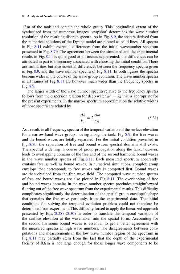
8 Analysis of Nonlinear Water-Waves 237
12 m of the tank and contain the whole group. This longitudinal extent of thesynthesized from the numerous images ‘snapshot’ determines the wave numberresolution of the resulting discrete spectra. As in Fig. 8.9, the spectra derived fromthe numerical solutions of the Dysthe model are plotted as solid lines. All spectrain Fig. 8.11 exhibit essential differences from the initial wavenumber spectrumpresented in Fig. 8.7b. The agreement between the simulated and the experimentalresults in Fig. 8.11 is quite good at all instances presented; the differences can beattributed in part to inaccuracy associated with choosing the initial condition. Thereare similarities but also essential differences between the frequency spectra givenin Fig. 8.9, and the wave number spectra of Fig. 8.11. In both figures the spectrabecome wider in the course of the wave group evolution. The wave number spectrain all frames of Fig. 8.11 are however much wider than the frequency spectra inFig. 8.9.
The larger width of the wave number spectra relative to the frequency spectrafollows from the dispersion relation for deep water !2 D kg that is appropriate forthe present experiments. In the narrow spectrum approximation the relative widthsof those spectra are related by
�k
k0D 2
�!
!0(8.31)
As a result, in all frequency spectra of the temporal variation of the surface elevationfor a narrow-band wave group moving along the tank, Fig. 8.9, the free wavesand the bound waves are totally separated. For the initial condition presented inFig. 8.7b, the separation of free and bound waves spectral domains still exists.The spectral widening in course of group propagation along the tank, however,leads to overlapping domains of the free and of the second harmonic bound wavesin the wave number spectra of Fig. 8.11. Each measured spectrum apparentlycontains free as well as bound waves. In numerical simulations, complex groupenvelope that corresponds to free waves only is computed first. Bound wavesare then obtained from the free wave field. The computed wave number spectraof free and bound waves are also plotted in Fig. 8.11. The overlapping of freeand bound waves domains in the wave number spectra precludes straightforwardfiltering out of the free wave spectrum from the experimental results. This difficultycomplicates significantly the determination of the spatial group envelope’s shapethat contains the free-wave part only, from the experimental data. The initialconditions for solving the temporal evolution problem could not therefore bedetermined from experiment. This difficulty forced to apply the linearized approachpresented by Eqs. (8.28)–(8.30) in order to translate the temporal variation ofthe surface elevation at the wavemaker into the spatial form. Accounting forthe second harmonic bound waves is essential to get a better agreement withthe measured spectra at high wave numbers. The disagreements between com-putations and measurements in the low wave number region of the spectrum inFig. 8.11 may partially stem from the fact that the depth of the experimentalfacility of 0.6 m is not large enough for those longer wave components to be
238 L. Shemer
considered deep. The low wave number bound waves may become significantand can constitute a important contribution to the spectral shape. The validityof Dysthe equation that served as the theoretical model in the present study,however, is restricted to deep waves. The long bound waves were therefore notconsidered.
Theoretical studies of nonlinear water-waves are often performed by solvingtemporal evolution models, while in laboratory as well as in field experiments sur-face elevation variation with time at fixed locations is usually recorded; sometimesthese data also contain information on the wave propagation directions. Attemptsare sometimes made to translate the measured by point sensors frequency spectruminto the corresponding wave number (or wave vector in the two-dimensional case)spectrum. However, direct quantitative comparison of the frequency and the wavenumber spectra can not be carried out in a consistent way. Instantaneous snapshotof the whole wave field taken to get the wave number spectrum, on one hand, andmeasurements of the temporal variation of the surface elevation variation with timeat a fixed location to get the wave frequency spectrum, on the other hand, constituteessentially different ways of studying an evolving in space and in time water-wavefield.
Moreover, as demonstrated in this section, direct computation of the wavenumber spectrum from the measured frequency spectrum can not be carried outeven assuming that the evolution is slow as compared to the relevant temporalscale (represented by the duration of continuous sampling that determines thefrequency resolution of the spectrum) and the spatial scale (the extent of theimaged wave field that determines the wave number spatial resolution) of the dataacquisition process. The linear dispersion relation between wave frequencies andwave numbers only holds for the free wave components. Therefore, it is possiblein principle to relate quantitatively frequency and wave number spectra for thefree wave domain only. Comparison of the frequencies and wave numbers thatcorrespond to the spectrum peaks and clearly represent free waves in Figs. 8.9 and8.11, respectively, indeed reveals that they are related by the deep water dispersionrelation. The present results, however, demonstrate that in general separation ofthe wave number spectra into free and bound waves is not always possible. Fora relatively narrow initial free-wave spectrum, the high frequency/wave numberpart of the spectrum consists almost exclusively of bound components. Thecalculation of spectral bound components from the free wave spectrum is oftennot straightforward and requires information on the phases of each free wavecomponent. Such information is usually not readily available in reported data onthe experimentally measured frequency spectra. It thus appears virtually impossibleto evaluate quantitatively the shape of the high end of the wave number spectrumfrom the measured surface elevation variation in time at a fixed location and thecorresponding frequency spectrum the shape of the high end of the wave numberspectrum.
8 Analysis of Nonlinear Water-Waves 239
8.4.3 Experimental Studies of Evolution of Peregrine Breather
Shemer and Alperovich [57] applied both NLS and Dysthe models to the problem ofextremely steep freak (or rogue) waves. A possibility to generate deterministic steepwaves is of special interest. The NLS equation attracts considerable interest in thisrespect since it admits breather type soliton solutions. The so-called Kuznetsov-Mabreathing solitons present spatially localized patterns that oscillate in time [30, 36].Akhmediev breather [1] is a related type of solitons that is periodic in space. Whenthe periodicity in time and space tends to infinity, both these types of solution tendto a simple Peregrine soliton [50] that is localized in time and space and breathesonly once. In scaled variables, Eq. (8.7), the complex envelope of Peregrine breather(PB) is written as
A.X; �/ D �p2
1 � 4.1� 4iX/
1C 4�2 C 16X2
�e�2iX : (8.32)
At the origin of the scaled coordinate system A.0; 0/ D 3p2 , and A.X !
˙1; � ! ˙1/ D p2 , so the maximum wave amplitude at the origin exceeds the
background amplitude by a factor of 3.Experimental observations of PB for water waves were recently presented in
several publications, see, e.g. [8]. These observations show that an initially small“hump” in a nearly monochromatic wave train may indeed evolve along the tankin a qualitative agreement with Eq. (8.32). Nevertheless, some marked quantitativedifferences between experiments and calculations could not be attributed solely toexperimental inaccuracy. The Peregrine breather was suggested as a major routeto deterministic freak waves’ generation [70]. The importance of PB for freakwater waves prompted a closer experimental investigation of its qualitative andquantitative characteristics.
Measurements of wave group evolution along the TAU tank were performed at 72locations along the tank, up to the distance of 13.3 m from the wavemaker. At everycarriage location, three realizations of the prescribed wave field were recorded,with the sufficient time delay between the consecutive events to ensure decay ofany disturbances left in the tank from the previous run. Each measurement session,including probe calibration, wave generation, data recording and carriage movementwas performed automatically utilizing a LabView program.
Selection of wave parameters in any given experimental facility is largelyprescribed by the scaling relations given by Eq. (8.7). To enable investigation ofthe wave form evolution up to the maximum amplification and beyond, as well asin order to mitigate the effect of contamination by reflected waves that cannot befully eliminated, the maximum amplification location x0 should be sufficiently farfrom the end of the tank. For the TAU facility, this means that X0 should not exceedabout 10 m. The values of A.X; �/ defined by Eq. (8.32) differ notably from thebackground envelope only for X < 1. Noticeable variation of the breather maximumbetween the wavemaker at x D 0 and X0 can be expected if X.x0/ D �2k0x0 D O.1/,
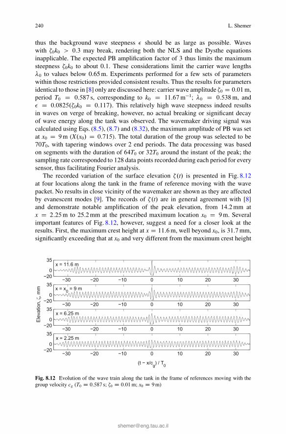
240 L. Shemer
thus the background wave steepness � should be as large as possible. Waveswith �0k0 > 0:3 may break, rendering both the NLS and the Dysthe equationsinapplicable. The expected PB amplification factor of 3 thus limits the maximumsteepness �0k0 to about 0.1. These considerations limit the carrier wave lengths�0 to values below 0.65 m. Experiments performed for a few sets of parameterswithin those restrictions provided consistent results. Thus the results for parametersidentical to those in [8] only are discussed here: carrier wave amplitude �0 D 0:01m,period T0 D 0:587 s, corresponding to k0 D 11:67m�1; �0 D 0:538m, and� D 0:0825.�0k0 D 0:117/. This relatively high wave steepness indeed resultsin waves on verge of breaking, however, no actual breaking or significant decayof wave energy along the tank was observed. The wavemaker driving signal wascalculated using Eqs. (8.5), (8.7) and (8.32), the maximum amplitude of PB was setat x0 D 9m (X.x0/ D 0:715). The total duration of the group was selected to be70T0, with tapering windows over 2 end periods. The data processing was basedon segments with the duration of 64T0 or 32T0 around the instant of the peak; thesampling rate corresponded to 128 data points recorded during each period for everysensor, thus facilitating Fourier analysis.
The recorded variation of the surface elevation �.t/ is presented in Fig. 8.12at four locations along the tank in the frame of reference moving with the wavepacket. No results in close vicinity of the wavemaker are shown as they are affectedby evanescent modes [9]. The records of �.t/ are in general agreement with [8]and demonstrate notable amplification of the peak elevation, from 14.2 mm atx D 2:25m to 25.2 mm at the prescribed maximum location x0 D 9m. Severalimportant features of Fig. 8.12, however, suggest a need for a closer look at theresults. First, the maximum crest height at x D 11:6m, well beyond x0, is 31.7 mm,significantly exceeding that at x0 and very different from the maximum crest height
−30 −20 −10 0 10 20 30−20
0
35
−30 −20 −10 0 10 20 30−20
0
35
−30 −20 −10 0 10 20 30−20
0
35
Ele
vatio
n,ζ,
mm
−30 −20 −10 0 10 20 30−20
0
35
(t − x/cg) / T0
x = 11.6 m
x = 2.25 m
x = 6.25 m
x = x0 = 9 m
Fig. 8.12 Evolution of the wave train along the tank in the frame of references moving with thegroup velocity cg (T0 D 0:587 s; �0 D 0:01m; x0 D 9m)
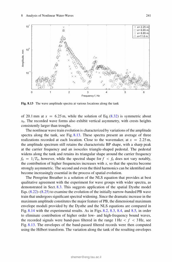
8 Analysis of Nonlinear Water-Waves 241
0 1 2 3 4 5 6
10−1
100
101
Frequency f, Hz
Am
plitu
de, m
m
x= 2.25 mx= 6.65 mx= 8.85 mx=11.6 m
Fig. 8.13 The wave amplitude spectra at various locations along the tank
of 20.1 mm at x D 6:25m, while the solution of Eq. (8.32) is symmetric aboutx0. The recorded wave forms also exhibit vertical asymmetry, with crests heightsconsistently larger than troughs.
The nonlinear wave train evolution is characterized by variations of the amplitudespectra along the tank, see Fig. 8.13. These spectra present an average of threerealizations recorded at each location. Close to the wavemaker, at x D 2:25m,the amplitude spectrum still retains the characteristic BP shape, with a sharp peakat the carrier frequency and an isosceles triangle-shaped pedestal. The pedestalwidens along the tank and retains its triangular shape around the carrier frequencyf0 D 1=T0, however, while the spectral shape for f < f0 does not vary notably,the contribution of higher frequencies increases with x, so that the spectra becomestrongly asymmetric. The second and even the third harmonics can be identified andbecome increasingly essential in the process of spatial evolution.
The Peregrine Breather is a solution of the NLS equation that provides at bestqualitative agreement with the experiment for wave groups with wider spectra, asdemonstrated in Sect. 8.3. This suggests application of the spatial Dysthe modelEqs. (8.22)–(8.25) to examine the evolution of the initially narrow-banded PB wavetrain that undergoes significant spectral widening. Since the dramatic increase in themaximum amplitude constitutes the major feature of PB, the dimensional maximumenvelope moduli provided by the Dysthe and the NLS equations are compared inFig. 8.14 with the experimental results. As in Figs. 8.2, 8.3, 8.4, and 8.5, in orderto eliminate contribution of higher order low- and high-frequency bound waves,the recorded signals were band-pass filtered in the range 1 Hz < f < 3 Hz, seeFig. 8.13. The envelopes of the band-passed filtered records were then computedusing the Hilbert transform. The variation along the tank of the resulting envelopes
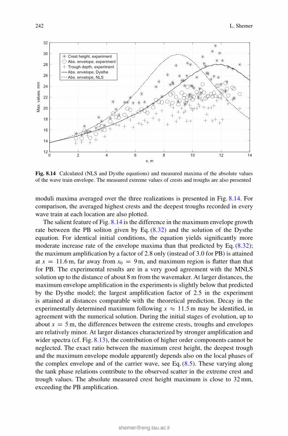
242 L. Shemer
0 2 4 6 8 10 12 1412
14
16
18
20
22
24
26
28
30
32
x, m
Max
. val
ues,
mm
Crest height, experimentAbs. envelope, experimentTrough depth, experimentAbs. envelope, DystheAbs. envelope, NLS
Fig. 8.14 Calculated (NLS and Dysthe equations) and measured maxima of the absolute valuesof the wave train envelope. The measured extreme values of crests and troughs are also presented
moduli maxima averaged over the three realizations is presented in Fig. 8.14. Forcomparison, the averaged highest crests and the deepest troughs recorded in everywave train at each location are also plotted.
The salient feature of Fig. 8.14 is the difference in the maximum envelope growthrate between the PB soliton given by Eq. (8.32) and the solution of the Dystheequation. For identical initial conditions, the equation yields significantly moremoderate increase rate of the envelope maxima than that predicted by Eq. (8.32);the maximum amplification by a factor of 2.8 only (instead of 3.0 for PB) is attainedat x D 11:6m, far away from x0 D 9m, and maximum region is flatter than thatfor PB. The experimental results are in a very good agreement with the MNLSsolution up to the distance of about 8 m from the wavemaker. At larger distances, themaximum envelope amplification in the experiments is slightly below that predictedby the Dysthe model; the largest amplification factor of 2.5 in the experimentis attained at distances comparable with the theoretical prediction. Decay in theexperimentally determined maximum following x 11:5m may be identified, inagreement with the numerical solution. During the initial stages of evolution, up toabout x D 5m, the differences between the extreme crests, troughs and envelopesare relatively minor. At larger distances characterized by stronger amplification andwider spectra (cf. Fig. 8.13), the contribution of higher order components cannot beneglected. The exact ratio between the maximum crest height, the deepest troughand the maximum envelope module apparently depends also on the local phases ofthe complex envelope and of the carrier wave, see Eq. (8.5). These varying alongthe tank phase relations contribute to the observed scatter in the extreme crest andtrough values. The absolute measured crest height maximum is close to 32 mm,exceeding the PB amplification.
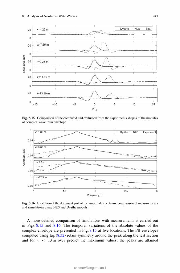
8 Analysis of Nonlinear Water-Waves 243
0
20
0
20
0
20
0
20
−15 −10 −5 0 5 10 150
20
t /T0
Env
elop
e, m
m
Dysthe NLS Exp.x=4.25 m
x=7.65 m
x=9.25 m
x=11.65 m
x=13.30 m
Fig. 8.15 Comparison of the computed and evaluated from the experiments shapes of the modulesof complex wave train envelope
0.05
11
0.05
11
0.05
11
Am
plitu
de, m
m
1 1.5 2 2.5 3
0.05
11
Frequency, Hz
Dysthe NLS Experiment
x=12.9 m
x= 9.0 m
x= 5.65 m
x= 1.85 m
Fig. 8.16 Evolution of the dominant part of the amplitude spectrum: comparison of measurementsand simulations using NLS and Dysthe models
A more detailed comparison of simulations with measurements is carried outin Figs. 8.15 and 8.16. The temporal variations of the absolute values of thecomplex envelope are presented in Fig. 8.15 at five locations. The PB envelopescomputed using Eq. (8.32) retain symmetry around the peak along the test sectionand for x < 13m over predict the maximum values; the peaks are attained

244 L. Shemer
somewhat later as compared to the Dysthe model. Good quantitative agreementexists between experiments and computations based on Eqs. (8.22)–(8.25) up tox D 9:25m. The mNLS model correctly describes the wave group asymme-try around the peak value, with the front being much steeper than the back.The discrepancies between the experimental and numerical results then increasewith x.
The evolution of the computed and the measured spectra with the distance fromthe wavemaker is demonstrated in Fig. 8.16. Only the leading order part of thespectrum around the carrier wave frequency directly computed from the numericalsimulations is plotted. The results of simulations are in excellent agreementwith experiments at all locations. The higher frequency part of the PB NLSspectrum agrees with experiment and with the Dysthe computations up to theprescribed maximum at x0 D 9m. Beyond this point, the higher frequency partof the NLS-derived spectrum starts to shrink, no such decrease is observed inFig. 8.16 in the measured spectral amplitudes and in MNLS results. Up to x0,the lower frequency part of the spectrum is significantly below the NLS-derivedprediction. After the maximum wave train height is attained, the bottom plateindicates that the spectral widening becomes more prominent at lower frequen-cies.
These results thus demonstrate significant quantitative and qualitative differencesbetween the spatial evolution of the NLS Peregrine soliton and the experiments.The measurements confirm that due to the focusing properties of the NLSequation, a small hump in a nearly monochromatic wave train can indeedbe amplified as suggested by the PB solution. The amplification, however, isslower and weaker than predicted, so that the maximum gain of less than 3 isattained farther away than the PB maximum. The growth in the wave height isaccompanied by a significant spectral widening, initially at frequencies exceedingf0 and then at lower frequencies. As was the case with other initially narrow-banded wave group shapes considered in Sect. 8.3, this widening violates thebasic assumptions in the derivation of the NLS equation for water gravity waves.As the wave spectrum widens and becomes increasingly asymmetric with thedistance, the deviation of the PB NLS-derived wave and spectral shapes fromthose observed in the experiments and in the solutions of Dysthe equationenhances.
The relatively simple Dysthe model thus captures accurately fine details ofthe observed wave field evolution even for peak steepness approaching breakingconditions. The remarkable feature of the NLS Peregrine soliton is its reversibility.The results presented above suggest, however, that the wave height growth is notreversible. Both the available experimental data and Dysthe simulations show thatthe decrease in the maximum wave height following the maximum is only partial.The soliton observed in the experiments and described fairly well by the Dysthemodel in fact does not ‘breathe’.
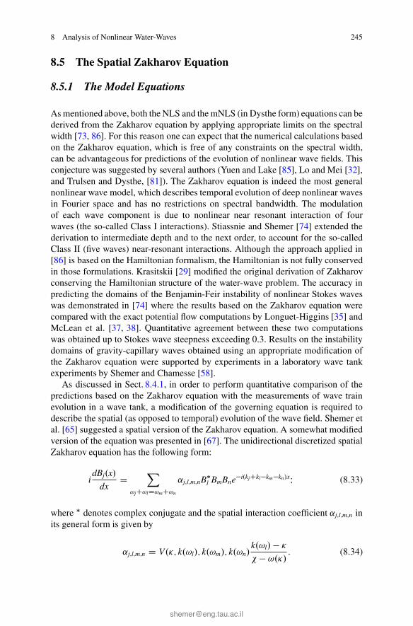
8 Analysis of Nonlinear Water-Waves 245
8.5 The Spatial Zakharov Equation
8.5.1 The Model Equations
As mentioned above, both the NLS and the mNLS (in Dysthe form) equations can bederived from the Zakharov equation by applying appropriate limits on the spectralwidth [73, 86]. For this reason one can expect that the numerical calculations basedon the Zakharov equation, which is free of any constraints on the spectral width,can be advantageous for predictions of the evolution of nonlinear wave fields. Thisconjecture was suggested by several authors (Yuen and Lake [85], Lo and Mei [32],and Trulsen and Dysthe, [81]). The Zakharov equation is indeed the most generalnonlinear wave model, which describes temporal evolution of deep nonlinear wavesin Fourier space and has no restrictions on spectral bandwidth. The modulationof each wave component is due to nonlinear near resonant interaction of fourwaves (the so-called Class I interactions). Stiassnie and Shemer [74] extended thederivation to intermediate depth and to the next order, to account for the so-calledClass II (five waves) near-resonant interactions. Although the approach applied in[86] is based on the Hamiltonian formalism, the Hamiltonian is not fully conservedin those formulations. Krasitskii [29] modified the original derivation of Zakharovconserving the Hamiltonian structure of the water-wave problem. The accuracy inpredicting the domains of the Benjamin-Feir instability of nonlinear Stokes waveswas demonstrated in [74] where the results based on the Zakharov equation werecompared with the exact potential flow computations by Longuet-Higgins [35] andMcLean et al. [37, 38]. Quantitative agreement between these two computationswas obtained up to Stokes wave steepness exceeding 0.3. Results on the instabilitydomains of gravity-capillary waves obtained using an appropriate modification ofthe Zakharov equation were supported by experiments in a laboratory wave tankexperiments by Shemer and Chamesse [58].
As discussed in Sect. 8.4.1, in order to perform quantitative comparison of thepredictions based on the Zakharov equation with the measurements of wave trainevolution in a wave tank, a modification of the governing equation is required todescribe the spatial (as opposed to temporal) evolution of the wave field. Shemer etal. [65] suggested a spatial version of the Zakharov equation. A somewhat modifiedversion of the equation was presented in [67]. The unidirectional discretized spatialZakharov equation has the following form:
idBj.x/
dxD
X
!jC!lD!mC!n
˛j;l;m;nB�l BmBne�i.kjCkl�km�kn/xI (8.33)
where � denotes complex conjugate and the spatial interaction coefficient ˛j;l;m;n inits general form is given by
˛j;l;m;n D V.�; k.!l/; k.!m/; k.!n/k.!l/� �
� � !.�/: (8.34)
246 L. Shemer
Here � D k.!m/ C k.!n/ � k.!l/ and � D !m C !n � !l: In Eq. (8.34), thevalues of V represent the quartet interaction coefficient in the temporal Zakharovequation as given by Krasitskii [29]. Equations (8.33), (8.34) accurately describethe slow evolution along the tank of each free spectral component Bj D B.!j/ of thesurface elevation spectrum in inviscid fluid of constant (infinite or finite) depth. Thedependent variables B.!j; x/ are related to the generalized complex “amplitudes”a.!j; x/ composed of the Fourier transforms of the surface elevation O�.!j; x/ and ofthe velocity potential at the free surface O .!j; x/:
a.!; x/ D .g
2!/1=2 O�.!; x/C i.
!
2g/1=2 O .!; x/ (8.35)
The amplitudes a.!j/ can be seen as consisting of a sum of free and the boundwaves. The appropriate modification of Eq. (8.26) is
a.!j; x/ D ��B.!j; x/C �2B0.!j; x/C �3B00.!j; x/
�eikx (8.36)
The higher order bound components B0 and B00 can be computed at each locationonce the free wave solution Bj.x/ is known. Only bound waves of the second orderresulting from interactions of all possible wave pairs i and j; i; j D 1; : : :N, areconsidered here. Those waves have frequencies !i C !j and !i � !j . The phasevelocity of these components depends on the parent free waves and can not bedetermined using Eq. (8.6). The corresponding formulae, as well as the kernelsnecessary for their computations are given in [29, 74]. Expressions given in theAppendix of [74] are used for computation of the second order bound waves.Inversion of Eq. (8.35) allows computing the Fourier components of the surfaceelevation. Inverse Fourier transform then yields the temporal variation for thesurface elevation �.
The spatial Zakharov equation given by Eqs. (8.33)–(8.35) was verified experi-mentally by Shemer et al. [65]. As in Sect. 8.3, the simplest possible initial wavetrains were considered given by Eqs. (8.2)–(8.4). The experiments were performedin the TAU wave tank described in Sect. 8.2. Similarly to [64], two carrier waveperiods, T0 D 0:7 s and T0 D 0:9 s were employed in the experiments.
The wave train excited by a bi-chromatic driving signal given by Eq. (8.2) withcarrier wave period T0 D 0:9 applied at the water depth h D 0:6m for the highamplitude case, � D 0:21, is studied in Fig. 8.17. Note that the dimensionless depthk0h D 3:0 in this case corresponds to intermediate water depth (cf. Sect. 8.3),thus the deep-water Dysthe equation is inapplicable. Due to imperfections, thespectral contents of surface elevation variation in the vicinity of the wavemakeris somewhat different from that of the driving signal and varies slightly fromone experimental run to another. An example of the surface elevation spectrummeasured in the tank in a close vicinity of the wavemaker (x D 0:24m) isplotted in Fig. 8.17a. The corresponding spectrum measured at a remote location(x D 9:47m) is presented in Fig. 8.17c. The spectrum presented in Fig. 8.17ais characterized by two dominant peaks of slightly unequal amplitudes of about

8 Analysis of Nonlinear Water-Waves 247
Fig. 8.17 Left column: frequency spectra of the surface elevation, right column: surface elevationfor bi-chromatic driving signal (8.2), T0 D 0:9 s, � D 0:21. Panels (a, b, e, f): x D 0:24m; panels(c, d, g, h): x D 9:47m. Panels (a, c, e, g)—measurements; panels (b, d, f, h)—simulations basedon 12 free modes. The open circles in panels (b) and (d) denote bound waves
2 cm each at frequencies f1 D .!0 �˝/=2� and f1 D .!0 C ˝/=2� and severallesser peaks with amplitudes smaller than 0.25 cm. The frequency resolution ofthe experimentally obtained spectra is �f D .f2 � f1/=2, in agreement with theperiod of the driving signal (8.2). Minor peaks are observed in Fig. 8.17a, c at thecarrier wave frequency f0 D !0=2� , as well as at frequencies separated from f0 byinteger multiples of 2�f . Comparison of panels (a) and (c) on Fig. 8.17 indicates
248 L. Shemer
that those peaks remain of minor importance along the tank. Introduction of theseharmonics into the initial condition in a number of numerical simulations resultedin a similar behavior, and those peaks remained small throughout the whole processof the spatial evolution. These experimental and numerical results therefore providejustification for reducing the spectral resolution of computations with the drivingsignal given the Eq. (8.2) by disregarding those harmonics. The initial spectralshape corresponding to the dominant peaks measured in the tank is selected incomputations, see Fig. 8.17c. The bound components are also plotted in Fig. 8.17b,d. It should be noted that in contrast to the model simulations, the free and boundcomponents could not be separated in experimental observations. The simulatedbound components are plotted as open symbols, while the free waves in those panelsare plotted as filled symbols. The comparison of the simulated and measured spectraat a remote location, Fig. 8.17c, d shows very good agreement.
The temporal variation of the surface elevation demonstrates that the simulationsreflect properly the evolution of the group shape as well. The envelope shapedevelops both left-right and trough-crest asymmetries, as can be clearly seen in theexperimental results as well as in the simulations, Fig. 8.17g, h. Similar left-rightasymmetry, which is manifested in the forward leaning of the wave group front, wasreported in [32] and in [64] for an initial bimodal spectrum.
The results for the same conditions and at the same locations as in Fig. 8.17but for the driving signal given by Eq. (8.3) are presented in Fig. 8.18. Both thesimulated results and the experimental observations demonstrate similar energyspreading in the course of the propagation of waves away from the wavemaker.This spreading can be observed both in the amplitude spectra and in the surfaceelevation.
These and additional results presented in [21, 65] demonstrate that simulationsbased on the set of the discrete Eqs. (8.33)–(8.35) that constitutes the spatialunidirectional version of the Zakharov equation compared favorably with theexperimental results in deep and intermediate depth water. However, in order toattain these results, in some occasions the wave frequency spectrum consideredincluded quite a large number of free modes N. The number of equations in theset is equal to N, while the number of nonlinear terms in the resulting set of ODEsis growing roughly proportionally to N3 [21].
8.5.2 The Spatial Zakharov Equation vs. the Dysthe Model
The considerable numerical effort required to solve the set of ordinary differentialequations resulting from the spatial Zakharov model prompted Shemer et al.[66] to examine the limits of applicability of the Dysthe equation that requiresessentially lesser computer resources, by direct comparison of the simulationsresults obtained for wave groups with spectra of varying width using both modelswith measurements carried out in the TAU wave tank. Note that in the derivation ofthe Dysthe equation it is assumed that �!=!0 D O.�/.
8 Analysis of Nonlinear Water-Waves 249
Fig. 8.18 Left column: frequency spectra of the surface elevation, right column: surface elevationfor bi-chromatic driving signal (8.3), T0 D 0:9 s, � D 0:21. Panels (a, b, e, f): x D 0:24m; panels(c, d, g, h): x D 9:47m. Panels (a, c, e, g) - measurements; panels (b, d, f, h) - simulations basedon 12 free modes. The open circles in panels (b) and (d) denote bound waves
The Gaussian-shaped driving signal given by Eq. (8.4) is particularly suited forthat purpose. Its energy spectrum also has a Gaussian shape with the relative widthat the energy level of 1/2 of the spectrum maximum given by
�!
!0D 1
m�
r1
2ln2: (8.37)

250 L. Shemer
Fig. 8.19 Measured and computed variation of the instantaneous surface elevation at threelocations along the tank for T0 D 0:7 s; � D 0:24 and the Gaussian forcing signal with m D 4:0.Upper row—experiment, middle row—Zakharov equation, bottom row—Dysthe model
The value of the parameter m thus determines the spectral width.Carrier wave period T0 D 0:7 s was selected, corresponding to the wave number
k0 D 8:22 1/m, so that k0h 5, and the deep-water dispersion relation is satisfied.The forcing amplitude a0 was chosen so that the maximum wave amplitude in thegroup a0 D 2:92 cm, corresponding to the maximum wave steepness k0a0 D � D0:24. For the value of m D 4:0 selected in the experiments, the relative spectrumwidth �!=!0 D 0:047 < �, thus satisfying the narrow spectrum assumption of theDysthe model.
Comparison of the numerical simulations of the temporal and spatial variationof the surface elevation performed according to both models with the experimentsis carried out in Fig. 8.19. The spatial Zakharov equation is solved by using themodified Runge-Kutta method following the procedure described in [65]. Theresults are shown at three locations: close to the wavemaker, in the middle ofthe tank and far away from the wavemaker. The experimental results are band-pass filtered to eliminate the contribution of bound waves. The total number offree modes considered in the solution of the Zakharov equation (8.33), N D 60,although much less modes are actually required to obtain satisfactory results.Close to the wavemaker, the group envelope still retains its Gaussian shape, butfarther away strong distortion of the initially symmetric shape appears, and thecharacteristic triangular shape of the envelope emerges. Both theoretical models
8 Analysis of Nonlinear Water-Waves 251
faithfully describe the experimental oscillations, including the fine features of theobserved wave shapes.
The agreement between the numerical results of the Dysthe and the Zakharovmodels is observed in Fig. 8.19. These results, together with extensive comparisonof the numerical simulations based on the Zakharov equation with wave tank experi-ments carried out in [65] that were presented in part in Sect. 8.5.1 demonstrated thatthe spatial Zakharov equation represents an adequate model to describe evolutionof a nonlinear wave field along the tank. In the narrow spectrum case, resultsof Fig. 8.19 clearly demonstrate that the Dysthe model is sufficient to emulateappropriately the details of the wave field evolution.
Generation of narrow initial wave group envelopes (with correspondingly wideinitial spectrum) represents not an easy task in a relatively short experimental wavetank, in part due to the presence of long waves in the spectrum. On the otherhand, the validity of the spatial Zakharov model for wave groups with narrowinitial spectra was confirmed by extensive experiments. Since this model is freeof any restrictions on the spectral width, the numerical solutions based on theZakharov equation can serve as a basis to determine the domain of applicabilityof the Dysthe model. Computations based on both those models were carried outfor the initial conditions that violate the formal limitations on the spectral widthinherent to the Dysthe model. Simulations were carried out for the carrier waveperiod and steepness as in Fig. 8.19 and three values of the coefficient m in Eq. (8.4),m D 1:0; 0:6 and 0.4. For m D 1:0, the effective relative spectral width givenby Eq. (8.37) is 0.19, just below the value of �. For m D 0:6, �!=!0 D 0:31,somewhat higher that the maximum wave steepness. Finally, for m D 0:4, therelative initial spectrum width attains an extremely high value of 0.47, exceedingthe maximum possible steepness of propagating deep gravity waves. Variation ofthe surface elevation with time and the amplitude spectra are presented at threedistances from the location of wave generation, at x D 5m; x D 10m and x D 20m.
Results for the surface elevation variation with the distance for m D 1:0 arepresented in Fig. 8.20. Strong dispersion leads to dramatic variation of the groupshape, which is obvious in both computations. The resemblance between the resultsof both models seems to indicate that the Dysthe model remains adequate for theseparameters even at relatively large distances [x D 20m corresponds to more than 26carrier wave lengths and to the dimensionless distance X D 9:47, see Eq. (8.7)].Additional insight into the nonlinear physics of the wave group transformationalong the tank is obtained by analyzing the amplitude spectra of the surfaceelevation. The spectra at the three selected locations are compared with the initialspectral Gaussian shape in Fig. 8.21. The similarity between the two simulationsis impressive, excluding the low frequency range. The Dysthe model correctlyrepresents the gradual narrowing of the high-frequency part of the spectrum withthe distance, with the corresponding growth of the peak value.
For m D 0:6, the Dysthe-based simulated temporal variation of the surfaceelevation at different locations along the tank plotted in Fig. 8.22 still comparefavorably with the Zakharov computations, although in this case the agreementbecomes less impressive at a larger distance of 20 m. The groups retain their identity

252 L. Shemer
Fig. 8.20 Wave field evolution along the tank for carrier wave parameters as in Fig. 8.19 andmD 1:0
up to the distance of about x D 10m; farther away the faster moving longer wavespenetrate the slower moving shorter waves of the previous group.
The corresponding Dysthe-derived amplitude spectra, Fig. 8.23, retain definitesimilarity to those obtained using the Zakharov equation, especially at higherfrequencies. As in Fig. 8.21, in both simulations the spectrum becomes narrowerwith the distance, although for m D 0:6 this effect is less pronounced than for m D1:0. The rate of variation of the spectrum in Fig. 8.23 is quite fast at the first stages
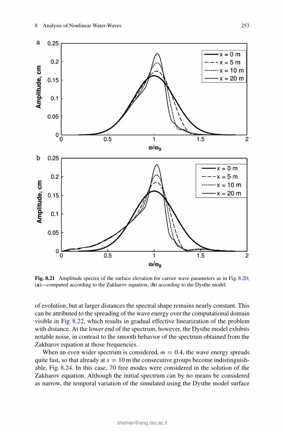
8 Analysis of Nonlinear Water-Waves 253
Fig. 8.21 Amplitude spectra of the surface elevation for carrier wave parameters as in Fig. 8.20;(a)—computed according to the Zakharov equation; (b) according to the Dysthe model
of evolution, but at larger distances the spectral shape remains nearly constant. Thiscan be attributed to the spreading of the wave energy over the computational domainvisible in Fig. 8.22, which results in gradual effective linearization of the problemwith distance. At the lower end of the spectrum, however, the Dysthe model exhibitsnotable noise, in contrast to the smooth behavior of the spectrum obtained from theZakharov equation at those frequencies.
When an even wider spectrum is considered, m D 0:4, the wave energy spreadsquite fast, so that already at x D 10m the consecutive groups become indistinguish-able, Fig. 8.24. In this case, 70 free modes were considered in the solution of theZakharov equation. Although the initial spectrum can by no means be consideredas narrow, the temporal variation of the simulated using the Dysthe model surface
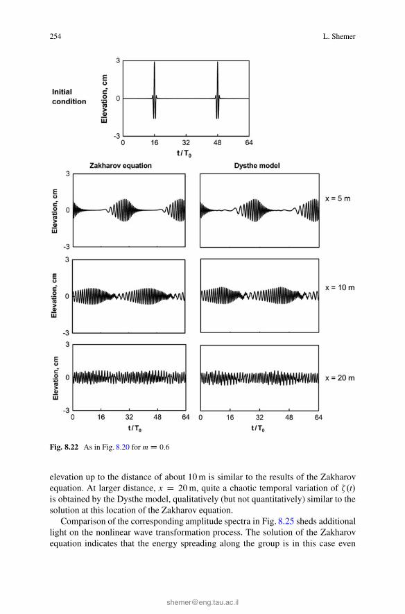
254 L. Shemer
Fig. 8.22 As in Fig. 8.20 for mD 0:6
elevation up to the distance of about 10 m is similar to the results of the Zakharovequation. At larger distance, x D 20m, quite a chaotic temporal variation of �.t/is obtained by the Dysthe model, qualitatively (but not quantitatively) similar to thesolution at this location of the Zakharov equation.
Comparison of the corresponding amplitude spectra in Fig. 8.25 sheds additionallight on the nonlinear wave transformation process. The solution of the Zakharovequation indicates that the energy spreading along the group is in this case even
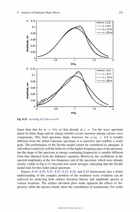
8 Analysis of Nonlinear Water-Waves 255
Fig. 8.23 As in Fig. 8.21 for mD 0:6
faster than that for m D 0:6, so that already at x D 5m the wave spectrumattain its finite shape and no energy transfer occurs anymore among various wavecomponents. This final spectrum shape, however, for !=!0 > 0:8 is notablydifferent from the initial Gaussian spectrum; it is narrower and exhibits a widerpeak. The performance of the Dysthe model cannot be considered as adequate. Itstill reflects relatively well the behavior of the higher-frequency part of the spectrum,but the shape of the spectrum at energy-containing frequencies is notably differentfrom that obtained from the Zakharov equation. Moreover, the oscillations in thespectral amplitudes at the low-frequency end of the spectrum, which were alreadyclearly visible in Fig. 8.23, become now much stronger, indicating that the Dysthemodel fails for this wider initial spectrum.
Figures 8.19, 8.20, 8.21, 8.22, 8.23, 8.24, and 8.25 demonstrate that a betterunderstanding of the complex problem of the nonlinear wave evolution can beachieved by analyzing both surface elevation history and amplitude spectra atvarious locations. The surface elevation plots make apparent the effects of dis-persion, while the spectra clearly show the contribution of nonlinearity. For wider
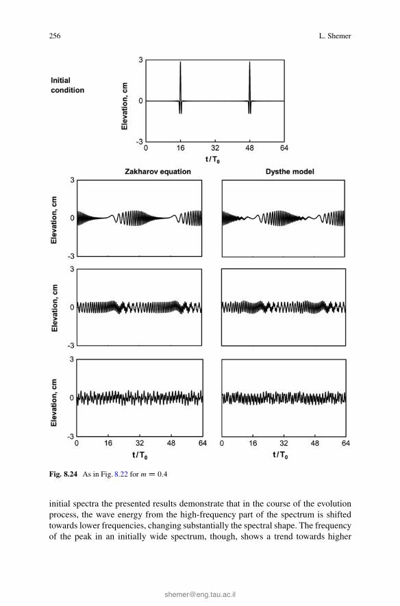
256 L. Shemer
Fig. 8.24 As in Fig. 8.22 for mD 0:4
initial spectra the presented results demonstrate that in the course of the evolutionprocess, the wave energy from the high-frequency part of the spectrum is shiftedtowards lower frequencies, changing substantially the spectral shape. The frequencyof the peak in an initially wide spectrum, though, shows a trend towards higher
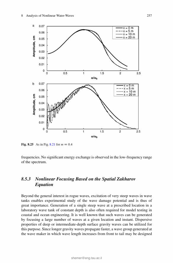
8 Analysis of Nonlinear Water-Waves 257
Fig. 8.25 As in Fig. 8.21 for mD 0:4
frequencies. No significant energy exchange is observed in the low-frequency rangeof the spectrum.
8.5.3 Nonlinear Focusing Based on the Spatial ZakharovEquation
Beyond the general interest in rogue waves, excitation of very steep waves in wavetanks enables experimental study of the wave damage potential and is thus ofgreat importance. Generation of a single steep wave at a prescribed location in alaboratory wave tank of constant depth is also often required for model testing incoastal and ocean engineering. It is well known that such waves can be generatedby focusing a large number of waves at a given location and instant. Dispersiveproperties of deep or intermediate-depth surface gravity waves can be utilized forthis purpose. Since longer gravity waves propagate faster, a wave group generated atthe wave maker in which wave length increases from front to tail may be designed
258 L. Shemer
to focus the wave energy at a desired location. Such wave sequence can be seen as agroup that is modulated both in amplitude and in frequency. In the frequency space, asingle steep wave constitutes a superposition of a number of harmonics, each havinga moderate steepness that can easily be generated by a wavemaker; these harmonicsreach the prescribed location with identical phases, so that the amplitude of theresulting wave is a sum of amplitudes of all frequency components. Focusing istherefore more effective when the number of free wave harmonics initially generatedat the wavemaker is large. Excitation of a single wave with extreme amplitudethus requires wide spectrum of the initial wave group generated at the wavemaker.Very steep (freak) wave therefore can be seen as a wave group with a very narrowenvelope and correspondingly wide spectrum. Results of Sect. 8.5.2 demonstratethat the narrow-banded Dysthe model is not suitable for wider spectra. It is thusnatural to apply the spatial Zakharov equation given by Eqs. (8.33)–(8.35) for thisproblem.
The goal of the study carried out by Shemer et al. [67] was to generate a singlesteep wave at a prescribed focusing location xf in the tank. The wave is presented bya wave group given by (8.4) with the width parameter m D 0:6, see the upper panelin Fig. 8.22. In order to compute the wavemaker driving signal required to obtainthe desired wave group shape at the distance xf from the wavemaker, the spectrumcorresponding to Eq. (8.4) plotted in Fig. 8.23 is integrated from xf backwards up tothe wavemaker at x D 0. Due to an essentially nonlinear character of the steep wavesstudied, see also [7], the resulting spectrum at the wavemaker is notably differentfrom the Gaussian shape at the focusing location xf . Experiments on nonlinearfocusing were carried out in both facilities described in Sect. 8.2: in the large wavetank in Hanover, GWK, and in TAU. These experimental facilities differ in size byan order of magnitude.
The experiments in GWK were carried out for two carrier wave periods, T0 D2:8 s (carrier wave length �0 D 12:1m) and T0 D 4:34 s (carrier wave length�0 D 25:0m), corresponding to dimensionless depths of k0h D 2:59 and k0h D1:26, respectively. For the shorter carrier wave length, the deep-water dispersionrelation is satisfied approximately, whereas for the longer carrier wave, water atwave number corresponding to �0 D 25m cannot be considered deep. Even for�0 D 12:1m, since wide-spectrum wave groups were considered, intermediate-depth waves were present. Therefore, in all expressions finite-depth version ofthe interaction coefficients were used. The focusing location, xf , in the GWKexperiments was located at the dimensionless distance xf=�0 of about 10 carrierwave lengths from the wavemaker for �0 D 12:1m, and at half that distance interms of the wave lengths for �0 D 25:0m.
The designed temporal variation of the surface elevation at the wavemaker �des D�.x; t/ was computed by backward integration of (8.33) from the focusing locationto x D 0. For each carrier wave period T0 and focusing location xf , the solution ofthe system of N ODEs, N being the total number of wave harmonics considered,was obtained for distances ranging from the wavemaker location at x D 0 upto xf and beyond. The number of free wave harmonics N considered in thosecomputations was in the range from 56 to 76. The wavemaker driving signal was

8 Analysis of Nonlinear Water-Waves 259
then calculated from �des employing the wavemaker transfer function. This functionrelates the amplitudes and phases of the harmonic wavemaker displacement at agiven frequency to the corresponding parameters of the propagating monochromaticwave. For a given wavemaker shape, i.e. piston or paddle, this function can be foundusing the linear wavemaker theory (see, e.g. [9]). It is well known, however, that forfinite amplitude waves significant nonlinear effects may become important (see, e.g.[12]). The complex wavemaker transfer function for a given experimental facility istherefore found empirically by performing a series of experiments on excitationof monochromatic waves. Generation of water gravity waves by a wavemaker is,however, an essentially nonlinear process [53]. To account for the nonlinearity ofwave generation, an experimental procedure was applied, in which the wavemakerdriving signal was adjusted iteratively to obtain the desired wave train shape at aprescribed location away from the wavemaker, thus eliminating effect of evanescentmodes. The details of this iterative procedure were presented in [67]. In GWK,adjustment was carried out at x D 52:2m.
Evolution of the wave group shape along the tank is illustrated in Fig. 8.26.The solid line shows the variation of the surface elevation computed by backwardintegration of Eq. (8.33) starting from the prescribed Gaussian shape given byEq. (8.4) at the focusing location, with the carrier wave period T0 D 2:8 s (frequencyf0 D 0:357Hz) and steepness �0k0 D 0:3. Computations are carried out for N D 76
harmonics, corresponding to frequencies in the range 0.039 Hz � f � 0.76 Hz. Thesystem of 76 ODEs was solved using the Runge-Kutta procedure with integrationstep of 5 cm. Test of the integration procedure with the halved integration step of2.5 cm demonstrated that the solution remains insensitive to step size variation.Surface elevation variation is shown at this figure also for the wavemaker location(actually, the wave gauge is attached at the distance of 5 cm from the piston surface),and for the location of the wavemaker driving signal adjustment x D 52:2m. Theresults of measurements by the corresponding wave gauges are plotted as well.Note that as the time reference from here on in this subsection is the instant ofthe initiation of the wavemaker motion.
The agreement between the water elevation measurements and the correspondingcomputations in Fig. 8.26a is quite good even though only free wave componentsare accounted for in the computations. The selected value of m D 0:6 in (8.4) yieldsindeed a narrow wave group with a single steep wave at the focusing location. Theperiod of waves within the group at the wavemaker gradually increases, resulting ina quite complicated envelope shape, in contrast to the symmetric Gaussian shape atthe focusing. This group envelope shape is also reproduced well in the numericalsimulations. This agreement is particularly good at the adjustment location x D52:2m. The maximum wave crest height above the mean water level that is about0.2 m at the wavemaker increases to more than 0.6 m at the focusing location. Theagreement of experiments and computations is less impressive at the wavemaker,most probably due to effect of the evanescent modes. The measured crest heightat the focusing location is notably higher than the computed value. Disagreementbetween experiments and computations also manifests itself in some asymmetry of
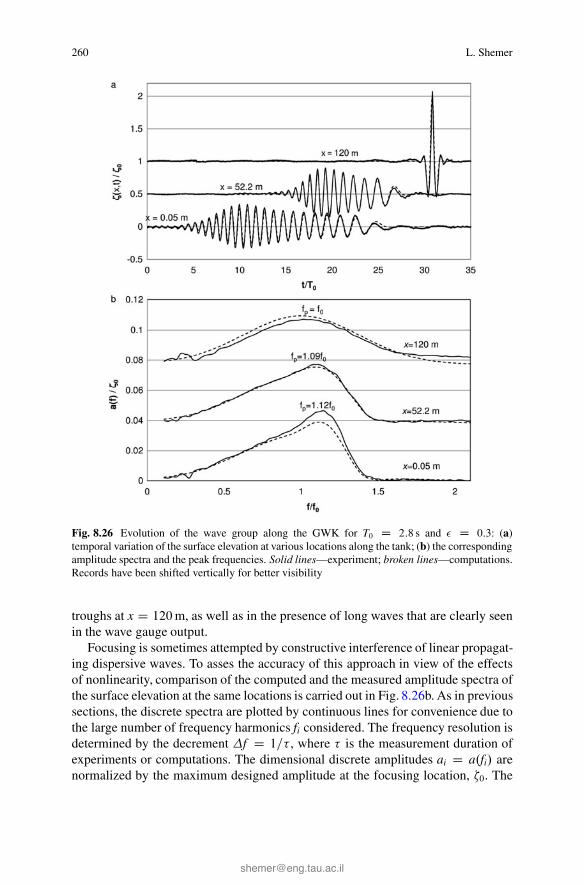
260 L. Shemer
Fig. 8.26 Evolution of the wave group along the GWK for T0 D 2:8 s and � D 0:3: (a)temporal variation of the surface elevation at various locations along the tank; (b) the correspondingamplitude spectra and the peak frequencies. Solid lines—experiment; broken lines—computations.Records have been shifted vertically for better visibility
troughs at x D 120m, as well as in the presence of long waves that are clearly seenin the wave gauge output.
Focusing is sometimes attempted by constructive interference of linear propagat-ing dispersive waves. To asses the accuracy of this approach in view of the effectsof nonlinearity, comparison of the computed and the measured amplitude spectra ofthe surface elevation at the same locations is carried out in Fig. 8.26b. As in previoussections, the discrete spectra are plotted by continuous lines for convenience due tothe large number of frequency harmonics fi considered. The frequency resolution isdetermined by the decrement �f D 1=� , where � is the measurement duration ofexperiments or computations. The dimensional discrete amplitudes ai D a.fi/ arenormalized by the maximum designed amplitude at the focusing location, �0. The
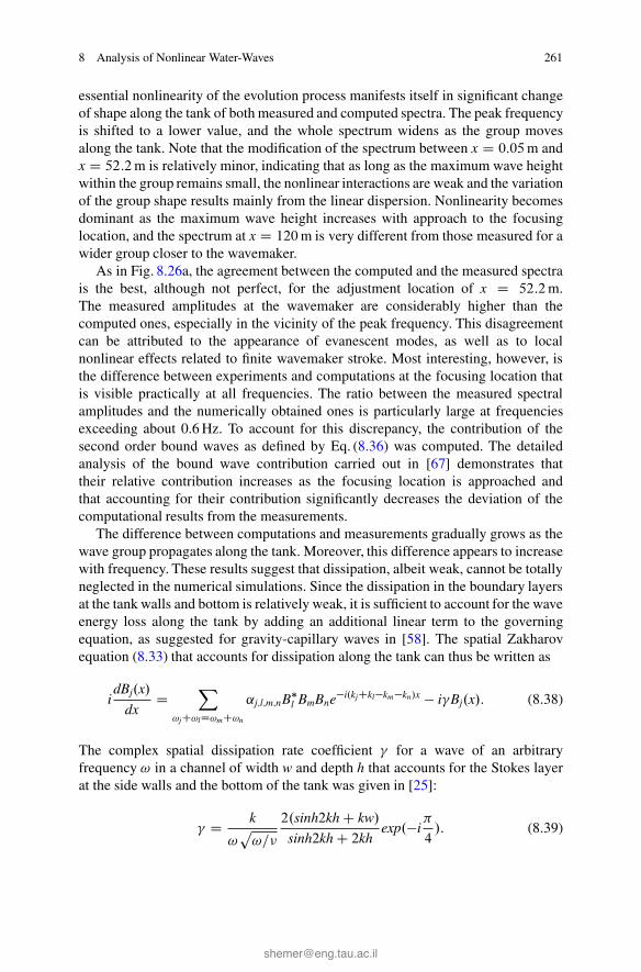
8 Analysis of Nonlinear Water-Waves 261
essential nonlinearity of the evolution process manifests itself in significant changeof shape along the tank of both measured and computed spectra. The peak frequencyis shifted to a lower value, and the whole spectrum widens as the group movesalong the tank. Note that the modification of the spectrum between x D 0:05m andx D 52:2m is relatively minor, indicating that as long as the maximum wave heightwithin the group remains small, the nonlinear interactions are weak and the variationof the group shape results mainly from the linear dispersion. Nonlinearity becomesdominant as the maximum wave height increases with approach to the focusinglocation, and the spectrum at x D 120m is very different from those measured for awider group closer to the wavemaker.
As in Fig. 8.26a, the agreement between the computed and the measured spectrais the best, although not perfect, for the adjustment location of x D 52:2m.The measured amplitudes at the wavemaker are considerably higher than thecomputed ones, especially in the vicinity of the peak frequency. This disagreementcan be attributed to the appearance of evanescent modes, as well as to localnonlinear effects related to finite wavemaker stroke. Most interesting, however, isthe difference between experiments and computations at the focusing location thatis visible practically at all frequencies. The ratio between the measured spectralamplitudes and the numerically obtained ones is particularly large at frequenciesexceeding about 0.6 Hz. To account for this discrepancy, the contribution of thesecond order bound waves as defined by Eq. (8.36) was computed. The detailedanalysis of the bound wave contribution carried out in [67] demonstrates thattheir relative contribution increases as the focusing location is approached andthat accounting for their contribution significantly decreases the deviation of thecomputational results from the measurements.
The difference between computations and measurements gradually grows as thewave group propagates along the tank. Moreover, this difference appears to increasewith frequency. These results suggest that dissipation, albeit weak, cannot be totallyneglected in the numerical simulations. Since the dissipation in the boundary layersat the tank walls and bottom is relatively weak, it is sufficient to account for the waveenergy loss along the tank by adding an additional linear term to the governingequation, as suggested for gravity-capillary waves in [58]. The spatial Zakharovequation (8.33) that accounts for dissipation along the tank can thus be written as
idBj.x/
dxD
X
!jC!lD!mC!n
˛j;l;m;nB�l BmBne�i.kjCkl�km�kn/x � iBj.x/: (8.38)
The complex spatial dissipation rate coefficient for a wave of an arbitraryfrequency ! in a channel of width w and depth h that accounts for the Stokes layerat the side walls and the bottom of the tank was given in [25]:
D k
!p!=�
2.sinh2kh C kw/
sinh2kh C 2khexp.�i
�
4/: (8.39)
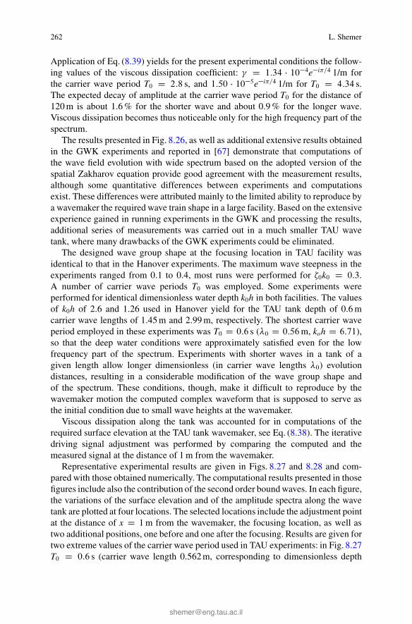
262 L. Shemer
Application of Eq. (8.39) yields for the present experimental conditions the follow-ing values of the viscous dissipation coefficient: D 1:34 � 10�4e�i�=4 1/m forthe carrier wave period T0 D 2:8 s, and 1:50 � 10�5e�i�=4 1/m for T0 D 4:34 s.The expected decay of amplitude at the carrier wave period T0 for the distance of120 m is about 1.6 % for the shorter wave and about 0.9 % for the longer wave.Viscous dissipation becomes thus noticeable only for the high frequency part of thespectrum.
The results presented in Fig. 8.26, as well as additional extensive results obtainedin the GWK experiments and reported in [67] demonstrate that computations ofthe wave field evolution with wide spectrum based on the adopted version of thespatial Zakharov equation provide good agreement with the measurement results,although some quantitative differences between experiments and computationsexist. These differences were attributed mainly to the limited ability to reproduce bya wavemaker the required wave train shape in a large facility. Based on the extensiveexperience gained in running experiments in the GWK and processing the results,additional series of measurements was carried out in a much smaller TAU wavetank, where many drawbacks of the GWK experiments could be eliminated.
The designed wave group shape at the focusing location in TAU facility wasidentical to that in the Hanover experiments. The maximum wave steepness in theexperiments ranged from 0.1 to 0.4, most runs were performed for �0k0 D 0:3.A number of carrier wave periods T0 was employed. Some experiments wereperformed for identical dimensionless water depth k0h in both facilities. The valuesof k0h of 2.6 and 1.26 used in Hanover yield for the TAU tank depth of 0.6 mcarrier wave lengths of 1.45 m and 2.99 m, respectively. The shortest carrier waveperiod employed in these experiments was T0 D 0:6 s (�0 D 0:56m, koh D 6:71),so that the deep water conditions were approximately satisfied even for the lowfrequency part of the spectrum. Experiments with shorter waves in a tank of agiven length allow longer dimensionless (in carrier wave lengths �0) evolutiondistances, resulting in a considerable modification of the wave group shape andof the spectrum. These conditions, though, make it difficult to reproduce by thewavemaker motion the computed complex waveform that is supposed to serve asthe initial condition due to small wave heights at the wavemaker.
Viscous dissipation along the tank was accounted for in computations of therequired surface elevation at the TAU tank wavemaker, see Eq. (8.38). The iterativedriving signal adjustment was performed by comparing the computed and themeasured signal at the distance of 1 m from the wavemaker.
Representative experimental results are given in Figs. 8.27 and 8.28 and com-pared with those obtained numerically. The computational results presented in thosefigures include also the contribution of the second order bound waves. In each figure,the variations of the surface elevation and of the amplitude spectra along the wavetank are plotted at four locations. The selected locations include the adjustment pointat the distance of x D 1m from the wavemaker, the focusing location, as well astwo additional positions, one before and one after the focusing. Results are given fortwo extreme values of the carrier wave period used in TAU experiments: in Fig. 8.27T0 D 0:6 s (carrier wave length 0.562 m, corresponding to dimensionless depth
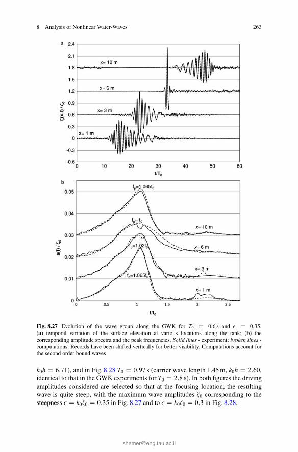
8 Analysis of Nonlinear Water-Waves 263
Fig. 8.27 Evolution of the wave group along the GWK for T0 D 0:6 s and � D 0:35.(a) temporal variation of the surface elevation at various locations along the tank; (b) thecorresponding amplitude spectra and the peak frequencies. Solid lines - experiment; broken lines -computations. Records have been shifted vertically for better visibility. Computations account forthe second order bound waves
k0h D 6:71), and in Fig. 8.28 T0 D 0:97 s (carrier wave length 1.45 m, k0h D 2:60,identical to that in the GWK experiments for T0 D 2:8 s). In both figures the drivingamplitudes considered are selected so that at the focusing location, the resultingwave is quite steep, with the maximum wave amplitudes �0 corresponding to thesteepness � D k0�0 D 0:35 in Fig. 8.27 and to � D k0�0 D 0:3 in Fig. 8.28.
264 L. Shemer
Fig. 8.28 Evolution of the wave group along the GWK for T0 D 0:97s and � D 0: (a) temporalvariation of the surface elevation at various locations along the tank; (b) the correspondingamplitude spectra and the peak frequencies. Solid lines - experiment; broken lines - computations.Records have been shifted vertically for better visibility. Computations account for the secondorder bound waves
Focusing location as far as possible from the wavemaker ensures longer evolutiondomain but requires lower wave heights at the wavemaker. In view of difficultiesin faithful reproduction of group shapes with very low wave heights, the focusingdistance of 6 m was selected in Fig. 8.27, relatively short compared to the tanklength, and constitutes about 10.7 carrier wave lengths �0. To improve the accuracyof results, the maximum wave steepness in this case is also chosen to be somewhathigher than that for longer carrier waves. In computations, 131 frequency harmonicswere considered, covering free wave frequency range of 0.125 Hz� f � 3:375Hz.
8 Analysis of Nonlinear Water-Waves 265
For a longer wave in Fig. 8.28 with T0 D 0:97 s (106 free harmonics, 0.1 Hz � f �2.2 Hz), focusing is designed to occur at a larger distance from the wavemaker,x D 10m. Note, however, that in terms of the carrier wave lengths those focusingdistances of 6:9�0 is shorter than in Fig. 8.27.
A very good agreement between the computed superposition of the free and thesecond order bound waves and the measurements is obtained for the variation ofthe wave group shape along the tank. Similarly good agreement is observed in allamplitude spectra in Figs. 8.27b and 8.28b for each one of the spectral harmonic.Modulation of the amplitude and of the frequency within the group is clearly seenin Figs. 8.27a and 8.28a at x D 1m; the maximum wave amplitude within thegroup then increases towards the focusing location. At the focusing, a single steepwave with height very close to the designed value is obtained in all cases. Closeto the wavemaker, the envelope of the wave group with the shortest carrier wavein Fig. 8.27a is more asymmetric than in the other case. The amplitude spectraallow estimation of variation of contribution of each harmonic in the course of theevolution. The spectral shape variation in both Figs. 8.27b and 8.28b is quite similar,indicating that the variation of dimensionless depth does not affect the evolutionpattern strongly. The spectrum has the maximum width at the focusing location,while close to the wavemaker it is somewhat narrower. The peak frequency driftsin the course of the evolution process. The minimum value of the peak frequency,corresponding to that of the carrier wave, is obtained at the focusing location. Theupward shift of the peak frequency from the carrier wave value increases with thedistance from the focusing location. The full symmetry of the spectral shapes atequal distances from the focusing is violated by the viscous dissipation; this effectis more visible for free harmonics at higher frequencies.
Results on evolution of wave groups with wide spectra presented above wereobtained in two wave tanks that differ in size considerably. In spite of that, theevolution patterns observed in the experiments and obtained in the numericalsimulations are quite similar in both facilities. Those patterns are determined bycombination of linear and nonlinear contributions. The effects of nonlinearity aregoverned by the maximum wave steepness at the focusing location, � D �0k0. Thevalues of � in experiments and computations in both facilities were very close, andthe results presented above are mostly for high values of the maximum steepnessof about � D 0:3. Nonlinear effects are readily identified in the variation of thespectral shapes that would remain constant if nonlinearity were negligible. Resultsof Figs. 8.26b–8.28b demonstrate that the variations of the spectral shape with thedistance from the wavemaker obtained in both facilities were essential.
Evolution of the wave group shape along the tank, while being dependent onnonlinearity, is strongly affected by linear effects. The dominant linear effect inthe evolution process is the dispersion that for gravity waves depends on thedimensionless water depth, k0h. The dimensionless water depth was in the range of2:6 � kh � 6:7 for the TAU tank, and had the values of k0h D 2:6 and k0h D 1:26
in the GWK experiments. For the majority of cases carrier waves can be seen thusas propagating over deep water. It should be reiterated, however, that since wavegroups with wide spectra were considered, the free wave spectrum always contained
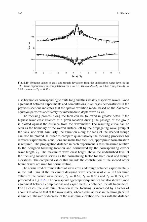
266 L. Shemer
Fig. 8.29 Extreme values of crest and trough deviations from the undisturbed water level in theTAU tank: experiments vs. computations for � D 0:3. Diamonds—T0 D 0:6 s; triangles—T0 D0:85 s; circles—T0 D 0:97 s
also harmonics corresponding to quite long and thus weakly dispersive waves. Goodagreement between experiments and computations in all cases demonstrated in theprevious sections indicates that the spatial evolution model based on the Zakharovequation performs adequately for intermediate-depth wave as well.
The focusing process along the tank can be followed in greater detail if thehighest wave crest attained at a given location during the passage of the groupis plotted against the distance from the wavemaker. The resulting curve can beseen as the boundary of the wetted surface left by the propagating wave group atthe tank side wall. Similarly, the variation along the tank of the deepest troughcan also be plotted. In order to compare quantitatively the focusing processes fordifferent experimental conditions and in the two facilities, appropriate normalizationis required. The propagation distance in each experiment is thus measured relativeto the designed focusing location and normalized by the corresponding carrierwave length �0. The maximum wave crest height above the undisturbed level atthe focusing location serves as the normalizing factor for both crest and troughelevations. The computed values that include the contribution of the second orderbound waves are used for normalization.
The normalized extreme values of wave crest and trough obtained experimentallyin the TAU tank at the maximum designed wave steepness of � D 0:3 for threevalues of the carrier wave period, T0 D 0:6 s, T0 D 0:85 s and T0 D 0:97 s, arepresented in Fig. 8.29. The corresponding computed quantities are also shown. Goodagreement between computations and experiments is obtained for all frequencies.For all cases, the maximum elevation at the focusing is increased by a factor ofabout 3 relative to that at the wavemaker, whereas the increase in the through depthis smaller. The rate of decrease of the maximum elevation declines with the distance
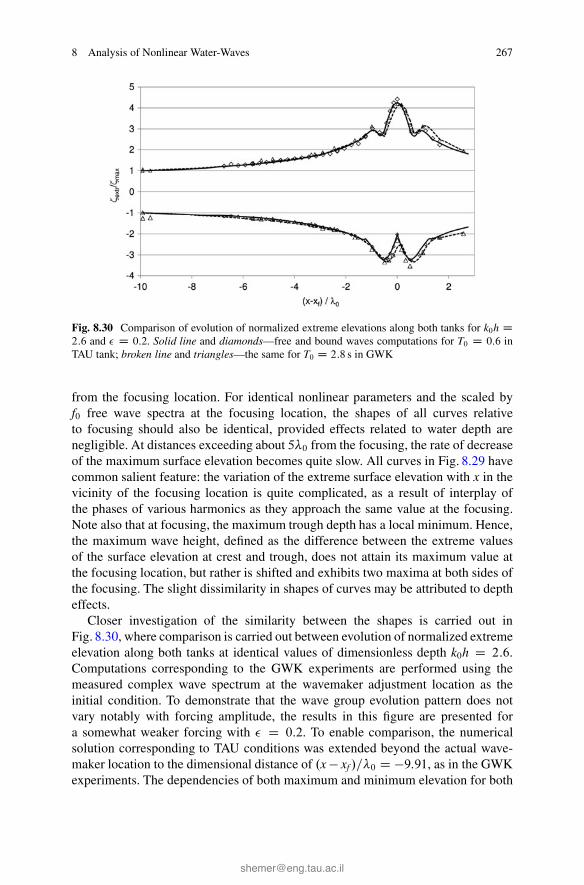
8 Analysis of Nonlinear Water-Waves 267
Fig. 8.30 Comparison of evolution of normalized extreme elevations along both tanks for k0h D2:6 and � D 0:2. Solid line and diamonds—free and bound waves computations for T0 D 0:6 inTAU tank; broken line and triangles—the same for T0 D 2:8 s in GWK
from the focusing location. For identical nonlinear parameters and the scaled byf0 free wave spectra at the focusing location, the shapes of all curves relativeto focusing should also be identical, provided effects related to water depth arenegligible. At distances exceeding about 5�0 from the focusing, the rate of decreaseof the maximum surface elevation becomes quite slow. All curves in Fig. 8.29 havecommon salient feature: the variation of the extreme surface elevation with x in thevicinity of the focusing location is quite complicated, as a result of interplay ofthe phases of various harmonics as they approach the same value at the focusing.Note also that at focusing, the maximum trough depth has a local minimum. Hence,the maximum wave height, defined as the difference between the extreme valuesof the surface elevation at crest and trough, does not attain its maximum value atthe focusing location, but rather is shifted and exhibits two maxima at both sides ofthe focusing. The slight dissimilarity in shapes of curves may be attributed to deptheffects.
Closer investigation of the similarity between the shapes is carried out inFig. 8.30, where comparison is carried out between evolution of normalized extremeelevation along both tanks at identical values of dimensionless depth k0h D 2:6.Computations corresponding to the GWK experiments are performed using themeasured complex wave spectrum at the wavemaker adjustment location as theinitial condition. To demonstrate that the wave group evolution pattern does notvary notably with forcing amplitude, the results in this figure are presented fora somewhat weaker forcing with � D 0:2. To enable comparison, the numericalsolution corresponding to TAU conditions was extended beyond the actual wave-maker location to the dimensional distance of .x � xf /=�0 D �9:91, as in the GWKexperiments. The dependencies of both maximum and minimum elevation for both
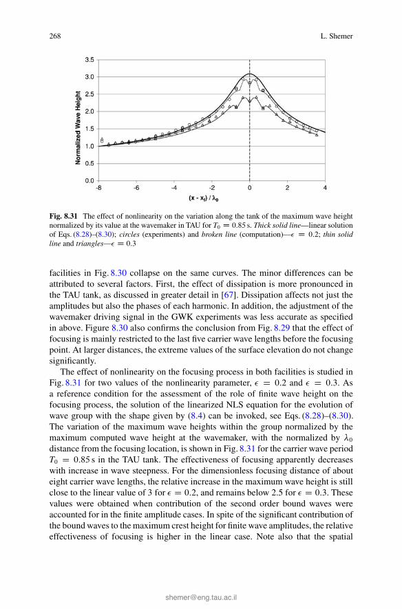
268 L. Shemer
Fig. 8.31 The effect of nonlinearity on the variation along the tank of the maximum wave heightnormalized by its value at the wavemaker in TAU for T0 D 0:85 s. Thick solid line—linear solutionof Eqs. (8.28)–(8.30); circles (experiments) and broken line (computation)—� D 0:2; thin solidline and triangles—� D 0:3
facilities in Fig. 8.30 collapse on the same curves. The minor differences can beattributed to several factors. First, the effect of dissipation is more pronounced inthe TAU tank, as discussed in greater detail in [67]. Dissipation affects not just theamplitudes but also the phases of each harmonic. In addition, the adjustment of thewavemaker driving signal in the GWK experiments was less accurate as specifiedin above. Figure 8.30 also confirms the conclusion from Fig. 8.29 that the effect offocusing is mainly restricted to the last five carrier wave lengths before the focusingpoint. At larger distances, the extreme values of the surface elevation do not changesignificantly.
The effect of nonlinearity on the focusing process in both facilities is studied inFig. 8.31 for two values of the nonlinearity parameter, � D 0:2 and � D 0:3. Asa reference condition for the assessment of the role of finite wave height on thefocusing process, the solution of the linearized NLS equation for the evolution ofwave group with the shape given by (8.4) can be invoked, see Eqs. (8.28)–(8.30).The variation of the maximum wave heights within the group normalized by themaximum computed wave height at the wavemaker, with the normalized by �0distance from the focusing location, is shown in Fig. 8.31 for the carrier wave periodT0 D 0:85 s in the TAU tank. The effectiveness of focusing apparently decreaseswith increase in wave steepness. For the dimensionless focusing distance of abouteight carrier wave lengths, the relative increase in the maximum wave height is stillclose to the linear value of 3 for � D 0:2, and remains below 2.5 for � D 0:3. Thesevalues were obtained when contribution of the second order bound waves wereaccounted for in the finite amplitude cases. In spite of the significant contribution ofthe bound waves to the maximum crest height for finite wave amplitudes, the relativeeffectiveness of focusing is higher in the linear case. Note also that the spatial
8 Analysis of Nonlinear Water-Waves 269
variation of the maximum wave height obtained from the linear solution is smoothalso around the focusing location, in contrast to the behavior of the computed andexperimental results for finite amplitudes.
8.6 Statistics of Nonlinear Unidirectional Water Waves
Sections 8.3–8.5 describe evolution of unidirectional deterministic waves alongwave tanks. As stressed in the Introduction, nonlinear ocean waves, however, arestochastic in nature. Theoretical investigations aimed at describing the statisticalproperties of nonlinear wave fields were originated by Longuet-Higgins [33] whoshowed that for a narrow-banded wave field with random phases, wave heightssatisfy the Rayleigh distribution. An improved model that takes into accountnonlinear effects has been suggested later [34]. More recently, numerous modelsappropriate to unidirectional wave fields were proposed, see [43, 77–79] andadditional references therein. The probability of appearance of very high roguewaves attracts particular attention. The relatively high occurrence of those wavesthat may exceed the predictions based on the Rayleigh distribution suggests that theoccurrence of freak waves is related to nonlinearity of the wave field. Determinationof freak waves’ probability for a given sea state is important practically and requiresin depth study using the most advanced theoretical approaches and laboratoryexperiments.
The effect of directional spreading on the statistics of random waves wasalso considered in a number of numerical and experimental studies [48, 72, 83].Measurements of the evolution of unidirectional random wave fields have beenperformed in very large experimental installations [45, 46, 48, 72]. The presentsection summarizes the results of experimental and numerical investigations of theevolution of a random wave field in a large wave tank presented in [62, 68, 69].In these studies variation along the tank of various statistical properties of thewave field is investigated for a range of parameters in view of their relevance toappearance of freak waves. The effects of nonlinearity and of spectral shape wereinvestigated. The experiments were carried out in the Large Wave Channel (GWK)in Hanover. Spatial evolution of numerous realizations of a wave field that haveidentical initial frequency power spectra for the free wave components and randomphases in each realization was studied.
The dimensionless spectral width � is of a random wave field is defined as
� Dq.m0m2=m2
1/� 1; (8.40)
where the jth spectral moment of the power spectrum S.!/ is
mj Dˆ !max
!min
!jS.!/d!: (8.41)

270 L. Shemer
0.2 0.4 0.6 0.8 1 1.2 1.4 1.6
1
2
3
4
5
6
7
8
9
10x 10−4
Pow
er, m
2 s
Frequency, Hz
Gauss ν=0.045
Gauss ν=0.09
Gauss ν=0.16
JONSWAP ν=0.2
Rectangular ν=0.045
Fig. 8.32 Initial spectral shapes of the surface elevation
In (8.41), the integration is carried out over the free waves’ frequency domainonly. The following initial free wave spectral shapes were considered: (a) a narrowGaussian spectrum corresponding to (8.4) as in Sects. 8.3–8.5, with m D 3:5
resulting in � D 0:045; (b) rectangular spectrum with fmax;min D f0 ˙ 0:047Hz;� D 0:045; (c) an intermediate width Gaussian spectrum with � D 0:09; (d) awide Gaussian spectrum with � D 0:16; (e) JONSWAP spectrum, see e.g. Goda[13]:
S.f / D Af�5exp��1:25.T0f /�4
� expŒ�.T0f�1/2=22�: (8.42)
In (8.42), A is an adjustable amplitude parameter, the peak enhancement parameter D 7; D 0:07 for f � f0; D 0:09 for f > f0. These parameters yield thedimensionless width � D 0:20. The initial spectral shapes are plotted in Fig. 8.32.
To follow variation of the wave field over distances containing as many dominantwave lengths �0 as possible, the shortest possible carrier wave period T0 D 1:5 swas selected based on the frequency response of the hydraulically-driven GWKwavemaker. The corresponding wave length �0 D 3:51m and the dimensionlesswater depth k0h D 8:95 1. For each initial shape of the spectrum, theselected duration of the basic unit of the wavemaker driving signal was 81.92 s,corresponding to 4096 data points at the wavemaker driver frequency of 50 Hzand the spectral resolution of the driving signal of 1/81.92 Hz. In every realizationof a given spectrum this basic unit was repeated twice. The measured in thevicinity of the wavemaker spectral amplitudes of each harmonic do not remainfully deterministic due to nonlinear response of the water-wave field to the non-monochromatic wavemaker motion; each of them varies in different realizationsof the spectrum around the prescribed value. For random waves, the nonlinearity
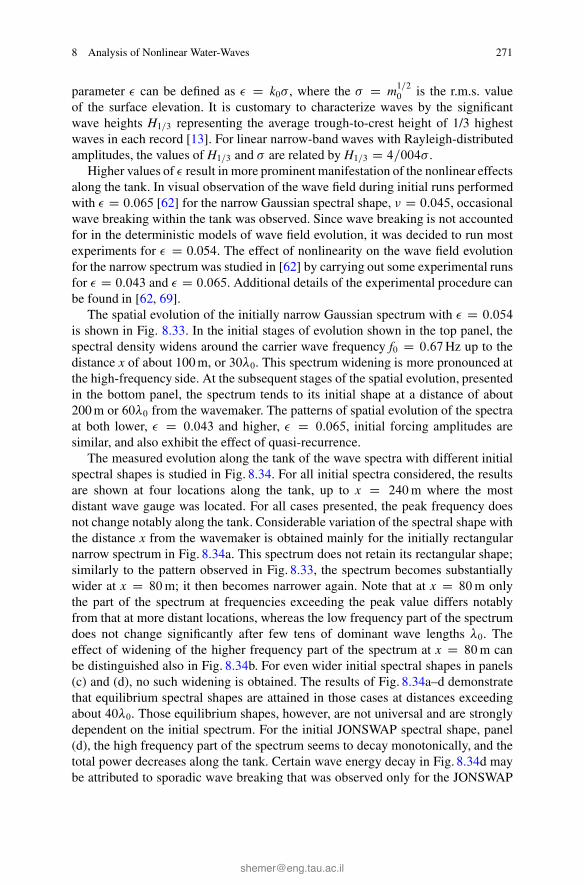
8 Analysis of Nonlinear Water-Waves 271
parameter � can be defined as � D k0� , where the � D m1=20 is the r.m.s. value
of the surface elevation. It is customary to characterize waves by the significantwave heights H1=3 representing the average trough-to-crest height of 1/3 highestwaves in each record [13]. For linear narrow-band waves with Rayleigh-distributedamplitudes, the values of H1=3 and � are related by H1=3 D 4=004� .
Higher values of � result in more prominent manifestation of the nonlinear effectsalong the tank. In visual observation of the wave field during initial runs performedwith � D 0:065 [62] for the narrow Gaussian spectral shape, � D 0:045, occasionalwave breaking within the tank was observed. Since wave breaking is not accountedfor in the deterministic models of wave field evolution, it was decided to run mostexperiments for � D 0.054. The effect of nonlinearity on the wave field evolutionfor the narrow spectrum was studied in [62] by carrying out some experimental runsfor � D 0:043 and � D 0:065. Additional details of the experimental procedure canbe found in [62, 69].
The spatial evolution of the initially narrow Gaussian spectrum with � D 0:054
is shown in Fig. 8.33. In the initial stages of evolution shown in the top panel, thespectral density widens around the carrier wave frequency f0 D 0:67Hz up to thedistance x of about 100 m, or 30�0. This spectrum widening is more pronounced atthe high-frequency side. At the subsequent stages of the spatial evolution, presentedin the bottom panel, the spectrum tends to its initial shape at a distance of about200 m or 60�0 from the wavemaker. The patterns of spatial evolution of the spectraat both lower, � D 0:043 and higher, � D 0:065, initial forcing amplitudes aresimilar, and also exhibit the effect of quasi-recurrence.
The measured evolution along the tank of the wave spectra with different initialspectral shapes is studied in Fig. 8.34. For all initial spectra considered, the resultsare shown at four locations along the tank, up to x D 240m where the mostdistant wave gauge was located. For all cases presented, the peak frequency doesnot change notably along the tank. Considerable variation of the spectral shape withthe distance x from the wavemaker is obtained mainly for the initially rectangularnarrow spectrum in Fig. 8.34a. This spectrum does not retain its rectangular shape;similarly to the pattern observed in Fig. 8.33, the spectrum becomes substantiallywider at x D 80m; it then becomes narrower again. Note that at x D 80m onlythe part of the spectrum at frequencies exceeding the peak value differs notablyfrom that at more distant locations, whereas the low frequency part of the spectrumdoes not change significantly after few tens of dominant wave lengths �0. Theeffect of widening of the higher frequency part of the spectrum at x D 80m canbe distinguished also in Fig. 8.34b. For even wider initial spectral shapes in panels(c) and (d), no such widening is obtained. The results of Fig. 8.34a–d demonstratethat equilibrium spectral shapes are attained in those cases at distances exceedingabout 40�0. Those equilibrium shapes, however, are not universal and are stronglydependent on the initial spectrum. For the initial JONSWAP spectral shape, panel(d), the high frequency part of the spectrum seems to decay monotonically, and thetotal power decreases along the tank. Certain wave energy decay in Fig. 8.34d maybe attributed to sporadic wave breaking that was observed only for the JONSWAP
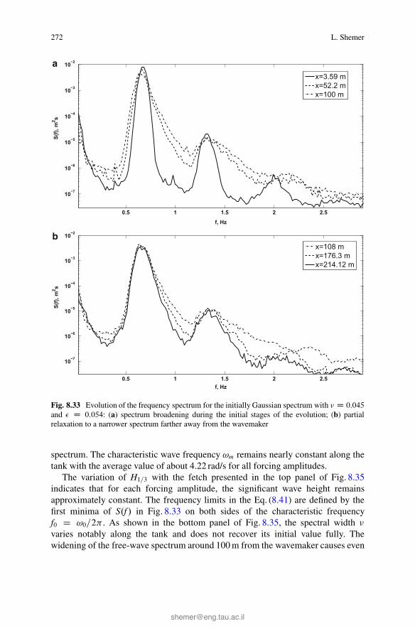
272 L. Shemer
0.5 1 1.5 2 2.5
10−7
10−6
10−5
10−4
10−3
10−2S(
f), m
2 s
f, Hz
x=3.59 mx=52.2 mx=100 m
0.5 1 1.5 2 2.5
10−7
10−6
10−5
10−4
10−3
10−2
S(f),
m2 s
f, Hz
x=108 mx=176.3 mx=214.12 m
a
b
Fig. 8.33 Evolution of the frequency spectrum for the initially Gaussian spectrum with � D 0:045
and � D 0:054: (a) spectrum broadening during the initial stages of the evolution; (b) partialrelaxation to a narrower spectrum farther away from the wavemaker
spectrum. The characteristic wave frequency !m remains nearly constant along thetank with the average value of about 4.22 rad/s for all forcing amplitudes.
The variation of H1=3 with the fetch presented in the top panel of Fig. 8.35indicates that for each forcing amplitude, the significant wave height remainsapproximately constant. The frequency limits in the Eq. (8.41) are defined by thefirst minima of S.f / in Fig. 8.33 on both sides of the characteristic frequencyf0 D !0=2� . As shown in the bottom panel of Fig. 8.35, the spectral width �varies notably along the tank and does not recover its initial value fully. Thewidening of the free-wave spectrum around 100 m from the wavemaker causes even
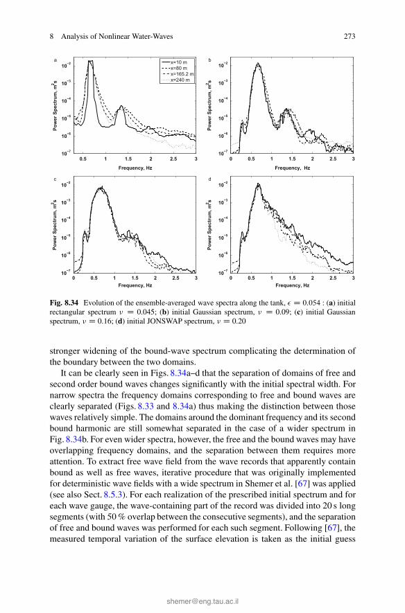
8 Analysis of Nonlinear Water-Waves 273
0.5 1 1.5 2 2.5 310−7
10−6
10−5
10−4
10−3
10−2
Pow
er S
pect
rum
, m2 s
Frequency, Hz
x=10 mx=80 mx=165.2 mx=240 m
a
0 0.5 1 1.5 2 2.5 310−7
10−6
10−5
10−4
10−3
10−2
Pow
er S
pect
rum
, m2 s
Frequency, Hz
b
0 0.5 1 1.5 2 2.5 310−7
10−6
10−5
10−4
10−3
10−2
Pow
er S
pect
rum
, m2 s
Frequency, Hz
c
0 0.5 1 1.5 2 2.5 310−7
10−6
10−5
10−4
10−3
10−2
Pow
er S
pect
rum
, m2 s
Frequency, Hz
d
Fig. 8.34 Evolution of the ensemble-averaged wave spectra along the tank, � D 0:054 : (a) initialrectangular spectrum � D 0.045; (b) initial Gaussian spectrum, � D 0.09; (c) initial Gaussianspectrum, � D 0.16; (d) initial JONSWAP spectrum, � D 0.20
stronger widening of the bound-wave spectrum complicating the determination ofthe boundary between the two domains.
It can be clearly seen in Figs. 8.34a–d that the separation of domains of free andsecond order bound waves changes significantly with the initial spectral width. Fornarrow spectra the frequency domains corresponding to free and bound waves areclearly separated (Figs. 8.33 and 8.34a) thus making the distinction between thosewaves relatively simple. The domains around the dominant frequency and its secondbound harmonic are still somewhat separated in the case of a wider spectrum inFig. 8.34b. For even wider spectra, however, the free and the bound waves may haveoverlapping frequency domains, and the separation between them requires moreattention. To extract free wave field from the wave records that apparently containbound as well as free waves, iterative procedure that was originally implementedfor deterministic wave fields with a wide spectrum in Shemer et al. [67] was applied(see also Sect. 8.5.3). For each realization of the prescribed initial spectrum and foreach wave gauge, the wave-containing part of the record was divided into 20 s longsegments (with 50% overlap between the consecutive segments), and the separationof free and bound waves was performed for each such segment. Following [67], themeasured temporal variation of the surface elevation is taken as the initial guess
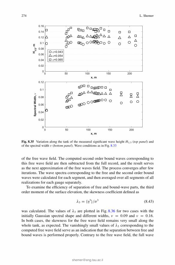
274 L. Shemer
0 50 100 150 2000
0.02
0.04
0.06
0.08
0.1
0.12
0.14
0.16
H1/
3, m
x, m
ε=0.043ε=0.054ε=0.065
0 50 100 150 2000
0.02
0.04
0.06
0.08
0.1
0.12
x, m
Spec
tral
Wid
th, ν
Fig. 8.35 Variation along the tank of the measured significant wave height H1=3 (top panel) andof the spectral width � (bottom panel). Wave conditions as in Fig. 8.33
of the free wave field. The computed second order bound waves corresponding tothis free wave field are then subtracted from the full record, and the result servesas the next approximation of the free waves field. The process converges after fewiterations. The wave spectra corresponding to the free and the second order boundwaves were calculated for each segment, and then averaged over all segments of allrealizations for each gauge separately.
To examine the efficiency of separation of free and bound-wave parts, the thirdorder moment of the surface elevation, the skewness coefficient defined as
�3 D h�3i=�3 (8.43)
was calculated. The values of �3 are plotted in Fig. 8.36 for two cases with theinitially Gaussian spectral shape and different widths, � D 0:09 and � D 0:16.In both cases, the skewness for the free wave field remains very small along thewhole tank, as expected. The vanishingly small values of �3 corresponding to thecomputed free wave field serve as an indication that the separation between free andbound waves is performed properly. Contrary to the free wave field, the full wave
8 Analysis of Nonlinear Water-Waves 275
0 50 100 150 200 2500
0.02
0.04
0.06
0.08
0.1
0.12
0.14
0.16
0.18
0.2
x, m
Free waves onlyFull record
λ3
0 50 100 150 200 2500
0.02
0.04
0.06
0.08
0.1
0.12
0.14
0.16
0.18
0.2
x, m
λ3
Fig. 8.36 The variation along the tank of the skewness �3 for the initial spectra with the Gaussianshape: � D 0:09—top panel; � D 0:16—bottom panel
field exhibits significant positive values of �3 that are quite similar for both initialspectral widths along the whole tank, being mostly somewhat below �3 D 0:2.These positive values of �3 result from the crest-trough asymmetry of nonlinearwaves that apparently is sensitive primarily to the nonlinearity, which is very similarin both panels of Fig. 8.36. The only significant differences between the two panelsoccurs for an initially narrower spectrum where at about x D 70m the values of �3grow notably to attain maximum that exceeds 0.2. This variation of the skewnesscoefficient with the distance in the top panel is qualitatively similar to that reportedin Shemer and Sergeeva [62] for initially narrower Gaussian spectrum.
The variation along the tank of the spectral width � computed according toEqs. (8.40), (8.41), with integration in Eq. (8.41) carried out for the free wavefield only, is presented in Fig. 8.37. The variation of � with the distance x fromthe wavemaker is virtually identical for both Gaussian and rectangular spectrawith identical initial value of � = 0.045. For this initially very narrow spectrum,

276 L. Shemer
0 50 100 150 200 2500
0.05
0.1
0.15
0.2
0.25
0.3
x, m
Rect ν=0.045Gauss ν=0.09Gauss ν=0.16JONSWAP ν=0.2Gauss ν=0.045
ν
Fig. 8.37 The spectral width � as a function of the distance from the wavemaker for differentinitial spectral shapes
the number of discrete free harmonics in the wavemaker driving signal is lessthan 10 in both cases. The actual difference the initial spectra is thus not verysignificant, and in fact after about 50 m, the ensemble averaged spectra becomeessentially identical. The results of Fig. 8.37 are presented for all wave gaugesemployed and corroborate the qualitative conclusion obtained from observing thespectra in Fig. 8.34 that the evolution of the spectral width along the tank is stronglydependent on the initial values of �. For all Gaussian shapes considered, as well asfor the initially rectangular free wave spectrum, the spectral width seems to attain aquasi-equilibrium value at distances exceeding about 170 m (about 50�0) from thewavemaker. Those quasi-equilibrium spectral widths are different for all spectralshapes considered. For initially very narrow spectra with � D 0:045, the quasi-equilibrium width corresponds to � 0:08, while for the initially widest Gaussianspectral shape employed in the present experiments, as well as for the JONSWAPspectrum, the far-field value of � is nearly twice larger, attaining � 0.15. Theevolution of the spectral width of random wave field with the initial spectral shapegiven by (8.42) (JONSWAP spectrum) is somewhat different from that observedfor other initial conditions. The initial width of this spectrum exceeds that of otherspectral shapes considered. The values of � in Fig. 8.37 tend to decrease along thetank, so that at x > 200m the spectral width in this series of experiments fallsbelow values of � that correspond to the initially narrower Gaussian spectrum. Thedecrease in the spectral width with the distance seems to be closely related to decayto the level of nonlinearity along the tank as discussed with relation to Fig. 8.34d.
The deviation of the wave field statistics from Gaussianity can be characterizedby the fourth momentum, the kurtosis �4:
�4 D h�4i=�4: (8.44)

8 Analysis of Nonlinear Water-Waves 277
0 50 100 150 200 2502
2.2
2.4
2.6
2.8
3
3.2
3.4
3.6
3.8
4
x, m
Free waves onlyFull record
λ4
Fig. 8.38 Variation of full and dynamic (for free waves only) kurtosis �4 along the tank for theinitial Gaussian spectrum, � = 0.16
For a Gaussian wave field, �4 D 3. The variation of �4 with the distance x is plottedin Fig. 8.38 for a Gaussian-shaped initial spectrum. The kurtosis values calculatedfor the random wave field that contains free waves only do not differ significantlyfrom �4.x/ based on the full wave records. The contribution of second order boundwaves to �4, although apparently always positive, appears to be insignificant. Theseobservations differ somewhat from the numerical results of Annenkov and Shrira[4] who carried out Monte Carlo simulations of temporal evolution of initiallyunidirectional wave field using the Zakharov [86] equation. The simulations in [4]were performed for the spectral width similar to that of Fig. 8.38, but for highernonlinearity of the wave field. Their numerical results indicate that while the partof kurtosis due to free waves only (dubbed in this study the “dynamic” kurtosisfollowing Janssen [20]) is indeed dominant in the determination of the total value of�4, the contribution of bound waves nevertheless remains important. The variationof kurtosis along the tank presented in Fig. 8.38 exhibits both similarities anddifferences with the results of previous studies. In agreement with both [4, 62],during the initial stages of evolution, up to about 70 m (or 20�0) the values ofkurtosis increase sharply, and decrease farther away from the wavemaker, exhibitingsome oscillations. It should be stressed, however, that the deviations of �4 from thevalue of 3 that corresponds to the Gaussian distribution are relatively modest and inmost cases do not exceed 0.5. This is in contrast with the results of [4, 62], where theexcursions of �4 from the value that corresponds to the Gaussian distribution weremuch more significant. It is also worth noting that starting from about x D 120m,the kurtosis assumes values that are mostly below �4 D 3, thus indicating thatdeviations from Gaussianity for wider spectra are qualitatively different from thoseobserved for the narrow initial spectrum.
The experimentally determined wave height distributions F.H/, normalized bythe r.m.s. values of the surface elevation � , are presented in Fig. 8.39 for the
278 L. Shemer
0 1 2 3 4 5 6 7 8 9 1010
−4
10−3
10−2
10−1
100
Relative Wave Height
Experiment x=20 m Experiment x=55.2 m TF x=20 m TF x=55.2 m Rayleigh
F(h)
0 1 2 3 4 5 6 7 8 9 1010−4
10−3
10−2
10−1
100
Relative Wave Height
Experiment x=80 m Experiment x=110 m TF x=80 m TF x=110 m Rayleigh
F(h)
0 1 2 3 4 5 6 7 8 9 1010−4
10−3
10−2
10−1
100
Relative Wave Height
Experiment x=150 m Experiment x=220 m TF x=150 m TF x=220 m Rayleigh
F(h)
Fig. 8.39 Comparison of the normalized by � experimentally determined wave height probabilitydistributions with the Rayleigh and the third order Tayfun-Fedele distributions at various locationsalong the tank for the initially Gaussian spectrum with � D 0:16
8 Analysis of Nonlinear Water-Waves 279
initially Gaussian spectrum with � D 0:16 at 6 distances from the wavemaker.The experimental results are compared with the Rayleigh distribution, as well aswith the distribution developed by Tayfun and Fedele [79] that accounts for thenonlinearities of the third order. The experimental curves do not differ significantlyfrom the Rayleigh distribution, as long as the wave heights do not exceed about 4� ,although some deviations are observed, most prominently at x = 80, 150 and 220 m.For higher values of H=� , deviations of the wave height probability distributionsfrom the Rayleigh shape in both directions seem to be closely related to the localvalue of �4. The measured probability distributions exceed the Rayleigh valueswhen the local kurtosis is above 3, and fall below the corresponding Rayleighvalues for �3 < 3. The oscillations of the distribution tails are predicted reasonablywell by the Tayfun and Fedele distribution. It should be stressed, however, thatthe theoretical distribution in most cases seems to over predict the probability ofappearance of the steepest waves in the ensemble. A prominent feature of thedistributions plotted in Fig. 8.39 is the virtual absence in the accumulated ensembleof waves with heights exceeding 8� that can be considered as “freak”I waves. Thisresult is quite different from the distributions presented in Shemer and Sergeeva [62]for a narrow Gaussian-shaped initial spectrum (� D 0:045), where the probabilityof extremely high waves was significantly larger than that corresponding to theRayleigh distribution. Moreover, in the measured distributions plotted in Fig. 8.39the tail of the distribution that corresponds to the steepest waves in the ensembleturns sharply down. This part of the distribution is in most cases not presentedadequately by the Tayfun-Fedele curves. The corresponding distributions for wavecrests and troughs are presented in Shemer et al. [69]. Due to the wave asymmetrythe crest heights attain higher values that the troughs.
In [68] the advantage was taken of the accumulated in [62, 69] experimentalresults to examine the accuracy of simulating the spatial evolution of a randomunidirectional wave field by nonlinear envelope models. Monte Carlo-type simu-lations were performed over large scales unique to the GWK. The experimentallydetermined temporal variation of the surface elevation in the vicinity of thewavemaker in each random-phased realization of the given spectrum was used toderive the corresponding initial condition for numerical simulations. The emphasisis put on the narrow-banded initial Gaussian spectrum with the spectral width of� D 0:045 and steepness � D 0:054 in order not to deviate too far from the domainof validity of the envelope models.
The accuracy of the envelope model equations for prediction of the spatialevolution of individual wave groups is examined first. As demonstrated in Sects. 8.3and 8.4, the NLS equation is inadequate to describe evolution of narrow-bandednonlinear deterministic wave groups with symmetric envelopes even for relativelyshort propagation distances, while the application of the modified NLS, or Dysthe,equation yields considerably better agreement with experiments. In Fig. 8.40 theaccuracy of simulations based on these two models is examined on an exampleof a single realization in the GWK experiments. The contribution of bound wavesis accounted for in the numerical simulations. Due to random phases of freeharmonics, the group envelope in each realization has an irregular shape. For the
280 L. Shemer
125 130 135 140 145 150 155 160 165 170−0.1
0
0.1 x=52.19 m (NLS)ζ,
m
180 185 190 195 200 205 210 215 220 225 230−0.1
0
0.1 x=116 m (NLS)
ζ, m
185 190 195 200 205 210 215 220 225 230−0.1
−0.050
0.050.1 x=120 m (Dysthe)
ζ, m
210 215 220 225 230 235 240 245 250 255−0.1
−0.050
0.050.1 x=151.2 m (Dysthe)
ζ, m
250 255 260 265 270 275 280 285 290 295 300−0.1
0
0.1 x=200 m (Dysthe)
ζ, m
t, s
Fig. 8.40 Comparison of the NLS and Dysthe simulations of spatial evolution of a singlerealization with experiments at various distances from the wavemaker: broken lines—experiments;solid lines—simulation
NLS simulations, the measured and the computed surface elevations are presentedat two distances x from the wavemaker. The results at x D 52:2m show that alreadyat a relatively short distance corresponding to about 15�0, notable differences appearbetween computations and measurements. At a larger distance corresponding toabout 33�0, any quantitative agreement between the simulated and the measuredwave fields practically ceases to exist. Nevertheless, some qualitative features ofthe group shapes, such as focusing of wave energy visible in the first group at
8 Analysis of Nonlinear Water-Waves 281
x D 116m, as well the distribution of waves within individual groups, are retainedto some extent in the NLS simulations. At even larger distances, any resemblancebetween the computations and the measurements fades away. The three bottompanels of Fig. 8.40 convincingly demonstrates that the performance of the Dysthemodel is far superior to that of the NLS equation. The measured and the computedtemporal variation of the surface elevation is presented at 3 distances from thewavemaker, all exceeding the values of x in the two top panels of Fig. 8.40.Excellent qualitative agreement between the simulations and the experiments isobtained for the whole extent of the measurements domain. The results at x D120m ( 35�0) exhibit good quantitative agreement between computations andmeasurements, although some deviations are visible. The quantitative agreementseems to deteriorate somewhat with the distance.
The statistical quantitative analysis of the deviation of the Dysthe simulationsfrom the experiment carried out in Shemer et al. [68] suggests that the modified NLSmodel provides a quantitatively accurate description of the deterministic nonlinearwave field up to distances of the order of O.102�0). The results of Fig. 8.40 thusindicate that evolution of an individual realization of a random wave field canbe described adequately over large distances by the Dysthe model, whereas theNLS equation is at best appropriate for revealing some qualitative properties of theevolution process.
The relevance of those nonlinear envelope evolution equations to prediction ofthe statistical properties of the unidirectional random wave field is now considered.The experimental results on variation along the tank of the power spectrum ofthe surface elevation, which is one of the most important statistical parametersdescribing random wave field, are compared in Fig. 8.41 with simulations basedon both models. The initial spectrum, as measured at x D 3:59m, is also plottedas a reference. The free wave part of this spectrum, which is based on the initialgroup shape given by Eq. (8.4), is also symmetric relative to the carrier wavefrequency and has a shape close to Gaussian, as expected. Since the initial spectrumis quite narrow for the value of m D 3:5 in Eq. (8.4), the frequency domainsof the second and the third order bound waves are clearly separated. The initialspectral shape undergoes fast variations and already at x D 52:2m (x 15�0)the free wave spectrum changes notably. The spectrum becomes wider and developsvisible asymmetry. The Dysthe model faithfully describes both these effects, and theagreement between the computed and the measured surface elevation spectrum inthe free wave frequency domain remains good at all distances from the wavemaker.In simulations based on the NLS equation the widening of the free waves spectrumis obtained as well. However, the NLS model is incapable to reflect the asymmetry ofthe developing spectral shape. As noticed in Sect. 8.3, the initially symmetric shapeof the group envelope is retained by the NLS equation in the process of evolution.In the experiments described in this section, the symmetry of the envelope of thegenerating group as given by Eq. (8.4) is lost once random phases are prescribedto the various harmonics. The power spectrum of Eq. (8.4), however, remainssymmetric relative to the carrier wave frequency. Since the experiments clearlyshow that the frequency spectrum loses its symmetry quite fast, the agreement of

282 L. Shemer
0 0.5 1 1.5 2 2.5
10−5
10−2
Spec
trum
, m2 s Initial
ExperimentCSE SimulationMNLS Simulation
0 0.5 1 1.5 2 2.5
10−5
10−2
Spec
trum
, m2 s
f, Hz
x = 100 m
x = 52.2 m
0 0.5 1 1.5 2 2.5
10−5
10−2
Spec
trum
, m2 s
0 0.5 1 1.5 2 2.5
10−5
10−2
f, Hz
Spec
trum
, m2 s
x = 151.2 m
x = 214.12 m
Fig. 8.41 Ensemble averaged spectra: measurements vs. computations using the cubic NLSequation and the Dysthe model
the spectra computed using the NLS equation with the experiments is imperfect,and the NLS-based free wave frequency spectra are significantly wider than eitherthose derived from the Dysthe simulations or the measured ones. The width of thefree waves’ spectrum seems to attain maximum at distances about 100 m, and thendecreases somewhat.
The agreement between the second order bound waves as measured in theexperiment and as computed using the Dysthe model is reasonable at all distancesfrom the wavemaker. Those waves have amplitudes that are comparable with thesensitivity of the wave gauges. The simulations based on both models agree quite
8 Analysis of Nonlinear Water-Waves 283
well with the measurements around the peak of the second order bound waves(close to 1.3 Hz); away from the peak the Dysthe simulations yield a much betteragreement with the experiments than the NLS equation. The dip in the spectrumbetween the domains of free and second order bound waves is much deeper insimulations than in experiments. This can be attributed to the limited accuracy ofthe wave gauges.
The results of Figs. 8.40 and 8.41 clearly demonstrate good quantitative andqualitative agreement of the Dysthe model simulations with the experiments for alldistances from the wavemaker covered in the GWK experiments, with deviationsthat can be plausibly attributed to experimental inaccuracies. Such an agreementseems to justify the extension of simulations to distances beyond the domain ofexperiments in order to gain some insight on the wave field evolution patternat longer scales. In sequel, the results of simulations are presented for distancesexceeding the actual length of the GWK by a factor of 2, whereas the experimentalresults apparently are only shown where available.
The computed and the derived from the experiments variations with x of thespectral width of the free wave part of the spectrum, �, as well as of the skewness �3and of kurtosis �4 are plotted in Fig. 8.42. The computed values of �, Fig. 8.42a forboth model equations are in a reasonable agreement with the experimental results.Both models correctly predict the experimentally observed spectral widening, with� increasing nearly twice from its initial value � 0.45 during the first 100 mof the evolution. The spectral width then decreases somewhat. The simulationsfarther away from the wavemaker exhibit irregular, relatively weak oscillations ofthe spectral width (around the mean value of � 0.65 for the Dysthe model and of� 0.75 for the NLS model); the characteristic length scale of these oscillationsexceeds 100 m, or about 30�0.
The variation of the skewness �3 along the tank, as measured in the experiment,is compared in Fig. 8.42b with the results of simulations based on both models. Themodels yield values of �3 that are quite close to the measurements. The dependenceof �3 on the distance x in Fig. 8.42b bears some similarity to the behavior of �.x/ inthe panel (a) of this figure. The skewness coefficient increases quite sharply initially,up to about x D 100m, and then decreases somewhat, exhibiting relatively weakvariability at length scales similar to those of Fig. 8.42a. The values of �3 werealso calculated for the surface elevation records that were band-pass filtered for thefree waves’ domain, fmin � f � fmax. The variation of the skewness coefficient �3that represent free waves only is also plotted in Fig. 8.42b. The values of �3 dueto free waves are virtually zero at all locations, both in the experiments and in thesimulations based on the Dysthe model (similar results obtained within NLS modelare not presented). The results of Fig. 8.42b thus demonstrate that skewness, whichis determined nearly solely by the contribution of the bound waves, is adequatelydescribed by both envelope equations.
Variation of the kurtosis coefficient �4 along the tank is presented in Fig. 8.42c.Again, the Dysthe model yields good agreement with the experiments, while theNLS equation significantly overestimates the maximum values of the kurtosis in thetransitional domain at about 50 m < x < 120 m. At larger distances the predictions
284 L. Shemer
0 100 200 300 400 5000.04
0.05
0.06
0.07
0.08
0.09
0.1
x, m
Experiment NLS Dysthe
ν
0 100 200 300 400 500−0.1
0
0.1
0.2
0.3
0.4
x, m
ExperimentNLSDystheExperiment: free wavesDysthe: free waves
λ3
0 100 200 300 400 5002
3
4
5
6
7
x, m
λ4
Fig. 8.42 Computed and measured variations along the tank of the spectral width � (a), skewness�3 (b) and kurtosis �4 (c)
8 Analysis of Nonlinear Water-Waves 285
0 2 4 6 8 1010−4
10−3
10−2
10−1
100
ExperimentNLSDystheRayleigh
0 2 4 6 8 1010−4
10−3
10−2
10−1
100
F(h)
x = 126 mx = 100 m
0 2 4 6 8 1010−4
10−3
10−2
10−1
100
Wave Height0 2 4 6 8 10
10−4
10−3
10−2
10−1
100
Wave Height
F(h)
x = 176 m x = 400 m
Fig. 8.43 Computed and measured wave height distributions at several distances from thewavemaker for the Gaussian driving signal given by Eq. (8.4) with mD 3:5 and � = 0.054
based on both those models seem to be closer, and the computed values of �4 varysomewhat (at the characteristic length scale of about 30 carrier wave lengths, similarto other statistical parameters), but remains in the vicinity of �4 4, indicating thatthe wave field departs significantly from the Gaussian distribution. As in Fig. 8.38,an attempt is made to separate the “dynamic” kurtosis �4d based on free waves only.The results at large distances from the wavemaker differ somewhat from those of [4]and do show any substantial difference between �4d and the full kurtosis �4. Thisdiscrepancy may be attributed in part to the total lack of 2D effects in the simulationsbased on the Dysthe model.
Measured and computed from Dysthe and NLS simulations wave heightexceedance distributions for different locations along the tank are plotted inFig. 8.43. The exceedance distributions are normalized by the standard deviation� of the surface elevation variation. The Rayleigh distribution for the scaled waveheight is plotted as well. The wave height exceedance distributions derived fromboth models agree well with the measured probabilities. In simulations as well asin experiments, the Rayleigh distribution overestimates the exceedance probabilityfor H < 4� and underestimates it for higher values of wave heights. Moreover, themodels are capable of providing adequate prediction of probability of appearance ofwaves with heights below 8� . Both simulation and the experiment clearly indicatethat the probability of those extremely high waves exceeds that corresponding tothe Rayleigh distribution by an order of magnitude. Still, since the probability of
286 L. Shemer
such high waves is quite low, spread of data in Fig. 8.43 for H > 8� is evidentboth for the distributions based on the laboratory data and those obtained from thenumerical simulations. This spread seems to be a result of insufficient size of theensemble. The behavior of the distribution tail in Fig. 8.43 is qualitatively differentfrom the wider spectrum case plotted in Fig. 8.39 where no extremely high waveswith H > 8� that may be considered ‘rogue’ waves were detected. As demonstratedin [69], rogue wave were not recorded ion experiments with even wider JONSWAPspectrum. The correlation between the probability appearance of extremely highwaves and kurtosis was demonstrated in that study as well.
8.7 Discussion and Conclusions
The total body of presented experimental and numerical results allows drawingsome conclusions regarding mechanisms leading to appearance of extremely steep(rogue) waves. As mentioned in the Introduction, in recent years, the problem ofappearance of those waves in the ocean is often related in the literature to specificproperties of the NLS equation that admits breather type soliton solutions. Asstressed in Sect. 8.3, the NLS equation is the simplest theoretical model describingevolution of unidirectional gravity waves that is valid only for narrow-banded wavegroups. The breathing solitons represent spatially, temporally, or both, localizedpatterns in which an initially small “hump” in a nearly monochromatic wave trainis amplified attaining wave heights that exceed significantly the initial level. Thewave evolution patterns that are characteristic for the NLS breathers in deep waterbear resemblance to appearance of freak waves in the ocean and for that reasonattract considerable attention. It was asserted in some studies that different typesof breathers were indeed observed in laboratory experiments. On the other hand,Shemer and Alperovich [57] demonstrated that for a Peregrine Breather (PB), theagreement between the experiments and measurements is only obtained at theinitial stages of the wave train evolution, (see Sect. 8.4.3). Similar conclusionswere obtained in fully nonlinear simulations by Slunyaev and Shrira [71] and byShemer and Ee [60]. The velocity of propagation of the ‘hump’ in the PB envelopediffers from the linear group velocity cg as assumed in the NLS equation. Similarly,envelope maxima of other narrow-banded wave groups of different shapes studiedin Sects. 8.3–8.5 also propagate with velocity exceeding cg. The faster movement ofthe highest crest in the group is correctly described by the modified NLS (Dysthe)equation. The failure of the NLS model to describe adequately the propagationof breathers beyond the initial stages was attributed in Sect. 8.4 to considerablespectral widening associated with amplification of the steepest wave that violatesthe basic assumptions adopted in the derivation of the NLS equation. The NLSequation results in symmetric shapes, whereas in experiments as well as in theDysthe simulations essentially asymmetric wave shapes were observed. It shouldbe noted that the fully nonlinear simulations [71] did not show the left-rightasymmetry. As demonstrated by Shemer and Dorfman [59], the symmetry of the
8 Analysis of Nonlinear Water-Waves 287
spatial distribution may differ from that in the temporal presentation, cf. Figs. 8.8and 8.10. The numerical simulations carried out in [60] indeed demonstrated thatthe asymmetry in the spatial ‘snapshot’ of PB is barely noticeable, whereas in thetemporal variation �.t/ is becomes more prominent.
The limited validity of the NLS equation thus leads to significant deviation ofthe PB shape from the NLS solution given by Eq. (8.32) in measurements as wellas in more advanced computations based on either Dysthe equation or on the fullynonlinear approach. The question therefore arises whether different solitons indeedrepresent a special class of wave shapes that differ essentially from non-solitonwave envelopes and constitute prototype of rogue waves as often suggested, see e.g.[70]. In fact, notable amplification of both the maximum wave crests and maximumenvelope values occurs in the course of evolution in deep water of initially narrow-banded deterministic wave groups with different initial shapes, see Fig. 8.5 andadditional results presented in [21, 64–66]. All characteristic features that often arespecifically attributed to the evolution of NLS breathers were in fact observed for avariety of arbitrarily selected initial wave group shapes. The increase of maximumcrest height may be seen as manifestation of the focusing properties of the NLSequation. Indeed, no such focusing was observed for experiments conducted inshallower water, when the coefficient of the nonlinear term in the NLS equationnearly vanishes or becomes negative, see Sect. 8.3. Moreover, as demonstrated in[62, 69], initially narrow-banded random-phased wave groups with no characteristicenvelope shape also exhibit strong wave height amplification accompanied bysignificant spectral widening in the process of their evolution along the tank, seeSect. 8.6.
It thus appears that NLS breathers do not possess any special qualities distinctfrom those of any initially narrow banded wave groups. They seem to be essentiallyirrelevant to rogue wave formation even in unidirectional and controlled setting oflaboratory wave tank experiments. As stressed in [56], all types of breathers, aswell as rogue waves that were actually recorded in the ocean, exhibit fast variationof the wave train envelope (on scales comparable with the dominant wave period)and are essentially wide-banded. The emergence of a single high wave can be seenas resulting from a positive interference of numerous harmonics. In this sense,both breathers and rogues waves in the ocean (such as the well-known New Yearwave, see e.g [23]) are not different from those observed by focusing of an initiallywide-banded unidirectional wave train [67] as presented in Sect. 8.5.3. The relationbetween the height of the steepest wave in the train of finite duration and the shapeof its discrete spectrum can be examined on the basis of simple considerations. Fora given complex amplitude spectrum of the surface elevation ai D a.!i/, the crestheight cannot exceed the value attained when the phases of all harmonics coincide:�max D P jaij (perfect coherence). For an initially nearly monochromatic wavewith a narrow spectrum, like PB away from the focusing location, the energy isconcentrated at the carrier wave frequency, so that the ‘hump’ does not exceedsignificantly the background carrier wave and �max jacarrierj. In the initiallynarrow spectrum, nonlinear interactions among neighboring harmonics are strongleading to fast widening of the spectrum [55]. The energy conservation at the leading
288 L. Shemer
order requires that at any instantP
ai2.t/ jacarrier.t D 0/j2. The maximum
possible wave corresponding to the sum of the amplitudes of all harmonics in thespectrum thus can be obtained when the wave energy is distributed uniformly amongnumerous harmonics. In this respect it can be noted that the Dirac ı-functions thatcan be seen as an ultimate model of a rogue wave, has uniform white spectrum.Therefore in order to obtain a single extremely steep wave in the evolution process,significant spectral widening needs to occur. The rogue wave in deterministic aswell as in a random wave field then can be seen a result of an essentially linearconstructive interference of numerous harmonics [62, 67, 69]. Note that the relativeto the background amplification of the maximum wave crest due to nonlinearfocusing as a result of constructive interference may exceed the threefold gain of thePeregrine breather, see Fig. 8.30. The role of nonlinearity in this process is limited tomodification of the initial spectrum to the prescribed shape at the focusing locationsidentical phases of all harmonics.
An even stronger amplification of the steepest wave was recorded in experimentson initially narrow-banded random wave groups by Shemer and Sergeeva [62].Themechanism leading to appearance of rogue waves in that case seems to besimilar to that suggested for focusing of deterministic waves. For narrow initialspectrum, a relatively small number of harmonics with close frequencies interactstrongly generating new sideband harmonics [55]. The complex amplitudes inthe initial spectrum have random phases, however, in each realization the newlygenerated sideband harmonics have phases related to those of their ‘parents’. Oncethose harmonics grow to be sufficiently strong, the probability of appearance ofextreme waves increases due to their intrinsic coherence. Increase in the number ofharmonics in the initial spectrum, either by widening or by directional spreading,effectively eliminates this mechanism, resulting in virtual absence of freak waves inthose cases, in agreement with experimental observations. Note also that contrary tothe instantaneous surface shape that can vary fast due to the change of phases of theharmonics at fast time and space scales, the spectral modifications are essentiallynonlinear and thus occur on slow scales. It thus appears that rogue waves constitutean inherently wide-banded phenomenon where separation of slow/fast scales is notapplicable. This renders the intrinsically narrow-banded NLS equation inadequatefor quantitatively accurate modeling.
In summary, a thorough examination of performance of different unidirectionalnonlinear wave models, based on a detailed quantitative comparison of modelpredictions with extensive experimental results is presented. Deterministic wavegroups as well as random wave fields in deep and intermediate-depth water wereinvestigated. Experiments were carried out in two facilities that differ significantlyin size and for a wide range of characteristic wave parameters, i.e nonlinearity,spectral width and envelope or spectral shape. The consistent approach was adoptedin the experiments in both facilities to make it possible to identify the effect ofscaling. Advantages and disadvantages of larger size of the experimental facilityare discussed. The dimensionless parameters that determine the effective sizeof the facility are introduced; under certain conditions, a smaller tank that has
8 Analysis of Nonlinear Water-Waves 289
greater flexibility in running experiments can be advantageous for studies of spatialevolution problems due to higher accuracy of results and possibility to carry outlarge number of experimental runs at a reasonable price. On the other hand, formany applications the absolute (dimensional) wave height is important. In thosecases, bigger facilities offer substantial benefits.
An effective method developed for identification of the instantaneous contact lineshapes in a sequence of recorded video images allows studying temporal evolutionof the instantaneous wave field in the whole tank and thus determination of thewavenumber spectra and of their variation in time. This ability is important forcarrying out quantitative comparison of prediction of nonlinear evolution modelswith the experimental results. The suggested in [59] experimental approach enablesstudying both the spatial and the temporal evolution of narrow-banded unidirec-tional wave groups. The essential differences between the temporal and the spatialformulation of the evolution problem are specified in Sect. 8.4.2. The temporalevolution is routinely considered in theoretical studies of water waves based on theZakharov equation and on fully nonlinear simulations. In laboratory tanks wavesevolve in space rather than in time. The shapes of the spectra are apparently quitedifferent in the spatial and temporal formulations; the wave number spectra aretwice wider than the corresponding frequency spectra. As specified in [59, 60],direct quantitative comparison of theoretical results based on the temporal evolutionapproach with experiments is far from being straightforward. For a narrow-boundedspectrum, the group velocity cg enables simple transition between the spatial and thespatial formulations, as demonstrated by Lo and Mei [32] for the NLS and Dystheequations. The benefit offered by the NLS equation, however, is limited, as thismodel is incapable of describing the finer features of the propagating wave group,and may provide quantitative results with reasonable accuracy only as long as thespectrum remains very narrow, Sect. 8.3, or for some statistical parameters, Sect. 8.6.Nevertheless, the applicability of the analytic solution of NLS equation for thePeregrine breather given by Eq. (8.32) to the early stages of wave group evolutionwas recently utilized by Shemer and Liberzon [61] to study experimentally theinception of a spilling breaker. The modified Dysthe equation that is formally validas long as the spectral width does not exceed nonlinearity, proved to be a an accuratemodel for description of the spatial evolution of both deterministic and randomdeep-water wave groups with moderate spectrum width. However, for an even widerspectrum, the Dysthe equation ceases to be valid.
The Zakharov equation that is free of any restriction on the spectral width isthus the most appropriate third order model for wide-banded wave groups. Themodification of the standard temporal version of the Zakharov equation to theform that describes evolution in space is required for quantitative comparison ofthe theoretical and experimental results. For a wide spectrum, the group velocityis not defined, thus the straightforward transformation used for transition fromtemporal to spatial evolution formulation for the NLS and Dysthe equations is notapplicable. Generalization of the notion of the group velocity for a wide spectrumwas suggested in [67] resulting the spatial version of the Zakharov equation givenby Eqs. (8.33) and (8.34). The validity of this equation for description of evolution
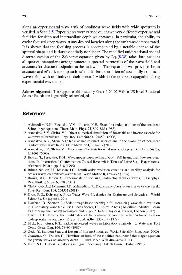
290 L. Shemer
along an experimental wave tank of nonlinear wave fields with wide spectrum isverified in Sect. 8.5. Experiments were carried out in two very different experimentalfacilities for deep and intermediate depth water-waves. In particular, the ability toexcite focused steep waves at any desired location along the tank was demonstrated.It is shown that the focusing process is accompanied by a notable change of thespectral shape and is thus essentially nonlinear. The modified unidirectional spatialdiscrete version of the Zakharov equation given by Eq. (8.38) takes into accountall quartet interactions among numerous spectral harmonics of the wave field andaccounts for viscous dissipation at the tank walls. This equations was proved to be anaccurate and effective computational model for description of essentially nonlinearwave fields with no limits on their spectral width in the course propagation alongexperimental wave tanks.
Acknowledgements The support of this study by Grant # 2010219 from US-Israel BinationalScience Foundation is gratefully acknowledged.
References
1. Akhmediev, N.N., Eleonskii, V.M., Kulagin, N.E.: Exact first-order solutions of the nonlinearSchrödinger equation. Theor. Math. Phys. 72, 809–818 (1987)
2. Annenkov, S.Y., Shrira, V.I.: Direct numerical simulation of downshift and inverse cascade forwater wave turbulence. Phys. Rev. Lett. 96(20), 204501 (2006)
3. Annenkov, S.Y., Shrira V.I.: Role of non-resonant interactions in the evolution of nonlinearrandom water wave fields. Fluid Mech. 561, 181–207 (2006)
4. Annenkov, S.Y., Shrira, V.I.: Evolution of kurtosis for wind waves. Geophys. Res. Lett. 36(13),L13603 (2009)
5. Barnes, T., Peregrine, D.H.: Wave groups approaching a beach: full irrotational flow computa-tions. In: International Conference on Coastal Research in Terms of Large Scale Experiments,Abstracts, Poland, pp. 7–8 (1995)
6. Brinch-Nielsen, U., Jonsson, I.G.: Fourth order evolution equation and stability analysis forStokes waves on arbitrary water depth. Wave Motion 8, 455–472 (1986)
7. Brown, M.G., Jensen A.: Experiments on focusing unidirectional water waves. J. Geophys.Res. 106(C8) 917–16, 928 (2001)
8. Chabchoub, A., Hoffmann N.P., Akhmediev, N.: Rogue wave observation in a water wave tank.Phys. Rev. Lett. 106, 204502 (2011)
9. Dean, R.G., Dalrymple, R.A.: Water Wave Mechanics for Engineers and Scientists. WorldScientific, Singapore (1991)
10. Dorfman, B., Shemer, L.: Video image-based technique for measuring wave field evolutionin a laboratory wave tank. In: Guedes Soares, C., Kolev, P. (eds.) Maritime Industry, OceanEngineering and Coastal Resources, vol. 2, pp. 711–720. Taylor & Francis, London (2007)
11. Dysthe, K.B.: Note on the modification of the nonlinear Schrödinger equation for applicationto deep water waves. Proc. R. Soc. Lond. A369, 105–114 (1979)
12. Flick, R.E., Guza, R.T.: Paddle generated waves in laboratory channels. J. Waterway PortCoast. Ocean Eng. 106, 79–96 (1980)
13. Goda, Y.: Random Seas and Design of Marine Structures. World Scientific, Singapore (2000)14. Gramstad, O., Trulsen, K.: Hamiltonian form of the modified nonlinear Schrödinger equation
for gravity waves on arbitrary depth. J. Fluid. Mech. 670, 404–426 (2011)15. Hahn, S.L.: Hilbert Transforms in Signal Processing. Artech House, Boston (1996)
8 Analysis of Nonlinear Water-Waves 291
16. Hasimoto, H., Ono, J.: Nonlinear modulation of gravity waves. J. Phys. Soc. Jpn. 33, 805–811(1972)
17. Hasselmann, K.: On the nonlinear energy transfer in a gravity wave spectrum. Part 1. Generaltheory. J. Fluid Mech. 12, 481–500 (1962)
18. Hasselmann, K., Barnett, T.P, Bouws, E., Carlson, H., Cartwright, D.E., Enke, K., Ewing, J.A.,Gienapp, H., Hasselmann, D.E., Krusemann, P., Meerburg, A., Müller, P., Olbers, D.J., Richter,K., Sell, W., Walden, H.: Measurements of wind-wave growth and swell decay during the JointNorth Sea. Deutsche Hydrographische Zeitschrift 8(Suppl A), 1–95 (1973)
19. Hogan, S.J.: The potential form of the fourth-order evolution equation for deep-water gravity-capillary waves. Phys. Fluids 29, 3479–3480 (1986)
20. Janssen, P.A.E.M.: Nonlinear four-wave interactions and freak waves. J. Phys. Ocean. 33,863–884 (2003)
21. Jiao, H.-Y.: Experimental measurements and numerical simulations of nonlinear water-wavegroups. Ph.D. Thesis, Tel-Aviv University (1999)
22. Johannessen, T.B., Swan, C.: On the nonlinear dynamics of wave groups produced by thefocusing of surface-water waves Proc. R. Soc. A459, 1021–1052 (2003)
23. Kharif, C., Pelinovsky, E., Slunyaev, A.: Rogue Waves in the Ocean. Springer, Berlin (2009)24. Kharif, C., Kraenkel, R., Manna, M., Thomas, R.: The modulational instability in deep water
under action of wind and dissipation. J. Fluid Mech. 664, 138–149 (2010)25. Kit, E., Shemer, L.: On dissipation coefficients in a wave tank. Acta Mech. 77, 171–180 (1989)26. Kit, E., Shemer, L.: Spatial versions of the Zakharov and Dysthe evolution equations for deep
water gravity waves. J. Fluid Mech. 450, 201–205 (2002)27. Kit, E., Pelinovsky, E., Talipova, T.: Transformation of probability distribution of wind waves
in coastal zone. In: Proceedings of the COPEDEC IV, Brazil, pp. 2344–2353 (1995)28. Kit, E., Shemer, L., Pelinovsky, E., Talipova, T., Eitan, O., Jiao, H.-Y.: Nonlinear wave group
evolution in shallow water. J. Waterway Port Coast. Ocean Eng. 126, 221–228 (2000)29. Krasitskii, V.P.: On reduced equations in the Hamiltonian theory of weakly nonlinear surface
waves. J. Fluid Mech. 272, 1–20 (1994)30. Kuznetsov, E.A.: Solitons in a parametrically unstable plasma. Sov. Phys. Dokl. (English
Transl.) 22, 575–577 (1977)31. Lake, B.M., Yuen, H.C., Rungaldier, H., Ferguson, W.E.: Nonlinear deep-water waves: theory
and experiment. Part 2. Evolution of a continuous wave train. J. Fluid Mech. 83, 49–74 (1977)32. Lo, E., Mei, C.C.: A numerical study of water-wave modulation based on a higher-order
nonlinear Schrödinger equation. J. Fluid Mech. 150, 395–416 (1985)33. Longuet-Higgins, M.: On the statistical distribution of the heights of sea waves. J. Mar. Res.
11, 245–266 (1952)34. Longuet-Higgins, M.: The effect of nonlinearities on statistical distributions in the theory of
sea waves. Fluid Mech. 17, 459–480 (1963)35. Longuet-Higgins, M.: The instabilities of gravity waves of finite amplitude in deep water. II.
Subharmonics. Proc. R. Soc. Lond. Ser. A 360, 489–505 (1978)36. Ma, Y.C.: The perturbed plane wave solutions of the cubic nonlinear Schrödinger equation.
Stud. Appl. Math. 60, 43 (1979)37. McLean, J.W.: Instabilities of finite amplitude water waves. Fluid Mech. 114, 331–341 (1982)38. McLean, J.W., Ma, Y.C., Martin, D.U., Saffman, P.G., Yuen, H.C.: A new type of three-
dimensional instability of finite amplitude gravity waves. Phys. Rev. Lett. 46, 817–820 (1981)39. Mei, C.C.: The Applied Dynamics of Ocean Surface Waves. World Scientific, Singapore
(1989)40. Melville, W.K.: Wave modulation and breakdown. Fluid Mech. 128, 489–506 (1983)41. Mori, N., Onorato, M., Janssen, P.A.E.M., Osborne, A.R., Serio, M.: On the extreme statistics
of long-crested deep water waves: theory and experiments. J. Geophys. Res. 112, C09011(2007)
42. Nazarenko, S.V.: Wave Turbulence. Springer, Berlin (2011)43. Naess, A.: On the distribution of crest-to-trough wave heights. Ocean Eng. 12, 221–234 (1985)

292 L. Shemer
44. Ochi, M.K.: Stochastic analysis and probabilistic prediction of random seas. Adv. Hydrosci.13, 217–375 (1982)
45. Onorato, M, Osborne, A.R, Serio, M, Cavaleri, L.: Modulational instability and non-Gaussianstatistics in experimental random water-wave trains. Phys. Fluid. 17, 078101 (2005)
46. Onorato, M, Osborne, A.R, Serio, M, Cavaleri, L., Brandini, C., Stansberg, C.T.: Extremewaves, modulational instability and second order theory: wave flume experiments on irregularwaves. Eur. J. Mech. B Fluids 25, 586–601 (2006)
47. Onorato M., Osborne A.R., Serio M.: On the relation between two numerical methods for thecomputation of random gravity waves. Eur. J. Mech. B Fluids 26, 43–48 (2007)
48. Onorato, M., Onorato, M., Cavalieri, L., Fouques, S., Gramstad, O., Jansses, P.A.E.M.,Monbaliu, J., Osborne, A.R., Pakozdi, C., Serio, M., Stansberg, C.T., Toffoli, A., Trulsen, K.:Statistical properties of mechanically generated surface gravity waves: a laboratory experimentin a three-dimensional wave basin. J. Fluid Mech. 627, 235–257 (2009)
49. Pelinovsky, E., Kharif, C.: Simplified model of the freak wave formation from the randomwave field. In: Miloh, T., Zilman, G. (eds.) Proceedings of 15th International Workshop onWater Waves and Floating Bodies, Caesaria, pp. 142–145 (2000)
50. Peregrine, D.H.: Water waves, nonlinear Schrödinger equations and their solutions. J. Aust.Math. Soc. Ser. B 25, 16–43 (1983)
51. Phillips, O.M.: On the dynamics of unsteady gravity waves of finite amplitude. Part 1. Theelementary interactions. J. Fluid Mech. 9, 193–217 (1960)
52. Phillips, O.M.: Wave interactions: the evolution of an idea. Fluid Mech. 106, 215–227 (1981)53. Schäffer, H.A.: Second order wavemaker theory for irregular waves. Ocean Eng. 23, 47–88
(1996)54. Shahul Hameed, T.S., Baba, M.: Wave height distribution in shallow water. Ocean Eng. 12,
309–319 (1985)55. Shemer, L: On Benjamin-Feir instability and evolution of a nonlinear wave with finite-
amplitude sidebands. Nat. Hazards Earth Syst. Sci. 10, 2421–2427 (2010)56. Shemer, L.: The advantages and limitations of the nonlinear Schrödinger equation in descrip-
tion of evolution of nonlinear water-wave groups.Proc. Est. Acad. Sci. 64(3), 17 (2015)57. Shemer, L., Alperovich, L.: Peregrine breather revisited. Phys. Fluids 25(1) 051701 (2013)58. Shemer, L., Chamesse, M.: Experiments on nonlinear gravity-capillary waves. Fluid Mech.
380, 205–232 (1999)59. Shemer, L., Dorfman, B.: Experimental and numerical study of spatial and temporal evolution
of nonlinear wave groups. Nonlinear Process. Geophys. 15, 931–942 (2008)60. Shemer, L., Ee, B.K.: Steep unidirectional wave groups - fully nonlinear simulations vs.
experiments. Proc. 34th Int. Conf. on Offshore Mechanics and Arctic Engineering, St. John’s,Newfoundland, Canada (ASME Paper OMAE2015-41057)
61. Shemer, L., Liberzon, D.: Lagrangian kinematics of steep waves up to the inception of a spillingbreaker. Phys. Fluids 26(1), 016601 (2014)
62. Shemer, L., Sergeeva, A.: An experimental study of spatial evolution of statistical parametersin a unidirectional narrow-banded random wavefield. J. Geophys. Res. 114, C01015 (2009)
63. Shemer, L., Kit, E., Miloh, T.: Measurements of two- and three-dimensional waves in a channelincluding the vicinity of cut-off frequencies. Exp. Fluids 5, 66–72 (1987)
64. Shemer, L., Kit, E., Jiao, H.-Y, Eitan, O.: Experiments on nonlinear wave groups in intermedi-ate water depth. J. Waterway Port Coast. Ocean Eng. 124, 320–327 (1998)
65. Shemer, L., Jiao, H.-Y., Kit, E., Agnon, Y.: Evolution of a nonlinear wave field along a tank:experiments and numerical simulations based on the spatial Zakharov equation. Fluid Mech.427, 107–129 (2001)
66. Shemer, L., Kit, E., Jiao, H.-Y.: An experimental and numerical study of the spatial evolutionof unidirectional nonlinear water-wave groups. Phys. Fluids 14, 3380–3390 (2002)
67. Shemer, L., Goulitski, K., Kit, E.: Evolution of wide-spectrum wave groups in a tank: anexperimental and numerical study. Eur. J. Mech. B Fluids 26, 193 (2007)

8 Analysis of Nonlinear Water-Waves 293
68. Shemer, L., Sergeeva, A., Slunyaev, A.: Applicability of envelope model equations forsimulation of narrow-spectrum unidirectional random field evolution: experimental validation.Phys. Fluids 22, 011601 (2010)
69. Shemer, L., Sergeeva, A., Liberzon, D.: Effect of the initial spectrum on the spatial evolutionof statistics of unidirectional nonlinear random waves. J. Geophys. Res. 115, C12039 (2010)
70. Shrira, V.I., Geogjaev, V.V.: What makes the Peregrine soliton so special as a prototype of freakwaves? J. Eng. Math. 67, 11–22 (2010)
71. Slunyaev, V.V., Shrira, V.I.: On the highest non-breaking wave in a group: fully nonlinear waterwave breathers versus weakly nonlinear theory. Fluid Mech. 735, 203–248 (2013)
72. Socquet-Juglard, H., Dysthe, K, Trulsen, K., Krogstad, H.E., Liu, J.: Distribution of surfacegravity waves during spectral changes. Fluid Mech. 542, 195–216 (2005)
73. Stiassnie, M.: Note on the modified nonlinear Schrödinger equation for deep water waves.Wave Motion 6, 431–433 (1984)
74. Stiassnie, M., Shemer, L.: On modifications of the Zakharov equation for surface gravity waves.Fluid Mech. 143, 47–67 (1984)
75. Stiassnie, M., Shemer, L.: On the interaction of four water-waves. Wave Motion 41, 307–328(2005)
76. Su, M.Y.: Evolution of groups of gravity waves with moderate to high steepness. Phys. Fluids25, 2167–2174 (1982)
77. Tayfun, M.A.: Narrow-band nonlinear sea waves. J. Geophys. Res. 85(C3), 1548–1552 (1980)78. Tayfun, M.A.: Statistics of nonlinear wave crests and groups. Ocean Eng. 33, 1589–1622
(2006)79. Tayfun, M.A., Fedele, F.: Wave height distributions and nonlinear effects. Ocean Eng. 34,
1631–1649 (2007)80. Trulsen, K., Dysthe, K.B.: A modified nonlinear Schrödinger equation for broader bandwidth
gravity waves on deep water. Wave Motion 24, 281–289 (1996)81. Trulsen, K., Dysthe, K.B.: Frequency downshift in three-dimensional wave trains in a deep
basin. Fluid Mech. 352, 359–373 (1997)82. Trulsen, K., Kliakhandler, I., Dysthe, K.B., Velarde, M.G.: On weakly nonlinear modulation of
waves on deep water. Phys. Fluids 12, 2432–2437 (2000)83. Waseda, T., Kinishita, T., Tamura, H.: Evolution of a random directional wave and freak wave
occurrence. J. Phys. Ocean 39, 621–639 (2009)84. Yuen, H.C., Lake, B.M.: Nonlinear deep water waves: theory and experiment. Phys. Fluids 18,
956–960 (1975)85. Yuen, H.C., Lake, B.M.: Nonlinear dynamics of deep water gravity waves. Adv. Appl. Mech.
22, 67–229 (1982)86. Zakharov, V.E.: Stability of periodic waves of finite amplitude on a surface of deep fluid. J.
Appl. Mech. Tech. Phys. (English Transl.) 2, 190–194 (1968)87. Zakharov, V.: Statistical theory of gravity and capillary waves on the surface of a finite-depth
fluid. Eur. J. Mech. B Fluids 18, 327–344 (1999)88. Zakharov, V.E., Shabat, A.B.: Exact theory of two-dimensional self-focusing and one-
dimensional self-modulation of waves in nonlinear media. Sov. Phys. JETP 34, 62–69 (1972)


![1 [Ni 0 L]-catalyzed cyclodimerization of butadiene: A computational study based on the generic [Ni 0 (butadiene) 2 PH 3 ] catalyst. Sven Tobisch and Tom](https://img.pdfslide.net/doc/110x75/56649d2c5503460f94a017d8/1-ni-0-l-catalyzed-cyclodimerization-of-butadiene-a-computational-study.jpg)