Embed Size (px)
Citation preview
Outlines
Elimination Theory, Commutative Algebra andApplications
Laurent Buse
INRIA Sophia-Antipolis, France
March 2, 2005
Laurent Buse Elimination Theory, Commutative Algebra and Applications
OutlinesPart I: Residual resultants in P2
Part II: Implicitization Problem
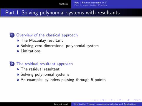
Part I: Solving polynomial systems with resultants
1 Overview of the classical approachThe Macaulay resultantSolving zero-dimensional polynomial systemLimitations
2 The residual resultant approachThe residual resultantSolving polynomial systemsAn example: cylinders passing through 5 points
Laurent Buse Elimination Theory, Commutative Algebra and Applications
OutlinesPart I: Residual resultants in P2
Part II: Implicitization Problem
Part II: Implicitization problem for curves and surfaces
3 Implicitization of rational plane curvesUsing resultantsUsing moving linesUsing syzygies
4 Implicitization of rational surfacesUsing resultantsUsing syzygies
Laurent Buse Elimination Theory, Commutative Algebra and Applications
Classical approachResidual approach
Part I
Solving polynomial systems with resultants
Laurent Buse Elimination Theory, Commutative Algebra and Applications
Classical approachResidual approach
The Macaulay resultantSolving zero-dimensional polynomial systemLimitations
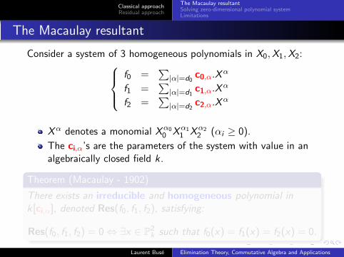
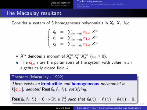
The Macaulay resultant
Consider a system of 3 homogeneous polynomials in X0,X1,X2:f0 =
∑|α|=d0
c0,α.Xα
f1 =∑|α|=d1
c1,α.Xα
f2 =∑|α|=d2
c2,α.Xα
Xα denotes a monomial Xα00 Xα1
1 Xα22 (αi ≥ 0).
The ci,α’s are the parameters of the system with value in analgebraically closed field k.
Theorem (Macaulay - 1902)
There exists an irreducible and homogeneous polynomial ink[ci,α], denoted Res(f0, f1, f2), satisfying:
Res(f0, f1, f2) = 0 ⇔ ∃x ∈ P2k such that f0(x) = f1(x) = f2(x) = 0.
Laurent Buse Elimination Theory, Commutative Algebra and Applications
Classical approachResidual approach
The Macaulay resultantSolving zero-dimensional polynomial systemLimitations
Computing the Macaulay resultant
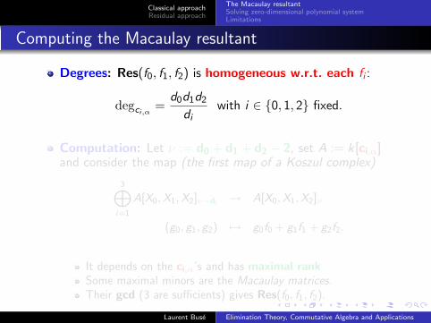
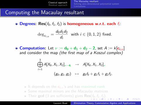
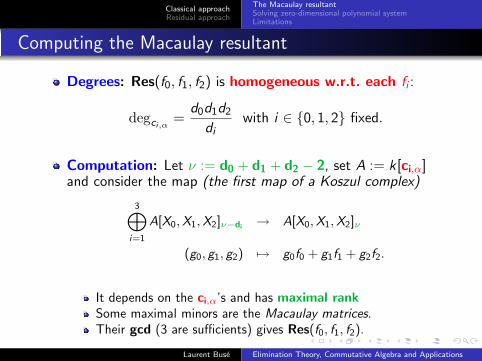
Degrees: Res(f0, f1, f2) is homogeneous w.r.t. each fi :
degci,α=
d0d1d2
diwith i ∈ {0, 1, 2} fixed.
Computation: Let ν := d0 + d1 + d2 − 2, set A := k[ci,α]and consider the map (the first map of a Koszul complex)
3⊕i=1
A[X0,X1,X2]ν−di → A[X0,X1,X2]ν
(g0, g1, g2) 7→ g0f0 + g1f1 + g2f2.
It depends on the ci,α’s and has maximal rankSome maximal minors are the Macaulay matrices.Their gcd (3 are sufficients) gives Res(f0, f1, f2).
Laurent Buse Elimination Theory, Commutative Algebra and Applications
Classical approachResidual approach
The Macaulay resultantSolving zero-dimensional polynomial systemLimitations
Computing the Macaulay resultant
Degrees: Res(f0, f1, f2) is homogeneous w.r.t. each fi :
degci,α=
d0d1d2
diwith i ∈ {0, 1, 2} fixed.
Computation: Let ν := d0 + d1 + d2 − 2, set A := k[ci,α]and consider the map (the first map of a Koszul complex)
3⊕i=1
A[X0,X1,X2]ν−di → A[X0,X1,X2]ν
(g0, g1, g2) 7→ g0f0 + g1f1 + g2f2.
It depends on the ci,α’s and has maximal rankSome maximal minors are the Macaulay matrices.Their gcd (3 are sufficients) gives Res(f0, f1, f2).
Laurent Buse Elimination Theory, Commutative Algebra and Applications
Classical approachResidual approach
The Macaulay resultantSolving zero-dimensional polynomial systemLimitations
Recovering the Chow form
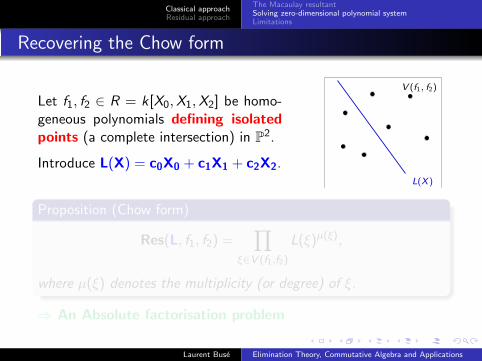
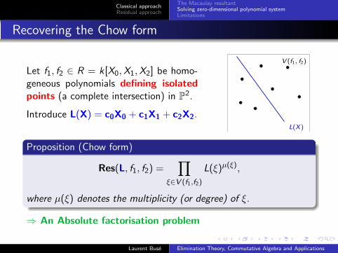
Let f1, f2 ∈ R = k[X0,X1,X2] be homo-geneous polynomials defining isolatedpoints (a complete intersection) in P2.
Introduce L(X) = c0X0 + c1X1 + c2X2.L(X )
V (f1, f2)
Proposition (Chow form)
Res(L, f1, f2) =∏
ξ∈V (f1,f2)
L(ξ)µ(ξ),
where µ(ξ) denotes the multiplicity (or degree) of ξ.
⇒ An Absolute factorisation problem
Laurent Buse Elimination Theory, Commutative Algebra and Applications
Classical approachResidual approach
The Macaulay resultantSolving zero-dimensional polynomial systemLimitations
Recovering the Chow form
Let f1, f2 ∈ R = k[X0,X1,X2] be homo-geneous polynomials defining isolatedpoints (a complete intersection) in P2.
Introduce L(X) = c0X0 + c1X1 + c2X2.L(X )
V (f1, f2)
Proposition (Chow form)
Res(L, f1, f2) =∏
ξ∈V (f1,f2)
L(ξ)µ(ξ),
where µ(ξ) denotes the multiplicity (or degree) of ξ.
⇒ An Absolute factorisation problem
Laurent Buse Elimination Theory, Commutative Algebra and Applications

Classical approachResidual approach
The Macaulay resultantSolving zero-dimensional polynomial systemLimitations
Recovering multiplication maps
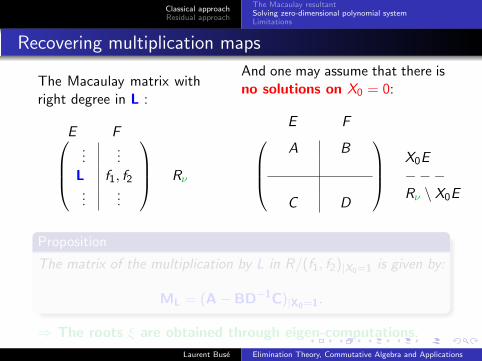
The Macaulay matrix withright degree in L :
E F...
...L f1, f2...
...
Rν
And one may assume that there isno solutions on X0 = 0:
E FA B
C D
X0E−−−Rν \ X0E
Proposition
The matrix of the multiplication by L in R/(f1, f2)|X0=1 is given by:
ML = (A− BD−1C)|X0=1.
⇒ The roots ξ are obtained through eigen-computations.
Laurent Buse Elimination Theory, Commutative Algebra and Applications
Classical approachResidual approach
The Macaulay resultantSolving zero-dimensional polynomial systemLimitations
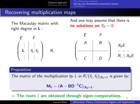
Recovering multiplication maps
The Macaulay matrix withright degree in L :
E F...
...L f1, f2...
...
Rν
And one may assume that there isno solutions on X0 = 0:
E FA B
C D
X0E−−−Rν \ X0E
Proposition
The matrix of the multiplication by L in R/(f1, f2)|X0=1 is given by:
ML = (A− BD−1C)|X0=1.
⇒ The roots ξ are obtained through eigen-computations.
Laurent Buse Elimination Theory, Commutative Algebra and Applications
Classical approachResidual approach
The Macaulay resultantSolving zero-dimensional polynomial systemLimitations
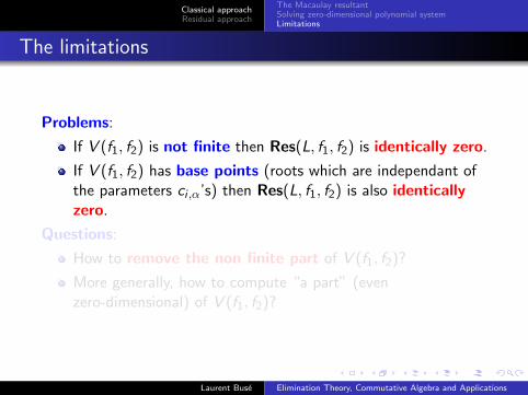
The limitations
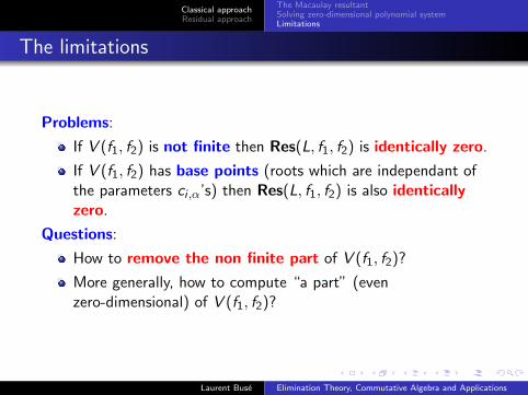
Problems:
If V (f1, f2) is not finite then Res(L, f1, f2) is identically zero.
If V (f1, f2) has base points (roots which are independant ofthe parameters ci ,α’s) then Res(L, f1, f2) is also identicallyzero.
Questions:
How to remove the non finite part of V (f1, f2)?
More generally, how to compute “a part” (evenzero-dimensional) of V (f1, f2)?
Laurent Buse Elimination Theory, Commutative Algebra and Applications
Classical approachResidual approach
The Macaulay resultantSolving zero-dimensional polynomial systemLimitations
The limitations
Problems:
If V (f1, f2) is not finite then Res(L, f1, f2) is identically zero.
If V (f1, f2) has base points (roots which are independant ofthe parameters ci ,α’s) then Res(L, f1, f2) is also identicallyzero.
Questions:
How to remove the non finite part of V (f1, f2)?
More generally, how to compute “a part” (evenzero-dimensional) of V (f1, f2)?
Laurent Buse Elimination Theory, Commutative Algebra and Applications
Classical approachResidual approach
The Macaulay resultantSolving zero-dimensional polynomial systemLimitations
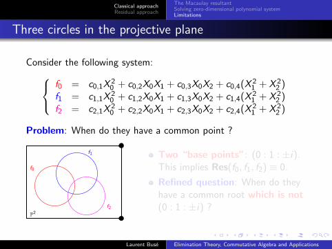
Three circles in the projective plane
Consider the following system:f0 = c0,1X
20 + c0,2X0X1 + c0,3X0X2 + c0,4(X
21 + X 2
2 )f1 = c1,1X
20 + c1,2X0X1 + c1,3X0X2 + c1,4(X
21 + X 2
2 )f2 = c2,1X
20 + c2,2X0X1 + c2,3X0X2 + c2,4(X
21 + X 2
2 )
Problem: When do they have a common point ?
f1
f2
P2
f0
Two “base points”: (0 : 1 : ±i).This implies Res(f0, f1, f2) ≡ 0.
Refined question: When do theyhave a common root which is not(0 : 1 : ±i) ?
Laurent Buse Elimination Theory, Commutative Algebra and Applications
Classical approachResidual approach
The Macaulay resultantSolving zero-dimensional polynomial systemLimitations
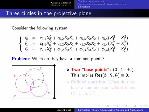
Three circles in the projective plane
Consider the following system:f0 = c0,1X
20 + c0,2X0X1 + c0,3X0X2 + c0,4(X
21 + X 2
2 )f1 = c1,1X
20 + c1,2X0X1 + c1,3X0X2 + c1,4(X
21 + X 2
2 )f2 = c2,1X
20 + c2,2X0X1 + c2,3X0X2 + c2,4(X
21 + X 2
2 )
Problem: When do they have a common point ?
f1
f2
P2
f0
Two “base points”: (0 : 1 : ±i).This implies Res(f0, f1, f2) ≡ 0.
Refined question: When do theyhave a common root which is not(0 : 1 : ±i) ?
Laurent Buse Elimination Theory, Commutative Algebra and Applications
Classical approachResidual approach
The residual resultantSolving polynomial systemsAn example: cylinders passing through 5 points
The setting
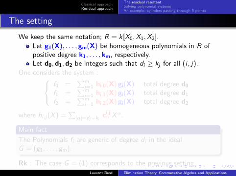
We keep the same notation; R = k[X0,X1,X2].
Let g1(X), . . . , gm(X) be homogeneous polynomials in R ofpositive degree k1, . . . , km, respectively.Let d0,d1,d2 be integers such that di ≥ kj for all (i , j).
One considers the system :f0 =
∑mi=1 hi,0(X) gi(X) total degree d0
f1 =∑m
i=1 hi,1(X) gi(X) total degree d1
f2 =∑m
i=1 hi,2(X) gi(X) total degree d2
where hi ,j(X ) =∑|α|=dj−ki
ci,jα Xα.
Main fact
The Polynomials fi are generic of degree di in the idealG = (g1, . . . , gm).
Rk : The case G = (1) corresponds to the previous setting.Laurent Buse Elimination Theory, Commutative Algebra and Applications
Classical approachResidual approach
The residual resultantSolving polynomial systemsAn example: cylinders passing through 5 points
The setting
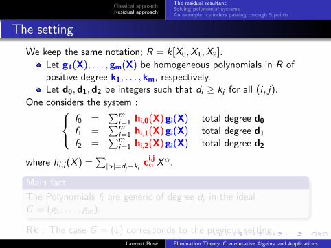
We keep the same notation; R = k[X0,X1,X2].
Let g1(X), . . . , gm(X) be homogeneous polynomials in R ofpositive degree k1, . . . , km, respectively.Let d0,d1,d2 be integers such that di ≥ kj for all (i , j).
One considers the system :f0 =
∑mi=1 hi,0(X) gi(X) total degree d0
f1 =∑m
i=1 hi,1(X) gi(X) total degree d1
f2 =∑m
i=1 hi,2(X) gi(X) total degree d2
where hi ,j(X ) =∑|α|=dj−ki
ci,jα Xα.
Main fact
The Polynomials fi are generic of degree di in the idealG = (g1, . . . , gm).
Rk : The case G = (1) corresponds to the previous setting.Laurent Buse Elimination Theory, Commutative Algebra and Applications

Classical approachResidual approach
The residual resultantSolving polynomial systemsAn example: cylinders passing through 5 points
The setting
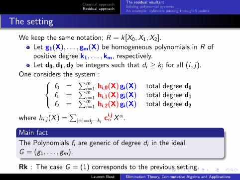
We keep the same notation; R = k[X0,X1,X2].
Let g1(X), . . . , gm(X) be homogeneous polynomials in R ofpositive degree k1, . . . , km, respectively.Let d0,d1,d2 be integers such that di ≥ kj for all (i , j).
One considers the system :f0 =
∑mi=1 hi,0(X) gi(X) total degree d0
f1 =∑m
i=1 hi,1(X) gi(X) total degree d1
f2 =∑m
i=1 hi,2(X) gi(X) total degree d2
where hi ,j(X ) =∑|α|=dj−ki
ci,jα Xα.
Main fact
The Polynomials fi are generic of degree di in the idealG = (g1, . . . , gm).
Rk : The case G = (1) corresponds to the previous setting.Laurent Buse Elimination Theory, Commutative Algebra and Applications
Classical approachResidual approach
The residual resultantSolving polynomial systemsAn example: cylinders passing through 5 points
The setting
We keep the same notation; R = k[X0,X1,X2].
Let g1(X), . . . , gm(X) be homogeneous polynomials in R ofpositive degree k1, . . . , km, respectively.Let d0,d1,d2 be integers such that di ≥ kj for all (i , j).
One considers the system :f0 =
∑mi=1 hi,0(X) gi(X) total degree d0
f1 =∑m
i=1 hi,1(X) gi(X) total degree d1
f2 =∑m
i=1 hi,2(X) gi(X) total degree d2
where hi ,j(X ) =∑|α|=dj−ki
ci,jα Xα.
Main fact
The Polynomials fi are generic of degree di in the idealG = (g1, . . . , gm).
Rk : The case G = (1) corresponds to the previous setting.Laurent Buse Elimination Theory, Commutative Algebra and Applications
Classical approachResidual approach
The residual resultantSolving polynomial systemsAn example: cylinders passing through 5 points
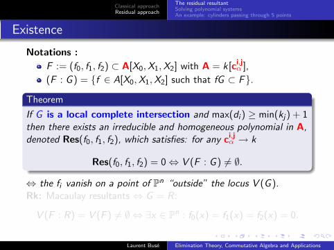
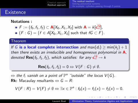
Existence
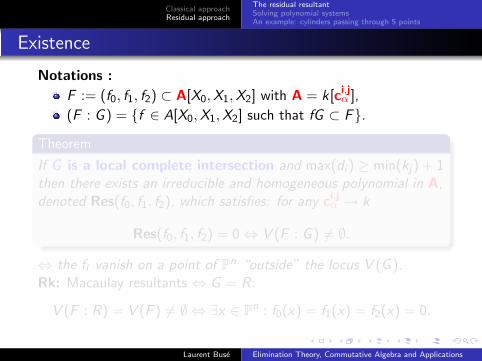
Notations :
F := (f0, f1, f2) ⊂ A[X0,X1,X2] with A = k[ci,jα ],
(F : G ) = {f ∈ A[X0,X1,X2] such that fG ⊂ F}.
Theorem
If G is a local complete intersection and max(di ) ≥ min(kj) + 1then there exists an irreducible and homogeneous polynomial in A,denoted Res(f0, f1, f2), which satisfies: for any ci,j
α → k
Res(f0, f1, f2) = 0 ⇔ V (F : G ) 6= ∅.
⇔ the fi vanish on a point of Pn “outside” the locus V (G ).Rk: Macaulay resultants ⇔ G = R:
V (F : R) = V (F ) 6= ∅ ⇔ ∃x ∈ Pn : f0(x) = f1(x) = f2(x) = 0.
Laurent Buse Elimination Theory, Commutative Algebra and Applications
Classical approachResidual approach
The residual resultantSolving polynomial systemsAn example: cylinders passing through 5 points
Existence
Notations :
F := (f0, f1, f2) ⊂ A[X0,X1,X2] with A = k[ci,jα ],
(F : G ) = {f ∈ A[X0,X1,X2] such that fG ⊂ F}.
Theorem
If G is a local complete intersection and max(di ) ≥ min(kj) + 1then there exists an irreducible and homogeneous polynomial in A,denoted Res(f0, f1, f2), which satisfies: for any ci,j
α → k
Res(f0, f1, f2) = 0 ⇔ V (F : G ) 6= ∅.
⇔ the fi vanish on a point of Pn “outside” the locus V (G ).Rk: Macaulay resultants ⇔ G = R:
V (F : R) = V (F ) 6= ∅ ⇔ ∃x ∈ Pn : f0(x) = f1(x) = f2(x) = 0.
Laurent Buse Elimination Theory, Commutative Algebra and Applications
Classical approachResidual approach
The residual resultantSolving polynomial systemsAn example: cylinders passing through 5 points
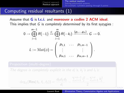
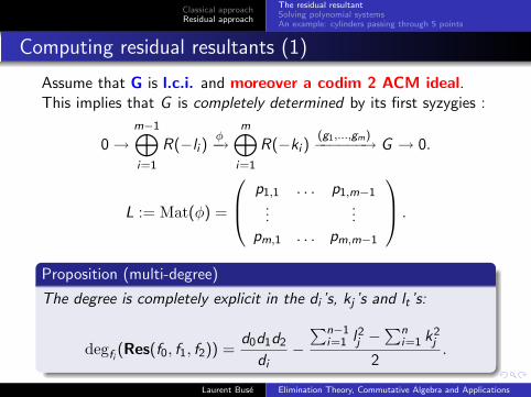
Computing residual resultants (1)
Assume that G is l.c.i. and moreover a codim 2 ACM ideal.This implies that G is completely determined by its first syzygies :
0 →m−1⊕i=1
R(−li )φ−→
m⊕i=1
R(−ki )(g1,...,gm)−−−−−−→ G → 0.
L := Mat(φ) =
p1,1 . . . p1,m−1...
...pm,1 . . . pm,m−1
.
Proposition (multi-degree)
The degree is completely explicit in the di ’s, kj ’s and lt ’s:
degfi (Res(f0, f1, f2)) =d0d1d2
di−
∑n−1i=1 l2j −
∑ni=1 k2
j
2.
Laurent Buse Elimination Theory, Commutative Algebra and Applications
Classical approachResidual approach
The residual resultantSolving polynomial systemsAn example: cylinders passing through 5 points
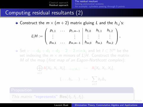
Computing residual resultants (2)
Construct the m × (m + 2) matrix gluing L and the hi ,j ’s:
L|H :=
p1,1 . . . p1,m−1 h1,0 h1,1 h1,2
......
......
...pm,1 . . . pm,m−1 hm,0 hm,1 hm,2
,
Set ν := d0 + d1 + d2 − 2− 2min kj and let I ⊂ Nm be theset indexing the m ×m minors of L|H. Construct the matrixM of the map (first map of an Eagon-Northcott complex):⊕
s∈I
A[X0,X1,X2]ν−deg(∆s) → A[X0,X1,X2]ν
(. . . , bs , . . .) 7→∑s∈I
bs∆s
Proposition
This matrix “represents” Res(f0, f1, f2).
Laurent Buse Elimination Theory, Commutative Algebra and Applications
Classical approachResidual approach
The residual resultantSolving polynomial systemsAn example: cylinders passing through 5 points
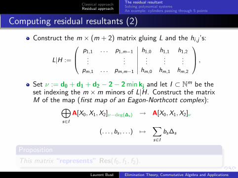
Computing residual resultants (2)
Construct the m × (m + 2) matrix gluing L and the hi ,j ’s:
L|H :=
p1,1 . . . p1,m−1 h1,0 h1,1 h1,2
......
......
...pm,1 . . . pm,m−1 hm,0 hm,1 hm,2
,
Set ν := d0 + d1 + d2 − 2− 2min kj and let I ⊂ Nm be theset indexing the m ×m minors of L|H. Construct the matrixM of the map (first map of an Eagon-Northcott complex):⊕
s∈I
A[X0,X1,X2]ν−deg(∆s) → A[X0,X1,X2]ν
(. . . , bs , . . .) 7→∑s∈I
bs∆s
Proposition
This matrix “represents” Res(f0, f1, f2).
Laurent Buse Elimination Theory, Commutative Algebra and Applications
Classical approachResidual approach
The residual resultantSolving polynomial systemsAn example: cylinders passing through 5 points
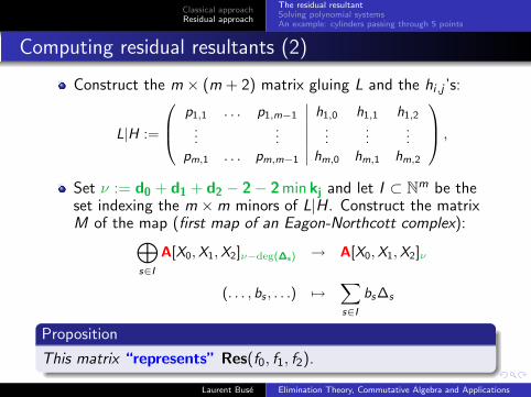
Computing residual resultants (2)
Construct the m × (m + 2) matrix gluing L and the hi ,j ’s:
L|H :=
p1,1 . . . p1,m−1 h1,0 h1,1 h1,2
......
......
...pm,1 . . . pm,m−1 hm,0 hm,1 hm,2
,
Set ν := d0 + d1 + d2 − 2− 2min kj and let I ⊂ Nm be theset indexing the m ×m minors of L|H. Construct the matrixM of the map (first map of an Eagon-Northcott complex):⊕
s∈I
A[X0,X1,X2]ν−deg(∆s) → A[X0,X1,X2]ν
(. . . , bs , . . .) 7→∑s∈I
bs∆s
Proposition
This matrix “represents” Res(f0, f1, f2).
Laurent Buse Elimination Theory, Commutative Algebra and Applications
Classical approachResidual approach
The residual resultantSolving polynomial systemsAn example: cylinders passing through 5 points
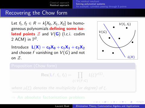
Recovering the Chow form
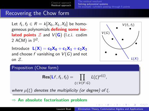
Let f1, f2 ∈ R = k[X0,X1,X2] be homo-geneous polynomials defining some iso-lated points Z and V (G) (l.c.i. codim2 ACM) in P2.
Introduce L(X) = c0X0 + c1X1 + c2X2
and choose f vanishing on V (G ) and noton Z. L(X )
V (f1, f2)
V (G)
Proposition (Chow form)
Res(Lf , f1, f2) =∏
ξ∈V (F :G)
L(ξ)µ(ξ),
where µ(ξ) denotes the multiplicity (or degree) of ξ.
⇒ An absolute factorisation problem
Laurent Buse Elimination Theory, Commutative Algebra and Applications
Classical approachResidual approach
The residual resultantSolving polynomial systemsAn example: cylinders passing through 5 points
Recovering the Chow form
Let f1, f2 ∈ R = k[X0,X1,X2] be homo-geneous polynomials defining some iso-lated points Z and V (G) (l.c.i. codim2 ACM) in P2.
Introduce L(X) = c0X0 + c1X1 + c2X2
and choose f vanishing on V (G ) and noton Z. L(X )
V (f1, f2)
V (G)
Proposition (Chow form)
Res(Lf , f1, f2) =∏
ξ∈V (F :G)
L(ξ)µ(ξ),
where µ(ξ) denotes the multiplicity (or degree) of ξ.
⇒ An absolute factorisation problem
Laurent Buse Elimination Theory, Commutative Algebra and Applications
Classical approachResidual approach
The residual resultantSolving polynomial systemsAn example: cylinders passing through 5 points
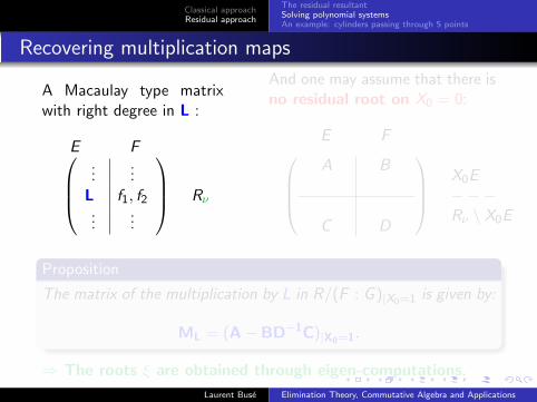
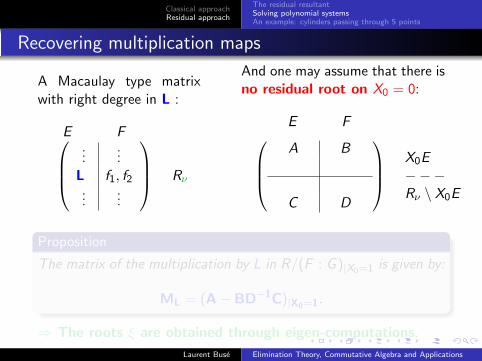
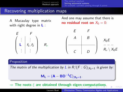
Recovering multiplication maps
A Macaulay type matrixwith right degree in L :
E F...
...L f1, f2...
...
Rν
And one may assume that there isno residual root on X0 = 0:
E FA B
C D
X0E−−−Rν \ X0E
Proposition
The matrix of the multiplication by L in R/(F : G )|X0=1 is given by:
ML = (A− BD−1C)|X0=1.
⇒ The roots ξ are obtained through eigen-computations.
Laurent Buse Elimination Theory, Commutative Algebra and Applications
Classical approachResidual approach
The residual resultantSolving polynomial systemsAn example: cylinders passing through 5 points
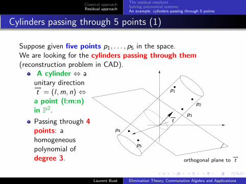
Cylinders passing through 5 points (1)
Suppose given five points p1, . . . , p5 in the space.We are looking for the cylinders passing through them(reconstruction problem in CAD).
A cylinder ⇔ aunitary direction−→t = (l ,m, n) ⇔a point (l:m:n)in P2.
Passing through 4points: ahomogeneouspolynomial ofdegree 3.
−→t
orthogonal plane to−→t
p1
p2
p3
p4
p5
Laurent Buse Elimination Theory, Commutative Algebra and Applications
Classical approachResidual approach
The residual resultantSolving polynomial systemsAn example: cylinders passing through 5 points
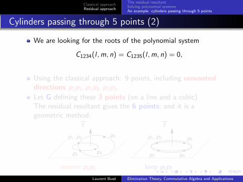
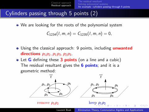
Cylinders passing through 5 points (2)
We are looking for the roots of the polynomial system
C1234(l ,m, n) = C1235(l ,m, n) = 0,
Using the classical approach: 9 points, including unwanteddirections p1p2, p1p3, p2p3.
Let G defining these 3 points (on a line and a cubic)The residual resultant gives the 6 points; and it is ageometric method:
p1, p2
p3p4
p5
p3
p1, p2
p4
p5
−→t
−→t
remove p1p2 keep p1p2
Laurent Buse Elimination Theory, Commutative Algebra and Applications
Classical approachResidual approach
The residual resultantSolving polynomial systemsAn example: cylinders passing through 5 points
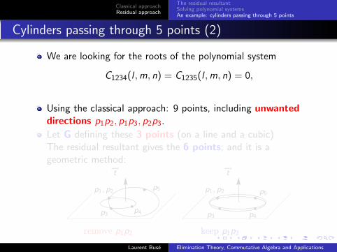
Cylinders passing through 5 points (2)
We are looking for the roots of the polynomial system
C1234(l ,m, n) = C1235(l ,m, n) = 0,
Using the classical approach: 9 points, including unwanteddirections p1p2, p1p3, p2p3.
Let G defining these 3 points (on a line and a cubic)The residual resultant gives the 6 points; and it is ageometric method:
p1, p2
p3p4
p5
p3
p1, p2
p4
p5
−→t
−→t
remove p1p2 keep p1p2
Laurent Buse Elimination Theory, Commutative Algebra and Applications
Implicitization of curvesImplicitization of surfaces
Part II
Implicitization problem
Laurent Buse Elimination Theory, Commutative Algebra and Applications
Implicitization of curvesImplicitization of surfaces
Using resultantsUsing moving linesUsing syzygies
The implicitization problem for curves
Suppose given a generically finite rational map
P1 φ−→ P2
x := (x0 : x1) 7→ (f1(x) : f2(x) : f3(x)),
where f1(x), f2(x), f3(x) are homogeneous of the same degree d.Its closed image is an irreducible curve C in P2. We would like tocompute its implicit equation that we will denote C (T1,T2,T3).
Proposition (degree of C)
d − deg(gcd(f1, f2, f3)) =
{0 if φ not gen. finite,
deg(φ)deg(C) otherwise.
Laurent Buse Elimination Theory, Commutative Algebra and Applications
Implicitization of curvesImplicitization of surfaces
Using resultantsUsing moving linesUsing syzygies
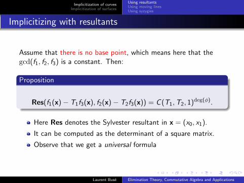
Implicitizing with resultants
Assume that there is no base point, which means here that thegcd(f1, f2, f3) is a constant. Then:
Proposition
Res(f1(x)− T1f3(x), f2(x)− T2f3(x)) = C (T1,T2, 1)deg(φ).
Here Res denotes the Sylvester resultant in x = (x0, x1).
It can be computed as the determinant of a square matrix.
Observe that we get a universal formula
Laurent Buse Elimination Theory, Commutative Algebra and Applications
Implicitization of curvesImplicitization of surfaces
Using resultantsUsing moving linesUsing syzygies
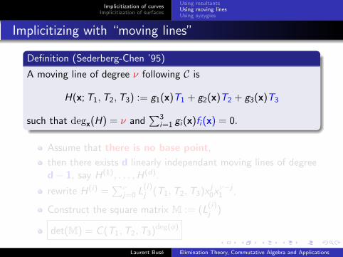
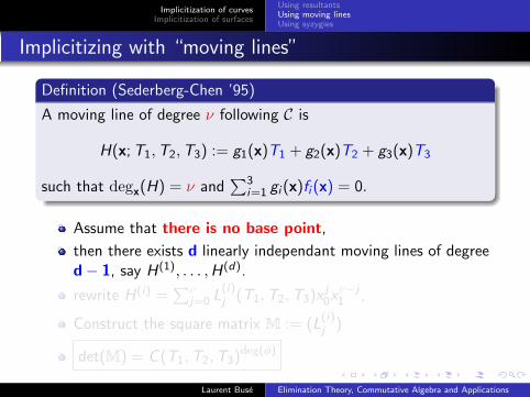
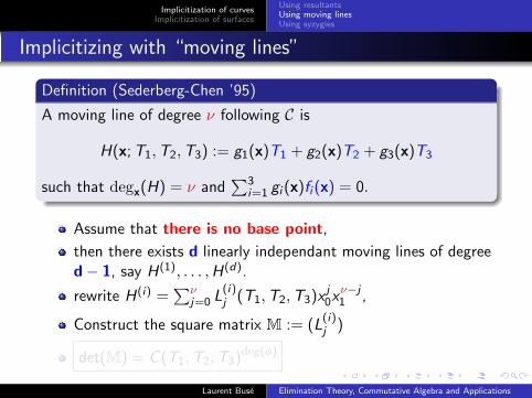
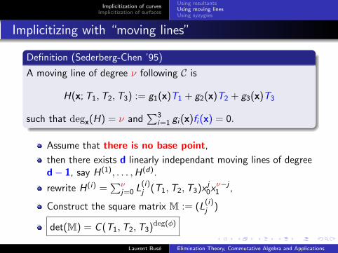
Implicitizing with “moving lines”
Definition (Sederberg-Chen ’95)
A moving line of degree ν following C is
H(x;T1,T2,T3) := g1(x)T1 + g2(x)T2 + g3(x)T3
such that degx(H) = ν and∑3
i=1 gi (x)fi (x) = 0.
Assume that there is no base point,
then there exists d linearly independant moving lines of degreed− 1, say H(1), . . . ,H(d).
rewrite H(i) =∑ν
j=0 L(i)j (T1,T2,T3)x
j0x
ν−j1 ,
Construct the square matrix M := (L(i)j )
det(M) = C (T1,T2,T3)deg(φ)
Laurent Buse Elimination Theory, Commutative Algebra and Applications
Implicitization of curvesImplicitization of surfaces
Using resultantsUsing moving linesUsing syzygies
Implicitizing with “moving lines”
Definition (Sederberg-Chen ’95)
A moving line of degree ν following C is
H(x;T1,T2,T3) := g1(x)T1 + g2(x)T2 + g3(x)T3
such that degx(H) = ν and∑3
i=1 gi (x)fi (x) = 0.
Assume that there is no base point,
then there exists d linearly independant moving lines of degreed− 1, say H(1), . . . ,H(d).
rewrite H(i) =∑ν
j=0 L(i)j (T1,T2,T3)x
j0x
ν−j1 ,
Construct the square matrix M := (L(i)j )
det(M) = C (T1,T2,T3)deg(φ)
Laurent Buse Elimination Theory, Commutative Algebra and Applications
Implicitization of curvesImplicitization of surfaces
Using resultantsUsing moving linesUsing syzygies
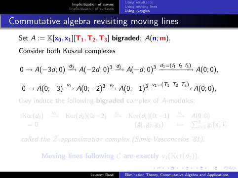
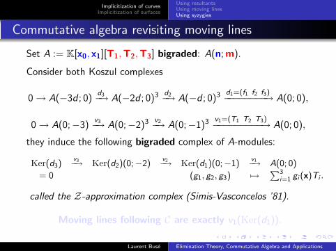
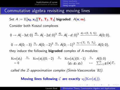
Commutative algebra revisiting moving lines
Set A := K[x0, x1][T1,T2,T3] bigraded: A(n;m).
Consider both Koszul complexes
0 → A(−3d ; 0)d3−→ A(−2d ; 0)3
d2−→ A(−d ; 0)3d1=(f1 f2 f3)−−−−−−−−→ A(0; 0),
0 → A(0;−3)v3−→ A(0;−2)3
v2−→ A(0;−1)3v1=(T1 T2 T3)−−−−−−−−−→ A(0; 0),
they induce the following bigraded complex of A-modules:
Ker(d3)v3−→ Ker(d2)(0;−2)
v2−→ Ker(d1)(0;−1)v1−→ A(0; 0)
= 0 (g1, g2, g3) 7→∑3
i=1 gi (x)Ti .
called the Z-approximation complex (Simis-Vasconcelos ’81).
Moving lines following C are exactly v1(Ker(d1)).
Laurent Buse Elimination Theory, Commutative Algebra and Applications
Implicitization of curvesImplicitization of surfaces
Using resultantsUsing moving linesUsing syzygies
Implicitizing with syzygies
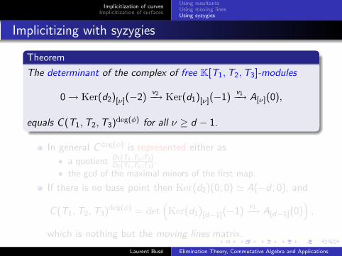
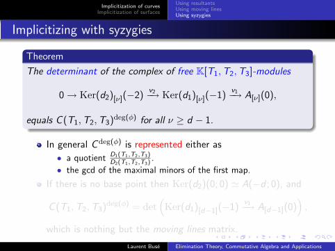
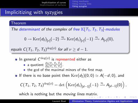
Theorem
The determinant of the complex of free K[T1,T2,T3]-modules
0 → Ker(d2)[ν](−2)v2−→ Ker(d1)[ν](−1)
v1−→ A[ν](0),
equals C (T1,T2,T3)deg(φ) for all ν ≥ d − 1.
In general Cdeg(φ) is represented either as
• a quotient D1(T1,T2,T3)D2(T1,T2,T3)
.
• the gcd of the maximal minors of the first map.
If there is no base point then Ker(d2)(0; 0) ' A(−d ; 0), and
C (T1,T2,T3)deg(φ) = det
(Ker(d1)[d−1](−1)
v1−→ A[d−1](0))
,
which is nothing but the moving lines matrix.
Laurent Buse Elimination Theory, Commutative Algebra and Applications
Implicitization of curvesImplicitization of surfaces
Using resultantsUsing moving linesUsing syzygies
Implicitizing with syzygies
Theorem
The determinant of the complex of free K[T1,T2,T3]-modules
0 → Ker(d2)[ν](−2)v2−→ Ker(d1)[ν](−1)
v1−→ A[ν](0),
equals C (T1,T2,T3)deg(φ) for all ν ≥ d − 1.
In general Cdeg(φ) is represented either as
• a quotient D1(T1,T2,T3)D2(T1,T2,T3)
.
• the gcd of the maximal minors of the first map.
If there is no base point then Ker(d2)(0; 0) ' A(−d ; 0), and
C (T1,T2,T3)deg(φ) = det
(Ker(d1)[d−1](−1)
v1−→ A[d−1](0))
,
which is nothing but the moving lines matrix.
Laurent Buse Elimination Theory, Commutative Algebra and Applications
Implicitization of curvesImplicitization of surfaces
Using resultantsUsing syzygies
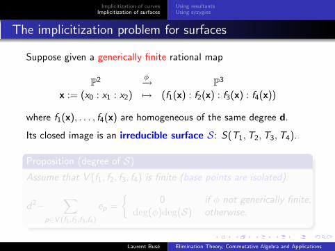
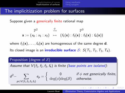
The implicitization problem for surfaces
Suppose given a generically finite rational map
P2 φ−→ P3
x := (x0 : x1 : x2) 7→ (f1(x) : f2(x) : f3(x) : f4(x))
where f1(x), . . . , f4(x) are homogeneous of the same degree d.
Its closed image is an irreducible surface S: S(T1,T2,T3,T4).
Proposition (degree of S)
Assume that V (f1, f2, f3, f4) is finite (base points are isolated):
d2−∑
p∈V (f1,f2,f3,f4)
ep =
{0 if φ not generically finite,
deg(φ)deg(S) otherwise.
Laurent Buse Elimination Theory, Commutative Algebra and Applications
Implicitization of curvesImplicitization of surfaces
Using resultantsUsing syzygies
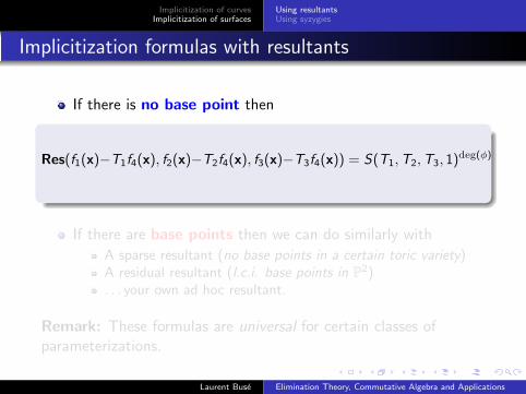
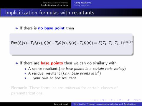
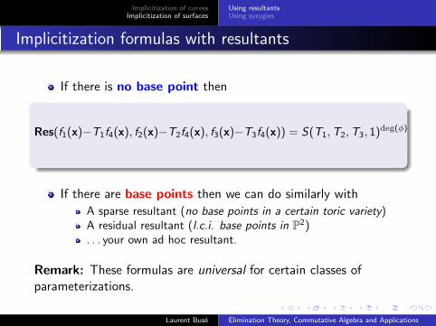
Implicitization formulas with resultants
If there is no base point then
Res(f1(x)−T1f4(x), f2(x)−T2f4(x), f3(x)−T3f4(x)) = S(T1,T2,T3, 1)deg(φ)
If there are base points then we can do similarly with
A sparse resultant (no base points in a certain toric variety)A residual resultant (l.c.i. base points in P2). . . your own ad hoc resultant.
Remark: These formulas are universal for certain classes ofparameterizations.
Laurent Buse Elimination Theory, Commutative Algebra and Applications
Implicitization of curvesImplicitization of surfaces
Using resultantsUsing syzygies
Implicitizing with syzygies (1)
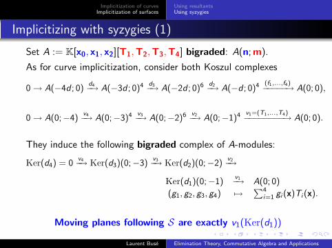
Set A := K[x0, x1, x2][T1,T2,T3,T4] bigraded: A(n;m).
As for curve implicitization, consider both Koszul complexes
0 → A(−4d ; 0)d4−→ A(−3d ; 0)4
d3−→ A(−2d ; 0)6d2−→ A(−d ; 0)4
(f1,...,f4)−−−−−→ A(0; 0),
0 → A(0;−4)v4−→ A(0;−3)4
v3−→ A(0;−2)6v2−→ A(0;−1)4
v1=(T1,...,T4)−−−−−−−−→ A(0; 0).
They induce the following bigraded complex of A-modules:
Ker(d4) = 0v4−→ Ker(d3)(0;−3)
v3−→ Ker(d2)(0;−2)v2−→
Ker(d1)(0;−1)v1−→ A(0; 0)
(g1, g2, g3, g4) 7→∑4
i=1 gi (x)Ti (x).
Moving planes following S are exactly v1(Ker(d1))
Laurent Buse Elimination Theory, Commutative Algebra and Applications
Implicitization of curvesImplicitization of surfaces
Using resultantsUsing syzygies
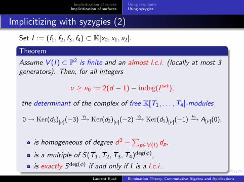
Implicitizing with syzygies (2)
Set I := (f1, f2, f3, f4) ⊂ K[x0, x1, x2].
Theorem
Assume V (I ) ⊂ P2 is finite and an almost l.c.i. (locally at most 3generators). Then, for all integers
ν ≥ ν0 := 2(d − 1)− indeg(I sat),
the determinant of the complex of free K[T1, . . . ,T4]-modules
0 → Ker(d3)[ν](−3)v3−→ Ker(d2)[ν](−2)
v2−→ Ker(d1)[ν](−1)v1−→ A[ν](0),
is homogeneous of degree d2 −∑
p∈V (I ) dp,
is a multiple of S(T1,T2,T3,T4)deg(φ),
is exactly Sdeg(φ) if and only if I is a l.c.i..
Laurent Buse Elimination Theory, Commutative Algebra and Applications
Implicitization of curvesImplicitization of surfaces
Using resultantsUsing syzygies
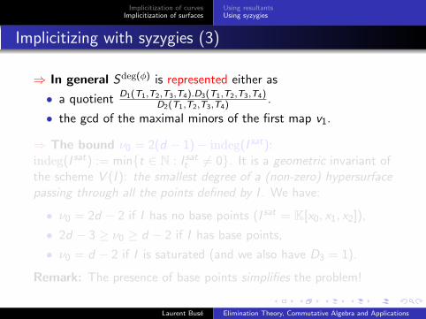
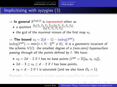
Implicitizing with syzygies (3)
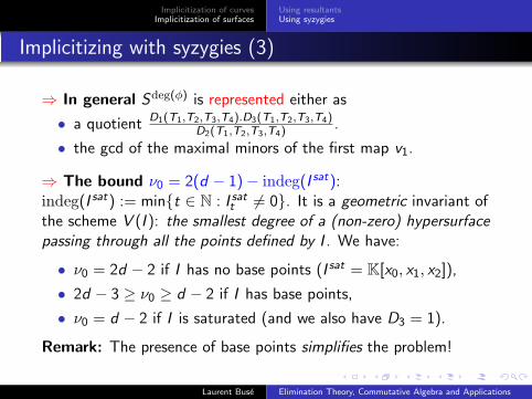
⇒ In general Sdeg(φ) is represented either as
• a quotient D1(T1,T2,T3,T4).D3(T1,T2,T3,T4)D2(T1,T2,T3,T4)
.
• the gcd of the maximal minors of the first map v1.
⇒ The bound ν0 = 2(d − 1)− indeg(I sat):indeg(I sat) := min{t ∈ N : I sat
t 6= 0}. It is a geometric invariant ofthe scheme V (I ): the smallest degree of a (non-zero) hypersurfacepassing through all the points defined by I . We have:
• ν0 = 2d − 2 if I has no base points (I sat = K[x0, x1, x2]),
• 2d − 3 ≥ ν0 ≥ d − 2 if I has base points,
• ν0 = d − 2 if I is saturated (and we also have D3 = 1).
Remark: The presence of base points simplifies the problem!
Laurent Buse Elimination Theory, Commutative Algebra and Applications
Implicitization of curvesImplicitization of surfaces
Using resultantsUsing syzygies
Implicitizing with syzygies (3)
⇒ In general Sdeg(φ) is represented either as
• a quotient D1(T1,T2,T3,T4).D3(T1,T2,T3,T4)D2(T1,T2,T3,T4)
.
• the gcd of the maximal minors of the first map v1.
⇒ The bound ν0 = 2(d − 1)− indeg(I sat):indeg(I sat) := min{t ∈ N : I sat
t 6= 0}. It is a geometric invariant ofthe scheme V (I ): the smallest degree of a (non-zero) hypersurfacepassing through all the points defined by I . We have:
• ν0 = 2d − 2 if I has no base points (I sat = K[x0, x1, x2]),
• 2d − 3 ≥ ν0 ≥ d − 2 if I has base points,
• ν0 = d − 2 if I is saturated (and we also have D3 = 1).
Remark: The presence of base points simplifies the problem!
Laurent Buse Elimination Theory, Commutative Algebra and Applications
Implicitization of curvesImplicitization of surfaces
Using resultantsUsing syzygies
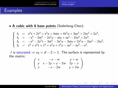
Examples
• A cubic with 6 base points (Sederberg-Chen):f1 = s2t + 2t3 + s2u + 4stu + 4t2u + 3su2 + 2tu2 + 2u3,f2 = −s3 − 2st2 − 2s2u − stu + su2 − 2tu2 + 2u3,f3 = −s3 − 2s2t − 3st2 − 3s2u − 3stu + 2t2u − 2su2 − 2tu2,f4 = s3 + s2t + t3 + s2u + t2u − su2 − tu2 − u3.
I is saturated ⇒ ν0 = d − 2 = 1. The surface is represented bythe matrix: x −z − w y + w
y x − 2y + z − 2w 2y − zz −x − 2w y + 2w
.
Laurent Buse Elimination Theory, Commutative Algebra and Applications
Implicitization of curvesImplicitization of surfaces
Using resultantsUsing syzygies
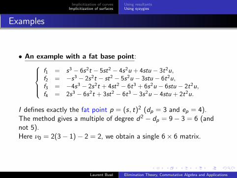
Examples
• An example with a fat base point:f1 = s3 − 6s2t − 5st2 − 4s2u + 4stu − 3t2u,f2 = −s3 − 2s2t − st2 − 5s2u − 3stu − 6t2u,f3 = −4s3 − 2s2t + 4st2 − 6t3 + 6s2u − 6stu − 2t2u,f4 = 2s3 − 6s2t + 3st2 − 6t3 − 3s2u − 4stu + 2t2u.
I defines exactly the fat point p = (s, t)2 (dp = 3 and ep = 4).The method gives a multiple of degree d2 − dp = 9− 3 = 6 (andnot 5).Here ν0 = 2(3− 1)− 2 = 2, we obtain a single 6× 6 matrix.
Laurent Buse Elimination Theory, Commutative Algebra and Applications

![Commutative Algebra - Cornell Universitypi.math.cornell.edu/.../partiii/files/commalgnotes.pdf · 2018-08-23 · Commutative algebra is about commutative rings: Z, k[x1,...,xn], etc](https://img.pdfslide.net/doc/110x75/5f157dcc3ba58c0b6a7eac81/commutative-algebra-cornell-2018-08-23-commutative-algebra-is-about-commutative.jpg)