Embed Size (px)
Citation preview
EM algorithm coupled with particle filter for maximumlikelihood parameter estimation of stochastic differen-tial mixed-effects models
Sophie Donnet
Laboratoire Ceremade, Université Paris Dauphine, France
Adeline Samson
UMR CNRS 8145, Laboratoire MAP5, Université Paris Descartes, France
Abstract . Biological processes measured repeatedly among a series of individuals are stan-dardly analyzed by mixed models. These biological processes can be adequately modeled byparametric Stochastic Differential Equations (SDEs). We focus on the parametric maximumlikelihood estimation of this mixed-effects model defined by SDE. As the likelihood is not ex-plicit, we propose a stochastic version of the Expectation-Maximization algorithm combinedwith the Particle Markov Chain Monte Carlo method. When the transition density of the SDEis explicit, we prove the convergence of the SAEM-PMCMC algorithm towards the maximumlikelihood estimator. Two simulated examples are considered: an Ornstein-Uhlenbeck pro-cess with two random parameters and a time-inhomogeneous SDE (Gompertz SDE) with astochastic volatility error model and three random parameters. When the transition density isunknown, we prove the convergence of a different version of the algorithm based on the Eulerapproximation of the SDE towards the maximum likelihood estimator.
Keywords. Mixed models, Stochastic Differential Equations, SAEM algorithm, ParticleFilter, PMCMC, Stochastic volatility, Time-inhomogeneous SDE
1. Introduction
Biological processes are usually measured repeatedly among a collection of individuals orexperimental animals. The parametric statistical approach commonly used to discriminatebetween the inter-subjects variability (the variance of the individual regression parameters)and the residual variability (measurement noise) is the mixed-effects model methodology(Pinheiro and Bates, 2000). The choice of the regression function depends on the context.Dynamical processes are frequently described by deterministic models defined as ordinarydifferential equations. However, these functions may not capture the exact process, sinceresponses for some individuals may display local "random" fluctuations. These phenomenaare not due to error measurements but are induced by an underlying biological processthat is still unknown or unexplained today. The perturbation of deterministic models bya random component leads to the class of stochastic differential equations (SDEs). In thispaper we develop a parametric estimation method for mixed model defined by an SDEprocess, called SDE mixed model. Note that SDE mixed models can be viewed as anextension of state space models with random parameters.Except in the linear case, the likelihood of standard mixed models is intractable in a closedform, making the estimation a hard task. Davidian and Giltinan (1995), Wolfinger (1993),
2 Donnet and Samson
Pinheiro and Bates (2000) and Kuhn and Lavielle (2005) develop various methods for de-terminitic regression function.
When the regression term is the realization of a diffusion process, the estimation is mademore complicated by the difficulties deriving from the SDEs. Parametric estimation ofSDE with random parameters (without measurement noise) has been studied by Ditlevsenand De Gaetano (2005), Picchini et al. (2010) or Oravecz et al. (2009) in a Bayesian con-text. SDE mixed model estimation, including measurement noise modeling, is more com-plex and has received little attention. Overgaard et al. (2005) and Tornøe et al. (2005)build estimators based on an extended Kalman filter but without proving the convergenceof the algorithm. Donnet and Samson (2008) propose to use a stochastic version of theExpectation-Maximisation algorithm. However, the method involves Markov Chain MonteCarlo (MCMC) samplers which have proved their slow mixing properties in the context ofstate space models with random parameters.
For state space models with fixed known parameters, the Sequential Monte Carlo (SMC)algorithms have demonstrated their efficiency. However, these techniques are difficult toextent to the case of unknown parameters (Casarin and Marin, 2009). Recently, Andrieuet al. (2010) developed a powerful algorithm combining MCMC and SMC, namely theParticle Markov Chain Monte Carlo (PMCMC), taking the advantage of the strength ofits two components. Besides, its convergence toward the exact distribution of interest isestablished.
To our knowledge, PMCMC methods have been used for parameter estimation only in aBayesian context and for models without random individual parameters. We propose tofocus on maximum likelihood estimation for SDE mixed models by combining a PMCMCalgorithm with the SAEM algorithm. When the transition density of the SDE is explicit,we prove the convergence of the SAEM-PMCMC algorithm towards the maximum like-lihood estimator. Two simulated examples are considered, an Ornstein-Uhlenbeck mixedSDE model observed with additive noise and a stochastic volatility mixed model with atime-inhomogeneous SDE, showing the increase in accuracy for the SAEM-PMCMC esti-mates compared with the SAEM-MCMC algorithm (Donnet and Samson, 2008). Whenthe transition density is unknown, we prove the convergence of a different version of thealgorithm towards the maximum likelihood estimator.
The paper is organized as follows. In Section 2, we present the SDE mixed model. InSection 3, an estimation method is proposed when the transition density of the SDE isexplicit. Section 4 shows numerical results based on simulated data in this case. In Section5, we extend the approach to general SDEs and prove the convergence of the proposedalgorithm. In Section 6 we conclude and discuss the advantages and limitations of ourapproach.
2. Mixed model defined by stochastic differential equation
2.1. Model and notations
Let y = (yij)1≤i≤n,0≤j≤Jidenote the data, where yij is the noisy measurement of the
observed process for individual i at time tij ≥ ti0, for i = 1, . . . , n, j = 0, . . . , Ji. Letyi,0:Ji
= (yi0, . . . , yiJi) denote the data vector of subject i. We consider that the yij ’s are
governed by a mixed-effects model based on a stochastic differential equation defined as
SDE mixed-effects models 3
follows:
yij = g(Xij , εij), εij ∼i.i.d. N (0, σ2), (1)
dXit = a(Xit, t, φi)dt+ b(Xit, t, φi, γ)dBit, Xiti0 |φi ∼ π0(·|φi) (2)
φi ∼i.i.d. p(φ;β). (3)
In equation (1), (εij)i,j are i.i.d Gaussian random variables of variance σ2 representing themeasurement errors and g is the known error model function. The function g(x, ε) = x+ εleads to an additive error model. Multiplicative error models or stochastic volatility modelscan be considered with g(x, ε) = x(1 + ε) or g(x, ε) = f(x) exp(ε) with a known function f .For each individual i, (Xij)0≤j≤Ji
are the values at discrete times (tij)0≤j≤Jiof the con-
tinuous process (Xit)t≥ti0 = (Xit(φi))t≥ti0 defined by equation (2). This process is properto each individual through the individual parameters φi ∈ Rp involved in the drift andvolatility functions a and b and an individual Brownian motion (Bit)t≥ti0 . Functions a andb – which may be functions of time, leading to time-inhomogeneous SDEs – are common tothe n subjects. They are assumed to be sufficiently regular (with linear growth) to ensurea unique strong solution (Oksendal, 2007). Besides, b depends on an unknown additionalvolatility parameter γ. The (Bit) and φk are assumed to be mutually independent for all1 ≤ i, k ≤ n. The initial condition Xi0 of process (Xit)t≥ti0 , conditionally to the individualparameter φi is random with distribution π0(·|φi). In the following,Xi,0:Ji
= (Xi0, . . . , XiJi)
denotes the vector of the i-th process realization at observation times (tij) for i = 1, . . . , nand X = (X1, . . . , Xn) denotes the whole vector of processes at observation times, for allindividuals. The individual parameters φi are assumed to be distributed with a densityp(φ;β) depending on parameter β. We denote Φ = (φ1, . . . , φn) the vector of all individualparameter vectors.For simplicity purpose, we restrict to a same number of observations per subject: Ji = Jfor all i. The extension to the general case is straightforward.
2.2. Likelihood functionLet θ = (β, γ, σ) be the parameter vector of interest which belongs to some open subset Θof the Euclidean space Rq with q the number of unknown parameters. Our objective is topropose a maximum likelihood estimation of θ. The likelihood function is well-defined underthe assumption of existence of a strong solution to (2). We denote x 7→ p(x, t−s, s|xs, φi; θ)the density of Xit given φi and Xis = xs, s < t. This allows us to write the likelihood ofmodel (1-3) as
p(y; θ) =
n∏
i=1
∫p(yi,0:J |Xi,0:J ;σ)p(Xi,0:J |φi; γ)p(φi;β)dφidXi,0:J , (4)
where p(y|x;σ), p(x|φ; γ) and p(φ;β) are density functions of the observations given thediffusion process, the diffusion process given the individual parameters and the individ-ual parameters, respectively. By independence of the measurement errors (εij), we have
p(yi,0:J |Xi,0:J ;σ) =∏J
j=0 p(yij |Xij ;σ) where p(yij |Xij ;σ) is the density function associatedto the error model (1). The Markovian property of the diffusion process (Xit) implies
p(Xi,0:J |φi; θ) = π0(Xi0|φi)
J∏
j=1
p(Xij ,∆ij , tij−1|Xi j−1, φi; γ),
4 Donnet and Samson
where ∆ij = tij − tij−1. Except for a mixed Wiener process with drift and additive noise,the integral (4) has no-closed form.
Maximizing (4) with respect to θ yields the corresponding Maximum Likelihood Estimate
(MLE) θ of the SDE mixed model (1-3). As the likelihood (4) is not explicit, it has to benumerically evaluated or maximized. This requires eitheir to know the transition densitiesexplicitely (see Section 3) or to approximate it by an Euler scheme (see Section 5).
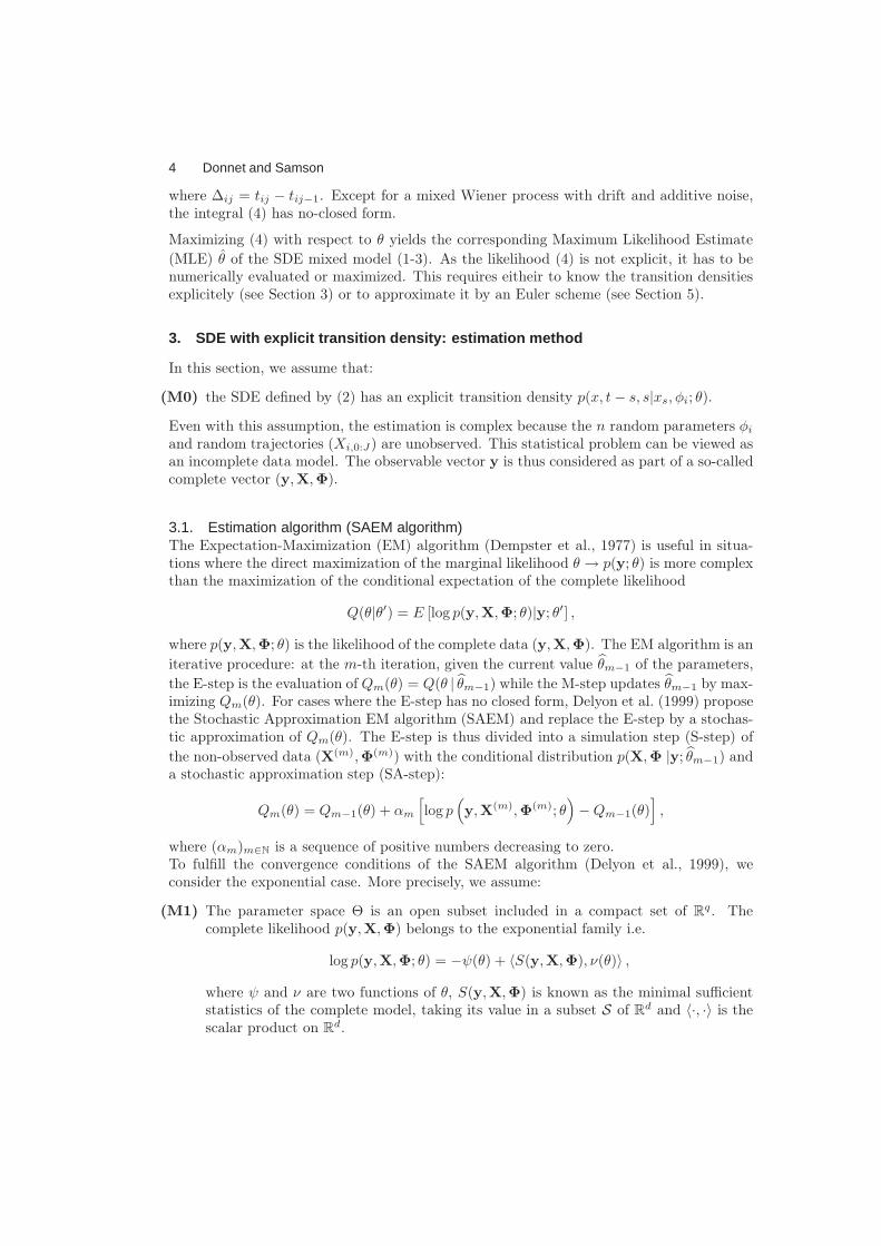
3. SDE with explicit transition density: estimation method
In this section, we assume that:
(M0) the SDE defined by (2) has an explicit transition density p(x, t− s, s|xs, φi; θ).
Even with this assumption, the estimation is complex because the n random parameters φi
and random trajectories (Xi,0:J) are unobserved. This statistical problem can be viewed asan incomplete data model. The observable vector y is thus considered as part of a so-calledcomplete vector (y,X,Φ).
3.1. Estimation algorithm (SAEM algorithm)The Expectation-Maximization (EM) algorithm (Dempster et al., 1977) is useful in situa-tions where the direct maximization of the marginal likelihood θ → p(y; θ) is more complexthan the maximization of the conditional expectation of the complete likelihood
Q(θ|θ′) = E [log p(y,X,Φ; θ)|y; θ′] ,
where p(y,X,Φ; θ) is the likelihood of the complete data (y,X,Φ). The EM algorithm is an
iterative procedure: at the m-th iteration, given the current value θm−1 of the parameters,
the E-step is the evaluation of Qm(θ) = Q(θ | θm−1) while the M-step updates θm−1 by max-imizing Qm(θ). For cases where the E-step has no closed form, Delyon et al. (1999) proposethe Stochastic Approximation EM algorithm (SAEM) and replace the E-step by a stochas-tic approximation of Qm(θ). The E-step is thus divided into a simulation step (S-step) of
the non-observed data (X(m),Φ(m)) with the conditional distribution p(X,Φ |y; θm−1) anda stochastic approximation step (SA-step):
Qm(θ) = Qm−1(θ) + αm
[log p
(y,X(m),Φ(m); θ
)−Qm−1(θ)
],
where (αm)m∈N is a sequence of positive numbers decreasing to zero.To fulfill the convergence conditions of the SAEM algorithm (Delyon et al., 1999), weconsider the exponential case. More precisely, we assume:
(M1) The parameter space Θ is an open subset included in a compact set of Rq. Thecomplete likelihood p(y,X,Φ) belongs to the exponential family i.e.
log p(y,X,Φ; θ) = −ψ(θ) + 〈S(y,X,Φ), ν(θ)〉 ,
where ψ and ν are two functions of θ, S(y,X,Φ) is known as the minimal sufficientstatistics of the complete model, taking its value in a subset S of Rd and 〈·, ·〉 is thescalar product on Rd.
SDE mixed-effects models 5
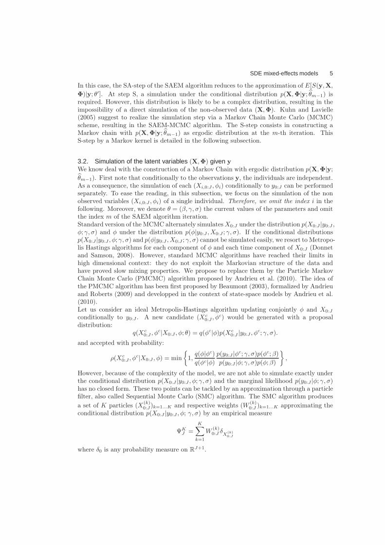
In this case, the SA-step of the SAEM algorithm reduces to the approximation of E[S(y,X,
Φ)|y; θ′]. At step S, a simulation under the conditional distribution p(X,Φ|y; θm−1) isrequired. However, this distribution is likely to be a complex distribution, resulting in theimpossibility of a direct simulation of the non-observed data (X,Φ). Kuhn and Lavielle(2005) suggest to realize the simulation step via a Markov Chain Monte Carlo (MCMC)scheme, resulting in the SAEM-MCMC algorithm. The S-step consists in constructing aMarkov chain with p(X,Φ|y; θm−1) as ergodic distribution at the m-th iteration. ThisS-step by a Markov kernel is detailed in the following subsection.
3.2. Simulation of the latent variables (X,Φ) given y
We know deal with the construction of a Markov Chain with ergodic distribution p(X,Φ|y;
θm−1). First note that conditionally to the observations y, the individuals are independent.As a consequence, the simulation of each (Xi,0:J , φi) conditionally to y0:J can be performedseparately. To ease the reading, in this subsection, we focus on the simulation of the nonobserved variables (Xi,0:J , φi) of a single individual. Therefore, we omit the index i in thefollowing. Moreover, we denote θ = (β, γ, σ) the current values of the parameters and omitthe index m of the SAEM algorithm iteration.Standard version of the MCMC alternately simulatesX0:J under the distribution p(X0:J |y0:J ,φ; γ, σ) and φ under the distribution p(φ|y0:J , X0:J ; γ, σ). If the conditional distributionsp(X0:J |y0:J , φ; γ, σ) and p(φ|y0:J , X0:J ; γ, σ) cannot be simulated easily, we resort to Metropo-lis Hastings algorithms for each component of φ and each time component of X0:J (Donnetand Samson, 2008). However, standard MCMC algorithms have reached their limits inhigh dimensional context: they do not exploit the Markovian structure of the data andhave proved slow mixing properties. We propose to replace them by the Particle MarkovChain Monte Carlo (PMCMC) algorithm proposed by Andrieu et al. (2010). The idea ofthe PMCMC algorithm has been first proposed by Beaumont (2003), formalized by Andrieuand Roberts (2009) and developped in the context of state-space models by Andrieu et al.(2010).Let us consider an ideal Metropolis-Hastings algorithm updating conjointly φ and X0:J
conditionally to y0:J . A new candidate (Xc0:J , φ
c) would be generated with a proposaldistribution:
q(Xc0:J , φ
c|X0:J , φ; θ) = q(φc|φ)p(Xc0:J |y0:J , φc; γ, σ).
and accepted with probability:
ρ(Xc0:J , φ
c|X0:J , φ) = min
1,q(φ|φc)
q(φc|φ)
p(y0:J |φc; γ, σ)p(φc;β)
p(y0:J |φ; γ, σ)p(φ;β)
,
However, because of the complexity of the model, we are not able to simulate exactly underthe conditional distribution p(X0:J |y0:J , φ; γ, σ) and the marginal likelihood p(y0:J |φ; γ, σ)has no closed form. These two points can be tackled by an approximation through a particlefilter, also called Sequential Monte Carlo (SMC) algorithm. The SMC algorithm produces
a set of K particles (X(k)0:J )k=1...K and respective weights (W
(k)0:J )k=1...K approximating the
conditional distribution p(X0:J |y0:J , φ; γ, σ) by an empirical measure
ΨKJ =
K∑
k=1
W(k)0:J δX(k)
0:J
where δ0 is any probability measure on RJ+1.
6 Donnet and Samson
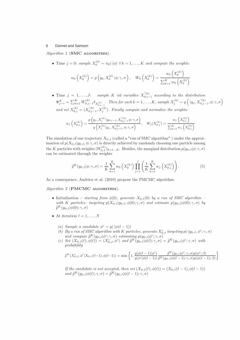
Algorithm 1 (SMC algorithm).
• Time j = 0: sample X(k)0 ∼ π0(·|φ) ∀ k = 1, . . . ,K and compute the weights:
w0
(X
(k)0
)= p
(y0, X
(k)0 |φ; γ, σ
), W0
(X
(k)0
)=
w0
(X
(k)0
)
∑Kk=1 w0
(X
(k)0
)
• Time j = 1, . . . , J : sample K iid variables X′(k)0:j−1 according to the distribution
ΨKj−1 =
∑Kk=1W
(k)0:j−1δX(k)
0:j−1. Then for each k = 1, . . . ,K, sample X
(k)j ∼ q
(·|yj, X
′(k)0:j−1, φ; γ, σ
)
and set X(k)0:j = (X
′(k)0:j−1, X
(k)j ). Finally compute and normalize the weights:
wj
“X
(k)0:j
”=
p“yj , X
(k)j |y0:j−1, X
′(k)0:j−1φ; γ, σ
”
q“X
(k)j |yj , X
′(k)0:j−1, φ; γ, σ
” , Wj(X(k)0:j ) =
wj
“X
(k)0:j
”
PK
k=1 wj
“X
(k)0:j
”
The simulation of one trajectoryX0:J (called a "run of SMC algorithm" ) under the approx-imation of p(X0:J |y0:J , φ; γ, σ) is directly achieved by randomly choosing one particle among
theK particles with weights (W(k)0:J )k=1...K . Besides, the marginal distribution p(y0:J |φ; γ, σ)
can be estimated through the weights
pK(y0:J |φ; γ, σ) =1
K
K∑
k=1
w0
(X
(k)0
) J∏
j=1
(1
K
K∑
k=1
wj
(X
(k)0:j
)). (5)
As a consequence, Andrieu et al. (2010) propose the PMCMC algorithm:
Algorithm 2 (PMCMC algorithm).
• Initialization : starting from φ(0), generate X0:J(0) by a run of SMC algorithm –with K particles– targeting p(X0:J |y0:J , φ(0); γ, σ) and estimate p(y0:J |φ(0); γ, σ) bypK(y0:J |φ(0); γ, σ)
• At iteration ℓ = 1, . . . , N
(a) Sample a candidate φc ∼ q(·|φ(ℓ − 1))(b) By a run of SMC algorithm with K particles, generate Xc
0:J targeting p(·|y0:J , φc; γ, σ)and compute pK(y0:J |φc; γ, σ) estimating p(y0:J |φc; γ, σ)
(c) Set (X0:J(ℓ), φ(ℓ)) = (Xc0:J , φ
c) and pK(y0:J |φ(ℓ); γ, σ) = pK(y0:J |φc; γ, σ) withprobability
bρK(Xc0:J , φ
c|X0:J (ℓ−1), φ(ℓ−1)) = min
1,
q(φ(ℓ − 1)|φc)
q(φc|φ(ℓ − 1))
bpK(y0:J |φc; γ, σ)p(φc; β)
bpK(y0:J |φ(ℓ − 1); γ, σ)p(φ(ℓ − 1); β)
ff
If the candidate is not accepted, then set (X0:J(ℓ), φ(ℓ)) = (X0:J(ℓ − 1), φ(ℓ− 1))and pK(y0:J |φ(ℓ); γ, σ) = pK(y0:J |φ(ℓ− 1); γ, σ)
SDE mixed-effects models 7
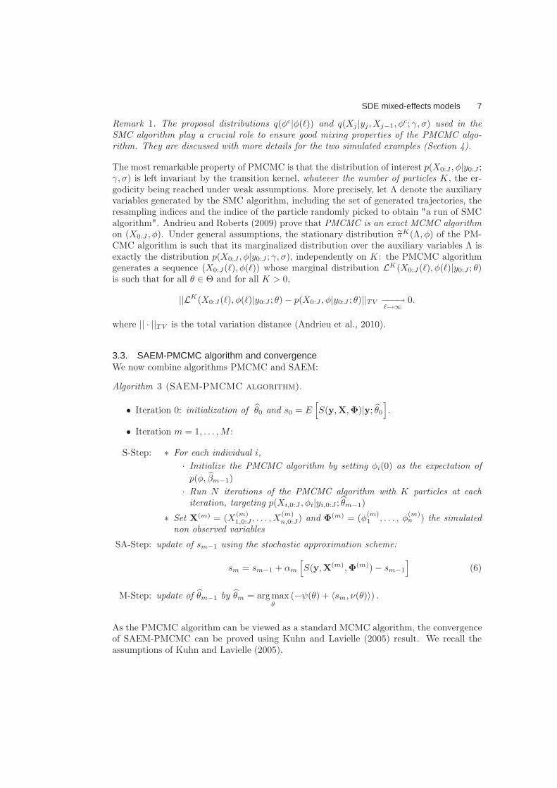
Remark 1. The proposal distributions q(φc|φ(ℓ)) and q(Xj |yj, Xj−1, φc; γ, σ) used in the
SMC algorithm play a crucial role to ensure good mixing properties of the PMCMC algo-rithm. They are discussed with more details for the two simulated examples (Section 4).
The most remarkable property of PMCMC is that the distribution of interest p(X0:J , φ|y0:J ;γ, σ) is left invariant by the transition kernel, whatever the number of particles K, the er-godicity being reached under weak assumptions. More precisely, let Λ denote the auxiliaryvariables generated by the SMC algorithm, including the set of generated trajectories, theresampling indices and the indice of the particle randomly picked to obtain "a run of SMCalgorithm". Andrieu and Roberts (2009) prove that PMCMC is an exact MCMC algorithmon (X0:J , φ). Under general assumptions, the stationary distribution πK(Λ, φ) of the PM-CMC algorithm is such that its marginalized distribution over the auxiliary variables Λ isexactly the distribution p(X0:J , φ|y0:J ; γ, σ), independently on K: the PMCMC algorithmgenerates a sequence (X0:J(ℓ), φ(ℓ)) whose marginal distribution LK(X0:J(ℓ), φ(ℓ)|y0:J ; θ)is such that for all θ ∈ Θ and for all K > 0,
||LK(X0:J (ℓ), φ(ℓ)|y0:J ; θ) − p(X0:J , φ|y0:J ; θ)||TV −−−→ℓ→∞
0.
where || · ||TV is the total variation distance (Andrieu et al., 2010).
3.3. SAEM-PMCMC algorithm and convergenceWe now combine algorithms PMCMC and SAEM:
Algorithm 3 (SAEM-PMCMC algorithm).
• Iteration 0: initialization of θ0 and s0 = E[S(y,X,Φ)|y; θ0
].
• Iteration m = 1, . . . ,M :
S-Step: ∗ For each individual i,
· Initialize the PMCMC algorithm by setting φi(0) as the expectation of
p(φ, βm−1)
· Run N iterations of the PMCMC algorithm with K particles at eachiteration, targeting p(Xi,0:J , φi|yi,0:J ; θm−1)
∗ Set X(m) = (X(m)1,0:J , . . . , X
(m)n,0:J) and Φ(m) = (φ
(m)1 , . . . , φ
(m)n ) the simulated
non observed variables
SA-Step: update of sm−1 using the stochastic approximation scheme:
sm = sm−1 + αm
[S(y,X(m),Φ(m)) − sm−1
](6)
M-Step: update of θm−1 by θm = argmaxθ
(−ψ(θ) + 〈sm, ν(θ)〉) .
As the PMCMC algorithm can be viewed as a standard MCMC algorithm, the convergenceof SAEM-PMCMC can be proved using Kuhn and Lavielle (2005) result. We recall theassumptions of Kuhn and Lavielle (2005).
8 Donnet and Samson
(M2) The functions ψ(θ) and ν(θ) are twice continuously differentiable on Θ.
(M3) The function s : Θ −→ S defined as s(θ) =∫S(y,X,Φ)p(X,Φ|y; θ)dXdΦ is contin-
uously differentiable on Θ.
(M4) The function ℓ(θ) = log p(y, θ) is continuously differentiable on Θ and
∂θ
∫p(y,X,Φ; θ)dXdΦ =
∫∂θp(y,X,Φ; θ)dXdΦ.
(M5) Define L : S × Θ −→ R as L(s, θ) = −ψ(θ) + 〈s, ν(θ)〉. There exists a function
θ : S −→ Θ such that
∀θ ∈ Θ, ∀s ∈ S, L(s, θ(s)) ≥ L(s, θ).
(SAEM1) The positive decreasing sequence of the stochastic approximation (αm)m≥0 is suchthat
∑m αm = ∞ and
∑m α2
m <∞.
(SAEM2) ℓ : Θ → R and θ : S → Θ are d times differentiable, where d is the dimension ofS(y,X,Φ).
(SAEM3) For all θ ∈ Θ,∫||S(y,X,Φ)||2 p(X,Φ|y; θ)dXdΦ < ∞ and the function Γ(θ) =
Covθ(S(X,Φ)) is continuous.
(SAEM4) S is a bounded function.
(SAEM5) The transition probability Πθ of the PMCMC algorithm is Lipschitz in θ and generatesa uniformly ergodic chain. The Markov chain (X(m),Φ(m))m≥0 takes its values in acompact subset.
We comment the different assumptions.Assumption (M0) is a strong hypothesis, which is partially relaxed in Section 5.Assumptions (M1-M5), (SAEM1-SAEM3) are standard and not restrictive.Assumption (SAEM4) and the compacity assumption of (SAEM5) are the most restrictiveand not really realistic. They could be relaxed using a principle of random boundariespresented in Allassonnière et al. (2009).Assumption (SAEM5) is verified by the PMCMC algorithm depending on the proposaldistributions. Indeed, the Lispchitz property holds if the complete likelihood is continuouslyderivable which is the case under (M2-M3) and if θ remains in a compact set, which isrealistic in practice. About the uniform ergodicity, Andrieu et al. (2010) prove that if thenoise density p(y|X ;σ) is bounded above
supy,X
p(y|X ;σ) < Mσ, (7)
PMCMC inherits the convergence properties of the corresponding ideal MCMC algorithm.For instance, if q(φc|φ) = p(φc;β) then the kernel of the ideal MCMC q(Xc
0:J , φc) =
p(φc;β)p(Xc0:J |y0:J , φc; γ, σ) is independent. For this kernel, the ratio p(X0:J ,φ|y0:J)
q(X0:J ,φ) is bounded
if (7) holds, ensuring the uniform ergodicity (Tierney, 1994).
SDE mixed-effects models 9
Theorem 1. Assume that (M0-5), (SAEM1-5) hold. Under the assumption that smm≥0
takes its values in a compact subset, the sequence θm supplied by the SAEM-PMCMC algo-rithm converges a.s. towards a (local) maximum of the log-likelihood ℓ(θ) = log p(y; θ).
Remark that despite the SMC approximation in the PMCMC algorithm, the fact that themarginal stationary distribution of MCMC is the exact conditional distribution p(X,Φ|y; θ)is sufficient to prove the convergence of SAEM-PMCMC.
4. SDE with explicit transition density: simulation study
The respective performances of the SAEM implemented with a standard MCMC and of theSAEM combined with the PMCMC are compared to two models of various complexity: theOrnstein-Uhlenbeck process and the time-inhomogeneous Gompertz process.In order to validate our results, we perform a large scale simulation study with varioussets of parameters and designs (n, J). Moreover, we study the influence of the number ofparticles and of the proposals involved the SMC algorithm.We compare the results using a biais and RMSE criteria. More precisely, for each condition(parameters, design, number of iterations) 100 datasets are generated. The correspondingestimate is obtained on each data set using both the SAEM-PMCMC algorithm and theSAEM-MCMC algorithm. Let θr denote the estimate of θ obtained on the r-th simulateddataset, for r = 1, . . . , 100 by the corresponding algorithm. The relative bias 1
100
∑r(θr −
θ)/θ and relative root mean square error (RMSE)√
1100
∑r(θr − θ)2/θ2 for each component
of θ are computed for both algorithms.The SAEM algorithm requires initial value θ0 and the choice of the sequence (αm)m≥0.The initial values are chosen arbitrarily as the convergence of the SAEM algorithm littledepends on the initialization. The step of the stochastic approximation scheme is chosen asrecommended by Kuhn and Lavielle (2005): αm = 1 during the first iterations 1 ≤ m ≤M1,and αm = 1
(m−M1)0.8 during the subsequent ones. Indeed, the initial guess θ0 might be
far from the maximum likelihood value and the first iterations with αm = 1 allow thesequence of estimates to converge to a neighborhood of the maximum likelihood estimate.Subsequently, smaller step sizes during M − M1 additional iterations ensure the almostsure convergence of the algorithm to the maximum likelihood estimate. We implement theSAEM algorithm with M1 = 60 and M = 100 iterations.
4.1. Example 1: Ornstein-Uhlenbeck process4.1.1. Ornstein-Uhlenbeck mixed model
The Ornstein-Uhlenbeck process has been widely used in neuronal modeling, biology, andfinance (see e.g. Kloeden and Platen, 1992). Consider an SDE mixed model driven by theOrnstein-Uhlenbeck process and an additive error model
yij = Xij + εij , εij ∼ N (0, σ2),
dXit = −(Xit
τi− κi
)dt+ γdBit, X0 = 0
where κi ∈ R, τi > 0. We set φi = (log(τi), κi) the vector of individual random parameters.We assume that log(τi) ∼i.i.d. N (log(τ), ω2
τ ), κi ∼i.i.d. N (κ, ω2κ). The parameter vector is
10 Donnet and Samson
θ = (log τ, κ, ωτ , ωκ, γ, σ). This model can be easily discretized, resulting in a state-spacemodel with random individual parameters:
yij = Xij + εij , εij ∼ N (0, σ2),
Xij = X iij−1e
−∆ijτi − κiτi(1 − e−∆ijτi) + ηij ,
ηij ∼ N(0, γ2τi(1 − e−∆ijτi)
).
The vector Xi = (xi1, . . . , xiJ ) conditional on φi is Gaussian with mean vector miX andcovariance matrix GiX equal to
miX =(τiκi
(1 − e
−ti1τi
), . . . , τiκi
(1 − e
−tiJτi
))′,
GiX =
(τiγ
2
2
(1 − e
−2min(tij ,tik)
τi
)e−
|tij−tik|
τi
)
1≤j,k≤J
,(8)
where ′ is the transposed vector. Altough this SDE is linear, the Gaussian transition densityp(Xij ,∆ij , tij−1|Xij−1, φi; θ) is a nonlinear function of φi. Thus, the likelihood has no closedform and the exact estimator of θ is unavailable.This example is a toy example. First, we compare the performances of the SAEM algo-rithm implemented with a simple MCMC to those of the SAEM-PMCMC algorithm. Next,we compare the influence of the number of particles K and the choice of the proposaldistribution q(Xtij
| Xij−1, yij , φi; θ) in the SAEM-PMCMC.
4.1.2. Simulation step of the SAEM algorithm
Whereas the conditional distribution p(Xi,1:J |, yi,0:J , φi; θ) is Gaussian, the joint distributionp(Xi,1:J , φi|, yi,0:J , φi; θ) is not explicitly and we have to resort to a approximate simulationat the S-step.A first solution is to implement a standard MCMC algorithm, alternatively simulatingunder the distributions p(Xi,1:J |, yi,0:J , φi; θ) and p(φi|, yi,0:J , Xi,1:J ; θ) for each subject.The posterior distribution p(Xi,1:J |, yi,0:J , φi; θ) is Gaussian with easily computable meanvector and variance matrix derived from (8). Similarly, the posterior distribution of κi isGaussian with explicit mean and variance. On the other hand, the posterior distribution ofτi is not explicit and we use a Metropolis-Hastings step with a random walk proposal.If we consider implementing a PMCMC kernel at the S-step, we have to choose two pro-posals q(Xtij
| Xij−1, yij , φi; θ) and q(·|φi). In this particular linear example, the proposalq(Xij |Xij−1, yij , φi; θ) can be the optimal proposal, the exact posterior density p(Xij |Xij−1,yij , φi; θ), which minimizes the variance of the particle weights. Indeed, this distributionis explicit for the Ornstein-Uhlenbeck, Gaussian with conditional mean and variance easilycomputable.As an alternative, we also consider the transition density p(Xij |Xij−1, φi; θ) as proposal.The proposal q(·|φ) for the individual parameters φ within the PMCMC algorithm is aclassical random walk on each component of vector φ.
4.1.3. Maximization step of the SAEM algorithm
The SAEM algorithm is based on the computation of the sufficient statistics for the maxi-mization step. The statistics for the parameters µ = (log τ, κ), Ω = diag(ω2
τ , ω2κ) and σ are
SDE mixed-effects models 11
the three classic ones for mixed models (see e.g. Samson et al., 2007):
S1(y, X,Φ) =
n∑
i=1
φi, S2(y, X,Φ) =
n∑
i=1
φiφ′i,
S3(y, X,Φ) =n∑
i=1
(yi −Xi)′(yi −Xi).
Let s1m, s2m, s3m denote the corresponding stochastic approximated conditional expecta-tions at iteration m of SAEM. The M step for these parameters reduces to
µ(m) =1
ns1m Ω(m) =
1
ns2m − 1
n2s1ms
′1m σ(m) =
√1
ns3m
The sufficient statistic corresponding to the parameter γ depends on the SDE. For theOrnstein-Uhlenbeck, we have
S4(y, X,Φ) =
n∑
i=1
J∑
j=1
(X i
itij−X i
itij−1e−∆ijτi − κiτi(1 − e−∆ijτi)
)2
.
The M step is thus γ(m) =√
1nJs4m.
Convergence assumptions (M0-5), (SAEM1-2) are easily checked on this example. (SAEM3)is implied by (SAEM4). (SAEM4) is not theoretically verified even if in practice, this is nota problem. Finally, given our choice of proposals for PMCMC, (SAEM5) also holds, thecompacity being verified in practice.
4.1.4. Simulation design and results
Two different designs are used for the simulations with equally spaced observation times:n = 20, J = 40, ∆ = 0.5 and n = 40, J = 20, ∆ = 1, t0 = 0. Two sets of parameter valuesare used. The first set is log(τ) = 0.6, κ = 1, ωτ = 0.1, ωκ = 0.1, γ = 0.05, σ = 0.05.The second set uses greater variances and is log(τ) = log(10), κ = 1, ωτ = 0.1, ωκ = 0.1,γ = 1, σ = 1. For each design and each set of parameter values, one hundred datasets aresimulated.The SAEM-PMCMC and SAEM-MCMC algorithms are initialized. For the first set of
parameters, we set log(τ)0 = 1.1, κ0 = 1.5, ωτ 0 = 0.5, ωκ0 = 0.5, γ0 = 0.25 and σ0 = 0.25,i.e. the initial standard deviations are 5 times greater than the true standard deviations.
For the second set of parameters, we set log(τ)0 = log(10) + 0.5, κ0 = 1.5, ωτ 0 = 0.5,ωκ0 = 0.5, γ0 = 5 and σ0 = 5. The SAEM-MCMC algorithm is implemented with N = 100MCMC iterations. Several values of N and K are used in the SAEM-PMCMC algorithm.Figure 1 presents the convergence of the SAEM-PMCMC algorithm for one dataset sim-ulated with the second set of parameters, n = 40 and J = 20. This illustrates the lowdependence of the initialization of SAEM and the quick convergence in a small neighbor-hood of the maximum likelihood.Table 1 presents the bias and RMSE (%) of the SAEM-PMCMC and SAEM-MCMC al-gorithms obtained for the two designs and two sets of parameters. The results are almostidentical for both algorithms and very satisfactory (bias less than 3% and RMSE less than
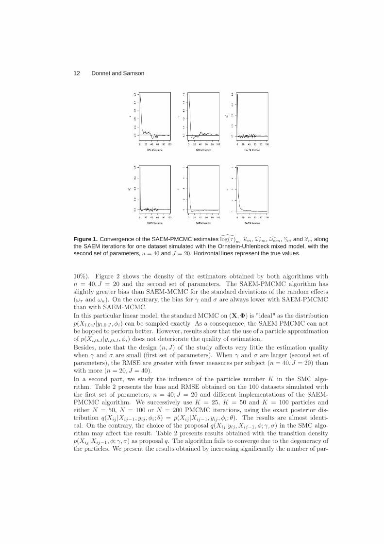
12 Donnet and Samson
Figure 1. Convergence of the SAEM-PMCMC estimates log(τ )m
, bκm, cωτ m, cωκm, bγm and bσm alongthe SAEM iterations for one dataset simulated with the Ornstein-Uhlenbeck mixed model, with thesecond set of parameters, n = 40 and J = 20. Horizontal lines represent the true values.
10%). Figure 2 shows the density of the estimators obtained by both algorithms withn = 40, J = 20 and the second set of parameters. The SAEM-PMCMC algorithm hasslightly greater bias than SAEM-MCMC for the standard deviations of the random effects(ωτ and ωκ). On the contrary, the bias for γ and σ are always lower with SAEM-PMCMCthan with SAEM-MCMC.
In this particular linear model, the standard MCMC on (X,Φ) is "ideal" as the distributionp(Xi,0:J |yi,0:J , φi) can be sampled exactly. As a consequence, the SAEM-PMCMC can notbe hopped to perform better. However, results show that the use of a particle approximationof p(Xi,0:J |yi,0:J , φi) does not deteriorate the quality of estimation.
Besides, note that the design (n, J) of the study affects very little the estimation qualitywhen γ and σ are small (first set of parameters). When γ and σ are larger (second set ofparameters), the RMSE are greater with fewer measures per subject (n = 40, J = 20) thanwith more (n = 20, J = 40).
In a second part, we study the influence of the particles number K in the SMC algo-rithm. Table 2 presents the bias and RMSE obtained on the 100 datasets simulated withthe first set of parameters, n = 40, J = 20 and different implementations of the SAEM-PMCMC algorithm. We successively use K = 25, K = 50 and K = 100 particles andeither N = 50, N = 100 or N = 200 PMCMC iterations, using the exact posterior dis-tribution q(Xij |Xij−1, yij , φi; θ) = p(Xij |Xij−1, yij , φi; θ). The results are almost identi-cal. On the contrary, the choice of the proposal q(Xij |yij , Xij−1, φ; γ, σ) in the SMC algo-rithm may affect the result. Table 2 presents results obtained with the transition densityp(Xij |Xij−1, φ; γ, σ) as proposal q. The algorithm fails to converge due to the degeneracy ofthe particles. We present the results obtained by increasing significantly the number of par-
SDE mixed-effects models 13
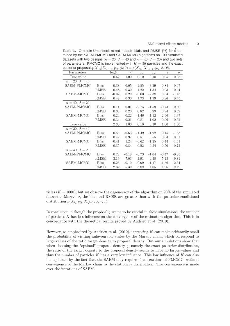
Table 1. Ornstein-Uhlenbeck mixed model: biais and RMSE (%) for bθ ob-tained by the SAEM-PMCMC and SAEM-MCMC algorithms on 100 simulateddatasets with two designs (n = 20, J = 40 and n = 40, J = 20) and two setsof parameters. PMCMC is implemented with K = 50 particles and the exactposterior proposal q(Xtij |Xtij−1 , yij , φi; θ) = p(Xtij |Xtij−1 , yij , φi; θ).
Parameters log(τ ) κ ωτ ωκ γ σ
True value 0.62 1.00 0.10 0.10 0.05 0.05
n = 20, J = 40SAEM-PMCMC Bias 0.38 0.05 -2.55 -3.29 -0.84 0.07
RMSE 0.48 0.30 1.22 1.34 0.93 0.44
SAEM-MCMC Bias -0.02 0.29 -0.60 -2.38 3.34 -1.43
RMSE 0.49 0.30 1.23 1.29 0.96 0.45
n = 40, J = 20SAEM-PMCMC Bias 0.11 0.01 -2.75 -1.59 -0.73 0.50
RMSE 0.33 0.20 0.82 0.99 0.94 0.52
SAEM-MCMC Bias -0.24 0.22 -1.46 -1.12 2.96 -1.37
RMSE 0.34 0.21 0.81 1.02 0.96 0.55
True value 2.30 1.00 0.10 0.10 1.00 1.00
n = 20, J = 40SAEM-PMCMC Bias 0.55 -0.63 -1.49 -1.92 0.15 -1.33
RMSE 0.42 0.97 0.51 0.55 0.64 0.81
SAEM-MCMC Bias -0.41 1.24 -0.62 -1.25 0.44 -1.61
RMSE 0.35 0.84 0.52 0.54 0.56 0.72
n = 40, J = 20SAEM-PMCMC Bias 0.28 -0.18 -0.73 -1.04 -0.47 -0.03
RMSE 3.19 7.03 3.91 4.38 5.45 9.81
SAEM-MCMC Bias 0.26 -0.19 -0.99 -1.17 -1.59 2.64
RMSE 2.32 5.39 3.89 4.05 4.96 9.42
ticles (K = 1000), but we observe the degeneracy of the algorithm on 90% of the simulateddatasets. Morevoer, the bias and RMSE are greater than with the posterior conditionaldistribution p(Xij |yij , Xij−1, φ; γ, σ).
In conclusion, although the proposal q seems to be crucial in these simulations, the numberof particles K has less influence on the convergence of the estimation algorithm. This is inconcordance with the theoretical results proved by Andrieu et al. (2010).
However, as emphasized by Andrieu et al. (2010), increasing K can make arbitrarily smallthe probability of visiting unfavourable states by the Markov chain, which correspond tolarge values of the ratio target density to proposal density. But our simulations show thatwhen choosing the "optimal" proposal density q, namely the exact posterior distribution,the ratio of the target density to the proposal density seems to have no larges values andthus the number of particles K has a very low influence. This low influence of K can alsobe explained by the fact that the SAEM only requires few iterations of PMCMC, withoutconvergence of the Markov chain to the stationary distribution. The convergence is madeover the iterations of SAEM.
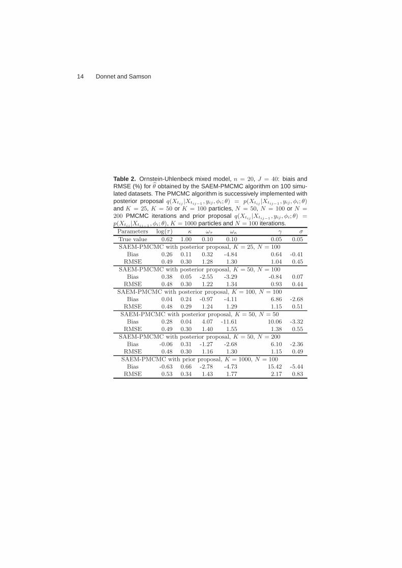
14 Donnet and Samson
Table 2. Ornstein-Uhlenbeck mixed model, n = 20, J = 40: biais andRMSE (%) for bθ obtained by the SAEM-PMCMC algorithm on 100 simu-lated datasets. The PMCMC algorithm is successively implemented withposterior proposal q(Xtij |Xtij−1 , yij , φi; θ) = p(Xtij |Xtij−1 , yij , φi; θ)and K = 25, K = 50 or K = 100 particles, N = 50, N = 100 or N =200 PMCMC iterations and prior proposal q(Xtij |Xtij−1 , yij , φi; θ) =p(Xtij |Xtij−1 , φi; θ), K = 1000 particles and N = 100 iterations.Parameters log(τ ) κ ωτ ωκ γ σ
True value 0.62 1.00 0.10 0.10 0.05 0.05
SAEM-PMCMC with posterior proposal, K = 25, N = 100Bias 0.26 0.11 0.32 -4.84 0.64 -0.41
RMSE 0.49 0.30 1.28 1.30 1.04 0.45
SAEM-PMCMC with posterior proposal, K = 50, N = 100Bias 0.38 0.05 -2.55 -3.29 -0.84 0.07
RMSE 0.48 0.30 1.22 1.34 0.93 0.44
SAEM-PMCMC with posterior proposal, K = 100, N = 100Bias 0.04 0.24 -0.97 -4.11 6.86 -2.68
RMSE 0.48 0.29 1.24 1.29 1.15 0.51
SAEM-PMCMC with posterior proposal, K = 50, N = 50Bias 0.28 0.04 4.07 -11.61 10.06 -3.32
RMSE 0.49 0.30 1.40 1.55 1.38 0.55
SAEM-PMCMC with posterior proposal, K = 50, N = 200Bias -0.06 0.31 -1.27 -2.68 6.10 -2.36
RMSE 0.48 0.30 1.16 1.30 1.15 0.49
SAEM-PMCMC with prior proposal, K = 1000, N = 100Bias -0.63 0.66 -2.78 -4.73 15.42 -5.44
RMSE 0.53 0.34 1.43 1.77 2.17 0.83
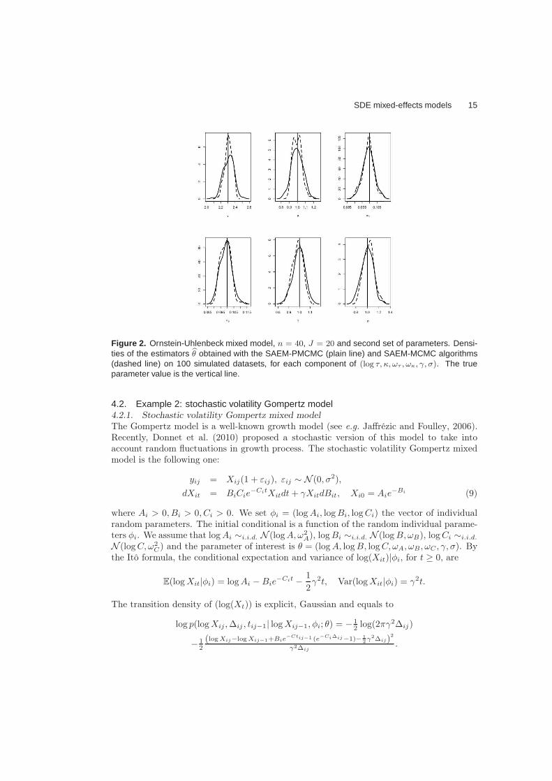
SDE mixed-effects models 15
Figure 2. Ornstein-Uhlenbeck mixed model, n = 40, J = 20 and second set of parameters. Densi-ties of the estimators bθ obtained with the SAEM-PMCMC (plain line) and SAEM-MCMC algorithms(dashed line) on 100 simulated datasets, for each component of (log τ, κ, ωτ , ωκ, γ, σ). The trueparameter value is the vertical line.
4.2. Example 2: stochastic volatility Gompertz model4.2.1. Stochastic volatility Gompertz mixed model
The Gompertz model is a well-known growth model (see e.g. Jaffrézic and Foulley, 2006).Recently, Donnet et al. (2010) proposed a stochastic version of this model to take intoaccount random fluctuations in growth process. The stochastic volatility Gompertz mixedmodel is the following one:
yij = Xij(1 + εij), εij ∼ N (0, σ2),
dXit = BiCie−CitXitdt+ γXitdBit, Xi0 = Aie
−Bi (9)
where Ai > 0, Bi > 0, Ci > 0. We set φi = (logAi, logBi, logCi) the vector of individualrandom parameters. The initial conditional is a function of the random individual parame-ters φi. We assume that logAi ∼i.i.d. N (logA,ω2
A), logBi ∼i.i.d. N (logB,ωB), logCi ∼i.i.d.
N (logC, ω2C) and the parameter of interest is θ = (logA, logB, logC, ωA, ωB, ωC , γ, σ). By
the Itô formula, the conditional expectation and variance of log(Xit)|φi, for t ≥ 0, are
E(logXit|φi) = logAi −Bie−Cit − 1
2γ2t, Var(logXit|φi) = γ2t.
The transition density of (log(Xt)) is explicit, Gaussian and equals to
log p(logXij ,∆ij , tij−1| logXij−1, φi; θ) = − 12 log(2πγ2∆ij)
− 12
(log Xij−log Xij−1+Bie−Ctij−1 (e−Ci∆ij−1)− 1
2γ2∆ij)2
γ2∆ij.
16 Donnet and Samson
which is a nonlinear function of φi. As a consequence, the likelihood has no closed formand the exact estimator of θ is unavailable.
4.2.2. Simulation step of the SAEM algorithm
First, the S step of the SAEM algorithm is tackled with a standard MCMC algorithm. Dueto the multiplicative structure of the observation noise, the distribution p(Xi,0:J |yi,0:J , φi, θ)is no more explicit and we have to resort to a random walk proposal to simulate the trajec-tories Xi,0:J conditionally to the observations yi,0:J . The components of Xi,0:J are updatedtime by time using a random walk proposal. A random walk proposal is also used to simulatethe individual parameters φi from the conditional distribution.Secondly, we implement the SAEM-PMCMC algorithm and the proposal q(Xij |Xij−1, yij ,φi; θ) has to be chosen. We propose to approximate the ideal proposal p(Xij |Xij−1, yij , φi; θ)by a Gaussian distribution with mean and variance deduced from the true ones. Moreprecisely, we consider the following proposal on logXtij
q(logXtij| logXij−1, yij , φi; θ) = N (mXij ,post,ΓXij ,post),
with
ΓXij ,post =(σ−2 + (γ2∆ij)
−1)−1
,
mXij ,post = ΓXij ,post µXij ,post,
µXij ,post =
(log yij
σ2+
1
γ2∆ij
(logXij−1 −Bie
−Citij−1 (e−Ci∆ij − 1) − γ2∆ij
2
)).
and then take the exponential to obtain a candidate for Xtij. The proposal q(·|φ) for the
individual parameters φ within the PMCMC algorithms is a classical random walk on eachcomponent of the vector φ.
4.2.3. Maximization step of the SAEM algorithm
Within the SAEM algorithm, for parameters µ = (logA, logB, logC), Ω = diag(ω2A, ω
2B, ω
2C)
and σ, the sufficient statistics and the M step are the same as in Example 1. As the pa-rameter γ appears both in the expectation and the variance of log(Xt)|φ, its estimator isnot the same as in Example 1. The sufficient statistic corresponding to γ is
S4(y, logX,Φ) =
n∑
i=1
J∑
i=1
∆ij
(logXitij
− logXitij−1 +Bie−Citij−1 (e−Ci∆ij − 1)
)2.
Let s4m denote the stochastic approximation of this sufficient statistic at iteration m of theSAEM algorithm. For the sake of simplicity, we assume that the step size ∆ij is a constant∆. The estimator γm at iteration m is deduced by maximizing the complete likelihood:
γm =
√2
∆
(−1 +
√1 +
s4m
nJ
)
When ∆ij is not a constant, the estimator is more complex but also explicit.
SDE mixed-effects models 17
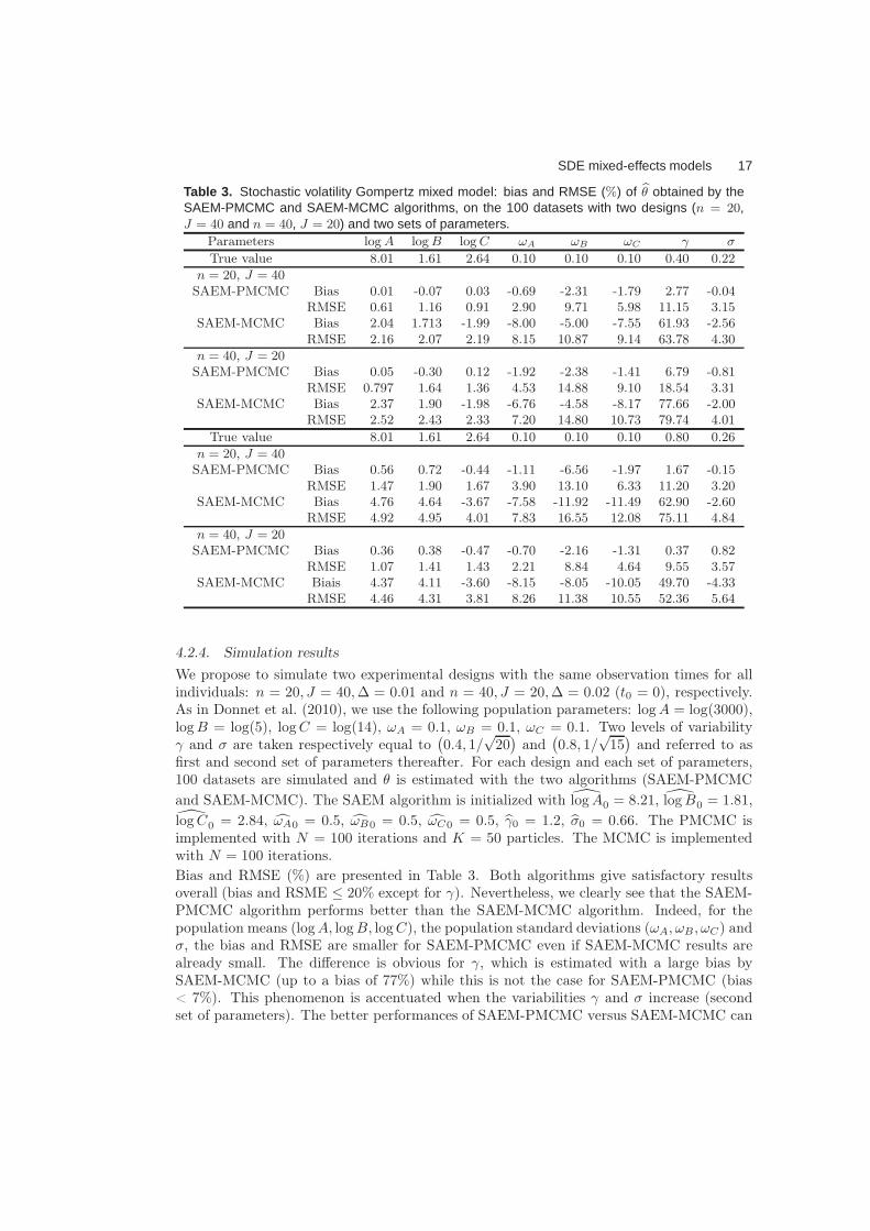
Table 3. Stochastic volatility Gompertz mixed model: bias and RMSE (%) of bθ obtained by theSAEM-PMCMC and SAEM-MCMC algorithms, on the 100 datasets with two designs (n = 20,J = 40 and n = 40, J = 20) and two sets of parameters.
Parameters log A log B log C ωA ωB ωC γ σ
True value 8.01 1.61 2.64 0.10 0.10 0.10 0.40 0.22
n = 20, J = 40SAEM-PMCMC Bias 0.01 -0.07 0.03 -0.69 -2.31 -1.79 2.77 -0.04
RMSE 0.61 1.16 0.91 2.90 9.71 5.98 11.15 3.15
SAEM-MCMC Bias 2.04 1.713 -1.99 -8.00 -5.00 -7.55 61.93 -2.56
RMSE 2.16 2.07 2.19 8.15 10.87 9.14 63.78 4.30
n = 40, J = 20SAEM-PMCMC Bias 0.05 -0.30 0.12 -1.92 -2.38 -1.41 6.79 -0.81
RMSE 0.797 1.64 1.36 4.53 14.88 9.10 18.54 3.31
SAEM-MCMC Bias 2.37 1.90 -1.98 -6.76 -4.58 -8.17 77.66 -2.00
RMSE 2.52 2.43 2.33 7.20 14.80 10.73 79.74 4.01
True value 8.01 1.61 2.64 0.10 0.10 0.10 0.80 0.26
n = 20, J = 40SAEM-PMCMC Bias 0.56 0.72 -0.44 -1.11 -6.56 -1.97 1.67 -0.15
RMSE 1.47 1.90 1.67 3.90 13.10 6.33 11.20 3.20
SAEM-MCMC Bias 4.76 4.64 -3.67 -7.58 -11.92 -11.49 62.90 -2.60
RMSE 4.92 4.95 4.01 7.83 16.55 12.08 75.11 4.84
n = 40, J = 20SAEM-PMCMC Bias 0.36 0.38 -0.47 -0.70 -2.16 -1.31 0.37 0.82
RMSE 1.07 1.41 1.43 2.21 8.84 4.64 9.55 3.57
SAEM-MCMC Biais 4.37 4.11 -3.60 -8.15 -8.05 -10.05 49.70 -4.33
RMSE 4.46 4.31 3.81 8.26 11.38 10.55 52.36 5.64
4.2.4. Simulation results
We propose to simulate two experimental designs with the same observation times for allindividuals: n = 20, J = 40,∆ = 0.01 and n = 40, J = 20,∆ = 0.02 (t0 = 0), respectively.As in Donnet et al. (2010), we use the following population parameters: logA = log(3000),logB = log(5), logC = log(14), ωA = 0.1, ωB = 0.1, ωC = 0.1. Two levels of variabilityγ and σ are taken respectively equal to
(0.4, 1/
√20)
and(0.8, 1/
√15)
and referred to asfirst and second set of parameters thereafter. For each design and each set of parameters,100 datasets are simulated and θ is estimated with the two algorithms (SAEM-PMCMC
and SAEM-MCMC). The SAEM algorithm is initialized with logA0 = 8.21, logB0 = 1.81,
logC0 = 2.84, ωA0 = 0.5, ωB0 = 0.5, ωC0 = 0.5, γ0 = 1.2, σ0 = 0.66. The PMCMC isimplemented with N = 100 iterations and K = 50 particles. The MCMC is implementedwith N = 100 iterations.
Bias and RMSE (%) are presented in Table 3. Both algorithms give satisfactory resultsoverall (bias and RSME ≤ 20% except for γ). Nevertheless, we clearly see that the SAEM-PMCMC algorithm performs better than the SAEM-MCMC algorithm. Indeed, for thepopulation means (logA, logB, logC), the population standard deviations (ωA, ωB, ωC) andσ, the bias and RMSE are smaller for SAEM-PMCMC even if SAEM-MCMC results arealready small. The difference is obvious for γ, which is estimated with a large bias bySAEM-MCMC (up to a bias of 77%) while this is not the case for SAEM-PMCMC (bias< 7%). This phenomenon is accentuated when the variabilities γ and σ increase (secondset of parameters). The better performances of SAEM-PMCMC versus SAEM-MCMC can
18 Donnet and Samson
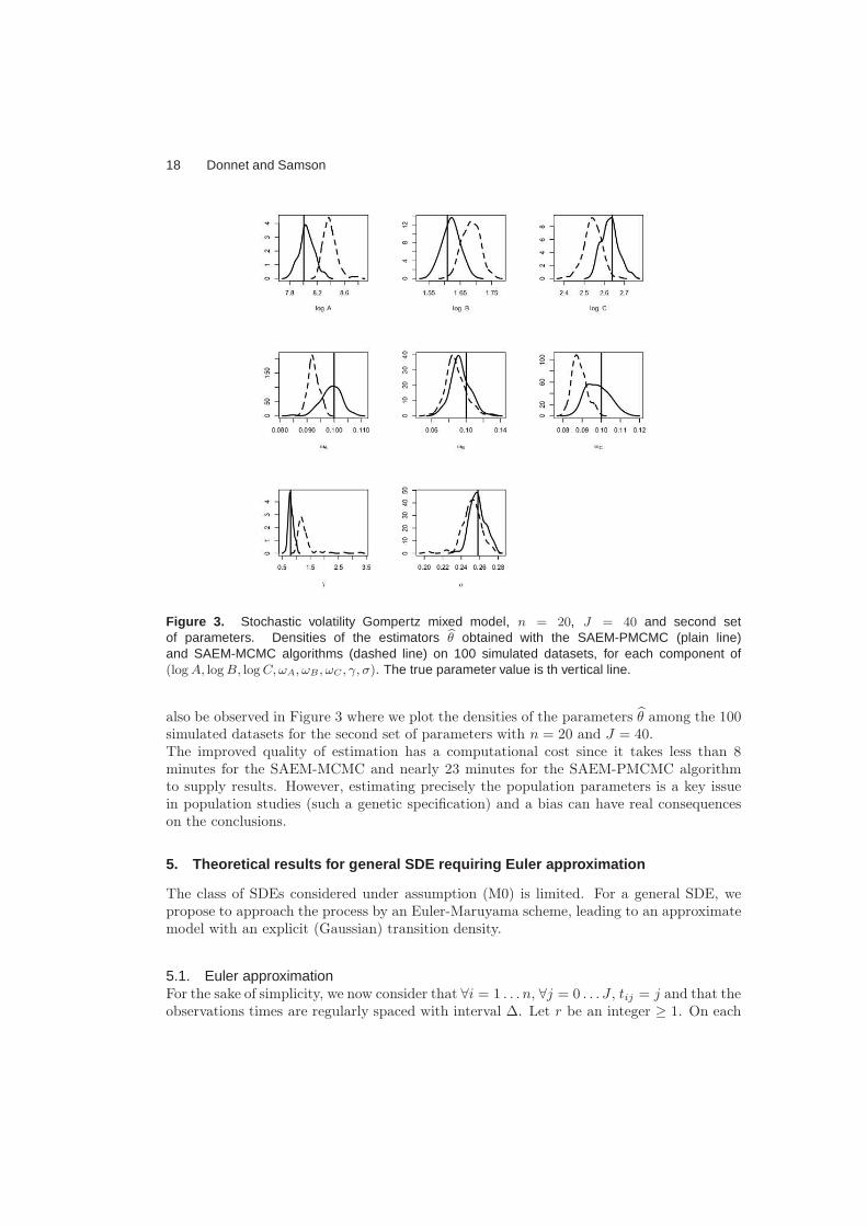
Figure 3. Stochastic volatility Gompertz mixed model, n = 20, J = 40 and second setof parameters. Densities of the estimators bθ obtained with the SAEM-PMCMC (plain line)and SAEM-MCMC algorithms (dashed line) on 100 simulated datasets, for each component of(log A, log B, log C, ωA, ωB , ωC , γ, σ). The true parameter value is th vertical line.
also be observed in Figure 3 where we plot the densities of the parameters θ among the 100simulated datasets for the second set of parameters with n = 20 and J = 40.The improved quality of estimation has a computational cost since it takes less than 8minutes for the SAEM-MCMC and nearly 23 minutes for the SAEM-PMCMC algorithmto supply results. However, estimating precisely the population parameters is a key issuein population studies (such a genetic specification) and a bias can have real consequenceson the conclusions.
5. Theoretical results for general SDE requiring Euler appr oximation
The class of SDEs considered under assumption (M0) is limited. For a general SDE, wepropose to approach the process by an Euler-Maruyama scheme, leading to an approximatemodel with an explicit (Gaussian) transition density.
5.1. Euler approximationFor the sake of simplicity, we now consider that ∀i = 1 . . . n, ∀j = 0 . . . J , tij = j and that theobservations times are regularly spaced with interval ∆. Let r be an integer ≥ 1. On each
SDE mixed-effects models 19
interval time [tj , tj+1[, we define an approximate diffusion by the recursive Euler-Maruyamascheme of step size 1/r by : Xi0(r) ∼ π0(·|φi) and
Xij(0) = Xij−1(r),
Xij(u + 1) = Xij(u) +1
ra(Xij(u), tj−1 + u/r, φi) (10)
+
√1
rb(Xij(u), tj−1 + u/r, φi, γ)Uu
where the variables Uu are iid unit centered Gaussian. Then Xij(r) is a realization of theapproximate diffusion at time tj . We consider the error model
yij = g(Xij(r), εij) (11)
Equations (10), (11) and (3) define the so-called approximate mixed model. Under thismodel, the likelihood of the observations y is :
p(r)(y; θ) =n∏
i=1
∫p(yi,0:J |Xi,0:J (r);σ)p(r)(Xi,0:J(r)|φi; γ)p(φi;β)dφidXi,0:J(r),
where p(r)(Xi,0:J(r)|φi; θ) is the density of the Euler approximation Xij(r) given φi.
5.2. SAEM-PMCMC on the approximate Euler modelA first approach to estimate θ is to use the algorithm SAEM-PMCMC presented in Section3 on the approximate model. In that case, Theorem 1 implies the following corollary:
Corollary 1. Assume that (M1-5), (SAEM1-5) hold for the approximate model. Under
the assumption that smm≥0 takes its values in a compact subset, the sequence θmm≥0
generated by the algorithm SAEM-PMCMC on the approximate Euler model converges to a(local) maximum of the likelihood p(r)(y; θ) of the approximate model.
The main limit of this result is that the SAEM-PMCMC converges to the maximum ofthe Euler approximate likelihood p(r)(y; θ) instead of the maximum of the exact likelihoodp(y; θ). Donnet and Samson (2008) prove that there exists a constant C such that the totalvariation distance between p(r)(y; θ) and the exact likelihood p(y; θ) can be bounded by
||p(r)(y; θ) − p(y; θ)||TV ≤ C
r
This results says that the two likelihoods are close but this does not imply that the twomaxima are close.A solution would be to consider r → ∞, so that the Euler approximation converges to theexact diffusion. This requires r to increase along the iterations of the SAEM algorithm, alsoimplying the Euler approximate model and the likelihood to change with the iterations. Theconcept of stationary distribution of PMCMC is no more valid in this context. We couldimagine a reversible jump approach for the simulation step of the SAEM algorithm. Buteven in this case, as the approximate likelihood changes with the iterations, it is not possibleto prove the convergence of the SAEM algorithm.
20 Donnet and Samson
From a practical point of view, the choice of r is sensitive because it adds intermediatelatent variables to the model. A large value of r is prefered as the Euler approximatelikelihood is closer to the exact likelihood. However, it is well known that a large volumeof latent variables is difficult to handle within a MCMC or PMCMC approach. This hasbeen discussed by Roberts and Stramer (2001) in a general diffusion context and by Donnetand Samson (2008) for SDE mixed models. Furthermore, as emphasized by Roberts andStramer (2001), when r → ∞, MCMC algorithms with r additional latent variables areunable to correctly estimate γ. Indeed, in that case, the density p(r)(xj |xj−1, φ; γ) of theEuler approximate diffusion converges to the likelihood of the continuous path (Xt)t∈[tj−1,tj]
given by the Girsanov formula. It is well-known that it is not possible to estimate thevolatility from this continuous path likelihood.
5.3. Exact theoretical convergence for a SAEM algorithm coupled with a SMC algorithmTo circumvent the problem of the estimation of γ, we restrict to the estimation of
θ = (β, σ)
with γ assumed to be known. To estimate θ, we propose a theoretical algorithm couplingSAEM with a naive SMC. This algorithm is known to have bad numerical properties (this
is the reason why we do not implement it) but we prove that it supplies a sequence (θm)m∈N
converging a.s. towards a local maximum of the exact likelihood log p(y; θ). This theoreticalresult yields to a consequent improvement of Corollary 1.
Now, we present the SMC that we propose to use in the simulation step of the SAEMalgorithm. In the literature, SMC algorithms have originally a filtering purpose to approx-imate the distribution p(X0:J |φ, y0:J ; θ). However, they have been rapidly extended to thecase where the parameters φ are also sampled. In the following, we present a naive SMCextension targeting the distribution p(r)(X0:J , φ|y0:J ; θ) of the approximate model.
Algorithm 4 (Naive SMC algorithm with parameters sampling).
• Time j = 0: ∀ k = 1, . . . ,K, sample φ(k)0 ∼ p(·;β) and X
(k)0 ∼ π0(·|φ(k)
0 ) and computethe weights:
W0
(φ
(k)0 , X
(k)0
)∝ p(r)
(y0, X
(k)0 , φ
(k)0 ; θ
)
• Time j = 1, . . . , J : sample K iid variables (φ′(k)j−1, X
′(k)0:j−1) according to the law ΨK
j−1 =∑K
k=1W(k)0:j−11φ
(k)j−1,X
(k)0:j−1
. Then for each k = 1, . . . ,K, sample X(k)j ∼ q(r)
(·|yj , X
′(k)0:j−1,
φ′(k)j−1; γ, σ
)and set φ
(k)j = φ
′(k)j−1 and X
(k)0:j = (X
′(k)0:j−1, X
(k)j ). Finally compute and nor-
malize the weights:
Wj
(φ
(k)j , X
(k)0:j
)∝p(r)
(yj, X
(k)j |y0:j−1, X
′(k)0:j−1φ
′(k)j−1; γ, σ
)
q(r)
(X
(k)j |yj , X
′(k)0:j−1, φ
′(k)j−1; γ, σ
) ,
We consider a SAEM algorithm in which the simulation step is performed by this naiveSMC sampler. To ensure the convergence of this estimation algorithm towards the exact
SDE mixed-effects models 21
maximum likelihood, we need the number of particles K and the step size 1/r of the Eulerapproximation to vary along the iterations of the SAEM algorithm. Thus Km and rmdenote the number of particles and the step size of the Euler scheme at iteration m ofthe SAEM algorithm. We denote by (θm)m∈N the sequence of estimates supplied by thisalgorithm. Technical assumptions (E1-4) are required to prove the convergence of the naiveSMC sampler and are presented in Appendix.
Theorem 2. Assume that there exists a constant c > 1 such that Km varies along theiterations:
Km = O (log(m)c)
and that rm = minr ∈ N | r ≥√Km. Assume that (M1-5), (SAEM1-4), (E1-4) hold
for the exact model. Then, with probability 1, limm→∞ d(θm,L) = 0 where L = θ ∈Θ, ∂θℓ(θ) = 0 is the set of stationary points of the exact log-likelihood ℓ(θ) = log p(y; θ).
Theorem 2 is proved in Appendix 7.2. This theoretical result is noteworthy. Indeed, evenif the SAEM-SMC algorithm is performed on the approximate Euler model, the algorithmconverges to the maximum of the exact likelihood. This is due to the convergence of theEuler approximate SMC towards the exact filter distribution. This powerful result has firstbeen proved by Del Moral et al. (2001). We propose an extension of their results to ourSMC (see Lemma 1 in Appendix 7.1). Then, by generalizing the proof of convergence of theSAEM algorithm to an approximate simulation step, we are able to deduce the convergenceof the estimates to the maximum of the exact likelihood.The naive SMC algorithm 4 provides an asymptotically consistent estimate of the targetdistribution p(r)(X0:J , φ|y0:J ; θ) under very weak assumptions but has proved bad propertiesin practice (in particular a degeneracy of the parameters due to the resampling step). Itcan be improved by including a MCMC step on the parameters φ (Doucet et al., 2001).Although these algorithms remains poorly efficient in practice (explaining the developementof the PMCMC algorithm for instance), they allow to prove this theorem.
6. Discussion
The stochastic differential mixed-effects models are quite widespread in the applied statisticsfield. However, in the absence of efficient and computationally reasonable estimation meth-ods, a simplifying assumption is often made: either the observation noise or the volatilityterm are standardly neglected.In this paper we present an EM algorithm combined with a Particular Monte Carlo MarkovChain method to estimate parameters in stochastic differential mixed-effects models includ-ing observation noise. We prove the convergence of the algorithm towards the maximumlikelihood estimator when the transition density is explicit. This proof is classical as thePMCMC acts as an exact marginal MCMC. On the contrary, when we consider SDE withunexplicit transition density, we prove the convergence of the SAEM-PMCMC algorithm tothe maximum likelihood of an approximate model obtained by a Euler scheme. We are notable to prove the convergence of this algorithm to the exact maximum likelihood. But wepropose the convergence of a SAEM-SMC algorithm to the exact maximum likelihood.The suggested method supplies accurate parameter estimation in a really moderate com-putational time on practical examples. Moreover, it is not restricted to homogeneous timeSDE. On various simulated datasets, we illustrate the superiority of this method over the
22 Donnet and Samson
SAEM algorithm combined with a standard MCMC algorithm. This efficiency is due tothe fact that the PMCMC algorithm takes advantage of the Markovian properties of thenon-observed process.A major advantage of this methodology is its automatic implementation. Indeed the gen-eration of the non-observed process does involves less tuning parameters than a standardMCMC, such as the size of the random move in the random walk Metropolis-Hastings algo-rithm. For example, the number of particles is not crucial, as illustrated in Example 1. Inthis paper we present a PMCMC algorithm where all the particles are re-sampled at eachiteration. Many other resampling distributions have been proposed in the literature, tryingto achieve an optimal procedure. West (1993) developed an effective method of adaptiveimportance sampling to address this issue. The procedure developed by Pitt and Shephard(2001) is similar in spirit and has real computational advantages. A stratified resamplingis proposed in Kitawaga (1996). Each resampling distribution implies a specific update ofthe weights.
Acknowledgments
Sophie Donnet has been financially supported by the french program ANR BigMC.
References
Allassonnière, S., E. Kuhn, and A. Trouvé (2009). Construction of bayesian deformable mod-els via stochastic approximation algorithm: A convergence study. to appear in Bernoulli..
Andrieu, C., A. Doucet, and R. Holenstein (2010). Particle Markov chain Monte Carlomethods. J. R. Statist. Soc. B (72), 1–33.
Andrieu, C. and G. O. Roberts (2009). The pseudo-marginal approach for efficient MonteCarlo computations. Ann. Statist. 37 (2), 697–725.
Beaumont, M. (2003). Estimation of population growth or decline in genetically monitoredpopulations. Genetics (164), 1139–1160.
Casarin, R. and J.-M. Marin (2009). Online data processing: comparison of Bayesianregularized particle filters. Electron. J. Stat. 3, 239–258.
Davidian, M. and D. Giltinan (1995). Nonlinear models to repeated measurement data.Chapman and Hall.
Del Moral, P., J. Jacod, and P. Protter (2001). The Monte-Carlo method for filtering withdiscrete-time observations. Probab. Theory Related Fields 120 (3), 346–368.
Delyon, B., M. Lavielle, and E. Moulines (1999). Convergence of a stochastic approximationversion of the EM algorithm. Ann. Statist. 27, 94–128.
Dempster, A., N. Laird, and D. Rubin (1977). Maximum likelihood from incomplete datavia the EM algorithm. Jr. R. Stat. Soc. B 39, 1–38.
Ditlevsen, S. and A. De Gaetano (2005). Stochastic vs. deterministic uptake of dodecane-dioic acid by isolated rat livers. Bull. Math. Biol. 67, 547–561.

SDE mixed-effects models 23
Donnet, S., J. Foulley, and A. Samson (2010). Bayesian analysis of growth curves usingmixed models defined by stochastic differential equations. Biometrics 66, 733–741.
Donnet, S. and A. Samson (2008). Parametric inference for mixed models defined by stochas-tic differential equations. ESAIM P&S 12, 196–218.
Doucet, A., N. de Freitas, and N. Gordon (2001). An introduction to sequential MonteCarlo methods. In Sequential Monte Carlo methods in practice, Stat. Eng. Inf. Sci., pp.3–14. New York: Springer.
Jaffrézic, F. and J. Foulley (2006). Modelling variances with random effects in non linearmixed models with an example in growth curve analysis. XXIII International BiometricConference, Montreal, 16-21 juillet .
Kitawaga, G. (1996). Monte carlo filter and smoother for non-gaussian nonlinear state spacemodels. J. Comp. Graph. Statist. (5), 1–25.
Kloeden, P. E. and E. Platen (1992). Numerical solution of stochastic differential equations,Volume 23 of Applications of Mathematics (New York). Berlin: Springer-Verlag.
Kuhn, E. and M. Lavielle (2005). Maximum likelihood estimation in nonlinear mixed effectsmodels. Comput. Statist. Data Anal. 49, 1020–1038.
Oksendal, B. (2007). Stochastic differential equations: an introduction with applications.Berlin-Heidelberg: Springer-Verlag.
Oravecz, Z., F. Tuerlinckx, and J. Vandekerckhove (2009). A hierarchical Ornstein-Uhlenbeck model for continuous repeated measurement data. Psychometrika (74), 395–418.
Overgaard, R., N. Jonsson, C. Tornøe, and H. Madsen (2005). Non-linear mixed-effectsmodels with stochastic differential equations: Implementation of an estimation algorithm.J Pharmacokinet. Pharmacodyn. 32 (1), 85–107.
Picchini, U., A. De Gaetano, and S. Ditlevsen (2010). Stochastic differential mixed-effectsmodels. Scand. J. Statist. 37, 67–90.
Pinheiro, J. and D. Bates (2000). Mixed-effect models in S and Splus. Springer-Verlag.
Pitt, M. and N. Shephard (2001). Auxiliary variable based particle filters. In SequentialMonte Carlo methods in practice, Stat. Eng. Inf. Sci., pp. 273–293. New York: Springer.
Roberts, G. O. and O. Stramer (2001). On inference for partially observed nonlinear diffu-sion models using the Metropolis-Hastings algorithm. Biometrika 88 (3), 603–621.
Samson, A., M. Lavielle, and F. Mentré (2007). The SAEM algorithm for group compar-ison tests in longitudinal data analysis based on non-linear mixed-effects model. Stat.Med. 26 (27), 4860–4875.
Tierney, L. (1994). Markov chains for exploring posterior distributions. Ann. Statist. 22 (4),1701–1762.

24 Donnet and Samson
Tornøe, C., R. Overgaard, H. Agersø, H. Nielsen, H. Madsen, and E. Jonsson (2005).Stochastic differential equations in NONMEM: implementation, application, and com-parison with ordinary differential equations. Pharm. Res. 22 (8), 1247–58.
West, M. (1993). Approximating posterior distributions by mixtures. J. Roy. Statist. Soc.Ser. B 55 (2), 409–422.
Wolfinger, R. (1993). Laplace’s approximation for nonlinear mixed models.Biometrika 80 (4), 791–795.
7. Appendix
7.1. Convergence of the Euler approximate naive SMCLet us introduce some notations. For any bounded Borel function f taking real values, wedenote πjθf = E (f(X0:j, φ)|y0:j ; θ) the conditional expectation under the exact smoothing
distribution of the exact model p(X0:j, φ|y0:j ; θ) and Ψ(K)J,θ f =
∑Kk=1W
(k)0:J f(φ(k), X
(k)0:J ) the
conditional expectation under the naive SMC distribution of the approximate model withK particles and a Euler step size r = minr ∈ N | r ≥
√K.
Lemma 1. Assume that
E1. The functions a and b are two times differentiable with derivatives w.r.t x and φ allorders up to 2 uniformly bounded w.r.t φ
E2. Θ is included in a compact set C. Besides, the functions θ 7→ π(φ;β) and σ 7→ p(y|x;σ)are continuous on C.
E3. f is a function of (φ,X0:J ) taking its values into R, uniformly boundedE4. There exist κ1 and κ2 independent of σ such that p(y|x, σ) ≤ κ1 and such that
p(r)
(yj , X
(k)j |y0:j−1, X
′(k)0:j−1φ
′(k)j−1; γ, σ
)
q(X
(k)j |yj , X
′(k)0:j−1, φ
′(k)j−1; γ, σ
) ≤ κ2
Then, for any ε > 0, for any j = 1, . . . , J , there exist constants C1 and C2 independent ofθ such that
P
(∣∣∣Ψ(K)j,θ f − πj,θf
∣∣∣ ≥ δ)≤ C1 exp
(−K δ2
C2
)
Proof. Following Del Moral et al. (2001) proof, let us define the empirical measure Ψ′(K)j,θ f =
∑Kk=1W
(k)0:j f(φ
′(k), X′(k)0:j ) where X
′(k)0:j has been defined in algorithm 4. Set the σ-filed G
generated by the variables φ(k)0 , X
(k)0 , . . . , φ
(k)j , X
(k)0:j . We have
Ψ′(K)j,θ f − Ψ
(K)j,θ f =
1
K
K∑
k=1
ηk − E(ηk|G)
with ηk = f(φ′(k)j , X
′(k)0:j ). By deviation inequalities, under assumption (E3), we obtain that
there exist two constants such that
P(|Ψ′(K)j,θ f − Ψ
(K)j,θ f | ≥ δ) ≤ A1 exp
(−KA2δ
2
‖f‖2
)
SDE mixed-effects models 25
Next, we introduce the kernels Hj such that :
Hjf(φ,X0:j−1) =
∫p(yj |xj)p(xj |X0:j−1, φ)p(φ)f(φ,X0:j−1, xj)dφdxj
Thus we have
πjf =πj−1Hjf
πj−1Hj1
and the same definitions on the Euler approximate model, with kernels HKj by
HKj f(φ,X0:j−1) =
∫p(yj |xj)p(r)(xj |X0:j−1, φ)p(φ)f(φ,X0:j−1, xj)dφdxj
such that πKj f = Er(f(φ,X0:j−1)|y0:j ; θ) the conditional expectation under the approximate
model is
πKj f =
πKj−1H
Kj f
πKj−1H
Kj 1
Then, considering the σ-filed G generated by the variables φ′(k)0 , X
′(k)0 , . . . , φ
′(k)j−1, X
′(k)0:j−1 we
can write
W(k)0:j f − Ψ
′Kj Hjf =
1
K
K∑
k=1
ηk − E(ηk|G)
with ηk = f(φ(k)j , X
(k)0:j )
p(r)
“
yj ,X(k)j |y0:j−1,X
′(k)0:j−1φ
′(k)j−1;γ,σ
”
q“
X(k)j |yj,X
′(k)0:j−1,φ
′(k)j−1;γ,σ
” . We have to bound |ηk| and E(|ηk|2|G).
Assumption (E4) implies that there exist two constants C1, C2 such that
|ηk| ≤ C1||f ||, E(|ηk|2|G) ≤ C2||f ||2
Deviation inequalities imply that there exists a constant C such that
P
(∣∣∣W (k)0:j f − Ψ
′Kj Hjf
∣∣∣ ≥ δ)≤ 2e
−K δ2
C||f||2
With similar arguments than Del Moral et al. (2001) and assumptions (E1-2), we prove byinduction that there exist two constants A1 and A2 such that
P(|πjθf − Ψ(K)j,θ f | ≥ δ) ≤ A1 exp
(−K δ2
A2‖f‖2
)
where A1 = 3j+2, A2 = C(8ρ)j+1 with C = 2 + 2α and ρ = 2κJ+1/εJ+1, where α isthe constant quantifying the error induced by the Euler scheme and εJ+1 = HJ . . .H11.With regularities assumptions and assumptions (E1-2), we can prove that the constants areindependent of θ.
26 Donnet and Samson
7.2. Proof of Theorem 2Proof. At iteration m, the simulation step provides (X(m),Φ(m)) simulated with an ap-
proximate distribution Ψ(Km)
J,θm
= ⊗ni=1Ψ
(Km)
i,J,θm
where Ψ(Km)
i,J,θm
is the empirical measure ob-
tained by the naive SMC for individual i. The stochastic approximation step of the SAEM-SMC algorithm can be decomposed into:
sm+1 = sm + αm(S(y,X(m),Φ(m)) − sm)
= sm + αmh(sm) + αmem + αmRm
withh(sm) = E(S(y,X,Φ)|y, θ(sm)) − sm
em = S(y,X(m),Φ(m)) − Ψ(Km)
J,θ(sm)S(y,X,Φ)
Rm = Ψ(Km)
J,θ(sm)S(y,X,Φ) − E(S(y,X,Φ)|y, θ(sm))
Following Theorem 2 of Delyon et al. (1999) on the convergence of Robbins-Monro scheme,the convergence of SAEM-SMC to the set of stationary points of the exact log-likelihoodℓ(θ) is ensured if we prove the following assertions:
(a) The function V (s) = −ℓ(θ(s)) is such that for all s ∈ S, F (s) = 〈∂sV (s), h(s)〉 ≤ 0and such that the set V (s, F (s) = 0) is of zero measure.
(b) limm→∞
∑mk=1 αkek exists and is finite with probability 1.
(c) limm→∞Rm = 0 with probability 1.
• To prove assertion 1, we first remark that, as γ is known and θ = (β, σ), we have
∂θ log p(y,X,Φ; θ) = ∂θ log p(r)(y,X,Φ; θ)
∂θ log p(y; θ) = ∂θ log p(r)(y; θ)
Thus under (M1-M5), (SAEM2), the functions h(s) = s(θ(s))−s and V (s) = −ℓ(θ(s))verify
〈∂sV (s), h(s)〉 = −〈∂sℓ(θ(s)), h(s)〉 ≤ 0
With similar arguments than Lemma 2 of Delyon et al. (1999), we can also prove thatthe set V (s, F (s) = 0) is of zero measure.
• Assertion 2 is proved following Theorem 5 of Delyon et al. (1999). Note F = Fmm≥0
the increasing family of σ-algebra generated by all the random variables used by theSMC algorithm until the mth iteration. By construction of the simulation step, thesimulated variables (X(1),Φ(1)), . . . , (X(m),Φ(m)) given θ0, . . . , θm are independent.Consequently, we have that for any positive Borel function f ,
E(f(X(m+1),Φ(m+1))|Fm) = Ψ(Km)J,θ f
We can then prove that∑m
k=1 αkek is a martingale, bounded in L2 under assumptions(M5) and (SAEM1-4).
• We now prove the almost sure convergence of Rm (assertion 3). The term Rm isof dimension d. It converges a.s. i.f.f. each of its component converges a.s. As a
SDE mixed-effects models 27
consequence, for the sake of simplicity, we suppose that d equals 1. Applying Borel-Cantelli lemma, it is sufficient to prove that
∑m≥0 P (|Rm| ≥ ǫ) < ∞ for all ǫ > 0.
We haveRm = Ψ
(Km)
J,θ(sm)S − π
J,θ(sm)S
where πJ,θS = E(S(X,Φ)|y; θ) First, by independence of the individual i = 1 . . . n,we can decompose S into a sum of n terms S(X,Φ) =
∑ni=1 Si(Xi,0:J , φi). and write:
P
(∣∣∣Ψ(Km)
J,θ(sm)S − π
J,θ(sm)S∣∣∣ ≥ δ
)=
P
(∣∣∣∣∣
n∑
i=1
Ψ(K)
J,θ(sm)Si −
n∑
i=1
E(Si(Xi,0:J , φi)|yi,0:J ; θ(sm))
∣∣∣∣∣ ≥ δ
)
≤n∑
i=1
P
(∣∣∣Ψ(K)
J,θ(sm)Si − π
i,J,θ(sm)Si
∣∣∣ ≥ δ
n
)
with πi,J,θ(sm)Si = E(Si(Xi,0:J , φi)|yi,0:J ; θ). Now, we bound each term of the sum by
Lemma 1 and under assumptions (SAEM4), (E1-E2). This implies the almost sureconvergence of (Rm) towards 0.
The corresponding author for negotiations concerning the manuscript isAdeline Samson ([email protected])Laboratoire MAP5Universite Paris Descartes45 rue des St Peres75006 ParisFrance