Embedded Value: Practice and Theory

Robert Frasca1 and Ken LaSorella2

Published in the March 2009 issue of the Actuarial Practice Forum Copyright 2009 by the Society of Actuaries. All rights reserved by the Society of Actuaries. Permission is granted to make brief excerpts for a published review. Permission is also granted to make limited numbers of copies of items in this publication for personal, internal, classroom or other instructional use, on condition that the foregoing copyright notice is used so as to give reasonable notice of the Society's copyright. This consent for free limited copying without prior consent of the Society does not extend to making copies for general distribution, for advertising or promotional purposes, for inclusion in new collective works or for resale. © 2009 Society of Actuaries

1 Robert Frasca, FSA, MAAA, is Executive Director, Ernst & Young LLP in Boston, Mass. He can be reached at rob.frasca@ey.com. 2 Ken LaSorella, FSA, MAAA, is Vice President, US GAAP, Sun Life Financial in Wellesley Hills, Mass. He can be reached at ken.lasorella@sunlife.com.

Acknowledgments The authors of this paper have drawn liberally and often verbatim from the American Academy of Actuaries’ Embedded Value Reporting practice note (EV practice note), which is in Q&A format and in draft form at the writing of this paper. The authors would like to thank the members of the Academy’s Life Financial Reporting Committee (LFRC) for producing the note and in particular the following contributing authors: Robert Frasca, James Garvin, Noel Harewood, Edward Jarrett, Ken LaSorella, Patricia Matson, James Norman, Jack Walton, and Darin Zimmerman. In addition, the authors would like to thank Patricia Matson for her valuable contribution to, and thorough review of, this paper. 1. Introduction The long-term nature of insurance contracts has historically made it difficult to assess properly the financial performance of insurance companies relative to one another and over time. The traditional, formula-based approaches of statutory reserving provide a commonly used basis for assessing company solvency, but they fail to distinguish movements in reserve margins from economic earnings in a reporting period. Similarly, for most products, U.S. GAAP-like methods, while focused on cost-based approaches for the measurement of earnings, use valuation methods or assumptions that do not directly reflect the impact of changes in the prevailing economic environment on the value of an insurance company. “Embedded value” (EV) is a financial measurement basis applied primarily to long-duration insurance business that provides an alternative means of measuring the value of such business at any point in time and of assessing the financial performance of the business over time. It addresses many of the criticisms leveled at various accounting methodologies. Although not technically an accounting basis, EV has evolved to embody a codified collection of rules and practices that are almost universally recognized as defining the methodology. Today EV is an important measuring stick in Europe, Canada, and other countries, and often the primary measuring stick, of financial performance for insurance companies over time and in relation to peers. Companies routinely use EV for such diverse purposes as justification for stock prices and acquisition purchase prices, performance measurement for executive compensation, profitability analysis for lines of business, and assessment of returns for capital allocation purposes. Briefly stated, EV is a measurement of the value that shareholders own in an insurance enterprise, comprised of capital, surplus, and the present value of earnings to be generated from the existing business. More formally EV has been described as the “consolidated value of the shareholders’ interests in the covered business.”3 EV is a concept very similar to the actuarial appraisal value of a company, as that value is typically encountered in the vocabulary of mergers and acquisitions. It differs from the actuarial appraisal value primarily in three ways: (1) actuarial appraisals typically assign 3 CFO Forum, European Embedded Value Principles, May 2004, p. 1.

a value to the contribution of future new business whereas EV does not, (2) actuarial appraisals are typically calculated using higher discount rates than EV, and (3) expense assumptions used in calculating EV are typically more company specific than those used in actuarial appraisals, where the assumptions tend to be more reflective of the prevailing sentiment of the market. Otherwise, actuarial appraisals and EV are one-and-the-same concepts, though applied for different purposes. The history of EV in the insurance industry dates back at least to the 1980s, when companies in the United Kingdom started routinely to disclose EV. In December 2001 the Association of British Insurers (ABI) developed guidelines for the calculation of EV for long-term insurance business. EV calculated under these guidelines was referred to as the “achieved profits method” (APM). These guidelines covered key aspects of calculating EV, including the setting of assumptions, determination of discount rates, and treatment of encumbered capital. Although not formally required, it is believed that all U.K. companies abided by these rules until they were usurped by the publication in May 2004 of guidelines for calculating European embedded value. “European embedded value” (EEV) is the name given to EV calculated pursuant to guidance contained in a paper titled European Embedded Value Principles issued in May 2004 by the CFO Forum, a discussion group composed of the CFOs of the major European insurance companies. The intent of these principles was to improve the allowance for risk in reported financial results, to increase the transparency and consistency of EV reporting in Europe, and to improve disclosures around the degree of risk inherent in the business. In addition to covering some of the same ground as defined in the APM, the EEV principles cover such topics as the application of EV to embedded options and guarantees as well as sensitivity testing and disclosure. The CFO Forum’s work on EEV is fully endorsed by the ABI. Further guidance was published by the CFO Forum for application to year-end 2006 EEV reporting. Although the CFO Forum remains the primary source of EV principles worldwide, additional guidance is available as well. For example, in Canada principles used to calculate EV are contained within a paper published in draft by the Canadian Institute of Actuaries in September 2000. While not representing codified rules, these principles are widely observed in the industry in Canada. In the United States some guidance on EV is contained in the Actuarial Standard of Practice 19, Appraisals of Casualty, Health, and Life Insurance Businesses, though the focus here is on actuarial appraisals as opposed to EV. Today many companies around the world routinely calculate and publish EV. In Europe virtually every company reports and analyzes EV in its annual report as do companies in Australia, South Africa, and, to a large extent, Japan. Canadian companies started publicly disclosing EV results in 2001 at the encouragement of the Office of the Superintendent of Financial Institutions, the Canadian regulatory body. Several insurance companies in the United States calculate EV as well, though there is currently no disclosure requirement for U.S. companies. Given the interest in EV in the investment analyst community, its perceived advantages in assessing shareholder value and its

ubiquitous application by insurance companies in Europe, it seems likely that application and disclosure of EV in the United States will continue to grow. The purpose of this paper is to provide an overview of EV concepts and methodologies as they are typically applied in the insurance industry today. Because EV is a fairly sophisticated measurement technique, it is impossible to present such an overview in any sort of detail without providing the underlying mathematical equations that are used in the EV calculations and analyses. However, despite the large number of equations, the intent of the paper is to elucidate concepts and to make the determination and interpretation of EV intuitive, at the expense of dispensing with mathematical rigor. Furthermore, the paper resorts primarily to defining EV in terms of EEV established by the CFO Forum in 2004. The CFO Forum released new guidance in June 2008 on market-consistent embedded value (MCEV) in a paper titled Market Consistent Embedded Value Principles, effectively bringing EEV into a risk-neutral, market-consistent setting. There is a brief discussion of MCEV in an appendix to this paper, and, at the time of writing this paper, the Academy has begun work on a practice note covering MCEV. 2. EV Mechanics and Formulas The basic components of EV are adjusted net worth (ANW) and in-force business value (IBV), the sum of which defines EV for a reporting entity: .EV ANW IBV= + (1)

2.1 Adjusted Net Worth (ANW) ANW is the realizable value of capital and surplus. Statutory capital and surplus are adjusted to include certain liabilities that are, in essence, allocations of surplus (e.g. Asset Valuation Reserve in the United States) and nonadmitted assets that have realizable value. This process automatically excludes the value of intangible assets identified in other accounting bases, such as U.S. GAAP goodwill, because such intangibles typically have no realizable value (i.e., they could not be readily distributed to shareholders). Because ANW includes both required capital (RC) and free surplus (FS), the entire amount of ANW is not distributable. Consequently, two approaches for deriving ANW have emerged in practice. In the more literal approach, only FS is marked to market and tax effected, because only this residual amount is considered to be distributable. In the less literal, and possibly more practical, approach, the entire adjusted statutory capital and surplus is marked to market and tax effected. With the former approach, assets supporting RC are assumed to earn book rates of return; with the latter approach, a notional sale is assumed, and assets supporting RC (as well as FS) are assumed to earn market rates of return. These rate-of-return assumptions are required for computing the cost of capital, which will be subsequently discussed.

2.2 In-Force Business Value (IBV) IBV is the present value of after-tax statutory book profits (PVBP) less the present value of the cost of capital (PVCoC), both computed with best-estimate assumptions at the date of valuation and discounted to the valuation date at a risk discount rate (RDR). In formula form: .IBV PVBP PVCoC= − (2) 2.2.1 Book Profits For a particular reporting period, statutory book profit is the after-tax net income achieved after resetting invested assets at the beginning of that period exactly equal to the net statutory liabilities (for simplicity, statutory reserves). Items included in statutory book profit are those typically found in statutory income statements. A partial list would include the sum of premiums, investment income, capital gains, and fee income, less the sum of claims, surrenders, maturities, commissions, expenses, dividends, experience refunds, the increase in statutory reserves, and taxes. In jurisdictions where U.S. statutory accounting does not apply, local regulatory accounting should define book profit. Some actuarial models, especially pricing models, do not internally reset assets to equal statutory reserves at the start of each accounting period in the projection. Instead, such models project undistributed (self-generated) assets, allowing surplus to accumulate. However, book profits can be derived by assuming that any excess of surplus at the end of an accounting period over surplus at the beginning of the accounting period, accumulated at an after-tax rate of return, has been contributed by the book of business (hence, the term book profit).With i representing the after-tax rate of return on invested assets supporting surplus, one possible formula for book profit is 1 (1 ).t t t tBP Surplus Surplus i−= − × + (3) This formula assumes there have been no distributions to shareholders (shareholder dividends) or amounts of paid-in capital during accounting period t. If amounts have been paid to or from surplus during the accounting period, book profit must be adjusted to reflect the timing and amount of such cash flows. Also, because projected accounting periods might be other than annual (e.g., quarterly or monthly), i is assumed to be the earned rate over the corresponding period. 2.2.2 Required Capital (RC) RC is the amount of capital the company has allocated to the in-force business. Definitions of required capital are context specific and vary across companies and geographies. For Canadian and U.S. business, one common definition is the minimum capital required to avoid regulator actions (i.e., x % of NAIC-authorized control-level risk-based capital [RBC] in the United States, or y % of the minimum continuing capital and surplus requirement [MCCSR] in Canada). Other percentages or capital levels are

also used (e.g., a percentage of risk-based capital formulae of rating agencies or a percentage of economic capital). The underlying percentages are usually tied to the organization’s desired financial strength ratings. 2.2.3 Cost of Capital For simplicity, let us first assume there is no debt backing RC. The cost of capital for a given period assumes investors wish to earn the risk discount rate (RDR) on capital that cannot be distributed (i.e., on RC). Because assets supporting RC are expected to earn an after-tax investment rate of return, the cost of capital for accounting period t is the RC at the beginning of the period multiplied by the excess of the RDR over the after-tax investment rate of return. In formula form: 1 ( ).t t tCostofCapital RC RDR i−= × − (4) The present value of the cost of capital is simply the present value of each period’s cost of capital in the projection, discounted to the valuation date at the RDR (subsequently discussed). 2.2.4 Risk Discount Rate (RDR) The RDR is one means of reflecting the risks inherent in the business. Most often the RDR is assumed to be a risk discount rate that is consistent with the reporting entity’s cost of equity capital. Although the RDR may be allowed to vary with time (consistent with the term structure of interest rates), a constant RDR is typically encountered in practice. However, for reporting entities with multinational operations, RDRs will typically vary by country. For example, a multinational entity might use one RDR for its U.S. business, another for its Canadian business, and yet another for its Hong Kong business. For business within a particular country, separate RDRs might be used for each line of business or major product line, but the more common practice is to use either one RDR for all in-force business or, alternatively, one for general account products and another for separate account products. Sometimes, as subsequently discussed, the RDR is defined as a weighted average cost of capital (WACC), as opposed to the cost of equity capital. Several models and methods are available to estimate a company’s cost of equity capital. The one most often encountered in practice is the capital asset pricing model (CAPM), which can be found in most finance textbooks. CAPM defines the cost of equity capital as the company’s expected total rate of return on its equity. This expected rate of return is assumed to be a function of the risk-free rate of return, the market equity risk premium (expected market rate of return in excess of the risk-free rate), and a company’s beta (a measure of its volatility relative to that of the market). To illustrate, let RF = the pre-tax risk-free rate of return (often the 10-year Treasury) RM = the expected market total rate of return (e.g., S&P 500 total return) (RM − RF) = the market equity risk premium

β = beta, a measure of relative risk of a company’s stock to that of the market and4 e = expected company total rate of return (i.e., its cost of equity capital), defined by CAPM as

( ).e RF RM RFβ= + × − (5) For the period 1926–2007, the average market equity risk premium is just over 7%. Some believe a lower equity risk premium in the neighborhood of 3–4% may be more appropriate for future projection. Nevertheless, for illustrative purposes, assume the expected market equity risk premium is 7%, the risk-free rate is 5%, and a particular company’s beta is one.5 Thus the cost of equity capital derived by CAPM is e = 5% + (1 × 7%) = 12%. This assumption set would produce a cost of equity capital close to the market’s historical total rate of return. If we were to assume a 3.5% market equity risk premium instead, the CAPM formula would produce a cost of equity capital of 8.5%. For some insurance companies offering less risky traditional products, a beta of less than one might be experienced. However, for those insurance companies offering more exotic products, such as variable annuities with guaranteed minimum accumulation benefits, equity indexed annuities, and no-lapse guarantees, betas can exceed one. Some other models and methods available to estimate the cost of equity capital include the buildup method, discounted cash flow method, arbitrage pricing theory (APT), and Fama-French three-factor model. The last two include more than one beta, each measuring a specific risk. These other models can be found in most finance textbooks. In addition, some have used CAPM with an adjustment for company size to better reflect the additional riskiness of smaller companies. Further discussion of these other models and methods is beyond the scope of this paper. 2.3 Debt and Debt-like Capital In the United Kingdom, where EV calculations originated, debt was not typically considered. Consequently the RDR has typically been based on the cost of equity capital. Furthermore, in some jurisdictions conventional debt cannot be used to fund capital requirements. In the United States, for example, borrowing money creates an offsetting liability resulting in no increase in statutory surplus. This further supports interpreting the RDR as the cost of equity capital. This interpretation was adopted by Canadian EV even though certain qualifying debt, subject to limitation, can be used to fund Canadian capital requirements (e.g., qualified debt can provide up to 25% of Tier 2 capital in MCCSR). In EV reported by Canadian companies, the cost of debt is typically recognized explicitly in 4 Technically beta is defined as the covariance of a stock’s total return with that of the market, divided by the variance of market’s total return. It is also defined as a stock’s systematic risk, which is the slope of the regression line obtained by regressing the stock’s excess returns (over the risk-free rate) against the market’s excess returns. 5 A beta of less than one would generate a lower expected rate of return than the market’s, along with less expected volatility. Likewise, a beta of more than one would generate a higher expected rate of return than the market’s, along with more expected volatility. A negative beta would indicate a negative correlation with expected market returns.

IBV via the cost of capital (i.e., an expanded cost of capital formula subsequently presented). However, even in jurisdictions where conventional debt cannot be used to fund capital requirements, there are debtlike instruments, such as surplus notes, capital notes, or preferred shares, that might be combined with equity capital to fund total capital requirements. In addition, often money can be borrowed and shares issued at the holding company level to fund capital requirements of an insurance subsidiary. As a result, the method of computing IBV with an RDR that reflects both the cost of equity capital and the cost of debt also has its place in EV. 2.3.1 Explicit Recognition of Debt in Cost of Capital One way that debt can be reflected in EV is by introducing the cost of debt (debt service) into the cost of capital formula. Assuming the RDR to be the cost of equity capital, the excess of the RDR over the after-tax rate of return on invested assets is to be applied only to the portion of RC funded with equity (i.e., not funded with debt). Assume the portion of RC funded with debt is D, at an after-tax cost of debt, d. The result is a slightly expanded form of the cost of capital formula given by formula (4): 1 1 1[( ) ( )] [ ( )].t t t t t t tCostofCapital RC D RDR i D d i− − −= − × − + × − (6) 2.3.2 Implicit Recognition of Debt in the RDR The above approach reflects debt explicitly in the cost of capital formula. Alternatively debt can be reflected implicitly in the RDR. With this approach the RDR is the weighted average cost of capital (WACC) often encountered in finance theory. For example, if only two sources of capital are considered, debt (D) and equity (E), and the cost of each is d and e, respectively, then RDR can be defined as follows:

.WACCE DRDR e d

E D E D⎛ ⎞ ⎛ ⎞= × + ×⎜ ⎟ ⎜ ⎟+ +⎝ ⎠ ⎝ ⎠

(7)

With RDR so defined, the cost of capital would be computed as if there were no debt (i.e., the entire RC would be multiplied by [RDR − it]). The formula for WACC can be expanded to include other sources of capital. For example, to include a third source, preferred stock (P) at a cost, p, the denominators would be expanded to (E + D + P) and a third term, p × P / (E + D + P), would be added. 2.3.3 Comparison of Implicit and Explicit Recognition of Debt In summary, the RDR can be either the cost of equity capital or a weighted average cost of capital. If the former, any debt is reflected explicitly in the cost of capital; if the latter,

debt is reflected implicitly in the RDR. It can be shown mathematically that, if the following two conditions are satisfied, identical results can be obtained:

1. The values for equity and debt used in WACC are fair values. This is the common definition provided in finance textbooks (despite practitioners sometimes using more readily available book values to derive WACC) and

2. Debt is maintained at a constant percentage of the present value of distributable earnings (PVDE) throughout the projection period.

If the above conditions are not met, WACC would have to take the form of a series of risk discount rates that vary over the projection period in order to match results obtained by explicit recognition of debt. For example, WACCt would represent the specific debt-equity mix applicable to period t in the projection. 2.4 IBV and the Present Value of Distributable Earnings The present value of distributable earnings (PVDE) is often encountered in acquisitions. Although similar in concept to IBV, there are differences. A key difference is the fact that PVDE is typically calculated using a starting level of capital and includes distributions of that capital, whereas IBV is calculated without distributions of capital (with a separate adjustment for cost of capital). For simplicity, assume the following: no debt, capital for the acquisition appraisal equal to RC, and an appraisal discount rate equal to the RDR. Distributable earnings (DE) can then be defined as after-tax net income, which includes the after-tax statutory book profit, plus investment income on assets supporting RC, plus any release of RC (positive or negative). In short, DE for a period represents the maximum dividends that can be distributed to shareholders while maintaining minimum capital requirements. In formula form: 1 1( ) ( ).t t t t t tDE BP i RC RC RC− −= + × + − (8) Subtracting and adding 1−× tRCRDR to the right-hand side of the equation gives

1

1

[( ) ][(1 ) ] .

t t t t

t t

DE BP RDR i RCRDR RC RC

−

−

= − − ×+ + × −

(9)

Working the first line of the DE formula, projecting the terms on the right-hand side to the end of the projection period and computing the present value at the RDR gives the standard definition of IBV (i.e., the present value of book profits less the present value of cost of capital charges). Projecting the terms of the second line and computing the present value at the RDR gives RCt−1 (i.e., starting capital at the beginning of the reporting period).6 Dropping subscripts for convenience, in formula form:

6 Because the entire initial RC will eventually be distributed, the latter computation is equivalent to projecting interest and principal payments on a mortgage and discounting such cash flows at the same rate of interest. The result is the initial outstanding principal. Hence, because the same RDR is used to project interest on RC as well as discount such interest and releases of RC, the result is the initial RC at the beginning of the reporting period.

.PVDE IBV RC= + (10) Consequently, if all assumptions are exactly the same, IBV can be obtained from PVDE by simply subtracting the initial RC at the valuation date. Specifically, .IBV PVDE RC= − (11) The above formula applies as well to the situation in which debt is reflected implicitly in the RDR (i.e., RDR equals a WACC). However, for explicit recognition of debt, distributable earnings defined above would be reduced by the cost of debt service and repayments of debt (positive or negative), leading to the following expanded formulas for DE and PVDE: 1 1 1 1( ) ( ) ( ) ( ),t t t t t t t t t tDE BP i RC RC RC d D D D− − − −= + × + − − × − − (12) ( ).PVDE IBV RC D= + − (13) Consequently, the counterpart to formula (11) is ( ).IBV PVDE RC D= − − (14) 2.5 IBV and the Value of Business Acquired (VOBA) Although at least one approach to VOBA takes the form of an IBV computation, there are differences in accounting bases, assumptions, and the definition of RDR. For example, if U.S. GAAP reserves were greater than statutory reserves, greater profits would be expected to emerge as such excess reserves release into GAAP income. Consequently, if VOBA is derived from IBV, an adjustment must be made for statutory/GAAP reserve differences. In addition, EV best-estimate assumptions (discussed subsequently in this paper) assume a going concern and are mostly company specific. Because VOBA is intended to satisfy the fair value requirements of SFAS 141, assumptions tend to be more market based. For example, a selling company’s assumed maintenance expenses of $80 per policy (based on experience and deemed appropriate for EV) might be supplanted with more typical market expenses of $60 per policy, reflecting economies of scale obtained by a potential purchaser. In addition, as previously discussed, the RDR used to compute IBV is more often based on the assumed cost of equity capital, allowing a particular company’s capital structure to be reflected in the net cost of capital (e.g., debt equal to 25% of required capital). In contrast, the RDR used in the computation of VOBA is almost invariably a WACC, reflecting the capital structure (blend of debt and equity capital) of the acquirer (or the cost of that capital structure typically encountered in the market place).

2.6 Value of New Business (VNB) VNB is the value of new business sold in the particular reporting period (e.g., calendar year for annual reporting). It does not reflect the value of future new business to be sold in future reporting periods. The value of future new business capacity valued in actuarial appraisals represents the value of a certain number of years of future new business as opposed to just one period’s worth of new business in EV. For a block of new business written during the reporting period, the basic definition of VNB is exactly the same as IBV (i.e., the present value of book profits less the present value of the cost of capital). Typically VNB is valued at the point of sale (one moment before the first premium and any acquisition expenses are incurred). However, in some disclosures (discussed in Section 5), VNB for the reporting period is accumulated at the RDR to the end of the reporting period. As with IBV, assumptions underlying VNB should be best-estimate assumptions. 2.7 Use of EV to Support an Appraisal In general, EV cannot be used directly to produce an actuarial appraisal or to estimate the value of a company’s stock. As previously mentioned, EV is not an actuarial appraisal. In addition to ANW and IBV, an actuarial appraisal includes the value of future new business capacity, a critical component of any actuarial appraisal. VNB reflects only the value of business sold in the recent reporting period; it does not reflect future performance, with respect to either sales volumes, product mix, or profit margins. Also, an actuarial appraisal might not use exactly the same assumptions as are used for EV. For example, a prospective buyer’s interpretation of risk and uncertainty and the desire to increase shareholder value commensurate with the risks undertaken in an acquisition might lead to selection of an RDR above that used for EV.

Although EV analysis does not attempt to deliver an actuarial appraisal or attempt to place a value on the company’s stock, a major purpose of EV disclosure is still to provide analysts with additional information that can be used to better value the company. Given ANW, IBV, VNB, and some sensitivity analysis, an analyst can examine historical financial data, make assumptions about future growth, modify IBV and VNB based on independent assumptions and modeling, and finally, select a multiple of modified VNB to be added to modified EV. The result would be a somewhat independent valuation of the company’s market value. In short, access to EV disclosure information, in addition to normal financial and nonfinancial information, might provide additional benefit to an analyst.

3. Assumptions One of the most important elements of the calculation of EV is the selection of appropriate assumptions to use in the calculations. Because it lends itself to considerable judgment and subjectivity, a clearly defined process around the selection of assumptions is critical if EV is to be a reliable measure of performance within a company over time and a consistent tool for comparing performance across companies within a given time

frame. EV can be very sensitive to the level of key assumptions, so even a small shift in these assumptions can have significant impact on the calculation of EV and, consequently, on the perception of company performance within the time period during which a change in a key assumption is made. Therefore, care must be taken in setting assumptions properly, and consistently. 3.1 Types of Assumptions Assumptions used in the calculation of EV can be grouped into two broad categories: noneconomic projection assumptions and economic assumptions. “Economic” assumptions are those assumptions that relate to the existing and future economic environment. Examples of economic assumptions include interest rates, asset default rates, credit spreads on reinvested assets, and rates of inflation. Broadly speaking, economic assumptions are readily observable assumptions that apply broadly across the economy and are not limited to the relatively narrow business of insurance. Economic assumptions should be updated at each valuation date. “Noneconomic” assumptions are those assumptions that relate to the existing and future operating environment of the company and are typically those assumptions that are narrowly focused on the business for which EV is being calculated or the company in which the business resides. Policyholder behavior assumptions, mortality rates, and interest-crediting strategies are three examples of assumptions that would be deemed noneconomic. Noneconomic assumptions should be actively reviewed for continued appropriateness ideally at each valuation date but certainly no less frequently than annually. It is worth noting that certain assumptions do not fit neatly into either the economic or noneconomic definitions. These include assumptions that have elements of both economy-wide and narrower applicability. The assumed inflation rate on claim costs, for example, reflects both an economy-wide element (the general rate of inflation) and a company-specific element (the claim costs of the particular company) and therefore may be viewed as straddling the definitions. The relatively few assumptions that defy distinct classification are not significant enough to impact materially the considerations on the setting of assumptions that follow. 3.2 Noneconomic Assumptions All noneconomic assumptions used to calculate EV should be “best estimate assumptions” and should be “entity specific.” This means that the assumptions should reflect management’s unbiased estimate of future experience based on the specific circumstances of the company in which the business resides. These assumptions need not be consistent with what the market’s perception of what such assumptions should be. The assumptions will generally reflect a combination of historical experience observed by the company and management’s expectation of how such experience may change in the future. This means that observed trends may be extrapolated in establishing assumptions (e.g., mortality improvement), though it is typically not considered appropriate to assume

improvement in unit expenses beyond the valuation date, except in the case of start-up operations. Because noneconomic assumptions are intended to be best estimates, it is not appropriate to include any provision for adverse deviation. When setting mortality and morbidity assumptions, companies will typically combine their own experience with industry data to arrive at their assumptions. The weighting that a company places on these two components is typically determined by the credibility of the company’s own experience. Companies will often express their assumptions as percentages of existing industry tables with the percentages representing the companies’ reflection of their unique experience and underwriting philosophies. There is no set rule that determines the granularity of a company’s mortality or morbidity assumptions; some companies will have unique assumptions for each product form, whereas others will have aggregate assumptions that apply across multiple generations of products. For products subject to substantial mortality risk, it is common for companies to reflect mortality improvement in their mortality assumptions for EV calculations. As with the underlying base mortality assumption, the assumption for mortality improvement typically reflects a combination of industry and company-specific experience-based assumptions. Care should be taken to reflect changes in the mix of business that are expected to emerge over time. This can often be addressed through the use of different improvement factors for different types of business. The potential for antiselection at renewal periods (e.g., on level term life insurance) should be considered as well. Persistency rates represent another noneconomic assumption to which EV calculations may be very sensitive. As with mortality and morbidity assumptions, persistency rates are typically set by considering both industry data and a company’s own experience. However, because of the differences of product design, distribution systems, and policyholder service models observed across companies, persistency rates tend to rely more on company-specific data than either mortality or morbidity assumptions. Persistency rates should consider the relationship between customer behavior, product design, and investment performance. There is likely to be a direct relationship between persistency and interest rates for interest-sensitive business. For flexible-premium products, premium persistency rates should consider both the distribution channel and the economic environment. Generally rates are set by both product type and duration. For business with renewable terms or fixed surrender charge periods, allowance for selection can be made by using shock lapse rates at the end of the surrender charge period. Expenses are an example of another assumption that relies more on company-specific circumstances and experience than on industry data. All expenses should be reflected in EV calculations, including acquisition costs (to the extent associated with existing business covered within the value of in-force business), maintenance expenses, and overhead. As noted earlier, it is usually considered inappropriate (though certainly not unprecedented) to project improvements in unit expenses beyond the valuation date unless associated with a start-up line of business. “One time” expenses should be

evaluated critically and care taken before eliminating them from future expense assumptions because, although specific one-time expenses do not typically recur, new, unanticipated one-time costs are constantly arising to take their place. It would appear appropriate, therefore, for a reasonable best estimate of expenses to include an anticipation of “unanticipated” one-time costs by projecting them to recur at recently observed levels. It is typical to reflect some expectation for expense inflation within the expense assumption. The assumption for expense inflation should reflect elements of market-wide price increases and therefore is normally set in conjunction with other economic assumptions, discussed below. Taxes, both federal and local, should also be projected using management’s best estimate of both the amount and timing of taxes paid. It would be appropriate to reflect projected changes in the tax laws provided such changes are management’s best estimate and have been documented as having a high probability of coming to pass. 3.3 Economic Assumptions For the calculation of EV (including EEV but not MCEV), the concepts applied for the setting of economic assumptions, which include things like investment return assumptions and discount rates, have been consistent with those used for the setting of noneconomic assumptions. Assumptions follow management’s best estimate, taking into account past experience and the economic environment as it exists on the valuation date. Investment returns are typically derived from a combination of the performance of the actual asset portfolios, company investment expenses, and expected default risks. Unless assets are perfectly matched to the liabilities, it would be usual for a reinvestment assumption to be part of the investment return assumption. The reinvestment rate is typically adjusted for investment expenses and for expected default risk. Investment expenses would be expected to reflect the local territory accounting. They are consistent with any service contracts in place and typically vary by asset class. Investment assumptions should not capitalize excess return without reflecting any additional risk. For example, increasing the investment return by assuming higher credit spreads should be offset by making an additional allowance for increased risk, possibly through the cost of capital and the RDR. The RDR is a combination of a risk-free rate of return to reflect the time value of money plus a risk margin to make prudent allowances for the risk that experience in future years may differ from that assumed. Typically the RDR reflects the cost of equity capital. Considerations used in determining the RDR including an appropriate assumption for the cost of equity capital are discussed in Section 2. However, as also noted in Section 2, the RDR may include an explicit reflection of the cost of debt if it is a source of capital funding. Two approaches are commonly used for determining the risk discount rates when the cost of debt is reflected: the “top-down” approach and the “bottom-up” approach.

Using the top-down approach, the RDR is calculated using a risk margin based upon a group weighted average cost of capital (“group WACC”). The group WACC is calculated using the equity cost of capital and an allowance for the impact of debt financing, if applicable, on a market value basis. The equity cost of capital would reflect a market-assessed risk factor that would aim to capture the market’s view of the effect of all types of risk of a company’s business, including operational and other noneconomic risk. The alternate bottom-up approach uses a product-based approach to reflect differences in risk inherent in each product group. The RDR so derived does not reflect a single cost of equity capital with a single market beta but instead reflects the expected volatility associated with each product line’s cash flows in the calculation of the EV for that product. These product-specific betas would be calculated to reflect the volatility of product cash flows and determined by considering how the profits for each product are affected by changes in expected returns on various asset classes. Converting this into a relative rate of return, product specific betas are calculated. An additional risk margin for nonmarket risks associated with the business would be added, though this might be calculated either at a product level or more simply at a group level. For companies with multinational operations, a country-specific RDR is often developed. This RDR incorporates both country-specific risk-free rates and assessments about country risk inherent in a country-specific risk margin. As alluded to earlier, considerations used to establish economic assumptions are different if EV is calculated on a market-consistent basis. A brief discussion of these considerations is contained in the Appendix. 4. Financial Options and Guarantees Financial options and guarantees are reflected in EV in two ways: intrinsic value and time value. Time value of financial options and guarantees (TVFOG) is generally given much more attention in EV calculations because it generally requires additional complexity and assumptions, such as a stochastic approach, while intrinsic value is normally obtained as a consequence of a base deterministic scenario. By definition, intrinsic value is the value of the financial options and guarantees at the valuation date assuming the current in-force is projected with best-estimate assumptions (typically a deterministic scenario). For example, assume we have a variable annuity contract with a guaranteed minimum death benefit (GMDB) of $100,000, representing a return of initial single premium. Further assume that the current account value (AV) is $80,000. The current exposure is $20,000 of death benefit, which would be expected to decline over the projection period in a base scenario that involves a steadily increasing AV. The intrinsic

value is then the present value of the future guaranteed minimum death benefits expected to be paid in excess of account value under the deterministic best-estimate assumptions. The intrinsic value would not generally be explicitly calculated, but would be included as part of the value of in-force business before the time value of financial options and guarantees is computed. It should be noted that, depending on market conditions and the timing of contracts purchased, the intrinsic value for many contracts might very well be zero. For example, a new contract with an AV equal to the GMDB would likely result in zero intrinsic value as would a contract that were well out-of-the-money (i.e., an AV much higher than the GMDB). The time value of financial options and guarantees (TVFOG)7 is the value of the financial options and guarantees given the potential changes in financial markets to increase or decrease the value of the options and guarantees before their expiry. In instances where a robust calculation is performed, TVFOG is generally calculated as the difference between the mean of a set of stochastic scenarios and a single best-estimate deterministic scenario. This best-estimate scenario would already include the intrinsic value of the financial options and guarantees. 4.1 Financial Options and Guarantees in Products and Benefit Features The following combinations of U.S. products and features typically involve valuations of TVFOG for EV:

• Variable annuities and variable universal life insurance policies with secondary guarantees, such as guaranteed minimum death benefit (GMDB), guaranteed minimum income benefit (GMIB), guaranteed minimum accumulation benefit (GMAB), guaranteed minimum withdrawal benefit (GMWB), and other GMXX benefits.

• Universal life insurance policies and deferred annuities with fixed interest rate subaccounts that guarantee minimum crediting rates, including periodic guaranteed rates and long-term interest rate floors.

• Options and crediting floors found in equity indexed annuity (EIA) contracts and other fixed annuities and investment contracts.

• Universal life insurance policies with no-lapse guarantees.

Although these are the most common products and benefits that involve financial options and guarantees, each product should be reviewed, and any options and guarantees should be captured in the TVFOG valuation. In addition, preparers of EV calculations typically quantify any options and guarantees inherent in the assets held in support of a block of business (e.g., in collateralized mortgage obligations [CMOs]). 7 Although the term TVFOG is gaining popularity primarily due to its reference in the CFO Forum’s EEV Principles document, TVFOG is sometimes reported under different names. For instance, it may be called time value of options and guarantees (TVOG), future options and guarantees (FOG), cost of future options and guarantees (CFOG), or another similar name.

4.2 Determination of TVFOG TVFOG can be calculated as the mean of the present value of distributable earnings for a set of stochastic scenarios minus the present value of distributable earnings for a single deterministic scenario (the base best-estimate scenario). All of these scenarios should be constructed using the same best-estimate assumptions and methodology. The set of stochastic scenarios varies in the projected asset return projections, while the deterministic scenario uses an average asset return projection that is typically consistent with the return assumption used in the overall EV calculation. In short, TVFOG should be calculated using assumptions, methodologies, and models consistent with those used in other calculations for EV. The general assumptions required to calculate TVFOG should be consistent with the assumptions (mortality, lapses, etc.) used in other EV calculations, as discussed in Section 3. A few considerations are of particular interest in stochastic approaches commonly utilized to calculate TVFOG. One is the set of stochastic simulations themselves that produce asset returns and discount rates for each stochastically generated scenario. The simulations might be based on a particular model or distribution such as the lognormal, regime-switching lognormal, Cox-Ingersoll-Ross, and others, and might also link fund performance through various covariance mechanisms such as the Cholesky factorization method. Stochastic approaches can vary significantly in complexity. A discussion of economic scenario generation models and techniques is beyond the scope of this paper. Another key element in stochastic simulations is the policyholder behavior algorithm. For example, the utilization of GMWB provisions in variable annuities should vary depending upon how far contracts are in the money. A policyholder with a significant benefit is much more likely to access such benefit than one with little to gain. Finally, management actions should be given consideration in developing the stochastic models. EV is designed to generate realistic results. Hence, management’s ability to modify discretionary product features should be taken into account whenever appropriate. For instance, during times of low interest rates and where contract provisions allow, fixed interest rates offered within annuities may be reduced to guaranteed minimum crediting floors in order to reduce a company’s exposure. Such types of management actions should be modeled, especially in cases where action plans are documented or historically demonstrable. Although the above discussion applies to the normal approach of computing TVFOG by means of a separate set of stochastic scenarios, other methods may be considered. For example, for simple options of fairly short duration, TVFOG can be accurately calculated (or reasonably approximated) using a closed-form solution, such as Black-Scholes. Likewise, although a separate set of stochastic scenarios run specifically for EV is desirable for computing TVFOG for more complex products, some companies have approximated TVFOG from results of stochastic scenarios generated for other purposes. Before accepting the use of short-cut approaches and stochastic runs designed

for other purposes, potential loss of accuracy and materiality should be carefully considered. 4.3 Real-World (Realistic) Probabilities vs. Risk-Neutral (Market-Consistent) Real-world probabilities are synonymous with best-estimate probabilities. Real-world probabilities and best-estimate assumptions, including assumptions of volatility and investment returns, can be used to generate stochastic scenarios. The results of a valuation based on the mean of such stochastic scenarios is a best-estimate (or expected) value. Alternatively a valuation based on the mean of stochastic scenarios generated with risk-neutral probabilities and market-consistent assumptions results in a market-consistent value. Actively traded options are generally valued on a market-consistent basis, which would include a market-based yield curve (e.g., Treasury or swap curve) and market implied volatility, and would not typically be valued on a best-estimate (real-world probability) basis. The CFO Forum’s EEV principles from 2004 indicate that techniques to value options should incorporate an allowance for stochastic variation in future economic conditions that is consistent with best-estimate assumptions. The CFO Forum’s accompanying document, Basis for Conclusions European Embedded Value Principles, states “the approach eventually adopted … incorporates the time value of financial options and guarantees by taking the expected value from a range of possible stochastic ‘real world’ outcomes.” The document also appears to reject both a pure risk-neutral approach for EEV as well as a hybrid approach in which the base EV uses real-world scenarios and TVFOG uses risk-neutral scenarios. Therefore, some companies have elected to follow a real-world, best-estimate approach for consistency with the 2004 CFO Forum documents. However, with the evolution of MCEV and the publication of MCEV principles in 2008, some companies calculate the entire EV, not just TVFOG, on a market-consistent (i.e., risk-neutral) basis. In such situations calculating TVFOG on a market-consistent basis would be in compliance with the general consistency objective of the EEV principles. Although the CFO Forum appears to have rejected a hybrid approach, a case can be made for its use. Those embedded options that are typically hedged are often valued in actuarial appraisals on a market-consistent basis. The reasoning is that the cost of hedging impacts distributable earnings. Because a primary objective of EV is to value distributable earnings, valuing TVFOG on a risk-neutral basis would appear to be consistent with that overriding objective. Consequently some companies believe that, regardless of how basic EV is computed, TVFOG should be valued on a market-consistent basis. Other considerations are whether a hedging program is in place (which may impact the choice of method) and the extent to which options and guarantees are reflected in the cost of capital and/or the RDR. When valuing TVFOG on a market-consistent

basis, caution should be exercised to properly reflect the interactivity of the valuation method and the method for capturing guarantees in the cost of capital and RDR. In summary, although the original EEV principles document does not require valuing TVFOG on a market-consistent basis, practice appears to be evolving toward such a valuation. For those reporting MCEV, there is no dispute, because TVFOG must be valued on a market-consistent basis in order to be consistent with the rest of EV. 5 Analysis of Movement The analysis of movement is a reconciliation between the opening and closing EV, with the difference between the two allocated to various explanatory categories. Generally the analysis of movement answers the question: Why did EV change over the reporting period? Many actuaries and investment analysts believe that the analysis of movement provides actionable management information. One method of analysis of movement decomposes the change in EV into the following broad categories with more detailed analysis provided for each category: • Contribution from new business • Contribution from in-force business • Contribution from free surplus • Capital movements • Other (e.g., foreign currency changes). In practice there are numerous ways of decomposing and analyzing these components varying significantly in degree of rigor and complexity. One such method attempts to separately analyze business unit performance by combining the first two components in an analysis of change in IBV and analysis of net income (source of earnings analysis). The remaining components would be combined into a type of analysis of free surplus movement.

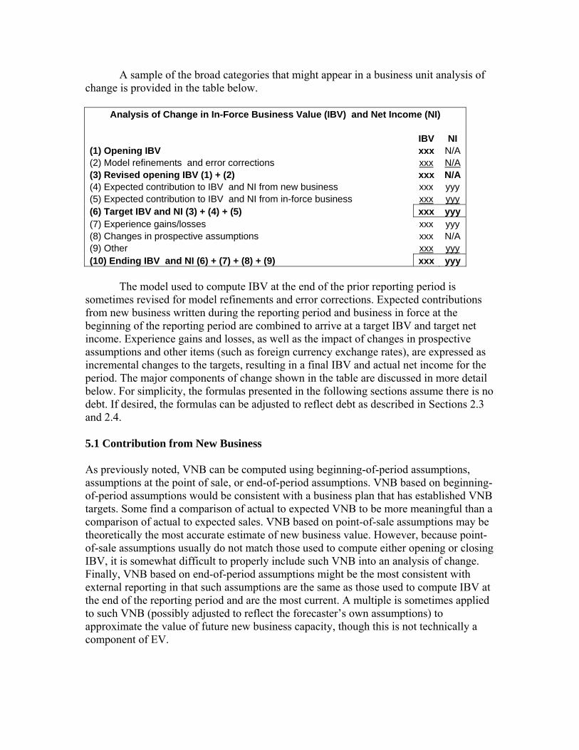
A sample of the broad categories that might appear in a business unit analysis of change is provided in the table below.

Analysis of Change in In-Force Business Value (IBV) and Net Income (NI) IBV NI (1) Opening IBV xxx N/A (2) Model refinements and error corrections xxx N/A (3) Revised opening IBV (1) + (2) xxx N/A (4) Expected contribution to IBV and NI from new business xxx yyy (5) Expected contribution to IBV and NI from in-force business xxx yyy (6) Target IBV and NI (3) + (4) + (5) xxx yyy (7) Experience gains/losses xxx yyy (8) Changes in prospective assumptions xxx N/A (9) Other xxx yyy (10) Ending IBV and NI (6) + (7) + (8) + (9) xxx yyy

The model used to compute IBV at the end of the prior reporting period is sometimes revised for model refinements and error corrections. Expected contributions from new business written during the reporting period and business in force at the beginning of the reporting period are combined to arrive at a target IBV and target net income. Experience gains and losses, as well as the impact of changes in prospective assumptions and other items (such as foreign currency exchange rates), are expressed as incremental changes to the targets, resulting in a final IBV and actual net income for the period. The major components of change shown in the table are discussed in more detail below. For simplicity, the formulas presented in the following sections assume there is no debt. If desired, the formulas can be adjusted to reflect debt as described in Sections 2.3 and 2.4. 5.1 Contribution from New Business As previously noted, VNB can be computed using beginning-of-period assumptions, assumptions at the point of sale, or end-of-period assumptions. VNB based on beginning-of-period assumptions would be consistent with a business plan that has established VNB targets. Some find a comparison of actual to expected VNB to be more meaningful than a comparison of actual to expected sales. VNB based on point-of-sale assumptions may be theoretically the most accurate estimate of new business value. However, because point-of-sale assumptions usually do not match those used to compute either opening or closing IBV, it is somewhat difficult to properly include such VNB into an analysis of change. Finally, VNB based on end-of-period assumptions might be the most consistent with external reporting in that such assumptions are the same as those used to compute IBV at the end of the reporting period and are the most current. A multiple is sometimes applied to such VNB (possibly adjusted to reflect the forecaster’s own assumptions) to approximate the value of future new business capacity, though this is not technically a component of EV.

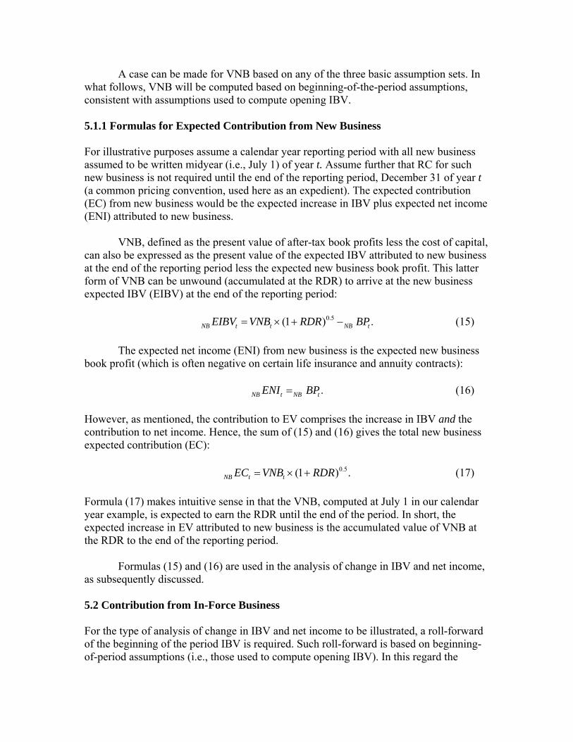
A case can be made for VNB based on any of the three basic assumption sets. In what follows, VNB will be computed based on beginning-of-the-period assumptions, consistent with assumptions used to compute opening IBV. 5.1.1 Formulas for Expected Contribution from New Business For illustrative purposes assume a calendar year reporting period with all new business assumed to be written midyear (i.e., July 1) of year t. Assume further that RC for such new business is not required until the end of the reporting period, December 31 of year t (a common pricing convention, used here as an expedient). The expected contribution (EC) from new business would be the expected increase in IBV plus expected net income (ENI) attributed to new business. VNB, defined as the present value of after-tax book profits less the cost of capital, can also be expressed as the present value of the expected IBV attributed to new business at the end of the reporting period less the expected new business book profit. This latter form of VNB can be unwound (accumulated at the RDR) to arrive at the new business expected IBV (EIBV) at the end of the reporting period: 0.5(1 ) .NB t t NB tEIBV VNB RDR BP= × + − (15) The expected net income (ENI) from new business is the expected new business book profit (which is often negative on certain life insurance and annuity contracts): .NB t NB tENI BP= (16) However, as mentioned, the contribution to EV comprises the increase in IBV and the contribution to net income. Hence, the sum of (15) and (16) gives the total new business expected contribution (EC): 0.5(1 ) .NB t tEC VNB RDR= × + (17) Formula (17) makes intuitive sense in that the VNB, computed at July 1 in our calendar year example, is expected to earn the RDR until the end of the period. In short, the expected increase in EV attributed to new business is the accumulated value of VNB at the RDR to the end of the reporting period. Formulas (15) and (16) are used in the analysis of change in IBV and net income, as subsequently discussed. 5.2 Contribution from In-Force Business For the type of analysis of change in IBV and net income to be illustrated, a roll-forward of the beginning of the period IBV is required. Such roll-forward is based on beginning-of-period assumptions (i.e., those used to compute opening IBV). In this regard the

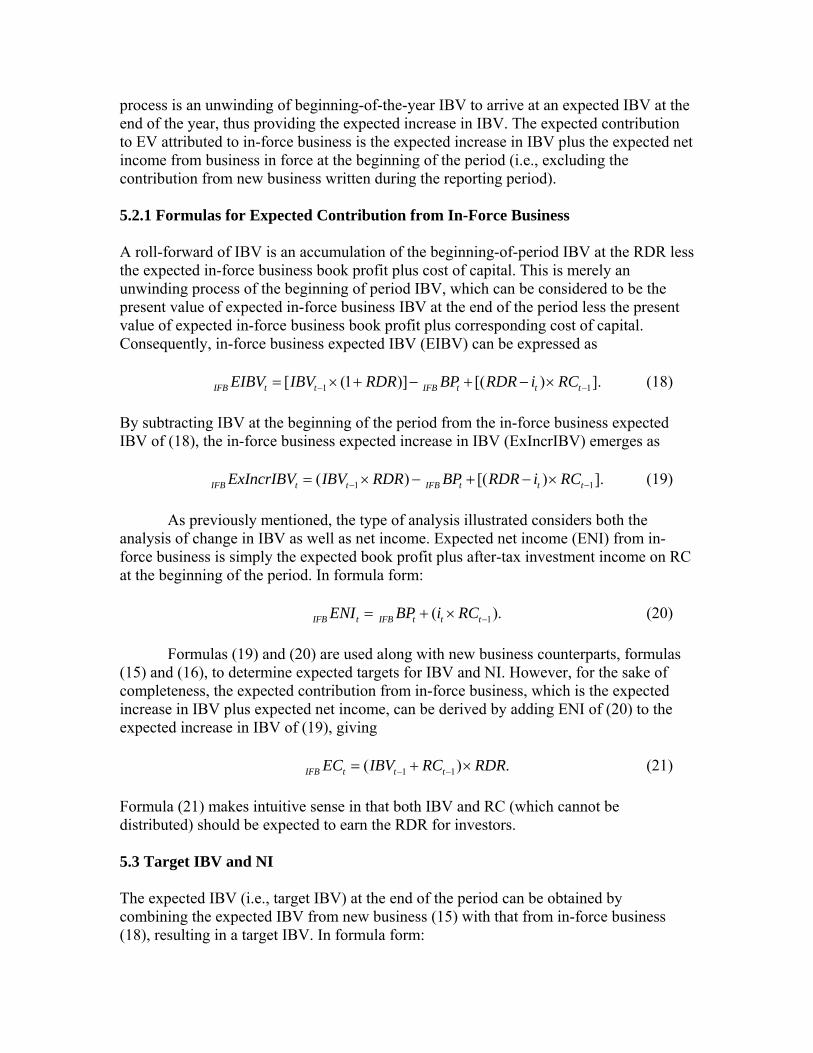
process is an unwinding of beginning-of-the-year IBV to arrive at an expected IBV at the end of the year, thus providing the expected increase in IBV. The expected contribution to EV attributed to in-force business is the expected increase in IBV plus the expected net income from business in force at the beginning of the period (i.e., excluding the contribution from new business written during the reporting period). 5.2.1 Formulas for Expected Contribution from In-Force Business A roll-forward of IBV is an accumulation of the beginning-of-period IBV at the RDR less the expected in-force business book profit plus cost of capital. This is merely an unwinding process of the beginning of period IBV, which can be considered to be the present value of expected in-force business IBV at the end of the period less the present value of expected in-force business book profit plus corresponding cost of capital. Consequently, in-force business expected IBV (EIBV) can be expressed as 1 1[ (1 )] [( ) ].IFB t t IFB t t tEIBV IBV RDR BP RDR i RC− −= × + − + − × (18) By subtracting IBV at the beginning of the period from the in-force business expected IBV of (18), the in-force business expected increase in IBV (ExIncrIBV) emerges as 1 1( ) [( ) ].IFB t t IFB t t tExIncrIBV IBV RDR BP RDR i RC− −= × − + − × (19) As previously mentioned, the type of analysis illustrated considers both the analysis of change in IBV as well as net income. Expected net income (ENI) from in-force business is simply the expected book profit plus after-tax investment income on RC at the beginning of the period. In formula form: 1( ).IFB t IFB t t tENI BP i RC −= + × (20) Formulas (19) and (20) are used along with new business counterparts, formulas (15) and (16), to determine expected targets for IBV and NI. However, for the sake of completeness, the expected contribution from in-force business, which is the expected increase in IBV plus expected net income, can be derived by adding ENI of (20) to the expected increase in IBV of (19), giving 1 1( ) .IFB t t tEC IBV RC RDR− −= + × (21) Formula (21) makes intuitive sense in that both IBV and RC (which cannot be distributed) should be expected to earn the RDR for investors. 5.3 Target IBV and NI The expected IBV (i.e., target IBV) at the end of the period can be obtained by combining the expected IBV from new business (15) with that from in-force business (18), resulting in a target IBV. In formula form:

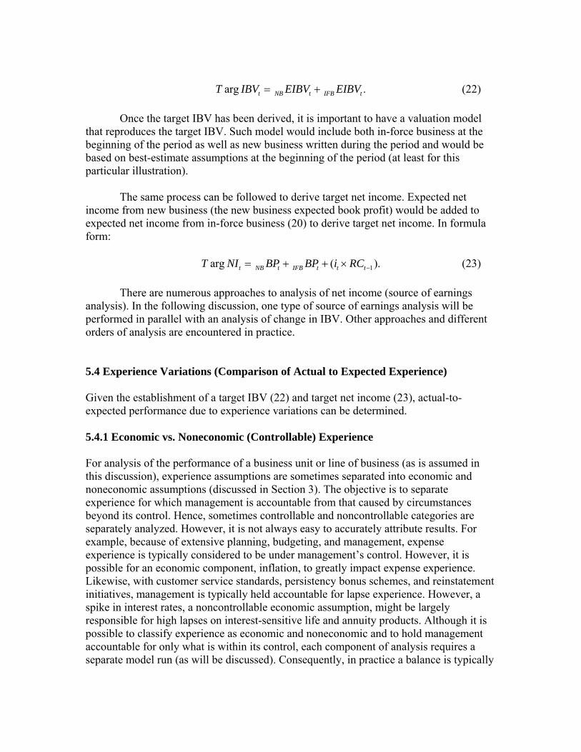
arg .t NB t IFB tT IBV EIBV EIBV= + (22) Once the target IBV has been derived, it is important to have a valuation model that reproduces the target IBV. Such model would include both in-force business at the beginning of the period as well as new business written during the period and would be based on best-estimate assumptions at the beginning of the period (at least for this particular illustration). The same process can be followed to derive target net income. Expected net income from new business (the new business expected book profit) would be added to expected net income from in-force business (20) to derive target net income. In formula form: 1arg ( ).t NB t IFB t t tT NI BP BP i RC −= + + × (23) There are numerous approaches to analysis of net income (source of earnings analysis). In the following discussion, one type of source of earnings analysis will be performed in parallel with an analysis of change in IBV. Other approaches and different orders of analysis are encountered in practice. 5.4 Experience Variations (Comparison of Actual to Expected Experience) Given the establishment of a target IBV (22) and target net income (23), actual-to-expected performance due to experience variations can be determined. 5.4.1 Economic vs. Noneconomic (Controllable) Experience For analysis of the performance of a business unit or line of business (as is assumed in this discussion), experience assumptions are sometimes separated into economic and noneconomic assumptions (discussed in Section 3). The objective is to separate experience for which management is accountable from that caused by circumstances beyond its control. Hence, sometimes controllable and noncontrollable categories are separately analyzed. However, it is not always easy to accurately attribute results. For example, because of extensive planning, budgeting, and management, expense experience is typically considered to be under management’s control. However, it is possible for an economic component, inflation, to greatly impact expense experience. Likewise, with customer service standards, persistency bonus schemes, and reinstatement initiatives, management is typically held accountable for lapse experience. However, a spike in interest rates, a noncontrollable economic assumption, might be largely responsible for high lapses on interest-sensitive life and annuity products. Although it is possible to classify experience as economic and noneconomic and to hold management accountable for only what is within its control, each component of analysis requires a separate model run (as will be discussed). Consequently, in practice a balance is typically

struck between equity and simplicity, restricting analysis to those assumptions that have the potential to provide actionable management information. 5.4.2 Interdependency of Experience Assumptions Another problem encountered in practice is that experience assumptions are not independent. For example, higher than expected mortality (i.e., more death claims) might also impact investment income, fund accumulation, expenses, persistency, and taxes. Although most such items impact net income without impacting IBV, some, such as fund accumulation and persistency, impact IBV as well. The existence of second- and even third-order effects complicates the process. There are two basic approaches to dealing with interaction of assumptions: independent assumption changes with model resets, and stepwise assumption changes with no model resets. The independent assumption approach replaces a particular modeled assumption in the target valuation model with corresponding actual experience. The difference between the target IBV and that obtained with the replaced assumption is attributed to that particular assumption. The target valuation model would then be rerun with actual experience relating to another assumption replacing the corresponding expected assumption in the target model. Continuing this process, the difference between the target IBV and the recomputed IBV, obtained with actual experience replacing expected, would be assigned to experience variation of the particular assumption being analyzed (replaced). Because of the interaction of assumptions, even if every experience assumption were so analyzed, it is extremely unlikely that the sum of target IBV and all of the incremental changes attributed to experience variations would equal a recomputed IBV with all expected assumptions replaced with actual experience. Consequently a characteristic of the independent assumption approach is that a residual change in IBV must be included. The same logic applies to analysis of net income (source of earnings analysis). Each material modeled expected assumption in the target IBV model is replaced with actual experience, and the difference in net income is quantified and attributed to an experience variation. As with analysis of change in IBV, a residual net income difference would likely be necessary. A stepwise approach is similar to the independent assumption approach described above, except the revised IBV model is not reset after an assumption is analyzed. For example, assume that mortality is the first experience assumption to be analyzed. The target IBV model is rerun with the expected mortality assumption supplanted by actual mortality experience. As with the independent assumption approach, the incremental change in IBV is assigned to mortality experience variation. However, the revised IBV model (which then reflects actual mortality experience) is then used to analyze the next experience assumption. Suppose lapses are to be analyzed next. Expected lapse experience in the revised IBV model (which reflects actual mortality experience) is replaced with actual lapse experience. The incremental change is attributed to lapse

experience (regardless of whether some of the lapse experience may have been contributed by the mortality experience previously analyzed). This process is repeated for other assumptions, with actual experience replacing the expected assumption in a stepwise manner. Practically speaking, there are far too many assumptions in EV models for each to be a candidate for analysis of experience variations in IBV and net income. Consequently only a few critical assumptions are analyzed in practice. The final IBV model run typically reflects experience variations of all assumptions, critical and noncritical. The difference between the final IBV and that of the immediately prior run reflects the aggregate contribution of the noncritical assumptions. The size of this final increment to IBV is a good indicator as to whether a sufficient number of critical assumptions have been identified and analyzed. 5.4.3 Changes in Valuation Basis and Cost of Capital Basis Because statutory valuation bases for in force business rarely change in the United States, it is unlikely that material changes in IBV or net income would result from changes in valuation basis for U.S. companies (reserve increases as a result of asset adequacy testing being a notable exception). However, in other jurisdictions, such as Canada, valuation assumptions are routinely unlocked at least annually, and margins for adverse deviation (MfADs) are typically reviewed, and possibly revised, at each valuation date. Consequently, some companies produce a separate section in an analysis of change exhibit, showing incremental increases/decreases to IBV and net income caused by various components of valuation basis change (mortality, morbidity, lapses, expenses, etc.), similar to the presentation of experience gains/losses previously discussed. Some presentations have devoted a separate section to incremental changes in IBV and net income caused by capital basis changes. Some examples of components of change are the level of minimum required capital (e.g., changes to the RBC or MCCSR formulas or adoption of economic capital), multiple of minimum capital, assumed after-tax earned rate on RC, and change in debt-equity ratio. For simplicity, the changes in IBV and net income attributable to valuation basis and capital basis changes might be combined into one line under experience variations. In this particular illustrative approach, no changes in valuation basis or cost of capital basis are assumed. 5.5 Changes in Prospective Assumptions Typically the same assumptions appearing in the analysis of experience variations also appear in the analysis of change caused by prospective assumption changes. The same approaches, independent assumption and stepwise, are taken to derive changes in IBV caused by changes in prospective assumptions. However, one additional assumption, the change in RDR, is typically shown as the last component of change. Prior to this last prospective assumption change, all valuations were performed at the same RDR, facilitating comparison and more effectively isolating incremental changes. However, the

final IBV must ultimately be computed with the end-of-period RDR, thus requiring the final prospective assumption change. 5.6 Contribution from Free Surplus Free surplus (FS) is the residual component of ANW that is not required to support in-force business. As previously discussed, the required capital (RC) portion of ANW required to support in-force business is expected to earn the RDR for shareholders. The residual, the amount that can be immediately distributed to shareholders, is generally not considered to be capital at risk. Hence, while FS resides in the company and is not distributed to shareholders, the expected return is the after-tax market rate of return on supporting assets. For our simple illustrative example, assume that there have been no capital movements, foreign currency changes, or other cash flows into or out of FS during the reporting period (e.g., no stockholder dividends, paid-in capital, surplus notes, or new shares issued). In addition, assume that migration between RC and FS occurs only at the end of the reporting period. With these simplifying assumptions, the quantum of FS at the beginning of the period would be expected to deliver an after-tax market rate of return. Consequently the expected contribution from FS is given by 1 .FS t t tEC FS i−= × (24) In practice, the forecast of the contribution from FS is a bit more complicated. For example, to arrive at FS, supporting assets are marked to market and tax effected, the objective being to arrive at the amount that can be immediately distributed. However, if supporting assets are not sold, capital gains tax would not be realized. The tax-effecting process creates a deferred tax liability that does not accrue at interest. Consequently a more accurate forecast of the expected contribution from FS would be based on an after-tax market rate of return applied to the pre-tax value of supporting assets. There are other subtleties that must be dealt with, such as adjustments for the timing of movements in and out of FS that were previously identified and conveniently assumed away for the sake of simplicity.8 Finally, as was done for IBV and net income in the business unit analysis of change, actual experience is compared to expected experience for FS as well. Actual experience is a fairly straightforward accounting reconciliation of opening and closing FS, with the change in FS, adjusted for capital movements, being compared to the expected contribution discussed above.

8 It is apparent that migration between RC and FS during the reporting period impacts the expected contributions of each. Unlike the illustrative example with an annual reporting period and all capital movements assumed to occur at the end of the reporting period, companies typically analyze capital movements at least quarterly, significantly mitigating the effects of capital migration between RC and FS and any capital movements into and out of the company.

5.7 Aggregate Contribution Applying the basic principles previously discussed, a less detailed higher-level analysis is sometimes performed at the aggregate company level (or by country of operation for a multinational company). Assume that ANW at the end of the reporting period is adjusted to remove the impact of any investor cash flows during the period (i.e., all such cash inflows and outflows are accumulated at interest to the end of the reporting period and removed from ending ANW). Then, the aggregate contribution (AC) to shareholders can be simply defined as the increase in EV as defined by (1): 1 1( ) ( ).t t t t tAC AdjANW ANW IBV IBV− −= − + − (25) Alternatively, adjusted ANW can be partitioned into RC and a residual, adjusted FS, leading to an alternative form: 1 1 1( ) [( ) ( )].t t t t t t tAC AdjFS FS IBV RC IBV RC− − −= − + + − + (26) For companies defining the value of in-force business in terms of the present value of distributable earnings (PVDE), use can be made of (11) to convert (26) into the following form: 1 1( ) ( ).t t t t tAC AdjFS FS PVDE PVDE− −= − + − (27) (Note that, in essence, AC is the same as Achieved Profits as defined by the Association of British Insurers, as noted in Section 1.) Expected contributions from new business, in-force business, and free surplus have been given by (17), (21), and (24), respectively. Continuing with the simplifying assumption of no capital cash flows during the annual reporting period, the expected aggregate contribution emerges as 0.5

1 1 1[ (1 ) ] [( ) ] [ ].t t t t t tEC VNB RDR IBV RC RDR FS i− − −= × + + + × + × (28) Formula (28) allows the actual aggregate contribution to be compared to expected for a high-level analysis of change. 5.8 Effective EV Rate The increase in EV (adjusted for investor cash flows) divided by the opening EV is sometimes used as a measure of value added expressed as a percentage. However, because VNB can be a major component of value added, it is possible for EV to increase significantly, while experience variations and changes in prospective assumptions might have adversely impacted EV. Consequently an EV effective rate, an alternative metric that removes what might be a disproportionate contribution from new business, might be

considered. The EV effective rate is best explained by reference to a simple fund example. Assume the opening fund value is $100, and $20 is added to the fund midyear. Assume also that the rate of return is 10%, and there are no redemptions. Then, at the end of one year, interest on the opening fund would be $10, and interest on the midyear contribution would be approximately $1 (i.e., 10% interest on $20 for 6 months), for a total of $11. The ending fund value would then be $131 (i.e., opening of $100 plus midyear contribution of $20 plus interest of $11). With these assumptions, we have an increase in fund value (value added) of $31, or 31% of opening value. This 31% is analogous to the increase in EV expressed as a percentage of opening EV. However, just as some of the EV value added has come from new business, some of the $31 of value added has come from new contributions ($20 in this example). The effective rate calculation would first remove the midyear contribution of $20 from the value added because it is more in the nature of principal than interest. In addition, it would increase the exposure from just the opening balance of $100 to $110 ($100 for a full year plus 50% of $20, which is invested for a half-year). The result is a numerator of $11 ($31 less $20) and a denominator of $110 ($100 plus 50% of $20), which gives exactly a 10% effective rate. The fund effective rate concept illustrated above can be applied to EV by means of the following formula:

1 1

1 1

[( ) ( ) ] .[ (0.5 )]

t t t t tt

t t t

AdjANW ANW IBV IBV VNBEffEVRateIBV ANW VNB

− −

− −

− + − −=

+ + × (29)

It should be noted that VNB in (29) is computed based on end-of-period assumptions, the same as used to compute IBV at the end of the reporting period. The effective EV rate should be compared to the expected RDR. If combined experience variations and prospective assumption changes produced a net decrease in value, the effective EV rate would be less than the RDR (and vice versa). 6. Disclosure Although EV is widely regarded as providing substantial insight into the financial strength of an insurance enterprise and how well that enterprise has performed over time, it also has been criticized as susceptible to manipulation through either the setting of assumptions or the application of methodologies that the outside observer does not fully understand. EV, as a tool for measuring the relative performance of companies, is meaningful only insofar as the observer can assume that the methodologies have been applied and the assumptions set in a consistent manner across companies or, to the extent that differences exist, that such difference are fully understood. Similarly, using EV to assess the performance of an individual enterprise over a period of time requires that the observer have full access to the analysis of movement over that time period and that changes in methodologies and assumptions are incorporated in such analysis. For these

reasons, adequate disclosure is as important an element of the process of reporting under EV as the accurate calculation of the numbers themselves. EV information related to an individual company can typically be found in the company annual report, if the company calculates EV and chooses to disclose the results. Virtually every large European company discloses EV information in these reports as do the large Canadian insurers. In Japan the number of companies reporting EV is limited, but growing, as it is elsewhere in Asia. In China reporting EV results is required. Disclosure of EV for U.S. companies is much less widespread and much more uneven. The disclosure of assumptions within these reports varies by company with some companies providing much fuller sets of information than others. The International Section of the Society of Actuaries typically publishes a compendium of disclosed financial assumptions used for EV in the fall issue of the International News. Aside from the basic elements of EV (including IBV, VNB, and ANW) the most informative information typically disclosed related to EV is the analysis of movement, as described in some detail in Section 5. When presented in sufficient detail, this presentation enables the reader to understand the EV profits arising from various sources and the causes for the changes in EV over time. The quality and detail of such analysis can vary from company to company. Beyond the analysis of movement, different observers will find different disclosure items more or less valuable in understanding a company’s EV. In part, the issue is one of personal preference. However, as a general rule, those items that have the most impact on the level of the EV are those that are most important to disclose. Many companies disclose the levels of key assumptions used in their EV calculations. These could include discount rates, policyholder behavior assumptions, and nonelective assumptions (e.g., mortality). Where an assumption is particularly critical, companies may also provide sensitivity tests to show by how much the EV would change were the assumptions different. This enables the reader to come to his or her own conclusion regarding how critical it is to the valuation. Items in which there is substantial subjectivity on the part of the company or company practice differs from commonly observed industry practice are particularly important to disclose. Understanding the sources of these items will lend insight into the comparability of results across companies and across time periods and may provide an indication of how likely a company is to be able to maintain or improve its financial performance, as measured by the change in EV, in the future. Considerable guidance around what items companies should disclose relative to their EV numbers is contained both within the CFO Forum’s paper European Embedded Value Principles and within a subsequent paper, Additional Guidance on European Embedded Value Disclosures, which was published in 2006. The disclosure items recommended by the CFO Forum are not technically “requirements,” insofar as the EEV principles laid down by the CFO Forum are not mandated by any regulatory body. However, they are routinely provided by the large European insurance companies that comprise the CFO Forum and by other companies disclosing EV as well. A company

cannot be deemed to be presenting EV in compliance with the CFO Forum guidance without them. Specific disclosure items are included within the core EV paper, European Embedded Value Principles. The required disclosures include the following:

• Key assumptions • How key assumptions were determined • Methodologies • Reconciliation of opening to closing EV by source • An analysis of the change in free surplus • Sensitivities to key assumptions.

Many of these disclosure items are defined in considerable detail within the EV guidance. In particular, a suggestion for the components that comprise the analysis of movement, or “return on EV,” is provided in the paper, and it provides a detailed analysis of how the EV changed over the reporting period in question. The 2006 paper is concerned primarily with assessing the sensitivity of the reported EV to key assumptions in the calculation of EV. These disclosures enable the readers to assess for themselves the importance of particular assumptions and to make approximate adjustments if comparing across companies with differing assumptions or if an assumption appears unreasonable in the reader’s judgment. The prescribed sensitivities to be disclosed include the effect of the following:

• 100 basis point increase in the risk discount rate • 100 basis point reduction in the interest rate environment • 10% decrease in equity or property values • 100 basis point increase in yield on equities or property • 10% decrease in maintenance expenses • 10% decrease in lapse rates • 5% decrease in mortality and morbidity rates.

In addition, companies generally disclose the following:

• The basis for determining required capital (for the cost of capital calculations) • The derivation of risk margins • The pattern of reinvestment yields.

Other disclosure items are defined in the 2006 paper as well. Disclosure requirements related to the achieved profits method used in the U.K. typically follow the CFO Forum requirements. In Canada, where EV practices are newer and less formally defined than they are in Europe, no formal rules exist. Although the Office of the Superintendent of Financial Institutions (OSFI) recognizes that the practice

of reporting EV is gaining popularity in Canada, it does not provide any guidance on how such calculations should be performed or the information related to the calculations that needs to be disclosed. The only guidance related to EV disclosure in Canada is contained in a draft paper prepared by the Canadian Institute of Actuaries, Interim Draft Paper on the Considerations in the Determination of Embedded Value for Public Disclosure in Canada, published in August 2000. It suggests that standard components of EV be disclosed (IBV, “free capital,” “locked-in capital”) and recommends that an analysis of the changes in EV from period to period be disclosed as well. It also suggests that key assumptions be reported. It encompasses the same elements of disclosure as suggested by the CFO Forum, though at a much less detailed level. A review of disclosure practices in Canada reflects little consistency across the few companies that publish EV and less detail than would typically be provided by a European company. In the United States neither the FASB, SEC, nor any other regulatory body provides any formal guidance with respect to the disclosure of information related to EV. Because EV is a valuation concept without formal regulations, some believe that reporting EV within public financial statements is not meaningful, particularly as a source for comparing performance across companies. This does not prevent companies from disclosing EV within the section of the financial statements devoted to management’s discussion and analysis (MD&A), though the practice is certainly not yet widespread in the United States. Such disclosures may lend insight into company performance across time periods and give the reader insight into how the company assesses its own performance internally, even if it is of little use in comparing results across companies. Despite the existence of guidance and the widespread view that meaningful disclosure is essential to the usefulness of EV, disclosure practices of companies continue to be criticized for their lack of clarity and completeness. There is variability in the level of disclosure provided around various key assumptions and methodologies even as companies comply with the disclosure guidelines published by the CFO Forum. Many observers believe that the level of disclosure provided by some companies is not sufficient to render a complete understanding of the meaning of the EV numbers provided. Consequently, comparability of results across companies is impossible to assess with any certainty. A common sentiment among observers is that companies provide enough information to be able to claim technical compliance with the CFO Forum guidelines while holding back on details that are necessary for a full understanding of their methods and assumptions. This might stem from a concern that fuller disclosure could compromise competitive position by providing rivals with privileged information about the company.

Appendix: Market-Consistent Embedded Value In June 2008 the CFO Forum issued Market Consistent Embedded Value Principles. Similar in form to European Embedded Value Principles, published in 2004, the 2008 paper reflects the continued evolution of EV to be on a market-consistent basis. In this way MCEV represents two significant improvements over EV. First, it results in a measurement basis that is more consistent with the fair value basis on which assets and many financial liabilities are priced and increasingly valued by banks and other financial institutions. Second, it improves consistency of measurement across companies by removing most of the subjectivity previously reflected in a company’s financial assumptions. Under MCEV, investment returns, before taxes and investment expenses, are assumed to equal the risk-free rate, as represented by the swap yield curve.9 This holds both for asset return assumptions and for the RDR. Similarly the value of financial options and guarantees should be valued using risk-neutral stochastic models. The use of risk-neutral assumptions and risk-free rates simplifies many of the calculations described earlier for the calculation of EV. For example, the cost of capital associated with hedgeable risks is largely eliminated because the RDR and the pretax, preinvestment expense returns on invested assets are both assumed to be the risk-free rate. What is left is merely a frictional cost of required capital, which captures the cost of investment expenses and taxes on investment income on assets backing required capital. The cost of capital associated with nonhedgeable risks is quantified directly using economic capital models to determine the amount of required capital to support such risks and a cost of capital charge reflective of the market’s demand to be compensated for such risk taking. Similarly the calculation of TVFOG is simplified to the extent that subjectivity is removed from the selection of assumptions and market-consistent inputs are used wherever available. Under MCEV the model used to calculate TVFOG must be calibrated to observed market prices for similar options and guarantees, enhancing the consistency in valuation of guarantees across companies and across products. These apparent simplifications aside, the analysis of movement of MCEV can be significantly more complicated than for EV, because it effectively involves tracking the movement of the fair values of both assets and liabilities. Movements in the economic environment and movements in the stochastic calculations need to be understood to perform a meaningful analysis.

9 Prior to the 2008 CFO Forum Principles, practice varied with respect to what was meant by the “risk-free rates.” Some companies, particularly those in the United Kingdom, used government bonds rates, though even here practice varied as different companies used different duration bonds or a full yield curve to represent the risk-free rate. Others used the swap curve to represent the risk-free rate. Today controversy remains as to whether the swap curve is an appropriate representation of a “risk-free” rate.

In addition to defining risk-neutral valuation as the underlying premise for EV calculations, the new MCEV guidance introduces the concept of “Group MCEV” by discussing considerations for bringing noncovered business within the MCEV umbrella. Briefly stated, the principles hold that noncovered business should be recognized within the Group MCEV at the unadjusted net asset value of such noncovered business as valued under International Financial Reporting Standards (IFRS). Some adjustments may be required where the underlying concepts of IFRS and MCEV are inconsistent (e.g., for the treatment of taxes). As with EEV, appropriate disclosure is seen as a critical element of MCEV reporting, and the June 2008 principles include extensive requirements related to disclosure and the analysis of change in MCEV between reporting periods, at both the covered business and group levels.