Jorg Wyckmans

StationsEmergency Ad Hoc Networks Through Mobile Base

Academic year 2015-2016Faculty of Engineering and ArchitectureChair: Prof. dr. ir. Daniël De ZutterDepartment of Information Technology

Master of Science in Computer Science Engineering Master's dissertation submitted in order to obtain the academic degree of

Counsellor: Dr. ir. Margot DeruyckSupervisors: Prof. dr. ir. Wout Joseph, Prof. dr. ir. Luc Martens

Jorg Wyckmans

StationsEmergency Ad Hoc Networks Through Mobile Base

Academic year 2015-2016Faculty of Engineering and ArchitectureChair: Prof. dr. ir. Daniël De ZutterDepartment of Information Technology

Master of Science in Computer Science Engineering Master's dissertation submitted in order to obtain the academic degree of

Counsellor: Dr. ir. Margot DeruyckSupervisors: Prof. dr. ir. Wout Joseph, Prof. dr. ir. Luc Martens

Preface

With the uprising of smart phones, being continuously connected to the internet has become

common in our modern civilization. A disruption of this connection can even cause panic for

people who cannot longer connect to the network and the people who are usually connected to the

affected users of the network. These disruptions are caused by a variety of events like storms,

large traffic accidents, fires or explosions.

To prevent panic in these situations and to ensure rapid resolution of the occurred disaster,

communication is paramount. To ensure the ability to communicate, an alternative network is

introduced in this master’s dissertation. This network should be flexible to allow unrolling it in

areas of which no data is available. The necessary amount of flexibility is provided by introducing

mobile base stations. Mobile base stations should have the ability to get in place on there own

and to create a network without any configuration beforehand.

In this master’s dissertation, three types of mobile base stations are introduced and analysed.

The influence of several parameters that are characteristic to the specific type of mobile base

station is investigated. Based on this investigation the advantages and disadvantages of the

different types are derived.

I would like to thank my supervisors Prof. dr. ir. Wout Joseph, Prof. dr. ir. Luc Martens

for the offered opportunity to create this master’s dissertation. Next to them, I would like to

thank my counsellor dr. ir. Margot Deruyck for her patience, explanation, feedback and help in

order to complete this dissertation.

As my time at Ghent University is reaching its end, I would like to thank my parents. They

have always supported me in every possible way and provided me with counselling and guidance.

Thanks to them I received every possible chance to complete my studies and enjoy them at the

same time.

Jorg Wyckmans, June 2016

Permission for Use of Content

The author gives permission to make this master’s dissertation available for consultation and to

copy parts of this master’s dissertation for personal use.

In the case of any other use, the copyright terms have to be respected, in particular with

regard to the obligation to state expressly the source when quoting results from this master’s

dissertation.

Jorg Wyckmans, June 2016

Emergency Ad Hoc Networks

Through Mobile Base StationsJorg Wyckmans

Master’s dissertation submitted in order to obtain the academic degree of

Master of Science in Computer Science Engineering

Academic year 2015–2016

Supervisors: Prof. dr. ir. Wout Joseph, Prof. dr. ir. Luc Martens

Counsellor: Dr. ir. Margot Deruyck

Faculty of Engineering and Architecture

Ghent University

Department of Information Technology

Chair: Prof. dr. ir. Daniel De Zutter

Summary

The modern day society got used to living in a connected way. People share their mood and

whereabouts all the time, news is brought to you only seconds after it happened and you can

pick up the telephone to call almost anyone in the world if you wanted to. This connectivity

has become a normal thing, so normal that people do not know what to do when it disappears.

Nevertheless large incidents like storms, traffic accidents or terrorist attacks can result in dis-

rupted connectivity when using the normal infrastructure. A solution for this connectivity loss

is to create a temporary emergency network to reconnect the affected users to the network.

This dissertation introduces three scenarios to create such an emergency ad hoc network. Since

these networks will be used when an unexpected incident occurs, no information about the

location or timing is known beforehand. The creation of the ad hoc network thus needs to

happen in a flexible way and must be independent of the area. To do so, mobile base stations

are used. Each introduced scenario discusses a different way to enable the base stations to be

mobile and the possibilities per scenario are investigated.

In order to analyse the feasibility of each of these scenarios, a scheduling tool is designed. This

tool uses several input parameters that describe the used scenario and proposes a network based

on these parameters. Based on the output of this tool it can be verified how efficient the scenario

is in a certain area. The tool can also be used to determine what the locations of the base stations

should be when the network is unrolled in the specified area.

Keywords

Mobile base stations, ad hoc networks, disaster resolution, LTE femtocell

Emergency Ad Hoc NetworksThrough Mobile Base Stations

Jorg Wyckmans

Supervisors: Dr. ir. Margot Deruyck, Prof. dr. ir. Wout Joseph, Prof. dr. ir. Luc Martens

Abstract— Communication is important to resolve disasters. In this re-search three different scenarios to create an emergency ad hoc network arediscussed. Using mobile LTE femtocells, such an emergency ad hoc networkcan be created with minimal effort. In order to do so a scheduling tool isintroduced. This tool is used to determine the feasibility of the different sce-narios and to propose a network that reconnects as many users as possible.

Keywords— Mobile base stations, ad hoc networks, disaster resolution,LTE femtocell

I. INTRODUCTION

THE modern day society got used to living in a connectedway. People share their mood and whereabouts all the time,

news is brought to you only seconds after it happened and youcan pick up the telephone to call almost anyone in the world ifyou wanted to. This connectivity has become a normal thing, sonormal that people do not know what to do when it disappears.Nevertheless large incidents like storms, traffic accidents or ter-rorist attacks can result in disrupted connectivity when using thenormal infrastructure. A solution for this connectivity loss is tocreate a temporary emergency network to reconnect the affectedusers to the network.

This research introduces three scenarios to create such anemergency ad hoc network. Since these networks will be usedwhen an unexpected incident occurs, no information about thelocation or timing is known beforehand. The creation of the adhoc network thus needs to happen in a flexible way and must beindependent of the area. To do so, mobile base stations are used.Each introduced scenario discusses a different way to enable thebase stations to be mobile.

In order to analyse the feasibility of each of these scenarios,a scheduling tool is designed. This tool uses several input pa-rameters that describe the used scenario and proposes a networkbased on these parameters. Based on the output of this tool itcan be verified how efficient the scenario is in a certain area.The tool can also be used to determine what the locations ofthe base stations should be when the network is unrolled in thespecified area.

In section II, the technology used for the mobile base sta-tions is introduced. In section III, the proposed scenarios arediscussed. In order to analyse these scenarios, a scheduling toolis introduced in section IV. Based on these scenarios and thescheduling tool a sensitivity analysis was conducted on the in-put parameters of the tool defined by the different scenarios. Theresults of this analysis can be found in section V. A conclusionand some possible future work is discussed in section VI.

II. MOBILE BASE STATIONS

In this research LTE (Long Term Evolution) femtocell basestations are considered. LTE and LTE Advanced are the lateststandards in mobile networking technology [1]. The technol-ogy is developed by the Third Generation Partnership Project(3GPP) and it is known to the larger public as 4G (Fourth Gen-eration). LTE is designed as a solution to combine the high mo-bility in cellular networks and the high data rates that can befound in fixed Local Area Networks [2]. It is based on an allIP (Internet Protocol) architecture and uses packet switching forits traffic, including voice traffic. Greater deployment feasibilityand extendibility of previous cellular technologies is achievedby using this all IP based structure. LTE uses licensed frequencybands only, which have to be acquired by the mobile connectiv-ity provider deploying the LTE network. The technology offersup to 300 Mb/s downlink capacity and 75 Mb/s uplink capacity.LTE Advanced can offer up to 1 Gb/s downlink and 500 Mb/suplink capacity [3].

LTE femtocells typically provide coverage in a range ofaround 100 meters around the base station and can be found inlarge buildings to provide indoor coverage. The short transmit-receive distance greatly lowers the transmit power and achievesa higher Signal to Interference plus Noise Ratio (SINR). Thismeans that the signal is less attenuated by environmental influ-ences. Another property of femtocells is that cell-to-cell inter-ference is rather small due to the low transmit powers used [4].

The choice for this technology is based on the following con-siderations. The main target group of the newly created ad hocnetwork are users carrying a smart phone. The most popularways to connect to the network using a smart phone are 4G orWiFi. These technologies provide similar services with simi-lar properties. However, due to the uncontrolled nature of theunlicensed band in which WiFi operates, the throughput can bedramatically poor when a lot of users are competing for the sameresources. This is problematic for the presented use case sinceit is all about reconnecting a large number of users in the sameplace. Next to that, LTE is optimised to handle (slow) movingusers whereas WiFi is not [5].

III. SCENARIOS

In order to make the LTE femtocells mobile, three differentkinds of carriers are proposed resulting in four different sce-narios. The proposed carriers are Unmanned Aerial Vehicles(UAV), emergency service vehicles and public transport vehi-cles.

A. Unmanned Aerial Vehicles

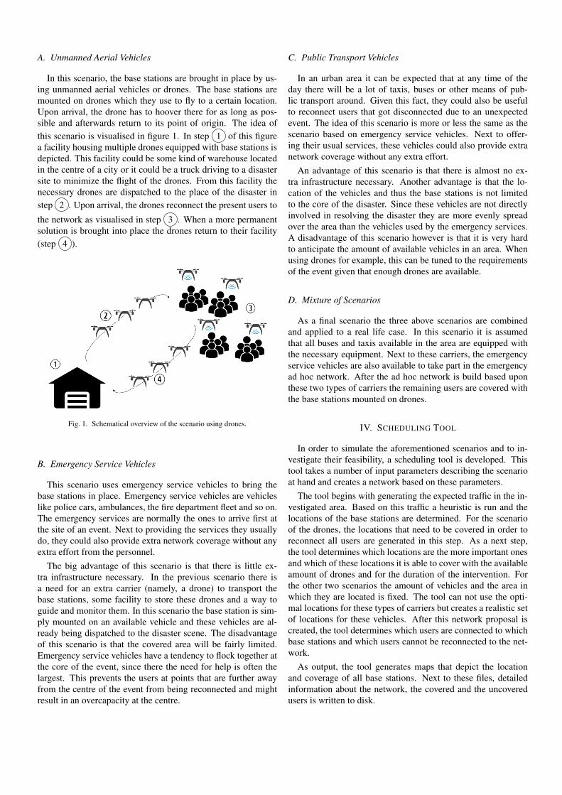
In this scenario, the base stations are brought in place by us-ing unmanned aerial vehicles or drones. The base stations aremounted on drones which they use to fly to a certain location.Upon arrival, the drone has to hoover there for as long as pos-sible and afterwards return to its point of origin. The idea ofthis scenario is visualised in figure 1. In step 1 of this figurea facility housing multiple drones equipped with base stations isdepicted. This facility could be some kind of warehouse locatedin the centre of a city or it could be a truck driving to a disastersite to minimize the flight of the drones. From this facility thenecessary drones are dispatched to the place of the disaster instep 2 . Upon arrival, the drones reconnect the present users to

the network as visualised in step 3 . When a more permanentsolution is brought into place the drones return to their facility(step 4 ).

Fig. 1. Schematical overview of the scenario using drones.

B. Emergency Service Vehicles

This scenario uses emergency service vehicles to bring thebase stations in place. Emergency service vehicles are vehicleslike police cars, ambulances, the fire department fleet and so on.The emergency services are normally the ones to arrive first atthe site of an event. Next to providing the services they usuallydo, they could also provide extra network coverage without anyextra effort from the personnel.

The big advantage of this scenario is that there is little ex-tra infrastructure necessary. In the previous scenario there isa need for an extra carrier (namely, a drone) to transport thebase stations, some facility to store these drones and a way toguide and monitor them. In this scenario the base station is sim-ply mounted on an available vehicle and these vehicles are al-ready being dispatched to the disaster scene. The disadvantageof this scenario is that the covered area will be fairly limited.Emergency service vehicles have a tendency to flock together atthe core of the event, since there the need for help is often thelargest. This prevents the users at points that are further awayfrom the centre of the event from being reconnected and mightresult in an overcapacity at the centre.

C. Public Transport Vehicles

In an urban area it can be expected that at any time of theday there will be a lot of taxis, buses or other means of pub-lic transport around. Given this fact, they could also be usefulto reconnect users that got disconnected due to an unexpectedevent. The idea of this scenario is more or less the same as thescenario based on emergency service vehicles. Next to offer-ing their usual services, these vehicles could also provide extranetwork coverage without any extra effort.

An advantage of this scenario is that there is almost no ex-tra infrastructure necessary. Another advantage is that the lo-cation of the vehicles and thus the base stations is not limitedto the core of the disaster. Since these vehicles are not directlyinvolved in resolving the disaster they are more evenly spreadover the area than the vehicles used by the emergency services.A disadvantage of this scenario however is that it is very hardto anticipate the amount of available vehicles in an area. Whenusing drones for example, this can be tuned to the requirementsof the event given that enough drones are available.

D. Mixture of Scenarios

As a final scenario the three above scenarios are combinedand applied to a real life case. In this scenario it is assumedthat all buses and taxis available in the area are equipped withthe necessary equipment. Next to these carriers, the emergencyservice vehicles are also available to take part in the emergencyad hoc network. After the ad hoc network is build based uponthese two types of carriers the remaining users are covered withthe base stations mounted on drones.

IV. SCHEDULING TOOL

In order to simulate the aforementioned scenarios and to in-vestigate their feasibility, a scheduling tool is developed. Thistool takes a number of input parameters describing the scenarioat hand and creates a network based on these parameters.

The tool begins with generating the expected traffic in the in-vestigated area. Based on this traffic a heuristic is run and thelocations of the base stations are determined. For the scenarioof the drones, the locations that need to be covered in order toreconnect all users are generated in this step. As a next step,the tool determines which locations are the more important onesand which of these locations it is able to cover with the availableamount of drones and for the duration of the intervention. Forthe other two scenarios the amount of vehicles and the area inwhich they are located is fixed. The tool can not use the opti-mal locations for these types of carriers but creates a realistic setof locations for these vehicles. After this network proposal iscreated, the tool determines which users are connected to whichbase stations and which users cannot be reconnected to the net-work.

As output, the tool generates maps that depict the locationand coverage of all base stations. Next to these files, detailedinformation about the network, the covered and the uncoveredusers is written to disk.

Parameter Type 1 Type 2Carrier Speed 15.0 m/s 12.0 m/sCarrier Power 5.0 A 13.0 ACarrier Power Usage 20.0 Ah 17.33 AhCarrier Battery Voltage 14.3 V 22.2 V

TABLE IPARAMETER VALUES USED FOR THE DRONES

V. RESULTS

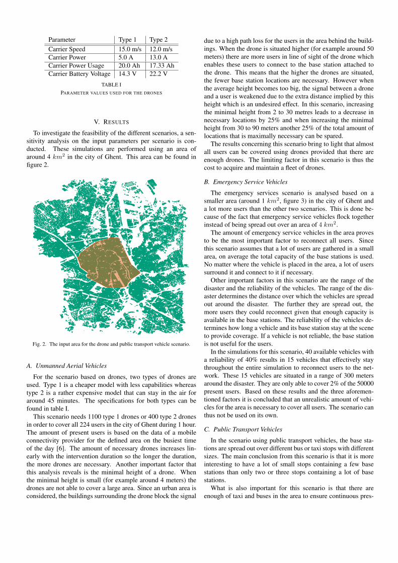
To investigate the feasibility of the different scenarios, a sen-sitivity analysis on the input parameters per scenario is con-ducted. These simulations are performed using an area ofaround 4 km2 in the city of Ghent. This area can be found infigure 2.

Fig. 2. The input area for the drone and public transport vehicle scenario.

A. Unmanned Aerial Vehicles

For the scenario based on drones, two types of drones areused. Type 1 is a cheaper model with less capabilities whereastype 2 is a rather expensive model that can stay in the air foraround 45 minutes. The specifications for both types can befound in table I.

This scenario needs 1100 type 1 drones or 400 type 2 dronesin order to cover all 224 users in the city of Ghent during 1 hour.The amount of present users is based on the data of a mobileconnectivity provider for the defined area on the busiest timeof the day [6]. The amount of necessary drones increases lin-early with the intervention duration so the longer the duration,the more drones are necessary. Another important factor thatthis analysis reveals is the minimal height of a drone. Whenthe minimal height is small (for example around 4 meters) thedrones are not able to cover a large area. Since an urban area isconsidered, the buildings surrounding the drone block the signal

due to a high path loss for the users in the area behind the build-ings. When the drone is situated higher (for example around 50meters) there are more users in line of sight of the drone whichenables these users to connect to the base station attached tothe drone. This means that the higher the drones are situated,the fewer base station locations are necessary. However whenthe average height becomes too big, the signal between a droneand a user is weakened due to the extra distance implied by thisheight which is an undesired effect. In this scenario, increasingthe minimal height from 2 to 30 metres leads to a decrease innecessary locations by 25% and when increasing the minimalheight from 30 to 90 meters another 25% of the total amount oflocations that is maximally necessary can be spared.

The results concerning this scenario bring to light that almostall users can be covered using drones provided that there areenough drones. The limiting factor in this scenario is thus thecost to acquire and maintain a fleet of drones.

B. Emergency Service Vehicles

The emergency services scenario is analysed based on asmaller area (around 1 km2, figure 3) in the city of Ghent anda lot more users than the other two scenarios. This is done be-cause of the fact that emergency service vehicles flock togetherinstead of being spread out over an area of 4 km2.

The amount of emergency service vehicles in the area provesto be the most important factor to reconnect all users. Sincethis scenario assumes that a lot of users are gathered in a smallarea, on average the total capacity of the base stations is used.No matter where the vehicle is placed in the area, a lot of userssurround it and connect to it if necessary.

Other important factors in this scenario are the range of thedisaster and the reliability of the vehicles. The range of the dis-aster determines the distance over which the vehicles are spreadout around the disaster. The further they are spread out, themore users they could reconnect given that enough capacity isavailable in the base stations. The reliability of the vehicles de-termines how long a vehicle and its base station stay at the sceneto provide coverage. If a vehicle is not reliable, the base stationis not useful for the users.

In the simulations for this scenario, 40 available vehicles witha reliability of 40% results in 15 vehicles that effectively staythroughout the entire simulation to reconnect users to the net-work. These 15 vehicles are situated in a range of 300 metersaround the disaster. They are only able to cover 2% of the 50000present users. Based on these results and the three aforemen-tioned factors it is concluded that an unrealistic amount of vehi-cles for the area is necessary to cover all users. The scenario canthus not be used on its own.

C. Public Transport Vehicles

In the scenario using public transport vehicles, the base sta-tions are spread out over different bus or taxi stops with differentsizes. The main conclusion from this scenario is that it is moreinteresting to have a lot of small stops containing a few basestations than only two or three stops containing a lot of basestations.

What is also important for this scenario is that there areenough of taxi and buses in the area to ensure continuous pres-

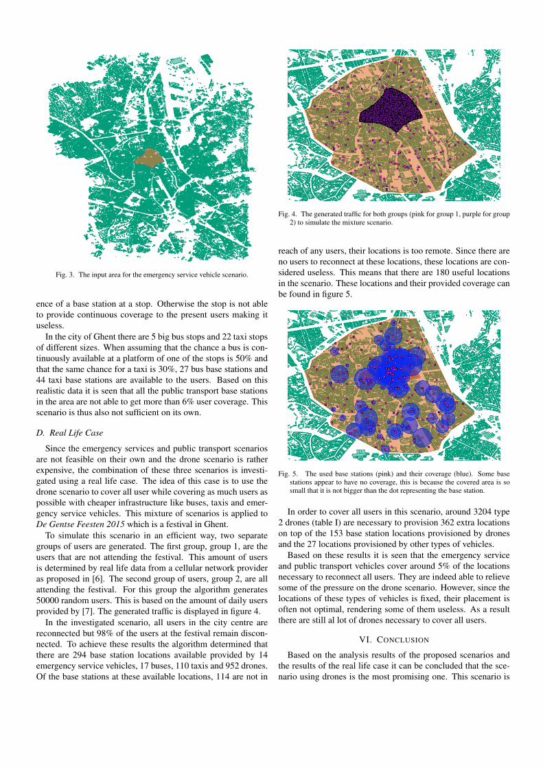
Fig. 3. The input area for the emergency service vehicle scenario.

ence of a base station at a stop. Otherwise the stop is not ableto provide continuous coverage to the present users making ituseless.

In the city of Ghent there are 5 big bus stops and 22 taxi stopsof different sizes. When assuming that the chance a bus is con-tinuously available at a platform of one of the stops is 50% andthat the same chance for a taxi is 30%, 27 bus base stations and44 taxi base stations are available to the users. Based on thisrealistic data it is seen that all the public transport base stationsin the area are not able to get more than 6% user coverage. Thisscenario is thus also not sufficient on its own.

D. Real Life Case

Since the emergency services and public transport scenariosare not feasible on their own and the drone scenario is ratherexpensive, the combination of these three scenarios is investi-gated using a real life case. The idea of this case is to use thedrone scenario to cover all user while covering as much users aspossible with cheaper infrastructure like buses, taxis and emer-gency service vehicles. This mixture of scenarios is applied toDe Gentse Feesten 2015 which is a festival in Ghent.

To simulate this scenario in an efficient way, two separategroups of users are generated. The first group, group 1, are theusers that are not attending the festival. This amount of usersis determined by real life data from a cellular network provideras proposed in [6]. The second group of users, group 2, are allattending the festival. For this group the algorithm generates50000 random users. This is based on the amount of daily usersprovided by [7]. The generated traffic is displayed in figure 4.

In the investigated scenario, all users in the city centre arereconnected but 98% of the users at the festival remain discon-nected. To achieve these results the algorithm determined thatthere are 294 base station locations available provided by 14emergency service vehicles, 17 buses, 110 taxis and 952 drones.Of the base stations at these available locations, 114 are not in

Fig. 4. The generated traffic for both groups (pink for group 1, purple for group2) to simulate the mixture scenario.

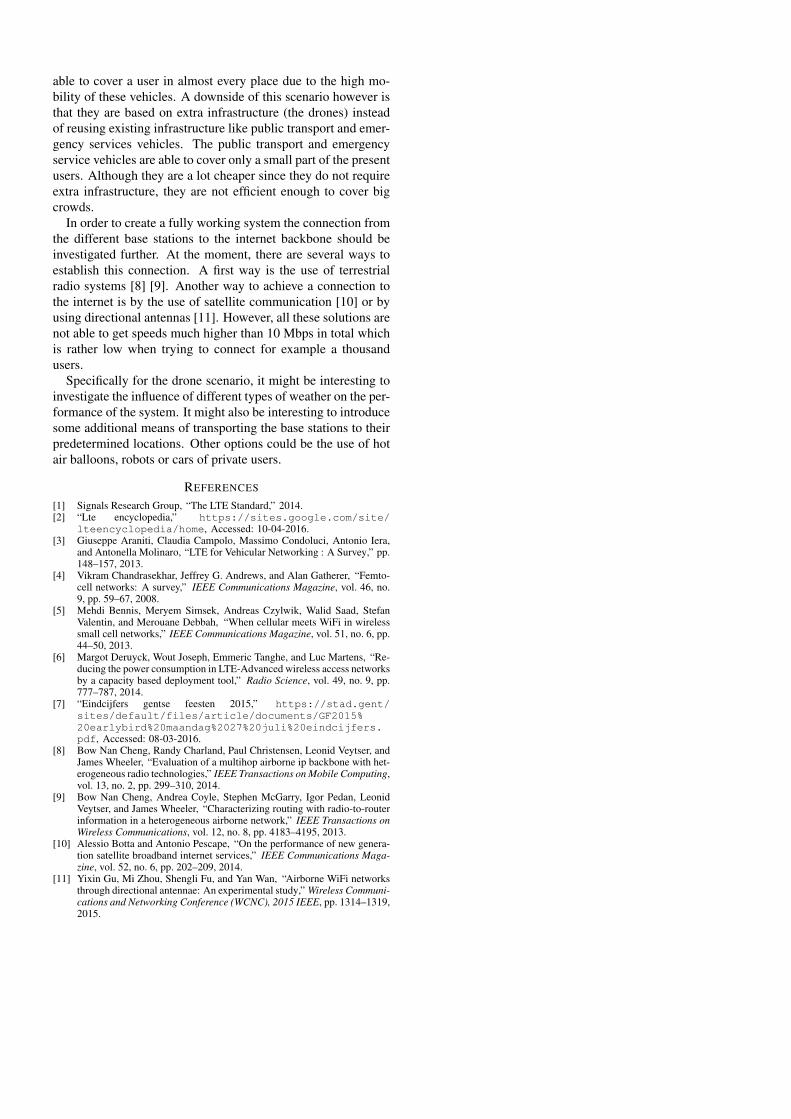
reach of any users, their locations is too remote. Since there areno users to reconnect at these locations, these locations are con-sidered useless. This means that there are 180 useful locationsin the scenario. These locations and their provided coverage canbe found in figure 5.

Fig. 5. The used base stations (pink) and their coverage (blue). Some basestations appear to have no coverage, this is because the covered area is sosmall that it is not bigger than the dot representing the base station.

In order to cover all users in this scenario, around 3204 type2 drones (table I) are necessary to provision 362 extra locationson top of the 153 base station locations provisioned by dronesand the 27 locations provisioned by other types of vehicles.

Based on these results it is seen that the emergency serviceand public transport vehicles cover around 5% of the locationsnecessary to reconnect all users. They are indeed able to relievesome of the pressure on the drone scenario. However, since thelocations of these types of vehicles is fixed, their placement isoften not optimal, rendering some of them useless. As a resultthere are still al lot of drones necessary to cover all users.

VI. CONCLUSION

Based on the analysis results of the proposed scenarios andthe results of the real life case it can be concluded that the sce-nario using drones is the most promising one. This scenario is

able to cover a user in almost every place due to the high mo-bility of these vehicles. A downside of this scenario however isthat they are based on extra infrastructure (the drones) insteadof reusing existing infrastructure like public transport and emer-gency services vehicles. The public transport and emergencyservice vehicles are able to cover only a small part of the presentusers. Although they are a lot cheaper since they do not requireextra infrastructure, they are not efficient enough to cover bigcrowds.

In order to create a fully working system the connection fromthe different base stations to the internet backbone should beinvestigated further. At the moment, there are several ways toestablish this connection. A first way is the use of terrestrialradio systems [8] [9]. Another way to achieve a connection tothe internet is by the use of satellite communication [10] or byusing directional antennas [11]. However, all these solutions arenot able to get speeds much higher than 10 Mbps in total whichis rather low when trying to connect for example a thousandusers.

Specifically for the drone scenario, it might be interesting toinvestigate the influence of different types of weather on the per-formance of the system. It might also be interesting to introducesome additional means of transporting the base stations to theirpredetermined locations. Other options could be the use of hotair balloons, robots or cars of private users.

REFERENCES

[1] Signals Research Group, “The LTE Standard,” 2014.[2] “Lte encyclopedia,” https://sites.google.com/site/

lteencyclopedia/home, Accessed: 10-04-2016.[3] Giuseppe Araniti, Claudia Campolo, Massimo Condoluci, Antonio Iera,

and Antonella Molinaro, “LTE for Vehicular Networking : A Survey,” pp.148–157, 2013.

[4] Vikram Chandrasekhar, Jeffrey G. Andrews, and Alan Gatherer, “Femto-cell networks: A survey,” IEEE Communications Magazine, vol. 46, no.9, pp. 59–67, 2008.

[5] Mehdi Bennis, Meryem Simsek, Andreas Czylwik, Walid Saad, StefanValentin, and Merouane Debbah, “When cellular meets WiFi in wirelesssmall cell networks,” IEEE Communications Magazine, vol. 51, no. 6, pp.44–50, 2013.

[6] Margot Deruyck, Wout Joseph, Emmeric Tanghe, and Luc Martens, “Re-ducing the power consumption in LTE-Advanced wireless access networksby a capacity based deployment tool,” Radio Science, vol. 49, no. 9, pp.777–787, 2014.

[7] “Eindcijfers gentse feesten 2015,” https://stad.gent/sites/default/files/article/documents/GF2015%20earlybird%20maandag%2027%20juli%20eindcijfers.pdf, Accessed: 08-03-2016.

[8] Bow Nan Cheng, Randy Charland, Paul Christensen, Leonid Veytser, andJames Wheeler, “Evaluation of a multihop airborne ip backbone with het-erogeneous radio technologies,” IEEE Transactions on Mobile Computing,vol. 13, no. 2, pp. 299–310, 2014.

[9] Bow Nan Cheng, Andrea Coyle, Stephen McGarry, Igor Pedan, LeonidVeytser, and James Wheeler, “Characterizing routing with radio-to-routerinformation in a heterogeneous airborne network,” IEEE Transactions onWireless Communications, vol. 12, no. 8, pp. 4183–4195, 2013.

[10] Alessio Botta and Antonio Pescape, “On the performance of new genera-tion satellite broadband internet services,” IEEE Communications Maga-zine, vol. 52, no. 6, pp. 202–209, 2014.

[11] Yixin Gu, Mi Zhou, Shengli Fu, and Yan Wan, “Airborne WiFi networksthrough directional antennae: An experimental study,” Wireless Communi-cations and Networking Conference (WCNC), 2015 IEEE, pp. 1314–1319,2015.

TABLE OF CONTENTS ix

Table of Contents

List of Figures xii

List of Tables xvi

List of Abbreviations xviii

1 Introduction 1

1.1 Problem . . . . . . . . . . . . . . . . . . . . . . . . . . . . . . . . . . . . . . . . . 1

1.2 Approach . . . . . . . . . . . . . . . . . . . . . . . . . . . . . . . . . . . . . . . . 2

1.3 Structure . . . . . . . . . . . . . . . . . . . . . . . . . . . . . . . . . . . . . . . . 2

2 State Of The Art 4

2.1 Mobile Ad Hoc Networks . . . . . . . . . . . . . . . . . . . . . . . . . . . . . . . 4

2.2 Airborne Base Stations . . . . . . . . . . . . . . . . . . . . . . . . . . . . . . . . . 5

2.3 Public Safety Networks . . . . . . . . . . . . . . . . . . . . . . . . . . . . . . . . 7

2.4 Connection to the Network Backbone . . . . . . . . . . . . . . . . . . . . . . . . 8

2.5 Network Deployment Tool . . . . . . . . . . . . . . . . . . . . . . . . . . . . . . . 9

2.6 Propagation Model . . . . . . . . . . . . . . . . . . . . . . . . . . . . . . . . . . . 11

3 Scenarios 14

3.1 Base Station Carriers . . . . . . . . . . . . . . . . . . . . . . . . . . . . . . . . . . 14

3.1.1 Unmanned Aerial Vehicles . . . . . . . . . . . . . . . . . . . . . . . . . . . 14

3.1.2 Emergency Service Vehicles . . . . . . . . . . . . . . . . . . . . . . . . . . 16

3.1.3 Public Transport Vehicles . . . . . . . . . . . . . . . . . . . . . . . . . . . 16

3.1.4 Mixture of Carriers . . . . . . . . . . . . . . . . . . . . . . . . . . . . . . . 17

3.2 Base Station Technology . . . . . . . . . . . . . . . . . . . . . . . . . . . . . . . . 17

3.2.1 LTE . . . . . . . . . . . . . . . . . . . . . . . . . . . . . . . . . . . . . . . 18

3.2.2 WiFi . . . . . . . . . . . . . . . . . . . . . . . . . . . . . . . . . . . . . . . 19

TABLE OF CONTENTS x

3.2.3 Comparison . . . . . . . . . . . . . . . . . . . . . . . . . . . . . . . . . . . 21

3.3 Important Parameters . . . . . . . . . . . . . . . . . . . . . . . . . . . . . . . . . 21

3.3.1 Unmanned Aerial Vehicles . . . . . . . . . . . . . . . . . . . . . . . . . . . 22

3.3.2 Emergency Services Vehicles . . . . . . . . . . . . . . . . . . . . . . . . . 23

3.3.3 Public Transport Vehicles . . . . . . . . . . . . . . . . . . . . . . . . . . . 24

4 Scheduling Tool 26

4.1 Algorithm . . . . . . . . . . . . . . . . . . . . . . . . . . . . . . . . . . . . . . . . 26

4.1.1 Unmanned Aerial Vehicles . . . . . . . . . . . . . . . . . . . . . . . . . . . 26

4.1.2 Emergency Service Vehicles . . . . . . . . . . . . . . . . . . . . . . . . . . 31

4.1.3 Public Transport Vehicles . . . . . . . . . . . . . . . . . . . . . . . . . . . 36

4.2 Number of Simulations . . . . . . . . . . . . . . . . . . . . . . . . . . . . . . . . . 40

4.2.1 Unmanned Aerial Vehicles . . . . . . . . . . . . . . . . . . . . . . . . . . . 41

4.2.2 Emergency Service Vehicles . . . . . . . . . . . . . . . . . . . . . . . . . . 44

4.2.3 Public Transport Vehicles . . . . . . . . . . . . . . . . . . . . . . . . . . . 47

5 Sensitivity Analysis 51

5.1 General Setup . . . . . . . . . . . . . . . . . . . . . . . . . . . . . . . . . . . . . . 51

5.2 Unmanned Aerial Vehicles . . . . . . . . . . . . . . . . . . . . . . . . . . . . . . . 51

5.2.1 Facility Capacity . . . . . . . . . . . . . . . . . . . . . . . . . . . . . . . . 53

5.2.2 Intervention Duration . . . . . . . . . . . . . . . . . . . . . . . . . . . . . 60

5.2.3 Height Margin Between Drone and Surface . . . . . . . . . . . . . . . . . 66

5.2.4 Maximal Height of a Carrier . . . . . . . . . . . . . . . . . . . . . . . . . 72

5.2.5 Conclusion . . . . . . . . . . . . . . . . . . . . . . . . . . . . . . . . . . . 75

5.3 Emergency Services Vehicles . . . . . . . . . . . . . . . . . . . . . . . . . . . . . . 77

5.3.1 Available Emergency Service Vehicles . . . . . . . . . . . . . . . . . . . . 77

5.3.2 Chance of Premature Departure . . . . . . . . . . . . . . . . . . . . . . . 80

5.3.3 Size of the Incident . . . . . . . . . . . . . . . . . . . . . . . . . . . . . . . 81

5.3.4 Conclusion . . . . . . . . . . . . . . . . . . . . . . . . . . . . . . . . . . . 82

5.4 Public Transportation Vehicles . . . . . . . . . . . . . . . . . . . . . . . . . . . . 84

5.4.1 Amount of Stops . . . . . . . . . . . . . . . . . . . . . . . . . . . . . . . . 84

5.4.2 Size of the Stops . . . . . . . . . . . . . . . . . . . . . . . . . . . . . . . . 88

5.4.3 Chance a Vehicle Is Present At a Platform of a Stop . . . . . . . . . . . . 93

5.4.4 Conclusion . . . . . . . . . . . . . . . . . . . . . . . . . . . . . . . . . . . 97

TABLE OF CONTENTS xi

6 Mixture of Carriers 100

6.1 Introduction . . . . . . . . . . . . . . . . . . . . . . . . . . . . . . . . . . . . . . . 100

6.2 Setup . . . . . . . . . . . . . . . . . . . . . . . . . . . . . . . . . . . . . . . . . . 101

6.2.1 Real Life Use Case . . . . . . . . . . . . . . . . . . . . . . . . . . . . . . . 101

6.2.2 Algorithm Parameters . . . . . . . . . . . . . . . . . . . . . . . . . . . . . 101

6.3 Results . . . . . . . . . . . . . . . . . . . . . . . . . . . . . . . . . . . . . . . . . . 106

6.3.1 Results for the Users in Group 1 . . . . . . . . . . . . . . . . . . . . . . . 106

6.3.2 Results for the Users in Group 2 . . . . . . . . . . . . . . . . . . . . . . . 108

6.4 Conclusion . . . . . . . . . . . . . . . . . . . . . . . . . . . . . . . . . . . . . . . 109

7 Conclusion and Future Work 111

Bibliography 115

LIST OF FIGURES xii

List of Figures

2.1 Schematical concept of a FANET [1]. . . . . . . . . . . . . . . . . . . . . . . . . . 6

2.2 Schematical concept of the transmission of WiFi signals over large distances using

directional antennas and unmanned aerial vehicles [2]. . . . . . . . . . . . . . . . 9

3.1 Schematical overview of the scenario using drones. . . . . . . . . . . . . . . . . . 15

3.2 Schematical overview of a WiFi Extended Service Set (ESS) [3]. . . . . . . . . . . 20

3.3 Schematical overview of the height margin. (figure based on [4]) . . . . . . . . . 23

3.4 Schematical overview of the range of an event. . . . . . . . . . . . . . . . . . . . 24

3.5 Schematical overview of a public transport stop. . . . . . . . . . . . . . . . . . . 25

4.1 Part of the algorithm based on drones responsible for the generation of random

traffic. . . . . . . . . . . . . . . . . . . . . . . . . . . . . . . . . . . . . . . . . . . 27

4.2 Part of the algorithm based on drones responsible for the generation of possible

base station locations. . . . . . . . . . . . . . . . . . . . . . . . . . . . . . . . . . 29

4.3 Part of the algorithm based on drones responsible for the generation of the optimal

network. . . . . . . . . . . . . . . . . . . . . . . . . . . . . . . . . . . . . . . . . . 30

4.4 Part of the algorithm based on drones responsible for the generation of the con-

strained network. . . . . . . . . . . . . . . . . . . . . . . . . . . . . . . . . . . . . 32

4.5 Part of the algorithm based on emergency service vehicles responsible for the

generation of the possible base station locations. . . . . . . . . . . . . . . . . . . 34

4.6 Part of the algorithm based on emergency service vehicles responsible for applying

constraints to the proposed base station locations. . . . . . . . . . . . . . . . . . 35

4.7 Part of the algorithm based on public transport vehicles responsible for generating

the requested amount of stops. . . . . . . . . . . . . . . . . . . . . . . . . . . . . 38

4.8 Part of the algorithm based on public transport vehicles responsible for generating

the amount of continuously available base stations per stop. . . . . . . . . . . . . 39

LIST OF FIGURES xiii

4.9 Influence of the number of simulations on the convergence of the average of a

certain parameter for the scenario using drones. . . . . . . . . . . . . . . . . . . . 44

4.10 Influence of the number of simulations on the convergence of the average of a

certain parameter for the scenario using emergency service vehilces. . . . . . . . . 47

4.11 Influence of the number of simulations on the convergence of the average of a

certain parameter for the scenario using public transport vehilces. . . . . . . . . 50

5.1 The area (orange) used as input for the algorithm. . . . . . . . . . . . . . . . . . 55

5.2 Influence of capacity on coverage using type 1 drones based on the hotspot technique. 56

5.3 Influence of capacity on coverage using type 1 drones based on the ratio technique. 57

5.4 Comparison of the influence of capacity on location coverage between the two

techniques using type 1 drones. . . . . . . . . . . . . . . . . . . . . . . . . . . . . 58

5.5 Comparison of the influence of capacity on user coverage between the two tech-

niques using type 1 drones. . . . . . . . . . . . . . . . . . . . . . . . . . . . . . . 58

5.6 Influence of capacity on coverage using type 2 drones based on the hotspot technique. 59

5.7 Influence of capacity on coverage using type 2 drones based on the ratio technique. 60

5.8 Comparison of the influence of capacity on location coverage between the two

techniques using type 2 drones. . . . . . . . . . . . . . . . . . . . . . . . . . . . . 61

5.9 Comparison of the influence of capacity on user coverage between the two tech-

niques using type 2 drones. . . . . . . . . . . . . . . . . . . . . . . . . . . . . . . 61

5.10 Influence of the intervention duration on coverage using type 1 drones based on

the ratio technique. . . . . . . . . . . . . . . . . . . . . . . . . . . . . . . . . . . . 64

5.11 Influence of the intervention duration on coverage using type 2 drones based on

the ratio technique. . . . . . . . . . . . . . . . . . . . . . . . . . . . . . . . . . . . 65

5.12 Influence of the intervention duration on the amount of necessary drones of both

types based on the ratio technique. . . . . . . . . . . . . . . . . . . . . . . . . . . 65

5.13 Influence of the height margin on the amount of necessary locations to get 100%

coverage using type 1 drones and based on the ratio technique. . . . . . . . . . . 68

5.14 Influence of the height margin on the amount of covered users using type 1 drones

and based on the ratio technique. . . . . . . . . . . . . . . . . . . . . . . . . . . . 68

5.15 Influence of the height margin on the power usage per base station using type 1

drones and based on the ratio technique. . . . . . . . . . . . . . . . . . . . . . . . 69

5.16 Influence of the height margin on the amount of necessary locations to get 100%

coverage using type 2 drones and based on the ratio technique. . . . . . . . . . . 70

LIST OF FIGURES xiv

5.17 Influence of the height margin on the amount of covered users using type 2 drones

and based on the ratio technique. . . . . . . . . . . . . . . . . . . . . . . . . . . . 71

5.18 Influence of the height margin on the power usage per base station using type 2

drones and based on the ratio technique. . . . . . . . . . . . . . . . . . . . . . . . 71

5.19 Influence of the maximal height a drone can reach on the reachability of base

station locations and users using type 1 drones and based on the ratio technique. 73

5.20 Influence of the maximal height a drone can reach on the coverage of base station

locations and users using type 1 drones and based on the ratio technique. . . . . 74

5.21 Influence of the maximal height a drone can reach on the coverage of base station

locations and users using type 2 drones and based on the ratio technique. . . . . 75

5.22 The area used as input for the algorithm based on emergency service vehicles. . . 78

5.23 Influence of the amount of vehicles present at the scene on the amount of covered

users. . . . . . . . . . . . . . . . . . . . . . . . . . . . . . . . . . . . . . . . . . . 79

5.24 Influence of the amount of vehicles present at the scene on the amount of Base

Stations. . . . . . . . . . . . . . . . . . . . . . . . . . . . . . . . . . . . . . . . . . 80

5.25 Influence of the departure chance of a vehicle on the amount of covered users. . . 81

5.26 Influence of the incident range on the amount of covered users. . . . . . . . . . . 83

5.27 Influence of the amount of bus stops on the maximal amount, the selected amount

and the used amount of base stations mounted on buses. . . . . . . . . . . . . . . 86

5.28 Influence of the amount of bus stops on the amount of users covered by buses. . . 87

5.29 Influence of the amount of taxi stops on the maximal amount, the selected amount

and the used amount of base stations mounted on taxis. . . . . . . . . . . . . . . 88

5.30 Influence of the amount of taxi stops on the amount of users covered by taxis. . . 89

5.31 Influence of the size of the bus stops on the maximal amount, the selected amount

and the used amount of base stations mounted on buses. . . . . . . . . . . . . . . 91

5.32 Illustration of the influence of different stop sizes. The coverage of a base station

at a platform is visualised by an orange circle. The entire stop is restricted to the

area within the blue circle. . . . . . . . . . . . . . . . . . . . . . . . . . . . . . . . 91

5.33 Influence of the size of the bus stops on the amount of users covered by buses. . . 92

5.34 Influence of the size of the taxi stops on the maximal amount, the selected amount

and the used amount of base stations mounted on taxis. . . . . . . . . . . . . . . 93

5.35 Influence of the size of the taxi stops on the amount of users covered by taxis. . . 94

5.36 Influence of the chance a bus stop is covered on the maximal amount, the selected

amount and the used amount of base stations mounted on buses. . . . . . . . . . 95

LIST OF FIGURES xv

5.37 Influence of the chance a bus stop is covered on the amount of users covered by

buses. . . . . . . . . . . . . . . . . . . . . . . . . . . . . . . . . . . . . . . . . . . 96

5.38 Influence of the chance a taxi stop is covered on the maximal amount, the selected

amount and the used amount of base stations mounted on taxis. . . . . . . . . . 97

5.39 Influence of the chance a taxi stop is covered on the amount of users covered by

taxis. . . . . . . . . . . . . . . . . . . . . . . . . . . . . . . . . . . . . . . . . . . . 98

6.1 A map of De Gentse Feesten 2015 [5]. . . . . . . . . . . . . . . . . . . . . . . . . 102

6.2 The area used for the mixture scenario. . . . . . . . . . . . . . . . . . . . . . . . 103

6.3 The generated traffic for both groups (pink for group 1, purple for group 2) to

simulate the mixture scenario. . . . . . . . . . . . . . . . . . . . . . . . . . . . . . 103

6.4 The emergency services based base stations (purple) and their coverage (blue) for

the users in group 1. . . . . . . . . . . . . . . . . . . . . . . . . . . . . . . . . . . 106

6.5 The public transport based base stations (purple) and their coverage (blue) for

the users in group 1. . . . . . . . . . . . . . . . . . . . . . . . . . . . . . . . . . . 107

6.6 The drone based base stations (purple) and their coverage (blue) for the users in

group 1. The white dot denotes the location of the used storage facility. . . . . . 108

6.7 The locations of the base stations (purple) and their coverage (blue) used to cover

the users in group 2. . . . . . . . . . . . . . . . . . . . . . . . . . . . . . . . . . . 109

LIST OF TABLES xvi

List of Tables

4.1 Parameter values used for the estimation of the necessary amount of simulations

for the scenario using drones. More information about these parameters can be

found in section 4.1.1. . . . . . . . . . . . . . . . . . . . . . . . . . . . . . . . . . 42

4.2 Parameter values used for the estimation of the necessary amount of simulations

for the scenario using emergency service vehicles. More information about these

parameters can be found in section 4.1.2 . . . . . . . . . . . . . . . . . . . . . . . 45

4.3 Parameter values used for the estimation of the necessary amount of simulations

for the scenario using public transport vehicles. More information about these

parameters can be found in section 4.1.3 . . . . . . . . . . . . . . . . . . . . . . . 48

5.1 Link Budget Table for a Femtocell Base Station. Based on [6] and [7] . . . . . . 52

5.2 Parameter values used for the first type of drone . . . . . . . . . . . . . . . . . . 53

5.3 Parameter values used for the second type of drone . . . . . . . . . . . . . . . . . 53

5.4 Parameter values used for the analysis of the influence of the facility capacity. . . 54

5.5 Parameter values used for the analysis of the influence of the intervention duration. 62

5.6 Parameter values used for the analysis of the influence of the height margin. . . . 66

5.7 Parameter values used for the analysis of the influence of the maximal allowed

height of a drone. . . . . . . . . . . . . . . . . . . . . . . . . . . . . . . . . . . . . 72

5.8 Parameter values used for the analysis of the influence of the amount of available

emergency service vehicles. . . . . . . . . . . . . . . . . . . . . . . . . . . . . . . 79

5.9 Parameter values used for the analysis of the influence of the chance a vehicles

leaves prematurely. . . . . . . . . . . . . . . . . . . . . . . . . . . . . . . . . . . . 81

5.10 Parameter values used for the analysis of the influence of the range of the incident. 82

5.11 Parameter values used for the analysis of the influence of the amount of bus and

taxi stops in the predefined area. . . . . . . . . . . . . . . . . . . . . . . . . . . . 85

5.12 Parameter values used for the analysis of the influence of the size of bus and taxi

stops in the predefined area. . . . . . . . . . . . . . . . . . . . . . . . . . . . . . . 89

LIST OF TABLES xvii

5.13 Parameter values used for the analysis of the influence of the chance a bus or taxi

is present at a platform of a stop in the predefined area. . . . . . . . . . . . . . . 94

6.1 Parameter values used for the analysis of the mixture scenario. . . . . . . . . . . 105

LIST OF ABBREVIATIONS xviii

List of Abbreviations

3GPP Third Generation Partnership Project

4G Fourth Generation

AODV Ad-Hoc on-Demand Distance Vector

BSS Basic Service Set

BSSID Basic Service Set Identifier

CA Carrier Aggregation

DRS Directional Radio System

DS Distribution System

DSDV Destination Sequenced Distance Vector

DSR Dynamic Source Routing

ESB Electronic Switch Beam radio system

ESS Extended Service Set

ESSID, SSID Extended Service Set Identifier

GRAND Green Radio Access Network Design

IBSS Independent Basic Service Set

IEEE Institute of Electrical and Electronics Engineers

IP Internet Protocol

LAP Low Altitude Aerial Platform

LTE Long Term Evolution

LIST OF ABBREVIATIONS xix

MANET Mobile ad hoc networks

MIMO Multiple-Input Multiple-Output

OFDM Orthogonal Frequency Divison Multiplexing

ORS Omnidirectional Radio System

SINR Interference plus Noise Ratio

TETRA Terrestrial Trunked Radio

UAV unmanned aerial vehicles

UMTS Universal Mobile Telecommunications System

WiFi Wireless Fidelity

WLAN Wireless Local Area Network

INTRODUCTION 1

Chapter 1

Introduction

1.1 Problem

Imagine a day or even an hour without being connected to the modern day communication

systems. Nowadays that is almost impossible to do. People share their mood and whereabouts

all the time, news is brought to you only seconds after it happened and you can pick up the

telephone to call almost anyone in the world if you wanted to. This connectivity has become a

normal thing. So normal that people do not know what to do when it disappears. Nevertheless

it still happens that this connectivity is disrupted by all kinds of unexpected events like for

example natural disasters, large traffic accidents and explosions. Due to the fact that people are

always connected, a disruption by any kind of unexpected event might cause a panic with the

person in question but also with all the people who are connected to that person on a normal

day.

A good example of a situation like this took place a couple of years ago, namely in 2011.

In August 2011, 60000 people were gathered in Hasselt, Belgium for an annual festival called

Pukkelpop. During the first day of the festival a local but fairly severe storm broke out. This

storm caused a lot of damage including the uprooting of trees and the collapse of a couple of

tents in which the festival was hosted. In the end, the storm lasted only a couple of minutes

but 140 people got injured and five people died. Due to the fact that the modern day society

is always connected, the news spread quickly across the country resulting in a lot of concerned

parents and friends. They tried to reach out to the people at the scene and vice versa to check

if they were all right. The enormous surge in need for connectivity caused the network to go

down, leaving a lot of people in the dark about the safety and whereabouts of their loved ones.

This kind of disastrous events can happen at any moment. Even with smaller events the

need to be connected to the network can be just as big as in the aforementioned example. Since

1.2 Approach 2

these events are hard to foresee it is also hard to prepare the available infrastructure for the

inevitable increase in need for connectivity. It might even occur that the infrastructure that is

normally available is damaged or destroyed. The main question that arises is the following one.

How could a sudden shortage or loss of connectivity be solved?

1.2 Approach

A possible solution could be to create an emergency ad hoc network using mobile base stations.

For example, base stations could be installed in emergency vehicles to reinstate connectivity at

the location of a disaster. Drones with base stations attached to them could be deployed to the

location of the disaster. When you are in a more urban area, base stations could be installed in

taxis and buses since it can be expected that there will be a lot of those in an urban area. All

these options have one goal, to reconnect the users at the disastrous event in order to enable

them to communicate with the rest of the world when the normal infrastructure is not sufficient.

In this master’s dissertation the feasibility of such an emergency ad hoc network is investi-

gated. For multiple scenarios using different ways to make the considered base stations mobile, a

sensitivity analysis on the configurable parameters is executed. During this analysis it is investi-

gated where for example the used base station carriers are best stored to enable fast deployment

or how much base stations are necessary to reconnect the users for a certain time. Next to those

parameters, the specific features of a base station carrier like battery life or in case of a drone,

flight time, are taken under consideration.

In order to perform this analysis, a planning tool was created. This planning tool takes into

account the specifics of a base station carrier and a certain disaster area. Using this information

it estimates where the mobile base stations are best located in order to recreate an optimal

amount of coverage. Doing so it takes into account the availability of these carriers, where

they are stored and it tries to deploy them as efficiently as possible. Meaning, one mobile base

station will reconnect as many users as possible. In the end the planning tool proposes a network

that reconnects as many users as possible based on the given input parameters. The sensitivity

analysis is thus performed by analysing the evolution of these proposed networks when using

different sets of configurations.

1.3 Structure

In order to provide the necessary background information to the reader, a state of the art

investigation was performed. The information obtained through this research can be found in

1.3 Structure 3

chapter 2. In the part following this research, the different scenarios are introduced (chapter 3).

This chapter determines which base station carriers will be used and what kind of base station

technologies might be interesting. In the subsequent chapter, chapter 4, the designed scheduling

tool is presented. Several aspects about the tool such as the underlying algorithm and some

design decisions are discussed. By using this tool, a sensitivity analysis is performed. The

results of this analysis can be found in chapter 5. The analysis focusses on different configurable

parameters and different desirable scenarios that were introduced in chapters 3 and 4. Based

on these results the viability of the entire idea is checked against the reality in the best way

possible. In chapter 6, a real life scenario concerning a festival in Ghent, Belgium is elaborated.

This is done in order to draw conclusions about the feasibility of the presented idea when all

possible scenarios are combined. In the last chapter, chapter 7, a conclusion is formed based on

the entire dissertation and possible future work is discussed.

STATE OF THE ART 4

Chapter 2

State Of The Art

2.1 Mobile Ad Hoc Networks

The goal of this masters dissertation is the creation of a new network without any pre-installed

infrastructure. Mobile ad hoc networks (MANET) are excellent for this job as they allow to work

with continuously changing links and topologies of the network. All devices in a MANET are

called nodes and serve an equal purpose. A node could be a smartphone, a laptop or anything

else with networking capacities. There is no central control node which is why each device in

a MANET needs to be equipped with the capabilities to maintain the necessary information

about the network.

Within a MANET the nodes are connected through wireless links. When a node wants to

join a network, it looks for a neighbour where it can find the necessary information about the

MANET. When the new node receives this information it makes the other nodes aware of its

presence in a way depending on the used routing protocol [8]. The different routing protocols

are discussed in a subsequent paragraph.

A MANET is a self-forming and self-healing network making it very flexibile and elliminating

the need for extensive configuration which is essential for a mobile environment [9]. However,

due to the absent central infrastructure a MANET assumes that the network information of a

node (such as its IP address and its netmask) are configured statically before the node enters

the network [10]. This creates a big limitation for the flexibility of the MANET technology.

In [8] an approach where all nodes keep information about the used IP addresses and other

network information is proposed. Using this approach the need to statically configure a node

before adding it to the network is eliminated. Upon entering the network the present nodes will

assign a valid IP address to the new node in mutual agreement and provide it with the necessary

network information.

2.2 Airborne Base Stations 5

In a MANET, nodes move independently from one another with different speeds and be-

haviours. Due to this flexible and unreliable structure of a MANET, routing becomes a lot

harder. Every node has to store the necessary routing information in order to reach other nodes

and the internet backbone [11]. To complete this goal, many routing protocols were developed

like Destination Sequenced Distance Vector (DSDV) , Dynamic Source Routing (DSR) and Ad-

Hoc on-Demand Distance Vector (AODV) with several expansions. These protocols can be

divided into three categories: proactive routing protocols, reactive routing protocols and hybrid

routing protocols. Proactive routing protocols are protocols in which each node maintains a

routing table of known destinations. This technique reduces the amount of control traffic but

requires more memory of the node and extra bandwidth when sending periodical messages to

keep the table up to date. Reactive routing protocols behave a little different. This kind of

protocol does not keep a routing table but floods the network with route discovery messages

when a message needs to be delivered to a certain node. This results in a lower memory usage

and a lower control traffic overhead but it requires more bandwidth and processing time to get

a message from one node to another. Hybrid routing protocols try to combine the best of both

worlds. They enable the use of the reduced control traffic from reactive routing protocols and

the reduction of route discovery delays from proactive routing protocols by maintaining some

form of a routing table [12].

As can be seen in the previous paragraph there exist many possible ways to organise an

ad hoc network and route messages through it. This makes it very hard to distinguish the

best protocol. Which routing protocol to use in an ad hoc network will depend on several

environmental features, the mobility of the nodes and the resulting reliability of the links between

those nodes. Since there are so many influencing factors, it is hard to compare different protocols

and finding an optimal one for a certain use case [13].

2.2 Airborne Base Stations

An interesting way to create mobile base stations is to mount them on flying vehicles like

helicopters, hot air balloons or drones. This form of mobile base stations can be used for a

big variety of use cases like for example when a network connection needs to be provided to

unreachable places [14].

There are two basic ways to create a network out of these airborne base stations [1]. The first

way is an infrastructure based approach. In this approach the network is formed and controlled

by a single ground base or a satellite and all base stations communicate with this infrastructure.

This approach has several disadvantages. First of all, each base station needs to have access to

2.2 Airborne Base Stations 6

additional hardware to communicate with the ground base or the satellite which increases the

cost and the power usage of the base station. Second, the proper functioning of the network

depends on the link quality between the base station and the ground base or satellite. If the

quality of this link is insufficient the base station might loose connection with the ground base

or the satellite rendering it inoperable. Third, there exists a range restriction between the base

station and the ground base or satellite. When the base stations wanders off too far from the

ground base or satellite, a connection will no longer be possible. This creates a rather large

restriction in the necessary mobility of the nodes.

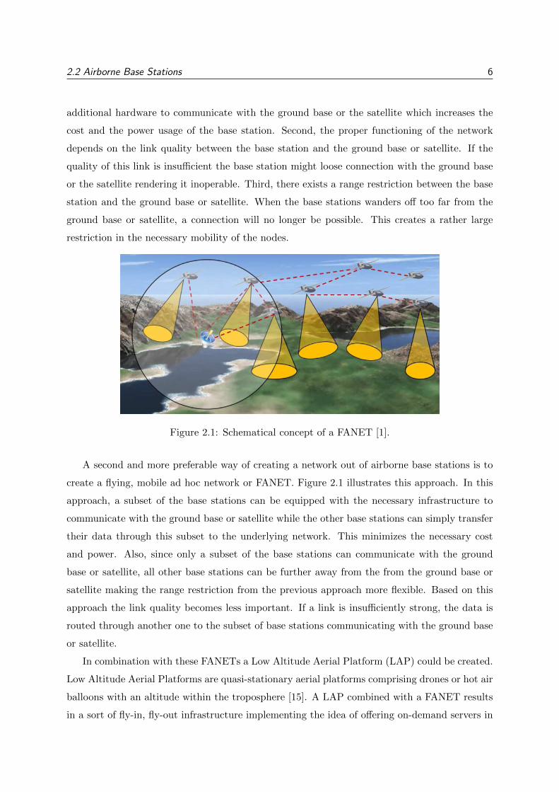
Figure 2.1: Schematical concept of a FANET [1].

A second and more preferable way of creating a network out of airborne base stations is to

create a flying, mobile ad hoc network or FANET. Figure 2.1 illustrates this approach. In this

approach, a subset of the base stations can be equipped with the necessary infrastructure to

communicate with the ground base or satellite while the other base stations can simply transfer

their data through this subset to the underlying network. This minimizes the necessary cost

and power. Also, since only a subset of the base stations can communicate with the ground

base or satellite, all other base stations can be further away from the from the ground base or

satellite making the range restriction from the previous approach more flexible. Based on this

approach the link quality becomes less important. If a link is insufficiently strong, the data is

routed through another one to the subset of base stations communicating with the ground base

or satellite.

In combination with these FANETs a Low Altitude Aerial Platform (LAP) could be created.

Low Altitude Aerial Platforms are quasi-stationary aerial platforms comprising drones or hot air

balloons with an altitude within the troposphere [15]. A LAP combined with a FANET results

in a sort of fly-in, fly-out infrastructure implementing the idea of offering on-demand servers in

2.3 Public Safety Networks 7

the air. The advantage of such an infrastructure in relation to their use with disastrous events

is that the created networks are very adaptable and potentially scalable [16]. This adaptability

allows the network to continuously improve link conditions by lowering the distance between a

sender and a receiver or avoiding obstacles. It also allows the network to operate in line-of-sight

conditions as much as possible, creating better signals and higher throughput [17].

2.3 Public Safety Networks

Public Safety Networks need to incorporate several characteristics since they are considered

mission critical. They need to be reliable, resilient and secure. Next to these characteristics

they need to offer some functionality like coverage, end-to-end performance and accessibility

to make them usable for the purpose of the public safety organisation. Other typical public

safety systems that need to be supported are fast vehicle localization, dispatching and group

communications [18].

Effective communications between and within these public safety organisations at crisis sites

is the key to success. Communicating efficiently or even sharing multimedia messages could help

them to assess the current situation better and thus intervene in a more efficient way.

Currently, public safety organisations use old legacy systems like the Terrestrial Trunked

Radio (TETRA) [19]. These TETRA terminals support a limited amount of communication

mechanisms like group calls, short data messaging and packet data. As can be seen, it would be

ideal to integrate these legacy systems with the newer broadband communication systems. Doing

so would enable a whole spectrum of new communication systems like broadband data services,

true concurrent voice and data services, simultaneous reception of many group calls, reduced

call setup and voice transmission delays and improved voice quality. In order to achieve this

integration several options need to be considered to upgrade the public safety communications

systems.

The first option is to evolve from the usage of TETRA to more currentday technologies like

4G and 5G. 4G and its successor 5G have the potential to revolutionize the communication

between the public safety services during disasters. The evolution from the current legacy

systems to 4G and 5G systems could transform the current platform to a much needed high-

speed communications tool. To enable this evolution, the Third Generation Partnership Project

(3GPP) incorporated the necessary functionality and capabilities into LTE advanced to meet

the requirements of a broadband public safety communications system [20].

The second option to upgrade the public safety communication system is the introduction of

airborne base stations as mentioned in section 2.2. Airborne base stations lend themselves well

2.4 Connection to the Network Backbone 8

for public safety communication due to their mobility and self organizing capabilities. These

features are highly necessary to deliver broadband connectivity at the time and the place where

it is most needed [21]. Using this kind of mobile base stations takes care of one of the biggest

disadvantages of current day public safety networks, namely their dependence on terrestrial

communications infrastructure [22].

A third and more advanced option is the use of coalitions between local devices [23]. The

idea of this option is that the devices of a group of public safety workers communicate directly

with each other without using the cellular network. This way a lot of energy could be saved,

some traffic can be offloaded from the network and communication between different parties can

become a lot smoother.

2.4 Connection to the Network Backbone

An emergency ad hoc network is only useful for a user when it can reconnect with the internet

through the created network. This implies that the ad hoc network that will be created needs

a certain connection to the network backbone. Such a connection can be achieved in multiple

ways. The three most common ways are discussed in the paragraphs below.

The first way that this can be achieved is with the use of terrestrial radio systems [24].

Examples of these systems are the Electronic Switch Beam (ESB) radio system, the Directional

Radio System (DRS) and the Omnidirectional Radio System (ORS) used by the Department

of Defence of the United States. These radios can provide a point-to-point connection from a

terrestrial base outside the disaster zone to one of the base stations from the ad hoc network

created inside the disaster zone. The maximal distance over which a connection can be estab-

lished using one of these technologies varies between 100 and 200 kilometres while providing an

average data rate of around 10 Mbps [25]. However, the closer the transmitting base station is

situated to the receiving ad hoc network the better link quality between the two can be reached

resulting in a better stability of the link and more throughput.

The second way to achieve a connection to the internet is by the use of satellite communica-

tion [26]. Such a connection has the same basic characteristics as with the terrestrial base station

connection. The connection is provided from outside the disaster area to one of the base stations

within the ad hoc network. Satellite communication is often not preferred by users because of

its poor performance. It is a technology mainly used in rural or remote areas where no other

options are available. However, around 2011 new satellites where launched with the primary

goal of providing high individual and aggregated performance when it comes to internet access.

Using these new satellites, downlink speeds of around 10 Mbps and uplink speeds of around 4

2.5 Network Deployment Tool 9

Mbps per user can be reached.

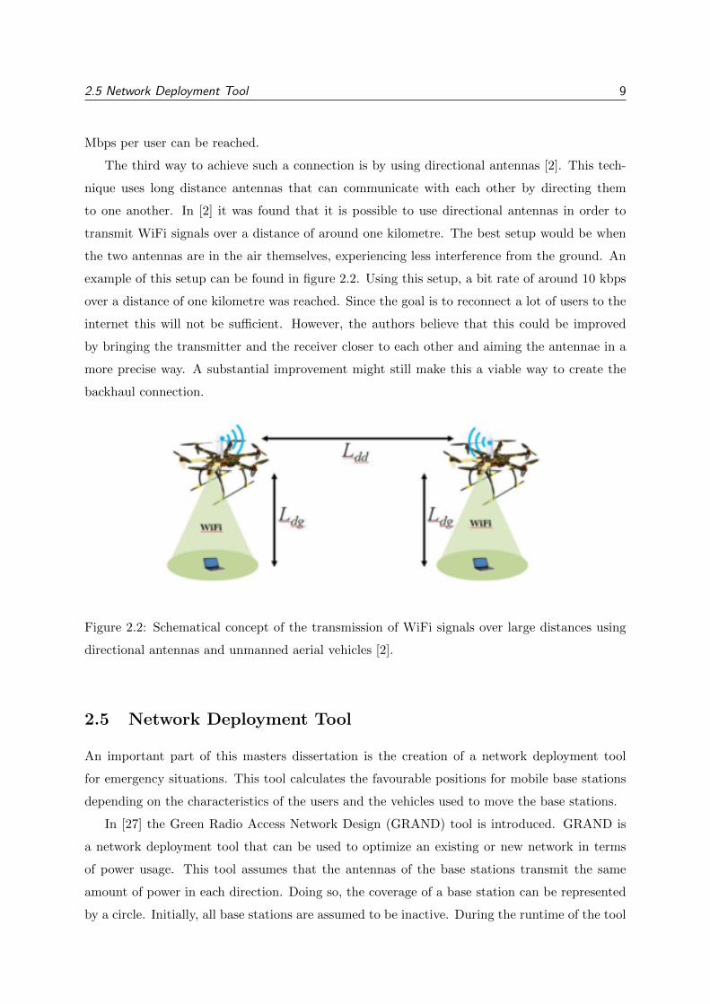
The third way to achieve such a connection is by using directional antennas [2]. This tech-

nique uses long distance antennas that can communicate with each other by directing them

to one another. In [2] it was found that it is possible to use directional antennas in order to

transmit WiFi signals over a distance of around one kilometre. The best setup would be when

the two antennas are in the air themselves, experiencing less interference from the ground. An

example of this setup can be found in figure 2.2. Using this setup, a bit rate of around 10 kbps

over a distance of one kilometre was reached. Since the goal is to reconnect a lot of users to the

internet this will not be sufficient. However, the authors believe that this could be improved

by bringing the transmitter and the receiver closer to each other and aiming the antennae in a

more precise way. A substantial improvement might still make this a viable way to create the

backhaul connection.

Figure 2.2: Schematical concept of the transmission of WiFi signals over large distances using

directional antennas and unmanned aerial vehicles [2].

2.5 Network Deployment Tool

An important part of this masters dissertation is the creation of a network deployment tool

for emergency situations. This tool calculates the favourable positions for mobile base stations

depending on the characteristics of the users and the vehicles used to move the base stations.

In [27] the Green Radio Access Network Design (GRAND) tool is introduced. GRAND is

a network deployment tool that can be used to optimize an existing or new network in terms

of power usage. This tool assumes that the antennas of the base stations transmit the same

amount of power in each direction. Doing so, the coverage of a base station can be represented

by a circle. Initially, all base stations are assumed to be inactive. During the runtime of the tool

2.5 Network Deployment Tool 10

all possible users and locations are inspected and four different actions can be performed to form

the network. The first action is activating a new base station. The second one is deactivating an

active base station. The third action is adding 1 dbm to the input power of an active base station

and the last one is subtracting 1 dbm from the input power of a base station. While the tool

performs these actions the network is updated until a stopping criteria is met. Depending on

this stopping criteria, an optimal network will be generated by the algorithm when it terminates.

In [28] the successor of the GRAND tool is introduced. This new version of the tool focusses

on some extra improvements. The tool is created to respond to the instantaneous bit rate that

the users in the considered area require. In [28] it is, among others things, used to investigate the

impact of three different features that are incorporated in LTE Advanced. The first feature is

Carrier Aggregation (CA) . When CA is used, the bit rate is increased by allowing the base sta-

tion to transmit at multiple carriers to the users. The second feature is the use of heterogeneous

networks where different base station types (macrocells, picocells, femtocells or others) can be

used in the same network. The third feature is the use of the Multiple-Input Multiple-Output

(MIMO) technology where the bit rate of a base station is increased by using more antennas.

In order to investigate the impact of these features, three dimensional geometrical data of the

considered area is necessary. In the case of this paper, the tool was applied to a suburban area

in Ghent, Belgium.

In [29] a tool similar to the one in [27] is introduced. The main difference between these two

network deployment tools is that the results in [29] focus on indoor femtocell networks. The tool

creates a network in two steps. First, the possible base station locations are generated. Every

building is a possible location for a base station. The tool will place this base station at the

center of a building in order to reduce the set of possible locations and to reduce the simulation

execution time. The second step makes use of the same four actions as the GRAND network

deployment tool does in order to create an optimal network in terms of power consumption.

Performing these actions, the tool creates different generations of the network until a certain

stopping criteria is met. The more generations are created, the better the created solutions will

get.

The network deployment tool for this master’s dissertation should also be able to determine

good locations for base stations while taking into account the bit rates required by the users.

Next to that it could be desirable that the newly designed tool takes the power consumptions

of the base stations into account and tries to minimize those. Parts of the network deployment

tools discussed in this section can thus be reused as a base for the network deployment tool

focussing on emergency ad hoc networks.

2.6 Propagation Model 11

2.6 Propagation Model

Propagation models provide a way to calculate the loss that a signal experiences over a certain

distance. Buildings tend to occur in almost every location. These buildings have different sizes,

shapes, heights and they are located at different, unpredictable distances from each other. When

deploying a femtocell network within a suburban area the possibility that the signal between a

user and a base station is blocked is quite big. This implies the need for a pathloss model that

takes into account the different aspects of a building and the difference between the path loss

when a user is in the line of sight of a base station and when it is not.

For a small cell network like a femtocell network, numerous propagation models exist. Exam-

ples are empirical models, the two-ray model, the Lee microcell model and the Walfish-Ikegami

model . All these models have their own advantages and disadvantages, however they are all

capable of precisely calculating the pathloss for a user in a femtocell network located in an

urban area [30]. For this master’s dissertation the decision was made to continue with the

Walfish-Ikegami model [31] since it is a model that performs accurately for femtocell networks

in suburban and urban areas [32].

Classical field strength models like the Okumura model [33] are generally used to calculate

the path loss in mobile radio applications. These models are not designed to be used in small

femtocell networks since they only take into account the direct line between the base station

and the user and will thus only be effective for base stations at great heights. To accommodate

this problem the European research committee COST 231 (Evolution of land mobile radio)

created a propagation model for estimating the urban transmission loss based on empirical and

deterministic models, the Walfish-Ikegami model.

When a very precise path loss prediction is required, the use of a site-specific propagation

model is the best way to go [32]. A site-specific model takes into account the specific charac-

teristics of the area in which the network will operate. This requires a lot of data gathering

beforehand which prevents it from being used for the use case presented in this master’s disserta-

tion. However, the use of a site-specific model in comparison to the use of the Walfisch-Ikegami

model only results in a moderate improvement. The Walfisch-Ikegami model will thus be a very

good model that requires little effort for a femtocell network.

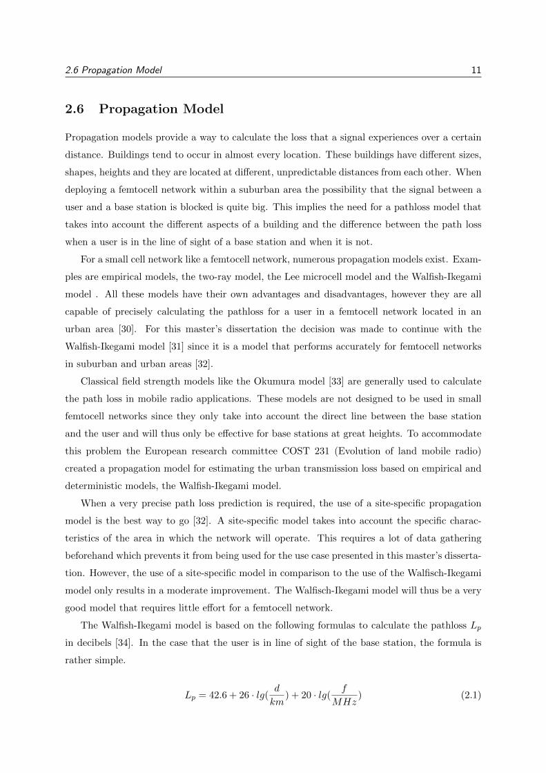
The Walfish-Ikegami model is based on the following formulas to calculate the pathloss Lp

in decibels [34]. In the case that the user is in line of sight of the base station, the formula is

rather simple.

Lp = 42.6 + 26 · lg(d

km) + 20 · lg(

f

MHz) (2.1)

2.6 Propagation Model 12

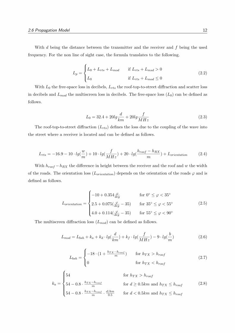
With d being the distance between the transmitter and the receiver and f being the used

frequency. For the non line of sight case, the formula translates to the following.

Lp =

L0 + Lrts + Lmod if Lrts + Lmsd > 0

L0 if Lrts + Lmod ≤ 0(2.2)

With L0 the free-space loss in decibels, Lrts the roof-top-to-street diffraction and scatter loss

in decibels and Lmod the multiscreen loss in decibels. The free-space loss (L0) can be defined as

follows.

L0 = 32.4 + 20lgd

km+ 20lg

f

MHz(2.3)

The roof-top-to-street diffraction (Lrts) defines the loss due to the coupling of the wave into

the street where a receiver is located and can be defined as follows.

Lrts = −16.9− 10 · lg(w

m) + 10 · lg(

f

MHz) + 20 · lg(

hroof − hRX

m) + Lorientation (2.4)

With hroof −hRX the difference in height between the receiver and the roof and w the width

of the roads. The orientation loss (Lorientation) depends on the orientation of the roads ϕ and is

defined as follows.

Lorientation =

−10 + 0.354 ϕ

deg for 0◦ ≤ ϕ < 35◦

2.5 + 0.075( ϕdeg − 35) for 35◦ ≤ ϕ < 55◦

4.0 + 0.114( ϕdeg − 35) for 55◦ ≤ ϕ < 90◦

(2.5)

The multiscreen diffraction loss (Lmsd) can be defined as follows.

Lmsd = Lbsh + ka + kd · lg(d

km) + kf · lg(

f

MHz)− 9 · lg(

b

m) (2.6)

Lbsh =

−18 · (1 +hTX−hroof

m ) for hTX > hroof

0 for hTX < hroof

(2.7)

ka =

54 for hTX > hroof

54− 0.8 · hTX−hroof

m for d ≥ 0.5km and hTX ≤ hroof

54− 0.8 · hTX−hroof

m · d/km0.5 for d < 0.5km and hTX ≤ hroof

(2.8)

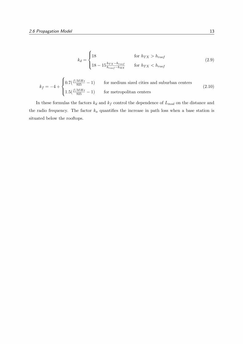
2.6 Propagation Model 13

kd =

18 for hTX > hroof

18− 15hTX−hroof

hroof−hRXfor hTX < hroof

(2.9)

kf = −4 +

0.7(f/MHz925 − 1) for medium sized cities and suburban centers

1.5(f/MHz925 − 1) for metropolitan centers

(2.10)

In these formulas the factors kd and kf control the dependence of Lmsd on the distance and

the radio frequency. The factor ka quantifies the increase in path loss when a base station is

situated below the rooftops.

SCENARIOS 14

Chapter 3

Scenarios

Different approaches are possible to create an emergency ad hoc network. The feasibility of

these approaches mainly depend on the kind of carrier used to make the base station mobile.

Next to the kind of carrier, the kind of base station itself can also vary. In this chapter the

different types of carriers are discussed in section 3.1. Possible technologies regarding the base

stations are discussed and compared in section 3.2. In section 3.3 it is concluded which scenarios

should be analysed and what parameters are interesting to investigate.

3.1 Base Station Carriers

When setting up an emergency ad hoc network it is important that the necessary infrastructure

to create a new network gets in place. In this dissertation three different scenarios with different

ways to mobilize base stations are discussed. The first scenario can be found in section 3.1.1.

In this scenario unmanned aerial vehicles (UAV) are used to mobilize the base stations and to

spread them over an area. In the second scenario, introduced in section 3.1.2, the possibility to

embed base stations into the vehicles used by the emergency services is taken under consider-

ation. As a third scenario, the use of taxis, cars of postal services and other types of vehicles

commonly present in urban areas is considered in section 3.1.3.

3.1.1 Unmanned Aerial Vehicles

Unmanned Aerial Vehicles or drones are getting more and more common. The last few years,

the simpler variants even got payable for the public. This trend led to an enormous increase

in applications for all kinds of use cases. In the case of emergency ad hoc networks, it has to

be possible to mount some kind of base station on a drone and let it fly to a certain location.

Upon arrival, it has to hoover there for as long as possible and afterwards return to its point of

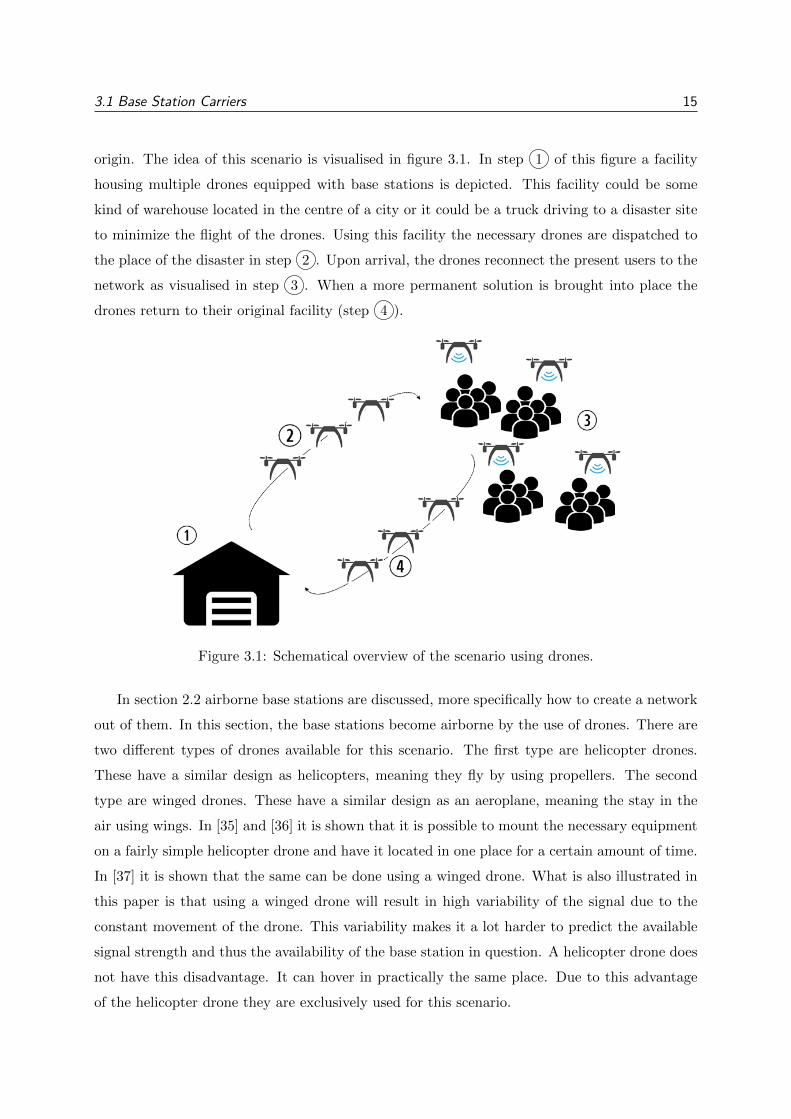
3.1 Base Station Carriers 15

origin. The idea of this scenario is visualised in figure 3.1. In step 1 of this figure a facility

housing multiple drones equipped with base stations is depicted. This facility could be some

kind of warehouse located in the centre of a city or it could be a truck driving to a disaster site

to minimize the flight of the drones. Using this facility the necessary drones are dispatched to

the place of the disaster in step 2 . Upon arrival, the drones reconnect the present users to the

network as visualised in step 3 . When a more permanent solution is brought into place the

drones return to their original facility (step 4 ).

Figure 3.1: Schematical overview of the scenario using drones.

In section 2.2 airborne base stations are discussed, more specifically how to create a network

out of them. In this section, the base stations become airborne by the use of drones. There are

two different types of drones available for this scenario. The first type are helicopter drones.

These have a similar design as helicopters, meaning they fly by using propellers. The second

type are winged drones. These have a similar design as an aeroplane, meaning the stay in the

air using wings. In [35] and [36] it is shown that it is possible to mount the necessary equipment

on a fairly simple helicopter drone and have it located in one place for a certain amount of time.

In [37] it is shown that the same can be done using a winged drone. What is also illustrated in

this paper is that using a winged drone will result in high variability of the signal due to the

constant movement of the drone. This variability makes it a lot harder to predict the available

signal strength and thus the availability of the base station in question. A helicopter drone does

not have this disadvantage. It can hover in practically the same place. Due to this advantage

of the helicopter drone they are exclusively used for this scenario.

3.1 Base Station Carriers 16

3.1.2 Emergency Service Vehicles

When an unexpected event like the one at Pukkelpop or a large traffic accident takes place,

emergency services will be dispatched to the event’s location. Emergency service vehicles are

vehicles like police cars, ambulances, the fire department fleet and so on. The emergency services

are the ones to arrive first at the site of a disastrous event. Next to providing the services they

usually do, they could also provide extra network coverage without any extra effort from the

personnel.

For this scenario the emergency service vehicles should be equipped with a certain type of

base station. With this extra infrastructure an emergency service vehicle could try to re-establish

the connection between the network and the present users once it arrives at the site.

The big advantage of this scenario is that there is little extra infrastructure needed. In

section 3.1.1 there was a need for an extra carrier (namely, a drone) to transport the base

stations, some facility to store these drones and a way to guide and monitor them. In this

scenario, no extra carrier is needed, the base stations are installed in the existing vehicle. Next

to that, the emergency vehicles are already being deployed to the sites where extra coverage

could be necessary which prevents the need for extra guidance or monitoring. The necessary

infrastructure is thus limited to the installed base stations. The disadvantage of this scenario is

that the covered area will be fairly limited. Emergency service vehicles have a tendency to flock

together at the core of the event, since the need for help is often the biggest at that location.

This prevents the users at points that are further away from the centre of the event from being

reconnected. The scenario of 3.1.1 does not have this disadvantage since the drones can be

evenly spread out over the area to provide a maximal amount of coverage.

3.1.3 Public Transport Vehicles

In an urban area it can be expected that at any time of the day there will be a lot of taxis,

buses or other means of public transport around. Given this fact, they could also be useful to

reconnect users that got disconnected due to an unexpected event. The idea of this scenario is

more or less the same as the idea in section 3.1.2. Next to providing their usual services, these

vehicles could also provide extra network coverage without any extra effort.

In order to make this scenario work, the available taxis and public transport vehicles need

to be equipped with a certain type of base station. When an unexpected event takes place it

is assumed that some of these vehicles are present since this scenario focusses solely on urban

areas. As long as the vehicles are present they are able to reconnect the users in their vicinity.

The advantage of this scenario is that there is almost no extra infrastructure necessary. The

3.2 Base Station Technology 17

base stations can be attached to the vehicle preventing the need for a dedicated carrier as in

section 3.1.1. Another advantage in comparison with the scenario proposed in section 3.1.2 is

that the location of these vehicles is not limited to the core of the event. Since these vehicles

are not directly involved in the event they will be more evenly spread out than the vehicles used

by the emergency services. This scenario will thus combine the advantages of the previous two

sections. A disadvantage of this scenario however is that it is very hard to anticipate the amount

of available vehicles in an area whereas in section 3.1.1 this can be tuned to the requirements of

the event when enough drones are available.

3.1.4 Mixture of Carriers

As a final scenario the three above scenarios are combined. In this scenario it is assumed that all

buses and taxis available in the area are equipped with the necessary equipment as discussed in

section 3.1.3. Next to these carriers, the emergency service vehicles introduced in section 3.1.2

will also be available to take part in the emergency ad hoc network. After the ad hoc network

is build based upon these two types of carriers the remaining users are covered with the base

stations mounted on drones from section 3.1.1.

The main purpose of this scenario is to verify how many drones would be necessary in a

certain area. The necessary infrastructure investments for the emergency service and public

transport vehicles are much lower than it is the case with drones. Therefore it is interesting

to use these cheaper types of carriers before deploying the expensive implementation based on

drones.

3.2 Base Station Technology

All kinds of technologies exist to connect users to the internet. In this master’s dissertation,

the focus lies on people using their cellphones to connect to a network. Long Term Evolution

(LTE) and Wi-Fi are among the most popular techniques to do so. In this section a comparison

is made between these two technologies. Based on this comparison, one technology is chosen to

be used by the base stations throughout this dissertation.

In section 3.2.1 LTE is introduced and discussed. In section 3.2.2, the same is done for

WiFi. In section 3.2.3 a comparison between both technologies is given and the best one for the

emergency ad hoc networking use case is chosen.

3.2 Base Station Technology 18

3.2.1 LTE

Long Term Evolution (LTE) and Long Term Evolution Advanced [38] are the latest standards

in mobile networking technology. The technology was developed by the Third Generation Part-

nership Project (3GPP) and it is known to the larger public as 4G (Fourth Generation) . LTE

was designed as a solution to combine the high mobility in cellular networks and the high data

rates that can be found in fixed Local Area Networks [39]. LTE is based on an all IP (Internet

Protocol) architecture and uses packet switching for all traffic, including voice traffic. Greater

deployment feasibility and extendibility using previous cellular technologies is achieved by using

this all IP based structure.

LTE uses licensed frequency bands only, which have to be acquired by the mobile connectivity

provider that is deploying the LTE network and thus the bands differ from region to region.

LTE features a great increase in speed and efficient frequency usage, enabling a user of LTE

to transmit and receive more data than with previous technologies like the Universal Mobile

Telecommunications System (UMTS) using the same amount of resources. LTE offers up to 300

Mb/s downlink capacity and up to 75 Mb/s uplink capacity. In order to achieve even higher

speeds, LTE Advanced puts more bits into each hertz of frequency, it binds together separate

frequency bands, it makes better use of cells and base stations to broaden the coverage and it

can use multiple antennas in a more efficient way. By incorporating these improvements, LTE

Advanced can offer up to 1 Gb/s downlink and 500 Mb/s uplink capacity [40].

The range of connectivity of a LTE based base station is divided into different categories.

Since LTE is a technology based on cellular networks, this range is categorised using cells. There

are three types of cells [41].

The first type of LTE cells are the small cells. This type contains two kind of cells namely

femtocells and picocells. Small cells typically provide coverage in a range of around 100 meters

around the base station and can be found in large buildings to provide indoor coverage. The

short transmit-receive distance greatly lowers the transmit power and achieves a higher Signal

to Interference plus Noise Ratio (SINR) . This means that the signal will be less attenuated

by environmental influences. Another property of small cells is that cell-to-cell interference is

rather small due to the low transmit powers used [42]. The main difference between picocells

and femtocells is the backhaul connection and the size of the cell. The backhaul connection

for picocells is usually provided by an operator whereas femtocells are usually connected to the

network of the home user. Next to this, the coverage area of a femtocell is usually around a few

tens of meters whereas picocells can cover an area of approximately 200 meters.

A bit bigger are the LTE microcells. These are the cells that can typically be found in for

3.2 Base Station Technology 19

example historical city centres and metro stations. Microcells can cover an area in a range of

around a few hundreds of meters. They require a lot more power than small cells.

The biggest cell available is a macrocell. Macrocells can typically provide coverage in a range

of a few kilometers around the base station. They are often placed along highways and on top

of buildings. The base stations used by this type of cell consume a lot of power and form the

foundation of the cellular network.

Due to the many advantages of small cells like their low power usage and their portability,

these will be the most suitable candidate for the use case presented in this master’s dissertation.

Since LTE femtocells are a bit smaller, they are easier to mount on for example a drone and

their power usage will be fairly limited. Next to that they are a bit more flexible in installation

since no operator needs to be consulted. The capacity of a wireless link can be increased with

the most certainty by bringing the transmitter and the receiver closer together [43]. The aim

will thus be to bring the base stations as close as possible to the users. This means that the

smaller range implied by a femtocell will be sufficient. Femtocells are the right fit for this use

case.

3.2.2 WiFi

WiFi is a technology that enables devices to connect to a Wireless Local Area Network (WLAN).

It can be defined as any WLAN technology based on the 802.11 standards created by the

Institute of Electrical and Electronics Engineers (IEEE) [44]. The term WiFi is an abbreviation

of Wireless Fidelity. WiFi is one of the most spread wireless networking technology, it can be

found almost everywhere in the world.

WiFi networks make use of radio waves to transmit information across a network [45]. The

technology operates in the unlicensed spectrum using the 2.4 GHz and 5 GHz frequency bands

and can typically connect devices in a range of 100 meters around a base station. Depending

on the used 802.11 standard and frequency, different data rates can be obtained. For example

802.11a uses the 5 GHz band and Orthogonal Frequency Divison Multiplexing (OFDM) to reach

a maximum of 54 Mb/s. 802.11b on the other hand uses the 2.4 GHz band resulting in a lower

data rate of maximally 11 Mb/s. 802.11g also uses this frequency band but combines it with

OFDM resulting in a maximum data rate of 54 Mb/s. Another popular and somewhat newer

standard, 802.11n, uses the 5 GHz band but is able to reach maximum rates of 140 Mb/s. One

of the most advanced WiFi standards is 802.11ac which can provide data rates up to 1 Gb/s.

All these standards behave differently but nevertheless, the newer ones preserve connectivity

possibilities with the older versions of the technology.

The 802.11 standard defines two modes of operation [3]. The first mode is the infrastructure

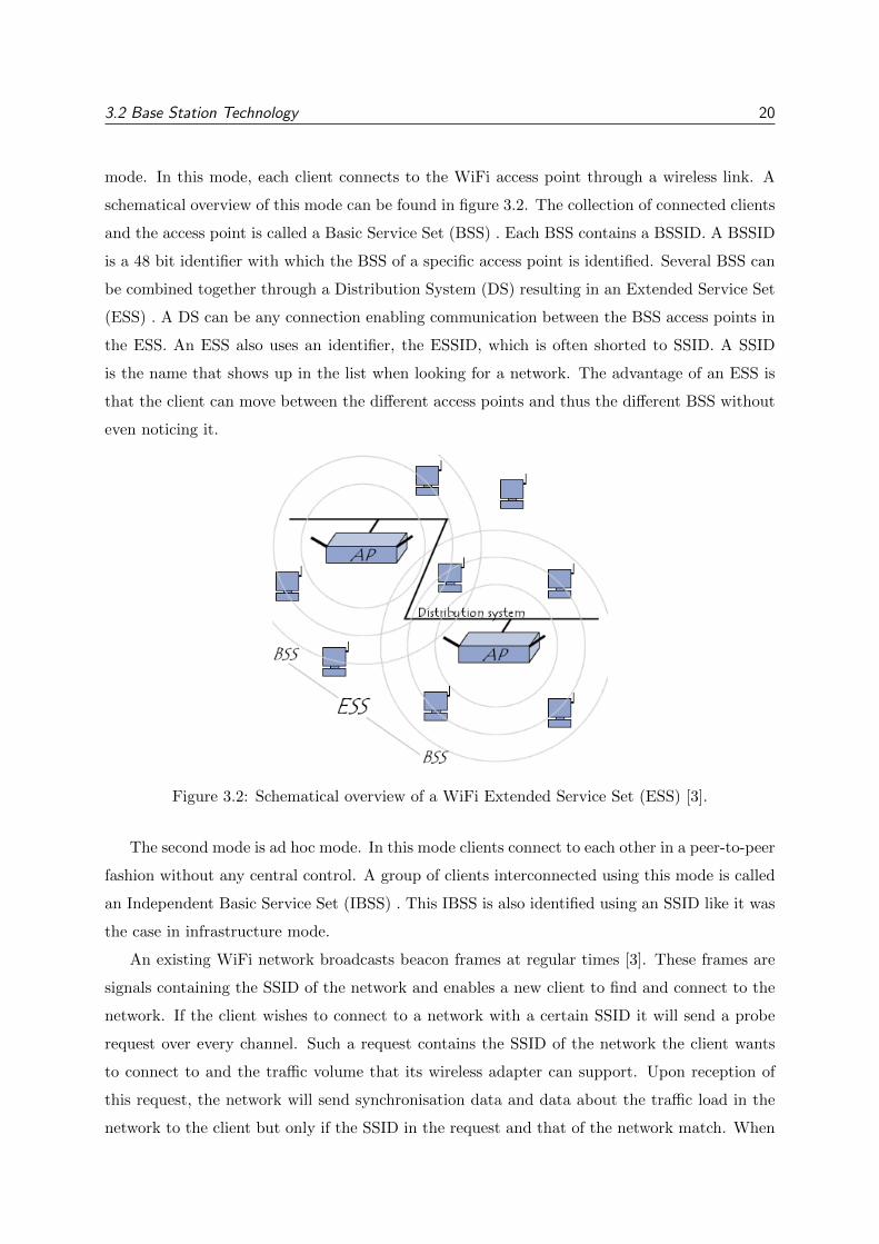
3.2 Base Station Technology 20

mode. In this mode, each client connects to the WiFi access point through a wireless link. A

schematical overview of this mode can be found in figure 3.2. The collection of connected clients

and the access point is called a Basic Service Set (BSS) . Each BSS contains a BSSID. A BSSID

is a 48 bit identifier with which the BSS of a specific access point is identified. Several BSS can

be combined together through a Distribution System (DS) resulting in an Extended Service Set

(ESS) . A DS can be any connection enabling communication between the BSS access points in

the ESS. An ESS also uses an identifier, the ESSID, which is often shorted to SSID. A SSID

is the name that shows up in the list when looking for a network. The advantage of an ESS is

that the client can move between the different access points and thus the different BSS without

even noticing it.

Figure 3.2: Schematical overview of a WiFi Extended Service Set (ESS) [3].

The second mode is ad hoc mode. In this mode clients connect to each other in a peer-to-peer

fashion without any central control. A group of clients interconnected using this mode is called

an Independent Basic Service Set (IBSS) . This IBSS is also identified using an SSID like it was

the case in infrastructure mode.

An existing WiFi network broadcasts beacon frames at regular times [3]. These frames are

signals containing the SSID of the network and enables a new client to find and connect to the

network. If the client wishes to connect to a network with a certain SSID it will send a probe

request over every channel. Such a request contains the SSID of the network the client wants

to connect to and the traffic volume that its wireless adapter can support. Upon reception of

this request, the network will send synchronisation data and data about the traffic load in the

network to the client but only if the SSID in the request and that of the network match. When

3.3 Important Parameters 21

the client receives this information it can use it to start communicating with the WiFi network.

WiFi networks use a packet switching paradigm in order to transmit and receive data. With

the introduction of voice over IP, even voice data can be transmitted over WiFi networks based

on the same packet switching paradigm [46].

3.2.3 Comparison

From the sections above it becomes clear that the properties of both technologies that are

important for the use case in this dissertation, are basically the same. This makes both LTE

femtocell and WiFi technologies suitable candidates for this use case.

However, due to the uncontrolled nature of the unlicensed band in which WiFi operates the

throughput can be dramatically poor when a lot of users are competing for the same resources.

This could be problematic for the presented use case since it is all about reconnecting a large

number of users in the same place. Next to that, LTE is optimised to handle (slow) moving

users whereas WiFi is not. Since the use case handles primarily about mobile users this is a big

advantage when using LTE as a base station technology [43].

Next to the technological advantages of LTE femtocell base stations in comparison to WiFi

base stations there is another, more specific, advantage. When all normal cellular connectivity

goes down due to a certain event, it might happen that the wired network is still up and running.

This means that if there are WiFi base stations in the area that are connected to this network,

users can also use these to reconnect to the network. When WiFi base stations would be used

instead of LTE femtocell base stations for the use case, there would be a strong increase of

active WiFi base stations in the area resulting in a lot of extra interference. However, when

LTE femtocell base stations are used, different frequency bands are used for the emergency ad

hoc network and the possibly remaining WiFi hotspots. This creates less interference and thus

the possibility to provide more users with the necessary connection.

Based on these elements, LTE femtocells were chosen as the technology for the base stations

analysed in this master’s dissertation. This technology will cause less interference for the possibly

still available WiFi hotspots and its fully optimized for mobile users on which the focus of the

proposed emergency ad hoc networks lies.

3.3 Important Parameters

In order to investigate the feasibility of the aforementioned scenarios several simulations will

be run. Each of these simulations will run based on a variation of different input parameters.

Doing so, the effect on the proposed scenario is investigated. In this manner the sensitivity of

3.3 Important Parameters 22

the scenario to certain values of the input parameters is determined.

Throughout all scenarios there are two common parameters. The first parameter is the

amount of users in the considered area. This parameter can be defined in two different ways.

On the one hand, the amount of users is inspired on real data for the considered area, depicting

what the necessary bit rates are within the area, on a normal day. On the other hand the

amount of users could be a random number. This can be useful to simulate unexpected events

where the amount of users within the area is abnormally large. For example, when the disaster

at Pukkelpop 2011 took place, there were a lot more people in the area than there would usually

be.

The second parameter is the duration of an intervention. An intervention can be defined as

the time during which the emergency network is dispatched, users are reconnected and a more

permanent solution is deployed. This dissertation only discusses emergency ad hoc networks, it

will not be the case that the network has to stay in place for days at a time. Instead it should

be used to bridge the gap between the event and the installation of a more permanent solution.

Since it is not known upfront how long this might take it is interesting to consider this parameter

in order to check what is feasible and what is not for the considered scenario.

3.3.1 Unmanned Aerial Vehicles

Next to the aforementioned common parameters, drones imply some other interesting parame-

ters. First, all the parameters concerning the capabilities of the specific drone itself. These are

the average speed of the drone, the total power that the battery can supply for the drone with

the attached base station and the average power usage of the drone itself during flight.

Second, the amount of available drones can be interesting to vary. As mentioned in section

3.1.1 the idea of this scenario is to place a storage facility or truck at a certain location. The

amount of available drones will be equal to the capacity of this facility or truck.

The third parameter is the height between the drone and the surface above which it is

hoovering. This parameter is illustrated in figure 3.3. The surface could be the street (ha) or

the rooftop of a building in which a user is located (hb). It is important to have this margin

since it is undesirable to place a drone to close to the surface where people could damage it or

to close to hanging cables and other obstacles around the area. Implementing this margin might

result in a weaker signal since the base station will be further away from the user. However,

when the base station is located higher it might be that more users are in the line of sight of

this base station resulting in less path loss and thus a stronger signal. This contradiction makes

this margin an interesting parameter to investigate.

The fourth parameter is the maximal height a drone can reach. As long as there are no

3.3 Important Parameters 23

Figure 3.3: Schematical overview of the height margin. (figure based on [4])

obstacles above them drones do not really have a height limitation. However the higher a drone

goes, the further away it will be from the user resulting in the same contradiction as with the

margin. What might be more interesting is what happens when the height is actually limited

and a drone can not pass over certain buildings. In that case, some users located inside a high

building might not be able to reconnect to a drone making the proposed solution useless for

these users. Depending on the height of the average user and the maximal height a drone is

allowed to reach, the solution for this scenario can get infeasible.

3.3.2 Emergency Services Vehicles

For the scenario using emergency service vehicles described in section 3.1.2 there are three

important parameters next to the amount of users and the duration. The first parameter is the

range of the disastrous event. Since emergency service vehicles are usually situated where help

is needed they will not occur in the entire area. Instead they will be focussed within an area

around the centre of the disaster. The size of this area is the range of the event and it can be

depicted as the circle in which emergency vehicles occur. In figure 3.4 such an area with range

R is visualised. Depending on the size of this circle the spread of the emergency service vehicles

over the area will vary. A small circle will result in a lot of emergency service vehicles crammed

together providing a lot of capacity to a small number of users whereas a large circle will result

in a better spread of the emergency service vehicles and thus a better division of the available

bit rate over the present users.

A second parameter is the total amount of emergency service vehicles that are available.

Since these vehicles are used to mobilize the base stations, the amount of these vehicles will

determine the amount of base stations available to reconnect the present users. Although this

parameter will vary depending on the disaster and cannot be requested or known upfront, it

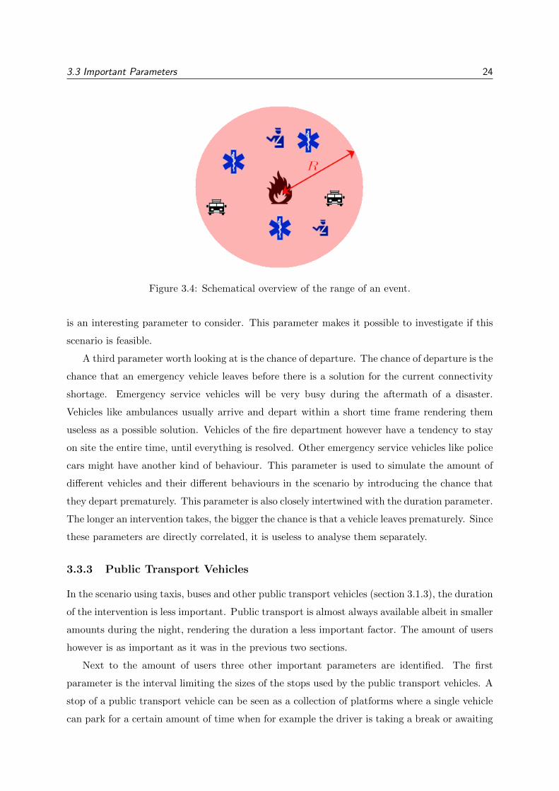
3.3 Important Parameters 24

Figure 3.4: Schematical overview of the range of an event.

is an interesting parameter to consider. This parameter makes it possible to investigate if this

scenario is feasible.

A third parameter worth looking at is the chance of departure. The chance of departure is the

chance that an emergency vehicle leaves before there is a solution for the current connectivity

shortage. Emergency service vehicles will be very busy during the aftermath of a disaster.

Vehicles like ambulances usually arrive and depart within a short time frame rendering them

useless as a possible solution. Vehicles of the fire department however have a tendency to stay

on site the entire time, until everything is resolved. Other emergency service vehicles like police

cars might have another kind of behaviour. This parameter is used to simulate the amount of

different vehicles and their different behaviours in the scenario by introducing the chance that

they depart prematurely. This parameter is also closely intertwined with the duration parameter.

The longer an intervention takes, the bigger the chance is that a vehicle leaves prematurely. Since

these parameters are directly correlated, it is useless to analyse them separately.

3.3.3 Public Transport Vehicles

In the scenario using taxis, buses and other public transport vehicles (section 3.1.3), the duration

of the intervention is less important. Public transport is almost always available albeit in smaller

amounts during the night, rendering the duration a less important factor. The amount of users

however is as important as it was in the previous two sections.

Next to the amount of users three other important parameters are identified. The first

parameter is the interval limiting the sizes of the stops used by the public transport vehicles. A

stop of a public transport vehicle can be seen as a collection of platforms where a single vehicle

can park for a certain amount of time when for example the driver is taking a break or awaiting

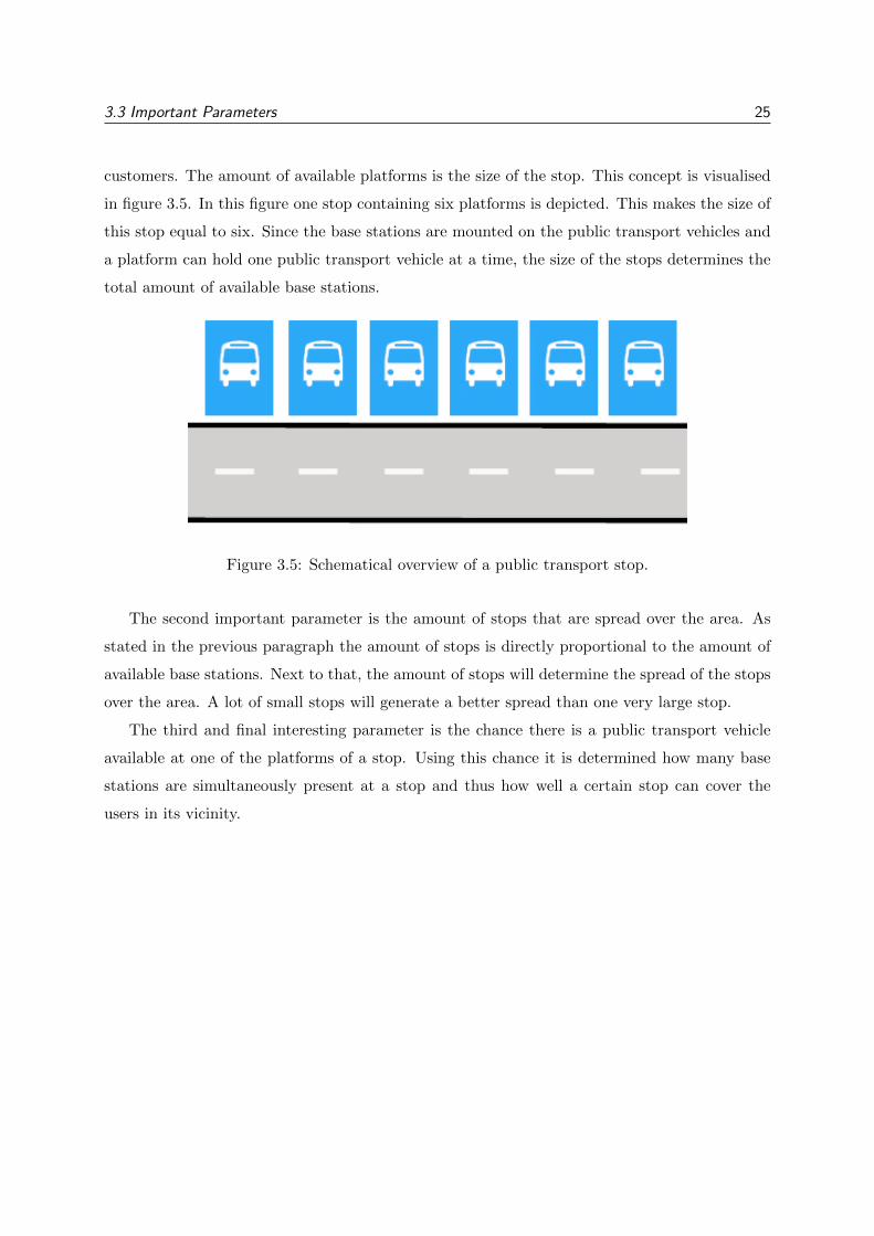
3.3 Important Parameters 25

customers. The amount of available platforms is the size of the stop. This concept is visualised

in figure 3.5. In this figure one stop containing six platforms is depicted. This makes the size of

this stop equal to six. Since the base stations are mounted on the public transport vehicles and

a platform can hold one public transport vehicle at a time, the size of the stops determines the

total amount of available base stations.

Figure 3.5: Schematical overview of a public transport stop.

The second important parameter is the amount of stops that are spread over the area. As

stated in the previous paragraph the amount of stops is directly proportional to the amount of

available base stations. Next to that, the amount of stops will determine the spread of the stops

over the area. A lot of small stops will generate a better spread than one very large stop.

The third and final interesting parameter is the chance there is a public transport vehicle

available at one of the platforms of a stop. Using this chance it is determined how many base

stations are simultaneously present at a stop and thus how well a certain stop can cover the

users in its vicinity.

SCHEDULING TOOL 26

Chapter 4

Scheduling Tool

In this chapter the creation and operation of a tool specifically designed for our use cases is

discussed. Making use of the properties and different technologies discussed in the previous

chapters, this tool creates an emergency ad hoc network for a geographically limited area. In

section 4.1 the algorithm for every scenario is discussed. In section 4.2, the amount of simulations

the tool needs to create in order to generate representative averages is investigated and the results

are discussed.

4.1 Algorithm

Every scenario introduced in chapter 3 has its own specific way of tackling the problem at hand.

In section 4.1.1 the algorithm to create an emergency ad hoc network using drones is discussed

in detail. The algorithm used to generate simulations based on emergency service vehicles is

discussed in section 4.1.2. As a final scenario, the algorithm for the generation of simulations

using public transport vehicles is discussed in section 4.1.3.

4.1.1 Unmanned Aerial Vehicles

The algorithm which uses unmanned aerial vehicles or drones is split into four parts. In section

4.1.1.1, the first part of the algorithm is described. In this part, the users, their related bit rate

and location are generated. In section 4.1.1.2 the suggested locations for the base stations which

could lead to a good solution are generated. The third part, which can be found in section

4.1.1.3, discusses the generation of a more optimal network in which the users are connected to

a certain base station and the useless base stations are filtered out. The final part, in section

4.1.1.4, takes into account the constraints implied by the base station carriers in order to create

a realistic solution based on the proposed network. In section 4.1.1.5 the output of the algorithm

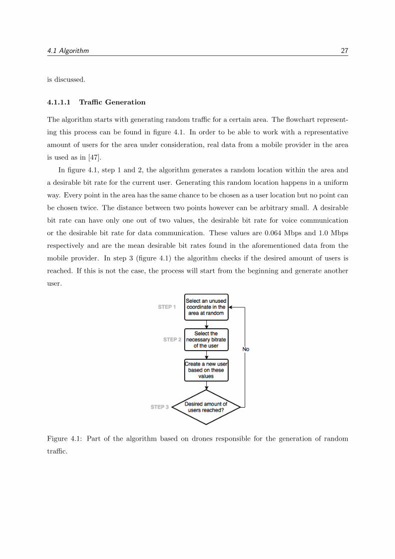
4.1 Algorithm 27

is discussed.

4.1.1.1 Traffic Generation

The algorithm starts with generating random traffic for a certain area. The flowchart represent-

ing this process can be found in figure 4.1. In order to be able to work with a representative

amount of users for the area under consideration, real data from a mobile provider in the area

is used as in [47].

In figure 4.1, step 1 and 2, the algorithm generates a random location within the area and

a desirable bit rate for the current user. Generating this random location happens in a uniform

way. Every point in the area has the same chance to be chosen as a user location but no point can

be chosen twice. The distance between two points however can be arbitrary small. A desirable

bit rate can have only one out of two values, the desirable bit rate for voice communication

or the desirable bit rate for data communication. These values are 0.064 Mbps and 1.0 Mbps

respectively and are the mean desirable bit rates found in the aforementioned data from the

mobile provider. In step 3 (figure 4.1) the algorithm checks if the desired amount of users is

reached. If this is not the case, the process will start from the beginning and generate another

user.

Figure 4.1: Part of the algorithm based on drones responsible for the generation of random

traffic.

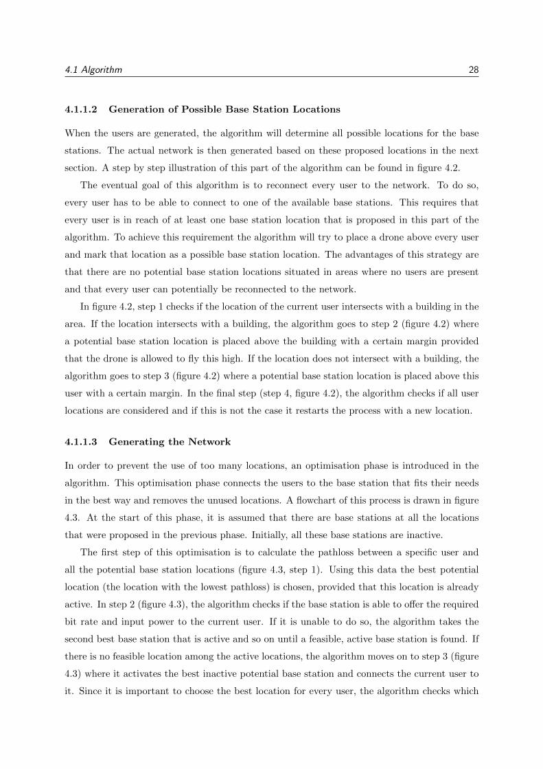
4.1 Algorithm 28

4.1.1.2 Generation of Possible Base Station Locations

When the users are generated, the algorithm will determine all possible locations for the base

stations. The actual network is then generated based on these proposed locations in the next

section. A step by step illustration of this part of the algorithm can be found in figure 4.2.

The eventual goal of this algorithm is to reconnect every user to the network. To do so,

every user has to be able to connect to one of the available base stations. This requires that

every user is in reach of at least one base station location that is proposed in this part of the

algorithm. To achieve this requirement the algorithm will try to place a drone above every user

and mark that location as a possible base station location. The advantages of this strategy are

that there are no potential base station locations situated in areas where no users are present

and that every user can potentially be reconnected to the network.

In figure 4.2, step 1 checks if the location of the current user intersects with a building in the

area. If the location intersects with a building, the algorithm goes to step 2 (figure 4.2) where

a potential base station location is placed above the building with a certain margin provided

that the drone is allowed to fly this high. If the location does not intersect with a building, the

algorithm goes to step 3 (figure 4.2) where a potential base station location is placed above this

user with a certain margin. In the final step (step 4, figure 4.2), the algorithm checks if all user

locations are considered and if this is not the case it restarts the process with a new location.

4.1.1.3 Generating the Network

In order to prevent the use of too many locations, an optimisation phase is introduced in the

algorithm. This optimisation phase connects the users to the base station that fits their needs

in the best way and removes the unused locations. A flowchart of this process is drawn in figure

4.3. At the start of this phase, it is assumed that there are base stations at all the locations

that were proposed in the previous phase. Initially, all these base stations are inactive.

The first step of this optimisation is to calculate the pathloss between a specific user and

all the potential base station locations (figure 4.3, step 1). Using this data the best potential

location (the location with the lowest pathloss) is chosen, provided that this location is already

active. In step 2 (figure 4.3), the algorithm checks if the base station is able to offer the required

bit rate and input power to the current user. If it is unable to do so, the algorithm takes the

second best base station that is active and so on until a feasible, active base station is found. If

there is no feasible location among the active locations, the algorithm moves on to step 3 (figure

4.3) where it activates the best inactive potential base station and connects the current user to

it. Since it is important to choose the best location for every user, the algorithm checks which

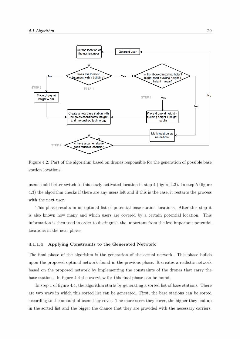
4.1 Algorithm 29

Figure 4.2: Part of the algorithm based on drones responsible for the generation of possible base

station locations.

users could better switch to this newly activated location in step 4 (figure 4.3). In step 5 (figure

4.3) the algorithm checks if there are any users left and if this is the case, it restarts the process

with the next user.

This phase results in an optimal list of potential base station locations. After this step it

is also known how many and which users are covered by a certain potential location. This

information is then used in order to distinguish the important from the less important potential

locations in the next phase.

4.1.1.4 Applying Constraints to the Generated Network

The final phase of the algorithm is the generation of the actual network. This phase builds

upon the proposed optimal network found in the previous phase. It creates a realistic network

based on the proposed network by implementing the constraints of the drones that carry the

base stations. In figure 4.4 the overview for this final phase can be found.

In step 1 of figure 4.4, the algorithm starts by generating a sorted list of base stations. There

are two ways in which this sorted list can be generated. First, the base stations can be sorted

according to the amount of users they cover. The more users they cover, the higher they end up

in the sorted list and the bigger the chance that they are provided with the necessary carriers.

4.1 Algorithm 30

Figure 4.3: Part of the algorithm based on drones responsible for the generation of the optimal

network.

The second way of sorting uses the amount of users in relation to the necessary amount of drones

carrying base stations as a measure. If a base station connects a lot of users without requiring a

lot of carriers, it ends up higher in the list and thus it increases its chance of being provisioned.

Using this list of sorted base stations, the algorithm starts looking for all base stations it

can provision with the available capacity of carriers. In order to do so, three things need to

be calculated. In step 2 (figure 4.4) the flight time from the facility to the required location

is calculated using the specified parameters of the carriers. After this, the power usage of the

carrier in combination with the mounted base station is calculated in step 3 (figure 4.4). Step

4 (figure 4.4) uses these two numbers to calculate the time the battery will last. Based on this

data, step 5 (figure 4.4) calculates the amount of carriers necessary to bridge the duration of the

entire intervention. Step 6 (figure 4.4) calculates the feasibility of the current location, using the

data of the previous steps. In case the round trip time of the carrier alone already drains the

battery, the location is marked as infeasible. If not, the algorithm checks whether or not there

4.1 Algorithm 31

are enough carriers left in the facility to provision this location during the entire intervention. If

there are enough carriers available, the location is marked as feasible and the necessary amount

of drones is subtracted from the total capacity. If the necessary amount of carriers exceeds the

remaining capacity of the facility, the location is marked as infeasible and the algorithm moves

on to the next location until no locations are left.

4.1.1.5 Output of the Algorithm

After doing all the necessary calculations the algorithm performs its last important step. It

gathers all the generated data and generates the necessary output. The output consists out of

two types of files. The first type are files that can be used as an overlay for a map. These files

contain the locations of all the users, the base stations and an estimate of the coverage of the

base stations. The second type of files are comma separated values files containing data of the

most important variables calculated throughout the algorithm as well as their averages and 95th

percentile.

The first important variable that is added to these files is the flight time to a location. This

is an interesting variable to observe since it affects the ability of the algorithm to cover a certain

location. The second important variable is the battery lifetime of a drone. This variable is an

important factor in determining if a drone can be used to cover a location or not and how long

it is able to cover it. Derived from these two variables a third important variable can be created,

the amount of carriers needed to cover a certain location throughout the entire intervention.

This variable will be used to investigate the exact influence of battery life and flight on the

ability to cover a certain location. The fourth variable is the amount of locations that were

present in the total network before the constraints were introduced. In combination with the

fifth parameter, the amount of infeasible locations, this parameter creates the ability to calculate

the percentage of covered locations. The last variable that is added to the files is the amount of

reconnected users. This way the influence of the variables mentioned above on the actual goal

of the algorithm, covering users, can be investigated.

4.1.2 Emergency Service Vehicles

The algorithm for the scenario that uses emergency service vehicles works basically in the same

way as the one using drones to mobilize the base stations.

In section 4.1.2.1 it is explained how the users are spread out over the defined area and

how their requested bit rate is calculated. In section 4.1.2.2 the possible locations where an

emergency service vehicle occurs are determined. Based on this list of possible locations, the

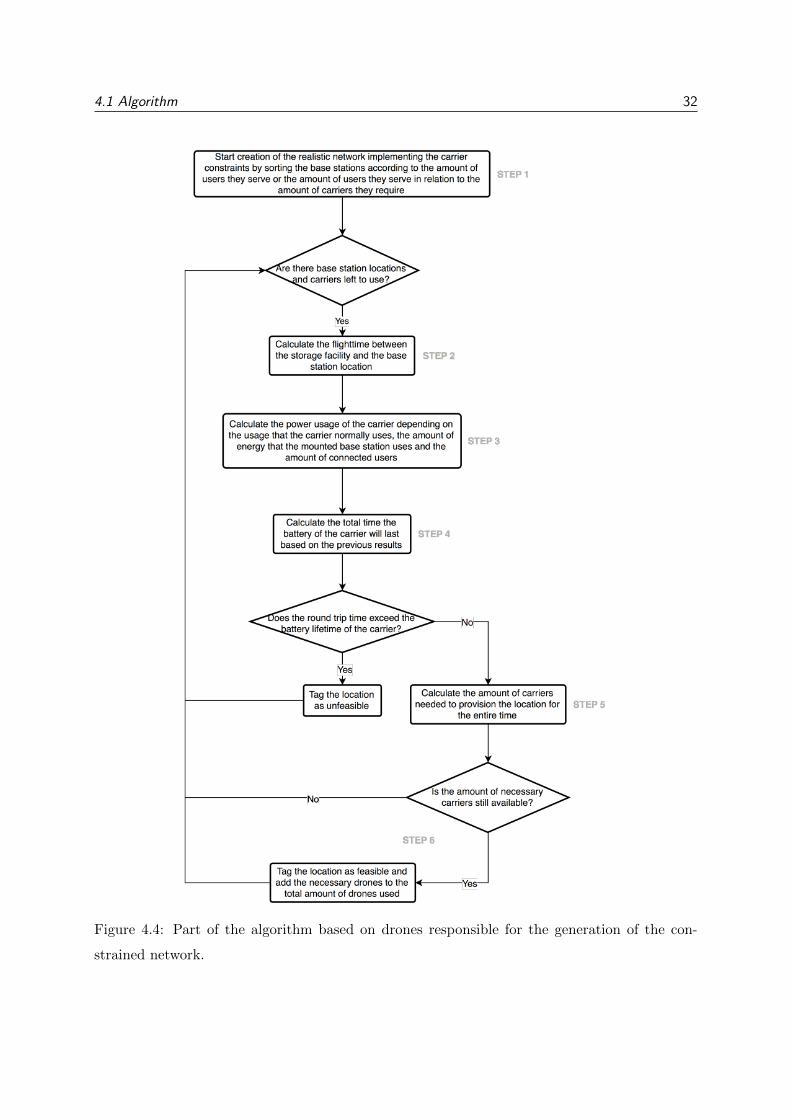
4.1 Algorithm 32

Figure 4.4: Part of the algorithm based on drones responsible for the generation of the con-

strained network.

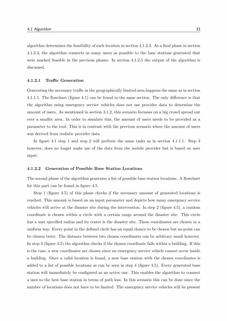
4.1 Algorithm 33

algorithm determines the feasibility of each location in section 4.1.2.3. As a final phase in section

4.1.2.4, the algorithm connects as many users as possible to the base stations generated that

were marked feasible in the previous phases. In section 4.1.2.5 the output of the algorithm is

discussed.

4.1.2.1 Traffic Generation

Generating the necessary traffic in the geographically limited area happens the same as in section

4.1.1.1. The flowchart (figure 4.1) can be found in the same section. The only difference is that

the algorithm using emergency service vehicles does not use provider data to determine the

amount of users. As mentioned in section 3.1.2, this scenario focusses on a big crowd spread out

over a smaller area. In order to simulate this, the amount of users needs to be provided as a

parameter to the tool. This is in contrast with the previous scenario where the amount of users

was derived from realistic provider data.

In figure 4.1 step 1 and step 2 will perform the same tasks as in section 4.1.1.1. Step 3

however, does no longer make use of the data from the mobile provider but is based on user

input.

4.1.2.2 Generation of Possible Base Station Locations

The second phase of the algorithm generates a list of possible base station locations. A flowchart

for this part can be found in figure 4.5.

Step 1 (figure 4.5) of this phase checks if the necessary amount of generated locations is

reached. This amount is based on an input parameter and depicts how many emergency service

vehicles will arrive at the disaster site during the intervention. In step 2 (figure 4.5), a random

coordinate is chosen within a circle with a certain range around the disaster site. This circle

has a user specified radius and its centre is the disaster site. These coordinates are chosen in a

uniform way. Every point in the defined circle has an equal chance to be chosen but no point can

be chosen twice. The distance between two chosen coordinates can be arbitrary small however.

In step 3 (figure 4.5) the algorithm checks if the chosen coordinate falls within a building. If this

is the case, a new coordinates are chosen since an emergency service vehicle cannot occur inside

a building. Once a valid location is found, a new base station with the chosen coordinates is

added to a list of possible locations as can be seen in step 4 (figure 4.5). Every generated base

station will immediately be configured as an active one. This enables the algorithm to connect

a user to the best base station in terms of path loss. In this scenario this can be done since the

number of locations does not have to be limited. The emergency service vehicles will be present

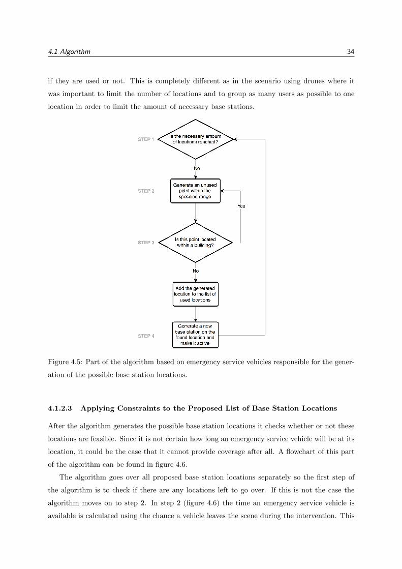
4.1 Algorithm 34

if they are used or not. This is completely different as in the scenario using drones where it

was important to limit the number of locations and to group as many users as possible to one

location in order to limit the amount of necessary base stations.

Figure 4.5: Part of the algorithm based on emergency service vehicles responsible for the gener-

ation of the possible base station locations.

4.1.2.3 Applying Constraints to the Proposed List of Base Station Locations

After the algorithm generates the possible base station locations it checks whether or not these

locations are feasible. Since it is not certain how long an emergency service vehicle will be at its

location, it could be the case that it cannot provide coverage after all. A flowchart of this part

of the algorithm can be found in figure 4.6.

The algorithm goes over all proposed base station locations separately so the first step of

the algorithm is to check if there are any locations left to go over. If this is not the case the

algorithm moves on to step 2. In step 2 (figure 4.6) the time an emergency service vehicle is

available is calculated using the chance a vehicle leaves the scene during the intervention. This

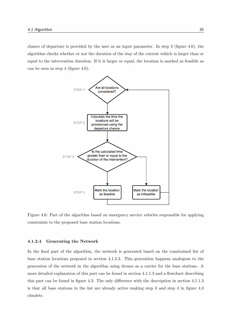
4.1 Algorithm 35

chance of departure is provided by the user as an input parameter. In step 3 (figure 4.6), the

algorithm checks whether or not the duration of the stay of the current vehicle is larger than or

equal to the intervention duration. If it is larger or equal, the location is marked as feasible as

can be seen in step 4 (figure 4.6).

Figure 4.6: Part of the algorithm based on emergency service vehicles responsible for applying

constraints to the proposed base station locations.

4.1.2.4 Generating the Network

In the final part of the algorithm, the network is generated based on the constrained list of

base station locations proposed in section 4.1.2.3. This generation happens analogous to the

generation of the network in the algorithm using drones as a carrier for the base stations. A

more detailed explanation of this part can be found in section 4.1.1.3 and a flowchart describing

this part can be found in figure 4.3. The only difference with the description in section 4.1.1.3

is that all base stations in the list are already active making step 3 and step 4 in figure 4.3

obsolete.

4.1 Algorithm 36

4.1.2.5 Output of the Algorithm

The output of the algorithm using emergency service vehicles is formatted in the same way as

the output from the algorithm using drones. The first type of files are comma separated value

files with all the data that was created during the execution of the algorithm. The second type

of files are files that can be used as an overlay for a map. These files contain the locations of all

the users, the base stations and an estimate of the coverage of the base stations.

The comma separated value files contain information about all the important variables within

the algorithm. The first important variable is the amount of users that are not covered at the

end of the simulation. Based on this variable it is determined how good the proposed solution

is for the problem at hand. The second important variable is the total time all emergency

vehicles were present. Using this variable, an assessment can be made of the stability of the

solution. The solution is stable when a lot of vehicles stay in place longer than the duration

of the intervention. It is unstable when the amount of available vehicles plummets after the

duration of the intervention. This means that if the intervention had taken just a few minutes

longer the solution would have been invalid. The third and fourth important variables are the

amounts of vehicles that were used to reconnect to the network and the total amount of vehicles

that left before the intervention terminated. Using these parameters in combination with the

total amount of available vehicles it can be decided if the simulation failed because of insufficient

capacity, a departure chance that was too big or bad placing of the vehicles with respect to the

users.

4.1.3 Public Transport Vehicles

The algorithm for the scenario that uses public transport vehicles works basically in the same

way as the one for the other scenarios.

In section 4.1.3.1 the mechanism to generate the necessary amount of users for the current

scenario is discussed. Next to the amount of users, a certain amount of stops for the public trans-

port vehicles needs to be generated. This is explained in section 4.1.3.2. After the generation of

the stops, the algorithm determines how many base stations can be linked to a certain stop in

section 4.1.3.3. By using this data, the algorithm can decide which users can be connected to

the network using one of the generated base stations. The details behind these decisions can be

found in section 4.1.3.4. As a final step the algorithm creates some files containing the output

of the algorithm. The format and contents of these files is discussed in section 4.1.3.5.

4.1 Algorithm 37

4.1.3.1 Traffic Generation

Generating the necessary amount of users for this scenario happens in exactly the same way as

described in section 4.1.1.1. A flowchart illustrating this phase of the algorithm can be found in

figure 4.1.

4.1.3.2 Generation of Stop Locations

Next to the generation of the users, the stops need to be generated. A stop is a place that

consists out of a certain number of platforms where a bus or a taxi can reside for a certain

amount of time while the drivers are taking a break for example. To define a stop, two elements

have to be chosen. First, the location of the stop needs to be selected. Second, the size of a stop

needs to be chosen in a random but uniform way from an interval which is a user defined input

parameter. A flowchart for this phase can be found in figure 4.7.

In figure 4.7, step 1, the algorithm checks whether or not the requested amount of stops is

reached. If the requested amount is not reached the algorithm continues with creating a new

stop in the following steps. In step 2 (figure 4.7) a new point within the boundaries of the

predefined area is generated. These points are generated in a uniform way, meaning every point

has the same chance of being chosen as long as it is situated within the confines of the area. No

point can be chosen twice however and the distance between two possible points can be arbitrary

small. After this point is generated, the size of the stop is generated in step 3 (figure 4.7). This

size is chosen in a uniform way between the minimal and maximal allowed size of a stop. The

size interval is also defined by the user of the algorithm. As a final step, the algorithm generates

a new stop based on the chosen location and the chosen size as can be seen in step 4 (figure 4.7).

Using the described logic, the algorithm generates two different lists of stops. On the one

hand it generates a list of bus stops based on the parameters provided by the user and specific

for this kind of public transport vehicle. On the other hand the algorithm generates a list of

taxi stops based on the parameters provided by the user and specific for this kind of public

transport vehicle. The reason the algorithm generates two lists is that bus and taxi stops can be

very different in size and the number of stops across the area. Keeping these two kinds separate

allows the algorithm to take these differences into account.

4.1.3.3 Generation of Possible Base Station Locations

As stated in the previous section a stop is a collection of platforms where a public transport

vehicle might be residing. Using the lists of stops generated in section 4.1.3.2 the algorithm

determines how many vehicles and thus base stations are available to the user at any given time.

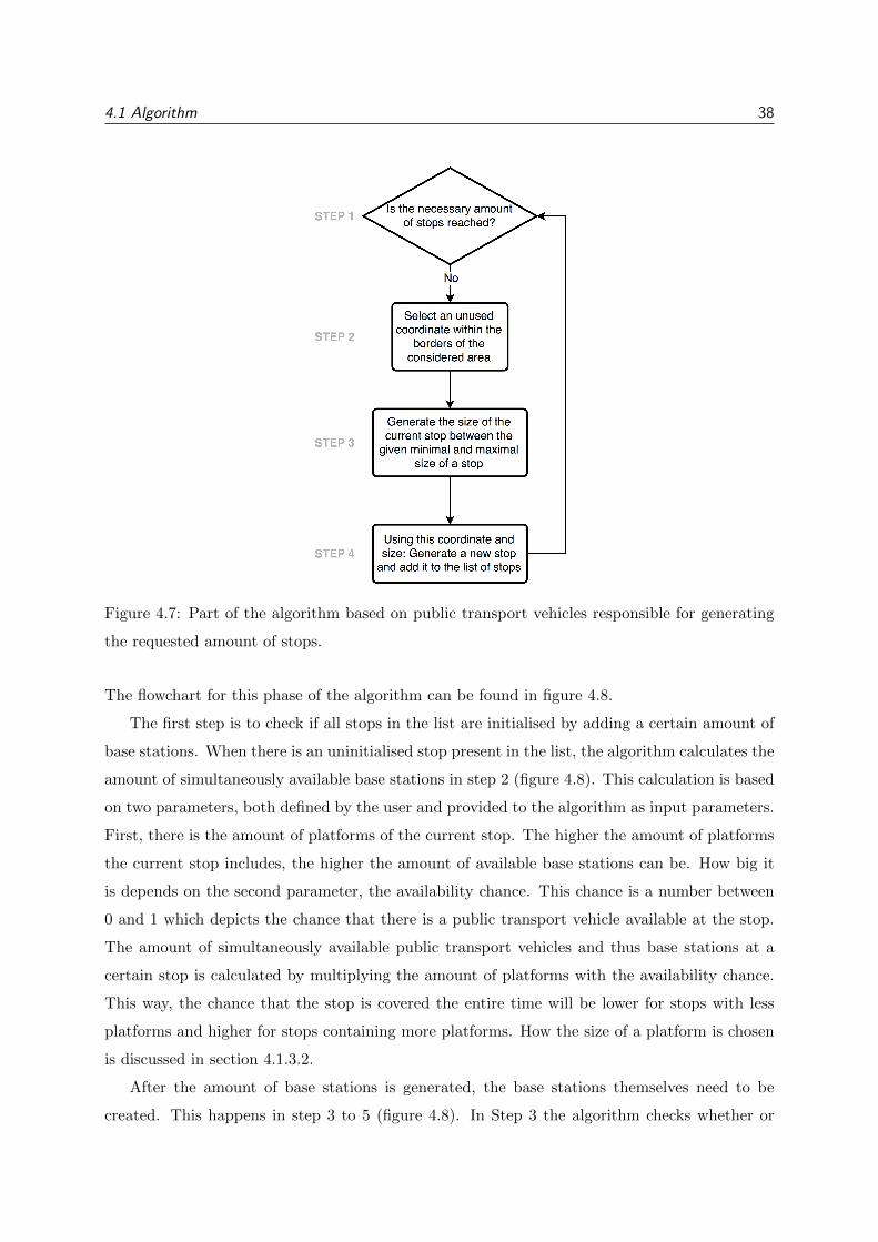
4.1 Algorithm 38

Figure 4.7: Part of the algorithm based on public transport vehicles responsible for generating

the requested amount of stops.

The flowchart for this phase of the algorithm can be found in figure 4.8.

The first step is to check if all stops in the list are initialised by adding a certain amount of

base stations. When there is an uninitialised stop present in the list, the algorithm calculates the

amount of simultaneously available base stations in step 2 (figure 4.8). This calculation is based

on two parameters, both defined by the user and provided to the algorithm as input parameters.

First, there is the amount of platforms of the current stop. The higher the amount of platforms

the current stop includes, the higher the amount of available base stations can be. How big it

is depends on the second parameter, the availability chance. This chance is a number between

0 and 1 which depicts the chance that there is a public transport vehicle available at the stop.

The amount of simultaneously available public transport vehicles and thus base stations at a

certain stop is calculated by multiplying the amount of platforms with the availability chance.

This way, the chance that the stop is covered the entire time will be lower for stops with less

platforms and higher for stops containing more platforms. How the size of a platform is chosen

is discussed in section 4.1.3.2.

After the amount of base stations is generated, the base stations themselves need to be

created. This happens in step 3 to 5 (figure 4.8). In Step 3 the algorithm checks whether or

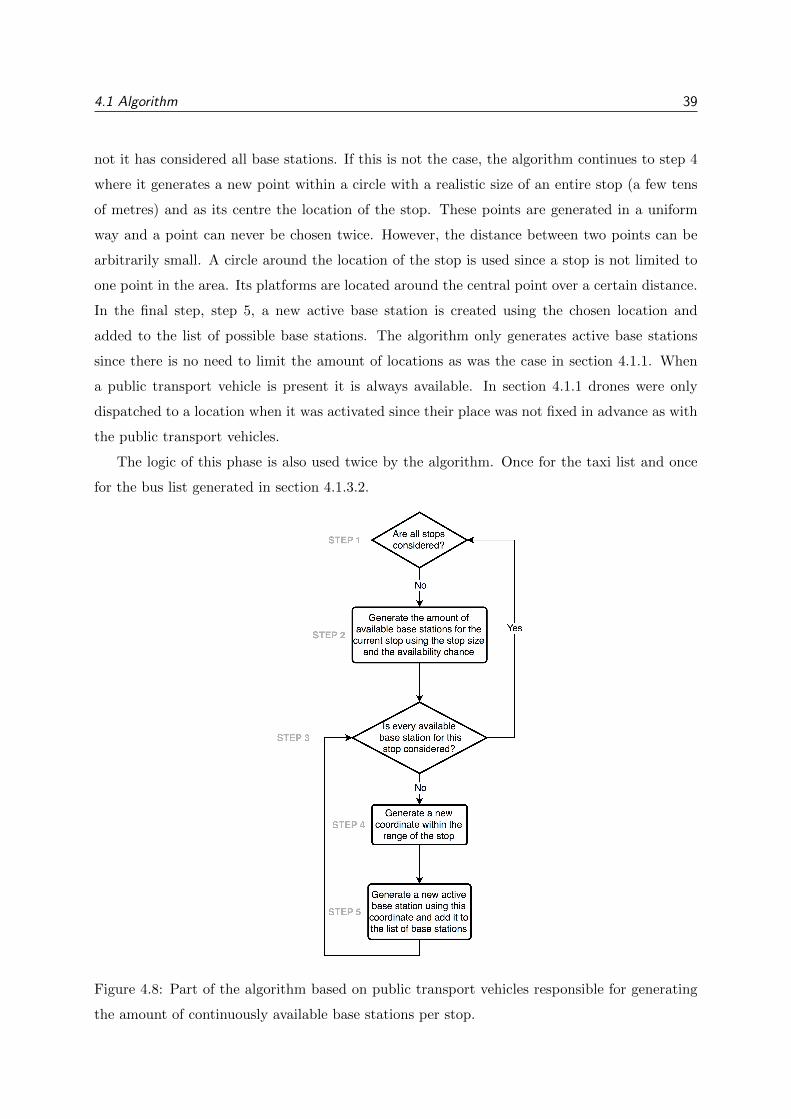
4.1 Algorithm 39

not it has considered all base stations. If this is not the case, the algorithm continues to step 4

where it generates a new point within a circle with a realistic size of an entire stop (a few tens

of metres) and as its centre the location of the stop. These points are generated in a uniform

way and a point can never be chosen twice. However, the distance between two points can be

arbitrarily small. A circle around the location of the stop is used since a stop is not limited to

one point in the area. Its platforms are located around the central point over a certain distance.

In the final step, step 5, a new active base station is created using the chosen location and

added to the list of possible base stations. The algorithm only generates active base stations

since there is no need to limit the amount of locations as was the case in section 4.1.1. When

a public transport vehicle is present it is always available. In section 4.1.1 drones were only

dispatched to a location when it was activated since their place was not fixed in advance as with

the public transport vehicles.

The logic of this phase is also used twice by the algorithm. Once for the taxi list and once

for the bus list generated in section 4.1.3.2.

Figure 4.8: Part of the algorithm based on public transport vehicles responsible for generating

the amount of continuously available base stations per stop.

4.2 Number of Simulations 40

4.1.3.4 Generating the Network

The generation of the final network happens in the same way as in section 4.1.1.3. A flowchart of

this generation can be found in figure 4.3. The input of this generation is a single list of proposed

base stations. Since the algorithm generated two lists in the previous phase, the algorithm will

combine these lists into a single list before passing it on to the final network generation phase.

4.1.3.5 Output of the Algorithm

The output of the algorithm using public transport vehicles is formatted in the same way as the

output from the algorithm using drones and emergency service vehicles. The first type of files

are comma separated value files with all the data that was created during the execution of the

algorithm. The second type of files are files that can be used as an overlay for a map. These

files contain the locations of all the users, the base stations and an estimate of the coverage of

the base stations.

The comma separated value files contain information about all the important variables within

the algorithm. Since the algorithm focusses on two categories, buses and taxis, these important

output variables are generated separately for every category.

The first set of important parameters contains the amount of base stations mounted on a

public transport vehicle for every category of public transport vehicles. More specifically the

maximal possible amount, the selected amount and the amount of eventually used base stations.

The maximal amount of base stations is the total amount of platforms that are available in

the simulation. Every platform can hold exactly one public transport vehicle and thus one

base station. The selected amount of base stations is a subset of the maximal amount of base

stations. It is the amount of base stations that are available after taking into account the

availability chance from section 4.1.3.3. The used amount of base stations is the amount of base

stations that are actually used to reconnect one or more users to the network.

The second set of important parameters contains the amount of covered users for every

category of public transport vehicles. This parameter can be used to assess the effectiveness of

the algorithm for the used set of input parameters. If the amount of covered users is high, this

proves that the algorithm generates a good solution for the given parameters. Whereas if it is

low, it proves the contrary.

4.2 Number of Simulations

Every created simulation depends on the random input data generated by the algorithm. This

random input data determines where the users of the current simulation are located, the locations

4.2 Number of Simulations 41

of emergency vehicles, the locations of public transport stops, the size of these stops and the

chance that a certain base station is available long enough. These differences between single

simulations might influence their ultimate conclusions. There could be more infeasible locations

due to the amount of users that are in high buildings or there could be a lot more necessary

locations when all users are very far apart. All public transport stops could be at the center

of the simulated area, leaving all the users at the borders uncovered or the size of a stop could

always be minimal or maximal. To account for these differences in the results, the written

scheduling tool has to perform a certain amount of simulations in order to find representative

averages for the parameters at hand.

In order to find a good amount of simulations, an analysis is performed for every scenario.

In section 4.2.1 the analysis is performed for the scenario in which drones are used to mobilize

the base stations. In section 4.2.2 this analysis is performed for the scenario in which emergency

service vehicles are used and in section 4.2.3 it is done for the scenario using public transport

vehicles.

4.2.1 Unmanned Aerial Vehicles

The algorithm using unmanned aerial vehicles or drones as a way to mobilize the base stations is

only sensitive to where the users are placed. Since this is decided randomly by the algorithm, it

could cause some deviating results. In this section the necessary amount of simulations needed

for this variant of the algorithm is investigated. In section 4.2.1.1 the used parameters and the

setup of the algorithm is discussed. In section 4.2.1.2 the analysis of the necessary amount of

simulations is performed and in section 4.2.1.3 a conclusion is drawn based on this analysis.

4.2.1.1 Setup

In order to find a suitable amount of simulations, the cumulative averages of all parameters was

investigated over 200 simulations. Doing so, the convergence of the parameters is investigated

and thus the optimal amount of simulations is found. The optimal amount of simulations is a

trade off between the amount of convergence of a certain parameter and the runtime that the

tool requires for all simulations. The runtime of the tool is an important factor that depends on

the amount of simulations and increases with about five minutes for one extra simulation. The

tool creates the recommended amount of simulations using the same values for all parameters in

every simulation. Since the tool will be used in scenarios where it is interesting to vary certain

parameters, the proposed amount of simulations will have to be generated for every variation

in the values of the parameters. A few simulations more or less will in this manner result in a

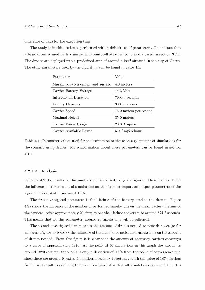
4.2 Number of Simulations 42

difference of days for the execution time.

The analysis in this section is performed with a default set of parameters. This means that

a basic drone is used with a simple LTE femtocell attached to it as discussed in section 3.2.1.

The drones are deployed into a predefined area of around 4 km2 situated in the city of Ghent.

The other parameters used by the algorithm can be found in table 4.1.

Parameter Value

Margin between carrier and surface 4.0 meters

Carrier Battery Voltage 14.3 Volt

Intervention Duration 7000.0 seconds

Facility Capacity 300.0 carriers

Carrier Speed 15.0 meters per second

Maximal Height 35.0 meters

Carrier Power Usage 20.0 Ampere

Carrier Available Power 5.0 Amperehour

Table 4.1: Parameter values used for the estimation of the necessary amount of simulations for

the scenario using drones. More information about these parameters can be found in section

4.1.1.

4.2.1.2 Analysis

In figure 4.9 the results of this analysis are visualised using six figures. These figures depict

the influence of the amount of simulations on the six most important output parameters of the

algorithm as stated in section 4.1.1.5.

The first investigated parameter is the lifetime of the battery used in the drones. Figure

4.9a shows the influence of the number of performed simulations on the mean battery lifetime of

the carriers. After approximately 20 simulations the lifetime converges to around 874.5 seconds.

This means that for this parameter, around 20 simulations will be sufficient.

The second investigated parameter is the amount of drones needed to provide coverage for

all users. Figure 4.9b shows the influence of the number of performed simulations on the amount

of drones needed. From this figure it is clear that the amount of necessary carriers converges

to a value of approximately 1870. At the point of 40 simulations in this graph the amount is

around 1880 carriers. Since this is only a deviation of 0.5% from the point of convergence and

since there are around 40 extra simulations necessary to actually reach the value of 1870 carriers

(which will result in doubling the execution time) it is that 40 simulations is sufficient in this

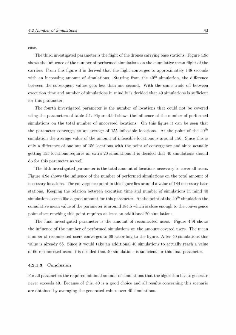
4.2 Number of Simulations 43

case.

The third investigated parameter is the flight of the drones carrying base stations. Figure 4.9c

shows the influence of the number of performed simulations on the cumulative mean flight of the

carriers. From this figure it is derived that the flight converges to approximately 148 seconds

with an increasing amount of simulations. Starting from the 40th simulation, the difference

between the subsequent values gets less than one second. With the same trade off between

execution time and number of simulations in mind it is decided that 40 simulations is sufficient

for this parameter.

The fourth investigated parameter is the number of locations that could not be covered

using the parameters of table 4.1. Figure 4.9d shows the influence of the number of performed

simulations on the total number of uncovered locations. On this figure it can be seen that

the parameter converges to an average of 155 infeasible locations. At the point of the 40th

simulation the average value of the amount of infeasible locations is around 156. Since this is

only a difference of one out of 156 locations with the point of convergence and since actually

getting 155 locations requires an extra 20 simulations it is decided that 40 simulations should

do for this parameter as well.

The fifth investigated parameter is the total amount of locations necessary to cover all users.

Figure 4.9e shows the influence of the number of performed simulations on the total amount of

necessary locations. The convergence point in this figure lies around a value of 184 necessary base

stations. Keeping the relation between execution time and number of simulations in mind 40

simulations seems like a good amount for this parameter. At the point of the 40th simulation the

cumulative mean value of the parameter is around 184.5 which is close enough to the convergence

point since reaching this point requires at least an additional 20 simulations.

The final investigated parameter is the amount of reconnected users. Figure 4.9f shows

the influence of the number of performed simulations on the amount covered users. The mean

number of reconnected users converges to 66 according to the figure. After 40 simulations this

value is already 65. Since it would take an additional 40 simulations to actually reach a value

of 66 reconnected users it is decided that 40 simulations is sufficient for this final parameter.

4.2.1.3 Conclusion

For all parameters the required minimal amount of simulations that the algorithm has to generate

never exceeds 40. Because of this, 40 is a good choice and all results concerning this scenario

are obtained by averaging the generated values over 40 simulations.

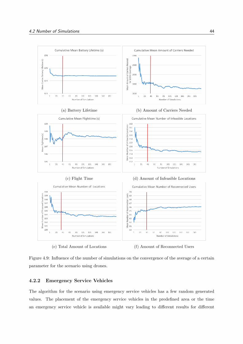
4.2 Number of Simulations 44

(a) Battery Lifetime (b) Amount of Carriers Needed

(c) Flight Time (d) Amount of Infeasible Locations

(e) Total Amount of Locations (f) Amount of Reconnected Users

Figure 4.9: Influence of the number of simulations on the convergence of the average of a certain

parameter for the scenario using drones.

4.2.2 Emergency Service Vehicles

The algorithm for the scenario using emergency service vehicles has a few random generated

values. The placement of the emergency service vehicles in the predefined area or the time

an emergency service vehicle is available might vary leading to different results for different

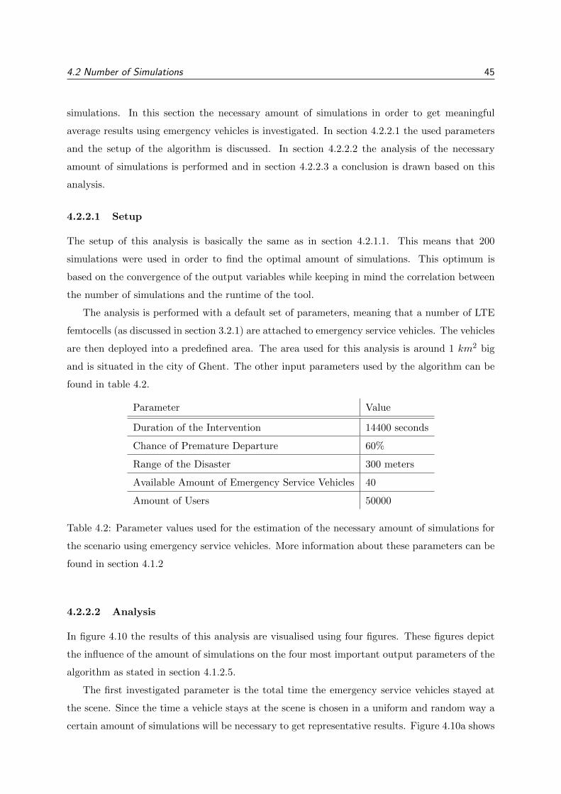
4.2 Number of Simulations 45

simulations. In this section the necessary amount of simulations in order to get meaningful

average results using emergency vehicles is investigated. In section 4.2.2.1 the used parameters

and the setup of the algorithm is discussed. In section 4.2.2.2 the analysis of the necessary

amount of simulations is performed and in section 4.2.2.3 a conclusion is drawn based on this

analysis.

4.2.2.1 Setup

The setup of this analysis is basically the same as in section 4.2.1.1. This means that 200

simulations were used in order to find the optimal amount of simulations. This optimum is

based on the convergence of the output variables while keeping in mind the correlation between

the number of simulations and the runtime of the tool.

The analysis is performed with a default set of parameters, meaning that a number of LTE

femtocells (as discussed in section 3.2.1) are attached to emergency service vehicles. The vehicles

are then deployed into a predefined area. The area used for this analysis is around 1 km2 big

and is situated in the city of Ghent. The other input parameters used by the algorithm can be

found in table 4.2.

Parameter Value

Duration of the Intervention 14400 seconds

Chance of Premature Departure 60%

Range of the Disaster 300 meters

Available Amount of Emergency Service Vehicles 40

Amount of Users 50000

Table 4.2: Parameter values used for the estimation of the necessary amount of simulations for

the scenario using emergency service vehicles. More information about these parameters can be

found in section 4.1.2

4.2.2.2 Analysis

In figure 4.10 the results of this analysis are visualised using four figures. These figures depict

the influence of the amount of simulations on the four most important output parameters of the

algorithm as stated in section 4.1.2.5.

The first investigated parameter is the total time the emergency service vehicles stayed at

the scene. Since the time a vehicle stays at the scene is chosen in a uniform and random way a

certain amount of simulations will be necessary to get representative results. Figure 4.10a shows

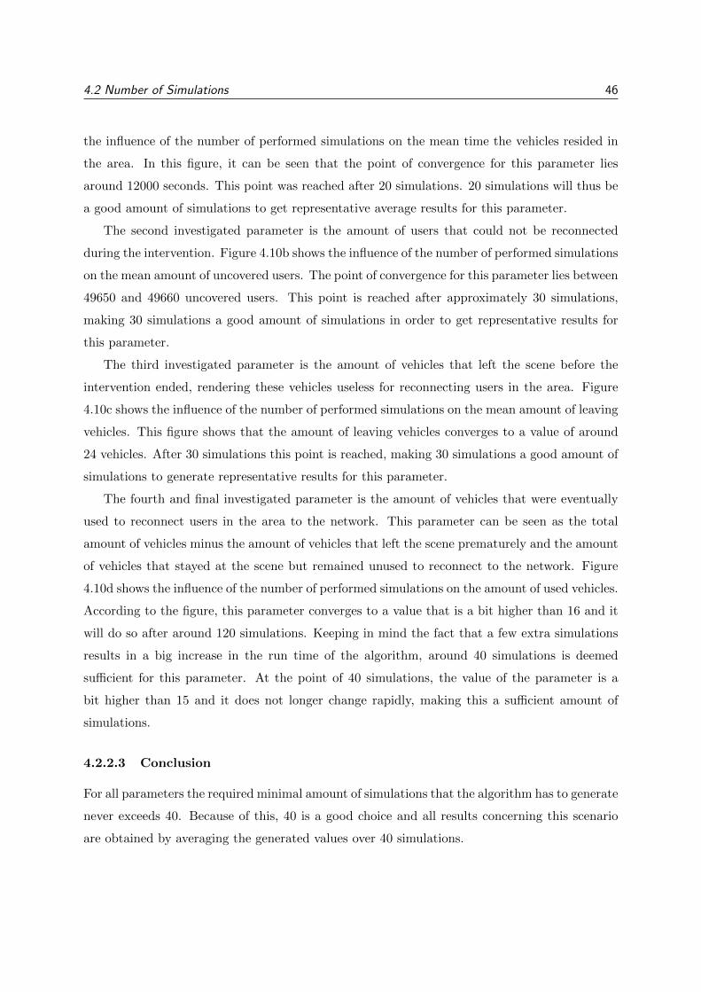
4.2 Number of Simulations 46

the influence of the number of performed simulations on the mean time the vehicles resided in

the area. In this figure, it can be seen that the point of convergence for this parameter lies

around 12000 seconds. This point was reached after 20 simulations. 20 simulations will thus be

a good amount of simulations to get representative average results for this parameter.

The second investigated parameter is the amount of users that could not be reconnected

during the intervention. Figure 4.10b shows the influence of the number of performed simulations

on the mean amount of uncovered users. The point of convergence for this parameter lies between

49650 and 49660 uncovered users. This point is reached after approximately 30 simulations,

making 30 simulations a good amount of simulations in order to get representative results for

this parameter.

The third investigated parameter is the amount of vehicles that left the scene before the

intervention ended, rendering these vehicles useless for reconnecting users in the area. Figure

4.10c shows the influence of the number of performed simulations on the mean amount of leaving

vehicles. This figure shows that the amount of leaving vehicles converges to a value of around

24 vehicles. After 30 simulations this point is reached, making 30 simulations a good amount of

simulations to generate representative results for this parameter.

The fourth and final investigated parameter is the amount of vehicles that were eventually

used to reconnect users in the area to the network. This parameter can be seen as the total

amount of vehicles minus the amount of vehicles that left the scene prematurely and the amount

of vehicles that stayed at the scene but remained unused to reconnect to the network. Figure

4.10d shows the influence of the number of performed simulations on the amount of used vehicles.

According to the figure, this parameter converges to a value that is a bit higher than 16 and it

will do so after around 120 simulations. Keeping in mind the fact that a few extra simulations

results in a big increase in the run time of the algorithm, around 40 simulations is deemed

sufficient for this parameter. At the point of 40 simulations, the value of the parameter is a

bit higher than 15 and it does not longer change rapidly, making this a sufficient amount of

simulations.

4.2.2.3 Conclusion

For all parameters the required minimal amount of simulations that the algorithm has to generate

never exceeds 40. Because of this, 40 is a good choice and all results concerning this scenario

are obtained by averaging the generated values over 40 simulations.

4.2 Number of Simulations 47

(a) Time the Vehicles Stayed (b) Amount of Uncovered Users

(c) Amount of Vehicles that Left (d) Amount of Vehicles Used

Figure 4.10: Influence of the number of simulations on the convergence of the average of a certain

parameter for the scenario using emergency service vehilces.

4.2.3 Public Transport Vehicles

The algorithm for the scenario using public transport vehicles depends on random variables

based on several input parameters. Next to the location of the users and the stops, the stop size

and the amount of base stations at a stop can vary. These variations might results in different

conclusions for simulations using the same input parameters. In this section the necessary

amount of simulations is investigated to get representative average results. In section 4.2.3.1

the used parameters and the setup of the algorithm is discussed. In section 4.2.3.2 the analysis

of the necessary amount of simulations is performed for every parameter and in section 4.2.3.3

a conclusion is drawn based on this analysis.

4.2.3.1 Setup

The analysis of the number of simulations for the scenario using public transport vehicles is

based on the same basic setup of section 4.2.1.1. In order to check for the convergence of the

output variables, 200 simulations are used. In the end a conclusion is drawn keeping in mind

the correlation between the run time of the algorithm and the number of necessary simulations.

4.2 Number of Simulations 48

The analysis is performed with a default set of parameters. A simple LTE femtocell (as

discussed in section 3.2.1) is attached to either a taxi or a bus and then deployed into the

predefined area. This area is approximately 4 km2 big and is situated in the city of Ghent. The

other input parameters used by the algorithm can be found in table 4.3.

Parameter Value

Duration of the Intervention 14400 seconds

Maximal Size of a Bus Stop 20 platforms

Minimal Size of a Bus Stop 1 platform

Amount of Bus Stops 10

Maximal Size of a Taxi Stop 5 platforms

Minimal Size of a Taxi Stop 1 platform

Amount of Taxi Stops 40

Chance that Buses Are Continuously Available At a Stop 50%

Chance that Taxis Are Continuously Available At a Stop 30%

Table 4.3: Parameter values used for the estimation of the necessary amount of simulations for

the scenario using public transport vehicles. More information about these parameters can be

found in section 4.1.3

4.2.3.2 Analysis

In figure 4.11 the results of this analysis are visualised using four figures. These figures depict

the influence of the amount of simulations on the four most important output parameters of the

algorithm as stated in section 4.1.3.5.

The first investigated parameter is the amount of users that are reconnected to the network

by this scenario. Figure 4.11a shows the influence of the number of performed simulations on the

amount of covered users. As can be seen on the figure the amount of covered users converges to

around 24 covered users. This happens using approximately 35 simulations, making this amount

of simulations a good amount in order to reach representative average results.

The second investigated parameter is the maximal amount of base stations that can reside

in the area. This parameter can also be seen as the amount of base stations that is present when

every platform in the scenario is occupied by a vehicle and thus a base station. Figure 4.11b

shows the influence of the number of performed simulations on this amount. Around simulation

60 the maximal amount of base stations converges to 224. When we take a closer look at the

figure we see that at the point of the 40th simulation, the value of the parameter has already

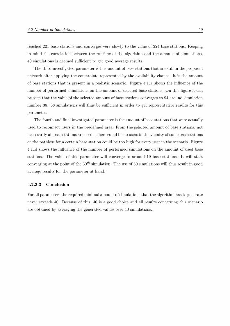
4.2 Number of Simulations 49

reached 221 base stations and converges very slowly to the value of 224 base stations. Keeping

in mind the correlation between the runtime of the algorithm and the amount of simulations,

40 simulations is deemed sufficient to get good average results.

The third investigated parameter is the amount of base stations that are still in the proposed

network after applying the constraints represented by the availability chance. It is the amount

of base stations that is present in a realistic scenario. Figure 4.11c shows the influence of the

number of performed simulations on the amount of selected base stations. On this figure it can

be seen that the value of the selected amount of base stations converges to 94 around simulation

number 38. 38 simulations will thus be sufficient in order to get representative results for this

parameter.

The fourth and final investigated parameter is the amount of base stations that were actually

used to reconnect users in the predefined area. From the selected amount of base stations, not

necessarily all base stations are used. There could be no users in the vicinity of some base stations

or the pathloss for a certain base station could be too high for every user in the scenario. Figure

4.11d shows the influence of the number of performed simulations on the amount of used base

stations. The value of this parameter will converge to around 19 base stations. It will start

converging at the point of the 30th simulation. The use of 30 simulations will thus result in good

average results for the parameter at hand.

4.2.3.3 Conclusion

For all parameters the required minimal amount of simulations that the algorithm has to generate

never exceeds 40. Because of this, 40 is a good choice and all results concerning this scenario

are obtained by averaging the generated values over 40 simulations.

4.2 Number of Simulations 50

(a) Amount of Covered Users (b) Maximal Amount of Base Stations

(c) Selected Amount of Base Stations (d) Used Amount of Base Stations

Figure 4.11: Influence of the number of simulations on the convergence of the average of a certain

parameter for the scenario using public transport vehilces.

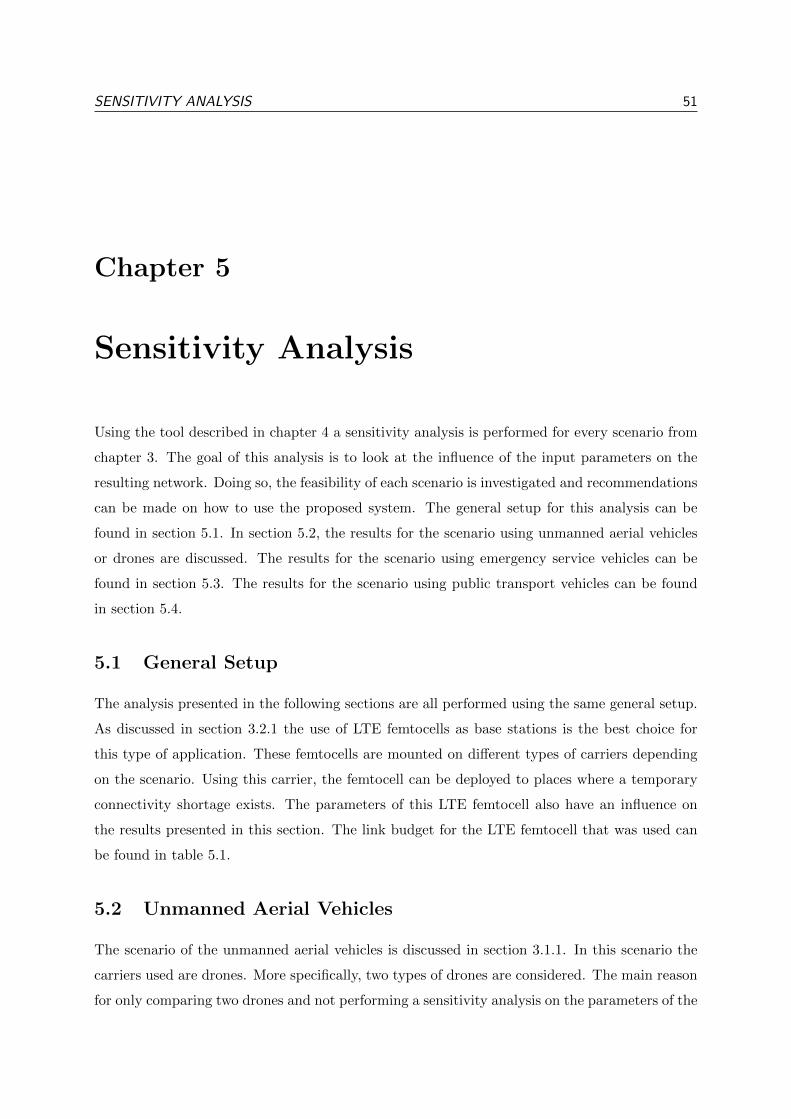
SENSITIVITY ANALYSIS 51

Chapter 5

Sensitivity Analysis

Using the tool described in chapter 4 a sensitivity analysis is performed for every scenario from

chapter 3. The goal of this analysis is to look at the influence of the input parameters on the

resulting network. Doing so, the feasibility of each scenario is investigated and recommendations

can be made on how to use the proposed system. The general setup for this analysis can be

found in section 5.1. In section 5.2, the results for the scenario using unmanned aerial vehicles

or drones are discussed. The results for the scenario using emergency service vehicles can be

found in section 5.3. The results for the scenario using public transport vehicles can be found

in section 5.4.

5.1 General Setup

The analysis presented in the following sections are all performed using the same general setup.

As discussed in section 3.2.1 the use of LTE femtocells as base stations is the best choice for

this type of application. These femtocells are mounted on different types of carriers depending

on the scenario. Using this carrier, the femtocell can be deployed to places where a temporary

connectivity shortage exists. The parameters of this LTE femtocell also have an influence on

the results presented in this section. The link budget for the LTE femtocell that was used can

be found in table 5.1.

5.2 Unmanned Aerial Vehicles

The scenario of the unmanned aerial vehicles is discussed in section 3.1.1. In this scenario the

carriers used are drones. More specifically, two types of drones are considered. The main reason

for only comparing two drones and not performing a sensitivity analysis on the parameters of the

5.2 Unmanned Aerial Vehicles 52

Parameter Value

Frequency (MHz) 2600

Maximum input power base station antenna (dBm) 33

Antenna gain base station (dBi) 4

Soft handover gain (dB) 0

Feeder loss BS (dB) 0

Fade margin (dB) 10

Interferencemargin (dB) 2

Receiver Signal-to-Noise Ratio (dB) [−1.5, 3, 10.5, 14, 19, 23, 29.4]a

Number of used subcarriers 301

Number of total subcarriers 512

Bandwidth (MHz) 5

Noise figure mobile station (dB) 8

Implementation loss mobile station (dB) 0

a[1/3 QPSK, 1/2 QPSK, 2/3 QPSK, 1/2 16-QAM, 2/3 16-QAM, 4/5 16-QAM, 1/2 64-QAM, 2/3 64-QAM]

Table 5.1: Link Budget Table for a Femtocell Base Station. Based on [6] and [7]

drone as well is that it would go beyond the scope of this master’s dissertation. The parameters

of a drone like battery voltage, power usage, available power in the battery and others, are all

correlated with each other. For example a higher available power would mean a bigger and thus

heavier battery resulting in an increase in power usage. Knowing that these parameters are

correlated it is very hard to create random meaningful and realistic sets of parameters. That is

why it was opted to go with two very different but existing sets of parameters.

On the one hand there is the off the shelf drone which is affordable for the big public. This

drone is denoted as the type 1 drone from now on. The drone taken for this analysis is one that

was build by the Wireless & Cable research group of INTEC, a department at Ghent University

[48]. The specific parameters used in the analysis using this type of drone can be found in table

5.2.

On the other hand there is the more advanced drone which is a lot more expensive. This

drone is denoted as the type 2 drone from now on. The type 2 drone can carry more weight

and can stay in the air up until six times longer than the type 1 drone. The drone used for

this analysis is the microdrones md4-1000 model. The full specification and description of this

model can be found in [49], the parameters used for this analysis can be found in table 5.3.

The values in table 5.2 and 5.3 cannot be taken too strictly. Depending on the weather,

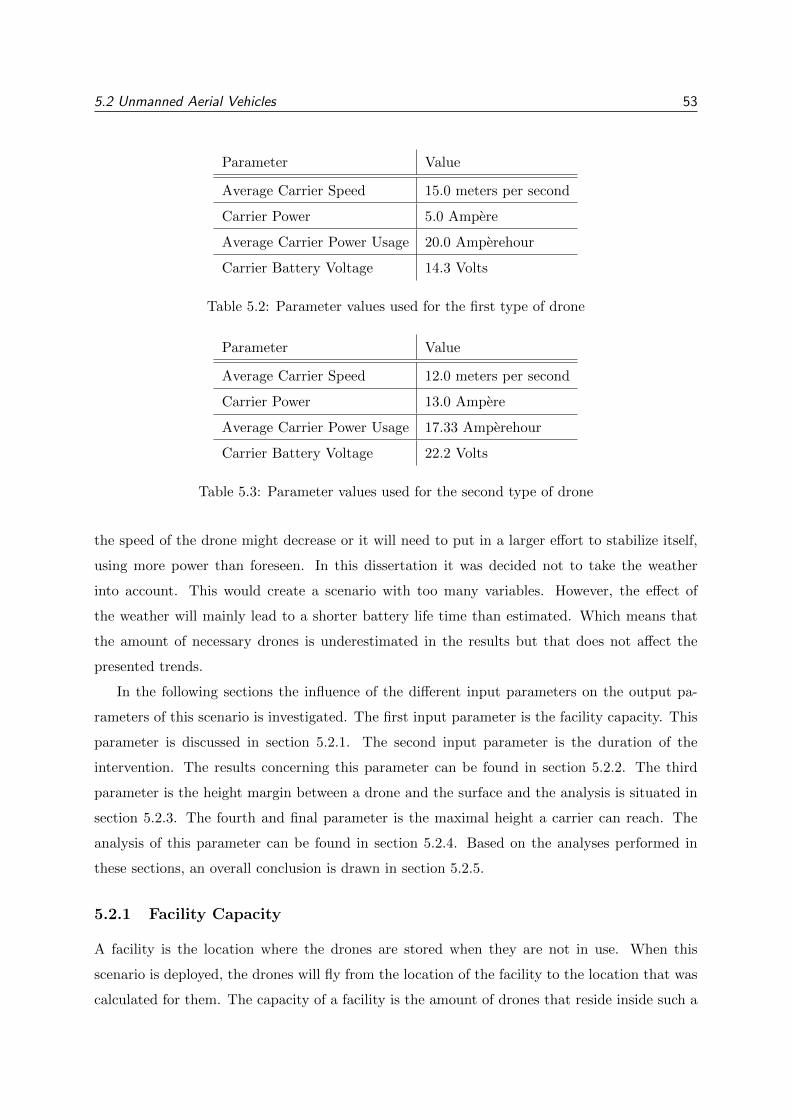
5.2 Unmanned Aerial Vehicles 53

Parameter Value

Average Carrier Speed 15.0 meters per second

Carrier Power 5.0 Ampere

Average Carrier Power Usage 20.0 Amperehour

Carrier Battery Voltage 14.3 Volts

Table 5.2: Parameter values used for the first type of drone

Parameter Value

Average Carrier Speed 12.0 meters per second

Carrier Power 13.0 Ampere

Average Carrier Power Usage 17.33 Amperehour

Carrier Battery Voltage 22.2 Volts

Table 5.3: Parameter values used for the second type of drone

the speed of the drone might decrease or it will need to put in a larger effort to stabilize itself,

using more power than foreseen. In this dissertation it was decided not to take the weather

into account. This would create a scenario with too many variables. However, the effect of

the weather will mainly lead to a shorter battery life time than estimated. Which means that

the amount of necessary drones is underestimated in the results but that does not affect the

presented trends.

In the following sections the influence of the different input parameters on the output pa-

rameters of this scenario is investigated. The first input parameter is the facility capacity. This

parameter is discussed in section 5.2.1. The second input parameter is the duration of the

intervention. The results concerning this parameter can be found in section 5.2.2. The third

parameter is the height margin between a drone and the surface and the analysis is situated in

section 5.2.3. The fourth and final parameter is the maximal height a carrier can reach. The

analysis of this parameter can be found in section 5.2.4. Based on the analyses performed in

these sections, an overall conclusion is drawn in section 5.2.5.

5.2.1 Facility Capacity

A facility is the location where the drones are stored when they are not in use. When this

scenario is deployed, the drones will fly from the location of the facility to the location that was

calculated for them. The capacity of a facility is the amount of drones that reside inside such a

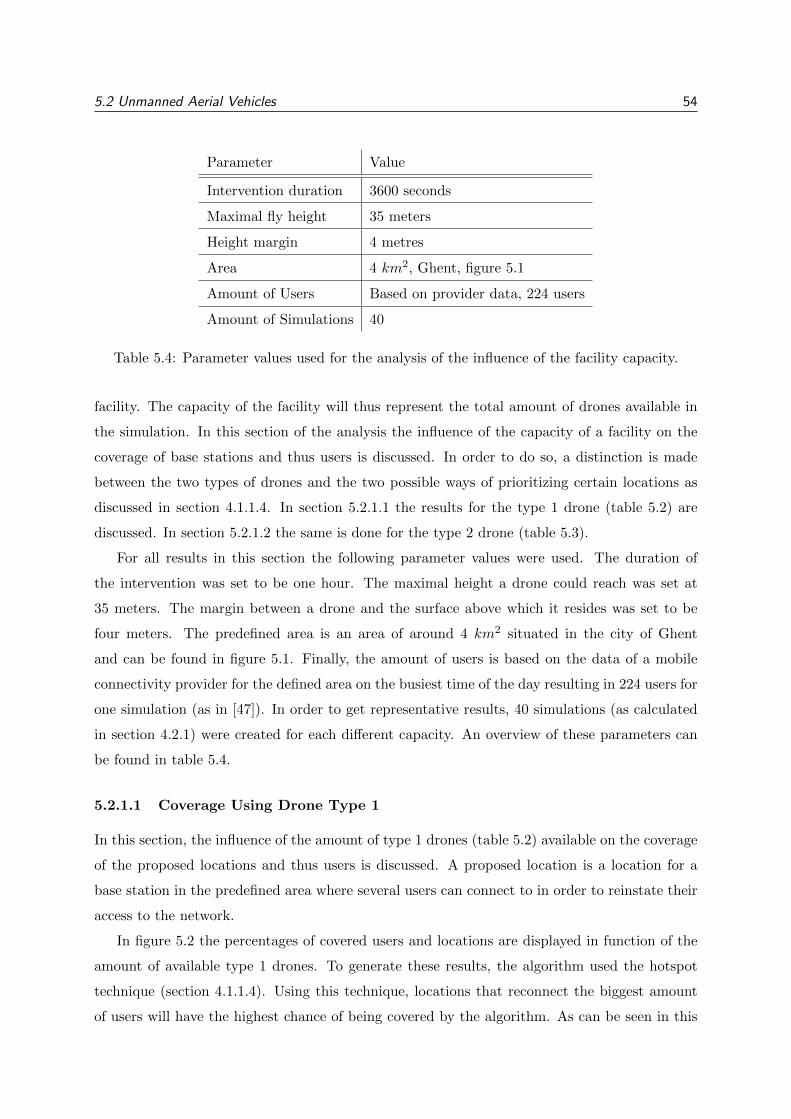
5.2 Unmanned Aerial Vehicles 54

Parameter Value

Intervention duration 3600 seconds

Maximal fly height 35 meters

Height margin 4 metres

Area 4 km2, Ghent, figure 5.1

Amount of Users Based on provider data, 224 users

Amount of Simulations 40

Table 5.4: Parameter values used for the analysis of the influence of the facility capacity.

facility. The capacity of the facility will thus represent the total amount of drones available in

the simulation. In this section of the analysis the influence of the capacity of a facility on the

coverage of base stations and thus users is discussed. In order to do so, a distinction is made

between the two types of drones and the two possible ways of prioritizing certain locations as

discussed in section 4.1.1.4. In section 5.2.1.1 the results for the type 1 drone (table 5.2) are

discussed. In section 5.2.1.2 the same is done for the type 2 drone (table 5.3).

For all results in this section the following parameter values were used. The duration of

the intervention was set to be one hour. The maximal height a drone could reach was set at

35 meters. The margin between a drone and the surface above which it resides was set to be

four meters. The predefined area is an area of around 4 km2 situated in the city of Ghent

and can be found in figure 5.1. Finally, the amount of users is based on the data of a mobile

connectivity provider for the defined area on the busiest time of the day resulting in 224 users for

one simulation (as in [47]). In order to get representative results, 40 simulations (as calculated

in section 4.2.1) were created for each different capacity. An overview of these parameters can

be found in table 5.4.

5.2.1.1 Coverage Using Drone Type 1

In this section, the influence of the amount of type 1 drones (table 5.2) available on the coverage

of the proposed locations and thus users is discussed. A proposed location is a location for a

base station in the predefined area where several users can connect to in order to reinstate their

access to the network.

In figure 5.2 the percentages of covered users and locations are displayed in function of the

amount of available type 1 drones. To generate these results, the algorithm used the hotspot

technique (section 4.1.1.4). Using this technique, locations that reconnect the biggest amount

of users will have the highest chance of being covered by the algorithm. As can be seen in this

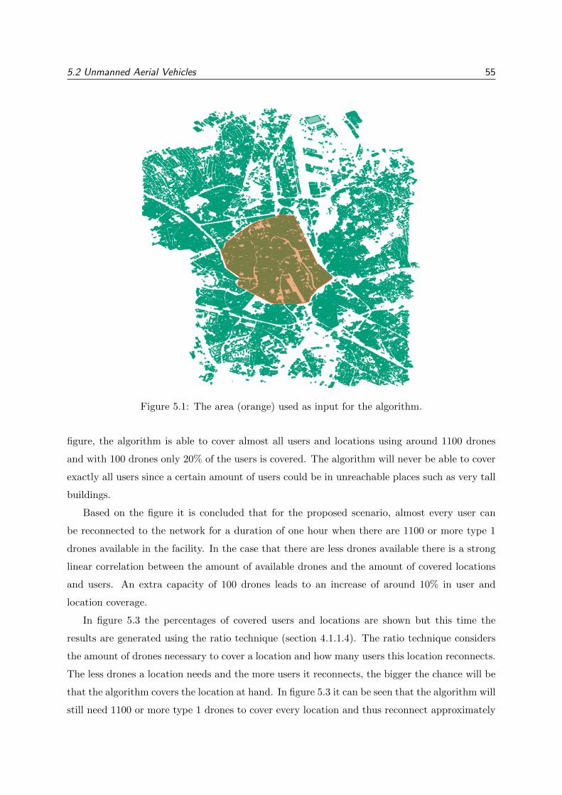
5.2 Unmanned Aerial Vehicles 55

Figure 5.1: The area (orange) used as input for the algorithm.

figure, the algorithm is able to cover almost all users and locations using around 1100 drones

and with 100 drones only 20% of the users is covered. The algorithm will never be able to cover

exactly all users since a certain amount of users could be in unreachable places such as very tall

buildings.

Based on the figure it is concluded that for the proposed scenario, almost every user can

be reconnected to the network for a duration of one hour when there are 1100 or more type 1

drones available in the facility. In the case that there are less drones available there is a strong

linear correlation between the amount of available drones and the amount of covered locations

and users. An extra capacity of 100 drones leads to an increase of around 10% in user and

location coverage.

In figure 5.3 the percentages of covered users and locations are shown but this time the

results are generated using the ratio technique (section 4.1.1.4). The ratio technique considers

the amount of drones necessary to cover a location and how many users this location reconnects.

The less drones a location needs and the more users it reconnects, the bigger the chance will be

that the algorithm covers the location at hand. In figure 5.3 it can be seen that the algorithm will

still need 1100 or more type 1 drones to cover every location and thus reconnect approximately

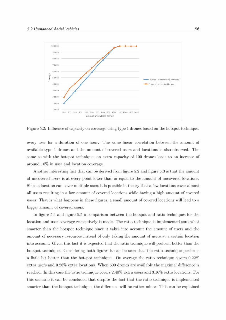
5.2 Unmanned Aerial Vehicles 56

Figure 5.2: Influence of capacity on coverage using type 1 drones based on the hotspot technique.

every user for a duration of one hour. The same linear correlation between the amount of

available type 1 drones and the amount of covered users and locations is also observed. The

same as with the hotspot technique, an extra capacity of 100 drones leads to an increase of

around 10% in user and location coverage.

Another interesting fact that can be derived from figure 5.2 and figure 5.3 is that the amount

of uncovered users is at every point lower than or equal to the amount of uncovered locations.

Since a location can cover multiple users it is possible in theory that a few locations cover almost

all users resulting in a low amount of covered locations while having a high amount of covered

users. That is what happens in these figures, a small amount of covered locations will lead to a

bigger amount of covered users.

In figure 5.4 and figure 5.5 a comparison between the hotspot and ratio techniques for the

location and user coverage respectively is made. The ratio technique is implemented somewhat

smarter than the hotspot technique since it takes into account the amount of users and the

amount of necessary resources instead of only taking the amount of users at a certain location

into account. Given this fact it is expected that the ratio technique will perform better than the

hotspot technique. Considering both figures it can be seen that the ratio technique performs

a little bit better than the hotspot technique. On average the ratio technique covers 0.22%

extra users and 0.28% extra locations. When 600 drones are available the maximal difference is

reached. In this case the ratio technique covers 2.40% extra users and 3.16% extra locations. For

this scenario it can be concluded that despite the fact that the ratio technique is implemented

smarter than the hotspot technique, the difference will be rather minor. This can be explained

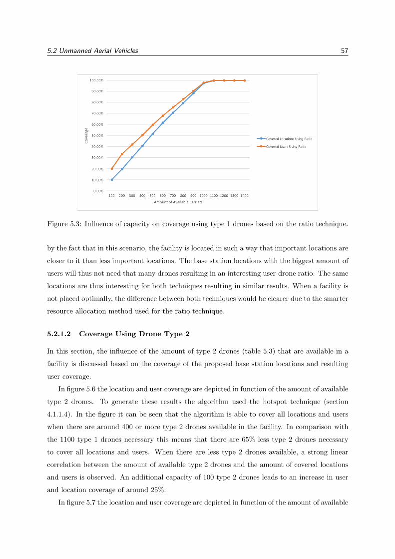
5.2 Unmanned Aerial Vehicles 57

Figure 5.3: Influence of capacity on coverage using type 1 drones based on the ratio technique.

by the fact that in this scenario, the facility is located in such a way that important locations are

closer to it than less important locations. The base station locations with the biggest amount of

users will thus not need that many drones resulting in an interesting user-drone ratio. The same

locations are thus interesting for both techniques resulting in similar results. When a facility is

not placed optimally, the difference between both techniques would be clearer due to the smarter

resource allocation method used for the ratio technique.

5.2.1.2 Coverage Using Drone Type 2

In this section, the influence of the amount of type 2 drones (table 5.3) that are available in a

facility is discussed based on the coverage of the proposed base station locations and resulting

user coverage.

In figure 5.6 the location and user coverage are depicted in function of the amount of available

type 2 drones. To generate these results the algorithm used the hotspot technique (section

4.1.1.4). In the figure it can be seen that the algorithm is able to cover all locations and users

when there are around 400 or more type 2 drones available in the facility. In comparison with

the 1100 type 1 drones necessary this means that there are 65% less type 2 drones necessary

to cover all locations and users. When there are less type 2 drones available, a strong linear

correlation between the amount of available type 2 drones and the amount of covered locations

and users is observed. An additional capacity of 100 type 2 drones leads to an increase in user

and location coverage of around 25%.

In figure 5.7 the location and user coverage are depicted in function of the amount of available

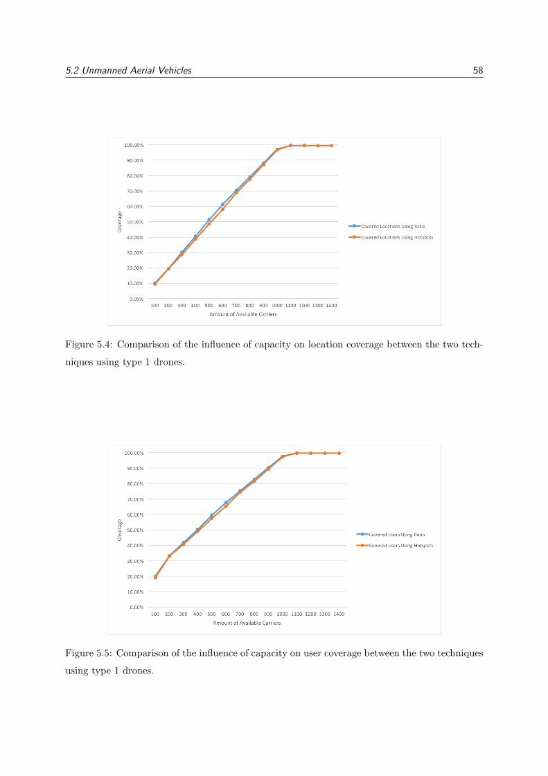
5.2 Unmanned Aerial Vehicles 58

Figure 5.4: Comparison of the influence of capacity on location coverage between the two tech-

niques using type 1 drones.

Figure 5.5: Comparison of the influence of capacity on user coverage between the two techniques

using type 1 drones.

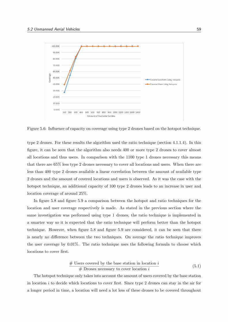
5.2 Unmanned Aerial Vehicles 59

Figure 5.6: Influence of capacity on coverage using type 2 drones based on the hotspot technique.

type 2 drones. For these results the algorithm used the ratio technique (section 4.1.1.4). In this

figure, it can be seen that the algorithm also needs 400 or more type 2 drones to cover almost

all locations and thus users. In comparison with the 1100 type 1 drones necessary this means

that there are 65% less type 2 drones necessary to cover all locations and users. When there are

less than 400 type 2 drones available a linear correlation between the amount of available type

2 drones and the amount of covered locations and users is observed. As it was the case with the

hotspot technique, an additional capacity of 100 type 2 drones leads to an increase in user and

location coverage of around 25%.

In figure 5.8 and figure 5.9 a comparison between the hotspot and ratio techniques for the

location and user coverage respectively is made. As stated in the previous section where the

same investigation was performed using type 1 drones, the ratio technique is implemented in

a smarter way so it is expected that the ratio technique will perform better than the hotspot

technique. However, when figure 5.8 and figure 5.9 are considered, it can be seen that there

is nearly no difference between the two techniques. On average the ratio technique improves

the user coverage by 0.01%. The ratio technique uses the following formula to choose which

locations to cover first.

# Users covered by the base station in location i

# Drones necessary to cover location i(5.1)

The hotspot technique only takes into account the amount of users covered by the base station

in location i to decide which locations to cover first. Since type 2 drones can stay in the air for

a longer period in time, a location will need a lot less of these drones to be covered throughout

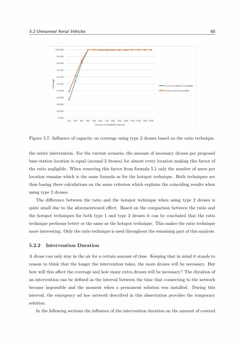
5.2 Unmanned Aerial Vehicles 60

Figure 5.7: Influence of capacity on coverage using type 2 drones based on the ratio technique.

the entire intervention. For the current scenario, the amount of necessary drones per proposed

base station location is equal (around 2 drones) for almost every location making this factor of

the ratio negligible. When removing this factor from formula 5.1 only the number of users per

location remains which is the same formula as for the hotspot technique. Both techniques are

thus basing there calculations on the same criterion which explains the coinciding results when

using type 2 drones.

The difference between the ratio and the hotspot technique when using type 2 drones is

quite small due to the aforementioned effect. Based on the comparison between the ratio and

the hotspot techniques for both type 1 and type 2 drones it can be concluded that the ratio

technique performs better or the same as the hotspot technique. This makes the ratio technique

more interesting. Only the ratio technique is used throughout the remaining part of this analysis.

5.2.2 Intervention Duration

A drone can only stay in the air for a certain amount of time. Keeping that in mind it stands to

reason to think that the longer the intervention takes, the more drones will be necessary. But

how will this affect the coverage and how many extra drones will be necessary? The duration of

an intervention can be defined as the interval between the time that connecting to the network

became impossible and the moment when a permanent solution was installed. During this

interval, the emergency ad hoc network described in this dissertation provides the temporary

solution.

In the following sections the influence of the intervention duration on the amount of covered

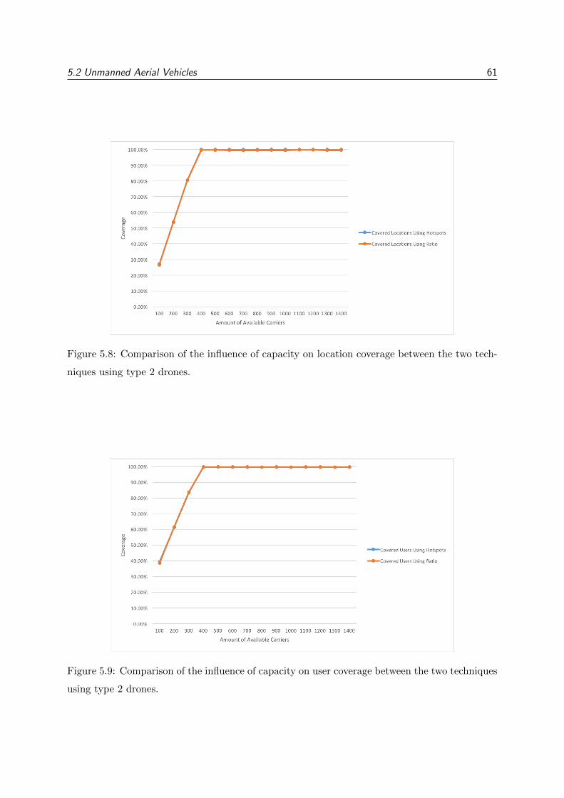
5.2 Unmanned Aerial Vehicles 61

Figure 5.8: Comparison of the influence of capacity on location coverage between the two tech-

niques using type 2 drones.

Figure 5.9: Comparison of the influence of capacity on user coverage between the two techniques

using type 2 drones.

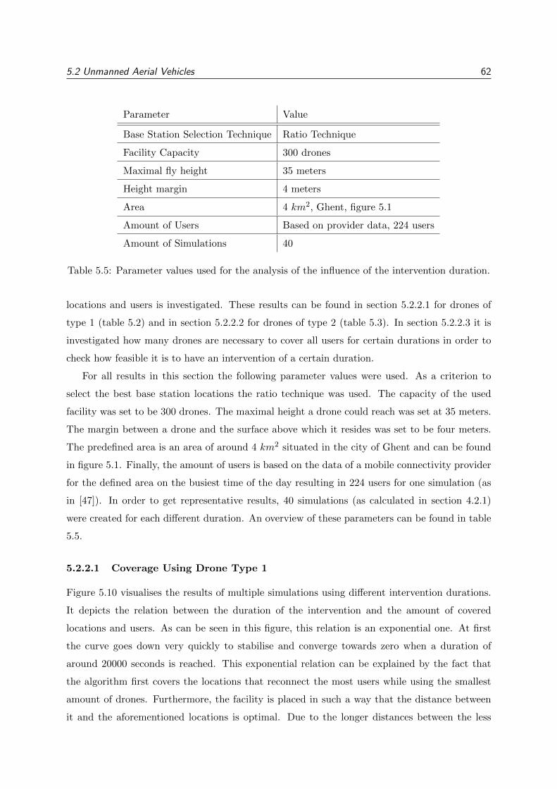
5.2 Unmanned Aerial Vehicles 62

Parameter Value

Base Station Selection Technique Ratio Technique

Facility Capacity 300 drones

Maximal fly height 35 meters

Height margin 4 meters

Area 4 km2, Ghent, figure 5.1

Amount of Users Based on provider data, 224 users

Amount of Simulations 40

Table 5.5: Parameter values used for the analysis of the influence of the intervention duration.

locations and users is investigated. These results can be found in section 5.2.2.1 for drones of

type 1 (table 5.2) and in section 5.2.2.2 for drones of type 2 (table 5.3). In section 5.2.2.3 it is

investigated how many drones are necessary to cover all users for certain durations in order to

check how feasible it is to have an intervention of a certain duration.

For all results in this section the following parameter values were used. As a criterion to

select the best base station locations the ratio technique was used. The capacity of the used

facility was set to be 300 drones. The maximal height a drone could reach was set at 35 meters.

The margin between a drone and the surface above which it resides was set to be four meters.

The predefined area is an area of around 4 km2 situated in the city of Ghent and can be found

in figure 5.1. Finally, the amount of users is based on the data of a mobile connectivity provider

for the defined area on the busiest time of the day resulting in 224 users for one simulation (as

in [47]). In order to get representative results, 40 simulations (as calculated in section 4.2.1)

were created for each different duration. An overview of these parameters can be found in table

5.5.

5.2.2.1 Coverage Using Drone Type 1

Figure 5.10 visualises the results of multiple simulations using different intervention durations.

It depicts the relation between the duration of the intervention and the amount of covered

locations and users. As can be seen in this figure, this relation is an exponential one. At first

the curve goes down very quickly to stabilise and converge towards zero when a duration of

around 20000 seconds is reached. This exponential relation can be explained by the fact that

the algorithm first covers the locations that reconnect the most users while using the smallest

amount of drones. Furthermore, the facility is placed in such a way that the distance between

it and the aforementioned locations is optimal. Due to the longer distances between the less

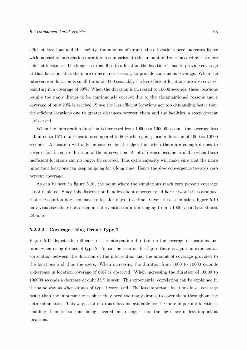
5.2 Unmanned Aerial Vehicles 63

efficient locations and the facility, the amount of drones these locations need increases faster

with increasing intervention duration in comparison to the amount of drones needed by the more

efficient locations. The longer a drone flies to a location the less time it has to provide coverage

at that location, thus the more drones are necessary to provide continuous coverage. When the

intervention duration is small (around 1000 seconds), the less efficient locations are also covered

resulting in a coverage of 80%. When the duration is increased to 10000 seconds, these locations

require too many drones to be continuously covered due to the aforementioned reasons and a

coverage of only 20% is reached. Since the less efficient locations get too demanding faster than

the efficient locations due to greater distances between them and the facilities, a steep descent

is observed.

When the intervention duration is increased from 10000 to 100000 seconds the coverage loss

is limited to 15% of all locations compared to 60% when going form a duration of 1000 to 10000

seconds. A location will only be covered by the algorithm when there are enough drones to

cover it for the entire duration of the intervention. A lot of drones become available when these

inefficient locations can no longer be covered. This extra capacity will make sure that the more

important locations can keep on going for a long time. Hence the slow convergence towards zero

percent coverage.

As can be seen in figure 5.10, the point where the simulations reach zero percent coverage

is not depicted. Since this dissertation handles about emergency ad hoc networks it is assumed

that the solution does not have to last for days at a time. Given this assumption, figure 5.10

only visualises the results from an intervention duration ranging from a 1000 seconds to almost

28 hours.

5.2.2.2 Coverage Using Drone Type 2

Figure 5.11 depicts the influence of the intervention duration on the coverage of locations and

users when using drones of type 2. As can be seen in this figure there is again an exponential

correlation between the duration of the intervention and the amount of coverage provided to

the locations and thus the users. When increasing the duration from 1000 to 10000 seconds

a decrease in location coverage of 60% is observed. When increasing the duration of 10000 to

100000 seconds a decrease of only 35% is seen. This exponential correlation can be explained in

the same way as when drones of type 1 were used. The less important locations loose coverage

faster than the important ones since they need too many drones to cover them throughout the

entire simulation. This way, a lot of drones become available for the more important locations,

enabling them to continue being covered much longer than the big share of less important

locations.

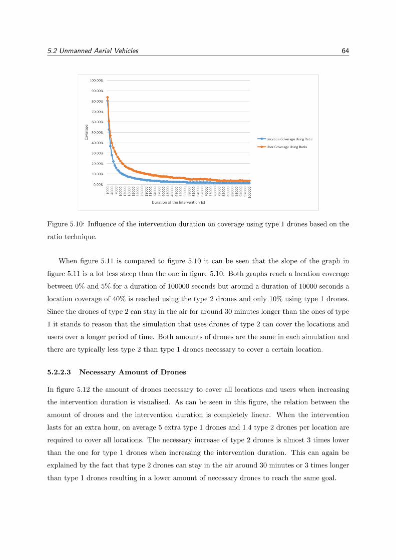
5.2 Unmanned Aerial Vehicles 64

Figure 5.10: Influence of the intervention duration on coverage using type 1 drones based on the

ratio technique.

When figure 5.11 is compared to figure 5.10 it can be seen that the slope of the graph in

figure 5.11 is a lot less steep than the one in figure 5.10. Both graphs reach a location coverage

between 0% and 5% for a duration of 100000 seconds but around a duration of 10000 seconds a

location coverage of 40% is reached using the type 2 drones and only 10% using type 1 drones.

Since the drones of type 2 can stay in the air for around 30 minutes longer than the ones of type

1 it stands to reason that the simulation that uses drones of type 2 can cover the locations and

users over a longer period of time. Both amounts of drones are the same in each simulation and

there are typically less type 2 than type 1 drones necessary to cover a certain location.

5.2.2.3 Necessary Amount of Drones

In figure 5.12 the amount of drones necessary to cover all locations and users when increasing

the intervention duration is visualised. As can be seen in this figure, the relation between the

amount of drones and the intervention duration is completely linear. When the intervention

lasts for an extra hour, on average 5 extra type 1 drones and 1.4 type 2 drones per location are

required to cover all locations. The necessary increase of type 2 drones is almost 3 times lower

than the one for type 1 drones when increasing the intervention duration. This can again be

explained by the fact that type 2 drones can stay in the air around 30 minutes or 3 times longer

than type 1 drones resulting in a lower amount of necessary drones to reach the same goal.

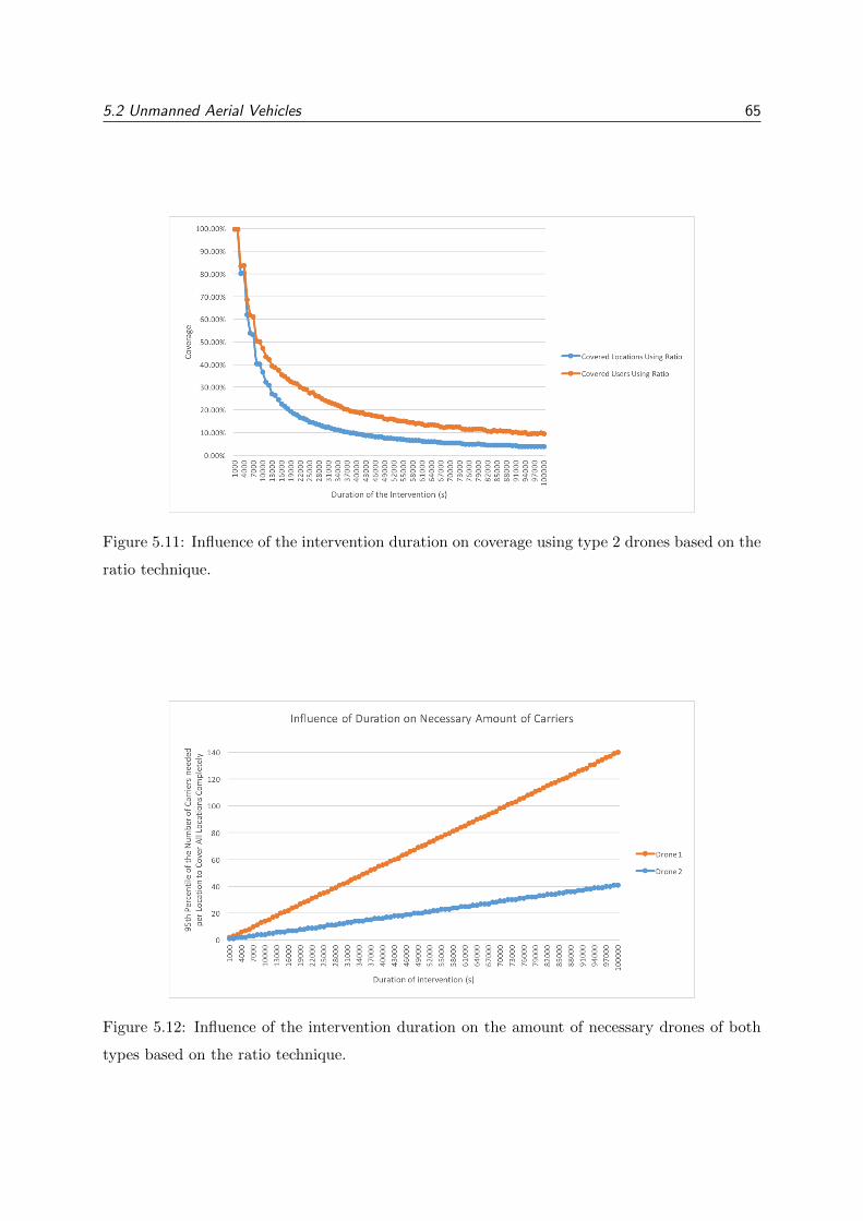
5.2 Unmanned Aerial Vehicles 65

Figure 5.11: Influence of the intervention duration on coverage using type 2 drones based on the

ratio technique.

Figure 5.12: Influence of the intervention duration on the amount of necessary drones of both

types based on the ratio technique.

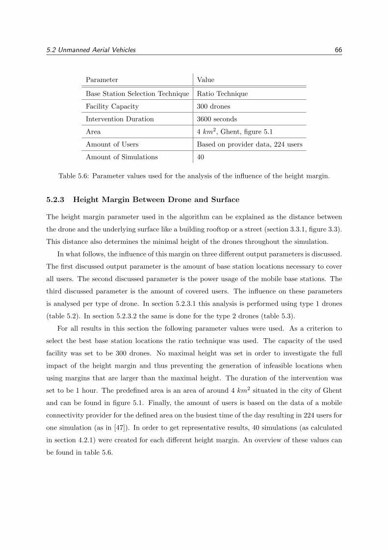
5.2 Unmanned Aerial Vehicles 66

Parameter Value

Base Station Selection Technique Ratio Technique

Facility Capacity 300 drones

Intervention Duration 3600 seconds

Area 4 km2, Ghent, figure 5.1

Amount of Users Based on provider data, 224 users

Amount of Simulations 40

Table 5.6: Parameter values used for the analysis of the influence of the height margin.

5.2.3 Height Margin Between Drone and Surface

The height margin parameter used in the algorithm can be explained as the distance between

the drone and the underlying surface like a building rooftop or a street (section 3.3.1, figure 3.3).

This distance also determines the minimal height of the drones throughout the simulation.

In what follows, the influence of this margin on three different output parameters is discussed.

The first discussed output parameter is the amount of base station locations necessary to cover

all users. The second discussed parameter is the power usage of the mobile base stations. The

third discussed parameter is the amount of covered users. The influence on these parameters

is analysed per type of drone. In section 5.2.3.1 this analysis is performed using type 1 drones

(table 5.2). In section 5.2.3.2 the same is done for the type 2 drones (table 5.3).

For all results in this section the following parameter values were used. As a criterion to

select the best base station locations the ratio technique was used. The capacity of the used

facility was set to be 300 drones. No maximal height was set in order to investigate the full

impact of the height margin and thus preventing the generation of infeasible locations when

using margins that are larger than the maximal height. The duration of the intervention was

set to be 1 hour. The predefined area is an area of around 4 km2 situated in the city of Ghent

and can be found in figure 5.1. Finally, the amount of users is based on the data of a mobile

connectivity provider for the defined area on the busiest time of the day resulting in 224 users for

one simulation (as in [47]). In order to get representative results, 40 simulations (as calculated

in section 4.2.1) were created for each different height margin. An overview of these values can

be found in table 5.6.

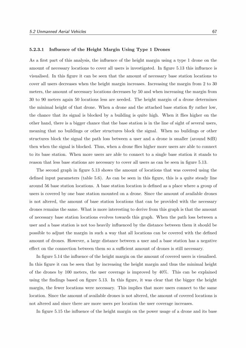
5.2 Unmanned Aerial Vehicles 67

5.2.3.1 Influence of the Height Margin Using Type 1 Drones

As a first part of this analysis, the influence of the height margin using a type 1 drone on the

amount of necessary locations to cover all users is investigated. In figure 5.13 this influence is

visualised. In this figure it can be seen that the amount of necessary base station locations to

cover all users decreases when the height margin increases. Increasing the margin from 2 to 30

meters, the amount of necessary locations decreases by 50 and when increasing the margin from

30 to 90 meters again 50 locations less are needed. The height margin of a drone determines

the minimal height of that drone. When a drone and the attached base station fly rather low,

the chance that its signal is blocked by a building is quite high. When it flies higher on the

other hand, there is a bigger chance that the base station is in the line of sight of several users,

meaning that no buildings or other structures block the signal. When no buildings or other

structures block the signal the path loss between a user and a drone is smaller (around 8dB)

then when the signal is blocked. Thus, when a drone flies higher more users are able to connect

to its base station. When more users are able to connect to a single base station it stands to

reason that less base stations are necessary to cover all users as can be seen in figure 5.13.

The second graph in figure 5.13 shows the amount of locations that was covered using the

defined input parameters (table 5.6). As can be seen in this figure, this is a quite steady line

around 56 base station locations. A base station location is defined as a place where a group of

users is covered by one base station mounted on a drone. Since the amount of available drones

is not altered, the amount of base station locations that can be provided with the necessary

drones remains the same. What is more interesting to derive from this graph is that the amount

of necessary base station locations evolves towards this graph. When the path loss between a

user and a base station is not too heavily influenced by the distance between them it should be

possible to adjust the margin in such a way that all locations can be covered with the defined

amount of drones. However, a large distance between a user and a base station has a negative

effect on the connection between them so a sufficient amount of drones is still necessary.

In figure 5.14 the influence of the height margin on the amount of covered users is visualised.

In this figure it can be seen that by increasing the height margin and thus the minimal height

of the drones by 100 meters, the user coverage is improved by 40%. This can be explained

using the findings based on figure 5.13. In this figure, it was clear that the bigger the height

margin, the fewer locations were necessary. This implies that more users connect to the same

location. Since the amount of available drones is not altered, the amount of covered locations is

not altered and since there are more users per location the user coverage increases.

In figure 5.15 the influence of the height margin on the power usage of a drone and its base

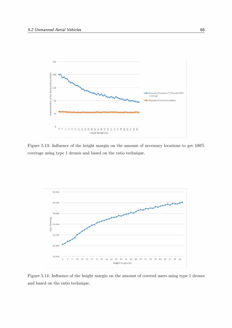
5.2 Unmanned Aerial Vehicles 68

Figure 5.13: Influence of the height margin on the amount of necessary locations to get 100%

coverage using type 1 drones and based on the ratio technique.

Figure 5.14: Influence of the height margin on the amount of covered users using type 1 drones

and based on the ratio technique.

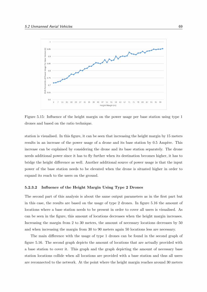
5.2 Unmanned Aerial Vehicles 69

Figure 5.15: Influence of the height margin on the power usage per base station using type 1

drones and based on the ratio technique.

station is visualised. In this figure, it can be seen that increasing the height margin by 15 meters

results in an increase of the power usage of a drone and its base station by 0.5 Ampere. This

increase can be explained by considering the drone and its base station separately. The drone

needs additional power since it has to fly further when its destination becomes higher, it has to

bridge the height difference as well. Another additional source of power usage is that the input

power of the base station needs to be elevated when the drone is situated higher in order to

expand its reach to the users on the ground.

5.2.3.2 Influence of the Height Margin Using Type 2 Drones

The second part of this analysis is about the same output parameters as in the first part but

in this case, the results are based on the usage of type 2 drones. In figure 5.16 the amount of

locations where a base station needs to be present in order to cover all users is visualised. As

can be seen in the figure, this amount of locations decreases when the height margin increases.

Increasing the margin from 2 to 30 meters, the amount of necessary locations decreases by 50

and when increasing the margin from 30 to 90 meters again 50 locations less are necessary.

The main difference with the usage of type 1 drones can be found in the second graph of

figure 5.16. The second graph depicts the amount of locations that are actually provided with

a base station to cover it. This graph and the graph depicting the amount of necessary base

station locations collide when all locations are provided with a base station and thus all users

are reconnected to the network. At the point where the height margin reaches around 30 meters

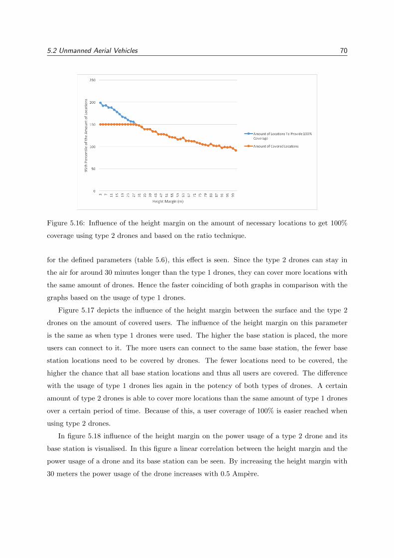
5.2 Unmanned Aerial Vehicles 70

Figure 5.16: Influence of the height margin on the amount of necessary locations to get 100%

coverage using type 2 drones and based on the ratio technique.

for the defined parameters (table 5.6), this effect is seen. Since the type 2 drones can stay in

the air for around 30 minutes longer than the type 1 drones, they can cover more locations with

the same amount of drones. Hence the faster coinciding of both graphs in comparison with the

graphs based on the usage of type 1 drones.

Figure 5.17 depicts the influence of the height margin between the surface and the type 2

drones on the amount of covered users. The influence of the height margin on this parameter

is the same as when type 1 drones were used. The higher the base station is placed, the more

users can connect to it. The more users can connect to the same base station, the fewer base

station locations need to be covered by drones. The fewer locations need to be covered, the

higher the chance that all base station locations and thus all users are covered. The difference

with the usage of type 1 drones lies again in the potency of both types of drones. A certain

amount of type 2 drones is able to cover more locations than the same amount of type 1 drones

over a certain period of time. Because of this, a user coverage of 100% is easier reached when

using type 2 drones.

In figure 5.18 influence of the height margin on the power usage of a type 2 drone and its

base station is visualised. In this figure a linear correlation between the height margin and the

power usage of a drone and its base station can be seen. By increasing the height margin with

30 meters the power usage of the drone increases with 0.5 Ampere.

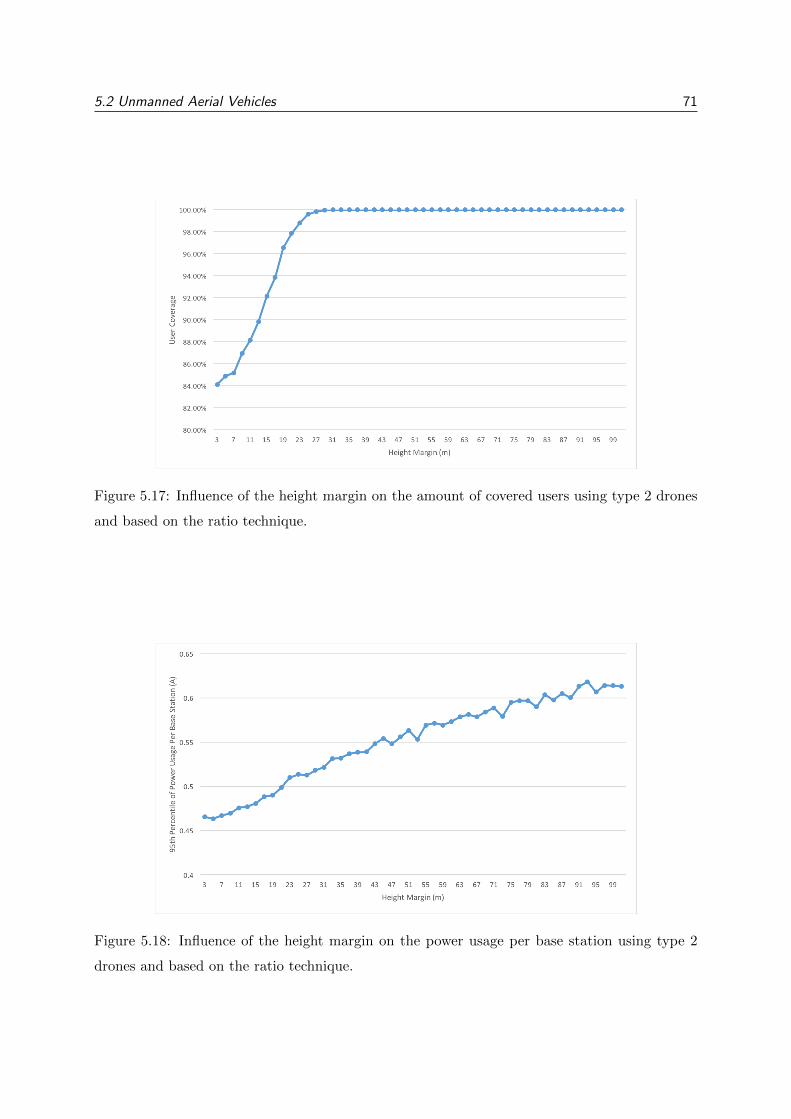
5.2 Unmanned Aerial Vehicles 71

Figure 5.17: Influence of the height margin on the amount of covered users using type 2 drones

and based on the ratio technique.

Figure 5.18: Influence of the height margin on the power usage per base station using type 2

drones and based on the ratio technique.

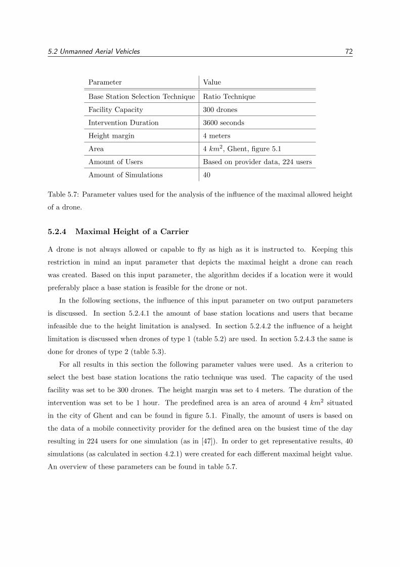
5.2 Unmanned Aerial Vehicles 72

Parameter Value

Base Station Selection Technique Ratio Technique

Facility Capacity 300 drones

Intervention Duration 3600 seconds

Height margin 4 meters

Area 4 km2, Ghent, figure 5.1

Amount of Users Based on provider data, 224 users

Amount of Simulations 40

Table 5.7: Parameter values used for the analysis of the influence of the maximal allowed height

of a drone.

5.2.4 Maximal Height of a Carrier

A drone is not always allowed or capable to fly as high as it is instructed to. Keeping this

restriction in mind an input parameter that depicts the maximal height a drone can reach

was created. Based on this input parameter, the algorithm decides if a location were it would

preferably place a base station is feasible for the drone or not.

In the following sections, the influence of this input parameter on two output parameters

is discussed. In section 5.2.4.1 the amount of base station locations and users that became

infeasible due to the height limitation is analysed. In section 5.2.4.2 the influence of a height

limitation is discussed when drones of type 1 (table 5.2) are used. In section 5.2.4.3 the same is

done for drones of type 2 (table 5.3).

For all results in this section the following parameter values were used. As a criterion to

select the best base station locations the ratio technique was used. The capacity of the used

facility was set to be 300 drones. The height margin was set to 4 meters. The duration of the

intervention was set to be 1 hour. The predefined area is an area of around 4 km2 situated

in the city of Ghent and can be found in figure 5.1. Finally, the amount of users is based on

the data of a mobile connectivity provider for the defined area on the busiest time of the day

resulting in 224 users for one simulation (as in [47]). In order to get representative results, 40

simulations (as calculated in section 4.2.1) were created for each different maximal height value.

An overview of these parameters can be found in table 5.7.

5.2 Unmanned Aerial Vehicles 73

Figure 5.19: Influence of the maximal height a drone can reach on the reachability of base station

locations and users using type 1 drones and based on the ratio technique.

5.2.4.1 Amount of Infeasible Locations and Users

The amount of base station locations and users that became infeasible by a certain height

limitation is not affected by the type of drone used. This output parameter merely represents

how many base station locations proposed by the algorithm are not taken into consideration for

the generation of the new network because they are too high. Figure 5.19 visualises the amount

of base station locations that became infeasible due to the use of a height limitation. The

figure also visualises the amount of users that can only connect to a base station in a restricted

location, no other base station locations are viable for these users leaving them uncovered purely

due to the enforced height restriction. As can be seen in this figure, around 50% of all locations

become infeasible when the maximal allowed height is less than 10 meters. When the maximal

height increases, the amount of infeasible locations and users drops rapidly and becomes almost

zero when a maximal height of around 30 meters is used. These results reveal that there are

not many buildings in the used area that are taller than 30 meters. The tallest building in the

area is around 120 meters high so the amount of infeasible locations will be completely zero if

a maximal height of more than 120 meters is used.

5.2.4.2 Influence Using Type 1 Drones

In figure 5.20 the influence of the maximal height on the amount of covered base station locations

and users is visualised. In this figure it can be seen that the amount of covered locations and

users only increases slightly (5% when increasing the maximal height from 4 to 40 metres after

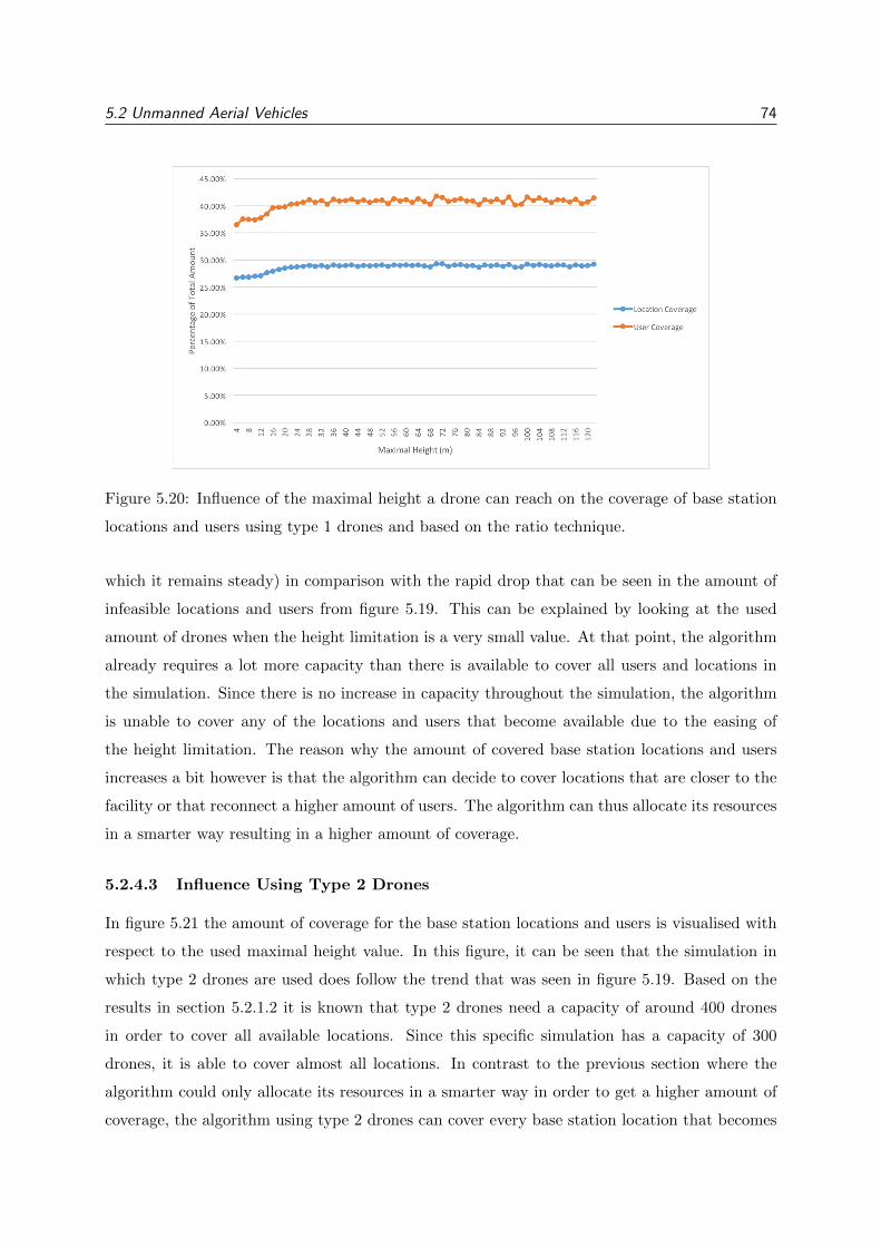
5.2 Unmanned Aerial Vehicles 74

Figure 5.20: Influence of the maximal height a drone can reach on the coverage of base station

locations and users using type 1 drones and based on the ratio technique.

which it remains steady) in comparison with the rapid drop that can be seen in the amount of

infeasible locations and users from figure 5.19. This can be explained by looking at the used

amount of drones when the height limitation is a very small value. At that point, the algorithm

already requires a lot more capacity than there is available to cover all users and locations in

the simulation. Since there is no increase in capacity throughout the simulation, the algorithm

is unable to cover any of the locations and users that become available due to the easing of

the height limitation. The reason why the amount of covered base station locations and users

increases a bit however is that the algorithm can decide to cover locations that are closer to the

facility or that reconnect a higher amount of users. The algorithm can thus allocate its resources

in a smarter way resulting in a higher amount of coverage.

5.2.4.3 Influence Using Type 2 Drones

In figure 5.21 the amount of coverage for the base station locations and users is visualised with

respect to the used maximal height value. In this figure, it can be seen that the simulation in

which type 2 drones are used does follow the trend that was seen in figure 5.19. Based on the

results in section 5.2.1.2 it is known that type 2 drones need a capacity of around 400 drones

in order to cover all available locations. Since this specific simulation has a capacity of 300

drones, it is able to cover almost all locations. In contrast to the previous section where the

algorithm could only allocate its resources in a smarter way in order to get a higher amount of

coverage, the algorithm using type 2 drones can cover every base station location that becomes

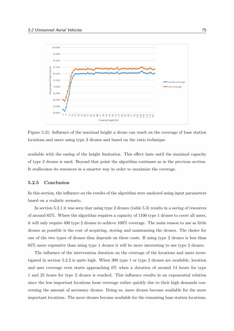
5.2 Unmanned Aerial Vehicles 75

Figure 5.21: Influence of the maximal height a drone can reach on the coverage of base station

locations and users using type 2 drones and based on the ratio technique.

available with the easing of the height limitation. This effect lasts until the maximal capacity

of type 2 drones is used. Beyond that point the algorithm continues as in the previous section.

It reallocates its resources in a smarter way in order to maximize the coverage.

5.2.5 Conclusion

In this section, the influence on the results of the algorithm were analysed using input parameters

based on a realistic scenario.

In section 5.2.1 it was seen that using type 2 drones (table 5.3) results in a saving of resources

of around 65%. Where the algorithm requires a capacity of 1100 type 1 drones to cover all users,

it will only require 400 type 2 drones to achieve 100% coverage. The main reason to use as little

drones as possible is the cost of acquiring, storing and maintaining the drones. The choice for

one of the two types of drones thus depends on these costs. If using type 2 drones is less than

65% more expensive than using type 1 drones it will be more interesting to use type 2 drones.

The influence of the intervention duration on the coverage of the locations and users inves-

tigated in section 5.2.2 is quite high. When 300 type 1 or type 2 drones are available, location

and user coverage even starts approaching 0% when a duration of around 14 hours for type

1 and 25 hours for type 2 drones is reached. This influence results in an exponential relation

since the less important locations loose coverage rather quickly due to their high demands con-

cerning the amount of necessary drones. Doing so, more drones become available for the more

important locations. The more drones become available for the remaining base station locations,

5.2 Unmanned Aerial Vehicles 76

the slower the convergence. In order to use this scenario in practice it is thus very important

to let the amount of drones increase with the foreseen duration of the intervention. It can be

concluded that a linear increase of the amount of drones is sufficient to nullify the effect of an

increasing intervention duration. When comparing type 1 and type 2 drones it can be seen

that the influence of an increasing intervention duration has a slower impact on type 2 drones.

When deploying this scenario in practice, type 2 drones will thus be more interesting when the

intervention duration is harder to estimate.

Based on the results in section 5.2.3 it can be concluded that increasing the height margin and

thus the minimal height of a drone and its base station results in a more economical solution.

Elevating the average position of the drone increases the chance that no obstacles or other

structures block the signal between a base station and a user. Because of this, the same base

station is accessible for more users than it was before. Since more users can connect to one base

station, the need for base stations decreases and thus the same amount of connectivity can be

reached using a smaller amount of base stations.

The difference between the usage of type 1 or type 2 drones in section 5.2.3 is rather small.

Since type 2 drones are more potent they can serve more unique locations than type 1 drones

can for the same amount of time. The bigger the minimal height, the lower the amount of base

station locations necessary to cover all users. Given these facts, the same amount of type 2

drones can cover all present users and locations with a lower height margin than type 1 drones

can since a lower margin implies more necessary locations. Type 2 drones will thus be the better

choice if the potential height margin is rather small and the same capacity of both drones is

available. When high altitudes can be reached it may however be more interesting to use type 1

drones since with the same amount of these cheaper drones, the same level of connectivity can

be reached. This is of course only true when it is assumed that the path loss does not get too

big because of the added distance that the larger margin creates.

In section 5.2.4 it is seen that a height limitation might have big consequences for the output

of the used algorithm. When the limitation is very severe (around 10 meters), up to 50% of all

base station locations and 40% of the users stay uncovered. For the used area, the limitation

looses its effect when it exceeds 30 meters. It is best to prevent such a limitation in real life

scenarios. When such a limitation is inevitable it is useful to look at the heights of all possible

base station locations to estimate the success rate of the scenario. This is however very hard to

do since the location of the intervention is not known beforehand.

Based on the results in this section it can be concluded that using the proposed scenario

and parameters the described connectivity problem could be solved. However, there are some

important requirements. The amount of available drones needs to be high enough and the height

5.3 Emergency Services Vehicles 77

cannot be too severely limited. When enough height can be reached, fewer drones need to be

utilized. An important factor that is not discussed in this section is the capacity of the backhaul

connection. Depending on the amount of users that need to be reconnected, more capacity will

be necessary. The capacity of this connection depends on the chosen technology to provide it.

As discussed in section 2.4 several possibilities exist and the right one needs to be chosen in

order to prevent the backhaul of becoming the bottleneck of the system.

5.3 Emergency Services Vehicles

The next scenario described in chapter 3 is the one that uses emergency service vehicles to get

the base stations in place (section 3.1.2). In this scenario, the placement of the base stations

is no longer planned ahead as was done with the scenario based on drones. Emergency service

vehicles can not be sent off to some predefined place, they will go to the place where their help

is needed the most. Because of this, this scenario will only be able to reconnect users within a

certain distance of the disaster site.

Emergency service vehicles are not likely to be spread out over an area of around 4 km2

which is why a smaller area was used for the following simulations. The input parameters in

this section are based on an event called ”De Gentse Feesten”. This is an annual event that lasts

for 10 days and is situated in a part of the city of Ghent that is around 1 km2 big (figure 5.22).

This event was attended by around 100 000 people every day in the year 2015 [50]. During the

simulations in this section it was assumed that around 50 000 people were at the event at the

same time and some kind of incident occurred at the center of the event area. This incident

required a certain amount of unspecified emergency service vehicles in which base stations were

installed.

In the following sections the influence of the different variable input parameters is investi-

gated. In section 5.3.1 the influence of the amount of emergency service vehicles that are present

in the area is investigated. The influence of the chance that a vehicle is present in the area but

leaves before the intervention is over is analysed in section 5.3.2. In section 5.3.3, the influence

of the size of the incident is investigated. Based on these three sections a conclusion concerning

this scenario is drawn in section 5.3.4.

5.3.1 Available Emergency Service Vehicles

The first input parameter analysed is the amount of vehicles that are available in the area. This

is the total amount of emergency service vehicles that have been in the area for a certain amount

of time during the intervention. It is not the amount of base stations that is eventually used to

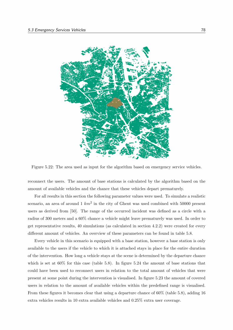
5.3 Emergency Services Vehicles 78

Figure 5.22: The area used as input for the algorithm based on emergency service vehicles.

reconnect the users. The amount of base stations is calculated by the algorithm based on the

amount of available vehicles and the chance that these vehicles depart prematurely.

For all results in this section the following parameter values were used. To simulate a realistic

scenario, an area of around 1 km2 in the city of Ghent was used combined with 50000 present

users as derived from [50]. The range of the occurred incident was defined as a circle with a

radius of 300 meters and a 60% chance a vehicle might leave prematurely was used. In order to

get representative results, 40 simulations (as calculated in section 4.2.2) were created for every

different amount of vehicles. An overview of these parameters can be found in table 5.8.

Every vehicle in this scenario is equipped with a base station, however a base station is only

available to the users if the vehicle to which it is attached stays in place for the entire duration

of the intervention. How long a vehicle stays at the scene is determined by the departure chance

which is set at 60% for this case (table 5.8). In figure 5.24 the amount of base stations that

could have been used to reconnect users in relation to the total amount of vehicles that were

present at some point during the intervention is visualised. In figure 5.23 the amount of covered

users in relation to the amount of available vehicles within the predefined range is visualised.

From these figures it becomes clear that using a departure chance of 60% (table 5.8), adding 16

extra vehicles results in 10 extra available vehicles and 0.25% extra user coverage.

5.3 Emergency Services Vehicles 79

Parameter Value

Area 1 km2, old city centre Ghent, figure 5.22

Number of Users 50000 users

Incident Range 300 meters

Chance a Vehicle Leaves Prematurely 60%

Number of Simulations 40

Table 5.8: Parameter values used for the analysis of the influence of the amount of available

emergency service vehicles.

Figure 5.23: Influence of the amount of vehicles present at the scene on the amount of covered

users.

Another element that can be derived from figure 5.23 is that the amount of covered users

is rather low, around 1.8% when 100 vehicles are used. This can be explained by the fact

that a LTE femtocell can only cover as many users as its properties allow him to. Since the

area is flooded with users that want to be reconnected, the base stations are saturated rather

quickly and no additional users can be reconnected. Based on figures 5.24 and 5.23 it can be

assumed that around 5000 well positioned, continuously available vehicles are necessary to cover

all users in the area. This is an enormous amount of emergency service vehicles to expect in a

realistic scenario. The scenario using emergency service vehicles with the current parameters is

practically infeasible.

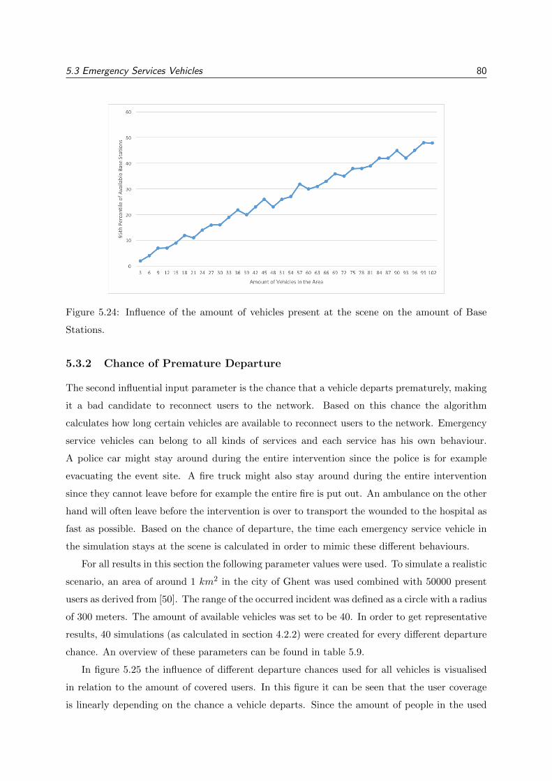
5.3 Emergency Services Vehicles 80

Figure 5.24: Influence of the amount of vehicles present at the scene on the amount of Base

Stations.

5.3.2 Chance of Premature Departure

The second influential input parameter is the chance that a vehicle departs prematurely, making

it a bad candidate to reconnect users to the network. Based on this chance the algorithm

calculates how long certain vehicles are available to reconnect users to the network. Emergency

service vehicles can belong to all kinds of services and each service has his own behaviour.

A police car might stay around during the entire intervention since the police is for example

evacuating the event site. A fire truck might also stay around during the entire intervention

since they cannot leave before for example the entire fire is put out. An ambulance on the other

hand will often leave before the intervention is over to transport the wounded to the hospital as

fast as possible. Based on the chance of departure, the time each emergency service vehicle in

the simulation stays at the scene is calculated in order to mimic these different behaviours.

For all results in this section the following parameter values were used. To simulate a realistic

scenario, an area of around 1 km2 in the city of Ghent was used combined with 50000 present

users as derived from [50]. The range of the occurred incident was defined as a circle with a radius

of 300 meters. The amount of available vehicles was set to be 40. In order to get representative

results, 40 simulations (as calculated in section 4.2.2) were created for every different departure

chance. An overview of these parameters can be found in table 5.9.

In figure 5.25 the influence of different departure chances used for all vehicles is visualised

in relation to the amount of covered users. In this figure it can be seen that the user coverage

is linearly depending on the chance a vehicle departs. Since the amount of people in the used

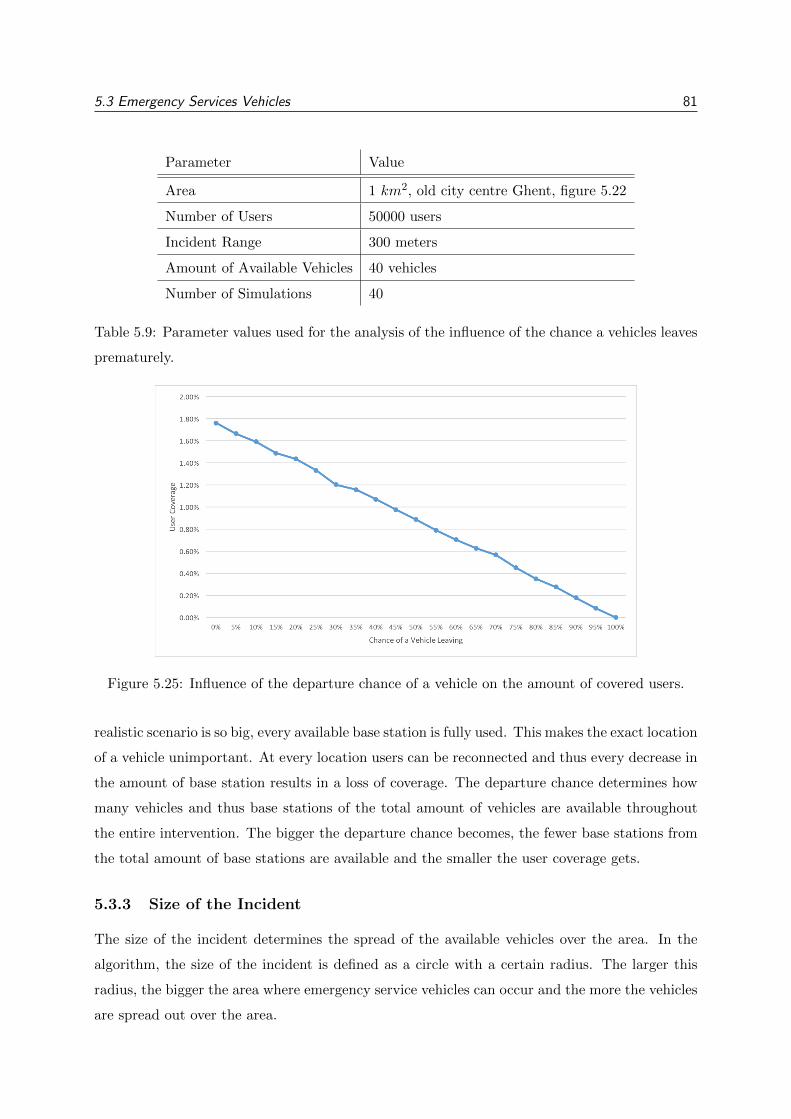
5.3 Emergency Services Vehicles 81

Parameter Value

Area 1 km2, old city centre Ghent, figure 5.22

Number of Users 50000 users

Incident Range 300 meters

Amount of Available Vehicles 40 vehicles

Number of Simulations 40

Table 5.9: Parameter values used for the analysis of the influence of the chance a vehicles leaves

prematurely.

Figure 5.25: Influence of the departure chance of a vehicle on the amount of covered users.

realistic scenario is so big, every available base station is fully used. This makes the exact location

of a vehicle unimportant. At every location users can be reconnected and thus every decrease in

the amount of base station results in a loss of coverage. The departure chance determines how

many vehicles and thus base stations of the total amount of vehicles are available throughout

the entire intervention. The bigger the departure chance becomes, the fewer base stations from

the total amount of base stations are available and the smaller the user coverage gets.

5.3.3 Size of the Incident

The size of the incident determines the spread of the available vehicles over the area. In the

algorithm, the size of the incident is defined as a circle with a certain radius. The larger this

radius, the bigger the area where emergency service vehicles can occur and the more the vehicles

are spread out over the area.

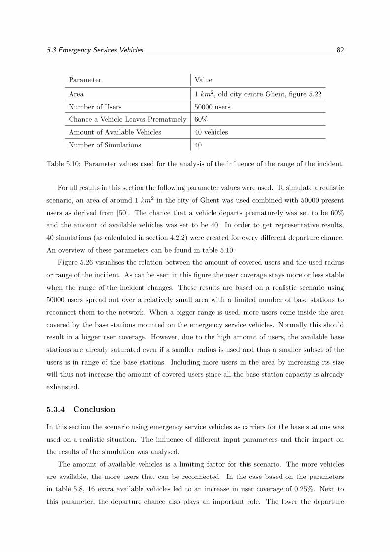
5.3 Emergency Services Vehicles 82

Parameter Value

Area 1 km2, old city centre Ghent, figure 5.22

Number of Users 50000 users

Chance a Vehicle Leaves Prematurely 60%

Amount of Available Vehicles 40 vehicles

Number of Simulations 40

Table 5.10: Parameter values used for the analysis of the influence of the range of the incident.

For all results in this section the following parameter values were used. To simulate a realistic

scenario, an area of around 1 km2 in the city of Ghent was used combined with 50000 present

users as derived from [50]. The chance that a vehicle departs prematurely was set to be 60%

and the amount of available vehicles was set to be 40. In order to get representative results,

40 simulations (as calculated in section 4.2.2) were created for every different departure chance.

An overview of these parameters can be found in table 5.10.

Figure 5.26 visualises the relation between the amount of covered users and the used radius

or range of the incident. As can be seen in this figure the user coverage stays more or less stable

when the range of the incident changes. These results are based on a realistic scenario using

50000 users spread out over a relatively small area with a limited number of base stations to

reconnect them to the network. When a bigger range is used, more users come inside the area

covered by the base stations mounted on the emergency service vehicles. Normally this should

result in a bigger user coverage. However, due to the high amount of users, the available base

stations are already saturated even if a smaller radius is used and thus a smaller subset of the

users is in range of the base stations. Including more users in the area by increasing its size

will thus not increase the amount of covered users since all the base station capacity is already

exhausted.

5.3.4 Conclusion

In this section the scenario using emergency service vehicles as carriers for the base stations was

used on a realistic situation. The influence of different input parameters and their impact on

the results of the simulation was analysed.

The amount of available vehicles is a limiting factor for this scenario. The more vehicles

are available, the more users that can be reconnected. In the case based on the parameters

in table 5.8, 16 extra available vehicles led to an increase in user coverage of 0.25%. Next to

this parameter, the departure chance also plays an important role. The lower the departure

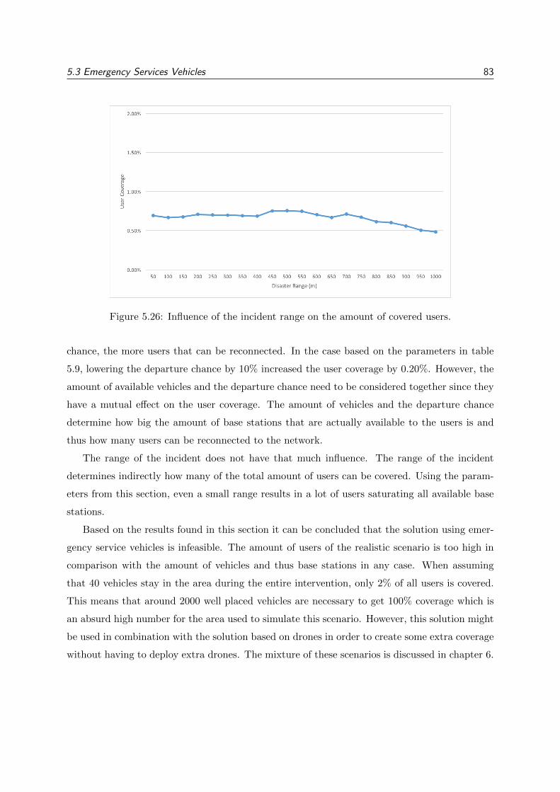
5.3 Emergency Services Vehicles 83

Figure 5.26: Influence of the incident range on the amount of covered users.

chance, the more users that can be reconnected. In the case based on the parameters in table

5.9, lowering the departure chance by 10% increased the user coverage by 0.20%. However, the

amount of available vehicles and the departure chance need to be considered together since they

have a mutual effect on the user coverage. The amount of vehicles and the departure chance

determine how big the amount of base stations that are actually available to the users is and

thus how many users can be reconnected to the network.

The range of the incident does not have that much influence. The range of the incident

determines indirectly how many of the total amount of users can be covered. Using the param-

eters from this section, even a small range results in a lot of users saturating all available base

stations.

Based on the results found in this section it can be concluded that the solution using emer-

gency service vehicles is infeasible. The amount of users of the realistic scenario is too high in

comparison with the amount of vehicles and thus base stations in any case. When assuming

that 40 vehicles stay in the area during the entire intervention, only 2% of all users is covered.

This means that around 2000 well placed vehicles are necessary to get 100% coverage which is

an absurd high number for the area used to simulate this scenario. However, this solution might

be used in combination with the solution based on drones in order to create some extra coverage

without having to deploy extra drones. The mixture of these scenarios is discussed in chapter 6.

5.4 Public Transportation Vehicles 84

5.4 Public Transportation Vehicles

In chapter 3, a third and final scenario is introduced (section 3.1.3). In this scenario the necessary

base stations are brought into place by public transport vehicles. The biggest difference with

the drone and the emergency services scenario is that public transport vehicles move around the

entire time, making them only useful when they stand still for a longer period of time or when

they replace each other at a certain location in order to provide continuous coverage at such a

location. These locations are called stops and they depict the gathering place for lots of public

transport vehicles.

In this section the type of public transport vehicles is limited to buses and taxis. These two

types of vehicles have a clear behaviour, they appear in almost every city and they form the

majority of public transport vehicles. To be able to base these simulations on realistic figures,

the situation for these two types of vehicles in the city of Ghent was investigated. From this

investigation it was concluded that the amount of bus stops is typically a lot lower than the

amount of taxi stops. However, a bus stop typically is bigger in size and thus contains more

platforms than a taxi stop [51, 52, 53]. These findings are also taken into consideration in the

following analyses.

Based on four input parameters, the feasibility and the requirements of an emergency ad hoc

network based on buses and taxis is analysed. In section 5.4.1, the influence of the amount of

stops in the area where buses or taxis can reside on the output of the algorithm is investigated.

In section 5.4.2, the same is done for the influence of the size of the different stops that are

spread out over the area. In section 5.4.3, the influence of the chance that a vehicle is covering

a certain stop on the results of the algorithm is analysed.

5.4.1 Amount of Stops

The amount of stops is the amount of gathering places for public transport vehicles spread out

across the used area. A stop in this dissertation is defined as one point in the area where multiple

platforms occur. A platform is a place where one public transport vehicle can be stationed for

a certain amount of time. Throughout the analysis in this section a split between stops of taxis

and stops of buses is made. They are used in the same simulation, covering the same area in

order to get the combined result but they are considered separately in order to investigate their

separate influence on the big picture.

For all results in this section the following parameter values were used. To simulate a realistic

scenario, the amount of bus stops was taken four times smaller than the amount of taxi stops

as derived from [51, 52]. The sizes of the bus stops however were taken bigger than the sizes

5.4 Public Transportation Vehicles 85

Parameter Value

Amount of Bus Stops x

Amount of Taxi Stops 4 · x

Bus Stop Size Uniformly Selected Element of [1, 20]

Taxi Stop Size Uniformly Selected Element of [1, 5]

Chance a Bus Is Available At a Platform 50%

Chance a Taxi Is Available At a Platform 30%

Area 4 km2, Ghent, figure 5.1

Amount of Users Based on provider data, 224 users

Amount of Simulations 40

Table 5.11: Parameter values used for the analysis of the influence of the amount of bus and

taxi stops in the predefined area.

of the taxi stops. The sizes of the bus stops were selected in a uniform way from the interval

[1, 20], the size of a bus stop can thus be any number between 1 and 20. The sizes of the taxi

stops were selected in a uniform way from the interval [1, 5], the size of a taxi stop can thus be

any number between 1 and 5. The chance a bus is continuously present at one of the platforms

of a certain stop was set to be 50% and the chance a taxi is continuously present at one of the

platforms of a certain stop was set to be 30%. The area that was used is approximately 4 km2

big and is situated in the city of Ghent (figure 5.1). Finally, the amount of users is based on

the data of a mobile connectivity provider for the defined area on the busiest time of the day

resulting in 224 users for one simulation (as in [47]). In order to get representative results, 40

simulations (as calculated in section 4.2.3) were created for every different amount of stops. An

overview of these parameters can be found in table 5.11.

5.4.1.1 Influence of the Amount of Bus Stops in the Area

Figure 5.27 visualises the effect of increasing the amount of bus stops on the amount of maximal,

selected and used base stations. Every base station is mounted on a bus. The maximal amount

of base stations is the amount of base stations if all platforms at every stop in the area are filled

for 100% with buses. The selected amount of base stations is the amount of base stations that

is actually spread over the platforms of all certain stop in the area when the availability chance

of a vehicle is taken into account. The used amount of stops is the amount of base stations that

were eventually used to reconnect users to the network.

As can be seen in figure 5.27, the maximal and selected amounts of base stations rise linearly

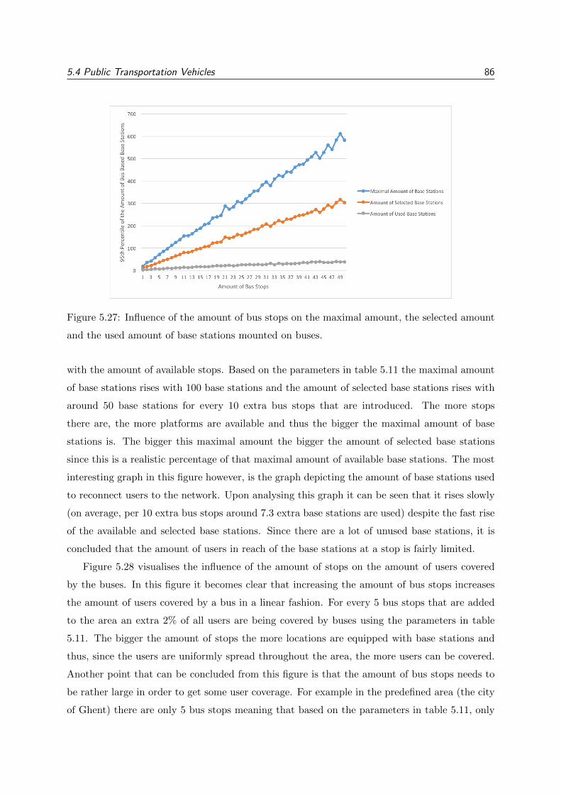
5.4 Public Transportation Vehicles 86

Figure 5.27: Influence of the amount of bus stops on the maximal amount, the selected amount

and the used amount of base stations mounted on buses.

with the amount of available stops. Based on the parameters in table 5.11 the maximal amount

of base stations rises with 100 base stations and the amount of selected base stations rises with

around 50 base stations for every 10 extra bus stops that are introduced. The more stops

there are, the more platforms are available and thus the bigger the maximal amount of base

stations is. The bigger this maximal amount the bigger the amount of selected base stations

since this is a realistic percentage of that maximal amount of available base stations. The most

interesting graph in this figure however, is the graph depicting the amount of base stations used

to reconnect users to the network. Upon analysing this graph it can be seen that it rises slowly

(on average, per 10 extra bus stops around 7.3 extra base stations are used) despite the fast rise

of the available and selected base stations. Since there are a lot of unused base stations, it is

concluded that the amount of users in reach of the base stations at a stop is fairly limited.

Figure 5.28 visualises the influence of the amount of stops on the amount of users covered

by the buses. In this figure it becomes clear that increasing the amount of bus stops increases

the amount of users covered by a bus in a linear fashion. For every 5 bus stops that are added

to the area an extra 2% of all users are being covered by buses using the parameters in table

5.11. The bigger the amount of stops the more locations are equipped with base stations and

thus, since the users are uniformly spread throughout the area, the more users can be covered.

Another point that can be concluded from this figure is that the amount of bus stops needs to

be rather large in order to get some user coverage. For example in the predefined area (the city

of Ghent) there are only 5 bus stops meaning that based on the parameters in table 5.11, only

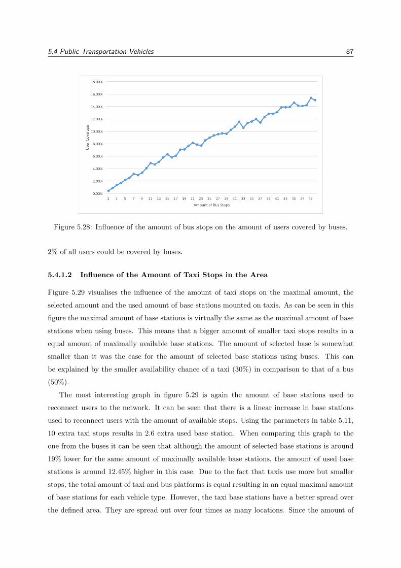
5.4 Public Transportation Vehicles 87

Figure 5.28: Influence of the amount of bus stops on the amount of users covered by buses.

2% of all users could be covered by buses.

5.4.1.2 Influence of the Amount of Taxi Stops in the Area

Figure 5.29 visualises the influence of the amount of taxi stops on the maximal amount, the

selected amount and the used amount of base stations mounted on taxis. As can be seen in this

figure the maximal amount of base stations is virtually the same as the maximal amount of base

stations when using buses. This means that a bigger amount of smaller taxi stops results in a

equal amount of maximally available base stations. The amount of selected base is somewhat

smaller than it was the case for the amount of selected base stations using buses. This can

be explained by the smaller availability chance of a taxi (30%) in comparison to that of a bus

(50%).

The most interesting graph in figure 5.29 is again the amount of base stations used to

reconnect users to the network. It can be seen that there is a linear increase in base stations

used to reconnect users with the amount of available stops. Using the parameters in table 5.11,

10 extra taxi stops results in 2.6 extra used base station. When comparing this graph to the

one from the buses it can be seen that although the amount of selected base stations is around

19% lower for the same amount of maximally available base stations, the amount of used base

stations is around 12.45% higher in this case. Due to the fact that taxis use more but smaller

stops, the total amount of taxi and bus platforms is equal resulting in an equal maximal amount

of base stations for each vehicle type. However, the taxi base stations have a better spread over

the defined area. They are spread out over four times as many locations. Since the amount of

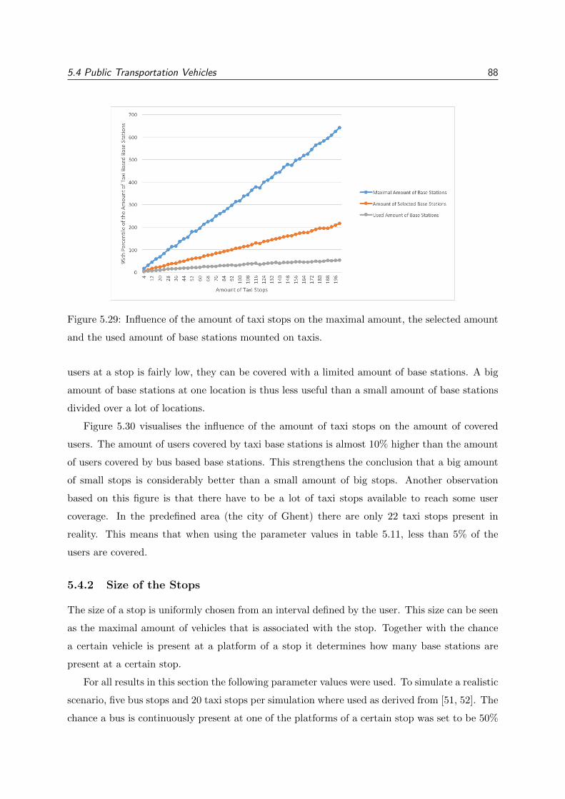
5.4 Public Transportation Vehicles 88

Figure 5.29: Influence of the amount of taxi stops on the maximal amount, the selected amount

and the used amount of base stations mounted on taxis.

users at a stop is fairly low, they can be covered with a limited amount of base stations. A big

amount of base stations at one location is thus less useful than a small amount of base stations

divided over a lot of locations.

Figure 5.30 visualises the influence of the amount of taxi stops on the amount of covered

users. The amount of users covered by taxi base stations is almost 10% higher than the amount

of users covered by bus based base stations. This strengthens the conclusion that a big amount

of small stops is considerably better than a small amount of big stops. Another observation

based on this figure is that there have to be a lot of taxi stops available to reach some user

coverage. In the predefined area (the city of Ghent) there are only 22 taxi stops present in

reality. This means that when using the parameter values in table 5.11, less than 5% of the

users are covered.

5.4.2 Size of the Stops

The size of a stop is uniformly chosen from an interval defined by the user. This size can be seen

as the maximal amount of vehicles that is associated with the stop. Together with the chance

a certain vehicle is present at a platform of a stop it determines how many base stations are

present at a certain stop.

For all results in this section the following parameter values were used. To simulate a realistic

scenario, five bus stops and 20 taxi stops per simulation where used as derived from [51, 52]. The

chance a bus is continuously present at one of the platforms of a certain stop was set to be 50%

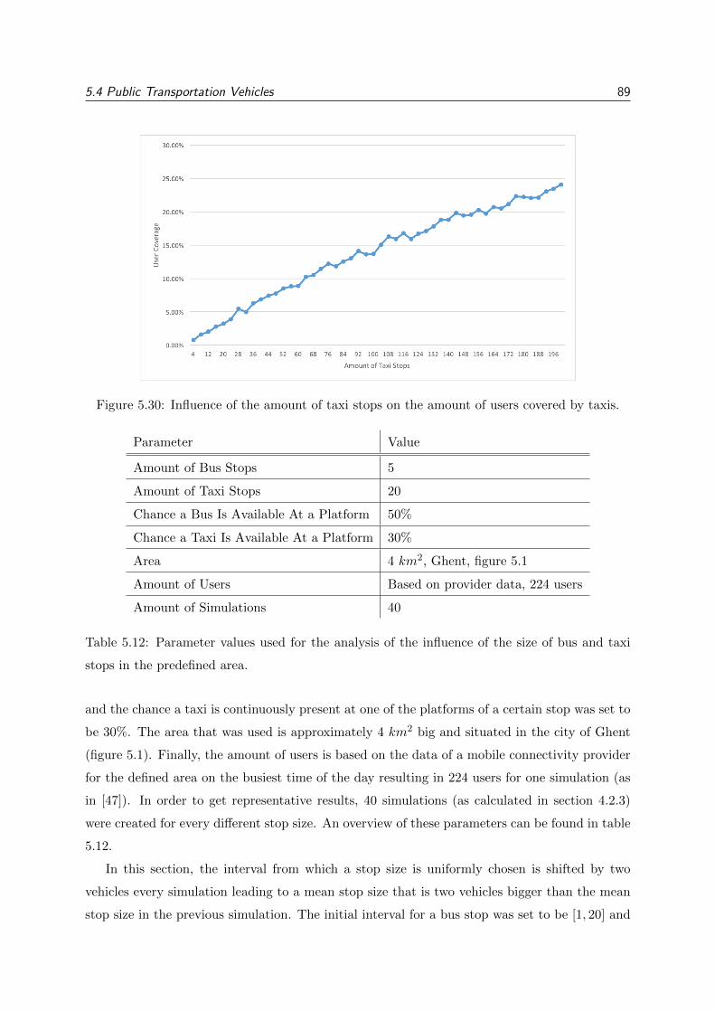
5.4 Public Transportation Vehicles 89

Figure 5.30: Influence of the amount of taxi stops on the amount of users covered by taxis.

Parameter Value

Amount of Bus Stops 5

Amount of Taxi Stops 20

Chance a Bus Is Available At a Platform 50%

Chance a Taxi Is Available At a Platform 30%

Area 4 km2, Ghent, figure 5.1

Amount of Users Based on provider data, 224 users

Amount of Simulations 40

Table 5.12: Parameter values used for the analysis of the influence of the size of bus and taxi

stops in the predefined area.

and the chance a taxi is continuously present at one of the platforms of a certain stop was set to

be 30%. The area that was used is approximately 4 km2 big and situated in the city of Ghent

(figure 5.1). Finally, the amount of users is based on the data of a mobile connectivity provider

for the defined area on the busiest time of the day resulting in 224 users for one simulation (as

in [47]). In order to get representative results, 40 simulations (as calculated in section 4.2.3)

were created for every different stop size. An overview of these parameters can be found in table

5.12.

In this section, the interval from which a stop size is uniformly chosen is shifted by two

vehicles every simulation leading to a mean stop size that is two vehicles bigger than the mean

stop size in the previous simulation. The initial interval for a bus stop was set to be [1, 20] and

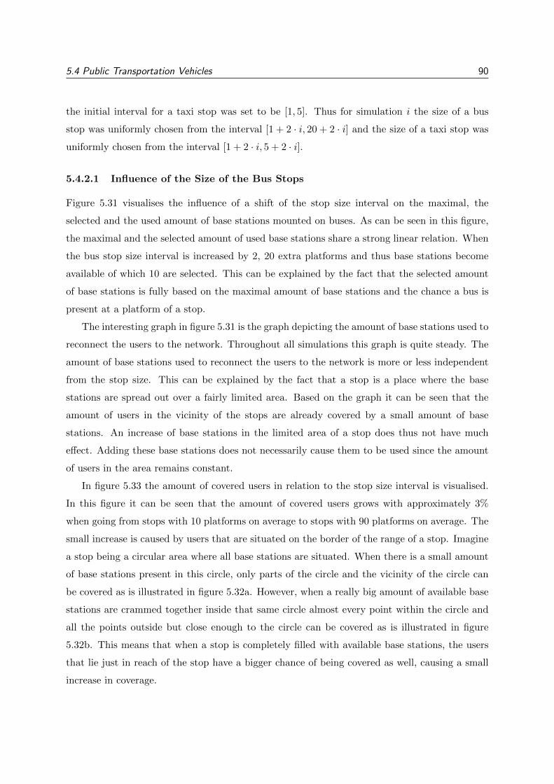
5.4 Public Transportation Vehicles 90

the initial interval for a taxi stop was set to be [1, 5]. Thus for simulation i the size of a bus

stop was uniformly chosen from the interval [1 + 2 · i, 20 + 2 · i] and the size of a taxi stop was

uniformly chosen from the interval [1 + 2 · i, 5 + 2 · i].

5.4.2.1 Influence of the Size of the Bus Stops

Figure 5.31 visualises the influence of a shift of the stop size interval on the maximal, the

selected and the used amount of base stations mounted on buses. As can be seen in this figure,

the maximal and the selected amount of used base stations share a strong linear relation. When

the bus stop size interval is increased by 2, 20 extra platforms and thus base stations become

available of which 10 are selected. This can be explained by the fact that the selected amount

of base stations is fully based on the maximal amount of base stations and the chance a bus is

present at a platform of a stop.

The interesting graph in figure 5.31 is the graph depicting the amount of base stations used to

reconnect the users to the network. Throughout all simulations this graph is quite steady. The

amount of base stations used to reconnect the users to the network is more or less independent

from the stop size. This can be explained by the fact that a stop is a place where the base

stations are spread out over a fairly limited area. Based on the graph it can be seen that the

amount of users in the vicinity of the stops are already covered by a small amount of base

stations. An increase of base stations in the limited area of a stop does thus not have much

effect. Adding these base stations does not necessarily cause them to be used since the amount

of users in the area remains constant.

In figure 5.33 the amount of covered users in relation to the stop size interval is visualised.

In this figure it can be seen that the amount of covered users grows with approximately 3%

when going from stops with 10 platforms on average to stops with 90 platforms on average. The

small increase is caused by users that are situated on the border of the range of a stop. Imagine

a stop being a circular area where all base stations are situated. When there is a small amount

of base stations present in this circle, only parts of the circle and the vicinity of the circle can

be covered as is illustrated in figure 5.32a. However, when a really big amount of available base

stations are crammed together inside that same circle almost every point within the circle and

all the points outside but close enough to the circle can be covered as is illustrated in figure

5.32b. This means that when a stop is completely filled with available base stations, the users

that lie just in reach of the stop have a bigger chance of being covered as well, causing a small

increase in coverage.

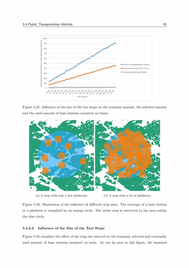
5.4 Public Transportation Vehicles 91

Figure 5.31: Influence of the size of the bus stops on the maximal amount, the selected amount

and the used amount of base stations mounted on buses.

(a) A stop with only a few platforms. (b) A stop with a lot of platforms.

Figure 5.32: Illustration of the influence of different stop sizes. The coverage of a base station

at a platform is visualised by an orange circle. The entire stop is restricted to the area within

the blue circle.

5.4.2.2 Influence of the Size of the Taxi Stops

Figure 5.34 visualises the effect of the stop size interval on the maximal, selected and eventually

used amount of base stations mounted on taxis. As can be seen in this figure, the maximal

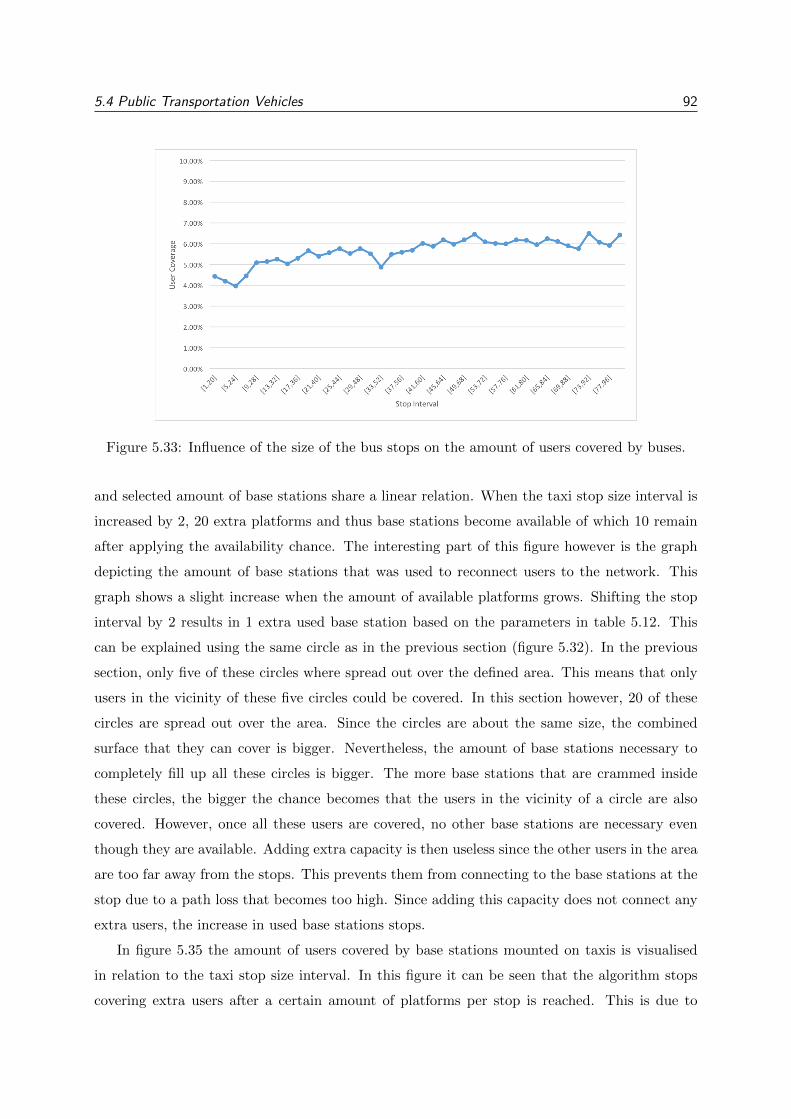
5.4 Public Transportation Vehicles 92

Figure 5.33: Influence of the size of the bus stops on the amount of users covered by buses.

and selected amount of base stations share a linear relation. When the taxi stop size interval is

increased by 2, 20 extra platforms and thus base stations become available of which 10 remain

after applying the availability chance. The interesting part of this figure however is the graph

depicting the amount of base stations that was used to reconnect users to the network. This

graph shows a slight increase when the amount of available platforms grows. Shifting the stop

interval by 2 results in 1 extra used base station based on the parameters in table 5.12. This

can be explained using the same circle as in the previous section (figure 5.32). In the previous

section, only five of these circles where spread out over the defined area. This means that only

users in the vicinity of these five circles could be covered. In this section however, 20 of these

circles are spread out over the area. Since the circles are about the same size, the combined

surface that they can cover is bigger. Nevertheless, the amount of base stations necessary to

completely fill up all these circles is bigger. The more base stations that are crammed inside

these circles, the bigger the chance becomes that the users in the vicinity of a circle are also

covered. However, once all these users are covered, no other base stations are necessary even

though they are available. Adding extra capacity is then useless since the other users in the area

are too far away from the stops. This prevents them from connecting to the base stations at the

stop due to a path loss that becomes too high. Since adding this capacity does not connect any

extra users, the increase in used base stations stops.

In figure 5.35 the amount of users covered by base stations mounted on taxis is visualised

in relation to the taxi stop size interval. In this figure it can be seen that the algorithm stops

covering extra users after a certain amount of platforms per stop is reached. This is due to

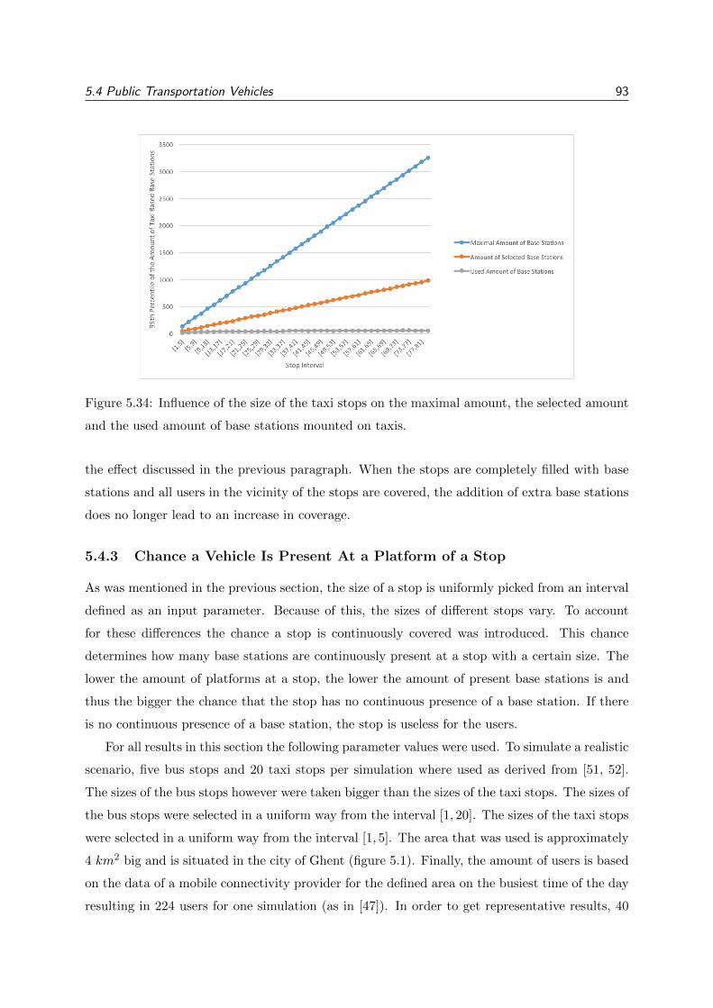
5.4 Public Transportation Vehicles 93

Figure 5.34: Influence of the size of the taxi stops on the maximal amount, the selected amount

and the used amount of base stations mounted on taxis.

the effect discussed in the previous paragraph. When the stops are completely filled with base

stations and all users in the vicinity of the stops are covered, the addition of extra base stations

does no longer lead to an increase in coverage.

5.4.3 Chance a Vehicle Is Present At a Platform of a Stop

As was mentioned in the previous section, the size of a stop is uniformly picked from an interval

defined as an input parameter. Because of this, the sizes of different stops vary. To account

for these differences the chance a stop is continuously covered was introduced. This chance

determines how many base stations are continuously present at a stop with a certain size. The

lower the amount of platforms at a stop, the lower the amount of present base stations is and

thus the bigger the chance that the stop has no continuous presence of a base station. If there

is no continuous presence of a base station, the stop is useless for the users.

For all results in this section the following parameter values were used. To simulate a realistic

scenario, five bus stops and 20 taxi stops per simulation where used as derived from [51, 52].

The sizes of the bus stops however were taken bigger than the sizes of the taxi stops. The sizes of

the bus stops were selected in a uniform way from the interval [1, 20]. The sizes of the taxi stops

were selected in a uniform way from the interval [1, 5]. The area that was used is approximately

4 km2 big and is situated in the city of Ghent (figure 5.1). Finally, the amount of users is based

on the data of a mobile connectivity provider for the defined area on the busiest time of the day

resulting in 224 users for one simulation (as in [47]). In order to get representative results, 40

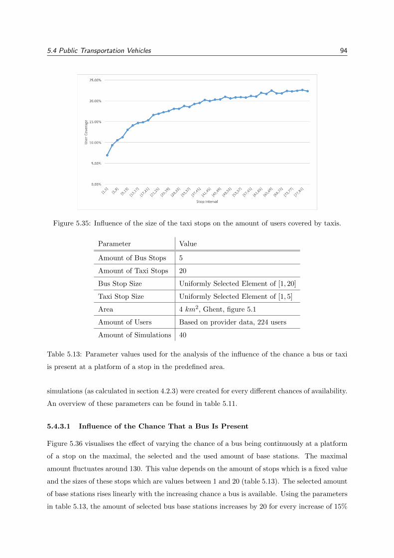
5.4 Public Transportation Vehicles 94

Figure 5.35: Influence of the size of the taxi stops on the amount of users covered by taxis.

Parameter Value

Amount of Bus Stops 5

Amount of Taxi Stops 20

Bus Stop Size Uniformly Selected Element of [1, 20]

Taxi Stop Size Uniformly Selected Element of [1, 5]

Area 4 km2, Ghent, figure 5.1

Amount of Users Based on provider data, 224 users

Amount of Simulations 40

Table 5.13: Parameter values used for the analysis of the influence of the chance a bus or taxi

is present at a platform of a stop in the predefined area.

simulations (as calculated in section 4.2.3) were created for every different chances of availability.

An overview of these parameters can be found in table 5.11.

5.4.3.1 Influence of the Chance That a Bus Is Present

Figure 5.36 visualises the effect of varying the chance of a bus being continuously at a platform

of a stop on the maximal, the selected and the used amount of base stations. The maximal

amount fluctuates around 130. This value depends on the amount of stops which is a fixed value

and the sizes of these stops which are values between 1 and 20 (table 5.13). The selected amount

of base stations rises linearly with the increasing chance a bus is available. Using the parameters

in table 5.13, the amount of selected bus base stations increases by 20 for every increase of 15%

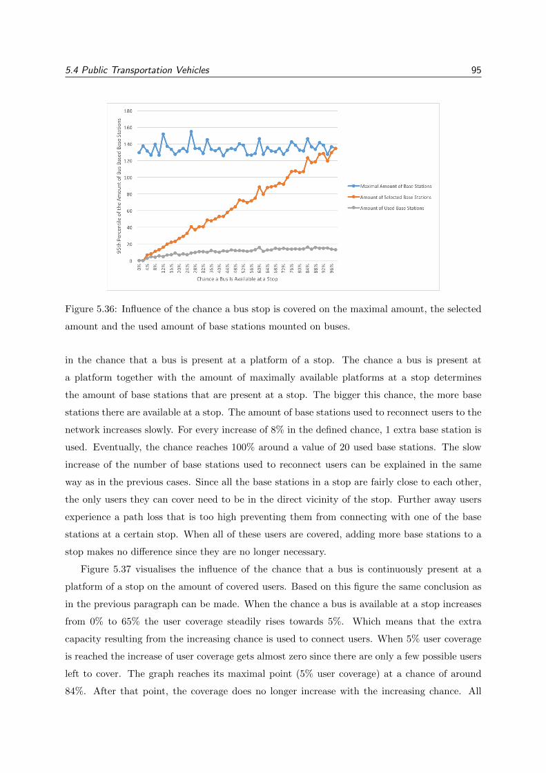
5.4 Public Transportation Vehicles 95

Figure 5.36: Influence of the chance a bus stop is covered on the maximal amount, the selected

amount and the used amount of base stations mounted on buses.

in the chance that a bus is present at a platform of a stop. The chance a bus is present at

a platform together with the amount of maximally available platforms at a stop determines

the amount of base stations that are present at a stop. The bigger this chance, the more base

stations there are available at a stop. The amount of base stations used to reconnect users to the

network increases slowly. For every increase of 8% in the defined chance, 1 extra base station is

used. Eventually, the chance reaches 100% around a value of 20 used base stations. The slow

increase of the number of base stations used to reconnect users can be explained in the same

way as in the previous cases. Since all the base stations in a stop are fairly close to each other,

the only users they can cover need to be in the direct vicinity of the stop. Further away users

experience a path loss that is too high preventing them from connecting with one of the base

stations at a certain stop. When all of these users are covered, adding more base stations to a

stop makes no difference since they are no longer necessary.

Figure 5.37 visualises the influence of the chance that a bus is continuously present at a

platform of a stop on the amount of covered users. Based on this figure the same conclusion as

in the previous paragraph can be made. When the chance a bus is available at a stop increases

from 0% to 65% the user coverage steadily rises towards 5%. Which means that the extra

capacity resulting from the increasing chance is used to connect users. When 5% user coverage

is reached the increase of user coverage gets almost zero since there are only a few possible users

left to cover. The graph reaches its maximal point (5% user coverage) at a chance of around

84%. After that point, the coverage does no longer increase with the increasing chance. All

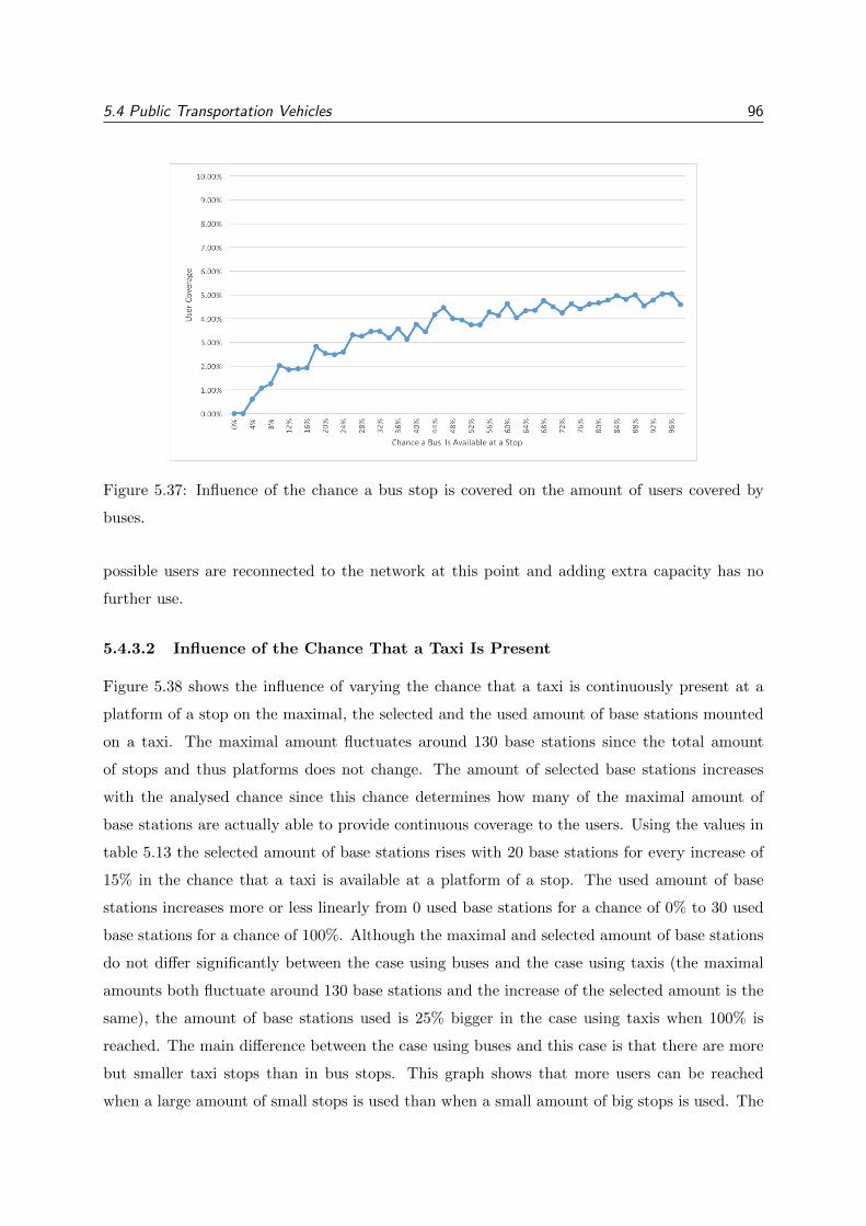
5.4 Public Transportation Vehicles 96

Figure 5.37: Influence of the chance a bus stop is covered on the amount of users covered by

buses.

possible users are reconnected to the network at this point and adding extra capacity has no

further use.

5.4.3.2 Influence of the Chance That a Taxi Is Present

Figure 5.38 shows the influence of varying the chance that a taxi is continuously present at a

platform of a stop on the maximal, the selected and the used amount of base stations mounted

on a taxi. The maximal amount fluctuates around 130 base stations since the total amount

of stops and thus platforms does not change. The amount of selected base stations increases

with the analysed chance since this chance determines how many of the maximal amount of

base stations are actually able to provide continuous coverage to the users. Using the values in

table 5.13 the selected amount of base stations rises with 20 base stations for every increase of

15% in the chance that a taxi is available at a platform of a stop. The used amount of base

stations increases more or less linearly from 0 used base stations for a chance of 0% to 30 used

base stations for a chance of 100%. Although the maximal and selected amount of base stations

do not differ significantly between the case using buses and the case using taxis (the maximal

amounts both fluctuate around 130 base stations and the increase of the selected amount is the

same), the amount of base stations used is 25% bigger in the case using taxis when 100% is

reached. The main difference between the case using buses and this case is that there are more

but smaller taxi stops than in bus stops. This graph shows that more users can be reached

when a large amount of small stops is used than when a small amount of big stops is used. The

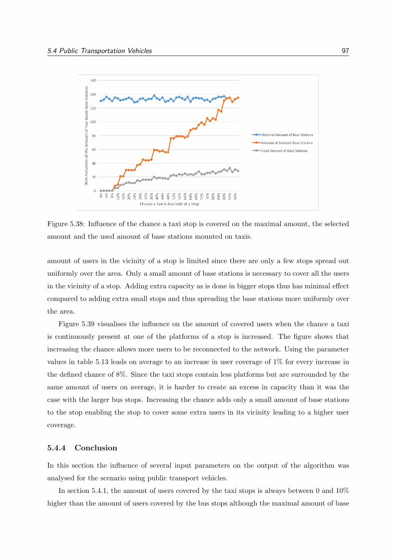
5.4 Public Transportation Vehicles 97

Figure 5.38: Influence of the chance a taxi stop is covered on the maximal amount, the selected

amount and the used amount of base stations mounted on taxis.

amount of users in the vicinity of a stop is limited since there are only a few stops spread out

uniformly over the area. Only a small amount of base stations is necessary to cover all the users

in the vicinity of a stop. Adding extra capacity as is done in bigger stops thus has minimal effect

compared to adding extra small stops and thus spreading the base stations more uniformly over

the area.

Figure 5.39 visualises the influence on the amount of covered users when the chance a taxi

is continuously present at one of the platforms of a stop is increased. The figure shows that

increasing the chance allows more users to be reconnected to the network. Using the parameter

values in table 5.13 leads on average to an increase in user coverage of 1% for every increase in

the defined chance of 8%. Since the taxi stops contain less platforms but are surrounded by the

same amount of users on average, it is harder to create an excess in capacity than it was the

case with the larger bus stops. Increasing the chance adds only a small amount of base stations

to the stop enabling the stop to cover some extra users in its vicinity leading to a higher user

coverage.

5.4.4 Conclusion

In this section the influence of several input parameters on the output of the algorithm was

analysed for the scenario using public transport vehicles.

In section 5.4.1, the amount of users covered by the taxi stops is always between 0 and 10%

higher than the amount of users covered by the bus stops although the maximal amount of base

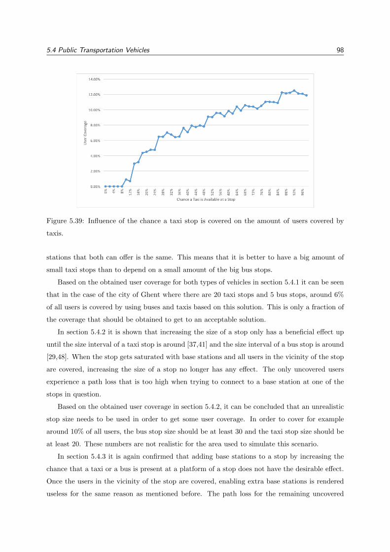
5.4 Public Transportation Vehicles 98

Figure 5.39: Influence of the chance a taxi stop is covered on the amount of users covered by

taxis.

stations that both can offer is the same. This means that it is better to have a big amount of

small taxi stops than to depend on a small amount of the big bus stops.

Based on the obtained user coverage for both types of vehicles in section 5.4.1 it can be seen

that in the case of the city of Ghent where there are 20 taxi stops and 5 bus stops, around 6%

of all users is covered by using buses and taxis based on this solution. This is only a fraction of

the coverage that should be obtained to get to an acceptable solution.

In section 5.4.2 it is shown that increasing the size of a stop only has a beneficial effect up

until the size interval of a taxi stop is around [37,41] and the size interval of a bus stop is around

[29,48]. When the stop gets saturated with base stations and all users in the vicinity of the stop

are covered, increasing the size of a stop no longer has any effect. The only uncovered users

experience a path loss that is too high when trying to connect to a base station at one of the

stops in question.

Based on the obtained user coverage in section 5.4.2, it can be concluded that an unrealistic

stop size needs to be used in order to get some user coverage. In order to cover for example

around 10% of all users, the bus stop size should be at least 30 and the taxi stop size should be

at least 20. These numbers are not realistic for the area used to simulate this scenario.

In section 5.4.3 it is again confirmed that adding base stations to a stop by increasing the

chance that a taxi or a bus is present at a platform of a stop does not have the desirable effect.

Once the users in the vicinity of the stop are covered, enabling extra base stations is rendered

useless for the same reason as mentioned before. The path loss for the remaining uncovered

5.4 Public Transportation Vehicles 99

users is too high to connect to a base station at this stop.

Furthermore it is concluded that to cover all users present at the stops, both the bus stops

and the taxi stops need an availability chance of around 84%. This means that at all times,

84% of the platforms of all stops need to be in use which is very unlikely to happen in a realistic

scenario. When more realistic figures like 50% for the bus stops and 30% for the taxi stops are

used the algorithm is not able to cover more than 10% of all users.

Using the results gathered throughout this section it becomes clear that by itself this scenario

is not able to offer a good solution for the stated connectivity problem. It could however be

a good way to decrease for example the amount of drones when used in combination with the

scenario based on drones.

MIXTURE OF CARRIERS 100

Chapter 6

Mixture of Carriers

6.1 Introduction

In the previous chapters three scenarios were introduced and their feasibility was investigated.

The first introduced scenario uses unmanned aerial vehicles to bring the base stations in place.

This scenario appeared to be feasible in the analysis (section 5.2) depending on the amount of

funding available to acquire the necessary drones. The second introduced scenario uses emer-

gency service vehicles to get the base stations in place. This scenario was applied to a smaller

area with a lot of users in order to analyse the feasibility of the scenario when a certain accident

or event occurs (section 5.3). Out of this analysis it was concluded that the amount of vehicles

present in the area was not high enough to cover more than 1000 users. The third introduced

scenario uses the public transport infrastructure of a city, specifically buses and taxis. The

analysis of this scenario is described in section 5.4. The outcome of this analysis was that the

realistic amount of taxi and bus stops in the determined area would be too low in order to cover

all users in the area.

In this chapter, all three scenarios are combined to analyse their cooperation in a realistic

use case. Based on chapter 5 it can be seen that the scenario using drones is the most promising.

However, the costs of acquiring and maintaining a lot of these drones can be quite high depending

on the used material. The two other scenarios can be used to lower the amount of necessary

drones and thus to reduce these costs. The infrastructure used by these other scenarios (buses,

taxis and emergency service vehicles) does not require a lot of extra effort to equip it with base

stations. Next to this, these carriers are definitely around when an event happens in an urban

area and the people present need an alternative connection to the network.

Section 6.2 introduces the setup considered to investigate the cooperation of all described

scenarios. In section 6.3 the results of the scheduling tool are visualised and explained. Finally,

6.2 Setup 101

in section 6.4, a conclusion is drawn about the feasibility and possible improved efficiency of this

mixture scenario.

6.2 Setup

6.2.1 Real Life Use Case

To investigate the feasibility of the mixture of all scenarios, a real life case is chosen. This

real life case is the city centre of Ghent during De Gentse Feesten 2015. De Gentse Feesten is

a festival organised in the historical city centre of Ghent and lasts for 10 days. In 2015, the

festival had around 100000 visitors each day [50]. Figure 6.1 shows the size of the festival and

the different locations that are spread out over the historical city centre.

For this simulation, it is assumed that something happened at the centre of the festival as can

be seen in figure 6.1. This event created a panic and an outage of all base stations present in the

city and at the festival, including the extra infrastructure provided by the festival organisers.

Emergency service vehicles are in place at the festival site. Public transport vehicles keep

performing their normal routes in order to prevent compromising the traffic in the entire city.

Before the permanent backup infrastructure is installed, four hours will have passed meaning

that the scenario has to be able to bridge this duration.

Figure 6.2 shows the observed area for this scenario. The area can be devided into two zones.

The big orange area will be called zone 1 from now on. It denotes the entire city centre of Ghent.

The other smaller and somewhat brighter orange zone will be called zone 2 from now on. This

area is the area where De Gentse Feesten are taking place during the simulation.

6.2.2 Algorithm Parameters

To simulate this scenario in an efficient way, two separate groups of users are generated. The

first group, group 1, are the users that are not attending the festival. This amount of users

is determined by real life data from a cellular network provider like in [47]. The second group

of users, group 2, are all attending the festival. For this group the algorithm generates 50000

random users. This is based on the amount of daily users provided by [50]. The generated traffic

is displayed in figure 6.3.

In order to use the three scenarios over these two groups of users, the algorithm starts with

covering all users in group 1. Since zone 1 includes zone 2, these users might also occur in the

area of zone 2. These users are not specifically at the festival site but rather in for example one

of the surrounding buildings.

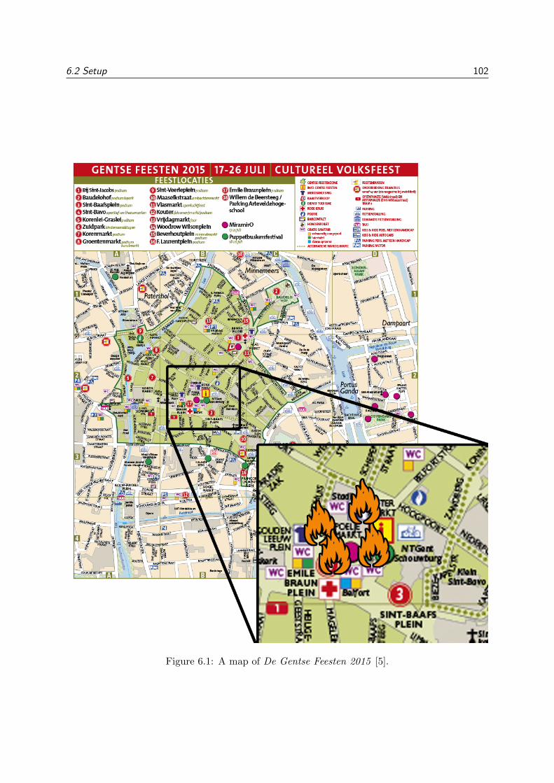
6.2 Setup 102

Figure 6.1: A map of De Gentse Feesten 2015 [5].

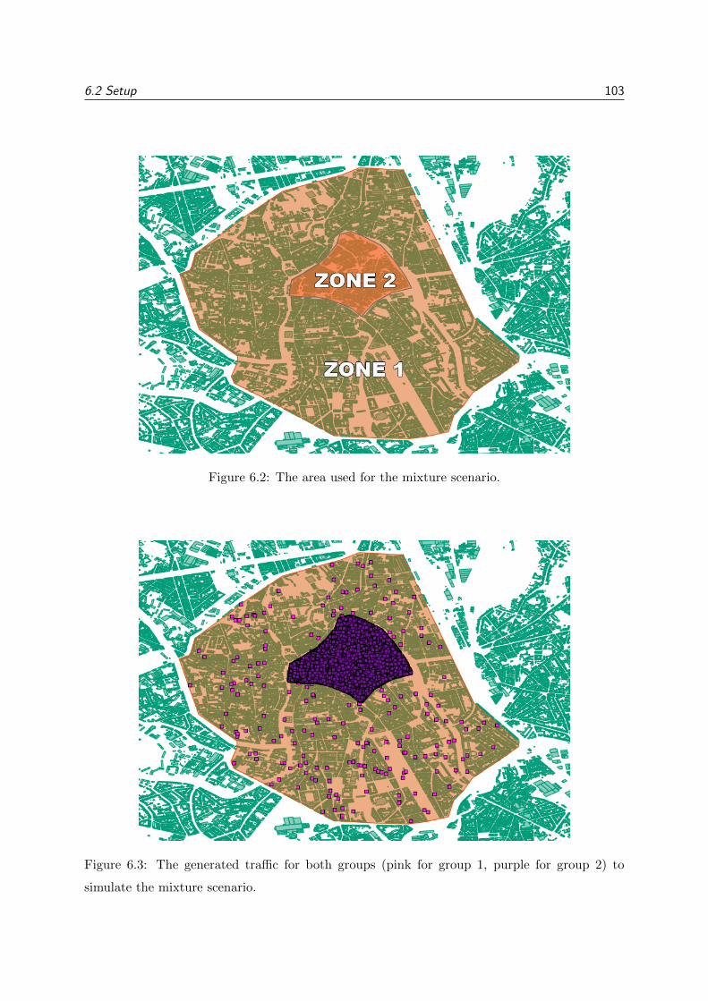
6.2 Setup 103

Figure 6.2: The area used for the mixture scenario.

Figure 6.3: The generated traffic for both groups (pink for group 1, purple for group 2) to

simulate the mixture scenario.

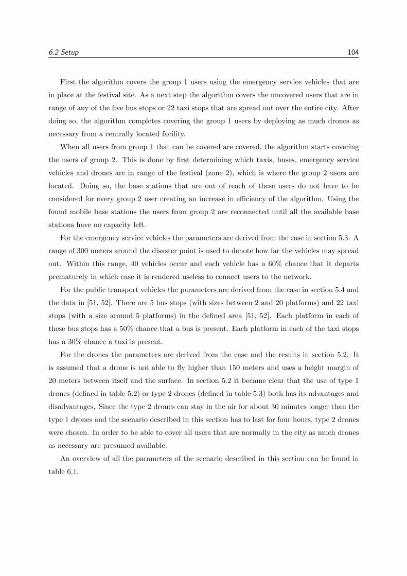
6.2 Setup 104

First the algorithm covers the group 1 users using the emergency service vehicles that are

in place at the festival site. As a next step the algorithm covers the uncovered users that are in

range of any of the five bus stops or 22 taxi stops that are spread out over the entire city. After

doing so, the algorithm completes covering the group 1 users by deploying as much drones as

necessary from a centrally located facility.

When all users from group 1 that can be covered are covered, the algorithm starts covering

the users of group 2. This is done by first determining which taxis, buses, emergency service

vehicles and drones are in range of the festival (zone 2), which is where the group 2 users are

located. Doing so, the base stations that are out of reach of these users do not have to be

considered for every group 2 user creating an increase in efficiency of the algorithm. Using the

found mobile base stations the users from group 2 are reconnected until all the available base

stations have no capacity left.

For the emergency service vehicles the parameters are derived from the case in section 5.3. A

range of 300 meters around the disaster point is used to denote how far the vehicles may spread

out. Within this range, 40 vehicles occur and each vehicle has a 60% chance that it departs

prematurely in which case it is rendered useless to connect users to the network.

For the public transport vehicles the parameters are derived from the case in section 5.4 and

the data in [51, 52]. There are 5 bus stops (with sizes between 2 and 20 platforms) and 22 taxi

stops (with a size around 5 platforms) in the defined area [51, 52]. Each platform in each of

these bus stops has a 50% chance that a bus is present. Each platform in each of the taxi stops

has a 30% chance a taxi is present.

For the drones the parameters are derived from the case and the results in section 5.2. It

is assumed that a drone is not able to fly higher than 150 meters and uses a height margin of

20 meters between itself and the surface. In section 5.2 it became clear that the use of type 1

drones (defined in table 5.2) or type 2 drones (defined in table 5.3) both has its advantages and

disadvantages. Since the type 2 drones can stay in the air for about 30 minutes longer than the

type 1 drones and the scenario described in this section has to last for four hours, type 2 drones

were chosen. In order to be able to cover all users that are normally in the city as much drones

as necessary are presumed available.

An overview of all the parameters of the scenario described in this section can be found in

table 6.1.

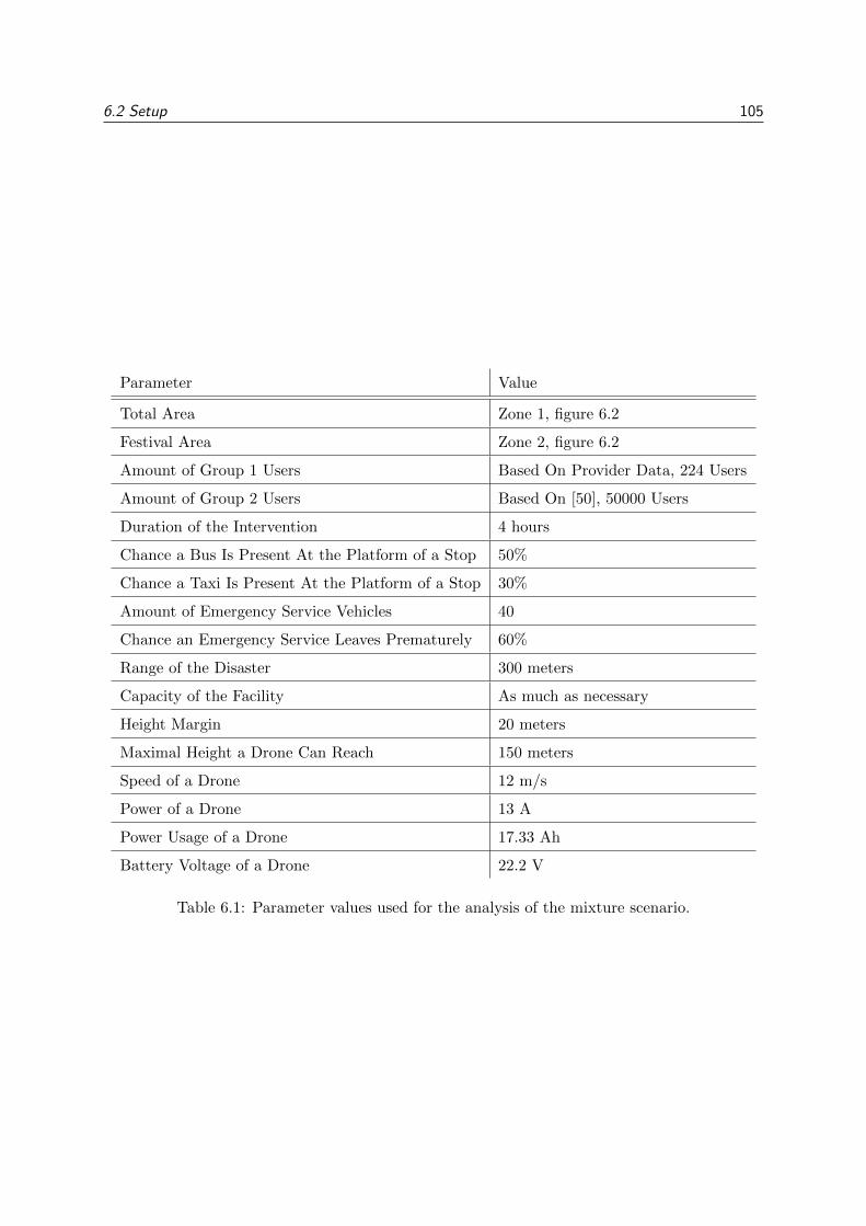
6.2 Setup 105

Parameter Value

Total Area Zone 1, figure 6.2

Festival Area Zone 2, figure 6.2

Amount of Group 1 Users Based On Provider Data, 224 Users

Amount of Group 2 Users Based On [50], 50000 Users

Duration of the Intervention 4 hours

Chance a Bus Is Present At the Platform of a Stop 50%

Chance a Taxi Is Present At the Platform of a Stop 30%

Amount of Emergency Service Vehicles 40

Chance an Emergency Service Leaves Prematurely 60%

Range of the Disaster 300 meters

Capacity of the Facility As much as necessary

Height Margin 20 meters

Maximal Height a Drone Can Reach 150 meters

Speed of a Drone 12 m/s

Power of a Drone 13 A

Power Usage of a Drone 17.33 Ah

Battery Voltage of a Drone 22.2 V

Table 6.1: Parameter values used for the analysis of the mixture scenario.

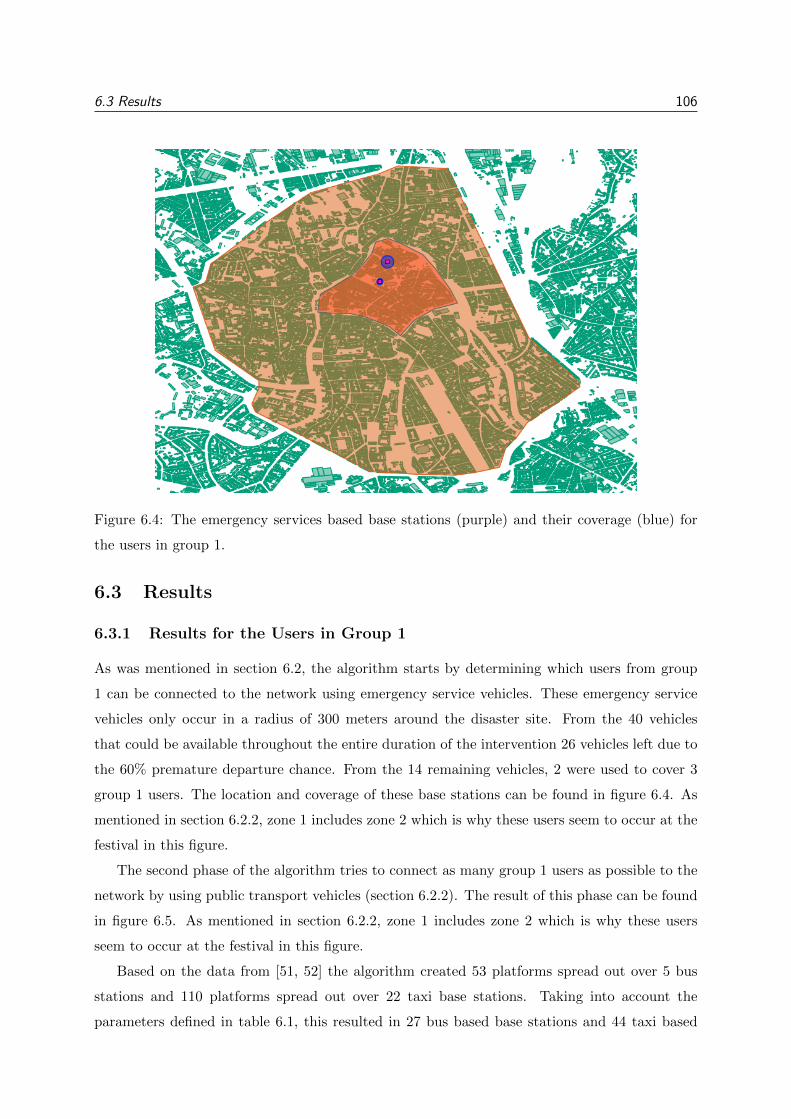
6.3 Results 106

Figure 6.4: The emergency services based base stations (purple) and their coverage (blue) for

the users in group 1.

6.3 Results

6.3.1 Results for the Users in Group 1

As was mentioned in section 6.2, the algorithm starts by determining which users from group

1 can be connected to the network using emergency service vehicles. These emergency service

vehicles only occur in a radius of 300 meters around the disaster site. From the 40 vehicles

that could be available throughout the entire duration of the intervention 26 vehicles left due to

the 60% premature departure chance. From the 14 remaining vehicles, 2 were used to cover 3

group 1 users. The location and coverage of these base stations can be found in figure 6.4. As

mentioned in section 6.2.2, zone 1 includes zone 2 which is why these users seem to occur at the

festival in this figure.

The second phase of the algorithm tries to connect as many group 1 users as possible to the

network by using public transport vehicles (section 6.2.2). The result of this phase can be found

in figure 6.5. As mentioned in section 6.2.2, zone 1 includes zone 2 which is why these users

seem to occur at the festival in this figure.

Based on the data from [51, 52] the algorithm created 53 platforms spread out over 5 bus

stations and 110 platforms spread out over 22 taxi base stations. Taking into account the

parameters defined in table 6.1, this resulted in 27 bus based base stations and 44 taxi based

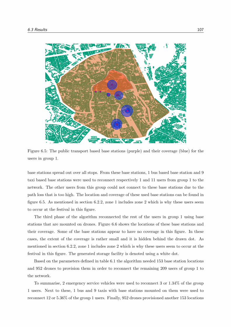
6.3 Results 107

Figure 6.5: The public transport based base stations (purple) and their coverage (blue) for the

users in group 1.

base stations spread out over all stops. From these base stations, 1 bus based base station and 9

taxi based base stations were used to reconnect respectively 1 and 11 users from group 1 to the

network. The other users from this group could not connect to these base stations due to the

path loss that is too high. The location and coverage of these used base stations can be found in

figure 6.5. As mentioned in section 6.2.2, zone 1 includes zone 2 which is why these users seem

to occur at the festival in this figure.

The third phase of the algorithm reconnected the rest of the users in group 1 using base

stations that are mounted on drones. Figure 6.6 shows the locations of these base stations and

their coverage. Some of the base stations appear to have no coverage in this figure. In these

cases, the extent of the coverage is rather small and it is hidden behind the drawn dot. As

mentioned in section 6.2.2, zone 1 includes zone 2 which is why these users seem to occur at the

festival in this figure. The generated storage facility is denoted using a white dot.

Based on the parameters defined in table 6.1 the algorithm needed 153 base station locations

and 952 drones to provision them in order to reconnect the remaining 209 users of group 1 to

the network.

To summarise, 2 emergency service vehicles were used to reconnect 3 or 1.34% of the group

1 users. Next to these, 1 bus and 9 taxis with base stations mounted on them were used to

reconnect 12 or 5.36% of the group 1 users. Finally, 952 drones provisioned another 153 locations

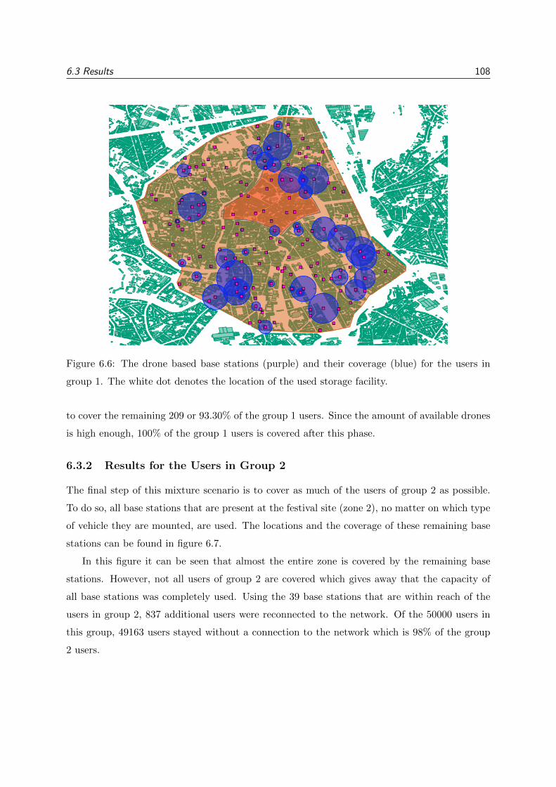
6.3 Results 108

Figure 6.6: The drone based base stations (purple) and their coverage (blue) for the users in

group 1. The white dot denotes the location of the used storage facility.

to cover the remaining 209 or 93.30% of the group 1 users. Since the amount of available drones

is high enough, 100% of the group 1 users is covered after this phase.

6.3.2 Results for the Users in Group 2

The final step of this mixture scenario is to cover as much of the users of group 2 as possible.

To do so, all base stations that are present at the festival site (zone 2), no matter on which type

of vehicle they are mounted, are used. The locations and the coverage of these remaining base

stations can be found in figure 6.7.

In this figure it can be seen that almost the entire zone is covered by the remaining base

stations. However, not all users of group 2 are covered which gives away that the capacity of

all base stations was completely used. Using the 39 base stations that are within reach of the

users in group 2, 837 additional users were reconnected to the network. Of the 50000 users in

this group, 49163 users stayed without a connection to the network which is 98% of the group

2 users.

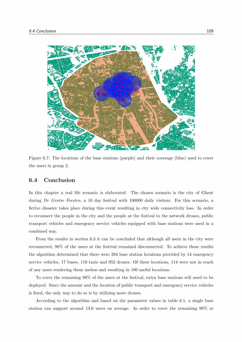
6.4 Conclusion 109

Figure 6.7: The locations of the base stations (purple) and their coverage (blue) used to cover

the users in group 2.

6.4 Conclusion

In this chapter a real life scenario is elaborated. The chosen scenario is the city of Ghent

during De Gentse Feesten, a 10 day festival with 100000 daily visitors. For this scenario, a

fictive disaster takes place during this event resulting in city wide connectivity loss. In order

to reconnect the people in the city and the people at the festival to the network drones, public

transport vehicles and emergency service vehicles equipped with base stations were used in a

combined way.

From the results in section 6.3 it can be concluded that although all users in the city were

reconnected, 98% of the users at the festival remained disconnected. To achieve these results

the algorithm determined that there were 294 base station locations provided by 14 emergency

service vehicles, 17 buses, 110 taxis and 952 drones. Of these locations, 114 were not in reach

of any users rendering them useless and resulting in 180 useful locations.

To cover the remaining 98% of the users at the festival, extra base stations will need to be

deployed. Since the amount and the location of public transport and emergency service vehicles

is fixed, the only way to do so is by utilizing more drones.

According to the algorithm and based on the parameter values in table 6.1, a single base

station can support around 13.6 users on average. In order to cover the remaining 98% or

6.4 Conclusion 110

49163 users at the festival, around 362 extra, well placed base stations are necessary. The base

stations need to be placed in such a way that they can cover around 13.6 users and thus that

there maximal capacity is used.

The facility storing the drones is situated centrally in the area and fairly close to the festival

site. From the results of the algorithm it is known that on average 6.22 drones are necessary to

cover one location during the intervention time of 4 hours. This means that in order to cover

the remaining uncovered users and thus to provision 362 extra base station locations, 2252 extra

drones of type 2 need to be available.

The overall conclusion in this chapter is that the public transport and emergency service

vehicles can alleviate some of the pressure on the drone scenario by connecting a part of the users.

In this case 5% of the locations necessary to cover all users could be provisioned by emergency

services and public transport vehicles. However, their locations cannot be chosen beforehand as

can be done with drones which often results in them being out of reach of all users. Because of

this disadvantage, the base stations provided by public transport and emergency service vehicles

can not be used to there full extent.

In order to cover the users in the city and at the event based on the parameter values in

table 6.1, around 3204 drones are necessary to provision 515 locations on top of the locations

provided by the other types of vehicles. Knowing that a drone of type 2 is sold for around 2000

dollars [54] which is 1755 euros, this means that an investment is needed of around 5.6 million

euros in order to acquire the necessary drones. No maintenance, installation of the base stations

or creation of the underlying system is taken into account in this price.

CONCLUSION AND FUTURE WORK 111

Chapter 7

Conclusion and Future Work

This master’s dissertation investigates the creation of emergency ad hoc networks to provide a

solution when the normal means of connecting to the network are compromised by a certain

event. In the past few years, several examples of these events occurred. For example, the

Pukkelpop disaster of 2011 in Hasselt, Belgium or the terrorist attacks of 2016 in Brussels’

Airport, Belgium. When both these events occurred, all usually available infrastructure in the

neighbourhood of the event stopped working. An emergency ad hoc network could have provided

the necessary connectivity to communicate with the outside world again making resolving the

disaster a lot easier.

An important factor in this idea is that the place where the network needs to be deployed is

not known in advance. To deal with this, placing the necessary base stations needs to happen

in a flexible way. The most desirable scenario is that these base stations are mobile and can get

to their predetermined position by themselves, setting up an entire network with minimal effort

when needed.

Three scenarios to create these mobile base stations are introduced. The first scenario uses

unmanned aerial vehicles or drones to connect users to the network. In this scenario, the base

stations are mounted on a drone and these drones are then stored in a facility. This facility

could be a building in a city centre or a big truck that drives to the disaster site to limit the

flight of the drones. In order to provision a certain location in the area, a drone will alternate

with a new one from the facility when its battery dies.

The second scenario uses emergency service vehicles on which a base station is mounted.

When a disastrous event occurs, a lot of emergency service vehicles will be dispatched to the

specific area. This means that equipping these vehicles with base stations might reinstate the

connectivity for the users in the area. However, a downside of this scenario is that the amount

of vehicles in the area is hard to predict and that their location is fixed which might not be

CONCLUSION AND FUTURE WORK 112

optimal for users to connect with the base station.

The third scenario uses base stations mounted on public transport vehicles. Public transport

vehicles like taxis and buses are very common in urban areas. The chance that these vehicles

are present in the environment of an urban disaster is rather large which makes them suitable

to reconnect users in the region to the network. The same downsides as with the emergency

services are present, it is hard to predict how many and where these vehicles will be.

The aforementioned base stations are LTE femtocells. LTE femtocells provide the flexibility

and capabilities that are necessary in an emergency ad hoc network. They are optimised for

slow moving users and the frequency bands LTE uses can handle a lot of users at a time.

In order to simulate and investigate the scenarios a scheduling tool was created. Based on

input parameters depending on the specific scenario, the scheduling tool proposes a network to

cover as many users as possible in a predefined area. It does this by going over all the users and

determining preferable base station positions to cover these users. The tool then determines

which locations are feasible resulting in a network with the defined restrictions.

Using the output of the scheduling tool, a sensitivity analysis was performed. Each scenario

was evaluated and per scenario conclusions were drawn based on their feasibility and necessary

properties.

The results concerning the drone scenario brought to light that almost all users could be

covered using drones. A limiting factor in this scenario however is the cost to acquire and

maintain the fleet of drones. Based on the amount of funding available this might be a deal-

breaker. The scenario needed 1100 type 1 drones or 400 type 2 drones in order to cover all

224 users in the city of Ghent during 1 hour. This amount rose linearly with the intervention

duration so the longer the duration the more drones were necessary. Another important factor

that this analysis discovered is the minimal height of a drone. When the minimal height is small

(for example around 4 meters) the drones are not able to cover a large area. Since an urban

area is considered, the buildings surrounding the drone block the signal due to a high path loss

for the users in the area behind the buildings. When the drone is situated higher (for example

around 50 meters) there are more users in line of sight of the drone which enables these users

to connect to the base station attached to the drone. This means that the higher the drones

are situated on average, the fewer base station locations are necessary in the network. However

when the average height becomes too big, the signal is weakened by the extra distance implied

by this height which is an undesired effect. The most suitable height depends from location to

location. If the surrounding buildings are low, a lower height can result in the same amount

of users that are in line of sight of the base station and the signal is not weakened due to the

extra distance. However, when the buildings are high, larger heights should be used. It is thus

CONCLUSION AND FUTURE WORK 113

preferable to analyse the situation for each location and choose the appropriate height.

The emergency services scenario was analysed based on a smaller area and a lot more users

than the other two scenarios. This was done because of the fact that emergency service vehicles

flock together instead of being spread out over an area of 4 km2. The amount of emergency

service vehicles in the area proved to be the most important factor to reconnect the users.

Since this scenario assumes that a lot of users are assembled together in a small area, the total

capacity of the base stations is used on average. No matter where the vehicle is placed in the

area, a lot of users will surround it and connect to it if necessary. Other important factors in

this scenario are the range of the disaster and the reliability of the vehicles. The range of the

disasters determines how far the vehicles are spread around the disaster. The further they are

spread out the more users they could reconnect given that enough capacity is available in the

base stations. The reliability of the vehicles determines how long a vehicle and its base station

stay at the scene to provide coverage. If a vehicle is not reliable, the base station is not useful

for the users. In the simulations for this scenario, 40 vehicles with a reliability of 40% situated

in a range of 300 meters around the disaster were only able to cover 2% of the 50000 present

users. Based on these results and the three aforementioned factors it could be concluded that an

unrealistic amount of vehicles for the area would be necessary to cover all users. This scenario

can thus not be used on its own.

In the scenario using public transport vehicles the base stations are spread out over different

bus or taxi stops that have different sizes. The main conclusion from this scenario is that it is

more interesting to have a lot of small stops containing a few base stations than only two or

three stops containing a lot of base stations. What is also important for this scenario is that

there are enough of taxi and buses in the area to ensure continuous presence of a base station at

a stop. Otherwise the stop would not be able to provide coverage to the present users making

it useless. Based on the realistic amounts of stops and vehicles in the observed area in Ghent it

could be seen that all the stops in the area where not able to get more than 6% user coverage.

This scenario is thus also not sufficient on its own.

Since the emergency services and public transport scenarios are not feasible on their own and

the drone scenario is rather expensive, the combination of these three scenarios was investigated.

The idea of the combination of these scenarios is to use the drone scenario to cover all user while

covering as much users as possible with cheaper infrastructure like buses, taxis and emergency

service vehicles. This mixture of scenarios was applied to a real life use case namely, De Gentse

Feesten 2015 which is a festival in Ghent. Based on this use case and the parameters found in

the three separate scenarios it was concluded that the emergency service and public transport

vehicles are indeed able to relieve some of the pressure (around 5% of the locations) on the drone

CONCLUSION AND FUTURE WORK 114

scenario. However, since the locations of these types of vehicles is fixed, their placement is often

not optimal rendering them useless. As a result there were still al lot of drones necessary to

cover all users making the entire solution rather expensive.

Based on the analysis results of the proposed scenarios and the results of the real life case

it can be concluded that the scenario using drones is the most promising one. This scenario is

able to cover a user in almost every place due to the high mobility of these vehicles. A downside

of this scenario however is that they are based on extra infrastructure (the drones) instead of

reusing existing infrastructure like public transport and emergency services vehicles. The public

transport and emergency service vehicles are able to cover only a small part of the present users.

Although they are a lot cheaper since they do not require extra infrastructure, they are not

efficient enough to cover big crowds.

In order to create a fully working system the connection from the different base stations to

the internet backbone should be investigated further. This connection is still a bottleneck of

the idea. In the proposed solutions for this connection, speeds of around 10 Mbps in total are

reached which is rather low when trying to connect for example a thousand users.

Specifically for the drone scenario, it might be interesting to investigate the influence of

different types of weather on the performance of the system. Next, it might also be interesting

to introduce some additional means of transporting the base stations to their predetermined

locations. Other options could be the use of hot air balloons, robots or cars of private users.

BIBLIOGRAPHY 115

Bibliography

[1] lker Bekmezci, Ozgur Koray Sahingoz, and amil Temel. Flying Ad-Hoc Networks

(FANETs): A survey. Ad Hoc Networks, 11(3):1254–1270, 2013.

[2] Yixin Gu, Mi Zhou, Shengli Fu, and Yan Wan. Airborne WiFi networks through directional

antennae: An experimental study. Wireless Communications and Networking Conference

(WCNC), 2015 IEEE, pages 1314–1319, 2015.

[3] Wifi modes of operation (802.11 or wi-fi). http://ccm.net/contents/

804-wifi-modes-of-operation-802-11-or-wi-fi. Accessed: 05-05-2016.

[4] Introduction to perspective. http://www.woodenpalette.com/?page_id=918. Accessed:

18-05-2016.

[5] Map ghent festivities. https://gentsefeesten-2015.stad.gent/en/practical/

map-ghent-festivities. Accessed: 10-05-2016.

[6] Margot Deruyck, Dieter De Vulder, Wout Joseph, and Luc Martens. Modelling the power

consumption in femtocell networks. 2012 IEEE Wireless Communications and Networking

Conference Workshops (WCNCW), (2):30–35, 2012.

[7] Margot Deruyck, Emmeric Tanghe, Wout Joseph, and Luc Martens. Modelling and opti-

mization of power consumption in wireless access networks. Computer Communications,

34(17):2036–2046, 2011.

[8] Sanket Nesargi and Ravi Prakash. MANETconf: Configuration of hosts in a mobile ad hoc

network. Proceedings - IEEE INFOCOM, 2:1059–1068, 2002.

[9] Silvia Giordano. Mobile Ad-Hoc Networks. 2000.

[10] D.a. Maltz, J. Broch, and D.B. Johnson. Quantitative lessons from a full-scale multi-hop

wireless ad hoc\nnetwork testbed. 2000 IEEE Wireless Communications and Networking

Conference. Conference Record (Cat. No.00TH8540), 3, 2000.

BIBLIOGRAPHY 116

[11] Ricardo De Oliveira Schmidt and M. A S Trentin. MANETs routing protocols evaluation

in a scenario with high mobility: MANET routing protocols performance and behavior.

NOMS 2008 - IEEE/IFIP Network Operations and Management Symposium: Pervasive

Management for Ubiquitous Networks and Services, pages 883–886, 2008.

[12] Alex Hinds, Michael Ngulube, Shaoying Zhu, and Hussain Al-Aqrabi. A Review of Routing

Protocols for Mobile Ad-Hoc NETworks (MANET). International Journal of Information

and Education Technology, 3(1):1–5, 2013.

[13] David Lundberg and Henrik Lundgren. Ad hoc Protocol Evaluation and Experiences of

Real World Ad Hoc Networking. 2002.

[14] The google loon project. http://www.google.com/loon/. Accessed: 19-04-2016.

[15] Akrama Al-Hourani, Sithamparanathan Kandeepan, and Simon Lardner. Optimal LAP

altitude for maximum coverage. IEEE Wireless Communications Letters, 3(6):569–572,

2014.

[16] Seng W. Loke. The Internet of Flying-Things: Opportunities and Challenges with Airborne

Fog Computing and Mobile Cloud in the Clouds. X(X):1–5, 2015.

[17] Mahdi Asadpour, Bertold Van Den Bergh, Domenico Giustiniano, Karin Anna Hummel,

and Sofie Pollin. Micro Aerial Vehicle Networks : An Experimental Analysis of Challenges

and Opportunities. (July):141–149, 2014.

[18] Tewfik Doumi, Mike F. Dolan, Said Tatesh, Alessio Casati, George Tsirtsis, Kiran An-

chan, and Dino Flore. LTE for public safety networks. IEEE Communications Magazine,

51(2):106–112, 2013.

[19] Apostolis K. Salkintzis. Evolving public safety communication systems by integrating

WLAN and TETRA networks. IEEE Communications Magazine, 44(1):38–46, 2006.

[20] International Telecommunications Union. Radiocommunication objectives and require-

ments for public protection and disaster relief. ITU-R Report M.2033, 2003.

[21] Arvind Merwaday. UAV Assisted Heterogeneous Networks for Public Safety Communica-

tions. pages 329–334, 2015.

[22] M. Portmann and A. Pirzada. Wireless Mesh Networks for Public Safety and Crisis Man-

agement Applications. IEEE Internet Computing, 12(1):18–25, 2008.

BIBLIOGRAPHY 117

[23] Elias Yaacoub and Osama Kubbar. Energy-efficient Device-to-Device communications in

LTE public safety networks. 2012 IEEE Globecom Workshops, GC Wkshps 2012, pages

391–395, 2012.

[24] Bow Nan Cheng, Randy Charland, Paul Christensen, Leonid Veytser, and James Wheeler.

Evaluation of a multihop airborne ip backbone with heterogeneous radio technologies. IEEE

Transactions on Mobile Computing, 13(2):299–310, 2014.

[25] Bow Nan Cheng, Andrea Coyle, Stephen McGarry, Igor Pedan, Leonid Veytser, and James

Wheeler. Characterizing routing with radio-to-router information in a heterogeneous air-

borne network. IEEE Transactions on Wireless Communications, 12(8):4183–4195, 2013.

[26] Alessio Botta and Antonio Pescape. On the performance of new generation satellite broad-

band internet services. IEEE Communications Magazine, 52(6):202–209, 2014.

[27] Margot Deruyck, Emmeric Tanghe, Wout Joseph, and Luc Martens. Modelling and opti-

mization of power consumption in wireless access networks. Computer Communications,

34(17):2036–2046, 2011.

[28] Margot Deruyck, Wout Joseph, Emmeric Tanghe, and Luc Martens. Reducing the power

consumption in LTE-Advanced wireless access networks by a capacity based deployment

tool. Radio Science, 49(9):777–787, 2014.

[29] Margot Deruyck, Dieter De Vulder, Wout Joseph, and Luc Martens. Modelling the power

consumption in femtocell networks. 2012 IEEE Wireless Communications and Networking

Conference Workshops (WCNCW), (2):30–35, 2012.

[30] Aleksandar Neskovic, Natasa Neskovic, and George Paunovic. Modern Approaches in Mod-

eling of Mobile Radio Systems Propagation Environment. IEEE Communications Surveys,

pages 2–12, 2000.

[31] Hemant Kumar Sharma. Enhanced Cost231 W.I. Propagation Model in Wireless Network.

International Journal of Computer Applications, 19(6):36–42, 2011.

[32] Leonard Piazzi and Henry L. Bertoni. Achievable accuracy of site-specific path-loss predic-

tions in residential environments. IEEE Transactions on Vehicular Technology, 48(3):922–

930, 1999.

[33] Sagar Patel, Ved Vyas Dwivedi, and Y P Kosta. A Parametric Characterization and Com-

parative Study of Okumura and Hata Propagation-loss- prediction Models for Wireless

Environment. 2(4):453–462, 2010.

BIBLIOGRAPHY 118

[34] K. Low. Comparison of urban propagation models with CW-measurements. [1992 Pro-

ceedings] Vehicular Technology Society 42nd VTS Conference - Frontiers of Technology,

(2):936–942, 1992.

[35] Theodore Reed, Joseph Geis, and Sven Dietrich. SkyNET : a 3G-enabled mobile attack

drone and stealth botmaster Approach Attack Framework. Proceedings of the 5th USENIX

conference on Offensive technologies, (WOOT’11):4–4, 2011.

[36] Joao Valente, David Sanz, Antonio Barrientos, Jaime Del Cerro, Angela Ribeiro, and

Claudio Rossi. An Air-Ground Wireless Sensor Network for Crop Monitoring. Sensors,

11(12):6088–6108, 2011.

[37] H. T. Kung, Chit-Kwan Lin, Tsung-Han Lin, Stephen J. Tarsa, and Dario Vlah. Mea-

suring diversity on a low-altitude UAV in a ground-to-air wireless 802.11 mesh network.

GLOBECOM Workshops (GC Wkshps), 2010 IEEE, pages 1799–1804, 2010.

[38] Signals Research Group. The LTE Standard. 2014.

[39] Lte encyclopedia. https://sites.google.com/site/lteencyclopedia/home. Accessed:

10-04-2016.

[40] Giuseppe Araniti, Claudia Campolo, Massimo Condoluci, Antonio Iera, and Antonella Moli-

naro. LTE for Vehicular Networking : A Survey. pages 148–157, 2013.

[41] Margot Deruyck and Willem Vereecken. Reducing the power consumption in wireless ac-

cess networks: Overview and recommendations. Progress In Electromagnetics Research,

132(October):255–274, 2012.

[42] Vikram Chandrasekhar, Jeffrey G. Andrews, and Alan Gatherer. Femtocell networks: A

survey. IEEE Communications Magazine, 46(9):59–67, 2008.

[43] Mehdi Bennis, Meryem Simsek, Andreas Czylwik, Walid Saad, Stefan Valentin, and Mer-

ouane Debbah. When cellular meets WiFi in wireless small cell networks. IEEE Commu-

nications Magazine, 51(6):44–50, 2013.

[44] Ieee 802.11 wlan standards. http://standards.ieee.org/about/get/802/802.11.html.

Accessed: 04-05-2016.

[45] What is wifi and how does it work? http://ccm.net/faq/

298-what-is-wifi-and-how-does-it-work. Accessed: 05-05-2016.

[46] Discover wifi. https://www.wi-fi.org/discover-wi-fi. Accessed: 10-04-2016.

BIBLIOGRAPHY 119

[47] Margot Deruyck, Wout Joseph, Emmeric Tanghe, and Luc Martens. Reducing the power

consumption in LTE-Advanced wireless access networks by a capacity based deployment

tool. Radio Science, 49(9):777–787, 2014.

[48] W. Joseph, S. Aerts, M. Vandenbossche, A. Thielens, L. Martens. Drone based measurement

system for radiofrequency exposure assessment. Bioelectromagnetics, 2016.

[49] Microdrones md4-1000: Robust and powerful uav model. https://www.microdrones.com/

en/products/md4-1000/technical-data/. Accessed: 10-03-2016.

[50] Eindcijfers gentse feesten 2015. https://stad.gent/sites/default/files/article/

documents/GF2015%20earlybird%20maandag%2027%20juli%20eindcijfers.pdf. Ac-

cessed: 08-03-2016.

[51] Belangrijkste tram- en buslijnen in het centrum van gent. http://gent.delijn.be/files/

attachments/.3148/gent_abstract_bus_maart2016.pdf. Accessed: 24-03-2016.

[52] Taxistandplaatsen in gent. https://mobiliteit.stad.gent/met-de-taxi/

taxistandplaatsen-gent. Accessed: 24-03-2016.

[53] Overzicht taxi- en vvb-vergunningen in belgie in 2015. http://www.gtl-taxi.be/8_0_0_

0_NL_Nieuws_32290_1. Accessed: 24-03-2016.

[54] Microdrones md4-1000 specifications. http://drones.specout.com/l/109/

Microdrones-MD4-1000. Accessed: 11-05-2016.