Emergent Collective Behavior in

Multi-Agent Systems: An Evolutionary

Perspective

Darren Pais

A Dissertation

Presented to the Faculty

of Princeton University

in Candidacy for the Degree

of Doctor of Philosophy

Recommended for Acceptance

by the Department of

Mechanical and Aerospace Engineering

Adviser: Professor Naomi Ehrich Leonard

November 2012

c© Copyright by Darren Pais, 2012.

All rights reserved.

Abstract

The study of collective behavior involves the analysis of interactions among a set

of agents that yield collective outcomes at the level of the group. The behavior is said

to be emergent when it cannot be understood simply as the sum of its constituent

parts. Further, group-level outcomes can in turn influence individual interactions.

The complexity of this interplay makes the study of emergence challenging and excit-

ing. This dissertation is focused on the study of emergent collective behavior from the

perspective of evolution. Evolution is a simple yet powerful algorithm, which when

acting on interacting entities in a dynamic environment, yields an array of fascinating

behavior as manifest in the natural world. Natural collectives display a wide variety

of cooperative behavior and have evolved to efficiently manage the inherent tradeoff

between robust behavior and adaptability to dynamic environments. These properties

have motivated the design of bio-inspired algorithms for sensing and decision-making

in robotic collectives. In this work, we study the evolutionary mechanisms for co-

operation and tradeoff management in biological collectives, with a focus on four

related topics: replicator-mutator dynamics, collective migration, collective pursuit

and evasion, and decision-making dynamics in swarms.

The replicator-mutator dynamics define a canonical model from evolutionary the-

ory and have recently been used to study the evolution of language and the behavioral

dynamics of social networks. While the analysis of stable equilibria of these dynamics

has been a focus in the literature, we prove that certain conditions suffice for the equa-

tions to exhibit stable limit cycles. These cycles correspond to oscillations of grammar

dominance in language evolution and to oscillations in behavioral preferences in so-

cial networks. For the collective migration problem, it is well-established that a small

group of leaders can guide a large swarm of followers. It is less clear how presumably

self-interested individuals have evolved to take on such divergent roles. We design a

network-based evolutionary model to understand the evolution of leadership in migra-

tion, with a focus on the role of network topology on the emergent dynamics. Pursuit

and evasive behaviors are ubiquitous in biology and are key drivers for collective

motion. We use computational simulations and analytical calculations to study a co-

evolving pursuit and evasive system, and incorporate the evolved strategies in a cyclic

pursuit-evasion collective motion model. The ‘stop-signaling’ inhibitory mechanism

has been recently shown to be critical to the decentralized decision-making dynamics

in honeybee swarms. We investigate bifurcations in a model of swarm decision-making

as a function of the stop-signal and the values of different alternatives, and present a

comprehensive analysis of the dynamics of the model.

iii

Acknowledgements

First, I would like to acknowledge my advisor Naomi Leonard. Naomi is a brilliant

scientist, an immensely creative researcher, and above all, a wonderful and caring

person. Naomi’s gentle persuasion to always think deeply and clearly about a prob-

lem, her discerning taste for exciting research questions, and her extraordinary ability

to make connections across diverse areas, have had an immense impact on my de-

velopment and growth as a graduate student. I am extremely grateful to Naomi for

allowing me the freedom to pursue my interests and for helping me build the confi-

dence to tackle challenging new problems. I will fondly remember the countless hours

spent discussing ideas in Naomi’s office and will always be grateful for her consistent

and detailed edits of numerous paper drafts and thesis chapters. Naomi’s constant

support and encouragement have made for a truly rewarding graduate school experi-

ence.

My committee members Phil Holmes and Simon Levin have been important

sources of guidance and support over the years. Much of this thesis rests on fun-

damental tools and ideas that I first encountered in classes that I took with Phil and

Simon, early on in graduate school. I am grateful for the interest that they have

taken in my research and my career. I am also tremendously grateful for their time

and effort spent in reading my thesis and providing meticulous feedback. The process

of editing this thesis with help from Naomi, Phil and Simon has been an invaluable

learning experience.

I am grateful to my thesis defense examiners Rob Stengel and Howard Stone for

taking an interest in my work and for being excellent role models. I appreciate their

willingness and enthusiasm to discuss a range of topics including teaching, careers,

jobs, and research styles; these discussions have left a lasting impression on me.

I immensely enjoyed the opportunity to assist Rob in teaching his ‘robotics and

intelligent systems’ course. Playing regular ‘noon hoops’ basketball with Howard at

Dillon Gym has been a unique privilege; Howard has the same impressive creativity

and energy on the basketball court that he does as a professor.

The Mechanical and Aerospace engineering (MAE) department at Princeton is

a vibrant and stimulating environment, and has been the prefect place to learn

the fundamentals of dynamics and control (D&C), and consider broad applications.

The quality of teaching and breath of research in D&C at Princeton is fantastic. I

would like to acknowledge the D&C faculty (Naomi, Phil, Rob, Jeremy Kasdin, Mike

Littman and Clancy Rowley) and my D&C classmates for helping me build a strong

iv

foundation and for introducing me to their diverse and exciting research interests

including planet finding, fluid flow control and neuronal network dynamics.

The work on honeybee swarms in Chapter 7 has come out of a recent collaboration

with James Marshall and Patrick Hogan at the University of Sheffield, which began

in 2011 at the Mathematical Biosciences Institute in Ohio. Working with James

and Patrick has been an extraordinary privilege. I have learnt a tremendous amount

from them, not only about the biology of honeybee swarms, but also about successful

approaches to interdisciplinary research and collaboration. I am grateful for the many

stimulating discussions we have had over the past two years; these discussions have

impacted several areas of this thesis. The work in Chapter 5 is inspired in large part

by the array of captivating experimental and computational work by Iain Couzin and

his collaborators, particularly, Vishu Guttal and Colin Torney. Iain is an extremely

gifted speaker and scientist. Interacting with him, Vishu, Colin, and the rest of the

Couzin group over the years has been tremendously rewarding.

I would like to acknowledge two former postdoctoral research scholars in our

group, Carlos Caicedo-Nunez and Ming Cao. Carlos and I collaborated closely on

the work presented in Chapter 4; I appreciate his algebraic tenacity and enthusiasm

for new ideas. Ming was a collaborator on my first graduate school research project

on tensegrity-based formation control, and was an important mentor during my ini-

tial years as a graduate student. I am grateful to both Carlos and Ming for their

friendship over the years. I am also grateful for the friendship and support from all

the members of the Leonard group, both past and present. Ben Nabet, Dan Swain,

Andy Stewart, Kendra Cofield, Stephanie Goldfarb, George Young, Tian Shen and

Paul Reverdy have all been good friends and always available to discuss new ideas.

The Princeton campus and the MAE department have been extremely supportive

and nurturing environments in which to think, interact and grow. I am grateful for

the many close friends that I have made here, beginning with my experience as a

first-year resident at the Graduate College. I hesitate to name all these individuals,

lest I mistakenly leave someone out. Suffice to say that each of them has impacted

me in a unique way and I hope we continue to remain in touch for many years to

come. I want to thank Anand Ashok, Katie Fitch, Paul Reverdy, David Turnbull and

George Young for helping me proof-read the final draft of this thesis. Of course, any

missed typos you may now find are their fault. I am grateful to the MAE graduate

administrators Jessica O’Leary and Jill Ray for making the paperwork seamless, and

for always having something encouraging to say, even on the toughest days.

v

My work as a graduate fellow at the McGraw Center for Teaching and Learning

has been extremely rewarding. I would like to acknowledge the McGraw center staff

(Carol Porter, Nic Voge, Jeff Himpele, Sandra Moskovitz) for their valuable guidance.

Much of this thesis was written in the comfort of the beautiful Princeton home of

Daisy Fitch and Professor Val Fitch. I thank them for the extraordinary opportunity

to spend my final Princeton summer in such a calm and peaceful environment; this

thesis would perhaps have taken significantly longer to complete without it.

Finally, I would like to thank my family for their love, support, and encouragement

over the years. I thank my sister for always helping me keep things in perspective and

for helping me stay balanced. She has been a constant cheerleader of my successes

and I value our relationship greatly. I thank my parents for giving us an open-minded

multicultural childhood that was fun and dynamic, with never a dull moment. Most

importantly, I thank them for helping us prioritize the right things in life and teaching

us the immense joy and value of learning. My parents always encouraged us to dream

big and I will forever be grateful to them for giving us the resources and ability to

freely follow our dreams, wherever that may lead.

My time at Princeton was supported by several generous fellowships, for which

I am deeply grateful: the Gordon Y. S. Wu first-year fellowship, the Martin Sum-

merfield memorial graduate fellowship, the Britt and Eli Harari fellowship for an

international student, and the Harold W. Dodds honorific fellowship. My research

was also supported in part by grants from the Office of Naval Research, the Air Force

Office of Scientific Research, the Army Research Office, and the National Science

Foundation.

This dissertation is labeled T-3247 in the records of the Department of Mechanical

and Aerospace Engineering.

vi

To my parents.

vii

Contents

Abstract . . . . . . . . . . . . . . . . . . . . . . . . . . . . . . . . . . . . . iii

Acknowledgements . . . . . . . . . . . . . . . . . . . . . . . . . . . . . . . iv

List of Figures . . . . . . . . . . . . . . . . . . . . . . . . . . . . . . . . . xi

1 Introduction 1

1.1 Overview of Topics . . . . . . . . . . . . . . . . . . . . . . . . . . . . 4

1.1.1 Replicator-Mutator Dynamics . . . . . . . . . . . . . . . . . . 4

1.1.2 Collective Migration . . . . . . . . . . . . . . . . . . . . . . . 5

1.1.3 Pursuit and Evasion . . . . . . . . . . . . . . . . . . . . . . . 7

1.1.4 Swarm Decision-Making . . . . . . . . . . . . . . . . . . . . . 7

1.2 Contributions and Thesis Outline . . . . . . . . . . . . . . . . . . . . 8

2 Background 10

2.1 Evolutionary Dynamics . . . . . . . . . . . . . . . . . . . . . . . . . . 10

2.2 Dynamical Systems Tools . . . . . . . . . . . . . . . . . . . . . . . . 16

2.3 Graph Theory Tools . . . . . . . . . . . . . . . . . . . . . . . . . . . 20

2.4 Stochastic Dynamics . . . . . . . . . . . . . . . . . . . . . . . . . . . 22

2.4.1 Random Points on a Simplex . . . . . . . . . . . . . . . . . . 25

3 Replicator-Mutator Dynamics in the Plane 26

3.1 Model Description . . . . . . . . . . . . . . . . . . . . . . . . . . . . 27

3.2 Motivation for Cycles . . . . . . . . . . . . . . . . . . . . . . . . . . . 30

3.3 Bifurcations with N = 2 Strategies . . . . . . . . . . . . . . . . . . . 32

3.4 Planar Analysis . . . . . . . . . . . . . . . . . . . . . . . . . . . . . . 33

4 Replicator-Mutator Dynamics in Higher Dimensions 41

4.1 Hopf Bifurcation Calculation . . . . . . . . . . . . . . . . . . . . . . 42

4.2 Criticality of Hopf Bifurcation . . . . . . . . . . . . . . . . . . . . . 45

4.3 Illustration of Bifurcations . . . . . . . . . . . . . . . . . . . . . . . 47

viii

4.4 One-Parameter Multi-Cycles . . . . . . . . . . . . . . . . . . . . . . 49

4.4.1 Case 2 Analysis . . . . . . . . . . . . . . . . . . . . . . . . . . 50

4.5 Extensions and Generalizations . . . . . . . . . . . . . . . . . . . . . 54

4.6 Final Remarks . . . . . . . . . . . . . . . . . . . . . . . . . . . . . . . 58

5 Evolutionary Dynamics of Collective Migration 59

5.1 Model Description . . . . . . . . . . . . . . . . . . . . . . . . . . . . 61

5.2 Evolutionary Dynamics in the All-to-all Limit . . . . . . . . . . . . . 66

5.2.1 Adaptive Dynamics Calculations . . . . . . . . . . . . . . . . 67

5.2.2 Adaptive Dynamics Results . . . . . . . . . . . . . . . . . . . 68

5.2.3 Evolutionary Simulations . . . . . . . . . . . . . . . . . . . . . 70

5.3 Evolutionary Dynamics with Limited Social Interactions . . . . . . . 72

5.3.1 Fast Timescale Results . . . . . . . . . . . . . . . . . . . . . . 72

5.3.2 Slow Timescale Evolutionary Dynamics . . . . . . . . . . . . 77

5.4 Dynamic Nodes and Bifurcations . . . . . . . . . . . . . . . . . . . . 80

5.5 Final Remarks . . . . . . . . . . . . . . . . . . . . . . . . . . . . . . . 84

6 Coevolutionary Dynamics of Pursuit and Evasion 87

6.1 Dynamics of Pursuit and Evasion . . . . . . . . . . . . . . . . . . . . 89

6.2 Evolutionary Dynamics . . . . . . . . . . . . . . . . . . . . . . . . . 93

6.2.1 Monte-Carlo Simulations . . . . . . . . . . . . . . . . . . . . . 94

6.2.2 Theoretical Analysis . . . . . . . . . . . . . . . . . . . . . . . 96

6.3 Collective Motion . . . . . . . . . . . . . . . . . . . . . . . . . . . . 99

6.4 Final Remarks . . . . . . . . . . . . . . . . . . . . . . . . . . . . . . . 101

7 Decision-Making Dynamics in Honeybee Swarms 103

7.1 Model Description . . . . . . . . . . . . . . . . . . . . . . . . . . . . 104

7.2 Symmetric Case . . . . . . . . . . . . . . . . . . . . . . . . . . . . . 106

7.3 Asymmetric Case . . . . . . . . . . . . . . . . . . . . . . . . . . . . . 108

7.4 Separation of Timescales . . . . . . . . . . . . . . . . . . . . . . . . 112

7.5 Stochastic Dynamics . . . . . . . . . . . . . . . . . . . . . . . . . . . 114

7.6 Discussion . . . . . . . . . . . . . . . . . . . . . . . . . . . . . . . . 117

8 Final Remarks 120

8.1 Conclusions . . . . . . . . . . . . . . . . . . . . . . . . . . . . . . . . 120

8.2 Common Themes . . . . . . . . . . . . . . . . . . . . . . . . . . . . . 122

8.3 Looking Ahead . . . . . . . . . . . . . . . . . . . . . . . . . . . . . . 123

ix

A Calculation of Lyapunov coefficient 127

B Supporting material for Chapter 3 128

C Supporting material for Chapter 4 130

C.1 Proof of Lemma 4.2 . . . . . . . . . . . . . . . . . . . . . . . . . . . . 130

C.2 Proof of Lemma 4.3 . . . . . . . . . . . . . . . . . . . . . . . . . . . . 131

C.3 Proof of Lemma 4.4 . . . . . . . . . . . . . . . . . . . . . . . . . . . . 133

C.4 Criticality analysis for Corollaries 4.1 and 4.2 . . . . . . . . . . . . . 135

D Supporting material for Chapter 5 136

E Supporting material for Chapter 6 138

E.1 Proof of Lemma 6.2 . . . . . . . . . . . . . . . . . . . . . . . . . . . . 138

E.2 Lemma E.1 used in Theorem 6.1 . . . . . . . . . . . . . . . . . . . . . 139

F Supporting material for Chapter 7 140

G Edge Detection 146

Bibliography 148

x

List of Figures

1.1 Robustness vs. adaptability in collective systems . . . . . . . . . . . . 2

2.1 Constant vs. dynamic fitness landscapes ? . . . . . . . . . . . . . . 12

2.2 Simplex phase space . . . . . . . . . . . . . . . . . . . . . . . . . . . 13

2.3 Pairwise invasibility plots . . . . . . . . . . . . . . . . . . . . . . . . . 15

2.4 Bifurcations in one-dimensional systems . . . . . . . . . . . . . . . . 17

2.5 Canonical Hopf bifurcation ? . . . . . . . . . . . . . . . . . . . . . . 18

2.6 Illustration of cusp catastrophe . . . . . . . . . . . . . . . . . . . . . 19

2.7 Illustration of graph adjacency and Laplacian . . . . . . . . . . . . . 20

2.8 Circulant graphs . . . . . . . . . . . . . . . . . . . . . . . . . . . . . 21

2.9 Spatially embedded graphs . . . . . . . . . . . . . . . . . . . . . . . . 22

2.10 Illustration of one-dimensional SDEs . . . . . . . . . . . . . . . . . . 23

2.11 Uniformly distributed points on ∆2 . . . . . . . . . . . . . . . . . . . 25

3.1 Simulation of RM dynamics with random payoff . . . . . . . . . . . . 31

3.2 Simulation of RM dynamics with random payoff and LCs . . . . . . . 31

3.3 Limit cycle for language dynamics . . . . . . . . . . . . . . . . . . . . 32

3.4 Bifurcations for N = 2 ? . . . . . . . . . . . . . . . . . . . . . . . . 33

3.5 One parameter graphs and bifurcations with mutation (Q1) ? . . . . 34

3.6 One parameter graphs and bifurcations with mutation (Q2) ? . . . . 35

3.7 Phase portraits for all-to-all payoff and N = 3 ? . . . . . . . . . . . 36

3.8 Phase portraits for directed cycle payoff and N = 3 ? . . . . . . . . 37

3.9 `1(α, β) in three dimensions for N = 3 . . . . . . . . . . . . . . . . . 39

3.10 Limit cycle bifurcations for N = 3 ? . . . . . . . . . . . . . . . . . . 39

3.11 Heteroclinic cycle ? . . . . . . . . . . . . . . . . . . . . . . . . . . . 40

4.1 Two-parameter circulant graph . . . . . . . . . . . . . . . . . . . . . 42

4.2 Criticality of bifurcation ? . . . . . . . . . . . . . . . . . . . . . . . 46

4.3 Effect of parameters α and β on bifurcations . . . . . . . . . . . . . . 47

4.4 Illustration of an infeasible Hopf bifurcation point . . . . . . . . . . . 48

4.5 One-parameter circulant graphs . . . . . . . . . . . . . . . . . . . . . 49

xi

4.6 Multi-cycles for N = 6 ? . . . . . . . . . . . . . . . . . . . . . . . . 51

4.7 N = 3 limit cycles for non-circulant payoff matrices . . . . . . . . . . 55

4.8 N > 3 limit cycles for non-circulant payoff matrices ? . . . . . . . . 56

4.9 Limit cycles for the dynamics (3.2) with random payoff graphs ? . . 57

5.1 Migratory performance as a function of investment kD . . . . . . . . 63

5.2 Steady-state migration speed . . . . . . . . . . . . . . . . . . . . . . . 66

5.3 Evolutionary singular strategies k∗ . . . . . . . . . . . . . . . . . . . 69

5.4 Simulations of the evolutionary dynamics in the all-to-all limit ? . . 71

5.5 Minimal root sets of social graph . . . . . . . . . . . . . . . . . . . . 74

5.6 Effect of social graph topology on evolutionary outcomes . . . . . . . 78

5.7 Evolutionary equilibria for lattice and random graphs . . . . . . . . . 80

5.8 Bifurcations of the adaptive node dynamics with N = 2 nodes ? . . 83

5.9 Bifurcations of the adaptive node dynamics with N = 10 nodes . . . . 84

5.10 Nodal dynamics for the undirected star ? . . . . . . . . . . . . . . . 84

5.11 Role of topology in determining locations of leaders ? . . . . . . . . 85

6.1 Cartoon trajectories of a pursuer and an evader . . . . . . . . . . . . 90

6.2 Simulations for the 9 pairs of competing pursuit & evasive strategies . 92

6.3 Monte-Carlo simulations . . . . . . . . . . . . . . . . . . . . . . . . . 95

6.4 Simulation of smooth dynamics (6.5) . . . . . . . . . . . . . . . . . . 99

6.5 Sensing topology for cyclic pursuit and evasion . . . . . . . . . . . . . 100

6.6 Simulations of pursuit-evasion collective dynamics . . . . . . . . . . . 101

6.7 Pursuit-evasion chains for large N . . . . . . . . . . . . . . . . . . . . 102

7.1 From microscopic to mean-field equations ? . . . . . . . . . . . . . . 105

7.2 Pitchfork bifurcation for the symmetric case . . . . . . . . . . . . . . 108

7.3 Bifurcation set for the asymmetric case ? . . . . . . . . . . . . . . . 109

7.4 Projected equilibria illustrating bifurcations ? . . . . . . . . . . . . 110

7.5 Full three-parameter bifurcation set . . . . . . . . . . . . . . . . . . 111

7.6 Timescale separation in the stop-signalling dynamics ? . . . . . . . 114

7.7 Stochastic dynamics comparisons ? . . . . . . . . . . . . . . . . . . 116

7.8 Stochastic dynamics simulations ? . . . . . . . . . . . . . . . . . . . 118

8.1 Three instances of hysteresis . . . . . . . . . . . . . . . . . . . . . . . 123

8.2 Exploration, cyclical domination, exploitation . . . . . . . . . . . . . 125

? denotes figures in color

xii

Chapter 1

Introduction

Seek simplicity, and distrust it. -Alfred North Whitehead (1861-1947)

Emergent collective behavior involves interactions between individual agents that yield

distinct patterns at the level of the group. Emergent systems have group level out-

comes that cannot be understood simply as the superposition of their constituent

elements, instead emergent group behavior is nonlinearly related to individual inter-

actions. Moreover, just as individual actions affect group outcomes, group outcomes

feed back to affect individual actions. This coupling between the microscopic indi-

vidual level and the macroscopic group level makes the study of emergent behavior

vibrant, exciting, and challenging. The past few decades have seen significant re-

search activity in applying computational and analytical tools to studying emergent

phenomena in a wide variety of applications. These include ecology [72, 49], cellular

biology [127, 21], animal behavior [126], disease dynamics [63, 20], climate [48], eco-

nomics [131] and more recently, robotic swarms [61, 65] and social networks [146, 4]

(the few examples cited here are a small sample from a vast literature).

For problems in biology, the evolutionary approach involves studying the fascinat-

ing array of observed behavior in natural collectives (flocks, schools, herds, etc.) from

the perspective of evolution by natural selection. This approach provides important

insights into the mechanisms that drive group behavior in natural collectives. The

development of mathematical models to explain evolutionary puzzles such as coop-

eration and altruism [62, 105, 84] in swarms, flocks, and schools, continues to be an

active area of research (see [88, 89, 70] for a recent debate on the topic).

In this thesis, we use a set of relatively simple and tractable evolutionary mod-

els to study emergent behavior in selected natural collective systems. We focus our

study on four areas described in §1.1, and utilize three related evolutionary models

in our analysis: replicator-mutator dynamics for a single population with discrete

1

strategies, adaptive dynamics for a single population with continuous strategies, and

coevolutionary replicator dynamics for a two-population system with discrete strate-

gies. Each of these models is described in detail in §2.1.

Robustness

Adap

tabili

ty

Engineered Formations

Emergent Social

Phenomena

Biological Collectives

e.g. tensegrity based formation control

e.g. collective migration (Ch 5), collective

pursuit and evasion (Ch 6) and honeybee

swarms (Ch 7)

e.g. replicator-mutator dynamics (Ch 3 and Ch 4)

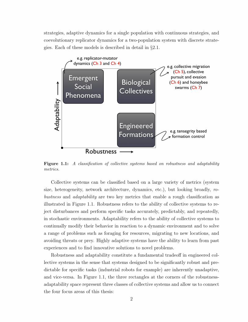
Figure 1.1: A classification of collective systems based on robustness and adaptabilitymetrics.

Collective systems can be classified based on a large variety of metrics (system

size, heterogeneity, network architecture, dynamics, etc.), but looking broadly, ro-

bustness and adaptability are two key metrics that enable a rough classification as

illustrated in Figure 1.1. Robustness refers to the ability of collective systems to re-

ject disturbances and perform specific tasks accurately, predictably, and repeatedly,

in stochastic environments. Adaptability refers to the ability of collective systems to

continually modify their behavior in reaction to a dynamic environment and to solve

a range of problems such as foraging for resources, migrating to new locations, and

avoiding threats or prey. Highly adaptive systems have the ability to learn from past

experiences and to find innovative solutions to novel problems.

Robustness and adaptability constitute a fundamental tradeoff in engineered col-

lective systems in the sense that systems designed to be significantly robust and pre-

dictable for specific tasks (industrial robots for example) are inherently unadaptive,

and vice-versa. In Figure 1.1, the three rectangles at the corners of the robustness-

adaptability space represent three classes of collective systems and allow us to connect

the four focus areas of this thesis:

2

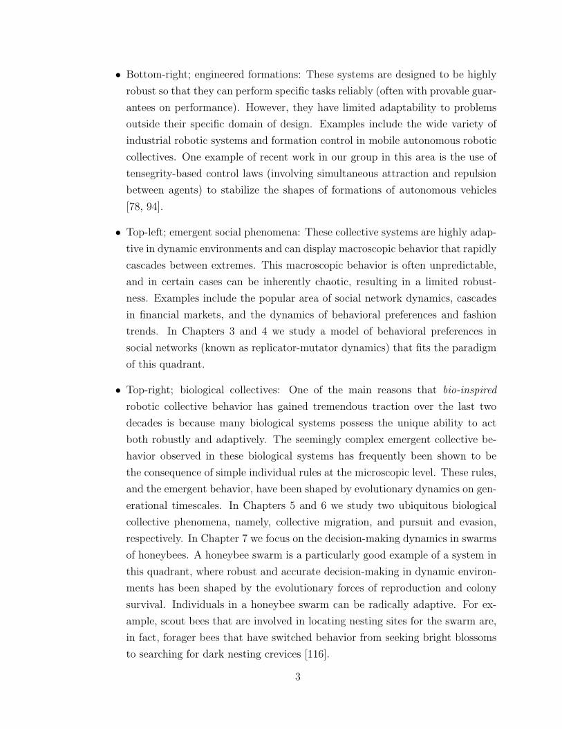
• Bottom-right; engineered formations: These systems are designed to be highly

robust so that they can perform specific tasks reliably (often with provable guar-

antees on performance). However, they have limited adaptability to problems

outside their specific domain of design. Examples include the wide variety of

industrial robotic systems and formation control in mobile autonomous robotic

collectives. One example of recent work in our group in this area is the use of

tensegrity-based control laws (involving simultaneous attraction and repulsion

between agents) to stabilize the shapes of formations of autonomous vehicles

[78, 94].

• Top-left; emergent social phenomena: These collective systems are highly adap-

tive in dynamic environments and can display macroscopic behavior that rapidly

cascades between extremes. This macroscopic behavior is often unpredictable,

and in certain cases can be inherently chaotic, resulting in a limited robust-

ness. Examples include the popular area of social network dynamics, cascades

in financial markets, and the dynamics of behavioral preferences and fashion

trends. In Chapters 3 and 4 we study a model of behavioral preferences in

social networks (known as replicator-mutator dynamics) that fits the paradigm

of this quadrant.

• Top-right; biological collectives: One of the main reasons that bio-inspired

robotic collective behavior has gained tremendous traction over the last two

decades is because many biological systems possess the unique ability to act

both robustly and adaptively. The seemingly complex emergent collective be-

havior observed in these biological systems has frequently been shown to be

the consequence of simple individual rules at the microscopic level. These rules,

and the emergent behavior, have been shaped by evolutionary dynamics on gen-

erational timescales. In Chapters 5 and 6 we study two ubiquitous biological

collective phenomena, namely, collective migration, and pursuit and evasion,

respectively. In Chapter 7 we focus on the decision-making dynamics in swarms

of honeybees. A honeybee swarm is a particularly good example of a system in

this quadrant, where robust and accurate decision-making in dynamic environ-

ments has been shaped by the evolutionary forces of reproduction and colony

survival. Individuals in a honeybee swarm can be radically adaptive. For ex-

ample, scout bees that are involved in locating nesting sites for the swarm are,

in fact, forager bees that have switched behavior from seeking bright blossoms

to searching for dark nesting crevices [116].

3

This thesis is the product of interdisciplinary research drawing from ideas in evo-

lutionary biology, animal behavior, engineering and applied mathematics. The back-

ground material in Chapter 2 introduces key tools from these areas that are used

throughout the thesis. Along with the exciting quest of understanding the complexity

of biological collectives, research in our group also strives to draw ideas and principles

from biology that can be applied to the design of robotic collectives. From the per-

spective of Figure 1.1, this effort involves utilizing ideas from the top-right quadrant

to push engineered systems (bottom right quadrant) up the adaptability axis, while

still managing the adaptability/robustness tradeoff. This is no easy challenge and will

remain an area of research emphasis going forward as autonomous collective systems

are tasked with solving increasingly complex problems. As a result, together with a

focus on understanding collective dynamics in the four areas described below, we also

consider how this understanding inspires engineering design in each case.

1.1 Overview of Topics

1.1.1 Replicator-Mutator Dynamics∗

The replicator-mutator dynamics define a canonical model from evolutionary theory

and represent the evolution of a discrete number of strategies in a single large popu-

lation. The dynamics have received significant attention recently as a model for the

evolution of language. They also provide a simple model for the analysis of behavior

dominance in social networks where replication is akin to imitation of individuals

subscribed to successful behaviors in a population, and mutation is akin to random

error in behavior selection. Much of the analysis of the dynamics has focused on

stable equilibria and their bifurcations. In this thesis we focus on the existence of

structurally stable limit cycles of the dynamics and prove that Hopf bifurcations oc-

cur, yielding these cycles. Stable limit cycles correspond to sustained oscillations in

strategy dominance across some or all of the population. The form of the dynamics

considered, and the interpretation of the oscillations, depends on the applications of

interest; the following are three motivating applications.

a) The replicator-mutator dynamics have been used in the development of a mathe-

matical framework for the evolution of language [85]. For a large population, the

strategies represent different grammars in the population and mutations reflect er-

rors in grammar transmission or learning from one generation to the next. A key

∗The discussion in this subsection appears verbatim in [93].

4

result is the bifurcation of the equilibria from a state where several grammars co-

exist in a population to a state of high grammatical coherence as mutations in the

population decrease (or equivalently, the fidelity of learning increases) [57, 75, 74].

Limit cycles of the replicator-mutator dynamics correspond to oscillations in the

dominance of the different grammars in the population. As noted in [76], oscilla-

tions appear to be more realistic than stable equilibria for the language dynamics

with timescales on the order of several centuries.

b) The replicator-mutator dynamics were recently proposed [90, 44] as a model for

behavior adoption in social networks, with a focus on the emergence of dominance

of particular behaviors in these networks. Simulations of the evolutionary social

network model show a transition from the dominance of a single strategy (behav-

ior), to the coexistence of several strategies, to the eventual collapse of dominance,

as the extent of mutation in the network increases. Limit cycles of the replicator-

mutator dynamics correspond to oscillations of behavior preference in this context,

for example cycles in trends or fashions.

c) The replicator-mutator dynamics can also be used to model decision-making dy-

namics in networked multi-agent systems. It has been shown that simple mod-

els with pairwise interactions between agents and noisy imitation of successful

strategies reduce (under certain conditions) to the replicator-mutator dynamics

[40, 7, 135, 134]. Recent papers have employed the replicator-mutator equations

to model wireless multi-agent networks [145, 130]. Hopf bifurcations of replicator-

mutator dynamics in this context address the exploration versus exploitation

tradeoff: few mutations favor fast convergence to a decision (exploitation) whereas

extensive mutations favor exploration of the decision space. In an intermediate

range, mutations can lead to limit cycles, which enable dynamic examination of

alternative choices.

1.1.2 Collective Migration

Collective migration is a natural phenomenon common in a number of species in-

cluding birds, fish, invertebrates and mammals [119, 42, 22, 6]. Animals migrate by

leveraging a variety of environmental cues such as nutrient and thermal gradients,

magnetic fields, odor cues, or visual markers [132, 30, 140, 133]. Measuring these

stochastic environmental signals is complicated and requires the investment of time

and energy, and the development of necessary physiological and sensory machinery.

5

Animals migrating collectively also have the ability to leverage social information from

neighbors in the group [15]. One way of doing so is by imitating invested neighbors

(via consensus processes such as attraction and alignment of heading) and thereby

effectively achieving good migratory performance, without paying the measurement

and processing cost.

Using agent-based models of collective migration, Couzin et al. [14] have shown

that a small group of designated leaders is capable of guiding a larger of group of

naive, socially interacting followers. This situation is similar, for example, to the way

in which a small number of informed scout bees directs a large swarm of uninformed

conspecifics to a new nest site [116, 120]. The ability of followers in such migratory

swarms to leverage the investments made by leaders in the group, and to gain the

benefits of successful migration without paying the associated costs, is perplexing

from an evolutionary perspective (this question is related to the broader puzzle of the

evolution of cooperation).

Our study of the evolutionary dynamics of collective migration is motivated in

large part by a recent paper by Guttal and Couzin [33] that addresses this evolutionary

question. Simulations in [33] show that the coexistence of leaders and followers in

migratory populations is a stable emergent outcome of the evolutionary dynamics

for a large region of the parameter space studied. The authors of [33] also examine

the role of anthropogenic influences on evolved population migration patterns by

studying the impact of increasing habitat fragmentation on the collective dynamics.

High levels of habitat fragmentation make it increasingly difficult for individuals to

measure external cues; migration is gradually lost because of the higher costs of

reaching more distant destinations [120]. Simulations in [33] illustrate a hysteretic

effect in restoring lost migration ability in the population - once migration ability is

lost for a threshold level of fragmentation, much greater habitat recovery is necessary

for the population to recover the ability to migrate.

We are also motivated by the paper by Torney et al. [132] that analytically vali-

dates the evolutionary branching simulated in [33] by studying a mean-field model of

migration dynamics. The mean-field model in [132] effectively prescribes an all-to-all

interconnection between the agents in the migratory system and serves as the starting

point for our work, which focuses explicitly on the role of the structure of a limited

interaction network on evolved outcomes. Indeed, the structure of the interaction

network between agents in a collective has been shown to be critical to the perfor-

mance of the collective, and to the emergent outcomes observed as a consequence of

the local interactions.

6

1.1.3 Pursuit and Evasion†

Pursuit and evasion behaviors play a critical role in predator foraging, prey survival,

mating and territorial battles in several species. Species such as bats and dragonflies

have evolved sophisticated dynamical strategies such as motion camouflage to disguise

themselves as stationary during aerial pursuit [77, 27]. Studies on migratory canni-

balistic locusts have revealed that pursuit and evasive behavior among conspecifics is

integral to the formation of mass-moving migratory bands in dense swarms [35, 5].

Recent experimental work on the dynamics of coordinated predator pursuit and prey

evasion among schooling fish has shown that collective behavior, among both preda-

tors and prey, plays a vital role in predator hunting and prey evasion under condi-

tions of considerable informational constraints (such as dynamic ocean environments)

[37, 45].

The pervasiveness of pursuit and evasion in nature motivates the examination of

winning strategies from an evolutionary perspective. Recently, Wei et al. [147] used

the evolutionary approach to study pursuit games, with dynamics derived in [50]. The

authors of [147, 50] use Monte-Carlo simulations and analytical calculations to study

three pursuit strategies competing against a field of deterministic or random nonre-

active evasive strategies (an evader with a nonreactive strategy has dynamics that

are uncoupled from those of the pursuer). The three chosen pursuit strategies (classi-

cal, constant bearing and motion camouflage) are biologically inspired. The authors

show convergence of the evolutionary game dynamics between the three strategies to

pure motion camouflage and motivate this result by empirical observations of motion

camouflage in hoverflies, dragonflies and bats [27]. We build on the work in [147] by

studying the coevolution of the three strategies of pursuit from [147] playing against

three distinct evasive strategies, two of which are reactive strategies (an evader with

a reactive strategy has dynamics that are coupled to those of the pursuer).

1.1.4 Swarm Decision-Making

Honeybee colonies reproduce by casting out swarms, each of which comprises a queen

accompanied by several thousand worker bees. A small fraction of the worker bees are

known as scout bees and perform the task of locating suitable nest sites for the swarm

by engaging in a decentralized democratic [116] decision-making process of choosing

among several competing options. This process involves the famous waggle dance

[144] in which scout bees advertise the location and quality of a suitable nest site by

†The discussion in this subsection is adapted from [96].

7

performing a distinctive dance on the surface of the swarm. The book by Seeley [116]

provides an engaging description of the waggle dance, as well as a detailed discussion

of the organization and behavior of honeybee swarms.

In a recent paper, Seeley et al. [118] have shown that scouts send inhibitory

stop-signals to other scouts advertising alternative nest sites, thereby causing these

scouts to cease dancing. This cross-inhibitory process has been shown to be critical

to the ability of swarms to make decisions effectively, particularly when choosing

between competing options of near-equal value. In this thesis we study bifurcations

in a model of honeybee swarm decision-making and illustrate the critical role played

by stop-signal inhibition in enabling swarms to manage the speed-accuracy tradeoff

inherent to most decision-making problems. We show that an intermediate evolved

level of stop-signaling is necessary for swarms to effectively make decisions when

presented with both equal and unequal alternatives. Our analysis also shows that

cross-inhibition is a potentially valuable mechanism for enabling effective collective

decision-making in decentralized artificial swarms.

1.2 Contributions and Thesis Outline

The chapters of this thesis are organized according to the four topics described in

§1.1. Chapter 2 comprises background material and establishes the mathematical

notation that will be used throughout the thesis. Background material is presented

in four main areas: Evolutionary Dynamics, Dynamical Systems, Graph Theory and

Stochastic Processes.

Chapters 3 and 4 focus on limit cycles and Hopf bifurcations of the replicator-

mutator dynamics. The analysis in Chapter 3 is restricted to N = 3 strategies and

the corresponding planar phase space. The restriction to N = 3 is convenient for

visualization and allows us to motivate the general results for N ≥ 3 strategies to

follow in Chapter 4. In Chapter 4 we prove conditions for the existence of stable

limit cycles arising from multiple distinct Hopf bifurcations of the dynamics in the

case of circulant fitness matrices. In the noncirculant case we illustrate how stable

limit cycles of the dynamics are coupled to embedded directed cycles in the payoff

graph. We study special conditions where multiple cycles in the payoff graph yield

multiple stable limit cycle attractors. The stability of the limit cycles is determined

by an analytical calculation of the first Lyapunov coefficient of the dynamics.

In Chapter 5 we study the role of the social interconnection network on the evo-

lutionary dynamics of collective migration. We design a networked migration model

8

and study evolution and adaptation as a function of network topology. Our model has

two timescales: the fast timescale corresponds to fitness/utility calculations and the

slow timescale corresponds to the evolution/adaptation of the network. We present

a comprehensive analysis of the all-to-all limit of the model and prove conditions for

population branching into leaders and followers. For networks with limited connec-

tivity, we derive analytical tools for computing fitness on the fast timescale and show

a minimum connectivity threshold necessary for branching. We also study a simple

model of selfish local adaptation of nodes on a graph, and illustrate bifurcations in

the dynamics as a function of increasing cost. We show the prominent role played by

network topology in determining the location of leaders in the adaptive network.

Chapter 6 focuses on the coevolutionary dynamics of pursuit and evasion. We

consider an evolutionary game between three strategies of pursuit (classical, con-

stant bearing, motion camouflage) and three strategies of evasion (classical, random,

optical-flow based). Pursuer and evader agents are modeled as self-propelled steered

particles with constant speed and strategy-dependent heading control. We use Monte-

Carlo simulations and theoretical analysis to show convergence of the evolutionary

dynamics to a pure strategy Nash equilibrium of classical pursuit versus classical eva-

sion. We extend our work to consider a novel pursuit and evasion based collective

motion scheme, motivated by collective pursuit and evasion in bands of migrating

cannibalistic locusts.

In Chapter 7 we study the collective decision-making dynamics of honeybee

swarms. The cross-inhibitory stop-signalling mechanism has been shown to be

critical to the decision-making dynamics in swarms of house-hunting honeybees.

We study a model of stop-signal based collective decision-making and present a

comprehensive picture of the dynamics and bifurcations of this model. We prove

a separation of timescales in the decision-making process and show how swarms

must evolve to an intermediate level of stop-signalling to address a fundamental

speed-accuracy tradeoff. We also present several stochastic simulations to help

elucidate the decision-making process.

Chapter 8 presents our conclusions and topics for future work. We discuss how

some of the analysis and conclusions of this thesis inspire algorithms for control and

decision-making in decentralized collective artificial systems.

9

Chapter 2

Background

In this chapter we describe some of the main mathematical tools that will be used

in the rest of the thesis and we establish notation. Each of the areas discussed in

the sections to follow is a significant domain of research by itself. Consequently, this

chapter is not intended to be a comprehensive presentation of these areas, but rather

an introduction to selected tools from these areas that will be useful going forward.

The cited references provide more detail.

In §2.1, we discuss models of evolutionary dynamics and make connections with

game theory, genetic algorithms, and optimization. §2.2 focuses on bifurcations in

continuous dynamical systems, including the Hopf bifurcation theorem, which features

prominently in Chapters 3 and 4. §2.3 introduces some notation and results from

graph theory and §2.4 introduces some basic results from stochastic dynamics; these

are employed in Chapters 5 and 7.

Basic Notation: Matrices are denoted in capital letters and vectors are denoted in

boldface lowercase letters. mij denotes the (i, j) element of matrix M (M = [mij] ∈RM×N) and xi denotes the ith element of vector x

(x = [ x1 · · · xN ]T ∈ RN

). 1

and 0 denote the vectors of ones and zeros respectively. D = [dij] = diag(x) denotes

a diagonal matrix with elements of vector x on the main diagonal, i.e. dii = xi and

dij = 0 for all i 6= j. The N ×N identity matrix is given by IN = diag(1N).

2.1 Evolutionary Dynamics

Evolutionary dynamics [142, 87, 41, 141] are, broadly speaking, an effort to cast

the basic tenets of Darwinian natural selection (replication, competition, strategy

dependent fitness, mutation) in a mathematical framework that can be simulated,

10

interpreted, and often rigorously analyzed. Our understanding of the evolutionary

process has its roots in Darwin’s three simple postulates [142, 16]:

1. Like tends to beget like, and there is heritable variation in traits associated with

each type of organism. (replication and mutation)

2. Among organisms there is a struggle for existence. (competition)

3. Heritable traits influence the struggle for existence. (strategy dependent fitness)

These postulates inherently define a game-theoretic interaction between individuals

in the population as a function of their strategies (expressed as phenotypes or traits),

and their interactions with the environment and other individuals. These strategies

and interactions map to payoffs, which in turn translate to reproductive fitness. The

game theoretic mechanism implies that evolutionary solutions are not necessarily

optimal in terms of maximizing the fitness of the population as a whole.

Nonetheless, the ability of evolutionary dynamics to shape natural systems to-

wards a fascinating array of effective solutions has inspired powerful tools for opti-

mization in engineering design, e.g. genetic algorithms [73]. In genetic optimization

algorithms, agents imitate the evolutionary process to search for local optima on

a constant landscape as shown in Figure 2.1. This is in contrast with biological

(game-theoretic) evolutionary dynamics where the strategies interact and influence

the landscape on which they are evolving (see Figure 2.1). In this thesis, we focus

on studying the outcomes of models of game-theoretic evolutionary dynamics, while

also making connections with how these solutions inspire the design of engineered

collective systems.

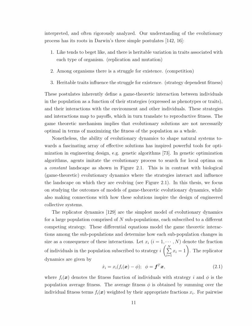
The replicator dynamics [129] are the simplest model of evolutionary dynamics

for a large population comprised of N sub-populations, each subscribed to a different

competing strategy. These differential equations model the game theoretic interac-

tions among the sub-populations and determine how each sub-population changes in

size as a consequence of these interactions. Let xi (i = 1, · · · , N) denote the fraction

of individuals in the population subscribed to strategy i

(N∑i=1

xi = 1

). The replicator

dynamics are given by

xi = xi(fi(x)− φ); φ = fTx, (2.1)

where fi(x) denotes the fitness function of individuals with strategy i and φ is the

population average fitness. The average fitness φ is obtained by summing over the

individual fitness terms fi(x) weighted by their appropriate fractions xi. For pairwise

11

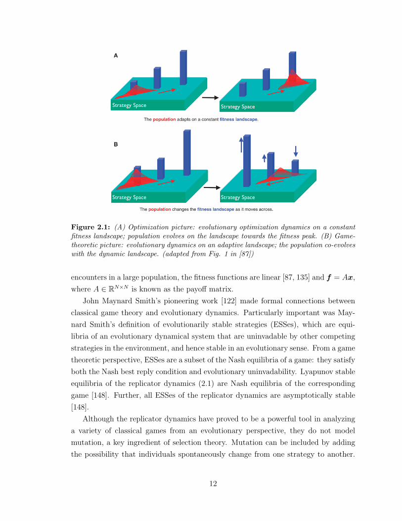
Figure 2.1: (A) Optimization picture: evolutionary optimization dynamics on a constantfitness landscape; population evolves on the landscape towards the fitness peak. (B) Game-theoretic picture: evolutionary dynamics on an adaptive landscape; the population co-evolveswith the dynamic landscape. (adapted from Fig. 1 in [87])

encounters in a large population, the fitness functions are linear [87, 135] and f = Ax,

where A ∈ RN×N is known as the payoff matrix.

John Maynard Smith’s pioneering work [122] made formal connections between

classical game theory and evolutionary dynamics. Particularly important was May-

nard Smith’s definition of evolutionarily stable strategies (ESSes), which are equi-

libria of an evolutionary dynamical system that are uninvadable by other competing

strategies in the environment, and hence stable in an evolutionary sense. From a game

theoretic perspective, ESSes are a subset of the Nash equilibria of a game: they satisfy

both the Nash best reply condition and evolutionary uninvadability. Lyapunov stable

equilibria of the replicator dynamics (2.1) are Nash equilibria of the corresponding

game [148]. Further, all ESSes of the replicator dynamics are asymptotically stable

[148].

Although the replicator dynamics have proved to be a powerful tool in analyzing

a variety of classical games from an evolutionary perspective, they do not model

mutation, a key ingredient of selection theory. Mutation can be included by adding

the possibility that individuals spontaneously change from one strategy to another.

12

This yields the replicator-mutator dynamics [9, 92] given by

xi =N∑j=1

xjfj(x)qji − xiφ; φ = fTx, (2.2)

where qij denotes the probability of mutation from strategy i to strategy j(N∑j=1

qij = 1

). The replicator-mutator dynamics have played a prominent role

in evolutionary theory and contain as limiting cases many other important equations

in biology [55]; these include models of language evolution [85], autocatalytic reaction

networks [124], and population genetics [36]. The dynamics have also recently been

employed to model social and multi-agent network interactions [90]. The replicator-

mutator equations have been shown in [92] to be equivalent to the generalized Price

equation from evolutionary genetics [105, 106]. The standard replicator dynamics

(2.1) can be obtained from the replicator-mutator dynamics (2.2) in the limit of zero

mutation (qii = 1 for all i and qij = 0 for all i 6= j).

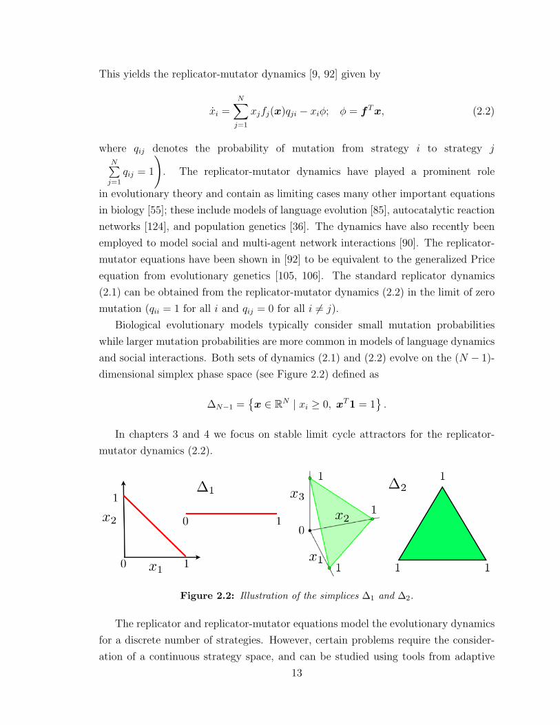
Biological evolutionary models typically consider small mutation probabilities

while larger mutation probabilities are more common in models of language dynamics

and social interactions. Both sets of dynamics (2.1) and (2.2) evolve on the (N − 1)-

dimensional simplex phase space (see Figure 2.2) defined as

∆N−1 ={x ∈ RN | xi ≥ 0, xT1 = 1

}.

In chapters 3 and 4 we focus on stable limit cycle attractors for the replicator-

mutator dynamics (2.2).

Figure 2.2: Illustration of the simplices ∆1 and ∆2.

The replicator and replicator-mutator equations model the evolutionary dynamics

for a discrete number of strategies. However, certain problems require the consider-

ation of a continuous strategy space, and can be studied using tools from adaptive

13

dynamics [25, 26, 18]. Adaptive dynamics are particularly well-suited for studying

the evolution of a one-dimensional trait in a population undergoing small mutations

in strategy. Consider a continuous strategy space parameterized by k ∈ [a, b] ⊂ R.

The fitness of a resident population with strategy kR is given by FR(kR). The adap-

tive dynamics approach considers the consequences of a small group of mutants with

strategy kM invading the resident population. Let FM(kR, kM) denote the fitness of

the mutants in the environment of the residents. The relative fitness of the mutants

with respect to the residents is known as the differential fitness and is given by

S(kR, kM) = FM(kR, kM)− FR(kR). (2.3)

The two-parameter function S allows us to predict which mutant strategies can invade

a particular resident population. For example, for a given resident strategy kR, the

values of kM that result in S > 0 correspond to the mutant strategies that when

rare, can invade the established resident population. Further, a study of the selection

landscape S can help us predict when we expect to see an evolutionarily stable [122]

monomorphic population (all individuals having the same strategy) and when we

expect to see opportunities for branching (speciation into sets of individuals having

different strategies) in evolutionary simulations.

The evolutionary dynamics of the resident strategy kR are given by

dkRdt

= α∂S

∂kM

∣∣∣∣kM =kR

=: α g(kR), (2.4)

where g(kR) is known as the selection gradient and α > 0 is related to the extent of

mutation in the population. As the strategy kR of the population evolves according

to (2.4), the small mutations kM about the resident strategy kR also evolve accord-

ingly. The sign of the selection gradient g(kR) is indicative of the direction in which

the strategy of the population will evolve. In particular, the strategy of the popula-

tion will increase for g(kR) > 0 and decrease for g(kR) < 0. Evolutionary singular

strategies k∗ correspond to a vanishing selection gradient g(k∗) = 0. Singular strate-

gies are evolutionary attractors for the population (also known as Convergent Stable

Strategies (CSS)) if they satisfy the condition

∂g

∂kR

∣∣∣∣kR=k∗

< 0. (2.5)

14

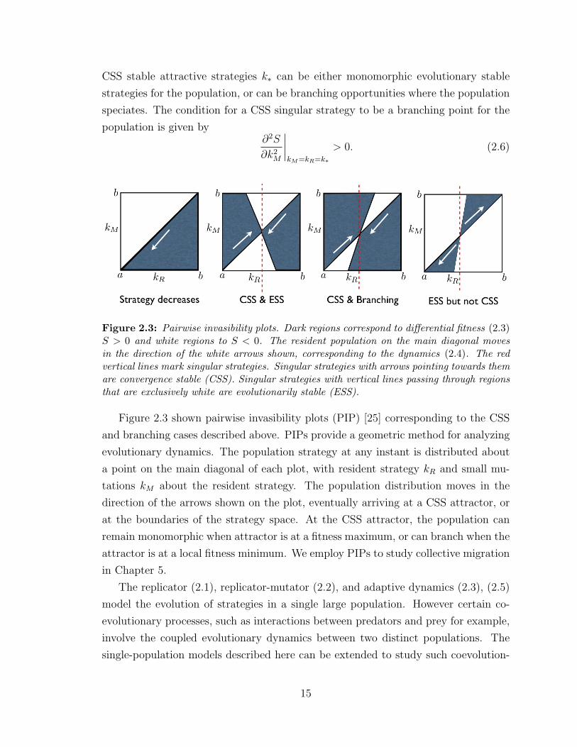
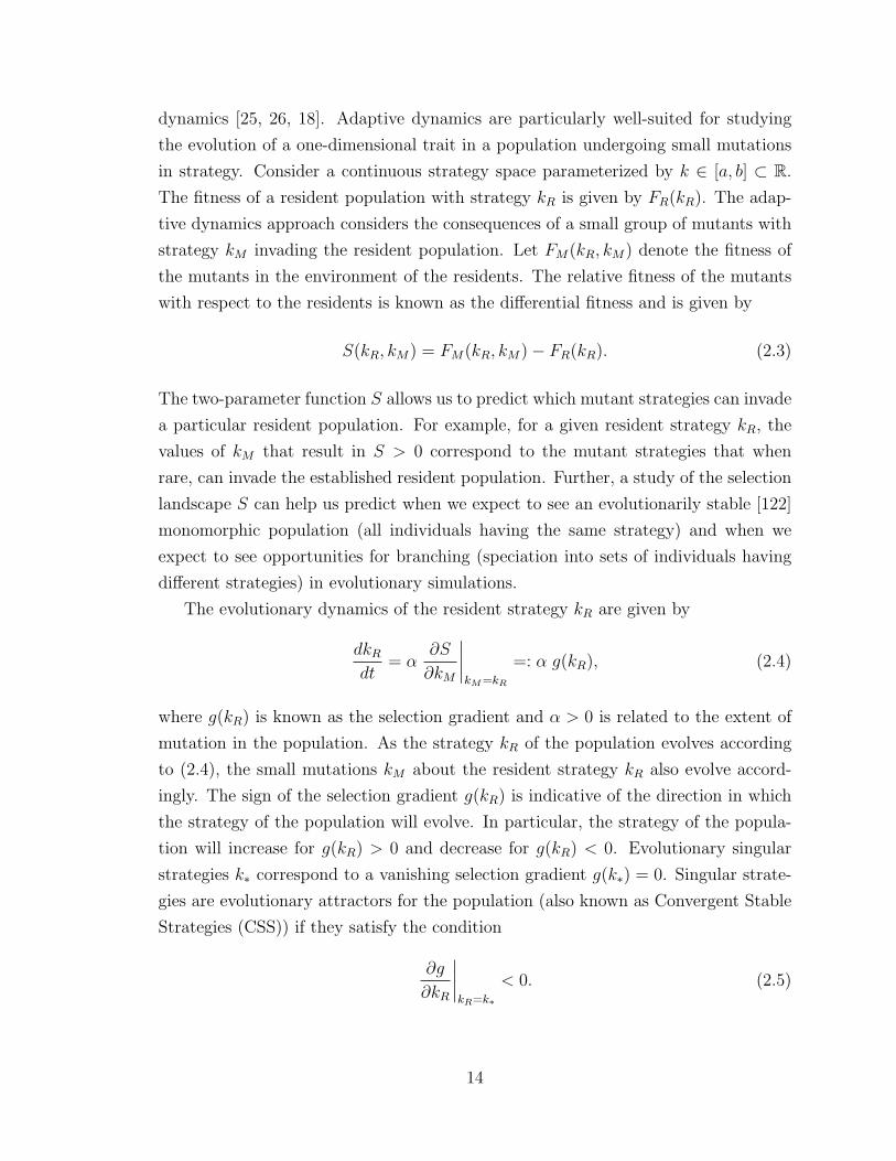
CSS stable attractive strategies k∗ can be either monomorphic evolutionary stable

strategies for the population, or can be branching opportunities where the population

speciates. The condition for a CSS singular strategy to be a branching point for the

population is given by∂2S

∂k2M

∣∣∣∣kM =kR=k∗

> 0. (2.6)

Figure 2.3: Pairwise invasibility plots. Dark regions correspond to differential fitness (2.3)S > 0 and white regions to S < 0. The resident population on the main diagonal movesin the direction of the white arrows shown, corresponding to the dynamics (2.4). The redvertical lines mark singular strategies. Singular strategies with arrows pointing towards themare convergence stable (CSS). Singular strategies with vertical lines passing through regionsthat are exclusively white are evolutionarily stable (ESS).

Figure 2.3 shown pairwise invasibility plots (PIP) [25] corresponding to the CSS

and branching cases described above. PIPs provide a geometric method for analyzing

evolutionary dynamics. The population strategy at any instant is distributed about

a point on the main diagonal of each plot, with resident strategy kR and small mu-

tations kM about the resident strategy. The population distribution moves in the

direction of the arrows shown on the plot, eventually arriving at a CSS attractor, or

at the boundaries of the strategy space. At the CSS attractor, the population can

remain monomorphic when attractor is at a fitness maximum, or can branch when the

attractor is at a local fitness minimum. We employ PIPs to study collective migration

in Chapter 5.

The replicator (2.1), replicator-mutator (2.2), and adaptive dynamics (2.3), (2.5)

model the evolution of strategies in a single large population. However certain co-

evolutionary processes, such as interactions between predators and prey for example,

involve the coupled evolutionary dynamics between two distinct populations. The

single-population models described here can be extended to study such coevolution-

15

ary processes; we will consider an extension of the replicator dynamics to model the

evolutionary dynamics of pursuit and evasion in Chapter 6.

2.2 Dynamical Systems Tools

A dynamical system is a mathematical model describing the time evolution of a set

of variables which collectively define the state of the system at any given point in

time. There is a rich set of tools in the dynamical system literature (for example

see [32, 59, 125]) for computing and understanding the solutions to these systems,

including the study of bifurcations. A bifurcation is a qualitative change in the solu-

tions of a dynamical system as a result of the smooth change in a system parameter

(known as the bifurcation parameter). Bifurcations that are detected by studying

small neighborhoods of equilibria and limit cycles of dynamical systems are known

as local bifurcations. In Chapters 3, 4, 5 and 7, we study local bifurcations of specific

continuous-time dynamical systems, and in this section we introduce the kinds of

bifurcations that appear in these chapters.

Consider the continuous-time dynamical system with state x ∈ RN and bifurcation

parameter µ ∈ R given by

x = f(x, µ), (2.7)

with the vector field f : RN × R 7→ RN . The range of behavior for one-dimensional

systems (x ∈ R) is limited; solutions either approach stable equilibria or diverge

to infinity. Nonetheless, the analysis of certain bifurcations in higher dimensional

systems can be reduced to studying one-dimensional normal forms (nonlinear analog

of matrix diagonalization or matrix Jordan normal form [32, 59]) by using the center

manifold theorem (see [32] for details). The four main bifurcations for one-dimensional

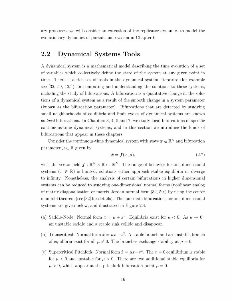
systems are given below, and illustrated in Figure 2.4.

(a) Saddle-Node: Normal form x = µ + x2. Equilibria exist for µ < 0. As µ → 0−

an unstable saddle and a stable sink collide and disappear.

(b) Transcritical: Normal form x = µx−x2. A stable branch and an unstable branch

of equilibria exist for all µ 6= 0. The branches exchange stability at µ = 0.

(c) Supercritical Pitchfork: Normal form x = µx−x3. The x = 0 equilibrium is stable

for µ < 0 and unstable for µ > 0. There are two additional stable equilibria for

µ > 0, which appear at the pitchfork bifurcation point µ = 0.

16

(d) Subcritical Pitchfork: Normal form x = µx+ x3. The x = 0 equilibrium is stable

for µ < 0 and unstable for µ > 0. There are two additional unstable equilibria

for µ < 0.

Figure 2.4: Illustration of the four canonical bifurcations in one-dimensional systems.Solid curves are stable equilibria and dashed curves are unstable. (a) Saddle-Node (b) Tran-scritical (c) Supercritical pitchfork (d) Subcritical pitchfork.

In addition to stable and unstable equilibria, N(≥2)-dimensional systems (x ∈RN) can also have periodic orbits, limit cycles, homo/hetero-clinic connections and

chaotic attractors (chaotic attractors may exist only for N ≥ 3, see the Poincare-

Bendixson theorem in [32] and Peixoto’s theorem in [32, 100]). Bendixson’s criterion

provides sufficient conditions for the nonexistence of periodic orbits for planar systems

(x ∈ R2) [32].

Theorem 2.1. (Bendixson’s Criterion) An autonomous planar vector field (2.7) de-

fined on a simply connected region D ⊂ R2 has no periodic orbits lying entirely in D

if ∂f1∂x1

+ ∂f2∂x2

is not identically zero and does not change sign in D.

One-parameter bifurcations in dynamical systems with a one- or two-dimensional

state space can be conveniently plotted in two and three dimensions respectively.

Constructing bifurcation plots is more challenging for higher dimensional (N ≥ 3)

systems, for which we can either plot projections in two or three dimensions (as in

Chapters 4 and 5), or construct reduced dimensional approximations of the dynamics

(as in Chapter 7).

For high dimensional systems, our focus in Chapter 4 will be on the existence of

stable limit cycles, arising out of Hopf bifurcations of the dynamics. The normal form

of the Hopf bifurcation is given by

x1 = µx1 − x2 + σx1(x21 + x2

2)

x2 = x1 + µx2 + σx2(x21 + x2

2),(2.8)

where σ = ±1 (σ = sign(`1(0)) from Theorem 2.2 below). The Hopf bifurcation point

is µ = 0. The origin is asymptotically stable for µ < 0 and unstable for µ > 0. The

17

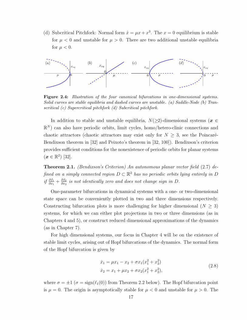
bifurcation is supercritical for σ = −1 and subcritical for σ = +1. The supercritical

bifurcation results in stable limit cycles of radius√µ for µ > 0 as shown in Figure

2.5. For general N ≥ 3 dimensional systems, the Hopf bifurcation theorem [32, 59]

µ

x1

x2

x1

x2

µ = !2

µ = 3

µ = !2

µ = 3

Figure 2.5: Bifurcation plot (left) for the supercritical Hopf bifurcation normal form (2.8).Blue curves are stable equilibria, red curves are unstable equilibria and magenta curvesare stable limit cycles. The two right plots are phase portraits for µ = −2 and µ = 3,corresponding to the grey slices on the bifurcation plot.

provides sufficient conditions for the existence of stable limit cycles arising out of

supercritical Hopf bifurcations.

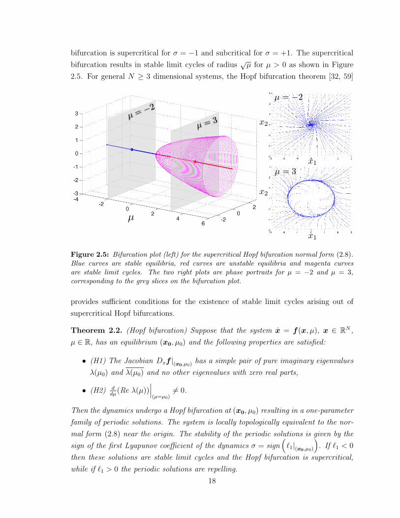
Theorem 2.2. (Hopf bifurcation) Suppose that the system x = f(x, µ), x ∈ RN ,

µ ∈ R, has an equilibrium (x0, µ0) and the following properties are satisfied:

• (H1) The Jacobian Dxf |(x0,µ0) has a simple pair of pure imaginary eigenvalues

λ(µ0) and λ(µ0) and no other eigenvalues with zero real parts,

• (H2) ddµ

(Re λ(µ))∣∣∣(µ=µ0)

6= 0.

Then the dynamics undergo a Hopf bifurcation at (x0, µ0) resulting in a one-parameter

family of periodic solutions. The system is locally topologically equivalent to the nor-

mal form (2.8) near the origin. The stability of the periodic solutions is given by the

sign of the first Lyapunov coefficient of the dynamics σ = sign(`1|(x0,µ0)

). If `1 < 0

then these solutions are stable limit cycles and the Hopf bifurcation is supercritical,

while if `1 > 0 the periodic solutions are repelling.

18

A key challenge is determining the right sets of coordinate transformations to con-

vert the center manifold dynamics to the normal form (2.8); details of the calculation

of the Lyapunov coefficient `1 are provided in Appendix A.

µ1

µ2

xeq

Bistable

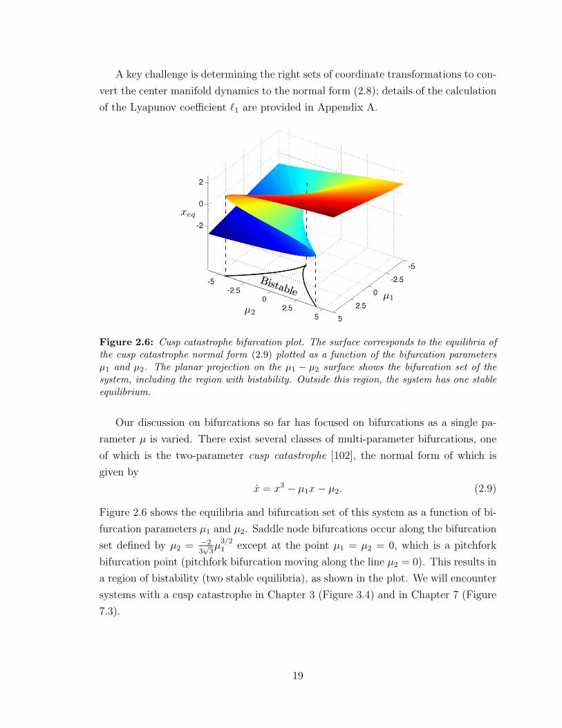
Figure 2.6: Cusp catastrophe bifurcation plot. The surface corresponds to the equilibria ofthe cusp catastrophe normal form (2.9) plotted as a function of the bifurcation parametersµ1 and µ2. The planar projection on the µ1 − µ2 surface shows the bifurcation set of thesystem, including the region with bistability. Outside this region, the system has one stableequilibrium.

Our discussion on bifurcations so far has focused on bifurcations as a single pa-

rameter µ is varied. There exist several classes of multi-parameter bifurcations, one

of which is the two-parameter cusp catastrophe [102], the normal form of which is

given by

x = x3 − µ1x− µ2. (2.9)

Figure 2.6 shows the equilibria and bifurcation set of this system as a function of bi-

furcation parameters µ1 and µ2. Saddle node bifurcations occur along the bifurcation

set defined by µ2 = −23√

3µ

3/21 except at the point µ1 = µ2 = 0, which is a pitchfork

bifurcation point (pitchfork bifurcation moving along the line µ2 = 0). This results in

a region of bistability (two stable equilibria), as shown in the plot. We will encounter

systems with a cusp catastrophe in Chapter 3 (Figure 3.4) and in Chapter 7 (Figure

7.3).

19

2.3 Graph Theory Tools

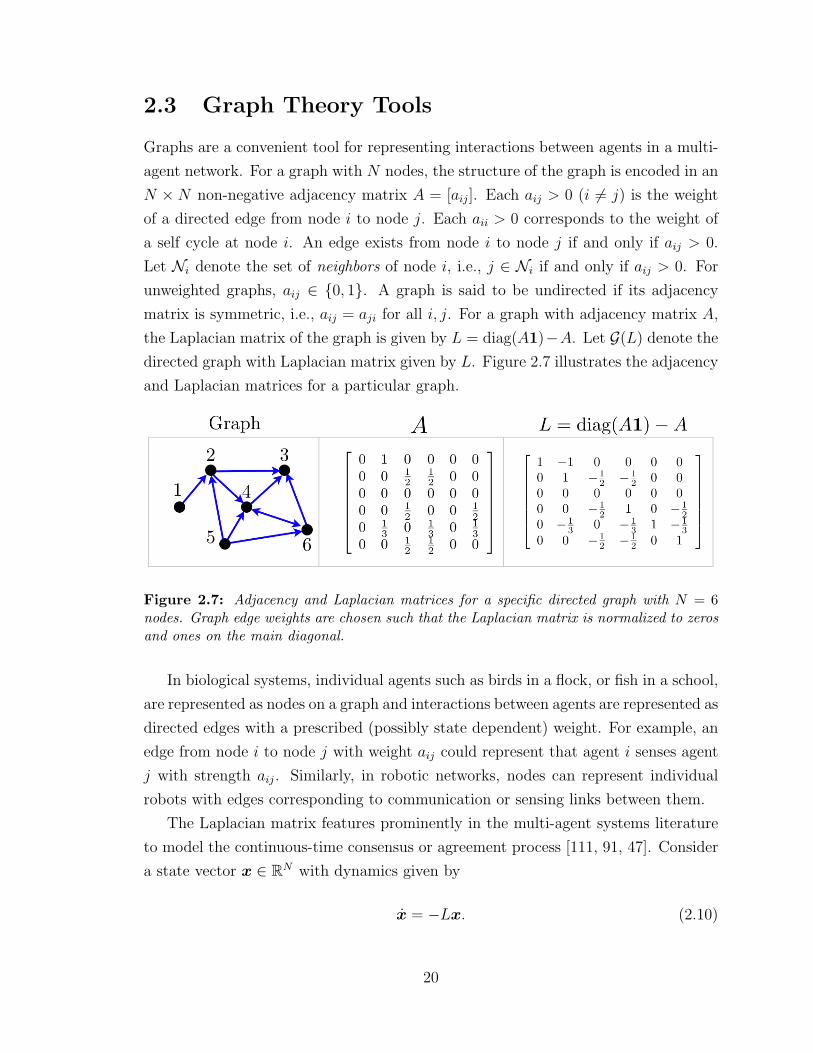
Graphs are a convenient tool for representing interactions between agents in a multi-

agent network. For a graph with N nodes, the structure of the graph is encoded in an

N × N non-negative adjacency matrix A = [aij]. Each aij > 0 (i 6= j) is the weight

of a directed edge from node i to node j. Each aii > 0 corresponds to the weight of

a self cycle at node i. An edge exists from node i to node j if and only if aij > 0.

Let Ni denote the set of neighbors of node i, i.e., j ∈ Ni if and only if aij > 0. For

unweighted graphs, aij ∈ {0, 1}. A graph is said to be undirected if its adjacency

matrix is symmetric, i.e., aij = aji for all i, j. For a graph with adjacency matrix A,

the Laplacian matrix of the graph is given by L = diag(A1)−A. Let G(L) denote the

directed graph with Laplacian matrix given by L. Figure 2.7 illustrates the adjacency

and Laplacian matrices for a particular graph.

Figure 2.7: Adjacency and Laplacian matrices for a specific directed graph with N = 6nodes. Graph edge weights are chosen such that the Laplacian matrix is normalized to zerosand ones on the main diagonal.

In biological systems, individual agents such as birds in a flock, or fish in a school,

are represented as nodes on a graph and interactions between agents are represented as

directed edges with a prescribed (possibly state dependent) weight. For example, an

edge from node i to node j with weight aij could represent that agent i senses agent

j with strength aij. Similarly, in robotic networks, nodes can represent individual

robots with edges corresponding to communication or sensing links between them.

The Laplacian matrix features prominently in the multi-agent systems literature

to model the continuous-time consensus or agreement process [111, 91, 47]. Consider

a state vector x ∈ RN with dynamics given by

x = −Lx. (2.10)

20

Here xi corresponds to the state of each node of the network and the dynamics (2.10)

correspond to agents on the graph updating their state to reach agreement with the

mean of their neighbors (as defined at the beginning of this section). The dynamics

(2.10) converge to the agreement subspace α1 for some scalar α if and only if the

directed graph corresponding to L (G(L)) is connected. Connectivity of G(L) requires

that there exists at least one node, labeled the root, such that a directed path exists

from every other node of the network to the root [111, 64, 110]. For example, the

graph in Figure 2.7 is connected with root node 3. In Chapter 5 we discuss graph

connectivity and consensus in more detail in the context of collective migration.

Figure 2.8: Illustration of circulant graphs for N = 6 nodes where each node has oneoutgoing edge.

In Chapters 3 and 4 we focus on a specific class of graph topologies with circulant

adjacency matrices. A circulant matrix is fully specified by its first row; the subse-

quent rows are cyclic permutations of the first row to the right with offset given by

the row index. Let circulant matrix C be given by

C = Circulant(c1, c2, · · · , cN) =

c1 c2 · · · · · · cN

cN c1 c2. . .

......

. . . . . . . . ....

... · · · cN c1 c2

c2 · · · · · · cN c1

. (2.11)

In Figure 2.8 we illustrate three circulant graph topologies. The symmetry of circulant

graphs, and corresponding well-known properties such as an analytical characteriza-

tion of eigenvalues and eigenvector of circulant adjacency and Laplacian matrices,

make these topologies particularly well-suited for analysis [43].

Graphs can also be constructed by considering the spatial embedding of nodes and

using spatial metrics to define the existence and weights of edges. This is particularly

21

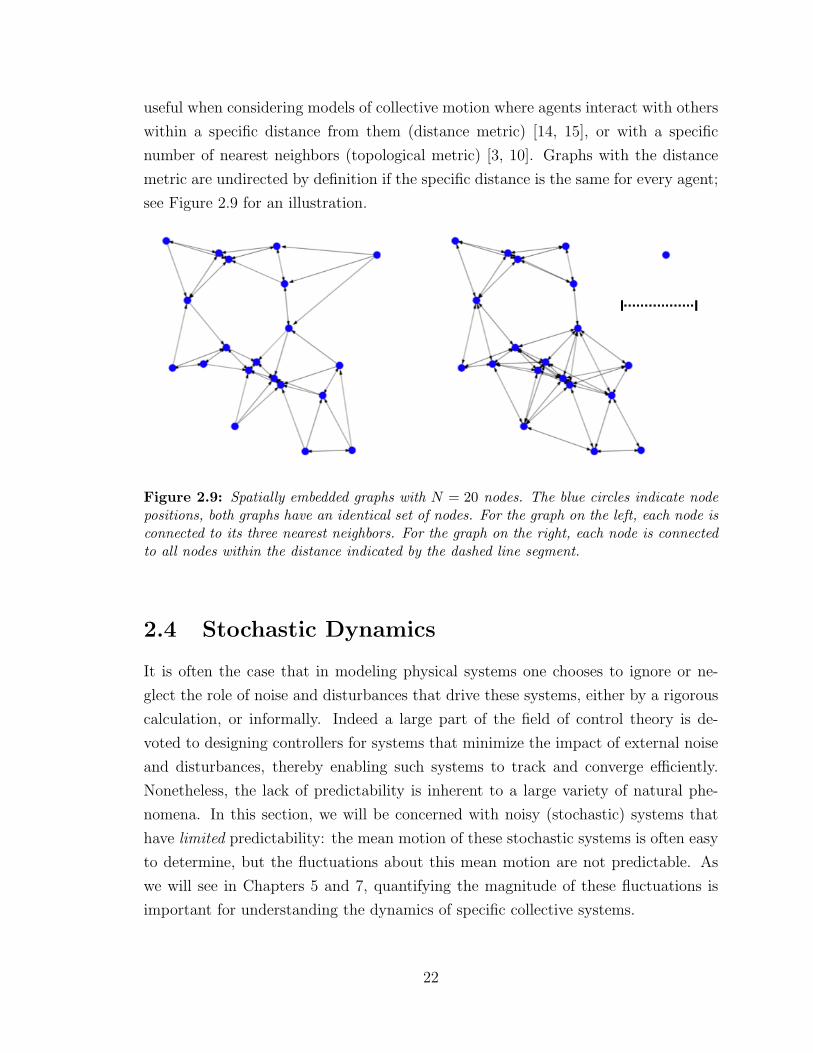
useful when considering models of collective motion where agents interact with others

within a specific distance from them (distance metric) [14, 15], or with a specific

number of nearest neighbors (topological metric) [3, 10]. Graphs with the distance

metric are undirected by definition if the specific distance is the same for every agent;

see Figure 2.9 for an illustration.

Figure 2.9: Spatially embedded graphs with N = 20 nodes. The blue circles indicate nodepositions, both graphs have an identical set of nodes. For the graph on the left, each node isconnected to its three nearest neighbors. For the graph on the right, each node is connectedto all nodes within the distance indicated by the dashed line segment.

2.4 Stochastic Dynamics

It is often the case that in modeling physical systems one chooses to ignore or ne-

glect the role of noise and disturbances that drive these systems, either by a rigorous

calculation, or informally. Indeed a large part of the field of control theory is de-

voted to designing controllers for systems that minimize the impact of external noise

and disturbances, thereby enabling such systems to track and converge efficiently.

Nonetheless, the lack of predictability is inherent to a large variety of natural phe-

nomena. In this section, we will be concerned with noisy (stochastic) systems that

have limited predictability: the mean motion of these stochastic systems is often easy

to determine, but the fluctuations about this mean motion are not predictable. As

we will see in Chapters 5 and 7, quantifying the magnitude of these fluctuations is

important for understanding the dynamics of specific collective systems.

22

The simplest one-dimensional stochastic system can be represented using an Ito

stochastic differential equation (SDE) [24]

dx = α(x, t)dt+ β(x, t)dW. (2.12)

Here x denotes the stochastic state variable, α(x, t) and β(x, t) are the drift and noise

intensity functions respectively, and dW is the standard Wiener increment. The

Wiener process dx = dW ⇐⇒ x(t) = W (t) has mean x(0) and variance that grows

linearly with time. There is a one-to-one correspondence between the SDE repre-

sentation of the stochastic process (2.12) and the Fokker-Planck (FP) representation

of the evolution of the probability density of the state x with time. Specifically, let

p(x, t) represent the probability density function of the state x at time t with initial

condition x(t = 0) = x0. Then p(x, t) evolves according to

∂p

∂t= − ∂

∂x[α(x, t)p(x, t)] +

1

2

∂2

∂x2

[β(x, t)2p(x, t)

], (2.13)

with initial distribution p(x, 0) = δ(x−x0). There is a complete equivalence between

the SDE (2.12) and the FP equation (2.13) with drift coefficient α(x, t) and diffusion

coefficient β(x, t)2 [24].

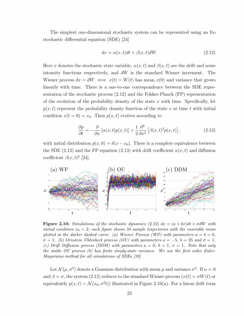
(a) WP (b) OU (c) DDM

t t t

x x x

Figure 2.10: Simulations of the stochastic dynamics (2.12) dx = (a + bx)dt + σdW withinitial condition x0 = 2; each figure shows 50 sample trajectories with the ensemble meanplotted in the darker dashed curve. (a) Wiener Process (WP) with parameters a = b = 0,σ = 1. (b) Ornstein Uhlenbeck process (OU) with parameters a = −5, b = 25 and σ = 1.(c) Drift Diffusion process (DDM) with parameters a = 0, b = 1, σ = 1. Note that onlythe stable OU process (b) has finite steady-state variance. We use the first order Euler-Mayurama method for all simulations of SDEs [39].

LetN (µ, σ2) denote a Gaussian distribution with mean µ and variance σ2. If α = 0

and β = σ, the system (2.12) reduces to the standard Wiener process (x(t) = σW (t) or

equivalently p(x, t) = N (x0, σ2t)) illustrated in Figure 2.10(a). For a linear drift term

23

α(x, t) = ax+b and constant noise term β(x, t) = σ the equation (2.12) corresponds to

the one-dimensional Ornstein-Uhlenbeck (OU) process. For a < 0 the OU process is

stable with a stationary steady state solution with mean E[x]ss = −b/a and variance

σ2ss = σ2/(2a). Equivalently lim

t→∞p(x, t) = N (−b

a, σ

2

2a). The stable OU is illustrated in

Figure 2.10(b). The SDE with α = b and β = σ is the continuum limit of the random

walk model and is also known as the drift diffusion model (DDM), widely studied

as a model for optimal decision making in neural systems [8]. This model does not

converge to a steady state solution, but rather has solution mean and variance that

grow linearly with time, i.e., p(x, t) = N (x0 + bt, σ2t). The DDM is illustrated in

Figure 2.10(c).

For a multi-dimensional stochastic state vector x ∈ RN , the multivariate stochas-

tic dynamics are given by

dx = α(x, t)dt+ β(x, t)dW , (2.14)

where α : RN ×R 7→ RN , β : RN ×R 7→ RN , and dW ∈ RN is the multi-dimensional

Wiener increment. Similar to (2.13), the mutivariate FP equation equivalent to (2.14)

is given by

∂p

∂t= −

∑i

∂

∂xi[αi(x, t)p(x, t)] +

1

2

∑i

∑j

∂2

∂xi∂xj

{[β(x, t)β(x, t)T

]ijp(x, t)

},

(2.15)

where p(x, t) is the multivariate probability density function for the state x(t) with

initial condition x(t = 0) = x0.

Let N (µ,Σ) denote the multivariate Gaussian distribution with mean µ and

covariance matrix Σ (symmetric, positive semi-definite). The multivariate Wiener

process is given by α = 0 and β = B where B is a constant matrix; this process has

solution p(x, t) = N (x0, BBT ). α = Ax + b and β = B results in the multivariate

OU process

dx = (Ax+ b)dt+BdW , (2.16)

where A ∈ RN×N and B ∈ RN×N are constant square matrices and b ∈ RN is a

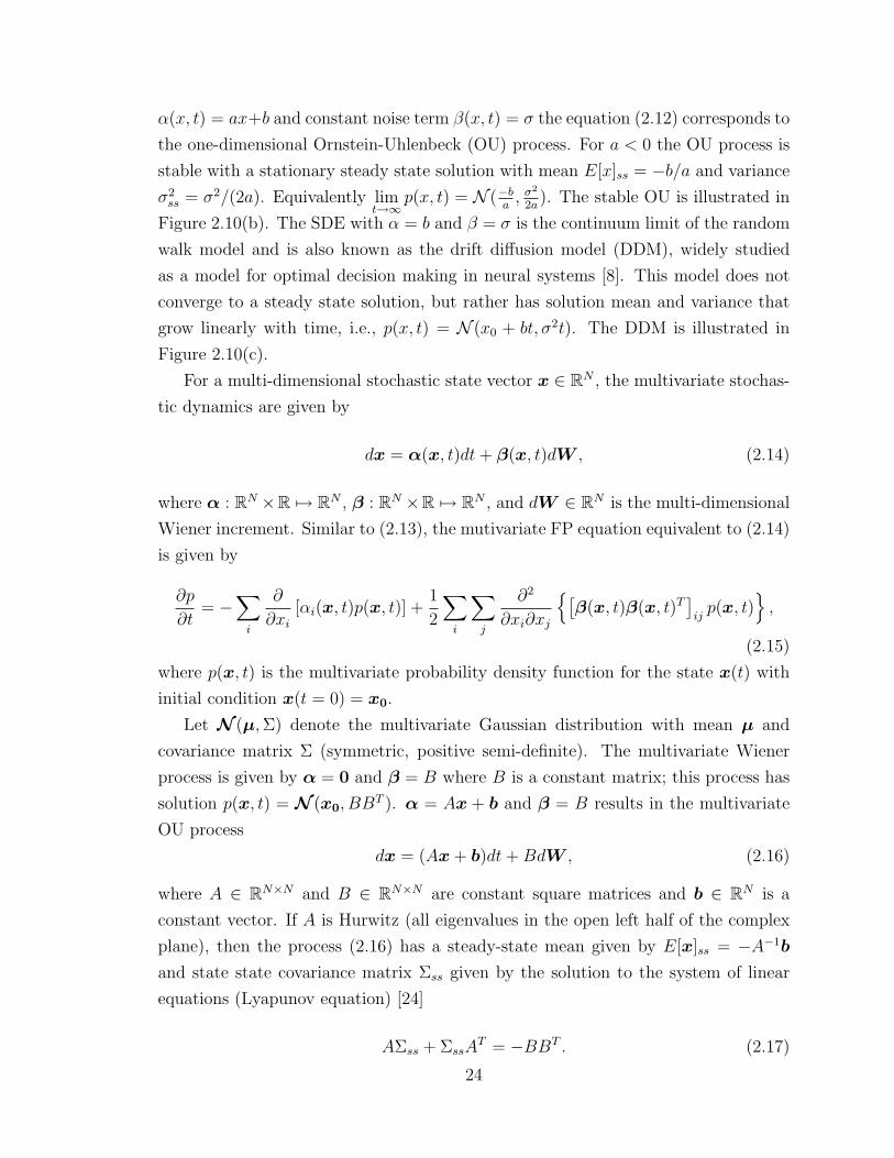
constant vector. If A is Hurwitz (all eigenvalues in the open left half of the complex

plane), then the process (2.16) has a steady-state mean given by E[x]ss = −A−1b

and state state covariance matrix Σss given by the solution to the system of linear

equations (Lyapunov equation) [24]

AΣss + ΣssAT = −BBT . (2.17)

24

We employ the system of equations (2.17) to study the evolutionary dynamics of a

networked migration model in Chapter 5.

Setting A = −L, b = b1 and B = σI in (2.16) results in a coupled version of the

DDM studied recently in [104]. Here L is the positive semi-definite Laplacian ma-

trix from (2.10) that encodes the networked coupling between different drift-diffusing

decision-making units.

2.4.1 Random Points on a Simplex

UNIFORM EXPONENTIAL

(a) (b)

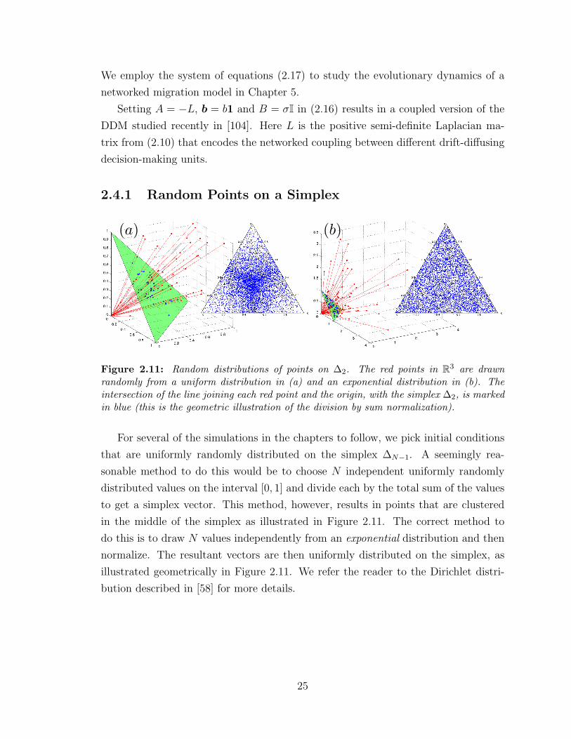
Figure 2.11: Random distributions of points on ∆2. The red points in R3 are drawnrandomly from a uniform distribution in (a) and an exponential distribution in (b). Theintersection of the line joining each red point and the origin, with the simplex ∆2, is markedin blue (this is the geometric illustration of the division by sum normalization).

For several of the simulations in the chapters to follow, we pick initial conditions

that are uniformly randomly distributed on the simplex ∆N−1. A seemingly rea-

sonable method to do this would be to choose N independent uniformly randomly

distributed values on the interval [0, 1] and divide each by the total sum of the values

to get a simplex vector. This method, however, results in points that are clustered

in the middle of the simplex as illustrated in Figure 2.11. The correct method to

do this is to draw N values independently from an exponential distribution and then

normalize. The resultant vectors are then uniformly distributed on the simplex, as

illustrated geometrically in Figure 2.11. We refer the reader to the Dirichlet distri-

bution described in [58] for more details.

25

Chapter 3

Replicator-Mutator Dynamics in

the Plane

As discussed in Chapters 1 and 2, the replicator-mutator dynamics define a canonical

model from evolutionary theory and have been recently applied to model the evolution

of language and the decision-making dynamics of social networks. In this chapter, we

study a form of the replicator-mutator dynamics and prove necessary and sufficient

conditions for the existence of stable limit cycles for N = 3 competing strategies;

we generalize these results to N ≥ 3 strategies in Chapter 4. Stable limit cycles

correspond to sustained oscillations in strategy dominance across some or all of the

population. The form of the dynamics considered, and the interpretation of the

oscillations, depends on the applications of interest; three motivating applications are

discussed in §1.1. The results presented in this chapter have been published in [97].

The analysis of the replicator-mutator dynamics in the literature has focused

primarily on stable limiting equilibrium behavior where the fitness terms are assumed

to have a lot of symmetry (e.g. [75, 85, 90]). However, the recent N = 2 analysis

in [56] (discussed in §3.3) shows that the symmetric case is structurally unstable and

that breaking symmetry in fitness yields qualitatively different bifurcations of the

dynamics. Further, in [76] the authors illustrate that the replicator-mutator dynamics

exhibit limit cycles and chaos for specific model parameter values. In this chapter,

we show that the limiting behaviors of the replicator-mutator dynamics are tied to

the structure of the fitness model, and we prove how breaking symmetry yields some

of the richer outcomes simulated in [76]. It is known that the replicator dynamics for

N ≥ 4 can generate limit cycles and chaos for particular choices of fitness [76, 124, 86].

Here we investigate the role that both fitness and mutation play in generating limit

cycles for the replicator-mutator dynamics.

26

With mutation strength as the bifurcation parameter, we prove that Hopf bifurca-

tions can occur for the replicator-mutator dynamics with N = 3 and characterize the

existence of stable limit cycles using an analytical derivation of the Hopf bifurcation

points and the corresponding first Lyapunov coefficients [32, 59]. It is important to

emphasize that the limit cycles discussed in this chapter are fundamentally different

from the rock-paper-scissors game dynamics cycles of the replicator equations (e.g.

[121, 53, 41]). This is because the limit cycles of the replicator-mutator dynamics here

are driven in part by mutation, and exist as a consequence of bifurcations that occur

as mutation strength changes. Indeed, in the absence of mutation, the corresponding

replicator game dynamics would yield stable equilibria at the simplex boundaries for

the models studied here.

3.1 Model Description∗

Consider a large population of agents and N distinct strategies Si, i = 1, 2, · · · , N .

Let xi ∈ [0, 1] be the fraction of individuals in the population with strategy Si such

thatN∑i=1

xi = 1. Let the population distribution vector x = [x1 , · · · , xN ]T . The

fitness fi of agents with strategy Si is given by

fi =N∑k=1

bikxk.

Let f = [f1 , · · · , fN ]T . Then f = Bx, where B = [bij] ∈ RN×N , and the average

population fitness is φ = fTx = xTBx. B is known as the payoff matrix where

bij ≥ 0 represents the payoff to an agent with strategy Si on interacting with an

agent with strategy Sj.

We assume that payoffs are all non-negative and that agents get a maximal payoff

(normalized to 1) on interacting with others subscribed to the same strategy. Hence

B satisfies

bii = 1 and bij ∈ [0, 1) for i 6= j. (3.1)

As noted in [90], the payoff matrix B can be interpreted from a graph theoretic

perspective as the adjacency matrix of a directed graph. The nodes of the graph

correspond to the strategies Si. The diagonal elements of B (bii = 1) correspond to

self-cycles at each node. Each of the non-zero off-diagonal elements bij corresponds to

∗This sections is presented verbatim as in [93].

27

the weight of a directed edge from node Si to node Sj. Symmetric payoff matrices B

correspond to undirected graphs. This graph theoretic viewpoint is important in our

work, particularly as a tool to visualize the structure of the payoff matrix. Consider

the following condition:

Condition 3.1. Every row and column of B has at least one non-zero off diagonal

element.

From the graph theoretic perspective, Condition 1 requires that every node of the

graph has at least one outgoing and one incoming link; this ensures that there are no

isolated disconnected nodes of the payoff graph. We will restrict to examining graphs

that satisfy Condition 1.

Next we define qij to be the probability that agents with strategy Si mutate

(spontaneously change) to strategy Sj. Note that since∑j

qij = 1, the mutation

matrix Q = [qij] is row stochastic. The elements of the mutation matrix Q are defined

in terms of a mutation parameter µ ∈ [0, 1]. The mutation parameter represents the

probability of error in replication. For example, µ = 0 denotes perfect replication and

no mutation whereas µ = 1 denotes pure mutation.

In this chapter, we use two specific models for the mutation matrix Q. The first

model defines the mutation probabilities qij as a function of the payoffs bij and the

mutation strength µ as follows:

qii = (1− µ), qij =µbij∑i 6=j bij

for i 6= j. (Q1)

The form of qij in (Q1) is motivated by the graph theoretic perspective on the

replicator-mutator dynamics and is a generalization of the structured mutational

models in [60, 56]. Intuitively, this model implies that spontaneous mutation to al-

ternative strategies is weighted in favor of strategies that yield higher payoff. The

mutation models in [90, 60, 75, 85] are special cases of (Q1) in which the payoff matrix

B is symmetric. We call (Q1) the dependent mutation model since (Q1) is dependent

on B.

The second mutation model we consider corresponds to a uniform random prob-

ability of mutating to alternative strategies as follows:

qii = (1− µ), qij =µ

N − 1for i 6= j. (Q2)

We call (Q2) the independent mutation model since (Q2) is independent of B.

28

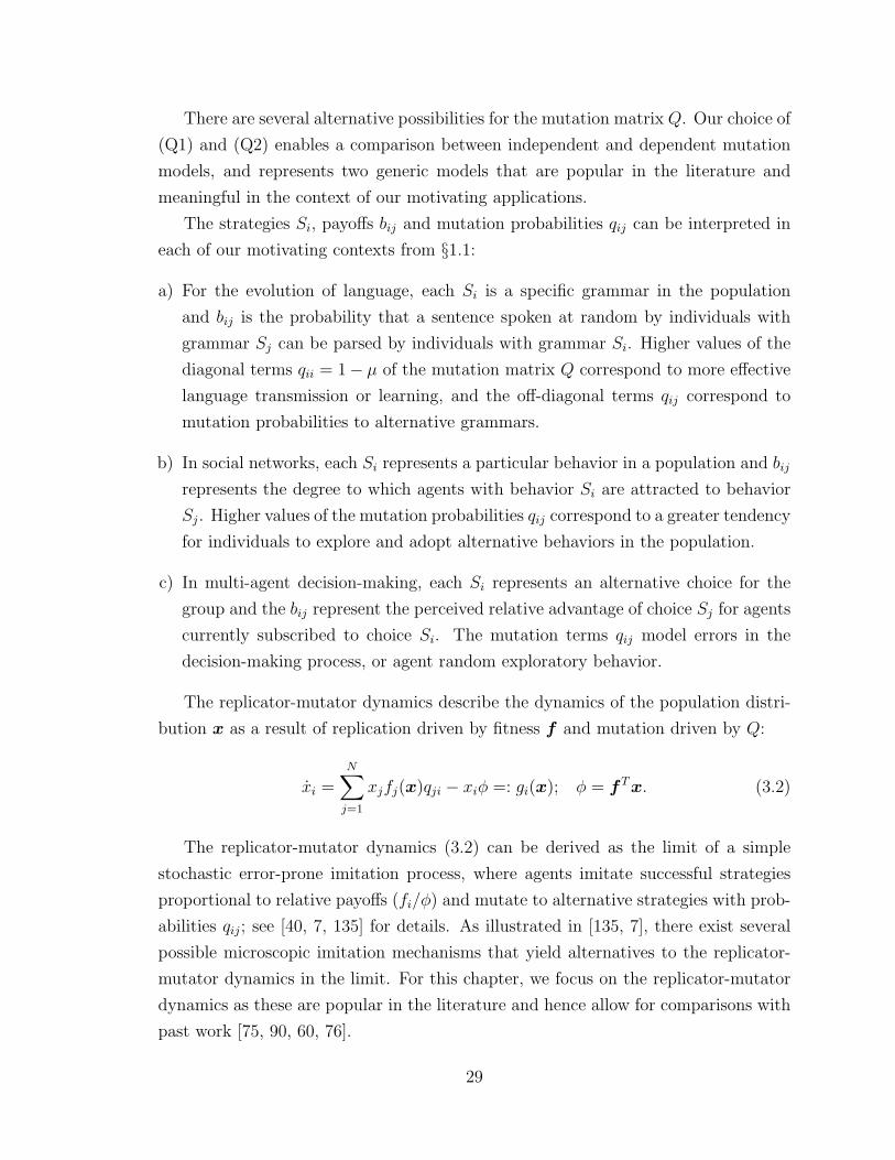
There are several alternative possibilities for the mutation matrix Q. Our choice of

(Q1) and (Q2) enables a comparison between independent and dependent mutation

models, and represents two generic models that are popular in the literature and

meaningful in the context of our motivating applications.

The strategies Si, payoffs bij and mutation probabilities qij can be interpreted in

each of our motivating contexts from §1.1:

a) For the evolution of language, each Si is a specific grammar in the population

and bij is the probability that a sentence spoken at random by individuals with

grammar Sj can be parsed by individuals with grammar Si. Higher values of the

diagonal terms qii = 1− µ of the mutation matrix Q correspond to more effective

language transmission or learning, and the off-diagonal terms qij correspond to

mutation probabilities to alternative grammars.

b) In social networks, each Si represents a particular behavior in a population and bij

represents the degree to which agents with behavior Si are attracted to behavior

Sj. Higher values of the mutation probabilities qij correspond to a greater tendency

for individuals to explore and adopt alternative behaviors in the population.

c) In multi-agent decision-making, each Si represents an alternative choice for the

group and the bij represent the perceived relative advantage of choice Sj for agents

currently subscribed to choice Si. The mutation terms qij model errors in the

decision-making process, or agent random exploratory behavior.

The replicator-mutator dynamics describe the dynamics of the population distri-

bution x as a result of replication driven by fitness f and mutation driven by Q:

xi =N∑j=1

xjfj(x)qji − xiφ =: gi(x); φ = fTx. (3.2)

The replicator-mutator dynamics (3.2) can be derived as the limit of a simple

stochastic error-prone imitation process, where agents imitate successful strategies

proportional to relative payoffs (fi/φ) and mutate to alternative strategies with prob-

abilities qij; see [40, 7, 135] for details. As illustrated in [135, 7], there exist several

possible microscopic imitation mechanisms that yield alternatives to the replicator-

mutator dynamics in the limit. For this chapter, we focus on the replicator-mutator

dynamics as these are popular in the literature and hence allow for comparisons with

past work [75, 90, 60, 76].

29

The dynamics (3.2) evolve on the (N − 1)-dimensional simplex phase space as

follows. Define the n-simplex as

∆n ={x ∈ Rn+1 | xi ≥ 0, xT1 = 1

},

where 1 is a column vector of ones of appropriate dimension. Let g(x) : RN → RN

be g(x) = [g1(x), · · · , gN(x)]T where gi(x) is defined in (3.2). One can compute

directly from (3.2) that xT1 = 1 =⇒ 1Tg(x) = 0. Hence xT1 = 1 is an invariant

hyperplane for the dynamics. Further, the non-negative orthant of RN is a trapping

region for the dynamics; this follows from the fact that xi|xi=0 ≥ 0. The intersection

of the invariant hyperplane and the non-negative orthant of RN is the simplex ∆N−1.

Hence ∆N−1 is a trapping region for the replicator-mutator dynamics (3.2) (see Figure

2.2 for an illustration of ∆1 and ∆2).

Given the restriction to the simplex ∆N−1, the N -dimensional dynamics (3.2) can

be reduced to an (N − 1)-dimensional system of equations:

xi = hi(x), i ∈ {1, 2, · · · , N − 1},

hi(x) := gi

(x1, x2, · · · , xN−1, 1−

N−1∑j=1

xj

),

(3.3)

where x = [x1, · · · , xN−1]T and h : RN−1 → RN−1.

For µ = 0, the replicator-mutator dynamics reduce to the replicator dynamics

(2.1) with payoff matrix B (3.1). Since B is diagonally dominant, the corresponding

replicator dynamics are fairly constrained [74]. In particular, the vertices of the

simplex (pure strategies xi = 1, xj 6=i = 0) are asymptotically stable, and are also the

only evolutionarily stable states.

3.2 Motivation for Cycles†

Our motivation to prove the existence of limit cycles in replicator-mutator dynamics

comes in part from simulations of the dynamics (3.2) for random payoff matrices

B (bij chosen from the uniform distribution on the interval [0, 1) for i 6= j), which

frequently exhibit oscillations. Figure 3.1 shows one simulation of the dynamics that

is typical for mutation matrix (Q1) or (Q2). The dynamics in this simulation illustrate

the transition from dominance of a single strategy (Figure 3.1(a)), to the coexistence

†This section is presented verbatim as in [93], except for the last paragraph and Figure 3.3.

30

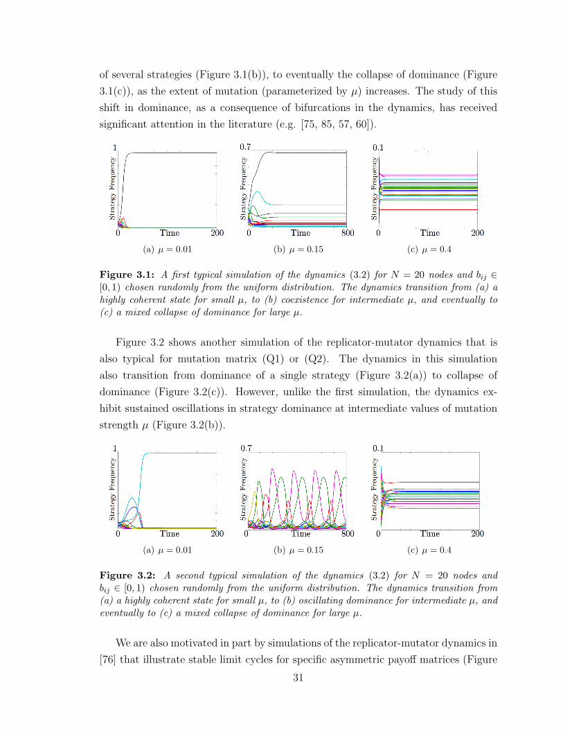
of several strategies (Figure 3.1(b)), to eventually the collapse of dominance (Figure

3.1(c)), as the extent of mutation (parameterized by µ) increases. The study of this

shift in dominance, as a consequence of bifurcations in the dynamics, has received

significant attention in the literature (e.g. [75, 85, 57, 60]).

(a) µ = 0.01 (b) µ = 0.15 (c) µ = 0.4

Figure 3.1: A first typical simulation of the dynamics (3.2) for N = 20 nodes and bij ∈[0, 1) chosen randomly from the uniform distribution. The dynamics transition from (a) ahighly coherent state for small µ, to (b) coexistence for intermediate µ, and eventually to(c) a mixed collapse of dominance for large µ.

Figure 3.2 shows another simulation of the replicator-mutator dynamics that is

also typical for mutation matrix (Q1) or (Q2). The dynamics in this simulation

also transition from dominance of a single strategy (Figure 3.2(a)) to collapse of

dominance (Figure 3.2(c)). However, unlike the first simulation, the dynamics ex-

hibit sustained oscillations in strategy dominance at intermediate values of mutation

strength µ (Figure 3.2(b)).

(a) µ = 0.01 (b) µ = 0.15 (c) µ = 0.4

Figure 3.2: A second typical simulation of the dynamics (3.2) for N = 20 nodes andbij ∈ [0, 1) chosen randomly from the uniform distribution. The dynamics transition from(a) a highly coherent state for small µ, to (b) oscillating dominance for intermediate µ, andeventually to (c) a mixed collapse of dominance for large µ.

We are also motivated in part by simulations of the replicator-mutator dynamics in

[76] that illustrate stable limit cycles for specific asymmetric payoff matrices (Figure

31

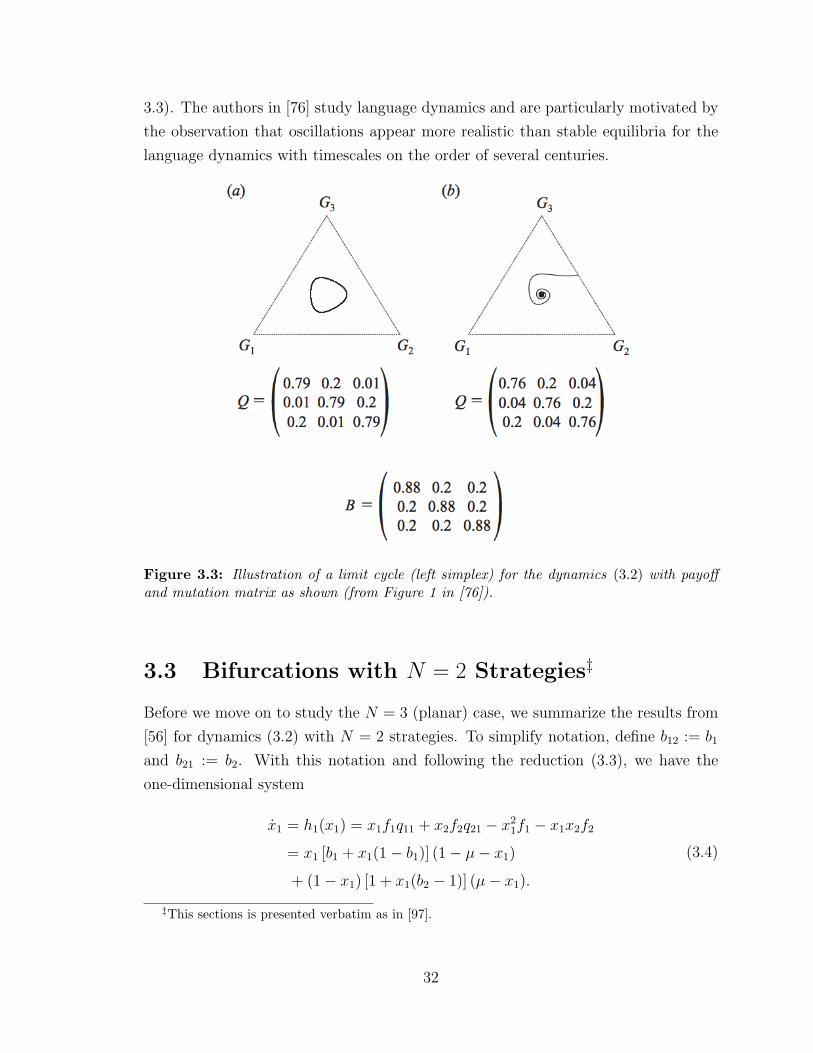
3.3). The authors in [76] study language dynamics and are particularly motivated by

the observation that oscillations appear more realistic than stable equilibria for the

language dynamics with timescales on the order of several centuries.

Figure 3.3: Illustration of a limit cycle (left simplex) for the dynamics (3.2) with payoffand mutation matrix as shown (from Figure 1 in [76]).

3.3 Bifurcations with N = 2 Strategies‡

Before we move on to study the N = 3 (planar) case, we summarize the results from

[56] for dynamics (3.2) with N = 2 strategies. To simplify notation, define b12 := b1

and b21 := b2. With this notation and following the reduction (3.3), we have the

one-dimensional system

x1 = h1(x1) = x1f1q11 + x2f2q21 − x21f1 − x1x2f2

= x1 [b1 + x1(1− b1)] (1− µ− x1)

+ (1− x1) [1 + x1(b2 − 1)] (µ− x1).

(3.4)

‡This sections is presented verbatim as in [97].

32

Figure 3.4 shows the equilibria of the dynamics (3.4), and their stability, as a func-

tion of the bifurcation parameter µ. The bifurcation plot shows a transition from

bistability to a mixed equilibrium via a pitchfork bifurcation in the case b1 = b2. The

pitchfork bifurcation is structurally unstable; for b1 6= b2 a saddle-node bifurcation

occurs at a critical value µc as shown in Figure 3.4. Three branches of equilibria exist.

One of the branches remains stable for all µ and approaches x1 = 0.5 as µ approaches

1. The other two branches exist for µ < µc and collide in a saddle-node bifurcation at

µc. Note that b1 6= b2 corresponds to a directed payoff graph between the two nodes.

Figure 3.4: Three bifurcation plots for N = 2 nodes with parameters b1 = 0.2 and b2 =0.2, 0.25 and 0.5. Blue curves are the stable equilibria and the red curves are the unstableequilibria. Similar to Figure 14 of [56].

A key observation from Figure 3.4 is that directed payoff graphs yield qualitatively

different bifurcations when compared to undirected (symmetric) payoffs; this feature

persists in higher dimensions. The equilibria and bifurcations plotted in Figure 3.4

correspond to vertical slices through a cusp catastrophe, the normal form of which is

given in §2.2 and plotted in Figure 2.6.

3.4 Planar Analysis§

To build intuition for our general results in Chapter 4, we focus here on the bifurca-

tions of the dynamics (3.2) as a function of the bifurcation parameter µ for N = 3

§This sections is presented verbatim as in [93] except for the discussion of the topology cases,which is taken from [97], and Figures 3.7 and 3.9, which are new.

33

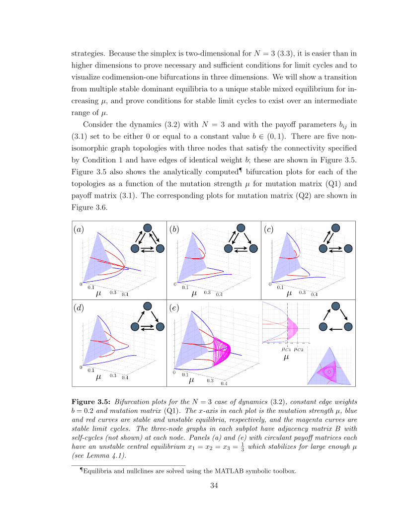
strategies. Because the simplex is two-dimensional for N = 3 (3.3), it is easier than in

higher dimensions to prove necessary and sufficient conditions for limit cycles and to

visualize codimension-one bifurcations in three dimensions. We will show a transition

from multiple stable dominant equilibria to a unique stable mixed equilibrium for in-

creasing µ, and prove conditions for stable limit cycles to exist over an intermediate

range of µ.

Consider the dynamics (3.2) with N = 3 and with the payoff parameters bij in

(3.1) set to be either 0 or equal to a constant value b ∈ (0, 1). There are five non-

isomorphic graph topologies with three nodes that satisfy the connectivity specified

by Condition 1 and have edges of identical weight b; these are shown in Figure 3.5.

Figure 3.5 also shows the analytically computed¶ bifurcation plots for each of the

topologies as a function of the mutation strength µ for mutation matrix (Q1) and

payoff matrix (3.1). The corresponding plots for mutation matrix (Q2) are shown in

Figure 3.6.

Figure 3.5: Bifurcation plots for the N = 3 case of dynamics (3.2), constant edge weightsb = 0.2 and mutation matrix (Q1). The x-axis in each plot is the mutation strength µ, blueand red curves are stable and unstable equilibria, respectively, and the magenta curves arestable limit cycles. The three-node graphs in each subplot have adjacency matrix B withself-cycles (not shown) at each node. Panels (a) and (e) with circulant payoff matrices eachhave an unstable central equilibrium x1 = x2 = x3 = 1

3 which stabilizes for large enough µ(see Lemma 4.1).

¶Equilibria and nullclines are solved using the MATLAB symbolic toolbox.

34

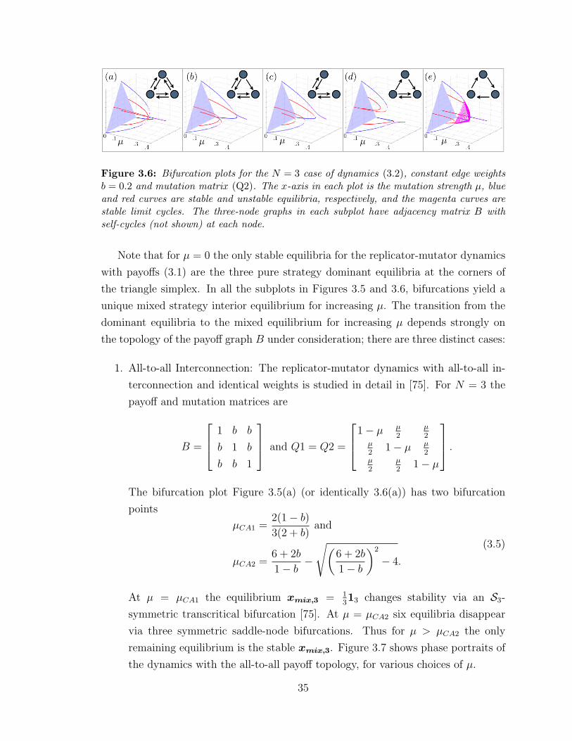
Figure 3.6: Bifurcation plots for the N = 3 case of dynamics (3.2), constant edge weightsb = 0.2 and mutation matrix (Q2). The x-axis in each plot is the mutation strength µ, blueand red curves are stable and unstable equilibria, respectively, and the magenta curves arestable limit cycles. The three-node graphs in each subplot have adjacency matrix B withself-cycles (not shown) at each node.

Note that for µ = 0 the only stable equilibria for the replicator-mutator dynamics

with payoffs (3.1) are the three pure strategy dominant equilibria at the corners of

the triangle simplex. In all the subplots in Figures 3.5 and 3.6, bifurcations yield a

unique mixed strategy interior equilibrium for increasing µ. The transition from the

dominant equilibria to the mixed equilibrium for increasing µ depends strongly on

the topology of the payoff graph B under consideration; there are three distinct cases:

1. All-to-all Interconnection: The replicator-mutator dynamics with all-to-all in-

terconnection and identical weights is studied in detail in [75]. For N = 3 the

payoff and mutation matrices are

B =

1 b b

b 1 b

b b 1

and Q1 = Q2 =

1− µ µ2

µ2

µ2

1− µ µ2

µ2

µ2

1− µ

.The bifurcation plot Figure 3.5(a) (or identically 3.6(a)) has two bifurcation

points

µCA1 =2(1− b)3(2 + b)

and

µCA2 =6 + 2b

1− b −√(

6 + 2b

1− b)2

− 4.

(3.5)

At µ = µCA1 the equilibrium xmix,3 = 1313 changes stability via an S3-

symmetric transcritical bifurcation [75]. At µ = µCA2 six equilibria disappear

via three symmetric saddle-node bifurcations. Thus for µ > µCA2 the only

remaining equilibrium is the stable xmix,3. Figure 3.7 shows phase portraits of

the dynamics with the all-to-all payoff topology, for various choices of µ.

35

(a) µ = 0 (b) µ = 0.1 < µC1

(c) µ = 0.25 ∈ (µC1, µC2) (d) µ = 0.3 > µC2

Figure 3.7: Phase portraits for dynamics (3.2) and with all-to-all payoff as in Figure3.5(a) or Figure 3.6(a). The figure on the left of each of the four sub-figures showsnullclines (red x1 = 0, green x2 = 0 and magenta x3 = 0), vector field (grey arrows)and fixed points (filled circles are stable, unfilled circles are unstable). The figure onthe right of each of the four sub-figures shows sample trajectories for randomly choseninitial conditions. The color scale indicates the magnitude of the flow (vector field)with hot colors corresponding to fast flow. b = 0.2 for this set of plots which givesµCA1 = 0.2424 and µCA2 = 0.2540 from (3.5).

2. Limited Interconnections: The bifurcation plots for graphs in Figures 3.5(b)-(d)

and Figures 3.6(b)-(d) each have a stable branch of equilibria for all µ. They

also have two other stable and four unstable equilibria at µ = 0 which disappear

in saddle-node bifurcations as µ increases. Perturbations of the structurally un-

stable symmetric all-to-all case yield bifurcations that are qualitatively similar

to the limited interconnection cases, much like the N = 2 bifurcations in Figure

3.4.

3. Directed Cycle Interconnection: The bifurcation plots in Figures 3.5(e) and

3.6(e) correspond to a directed cycle interconnection between nodes with payoff

and mutation matrices

B =

1 b 0

0 1 b

b 0 1

, Q1 =

1− µ µ 0

0 1− µ µ

µ 0 1− µ

and Q2 =

1− µ µ2

µ2

µ2

1− µ µ2

µ2

µ2

1− µ

.36

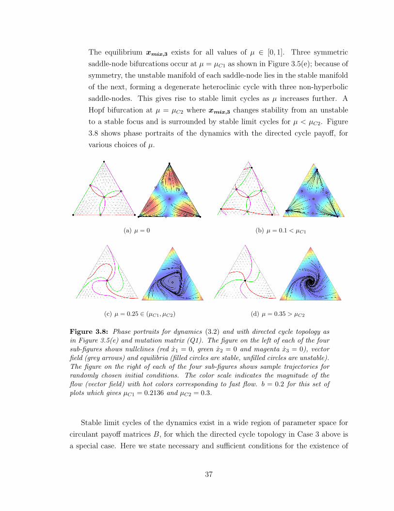
The equilibrium xmix,3 exists for all values of µ ∈ [0, 1]. Three symmetric

saddle-node bifurcations occur at µ = µC1 as shown in Figure 3.5(e); because of

symmetry, the unstable manifold of each saddle-node lies in the stable manifold

of the next, forming a degenerate heteroclinic cycle with three non-hyperbolic

saddle-nodes. This gives rise to stable limit cycles as µ increases further. A

Hopf bifurcation at µ = µC2 where xmix,3 changes stability from an unstable

to a stable focus and is surrounded by stable limit cycles for µ < µC2. Figure

3.8 shows phase portraits of the dynamics with the directed cycle payoff, for

various choices of µ.

(a) µ = 0 (b) µ = 0.1 < µC1

(c) µ = 0.25 ∈ (µC1, µC2) (d) µ = 0.35 > µC2

Figure 3.8: Phase portraits for dynamics (3.2) and with directed cycle topology asin Figure 3.5(e) and mutation matrix (Q1). The figure on the left of each of the foursub-figures shows nullclines (red x1 = 0, green x2 = 0 and magenta x3 = 0), vectorfield (grey arrows) and equilibria (filled circles are stable, unfilled circles are unstable).The figure on the right of each of the four sub-figures shows sample trajectories forrandomly chosen initial conditions. The color scale indicates the magnitude of theflow (vector field) with hot colors corresponding to fast flow. b = 0.2 for this set ofplots which gives µC1 = 0.2136 and µC2 = 0.3.

Stable limit cycles of the dynamics exist in a wide region of parameter space for

circulant payoff matrices B, for which the directed cycle topology in Case 3 above is

a special case. Here we state necessary and sufficient conditions for the existence of

37

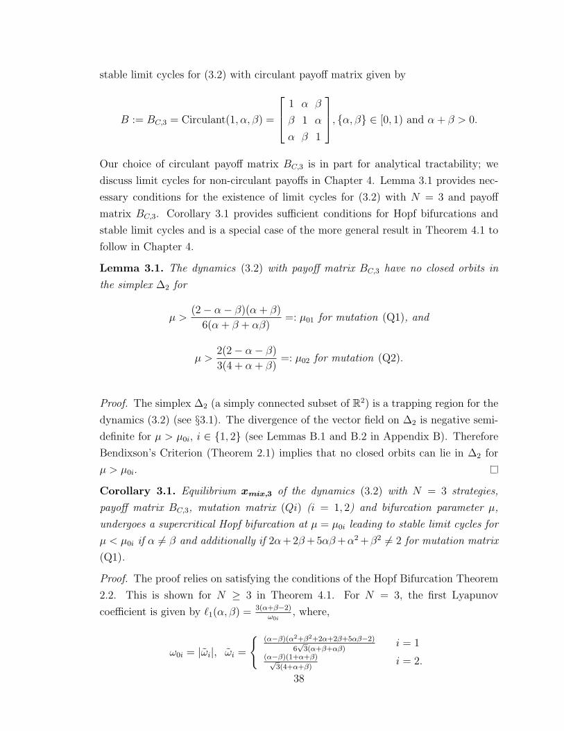
stable limit cycles for (3.2) with circulant payoff matrix given by

B := BC,3 = Circulant(1, α, β) =

1 α β

β 1 α

α β 1

, {α, β} ∈ [0, 1) and α + β > 0.

Our choice of circulant payoff matrix BC,3 is in part for analytical tractability; we

discuss limit cycles for non-circulant payoffs in Chapter 4. Lemma 3.1 provides nec-

essary conditions for the existence of limit cycles for (3.2) with N = 3 and payoff

matrix BC,3. Corollary 3.1 provides sufficient conditions for Hopf bifurcations and

stable limit cycles and is a special case of the more general result in Theorem 4.1 to

follow in Chapter 4.

Lemma 3.1. The dynamics (3.2) with payoff matrix BC,3 have no closed orbits in

the simplex ∆2 for

µ >(2− α− β)(α + β)

6(α + β + αβ)=: µ01 for mutation (Q1), and

µ >2(2− α− β)

3(4 + α + β)=: µ02 for mutation (Q2).

Proof. The simplex ∆2 (a simply connected subset of R2) is a trapping region for the

dynamics (3.2) (see §3.1). The divergence of the vector field on ∆2 is negative semi-

definite for µ > µ0i, i ∈ {1, 2} (see Lemmas B.1 and B.2 in Appendix B). Therefore

Bendixson’s Criterion (Theorem 2.1) implies that no closed orbits can lie in ∆2 for

µ > µ0i.

Corollary 3.1. Equilibrium xmix,3 of the dynamics (3.2) with N = 3 strategies,

payoff matrix BC,3, mutation matrix (Qi) (i = 1, 2) and bifurcation parameter µ,

undergoes a supercritical Hopf bifurcation at µ = µ0i leading to stable limit cycles for

µ < µ0i if α 6= β and additionally if 2α+ 2β+ 5αβ+α2 +β2 6= 2 for mutation matrix

(Q1).

Proof. The proof relies on satisfying the conditions of the Hopf Bifurcation Theorem

2.2. This is shown for N ≥ 3 in Theorem 4.1. For N = 3, the first Lyapunov

coefficient is given by `1(α, β) = 3(α+β−2)ω0i

, where,

ω0i = |ωi|, ωi =

{(α−β)(α2+β2+2α+2β+5αβ−2)

6√

3(α+β+αβ)i = 1

(α−β)(1+α+β)√3(4+α+β)

i = 2.

38

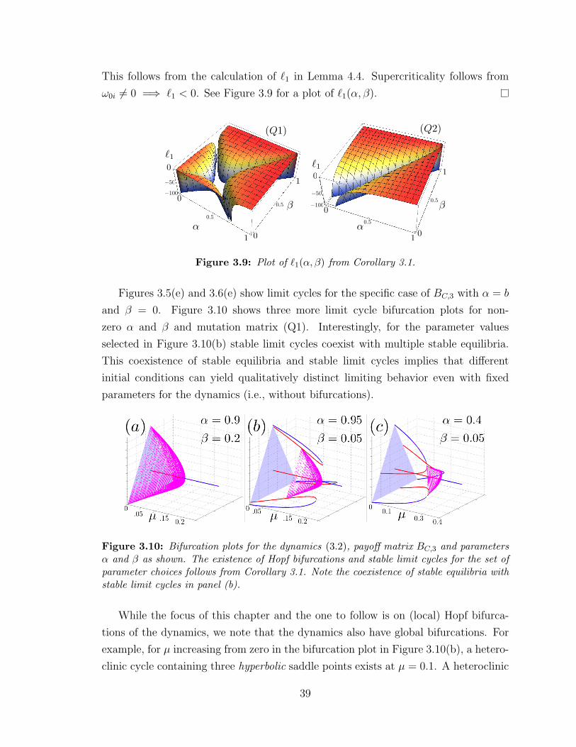
This follows from the calculation of `1 in Lemma 4.4. Supercriticality follows from

ω0i 6= 0 =⇒ `1 < 0. See Figure 3.9 for a plot of `1(α, β).

!!

!!

!1!1

00

0

0

0

0

11

0.5

0.50.5

0.5

11

!50

!100

!50

!100

(Q1) (Q2)

Figure 3.9: Plot of `1(α, β) from Corollary 3.1.

Figures 3.5(e) and 3.6(e) show limit cycles for the specific case of BC,3 with α = b

and β = 0. Figure 3.10 shows three more limit cycle bifurcation plots for non-

zero α and β and mutation matrix (Q1). Interestingly, for the parameter values

selected in Figure 3.10(b) stable limit cycles coexist with multiple stable equilibria.

This coexistence of stable equilibria and stable limit cycles implies that different

initial conditions can yield qualitatively distinct limiting behavior even with fixed

parameters for the dynamics (i.e., without bifurcations).

Figure 3.10: Bifurcation plots for the dynamics (3.2), payoff matrix BC,3 and parametersα and β as shown. The existence of Hopf bifurcations and stable limit cycles for the set ofparameter choices follows from Corollary 3.1. Note the coexistence of stable equilibria withstable limit cycles in panel (b).

While the focus of this chapter and the one to follow is on (local) Hopf bifurca-

tions of the dynamics, we note that the dynamics also have global bifurcations. For

example, for µ increasing from zero in the bifurcation plot in Figure 3.10(b), a hetero-

clinic cycle containing three hyperbolic saddle points exists at µ = 0.1. A heteroclinic

39

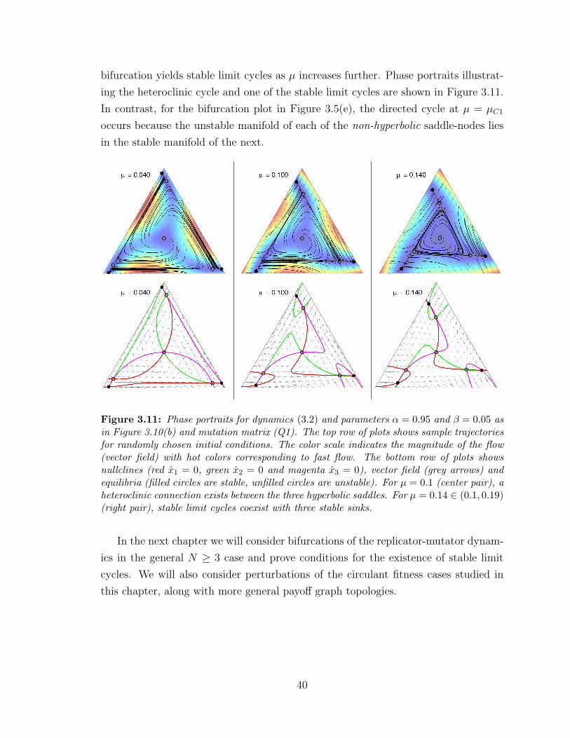
bifurcation yields stable limit cycles as µ increases further. Phase portraits illustrat-

ing the heteroclinic cycle and one of the stable limit cycles are shown in Figure 3.11.

In contrast, for the bifurcation plot in Figure 3.5(e), the directed cycle at µ = µC1

occurs because the unstable manifold of each of the non-hyperbolic saddle-nodes lies

in the stable manifold of the next.

Figure 3.11: Phase portraits for dynamics (3.2) and parameters α = 0.95 and β = 0.05 asin Figure 3.10(b) and mutation matrix (Q1). The top row of plots shows sample trajectoriesfor randomly chosen initial conditions. The color scale indicates the magnitude of the flow(vector field) with hot colors corresponding to fast flow. The bottom row of plots showsnullclines (red x1 = 0, green x2 = 0 and magenta x3 = 0), vector field (grey arrows) andequilibria (filled circles are stable, unfilled circles are unstable). For µ = 0.1 (center pair), aheteroclinic connection exists between the three hyperbolic saddles. For µ = 0.14 ∈ (0.1, 0.19)(right pair), stable limit cycles coexist with three stable sinks.

In the next chapter we will consider bifurcations of the replicator-mutator dynam-

ics in the general N ≥ 3 case and prove conditions for the existence of stable limit

cycles. We will also consider perturbations of the circulant fitness cases studied in

this chapter, along with more general payoff graph topologies.

40

Chapter 4

Replicator-Mutator Dynamics in

Higher Dimensions ∗

In Chapter 3 we looked at Hopf bifurcations for the replicator-mutator dynamics (3.2)

with N = 3 strategies and circulant payoff matrix BC,3. While the focus on three

strategies was convenient for visualization, the simulations in Figure 3.2 indicate that

the dynamics have stable limit cycles in higher dimensions as well (N ≥ 4). In this

chapter, we show that this is indeed the case by proving two main results. Theorem

4.1 shows that the dynamics undergo multiple Hopf bifurcations at distinct bifurcation

points for N ≥ 3, and Lemma 4.4 provides analytical conditions for the stability of

the limit cycles arising from these Hopf bifurcations.

We focus on the dynamics with circulant payoff matrix BC,N ∈ RN×N , N ≥ 3

given by

BC,N := Circulant(1, α, 0, · · · , 0, β), {α, β} ∈ [0, 1) and α + β > 0, (4.1)

and mutation matrices (Q1) and (Q2). The directed graph corresponding to the

payoff matrix BC,N is illustrated in Figure 4.1.

We have chosen to study the circulant two-parameter payoff structure BC,N both

for purposes of tractability and to gain important insights regarding Hopf bifurcations

of the dynamics in N dimensions. In particular, we show the existence of multiple

Hopf bifurcations as several distinct pairs of eigenvalues cross the imaginary axis with

increasing mutation parameter µ in §4.1. Further, the criticality of the bifurcations,

and correspondingly the existence of stable limit cycles, depends on the choice of

parameters α and β, unlike the N = 3 case where all existing bifurcations are super-

∗Sections 4.1–4.5 are presented verbatim as in [93].

41

1 2

3

4

N

N!1

BC,N =

!""""""""#

1 ! 0 · · · 0 "" 1 ! 0

0 " 1 !...

.... . . . . . . . . 0

0 " 1 !! 0 · · · 0 " 1

$%%%%%%%%&

!!

. . .

Figure 4.1: Graph topology corresponding to the payoff matrix BC,N from (4.1).

critical; this is shown in §4.2. The illustrations in §4.2 and §4.3 show that the choice

of the mutation matrix (Q1) or (Q2) plays an important role in determining the exis-

tence and criticality of the Hopf bifurcations. In §4.4 we extend the results from the

previous sections to study multi-cycle dynamics for one-paramter graphs and show

the existence of multiple stable limit cycle attractors. §4.5 focuses on generalizations

to non-circulant and random payoff graphs and shows the tight connection between

the existence of embedded cycles in these graphs and corresponding limit cycles of

the dynamics.

4.1 Hopf Bifurcation Calculation

For payoff matrix BC,N , the equilibrium xmix,N = 1N

1N =[

1N· · · 1

N

]T∈ RN under-

goes Hopf bifurcations. Lemma 4.1 shows that xmix,N is always an equilibrium of

(3.2) for circulant B.

Lemma 4.1. If the payoff matrix B is circulant, then xmix,N is an equilibrium of

the replicator-mutator dynamics (3.2) with mutation matrix (Q1) or (Q2).

Proof. Suppose B is circulant. Then 1 is an eigenvector of B with eigenvalue

rB =N∑j=1

b1j, i.e., B1 = rB1. Matrix Q is also circulant by construction from

(Q1) and (Q2). This means thatN∑j=1

qji =N∑j=1

qij = 1. Let x = xmix,N . Then

f = Bxmix,N = 1NB1 = rB

N1. From (3.2),

xi

∣∣∣xmix,N

=1

N

N∑j=1

fj

(qji − 1

N

)=rBN2

N∑j=1

qji − rBN2

= 0,

and xmix,N is an equilibrium.

42

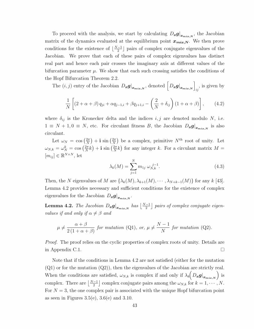
To proceed with the analysis, we start by calculating Dxg|xmix,N, the Jacobian

matrix of the dynamics evaluated at the equilibrium point xmix,N . We then prove

conditions for the existence of bN−12c pairs of complex conjugate eigenvalues of the

Jacobian. We prove that each of these pairs of complex eigenvalues has distinct

real part and hence each pair crosses the imaginary axis at different values of the

bifurcation parameter µ. We show that each such crossing satisfies the conditions of

the Hopf Bifurcation Theorem 2.2.

The (i, j) entry of the Jacobian Dxg|xmix,N, denoted

[Dxg|xmix,N

]ij

, is given by

1

N

[(2 + α + β) qji + αqj−1,i + βqj+1,i −

(2

N+ δij

)(1 + α + β)

], (4.2)

where δij is the Kronecker delta and the indices i, j are denoted modulo N , i.e.

1 ≡ N + 1, 0 ≡ N , etc. For circulant fitness B, the Jacobian Dxg|xmix,Nis also

circulant.

Let ωN = cos(

2πN

)+ i sin

(2πN

)be a complex, primitive N th root of unity. Let

ωN,k = ωkN = cos(

2πNk)

+ i sin(

2πNk)

for any integer k. For a circulant matrix M =

[mij] ∈ RN×N , let

λk(M) =N∑j=1

m1j ωj−1N,k . (4.3)

Then, the N eigenvalues of M are {λk(M), λk+1(M), · · · , λN+k−1(M)} for any k [43].

Lemma 4.2 provides necessary and sufficient conditions for the existence of complex

eigenvalues for the Jacobian Dxg|xmix,N.

Lemma 4.2. The Jacobian Dxg|xmix,Nhas

⌊N−1

2

⌋pairs of complex conjugate eigen-

values if and only if α 6= β and

µ 6= α + β

2 (1 + α + β)for mutation (Q1), or, µ 6= N − 1

Nfor mutation (Q2).

Proof. The proof relies on the cyclic properties of complex roots of unity. Details are

in Appendix C.1.

Note that if the conditions in Lemma 4.2 are not satisfied (either for the mutation

(Q1) or for the mutation (Q2)), then the eigenvalues of the Jacobian are strictly real.

When the conditions are satisfied, ωN,k is complex if and only if λk

(Dxg|xmix,N

)is

complex. There are⌊N−1

2

⌋complex conjugate pairs among the ωN,k for k = 1, · · · , N .

For N = 3, the one complex pair is associated with the unique Hopf bifurcation point

as seen in Figures 3.5(e), 3.6(e) and 3.10.

43

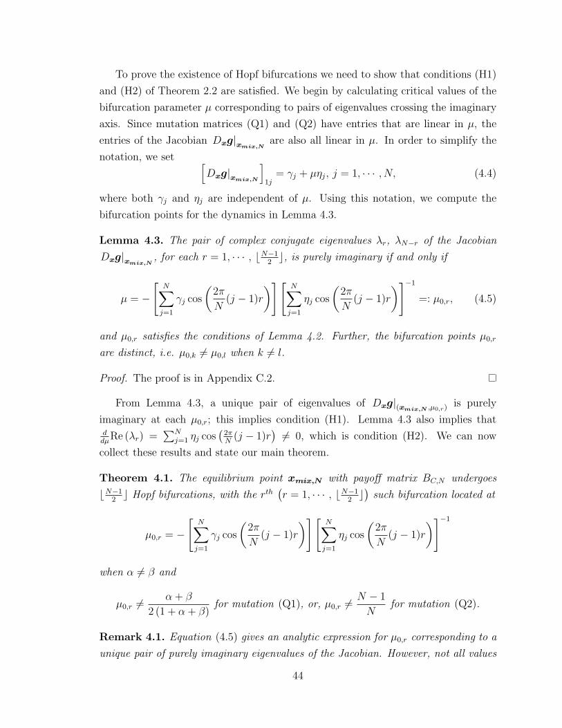
To prove the existence of Hopf bifurcations we need to show that conditions (H1)

and (H2) of Theorem 2.2 are satisfied. We begin by calculating critical values of the

bifurcation parameter µ corresponding to pairs of eigenvalues crossing the imaginary

axis. Since mutation matrices (Q1) and (Q2) have entries that are linear in µ, the

entries of the Jacobian Dxg|xmix,Nare also all linear in µ. In order to simplify the

notation, we set [Dxg|xmix,N

]1j

= γj + µηj, j = 1, · · · , N, (4.4)

where both γj and ηj are independent of µ. Using this notation, we compute the

bifurcation points for the dynamics in Lemma 4.3.

Lemma 4.3. The pair of complex conjugate eigenvalues λr, λN−r of the Jacobian

Dxg|xmix,N, for each r = 1, · · · , bN−1

2c, is purely imaginary if and only if

µ = −[

N∑j=1

γj cos

(2π

N(j − 1)r

)][ N∑j=1

ηj cos

(2π

N(j − 1)r

)]−1

=: µ0,r, (4.5)

and µ0,r satisfies the conditions of Lemma 4.2. Further, the bifurcation points µ0,r

are distinct, i.e. µ0,k 6= µ0,l when k 6= l.

Proof. The proof is in Appendix C.2.

From Lemma 4.3, a unique pair of eigenvalues of Dxg|(xmix,N ,µ0,r) is purely

imaginary at each µ0,r; this implies condition (H1). Lemma 4.3 also implies thatddµ

Re (λr) =∑N

j=1 ηj cos(

2πN

(j − 1)r) 6= 0, which is condition (H2). We can now

collect these results and state our main theorem.

Theorem 4.1. The equilibrium point xmix,N with payoff matrix BC,N undergoes

bN−12c Hopf bifurcations, with the rth

(r = 1, · · · , bN−1

2c) such bifurcation located at

µ0,r = −[

N∑j=1

γj cos

(2π

N(j − 1)r

)][ N∑j=1

ηj cos

(2π

N(j − 1)r

)]−1

when α 6= β and

µ0,r 6= α + β

2 (1 + α + β)for mutation (Q1), or, µ0,r 6= N − 1

Nfor mutation (Q2).

Remark 4.1. Equation (4.5) gives an analytic expression for µ0,r corresponding to a

unique pair of purely imaginary eigenvalues of the Jacobian. However, not all values

44

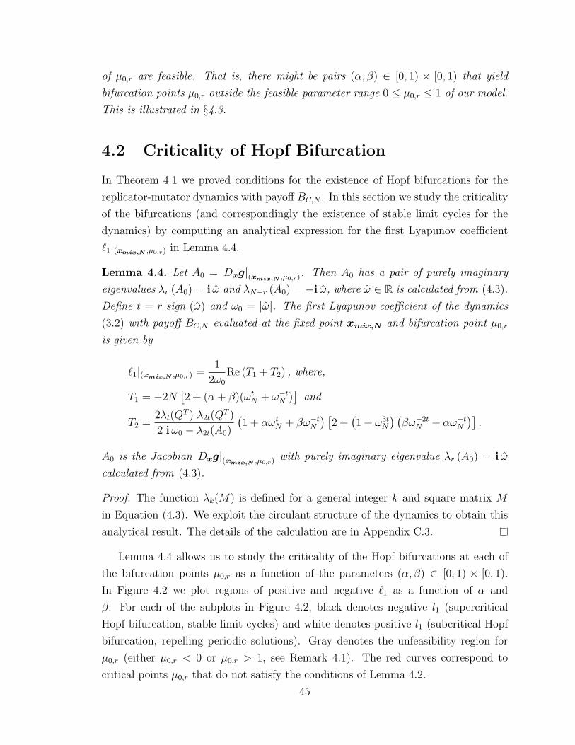
of µ0,r are feasible. That is, there might be pairs (α, β) ∈ [0, 1) × [0, 1) that yield

bifurcation points µ0,r outside the feasible parameter range 0 ≤ µ0,r ≤ 1 of our model.

This is illustrated in §4.3.

4.2 Criticality of Hopf Bifurcation

In Theorem 4.1 we proved conditions for the existence of Hopf bifurcations for the

replicator-mutator dynamics with payoff BC,N . In this section we study the criticality

of the bifurcations (and correspondingly the existence of stable limit cycles for the

dynamics) by computing an analytical expression for the first Lyapunov coefficient

`1|(xmix,N ,µ0,r) in Lemma 4.4.

Lemma 4.4. Let A0 = Dxg|(xmix,N ,µ0,r). Then A0 has a pair of purely imaginary

eigenvalues λr (A0) = i ω and λN−r (A0) = −i ω, where ω ∈ R is calculated from (4.3).

Define t = r sign (ω) and ω0 = |ω|. The first Lyapunov coefficient of the dynamics

(3.2) with payoff BC,N evaluated at the fixed point xmix,N and bifurcation point µ0,r

is given by

`1|(xmix,N ,µ0,r) =1

2ω0

Re (T1 + T2) , where,

T1 = −2N[2 + (α + β)(ωtN + ω−tN )

]and

T2 =2λt(Q

T ) λ2t(QT )

2 iω0 − λ2t(A0)

(1 + αωtN + βω−tN

) [2 +

(1 + ω3t

N

) (βω−2t

N + αω−tN)].

A0 is the Jacobian Dxg|(xmix,N ,µ0,r) with purely imaginary eigenvalue λr (A0) = i ω

calculated from (4.3).

Proof. The function λk(M) is defined for a general integer k and square matrix M

in Equation (4.3). We exploit the circulant structure of the dynamics to obtain this

analytical result. The details of the calculation are in Appendix C.3.

Lemma 4.4 allows us to study the criticality of the Hopf bifurcations at each of

the bifurcation points µ0,r as a function of the parameters (α, β) ∈ [0, 1) × [0, 1).

In Figure 4.2 we plot regions of positive and negative `1 as a function of α and

β. For each of the subplots in Figure 4.2, black denotes negative l1 (supercritical

Hopf bifurcation, stable limit cycles) and white denotes positive l1 (subcritical Hopf

bifurcation, repelling periodic solutions). Gray denotes the unfeasibility region for

µ0,r (either µ0,r < 0 or µ0,r > 1, see Remark 4.1). The red curves correspond to

critical points µ0,r that do not satisfy the conditions of Lemma 4.2.

45

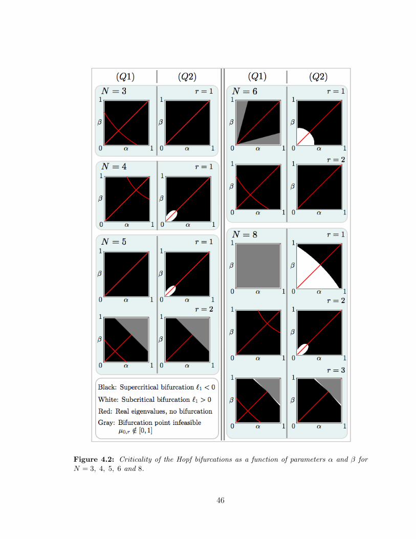
Figure 4.2: Criticality of the Hopf bifurcations as a function of parameters α and β forN = 3, 4, 5, 6 and 8.

46

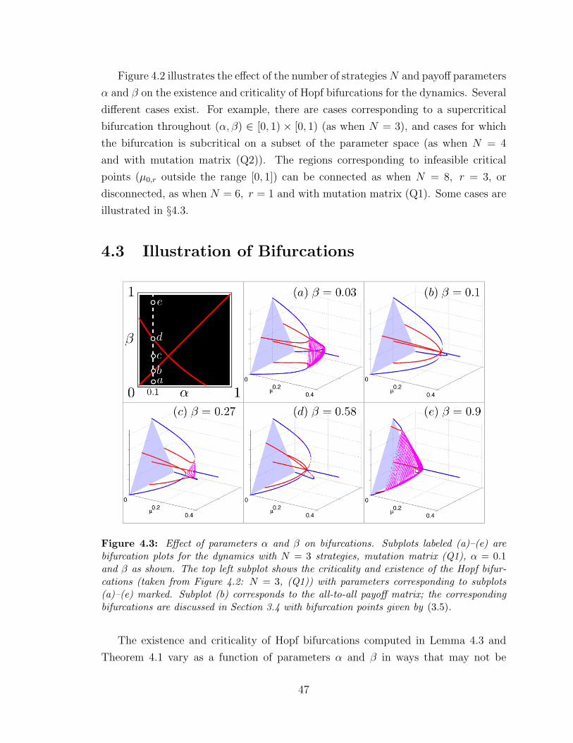
Figure 4.2 illustrates the effect of the number of strategiesN and payoff parameters

α and β on the existence and criticality of Hopf bifurcations for the dynamics. Several

different cases exist. For example, there are cases corresponding to a supercritical

bifurcation throughout (α, β) ∈ [0, 1) × [0, 1) (as when N = 3), and cases for which

the bifurcation is subcritical on a subset of the parameter space (as when N = 4

and with mutation matrix (Q2)). The regions corresponding to infeasible critical

points (µ0,r outside the range [0, 1]) can be connected as when N = 8, r = 3, or

disconnected, as when N = 6, r = 1 and with mutation matrix (Q1). Some cases are

illustrated in §4.3.

4.3 Illustration of Bifurcations

Figure 4.3: Effect of parameters α and β on bifurcations. Subplots labeled (a)–(e) arebifurcation plots for the dynamics with N = 3 strategies, mutation matrix (Q1), α = 0.1and β as shown. The top left subplot shows the criticality and existence of the Hopf bifur-cations (taken from Figure 4.2: N = 3, (Q1)) with parameters corresponding to subplots(a)–(e) marked. Subplot (b) corresponds to the all-to-all payoff matrix; the correspondingbifurcations are discussed in Section 3.4 with bifurcation points given by (3.5).

The existence and criticality of Hopf bifurcations computed in Lemma 4.3 and

Theorem 4.1 vary as a function of parameters α and β in ways that may not be

47

Infeasible

Figure 4.4: Bifurcation plots for the dynamics with N = 6 strategies, parameters α = 0.8,β = 0.05, and mutation matrix as indicated on each subplot. In the case of the left subplotwith mutation matrix (Q1), the Hopf bifurcation point µ0,1 = 1.24 lies outside the feasiblerange µ ∈ [0, 1].

immediately obvious. In this section, we explore the parameter dependence of the

Hopf bifurcations using a set of selected simulations to help illustrate this variation.

Figure 4.3 shows bifurcation plots for the dynamics with N = 3 and mutation

matrix (Q1). Parameter α is set to 0.1 and β is varied between 0 and 1. Looking

at the corresponding criticality plot in Figure 4.3 (reproduced from Figure 4.2), we

expect that the bifurcation is supercritical for all β except at two points labeled (b)

and (d). These are precisely the points that violate the conditions of Lemma 4.2 and

Theorem 4.1. i.e., at (b), α = β = 0.1 and at (d), µ0,1 = α+β2(1+α+β)

for α = 0.1 and

β = 0.58. As a result, the bifurcation plots show the existence of stable limit cycles

for all values of β along the line α = 0.1, except at the points (b) and (d). In Figure

4.3 stable limit cycles are apparent in Figures 4.3(a), 4.3(c) and 4.3(e), but not in

4.3(b) and 4.3(d). The payoff topology corresponding to the parameters in 4.3(b) is

fully symmetric, with a bifurcation plot analogous to Figure 3.5(a).

Figure 4.4 shows the bifurcation plots for the dynamics with N = 6, α = 0.8,

β = 0.05, and mutation matrices (Q1) and (Q2). The corresponding criticality plots

in Figure 4.2 show that the supercritical Hopf bifurcation point µ0,1 lies outside the

feasible range µ ∈ [0, 1] for (Q1) and inside the feasible range for (Q2), for the chosen

parameters. This is illustrated in Figure 4.4; the left plot shows a Hopf bifurcation at

µ = 1.249 while the right plot shows a Hopf bifurcation at µ = 0.363. The left plot

in Figure 4.4 also illustrates that infeasible supercritical bifurcation points can yield

stable limit cycles within the range of feasible µ.

48

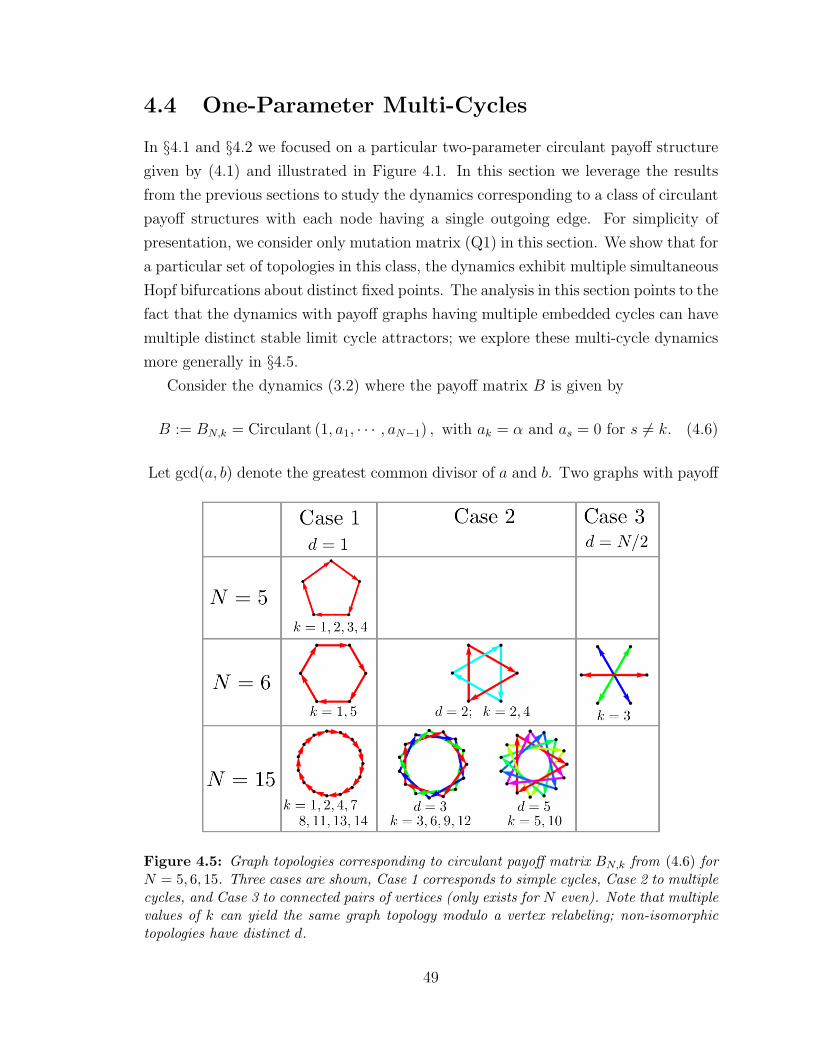
4.4 One-Parameter Multi-Cycles

In §4.1 and §4.2 we focused on a particular two-parameter circulant payoff structure

given by (4.1) and illustrated in Figure 4.1. In this section we leverage the results

from the previous sections to study the dynamics corresponding to a class of circulant

payoff structures with each node having a single outgoing edge. For simplicity of

presentation, we consider only mutation matrix (Q1) in this section. We show that for

a particular set of topologies in this class, the dynamics exhibit multiple simultaneous

Hopf bifurcations about distinct fixed points. The analysis in this section points to the

fact that the dynamics with payoff graphs having multiple embedded cycles can have

multiple distinct stable limit cycle attractors; we explore these multi-cycle dynamics

more generally in §4.5.

Consider the dynamics (3.2) where the payoff matrix B is given by

B := BN,k = Circulant (1, a1, · · · , aN−1) , with ak = α and as = 0 for s 6= k. (4.6)

Let gcd(a, b) denote the greatest common divisor of a and b. Two graphs with payoff

Figure 4.5: Graph topologies corresponding to circulant payoff matrix BN,k from (4.6) forN = 5, 6, 15. Three cases are shown, Case 1 corresponds to simple cycles, Case 2 to multiplecycles, and Case 3 to connected pairs of vertices (only exists for N even). Note that multiplevalues of k can yield the same graph topology modulo a vertex relabeling; non-isomorphictopologies have distinct d.

49

matrices BN,k1 and BN,k2 are isomorphic if and only if gcd(N, k1)=gcd(N, k2). Hence,

among the payoff matrices BN,k, the set of matrices BN,d where d belongs to the set

of proper divisors of N , corresponds to a set of non-isomorphic graph topologies. We

split the set of graph topologies with payoff BN,d (d a proper divisor of N) into three

distinct cases as described below:

(1) d = 1, the graph is a directed cycle containing all vertices

(2) 1 < d < N/2, the graph consists of d disjoint cycles, each of length N/d

(3) d = N/2, the graph consists of N/2 disjoint pairs of connected vertices. This

case exists only for N even.

Figure 4.5 illustrates the three cases of graph topologies for N = 5, 6, and 15.

In addition to xmix,N , the dynamics with payoff matrix BN,d and mutation matrix

(Q1) have d equilibria denoted xj,d,N and given by

xj,d,N =[

0Tj−1dN

0Td−j · · · 0Tj−1dN

0Td−j

]T∈ RN , j = 1, · · · , d. (4.7)

In Case 1, d = 1, and correspondingly j = 1, and x1,1,N = xmix,N . For a given N

and d 6= 1, the d equilibria xj,d,N are cyclically and symmetrically spaced around

xmix,N . Case 1 is studied in detail in §4.1 and obtained by setting β = 0 (a simple

one-parameter cycle). For the topology with pairs of connected nodes in Case 3, the

Jacobian of (3.2) evaluated at the equilibrium xmix,N , or also at any of the equilibria

xj,N/2,N , is real and symmetric and therefore has only real eigenvalues. Thus the

system cannot have Hopf bifurcations for these equilibria in this case. We henceforth

focus on Case 2 and study the dynamics with payoff topologies comprising multiple

cycles.

4.4.1 Case 2 Analysis

We begin the analysis of the dynamics with multi-cycle graph topologies by first look-

ing at the case N = 6, d = 2 (payoff B6,2), before generalizing to higher dimensions.

The two disjoint cycles in the graph corresponding to B6,2 suggest that the behavior

of the system might be similar to that observed for the N = 3 cycles in Chapter

3. Indeed, simulations of the dynamics shown in Figure 4.6 suggest the existence

of two stable limit cycle attractors, each dominated exclusively by three strategies,

corresponding to the connected nodes of the graph. Further, simulations of the phase

50

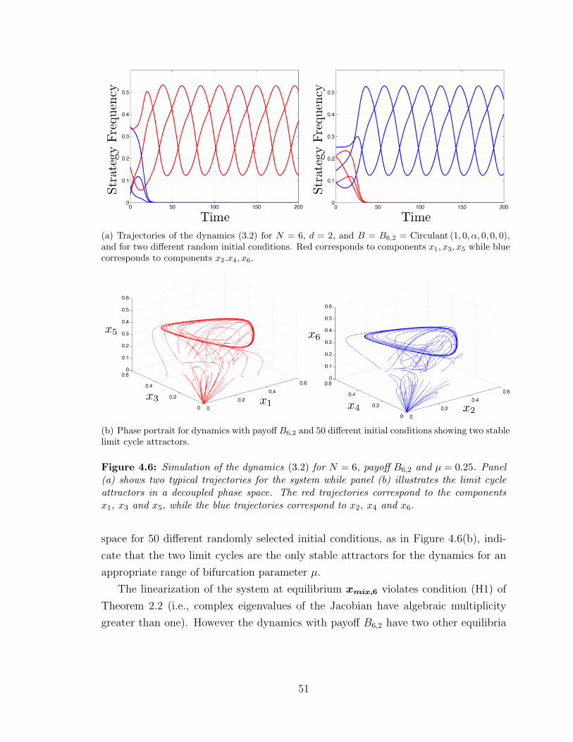
(a) Trajectories of the dynamics (3.2) for N = 6, d = 2, and B = B6,2 = Circulant (1, 0, α, 0, 0, 0),and for two different random initial conditions. Red corresponds to components x1, x3, x5 while bluecorresponds to components x2.x4, x6.

(b) Phase portrait for dynamics with payoff B6,2 and 50 different initial conditions showing two stablelimit cycle attractors.

Figure 4.6: Simulation of the dynamics (3.2) for N = 6, payoff B6,2 and µ = 0.25. Panel(a) shows two typical trajectories for the system while panel (b) illustrates the limit cycleattractors in a decoupled phase space. The red trajectories correspond to the componentsx1, x3 and x5, while the blue trajectories correspond to x2, x4 and x6.

space for 50 different randomly selected initial conditions, as in Figure 4.6(b), indi-

cate that the two limit cycles are the only stable attractors for the dynamics for an

appropriate range of bifurcation parameter µ.

The linearization of the system at equilibrium xmix,6 violates condition (H1) of

Theorem 2.2 (i.e., complex eigenvalues of the Jacobian have algebraic multiplicity

greater than one). However the dynamics with payoff B6,2 have two other equilibria

51

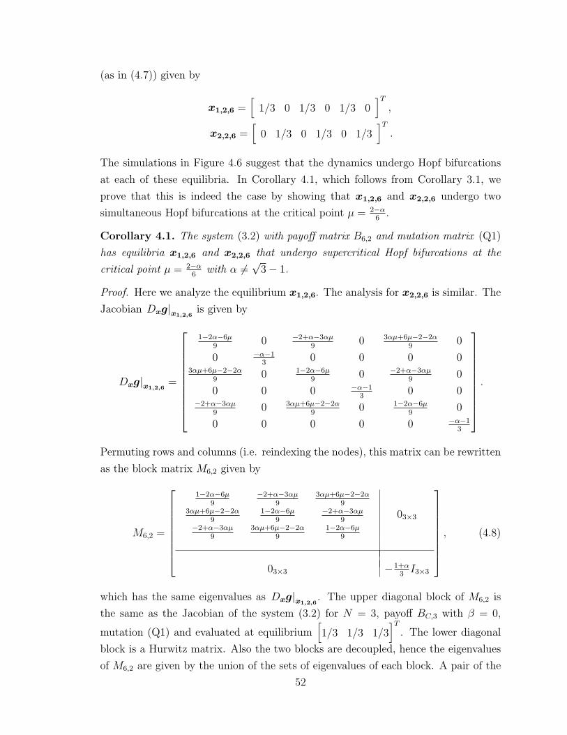
(as in (4.7)) given by

x1,2,6 =[

1/3 0 1/3 0 1/3 0]T

,

x2,2,6 =[

0 1/3 0 1/3 0 1/3]T.

The simulations in Figure 4.6 suggest that the dynamics undergo Hopf bifurcations

at each of these equilibria. In Corollary 4.1, which follows from Corollary 3.1, we

prove that this is indeed the case by showing that x1,2,6 and x2,2,6 undergo two

simultaneous Hopf bifurcations at the critical point µ = 2−α6

.

Corollary 4.1. The system (3.2) with payoff matrix B6,2 and mutation matrix (Q1)

has equilibria x1,2,6 and x2,2,6 that undergo supercritical Hopf bifurcations at the

critical point µ = 2−α6

with α 6= √3− 1.

Proof. Here we analyze the equilibrium x1,2,6. The analysis for x2,2,6 is similar. The

Jacobian Dxg|x1,2,6is given by

Dxg|x1,2,6=

1−2α−6µ9

0 −2+α−3αµ9

0 3αµ+6µ−2−2α9

0

0 −α−13

0 0 0 03αµ+6µ−2−2α

90 1−2α−6µ

90 −2+α−3αµ

90

0 0 0 −α−13

0 0−2+α−3αµ

90 3αµ+6µ−2−2α

90 1−2α−6µ

90

0 0 0 0 0 −α−13

.

Permuting rows and columns (i.e. reindexing the nodes), this matrix can be rewritten

as the block matrix M6,2 given by

M6,2 =

1−2α−6µ9

−2+α−3αµ9

3αµ+6µ−2−2α9

3αµ+6µ−2−2α9

1−2α−6µ9

−2+α−3αµ9

−2+α−3αµ9

3αµ+6µ−2−2α9

1−2α−6µ9

03×3

03×3 −1+α3I3×3

, (4.8)

which has the same eigenvalues as Dxg|x1,2,6. The upper diagonal block of M6,2 is

the same as the Jacobian of the system (3.2) for N = 3, payoff BC,3 with β = 0,

mutation (Q1) and evaluated at equilibrium[1/3 1/3 1/3

]T. The lower diagonal

block is a Hurwitz matrix. Also the two blocks are decoupled, hence the eigenvalues

of M6,2 are given by the union of the sets of eigenvalues of each block. A pair of the

52

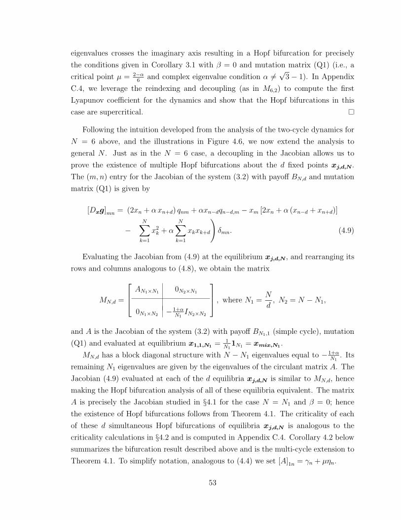
eigenvalues crosses the imaginary axis resulting in a Hopf bifurcation for precisely

the conditions given in Corollary 3.1 with β = 0 and mutation matrix (Q1) (i.e., a

critical point µ = 2−α6

and complex eigenvalue condition α 6= √3 − 1). In Appendix

C.4, we leverage the reindexing and decoupling (as in M6,2) to compute the first

Lyapunov coefficient for the dynamics and show that the Hopf bifurcations in this

case are supercritical.

Following the intuition developed from the analysis of the two-cycle dynamics for

N = 6 above, and the illustrations in Figure 4.6, we now extend the analysis to

general N . Just as in the N = 6 case, a decoupling in the Jacobian allows us to

prove the existence of multiple Hopf bifurcations about the d fixed points xj,d,N .

The (m,n) entry for the Jacobian of the system (3.2) with payoff BN,d and mutation

matrix (Q1) is given by

[Dxg]mn = (2xn + αxn+d) qnm + αxn−dqn−d,m − xm [2xn + α (xn−d + xn+d)]

−(

N∑k=1

x2k + α

N∑k=1

xkxk+d

)δmn. (4.9)

Evaluating the Jacobian from (4.9) at the equilibrium xj,d,N , and rearranging its

rows and columns analogous to (4.8), we obtain the matrix

MN,d =

AN1×N1 0N2×N1

0N1×N2 −1+αN1IN2×N2

, where N1 =N

d, N2 = N −N1,

and A is the Jacobian of the system (3.2) with payoff BN1,1 (simple cycle), mutation

(Q1) and evaluated at equilibrium x1,1,N1 = 1N1

1N1 = xmix,N1 .

MN,d has a block diagonal structure with N −N1 eigenvalues equal to −1+αN1

. Its

remaining N1 eigenvalues are given by the eigenvalues of the circulant matrix A. The

Jacobian (4.9) evaluated at each of the d equilibria xj,d,N is similar to MN,d, hence

making the Hopf bifurcation analysis of all of these equilibria equivalent. The matrix

A is precisely the Jacobian studied in §4.1 for the case N = N1 and β = 0; hence

the existence of Hopf bifurcations follows from Theorem 4.1. The criticality of each

of these d simultaneous Hopf bifurcations of equilibria xj,d,N is analogous to the

criticality calculations in §4.2 and is computed in Appendix C.4. Corollary 4.2 below

summarizes the bifurcation result described above and is the multi-cycle extension to

Theorem 4.1. To simplify notation, analogous to (4.4) we set [A]1n = γn + µηn.

53

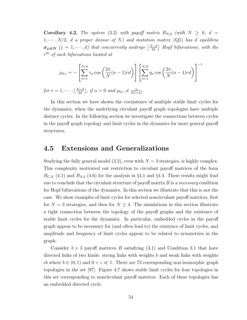
Corollary 4.2. The system (3.2) with payoff matrix BN,d (with N ≥ 6, d =

1, · · · , N/2, d a proper divisor of N) and mutation matrix (Q1) has d equilibria

xj,d,N (j = 1, · · · , d) that concurrently undergo⌊N−d

2d

⌋Hopf bifurcations, with the

rth of such bifurcations located at

µ0,r = −N/d∑n=1

γn cos

(2π

N(n− 1)rd

)N/d∑n=1

ηn cos

(2π

N(n− 1)rd

)−1

for r = 1, · · · , bN−d2dc, if α > 0 and µ0,r 6= α

2(1+α).

In this section we have shown the coexistence of multiple stable limit cycles for

the dynamics, when the underlying circulant payoff graph topologies have multiple

distinct cycles. In the following section we investigate the connections between cycles

in the payoff graph topology and limit cycles in the dynamics for more general payoff

structures.

4.5 Extensions and Generalizations

Studying the fully general model (3.2), even with N = 3 strategies, is highly complex.

This complexity motivated our restriction to circulant payoff matrices of the form

BC,N (4.1) and BN,d (4.6) for the analysis in §4.1 and §4.4. These results might lead

one to conclude that the circulant structure of payoff matrix B is a necessary condition

for Hopf bifurcations of the dynamics. In this section we illustrate that this is not the

case. We show examples of limit cycles for selected noncirculant payoff matrices, first

for N = 3 strategies, and then for N ≥ 4. The simulations in this section illustrate

a tight connection between the topology of the payoff graphs and the existence of

stable limit cycles for the dynamics. In particular, embedded cycles in the payoff

graph appear to be necessary for (and often lead to) the existence of limit cycles, and

amplitude and frequency of limit cycles appear to be related to symmetries in the

graph.

Consider 3 × 3 payoff matrices B satisfying (3.1) and Condition 3.1 that have

directed links of two kinds: strong links with weights b and weak links with weights

εb where b ∈ (0, 1) and 0 < ε� 1. There are 73 corresponding non-isomorphic graph

topologies in the set [97]. Figure 4.7 shows stable limit cycles for four topologies in

this set corresponding to noncirculant payoff matrices. Each of these topologies has

an embedded directed cycle.

54

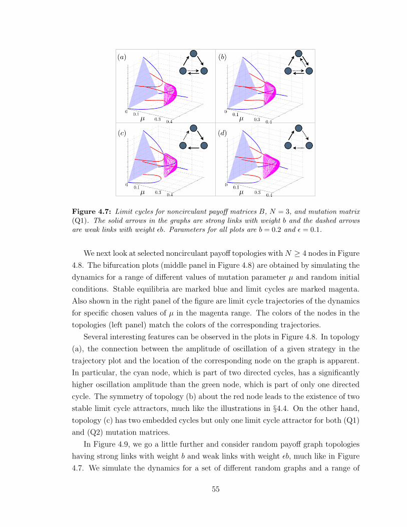
Figure 4.7: Limit cycles for noncirculant payoff matrices B, N = 3, and mutation matrix(Q1). The solid arrows in the graphs are strong links with weight b and the dashed arrowsare weak links with weight εb. Parameters for all plots are b = 0.2 and ε = 0.1.

We next look at selected noncirculant payoff topologies withN ≥ 4 nodes in Figure

4.8. The bifurcation plots (middle panel in Figure 4.8) are obtained by simulating the

dynamics for a range of different values of mutation parameter µ and random initial

conditions. Stable equilibria are marked blue and limit cycles are marked magenta.

Also shown in the right panel of the figure are limit cycle trajectories of the dynamics

for specific chosen values of µ in the magenta range. The colors of the nodes in the

topologies (left panel) match the colors of the corresponding trajectories.

Several interesting features can be observed in the plots in Figure 4.8. In topology

(a), the connection between the amplitude of oscillation of a given strategy in the

trajectory plot and the location of the corresponding node on the graph is apparent.

In particular, the cyan node, which is part of two directed cycles, has a significantly

higher oscillation amplitude than the green node, which is part of only one directed

cycle. The symmetry of topology (b) about the red node leads to the existence of two

stable limit cycle attractors, much like the illustrations in §4.4. On the other hand,

topology (c) has two embedded cycles but only one limit cycle attractor for both (Q1)

and (Q2) mutation matrices.

In Figure 4.9, we go a little further and consider random payoff graph topologies

having strong links with weight b and weak links with weight εb, much like in Figure

4.7. We simulate the dynamics for a set of different random graphs and a range of

55

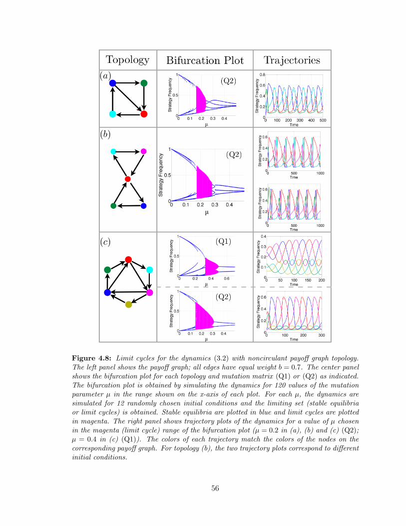
Figure 4.8: Limit cycles for the dynamics (3.2) with noncirculant payoff graph topology.The left panel shows the payoff graph; all edges have equal weight b = 0.7. The center panelshows the bifurcation plot for each topology and mutation matrix (Q1) or (Q2) as indicated.The bifurcation plot is obtained by simulating the dynamics for 120 values of the mutationparameter µ in the range shown on the x-axis of each plot. For each µ, the dynamics aresimulated for 12 randomly chosen initial conditions and the limiting set (stable equilibriaor limit cycles) is obtained. Stable equilibria are plotted in blue and limit cycles are plottedin magenta. The right panel shows trajectory plots of the dynamics for a value of µ chosenin the magenta (limit cycle) range of the bifurcation plot (µ = 0.2 in (a), (b) and (c) (Q2);µ = 0.4 in (c) (Q1)). The colors of each trajectory match the colors of the nodes on thecorresponding payoff graph. For topology (b), the two trajectory plots correspond to differentinitial conditions.

56

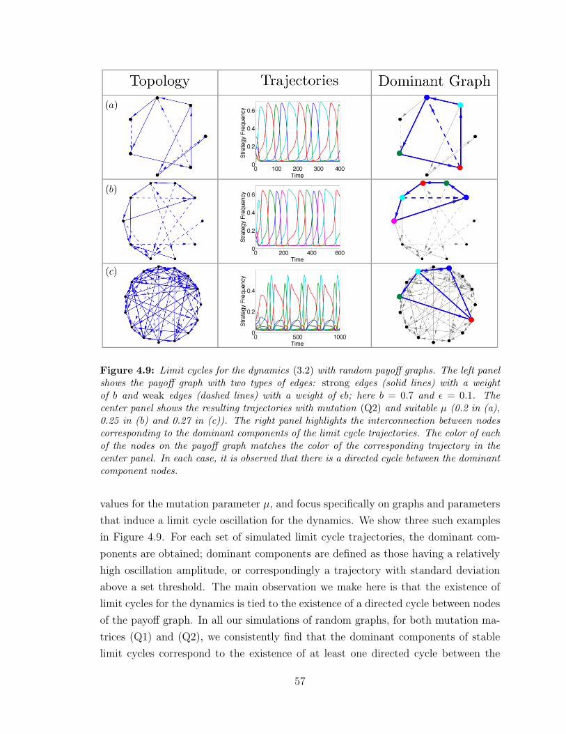
Figure 4.9: Limit cycles for the dynamics (3.2) with random payoff graphs. The left panelshows the payoff graph with two types of edges: strong edges (solid lines) with a weightof b and weak edges (dashed lines) with a weight of εb; here b = 0.7 and ε = 0.1. Thecenter panel shows the resulting trajectories with mutation (Q2) and suitable µ (0.2 in (a),0.25 in (b) and 0.27 in (c)). The right panel highlights the interconnection between nodescorresponding to the dominant components of the limit cycle trajectories. The color of eachof the nodes on the payoff graph matches the color of the corresponding trajectory in thecenter panel. In each case, it is observed that there is a directed cycle between the dominantcomponent nodes.

values for the mutation parameter µ, and focus specifically on graphs and parameters

that induce a limit cycle oscillation for the dynamics. We show three such examples

in Figure 4.9. For each set of simulated limit cycle trajectories, the dominant com-

ponents are obtained; dominant components are defined as those having a relatively

high oscillation amplitude, or correspondingly a trajectory with standard deviation

above a set threshold. The main observation we make here is that the existence of

limit cycles for the dynamics is tied to the existence of a directed cycle between nodes

of the payoff graph. In all our simulations of random graphs, for both mutation ma-

trices (Q1) and (Q2), we consistently find that the dominant components of stable

limit cycles correspond to the existence of at least one directed cycle between the

57

corresponding nodes of the payoff graph, as illustrated in the right panel of Figure

4.9.

The purpose of the simulations in this section is to illustrate that one can break

symmetry in the payoff graph significantly (as compared to the modest symmetry

breaking that yields the circulant structures analyzed in this chapter) and still obtain

stable limit cycles for the dynamics, even in the case of random graph topologies, as

long as the topologies have at least one embedded cycle. In addition to limit cycles,

the dynamics can also have chaotic attractors as found in [74, 76]. We have not seen

chaotic attractors for the payoff topologies and mutation matrices (Q1) and (Q2)

studied in this chapter; we conjecture that alternative mutation models such as the

one used in [76] will exhibit chaotic dynamics.

4.6 Final Remarks

Much of the existing analysis of the replicator-mutator dynamics has been focused

on stable equilibria. The analysis in the literature has also primarily considered

payoff and mutation matrices that are symmetric, which correspond to undirected

payoff graph topologies. Recent work [60] on a graph theoretic model of language

dynamics has shown that the graph connectivity plays a critical role in determining

the location of bifurcation points in the dynamics, but the restriction to undirected

graphs confines the range of limiting behavior to stable equilibria. In [76], it is shown

that considering asymmetric payoff and mutation matrices (corresponding to directed

graphs) can yield limit cycle behavior and even chaos for replicator-mutator dynamics.

Here we have proved conditions guaranteeing stable limit cycles in the replicator-

mutator dynamics. These arise as a consequence of Hopf bifurcations for N ≥ 3

strategies and for circulant payoff matrices. From a graph perspective, we showed

how breaking symmetry by considering directed graphs allows for oscillatory limiting

behavior. We emphasize that the limit cycles are not restricted to circulant payoffs,

but can exist for noncirculant payoffs as shown in §4.5. The simulations in §4.5

illustrate the connection between embedded directed cycles in the payoff graph and

the existence of stable limit cycles for the dynamics. A Hopf bifurcation analysis

of these more general cases is an intended future direction. We will also explore the

effects of the structure of the mutation matrix, beyond (Q1) and (Q2) considered here,

as a step towards understanding the transition to chaos illustrated in [76]. Further

directions of future research, including applications to the design of decision-making

protocols in multi-agent robotic systems, are discussed in Chapter 8.

58

Chapter 5

Evolutionary Dynamics of

Collective Migration

Collective migration is a ubiquitous natural phenomenon common in a number of

species including birds, fish, invertebrates and mammals [119, 42, 22, 6]. The mi-

gratory process is often an adaptive response to conditions such as competition for

resources in a dynamic environment, seasonal variability, and selection of new habi-

tats for breeding, for example [132, 119]. Animals perform such migratory tasks by

leveraging a variety of environmental cues such as nutrient and thermal gradients,

magnetic fields, odor cues, or visual markers [132, 30, 140, 133]. Measuring these

stochastic environmental signals is complicated and requires the investment of time

and energy, as well as the development of necessary physiological and sensory machin-

ery such as vision in insects and vertebrates [42] and chemical signaling in bacteria

[136]. Along with environmental cues, animals migrating collectively also have the

ability to leverage social information from neighbors in the group [15]. One way of

doing so is by imitating invested neighbors (via consensus processes such as attraction

and alignment of heading) and thereby effectively achieving good migratory perfor-

mance, without paying the measurement and processing cost. The interplay between

costly information acquisition from the environment and relatively less expensive so-

cial information from the group raises two pertinent questions regarding leadership

and social interactions in migratory populations.

The first question relates to the migratory performance of large groups in the

presence of a limited number of leaders, i.e., can a subset of informed leaders effectively

lead a large group? The authors in [14] address this question using individual-based

simulations (involving attraction, repulsion and alignment between individuals) and

demonstrate that in a group of socially interacting individuals, a small fraction of

59

informed leaders can effectively determine the direction of travel of a large group of

uninformed followers. Further, they show that for a fixed fraction of leaders, the

accuracy of group direction improves with increasing group size.

The second question relates to the evolution of leadership in collective migration,

i.e., under what conditions is the coexistence of invested leaders and social follow-

ers stable in an evolutionarily sense? This question is especially pertinent when the

cost of investing in signal acquisition is sufficiently high; followers can leverage the

investments made by leaders via social interactions, without paying the investment

costs. In a recent paper [33] (also see related commentary [120]), the authors address

this question using an individual-based model (similar to [14]) and evolutionary sim-

ulations, and show that under certain conditions, the specialization of groups into

coexisting leaders and followers (also known as branching or speciation) is a stable

evolutionary outcome.

Individual-based bio-inspired models such as those used in [14, 33] provide im-

portant insights about the relevant biological processes being modeled, but are chal-

lenging to analyze. In particular, it can be difficult to ascertain what aspects of the

low-level interactions (social network topology, cost functions, movement dynamics,

etc.) are most critical to the observed high-level behavior of interest (evolution of

leadership for example). This analysis can be done more effectively by constructing

appropriate simpler (lower-dimensional) models that capture the relevant high-level

behavior, while also being tractable for analysis. In [132], the authors construct one

such lower-dimensional mean-field approximation to the evolutionary model studied

in [33], and using tools from evolutionary adaptive dynamics [25, 26] prove conditions

for the branching of a migrating population into leader and follower groups.

While simpler models have the advantage of analytical tractability, this comes

at the cost of abstracting some potentially important features of the corresponding

detailed model. In the case of the migration model in [132], the mean-field approach

effectively prescribes an all-to-all social interaction topology between the individuals

in order to reduce dimensionality; this ignores the potentially important role of limited

social interactions. Indeed, it has been shown [98, 151, 3, 10] that network topology

plays a critical role in determining outcomes in biological as well as robotic collectives.

In this chapter, we design a model to study the evolution of collective migration

that is explicitly dependent on the social interaction graph topology. We present a

comprehensive analysis of the all-to-all limit of the model, recovering the speciation

results of the mean-field analysis in [132], and demonstrating the hysteretic effect

associated with recovering lost migration ability described in [33, 34]. We then go

60

on to study the effect of topology on the evolutionary model, and show a minimum

social connectivity threshold necessary for the evolution of leadership in migration.

Our evolutionary model has two timescales. The fast timescale corresponds to the

stochastic migration dynamics and individual fitness computations as a consequence

of migratory performance. The slow timescale corresponds to the evolutionary dy-

namics of the population and changes in population strategy distribution as a conse-

quence of replication and mutation. A key advantage of our model is that it allows for

analytically computing fitness on the fast timescale by solving a set of coupled linear

equations. For the detailed model in [33], the fitness computation requires extensive

Monte-Carlo simulations using agent-based models. On the other hand, the detailed

model has the advantage of incorporating a time-varying social interconnection topol-

ogy between individuals, which eventually results in fission-fusion spatial dynamics

(where groups constantly merge and split) described in [33]; the model studied in this

chapter assumes a time-invariant social interaction graph for fitness computation. In

ongoing work on generalizing the model presented here to time-varying graphs, we

intend to investigate the observed fission-fusion result of the detailed model.

There is significant recent interest in understanding the mechanisms of interaction,

signal processing and information transfer in evolved natural collectives in order to

design better algorithms for collective motion and decision-making in robotic groups

[128, 98, 66, 142]. Robotic collectives often have resource constraints (analogous to

the measurement and processing cost for migration tracking), operate in dynamic

and stochastic environments, and interact with neighbors on some networked graph

topology. In Section 5.4, we consider the migration model from this multi-agent

robotic perspective and study a simple model of adaptive dynamic nodes on a network.

We illustrate the critical role that the structure of the interaction graph plays in

determining the location of leaders (highly invested nodes) in the adaptive network

and in bifurcations in the nodal dynamics as a function of increasing cost.

The outline of this chapter is as follows. In Section 5.1 we present our graph-

dependent evolutionary migration model and study its all-to-all limit in Section 5.2.

We study evolutionary dynamics with limited interconnection in Section 5.3 and focus

on adaptive dynamic nodes in small networks in Section 5.4.

5.1 Model Description

Our model is derived from the mean-field migration model in [132] with two key

modifications; we explicitly account for a limited social interaction graph topology

61

in the dynamics and we introduce a slightly modified social noise model to allow

for analytical fitness computations as a function of graph topology and individual

investments, as described below.

Consider a set of N agents indexed by i ∈ {1, · · · , N} that each intend to control

their direction of migration represented by a stochastic scalar variable xi ∈ R, thereby

tracking some desired ‘true’ direction µ ∈ R with high fidelity. Accurate tracking of

the desired direction µ over time may correspond to benefits such as improvement

in environmental conditions for foraging, predator evasion, early access to breeding

grounds, etc. Following [132], the stochastic dynamics of each agent are given by

dxi = kidxDi + (1− ki)dxSi, (5.1)

where dxDi and dxSi are the driven tracking and social consensus stochastic processes

respectively. ki ∈ [0, 1] is an adaptive parameter that tunes the level of investment

made by agent i in the driven and social processes. ki = 1, for example, corresponds

to an individual i fully invested in the tracking process and ignoring social information

from neighbors, while ki = 0 corresponds to the individual exclusively leveraging so-

cial information without tracking the environmental signal. The ki’s are the adaptive

evolutionary parameters in the simulations and analysis in the sections to follow.

The driven process dxDi is modeled as an Ornstein-Uhlenbeck stochastic process

[137, 24] of the form

dxDi = −kDi(xi − µ)dt+ σDdWDi. (5.2)

Here, the parameter kDi ≥ 0 corresponds to the gain associated with tracking, σ2D > 0

is the noise intensity associated with measuring the environmental signal µ, and dWDi

represents the standard Wiener increment. For kDi > 0, the process (5.2) has a

steady-state mean and variance given by

E [xi] = µ, E[(xi − µ)2

]=

σ2D

2kDi. (5.3)

Higher values of tracking gain kDi result in lower steady-state variance in migration

direction xi, which corresponds to improved tracking. Figure 5.1 shows the spatial dy-

namics of migrating agents with driven process (5.2) and varying levels of investment

kDi, illustrating the effect of increasing investment on improved tracking performance.

We use basic tools from graph theory [111, 91, 47] (see also §2.3) to model the

social consensus process. Individuals are modeled as nodes on a directed social inter-

62

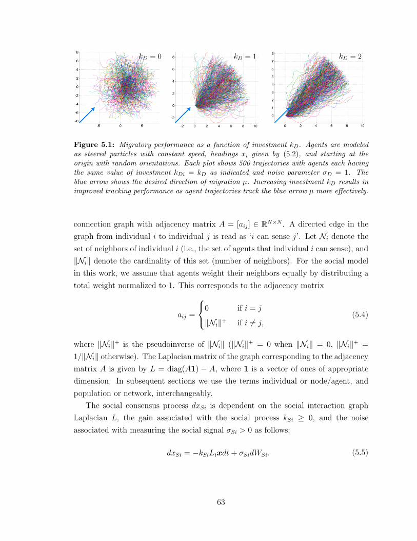
Figure 5.1: Migratory performance as a function of investment kD. Agents are modeledas steered particles with constant speed, headings xi given by (5.2), and starting at theorigin with random orientations. Each plot shows 500 trajectories with agents each havingthe same value of investment kDi = kD as indicated and noise parameter σD = 1. Theblue arrow shows the desired direction of migration µ. Increasing investment kD results inimproved tracking performance as agent trajectories track the blue arrow µ more effectively.

connection graph with adjacency matrix A = [aij] ∈ RN×N . A directed edge in the

graph from individual i to individual j is read as ‘i can sense j’. Let Ni denote the

set of neighbors of individual i (i.e., the set of agents that individual i can sense), and

‖Ni‖ denote the cardinality of this set (number of neighbors). For the social model

in this work, we assume that agents weight their neighbors equally by distributing a

total weight normalized to 1. This corresponds to the adjacency matrix

aij =

0 if i = j

‖Ni‖+ if i 6= j,(5.4)

where ‖Ni‖+ is the pseudoinverse of ‖Ni‖ (‖Ni‖+ = 0 when ‖Ni‖ = 0, ‖Ni‖+ =

1/‖Ni‖ otherwise). The Laplacian matrix of the graph corresponding to the adjacency

matrix A is given by L = diag(A1) − A, where 1 is a vector of ones of appropriate

dimension. In subsequent sections we use the terms individual or node/agent, and

population or network, interchangeably.

The social consensus process dxSi is dependent on the social interaction graph

Laplacian L, the gain associated with the social process kSi ≥ 0, and the noise

associated with measuring the social signal σSi > 0 as follows:

dxSi = −kSiLixdt+ σSidWSi. (5.5)

63

In the social process (5.5), dWSi is the standard Wiener increment, and Li denotes

the ith row of the Laplacian matrix L. Let x be the vector of individual directions

xi. Then Lix = ‖Ni‖+∑

j∈Ni(xi − xj).

Following the setup in [132], we make a simplification to reduce the parameter

space to one dimension by assuming that the gains are proportional to the relative

investments in each process, i.e., kDi = ki and kSi = 1 − ki. Substituting this

simplification in (5.2), (5.5) and (5.1) we have

dxi = kidxDi + (1− ki)dxSi= −k2

i (xi − µ)dt− (1− ki)2Lixdt+√k2i σ

2D + (1− ki)2σ2

Si dWi.(5.6)

In order to simplify the notation we make a coordinate transformation and define the

normalized direction xi as

xi =xi − µσD

, and correspondingly x =x− µ1

σD. (5.7)

Substituting the transformation (5.7) in (5.6) and observing that Li1 = 0 we have

the normalized dynamics

dxi = −k2i xidt− (1− ki)2Lixdt+

√k2i + (1− ki)2

σ2Si

σ2D

dWi. (5.8)

The social noise term σSi reflects the difficulty that agents have in extracting social

information gained from interactions with neighbors. In [132], it is assumed that this

difficulty (magnitude of σSi) decreases as the ordering or coherence of the population

increases. Here we take a slightly different local (and graph dependent) approach and

relate the social noise term for an individual agent to the average investment of the

neighbors of that agent (i.e. average magnitude of parameter kj, j ∈ Ni). Specifically,

agents that interact socially with neighbors having a high level of investment, have a

correspondingly lower social noise term, and are hence better able to extract social

information from their neighbors. The specific relationship can take many forms, but

for simplicity we use a linear relationship between the ratio σ2Si/σ

2D and the average

neighborhood investment,σ2Si

σ2D

= β2(1− knbhd,i), (5.9)

where knbhd,i is the average value of the investment made by the neighbors of agent i

and β2 is a social noise scaling parameter. In vector form, knbhd = Ak.

64

The stochastic system (5.8) can be written compactly in matrix form as

dx = −(K1 +K2L)x dt+ SdW , (5.10)

where the diagonal matrices K1, K2 and S are given by K1 = diag(k2i ), K2 =

diag ((1− ki)2) and S = diag(√

k2i + β2(1− k2

i )(1− knbhd,i))

.

As discussed in [33, 132], the long-term migratory performance of an individual

with dynamics (5.8) can be computed by projecting the steady-state distribution

of directions xi in the desired direction of migration µ. This quantity is given by

exp(−σ2

ss,i

2

), where σ2

ss,i is the steady-state variance of xi, and corresponds to the

expected migration speed of an individual i in the desired direction µ. The fitness or

utility of an agent as a function of the steady state migratory performance and the

level of investment ki is defined in [33, 132] as

Fi = exp

(−σ2ss,i

2

)exp

(−ck2i

), (5.11)

where the second term of the fitness function models the cost associated with in-

vestment in tracking with a scaling cost parameter c > 0. The choice of cost func-

tion (5.11) is not unique; the multiplicative exponential form is chosen for analytical

tractability. Simulations in [132, 33] show that reasonable variations of fitness func-

tion yield qualitatively comparable results. The saturating form of the performance

function exp(−σ2

ss,i

2

)as a function of investment can be interpreted as modeling the

diminishing returns of increasing investment. Further, the quadratic form of the cost

ck2i implies that higher investments in the driven process are increasingly costly. In

the absence of any social interactions, the optimal strategy for solitary migrating

individuals can be found by maximizing (5.11) with respect to kDi resulting in

kD,opt =3

√σ2D

8c. (5.12)

While disconnected individuals adopt the optimal strategy from (5.12), the pres-

ence of social interactions between individuals dramatically alters this picture; along

with having the ability to invest in measuring the environmental signal, migrating

individuals can leverage relatively less expensive social information available from

neighbors by effectively imitating or flocking with their neighbors. We explore this

dynamic in the sections to follow.

65

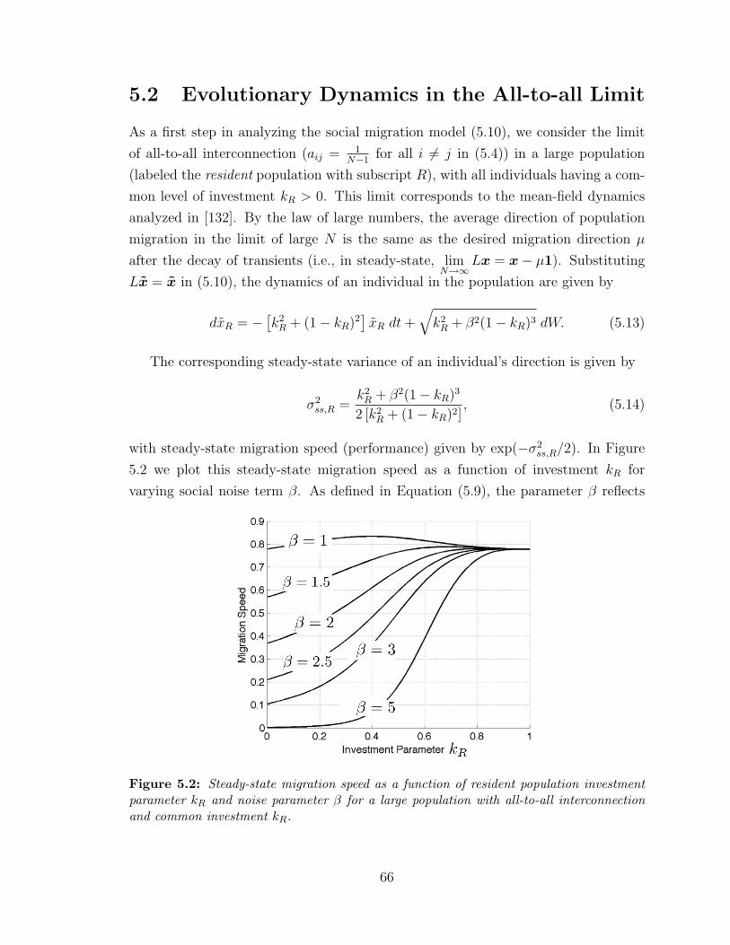
5.2 Evolutionary Dynamics in the All-to-all Limit

As a first step in analyzing the social migration model (5.10), we consider the limit

of all-to-all interconnection (aij = 1N−1

for all i 6= j in (5.4)) in a large population

(labeled the resident population with subscript R), with all individuals having a com-

mon level of investment kR > 0. This limit corresponds to the mean-field dynamics

analyzed in [132]. By the law of large numbers, the average direction of population

migration in the limit of large N is the same as the desired migration direction µ

after the decay of transients (i.e., in steady-state, limN→∞

Lx = x− µ1). Substituting

Lx = x in (5.10), the dynamics of an individual in the population are given by

dxR = − [k2R + (1− kR)2

]xR dt+

√k2R + β2(1− kR)3 dW. (5.13)

The corresponding steady-state variance of an individual’s direction is given by

σ2ss,R =

k2R + β2(1− kR)3

2 [k2R + (1− kR)2]

, (5.14)

with steady-state migration speed (performance) given by exp(−σ2ss,R/2). In Figure

5.2 we plot this steady-state migration speed as a function of investment kR for

varying social noise term β. As defined in Equation (5.9), the parameter β reflects

Figure 5.2: Steady-state migration speed as a function of resident population investmentparameter kR and noise parameter β for a large population with all-to-all interconnectionand common investment kR.

66

the strength of the noise from social interactions relative to the noise associated with

the tracking process. In Figure 5.2 we see that the migration performance saturates

at high levels of investment kR, and remains low over greater kR ranges, for large β.

We use β > 2 in this work to model noisier social interactions relative to tracking

(consistent with [132]); this provides an incentive for individuals to invest in the

tracking process.

Now consider the evolution of strategies for such an all-to-all connected popu-

lation. A key part of any evolutionary algorithm is the computation of fitness of

individuals in the population as a function of strategy distribution, model parame-

ters, environmental conditions, and other such features. In certain cases (such as the

all-to-all limit here), fitness can be analytically computed, which allows for an explicit

calculation of the outcomes of the evolutionary process using tools from adaptive dy-

namics [25, 26, 18]. Adaptive dynamics are well-suited for studying the evolution of

a continuous one-dimensional trait in a population undergoing small mutations (see

§2.1 for a detailed discussion).

5.2.1 Adaptive Dynamics Calculations

Using (5.14) and (5.11), the fitness of an individual in the resident population with

dynamics (5.13) is given by

FR(kR) = exp

(−k

2R + β2(1− kR)3

4(2k2R − 2kR + 1)

− ck2R

). (5.15)

Consider a small population of mutants with strategy kM interacting with each other

and with all the residents. The mutants (owing to their small numbers) will experience

the same social noise as the residents so that they have dynamics given by

dxM = − [k2M + (1− kM)2

]xM dt+

√k2M + β2(1− kR)(1− kM)2 dW. (5.16)

Correspondingly, the fitness of individuals in the mutant population is given by

FM(kR, kM) = exp

(−k

2M + β2(1− kR)(1− kM)2

4(2k2M − 2kM + 1)

− ck2M

). (5.17)

The relative fitness of the mutant strategy in the environment of the resident is known

as the differential fitness and is given by (2.3),

S(kR, kM) = FM(kR, kM)− FR(kR). (5.18)

67

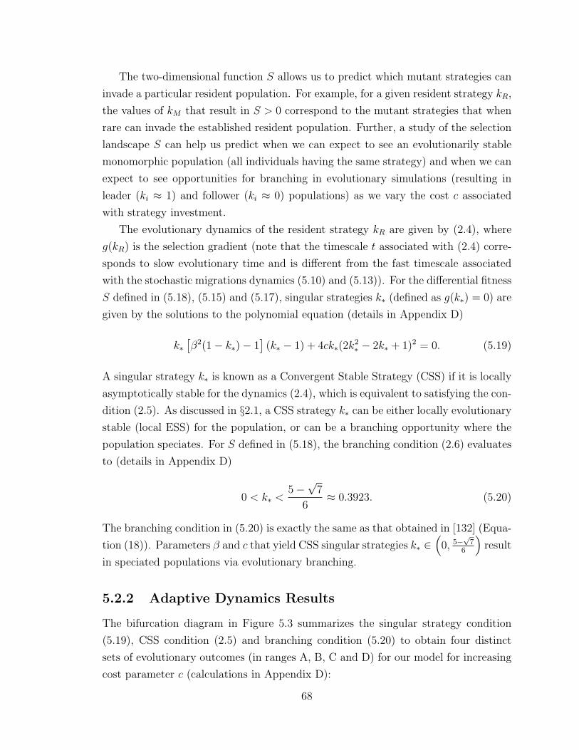
The two-dimensional function S allows us to predict which mutant strategies can

invade a particular resident population. For example, for a given resident strategy kR,

the values of kM that result in S > 0 correspond to the mutant strategies that when

rare can invade the established resident population. Further, a study of the selection

landscape S can help us predict when we can expect to see an evolutionarily stable

monomorphic population (all individuals having the same strategy) and when we can

expect to see opportunities for branching in evolutionary simulations (resulting in

leader (ki ≈ 1) and follower (ki ≈ 0) populations) as we vary the cost c associated

with strategy investment.

The evolutionary dynamics of the resident strategy kR are given by (2.4), where

g(kR) is the selection gradient (note that the timescale t associated with (2.4) corre-

sponds to slow evolutionary time and is different from the fast timescale associated

with the stochastic migrations dynamics (5.10) and (5.13)). For the differential fitness

S defined in (5.18), (5.15) and (5.17), singular strategies k∗ (defined as g(k∗) = 0) are

given by the solutions to the polynomial equation (details in Appendix D)

k∗[β2(1− k∗)− 1

](k∗ − 1) + 4ck∗(2k

2∗ − 2k∗ + 1)2 = 0. (5.19)

A singular strategy k∗ is known as a Convergent Stable Strategy (CSS) if it is locally

asymptotically stable for the dynamics (2.4), which is equivalent to satisfying the con-

dition (2.5). As discussed in §2.1, a CSS strategy k∗ can be either locally evolutionary

stable (local ESS) for the population, or can be a branching opportunity where the

population speciates. For S defined in (5.18), the branching condition (2.6) evaluates

to (details in Appendix D)

0 < k∗ <5−√7

6≈ 0.3923. (5.20)

The branching condition in (5.20) is exactly the same as that obtained in [132] (Equa-

tion (18)). Parameters β and c that yield CSS singular strategies k∗ ∈(

0, 5−√

76

)result

in speciated populations via evolutionary branching.

5.2.2 Adaptive Dynamics Results

The bifurcation diagram in Figure 5.3 summarizes the singular strategy condition

(5.19), CSS condition (2.5) and branching condition (5.20) to obtain four distinct

sets of evolutionary outcomes (in ranges A, B, C and D) for our model for increasing

cost parameter c (calculations in Appendix D):

68

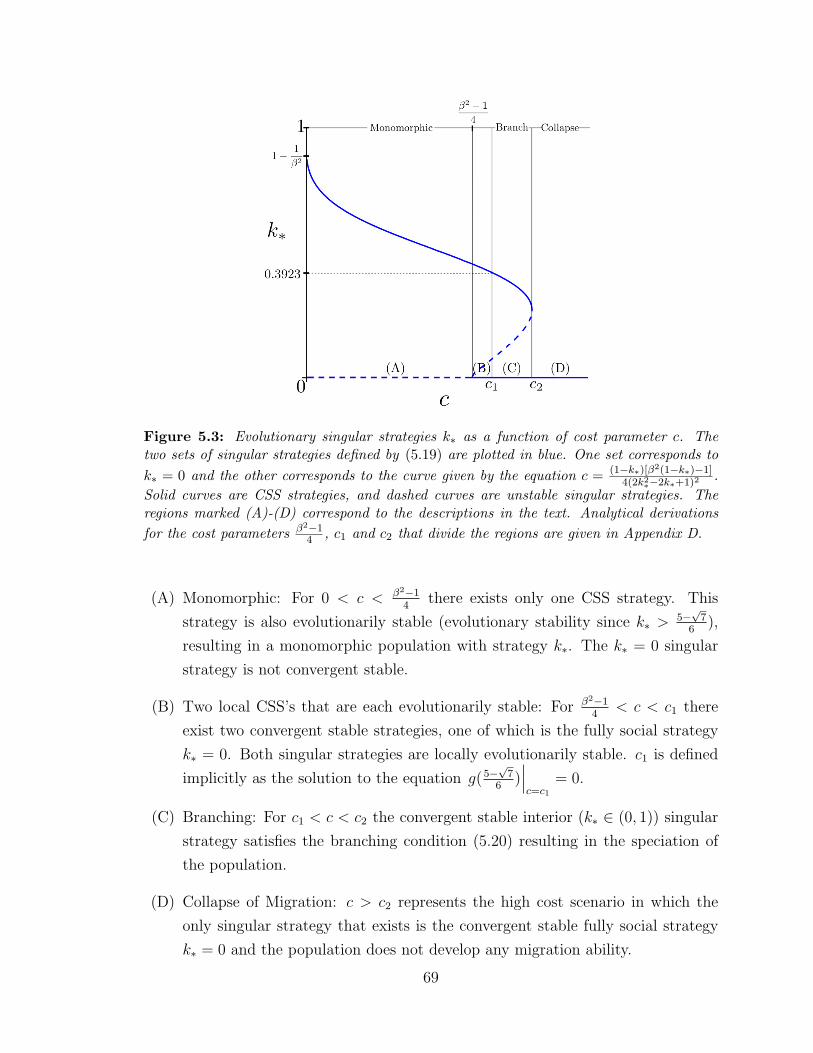
Figure 5.3: Evolutionary singular strategies k∗ as a function of cost parameter c. Thetwo sets of singular strategies defined by (5.19) are plotted in blue. One set corresponds tok∗ = 0 and the other corresponds to the curve given by the equation c = (1−k∗)[β2(1−k∗)−1]

4(2k2∗−2k∗+1)2

.Solid curves are CSS strategies, and dashed curves are unstable singular strategies. Theregions marked (A)-(D) correspond to the descriptions in the text. Analytical derivationsfor the cost parameters β2−1

4 , c1 and c2 that divide the regions are given in Appendix D.

(A) Monomorphic: For 0 < c < β2−14

there exists only one CSS strategy. This

strategy is also evolutionarily stable (evolutionary stability since k∗ >5−√

76

),

resulting in a monomorphic population with strategy k∗. The k∗ = 0 singular

strategy is not convergent stable.

(B) Two local CSS’s that are each evolutionarily stable: For β2−14

< c < c1 there

exist two convergent stable strategies, one of which is the fully social strategy

k∗ = 0. Both singular strategies are locally evolutionarily stable. c1 is defined

implicitly as the solution to the equation g(5−√

76

)∣∣∣c=c1

= 0.

(C) Branching: For c1 < c < c2 the convergent stable interior (k∗ ∈ (0, 1)) singular

strategy satisfies the branching condition (5.20) resulting in the speciation of

the population.

(D) Collapse of Migration: c > c2 represents the high cost scenario in which the

only singular strategy that exists is the convergent stable fully social strategy

k∗ = 0 and the population does not develop any migration ability.

69

These four cases constitute a comprehensive picture of the evolutionary dynamics

of the migration model (5.10) in the all-to-all limit, and encompass key features of the

branching calculations in [132] and evolutionary simulations in [33]. The existence of

two locally evolutionary stable attractors in case (B) above implies that the evolu-

tionary dynamics can potentially yield speciated outcomes in the population without

evolutionary branching (case (C)). We illustrate this using simulations in §5.2.3.

A hysteretic effect associated with restoring population migration ability once

destroyed is apparent in Figure 5.3. In particular, once migration ability in the pop-

ulation is lost for high cost parameter c > c2, the cost parameter needs to be reduced

below the level β2−14

(< c1 < c2) for migration ability to be regained. This compares

to the simulations in [33, 34] where agent-based models are used to study the effect

of habitat fragmentation on the evolution of migration. In these simulations, the

authors study the impacts of progressively more fragmented habitats on migratory

outcomes, and show that once migration ability is lost for a threshold level of frag-

mentation, much greater habitat recovery is necessary to restore lost migration ability

(a hysteretic effect). Higher levels of habitat fragmentation are comparable to higher

cost parameter c.

5.2.3 Evolutionary Simulations∗

In Figure 5.4 we show the pairwise invasability plots (PIPs) [25, 26, 18] (see Figure

2.3 in §2.1 for a description) of the differential fitness S(kR, kM) for increasing cost

c to illustrate the four sets of outcomes described above. These plots show the sign

of S as a function of the resident and mutant population strategies. Dark regions

correspond to differential fitness S > 0 and allow mutant invasions; white regions

correspond to S < 0 and prohibit mutant invasions. Comparing the PIPs from Figure

5.4 to the canonical classes of PIPs in Figure 2.3, we see conditions for an initially

monomorphic population for low values of cost parameter c, a branching speciated

solution for intermediate values of c, and for high values of c we see conditions that

prevent individuals from developing any significant investment, i.e., the population is

unable to develop any significant migration ability.

We confirm our predictions from the adaptive dynamics analysis by running evo-

lutionary simulations in the case of a monomorphic initial condition and also a uni-

formly randomly distributed initial condition as shown in Figure 5.4 (bottom two

rows). These simulations comprise the roulette-wheel selection and small mutation

∗Results from this subsection were presented at the SIAM Conference on Applications of Dy-namical Systems, Snowbird, UT, 2011.

70

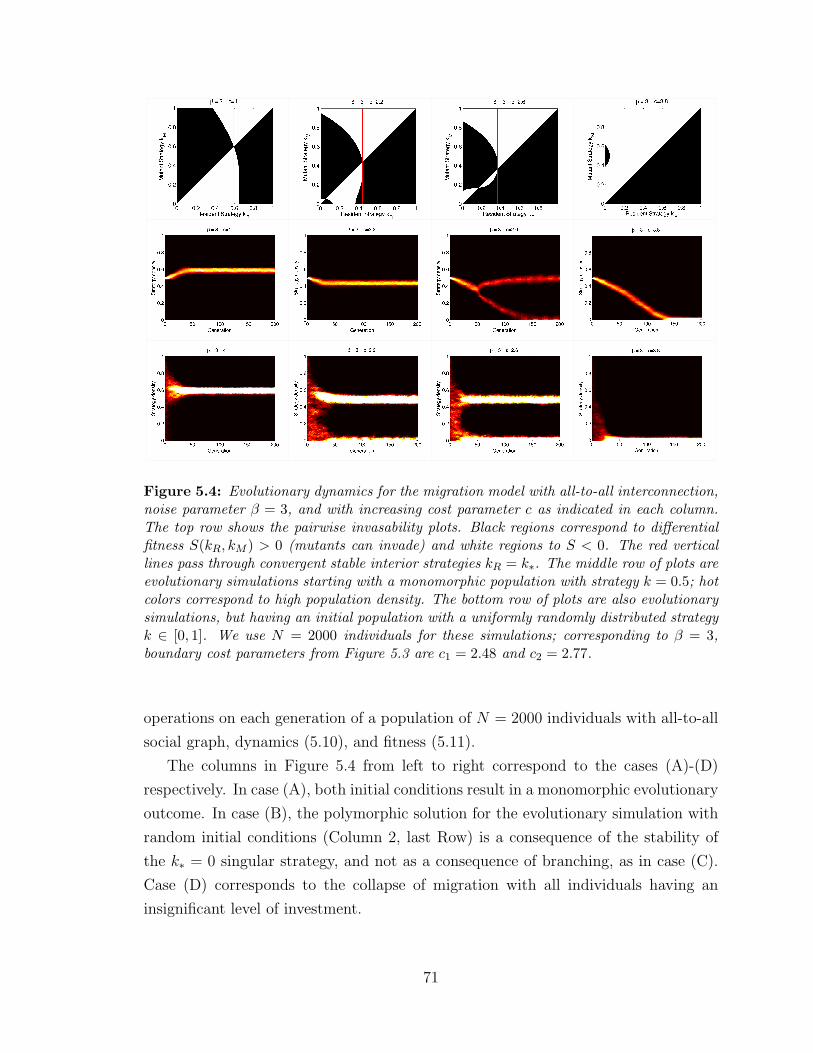
Figure 5.4: Evolutionary dynamics for the migration model with all-to-all interconnection,noise parameter β = 3, and with increasing cost parameter c as indicated in each column.The top row shows the pairwise invasability plots. Black regions correspond to differentialfitness S(kR, kM ) > 0 (mutants can invade) and white regions to S < 0. The red verticallines pass through convergent stable interior strategies kR = k∗. The middle row of plots areevolutionary simulations starting with a monomorphic population with strategy k = 0.5; hotcolors correspond to high population density. The bottom row of plots are also evolutionarysimulations, but having an initial population with a uniformly randomly distributed strategyk ∈ [0, 1]. We use N = 2000 individuals for these simulations; corresponding to β = 3,boundary cost parameters from Figure 5.3 are c1 = 2.48 and c2 = 2.77.

operations on each generation of a population of N = 2000 individuals with all-to-all

social graph, dynamics (5.10), and fitness (5.11).

The columns in Figure 5.4 from left to right correspond to the cases (A)-(D)

respectively. In case (A), both initial conditions result in a monomorphic evolutionary

outcome. In case (B), the polymorphic solution for the evolutionary simulation with

random initial conditions (Column 2, last Row) is a consequence of the stability of

the k∗ = 0 singular strategy, and not as a consequence of branching, as in case (C).

Case (D) corresponds to the collapse of migration with all individuals having an

insignificant level of investment.

71

The analysis in this section shows the range of evolutionary outcomes for the

migration model with all-to-all social interconnection. We are particularly motivated

by conditions that result in the speciation or branching of the population into invested

leaders and social followers. In the following section we study the role that limited

social interconnection topology plays in the emergence of this evolutionary branching.

5.3 Evolutionary Dynamics with Limited Social

Interactions†

In this section we study the role that graph topology plays in the evolutionary dy-

namics of the migration model (5.10). While the all-to-all topology assumption of

§5.2 allows for a detailed analysis of the evolutionary dynamics in a large population,

it is unrealistic for most biological and decentralized artificial systems. In §5.3.1,

we relax the all-to-all assumption and study the migration model (5.10) with limited

interconnection. We prove two main results. Theorem 5.1 provides necessary and suf-

ficient conditions for a population with limited interconnections to develop the ability

to migrate. Theorem 5.2 presents an analytical technique for computing migratory

performance (solution to fast timescale dynamics) as a function of interconnection

topology and individual node investments.

In §5.3.2 we utilize the analytical fast timescale calculation from Theorem 5.2 to

simulate evolutionary dynamics for three classes of limited interconnection topologies:

undirected ring lattices, undirected random graphs, and directed random graphs.

In each case, the simulations show a minimum connectivity threshold necessary for

speciated evolutionary outcomes in the population.

5.3.1 Fast Timescale Results

As we will see in Theorem 5.2, the steady-state probability distribution of the state

x for the migration dynamics (5.10) exists if and only if the zero equilibrium of the

noise-free form of the dynamics (5.10) are asymptotically stable. The noise-free form

of the dynamics (5.10) are given by

˙x = M x, where M = −(K1 +K2L). (5.21)

†Results from this section were presented at the SIAM Conference on Applications of DynamicalSystems, Snowbird, UT, 2011.

72

Intuitively, the asymptotic stability of the zero equilibrium of the noise-free dy-

namics (5.21) corresponds to the population developing the ability to collectively

migrate since x → 0 =⇒ x → µ1. The lack of asymptotic stability for (5.21)

implies that there exist individuals in the population that do not have an ability to

migrate because their direction states xi diverge away from the desired direction µ,

and correspondingly, the steady-state variance of xi given by σ2ss,i does not exist. The

linear dynamics (5.21) are asymptotically stable if and only if matrix M is Hurwitz

[113], i.e., all eigenvalues of M have real part strictly less than 0. Lemmas 5.1 and 5.2

provide necessary and sufficient conditions, respectively, for matrix M to be Hurwitz.

Lemma 5.1. If matrix M is Hurwitz, then there exists some node i such that ki > 0.

Proof. If the condition is not satisfied, i.e., ki=0 for all i ∈ {1, · · · , N}, then M = −L.

The Laplacian matrix L has a zero eigenvalue associated with the eigenvector 1 and

hence M is not Hurwitz.

Lemma 5.2. If ki > 0 for all i ∈ {1, · · · , N}, then M is Hurwitz.

Proof. This can be checked by a straightforward application of the Gershgorin circle

theorem [43]. The Laplacian matrix L is given by L = [lij]. The eigenvalues of M lie

in the union of N disks, each centered about −k2i − (1−ki)2lii with radius (1−ki)2lii.

If ki > 0 for all i, then the disks all lie strictly in the left half complex plane.

Lemmas 5.1 and 5.2 are extreme cases of investment that can be interpreted in the

context of migration as follows. Lemma 5.1 says that regardless of social interconnec-

tion topology, the population does not develop migration ability unless at least one

individual is invested in acquiring the external signal µ. Lemma 5.2 says that if all

individuals in the population are invested, then the population develops the ability to

migrate in the direction µ, for any social graph. In Theorem 5.1 we derive necessary

and sufficient conditions for the population to develop migration ability (matrix M

Hurwitz) that depend explicitly on the topology of the social interconnection graph.

The proof of Theorem 5.1 requires the following lemma from [110] (see also [111, 64]).

Lemma 5.3. For a general Laplacian matrix L = [lij] ∈ RN×N given by lij ≤ 0 for

i 6= j andN∑j=1

lij = 0 for all i ∈ {1, · · · , N}, the following conditions are equivalent:

(i) L has a simple zero eigenvalue and all of the other eigenvalues have positive

real parts.

73

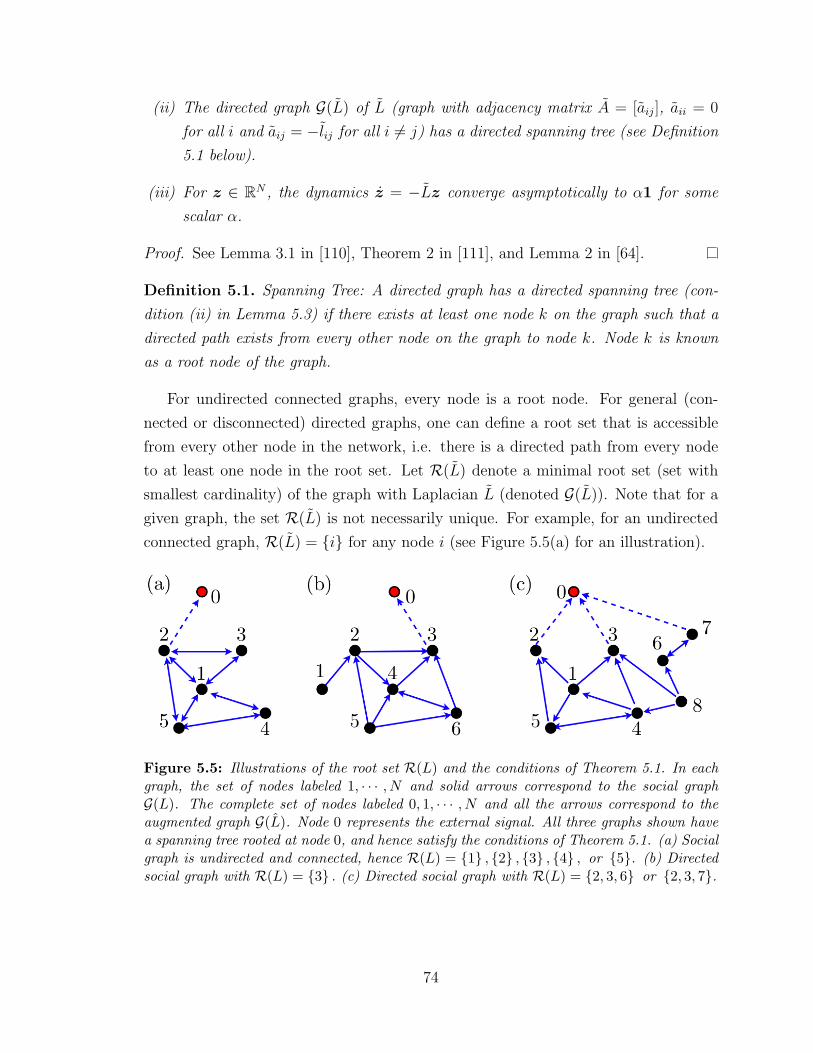
(ii) The directed graph G(L) of L (graph with adjacency matrix A = [aij], aii = 0

for all i and aij = −lij for all i 6= j) has a directed spanning tree (see Definition

5.1 below).

(iii) For z ∈ RN , the dynamics z = −Lz converge asymptotically to α1 for some

scalar α.

Proof. See Lemma 3.1 in [110], Theorem 2 in [111], and Lemma 2 in [64].

Definition 5.1. Spanning Tree: A directed graph has a directed spanning tree (con-

dition (ii) in Lemma 5.3) if there exists at least one node k on the graph such that a

directed path exists from every other node on the graph to node k. Node k is known

as a root node of the graph.

For undirected connected graphs, every node is a root node. For general (con-

nected or disconnected) directed graphs, one can define a root set that is accessible

from every other node in the network, i.e. there is a directed path from every node

to at least one node in the root set. Let R(L) denote a minimal root set (set with

smallest cardinality) of the graph with Laplacian L (denoted G(L)). Note that for a

given graph, the set R(L) is not necessarily unique. For example, for an undirected

connected graph, R(L) = {i} for any node i (see Figure 5.5(a) for an illustration).

Figure 5.5: Illustrations of the root set R(L) and the conditions of Theorem 5.1. In eachgraph, the set of nodes labeled 1, · · · , N and solid arrows correspond to the social graphG(L). The complete set of nodes labeled 0, 1, · · · , N and all the arrows correspond to theaugmented graph G(L). Node 0 represents the external signal. All three graphs shown havea spanning tree rooted at node 0, and hence satisfy the conditions of Theorem 5.1. (a) Socialgraph is undirected and connected, hence R(L) = {1} , {2} , {3} , {4} , or {5}. (b) Directedsocial graph with R(L) = {3} . (c) Directed social graph with R(L) = {2, 3, 6} or {2, 3, 7}.

74

Theorem 5.1. Matrix M from (5.21) is Hurwitz if and only if there exists a minimal

root set R(L) such that kj > 0 for all nodes j ∈ R(L), where L is the Laplacian matrix

of the social graph with adjacency matrix (5.4).

Proof. Define the normalized external signal state (xi = µ in (5.7)) x0 = 0 and the

augmented state vector z = [x0 x]T . Consider the dynamics

z =

[˙x0

˙x

]= −

[0 0N×1

−K11 −M

][x0

x

]= −Lz. (5.22)

Then L satisfies the properties of general Laplacian matrices given in Lemma 5.3.

The graph corresponding to Laplacian L is the same as the graph corresponding to

Laplacian K2L with an additional node (labeled 0, with state x0) having incoming

links with weights k2j from all nodes j = 1, · · · , N (see Figure 5.5 for an illustration,

links to node 0 are shown as dashed arrows).

Since node 0 of G(L) has no outgoing links, from Definition 5.1 we have the

following condition,

G(L) has a spanning tree ⇐⇒ R(L) = {0} . (5.23)

We claim the following

G(L) has a spanning tree =⇒ ∃ R(L) s.t. kj > 0 for all j ∈ R(L). (5.24)

We prove the statement above by contradiction. Assume that G(L) has a spanning

tree and for each root set R(L), there exists a node j such that kj = 0. Since G(L)

has a spanning tree, R(L) = {0}, which means that there is a directed path from

every node to node 0. Now consider any root set R(L). Since kj = 0, node j in R(L)

can only reach node 0 by a path to a node m /∈ R(L), for which km > 0. However,

if such a path exists, then the set R(L) where node j is replaced with node m is

another root set. By assumption we must have km = 0. Thus there exists no directed

path from node j to node 0. Hence G(L) does not have a spanning tree and we have

proved the claim.

Consider any root set R(L) and assume that kj > 0 for all j ∈ R(L). Then all

nodes j ∈ R(L) are connected to node 0 of G(L). For all nodes m /∈ R(L), either

km > 0 and m has a direct link to node 0, or km = 0 in which case m has a link to at

least one other node on a directed path to the root node 0, via an element of R(L).

75

Hence

∃ R(L) s.t. kj > 0 for all j ∈ R(L) =⇒ G(L) has a spanning tree . (5.25)

Combining (5.23), (5.24) and (5.25), we have the condition,

∃ R(L) s.t. kj > 0 ∀j ∈ R(L) ⇐⇒ G(L) has a spanning tree

⇐⇒ R(L) = {0} . (5.26)

From Lemma 5.3, G(L) has a spanning tree if and only if the dynamics (5.22)

converge asymptotically to α1 for some scalar α. However in (5.22), the state x0 = 0

is invariant and hence α = 0. The linear dynamics (5.21) converge asymptotically to

0 if and only if matrix M is Hurwitz [113]. This gives the condition

G(L) has a spanning tree ⇐⇒ M is Hurwitz. (5.27)

Combining (5.26) and (5.27) we have the desired result.

Sets of root nodes R(L) are illustrated for a set of simple social graphs in Figure

5.5. The directed connected graph in Figure 5.5(b) has a single root node, whereas

the graph in Figure 5.5(c) has two possible minimal sets of root nodes.

We now return to the noisy migration model given by the system of stochastic

equations (5.10). In order to compute the fitness of an individual in a migratory

collective using (5.11), a computation of the steady-state variance of the individuals

dynamics σ2ss,i is necessary. This quantity in turn depends on the level of investment

of the individuals in the network (represented by the vector k) and the underlying

topology of the social interconnection graph G(L), and can be computed by solving

the matrix Lyapunov equation, as shown in Theorem 5.2 (see also [151, 103] for related

results on the consensus and drift-diffusion models respectively).

Theorem 5.2. For the stochastic dynamics (5.10) with social graph G(L), suppose

there exists an R(L) such that kj > 0 for all j ∈ R(L). Then the system of stochastic

differential equations (5.10) has steady-state mean limt→∞

E [x(t)] = 0 and steady-state

covariance matrix Σ = limt→∞

E[x(t)T x(t)

]given by the solution to the Lyapunov equa-

tion (K1 +K2L)Σ + Σ(K1 +K2L)T = SST .

Proof. The system (5.10) is a multivariate Ornstein-Uhlenbeck process with mean

given by [24]

E [x(t)] = exp (Mt)E [x(0)] .

76

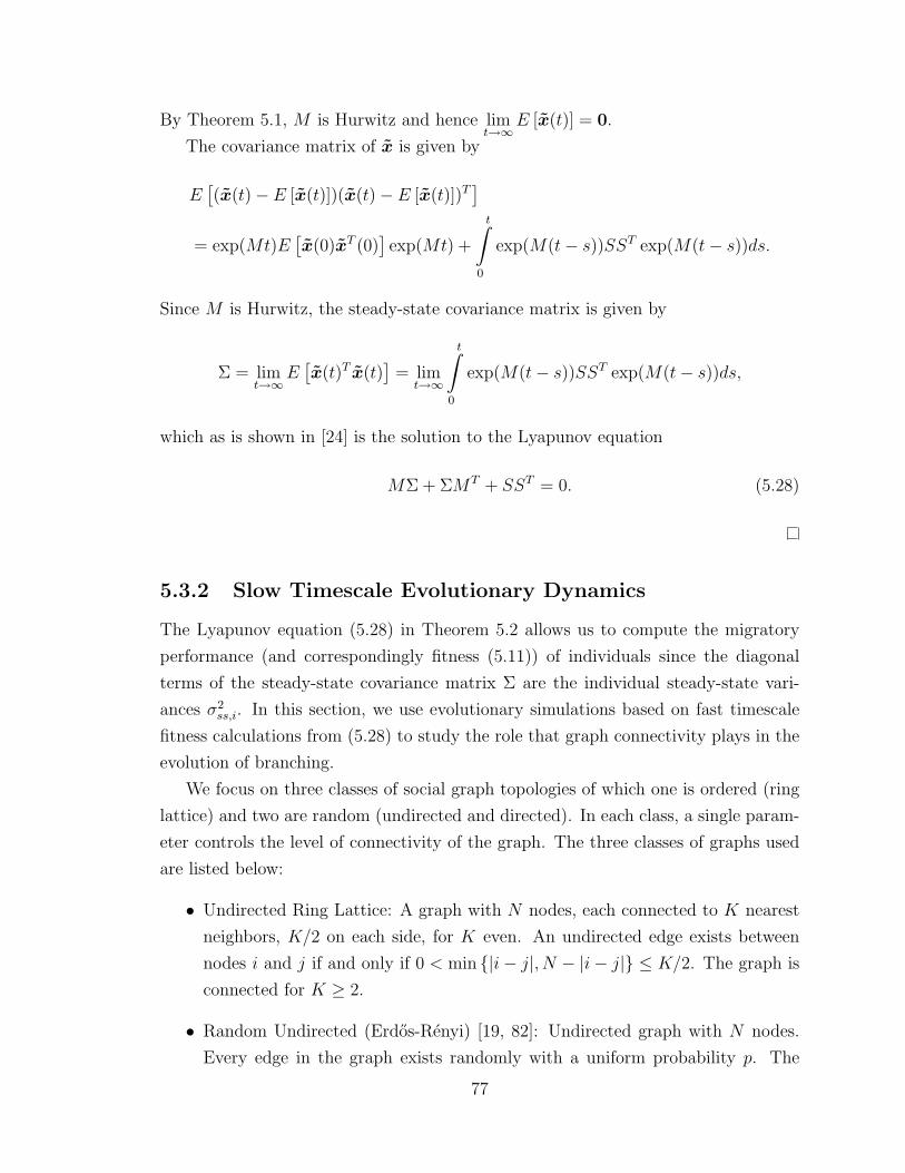
By Theorem 5.1, M is Hurwitz and hence limt→∞

E [x(t)] = 0.

The covariance matrix of x is given by

E[(x(t)− E [x(t)])(x(t)− E [x(t)])T

]= exp(Mt)E

[x(0)xT (0)

]exp(Mt) +

t∫0

exp(M(t− s))SST exp(M(t− s))ds.

Since M is Hurwitz, the steady-state covariance matrix is given by

Σ = limt→∞

E[x(t)T x(t)

]= lim

t→∞

t∫0

exp(M(t− s))SST exp(M(t− s))ds,

which as is shown in [24] is the solution to the Lyapunov equation

MΣ + ΣMT + SST = 0. (5.28)

5.3.2 Slow Timescale Evolutionary Dynamics

The Lyapunov equation (5.28) in Theorem 5.2 allows us to compute the migratory

performance (and correspondingly fitness (5.11)) of individuals since the diagonal

terms of the steady-state covariance matrix Σ are the individual steady-state vari-

ances σ2ss,i. In this section, we use evolutionary simulations based on fast timescale

fitness calculations from (5.28) to study the role that graph connectivity plays in the

evolution of branching.

We focus on three classes of social graph topologies of which one is ordered (ring

lattice) and two are random (undirected and directed). In each class, a single param-

eter controls the level of connectivity of the graph. The three classes of graphs used

are listed below:

• Undirected Ring Lattice: A graph with N nodes, each connected to K nearest

neighbors, K/2 on each side, for K even. An undirected edge exists between

nodes i and j if and only if 0 < min {|i− j|, N − |i− j|} ≤ K/2. The graph is

connected for K ≥ 2.

• Random Undirected (Erdos-Renyi) [19, 82]: Undirected graph with N nodes.

Every edge in the graph exists randomly with a uniform probability p. The

77

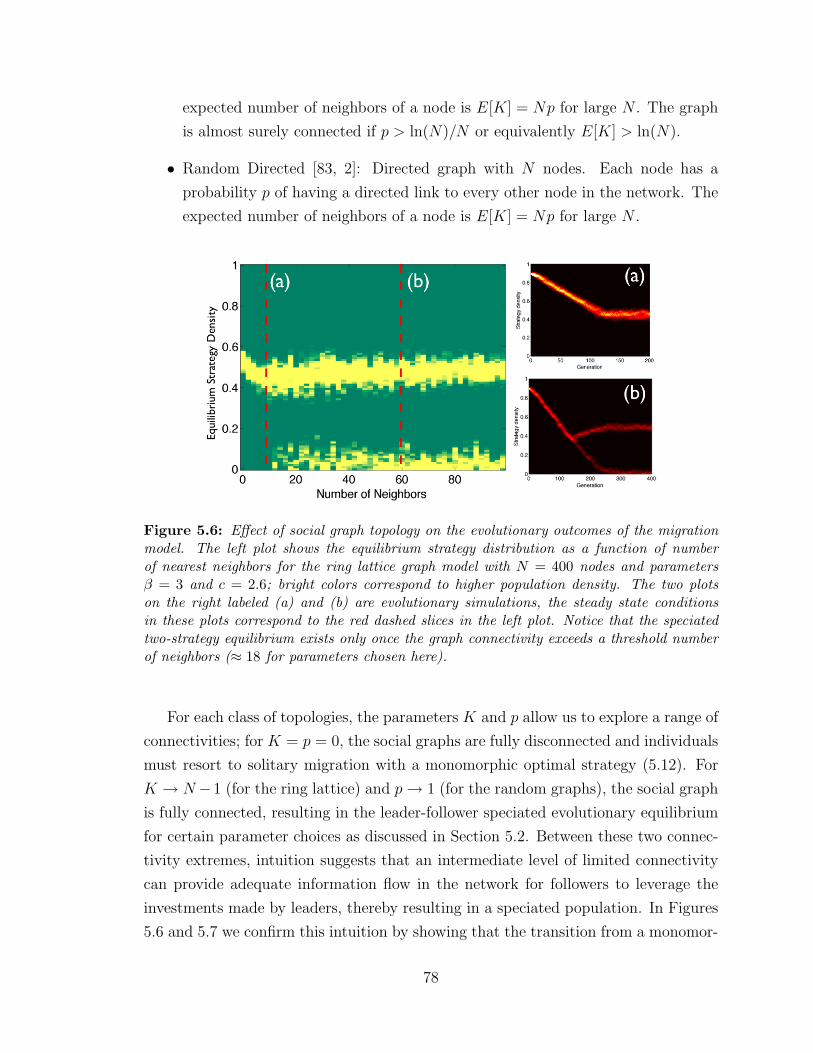
expected number of neighbors of a node is E[K] = Np for large N . The graph

is almost surely connected if p > ln(N)/N or equivalently E[K] > ln(N).

• Random Directed [83, 2]: Directed graph with N nodes. Each node has a

probability p of having a directed link to every other node in the network. The

expected number of neighbors of a node is E[K] = Np for large N .

Figure 5.6: Effect of social graph topology on the evolutionary outcomes of the migrationmodel. The left plot shows the equilibrium strategy distribution as a function of numberof nearest neighbors for the ring lattice graph model with N = 400 nodes and parametersβ = 3 and c = 2.6; bright colors correspond to higher population density. The two plotson the right labeled (a) and (b) are evolutionary simulations, the steady state conditionsin these plots correspond to the red dashed slices in the left plot. Notice that the speciatedtwo-strategy equilibrium exists only once the graph connectivity exceeds a threshold numberof neighbors (≈ 18 for parameters chosen here).

For each class of topologies, the parameters K and p allow us to explore a range of

connectivities; for K = p = 0, the social graphs are fully disconnected and individuals

must resort to solitary migration with a monomorphic optimal strategy (5.12). For

K → N −1 (for the ring lattice) and p→ 1 (for the random graphs), the social graph

is fully connected, resulting in the leader-follower speciated evolutionary equilibrium

for certain parameter choices as discussed in Section 5.2. Between these two connec-

tivity extremes, intuition suggests that an intermediate level of limited connectivity

can provide adequate information flow in the network for followers to leverage the

investments made by leaders, thereby resulting in a speciated population. In Figures

5.6 and 5.7 we confirm this intuition by showing that the transition from a monomor-

78

phic, to a branched evolutionary solution as a function of topology (parameterized

by K and p), occurs at an intermediate threshold level of connectivity.

For the simulation in Figure 5.6 we use the ring lattice topology for the social graph

with N = 400 individuals and choose a set of parameters for which the all-to-all social

graph is known to have a two-strategy solution, β = 3 and c = 2.6 (see Figure 5.4,

column 3). For a range of values of the number of neighbors K = 2, 4, · · · , 100, we

compute the fitness of individuals using (5.28) and (5.11) and evolve the strategies of

the populations to an evolutionary steady state. This steady-state strategy distribu-

tion is plotted as a function of number of neighbors K in the figure. We see that there

exists an intermediate threshold for social connectivity (given by K ≈ 18) that allows

for adequate information flow in the network to result in evolutionary branching. In

particular, social graphs that are much sparser (fewer edges) than the all-to-all case

analyzed in Section 5.2 can yield speciated evolutionary outcomes.

In Figure 5.7 we present simulations similar to those described for Figure 5.6

above, for all three classes of social graph topologies (ring lattice, undirected ran-

dom, directed random) and for N = 200, 400, 600. In each case, we see a threshold

connectivity for evolutionary branching that is higher than the minimum thresholds

for the social graph to be connected. We also see that the number of individuals in

the population N does not have a significant affect on this threshold in the range

considered. Further, the location of the threshold is dependent on the class of graph

being considered; the two classes of random graphs have lower thresholds than the

ordered ring lattice.

The simulations in this section illustrate the significant effect of limited social

graph connectivity on the evolution of branching in migration. In particular, we show

that social connectivity above threshold levels can yield speciated outcomes in the

evolutionary dynamics. The thresholds depend on the classes of social graph topology

being considered. Determining the analytical minimum connectivity threshold as

function of parameters β, c and class of graph, is a topic of ongoing work. We

also intend to look at other classes of graph topologies such as spatially embedded

graphs with a topological metric on connectivity (such as in [3]), and classes of small-

world graphs parameterized by a single rewiring parameter [146, 82] (the ring lattice

and undirected random graphs considered here are two extreme limits of the Watts-

Strogatz small world model).

79

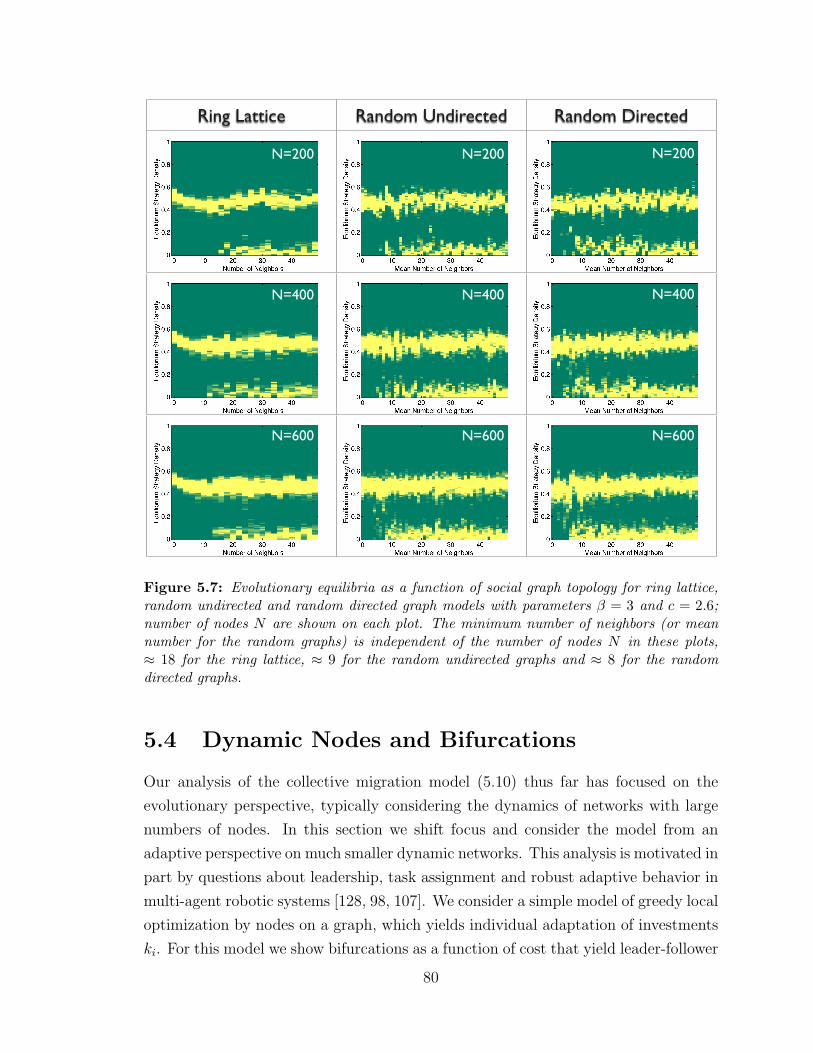
Ring Lattice Random Undirected Random Directed

N=200

N=400

N=600

N=200

N=400

N=600

N=200

N=400

N=600

Figure 5.7: Evolutionary equilibria as a function of social graph topology for ring lattice,random undirected and random directed graph models with parameters β = 3 and c = 2.6;number of nodes N are shown on each plot. The minimum number of neighbors (or meannumber for the random graphs) is independent of the number of nodes N in these plots,≈ 18 for the ring lattice, ≈ 9 for the random undirected graphs and ≈ 8 for the randomdirected graphs.

5.4 Dynamic Nodes and Bifurcations

Our analysis of the collective migration model (5.10) thus far has focused on the

evolutionary perspective, typically considering the dynamics of networks with large

numbers of nodes. In this section we shift focus and consider the model from an

adaptive perspective on much smaller dynamic networks. This analysis is motivated in

part by questions about leadership, task assignment and robust adaptive behavior in

multi-agent robotic systems [128, 98, 107]. We consider a simple model of greedy local

optimization by nodes on a graph, which yields individual adaptation of investments

ki. For this model we show bifurcations as a function of cost that yield leader-follower

80

emergent behavior as equilibria of the adaptive process. We also illustrate the critical

role played by graph topology in determining the location of leaders in the network

of adaptive nodes using several examples.

Consider a system of interconnected agents with fast-timescale tracking dynamics

given by (5.10). Further, suppose that each agent seeks to maximize its local utility

function by adapting its investment parameter ki. We assume that the utility function

for each agent Ui is given by the fitness function (5.11),

Ui = exp

(−σ2ss,i

2

)exp

(−ck2i

). (5.29)

In this setting, the utility function for a focal agent i depends on the agent’s invest-

ment ki, as well as the investments of other nodes in the network; we assume that

the agent can measure its own utility, but not the investments of other nodes. Given

the measured local utility Ui, agents modify their investments ki on a slow timescale

by climbing the gradient of their local utility to reach its local maximum,

dkidt

=∂Ui∂ki

. (5.30)

Our goal is to study the outcomes of this simple adaptive process by computing

equilibria of the dynamics defined by (5.30), (5.29) and (5.10), and studying their

bifurcations. Let Ui = lnUi and consider the non-homogeneous time scaling τ =t∫

0

Ui(σ)dσ. Then the dynamics (5.30) transform to

ki =dkidτ

=∂Ui∂ki

=∂

∂ki

(−σ2ss,i

2− ck2

i

), i = {1, · · · , N} . (5.31)

The dynamics (5.31) are identical to (5.30), modulo the time-scaling, and are nota-

tionally simpler. In particular, the equilibria of (5.31) are identical to those of (5.30).

We focus on these dynamics for the remainder of the section.

We first look at the simplest case of the dynamics with N = 2 nodes, with an

all-to-all graph. The steady-state covariance matrix Σ (from (5.28)) in this case can

be computed analytically [24] as

Σ =(Det M)SST + [−M + (Tr M)]SST [−M + (Tr M)]T

−2(Det M)(Tr M), (5.32)

81

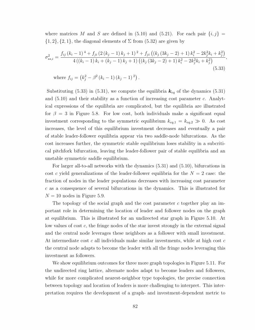
where matrices M and S are defined in (5.10) and (5.21). For each pair {i, j} =

{1, 2}, {2, 1}, the diagonal elements of Σ from (5.32) are given by

σ2ss,i =

fij (ki − 1) 4 + fji (2 (kj − 1) kj + 1) 2 + fji((kj (3kj − 2) + 1) k2

i − 2k2jki + k2

j

)4 ((ki − 1) ki + (kj − 1) kj + 1)

((kj (3kj − 2) + 1) k2

i − 2k2jki + k2

j

) ,

(5.33)

where fij =(k2j − β2 (ki − 1) (kj − 1) 2

).

Substituting (5.33) in (5.31), we compute the equilibria keq of the dynamics (5.31)

and (5.10) and their stability as a function of increasing cost parameter c. Analyt-

ical expressions of the equilibria are complicated, but the equilibria are illustrated

for β = 3 in Figure 5.8. For low cost, both individuals make a significant equal

investment corresponding to the symmetric equilibrium keq,1 = keq,2 � 0. As cost

increases, the level of this equilibrium investment decreases and eventually a pair

of stable leader-follower equilibria appear via two saddle-node bifurcations. As the

cost increases further, the symmetric stable equilibrium loses stability in a subcriti-

cal pitchfork bifurcation, leaving the leader-follower pair of stable equilibria and an

unstable symmetric saddle equilibrium.

For larger all-to-all networks with the dynamics (5.31) and (5.10), bifurcations in

cost c yield generalizations of the leader-follower equilibria for the N = 2 case: the

fraction of nodes in the leader populations decreases with increasing cost parameter

c as a consequence of several bifurcations in the dynamics. This is illustrated for

N = 10 nodes in Figure 5.9.

The topology of the social graph and the cost parameter c together play an im-

portant role in determining the location of leader and follower nodes on the graph

at equilibrium. This is illustrated for an undirected star graph in Figure 5.10. At

low values of cost c, the fringe nodes of the star invest strongly in the external signal

and the central node leverages these neighbors as a follower with small investment.

At intermediate cost c all individuals make similar investments, while at high cost c

the central node adapts to become the leader with all the fringe nodes leveraging this

investment as followers.

We show equilibrium outcomes for three more graph topologies in Figure 5.11. For

the undirected ring lattice, alternate nodes adapt to become leaders and followers,

while for more complicated nearest-neighbor type topologies, the precise connection

between topology and location of leaders is more challenging to interpret. This inter-

pretation requires the development of a graph- and investment-dependent metric to

82

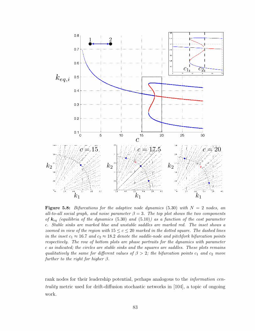
1 2

c

k1 k1 k1

k2 k2 k2

c = 15 c = 17.5 c = 20

c1 c2

keq,i

Figure 5.8: Bifurcations for the adaptive node dynamics (5.30) with N = 2 nodes, anall-to-all social graph, and noise parameter β = 3. The top plot shows the two componentsof keq (equilibria of the dynamics (5.30) and (5.10)) as a function of the cost parameterc. Stable sinks are marked blue and unstable saddles are marked red. The inset shows azoomed in view of the region with 15 ≤ c ≤ 20 marked in the dotted square. The dashed linesin the inset c1 ≈ 16.7 and c2 ≈ 18.2 denote the saddle-node and pitchfork bifurcation pointsrespectively. The row of bottom plots are phase portraits for the dynamics with parameterc as indicated; the circles are stable sinks and the squares are saddles. These plots remainsqualitatively the same for different values of β > 2; the bifurcation points c1 and c2 movefurther to the right for higher β.

rank nodes for their leadership potential, perhaps analogous to the information cen-

trality metric used for drift-diffusion stochastic networks in [104], a topic of ongoing

work.

83

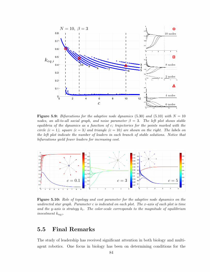
keq,i

c

10 nodes

8 nodes

2 nodes

4 nodes

6 nodes

10 98 7 6

345

N = 10, ! = 3

Figure 5.9: Bifurcations for the adaptive node dynamics (5.30) and (5.10) with N = 10nodes, an all-to-all social graph, and noise parameter β = 3. The left plot shows stableequilibria of the dynamics as a function of c; trajectories for the points marked with thecircle (c = 1), square (c = 3) and triangle (c = 10) are shown on the right. The labels onthe left plot indicate the number of leaders in each branch of stable solutions. Notice thatbifurcations yield fewer leaders for increasing cost.

c = 3 c = 5c = 0.1

Figure 5.10: Role of topology and cost parameter for the adaptive node dynamics on theundirected star graph. Parameter c is indicated on each plot. The x-axis of each plot is timeand the y-axis is strategy ki. The color-scale corresponds to the magnitude of equilibriuminvestment keq,i.

5.5 Final Remarks

The study of leadership has received significant attention in both biology and multi-

agent robotics. One focus in biology has been on determining conditions for the

84

Figure 5.11: Role of topology in determining locations of leaders on the social graph.Parameters for all three plots are β = 3 and c = 4. The colors of nodes on each plotcorrespond to equilibrium investments ki for the dynamics (5.30) and (5.10) with magnitudesindicated in the color-bar. The left graph is an undirected star with N = 10 nodes. Thetwo right plots show a random spatial embedding of nodes with two different interconnectionmodels. In the middle plot, each node is connected to its three nearest neighbors (topologicalmetric) and in the right-most plot, each node is connected to all neighbors within a fixedradius given by the dashed line drawn (distance metric).

stable evolution of leadership behavior in collective systems, since followers in such

systems have good performance at a lower cost. In networked robotic systems, the

leader-follower paradigm has been studied in a variety of contexts as a tool to design

control protocols that achieve desired performance. In this work we focus on the role

that the social graph connectivity plays in a networked model of collective migration.

We use tools from adaptive dynamics to study the all-to-all limit of the evolutionary

model and derive bounds for branching of the population into leader and follower

groups. For limited connectivity, we prove necessary and sufficient conditions for

convergence of the noise-free migration model, and show that fitness of individuals in

the stochastic model can be derived analytically using the Lyapunov equation. For

random networks and lattices, we show a minimum connectivity bound that yields

evolutionary branching in the population. In the final section, we study smaller

networks inspired by collective robotic systems, and show that the network topology

plays a critical role in determining the location of leaders in the adaptive system.

Our goal here was not to design the best system for a given task, as is often

the case in the leader-follower work, but rather to understand the role of networked

topology in the emergence of leadership. One interesting avenue for future work is

to understand where the top-down engineering design approach meets the bottom-up

adaptive approach taken in this chapter. This understanding will aid in the design of

85

collective systems that are near optimal, and also robust to failures such as lost nodes

or links. For the evolutionary model, further work involves analytically deriving the

minimal connectivity threshold for branching, and generalizing to study arbitrary

social graphs, beyond the lattice and random networks studied here.

86

Chapter 6

Coevolutionary Dynamics of

Pursuit and Evasion

Pursuit and evasion behaviors are widely observed in nature and play a critical role

in predator foraging, prey survival, mating, and territorial battles in several species.

Species such as bats and dragonflies have evolved sophisticated dynamical strategies

such as motion camouflage to disguise themselves as stationary during aerial pursuit

[77, 27]. Studies on migratory cannibalistic locusts have revealed that pursuit and

evasive behavior among conspecifics is integral to the formation of mass-moving mi-

gratory bands in dense swarms [35, 5]. Recent experimental work on the dynamics of

coordinated predator pursuit and prey evasion among schooling fish has shown that

collective behavior, among both predators and prey, plays a vital role in predator

hunting and prey evasion under conditions of considerable informational constraints

(such as dynamic ocean environments) [37, 45].

Pursuit-evasion contests have been studied extensively from a game-theoretic per-

spective as differential games [46]. Unlike classical (matrix-based) games, the dy-

namics of players in differential games are modeled using differential equations, with

payoffs corresponding to particular states of the system, or to system trajectories.

In engineering, pursuit and evasion games have received much attention, particularly

in the context of missile guidance and avoidance [101, 51] and aircraft pursuit and

evasion [108, 81]. The book by Nahin [80] provides a review of the topic along with

relevant historical background.

The pervasiveness of pursuit and evasion in nature motivates the examination of

winning strategies from an evolutionary perspective. Here one can think of a strategy

as a control law that a particular pursuer (evader) employs to capture (escape). Cor-

relates of evolutionary fitness, such as time-to-capture, provide natural metrics that

87

connect the dynamics of individual pursuer-evader pairs to evolutionary dynamics of

populations comprising individuals playing different strategies. ESSes of the pursuit-

evasion game point to strategies or behaviors one would expect to observe in nature.

Recently, Wei et al. [147] used the evolutionary approach to study pursuit games with

dynamics derived in [50]. The authors of [147, 50] use Monte-Carlo simulations and

analytical calculations to study three pursuit strategies competing against a field of

deterministic or random nonreactive evasive strategies (an evader with a nonreactive

strategy has dynamics that are uncoupled from those of the pursuer). The three

chosen pursuit strategies (classical, constant bearing and motion camouflage) are bi-

ologically inspired. The authors show convergence of the evolutionary game dynamics

between the three strategies to pure motion camouflage and motivate this result by

empirical observations of motion camouflage in hoverflies, dragonflies and bats [27].

In this chapter, we build on the work in [147] by studying the coevolution of the

three strategies of pursuit from [147] playing against three distinct evasive strategies,

two of which are reactive strategies (an evader with a reactive strategy has dynamics

that are coupled to those of the pursuer). In contrast to the analysis in Chapters 3,

4 and 5, which involve the evolutionary dynamics of a single population, the analysis

in this chapter involves the interaction between two distinct populations (pursuers

and evaders). This will require us to look at an extension of the standard replicator

equations to a double simplex phase space.

We use Monte-Carlo simulations and theoretical analysis to show convergence to

an equilibrium of classical pursuit versus classical evasion. We point out that extend-

ing the ‘games against nature’ approach [147] (evolution of pursuers with respect to

nonreactive evaders) to competitions between two sets of strategies does not result

in a motion camouflage as the winning pursuit strategy, as in [147]. Indeed, the

environment of evasive strategies that a pursuer population encounters is critical to

determining the winning pursuit strategy. It is anticipated that analysis of strat-

egy spaces different again from those studied in the present chapter will yield other

interesting evolutionary outcomes.

We explore the winning strategies (classical pursuit and classical evasion) in a

collective motion model with agents pursuing and evading designated neighbors on

a cyclical interaction topology. This exploration is motivated by collective motion

in cannibalistic locusts [5] and has strong parallels to prior work in cyclic pursuit

[23, 67, 69, 68]. Simulation results suggest a rich set of solutions for this collective

motion model.

88

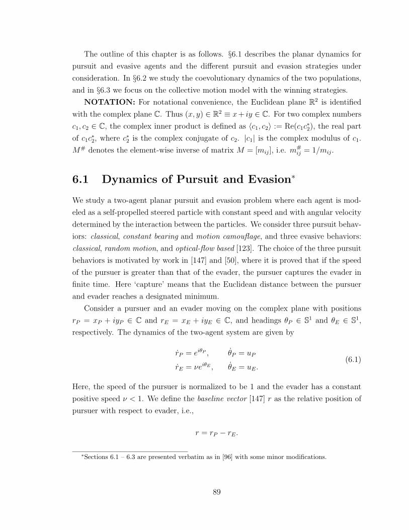
The outline of this chapter is as follows. §6.1 describes the planar dynamics for

pursuit and evasive agents and the different pursuit and evasion strategies under

consideration. In §6.2 we study the coevolutionary dynamics of the two populations,

and in §6.3 we focus on the collective motion model with the winning strategies.

NOTATION: For notational convenience, the Euclidean plane R2 is identified

with the complex plane C. Thus (x, y) ∈ R2 ≡ x+ iy ∈ C. For two complex numbers

c1, c2 ∈ C, the complex inner product is defined as 〈c1, c2〉 := Re(c1c∗2), the real part

of c1c∗2, where c∗2 is the complex conjugate of c2. |c1| is the complex modulus of c1.

M# denotes the element-wise inverse of matrix M = [mij], i.e. m#ij = 1/mij.

6.1 Dynamics of Pursuit and Evasion∗

We study a two-agent planar pursuit and evasion problem where each agent is mod-

eled as a self-propelled steered particle with constant speed and with angular velocity

determined by the interaction between the particles. We consider three pursuit behav-

iors: classical, constant bearing and motion camouflage, and three evasive behaviors:

classical, random motion, and optical-flow based [123]. The choice of the three pursuit

behaviors is motivated by work in [147] and [50], where it is proved that if the speed

of the pursuer is greater than that of the evader, the pursuer captures the evader in

finite time. Here ‘capture’ means that the Euclidean distance between the pursuer

and evader reaches a designated minimum.

Consider a pursuer and an evader moving on the complex plane with positions

rP = xP + iyP ∈ C and rE = xE + iyE ∈ C, and headings θP ∈ S1 and θE ∈ S1,

respectively. The dynamics of the two-agent system are given by

rP = eiθP , θP = uP

rE = νeiθE , θE = uE.(6.1)

Here, the speed of the pursuer is normalized to be 1 and the evader has a constant

positive speed ν < 1. We define the baseline vector [147] r as the relative position of

pursuer with respect to evader, i.e.,

r = rP − rE.

∗Sections 6.1 – 6.3 are presented verbatim as in [96] with some minor modifications.

89

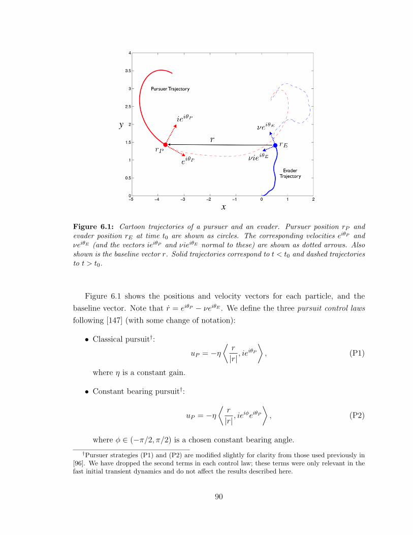
Figure 6.1: Cartoon trajectories of a pursuer and an evader. Pursuer position rP andevader position rE at time t0 are shown as circles. The corresponding velocities eiθP andνeiθE (and the vectors ieiθP and νieiθE normal to these) are shown as dotted arrows. Alsoshown is the baseline vector r. Solid trajectories correspond to t < t0 and dashed trajectoriesto t > t0.

Figure 6.1 shows the positions and velocity vectors for each particle, and the

baseline vector. Note that r = eiθP − νeiθE . We define the three pursuit control laws

following [147] (with some change of notation):

• Classical pursuit†:

uP = −η⟨r

|r| , ieiθP

⟩, (P1)

where η is a constant gain.

• Constant bearing pursuit†:

uP = −η⟨r

|r| , ieiφeiθP

⟩, (P2)

where φ ∈ (−π/2, π/2) is a chosen constant bearing angle.

†Pursuer strategies (P1) and (P2) are modified slightly for clarity from those used previously in[96]. We have dropped the second terms in each control law; these terms were only relevant in thefast initial transient dynamics and do not affect the results described here.

90

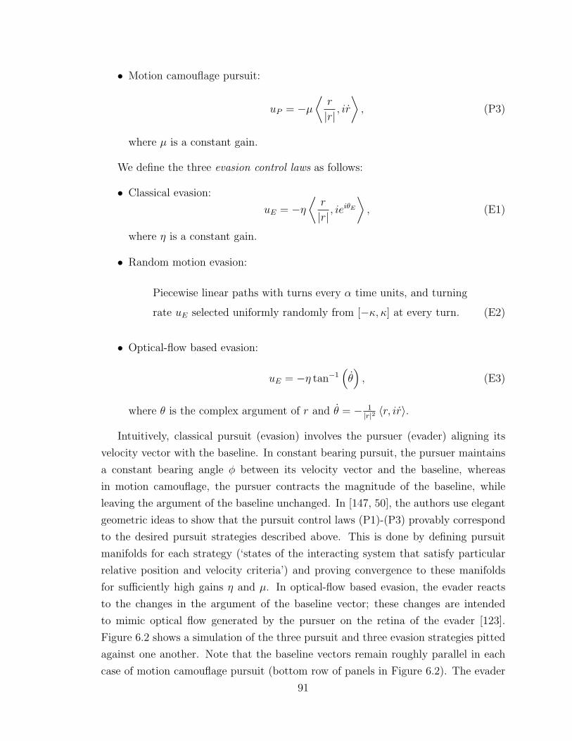
• Motion camouflage pursuit:

uP = −µ⟨r

|r| , ir⟩, (P3)

where µ is a constant gain.

We define the three evasion control laws as follows:

• Classical evasion:

uE = −η⟨r

|r| , ieiθE

⟩, (E1)

where η is a constant gain.

• Random motion evasion:

Piecewise linear paths with turns every α time units, and turning

rate uE selected uniformly randomly from [−κ, κ] at every turn. (E2)

• Optical-flow based evasion:

uE = −η tan−1(θ), (E3)

where θ is the complex argument of r and θ = − 1|r|2 〈r, ir〉.

Intuitively, classical pursuit (evasion) involves the pursuer (evader) aligning its

velocity vector with the baseline. In constant bearing pursuit, the pursuer maintains

a constant bearing angle φ between its velocity vector and the baseline, whereas

in motion camouflage, the pursuer contracts the magnitude of the baseline, while

leaving the argument of the baseline unchanged. In [147, 50], the authors use elegant

geometric ideas to show that the pursuit control laws (P1)-(P3) provably correspond

to the desired pursuit strategies described above. This is done by defining pursuit

manifolds for each strategy (‘states of the interacting system that satisfy particular

relative position and velocity criteria’) and proving convergence to these manifolds

for sufficiently high gains η and µ. In optical-flow based evasion, the evader reacts

to the changes in the argument of the baseline vector; these changes are intended

to mimic optical flow generated by the pursuer on the retina of the evader [123].

Figure 6.2 shows a simulation of the three pursuit and three evasion strategies pitted

against one another. Note that the baseline vectors remain roughly parallel in each

case of motion camouflage pursuit (bottom row of panels in Figure 6.2). The evader

91

trajectory in optical-flow based evasion is a straight line when competing against a

motion camouflage pursuit strategy.

P

P

PP

P

P P

P

P

E

E

E

E

E

E

E

E

E

(P1)

(P2)

(P3)

(E3)(E2)(E1)

Figure 6.2: Simulated trajectories of each of the nine pairs of competing pursuit and eva-sive strategies. The rows correspond to pursuit control laws (P1), (P2) and (P3) respectivelyand the columns correspond to evasive control laws (E1), (E2) and (E3) respectively. Forexample, the plot in the middle corresponds to constant bearing pursuit versus random mo-tion evasion. The starting positions are indicated with ‘P’ and ‘E’. In all plots the evader(E) starts at the origin with θE(0) = 0. The pursuers (P) in columns 1 and 3 start atrP (0) = 5 + 3i with a heading θP (0) = π. In the second column the pursuers start at ran-dom positions and with random headings. The straight lines in each plot are snapshots ofthe baseline vector at specific points in time.

For all control laws uP and uE defined above, Lemma 6.1 ensures that capture is

always possible in finite time.

Lemma 6.1. Consider dynamics (6.1) and control laws (P1)-(P3) and (E1)-(E3).

For every capture radius ε > 0 and every initial condition rP (0), rE(0) such that

|r(0)| = |rP (0)− rE(0)| > ε, there exists a finite capture time T such that |r(T )| = ε.

92

Proof. Refer to [147, 50] for proof. Note that the evasive controls (E1)-(E3) satisfy

the continuity and boundedness assumptions of Proposition 3.3 in [147].

The central question we ask in this chapter is which strategies win out in a co-

evolutionary contest between the three proposed pursuit strategies and the three

proposed evasive strategies? In [147] the authors studied the evolutionary dynamics

of the three pursuit strategies (P1)-(P3) playing against an environment of nonreac-

tive deterministic or random evasive strategies such as (E2). In the following section

we consider an evolutionary scenario in which the pursuit strategies coevolve with

reactive evasive strategies (E1) and (E3) as well.

6.2 Evolutionary Dynamics

To model the evolutionary dynamics of pursuer-evader interactions, fitnesses are de-

termined by the cumulative effect of several one-on-one contests between pursuers and

evaders such that a long time-to-capture for a particular contest corresponds to a high

evader fitness and a low pursuer fitness. Consider a pursuer population represented

by the population vector p =[p1 p2 p3

]T. Here pi, i ∈ {1, 2, 3}, corresponds to

the fraction of individuals in the population playing strategy (Pi). Hence the vector

p is restricted to the simplex ∆2. Similarly, the evader population is represented by

the population vector q =[q1 q2 q3

]Twhich is also restricted to ∆2. The fitness

vectors for the pursuer and evader populations are denoted by fP ∈ R3+ and fE ∈ R3

+

respectively, where fPi is the fitness of pursuit strategy (Pi) and fEj is the fitness of

evasive strategy (Ej) . Define population mean fitness by fP = pTfP and fE = qTfE.

We can now write down a discrete update equation for each population that

depends on the relative fitnesses of the different strategies in that population. For

transition from generation g to generation g+1, we have for i = 1, 2, 3 and j = 1, 2, 3:

pi(g + 1) = pi(g)fPi

fP

qj(g + 1) = qj(g)fEj

fE.

(6.2)

One can verify that the equations (6.2) ensure that each population vector remains

in the simplex ∆2. Intuitively, strategies with fitness greater than the population

mean fitness are favored. Given an expression for the fitness vectors, we can study

the outcomes of the dynamics (6.2). As in [147] we use time-to-capture as a measure

93

of fitness. The fitness of the set of pursuer strategies fP depends on the distribution

of evaders in the population q and fE depends on the distribution of pursuers in the

population p. This implies that the equations (6.2) are coupled. We simulate the

evolutionary dynamics (6.2) using Monte-Carlo calculations that determine fitnesses.

We then perform a theoretical analysis.

6.2.1 Monte-Carlo Simulations

We follow the setup in [147] for our Monte-Carlo experiments. The important step

is the construction of the capture time matrix T ∈ R3×3 such that tij > 0 represents

the time-to-capture for pursuit strategy (Pi) competing against evasive strategy (Ej).

Lemma 6.1 gives us that all elements of T are positive and finite. To construct T , we

perform nine simulations, one for each element of T , such that each simulation has a

pursuer and an evader starting from the same initial conditions. In each simulation

the evader starts at the origin with a heading of zero. The pursuer’s initial position is

chosen from a uniform distribution on the square [−10, 10]× [−10, 10], and its initial

heading from a uniform distribution on S1. The other parameters are the same for

each simulation: η = µ = 10, ν = .6, ε = 0.05, φ = 0.3, α = 0.2, and κ = 2.

The results presented here remain qualitatively consistent for reasonable variations of

these parameters. A detailed study of the effect of each parameter on capture times

is a direction of future work.

For each generation, we compute ten time matrices T k =[tkij], k ∈ {1, . . . , 10},

such that each matrix corresponds to a different choice of pursuer initial conditions

and evader random trajectory for column 2 (note that T k denotes the kth time matrix,

not to be confused with matrix multiplication). The average matrix T =[tij]

is

defined by tij =1

10

10∑k=1

tkij. Let T (g) denote the average time matrix computed at

generation g. For matrices M(g) = T#

(g) and N(g) = TT

(g), the fitness vectors are

defined by

fP (g) = M(g)q(g)

fE(g) = N(g)p(g).(6.3)

The inverse and direct relationships between the time matrix and fitness for pursuers

and evaders, respectively, ensure that high capture times have asymmetric fitness

consequences for pursuers and evaders. Fitnesses (6.3) also encode the frequency

dependence and coupling of the evolutionary dynamics (6.2) since the fitness of a

94

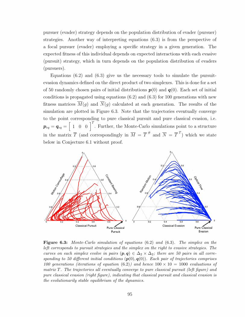
pursuer (evader) strategy depends on the population distribution of evader (pursuer)

strategies. Another way of interpreting equations (6.3) is from the perspective of

a focal pursuer (evader) employing a specific strategy in a given generation. The

expected fitness of this individual depends on expected interactions with each evasive

(pursuit) strategy, which in turn depends on the population distribution of evaders

(pursuers).

Equations (6.2) and (6.3) give us the necessary tools to simulate the pursuit-

evasion dynamics defined on the direct product of two simplexes. This is done for a set

of 50 randomly chosen pairs of initial distributions p(0) and q(0). Each set of initial

conditions is propagated using equations (6.2) and (6.3) for 100 generations with new

fitness matrices M(g) and N(g) calculated at each generation. The results of the

simulation are plotted in Figure 6.3. Note that the trajectories eventually converge

to the point corresponding to pure classical pursuit and pure classical evasion, i.e.

peq = qeq =[

1 0 0]T

. Further, the Monte-Carlo simulations point to a structure

in the matrix T (and correspondingly in M = T#

and N = TT

) which we state

below in Conjecture 6.1 without proof.

Motio

n C

am

oufla

ge

Classical Pursuit

Consta

nt B

earin

g Random

Motio

n

Classical Evasion

Rela

tive H

eadin

g C

hange

Optical Flow

Figure 6.3: Monte-Carlo simulation of equations (6.2) and (6.3). The simplex on theleft corresponds to pursuit strategies and the simplex on the right to evasive strategies. Thecurves on each simplex evolve in pairs (p, q) ∈ ∆2 × ∆2; there are 50 pairs in all corre-sponding to 50 different initial conditions (p(0), q(0)). Each pair of trajectories comprises100 generations (iterations of equation (6.2)) and hence 100 × 10 = 1000 evaluations ofmatrix T . The trajectories all eventually converge to pure classical pursuit (left figure) andpure classical evasion (right figure), indicating that classical pursuit and classical evasion isthe evolutionarily stable equilibrium of the dynamics.

95

Conjecture 6.1. The first column of matrix T is dominant, i.e. ti1 > ti2 and ti1 > ti3

for all i. Further, in the first column t11 < t21 and t11 < t31.

The claim in Conjecture 6.1 is made as a consequence of Monte-Carlo computa-

tions of matrix T and consistent observations of the proposed matrix structure. A

rigorous proof of Conjecture 6.1 requires careful analytical computations of capture

times for the different strategies, a topic for future work. The structure of Conjec-

ture 6.1 provides a useful tool for analyzing the evolutionary dynamics on the direct

product of two simplexes and for proving convergence properties. We investigate this

in the following subsection.

6.2.2 Theoretical Analysis

For some small time step ∆t > 0, we can rewrite the equations (6.2) as follows:

1

∆t(pi(g + 1)− pi(g)) = pi(g)

fPi − fP∆t fP

1

∆t(qj(g + 1)− qj(g)) = qj(g)

fEj − fE∆t fE

.

In the limit ∆t→ 0 and with a change of timescale, we arrive at the set of differential

equations

pi =pi

fP

(fPi − fP

)qj =

qj

fE

(fEj − fE

).

(6.4)

Consider a constant matrix T that obeys the structure of Conjecture 6.1. Further let

M = T# and N = T T . Defining fitness vectors fP = Mq and fE = Np analogous

to equation (6.3), and substituting into (6.4) we get

pi =pi

pTMq

((Mq)i − pTMq

)qj =

qjqTNp

((Np)j − qTNp

).

(6.5)

Equations (6.5) are a form of the replicator dynamics (see Chapter 2) for two interact-

ing populations with fitnesses defined by linear functions of the population distribu-

tions. Critical to arriving at equations (6.5) is the assumption that T is constant and

thus M and N are constant, which is justified by a ‘law of large numbers’ argument

96

[147]. Further, the assumption makes the analysis of equations (6.5) tractable, and

hence allows us to formally investigate the convergence shown in the Monte-Carlo

experiments.

The system of equations (6.5) is a four-dimensional system evolving on ∆2 ×∆2.

There are several possible solutions of the dynamics on these simplexes. For instance,

all vertex pairs (pairs of pure strategies) are fixed points. Further, a strategy that is

initially absent does not emerge, i.e., pi(0) = 0 =⇒ pi(t) = 0, ∀t, and the same holds

for qj (replicator dynamics are said to be non-innovative as they lack mutation). In

order to investigate the coupled replicator dynamical system (6.5), we first study the

simpler single population replicator dynamics given by

qi =qiqTf

(fi − qTf

), for i = 1, 2, 3. (6.6)

The fitness functions for the system of equations (6.6) are assumed to satisfy the

following properties:

• Property 1: fi ≡ fi(t), i = 1, 2, 3, are each distinct functions of time, i.e.,

fi 6= fj pointwise. If this were not the case then populations i and j would be

indistinguishable from the perspective of evolutionary dynamics.

• Property 2: The functions fi(t) are each globally Lipschitz, bounded and posi-

tive for all t ≥ 0.

• Property 3: The functions fi(t) have a single dominant fitness; without loss of

generality, f3(t) > f2(t) and f3(t) > f1(t) for all t ≥ 0.

Lemma 6.2. Assume initial conditions are restricted to the domain D =

{q ∈ ∆2|q3 > 0}. The dynamics (6.6), satisfying Properties 1-3, have a unique

asymptotically stable equilibrium point qeq =[

0 0 1]T

attracting all initial

conditions in D.

Proof. The proof is in Appendix E.1.

The case of Lemma 6.2 with each fi constant is considered in [147]. We now return

to the coupled set of equations (6.5) and state the main theorem of this section. Here

we employ the dominant structure of matrix T , assuming that Conjecture 6.1 holds,

to prove convergence.

Theorem 6.1. Assume initial conditions are restricted to the domain D2 =

{(p, q) ∈ ∆2 ×∆2|p1 > 0, q1 > 0}. Let matrix T satisfy Conjecture 6.1 with M = T#

97

and N = T T . Then, the coupled replicator dynamics (6.5) have a unique asymp-

totically stable equilibrium point peq = qeq =[

1 0 0]T

attracting all initial

conditions in D2.

Proof. The invariance of the domain D2 with respect to the dynamics (6.5) follows

from the invariance of the domain D in the proof of Lemma 6.2. The column dominant

structure of matrix T implies that the first element of the fitness vector fE = Np =

T Tp is dominant. That is, regardless of the population distribution p at any time

instant, fE1 > fE2 and fE1 > fE3. Hence we can use Lemma 6.2 to conclude that

regardless of the evolution of the population vector p, the population vector q will

asymptotically converge to qeq =[

1 0 0]T

.

Asymptotic stability implies that for every ε > 0 there exists a time t1 ≥ 0 such

that t > t1 =⇒ ‖q − qeq‖ < ε. From the calculations in Lemma E.1 in Appendix E,

‖q − qeq‖ < ε =⇒ fP1 > fP2 and fP1 > fP3 for

ε = min

{2(m11 −m21)

(m11 −m21) + ‖M‖1

,2(m11 −m31)

(m11 −m31) + ‖M‖1

}.

Hence we can apply Lemma 6.2 again to the dynamics of p to conclude that after time

t1, the population vector p will also asymptotically converge to peq =[

1 0 0]T

.

In Figure 6.4 we simulate the dynamics in equations (6.5), for a particular cal-

culation of matrix T , showing smooth convergence to the unique stable equilibrium.

This can be compared to the Monte-Carlo simulations of Figure 6.3. From a game-

theoretic perspective, the stable equilibrium point corresponds to the single unique

pure Nash equilibrium of the bi-matrix game, for payoff matrices M and N .

In this section we have performed a computational and theoretical analysis of

the evolutionary dynamics corresponding to the competition between a population of

pursuers and a population of evaders, each having three strategies. We have shown

convergence to a unique stable pure-strategy equilibrium corresponding to classical

pursuit and classical evasion. This differs from the solution in [147], where the au-

thors study the three pursuit strategies as a ‘game against nature’, each competing

independently against nonreactive evasive strategies. There the evolutionary dynam-

ics converge to the motion camouflage pursuit strategy. The competition of pursuers

with a reactive set of evaders introduces a rich set of possibilities for evolutionary

outcomes. Indeed, by comparison to the results of [147], we see that making avail-

able alternative evader strategies affects the evolved strategies for both pursuers and

98

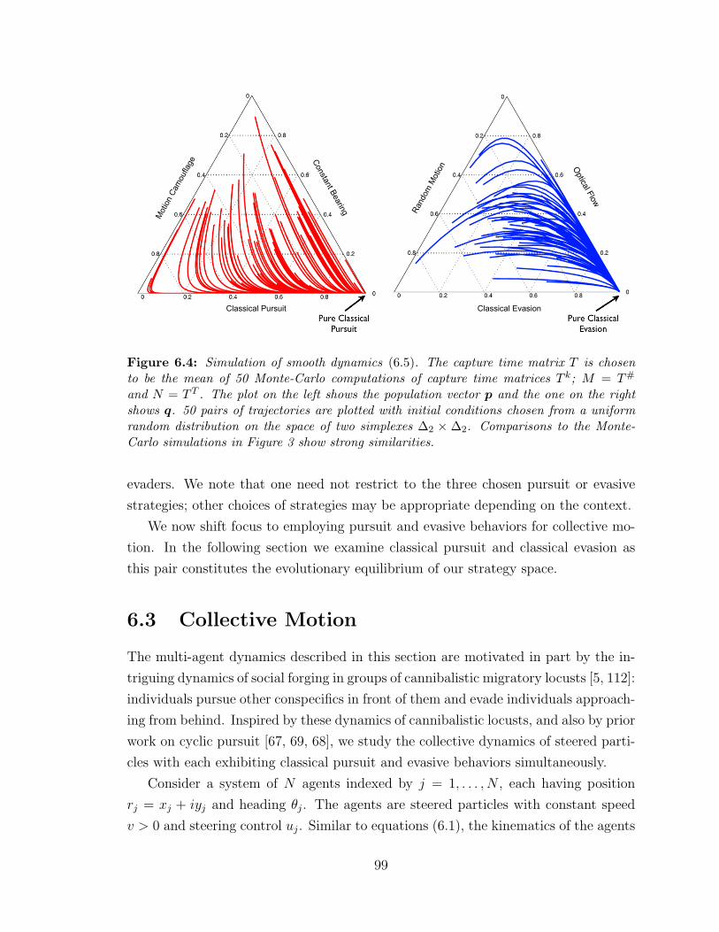
Motio

n C

am

oufla

ge

Classical Pursuit

Consta

nt B

earin

g Random

Motio

n

Classical Evasion

Rela

tive H

eadin

g C

hange

Optical Flow

Figure 6.4: Simulation of smooth dynamics (6.5). The capture time matrix T is chosento be the mean of 50 Monte-Carlo computations of capture time matrices T k; M = T#

and N = T T . The plot on the left shows the population vector p and the one on the rightshows q. 50 pairs of trajectories are plotted with initial conditions chosen from a uniformrandom distribution on the space of two simplexes ∆2 × ∆2. Comparisons to the Monte-Carlo simulations in Figure 3 show strong similarities.

evaders. We note that one need not restrict to the three chosen pursuit or evasive

strategies; other choices of strategies may be appropriate depending on the context.

We now shift focus to employing pursuit and evasive behaviors for collective mo-

tion. In the following section we examine classical pursuit and classical evasion as

this pair constitutes the evolutionary equilibrium of our strategy space.

6.3 Collective Motion

The multi-agent dynamics described in this section are motivated in part by the in-

triguing dynamics of social forging in groups of cannibalistic migratory locusts [5, 112]:

individuals pursue other conspecifics in front of them and evade individuals approach-

ing from behind. Inspired by these dynamics of cannibalistic locusts, and also by prior

work on cyclic pursuit [67, 69, 68], we study the collective dynamics of steered parti-

cles with each exhibiting classical pursuit and evasive behaviors simultaneously.

Consider a system of N agents indexed by j = 1, . . . , N , each having position

rj = xj + iyj and heading θj. The agents are steered particles with constant speed

v > 0 and steering control uj. Similar to equations (6.1), the kinematics of the agents

99

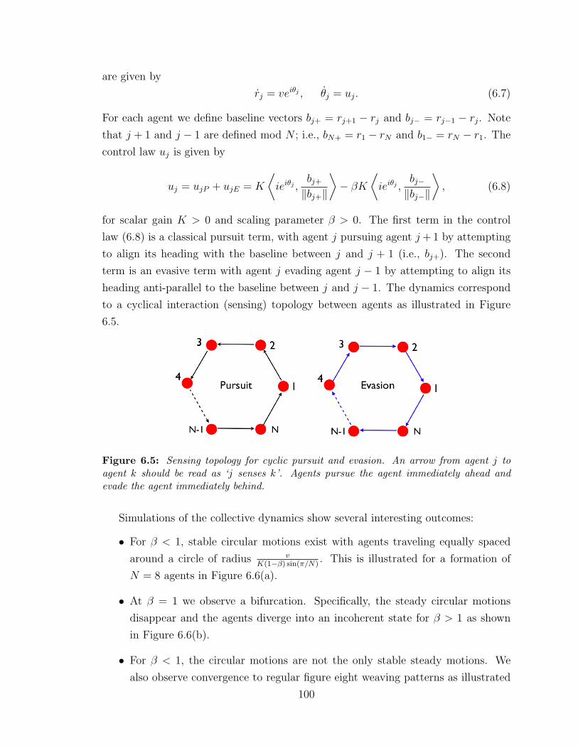
are given by

rj = veiθj , θj = uj. (6.7)

For each agent we define baseline vectors bj+ = rj+1 − rj and bj− = rj−1 − rj. Note

that j + 1 and j − 1 are defined mod N ; i.e., bN+ = r1 − rN and b1− = rN − r1. The

control law uj is given by

uj = ujP + ujE = K

⟨ieiθj ,

bj+‖bj+‖

⟩− βK

⟨ieiθj ,

bj−‖bj−‖

⟩, (6.8)

for scalar gain K > 0 and scaling parameter β > 0. The first term in the control

law (6.8) is a classical pursuit term, with agent j pursuing agent j + 1 by attempting

to align its heading with the baseline between j and j + 1 (i.e., bj+). The second

term is an evasive term with agent j evading agent j − 1 by attempting to align its

heading anti-parallel to the baseline between j and j − 1. The dynamics correspond

to a cyclical interaction (sensing) topology between agents as illustrated in Figure

6.5.

Figure 6.5: Sensing topology for cyclic pursuit and evasion. An arrow from agent j toagent k should be read as ‘j senses k’. Agents pursue the agent immediately ahead andevade the agent immediately behind.

Simulations of the collective dynamics show several interesting outcomes:

• For β < 1, stable circular motions exist with agents traveling equally spaced

around a circle of radius vK(1−β) sin(π/N)

. This is illustrated for a formation of

N = 8 agents in Figure 6.6(a).

• At β = 1 we observe a bifurcation. Specifically, the steady circular motions

disappear and the agents diverge into an incoherent state for β > 1 as shown

in Figure 6.6(b).

• For β < 1, the circular motions are not the only stable steady motions. We

also observe convergence to regular figure eight weaving patterns as illustrated

100

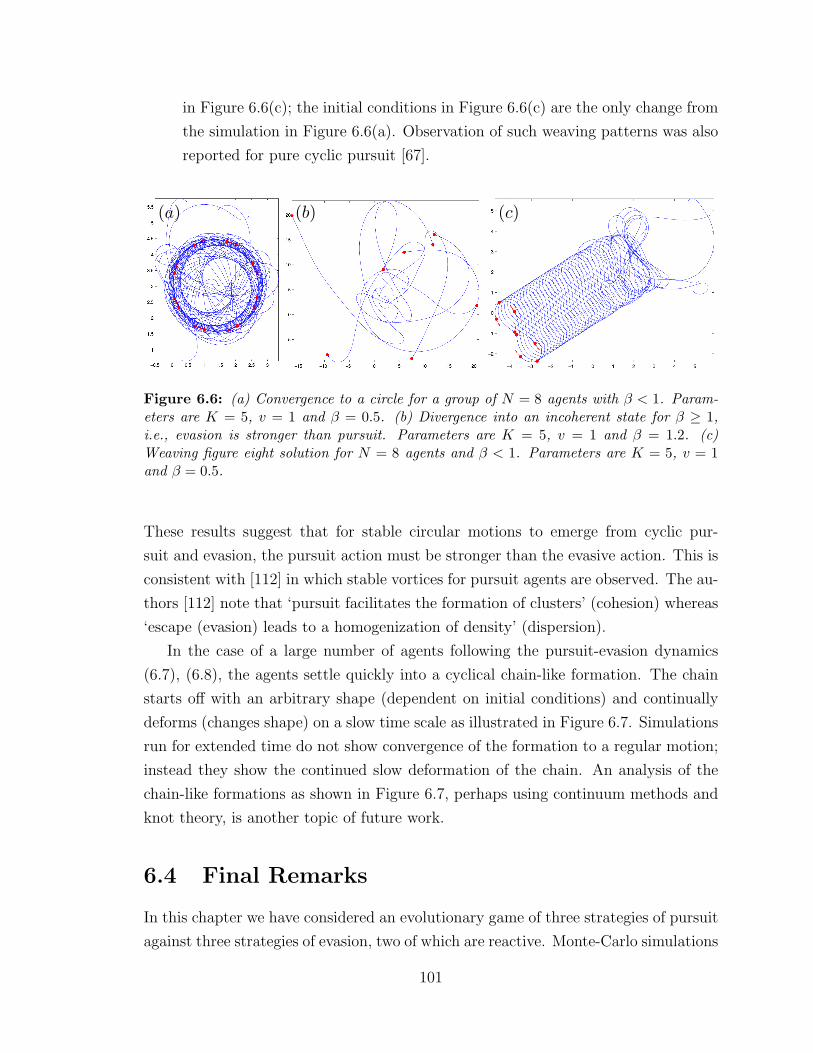
in Figure 6.6(c); the initial conditions in Figure 6.6(c) are the only change from

the simulation in Figure 6.6(a). Observation of such weaving patterns was also

reported for pure cyclic pursuit [67].

(a) (b) (c)

Figure 6.6: (a) Convergence to a circle for a group of N = 8 agents with β < 1. Param-eters are K = 5, v = 1 and β = 0.5. (b) Divergence into an incoherent state for β ≥ 1,i.e., evasion is stronger than pursuit. Parameters are K = 5, v = 1 and β = 1.2. (c)Weaving figure eight solution for N = 8 agents and β < 1. Parameters are K = 5, v = 1and β = 0.5.

These results suggest that for stable circular motions to emerge from cyclic pur-

suit and evasion, the pursuit action must be stronger than the evasive action. This is

consistent with [112] in which stable vortices for pursuit agents are observed. The au-

thors [112] note that ‘pursuit facilitates the formation of clusters’ (cohesion) whereas

‘escape (evasion) leads to a homogenization of density’ (dispersion).

In the case of a large number of agents following the pursuit-evasion dynamics

(6.7), (6.8), the agents settle quickly into a cyclical chain-like formation. The chain

starts off with an arbitrary shape (dependent on initial conditions) and continually

deforms (changes shape) on a slow time scale as illustrated in Figure 6.7. Simulations

run for extended time do not show convergence of the formation to a regular motion;

instead they show the continued slow deformation of the chain. An analysis of the

chain-like formations as shown in Figure 6.7, perhaps using continuum methods and

knot theory, is another topic of future work.

6.4 Final Remarks

In this chapter we have considered an evolutionary game of three strategies of pursuit

against three strategies of evasion, two of which are reactive. Monte-Carlo simulations

101

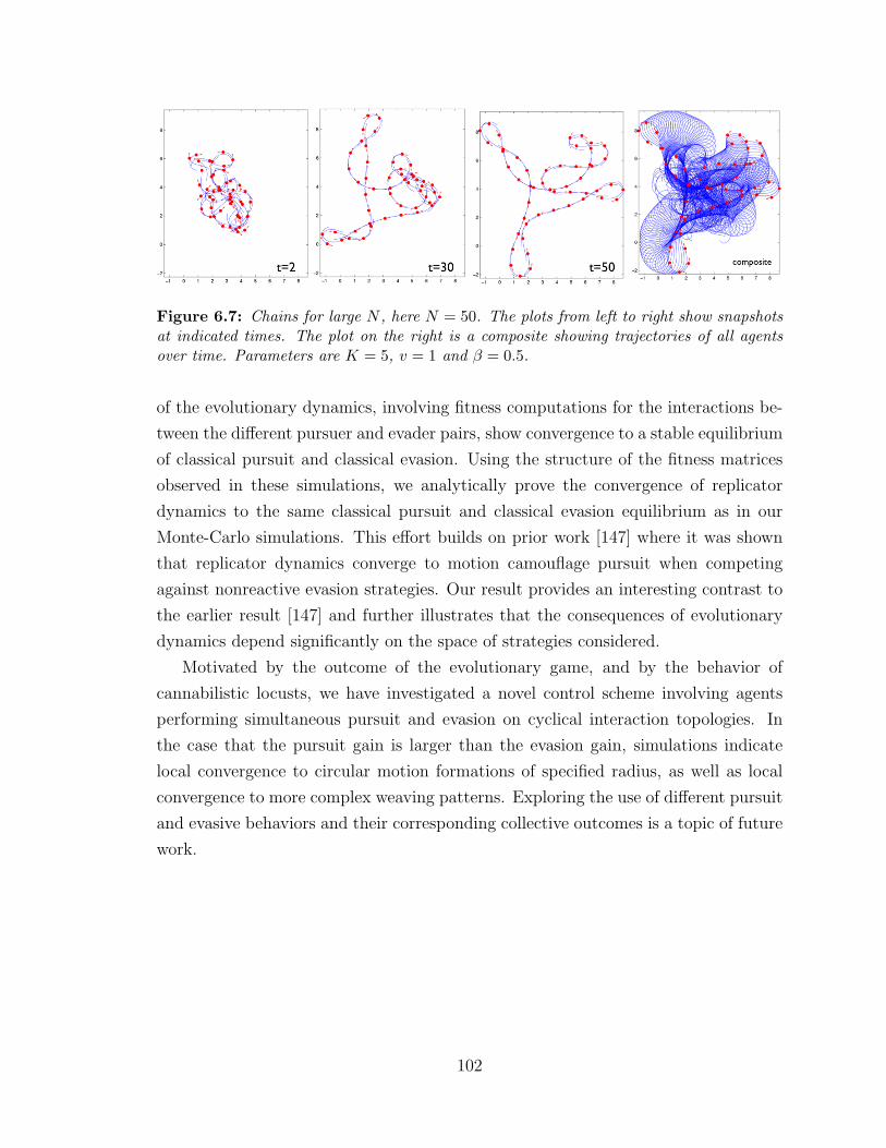
Figure 6.7: Chains for large N , here N = 50. The plots from left to right show snapshotsat indicated times. The plot on the right is a composite showing trajectories of all agentsover time. Parameters are K = 5, v = 1 and β = 0.5.

of the evolutionary dynamics, involving fitness computations for the interactions be-

tween the different pursuer and evader pairs, show convergence to a stable equilibrium

of classical pursuit and classical evasion. Using the structure of the fitness matrices

observed in these simulations, we analytically prove the convergence of replicator

dynamics to the same classical pursuit and classical evasion equilibrium as in our

Monte-Carlo simulations. This effort builds on prior work [147] where it was shown

that replicator dynamics converge to motion camouflage pursuit when competing

against nonreactive evasion strategies. Our result provides an interesting contrast to

the earlier result [147] and further illustrates that the consequences of evolutionary

dynamics depend significantly on the space of strategies considered.

Motivated by the outcome of the evolutionary game, and by the behavior of

cannabilistic locusts, we have investigated a novel control scheme involving agents

performing simultaneous pursuit and evasion on cyclical interaction topologies. In

the case that the pursuit gain is larger than the evasion gain, simulations indicate

local convergence to circular motion formations of specified radius, as well as local

convergence to more complex weaving patterns. Exploring the use of different pursuit

and evasive behaviors and their corresponding collective outcomes is a topic of future

work.

102

Chapter 7

Decision-Making Dynamics in

Honeybee Swarms

A honeybee colony∗ is a fascinating natural example of an emergent system where an

aggregation of thousands of individuals functions together as a composite integrated

unit. Other examples include the gigantic colonies of leafcutter ants [149], army ants

[13], or fungus growing termites [1, 116]. The colony functions as a truly decentralized

system where local interactions among the bees yield group-level structure and func-

tion, critical to survival. A typical bee colony is composed mostly of (predominantly)

sterile female worker bees, all of whom are daughters of the one fertile queen bee that

lives in their midst [116]. A small set of male drone bees in the colony performs the

fundamental reproductive task of mating with young queen bees from other nearby

colonies. The worker bees perform most of the colony survival tasks including for-

aging, rearing the queen for reproduction, hive construction, and scouting for new

potential nest sites during swarming. The scout bees in the swarm are among the

most experienced, and correspondingly oldest, forager workers [28]. The focus of this

chapter is on the decision-making dynamics of nest site selection among these scout

bees during the colony swarming process. The book by Seeley [116] is an excellent

reference for an in-depth look at all of the other captivating elements of honeybee

colonies, in addition to the swarm decision-making discussed here.

Honeybee colonies reproduce by casting swarms, each of which comprises a queen

accompanied by several thousand worker bees. A small fraction of the worker bees

are known as scout bees and perform the task of locating suitable nest sites for the

∗While we use the term honeybee quite generally, the experimental evidence for the features ofhoneybees and swarms described in this chapter comes from Apis mellifera, the most commonlydomesticated species [116].

103

swarm by engaging in a democratic [116] decision-making process of choosing among

several competing options. This process involves the famous waggle dance [144] in

which scouts advertise the location and quality of suitable nest sites by performing

a distinctive dance on the surface of the swarm (the waggle dance is also used in

foraging to signal flower locations). The collective nest site selection process among

the scouts is known to have several of the typical elements of decentralized decision-

making systems: commitment of individuals to options after sampling, recruitment

of uncommitted individuals by those already subscribed to an option, and decay of

preference affiliation over time (akin to the ‘leaking’ in leaky-accumulator models of

neuronal decision-making [8]). Seeley et al. in a recent paper [118] have shown that

scouts also send inhibitory stop signals to other scouts advertising alternative nest

sites, thereby causing these scouts to cease dancing. This cross-inhibitory process

has been shown to be critical to the ability of swarms to make decisions effectively,

particularly when choosing between competing options of near-equal value.

In this chapter we study bifurcations in an analytical model of honeybee swarm

decision-making from [118] and illustrate the critical role played by stop-signal inhibi-

tion in enabling swarms to manage the speed-accuracy tradeoff in the decision-making

problem. The model from [118] is described in §7.1. §7.2 summarizes the analysis

of the symmetric case of options with equal value from [118] and illustrates a pitch-

fork bifurcation in the dynamics. In §7.3 we present a general description of the

bifurcations of the model for the asymmetric case of options with unequal value, and

illustrate how the pitchfork bifurcation in the symmetric case is one slice through a

more general cusp catastrophe bifurcation set corresponding to the dynamics. In §7.4

we show that the model has two timescales and derive an analytical expression for

the slow manifold of the dynamics. We study a stochastic version of the model in

§7.5 and summarize our findings in §7.6.

7.1 Model Description

We study a mean-field model of the swarm decision-making dynamics derived in [118].

We restrict to looking at the decision-making process of choosing between two options

A and B for analytical tractability. Also, while scouts might advertise several options

(on the order of 10 [116]) early on in the selection activity, only two or three options

usually remain in the more advanced stages. The model has states yA, yB and yU

corresponding to the fraction of scouts subscribed to (i.e., dancing for) option A, the

fraction subscribed to option B, and the fraction uncommitted (U) to either option,

104

respectively. The vector y = [yA yB yU ]T is a simplex vector satisfying yi ≥ 0 for all

i ∈ {A,B, U} and yA + yB + yU = 1. The dynamics have four main processes:

• Commitment: Uncommitted scout bees commit to an option upon indepen-

dently encountering one in the scouting process at rate γi for option i ∈ {A,B}.

• Recruitment: Scout bees committed to a particular option recruit uncommitted

scouts to subscribe to that option (using the waggle dance) at rate ρi for option

i ∈ {A,B}.

• Decay: The number of waggle dance circuits declines over time due to the fading

interest of a committed scout at rate αi for option i ∈ {A,B}. Decay has been

shown to be essential to consensus forming in the decision-making dynamics

[115].

• Stop-signal: By the cross-inhibitory mechanism, scouts subscribed to a partic-

ular option inhibit those subscribed to alternative options at rate σi for option

i ∈ {A,B}. The stop-signal is known to reduce waggle dancing and is typically

delivered as a vibrational signal by the sender butting her head against the

dancer [118].

COMMITMENT

RECRUITMENT

DECAY

STOP-SIGNAL

U!A! A U

!B! B

A + U!A! 2A B + U

!B! 2B

A!A! U B

!B! U

A + B!A! A + U B + A

!B! B + U

yA = !AyU + "AyAyU ! #AyA ! $ByAyB

yB = !ByU + "ByByU ! #ByB ! $AyByA

Figure 7.1: Connections between the microscopic (top) and macroscopic (bottom) descrip-tions of the swarm decision-making dynamics. The set of four categories on the top showthe four processes that are part of the decision-making dynamics (commitment, recruitment,decay, stop-signal), and the microscopic rate equations corresponding to each (for exampleU

γA→ A denotes the transition from U to A at rate γA). The bottom pair of macroscopicmean-field equations (7.1) is color-coded to match each of the four processes.

105

The microscopic rate equations for the four processes described above are shown

in Figure 7.1 (top). The corresponding mean-field equations are given by

dyAdt

= γAyU + ρAyAyU − αAyA − σByAyBdyBdt

= γByU + ρByByU − αByB − σAyByA.(7.1)

These equations have been derived rigorously in [118] as a system-size expansion

[139, 24] of the microscopic master equations [24]. Note that yU = −yA − yB.

The nest sites of swarms are typically tree cavities that provide good protection

from predators and from harsh environmental conditions. Scout bees evaluate poten-

tial nest sites on a variety of metrics including cavity volume, cavity entrance size,

height of the entrance from the ground, and the presence of earlier combs [143]. Fur-

ther, various studies [31, 29, 116] have shown that scout bees have an innate scale of

absolute nest site goodness or value that encapsulates these metrics. We use vi > 0

to denote this absolute value of nest site i ∈ {A,B}. Following the parameterization

used previously in [118], we assume that all of the rates γi, ρi, and αi may depend

on the value vi of the potential nest site with which they are associated. We set the

commitment and recruitment rates γi = vi and ρi = vi, and the decay rates αi = 1vi

.

The parameterization in [118] also assumes that the stop-signal rate σi is independent

of site choice and hence σA = σB = σ. Substituting for these rates in (7.1) we obtain

a pair of quadratic differential equations in three parameters vA, vB, and σ:

dyAdt

= − 1

vAyA + vAyU(1 + yA)− σyAyB

dyBdt

= − 1

vByB + vByU(1 + yB)− σyAyB.

(7.2)

Our analysis of bifurcations and timescale separation in the sections to follow focuses

on this pair of coupled equations.

7.2 Symmetric Case

The symmetric case of equal options vA = vB = v was studied in [118]; we summarize

the results here. Substituting vA = vB = v in (7.2), the symmetric dynamics are

106

given bydyAdt

=−yAv

+ vyU(1 + yA)− σyAyBdyBdt

=−yBv

+ vyU(1 + yB)− σyAyB.(7.3)

The dynamics (7.3) have three sets of equilibria (the fourth equilibrium set is

always outside the simplex ∆2) denoted (yAeq, yBeq) and given by

p1 =

(2v2

1 + v2 +√

1 + 2v2 + 9v4 + 4v3σ,

2v2

1 + v2 +√

1 + 2v2 + 9v4 + 4v3σ

)p2 =

(1

2− 1

2v2+

1

2v2

√(v2 − 1)2 − 4v3

σ,1

2− 1

2v2− 1

2v2

√(v2 − 1)2 − 4v3

σ

)(7.4)

p3 =

(1

2− 1

2v2− 1

2v2

√(v2 − 1)2 − 4v3

σ,1

2− 1

2v2+

1

2v2

√(v2 − 1)2 − 4v3

σ

).

These equilibria correspond to a pitchfork bifurcation in the dynamics with a bifur-

cation set (parameterized by v):

σ∗ =4v3

(v2 − 1)2. (7.5)

For σ < σ∗, the equilibria p2 and p3 from (7.4) are imaginary and p1 is stable. A

pitchfork bifurcation occurs at σ = σ∗ resulting in two stable equilibria p2 and p3 and

one unstable equilibrium p1 for σ > σ∗, as illustrated in Figure 7.2 (see also Case 1

in Figure 7.4).

The pitchfork bifurcation describes an important feature of the stop-signal based

cross-inhibition on the decision dynamics. For values of stop-signal below the thresh-

old σ∗, the only stable equilibrium of the dynamics is the symmetric (yA = yB)

equilibrium resulting in a deadlock in the decision-making process with equal frac-

tions of the population subscribed to each option. This situation is suboptimal from

a speed-accuracy perspective since the time spent in deadlock between equal options

does not yield any greater accuracy in decision-making. Ideally, we would like for

the system to be able to spontaneously ‘flip a coin’ between the equal alternatives in

order to make a fast decision. This is exactly what is enabled by the cross-inhibitory

mechanism. Post bifurcation (σ > σ∗), the two stable equilibria correspond to a

choice of one of the two alternatives, and the system dynamics are attracted to one

or the other based on initial conditions, thereby breaking deadlock (see inset phase

portraits in Figure 7.3).

107

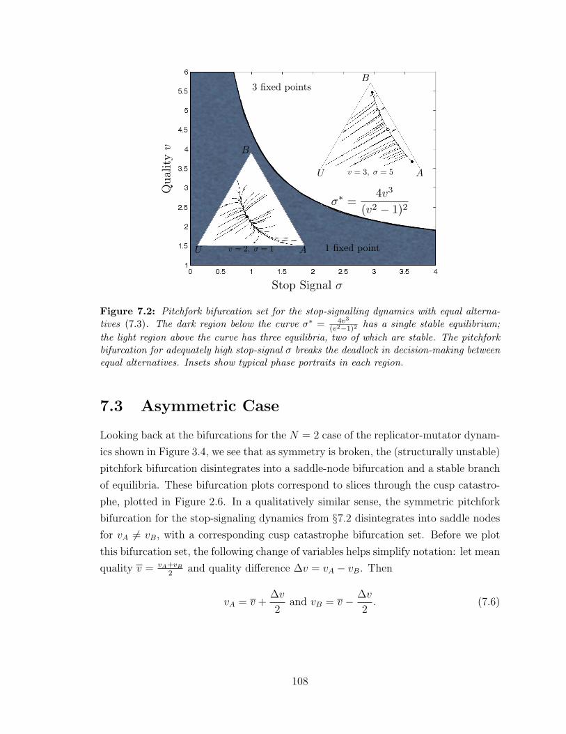
Stop Signal !

1 fixed point

3 fixed points

A

B

U

A

B

UQ

ualit

yv

v = 2, ! = 1

v = 3, ! = 5

!! =4v3

(v2 ! 1)2

Figure 7.2: Pitchfork bifurcation set for the stop-signalling dynamics with equal alterna-tives (7.3). The dark region below the curve σ∗ = 4v3

(v2−1)2has a single stable equilibrium;

the light region above the curve has three equilibria, two of which are stable. The pitchforkbifurcation for adequately high stop-signal σ breaks the deadlock in decision-making betweenequal alternatives. Insets show typical phase portraits in each region.

7.3 Asymmetric Case

Looking back at the bifurcations for the N = 2 case of the replicator-mutator dynam-

ics shown in Figure 3.4, we see that as symmetry is broken, the (structurally unstable)

pitchfork bifurcation disintegrates into a saddle-node bifurcation and a stable branch

of equilibria. These bifurcation plots correspond to slices through the cusp catastro-

phe, plotted in Figure 2.6. In a qualitatively similar sense, the symmetric pitchfork

bifurcation for the stop-signaling dynamics from §7.2 disintegrates into saddle nodes

for vA 6= vB, with a corresponding cusp catastrophe bifurcation set. Before we plot

this bifurcation set, the following change of variables helps simplify notation: let mean

quality v = vA+vB

2and quality difference ∆v = vA − vB. Then

vA = v +∆v

2and vB = v − ∆v

2. (7.6)

108

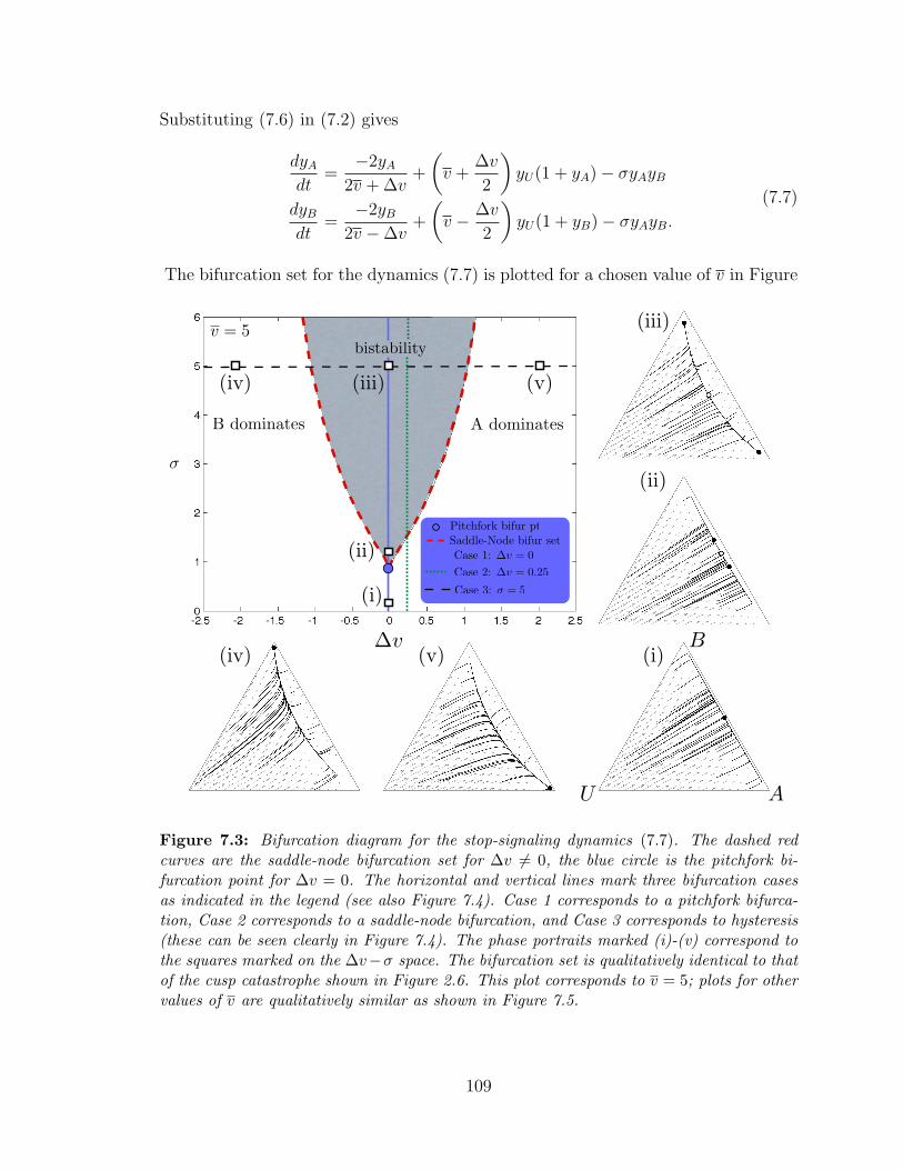
Substituting (7.6) in (7.2) gives

dyAdt

=−2yA

2v + ∆v+

(v +

∆v

2

)yU(1 + yA)− σyAyB

dyBdt

=−2yB

2v −∆v+

(v − ∆v

2

)yU(1 + yB)− σyAyB.

(7.7)

The bifurcation set for the dynamics (7.7) is plotted for a chosen value of v in Figure

A dominatesB dominates

bistability

!v

!

v = 5

Pitchfork bifur ptSaddle-Node bifur setCase 1: !v = 0Case 2: !v = 0.25

Case 3: ! = 5(i)

(ii)

(iii)(iv) (v)

(v)(iv)

(iii)

(ii)

(i)

A

B

U

!v

Figure 7.3: Bifurcation diagram for the stop-signaling dynamics (7.7). The dashed redcurves are the saddle-node bifurcation set for ∆v 6= 0, the blue circle is the pitchfork bi-furcation point for ∆v = 0. The horizontal and vertical lines mark three bifurcation casesas indicated in the legend (see also Figure 7.4). Case 1 corresponds to a pitchfork bifurca-tion, Case 2 corresponds to a saddle-node bifurcation, and Case 3 corresponds to hysteresis(these can be seen clearly in Figure 7.4). The phase portraits marked (i)-(v) correspond tothe squares marked on the ∆v−σ space. The bifurcation set is qualitatively identical to thatof the cusp catastrophe shown in Figure 2.6. This plot corresponds to v = 5; plots for othervalues of v are qualitatively similar as shown in Figure 7.5.

109

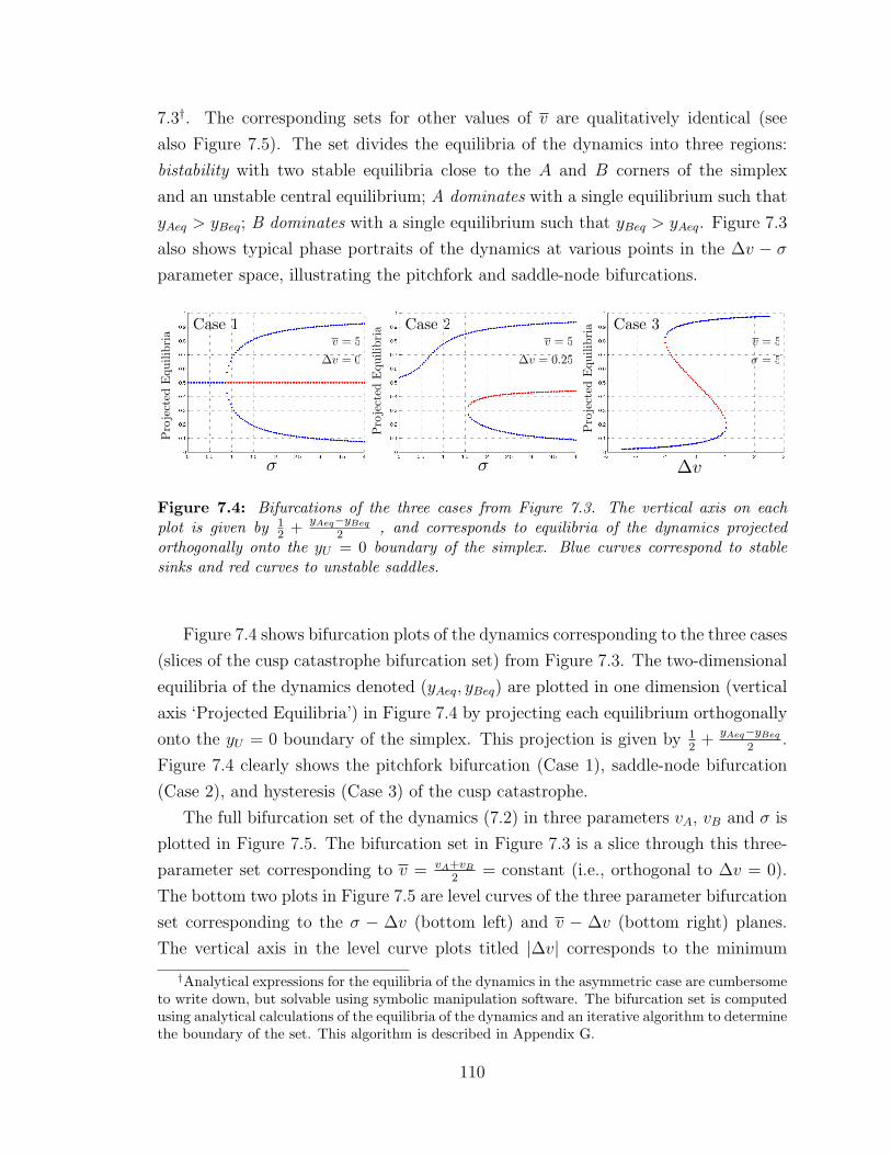
7.3†. The corresponding sets for other values of v are qualitatively identical (see

also Figure 7.5). The set divides the equilibria of the dynamics into three regions:

bistability with two stable equilibria close to the A and B corners of the simplex

and an unstable central equilibrium; A dominates with a single equilibrium such that

yAeq > yBeq; B dominates with a single equilibrium such that yBeq > yAeq. Figure 7.3

also shows typical phase portraits of the dynamics at various points in the ∆v − σparameter space, illustrating the pitchfork and saddle-node bifurcations.

! ! !v

Pro

ject

edE

quili

bria

Pro

ject

edE

quili

bria

Pro

ject

edE

quili

bria

v = 5!v = 0

v = 5!v = 0.25

v = 5! = 5

Case 1 Case 2 Case 3

Figure 7.4: Bifurcations of the three cases from Figure 7.3. The vertical axis on eachplot is given by 1

2 + yAeq−yBeq

2 , and corresponds to equilibria of the dynamics projectedorthogonally onto the yU = 0 boundary of the simplex. Blue curves correspond to stablesinks and red curves to unstable saddles.

Figure 7.4 shows bifurcation plots of the dynamics corresponding to the three cases

(slices of the cusp catastrophe bifurcation set) from Figure 7.3. The two-dimensional

equilibria of the dynamics denoted (yAeq, yBeq) are plotted in one dimension (vertical

axis ‘Projected Equilibria’) in Figure 7.4 by projecting each equilibrium orthogonally

onto the yU = 0 boundary of the simplex. This projection is given by 12

+yAeq−yBeq

2.

Figure 7.4 clearly shows the pitchfork bifurcation (Case 1), saddle-node bifurcation

(Case 2), and hysteresis (Case 3) of the cusp catastrophe.

The full bifurcation set of the dynamics (7.2) in three parameters vA, vB and σ is

plotted in Figure 7.5. The bifurcation set in Figure 7.3 is a slice through this three-

parameter set corresponding to v = vA+vB

2= constant (i.e., orthogonal to ∆v = 0).

The bottom two plots in Figure 7.5 are level curves of the three parameter bifurcation

set corresponding to the σ − ∆v (bottom left) and v − ∆v (bottom right) planes.

The vertical axis in the level curve plots titled |∆v| corresponds to the minimum

†Analytical expressions for the equilibria of the dynamics in the asymmetric case are cumbersometo write down, but solvable using symbolic manipulation software. The bifurcation set is computedusing analytical calculations of the equilibria of the dynamics and an iterative algorithm to determinethe boundary of the set. This algorithm is described in Appendix G.

110

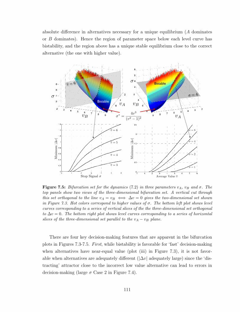
absolute difference in alternatives necessary for a unique equilibrium (A dominates

or B dominates). Hence the region of parameter space below each level curve has

bistability, and the region above has a unique stable equilibrium close to the correct

alternative (the one with higher value).

Bistable

!! =4v3

(v2 ! 1)2

!

vB vA

vA vB

Stop Signal !

Min

imum

|!v|

v = 3

v = 4

v = 5

v = 6M

inim

um|!

v|

! = 1

! = 2

! = 4

! = 8

Average Value v

!

v = 6

! = 4

Bistable

Figure 7.5: Bifurcation set for the dynamics (7.2) in three parameters vA, vB and σ. Thetop panels show two views of the three-dimensional bifurcation set. A vertical cut throughthis set orthogonal to the line vA = vB ⇐⇒ ∆v = 0 gives the two-dimensional set shownin Figure 7.3. Hot colors correspond to higher values of σ. The bottom left plot shows levelcurves corresponding to a series of vertical slices of the the three-dimensional set orthogonalto ∆v = 0. The bottom right plot shows level curves corresponding to a series of horizontalslices of the three-dimensional set parallel to the vA − vB plane.

There are four key decision-making features that are apparent in the bifurcation

plots in Figures 7.3-7.5. First, while bistability is favorable for ‘fast’ decision-making

when alternatives have near-equal value (plot (iii) in Figure 7.3), it is not favor-

able when alternatives are adequately different (|∆v| adequately large) since the ‘dis-

tracting’ attractor close to the incorrect low value alternative can lead to errors in

decision-making (large σ Case 2 in Figure 7.4).

111

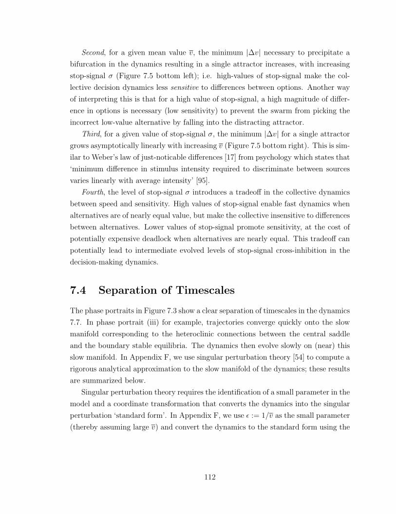
Second, for a given mean value v, the minimum |∆v| necessary to precipitate a

bifurcation in the dynamics resulting in a single attractor increases, with increasing

stop-signal σ (Figure 7.5 bottom left); i.e. high-values of stop-signal make the col-

lective decision dynamics less sensitive to differences between options. Another way

of interpreting this is that for a high value of stop-signal, a high magnitude of differ-

ence in options is necessary (low sensitivity) to prevent the swarm from picking the

incorrect low-value alternative by falling into the distracting attractor.

Third, for a given value of stop-signal σ, the minimum |∆v| for a single attractor

grows asymptotically linearly with increasing v (Figure 7.5 bottom right). This is sim-

ilar to Weber’s law of just-noticable differences [17] from psychology which states that

‘minimum difference in stimulus intensity required to discriminate between sources

varies linearly with average intensity’ [95].

Fourth, the level of stop-signal σ introduces a tradeoff in the collective dynamics

between speed and sensitivity. High values of stop-signal enable fast dynamics when

alternatives are of nearly equal value, but make the collective insensitive to differences

between alternatives. Lower values of stop-signal promote sensitivity, at the cost of

potentially expensive deadlock when alternatives are nearly equal. This tradeoff can

potentially lead to intermediate evolved levels of stop-signal cross-inhibition in the

decision-making dynamics.

7.4 Separation of Timescales

The phase portraits in Figure 7.3 show a clear separation of timescales in the dynamics

7.7. In phase portrait (iii) for example, trajectories converge quickly onto the slow

manifold corresponding to the heteroclinic connections between the central saddle

and the boundary stable equilibria. The dynamics then evolve slowly on (near) this

slow manifold. In Appendix F, we use singular perturbation theory [54] to compute a

rigorous analytical approximation to the slow manifold of the dynamics; these results

are summarized below.

Singular perturbation theory requires the identification of a small parameter in the

model and a coordinate transformation that converts the dynamics into the singular

perturbation ‘standard form’. In Appendix F, we use ε := 1/v as the small parameter

(thereby assuming large v) and convert the dynamics to the standard form using the

112

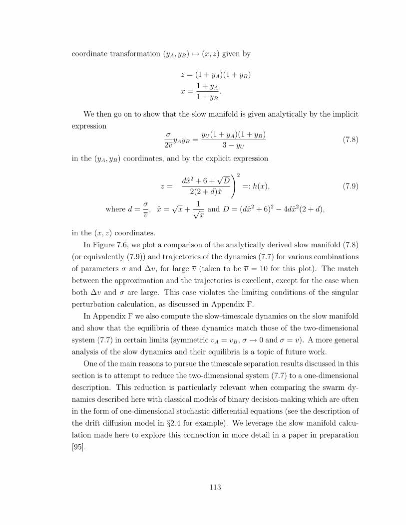
coordinate transformation (yA, yB) 7→ (x, z) given by

z = (1 + yA)(1 + yB)

x =1 + yA1 + yB

.

We then go on to show that the slow manifold is given analytically by the implicit

expressionσ

2vyAyB =

yU(1 + yA)(1 + yB)

3− yU (7.8)

in the (yA, yB) coordinates, and by the explicit expression

z =

(dx2 + 6 +

√D

2(2 + d)x

)2

=: h(x), (7.9)

where d =σ

v, x =

√x+

1√x

and D = (dx2 + 6)2 − 4dx2(2 + d),

in the (x, z) coordinates.

In Figure 7.6, we plot a comparison of the analytically derived slow manifold (7.8)

(or equivalently (7.9)) and trajectories of the dynamics (7.7) for various combinations

of parameters σ and ∆v, for large v (taken to be v = 10 for this plot). The match

between the approximation and the trajectories is excellent, except for the case when

both ∆v and σ are large. This case violates the limiting conditions of the singular

perturbation calculation, as discussed in Appendix F.

In Appendix F we also compute the slow-timescale dynamics on the slow manifold

and show that the equilibria of these dynamics match those of the two-dimensional

system (7.7) in certain limits (symmetric vA = vB, σ → 0 and σ = v). A more general

analysis of the slow dynamics and their equilibria is a topic of future work.

One of the main reasons to pursue the timescale separation results discussed in this

section is to attempt to reduce the two-dimensional system (7.7) to a one-dimensional

description. This reduction is particularly relevant when comparing the swarm dy-

namics described here with classical models of binary decision-making which are often

in the form of one-dimensional stochastic differential equations (see the description of

the drift diffusion model in §2.4 for example). We leverage the slow manifold calcu-

lation made here to explore this connection in more detail in a paper in preparation

[95].

113

!v = 0

!v = 0

!v = O(1)

!v = O(1)

!v = O(v)

!v = O(v)

! = O(1) ! = O(1) ! = O(1)

! = O(v) ! = O(v) ! = O(v)

Figure 7.6: Comparison between the analytically computed slow manifold h(x) plottedin magenta and simulations of the stop-signaling dynamics (7.7). The match between theanalytical slow manifold and the simulations is excellent, except for the case ∆v = O(v),σ = O(v). For this set of plots, v = 10, O(v) ≡ 10 and O(1) ≡ 1.

7.5 Stochastic Dynamics

Our analysis thus far has focused on bifurcations and timescale separation of the

deterministic mean-field decision-making model (7.1). It is important to recognize,

however, that the evaluations made by individual scout bees of nest site values vi are

inherently noisy. Experiments have shown that there is much overlap in distributions

of dance strength (and correspondingly judgements of value) between scouts advertis-

ing a medium-quality and a high-quality nest site during the decision-making process

[117]. Despite this noisy individual reporting of quality, there are clear differences in

mean qualities reported, resulting in a sharp distinction at the swarm level.

In this section, we move beyond the deterministic model (7.1), and build a stochas-

tic model to capture this inherent variability. The dynamics of this model can then

be compared to other standard stochastic models of decision-making, such as the

drift diffusion model (Figure 2.10(c)) which has been shown to optimally address the

speed-accuracy tradeoff in two-alternative forced choice tasks [8]. We assume that

the rates γi, ρi and αi in (7.1) that depend on the stochastic measurement vi are each

subject to variability. Similar to the setup in [71], we add independent white noise

terms of variance k2 to each of these rates (for example αi 7→ αi + kηαiwhere ηαi

114

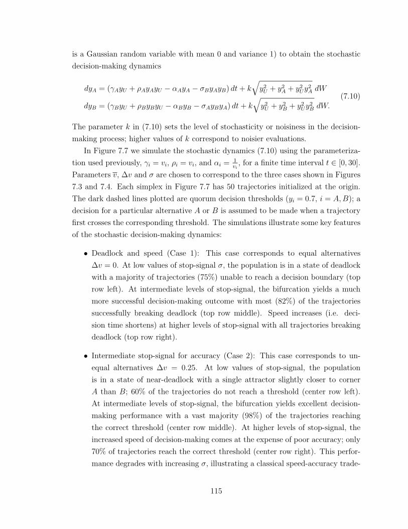
is a Gaussian random variable with mean 0 and variance 1) to obtain the stochastic

decision-making dynamics

dyA = (γAyU + ρAyAyU − αAyA − σByAyB) dt+ k√y2U + y2

A + y2Uy

2A dW

dyB = (γByU + ρByByU − αByB − σAyByA) dt+ k√y2U + y2

B + y2Uy

2B dW.

(7.10)

The parameter k in (7.10) sets the level of stochasticity or noisiness in the decision-

making process; higher values of k correspond to noisier evaluations.

In Figure 7.7 we simulate the stochastic dynamics (7.10) using the parameteriza-

tion used previously, γi = vi, ρi = vi, and αi = 1vi

, for a finite time interval t ∈ [0, 30].

Parameters v, ∆v and σ are chosen to correspond to the three cases shown in Figures

7.3 and 7.4. Each simplex in Figure 7.7 has 50 trajectories initialized at the origin.

The dark dashed lines plotted are quorum decision thresholds (yi = 0.7, i = A,B); a

decision for a particular alternative A or B is assumed to be made when a trajectory

first crosses the corresponding threshold. The simulations illustrate some key features

of the stochastic decision-making dynamics:

• Deadlock and speed (Case 1): This case corresponds to equal alternatives

∆v = 0. At low values of stop-signal σ, the population is in a state of deadlock

with a majority of trajectories (75%) unable to reach a decision boundary (top

row left). At intermediate levels of stop-signal, the bifurcation yields a much

more successful decision-making outcome with most (82%) of the trajectories

successfully breaking deadlock (top row middle). Speed increases (i.e. deci-

sion time shortens) at higher levels of stop-signal with all trajectories breaking

deadlock (top row right).

• Intermediate stop-signal for accuracy (Case 2): This case corresponds to un-

equal alternatives ∆v = 0.25. At low values of stop-signal, the population

is in a state of near-deadlock with a single attractor slightly closer to corner

A than B; 60% of the trajectories do not reach a threshold (center row left).

At intermediate levels of stop-signal, the bifurcation yields excellent decision-

making performance with a vast majority (98%) of the trajectories reaching

the correct threshold (center row middle). At higher levels of stop-signal, the

increased speed of decision-making comes at the expense of poor accuracy; only

70% of trajectories reach the correct threshold (center row right). This perfor-

mance degrades with increasing σ, illustrating a classical speed-accuracy trade-

115

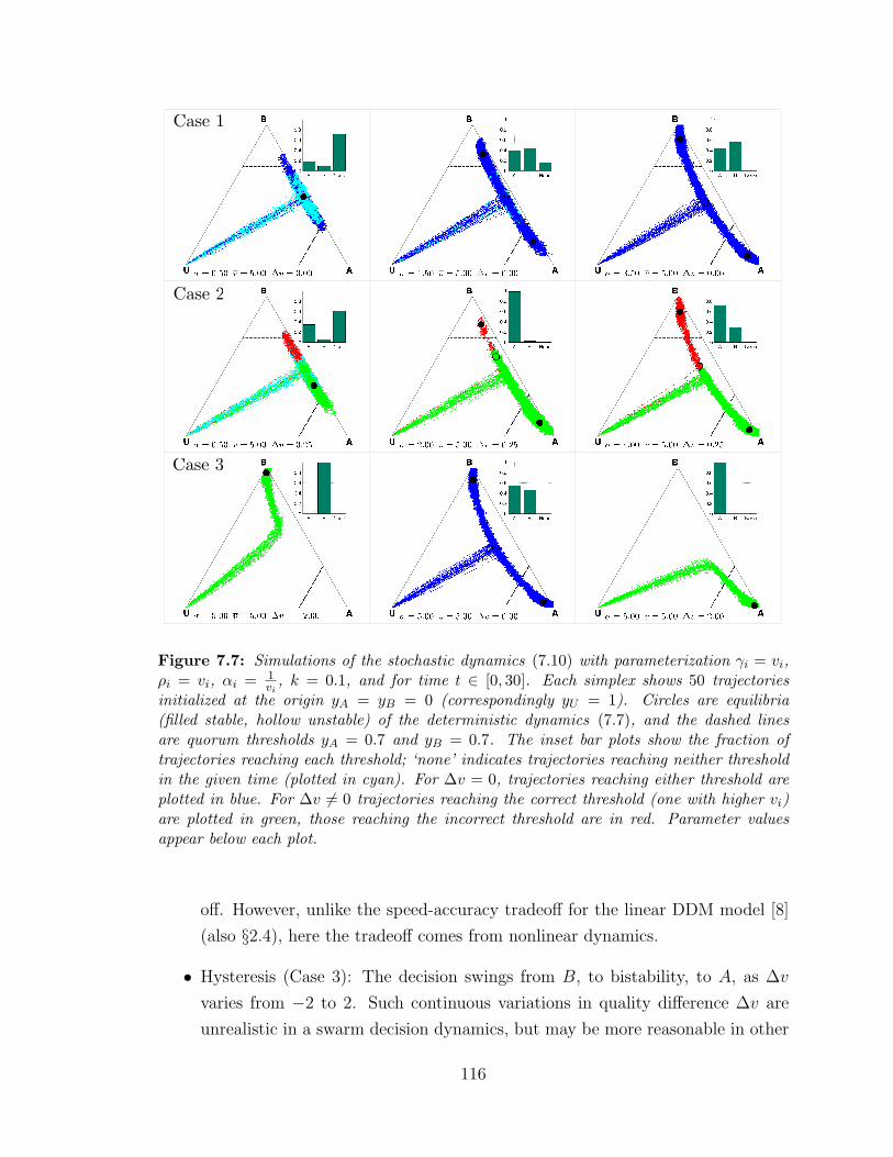
Case 1

Case 2

Case 3

Figure 7.7: Simulations of the stochastic dynamics (7.10) with parameterization γi = vi,ρi = vi, αi = 1

vi, k = 0.1, and for time t ∈ [0, 30]. Each simplex shows 50 trajectories

initialized at the origin yA = yB = 0 (correspondingly yU = 1). Circles are equilibria(filled stable, hollow unstable) of the deterministic dynamics (7.7), and the dashed linesare quorum thresholds yA = 0.7 and yB = 0.7. The inset bar plots show the fraction oftrajectories reaching each threshold; ‘none’ indicates trajectories reaching neither thresholdin the given time (plotted in cyan). For ∆v = 0, trajectories reaching either threshold areplotted in blue. For ∆v 6= 0 trajectories reaching the correct threshold (one with higher vi)are plotted in green, those reaching the incorrect threshold are in red. Parameter valuesappear below each plot.

off. However, unlike the speed-accuracy tradeoff for the linear DDM model [8]

(also §2.4), here the tradeoff comes from nonlinear dynamics.

• Hysteresis (Case 3): The decision swings from B, to bistability, to A, as ∆v

varies from −2 to 2. Such continuous variations in quality difference ∆v are

unrealistic in a swarm decision dynamics, but may be more reasonable in other

116

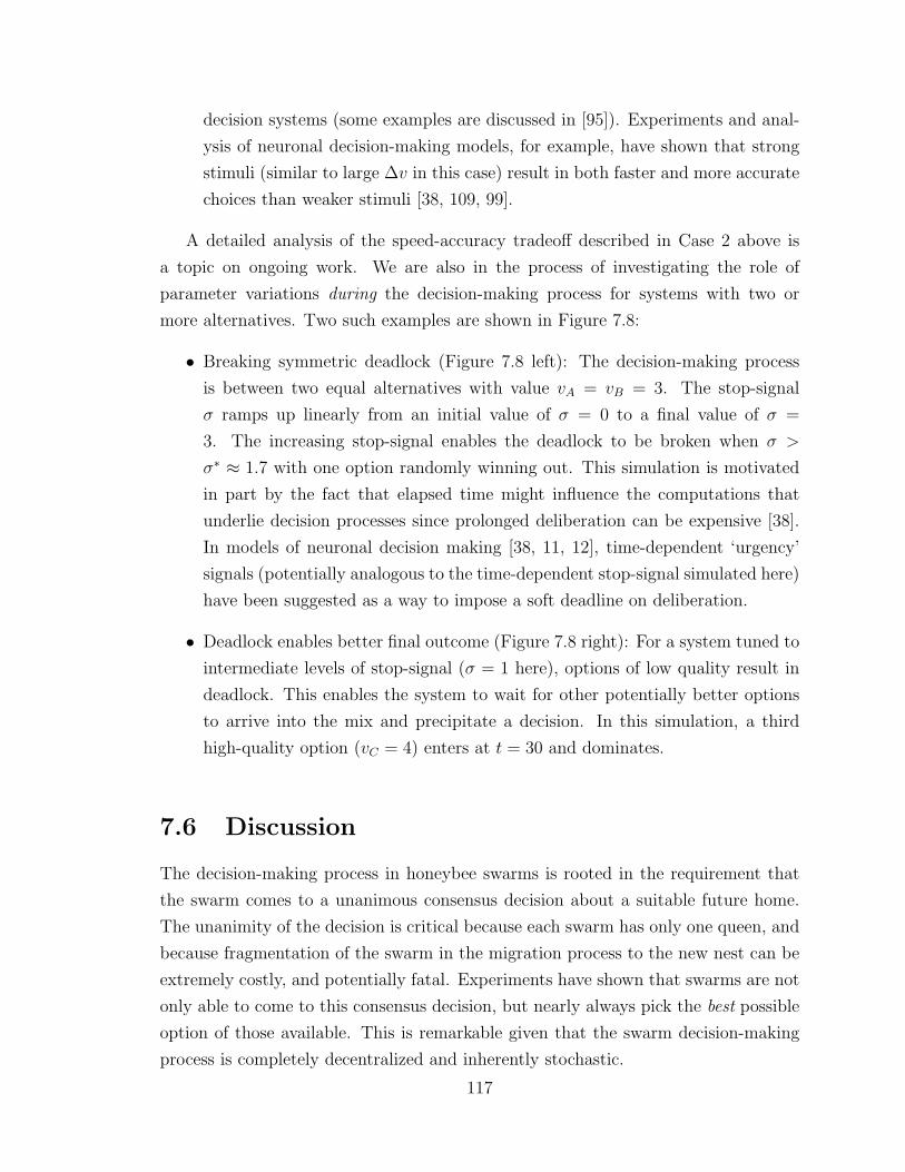
decision systems (some examples are discussed in [95]). Experiments and anal-

ysis of neuronal decision-making models, for example, have shown that strong

stimuli (similar to large ∆v in this case) result in both faster and more accurate

choices than weaker stimuli [38, 109, 99].

A detailed analysis of the speed-accuracy tradeoff described in Case 2 above is

a topic on ongoing work. We are also in the process of investigating the role of

parameter variations during the decision-making process for systems with two or

more alternatives. Two such examples are shown in Figure 7.8:

• Breaking symmetric deadlock (Figure 7.8 left): The decision-making process

is between two equal alternatives with value vA = vB = 3. The stop-signal

σ ramps up linearly from an initial value of σ = 0 to a final value of σ =

3. The increasing stop-signal enables the deadlock to be broken when σ >

σ∗ ≈ 1.7 with one option randomly winning out. This simulation is motivated

in part by the fact that elapsed time might influence the computations that

underlie decision processes since prolonged deliberation can be expensive [38].

In models of neuronal decision making [38, 11, 12], time-dependent ‘urgency’

signals (potentially analogous to the time-dependent stop-signal simulated here)

have been suggested as a way to impose a soft deadline on deliberation.

• Deadlock enables better final outcome (Figure 7.8 right): For a system tuned to

intermediate levels of stop-signal (σ = 1 here), options of low quality result in

deadlock. This enables the system to wait for other potentially better options

to arrive into the mix and precipitate a decision. In this simulation, a third

high-quality option (vC = 4) enters at t = 30 and dominates.

7.6 Discussion

The decision-making process in honeybee swarms is rooted in the requirement that

the swarm comes to a unanimous consensus decision about a suitable future home.

The unanimity of the decision is critical because each swarm has only one queen, and

because fragmentation of the swarm in the migration process to the new nest can be

extremely costly, and potentially fatal. Experiments have shown that swarms are not

only able to come to this consensus decision, but nearly always pick the best possible

option of those available. This is remarkable given that the swarm decision-making

process is completely decentralized and inherently stochastic.

117

Time

Pop

ulat

ion

Freq

uenc

yy i

!

v = 3!v = 0

!! ! 1.7

Time

Time

Pop

ulat

ion

Freq

uenc

yy i

Figure 7.8: Simulations of the stochastic dynamics. (left) A deadlocked population is ableto converge to a decision by picking one of two equal alternatives by slowly ramping up thestop-signal; the critical value of stop-signal for the pitchfork bifurcation is marked on thebottom plot. (right) For time t < 30 the population is deadlocked while choosing betweentwo low-value (v = 1) equal alternatives; a third high-value alternative (vC = 4) enters thepicture at t = 30, precipitating a decision in favor of this alternative.

As discussed in [116], there are two hypotheses for building consensus in a system.

The first is known as the compare and convert hypothesis and corresponds to agents

comparing their current state to neighbors and switching states to match those of

neighbors with better outcomes. This is reminiscent of the imitation mechanism

of the replicator-mutator dynamics in Chapters 3 and 4. The second is known as

the retire and rest hypothesis in which agents have a decaying (leaking) interest in

an option, thereby making each participant highly flexible in the decision-making

process.

Experiments have shown that scouts in a honeybee swarm do not directly compare

the options available, but instead rely on their decentralized interactions (recruitment,

commitment, etc.) to produce a consensus outcome. It has also been shown that

scouts decrease the number of dance circuits performed over time resulting in a de-

cayed interest in the corresponding option. In addition to this decay, in this chapter

we have shown the critical role played by the stop-signal cross-inhibitory mecha-

nism in enabling effective swarm decision-making. Stop-signaling enables breaking

deadlocks between equal alternatives and tunes the sensitivity of the dynamics to

differences between alternatives. We prove a separation of timescales in the decision-

118

making model, thereby enabling a reduction of the dynamics to a one-dimensional

system. Leveraging this reduction to make detailed comparisons between the stochas-

tic swarm dynamics derived here, and other classical models of neuronal collective

decision-making, is an important avenue of future work.

119

Chapter 8

Final Remarks

This thesis studies emergent collective behavior in selected biological systems from the

perspective of evolution by natural selection. Our main aim has been to understand

the mechanisms that endow biological collectives with extraordinary robustness and

adaptability, and to leverage this understanding to inspire effective decision-making

and collective motion protocols in artificial decentralized systems. We study four

related topics: replicator-mutator dynamics, collective migration, pursuit and evasion,

and swarm decision-making. The main conclusions from each of these topics are

presented in §8.1. §8.2 comprises some of the common themes between the topics that

have emerged through the analysis. We look ahead to future directions of investigation

in §8.3.

8.1 Conclusions

Replicator-mutator dynamics: Much of the existing analysis of the replicator-mutator

dynamics has focused on stable equilibria. The analysis in the literature has also

primarily considered payoff and mutation matrices that are symmetric, which cor-

respond to undirected payoff graph topologies. Here we prove conditions such that

stable limit cycles in the replicator-mutator dynamics arise as a consequence of Hopf

bifurcations for N ≥ 3 strategies and circulant payoff matrices. From a graph the-

oretic perspective, we show how breaking symmetry by considering directed graphs

allows for oscillatory limiting behavior. We emphasize that the limit cycles are not

restricted to circulant payoffs, but can exist for more general noncirculant cases as

well. The simulations in Chapter 4 illustrate the structural stability in the dynamics

to perturbations of circulant payoff, and show the tight connections between embed-

120

ded directed cycles in the payoff graph and the existence of stable limit cycles of the

dynamics.

Collective migration: The study of leadership has received significant attention

in both biology and multi-agent robotics. Agent-based simulations and experiments

with fish schools have shown that a small group of leaders is capable of guiding

the motion of a large group of followers. The ability of followers to leverage the

investments made by leaders and essentially operate as free-riders in the system is

an evolutionary paradox. In this work we focus on the role that the social graph

connectivity plays in the evolutionary dynamics of a networked model of collective

migration. We use tools from adaptive dynamics to study the all-to-all limit of the

evolutionary model and derive bounds for branching of the population into leader and

follower groups. For limited connectivity, we prove necessary and sufficient conditions

for convergence of the noise-free migration model, and show that fitness of individuals

in the stochastic model can be derived analytically using the Lyapunov equation. For

random networks and lattices, we show a minimum connectivity bound that yields

evolutionary population branching into leaders and followers. We also study a simple

model of greedy adaptive nodes on small networks, inspired by collective robotic

systems. We show that the network topology plays a critical role in determining the

location of leaders in the adaptive system; we study bifurcations in node leadership

as a function of investment costs.

Pursuit and evasion: Building on previous work that focuses on the evolutionary

dynamics of three pursuit strategies playing against an environment of nonreactive

evaders, we study an evolutionary game of three strategies of pursuit against three

strategies of evasion, two of which are reactive. Monte-Carlo simulations of the evo-

lutionary dynamics show convergence to a stable equilibrium of classical pursuit and

classical evasion. Using the structure of the fitness matrices observed in these sim-

ulations, we analytically prove the convergence of replicator dynamics to the same

classical pursuit and classical evasion equilibrium as in our Monte-Carlo simulations.

We then go on to incorporate the winning pursuit and evasive strategies in a novel

collective motion scheme and show conditions for the convergence of the dynamics to

circular formations and more complex weaving patterns.

Swarm decision-making: We study bifurcations in a mean-field model of honeybee

swarm decision-making and illustrate the critical role played by stop-signal cross-

inhibition in enabling swarms to break deadlocks between equal alternatives and

manage sensitivity to differences between unequal options. We carefully illustrate the

cusp catastrophe bifurcation set of the dynamics and prove a timescale separation that

121

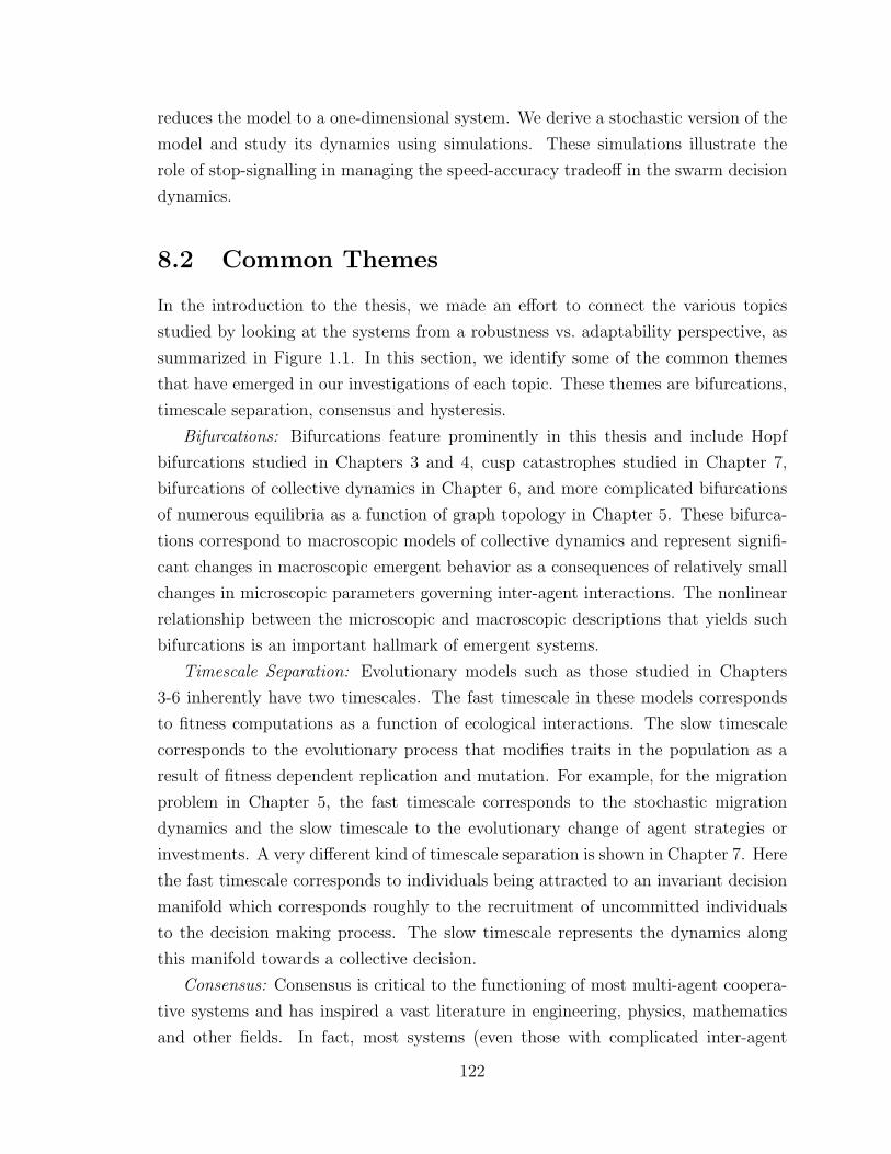
reduces the model to a one-dimensional system. We derive a stochastic version of the

model and study its dynamics using simulations. These simulations illustrate the

role of stop-signalling in managing the speed-accuracy tradeoff in the swarm decision

dynamics.

8.2 Common Themes

In the introduction to the thesis, we made an effort to connect the various topics

studied by looking at the systems from a robustness vs. adaptability perspective, as

summarized in Figure 1.1. In this section, we identify some of the common themes

that have emerged in our investigations of each topic. These themes are bifurcations,

timescale separation, consensus and hysteresis.

Bifurcations: Bifurcations feature prominently in this thesis and include Hopf

bifurcations studied in Chapters 3 and 4, cusp catastrophes studied in Chapter 7,

bifurcations of collective dynamics in Chapter 6, and more complicated bifurcations

of numerous equilibria as a function of graph topology in Chapter 5. These bifurca-

tions correspond to macroscopic models of collective dynamics and represent signifi-

cant changes in macroscopic emergent behavior as a consequences of relatively small

changes in microscopic parameters governing inter-agent interactions. The nonlinear

relationship between the microscopic and macroscopic descriptions that yields such

bifurcations is an important hallmark of emergent systems.

Timescale Separation: Evolutionary models such as those studied in Chapters

3-6 inherently have two timescales. The fast timescale in these models corresponds

to fitness computations as a function of ecological interactions. The slow timescale

corresponds to the evolutionary process that modifies traits in the population as a

result of fitness dependent replication and mutation. For example, for the migration

problem in Chapter 5, the fast timescale corresponds to the stochastic migration

dynamics and the slow timescale to the evolutionary change of agent strategies or

investments. A very different kind of timescale separation is shown in Chapter 7. Here

the fast timescale corresponds to individuals being attracted to an invariant decision

manifold which corresponds roughly to the recruitment of uncommitted individuals

to the decision making process. The slow timescale represents the dynamics along

this manifold towards a collective decision.

Consensus: Consensus is critical to the functioning of most multi-agent coopera-

tive systems and has inspired a vast literature in engineering, physics, mathematics

and other fields. In fact, most systems (even those with complicated inter-agent

122

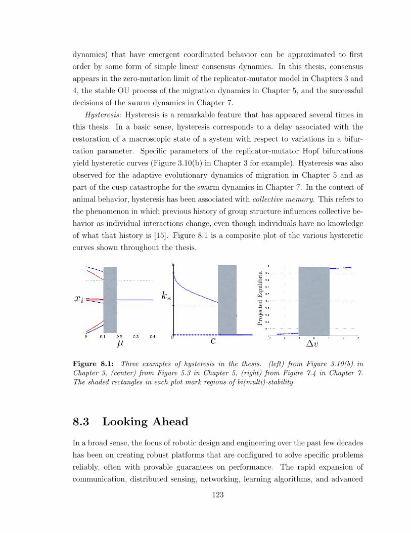
dynamics) that have emergent coordinated behavior can be approximated to first

order by some form of simple linear consensus dynamics. In this thesis, consensus

appears in the zero-mutation limit of the replicator-mutator model in Chapters 3 and

4, the stable OU process of the migration dynamics in Chapter 5, and the successful

decisions of the swarm dynamics in Chapter 7.

Hysteresis: Hysteresis is a remarkable feature that has appeared several times in

this thesis. In a basic sense, hysteresis corresponds to a delay associated with the

restoration of a macroscopic state of a system with respect to variations in a bifur-

cation parameter. Specific parameters of the replicator-mutator Hopf bifurcations

yield hysteretic curves (Figure 3.10(b) in Chapter 3 for example). Hysteresis was also

observed for the adaptive evolutionary dynamics of migration in Chapter 5 and as

part of the cusp catastrophe for the swarm dynamics in Chapter 7. In the context of

animal behavior, hysteresis has been associated with collective memory. This refers to

the phenomenon in which previous history of group structure influences collective be-

havior as individual interactions change, even though individuals have no knowledge

of what that history is [15]. Figure 8.1 is a composite plot of the various hysteretic

curves shown throughout the thesis.

µ

xi

!v

Pro

ject

edE

quili

bria

0

1

c

k!

Figure 8.1: Three examples of hysteresis in the thesis. (left) from Figure 3.10(b) inChapter 3, (center) from Figure 5.3 in Chapter 5, (right) from Figure 7.4 in Chapter 7.The shaded rectangles in each plot mark regions of bi(multi)-stability.

8.3 Looking Ahead

In a broad sense, the focus of robotic design and engineering over the past few decades

has been on creating robust platforms that are configured to solve specific problems

reliably, often with provable guarantees on performance. The rapid expansion of

communication, distributed sensing, networking, learning algorithms, and advanced

123

software, however, have enabled a new generation of intelligent and interconnected

multi-agent systems. These systems are often comprised of individual platforms or

agents that are simple and robust, but can have collective emergent group behavior

that is highly complex.

Two areas that are currently undergoing this transition from the focus on the

individual agent, to the focus on both the individual as well as the collective, are

autonomous driving for cars on the highway, and collective swarm robotics. In au-

tonomous driving [138, 52], one of the main challenges involves the design of control

protocols that leverage inter-agent interactions (sensing and communication between

vehicles) to produce optimal group-level outcomes (efficient traffic flow and safe high-

way maneuvers). The alignment of individual interests (“I want to get there fast”) and

group outcomes (overall traffic flow) poses an important challenge in such systems,

and relates back to the evolutionary paradox of cooperation in natural swarms.

The developing area of swarm robotics focuses on using hundreds of relatively

cheap and expendable robotic platforms that have limited sensing and communica-

tion capabilities, to perform collective tasks with a high degree of parallelism [79, 114].

These systems are designed to have significant flexibility and adaptability for appli-

cations such as foraging for information in dynamic and hazardous environments,

distributed sensing, and distributed task allocation (the Robobees project at Harvard

is a nice example [150, 79]). A key challenge in this area is the design of inter-

agent control laws that yield provable collective solutions while still maintaining the

adaptability and scalability of the system.

The impressive robust and adaptive behavior of biological collectives serves as

an important source of inspiration in the design of bio-inspired algorithms for artifi-

cial multi-agent systems, including the two examples above. This is because natural

collectives possess several attributes that are highly desirable for these artificial sys-

tems. The honeybee swarms studied in Chapter 7 are an excellent example: the

decision-making in these swarms is completely decentralized, extensively accurate,

highly adaptive, and robust to noise and disturbances. The analysis in Chapter 7

shows that cross-inhibition is a critical component of effective decision-making dynam-

ics in honeybee swarms. We propose that cross-inhibition is a potentially important

ingredient (along with recruitment, commitment and decay) for effective decision-

making in robotic swarms as well. Hence, the study of cross-inhibition in the context

of robotic swarms is a topic for future investigation.

Another important feature of natural collectives is the ability to rapidly transi-

tion between different regimes of behavior (collective foraging to prey evasion, for

124

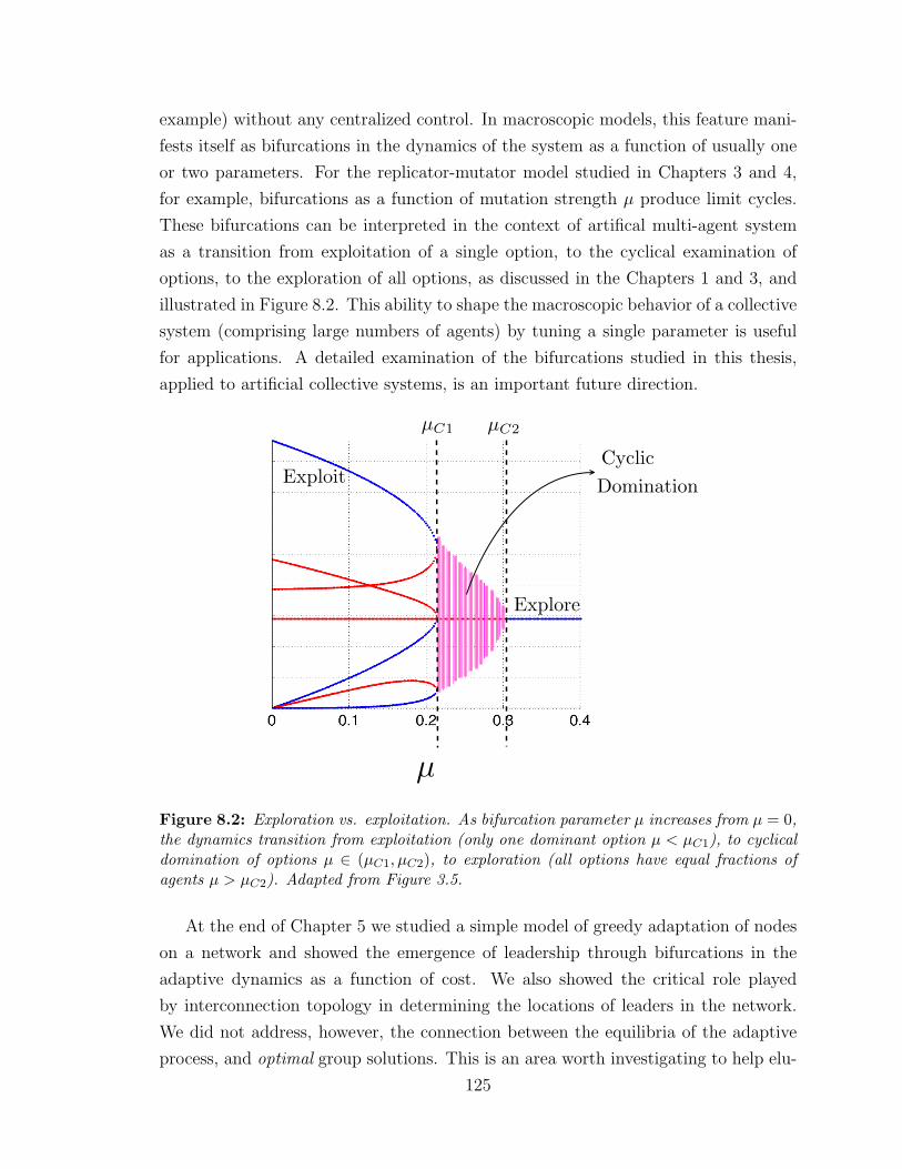
example) without any centralized control. In macroscopic models, this feature mani-

fests itself as bifurcations in the dynamics of the system as a function of usually one

or two parameters. For the replicator-mutator model studied in Chapters 3 and 4,

for example, bifurcations as a function of mutation strength µ produce limit cycles.

These bifurcations can be interpreted in the context of artifical multi-agent system

as a transition from exploitation of a single option, to the cyclical examination of

options, to the exploration of all options, as discussed in the Chapters 1 and 3, and

illustrated in Figure 8.2. This ability to shape the macroscopic behavior of a collective

system (comprising large numbers of agents) by tuning a single parameter is useful

for applications. A detailed examination of the bifurcations studied in this thesis,

applied to artificial collective systems, is an important future direction.

µ

µC1 µC2

Exploit

Explore

CyclicDomination

Figure 8.2: Exploration vs. exploitation. As bifurcation parameter µ increases from µ = 0,the dynamics transition from exploitation (only one dominant option µ < µC1), to cyclicaldomination of options µ ∈ (µC1, µC2), to exploration (all options have equal fractions ofagents µ > µC2). Adapted from Figure 3.5.

At the end of Chapter 5 we studied a simple model of greedy adaptation of nodes

on a network and showed the emergence of leadership through bifurcations in the

adaptive dynamics as a function of cost. We also showed the critical role played

by interconnection topology in determining the locations of leaders in the network.

We did not address, however, the connection between the equilibria of the adaptive

process, and optimal group solutions. This is an area worth investigating to help elu-

125

cidate the connections between a local bottom-up process such as greedy adaptation

and a global top-down optimal design approach. The fundamental tradeoff here is

that local approaches, while being highly adaptive, reconfigurable to compensate for

loss of agents, and computationally inexpensive, can come at the cost of suboptimal

group performance. Understanding this tradeoff carefully, especially as a function of

graph topology, is another potential future direction.

The rich variety of collective dynamics in swarms, flocks, schools and herds has in-

spired a generation of scientists and engineers. Recent advances in experimental and

computational technology have enabled a careful examination of the mechanisms that

produce the observed rich emergent behavior, including through the lens of evolution.

The ongoing quest to better understand the interaction patterns in biological collec-

tives, coupled with innovative bio-inspired ideas for artificial multi-agent systems, will

continue to be an exciting area of research going forward.

126

Appendix A

Calculation of Lyapunov coefficient

As stated in Theorem 2.2, the sign of the first Lyapunov coefficient `1|(x0,µ0) evaluated

at the fixed point x0 and bifurcation point µ0 determines the criticality of the Hopf

bifurcation. What follows are the expressions for calculating `1|(x0,µ0) as presented in

[59].

Consider the N -dimensional dynamical system x = f(x, µ) where x ∈ RN and

µ ∈ R. Let A0 = Dxf |(x0,µ0), where x0 ∈ RN , µ0 ∈ R. A0 has two purely imaginary

complex conjugate eigenvalues, given by ±iω0, where ω0 > 0. Define T1, T2 and T3 as

T1 = 〈p,C (q, q, q)〉T2 =

⟨p,B

(q, (2iω0 − A0)−1

B (q, q))⟩

T3 = −2⟨p,B

(q, A−1

0 B (q, q))⟩.

Here 〈r, s〉 = r · s is the complex inner product between two complex vectors, and

q and p are respectively the normalized eigenvector and adjoint-eigenvector of A0

satisfying A0q = iω0q, AT0 p = −iω0p, and normalization 〈p, q〉 = 1. B and C are

high dimensional tensors given by

B (r, s) =

B1 (r, s)

B2 (r, s)...

BN (r, s)

, Bi (r, s) =∑k,l

∂2fi∂xk∂xl

∣∣∣∣x=x0

rksl

C (r, s, t) =

C1 (r, s, t)

C2 (r, s, t)...

CN (r, s, t)

, Ci (r, s, t) =∑k,l,m

∂3fi∂xk∂xl∂xm

∣∣∣∣x=x0

rksltm

127

The first Lyapunov coefficient `1|(x0,µ0) is given by

`1|(x0,µ0) =1

2ω0

Re(T1 + T2 + T3).

Appendix B

Supporting material for Chapter 3

Lemma B.1. The divergence of the vector field g(x) restricted to the simplex ∆N−1

is given by

∇ · g(x)∣∣∣x∈∆N−1

= ∇ · h(x)

= 1T[(1− µ)B + ST

]x− xT [NB +BT

]x,

where S = Q ◦B, the element-wise product of Q and B.

Proof. The divergence is given by

∇ · h(x) =N−1∑i=1

∂hi∂xi

=N∑i=1

∂gi∂xi−

N∑i=1

∂gi∂xN

. (B.1)

We substitute for gi(x) from (3.2) in the first term of the difference in (B.1) and

using (3.1) and (3.3) we have

N∑i=1

∂gi∂xi

=∑i

∂

∂xi

[xi(fiqii − φ) +

∑j 6=i

xjfjqji

]

=∑i

[fiqii + xiqii

∂fi∂xi− φ− xi ∂φ

∂xi+∑j 6=i

xjqjibji

]

= (1− µ)1TBx+ (1− µ)−Nφ− xT ∂φ∂x

+∑i

∑j 6=i

xjqjibji

128

= (1− µ)1TBx+ (1− µ)−Nφ− xT (B +BT )x+∑i

∑j 6=i

xjsji

= 1T[(1− µ)B + ST

]x− xT [(N + 1)B +BT

]x. (B.2)

where the last equality follows by∑i

∑j 6=i

xjsji = 1TSTx− (1− µ). Computing the

second term in the difference in (B.1) and usingN∑i=1

qji = 1 we have

N∑i=1

∂gi∂xN

=∂

∂xN

[N∑i=1

N∑j=1

xjfjqji − xiφ]

=∂

∂xN

[(1−

N∑i=1

xi)φ

]= −φ = −xTBx.

(B.3)

Substituting (B.2) and (B.3) in (B.1) we get the desired result.

Lemma B.2. Let B be circulant and invertible and define the row sums of B and B◦Bas rB :=

N∑j=1

bij and rB◦B :=N∑j=1

b2ij respectively, for any row i. Then the divergence

∇ · h(x) ≤ 0 on the simplex ∆N−1 if

µ ≥ (N − rB)(rB − 1)

N (r2B − rB◦B)

for mutation (Q1) ,

µ ≥ (N − 1)(N − rB)

N (N +NrB − 2rB)for mutation (Q2).

Proof. From Lemma B.1, the divergence ∇ · h(x) is negative semi-definite on the

simplex if

maxx∈∆N−1

1T[(1−µ)B+ST

]x ≤ min

x∈∆N−1

xT[NB+BT

]x. (B.4)

The term on the left hand side (LHS) of (B.4) is the maximum of a convex combination

of non-negative scalars and hence evaluates to

LHS = maxi

N∑j=1

(1− µ)bji + sij

= (1− µ) maxi

N∑j=1

bji + (1− µ) + µmaxi

∑j 6=i

bijqij

129

=

(1− µ)(1 + rB) + µ(rB◦B−1rB−1

)for mutation (Q1)

(1− µ)(1 + rB) + µ(rB−1)N−1

for mutation (Q2)(B.5)

The term on the right hand side (RHS) of (B.4) is the minimum of a quadratic

form that is positive on the simplex. Given that B is circulant and invertible (an

N × N circulant matrix B of the form (3.1) is always invertible for N prime [43]),

this quadratic form has an isolated minimum at xmix = 1N

1. Thus,

RHS = minx∈∆N−1

xT[NB +BT

]x

=N + 1

N21TB1 =

N + 1

NrB. (B.6)

Substituting (B.6) and (B.5) in (B.4) and some rearranging gives the desired result.

Appendix C

Supporting material for Chapter 4

C.1 Proof of Lemma 4.2

Proof. To simplify notation in this proof, we denote the Jacobian Dxg|xmix,Nas

matrix A. Since A is circulant, its eigenvalues are given by (4.3). From (4.3) we see

that the eigenvalue λk(A) cannot be complex when ωkN is real. To guarantee complex

ωkN , let k be given by

k ∈{1, · · · , N − 1} N odd

{1, · · · , N − 1} \ {N2} N even.

One can then verify that λN−k(A) = λk(A). Hence, as long as the λk(A) are complex,

A has⌊N−1

2

⌋complex conjugate pairs of eigenvalues. Now we compute Im (λk(A))

130

and hence obtain conditions for the existence of complex λk(A). The calculations

differ slightly between mutation matrices (Q1) and (Q2) as shown below. We obtain

a simplified expression for the imaginary component of the eigenvalues by grouping

identical terms of A and using the identityN∑j=1

ωjkN = 0.

• Mutation (Q1):

Im (λk(A)) =

(a12 − a1N) sin(

2πNk)

N = 3, 4, 5

(a12 − a1N) sin(

2πNk)

+ (a13 − a1,N−1) sin(

2πN

2k)

N ≥ 6

• Mutation (Q2):

Im (λk(A)) = (a12 − a1N) sin

(2π

Nk

)N ≥ 3

Substituting for the aij terms from (4.2),

Im (λk(A)) = 0 ⇐⇒(α− β)

(1− µ− µ (2+α+β)

α+β

)= 0 mutation (Q1)

(α− β)(1− µ− µ

N−1

)= 0 mutation (Q2).

(C.1)

The conditions of the Lemma follow from the expressions in (C.1).

C.2 Proof of Lemma 4.3

Proof. To simplify notation in this proof, we denote the Jacobian Dxg|xmix,Nas

matrix A. From Lemma 4.2, for r = 1, · · · , ⌊N−12

⌋, λr(A) is complex. Using the

notation a1j = γj + µηj we obtain

Re (λr(A)) =N∑j=1

γj cos

(2π

N(j − 1)r

)+ µ

N∑j=1

ηj cos

(2π

N(j − 1)r

)

which is zero if and only if

µ = −[

N∑j=1

γj cos

(2π

N(j − 1)r

)][ N∑j=1

ηj cos

(2π

N(j − 1)r

)]−1

=: µ0,r. (C.2)

Before we proceed, we need to establish that µ0,r is indeed well defined; that is,

the denominator in (C.2) is non-zero. Let dr denote the denominator of µ0,r. For

131

N = 3, dr = 6(α + β + αβ) 6= 0 for mutation (Q1) and dr = 3(4 + α + β) 6= 0

for mutation (Q2); for N = 4, dr = 2(α + β + 2αβ) 6= 0 for mutation (Q1) and

dr = 4(2 + α + β) 6= 0 for mutation (Q2). For N ≥ 5, by grouping identical terms,

using the identityN∑j=1

ωjrN = 0 and replacing the expressions for ηj in terms of α and

β we have,

dr 6= 0 ⇐⇒2 (α + β)

(cos(

2πNr)− 1

)+ 2αβ

(cos(

2πN

2r)− 1

) 6= 0 mutation (Q1)

cos(

2πNr) 6= −2+α+β

α+βmutation (Q2).

The conditions above can be verified to always hold given that the cosine function is

bounded between −1 and 1 and α and β satisfy the conditions in (4.1).

Finally, we establish that if r, s = 1, · · · ⌊N−12

⌋, r 6= s then µ0,r 6= µ0,s, i.e. the

bifurcation points are distinct. If N = 3, 4, Lemma 4.2 establishes that there is only

one bifurcation point. For N = 5, the two critical points can be shown to be distinct

by a direct calculation. Here we show the distinctness of the critical points in the

cases N ≥ 6. Using (C.2),

µ0,r 6= µ0,s ⇐⇒∑N

j=1 γj cos(

2πN

(j − 1)r)∑N

j=1 ηj cos(

2πN

(j − 1)r) 6= ∑N

j=1 γj cos(

2πN

(j − 1)s)∑N

j=1 ηj cos(

2πN

(j − 1)s) . (C.3)

By grouping identical terms, using the identityN∑j=1

ωjrN = 0, and replacing the

expressions for γj and ηj in terms of α and β, we find that

(C.3) ⇐⇒

(1 + α + β + 2αβ) (α + β)

+2αβ[cos(

2πNr)

+ cos(

2πNs)]

+2 (α + β)αβ[cos(

2πNr)

cos(

2πNs)] 6= 0 mutation (Q1)

cos(

2πNr) 6= cos

(2πNs)

mutation (Q2).

(C.4)

For mutation (Q1), the left hand side of the inequality in (C.4) can be bounded

below by (α− β)2 + (α + β) > 0. For mutation (Q2), the condition in (C.4) is

equivalent to the initial hypothesis of r 6= s. The distinctness result now follows.

132

C.3 Proof of Lemma 4.4

Proof. Here we compute the terms T1, T2 and T3 from Appendix A to obtain a

simplified analytical expression for the first Lyapunov coefficient `1|(xmix,N ,µ0,r). For

a circulant matrix M ∈ RN×N , let {(λk,vk)} be an eigenvalue–right eigenvector pair

(Mvk = λkvk), where

vk =[

1 ωkN ω2kN · · · ω

(N−1)kN

]Tand λk (M) =

N∑j=1

m1j ω(j−1)kN . (C.5)

We compute `1|(xmix,N ,µ0,r) as a function of the parameters α and β. From Appendix

A, the Jacobian Dxg|(xmix,N ,µ0,r) is denoted by A0 with eigenvalue λr(A0) = i ω. Let

ω0 = |ω|, t = r sign (ω), and q = vt. Note that A0q = iω0q.

Computing T1

Direct calculation and simplification gives

Ci (q, q, q) = −2N[2 + (α + β)ωtN + (α + β)ω−tN

]ω

(i−1)tN .

Hence

C (q, q, q) = −2N[2 + (α + β)ωtN + (α + β)ω−tN

]q,

which leads to

T1 = 〈p,C (q, q, q)〉 = −2N[2 + (α + β)ωtN + (α + β)ω−tN

] 〈p, q〉= −2N

[2 + (α + β)

(ωtN + ω−tN

)]. (C.6)

Computing T2

We compute

B (q, q) = 2[1 + αωtN + βω−tN

]QTv2t.

Since Q is circulant, so is QT and v2t is a right eigenvector. Then

B (q, q) = 2[1 + αωtN + βω−tN

]λ2t

(QT)v2t.

For each eigenvector-eigenvalue pair v, λ of A0, direct calculation shows that

1/ (2iω0 − λ) is the corresponding eigenvalue for the eigenvector v of (2iω0I − A0)−1,

133

where I denotes the identity matrix. Then,

(2iω0I − A0)−1B (q, q) = 2

[1 + αωtN + βω−tN

]λ2t

(QT)

2iω0 − λ2t (A0)v2t.

Since B (x, κy) = κB (x,y) for any κ ∈ C, then

B(q, (2iω0 − A0)−1

B (q, q))

= 2

[1 + αωtN + βω−tN

]λ2t

(QT)

2iω0 − λ2t (A0)B (q,v2t) .

A calculation similar to that for B (q, q) gives

Bi (q,v2t) =[βω−2t

N + αω−tN + 2 + βωtN + αω2tN

] N∑j=1

qji ω(j−1)tN .

Hence

B (q,v2t) =(βω−2t

N + αω−tN + 2 + βωtN + αω2tN

)λt(QT)q.

This implies that

B(q, (2iω0 − A0)−1

B (q, q))

=2λt(QT)λ2t

(QT)

2iω0 − λ2t (A0)

(1 + αωtN + βω−tN

) [βω−2t

N + αω−tN + 2 + βωtN + αω2tN

]q,

and

T2 =⟨p,B

(q, (2iω0 − A0)−1

B (q, q))⟩

=2λt(QT)λ2t

(QT)

2iω0 − λ2t (A0)

(1 + αωtN + βω−tN

) [βω−2t

N + αω−tN + 2 + βωtN + αω2tN

]. (C.7)

Computing T3

We show that B (q, q) = 0.

Bi (q, q) = −2− (α + β)(ωtN + ω−tN

)+[2 + (α + β)

(ωtN + ω−tN

)] N∑j=1

qji

=[2 + (α + β)

(ωtN + ω−tN

)] [−1 +N∑j=1

qji

]= 0, (C.8)

134

where the last equality comes from the fact that Q is a doubly-stochastic matrix.

This implies

T3 = −2⟨p,B

(q, A−1

0 B (q, q))⟩

= −2 〈p,B (q,0)〉 = 0.

Combining the previous expressions for T1, T2 and T3, the result follows.

C.4 Criticality analysis for Corollaries 4.1 and 4.2

In this section we establish that the Lyapunov coefficient at each of the d concur-

rent Hopf Bifurcations of the equilibria xj,d,N is identical to that at the equilibrium

xmix,N/d for the simple cycle payoff BC,N/d with β = 0 (i.e. BN/d,1). The mutation

matrix used is (Q1). Let N/d = N1 and N2 = N −N1.

In order to simplify the calculations, consider the payoff matrix BN,d given by

BN,d =

BN1,1 0N1×N1 · · · 0N1×N1

0N1×N1 BN1,1 · · · 0N1×N1

......

. . ....

0N1×N1 0N1×N1 · · · BN1,1

.

BN,d is obtained by relabeling the graph nodes corresponding to BN,d such that index

labels for connected nodes are consecutive. The payoff graph topology induced by

BN,d is isomorphic to that of BN,d, see Figure 4.5. The dynamics (3.2), with payoff

BN,d and mutation (Q1) have equilibria xj =[0TN1(j−1)

1N1

1TN10TN1(d−j)

]T, which

correspond to the equilibria xj,d,N . The Jacobian of the system above evaluated

at the equilibrium x1 is precisely MN,d in (4.8). Using this definition of payoff, we

compute the first Lyapunov coefficient as described in Appendix A. We focus on

equilibrium x1; the analysis for the other xj is equivalent.

The eigenvalues λk and eigenvectors vk of a circulant matrix are defined in (C.5).

Let the Jacobian MN,d evaluated at the critical point µ0,r (defined in Corollary 4.2)

be denoted as

A0 =

A0 0N2×N1

0N1×N2 −1+αN1IN2×N2

,

135

with eigenvalue λr (A0) = i ω. Let ω0 = |ω|, t = r sign(ω), q = vt (A0), q =[qT 0Td(N1−1)

]Tand 〈p, q〉 = 1. Note that A0q = iω0q and hence A0q = iω0q. Let

Q be the (Q1) mutation matrix corresponding to BN,d and Q be the (Q1) mutation

matrix corresponding to BN,d.

With these definitions, we follow the calculations in Appendix A and compute

each of the terms T1, T2 and T3 given below. A comparison of each of these terms,

to the corresponding terms in Appendix C.3 shows that the Lyapunov coefficient is

identical (when N 7→ N1, β 7→ 0 in (C.6), (C.7) and (C.8)).

T1 =⟨p,C

(q, q, q

)⟩= −2N1

[2 + αωtN1

+ αω−tN1

],

T2 =

⟨p,B

(q,(

2iω0 − A0

)−1

B (q, q)

)⟩=

2λt(QT)λ2t

(QT)

2iω0 − λ2t (A0)

(1 + αωtN1

) [αω−tN1

+ αω2tN1

+ 2],

T3 = −2⟨p,B

(q, A−1

0 B(q, q

))⟩= 0.

Appendix D

Supporting material for Chapter 5

In this appendix we discuss the details of the adaptive dynamics analysis from Section

5.2. Define the function

G(kR, kM) =k2M + (1− kM)2β2(1− kR)

4(2k2M − 2kM + 1)

+ ck2M .

Then the differential fitness from (2.3) is given by

S = exp[−G(kR, kM)]− exp[−G(kR, kR)].

136

The selection gradient g(kR) is given by

g(kR) =∂S

∂kM

∣∣∣∣kM =kR

= − exp[−G(kR, kR)]

(kM(1− kM)[1 + β2(kR − 1)]

2(2k2M − 2kM + 1)2

+ 2ckM

).

Solving for the singular strategy condition g(k∗) = 0 gives the expression (5.19)

k∗(1− k∗)[1 + β2(k∗ − 1)] + 4ck∗(2k2∗ − 2k∗ + 1)2 = 0.

This expression has two sets of solutions that are plotted in Figure 5.3. One set

corresponds to k∗ = 0 and the other is defined implicitly by the equation

c =(k∗ − 1)[1 + β2(k∗ − 1)]

4(2k2∗ − 2k∗ + 1)2

=: c(k∗). (D.1)

To determine conditions for evolutionary branching we compute

∂2S

∂k2M

∣∣∣∣kM =kR=k∗

= − exp [−G(k∗, k∗)](1− β2 + β2k∗) (3k∗ − 10k2

∗ + 6k3∗)

2 (1− 2k∗ + 2k2∗)

3 .

Hence the branching condition ∂2S∂k2

M

∣∣∣kM =kR=k∗

> 0 corresponds to

(β2(1− k∗)− 1) k∗ (3− 10k∗ + 6k2∗)

2 (1− 2k∗ + 2k2∗)

3 > 0. (D.2)

The zeros of function above in the range k∗ ∈ [0, 1] are 0, 5−√

76

, and 1 − 1β2 . A

derivative test shows that the condition (D.2) is satisfied for k∗ ∈(

0, 5−√

76

).

The critical cost parameter c1 in Figure 5.3, corresponds to the maximum singular

value k∗ for branching and is given from (D.1) by c1 = c(

5−√

76

). The parameter c2 is

determined by calculating the local maximum of the function c(k∗) as seen in Figure

5.3. We use the notation c(kcrit) = c2. kcrit can be calculated analytically and is

given by a particular root of a cubic equation. The analytical expression for kcrit (and

correspondingly c2) is cumbersome and hence is left out of this text. Nonetheless, the

sketch in Figure 5.3 clearly conveys the main ideas.

Finally we discuss the convergence stability of the singular strategies. The con-

vergence stability condition is given by (2.5). For the k∗ = 0 singular strategy,

∂g

∂kR

∣∣∣∣kR=0

= exp

[−β2

4

]β2 − 1− 4c

2, hence

∂g

∂kR

∣∣∣∣kR=0

< 0 ⇐⇒ c >β2 − 1

4.

137

For the second singular strategy curve defined implicitly by (D.1), the derivative

term in the convergence stability condition evaluates to

∂g

∂kR

∣∣∣∣kR=k∗

= −k∗ [3− 10k∗ + 6k2∗ + 2β2 (−1 + 5k∗ − 6k2

∗ + 2k3∗)] exp [−G(k∗, k∗)]

2 (1− 2k∗ + 2k2∗)

3

The interior root of ∂g∂kR

∣∣∣kR=k∗

= 0 is precisely the value kcrit that maximizes c(k∗)

(since c = c(k∗) ≡ g(k∗) = 0); this root corresponds to c2 (see above). Hence one

can verify that the singular strategies corresponding to the curve (D.1) are stable for

k∗ > kcrit and unstable for k∗ < kcrit as shown in Figure 5.3.

Appendix E

Supporting material for Chapter 6

E.1 Proof of Lemma 6.2

Proof. D is invariant with respect to the dynamics (6.6) since all boundaries of D are

invariant (qi ∈ {0, 1} =⇒ qi = 0), and further q3(0) > 0 =⇒ q3(t) > 0 for all t > 0

since

q3 =q3f3

qTf− q3 ≥ −q3 =⇒ q3(t) ≥ q3(0)e−t > 0.

Using the constraint qT13 = 1, we restate the dynamics (6.6) as a two-dimensional

system,

q1 =q1

f(f31(t)(q1 − 1) + f32(t)q2)

q2 =q2

f(f32(t)(q2 − 1) + f31(t)q1) ,

(E.1)

where f32(t) = f3(t) − f2(t) > 0, f31(t) = f3(t) − f1(t) > 0, and f = qTf =

f3− q1f31− q2f32. One can check that the only three equilibria of the system (E.1) in

138

∆2 (given properties (1)-(3)) are the vertices (qeq1, qeq2) = (0, 0), (0, 1), (1, 0), of which

(0, 0) is the only equilibrium in D.

Linearization about the (0, 0) equilibrium gives the dynamics,[q1

q2

]=

[−f31/f3 0

0 −f32/f3

][q1

q2

].

This non-autonomous linear system in diagonal form can be solved easily as

qi(t) = qi(0)exp

(−∫ t

0

f3i(t)

f3(t)dt

), i = 1, 2.

For i = 1, 2, limt→∞

qi(t) = 0 and hence the (0, 0) equilibrium point of the non-

autonomous system (E.1) is locally asymptotically stable by Theorem 4.13 of [54].

To prove that the invariant domain D is the region of attraction for the asymptoti-

cally stable (0, 0) equilibrium point of (E.1), we use a Lyapunov function V = q1 +q2.

V is positive definite on D with a unique minimum: V = 0 ⇐⇒ q1 = q2 = 0. We

compute

V = q1 + q2 =1

f(q1f31 + q2f32)(q1 + q2 − 1) < 0.

Since V is negative definite on the domain D, by Theorem 4.9 of [54] we have that D

is the region of attraction for the equilibrium point qeq1 = 0, qeq2 = 0 (and qeq3 = 1).

Hence the equilibrium point qeq =[

0 0 1]T

is the asymptotically stable limit for

all q(0) ∈ D.

E.2 Lemma E.1 used in Theorem 6.1

Lemma E.1. Let q ∈ ∆2, qeq =[

1 0 0]T

and fP = Mq, where M = T# and T

satisfies Conjecture 6.1. Then ‖q − qeq‖ < ε =⇒ fP1 > fP2 and fP1 > fP3, where

ε ≤ min{

2(m11−m21)(m11−m21)+‖M‖1 ,

2(m11−m31)(m11−m31)+‖M‖1

}.

Proof. ‖q − qeq‖1 < ε =⇒ q1 > 1− ε2, q2 <

ε2

and q3 <ε2. Suppose that

ε ≤ 2(m11 −m21)

(m11 −m21) + ‖M‖1

=⇒ ε <2(m11 −m21)

(m11 −m21) + (m22 +m23)

=⇒ (m11 −m21)(

1− ε

2

)> (m22 +m23)

ε

2

139

=⇒ (m11 −m21)q1 > m22q2 +m23q3

=⇒ (m11 −m21)q1 > m22q2 +m23q3 −m12q2 −m13q3

=⇒[m11 m12 m13

]Tq >

[m21 m22 m23

]Tq, or fP1 > fP2. (E.2)

Similarly one can show that

ε ≤ 2(m11 −m31)

(m11 −m31) + ‖M‖1

=⇒ fP1 > fP3. (E.3)

Combining (E.2) and (E.3) we get the desired result.

Appendix F

Supporting material for Chapter 7

This appendix comprises the details of the timescale separation calculation for the

stop-signalling dynamics (7.7),

dyAdt

=−2yA

2v + ∆v+

(v +

∆v

2

)yU(1 + yA)− σyAyB

dyBdt

=−2yB

2v −∆v+

(v − ∆v

2

)yU(1 + yB)− σyAyB.

We perform a nonlinear coordinate transformation of the dynamics (7.7) and apply

singular perturbation theory to separate timescales and derive an analytic expression

for the slow manifold (heteroclinic connections). Assuming large v, define ε := 1v

as

the small parameter for the timescale separation calculations. We follow the notation

used in Chapter 11 of [54] and apply Tikhonov’s Theorem (Theorem 11.1 in [54]) to

prove the timescale separation.

140

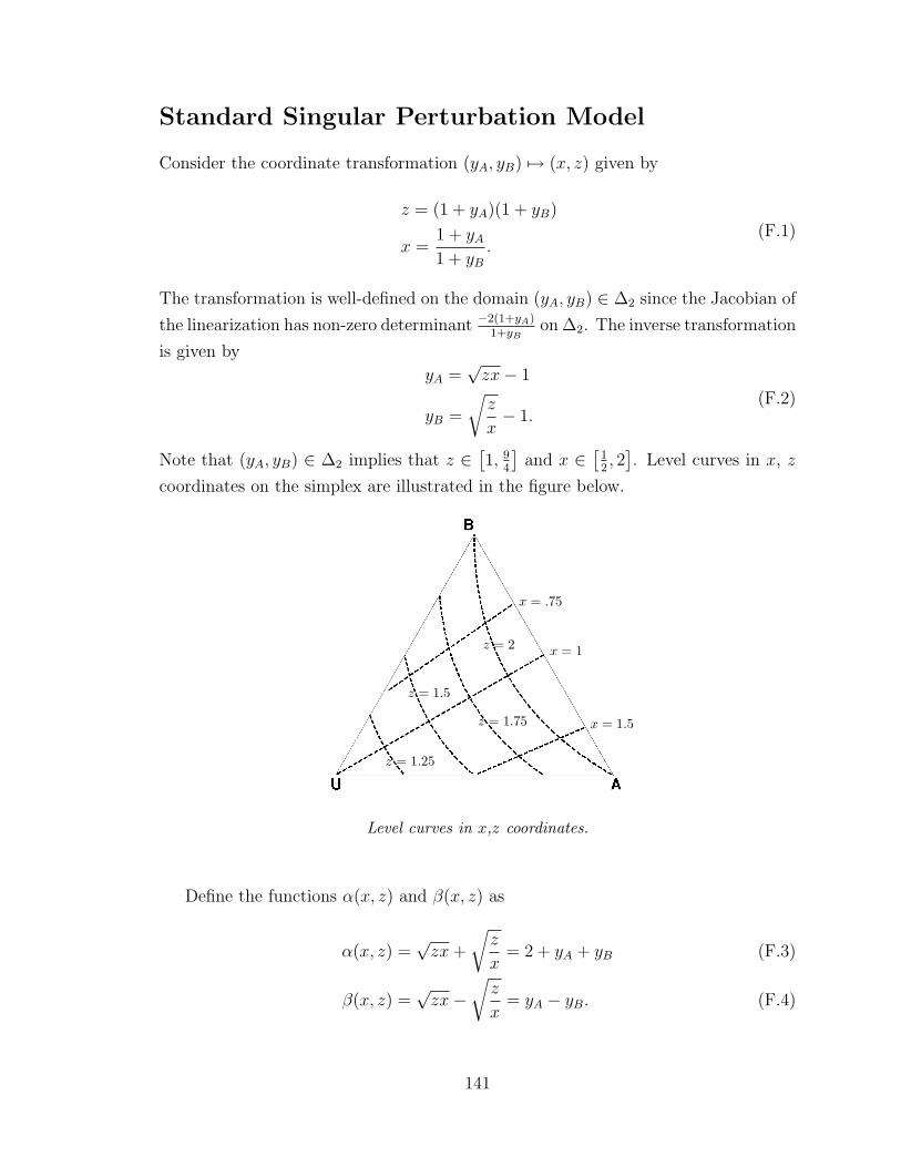
Standard Singular Perturbation Model

Consider the coordinate transformation (yA, yB) 7→ (x, z) given by

z = (1 + yA)(1 + yB)

x =1 + yA1 + yB

.(F.1)

The transformation is well-defined on the domain (yA, yB) ∈ ∆2 since the Jacobian of

the linearization has non-zero determinant −2(1+yA)1+yB

on ∆2. The inverse transformation

is given by

yA =√zx− 1

yB =

√z

x− 1.

(F.2)

Note that (yA, yB) ∈ ∆2 implies that z ∈ [1, 94

]and x ∈ [1

2, 2]. Level curves in x, z

coordinates on the simplex are illustrated in the figure below.

z = 2

z = 1.75

z = 1.5

z = 1.25

x = 1

x = 1.5

x = .75

Level curves in x,z coordinates.

Define the functions α(x, z) and β(x, z) as

α(x, z) =√zx+

√z

x= 2 + yA + yB (F.3)

β(x, z) =√zx−

√z

x= yA − yB. (F.4)

141

Then,

yAyB = z + 1− α, yA + yB = α− 2, and yU = 3− α. (F.5)

Computing the time derivative of z and substituting from (7.7), (F.3), (F.4) and

(F.5) we get

z = yB(1 + yA) + yA(1 + yB)

=2

4v2 −∆v2[∆v β(x, z)− 2v(2z − α(x, z))]

+ 2vz(3− α(x, z))− σα(x, z)(z + 1− α(x, z)).

(F.6)

Computing the time derivative of x and substituting from (7.7), (F.3), (F.4) and

(F.5) we get

x =yA(1 + yB)− yB(1 + yA)

(1 + yB)2

=x∆v(4z − 2α(x, z))− 4xvβ(x, z)

4v2z − z(∆v)2+ x∆v(3− α(x, z))

+σxβ(x, z)

z(z + 1− α(x, z)).

(F.7)

With small parameter ε = 1/v and ratio d = σ/v, the transformed dynamics

(F.6), (F.7) can be written as a singular perturbation problem in standard form,

εdz

dt= 2z(3− α)− dα(z + 1− α)

+2ε3β∆v

4− ε2(∆v)2− 4(2z − α)ε2

4− ε2(∆v)2=: g(x, z, ε) (F.8)

dx

dt= x(3− α)∆v +

σβx

z(z + 1− α)

− 4βxε

4z − zε2(∆v)2+x(4z − 2α)ε2∆v

4z − zε2(∆v)2=: f(x, z, ε). (F.9)

To ensure that the ε→ 0 limit is well-defined we assume

limv→∞

∆v

v= lim

ε→0ε∆v = 0. (F.10)

Slow Manifold Calculation

The slow manifold is given by the root of g(x, z, 0) = 0.

g(x, z, 0) = 0 =⇒ 2z(3− α(x, z))− dα(x, z)(z + 1− α(x, z)) = 0

142

=⇒ 2zyU − dα(x, z)(z + 1− α) = 0

=⇒ 2(1 + yA)(1 + yB)yU = d(3− yU)(yAyB)

=⇒ d

2yAyB =

yU(1 + yA)(1 + yB)

3− yU . (F.11)

(F.11) is an implicit expression for the slow manifold. Define the function x =√x + 1√

x. Then α(x, z) =

√zx. In order to obtain an explicit expression we rewrite

(F.11) in the (x, z) coordinates as follows,

g(x, z, 0) = 0 =⇒ 2z(3− α(x, z))− dα(x, z)(z + 1− α(x, z)) = 0

=⇒ 2z(3−√zx)− d√zx(z + 1−√zx) = 0

=⇒ 6√z − 2zx− dxz − dx+ dx2

√z = 0

=⇒ (2 + d)xz − (dx2 + 6)√z + dx = 0. (F.12)

(F.12) is quadratic in√z. The solutions to the quadratic are given by

√z =

dx2 + 6±√D2(2 + d)x

, (F.13)

where the discriminant D = d2x4 + 36 + 4dx2 − 4d2x2. Hence we have two distinct

solutions for the slow manifold given by

z =

(dx2 + 6 +

√D

2(2 + d)x

)2

,

(dx2 + 6−√D

2(2 + d)x

)2

. (F.14)

The second solution in (F.14) lies outside the feasible domain z ∈ [1, 94] (and corre-

spondingly (yA, yB) ∈ ∆2) and is hence rejected.

To summarize, the slow manifold is given by

z =

(dx2 + 6 +

√D

2(2 + d)x

)2

=: h(x)

where x =√x+

1√x

and D = (dx2 + 6)2 − 4dx2(2 + d).

(F.15)

143

Attractively of the Slow Manifold

The boundary layer dynamics are given by

dy

dτ= g(x, y + h(x), 0), (F.16)

where x is treated as fixed parameter. Stability of the boundary layer dynamics

requires the exponential stability of its origin, uniformly in the fixed parameter x

[54]. To test for exponential stability of the origin, we compute the Jacobian of the

dynamics (F.16) evaluated at the origin

∂

∂yg(x, y + h(x), 0)

∣∣∣∣y=0

= − 1

12

√1296 +

(1 + x)2σ (24x+ (x− 1)2σ)

x2(F.17)

and note that ∂∂yg(x, y + h(x), 0)

∣∣∣y=0

< 0 for all x ∈ [12, 2].

Reduced Dynamics of the Slow Model

The reduced dynamics on the slow manifold defined by (F.15) are given by

x = f (x, h(x), 0)

=σx

h(x)[h(x) + 1− α (x, h(x))] β (x, h(x)) + x(3− α (x, h(x)) ∆v. (F.18)

The general expression for the equilibria of (F.18) is complicated. Nonetheless, ana-

lytical solutions can be obtained for two special cases described below.

Special Cases

• d = O(ε): The slow manifold is given by the d → 0 limit of the expression

(F.15),

limd→0

h(x) =9x

(x+ 1)2, (F.19)

which corresponds to yU = 1 − yA − yB = 0. Another way of seeing this is

computing g(x, z, 0) from (F.6) in the limit d → 0, which gives 2z(3 − α) =

0 ⇐⇒ 3 − α = 0 ⇐⇒ yU = 0. The reduced dynamics on the slow manifold

144

are given by substituting (F.19) in (F.18)

x = f (x, h(x), 0)

= σ(x+ 1)2

9

[9x

(x+ 1)2+ 1− α

(x,

9x

(x+ 1)2

)]β

(x,

9x

(x+ 1)2

)= σ

(x+ 1)2

9

[9x

(x+ 1)2− 2

]3(x− 1)

(x+ 1).

(F.20)

Equilibria of (F.20) are xeq = −1, 12, 1, 2. These equilibria and their stability

are summarized in Table F.1. The two stable equilibria, xeq = 12

and xeq = 2,

correspond to yB = 1 and yA = 1, respectively. The unstable equilibrium

zeq = 1 corresponds to yA = yB = 12. The xeq = −1 equilibrium is rejected since

the dynamics are only defined for x ∈ [12, 2].

Table F.1: Equilibria and stability for the reduced dynamics (F.20)xeq

12

1 2

zeq 2 94

2

yAeq = 2xeq−1

xeq+10 1

21

yBeq = 1− yAeq 1 12

0

∂f(x,h(x),0)∂x

∣∣∣∣x=xeq

−σ3

σ6

−σ3

Stability Stable Unstable Stable

• d = 1, ∆v = 0: A general expression for the equilibria of (F.18), even for

the symmetric case ∆v = 0, is challenging to determine. However, for d = 1,

analytical expressions for the equilibria and their stability are summarized in

Table F.2. In practice, the expressions from Table F.2 hold for a broad range

of d as long as v is sufficiently large.

Note that from Equation (7.4) (and assuming σ = O(v)),

limv→∞

p1 = limv→∞

2

1v2

+ 1 +√

1v4

+ 2v2

+ 9 + 4,

2

1v2

+ 1 +√

1v4

+ 2v2

+ 9 + 4

=

(2

1 +√

13,

2

1 +√

13

),

145

Table F.2: Equilibria and stability for the reduced dynamics (F.18) with d = 1 and ∆v = 0xeq 2 1 1

2

zeq 2 118

(19 + 5√

13) 2

yAeq 1 21+√

130

yBeq 0 21+√

131

∂f(x,h(x),0)∂x

∣∣∣∣x=xeq

−4σ15

4−√

133

σ −4σ15

Stability Stable Unstable Stable

which is precisely the unstable equilibrium point corresponding to xeq = 1 in

Table F.2. Similarly, for σ = O(v), limv→∞

p2 = (1, 0) and limv→∞

p3 = (0, 1), which

are precisely the two stable equilibria corresponding to xeq = 2 and xeq = 12

in

Table F.2, respectively. Hence, the equilibria of the reduced dynamics (F.18)

and their stability match exactly those of the full dynamics computed in (7.4),

in the limit as v →∞ and σ = O(v).

Appendix G

Edge Detection

This section describes a simple algorithm to find the boundaries of an object in

a specified region R of parameter space. Though we use the planar case R2 for

illustration, the algorithm works generally in RN . The region R is assumed to contain

a domain D, the boundary of which we intend to find.

Assumptions:

1. For each point p ∈ R ⊂ RN , there is a map f : RN 7→ {0, 1} such that f(p) = 1

denotes a point inside the domain D and f(p) = 0 denotes a point outside D.

146

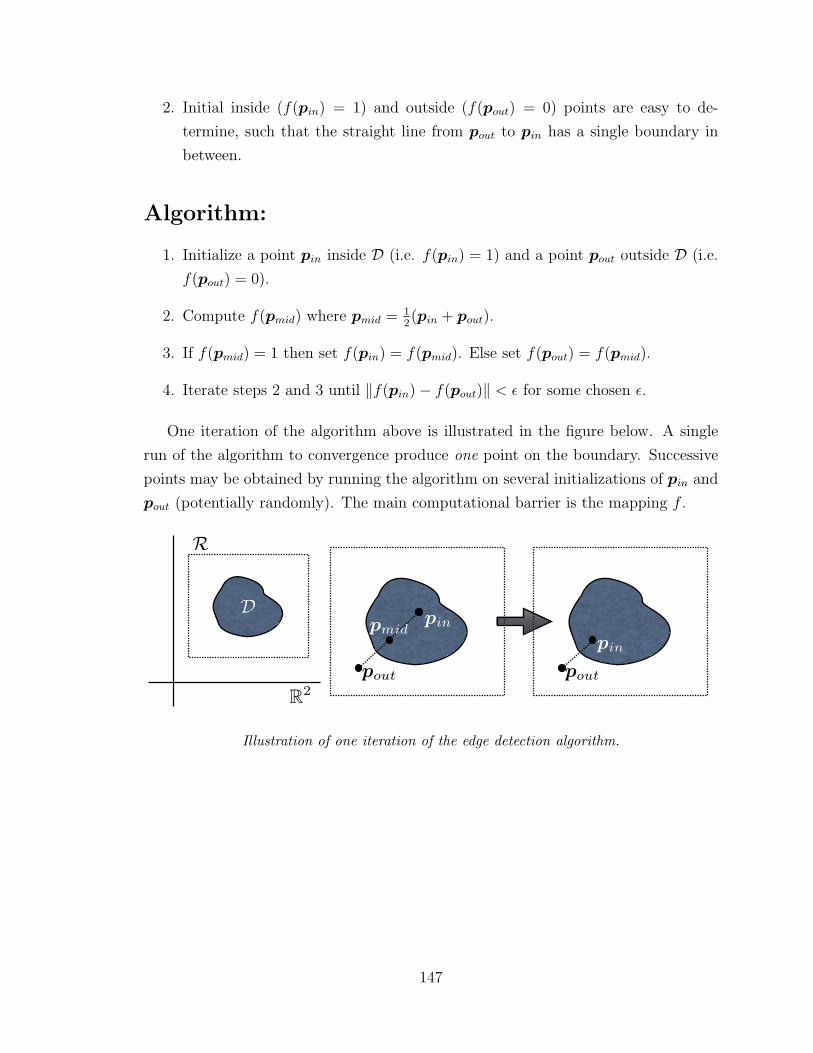
2. Initial inside (f(pin) = 1) and outside (f(pout) = 0) points are easy to de-

termine, such that the straight line from pout to pin has a single boundary in

between.

Algorithm:

1. Initialize a point pin inside D (i.e. f(pin) = 1) and a point pout outside D (i.e.

f(pout) = 0).

2. Compute f(pmid) where pmid = 12(pin + pout).

3. If f(pmid) = 1 then set f(pin) = f(pmid). Else set f(pout) = f(pmid).

4. Iterate steps 2 and 3 until ‖f(pin)− f(pout)‖ < ε for some chosen ε.

One iteration of the algorithm above is illustrated in the figure below. A single

run of the algorithm to convergence produce one point on the boundary. Successive

points may be obtained by running the algorithm on several initializations of pin and

pout (potentially randomly). The main computational barrier is the mapping f .

R2

R

Dpinpmid

pout

pin

pout

Illustration of one iteration of the edge detection algorithm.

147

Bibliography

[1] D. Aanen, P. Eggleton, C. Rouland-Lefevre, T. Guldberg-Frøslev,S. Rosendahl, and J. Boomsma, The evolution of fungus-growing termites andtheir mutualistic fungal symbionts, Proceedings of the National Academy of Sciences,99 (2002), pp. 14887–14892.

[2] R. Albert and A. L. Barabasi, Statistical mechanics of complex networks, Rev.Mod. Phys., 74 (2002), pp. 47–97.

[3] M. Ballerini, N. Cabibbo, R. Candelier, A. Cavagna, E. Cisbani, I. Giar-dina, V. Lecomte, A. Orlandi, G. Parisi, A. Procaccini, et al., Interactionruling animal collective behavior depends on topological rather than metric distance:Evidence from a field study, Proceedings of the National Academy of Sciences, 105(2008), pp. 1232–1237.

[4] A. Barabasi, H. Jeong, Z. Neda, E. Ravasz, A. Schubert, and T. Vicsek,Evolution of the social network of scientific collaborations, Physica A: Statistical Me-chanics and its Applications, 311 (2002), pp. 590–614.

[5] S. Bazazi, J. Buhl, J. Hale, M. Anstey, G. Sword, S. Simpson, andI. Couzin, Collective motion and cannibalism in locust migratory bands, CurrentBiology, 18 (2008), pp. 735–739.

[6] P. Berthold, A. Helbig, G. Mohr, and U. Querner, Rapid microevolution ofmigratory behaviour in a wild bird species, Nature, 360 (1992), pp. 668–670.

[7] A. Bladon, T. Galla, and A. McKane, Evolutionary dynamics, intrinsic noise,and cycles of cooperation, Physical Review E, 81 (2010), pp. 66122–66133.

[8] R. Bogacz, E. Brown, J. Moehlis, P. Holmes, and J. Cohen, The physicsof optimal decision making: a formal analysis of models of performance in two-alternative forced-choice tasks, Psychological Review, 113 (2006), pp. 700–765.

[9] R. Burger, Mathematical properties of mutation-selection models, Genetica, 102-103(1998), pp. 279–298.

[10] A. Cavagna, A. Cimarelli, I. Giardina, G. Parisi, R. Santagati, F. Ste-fanini, and M. Viale, Scale-free correlations in starling flocks, Proceedings of theNational Academy of Sciences, 107 (2010), pp. 11865–11870.

[11] A. Churchland, R. Kiani, and M. Shadlen, Decision-making with multiple al-ternatives, Nature Neuroscience, 11 (2008), pp. 693–702.

148

[12] P. Cisek, G. Puskas, and S. El-Murr, Decisions in changing conditions: theurgency-gating model, The Journal of Neuroscience, 29 (2009), pp. 11560–11571.

[13] I. Couzin and N. Franks, Self-organized lane formation and optimized traffic flowin army ants, Proceedings of the Royal Society of London. Series B: Biological Sci-ences, 270 (2003), pp. 139–146.

[14] I. Couzin, J. Krause, N. Franks, and S. Levin, Effective leadership and decision-making in animal groups on the move, Nature, 433 (2005), pp. 513–516.

[15] I. Couzin, J. Krause, R. James, G. Ruxton, and N. Franks, Collective memoryand spatial sorting in animal groups, Journal of Theoretical Biology, 218 (2002), pp. 1–11.

[16] C. Darwin, On the Origin of Species by Means of Natural Selection: or the Preserva-tion of Favored Races in the Struggle for Life, John Murray, Albemarle Street, 1st ed.,1859.

[17] S. Dehaene, The neural basis of the Weber–Fechner law: A logarithmic mentalnumber line, Trends in Cognitive Sciences, 7 (2003), pp. 145–147.

[18] O. Diekmann, A beginner’s guide to adaptive dynamics, Banach Center Publications,63 (2004), pp. 47–86.

[19] P. Erdos and A. Renyi, On the evolution of random graphs, in Publication of theMathematical Institute of the Hungarian Academy of Sciences, 1960.

[20] S. Eubank, H. Guclu, V. Kumar, M. Marathe, A. Srinivasan, Z. Toroczkai,and N. Wang, Modelling disease outbreaks in realistic urban social networks, Nature,429 (2004), pp. 180–184.

[21] P. Friedl and D. Gilmour, Collective cell migration in morphogenesis, regenera-tion and cancer, Nature Reviews Molecular Cell Biology, 10 (2009), pp. 445–457.

[22] J. Fryxell and A. Sinclair, Causes and consequences of migration by large her-bivores, Trends in Ecology & Evolution, 3 (1988), pp. 237–241.

[23] K. Galloway, E. Justh, and P. Krishnaprasad, Portraits of cyclic pursuit, inProc. 50th IEEE Conference on Decision and Control, 2011, pp. 2724–2731.

[24] C. Gardiner, Handbook of Stochastic Methods: for Physics, Chemistry and the Nat-ural Sciences, Springer, 4th ed., 2009.

[25] S. Geritz, E. Kisdi, G. Meszena, and J. Metz, Evolutionarily singular strategiesand the adaptive growth and branching of the evolutionary tree, Evolutionary Ecology,12 (1997), pp. 35–57.

[26] S. Geritz, J. Metz, E. Kisdi, and G. Meszena, Dynamics of adaptation andevolutionary branching, Physical Review Letters, 78 (1997), pp. 2024–2027.

[27] K. Ghose, T. K. Horiuchi, P. S. Krishnaprasad, and C. F. Moss, Echolocatingbats use a nearly time-optimal strategy to intercept prey, PLoS Biology, 4 (2006),pp. 0865–0873.

149

[28] D. Gilley, The identity of nest-site scouts in honeybee swarms, Apidologie, 29 (1998),pp. 229–240.

[29] M. Giurfa, J. Nunez, L. Chittka, and R. Menzel, Colour preferences of flower-naive honeybees, Journal of Comparative Physiology A: Neuroethology, Sensory, Neu-ral, and Behavioral Physiology, 177 (1995), pp. 247–259.

[30] J. Gould, Animal navigation: the evolution of magnetic orientation, Current Biol-ogy, 18 (2008), pp. R482–R484.

[31] J. Gould and W. Towne, Honey bee learning, Advances in Insect Physiology, 20(1988), pp. 55–86.

[32] J. Guckenheimer and P. Holmes, Nonlinear Oscillations, Dynamical Systems,and Bifurcations of Vector Fields, Springer, 2002.

[33] V. Guttal and I. Couzin, Social interactions, information use, and the evolutionof collective migration, Proceedings of the National Academy of Sciences, 107 (2010),pp. 16172–16177.

[34] , Leadership, collective motion and the evolution of migratory strategies, Com-municative & Integrative Biology, 4 (2011), pp. 294–298.

[35] V. Guttal, P. Romanczuk, S. Simpson, G. Sword, and I. Couzin, Cannibalismcan drive the evolution of behavioural phase polyphenism in locusts, Ecology Letters,15 (2012), pp. 1158–1166.

[36] K. Hadeler, Stable polymorphisms in a selection model with mutation, SIAM Journalon Applied Mathematics, 41 (1981), pp. 1–7.

[37] N. Handegard, K. Boswell, C. Ioannou, S. Leblanc, D. Tjøstheim, andI. Couzin, The dynamics of coordinated group hunting and collective informationtransfer among schooling prey, Current Biology, 22 (2012), pp. 1213 – 1217.

[38] T. Hanks, M. Mazurek, R. Kiani, E. Hopp, and M. Shadlen, Elapsed decisiontime affects the weighting of prior probability in a perceptual decision task, The Journalof Neuroscience, 31 (2011), pp. 6339–6352.

[39] D. Higham, An algorithmic introduction to numerical simulation of stochastic dif-ferential equations, SIAM Review, 43 (2001), pp. 525–546.

[40] J. Hofbauer and K. Sigmund, Evolutionary Games and Replicator Dynamics,Cambridge University Press, 1998.

[41] , Evolutionary game dynamics, Bulletin of the American Mathematical Society,40 (2003), pp. 479–520.

[42] R. Holland, M. Wikelski, and D. Wilcove, How and why do insects migrate?,Science, 313 (2006), pp. 794–796.

[43] R. Horn and C. Johnson, Matrix Analysis, Cambridge University Press, 1990.

[44] I. Hussein, An individual-based evolutionary dynamics model for networked socialbehaviors, in Proceedings of the American Control Conference, 2009, pp. 5789–5796.

150

[45] C. C. Ioannou, V. Guttal, and I. D. Couzin, Predatory fish select for coordinatedcollective motion in virtual prey, Science, 337 (2012), pp. 1212–1215.

[46] R. Isaacs, Differential Games: A Mathematical Theory with Applications to Warfareand Pursuit, Control and Optimization, Dover Publications, 1999.

[47] A. Jadbabaie, J. Lin, and A. Morse, Coordination of groups of mobile au-tonomous agents using nearest neighbor rules, IEEE Transactions on Automatic Con-trol, 48 (2003), pp. 988–1001.

[48] M. Janssen, Use of complex adaptive systems for modeling global change, Ecosys-tems, 1 (1998), pp. 457–463.

[49] S. E. Jorgensen, B. C. Patten, and M. Straskraba, Ecosystems emerging:toward an ecology of complex systems in a complex future, Ecological Modelling, 62(1992), pp. 1–27.

[50] E. Justh and P. Krishnaprasad, Steering laws for motion camouflage, Proceed-ings of the Royal Society A, 462 (2006), pp. 3629–3643.

[51] J. Karelahti, K. Virtanen, and T. Raivio, Near-optimal missile avoidance tra-jectories via receding horizon control, Journal of Guidance Control and Dynamics, 30(2007), pp. 1287–1298.

[52] S. Kato, S. Tsugawa, K. Tokuda, T. Matsui, and H. Fujii, Vehicle controlalgorithms for cooperative driving with automated vehicles and intervehicle communi-cations, IEEE Transactions on Intelligent Transportation Systems, 3 (2002), pp. 155–161.

[53] B. Kerr, M. Riley, M. Feldman, B. Bohannan, et al., Local dispersal promotesbiodiversity in a real-life game of rock-paper-scissors, Nature, 418 (2002), pp. 171–174.

[54] H. Khalil, Nonlinear Systems, Prenctice Hall, 3rd ed., 2002.

[55] N. Komarova, Replicator-mutator equation, universality property and populationdynamics of learning, Journal of Theoretical Biology, 230 (2004), pp. 227–239.

[56] N. Komarova and S. Levin, Eavesdropping and language dynamics, Journal ofTheoretical Biology, 264 (2010), pp. 104–118.

[57] N. Komarova, P. Niyogi, and M. Nowak, The evolutionary dynamics of grammaracquisition, Journal of Theoretical Biology, 209 (2001), pp. 43–59.

[58] S. Kotz, N. Johnson, and N. Balakrishnan, Continuous Multivariate Distribu-tions: Models and Applications, vol. 1, Wiley-Interscience, 2000.

[59] Y. Kuznetsov, Elements of Applied Bifurcation Theory, Springer, 1998.

[60] Y. Lee, T. Collier, C. Taylor, and R. Olfati-Saber, Simplicity from com-plexity: emergence of cohesion in the evolutionary dynamics of grammar networks,Evolutionary Ecology, 11 (2009), pp. 433–445.

[61] K. Lerman, A. Martinoli, and A. Galstyan, A review of probabilistic macro-scopic models for swarm robotic systems, Swarm Robotics, (2005), pp. 143–152.

151

[62] S. Levin, Complex adaptive systems: exploring the known, the unknown and theunknowable, Bulletin of the American Mathematical Society, 40 (2003), pp. 3–20.

[63] S. Levin and R. Durrett, From individuals to epidemics, Philosophical Trans-actions of the Royal Society of London. Series B: Biological Sciences, 351 (1996),pp. 1615–1621.

[64] Z. Lin, B. Francis, and M. Maggiore, Necessary and sufficient graphical condi-tions for formation control of unicycles, IEEE Transactions on Automatic Control,50 (2005), pp. 121–127.

[65] S. Mannor and J. Shamma, Multi-agent learning for engineers, Artificial Intelli-gence, 171 (2007), pp. 417–422.

[66] S. Marras and M. Porfiri, Fish and robots swimming together: attraction towardsthe robot demands biomimetic locomotion, Journal of The Royal Society Interface, 9(2012), pp. 1856–1868.

[67] J. Marshall, Coordinated autonomy: Pursuit formations of multivehicle systems,PhD thesis, University of Toronto, Toronto, Ontario, Canada, 2005.

[68] J. Marshall, M. Broucke, and B. Francis, Formations of vehicles in cyclicpursuit, IEEE Transactions on Automatic Control, 49 (2004), pp. 1963–1974.

[69] , Pursuit formations of unicycles, Automatica, 42 (2006), pp. 3–12.

[70] J. A. R. Marshall, Group selection and kin selection: formally equivalent ap-proaches, Trends in Ecology & Evolution, 26 (2011), pp. 325–332.

[71] J. A. R. Marshall, R. Bogacz, A. Dornhaus, R. Planque, T. Kovacs, andN. Franks, On optimal decision-making in brains and social insect colonies, Journalof the Royal Society Interface, 6 (2009), pp. 1065–1074.

[72] B. T. Milne, Motivation and benefits of complex systems approaches in ecology,Ecosystems, 1 (1998), pp. 449–456.

[73] M. Mitchell, An Introduction to Genetic Algorithms, Bradford, 1998.

[74] W. Mitchener, A Mathematical Model of Human Languages: The Interaction ofGame Dynamics & Learning Processes, Princeton University, 2003.

[75] , Bifurcation analysis of the fully symmetric language dynamical equation, Jour-nal of Mathematical Biology, 46 (2003), pp. 265–285.

[76] W. Mitchener and M. Nowak, Chaos and language, Proceedings of the RoyalSociety B: Biological Sciences, 271 (2004), pp. 701–704.

[77] A. Mizutani, J. Chahl, and M. Srinivasan, Motion camouflage in dragonflies,Nature, 423 (2003), pp. 604–605.

[78] B. Nabet, Dynamics and Control in Natural and Engineered Multi-Agent Systems,PhD thesis, Princeton University, Princeton, NJ, 2009.

152

[79] R. Nagpal, S. Berman, and A. Halasz, Optimization of stochastic strategies forspatially inhomogeneous robot swarms: A case study in commercial pollination, inProceedings of the International Conference on Intelligent Robots and Systems, 2011,pp. 25–30.

[80] P. Nahin, Chases and Escapes: The Mathematics of Pursuit and Evasion, PrincetonUniversity Press, 2007.

[81] F. Neuman, On the approximate solution of complex combat games., Journal of Guid-ance, Control, and Dynamics, 13 (1990), pp. 128–136.

[82] M. Newman, Models of the small world, Journal of Statistical Physics, 101 (2000),pp. 819–841.

[83] M. Newman, S. Strogatz, and D. Watts, Random graphs with arbitrary degreedistributions and their applications, Physical Review E, 64 (2001), pp. 026118–026133.

[84] M. Nowak, Five rules for the evolution of cooperation, Science, 314 (2006), pp. 1560–1563.

[85] M. Nowak, N. Komarova, and P. Niyogi, Evolution of universal grammar, Sci-ence, 291 (2001), pp. 114–118.

[86] M. Nowak and K. Sigmund, Chaos and the evolution of cooperation, Proceedingsof the National Academy of Sciences, 90 (1993), pp. 5091–5094.

[87] , Evolutionary dynamics of biological games, Science, 303 (2004), pp. 793–799.

[88] M. Nowak, C. Tarnita, and E. Wilson, The evolution of eusociality, Nature, 466(2010), pp. 1057–1062.

[89] S. Okasha, Altruism researchers must cooperate, Nature, 467 (2010), pp. 653–655.

[90] R. Olfati-Saber, Evolutionary dynamics of behavior in social networks, in 46thIEEE Conference on Decision & Control, 2007, pp. 4051–4056.

[91] R. Olfati-Saber, J. Fax, and R. Murray, Consensus and cooperation in net-worked multi-agent systems, Proceedings of the IEEE, 95 (2007), pp. 215–233.

[92] K. Page and M. Nowak, Unifying evolutionary dynamics, Journal of TheoreticalBiology, 219 (2002), pp. 93–98.

[93] D. Pais, C. Caicedo-Nunez, and N. Leonard, Hopf bifurcations and limit cyclesin evolutionary network dynamics, SIAM Journal on Applied Dynamical Systems, (inpress).

[94] D. Pais, M. Cao, and N. Leonard, Formation shape and orientation control us-ing projected collinear tensegrity structures, in Proceedings of the American ControlConference, IEEE, 2009, pp. 610–615.

[95] D. Pais, P. Hogan, T. Schlegel, N. Franks, N. Leonard, and J. A. R.Marshall, Value-sensitive decision-making in a model of collective choice, (in prep).

153

[96] D. Pais and N. Leonard, Pursuit and evasion: Evolutionary dynamics and collec-tive motion, in Proceedings of the AIAA Guidance, Navigation and Control confer-ence, 2010, DOI: 10.2514/6.2010-7584.

[97] , Limit cycles in replicator-mutator network dynamics, in Proceedings of the 50thIEEE Conference on Decision and Control, 2011, pp. 3922 –3927.

[98] D. Paley, N. Leonard, R. Sepulchre, D. Grunbaum, and J. Parrish, Os-cillator models and collective motion, Control Systems Magazine, IEEE, 27 (2007),pp. 89–105.

[99] J. Palmer, A. Huk, and M. Shadlen, The effect of stimulus strength on the speedand accuracy of a perceptual decision, Journal of Vision, 5 (2005).

[100] M. Peixoto, Structural stability on two dimensional manifolds, Topology, 1 (1962),pp. 101–120.

[101] M. Pontani and B. Conway, Optimal interception of evasive missile warheads: nu-merical solution of the differential game, Journal of Guidance Control and Dynamics,31 (2008), pp. 1111–1122.

[102] T. Poston and I. Stewart, Catastrophe Theory and its Applications, vol. 2, DoverPublications, 1996.

[103] I. Poulakakis, L. Scardovi, and N. Leonard, Coupled stochastic differentialequations and collective decision making in the two-alternative forced-choice task, inProceedings of the American Control Conference (ACC), 2010, pp. 69 –74.

[104] , Node certainty in collective decision making, in Proceedings of the Conferenceon Decision and Control (CDC), IEEE, 2012 to appear.

[105] G. Price, Selection and covariance, Nature, 227 (1970), pp. 520–21.

[106] , Extension of covariance selection mathematics, Annals of Human Genetics, 35(1972), pp. 485–490.

[107] A. Rahmani, M. Ji, M. Mesbahi, and M. Egerstedt, Controllability of multi-agent systems from a graph-theoretic perspective, SIAM Journal of Control and Opti-mization, 48 (2009), pp. 162–186.

[108] T. Raivio and H. Ehtamo, Visual aircraft identification as a pursuit-evasion game,Journal of Guidance, Control and Dynamics, 23 (2000), pp. 701–708.

[109] R. Ratcliff and J. Rouder, Modeling response times for two-choice decisions,Psychological Science, 9 (1998), pp. 347–356.

[110] W. Ren, Multi-vehicle consensus with a time-varying reference state, Systems &Control Letters, 56 (2007), pp. 474–483.

[111] W. Ren, R. Beard, and T. McLain, Coordination variables and consensus buildingin multiple vehicle systems, V. Kumar, N.E. Leonard, A.S. Morse (Eds.), CooperativeControl: Lecture Notes in Control and Information Sciences, (2005), pp. 439–442.

154

[112] P. Romanczuk, I. Couzin, and L. Schimansky-Geier, Collective motion due toindividual escape and pursuit response, Physical Review Letters, 102 (2009), p. 10602.

[113] W. Rugh, Linear System Theory, Prentice-Hall, Inc., 1996.

[114] E. Sahin, Swarm robotics: From sources of inspiration to domains of application,Swarm Robotics, (2005), pp. 10–20.

[115] T. Seeley, Consensus building during nest-site selection in honey bee swarms: theexpiration of dissent, Behavioral Ecology and Sociobiology, 53 (2003), pp. 417–424.

[116] , Honeybee Democracy, Princeton University Press, 2010.

[117] T. Seeley and P. Visscher, Sensory coding of nest-site value in honeybee swarms,Journal of Experimental Biology, 211 (2008), pp. 3691–3697.

[118] T. Seeley, P. Visscher, T. Schlegel, P. Hogan, N. Franks, and J. A. R.Marshall, Stop signals provide cross inhibition in collective decision-making by hon-eybee swarms, Science, 335 (2012), pp. 108–111.

[119] A. Shaw and S. Levin, To breed or not to breed: a model of partial migration, Oikos,120 (2011), pp. 1871–1879.

[120] S. J. Simpson and G. A. Sword, Evolving migration, Proceedings of the NationalAcademy of Sciences, 107 (2010), pp. 16753–16754.

[121] B. Sinervo and C. Lively, The rock-paper-scissors game and the evolution of al-ternative male strategies, Nature, 380 (1996), pp. 240–243.

[122] J. Smith, Evolution and the Theory of Games, Cambridge University Press, 1982.

[123] M. V. Srinivasan and S. Zhang, Visual motor computations insects, Annual Re-view of Neuroscience, 27 (2004), pp. 679–696.

[124] P. Stadler and P. Schuster, Mutation in autocatalytic reaction networks, Journalof Mathematical Biology, 30 (1992), pp. 597–632.

[125] S. Strogatz, Nonlinear Dynamics and Chaos: with Applications to Physics, Biology,Chemistry, and Engineering, Westview Press, 1994.

[126] D. Sumpter, Collective animal behavior, Princeton University Press, 2010.

[127] M. Surette, M. Miller, and B. Bassler, Quorum sensing in escherichia coli,salmonella typhimurium, and vibrio harveyi: a new family of genes responsible forautoinducer production, Proceedings of the National Academy of Sciences, 96 (1999),pp. 1639–1644.

[128] D. Swain, I. Couzin, and N. Leonard, Real-time feedback-controlled robotic fishfor behavioral experiments with fish schools, Proceedings of the IEEE, 100 (2012),pp. 150 –163.

[129] P. Taylor and L. Jonker, Evolutionary stable strategies and game dynamics,Mathematical Biosciences, 40 (1978), pp. 145–156.

155

[130] H. Tembine, E. Altman, R. El-Azouzi, and Y. Hayel, Evolutionary games inwireless networks, IEEE Transactions on Systems, Man, and Cybernetics, Part B, 40(2010), pp. 634–646.

[131] L. Tesfatsion, Economic agents and markets as emergent phenomena, Proceedingsof the National Academy of Sciences, 99 (2002), pp. 7191–7192.

[132] C. Torney, S. Levin, and I. Couzin, Specialization and evolutionary branchingwithin migratory populations, Proceedings of the National Academy of Sciences, 107(2010), pp. 20394–20399.

[133] C. Torney, Z. Neufeld, and I. Couzin, Context-dependent interaction leads toemergent search behavior in social aggregates, Proceedings of the National Academyof Sciences, 106 (2009), pp. 22055–22060.

[134] A. Traulsen, J. Claussen, and C. Hauert, Coevolutionary dynamics: from finiteto infinite populations, Physical Review Letters, 95 (2005), pp. 238701–238704.

[135] , Coevolutionary dynamics in large, but finite populations, Physical Review E, 74(2006), pp. 11901–11908.

[136] X. Trepat, M. Wasserman, T. Angelini, E. Millet, D. Weitz, J. Butler,and J. Fredberg, Physical forces during collective cell migration, Nature Physics,5 (2009), pp. 426–430.

[137] G. Uhlenbeck and L. Ornstein, On the theory of the brownian motion, PhysicalReview, 36 (1930), p. 823.

[138] C. Urmson, J. Anhalt, D. Bagnell, C. Baker, R. Bittner, M. Clark,J. Dolan, D. Duggins, T. Galatali, C. Geyer, et al., Autonomous drivingin urban environments: Boss and the urban challenge, Journal of Field Robotics, 25(2008), pp. 425–466.

[139] N. Van Kampen, Stochastic Processes in Physics and Chemistry, vol. 1, North Hol-land, 1992.

[140] N. Vickers, Mechanisms of animal navigation in odor plumes, The Biological Bul-letin, 198 (2000), pp. 203–212.

[141] T. Vincent and J. Brown, Evolutionary Game Theory, Natural Selection, andDarwinian Dynamics, Cambridge University Press, 2005.

[142] T. Vincent and T. Vincent, Evolution and control system design: The evolution-ary game, Control Systems Magazine, IEEE, 20 (2000), pp. 20–35.

[143] P. Visscher, Group decision making in nest-site selection among social insects, An-nual Reviews Entomology, 52 (2007), pp. 255–275.

[144] K. Von Frisch, The Dance Language and Orientation of Bees, Harvard UniversityPress, 1967.

[145] Y. Wang and I. Hussein, Evolutionary bandwidth allocation and routing in large-scale wireless sensor networks, in Proceedings of the American Control Conference,2010, pp. 1850–1855.

156

[146] D. J. Watts and S. H. Strogatz, Collective dynamics of ‘small-world’ networks,Nature, 393 (1998), pp. 440–442.

[147] E. Wei, E. Justh, and P. Krishnaprasad, Pursuit and an evolutionary game,Proceedings of the Royal Society A, 465 (2009), pp. 1539–1559.

[148] J. Weibull, Evolutionary Game Theory, The MIT press, 1997.

[149] E. Wilson, Caste and division of labor in leaf-cutter ants (hymenoptera: Formicidae:Atta), Behavioral Ecology and Sociobiology, 14 (1983), pp. 47–54.

[150] R. Wood, The first takeoff of a biologically inspired at-scale robotic insect, IEEETransactions on Robotics, 24 (2008), pp. 341–347.

[151] G. Young, L. Scardovi, and N. Leonard, Robustness of noisy consensus dynam-ics with directed communication, in Proceedings of the American Control Conference,2010, pp. 6312–6317.

157