Emerging collective behavior and local properties of financial dynamics in a public investment game

ARTICLE IN PRESS

0378-4371/$ - se

doi:10.1016/j.ph

�CorrespondE-mail addr

[email protected]

Physica A 371 (2006) 610–626

www.elsevier.com/locate/physa

Emerging collective behavior and local properties of financialdynamics in a public investment game

Roberto da Silvaa,�, Ana L.C. Bazzana, Alexandre T. Baravierab, Sılvio R. Dahmenc

aInstituto de Informatica, Universidade Federal do Rio Grande do Sul, BrazilbInstituto de Matematica, Universidade Federal do Rio Grande do Sul, Brazil

cInstituto de Fısica, Universidade Federal do Rio Grande do Sul, Brazil

Received 18 January 2006; received in revised form 2 March 2006

Available online 2 May 2006

Abstract

In this paper we consider a simple model of a society of economic agents, namely a variation of the well known ‘‘public

investment game,’’ where each agent can contribute with a discrete quantity, i.e., cooperate to increase the benefits of the

group. Interactions take place among nearest neighbors and depend on the motivation level (insider information, economy

prospects). The profit is used to update individual motivations. We first explore a deterministic scenario and the existence

of fixed points and attractors. We also consider the presence of noise, where profits fluctuate stochastically. In this scenario

we analyze the global persistence as a function of time—a measure of the probability that the amount of money of the

entire group remains at least equal to its initial value. Our simulations show that this quantity has a power law behavior.

We have also performed simulations with a population of heterogeneous agents, including deceivers and conservatives. We

show that, although there is no regular pattern regarding the average wealth, robust power laws for persistence do exist

and argue that this can be used to characterize the emerging collective behavior. The influence of the motivation updating

and the presence of conservatives and deceivers on persistence is also studied. Simulations for the local persistence

exploring two different versions of this concept: the probability of a particular agent not going bankrupt (i.e., remaining

wealth X0 up to time t) and the probability of a particular agent making more money than he initially had. Different

power law behaviors are also observed in these situations.

r 2006 Elsevier B.V. All rights reserved.

Keywords: Public investment game; Dynamical systems; Monte Carlo simulations

1. Introduction

Quantifying probabilities of financial damages of an investor group is a complex task given the largenumber of relevant variables, which depend not only on characteristics of financial agents, but also on howthey interact and peculiarities of companies where the investment will be performed, be it public or private.

e front matter r 2006 Elsevier B.V. All rights reserved.

ysa.2006.03.051

ing author.

esses: [email protected] (R. da Silva), [email protected] (A.L.C. Bazzan), [email protected] (A.T. Baraviera),

gs.br (S.R. Dahmen).

www.elsevier.com/locate/physa

dx.doi.org/10.1016/j.physa.2006.03.051

mailto:[email protected]




ARTICLE IN PRESSR. da Silva et al. / Physica A 371 (2006) 610–626 611

In the fields of complex systems in statistical mechanics as well as of multiagent systems there is an extensivelist of publications on nontrivial phenomena which arise due to the interplay between microscopic (individual)rules and macroscopic (group) behavior (see Refs. [1,2] for other references). In the context of socioeconomicbehavior this has been thoroughly discussed by Durlauf [3]. In this paper we are interested in simulating thedynamics of models based on the so called ‘‘public investment game’’ [4] and understanding its properties. Theapproach is more descriptive than normative, given that it allows the study of the influence of individuals onmacroscale.

In its original version this game assumes that one wishes to model public spending on some work for thecommunity: roads, bridges, libraries. Players are offered the opportunity to invest their money into a commonpool, and profits (obtained from tolls, membership fees) are equally distributed among all participantsirrespective of their contributions. Clearly it would be ‘‘fair’’ for people with similar amounts of money to paythe same quantity for those items. However individuals are different, as they have different social conditionswhich means that some can invest less than others. Each player, being ‘‘blind’’ as to what regards others’contributions, would, if it were also ‘‘rational,’’ default and invest nothing. Thus for purely rational playersthe dominant solution is to default.

In order to give this model a realistic taste, we let agents interact and invest taking into account the actionsof their immediate neighbors, as controlled by a binary variable we call ‘‘motivation,’’ whose update dependson a random variable. For example, whether or not a road is well built is a random event once this depends onweather, quality of building materials, and these may affect how players evaluate the investment.

The return per agent is a function of the average investment, in a close relation to cooperative game-theory.Later, we analyze noncooperative situations and associate some personalities to agents, analyzing how specificidiosyncratic types perform. In particular we are interested in the influence of deceivers, a version of the egoistagents which appeared in the context of the Iterated Prisoners’ Dilemma in Ref. [5].

Our analysis is centered on the concept of local [6,7] and global persistence [8]. The former derives from theworks about coarsening phenomena in spins systems at zero temperature, here denoted by QðtÞ. The latter is acollective version of this concept, denoted PðtÞ, consisting of a order parameter to study critical phenomena inspin systems. In this paper, both measures were adapted to a game-theoretical context such as the probabilityof keeping a positive balance relative to the initial amount invested. Particularly, we analyzed the scalingeffects and the influence of some kind of special economic agents on the model.

This paper is organized as follows: in the next section we briefly discuss stochastic processes and the conceptof persistence in a financial context. In Section 3 we present our model and the definition of the updating rulesfor a society of L economic agents. We first study the deterministic case in Section 4, followed by Monte Carlo(MC) simulations for the global ðPðtÞÞ as well as in the local ðQðtÞÞ persistence in Section 5 and conclude withSection 6.

2. Stochastic processes and persistence in financial markets

Economic analyses have recently encompassed interactions among individuals, as opposed to individual-specific determinants of behavior, in the set of causal factors governing game decisions. This has led to achange in the mathematical apparatus from deterministic to stochastic approaches [3]. An interesting and wellknown quantity in the theory of stochastic process is the probability of a random variable to return to itsinitial condition for the first time, also called first return probability [9,10].

For example, a random walker is called recurrent relative to a site of the lattice if after a finite number ofsteps it returns to this same site. Polya’s theorem [10], asserts that in d ¼ 1 or 2 this return always occurs,whereas in d ¼ 3 this does not necessarily happen. This means there is a chance the random walker will neverreturn to the point from where it started.

In the context of games, simple questions can be posed such as the necessary time for a gambler that hasstarted a bridge game with a certain quantity of money to go bankrupt or for two gamblers to reach a draw [9].

In fact, a simple game of heads or tails with an unbiased coin can lead to a nontrivial behavior when we lookfor the distribution of first time passage (or first time return). Defining a random variable, such that xi ¼ þ1(head) and xi ¼ �1 (tail), the first time passage can be defined as the instant of time (number of the trials heredenoted by n) in which the random variable Sn ¼

Pni¼1xi assumes a null value for the first time. The first time

ARTICLE IN PRESSR. da Silva et al. / Physica A 371 (2006) 610–626612

passage distribution is known for this case [9] and has a asymptotic polynomial behavior in the limit n!1,namely pn�n�3=2, where pn is the probability of the first time passage occurring at instant n.

These ideas can be used in many different contexts, as for example in population dynamics in biology: giventhat a population has dwindled due to some plague, how much time will it take for them to recover theiroriginal population, if ever? An analogy with public investment model is also straightforward: if a member of agroup starts with a certain amount of money invested in assets, how long does it take for him to get at least thevalue initially invested?

As in population dynamics, agents in a public investment game are not alone and their individual actionscannot usually alter significantly the dynamics. However, their collective behavior, as for example the sellingstampede caused by some expectation of political turmoil may lead the whole systems to insolvency. There areextrinsic factors which may affect the dynamics of the game, but it is unquestionable that agents do play asignificant role when acting as a group. Such complex behavior which arises from collective actions has beenextensively studied in the context of nonequilibrium processes in statistical mechanics.

Among the many relevant quantities of interest in the modelling of nonequilibrium dynamics of complexsystems there is the concept of persistence, i.e., the characterization of the time it takes for a particular quantitynot to change its state from its given t ¼ 0 configuration. For the sake of clarity, we take an example from thefield of nonequilibrium spin dynamics: defining QðtÞ as the probability that a particular spin will not flip up totime t, for zero temperature and for the Ising and Potts models this quantity was shown to behave as [6,7]

QðtÞ�t�yl , (1)

where the persistence exponent yl describes the nonequilibrium relaxation of the system. This has beendetermined through coarsening simulations since one expects that the fraction of spins which do not change upto t represents a good estimate of QðtÞ. From dynamics at T ¼ 0, the behavior (1) has been observed in manyspins systems such as q-states Potts Model [6,7] and the Blume Capel model [11].

Basically, this quantity is measured by taking the fraction of spins that have not changed since the beginningof the simulation. For this purpose, Metropolis, Glauber and Gibbs sampling dynamics can be used, adaptingin the limit T ! 0, because the dynamics in this condition is greatly affected by local blocking configurations.

This information is local and in the context of game theorical MC simulations should answer questionsabout probabilities associated to financial damages of a particular player. However we also might be interestedin knowing about the money of a set of economic agents. In Ref. [8] a global definition of persistence wasintroduced and defined as the probability PðtÞ for the random variable Cðt0Þ ¼ jðt0Þ � hjðt0Þi, associated to anorder parameter jðt0Þ not to change its sign up to time t. More specifically these ideas were applied in Ref. [8]for the Ising Model, where at ðT ¼ TcÞ the global persistence has the same polynomial behavior characterizedby power law (1), characterized for exponent ygðPðtÞ�t�ygÞ. These ideas can be extended to other systems too[12,13].

Within this scenario, one of our goals is to characterize the statistical properties of the our modifiedeconomic game introduced next. For this purpose, we have performed a series of MC simulations for a gamewhere the investment is made by agents depending on the actions of its nearest neighbors and their motivation,as explained next. This parameter is updated as a function of the profit of the group. The global and localpersistence are analyzed and a scaling study is performed.

The definition of the model and the use of the global persistence for its characterization were recentlyexplored in Ref. [14]. Here, an extension of this model is presented to include more general aspects as well as adescription of the local aspects.

3. The model

We consider a game of L investors or economic agents, each of which, starting the game with a quantity w0

of money, can invest a particular quantity Si 2 f0; 1; 2g. Agents invest cooperatively, in the sense that theaverage of the profit of the group influences the investment ‘‘motivation’’ level of each agent. This motivationlevel is modelled by a binary variable si 2 f0; 1g, where si ¼ 1 means that the agent is motivated and si ¼ 0means that it is not. This abstraction aims at capturing issues such as insider information and economicprospects as perceived by agents.

ARTICLE IN PRESS

Table 1

Investment rules mapping motivation levels to investment, for each pair of agents

Motivation level Investment level

si ¼ 1 and siþ1 ¼ 1 Si ¼ 2

si ¼ 0 and siþ1 ¼ 1 Si ¼ 1

si ¼ 1 and siþ1 ¼ 0 Si ¼ 1

si ¼ 0 and siþ1 ¼ 0 Si ¼ 0

R. da Silva et al. / Physica A 371 (2006) 610–626 613

The algorithm that describes the evolution of dynamics of the group is locally constrained, meaning that eachagent interacts only with its two closest neighbors. Thus, each time an interaction occurs, it is between agents labelledi and i þ 1 (i � 1 also interacts with i on its turn). The interaction rules are presented in Table 1. As one may seefrom this table, if an agent is unmotivated it influences its neighbor as to make him invest less than it actually could.

To update the motivation level of the agents, we represent the average investment of all agents in the tthiteration as

SðtÞ ¼1

L

XL

k¼1

SkðtÞ ¼1

L

XL

k¼1

½sk�1ðtÞ þ skðtÞ� ¼2

L

XL

k¼1

skðtÞ, (2)

where periodic boundary conditions are assumed.To keep the model simple we assume at this stage that the overall profit is modulated by a random variable r

(noise) uniformly distributed in r 2 ½�1; 1�, and the return per agent is given by

gkðtÞ ¼ 2½aþ br�

L

XL

j¼1

sjðtÞ � sk�1ðtÞ � skðtÞ. (3)

According to this formula, when b ¼ 0 we have the deterministic case. On the other hand, if a ¼ 1 and b ¼ 12,

profits ð0oro1Þ and losses ð�1oro0Þ are allowed only within a range which depends on the meaninvestment SðtÞ. Individually agents can be better off or not. Besides, at each time each agent has anaccumulated wealth given by

W kðtþ 1Þ ¼W kðtÞ þ gkðtÞ, (4)

where W kð1Þ ¼ w0, k ¼ 1; . . . ;L. We update the motivation at each time step by the profit rate gkðtÞ:

skðtþ 1Þ ¼

1

21þ

gkðtÞ

jgkðtÞj

� �if gkðtÞa0;

0 otherwise:

8<: (5)

This update is based on a simple principle: an agent’s wealth relies on the wealth of the group. However,since agents are autonomous and there is room for cheating, we end up with two kinds of situations: one inwhich everyone is cooperative, and another where different types of individual behaviors are simulated. Wewill first explore this public investment game for the case b ¼ 0, i.e., without noise.

4. Deterministic case ðb ¼ 0Þ

Let us denote r0 ¼PL

k¼1skð0Þ=L the initial density of optimists (agents that have motivation level equal to1). Since for b ¼ 0, r0 ¼ 0 (all agents unmotivated) is a fixed point of the model (nobody invests, no matter thevalue of a), in what follows we will consider only the case r040. Then the total investment (contributionof all agents) is g ¼

PLk¼1ðsk�1 þ skÞ ¼ 2

PLk¼1sk ¼ 2Lr0. Hence, the profit per agent is given by

gk ¼ að2r0L=LÞ � sk � sk�1 ¼ 2r0a� sk � sk�1. For a global profit, clearly, we have to impose the globalcondition

PLk¼1gk ¼ 2ar� 2r40) a41.

We turn our attention first to the case of global financial losses, i.e., ao1. For this case if we start with aconfiguration s1 ¼ ðs1; . . . ;sLÞ ¼ ð1; 1; . . . 1Þ, i.e., r0 ¼ 1, for the first investment, all agents will lose moneyand the next configuration is the fixed point where all agents are unmotivated, s ¼ s0 ¼ ð0; 0; . . .Þ.


Let us now assume a41; then it is easy to show that the state r ¼ 1 is also a fixed point of the model. Usingthe expression of the profit per agent we see that r041=a implies gk40 for all k, i.e., the profit is positive evenfor the agents who have invested 2. Thus all motivated participants remain motivated and the unmotivatedones (agents that did not invest money) change their motivation to 1.

Now consider a41 and the density such that 0oroð12Þð1� 1=aÞ. We are interested in those agents that will

flip to 1 in the next step. To estimate their number, we bind those elements that will flip to 0: consider aconfiguration C composed by a set E1;01 of elements of the sequence that are 1 or 0 with a 1 as its left neighborand by the complement of E1;01, i.e., a sequence of elements that are 0:

C � 1010 . . . 10|fflfflfflfflfflfflffl{zfflfflfflfflfflfflffl}The set E1;01

0000 . . . 00|fflfflfflfflfflfflffl{zfflfflfflfflfflfflffl}The complement of E1;01

. (6)

Clearly, the image of each point in E1;01 is 0. The cardinality of this set is at most twice the cardinality of 1’s inthe initial configuration, i.e., it is smaller than 2n1 (n1 being the numbers of 1’s in the configuration); hence, thecomplementary set has cardinality larger than L� 2n1 ¼ L� 2Lr. The image of each point on thiscomplementary set, which is 0 with a 0 as its left neighbor, is 1 and so after one step we have the density of 1’slarger than ð1=LÞðL� 2LrÞX1� 2rX1=a, above the threshold. This implies that in the second step all pointsflip to 1 and the state s1 ¼ ð1; . . . ; 1Þ is reached again.

In the remaining cases our simulations show two distinct behaviors: either oscillatory (between twodensities) or going to s0 or s1. We can illustrate both with the following examples.

First, assuming a ¼ 0:5, r0 ¼ 0:6 and considering the initial configuration C ¼ ð0; 1; 1; 1; 0Þ for n ¼ 5 agents,the dynamics (p.b.c.) is given by

step 1 : 01110 : r1 ¼ 0:6;

step 2 : 10000 : r2 ¼ 0:2;

step 3 : 00111 : r1 ¼ 0:6;

step 4 : 01000 : r2 ¼ 0:2;

step 5 : 10011 : r1 ¼ 0:6;

..

.

As described above, this is an oscillatory behavior which may convey the wrong idea that some density cancreate oscillations. For example, take C0 ¼ ð1; 0; 1; 1; 0Þ, with exactly the same initial density. In this case wehave:

step 1 : 10110 : r1 ¼ 0:6;

step 2 : 00000 : r2 ¼ 0:0;

..

.

To understand this situation we need to explore the fact that our model can be seen as a kind of cellularautomata (CA). In fact, the dynamics of the model can be described by the way it maps 00, 01, 10 and 11 into 0or 1. But this mapping depends on the density, since the profit per agent is density-dependent. In some cases,like in the first example above, the mapping is

f : 00 7!1; 01; 10; 11 7!0.

In the second example we have the iteration of this map f and also of

00; 01; 10; 11 7!0.

After step 2 the mapping leads to a fixed point. Another CA that may appear in our dynamics is

g: 00; 01; 10 7!1; 11 7!0.

For the cases where only one CA map (f or g) is iterated, it can be rigorously shown [15] that the long-timebehavior is exactly an oscillation between two values of the density, and after two iterations the only effect is ashift of the initial configuration, as can be seen in the first example above.

ARTICLE IN PRESS

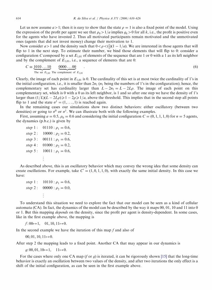
Fig. 1. Phase diagram for the game in the case b ¼ 0.


The condition for the occurrence of this behavior is the following: for map f, it is necessary that theinequality 2ar� 1o0, i.e., ro1=ð2aÞ hold for all densities as one iterates. This holds only if we assume ap0:5.

For map g, the conditions are 2ar� 140 and 2ar� 2o0 for all densities during iterations. We could notfind an easy way to ensure these conditions for a given configuration and so those cases remain as an object offurther study. But, supported by numerical evidences (see figures in the next section), we conjecture that,independent of the initial configuration, the map either goes to an oscillatory state (between two densities) orconverges to a fixed point s0 or s1.

Fig. 1 summarizes all possibilities for the dynamical system in a phase diagram.Region I represents the situation where the system is attracted to an oscillatory behavior between pairs of

densities, except for r0 ¼ 1 or 0. In these two cases, the system is attracted to the fixed point r ¼ 0. In regionII, numerical results (see next section) show that the system is either attracted to r ¼ 1 or oscillates betweentwo densities (no other situation was observed). In region III, the system is always attracted to r ¼ 1.

4.1. Numerical experiments

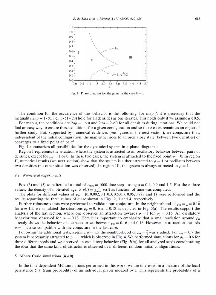
Eqs. (3) and (5) were iterated a total of tmax ¼ 1000 time steps, using a ¼ 0:1, 0.9 and 1.5. For these threevalues, the density of motivated agents rðtÞ ¼

PLi¼1siðtÞ as function of time was computed.

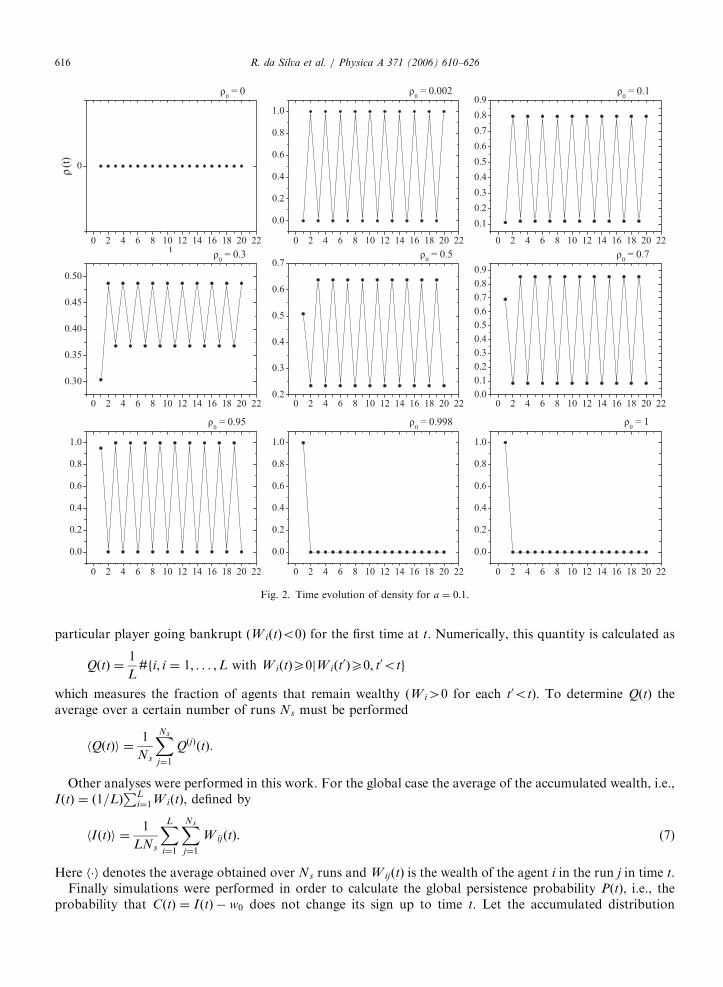
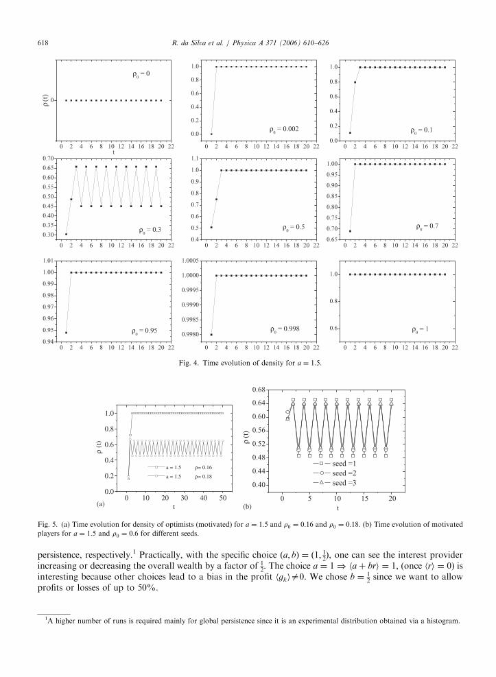
The plots for different values of r0 ¼ ð0; 0:002; 0:1; 0:3; 0:5; 0:7; 0:95; 0:998 and 1Þ were performed and theresults regarding the three values of a are shown in Figs. 2, 3 and 4, respectively.

Further robustness tests were performed to validate our conjecture. In the neighborhood of r0 ¼16¼ 0:16

for a ¼ 1:5, we simulated the situations r0 ¼ 0:16 and 0.18 as depicted in Fig. 5(a). The results support theanalysis of the last section, where one observes an attraction towards r ¼ 1 for r0 ¼ 0:16. An oscillatorybehavior was observed for r0 ¼ 0:18. Here it is important to emphasize that a small variation around r0already shows the behavior one expects to see between r0 ¼ 0:16 and 0.18. However an attraction towardsr ¼ 1 is also compatible with the conjecture in the last case.

Following the additional tests, keeping a ¼ 1:5 the neighborhood of r0 ¼23was studied. For r0 ¼ 0:7 the

system is necessarily attracted to r ¼ 1 which is observed in Fig. 4. We performed simulations for r0 ¼ 0:6 forthree different seeds and we observed an oscillatory behavior (Fig. 5(b)) for all analyzed seeds corroboratingthe idea that the same kind of attractor is observed over different random initial configurations.

5. Monte Carlo simulations (ba0)

In the time-dependent MC simulations performed in this work, we are interested in a measure of the localpersistence QðtÞ (ruin probability) of an individual player indexed by i. This represents the probability of a

ARTICLE IN PRESS

Fig. 2. Time evolution of density for a ¼ 0:1.

R. da Silva et al. / Physica A 371 (2006) 610–626616

particular player going bankrupt ðW iðtÞo0Þ for the first time at t. Numerically, this quantity is calculated as

QðtÞ ¼1

L#fi; i ¼ 1; . . . ;L with W iðtÞX0jW iðt

0ÞX0; t0otg

which measures the fraction of agents that remain wealthy (W i40 for each t0ot). To determine QðtÞ theaverage over a certain number of runs Ns must be performed

hQðtÞi ¼1

Ns

XNs

j¼1

QðjÞðtÞ.

Other analyses were performed in this work. For the global case the average of the accumulated wealth, i.e.,IðtÞ ¼ ð1=LÞ

PLi¼1W iðtÞ, defined by

hIðtÞi ¼1

LNs

XL

i¼1

XNs

j¼1

W ijðtÞ. (7)

Here h�i denotes the average obtained over Ns runs and W ijðtÞ is the wealth of the agent i in the run j in time t.Finally simulations were performed in order to calculate the global persistence probability PðtÞ, i.e., the

probability that CðtÞ ¼ IðtÞ � w0 does not change its sign up to time t. Let the accumulated distribution

ARTICLE IN PRESS



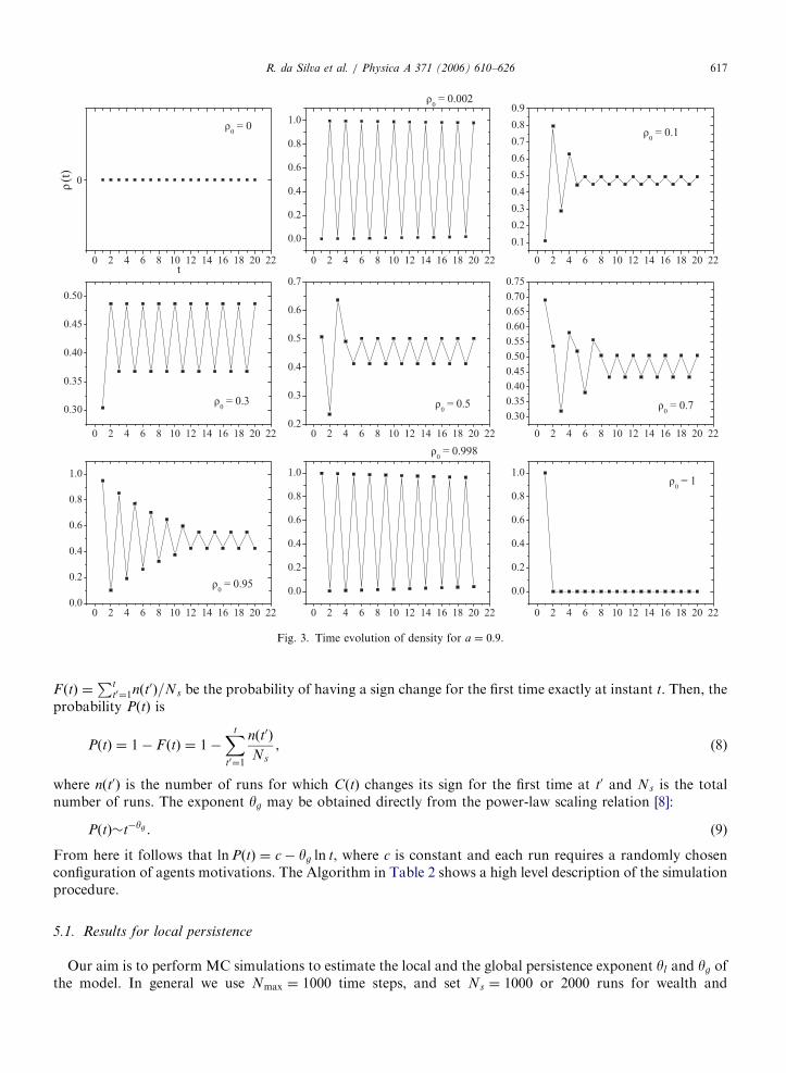
F ðtÞ ¼Pt

t0¼1nðt0Þ=Ns be the probability of having a sign change for the first time exactly at instant t. Then, the

probability PðtÞ is

PðtÞ ¼ 1� F ðtÞ ¼ 1�Xt

t0¼1

nðt0Þ

Ns

, (8)

where nðt0Þ is the number of runs for which CðtÞ changes its sign for the first time at t0 and Ns is the totalnumber of runs. The exponent yg may be obtained directly from the power-law scaling relation [8]:

PðtÞ�t�yg . (9)

From here it follows that lnPðtÞ ¼ c� yg ln t, where c is constant and each run requires a randomly chosenconfiguration of agents motivations. The Algorithm in Table 2 shows a high level description of the simulationprocedure.

5.1. Results for local persistence

Our aim is to perform MC simulations to estimate the local and the global persistence exponent yl and yg ofthe model. In general we use Nmax ¼ 1000 time steps, and set Ns ¼ 1000 or 2000 runs for wealth and

ARTICLE IN PRESS


0 10 20 30 40 500.0

0.2

0.4

0.6

0.8

1.0

ρ (t

)

t

a = 1.5 ρ= 0.16

a = 1.5 ρ= 0.18

(a) (b)

Fig. 5. (a) Time evolution for density of optimists (motivated) for a ¼ 1:5 and r0 ¼ 0:16 and r0 ¼ 0:18. (b) Time evolution of motivated

players for a ¼ 1:5 and r0 ¼ 0:6 for different seeds.


persistence, respectively.1 Practically, with the specific choice ða; bÞ ¼ ð1; 12Þ, one can see the interest provider

increasing or decreasing the overall wealth by a factor of 12. The choice a ¼ 1) haþ bri ¼ 1, (once hri ¼ 0) is

interesting because other choices lead to a bias in the profit hgkia0. We chose b ¼ 12since we want to allow

profits or losses of up to 50%.

1A higher number of runs is required mainly for global persistence since it is an experimental distribution obtained via a histogram.

ARTICLE IN PRESS

Table 2

Estimate of global persistence in the context of the MC simulations

Procedure: Global Persistence Algorithm

INPUT: Ns number of samples; Nmax max. number of Monte Carlo steps;

FOR i ¼ 1; . . . ;Ns

� Choose a random configuration to start the simulations

�NMC :¼1 (initializing the MC steps)

WHILE ðNMCpNmaxÞ and ðPL

i¼1W iðNMCXL � o0ÞÞ

NMC ¼ NMC þ 1

� The investment of all agents is taken according to motivation rules (Table 1)

� Update of motivation of agents according to the rules based on profit (Eq. (5))

IF ðPL

i¼1W iðNMCÞoL � o0Þ THEN

pðNMCÞ ¼ pðNMCÞ þ 1

ENDIF

ENDWHILE

ENDFOR

WRITE NMC ; ð1� 1NS

PNMC�1i¼1 pðiÞÞ; to NMC ¼ 1; . . . ;Nmax

END

Fig. 6. Time evolution of QðtÞ using the uniform approach. For the three values checked wmax ¼ 2; 5; 10 we can identify robust power laws.


Our first results regarding local persistence relates to the ruin of a player. We study the time evolution of thisprobability by looking at whether in the simulation step t a particular agent goes bankrupt for the first time).We perform experiments of QðtÞ as function of t, such that W ið1Þ ¼ wi

0 using two approaches:

1.
Uniform approach: Each agent receives an initial value wi0 (a uniform random variable) between ½0;wmax�;
2.
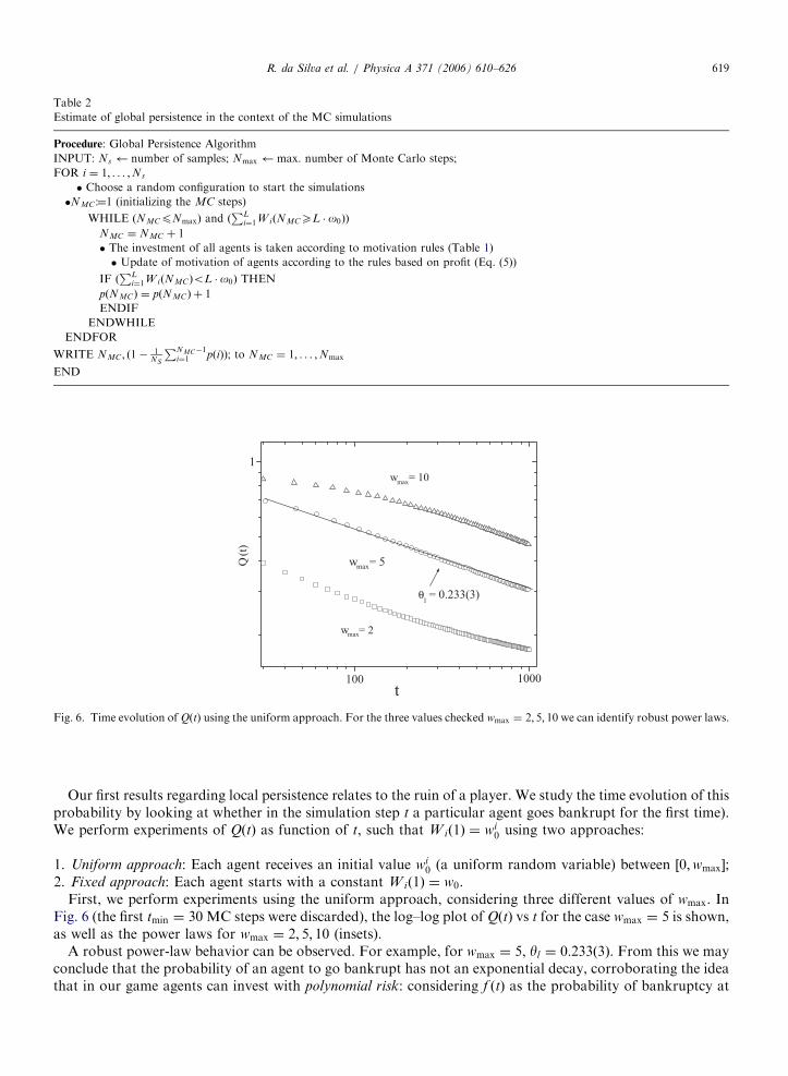
Fixed approach: Each agent starts with a constant W ið1Þ ¼ w0.First, we perform experiments using the uniform approach, considering three different values of wmax. In
Fig. 6 (the first tmin ¼ 30 MC steps were discarded), the log–log plot of QðtÞ vs t for the case wmax ¼ 5 is shown,as well as the power laws for wmax ¼ 2; 5; 10 (insets).

A robust power-law behavior can be observed. For example, for wmax ¼ 5, yl ¼ 0:233ð3Þ. From this we mayconclude that the probability of an agent to go bankrupt has not an exponential decay, corroborating the ideathat in our game agents can invest with polynomial risk: considering f ðtÞ as the probability of bankruptcy at


time t and QðtÞ ¼ 1�Pt

t0¼1f ðt0Þ, we have

f ðtÞ ¼ QðtÞ �Qðt� 1Þ

¼ �dQðtÞ

dtþX1n¼2

ð�1Þn

n!

dnQðtÞ

dtn

¼ cyl

tylþ1þOðtylþ2Þ �

t!1c

yl

tylþ1

since we expected polynomial behavior fitted by QðtÞ ¼ qINF þ ct�yl with qINF and c constants.Further, it must be said that for tmax ¼ 1000 (which was the case here) there is a greater chance of ruin to

happen for values of t larger than tmax, once the probability of ruin to happen for t4tmax, QðtmaxÞ isapproximately 0.30. Alternatively, it is interesting to analyze the same measure looking at the local persistencein the sense of the first return, i.e., the probability of a particular agent remaining wealthy (W iðt

0ÞXw0 up tot0 ¼ t).

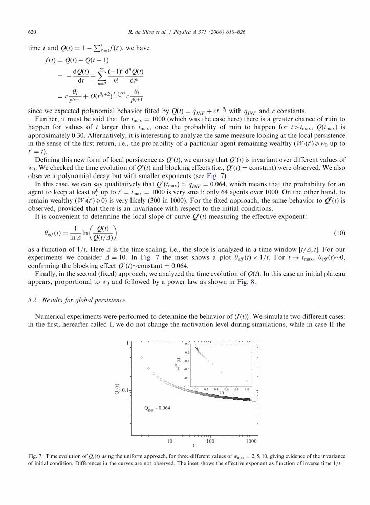
Defining this new form of local persistence as QrðtÞ, we can say that QrðtÞ is invariant over different values ofw0. We checked the time evolution of QrðtÞ and blocking effects (i.e., QrðtÞ ¼ constant) were observed. We alsoobserve a polynomial decay but with smaller exponents (see Fig. 7).

In this case, we can say qualitatively that QrðtmaxÞ ’ qINF ¼ 0:064, which means that the probability for anagent to keep at least w0

i up to t0 ¼ tmax ¼ 1000 is very small: only 64 agents over 1000. On the other hand, toremain wealthy (W iðt

0ÞX0) is very likely (300 in 1000). For the fixed approach, the same behavior to QrðtÞ isobserved, provided that there is an invariance with respect to the initial conditions.

It is convenient to determine the local slope of curve QrðtÞ measuring the effective exponent:

yeff ðtÞ ¼1

lnDln

QðtÞ

Qðt=DÞ

� �(10)

as a function of 1=t. Here D is the time scaling, i.e., the slope is analyzed in a time window ½t=D; t�. For ourexperiments we consider D ¼ 10. In Fig. 7 the inset shows a plot yeff ðtÞ � 1=t. For t! tmax, yeff ðtÞ�0,confirming the blocking effect QrðtÞ�constant ¼ 0:064.

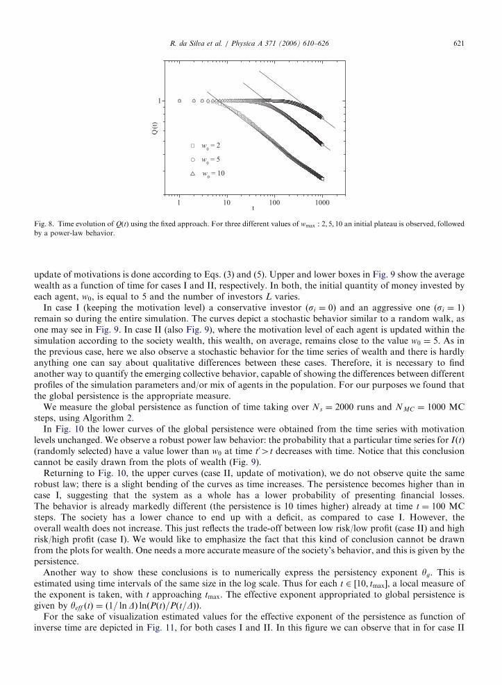
Finally, in the second (fixed) approach, we analyzed the time evolution of QðtÞ. In this case an initial plateauappears, proportional to w0 and followed by a power law as shown in Fig. 8.

5.2. Results for global persistence

Numerical experiments were performed to determine the behavior of hIðtÞi. We simulate two different cases:in the first, hereafter called I, we do not change the motivation level during simulations, while in case II the

Fig. 7. Time evolution of QrðtÞ using the uniform approach, for three different values of wmax ¼ 2; 5; 10, giving evidence of the invariance

of initial condition. Differences in the curves are not observed. The inset shows the effective exponent as function of inverse time 1=t.

ARTICLE IN PRESS

Fig. 8. Time evolution of QðtÞ using the fixed approach. For three different values of wmax : 2; 5; 10 an initial plateau is observed, followed

by a power-law behavior.


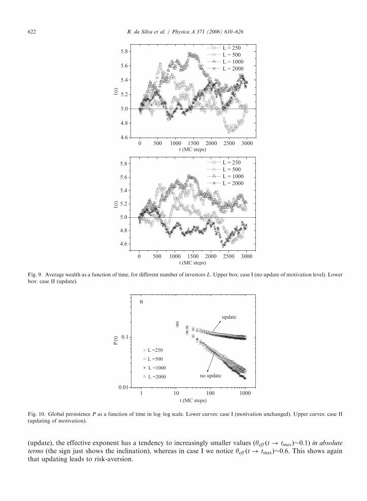
update of motivations is done according to Eqs. (3) and (5). Upper and lower boxes in Fig. 9 show the averagewealth as a function of time for cases I and II, respectively. In both, the initial quantity of money invested byeach agent, w0, is equal to 5 and the number of investors L varies.

In case I (keeping the motivation level) a conservative investor (si ¼ 0) and an aggressive one (si ¼ 1)remain so during the entire simulation. The curves depict a stochastic behavior similar to a random walk, asone may see in Fig. 9. In case II (also Fig. 9), where the motivation level of each agent is updated within thesimulation according to the society wealth, this wealth, on average, remains close to the value w0 ¼ 5. As inthe previous case, here we also observe a stochastic behavior for the time series of wealth and there is hardlyanything one can say about qualitative differences between these cases. Therefore, it is necessary to findanother way to quantify the emerging collective behavior, capable of showing the differences between differentprofiles of the simulation parameters and/or mix of agents in the population. For our purposes we found thatthe global persistence is the appropriate measure.

We measure the global persistence as function of time taking over Ns ¼ 2000 runs and NMC ¼ 1000 MCsteps, using Algorithm 2.

In Fig. 10 the lower curves of the global persistence were obtained from the time series with motivationlevels unchanged. We observe a robust power law behavior: the probability that a particular time series for IðtÞ

(randomly selected) have a value lower than w0 at time t04t decreases with time. Notice that this conclusioncannot be easily drawn from the plots of wealth (Fig. 9).

Returning to Fig. 10, the upper curves (case II, update of motivation), we do not observe quite the samerobust law; there is a slight bending of the curves as time increases. The persistence becomes higher than incase I, suggesting that the system as a whole has a lower probability of presenting financial losses.The behavior is already markedly different (the persistence is 10 times higher) already at time t ¼ 100 MCsteps. The society has a lower chance to end up with a deficit, as compared to case I. However, theoverall wealth does not increase. This just reflects the trade-off between low risk/low profit (case II) and highrisk/high profit (case I). We would like to emphasize the fact that this kind of conclusion cannot be drawnfrom the plots for wealth. One needs a more accurate measure of the society’s behavior, and this is given by thepersistence.

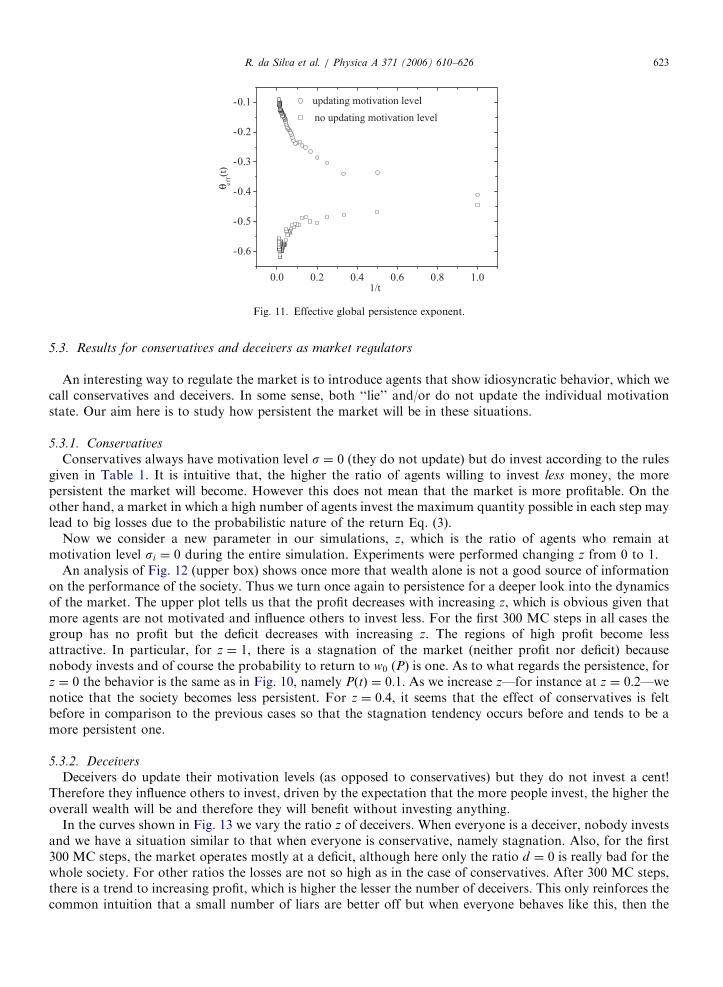
Another way to show these conclusions is to numerically express the persistency exponent yg. This isestimated using time intervals of the same size in the log scale. Thus for each t 2 ½10; tmax�, a local measure ofthe exponent is taken, with t approaching tmax. The effective exponent appropriated to global persistence isgiven by yeff ðtÞ ¼ ð1= lnDÞ lnðPðtÞ=Pðt=DÞÞ.

For the sake of visualization estimated values for the effective exponent of the persistence as function ofinverse time are depicted in Fig. 11, for both cases I and II. In this figure we can observe that in for case II

ARTICLE IN PRESS

Fig. 10. Global persistence P as a function of time in log–log scale. Lower curves: case I (motivation unchanged). Upper curves: case II

(updating of motivation).

Fig. 9. Average wealth as a function of time, for different number of investors L. Upper box: case I (no update of motivation level). Lower

box: case II (update).


(update), the effective exponent has a tendency to increasingly smaller values ðyeff ðt! tmaxÞ�0:1Þ in absolute

terms (the sign just shows the inclination), whereas in case I we notice yeff ðt! tmaxÞ�0:6. This shows againthat updating leads to risk-aversion.

ARTICLE IN PRESS

Fig. 11. Effective global persistence exponent.


5.3. Results for conservatives and deceivers as market regulators

An interesting way to regulate the market is to introduce agents that show idiosyncratic behavior, which wecall conservatives and deceivers. In some sense, both ‘‘lie’’ and/or do not update the individual motivationstate. Our aim here is to study how persistent the market will be in these situations.

5.3.1. Conservatives

Conservatives always have motivation level s ¼ 0 (they do not update) but do invest according to the rulesgiven in Table 1. It is intuitive that, the higher the ratio of agents willing to invest less money, the morepersistent the market will become. However this does not mean that the market is more profitable. On theother hand, a market in which a high number of agents invest the maximum quantity possible in each step maylead to big losses due to the probabilistic nature of the return Eq. (3).

Now we consider a new parameter in our simulations, z, which is the ratio of agents who remain atmotivation level si ¼ 0 during the entire simulation. Experiments were performed changing z from 0 to 1.

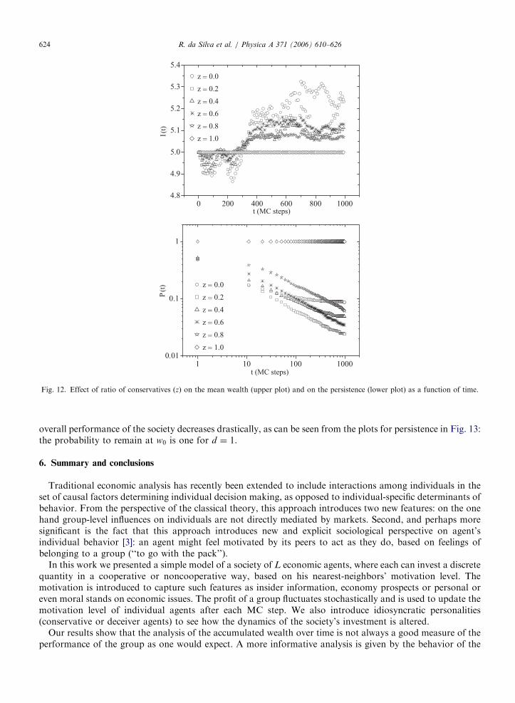
An analysis of Fig. 12 (upper box) shows once more that wealth alone is not a good source of informationon the performance of the society. Thus we turn once again to persistence for a deeper look into the dynamicsof the market. The upper plot tells us that the profit decreases with increasing z, which is obvious given thatmore agents are not motivated and influence others to invest less. For the first 300 MC steps in all cases thegroup has no profit but the deficit decreases with increasing z. The regions of high profit become lessattractive. In particular, for z ¼ 1, there is a stagnation of the market (neither profit nor deficit) becausenobody invests and of course the probability to return to w0 (P) is one. As to what regards the persistence, forz ¼ 0 the behavior is the same as in Fig. 10, namely PðtÞ ¼ 0:1. As we increase z—for instance at z ¼ 0:2—wenotice that the society becomes less persistent. For z ¼ 0:4, it seems that the effect of conservatives is feltbefore in comparison to the previous cases so that the stagnation tendency occurs before and tends to be amore persistent one.

5.3.2. Deceivers

Deceivers do update their motivation levels (as opposed to conservatives) but they do not invest a cent!Therefore they influence others to invest, driven by the expectation that the more people invest, the higher theoverall wealth will be and therefore they will benefit without investing anything.

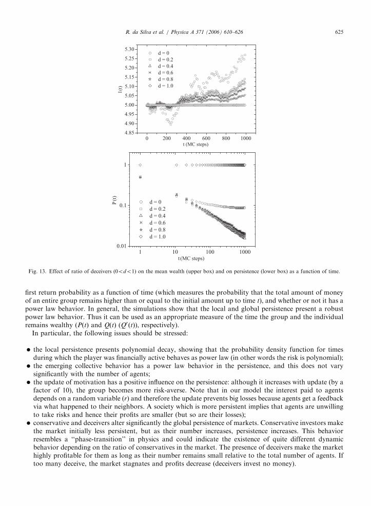
In the curves shown in Fig. 13 we vary the ratio z of deceivers. When everyone is a deceiver, nobody investsand we have a situation similar to that when everyone is conservative, namely stagnation. Also, for the first300 MC steps, the market operates mostly at a deficit, although here only the ratio d ¼ 0 is really bad for thewhole society. For other ratios the losses are not so high as in the case of conservatives. After 300 MC steps,there is a trend to increasing profit, which is higher the lesser the number of deceivers. This only reinforces thecommon intuition that a small number of liars are better off but when everyone behaves like this, then the

ARTICLE IN PRESS

.

.

Fig. 12. Effect of ratio of conservatives (z) on the mean wealth (upper plot) and on the persistence (lower plot) as a function of time.


overall performance of the society decreases drastically, as can be seen from the plots for persistence in Fig. 13:the probability to remain at w0 is one for d ¼ 1.

6. Summary and conclusions

Traditional economic analysis has recently been extended to include interactions among individuals in theset of causal factors determining individual decision making, as opposed to individual-specific determinants ofbehavior. From the perspective of the classical theory, this approach introduces two new features: on the onehand group-level influences on individuals are not directly mediated by markets. Second, and perhaps moresignificant is the fact that this approach introduces new and explicit sociological perspective on agent’sindividual behavior [3]: an agent might feel motivated by its peers to act as they do, based on feelings ofbelonging to a group (‘‘to go with the pack’’).

In this work we presented a simple model of a society of L economic agents, where each can invest a discretequantity in a cooperative or noncooperative way, based on his nearest-neighbors’ motivation level. Themotivation is introduced to capture such features as insider information, economy prospects or personal oreven moral stands on economic issues. The profit of a group fluctuates stochastically and is used to update themotivation level of individual agents after each MC step. We also introduce idiosyncratic personalities(conservative or deceiver agents) to see how the dynamics of the society’s investment is altered.

Our results show that the analysis of the accumulated wealth over time is not always a good measure of theperformance of the group as one would expect. A more informative analysis is given by the behavior of the

ARTICLE IN PRESS

Fig. 13. Effect of ratio of deceivers (0odo1) on the mean wealth (upper box) and on persistence (lower box) as a function of time.


first return probability as a function of time (which measures the probability that the total amount of moneyof an entire group remains higher than or equal to the initial amount up to time t), and whether or not it has apower law behavior. In general, the simulations show that the local and global persistence present a robustpower law behavior. Thus it can be used as an appropriate measure of the time the group and the individualremains wealthy (PðtÞ and QðtÞ (QrðtÞ), respectively).

In particular, the following issues should be stressed:

�
the local persistence presents polynomial decay, showing that the probability density function for timesduring which the player was financially active behaves as power law (in other words the risk is polynomial); � the emerging collective behavior has a power law behavior in the persistence, and this does not vary
significantly with the number of agents;
� the update of motivation has a positive influence on the persistence: although it increases with update (by a
factor of 10), the group becomes more risk-averse. Note that in our model the interest paid to agentsdepends on a random variable (r) and therefore the update prevents big losses because agents get a feedbackvia what happened to their neighbors. A society which is more persistent implies that agents are unwillingto take risks and hence their profits are smaller (but so are their losses);
� conservative and deceivers alter significantly the global persistence of markets. Conservative investors make
the market initially less persistent, but as their number increases, persistence increases. This behaviorresembles a ‘‘phase-transition’’ in physics and could indicate the existence of quite different dynamicbehavior depending on the ratio of conservatives in the market. The presence of deceivers make the markethighly profitable for them as long as their number remains small relative to the total number of agents. Iftoo many deceive, the market stagnates and profits decrease (deceivers invest no money).


It would be interesting to study a situation where agents can also change their type, going from conservativeto aggressive and deceiver. This should reflect the fact that markets influence people, changing their behavior,as for example the news that bond prices are going up. This kind of information might lead one to feel temptedto make a bigger profit on a short stint and, from this perspective, to better characterize how agents gain orlose one has to go from the society (global persistence) to the individual (local persistence) level. This we planon investigating in a future work.

References

[1] M. Schillo, K. Fischer, C.T. Klein, The micro-macro link in dai and sociology, in: Proceeding of the Second International Workshop

on Multi-agents Based Simulation, Springer, New York, 2000, pp. 133–148.

[2] J. Epstein, R. Axtell, Growing Artificial Societies Social Science From the Bottom Up, MIT Press, Cambridge, MA, 1996.

[3] S.N. Durlauf, How can statistical mechanics contribute to social science?, Proc. Nat. Acad. Sci. USA 96 (1999) 10582–10584.

[4] D. Ashlock, Evolutionary Computation for Modeling and Optimization, Springer, New York, 2005.

[5] A.L.C. Bazzan, R. Bordini, J. Campbell, Moral sentiments in multi-agent systems, in: Intelligent Agents V, Lecture Notes in Artificial

Intelligence, vol. 1555, Springer, New York, 1999, pp. 113–131.

[6] B. Derrida, A.J. Bray, C. Godreche, Nontrivial exponents in the zero-temperature dynamics of the 1D Ising and Potts models,

J. Phys. A 27 (1994) L357.

[7] D. Stauffer, Ising spinoidal decomposition at T ¼ 0 in one to 5 dimensions, J. Phys. A 27 (1994) 5029.

[8] S.N. Majumdar, A.J. Bray, S.J. Cornell, C. Sire, Global persistence exponent for nonequilibrium critical dynamics, Phys. Rev. Lett.

77 (18) (1996) 3704–3707.

[9] W. Feller, An Introduction to Probability Theory and Its Applications, vol. 1, Wiley, New York, USA, 1968.

[10] E.W. Montroll, B.J. West, On an enriched collection of stochastic process, in: E.W. Montroll, J.L. Lebowitz (Eds.), Fluctuation

Phenomena, North-Holland, Amsterdam, 1979.

[11] R. da Silva, S.R. Dahmen, Local persistence and blocking in the two-dimensional Blume-Capel model, Braz. J. Phys. 34 (4A) (2004)

1469.

[12] R. da Silva, N. Alves Jr., Dynamic exponents of a probabilistic three-state cellular automaton, Physica A 350 (2005) 263.

[13] R. da Silva, N.A. Alves, J.R. Drugowich de Felicio, Global persistence exponent of the two-dimensional Blume–Capel model, Phys.

Rev. E 67 (5) (2003) 057102.

[14] R. da Silva, A.C. Bazzan, A.T. Baraviera, S.R. Dahmen, Emerging collective behavior in a simple artificial financial market, in:

Proceedings of the Fourth International Joint Conference on Autonomous Agents and Multi Agent Systems, ACM, Utrecht, 2005.

[15] E. Jen, Cylindrical cellular automata, Commun. Math. Phys. 118 (4) (1988) 569–590.

Documents

Emerging collective behavior and local properties of financial dynamics in a public investment game