Emerging Methods For Conservation Laws · Emerging Methods For Conservation Laws Ram Nair Institute for Mathematics Applied to the Geosciences (IMAGe) National Center for Atmospheric

Emerging Methods For Conservation Laws

Ram Nair

Institute for Mathematics Applied to the Geosciences (IMAGe)National Center for Atmospheric Research

2008 ASP Colloquium: Numerical Techniques for Global

Atmospheric Models

June 9th NCAR, Boulder CO 80305, USA.

Ram Nair Emerging Methods For Conservation Laws

Hyperbolic Conservation Laws

Conservation laws are systems of nonlinear partial differential equations (PDEs)on conservation (flux) form and can be written:

∂

∂tU(x, t) +

3X

j=1

∂

∂xjFj (U, x, t) = S(U),

where

U(x, t) is a vector function in 3D space coordinate x and time t > 0.Fj are given flux vectors dependent on (U, x, t) and include diffusive andconvective effectsS(U) is the source term

E.g: Navier-Stokes equations for compressible and incompressible flows can bewritten in this form with U representing mass, momentum and energy, S(U)representing exterior forces.

A large class of atmospheric equations of motion can be cast in this form.

Scalar conservation law (e.g., mass continuity equation):

∂ρ

∂t+ ∇ · (ρV) = 0; ρt + div(ρV) = 0


Numerical Methods for Solving Conservation Laws

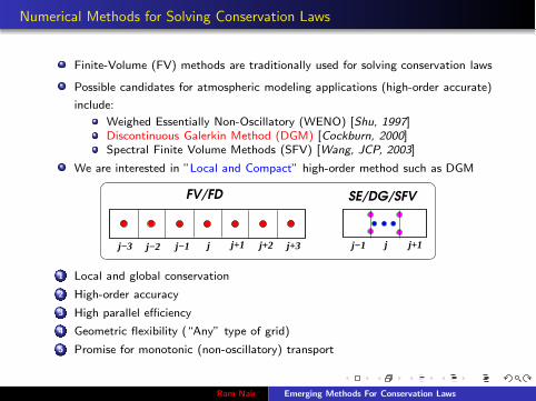
Finite-Volume (FV) methods are traditionally used for solving conservation laws

Possible candidates for atmospheric modeling applications (high-order accurate)

include:

Weighed Essentially Non-Oscillatory (WENO) [Shu, 1997]Discontinuous Galerkin Method (DGM) [Cockburn, 2000]Spectral Finite Volume Methods (SFV) [Wang, JCP, 2003]

We are interested in ”Local and Compact” high-order method such as DGM

j j+1 j+2j−3 j−1 j+3 j j+1

FV/FD SE/DG/SFV

j−2 j−1

1 Local and global conservation

2 High-order accuracy

3 High parallel efficiency

4 Geometric flexibility (“Any” type of grid)

5 Promise for monotonic (non-oscillatory) transport


Discontinuous Galerkin Method (DGM) in 1D

1D scalar conservation law:

∂U

∂t+

∂F (U)

∂x= 0 in Ω × (0, T ),

U0(x) = U(x , t = 0), ∀x ∈ Ω

E.g., F (U) = c U (Linear advection), F (U) = U2/2 (Burgers’ Equation)

The domain Ω (periodic) is partitioned into Nx non-overlapping elements(intervals) Ij = [xj−1/2, xj+1/2], j = 1, . . . , Nx , and ∆xj = (xj+1/2 − xj−1/2)

j−1

x x x xj+1/2j−1/2 j+3/2j−3/2

j+1IjII


DGM-1D: Weak Formulation

A weak formulation of the problem for the approximate solution Uh is obtained bymultiplying the PDE by a test function ϕh(x) and integrating over an element Ij :

Z

Ij

»

∂Uh

∂t+

∂F (Uh)

∂x

–

ϕh(x)dx = 0, Uh, ϕh ∈ Vh

Integrating the second term by parts =⇒Z

Ij

∂Uh(x , t)

∂tϕh(x)dx −

Z

Ij

F (Uh(x , t))∂ϕh

∂xdx +

F (Uh(xj+1/2, t)) ϕh(x−

j+1/2) − F (Uh(xj−1/2, t)) ϕh(x

+j−1/2

) = 0,

where ϕ(x−) and ϕ(x+) denote ”left” and ”right” limits.

R

x j−1/2 x j+1/2

I j

+ +_ ( )( )( ) _( )

L L R


DGM-1D: Flux term (“Gluing” the discontinuous element edges)

R

x j−1/2 x j+1/2

I j

+ +_ ( )( )( ) _( )

L L R

Flux function F (Uh) is discontinuous at the interfaces xj±1/2

F (Uh) is replaced by a numerical flux function F (Uh), dependent on the left andright limits of the discontinuous function U. At the interface xj+1/2,

F (Uh)j+1/2(t) = F (Uh(x−

j+1/2, t), Uh(x

+j+1/2

, t))

Typical flux formulae (Approx. Reimann Solvers): Gudunov, Lax-Friedrichs,Roe, HLLC, etc.

Lax-Friedrichs nurmerical flux formula:-

F (Uh) =1

2

h

(F (U−

h ) + F (U+h )) − α(U+

h − U−

h )i

.


DGM-1D: Space Discretization (Evaluation of the Integrals)

Map every element Ij onto the reference element [−1,+1] by introducing a localcoordinate ξ ∈ [−1,+1] s.t.,

ξ =2 (x − xj)

∆xj, xj = (xj−1/2 + xj+1/2)/2 ⇒ ∂

∂x=

2

∆xj

∂

∂ξ.

Use a high-order Gaussian quadrature such as the Gauss-Legendre (GL) orGauss-Lobatto-Legendre (GLL) quadrature rule. The GLL qudrature is ‘exact’for polynomials of degree up to 2N − 1.

Z 1

−1f (ξ)dξ ≈

NX

n=0

wnf (ξn); for GLL, ξn ⇐ (1 − ξ2)P′ℓ(ξ) = 0

Regular

x j−1/2 xj+1/2

jI

+1− 1

ξ

GLL Grid

Reference ElementElement


DGM-1D: Representation of Test function & Approximate Solution

−1 −0.5 0 0.5 1−1

−0.5

0

0.5

1

Legendre Polynomials (Degree <=4)

x

L(x)

The model basis set for the Pk DG method consists of Legendre polynomials,B = Pℓ(ξ), ℓ = 0, 1, . . . , k.Test function ϕh(x) and approximate solution Uh(x) belong to B

Uh(ξ, t) =k

X

ℓ=0

Uℓh (t) Pℓ(ξ) for − 1 ≤ ξ ≤ 1, where

Uℓh(t) =

2ℓ + 1

2

Z 1

−1Uh(ξ, t) Pℓ(ξ) dξ ℓ = 0, 1, . . . , k.

Z 1

−1Pm(x)Pn(x)dx =

2

2m + 1δm,n ⇐ Orthogonality

Uℓh (t) is the degrees of freedom (dof) evolves w.r.t time.


DGM-1D: Modal Basis Set for a “P2” Method

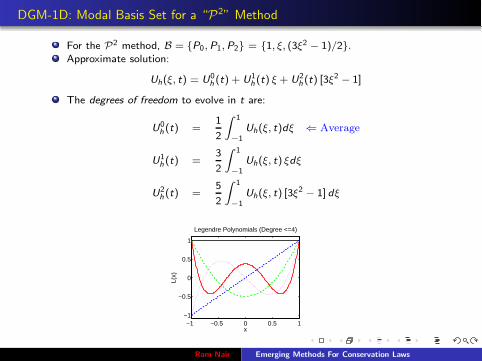
For the P2 method, B = P0, P1, P2 = 1, ξ, (3ξ2 − 1)/2.Approximate solution:

Uh(ξ, t) = U0h (t) + U1

h (t) ξ + U2h (t) [3ξ2 − 1]

The degrees of freedom to evolve in t are:

U0h (t) =

1

2

Z 1

−1Uh(ξ, t)dξ ⇐ Average

U1h (t) =

3

2

Z 1

−1Uh(ξ, t) ξdξ

U2h (t) =

5

2

Z 1

−1Uh(ξ, t) [3ξ2 − 1] dξ

−1 −0.5 0 0.5 1−1

−0.5

0

0.5

1


x

L(x)


DGM-1D: Orthogonal Basis Set (Modal Vs Nodal)

Modal basis functions Nodal basis functions

−1 −0.5 0 0.5 1−1

−0.5

0

0.5

1


x

L(x)

−1 −0.5 0 0.5 1−1

−0.5

0

0.5

1

4th Degree Lagrange Basis Functions

x

h(x)

The nodal basis set B is constructed using Lagrange-Legendre polynomials hi (ξ)with roots at Gauss-Lobatto quadrature points (physical space).

Uj (ξ) =k

X

j=0

Uj hj (ξ) for − 1 ≤ ξ ≤ 1,

hj (ξ) =(ξ2 − 1)P′

k (ξ)

k(k + 1) Pk(ξj ) (ξ − ξj ),

Z 1

−1hi (ξ)hj (ξ) = wi δij .

Nodal version was shown to be more computationally efficient than the Modalversion (see, Levy, Nair & Tufo, Comput. & Geos. 2007)

Modal version is more “friendly” with monotic limiting


DG-1D: Explicit Time Integration

Finally, the weak formulation leads the PDE to the time dependent ODE

Z

Ij

»

∂Uh

∂t+

∂F (Uh)

∂x

–

ϕh(x)dx = 0 ⇒ d

dtUℓ

h (t) = L(Uh) in (0, T ) × Ω

Example: For the P1 case on an element Ij , we need to solve:

d

dtU0

h (t) =−1

∆xj[F (ξ = 1, t) − F (ξ = −1, t)]

d

dtU1

h (t) =−3

∆xj

„

[F (ξ = 1, t) + F (ξ = −1, t)] −Z 1

−1Uh(ξ, t) dξ

«

Solve the ODEs for the modes at new time level Uℓh (t + ∆t) For the P1 case,

Uh(ξ, t + ∆t) = U0h (t + ∆t) + Uh(ξ, t + ∆t) ξ

j−1/2

DG

x x

FV

j−1/2 j+1/2j+1/2 j+3/2J−3/2 I Ij−1 I Ij+1jjx xxx


Time Integration

For the ODE of the form,

d

dtU(t) = L(U) in (0, T ) × Ω

Strong Stability Preserving third-order Runge-Kutta (SSP-RK) scheme (Gottliebet al., SIAM Review, 2001)

U(1) = Un + ∆tL(Un)

U(2) =3

4Un +

1

4U(1) +

1

4∆tL(U(1))

Un+1 =1

3Un +

2

3U(2) +

2

3∆tL(U(2)).

where the superscripts n and n + 1 denote time levels t and t + ∆t, respectively

The Courant number for the DG scheme is estimated to be 1/(2k + 1), where kis the degree of the polynomial (Cockburn and Shu, 1989).

For the linear case, CFL limit is 1/3.


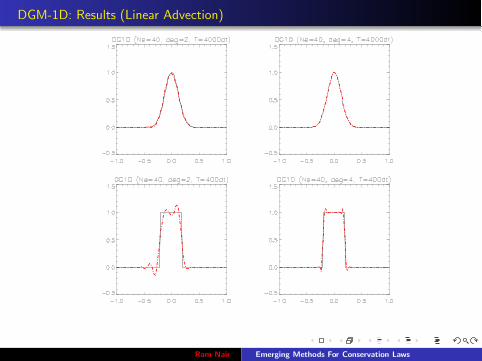
DGM-1D: Results (Linear Advection)


DG-2D Spatial Discretization for an Element Ω

2D Scalar conservation law

∂U

∂t+ ∇ · F(U) = S(U), in Ω × (0, T ); ∀ (x1, x2) ∈ Ω

where U = U(x1, x2, t), ∇ ≡ (∂/∂x1, ∂/∂x2), F = (F , G) is the flux function, and Sis the source term.

Weak Galerkin formulation: Multiplication of the basic equation by a testfunction ϕh ∈ Vh and integration over an element Ω.

∂

∂t

Z

ΩUh ϕh dΩ −

Z

ΩF(Uh) · ∇ϕh dΩ +

Z

ΓF(Uh) · ~n ϕh dΓ =

Z

ΩS(Uh) ϕhdΩ

where Uh is an approximate solution in Vh.

Can be extended to a system of equations


DG-2D: The Flux Term

U +hU_

Uh Uhh

After Num. Flux Operation

Element (Left) Element (Right)Element (Right)Element (Left)

Along the boundaries (Γ) of an element the solution Uh is discontinuous (U−

h

and U+h are the left and right limits).

Therefore, the analytic flux F(Uh) · ~n must be replaced by a numerical flux suchas the Lax-Friedrichs Flux:

F(Uh) · ~n =1

2

h

(F(U−

h ) + F(U+h )) · ~n − α(U+

h − U−

h )i

.

For the SW system, α is the upper bound on the absolute value of eigenvaluesof the flux Jacobian F′(U); (Nair et al., 2005)

α1 = max“

|u1| +√

Φ G 11”

, α2 = max“

|u2| +√

Φ G 22”


The DG, SE & FV Methods

C

DG SE

FVBoundary Discontinuity Continuous 0

DGM is a hybrid approach (DG ⇐ SE + FV)

The domain D is partitioned into non-overlapping elements Ωij suchthat the element boundaries are discontinuous.

Based on conservation laws but exploits the spectral expansion ofSE method and treats the element boundaries using FV “tricks.”


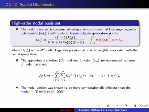
DG-2D: Spatial Discretization

High-order nodal basis set

The nodal basis set is constructed using a tensor-product of Lagrange-Legendrepolynomials (hi (ξ)) with roots at Gauss-Lobatto quadrature points.

hi (ξ) =(ξ2 − 1) P′

N(ξ)

N(N + 1) PN(ξi ) (ξ − ξi );

Z 1

−1hi (ξ)hj (ξ) = wi δij .

where PN(ξ) is the Nth order Legendre polynomial, and wi weights associated with theGauss quadrature.

The approximate solution (Uh) and test function (ϕh) are represented in termsof nodal basis set.

Uij (ξ, η) =N

X

i=0

NX

j=0

Uij hi (ξ) hj (η) for − 1 ≤ ξ, η ≤ 1,

The nodal version was shown to be more computationally efficient than themodal in (Dennis et al., 2006).


DG-2D System: Explicit Time Integration

Final form for the nodal discretization leads to the ODE:d

dtUij(t) =

4

∆x1i ∆x2

j wiwj[IGrad + IFlux + ISource ] ,

Evaluate the integrals (RHS) using GLL quadrature rule.

“Mass matrix” is diagonal (i.e., decoupled system of ODEs tosolve)

For a system of conservation laws, solve the ODE system:

d

dtU = L(U) in (0,T ) × Ω

Time integration: Explicit third-order Runge-Kutta (SSP)scheme (Gottlieb et al., 2001)


DG-2D Gaussin Hill Advection (Levy, Nair & Tufo, 2007)


Monotonic Limiter: Piecewise Linear Method (PLM) [van Leer (1979)]

Godunov theorem (1959): “Linear numerical schemes for solving PDE’s, havingthe property of not generating new extrema (monotone scheme), can be at mostfirst-order accurate.”

We consider monotonic limiter introduced by van Leer (1979) in MUSCLscheme (Monotone Upwind Schemes for Conservation Laws).

j−1/2

x x

u uujj−1 j+1

j+1/2

Piecewise linear approximations for cell averages U j

For the PLM, density distribution in a cell Ij = [xj−1/2, xj+1/2], with slope Ux,j :

U(x)j = U j + (x − xj)Ux,j , U j =1

∆xj

Z xj+1/2

xj−1/2

Uj (x)dx ,


Monotonic Limiting (minmod) in MUSCL Scheme

A minmod limiter essentially chooses the min of absolute value of the ‘left’ and‘right’ slopes if both preserve the same sign, but sets to zero slope if the signsare opposite.

U(x)j = U j + (x − xj)Ux,j , Ux,j ⇐ minmod(Ux,j ,Ux,j−1/2, Ux,j+1/2)

minmod(a, b, c) =

s min(|a|, |b|, |c|) if s = sign(a) = sign(b) = sign(c);0 otherwise .

Ux,j−1/2 =U j − U j−1

(∆xj + ∆xj−1)/2, Ux,j+1/2 =

U j+1 − U j

(∆xj+1 + ∆xj)/2

j−1/2

x x

u uujj−1 j+1

j+1/2


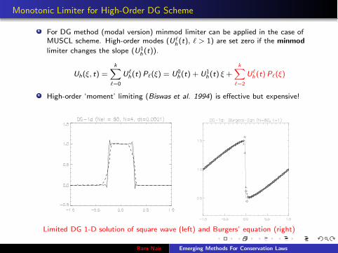
Monotonic Limiter for High-Order DG Scheme

For DG method (modal version) minmod limiter can be applied in the case ofMUSCL scheme. High-order modes (Uℓ

h (t), ℓ > 1) are set zero if the minmod

limiter changes the slope (U1h (t)).

Uh(ξ, t) =k

X

ℓ=0

Uℓh(t) Pℓ(ξ) = U0

h (t) + U1h (t) ξ +

kX

ℓ=2

Uℓh (t) Pℓ(ξ)

High-order ‘moment’ limiting (Biswas et al. 1994) is effective but expensive!

Limited DG 1-D solution of square wave (left) and Burgers’ equation (right)


Limiter: Extension to DG- 2D problems

The minmod limiter can be applied in x and y -direction sequentially, however itis very diffusive.

Uh(x , y , t) = Uh(t) + Ux (t)ξ + Uy (t)η

For high-order DG method, a tensor-product of 1-D limiter such as the momentlimiter (Krivonodova, 2008) or WENO limiter (Qui & Shu, 2005) may beapplied. But in general, they do not preserve positivity.

i−1,j+1

Ω ΩΩ

Ω

Ω

ΩΩ

ΩΩ

i−1,j i+1,ji,j

i+1,j−1

i+1,j+1

i−1,j−1 i,j−1

i,j+1

A new limiter developed for DGM transport problems, selectively applies slopelimiting employs a 3 × 3 element stencil and positivity as a constraint.


DG-2D P1 Case: Solid-Body Rotation (Leveque, 2004) Test

The minmod limiter preserves positivity, but too diffusive.Selective application of the slope limiter is desirable (preserves high-order natureof the solution).

DG 2-D solution with minmod limiter (left) and constrained slope limiter (right)


DG-2D P2 Case: Non-limited Solution (Leveque (2004) Test)

Solid-Body rotation of a cosine-cone and a square block after one revolution without limiting.


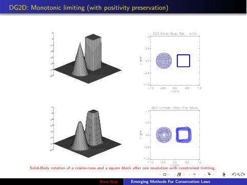
DG2D: Monotonic limiting (with positivity preservation)

Solid-Body rotation of a cosine-cone and a square block after one revolution with constrained limiting.


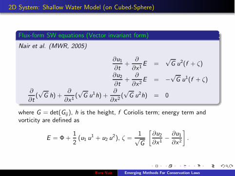
2D System: Shallow Water Model (on Cubed-Sphere)

Flux-form SW equations (Vector invariant form)

Nair et al. (MWR, 2005)

∂u1

∂t+

∂

∂x1E =

√G u2(f + ζ)

∂u2

∂t+

∂

∂x2E = −

√G u1(f + ζ)

∂

∂t(√

G h) +∂

∂x1(√

G u1h) +∂

∂x2(√

G u2h) = 0

where G = det(Gij ), h is the height, f Coriolis term; energy term andvorticity are defined as

E = Φ +1

2(u1 u1 + u2 u2), ζ =

1√G

[

∂u2

∂x1− ∂u1

∂x2

]

.


DG SW Model: Computational Domain

(8x8)

(1, −1)

(1, 1)(−1, 1)

(−1, −1)

η

ξ

GLL Grid

Cubed-Sphere (Ne = 5) with 8 × 8 GLL points

Flux is the only “communicator” at the element edges

Each face of the cubed-sphere is partitioned into Ne × Ne

rectangular non-overlapping elements (i.e., total 6 × N2e ).

Each element is mapped onto the Gauss-Lobatto-Legendre(GLL) grid defined by −1 ≤ ξ, η ≤ 1, for integration.


Horizontal Advection: Cosine-bell Advection

Nodal version of DGM is computationally more efficient (Dennis et al. 2006) ascompared to the Modal version.

Nodal Vs Modal run, time traces for normalized ℓ1,ℓ2 and ℓ∞ errors

Cosine-Bell Movie


Cosine-Bell with monotonic limiter


Convergence Results - Advection (Cubed Sphere) [Levy, Nair & Tufo, 2007]

24 96 384 1536 614410

−12

10−9

10−6

10−3

100

h−error, Ng = 6

Rel

ativ

e E

rror

(lo

g sc

ale)

Number of Elements (log scale)

ModalNodal

4 5 6 7 8 9 1010

−12

10−9

10−6

10−3

100

p−error, Ne = 384

Rel

ativ

e E

rror

(lo

g sc

ale)

N

ModalNodal

h-error: Measured by leaving the number of nodes per element constant butincreasing the number of elements.

p-error: Measured by leaving the number of elements constant but increasingthe number of nodes per element


Horizontal Advection: Moving Vortices on the Sphere

Initial field and DG solution after 12 days. Max error is O(10−5)

Deformational Flow Test: Nair & Jablonowski (MWR, 2008)

The vortices are located at diametrically opposite sides of thesphere, the vortices deform as they move along a prescribedtrajectory.

Analytical solution is known and the trajectory is chosen to be agreat circle along the NE direction (α = π/4).


SW Test-2: Geostrophic Flow (Nair et al., MWR 2005)

High-order accuracy and spectral convergence

Steady state geostrophic flow (α = π/4). Max height error is O(10−6) m.


SW Test-5: Flow over a Mountain (Dennis et al. 2006)

No “spectral ringing” for the height fields

Flow over a mountain (≈ 0.5o ). Initial height field (left) initial and after 15 days of integration (right)

SW5 Movie


HOMME (High-Order Method Modeling Environment)

The Discontinuous Galerkin (DG) model is a conservative option in theHOMME framework

HOMME Grid: The sphere is decomposed into 6 identical regions, using the

equiangular projection (Sadourny, 1972)

Local coordinate systems are free of singularitiesCreates a non-orthogonal curvilinear coordinate system

Cubed Sphere Geometry: Logical cube-face orientation

z

4 F 2 F 3F 1

F 6

F 5(Top)

F 1

(Bottom)

x

yF


HOMME Grid System

Metric Tensor Gij , [Cubed-Sphere Sphere] Transform

Central angles x1, x2 ∈ [−π/4, π/4] are the independent variables.

Gij =R2

ρ4 cos2 x1 cos2 x2

[

1 + tan2 x1 − tan x1 tan x2

− tan x1 tan x2 1 + tan2 x2

]

where ρ2 = 1 + tan2 x1 + tan2 x2, i , j ∈ 1, 2

Metric tensor in terms of longitude-latitude (λ, θ):

Gij = AT A; A =

[

R cos θ ∂λ/∂x1 R cos θ ∂λ/∂x2

R ∂θ/∂x1 R ∂θ/∂x2

]

The matrix A is used for transforming spherical velocity (u, v) tothe covariant (u1, u2) and contravariant (u1, u2) vectors.


Hydrostatic Prognostic Equations in Flux Form (Curvilinear coordinates)

∂u1

∂t+ ∇c · E1 + η

∂u1

∂η=

√Gu2 (f + ζ) − R T

∂

∂x1(ln p)

∂u2

∂t+ ∇c · E2 + η

∂u2

∂η= −

√Gu1 (f + ζ) − R T

∂

∂x2(ln p)

∂

∂t(m) + ∇c ·

(

Ui m)

+∂(mη)

∂η= 0

∂

∂t(mΘ) + ∇c ·

(

Ui Θ m)

+∂(mη Θ)

∂η= 0

∂

∂t(mq) + ∇c ·

(

Ui q m)

+∂(mη q)

∂η= 0

m ≡√

G∂p

∂η,∇c ≡

„

∂

∂x1,

∂

∂x2

«

, η = η(p, ps ), G = det(Gij ),∂Φ

∂η= −R T

p

∂p

∂η.

Where m is the mass function, Θ is the potential temperature and q is the moisture

variable. Ui = (u1, u2), E1 = (E , 0), E2 = (0, E); E = Φ + 12

`

u1u1 + u2u

2´

is the

energy term. Φ is the geopotential, ζ is the relative vorticity, and f is the Coriolis term.


Vertical Lagrangian Coordinates (Starr, 1945; Lin 2004)

A “vanishing trick” for vertical advection terms!

Terrain-following Eulerian surfaces are treated as material surfaces.

The resulting Lagrangian surfaces are free to move up or downdirection.

top

Topography

δp

k

k

ps

pVertically Moving Lagrangian Surfaces

Φs

−1/2

+1/2

k


The Remapping of Lagrangian Variables

Vertically moving Lagrangian Surfaces

Over time, Lagrangian surfaces deform and thus must be remapped.

The velocity fields (u1, u2), and total energy (ΓE ) are remapped onto thereference coordinates using the 1-D conservative cell-integrated semi-Lagrangian(CISL) method (Nair & Machenhauer, 2002)

E

E

∆P∆P

t

= Pressure thicknessP∆ Lagrangian Surface

Terrain−following Lagrangian control−volume coordinates

L2

L1

1

2

t +∆t

Topography

Remapping: Lauritzen & Nair, MWR, 2008; Norman & Nair, MWR, 2008)


DG-3D: Baroclinic Instability Test

(JW-Test) Jablonowski & Williamson (QJRMS, 2006)

To assess the evolution of an idealized baroclinic wave in theNorthern Hemisphere.

The initial conditions are quasi-realistic and defined by analyticexpressions. Analytic solutions do not exist.

Initial Conditions


JW-Test: Evolution of Surface Pressure over the NH

Baroclinic waves are triggered by perturbing the velocity field at (20E, 40N)

This test case recommends up to 30 days of model simulation

Ne = Nv = 8 (approx. 1.6) with 26 vertical levels and ∆t = 30 Sec.


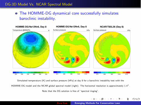
DG-3D Model Vs. NCAR Spectral Model

The HOMME-DG dynamical core successfully simulatesbaroclinic instability.

Simulated temperature (K) and surface pressure (hPa) at day 8 for a baroclinic instability test with the

HOMME-DG model and the NCAR global spectral model (right). The horizontal resolution is approximately 1.4 .

Note that the DG solution is free of “spectral ringing”.


DG Model Vs. NCAR Climate Models (Nair et al. Comput & Fluids, , 2008)

Simulated surface pressure at day 11 for a baroclinic instability test with DG model, and NCAR global spectral

model and a FV model. The models use 26 vertical levels and with approximate horizontal resolution of 0.7 .


Parallel Performance (3D) - Frost [IBM BG/L]

DG-3D parallel performance: Sustained Mflops on IBM BG/L(1024 DP nodes, 700 MHz PPC 440s): Approx. 9% peak

Held-Suarez (preliminary) test: 800 days idealized climatesimulation (1 resolution, 26 vertical levels, ∆t = 10 Sec)

32 64 128 256 512 1024 20480

50

100

150

200

250

300

Processor

MF

LOP

Sustaind FLOP Per Processor

1944 elements: 1 task/node (CO)1944 elements: 2 task/node (VN)7776 elements: 1 tasks/node (CO)7776 elements: 2 tasks/node (VN)

Parallel performance (strong scaling) results for JW-Test Held-Suarez test (800 days) .


Summary

The DG methods (third or fourth-order) is a good choice for solvingconservation laws as applied in atmospheric sciences (localconservation and monotonic transport).

The preliminary idealized test results and parallel scaling results areimpressive and comparable to the SE version in HOMME.

The explicit R-K time integration scheme is robust for the DG-3Dmodel, but very time-step restrictive.

More efficient time integration schemes are required for practicalclimate simulations. Possible approaches: Semi-implicit, IMEX-RK,Rosenbrock with optimized Schwarz, etc..


Documents

Emerging Methods For Conservation Laws · Emerging Methods For Conservation Laws Ram Nair Institute for Mathematics Applied to the Geosciences (IMAGe) National Center for Atmospheric