Emission Lines for BAO: Ground & Space M. Lampton UCB SSL 1 Dec 2006 Rewrites May 2007, Sept 2009, Nov 2009

Emission Lines for BAO: Ground & Space

M. LamptonUCB SSL

1 Dec 2006Rewrites May 2007, Sept 2009, Nov 2009

M.Lampton Sept 2009 2

Intro

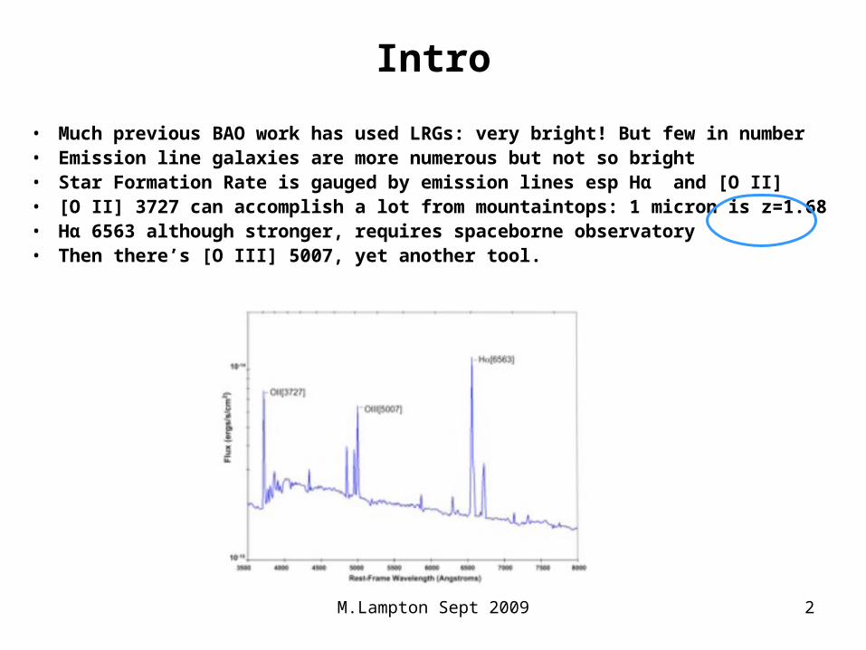
• Much previous BAO work has used LRGs: very bright! But few in number• Emission line galaxies are more numerous but not so bright• Star Formation Rate is gauged by emission lines esp Hα and [O II]• [O II] 3727 can accomplish a lot from mountaintops: 1 micron is z=1.68• Hα 6563 although stronger, requires spaceborne observatory• Then there’s [O III] 5007, yet another tool.


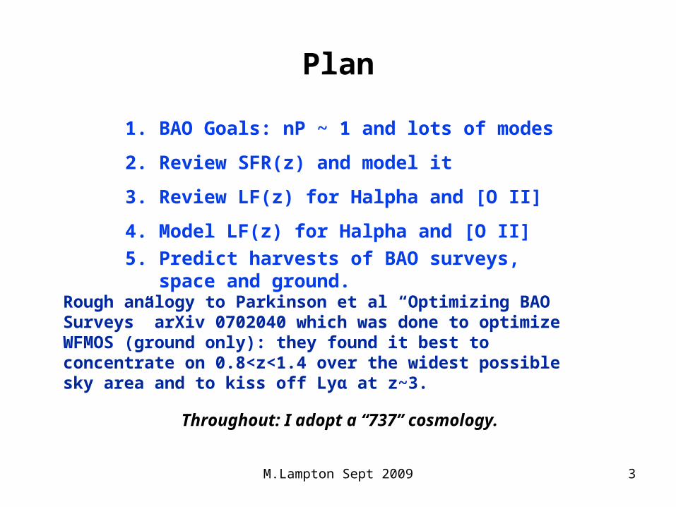
Plan

1. BAO Goals: nP ~ 1 and lots of modes

2. Review SFR(z) and model it

3. Review LF(z) for Halpha and [O II]

4. Model LF(z) for Halpha and [O II]

5. Predict harvests of BAO surveys, space and ground.

Rough analogy to Parkinson et al “Optimizing BAO Surveys” arXiv 0702040 which was done to optimize WFMOS (ground only): they found it best to concentrate on 0.8<z<1.4 over the widest possible sky area and to kiss off Lyα at z~3.

Throughout: I adopt a “737” cosmology.


Step 1: Uncertainties in the Acoustic Scale Lengthe.g. Blake et al 0510239 (2005); see also Reid et al 0907.1659

33-4

33-4

BAO

BAO

3

Mpc h 10P galaxies, blueFor

Mpc h102~ P galaxies, redFor

.0.2rad/Mpck rad/Mpc 0.07

with)P(kP and

Mpcper galaxiesn where

nP

11

Nmodes

1

X

X

Shot noiseCosmic varianceP(k) from Cole et al 2dFGRS arXiv 0501174, Fig.15


Step 2: SFR, Hα, [O II] are strongly correlated

Local, SDSS: Sumiyoshi et al arXiv:0902.2064 (2009) Fig 3 Local; Kennicutt, Ap.J. 388, 310 (1992)

Hα 6563 singlet Sum of 3727, 3729


Step 2: ELGs are widely used for SFR estimationLy et al., ApJ 657 738 (2007)


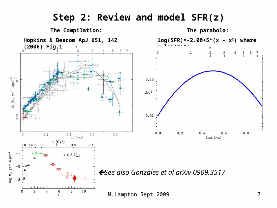
Step 2: Review and model SFR(z)The Compilation:

Hopkins & Beacom ApJ 651, 142 (2006) Fig.1

The parabola:

log(SFR)=-2.00+5*(x – x2) where x=log(z+1)

See also Gonzales et al arXiv 0909.3517


Step 3: LF data, Hα, continuedfaint end: Subaru; Ly et al., Subaru, ApJ 657 738 (2007), Fig 10

z=0.08 z=0.24

z=0.40


HiZELS: a high redshift survey of Hα emitters. I: the cosmic star-formation rate and clustering at z = 2.23

J. E. Geach et al; UKIRT HiZELS: NIR narrowband at 2.12um, COSMOS field 0.6 sqdeg

arXiv:0805.2861v1

http://lanl.arxiv.org/abs/0805.2861v1


MULTI-WAVELENGTH CONSTRAINTS ON THE COSMIC STAR FORMATION HISTORY FROM SPECTROSCOPY: THE REST-FRAME UV, H, AND INFRARED

LUMINOSITY FUNCTIONS AT REDSHIFTS 1.9<z < 3.41Reddy et al arXiv:0706.4091: 2000 SpectroZ, 15000 PhotoZ; Steidel Keck I w/ LRIS (2004)


Step 3: LF data [O II]Ly et al., Subaru w/ narrowband filters; ApJ 657 738 (2007) Fig 12

z=0.89 z=0.91

z=1.19 z=1.47


Step 3: LF data, [O II], continuedZhu et al., arXiv 0811.3035: DEEP2 (Keck II + DEIMOS), 14000 galaxies


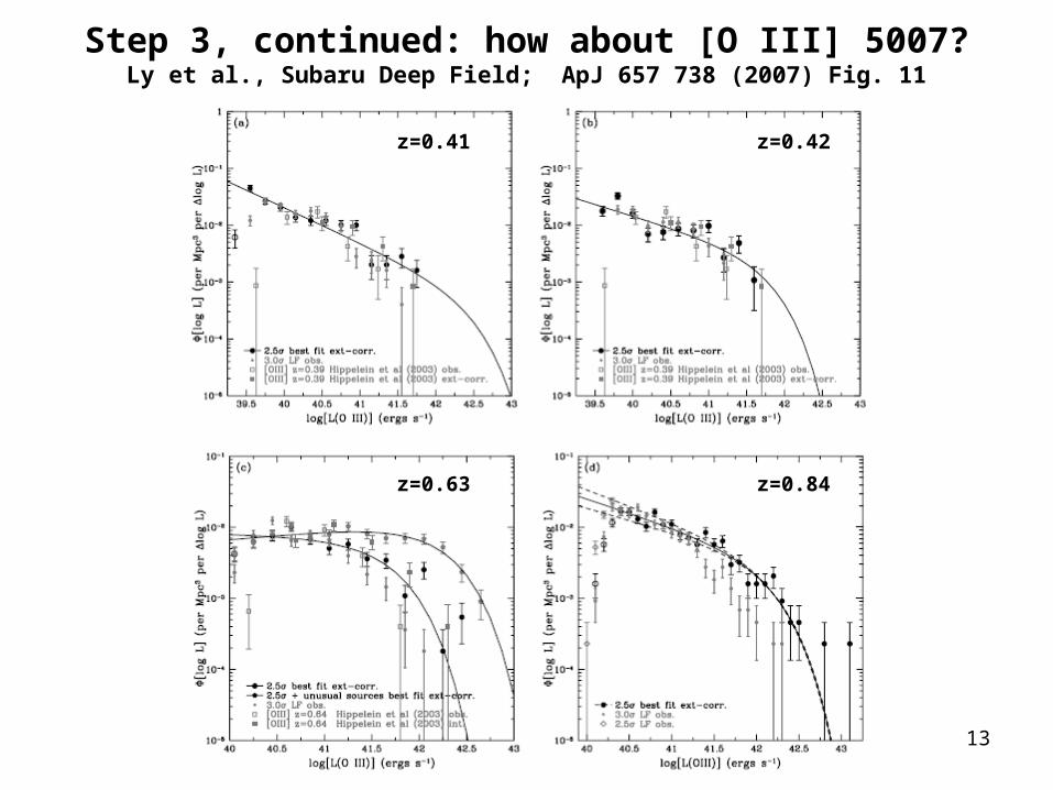
Step 3, continued: how about [O III] 5007?Ly et al., Subaru Deep Field; ApJ 657 738 (2007) Fig. 11

z=0.41 z=0.42

z=0.63 z=0.84


Step 3 concluding:

LF compilationSumiyoshi et al:

Compilation based on data from SDF;

arXiv 0902.2064

Halpha [O II]

0.5<z<1.0

1.0<z<1.4

1.4<z<1.7


Step 4: Model the LF(z) for each line

• Abell model (ARAA v.3, 1-22, 1965) parameters Lb, Nb at the break;

– Nearly flat power law at faint end

– Break

– Nearly inverse-square power law at bright end

• Schechter model (ApJ 203, 297-306, 1976) parameters L*, Φ* at the break;

– Nearly flat power law at faint end

– Break

– Exponential decrease at bright end

• Both developed for galaxy continuua

• They differ only at the bright end: Abell=slope; Schechter=dropoff.

• Which might apply for line emission?

• Because of the log-log straight-line LFs seen in DEEP2 (which go to very sparse densities) I adopt the Abell model here.

• Other adopters: Hao et al 0501042 (ELGs); Croom et al MNRAS 349 1397 2004 (QSOs) 1]N/N)2ln(exp[2

LL(N)

inverse... analytican has Abell Integral

LNln(2)

πLdL

dL

dN density Luminosity

)2ln(

)/LL1ln(NN

LL

LN

)2ln(

ln(10)

dLog(L)

dN

LL

LN

)2ln(

1

dLn(L)

dN

b

b

bb

22bb

L

22b

2bb

22b

2bb

Simplest Abell Luminosity Function


Step 4: Hα LF modellog(Nb) = -3.5+2.0*(x-x²)

log(Lb) = +41.5+3.0*(x-x²)

where x = log10(1+z)

0.5<z<1.0

1.0<z<1.4

1.4<z<1.7

Sumiyoshi et al (2009)


Step 4: [O II] LF modellog(Nb) = -3.5+2.0*(x-x²)

log(Lb) = +41.1+3.0*(x-x²)

where x = log10(1+z)

0.5<z<1.0

1.0<z<1.4

1.4<z<1.7

Sumiyoshi et al (2009)


Step 4: [O II] modellog(Nb) = -3.5+2.0*(x-x²)

log(Lb) = +41.1+3.0*(x-x²)

DEEP2; Zhu et al., arXiv 0811.3035


Step 5: Survey Yieldassumes “737” universe

microns2erg/sec.cm2

2

z

032

m

HC

L

2

22C

2L

P5.035E15hc

P sphotons/mF

redshiftz

cm 0.173z0.515z1

z1.325E28

)33(1

dyDD

distance luminosityD

erg/sec source, line theof luminosityL

.secerg/cm flux,power observedP

z)(14D

L

4D

LP

yyy


For a given nP, what Hα flux do we expect?

This extrapolated LF based on Sumiyoshi has many uncertainties, and the JDEM BAO team has recommended a higher sensitivity, ~ 1.6E-16 erg/cm2s

NEWS FLASH : Previously sought nP=1 and Zmax=2; but Linder and others (this conference) recommend NP=2 or even 3; Zmax=1.7 not 2.0

Abell distribution eyeball fitted to Sumiyoshi et al 2009 Hα


For a given nP, what [O II] flux do we expect?

Abell distribution eyeball fitted to Sumiyoshi et al 2009 [O II] 3727+3729

BigBOSS White Paper Fig.2 based on DEEP2 and VVDS

Goal: doublet flux ~ 1E-16 erg from this alone. But atmospheric observing complications and uncertainties about the LF at z>1.5 argue for higher sensitivity; working goal = 2.5E-17 erg/cm2sec for each component.


A Telescope area for 3.8m Mayall 7.5 m²

Tobs Exposure time 1ksec to 4ksec

F Target line flux: 2.5E-17 erg/cm2s

Ta Atmosphere transmission GeminiZenith5mm1.414

Ts Spectrometer transmission 0.5

Q Sensor quantum efficiency 0.9

Bsky Brightness of sky √2 · GeminiZenith

Ωresol Solid angle, one fiber on sky 1.5 sq arcsec

Δλ Wavelength spanned by one fiber 2.8E-4 um

Nread RSS read noise pixels on one fiber 6 √44 =40 el

SNR Signal to noise ratio desired 8

QTTTA

NQTBTA

NQTBTA

QTTTA

saobs

readsresolobs

readsresolobs

saobs

2

2

SNRF

FSNR

BigBOSS

[O II] 3727,3729

Model MDLFs


Atmospheric Transmission at Gemini Northpresumably similar at KPNO?

http://www.gemini.edu/sciops/ObsProcess/obsConstraints/ocTransSpectra.html

5.0mm H2O

U B V R I Z Y J H K


Atmospheric Emissionhttp://www.gemini.edu/node/10781?q=node/10787#OpticalSkySpectrum


MDLF Results for BigBOSSGoal is to use < 1 hour exposures and get SNR=8 (see chart 22)…

at z=2: 2.5E-17 erg/cm2s, will need the whole 4ksecat z=1: 1E-16 erg/cm2s, will need < 1 ksec

At Tobs = 1 h, 4000 fibers and 100 nights/year at 8h/night is 3 million targets per year -- and of course there is additional yield since most targets have z<2.0 and so won’t need the full 4000 seconds of exposure each,so smart fiber reallocation can improve yield rather than SNR.


A Atelescope, 1.0m, 25% area obstructed 0.59 m²

Tobs Observing time per target 1000 sec

F Target line flux: 1.6E-16 erg/cm2s

Ts Spectrometer transmission 0.7

Q Sensor quantum efficiency 0.9

Bzodi Brightness of sky, ph/m2.sec.micron 2 · NEPzodi

Ωresol Solid angle, 2x2 pixels on sky 1.0 sq arcsec

Δλ Wavelength span seen by each pixel 0.7 microns

Nread RSS read noise for 2x2 pixels 8√4 = 16electrons

SNR Desired signal to noise ratio 6.0

QTTA

NQTBTA

NQTBTA

QTTA

sobs

readsresolzodiobs

readsresolzodiobs

sobs

2

2

SNRF

FSNR

JDEM, Hα 6563

Model MDLF


MDLF Results for JDEM Goal is to use ~ 1ksec exposures Hα and get SNR>6…

at z=2: can get to 2.5E-16 erg/cm2s, using 1ksecat z=1: with 1ksec will gain improved SNR

At 1 kilosec exposures, 6 MCT sensors & 0.5 arcsec pixels, the FOV is 0.46 sq degrees. With 100 sec lost per maneuver and 70% on orbit efficiency, the net survey rate is 9000 square degrees per year.


Recent Relevant Results!

• Geach et al “Empirical Halpha emitter count predictions for dark energy surveys” arXiv 0911.0686: ELGs, Ha, 0.5<z<2.

• Parkinson et al “Optimizing BAO surveys II: curvature, redshifts, and external datasets” arXiv 0905.3410

• Hutsi, “Power spectrum of the maxBCG sample: detection of AO using galaxy clusters” arXiv 0910.0492

• Stril et al, “Testing Standard Cosmology with Large Scale Structure” arXiv0910.1833; specifically compares BigBOSS vs JDEM-PS.

Conclusions

• JDEM-BAO: entirely feasible!

• BigBOSS: entirely feasible!

Documents

Emission Lines for BAO: Ground & Space M. Lampton UCB SSL 1 Dec 2006 Rewrites May 2007, Sept 2009, Nov 2009