Comment on “Collision and radiative processes in

emission of atmospheric carbon dioxide”

M. Lino da Silva and J. Vargas

Instituto de Plasmas e Fusao Nuclear, Instituto Superior Tecnico, Universidade de

Lisboa, Av. Rovisco Pais 1, 1049-001, Lisboa, Portugal

E-mail: mlinodasilva@tecnico.ulisboa.pt

December 2019

Abstract. Recently, Smirnov published a paper (B. M. Smirnov, ”Collision and

radiative processes in emission of atmospheric carbon dioxide”, 2018, J. Phys. D.:

Appl. Phys., Vol. 51, No. 21, pp. 214004) which dismisses the role of increasing

concentrations of anthropogenic CO2 on global warming of planet Earth. We show

that these conclusions are the consequence of two flaws in Smirnov’s theoretical model

which neglect the effects of the increased concentrations of CO2 on the absorption

of Earth’s blackbody radiation in the 12–15µm region. The influence of doubling the

concentration of CO2 in the atmosphere on the surface temperature is not ∆T = 0.02K,

or even ∆T = 0.4K if only one of the two mistakes in Smirnov’s analysis is corrected.

The correct value lies within ∆T = 1.1 − 1.3K as outlined by other authors analysis

using simplified, yet more theoretically consistent models.

Foreword

Originally, this comment to the article: B. M. Smirnov, ”Collision and radiative processes in emission

of atmospheric carbon dioxide”, 2018, J. Phys. D.: Appl. Phys., Vol. 51, No. 21, pp. 214004, was

submitted to J. Phys. D: Appl. Phys. No agreement between the authors and the editorial board

could be achieved regarding the proper size and structure to the comment to this article, and as such

the authors decided not to pursue publication in J. Phys. D.: Appl. Phys., instead publishing the

comment in its original form in arXiv. A few suggestions from the editorial board from J. Phys. D:

Appl. Phys. were nonetheless integrated in this final version of our comment to Smirnov’s article.

Introduction

The authors have been pointed out to this article by Smirnov which claims anthropogenic

CO2 sources to be negligible as regarding global warming effects. This is a surprising

conclusion that directly contradicts a large amount of research in the last decades,

regarding the topic of global warming. Upon close inspection we have been able to

identify two different mistakes in the methodology of the work that lead to this flawed

conclusion.

arX

iv:2

002.

1060

1v2

[as

tro-

ph.E

P] 2

6 Fe

b 20

20

2

Upon this first review, and after our decision to write a rebuttal of the article

conclusions, we felt that a more extensive comment was warranted: Providing a

summary of the major works regarding the monitoring of energy exchange processes

at global Earth level would add a better insight on the consensus that has been formed

at the scientific community level regarding the impact of anthropogenic CO2 sources on

climate change. Since this is a topic with very high impact societal impact, we hope to

provide a summary of the major findings regarding this topic, thereby unambiguously

dispelling any misconceptions that may arise from works such as the one in review.

This comment to the article by Smirnov is split into three sections. Section 1

provides a summary on the energy budget of the Earth, as determined by detailed

measurements over the last decade. Section 2 examines in detail the shortcomings

of Smirnov’s work, and Section 3 presents a model that relies on the same initial

data as Smirnov, but yields the correct conclusions, as it follows a more appropriate

methodology. The reader with less available time will still be able to quickly refer to

Section 2 to understand the flaws of Smirnov’s work, which is the main objective of this

comment.

1. Earth’s Energy Budget: A Short Summary

The values of the heat fluxes for these different energy exchange processes are known to

good accuracy, as these have been determined from the average of ten years of recorded

data [3, 4]. These are presented in Fig. 1

Figure 1. Earth’s energy budget [5]

3

If this equilibrium is disrupted (like for example when the opacity of the atmosphere

increases due to anthropogenic factors or other), the energy flux imbalance (in this

example due to less energy escaping to Space when compared to the energy from the

Sun irradiation) will lead to a new equilibrium state, with different temperatures. This

change is not instantaneous, owing to the large thermal inertia from the Earth (mostly

due to the large volume of its oceans), and may take many years before a new stable

thermodynamic equilibrium is reached. In the 2005–2010 year interval, this imbalance

was estimated to be around 0.6W m−2 [6].

1.1. Atmospheric opacity and its influence on Earth’s energy balance

Here we shortly discuss the downward solar radiative fluxes and the associated losses in

the path from the edge of the atmosphere towards the surface, and the outward Earth

surface and atmospheric radiative fluxes towards Space.

Solar fluxes follow closely a Planck blackbody distribution with a characteristic

temperature around 5,780K. 98% of the radiative power is emitted in the 0.25–4

µm range. Radiative emission from the Earth’s surface follows a Planck blackbody

distribution with a characteristic temperature of 288K. 98% of the radiative power

is emitted in the 5–80 µm range. Finally, atmospheric emission fluxes do not follow

a blackbody distribution, but are limited by a Planck blackbody at a characteristic

temperature of 217K in the tropopause and 287K in the boundary layer region [7]. One

first important remark is that both inbound Solar fluxes and outbound Earth fluxes

have essentially no overlap spectrally-speaking. A comparison of both radiative fluxes

is presented in Fig. 2.

0 5 10 15 20 25Wavelength, μm

100

101

102

103

Radiative Flux

, kW/m

2 /μm

Earth SurfaceSun at Atmospheres edge

Figure 2. Comparison between the downward Solar radiative fluxes and the upward

Earth radiative fluxes

4

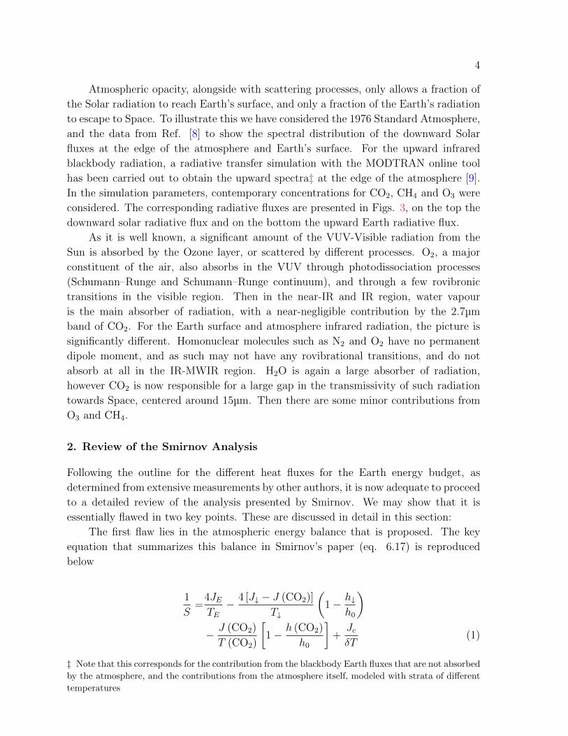
Atmospheric opacity, alongside with scattering processes, only allows a fraction of

the Solar radiation to reach Earth’s surface, and only a fraction of the Earth’s radiation

to escape to Space. To illustrate this we have considered the 1976 Standard Atmosphere,

and the data from Ref. [8] to show the spectral distribution of the downward Solar

fluxes at the edge of the atmosphere and Earth’s surface. For the upward infrared

blackbody radiation, a radiative transfer simulation with the MODTRAN online tool

has been carried out to obtain the upward spectra‡ at the edge of the atmosphere [9].

In the simulation parameters, contemporary concentrations for CO2, CH4 and O3 were

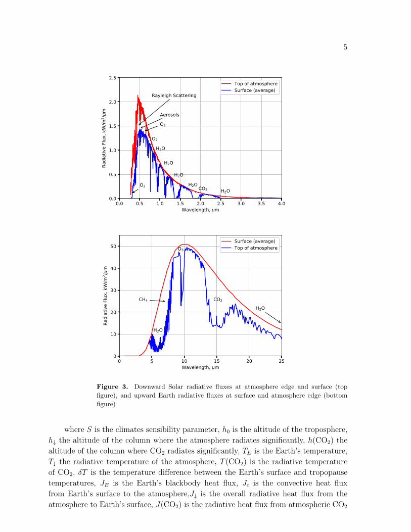
considered. The corresponding radiative fluxes are presented in Figs. 3, on the top the

downward solar radiative flux and on the bottom the upward Earth radiative flux.

As it is well known, a significant amount of the VUV-Visible radiation from the

Sun is absorbed by the Ozone layer, or scattered by different processes. O2, a major

constituent of the air, also absorbs in the VUV through photodissociation processes

(Schumann–Runge and Schumann–Runge continuum), and through a few rovibronic

transitions in the visible region. Then in the near-IR and IR region, water vapour

is the main absorber of radiation, with a near-negligible contribution by the 2.7µm

band of CO2. For the Earth surface and atmosphere infrared radiation, the picture is

significantly different. Homonuclear molecules such as N2 and O2 have no permanent

dipole moment, and as such may not have any rovibrational transitions, and do not

absorb at all in the IR-MWIR region. H2O is again a large absorber of radiation,

however CO2 is now responsible for a large gap in the transmissivity of such radiation

towards Space, centered around 15µm. Then there are some minor contributions from

O3 and CH4.

2. Review of the Smirnov Analysis

Following the outline for the different heat fluxes for the Earth energy budget, as

determined from extensive measurements by other authors, it is now adequate to proceed

to a detailed review of the analysis presented by Smirnov. We may show that it is

essentially flawed in two key points. These are discussed in detail in this section:

The first flaw lies in the atmospheric energy balance that is proposed. The key

equation that summarizes this balance in Smirnov’s paper (eq. 6.17) is reproduced

below

1

S=

4JETE− 4 [J↓ − J (CO2)]

T↓

(1− h↓

h0

)− J (CO2)

T (CO2)

[1− h (CO2)

h0

]+JcδT

(1)

‡ Note that this corresponds for the contribution from the blackbody Earth fluxes that are not absorbed

by the atmosphere, and the contributions from the atmosphere itself, modeled with strata of different

temperatures

5

0.0 0.5 1.0 1.5 2.0 2.5 3.0 3.5 4.0Wavelength, μm

0.0

0.5

1.0

1.5

2.0

2.5

Radiative Flux, kW/m

2 /μm

O2

H2O

H2O

H2O

H2OCO2 H2O

Rayleigh Scattering

AerosolsO3

O2

Top of atmosphereSurface (average)

0 5 10 15 20 25Wavelength, μm

0

10

20

30

40

50

Radiative Flux, kW/m

2 /μm

H2O

O3

CO2CH4

H2O

Surface (average)Top of atmosphere

Figure 3. Downward Solar radiative fluxes at atmosphere edge and surface (top

figure), and upward Earth radiative fluxes at surface and atmosphere edge (bottom

figure)

where S is the climates sensibility parameter, h0 is the altitude of the troposphere,

h↓ the altitude of the column where the atmosphere radiates significantly, h(CO2) the

altitude of the column where CO2 radiates significantly, TE is the Earth’s temperature,

T↓ the radiative temperature of the atmosphere, T (CO2) is the radiative temperature

of CO2, δT is the temperature difference between the Earth’s surface and tropopause

temperatures, JE is the Earth’s blackbody heat flux, Jc is the convective heat flux

from Earth’s surface to the atmosphere,J↓ is the overall radiative heat flux from the

atmosphere to Earth’s surface, J(CO2) is the radiative heat flux from atmospheric CO2

6

to Earth’s surface.

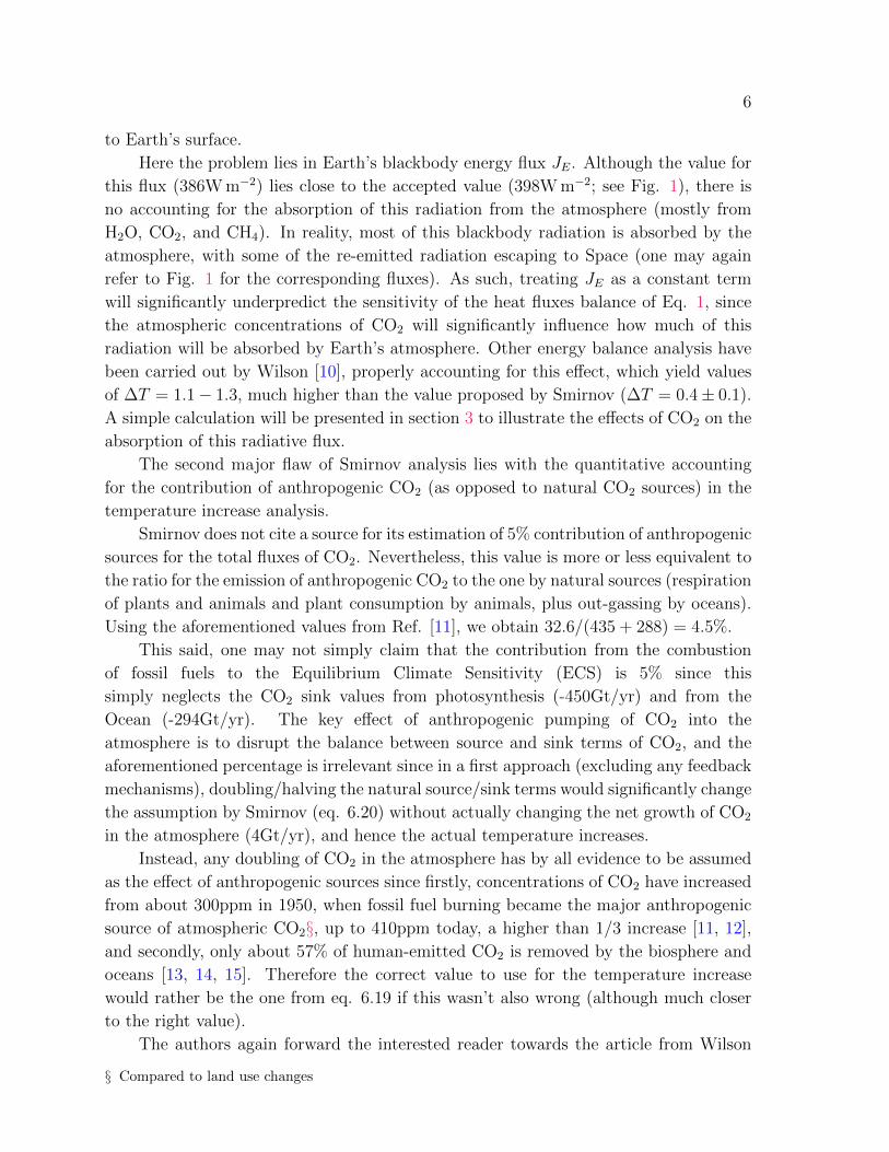
Here the problem lies in Earth’s blackbody energy flux JE. Although the value for

this flux (386W m−2) lies close to the accepted value (398W m−2; see Fig. 1), there is

no accounting for the absorption of this radiation from the atmosphere (mostly from

H2O, CO2, and CH4). In reality, most of this blackbody radiation is absorbed by the

atmosphere, with some of the re-emitted radiation escaping to Space (one may again

refer to Fig. 1 for the corresponding fluxes). As such, treating JE as a constant term

will significantly underpredict the sensitivity of the heat fluxes balance of Eq. 1, since

the atmospheric concentrations of CO2 will significantly influence how much of this

radiation will be absorbed by Earth’s atmosphere. Other energy balance analysis have

been carried out by Wilson [10], properly accounting for this effect, which yield values

of ∆T = 1.1− 1.3, much higher than the value proposed by Smirnov (∆T = 0.4± 0.1).

A simple calculation will be presented in section 3 to illustrate the effects of CO2 on the

absorption of this radiative flux.

The second major flaw of Smirnov analysis lies with the quantitative accounting

for the contribution of anthropogenic CO2 (as opposed to natural CO2 sources) in the

temperature increase analysis.

Smirnov does not cite a source for its estimation of 5% contribution of anthropogenic

sources for the total fluxes of CO2. Nevertheless, this value is more or less equivalent to

the ratio for the emission of anthropogenic CO2 to the one by natural sources (respiration

of plants and animals and plant consumption by animals, plus out-gassing by oceans).

Using the aforementioned values from Ref. [11], we obtain 32.6/(435 + 288) = 4.5%.

This said, one may not simply claim that the contribution from the combustion

of fossil fuels to the Equilibrium Climate Sensitivity (ECS) is 5% since this

simply neglects the CO2 sink values from photosynthesis (-450Gt/yr) and from the

Ocean (-294Gt/yr). The key effect of anthropogenic pumping of CO2 into the

atmosphere is to disrupt the balance between source and sink terms of CO2, and the

aforementioned percentage is irrelevant since in a first approach (excluding any feedback

mechanisms), doubling/halving the natural source/sink terms would significantly change

the assumption by Smirnov (eq. 6.20) without actually changing the net growth of CO2

in the atmosphere (4Gt/yr), and hence the actual temperature increases.

Instead, any doubling of CO2 in the atmosphere has by all evidence to be assumed

as the effect of anthropogenic sources since firstly, concentrations of CO2 have increased

from about 300ppm in 1950, when fossil fuel burning became the major anthropogenic

source of atmospheric CO2§, up to 410ppm today, a higher than 1/3 increase [11, 12],

and secondly, only about 57% of human-emitted CO2 is removed by the biosphere and

oceans [13, 14, 15]. Therefore the correct value to use for the temperature increase

would rather be the one from eq. 6.19 if this wasn’t also wrong (although much closer

to the right value).

The authors again forward the interested reader towards the article from Wilson

§ Compared to land use changes

7

[10] which elegantly outlines several approaches with different levels of complexity for

solving this problem, also outlining several well known feedback effects in climate change

modeling.

3. A Quick Illustration of the Contribution of CO2 to Atmosphere

Radiative Forcing

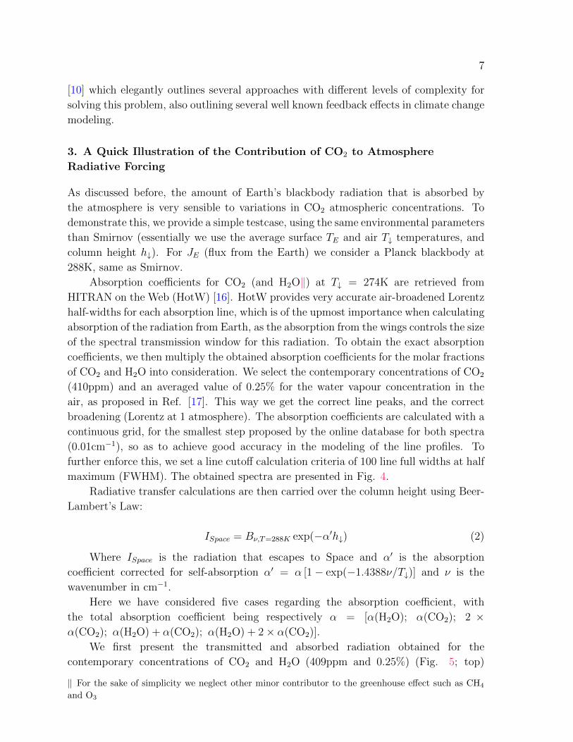
As discussed before, the amount of Earth’s blackbody radiation that is absorbed by

the atmosphere is very sensible to variations in CO2 atmospheric concentrations. To

demonstrate this, we provide a simple testcase, using the same environmental parameters

than Smirnov (essentially we use the average surface TE and air T↓ temperatures, and

column height h↓). For JE (flux from the Earth) we consider a Planck blackbody at

288K, same as Smirnov.

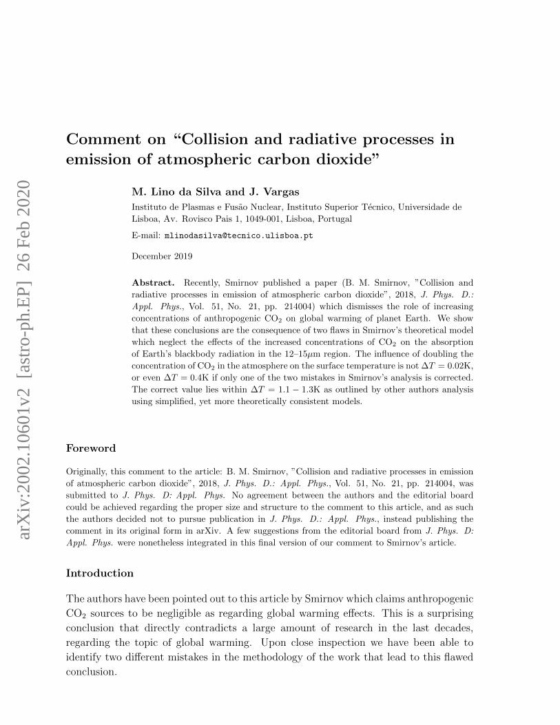
Absorption coefficients for CO2 (and H2O‖) at T↓ = 274K are retrieved from

HITRAN on the Web (HotW) [16]. HotW provides very accurate air-broadened Lorentz

half-widths for each absorption line, which is of the upmost importance when calculating

absorption of the radiation from Earth, as the absorption from the wings controls the size

of the spectral transmission window for this radiation. To obtain the exact absorption

coefficients, we then multiply the obtained absorption coefficients for the molar fractions

of CO2 and H2O into consideration. We select the contemporary concentrations of CO2

(410ppm) and an averaged value of 0.25% for the water vapour concentration in the

air, as proposed in Ref. [17]. This way we get the correct line peaks, and the correct

broadening (Lorentz at 1 atmosphere). The absorption coefficients are calculated with a

continuous grid, for the smallest step proposed by the online database for both spectra

(0.01cm−1), so as to achieve good accuracy in the modeling of the line profiles. To

further enforce this, we set a line cutoff calculation criteria of 100 line full widths at half

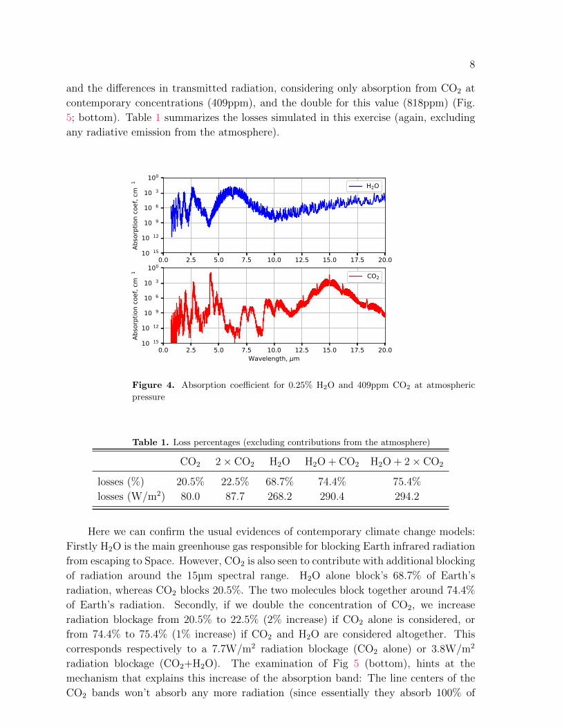
maximum (FWHM). The obtained spectra are presented in Fig. 4.

Radiative transfer calculations are then carried over the column height using Beer-

Lambert’s Law:

ISpace = Bν,T=288K exp(−α′h↓) (2)

Where ISpace is the radiation that escapes to Space and α′ is the absorption

coefficient corrected for self-absorption α′ = α [1− exp(−1.4388ν/T↓)] and ν is the

wavenumber in cm−1.

Here we have considered five cases regarding the absorption coefficient, with

the total absorption coefficient being respectively α = [α(H2O); α(CO2); 2 ×α(CO2); α(H2O) + α(CO2); α(H2O) + 2× α(CO2)].

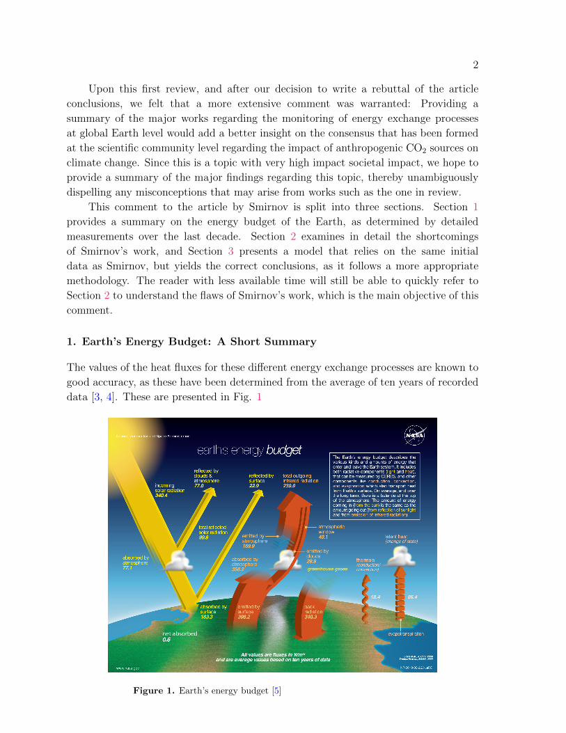
We first present the transmitted and absorbed radiation obtained for the

contemporary concentrations of CO2 and H2O (409ppm and 0.25%) (Fig. 5; top)

‖ For the sake of simplicity we neglect other minor contributor to the greenhouse effect such as CH4

and O3

8

and the differences in transmitted radiation, considering only absorption from CO2 at

contemporary concentrations (409ppm), and the double for this value (818ppm) (Fig.

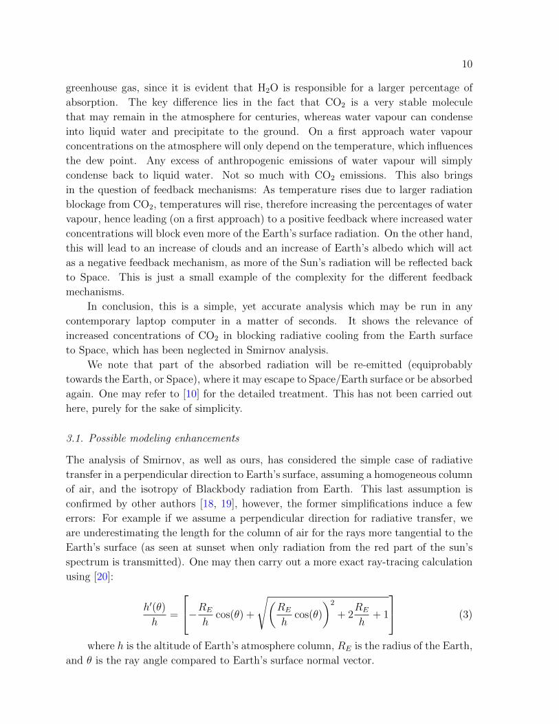
5; bottom). Table 1 summarizes the losses simulated in this exercise (again, excluding

any radiative emission from the atmosphere).

0.0 2.5 5.0 7.5 10.0 12.5 15.0 17.5 20.010−1510−1210−910−610−3100

Absorptio

n coef, c

m−1 H2O

0.0 2.5 5.0 7.5 10.0 12.5 15.0 17.5 20.0Wa elength, μm

10−1510−1210−910−610−3100

Absorptio

n coef, c

m−1 CO2

Figure 4. Absorption coefficient for 0.25% H2O and 409ppm CO2 at atmospheric

pressure

Table 1. Loss percentages (excluding contributions from the atmosphere)

CO2 2× CO2 H2O H2O + CO2 H2O + 2× CO2

losses (%) 20.5% 22.5% 68.7% 74.4% 75.4%

losses (W/m2) 80.0 87.7 268.2 290.4 294.2

Here we can confirm the usual evidences of contemporary climate change models:

Firstly H2O is the main greenhouse gas responsible for blocking Earth infrared radiation

from escaping to Space. However, CO2 is also seen to contribute with additional blocking

of radiation around the 15µm spectral range. H2O alone block’s 68.7% of Earth’s

radiation, whereas CO2 blocks 20.5%. The two molecules block together around 74.4%

of Earth’s radiation. Secondly, if we double the concentration of CO2, we increase

radiation blockage from 20.5% to 22.5% (2% increase) if CO2 alone is considered, or

from 74.4% to 75.4% (1% increase) if CO2 and H2O are considered altogether. This

corresponds respectively to a 7.7W/m2 radiation blockage (CO2 alone) or 3.8W/m2

radiation blockage (CO2+H2O). The examination of Fig 5 (bottom), hints at the

mechanism that explains this increase of the absorption band: The line centers of the

CO2 bands won’t absorb any more radiation (since essentially they absorb 100% of

9

0 5 10 15 20 25 30 35 40Wavelength, μm

0.0

0.1

0.2

0.3

0.4

0.5

0.6

0.7

0.8

0.9

Radiative Flux, kW/m

2 /μm

Absorbed CO2Absorbed H2OTransmitted

4 6 8 10 12 14 16 18 20 22Wavelength, μm

0.0

0.1

0.2

0.3

0.4

0.5

0.6

0.7

0.8

0.9

Radi

ativ

e Fl

ux, k

W/m

2 /μm

Earth SurfaceAbsorbed CO2Absorbed 2xCO2

Figure 5. Transmitted Earth radiation towards Space (green); Absorbed by H2O

(blue) and absorbed by CO2 (red); top figure. Transmitted radiation towards Space

for 409ppm CO2 and doubled concentration of CO2; bottom figure

the incoming radiation, however as CO2 concentrations increase, so will the absorbing

intensity of the wings, farther from the line center. Then this will lead to more radiation

absorption on the edges of the spectral window where CO2 absorbs radiation, thereby

effectively increasing the spectral range of the blockage. This is what is seen in the

bottom part of figure 5¶.

One may then find it surprising on a first approach to focus on CO2 as the main

¶ We note that we have smoothed the simulation results for enhancing the visualization of this

mechanism

10

greenhouse gas, since it is evident that H2O is responsible for a larger percentage of

absorption. The key difference lies in the fact that CO2 is a very stable molecule

that may remain in the atmosphere for centuries, whereas water vapour can condense

into liquid water and precipitate to the ground. On a first approach water vapour

concentrations on the atmosphere will only depend on the temperature, which influences

the dew point. Any excess of anthropogenic emissions of water vapour will simply

condense back to liquid water. Not so much with CO2 emissions. This also brings

in the question of feedback mechanisms: As temperature rises due to larger radiation

blockage from CO2, temperatures will rise, therefore increasing the percentages of water

vapour, hence leading (on a first approach) to a positive feedback where increased water

concentrations will block even more of the Earth’s surface radiation. On the other hand,

this will lead to an increase of clouds and an increase of Earth’s albedo which will act

as a negative feedback mechanism, as more of the Sun’s radiation will be reflected back

to Space. This is just a small example of the complexity for the different feedback

mechanisms.

In conclusion, this is a simple, yet accurate analysis which may be run in any

contemporary laptop computer in a matter of seconds. It shows the relevance of

increased concentrations of CO2 in blocking radiative cooling from the Earth surface

to Space, which has been neglected in Smirnov analysis.

We note that part of the absorbed radiation will be re-emitted (equiprobably

towards the Earth, or Space), where it may escape to Space/Earth surface or be absorbed

again. One may refer to [10] for the detailed treatment. This has not been carried out

here, purely for the sake of simplicity.

3.1. Possible modeling enhancements

The analysis of Smirnov, as well as ours, has considered the simple case of radiative

transfer in a perpendicular direction to Earth’s surface, assuming a homogeneous column

of air, and the isotropy of Blackbody radiation from Earth. This last assumption is

confirmed by other authors [18, 19], however, the former simplifications induce a few

errors: For example if we assume a perpendicular direction for radiative transfer, we

are underestimating the length for the column of air for the rays more tangential to the

Earth’s surface (as seen at sunset when only radiation from the red part of the sun’s

spectrum is transmitted). One may then carry out a more exact ray-tracing calculation

using [20]:

h′(θ)

h=

−RE

hcos(θ) +

√(RE

hcos(θ)

)2

+ 2RE

h+ 1

(3)

where h is the altitude of Earth’s atmosphere column, RE is the radius of the Earth,

and θ is the ray angle compared to Earth’s surface normal vector.

11

Another improvement includes accounting for the difference in temperature and

pressure in the air column. As the altitude increases, the density will decrease and the

Lorentz broadening mechanisms will be less marked. Furthermore, Doppler broadening

will also decrease as the result of lower temperatures. This will lead to spectral lines

closer to diracs, with obvious impact on radiative transfer. However Wilson notes [10]

that simulations accounting for both these improvements yield similar results to the more

simplistic approach, which means that likely these two simplifications cancel out to a

given degree (ignoring tangential rays underpredicts radiation absorption, and ignoring

lower line broadening at higher altitudes overpredicts absorption.

4. Concluding Remarks

We have shown that the influence of doubling the concentration of CO2 in the

atmosphere on the surface temperature is not ∆T = 0.02K as claimed by Smirnov,

or even ∆T = 0.4K if the correct fraction of the anthropogenic sources is considered

for the doubling of CO2 concentrations in the atmosphere (100% instead of 5%). Only

if one considers the influence on this doubling of CO2 concentrations on the energy

flux JE that escapes from Earth, may one obtain a more correct value lying within

∆T = 1.1− 1.3K [10].

Atmospheric heating from anthropogenic CO2 is a topic with very high societal

impact, and as such should not be treated lightly. The last decade has brought a large

wealth of new, large scale experimental and modeling works that have significantly

reduced the uncertainties of several key mechanisms of global warming, namely feedback

mechanisms [11]. Some uncertainties remain, namely regarding the effects of aerosols,

and the future trends of climate change, however, as illustrated in section 3, modeling

improvements and available computational power make it a trivial exercise to develop

simple models that may evidence the key role of CO2 regarding the imbalance of Earth’s

energy budget, obviously excluding any feedback mechanisms, as a zero-order approach.

This is not to say that climate warming may no longer be considered complex

topic, least one forget that the different feedback mechanisms to be accounted quickly

complexify the necessary models and calculations, and that there are further issues

with significant societal impact that need addressing, such as ocean acidification from

increased concentrations from CO2; the increase in re-circulation in the atmosphere

(with the increase of extreme weather phenomena) resulting from the ocean temperature

increase; or the impact on ocean currents.

5. Bibliography

[1] B. M. Smirnov, ”Collision and radiative processes in emission of atmospheric carbon dioxide”,

2018, J. Phys. D: Appl. Phys. , Vol. 51, No. 21, pp. 214004.

[2] https://commons.wikimedia.org/wiki/File:Earth_heat_balance_Sankey_diagram.svg, re-

trieved in 12th Dec. 2019.

12

[3] N. G. Loeb, B. A. Wielicki, D. R. Doelling, G. L. Smith, D. F. Keyes, S. Kato, N. Manalo–

Smith, and T. Wong., 2009, “Toward optimal closure of the Earth’s top-of-atmosphere radiation

budget,” Journal of Climate, Vol. 22, No. 3, pp. 748–766.

[4] K. E. Trenberth, J. T. Fasullo, and J. Kiehl, 2009, “Earth’s global energy budget,” Bulletin of the

American Meteorological Society, Vol. 90, No. 3, pp. 311–324.

[5] https://commons.wikimedia.org/wiki/File:The-NASA-Earth’s-Energy-Budget-Poster-Radiant-

Energy-System-satellite-infrared-radiation-fluxes.jpg, retrieved in 12th Dec. 2019.

[6] J. Hansen, Mki. Sato, P. Kharecha, and K. von Schuckmann, 2011, “Earth’s energy imbalance and

implications,” Atmos. Chem. Phys., Vol. 11, pp. 13421–13449, doi:10.5194/acp-11-13421-2011.

[7] G. Bianchini, U. Cortesi, and B. Carli, 2003, “Emission fourier transform spectroscopy for remote

sensing of the Earth’s atmosphere,” Annals of Geophysics, Vol. 46, No. 2, pp. 205–222.

[8] American Society for Testing and Materials. Committee G03 on Weathering and Durability,

“Standard tables for reference Solar spectral irradiances: Direct normal and hemispherical on

37º tilted Surface,” ASTM International, 2003.

[9] http://climatemodels.uchicago.edu/modtran/modtran.html, retrieved in 28th Dec. 2019.

[10] D. J. Wilson, , and J. Gea–Banacloche, 2012, “Simple model to estimate the contribution of

atmospheric CO2 to the Earth’s greenhouse effect,” American Journal of Physics, Vol. 80, No.

4, pp. 306–315.

[11] P. Ciais, C. Sabine, G. Bala, L. Bopp, V. Brovkin, J. Canadell, A. Chhabra, R. DeFries, J.

Galloway, M. Heimann, C. Jones, C. Le Quere, R. B. Myneni, S. Piao and P. Thornton, 2013,

“Carbon and other biogeochemical cycles” In: Climate Change 2013: The Physical Science Basis.

Contribution of Working Group I to the Fifth Assessment Report of the Intergovernmental Panel

on Climate Change [Stocker, T.F., D. Qin, G.-K. Plattner, M. Tignor, S.K. Allen, J. Boschung,

A. Nauels, Y. Xia, V. Bex and P.M. Midgley (eds.)]. Cambridge University Press, Cambridge,

United Kingdom and New York, NY, USA.

[12] H. Hellevang and P. Aagaard, 2015, “Constraints on natural global atmospheric CO2 fluxes from

1860 to 2010 using a simplified explicit forward model,” Scientific Reports, Vol. 5, No. 17352.

[13] J. G. Canadell,, C. Le Quere, M. R. Raupach, C. B. Field, E. T. Buitenhuis, P. Ciais, T. J.

Conway, N. P. Gillett, R. A. Houghton, and G. Marland, 2007, “Contributions to accelerating

atmospheric CO2 growth from economic activity, carbon intensity, and efficiency of natural

sinks,” Proceedings of the National Academy of Sciences, Vol. 104, No. 47, pp. 18866–18870.

[14] C. Le Quere, M. R. Raupach, J. G. Canadell, G. Marland, L. Bopp, P. Ciais, T. J. Conway et al,

2009, “Trends in the sources and sinks of carbon dioxide,” Nature Geoscience, Vol. 2, No. 12,

831, 6 pp.

[15] J. Huang, and M. B. McElroy, 2012, “The contemporary and historical budget of atmospheric

CO2,” Canadian Journal of Physics, Vol. 90, No. 8, pp. 707–716.

[16] http://hitran.iao.ru/molecule/simlaunch, retrieved in 26th Dec. 2019.

[17] K. Lodders, and B. Fegley Jr, “Chemistry of the Solar system,” Royal Society of Chemistry, 2015.

[18] B.–H Tang,, Z.–H. Li, and Y. Bi, 2009, “Estimation of land surface directional emissivity in

mid-infrared channel around 4.0 µm from MODIS data,” Optics Express, Vol. 17, No. 5, pp.

3173–3182.

[19] T. J. Warren, N. E. Bowles, K. Donaldson Hanna, and J. L. Bandfield, 2019, “Modeling the angular

dependence of emissivity of randomly rough surfaces,” Journal of Geophysical Research: Planets,

Vol. 124, No. 2, pp. 585–601.

[20] M. Vollmer, and S. D. Gedzelman, 2006, “Colours of the Sun and Moon: the role of the optical

air mass,” European Journal of Physics, Vol. 27, No. 2, pp. 299–309.