Emission reductions and ecological response: Management models for acid rain control

Pergmon Socio-Econ. Plann. Sci. Vol. 30, No. 1, pp. 15-26, 1996

Published by Elsevier Science Ltd. Printed in Great Britain 0038-0121/96 $15.00 + 0.00

00380121(95)00025-9

Emission Reductions and Ecological Response: Management Models for Acid

Rain Control H U G H ELLIS I, PAUL L. RINGOLD 2 and GEORGE R. HOLDREN JR 3

~Department of Geography and Environmental Engineering, The Johns Hopkins University, Baltimore, MD 21218, U.S.A.

2United States Environmental Protection Agency, National Health and Environmental Effects Labora- tory, ORD, 200 SW 35th Street, Corvallis, OR 97333, U.S.A.

3Water and Land Resources Department, Pacific Northwest Laboratories, MSIN K6-81, P.O. Box 999, Richland, WA 99352, U.S.A.

Abstract--Presented in this paper is a series of optimization analyses for acid rain control in eastern North America. The analyses involve models that minimize cost or emissions removed subject to environmental quality restrictions at selected sensitive receptor locations. Site-specific critical loads are the measures of environmental quality, where critical loads are roughly interpreted as levels of areal pollutant deposition beyond which deleterious ecological effects are thought to occur. Our approach is demonstrated with an application that includes critical loads estimated for 768 lakes in the Adirondacks. As well, a stratified random subsample of 122 sites is modeled to assess the effects of sampling intensity on the control scenarios that are identified through the optimization procedures. Two different models for estimating site-specific critical loads are used and their effects on control strategies are assessed. From a somewhat broader perspective, this work is a demonstration of the feasibility and usefulness of large-scale integrated assessment and the role that operations research methods can play in that process.

INTRODUCTION

For industrial nations, regulating gaseous pollutant emissions offers a rational means for reducing potential health and welfare risks. As a result, emission control approaches have been incorporated into national laws and into bi- and multilateral agreements among countries sharing common airsheds. Numerous policy concerns, for example, costs, benefits, equity, achievability, enforceabil- ity and technological approaches (best available technology, uniform percentage reductions, ambient air quality standards) have been raised in the pursuit of attaining national and international agreements. Given the costs of implementing many control strategies--current estimates for implementing the 1990 Clean Air Act Amendments (CAAA) (U.S. Congress [34]) are about $5 billion annually--it is not surprising that considerable debate continues regarding the merits of many individual steps in legislation such as the CAAA.

Air quality regulations derived from analyses that explicitly link source emissions and resultant environmental effects have drawn considerable attention because they promise levels of cost-effectiveness superior to alternatives that are strictly source based. Such approaches can be criticized because of the difficulty in achieving a level of scientific certainty satisfactory to all of the parties involved. Moreover, it has not been possible to implement objective approaches employing ecological end-points as the decision criteria because, until recently, such ecological criteria have not been available. But the situation has changed significantly with the development of critical loads [16, 28]. Critical loads are secondary deposition standards, i.e. not health-based, designed to protect sensitive components of terrestrial and aquatic ecosystems.

In the U.S., recent domestic and international agreements mandate the examination of a critical loads approach as a potential means for establishing atmospheric emission standards for sulfur and nitrogen. Section 404 in Title IV of the CAAA states that by 15 November 1993, the EPA must transmit . . , a report on the feasibility and effectiveness of an acid deposition standard or standards to protect sensitive and critically sensitive aquatic and terrestrial resources.

Disclaimer: This paper has not been formally reviewed by the U.S. Environmental Protection Agency and should not be construed to represent Agency policy.

15

16 Hugh Ellis et al.

The current EPA study seeks to:

1. Identify sensitive resources in the U.S. and Canada. 2. Describe the nature and numerical value of a deposition standard. 3. Describe use of such standards by other nations or by individual states. 4. Describe measures to integrate such standards into Title IV of the Clean Air Act. 5. Describe state-of-knowledge of source-receptor relationships and other ongoing research;

what would be needed to make such a program feasible. 6. Describe impediments to implementation; cost-effectiveness of deposition standards com-

pared to other control strategies, including ambient air quality standards, NSPS, and Title IV requirements.

It is our view that Section 404 demands, in essence, integrated assessment. With that in mind, the primary purpose of this paper is to link critical loads with source-receptor deposition models and associated emission inventories and, hence, conduct an integrated assessment that helps to determine how emission reduction strategies might be developed. We demonstrate the strong interdependence among ecologists, atmospheric modelers and policy analysts that must occur to develop rational approaches to these complex, value-laden issues.

THE CRITICAL LOADS CONCEPT

According to current international usage, a critical load is that amount of pollutant deposition beyond which, given current knowledge, measurable deleterious effects to selected sensitive ecosystem components will occur. The criteria used to define critical loads are usually biologically derived, for example, loss of biodiversity or of a sport fishery, reduced net primary productivity or reduced reproductive success. Because of the complexity of these issues, however, it is common to specify chemical surrogates, or indicators, to provide a direct link between pollutant loadings and biological effects.

In setting a critical load, a value or a change in the value of the indicator is set that identifies the point at which arbitrary deleterious effects become apparent. This value of the indicator--the end point--serves as the benchmark against which projected responses of the ecosystem to a particular level of deposition are gauged.t

This work deals only with the chronic acidification effects of sulfur deposition on lakes. Clearly, ecosystems are complex entities consisting of multiple components, each of which responds to perturbations (e.g. acidic sulfate deposition) in different ways. Critical loads, therefore, are not fundamental properties of ecosystems per se but rather are characteristics of specific parts of the system. In this context, single measures of ecosystem health will rarely be sufficient to characterize the total ecosystem response to any anthropogenic ecological stress--but they are a place to start. It is important as well to bear in mind that the critical load estimates used here are technical estimates developed to demonstrate methodologies. They do not reflect the estimates that might be derived from a formal or an informal standard-setting process.

Developing critical loads estimates

There exist several reasons for studying chronic acidification in the context of emission control management models. First, there exist good, regional, aquatic data bases that allow us to pursue the chronic acidification issue in a fairly rigorous manner. Second, we can reliably model longer term (yearly average) sulfur deposition--and such deposition clearly plays a dominant role in surface water acidification [20, 26, 27].

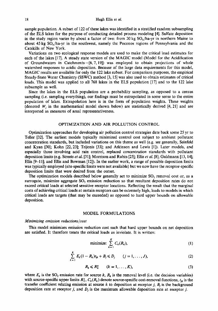
Lake data used here are taken from the U.S. EPA Eastern Lake Survey (ELS) [21, 24]. The sample includes data on 768 lakes collected during fall turnover in 1984. The lakes in the study are a probability sampling of lakes in the region, which is shown in Fig. 1. They range in size from 4 to 2000 ha, with the lakes in the size class of 4 to 8 ha being slightly underrepresented in the

tAlthough a general consensus is emerging that pH values of less than about 6.0 portend deterioration of cold water sport fisheries [2, 29], certain parts of the country (e.g. Florida) are able to sustain remarkable healthy warm water fisheries in systems with surprisingly low pH values.

Acid rain control and ecological response 17

• i go D • o •

• o" "~" °~." :" • o'o • e o--ee"e oe • • -o.:...~'-.... ~,

~ , , , • • • d l ~

~.~.....;--~-: " - ~ eeI6e • | eo~ • •

l o g roll • • o ° •

i o% l

>- Z

11.

~o

o


sample population. A subset of 122 of these lakes was identified in a stratified random subsampling of the ELS lakes for the purpose of conducting detailed process modeling [4]. Sulfate deposition in the study region varies by about a factor of two: from 20 kg SO4/ha-yr in northern Maine to about 45 kg SO4/ha-yr in the southwest, namely the Poconos regions of Pennsylvania and the Catskills of New York.

Variations on two ecological response models are used to make the critical load estimates for each of the lakes [17]. A steady state version of the MAGIC model (Model for the Acidification of Groundwaters in Catchments--[6,7, 19]) was employed to obtain projections of whole watershed responses to acidic deposition. Because of the large data requirements for this model, MAGIC results are available for only the 122 lake subset. For comparison purposes, the empirical Steady-State Water Chemistry (SSWC) method [3, 15] was also used to obtain estimates of critical loads. This model was applied to all 768 lakes in the ELS population [17] and to the 122 lake subsample as well.

Since the lakes in the ELS population are a probability sampling, as opposed to a census sampling (i.e. sampling everything), our findings must be extrapolated in some sense to the entire population of lakes. Extrapolation here is in the form of population weights. These weights (denoted Wj in the mathematical model shown below) are statistically derived [4, 21] and are interpreted as measures of areal representativeness.

OPTIMIZATION AND AIR POLLUTION CONTROL

Optimization approaches for developing air pollution control strategies date back some 25 yr to Teller [32]. The earliest models typically minimized control cost subject to ambient pollutant concentration standards, but included variations on this theme as well (e.g. see generally, Seinfeld and Kyan [30]; Kohn [22, 23]; Trijonis [33]; and Atkinson and Lewis [1]). Later models, and especially those involving acid rain control, replaced concentration standards with pollutant deposition limits (e.g. Streets et al. [31]; Morrison and Rubin [25]; Ellis et al. [8]; Guldmann [13, 14]; Ellis [9-11]; and Ellis and Bowman [12]). In the earlier work, a range of possible deposition limits was typically employed (site-specific limits were not available) but we now have the receptor-specific deposition limits that were desired from the outset.

The optimization models described below generally act to minimize SO2 removal cost or, as a surrogate, minimize aggregate SO2 emission reduction so that resultant deposition rates do not exceed critical loads at selected sensitive receptor locations. Reflecting the result that the marginal costs of achieving critical loads at certain receptors can be extremely high, leads to models in which critical loads are targets (that may be exceeded) as opposed to hard upper bounds on allowable deposition.

MODEL FORMULATIONS

Minimizing emission reductions~cost

This model minimizes emission reduction cost such that hard upper bounds on net deposition are satisfied. It therefore treats the critical loads as inviolate. It is written:

K

minimize: ~ Ck(Rk), (1) k = l

K

Ek(1 -- Rk)tjk + Bj <~ Dj ( j = 1 . . . . . J), (2) k = l

Rk ~ R~ (k = 1 . . . . . K), (3)

where Ek is the SO2 emission rate for source k, R k is the removal level (i.e. the decision variables) with source-specific upper limits R~, Ck(Rk) denote source-specific cost-removal functions, tjk is the transfer coefficient relating emission at source k to deposition at receptor j, Bj is the background deposition rate at receptor j, and Dj is the maximum allowable deposition rate at receptor j.


Mult iobject ive mode l

As noted earlier, when the Dj are interpreted as critical loads, our data and assumptions (e.g. only the large point sources are controlled) lead to the result that the deposition constraints cannot be satisfied even with all SO2 removal levels (Rk) set to their upper limits R~. Feasibility can be obtained by sequentially removing receptors from the model or (equivalently) relaxing maximum allowable deposition rates at those receptor locations where infeasibility occurs. We implemented the latter approach and relaxed the strict requirement for critical load satisfaction at all receptors. The intent here was to trade-off aggregate measures of critical load exceedences against measures of the costs of control. Exceedences were allowed in the model by modifying constraints (2) to yield:

K

~. E k ( 1 - - R k ) t j k + B j + U j - - V j = D j ( j = l . . . . . J), (4) kffil

where the new decision variables (Uj, Vj) represent, respectively, oversatisfaction (deposition less than the critical load) and exceedence (deposition greater than the critical load). The original objective function of the model [equation (1)] is then augmented by a second objective to minimize the sum of critical load exceedences (Vj), which is equivalent to minimizing average exceedence. A more conservative variant minimizes maximum population-weighted exceedence. When com- pared to models that minimize average exceedence, minmax solutions would tend to have a smaller maximum exceedence, but a slightly higher average exceedence, which is the tradeoff one would expect. From a mathematical programming perspective, the exceedence models described above are, in essence, penalty models and, more specifically, models with linear, asymmetric penalty functions.

The model that was implemented is therefore multiobjective (e.g. see, generally, Cohon [5]) and serves to minimize control cost and average critical load population-weighted exceedence. It is written:

minimize: F~/. Ck(Rk) + F~. ~ Vj , (5) kffil

~ Ek(1 -- Rk)tjk + Bj + Uj - Vj = Dj ( j = 1 . . . . , J), (6) kffil

R k <~ RUk (k = 1 . . . . . K) . (7)

Here the objective weights F~ and F~2 are arbitrary and function only to generate the tradeoff between cost and average exceedence (they do not, for example, represent decision-maker preferences). The Wj represent the so-called population weights mentioned earlier.

IMPLEMENTATION

Along with the receptor configuration described earlier, there exist eight categories of sources in the optimization models, shown in Table 1. In this abbreviated taxonomy, "large" refers to sources with annual 1980 SO2 emissions above 19kT (only these large sources are controllable in the model); power plants are electric utilities; small plants are aggregated into idealized emission-weighted centroids in each state and province; and industrial sources refer to nonferrous smelters and other assorted non-utility sources. The transfer coefficients relating emissions from these 322 sources to deposition at either 122 or 768 receptors were generated using the MOE Statistical long-range transport simulation model [35].

Table I. S02 emission sources

Source type Number Emissions (kT/yr)

"Large" U.S. power plants "Large" U.S. industrial sources "Large" Canadian power plants "Large" Canadian industrial sources "Area" U.S. power plant source regions "Area" U.S. industrial source regions "Area" Canadian power plant source regions "Area" Canadian industrial source regions

176 12,676 38 1516

9 543 7 2169

32 1813 42 6274

9 187 9 1523


Cost-removal functions for the 230 large sources are described in Ref. [8]. Costs are expressed as net present values amortized over 20 yr with a 6% net-of-inflation discount rate. These cost- removal functions clearly are dated and thus must be viewed solely as rough indicators. They suffice for our purposes in that we believe these functions to be (at least) internally consistent; and it is relative--not total---costs that play a major role in shaping control strategies.

The results presented next were generated using the multiobjective model described above. Each set of analyses was replicated for the three different sets of critical loads described earlier: SSWC with 768 receptors, SSWC with 122 receptors and MAGIC with 122 receptors. We employed nine different pairs of arbitrary objective function weights per set of analyses so as to produce tradeoffs between control cost and differing measures of critical load exceedence. Every analysis therefore involved 3 × 9 = 27 optimizations.

RESULTS

Tradeoffs between aggregate SOe removal and critical load exceedences--the SSWC768 case

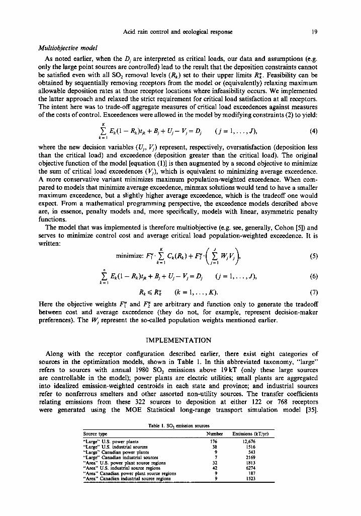
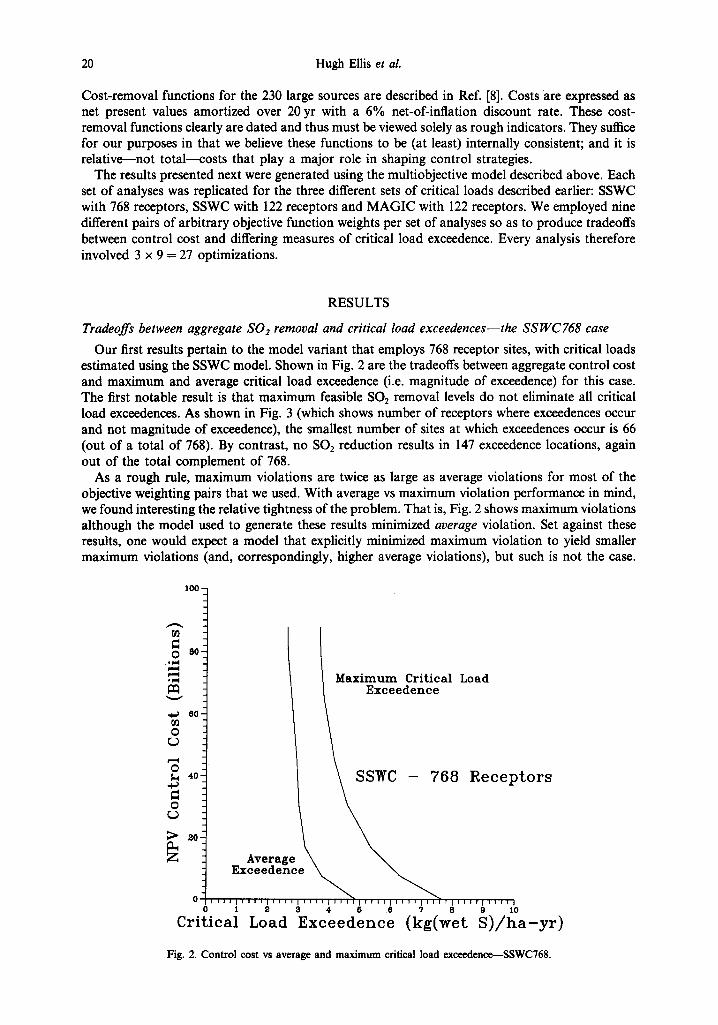
Our first results pertain to the model variant that employs 768 receptor sites, with critical loads estimated using the SSWC model. Shown in Fig. 2 are the tradeoffs between aggregate control cost and maximum and average critical load exceedence (i.e. magnitude of exceedence) for this case. The first notable result is that maximum feasible SO2 removal levels do not eliminate all critical load exceedences. As shown in Fig. 3 (which shows number of receptors where exceedences occur and not magnitude of exceedence), the smallest number of sites at which exceedences occur is 66 (out of a total of 768). By contrast, no SO: reduction results in 147 exceedence locations, again out of the total complement of 768.

As a rough rule, maximum violations are twice as large as average violations for most of the objective weighting pairs that we used. With average vs maximum violation performance in mind, we found interesting the relative tightness of the problem. That is, Fig. 2 shows maximum violations although the model used to generate these results minimized average violation. Set against these results, one would expect a model that explicitly minimized maximum violation to yield smaller maximum violations (and, correspondingly, higher average violations), but such is not the case.

100 -

0 . ° ~

,F-I

0

0

0 L)

Z

80,

60.

40"

2O -

0 0

C r i t i c a l

Maximum Critical Load Exceedence

C - 7 6 8 R e c e p t o r s

A v e r a g e ~ ~ Exceedence ~ ~

I I I I I I I I I I I I I l l l l l l l l l l l l l f l l l l l l l l l l l r l l l f l l l l l l I 1 2 3 4 6 6 7 8 9 10

L o a d E x c e e d e n c e ( k g ( w e t S ) / h a - y r )

Fig. 2. Control cost vs average and maximum critical load exceedence--SSWC768.


100 -

o • p,,,l

V

r ~

o L)

o

o

2;

8 0 -

6 0 - _

4 0 -

2 0 - -

i I l l I l l I I l l I I ~ I I I I I I I I l l I I I I D I I I I I I r I i i i i r T i r

60 70 8 0 9 0 1 0 0 1 1 0 1 2 0 1 3 0 1 4 0 1 5 0

N u m b e r o f E x c e e d e n c e s

Fig. 3. Control cost vs number of critical load exceedences--SSWC768.

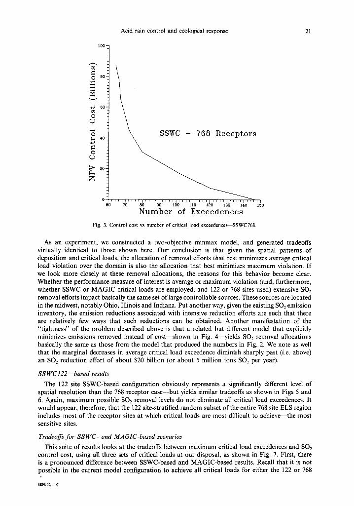
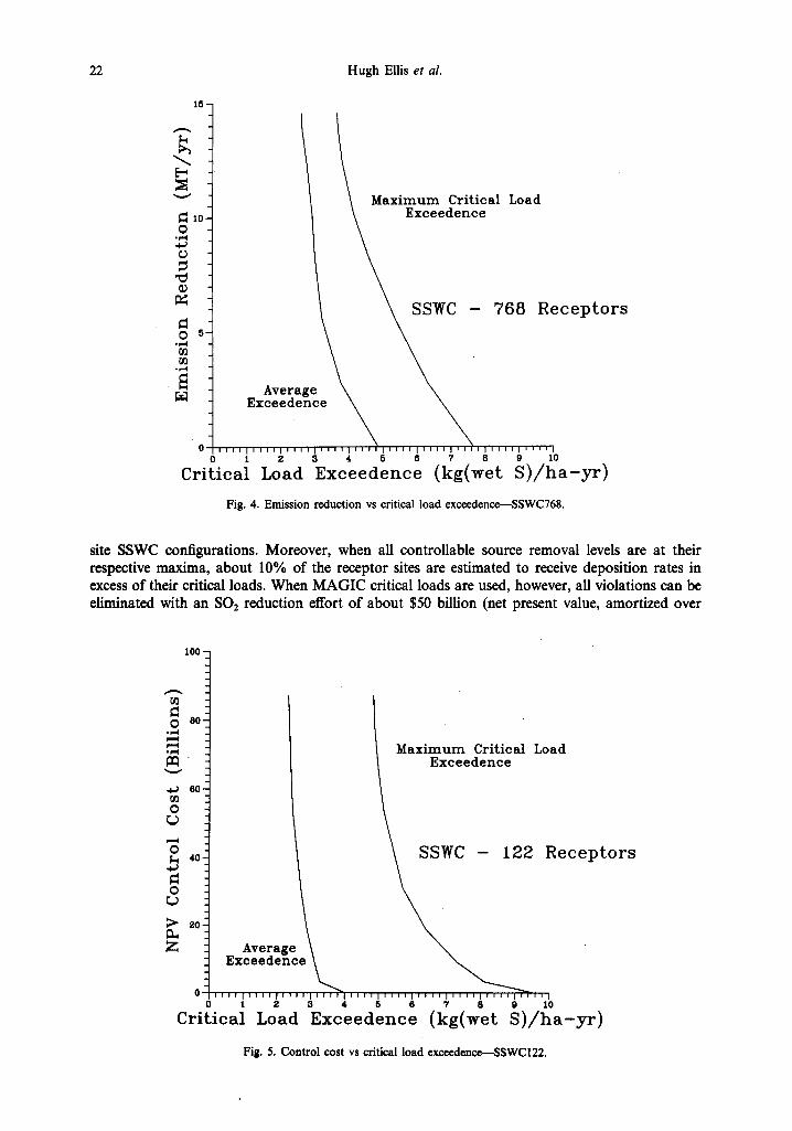
As an experiment, we constructed a two-objective minmax model, and generated tradeoffs virtually identical to those shown here. Our conclusion is that given the spatial patterns of deposition and critical loads, the allocation of removal efforts that best minimizes average critical load violation over the domain is also the allocation that best minimizes maximum violation. If we look more closely at these removal allocations, the reasons for this behavior become clear. Whether the performance measure of interest is average or maximum violation (and, furthermore, whether SSWC or MAGIC critical loads are employed, and 122 or 768 sites used) extensive SO2 removal efforts impact basically the same set of large controllable sources. These sources are located in the midwest, notably Ohio, Illinois and Indiana. Put another way, given the existing SO2 emission inventory, the emission reductions associated with intensive reduction efforts are such that there are relatively few ways that such reductions can be obtained. Another manifestation of the "tightness" of the problem described above is that a related but different model that explicitly minimizes emissions removed instead of cost--shown in Fig. 4~yields SO2 removal allocations basically the same as those from the model that produced the numbers in Fig. 2. We note as well that the marginal decreases in average critical load exceedence diminish sharply past (i.e. above) an SO2 reduction effort of about $20 billion (or about 5 million tons SO2 per year).

SSWC122--based results

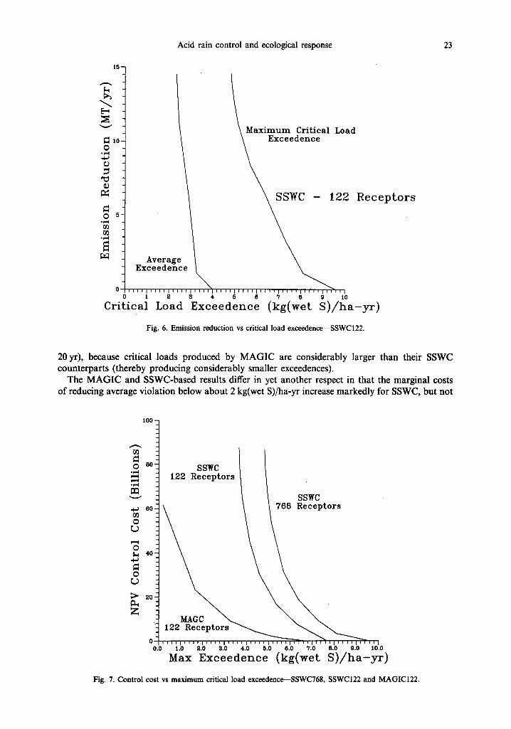
The 122 site SSWC-based configuration obviously represents a significantly different level of spatial resolution than the 768 receptor case--but yields similar tradeoffs as shown in Figs 5 and 6. Again, maximum possible SO2 removal levels do not eliminate all critical load exceedences. It would appear, therefore, that the 122 site-stratified random subset of the entire 768 site ELS region includes most of the receptor sites at which critical loads are most difficult to achieve--the most sensitive sites.

Tradeoffs for SSWC- and MAGIC-based scenarios

This suite of results looks at the tradeoffs between maximum critical load exceedences and SO2 control cost, using all three sets of critical loads at our disposal, as shown in Fig. 7. First, there is a pronounced difference between SSWC-based and MAGIC-based results. Recall that it is not possible in the current model configuration to achieve all critical loads for either the 122 or 768

$EPS 30/I---C


v

I0 O ,r.4

C9

09

O 5

-L=.4

Average Exceedence

mum Critical Load Exceedence

SSWC - 768 R e c e p t o r s

0 1 2 3 4 5 6 7 8 9 10

Critical Load Exeeedence (kg(wet S)/ha-yr)

Fig. 4. Emission reduction vs critical load exceedence~SSWC768.

site SSWC configurations. Moreover, when all controllable source removal levels are at their respective maxima, about I0% of the receptor sites arc estimated to receive deposition rates in excess of their critical loads. When MAGIC critical loads arc used, however, all violations can be eliminated with an SO2 reduction effort of about $50 billion (net present value, amortized over

100

O 80 , I l l

, I l l

-l~ 60

O

0 40-

Q

~;~ 20'

Z

0

Critical

Maximum Critical Load Exceedence

SSWC - 122 R e c e p t o r s

Average \ E x c e e d e n c e ~ . ~ .

i I I I l l l l l [ l l l l l l l l l l l l l l l l I I I 1 2 3 4 5 6 ? 8 9 10

Load Exceedence (kg(wet S)/ha-yr)

Fig. 5. Control cost vs critical load exceedence--SSWC122.


15-

V

10. O - ,~=~

O

O 5-

,p-4

Average Exceedence l l l l l l l l l l I l l l l l l l ~ l

0 1 2 3 4

C r i t i c a l L o a d E x c e e d e n c e

~Maximum Critical Load

Exceedence 22 Receptors

l l l l l l l l l l l l , l l l l l l l l l l l l l l l l I 5 6 7 8 9 1 0

(kg(wet S)/ha-yr)

Fig. 6. Emission reduction vs critical load exceedcnce---SSWC122.

20 yr), because critical loads produced by MAGIC are considerably larger than their SSWC counterparts (thereby producing considerably smaller exceedences).

The MAGIC and SSWC-based results differ in yet another respect in that the marginal costs of reducing average violation below about 2 kg(wet S)/ha-yr increase markedly for SSWC, but not

100

0 80 .p,-I

.L,-I

60 r~ 0

0 40--

~.~

@ L~

so-

Z

0 0.0

SSWC 1 122 R e c e p t o r s /

sswc tors

~AGC ~ \ \ 122 Receptors ~ . ~ . . . _ ~ , " - ~ ~ . . ~

~ l l l l l l ~ I I I I | i i i i I i I i t I t.O 2.0 3.0 4.0 5.0 6.0 7.0 8.0 9.0 10.0

Max Exceedence (kg(wet S)/ha-yr)

Fig. 7. Control cost vs maximum critical load excvedencc---SSWC768, SSWCI22 and MAGIC122.

24 H u g h Ellis et al.

1 0 0

O .~=~ I===1

. e l

O r..)

O

O L)

Z

80.

60,

4O -

2 0

0 3 .0

~ SSWC - 7 6 8

sswc \

4 .0 5 .0 6 .0 7 .0 8 .0 9 .0 10 ,0 11 .0 12 .0

M a x E x c e e d e n c e ( k g ( w e t S ) / h a - y r )

Fig. 8. Control cost vs maximum regionalized critical load exeeedence---SSWC768.

so for MAGIC. Finally, although the magnitudes of the critical loads from these two modeling approaches differ, they do identify the same general areas as relatively most sensitive.

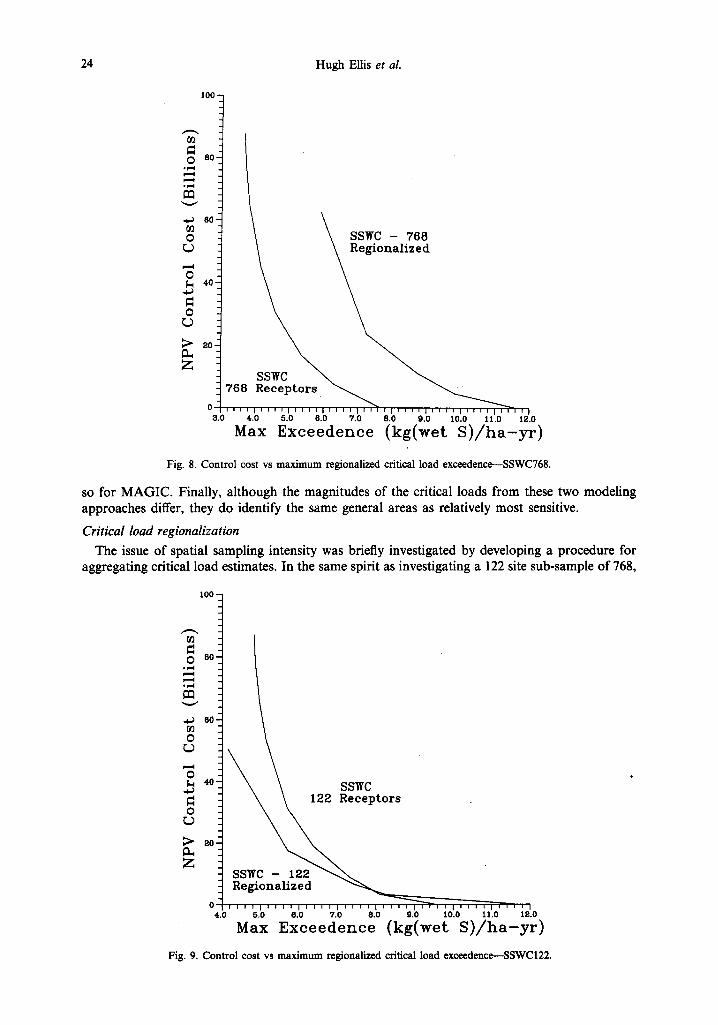
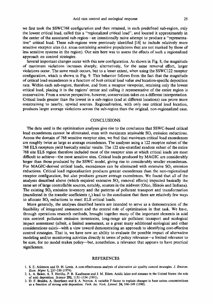
Critical load regionalization The issue of spatial sampling intensity was briefly investigated by developing a procedure for

aggregating critical load estimates. In the same spirit as investigating a 122 site sub-sample of 768,

100 -

0 so. o ~

.e ' l a~

e.~ 6o.

O r.)

O 4o.

O

a, Z

0 4 .0

•/ SSWC

Regionalized ~~~__._._~ i l l J l l l l l l l l l J l l l l l l l l l l l l l l l l l ~ l l l l ~ l l I

5.0 8.0 7.0 8.0 9.0 10.0 11.0 12.0

M a x E x c e e d e n c e ( k g ( w e t S ) / h a - y r )

Fig. 9. Control cost vs maximum rcgionalized critical load exeeedence--SSWC122.


we first took the SSWC768 configuration and then retained, in each predefined sub-region, only the lowest critical load, called this a "regionalized critical load", and located it approximately in the center of the associated sub-region--an intentionally naive attempt to produce a "representative" critical load. These sub-regions were previously identified [18] to include relatively more sensitive receptor sites (i.e. areas containing sensitive populations that are not masked by those of less sensitive systems in the region). Our aim here was to assess the effects of such a regionalized approach on control strategies.

Several important changes occur with this new configuration. As shown in Fig. 8, the magnitude of maximum violations increases sharply; alternatively, for the same removal effort, larger violations occur. The same result occurs, but to a lesser extent, when using the SSWC122 receptor configuration, which is shown in Fig. 9. This behavior follows from the fact that the magnitude of critical load exceedences is a function of both critical load value and location-specific deposition rate. Within each sub-region, therefore, and from a receptor viewpoint, retaining only the lowest critical load, placing it in the regions' center and calling it representative of the entire region is conservative. From a source perspective, however, conservatism takes on a different interpretation. Critical loads greater than the lowest in a sub-region (and at different locations) can prove more constraining to nearby, upwind sources. Regionalization, with only one critical load location, produces larger average violations across the sub-region than the original, non-regionalized case.

CONCLUSIONS

The data used in the optimization analyses give rise to the conclusion that SSWC-based critical load exceedences cannot be eliminated, even with maximum attainable SO2 emission reductions. Across the domain of 768 sensitive receptor sites, we find that maximum critical load exceedences are roughly twice as large as average exceedences. The analyses using a 122 receptor subset of the 768 ELS receptors yield basically similar results. The 122 site-stratified random subset of the entire 768 site ELS region therefore included most of the receptor sites at which critical loads are most difficult to achieve--the most sensitive sites. Critical loads produced by MAGIC are considerably larger than those produced by the SSWC model, giving rise to considerably smaller exceedences. For MAGIC-derived critical loads, exceedences can be eliminated with extensive SO2 emission reductions. Critical load regionalization produces greater exceedences than the non-regionalized receptor configuration, but also produces greater average exceedences. We found that all of the analyses described above (which required extensive SO2 removal efforts) impacted basically the same set of large controllable sources, notably, sources in the midwest (Ohio, Illinois and Indiana). The existing SO2 emission inventory and the patterns of pollutant transport and transformation (manifested in the transfer coefficients to) lead to the conclusion that there are relatively few ways to allocate SO2 reductions to meet ELS critical loads.

More generally, the analyses described herein are intended to serve as a demonstration of the feasibility of integrated assessment and the central role of optimization in that task. We have, through operations research methods, brought together many of the important elements in acid rain control: pollutant emission inventories, long-range air pollutant transport and ecological impact assessment (albeit, a limited assessment, as a great many additional ecological and other considerations exist)--with a view toward demonstrating an approach to identifying cost-effective control strategies. That is, we have now an ability to evaluate the possible impact of alternative modeling and/or monitoring activities directly in terms of policy relevance--a limited relevance to be sure, for no model makes policy--but, nonetheless, a relevance that appears to have practical significance.

REFERENCES

1. S. E. Atkinson and D. H. Lewis. A cost-effectiveness analysis of alternative air quality control strategies. J. Environ. Econ. Mgmt 1, 237-250 (1974).

2. L. A. Baker, A. T. Herlihy, P. R. Kaufmann and J. M. Eilers. Acidic lakes and streams in the United States: the role of acid deposition. Science 252, 1151-1154 (1991).

3. D. F. Brakke, A. Henriksen and S. A. Norton, A variable F-factor to explain changes in base cation concentrations as a function of strong acid deposition. Verh. Int. Verh. Limnol. 24, 146-149 (1990).


4. M. R. Church et al. Direct/delayed response project: future effects of long-term sulfur deposition on surface water chemistry in the northeast and Southern Blue Ridge Province. Report EPA/600/3-89/061a<l, U.S. EPA, Washington, DC (1989).

5. J. L. Cohon. Multiobjective Programming and Planning. Academic Press, New York (1978). 6. B. J. Cosby, G. M. Hornberger, J. N. Galloway and R. F. Wright. Modelling the effects of acid deposition: assessments

of a lumped parameter model of soil water and stream water chemistry. Wat. Resour. Res. 21, 51-63 (1985). 7. B. J. Cosby, R. F. Wright, G. M. Hornberger and J. N. Galloway. Modelling the effects of acid deposition: estimation

of long-term water quality responses in a small forested catchment. )Vat. Resour. Res. 21, 1591-1601 (1985). 8. J. H. Ellis, E. A. McBean and G. J. Farquhar. Deterministic linear programming model for acid rain abatement. ASCE

J. Environ. Engng 111, 119-139 (1985). 9. J. H. Ellis. Multiobjective mathematical programming models for acid rain control. Eur. J. Oper. Res. 35, 365-377

(1988). 10. J. H. Ellis. Acid rain control strategies: options exist despite scientific uncertainties. Environ. Sci. Technol. 22, 1248-1255

(1988). 11. J. H. Ellis. Integrating multiple long-range transport models into optimization methodologies for acid rain policy

analysis. Eur. J. Operl Res. 46, 313-321 (1990). 12. J. H. Ellis and M. L. Bowman. Critical loads and development of acid rain control options. ASCE J. Environ. Engng

120, 273-290 (1994). 13. J. M. Guldman. Chance-constrained dynamic model of air quality management. ASCE J. Environ. Engng 114,

1116-1135 (1988). 14. J. M. Guidman. Interactions between weather stochasticity and the locations of pollution sources and receptors in air

quality planning: a chance-constrained approach. Geogr. Anal. 18, 198-214 (1986). 15. A. Henriksen. A simple approach for identifying and measuring acidification of freshwater. Nature 278, 542-545 (1979). 16. J-P. Hettelingh, R. J. Downing and P. A. M. de Smet. Mapping critical loads for Europe. CCE Technical Report No.

1, July (1991). 17. G. R. Holdren, B. J. Cosby, D. Mamorek, R. Santore, C. Hunsaker, D. Bernard, J. Aber, C. Driscoll, L. Pardo, R.

S. Turner and T. C. Strickland. A national critical loads framework for establishing pollution loading standards: IV. Model selection, applications and critical loads mapping. Envir. Mgmt 17, 355-363 (1993).

18. G. R. Holdren Jr, T. C. Strickland, P. W. Shaffer, P. F. Ryan, P. L. Ringold and R. S. Turner. Sensitivity of critical load estimates for surface waters to model selection and regionalization schemes. J. Environ. QuaL 22, 279-289 (1993).

19. G. M. Hornberger, B. J. Cosby and J. N. Galloway. Modeling the effects of acid deposition: uncertainty and spatial variability in estimation of long-term sulfate dynamics in a region. Wat. Resour. Res. 22, 1293-1302 (1986).

20. ISDME, International sulfur deposition model evaluation. Report EPA-600/3-87-008, USEPA, Washington, DC (1987).

21. P. Kanciruk et al. Characteristics of Lakes in the Eastern United States, Vol. III: Data Compendium of Site Characteristics and Chemical Variables. EPA/600/4-86/007c, U.S. EPA, Washington, DC (1986).

22. R. E. Kohn, Application of linear programming to a controversy on air pollution control. Mgmt Sci. 17, B609-B621 (1971).

23. R. E. Kohn, .4 Linear Programming Model for Air Pollution Control. The MIT Press, Cambridge, MA (1978). 24. R. A. Linthurst et al. Characteristics of Lakes in the Eastern United States, Vol. I: Population Descriptions and

Physico-chemical Relationships. EPA/600/4-86/007a, U.E. EPA, Washington, DC (1986). 25. M. B. Morrison and E. S. Rubin. A linear programming model for acid rain policy analysis. J. Air Poll. Contr. Assoc.

35, 1137-1148 0985). 26. National Acid Precipitation Assessment Program (NAPAP). Acidic Deposition: State of Science and Technology,

National Acid Precipitation Assessment Program, Washington, DC (1991). 27. National Acid Precipitation Assessment Program (NAPAP). Models Planned for Use in the NAPAP Integrated

Assessment, National Acid Precipitation Assessment Program, Washington, DC (1989). 28. J. Nilsson and P. Grennfelt (Eds). Critical loads for sulfur and nitrogen: Report from a workshop held at Skokloster,

Sweden, 19-24 March 1989. UN/ECE and Nordic Council of Ministers, NORD (1988). 29. D. W. Schindler. The effects of acid rain on freshwater ecosystems. Science 239, 149-157 0988). 30. J. H. Seinfeld and C. P. Kyan. Determination of optimal air pollution control strategies. Socio-Econ. Plann. Sci. 5,

173-190 (1971). 31. D. G. Streets, D. A. Hanson and L. D. Carter. Targeted strategies for control of acidic deposition. J. Air Poll. Contr.

Assoc. 34, I187-1197 0984). 32. A. Teller. The use of linear programming to estimate the cost of some alternative air pollution abatement policies. Proc.

IBM Scientific Computing Symp. on Water and Air Resource Management, pp. 345-353 (1968). 33. J. C. Trijonis. Economic air pollution control model for Los Angeles County in 1975. Environ. Sci. Technol. 8, 811~826

(1974). 34. United States Congress. Public Law 101-549, 15 November (1990). 35. A. Venkatram, B. E. Ley and S. Y. Wong. A statistical model to estimate long-term concentrations of pollutants

associated with long-range transport. Atmos. Environ. 16, 249-257 (1982).

Documents

Emission reductions and ecological response: Management models for acid rain control