1

Emission Series and Emitting

Quantum States:

Visible H Atom Emission Spectrum

Experiment 6

#6 Emission Series and Emitting Quantum States:

Visible H Atom Emission Spectrum

Goal:

� To determine information regarding the quantum

states of the H atom

Method:

� Calibrate a spectrometer using He emission lines

� Observe the visible emission lines of H atoms

� Determine the initial and final quantum states

responsible for the visible emission spectrum, as

well as the Rydberg constant

2

Electromagnetic Radiation

Oscillating electric and magnetic fields

Light Energy

�Wavelength λλλλ distance peak-to-peak

�Frequency νννν oscillations per second

�Energy E ∝∝∝∝ νννν faster oscillation = more E

3

Electromagnetic Spectrum

Visible Emission

Wavelengths, λ, increase

Energies decrease

Electronic transitions (“e- jumps”)

400 nm 500 nm 600 nm 700 nm

4

Dual Nature of Light/Relationships

h Planck’s constant = 6.626×10-34 J.s

Units J = (J.s) (s-1)

c speed of light = 2.998×108 m.s-1

Units s-1 = (m.s-1)/(m)

hνE =

λ

cν =

1. Wave wavelength, λ

frequency, ν

2. Particle photon = “packet”

E = hν

Using the Equations

(a) Calculate the frequency of 460nm blue light.

1-14

9

8

1052.6

nm101

m1nm) (460

)s

m1099.2(

c

s×=

×

×

==λ

ν

(b) Calculate the energy of 460 nm blue light.

J

ssJ

19-

11434-

1032.4

)106.52)(10(6.626

hhc

E

×=

×⋅×=

==

−

νλ

5

Spectroscopy

Spectroscopy: study of interaction of light with matter

hν: photon

1. Absorption: matter + hν → matter*

2. Emission: matter* → matter + hν

Energy change in matter: ∆∆∆∆Ematter = Ehνννν

Discrete Energy Levels

Observed energy level changes:

∆E = Ehν = Efinal – Einitial

Ground state atom Absorption Emission

6

“Discrete” Atomic Emission

Atomic absorption: electrons excited to higher energy levels

Atomic emission: excited electrons lose energy

Incandescent

Hot Gas

Cold Gas

Continuous

Discrete Emission

Discrete Absorption

Quantized Energy Levels

Ehν = ∆Elevels

∆E = Ef – Ei

Absorption: Ef > Ei

Emission: Ef < Ei

7

Hydrogen Emission Spectrum©The McGraw-Hill Companies. Permission required for reproduction or display

H atom emission

1) Electrical energy excites H H + energy →→→→ H*

� initial quantum state ni = 2, 3, 4, 5, 6, …

2) H* loses energy H* →→→→ H + hνννν

� final quantum state nf = 1, 2, 3, …

nf < ni

You observe several ∆Etransitions ≡ visible λs

� ni’s levels > nf

� nf end at same nf

You determine ni’s and nf

8

Hydrogen Atom and Emission

Lyman

Balmer

Paschen

Ground State:

n = 1

Excited States:

n = 2, 3, 4, …

Rydberg Equation

A “series” is associated with two quantum numbers:

Lyman: ni = 2, 3, 4, … nf = 1

Balmer: ni = 3, 4, 5, … nf = 2

Paschen: ni = 4, 5, 6, … nf = 3

RH = 1.096776×107m-1 = 2.180×10-18 J = 2πe4m/h3c

−=

22

11

if

Hhυnn

RE

levelsifhν ∆EEEE =−=General transition eq’n:

Hydrogen atomic

emission lines fit

(Rydberg eq’n):

9

Incre

asing

λλλλ

(decrea

sing E

, sma

ller ∆∆∆∆

E)n = principal E states

(principal quantum #s)

Hydrogen Atomic Emission

−=

22

11

if

Hhυnn

RE

En

ergy

→

Part 1 Correlate color with wavelength

� Use lucite rod

� 20 nm intervals, 400–700 nm λλλλ, color

� Boundary λs λλλλshort, λλλλlong

� λ of max. intensity λλλλmax

Observe Hg atomic emission (handheld specs)

10

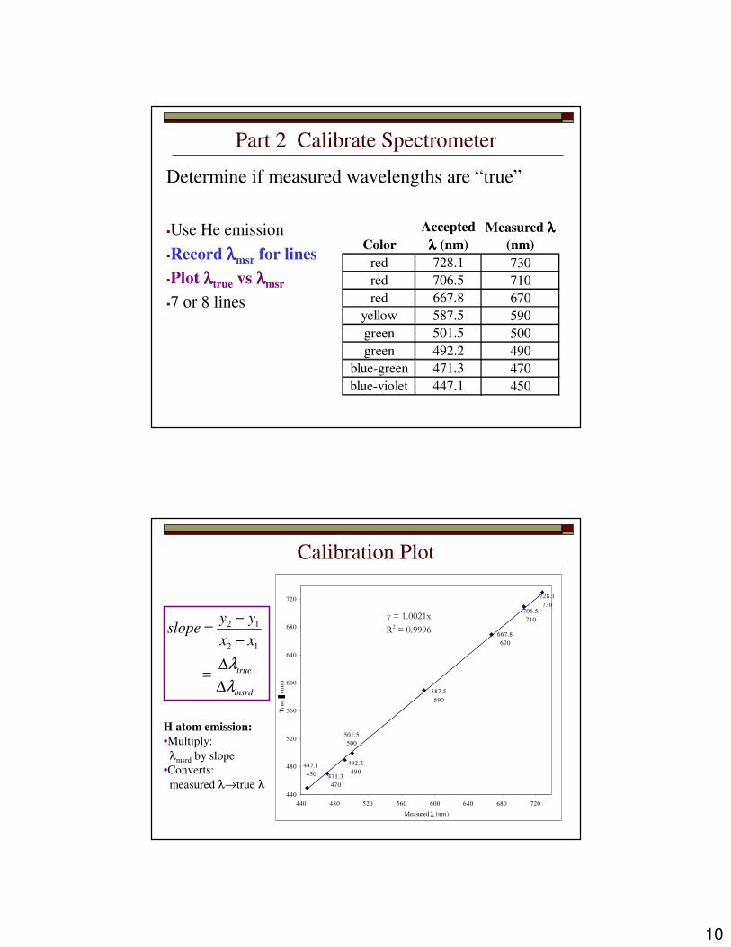
Part 2 Calibrate Spectrometer

Determine if measured wavelengths are “true”

�Use He emission

�Record λλλλmsr for lines

�Plot λλλλtrue vs λλλλmsr

�7 or 8 lines

Color

Accepted

λλλλ (nm)

Measured λ λ λ λ

(nm)

red 728.1 730

red 706.5 710

red 667.8 670

yellow 587.5 590

green 501.5 500

green 492.2 490

blue-green 471.3 470

blue-violet 447.1 450

Calibration Plot

msrd

true

xx

yyslope

λ

λ

∆

∆=

−

−=

12

12

H atom emission:

•Multiply:

λmsrd by slope

•Converts:

measured λ→true λ

728.1

730706.5

710

667.8

670

587.5

590

447.1

450 471.3

470

492.2

490

501.5

500

y = 1.0021x

R2 = 0.9996

440

480

520

560

600

640

680

720

440 480 520 560 600 640 680 720

Measured λ (nm)

Tru

e

(n

m)

11

Part 3 Record H emission λs

�Record color, λλλλmsr (3 or 4 lines) color, λλλλmsr

�Determine λλλλtrue λλλλtrue

�Calculate Ehννννfrom λλλλtrue Ehνννν

Units: E in J

h in J.s

c in m/s

λ in m

)()(

*

)(

*

)(2)(2 22 linesggg

e

g hHHHH ν+→→→−

)()(2

*

)(2 bandsgg hHH ν+→

λ

hcE h ν =

Questions/Data Analysis

1) Does your data match the Balmer series

(it should; nfinal = 2?)

2) What is ninitial for each line?

3) What is your experimental RH?

12

Hydrogen Lines / Analysis

4.8×10-19410violet

4.6×10-19430blue-violet

4.1×10-19490blue-green

3.0×10-19660red

∆E (J)λ (nm)Color

atom

if

Hhυ ∆Enn

RE =

−=

22

11

One way to think about the data

Are we observing the Balmer series, as predicted?

Balmer: nf = 2 3→2, 4→2, 5→2

These would be the three lowest energy transitions

Example data:

Literature Observed

λ (nm) Color λ (nm) ∆E (J)

410.1 violet 400 5.0E-19

434.0 blue-violet 430 4.6E-19

486.1 blue-green 500 4.0E-19

656.2 red 650 3.1E-19

13

Compare calculated ∆E to observed ∆E

EH atom ∝ 1/n2 = RH/n2 so calculate ∆E between levels and compare to observed E’s

Experiment matches Balmer well (<5% error)

%

λ (nm) Color ∆E (J) λ (nm) Color ∆E (J) error

410.1 violet 4.84E-19 400 violet 5.0E-19 2.6

434.0 blue-violet 4.58E-19 430 blue-violet 4.6E-19 1.0

486.1 blue-green 4.09E-19 500 blue-green 4.0E-19 2.7

656.2 red 3.03E-19 650 red 3.1E-19 1.0

Theoretical Observed

How? Plot ∆∆∆∆Eatom vs. 1/ni2

Rearranged Rydberg equation fits:

HRslope −=

22

1

f

H

i

Hatomn

R

nR∆E

bxmy

+

−=

+=

2intercepty

f

H

n

R=−

22

11 :

0 :interceptx

if nnso

∆E

=

=−

14

Example plot data

color nm Ef-Ei (J) ni nf 1/ni2

--- 0 0 2 2 0.250

red 660 3.0E-19 3 2 0.111

blue-green 490 4.1E-19 4 2 0.063

blue-violet 430 4.6E-19 5 2 0.040

violet 410 4.8E-19 6 2 0.028

y-axis x-axis

Corrected λ Balmer

22

1

f

H

i

Hatomn

R

nR∆E

bxmy

+

−=

+=

Balmer Series

y = -2x10-18

x + 6x10-19

R2 = 0.9878

0.0E+00

1.0E-19

2.0E-19

3.0E-19

4.0E-19

5.0E-19

6.0E-19

0.000 0.050 0.100 0.150 0.200 0.250

1/n2

Ef-

Ei

Example Balmer Rydberg Plot

Slope (~RH):

2×10-18J

Close to RH

2.18×10-18J

x-intercept:

~0.24

Close to 0.25

~1/22

λ (nm) Color λ (nm) ∆E (J)

410.1 violet 400 5.0E-19

434.0 blue-violet 430 4.6E-19

486.1 blue-green 500 4.0E-19

656.2 red 650 3.1E-19

15

Balmer (nf = 2) – plot ∆E vs. 1/ni2

y = -2x10-18

x + 5x10-19

R2 = 0.9988

0.0E+00

1.0E-19

2.0E-19

3.0E-19

4.0E-19

5.0E-19

0.000 0.050 0.100 0.150 0.200 0.250

1/ni2

∆∆ ∆∆E

Good:

Slope ≈ –RH

x-intercept:

1 22

so

nf = 2

~ 0.25 =

This plot verifies our data – we observed the Balmer series!

As an extension (extra)

1) Data for:

Balmer (nf = 2) or Paschen (nf = 3)

2) Transitions are 3 lowest energy:

Balmer (ni = 5, 4, 3) or Paschen (ni = 6, 5, 4)

nm Ef-Ei (J) ni nf 1/ni2

ni nf 1/ni2

0 0 2 2 x-intercept 3 3 x-intercept

660 3.0E-19 3 2 0.111 4 3 0.063

490 4.1E-19 4 2 0.063 5 3 0.040

430 4.6E-19 5 2 0.040 6 3 0.028

Balmer Paschen

16

Graphs

Prepare two graphs (Balmer and Paschen)

� x-axis should extend to x-intercept (y = 0)

� y-axis should be appropriate

Draw best-fit straight line

� Find slope (one should be close to –RH)

� Find relative error in experimental RH

� Match λλλλ and color to ni and nf

Paschen (nf = 3)

Not too good

Slope ≠ RH

x-int. ≠ 1/32

y = -4x10-18

x + 6x10-19

R2 = 0.9969

0.0E+00

1.0E-19

2.0E-19

3.0E-19

4.0E-19

5.0E-19

0.000 0.020 0.040 0.060 0.080 0.100 0.120 0.140

1/ni2

∆E

17

Balmer (nf = 2)

y = -2x10-18

x + 5x10-19

R2 = 0.9988

0.0E+00

1.0E-19

2.0E-19

3.0E-19

4.0E-19

5.0E-19

0.000 0.050 0.100 0.150 0.200 0.250

1/ni2

∆∆ ∆∆E

Good:

Slope ≈ –RH

x-intercept:

1 22

so

nf = 2

~ 0.25 =

Balmer Series

y = -2x10-18

x + 6x10-19

R2 = 0.9878

0.0E+00

1.0E-19

2.0E-19

3.0E-19

4.0E-19

5.0E-19

6.0E-19

0.000 0.050 0.100 0.150 0.200 0.250

1/n2

Ef-

Ei

Example Balmer Rydberg Plot

Slope (~RH):

2×10-18J

Close to RH

2.18×10-18J

x-intercept:

~0.24

Close to 0.25

~1/22

λ (nm) Color λ (nm) ∆E (J)

410.1 violet 400 5.0E-19

434.0 blue-violet 430 4.6E-19

486.1 blue-green 500 4.0E-19

656.2 red 650 3.1E-19

18

Data

color nm Ef-Ei (J) ni nf

--- 0 0 2 2

red 660 3.0E-19 3 2

blue-green 490 4.1E-19 4 2

blue-violet 430 4.6E-19 5 2

Balmer

Experimental RH: 2 ×10-18 J

1/λ vs.

1/ni2

Atomic Hydrogen Emission Lines

0

20000

40000

60000

80000

100000

120000

0.000 0.200 0.400 0.600 0.800 1.000

1/n2

cm

Lyman

Balmer

Paschen

19

ReportAbstract

Results

� 2a: Calibration data and plot

� 2b: Table

� Series plot (Balmer plot)

depending on your analysis choice

� RH and error from literature

� Predicted wavelengths and error

Sample calculations of:

� photon energy and Rydberg slope

Discussion/review questions