Embed Size (px)
Citation preview
EMM Flow Diagram
for structural modelestimated parameters
datasimulated
modelauxiliary
EMM
modelstructural
SNPobserved data
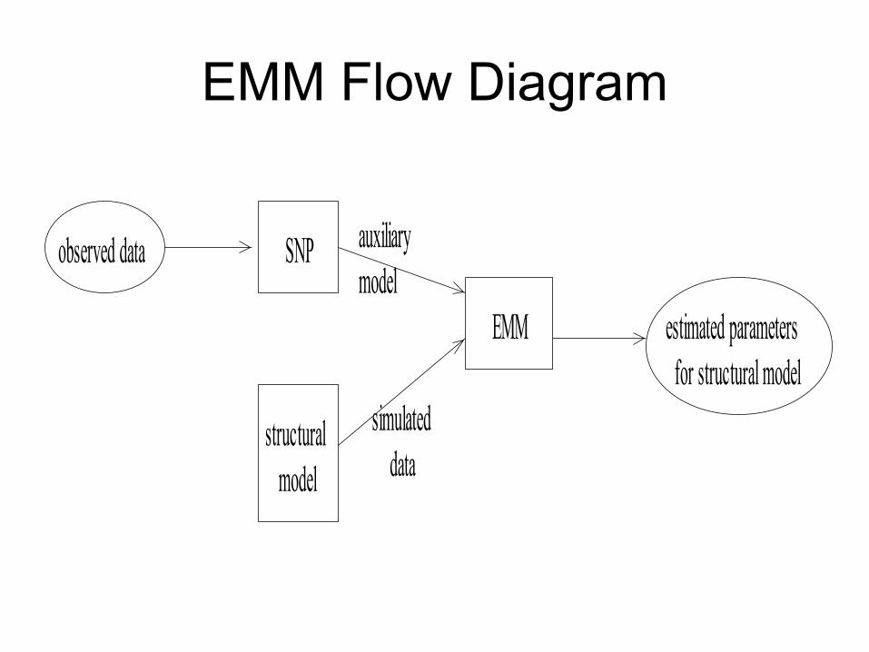
Simulate MA(1) Data Using gensim Function
MA1.gensim <- function(rho, n.sim=100, n.var=1, n.burn=25, aux=NULL) {
# simulate from MA(1) model # y(t) = e(t) - theta*e(t-1), e(t) ~ iid N(0,sigma^2) # rho = (theta,sigma2)' # aux is a list with components # innov = standard normals used for simulation # start.innov = standard normals used for start up values
ans = arima.sim(model = list(ma=rho[1]), innov = aux$innov*sqrt(rho[2]), start.innov = aux$innov.start*sqrt(rho[2]))
ans}
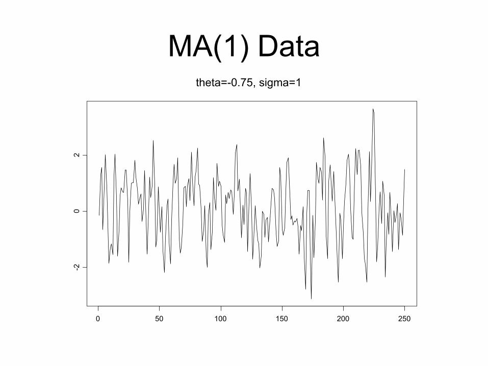
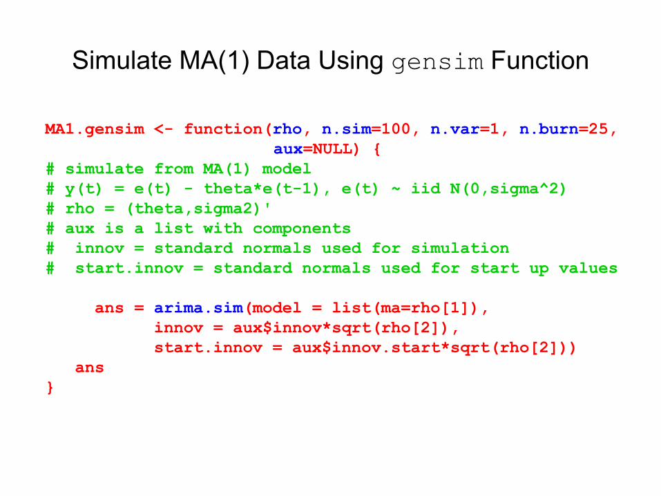
MA(1) Datatheta=-0.75, sigma=1
0 50 100 150 200 250
-20
2

MA(1) Data
Lag
AC
F
0 5 10 15 20
0.0
0.2
0.4
0.6
0.8
1.0
Series : MA1.sim
Lag
Par
tial A
CF
0 5 10 15 20
-0.2
0.0
0.2
0.4
Series : MA1.sim
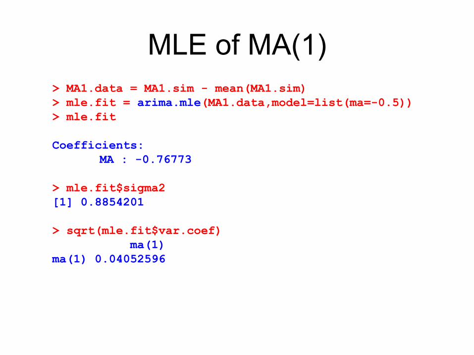
MLE of MA(1)> MA1.data = MA1.sim - mean(MA1.sim) > mle.fit = arima.mle(MA1.data,model=list(ma=-0.5)) > mle.fit
Coefficients:MA : -0.76773
> mle.fit$sigma2[1] 0.8854201
> sqrt(mle.fit$var.coef)ma(1)
ma(1) 0.04052596

Fit AR(3) Auxiliary Model> ar3.fit = SNP(data=MA1.sim, model=SNP.model(ar=3))> class(ar3.fit)[1] "SNP"> summary(ar3.fit)Model: Gaussian VAR
Conditional Mean Coefficients:mu ar(1) ar(2) ar(3)
coef -0.0039 0.7205 -0.4307 0.2114(std.err) 0.0517 0.0626 0.0672 0.0630(t.stat) -0.0749 11.5170 -6.4077 3.3549
Conditional Variance Coefficients:sigma2
coef 0.8052(std.err) 0.0424(t.stat) 19.0124
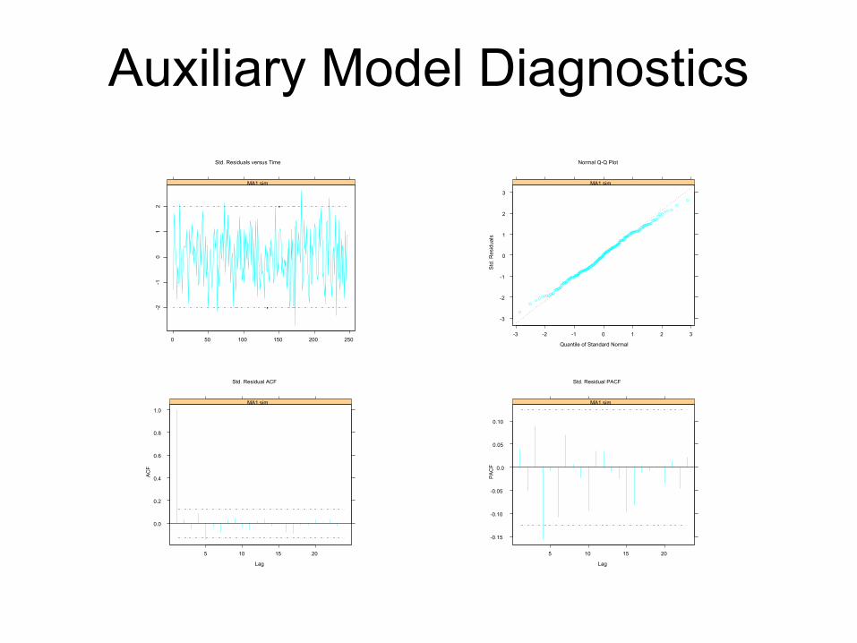
Auxiliary Model Diagnostics-2
-10
12
0 50 100 150 200 250
MA1.sim
Std. Residuals versus Time
-3
-2
-1
0
1
2
3
-3 -2 -1 0 1 2 3
MA1.sim
Quantile of Standard Normal
Std
. Res
idua
ls
Normal Q-Q Plot
0.0
0.2
0.4
0.6
0.8
1.0
5 10 15 20
MA1.sim
Lag
AC
F
Std. Residual ACF
-0.15
-0.10
-0.05
0.0
0.05
0.10
5 10 15 20
MA1.sim
Lag
PA
CF
Std. Residual PACF
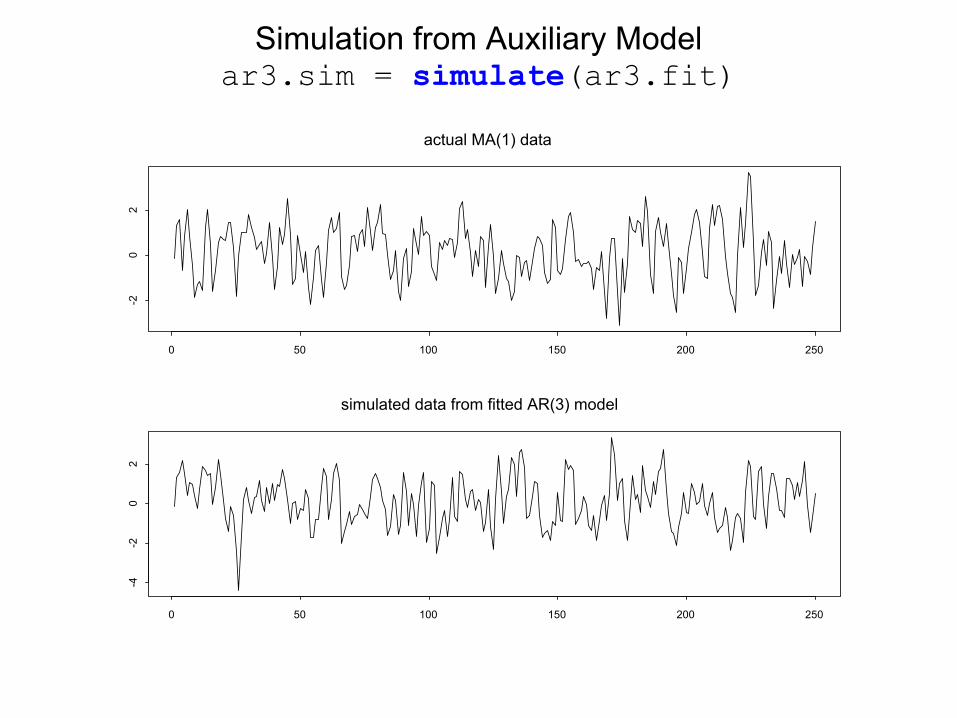
Simulation from Auxiliary Modelar3.sim = simulate(ar3.fit)
actual MA(1) data
0 50 100 150 200 250
-20
2
simulated data from fitted AR(3) model
0 50 100 150 200 250
-4-2
02

Diagnostics from Simulated Auxiliary Model
Lag
AC
F
0 5 10 15 20
-0.2
0.2
0.4
0.6
0.8
1.0
Series : ar3.sim
Lag
Par
tial A
CF
0 5 10 15 20
-0.2
0.0
0.2
0.4
Series : ar3.sim
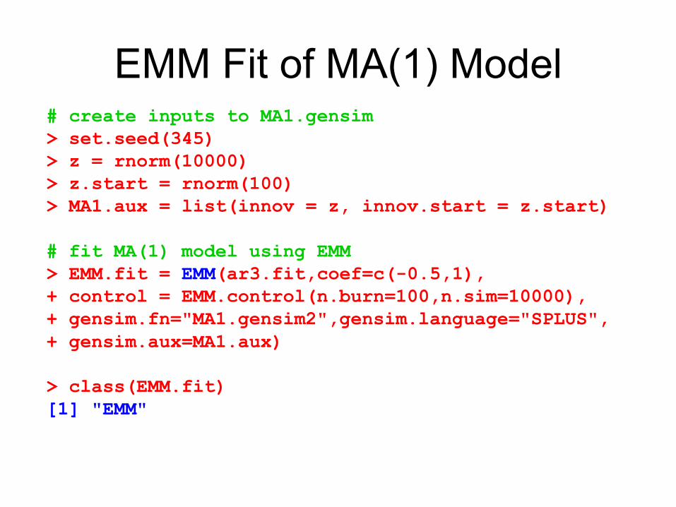
EMM Fit of MA(1) Model# create inputs to MA1.gensim> set.seed(345) > z = rnorm(10000) > z.start = rnorm(100) > MA1.aux = list(innov = z, innov.start = z.start)
# fit MA(1) model using EMM> EMM.fit = EMM(ar3.fit,coef=c(-0.5,1), + control = EMM.control(n.burn=100,n.sim=10000), + gensim.fn="MA1.gensim2",gensim.language="SPLUS",+ gensim.aux=MA1.aux)
> class(EMM.fit)[1] "EMM"
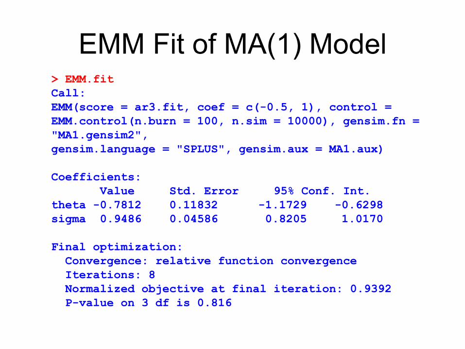
EMM Fit of MA(1) Model> EMM.fitCall:EMM(score = ar3.fit, coef = c(-0.5, 1), control = EMM.control(n.burn = 100, n.sim = 10000), gensim.fn = "MA1.gensim2", gensim.language = "SPLUS", gensim.aux = MA1.aux)
Coefficients:Value Std. Error 95% Conf. Int.
theta -0.7812 0.11832 -1.1729 -0.6298sigma 0.9486 0.04586 0.8205 1.0170
Final optimization:Convergence: relative function convergence Iterations: 8 Normalized objective at final iteration: 0.9392P-value on 3 df is 0.816
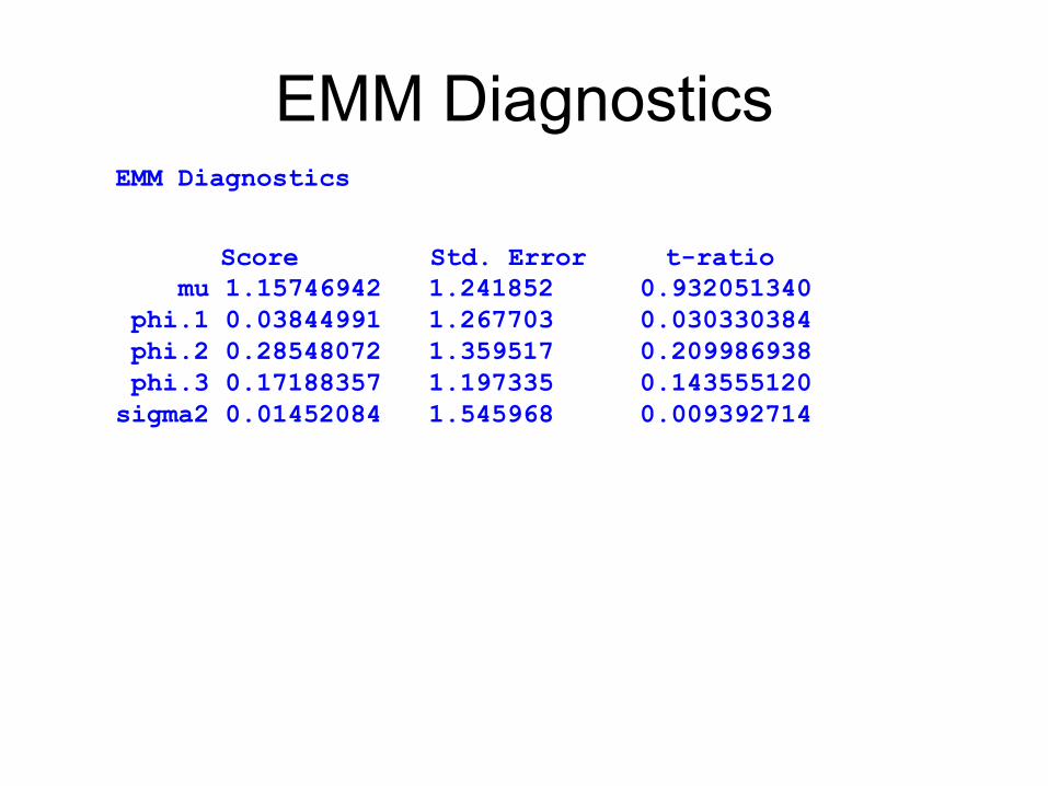
EMM DiagnosticsEMM Diagnostics
Score Std. Error t-ratio mu 1.15746942 1.241852 0.932051340
phi.1 0.03844991 1.267703 0.030330384phi.2 0.28548072 1.359517 0.209986938phi.3 0.17188357 1.197335 0.143555120sigma2 0.01452084 1.545968 0.009392714
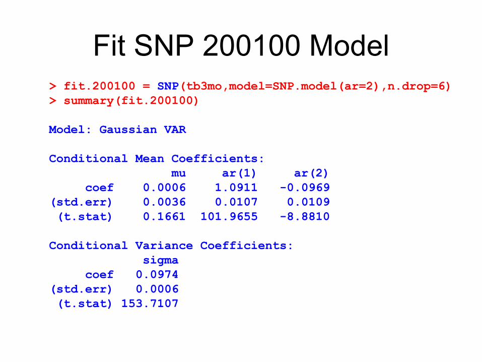
Fit SNP 200100 Model> fit.200100 = SNP(tb3mo,model=SNP.model(ar=2),n.drop=6)> summary(fit.200100)
Model: Gaussian VAR
Conditional Mean Coefficients:mu ar(1) ar(2)
coef 0.0006 1.0911 -0.0969(std.err) 0.0036 0.0107 0.0109(t.stat) 0.1661 101.9655 -8.8810
Conditional Variance Coefficients:sigma
coef 0.0974(std.err) 0.0006(t.stat) 153.7107
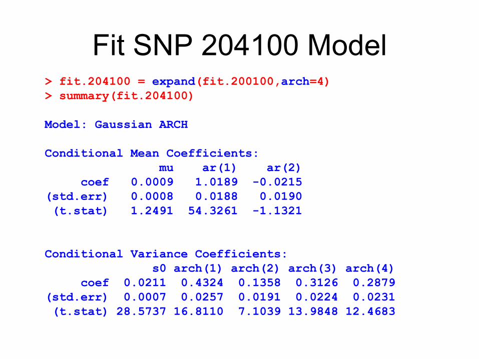
Fit SNP 204100 Model> fit.204100 = expand(fit.200100,arch=4)> summary(fit.204100)
Model: Gaussian ARCH
Conditional Mean Coefficients:mu ar(1) ar(2)
coef 0.0009 1.0189 -0.0215(std.err) 0.0008 0.0188 0.0190(t.stat) 1.2491 54.3261 -1.1321
Conditional Variance Coefficients:s0 arch(1) arch(2) arch(3) arch(4)
coef 0.0211 0.4324 0.1358 0.3126 0.2879(std.err) 0.0007 0.0257 0.0191 0.0224 0.0231(t.stat) 28.5737 16.8110 7.1039 13.9848 12.4683
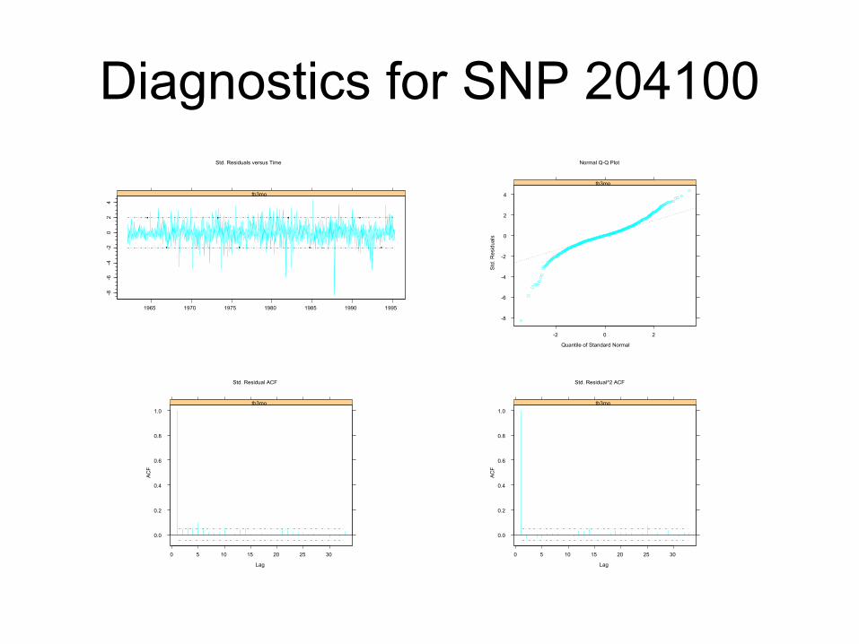
Diagnostics for SNP 204100-8
-6-4
-20
24
1965 1970 1975 1980 1985 1990 1995
tb3mo
Std. Residuals versus Time
-8
-6
-4
-2
0
2
4
-2 0 2
tb3mo
Quantile of Standard Normal
Std
. Res
idua
ls
Normal Q-Q Plot
0.0
0.2
0.4
0.6
0.8
1.0
0 5 10 15 20 25 30
tb3mo
Lag
AC
F
Std. Residual ACF
0.0
0.2
0.4
0.6
0.8
1.0
0 5 10 15 20 25 30
tb3mo
Lag
AC
F
Std. Residual^2 ACF
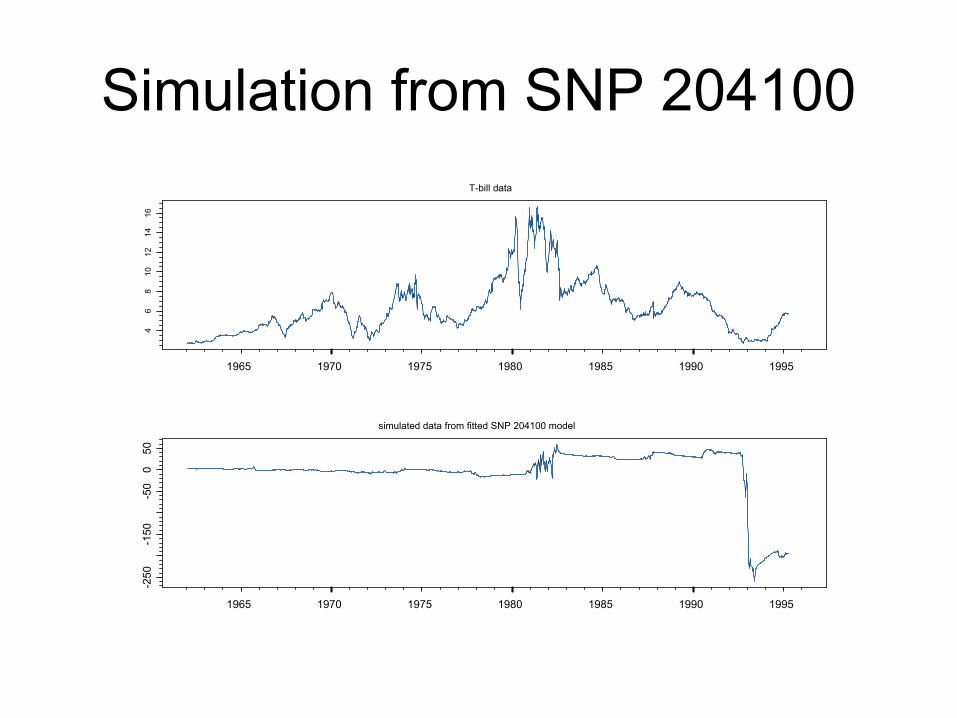
Simulation from SNP 204100T-bill data
1965 1970 1975 1980 1985 1990 1995
46
810
1214
16
simulated data from fitted SNP 204100 model
1965 1970 1975 1980 1985 1990 1995
-250
-150
-50
050
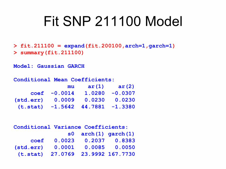
Fit SNP 211100 Model> fit.211100 = expand(fit.200100,arch=1,garch=1)> summary(fit.211100)
Model: Gaussian GARCH
Conditional Mean Coefficients:mu ar(1) ar(2)
coef -0.0014 1.0280 -0.0307(std.err) 0.0009 0.0230 0.0230(t.stat) -1.5642 44.7881 -1.3380
Conditional Variance Coefficients:s0 arch(1) garch(1)
coef 0.0023 0.2037 0.8383(std.err) 0.0001 0.0085 0.0050(t.stat) 27.0769 23.9992 167.7730
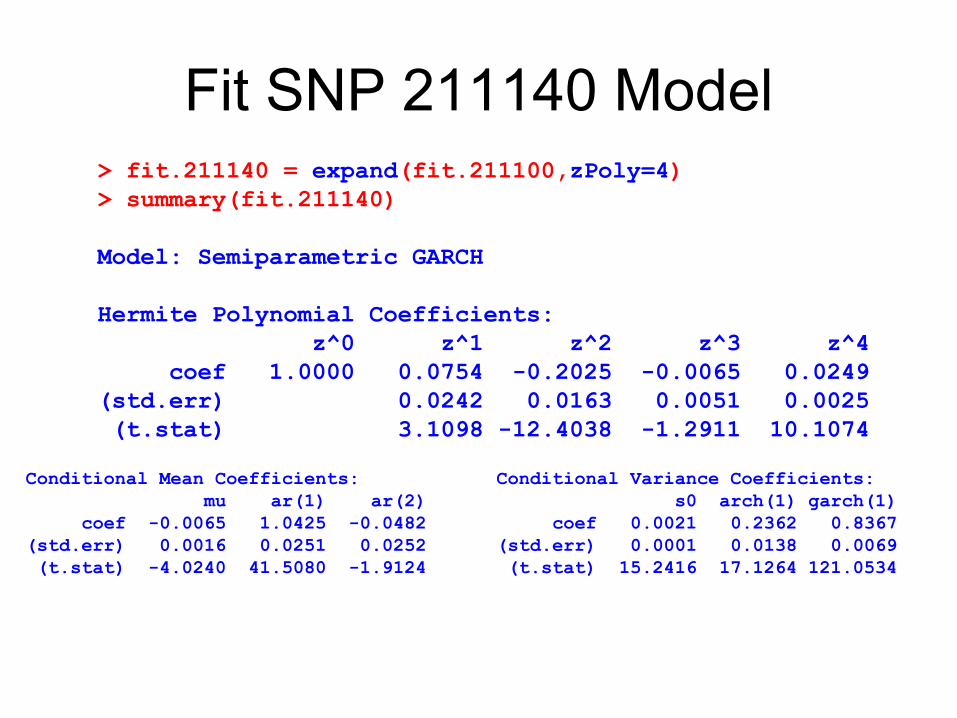
Fit SNP 211140 Model> fit.211140 = expand(fit.211100,zPoly=4)> summary(fit.211140)
Model: Semiparametric GARCH
Hermite Polynomial Coefficients:z^0 z^1 z^2 z^3 z^4
coef 1.0000 0.0754 -0.2025 -0.0065 0.0249(std.err) 0.0242 0.0163 0.0051 0.0025(t.stat) 3.1098 -12.4038 -1.2911 10.1074
Conditional Mean Coefficients:mu ar(1) ar(2)
coef -0.0065 1.0425 -0.0482(std.err) 0.0016 0.0251 0.0252(t.stat) -4.0240 41.5080 -1.9124
Conditional Variance Coefficients:s0 arch(1) garch(1)
coef 0.0021 0.2362 0.8367(std.err) 0.0001 0.0138 0.0069(t.stat) 15.2416 17.1264 121.0534
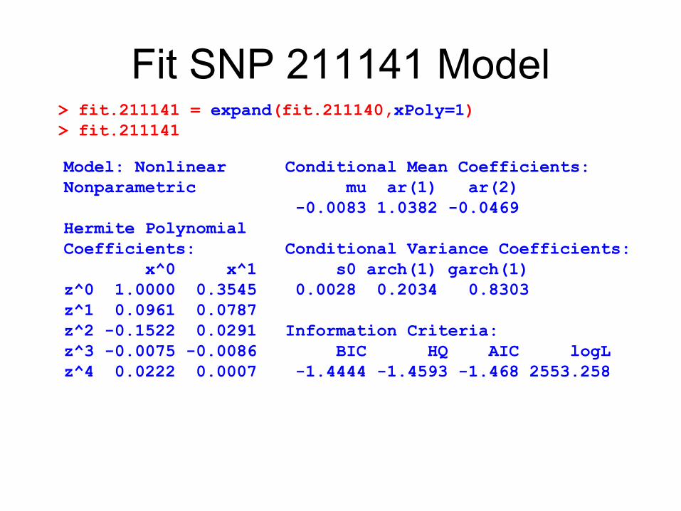
Fit SNP 211141 Model> fit.211141 = expand(fit.211140,xPoly=1)> fit.211141
Model: Nonlinear Nonparametric
Hermite Polynomial Coefficients:
x^0 x^1 z^0 1.0000 0.3545z^1 0.0961 0.0787z^2 -0.1522 0.0291z^3 -0.0075 -0.0086z^4 0.0222 0.0007
Conditional Mean Coefficients:mu ar(1) ar(2)
-0.0083 1.0382 -0.0469
Conditional Variance Coefficients:s0 arch(1) garch(1)
0.0028 0.2034 0.8303
Information Criteria:BIC HQ AIC logL
-1.4444 -1.4593 -1.468 2553.258

SNP Tuning Parameters
Lags in x part of Polynomial P(z,x)
lagPLp
Degree of x in P(z,x)xPolyKx
Degree of z in P(z,x)zPolyKz
GARCH laggarchLg
ARCH lagarchLr
VAR lagarLu
InterpretationSPLUS argumentParameter

Taxonomy of SNP Models
Nonlinear nonparametricLu≥0, Lg≥0, Lr≥0, Lp>0, Kz>0, Kx>0Semiparametric GARCHLu≥0, Lg>0, Lr=0, Lp≥0, Kz>0, Kx=0Gaussian GARCHLu≥0, Lg>0, Lr=0, Lp≥0, Kz=0, Kx=0Semiparametric ARCHLu≥0, Lg=0, Lr>0, Lp≥0, Kz>0, Kx=0Gaussian ARCHLu≥0, Lg=0, Lr>0, Lp≥0, Kz=0, Kx=0Semiparametric VARLu>0, Lg=0, Lr=0, Lp≥0, Kz>0, Kx=0Gaussian VARLu>0, Lg=0, Lr=0, Lp≥0, Kz=0, Kx=0iid GaussianLu=0, Lg=0, Lr=0, Lp≥0, Kz=0, Kx=0Auxilary model for ytParameter Setting

Log Spline Transformation
x
x.tra
ns
-5 0 5
-50
5
−σtr σtr

Fit SNP 204100 with Spline Transformation
> fit.204100.s =+ SNP(tb3mo,model=SNP.model(ar=2,arch=4),n.drop=6,+ control=SNP.control(xTransform="spline",inflection=4))> fit.240100.s
Model: Gaussian ARCH
Conditional Mean Coefficients:mu ar(1) ar(2)
0.0009 1.0189 -0.0215
Conditional Variance Coefficients:s0 arch(1) arch(2) arch(3) arch(4)
0.0211 0.4324 0.1358 0.3126 0.2879
Information Criteria:BIC HQ AIC logL
-1.3418 -1.3498 -1.3544 2349.84
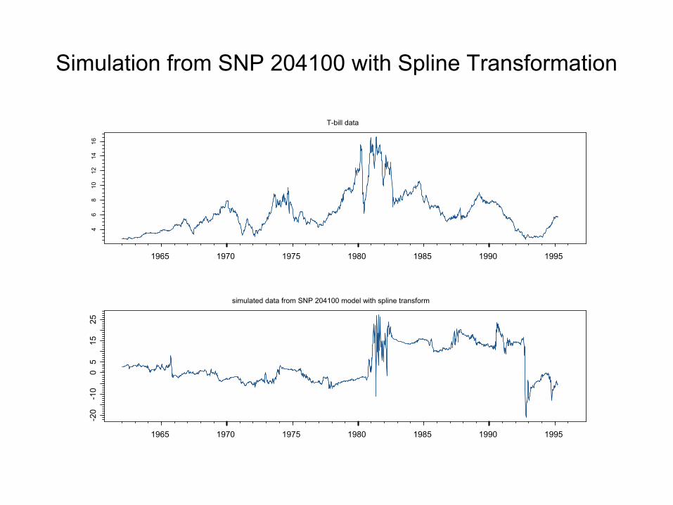
Simulation from SNP 204100 with Spline Transformation
T-bill data
1965 1970 1975 1980 1985 1990 1995
46
810
1214
16
simulated data from SNP 204100 model with spline transform
1965 1970 1975 1980 1985 1990 1995
-20
-10
05
1525

SNP: Automatic Model Selection
> fit.auto = SNP.auto(tb3mo,n.drop=6,+ control=SNP.control(xTransform="spline",+ inflection=4),+ arMax=4,zPolyMax=8,xPolyMax=4,lagPMax=4)Initializing using a Gaussian model ...Expanding the order of VAR: 1234Expanding toward GARCH model ...Expanding the order of z-polynomial: 12345678Expanding the order of x-polynomial: 1234
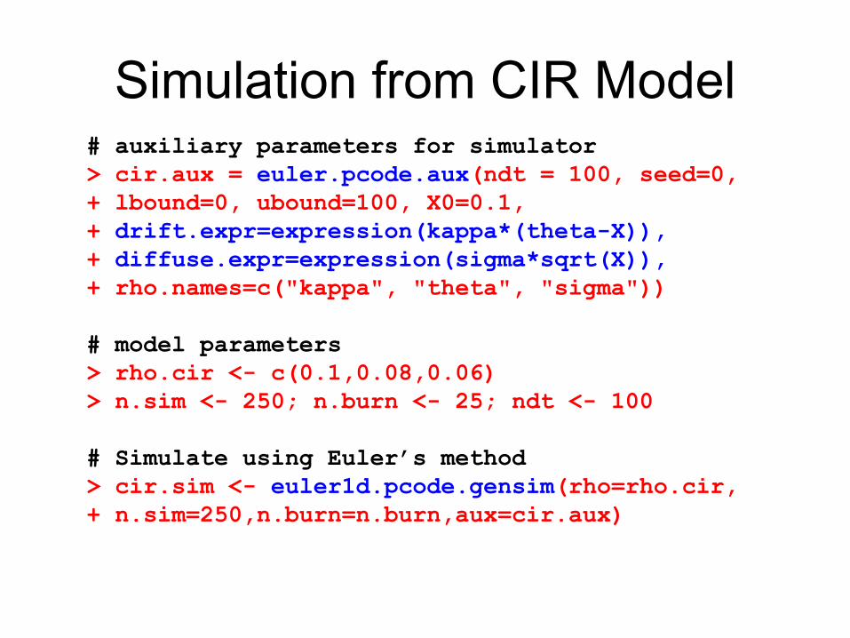
Simulation from CIR Model# auxiliary parameters for simulator> cir.aux = euler.pcode.aux(ndt = 100, seed=0, + lbound=0, ubound=100, X0=0.1, + drift.expr=expression(kappa*(theta-X)),+ diffuse.expr=expression(sigma*sqrt(X)),+ rho.names=c("kappa", "theta", "sigma"))
# model parameters> rho.cir <- c(0.1,0.08,0.06) > n.sim <- 250; n.burn <- 25; ndt <- 100
# Simulate using Euler’s method> cir.sim <- euler1d.pcode.gensim(rho=rho.cir,+ n.sim=250,n.burn=n.burn,aux=cir.aux)
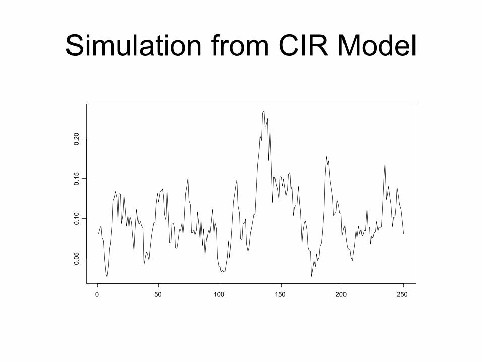
Simulation from CIR Model
0 50 100 150 200 250
0.05
0.10
0.15
0.20
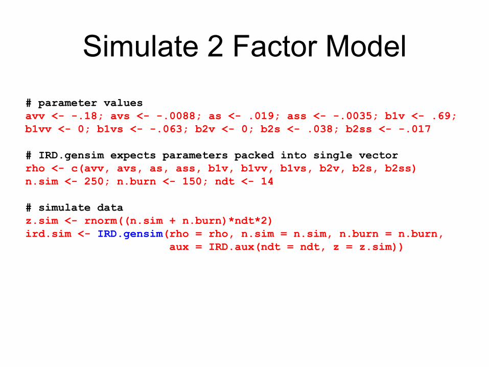
Simulate 2 Factor Model# parameter valuesavv <- -.18; avs <- -.0088; as <- .019; ass <- -.0035; b1v <- .69; b1vv <- 0; b1vs <- -.063; b2v <- 0; b2s <- .038; b2ss <- -.017
# IRD.gensim expects parameters packed into single vector rho <- c(avv, avs, as, ass, b1v, b1vv, b1vs, b2v, b2s, b2ss)n.sim <- 250; n.burn <- 150; ndt <- 14
# simulate dataz.sim <- rnorm((n.sim + n.burn)*ndt*2)ird.sim <- IRD.gensim(rho = rho, n.sim = n.sim, n.burn = n.burn,
aux = IRD.aux(ndt = ndt, z = z.sim))
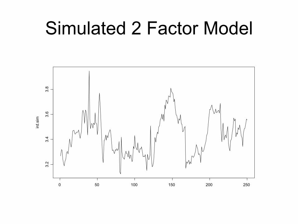
Simulated 2 Factor Modelird
.sim
0 50 100 150 200 250
3.2
3.4
3.6
3.8
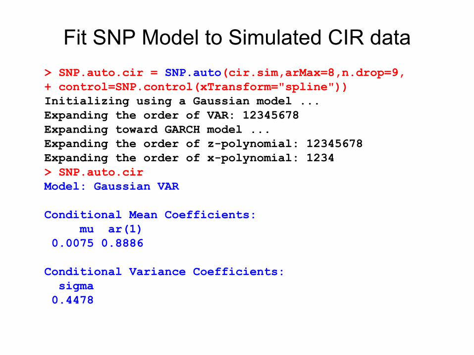
Fit SNP Model to Simulated CIR data> SNP.auto.cir = SNP.auto(cir.sim,arMax=8,n.drop=9,+ control=SNP.control(xTransform="spline"))Initializing using a Gaussian model ...Expanding the order of VAR: 12345678Expanding toward GARCH model ...Expanding the order of z-polynomial: 12345678Expanding the order of x-polynomial: 1234> SNP.auto.cirModel: Gaussian VAR
Conditional Mean Coefficients:mu ar(1)
0.0075 0.8886
Conditional Variance Coefficients:sigma
0.4478
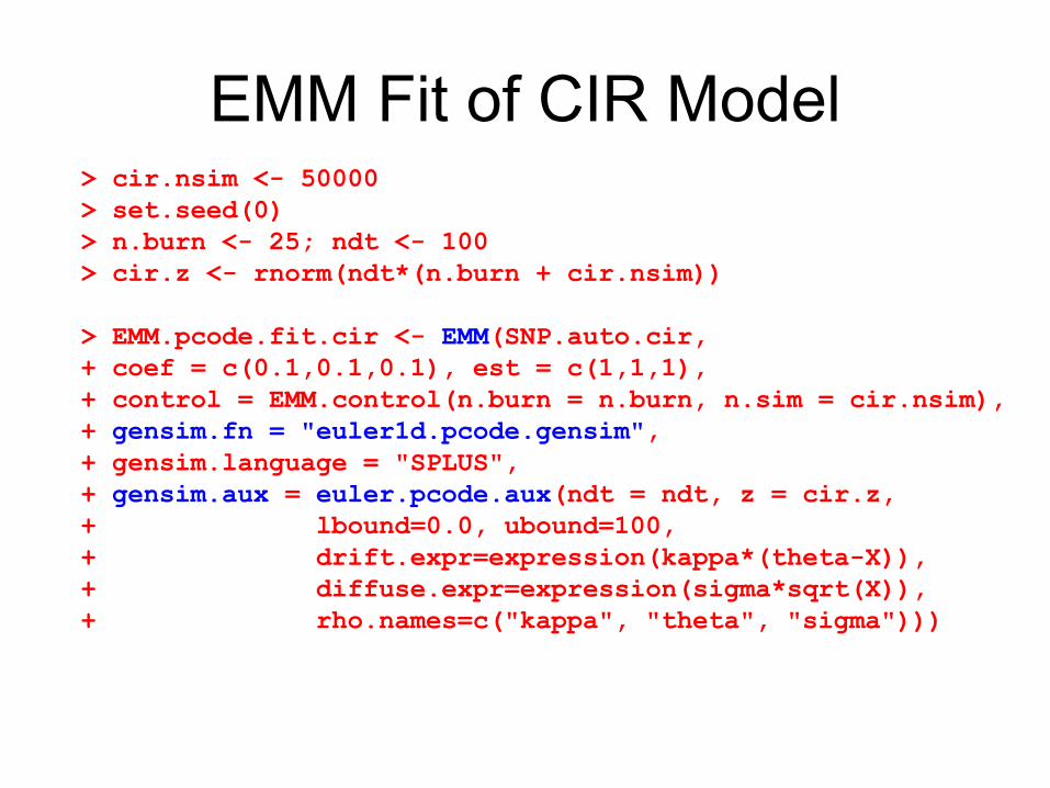
EMM Fit of CIR Model> cir.nsim <- 50000 > set.seed(0) > n.burn <- 25; ndt <- 100> cir.z <- rnorm(ndt*(n.burn + cir.nsim))
> EMM.pcode.fit.cir <- EMM(SNP.auto.cir, + coef = c(0.1,0.1,0.1), est = c(1,1,1), + control = EMM.control(n.burn = n.burn, n.sim = cir.nsim), + gensim.fn = "euler1d.pcode.gensim", + gensim.language = "SPLUS", + gensim.aux = euler.pcode.aux(ndt = ndt, z = cir.z, + lbound=0.0, ubound=100, + drift.expr=expression(kappa*(theta-X)), + diffuse.expr=expression(sigma*sqrt(X)), + rho.names=c("kappa", "theta", "sigma")))
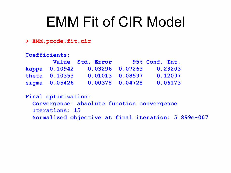
EMM Fit of CIR Model> EMM.pcode.fit.cir
Coefficients:Value Std. Error 95% Conf. Int.
kappa 0.10942 0.03296 0.07263 0.23203theta 0.10353 0.01013 0.08597 0.12097sigma 0.05426 0.00378 0.04728 0.06173
Final optimization:Convergence: absolute function convergence Iterations: 15 Normalized objective at final iteration: 5.899e-007