CE

UeT

DC

olle

ctio

n

Empirical Assessment of the Gender Wage Gap:

An Application for East Germany During Transition (1990-1994)

By

Katalin Springel

Submitted to

Central European University

Department of Economics

In partial fulfillment of the requirements

for the degree of Master of Arts in Economics

Supervisor: Professor John Earle

Budapest, Hungary

2011

CE

UeT

DC

olle

ctio

n

i

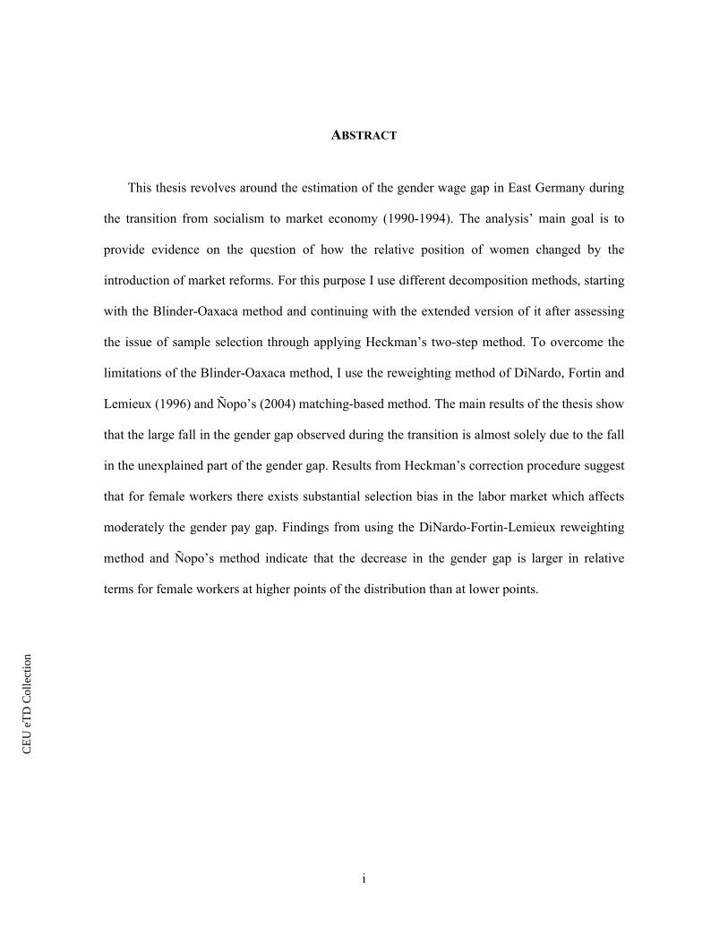
ABSTRACT

This thesis revolves around the estimation of the gender wage gap in East Germany during

the transition from socialism to market economy (1990-1994). The analysis’ main goal is to

provide evidence on the question of how the relative position of women changed by the

introduction of market reforms. For this purpose I use different decomposition methods, starting

with the Blinder-Oaxaca method and continuing with the extended version of it after assessing

the issue of sample selection through applying Heckman’s two-step method. To overcome the

limitations of the Blinder-Oaxaca method, I use the reweighting method of DiNardo, Fortin and

Lemieux (1996) and Ñopo’s (2004) matching-based method. The main results of the thesis show

that the large fall in the gender gap observed during the transition is almost solely due to the fall

in the unexplained part of the gender gap. Results from Heckman’s correction procedure suggest

that for female workers there exists substantial selection bias in the labor market which affects

moderately the gender pay gap. Findings from using the DiNardo-Fortin-Lemieux reweighting

method and Ñopo’s method indicate that the decrease in the gender gap is larger in relative

terms for female workers at higher points of the distribution than at lower points.

CE

UeT

DC

olle

ctio

n

ii

ACKNOWLEDGEMENTS

I would like to thank three people for their advice and support. First, I wish to express my

gratitude to my supervisor, Professor John Earle for his excellent teaching, support and guidance

he has given me during my studies and the writing of the thesis. I would also like to thank

Professor Álmos Telegdy for the interesting and stimulating Labor Economics lectures which

influenced me in choosing the topic for my thesis. Finally, I am grateful to Professor Gábor

Kézdi for his Econometrics lectures that has given me the knowledge to accomplish this work.

CE

UeT

DC

olle

ctio

n

iii

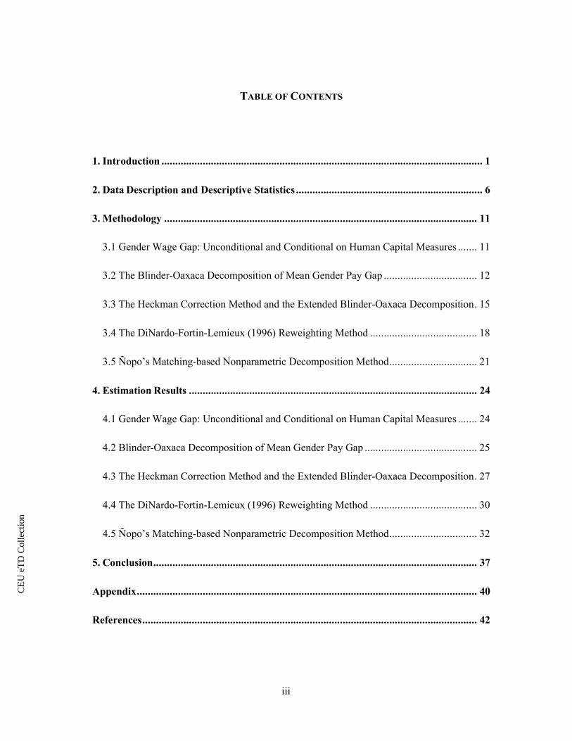
TABLE OF CONTENTS

1. Introduction ..................................................................................................................... 1

2. Data Description and Descriptive Statistics .................................................................... 6

3. Methodology .................................................................................................................. 11

3.1 Gender Wage Gap: Unconditional and Conditional on Human Capital Measures ....... 11

3.2 The Blinder-Oaxaca Decomposition of Mean Gender Pay Gap .................................. 12

3.3 The Heckman Correction Method and the Extended Blinder-Oaxaca Decomposition . 15

3.4 The DiNardo-Fortin-Lemieux (1996) Reweighting Method ....................................... 18

3.5 Ñopo’s Matching-based Nonparametric Decomposition Method ................................ 21

4. Estimation Results ......................................................................................................... 24

4.1 Gender Wage Gap: Unconditional and Conditional on Human Capital Measures ....... 24

4.2 Blinder-Oaxaca Decomposition of Mean Gender Pay Gap ......................................... 25

4.3 The Heckman Correction Method and the Extended Blinder-Oaxaca Decomposition . 27

4.4 The DiNardo-Fortin-Lemieux (1996) Reweighting Method ....................................... 30

4.5 Ñopo’s Matching-based Nonparametric Decomposition Method ................................ 32

5. Conclusion ...................................................................................................................... 37

Appendix ............................................................................................................................ 40

References .......................................................................................................................... 42

CE

UeT

DC

olle

ctio

n

1

1. INTRODUCTION

Since its re-unification with West Germany, East Germany (former German Democratic

Republic) has experienced a course of profound economic and political changes during its

transition from socialism to a market economy, changes that have had great influence on

women’s relative position. During socialism, a political system that (at least in principal)

heavily emphasized the idea of bringing men and women into equal positions in the labor

market had prevailed, leading to high labor force participation rates among women thanks to

labor market institutions such as maternity leave and (relatively) high minimum wages and

social entitlements such as day care benefits and housing (Brainerd, 2000). Over the years of

transition that followed, East Germany, just like all other formerly socialist countries, has

experienced a dramatic widening of the wage structure as well as a significant increase in its

wage level as a result of intensive collective bargaining to reach parity with levels of wages in

West Germany in 1994 (Brainerd, 2000).

As formerly socialist countries shared a similar economic environment before the

transition and implemented market reforms during the transition that had many common

aspects, one would expect similar changes in the male-female wage differentials to be present.

Nevertheless, countries of the former Soviet Union seem to have experienced a substantial

increase in the gender gap compared to East Germany and other Eastern European countries.

Hence, questions were raised concering the underlying reasons of the favorable change in

womens’ relative positions in these countries. The observed narrowing of the gender pay gaps

may have been a result of improvement in gender-specific factors that include women’s

relative level of measured and unmeasured labor market skills as well as potential decrease in

discrimination against female workers (Blau and Kahn, 1997 and 2000).1 Findings of Hunt

(2002) for East Germany seem to support this hypothesis, since according to Hunt’s results

1Discrimination in wages is defined as follow: It occurs if workers of two different groups with equal marginal productivity receive different wages.

CE

UeT

DC

olle

ctio

n

2

the gender-specific factors dominated in the change of the gender wage differential and

worked in favor of women during the years of transition.

The aim of this thesis is to examine the gender wage gap in East Germany right before

and after the transformation from central planning to a market economy, providing evidence

on the question of how the relative position of women changed by the introduction of market

reforms, that is, whether the male-female wage differential truly decreased or increased

during the transition from 1990 to 1994. I am interested in how much of the wage gaps

between the two genders are due to observed factors or unobserved factors, possibly including

discrimination. For this purpose, I use various decomposition methods on a data set that was

assembled from the German Socio-Economic Panel spanning four years (from 1990 to 1994).

Since observed changes can have different effects at different points of the wage distributions

of female and male workers respectively, the decomposition analysis I implement in this

thesis goes beyond the mean and allows for decomposition of the gender gap at different

quantiles of the wage density functions. Finally, an important aspect of the analysis is that it

takes into account the validity of the implemented decomposition methods because of

nonrandom sample selection and lack of common support (as discussed later) are carefully

considered.

Due to the usefulness of the decomposition techniques in quantifying the contribution of

multiple factors to differences in outcomes, I first use the widely utilized and known

decomposition method based on the seminal works of Blinder (1973) and Oaxaca (1973).

While this technique is widely used in the literature of gender wage gap and its simplicity

makes it appealing, it suffers from many limitations. Firstly, the Blinder-Oaxaca method

cannot be extended to the case of other general distributional statistics beyond the mean. This

is a very important limitation since decompositions at mean provide very little information

concerning what happens at other points of the wage distribution which could be very

CE

UeT

DC

olle

ctio

n

3

important in identifying the sources of the gender gap e.g. “glass ceiling” effect. Secondly,

this method is based on very restrictive assumptions such as linear relationship between the

outcome variable and the covariates. This condition can be easily violated, for example in

case there are non-linearities in the returns to education, e.g. “sheepskin effect”. Thirdly, in

presence of nonrandom sample selection, which I assume to be true and substantial for East

Germany over the considered period (Hunt, 2002, p.148), this method will give inconsistent

estimates. Finally, implementation of the Blinder-Oaxaca method might face problems when

there is lack of common support in the distribution of covariates (Fortin, Lemieux and Firpo,

2010).

To address the above discussed limitations of the Blinder-Oaxaca method, first I apply

Heckman’s method to correct for potential sample selection bias (Heckman, 1979), then I use

the extended Blinder-Oaxaca decomposition to quantify the contribution of sample selection

to the overall gender gap. The question of selectivity bias is of particular concern in the

present case as the employment rate of female workers declined significantly more during the

transitional years than the male labor force participation rates (Bonin and Euwals, 2001). The

underlying reason could be higher unemployment risk for low wage earners who were

disproportionately women (Hunt, 2002) or increased discrimination against working women

that can be a result of lower state control over firms that might have allowed employers to

take such actions more openly (Brainerd, 2000).2 Therefore, concerning the direction of the

bias, I expect female workers to be a positively selected group in terms of their unobserved

characteristics, meaning that working women earn more on average than non-working women

would if they would decide to participate in the labor force.

Next, I utilize two methods: one is a regression-based (semi-parametric) reweighting

method as in DiNardo, Fortin and Lemieux (1996); the other is a matching-based

2I would like to note that the effect of transition on discrimination against women might have been positive if discrimination became too costly to maintain in a competitive market economy (Becker, 1957).

CE

UeT

DC

olle

ctio

n

4

nonparametric decomposition approach introduced by Ñopo (2008). These methods, in

comparison with the Blinder-Oaxaca decomposition, both can be extended to other

distributional statistics and they do not impose the restrictive assumption of linear functional

form of conditional wage expectations that could be a source of potential misspecification.

Additionally, the two methods in question do not require the zero conditional mean

assumption to hold; instead, it can be replaced by the weaker unconfoundedness condition (or

ignorability) that only requires the unobservables’ conditional distribution given covariates X

to be the same for both working men and women as opposed to the unobservables’ (mean)

independency of covariates X.

The advantage of matching over the reweighting method is related to the common

support problem, under which, as Frölich (2004) noted, reweighting procedure in particular

performs quite poorly. Thus, I utilize Ñopo’s matching-based decomposition technique that

accounts for this problem to see how the results from traditional regression-based

decomposition techniques, the Blinder-Oaxaca and DiNardo-Fortin-Lemieux methods in

particular, compare. On the other hand, it is important to emphasize that Ñopo’s

decomposition method might face the problem of high dimensionality whereas in case of the

reweighting method this problem is reduced, therefore the usage of the latter remains relevant.

However, decomposition techniques in general are not without limitations. Firstly,

according to Fortin, Lemieux and Firpo (2010), decomposition methods follow a partial

equilibrium approach which inherently assumes that in the construction of counterfactuals for

one group, observed outcomes for the other can be utilized. Secondly, decompositions might

not aid the unveiling of mechanisms describing relationship between the outcome variable

(the wage in present case) and various factors.

The results show that there was a significant decrease in the observed gender wage gap

during the transition and the traditional Blinder-Oaxaca method reveals that this decrease is

CE

UeT

DC

olle

ctio

n

5

almost solely due to the significant fall in the “Renumeration” effect or unexplained part of

the gender pay gap which largely dominates the determination of the male-female wage

differentials in both years leaving nearly no role for human capital measures like education or

work experience. The results from Heckman’s selection correction method suggest that for

female workers there exists substantial selection bias in the labor market, while for male

workers no evidence on sample selection can be obtained. By applying the extended Blinder-

Oaxaca method I show that selectivity bias affects moderately the determination of the gender

pay gap. Findings from implementing the DiNardo-Fortin-Lemieux reweighting method

indicate that in both years the gender wage gap is significantly larger for working women at

the lower quantiles of the wage distribution than at the higher ones. Furthermore, the decrease

in the gender gap occuring at all points of the wage distribution is larger in relative terms for

female workers at higher points of the distribution than at lower points. Finally, by using

Ñopo’s procedure I show support for the results of the reweighting method as well as find

(moderate) evidence on the presence of such highly rewarded individual labor market skills

that are obtained solely by working men.

The rest of the paper is organized as follows. Chapter 2 describes the data set constructed

for the analysis as well as the utilized variables in detail, and presents the descriptive

statistics. Chapter 3 provides the methodological framework applied to examine the gender

wage gap, while the results of the empirical analysis are presented in Chapter 4. The paper

ends with the conclusion where I sum up the results and outline some possibilities to extend

the present analysis.

CE

UeT

DC

olle

ctio

n

6

2. DATA DESCRIPTION AND DESCRIPTIVE STATISTICS

This chapter describes the data set utilized in this analysis assembled from the German

Socio-Economic Panel for East Germany.3 I used data from 1990 when individuals from East

Germany were surveyed just before the re-unification and from 1994. I chose these years

because this way the observed period is short enough to ensure that the observed changes

reflect the effects of market reforms associated with the transition from socialism to market

economy. The reason I chose this data set is because it provides a large set of harmonized

variables on household and personal level making it very appealing for the present analysis.

The sample was restricted to workers with nonzero working hours and a valid wage who are

not self-employed, not in a training program (apprenticeship), not in the agricultural sector,

nor completing compulsory military service. I do not include self-employed individuals,

because it is difficult to distinguish between returns to human capital from returns to physical

capital. Similarly, I do not take individuals in the agricultural sector since their earnings are

likely to be explained also by random factors like weather conditions. The sample was

trimmed at the bottom and the top 1% of wage observations in order to get rid of implausibly

low and high wages. In addition, the sample was restricted to individuals aged 18 to 60 since

individuals younger than 18 or older than 60 are most probably also involved in decisions

concerning education and (early) retirement that are different from the employment decision.

Following the work of Fortin and Lemieux (1998) part-time workers are not excluded from

the sample along full-time workers, but each observation in the sample is weighted by the

number of weekly hours worked. This way more weight is put on workers who provide

relatively more hours of work to the labor market, thus through this procedure each worker’s

contribution is better reflected. Finally, missing values observed account for less than 1% of

the final sample and they were generated with the simple procedure of unconditional mean

3 By East Germany I mean the former German Democratic Republic which ceased to exist in 1990 after its unification with West Germany (former Federal Republic of Germany).

CE

UeT

DC

olle

ctio

n

7

imputation. The idea of this method is to simply replace the missing values observed in the

data set with the arithmethic average of the observed values on the same variable over the

other observations (Little and Rubin 1987). This imputation method provides unbiased,

consistent estimators if missing values are missing either completely at random or at random,

but it underestimates variability/variance.

The set of variables used for the present analysis includes wages, gender, level of

education, and years of actual work experience. The wage variable (��, which denotes the

logarithm of the worker’s wage for time period �) is a measure of the monthly, gross amount

(not adjusted for end of year bonuses) earned by the workers. The gender variable (������) is a dummy, which takes the value of one if the individual is female, and zero otherwise. The

highest level of education attained by the workers was captured by using a set of four dummy

variables (����� �ℎ����, ��������������, ��������� ℎ�� and ����� ���) that

corresponds to only general classroom education, classroom vocational training, participation

in the dual-system that stands for classroom education and work in a firm, and to the

completion of university, respectively. The actual working experience variable (���������) gives a measure of the entire period of employment in the respondent’s working career up to

the point when the survey was taken. It gives the length of time in years with months in

decimal form.

Furthermore, I used the following set of instrumental variables for Heckman’s two-step

correction model: marital status, presence of young children, an indicator for the head of

household and nonlabor household financial variables (child allowance and income from

interests/dividends). The marital status variable (�������) is a dummy, which takes the value

of one if the individual is married, and zero otherwise. I used a set of two variables to capture

the presence of young children in the household (�ℎ���0_5 and �ℎ���6_16): the number of

children under the age of five as well as the number of children between six and sixteen. In

CE

UeT

DC

olle

ctio

n

8

addition, I included interaction terms between number of children and number of adults in the

household. The indicator for the head of household is a dummy variable (ℎℎ���) that takes

the value of one if it is true for the individual, and zero otherwise. The contents of the two

nonlabor household income variables are as follows: the child allowance variable (��ℎ����) measures the logarithm of monthly, gross amount of child allowance while the ����� dummy

variable takes the value of one if the individual had nonzero amount of income from interests

and dividends in the last year, and zero otherwise.

Following Oaxaca’s study (1973) I do not include occupational or job position dummies

in the model, as they may already be the result of discrimination (“pre-labor market

discrimination”). Hence, controlling for occupational differences between female and male

workers would result in the underestimation of the effects of discrimination by eliminating

“some of the effects of occupational barriers as sources of discrimination” (Oaxaca, 1973,

p.699). For similar reasons I also do not include industry dummy variables in the analysis. I

would like to note that unionization which is expected to contribute to the evolvement of the

gender pay gap as suggested by many studies (Blau and Kahn, 1997 and DiNardo, Fortin and

Lemieux, 1996) is not included in this analysis due to lack of data.

The descriptive statistics of the variables used in the analysis (Table 1 in the Appendix)

reveal several differences between female and male workers as well as various changes during

the examined period that are different across gender. First of all, it is easy to see from the

table that men and women in the sample have experienced some different changes in

educational attainment over the period. The proportion of women in the sample with an

apprenticeship or with general schooling as the highest level of education declined more than

the same proportion of men in the sample (which remained quite stable during 1990-1994)

which - since we can assume that few individuals change their education - can indicate that

women with lower level of education disproportionately left employment. This seems to

CE

UeT

DC

olle

ctio

n

9

support the hypothesis that there might be a strong selection effect in the sample of female

workers4 which could result in such change in the composition of educational attainment. In

addition, this is in line with the findings of Hunt (2002) who notes an even more drastic fall

among working women with apprenticeship during transition. Secondly, Table 1 shows that in

both years women in the sample have lower level of actual experience on average than men as

well as they are slightly younger on average.

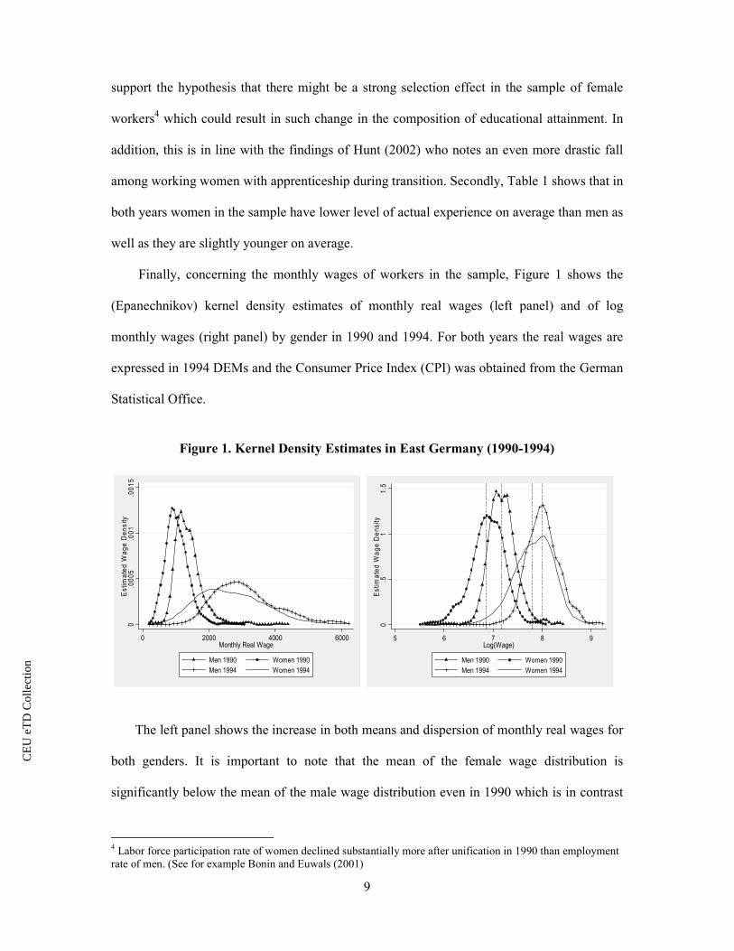
Finally, concerning the monthly wages of workers in the sample, Figure 1 shows the

(Epanechnikov) kernel density estimates of monthly real wages (left panel) and of log

monthly wages (right panel) by gender in 1990 and 1994. For both years the real wages are

expressed in 1994 DEMs and the Consumer Price Index (CPI) was obtained from the German

Statistical Office.

Figure 1. Kernel Density Estimates in East Germany (1990-1994)

The left panel shows the increase in both means and dispersion of monthly real wages for

both genders. It is important to note that the mean of the female wage distribution is

significantly below the mean of the male wage distribution even in 1990 which is in contrast

4 Labor force participation rate of women declined substantially more after unification in 1990 than employment rate of men. (See for example Bonin and Euwals (2001)

0.0

005

.001

.001

5E

stim

ate

d W

age D

ensity

0 2000 4000 6000Monthly Real Wage

Men 1990 Women 1990

Men 1994 Women 1994

0.5

11.5

Estim

ate

d W

age D

ensity

5 6 7 8 9Log(Wage)

Men 1990 Women 1990

Men 1994 Women 1994

CE

UeT

DC

olle

ctio

n

10

with the “equal pay for equal work” idea that was heavily emphasized during socialism. The

right panel shows that there is substantial difference between the average log wages (indicated

by the dashed vertical lines) of men and women in the sample – the raw gender wage gap –

and that this difference shrank during the considered period. In addition, the panels of Figure

1 show that the unadjusted male-female wage differential declined at all quantiles of the wage

distribution from 1990 to 1994 and that both wage densities became less skewed to the left.

Table 2 (in the Appendix) presents the descriptive statistics of the instrumental variables

from which I would only like to emphasize the fact that while proportion of married men and

women in the sample on average remained quite stable during transition, the average number

of children in the household under the age of five declined for both genders and increased for

children between six and sixteen.

CE

UeT

DC

olle

ctio

n

11

3. METHODOLOGY

In this chapter, following the presentation of the data set used, I describe the

methodology implemented in the thesis. First, I start with estimating the gender wage gap

unconditional and conditional on selected human capital characteristics. Next, I decompose

the gender wage gap with the Blinder-Oaxaca technique followed by the implementation of

Heckman’s correction method to adjust for sample selection. Then, I use DiNardo-Fortin-

Lemieux reweighting method to decompose the gender differences in wages at all points of

the wage distribution. Finally, I use Ñopo’s matching-based procedure to overcome the

limitations of the DiNardo-Fortin-Lemieux reweighting method and Blinder-Oaxaca method

related to the “support problem”.

3.1 Gender Wage Gap: Unconditional and Conditional on Human Capital Measures

The starting point of this paper is to simply calculate the unconditional male-female pay

gap at means for each year in order to attain an overall picture of the actual gender wage gap:

(1)� ,� −�",� where �, ,� is the logarithm of male wages, while �",� is the logarithm of female wages.

Since this measure does not reveal too much information, for example about the sources of

the male-female wage differentials, I continue with estimating the gender wage gap for time

period � conditional on a set of human capital measures. The estimation of the conditional

gender wage gap is based on the traditional Mincer earnings equation (Bosworth et al. 1996):

(2)�� = % + ' ∗ )� + * ∗ ������ + �� where �� is the logarithm of monthly wages, )� denotes an array of control variables

including the schooling dummy variables (where the omitted or reference category is

��������������), the experience and the square of experience divided by 100, ������ is the gender dummy variable, and �� is the error term. The variable of interest is the

coefficient on the gender dummy variable, *, which indicates the gender gap in pay

CE

UeT

DC

olle

ctio

n

12

conditional on the above described control variables. I use OLS estimation method and White

Heteroskedasticity-Consistent Standard Errors to take into account possible heteroskedasticity

in the error term. Following the works of Heckman, Lochner and Todd (2003) and Lemieux

(2006), in addition to the above described specification, I also estimate a model that includes

an interaction term between schooling dummies and experience as well as one in which a

linear and a quadratic term of years of education are included instead of schooling dummies.

However, while these wage regression models contribute to the better understanding of the

evolution of the gender wage gap, the simple OLS estimation method described above suffers

from several drawbacks and for consistent estimation of the parameters a set of restrictive

assumptions are required. These assumptions include exogeneity of explanatory variables,

random sample selection and no misspecification may arise due to omitted right-hand side

variables. It is important to note that thorough discussion and assessment of these assumptions

is beyond the scope of this paper and thus it will not be dealt with in depth. To gain a better

view into the composition and development of gender gap in pay, as a next step, I turn to

different aggregate decomposition methods. In this thesis I only focus on aggregate

decomposition methods, techniques that decompose the total gap into “Endowment” and

“Renumeration” effects, and will not include detailed decompositions which involves

subdivision of these two effects into respective contributions of included covariates.

3.2 The Blinder-Oaxaca Decomposition of Mean Gender Pay Gap

The most common approach used to identify and quantify the causes of male-female

wage differential is the Blinder-Oaxaca decomposition method suggested by Blinder (1973)

and Oaxaca (1973) in their seminal work. This technique, replacing traditional linear

regression methods incorporating a gender dummy variable, have the advantage that it allows

for the separation of observable and unobservable effects (in the latter, discrimination being

included); however, it suffers from several deficiencies. Following the standard approach in

CE

UeT

DC

olle

ctio

n

13

econometrics, first I discuss the aim of the method applied and the assumptions required to

interpret the obtained estimates, and then I show the estimation procedure itself.

Assumptions

The aim of the Blinder-Oaxaca method is to divide the overall gender wage gap at means

into two parts, into a term that is attributable to differences in female and male wage

structures, and a part attributable to differences in female and male workers’ observed

characteristics. The Blinder-Oaxaca method is based on the standard assumption of linear

relation of the outcome variable (+) to the covariates ()) in the underlying wage setting

model (I) and on the restrictive assumption of zero conditional mean (II):

(3)+-. = '/0 +1 ).23245

'-2 + �/.6ℎ���7 = 8, 9��:;�-.<).= = 0

Additionally, this decomposition builds on the assumption of “overlapping support” (III) that

requires an overlap in observable characteristics across gender, meaning that provided the

assumption holds, there is no such value of the covariates () = �) or of the error term (� = �) that could serve as an identifier of membership into one of the genders.

Procedure

The Blinder-Oaxaca decomposition of the gender gap for period � can be estimated as:

(4)Δ� = � ,� −�",� = ;) ,� − )",�= ∗ '@ ,� + )",� ∗ ;'@ ,� − '@",�= This method decomposes the differences in female and male wages at the mean into two

components: “Endowment” effect (also called “Composition” or “Explained” effect) and

“Renumeration” effect (also called “Wage Structure” or “Unexplained” effect). The

“Endowment” effect - the first term on the right-hand side of equation (4) - measures the part

of the gender gap due to differences in the average human capital characteristics, while the

“Renumeration” component - the second term on the right-hand side of equation (4) -

captures the effects due to differences in estimated coefficients. The latter component has also

CE

UeT

DC

olle

ctio

n

14

been called as the measure of discrimination. For simplicity I adopt the male wage structure

as the nondiscriminatory norm, as it is done in most studies. Alternative choices for

nondiscriminatory wage standard can be the female wage structure or one estimated from

pooled sample of the two genders.

Limitations

While the Blinder-Oaxaca procedure is very simple to implement and widely used in the

gender pay gap literature, it suffers from many drawbacks. First of all, the Blinder-Oaxaca

decomposition cannot be extended to the case of general distributional statistics other than the

mean. This limitation is noteworthy since decomposing gender wage differences at mean do

not provide information regarding other points of the wage distribution even though that can

be very important in identifying the underlying reasons of the gender differential e.g. “glass

ceiling” effect. Secondly, this method is based on very restrictive assumptions (as discussed

previously), thus it might not provide consistent estimates when the conditional mean is a

non-linear function or when the problem of endogeneity arises. The simplest example is the

case of omitted unobserved ability: individuals with higher innate ability will attain higher

level of education as well as higher wages, thus estimated returns to education will be biased

(“ability bias”) when unobserved ability is not included in the wage setting model. Thirdly, in

presence of nonrandom sample selection, which I assume to be true and substantial for East

Germany over the considered period (Hunt, 2002, p.148), this method will give inconsistent

estimates. Finally, lack of common support can impose problems (referred to as “support”

problem in the literature) when applying the Blinder-Oaxaca method (Fortin, Lemieux and

Firpo, 2010). The “support” problem relates to the fact that male and female workers may not

only differ in human capital characteristics, but also the distributions of these variables can

overlap very little. The issue of the lack of common support is mostly neglected in the

literature of gender wage gap, even though it can be important from a policy point of view as

CE

UeT

DC

olle

ctio

n

15

well, since gender differences in the distribution of covariates can reflect pre-labor market

discrimination as female workers might face barriers in reaching certain individual

charateristics that male workers achieve.

3.3 The Heckman Correction Method and the Extended Blinder-Oaxaca Decomposition

As the next step I use Heckman’s two-step sample correction procedure to correct for

non-random sample selection (Heckman, 1979). Selectivity bias might be found at two stages

of the employment process: at the stage of entering the labor market or when an occupation is

chosen, but in the present thesis only the first case is going to be considered. Selectivity in

participation exists if the working individuals do not form a random subgroup of the sampled

population, but differ systematically from those who are not employed. In other words, if the

determinants of the participation decisions are uncorrelated with the determinants of

individual wages, the fact that not employed individuals and their wages are not observed

could be simply ignored. However, such an assumption is unlikely to hold in practice. Sample

selection bias are particularly important in case of East Germany during the transition as the

employment rate of working women declined substantially more over this period than the

employment rate of their male counterparts. Thus, regarding the direction of the selectivity

bias, I expect female workers to be positively selected into employment, meaning that female

workers earn more on average than women who are currently not working would if they

would decide to become employed. Concerning male workers I expect to find no evidence on

significant sample selection. I would like to emphasize that while its ease of implementation

makes the Heckman’s correction method appealing, it has a rather limited structure, it is

highly parameterized and the identification conditions that are required to successfully

perform the method are potentially serious (Vella, 1998).

CE

UeT

DC

olle

ctio

n

16

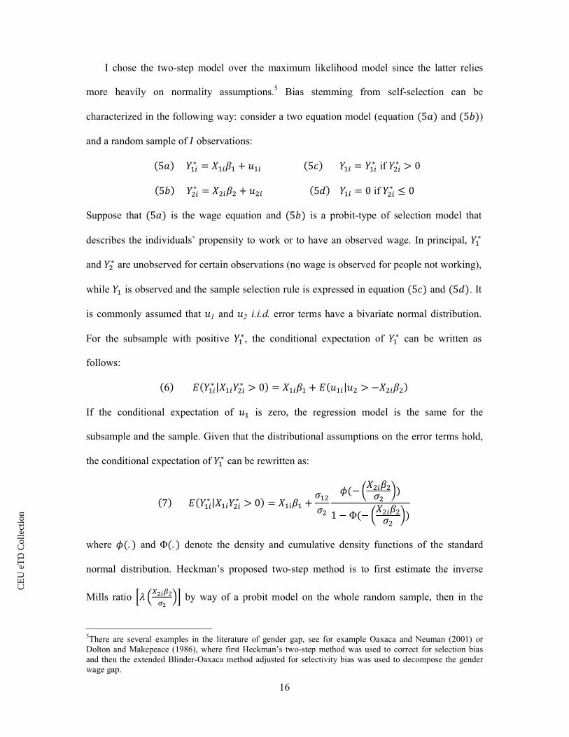
I chose the two-step model over the maximum likelihood model since the latter relies

more heavily on normality assumptions.5 Bias stemming from self-selection can be

characterized in the following way: consider a two equation model (equation (5�) and (5A)) and a random sample of B observations:

(5�)+5.∗ = )5.'5 + �5. (5�)+5. = +5.∗ if +C.∗ > 0

(5A)+C.∗ = )C.'C + �C. (5�)+5. = 0 if +C.∗ ≤ 0

Suppose that (5�) is the wage equation and (5A) is a probit-type of selection model that

describes the individuals’ propensity to work or to have an observed wage. In principal, +5∗ and +C∗ are unobserved for certain observations (no wage is observed for people not working),

while +5 is observed and the sample selection rule is expressed in equation (5�) and (5�). It is commonly assumed that �1 and �2 i.i.d. error terms have a bivariate normal distribution.

For the subsample with positive +5∗, the conditional expectation of +5∗ can be written as

follows:

(6):(+5.∗ |)5.+C.∗ > 0) = )5.'5 + :(�5.|�C > −)C.'C) If the conditional expectation of �5 is zero, the regression model is the same for the

subsample and the sample. Given that the distributional assumptions on the error terms hold,

the conditional expectation of +5∗ can be rewritten as:

(7):(+5.∗ |)5.+C.∗ > 0) = )5.'5 + H5CHCI(−J)C.'CHC K)1 − Φ(− J)C.'CHC K)

where I(. ) and Φ(. ) denote the density and cumulative density functions of the standard

normal distribution. Heckman’s proposed two-step method is to first estimate the inverse

Mills ratio MN OPQRSQTQ UV by way of a probit model on the whole random sample, then in the

5There are several examples in the literature of gender gap, see for example Oaxaca and Neuman (2001) or Dolton and Makepeace (1986), where first Heckman’s two-step method was used to correct for selection bias and then the extended Blinder-Oaxaca method adjusted for selectivity bias was used to decompose the gender wage gap.

CE

UeT

DC

olle

ctio

n

17

second step estimate equation (8) on the subsample with positive +5∗ by using OLS

estimation method:

(8)+5. = )5.'5 + H5CHC N@ J)C.'CHC K + X.

It is important to note that as long as �C has a normal distribution and X5 is independent

of N, the Heckman’s two-step estimator is consistent, but it is not efficient. Heckman proposes

to test for selectivity bias by way of a t-test on the coefficient of N. While this method has

been widely used in the literature, it relies on restrictive assumptions, and its implementation

involves several problematic issues, therefore it needs very careful consideration and caution

when interpreting the results. (For further details see for example Puhani, 2000)

One of the most important problems is that the inclusion of the inverse Mills ratio often

results in multicollinearity. Since the inverse Mills ratio is estimated by a non-linear probit

model, the correction term N and )5 will never be perfectly correlated. However, the probit

model will be linear for the mid-range values of )5; therefore, in the absence of exclusion

restrictions the wage equation will suffer from inflated standard errors due to strong

multicollinearity. The best solution is to incorporate exclusion restrictions,6 since with valid

instruments, the inverse Mills ratio and the set of controls included in the wage equation ()5) will be less correlated, reducing the collinearity as well as facilitating model identification.

Therefore, I use a set of exclusion restrictions in the analysis, namely marital status, presence

of young children in the household, interaction term between number of adults and number of

young children in the household, indicator of the head of household and nonlabor household

financial variables. I expect that marriage lowers the probability to work for females and

increases it for males. While both the presence of young children in the household (with

stronger effect expected if they are younger than five rather than between six and sixteen) and

6 Exclusion restrictions are variables that affect the selection process as they contribute to the determination of the propensity to work, but they do not affect the wage equation.

CE

UeT

DC

olle

ctio

n

18

higher nonlabor income are expected to lower the probability to work (especially for women),

being the head of household and the interaction term are expected to increase this probability.

I test for collinearity by regressing the inverse Mills ratio on )5, where a large YC indicates

strong multicollinearity.

Finally, since I am interested in the male-female wage differential and its evolvement, I

integrate the selection correction into the Blinder-Oaxaca decomposition method. The

consequences of sample selection correction are twofold. On the one hand, the estimated rates

of return differ, on the other hand, a selection correction term adds to the “Endowment” and

“Renumeration” components. There are several proposed ways in the literature on how to

handle the selection correction term within the decomposition of the wage gap. See for

instance Neuman and Oaxaca (2004) or Dolton and Makepeace (1986). I chose to treat the

gender differences in selectivity as a third separate component of the wage decomposition:

(9)Δ� = � ,� −�",� = ;) ,� − )",�= ∗ '@ ,� + )",� ∗ ;'@ ,� − '@",�= + ([\ ,�N@ ,� − [\",�N@",�) where [\ is an estimate of (H5C HC⁄ ) and N@ is an estimate of the Inverse Mills Ratio. I chose this

specification as I am interested in the overall contribution of selection effects to the wage gap.

3.4 The DiNardo-Fortin-Lemieux (1996) Reweighting Method

Next, I apply the inverse probability reweighting decomposition method introduced by

DiNardo, Fortin and Lemieux (1996). The goal of this method is to go beyond summary

measures such as the mean or variance and establish decomposition of the gender wage gap

into unexplained and explained parts at all points of the wage distribution by construction of

counterfactual wage density function. The method is based on the assumptions of ignorability,

overlapping support and invariance of conditional distributions. The invariance assumption

requires that the conditional wage distribution � (6|�, �) (where 8 takes value of one when

individual is male, zero otherwise) can be extrapolated for �^) (Fortin, Lemieux and Firpo,

2010).

CE

UeT

DC

olle

ctio

n

19

The density of log wages (� (6) for men and �"(6) for women, respectively) can be

written as follows:

(10�)� (6) = _� (6|�, �)(�|8 = 1)��

(10A)�"(6) = _�"(6|�, �)(�|9 = 1)��

where �-(6|�, �) is the conditional wage distribution given gender status (7 = 8, 9) and

observed individual characteristics ()); (�|7 = 1) denotes the distribution of covariates

conditional upon gender; 8 and 9 are variables indicating gender status7; and the vector of

observed individual characteristics is denoted by �^) while � is the unobserved term. The

counterfactual density function – which is a function of counterfactual wage distribution that

can be referred to as the distribution of wages that would prevail for female workers if they

were paid like their male counterparts – is constructed in the following way in the spirit of

DiNardo, Fortin and Lemieux’s work (1996):

(10�)�̀ (6) = _� (6|�, �)a(�)(�|8 = 1)��

where a(�) is the reweighting function defined as a(�) = (�|9 = 1)/(�|8 = 1) which

expression can be reformulated by using Bayes’ rules in the following way:

(11)a(�) = Pr(9 = 1|�) /Pr(9 = 1)Pr(8 = 1|�) /Pr(8 = 1)

It is important to note the construction of the counterfactual relies on the assumption of

invariance and that I chose to estimate it using the male wage structure as the

nondiscriminatory norm. In general, it can be stated that the male wage structure is closer to a

nondiscriminatory norm than the female one and I assumed that relative changes in the female

workers’ wage position does not influence the male wage structure. Also, I chose the male

wage structure as nondiscriminatory norm for ease of comparability since most studies do the

7 8 takes value of one when individual is male, zero otherwise, and 9 takes value of one when individual is female, zero otherwise.

CE

UeT

DC

olle

ctio

n

20

same. However, there are other alternative solutions used, e.g. choice of pooled wage

structure.

The estimation procedure can be implemented in as follows. First, estimating the

probability model for Pr(8 = 1|�) using probit model on the pooled sample of both genders:

(12)Pr(8 = 1|�) = Pr(� > e(�)') = 1 − Φ(−e(�)') where Pr(8 = 1|�)is the probability of being male given �; Φ(. ) is the cumulative normal

distribution and e(�) is vector of covariates that includes schooling and experience. Next,

computing the value of the reweighting factor utilizing the predicted probabilities:

(13)a\(�) = Prg(9 = 1|�) /Prg(9 = 1)Prg(8 = 1|�) /Prg(8 = 1)

Lastly, estimating the wage densities for both genders and the counterfactual density (with the

help of a\(�)) by utilizing kernel density methods (equations (14�) − (14�)):

(14�)�@ (6) =1[.ℎ h J

6 −�.ℎ K

.i

(14A)�@"(6) =1[.ℎ h J

6 −�.ℎ K

.i"

(14�)�@̀ (6) =1[.ℎ a\(�.)h J

6 −�.ℎ K

.i

where�@-(6) is the estimated wage density; [. is the weight adjusting for hours worked; h(. ) is the kernel function; ℎ is the bandwidth and �. is observation of wage in the sample. The

Gaussian kernel function was chosen for the estimation and for the bandwidth I chose the

default setting in Stata statistical software package which is based on Silverman’s (1986) rule

of thumb optimal bandwidth. Once the estimates of wage densities are obtained, they can be

utilized to construct the decomposition of the gender wage gap that allows the examination of

differences at different quantiles of the wage distribution:

(15)Δj(k) = O�@ (6) − �@̀ (6)U + ;�@̀ (6) − �@"(6)=

CE

UeT

DC

olle

ctio

n

21

where the first term of the right-hand side of equation (15) captures the “Endowment” effect

and the second term stands for the “Renumeration” effect.

3.5 Ñopo’s Matching-based Nonparametric Decomposition Method

As a final step I use Ñopo’s nonparametric decomposition procedure which is based on

exact matching (Ñopo, 2004). This method aims at providing a decomposition of the overall

gender gap that accounts for the “support” problem and relies on the key assumption of

ignorability. The advantage of this technique is that it can be extended to other distributional

statistics and does not impose the restrictive assumption of linear functional form in contrast

with the Blinder-Oaxaca decomposition. Moreover, it relies on the weaker unconfoundedness

condition and does not require the unobservables’ (mean) independency of covariates X as the

Blinder-Oaxaca decomposition does. Finally, Ñopo’s matching-based method accounts for the

“support” problem, under which the implementation of Blinder-Oaxaca procedure and the

DiNardo-Fortin-Lemieux method might face severe problems. The main disadvantage of

Ñopo’s method is that it might suffer from the problem of high dimensionality, but using

propensity score matching instead of exact matching could reduce this problem.

Let l = (l ∩ l") be the common support and �n| = �() ∈ l|8) = p �9 (�)n the

probability measure of the set l under the distribution �9 (. ). Then, the male population

(and similarly the female population) can be divided into two subpopulations composed of

individuals that belong either to the common support l or are out of the common support l:

(16):(�|8) = :n(�|8)�n| + :n(�|8)�n< = �n< q:n(�|8) − :n(�|8)r + :n(�|8)

(17):(�|9) = �n<"q:n(�|9) − :n(�|9)r + :n(�|9) Using equation (16) and (17), the total gender wage differential s∆≡ :(�|8) − :(�|9)v can be written in the following form:

CE

UeT

DC

olle

ctio

n

22

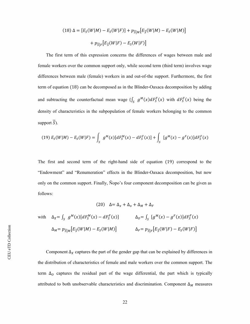
(18)Δ = s:n(�|8) − :n(�|9)v + �n< q:n(�|8) − :n(�|8)r

+ �n<"q:n(�|9) − :n(�|9)r The first term of this expression concerns the differences of wages between male and

female workers over the common support only, while second term (third term) involves wage

differences between male (female) workers in and out-of-the support. Furthermore, the first

term of equation (18) can be decomposed as in the Blinder-Oaxaca decomposition by adding

and subtracting the counterfactual mean wage (p (�)�9n"(�)n with �9n"(�) being the

density of characteristics in the subpopulation of female workers belonging to the common

support l).

(19):n(�|8) − :n(�|9) = _ (�)s�9n (�) − �9n"(�)v +n_ s (�) − "(�)v�9n"(�)n

The first and second term of the right-hand side of equation (19) correspond to the

“Endowment” and “Renumeration” effects in the Blinder-Oaxaca decomposition, but now

only on the common support. Finally, Ñopo’s four component decomposition can be given as

follows:

(20)∆= ∆w + ∆x + ∆ + ∆"

with ∆P= p (�)s�9n (�) − �9n"(�)vn ∆y= p s (�) − "(�)v�9n"(�)n

∆ = �n< q:n(�|8) − :n(�|8)r ∆"= �n<"q:n(�|9) − :n(�|9)r

Component∆P captures the part of the gender gap that can be explained by differences in

the distribution of characteristics of female and male workers over the common support. The

term ∆y captures the residual part of the wage differential, the part which is typically

attributed to both unobservable characteristics and discrimination. Component ∆ measures

CE

UeT

DC

olle

ctio

n

23

the part of the gender wage differential that can be explained by differences between men in

the common support and men out of the common support. This term accounts for the part of

the wage gap that can be attributed to the fact that some characteristics that male workers own

are not observed among female workers and if this term is positive, it means that these

characteristics are highly rewarded in the labor market. Component ∆" can be defined in a

similar way for female workers in and out of common support. The exact matching algorithm

can be summarized as follows. First, for each female worker all male workers with same

characteristics are selected, that is, matching is done with replacement meaning that the same

man can be selected more than once (One-to-many matching). Second, the counterfactual

wage for each female workers is computed as an average of all the matched male workers’

wage. Finally, the previously described four components are calculated.

CE

UeT

DC

olle

ctio

n

24

4. ESTIMATION RESULTS

4.1 Gender Wage Gap: Unconditional and Conditional on Human Capital Measures

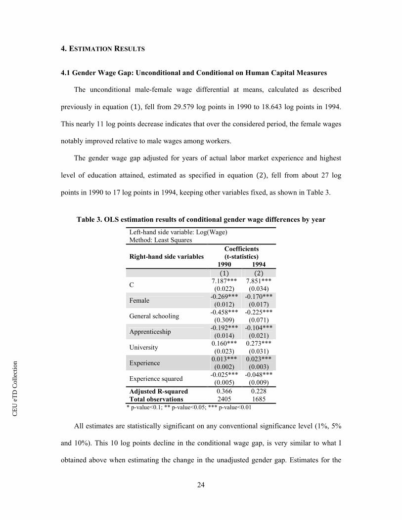
The unconditional male-female wage differential at means, calculated as described

previously in equation (1), fell from 29.579 log points in 1990 to 18.643 log points in 1994.

This nearly 11 log points decrease indicates that over the considered period, the female wages

notably improved relative to male wages among workers.

The gender wage gap adjusted for years of actual labor market experience and highest

level of education attained, estimated as specified in equation (2), fell from about 27 log

points in 1990 to 17 log points in 1994, keeping other variables fixed, as shown in Table 3.

Table 3. OLS estimation results of conditional gender wage differences by year

Left-hand side variable: Log(Wage) Method: Least Squares

Right-hand side variables Coefficients (t-statistics)

1990 1994

(1) (2)

C 7.187*** (0.022)

7.851*** (0.034)

Female -0.269***

(0.012) -0.170***

(0.017)

General schooling -0.458***

(0.309) -0.225***

(0.071)

Apprenticeship -0.192***

(0.014) -0.104***

(0.021)

University 0.160*** (0.023)

0.273*** (0.031)

Experience 0.013*** (0.002)

0.023*** (0.003)

Experience squared -0.025***

(0.005) -0.048***

(0.009) Adjusted R-squared Total observations

0.366 2405

0.228 1685

* p-value<0.1; ** p-value<0.05; *** p-value<0.01

All estimates are statistically significant on any conventional significance level (1%, 5%

and 10%). This 10 log points decline in the conditional wage gap, is very similar to what I

obtained above when estimating the change in the unadjusted gender gap. Estimates for the

CE

UeT

DC

olle

ctio

n

25

schooling dummies show that with respect to the omitted category (��������� �ℎ���), workers with university degree earned more on average in both years, while workers with

general schooling or apprenticeship earned less on average over the period, holding all other

variables fixed. The return to education (represented by coefficient estimates on schooling

dummies) increased for all level of highest educational attainment from 1990 to 1994. As for

estimates on experience, for both years the more experienced workers earn more than the less

experienced ones until they reach a certain number of years of experience (26 and 24,

respectively), keeping all other variables fixed. The return to labor market experience

increased from 1990 to 1994, but also its rate of decrease was higher in 1994. According to

the adjusted R-squared, 36.6% of the sample variation in log wages was explained by

schooling and experience in 1990, which decreased to 22.8% in 1994, meaning that during

transition the explanatory power of the included human capital measures with respect to log

wages decreased. I also estimated two alternative versions8 of the model presented in equation

(2), but both specifications resulted in coefficient estimates very similar to the ones presented

in Table 3, thus they are not reported here. Nevertheless, the estimation of these wage

regression models does not allow one to identify and quantify the different sources of the

gender gap, hence, to gain a better understanding of the composition and of the evolvement of

male-female wage differential, I continue my analysis with various aggregate decomposition

techniques.

4.2 Blinder-Oaxaca Decomposition of Mean Gender Pay Gap

The estimation results from the Blinder-Oaxaca decomposition estimated on the whole

sample as specified in equation (4) show that the “Renumeration” effect’s contribution

8One of them included an interaction term between schooling dummies and experience while in the other one a linear and a quadratic term of years of education were included instead of schooling dummies.

CE

UeT

DC

olle

ctio

n

26

dominates in the determination of the gender wage gap, while the “Endowment” effect plays a

very insubstantial role in both years (see Table 4).

Table 4. The Blinder-Oaxaca decomposition of the gender wage gap

Year Gender wage gap “Endowment” effect “Renumeration” effect Obs

(1 + 2) (1) (2) 1990 0.296 0.020 0.276 2405 1994 0.186 0.014 0.172 1685

The sharp decline observed in the male-female wage differential is solely a consequence

of the decrease in “Renumeration” effect, meaning that the wage gain women would

experience, given their mean individual characteristics if they were renumerated like men,

substantially decreased from 1990 to 1994. This can be a result of improvement in women’s

relative level of unmeasured labor market skills, a potential decline in discrimination against

females, as well as a consequence of the disproportionate quits of low-skilled female workers

from the labor market. Some support for the last factor can be observed in the descriptive

statistics (as noted in Chapter 2) as proportion of women in the sample with apprenticehip or

general schooling declined more than the same proportion of men sampled. Concerning the

“Endowment” effect, from the results it is obvious that the existing differential between male

and female workers’ wages cannot be explained by gender differences in actual experience

and educational attainment. While the magnitude of obtained estimates for the explained gap

might seem too low, they are in line with estimates obtained for other formerly socialist

countries during the period of transition, see for example Oglobin (1999) for Russia or

Adamchik and Bedi (2001) for Poland. In addition, in case of countries undergoing transition,

labor market experience is expected to play a much smaller role in the evolution of the gender

wage gap, as general human capital acquired before the change of regime became obsolete

afterwards (Orlowski and Riphahn, 2009).

CE

UeT

DC

olle

ctio

n

27

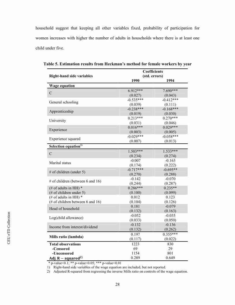
4.3 The Heckman Correction Method and the Extended Blinder-Oaxaca Decomposition

As the next step I use Heckman’s two-step sample correction method to correct for

potential sample selection bias that seems to be particularly important for women in the

present case. The results from Heckman’s procedure in Table 5 include estimates for the wage

equation and the participation equation for women. Results of the correction method obtained

for men are not reported in the thesis since – according to the t-test for selectivity bias on the

coefficients of the inverse Mills ratio – no evidence of selectivity bias can be found for men

during the examined period. The estimated coefficients on the inverse Mills ratio for men

were negative, but very close to zero. On the other hand, the estimated coefficients of the

inverse Mills ratio are positive (and strongly significant in 1994) for women, suggesting the

presence of sample selection. The found positive selectivity bias for women indicates that

women selected into employment earn more on average than non-working women would if

they would decide to participate in the labor force.

It is important to note that in the participation equation, along the exclusion restrictions

earlier mentioned, the right-hand side variables of the wage equation (schooling dummies and

experience) are also included. The coefficient estimates on these variables correspond to what

one would expect – education has strong positive effect on participation, while experience has

parabolic effects – but they are not reported in the thesis.

Concerning the exclusion restrictions, results in Table 5 show that while some of the

variables chosen as instruments are highly significant and have a strong effect on participation

in the labor market (namely the number of children in the household under five and their

interaction with number of adults in the household), most of them are either insignificant or

the magnitude of their coefficients is very small. According to the results, the higher the

number of children in the household under five, the lower the probability of participation will

be, while the estimated coefficients on their interaction with number of adults in the

CE

UeT

DC

olle

ctio

n

28

household suggest that keeping all other variables fixed, probability of participation for

women increases with higher the number of adults in households where there is at least one

child under five.

Table 5. Estimation results from Heckman’s method for female workers by year

Right-hand side variables Coefficients (std. errors)

1990 1994 Wage equation

C 6.912*** (0.027)

7.690*** (0.043)

General schooling -0.535***

(0.039) -0.412***

(0.111)

Apprenticeship -0.238***

(0.019) -0.168***

(0.030)

University 0.213*** (0.031)

0.270*** (0.046)

Experience 0.016*** (0.003)

0.029*** (0.005)

Experience squared -0.029***

(0.007) -0.058***

(0.013) Selection equation1)

C 1.503*** (0.234)

1.533*** (0.274)

Marital status -0.007 (0.174)

-0.163 (0.222)

# of children (under 5) -0.717***

(0.270) -0.695** (0.288)

# of children (between 6 and 16) -0.142 (0.244)

-0.070 (0.287)

(# of adults in HH) * (# of children under 5)

0.286*** (0.100)

0.235** (0.099)

(# of adults in HH) * (# of children between 6 and 16)

0.012 (0.104)

0.123 (0.126)

Head of household 0.181

(0.132) -0.079 (0.163)

Log(child allowance) -0.052 (0.033)

-0.035 (0.050)

Income from interest/dividend -0.132 (0.132)

-0.136 (0.262)

Mills ratio (lambda) 0.197

(0.117) 0.355*** (0.022)

Total observations -Censored -Uncensored z{|. } − ~�����{�)

1223 69

1154 0.289

830 29

801 0.649

* p-value<0.1; ** p-value<0.05; *** p-value<0.01 1) Right-hand side variables of the wage equation are included, but not reported. 2) Adjusted R-squared from regressing the inverse Mills ratio on controls of the wage equation.

CE

UeT

DC

olle

ctio

n

29

Concerning the problem of collinearity, the adjusted R-squared from regressing the

inverse Mills ratio on the control variables of the wage equation shows that in year 1990

multicollinearity most probably does not arise as a problem since the R-squared is very low.

In contrast, the adjusted R-squared for year 1994 is much higher, indicating that collinearity

might be a problem. It is worth mentioning that the number of censored observations are very

small as a result of a series of restrictions imposed on the sample (for example only

individuals between 18 and 60 are considered), thus the grounds for considering selection in

the sample are questionable.

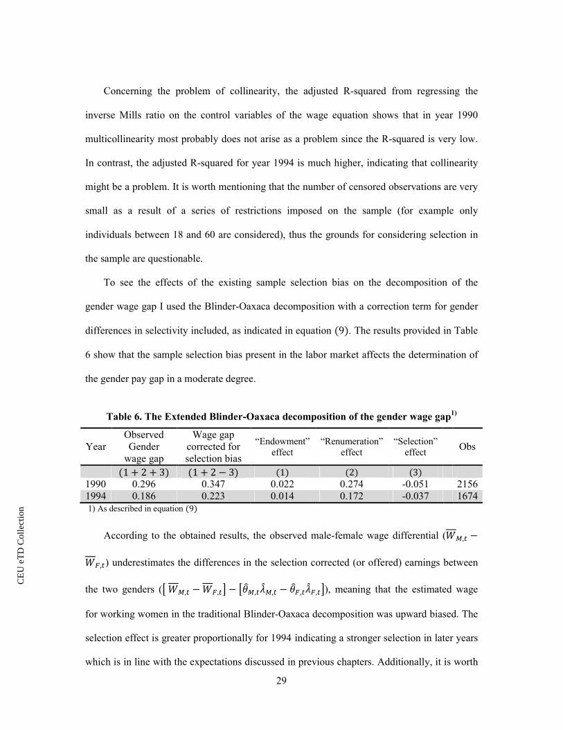
To see the effects of the existing sample selection bias on the decomposition of the

gender wage gap I used the Blinder-Oaxaca decomposition with a correction term for gender

differences in selectivity included, as indicated in equation (9). The results provided in Table

6 show that the sample selection bias present in the labor market affects the determination of

the gender pay gap in a moderate degree.

Table 6. The Extended Blinder-Oaxaca decomposition of the gender wage gap1)

Year Observed Gender

wage gap

Wage gap corrected for selection bias

“Endowment” effect

“Renumeration” effect

“Selection” effect Obs

(1 + 2 + 3) (1 + 2 − 3) (1) (2) (3) 1990 0.296 0.347 0.022 0.274 -0.051 2156 1994 0.186 0.223 0.014 0.172 -0.037 1674 1) As described in equation (9)

According to the obtained results, the observed male-female wage differential (� ,� −�",�) underestimates the differences in the selection corrected (or offered) earnings between

the two genders (q� ,� −�",�r − q[\ ,�N@ ,� − [\",�N@",�r), meaning that the estimated wage

for working women in the traditional Blinder-Oaxaca decomposition was upward biased. The

selection effect is greater proportionally for 1994 indicating a stronger selection in later years

which is in line with the expectations discussed in previous chapters. Additionally, it is worth

CE

UeT

DC

olle

ctio

n

30

noting that correcting for selectivity bias does not have any effect on the estimates of

“Renumeration” effect. Comparing these results with the findings of Hunt (2002), I arrive to a

different conclusion regarding the role of sample selection in the change of the gender gap

during transition. While I found evidence on strong positive selection effect in the sample of

working women, I did not find evidence supporting Hunt’s statement that almost half of the

closing of the gap between 1990 and 1994 is a result of the disproportionate exits of low-

skilled and low-paid women from the labor force. According to the results presented in Table

6, the male-female wage gap corrected for selection bias decreased by 12 log points during

the transition from socialism to market economy.

4.4 The DiNardo-Fortin-Lemieux (1996) Reweighting Method

Since the traditional Blinder-Oaxaca decomposition technique cannot be extended to the

case of other general distributional statistics besides the mean and it imposes the restrictive

assumption of linear functional form, I continue the analysis with the reweighting

decomposition method introduced in the work of DiNardo, Fortin and Lemieux (1996) which

solves both of the above mentioned limitations. The fact that the reweighting method allows

for going beyond summary statistics like the mean or the variance is a very important

advantage since decompositions at mean provide very little information concerning the

sources of the gender gap at other points of the wage distribution which could be very

important e.g. “glass ceiling” effect. Similarly for the relaxation of the linearity assumption it

can be said that since the outcome variable (log wage) can be related non-linearly to

covariates, for example one can think of the “sheepskin effect”, the usage of the reweighting

method is highly advantageous. Additionally, this method does not require the zero

conditional mean assumption to hold in contrast with the Blinder-Oaxaca method.

Figure 2 shows the (Epanechnikov) kernel density estimates of log monthly wages by

gender in 1990 and 1994 and the constructed counterfactual density function of female wages.

CE

UeT

DC

olle

ctio

n

31

Figure 2. Kernel Density Estimates in East Germany (1990-1994)

a) 1990

b) 1994

0.5

11.5

Estim

ate

d W

age D

ensity

5 6 7 8 9Log(Wage)

Men 1990 Women 1990

Counterfactual - Reweighted Women 1990

0.5

11.5

Estim

ate

d W

age D

ensity

6 7 8 9Log(Wage)

Men 1994 Women 1994

Counterfactual - Reweighted Women 1994

CE

UeT

DC

olle

ctio

n

32

From the constructed counterfactual wage density function which is the density function

of wages that would have prevailed for female workers if they were paid like their male

counterparts, it can be seen that the “Endowment” effect (in line with all previously obtained

results in the thesis) was very small at all quantiles, playing close to zero role in the

determining of the male-female pay gap and suggesting that differences between female and

male workers’ measured labor market skills were really small. From Figure 2a) it can be

inferred that there was a considerable unadjusted gender gap at all quantiles of the wage

distribution in 1990 and that the wage differential was substantially larger for the lower

quantiles than the upper ones. Figure 2b) shows that the gender wage gap decreased greatly at

each point of the wage distribution from 1990 to 1994. In addition, it can be stated that

similarly to 1990, the contribution of “Renumeration” effect determined mainly the gender

gap, although its magnitude decreased significantly during the transition.

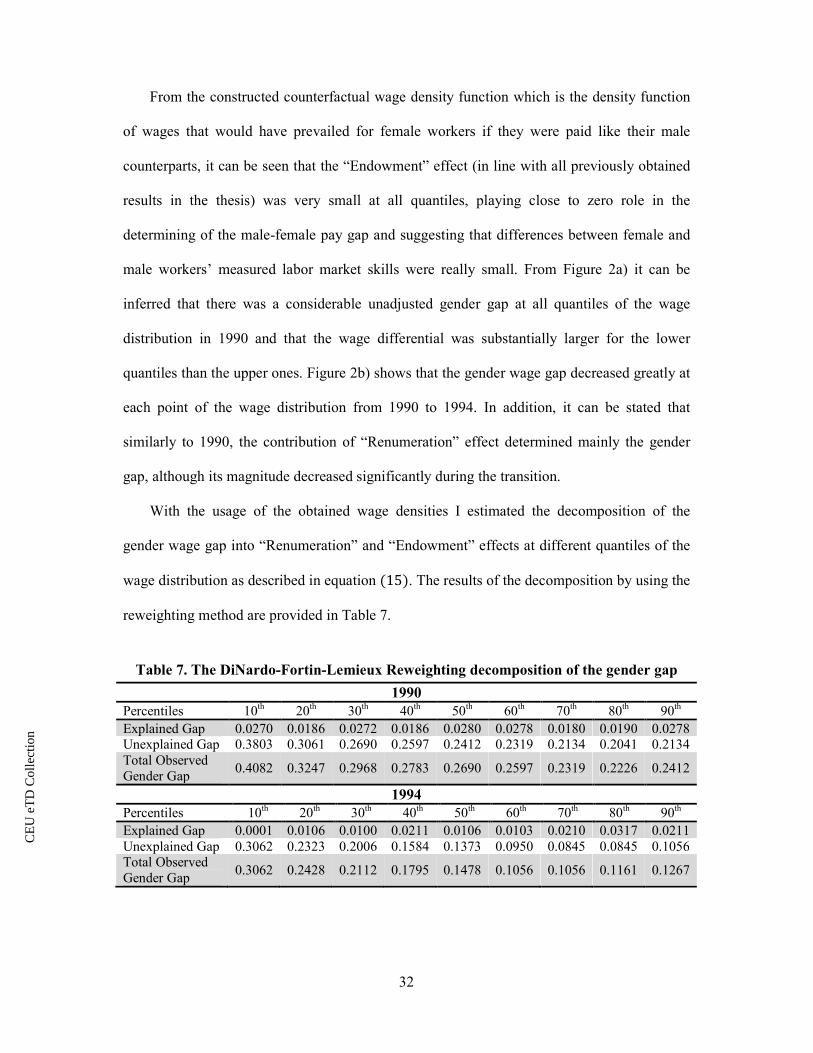
With the usage of the obtained wage densities I estimated the decomposition of the

gender wage gap into “Renumeration” and “Endowment” effects at different quantiles of the

wage distribution as described in equation (15). The results of the decomposition by using the

reweighting method are provided in Table 7.

Table 7. The DiNardo-Fortin-Lemieux Reweighting decomposition of the gender gap

1990 Percentiles 10th 20th 30th 40th 50th 60th 70th 80th 90th Explained Gap 0.0270 0.0186 0.0272 0.0186 0.0280 0.0278 0.0180 0.0190 0.0278 Unexplained Gap 0.3803 0.3061 0.2690 0.2597 0.2412 0.2319 0.2134 0.2041 0.2134 Total Observed Gender Gap

0.4082 0.3247 0.2968 0.2783 0.2690 0.2597 0.2319 0.2226 0.2412

1994 Percentiles 10th 20th 30th 40th 50th 60th 70th 80th 90th Explained Gap 0.0001 0.0106 0.0100 0.0211 0.0106 0.0103 0.0210 0.0317 0.0211 Unexplained Gap 0.3062 0.2323 0.2006 0.1584 0.1373 0.0950 0.0845 0.0845 0.1056 Total Observed Gender Gap

0.3062 0.2428 0.2112 0.1795 0.1478 0.1056 0.1056 0.1161 0.1267

CE

UeT

DC

olle

ctio

n

33

Naturally, the estimation results presented in Table 7 are in support of the earlier

examination of Figure 2, but they provide some additional important details. The gender gap

declined at all quantiles with approximately 10 log points, meaning that female workers’

wages relative to male workers’ wages improved much more proportionally at the higher

quantiles of the wage distribution than at the lower quantiles. Furthermore, it can be observed

that the explained part of the gender gap was relatively uniform across the wage distribution

in both years. Finally, the “Endowment” effect declined in all, but one decile (the 8th decile)

where it even increased from 1990 to 1994.

4.5 Ñopo’s Matching-based Nonparametric Decomposition Method

Finally, as the last step in the thesis I implemented the decomposition of the male-female

wage differentials based on Ñopo’s proposed nonparametric technique. The advantages of this

method over the traditional Blinder-Oaxaca decomposition are similar to the previously

applied DiNardo-Fortin-Lemieux reweighting method. Namely, Ñopo’s method also can be

extended to general distributional statistics other than the mean, it does not impose the

assumption of linear functional form of conditional wage expectations and it does not require

the unobservables’ (mean) independency of covariates X. However, Ñopo’s technique has an

additional advantage over the other two methods, that is, it accounts for the so-called

“support” problem. Moreover, it allows direct comparison with the Blinder-Oaxaca

decomposition when estimated at the means. The disadvantage of Ñopo’s method is that it

might face the problem of high dimensionality, a problem reduced in the previously applied

reweighting technique. Table 8 presents the estimated results of Ñopo’s decomposition

method where the matching was based on educational dummies and experience.9

9 Experience and experience squared were replaced by a set of five dummies: under ten; between ten and twenty; between twenty and thirty; between thirty and forty; and between forty and fifty years. No individual in the sample had more than fifty years of experience.

CE

UeT

DC

olle

ctio

n

34

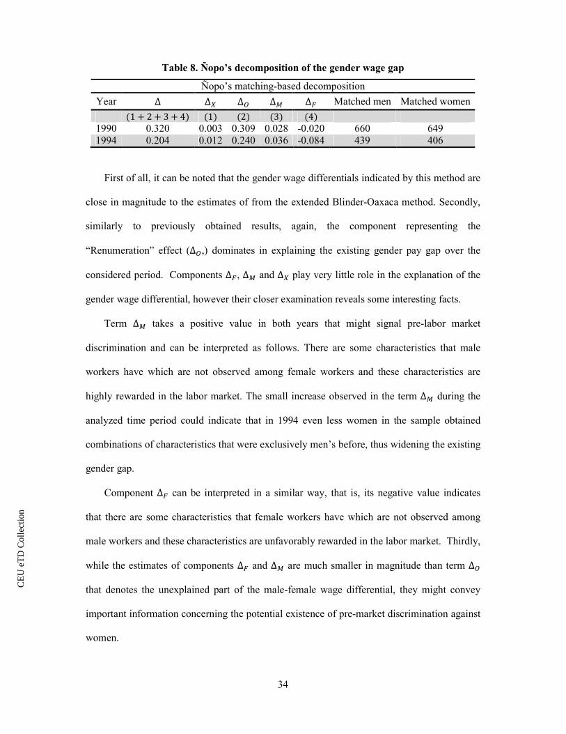
Table 8. Ñopo’s decomposition of the gender wage gap

Ñopo’s matching-based decomposition

Year ∆ ∆P ∆y ∆ ∆" Matched men Matched women

(1 + 2 + 3 + 4) (1) (2) (3) (4) 1990 0.320 0.003 0.309 0.028 -0.020 660 649 1994 0.204 0.012 0.240 0.036 -0.084 439 406

First of all, it can be noted that the gender wage differentials indicated by this method are

close in magnitude to the estimates of from the extended Blinder-Oaxaca method. Secondly,

similarly to previously obtained results, again, the component representing the

“Renumeration” effect (∆y,) dominates in explaining the existing gender pay gap over the

considered period. Components ∆", ∆ and ∆P play very little role in the explanation of the

gender wage differential, however their closer examination reveals some interesting facts.

Term ∆ takes a positive value in both years that might signal pre-labor market

discrimination and can be interpreted as follows. There are some characteristics that male

workers have which are not observed among female workers and these characteristics are

highly rewarded in the labor market. The small increase observed in the term ∆ during the

analyzed time period could indicate that in 1994 even less women in the sample obtained

combinations of characteristics that were exclusively men’s before, thus widening the existing

gender gap.

Component ∆" can be interpreted in a similar way, that is, its negative value indicates

that there are some characteristics that female workers have which are not observed among

male workers and these characteristics are unfavorably rewarded in the labor market. Thirdly,

while the estimates of components ∆" and ∆ are much smaller in magnitude than term ∆y

that denotes the unexplained part of the male-female wage differential, they might convey

important information concerning the potential existence of pre-market discrimination against

women.

CE

UeT

DC

olle

ctio

n

35

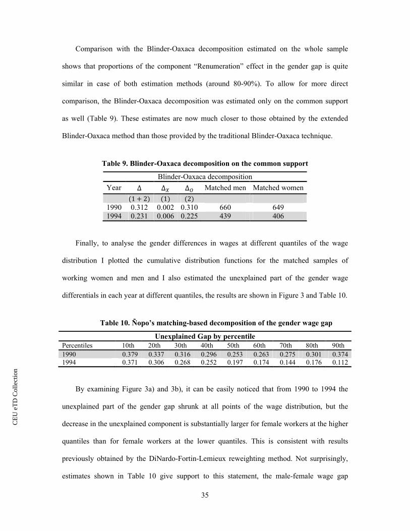
Comparison with the Blinder-Oaxaca decomposition estimated on the whole sample

shows that proportions of the component “Renumeration” effect in the gender gap is quite

similar in case of both estimation methods (around 80-90%). To allow for more direct

comparison, the Blinder-Oaxaca decomposition was estimated only on the common support

as well (Table 9). These estimates are now much closer to those obtained by the extended

Blinder-Oaxaca method than those provided by the traditional Blinder-Oaxaca technique.

Table 9. Blinder-Oaxaca decomposition on the common support

Blinder-Oaxaca decomposition

Year ∆ ∆P ∆y Matched men Matched women

(1 + 2) (1) (2) 1990 0.312 0.002 0.310 660 649 1994 0.231 0.006 0.225 439 406

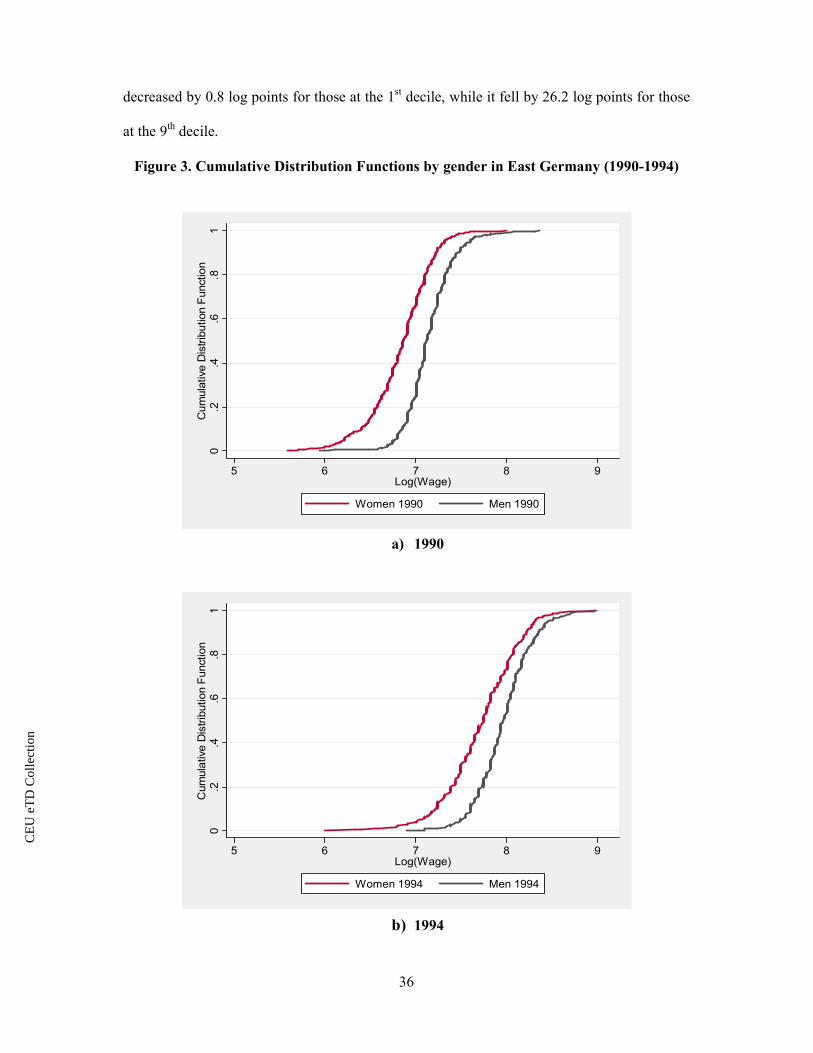
Finally, to analyse the gender differences in wages at different quantiles of the wage

distribution I plotted the cumulative distribution functions for the matched samples of

working women and men and I also estimated the unexplained part of the gender wage

differentials in each year at different quantiles, the results are shown in Figure 3 and Table 10.

Table 10. Ñopo’s matching-based decomposition of the gender wage gap

Unexplained Gap by percentile Percentiles 10th 20th 30th 40th 50th 60th 70th 80th 90th 1990 0.379 0.337 0.316 0.296 0.253 0.263 0.275 0.301 0.374 1994 0.371 0.306 0.268 0.252 0.197 0.174 0.144 0.176 0.112

By examining Figure 3a) and 3b), it can be easily noticed that from 1990 to 1994 the

unexplained part of the gender gap shrunk at all points of the wage distribution, but the

decrease in the unexplained component is substantially larger for female workers at the higher

quantiles than for female workers at the lower quantiles. This is consistent with results

previously obtained by the DiNardo-Fortin-Lemieux reweighting method. Not surprisingly,

estimates shown in Table 10 give support to this statement, the male-female wage gap

CE

UeT

DC

olle

ctio

n

36

decreased by 0.8 log points for those at the 1st decile, while it fell by 26.2 log points for those

at the 9th decile.

Figure 3. Cumulative Distribution Functions by gender in East Germany (1990-1994)

a) 1990

b) 1994

0.2

.4.6

.81

Cum

ula

tive D

istrib

ution F

unction

5 6 7 8 9Log(Wage)

Women 1990 Men 1990

0.2

.4.6

.81

Cum

ula

tive D

istrib

ution F

unction

5 6 7 8 9Log(Wage)

Women 1994 Men 1994

CE

UeT

DC

olle

ctio

n

37

5. CONCLUSION

In this thesis I showed that the relative position of women improved during the economic

transition from socialism to market economy in East Germany between 1990 and 1994,

meaning that the observed gender wage differential substantially decreased over the

considered period. I examined the underlying reasons behind the gender gap and its change in

order to see whether there was a true decline in the male-female wage differential, meaning

either an improvement in women’s relative level of measured and unmeasured labor market

characteristics or a potential decrease in discrimination against female workers, or the

narrowing of the gender gap is simply a result of disproportionate quits of low-skilled and

low-earner women from employment.

For this purpose, after briefly exploring the existing gender gap and its constituting

components, I first implemented Heckman’s two-step correction method to adjust for

potential selection bias. While I found no evidence for selectivity bias for men, I found

positive selection for women into employment during the observed period in line with

findings of Hunt (2002). This result could suggest that the transition to market economy

influenced low-skilled and low-earner female workers unfavorably, if it does not reflect

voluntary withdrawal from participating in the labor force, for instance if it is due to

discriminatory actions of employers against women or it is a consequence of reduction in

maternity leave, child care and other social entitlements. From the extended Blinder-Oaxaca

decomposition adjusted for sample selection one can see that the observed wage gap

underestimates the offered wage gap in each year. However, after correcting for the found

sample selection bias in the estimation of the change in the offered wage gaps from 1990 to

1994, I still found a decline in the male-female wage differential that is of the same magnitude

as previously. This indicates that the substantial fall observed in the gender gap cannot be

CE

UeT

DC

olle

ctio

n

38

accounted for solely (or in a large part) by the exits of low-skilled workers from labor force

participation who were disproportionately women.

Next, I continued with decomposition methods escaping the limitations involved with the

restrictive assumptions of the traditional Blinder-Oaxaca procedure. First, I implemented a

reweighting method suggested by DiNardo, Fortin and Lemieux (1996). This technique

allows for the decomposition of the gender gap at different quantiles of the wage distribution

while relying on weaker assumptions than the Blinder-Oaxaca decomposition. Using the

reweighting procedure, I found that the existing wage gap is significantly larger for female

workers at the lower quantiles of the wage distribution than for female workers at the higher

quantiles in both years. Furthermore, the obtained results also showed that while the male-

female pay gap decreased at each quantile of the distribution over the period, the estimated

fall was larger in relative terms for working women at higher points of the distribution than at

lower points. These results indicate that while working women all enjoyed a relative wage

growth during the transition, low-skilled and low-earner female workers experienced these

favorable changes only at a much smaller degree. Moreover, the decomposition of the total

gender gap into unexplained and explained components (“Renumeration” and “Endowment”

effects) revealed that only a very small fraction of the male-female wage differential can be

accounted for by differences in the human capital measures (educational attainment and labor

market experience) included in the analysis. This is important also from a policy point of

view, since present analysis suggests that to achieve substantial improvement in female

workers’ relative situation, more research needs to be done concerning the possible sources of

the dominating unexplained part of the gender wage gap.

Then, I applied an exact matching-based decomposition technique introduced by Ñopo

(2004) that not only incorporates all the advantages of the previously described reweighting

method, but also accounts for the “support” problem in the distribution of human capital

CE

UeT

DC

olle

ctio

n

39

characteristics included in the analysis as opposed to the Blinder-Oaxaca and the DiNardo-

Fortin-Lemieux methods that both perform poorly in case of lack common support. The

obtained results are consistent with the findings of the reweighting method. The estimates

indicate that the unexplained part of the male-female wage gap fell at all points of the wage

distribution during the transition and that this decrease was substantially larger for female

workers at the higher quantiles than for female workers at the lower quantiles. Furthermore, I

found evidence that there are such highly rewarded individual characteristics on the labor

market that are attained exclusively by male workers. It is important to note that this method

is also subject to some limitations, since it is based on exact matching it might suffer from the

problem of high dimensionality.

Finally, there are a couple of possible extensions to the study done so far that could be

conducted in future research. Firstly, since Heckman’s two-step sample selection correction

method is highly sensitive to the distributional assumptions placed on the error terms and the

specification of both the wage and the participation models (see Puhani, 2000), I would

suggest to depart from this method and use available semi-parametric or nonparametric

methods that relax the restrictive assumptions imposed by Heckman’s method (see Vella,

1998). Additionally, a natural extension would be to use propensity score matching instead of

exact matching in the case of Ñopo’s decomposition technique so as to avoid the problem of

high dimensionality.

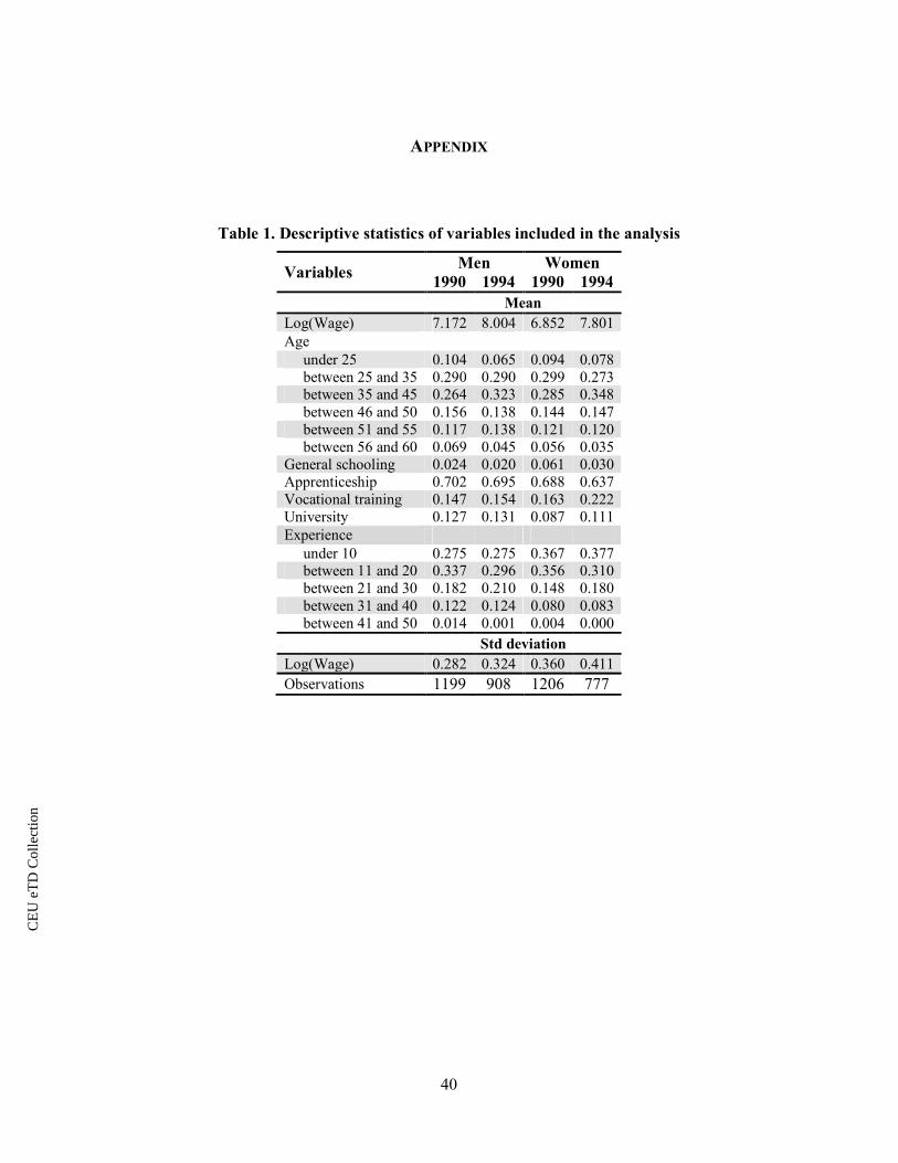
CE

UeT

DC

olle

ctio

n

40

APPENDIX

Table 1. Descriptive statistics of variables included in the analysis

Variables Men Women

1990 1994 1990 1994 Mean Log(Wage) 7.172 8.004 6.852 7.801 Age under 25 0.104 0.065 0.094 0.078 between 25 and 35 0.290 0.290 0.299 0.273 between 35 and 45 0.264 0.323 0.285 0.348 between 46 and 50 0.156 0.138 0.144 0.147 between 51 and 55 0.117 0.138 0.121 0.120 between 56 and 60 0.069 0.045 0.056 0.035 General schooling 0.024 0.020 0.061 0.030 Apprenticeship 0.702 0.695 0.688 0.637 Vocational training 0.147 0.154 0.163 0.222 University 0.127 0.131 0.087 0.111 Experience under 10 0.275 0.275 0.367 0.377 between 11 and 20 0.337 0.296 0.356 0.310 between 21 and 30 0.182 0.210 0.148 0.180 between 31 and 40 0.122 0.124 0.080 0.083 between 41 and 50 0.014 0.001 0.004 0.000 Std deviation Log(Wage) 0.282 0.324 0.360 0.411 Observations 1199 908 1206 777

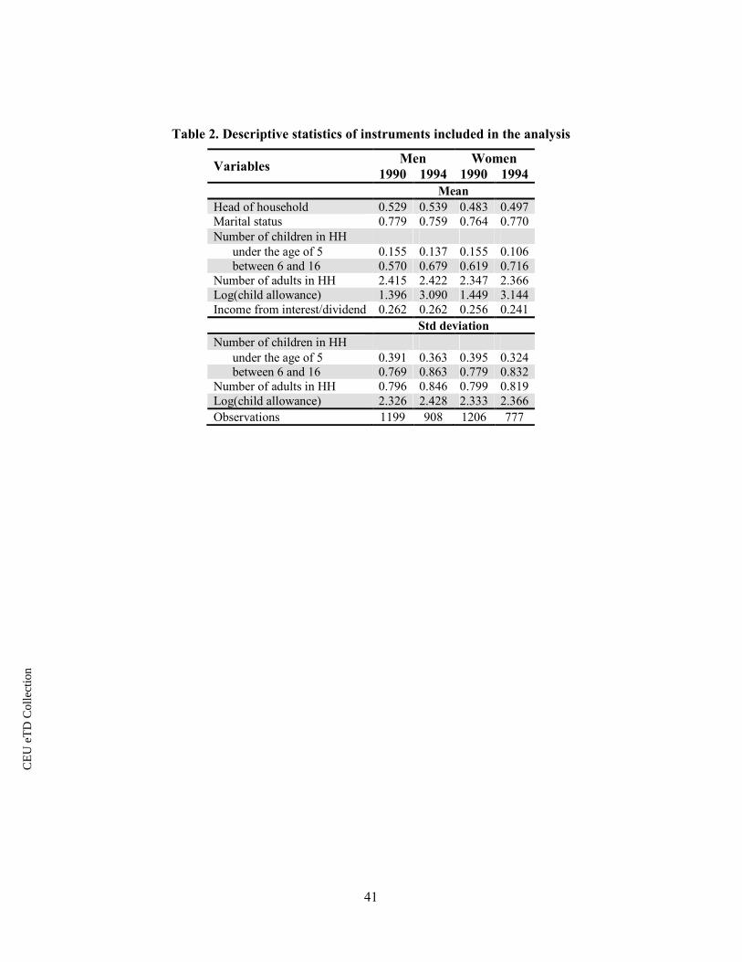
CE

UeT

DC

olle

ctio

n

41

Table 2. Descriptive statistics of instruments included in the analysis

Variables Men Women

1990 1994 1990 1994 Mean Head of household 0.529 0.539 0.483 0.497 Marital status 0.779 0.759 0.764 0.770 Number of children in HH under the age of 5 0.155 0.137 0.155 0.106 between 6 and 16 0.570 0.679 0.619 0.716 Number of adults in HH 2.415 2.422 2.347 2.366 Log(child allowance) 1.396 3.090 1.449 3.144 Income from interest/dividend 0.262 0.262 0.256 0.241 Std deviation Number of children in HH under the age of 5 0.391 0.363 0.395 0.324 between 6 and 16 0.769 0.863 0.779 0.832 Number of adults in HH 0.796 0.846 0.799 0.819 Log(child allowance) 2.326 2.428 2.333 2.366 Observations 1199 908 1206 777

CE

UeT

DC

olle

ctio

n

42

REFERENCES

Adamchik, Vera A., and Arjun S. Bedi. 2001. “Persistence of the gender pay differential in

a transition economy.” No 349, ISS Working Papers - General Series, International Institute

of Social Studies of Erasmus University (ISS), The Hague.

Becker, Gary S.. 1957. The Economics of Discrimination. Chicago: University of Chicago

Press.

Blau, Francine D., and Lawrence M. Kahn. 1997. “Swimming Upstream: Trends in the

Gender Wage Differential in the 1980s.” Journal of Labor Economics, 15: 1-42.

Blau, Francine D., and Lawrence M. Kahn. 2000. “Gender Differences in Pay.” The

Journal of Economic Perspectives, 14: 75-99.

Blinder, Alan S.. 1973. “Wage Discrimination: Reduced Form and Structural Estimates.” The

Journal of Human Resources, 8(4): 436-455.

Bonin, Holger and Rob Euwals. 2001. “ “Labor Supply Preferences of East German Women

after German Unification.” WDI Working Paper.

Bosworth, Derek, Peter Dawkins and Thorsten Stromback. 1996. The Economics of the

Labor Market. Addison Wesley Longman, 1996

Brainerd, Elizabeth. 2000. “Women in Transition: Changes in Gender Wage Differentials in

Eastern Europe and the Former Soviet Union”. Industrial and Labor Relations Review,

54(1):138-162.

DiNardo, John E., Nicole M. Fortin and Thomas Lemieux. 1996. “Labor Market

Institutions and the Distribution of Wages, 1973-1992: A Semiparametric Approach.”

Econometrica, 64(5): 1001-1044.

CE

UeT

DC

olle

ctio

n

43

Dolton, Peter J., and Gerald H. Makepeace. 1986. “Sample Selection and Male-Female

Earnings Differentials in the Graduate Labour Market.” Oxford Economic Papers, 38: 317-

341.

Federal Statistical Office. 2011. Consumer Prices.

http://www.destatis.de/jetspeed/portal/cms/Sites/destatis/Internet/EN/Content/Statistics/Time

Series/EconomicIndicators/BasicData/Content100/vpi101a.psml (accessed May 1, 2011)

Fortin, Nicole M., Thomas Lemieux and Sergio Firpo. 2010. “Decomposition Methods in

Economics.” NBER Working Papers 16045.

Frölich, Marcus. 2004. “Finite-Sample Properties of Propensity-Score Matching and

Weighting Estimators.” Review of Economics and Statistics, 86: 77-90.

Heckman, James J.. 1979. “Sample Selection Bias as a Specification Error.” Econometrica,

47(1): 153-61.

Heckman, James J., Lance J. Lochner and Petra E. Todd. 2003. “Fifty years of Mincer

earnings regressions.” NBER Working Papers 9732.

Hunt, Jennifer. 2002. “The Transition in East Germany: When Is a Ten-Point Fall in the

Gender Wage Gap Bad News?” Journal of Labor Economics, 20(1): 148-169

Kunze, Astrid. 2000. “The Determination of Wages and the Gender Wage Gap: A Survey.”

IZA Working Paper, Discussion Paper No.193. University College London.

Lemieux, Thomas. 2006. “The “Mincer Equation” Thirty Years after Schooling, Experience,

and Earnings.” In Jacob Mincer: A Pioneer of Modern Labor Economics, ed. S. Grossbard-

Shechtman, 127-145. Springer Verlag.

Little, Roderick J. A. and Donald B. Rubin. 1987. Statistical analysis with missing data.

New York: John Wiley & Sons.

CE

UeT

DC

olle

ctio

n

44

Neuman, Shoshana, and Ronald L. Oaxaca. 2004. “Wage Decompositions with Selectivity-

Corrected Wage Equations: A Methodological Note.” Journal of Economic Inequality, 2(1):

3-10.

Ñopo, Hugo. 2008. “Matching as a Tool to Decompose Wage Gaps.” The Review for

Economics and Statistics, 90(2): 290-299.

Oaxaca, Ronald. 1973. “Male-Female Wage Differentials in Urban Labor Markets.”

International Economic Review, 14(3): 693-709.

Ogloblin, Constantin. 1999. “The Gender Earnings Differential in the Russian Transition

Economy.” Industrial and Labor Relations Review, 52(4):602-27.

Orlowski, Robert and Regina T. Riphahn. 2009. “The East German wage structure after

transition.” Economics of Transition, 17(4): 629-659.

Puhani, Patrik A. 2000. “The Heckman Correction for Sample Selection and its Critique.”

Journal of Economic Surveys, 14(1).

Silverman, Bernard W.. 1986. Density Estimation for Statistics and Data Analysis. London:

Chapman and Hall.

Socio-Economic Panel (SOEP). Data for years 1984-2009, version 26, SOEP, 2010.

Vella, Francis. 1998. “Estimating Models with Sample Selection Bias: A Survey.” Journal of

Human Resources, University of Wisconsin Press, 33(1):127-169.