Empirical Bayes Estimates of Parameters from the Logistic

A C T Research Report Series 9 7 -6

Empirical Bayes Estimates of Parameters from the Logistic Regression Model

Walter M. Houston

David J. Woodruff

August 1997

For additional copies write:ACT Research Report Series POBox 168Iowa City, Iowa 52243-0168

© 1997 by ACT, Inc, All rights reserved.

EMPIRICAL BAYES ESTIMATES OF PARAMETERS FROM THE LOGISTIC REGRESSION MODEL

Walter M. Houston David J. Woodruff

ABSTRACT

Maximum likelihood and least-squares estimates of parameters from the logistic regression

model are derived from an iteratively reweighted linear regression algorithm. Empirical Bayes

estimates are derived using an m-group regression model to regress the within-group estimates

toward common values. The m-group regression model assumes that the parameter vectors from

m groups are independent, and identically distributed, observations from a multivariate normal

"prior" distribution. Based on asymptotic normality of maximum likelihood estimates, the

posterior distributions are multivariate normal. Under the assumption that the parameter vectors

from the m groups are exchangeable, the hyperparameters of the common prior distribution are

estimated using the EM algorithm. Results from an empirical study of the relative stability of

the empirical Bayes and maximum likelihood estimates are consistent with those reported

previously for the m-group regression model. Estimators that use collateral information from

exchangeable groups to regress within-group parameter estimates toward a common value are

more stable than estimators calculated exclusively from within-group data.

EMPIRICAL BAYES ESTIMATES OF PARAMETERS FROM THE LOGISTIC REGRESSION MODEL

Logistic regression is used in many areas of substantive interest in the social and

biological sciences to model the conditional expectation (probability) of a binary dependent

variable as a function of an observed (or latent) vector of covariates. In some applications, the

parameters of the logistic regression function must be estimated from small samples, which can

result in parameter estimates with large sampling variability. For example, ACT uses logistic

regression to model the probability of success within specific college courses. Using current

estimation procedures, a minimum sample size of 45 within-course observations is required.

Further, because the estimation algorithm for the parameters of the logistic regression model is

iterative, parameter estimates based on small samples may fail to converge, or converge to local,

rather than global, stationary points.

One way to stabilize parameter estimates is to use collateral information from

"exchangeable" groups (Lindley, 1971) to refine the within-group estimates. Bayesian m-group

regression models have been shown to increase the prediction accuracy and stability of the

parameter estimates, relative to estimates that ignore collateral information.

In m-group regression models, the parameter vectors within each of m exchangeable

groups are assumed to be independent and identically distributed observations with a common

probability density function. When this common distribution is treated as a "prior" distribution,

posterior distributions and associated inferences follow from standard Bayesian theory (DeGroot,

1970). The effect of the prior distribution is to regress the within-group maximum likelihood

estimates toward common values. The extent of the regression effect is inversely related to the

precision of the within-group estimates; as the precision of the within-group estimate decreases,

the empirical Bayes estimate moves closer to the prior mean. As the precision increases, the

maximum likelihood and empirical Bayes estimates converge. Estimators that regress within-

group parameter estimates toward common values (often referred to as "regressed" or "shrinkage"

estimators) are also found in classical theory (James & Stein, 1961; Evans & Stark, 1996).

The parameters of the prior distribution are often referred to as "hyperparameters", to

distinguish them from the parameters of the logistic regression function. There are different

methods for estimating the hyperparameters. A fully Bayesian analysis requires a prior density

for the hyperparameters (Novick, Jackson, Thayer, and Cole, 1972). The posterior density of the

parameter vector is found by integrating the joint posterior density of the parameters and

hyperparameters with respect to the hyperparameters. Since these integrals are seldom

expressible in a closed form, numerical integration procedures are often required. Markov chain

sampling schemes, such as the Gibbs sampler (Tanner, 1993), are currently under investigation

as an alternative to the numerical methods used previously.

Empirical Bayesian approaches (Braun, Jones, Rubin, & Thayer, 1983; Houston &

Sawyer, 1988; Rubin, 1980), in contrast, derive maximum likelihood estimates of the

hyperparameters using the EM algorithm (Dempster, Laird, & Rubin; 1977). The estimated

hyperparameters are used in calculating the prior and posterior densities for the within-group

parameters.

The first section of the paper is concerned with parameter estimation and model fit for

the logistic regression model within a single group. An iteratively reweighted linear regression

algorithm is used to derive maximum likelihood and least-squares estimates of the parameter

vector of the logistic regression function. A chi-square test of the hypothesis of model fit is

derived, based on the mean squared error (MSE) from the weighted linear regression model used

2

in the estimation algorithm. The use of a linear regression algorithm makes many of the

diagnostic procedures developed for the linear model applicable, with a modification of MSE,

to the logistic model, as well.

In the next section, collateral information across m exchangeable groups is used to refine

the within-group maximum likelihood estimates. Empirical Bayes estimates are derived from a

Bayesian m-group regression model. In this model, the parameter vectors of the logistic

regression function are assumed to be independent and identically distributed observations from

a multivariate normal distribution.

In the final section of the paper, an application involving college course placement data

(grades in specific college courses and standardized achievement test scores) is presented. An

empirical study uses these data to compare the stability of the empirical Bayes and maximum

likelihood estimates.

Model Specification

Let Yj denote a binary random variable, and let Xj denote a (p x 1) vector of covariates,

for subject i (i = 1 to n). The logistic regression model may be expressed as

The logistic regression function, p ^S ^), has range 0 to 1, with the parameter vector 0 and

covariate vector as arguments. It is assumed that the (i = 1 to n) are stochastically

The Logistic Regression Model

Y i = P i(e ’x i) + £ i>(I)

+ (2)1 + exp iXj e

independent, with E(Ej) = 0. Conditional on Xj and 0, the Yj (i = 1 to n) are independent

Bernoulli random variables with mean pj = Pj(0,Xj) and variance = pj * (1 - pj).

Both maximum likelihood and least-squares estimates of the parameter vector 0 can be

derived using an iteratively reweighted linear regression algorithm.

Maximum Likelihood Estimation

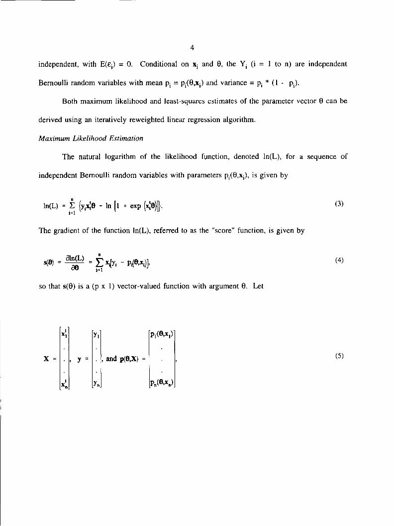
The natural logarithm of the likelihood function, denoted ln(L), for a sequence of

independent Bernoulli random variables with parameters pÔjXj), is given by

(3)

The gradient of the function ln(L), referred to as the "score” function, is given by

(4)

so that s(0) is a (p x 1) vector-valued function with argument 0. Let

where X is an (n x p) matrix with the ith row equal to x■*, y is an (n x 1) column vector with

the ith element equal to yv and p(0,X) is an (n x 1) column vector with the ith element equal

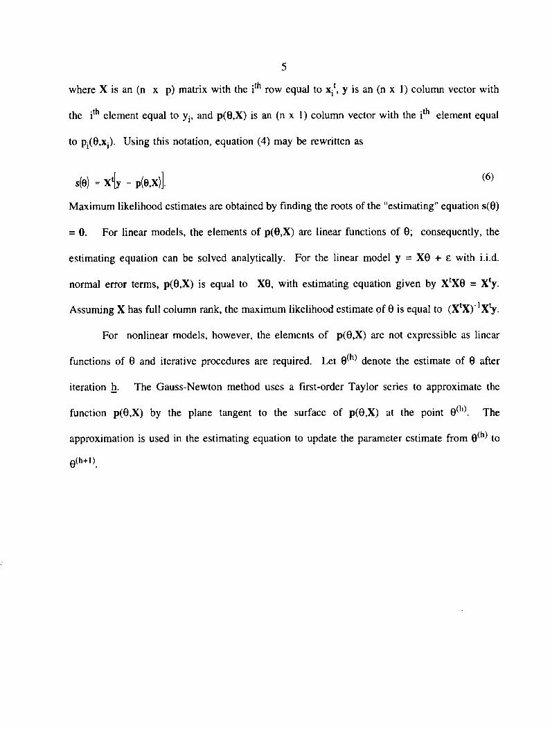
to pÔ.Xj). Using this notation, equation (4) may be rewritten as

s(e) = X*[y - p(e,x)]. (6)

Maximum likelihood estimates are obtained by finding the roots of the "estimating" equation s(0)

= 0. For linear models, the elements of p(0,X) are linear functions of 0; consequently, the

estimating equation can be solved analytically. For the linear model y = X0 + e with i.i.d.

normal error terms, p(0,X) is equal to X0, with estimating equation given by XlX0 = Xly-

Assuming X has full column rank, the maximum likelihood estimate of 0 is equal to (XtX)"1Xty-

For nonlinear models, however, the elements of p(0,X) are not expressible as linear

functions of 0 and iterative procedures are required. Let 0 ^ denote the estimate of 0 after

iteration h. The Gauss-Newton method uses a first-order Taylor series to approximate the

function p(0,X) by the plane tangent to the surface of p(0,X) at the point 0*h\ The

approximation is used in the estimating equation to update the parameter estimate from 0 ^ to

0(h+1).

5

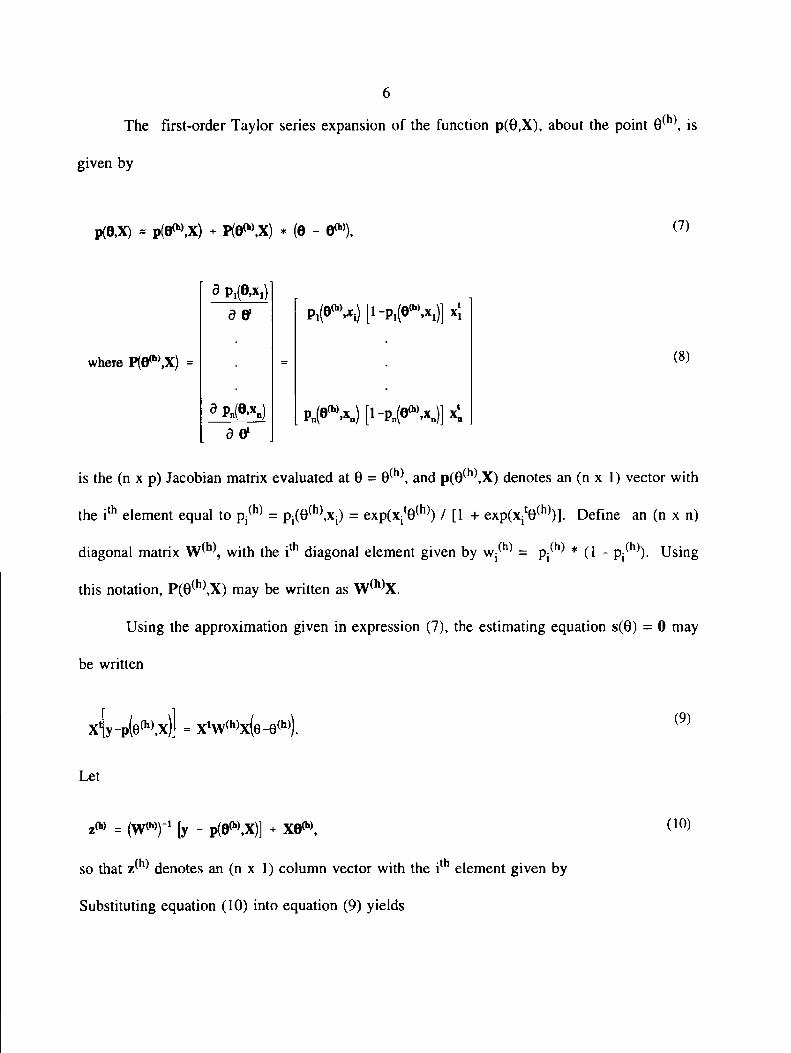
The first-order Taylor series expansion of the function p(0,X), about the point 0 h\ is

given by

6

p(0,X) * pfe^X) + P(0W,X) * (0 - 000), (7)

d &

where P(0(h),X) = (8)

d Pn(6>Xn) a o>

is the (n x p) Jacobian matrix evaluated at 0 = 0*h\ and p(0^h\X) denotes an (n x 1) vector with

the ilh element equal to p ^ = pÔ^Xj) = exp(xit0fh ) / [1 + exp(xit0(h )]. Define an (n x n)

diagonal matrix W ^ , with the ith diagonal element given by w -^ = p ^ * (1 - p / h ). Using

this notation, P(0*h\X) may be written as W ^X .

Using the approximation given in expression (7), the estimating equation s(0) = 0 may

be written

(9)

Let

z0» = (w(lV [y - p(0(h)>X)] + X0(h),

so that z(h) denotes an (n x 1) column vector with the i element given by

Substituting equation (10) into equation (9) yields

( 10)

xtw(h)z(h) = xtw(h)xe. (12

Equation (12) represents the estimating equation for the weighted linear regression of z ^ on xt,

with weight w^hl

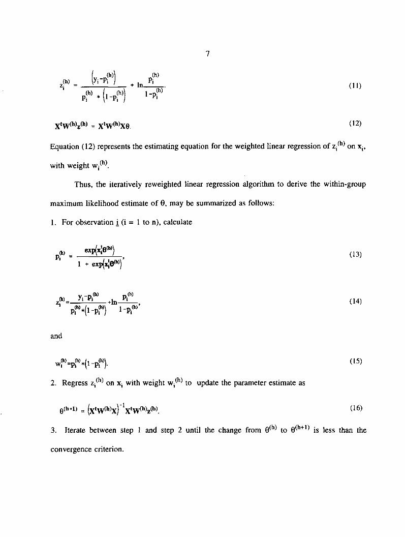
Thus, the iteratively reweighted linear regression algorithm to derive the within-group

maximum likelihood estimate of 0, may be summarized as follows:

1. For observation i (i = 1 to n), calculate

o.) . expfc1 ) (13)1 +

z ^ ^ L ^ m - g L L (14)p ^ i - p H ' I ?

and

w^ ^ ^ - pH- ° 5)

2. Regress on xi with weight w ^ to update the parameter estimate as

e(h+1) = (xtw(h)x) X ^ z^ . (16

3. Iterate between step 1 and step 2 until the change from 0*h to 0^h+1 is less than the

convergence criterion.

8

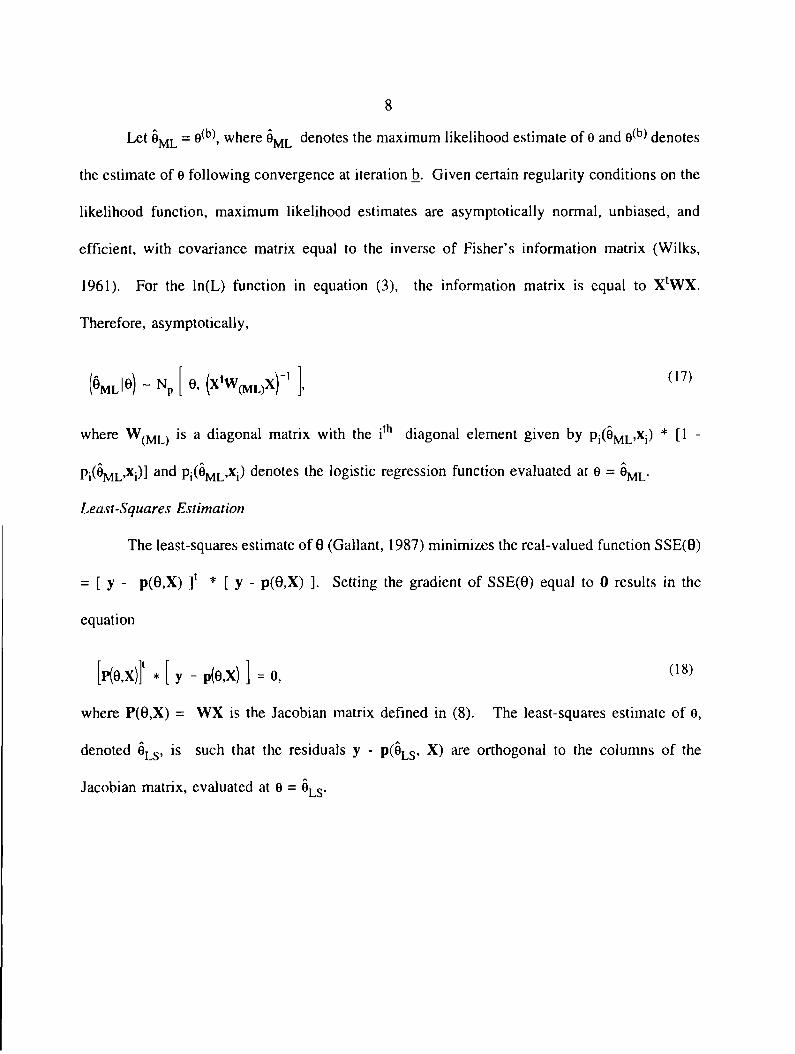
Let §ML = 0 ^ , where 0ML denotes the maximum likelihood estimate of 9 and 0 ^ denotes

the estimate of 6 following convergence at iteration b. Given certain regularity conditions on the

likelihood function, maximum likelihood estimates are asymptotically normal, unbiased, and

efficient, with covariance matrix equal to the inverse of Fisher’s information matrix (Wilks,

1961). For the ln(L) function in equation (3), the information matrix is equal to XlWX.

Therefore, asymptotically,

Pi(6ML>xi)] a°d Pj(^ML’xi) denotes the logistic regression function evaluated at e = 0ML.

Least-Squares Estimation

The Ieast-squares estimate of 0 (Gallant, 1987) minimizes the real-valued function SSE(0)

= [ y - P(0>X) ]l * [ y - p(0,X) ]. Setting the gradient of SSE(0) equal to 0 results in the

equation

where P(0,X) = WX is the Jacobian matrix defined in (8). The least-squares estimate of 0,

(17)

where W^ML is a diagonal matrix with the ith diagonal element given by Pj(0ML,xi) * [1 “

[p(e,x)]t * [ y - p(e,x) ] = 0, (18)

denoted 0LS, is such that the residuals y - p(0LS, X) are orthogonal to the columns of the

Jacobian matrix, evaluated at 0 = §LS.

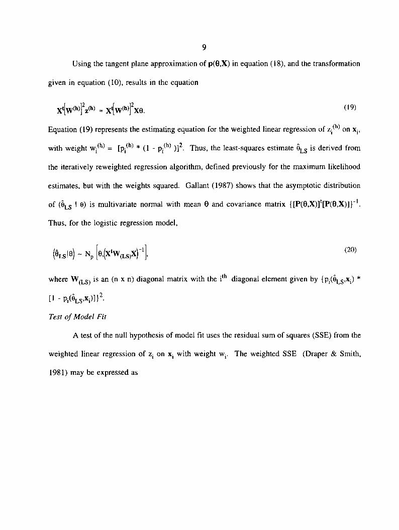
Using the tangent plane approximation of p(0,X) in equation (18), and the transformation

given in equation (10), results in the equation

x{wH2z(h) - x{w<h>pxe. (19)

Equation (19) represents the estimating equation for the weighted linear regression of on Xj,

with weight w ^ = [ p ^ * (1 - p^h* )]2. Thus, the least-squares estimate eLS is derived from

the iteratively reweighted regression algorithm, defined previously for the maximum likelihood

estimates, but with the weights squared. Gallant (1987) shows that the asymptotic distribution

of (eLS I e) is multivariate normal with mean 0 and covariance matrix {[P(0,X)]t[P(0,X)]}"1.

Thus, for the logistic regression model,

9

|U Awhere W^LS is an (n x n) diagonal matrix with the i diagonal element given by {Pi(eLs,xi *

[1 - pi(eLS,xi)])2.

Test of Model Fit

A test of the null hypothesis of model fit uses the residual sum of squares (SSE) from the

weighted linear regression of Zj on Xj with weight w4. The weighted SSE (Draper & Smith,

1981) may be expressed as

10

(21)

where

ft = r ( V ’4 (22)

and Wj and Zj are evaluated at e = eML. An equivalent expression for the weighted SSE is given

A = W -W XfXtW X^X'W (24)

is an (n x n) projection matrix, with rank(A) = n - and the elements of z and W are evaluated

at 9 = 0ML. Because the yx (i = 1 to n) in equation (20) are independent random variables with

mean = Pj(0ML»xi) anc* vafiance * 0 - fyX the (asymptotic) distribution of SSE is chi-square

with n - ^ degrees of freedom.

Let MSE = SSE / (n - p). The null hypothesis of model fit is rejected (at level a) if

where / 2(n - p; a/2) and %2(n - p; l-a/2) denote the 100*a/2 percentile and 100*(l-a/2)

percentile, respectively, of the chi-square distribution with n - £ degrees of freedom. Under the

hypothesis of model fit, the expected value of MSE is equal to 1.

Because parameter estimates are derived from a weighted linear regression algorithm,

many of the inferential and diagnostic procedures developed for linear regression models are

by

SSE = (z-z)tW(z-z) = ztAz, (23)

where

(n-p)*MSE < X(„-b«/2) or (n-p)*MSE > X(„-P;i-«w (25)

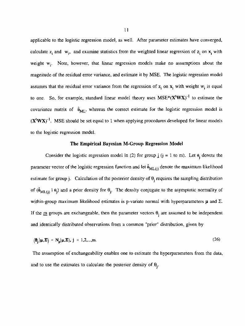
applicable to the logistic regression model, as well. After parameter estimates have converged,

calculate and wi5 and examine statistics from the weighted linear regression of zx on Xj with

weight Wj. Note, however, that linear regression models make no assumptions about the

magnitude of the residual error variance, and estimate it by MSE. The logistic regression model

assumes that the residual error variance from the regression of zi on x■ with weight Wj is equal

to one. So, for example, standard linear model theory uses MSE*(XtW X)'1 to estimate the

covariance matrix of 0ML, whereas the correct estimate for the logistic regression model is

(XtW X)'1. MSE should be set equal to 1 when applying procedures developed for linear models

to the logistic regression model.

The Empirical Bayesian M-Group Regression Model

Consider the logistic regression model in (2) for group j (j = 1 to m). Let 0j denote the

parameter vector of the logistic regression function and let 9ml(j) denote the maximum likelihood

estimate for group j. Calculation of the posterior density of 0j requires the sampling distribution

of (0ML(j) I ej) anc* a Prior density for 0j. The density conjugate to the asymptotic normality of

within-group maximum likelihood estimates is p-variate normal with hyperparameters fi and £.

If the m groups are exchangeable, then the parameter vectors 0j are assumed to be independent

and identically distributed observations from a common "prior" distribution, given by

(B > ,E ) - Np(n,E), j = 1,2.... m. (26)

The assumption of exchangeability enables one to estimate the hyperparameters from the data,

and to use the estimates to calculate the posterior density of 0j.

11

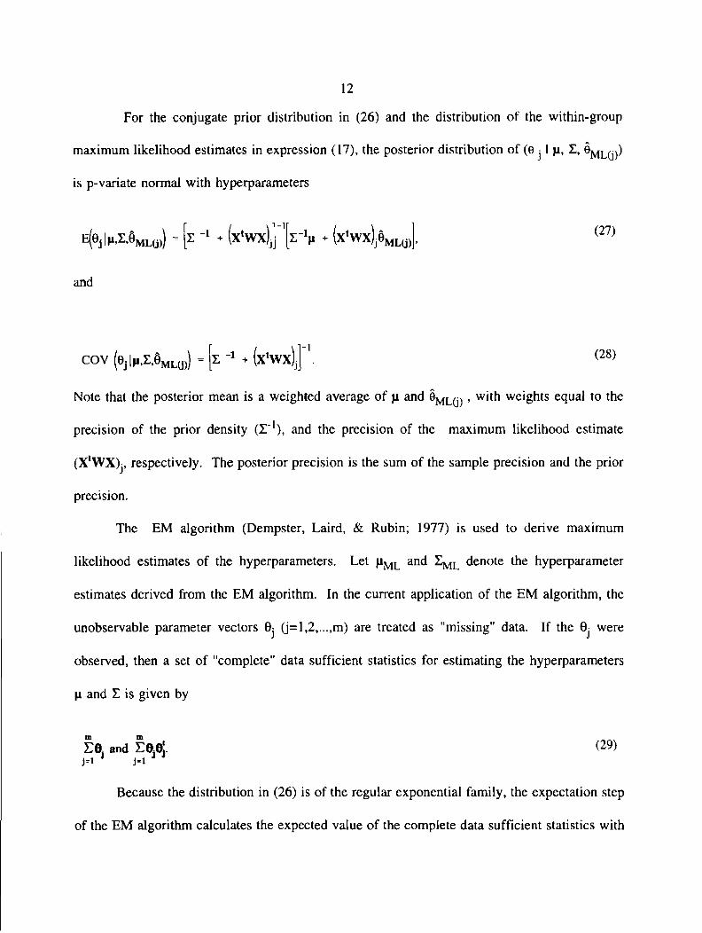
For the conjugate prior distribution in (26) and the distribution of the within-group

maximum likelihood estimates in expression (17), the posterior distribution of (0 j I p, 1, 0ML(j))

is p-variate normal with hyperparameters

12

E(ei|M,i,§ML0)) = [z -1 ♦ (x'wxlj [i-V + (x*wx)j§ML{j) (27)

and

cov (ej|M,x,eML(j)) - [i -> - (x*wx)J (28)

Note that the posterior mean is a weighted average of p and 0MLj(j) > wifh weights equal to the

precision of the prior density (X-1), and the precision of the maximum likelihood estimate

(XlWX)j, respectively. The posterior precision is the sum of the sample precision and the prior

precision.

The EM algorithm (Dempster, Laird, & Rubin; 1977) is used to derive maximum

likelihood estimates of the hyperparameters. Let pML and denote the hyperparameter

estimates derived from the EM algorithm. In the current application of the EM algorithm, the

unobservable parameter vectors 0j (j=l,2,...,m) are treated as "missing" data. If the 0j were

observed, then a set of "complete" data sufficient statistics for estimating the hyperparameters

\i and E is given by

EOj and EOjOj. (^9)j=i j-i

Because the distribution in (26) is of the regular exponential family, the expectation step

of the EM algorithm calculates the expected value of the complete data sufficient statistics with

respect to the conditional distribution of the missing data, given the observed data and current

hyperparameter estimates. In the present application, this conditional distribution is the posterior

distribution of (Gj I n(k),Z k\§ML(jp, where j / k) and X denote estimates of the hyperparameters

after the kth iteration. Thus, at the expectation step, and for groups j = 1 to m, calculate

ij = E(0j |M(k),Z(k),9MLU))=|s(k)-1 ■* (x‘Wx)j] '[E<k)-V <k) + (xlWx)j§ML(j)(30)

and

Bj = E(ejej |li<k).Z<k>,&ML(,)) = [(x(k))~'+ (x‘wx)j 1 + aja], (31)

where aj is the posterior mean in equation (27) evaluated at the current hyperparameter estimates.

At the maximization step, the hyperparameter estimates are updated as

,(k+l) = 1 S— L a,, m j=i

(32)

and

(33)

The EM algorithm iterates between the expectation step, given in (30) and (31), and the

maximization step, given in (32) and (33), until the hyperparameter estimates stabilize.

14

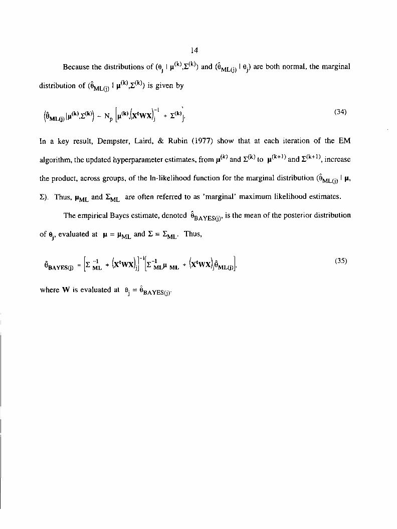
Because the distributions of (0j I and (9mL(j) 1 eP ^ norma^ lê marginal

distribution of (0 1 ) I M(k),Z(k)) is given by

(®ML<><k)'l(k>) - NP [M ^'ix'wxjr1 + I<W(34)

In a key result, Dempster, Laird, & Rubin (1977) show that at each iteration of the EM

algorithm, the updated hyperparameter estimates, from and zf® to ^ k+1) and 5^k+1\ increase

the product, across groups, of the ln-likelihood function for the marginal distribution (^mlG) '

Z). Thus, and are often referred to as ’marginal’ maximum likelihood estimates.

The empirical Bayes estimate, denoted ©bayesO)’ *s mean °f posterior distribution

of 0j, evaluated at fi = jiML and 2 = Thus,

0BAYESG) z MV ♦ ( x 'w x J J ' l z - ^ m l + b to x)fa u s> .(35)

where W is evaluated at 0j = ®BAYES(j)'

Application

In support of its user institutions, ACT offers a Course Placement Service (ACT, 1994)

to assist colleges and universities in making course placement decisions for their first-year

students. Placement decision rules, based on one or more test variables, are evaluated in terms

of the estimated proportions of correct and incorrect decisions. Logistic regression is used to

model the probability of success in the course (defined, for example, as a course grade of a ’B’

or better) as a function of test score. Estimated conditional probabilities of success from the

fitted logistic regression function are combined with the marginal distribution of test scores to

estimate the proportion of correct and incorrect decisions for a given decision rule.

One source of error variance in the estimated proportions is variance associated with

estimating the parameters of the logistic regression function. Because the logistic regression

function is specific to each course at each institution, small sample sizes are not uncommon. To

control error variance in the parameter estimates, and thus in the estimated proportions of correct

and incorrect decisions, a minimum sample size of 45 is required. To the extent they reduce

error variance in estimating the logistic regression parameters, Bayesian estimation procedures

might permit a reduction in the sample size required to achieve an acceptable level of precision.

In 1991, at the request of the Oklahoma State Board of Regents, ACT was asked to

establish common placement rules for several college courses, including English Composition,

College Algebra, American History, and Physics. Schools with 10 or more within-course

observations were included in the analysis. To help satisfy the exchangeability assumption, 2-

year and 4-year institutions were analyzed separately. Semester and end-of-year course grade

data for the Fall 1991 incoming freshman classes at 14 colleges and universities were matched

15

by social security number against ACT Assessment history files to append ACT Assessment test

scores to the course grade data. All subsequent analyses were based on these matched data.

16

TABLE 1

Empirical Bayes and Maximum Likelihood Parameter Estimates for English Composition at 2-year Institutions

Estimation procedure

Number of Bayes Maximum likelihood

observations Intercept Slope Intercept Slope

91 -5.02 0.28 -6.15 0.34

102 -3.07 0.19 -2.54 0.16

171 -4.54 0.30 -5.78 0.38

61 -4.55 0.28 -5.95 0.37

136 -4.09 0.25 -4.28 0.26

58 -2.61 0.16 -1.42 0.10

247 -3.50 0.23 -3.45 0.23

152 -3.97 0.22 -3.95 0.21

179 -4.21 0.23 -4.20 0.23

82 -3.03 0.18 -1.94 0.13

43 -4.45 0.25 -6.47 0.35

110 -5.92 0.33 -8.46 0.47

245 -5.63 0.28 -7.19 0.35

336 -2.04 0.10 -1.620.08

Logistic regression was used to model the probability of success in the course, defined

as a course grade of ’B’ or better, as a function of ACT Composite score. Table 1 presents

empirical Bayes and maximum likelihood estimates of 0j (j=l,2,...,14) for the English

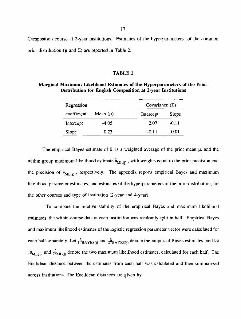
Composition course at 2-year institutions. Estimates of the hyperparameters of the common

prior distribution (fj and X) are reported in Table 2.

TABLE 2

Marginal Maximum Likelihood Estimates of the Hyperparameters of the Prior Distribution for English Composition at 2-year Institutions

17

Regression Covariance (E)

coefficient Mean (ji) Intercept Slope

Intercept -4.05 2.07 -0.11

Slope 0.23 -0.11 0.01

The empirical Bayes estimate of 0j is a weighted average of the prior mean ji, and the

within-group maximum likelihood estimate 0ML(j)» weights equal to the prior precision and

the precision of 6ml0) » respectively. The appendix reports empirical Bayes and maximum

likelihood parameter estimates, and estimates of the hyperparameters of the prior distribution, for

the other courses and type of institution (2-year and 4-year).

To compare the relative stability of the empirical Bayes and maximum likelihood

estimates, the within-course data at each institution was randomly split in half. Empirical Bayes

and maximum likelihood estimates of the logistic regression parameter vector were calculated for

each half separately. Let i^bayesO) anc* 2®BAYES(j) ênote empirical Bayes estimates, and let

i§ML(j) a°d 2®ML(j) denote two maximum likelihood estimates, calculated for each half. The

Euclidean distance between the estimates from each half was calculated and then summarized

across institutions. The Euclidean distances are given by

18

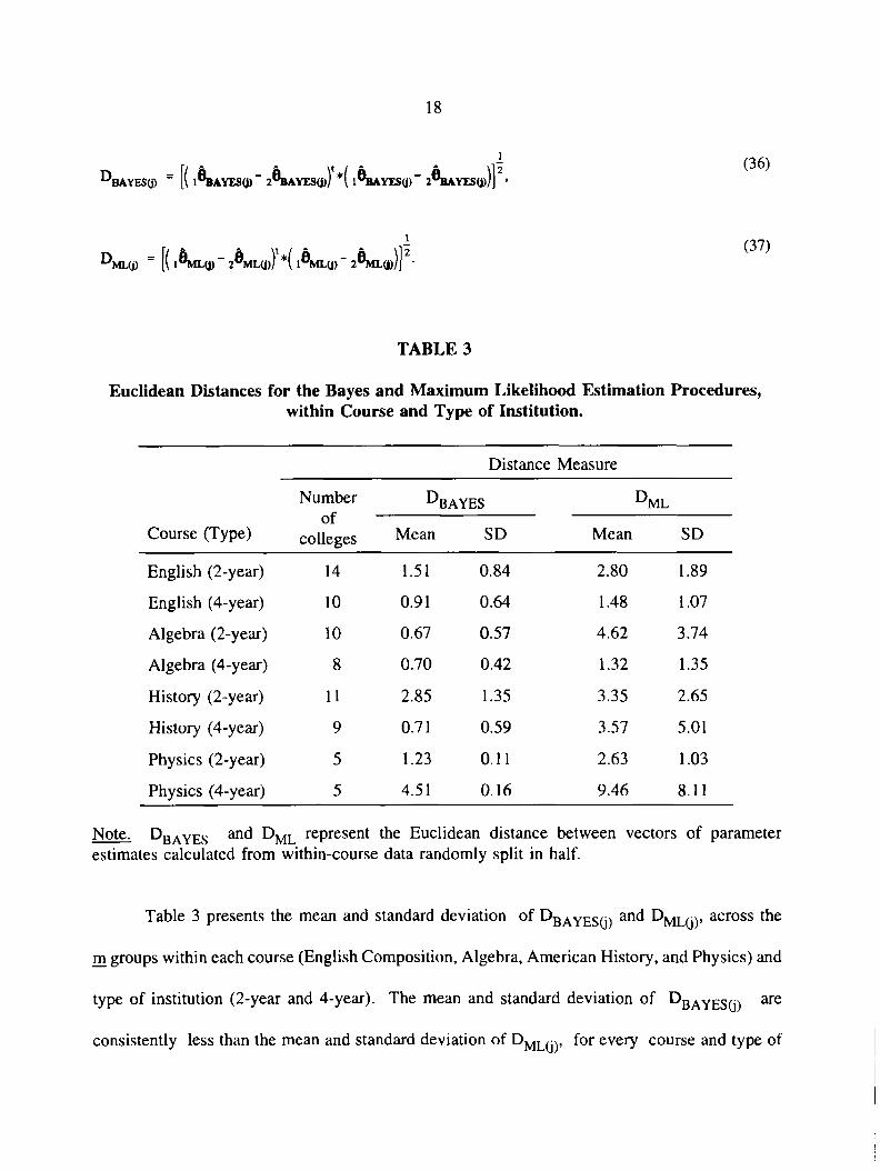
^BAYES(j) ” [( 1 ®BAYES(j) 2®BAYES(j)) *( l®BAYES(j) 2®BAYES(j))] ’(36)

(37)

TABLE 3

Euclidean Distances for the Bayes and Maximum Likelihood Estimation Procedures,within Course and Type of Institution.

Course (Type)

Distance Measure

Numberof

colleges

DiBAYES d m l

Mean SD Mean SD

English (2-year) 14 1.51 0.84 2.80 1.89

English (4-year) 10 0.91 0.64 1.48 1.07

Algebra (2-year) 10 0.67 0.57 4.62 3.74

Algebra (4-year) 8 0.70 0.42 1.32 1.35

History (2-year) 11 2.85 1.35 3.35 2.65

History (4-year) 9 0.71 0.59 3.57 5.01

Physics (2-year) 5 1.23 0 . 1 1 2.63 1.03

Physics (4-year) 5 4.51 0.16 9.46 8.11

Note. DBAyes ant* ^ML rePresent the Euclidean distance between vectors of parameter estimates calculated from within-course data randomly split in half.

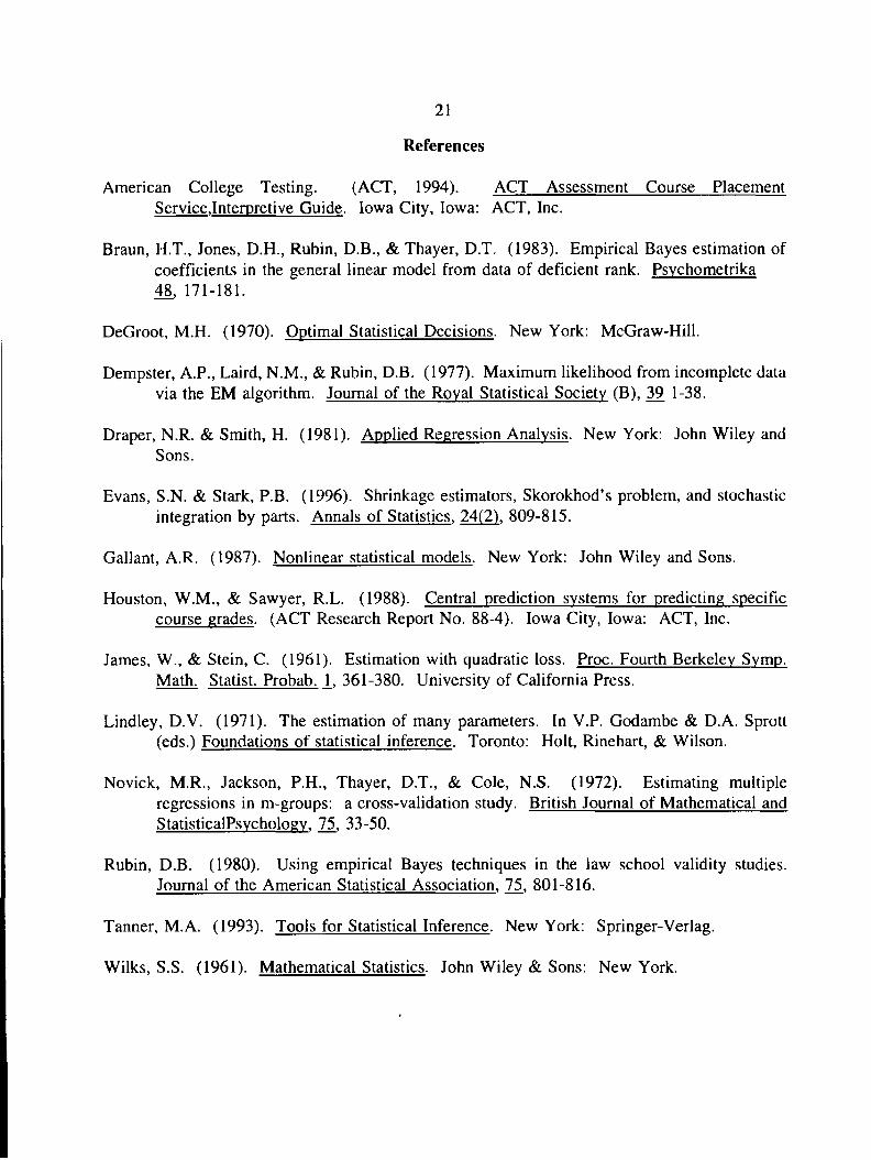
Table 3 presents the mean and standard deviation of Dbayes<J) and DML^ , across the

m groups within each course (English Composition, Algebra, American History, and Physics) and

type of institution (2-year and 4-year). The mean and standard deviation of DbayeS(j) are

consistently less than the mean and standard deviation of DML^ , for every course and type of

Eucl

idea

n di

stan

ce

institution. These results suggest the effectiveness of the m-group regression procedure in

stabilizing parameter estimates, relative to within-group maximum likelihood estimates.

FIGURE 1

Euclidean Distance between Estimated Parameter Vectors as a Function of Sample Size

19

Number of Observations

A plot of the Euclidean distances (Dbayes<J) ^ML(j)) versus sample size is presented

in Figure 1 for the English Composition course at 2-year institutions. Figure 1 suggests that the

m-group regression procedure might permit a reduction in the minimum sample size requirement,

without sacrificing the precision of the estimates using the current estimation procedure and

sample size requirement. Figure 1 also suggests that the relative advantage of the m-group

regression procedure over within-group maximum likelihood estimation, in terms of increased

stability in the estimates, is a decreasing function of sample size, with the m-group regression

procedure more advantageous as within-group sample sizes decrease.

20

References

21

American College Testing. (ACT, 1994). ACT Assessment Course Placement ServiceJnterpretive Guide. Iowa City, Iowa: ACT, Inc.

Braun, H.T., Jones, D.H., Rubin, D.B., & Thayer, D.T. (1983). Empirical Bayes estimation of coefficients in the general linear model from data of deficient rank. Psvchometrika 48, 171-181.

DeGroot, M.H. (1970). Optimal Statistical Decisions. New York: McGraw-Hill.

Dempster, A.P., Laird, N.M., & Rubin, D.B. (1977). Maximum likelihood from incomplete data via the EM algorithm. Journal of the Royal Statistical Society (B), 39 1-38.

Draper, N.R. & Smith, H. (1981). Applied Regression Analysis. New York: John Wiley and Sons.

Evans, S.N. & Stark, P.B. (1996). Shrinkage estimators, Skorokhod’s problem, and stochastic integration by parts. Annals of Statistics, 24(2), 809-815.

Gallant, A.R. (1987). Nonlinear statistical models. New York: John Wiley and Sons.

Houston, W.M., & Sawyer, R.L. (1988). Central prediction systems for predicting specific course grades. (ACT Research Report No. 88-4). Iowa City, Iowa: ACT, Inc.

James, W., & Stein, C. (1961). Estimation with quadratic loss. Proc. Fourth Berkeley Symp. Math. Statist. Probab. 1, 361-380. University of California Press.

Lindley, D.V. (1971). The estimation of many parameters. In V.P. Godambe & D.A. Sprott (eds.) Foundations of statistical inference. Toronto: Holt, Rinehart, & Wilson.

Novick, M.R., Jackson, P.H., Thayer, D.T., & Cole, N.S. (1972). Estimating multiple regressions in m-groups: a cross-validation study. British Journal of Mathematical and StatisticalPsychology. 75. 33-50.

Rubin, D.B. (1980). Using empirical Bayes techniques in the law school validity studies. Journal of the American Statistical Association. 75. 801-816.

Tanner, M.A. (1993). Tools for Statistical Inference. New York: Springer-Verlag.

Wilks, S.S. (1961). Mathematical Statistics. John Wiley & Sons: New York.

Appendix

Parameter and Hyperparameter Estimates, by Course and Type of Institution.

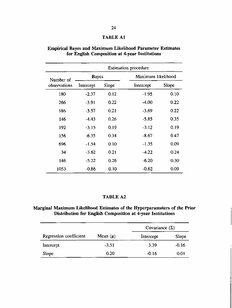
Table A1 reports the empirical Bayes and maximum likelihood parameter estimates of 0j

(j=l to 10) for the English Composition course at 4-year institutions. Table A2 reports the

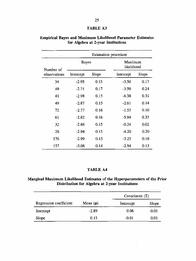
estimated hyperparameters (n and Z) of the prior distribution for 0j. Table A3 and Table A4

report parameter and hyperparameter estimates, respectively, for the College Algebra course at

2-year institutions. Table A5 and Table A6 report parameter and hyperparameter estimates,

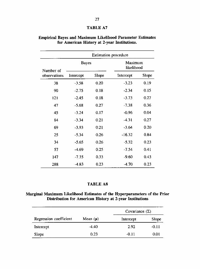
respectively, for the College Algebra course at 4-year institutions. Table A7 and Table A8 report

parameter and hyperparameter estimates, respectively, for the American History course at 2-year

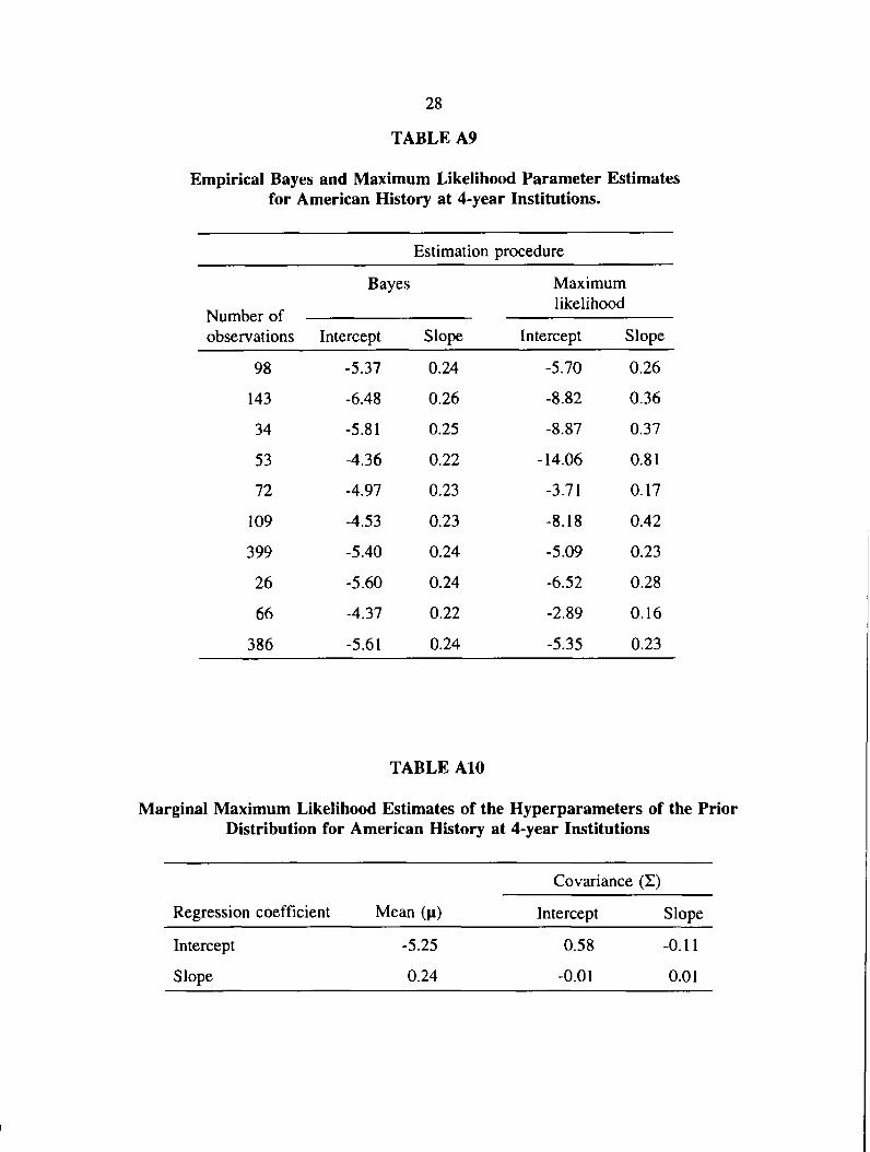
institutions. Table A9 and Table A 10 report parameter and hyperparameter estimates,

respectively, for the American History course at 4-year institutions. Table A ll and Table A 12

report parameter and hyperparameter estimates, respectively, for the Physics course at 2-year

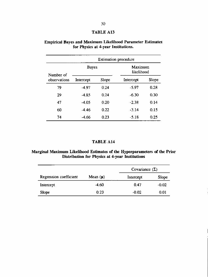
institutions. Table A13 and Table A 14 report parameter and hyperparameter estimates,

respectively, for the Physics course at 4-year institutions. The number of institutions ranged from

5, for both Physics’ courses, to 12, for the American History course at 2-year institutions).

23

24

TABLE A1

Empirical Bayes and Maximum Likelihood Parameter Estimatesfor English Composition at 4-year Institutions


Number of ■ observations

Bayes Maximum likelihood

Intercept Slope Intercept Slope

180 -2.37 0.12 -1.95 0.10

266 -3.91 0.22 -4.00 0.22

186 -3.57 0.21 -3.69 0.22

146 -4.43 0.26 -5.85 0.35

192 -3.15 0.19 -3.12 0.19

156 -6.35 0.34 -8.67 0.47

696 -1.54 0.10 -1.35 0.09

34 -3.62 0.21 -4.22 0.24

146 -5.22 0.26 -6.20 0.30

1053 -0.86 0.10 -0.62 0.09

TABLE A2

Marginal Maximum Likelihood Estimates of the Hyperparameters of the Prior Distribution for English Composition at 4-year Institutions

Covariance (Z)

Regression coefficient Mean (p) Intercept Slope

Intercept

Slope

-3.51

0.20

3.39

-0.16

-0.16

0.01

25

TABLE A3

Empirical Bayes and Maximum Likelihood Parameter Estimatesfor Algebra at 2-year Institutions


Number of observations

Bayes Maximumlikelihood


34 -2.95 0.15 -3.50 0.17

49 -2.71 0.17 -3.59 0.24

41 -2.98 0.15 -6.38 0.31

49 -2.87 0.15 -2.61 0.14

72 -2.77 0.16 -1.55 0.10

61 -2.82 0.16 -5.94 0.33

32 -2.86 0.15 -0.24 0.02

26 -2.94 0.15 -4.20 0.20

176 -2.99 0.15 -3.25 0.16

157 -3.06 0.14 -2.94 0.13

TABLE A4

Marginal Maximum Likelihood Estimates of the Hyperparameters of the Prior Distribution for Algebra at 2-year Institutions

Covariance (X)

Regression coefficient Mean (p) Intercept Slope

Intercept

Slope

-2.89

0.15

0.06

-0.01

-0.01

0.01

26

TABLE A5

Empirical Bayes and Maximum Likelihood Parameter Estimatesfor Algebra at 4-Year Institutions.




Intercept Slope Intercept ;Slope

113 -3.85 0.18 -4.07 0.19

121 -4.67 0.21 -6.39 0.29

102 -4.50 0.20 -5.53 0.25

67 -3.76 0.17 -5.98 0.31

62 -3.84 0.17 -3.97 0.18

549 -4.00 0.16 -3.85 0.15

94 -4.47 0.20 -5.77 0.26

772 -1.67 0.09 -1.29 0.08

TABLE A6

Marginal Maximum Likelihood Estimates of the Hyperparameters of the Prior Distribution for Algebra at 4-year Institutions

Covariance (£)

Regression coefficient Mean (n) Intercept Slope

Intercept

Slope

-3.85

0.17

1.40

-0.06

-0.06

0.01

27

TABLE A7

Empirical Bayes and Maximum Likelihood Parameter Estimatesfor American History at 2-year Institutions.





38 -3.58 0.20 -3.23 0.19

90 -2.75 0.18 -2.34 0.15

121 -2.45 0.18 -3.73 0.27

47 -5.68 0.27 -7.38 0.36

45 -3.24 0.17 -0.96 0.04

84 -3.34 0.21 -4.31 0.27

69 -3.93 0.21 -3.64 0.20

25 -5.34 0.26 -16.32 0.84

34 -5.65 0.26 -5.32 0.23

57 -4.69 0.25 -7.54 0.41

147 -7.35 0.33 -9.60 0.43

288 -4.83 0.23 -4.70 0.23

TABLE A8

Marginal Maximum Likelihood Estimates of the Hyperparameters of the Prior Distribution for American History at 2-year Institutions

Covariance (X)


Intercept -4.40 2.92 -0.11

Slope 0.23 -0.11 0.01

28

TABLE A9

Empirical Bayes and Maximum Likelihood Parameter Estimatesfor American History at 4-year Institutions.




Intercept Slope Intercept ;Slope

98 -5.37 0.24 -5.70 0.26

143 -6.48 0.26 -8.82 0.36

34 -5.81 0.25 -8.87 0.37

53 -4.36 0.22 -14.06 0.81

72 -4.97 0.23 -3.71 0.17

109 -4.53 0.23 -8.18 0.42

399 -5.40 0.24 -5.09 0.23

26 -5.60 0.24 -6.52 0.28

66 -4.37 0.22 -2.89 0.16

386 -5.61 0.24 -5.35 0.23

TABLE A10

Marginal Maximum Likelihood Estimates of the Hyperparameters of the Prior Distribution for American History at 4-year Institutions

Covariance (£)


Intercept

Slope

-5.25

0.24

0.58

-0.01

-0.11

0.01

29

TABLE A ll

Empirical Bayes and Maximum Likelihood Parameter Estimatesfor Physics at 2-year Institutions.





84 -3.05 0.16 -2.69 0.15

30 -3.07 0.16 -1.84 0.08

41 -3.13 0.16 -3.78 0.16

52 -3.13 0.16 -6.23 0.34

46 -3.05 0.16 -1.63 0.08

TABLE A12

Marginal Maximum Likelihood Estimates of the Hyperparameters of the Prior Distribution for Physics at 2-year Institutions

Covariance (X)


Intercept

Slope

-3.09

0.16

0.08

- 0.01

- 0.01

0.01

30

TABLE A13

Empirical Bayes and Maximum Likelihood Parameter Estimatesfor Physics at 4-year Institutions.





79 -4.97 0.24 -5.97 0.28

29 -4.85 0.24 -6.30 0.30

47 -4.05 0.20 -2.38 0.14

60 -4.46 0.22 -3.14 0.15

74 -4.66 0.23 -5.18 0.25

TABLE A14

Marginal Maximum Likelihood Estimates of the Hyperparameters of the Prior Distribution for Physics at 4-year Institutions

Covariance (1)

Regression coefficient Mean (fi) Intercept Slope

Intercept -4.60 0.47 -0.02

Slope 0.23 -0.02 0.01

Documents

Empirical Bayes Estimates of Parameters from the Logistic