Empirical Examination of Operational Loss Distribu- tions · Empirical Examination of Operational Loss Distribu-tions Svetlozar T. Rachev Institut fu¨r Statistik und Mathematische

Empirical Examination of Operational Loss Distribu-tions

Svetlozar T. Rachev

Institut fur Statistik und Mathematische WirtschaftstheorieUniversitat Karlsruhe

and

Department of Statistics and Applied ProbabilityUC Santa Barbara

Anna Chernobai

Department of Statistics and Applied ProbabilityUC Santa Barbara

Christian Menn

School of Operations Research and Industrial EngineeringCornell University

1 Introduction

Until very recently, it has been believed that banks are exposed to two maintypes of risks: credit risk (the counterparty failure risk) and market risk(the risk of loss due to changes in market indicators, such as interest ratesand exchange rates), in the order of importance. The remaining financialrisks have been put in the category of other risks, operational risk beingone of them. Recent developments in the financial industry have shownthat the importance of operational risk has been largely under-estimated.Newly defined capital requirements set by the Basel Committee for BankingSupervision in 2004, require financial institutions to estimate the capitalcharge to cover their operational losses [6].

This paper is organized as follows. In Section 2 we give the definitionof operational risk and describe the effect of the recent developments inthe global financial industry on banks’ exposures to operational risk. Thefollowing section, Section 3, will briefly outline the recent requirementsset by the Basel Committee regarding the capital charge for operationalrisk. After that we proceed to Section 4 that presents several alternativemodels that can be used for operational risk modeling. In Section 5 theclass of heavy-tailed αStable distributions and their extensions are defined

2 S.T. Rachev, A. Chernobai, C. Menn

and reviewed. Section 6 consists of the empirical analysis with real opera-tional risk data. Finally, Section 7 summarizes the findings and discussesdirections for future work.

2 Definition of Operational Risk in Finance

Operational risk has been recently defined as ‘the risk of loss resultingfrom inadequate or failed internal processes, people and systems or fromexternal events’ [4]. Examples include losses resulting from deliberate oraccidental accounting errors, equipment failures, credit card fraud, tax non-compliance, unauthorized trading activities, business disruptions due tonatural disasters and vandalism. Operational risk affects the soundnessand efficiency of all banking activities.

Until recently, the importance of operational risk has been highly under-estimated by the banking industry. The losses due to operational risk hasbeen largely viewed as unsubstantial in magnitude, with a minor impacton the banking decision-making and capital allocation. However, increasedinvestors’ appetites have led to significant changes in the global financialindustry during the last couple of decades - globalization and deregula-tion, accelerated technological innovation and revolutionary advances inthe information network, and increase in the scope of financial services andproducts. These have caused significant changes in banks’ risk profiles,making banks more vulnerable to various sources of risk. These changeshave also brought the operational risk to the center of attention of financialregulators and practitioners.

A number of large-scale (exceeding $1 billion in value) operational losses,involving high-profile financial institutions, have shaken the global financialindustry in the past two decades: BCCI (1991), Orange Country (1994),Barings Bank (1995), Daiwa Bank (1995), NatWest (1997), Allied IrishBanks (2002), the Enron scandal (2004), among others.

3 Capital Requirements for Operational Risk

The Basel Committee for Banking Supervision (BCBS) has brought intofocus the importance of operational risk in 1998 [2], and since 2001 bankregulators have been working on developing capital-based counter-measuresto protect the global banking industry against the risk of operational losses- that have demonstrated to possess a substantial, and at times vital, dan-ger to banks. It has been agreed to include operational risk into the scopeof financial risks for which the regulatory capital charge should be set [3].Currently in progress is the process of developing models for the quanti-

Operational Loss Distributions 3

tative assessment of operational risk, to be used for measuring the capitalcharge.

The Basel Capital Accord (Basel II) has been finalized in June 2004 [6].It explains the guidelines for financial institutions regarding the capital re-quirements for credit, market and operational risks (Pillar I), the frameworkfor the supervisory capital assessment scheme (Pillar II), and the marketdiscipline principles (Pillar III). Under the first Pillar, several approacheshave been proposed for the estimation of the regulatory capital charge.Bank is allowed to adopt one of the approaches, dependent upon fulfill-ment of a number of quantitative and qualitative requirements. The BasicIndicator Approach (that takes the capital charge to be a fixed fractionof the bank’s gross income) and the Standardized Approach (under whichthe capital charge is a sum of fixed proportions of the gross incomes acrossall business lines) are the ‘top-down’ approaches, since the capital chargeis determined ‘from above’ by the regulators; the Advanced MeasurementApproaches (that involve the exact form of the loss data distributions) arethe ‘bottom-up’ approaches, since the capital charge is determined ‘frombelow’, being driven by individual bank’s internal loss data history andpractices.

3.1 Loss Distribution Approach

The Loss Distribution Approach (LDA) is one of the proposed AdvancedMeasurement Approaches. It makes use of the exact operational loss fre-quency and severity distributions. A necessary requirement for banks toadopt this approach is an extensive internal database.

In the LDA, all bank’s activities are classified into a matrix of ‘busi-ness lines/event type’ combinations. Then, for each combination, usingthe internal loss data the bank estimates two distributions: (1) the lossfrequency and (2) severity. Based on these two estimated distributions,the bank computes the probability distribution function of the cumulativeoperational loss. The operational capital charge is computed as the simplesum of the one-year Value-at-Risk (VaR) measure (with confidence levelsuch as 99.9%) for each ‘business line/ event type’ pair. The capital charge


for a general case (8 business lines and 7 event types) can be expressed as:1

KLDA =8∑

j=1

7∑k=1

VaRjk. (3.1)

where KLDA is the one-year capital charge under the LDA, and VaR isthe Value-at-Risk risk measure,2 for a one-year holding period and highconfidence level (such as 99.9%), based on the aggregated loss distribution,for each ‘business line/event type’ jk combination.

4 Aggregated Stochastic Models for Operational Risk

Following the guidelines of the Basel Committee, the aggregated opera-tional loss process can be modeled by a random sum model, in which thesummands are composed of random amounts, and the number of such sum-mands is also a random process. The compound loss process is hence as-sumed to follow a stochastic process {St}t≥0 expressed by the followingequation:

St =Nt∑

k=0

Xk, Xkiid∼ Fγ , (4.1)

in which the loss magnitudes (severities) are described by the random in-dependently and identically distributed (iid) sequence {Xk} assumed tofollow the distribution function (cdf) Fγ that belong to a parametric fam-ily of continuous probability distributions, and the density fγ , and thecounting process Nt is assumed to follow a discrete counting process. Toavoid the possibility of negative losses, it is natural to restrict the supportof the severity distribution to the positive half-line R>0. Representation(4.1) generally assumes (and we also use this assumption) independence be-tween the frequency and severity distributions. The cdf of the compound

1Such representation perfect correlation between different ‘business lines/ event type’combinations. Ignoring possible dependence structures within the banking business lines’and event type profiles may result in overestimation of the capital charge under theLDA approach. The latest Basel II proposal suggested to take into account possibledependencies in the model [6]. Relevant models would involve using techniques such ascopulas (see for example numerous works by McNeil and Embrechts on the discussionof copulas), but this is outside the scope of this paper.

2VaR4t, 1−α is the risk measure that determines the highest amount of loss thatone can expect to lose over a pre-determined time interval (or holding period) 4t at apre-specified confidence level 1 − α. Detailed analysis of VaR models can be found in[11].


process is given by:

P (St ≤ s) =

∑∞

n=1 P (Nt = n) Fn∗γ (s) s > 0

P (Nt = 0) s = 0,(4.2)

where Fn∗γ denotes the n-fold convolution with itself.

We summarize the basic properties of such compound process by theexpressions for the mean and variance:3

Mean: ESt = ENt · EX,

Variance: VSt = ENt · VX + VNt · (EX)2.(4.3)

The upper (right) tail behavior has a simple expression for the specialcase when X belongs to the class of sub-exponential distributions, X ∼ S,such as Lognormal, Pareto or the heavy-tailed Weibull. Then the uppertail of the compound process can asymptotically be approximated by (seee.g. [10]):

Right tail: P (St > s) ∝ ENt · P (X > s), s →∞. (4.4)

4.1 Compound Homogeneous Poisson Process

A stochastic process of the form (4.1) and Nt following a Poisson processwith a fixed intensity lambda (λ) is called a compound homogeneous Poissonprocess. It assumes a fixed intensity of the number of loss events in a unit oftime. Incorporating the probability mass function of a Poisson distributioninto the basic model of Equation (4.2), the cdf of the compound processbecomes:

P (St ≤ s) =

∑∞

n=1(λt)ne−λt

n! Fn∗γ (s) s > 0

e−λt s = 0.(4.5)

The basic properties of a compound Poisson process can be summarizedusing Equations (4.3) and (4.4) as follows:

Mean: ESt = λt · EX,

Variance: VSt = λt · VX + λt · (EX)2,

Right tail: P (St > s) ∝ λt · P (X > s), s →∞, X ∼ S.

(4.6)

3Of course, this requires the existence of the first and second raw moments of the lossseverity distribution.


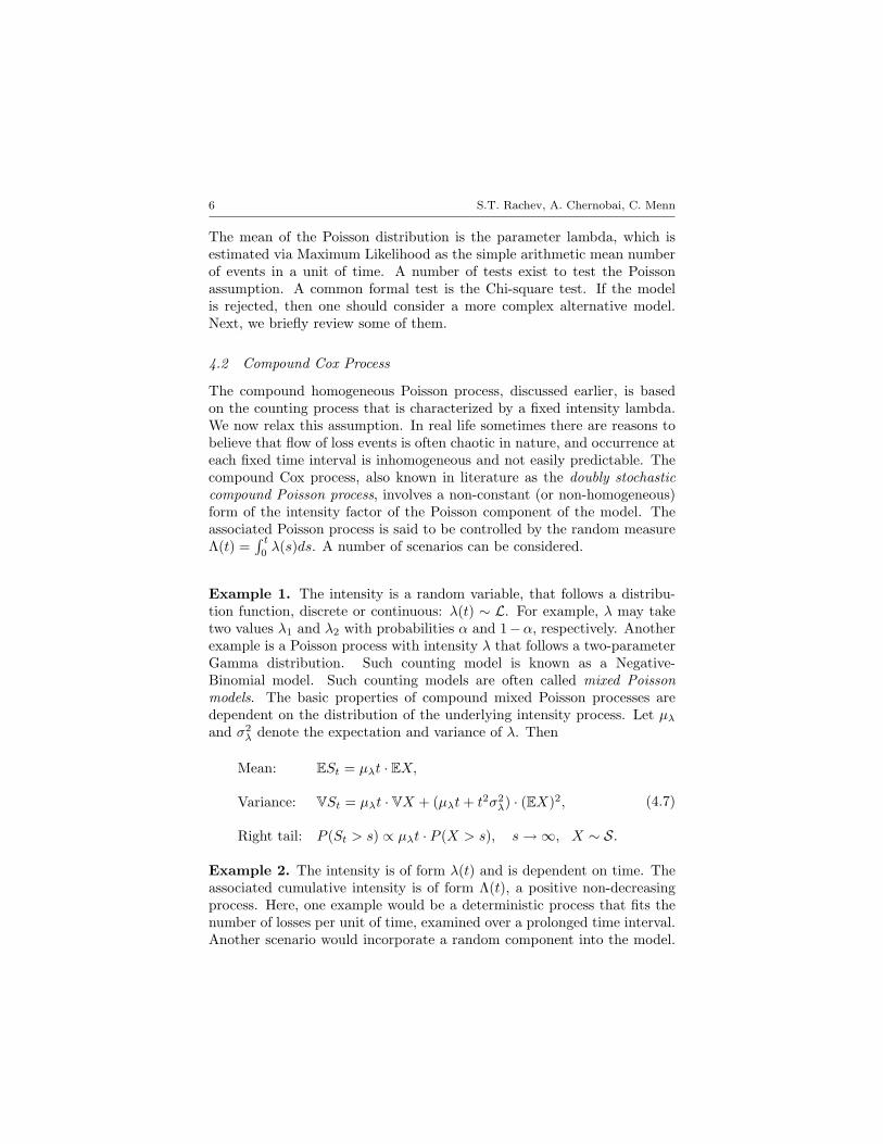
The mean of the Poisson distribution is the parameter lambda, which isestimated via Maximum Likelihood as the simple arithmetic mean numberof events in a unit of time. A number of tests exist to test the Poissonassumption. A common formal test is the Chi-square test. If the modelis rejected, then one should consider a more complex alternative model.Next, we briefly review some of them.

4.2 Compound Cox Process

The compound homogeneous Poisson process, discussed earlier, is basedon the counting process that is characterized by a fixed intensity lambda.We now relax this assumption. In real life sometimes there are reasons tobelieve that flow of loss events is often chaotic in nature, and occurrence ateach fixed time interval is inhomogeneous and not easily predictable. Thecompound Cox process, also known in literature as the doubly stochasticcompound Poisson process, involves a non-constant (or non-homogeneous)form of the intensity factor of the Poisson component of the model. Theassociated Poisson process is said to be controlled by the random measureΛ(t) =

∫ t

0λ(s)ds. A number of scenarios can be considered.

Example 1. The intensity is a random variable, that follows a distribu-tion function, discrete or continuous: λ(t) ∼ L. For example, λ may taketwo values λ1 and λ2 with probabilities α and 1−α, respectively. Anotherexample is a Poisson process with intensity λ that follows a two-parameterGamma distribution. Such counting model is known as a Negative-Binomial model. Such counting models are often called mixed Poissonmodels. The basic properties of compound mixed Poisson processes aredependent on the distribution of the underlying intensity process. Let µλ

and σ2λ denote the expectation and variance of λ. Then

Mean: ESt = µλt · EX,

Variance: VSt = µλt · VX + (µλt + t2σ2λ) · (EX)2,

Right tail: P (St > s) ∝ µλt · P (X > s), s →∞, X ∼ S.

(4.7)

Example 2. The intensity is of form λ(t) and is dependent on time. Theassociated cumulative intensity is of form Λ(t), a positive non-decreasingprocess. Here, one example would be a deterministic process that fits thenumber of losses per unit of time, examined over a prolonged time interval.Another scenario would incorporate a random component into the model.


Here, Brownian Motion and other stochastic models can be of use. Givena particular value of the intensity, the conditional compound Cox processcoincides with the compound homogeneous Poisson Process and preservesthe properties.

4.3 Renewal Process

Another approach to aggregate losses occurring at random times wouldbe to consider looking at the inter-arrival times, instead of the numberof arrivals, in a fixed time interval. Such models are called the renewalmodels. A Poisson counting process implies that the inter-arrival timesbetween the loss events are distributed as an Exponential random variablewith mean 1/λ. This assumption on the distribution of the inter-arrivaltimes can be relaxed, and a wider class of distributions can be fitted to theloss inter-arrival times data.

An excellent reference on random sum models and applications to fi-nancial data is [1].

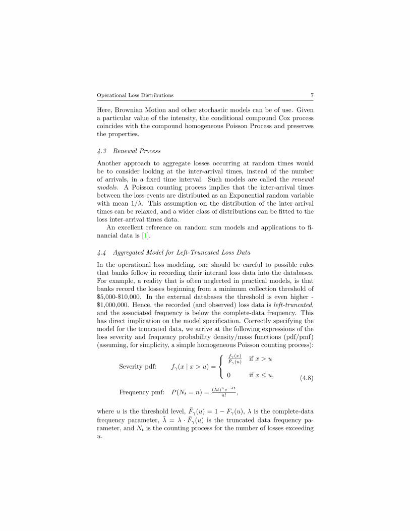
4.4 Aggregated Model for Left-Truncated Loss Data

In the operational loss modeling, one should be careful to possible rulesthat banks follow in recording their internal loss data into the databases.For example, a reality that is often neglected in practical models, is thatbanks record the losses beginning from a minimum collection threshold of$5,000-$10,000. In the external databases the threshold is even higher -$1,000,000. Hence, the recorded (and observed) loss data is left-truncated,and the associated frequency is below the complete-data frequency. Thishas direct implication on the model specification. Correctly specifying themodel for the truncated data, we arrive at the following expressions of theloss severity and frequency probability density/mass functions (pdf/pmf)(assuming, for simplicity, a simple homogeneous Poisson counting process):

Severity pdf: fγ(x | x > u) =

fγ(x)

Fγ(u)if x > u

0 if x ≤ u,

Frequency pmf: P (Nt = n) = (λt)ne−λt

n! ,

(4.8)

where u is the threshold level, Fγ(u) = 1 − Fγ(u), λ is the complete-datafrequency parameter, λ = λ · Fγ(u) is the truncated data frequency pa-rameter, and Nt is the counting process for the number of losses exceedingu.


In application to operational risk, the truncated compound Poissonmodel has been introduced and studied in [8]. Further studies include[7], [12].

5 Pareto αStable Distributions

A wide class of distributions that appear highly suitable for modeling op-erational losses is the class of αStable (or Pareto Stable) distributions.Although no closed-form density form (in the general case) poses difficul-ties in the estimations, αStable distributions possess a number of attractivefeatures that make them relevant in applications to a variety of financialmodels. An excellent reference on αStable is [14]. A profound discussionof applications to the financial data can be found in [13]. We now reviewthe definition and basic properties.

5.1 Definition of an αStable Random Variable

A random variable X is said to follow an αStable distribution – we use thenotation X ∼ Sα(σ, β, µ) – if for any n ≥ 2, there exist Cn > 0 and Dn ∈ Rsuch that

n∑k=1

Xkd= CnX + Dn, (5.1)

where Xk, k = 1, 2, ..., n are iid copies of X. The stability property isgoverned by the constant Cn = n1/α, 0 < α ≤ 2. The stability property isa useful and convenient property, and dictates that the distributional formof the variable is preserved under affine transformations. α = 2 correspondsto the Gaussian case. 0 < α < 2 refers to the non-Gaussian case. Whenwe refer to a Sα(σ, β, µ) distribution, we mean the latter case. Referenceson the Sα(σ, β, µ) distributions and properties include [14], [13].

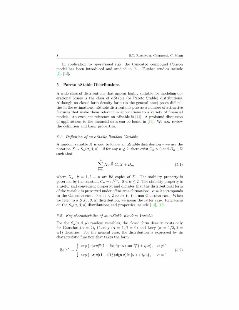
5.2 Key characteristics of an αStable Random Variable

For the Sα(σ, β, µ) random variables, the closed form density exists onlyfor Gaussian (α = 2), Cauchy (α = 1, β = 0) and Levy (α = 1/2, β =±1) densities. For the general case, the distribution is expressed by itscharacteristic function that takes the form:

EeiuX =

exp(−|σu|α(1− iβ(signu) tan πα

2 ) + iµu), α 6= 1

exp(−σ|u|(1 + iβ 2

π (signu) ln |u|) + iµu), α = 1

(5.2)


The four parameters4 defining the Sα(σ, β, µ) distribution are:

α, the index of stability: α ∈ (0, 2);

β, the skewness parameter: β ∈ [−1, 1];

σ, the scale parameter: σ ∈ R+;

µ, the location parameter: µ ∈ R.

Because of the four parameters, the distribution is highly flexible and suit-able for fitting to the data which is non-symmetric (skewed) and possessesa high peak (kurtosis) and heavy tails. The heaviness of tails is driven bythe power tail decay property (see next).

We briefly present the basic properties of the Sα(σ, β, µ) distribution.Let X ∼ Sα(σ, β, µ) with α < 2, then

Mean: EX =

{µ if α > 1∞ otherwise,

Variance: VX = ∞ (no second moment),

Tail: P (|X| > x) ∝ const · x−α, x →∞ (power tail decay).

(5.3)

5.3 Useful Transformations of Pareto Stable Random Variables

For α > 1 or |β| < 1, the support of Sα(σ, β, µ) distribution equals thewhole real line, and is useful for modeling data that can take negative andpositive values. It would be unwise to directly apply this distribution tothe operational loss data, because it takes only positive values. We suggestto use the following three transformations of the random variable to whichthe Stable law can be applied.

5.3.1 Symmetric αStable Random Variable

A random variable X is said to follow the symmetric αStable distribution,i.e. X ∼ SαS, if the Sα(σ, β, µ) distribution is symmetric and centeredaround zero. Then there are only two parameters that need to be estimated,α and σ, and the remaining two are β, µ = 0.

4The parametrization of αStable laws is not unique. The presented one has beenpropagated by Samorodnitsky and Taqqu [14]. An overview of the different approachescan be found in [15].


To apply SαS distribution to the operational loss severity data, one cando a simple transformation to the original data set: Y = [−X; X]. Theresulting random variable Y is then symmetric around zero:

fY (y) = g(y), g ∈ Sα(σ, 0, 0)

x = |y|, α ∈ (0, 2), σ > 0.(5.4)

5.3.2 log-αStable Random Variable

It is often convenient to work with the natural log transformation of theoriginal data. A typical example is the Lognormal distribution: if X followsa Lognormal distribution, then log X follows a Normal distribution withthe same location and scale parameters µ and σ. The same procedurecan be applied here. A random variable X is said to follow a log-αStabledistribution, i.e. X ∼ log Sα(σ, β, µ), if

fX(x) = g(ln x)x , g ∈ Sα(σ, β, µ)

x > 0, α ∈ (0, 2), β ∈ [−1, 1], σ, µ > 0.(5.5)

Fitting log Sα(σ, β, µ) distribution to data is appropriate when there is rea-son to believe that the data is very heavy-tailed, and the regular Sα(σ, β, µ)distribution may not capture the heaviness in the tails.

5.3.3 Truncated αStable Random Variable

Another scenario would involve a restriction on the density, rather thana transformation of the original data set. The support of the Sα(σ, β, µ)distribution can be restricted to the positive half-line, and the estimationpart would involve fitting a truncated Stable distribution of the form:

fX(x) = g(x)1−G(0) × Ix>0

where Ix>0 :=

{1 if x > 00 if x ≤ 0,

(5.6)

where g(x) ∈ Sα(σ, β, µ), and G(0) denotes the cdf of the Sα(σ, β, µ) dis-tribution at zero. Fitting the left-truncated Stable distribution to the datameans fitting the right tail of the distribution.


6 Empirical Examination of Operational Loss Data

In the previous sections we discussed the models that can be used to modeloperational losses. Choosing the right methodology is crucial for accuratelyestimating the operational risk regulatory capital charge. In addition, un-derstanding the structure of the underlying model that drives the processof the occurrences and severity of the losses is vital for the sound risk man-agement practices and control. In this section we examine the operationalloss data and derive conclusions regarding the loss distributions that wouldbe appropriate for modeling the data. We will in particular focus on theloss severity data.

6.1 Results of Basel Committee Loss Data Collection Exercise

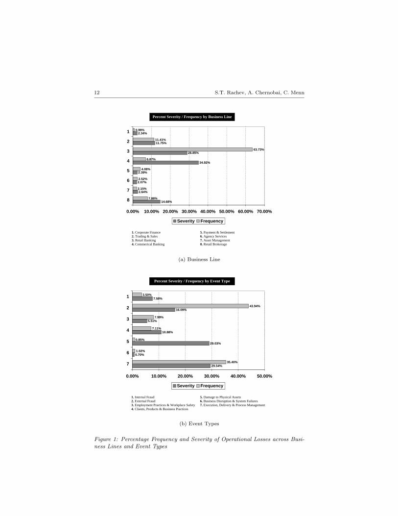
In 2002 the Risk Management Group of the BCBS carried out an Op-erational Loss Data Collection Excercise (OLDC) (also called the thirdQuantitative Impact Study (QIS3)) aimed at examining various aspects ofbanks’ internal operational loss data [5]. Banks activities were broadly di-vided into eight business lines and seven loss event types (see Figure 1 forthe full list of business lines and event types). Figure 1 demonstrates theseverity of losses (i.e. loss amount) and the frequency of losses (i.e. numberof losses) by business lines and event types, as a percentage of total. Theresults are based on the one year of loss data (collected in 2001) providedby 89 participant banks.

The results of the data collection exercise demonstrate a rough pic-ture for the non-uniform nature of the distribution of loss amounts andfrequency across various business lines and event types. The results alsosuggested that the losses are highly right-skewed and have a heavy righttail (i.e. the total loss amounts are highly driven by the high-magnitude‘tail events’) [5]. For example, the Commercial Banking business line in-cludes losses of a relatively low frequency (roughly 7% of total) but thesecond highest severity (roughly 35% of total). As for the losses classifiedby event type, the losses in the Damage to Physical Assets category (suchas losses due to natural disasters) account for less than 1% of the totalnumber of losses, but almost 30% of the aggregate amount. In particular,the ‘retail banking/ external fraud’ and ‘commercial banking/ damage tophysical assets’ combinations account for over 10% of the total loss amounteach, with the first pair accounting for 38% and the second for merely 0.1%of the total number of loss events [5].


Percent Severity / Frequency by Business Line

14.68%

2.64%

2.07%

2.39%

34.92%

28.85%

11.75%

2.34%

7.88%

2.15%

2.52%

4.08%

6.87%

63.73%

11.41%

0.99%

0.00% 10.00% 20.00% 30.00% 40.00% 50.00% 60.00% 70.00%

8

7

6

5

4

3

2

1

Severity Frequency

1. Corporate Finance 5. Payment & Settlement 2. Trading & Sales 6. Agency Services 3. Retail Banking 7. Asset Management 4. Commerical Banking 8. Retail Brokerage

(a) Business Line

Percent Severity / Frequency by Event Type

29.54%

0.70%

29.03%

10.88%

5.51%

16.09%

7.58%

35.40%

1.02%

0.85%

7.11%

7.99%

43.94%

3.50%

0.00% 10.00% 20.00% 30.00% 40.00% 50.00%

7

6

5

4

3

2

1

Severity Frequency

1. Internal Fraud 5. Damage to Physical Assets 2. External Fraud 6. Business Disruption & System Failures 3. Employment Practices & Workplace Safety 7. Execution, Delivery & Process Management4. Clients, Products & Business Practices

(b) Event Types

Figure 1: Percentage Frequency and Severity of Operational Losses across Busi-ness Lines and Event Types


6.2 Analysis of 1980-2002 External Operational Loss Data

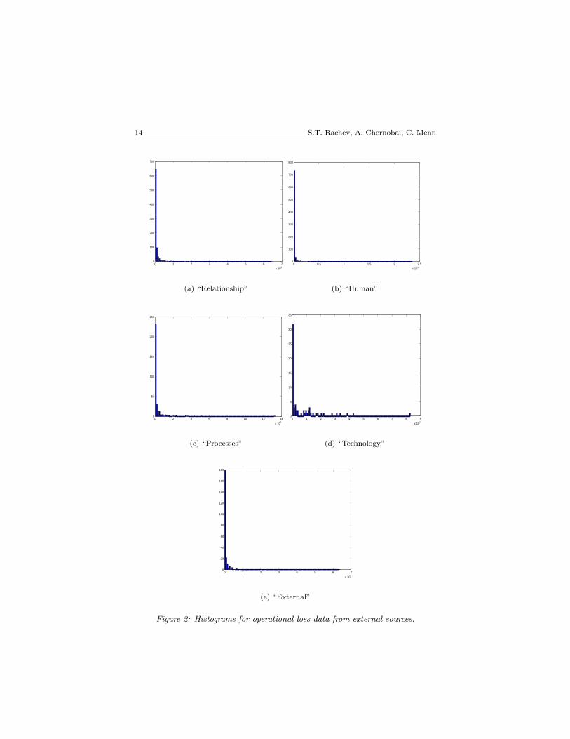
In this section we fit various distributions to the operational risk data, ob-tained from a major European operational loss data provider. The externaldatabase is comprised of operational loss events throughout the world. Theoriginal loss data cover losses in the period 1950-2002. As discussed earlier,the data in external databases are subject to minimum recording thresh-olds of $1 million. A few recorded data points were below $1 million innominal value, so we excluded them from the dataset. Furthermore, weexcluded the observations before 1980 because of relatively few data pointsavailable (which is most likely due to poor data recording practices). Thefinal dataset for the analysis covered losses in US dollars for the time periodbetween 1980 and 2002. It consists of five types of losses: “Relationship”(such as events related to legal issues, negligence and sales-related fraud),“Human” (such as events related to employee errors, physical injury andinternal fraud), “Processes” (such as events related to business errors, su-pervision, security and transactions), “Technology” (such as events relatedto technology and computer failure and telecommunications) and “Exter-nal” (such as events related to natural and man-made disasters and ex-ternal fraud). The loss amounts have been adjusted for inflation usingthe Consumer Price Index from the U.S. Department of Labor. The num-bers of data points of each of the “Relationship”, “Human”, “Processes”,“Technology”, and “External” types are n = 849, 813, 325, 67, and 233, re-spectively. Figure 2 presents the histograms for the five loss types of data.The histograms (the horizontal axis covers the entire range of the data)indicate the leptokurtic nature of the data: a very high peak is observedclose to zero, and an extended right tail indicates the right-skewness andhigh dispersion of the data values.

6.2.1 Operational Loss Frequency Process

Figure 3 portrays the annually aggregated number of losses for the “Ex-ternal” type losses, shown by the dotted-line. It suggests that the accu-mulation is somewhat similar to a continuous cdf-like process, supportingthe use of a non-homogeneous Poisson process. We consider two followingfunctions,5 each with four parameters:

5Of course, asymptotically (as time increases) such functions would produce a con-stant cumulative intensity. However, for this particular sample and this particular timeframe, this form of the intensity function appears to provide a good fit.


0 1 2 3 4 5 6 7

x 109

0

100

200

300

400

500

600

700

(a) “Relationship”

0 0.5 1 1.5 2 2.5

x 1010

0

100

200

300

400

500

600

700

800

(b) “Human”

0 2 4 6 8 10 12 14

x 109

0

50

100

150

200

250

(c) “Processes”

0 1 2 3 4 5 6 7 8 9

x 108

0

5

10

15

20

25

30

35

(d) “Technology”

0 1 2 3 4 5 6 7

x 109

0

20

40

60

80

100

120

140

160

180

(e) “External”

Figure 2: Histograms for operational loss data from external sources.


5 10 15 200

50

100

150

200

250

300

Year

Cum

ulat

ive

# lo

sses

actual Cubic I Cubic IIPoisson

Figure 3: Annual accumulated number of “External” operational losses, with fittednon-homogeneous and simple Poisson models.

• Type I: Lognormal cdf-like process of form:

Λ(t)=a+b√2πc

exp{− (log t− d)2

2c2

};

• Type II: Logweibull cdf-like process of form

Λ(t) = a− b exp{−c logd t

}.

We obtain the four parameters a, b, c, d by minimizing the Mean Square Er-ror. Table 1 demonstrates the estimated parameters and the Mean SquareError (MSE) and the Mean Absolute Error (MAE) for the cumulative inten-sities and a simple homogeneous Poisson process with a constant intensityfactor. Figure 3 shows the three fits plotted together with the actual aggre-gated number of events. The two non-linear fits appear to be superior tothe standard Poisson, for all 5 loss datasets. We thus reject the conjecturethat the counting process is simple Poisson.


Table 1: Fitted frequency functions to the “External” type losses.

process MSE MAE

Type I a b c d

2.02 305.91 0.53 3.21 16.02 2.708

Type II a b c d

237.88 236.30 0.00026 8.27 14.56 2.713

Poisson λ

10.13 947.32 24.67

6.2.2 Operational Loss Distributions

The following loss distributions were considered for this study.

• Exponential Exp(β) fX(x) = βe−βx

x ≥ 0, β > 0

• Lognormal LN (µ, σ) fX(x) = 1√2πσx

exp{− (log x−µ)2

2σ2

}x ≥ 0, µ, σ > 0

• Weibull Weib(β, τ) fX(x) = τβxτ−1 exp {−βxτ}x ≥ 0, β, τ > 0

• Logweibull logWeib(β, τ) fX(x) = 1xτβ(log x)τ−1 exp {−β(log x)τ}

x ≥ 0, β, τ > 0

• Log-αStable log Sα(σ, β, µ) fX(x) = g(ln x)x

, g ∈ Sα(σ, β, µ)

no closed-form density

x > 0, α ∈ (0, 2), β ∈ [−1, 1], σ, µ > 0

• Symmetric SαS(σ) fY (y) = g(y), g ∈ Sα(σ, 0, 0),

αStable no closed-form density

x = |y|, α ∈ (0, 2), σ > 0

All except the SαS distributions are defined on R+, making them applica-ble for the operational loss data. For the SαS distribution, we symmetrizedthe data by multiplying the losses by −1 and then adding them to the orig-inal dataset.


We fitted conditional loss distribution to the data (see Equation (4.8))with the minimum threshold of u = 1, 000, 000, using the method of Maxi-mum Likelihood. Parameter estimates are presented in Table 2.

Table 2: Estimated parameters for the loss data separated by event type.

γMLE “Rel.-ship” “Human” “Proc.” “Tech.” “Ext.”

Exp(β)

β 11.25·10−9 7.27·10−9 3.51·10−9 13.08·10−9 9.77·10−9

LN (µ, σ)

µ 16.1911 15.4627 17.1600 15.1880 15.7125

σ 2.0654 2.5642 2.3249 2.7867 2.3639

Weib(β, τ)

β 0.0032 0.0240 0.0021 0.0103 0.0108

τ 0.3538 0.2526 0.3515 0.2938 0.2933

logWeib(β, τ)

β 0.27·10−8 30.73·10−8 0.11·10−8 11.06·10−8 2.82·10−8

τ 7.0197 7.0197 7.1614 5.7555 6.2307

log Sα(σ, β, µ)

α 1.9340 1.4042 2.0000 2.0000 1.3313

β -1 -1 0.8195 0.8040 -1

σ 1.5198 2.8957 1.6476 1.9894 2.7031

µ 15.9616 10.5108 17.1535 15.1351 10.1928

SαS(σ)

α 0.6592 0.6061 0.5748 0.1827 0.5905

σ 1.0·107 0.71·107 1.99·107 0.17·107 0.71·107

6.2.3 Validation Tests for Loss Models

A variety of tests can be considered to examine the goodness of fit of thedistributions to the data. Typical tests include performing the Likelihood-Ratio test, examination of Quantile-Quantile plots, forecasting, and various


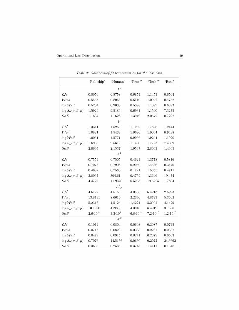
tests based on the comparison of the fitted distribution and the empiricaldistribution (the so-called EDF-based tests). In this paper, we focus onthe last testing procedure, because it allows us to compare separately thefits of the distributions around the center and around the tails of the data.

First, we compare the magnitudes of several EDF test statistics betweendifferent models. A lower test statistic value indicates a better fit (in thesense that the value of the norm, which is based on the distance betweenthe fitted and empirical cdf’s, is smaller). Second, we compare the p-values based on the EDF tests. p-values indicate the proportion of times inwhich the samples drawn from the same fitted distributions have a higherstatistic value. In other words, a higher p-value suggests a better fit. Thefollowing test statistics are considered: Kolmogorov-Smirnov (D), Kuiper(V ), quadratic Anderson-Darling (A2), quadratic “upper tail” Anderson-Darling (A2

up) and Cramer-von Mises (W 2), computed as

D = max{D+, D−}

,

V = D+ + D−,

A2 = n

∫ ∞

−∞

(Fn(x)− F (x))2

F (x)(1− F (x))dF (x),

A2up = n

∫ ∞

−∞

(Fn(x)− F (x))2

(1− F (x))2dF (x),

W 2 = n

∫ ∞

−∞(Fn(x)− F (x))2dF (x),

where D+ =√

n supx{Fn(x)−F (x)} and D− =√

n supx{F (x)−Fn(x)}.The A2

up statistic was introduced and studied in [9], and designed to putmost of the weight on the upper tail. Fn(x) is the empirical cdf, and F (x)is defined as

F (x) =

Fγ(x)−Fγ(u)

1−Fγ(u)x > u

0 x ≤ u.

Table 36 demonstrates that on the basis of the statistic values we wouldtend to conclude that Logweibull, Weibull or Lognormal densities describebest the dispersion of the operational loss data: the statistics are the lowestfor these models in most cases. However, if we wish to test the null thata given dataset belongs to a family of distributions (such as Lognormal or

6The fit of the exponential distribution is totally unsatisfactory and the results havebeen omitted for saving space.


Table 3: Goodness-of-fit test statistics for the loss data.

“Rel.-ship” “Human” “Proc.” “Tech.” “Ext.”

D

LN 0.8056 0.8758 0.6854 1.1453 0.6504

Weib 0.5553 0.8065 0.6110 1.0922 0.4752

logWeib 0.5284 0.9030 0.5398 1.1099 0.6893

log Sα(σ, β, µ) 1.5929 9.5186 0.6931 1.1540 7.3275

SαS 1.1634 1.1628 1.3949 2.0672 0.7222

V

LN 1.3341 1.5265 1.1262 1.7896 1.2144

Weib 1.0821 1.5439 1.0620 1.9004 0.9498

logWeib 1.0061 1.5771 0.9966 1.9244 1.1020

log Sα(σ, β, µ) 1.6930 9.5619 1.1490 1.7793 7.4089

SαS 2.0695 2.1537 1.9537 2.8003 1.4305

A2

LN 0.7554 0.7505 0.4624 1.3778 0.5816

Weib 0.7073 0.7908 0.2069 1.4536 0.3470

logWeib 0.4682 0.7560 0.1721 1.5355 0.4711

log Sα(σ, β, µ) 3.8067 304.61 0.4759 1.3646 194.74

SαS 4.4723 11.9320 6.5235 19.6225 1.7804

A2up

LN 4.6122 4.5160 4.0556 6.4213 2.5993

Weib 13.8191 8.6610 2.2340 4.8723 5.3662

logWeib 5.2316 4.5125 1.4221 5.2992 4.1429

log Sα(σ, β, µ) 10.1990 4198.9 4.0910 6.4919 3132.6

SαS 2.6·1014 3.3·1011 6.8·1014 7.2·1010 1.2·1010

W 2

LN 0.1012 0.0804 0.0603 0.2087 0.0745

Weib 0.0716 0.0823 0.0338 0.2281 0.0337

logWeib 0.0479 0.0915 0.0241 0.2379 0.0563

log Sα(σ, β, µ) 0.7076 44.5156 0.0660 0.2072 24.3662

SαS 0.3630 0.2535 0.3748 1.4411 0.1348


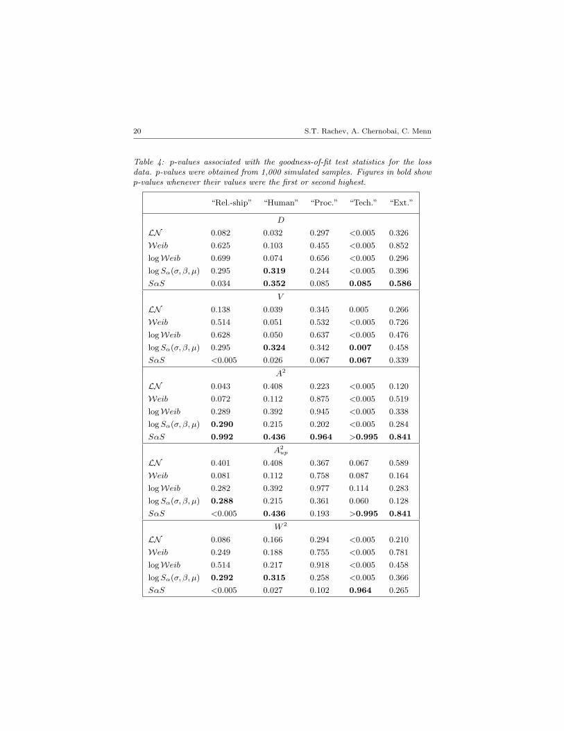
Table 4: p-values associated with the goodness-of-fit test statistics for the lossdata. p-values were obtained from 1,000 simulated samples. Figures in bold showp-values whenever their values were the first or second highest.

“Rel.-ship” “Human” “Proc.” “Tech.” “Ext.”

D

LN 0.082 0.032 0.297 <0.005 0.326

Weib 0.625 0.103 0.455 <0.005 0.852

logWeib 0.699 0.074 0.656 <0.005 0.296

log Sα(σ, β, µ) 0.295 0.319 0.244 <0.005 0.396

SαS 0.034 0.352 0.085 0.085 0.586

V

LN 0.138 0.039 0.345 0.005 0.266

Weib 0.514 0.051 0.532 <0.005 0.726

logWeib 0.628 0.050 0.637 <0.005 0.476

log Sα(σ, β, µ) 0.295 0.324 0.342 0.007 0.458

SαS <0.005 0.026 0.067 0.067 0.339

A2

LN 0.043 0.408 0.223 <0.005 0.120

Weib 0.072 0.112 0.875 <0.005 0.519

logWeib 0.289 0.392 0.945 <0.005 0.338

log Sα(σ, β, µ) 0.290 0.215 0.202 <0.005 0.284

SαS 0.992 0.436 0.964 >0.995 0.841

A2up

LN 0.401 0.408 0.367 0.067 0.589

Weib 0.081 0.112 0.758 0.087 0.164

logWeib 0.282 0.392 0.977 0.114 0.283

log Sα(σ, β, µ) 0.288 0.215 0.361 0.060 0.128

SαS <0.005 0.436 0.193 >0.995 0.841

W 2

LN 0.086 0.166 0.294 <0.005 0.210

Weib 0.249 0.188 0.755 <0.005 0.781

logWeib 0.514 0.217 0.918 <0.005 0.458

log Sα(σ, β, µ) 0.292 0.315 0.258 <0.005 0.366

SαS <0.005 0.027 0.102 0.964 0.265


Stable), then the test is not parameter-free, and we need to estimate thep-values for each hypothetical scenario. These results are demonstratedin Table 4. Now the situation is quite different from the one in Table 3.The numbers in bold indicate the cases in which log Sα(σ, β, µ) or SαS fitresulted in first or second highest p-values across the same group (i.e. forthe same type of EDF test for a range of distributions, with a particulardataset). As is clear from the table, in the majority of cases (17 out of 25)either log Sα(σ, β, µ) or SαS, or even both, resulted in the highest p-values.This supports the conjecture that the overall distribution of operationallosses7 are heavy-tailed. Fitting log Sα(σ, β, µ) or SαS distributions to thedata appears a valid solution.

7 Summary

The objective of this paper was to examine the models underlying in theoperational risk process. The conjecture that operational losses follow acompound Cox process was investigated for the external operational lossdata of five loss types covering a 23 year period. The results of the empir-ical analysis provide evidence of heavy tailedness of the data in the righttail. Moreover, fitting log Sα(σ, β, µ) distribution to the loss severity dataor symmetric Sα(σ, β, µ) distribution to the symmetrized data resulted inhigh p-values in a number of goodness of fit tests, suggesting a good fit.In particular, the two distributions are shown to fit the data very wellin the upper tail, which remains the central concern in the framework ofoperational risk modeling and regulation.

Furthermore, the paper suggested a number of models for the frequencyof losses. A simple Poisson process with a fixed intensity factor appearstoo restrictive and unrealistic. A non-homogeneous Poisson process witha time-varying intensity function was fitted to the loss data and showed asuperior fit to the homogeneous Poisson process.

Directions for future research include developing robust models for theoperational risk modeling. For example, with Sα(σ, β, µ) distributions, forthe case when the shape parameter α is below or equal to unity, the firstmoment (and hence the mean) and the second moment (hence the variance)do not exist, making such distribution difficult to use for practical purposes.Possible solutions would include working with trimmed data, truncateddata, or ‘Winsorized’ data, or splitting the dataset into two parts - the low-

7Another approach would be to split each data set into two parts: the main body ofthe data and the right tail. Some empirical evidence suggests that the two parts of thedata follow different laws. Extreme Value Theory is an approach that can be used forsuch analysis.


and medium-size losses and the tail losses - and analyzing the properties ofeach separately.

8 Acknowledgements

We are thankful to S. Stoyanov of the FinAnalytica Inc. for computationalassistance. We are also grateful to S. Truck for providing us with the dataon which the empirical study was based.

C. Menn is grateful for research support provided by the GermanAcademic Exchange Service (DAAD).

S.T. Rachev gratefully acknowledges research support by grants fromDivision of Mathematical, Life and Physical Sciences, College of Lettersand Science, University of California, Santa Barbara, the German ResearchFoundation (DFG) and the German Academic Exchange Service (DAAD).

References

[1] V. E. Bening and V. Y. Korolev. Generalized Poisson Models andtheir Applications in Insurance and Finance. VSP International Sci-ence Publishers, Utrecht, Boston, 2002.

[2] BIS. Operational risk management. http://www.bis.org, 1998.

[3] BIS. Consultative document: operational risk. http://www.bis.org,2001.

[4] BIS. Working paper on the regulatory treatment of operational risk.http://www.bis.org, 2001.

[5] BIS. The 2002 loss data collection exercise for operational risk: sum-mary of the data collected. http://www.bis.org, 2003.

[6] BIS. International convergence of capital measurement and capitalstandards. http://www.bis.org, 2004.

[7] A. Chernobai, C. Menn, S. T. Rachev, and S. Truck. Estimation ofoperational value-at-risk in the presence of minimum collection thresh-olds. Technical report, Department of Statistics and Applied Proba-bility, University of California Santa Barbara, 2005.

[8] A. Chernobai, C. Menn, S. Truck, and S. Rachev. A note on theestimation of the frequency and severity distribution of operationallosses. Mathematical Scientist, 30(2), 2005.

http://www.bis.org

http://www.bis.org

http://www.bis.org

http://www.bis.org

http://www.bis.org


[9] A. Chernobai, S. Rachev, and F. Fabozzi. Composite goodness-of-fittests for left-truncated loss samples. Technical report, Departmentof Statistics and Applied Probability, University of California SantaBarbara, 2005.

[10] P. Embrechts, C. Kluppelberg, and T. Mikosch. Modeling ExtremalEvents for Insurance and Finance. Springer-Verlag, Berlin, 1997.

[11] P. Jorion. Value-at-Risk: the New Benchmark for Managing FinancialRisk. McGraw-Hill, New York, second edition, 2000.

[12] M. Moscadelli, A. Chernobai, and S. T. Rachev. Treatment of missingdata in the field of operational risk: Effects on parameter estimates,EL, UL and CVaR measures. Operational Risk, June 2005.

[13] S. T. Rachev and S. Mittnik. Stable Paretian Models in Finance.John Wiley & Sons, New York, 2000.

[14] G. Samorodnitsky and M. S. Taqqu. Stable Non-Gaussian RandomProcesses. Stochastic Models with Infinite Variance. Chapman & Hall,London, 1994.

[15] V. M. Zolotarev. One-dimensional Stable Distributions. Translationsof Mathematical Monographs, vol. 65. American Mathematical Soci-ety, Providence, 1986.

Documents

Empirical Examination of Operational Loss Distribu- tions · Empirical Examination of Operational Loss Distribu-tions Svetlozar T. Rachev Institut fu¨r Statistik und Mathematische