Embed Size (px)
Citation preview

Logistics Research (2017) 10:1DOI 10.23773/2017_1
Empirical Lateral-Force-Model for Forklift Tires
Received: 22 March 2016 / Accepted: 21 March 2017 / Published online: 19 September 2017 © The Author(s) 2017 This article is published with Open Access at www.bvl.de/lore
Abstract Operational safety is the major aspect of acounterbalanced forklift’s design. A new test was in-
troduced with the standard DIN EN 16203 to test thelateral dynamic safety of forklifts. The measurementsinvolve high costs and effort to achieve reproducible re-
sults. Multibody simulations (MBS) are conducted tofacilitate the design of safety systems and understandthe safety limits of an industrial truck. An adequate tiremodel is an essential part of such simulation. A new
approach to forklift tire modeling is presented in thispaper. It involves measuring several common industrialtires on a drum tire testing apparatus and using them
to parametrize the tire model. The SUPREM model(German: Superelastisches Reifenmodell) uses a math-ematical modeling approach to describe lateral force
and lateral tire deformation based on wheel load, slipangle, slip rate, and driving velocity. For this easy-to-use model, 8 parameters are estimated from tire mea-surements for different tire types. Better tire approxi-mation leads to more accurate multibody simulationsand a deeper understanding of the dynamic behavior offorklifts. Better vehicle lateral stability can be achievedif the outcomes are considered in the design process ofa forklift. With this model highly dynamic multibodyforklift simulations according to DIN EN 16203 can becarried out.
Keywords Tires · Modeling · Multibody Simulation ·Lateral Force · Lateral Stability
1 Necessity of the multibody simulation
The dynamic stability plays a crucial role in the opera-tion of a forklift. It is determined by the geometrical di-mensions, the tire characteristics and the position of the
overall center of gravity. The tire performance deter-mines whether a vehicle tilts or slides into a sharp turn.To improve the dynamic stability and prevent forkliftsfrom tilting active systems such as Toyota’s “SAS” and
Jungheinrich’s “Curve Control” are used. In order toensure that a forklift truck is sufficiently safe to oper-ate, it is very important to have exact knowledge of the
dynamic properties of the tire.
Many attempts have been carried out to describethe dynamic stability quantitatively (see [4], [15] and
[16]). The standard DIN ISO 22915-2 describes simpletests for measuring the static and dynamic stabilitieson a tilting platform. The data on the behavior of a
vehicle in a bend can be deduced from the lateral tiltangle. The standard DIN EN 16203 has been developedto reach a definite conclusion regarding forklift dynamic
stability and to assess the influence of the active stabil-ity systems. The standard describes a course in whichan L-shaped sharp turn is made at full speed. The nec-essary width of the exit corridor for this maneuver isused as the benchmark.
The conduct of an L-test poses many difficulties.A particular challenge is posed by the technical effortneeded to achieve reproducible results. To reduce theexperimental effort required for new forklift prototypes,multibody simulations in which dynamic stability is as-sessed are carried out. A tire model is needed for amultibody simulation to be meaningful. Many numer-ical tire models represent the behavior of pneumatictires, for example, UA Tire Model [11] and Pacejka’s”Magic Formula” [20]. Many models are commercially
Original Article
Sergey [email protected]
Rainer Bruns
Konstantin Krivenkov
Sergey Stepanyuk1 | Rainer Bruns1 | Konstantin Krivenkov1
1 Professorship of Machine Elements and Technical Logistics Helmut Schmidt Universität, Holstenhofweg 85, 22043 Hamburg, Germany
2
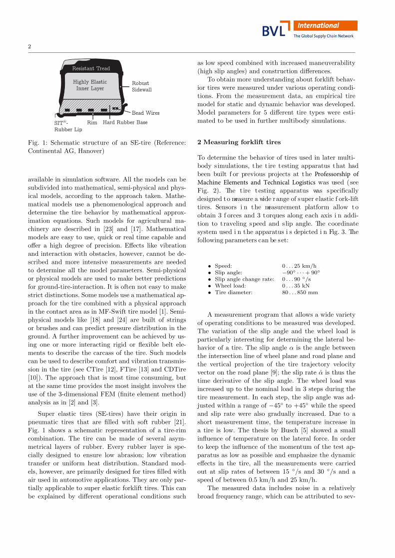
Resistant Tread
Highly ElasticInner Layer
RobustSidewall
Bead Wires
Hard Rubber BaseRimSIT -®
Rubber Lip
Fig. 1: Schematic structure of an SE-tire (Reference:Continental AG, Hanover)
available in simulation software. All the models can besubdivided into mathematical, semi-physical and phys-ical models, according to the approach taken. Mathe-matical models use a phenomenological approach anddetermine the tire behavior by mathematical approx-imation equations. Such models for agricultural ma-chinery are described in [23] and [17]. Mathematical
models are easy to use, quick or real time capable andoffer a high degree of precision. Effects like vibrationand interaction with obstacles, however, cannot be de-scribed and more intensive measurements are needed
to determine all the model parameters. Semi-physicalor physical models are used to make better predictionsfor ground-tire-interaction. It is often not easy to make
strict distinctions. Some models use a mathematical ap-proach for the tire combined with a physical approachin the contact area as in MF-Swift tire model [1]. Semi-physical models like [18] and [24] are built of strings
or brushes and can predict pressure distribution in theground. A further improvement can be achieved by us-ing one or more interacting rigid or flexible belt ele-
ments to describe the carcass of the tire. Such modelscan be used to describe comfort and vibration transmis-sion in the tire (see CTire [12], FTire [13] and CDTire[10]). The approach that is most time consuming, butat the same time provides the most insight involves theuse of the 3-dimensional FEM (finite element method)analysis as in [2] and [3].
Super elastic tires (SE-tires) have their origin inpneumatic tires that are filled with soft rubber [21].Fig. 1 shows a schematic representation of a tire-rimcombination. The tire can be made of several asym-metrical layers of rubber. Every rubber layer is spe-cially designed to ensure low abrasion; low vibrationtransfer or uniform heat distribution. Standard mod-els, however, are primarily designed for tires filled withair used in automotive applications. They are only par-tially applicable to super elastic forklift tires. This canbe explained by different operational conditions such
as low speed combined with increased maneuverability(high slip angles) and construction differences.
To obtain more understanding about forklift behav-ior tires were measured under various operating condi-tions. From the measurement data, an empirical tiremodel for static and dynamic behavior was developed.Model parameters for 5 different tire types were esti-mated to be used in further multibody simulations.
2 Measuring forklift tires
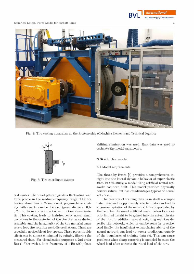
To determine the behavior of tires used in later multi-body s imulations, the t ire testing apparatus that hadbeen built f or previous projects at the Professorship of Machine Elements and Technical Logistics was used (see Fig. 2). The t ire testing apparatus was specifically
designed to measure a wide range of super elastic f ork-lifttires. Sensors i n the measurement platform allow to
obtain 3 f orces and 3 torques along each axis i n addi-tion to traveling speed and s lip angle. The coordinatesystem used i n the apparatus i s depicted i n Fig. 3. Thefollowing parameters can be set:
• Speed: 0 . . . 25 km/h• Slip angle: −90◦ · · · + 90◦
• Slip angle change rate: 0 . . . 90 ◦/s• Wheel load: 0 . . . 35 kN• Tire diameter: 80 . . . 850 mm
A measurement program that allows a wide varietyof operating conditions to be measured was developed.
The variation of the slip angle and the wheel load isparticularly interesting for determining the lateral be-havior of a tire. The slip angle α is the angle betweenthe intersection line of wheel plane and road plane andthe vertical projection of the tire trajectory velocityvector on the road plane [9]; the slip rate α is thus thetime derivative of the slip angle. The wheel load wasincreased up to the nominal load in 3 steps during thetire measurement. In each step, the slip angle was ad-justed within a range of −45◦ to +45◦ while the speedand slip rate were also gradually increased. Due to ashort measurement time, the temperature increase ina tire is low. The thesis by Busch [5] showed a small
influence of temperature on the lateral force. In orderto keep the influence of the momentum of the test ap-paratus as low as possible and emphasize the dynamiceffects in the tire, all the measurements were carriedout at slip rates of between 15 ◦/s and 30 ◦/s and aspeed of between 0.5 km/h and 25 km/h.
The measured data includes noise in a relativelybroad frequency range, which can be attributed to sev-
Empirical Lateral-Force-Model for Forklift Tires 3
Fig. 2: Tire testing apparatus at the Professorship of Machine Elements and Technical Logistics
Fig. 3: Tire coordinate system
eral causes. The tread pattern yields a fluctuating loadforce profile in the medium-frequency range. The tiretesting drum has a 2-component polyurethane coat-ing with quartz sand embedded (grain diameter 0,4-0,7 mm) to reproduce the tarmac friction characteris-tic. This coating leads to high-frequency noise. Smalldeviations in the centering of the tire that arise duringassembly and the irregularity of the tire material cause
severe low, tire-rotation-periodic oscillations. These areespecially noticeable at low speeds. These parasitic sideeffects can be almost eliminated by suitably filtering themeasured data. For visualization purposes a 2nd orderBessel filter with a limit frequency of 1 Hz with phase
shifting elimination was used. Raw data was used toestimate the model parameters.
3 Static tire model
3.1 Model requirements
The thesis by Busch [5] provides a comprehensive in-sight into the lateral dynamic behavior of super elastictires. In this study, a model using artificial neural net-works has been built. This model provides physicallycorrect values, but has disadvantages typical of neuralnetworks.
The creation of training data is in itself a compli-cated task and inopportunely selected data can lead toan over-adaptation of the network. It is compounded bythe fact that the use of artificial neural networks allowsonly limited insight to be gained into the actual physicsof the tire. In addition, several weighting matrices de-scribe the network, which is cumbersome in practice.And finally, the insufficient extrapolating ability of theneural network can lead to wrong predictions outsideof the boundaries of training data set. This can cause
problems when sharp cornering is modeled because thewheel load often exceeds the rated load of the tire.

4
For these reasons, an empirical approach was adoptedfor the Super Elastic Tire Model (SUPREM). TheSUPREM allows a high approximation quality to beachieved with a minimum of tests. At the same time,the model allows a deeper insight to be gained intothe behavior of the tire. Unlike a theoretical model(for example involving the use of an FEM calculation)the amount of computational work required should staylow.
The following objectives were pursued during thecreation of the model:
– The model must be valid for different types of SE-tires without the model structure being changed.
– The model should be easy to implement.– The number of input variables and parameters should
be kept low.– The model should be applicable to other types of
tires.– The effort required to parametrize the model using
the measured data should be low.
3.2 Static behavior of tires
Fig. 5 shows the typical lateral force behavior of an
SE-tire. The main factors are the slip angle α and thewheel load FZ which both have an impact on the lateralforce. The lateral force increases with higher wheel load,
while with higher slip angle the lateral force convergestowards a constant value.
2 4 6 8 100.6
0.7
0.8
0.9
1
Wheel Load in kN
Late
ral
Fri
ctio
nC
oeffi
cien
t
Fig. 4: Quasi-static lateral friction coefficient (Refer-ence: [5]) (Tire: 18x7-8; α = 45◦; v = 12 km/h); ratedload capacity 16180 N
If the slip rate is low, no hysteresis should form andthe graph passes through the graph origin. This be-
havior can be described as stationary and be approx-imated by a hyperbolic tangent function. It is origin-symmetrical and runs for rising angles to +1 or −1.The argument of the hyperbolic tangent function de-scribes the slope of the curve at the graph origin andhence the ”speed” at which the function reaches its finalvalue.
The function argument is affected by the slip angleand the wheel load. Larger slip angles lead to a higherlateral force that converges for high slip angle values. Ahigher wheel load causes higher maximum lateral forces,but reduces the influence of the slip angle on the overalllateral force. When the load on the wheels is higher, thestiffness of the materials used in such wheels increases,resulting in higher rotational stiffness. Increasing rota-tional stiffness leads to a deterioration in lateral forcetransmission at small slip angles. These observationslead to the following approach for describing the lat-eral force:
FY,stat = FZ · µ · tanh
(α
kα + kF2 · FZ
). (1)
FZ is the wheel load, µ is the coefficient of lateral fric-tion and kα and kF2 are parameters available for the
approximation of the model to the measured data. Pa-rameters kα and kF2 define load-independent and load-dependent parts of the normalization term and adjust
the influence of the slip angle on the lateral force.
Fig. 4 shows the quasi-static lateral friction coeffi-cient that was determined by measurement. The slip
angle α is set at 45◦. At this setup the maximum lat-eral force can be achieved. The wheel load was adjustedin 300 N steps up to 10 kN. Higher wheel loads could
not be measured due to high heat development in thetire. When the loads are low, lateral friction coefficientshows a nearly linear dependence. When the loads arehigher, especially when they are above the rated loadof the tire (rated wheel load of 18x7-8 tire is 16180 N),the linear approximation leads to incorrect results beingobtained because the modeled friction tends to zero and
can also become negative. This happens under forklifttruck safety test conditions where the wheel load canexceed twice the rated wheel load.
In further examinations, it was also determined thatthe lateral friction has a wheel load under proportionalbehavior. An approximation of the measured data by anexponential function with an estimated parameter kF1
leads to more accurate results being obtained. Theseobservations lead to the following approach for describ-ing the quasi-static friction coefficient:
µ = µB · exp
(− FZkF1
). (2)

Empirical Lateral-Force-Model for Forklift Tires 5
−50 −40 −30 −20 −10 10 20 30 40 50
−15
−10
−5
5
10
15
Slip Angle in ◦
Lateral Force in kN
Unfiltered
FZ = 4 kN
FZ = 8 kN
FZ = 16 kN
Fig. 5: Lateral force of an SE-tire (Tire: 18x7-8; v = 12 km/h; α = 25 ◦/s)
A standardized floor coating is used in the tire test ap-
paratus. If a ride on another surface is to be simulated,the coefficient of friction µB must be set accordingly.With this addition, the model can be interpreted asfollows:
FY,stat = FZ · µB · exp
(− FZkF1
)·
· tanh
(α
kα + kF2 · FZ
) (3)
4 Dynamic tire model
Damping effects arise during a dynamic force changein a wheel. They appear in the measured data as ahysteresis, which is approximately symmetrical to thegraph origin and is affected by the speed of the wheeland the temporary change of the lateral force. Such be-havior can be explained theoretically using the stringmodel (String-Type Tire Model) [19]. The tire contactpatch is described as an interconnection of several pre-stressed strings connected to tread elements and hav-ing a certain stiffness. The deformation that takes placedue to the load defines the transmission of lateral force.During a dynamic force change the transmission char-
acteristics of the string model can be approximated bya PT1 transfer behavior. In [22], examinations were car-
ried out on tractor tires and the results were found to
be consistent with PT1 transfer function behavior.
The entire tire model can be represented as a seriesconnection of a static non-linearity and a linear trans-mission function. Models like these are called Hammer-stein models and are a simplification of the Volterra se-
ries [14]. The general equation for the dynamic modelcan thus be formulated as follows:
FY,dyn + T · FY,dyn = FY,stat, (4)
where T is the time constant.
Several measurements at different slip rates (α =5 . . . 90 ◦/s) and speeds (v = 0.5 . . . 25 km/h) were car-ried out to verify the assumptions and determine thetime constant. As a benchmark, the value of the hys-teresis was selected when α = 0◦, because at this pointthe change of the lateral force is at its maximum and theslip rate is constant. This leads to the maximal value ofthe hysteresis. Test results can be seen in Figs. 6 and 7.
When the slip rate rises, the width of the hystere-sis increases. Increasing velocity at constant slip rateresults in a narrower hysteresis. The linear relationshipwith the slip rate confirmed a proportional transmissioncharacteristic with a delay of the first order. The timeconstant T , however, is only constant for a given vehiclespeed v. A detailed study at constant wheel load, con-stant slip rate and variable speeds (see Fig. 7) showed

6
0 5 10 15 20 250
2
4
6
Vehicle Speed in km/h
Wid
thof
the
Hyst
eres
isin
kN
Fig. 6: Measured width of the hysteresis at α = 0◦ as afunction of the vehicle speed (Tire: 18x7-8; FZ = 4 kN;α = 25 ◦/s)
0 20 40 60 80 1000
2
4
6
8
Slip Rate in ◦/s
Wid
thof
the
Hyst
eres
isin
kN
Fig. 7: Measured width of the hysteresis at α = 0◦ asa function of the slip rate (Tire: 18x7-8; FZ = 8 kN;v = 15 km/h)
that the time constant can be described by the follow-ing equation:
T = kd · (v · 1 h/km)−kv . (5)
The parameters kd and kv are estimated from mea-sured data. The parameter kv expresses the velocity de-pendence of the time constant. For just one measuredvelocity this parameter is set to 0, and only the constantpart kd is taken into account. A borderline case of this
function occurs at a very slow speed (v → 0). In thatcase, the equation 5 leads to a singularity. In the mea-surement at low velocities very high values of T couldbe calculated. This case is a limitation of the model. Inthe multibody simulation of the forklift, the tire modelis only switched on after a short straight accelerationphase up to a velocity above 0,05 m/s.
The dynamic tire model leads to a more complexcalculation process in the multibody simulation and
could result in instability during a numerical calcula-tion. Especially the need for differentiation may causea simulation to fail due to the occurrence of singular-ities. This can be prevented in many cases by adjust-ing the iteration step width. The static model providesgood stability and accuracy but only by small tempo-rary changes in the lateral force.
An L-test with a complete MBS model was car-ried out to estimate the magnitude of the slip rate.Rapid counter steering results in slip rates of more than50 ◦/s. As shown by a PT1 transfer behavior, the shearforce comes only with a delay, which makes extendedsteering phases necessary. It can therefore be concludedthat only the dynamic tire model should be used to re-alistically assess the dynamic stability.
5 Deformation of the tire
When lateral stress develops, a deformation arises and
leads to a displacement of the contact patch (see Fig. 8).This displacement of the outer wheels increases the ten-dency of a counterbalanced truck to tilt laterally. Thiseffect can be described in the multibody simulation ei-
ther by a displacement of the contact patch or by atilting torque. The torque method was used to sim-plify the implementation. The torque is a product of
the wheel load and the displacement in the y-direction(see Fig. 8). The torque is heavily dependent on thelateral force and is approximated linearly in the model:
MX = FZ ·∆y ≈FYkM
. (6)
The parameter kM is estimated from measured dataand describes this correlation. The torque is set at zerofor the inner wheels. Although the contact patch is
moved, the tilt edge of the vehicle as a whole is notaffected.
6 Influences of rim geometry
The model described has symmetrical lateral force prop-erties. According to measurements, that is not always
the case. The differences in the deformation of the tire,which are dependent on the direction of the slip, couldbe clearly observed during the measurements. The innerflange of the rim supports the tire when lateral stressdevelops and reduces the deformation. As can be de-duced from Fig. 8, significant deformation of the tirecan reduce the contact patch and reduce transmittableforces. This behavior has also been observed in the mea-surement data. The parameter kr is therefore inserted.

Empirical Lateral-Force-Model for Forklift Tires 7
Fig. 8: Tire deformation under lateral force (tire type: 18x7-8)
It maps the dependence of the force on direction:
kr(FY,dyn) =
{1 for FY,dyn < 0kr for FY,dyn ≥ 0
(7)
This factor differs greatly from 1 only in some types
of tires and is a product of distinct asymmetry of therim and the internal tire structure. Thus, the modelis extended by an additional nonlinearity of the linear
transfer function. The following function describes thelateral force in an SE-tire:
FY = kr(FY,dyn) · FY,dyn (8)
and therefore:
kr
(T · FY,dyn + FY,dyn
)=FZ · µB · exp
(− FZkF1
)·
·tanh
(α
kα + kF2 · FZ
) (9)
For time discrete systems with a step size of ∆t it leadsto following equations:
FY,dynn =1
T∆t + 1
[1
krFY,dynn +
T
∆tFY,dynn−1
], (10)
FY,dynn =1
T∆t + 1
[1
krFZ,n · µB · exp
(−FZ,nkF1
)·
·tanh
(αn
kα + kF2 · FZ,n
)+
T
∆tFY,dynn−1
].
(11)
7 Estimation of tire parameters
An optimization algorithm determines all six parame-ters of the model simultaneously from raw data. For
every time step in the measurement file the tire modelis evaluated. Deviations between model and measure-ment of every time step are used to calculate the Mean
Square Error (MSE) which is used as an optimizationfunction. The optimization is achieved with the Gen-eralized Reduced Gradient (GRG), wherein the start-
ing solution must be guessed. The solver minimizes thisfunction to achieve its minimum. At the end of the op-timization the model parameters are obtained at once.Numeric optimization does not always lead to a global
minimum of the function and can stuck in one of localminima. A good guess of the starting solution (modelparameters) can reduce calculation time needed. Al-though prior smoothing or filtering reduces the value ofthe optimization function, the impact on the estimatedparameters is negligible. A comparison of the measure-ment and simulation results can be seen in Fig. 9.
The extrapolation ability of the model was also ex-
amined. The model was not configured with the com-plete data set, but only up to a wheel load correspond-ing to half the rated load. The subsequent extrapola-tion showed a deviation of less than 10 % in the lateralforce. This ensures that even when short extreme loadsare applied in dynamic simulations, extrapolation ac-curacy is sufficient. In order to assess the quality of thetire model, it was necessary to define a quality measurethat corresponded to the coefficient of determinationand was above 99 % for the model described so thatthe model has a high accuracy. The model therefore issuitable for simulative forklift stability tests.

8
−50 −40 −30 −20 −10 10 20 30 40 50
−15
−10
−5
5
10
15
FZ = 4 kN
FZ = 8 kN
FZ = 16 kN
Slip Angle in ◦
Lateral Force in kN
Measurement
Model
Fig. 9: Comparison of the simulation results and the measured data (Tire: 18x7-8; v = 12 km/h; α = 25 ◦/s;
simulation at constant slip rate, measurement starts and stops at α = 0◦)
8 Tire parameters
The lateral behavior of five tire types was measured.Three tires (200/50-10, 150/75-8 and 18x7-8) were ex-
amined according to their dynamic properties at differ-ent speeds. The dynamic time constant of some tiresthat were measured earlier and recycled could only beestimated for a velocity of v = 12 km/h. Parameters of
the static model could be estimated in all cases.
Variations in the inner structure of the tires of dif-ferent manufacturers, tire designs as well as fluctuationsin the temperature and rubber mixture during the pro-
duction can lead to fluctuations of the estimated pa-rameters. One tire came from a different manufacturerand resulted in a very different lateral behavior (see tire18x7-8 Manufacturer 2 in Table 2). Apparently, this tirewas made out of a flexible rubber mixture. Curve fit-ting algorithms can also lead to fluctuations of calcu-lated parameters. Model parameters presented in thispaper may have their validity for a specific tire modelof a specific manufacturer and give a rough correlationbetween geometrical dimensions and estimated parame-ters. A specific tire type of a given manufacturer used ina multibody simulation should be measured. A greatersample size is needed to account for different tire mod-
els of the same type and make a rough prediction of thetire behavior possible.
A wide range of tires was selected for the measure-ment in order to take account of different outer diame-ters, rims, load capacities and widths. Tire types 5.00-8, 18x7-8 and 200/50-10 have nearly the same outer
diameter, but different widths. This helps to estimatethe influence of the tire geometry on the lateral behav-ior. Dimensions of measured tires are summarized in
Table 1 and estimated parameters in Table 2.The rubber layer of the tire transfers forces from the
vehicle to the road. The deformation capability of thislayer influences the tire behavior. To compare different
tires a cross-section-coefficient was defined as:
CSC =Dout −Din
2 ·W. (12)
It takes the width W and the height of the rubberbondage into account (half of the difference betweenthe tire diameter Dout and rim diameter Din).
The parameter kF1 describes the amount of lateralforce that can be transferred when a tire has a givenload. Thin and high tires with higher cross-section-coef-ficients permit greater deformation and can transfermerely lighter forces to the road. According to the mea-surement, a thin 5.00-8 tire can transfer nearly 50 % ofthe force compared to a wider 200/50-10 tire when theyhave a given load. As shown in Fig. 11a, tires with com-
parable cross-section-coefficients tend to have a similarkF1 value.

Empirical Lateral-Force-Model for Forklift Tires 9
Unit 15x4.5-8 5.00-8 18x7-8 150/75-8 200/50-1016x6-8
Type of rim 3.00 D-8 4.33 R-8 6.50 F-10
Width mm 110 126 176 156 196Diameter mm 376 459 454 417 452Rim diameter mm 203 203 203 203 254Tire height mm 86.5 128 125.5 107 99Cross-section
- 0.79 1.02 0.71 0.69 0.51coefficient
Load capacitykg 800 1090 1650 1150 1900
(steer wheel)Load capacity
kg 1040 1415 2145 1455 2470(load wheel)
Table 1: Dimensions and load capacity of industrial tires (DIN 7811-1 [6], DIN 7811-2 [7], DIN 7852 [8])
The reaction of a tire to a slip angle is described bythe parameter kα. A tire type with higher cross-section-coefficients can be deformed more easily along the z-axis and therefore transfer less lateral force at a given
slip angle. Higher values of the parameter kα lead toa smaller argument of the hyperbolic tangent functionand therefore lower lateral force at the given slip angle.Weaker influence of the slip angle (higher values for kα)
in tires with high cross-section-coefficient can be seenin Fig. 11b. The value of this parameter for wide tiresis between 8◦ and 10◦.
The two parameters kα and kF2 are used to normal-
ize the slip angle inside the hyperbolic tangent function.kα normalizes the value of the slip angle by a specificangle. kF2 takes the stiffening effects of the tire loadinto account. The maximal load capacity was chosen as
the reference load for estimating the normalization con-tribution of this term. Measurements show a correlationbetween the normalization terms (see Fig. 10).
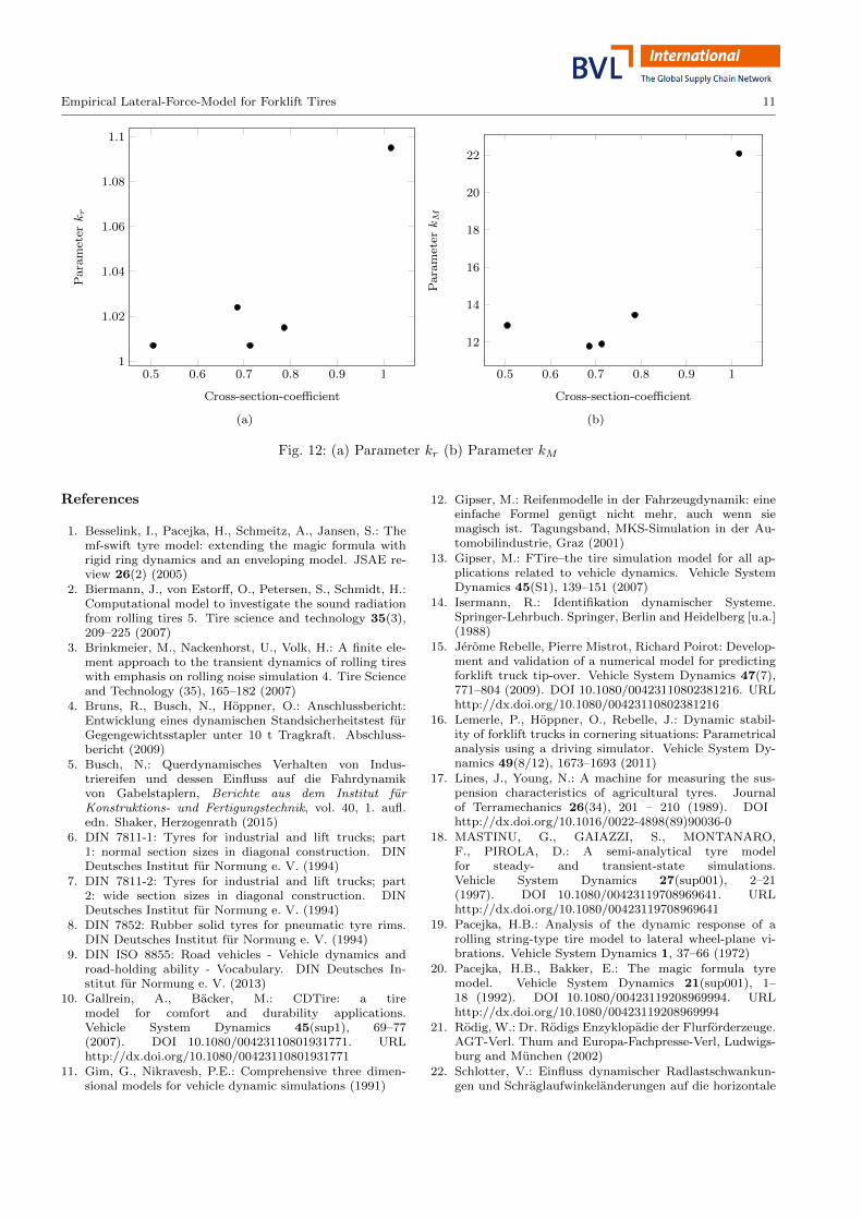
Direction-dependent parameter kr has a value of ap-
proximately 1 for wide tires and is slightly higher fortires with high cross-section-coefficient (see Fig. 12a).
The displacement of the contact area and thereforetorque along the x-axis is described by the linearizedparameter kM . This parameter has a strong correlation
with the cross-section-coefficient (see Fig. 12b). A flatand wide tire is less flexible and therefore better fordynamic vehicle stability.
kv and kd were able to be estimated for dynamicmodel parameters. The time constant T at a speed ofv = 12 km/h was estimated for all the tires. As thecross-section-coefficient lowers, the value of the timeconstant diminishes until it reaches a value near 0.11 s.
Measurements for more different tires are neededto make rough predictions about an unknown tire. Nomeasurements and therefore no assumptions were able
to be made for tires with load capacity above 3,5 t dueto limitations in the measurement apparatus.
8 10 12 14
5
10
15
20
25
Parameter kα in ◦
Contr
ibu
tion
of
wh
eel
load
in◦
Fig. 10: Load-dependent-term (kF2 · FZ,nominal) as afunction of the parameter kα in the normalization term
9 Summary
In this paper, a SUPREM model has been set up forsimulating SE-tires. It describes the transverse dynamic
behavior with high accuracy. The original model, basedon artificial neural networks, can be replaced by theSUPREM model without any loss of quality in approx-imation, but with significantly less complexity and witha potential for further adaptation. SUPREM modelshowed a better approximation quality especially forvery high and very low lateral forces due to neuralnetworks limitations. In the SUPREM model, a tireis described by six parameters only. By virtue of its

10
Para- Unit 15x4.5-8 5.00-8 18x7-8 18x7-8 150/75-8 200/50-10meter Manufacturer 2 Manufacturer 1 16x6-8
kF1 N 31451 25363 30522 50917 49241 55168kα ◦ 10.67 14.84 16.92 9.16 7.90 9.28kr - 1.015 1.095 1.16 1.007 1.024 1.007kF2
◦/N 6.58 · 10−4 1.65 · 10−3 3.44 · 10−4 7.87 · 10−4 1.70 · 10−3 6.58 · 10−4
kM - 13.45 22.09 14.84 11.91 11.79 12.90
kv - - - - 0.39 0.43 0.20kd s - - - 0.28 0.31 0.19Tv=12 km/h s 0.13 0.22 0.22 0.11 0.11 0.12
Table 2: Estimated tire parameters
0.5 0.6 0.7 0.8 0.9 1
30
40
50
Cross-section-coefficient
Para
met
erkF
1in
kN
(a)
0.5 0.6 0.7 0.8 0.9 1
8
10
12
14
Cross-section-coefficient
Para
met
erkα
in◦
(b)
Fig. 11: (a) Parameter kF1 (b) Parameter kα
clear structure, the model can be easily integrated into
many kinds of multibody simulation software withoutthe need for costly additional modules.
When several comparable studies were conductedwith the filtered and unfiltered data, it was found that
the noise had a low impact on the estimated parame-ters.
Further studies have shown that the dynamic be-havior is affected by high slip rates and must be takeninto account during stability simulations. Multiple in-dividual measurements must be carried out at differentspeeds to parametrize the hysteresis. The correlation ofthe slip rate with the width of the hysteresis requiresonly one parameter, so that only one measurement isnecessary. Only one measurement is necessary if a vehi-cle is examined in a simulation in which approximately
constant speeds are used.
Further studies must be conducted to ascertainwhether the model is applicable to other types of tiressuch as portal stacker tires or polymer rollers. The in-fluence of rubber and inner layer design used by differ-
ent manufacturers should be quantified. To validate themultibody simulation with this tire model additionalempirical investigations with a forklift should be car-ried out.
Empirical Lateral-Force-Model for Forklift Tires 11
0.5 0.6 0.7 0.8 0.9 11
1.02
1.04
1.06
1.08
1.1
Cross-section-coefficient
Para
met
erkr
(a)
0.5 0.6 0.7 0.8 0.9 1
12
14
16
18
20
22
Cross-section-coefficient
Para
met
erkM
(b)
Fig. 12: (a) Parameter kr (b) Parameter kM
References
1. Besselink, I., Pacejka, H., Schmeitz, A., Jansen, S.: Themf-swift tyre model: extending the magic formula withrigid ring dynamics and an enveloping model. JSAE re-view 26(2) (2005)
2. Biermann, J., von Estorff, O., Petersen, S., Schmidt, H.:Computational model to investigate the sound radiationfrom rolling tires 5. Tire science and technology 35(3),209–225 (2007)
3. Brinkmeier, M., Nackenhorst, U., Volk, H.: A finite ele-ment approach to the transient dynamics of rolling tireswith emphasis on rolling noise simulation 4. Tire Scienceand Technology (35), 165–182 (2007)
4. Bruns, R., Busch, N., Hoppner, O.: Anschlussbericht:Entwicklung eines dynamischen Standsicherheitstest furGegengewichtsstapler unter 10 t Tragkraft. Abschluss-bericht (2009)
5. Busch, N.: Querdynamisches Verhalten von Indus-triereifen und dessen Einfluss auf die Fahrdynamikvon Gabelstaplern, Berichte aus dem Institut furKonstruktions- und Fertigungstechnik, vol. 40, 1. aufl.edn. Shaker, Herzogenrath (2015)
6. DIN 7811-1: Tyres for industrial and lift trucks; part1: normal section sizes in diagonal construction. DINDeutsches Institut fur Normung e. V. (1994)
7. DIN 7811-2: Tyres for industrial and lift trucks; part2: wide section sizes in diagonal construction. DINDeutsches Institut fur Normung e. V. (1994)
8. DIN 7852: Rubber solid tyres for pneumatic tyre rims.DIN Deutsches Institut fur Normung e. V. (1994)
9. DIN ISO 8855: Road vehicles - Vehicle dynamics androad-holding ability - Vocabulary. DIN Deutsches In-stitut fur Normung e. V. (2013)
10. Gallrein, A., Backer, M.: CDTire: a tiremodel for comfort and durability applications.Vehicle System Dynamics 45(sup1), 69–77(2007). DOI 10.1080/00423110801931771. URLhttp://dx.doi.org/10.1080/00423110801931771
11. Gim, G., Nikravesh, P.E.: Comprehensive three dimen-sional models for vehicle dynamic simulations (1991)
12. Gipser, M.: Reifenmodelle in der Fahrzeugdynamik: eineeinfache Formel genugt nicht mehr, auch wenn siemagisch ist. Tagungsband, MKS-Simulation in der Au-tomobilindustrie, Graz (2001)
13. Gipser, M.: FTire–the tire simulation model for all ap-plications related to vehicle dynamics. Vehicle SystemDynamics 45(S1), 139–151 (2007)
14. Isermann, R.: Identifikation dynamischer Systeme.Springer-Lehrbuch. Springer, Berlin and Heidelberg [u.a.](1988)
15. Jerome Rebelle, Pierre Mistrot, Richard Poirot: Develop-ment and validation of a numerical model for predictingforklift truck tip-over. Vehicle System Dynamics 47(7),771–804 (2009). DOI 10.1080/00423110802381216. URLhttp://dx.doi.org/10.1080/00423110802381216
16. Lemerle, P., Hoppner, O., Rebelle, J.: Dynamic stabil-ity of forklift trucks in cornering situations: Parametricalanalysis using a driving simulator. Vehicle System Dy-namics 49(8/12), 1673–1693 (2011)
17. Lines, J., Young, N.: A machine for measuring the sus-pension characteristics of agricultural tyres. Journalof Terramechanics 26(34), 201 – 210 (1989). DOIhttp://dx.doi.org/10.1016/0022-4898(89)90036-0
18. MASTINU, G., GAIAZZI, S., MONTANARO,F., PIROLA, D.: A semi-analytical tyre modelfor steady- and transient-state simulations.Vehicle System Dynamics 27(sup001), 2–21(1997). DOI 10.1080/00423119708969641. URLhttp://dx.doi.org/10.1080/00423119708969641
19. Pacejka, H.B.: Analysis of the dynamic response of arolling string-type tire model to lateral wheel-plane vi-brations. Vehicle System Dynamics 1, 37–66 (1972)
20. Pacejka, H.B., Bakker, E.: The magic formula tyremodel. Vehicle System Dynamics 21(sup001), 1–18 (1992). DOI 10.1080/00423119208969994. URLhttp://dx.doi.org/10.1080/00423119208969994
21. Rodig, W.: Dr. Rodigs Enzyklopadie der Flurforderzeuge.AGT-Verl. Thum and Europa-Fachpresse-Verl, Ludwigs-burg and Munchen (2002)
22. Schlotter, V.: Einfluss dynamischer Radlastschwankun-gen und Schraglaufwinkelanderungen auf die horizontale

12
Kraftubertragung von Ackerschlepperreifen, Forschungs-bericht Agrartechnik des Arbeitskreises Forschung undLehre der MEG, vol. 437. Shaker, Aachen (2006)
23. Sharon, I.: Untersuchungen uber die Schwingungseigen-schaften großvolumiger Niederdruckreifen. (Forschungs-bericht Agrartechnik des Arbeitskreises Forschung undLehre der MEG [Max-Eyth-Gesellschaft]. Berlin (1975).Berlin, TU, Fachbereich Konstruktion u. Fertigung, Diss.v. 21.2.1975
24. Wang, Y.: Ein Simulationsmodell zum dy-namischen Schraglaufverhalten von Kraft-fahrzeugreifen bei beliebigen Felgenbewegun-gen. Fortschritt-Berichte VDI.: Verkehrstech-nik/Fahrzeugtechnik. VDI-Verlag (1993). URLhttps://books.google.de/books?id=JwpBmwEACAAJ