Embed Size (px)
Citation preview

Learning from Examples
Ravi Kothari Empirical Learning 2 / 35

Learning from Examples
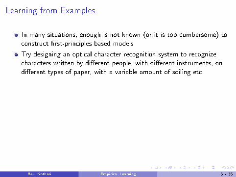
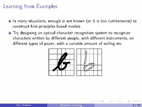
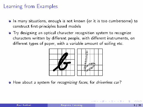
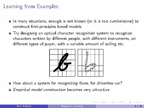
In many situations, enough is not known (or it is too cumbersome) toconstruct �rst-principles based models
Try designing an optical character recognition system to recognizecharacters written by di�erent people, with di�erent instruments, ondi�erent types of paper, with a variable amount of soiling etc.
How about a system for recognizing faces, for driverless car?
Empirical model construction becomes very attractive
Ravi Kothari Empirical Learning 3 / 35
Learning from Examples
In many situations, enough is not known (or it is too cumbersome) toconstruct �rst-principles based models
Try designing an optical character recognition system to recognizecharacters written by di�erent people, with di�erent instruments, ondi�erent types of paper, with a variable amount of soiling etc.
How about a system for recognizing faces, for driverless car?
Empirical model construction becomes very attractive
Ravi Kothari Empirical Learning 3 / 35

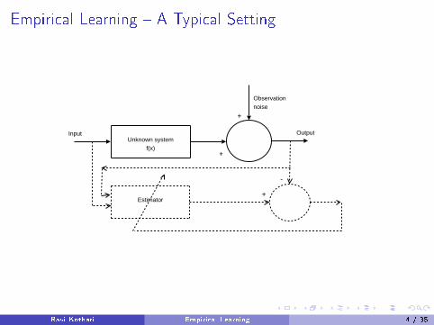
Empirical Learning � A Typical Setting
Unknown systemf(x)
+
+
Observation noise
Input Output
Estimator+
-
Ravi Kothari Empirical Learning 4 / 35
Empirical Learning � A Typical Setting
Unknown systemf(x)
+
+
Observation noise
Input Output
Estimator+
-
Ravi Kothari Empirical Learning 4 / 35

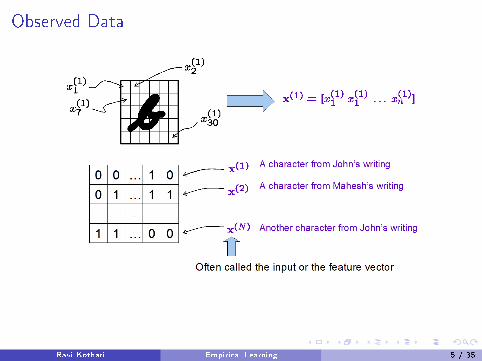
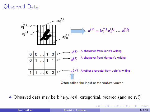
Observed Data
Observed data may be binary, real, categorical, ordered (and noisy!)
Ravi Kothari Empirical Learning 5 / 35
Observed Data
Observed data may be binary, real, categorical, ordered (and noisy!)
Ravi Kothari Empirical Learning 5 / 35
Observed Data
Observed data may be binary, real, categorical, ordered (and noisy!)
Ravi Kothari Empirical Learning 5 / 35

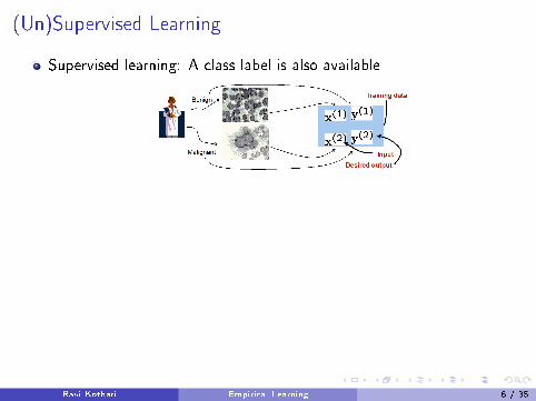
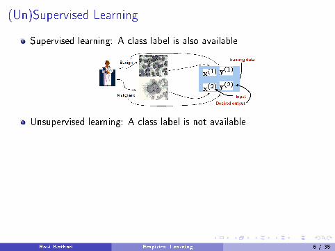
(Un)Supervised Learning
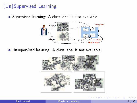
Supervised learning: A class label is also available
Unsupervised learning: A class label is not available
Ravi Kothari Empirical Learning 6 / 35

(Un)Supervised Learning
Supervised learning: A class label is also available
Unsupervised learning: A class label is not available
Ravi Kothari Empirical Learning 6 / 35
(Un)Supervised Learning
Supervised learning: A class label is also available
Unsupervised learning: A class label is not available
Ravi Kothari Empirical Learning 6 / 35
(Un)Supervised Learning
Supervised learning: A class label is also available
Unsupervised learning: A class label is not available
Ravi Kothari Empirical Learning 6 / 35
(Un)Supervised Learning
Supervised learning: A class label is also available
Unsupervised learning: A class label is not available
Ravi Kothari Empirical Learning 6 / 35

Some Learning Scenarios
Determining (credit-card or other types of) fraud
Speaker identi�cation, speech recognition
Drug design and bio-informatics
Driverless cars
Problem determination
Intrusion detection, surveillance
Ravi Kothari Empirical Learning 7 / 35
Some Learning Scenarios
Determining (credit-card or other types of) fraud
Speaker identi�cation, speech recognition
Drug design and bio-informatics
Driverless cars
Problem determination
Intrusion detection, surveillance
Ravi Kothari Empirical Learning 7 / 35
Some Learning Scenarios
Determining (credit-card or other types of) fraud
Speaker identi�cation, speech recognition
Drug design and bio-informatics
Driverless cars
Problem determination
Intrusion detection, surveillance
Ravi Kothari Empirical Learning 7 / 35
Some Learning Scenarios
Determining (credit-card or other types of) fraud
Speaker identi�cation, speech recognition
Drug design and bio-informatics
Driverless cars
Problem determination
Intrusion detection, surveillance
Ravi Kothari Empirical Learning 7 / 35
Some Learning Scenarios
Determining (credit-card or other types of) fraud
Speaker identi�cation, speech recognition
Drug design and bio-informatics
Driverless cars
Problem determination
Intrusion detection, surveillance
Ravi Kothari Empirical Learning 7 / 35
Some Learning Scenarios
Determining (credit-card or other types of) fraud
Speaker identi�cation, speech recognition
Drug design and bio-informatics
Driverless cars
Problem determination
Intrusion detection, surveillance
Ravi Kothari Empirical Learning 7 / 35
Learning � A Formal De�nition
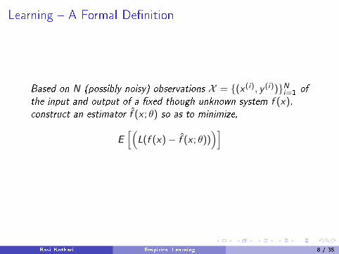
Based on N (possibly noisy) observations X = {(x (i), y (i))}Ni=1 of
the input and output of a �xed though unknown system f (x),construct an estimator f̂ (x ; θ) so as to minimize,
E[(
L(f (x)− f̂ (x ; θ)))]
Ravi Kothari Empirical Learning 8 / 35
Some Loss Functions
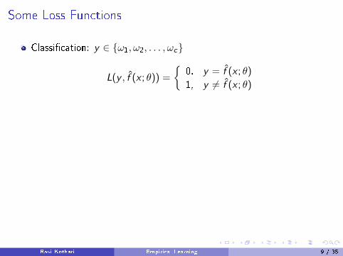
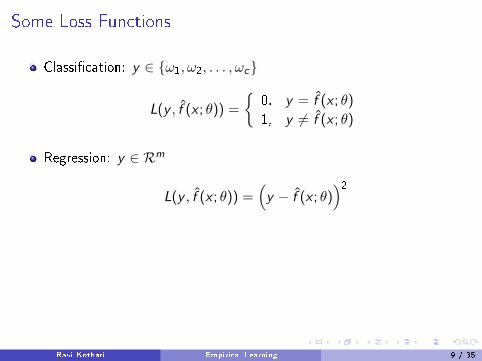
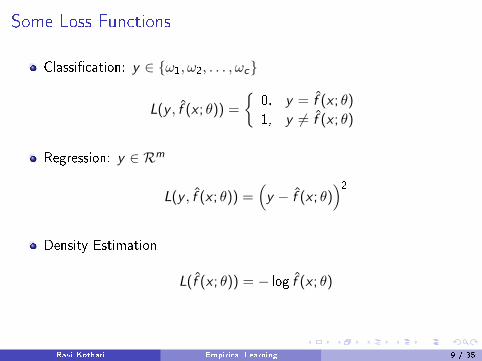
Classi�cation: y ∈ {ω1, ω2, . . . , ωc}
L(y , f̂ (x ; θ)) =
{0, y = f̂ (x ; θ)
1, y 6= f̂ (x ; θ)
Regression: y ∈ Rm
L(y , f̂ (x ; θ)) =(y − f̂ (x ; θ)
)2Density Estimation
L(f̂ (x ; θ)) = − log f̂ (x ; θ)
Ravi Kothari Empirical Learning 9 / 35
Some Loss Functions
Classi�cation: y ∈ {ω1, ω2, . . . , ωc}
L(y , f̂ (x ; θ)) =
{0, y = f̂ (x ; θ)
1, y 6= f̂ (x ; θ)
Regression: y ∈ Rm
L(y , f̂ (x ; θ)) =(y − f̂ (x ; θ)
)2Density Estimation
L(f̂ (x ; θ)) = − log f̂ (x ; θ)
Ravi Kothari Empirical Learning 9 / 35
Some Loss Functions
Classi�cation: y ∈ {ω1, ω2, . . . , ωc}
L(y , f̂ (x ; θ)) =
{0, y = f̂ (x ; θ)
1, y 6= f̂ (x ; θ)
Regression: y ∈ Rm
L(y , f̂ (x ; θ)) =(y − f̂ (x ; θ)
)2
Density Estimation
L(f̂ (x ; θ)) = − log f̂ (x ; θ)
Ravi Kothari Empirical Learning 9 / 35
Some Loss Functions
Classi�cation: y ∈ {ω1, ω2, . . . , ωc}
L(y , f̂ (x ; θ)) =
{0, y = f̂ (x ; θ)
1, y 6= f̂ (x ; θ)
Regression: y ∈ Rm
L(y , f̂ (x ; θ)) =(y − f̂ (x ; θ)
)2Density Estimation
L(f̂ (x ; θ)) = − log f̂ (x ; θ)
Ravi Kothari Empirical Learning 9 / 35

Example: The Bayes Classi�er (1/2)
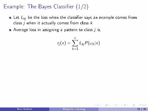
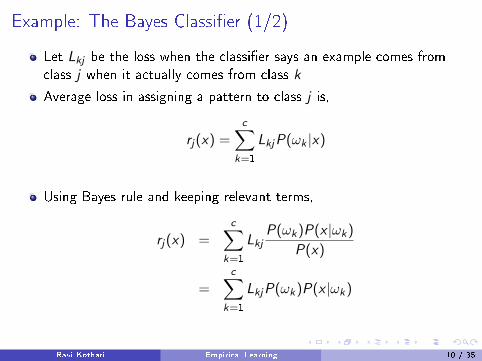
Let Lkj be the loss when the classi�er says an example comes fromclass j when it actually comes from class k
Average loss in assigning a pattern to class j is,
rj(x) =c∑
k=1
LkjP(ωk |x)
Using Bayes rule and keeping relevant terms,
rj(x) =c∑
k=1
LkjP(ωk)P(x |ωk)
P(x)
=c∑
k=1
LkjP(ωk)P(x |ωk)
Ravi Kothari Empirical Learning 10 / 35
Example: The Bayes Classi�er (1/2)
Let Lkj be the loss when the classi�er says an example comes fromclass j when it actually comes from class k
Average loss in assigning a pattern to class j is,
rj(x) =c∑
k=1
LkjP(ωk |x)
Using Bayes rule and keeping relevant terms,
rj(x) =c∑
k=1
LkjP(ωk)P(x |ωk)
P(x)
=c∑
k=1
LkjP(ωk)P(x |ωk)
Ravi Kothari Empirical Learning 10 / 35
Example: The Bayes Classi�er (2/2)
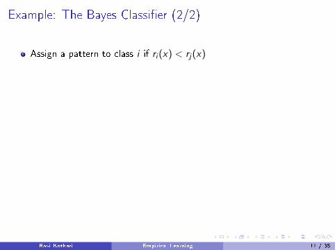
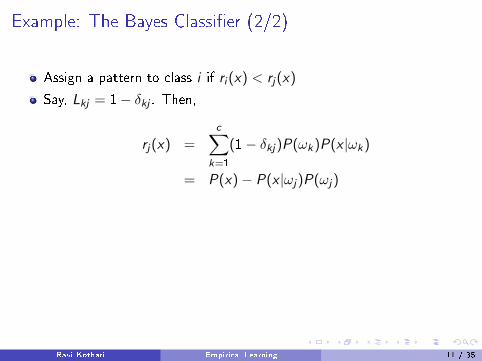
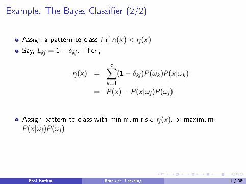
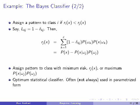
Assign a pattern to class i if ri (x) < rj(x)
Say, Lkj = 1− δkj . Then,
rj(x) =c∑
k=1
(1− δkj)P(ωk)P(x |ωk)
= P(x)− P(x |ωj)P(ωj)
Assign pattern to class with minimum risk, rj(x), or maximumP(x |ωj)P(ωj)
Optimum statistical classi�er. Often (not always) used in parametrizedform
Ravi Kothari Empirical Learning 11 / 35
Example: The Bayes Classi�er (2/2)
Assign a pattern to class i if ri (x) < rj(x)
Say, Lkj = 1− δkj . Then,
rj(x) =c∑
k=1
(1− δkj)P(ωk)P(x |ωk)
= P(x)− P(x |ωj)P(ωj)
Assign pattern to class with minimum risk, rj(x), or maximumP(x |ωj)P(ωj)
Optimum statistical classi�er. Often (not always) used in parametrizedform
Ravi Kothari Empirical Learning 11 / 35
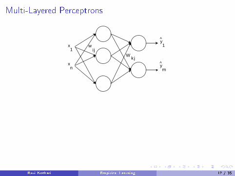
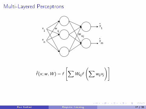
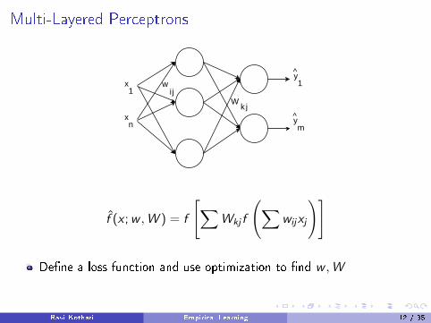
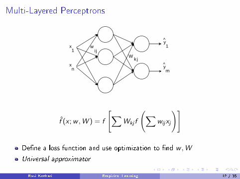
Multi-Layered Perceptrons
wij
Wk j
x1
xn
y1
^
ym
^
f̂ (x ;w ,W ) = f
[∑Wkj f
(∑wijxj
)]
De�ne a loss function and use optimization to �nd w ,W
Universal approximator
Ravi Kothari Empirical Learning 12 / 35
Multi-Layered Perceptrons
wij
Wk j
x1
xn
y1
^
ym
^
f̂ (x ;w ,W ) = f
[∑Wkj f
(∑wijxj
)]
De�ne a loss function and use optimization to �nd w ,W
Universal approximator
Ravi Kothari Empirical Learning 12 / 35
Multi-Layered Perceptrons
wij
Wk j
x1
xn
y1
^
ym
^
f̂ (x ;w ,W ) = f
[∑Wkj f
(∑wijxj
)]
De�ne a loss function and use optimization to �nd w ,W
Universal approximator
Ravi Kothari Empirical Learning 12 / 35
Multi-Layered Perceptrons
wij
Wk j
x1
xn
y1
^
ym
^
f̂ (x ;w ,W ) = f
[∑Wkj f
(∑wijxj
)]
De�ne a loss function and use optimization to �nd w ,W
Universal approximator
Ravi Kothari Empirical Learning 12 / 35
Multi-Layered Perceptrons
wij
Wk j
x1
xn
y1
^
ym
^
f̂ (x ;w ,W ) = f
[∑Wkj f
(∑wijxj
)]
De�ne a loss function and use optimization to �nd w ,W
Universal approximator
Ravi Kothari Empirical Learning 12 / 35

Aspects of Empirical Models
Active learning and focus of attention
Dimensionality reduction, feature selection
Model constructionI Learnability and error rate, scaling, rate of convergenceI Most non-parametric estimators are consistent in the asymptotic
(N →∞) sense
Model validation
Ravi Kothari Empirical Learning 14 / 35

Estimating the Prediction Error (1/2)
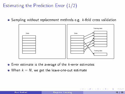
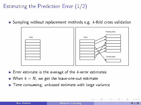
Sampling without replacement methods e.g. k-fold cross validation
Data Data
Training data
Testing data
Error estimate is the average of the k-error estimates
When k = N, we get the leave-one-out estimate
Time consuming, unbiased estimate with large variance
Ravi Kothari Empirical Learning 15 / 35
Estimating the Prediction Error (1/2)
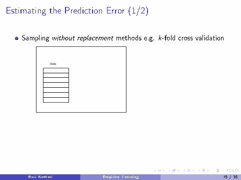
Sampling without replacement methods e.g. k-fold cross validation
Data
Data
Training data
Testing data
Error estimate is the average of the k-error estimates
When k = N, we get the leave-one-out estimate
Time consuming, unbiased estimate with large variance
Ravi Kothari Empirical Learning 15 / 35
Estimating the Prediction Error (1/2)
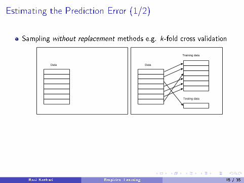
Sampling without replacement methods e.g. k-fold cross validation
Data Data
Training data
Testing data
Error estimate is the average of the k-error estimates
When k = N, we get the leave-one-out estimate
Time consuming, unbiased estimate with large variance
Ravi Kothari Empirical Learning 15 / 35
Estimating the Prediction Error (1/2)
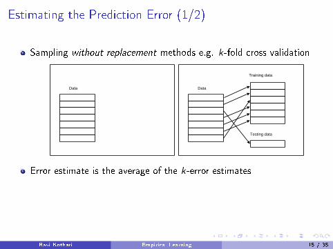
Sampling without replacement methods e.g. k-fold cross validation
Data Data
Training data
Testing data
Error estimate is the average of the k-error estimates
When k = N, we get the leave-one-out estimate
Time consuming, unbiased estimate with large variance
Ravi Kothari Empirical Learning 15 / 35
Estimating the Prediction Error (1/2)
Sampling without replacement methods e.g. k-fold cross validation
Data Data
Training data
Testing data
Error estimate is the average of the k-error estimates
When k = N, we get the leave-one-out estimate
Time consuming, unbiased estimate with large variance
Ravi Kothari Empirical Learning 15 / 35

Estimating the Prediction Error (2/2)
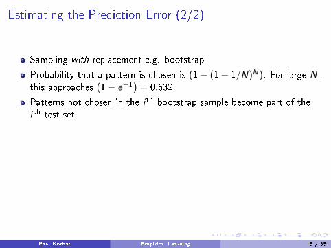
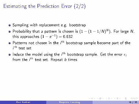
Sampling with replacement e.g. bootstrap
Probability that a pattern is chosen is (1− (1− 1/N)N). For large N,this approaches (1− e−1) = 0.632
Patterns not chosen in the i th bootstrap sample become part of thei th test set
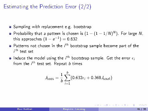
Induce the model using the i th bootstrap sample. Get the error εifrom the i th test set. Repeat b times
Jboot =1
b
b∑i=1
(0.632εi + 0.368Jtotal)
Ravi Kothari Empirical Learning 16 / 35
Estimating the Prediction Error (2/2)
Sampling with replacement e.g. bootstrap
Probability that a pattern is chosen is (1− (1− 1/N)N). For large N,this approaches (1− e−1) = 0.632
Patterns not chosen in the i th bootstrap sample become part of thei th test set
Induce the model using the i th bootstrap sample. Get the error εifrom the i th test set. Repeat b times
Jboot =1
b
b∑i=1
(0.632εi + 0.368Jtotal)
Ravi Kothari Empirical Learning 16 / 35

Average Case Analysis � The Bias-VarianceDecomposition
Ravi Kothari Empirical Learning 17 / 35
Optimal Response of an Estimator
y = f (x) + ε. So, the y obtained corresponding to t repeatedobservations of x are y(1), y(2), . . . , y(t)
What should the optimal estimator f̂ ∗(x ; θ) respond with?
J =(f̂ ∗(x ; θ)− y(1)
)2+(f̂ ∗(x ; θ)− y(2)
)2+
. . .+(f̂ ∗(x ; θ)− y(t)
)2Minimum of J is achieved when f̂ ∗(x ; θ) = (y(1), y(2), . . . , y(t))/t,i.e. E [y |x ]
Ravi Kothari Empirical Learning 18 / 35
Optimal Response of an Estimator
y = f (x) + ε. So, the y obtained corresponding to t repeatedobservations of x are y(1), y(2), . . . , y(t)
What should the optimal estimator f̂ ∗(x ; θ) respond with?
J =(f̂ ∗(x ; θ)− y(1)
)2+(f̂ ∗(x ; θ)− y(2)
)2+
. . .+(f̂ ∗(x ; θ)− y(t)
)2
Minimum of J is achieved when f̂ ∗(x ; θ) = (y(1), y(2), . . . , y(t))/t,i.e. E [y |x ]
Ravi Kothari Empirical Learning 18 / 35
Optimal Response of an Estimator
y = f (x) + ε. So, the y obtained corresponding to t repeatedobservations of x are y(1), y(2), . . . , y(t)
What should the optimal estimator f̂ ∗(x ; θ) respond with?
J =(f̂ ∗(x ; θ)− y(1)
)2+(f̂ ∗(x ; θ)− y(2)
)2+
. . .+(f̂ ∗(x ; θ)− y(t)
)2Minimum of J is achieved when f̂ ∗(x ; θ) = (y(1), y(2), . . . , y(t))/t,i.e. E [y |x ]
Ravi Kothari Empirical Learning 18 / 35
The Bias-Variance Decomposition
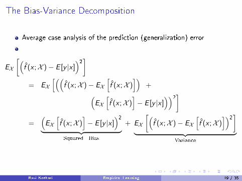
Average case analysis of the prediction (generalization) error
EX
[(f̂ (x ;X )− E [y |x ]
)2]= EX
[((f̂ (x ;X )− EX
[f̂ (x ;X )
])+(
EX
[f̂ (x ;X )
]− E [y |x ]
))2]=
(EX
[f̂ (x ;X )
]− E [y |x ]
)2︸ ︷︷ ︸
Squared Bias
+ EX
[(f̂ (x ;X )− EX
[f̂ (x ;X )
])2]︸ ︷︷ ︸
Variance
Ravi Kothari Empirical Learning 19 / 35
The Bias-Variance Decomposition
Average case analysis of the prediction (generalization) error
EX
[(f̂ (x ;X )− E [y |x ]
)2]= EX
[((f̂ (x ;X )− EX
[f̂ (x ;X )
])+(
EX
[f̂ (x ;X )
]− E [y |x ]
))2]=
(EX
[f̂ (x ;X )
]− E [y |x ]
)2︸ ︷︷ ︸
Squared Bias
+ EX
[(f̂ (x ;X )− EX
[f̂ (x ;X )
])2]︸ ︷︷ ︸
Variance
Ravi Kothari Empirical Learning 19 / 35

Bias
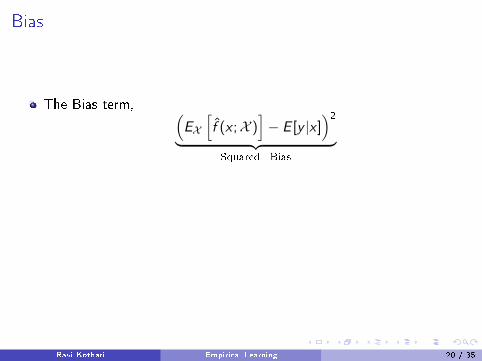
The Bias term, (EX
[f̂ (x ;X )
]− E [y |x ]
)2︸ ︷︷ ︸
Squared Bias
Measures deviation of the averaged estimator output from theaveraged system output
Bias is 0 even when a particular estimator has a large error which iscanceled out by an opposite error generated by another model
Ravi Kothari Empirical Learning 20 / 35
Bias
The Bias term, (EX
[f̂ (x ;X )
]− E [y |x ]
)2︸ ︷︷ ︸
Squared Bias
Measures deviation of the averaged estimator output from theaveraged system output
Bias is 0 even when a particular estimator has a large error which iscanceled out by an opposite error generated by another model
Ravi Kothari Empirical Learning 20 / 35

Variance
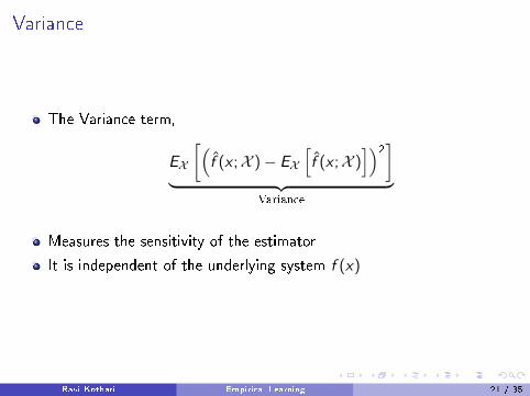
The Variance term,
EX
[(f̂ (x ;X )− EX
[f̂ (x ;X )
])2]︸ ︷︷ ︸
Variance
Measures the sensitivity of the estimator
It is independent of the underlying system f (x)
Ravi Kothari Empirical Learning 21 / 35
Variance
The Variance term,
EX
[(f̂ (x ;X )− EX
[f̂ (x ;X )
])2]︸ ︷︷ ︸
Variance
Measures the sensitivity of the estimator
It is independent of the underlying system f (x)
Ravi Kothari Empirical Learning 21 / 35
Variance
The Variance term,
EX
[(f̂ (x ;X )− EX
[f̂ (x ;X )
])2]︸ ︷︷ ︸
Variance
Measures the sensitivity of the estimator
It is independent of the underlying system f (x)
Ravi Kothari Empirical Learning 21 / 35
Variance
The Variance term,
EX
[(f̂ (x ;X )− EX
[f̂ (x ;X )
])2]︸ ︷︷ ︸
Variance
Measures the sensitivity of the estimator
It is independent of the underlying system f (x)
Ravi Kothari Empirical Learning 21 / 35

Understanding Bias and Variance
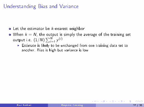
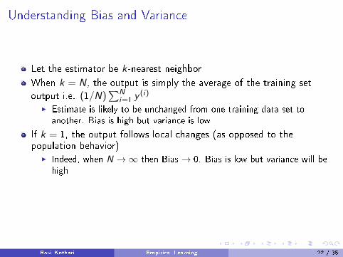
Let the estimator be k-nearest neighbor
When k = N, the output is simply the average of the training set
output i.e. (1/N)∑N
i=1 y(i)
I Estimate is likely to be unchanged from one training data set toanother. Bias is high but variance is low
If k = 1, the output follows local changes (as opposed to thepopulation behavior)
I Indeed, when N →∞ then Bias → 0. Bias is low but variance will behigh
The best solution is usually some intermediate k
Ravi Kothari Empirical Learning 22 / 35
Understanding Bias and Variance
Let the estimator be k-nearest neighbor
When k = N, the output is simply the average of the training set
output i.e. (1/N)∑N
i=1 y(i)
I Estimate is likely to be unchanged from one training data set toanother. Bias is high but variance is low
If k = 1, the output follows local changes (as opposed to thepopulation behavior)
I Indeed, when N →∞ then Bias → 0. Bias is low but variance will behigh
The best solution is usually some intermediate k
Ravi Kothari Empirical Learning 22 / 35

The Bias/Variance Trade-O�
Bias and Variance are complementary, i.e. reducing one (most often)increases the other
The trick is to allow one to increase if the other decreases more thanthe increase
Approaches like weight decay, pruning, growing, early stopping arebased on the above premise (avoid over�tting, i.e. tolerate increasedbias in the hope that variance reduces more)
Other approaches are based on aggregation (e.g. bagging � bootstrapaggregating, boosting)
Ravi Kothari Empirical Learning 23 / 35