International Journal of Economics and Finance; Vol. 8, No. 3; 2016

ISSN 1916-971X E-ISSN 1916-9728

Published by Canadian Center of Science and Education

123

Empirical Performance of Black-Scholes and GARCH Option Pricing

Models during Turbulent Times: The Indian Evidence

Aparna Bhat1 & Kirti Arekar

1

1 K. J. Somaiya Institute of Management Studies and Research, Mumbai, India

Correspondence: Aparna Bhat, K. J. Somaiya Institute of Management Studies and Research, Vidyavihar,

Mumbai – 400 077, India. Tel: 91-22-6728-3028. E-mail: aparnabhat@somaiya.edu

Received: December 21, 2015 Accepted: January 13, 2016 Online Published: February 25, 2016

doi:10.5539/ijef.v8n3p123 URL: http://dx.doi.org/10.5539/ijef.v8n3p123

Abstract

Exchange-traded currency options are a recent innovation in the Indian financial market and their pricing is as

yet unexplored. The objective of this research paper is to empirically compare the pricing performance of two

well-known option pricing models – the Black-Scholes-Merton Option Pricing Model (BSM) and Duan‟s

NGARCH option pricing model – for pricing exchange-traded currency options on the US dollar-Indian rupee

during a recent turbulent period. The BSM is known to systematically misprice options on the same underlying

asset but with different strike prices and maturities resulting in the phenomenon of the „volatility smile‟. This

bias of the BSM results from its assumption of a constant volatility over the option‟s life. The NGARCH option

pricing model developed by Duan is an attempt to incorporate time-varying volatility in pricing options. It is a

deterministic volatility model which has no closed-form solution and therefore requires numerical techniques for

evaluation. In this paper we have compared the pricing performance and examined the pricing bias of both

models during a recent period of volatility in the Indian foreign exchange market. Contrary to our expectations

the pricing performance of the more sophisticated NGARCH pricing model is inferior to that of the relatively

simple BSM model. However orthogonality tests demonstrate that the NGARCH model is free of the strike price

and maturity biases associated with the BSM. We conclude that the deterministic BSM does a better job of

pricing options than the more advanced time-varying volatility model based on GARCH.

Keywords: Black-Scholes-Merton, currency options, implied volatility, NGARCH, Non-Linear Least Squares

1. Introduction

The foreign currency derivatives market in India has been till recently mainly an over-the-counter (OTC) market

dominated by currency forwards, swaps and options. These derivatives were introduced after the process of

financial market reforms was initiated in 1993. Since the Indian foreign exchange market is dominated by banks

all currency derivatives were introduced in the OTC market with banks as the intermediaries. In order to further

develop the derivatives market in India and expand the existing menu of foreign exchange hedging tools

available to Indian residents the joint committee of the Reserve Bank of India (RBI) and Securities and

Exchange Board of India (SEBI) permitted the trading of currency futures contracts on recognized Indian stock

exchanges from August 2008. Futures contracts on the USDINR pair were introduced initially and the success of

these contracts led to the introduction of futures contracts on three other currency pairs. Trading of options on the

USDINR was allowed by the regulators from October 29, 2010. Both currency futures and options are currently

traded on three exchanges in India viz. the National Stock Exchange (NSE), the Bombay Stock Exchange (BSE)

and the Multi-Commodity Exchange (MCX).

The seminal work of Fisher Black and Myron Scholes (1973) and Robert Merton (1973) gave the financial world

the first model for pricing contingent claims or options. Although this model was originally intended for pricing

European options on non-dividend paying stocks it was later adapted to foreign currency options by Garman and

Kohlhagen (1983). The Garman Kohlhagen model is akin to the Black-Scholes-Merton (BSM) model with the

underlying asset being the foreign currency exchange rate expressed in terms of domestic currency. This adapted

BSM is the most popular model amongst practitioners due to its inherent ease of implementation. Empirical

studies however have unearthed several systematic differences between market prices of options and prices

derived from the BSM model. These differences are known as „biases‟ and are related to the strike price and time

to maturity of the option and the variance of the underlying asset. The BSM has been found to overprice and

www.ccsenet.org/ijef International Journal of Economics and Finance Vol. 8, No. 3; 2016

124

underprice options on the same underlying asset but with different strike prices and times to maturity. This has

resulted in the well-known phenomenon of the „volatility smile‟ and „volatility skew‟. The main reason for the

existence of the volatility smile is the restrictive assumption of the BSM that the underlying asset returns have a

constant mean and constant variance. Advanced option pricing models have tried to incorporate time-varying

volatility in place of the deterministic volatility of the BSM model. One such model was developed by Duan

(1995) who used a non-linear GARCH (NGARCH) model to price stock options which allows the incorporation

of heteroscedasticity in the asset returns.

This paper compares the empirical performance of the BSM and the NGARCH models in pricing options on the

USDINR currency pair during a recent volatile period in the Indian foreign exchange market. The main

contribution of this paper lies in the fact that to the best of our knowledge this is the first paper to empirically

examine the pricing performance of these two models in respect of currency options in India. We begin with the

null hypothesis that the NGARCH model which incorporates time-varying volatility should be able to price

options better than the constant volatility-based BSM during a highly volatile period. We attempt to identify the

better model on the basis of comparison of the pricing error and analysis of the pricing bias of the two models.

Our results have practical implications for practitioners and regulators alike.

The rest of the paper is organized as follows. Section 2 reviews the existing literature on option pricing models

with time-varying volatility. Section 3 describes the two option pricing models being examined. The data and

filter rules are presented and the calibration process explained in Section 4. We present the in-sample and

out-of-sample performance, pricing error statistics and orthogonality tests in Section 5. We conclude the paper

and explain limitations of the study in Section 6.

2. Literature Review

Some stylized facts of financial market volatility that have been well-documented in the literature are the

„persistence‟ and „clustering‟ of volatility and the „leverage effect‟. Volatility clustering refers to the fact that

periods of high volatility tend to occur together and so also periods of low volatility. Although asset returns are

not generally autocorrelated realized volatility of asset returns is found to be highly autocorrelated and persistent

giving rise to the „long memory‟ effect in financial markets. The „leverage effect‟ first observed by Black (1976)

refers to the negative correlation between current returns and future volatility. The failure of the BSM model in

capturing these stylized facts of financial market volatility is attributable to its strong assumption of a constant

volatility. Researchers have broadly taken two approaches in order to correct the assumption of constant

volatility in the BSM model. One approach is the continuous-time stochastic volatility models to price options.

Stochastic volatility models recognize a second source of volatility apart from the volatility of the returns, i.e the

„volatility of volatility‟. Implementation of stochastic volatility models is cumbersome. Early papers adopting

this approach include Scott (1986), Johnson and Shanno (1987), Hull and White (1987) and Melino and Turnbull

(1990). Heston (1993) was the first to develop a closed-form solution for pricing options on assets with

stochastic volatility.

The other approach in literature is the discrete-time time-varying volatility models using the autoregressive

conditional heteroscedastic (ARCH) and Generalized ARCH (GARCH) methods developed by Engle (1982) and

Bollerslev (1986) respectively. The GARCH model treats the variance forecast for the subsequent period as a

function of three elements: a long-run unconditional variance, a weighted squared innovation of the previous

period and a weighted variance of the previous period. Thus the variance forecast for tomorrow is „conditional‟

on the sum of the long-run unconditional variance, the squared innovation or „shock‟ of yesterday and

yesterday‟s conditional variance. The application of GARCH models for option valuation led to the emergence

of two basic categories of models in this area: the first is the affine model of Heston and Nandi (2000) which

yields a closed-form solution and the second is the non-affine model of Duan (1995) which requires numerical

techniques for valuation. Duan and Wei (1999) extended the GARCH model to pricing of foreign currency

options. Several papers have compared the empirical performance of GARCH models with that of the BSM

model and or stochastic volatility models. Hsieh and Ritchken (2000) compared the performance of the Duan

GARCH and Heston-Nandi GARCH models relative to each other and to the BSM model. They found that while

both GARCH models could explain the maturity and strike-price bias of the BSM model the out-of-sample

performance of the Duan GARCH model was better. Duan and Zhang (2001) examined the performance of the

GARCH model and the BSM model using data from the Hang Seng Index options before and after the Asian

financial crisis of 1998. They concluded that the pricing performance of the GARCH model was better during

the volatile period. Lehar, Schittenkopf and Scheicher (2002) compared the GARCH and Hull-White stochastic

volatility model with the benchmark BSM model and found that the GARCH model fared better than the other

two models in terms of pricing performance. However the performance of all three models in forecasting the

www.ccsenet.org/ijef International Journal of Economics and Finance Vol. 8, No. 3; 2016

125

value-at-Risk for an options portfolio was found to be unsatisfactory. Yung and Zhang (2003) compared the

empirical performance of the ad hoc Black-Scholes model of Dumas, Fleming and Whaley with that of the

EGARCH option pricing model and found that although the pricing performance of the EGARCH model was

better this superior performance was small and insignificant. Also the hedging performance of the EGARCH

model was found to be worse than that of the simpler ad hoc Black-Scholes model. Bollen and Rasiel (2003)

examined the performance of the regime-switching, GARCH and jump-diffusion models and concluded that all

these models were superior to the BSM model when fitting option prices. On the contrary Harikumar, Boyrie,

and Pak (2004) evaluated the performance of the BSM and GARCH option pricing models for call options on

three currencies, viz. the sterling, the Swiss franc and the yen and found that the BSM outperformed the GARCH

model. Christoffersen, Jacobs, and Mimouni (2006) compared the empirical performance of affine and

non-affine option pricing models. They found that the non-affine GARCH model performed better than the

affine Heston-Nandi GARCH model while the latter performed better than the affine Heston stochastic volatility

model. Huang, Wang, and Chen (2011) studied the pricing performance of the BSM, Hull-White and GARCH

option pricing models for the Taiwan Index Options market and concluded that the GARCH model performed

best in that market. Kaminsky (2013) examined the empirical performance of different versions of Duan‟s

GARCH model and the BSM model for pricing options on Poland‟s WIG20 stock index. He concluded that the

most accurate pricing models for the period under consideration were the Black model with a volatility term

structure and the GARCH model with student‟s t distribution. Jou, Wang, and Chiu (2013) examine the

performance of heterogenous autoregressive (HAR) models based on realized volatility in the SPX options

market during the crisis period of 2007-2008. They find that the HAR models are better than the NGARCH

model in predicting out-of-sample option prices probably because the former are based on realized volatility

which is closer to the implied volatility of options. Badescu, Kulperger, and Lazar (2008) find that an

asymmetric normal mixture GARCH model is better at predicting out-of-sample prices of S&P 500 call options

than the standard NGARCH (1,1) option pricing model. Although researchers such as Singh, Ahmed and Pachori

(2011) have studied the empirical performance of different models for pricing index options in India to the best

of our knowledge there has been no study till date in respect of options on the rupee-dollar currency pair. Our

paper aims to fill this gap by comparing the empirical performance of the BSM and the more sophisticated

GARCH option pricing model of Duan.

3. Description of the Models

The models examined are the BSM model and the NGARCH model of Duan (1999).

3.1 Black-Scholes-Merton Model (BSM)

The BSM model needs no introduction. According to the BSM the price of an option depends upon five inputs:

the option strike price, time to maturity of the option, the price of the underlying stock, the rate of interest and

volatility of the underlying stock returns. The model is based upon certain restrictive assumptions such as (i)

lognormal distribution of underlying returns with a mean µ and constant volatility σ (ii) constant risk-free rate

(iii) unlimited short-selling of securities permissible (iv) no dividends on underlying asset (v) absence of

transaction costs and taxes. The basic BSM model was adapted by Garman and Kohlhagen (1983) for pricing

European options on currencies as follows:

𝐶 = 𝑆0𝑒−𝑞𝑡𝑁(𝑑1) − 𝐾 ∗ 𝑒−𝑟𝑡𝑁(𝑑2) (1)

Where 𝑑1 = ln(

𝑆0𝐾

)+(𝑟−𝑞 +0.5∗𝜎2)∗𝑡

𝜎√𝑡

𝑑2 = 𝑑1 − 𝜎√𝑡

and C = call option on the currency, 𝑆0 = current exchange rate expressed as number of units of domestic

currency for the foreign currency, K = option strike price, r = risk-free interest rate for domestic currency, q =

risk-free rate for foreign currency, t = time to maturity of the option and 𝜎 = volatility of the underlying

exchange rate.

The only unobservable parameter in the above model is the volatility of the underlying asset. Several studies

have examined the efficacy of alternative measures of volatility to be input into the model. Although early work

used historical volatility of the underlying asset as an input to the BSM several researchers such as Latane and

Rendleman (1976), Chiras and Manaster (1978), Merville and Pieptea (1989) showed that the underlying

volatility implied in the traded prices of options is a better predictor of ex-post volatility than volatility estimated

from historical time-series. This measure of volatility is known in the literature as „implied volatility‟. It is that

estimate of volatility which when plugged into the BSM causes the model price to be equal to the observed

www.ccsenet.org/ijef International Journal of Economics and Finance Vol. 8, No. 3; 2016

126

market price of the option. This modified version of the classical BSM model which uses an option-implied

volatility instead of a constant volatility is popular with practitioners. We have used this modified form of the

BSM in the present study.

3.2 NGARCH Option Pricing Model

Duan (1995) was the first to apply the GARCH model for pricing options. Although there are several variants of

the GARCH model we have followed the non-linear asymmetric GARCH (1,1) model adapted by Duan (1999)

for pricing foreign currency options. This is because a low-order GARCH model incorporating the leverage

effect has been generally found adequate for characterizing time-series (Duan, 1999). Within Duan‟s framework

the underlying exchange-rate return (𝑒𝑡) is assumed to follow a nonlinear GARCH-M model under the physical

probability measure P.

ln (𝑒𝑡+1)

𝑒𝑡= 𝑟𝑑 − 𝑟𝑓 + 𝛿𝑡+1√𝑞𝑡+1 −

1

2 𝑞𝑡+1 + √𝑞𝑡+1 휀𝑡+1 (2)

Where 휀𝑡+1, conditional on information up to the time t+1 is a standard normal random variable, 𝑟𝑑 and 𝑟𝑓 are

the one-period, continuously compounded domestic and foreign risk-free interest rates respectively and 𝛿𝑡+1

denotes the unit risk premium for the exchange rate.

The conditional variance forecast is denoted by 𝑞𝑡+1 which is assumed to follow a GARCH process defined as:

𝑞𝑡+1 = 𝛼0 + 𝛼1𝑞𝑡(휀𝑡 − 𝜃)2 + 𝛼2𝑞𝑡 (3)

where 𝛼0 > 0, 𝛼1 ≥ 0, 𝛼2 ≥ 0 and 𝛼1(1 + 𝜃2) + 𝛼2 < 1 in order to ensure stationarity of the variance. The

parameter θ captures the negative correlation between returns and volatility and thus denotes the leverage effect.

It may be noted that the GARCH model subsumes the BSM model because in the special case when 𝛼1 =0 and

𝛼2 = 0, the variance process becomes homoscedastic and the GARCH model reduces to the BSM model.

In order to price options within the GARCH framework Duan defined an equilibrium price measure Q and

showed that the measure Q satisfied the local risk-neutral valuation relationship (LRNVR) when certain

conditions are fulfilled. Under the pricing measure Q,

ln (𝑒𝑡+1)

𝑒𝑡= 𝑟𝑑 − 𝑟𝑓 −

1

2 𝑞𝑡+1 + √𝑞𝑡+1휀𝑡+1

∗ (4)

where the variance process is:

𝑞𝑡+1 = 𝛼0 + 𝛼1𝑞𝑡(휀𝑡∗ − ( 𝛿𝑡 + 𝜃))2 + 𝛼2𝑞𝑡 (5)

and

휀𝑡+1∗ = 휀𝑡+1 + 𝛿𝑡+1, conditional on information up to the time t is a standard normal random variable under

measure Q. The new non-centrality parameter is θ* = 𝛿𝑡 + 𝜃 and the risk-neutral pricing measure can be

determined by four parameters which are 𝛼0, 𝛼1, 𝛼2 and θ*. Using Eq. 4 the exchange rate at maturity T, (𝑆𝑇),

can be computed numerically as:

𝑆𝑇 = 𝑆𝑡exp ((𝑟𝑑 − 𝑟𝑓)(𝑇 − 𝑡) − 1

2∑ 𝑞𝑖

𝑇𝑖=𝑡+1 + ∑ 𝑞𝑖휀𝑖

∗𝑇𝑖=𝑡+1 ) (6)

Since there is no closed-form solution for this problem the conditional distribution of 𝑆𝑇 given today‟s

exchange rate 𝑆𝑡 is determined by running Monte Carlo simulations. A large number of random paths are

generated and the exchange rates corresponding to each random path are calculated using eqns. (4) and (5).

Under the risk-neutral pricing measure Q the call option price at time t with a strike price of K and maturity of T

can be expressed as:

𝐶𝑎𝑙𝑙𝑡𝑓𝑥

= 𝑒−𝑟(𝑇−𝑡)𝐸𝑄[max(𝑒𝑇 − 𝐾, 0) /𝜑𝑡] (7)

In this paper we have used 10,000 simulations of the asset price path to estimate the exchange rate and option

payoff at the expiry date. The martingale property fails to hold exactly in simulation because of discretization

and sampling errors. We have used the Empirical Martingale Simulation (EMS) technique of Duan and Simonato

(1998) in order to achieve variance reduction and ensure that the martingale property is satisfied. The technique

is applied as follows for n stock price paths with m sub-intervals 𝑆𝑗𝑡𝑖 each (Chan & Wong, 2013).

We first set 𝑆𝑗∗(𝑡0) = 𝑆𝑗(𝑡0) = 𝑆0.

www.ccsenet.org/ijef International Journal of Economics and Finance Vol. 8, No. 3; 2016

127

At each point of time 𝑡1 … 𝑡𝑚, we calculate

𝑍𝑗𝑡𝑖 = 𝑆𝑗∗𝑡𝑖−1

𝑆𝑗𝑡𝑖

𝑆𝑗𝑡𝑖−1, for j = 1, …n

𝑍0𝑡𝑖 =1

𝑛𝑒−𝑟𝑡𝑖 ∑ 𝑍𝑗𝑡𝑖

𝑛

𝑗=1

Then the corrected j th stock price at time 𝑡𝑖 is given by

𝑆𝑗∗(𝑡𝑖) = 𝑆0

𝑍𝑗𝑡𝑖

𝑍0𝑡𝑖 (8)

After this correction the corrected stock price paths at each point of time satisfy the martingale condition.

4. Data and Methodology

The data under study comprises daily closing prices of call options on the USDINR currency pair traded on the

National Stock Exchange (NSE) from May 1, 2013 to October 31, 2013. As explained earlier this period was

selected for study because of the extreme volatility witnessed by the rupee-dollar pair over this period. The

options are European-style contracts which are cash-settled on expiry. Every option contract is for a notional

value of USD 1000 but the premium is quoted in Indian rupees. These contracts are traded on the Exchange

during 9.00 a.m. and 5.00 p.m. from Monday through Friday.

4.1 Data Screening Procedure

In line with existing literature we have applied certain rules for filtering the data: (i) option prices not satisfying

the lower boundary conditions for call options, (𝑐 ≥ max (𝑆0 − 𝐾 ∗ 𝑒−𝑟𝑡 , 0)) were excluded. (ii) options

maturing in less than five trading days were excluded as their prices may be quite erratic and not a reflection of

their fair value (iii) strike prices with a daily traded volume of less than ten contracts were excluded because

illiquid options may not be priced fairly. After applying these restrictions we were left with a data set of 3156

call option prices.

The filtered data have been analyzed along three different lines: (i)as per option moneyness (ii) as per option

maturity and (iii) as per moneyness-maturity. We have measured moneyness as the ratio of spot price to strike

price (S/K) and segregated the data in five different moneyness categories: Deep-out-of-the-money (DOTM: S/K

< 0.85), out-of-the-money (OTM: S/K >=0.85and < 0.95), at-the-money (ATM: S/K >=0.95 and < 1.05),

in-the-money (ITM: S/K >=1.05 and < 1.15) and deep-in-the-money (DITM: S/K >=1.15). We have further

segregated the option price data into three categories of maturity: short-term (< 30 days), medium-term (between

30 and 90 days) and long-term (greater than or equal to 90 days).

In order to estimate the initial structural parameters and initial conditional variance for the GARCH model we

have used historical data of daily returns of the USDINR for a sliding five-year window starting from May 1,

2008 and ending with September 30, 2013 obtained from the website of the RBI. The yields of treasury bills with

the maturity closest to the maturity of the option have been used as the risk-free rate of return for the INR and

USD and these have been retrieved from publications of the RBI and the database of the Federal Reserve Bank

of Atlanta (FRED) respectively. We have excluded all holidays and taken a year to be equal to 252 trading days.

4.2 Methodology and Model Calibration

Both the option pricing models examined in this study depend on unobservable parameters such as the spot

volatility in the BSM and the structural parameters 𝛼0, 𝛼1 , 𝛼2 and θ* in the GARCH models. One way of

estimating these parameters is by extracting them from the physical asset returns using econometric tools such as

maximum likelihood estimation. The BSM was originally used to estimate option prices using an estimate of

volatility based on historical observations. However such estimation from historical data reflects only past data

which may not be representative of the future. Several papers such as Bakshi, Cao and Chen (1997), Bates

(1991), Dumas, Fleming, and Whaley (1998), Heston and Nandi (2000), Hsieh and Ritchken (2000) have

followed the approach of minimizing the sum of squared errors between actual and theoretical option prices

using a non-linear least squares (NLLS) procedure in order to obtain market-implied volatility and structural

parameters. Parameters thus determined have the advantage of being based upon forward-looking information

contained in option prices. The procedure followed is to minimize the objective function which is simply the

sum of squared errors between the market price of the option and its model price.

www.ccsenet.org/ijef International Journal of Economics and Finance Vol. 8, No. 3; 2016

128

𝑓(Ω) = 𝑚𝑖𝑛𝜑 ∑ [𝐶𝑜𝑏𝑠,𝑖(𝐾, 𝑇) − 𝐶𝑀𝑜𝑑𝑒𝑙,𝑖(𝑥1, 𝑥2 … 𝑥𝑛)]2𝑛

𝑖=1 (9)

where Ω is the vector of parameter values to be determined by NLLS, 𝐶𝑜𝑏𝑠,𝑖(𝐾, 𝑇) is the market price of the i th

option and 𝐶𝑀𝑜𝑑𝑒𝑙,𝑖(𝑥1, 𝑥2 … 𝑥𝑛) is the model price of the i th option. Calibrating the BSM is relatively simple as

only one parameter, i.e. the underlying volatility has to be estimated. We have used implied volatility backed out

on the „t‟ day to price options on day „t+1‟ using the spot price, strike price, time to maturity and interest rates of

day t+1 thus giving us out-of-sample estimates of the option price.

In the case of the GARCH model we have used the underlying exchange rate returns data as well as the options

data for calibrating the model as per a two-step procedure.

We started with a five-year rolling window of daily exchange rate returns starting from May 1, 2008 ending with

April 30, 2013 and estimated the GARCH parameters 𝛼0, 𝛼1 𝛼2 and θ* from this data using maximum

likelihood estimation (MLE). These initial parameters were used to estimate the conditional variance on the first

day of the month, i.e. May 2, 2013 and then Monte Carlo simulations were employed to simulate the option

prices on May 2, 2013 as per the GARCH option pricing model. The second step was to calibrate the original

MLE parameters to market prices using the NLLS technique. These new „implied‟ structural parameters were

used as initial parameters to simulate option prices for the subsequent day, i.e. May 3, 2013. Again these

parameters were calibrated to market option prices using NLLS. At the end of the month the initial five-year

window was rolled forward by deleting the earliest month and adding a new month. The structural parameters on

the first day of the new month were again estimated by MLE. This two-step procedure has been followed for the

entire sample period. The calibrated „implied‟ parameters for each day have been used to determine

one-day-ahead option prices based on the strike prices, interest rates and spot exchange rates of the next day

using Monte Carlo simulation thus yielding out-of-sample estimates of the option price.

We have used Excel VBA code (Chan & Wong, 2013) to perform the Monte Carlo simulations required for

estimating the GARCH option model prices. Excel VBA has also been used to perform the minimization by

opting for the GRG Nonlinear method and limiting the number of iterations to 1500. No restrictions were placed

on the time taken for the iterations.

5. Empirical Performance and Observations

This section documents the implied volatility pattern and the out-of-sample pricing performance of the models.

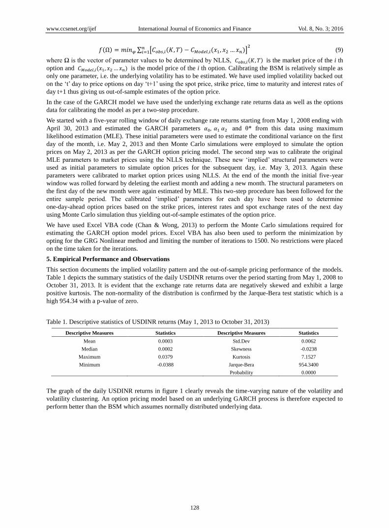
Table 1 depicts the summary statistics of the daily USDINR returns over the period starting from May 1, 2008 to

October 31, 2013. It is evident that the exchange rate returns data are negatively skewed and exhibit a large

positive kurtosis. The non-normality of the distribution is confirmed by the Jarque-Bera test statistic which is a

high 954.34 with a p-value of zero.

Table 1. Descriptive statistics of USDINR returns (May 1, 2013 to October 31, 2013)

Descriptive Measures Statistics Descriptive Measures Statistics

Mean 0.0003 Std.Dev 0.0062

Median 0.0002 Skewness -0.0238

Maximum 0.0379 Kurtosis 7.1527

Minimum -0.0388 Jarque-Bera 954.3400

Probability 0.0000

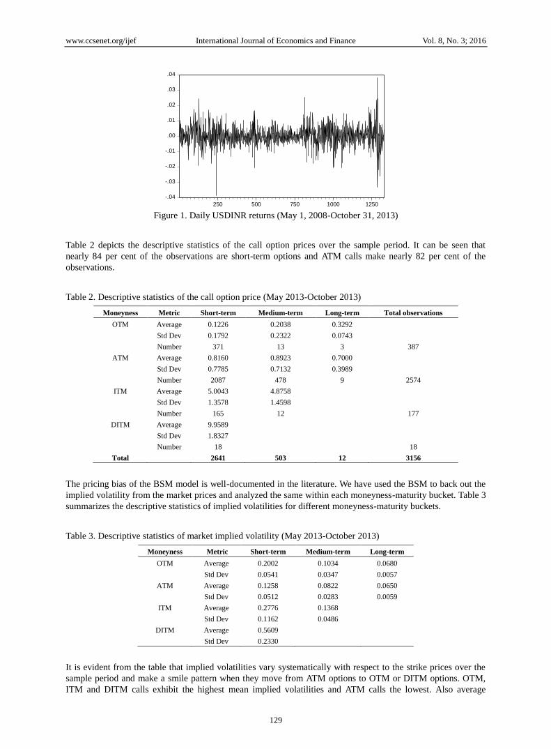
The graph of the daily USDINR returns in figure 1 clearly reveals the time-varying nature of the volatility and

volatility clustering. An option pricing model based on an underlying GARCH process is therefore expected to

perform better than the BSM which assumes normally distributed underlying data.

www.ccsenet.org/ijef International Journal of Economics and Finance Vol. 8, No. 3; 2016

129

Figure 1. Daily USDINR returns (May 1, 2008-October 31, 2013)

Table 2 depicts the descriptive statistics of the call option prices over the sample period. It can be seen that

nearly 84 per cent of the observations are short-term options and ATM calls make nearly 82 per cent of the

observations.

Table 2. Descriptive statistics of the call option price (May 2013-October 2013)

Moneyness Metric Short-term Medium-term Long-term Total observations

OTM Average 0.1226 0.2038 0.3292

Std Dev 0.1792 0.2322 0.0743

Number 371 13 3 387

ATM Average 0.8160 0.8923 0.7000

Std Dev 0.7785 0.7132 0.3989

Number 2087 478 9 2574

ITM Average 5.0043 4.8758

Std Dev 1.3578 1.4598

Number 165 12

177

DITM Average 9.9589

Std Dev 1.8327

Number 18

18

Total 2641 503 12 3156

The pricing bias of the BSM model is well-documented in the literature. We have used the BSM to back out the

implied volatility from the market prices and analyzed the same within each moneyness-maturity bucket. Table 3

summarizes the descriptive statistics of implied volatilities for different moneyness-maturity buckets.

Table 3. Descriptive statistics of market implied volatility (May 2013-October 2013)

Moneyness Metric Short-term Medium-term Long-term

OTM Average 0.2002 0.1034 0.0680

Std Dev 0.0541 0.0347 0.0057

ATM Average 0.1258 0.0822 0.0650

Std Dev 0.0512 0.0283 0.0059

ITM Average 0.2776 0.1368

Std Dev 0.1162 0.0486

DITM Average 0.5609

Std Dev 0.2330

It is evident from the table that implied volatilities vary systematically with respect to the strike prices over the

sample period and make a smile pattern when they move from ATM options to OTM or DITM options. OTM,

ITM and DITM calls exhibit the highest mean implied volatilities and ATM calls the lowest. Also average

-.04

-.03

-.02

-.01

.00

.01

.02

.03

.04

250 500 750 1000 1250

Daily USDINR log returns

www.ccsenet.org/ijef International Journal of Economics and Finance Vol. 8, No. 3; 2016

130

implied volatilities are seen to be highest for short-term options and tend to decline with increase in the maturity

of the option. The standard deviation of implied volatilities is higher for short-term ITM and DITM options but

declines for medium-term and long-term options.

In accordance with existing research we have used three yard-sticks for measuring the empirical performance of

the two models: (i) in-sample pricing errors (ii) out-of-sample pricing errors and (iii) Orthogonality tests. The

following three error metrics have been employed to judge the pricing performance of the two models.

1) Mean Absolute Percentage Error (MAPE). 1

𝑛∑ |

𝐶𝑖,𝑚𝑜𝑑𝑒𝑙−𝐶𝑖,𝑚𝑎𝑟𝑘𝑒𝑡

𝐶𝑖,𝑚𝑎𝑟𝑘𝑒𝑡|𝑛

𝑖=1 This is a measure of the

magnitude of the pricing error.

2) Mean Percentage Error (MPE) 1

𝑛∑

(𝐶𝑖,𝑚𝑜𝑑𝑒𝑙−𝐶𝑖,𝑚𝑎𝑟𝑘𝑒𝑡)

𝐶𝑖,𝑚𝑎𝑟𝑘𝑒𝑡

𝑛𝑖=1 . This is a measure of the direction of the

pricing error.

3) Mean Squared Error (MSE) 1

𝑛∑ (𝐶𝑖,𝑚𝑜𝑑𝑒𝑙 − 𝐶𝑖,𝑚𝑎𝑟𝑘𝑒𝑡)2𝑛

𝑖=1 . This is a measure of the volatility of the

pricing error.

5.1 In-Sample Performance

In-sample testing of the models reveals the consistency of the parameters with the option prices. Table 4 depicts

the mean and standard deviation for the parameter estimates for both models for each month of the sample

period. It is observed that the parameters of both models vary considerably over the sample period as evidenced

by their high standard deviations.

Table 4. Parameter estimates over the sample period (May 2013-October 2013)

Month

BSM NGARCH

σ 𝛼0 𝛼1 𝛼2 θ*

May 2013 Average 0.0664 0.0000 0.1000 0.8800 0.0000

StdDev 0.0045 0.0000 0.0000 0.0000 0.0000

June 2013 Average 0.0923 0.0000 0.1000 0.8800 0.0000

StdDev 0.0172 0.0000 0.0000 0.0000 0.0000

July 2013 Average 0.1052 0.0000 0.0979 0.7920 0.0576

StdDev 0.0185 0.0000 0.0013 0.0228 0.0013

August 2013 Average 0.1560 0.0000 0.0968 0.7831 0.0044

StdDev 0.0455 0.0000 0.0150 0.1163 0.0025

September 2013 Average 0.1931 0.0000 0.1206 0.6691 0.0007

StdDev 0.0271 0.0000 0.0470 0.1711 0.0001

October 2013 Average 0.1270 0.0000 0.0747 0.8095 0.0000

StdDev 0.0221 0.0000 0.0052 0.0707 0.0000

We have evaluated the in-sample performance of both models by comparing the market option prices with the

model prices computed using the estimated parameters of the current day. Specifically, we estimate structural

parameters Ω𝑡 at time t and use these parameters and other inputs such as the spot price, strike price, interest

rates and time to maturity at time t in order to price all options at time t. Table 5 shows the in-sample pricing

errors for different categories of moneyness.

Table 5. In-sample error statistics as per option moneyness

MAPE MPE MSE

Moneyness BSM GARCH BSM GARCH BSM GARCH

OTM 0.6302 0.5148 -0.595 -0.3148 0.0076 0.0132

ATM 0.1358 0.1875 -0.0694 -0.0057 0.0084 0.0203

ITM 0.0282 0.0276 -0.0248 -0.0231 0.0475 0.0465

DITM 0.0296 0.0295 -0.0296 -0.0295 0.2404 0.2405

www.ccsenet.org/ijef International Journal of Economics and Finance Vol. 8, No. 3; 2016

131

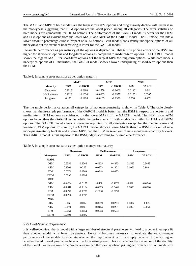
The MAPE and MPE of both models are the highest for OTM options and progressively decline with increase in

the moneyness suggesting that OTM options are the worst priced among all categories. The error statistics of

both models are comparable for DITM options. The performance of the GARCH model is better for the OTM

and ITM options as evident from the lower MAPE and MPE of the GARCH model. The BS model exhibits a

lower absolute percentage error in respect of ATM options. Both models consistently underprice options of all

moneyness but the extent of underpricing is lower for the GARCH model.

In-sample performance as per maturity of the options is depicted in Table 6. The pricing errors of the BSM are

higher for short-term options and long-term options as compared to medium-term options. The GARCH model

shows the highest MAPE for short-term options but the largest MPE for long-term options. While both models

underprice options of all maturities, the GARCH model shows a lower underpricing of short-term options than

the BSM.

Table 6. In-sample error statistics as per option maturity

MAPE MPE MSE

Maturity BSM GARCH BSM GARCH BSM GARCH

Short-term 0.2018 0.2203 -0.1558 -0.0606 0.0113 0.02

Medium-term 0.1026 0.1338 -0.0063 -0.0557 0.0185 0.0305

Long-term 0.128 0.1295 -0.0105 -0.0936 0.006 0.007

The in-sample performance across all categories of moneyness-maturity is shown in Table 7. The table clearly

shows that the in-sample performance of the GARCH model is better than the BSM in respect of short-term and

medium-term OTM options as evidenced by the lower MAPE of the GARCH model. The BSM prices ATM

options better than the GARCH model while the performance of both models is similar for ITM and DITM

options. The GARCH model shows a lower underpricing for all categories except for the medium-term and

long-term ATM options. To sum up, the GARCH model shows a lower MAPE than the BSM in six out of nine

moneyness-maturity buckets and a lower MPE than the BSM in seven out of nine moneyness-maturity buckets.

The GARCH model is thus superior to the BSM judged according to in-sample performance.

Table 7. In-sample error statistics as per option moneyness-maturity

Short-term Medium-term Long-term

Moneyness BSM GARCH BSM GARCH BSM GARCH

MAPE

OTM 0.6559 0.5265 0.4905 0.4873 0.1585 0.2053

ATM 0.1501 0.202 0.0973 0.1301 0.1066 0.1034

ITM 0.0274 0.0269 0.0348 0.0333

DITM 0.0296 0.0295

MPE

OTM -0.6204 -0.3157 -0.488 -0.4873 -0.0901 -0.0846

ATM -0.0918 -0.0164 0.0063 -0.0461 0.0023 -0.0826

ITM -0.0242 -0.0229 -0.0254 -0.0099

DITM -0.0296 -0.0295

MSE

OTM 0.0066 0.012 0.0219 0.0263 0.0034 0.005

ATM 0.0074 0.019 0.0164 0.0291 0.0055 0.0064

ITM 0.0461 0.0454 0.0543 0.0503

DITM 0.2404 0.2405

5.2 Out-of-Sample Performance

It is well-recognized that a model with a larger number of structural parameters will lead to a better in-sample fit

than another model with fewer parameters. Hence it becomes necessary to evaluate the out-of-sample

performance of the models to ascertain whether the improvement in fit is simply because of over-fitting or

whether the additional parameters have a true forecasting power. This also enables the evaluation of the stability

of the model parameters over time. We have examined the one-day-ahead pricing performance of both models by

www.ccsenet.org/ijef International Journal of Economics and Finance Vol. 8, No. 3; 2016

132

using the estimated structural parameters of the current day for pricing options on the subsequent day. These

out-of-sample forecasts have been compared with traded option prices to estimate the pricing error.

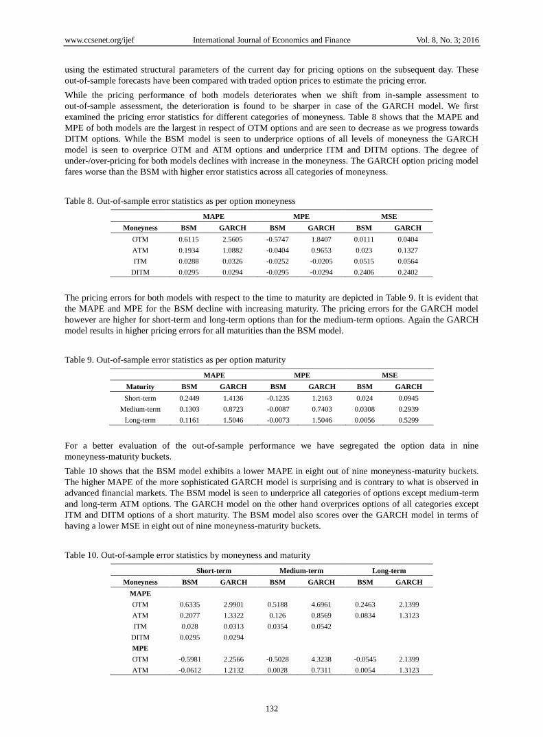
While the pricing performance of both models deteriorates when we shift from in-sample assessment to

out-of-sample assessment, the deterioration is found to be sharper in case of the GARCH model. We first

examined the pricing error statistics for different categories of moneyness. Table 8 shows that the MAPE and

MPE of both models are the largest in respect of OTM options and are seen to decrease as we progress towards

DITM options. While the BSM model is seen to underprice options of all levels of moneyness the GARCH

model is seen to overprice OTM and ATM options and underprice ITM and DITM options. The degree of

under-/over-pricing for both models declines with increase in the moneyness. The GARCH option pricing model

fares worse than the BSM with higher error statistics across all categories of moneyness.

Table 8. Out-of-sample error statistics as per option moneyness

MAPE MPE MSE

Moneyness BSM GARCH BSM GARCH BSM GARCH

OTM 0.6115 2.5605 -0.5747 1.8407 0.0111 0.0404

ATM 0.1934 1.0882 -0.0404 0.9653 0.023 0.1327

ITM 0.0288 0.0326 -0.0252 -0.0205 0.0515 0.0564

DITM 0.0295 0.0294 -0.0295 -0.0294 0.2406 0.2402

The pricing errors for both models with respect to the time to maturity are depicted in Table 9. It is evident that

the MAPE and MPE for the BSM decline with increasing maturity. The pricing errors for the GARCH model

however are higher for short-term and long-term options than for the medium-term options. Again the GARCH

model results in higher pricing errors for all maturities than the BSM model.

Table 9. Out-of-sample error statistics as per option maturity

MAPE MPE MSE

Maturity BSM GARCH BSM GARCH BSM GARCH

Short-term 0.2449 1.4136 -0.1235 1.2163 0.024 0.0945

Medium-term 0.1303 0.8723 -0.0087 0.7403 0.0308 0.2939

Long-term 0.1161 1.5046 -0.0073 1.5046 0.0056 0.5299

For a better evaluation of the out-of-sample performance we have segregated the option data in nine

moneyness-maturity buckets.

Table 10 shows that the BSM model exhibits a lower MAPE in eight out of nine moneyness-maturity buckets.

The higher MAPE of the more sophisticated GARCH model is surprising and is contrary to what is observed in

advanced financial markets. The BSM model is seen to underprice all categories of options except medium-term

and long-term ATM options. The GARCH model on the other hand overprices options of all categories except

ITM and DITM options of a short maturity. The BSM model also scores over the GARCH model in terms of

having a lower MSE in eight out of nine moneyness-maturity buckets.

Table 10. Out-of-sample error statistics by moneyness and maturity

Short-term Medium-term Long-term

Moneyness BSM GARCH BSM GARCH BSM GARCH

MAPE

OTM 0.6335 2.9901 0.5188 4.6961 0.2463 2.1399

ATM 0.2077 1.3322 0.126 0.8569 0.0834 1.3123

ITM 0.028 0.0313 0.0354 0.0542

DITM 0.0295 0.0294

MPE

OTM -0.5981 2.2566 -0.5028 4.3238 -0.0545 2.1399

ATM -0.0612 1.2132 0.0028 0.7311 0.0054 1.3123

www.ccsenet.org/ijef International Journal of Economics and Finance Vol. 8, No. 3; 2016

133

ITM -0.0246 -0.0212 -0.0275 0.0258

DITM -0.0295 -0.0294

MSE

OTM 0.0096 0.0276 0.0312 0.1347 0.0063 0.4718

ATM 0.0213 0.1002 0.0289 0.3042 0.0048 0.5409

ITM 0.05 0.0538 0.0561 0.1057

DITM 0.2406 0.2402

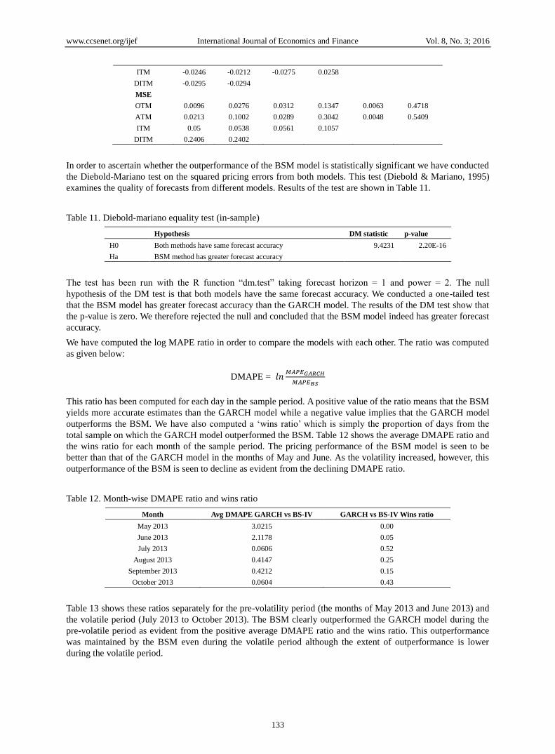
In order to ascertain whether the outperformance of the BSM model is statistically significant we have conducted

the Diebold-Mariano test on the squared pricing errors from both models. This test (Diebold & Mariano, 1995)

examines the quality of forecasts from different models. Results of the test are shown in Table 11.

Table 11. Diebold-mariano equality test (in-sample)

Hypothesis DM statistic p-value

H0 Both methods have same forecast accuracy 9.4231

2.20E-16

Ha BSM method has greater forecast accuracy

The test has been run with the R function “dm.test” taking forecast horizon = 1 and power = 2. The null

hypothesis of the DM test is that both models have the same forecast accuracy. We conducted a one-tailed test

that the BSM model has greater forecast accuracy than the GARCH model. The results of the DM test show that

the p-value is zero. We therefore rejected the null and concluded that the BSM model indeed has greater forecast

accuracy.

We have computed the log MAPE ratio in order to compare the models with each other. The ratio was computed

as given below:

DMAPE = 𝑙𝑛𝑀𝐴𝑃𝐸𝐺𝐴𝑅𝐶𝐻

𝑀𝐴𝑃𝐸𝐵𝑆

This ratio has been computed for each day in the sample period. A positive value of the ratio means that the BSM

yields more accurate estimates than the GARCH model while a negative value implies that the GARCH model

outperforms the BSM. We have also computed a „wins ratio‟ which is simply the proportion of days from the

total sample on which the GARCH model outperformed the BSM. Table 12 shows the average DMAPE ratio and

the wins ratio for each month of the sample period. The pricing performance of the BSM model is seen to be

better than that of the GARCH model in the months of May and June. As the volatility increased, however, this

outperformance of the BSM is seen to decline as evident from the declining DMAPE ratio.

Table 12. Month-wise DMAPE ratio and wins ratio

Month Avg DMAPE GARCH vs BS-IV GARCH vs BS-IV Wins ratio

May 2013 3.0215 0.00

June 2013 2.1178 0.05

July 2013 0.0606 0.52

August 2013 0.4147 0.25

September 2013 0.4212 0.15

October 2013 0.0604 0.43

Table 13 shows these ratios separately for the pre-volatility period (the months of May 2013 and June 2013) and

the volatile period (July 2013 to October 2013). The BSM clearly outperformed the GARCH model during the

pre-volatile period as evident from the positive average DMAPE ratio and the wins ratio. This outperformance

was maintained by the BSM even during the volatile period although the extent of outperformance is lower

during the volatile period.

www.ccsenet.org/ijef International Journal of Economics and Finance Vol. 8, No. 3; 2016

134

Table 13. DMAPE and wins ratio during volatile and pre-volatile periods

Period Avg DMAPE GARCH vs BS-IV GARCH vs BS-IV Wins ratio

Pre-volatile period 2.5911 0.02

Volatile period 0.2307 0.35

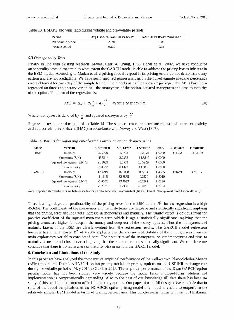
5.3 Orthogonality Tests

Finally in line with existing research (Madan, Carr, & Chang, 1998; Lehar et al., 2002) we have conducted

orthogonality tests to ascertain to what extent the GARCH model is able to address the pricing biases inherent in

the BSM model. According to Madan et al. a pricing model is good if its pricing errors do not demonstrate any

pattern and are not predictable. We have performed regression analysis on the out-of-sample absolute percentage

errors obtained for each day of the sample for both the models using the Eviews 7 package. The APEs have been

regressed on three explanatory variables – the moneyness of the option, squared moneyness and time to maturity

of the option. The form of the regression is:

𝐴𝑃𝐸 = 𝛼0 + 𝛼1𝑆

𝐾+ 𝛼2

𝑆

𝐾

2+ 𝛼3𝑡𝑖𝑚𝑒 𝑡𝑜 𝑚𝑎𝑡𝑢𝑟𝑖𝑡𝑦 (10)

Where moneyness is denoted by 𝑆

𝐾 and squared moneyness by

𝑆

𝐾

2.

Regression results are documented in Table 14. The standard errors reported are robust and heteroscedasticity

and autocorrelation-consistent (HAC) in accordance with Newey and West (1987).

Table 14. Results for regressing out-of-sample errors on option characteristics

Model Variable Coefficient Std. Error t-Statistic Prob. R-squared F-statistic

BSM Intercept 25.5729 1.6752 15.2658 0.0000 0.4562 881.3309

Moneyness (S/K) -46.5114 3.2336 -14.3840 0.0000

Squared moneyness (S/K)^2 21.1683 1.5573 13.5929 0.0000

Time to maturity -1.0372 0.1028 -10.0883 0.0000

GARCH Intercept 12.9219 16.6038 0.7783 0.4365 0.0429 47.0795

Moneyness (S/K) -8.1615 32.3835 -0.2520 0.8010

Squared moneyness (S/K)^2 -3.6022 15.7895 -0.2281 0.8196

Time to maturity -1.2771 1.2931 -0.9876 0.3234

Note. Reported standard errors are hetereoscedasticity and autocorrelation consistent (Bartlett kernel, Newey-West fixed bandwidth = 9).

There is a high degree of predictability of the pricing error for the BSM as the 𝑅2 for the regression is a high

45.62%. The coefficients of the moneyness and maturity terms are negative and statistically significant implying

that the pricing error declines with increase in moneyness and maturity. The „smile‟ effect is obvious from the

positive coefficient of the squared-moneyness term which is again statistically significant implying that the

pricing errors are higher for deep-in-the-money and deep-out-of-the-money options. Thus the moneyness and

maturity biases of the BSM are clearly evident from the regression results. The GARCH model regression

however has a much lower 𝑅2 of 4.28% implying that there is no predictability of the pricing errors from the

main explanatory variables considered here. The t-statistics of the moneyness, squaredmoneyness and time to

maturity terms are all close to zero implying that these terms are not statistically significant. We can therefore

conclude that there is no moneyness or maturity bias present in the GARCH model.

6. Conclusion and Limitations of the Study

In this paper we have analyzed the comparative empirical performance of the well-known Black-Scholes-Merton

(BSM) model and Duan‟s NGARCH option pricing model for pricing options on the USDINR exchange rate

during the volatile period of May 2013 to October 2013. The empirical performance of the Duan GARCH option

pricing model has not been studied very widely because the model lacks a closed-form solution and

implementation is computationally demanding. Also to the best of our knowledge till date there has been no

study of this model in the context of Indian currency options. Our paper aims to fill this gap. We conclude that in

spite of the added complexities of the NGARCH option pricing model this model is unable to outperform the

relatively simpler BSM model in terms of pricing performance. This conclusion is in line with that of Harikumar

www.ccsenet.org/ijef International Journal of Economics and Finance Vol. 8, No. 3; 2016

135

et al. (2004) who found that the BSM outperforms the GARCH model in respect of currency options. It is

however contrary to that of Bollen and Rasiel (2003) who conclude that GARCH models are an improvement

over the fixed smile model. Our second finding is that the GARCH model is free of the moneyness and maturity

biases exhibited by the BSM model as demonstrated by orthogonality tests. This result in is in line with that of

Lehar et al. (2002) and Hsieh and Ritchken (2000).

The limitations of this study are two-fold. First, we have focused on a volatile period in the recent history and

hence the sample period is short. The second limitation is that we have not analyzed the hedging performance of

the two models. We propose to do the same in a subsequent paper.

References

Badescu, A., Kulperger, R., & Lazar, E. (2008). Option valuation with normal mixture GARCH models. Studies

in Nonlinear Dynamics & Econometrics, 12(2), 1-40. http://dx.doi.org/ 10.2202/1558-3708.1580

Bakshi, G. S., Cao, C., & Chen, Z. W. (1997). Empirical performance of alternative option pricing models.

Journal of Finance, 52(5), 2003-2049. http://dx.doi.org/10.1111/j.1540-6261.1997.tb02749.x

Bates, D. (1991). The crash of ‟87: Was it expected? The evidence from options markets. Journal of Finance,

46(3), 1009-1044. http://dx.doi.org/10.1111/j.1540-6261.1991.tb03775.x

Black, F. (1976). Studies of stock price volatility changes. In Proceedings of the 1976 Meetings of the American

Statistical Association, pp. 171-181.

Black, F., & Scholes, M. (1973). The pricing of options and corporate liabilities. Journal of Political Economy,

81(3), 637-654. http://dx.doi.org/10.1086/260062

Bollen, N., & Rasiel, E. (2003). The performance of alternative valuation models in the OTC currency options

market. Journal of International Money and Finance, 22, 33-64.

http://dx.doi.org/10.1016/S0261-5606(02)00073-6

Bollerslev, T. (1986). Generalized Autoregressive Conditional Heteroscedasticity. Journal of Econometrics,

31(3), 307-327. http://dx.doi.org/10.1016/0304-4076(86)90063-1

Chan, N. H., & Wong, H. Y. (2013). Handbook of Financial Risk Management, Simulations and Case Studies.

Hoboken, NJ: Wiley. http://dx.doi.org/10.1002/9781118573570

Chirac, D. P., & Manaster, S. (1978). The information content of market prices and a test of market efficiency.

Journal of Financial Economics, 6, 213-234. http://dx.doi.org/10.1016/0304-405X(78)90030-2

Christoffersen, P., Jacobs, K., & Mimouni, K. (2006). An Empirical Comparison of Affine and Non-Affine

Models for Equity Index Options. http://dx.doi.org/10.2139/ssrn.891127

Diebold, F. X., & Mariano, R. S. (1995). Comparing predictive accuracy. Journal of Business and Economic

Statistics, 13(3), 253-263.

Duan, J. C. (1995). The GARCH option pricing model. Mathematical Finance 5(1), 13-32.

http://dx.doi.org/10.1111/j.1467-9965.1995.tb00099.x

Duan, J. C., & Simonato, J. G. (1998). Empirical martingale simulation for asset prices. Management Science,

44(9), 1218-1233. http://dx.doi.org/10.1287/mnsc.44.9.1218

Duan, J. C., & Wei, J. (1999). Pricing foreign currency and cross-currency options under GARCH. The Journal

of Derivatives, 7(1), 51-63. http://dx.doi.org/10.3905/jod.1999.319110

Duan, J. C., & Zhang, H. (2001). Pricing Hang Seng Index options around the Asian financial crisis- A GARCH

approach. Journal of Banking & Finance, 25(11), 1989-2014.

http://dx.doi.org/10.1016/S0378-4266(00)00166-7

Dumas, B., Fleming, J., & Whaley, R. (1998). Implied volatility functions: Empirical tests. Journal of Finance,

53(6), 2059-2106. http://dx.doi.org/10.1111/0022-1082.00083

Engle, R. F. (1982). Autoregressive conditional heteroscedasticity with estimates of variance of UK inflation.

Econometrica, 50(4), 987-1008. http://dx.doi.org/10.2307/1912773

Garman, M., & Kohlhagen, S. (1983). Foreign currency option values. Journal of International Money and

Finance, 2(3), 231-237. http://dx.doi.org/10.1016/S0261-5606(83)80001-1

Harikumar, T., Boyrie, M., & Pak, S. (2004). Evaluation of Black-Scholes and GARCH models using currency

call options data. Review of Quantitative Finance and Accounting, 23, 299-312.

www.ccsenet.org/ijef International Journal of Economics and Finance Vol. 8, No. 3; 2016

136

http://dx.doi.org/10.1023/B:REQU.0000049318.78363.3c

Heston, S. (1993). A closed-form solution for options with stochastic volatility with applications to bond and

currency options. The Review of Financial Studies, 6(2), 328-343. http://dx.doi.org/10.1093/rfs/6.2.327

Heston, S., & Nandi, S. (2000). A closed-form GARCH option valuation model. Review of Financial Studies,

13(3), 585-625. http://dx.doi.org/10.1093/rfs/13.3.585

Hsieh, K. C., & Ritchken, P. (2000). An empirical comparison of GARCH option pricing Models. Working paper,

Case Western Reserve University.

Huang, H., Wang, C., & Chen, S. (2011). Pricing Taiwan option market with GARCH and stochastic volatility.

Applied Financial Economics, 21(10), 747-754. http://dx.doi.org/10.1080/09603107.2010.535786

Hull, J., & White, A. (1987). The pricing of options on assets with stochastic volatilities. Journal of Finance,

42(2), 281-300. http://dx.doi.org/10.1111/j.1540-6261.1987.tb02568.x

Johnson, H., & Shanno, D. (1987). Option pricing when the variance is changing. Journal of Financial and

Quantitative Analysis, 22(2), 143-151. http://dx.doi.org/10.2307/2330709

Jou, Y. J., Wang, C. W., & Chiu, W. C. (2013). Is the realized volatility good for option pricing during the recent

financial crisis? Review of Quantitative Finance and Accounting, 40(1), 171-188.

http://dx.doi.org/10.1007/s11156-012-0285-0.

Kaminsky, S. (2013). The pricing of options on WIG20 using GARCH models. Working Paper No.6/2013(91),

University of Warsaw, Faculty of Economic Sciences.

Latane, H., & Rendleman, R. (1976). Standard Deviations of Stock price Ratios Implied in Option Prices. The

Journal of Finance, 3(2), 369-381. http://dx.doi.org/10.1111/j.1540-6261.1976.tb01892.x

Lehar, A., Scheicher, M., & Schittenkopf, C. (2002). GARCH vs. stochastic volatility: Option pricing and risk

management. Journal of Banking & Finance, 26(2/3), 323-345.

http://dx.doi.org/10.1016/S0378-4266(01)00225-4

Madan, D., Carr, P., & Chang, E. (1998). The variance gamma process and option pricing. European Finance

Review, 2, 79-105. http://dx.doi.org/10.1023/A:1009703431535

Melino, A., & Turnbull, S. (1991). The pricing of foreign currency options. Canadian Journal of Economics,

24(2), 251-281. http://dx.doi.org/10.2307/135623

Merton, R. C. (1973). Theory of rational option pricing. Bell Journal of Economics and Management Science,

4(1), 141-183. http://dx.doi.org/10.2307/3003143

Merville, L. J., & Pieptea, D. R. (1989). Stock price volatility, mean-reverting diffusion and noise. Journal of

Financial Economics, 3, 125-144. http://dx.doi.org/10.1016/0304-405x(89)90078-0

Newey, W., & West, K. (1987). A simple, positive semi-definite, heteroscedasticity and autocorrelation consistent

covariance matrix. Econometrica, 55(3), 703-08. http://dx.doi.org/10.2307/1913610

Scott, L. (1986). Option pricing when the variance changes randomly: Theory and an Application. Working

Paper, University of Illinois, Department of Finance, 1986.

Singh, V. K., Ahmed, N., & Pachori, P. (2011). Empirical analysis of GARCH and Practitioner Black-Scholes

model for pricing S&P CNX Nifty 50 index options of India. Decision, 38(2), 51-67.

Yung, H., & Zhang, H. (2003). An empirical investigation of the GARCH option pricing model: Hedging

performance. The Journal of Futures Markets, 23(12), 1191-1207. http://dx.doi.org/10.1002/fut.10109

Copyrights

Copyright for this article is retained by the author(s), with first publication rights granted to the journal.

This is an open-access article distributed under the terms and conditions of the Creative Commons Attribution

license (http://creativecommons.org/licenses/by/3.0/).