Empirical Performance of Covered-Call Strategy under Stochastic Volatility in Taiwan

Soochow Journal of Economics and Business

No.84 (March 2014)：25-46.

Empirical Performance of Covered-Call Strategy underStochastic Volatility in Taiwan

Chang-Chieh Hsieh* Chung-Gee Lin** Max Chen***

Abstract

This study examines the performances of conventional strategy and dynamic covered-

call strategies, including constant and stochastic volatilities environments in Taiwan. In ac-

cordance with prior literatures, the covered-call strategy may roughly boost portfolio return

in some specific moneyness. The monthly return of the conventional covered-call strategy

is slightly more than the pure futures buy-and-hold strategy on the average. The dynamic

strategies adjust the moneyness based on different exercise probabilities under constant vol-

atility and stochastic volatility. Finally, this study points out that the advantage of the dy-

namic strategy under stochastic volatility is more obvious than constant volatility or conven-

tional strategy.

Keywords: covered-call, dynamic strategy, moneyness, stochastic volatility.

* Corrseponding Author: Chang-Chieh Hsieh is a Ph.D. candidate in the Department of Economics,

Soochow University, Taiwan.** Chung-Gee Lin is a Professor of Finance in the Department of Financial Engineering and Actuarial

Mathematics, Soochow University, Taiwan.***Max Chen is an Assistant Professor in the Department of Finance, Ming Chuan University, Taiwan.

第八十四期

1. INTRODUCTION

The Black-Scholes is the most popular option pricing model in the world; however,

there are still some shortcomings. The previous research pointed out the case that the option

price is lower than the Black-Scholes price when stock price is quite close to exercise price,

and that the option price is higher than the Black-Scholes price when stock price is deeply

in or out of the money. Hence, we can expect that the price bias will be more severe in a

highly fluctuant market, such as emerging markets.

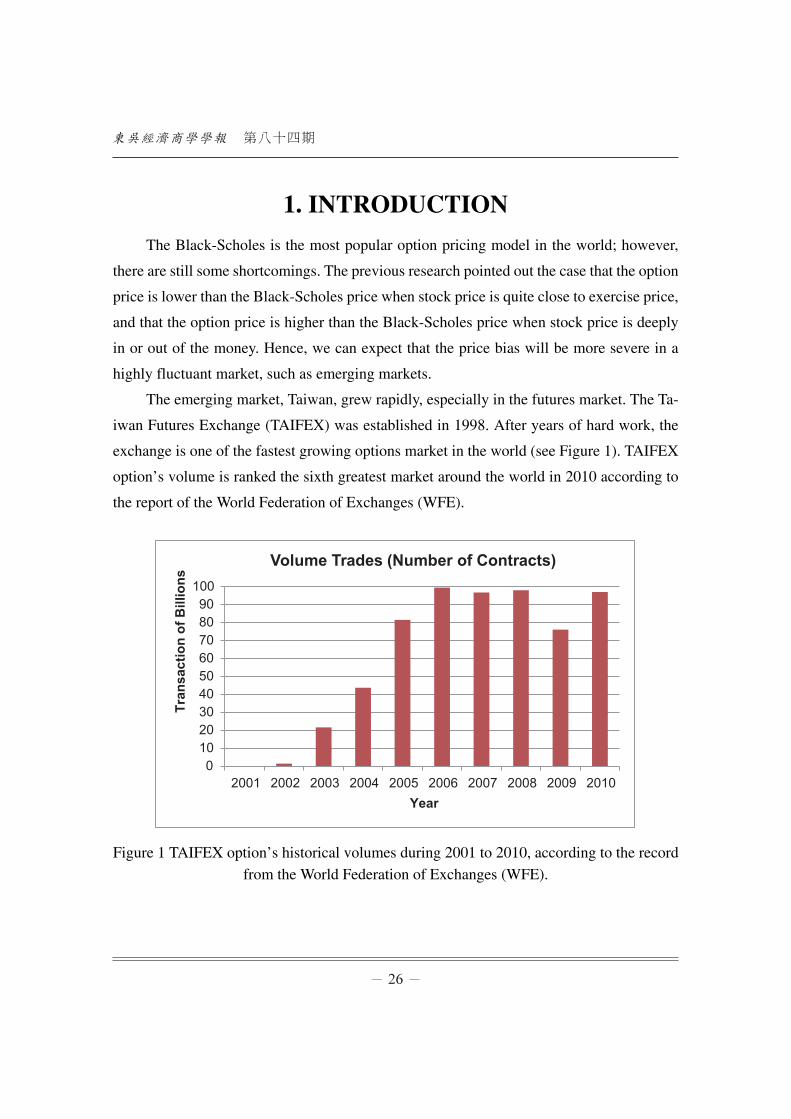
The emerging market, Taiwan, grew rapidly, especially in the futures market. The Ta-

iwan Futures Exchange (TAIFEX) was established in 1998. After years of hard work, the

exchange is one of the fastest growing options market in the world (see Figure 1). TAIFEX

option’s volume is ranked the sixth greatest market around the world in 2010 according to

the report of the World Federation of Exchanges (WFE).

0102030405060708090

100

2001 2002 2003 2004 2005 2006 2007 2008 2009 2010

Tran

sact

ion

of B

illio

ns

Year

Volume Trades (Number of Contracts)

Figure 1 TAIFEX option’s historical volumes during 2001 to 2010, according to the record

from the World Federation of Exchanges (WFE).

隨機波動效果下之掩護性買權實證績效於台灣市場

It is more reasonable to consider stochastic volatility instantaneously embedded in pri-

cing option. However, past researches about establishing a portfolio containing assets and

options almost did not consider the volatility disturbance. This paper is devoted to adoption

of the stochastic volatility model, the Heston model (1993). In addition, we also compare

Heston model’s performance with the Black-Scholes model’s, and expect to get more pre-

cise forecasting option prices in TAIFEX.

Covered-call (buy-write) option trading strategy, which is the portfolio combined by

one unit of the long underlying assets with writing one call option, has been being studied

in previous literatures and being assessed its performance. This trading strategy is the

simplest concept extended from the Capital Asset Pricing Model (CAPM) which is used to

hold negative correlation between asset and derivative to improve returns and to reduce ris-

ks. The trading strategy holders receive a premium when they sell a call option; in the mean-

time, the premium can reduce the cost of a single long position of the underlying asset. The

premium amount depends on the extension of the OTM (out-of-money) conditions. The tra-

ding strategy holders will receive the more premium as the option exercise price is closer to

current underlying asset. Another important factor is the underlying asset’s volatility, which

represents the fluctuated degree of the underlying asset. Therefore, choosing the appropriate

moneyness is a key to the performance of building a covered-call portfolio. Che and Fung

(2011) used the conventional buy-write (covered-call) strategy and a dynamic buy-write

strategy to test the performance on Hang Seng Index (HSI) in Hong Kong. Che and Fung

(2011) adopted HSI futures to substitute HSI in order to reduce the impact of transactional

cost and execution problems. They found that both strategies outperform the naked futures

position. Although the dynamic strategy uses various risk-adjusted measures, which usually

have lower returns than the conventional fixed strike strategy, the dynamic strategy outper-

forms the fixed strategy when the market is moderately volatile or being in a sharply rising

market.

Figelman (2008) introduces a simple theoretical framework which allows decompos-

ing the observed historical performance of covered-call strategy into three market compon-

ents: risk-free rate, equity risk premium, and implied-realized volatility spread. Figelman

(2008) pointed out that the covered-call strategy is highly correlated with the equity market

第八十四期

index (S&P 500), especially in the bull market. Hill et al. (2006), Feldman and Dhruv (2004)

and Whaley (2002) also investigated the covered-call strategies on the S&P500. They did

not obtain strong evidence to explain that covered-call strategies provided better perform-

ance than naked futures position. Nevertheless, they concluded that covered-call strategies

can effectively reduce risks (standard derivation).

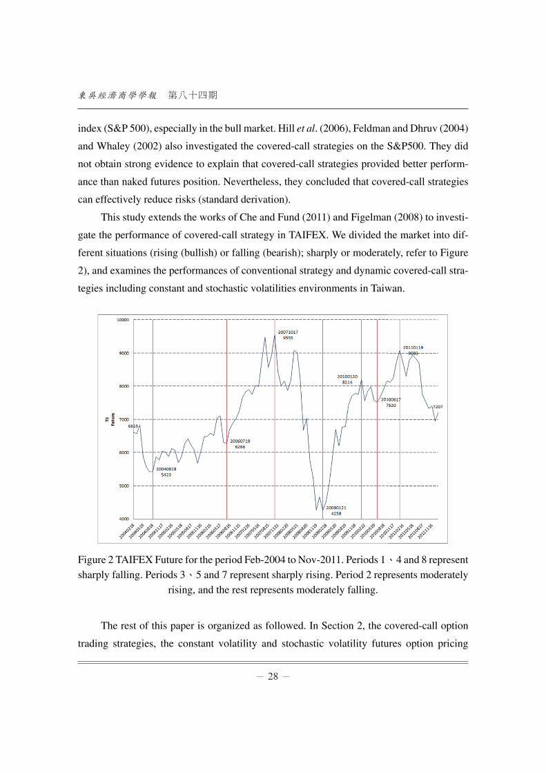
This study extends the works of Che and Fund (2011) and Figelman (2008) to investi-

gate the performance of covered-call strategy in TAIFEX. We divided the market into dif-

ferent situations (rising (bullish) or falling (bearish); sharply or moderately, refer to Figure

2), and examines the performances of conventional strategy and dynamic covered-call stra-

tegies including constant and stochastic volatilities environments in Taiwan.

Figure 2 TAIFEX Future for the period Feb-2004 to Nov-2011. Periods 1、4 and 8 represent

sharply falling. Periods 3、5 and 7 represent sharply rising. Period 2 represents moderatelyrising, and the rest represents moderately falling.

The rest of this paper is organized as followed. In Section 2, the covered-call option

trading strategies, the constant volatility and stochastic volatility futures option pricing


models, were introduced. Section 3 describes the data and defines four different market situ-

ations. The last section is the conclusion.

2. THE MODEL

Covered-call trading strategy, in this paper, is built as to buy index futures and simu-

ltaneously sell short European calls. Therefore, the volatility of the underlying futures and

option exercise price will affect the performance of the covered-call trading strategy. When

the volatility of the underlying futures increases, the income from the short sale from the call

options will increase. As the option is close to ATM (at the money) condition, the income

rises.

Building the covered-call strategy involves a position of short sale from futures call

options, resulting in involving the option pricing models. We first assume the volatility of

underlying futures is constant, in accordance with the Black (1976) model, shown in equa-

tion 1, which will be used for constructing the short sale from a call option position.

0 1 2( ) ( )c F N d XN d= −

21 0(ln( / ) / 2) /d F X T Tσ σ= + , 2

2 0(ln( / ) / 2) /d F X T Tσ σ= − . F0 is the price of under-

lying futures; X is the exercise price; T is the time to maturity at years. c and p represent call

and put options1.

Under the stochastic volatility environment, the Heston (1993) model, shown in equa-

tions 2 to 4, will be used for constructing the short sale from a call option position.

1,12t t t tdx r v dt v dz⎡ ⎤= − +⎢ ⎥⎣ ⎦

[ ] 2,t t t tdv k v dt v dzθ σ= − +

0 1 2c F P XP′ = −

where is the long-run mean of the variance. k is a mean reversion parameter. is the vol-

atility of volatility. x is ln (F). F is future price. X is the exercise price of call option. r is risk-

第八十四期

free interest rate. v is volatility. The quantities P1 and P2 are the probabilities that will be

exercised by the call option, conditional on the log of the last future price, xT＝ ln FT , and

on the last volatility vT. The risk-neutral dynamics was expressed as equations 2 and 3. z1 and

z2 are Weiner process. The rest details are provided in Appendix A.

The return from a covered-call is derived as below,

( ) ( )0

0 0 0

, 0Return SS C X Max F XF F

F F F−−

= + −

where FS is the last settlement price.

In this study, the selected exercise price is divided into (1) the fixed ratio model and

(2) the dynamic adjustment model. The rewards of fixed ratio models consist of a traditional

fixed exercise price and futures price in the beginning of the period. Exercise price is studied

for the degree of difference from 1% to 6% OTM during four specific ranges.

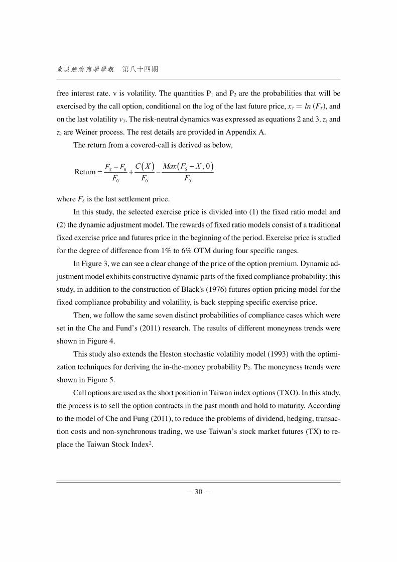
In Figure 3, we can see a clear change of the price of the option premium. Dynamic ad-

justment model exhibits constructive dynamic parts of the fixed compliance probability; this

study, in addition to the construction of Black's (1976) futures option pricing model for the

fixed compliance probability and volatility, is back stepping specific exercise price.

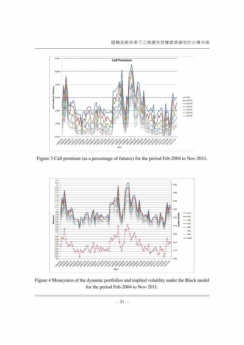
Then, we follow the same seven distinct probabilities of compliance cases which were

set in the Che and Fund’s (2011) research. The results of different moneyness trends were

shown in Figure 4.

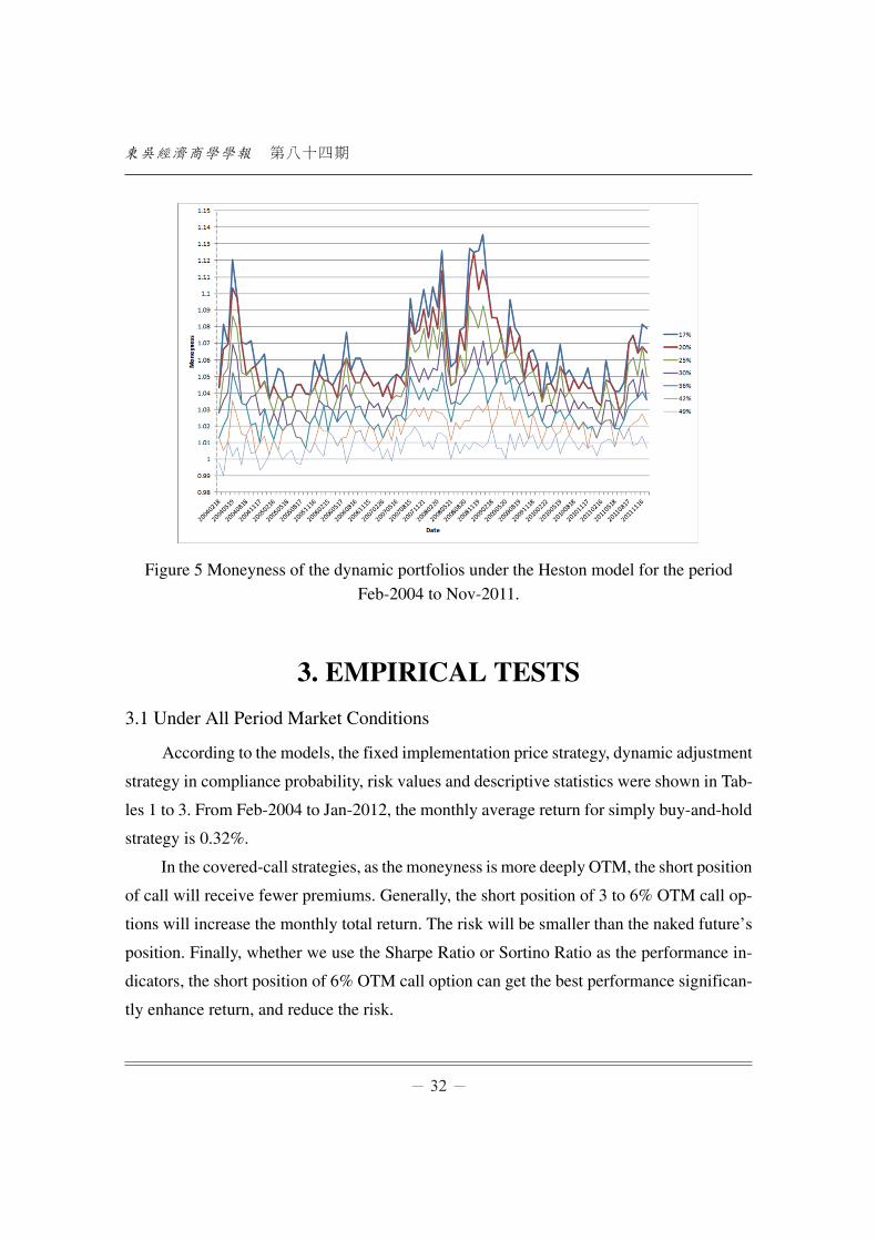
This study also extends the Heston stochastic volatility model (1993) with the optimi-

zation techniques for deriving the in-the-money probability P2. The moneyness trends were

shown in Figure 5.

Call options are used as the short position in Taiwan index options (TXO). In this study,

the process is to sell the option contracts in the past month and hold to maturity. According

to the model of Che and Fung (2011), to reduce the problems of dividend, hedging, transac-

tion costs and non-synchronous trading, we use Taiwan’s stock market futures (TX) to re-

place the Taiwan Stock Index2.


Figure 3 Call premium (as a percentage of futures) for the period Feb-2004 to Nov-2011.

Figure 4 Moneyness of the dynamic portfolios and implied volatility under the Black model

for the period Feb-2004 to Nov-2011.

第八十四期

Figure 5 Moneyness of the dynamic portfolios under the Heston model for the period

Feb-2004 to Nov-2011.

3. EMPIRICAL TESTS

3.1 Under All Period Market Conditions

According to the models, the fixed implementation price strategy, dynamic adjustment

strategy in compliance probability, risk values and descriptive statistics were shown in Tab-

les 1 to 3. From Feb-2004 to Jan-2012, the monthly average return for simply buy-and-hold

strategy is 0.32%.

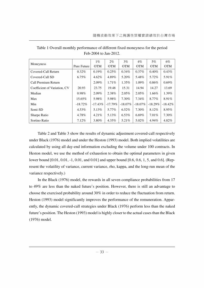
In the covered-call strategies, as the moneyness is more deeply OTM, the short position

of call will receive fewer premiums. Generally, the short position of 3 to 6% OTM call op-

tions will increase the monthly total return. The risk will be smaller than the naked future’s

position. Finally, whether we use the Sharpe Ratio or Sortino Ratio as the performance in-

dicators, the short position of 6% OTM call option can get the best performance significan-

tly enhance return, and reduce the risk.


Table 1 Overall monthly performance of different fixed moneyness for the period

Feb-2004 to Jan-2012.

MoneynessPure Future

1%OTM

2%OTM

3%OTM

4%OTM

5%OTM

6%OTM

Covered-Call Return 0.32% 0.19% 0.25% 0.34% 0.37% 0.40% 0.43%

Covered-Call SD 6.75% 4.62% 4.89% 5.20% 5.48% 5.72% 5.91%

Call Premium Return 2.09% 1.71% 1.35% 1.09% 0.86% 0.69%

Coefficient of Variation, CV 20.93 23.75 19.48 15.31 14.94 14.27 13.69

Median 0.98% 2.09% 2.38% 2.05% 2.05% 1.66% 1.39%

Max 15.65% 5.98% 5.98% 7.30% 7.34% 8.77% 8.91%

Min -18.72% -17.43% -17.79% -18.07% -18.07% -18.29% -18.42%

Semi-SD 4.53% 5.13% 5.77% 6.52% 7.30% 8.12% 8.95%

Sharpe Ratio 4.78% 4.21% 5.13% 6.53% 6.69% 7.01% 7.30%

Sortino Ratio 7.12% 3.80% 4.35% 5.21% 5.02% 4.94% 4.82%

Table 2 and Table 3 show the results of dynamic adjustment covered-call respectively

under Black (1976) model and under the Heston (1993) model. Both implied volatilities are

calculated by using all day-end information excluding the volume under 100 contracts. In

Heston model, we use the method of exhaustion to obtain the optimal parameters in given

lower bound [0.01, 0.01, -1, 0.01, and 0.01] and upper bound [0.6, 0.6, 1, 5, and 0.6]. (Rep-

resent the volatility of variance, current variance, rho, kappa, and the long-run mean of the

variance respectively.)

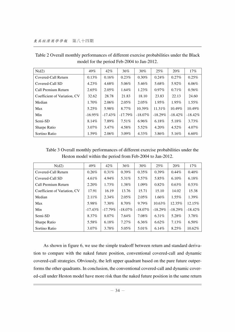
In the Black (1976) model, the rewards in all seven compliance probabilities from 17

to 49% are less than the naked future’s position. However, there is still an advantage to

choose the exercised probability around 30% in order to reduce the fluctuation from return.

Heston (1993) model significantly improves the performance of the remuneration. Appar-

ently, the dynamic covered-call strategies under Black (1976) perform less than the naked

future’s position. The Heston (1993) model is highly closer to the actual cases than the Black

(1976) model.

第八十四期

Table 2 Overall monthly performances of different exercise probabilities under the Black

model for the period Feb-2004 to Jan-2012.

N(d2) 49% 42% 36% 30% 25% 20% 17%


Covered-Call SD 4.23% 4.68% 5.06% 5.46% 5.68% 5.92% 6.06%

Call Premium Return 2.65% 2.05% 1.64% 1.23% 0.97% 0.71% 0.56%


Median 1.70% 2.06% 2.05% 2.05% 1.95% 1.95% 1.55%

Max 5.25% 5.98% 8.77% 10.39% 11.31% 10.49% 10.49%

Min -16.95% -17.43% -17.79% -18.07% -18.29% -18.42% -18.42%

Semi-SD 8.14% 7.89% 7.51% 6.96% 6.18% 5.18% 3.73%

Sharpe Ratio 3.07% 3.47% 4.58% 5.52% 4.20% 4.52% 4.07%

Sortino Ratio 1.59% 2.06% 3.09% 4.33% 3.86% 5.16% 6.60%

Table 3 Overall monthly performances of different exercise probabilities under the

Heston model within the period from Feb-2004 to Jan-2012.

N(d2) 49% 42% 36% 30% 25% 20% 17%


Covered-Call SD 4.61% 4.94% 5.31% 5.57% 5.85% 6.10% 6.18%

Call Premium Return 2.20% 1.73% 1.38% 1.09% 0.82% 0.63% 0.53%


Median 2.11% 2.34% 2.05% 2.05% 1.66% 1.55% 1.39%

Max 5.98% 7.30% 8.70% 9.79% 10.63% 12.35% 12.15%

Min -17.43% -17.79% -18.07% -18.07% -18.29% -18.29% -18.42%

Semi-SD 8.37% 8.07% 7.64% 7.08% 6.31% 5.28% 3.78%

Sharpe Ratio 5.58% 6.18% 7.27% 6.36% 6.62% 7.13% 6.50%

Sortino Ratio 3.07% 3.78% 5.05% 5.01% 6.14% 8.25% 10.62%

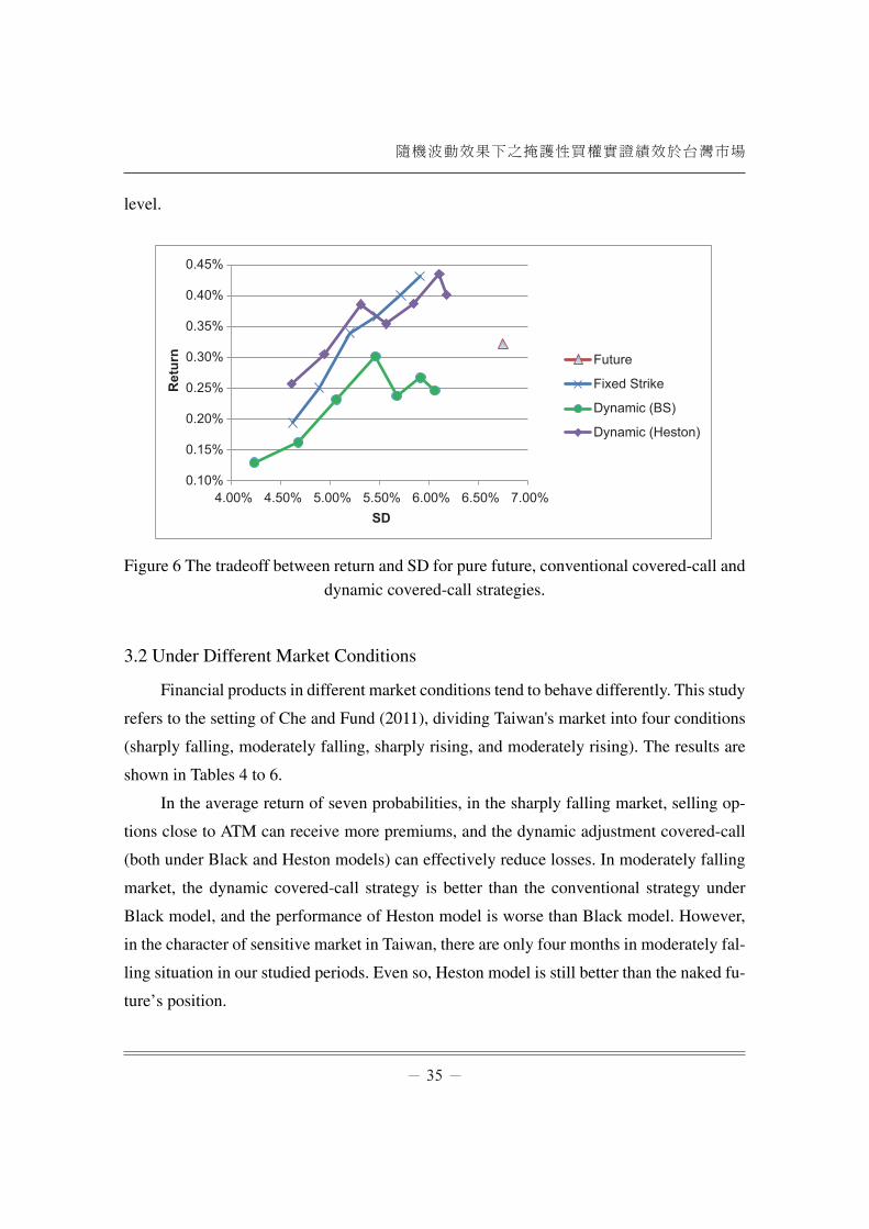
As shown in figure 6, we use the simple tradeoff between return and standard deriva-

tion to compare with the naked future position, conventional covered-call and dynamic

covered-call strategies. Obviously, the left upper quadrant based on the pure future outper-

forms the other quadrants. In conclusion, the conventional covered-call and dynamic cover-

ed-call under Heston model have more risk than the naked future position in the same return


level.

0.10%

0.15%

0.20%

0.25%

0.30%

0.35%

0.40%

0.45%

4.00% 4.50% 5.00% 5.50% 6.00% 6.50% 7.00%

Ret

urn

SD

Future

Fixed Strike

Dynamic (BS)

Dynamic (Heston)

Figure 6 The tradeoff between return and SD for pure future, conventional covered-call and

dynamic covered-call strategies.

3.2 Under Different Market Conditions

Financial products in different market conditions tend to behave differently. This study

refers to the setting of Che and Fund (2011), dividing Taiwan's market into four conditions

(sharply falling, moderately falling, sharply rising, and moderately rising). The results are

shown in Tables 4 to 6.

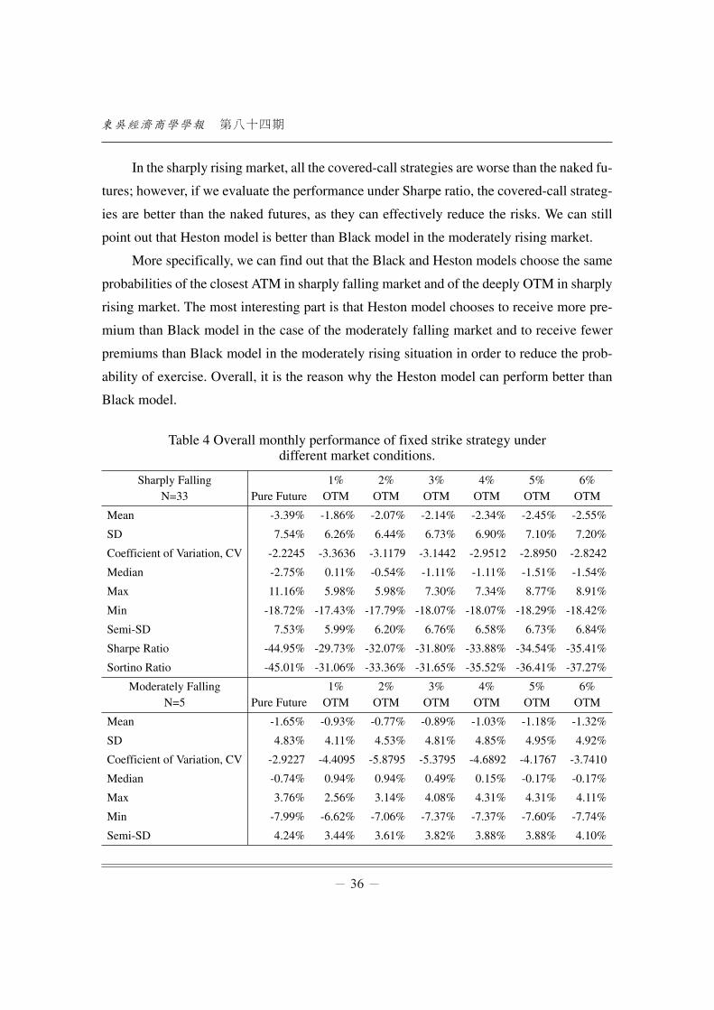
In the average return of seven probabilities, in the sharply falling market, selling op-

tions close to ATM can receive more premiums, and the dynamic adjustment covered-call

(both under Black and Heston models) can effectively reduce losses. In moderately falling

market, the dynamic covered-call strategy is better than the conventional strategy under

Black model, and the performance of Heston model is worse than Black model. However,

in the character of sensitive market in Taiwan, there are only four months in moderately fal-

ling situation in our studied periods. Even so, Heston model is still better than the naked fu-

ture’s position.

第八十四期

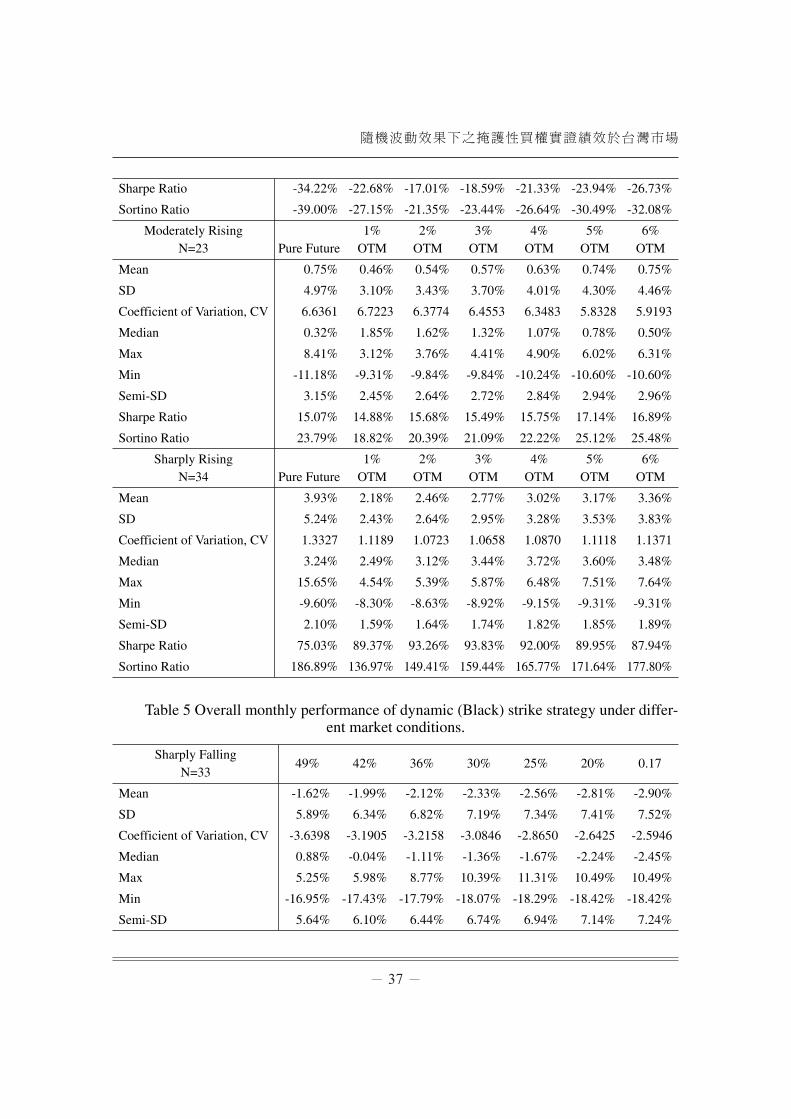
In the sharply rising market, all the covered-call strategies are worse than the naked fu-

tures; however, if we evaluate the performance under Sharpe ratio, the covered-call strateg-

ies are better than the naked futures, as they can effectively reduce the risks. We can still

point out that Heston model is better than Black model in the moderately rising market.

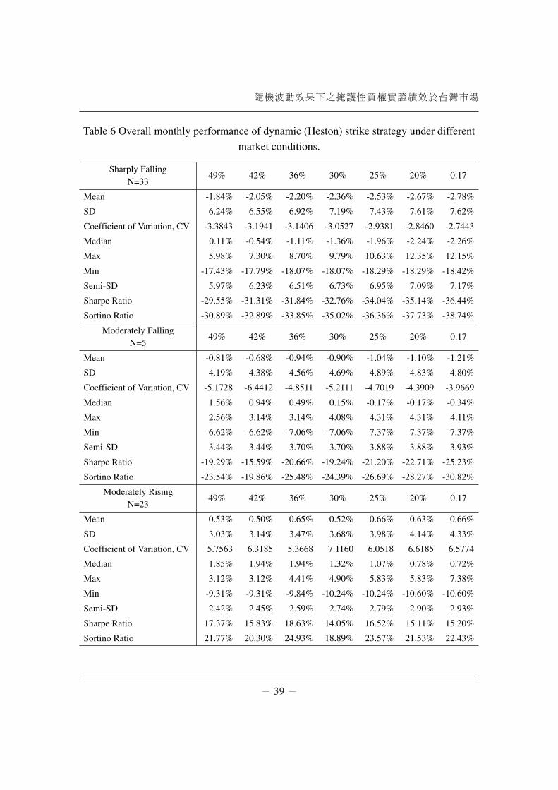
More specifically, we can find out that the Black and Heston models choose the same

probabilities of the closest ATM in sharply falling market and of the deeply OTM in sharply

rising market. The most interesting part is that Heston model chooses to receive more pre-

mium than Black model in the case of the moderately falling market and to receive fewer

premiums than Black model in the moderately rising situation in order to reduce the prob-

ability of exercise. Overall, it is the reason why the Heston model can perform better than

Black model.

Table 4 Overall monthly performance of fixed strike strategy underdifferent market conditions.

Sharply FallingN=33 Pure Future

1%OTM

2%OTM

3%OTM

4%OTM

5%OTM

6%OTM

Mean -3.39% -1.86% -2.07% -2.14% -2.34% -2.45% -2.55%

SD 7.54% 6.26% 6.44% 6.73% 6.90% 7.10% 7.20%

Coefficient of Variation, CV -2.2245 -3.3636 -3.1179 -3.1442 -2.9512 -2.8950 -2.8242

Median -2.75% 0.11% -0.54% -1.11% -1.11% -1.51% -1.54%

Max 11.16% 5.98% 5.98% 7.30% 7.34% 8.77% 8.91%

Min -18.72% -17.43% -17.79% -18.07% -18.07% -18.29% -18.42%

Semi-SD 7.53% 5.99% 6.20% 6.76% 6.58% 6.73% 6.84%

Sharpe Ratio -44.95% -29.73% -32.07% -31.80% -33.88% -34.54% -35.41%

Sortino Ratio -45.01% -31.06% -33.36% -31.65% -35.52% -36.41% -37.27%

Moderately FallingN=5 Pure Future

1%OTM

2%OTM

3%OTM

4%OTM

5%OTM

6%OTM

Mean -1.65% -0.93% -0.77% -0.89% -1.03% -1.18% -1.32%

SD 4.83% 4.11% 4.53% 4.81% 4.85% 4.95% 4.92%


Median -0.74% 0.94% 0.94% 0.49% 0.15% -0.17% -0.17%

Max 3.76% 2.56% 3.14% 4.08% 4.31% 4.31% 4.11%

Min -7.99% -6.62% -7.06% -7.37% -7.37% -7.60% -7.74%

Semi-SD 4.24% 3.44% 3.61% 3.82% 3.88% 3.88% 4.10%


Sharpe Ratio -34.22% -22.68% -17.01% -18.59% -21.33% -23.94% -26.73%

Sortino Ratio -39.00% -27.15% -21.35% -23.44% -26.64% -30.49% -32.08%

Moderately RisingN=23 Pure Future

1%OTM

2%OTM

3%OTM

4%OTM

5%OTM

6%OTM

Mean 0.75% 0.46% 0.54% 0.57% 0.63% 0.74% 0.75%

SD 4.97% 3.10% 3.43% 3.70% 4.01% 4.30% 4.46%


Median 0.32% 1.85% 1.62% 1.32% 1.07% 0.78% 0.50%

Max 8.41% 3.12% 3.76% 4.41% 4.90% 6.02% 6.31%

Min -11.18% -9.31% -9.84% -9.84% -10.24% -10.60% -10.60%

Sharply RisingN=34 Pure Future

1%OTM

2%OTM

3%OTM

4%OTM

5%OTM

6%OTM

Mean 3.93% 2.18% 2.46% 2.77% 3.02% 3.17% 3.36%

SD 5.24% 2.43% 2.64% 2.95% 3.28% 3.53% 3.83%


Median 3.24% 2.49% 3.12% 3.44% 3.72% 3.60% 3.48%

Max 15.65% 4.54% 5.39% 5.87% 6.48% 7.51% 7.64%

Min -9.60% -8.30% -8.63% -8.92% -9.15% -9.31% -9.31%

Semi-SD 2.10% 1.59% 1.64% 1.74% 1.82% 1.85% 1.89%

Semi-SD 3.15% 2.45% 2.64% 2.72% 2.84% 2.94% 2.96%

Sharpe Ratio 15.07% 14.88% 15.68% 15.49% 15.75% 17.14% 16.89%

Sortino Ratio 23.79% 18.82% 20.39% 21.09% 22.22% 25.12% 25.48%

Sharpe Ratio 75.03% 89.37% 93.26% 93.83% 92.00% 89.95% 87.94%

Sortino Ratio 186.89% 136.97% 149.41% 159.44% 165.77% 171.64% 177.80%

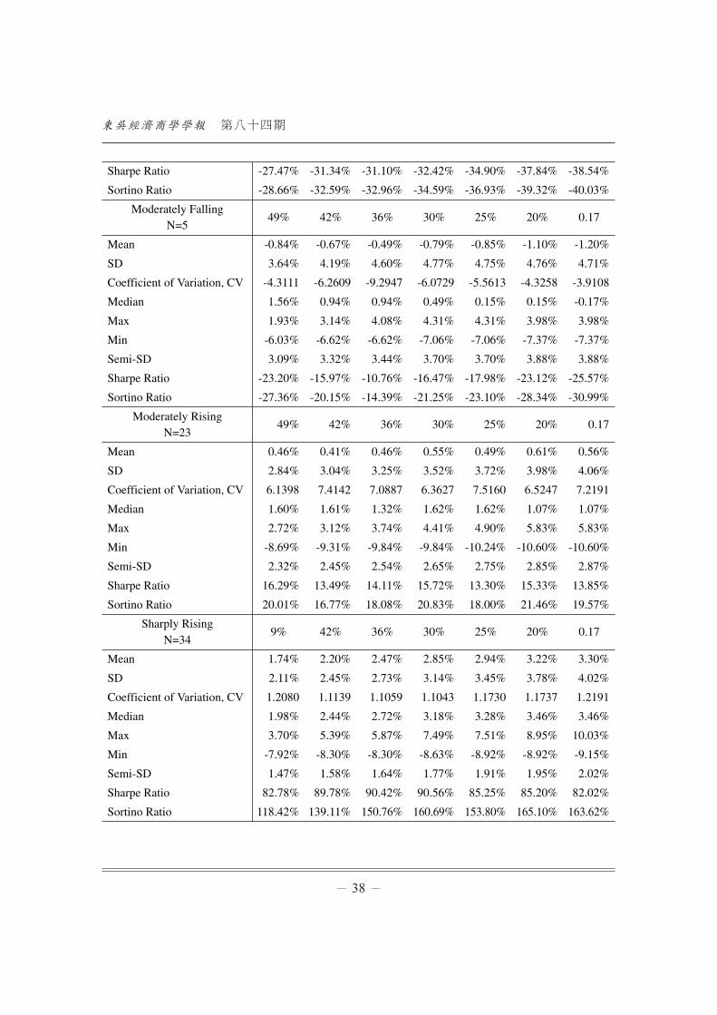
Table 5 Overall monthly performance of dynamic (Black) strike strategy under differ-ent market conditions.

Sharply FallingN=33

49% 42% 36% 30% 25% 20% 0.17

Mean -1.62% -1.99% -2.12% -2.33% -2.56% -2.81% -2.90%

SD 5.89% 6.34% 6.82% 7.19% 7.34% 7.41% 7.52%


Median 0.88% -0.04% -1.11% -1.36% -1.67% -2.24% -2.45%

Max 5.25% 5.98% 8.77% 10.39% 11.31% 10.49% 10.49%

Min -16.95% -17.43% -17.79% -18.07% -18.29% -18.42% -18.42%

Semi-SD 5.64% 6.10% 6.44% 6.74% 6.94% 7.14% 7.24%

第八十四期

Sharpe Ratio -27.47% -31.34% -31.10% -32.42% -34.90% -37.84% -38.54%

Sortino Ratio -28.66% -32.59% -32.96% -34.59% -36.93% -39.32% -40.03%

Moderately FallingN=5

49% 42% 36% 30% 25% 20% 0.17

Mean -0.84% -0.67% -0.49% -0.79% -0.85% -1.10% -1.20%

SD 3.64% 4.19% 4.60% 4.77% 4.75% 4.76% 4.71%


Median 1.56% 0.94% 0.94% 0.49% 0.15% 0.15% -0.17%

Max 1.93% 3.14% 4.08% 4.31% 4.31% 3.98% 3.98%

Min -6.03% -6.62% -6.62% -7.06% -7.06% -7.37% -7.37%

Semi-SD 3.09% 3.32% 3.44% 3.70% 3.70% 3.88% 3.88%

Sharpe Ratio -23.20% -15.97% -10.76% -16.47% -17.98% -23.12% -25.57%

Sortino Ratio -27.36% -20.15% -14.39% -21.25% -23.10% -28.34% -30.99%

Moderately RisingN=23

49% 42% 36% 30% 25% 20% 0.17

Mean 0.46% 0.41% 0.46% 0.55% 0.49% 0.61% 0.56%

SD 2.84% 3.04% 3.25% 3.52% 3.72% 3.98% 4.06%


Median 1.60% 1.61% 1.32% 1.62% 1.62% 1.07% 1.07%

Max 2.72% 3.12% 3.74% 4.41% 4.90% 5.83% 5.83%

Min -8.69% -9.31% -9.84% -9.84% -10.24% -10.60% -10.60%

Semi-SD 2.32% 2.45% 2.54% 2.65% 2.75% 2.85% 2.87%

Sharpe Ratio 16.29% 13.49% 14.11% 15.72% 13.30% 15.33% 13.85%

Sortino Ratio 20.01% 16.77% 18.08% 20.83% 18.00% 21.46% 19.57%

Sharply RisingN=34

9% 42% 36% 30% 25% 20% 0.17

Mean 1.74% 2.20% 2.47% 2.85% 2.94% 3.22% 3.30%

SD 2.11% 2.45% 2.73% 3.14% 3.45% 3.78% 4.02%


Median 1.98% 2.44% 2.72% 3.18% 3.28% 3.46% 3.46%

Max 3.70% 5.39% 5.87% 7.49% 7.51% 8.95% 10.03%

Min -7.92% -8.30% -8.30% -8.63% -8.92% -8.92% -9.15%

Semi-SD 1.47% 1.58% 1.64% 1.77% 1.91% 1.95% 2.02%

Sharpe Ratio 82.78% 89.78% 90.42% 90.56% 85.25% 85.20% 82.02%

Sortino Ratio 118.42% 139.11% 150.76% 160.69% 153.80% 165.10% 163.62%


Table 6 Overall monthly performance of dynamic (Heston) strike strategy under different

market conditions.

Sharply FallingN=33

49% 42% 36% 30% 25% 20% 0.17

Mean -1.84% -2.05% -2.20% -2.36% -2.53% -2.67% -2.78%

SD 6.24% 6.55% 6.92% 7.19% 7.43% 7.61% 7.62%


Median 0.11% -0.54% -1.11% -1.36% -1.96% -2.24% -2.26%

Max 5.98% 7.30% 8.70% 9.79% 10.63% 12.35% 12.15%

Min -17.43% -17.79% -18.07% -18.07% -18.29% -18.29% -18.42%

Semi-SD 5.97% 6.23% 6.51% 6.73% 6.95% 7.09% 7.17%

Sharpe Ratio -29.55% -31.31% -31.84% -32.76% -34.04% -35.14% -36.44%

Sortino Ratio -30.89% -32.89% -33.85% -35.02% -36.36% -37.73% -38.74%

Moderately FallingN=5

49% 42% 36% 30% 25% 20% 0.17

Mean -0.81% -0.68% -0.94% -0.90% -1.04% -1.10% -1.21%

SD 4.19% 4.38% 4.56% 4.69% 4.89% 4.83% 4.80%


Median 1.56% 0.94% 0.49% 0.15% -0.17% -0.17% -0.34%

Max 2.56% 3.14% 3.14% 4.08% 4.31% 4.31% 4.11%

Min -6.62% -6.62% -7.06% -7.06% -7.37% -7.37% -7.37%

Semi-SD 3.44% 3.44% 3.70% 3.70% 3.88% 3.88% 3.93%

Sharpe Ratio -19.29% -15.59% -20.66% -19.24% -21.20% -22.71% -25.23%

Sortino Ratio -23.54% -19.86% -25.48% -24.39% -26.69% -28.27% -30.82%

Moderately RisingN=23

49% 42% 36% 30% 25% 20% 0.17

Mean 0.53% 0.50% 0.65% 0.52% 0.66% 0.63% 0.66%

SD 3.03% 3.14% 3.47% 3.68% 3.98% 4.14% 4.33%


Median 1.85% 1.94% 1.94% 1.32% 1.07% 0.78% 0.72%

Max 3.12% 3.12% 4.41% 4.90% 5.83% 5.83% 7.38%

Min -9.31% -9.31% -9.84% -10.24% -10.24% -10.60% -10.60%

Semi-SD 2.42% 2.45% 2.59% 2.74% 2.79% 2.90% 2.93%

Sharpe Ratio 17.37% 15.83% 18.63% 14.05% 16.52% 15.11% 15.20%

Sortino Ratio 21.77% 20.30% 24.93% 18.89% 23.57% 21.53% 22.43%

第八十四期

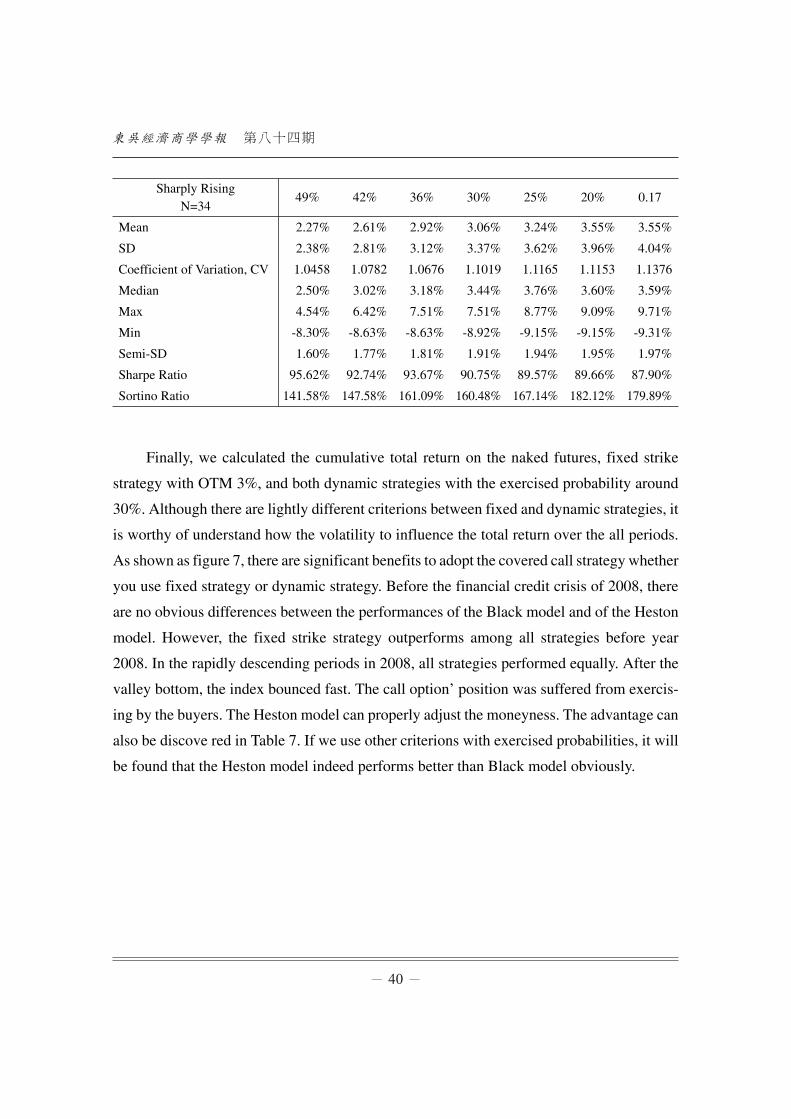
Sharply RisingN=34

49% 42% 36% 30% 25% 20% 0.17

Mean 2.27% 2.61% 2.92% 3.06% 3.24% 3.55% 3.55%

SD 2.38% 2.81% 3.12% 3.37% 3.62% 3.96% 4.04%


Median 2.50% 3.02% 3.18% 3.44% 3.76% 3.60% 3.59%

Max 4.54% 6.42% 7.51% 7.51% 8.77% 9.09% 9.71%

Min -8.30% -8.63% -8.63% -8.92% -9.15% -9.15% -9.31%

Semi-SD 1.60% 1.77% 1.81% 1.91% 1.94% 1.95% 1.97%

Sharpe Ratio 95.62% 92.74% 93.67% 90.75% 89.57% 89.66% 87.90%

Sortino Ratio 141.58% 147.58% 161.09% 160.48% 167.14% 182.12% 179.89%

Finally, we calculated the cumulative total return on the naked futures, fixed strike

strategy with OTM 3%, and both dynamic strategies with the exercised probability around

30%. Although there are lightly different criterions between fixed and dynamic strategies, it

is worthy of understand how the volatility to influence the total return over the all periods.

As shown as figure 7, there are significant benefits to adopt the covered call strategy whether

you use fixed strategy or dynamic strategy. Before the financial credit crisis of 2008, there

are no obvious differences between the performances of the Black model and of the Heston

model. However, the fixed strike strategy outperforms among all strategies before year

2008. In the rapidly descending periods in 2008, all strategies performed equally. After the

valley bottom, the index bounced fast. The call option’ position was suffered from exercis-

ing by the buyers. The Heston model can properly adjust the moneyness. The advantage can

also be discove red in Table 7. If we use other criterions with exercised probabilities, it will

be found that the Heston model indeed performs better than Black model obviously.


-50%

-40%

-30%

-20%

-10%

0%

10%

20%

30%

40%

50%

2004

0218

2004

0519

2004

0818

2004

1117

2005

0216

2005

0518

2005

0817

2005

1116

2006

0215

2006

0517

2006

0816

2006

1115

2007

0226

2007

0516

2007

0815

2007

1121

2008

0220

2008

0521

2008

0820

2008

1119

2009

0218

2009

0520

2009

0819

2009

1118

2010

0222

2010

0519

2010

0818

2010

1117

2011

0216

2011

0518

2011

0817

2011

1116

Cumulative Total Return

Future Fixed Strike Dynamic (BS) Dynamic (Heston)

Figure 7 The cumulative total return on the futures, fixed strike strategy with the

OTM 3%, dynamic (BS) strategy and dynamic (Heston) strategy with the

exercised probability around 30%.

Table 7 The performance is under conventional strategy and dynamic strategies

(Black and Heston models).

Total Period 0.17 0.2 0.25 0.3 0.36 0.42 0.49 Average Pure Future

Fixed Moneyness 0.3307%

Black Model 0.2464% 0.2673% 0.2382% 0.3016% 0.2319% 0.1626% 0.1297% 0.2254% 0.3225%

Heston Model 0.4018% 0.4354% 0.3873% 0.3544% 0.3859% 0.3052% 0.2574% 0.3610%

Sharply Falling 0.17 0.2 0.25 0.3 0.36 0.42 0.49 Average Pure Future

Fixed Moneyness -2.2347%

Black Model -2.8994% -2.8057% -2.5626% -2.3317% -2.1213% -1.9867% -1.6173% -2.3321% -3.3903%

Heston Model -2.7777% -2.6742% -2.5286% -2.3556% -2.2035% -2.0502% -1.8442% -2.3477%

Moderately Falling 0.17 0.2 0.25 0.3 0.36 0.42 0.49 Average Pure Future

Fixed Moneyness -1.0219%

Black Model -1.2035% -1.1006% -0.8548% -0.7861% -0.4946% -0.6690% -0.8443% -0.8504% -1.6542%

Heston Model -1.2120% -1.0978% -1.0366% -0.9024% -0.9426% -0.6824% -0.8089% -0.9547%

第八十四期

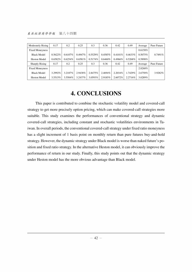
Moderately Rising 0.17 0.2 0.25 0.3 0.36 0.42 0.49 Average Pure Future


Black Model 0.5622% 0.6107% 0.4947% 0.5529% 0.4585% 0.4101% 0.4633% 0.5075% 0.7491%

Heston Model 0.6582% 0.6254% 0.6581% 0.5174% 0.6460% 0.4966% 0.5268% 0.5898%

Sharply Rising 0.17 0.2 0.25 0.3 0.36 0.42 0.49 Average Pure Future


Black Model 3.2992% 3.2187% 2.9438% 2.8475% 2.4694% 2.2034% 1.7429% 2.6750% 3.9282%

Heston Model 3.5515% 3.5504% 3.2437% 3.0593% 2.9185% 2.6072% 2.2716% 3.0289%

4. CONCLUSIONS

This paper is contributed to combine the stochastic volatility model and covered-call

strategy to get more precisely option pricing, which can make covered-call strategies more

suitable. This study examines the performances of conventional strategy and dynamic

covered-call strategies, including constant and stochastic volatilities environments in Ta-

iwan. In overall periods, the conventional covered-call strategy under fixed ratio moneyness

has a slight increment of 1 basis point on monthly return than pure futures buy-and-hold

strategy. However, the dynamic strategy under Black model is worse than naked future’s po-

sition and fixed ratio strategy. In the alternative Heston model, it can obviously improve the

performance of return in our study. Finally, this study points out that the dynamic strategy

under Heston model has the more obvious advantage than Black model.


Footnotes

1. Put option can be derived from put-call parity.

2. In the original Heston’s model, the underlying asset is stock price. We use the futures index to replace

the stock index in order to consider the time consistency compared to options and the Heston model

is comparable with the Black model.

第八十四期

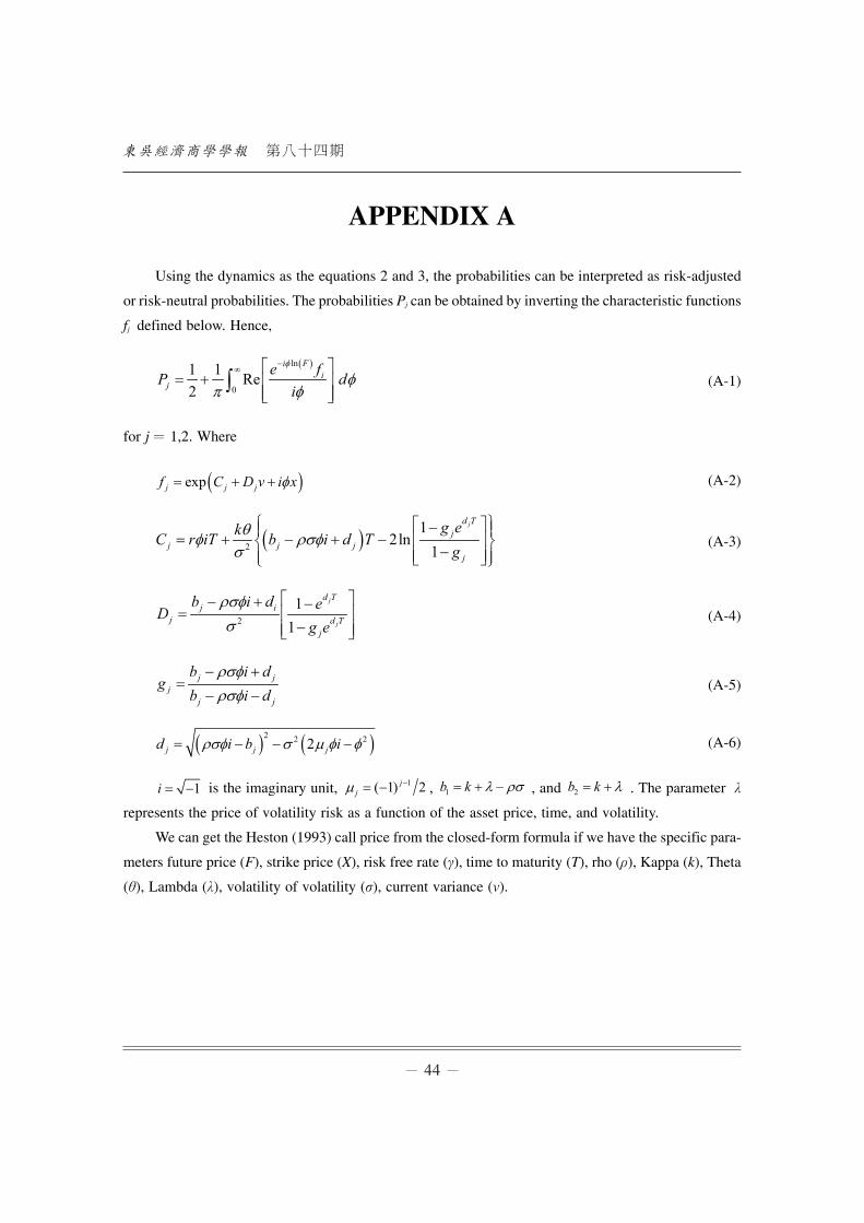
APPENDIX A

Using the dynamics as the equations 2 and 3, the probabilities can be interpreted as risk-adjusted

or risk-neutral probabilities. The probabilities Pj can be obtained by inverting the characteristic functions

fj defined below. Hence,

( )ln

0

1 1 Re 2

i Fi

je fP di

φ

φπ φ

−∞ ⎡ ⎤

= + ⎢ ⎥⎢ ⎥⎣ ⎦

∫ (A-1)

for j＝ 1,2. Where

( )expj j jf C D v i xφ= + + (A-2)

( )2

12ln

1

jd Tj

j j jj

g ekC r iT b i d Tg

θφ ρσφσ

⎧ ⎫⎡ ⎤−⎪ ⎪= + − + − ⎢ ⎥⎨ ⎬−⎢ ⎥⎪ ⎪⎣ ⎦⎩ ⎭(A-3)

2

11

j

j

d Tj i

j d Tj

b i d eDg e

ρσφσ

⎡ ⎤− + −= ⎢ ⎥

−⎢ ⎥⎣ ⎦(A-4)

j jj

j j

b i dg

b i dρσφρσφ

− +=

− −(A-5)

( ) ( )2 2 22j j jd i b iρσφ σ μ φ φ= − − − (A-6)

1i = − is the imaginary unit, 1( 1) 2jjμ

−= − , 1b k λ ρσ= + − , and 2b k λ= + . The parameter

represents the price of volatility risk as a function of the asset price, time, and volatility.

We can get the Heston (1993) call price from the closed-form formula if we have the specific para-

meters future price (F), strike price (X), risk free rate ( ), time to maturity (T), rho ( ), Kappa (k), Theta

( ), Lambda ( ), volatility of volatility ( ), current variance ( ).


REFERENCES

Black, F. (1976), “The pricing of commodity contracts.” Journal of Financial Economics, 3, 167-179.

Che, S. Y. S., and Fung, J. K. W. (2011), “The performance of alternative futures buy-write strategies.”

Journal of Futures Markets, 31, 1202-1227.

Feldman, B. and Dhruv, R. (2004), “Passive options-based investment strategies: The case of the CBOE

S&P 500 buy write index.” Ibbotson Associates, July 28, 2004.

Figelman, I. (2008), “Expected return and risk of covered call strategies.” The Journal of Portfolio Man-

agement, 34, 81-97.

Heston, S. L. (1993), “A closed-form solution for options with stochastic volatility with applications

to bond and currency options.” Review of Financial Studies, 2, 327-343.

Hill, J. M., Balasubramanian, V., Gregory, K., & Tierens, I. (2006), “Finding alpha via covered index

writing.” Financial Analysis Journal, 62, 29-46.

Whaley, R. E. (2002), “Return and risk of CBOE buy write monthly index.” Journal of Derivatives,

10, 35-42.

第八十四期

第八十四期

（民國一○三年三月）：25-46.

隨機波動效果下之掩護性買權實證

績效於台灣市場

謝長杰* 林忠機** 陳琪龍***

摘要

傳統的掩護性買權採用固定比例價外的買權作為賣出之標的，而動態調整

策略為採用隱含波動度反推固定履約機率下之價外買權作為賣出之標的。然而

以往文獻以及實務上皆未考量隨機波動效果的掩護性買權策略。因此本文檢驗

具有隨機波動效果下的動態調整策略，並與傳統與固定波動下動態調整的掩護

性買權策略作比較，並以買進並持有到到期下的裸部位近月期貨為比較基礎。

研究結果顯示，以平均的報酬績效作比較之下，傳統的掩護性買權報酬績效僅

些微高於裸期貨部位，固定波動下之掩護性買權報酬績效甚至比裸期貨部位還

來的更差，而以隨機波動模型下的掩護性買權策略績效表現最佳。

關鍵字：掩護性買權、動態調整策略、隨機波動

* 通訊作者，東吳大學經濟系博士候選人。** 東吳大學財務工程與精算數學系教授。***銘傳大學財務金融系助理教授。

Documents

Empirical Performance of Covered-Call Strategy under Stochastic Volatility in Taiwan