Empirical Properties of Closed and Open Economy DSGEModels of the Euro Area

Malin AdolfsonSveriges Riksbank

Stefan LaséenSveriges Riksbank

Jesper LindéIIES and Sveriges Riksbank

Mattias Villani∗

Sveriges Riksbank and Stockholm University

September 1, 2005

Abstract

In this paper, we compare the empirical properties of closed and open economy DSGEmodels estimated on Euro area data. The comparison is made along several dimensions; weexamine the models in terms of their marginal likelihoods, forecasting performance, variancedecompositions, and their transmission mechanisms of monetary policy.

Keywords: Open economy; Closed economy; DSGE model; Monetary policy; Forecasting;Bayesian inference.

JEL Classification Numbers: E40; E52; C11.

1. Introduction

Since the pioneering work of Smets and Wouters (2003), the interest in academia and centralbanks for developing and estimating dynamic stochastic general equilibrium (DSGE) models ofthe macroeconomy have grown considerably. In more recent work, Smets and Wouters (2004)have shown that closed economy dynamic general equilibrium models augmented with nominaland real frictions have forecasting properties in line with best practice time series models (i.e.,Bayesian VARs).

In this paper, we contrast a closed economy DSGE model with a model that accounts foropen economy aspects. Our DSGE model extends the closed economy model of Christiano,Eichenbaum and Evans (2005) by incorporating open economy elements such as incomplete ex-change rate pass-through and imperfect international financial integration. The closed economyversion of the model differ slightly from Smets and Wouters’ (2003) model in that it includes theworking capital channel (i.e., firms borrow money from a financial intermediary to finance theirwage bill), and a stochastic unit root technology shock as in Altig et al. (2003), which enablesus to work with trending data.

We estimate open and closed economy versions of this model on data for the Euro area duringthe period 1980Q1− 2002Q4. Our interest in modeling the Euro area as an open economy stem

∗Address: Sveriges Riksbank, SE-103 37 Stockholm, Sweden. E-mails: malin.adolfson@riksbank.se, ste-fan.laseen@riksbank.se, jesper.linde@riksbank.se, mattias.villani@riksbank.se. We would like to thank partici-pants at the conference “Dynamic Macroeconomic Theory” held in Copenhagen June 11-13, 2004, for helpfulcomments and discussions. The views expressed in this paper are solely the responsibility of the authors andshould not be interpreted as reflecting the views of the Executive Board of Sveriges Riksbank.

1

partly from the work of Lindé (2003), who shows that changes in net exports account for asubstantial fraction of the variation in output after a monetary policy shock in a 10-variablevector autoregressive (VAR) model estimated on Euro area data. In contrast, Lindé finds thatU.S. data imply that consumption and investment responses explain most of the fluctuation inoutput after a policy shock, while net exports only account for a small part. Consequently, itseems appropriate to model the U.S. as a closed economy but worth considering open economyaspects when estimating a model on Euro area data.

In the paper we adopt the assumption that foreign inflation, output and interest rate areexogenously given. This approximation is perhaps more suitable for a small open economy, butgiven the results by Lindé (2003) it is probably a less rudimentary statement than modeling theEuro area as a closed economy. In addition, there is some empirical support for this approxi-mation. By estimating a VAR model with ten Euro area variables and three foreign variables(”rest of the world” inflation, output and interest rate), we find that the Euro area variablesaccount for a small fraction of the variation in the foreign variables, around 10(20) percent atthe one(five) year horizon.1

We compare the estimated open and closed economy models in terms of their marginallikelihoods, their forecasting performance, the underlying sources of fluctuations in each model(variance decompositions), and the implications for the monetary transmission channel (impulseresponses).

The results show that there are no fundamental differences between the estimated parametersin the closed and open economy versions of the model. At a general level, the existence ofnominal and real frictions is crucial for both models’ ability to fit the data. However, there aresome differences in the estimated degree of the nominal and real frictions, which have effectson the dynamics of the two models. Impulse response analysis to an unexpected increase inthe interest rate (i.e. a positive monetary policy shock) reveal differences in the transmissionmechanism of monetary policy in the open and closed economy settings. The exchange ratechannel implies that inflation drops more heavily in the open economy model than in the closedeconomy version. For output, we find that the exchange rate channel is relatively unimportant,but there is nevertheless a substantial difference in the impulse responses, which is due to thedifferences in nominal and real rigidities in the two models.

The comparison of marginal likelihoods suggest that a closed economy version of the modelgives a better description of the domestic macroeconomic development than the open economymodel estimated on the same set of variables. Note though that a comparison cannot be madeagainst the complete open economy model since this is estimated on a different and richer setof variables, also including, for example, the exchange rate, exports and imports.

Since we cannot compare the marginal likelihoods of the closed economy model and the openeconomy model estimated on the full set of variables, we evaluate the forecasting performance ofthe open and closed DSGE models using traditional univariate and multivariate out-of-samplemeasures of the forecast accuracy. It is not clear what can be expected from this comparison apriori. The larger open economy version of the model naturally has the potential of providing amore detailed description of the economy, but this may also be a drawback if some aspect of theopen economy is poorly modelled. It is probably fair to say that the collective experience frommacroeconomic forecasting is that smaller models tend to out-perform larger ones. The generalfinding in this paper is that adding open economy features to the model improves the predictionson some of the variables, e.g. output and employment, whereas for other variables, such as

1The identifying assumption in the analysis is that the Euro area shocks have no contemporaneous effectson the foreign variables. Moreover, it should be noticed that the results are not much affected by changing thelag-length (we experimented with 1-4 lags).

2

inflation and investment, the closed economy model gives more accurate forecasts. However,the multivariate accuracy measures, which takes the joint forecasting performance of all sevendomestic variables into account, seems to propose the open economy model as the best forecastingtool for all horizons that we consider (1 to 16 quarters ahead).

We also find that the macroeconomic development is driven by very different disturbancesin the two models. The variance decompositions show that in the open economy model, “openeconomy shocks” are of high relevance for explaining the fluctuations in output and inflationin the short- to medium term horizon. In the closed economy model, most of the variation isinstead attributed to the two technology shocks (stationary and unit root) at the same horizons.

The remainder of the paper is organized as follows. In Section 2, we describe the openeconomy DSGE model and how to reduce it to obtain a closed economy setting. We discuss thetheoretical components of the model as well as the estimation outcomes in the open and closedeconomy frameworks. Section 3 contains the results from the comparison of the two models.Section 4 provides some concluding remarks.

2. The estimated DSGE model

This section gives an overview of the model economy, and presents the key equations in thetheoretical model. We will here discuss the model in its open economy form, but we explain inSection 2.2 how we parameterize it to obtain a closed economy specification.

The model is an open economy version of the DSGE model in Christiano et al. (2005)and Altig et al. (2003), developed in Adolfson, Laséen, Lindé and Villani (2005). As in theclosed economy setup, households maximize a utility function consisting of consumption, leisureand cash balances. However, in our open economy model the households consume a basketconsisting of domestically produced goods and imported goods. These products are suppliedby domestic and importing firms, respectively. We allow the imported goods to enter bothaggregate consumption as well as aggregate investment. This is needed when matching the jointempirical fluctuations in both imports and consumption since imports (and investment) are alot more volatile than consumption.

Households can save in domestic bonds and/or foreign bonds and hold cash. This choicebalances into an arbitrage condition pinning down expected exchange rate changes (i.e., anuncovered interest rate parity (UIP) condition). As in the closed economy model householdsrent capital to the domestic firms and decide how much to invest in the capital stock givencapital adjustment costs. These are costs to adjusting the investment rate as well as costs ofvarying the utilization rate of the capital stock. Each household is a monopoly supplier of adifferentiated labour service which implies that they can set their own wage. Wage stickiness isintroduced through an indexation variant of the Calvo (1983) model.

Domestic production follows a Cobb-Douglas function in capital and labour, and is exposedto stochastic technology growth as in Altig et al. (2003). The firms (domestic, importing andexporting) all produce differentiated goods and set prices according to an indexation variantof the Calvo model. By including nominal rigidities in the importing and exporting sectors weallow for short-run incomplete exchange rate pass-through to both import and export prices.2

In what follows we provide the optimization problems of the different firms and the households,and describe the behavior of the central bank.

2Since there are neither any distribution costs in the import and export sectors nor an endogenous pricing tomarket behaviour among the firms, there would be complete pass-through in the absence of nominal rigidities.

3

2.1. Model

The model economy includes four different categories of operating firms. These are domesticgoods firms, importing consumption, importing investment, and exporting firms, respectively.Within each category there is a continuum of firms that each produces a differentiated good.The domestic goods firms produce their goods out of capital and labour inputs, and sell themto a retailer which transforms the intermediate products into a homogenous final good that inturn is sold to the households. The final domestic good is a composite of a continuum of idifferentiated goods, each supplied by a different firm, which follows the constant elasticity ofsubstitution (CES) function

Yt =

⎡⎣ 1Z0

(Yi,t)1

λdt di

⎤⎦λdt

, 1 ≤ λdt <∞, (1)

where λdt is a stochastic process that determines the time-varying markup in the domestic goodsmarket. The demand for firm i’s differentiated product, Yi,t, follows

Yi,t =

ÃP di,t

P dt

!− λdtλdt−1

Yt. (2)

The domestic production is exposed to unit root technology growth as in Altig et al. (2003).The production function for intermediate good i is given by

Yi,t = z1−αt tKαi,tH

1−αi,t − ztφ, (3)

where zt is a unit-root technology shock, t is a covariance stationary technology shock, and Hi,t

denotes homogeneous labour hired by the ith firm. Notice that Ki,t is not the physical capitalstock, but rather the capital services stock, since we allow for variable capital utilization in themodel. A fixed cost ztφ is included in the production function. We set this parameter so thatprofits are zero in steady state, following Christiano et al. (2005).

We allow for working capital by assuming that a fraction ν of the intermediate firms’ wagebill has to be financed in advance. Cost minimization yields the following nominal marginal costfor intermediate firm i:

MCdt =

1

(1− α)1−α1

αα(Rk

t )α [Wt(1 + ν(Rt−1 − 1))]1−α

1

(zt)1−α1

t, (4)

where Rkt is the gross nominal rental rate per unit of capital services, Rt−1 the gross nominal

(economy wide) interest rate, andWt the nominal wage rate per unit of aggregate, homogeneous,labour Hi,t.

Each of the domestic goods firms is subject to price stickiness through an indexation variantof the Calvo (1983) model. Since we have a time-varying inflation target in the model we allowfor partial indexation to the current inflation target, but also to last period’s inflation rate inorder to allow for a lagged pricing term in the Phillips curve. Each intermediate firm facesin any period a probability (1 − ξd) that it can reoptimize its price. The reoptimized price isdenoted P d,new

t .3 The different firms maximize profits taking into account that there might not

3For the firms that are not allowed to reoptimize their price, we adopt the indexation scheme P dt+1 =

πdtκd (πct+1)

1−κd P dt where κd is an indexation parameter.

4

be a chance to optimally change the price in the future. Firm i therefore faces the followingoptimization problem when setting its price

maxPd,newt

Et∞Ps=0

(βξd)s υt+s[(

¡πdtπ

dt+1...π

dt+s−1

¢κd ¡πct+1πct+2...πct+s¢1−κd P d,newt )Yi,t+s

−MCdi,t+s(Yi,t+s + zt+sφ

j)],

(5)

where the firm is using the stochastic discount factor (βξd)s υt+s to make profits conditional

upon utility. β is the discount factor, and υt+s the marginal utility of the households’ nominalincome in period t+ s, which is exogenous to the intermediate firms. πdt denotes inflation in thedomestic sector, πct a time-varying inflation target of the central bank and MCd

i,t the nominalmarginal cost.

The first order condition of the profit maximization problem in equation (5) yields thefollowing log-linearized Phillips curve:³bπdt − bπct´ =

β

1 + κdβ

³Etbπdt+1 − ρπ bπct´+ κd

1 + κdβ

³bπdt−1 − bπct´ (6)

−κdβ (1− ρπ)

1 + κdβbπct + (1− ξd)(1− βξd)

ξd (1 + κdβ)

³cmcdt +bλdt´ ,

where a hat denotes log-linearized variables (i.e., Xt = dXt/X).We now turn to the import and export sectors. There is a continuum of importing consump-

tion and investment firms that each buys a homogenous good at price P ∗t in the world market,and converts it into a differentiated good through a brand naming technology. The exportingfirms buy the (homogenous) domestic final good at price P d

t and turn this into a differentiatedexport good through the same type of brand naming. The nominal marginal cost of the im-porting and exporting firms are thus StP ∗t and P d

t /St, respectively. The differentiated importand export goods are subsequently aggregated by an import consumption, import investmentand export packer, respectively, so that the final import consumption, import investment, andexport good is each a CES composite according to the following:

Cmt =

⎡⎣ 1Z0

¡Cmi,t

¢ 1λmct di

⎤⎦λmct

, Imt =

⎡⎣ 1Z0

¡Imi,t¢ 1

λmit di

⎤⎦λmit

, Xt =

⎡⎣ 1Z0

(Xi,t)1λxt di

⎤⎦λxt

,

(7)where 1 ≤ λjt < ∞ for j = {mc,mi, x} is the time-varying markup in the import consump-tion (mc), import investment (mi) and export (x) sector. By assumption the continuum ofconsumption and investment importers invoice in the domestic currency and exporters in theforeign currency. In order to allow for short-run incomplete exchange rate pass-through to im-port as well as export prices we therefore introduce nominal rigidities in the local currency price.This is modeled through the same type of Calvo setup as above. The price setting problemsof the importing and exporting firms are completely analogous to that of the domestic firmsin equation (5), and the demand for the differentiated import and export goods follow similarexpressions as to equation (2). In total there is thus four specific Phillips curve relations deter-mining inflation in the domestic, import consumption, import investment and export sectors.

In the model economy there is also a continuum of households which attain utility fromconsumption, leisure and real cash balances. The preferences of household j are given by

Ej0

∞Xt=0

βt

⎡⎢⎣ζct ln (Cj,t − bCj,t−1)− ζhtAL(hj,t)

1+σL

1 + σL+Aq

³Qj,t

ztPdt

´1− σq

1−σq⎤⎥⎦ , (8)

5

where Cj,t, hj,t and Qj,t/Pdt denote the j

th household’s levels of aggregate consumption, laboursupply and real cash holdings, respectively. Consumption is subject to habit formation throughbCj,t−1, such that the household’s marginal utility of consumption is increasing in the quantity ofgoods consumed last period. ζct and ζht are AR(1) preference shocks to consumption and laboursupply, respectively. To make cash balances in equation (8) stationary when the economy isgrowing they are scaled by the unit root technology shock zt. Households consume a basket ofdomestically produced goods and imported products which are supplied by the domestic andimporting consumption firms, respectively. Aggregate consumption is assumed to be given bythe following constant elasticity of substitution (CES) function:

Ct =

∙(1− ωc)

1/ηc³Cdt

´(ηc−1)/ηc+ ω

1/ηcc (Cm

t )(ηc−1)/ηc

¸ηc/(ηc−1), (9)

where Cdt and Cm

t are consumption of the domestic and imported good, respectively. ωc is theshare of imports in consumption, and ηc is the elasticity of substitution across consumptiongoods.

The households invest in a basket of domestically produced goods and imported investmentgoods to form the physical capital stock, and decide how much capital services to rent to thedomestic firms, given capital adjustment costs. These are costs to adjusting the investment rateas well as costs of varying the utilization rate of the physical capital stock. The households canincrease their capital stock by investing in additional physical capital (It), taking one period tocome in action, or by directly increasing the utilization rate of the capital at hand (ut = Kt/Kt).The capital accumulation equation for the physical capital stock (Kt) is given by

Kt+1 = (1− δ)Kt +Υt

³1− S (It/It−1)

´It, (10)

where S (It/It−1) determines the investment adjustment costs through the estimated parameterS00, and Υt is a stationary investment-specific technology shock. Total investment is assumed tobe given by a CES aggregate of domestically produced goods and imported investment goods(Idt and Imt , respectively) according to

It =

∙(1− ωi)

1/ηi³Idt

´(ηi−1)/ηi+ ω

1/ηii (Imt )

(ηi−1)/ηi¸ηi/(ηi−1)

, (11)

where ωi is the share of imports in investment, and ηi is the elasticity of substitution acrossinvestment goods.

Further, along the lines of Erceg, Henderson and Levin (2000), each household is a monopolysupplier of a differentiated labour service which implies that they can set their own wage. Afterhaving set their wage, households inelastically supply the firms’ demand for labour at the goingwage rate. Each household sells its labour to a firm which transforms household labour into ahomogenous good that is demanded by each of the domestic goods producing firms. Wage stick-iness is introduced through the Calvo (1983) setup, with partial indexation to last period’s CPIinflation rate, the current inflation target and the technology growth. Household j reoptimizesits nominal wage rate Wnew

j,t according to the following

maxWnewj,t

EtP∞

s=0 (βξw)s [−ζht+sAL

(hj,t+s)1+σL

1+σL+

υt+s(1−τyt+s)(1+τwt+s)

³¡πct ...π

ct+s−1

¢κw ¡πct+1...πct+s¢(1−κw) ¡µz,t+1...µz,t+s¢Wnewj,t

´hj,t+s],

(12)

6

where ξw is the probability that a household is not allowed to reoptimize its wage, τyt a labour

income tax, τwt a pay-roll tax (paid for simplicity by the households), and µz,t = zt/zt−1 is thegrowth rate of the permanent technology level.4

The households can save in domestic bonds and foreign bonds, and also hold cash. Thischoice balances into an arbitrage condition pinning down expected exchange rate changes (i.e.,an uncovered interest rate parity condition). To ensure a well-defined steady-state in the model,we assume that there is a premium on the foreign bond holdings which depends on the aggregatenet foreign asset position of the domestic households, following, e.g., Lundvik (1992) and Benigno(2001):

Φ(at, φt) = exp(−φa(at − a) + φt), (13)

where At ≡ (StB∗t )/(Ptzt) is the net foreign asset position, and φt is a shock to the risk premium.The budget constraint for the households is given by

Mt+1 + StB∗t+1 + P c

t Ct (1 + τ ct) + P it It + Pta(ut)Kt (14)

=

Rt−1 (Mt −Qt) +Qt +R∗t−1Φ(at−1, eφt−1)StB∗t+³1− τkt

´Rkt utKt + (1− τyt )

Wt

1 + τwtht +

³1− τkt

´Πt

−τkth(Rt−1 − 1) (Mt −Qt) +

³R∗t−1Φ(at−1, eφt−1)− 1´StB∗t +B∗t (St − St−1)

i+TRt +Dt,

where the right-hand side describes the resources at disposal. The households earn interest onthe amount of nominal domestic assets that are not held as cash,Mt−Qt. They can also save inforeign bonds B∗t , which pay a risk-adjusted pre-tax gross interest rate of R

∗t−1Φ(at−1,

eφt−1). St isthe nominal exchange rate (foreign currency per unit of domestic currency), Rk

t the gross nominalrental rate of capital, and Wt the nominal wage rate. The households earn income from rentingcapital and labour services (Kt and ht) to the intermediate firms, where ut denotes the varyingcapital utilization rate and Kt the physical capital stock. They pay taxes on consumption (τ ct),capital income (τkt ), labour income (τ

yt ), and on the pay-roll (τ

wt ). Πt denotes profits, TRt lump-

sum transfers from the government, and Dt the household’s net cash income from participatingin state contingent securities at time t. The right hand side describes how the households spendtheir resources on consumption and investment goods, priced at P c

t and P it respectively, on

future bond holdings, and pay the cost of varying the capital utilization rate Pta(ut)Kt, wherea(ut) is the utilization cost function.

Following Smets and Wouters (2003), monetary policy is approximated with the followinginstrument rule (expressed in log-linearized terms)

bRt = ρR bRt−1 + (1− ρR)£bπct + rπ

¡πct−1 − bπct¢+ ryyt−1 + rxxt−1

¤(15)

+r∆π

¡πct − πct−1

¢+ r∆y∆yt + εR,t,

where εR,t is an uncorrelated monetary policy shock. Thus, the central bank is assumed toadjust the short term interest rate in response to deviations of CPI inflation from the time-varying inflation target

¡πct − bπct¢, the output gap (yt, measured as actual minus trend output),

the real exchange rate (xt) and the interest rate set in the previous period. In addition, notethat the nominal interest rate adjusts directly to the inflation target. The output target used by

4For the households that are not allowed to reoptimize, the indexation scheme is Wj,t+1 =(πct)

κw (πct+1)(1−κw) µz,t+1W

newj,t , where κw.

7

the central bank is here defined to be the trend level of output. An alternative specification isto define the output target in terms of the level output that would have prevailed in the absenceof nominal rigidities. This model consistent output gap would to a larger extent probably comecloser to optimal monetary policy (see Woodford, 2003, for further discussion). However, DelNegro et al. (2004) show that a rule using the trend output gap is preferred over a rule withthe model consistent output gap, when estimating a closed economy DSGE model on US data.

To clear the final goods market, the foreign bond market, and the loan market, the followingthree constraints must hold in equilibrium:

Cdt + Idt +Gt + Cx

t + Ixt ≤ z1−αt tKαt H

1−αt − ztφ− a(ut)Kt, (16)

StB∗t+1 = StP

xt (C

xt + Ixt )− StP

∗t (C

mt + Imt ) +R∗t−1Φ(at−1, eφt−1)StB∗t , (17)

νWtHt = µtMt −Qt, (18)

where Cxt and Ixt are the foreign demand for export goods, P

∗t the foreign price level, and

µt = Mt+1/Mt is the monetary injection by the central bank. When defining the demand forexport goods, we introduce a stationary asymmetric technology shock z∗t = z∗t /zt, where z

∗t is

the permanent technology level abroad, to allow for different degrees of technological progressdomestically and abroad.

The structural shock processes in the model is given in log-linearized form by the univariaterepresentation

xt = ρxxt−1 + εx,t, εx,tiid∼ N

¡0, σ2x

¢where x = { µz,t, t, λ

jt , ζ

ct , ζ

ht , Υt, φt, εR,t, π

ct , z

∗t } and j = {d,mc,mi, x} .

Lastly, to simplify the analysis we adopt the assumption that the foreign prices, output(HP-detrended) and interest rate are exogenously given by an identified VAR(4) model.5 Thefiscal policy variables - taxes on capital income, labour income, consumption, and the pay-roll,together with (HP-detrended) government expenditures - are assumed to follow an identifiedVAR(2) model.6

To compute the equilibrium decision rules, we proceed as follows. First, we stationarize allquantities determined in period t by scaling with the unit root technology shock zt. Then, welog-linearize the model around the constant steady state and calculate a numerical solution withthe AIM algorithm developed by Anderson and Moore (1985).

2.2. Estimation

To estimate the model we use quarterly Euro area data for the period 1970Q1-2002Q4. The dataset employed here was first constructed by Fagan et al. (2001).7 In order to be able to identifythe 51 parameters in the open economy model we use data on the following 15 variables in theestimation: the domestic inflation rate πt; the growth rates in the real wage ∆wt (∆ denotes thefirst difference operator), consumption ∆ct, investment ∆it, GDP ∆yt, exports ∆ eXt, imports∆fMt; the short-run interest rate Rt; employment Et; the growth rates in the consumptiondeflator πdef,ct and the investment deflator πdef,it ; the real exchange rate xt; foreign inflation π∗t ;

5The reason why we include foreign output HP-detrended and not in growth rates in the VAR is that the levelof foreign output enters the model (e.g., in the aggregate resource constraint).

6 It should be noted that Adolfson et al. (2005) report that the fiscal shocks have small dynamic effects in themodel. This is because households are Ricadian and infinitively lived. Moreover, these shocks are transitory anddo not generate any wealth effects. Finally, the fiscal shocks are estimated to have relatively small variance.

7The Fagan data set includes foreign (i.e., rest of the world) output and inflation, but not a foreign interestrate. We therefore use the Fed funds rate as a proxy for R∗t .

8

the foreign interest rate R∗t ; and the growth rate in foreign output ∆y∗t .8 Including a large set of

variables facilitates identification of the underlying structural parameters in the economy. Forinstance, inclusion of the consumption and investment deflators along with the domestic andforeign GDP deflators implies that we can extract information about the unobserved importmarkup shocks. Unfortunately, as we adopt the assumption that firms in the export sector setprices in foreign currency, we are not able obtain appropriate data for export prices. This impliesthat the export price markup shock series will be weakly identified compared to other parts ofthe model. The reason for modeling the real variables in growth rates is that the unit roottechnology shock induces a common stochastic trend in the levels of these variables. Althoughthe parameters in the exogenous foreign VAR are pre-estimated, we still include the foreignvariables as observables in the estimation for two reasons. First, they enable identification ofthe asymmetric technology shock, as the foreign VAR is estimated using HP-detrended foreignoutput and we include actual foreign output growth as observable in the estimation.9 Second,they are informative about the parameters governing the propagation of foreign impulses to thedomestic economy. 13 structural shocks are estimated, out of which 11 follow AR(1) processesand two are white noise processes. Although we match 15 variables, this procedure does notinvolve singularity problems since 8 shocks are included as pre-estimated in the model (5 fiscaland 3 foreign). To calculate the likelihood function of the observed variables we apply theKalman filter where we use the period 1970Q1-1979Q4 to form a prior on the unobserved statevariables in 1979Q4, and then use the period 1980Q1-2002Q4 for inference.

To get a closed economy version of the model we must establish that the consumption andinvestment baskets only consist of domestically produced goods. That is, we set ωc = ωi = 0and ηc = ηi =∞.10 The 29 parameters pertaining to the domestic economy are then estimatedby matching the ‘domestic’ variables (πt, ∆ct, ∆it, ∆yt, ∆wt, Rt, Et).

A number of parameters are kept fixed throughout the estimation procedure of both theclosed and open economy versions of the model. Most of these parameters can be related to thesteady-state values of the observed variables in the model, and are therefore calibrated to matchthe sample mean of these.11

Table 1 shows the assumptions for the prior distribution of the estimated parameters. Thelocation of the prior distribution corresponds to a large extent to those in Smets and Wouters(2003) and the findings in Altig et al. (2003) on U.S. data. For more details about our choice

8There is no (official) data on aggregate hours worked, Ht, available for the euro area. Therefore, we useemployment Et in our estimations. Since employment is likely to respond more slowly to shocks than hoursworked, we model employment using Calvo-rigidity (following Smets and Wouters, 2003): ∆Et = βEt∆Et+1 +(1−ξe)(1−βξe)

ξeHt − Et . For reasons discussed in greater detail in Adolfson et al. (2005), we also take out a

linear trend in employment and the excess trend in imports and exports relative to the trend in GDP prior toestimation.

9We measure actual foreign output in the state-space representation as the sum of detrended foreign output,domestic productivity and the asymmetric technology shock. This enables us to identify the asymmetric technol-ogy shock since the process for detrended foreign output is identified from the VAR and the process for domesticproductivity from domestic quantities.10 In addition, we set λmc = λmi = 1, ξmc = ξmi = ξx = 0, φ = 0, and rx = 0 to ensure that all relative prices

are unity and that the effects of the three foreign VAR shocks, the asymmetric technology shock and the threeimport and export markup shocks are zero.11The calibrated parameters are set to the following: the money growth µ = 1.01; the discount factor β = 0.999;

the depreciation rate δ = 0.013; the capital share in production α = 0.29; the share of imports in consumption andinvestment ωc = 0.31 and ωi = 0.55, respectively; the steady-state tax rates on labour income and consumptionτy = 0.177 and τc = 0.125, respectively; government expenditures-output ratio 0.20. For reasons discussed ingreater detail in Adolfson et al. (2005), we also set the substitution elasticity between domestic and importedgoods ηc = 5 and the capital utilization parameter σa = 10

6.

9

of prior distributions, see Adolfson et al. (2005). Note that we use the same prior distributionfor the 29 domestic parameters in both the open and closed economy settings.

The joint posterior distribution of all estimated parameters is obtained in two steps. First,the posterior mode and Hessian matrix evaluated at the mode is computed by standard numericaloptimization routines. Second, the Hessian matrix is used in the Metropolis-Hastings algorithmto generate a sample from the posterior distribution (see Smets and Wouters (2003), and thereferences therein, for details).

3. Comparing the models

In Table 1 we report the posterior mode and marginal likelihoods for the closed and openeconomy versions of the model. There are no fundamental differences between the estimatedparameters in the two models; in both the closed and open economy specifications nominal andreal frictions are found to be of critical importance for the models’ adaptability to the data.There are, however, some differences that have effects on the dynamics of the two models. Thenominal frictions in terms of the price and wage stickinesses are somewhat smaller in the openeconomy model. As an example, the domestic price stickiness is 0.88 in the open economy settingcompared to 0.90 in the closed economy model. This implies an average duration of domesticprice contracts of 8 and 10 quarters, respectively, under the traditional assumption that thehouseholds own the capital stock. If we instead assume that capital is specific to each firm, wecan reinterpret our estimates of the price stickiness parameter to imply an average duration ofabout 4.5 quarters (see Altig et al., 2004) in the open economy model.

In contrast, the real frictions, in terms of habit formation and investment adjustment costs,are larger in the open economy setting than in the closed economy model. In the open economymodel the habit formation parameter b is estimated to be 0.69 compared to 0.63 in the closedeconomy version. Naturally, this implies that the real variables respond less to disturbances inthe open economy model compared to the closed economy model, while nominal variables reactmore heavily in the former. Compared to Christiano et al. (2005) who estimate their model bymatching the impulse response functions to a monetary policy shock, DSGE models that areestimated to match all the variability in the data typically imply a somewhat higher degree ofnominal and real frictions. This is case here as well as in Smets and Wouters (2003).

Figure 1 displays the impulse responses to a monetary policy shock in the open and closedeconomy models. In general, the impulse response functions show a hump-shaped pattern withthe maximum impact of a policy shock occurring after about one year in both the closed and openeconomy models. However, the magnitude of the responses differ considerably. For instance,domestic inflation reacts more to a monetary policy shock in the open economy setting (solid)than in the closed economy model, whereas the response of output is stronger in the closedeconomy model (dashed). To examine if these differences are due to the exchange rate channelin the transmission mechanism of monetary policy or discrepancies in the dynamics of the twomodels (i.e., the parameter differences discussed above), we also display the responses from aclosed economy version with parameters taken from the estimated full open economy model.The difference between the open economy and closed economy models with the same domesticparameters (solid and dotted lines, respectively) can thus be attributed to the exchange ratechannel. However, we see from Figure 1 that most of the difference between the closed andopen economy models for output cannot be ascribed to the exchange rate channel, instead it ismostly due to the different parameter estimates in the two models. For inflation, the exchangerate channel is most important around the peak, and less relevant at longer horizons. It shouldalso be noted that net exports fall considerably after the appreciation of the real exchange rate.

10

A marginal likelihood comparison (see, e.g., Smets and Wouters (in press)) of the open andclosed economy versions of the model is not straightforward since the closed economy version onlyincludes a subset of the 15 observed variables in the estimation. One approach is to comparethe marginal likelihood of the closed econony model, pc(xc), where xc denotes the subset ofclosed economy variables, to the marginal likelihood of the closed economy variables in the openeconomy model, which we denote by po(xc). Another approach is to compare the marginallikelihood of xc conditional on the open economy variables, xo, using the open economy model.Since po(xc|xo) = po(xc, xo)/po(xo), and po(xc, xo) is already available from the estimation onthe full set of variables, the latter approach boils down to computing the marginal likelihoodof xo in the open economy model. A problem with both these approaches is that the model isat best weakly identified if only a subset of the data is used for estimation. Even though wehave well defined prior distributions on the model parameters to aid identification, a vague prioron the underlying unobserved state variables in combination with the complex nature of theDSGE model resulted in numerically unstable marginal likelihoods.12 We have therefore chosenanother route for computing the marginal likelihood of the closed economy variables in the openeconomy model, where the 22 parameters pertaining to the open economy are calibrated andonly the 29 domestic parameters are estimated. The parameters referring to the open economyare calibrated to their posterior mode values from the full estimation on all 15 variables (seeTable 1).

The marginal likelihood seems to speak in favour of the closed economy model. The Bayesfactor on the open economy model estimated on seven variables is about 0.002, which indicatesthat the closed economy model provides a better description of the seven domestic variablesduring 1980Q1 − 2002Q4. In the light of the well known sensitivity of the marginal likelihoodin non-linear models to the choice of prior distribution, the difference in marginal likelihoodsof the two seven-variable models in Table 1 should not be over-emphasized. This is especiallyrelevant here since the two compared models differ by as much as 22 parameters. Consideringalso the fact that we are unable to compare the closed economy version of the model with thefull open economy model estimated on all 15 variables, leads us to examine the robustness ofthese results using other modes of model evaluation, such as out-of-sample forecasting precision.

The left panel in Table 2 shows the forecasting performance of the open and closed economymodels in terms of root mean squared errors of the seven domestic variables on various horizonsover the time period 1994Q1−2002Q4.13 The open economy model does slightly worse in termsof the (domestic) inflation forecasts in the medium to long-term horizons, but surpasses the long-term closed economy forecasts on output. The multivariate statistics (i.e., the log determinantof the mean square forecast error matrix of the domestic variables and the log predictive score(LPDS)) reported in the right panel in Table 2, however, indicate that the open economy modelperforms better on all horizons when the projections of all seven variables are jointly taken intoaccount. The log determinant statistic measures the multivariate point forecast accuracy whilethe LPDS measures the plausibility of the observed outcomes with respect to the predictivedistribution as a whole.

Finally, Table 3 summarizes the results from the variance decomposition of the seven domesticvariables at four and 20 quarters horizon using the posterior mode estimates of the parameters.14

12Even though the results varied between simulations, the two approaches both indicate a fairly strong preferencefor the closed economy model.13The forecasts are generated by sequentially expanding the sample in each quarter, and re-estimating the

parameters every year.14To save space we only report two horizons. The results from other horizons can be obtained from the authors

upon request.

11

As could be expected from the parameter estimates in Table 1, we see that the role of variousshocks for explaining the macroeconomic fluctuations differ between the two models. In theclosed economy model, the two “traditional” technology shocks, i.e., the unit root and stationarytechnology shocks, are much more important. At the one year horizon they account for 55 and35 percent of the fluctuations in inflation and output, respectively. After five years they accountfor about 70 percent of the fluctuations in output, which is line with the results in the early RBCliterature, and somewhat higher than the corresponding number reported by Smets and Wouters(2003). In contrast, in the open economy specification the effects of unit root technology shocksare in line with the VAR evidence in Altig et al. (2004) and Galí and Rabanal (2004). Thedifference in the role of unit root technology shocks in the two specifications is that in the openeconomy version other shocks are assigned a more prominent role in order for the model toaccount for the joint behaviour of inflation, output, export, import and the real exchange rate.At the five year horizon, we notice that the importing markup shocks come out as an importantsource of the variation in output. In particular, the import investment markup shock turns upas very important. The reason for this is that the import investment markup shock has a verystrong and persistent effect on the real exchange rate, which in turn influences output. Even ifwe conjectured in our discussion of Figure 1 that the exchange rate channel was not the mainmechanism for understanding the transmission of monetary policy shocks, it is still sufficientlyimportant for generating substantial output effects after a markup shock to import investmentgoods.

4. Concluding remarks

In the very last years, the monetary policy literature have witnessed a revival in estimationand implementation of DSGE models in monetary policy analysis. In this paper, we comparedthe empirical properties of the closed economy benchmark DSGE model with an open econ-omy version developed by Adolfson et al. (2005). By and large, the estimation results displaymany similarities. That is, nominal and real frictions are of crucial importance for the empiricaladaptability of both models. Despite the general similarity, the specific details of the estimationresults suggest some differences in the monetary transmission channel. Equally important, wefind that the sources of macroeconomic fluctuations in the two versions of the model differ con-siderably. In the open economy version of the model we find a larger role for “open-economy”shocks in order to account for the joint fluctuations in ”domestic” and ”open economy” vari-ables (e.g., output and the real exchange rate, respectively). In terms of the models’ forecastingperformance of the development of the seven key macrovariables; inflation, the real wage, em-ployment, nominal interest rate, consumption, investment and output, we find the two modelsto perform about equally well, with a slight edge for the open economy model.

Throughout the analysis, we maintain the assumption that the spillover effects from theEuro area shocks to the foreign economy are zero. This assumption is defended on the basis of asimple VAR analysis, which suggests that the spillover effects are small in the short- to mediumrun. However, it would be of interest to extend the analysis in this paper to multi-countrymodels allowing for such effects. Very recent and preliminary contributions of Adjémain et al.(2004) and Walque and Wouters (2004) estimate multi-country models of the Euro area and theU.S.. These papers, however, maintain the implicit assumption that no countries outside thesetwo currency areas influence or are affected by fluctuations in the U.S. and the Euro area. Thisassumption is a short-cut as is the case with our zero-spillover assumption.

Finally, the different sources behind aggregate fluctuations in the two models can be expectedto have effects on the conduct of monetary policy in the open and closed economy settings,

12

respectively. We leave for future work to analyze the implications for optimal monetary policy.

References

Adjémain, Stéphane, Matthieu Darracq Pariès and Frank Smets (2004) Structural Analysis ofUS and EA Business Cycles. Manuscript, European Central Bank.

Adolfson, Malin, Stefan Laséen, Jesper Lindé and Mattias Villani (2005) Bayesian Estimationof an Open Economy DSGE Model with Incomplete Pass-Through. Working Paper No.179, Sveriges Riksbank.

Altig, David, Lawrence Christiano, Martin Eichenbaum and Jesper Lindé (2003) The Role ofMonetary Policy in the Propagation of Technology Shocks. Manuscript, NorthwesternUniversity.

Altig, David, Lawrence Christiano, Martin Eichenbaum and Jesper Lindé (2004) Firm-SpecificCapital, Nominal Rigidities and the Business Cycle. Working Paper No. 176, SverigesRiksbank.

Anderson, Gary and George Moore (1985) A Linear Algebraic Procedure for Solving LinearPerfect Foresight Models. Economics Letters 17(3), 247-252.

Benigno, Pierpaolo (2001) Price Stability with Imperfect Financial Integration. Manuscript,New York University.

Calvo, Guillermo (1983) Staggered Prices in a Utility Maximizing Framework. Journal of Mon-etary Economics 12, 383-398.

Christiano, Lawrence, Martin Eichenbaum and Charles Evans (2005) Nominal Rigidities andthe Dynamic Effects of a Shock to Monetary Policy. Journal of Political Economy 113(1),1-45.

Del Negro, Marco, Frank Schorfheide, Frank Smets and Raf Wouters (2004), ”On the Fit andForecasting Performance of New Keynesian Models”, CEPR Discussion Paper No. 4848.

Erceg, Christopher, Dale Henderson and Andrew Levin (2000) Optimal Monetary Policy withStaggered Wage and Price Contracts. Journal of Monetary Economics 46(2), 281-313.

Fagan, Gabriel, Jerome Henry and Ricardo Mestre (2001) An Area-Wide Model (AWM) for theEuro Area. Working Paper No. 42. European Central Bank.

Galí, Jordi and Pau Rabanal (2004) Technology Shocks and Aggregate Fluctuations: How WellDoes the RBC Model Fit Postwar U.S. Data? In Gertler, Mark and Kenneth Rogoff (eds.),NBER Macroeconomics Annual 2004, pp. 225-288. Cambridge, MA: MIT Press.

Lindé, Jesper (2003) Comment on ”The Output Composition Puzzle: A Difference in the Mon-etary Transmission Mechanism in the Euro Area and U.S.” by Ignazio Angeloni, Anil KKasyap, Benoît Mojon and Daniele Terlizzese. Journal of Money, Credit and Banking35(6), 1309-1318.

Lundvik, Petter (1992) Foreign Demand and Domestic Business Cycles: Sweden 1891-1987. InBusiness Cycles and Growth, pp.61-96. Monograph Series No. 22, Institute for Interna-tional Economic Studies, Stockholm University.

13

Smets, Frank and Raf Wouters (2003) An Estimated Stochastic Dynamic General EquilibriumModel of the Euro Area. Journal of the European Economic Association 1(5), 1123-1175.

Smets, Frank and Raf Wouters (2004) Forecasting with a Bayesian DSGEModel. An Applicationto the Euro Area. Working Paper No. 389, European Central Bank.

Smets, Frank and Raf Wouters (in press) Comparing Shocks and Frictions in US and Euro AreaBusiness Cycles: A Bayesian DSGE Approach. Journal of Applied Econometrics.

Walque, Grégory de, and Raf Wouters (2004) An Open Economy DSGE Model Linking theEuro Area and the US Economy. Manuscript, National Bank of Belgium.

Woodford, Michael (2003) Interest and Prices: Foundations of a Theory of Monetary Policy.Princeton: Princeton University Press.

14

Table 1: Prior and posterior distributions

Sample period 1980Q1-2002Q4 Parameter Prior distribution Posterior distribution

Open (15 var.) Closed (7 var.) Open (7 var.)

type mean* std.dev

. /df

mode std. dev. (Hessian) mode std. dev.

(Hessian) mode std. dev. (Hessian)

Calvo wages wξ beta 0.675 0.050 0.697 0.047 0.738 0.042 0.707 0.048 Calvo domestic prices dξ beta 0.675 0.050 0.883 0.015 0.904 0.017 0.881 0.034 Calvo import cons. prices mcξ beta 0.500 0.100 0.463 0.059 calib. to 0.463 Calvo import inv. prices miξ beta 0.500 0.100 0.740 0.040 calib. to 0.740 Calvo export prices xξ beta 0.500 0.100 0.639 0.059 calib. to 0.639 Calvo employment eξ beta 0.675 0.100 0.792 0.022 0.796 0.022 0.802 0.026 Indexation wages wκ beta 0.500 0.150 0.516 0.160 0.201 0.031 0.188 0.088 Index. domestic prices dκ beta 0.500 0.150 0.212 0.066 0.392 0.142 0.352 0.141 Index..import cons. prices mcκ beta 0.500 0.150 0.161 0.074 calib. to 0.161 Index..import inv. prices miκ beta 0.500 0.150 0.187 0.079 calib. to 0.187 Indexation export prices xκ beta 0.500 0.150 0.139 0.072 calib. to 0.139 Markup domestic dλ inv. gamma 1.200 2 1.168 0.053 1.196 0.068 1.188 0.069 Markup imported cons. mcλ inv. gamma 1.200 2 1.619 0.063 calib. to 1.619 Markup imported invest. miλ inv. gamma 1.200 2 1.226 0.088 calib to. 1.226 Investment adj. cost ''~S normal 7.694 1.500 8.732 1.370 6.705 1.518 8.053 1.423 Habit formation b beta 0.650 0.100 0.690 0.048 0.629 0.051 0.668 0.045 Subst. elasticity invest. iη inv. gamma 1.500 4 1.669 0.273 calib. to 1.669 Subst. elasticity foreign fη inv. gamma 1.500 4 1.460 0.098 calib. to 1.460 Technology growth zµ trunc. normal 1.006 0.0005 1.005 0.000 1.005 0.001 1.006 0.001 Capital income tax kτ beta 0.120 0.050 0.137 0.042 0.250 0.042 0.232 0.044 Labour pay-roll tax wτ beta 0.200 0.050 0.186 0.050 0.190 0.051 0.186 0.050 Risk premium φ~ inv. gamma 0.010 2 0.145 0.047 calib. to 0.145

Unit root tech. shock zµρ beta 0.850 0.100 0.723 0.106 0.894 0.035 0.891 0.038

Stationary tech. shock ερ beta 0.850 0.100 0.909 0.030 0.974 0.009 0.956 0.027 Invest. spec. tech shock Υρ beta 0.850 0.100 0.750 0.041 0.458 0.094 0.537 0.118 Asymmetric tech. shock *~zρ beta 0.850 0.100 0.993 0.002 calib. to 0.993 Consumption pref. shock cζ

ρ beta 0.850 0.100 0.935 0.029 0.978 0.008 0.983 0.006 Labour supply shock hζρ

beta 0.850 0.100 0.675 0.062 0.513 0.096 0.476 0.089 Risk premium shock φρ ~ beta 0.850 0.100 0.991 0.008 calib. to 0.991 Imp. cons. markup shock mcλ

ρ beta 0.850 0.100 0.978 0.016 calib. to 0.978 Imp. invest. markup shock miλ

ρ beta 0.850 0.100 0.974 0.015 calib. to 0.974

Export markup shock xλρ beta 0.850 0.100 0.894 0.045 calib. to 0.894

Unit root tech. shock zµσ inv. gamma 0.200 2 0.130 0.025 0.138 0.029 0.153 0.033

Stationary tech. shock εσ inv. gamma 0.700 2 0.452 0.082 0.444 0.078 0.440 0.080 Invest. spec. tech. shock Υσ inv. gamma 0.200 2 0.424 0.046 0.562 0.073 0.539 0.083 Asymmetric tech. shock *~zσ inv. gamma 0.200 2 0.203 0.031 calib. to 0.203 Consumption pref. shock cζσ

inv. gamma 0.200 2 0.151 0.031 0.130 0.029 0.132 0.028 Labour supply shock hζ

σ inv. gamma 0.050 2 0.095 0.015 0.094 0.015 0.095 0.014 Risk premium shock φσ ~ inv. gamma 0.400 2 0.130 0.023 calib. to 0.130 Domestic markup shock dλ

σ inv. gamma 0.300 2 0.130 0.012 0.143 0.014 0.141 0.015 Imp. cons. markup shock mcλ

σ inv. gamma 0.300 2 2.548 0.710 calib. to 2.548 Imp. invest. markup shock

miλσ inv. gamma 0.300 2 0.292 0.079 calib. to 0.292

Export markup shock xλσ inv. gamma 0.300 2 0.977 0.214 calib. to 0.977

Monetary policy shock Rσ inv. gamma 0.150 2 0.133 0.013 0.145 0.015 0.143 0.016 Inflation target shock cπ

σ inv. gamma 0.050 2 0.044 0.012 0.042 0.012 0.043 0.012

Interest rate smoothing Rρ beta 0.800 0.050 0.874 0.021 0.892 0.024 0.877 0.022 Inflation response πr normal 1.700 0.100 1.710 0.067 1.728 0.090 1.729 0.047 Diff. infl response π∆r normal 0.300 0.100 0.317 0.059 0.319 0.070 0.341 0.065 Real exch. rate response xr normal 0.000 0.050 -0.009 0.008 calib. to -0.009 Output response yr normal 0.125 0.050 0.078 0.028 0.065 0.035 0.077 0.026 Diff. output response π∆r normal 0.0625 0.050 0.116 0.028 0.100 0.026 0.084 0.037

Log marginal likelihood -1909.34 -638.00 -644.52

*Note: For the inverse gamma distribution, the mode and the degrees of freedom are reported. Also, for the parameters

fimimcd ,,, ηηλλλ , and zµ the prior distributions are truncated at 1. The posterior samples of 550,000 draws were generated from the

posterior of which the first 50,000 draws were discarded as burn-in.

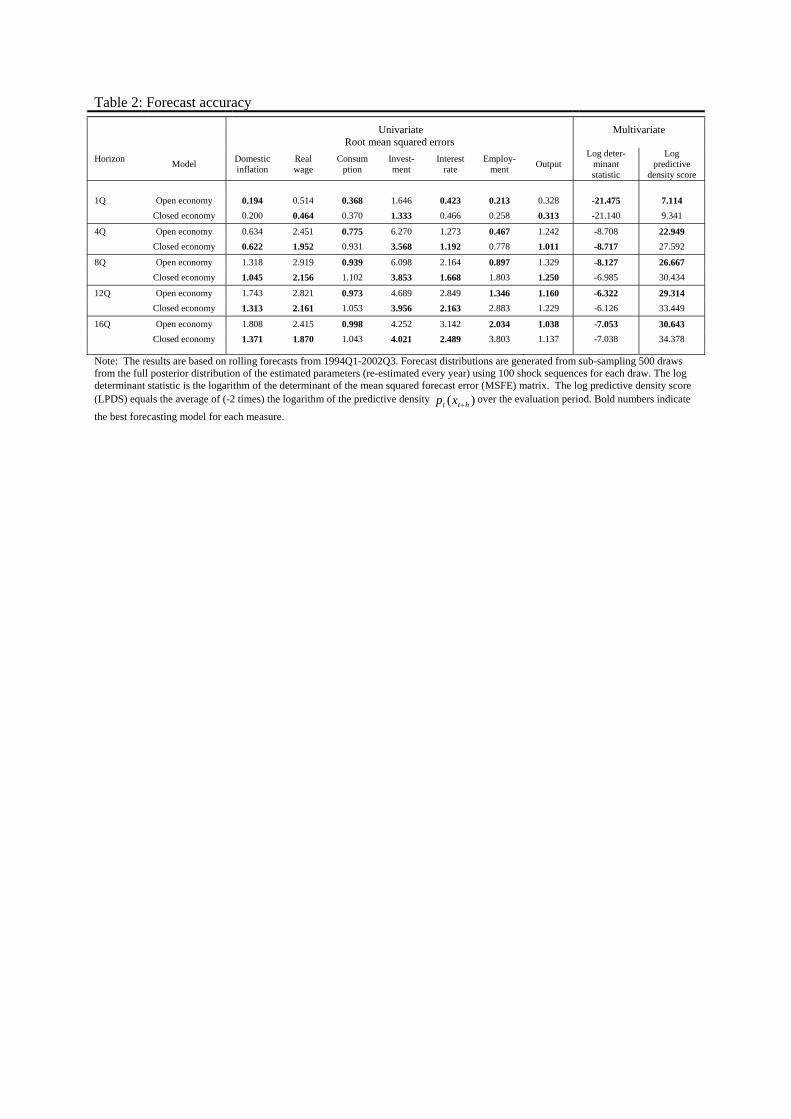
Table 2: Forecast accuracy

Univariate Root mean squared errors

Multivariate

Horizon Model Domestic

inflation Real wage

Consumption

Invest-ment

Interest rate

Employ-ment Output

Log deter-minant statistic

Log predictive

density score

1Q Open economy 0.194 0.514 0.368 1.646 0.423 0.213 0.328 -21.475 7.114 Closed economy 0.200 0.464 0.370 1.333 0.466 0.258 0.313 -21.140 9.341

4Q Open economy 0.634 2.451 0.775 6.270 1.273 0.467 1.242 -8.708 22.949 Closed economy 0.622 1.952 0.931 3.568 1.192 0.778 1.011 -8.717 27.592

8Q Open economy 1.318 2.919 0.939 6.098 2.164 0.897 1.329 -8.127 26.667 Closed economy 1.045 2.156 1.102 3.853 1.668 1.803 1.250 -6.985 30.434

12Q Open economy 1.743 2.821 0.973 4.689 2.849 1.346 1.160 -6.322 29.314 Closed economy 1.313 2.161 1.053 3.956 2.163 2.883 1.229 -6.126 33.449

16Q Open economy 1.808 2.415 0.998 4.252 3.142 2.034 1.038 -7.053 30.643 Closed economy 1.371 1.870 1.043 4.021 2.489 3.803 1.137 -7.038 34.378

Note: The results are based on rolling forecasts from 1994Q1-2002Q3. Forecast distributions are generated from sub-sampling 500 draws from the full posterior distribution of the estimated parameters (re-estimated every year) using 100 shock sequences for each draw. The log determinant statistic is the logarithm of the determinant of the mean squared forecast error (MSFE) matrix. The log predictive density score (LPDS) equals the average of (-2 times) the logarithm of the predictive density )( htt xp +

over the evaluation period. Bold numbers indicate

the best forecasting model for each measure.

Table 3: Variance decompositions

4 quarters Domestic inflation Real wage Consumption Investment Interest rate Employment Output Open Closed Open Closed Open Closed Open Closed Open Closed Open Closed Open Closed

Stationary technology 0.137 0.279 0.057 0.101 0.049 0.082 0.019 0.003 0.068 0.179 0.101 0.195 0.046 0.044

Unit root technology 0.078 0.239 0.199 0.332 0.089 0.325 0.052 0.188 0.036 0.220 0.025 0.180 0.107 0.316

Consumtion preference 0.069 0.015 0.054 0.049 0.327 0.267 0.073 0.081 0.125 0.076 0.142 0.132 0.119 0.107

Labour supply 0.288 0.143 0.460 0.347 0.094 0.044 0.037 0.025 0.131 0.087 0.127 0.060 0.088 0.036

Domestic markup 0.032 0.034 0.047 0.075 0.024 0.036 0.013 0.042 0.026 0.032 0.023 0.038 0.025 0.040

Investment specific technology 0.001 0.043 0.056 0.036 0.030 0.001 0.504 0.403 0.187 0.088 0.188 0.123 0.234 0.195

Monetary policy 0.067 0.059 0.038 0.047 0.098 0.172 0.060 0.183 0.101 0.177 0.104 0.189 0.104 0.182

Inflation target 0.142 0.168 0.005 0.001 0.024 0.054 0.018 0.062 0.079 0.121 0.023 0.059 0.025 0.060

Fiscal variables 0.017 0.020 0.011 0.011 0.012 0.019 0.005 0.013 0.014 0.020 0.020 0.023 0.016 0.020

Import consumption markup 0.085 0.022 0.023 0.049 0.007 0.019 0.024

Import investment markup 0.007 0.014 0.120 0.094 0.050 0.061 0.034

Risk premium 0.030 0.005 0.004 0.036 0.052 0.037 0.040

Asymmetric technology 0.007 0.000 0.002 0.004 0.006 0.001 0.001

Export markup 0.022 0.022 0.092 0.007 0.068 0.089 0.087

Foreign variables 0.020 0.009 0.011 0.027 0.049 0.040 0.050

20 quarters Stationary technology 0.018 0.298 0.086 0.173 0.058 0.154 0.040 0.200 0.052 0.256 0.016 0.071 0.058 0.173

Unit root technology 0.085 0.251 0.342 0.582 0.177 0.406 0.117 0.424 0.096 0.290 0.051 0.253 0.222 0.534

Consumtion preference 0.081 0.031 0.108 0.082 0.200 0.209 0.096 0.132 0.147 0.071 0.192 0.297 0.048 0.071

Labour supply 0.023 0.038 0.027 0.015 0.120 0.051 0.083 0.100 0.105 0.053 0.224 0.157 0.121 0.071

Domestic markup 0.003 0.002 0.012 0.016 0.001 0.005 0.001 0.005 0.003 0.001 0.002 0.003 0.000 0.005

Investment specific technology 0.200 0.100 0.235 0.072 0.228 0.096 0.055 0.017 0.143 0.090 0.016 0.052 0.150 0.050

Monetary policy 0.006 0.017 0.038 0.052 0.025 0.052 0.013 0.082 0.008 0.029 0.034 0.109 0.023 0.065

Inflation target 0.231 0.233 0.015 0.000 0.002 0.011 0.002 0.020 0.173 0.184 0.009 0.019 0.002 0.015

Fiscal variables 0.026 0.030 0.010 0.008 0.021 0.016 0.009 0.019 0.023 0.025 0.035 0.040 0.017 0.016

Import consumption markup 0.220 0.062 0.043 0.240 0.080 0.080 0.098

Import investment markup 0.042 0.035 0.081 0.265 0.102 0.272 0.200

Risk premium 0.017 0.013 0.007 0.010 0.004 0.001 0.014

Asymmetric technology 0.017 0.006 0.002 0.014 0.010 0.002 0.005

Export markup 0.022 0.004 0.032 0.031 0.035 0.058 0.031

Foreign variables 0.010 0.007 0.005 0.024 0.019 0.008 0.011

Figure 1: Impulse responses from a monetary policy shock

0 4 8 12 16

-0.08

-0.06

-0.04

-0.02

0Infl

0 4 8 12 16

-0.08

-0.06

-0.04

-0.02

0Wage

0 4 8 12 16

-0.3

-0.2

-0.1

0Cons

0 4 8 12 16

-0.8

-0.6

-0.4

-0.2

0Invest

0 4 8 12 16

-0.5

-0.4

-0.3

-0.2

-0.1

0X-rate

0 4 8 12 160

0.1

0.2

0.3

0.4

I-rate

0 4 8 12 16-0.25

-0.2

-0.15

-0.1

-0.05

0Employ

0 4 8 12 16

-0.3

-0.2

-0.1

0Output

0 4 8 12 16

-0.3

-0.2

-0.1

0Export

0 4 8 12 16-0.15

-0.1

-0.05

0

0.05

0.1

Import

0 4 8 12 16

-0.08

-0.06

-0.04

-0.02

0C. defl

0 4 8 12 16

-0.2

-0.15

-0.1

-0.05

0I. defl

OpenClosedClosed (open param.)