DI

SC

US

SI

ON

P

AP

ER

S

ER

IE

S

Forschungsinstitut zur Zukunft der ArbeitInstitute for the Study of Labor

Employment, Exchange Rates and Labour Market Rigidity

IZA DP No. 4891

April 2010

Fernando AlexandrePedro BaçãoJoão CerejeiraMiguel Portela

Employment, Exchange Rates and

Labour Market Rigidity

Fernando Alexandre University of Minho and NIPE

Pedro Bação

University of Coimbra and GEMF

João Cerejeira University of Minho and NIPE

Miguel Portela

University of Minho, NIPE and IZA

Discussion Paper No. 4891 April 2010

IZA

P.O. Box 7240 53072 Bonn

Germany

Phone: +49-228-3894-0 Fax: +49-228-3894-180

E-mail: iza@iza.org

Any opinions expressed here are those of the author(s) and not those of IZA. Research published in this series may include views on policy, but the institute itself takes no institutional policy positions. The Institute for the Study of Labor (IZA) in Bonn is a local and virtual international research center and a place of communication between science, politics and business. IZA is an independent nonprofit organization supported by Deutsche Post Foundation. The center is associated with the University of Bonn and offers a stimulating research environment through its international network, workshops and conferences, data service, project support, research visits and doctoral program. IZA engages in (i) original and internationally competitive research in all fields of labor economics, (ii) development of policy concepts, and (iii) dissemination of research results and concepts to the interested public. IZA Discussion Papers often represent preliminary work and are circulated to encourage discussion. Citation of such a paper should account for its provisional character. A revised version may be available directly from the author.

IZA Discussion Paper No. 4891 April 2010

ABSTRACT

Employment, Exchange Rates and Labour Market Rigidity* There is increasing evidence that the interaction between shocks and labour market institutions is crucial to understanding the dynamics of employment. In this paper, we show that the inclusion of labour adjustment costs in a trade model affects the impact of exchange rate movements on employment. We also explore how labour market rigidities interact with the degree of exposure to international competition and with the technology level. Our model-based predictions are consistent with estimates obtained using panel data for 23 OECD countries. Namely, our estimates suggest that employment in low-technology sectors that have a very high degree of openness to trade and are located in countries with more flexible labour markets are more sensitive to exchange rate changes. Our model and estimates therefore provide additional evidence on the importance of interacting external shocks and labour market institutions. JEL Classification: J23, F16, F41 Keywords: exchange rates, international trade, job flows, employment protection Corresponding author: Fernando Alexandre Escola de Economia e Gestão and NIPE University of Minho Campus de Gualtar 4710-057 Braga Portugal E-mail: falex@eeg.uminho.pt

* We are grateful for insightful comments and suggestions from Nicolas Berman, Luís Aguiar-Conraria and other participants at NIPE’s seminar.

1 Introduction

Globalization has increased the exposure of open economies to external shocks. The

almost instantaneous collapse of international trade in most developed and developing

countries in the last quarter of 2008, caused by the international �nancial crisis, is an

instance of how fast the transmission of shocks in the world economy can be. But the

world economy has been a­ icted by global shocks before. In the 1970s and in the 1980s,

when the industrialized countries were hit by oil shocks and by the turbulence in exchange

rate markets, following the demise of Bretton Woods, policymakers were vocal about

the impact of external shocks on competitiveness. The steady decline in manufacturing

employment and the increase in unskilled workers�unemployment contributed to keep

this issue in the headlines ever since. However, policymakers and scholars � see, e.g.,

Nickell (1997), Nickell et al. (2002), Blanchard (1999), Blanchard and Wolfers (2000)

and Blanchard and Portugal (2001) � have come to realize that the economic impact of

these and other shocks depends, among other factors, on labour market institutions, a

realization that has led many to urge for the implementation of labour reforms.1

The aim of this paper is thus to investigate, both theoretically and empirically, the

impact of exchange rate shocks on employment and the relation between this impact and

labour market institutions. Our approach brings together two strands of the literature

on international trade. One is composed of the studies, mainly empirical, that �nd a

signi�cant e¤ect, positively related to the degree of openness to trade, of exchange rate

movements on employment (e.g., Branson and Love, 1988, Revenga, 1992, Gourinchas,

1999, Campa and Goldberg, 2001, and Klein et al., 2003). The other is the new literature

on international trade that builds on the seminal paper by Melitz (2003) and highlights

the relationship between international trade and productivity. A recent example of this

literature is Berman et al. (2009), who add distribution costs to the Melitz model.

By doing that, they are able to show that heterogeneity in productivity across �rms

produces di¤erentiated price and output responses to exchange rate depreciations. Using

the same framework, Alexandre et al. (2009a) go one step further and show how the

degree of openness to trade and the level of productivity interact to determine the impact

of exchange rate movements on employment.

On the theoretical front, the present text provides a link between these international

trade models and the analysis of labour market institutions, and shows how labour mar-

ket rigidities, alongside openness and productivity, mediate the impact of exchange rates

1Calmfors and Dri¢ ll (1988) were among the �rst to discuss the implications of di¤erent labourmarket institutions for macroeconomic performance, namely the relationship between employment andthe bargaining structure. Dri¢ ll (2006) updates that study and surveys the recent literature on labourmarket institutions and macroeconomic performance.

2

movements on employment. The development of our theory rests on the introduction of

labour market frictions, in the form of hiring and �ring costs, in a trade model with het-

erogeneous �rms and distribution costs of the type developed in Berman et al. (2009).

Our results suggest that higher labour adjustment costs decrease the employment ex-

change rate elasticity, i.e., an increase in labour adjustment costs attenuates the impact

of exchange rate movements on labour demand. In our model, this result is robust to

di¤erent degrees of openness to trade, productivity and exchange rate persistence.

The themes of labour market institutions and international trade have already ap-

peared together in the new trade literature following Melitz (2003). For example, Fel-

bermayr et al. (2008) added wage bargaining and search frictions to the Melitz model.

Even more recently, Helpman and Itskhoki (2010) presented a two-sector version of the

Melitz model that also includes wage bargaining and search frictions. However, the focus

of these papers is on the comparative statics analysis of the economic implications of

trade liberalization. In fact, the exchange rate is not even mentioned in such papers. We

aim at �lling part of this theory gap.

On the empirical side, we estimate the response of employment to exchange rate

movements. We take into account the theoretical results and interact the exchange rate

with measures of openness, productivity and labour adjustment costs. Our proxy for

labour adjustment costs is the Employment Protection Legislation (EPL) index computed

by OECD, which has previously been shown (see, among other, Cingano et al., 2009) to

be related to labour adjustment costs. We use sector-level data from 23 OECD countries

covering the years 1988-2006. The results seem to corroborate the predictions of the

theoretical model: very open sectors, using a lower level of technology and facing less

labour rigidity are more sensitive to exchange rate movements.

The remainder of the paper is organized as follows. In section 2 we develop a trade

model with labour market rigidities that take the form of labour adjustment costs. Sec-

tion 3 sets the stage for our empirical test of the model�s predictions. There we describe

the main trends and patterns in manufacturing employment, exchange rates and employ-

ment legislation protection in OECD countries since the late 1980s. Section 4 presents

econometric evidence on the e¤ect of exchange rate changes on employment, in a panel

of OECD countries, and its interaction with openness, technology and labour market

rigidity. Section 5 concludes.

2 A trade model with labour adjustment costs

It has been shown (e.g., Bertola, 1990, 1992) that labour adjustment costs a¤ect �rms�

optimal decisions, preempt an e¢ cient allocation of resources and, in particular (Bertola,

3

1992, and Hopenhayn and Rogerson, 1993), that labour adjustment costs imply lower job

�ows.2 In this section we show that in an international trade model one manifestation

of this sort of e¤ect is that higher labour adjustment costs reduce the size of the labour

demand elasticity with respect to the exchange rate. Our presentation follows Melitz

(2003) and Berman et al. (2009), but we introduce labour adjustment costs into the

framework.

We start by describing the behaviour of the demand for the good that is exported.

To simplify, we assume that the exporting �rm only sells in market i. An alternative

interpretation is that the revenues and costs associated with exporting to country i are

separable from the rest of the �rm�s activities. We also assume, as is common in the

related literature �namely, Melitz (2003) and Berman et al. (2009) �and, more generally,

in modern macroeconomics, that the �rm is a monopolistic competitor. Therefore, the

price and quantity the �rm will set will depend on the size of a �nite price-elasticity

of demand for the good that the �rm produces. In our interpretation of the model�s

implications, this elasticity will also represent the degree of openness of country i. The

motivation for this interpretation is that, in a more open market, competition from

similar goods produced by other exporters to market i will be more intense, i.e., the

price-elasticity will be higher. Another paper that also makes this assumption explicitly

is Klein et al. (2003).

2.1 Demand

We assume that the representative consumer in country i maximizes a standard inter-

temporal utility function:

U = E0

1Xt=0

�tu(Cit) (1)

where � is the discount factor.

The period utility �ow is given by the Dixit-Stiglitz functional:

u (Cit) = Cit =

�Z�

xit (')1� 1

� d'

� 1

1� 1�

(2)

where � is the elasticity of substitution between any two varieties (besides being the

symmetric of the own price-elasticity) and xit(') is the consumption of variety ', i.e., '

indexes, over the set �, the goods available to the consumer. Below, we will also use '

to represent the level of productivity of the �rm that produces variety '. Given the form

2These theoretical predictions have found empirical support in several studies �see, e.g., Haltiwangeret al. (2006) and Gómez-Salvador et al. (2004).

4

of the utility function, the demand for variety ' will be given by:

xit(') = Cit

�pit(')

Pit

���(3)

For our purposes, we do not need to detail any more the behaviour of the represent-

ative consumer in country i. We will assume Cit to be an exogenous element in the �rm�s

problem, to which we now turn.

2.2 Exporting �rm

As we said before, the �rm that produces variety ', and exports it to country i, is a

monopolistic competitor in country i, the sole destination of its output. The price that

it charges in country i�s currency (pit(')) is given by:

pit(') =pt"it+ �iwit (4)

where pt is the period t price of the good in the domestic currency, "it is the period t price

of a foreign unit of currency in units of the domestic currency, �i are the distribution costs

in country i, measured in units of country i�s labour, and wit is the wage in country i, in

period t. The introduction of these distribution costs is the main innovation in Berman

et al. (2009) relatively to the trade model proposed by Melitz (2003). The presence of

distribution costs makes the elasticities of demand for variety ' with respect to the price

(pt) and with respect to the exchange rate functions of � and of other parameters in the

model, as we shall see below.

As in the related literature, the production function is assumed to be linear in the

labour input:

yt(') = 'Lt (5)

where ', as mentioned above, is a measure of productivity. The production costs include

labour costs (given the wage in the �rm�s country, wt), �xed costs and labour adjustment

costs:

ct(') = wtLt + Ft(') + wtA(�Lt) (6)

The focus of this paper is on labour adjustment costs, wtA(�Lt). For A(�Lt) �

labour adjustment costs measured in units of labour � we adopt the formulation proposed

by Pfann and Verspagen (1989):

A(�Lt) = �1 + exp(��Lt)� ��Lt +

2(�Lt)

2 (7)

5

In this formulation, when � 6= 0, labour adjustment costs are asymmetric: if � > 0,then hiring costs are higher than �ring costs; if � < 0, then the opposite is true. The

other parameter, , re�ects the symmetric component of the costs of adjusting labour.

The �rm chooses how much to produce and sets the price so as to maximize its present

value:

maxE0

1Xt=0

~�t [ptyt(')� ct(')] (8)

where ~�t is the current period discount factor for the cash �ow in period t. To simplify

the derivations below, we shall assume that ~�t = �t.

Given our setup, the optimal choices for price and quantity are given by:

pt =�

� � 1

�1 +

qit�i'

�+Bt

� wt'

(9)

and

yt = CitP�i w

��it

�� � 1�

�� �1 +Btqit'

+ �i

���(10)

where

qit ="itwitwt

(11)

denotes the real exchange rate and Bt includes current and future marginal costs of

adjusting labour:

Bt =Mt � �Et�wt+1wt

Mt+1

�(12)

with

Mt = � [exp (��Lt)� 1] + �Lt (13)

The non-linear nature of the model and the fact that Bt includes current and fu-

ture marginal costs of adjusting labour make the analysis of the relation between �rm

behaviour and exchange rate movements more complex. To proceed we resort to log-

linearization of equation (10).

2.3 Log-linearization

We begin by writing (10) as:

yt = Xt

�1 +Btqit'

+ �i

���(14)

6

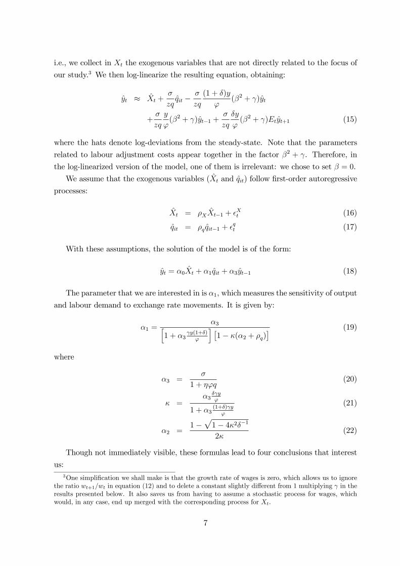
i.e., we collect in Xt the exogenous variables that are not directly related to the focus of

our study.3 We then log-linearize the resulting equation, obtaining:

yt � Xt +�

zqqit �

�

zq

(1 + �)y

'(�2 + )yt

+�

zq

y

'(�2 + )yt�1 +

�

zq

�y

'(�2 + )Etyt+1 (15)

where the hats denote log-deviations from the steady-state. Note that the parameters

related to labour adjustment costs appear together in the factor �2 + . Therefore, in

the log-linearized version of the model, one of them is irrelevant: we chose to set � = 0.

We assume that the exogenous variables (Xt and qit) follow �rst-order autoregressive

processes:

Xt = �XXt�1 + �Xt (16)

qit = �q qit�1 + �qt (17)

With these assumptions, the solution of the model is of the form:

yt = �0Xt + �1qit + �3yt�1 (18)

The parameter that we are interested in is �1, which measures the sensitivity of output

and labour demand to exchange rate movements. It is given by:

�1 =�3h

1 + �3 y(1+�)

'

i �1� �(�2 + �q)

� (19)

where

�3 =�

1 + �'q(20)

� =�3

� y'

1 + �3(1+�) y

'

(21)

�2 =1�

p1� 4�2��1

2�(22)

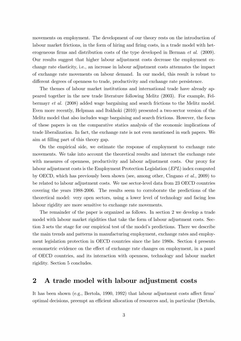
Though not immediately visible, these formulas lead to four conclusions that interest

us:3One simpli�cation we shall make is that the growth rate of wages is zero, which allows us to ignore

the ratio wt+1=wt in equation (12) and to delete a constant slightly di¤erent from 1 multiplying in theresults presented below. It also saves us from having to assume a stochastic process for wages, whichwould, in any case, end up merged with the corresponding process for Xt.

7

0.25

6.67

ρ q =0.5, φ =0.5

3σ

10

0γ

100

0.00

2.92

σ =7, ρ q =0.5

0φ

2

0γ

100

2.82

4.55

σ =7, φ =0.5

0ρ q

1

0γ

100

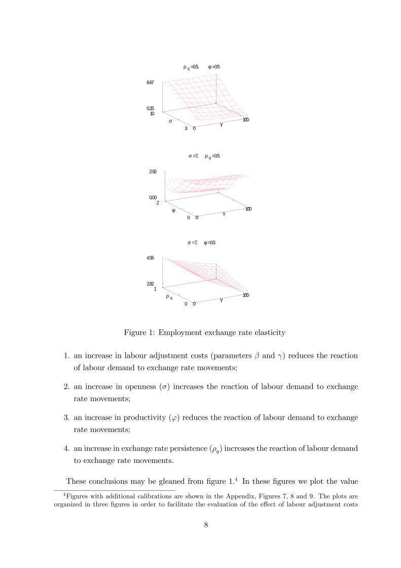
Figure 1: Employment exchange rate elasticity

1. an increase in labour adjustment costs (parameters � and ) reduces the reaction

of labour demand to exchange rate movements;

2. an increase in openness (�) increases the reaction of labour demand to exchange

rate movements;

3. an increase in productivity (') reduces the reaction of labour demand to exchange

rate movements;

4. an increase in exchange rate persistence (�q) increases the reaction of labour demand

to exchange rate movements.

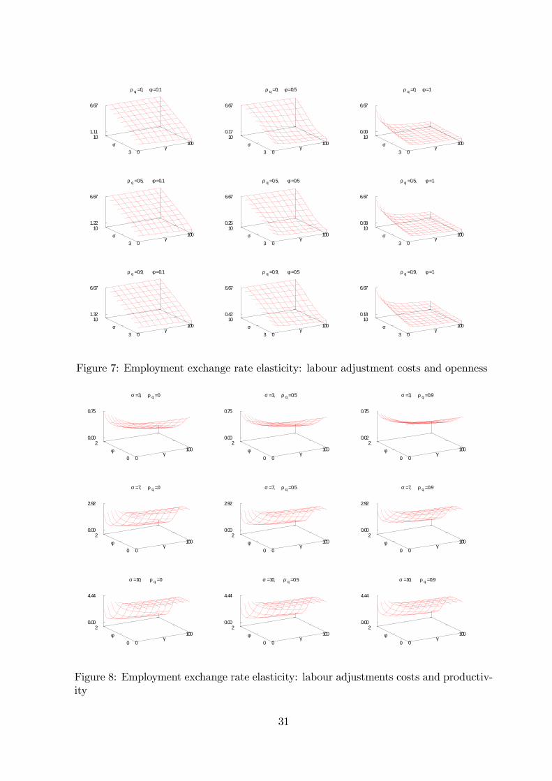
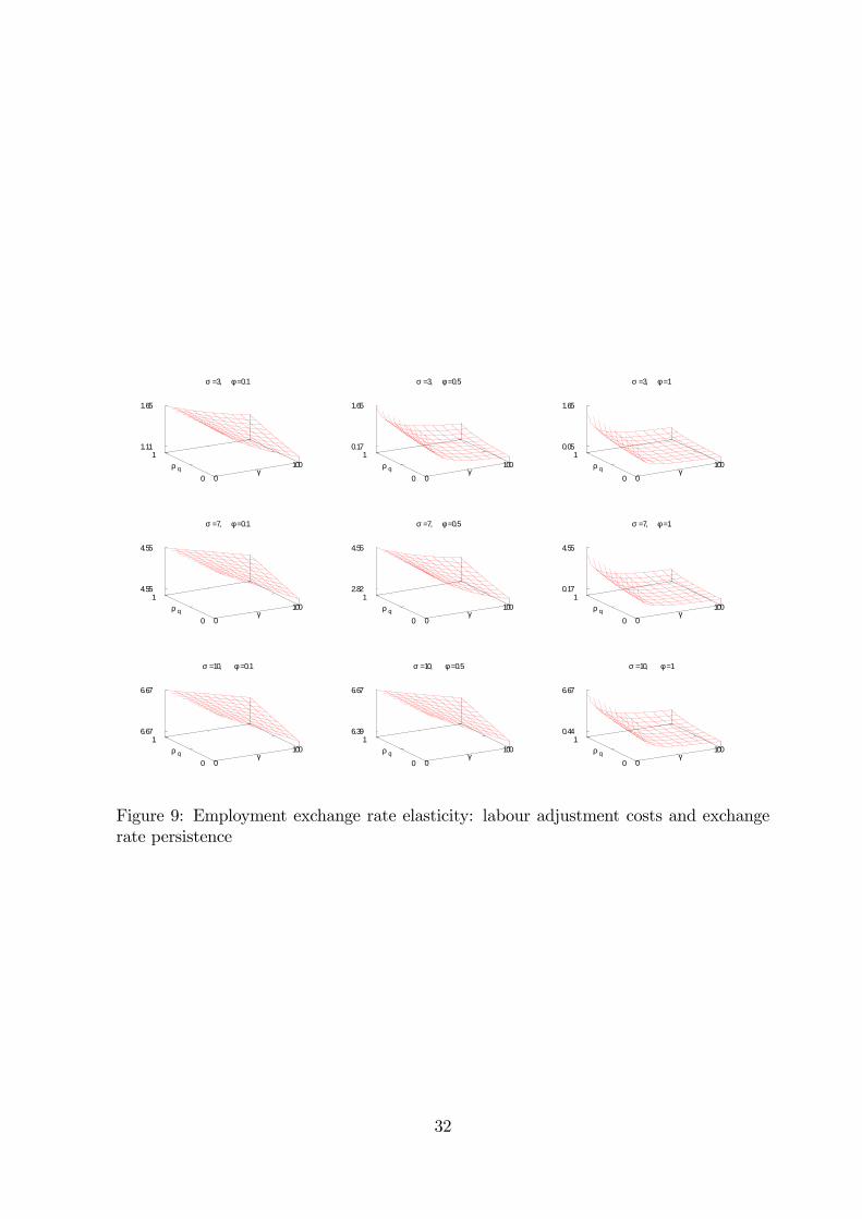
These conclusions may be gleaned from �gure 1.4 In these �gures we plot the value

4Figures with additional calibrations are shown in the Appendix, Figures 7, 8 and 9. The plots areorganized in three �gures in order to facilitate the evaluation of the e¤ect of labour adjustment costs

8

of �1 for di¤erent parameterizations and using di¤erent variables in the axis so that the

robustness of the patterns enumerated above may be veri�ed. The model parameters

were calibrated assuming � = 0:96, � = 0 and s = 0:3, as do Berman et al. (2009) in one

version of their computations. s represents the share of distribution costs in the good�s

price. This share has been estimated to represent between 40% and 60% of goods�prices

� see, e.g., Burstein et al. (2003) and Campa and Goldberg (2008). Setting s = 0:5

would not change the plots, only the scale: increasing the share of distribution costs

would reduce the size of the elasticity �1.

Our model suggests that empirical analyses of the reaction of employment to exchange

rate movements should �nd that low-productivity �rms, very open to trade and less

a¤ected by labour market rigidities should be more sensitive to the exchange rate. In

the empirical section of this paper we will use sector-level data. One of the drawbacks of

using this dataset is that it does not allow us to distinguish between �rms that do and

do not export. However, a similar model for non-exporting �rms would also lead to the

conclusion that the size of the impact of exchange rate movements on labour demand

declines when labour adjustment costs increase. Therefore, we expect that the same will

happen at the sector level. Note that we do not address the issue of �rm entry and exit

(the "extensive margin"). In Berman et al. (2009) �xed costs �Ft(') in Equation (6),

assumed to depend on the productivity level �are viewed as a payment that allows the

�rm to export to country i. Thus, in that setup �xed costs are important for the study

of �rms�entry and exit decisions concerning the destination market. Berman et al. show

that at the aggregate level these costs will in�uence the extensive margin elasticity of

exports with respect to the exchange rate. This is estimated to represent around 20% of

the elasticity of French exports with respect to the exchange rate. We therefore believe

that our model should be able to explain the bulk of the e¤ect of exchange rate changes

on employment.

3 Labour market institutions, employment and ex-

change rates

In this section, we describe very brie�y the main trends in manufacturing employment

per technology level (3.1), aggregate and sectoral exchange rates and openness (3.2) and

employment protection in OECD countries (3.3). We do this to motivate our empirical

analysis that aims at evaluating how employment protection has a¤ected the impact of

( ) on the labour demand elasticity with respect to the exchange rate. In each �gure the patterns aresimilar regardless of the calibration. The plots reveal that adjustment costs have a larger e¤ect on thevalue of �1 when the persistence of exchange rate shocks is low and when productivity is high.

9

0.1

.2.3

0.1

.2.3

0.1

.2.3

0.1

.2.3

1990 1995 2000 2005 1990 1995 2000 2005

 OECD 17 France

Germany Italy

Japan Portugal

UK United States

All Manufactures Low­Tech Manufactures

% in

 Tot

al E

mpl

oym

ent

Year

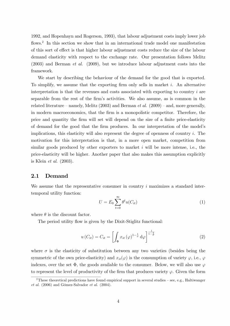
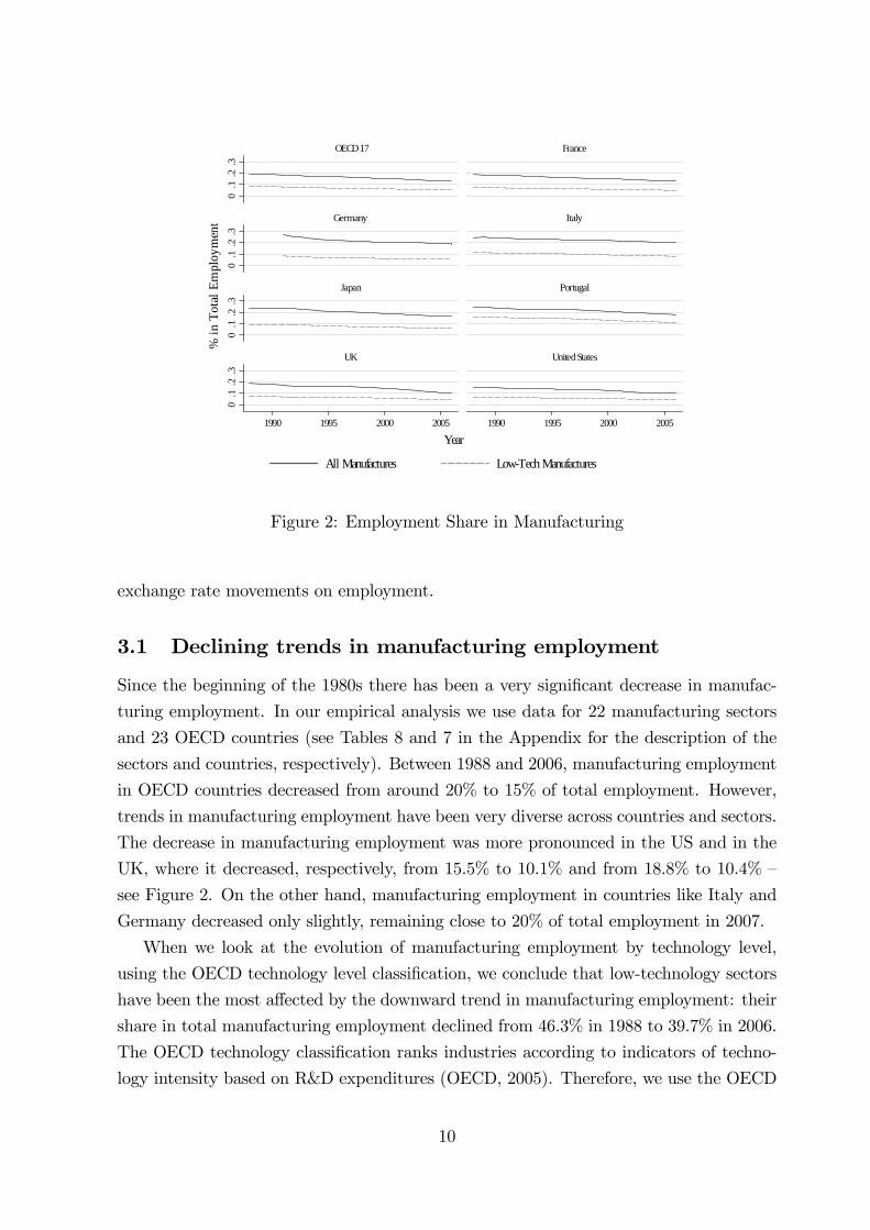
Figure 2: Employment Share in Manufacturing

exchange rate movements on employment.

3.1 Declining trends in manufacturing employment

Since the beginning of the 1980s there has been a very signi�cant decrease in manufac-

turing employment. In our empirical analysis we use data for 22 manufacturing sectors

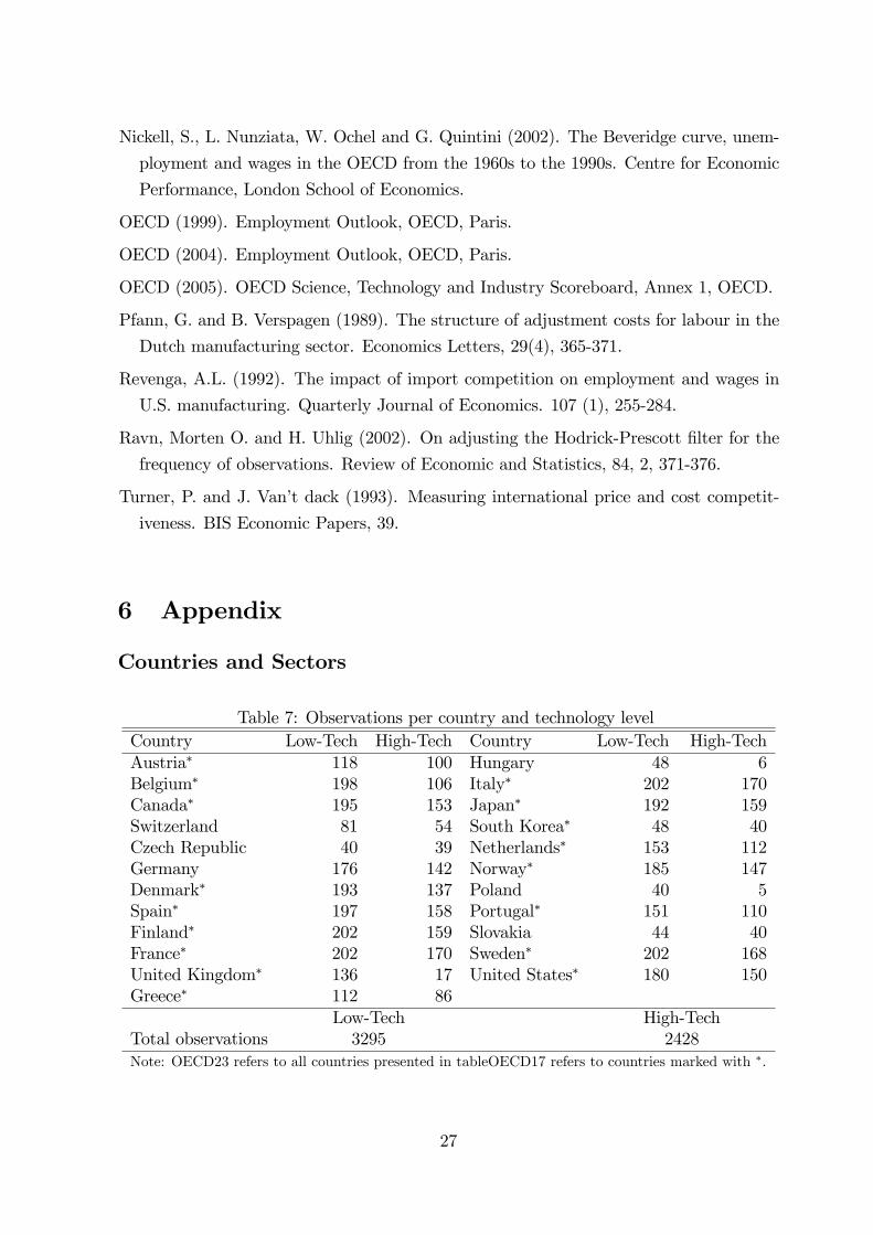
and 23 OECD countries (see Tables 8 and 7 in the Appendix for the description of the

sectors and countries, respectively). Between 1988 and 2006, manufacturing employment

in OECD countries decreased from around 20% to 15% of total employment. However,

trends in manufacturing employment have been very diverse across countries and sectors.

The decrease in manufacturing employment was more pronounced in the US and in the

UK, where it decreased, respectively, from 15.5% to 10.1% and from 18.8% to 10.4% �

see Figure 2. On the other hand, manufacturing employment in countries like Italy and

Germany decreased only slightly, remaining close to 20% of total employment in 2007.

When we look at the evolution of manufacturing employment by technology level,

using the OECD technology level classi�cation, we conclude that low-technology sectors

have been the most a¤ected by the downward trend in manufacturing employment: their

share in total manufacturing employment declined from 46.3% in 1988 to 39.7% in 2006.

The OECD technology classi�cation ranks industries according to indicators of techno-

logy intensity based on R&D expenditures (OECD, 2005). Therefore, we use the OECD

10

technology classi�cation as a proxy for the productivity parameter in the production func-

tion of our theoretical model, ', which can be understood as a total productivity factor

(or a Solow residual). In fact, a simple OLS regression of labour productivity, measured

as sectoral value added per employee, on OECD�s technology classes and capital per

employee, shows that high-technology sectors are more productive than low technology

sectors. Given that data on value added and on the stock of capital are available just

for a small sample of countries and years, we develop our analysis using the OECD�s

technology classi�cation.5

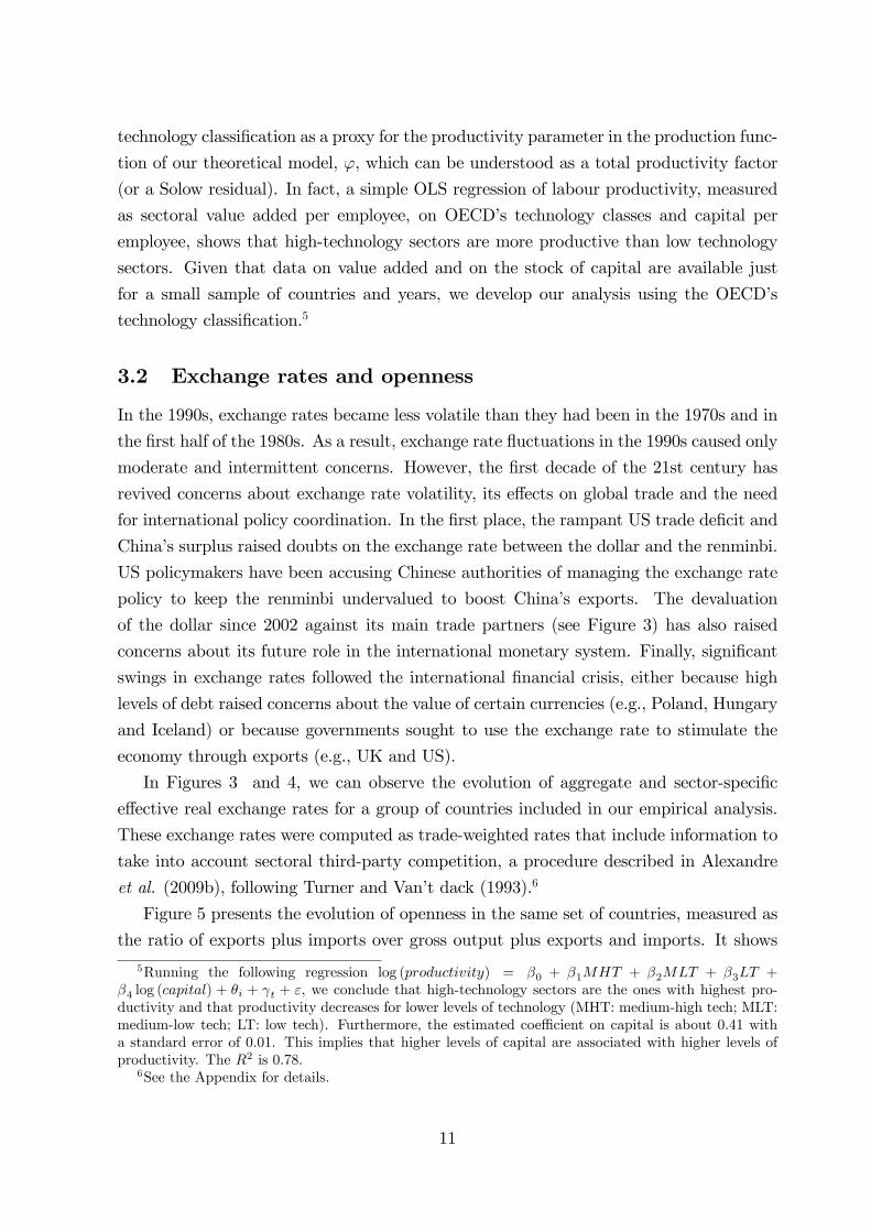
3.2 Exchange rates and openness

In the 1990s, exchange rates became less volatile than they had been in the 1970s and in

the �rst half of the 1980s. As a result, exchange rate �uctuations in the 1990s caused only

moderate and intermittent concerns. However, the �rst decade of the 21st century has

revived concerns about exchange rate volatility, its e¤ects on global trade and the need

for international policy coordination. In the �rst place, the rampant US trade de�cit and

China�s surplus raised doubts on the exchange rate between the dollar and the renminbi.

US policymakers have been accusing Chinese authorities of managing the exchange rate

policy to keep the renminbi undervalued to boost China�s exports. The devaluation

of the dollar since 2002 against its main trade partners (see Figure 3) has also raised

concerns about its future role in the international monetary system. Finally, signi�cant

swings in exchange rates followed the international �nancial crisis, either because high

levels of debt raised concerns about the value of certain currencies (e.g., Poland, Hungary

and Iceland) or because governments sought to use the exchange rate to stimulate the

economy through exports (e.g., UK and US).

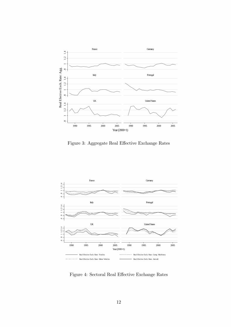
In Figures 3 and 4, we can observe the evolution of aggregate and sector-speci�c

e¤ective real exchange rates for a group of countries included in our empirical analysis.

These exchange rates were computed as trade-weighted rates that include information to

take into account sectoral third-party competition, a procedure described in Alexandre

et al. (2009b), following Turner and Van�t dack (1993).6

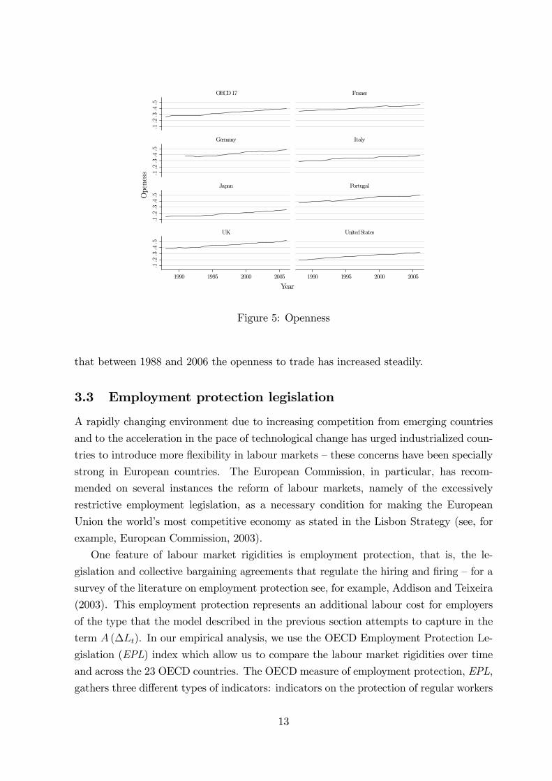
Figure 5 presents the evolution of openness in the same set of countries, measured as

the ratio of exports plus imports over gross output plus exports and imports. It shows

5Running the following regression log (productivity) = �0 + �1MHT + �2MLT + �3LT +�4 log (capital) + �i + t + ", we conclude that high-technology sectors are the ones with highest pro-ductivity and that productivity decreases for lower levels of technology (MHT: medium-high tech; MLT:medium-low tech; LT: low tech). Furthermore, the estimated coe¢ cient on capital is about 0.41 witha standard error of 0.01. This implies that higher levels of capital are associated with higher levels ofproductivity. The R2 is 0.78.

6See the Appendix for details.

11

.81

1.2

1.4

.81

1.2

1.4

.81

1.2

1.4

1990 1995 2000 2005 1990 1995 2000 2005

France Germany

Italy Portugal

UK United States

Real

 Efe

ctiv

e Exc

h. R

ate:

 Agg

.

Year (2000=1)

Figure 3: Aggregate Real E¤ective Exchange Rates

.6.8

11.

21.

4.6

.81

1.4

1.2

.6.8

11.

21.

4

1990 1995 2000 2005 1990 1995 2000 2005

France Germany

Italy Portugal

UK United States

Real Efective Exch. Rate: Textiles Real Efective Exch. Rate: Comp. Machinery

Real Efective Exch. Rate: Motor Vehicles Real Efective Exch. Rate: Aircraft

Year (2000=1)

Figure 4: Sectoral Real E¤ective Exchange Rates

12

.1.2

.3.4

.5.1

.2.3

.4.5

.1.2

.3.4

.5.1

.2.3

.4.5

1990 1995 2000 2005 1990 1995 2000 2005

 OECD 17 France

Germany Italy

Japan Portugal

UK United States

Ope

ness

Year

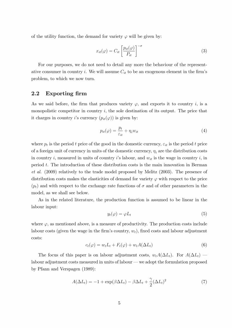
Figure 5: Openness

that between 1988 and 2006 the openness to trade has increased steadily.

3.3 Employment protection legislation

A rapidly changing environment due to increasing competition from emerging countries

and to the acceleration in the pace of technological change has urged industrialized coun-

tries to introduce more �exibility in labour markets �these concerns have been specially

strong in European countries. The European Commission, in particular, has recom-

mended on several instances the reform of labour markets, namely of the excessively

restrictive employment legislation, as a necessary condition for making the European

Union the world�s most competitive economy as stated in the Lisbon Strategy (see, for

example, European Commission, 2003).

One feature of labour market rigidities is employment protection, that is, the le-

gislation and collective bargaining agreements that regulate the hiring and �ring �for a

survey of the literature on employment protection see, for example, Addison and Teixeira

(2003). This employment protection represents an additional labour cost for employers

of the type that the model described in the previous section attempts to capture in the

term A (�Lt). In our empirical analysis, we use the OECD Employment Protection Le-

gislation (EPL) index which allow us to compare the labour market rigidities over time

and across the 23 OECD countries. The OECD measure of employment protection, EPL,

gathers three di¤erent types of indicators: indicators on the protection of regular workers

13

01

23

40

12

34

01

23

40

12

34

1990 1995 2000 2005 1990 1995 2000 2005

 OECD 23 Denmark

France Germany

Italy Portugal

UK United States

EPL

Year

Figure 6: Employment Protection Legislation

against individual dismissal; indicators of speci�c requirements for collective dismissals;

and indicators of the regulation of temporary forms of employment (OECD, 1999 and

2004).

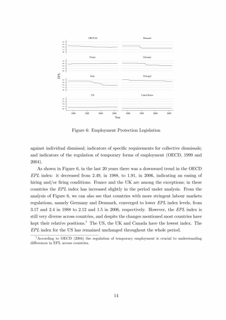
As shown in Figure 6, in the last 20 years there was a downward trend in the OECD

EPL index: it decreased from 2.49, in 1988, to 1.91, in 2006, indicating an easing of

hiring and/or �ring conditions. France and the UK are among the exceptions; in these

countries the EPL index has increased slightly in the period under analysis. From the

analysis of Figure 6, we can also see that countries with more stringent labour markets

regulations, namely Germany and Denmark, converged to lower EPL index levels, from

3.17 and 2.4 in 1988 to 2.12 and 1.5 in 2006, respectively. However, the EPL index is

still very diverse across countries, and despite the changes mentioned most countries have

kept their relative positions.7 The US, the UK and Canada have the lowest index. The

EPL index for the US has remained unchanged throughout the whole period.

7According to OECD (2004) the regulation of temporary employment is crucial to understandingdi¤erences in EPL across countries.

14

4 Empirical evidence

4.1 Estimation strategy

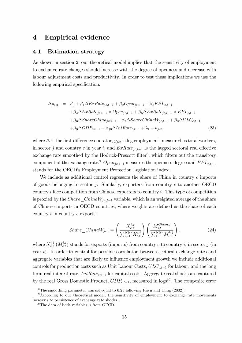
As shown in section 2, our theoretical model implies that the sensitivity of employment

to exchange rate changes should increase with the degree of openness and decrease with

labour adjustment costs and productivity. In order to test these implications we use the

following empirical speci�cation:

�yjct = �0 + �1�ExRatejc;t�1 + �2Openjc;t�1 + �3EPLc;t�1

+�4�ExRatejc;t�1 �Openjc;t�1 + �5�ExRatejc;t�1 � EPLc;t�1+�6�ShareChinajc;t�1 + �7�ShareChinaWjc;t�1 + �8�ULCc;t�1

+�9�GDPc;t�1 + �10�IntRatec;t�1 + �t + ujct; (23)

where� is the �rst-di¤erence operator, yjct is log employment, measured as total workers,

in sector j and country c in year t, and ExRatejc;t�1 is the lagged sectoral real e¤ective

exchange rate smoothed by the Hodrick-Prescott �lter8, which �lters out the transitory

component of the exchange rate.9 Openjc;t�1 measures the openness degree and EPLc;t�1stands for the OECD�s Employment Protection Legislation index.

We include as additional control regressors the share of China in country c imports

of goods belonging to sector j. Similarly, exporters from country c to another OECD

country i face competition from Chinese exporters to country i. This type of competition

is proxied by the Share_ChinaWj;c;t�1 variable, which is an weighted average of the share

of Chinese imports in OECD countries, where weights are de�ned as the share of each

country i in country c exports:

Share_ChinaWjc;t =

X i;jc;tPN(t)

i=1 Xi;jc;t

! MChina;ji;tPN(t)k=1 M

k;ji;t

!: (24)

where X i;jc;t (M

i;jc;t ) stands for exports (imports) from country c to country i, in sector j (in

year t). In order to control for possible correlation between sectoral exchange rates and

aggregate variables that are likely to in�uence employment growth we include additional

controls for production costs such as Unit Labour Costs, ULCc;t�1 for labour, and the long

term real interest rate, IntRatec;t�1 for capital costs. Aggregate real shocks are captured

by the real Gross Domestic Product, GDPc;t�1, measured in logs10. The composite error

8The smoothing parameter was set equal to 6.25 following Ravn and Uhlig (2002).9According to our theoretical model, the sensitivity of employment to exchange rate movements

increases to persistence of exchange rate shocks.10The data of both variables is from OECD.

15

term is de�ned as ujct = �jc + "jct, where �jc is a set of sector/country speci�c dummies.

Finally, equation (23) also includes time dummies, �t, to account for common technology

shocks that a¤ect all sectors and countries.

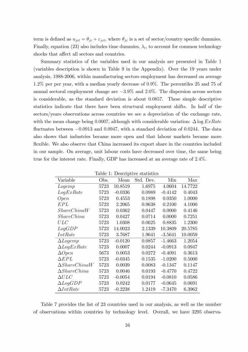
Summary statistics of the variables used in our analysis are presented in Table 1

(variables description is shown in Table 9 in the Appendix). Over the 19 years under

analysis, 1988-2006, within manufacturing sectors employment has decreased on average

1:2% per per year, with a median yearly decrease of 0:9%. The percentiles 25 and 75 of

annual sectoral employment change are �3:9% and 2:0%. The dispersion across sectors

is considerable, as the standard deviation is about 0:0857. These simple descriptive

statistics indicate that there have been structural employment shifts. In half of the

sectors/years observations across countries we see a depreciation of the exchange rate,

with the mean change being 0:0007, although with considerable variation: � logExRate

�uctuates between �0:0913 and 0:0947, with a standard deviation of 0:0244. The dataalso shows that industries became more open and that labour markets became more

�exible. We also observe that China increased its export share in the countries included

in our sample. On average, unit labour costs have decreased over time, the same being

true for the interest rate. Finally, GDP has increased at an average rate of 2:4%.

Table 1: Descriptive statisticsVariable Obs. Mean Std. Dev. Min MaxLogemp 5723 10.8519 1.6975 4.0604 14.7722LogExRate 5723 -0.0336 0.0989 -0.4142 0.4043Open 5723 0.4553 0.1898 0.0350 1.0000EPL 5723 2.2065 0.9638 0.2100 4.1000ShareChinaW 5723 0.0362 0.0447 0.0000 0.4146ShareChina 5723 0.0427 0.0714 0.0000 0.7251ULC 5723 1.0308 0.0625 0.8835 1.2300LogGDP 5723 14.0023 2.1339 10.3809 20.5785IntRate 5723 3.7687 1.9641 -3.5641 10.0059�Logemp 5723 -0.0120 0.0857 -1.4663 1.2054�LogExRate 5723 0.0007 0.0244 -0.0913 0.0947�Open 5673 0.0053 0.0272 -0.4091 0.3613�EPL 5723 -0.0345 0.1535 -1.0200 0.5000�ShareChinaW 5723 0.0039 0.0083 -0.1347 0.1147�ShareChina 5723 0.0046 0.0193 -0.4770 0.4722�ULC 5723 -0.0054 0.0194 -0.0810 0.0586�LogGDP 5723 0.0242 0.0177 -0.0645 0.0691�IntRate 5723 -0.2238 1.2419 -7.3470 6.3962

Table 7 provides the list of 23 countries used in our analysis, as well as the number

of observations within countries by technology level. Overall, we have 3295 observa-

16

tions for medium-low- and low-technology industries and 2428 observations for high- and

medium-high-technology industries. For some countries the number of observations is

relatively low, particularly for Slovakia, Poland, South Korea, Hungary, Czech Republic

and Switzerland.

Table 2: Observations per country and technology levelCountry Low-Tech High-Tech Country Low-Tech High-TechAustria� 118 100 Hungary 48 6Belgium� 198 106 Italy� 202 170Canada� 195 153 Japan� 192 159Switzerland 81 54 South Korea� 48 40Czech Republic 40 39 Netherlands� 153 112Germany 176 142 Norway� 185 147Denmark� 193 137 Poland 40 5Spain� 197 158 Portugal� 151 110Finland� 202 159 Slovakia 44 40France� 202 170 Sweden� 202 168United Kingdom� 136 17 United States� 180 150Greece� 112 86

Low-Tech High-TechTotal observations 3295 2428Note: OECD23 refers to all countries presented in tableOECD17 refers to countries marked with �.

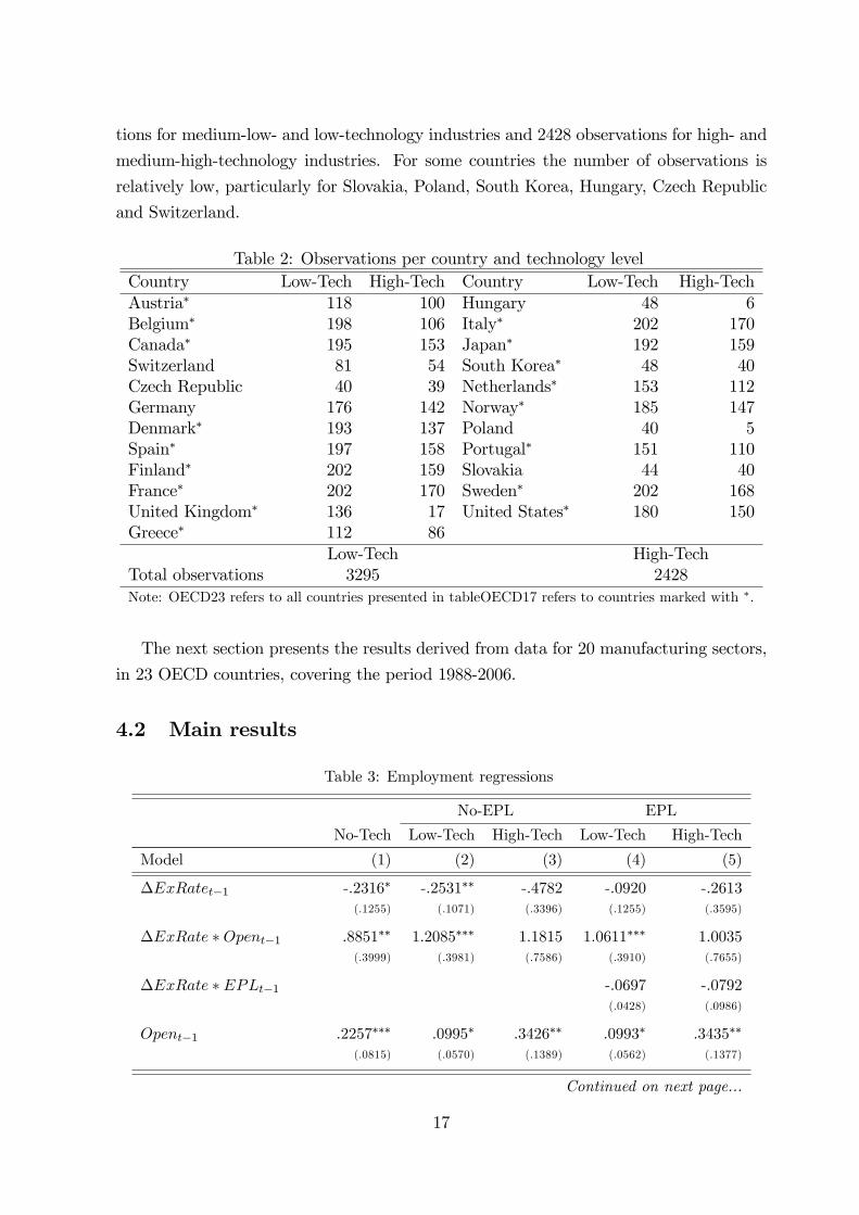
The next section presents the results derived from data for 20 manufacturing sectors,

in 23 OECD countries, covering the period 1988-2006.

4.2 Main results

Table 3: Employment regressions

No-EPL EPL

No-Tech Low-Tech High-Tech Low-Tech High-Tech

Model (1) (2) (3) (4) (5)

�ExRatet�1 -.2316� -.2531�� -.4782 -.0920 -.2613(.1255) (.1071) (.3396) (.1255) (.3595)

�ExRate �Opent�1 .8851�� 1.2085��� 1.1815 1.0611��� 1.0035(.3999) (.3981) (.7586) (.3910) (.7655)

�ExRate � EPLt�1 -.0697 -.0792(.0428) (.0986)

Opent�1 .2257��� .0995� .3426�� .0993� .3435��

(.0815) (.0570) (.1389) (.0562) (.1377)

Continued on next page...

17

... table 3 continued

No-EPL EPL

No-Tech Low-Tech High-Tech Low-Tech High-Tech

Model (1) (2) (3) (4) (5)

EPLt�1 -.0158��� -.0227��

(.0043) (.0091)

�ShareChinaWeightt�1 .0141 -.0626 .2435 -.0638 .2178(.2000) (.1636) (.4529) (.1652) (.4487)

�ShareChinat�1 -.1243�� -.0815 -.3486 -.0820� -.3237(.0606) (.0498) (.2276) (.0498) (.2242)

�ULCt�1 .0163 -.1323�� .2003 -.1211� .2128(.0879) (.0626) (.1786) (.0627) (.1750)

�GDPt�1 .5959��� .7599��� .3965 .7800��� .4123(.1269) (.0958) (.2569) (.0939) (.2606)

�InterestRatet�1 -.0010 -.0013 -.0008 -.0012 -.0005(.0012) (.0009) (.0026) (.0009) (.0026)

Countries 23 23 23 23 23

Observations 5723 3295 2428 3295 2428

Adj. R2 .0504 .1068 .0422 .1137 .0444

LogLikelihood 6421.615 5417.503 1975.572 5431.425 1979.432

Notes: Signi�cance levels: � : 10% �� : 5% � � � : 1%. Robust standard errors

in parenthesis. All regressions are estimated by �xed-e¤ects at the sector/country level, and

include time dummies. The dependent variable is �LogEmploymentjct.

Equation (23) is estimated by the within estimator, with sector/country �xed-e¤ects;

standard errors are robust and clustered within sectors/countries pairs in order to allow

for intra-group correlation. Table 3 shows the results of our estimations. Our �rst es-

timates, column (1), do not distinguish for the level of technology and for labour market

rigidities. The results indicate that the employment exchange rate elasticity increases

with the degree of openness. The interaction coe¢ cient is 0:8851 and statistically sig-

ni�cant at the 5% level (its standard error is 0:3999). The employment exchange rate

elasticity for closed sectors, evaluated at the 10th percentile of openness distribution,

is not statistically di¤erent from zero (the elasticity is �0:032 with a joint signi�canceF�test p�value of 0:591). For open sectors, computed at the 90th percentile of opennessdistribution, we obtain an elasticity of 0:404 with a corresponding p� value for the jointsigni�cance test of 0:028; a 1 percent exchange rate depreciation is associated with a 0:4

percent increase in employment. From our results we can also conclude that more open

18

sectors, on average, create more employment: a 1 point increase in the openness index

is associated with an employment increase of 0:23%. Looking to the additional set of

regressors, we observe that imports from China have a negative impact on employment

growth, while, as expected, positive income variations generate further employment gains.

Although not statistically signi�cant, the unit labour costs (ULC) and the real interest

rate have the expected impact on employment innovations. Throughout our estimations

we are using a sample of 22 industries across 23 countries, as described above, which

correspond to 5723 observations. These are divided between 3295 observations in the low

technology economic activities, and 2428 observations in the high technology industries.

The estimates in columns (2) and (3) account for di¤erent levels of technology and

columns (4) and (5) include the labour market rigidity variable. We used these results

to quantify the e¤ects of exchange rate movements on employment in di¤erent degrees of

openness and labour market rigidities (Table 4). We evaluate the employment elasticity

at the 90th and 10th percentile of openness, Open (+) and Open (-), respectively. For each

degree of openness, and for the models that include employment protection legislation

(EPL), we further evaluate the elasticity from high to low levels of EPL; i.e., at the 95th,

50th and 5th percentiles of EPL.

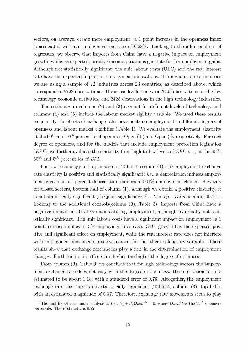
For low technology and open sectors, Table 4, column (1), the employment exchange

rate elasticity is positive and statistically signi�cant; i.e., a depreciation induces employ-

ment creation: a 1 percent depreciation induces a 0:61% employment change. However,

for closed sectors, bottom half of column (1), although we obtain a positive elasticity, it

is not statistically signi�cant (the joint signi�cance F � test�s p� value is about 0:7).11.Looking to the additional controls(column (3), Table 3), imports from China have a

negative impact on OECD�s manufacturing employment, although marginally not stat-

istically signi�cant. The unit labour costs have a signi�cant impact on employment: a 1

point increase implies a 13% employment decrease. GDP growth has the expected pos-

itive and signi�cant e¤ect on employment, while the real interest rate does not interfere

with employment movements, once we control for the other explanatory variables. These

results show that exchange rate shocks play a role in the determination of employment

changes. Furthermore, its e¤ects are higher the higher the degree of openness.

From column (3), Table 3, we conclude that for high technology sectors the employ-

ment exchange rate does not vary with the degree of openness: the interaction term is

estimated to be about 1:18, with a standard error of 0:76. Altogether, the employment

exchange rate elasticity is not statistically signi�cant (Table 4, column (3), top half),

with an estimated magnitude of 0:37. Therefore, exchange rate movements seem to play

11The null hypothesis under analysis is H0 : �1 + �4Open95 = 0, where Open95 is the 95th openness

percentile. The F statistic is 9:72.

19

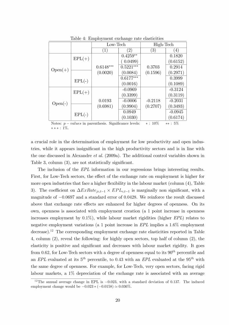
Table 4: Employment exchange rate elasticitiesLow-Tech High-Tech

(1) (2) (3) (4)

Open(+)

EPL(+)

0.6148���

(0.0020)

0.4259��

0.3703(0.1596)

0.1820( 0.0499) (0.6152)0.5221��� 0.2914(0.0084) (0.2971)

EPL(-)0.6177��� 0.3999(0.0016) (0.1089)

Open(-)

EPL(+)

0.0193(0.6981)

-0.0969

-0.2118(0.2707)

-0.3124(0.3399) (0.3119)-0.0006 -0.2031(0.9904) (0.3493)

EPL(-)0.0949 -0.0945(0.1030) (0.6174)

Notes: p � values in parenthesis. Signi�cance levels: � : 10% �� : 5%� � � : 1%.

a crucial role in the determination of employment for low productivity and open indus-

tries, while it appears insigni�cant in the high productivity sectors and is in line with

the one discussed in Alexandre et al. (2009a). The additional control variables shown in

Table 3, column (3), are not statistically signi�cant.

The inclusion of the EPL information in our regressions brings interesting results.

First, for Low-Tech sectors, the e¤ect of the exchange rate on employment is higher for

more open industries that face a higher �exibility in the labour market (column (4), Table

3). The coe¢ cient on �ExRatejc;t�1 � EPLc;t�1 is marginally non signi�cant, with amagnitude of �0:0697 and a standard error of 0:0428. We reinforce the result discussedabove that exchange rate e¤ects are enhanced for higher degrees of openness. On its

own, openness is associated with employment creation (a 1 point increase in openness

increases employment by 0:1%), while labour market rigidities (higher EPL) relates to

negative employment variations (a 1 point increase in EPL implies a 1:6% employment

decrease).12 The corresponding employment exchange rate elasticities reported in Table

4, column (2), reveal the following: for highly open sectors, top half of column (2), the

elasticity is positive and signi�cant and decreases with labour market rigidity. It goes

from 0:62, for Low-Tech sectors with a degree of openness equal to its 90th percentile and

an EPL evaluated at its 5th percentile, to 0:43 with an EPL evaluated at the 95th with

the same degree of openness. For example, for Low-Tech, very open sectors, facing rigid

labour markets, a 1% depreciation of the exchange rate is associated with an average

12The annual average change in EPL is �0:023, with a standard deviation of 0:137. The inducedemployment change would be �0:023 � (�0:0158) ' 0:036%.

20

employment increase of about 0:43%. Turning our attention to closed sectors we observe

that in face of �exible labour markets the employment exchange rate elasticity is 0:0949,

and marginally non-signi�cant (the standard error is 0:1030). With the increase in the

degree of rigidity the exchange rate e¤ects on employment become clearly insigni�cant.

The results for the additional covariates provide a consistent story: (i) competition from

China a¤ects negatively employment changes, (ii) an increase in the unit labour costs

reduces employment, and (iii) income positive variations are associated with employment

creation; a 1% increase in GDP created 0:78% more employment.

For High-Tech industries, column (5), Table 3, both openness and labour market ri-

gidities do not play on the e¤ect of exchange rate innovations on employment variations.

At the same time, the employment exchange rate elasticity, Table 4, column (4), is not

signi�cant. An interesting result is the one where in very open High-Tech industries with

�exible labour markets, the employment exchange rate elasticity is about 0:4, and margin-

ally non-signi�cant at the 10% level (the associated p� value is 0:1089). Such elasticityis still about 2/3 of the one obtained for Low-Tech industries. These results con�rm

the conclusion that exchange rate movements are particularly relevant for employment

determination in low productivity sectors and these e¤ects decrease monotonically with

labour market rigidity. Also, openness has an important e¤ect on employment variations;

for example, a 1 point increase in the openness index implies a variation of about 0:34%

in employment (Table 3, column 5), and labour market rigidities are associated with an

employment reductions; a 1 point increase in EPL decreases employment by 2:3%. For

High-Tech sectors the additional set of regressors does not seem to play a relevant role.

Finally, looking to the overall signi�cance of the regressions presented in Table 3,

we conclude that our model is more successful in explaining employment movements for

Low-Tech industries. An adjusted R2 of 11% for Low-Tech (columns 2 and 4) compares

to 4% for High-Tech (columns 3 and 5). This conclusion is reinforced by the analysis of

the loglikelihood.

4.3 Sensitivity analysis

In what follows we discuss two alternative speci�cations of equation (23). We extend the

estimates presented in columns (4) and (5) of Table 3 by, �rst, replacing Openjc;t�1 and

EPLc;t�1 by their �rst-di¤erences counterparts, and, second, eliminating these variables

from our speci�cation, while keeping their interactions with the exchange rate. The

estimates, and corresponding elasticities, are presented in Tables 5 and 6, respectively.

The new set of estimates indicates that there are no major changes in our results.

Some of the estimates, and corresponding elasticities, become statistically signi�cant,

21

reinforcing the results discussed in the previous section. By including both openness and

EPL in lagged changes, instead of levels, we now observe that for High-Tech the exchange

rate e¤ects are also mediated by the degree of openness. This results is valid for both

speci�cations, columns (2) and (4), Table 5. As before, exchange rate e¤ects seem not

to be determined by labour market rigidities for High-Tech industries. From column (2),

we also conclude in favour of the relevant role of GDP on employment movements in the

High-Tech economic activities. Although the estimate on this coe¢ cient has always been

positive, only under this particular speci�cation of the model we obtain a statistically

signi�cant result. Comparing to the Low-Tech estimate, the estimated coe¢ cient is

about 2/3, implying a lower e¤ect of GDP the High-Tech labour market. Excluding

both openness and EPL on their own from the regression, column (4), GDP is again

statistically insigni�cant, even though positive. One possible interpretation for these

results is that the degree of openness might be correlated with income levels. This way,

in Table 3, columns (3) and (5), most of the e¤ect is captured by openness. By taking

�rst-di¤erences of openness, as well as of EPL, or by eliminating these two variables from

the model, we let GDP show its main e¤ect, even for High-Tech.

Table 5: Employment regressions

Low-Tech High-Tech Low-Tech High-Tech

Model (1) (2) (3) (4)

�ExRatet�1 -.0788 -.3653 -.1248 -.2313(.1203) (.4154) (.1247) (.3687)

�ExRate �Opent�1 1.2254��� 1.6339� 1.3437��� 1.4180�

(.3713) (.8626) (.3844) (.7711)

�ExRate � EPLt�1 -.1068�� -.1365 -.0980�� -.1592(.0423) (.1012) (.0428) (.1017)

�Opent�1 -.0817 -.0328(.0638) (.0868)

�EPLt�1 -.0033 -.0043(.0065) (.0199)

�ShareChinaWeightt�1 -.0913 .3057 -.0846 .2868(.1599) (.4552) (.1645) (.4568)

�ShareChinat�1 -.0745� -.3050 -.0794� -.2951(.0438) (.2268) (.0467) (.2271)

�ULCt�1 -.1632��� .0802 -.1582��� .1520(.0627) (.1525) (.0602) (.1821)

�GDPt�1 .8199��� .5022� .7653��� .3622

Continued on next page...

22

... table 5 continued

Low-Tech High-Tech Low-Tech High-Tech

Model (1) (2) (3) (4)

(.0948) (.2886) (.0951) (.2758)

�InterestRatet�1 -.0013 .00004 -.0013 -.0007(.0009) (.0024) (.0009) (.0025)

Countries 23 23 23 23

Observations 3273 2400 3295 2428

Adj. R2 .1097 .0286 .1038 .0282

LogLikelihood 5417.134 1954.527 5412.136 1957.976

Notes: Signi�cance levels: � : 10% �� : 5% � � � : 1%. Robust

standard errors in parenthesis. All regressions are estimated by �xed-e¤ects at

the sector/country level, and include time dummies. The dependent variable is

�LogEmploymentjct.

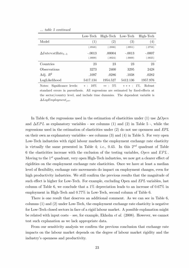
In Table 6, the regressions used in the estimation of elasticities under (1) use �Open

and �EPL as explanatory variables - see columns (1) and (2) in Table 5 -, while the

regressions used in the estimation of elasticities under (2) do not use openness and EPL

on their own as explanatory variables - see columns (3) and (4) in Table 5. For very open

Low-Tech industries with rigid labour markets the employment exchange rate elasticity

is virtually the same presented in Table 4; i.e., 0:43. In this 2nd quadrant of Table

6 the elasticities increase with the exclusion of the testing variables, Open and EPL .

Moving to the 1st quadrant, very open High-Tech industries, we now get a clearer e¤ect of

rigidities on the employment exchange rate elasticities. Once we have at least a median

level of �exibility, exchange rate movements do impact on employment changes, even for

high productivity industries. We still con�rm the previous results that the magnitude of

such e¤ect is higher for Low-Tech. For example, excluding Open and EPL variables, last

column of Table 6, we conclude that a 1% depreciation leads to an increase of 0:67% in

employment in High-Tech and 0:77% in Low-Tech, second column of Table 6.

There is one result that deserves an additional comment. As we can see in Table 6,

columns (1) and (2) under Low-Tech, the employment exchange rate elasticity is negative

for Low-Tech closed sectors in face of a rigid labour market. A possible explanation might

be related with input costs �see, for example, Ekholm et al. (2008). However, we cannot

test such explanation as we lack appropriate data.

From our sensitivity analysis we con�rm the previous conclusion that exchange rate

impacts on the labour market depends on the degree of labour market rigidity and the

industry�s openness and productivity.

23

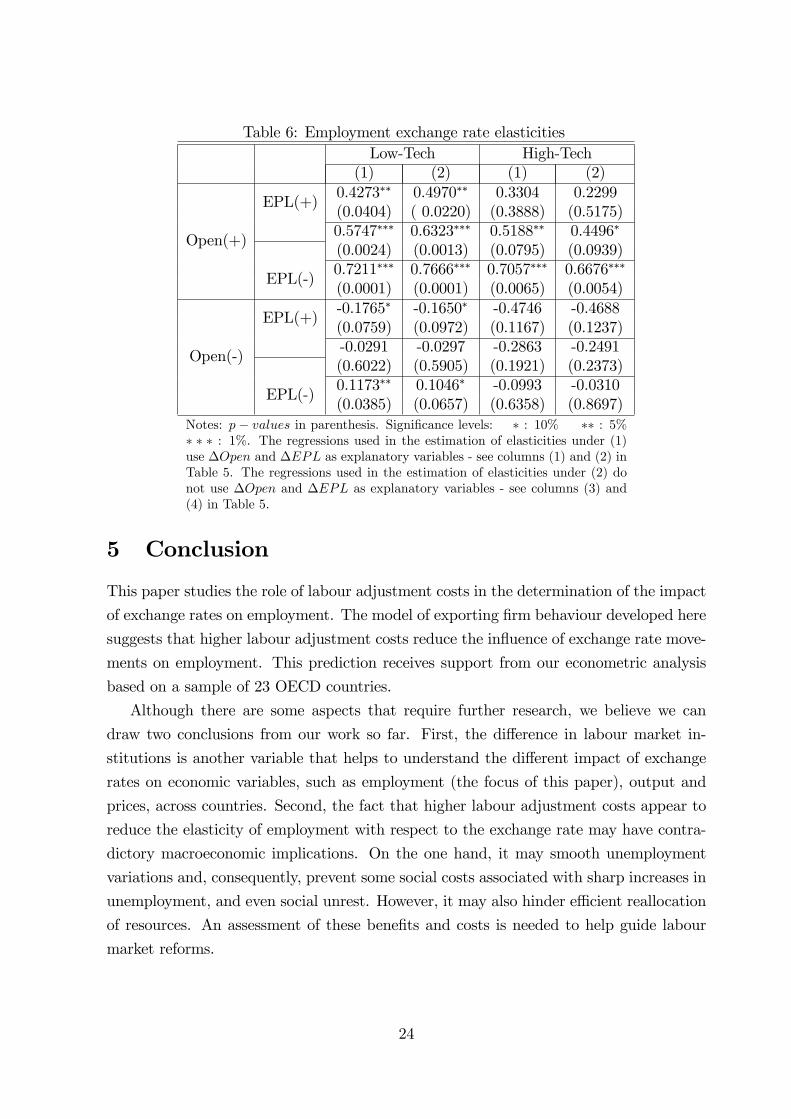
Table 6: Employment exchange rate elasticitiesLow-Tech High-Tech

(1) (2) (1) (2)

Open(+)

EPL(+)0.4273�� 0.4970�� 0.3304 0.2299(0.0404) ( 0.0220) (0.3888) (0.5175)0.5747��� 0.6323��� 0.5188�� 0.4496�

(0.0024) (0.0013) (0.0795) (0.0939)

EPL(-)0.7211��� 0.7666��� 0.7057��� 0.6676���

(0.0001) (0.0001) (0.0065) (0.0054)

Open(-)

EPL(+)-0.1765� -0.1650� -0.4746 -0.4688(0.0759) (0.0972) (0.1167) (0.1237)-0.0291 -0.0297 -0.2863 -0.2491(0.6022) (0.5905) (0.1921) (0.2373)

EPL(-)0.1173�� 0.1046� -0.0993 -0.0310(0.0385) (0.0657) (0.6358) (0.8697)

Notes: p � values in parenthesis. Signi�cance levels: � : 10% �� : 5%� � � : 1%. The regressions used in the estimation of elasticities under (1)use �Open and �EPL as explanatory variables - see columns (1) and (2) inTable 5. The regressions used in the estimation of elasticities under (2) donot use �Open and �EPL as explanatory variables - see columns (3) and(4) in Table 5.

5 Conclusion

This paper studies the role of labour adjustment costs in the determination of the impact

of exchange rates on employment. The model of exporting �rm behaviour developed here

suggests that higher labour adjustment costs reduce the in�uence of exchange rate move-

ments on employment. This prediction receives support from our econometric analysis

based on a sample of 23 OECD countries.

Although there are some aspects that require further research, we believe we can

draw two conclusions from our work so far. First, the di¤erence in labour market in-

stitutions is another variable that helps to understand the di¤erent impact of exchange

rates on economic variables, such as employment (the focus of this paper), output and

prices, across countries. Second, the fact that higher labour adjustment costs appear to

reduce the elasticity of employment with respect to the exchange rate may have contra-

dictory macroeconomic implications. On the one hand, it may smooth unemployment

variations and, consequently, prevent some social costs associated with sharp increases in

unemployment, and even social unrest. However, it may also hinder e¢ cient reallocation

of resources. An assessment of these bene�ts and costs is needed to help guide labour

market reforms.

24

References

Addison, J. and P. Teixeira (2003). The economics of employment protection. Journal

of Labour Research, 24(1), 85-129.

Alexandre, F., P. Bação, J. Cerejeira and M. Portela (2009a). Employment and exchange

rates: the role of openness and technology. IZA Discussion Paper No. 4191. Institute

for the Study of Labor, Bonn.

Alexandre, F., P. Bação, J. Cerejeira and M. Portela (2009b). Aggregate and sector-

speci�c exchange rates for the Portuguese economy, Notas Económicas, 30.

Berman, N., P. Martin and T. Mayer (2009). How do di¤erent exporters react to exchange

rate changes? Theory, empirics and aggregate implications. CEPR Discussion Paper

Series No. 7493. Centre for Economic Policy Research.

Bertola, G. (1990). Job security, employment and wages. European Economic Review,

34, June, 851-86.

Bertola, G. (1992). Labor turnover costs and average labor demand. Journal of Labor

Economics, 10(4), 389�411.

Blanchard, O. (1999). European unemployment: the role of shocks and institutions, Ba¢

Lecture, Rome.

Blanchard, O. and P. Portugal (2001). What hides behind an unemployment rate: Com-

paring Portuguese and U.S. labor markets, 91(1), 187-207.

Blanchard, O. and J. Wolfers (2000). The role of shocks and institutions in the rise

of European unemployment: the aggregate evidence. The Economic Journal, 110,

March, C1-C33.

Branson, W. and J. Love (1988). U.S. manufacturing and the real exchange rate. In R.

Marston, ed., Misalignments of exchange rates: e¤ects on trade and industry. Chicago

University Press.

Burstein, A., J. Neves and S. Rebelo (2003). Distribution costs and real exchange rate

dynamics during exchange-rate-based stabilizations. Journal of Monetary Economics,

50(6), 1189-1214.

Calmfors L. and J. Dri¢ ll (1988). Bargaining structure, corporatism, and macroeconomic

performance. Economic Policy, 6, 14-61.

Campa, J. and L. Goldberg (2001). Employment versus wage adjustment and the US

dollar. Review of Economics and Statistics, 83 (3), 477-489.

25

Campa, J. and L. Goldberg (2008). The insensitivity of the CPI to exchange rates:

distribution margins, imported inputs, and trade exposure, Review of Economics and

Statistics, Forthcoming.

Cingano, F., M. Leonardi, J. Messina and G. Pica (2009). The e¤ect of employment

protection legislation and �nancial market imperfections on investment: evidence from

a �rm-level panel of EU countries. Economic Policy 61: 117-163.

Dri¢ ll, J. (2006). The Centralization of Wage Bargaining Revisited: What Have We

Learned? Journal of Common Market Studies, 44(4), 731-756.

European Commission (2003). 2003 Adopted employment guidelines. Available at

http://europa.eu.int/eur-lex/pri/en/oj/dat/2003/l_197/l_19720030805en00130

021.pdf.

Ekholm, K., A. Moxnes and K.H. Ulltveit-Moe (2008). Manufacturing restructuring and

the role of real exchange rate shocks: a �rm level analysis. CEPR Discussion paper

no. 6904.

Felbermayr, G., J. Prat and H. Schmerer (2008). Globalization and Labor Market Out-

comes: Wage Bargaining, Search Frictions, and Firm Heterogeneity, IZA Discussion

Papers No. 3363, Bonn.

Gómez-Salvador, R., J. Messina and G. Vallanti (2004). Gross job �ows and institutions

in Europe. Labour Economics, 11, 469-485.

Gourinchas, P. (1999). Exchange rates do matter: French job reallocation and exchange

rate turbulence, 1984-1992. European Economic Review, 43, 1279-1316.

Haltiwanger, J., S. Scarpeta and H. Schweiger (2006). Assessing job �ows across coun-

tries: the role of industry, �rm size and regulations. IZA Discussion Paper No. 2450.

Helpman, E. and O. Itskhoki (2010). Labour market rigidities, trade and unemployment.

Review of Economic Studies, Forthcoming.

Hopenhayn, H. and R. Rogerson (1993). Job turnover and policy evaluation: A general

equilibrium analysis. Journal of Political Economy, 101(5), 915�938.

Klein, M.K., S. Schuh and R. Triest (2003). Job creation, job destruction, and the real

exchange rate. Journal of International Economics, 59, 239-265.

Melitz, M.J. (2003). The impact of trade on intra-industry reallocations and aggregate

industry productivity. Econometrica. 71(6), 1695-1725.

Nickell, S. (1997). Unemployment and labour market rigidities: Europe versus North-

America. Journal of Economic Perspectives, 11, 55-74.

26

Nickell, S., L. Nunziata, W. Ochel and G. Quintini (2002). The Beveridge curve, unem-

ployment and wages in the OECD from the 1960s to the 1990s. Centre for Economic

Performance, London School of Economics.

OECD (1999). Employment Outlook, OECD, Paris.

OECD (2004). Employment Outlook, OECD, Paris.

OECD (2005). OECD Science, Technology and Industry Scoreboard, Annex 1, OECD.

Pfann, G. and B. Verspagen (1989). The structure of adjustment costs for labour in the

Dutch manufacturing sector. Economics Letters, 29(4), 365-371.

Revenga, A.L. (1992). The impact of import competition on employment and wages in

U.S. manufacturing. Quarterly Journal of Economics. 107 (1), 255-284.

Ravn, Morten O. and H. Uhlig (2002). On adjusting the Hodrick-Prescott �lter for the

frequency of observations. Review of Economic and Statistics, 84, 2, 371-376.

Turner, P. and J. Van�t dack (1993). Measuring international price and cost competit-

iveness. BIS Economic Papers, 39.

6 Appendix

Countries and Sectors

Table 7: Observations per country and technology levelCountry Low-Tech High-Tech Country Low-Tech High-TechAustria� 118 100 Hungary 48 6Belgium� 198 106 Italy� 202 170Canada� 195 153 Japan� 192 159Switzerland 81 54 South Korea� 48 40Czech Republic 40 39 Netherlands� 153 112Germany 176 142 Norway� 185 147Denmark� 193 137 Poland 40 5Spain� 197 158 Portugal� 151 110Finland� 202 159 Slovakia 44 40France� 202 170 Sweden� 202 168United Kingdom� 136 17 United States� 180 150Greece� 112 86

Low-Tech High-TechTotal observations 3295 2428Note: OECD23 refers to all countries presented in tableOECD17 refers to countries marked with �.

27

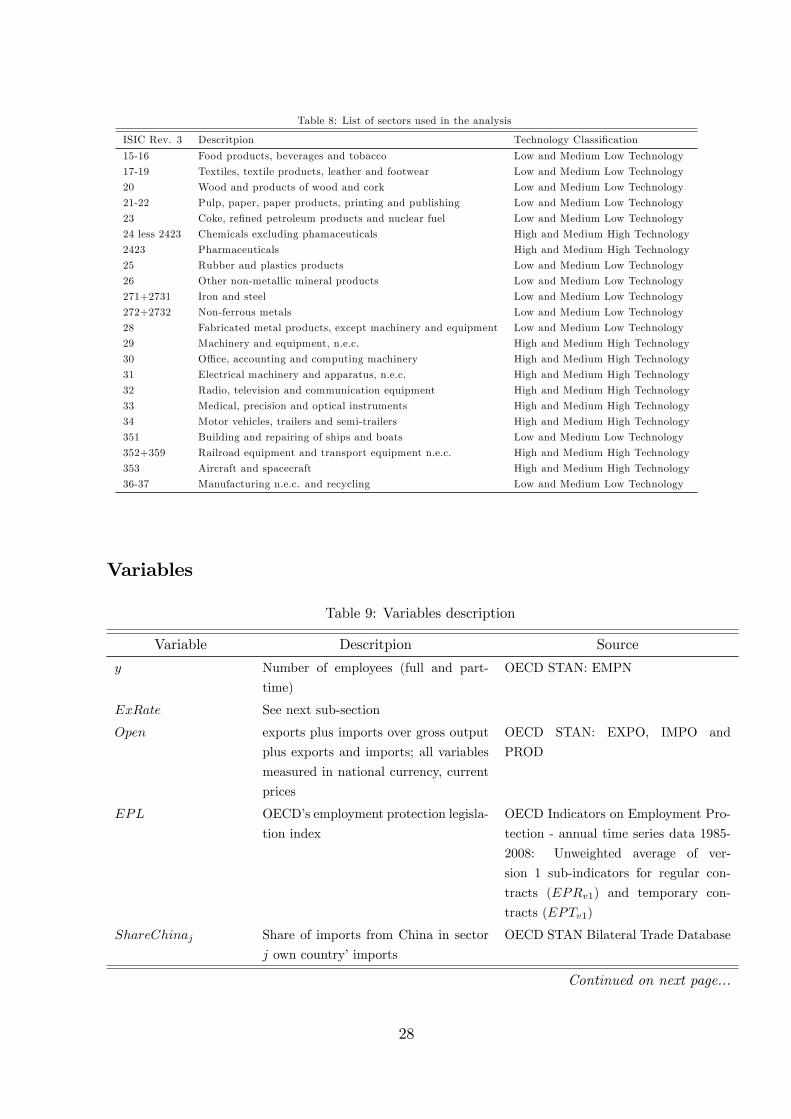
Table 8: List of sectors used in the analysis

ISIC Rev. 3 Descritpion Technology Classi�cation

15-16 Food products, beverages and tobacco Low and Medium Low Technology

17-19 Textiles, textile products, leather and footwear Low and Medium Low Technology

20 Wood and products of wood and cork Low and Medium Low Technology

21-22 Pulp, paper, paper products, printing and publishing Low and Medium Low Technology

23 Coke, re�ned petroleum products and nuclear fuel Low and Medium Low Technology

24 less 2423 Chemicals excluding phamaceuticals High and Medium High Technology

2423 Pharmaceuticals High and Medium High Technology

25 Rubber and plastics products Low and Medium Low Technology

26 Other non-metallic mineral products Low and Medium Low Technology

271+2731 Iron and steel Low and Medium Low Technology

272+2732 Non-ferrous metals Low and Medium Low Technology

28 Fabricated metal products, except machinery and equipment Low and Medium Low Technology

29 Machinery and equipment, n.e.c. High and Medium High Technology

30 O¢ ce, accounting and computing machinery High and Medium High Technology

31 Electrical machinery and apparatus, n.e.c. High and Medium High Technology

32 Radio, television and communication equipment High and Medium High Technology

33 Medical, precision and optical instruments High and Medium High Technology

34 Motor vehicles, trailers and semi-trailers High and Medium High Technology

351 Building and repairing of ships and boats Low and Medium Low Technology

352+359 Railroad equipment and transport equipment n.e.c. High and Medium High Technology

353 Aircraft and spacecraft High and Medium High Technology

36-37 Manufacturing n.e.c. and recycling Low and Medium Low Technology

Variables

Table 9: Variables description

Variable Descritpion Source

y Number of employees (full and part-

time)

OECD STAN: EMPN

ExRate See next sub-section

Open exports plus imports over gross output

plus exports and imports; all variables

measured in national currency, current

prices

OECD STAN: EXPO, IMPO and

PROD

EPL OECD�s employment protection legisla-

tion index

OECD Indicators on Employment Pro-

tection - annual time series data 1985-

2008: Unweighted average of ver-

sion 1 sub-indicators for regular con-

tracts (EPRv1) and temporary con-

tracts (EPTv1)

ShareChinaj Share of imports from China in sector

j own country�imports

OECD STAN Bilateral Trade Database

Continued on next page...

28

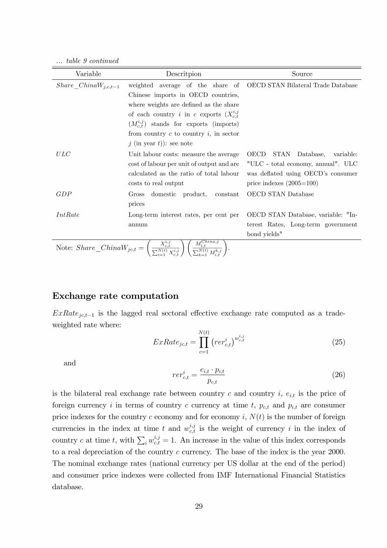
... table 9 continued

Variable Descritpion Source

Share_ChinaWj;c;t�1 weighted average of the share of

Chinese imports in OECD countries,

where weights are de�ned as the share

of each country i in c exports (Xi;jc;t

(M i;jc;t ) stands for exports (imports)

from country c to country i, in sector

j (in year t)): see note

OECD STAN Bilateral Trade Database

ULC Unit labour costs: measure the average

cost of labour per unit of output and are

calculated as the ratio of total labour

costs to real output

OECD STAN Database, variable:

"ULC - total economy, annual". ULC

was de�ated using OECD�s consumer

price indexes (2005=100)

GDP Gross domestic product, constant

prices

OECD STAN Database

IntRate Long-term interest rates, per cent per

annum

OECD STAN Database, variable: "In-

terest Rates, Long-term government

bond yields"

Note: Share_ChinaWjc;t =

�Xi;jc;tPN(t)

i=1 Xi;jc;t

��MChina;ji;tPN(t)k=1 M

k;ji;t

�.

Exchange rate computation

ExRatejc;t�1 is the lagged real sectoral e¤ective exchange rate computed as a trade-

weighted rate where:

ExRatejc;t =

N(t)Yc=1

�reric;t

�wi;jc;t (25)

and

reric;t =ei;t � pi;tpc;t

(26)

is the bilateral real exchange rate between country c and country i, ei;t is the price of

foreign currency i in terms of country c currency at time t, pc;t and pi;t are consumer

price indexes for the country c economy and for economy i, N(t) is the number of foreign

currencies in the index at time t and wi;jc;t is the weight of currency i in the index of

country c at time t, withP

iwi;jc;t = 1. An increase in the value of this index corresponds

to a real depreciation of the country c currency. The base of the index is the year 2000.

The nominal exchange rates (national currency per US dollar at the end of the period)

and consumer price indexes were collected from IMF International Financial Statistics

database.

29

We computed exchange rate weights in order to include information that would allow

us to take into account for sectoral third-party competition. We followed Turner and

Van�t dack (1993) and de�ned the weight wj;ic;t given to i�s country currency in the double-

weighted e¤ective index as

wj;ic;t =

M i;jc;t

X i;jc;t +j M

i;jc;t

!wi;jM;c;t +

X i;jc;t

X i;jc;t +M

i;jc;t

!wi;jX;c;t (27)

where wi;jX;c;t is de�ned as

wi;jX;c;t =

X i;jc;tPN(t)

i=1 Xi;jc;t

!0BB@ ji;t

ji;t +Xh 6=i;c

Xh;ji;t

1CCA+Xk 6=i

Xk;jc;tPN(t)

k=1 Xk;jc;t

!0BB@ Xk;ji;t

jk;t +Xh 6=k;c

Xk;jh;t

1CCA(28)

In the formulas, X i;jc;t (M

i;jc;t ) stands for exports (imports) from country c to country i,

in sector j (in year t).

Data on trade is from OECD STAN Bilateral Trade Database (OECD, 2008).

Figures

30

1.11

6.67

ρ q =0, φ =0.1

3σ

10

0γ

100

0.17

6.67

ρ q =0, φ =0.5

3σ

10

0γ

100

0.00

6.67

ρ q =0, φ =1

3σ

10

0γ

100

1.22

6.67

ρ q =0.5, φ =0.1

3σ

10

0γ

100

0.25

6.67

ρ q =0.5, φ =0.5

3σ

10

0γ

100

0.08

6.67

ρ q =0.5, φ =1

3σ

10

0γ

100

1.32

6.67

ρ q =0.9, φ =0.1

3σ

10

0γ

100

0.42

6.67

ρ q =0.9, φ =0.5

3σ

10

0γ

100

0.18

6.67

ρ q =0.9, φ =1

3σ

10

0γ

100

Figure 7: Employment exchange rate elasticity: labour adjustment costs and openness

0.00

0.75

σ =3, ρ q =0

0φ

2

0γ

100

0.00

0.75

σ =3, ρ q =0.5

0φ

2

0γ

100

0.02

0.75

σ =3, ρ q =0.9

0φ

2

0γ

100

0.00

2.92

σ =7, ρ q =0

0φ

2

0γ

100

0.00

2.92

σ =7, ρ q =0.5

0φ

2

0γ

100

0.00

2.92

σ =7, ρ q =0.9

0φ

2

0γ

100

0.00

4.44

σ =10, ρ q =0

0φ

2

0γ

100

0.00

4.44

σ =10, ρ q =0.5

0φ

2

0γ

100

0.00

4.44

σ =10, ρ q =0.9

0φ

2

0γ

100

Figure 8: Employment exchange rate elasticity: labour adjustments costs and productiv-ity

31

1.11

1.65

σ =3, φ =0.1

0ρ q

1

0γ

100

0.17

1.65

σ =3, φ =0.5

0ρ q

1

0γ

100

0.05

1.65

σ =3, φ =1

0ρ q

1

0γ

100

4.55

4.55

σ =7, φ =0.1

0ρ q

1

0γ

100

2.82

4.55

σ =7, φ =0.5

0ρ q

1

0γ

100

0.17

4.55

σ =7, φ =1

0ρ q

1

0γ

100

6.67

6.67

σ =10, φ =0.1

0ρ q

1

0γ

100

6.39

6.67

σ =10, φ =0.5

0ρ q

1

0γ

100

0.44

6.67

σ =10, φ =1

0ρ q

1

0γ

100

Figure 9: Employment exchange rate elasticity: labour adjustment costs and exchangerate persistence

32