EMPLOYMENT PAPER

2002/44

EXTERNAL LIBERALIZATION, MACROECONOMIC

INSTABILITY AND THE LABOUR MARKET IN

BRAZIL

Matias Vernengo Assistant Professor Kalamazoo College

Michigan, Illinois

Employment Sector

International Labour Office, Geneva

2

Foreword

This is one of the case studies prepared within the framework of the research project on “global economic integration and employment policy” carried out by the Employment Policy Department. The case studies are designed to provide detailed empirical assessment of the effects of growth of manufactured trade, induced by trade liberalization, on manufacturing employment and wages in a carefully selected set of countries. While there is widespread concern about the effects, they remain inadequately understood. There exists a large literature on the experience of industrialized countries, but controversies abound. On developing countries, the literature is extremely limited. Given this backdrop, the case studies are expected to make a substantial contribution to our understanding of the changes being engendered by globalization, a subject of much current interest to international organizations, national policy makers, the academic community and civil society organizations.

The paper argues that, in Brazil, trade liberalization, which occurred only in the early 1990s, led to rather puzzling developments. It failed to stimulate manufactured exports but substantially boosted manufactured imports, thus worsening the trade balance. And it increased the share of capital-intensive manufactures, and correspondingly reduced the share of labour-intensive manufactures, in total manufactured exports. As a result, manufacturing output stagnated while the share of high-skill capital-intensive industries in total manufacturing output increased quite significantly. At the same time, a combination of increased capital inflow and increased exposure to international competition stimulated the growth of labour productivity. The labour market effects of these developments were naturally adverse: aggregate manufacturing employment fell, employment of low-skilled labour fell more sharply than that of high-skilled labour and there was a significant rise in wage inequality.

These developments can be traced to the macroeconomic context in which trade

liberalization was pursued. In the early 1990s, Brazil’s economy faced huge problems of high inflation and unsustainable external debt. In such a context, trade liberalization and exchange -rate-based stabilization were pursued simultaneously. This made the economy extremely vulnerable to fluctuations in capital flows, which affected growth and trade through their mutually contradictory effects on investment and exchange rate. The effects of trade liberalization on manufacturing employment and wages have to be understood within this wider context.

Rashid Amjad Director a.i.

Employment Strategy Department

3

Acknowledgement I would like to thank, without implicating, Alcino Câmara Neto, Ajit Ghose and Lance Taylor. Also I would like to thank Alana Shaw for the research assistance.

4

Contents Page Foreword Acknowledgement 1. Introduction ……………………………………………………………. 1 2. The macroeconomic context of trade liberalization …………………… 2 3. Trade liberalization, trade performance and growth ………………….. 9 4. Trade liberalization and the manufacturing sector ……………………. 17 5. Effects of liberalization on employment and wages …………………… 22 6. Concluding remarks ……………………………………………………. 33 References ………………………………………………………………………. 35

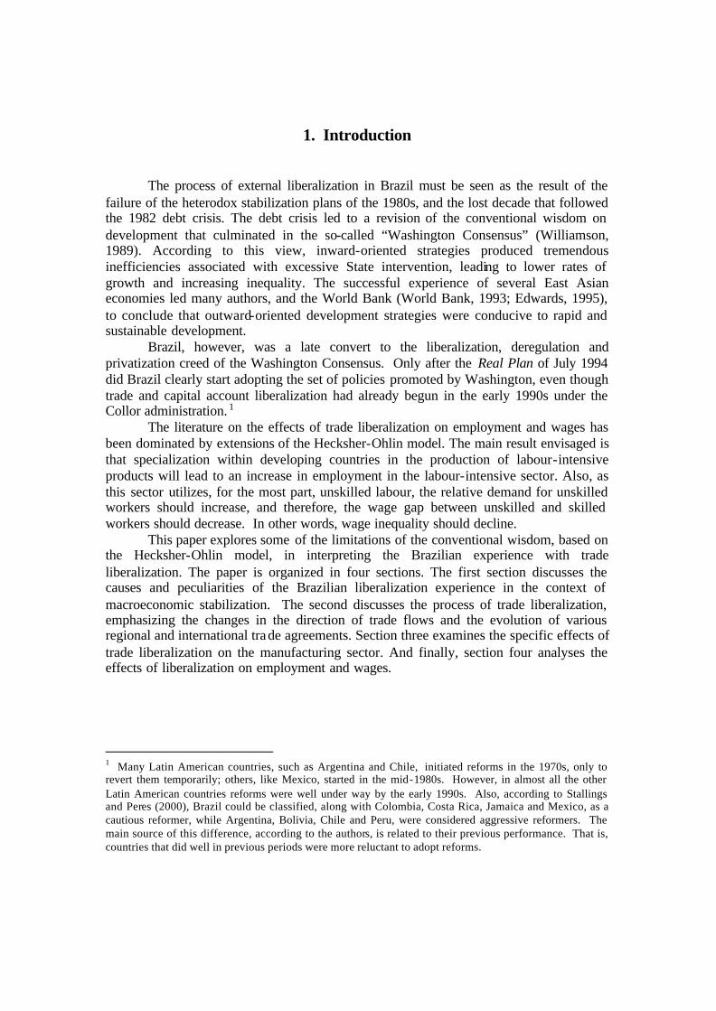
1. Introduction

The process of external liberalization in Brazil must be seen as the result of the

failure of the heterodox stabilization plans of the 1980s, and the lost decade that followed the 1982 debt crisis. The debt crisis led to a revision of the conventional wisdom on development that culminated in the so-called “Washington Consensus” (Williamson, 1989). According to this view, inward-oriented strategies produced tremendous inefficiencies associated with excessive State intervention, leading to lower rates of growth and increasing inequality. The successful experience of several East Asian economies led many authors, and the World Bank (World Bank, 1993; Edwards, 1995), to conclude that outward-oriented development strategies were conducive to rapid and sustainable development.

Brazil, however, was a late convert to the liberalization, deregulation and privatization creed of the Washington Consensus. Only after the Real Plan of July 1994 did Brazil clearly start adopting the set of policies promoted by Washington, even though trade and capital account liberalization had already begun in the early 1990s under the Collor administration. 1

The literature on the effects of trade liberalization on employment and wages has been dominated by extensions of the Hecksher-Ohlin model. The main result envisaged is that specialization within developing countries in the production of labour-intensive products will lead to an increase in employment in the labour-intensive sector. Also, as this sector utilizes, for the most part, unskilled labour, the relative demand for unskilled workers should increase, and therefore, the wage gap between unskilled and skilled workers should decrease. In other words, wage inequality should decline.

This paper explores some of the limitations of the conventional wisdom, based on the Hecksher-Ohlin model, in interpreting the Brazilian experience with trade liberalization. The paper is organized in four sections. The first section discusses the causes and peculiarities of the Brazilian liberalization experience in the context of macroeconomic stabilization. The second discusses the process of trade liberalization, emphasizing the changes in the direction of trade flows and the evolution of various regional and international trade agreements. Section three examines the specific effects of trade liberalization on the manufacturing sector. And finally, section four analyses the effects of liberalization on employment and wages.

1 Many Latin American countries, such as Argentina and Chile, initiated reforms in the 1970s, only to revert them temporarily; others, like Mexico, started in the mid-1980s. However, in almost all the other Latin American countries reforms were well under way by the early 1990s. Also, according to Stallings and Peres (2000), Brazil could be classified, along with Colombia, Costa Rica, Jamaica and Mexico, as a cautious reformer, while Argentina, Bolivia, Chile and Peru, were considered aggressive reformers. The main source of this difference, according to the authors, is related to their previous performance. That is, countries that did well in previous periods were more reluctant to adopt reforms.

2

2. The macroeconomic context of trade liberalization

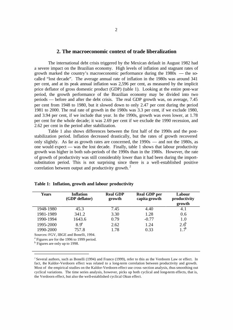
The international debt crisis triggered by the Mexican default in August 1982 had a severe impact on the Brazilian economy. High levels of inflation and stagnant rates of growth marked the country’s macroeconomic performance during the 1980s — the so-called “lost decade”. The average annual rate of inflation in the 1980s was around 341 per cent, and at its peak annual inflation was 2,596 per cent, as measured by the implicit price deflator of gross domestic product (GDP) (table 1). Looking at the entire post-war period, the growth performance of the Brazilian economy may be divided into two periods — before and after the debt crisis. The real GDP growth was, on average, 7.45 per cent from 1948 to 1980, but it slowed down to only 2.47 per cent during the period 1981 to 2000. The real rate of growth in the 1980s was 3.3 per cent, if we exclude 1980, and 3.94 per cent, if we include that year. In the 1990s, growth was even lower, at 1.78 per cent for the whole decade; it was 2.69 per cent if we exclude the 1990 recession, and 2.62 per cent in the period after stabilization.

Table 1 also shows differences between the first half of the 1990s and the post-stabilization period. Inflation decreased drastically, but the rates of growth recovered only slightly. As far as growth rates are concerned, the 1990s — and not the 1980s, as one would expect — was the lost decade. Finally, table 1 shows that labour productivity growth was higher in both sub-periods of the 1990s than in the 1980s. However, the rate of growth of productivity was still considerably lower than it had been during the import-substitution period. This is not surprising since there is a well-established positive correlation between output and productivity growth. 2

Table 1: Inflation, growth and labour productivity

Years Inflation (GDP deflator)

Real GDP growth

Real GDP per capita growth

Labour productivity

growth 1948-1980 45.3 7.45 4.40 4.1 1981-1989 341.2 3.30 1.28 0.6 1990-1994 1643.6 0.79 -0.77 1.0 1995-2000 8.9a 2.62 1.24 2.6b 1990-2000 757.8 1.78 0.33 1.7b

Sources: FGV, IBGE and Bonelli, 1994. a Figures are for the 1996 to 1999 period. b Figures are only up to 1998. 2 Several authors, such as Bonelli (1994) and Franco (1999), refer to this as the Verdoorn Law or effect. In fact, the Kaldor-Verdoorn effect was related to a long-term correlation between productivity and growth. Most of the empirical studies on the Kaldor-Verdoorn effect use cross -section analysis, thus smoothing out cyclical variations. The time series analysis, however, picks up both cyclical and long-term effects, that is, the Verdoorn effect, but also the well-established cyclical Okun effect.

3

The results in table 1 show that the effects of the debt crisis were powerful. Yet the crisis did not lead immediately to a dramatic change in policy orientation in Brazil, at least in the direction of liberalization. Arguably, the extremely successful growth performance in the post-war period, at an average annual rate of 7.45 per cent, led to considerable inertia in policy formulation. The 1980s were marked by heterodox stabilization plans that built on the structuralist explanations of inflation, according to which inflation was caused mainly by balance-of-payments constraints and propagated by generalized indexation (Arida and Lara-Resende, 1985; Lopes, 1986). According to this view, both a fixed exchange rate and de -indexation were crucial for successful stabilization. All the heterodox plans (Cruzado, Cruzado II, Verão, and Bresser) froze domestic prices and eliminated wage indexation rules in order to eliminate inertial inflation. 3

According to the structuralist view, two problems persisted in the early 1990s, which made any attempts at stabilization difficult. First, indexation prevented incomes from being eroded, but it also tended to freeze the pre-existing set of relative prices that did not necessarily correspond to the equilibrium set, that is to say, the one that was desired by economic agents. Hence, a price freeze and the elimination of indexation rules would also have tended to freeze an out-of-equilibrium relative price structure. When the freeze was removed prices exploded, as agents tried to impose their incompatible income claims. In this case, Amadeo (1994) suggests that a social pact is needed if stabilization is to succeed.

3 The Collor plan is more difficult to classify. Prices were frozen for only one month, but the main component of the plan was the blocking of all financial assets for 18 months, and reducing the holdings of M4 by almost 70 per cent. For a discussion of the technical aspects of the plan, see Simonsen (1990).

4

-8

-4

0

4

8

40

80

120

160

200

240

1975 1980 1985 1990 1995 2000

BT (left scale) E (right scale)

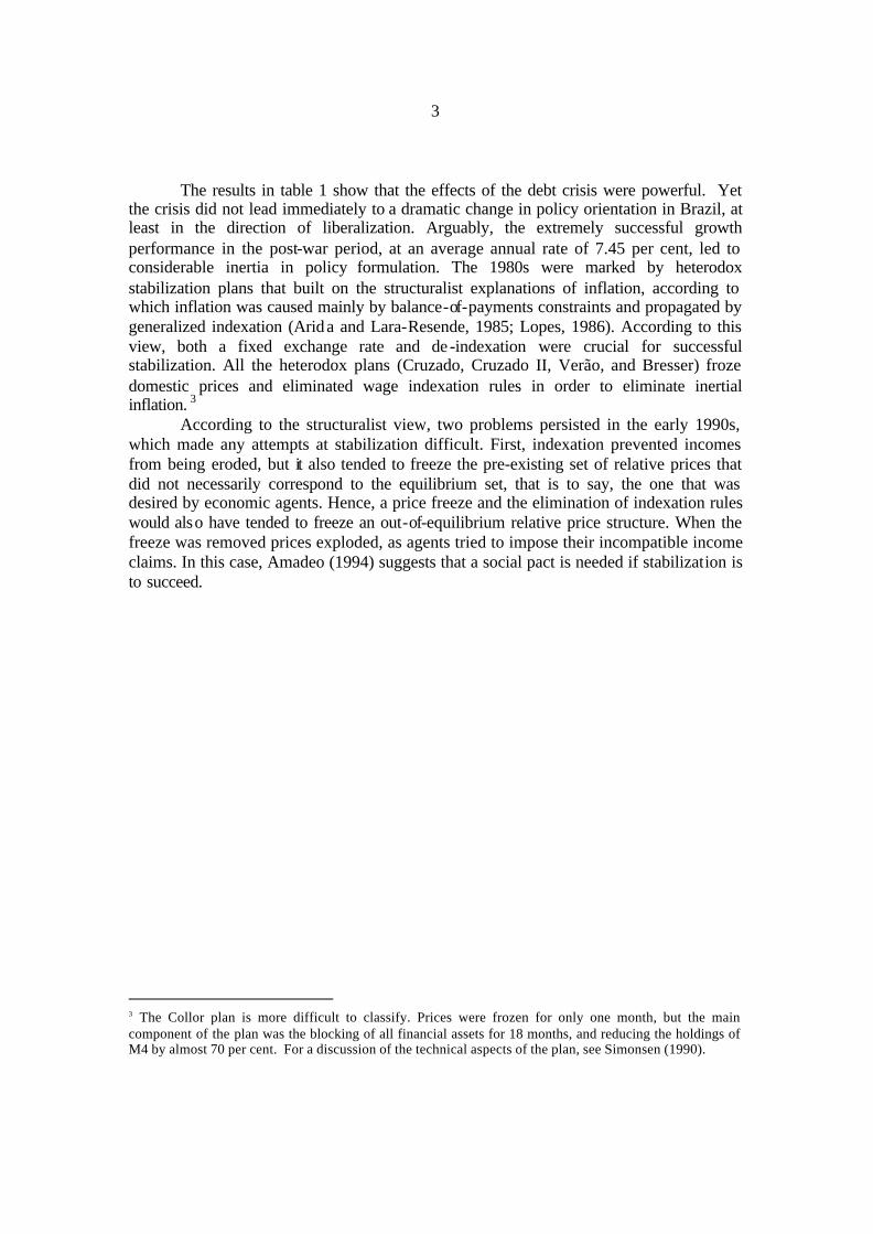
FIGURE 1 Trade Balance and Real Exchange Rate

Source: FGV Data (see references)

The second problem was the outflow of capital caused by the debt crisis. In fact, the debt crises not only brought a halt to external financing, but also reversed the direction of capital flows, forcing a huge drain of resources from Brazil to developed countries (Cardoso and Fishlow, 1988). Figure 1 shows the large trade surpluses (positive BT) that were generated in order to pay for servicing the foreign debt, and the variation in the real exchange rate (E) needed to obtain those surpluses. A trade deficit of 2.2 per cent of GDP in 1980 was transformed into a trade surplus of 5.9 per cent of GDP in 1984. It must be emphasized that this was achieved through large devaluations (expenditure switching) and also by a reduction in the rate of growth (expenditure changing).

The foreign exchange shortage led to the suspension of payments for the servicing of external obligations in 1987. However, this episode was short-lived and Brazil resumed payments in 1988. Not long after the Brazilian moratorium, in March 1989 the United States Government announced the Brady Plan. 4 This major programme of restructuring of the terms of obligations was based on the recognition that the existing debt could not be serviced on its original terms. The Brady Pla n and the structural

4 In March 1989, then United States Treasury Secretary, Nicholas F. Brady, articulated new principles for addressing the debt crisis that had plagued Latin America for most of the 1980s. The plan aimed at restoring debtor country access to voluntary capital markets; in retrospect, it was remarkably successful.

5

adjustment loans of the World Bank were negotiated on the basis of capacity to repay, which in turn was seen as being dependent on the implementation of reforms. The Brazilian experience indicates that debt crises are instrumental in forcing countries into restructuring their economies along market-friendly lines, although such restructuring may take time.

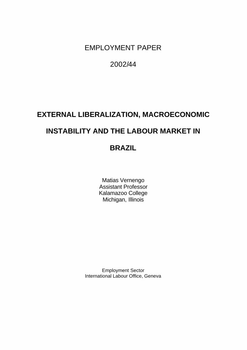
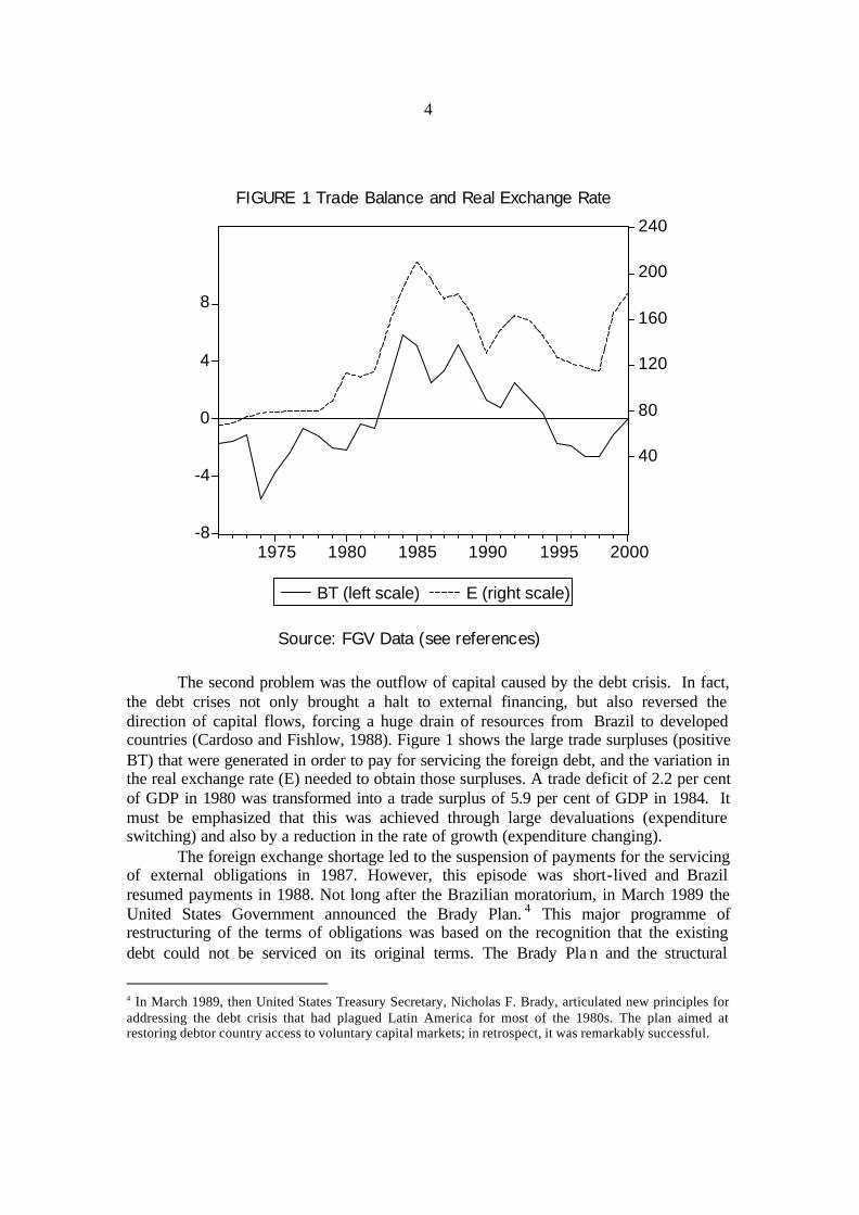
In the early 1990s, at the time of the Brady negotiations, capital inflows into Latin America resumed, leading to the new problem of how to cope with these increasing and volatile inflows (Agosin and Ffrench-Davis, 1996). Figure 2 shows that the resumption of capital flows, indicated by the change in the capital account balance, led to an unprecedented accumulation of foreign reserves (FR); foreign reserves increased from less than US$ 10 billion after the default to almost US$ 60 billion in the late 1990s. According to Calvo, Leiderman, and Reinhart (1993), the main reason for this change in the direction of capital flows was external, namely the recession in the United States and the reduction in United States interest rates.

-20000

-10000

0

10000

20000

30000

40000

50000

60000

1975 1980 1985 1990 1995 2000

KA FR

F I G U R E 2 C a p i t a l A c c o u n t a n d F o r e i g n R e s e r v es (in million dollars)

S o u r c e : B o l e t i m B a n c o C e n t r a l

6

The main question in the early 1990s was whether to implement the reforms after stabilizing the economy or simultaneously with that process. Stabilization was not seen as a pre-condition for the actual execution of the reforms. 5 In fact, one of the arguments for trade liberalization was that it would have a stabilizing effect on the price of tradable goods. The Collor Plan, implemented in March 1990, was the last of six heterodox stabilization plans, all of which failed to reduce inflation rates to reasonable levels. As with all previous plans, stability was short-lived. The generally accepted conclusion was that heterodoxy had failed, and that a great deal of orthodoxy would be needed to solve the inflationary problem.

As can be seen in figure 2, foreign reserves began accumulating only in the aftermath of the Collor Plan. This accumulation of reserves enabled a successful exchange-rate-based stabilization plan in 1994 along the lines of the plans implemented in other Latin American economies. The Real Plan was designed to follow the consensus on shock therapy, which appeared to include some of the lessons from the heterodox plans of the 1980s. According to Bruno (1993, p. 7), “the root of high chronic inflation, like hyperinflation, turns out to lie in the existence of a large public-sector deficit, the quasi-stability of the dynamic process … [comes] from an inherent inertia strongly linked with a high degree of indexation or accommodation of the key nominal magnitudes (wages, the exchange rate, and monetary aggregates) to the lagged movements of the price level.”

The shock therapy implied that the adoption of a fixed exchange rate regime would eliminate the propagation mechanism, but successful stabilization would require fiscal reform. In general, the explanation for the advantages of exchange rates as anchors is rooted in the literature on credibility and time consistency rather than on inertial inflation (Edwards, 1995, p. 101). With respect to exchange rate regimes, this debate has been translated into the consensual view that fixed exchange rate systems create environments that are more prone to produce fiscal discipline and low inflation. The argument is that if foreign central banks were to be committed to price stability, then a worldwide concerted assault on inflation would be successful. In this sense, fixing the exchange rate might be a good strategy for fighting inflat ion. This was the basic argument in favour of exchange-rate-based stabilization policies in Latin America, in particular in the Southern Cone stabilization plans of the 1970s and, more recently, in the Convertibility Plan in Argentina and the dollarization experiment in Ecuador.

Interestingly enough, the 1994 Brazilian exchange -rate-based stabilization plan seems to have been more in line with the heterodox plans of the 1980s than is generally assumed. 6 First, the de-indexation process was engineered in a way that resembles the Larida proposal of the mid-1980s; a new unit of account, corrected for inflation by the

5 In contrast with the Brazilian Government, economists in general viewed stability as a pre-condition for implementation of the reforms. They argued that high and variable inflation would distort the signals transmitted by relative prices, and that would lead to inefficient allocation of resources and lower rates of growth. 6 The case of Mexico, where a social pact was crucial for stability, also contains some heterodox features. Argentina and Chile, on the other hand, adopted typical orthodox stabilizatio n programmes.

7

average of three different inflation indexes, was introduced. The result was that inflation accelerated in terms of the old currency but not in terms of the new unit of account. This process had a great advantage over the previous price freezes, since it allowed relative prices to change before monetary reform. 7 The adjustment of relative prices in the transition period increased the distributive neutrality of monetary reform.

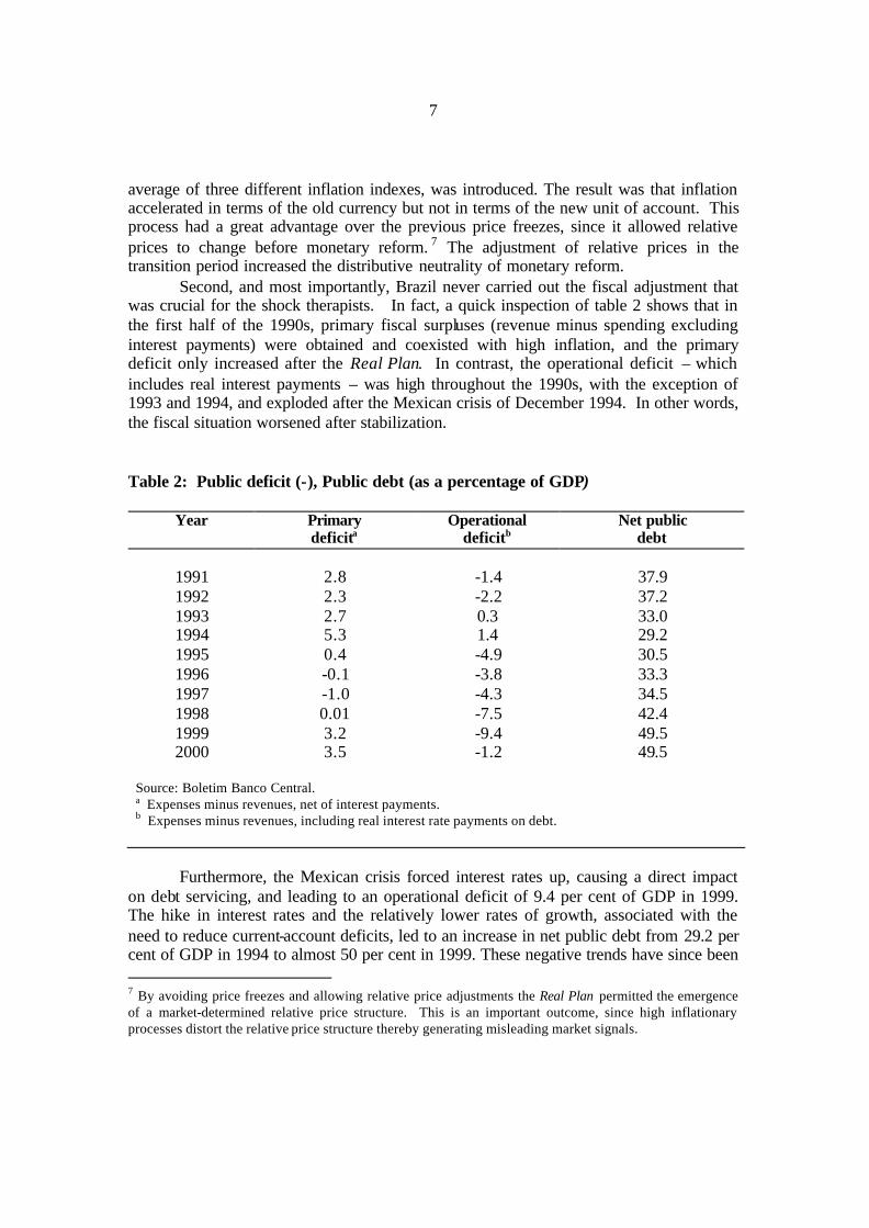
Second, and most importantly, Brazil never carried out the fiscal adjustment that was crucial for the shock therapists. In fact, a quick inspection of table 2 shows that in the first half of the 1990s, primary fiscal surpluses (revenue minus spending excluding interest payments) were obtained and coexisted with high inflation, and the primary deficit only increased after the Real Plan. In contrast, the operational deficit – which includes real interest payments – was high throughout the 1990s, with the exception of 1993 and 1994, and exploded after the Mexican crisis of December 1994. In other words, the fiscal situation worsened after stabilization.

Table 2: Public deficit (-), Public debt (as a percentage of GDP)

Year Primary deficita

Operational deficitb

Net public debt

1991

2.8

-1.4

37.9

1992 2.3 -2.2 37.2 1993 2.7 0.3 33.0 1994 5.3 1.4 29.2 1995 0.4 -4.9 30.5 1996 -0.1 -3.8 33.3 1997 -1.0 -4.3 34.5 1998 0.01 -7.5 42.4 1999 3.2 -9.4 49.5 2000 3.5 -1.2 49.5

Source: Boletim Banco Central. a Expenses minus revenues, net of interest payments. b Expenses minus revenues, including real interest rate payments on debt.

Furthermore, the Mexican crisis forced interest rates up, causing a direct impact

on debt servicing, and leading to an operational deficit of 9.4 per cent of GDP in 1999. The hike in interest rates and the relatively lower rates of growth, associated with the need to reduce current-account deficits, led to an increase in net public debt from 29.2 per cent of GDP in 1994 to almost 50 per cent in 1999. These negative trends have since been 7 By avoiding price freezes and allowing relative price adjustments the Real Plan permitted the emergence of a market-determined relative price structure. This is an important outcome, since high inflationary processes distort the relative price structure thereby generating misleading market signals.

8

reversed to a considerable extent. Growth resumed in the aftermath of the 1999 depreciation, and interest rates were reduced from more than 40 per cent on an annual basis to around 19 per cent. Yet, despite the recent improvement, the evidence clearly shows that the public deficit, especially the operational deficit, and public debt increased after stabilization. These developments indicate that the fiscal problem is the result of the stabilization process and not a symptom of inflationary pressures.8

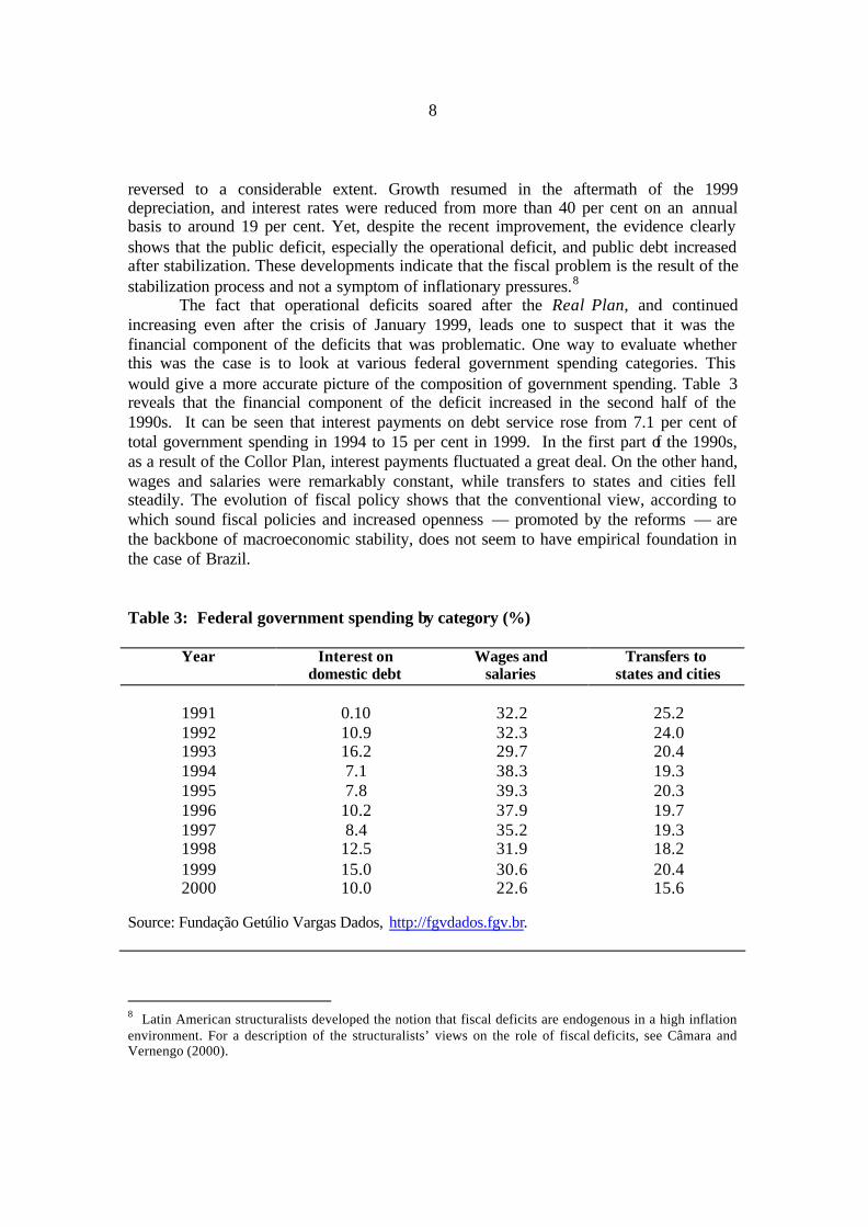
The fact that operational deficits soared after the Real Plan, and continued increasing even after the crisis of January 1999, leads one to suspect that it was the financial component of the deficits that was problematic. One way to evaluate whether this was the case is to look at various federal government spending categories. This would give a more accurate picture of the composition of government spending. Table 3 reveals that the financial component of the deficit increased in the second half of the 1990s. It can be seen that interest payments on debt service rose from 7.1 per cent of total government spending in 1994 to 15 per cent in 1999. In the first part of the 1990s, as a result of the Collor Plan, interest payments fluctuated a great deal. On the other hand, wages and salaries were remarkably constant, while transfers to states and cities fell steadily. The evolution of fiscal policy shows that the conventional view, according to which sound fiscal policies and increased openness — promoted by the reforms — are the backbone of macroeconomic stability, does not seem to have empirical foundation in the case of Brazil.

Table 3: Federal government spending by category (%)

Year Interest on domestic debt

Wages and salaries

Transfers to states and cities

1991

0.10

32.2

25.2

1992 10.9 32.3 24.0 1993 16.2 29.7 20.4 1994 7.1 38.3 19.3 1995 7.8 39.3 20.3 1996 10.2 37.9 19.7 1997 8.4 35.2 19.3 1998 12.5 31.9 18.2 1999 15.0 30.6 20.4 2000 10.0 22.6 15.6

Source: Fundação Getúlio Vargas Dados, http://fgvdados.fgv.br.

8 Latin American structuralists developed the notion that fiscal deficits are endogenous in a high inflation environment. For a description of the structuralists’ views on the role of fiscal deficits, see Câmara and Vernengo (2000).

9

It is correct to argue that reforms played a role in attracting capital inflows in the 1990s, and that such inflows were crucial for the exchange-rate-based stabilization programme. In that respect, it is correct to say that the reforms were instrumental in achieving price stability. However, the reforms and the capital inflows created several further imbalances: the high interest rate needed to attract capital inflows worsened the fiscal deficit and led to an appreciation of the exchange rate. This, in turn, created recurrent problems of balance-of-payments sustainability.

In addition, the liberalization of both the current and the capital accounts has imposed severe limits on the ability of the government to use monetary and fiscal policies for macroeconomic management. Stabilization together with liberalization had severe impacts on the ability to grow without generating unsustainable current-account deficits; it led to increasing unemployment and negative effects on income distribution as far as wage differentials were concerned (Amadeo, 1996). It should be emphasized that during the early 1990s, the external liberalization process was concomitant with a high degree of macroeconomic instability and that this had significant effects on the evolution of the economy.

3. Trade liberalization, trade performance and growth

The notion that trade liberalization is an optimal development strategy has become a dominant feature of mainstream economics. In addition, conventional wisdom has it that openness in the capital account leads to higher rates of growth. Above all, the contrasting experiences of the relatively closed Latin American economies and the relatively open East Asian economies has led many authors (e.g. World Bank, 1993; Edwards, 1995) to argue that outward-oriented development strategies are more conducive to growth. 9

However, the literature on the advantages of economic openness is far from consensual; measures of openness do not seem to be consistent across studies (Pritchett, 1996). Taylor (1991a, p. 100) argues that structuralist models of both commodity and capital flows suggest that openness or a hands -off policy in either market will not necessarily lead to faster growth or less costly adjustment to external shocks. Furthermore, Rodriguez and Rodrik (1999) find little evidence that open trade policies are significantly associated with higher growth. In their recent study on the effects of structural adjustment reforms in Latin America, Stallings and Peres (2000) found that capital and current account liberalization had a significant but small effect on growth.

9 In general, the terms outward orientation and openness are used without distinction. One must note, however, that openness refers to absence of restrictions to trade and capital flows, whereas outward orientation means emphasizing the role of foreign markets as an outlet for domestic production.

10

12

14

16

18

20

22

24

26

1975 1980 1985 1990 1995 2000

OPENNESS TREND

S o u r c e : I P E A D a t a a n d a u t h o r ' s c a l c u l a t i o n s

F I U R D e g r e FIGURE 3 Degree of Openness

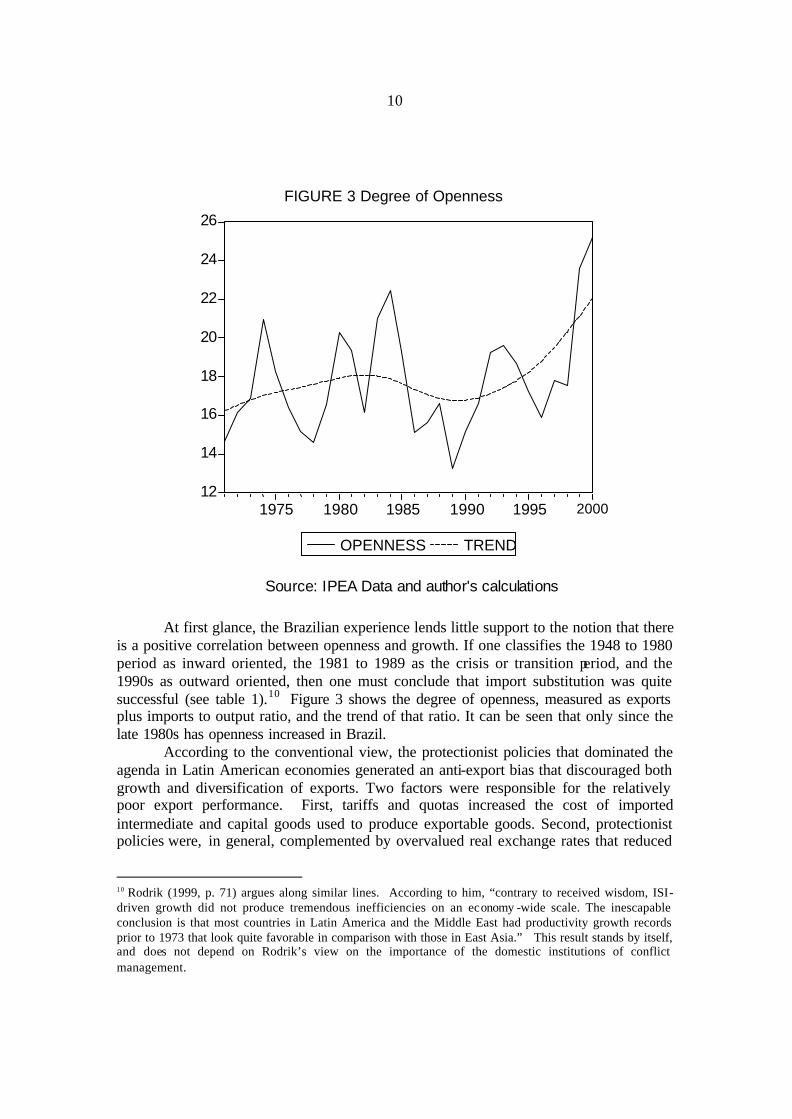
At first glance, the Brazilian experience lends little support to the notion that there is a positive correlation between openness and growth. If one classifies the 1948 to 1980 period as inward oriented, the 1981 to 1989 as the crisis or transition period, and the 1990s as outward oriented, then one must conclude that import substitution was quite successful (see table 1).10 Figure 3 shows the degree of openness, measured as exports plus imports to output ratio, and the trend of that ratio. It can be seen that only since the late 1980s has openness increased in Brazil.

According to the conventional view, the protectionist policies that dominated the agenda in Latin American economies generated an anti-export bias that discouraged both growth and diversification of exports. Two factors were responsible for the relatively poor export performance. First, tariffs and quotas increased the cost of imported intermediate and capital goods used to produce exportable goods. Second, protectionist policies were, in general, complemented by overvalued real exchange rates that reduced

10 Rodrik (1999, p. 71) argues along similar lines. According to him, “contrary to received wisdom, ISI-driven growth did not produce tremendous inefficiencies on an economy -wide scale. The inescapable conclusion is that most countries in Latin America and the Middle East had productivity growth records prior to 1973 that look quite favorable in comparison with those in East Asia.” This result stands by itself, and does not depend on Rodrik’s view on the importance of the domestic institutions of conflict management.

11

the competitiveness of exports. However, in the case of Brazil, at least, it is difficult to agree with Edwards’ (1995, p. 41) view according to which “the ever-growing presence of the state in the 1950-80 period eventually stifled efficiency and growth.”11 In addition, in Brazil, since the late 1960s, the aim has been to maintain a relatively competitive exchange rate regime in order to promote exports.12 On the other hand, the reduction of tariff and non-tariff barriers was only intensified in the late 1980s. That is, trade liberalization was initiated during the period of high inflation.

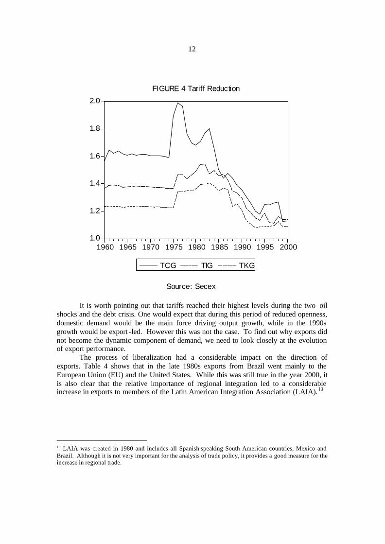
Figure 4 shows the reduction of average tariffs for consumption (TCG), capital (TKG) and intermediate goods (TIG), and a reduced dispersion of the tariff structure. It is interesting to note that by the late 1980s tariffs were already lower than in the 1960s, and considerably lower than they were during the periods of the oil shocks and the debt crisis. This seems to indicate that the main constraint on imports after the debt crisis was the shortage of foreign exchange rather than protectionism per se (Resende, 2000).

11 The debt crisis might be seen as the inevitable result of the import -substitution policies. However, two important considerations are relevant. First, import-substitution policies were also pursued in Asia and did not lead to a debt crisis. Also, contagion effects were crucial in the unfolding of the Latin American debt crisis. Hence, international capital markets put countries like Brazil that had been quite successful in the same category as those that were less successful. 12 From 1967 onwards, Brazil promoted a reduction in tariffs and a crawling peg system that maintained a relatively depreciated exchange rate. This liberalizing experience was partially successful in increasing the level of manufactured exports.

12

1.0

1.2

1.4

1.6

1.8

2.0

1960 1965 1970 1975 1980 1985 1990 1995 2000

TCG TIG TKG

FIGURE 4 Tariff Reduction

Source: Secex

It is worth pointing out that tariffs reached their highest levels during the two oil shocks and the debt crisis. One would expect that during this period of reduced openness, domestic demand would be the main force driving output growth, while in the 1990s growth would be export -led. However this was not the case. To find out why exports did not become the dynamic component of demand, we need to look closely at the evolution of export performance.

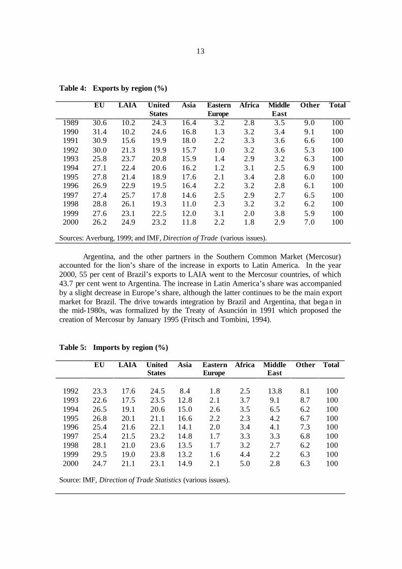
The process of liberalization had a considerable impact on the direction of exports. Table 4 shows that in the late 1980s exports from Brazil went mainly to the European Union (EU) and the United States. While this was still true in the year 2000, it is also clear that the relative importance of regional integration led to a considerable increase in exports to members of the Latin American Integration Association (LAIA).13

13 LAIA was created in 1980 and includes all Spanish-speaking South American countries, Mexico and Brazil. Although it is not very important for the analysis of trade policy, it provides a good measure for the increase in regional trade.

13

Table 4: Exports by region (%)

EU LAIA United States

Asia Eastern Europe

Africa Middle East

Other Total

1989 30.6 10.2 24.3 16.4 3.2 2.8 3.5 9.0 100 1990 31.4 10.2 24.6 16.8 1.3 3.2 3.4 9.1 100 1991 30.9 15.6 19.9 18.0 2.2 3.3 3.6 6.6 100 1992 30.0 21.3 19.9 15.7 1.0 3.2 3.6 5.3 100 1993 25.8 23.7 20.8 15.9 1.4 2.9 3.2 6.3 100 1994 27.1 22.4 20.6 16.2 1.2 3.1 2.5 6.9 100 1995 27.8 21.4 18.9 17.6 2.1 3.4 2.8 6.0 100 1996 26.9 22.9 19.5 16.4 2.2 3.2 2.8 6.1 100 1997 27.4 25.7 17.8 14.6 2.5 2.9 2.7 6.5 100 1998 28.8 26.1 19.3 11.0 2.3 3.2 3.2 6.2 100 1999 27.6 23.1 22.5 12.0 3.1 2.0 3.8 5.9 100 2000 26.2 24.9 23.2 11.8 2.2 1.8 2.9 7.0 100

Sources: Averburg, 1999; and IMF, Direction of Trade (various issues).

Argentina, and the other partners in the Southern Common Market (Mercosur)

accounted for the lion’s share of the increase in exports to Latin America. In the year 2000, 55 per cent of Brazil’s exports to LAIA went to the Mercosur countries, of which 43.7 per cent went to Argentina. The increase in Latin America’s share was accompanied by a slight decrease in Europe’s share, although the latter continues to be the main export market for Brazil. The drive towards integration by Brazil and Argentina, that began in the mid-1980s, was formalized by the Treaty of Asunción in 1991 which proposed the creation of Mercosur by January 1995 (Fritsch and Tombini, 1994).

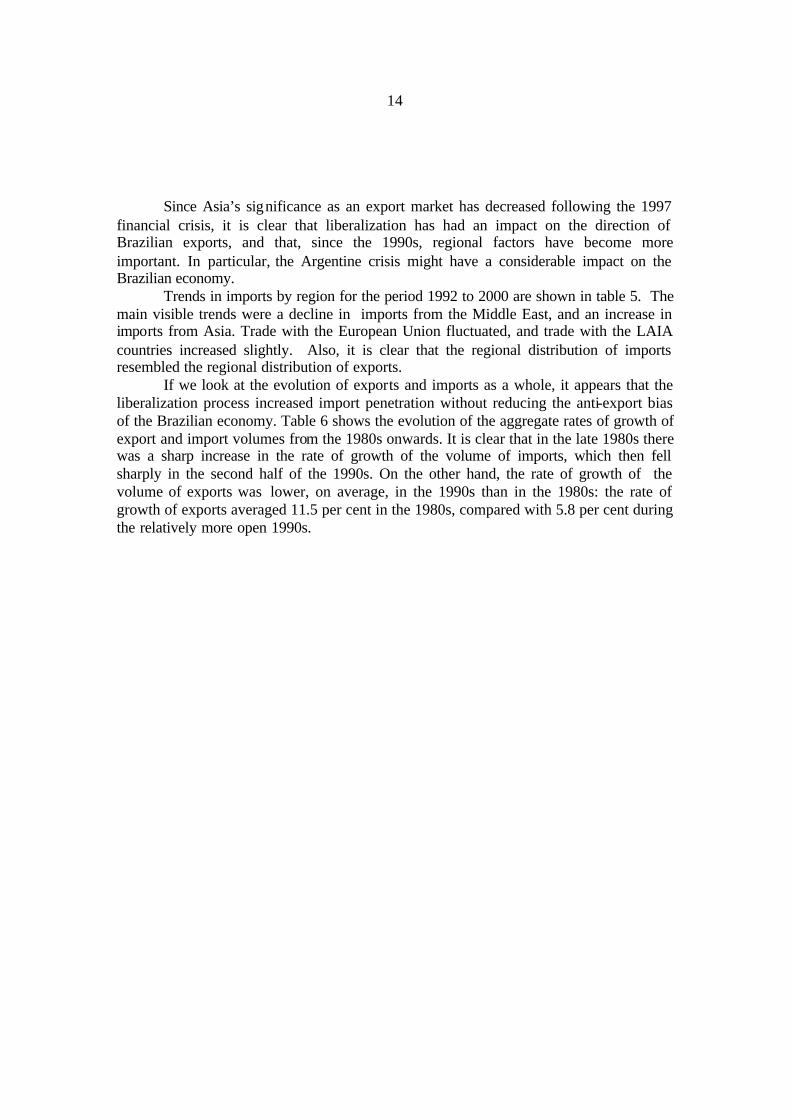
Table 5: Imports by region (%)

EU LAIA United States

Asia Eastern Europe

Africa Middle East

Other Total

1992

23.3

17.6

24.5

8.4

1.8

2.5

13.8

8.1

100

1993 22.6 17.5 23.5 12.8 2.1 3.7 9.1 8.7 100 1994 26.5 19.1 20.6 15.0 2.6 3.5 6.5 6.2 100 1995 26.8 20.1 21.1 16.6 2.2 2.3 4.2 6.7 100 1996 25.4 21.6 22.1 14.1 2.0 3.4 4.1 7.3 100 1997 25.4 21.5 23.2 14.8 1.7 3.3 3.3 6.8 100 1998 28.1 21.0 23.6 13.5 1.7 3.2 2.7 6.2 100 1999 29.5 19.0 23.8 13.2 1.6 4.4 2.2 6.3 100 2000 24.7 21.1 23.1 14.9 2.1 5.0 2.8 6.3 100

Source: IMF, Direction of Trade Statistics (various issues).

14

Since Asia’s significance as an export market has decreased following the 1997 financial crisis, it is clear that liberalization has had an impact on the direction of Brazilian exports, and that, since the 1990s, regional factors have become more important. In particular, the Argentine crisis might have a considerable impact on the Brazilian economy.

Trends in imports by region for the period 1992 to 2000 are shown in table 5. The main visible trends were a decline in imports from the Middle East, and an increase in imports from Asia. Trade with the European Union fluctuated, and trade with the LAIA countries increased slightly. Also, it is clear that the regional distribution of imports resembled the regional distribution of exports.

If we look at the evolution of exports and imports as a whole, it appears that the liberalization process increased import penetration without reducing the anti-export bias of the Brazilian economy. Table 6 shows the evolution of the aggregate rates of growth of export and import volumes from the 1980s onwards. It is clear that in the late 1980s there was a sharp increase in the rate of growth of the volume of imports, which then fell sharply in the second half of the 1990s. On the other hand, the rate of growth of the volume of exports was lower, on average, in the 1990s than in the 1980s: the rate of growth of exports averaged 11.5 per cent in the 1980s, compared with 5.8 per cent during the relatively more open 1990s.

15

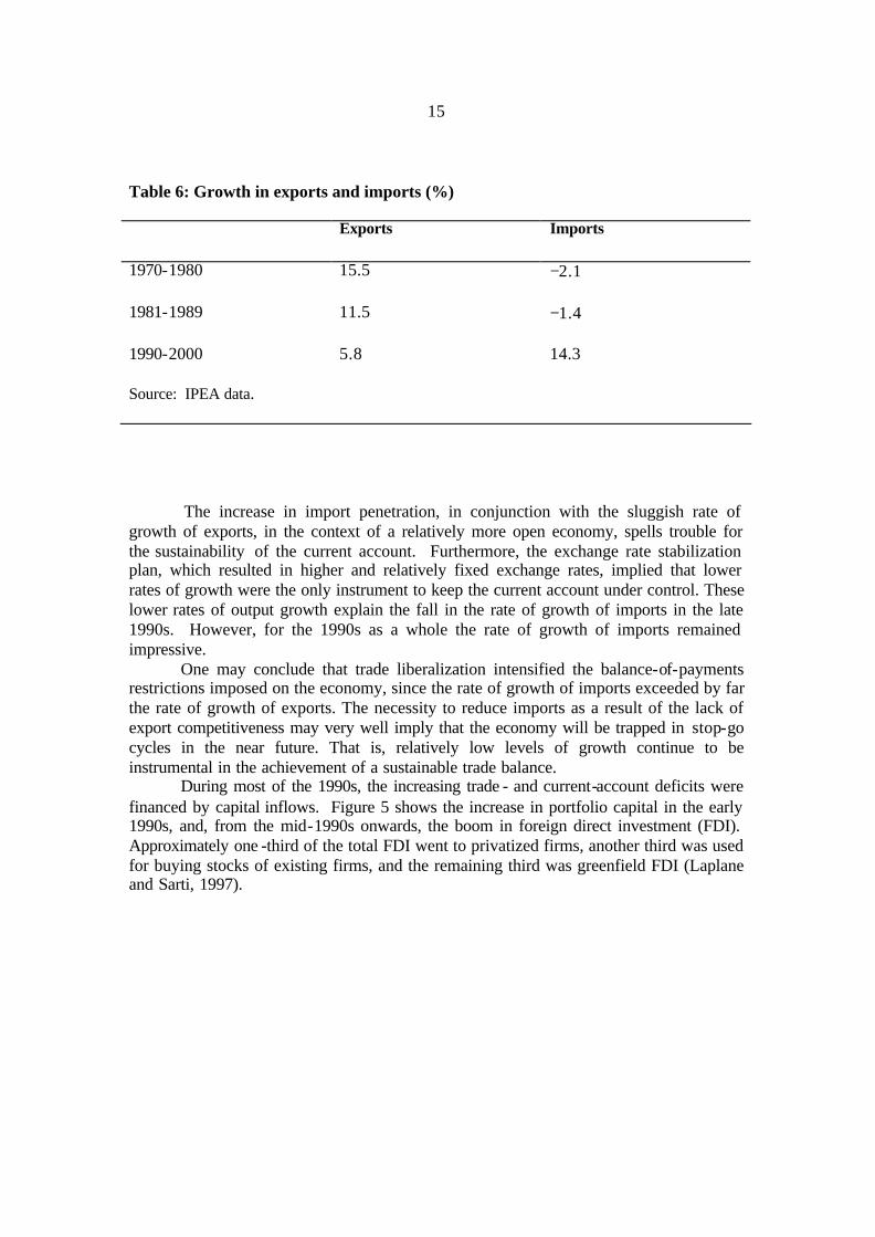
Table 6: Growth in exports and imports (%)

Exports Imports

1970-1980 15.5 −2.1

1981-1989 11.5 −1.4

1990-2000 5.8 14.3

Source: IPEA data.

The increase in import penetration, in conjunction with the sluggish rate of

growth of exports, in the context of a relatively more open economy, spells trouble for the sustainability of the current account. Furthermore, the exchange rate stabilization plan, which resulted in higher and relatively fixed exchange rates, implied that lower rates of growth were the only instrument to keep the current account under control. These lower rates of output growth explain the fall in the rate of growth of imports in the late 1990s. However, for the 1990s as a whole the rate of growth of imports remained impressive.

One may conclude that trade liberalization intensified the balance-of-payments restrictions imposed on the economy, since the rate of growth of imports exceeded by far the rate of growth of exports. The necessity to reduce imports as a result of the lack of export competitiveness may very well imply that the economy will be trapped in stop-go cycles in the near future. That is, relatively low levels of growth continue to be instrumental in the achievement of a sustainable trade balance.

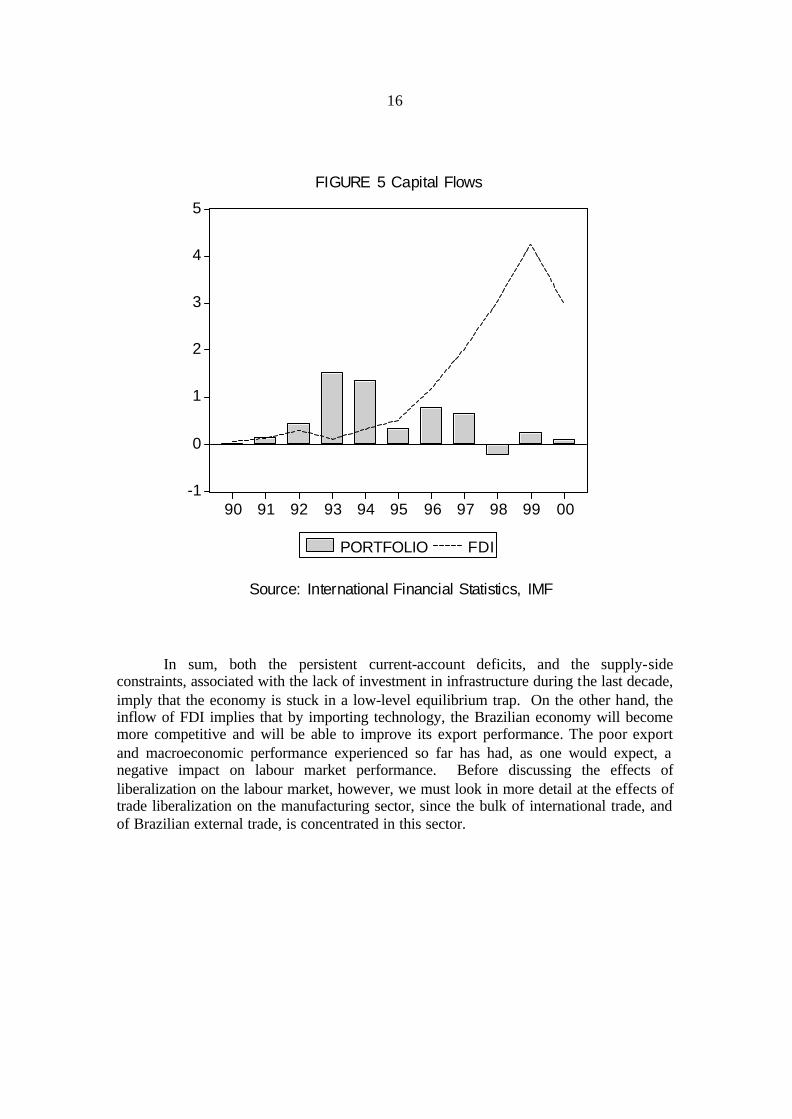
During most of the 1990s, the increasing trade - and current-account deficits were financed by capital inflows. Figure 5 shows the increase in portfolio capital in the early 1990s, and, from the mid-1990s onwards, the boom in foreign direct investment (FDI). Approximately one -third of the total FDI went to privatized firms, another third was used for buying stocks of existing firms, and the remaining third was greenfield FDI (Laplane and Sarti, 1997).

16

-1

0

1

2

3

4

5

90 91 92 93 94 95 96 97 98 99 00

PORTFOLIO FDI

FIGURE 5 Capital Flows

Source: International Financial Statistics, IMF

In sum, both the persistent current-account deficits, and the supply-side

constraints, associated with the lack of investment in infrastructure during the last decade, imply that the economy is stuck in a low-level equilibrium trap. On the other hand, the inflow of FDI implies that by importing technology, the Brazilian economy will become more competitive and will be able to improve its export performance. The poor export and macroeconomic performance experienced so far has had, as one would expect, a negative impact on labour market performance. Before discussing the effects of liberalization on the labour market, however, we must look in more detail at the effects of trade liberalization on the manufacturing sector, since the bulk of international trade, and of Brazilian external trade, is concentrated in this sector.

17

4. Trade liberalization and the manufacturing sector

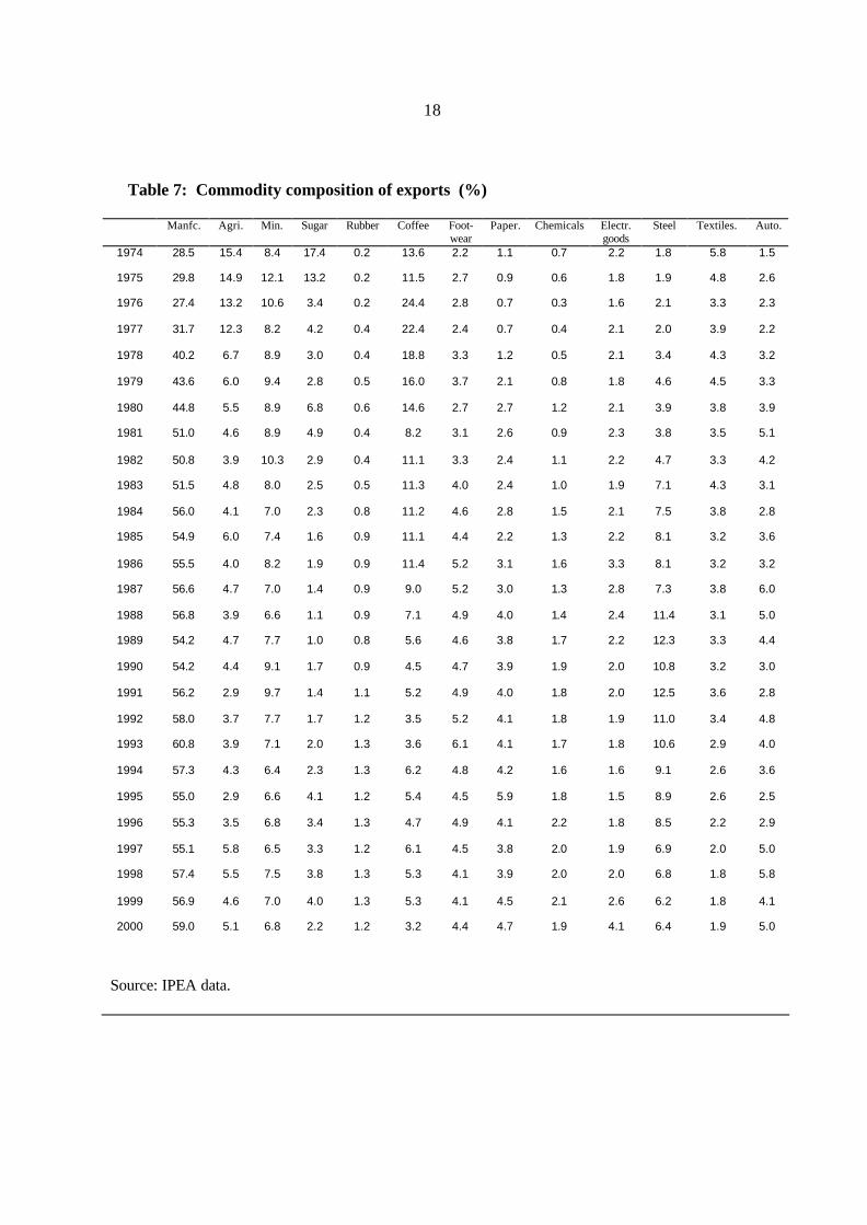
In the previous section, we saw that liberalization and regional integration did have an impact on Brazil’s trade performance with regard to the direction of trade. But their impacts with respect to the commodity composition of trade are less clear. Table 7 shows exports by category from 1974 to 2000. The share of manufactured exports in total exports rose from 28.5 per cent in 1974 to about 60 per cent in 2000. The share of agricultural exports fell from 15.4 per cent to about 5 per cent in 2000, while exports of the mining sector were relatively constant. The remaining exports, composed of semi-manufactured goods and services, are not shown in the table.

Sugar, coffee, and textile exports fell considerably, in part as a result of the industrialization process, and, in the case of the textile sector, as a result of competition from Asian countries. On the other hand, exports of the footwear, electronic, steel and automotive sectors increased. The case of steel is particularly interesting, since, after increasing to 12.5 per cent of total exports in 1991, steel exports fell to almost half that level towards the end of the decade. This seems to have been mainly due to restrictions imposed on Brazilian steel imports by the United States.

However, these changes in the commodity composition of exports cannot be considered a direct outcome of liberalization. In fact, quite the opposite is true. Looking at the trends more closely, it can be observed that most changes occurred from the mid-1970s to the early and mid-1980s, that is before liberalization was introduced. Hence the process of liberalization is not directly related to these changes.

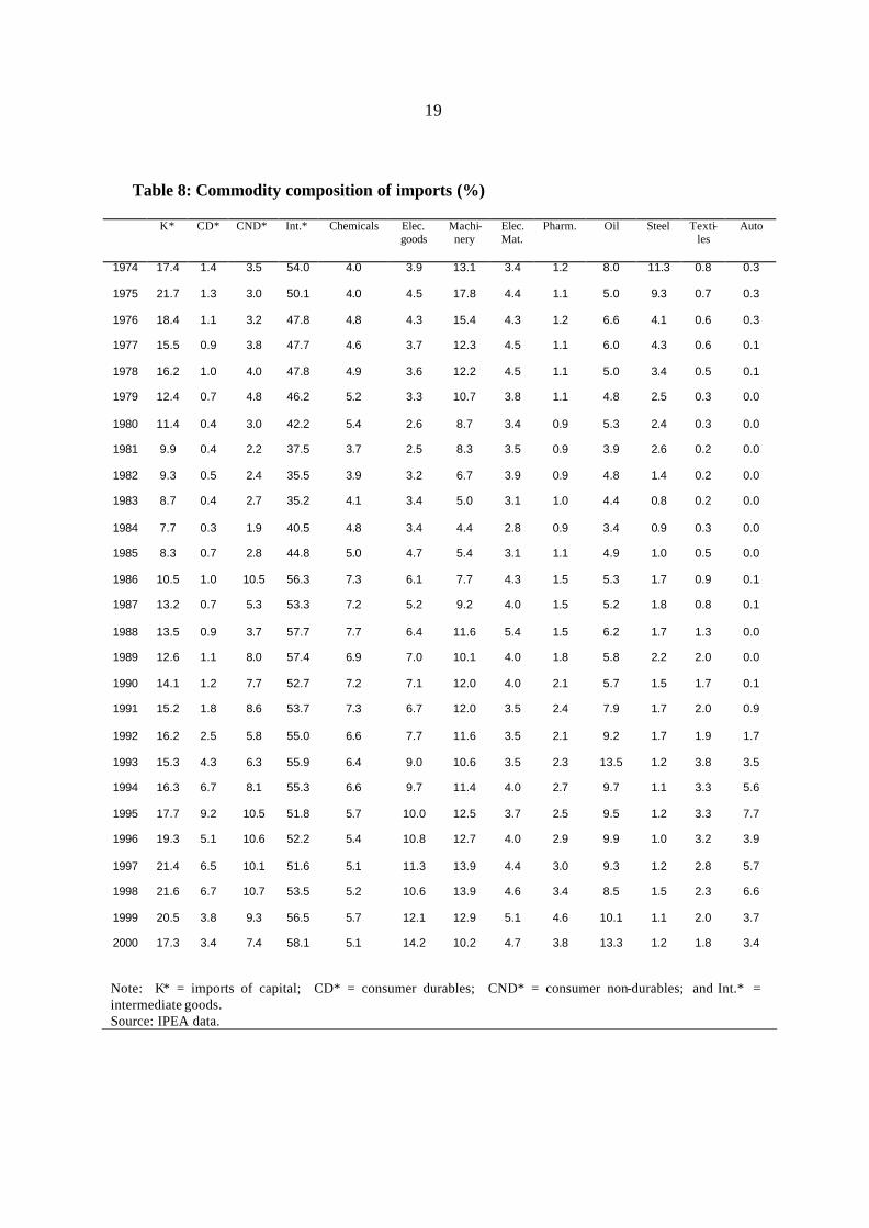
Table 8 shows the evolution of imports by commodity categories. The first four columns show imports of capital goods, consumer durables, consumer non-durables, and intermediate goods. It is clear that imports of both capital and intermediate goods declined during the debt crisis period, and returned to normal levels in the 1990s. On the other hand, imports of consumer goods clearly increased after liberalization. In particular, imports of goods from the electronic, pharmaceutical, textile and automotive sectors seem to have increased. Imports from the steel sector, on the other hand, fell drastically.

In contrast to the commodity composition of exports, that of imports seems to have changed as a result of the liberalization process. The changes described above occurred from the mid-1980s to the present, and thus fall within the period of trade liberalization. Hence, one may conclude that the process of liberalization affected imports more than it did exports. This is particularly striking since one of the main justifications for the liberalization process was to change the anti-export bias of the import-substituting development strategy.

18

Table 7: Commodity composition of exports (%)

Manfc. Agri. Min. Sugar Rubber Coffee Foot-wear

Paper. Chemicals Electr. goods

Steel Textiles. Auto.

1974 28.5 15.4 8.4 17.4 0.2 13.6 2.2 1.1 0.7 2.2 1.8 5.8 1.5

1975 29.8 14.9 12.1 13.2 0.2 11.5 2.7 0.9 0.6 1.8 1.9 4.8 2.6

1976 27.4 13.2 10.6 3.4 0.2 24.4 2.8 0.7 0.3 1.6 2.1 3.3 2.3

1977 31.7 12.3 8.2 4.2 0.4 22.4 2.4 0.7 0.4 2.1 2.0 3.9 2.2

1978 40.2 6.7 8.9 3.0 0.4 18.8 3.3 1.2 0.5 2.1 3.4 4.3 3.2

1979 43.6 6.0 9.4 2.8 0.5 16.0 3.7 2.1 0.8 1.8 4.6 4.5 3.3

1980 44.8 5.5 8.9 6.8 0.6 14.6 2.7 2.7 1.2 2.1 3.9 3.8 3.9

1981 51.0 4.6 8.9 4.9 0.4 8.2 3.1 2.6 0.9 2.3 3.8 3.5 5.1

1982 50.8 3.9 10.3 2.9 0.4 11.1 3.3 2.4 1.1 2.2 4.7 3.3 4.2

1983 51.5 4.8 8.0 2.5 0.5 11.3 4.0 2.4 1.0 1.9 7.1 4.3 3.1

1984 56.0 4.1 7.0 2.3 0.8 11.2 4.6 2.8 1.5 2.1 7.5 3.8 2.8

1985 54.9 6.0 7.4 1.6 0.9 11.1 4.4 2.2 1.3 2.2 8.1 3.2 3.6

1986 55.5 4.0 8.2 1.9 0.9 11.4 5.2 3.1 1.6 3.3 8.1 3.2 3.2

1987 56.6 4.7 7.0 1.4 0.9 9.0 5.2 3.0 1.3 2.8 7.3 3.8 6.0

1988 56.8 3.9 6.6 1.1 0.9 7.1 4.9 4.0 1.4 2.4 11.4 3.1 5.0

1989 54.2 4.7 7.7 1.0 0.8 5.6 4.6 3.8 1.7 2.2 12.3 3.3 4.4

1990 54.2 4.4 9.1 1.7 0.9 4.5 4.7 3.9 1.9 2.0 10.8 3.2 3.0

1991 56.2 2.9 9.7 1.4 1.1 5.2 4.9 4.0 1.8 2.0 12.5 3.6 2.8

1992 58.0 3.7 7.7 1.7 1.2 3.5 5.2 4.1 1.8 1.9 11.0 3.4 4.8

1993 60.8 3.9 7.1 2.0 1.3 3.6 6.1 4.1 1.7 1.8 10.6 2.9 4.0

1994 57.3 4.3 6.4 2.3 1.3 6.2 4.8 4.2 1.6 1.6 9.1 2.6 3.6

1995 55.0 2.9 6.6 4.1 1.2 5.4 4.5 5.9 1.8 1.5 8.9 2.6 2.5

1996 55.3 3.5 6.8 3.4 1.3 4.7 4.9 4.1 2.2 1.8 8.5 2.2 2.9

1997 55.1 5.8 6.5 3.3 1.2 6.1 4.5 3.8 2.0 1.9 6.9 2.0 5.0

1998 57.4 5.5 7.5 3.8 1.3 5.3 4.1 3.9 2.0 2.0 6.8 1.8 5.8

1999 56.9 4.6 7.0 4.0 1.3 5.3 4.1 4.5 2.1 2.6 6.2 1.8 4.1

2000 59.0 5.1 6.8 2.2 1.2 3.2 4.4 4.7 1.9 4.1 6.4 1.9 5.0

Source: IPEA data.

19

Table 8: Commodity composition of imports (%)

K* CD* CND* Int.* Chemicals Elec. goods

Machi- nery

Elec. Mat.

Pharm. Oil Steel Texti- les

Auto

1974 17.4 1.4 3.5 54.0 4.0 3.9 13.1 3.4 1.2 8.0 11.3 0.8 0.3

1975 21.7 1.3 3.0 50.1 4.0 4.5 17.8 4.4 1.1 5.0 9.3 0.7 0.3

1976 18.4 1.1 3.2 47.8 4.8 4.3 15.4 4.3 1.2 6.6 4.1 0.6 0.3

1977 15.5 0.9 3.8 47.7 4.6 3.7 12.3 4.5 1.1 6.0 4.3 0.6 0.1

1978 16.2 1.0 4.0 47.8 4.9 3.6 12.2 4.5 1.1 5.0 3.4 0.5 0.1

1979 12.4 0.7 4.8 46.2 5.2 3.3 10.7 3.8 1.1 4.8 2.5 0.3 0.0

1980 11.4 0.4 3.0 42.2 5.4 2.6 8.7 3.4 0.9 5.3 2.4 0.3 0.0

1981 9.9 0.4 2.2 37.5 3.7 2.5 8.3 3.5 0.9 3.9 2.6 0.2 0.0

1982 9.3 0.5 2.4 35.5 3.9 3.2 6.7 3.9 0.9 4.8 1.4 0.2 0.0

1983 8.7 0.4 2.7 35.2 4.1 3.4 5.0 3.1 1.0 4.4 0.8 0.2 0.0

1984 7.7 0.3 1.9 40.5 4.8 3.4 4.4 2.8 0.9 3.4 0.9 0.3 0.0

1985 8.3 0.7 2.8 44.8 5.0 4.7 5.4 3.1 1.1 4.9 1.0 0.5 0.0

1986 10.5 1.0 10.5 56.3 7.3 6.1 7.7 4.3 1.5 5.3 1.7 0.9 0.1

1987 13.2 0.7 5.3 53.3 7.2 5.2 9.2 4.0 1.5 5.2 1.8 0.8 0.1

1988 13.5 0.9 3.7 57.7 7.7 6.4 11.6 5.4 1.5 6.2 1.7 1.3 0.0

1989 12.6 1.1 8.0 57.4 6.9 7.0 10.1 4.0 1.8 5.8 2.2 2.0 0.0

1990 14.1 1.2 7.7 52.7 7.2 7.1 12.0 4.0 2.1 5.7 1.5 1.7 0.1

1991 15.2 1.8 8.6 53.7 7.3 6.7 12.0 3.5 2.4 7.9 1.7 2.0 0.9

1992 16.2 2.5 5.8 55.0 6.6 7.7 11.6 3.5 2.1 9.2 1.7 1.9 1.7

1993 15.3 4.3 6.3 55.9 6.4 9.0 10.6 3.5 2.3 13.5 1.2 3.8 3.5

1994 16.3 6.7 8.1 55.3 6.6 9.7 11.4 4.0 2.7 9.7 1.1 3.3 5.6

1995 17.7 9.2 10.5 51.8 5.7 10.0 12.5 3.7 2.5 9.5 1.2 3.3 7.7

1996 19.3 5.1 10.6 52.2 5.4 10.8 12.7 4.0 2.9 9.9 1.0 3.2 3.9

1997 21.4 6.5 10.1 51.6 5.1 11.3 13.9 4.4 3.0 9.3 1.2 2.8 5.7

1998 21.6 6.7 10.7 53.5 5.2 10.6 13.9 4.6 3.4 8.5 1.5 2.3 6.6

1999 20.5 3.8 9.3 56.5 5.7 12.1 12.9 5.1 4.6 10.1 1.1 2.0 3.7

2000 17.3 3.4 7.4 58.1 5.1 14.2 10.2 4.7 3.8 13.3 1.2 1.8 3.4

Note: K* = imports of capital; CD* = consumer durables; CND* = consumer non-durables; and Int.* = intermediate goods. Source: IPEA data.

20

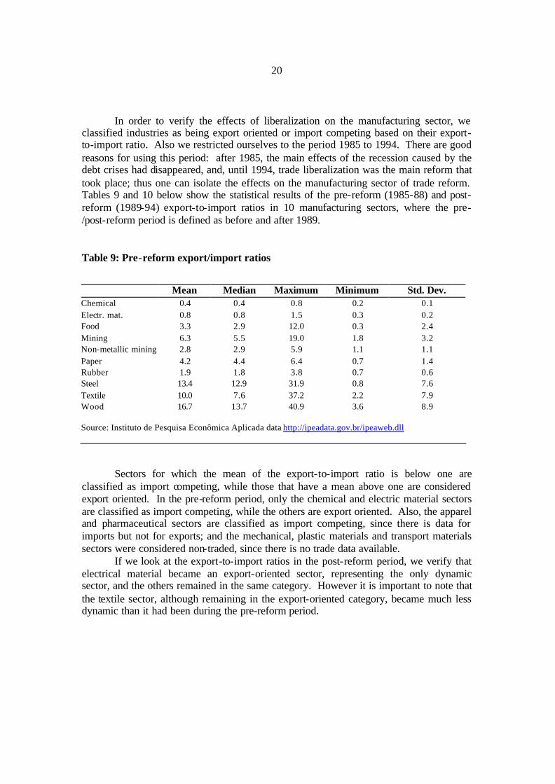
In order to verify the effects of liberalization on the manufacturing sector, we classified industries as being export oriented or import competing based on their export-to-import ratio. Also we restricted ourselves to the period 1985 to 1994. There are good reasons for using this period: after 1985, the main effects of the recession caused by the debt crises had disappeared, and, until 1994, trade liberalization was the main reform that took place; thus one can isolate the effects on the manufacturing sector of trade reform. Tables 9 and 10 below show the statistical results of the pre-reform (1985-88) and post-reform (1989-94) export-to-import ratios in 10 manufacturing sectors, where the pre-/post-reform period is defined as before and after 1989.

Table 9: Pre-reform export/import ratios

Sectors for which the mean of the export-to-import ratio is below one are classified as import competing, while those that have a mean above one are considered export oriented. In the pre-reform period, only the chemical and electric material sectors are classified as import competing, while the others are export oriented. Also, the apparel and pharmaceutical sectors are classified as import competing, since there is data for imports but not for exports; and the mechanical, plastic materials and transport materials sectors were considered non-traded, since there is no trade data available.

If we look at the export-to-import ratios in the post-reform period, we verify that electrical material became an export-oriented sector, representing the only dynamic sector, and the others remained in the same category. However it is important to note that the textile sector, although remaining in the export-oriented category, became much less dynamic than it had been during the pre-reform period.

Mean Median Maximum Minimum Std. Dev. Chemical 0.4 0.4 0.8 0.2 0.1 Electr. mat. 0.8 0.8 1.5 0.3 0.2 Food 3.3 2.9 12.0 0.3 2.4 Mining 6.3 5.5 19.0 1.8 3.2 Non-metallic mining 2.8 2.9 5.9 1.1 1.1 Paper 4.2 4.4 6.4 0.7 1.4 Rubber 1.9 1.8 3.8 0.7 0.6 Steel 13.4 12.9 31.9 0.8 7.6 Textile 10.0 7.6 37.2 2.2 7.9 Wood 16.7 13.7 40.9 3.6 8.9 Source: Instituto de Pesquisa Econômica Aplicada data http://ipeadata.gov.br/ipeaweb.dll

21

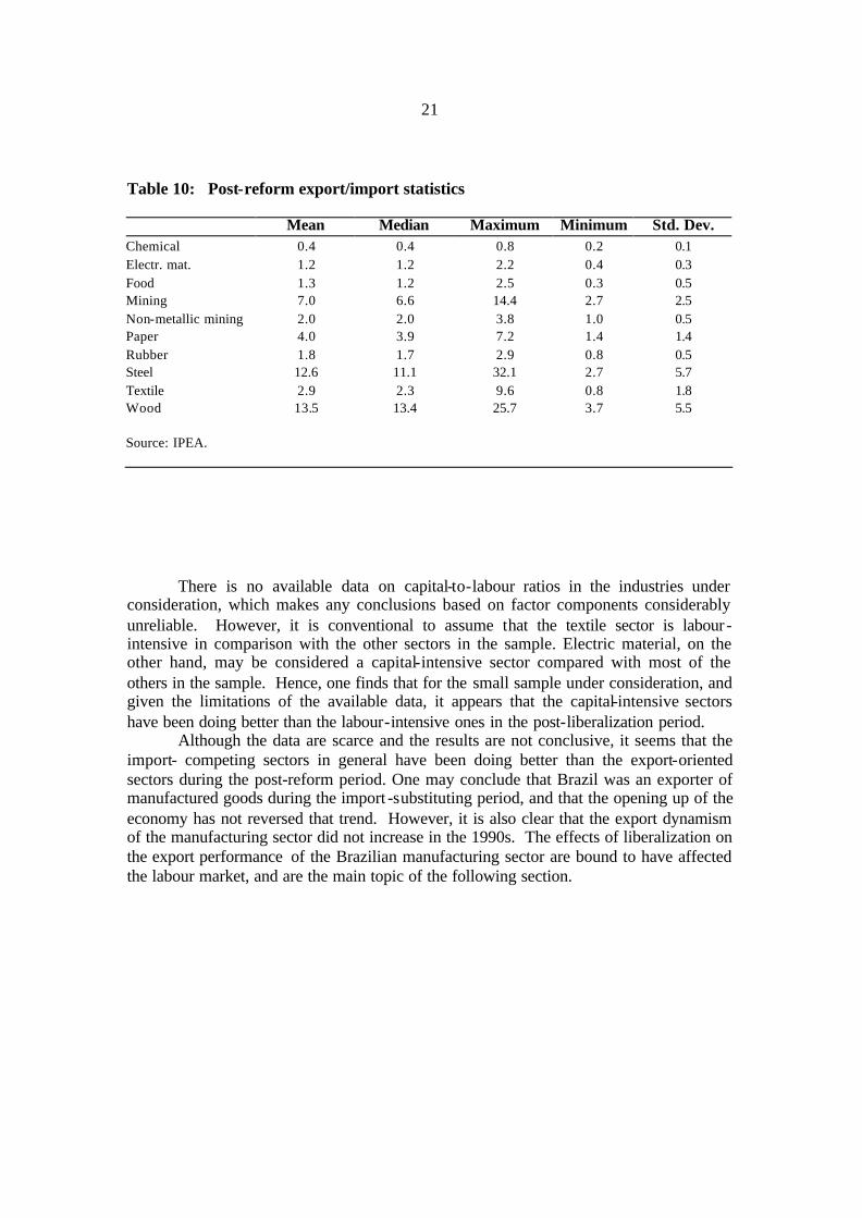
Table 10: Post-reform export/import statistics

Mean Median Maximum Minimum Std. Dev. Chemical 0.4 0.4 0.8 0.2 0.1 Electr. mat. 1.2 1.2 2.2 0.4 0.3 Food 1.3 1.2 2.5 0.3 0.5 Mining 7.0 6.6 14.4 2.7 2.5 Non-metallic mining 2.0 2.0 3.8 1.0 0.5 Paper 4.0 3.9 7.2 1.4 1.4 Rubber 1.8 1.7 2.9 0.8 0.5 Steel 12.6 11.1 32.1 2.7 5.7 Textile 2.9 2.3 9.6 0.8 1.8 Wood 13.5 13.4 25.7 3.7 5.5 Source: IPEA.

There is no available data on capital-to-labour ratios in the industries under

consideration, which makes any conclusions based on factor components considerably unreliable. However, it is conventional to assume that the textile sector is labour -intensive in comparison with the other sectors in the sample. Electric material, on the other hand, may be considered a capital-intensive sector compared with most of the others in the sample. Hence, one finds that for the small sample under consideration, and given the limitations of the available data, it appears that the capital-intensive sectors have been doing better than the labour-intensive ones in the post-liberalization period.

Although the data are scarce and the results are not conclusive, it seems that the import- competing sectors in general have been doing better than the export-oriented sectors during the post-reform period. One may conclude that Brazil was an exporter of manufactured goods during the import -substituting period, and that the opening up of the economy has not reversed that trend. However, it is also clear that the export dynamism of the manufacturing sector did not increase in the 1990s. The effects of liberalization on the export performance of the Brazilian manufacturing sector are bound to have affected the labour market, and are the main topic of the following section.

22

5. Effects of liberalization on employment and wages

The effects of liberalization on the relative wage structure can be understood with the help of a simple structuralist model with a fixed-price/flex-price market distinction (Taylor, 2001). The fixed-price sector corresponds to the tradable sector, where mark-ups are assumed to be relatively constant, and output and employment are determined by effective demand. In the non-tradable sector, the flex-market, the labour market works as a buffer, absorbing excess supply or demand for labour in the tradable sector, and productivity in the non-tradable sector is considerably lower than in the tradable sector.

Liberalization switches demand towards imports, leading to trade deficits and reducing output in the tradable sector. In addition, real appreciation further weakens the tradable sector. Workers are then absorbed in the non-tradable sector, so that the overall rate of unemployment, at least initially, does not increase much. Assuming for simplicity’s sake, that the tradable sector corresponds to the industrial sector, and that services are the non-tradable sector, one may conclude that liberalization leads to a process of deindustrialization. Using data on the metropolitan area of São Paulo, the industrial core of Brazil, we found that in 1990, 48.7 per cent of all the workers in the private sector were employed in the industrial sector, compared to only 32 per cent in 1999. The reverse was true for services, which showed an increase from 32.9 per cent to 48.8 per cent of total employed workers during the same period. This tends to confirm Pieper’s argument (2000) that Brazil is an acute example of deindustrialization.

In addition, the increasing exposure to foreign competition implies a change in relative prices against the tradable sector. According to conventional wisdom, the rise in the price of non-tradable goods vis-à-vis tradable goods might lead to a fall in real wages in the non-tradable sector, and hence to an increase in the demand for labour in that sector. In other words, the fall in real wages allows labour demand to increase and reduces unemployment. According to the structuralist view, the level of employment in the non-tradable sector also depends on effective demand. If effective demand increases in the non-tradable sector, the capacity to increase employment is enhanced. To the extent that wages are able to keep pace with prices, wages in the non-tradable sector may or may not rise relative to wages in the tradable sector.

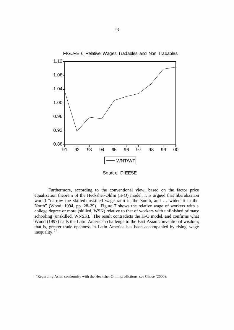
Once again, if we use data for the metropolitan area of São Paulo, we can see in figure 6 that the average income of the non-tradable sector (WNT) rose against the average income of the industrial sector (WT). The data contradicts the conventional view, since there seems to be a positive correlation between employment and wages. That is, the relative increase in the level of employment in the services sector is accompanied by a relative increase in wages.

23

0.88

0.92

0.96

1.00

1.04

1.08

1.12

91 92 93 94 95 96 97 98 99 00

WNT/WT

F I G U R E 6 R e l a t i v e W a g e s : T r a d a b l e s a n d N o n T r a d a b l e s

S o u r c e : D I E E S E

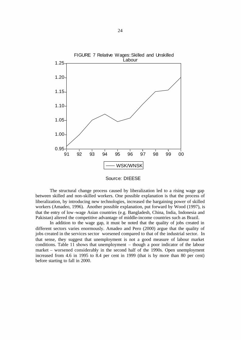
Furthermore, according to the conventional view, based on the factor price

equalization theorem of the Hecksher-Ohlin (H-O) model, it is argued that liberalization would “narrow the skilled-unskilled wage ratio in the South, and … widen it in the North” (Wood, 1994, pp. 28-29). Figure 7 shows the relative wage of workers with a college degree or more (skilled, WSK) relative to that of workers with unfinished primary schooling (unskilled, WNSK). The result contradicts the H-O model, and confirms what Wood (1997) calls the Latin American challenge to the East Asian conventional wisdom; that is, greater trade openness in Latin America has been accompanied by rising wage inequality. 14

14 Regarding Asian conformity with the Hecksher-Ohlin predictions, see Ghose (2000).

24

0.95

1.00

1.05

1.10

1.15

1.20

1.25

91 92 93 94 95 96 97 98 99 00

WSK/WNSK

F I G U R E 7 R e l a t i v e W a g e s : S k i l l e d a n d U n s k i l l ed Labour

S o u r c e : D I E E S E

The structural change process caused by liberalization led to a rising wage gap between skilled and non-skilled workers. One possible explanation is that the process of liberalization, by introducing new technologies, increased the bargaining power of skilled workers (Amadeo, 1996). Another possible explanation, put forward by Wood (1997), is that the entry of low -wage Asian countries (e.g. Bangladesh, China, India, Indonesia and Pakistan) altered the competitive advantage of middle-income countries such as Brazil.

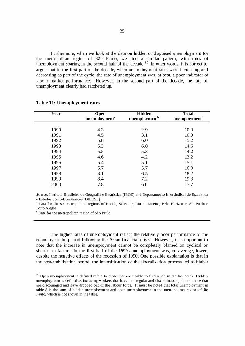
In addition to the wage gap, it must be noted that the quality of jobs created in different sectors varies enormously. Amadeo and Pero (2000) argue that the quality of jobs created in the services sector worsened compared to that of the industrial sector. In that sense, they suggest that unemployment is not a good measure of labour market conditions. Table 11 shows that unemployment – though a poor indicator of the labour market – worsened considerably in the second half of the 1990s. Open unemployment increased from 4.6 in 1995 to 8.4 per cent in 1999 (that is by more than 80 per cent) before starting to fall in 2000.

25

Furthermore, when we look at the data on hidden or disguised unemployment for the metropolitan region of São Paulo, we find a similar pattern, with rates of unemployment soaring in the second half of the decade.15 In other words, it is correct to argue that in the first part of the decade, when unemployment rates were increasing and decreasing as part of the cycle, the rate of unemployment was, at best, a poor indicator of labour market performance. However, in the second part of the decade, the rate of unemployment clearly had ratcheted up.

Table 11: Unemployment rates

Year Open unemploymenta

Hidden unemploymentb

Total unemploymentb

1990

4.3

2.9

10.3

1991 4.5 3.1 10.9 1992 5.8 6.0 15.2 1993 5.3 6.0 14.6 1994 5.5 5.3 14.2 1995 4.6 4.2 13.2 1996 5.4 5.1 15.1 1997 5.7 5.7 16.0 1998 8.1 6.5 18.2 1999 8.4 7.2 19.3 2000 7.8 6.6 17.7

Source: Instituto Brasileiro de Geografia e Estatistica (IBGE) and Departamento Intersindical de Estatística e Estudos Sócio-Econômicos (DIEESE) a Data for the six metropolitan regions of Recife, Salvador, Rio de Janeiro, Belo Horizonte, São Paulo e Porto Alegre b Data for the metropolitan region of São Paulo

The higher rates of unemployment reflect the relatively poor performance of the economy in the period following the Asian financial crisis. However, it is important to note that the increase in unemployment cannot be completely blamed on cyclical or short-term factors. In the first half of the 1990s unemployment was, on average, lower, despite the negative effects of the recession of 1990. One possible explanation is that in the post-stabilization period, the intensification of the liberalization process led to higher

15 Open unemployment is defined refers to those that are unable to find a job in the last week. Hidden unemployment is defined as including workers that have an irregular and discontinuous job, and those that are discouraged and have dropped out of the labour force. It must be noted that total unemployment in table 8 is the sum of hidden unemployment and open unemployment in the metropolitan region of São Paulo, which is not shown in the table.

26

rates of unemployment in the long run. If this is the case, the recovery from the 1998-99 crisis will not be sufficient to reduce unemployment to pre-reform levels.

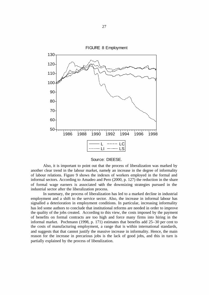
The increase in unemployment in the second half of the 1990s, in particular after 1997, masks the differences in evolution of employment among sectors. Figure 8 shows the indexes for employment levels in the economy as a whole (L), in the industrial sector (LI), in commerce (LC) and in the service sector (LS). It is clear that industrial employment has been falling throughout the liberalization period, starting in the late 1980s. Employment in the commerce and service sectors, on the other hand, has followed a cyclical behaviour. It recovered from the recession of the early 1980s and fell as much as industrial employment during the recession of the early 1990s. Yet, in contrast to industrial employment, during the 1990s non-industrial employment also experienced a cyclical fluctuation, increasing after the recession in the mid-1990s and falling after the external shocks of the Tequila and Asian crises.

The 1995 to 1997 period, between the Tequila and the Asian crises, is particularly interesting. In these two years, industrial employment fell, but the increases in employment in the commerce and service sectors were more than enough to compensate for that fall. As a result, employment in the economy as a whole was relatively constant. This explains why, in contrast with the Argentinean experience of exchange-rate-based stabilization, unemployment did not increase immediately in Brazil.

27

50

60

70

80

90

100

110

120

130

1986 1988 1990 1992 1994 1996 1998

LLI

LCLS

Source: DIEESE.

FIGURE 8 Employment

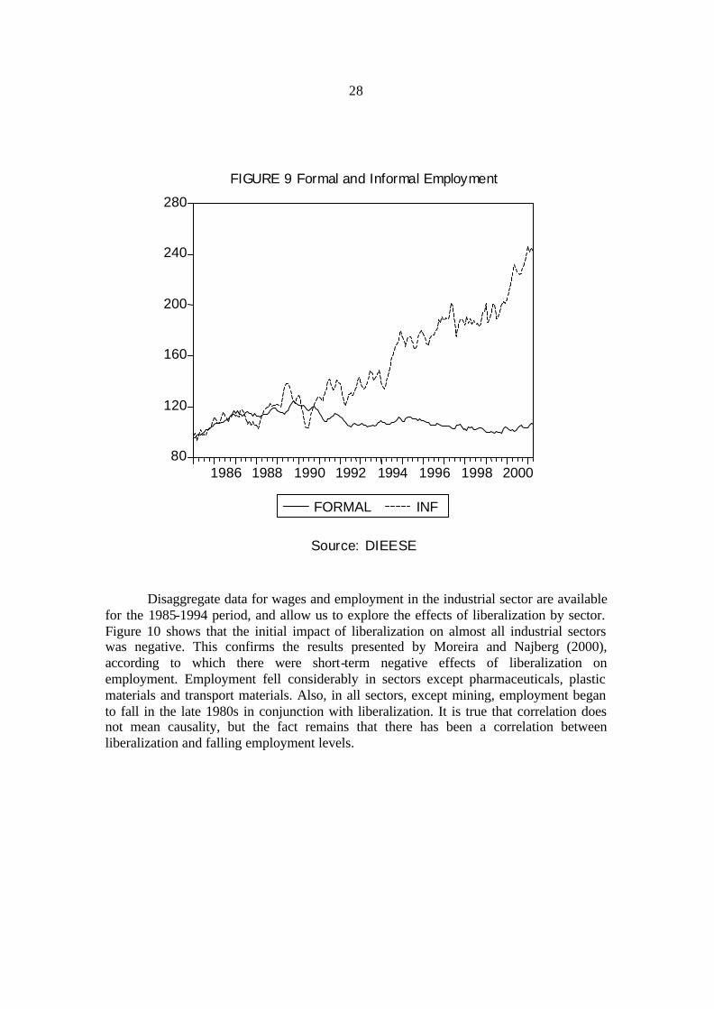
Also, it is important to point out that the process of liberalization was marked by

another clear trend in the labour market, namely an increase in the degree of informality of labour relations. Figure 9 shows the indexes of workers employed in the formal and informal sectors. According to Amadeo and Pero (2000, p. 127) the reduction in the share of formal wage earners is associated with the downsizing strategies pursued in the industrial sector after the liberalization process.

In summary, the process of liberalization has led to a marked decline in industrial employment and a shift to the service sector. Also, the increase in informal labour has signalled a deterioration in employment conditions. In particular, increasing informality has led some authors to conclude that institutional reforms are needed in order to improve the quality of the jobs created. According to this view, the costs imposed by the payment of benefits on formal contracts are too high and force many firms into hiring in the informal market. Pochmann (1998, p. 171) estimates that benefits add 25–30 per cent to the costs of manufacturing employment, a range that is within international standards, and suggests that that cannot justify the massive increase in informality. Hence, the main reason for the increase in precarious jobs is the lack of good jobs, and this in turn is partially explained by the process of liberalization.

28

80

120

160

200

240

280

1986 1988 1990 1992 1994 1996 1998 2000

FORMAL INF

S o u r c e : D I E E S E

F I G U R E 9 F o r m a l a n d I n f o r m a l E m p l o y m e n t

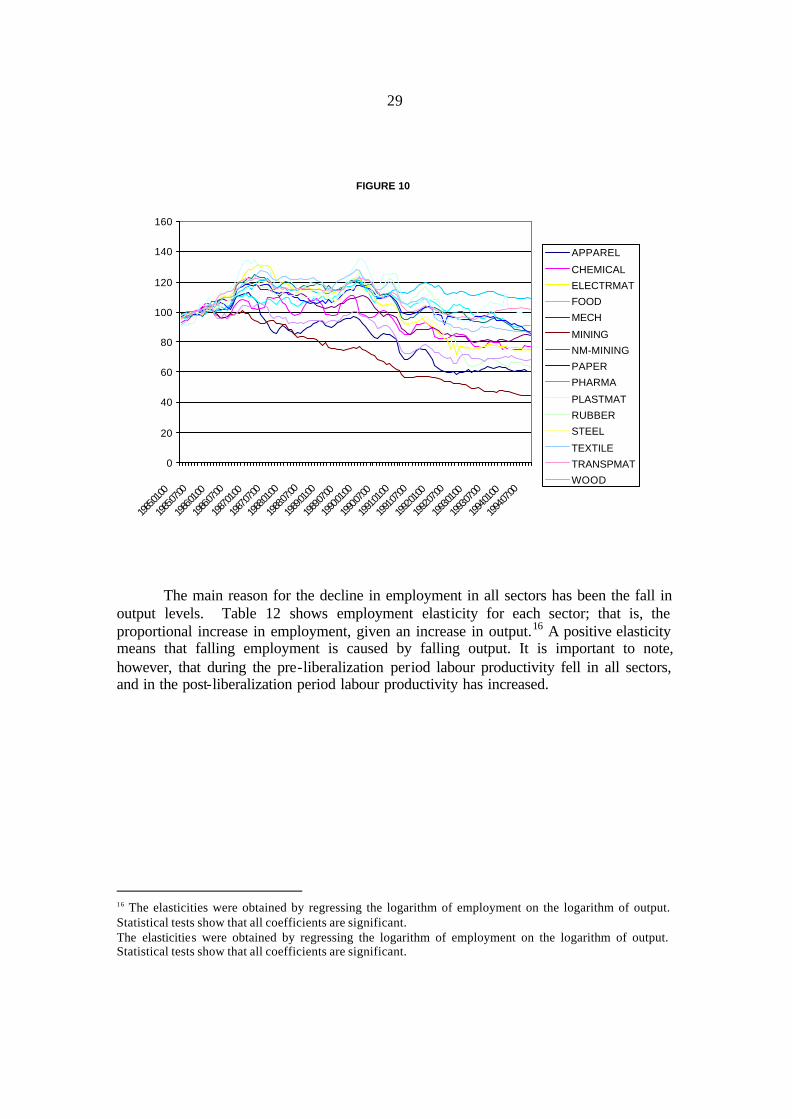
Disaggregate data for wages and employment in the industrial sector are available

for the 1985-1994 period, and allow us to explore the effects of liberalization by sector. Figure 10 shows that the initial impact of liberalization on almost all industrial sectors was negative. This confirms the results presented by Moreira and Najberg (2000), according to which there were short-term negative effects of liberalization on employment. Employment fell considerably in sectors except pharmaceuticals, plastic materials and transport materials. Also, in all sectors, except mining, employment began to fall in the late 1980s in conjunction with liberalization. It is true that correlation does not mean causality, but the fact remains that there has been a correlation between liberalization and falling employment levels.

29

FIGURE 10

0

20

40

60

80

100

120

140

160

1985:0

1:00

1985:0

7:00

1986:0

1:00

1986:0

7:00

1987:0

1:00

1987:0

7:00

1988:0

1:00

1988

:07:00

1989:0

1:00

1989:0

7:00

1990:0

1:00

1990:0

7:00

1991:0

1:00

1991:0

7:00

1992:0

1:00

1992:0

7:00

1993:0

1:00

1993:0

7:00

1994:0

1:00

1994:0

7:00

APPAREL

CHEMICAL

ELECTRMAT

FOOD

MECH

MINING

NM-MINING

PAPER

PHARMA

PLASTMAT

RUBBER

STEEL

TEXTILE

TRANSPMAT

WOOD

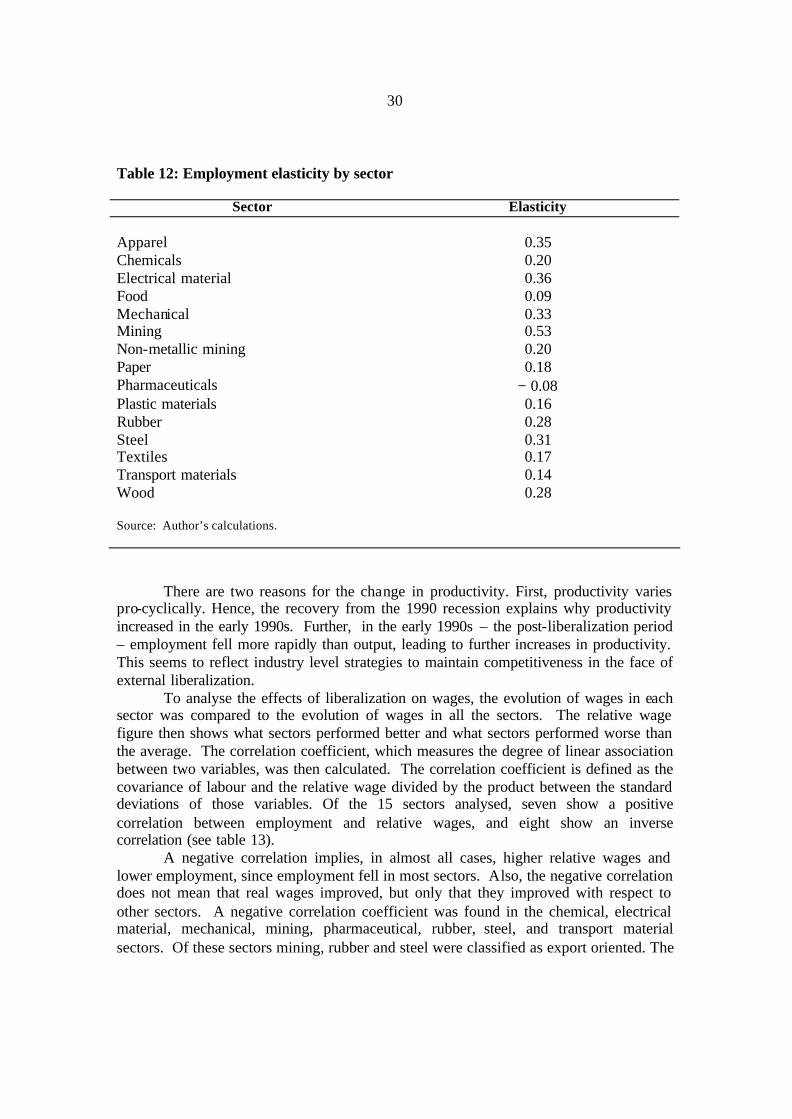
The main reason for the decline in employment in all sectors has been the fall in output levels. Table 12 shows employment elasticity for each sector; that is, the proportional increase in employment, given an increase in output.16 A positive elasticity means that falling employment is caused by falling output. It is important to note, however, that during the pre-liberalization period labour productivity fell in all sectors, and in the post-liberalization period labour productivity has increased.

16 The elasticities were obtained by regressing the logarithm of employment on the logarithm of output. Statistical tests show that all coefficients are significant. The elasticities were obtained by regressing the logarithm of employment on the logarithm of output. Statistical tests show that all coefficients are significant.

30

Table 12: Employment elasticity by sector

Sector Elasticity Apparel

0.35

Chemicals 0.20 Electrical material 0.36 Food 0.09 Mechanical 0.33 Mining 0.53 Non-metallic mining 0.20 Paper 0.18 Pharmaceuticals − 0.08 Plastic materials 0.16 Rubber 0.28 Steel 0.31 Textiles 0.17 Transport materials 0.14 Wood 0.28 Source: Author’s calculations.

There are two reasons for the change in productivity. First, productivity varies pro-cyclically. Hence, the recovery from the 1990 recession explains why productivity increased in the early 1990s. Further, in the early 1990s – the post-liberalization period – employment fell more rapidly than output, leading to further increases in productivity. This seems to reflect industry level strategies to maintain competitiveness in the face of external liberalization.

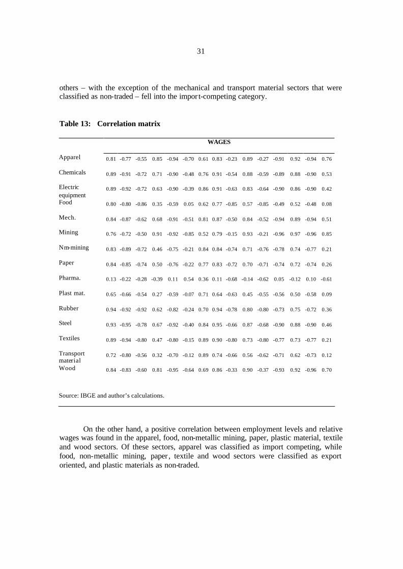
To analyse the effects of liberalization on wages, the evolution of wages in each sector was compared to the evolution of wages in all the sectors. The relative wage figure then shows what sectors performed better and what sectors performed worse than the average. The correlation coefficient, which measures the degree of linear association between two variables, was then calculated. The correlation coefficient is defined as the covariance of labour and the relative wage divided by the product between the standard deviations of those variables. Of the 15 sectors analysed, seven show a positive correlation between employment and relative wages, and eight show an inverse correlation (see table 13).

A negative correlation implies, in almost all cases, higher relative wages and lower employment, since employment fell in most sectors. Also, the negative correlation does not mean that real wages improved, but only that they improved with respect to other sectors. A negative correlation coefficient was found in the chemical, electrical material, mechanical, mining, pharmaceutical, rubber, steel, and transport material sectors. Of these sectors mining, rubber and steel were classified as export oriented. The

31

others – with the exception of the mechanical and transport material sectors that were classified as non-traded – fell into the impor t-competing category.

Table 13: Correlation matrix

WAGES

Apparel 0.81 -0.77 -0.55 0.85 -0.94 -0.70 0.61 0.83 -0.23 0.89 -0.27 -0.91 0.92 -0.94 0.76

Chemicals 0.89 -0.91 -0.72 0.71 -0.90 -0.48 0.76 0.91 -0.54 0.88 -0.59 -0.89 0.88 -0.90 0.53

Electric equipment

0.89 -0.92 -0.72 0.63 -0.90 -0.39 0.86 0.91 -0.63 0.83 -0.64 -0.90 0.86 -0.90 0.42

Food 0.80 -0.80 -0.86 0.35 -0.59 0.05 0.62 0.77 -0.85 0.57 -0.85 -0.49 0.52 -0.48 0.08

Mech. 0.84 -0.87 -0.62 0.68 -0.91 -0.51 0.81 0.87 -0.50 0.84 -0.52 -0.94 0.89 -0.94 0.51

Mining 0.76 -0.72 -0.50 0.91 -0.92 -0.85 0.52 0.79 -0.15 0.93 -0.21 -0.96 0.97 -0.96 0.85

Nm-mining 0.83 -0.89 -0.72 0.46 -0.75 -0.21 0.84 0.84 -0.74 0.71 -0.76 -0.78 0.74 -0.77 0.21

Paper 0.84 -0.85 -0.74 0.50 -0.76 -0.22 0.77 0.83 -0.72 0.70 -0.71 -0.74 0.72 -0.74 0.26

Pharma. 0.13 -0.22 -0.28 -0.39 0.11 0.54 0.36 0.11 -0.68 -0.14 -0.62 0.05 -0.12 0.10 -0.61

Plast mat. 0.65 -0.66 -0.54 0.27 -0.59 -0.07 0.71 0.64 -0.63 0.45 -0.55 -0.56 0.50 -0.58 0.09

Rubber 0.94 -0.92 -0.92 0.62 -0.82 -0.24 0.70 0.94 -0.78 0.80 -0.80 -0.73 0.75 -0.72 0.36

Steel 0.93 -0.95 -0.78 0.67 -0.92 -0.40 0.84 0.95 -0.66 0.87 -0.68 -0.90 0.88 -0.90 0.46

Textiles 0.89 -0.94 -0.80 0.47 -0.80 -0.15 0.89 0.90 -0.80 0.73 -0.80 -0.77 0.73 -0.77 0.21

Transport material

0.72 -0.80 -0.56 0.32 -0.70 -0.12 0.89 0.74 -0.66 0.56 -0.62 -0.71 0.62 -0.73 0.12

Wood 0.84 -0.83 -0.60 0.81 -0.95 -0.64 0.69 0.86 -0.33 0.90 -0.37 -0.93 0.92 -0.96 0.70

Source: IBGE and author’s calculations.

On the other hand, a positive correlation between employment levels and relative wages was found in the apparel, food, non-metallic mining, paper, plastic material, textile and wood sectors. Of these sectors, apparel was classified as import competing, while food, non-metallic mining, paper , textile and wood sectors were classified as export oriented, and plastic materials as non-traded.

32

If one assumes that a negative correlation implies a better performance, at least with respect to other industrial sectors, and a positive correlation entails a negative performance, then no clear pattern appears to be associated with the external orientation of the industrial activity.

0.92

0.96

1.00

1.04

1.08

1.12

85 86 87 88 89 90 91 92 93

WEO/WIC WTREND

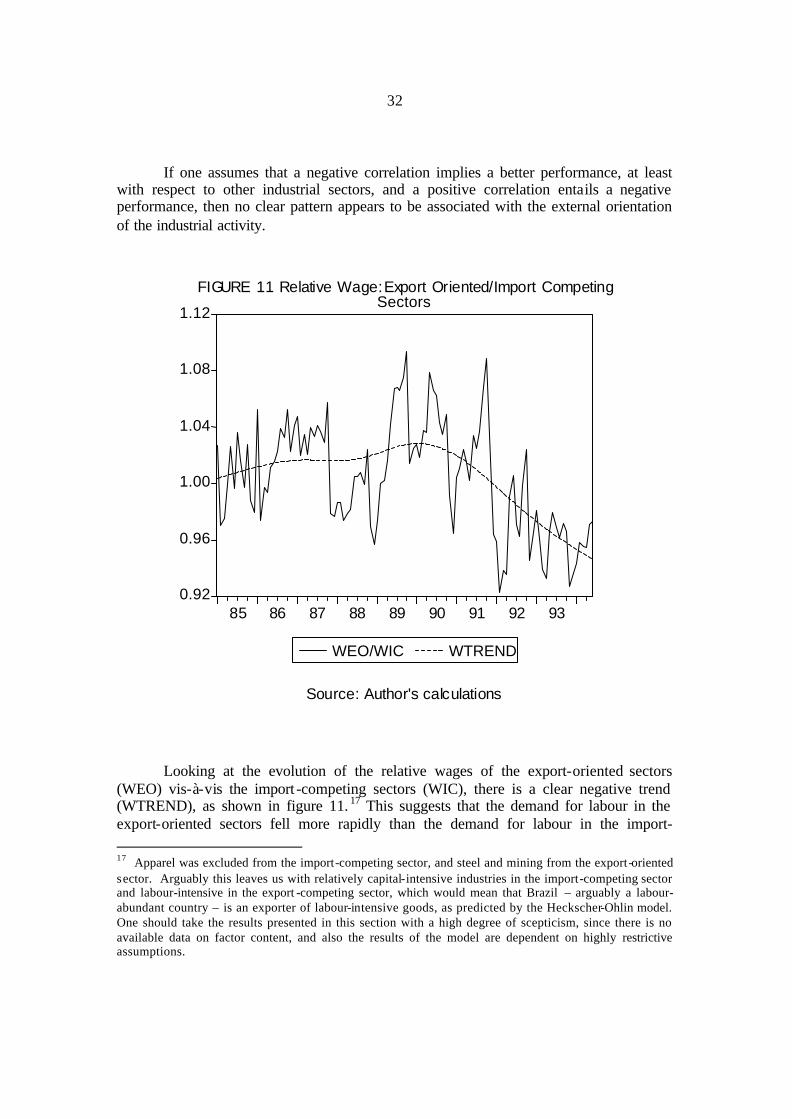
F I G U R E 1 1 R e la t i v e W a g e: E x p o r t O r i e n t e d / I m p o r t C o m p e t i ng Sectors

S o u r c e : A u t h o r ' s c a l c u l a t i o n s

Looking at the evolution of the relative wages of the export-oriented sectors (WEO) vis-à-vis the import -competing sectors (WIC), there is a clear negative trend (WTREND), as shown in figure 11. 17 This suggests that the demand for labour in the export-oriented sectors fell more rapidly than the demand for labour in the import- 17 Apparel was excluded from the import-competing sector, and steel and mining from the export-oriented sector. Arguably this leaves us with relatively capital-intensive industries in the import-competing sector and labour-intensive in the export -competing sector, which would mean that Brazil – arguably a labour- abundant country – is an exporter of labour-intensive goods, as predicted by the Heckscher-Ohlin model. One should take the results presented in this section with a high degree of scepticism, since there is no available data on factor content, and also the results of the model are dependent on highly restrictive assumptions.

33

competing sectors, and hence that the import-competing sectors did better, in general, than the export-oriented sectors. This is also consistent with the overall poor performance of exports in the post-liberalization period.

If one assumes that the import-competing chemical and electrical material sectors are capital-intensive compared with the export-oriented food, non-metallic mining, paper, textile, and wood sectors, it may be concluded that the relative demand for skilled labour, used in the capital-intensive sectors, fell less than the demand for unskilled labour, used in the labour-intensive sectors. This result fits in with the stylized facts about Brazil in the 1990s, according to which the skill premium increased, and confirms the Latin American paradox noted by Wood (1997).

The question then is what went wrong with the Hecksher-Ohlin prediction in the Brazilian case? One possible explanation is that the post-liberalization period has been concomitant with either high inflation or a highly appreciated real exchange rate. High inflation produces perverse incentives for companies. Costs or quality matter less than the speed with which firms get goods into the shops and invest the revenue in financial markets. High inflation means that the most important sort of engineering is financial. Also, an appreciated exchange rate within a more open environment does not lead to improvements in foreign competitiveness. Hence, one may conclude that the persistence of macroeconomic instability in the form of inflation in the first half of the 1990s and real exchange rate appreciation in the second half, hurt the ability of labour-intensive export-oriented industries to reap the benefits of liberalization.

6. Concluding Remarks

Liberalization has created the need for maintaining low rates of growth in order to keep, or at least try to keep, the current account under control. One of the consequences of low rates of growth has been the increase in unemployment rates since 1997. The improvement after the depreciation of 1999 may be short-lived, as has been dramatically shown by the constraints in energy supply and the persistent current-account deficit. Additionally, in Brazil, rising capital inflows following liberalization led to real exchange rate appreciation, which offset liberalization's incentives for traded goods production and created increasing inequality between wages of workers in the tradable and non-tradable sectors. Appreciation, in turn, can be linked to high real interest rates, which added to production costs and to the financial costs of the public debt.

Moreover, the persistent inflation in the first half of the 1990s, and real appreciation in the second half badly hurt the export performance of the Brazilian manufacturing sector. This in turn led to an increase in the skill premium, and to increasing inequality between skilled and unskilled workers.

Policy alternatives in an increasingly interdependent world are difficult to implement. It is true that the process of liberalization of the current account has been consolidated through a series of multilateral and bilateral trade agreements, in particular MERCOSUR, and now the upcoming Free Trade Area of the Americas (FTAA), that conform with World Trade Organization (WTO) rules. Thus the scope for changes in trade policies, even when desirable, is limited. However, the recent discussions on the

34

Brazil’s adjustment policies, and the favourable ruling by the WTO on the Brazil’s dispute with Canada over subsidies to EMBRAERR, show that there is considerable room for alternative policies. Furthermore, capital account liberalization has been incomplete in Brazil, and there are possibilities for change, in particular, after the wave of criticism evoked by the Asian and Russian crises.

35

References

Agosin, M.; French-Davis, R. 1996. Managing Capital Inflows in Latin America. (New York, Office of Development Studies), Discussion Paper No 8.

Amadeo, E. 1994. Institutions, Inflation and Unemployment (Aldershot, Edward Elgar). Amadeo, E. 1996. “The knife-edge of exchange rate based stabilization,” in UNCTAD Review,

pp. 1-25. Amadeo, E.; V. Pero. 2000. “Adjustment, stabilization and the structure of employment in

Brazil”, in Journal of Development Studies, 36(4), pp. 120-148. Arida, P.; Lara-Resende, A. 1985. “Inertial inflation and monetary reform in Brazil”, in J.

Williamson (ed.), Inflation and Indexation (Washington, DC, Institute for International Economics).

Averburg, A. 1999. “Abertura e integração comercial Brasileira na década de 90,” in F.

Giambiagi, F. and Moreira, M. (eds.) A Economia Brasileira nos Anos 90 (Rio de Janeiro, BNDES).

Boletim Banco Central (various issues) (Rio de Janeiro, Central Bank of Brazil) Bonelli, R. 1994. “Productivity growth and industrial exports in Brazil,” in CEPAL Review , 52,

April, pp. 71-89. Bruno, M. 1993. Crisis, Stabilization, and Economic Reform: Therapy by Consensus, (Oxford,

Clarendon Press). Calvo, G.; Leiderman, L.; Reinhart, C. 1993. Capital inflows and real exchange rate

appreciation in Latin America (Washington, DC, IMF) IMF Staff Papers, 40(1). Câmara, A.; Vernengo, M. 2000. “The German balance of payments school and the Latin

American neo-structuralists”, in Rochon, L-P. and Vernengo, M. (eds.), Credit, Interest Rates and the Open Economy (Cheltenham, Edward Elgar).

Cardos o, E.; Fishlow, A. 1989. The Macroeconomics of the Brazilian External Debt (Brazilian

translation) (São Paulo, Brasiliense). DIEESE, Departamento Intersindical de Estatística e Estudos Sócio-Econômicos, at website:

http://www.dieese.org.br/ped/ped.html. International Monetary Fund. Various issues. Directions of Trade (Washington DC).

36

Edwards, S. 1995. Crisis and Reform in Latin America: From Despair to Hope. (Washington, DC, World Bank).

Franco, G. 1999. O Desafio Brasileiro: ensaios sobre desenvolvimento, globalização e moeda

(São Paulo, Editora 34). Fundação Getúlio Vargas (FGV Dados) at website: http://fgvdados.fgv.br/. Fritsch W. and Tombini, A. 1994. “The Mercosul: An Overview”, in Bouzas R. and Ros J, eds.

Economic Integration in the Western Hemisphere (Notre Dame, London, University of Notre Dame Press).

Ghose, A.K. 2000 “Trade liberalization, employment and global inequality”, in International

Labour Review , 139 (3), pp. 281-304. Instituto Brasileiro de Geografia e Estatistica, Pesquisa Mensal de Emprego (IBGE/PME)

(various dates). Boletim, several issues. International Monetary Fund. Various issues. International Financial Statistics, (Washington

DC). IPEA Data, http://ipeadata.gov.br/ipeaweb.dll, Instituto de Pesquisa Econômica Aplicada. Laplane, M.; Sarti, F. 1997. “Investimento direto estrangeiro e a retomada do crescimento

sustentado nos anos noventa”, in Economia e Sociedade, 8. Lopes, F. 1986. O Choque Heterdoxo (Rio de Janeiro: Campus). Moreira, M.M.; Najberg, S. 2000. “Trade liberalization in Brazil: Creating or exporting jobs”, in

Journal of Development Studies, 36 (3), pp. 78-96. Pieper, U. 2000. “Deindustrialization and the social and economic sustainability nexus in

developing countries,” in Journal of Development Studies, 36(4).

Pochmann, M. 1998. O Trabalho Sob Fogo Cruzado (Rio de Janeiro, Contexto). Pritchett, L. 1996. “Measuring outward orientation in LDCs: Can it be done?”, in Journal of

Development Economics, 49, pp. 307-335. Resende, M. 2000. Crescimento Econômico, Disponibilidade de Divisas e Importação Total por

Categoria de Uso no Brasil. Texto para Discussão No 714 (Brasilia, IPEA). Rodriguez, F.; Rodrik, D. 1999. Trade Policy and Economic Growth: a Skeptic’s Guide to the

Cross-National Evidence, NBER Working Paper No 7081 (Cambridge, MA).

37

Rodrik, D. (1999). The new global economy and developing countries: Making openness work, Policy Essay No 24 (Washington, D.C., Overseas Development Council).

Simonsen, M. H. 1990. “Aspectos teóricos do Plano Collor,” in de Faro, C (ed.), O Plano Collor.

(Rio de Janeiro, Livros Técnicos e Científicos Editora). Stallings, B.; Peres, W. 2000. Growth, Employment and Equity (Washington, DC, Brookings

Institute). Taylor, L. 1991. “Economic openness: problems to the century’s end”, in Banuri, T. (ed.),

Economic Liberalization: No Panacea (Oxford, Clarendon Press). Taylor, L. 2001. “Outcomes of external liberalization and policy implications”, in Taylor, L.

(ed.) External Liberalization, Economic Performance, and Social Policy (New York, Oxford University Press).

Williamson, J. 1989. “What Washington means by policy reform”, in J. Williamson, (ed.) Latin

American Adjustment: How Much Has Happened? (Washington, DC, Institute for International Economics).

Wood, A. 1994. North-South Trade, Employment and Inequality (Oxford, Clarendon Press). Wood, A. 1997. “Openness and wage inequality in developing countries,” in The World Bank

Economic Review, 11(1), pp. 33-57. World Bank (1993), The East Asian Miracle. Policy Research Report (New York, Oxford

University Press).