Empty Promises and Arbitrage · The usual presentation of the fundamental theorem of asset pricing typ-ically ignores payoffs in states to which the agent assigns zero probabil-ity

Empty Promises and ArbitrageGregory A. WillardMassachusetts Institute of Technology

Philip H. DybvigWashington University in Saint Louis

Analysis of absence of arbitrage normally ignores payoffs in states to which theagent assigns zero probability. We extend the fundamental theorem of asset pricingto the case of “no empty promises” in which the agent cannot promise arbitrarilylarge payments in some states. There is a superpositive pricing rule that can assignpositive price to claims in zero probability states important to the market as wellas assigning positive prices to claims in the states of positive probability. Withcontinuous information arrival, no empty promises can be enforced by shuttingdown the agent’s subsequent investments once wealth hits zero.

Dogmatic disagreements create arbitrage opportunities in competitive mar-kets that are sufficiently complete. There may be someone in the economywho is certain (correctly or not on objective grounds) that gold prices willgo up and someone else who believes there is a positive probability that goldprices will go down. The first person will have an arbitrage opportunity ifat-the-money put options on gold have a positive price, while the secondperson will have an arbitrage opportunity if at-the-money put options ongold have a zero or negative price. Similarly, if some people are sure theirfavorite sport teams or horses will win but others are not so sure, any oddsposted by a competitive bookmaker will imply arbitrage for one group orthe other.1 In practice, however, dogmatic differences in beliefs do not im-ply actual arbitrage that can be used to generate arbitrarily large profitsbecause people have limited resources and cannot make “empty promises”of payments that exceed their own ability to pay in states the market caresabout, even if those are states they personally believe to be impossible. Thepurpose of this article is to extend the study of the absence of arbitrage tosituations in which no empty promises are permitted.

We thank Mark Loewenstein, HrvojeSikic, Jie Wu, and an anonymous referee for useful discussions. Anearlier version of this article appears in Willard’s doctoral thesis at Washington University in Saint Louis.Address correspondence to Gregory A. Willard, Sloan School of Management, Massachusetts Instituteof Technology, 50 Memorial Dr., E52-431, Cambridge, MA 02142-1347.

1 These arbitrages are generally still present in the presence of finite spreads. Our analysis assumes strictprice-taking without a spread, but as can be seen from the analysis of Jouini and Kallal (1995), absenceof arbitrage in the presence of a spread is the same as the existence of prices within a spread that do notadmit arbitrage, and this would be true of our notion of “robust arbitrage” as well.

The Review of Financial StudiesSpecial 1999 Vol. 12, No. 4, pp. 807–834c© 1999 The Society for Financial Studies

The Review of Financial Studies / v 12 n 41999

The fundamental theorem of asset pricing asserts the equivalence of theabsence of arbitrage, the existence of a positive linear pricing rule, and theexistence of an optimal demand for some agent who prefers more to less.2

This result is important, for example, since it tells us that if asset priceprocesses admit no arbitrage, then they are consistent with equilibrium(in a single-agent economy for the agent whose existence is ensured bythe theorem). In other words, assuming equilibrium places no more andno less restriction on prices than assuming no arbitrage, absent additionalassumptions.

The usual presentation of the fundamental theorem of asset pricing typ-ically ignores payoffs in states to which the agent assigns zero probabil-ity. A linear pricing rule that attaches a positive price to a state that theagent believes is impossible would be inconsistent with expected utilitymaximization in competitive markets since selling short the correspondingArrow–Debreu security provides consumption now with zero probability offuture loss. On the other hand, a zero or negative state price would be incon-sistent with utility maximization if the agent believes the state is possiblesince buying the Arrow–Debreu security for some state is an arbitrage, anda marginal purchase makes the agent better off.

Preventing an agent from making empty promises can rule out strategiesthat exploit positive prices in states to which the agent assigns zero prob-ability. We model this as a nonnegative wealth constraint that is imposedin all states deemed to be “important” by a regulatory agency, consensusmarket beliefs, or some other mechanism. The shadow price of the bindingconstraint equals the price of the impossible state, restoring consistencybetween linear pricing and expected utility maximization. We state a newversion of the fundamental theorem which equates absence of robust arbi-trages (defined to be arbitrages not requiring empty promises), existence ofa superlinear pricing rule (which may give positive price to states valuedby the market even if the agent believes them impossible), and existence ofan optimum for an agent who prefers more to less and cannot make emptypromises.

A potential conceptual problem with the general analysis is one of en-forcement: How do we ensure that an agent will choose a strategy that doesnot make empty promises in states of nature that the agent believes willnever happen? Our main result on enforcement is that, whenever informa-tion arrives continuously, the no-empty-promises condition can be enforcedby shutting down all investments for the rest of the time once the agent’swealth hits zero. Continuous information arrival implies that the portfoliovalue is continuous and therefore must hit zero before going negative. This

2 See Ross (1978) and Dybvig and Ross (1987) for discussions of the fundamental theorem of asset pricingin the traditional setting.

808

Empty Promises and Arbitrage

property means that if the market halts the agent’s trading the first timethe wealth hits zero, then the wealth cannot become negative. Being ableto enforce the no-empty-promises condition using only the paths of wealthis important because it eliminates the market’s need to know the agent’sstrategy in all important states.3 By contrast, monitoring the path of wealthwould be insufficient to enforce no empty promises if information arrivalwere discontinuous (as it would be in a discrete-time model or a modelwith unpredictable jumps) because the market may be unable to anticipatewhether wealth will become negative. We can compare this to the marking-to-market process in futures markets. Daily marking to market presumablyapproximates continuous information arrival in that it permits exchanges tostop the activity of any trader who is in danger of having negative wealth,regardless of the trader’s view of the future direction of the market. Marking-to-market would be less effective if it were done monthly or if daily pricevariation were more volatile, both of which represent more discontinuousinformation arrival, requiring more margin money to complement markingto market.

In related work, Hindy (1995) studies the viability of a pricing rule whenthe agent must maintain a level of “risk-adjusted” equity. Hindy claims thatviability is equivalent to the existence of a linear pricing rule which is thesum of two linear rules, one representing marginal utility of consumptionand the other representing the shadow price of his solvency constraint. Ourpricing rule has a similar decomposition, and dogmatic differences in beliefsprovide a natural reason for the shadow price to be nontrivial, somethingabsent in Hindy’s analysis. In addition, our setting allows interesting optionpricing and investment models (such as the Black–Scholes model) becausewe allow unbounded consumption and investment strategies. We also allowmarkets to be incomplete.

Several studies consider consumption and investment problems whenagents disagree about the possible returns of risky assets. Wu (1991) andPikovsky and Karatzas (1996) study optimal consumption in a model inwhich an agent has logarithmic preferences and “anticipates” future assetprices. Bergman (1996) argues that arbitrarily conditioning return processesto lie in some range may produce arbitrage opportunities; our results sug-gest that these arbitrages can be ruled out by a no-empty-promises condi-tion. Loewenstein and Willard (1997) use results presented here to studyequilibrium trading strategies and prices when agents face unforeseen con-tingencies.

3 The difference here is analogous to the difference between using expected square integrability and usinga nonnegative wealth constraint to rule out doubling strategies in a continuous-time model. Determiningexpected square integrability requires the market to know the agent’s strategy in every state of nature;by contrast, a nonnegative wealth constraint requires only knowledge of the agent’s wealth along theobserved path.

809


Section 1 contains examples that illustrate the use of the no-empty-promises constraint. Section 2 contains the fundamental theorem of assetpricing with no empty promises for a single-period model with a finitenumber of states. Section 3 extends this result to a continuous-time modelin which returns are assumed to be general special semimartingales. InSection 4, we show that the no-empty-promises condition can be enforcedby shutting down investments when wealth hits zero, provided returns arecontinuous. Section 5 concludes.

1. Examples

We illustrate the connection between empty promises and arbitrage in anumber of discrete- and continuous-time examples. In each of our examples,the agent has initial endowmentw > 1 and preferencesc0+ logc1, wherec0andc1 represent current and terminal consumption, respectively. Assumingseparable linear-logarithmic utility is in no way essential for the results, butthis choice does simplify computation. The agent takes prices as given andconditions on information available at the start of trade. General results aregiven in later sections.

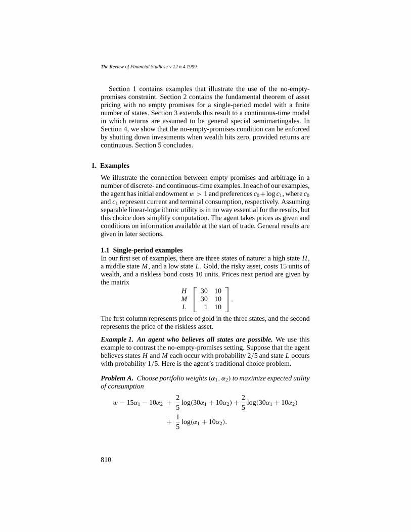
1.1 Single-period examplesIn our first set of examples, there are three states of nature: a high stateH ,a middle stateM , and a low stateL. Gold, the risky asset, costs 15 units ofwealth, and a riskless bond costs 10 units. Prices next period are given bythe matrix

HML

30 1030 101 10

.The first column represents price of gold in the three states, and the secondrepresents the price of the riskless asset.

Example 1. An agent who believes all states are possible.We use thisexample to contrast the no-empty-promises setting. Suppose that the agentbelieves statesH andM each occur with probability 2/5 and stateL occurswith probability 1/5. Here is the agent’s traditional choice problem.

Problem A. Choose portfolio weights(α1, α2) to maximize expected utilityof consumption

w − 15α1− 10α2 + 2

5log(30α1+ 10α2)+ 2

5log(30α1+ 10α2)

+ 1

5log(α1+ 10α2).

810


From the first-order conditions, the solution to Problem A equalsα1 =23/525 andα2 = 6/175.

Example 2. An agent who believes a state is impossible.Here the agentis certain gold will outperform the bond: suppose the agent believes statesH and M each occur with probability 1/2. Problem B is the traditionalconsumption choice problem.

Problem B. Choose portfolio weights(α1, α2) to maximize expected utilityof consumption

w − 15α1− 10α2+ 1

2log(30α1+ 10α2)+ 1

2log(30α1+ 10α2).

Problem B does not have a solution because there is an arbitrage. Forexample, lending 3/2 units of the bond and buying 1 unit of the gold costsnothing but returns 15 units for sure under the agent’s beliefs. The agentcan reach any level of expected utility by undertaking enough of these nettrades. However, for each trade the agent promises to pay 14 units of wealthin the event that stateL occurs. In using this trade to construct the arbitrage,the agent promises to pay successively larger amounts of wealth conditionalon stateL, thus making an “empty promise” because potential losses willeventually exceed any given initial endowment.

The following choice problem has a solution because a no-empty-promises constraint rules out strategies that make these empty promises.

Problem C. Choose portfolio weights(α1, α2) to maximize expected utilityof consumption

w − 15α1− 10α2+ 1

2log(30α1+ 10α2)+ 1

2log(30α1+ 10α2)

subject to the no-empty-promises constraint given by30α1+10α2 ≥ 0 andα1+ 10α2 ≥ 0.

The solution to Problem C isα1 = 1/14 andα2 = −1/140. The shadowprice on the binding no-empty-promises constraint (α1+ 10α2 ≥ 0) equals15/29, the market price of the Arrow–Debreu security for the low state. Theshadow price takes up the slack between zero marginal utility and a positivestate price. Notice that the no-empty-promises constraint in this example isweaker than a no-short-sales constraint sinceα1 can be arbitrarily negativeif α2 is positive enough to cover the position.

Here is an example to show that the no-empty-promises constraint doesnot always eliminate arbitrage opportunities.

Example 3. A robust arbitrage opportunity.Suppose that the spot prices

811


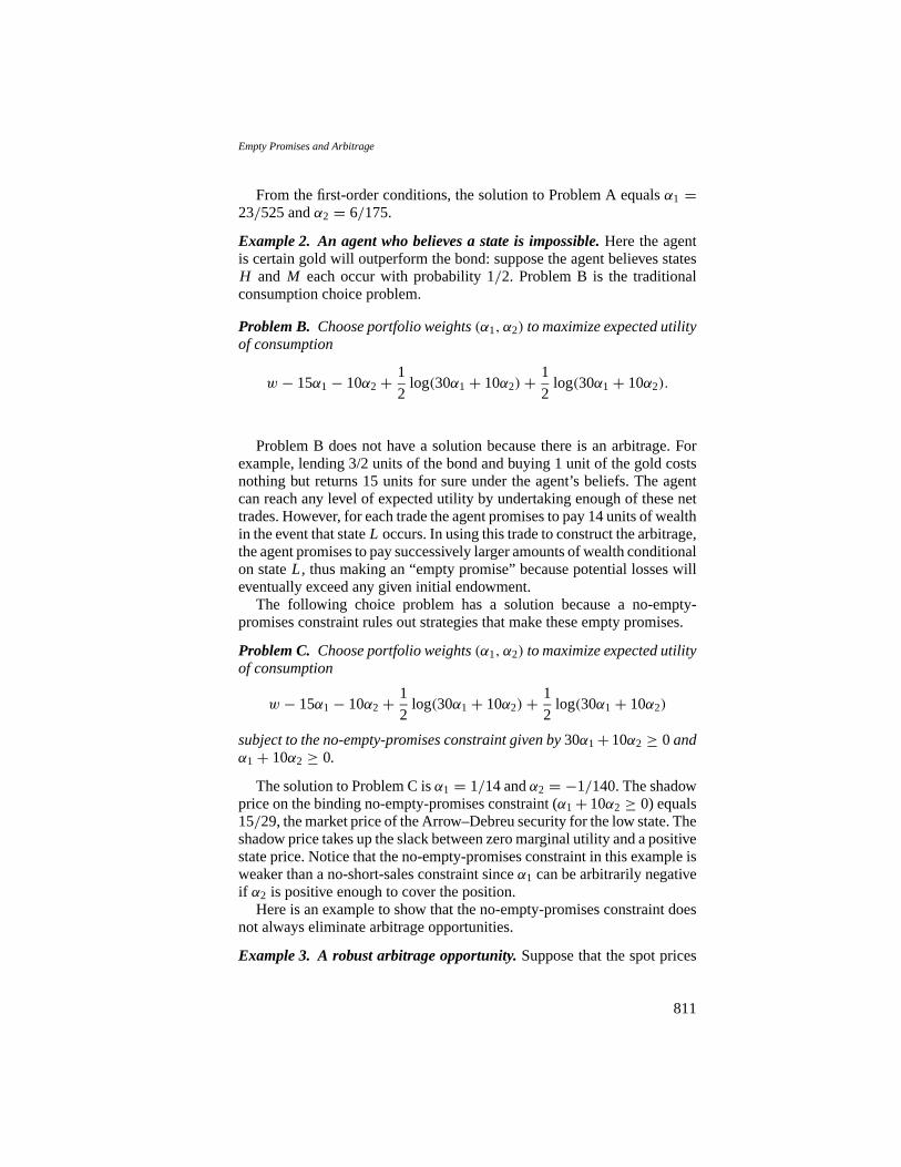
of gold and the riskless bond are [10, 10], and next period’s prices aregiven by

HML

10 1010 100 10

.There is a solution to the choice problem when the agent believes stateL is impossible, but there is no solution whenever the agent believes thegold price will fall with positive probability. This is true even under theno-empty-promises constraint because an at-the-money put option on goldhas zero cost, has nonnegative payoffs, and pays a positive amount withpositive probability.

In these examples we see that (i) there may be no arbitrage opportunities ifthe agent assigns positive probabilities to all states in which portfolios of theassets can have positive payoffs, even in the absence of a no-empty-promisesconstraint; (ii) if the agent assigns some of these states zero probability,then the resulting arbitrages may be ruled out by preventing the agent frommaking empty promises; and (iii) there may be “robust” arbitrages that willbe available whether or not empty promises are permitted.

1.2 Continuous-time examplesWe now demonstrate that similar conclusions hold in examples in whichthe agent trades continuously over a time interval [0, T ]. In this section theexposition is informal with a few details in footnotes; formal definitions andproofs are given in a later section.

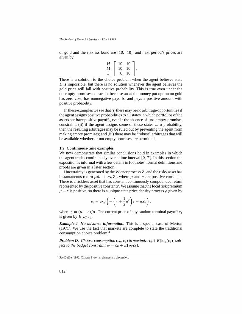
Uncertainty is generated by the Wiener processZ, and the risky asset hasinstantaneous returnµdt + σd Zt , whereµ andσ are positive constants.There is a riskless asset that has constant continuously compounded returnrepresented by the positive constantr . We assume that the local risk premiumµ− r is positive, so there is a unique state price density processρ given by

ρt = exp

(−(

r + 1

2η2)

t − ηZt

),

whereη = (µ− r )/σ . The current price of any random terminal payoffc1is given byE[ρTc1].

Example 4. No advance information.This is a special case of Merton(1971). We use the fact that markets are complete to state the traditionalconsumption choice problem.4

Problem D. Choose consumption(c0, c1) to maximize c0+E[log(c1)] sub-ject to the budget constraintw = c0+ E[ρTc1].

4 See Duffie (1992, Chapter 8) for an elementary discussion.

812


The solution to Problem D isc0 = w − 1 andc1 = ρ−1T . The trading

strategy that finances this consumption is

θt = Wt

(µ− r

σ 2

),

which invests a constant proportion of wealth in the risky asset.5

Our second example considers a case of advance information.

Example 5. Advance information I.Suppose the agent conditions prior tothe start of trade on the belief that the terminal risky return will exceedthe riskless return; that is,µT + σ ZT > rT or equivalentlyZT > −ηT .Problem E states the traditional choice problem.

Problem E. Choose(c0, c1) to maximize c0 + E[log(c1) | ZT > −ηT ]subject to the budget constraintw = c0+ E[ρTc1].

This problem has no solution because the agent can write put optionspaying only in states for whichZT is less than or equal to−ηT . This addscurrent consumption without violating the budget constraint and withoutdecreasing expected utility. (The puts are never exercised under the agent’sbeliefs.) A problem is that states of nature to which the agent assigns zeroprobability have positive market prices. As in the finite-state example, ano-empty-promises constraint can restore the existence of a solution.

Problem F. Choose consumption(c0, c1) to maximize c0 + E[log(c1) |ZT > −ηT ] subject to the budget constraintw = c0 + E[ρTc1] and theno-empty-promises constraint c1 ≥ 0 almost surely (in the unconditionalprobabilities).

Problem F has a solution given byc0 = w − 1 and

c1 ={

1N(−η√T)

ρ−1T ZT > ηT

0 ZT ≤ ηT,

where N(·) is the cumulative distribution function of a standard normalrandom variable. The trading strategy that finances this consumption is

θt = Wt

(µ− r

σ 2+ φ(t, Zt )

),

5 Our class of admissible trading strategies includes those for which each strategyθ is predictable andexpected square integrable:

E

[∫ T

0

ρ2t θ

2t dt

]< +∞.

This guarantees that discounted wealth is a martingale under the risk-neutral probability measure.

813


which is the strategy of the original Merton problem (Example 4) plus aterm φ which represents selling consumption when the risky asset overthe whole period falls below the riskless return. (This additional amountis approximately zero when the risky asset’s prior returns are much largerthan the riskless return.) This term is defined by

φ(t, y) ≡n(

y−ηT√T−t

)1√T−t

σN(

y−ηT√T−t

) for all t ∈ [0, T)

andφ(T, y) = 0, wheren is the density function for a standard randomnormal random variable.6 As in the finite-state model, the shadow price ofthe no-empty-promises constraint takes up the slack between the positivestate price density and the zero marginal utility of consumption in impossiblestates.

Example 6. Advance information II.In our final example, we suppose thatthe agent knows exactly the terminal price of the risky asset, sayST = 120.Here is the traditional choice problem.

Problem G. Choose consumption(c0, c1) to maximize c0 + E[log(c1) |ST = 120]subject to the budget constraintw = c0+ E[ρTc1].

Problem H includes the no-empty-promises constraint.

Problem H. Choose consumption(c0, c1) to maximize c0 + E[log(c1) |ST = 120]subject to the budget constraintw = c0+ E[ρTc1] and subjectto the no-empty-promises constraint c1 ≥ 0 almost surely.

No solution exists to either problem. We demonstrate this by constructinga “robust free lunch,” which is an arbitrage payoff in the limit that does not

6 Here is a proof that this strategy is optimal for Problem F. Define the function

h(t, y) ≡P(

ZT > η√

T∣∣ Zt = y

)N(−η√T)

=N( y−ηT√

T−t)

N(−η√T).

The processMt ≡ h(t, Zt ) is a martingale under the agent’s prior beliefs, and Ito’s lemma implies thatd Mt = Mtσφ(t, Zt )d Zt . DefineWt ≡ ρ−1

t Mt , and note thatW0 = 1 andWT = c1, wherec1 is given inthe solution to Problem F. To show thatW is the wealth process that finances the optimal consumption,we need to solve for the optimal trading strategy. Ito’s lemma implies

dWt = Mt dρ−1t + ρ−1d Mt + ρ−1Mtησφdt

= ρ−1Mt (r + η2)dt + ρ−1Mtηd Zt + ρ−1Mtσφd Zt + ρ−1Mtησφdt

= rWt dt +Wt

(η

σ+ φ){(µ− r )dt + σd Zt }.

Comparing this to the budget equation [Equation (2)] in the continuous-time section yields the claimedoptimal portfolio strategy. This strategy satisfies the expected square integrability condition because oftheL2-isometry of stochastic integrals.

814


require empty promises. This robust free lunch will exploit the agent’s beliefthatST = 120 for sure and the zero market price of this event. We constructthe robust free lunch using a sequence of butterfly spreads:7 Let 0< ε < 120be given, and consider the payoff at maturity equal to max{0, ε−|ST−120|},which can be constructed using a long position in twoT-maturity Europeancalls with an exercise price of 120 and a short position in twoT-maturityEuropean calls, one having an exercise price 120− ε and the other 120+ ε.The value of the long position equals

−ε2{

BS(120+ ε)− 2BS(120)+ BS(120− ε)ε2

},

whereBS(K ) gives the Black–Scholes price of a European call with ex-ercise priceK and maturityT . As ε decreases to 0, the bracketed termconverges to the (finite) second derivative of the Black–Scholes price withrespect to the exercise price evaluated atK = 120. The price of the spreadis O(ε2), and an agent with a fixed endowment can purchaseO(1/ε2)

spreads.8 Each spread paysε conditional onST = 120, so the portfolio’spayoff isO(1/ε). Asε decreases to 0, the terminal payoff increases withoutbound conditional onST being equal to 120, so there is no optimum, evenunder the no-empty-promises constraint.

We draw the similar conclusions from the continuous-time examples asfrom the finite-state examples: (i) There are no arbitrage opportunities ifthe agents beliefs are positive on any event for which the state prices arepositive. (ii) A no-empty-promises constraint can rule out arbitrage if theagent attaches zero probability to some states which have positive implicitprices. (iii) A “robust arbitrage” exists if the agent believes that a state ispossible and it has a zero price.

2. The Single-Period Analysis

Having considered several examples which illustrate our no-empty-promisessetting, we now turn to our general results. The starting point of our anal-ysis is the standard neoclassical choice problem with finitely many states,no taxes or transaction costs, and possibly incomplete markets. Consistentwith the partial equilibrium spirit of arbitrage arguments, we will considerthe choice problem faced by an individual agent and will condition ouranalysis on the agent’s (possibly endogenous) information at the start of theperiod. An agent’s endowment includes a nonrandom nonnegative initial

7 Recall that a butterfly spread is a portfolio consisting of a short position in two call options at a givenexercise priceX and a long position in two call options, one of which has an exercise price higher thanX and one of which has an exercise price lower thanX. (This is a bet that the stock price at maturity willbe nearX.)

8 A function f (x) is O(xk) if f (x)/xk is bounded asx decreases to 0.

815


endowmentω0 and random nonnegative terminal endowment representedas a vector(ω11, . . . , ω12) of payoffs across states of nature 1, . . . , 2. (Ofcourse, this includes as a special case the assumption that allω1θ ’s are zeroand all endowment is received initially.) Investment opportunities are rep-resented by an asset price vectorP and a2× N matrix X of terminal assetpayoffs. The typical entryXθn of X is the payoff of securityn in stateθ . Theagent’s beliefs are given by a vectorπ of state probabilities, nonnegativeand summing to one, and the agent’s preferences are represented by a vonNeumann–Morgenstern utility functionu(c0, c1) = u0(c0) + u1(c1), ad-ditively separable over time and strictly increasing and continuous in botharguments, which are initial and terminal consumption. We further requirethat the domain ofu allows increases in consumption: if(c0, c1) is in thedomain ofu, then so must be(c0

′, c1′) wheneverc0

′ ≥ c0 andc1′ ≥ c1.

While we have assumed thatu is additively separable over time, our resultswould be the same, with the same proofs, for various classes of preferences,with or without additive separability, continuity, differentiability, concavity,or state independence; what really matters is that we have a sufficiently richclass in which more is preferred to less and the agent cares only about statesthat happen with positive probability. The results do not get “stronger” or“weaker” as we vary our assumptions on the class of utility functions: someget stronger while others get weaker as we restrict the class.

The agent’s choice variable is the portfolio weight vectorα measured inunits of shares purchased. Given these assumptions, the traditional choiceproblem is Problem 1.

Problem 1. Choose a vectorα of portfolio weights to maximize expectedutility of consumption

∑θ |πθ>0πθu(ω0− Pα, ω1θ + (Xα)θ ).

We will be concerned with a choice problem with the additionalno-empty-promisesconstraint that it is not feasible to make promises that cannotbe met in some set2∗ ⊆ {1,2, . . . , 2} of states. This is motivated by arequirement that trading partners will not permit the agent to risk insolvency.In some contexts, we could interpret2∗ to be the set of possible states givenconsensus beliefs, or a superset of those possible states: leaving this issuevague permits application of the analysis to circumstances in which it is notobvious what is meant by consensus beliefs. With the no-empty-promisescondition, we have Problem 2.9

Problem 2. Choose a vectorα of portfolio weights to maximize expectedutility of consumption

∑θ |πθ>0πθu(ω0−Pα, ω1θ+(Xα)θ ) subject to(∀θ ∈

2∗)(ω1θ + (Xα)θ ≥ 0).

9 For symmetry, it might be reasonable to impose a no-empty-promises constraint on initial consumptionas well; this would change nothing in the analysis. Similarly, putting a lower bound different from zeroon consumption in states the market cares about would not change anything.

816


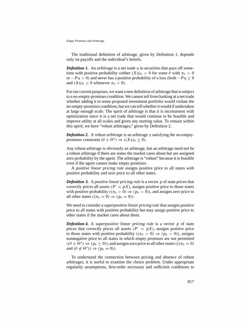
The traditional definition of arbitrage, given by Definition 1, dependsonly on payoffs and the individual’s beliefs.

Definition 1. An arbitrageis a net tradeη in securities that pays off some-time with positive probability(either(Xη)θ > 0 for someθ with πθ > 0or−Pη > 0) and never has a positive probability of a loss(both−Pη ≥ 0and(Xη)θ ≥ 0 wheneverπθ > 0).

For our current purposes, we want a new definition of arbitrage that is subjectto a no-empty-promises condition. We cannot tell from looking at a net tradewhether adding it to some proposed investment portfolio would violate theno-empty-promises condition, but we can tell whether it would if undertakenat large enough scale. The spirit of arbitrage is that it is inconsistent withoptimization since it is a net trade that would continue to be feasible andimprove utility at all scales and given any starting value. To remain withinthis spirit, we have “robust arbitrages,” given by Definition 2.

Definition 2. A robust arbitrageis an arbitrageη satisfying the no-empty-promises constraint(θ ∈ 2∗)⇒ ((Xη)θ ≥ 0).

Any robust arbitrage is obviously an arbitrage, but an arbitrage need not bea robust arbitrage if there are states the market cares about but are assignedzero probability by the agent. The arbitrage is “robust” because it is feasibleeven if the agent cannot make empty promises.

A positive linear pricing ruleassigns positive price to all states withpositive probability and zero price to all other states.

Definition 3. A positive linear pricing ruleis a vectorp of state prices thatcorrectly prices all assets(P′ = pX), assigns positive price to those stateswith positive probability((πθ > 0)⇒ (pθ > 0)), and assigns zero price toall other states((πθ = 0)⇒ (pθ = 0)).

We need to consider asuperpositive linear pricing rulethat assigns positiveprice to all states with positive probability but may assign positive price toother states if the market cares about them.

Definition 4. A superpositive linear pricing ruleis a vector p of stateprices that correctly prices all assets(P′ = pX), assigns positive priceto those states with positive probability((πθ > 0) ⇒ (pθ > 0)), assignsnonnegative price to all states in which empty promises are not permitted((θ ∈ 2∗)⇒ (pθ ≥ 0)), and assigns zero price to all other states(((πθ = 0)and(θ 6∈ 2∗))⇒ (pθ = 0)).

To understand the connection between pricing and absence of robustarbitrages, it is useful to examine the choice problem. Under appropriateregularity assumptions, first-order necessary and sufficient conditions to

817


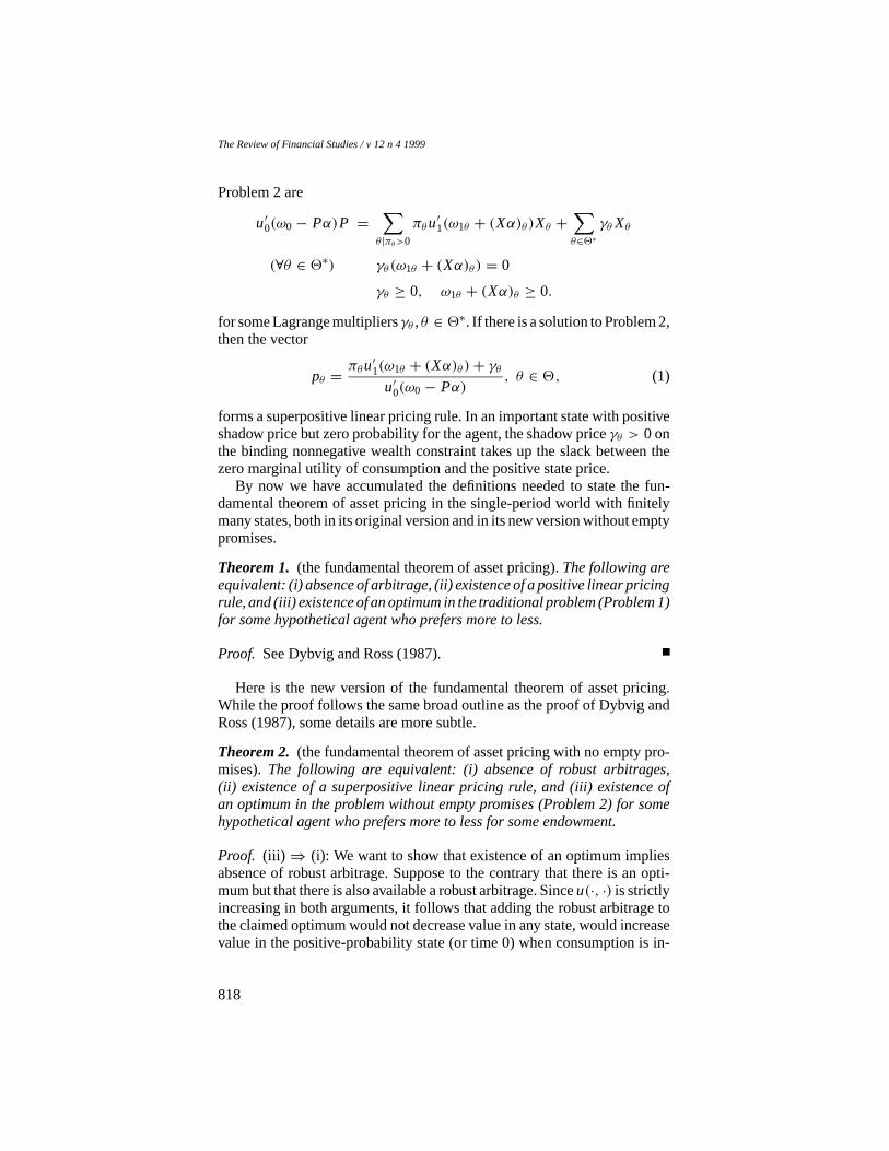
Problem 2 are

u′0(ω0− Pα)P =∑θ |πθ>0

πθu′1(ω1θ + (Xα)θ )Xθ +

∑θ∈2∗

γθ Xθ

(∀θ ∈ 2∗) γθ (ω1θ + (Xα)θ ) = 0

γθ ≥ 0, ω1θ + (Xα)θ ≥ 0.

for some Lagrange multipliersγθ ,θ ∈ 2∗. If there is a solution to Problem 2,then the vector

pθ = πθu′1(ω1θ + (Xα)θ )+ γθu′0(ω0− Pα)

, θ ∈ 2, (1)

forms a superpositive linear pricing rule. In an important state with positiveshadow price but zero probability for the agent, the shadow priceγθ > 0 onthe binding nonnegative wealth constraint takes up the slack between thezero marginal utility of consumption and the positive state price.

By now we have accumulated the definitions needed to state the fun-damental theorem of asset pricing in the single-period world with finitelymany states, both in its original version and in its new version without emptypromises.

Theorem 1. (the fundamental theorem of asset pricing).The following areequivalent: (i) absence of arbitrage, (ii) existence of a positive linear pricingrule, and (iii) existence of an optimum in the traditional problem (Problem 1)for some hypothetical agent who prefers more to less.

Proof. See Dybvig and Ross (1987).

Here is the new version of the fundamental theorem of asset pricing.While the proof follows the same broad outline as the proof of Dybvig andRoss (1987), some details are more subtle.

Theorem 2. (the fundamental theorem of asset pricing with no empty pro-mises).The following are equivalent: (i) absence of robust arbitrages,(ii) existence of a superpositive linear pricing rule, and (iii) existence ofan optimum in the problem without empty promises (Problem 2) for somehypothetical agent who prefers more to less for some endowment.

Proof. (iii) ⇒ (i): We want to show that existence of an optimum impliesabsence of robust arbitrage. Suppose to the contrary that there is an opti-mum but that there is also available a robust arbitrage. Sinceu(·, ·) is strictlyincreasing in both arguments, it follows that adding the robust arbitrage tothe claimed optimum would not decrease value in any state, would increasevalue in the positive-probability state (or time 0) when consumption is in-

818


creased, and would not violate the no-empty-promises constraint. Thereforeit would dominate the claimed optimum, which is a contradiction.

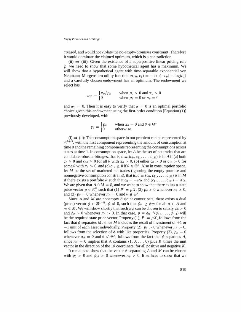
(ii) ⇒ (iii): Given the existence of a superpositive linear pricing rulep, we need to show that some hypothetical agent has a maximum. Wewill show that a hypothetical agent with time-separable exponential vonNeumann–Morgenstern utility functionu(c0, c1) = −exp(−c0)+ log(c1)

and a carefully chosen endowment has an optimum. The endowment weselect has

ω1θ ={πθ/pθ when pθ > 0 andπθ > 00 whenpθ = 0 orπθ = 0

andω0 = 0. Then it is easy to verify thatα = 0 is an optimal portfoliochoice given this endowment using the first-order condition [Equation (1)]previously developed, with

γθ ={

pθ whenπθ = 0 andθ ∈ 2∗0 otherwise.

(i) ⇒ (ii): The consumption space in our problem can be represented by<1+2, with the first component representing the amount of consumption attime 0 and the remaining components representing the consumptions acrossstates at time 1. In consumption space, letA be the set of net trades that arecandidate robust arbitrages, that is,c ≡ (c0, c11, . . . , c12) is in A if (a) bothc0 ≥ 0 andc1θ ≥ 0 for all θ with πθ > 0, (b) eitherc0 > 0 or c1θ > 0 forsomeθ with πθ > 0, and (c)c1θ ≥ 0 if θ ∈ 2∗. Also in consumption space,let M be the set of marketed net trades (ignoring the empty promise andnonnegative consumption constraint), that is,c ≡ (c0, c11, . . . , c12) is in Mif there exists a portfolioα such thatc0 = −Pα and(c11, . . . , c12) = Xα.We are given thatA∩M = ∅, and we want to show that there exists a stateprice vectorp ∈ <2+ such that (1)P′ = pX, (2) pθ > 0 wheneverπθ > 0,and (3)pθ = 0 wheneverπθ = 0 andθ 6∈ 2∗.

Since A and M are nonempty disjoint convex sets, there exists a dual(price) vectorφ ∈ <1+2, φ 6= 0, such thatφa ≥ φm for all a ∈ A andm ∈ M . We will show shortly that such aφ can be chosen to satisfyφ0 > 0andφθ > 0 wheneverπθ > 0. In that case,p ≡ φ0

−1(φ11, . . . , φ12) willbe the required state price vector. Property (1),P′ = pX, follows from thefact thatφ separatesM , sinceM includes the result of investment of+1 or−1 unit of each asset individually. Property (2),pθ > 0 wheneverπθ > 0,follows from the selection ofφ with like properties. Property (3),pθ = 0wheneverπθ = 0 andθ 6∈ 2∗, follows from the fact thatφ separatesA,sinceπθ = 0 implies thatA contains(1,0, . . . ,0) plus K times the unitvector in the direction of the 1θ coordinate, for all positive and negativeK .

It remains to show that the vectorφ separatingA andM can be chosenwith φ0 > 0 andφ1θ > 0 wheneverπθ > 0. It suffices to show that we

819


can choose separateφ’s to make each corresponding element (φ0 or φ1θ )positive, since the sum of suchφ’s will still separateA and M but willmake them all positive. Fixθ with πθ > 0, and suppose there are no robustarbitrages. (The argument forφ0 is identical; only the notation is slightlydifferent.) Arguing by contradiction, assume noφ separatingA andM hasφ1θ > 0. Recall that the dual to a setX ∈ <N is defined to be the convexset X+ ∈ <N defined byX+ ≡ {y | (∀x ∈ X) yx ≥ 0}. The set ofφ’sseparatingA andM is given by the nonzero elements ofA+ ∩ (−M)+.10

Since (by our assumption in the argument by contradiction) noφ sepa-rating M and A hasφ1θ > 0, and since noφ separatingA and M canhaveφ1θ < 0 (or it would not separateA, sinceπθ > 0), it follows thatA+ ∩ M+ ⊆ {φ | φ1θ = 0}, or equivalently,{φ | φ1θ = 0}+ ⊂ (A+ ∩M+)+ [by property (i) of convex cones given before Karlin (1959) Theo-rem 5.3.1]. By the duality theorem for closed convex cones [Karlin (1959),Theorem B.3.1, parts I and II], it follows, using the usual overline notation

for set closure, that{φ | φ1θ = 0}+ ⊆ (A+∩M+)+ ⊆ M + A = M+ A =M + A, where the first equality follows from the fact thatA is a poly-hedral cone andM is a subspace [Rockafellar (1970), Theorem 20.3], andthe second equality comes from the fact thatM is closed. However, thiscontradicts absence of robust arbitrage, since the set{φ | φ1θ = 0}+ in-cludes the vector with all zeros except for−1 in the component 1θ , andthereforeM includes an element ofA plus the vector of all zeros except for1 in the component 1θ , which is itself an element ofA. This completes theproof that (i)⇒ (ii).

3. The Continuous-Time Analysis

We now turn to the continuous-time version of the fundamental theoremof asset pricing without empty promises. The intuition of the finite-stateresults holds once we add structure to accommodate infinite-dimensionalstate spaces typically used in investments and option pricing.

3.1 DefinitionsThe agent trades finitely many risky securities in a frictionless, competitive,and possibly incomplete market over a trading interval [0, T ]. Securityreturns are defined on a probability space(Ä,F, P), whereÄ contains theset of states of nature and theσ -algebraF contains the events distinguishableat timeT . The probability measureP is a reference measure and is usedonly to define returns in states to which the agent may or may not assignpositive probability. We have no need to specify separately the price and

10 Since the setM of marketed net trades is a subspace,−M = M and therefore(−M)+ is the same asM+,but this fact is not needed for the proof.

820


dividend processes, so we simply assume that returns are generated by somespecial semimartingale processG, as in Back (1991).11 We also assume thatthere is an asset with a locally riskless instantaneous return represented byrtdt. Return processes and their coefficients are assumed to be adaptedto a given right-continuous complete filtrationF = {Ft : t ∈ [0, T ]} thatsatisfiesFT = F . Corresponding to a given trading strategyθ for the riskyassets, there is a right-continuous wealth process that satisfies

(∀t ∈ [0, T ]) Wt = W0+∫ t

0ruWu du+

∫ t

0θu dGu, (2)

P almost everywhere. To ensure that the process in Equation (2) is welldefined, we assume that each trading strategy isF predictable and satisfiesintegrability conditions used to define stochastic integrals. Let2 denotethe linear space of these strategies for which Equation (2) has a uniquesolution.12

The agent’s beliefs are represented by a probability measurePI . Weassume thatPI is absolutely continuous relative to the reference measureP so that, after the fact, the agent and the market agree on trading profits.13

Preferences for consumption plans(c0, c1) are represented by the expectedutility function

U (c0, c1) ≡ u0(c0)+∫Ä

u1(ω, c1(ω))PI (dω),

whereu0(·) andu1(ω, ·) are continuous, increasing, and defined on<+. Theexamples in Section 1 are special cases of this setting whenP is interpretedas a weighted average of the agent’s prior and conditional beliefs.

We now define the commodity space for the agent. In infinite-state modelssuch as ours, the topology of the commodity space is important because itinfluences the definitions of arbitrage and linear pricing. In our case, thetopology must also allow convergence in important states of nature, even ifthe agent assigns them zero probability. A commodity space that is suitablefor our purposes isC ≡ < × L p(Ä,F, P), for some 1≤ p < ∞, whereL p(Ä,F, P) is the space ofP-equivalent random variables that have finite

11 A special semimartingale is a process that is uniquely representable as the sum of a predictable right-continuous finite-variation process and a right-continuous local martingale [Dellacherie and Meyer (1982,VII.23)]. A special semimartingale may be discontinuous.

12 Predictability requires strategies at timet to depend on information available only strictly before timet .See Dellacherie and Meyer (1982, Chapter VIII) for conditions sufficient to define stochastic integralsand Protter (1990, Chapter 5.3) for conditions sufficient to ensure unique solutions.

13 In discrete models, trading profits are defined sample path by sample path, and this would not be an issue,but stochastic integrals defining trading profits in continuous time are not. Agreeing on trading profitsafter the fact does seem to be a feature of the actual economy, and absolute continuity ofPI in P impliesthat two agents agree on trading profits almost surely in bothP andPI . This seems like a very minimalsort of rationality assumption for us to make.

821


pth moments.14 We will take convergence and continuity to be in the productnorm topology onC.

The traditional choice problem of the agent is given in Problem 3.

Problem 3. Choose consumption(c0, c1) ∈ C to maximize expected utilityU (c0, c1) subject to the following conditions:

(a) There is a trading strategyθ ∈ 2 for which wealth satisfies Equa-tion (2) and the conditions W0 ≤ w − c0 and c1 ≤ WT, P almost surely.

(b) c1 and W are nonnegative in states important to the agent(PI (c1 ≥0) = 1) and((∀t ∈ [0, T ]), Wt ≥ 0), PI almost surely).15

In the no-empty-promises setting, the agent faces the additional con-straint of being unable to make “empty promises” in some subsetÄ∗ of im-portant states: the agent must maintain nonnegative wealth alongP almostall pathst 7→ Wt (ω),ω ∈ Ä∗. We assume thatÄ∗ belongs to theσ -algebraF . As in the finite-state model, the no-empty-promises constraint may bemotivated by a requirement that trading partners will not permit the agentto risk insolvency. Notice that ifP(Ä∗) = 0, then the no-empty-promisesrestriction is vacuous, and the problem would be essentially the same withor without empty promises.

We include the no-empty-promises constraint in Problem 4.


(a) There is a trading strategyθ ∈ 2 for which wealth satisfies Equa-tion (2) and the conditions W0 ≤ w − c0 and c1 ≤ WT, P almost surely,

(b) c1 and W are nonnegative in states important to the agent(PI (c1 ≥0) = 1) and((∀t ∈ [0, T ]), Wt ≥ 0), PI almost surely).

(c) Consumption and wealth satisfy the no-empty-promises condition(c1 ≥ 0 and((∀t ∈ [0, T ]), Wt ≥ 0), for P almost allω ∈ Ä∗).

Unlike Problem 3, Problem 4 includes the no-empty-promises constraint(c), which requires consumption and the paths of wealth to be nonnegativein almost all states important to the market.

We now define a traditional arbitrage. The intuition is similar to thefinite-state setting except that a nonnegative wealth constraint is imposedonly along paths the agent cares about.

14 An additional assumption that the Radon–Nikodym derivatived PI

d P is essentially bounded would ensurethat the commodity space is consistent for all agents and any consumption plan isp integrable againstany agent’s beliefs. This assumption is satisfied, for example, in our finite-state analysis and Examples 4and 5 of Section 1; however, we do not use this assumption in our analysis.

15 The agent can choose arbitrarily negative consumption in states occurring with zeroPI probability becausethese states do not enter into the expected utility calculation.

822


Definition 5. An arbitrage opportunityis a consumption plan(c0, c1) ∈ Cfinanced by a trading strategyθ ∈ 2 such that

(a) Wealth satisfies Equation (2) with no initial investment(c0 = −W0).(b) Wealth is nonnegative on paths the agent believes are possible; that

is, ((∀t ∈ [0, T ]) Wt ≥ 0), PI almost surely.(c) The agent believes that(c0, c1) is nonnegative and provides positive

consumption with positive probability; that is, [PI (c1 ≥ 0) = 1 andc0 ≥ 0]and [eitherPI (c1 > 0) > 0 orc0 > 0].

A robust arbitrage additionally enforces the no-empty-promises condi-tion along paths the market cares about. It is “robust” because it will befeasible even if no empty promises are permitted.

Definition 6. A robust arbitrageis an arbitrage opportunity which satisfiesthe no-empty-promises constraint:((∀t ∈ [0, T ]) Wt ≥ 0) for P almost allω ∈ Ä∗.

In general, we cannot tell whether adding a given net trade to some un-known portfolio violates the nonnegative wealth or the no-empty-promisesconstraint of an investor; however, we can tell if it will when undertakenat an arbitrarily large scale. The spirit of arbitrage is that it is inconsistentwith optimization since it is a net trade which would continue to be feasibleand improve utility at all scales and given any initial feasible plan. Bothdefinitions of arbitrage here remain within this spirit.

In contrast to the finite-state case, the set of marketed net trades generallyis not the intersection of an affine subspace with the positive orthant due tofree disposal implicit in the financing conditionc1 ≤ WT , and more subtly,due to suicidal strategies even ifc1 = WT holds.16 However, this set doesform a convex cone, which we denote byM . Formally, M is the convexcone of marketed net trades ignoring nonnegative consumption constraints:the set of(c0, c1) ∈ C such that (a) there is a trading strategyθ ∈ 2 withW satisfying Equation (2) and the conditionsc0 ≤ −W0 andc1 ≤ WT , and(b) the condition((∀t ∈ [0, T ]) Wt ≥ 0) holdsPI almost surely. SimilarlydefineM for the no-empty-promises setting by adding to (b) the conditionthat((∀t ∈ [0, T ]) Wt ≥ 0) for P almost allω ∈ Ä∗.

Here is the definition of a positive linear pricing rule. In this and thefollowing definitions, we useL p to denote the linear spaceL p(Ä,F, P).

Definition 7. A continuous linear functionalψ : L p→ < defines a positivelinear pricing rule if it satisfies the following conditions:

(a) Each net trade(c0, c1) ∈ M has a nonpositive price equal toc0 +ψ(c1) ≤ 0.

16 An example of a “suicidal strategy” is a doubling strategy run in reverse. A suicidal strategy is a net tradethat permits an agent to throw away wealth; see Dybvig and Huang (1989) for an analysis of doublingand suicidal strategies in the presence of a nonnegative wealth constraint.

823


(b) Any terminal consumption planc1 which the investor believes ispositive has a positive price(i.e., togetherPI (c1 > 0) > 0 andPI (c1 ≥0) = 1 imply thatψ(c1) > 0).

(c) For any terminal consumption planc1 for which there is a feasibletrading strategyθ ∈ 2 such that wealth satisfies Equation (2) and theconditionc1 ≤ WT , we haveψ(c1) ≤ W0.

(d) Terminal consumption plans positive only on events to which theagent assigns zero probability are costless(i.e., (∀E ∈ F)(PI (E) = 0⇒ψ(1E) = 0)).17

Here is the definition of a “superpositive” linear pricing rule which mayassign positive prices to important states, even to those impossible from theagent’s perspective.

Definition 8. A continuous linear functionalψ : L p→ < defines a super-positive linear pricing rule if it satisfies the following conditions:

(a) Any net trade(c0, c1) ∈ M has a nonpositive price equal toc0 +ψ(c1) ≤ 0.

(b) Any terminal consumption planc1 that satisfies the no-empty-promises condition and which the agent believes is positive has a posi-tive terminal price(i.e., the conditionsPI (c1 > 0) > 0, PI (c1 ≥ 0) = 1,andc1 ≥ 0 for P almost allω ∈ Ä∗ imply thatψ(c1) > 0).

(c) For anyc1 for which there is a feasible strategyθ ∈ 2 such thatwealth satisfies Equation (2) andc1 ≤ WT , we haveψ(c1) ≤ W0.

(d) Consumption plans that are positive only on events that are importantto neither the agent nor the market are costless(i.e., (∀E ∈ F)([ PI (E) =0 & P(E ∩Ä∗) = 0]⇒ ψ(1E) = 0)).

We now formalize a notion of arbitrage in this continuous-time setting.We will use the concept of a “free lunch” to extend the notion of arbitrage toinclude continuity and free disposal.18 A free lunch differs from an arbitragein that a free lunch relies on the topology of the commodity space. Thetrouble with a free lunch is that each consumption plan in the sequencemay be infeasible, yet the limit is called a free lunch. A free lunch will beattractive if there exists an agent in the economy who is willing to absorb adeviation that is “small” in the topology.19

We now define the notation that we use to define a robust free lunch. Let

17 The indicator function 1E equals 1 ifω ∈ E and 0 otherwise.18 Absence of arbitrage is generally insufficient to guarantee the existence of a continuous linear pricing rule.

A problem is that the interior of the nonnegative orthant is empty in most interesting infinite-dimensionalspaces, thus invalidating most separating hyperplane theorems. See Ross (1978), Kreps (1981), and Backand Pliska (1991) for more details.

19 This agent cannot be our agent because adding the topologically small deviation may cause our agent’sconsumption to lie outside the consumption set.

824


A be candidate arbitrage payoffs in the traditional setting,

A ≡ {(c0, c1) ∈ C: PI (c1 ≥ 0) = 1 and [PI (c1 > 0) > 0 orc0 > 0]},

and similarly defineA in the no-empty-promises setting to be

A ≡ A∩ {(c0, c1) ∈ C: c1 ≥ 0 for P-almost allω ∈ Ä∗} .Note thatA and A are convex cones that exclude the origin. LetX denoteclosure in the product norm topology for a subsetX of C. Here is a versionof arbitrage which suits our purpose.

Definition 9. A free lunchis a candidate arbitrage which is the limit of asequence of net trades less free disposal taken in states important to theagent; that is, it is an element ofA ∩ (M − A). A robust free lunchis acandidate robust arbitrage which is the limit of a similar sequence with freedisposal taken additionally in states important to the market; that is, it is an

element ofA∩ (M − A).

Note that a robust arbitrage is a robust free lunch. The limit of the se-quence of portfolios of butterfly spreads in Example 6 of Section 1 is anexample of a robust free lunch. Note, however, that none of the portfoliosin the sequence is a robust arbitrage because of the (arbitrarily small butfixed) initial wealth required to purchase the portfolio.

Free disposal in this setting allows us to consider sequences of net tradeswhich might otherwise become “too good” to remain in the commodityspace by freely disposing of consumption in states important to either theagent or the market. This is needed for technical reasons: a consumptionsequence becoming larger and larger in important states may not convergeand would fail to be an arbitrage opportunity. The definition of a free lunchcaptures our intuition that something dominating an arbitrage payoff inimportant states also should be an arbitrage opportunity.

We now turn to our definition of optimality. Back and Pliska (1991)suggest that something stronger than optimality is required for the existenceof an optimum for some agent to imply either continuous linear pricing orabsence of free lunches. Their suggestion applies here.20 Our final definitionprovides a notion of optimality sufficient for our purpose.

Definition 10. An optimal consumption demand(c0, c1) is called astrongoptimumif it is also optimal in the closure of the set that consists of theelements in the budget set plus net trades less free disposal.

20 This is again a problem of the empty interior of the nonnegative orthant of the commodity space. Previousstudies of the fundamental theorem often assume that preferences are continuous and defined over negativeconsumption. [See, for example, Kreps (1981) and Back (1991)]. Our model requires something differentbecause we rule out negative consumption.

825


The budget set, the set of marketed net trades, and the set of potentialarbitrage opportunities depend on whether or not the agent faces the no-empty-promises constraint. LetB denote the budget set of consumptionsatisfying (a) and (b) in the traditional choice problem (Problem 3), and letB denote the analogous budget set for Problem 4. Strong optimality in theno-empty-promises problem, for example, requires the agent to be unableto approximate a consumption plan providing higher expected utility than(c0, c1) using a sequence from the setB+ M − A. The need to take closurearises becauseB+ M − A may not be closed, even if the individual setsB,M , andA are.21

3.2 ResultsWe now have enough to state a continuous-time version of the traditionalfundamental theorem of asset pricing.

Theorem 3. (the fundamental theorem of asset pricing).The followingstatements are true. (i) The absence of free lunches is equivalent to theexistence of a positive linear pricing rule. (ii) If there exists a positivelinear pricing rule, then there exists a solution to Problem 3 for some hy-pothetical agent who prefers more to less. (iii) If there exists a solution toProblem 3 for an agent who prefers more to less, then there are no arbitrageopportunities. If, in addition, there is a strong optimum for Problem 3, thenthere are no free lunches.

Theorem 3 can be proven by adapting the proof of our next theorem, so wepostpone the proof of Theorem 3. Here is the version of the fundamentaltheorem of asset pricing that has the no-empty-promises constraint.

Theorem 4. (the fundamental theorem of asset pricing without emptypromises).The following statements are true. (i) The absence of robustfree lunches is equivalent to the existence of a superpositive linear pricingrule. (ii) If there exists a superpositive linear pricing rule, then there exists asolution to Problem 4 for some hypothetical agent who prefers more to less.(iii) If there exists a solution to Problem 4 for an agent who prefers more toless, then there are no robust arbitrage opportunities. If, in addition, thereis a strong optimum for Problem 4, then there are no robust free lunches.

Proof of Theorem 4. (i) Suppose there are no robust free lunches; by defini-

tion, this means thatA∩(M − A) = ∅. The set of marketed net tradesM andthe set of potential robust arbitrage payoffsA are nonempty disjoint convexcones, so we can use the separation theorem of Clark (1993, Theorem 5)

21 The appendix of Dybvig and Huang (1989) presents an example of this in a portfolio problem, buterrors in the typesetting make the example unreadable. The original correct version is available fromDybvig.

826


to obtain a continuous linear functionalφ: C → < that strictly separatesM from A; that is,φ satisfies the condition(∀a ∈ A)(∀m ∈ M) φ(m) ≤0< φ(a).22 Let E be an arbitrary event that occurs with positivePI prob-ability. Notice that the consumption plan(1,0), which provides one unit ofconsumption today and none next period, and the consumption plan(0,1E),which provides no consumption today and one unit next period if eventEoccurs, are potential robust arbitrage opportunities. Becauseφ separatesAandM , the inequalitiesφ(1,0) > 0 andφ(0,1E) > 0 must hold.

We will now useφ to construct our continuous superpositive linear pric-ing rule. Define a new continuous linear functionalφ by

φ(c0, c1) = φ(c0, c1)

φ(1,0)= c0φ(1,0)+ φ(0, c1)

φ(1,0)≡ c0+ ψ(c1).

(Recall thatc0 is nonrandom andφ is linear.) It is easy to check thatφ is alsoa continuous linear functional that separatesM from A, so condition (a) ofDefinition 8 holds. Condition (b) is true forφ, and it is true forφ for the samereasons. To verify condition (c), note that ifc1 is financed byW0, then theconsumption plan(−W0, c1) is a net trade inM . Thus condition (a) impliesthatψ(c1) ≤ W0. We now need to show that condition (d) holds. LetE ∈ Fbe an arbitrary event. For any given whole numbern, the consumption plan(0, 1

n1Ä + 1E) belongs toA and must have a positive price; therefore,ψ(1E) ≥ 0 by the continuity ofφ. Furthermore, note that for anyE ∈ Fwith PI (E) = 0 andP(E ∩Ä∗) = 0, the consumption plan(0,1Ä+ λ1E)

belongs toA for all realλ. Strict separation requires the condition

ψ(1Ä + λ1E) = ψ(1Ä)+ λψ(1E) > 0 for all realλ

to hold, which would be true only ifψ(1E) = 0. Thusψ defines a continuoussuperpositive linear pricing rule.

Conversely, suppose that we are given someψ that defines a superpositivelinear pricing rule; we want to show that there are no robust free lunches.Suppose to the contrary that one exists; we will obtain a contradiction.For m = (c0, c1) ∈ C, define the continuous linear functionalφ(m) =c0 + ψ(c1). Our contrary hypothesis is that there exists a sequence{mn −an} ⊂ M − A converging to somea ∈ A. This is impossible becauseφ iscontinuous and by definition must satisfy the condition(∀n) φ(mn−an) <

φ(mn) ≤ 0< φ(a). Therefore, there cannot be a robust arbitrage.(ii) We now want to show that there exists an optimum to the consumption

choice problem of a hypothetical agent who faces a no-empty-promisesconstraint, but we must develop some notation first. Letξ I define the Radon–

22 Specifically, Clark shows that two nonempty convex conesJ andK (with vertices at the origin) in a sepa-rable Banach space (like our consumption space) can be strictly separated if and only ifJ∩ (K − J) = ∅.

827


Nikodym derivatived PI /d P, and letψ be the linear functional that definesthe given superpositive linear pricing rule. The Riesz representation theoremimplies that there existsν ∈ Lq(Ä,F, P), 1/q + 1/p = 1, such that

ψ(c1) = E[νc1] for all c1 ∈ L p(Ä,F, P). (3)

Becauseψ defines a superpositive linear pricing rule,ν(ω) ≥ 0, PI almostsurely and forP almost allω ∈ Ä∗, andν(ω) > 0 if ξ I (ω) > 0.

We now demonstrate that there is a solution to Problem 4 for an agentwith initial endowmentw = 0 and state-dependent preferences

U (c0, c1) = −exp(−c0)−∫Ä

exp(−(y(ω)+ c1(ω)))PI (dω),

where

y(ω) ={

log ξ I (ω)

ν(ω)if ξ I (ω) > 0

0 if ξ I (ω) = 0.

Consider the following new choice problem: choose(c0, c1) ∈ C to maxi-mizeU (c0, c1) subject to the budget constraintc0+ψ(c1) = c0+E[νc1] ≤0 and the nonnegativity conditionc1 ≥ 0, that holdsPI almost surely andfor P almost allω ∈ Ä∗. A solution to this new problem is optimal forProblem 4 if there is a trading strategy that finances it. First-order sufficientconditions for a solution to the new problem are

ξ I (ω)exp(−(y(ω)+ c1(ω)))+ λ1(ω) = γ ν(ω)exp(−c0)+ λ0 = γγ (c0+ E[νc1)]) = 0

λ1(ω)c1(ω) = 0, andλ0c0 = 0 almost surely

for some Lagrange multipliersλ1 ∈ Lq+ andλ0, γ ∈ <+ [see, e.g., Duffie

(1988, p. 77)]. The Lagrange multipliersλ0 andλ1 are the shadow prices forthe nonnegative constraints onc0 andc1, respectively, andγ is the marginalutility of wealth. A solution to the new problem isc0 = 0,c1 ≡ 0,γ = 1, andλ(ω) = ν(ω) if ξ I (ω) = 0 holds andλ(ω) = 0 otherwise. The multiplierλ belongs toLq

+ since it satisfies 0≤ λ ≤ ν andν ∈ Lq+, soc1, λ, andγ

satisfy the first-order and the complementary slackness conditions. This isa solution to Problem 4 sinceθ ≡ 0 is trivially feasible and financesc1.

(iii) The existence of an optimal demand rules out robust arbitrage op-portunities, for the net trade could be added to any candidate optimum,increasing expected utility without violating the no-empty-promises con-straint. If(c0, c1) is a strong optimum, then the intersection of(c0, c1)+ A

with (B+ M − A)must be empty since preferences are monotonically in-

828


creasing. Because(c0, c1) ∈ B, we haveA ∩ (M − A) = ∅, which is thecondition for absence of robust free lunches. This finishes our proof.

Remark: Hindy (1995) writes his pricing rule as the sum of the direct con-tribution to expected utility and the shadow price of his solvency constraint.In our notation, the price in Equation (3) can be written as

ψ(c1) = E[1{ξ I>0}νc1

]+ E[1{ξ I=0}νc1

] ≡ ψ I (c1)+ ψ∗(c1).

whereψ I andψ∗ are continuous linear functionals. The latter is nontrivialwhenever the no-empty-promises constraint is binding and nonvacuous (i.e.,P({ξ I = 0}∩Ä∗}) > 0). Thusψ∗ can be interpreted as the shadow price ofthe no-empty-promises constraint, analogous to Hindy’s “solvency price.”For the examples in Section 1, the state price density in the original problemby Merton could be used to define a superpositive linear pricing rule for anagent who has advance information. In these examples, the linear functionalψ∗ would be nontrivial.

We now prove Theorem 3.

Proof of Theorem 3. We make use of our work in the proof of Theorem 4.(i) The proof of parts (a), (b), and (c) of Definition 7 is exactly the same as thecorresponding parts of Definition 8 given in the proof of Theorem 4, whereA andM are replaced byA andM , respectively. To prove part (d), note thatfor any E ∈ F that satisfies the conditionPI (E) = 0, the correspondingconsumption plan(0,1Ä+λ1E) belongs toA for all realλ. Strict separationimplies that

ψ(1Ä + λ1E) = ψ(1Ä)+ λψ(1E) > 0 for all realλ,

which holds only if the conditionψ(1E) = 0 is satisfied.(ii) This part is nearly the same, except for the absence of the no-empty-

promises constraint. However, the sets{ν(ω) > 0} and{ξ I (ω) > 0} differonly by a nullset, so analogous first-order conditions hold at an optimum.

(iii) Apply the same argument toA andM .

4. Enforcement of No Empty Promises

A potential conceptual problem with the general analysis is one of enforce-ment: How do we ensure that an agent chooses a strategy with nonnegativewealth in states that the agent believes will never happen? We now showthat if information arrival is continuous, then shutting down the agent’s in-vestments for the duration once wealth hits zero is essentially equivalent toruling out empty promises. With continuous information arrival, the marketknows the agent’s wealth cannot go below zero without first hitting zero.By contrast, the wealth could jump from positive to negative without warn-

829


ing in a model with discrete trading or unpredictable jumps in the returndistribution.

For simplicity, we assume that the risky assets’ instantaneous returns arerepresented by

µtdt + σtd Zt ,

whereZ is a standard multidimensional Brownian motion. We follow theusual practice of defining the filtrationF, which represents informationarrival, to be the filtration generated byZ and augmented withP nullsets;this filtration is continuous [Karatzas and Shreve (1988, Section 2.2.7)].

Trading strategies must satisfy the conditions assumed in Section 4, in-cluding those needed to define stochastic integrals. In particular, tradingstrategies must be predictable. Modifying a strategy to stop investmentwhen wealth first hits zero will not violate any of these conditions, sincethe time when wealth first hits zero is a stopping time.

For implementation, we want to think of two different types of stoppingtimes. A private version of stopping time available to the agent is the usualdefinition of stopping time. In this definition it is assumed that the stochasticprocess is known (in this case from knowledge of the agent’s strategy). Apublic type of stopping time is one that depends on the wealth historyand not on knowledge of the agent’s particular strategy. An example of apublic stopping time is stopping when the agent’s wealth hits zero, which issomething the market can implement without knowing the agent’s strategy.An example of a private stopping time is the last time before wealth first goesnegative (which is a stopping time because of the continuous informationarrival). A private stopping time is available to the agent (to whom thestrategy is known) for construction of an arbitrage, but not to the market’sregulatory mechanism. Our proof of enforceability of no-empty-promisesuses stopping when wealth hits zero, which is our example of a publicstopping time.

We state a new consumption choice problem which includes a constraintthat shuts down the agent’s investment when wealth first hits zero.


(a) There is a trading strategyθ ∈ 2 for which wealth satisfies Equa-tion (2) and the conditions W0 ≤ w − c0 and c1 ≤ WT, P almost surely.

(b) c1 and W are nonnegative in states important to the agent(PI (c1 ≥0) = 1) and((∀t ∈ [0, T ]), Wt ≥ 0), PI almost surely).

(c) The agent’s trades are shut down at the first instant that wealthbecomes zero; that is,((∀t)(Wt = 0⇒ (∀s> t)θs = Ws = 0)), PI almostsurely.

Problem 5 differs from Problem 4 only in constraint (c): the no-empty-promises condition in Problem 4 is replaced by the shutdown constraint in

830


Problem 5. In the shutdown constraint, we use the agent’s information setsince optimization is from the agent’s perspective. Nothing essential wouldbe changed if we required this to hold in states important to the market aswell.

We now state our main result on enforcement. It says that from theperspective of optimal choice, the no-empty-promises constraint can bereplaced by a constraint that shuts down the agent’s investment when wealthfirst hits zero.

Theorem 5.Assume that information arrival is continuous and that Prob-lem 4 or Problem 5 has a solution. Further assume that there exists atrading strategy giving a payoff bounded below away from zero and a pos-itive wealth process (as there would if there exists a locally riskless assetwith a nonnegative interest rate process). Then the problems are equivalentin the following sense:

(i) Suppose(θ,W,C) is feasible in one of Problem 4 and Problem 5. Thendefine the new strategy,(θ , W, C), by closing out the agent’s investmentswhen wealth hits zero. Let

τ ={

min{t | Wt ≤ 0} if such a t existsT otherwise.

Letting ∧ indicate the minimum, we defineθt ≡ θt1{t<τ }, Wt ≡ Wt∧τ ,and C ≡ C1{τ<T}. This new strategy is just as desirable to the agent as(θ,W,C) and is feasible for both problems.

(ii) There is a strategy(θ,W,C) that is a solution to both Problem 4 andProblem 5.

We now prove Theorem 5.

Proof of Theorem 5. (i) Feasibility requiresθ to be predictable and to satisfythe integrability conditions needed to define stochastic integrals. It will bepredictable because it is adapted and because adapted strategies coincidewith predictable ones whenever information arrival is continuous. It willbe integrable because, by construction, integrals of the modified strategyθ

equal integrals of the original strategyθ up to the stopping timeτ .23 Thusthe new strategies are integrable if the original strategies are.

The statement that the two strategies are equally desirable follows froma claim thatWT = WT , PI almost surely, which we now show. If(θ,W,C)is feasible for Problem 5, the claim is immediate because stopping wealth

23 The fact thatτ is a stopping time follows from the fact that optional and predictable times coincidewhenever informational arrival is continuous [see Karatzas and Shreve (1988, Problem 1.2.7)].

831


is redundant on paths ofPI -positive probability given the shutdown con-straint. To prove the claim when(θ,W,C) is feasible only in Problem 4,we show that if it is false then there is a robust arbitrage available to theagent, which will be a contradiction to the assumption that Problem 4 orProblem 5 has a solution.

Suppose that the claim is false. ThePI -nonnegative wealth constraintimplies that there is aPI -positive probability setE that contains paths alongwhich wealth hits zero and then eventually becomes positive by timeT ; notethat 0= WT < WT on E. Define a new stopping timeτ ′ by inf{t |Wt < 0} ifsuch at exists orT otherwise. The trading strategyθt1{t∈[τ,τ ′)}, which startsinvestment atτ and shuts it down when wealth first becomes negative, paysa PI -positive amount onE and ensures that wealth satisfies no-empty-promises (i.e., wealth is pathwise nonnegativeP almost surely). Thus wehave constructed a robust arbitrage.

The existence of the robust arbitrage immediately rules out an optimumfor Problem 4. Adding the arbitrage to an arbitrary feasible strategy inProblem 5 may be infeasible, however, because the shutdown constraintmay stop investment before the arbitrage is complete. Thus we will ruleout a solution to Problem 5 by showing that the agent can shift a smallamount of initial wealth from the strategy to make the arbitrage available,and for a small enough transfer the arbitrage will make it worthwhile at largeenough scale. Together these will imply a contradiction to our assumptionthat Problem 4 or Problem 5 has a solution.

Let B be the payoff of a trading strategy giving a payoff bounded belowaway from zero and a positive wealth process, scaled to costw0 initially.Furthermore, letX > 0, X 6= 0 be the payoff to the arbitrage strategy asconstructed above. Using free disposal if necessary, we may assume withoutloss of generality thatX is a bounded random variable. Monotonicity impliesthat any terminal consumption planC in a candidate optimum will be strictlyless desirable thanC+ X; however, the latter may be infeasible, since ifCinvolves wealth hitting zero, then the agent may be shut down before thearbitrage generatingX has been played out. Letε andn be positive numbers.The consumption plan(1 − ε)C + εB + nX, formed by shifting someinitial wealth fromC to B, is feasible because it requires initial investmentw0 and because the investment inB prevents wealth from hitting zero. Ifutility U is bounded, expected utility is continuous inε andn by dominatedconvergence, and forn = 1 and small enoughε, (1− ε)C + εB + X isstrictly preferred toC. If U is unbounded, then we can choosen to be largeandε (which may depend onn and can be uniformly bounded below byan arbitrary positive number) to obtain unbounded expected utility on thePI -positive probability set of states withX > 0. In either case, Problem 5cannot have a solution, and our claim is proven.

(ii) By (i), just useτ to construct a new solution to the problem that isgiven to have a solution.

832


5. Conclusion

We have demonstrated a version of the fundamental theorem of asset pricingwhen agents have dogmatic differences of opinion but are prevented frommaking empty promises. The primary difference is that linear pricing willbe superpositive since a state assigned zero probability by the agent mayhave a positive price if it is important to the market. Superpositive linearpricing is reconciled with expected utility maximization by ruling out emptypromises in important states. The shadow price of the no-empty-promisesconstraint takes up slack between positive state prices and zero marginalutility. These results are proven for finite-state and continuous-time models.

With continuous information arrival, the no-empty-promises constraintcan be enforced by permanently shutting down the agent’s investments fromthe time wealth first hits zero.

ReferencesBack, K., 1991, “Asset Pricing for General Processes,”Journal of Mathematical Economics, 20, 371–395.

Back, K., and S. Pliska, 1991, “On the Fundamental Theorem of Asset Pricing with an Infinite StateSpace,”Journal of Mathematical Economics, 20, 1–18.

Bergman, Y., 1996, “Equilibrium Asset Price Ranges,” working paper, Hebrew University.

Clark, S., 1993, “The Valuation Problem in Arbitrage Price Theory,”Journal of Mathematical Economics,22, 463–478.

Dellacherie, C., and P.-A. Meyer, 1982,Probabilities and Potential, North-Holland, Amsterdam.

Duffie, D., 1988,Securities Markets, Academic Press, San Diego, CA.

Duffie, D., 1992,Dynamic Asset Pricing Theory, Princeton University Press, Princeton, NJ.

Dybvig, P., and C. Huang, 1989, “Nonnegative Wealth, Absence of Arbitrage, and Feasible ConsumptionPlans,”Review of Financial Studies, 1, 377–401.

Dybvig, P., and S. Ross, 1987, “Arbitrage,” in J. Eatwell, et al. (eds.),The New Palgrave: Finance,MacMillan Press, New York.

Hindy, A., 1995, “Viable Prices in Financial Markets with Solvency Constraints,”Journal of MathematicalEconomics, 24, 105–135.

Jouini, E., and H. Kallal, 1995, “Martingales and Arbitrage in Securities Markets with Transactions Costs,”Journal of Economic Theory, 5, 197–232.

Karatzas, I., and S. Shreve, 1988,Brownian Motion and Stochastic Calculus, Springer-Verlag, New York.

Karlin, S., 1959,Mathematical Methods and Theory in Games, Programming, and Economics, Addison-Wesley, Mineola, NY.

Kreps, D., 1981, “Arbitrage and Equilibrium in Economies with Infinitely Many Commodities,”Journalof Mathematical Economics, 8, 15–35.

Loewenstein, M., and G. Willard, 1997, “Unknowingly Avoiding Default in Unforeseen Contingencies:Equilibrium in a Production Economy,” working paper, Massachusetts Institute of Technology.

833


Merton, R., 1971, “Optimum Consumption and Portfolio Rules in a Continuous-Time Model,”Journalof Economic Theory, 3, 373–413.

Pikovsky, I., and I. Karatzas, 1996, “Anticipative Portfolio Optimization,”Advances in AppliedProbability, 28, 1095–1122.

Protter, P., 1990,Stochastic Integration and Differential Equations, Springer-Verlag, New York.

Rockafellar, T., 1970,Convex Analysis, Princeton University Press, Princeton, NJ.

Ross, S., 1978, “A Simple Approach to the Valuation of Risky Streams,”Journal of Business, 51, 453–485.

Wu, J., 1991, “Information Structure, Optimal Dynamic Portfolio Strategies, and the Intensity of Trading,”Ph.D. dissertation, Washington University, Saint Louis.

834

Documents

Empty Promises and Arbitrage · The usual presentation of the fundamental theorem of asset pricing typ-ically ignores payoffs in states to which the agent assigns zero probabil-ity