Emulation of Target Trials to Study the Effectiveness and Safety of Medical Interventions

CitationHuitfeldt, Anders. 2015. Emulation of Target Trials to Study the Effectiveness and Safety of Medical Interventions. Doctoral dissertation, Harvard T.H. Chan School of Public Health.

Permanent linkhttp://nrs.harvard.edu/urn-3:HUL.InstRepos:23205172

Terms of UseThis article was downloaded from Harvard University’s DASH repository, and is made available under the terms and conditions applicable to Other Posted Material, as set forth at http://nrs.harvard.edu/urn-3:HUL.InstRepos:dash.current.terms-of-use#LAA

Share Your StoryThe Harvard community has made this article openly available.Please share how this access benefits you. Submit a story .

Accessibility

 

EMULATION OF TARGET TRIALS TO STUDY THE EFFECTIVENESS

AND SAFETY OF MEDICAL INTERVENTIONS

ANDERS HUITFELDT

A Dissertation Submitted to the Faculty of

The Harvard T.H. Chan School of Public Health

in Partial Fulfillment of the Requirements

for the Degree of Doctor of Science

in the Department of Epidemiology

Harvard University

Boston, Massachusetts.

November 2015

ii    

Dissertation Advisor: Dr. Miguel A. Hernán Anders Huitfeldt

Emulation of Target Trials to Study the Effectiveness and Safety of Medical Interventions

Abstract

Ideally, clinical guidelines would be informed by well-designed randomized experiments.

However, it is generally not possible to conduct a randomized trial for every clinically relevant

decision. Decision makers therefore often have to rely on observational data. Guidelines that

rely on observational data due to the absence of randomized trials benefit when the analysis

mimics the analysis of a hypothetical target trial. This can be achieved by explicitly formulating

the protocol of the target trial, and thoroughly discussing the feasibility of the conditions that

must be met in order to validly emulate the target trial using observational data.

In chapter one, we discuss the emulation of trials that compare the effects of different timing

strategies, that is, strategies that vary the frequency of delivery of a medical intervention or

procedures, and provide an application to surveillance for colorectal cancer. In chapter two, we

discuss a study design that attempts to avoid bias by comparing initiators of the treatment of

interest with initiators of an “active comparator” that is believed to be inactive for the

outcome, in order to emulate a randomized trial that compares the treatment of interest with

an inactive comparator. In chapter three, we describe a new method that combines

randomized trial data and external information to emulate a different target trial. We apply this

iii    

method to a randomized trial of postmenopausal hormone therapy in order to emulate a trial

of a joint intervention on hormone therapy and statin therapy.

iv    

TABLE OF CONTENTS

Title Page ....................................................................................................................................... i

Abstract ......................................................................................................................................... ii

Table of Contents ......................................................................................................................... iv

List of Figures ................................................................................................................................ v

List of Tables ................................................................................................................................ vi

Acknowledgements ..................................................................................................................... vii

Litany of Tarski ............................................................................................................................... x

Chapter 1 ...................................................................................................................................... 1 Methods to estimate the comparative effectiveness of clinical strategies that administer the same intervention at different times

Chapter 2 ................................................................................................................................... 30 Comparative effectiveness research using observational data: Active comparators to emulate target trials with inactive comparators

Chapter 3 ................................................................................................................................... 56 Can the results of the WHI E+P trial be explained by differential statin initiation?

Appendix to Chapter 1 ............................................................................................................. 103

Appendix to Chapter 3 ............................................................................................................. 105  

 

v      

LIST OF FIGURES

FIGURE 1.1: FLOWCHART OF SELECTION OF THE 2190 ELIGIBLE INDIVIDUALS 7 FIGURE 1.2: THE THREE TRIAL TYPES CONSIDERED IN CHAPTER 1 13 FIGURE 1.3: ESTIMATED SURVIVAL CURVES FOR TRIALS #2 AND #3 24 FIGURE 2.1: VENN DIAGRAMS SHOWING THE GROUPS COMPARED 44 FIGURE 3.1: STATIN INITIATION OVER TIME IN THE WHI TRIAL 66 FIGURE 3.2: SURVIVAL CURVES PREDICTED FROM STANDARD MODELS 71 FIGURE 3.3: SURVIVAL CURVES PREDICTED FROM STANDARD MODELS 72 FIGURE 3.4: KAPLAN MEIER CURVES FOR WHI E+P TRIAL 73 FIGURE 3.5: KAPLAN MEIER CURVE FOR CENSORING 82 FIGURE 3.6: ADJUSTED KAPLAN-MEIER CURVE FROM SNAFTM MODEL 96 FIGURE 3.7: ADJUSTED KAPLAN MEIER CURVE FROM SNCFTM MODEL 97 FIGURE A.1: CAUSAL DIRECTED ACYCLIC GRAPH 104

vi    

LIST OF TABLES

TABLE 1.1: CHARACTERISTIC OF 2190 ELIGIBLE INDIVIDUALS 8 TABLE 1.2: ESTIMATED RISK OF COLORECTAL CANCER AT 5 AND 10 YEARS 25 TABLE 2.1: EXAMPLES OF OBSERVATIONAL STUDIES THAT USE ACTIVE COMPARATORS 35 TABLE 3.1: CHARACTERISTICS OF PARTICIPANTS IN WHI E+P TRIAL 63 TABLE 3.2: LABORATORY RESULTS IN CORE ANALYTES SUBSAMPLE 64 TABLE 3.3: CHARACTERISTICS OF PARTICIPANTS IN THE ASCOT-LLA TRIAL 65 TABLE 3.4: HAZARD RATIOS ASSOCIATED WITH HRT AND STATINS 70 TABLE 3.5: PARAMETER ESTIMATES FROM WEIGHT MODELS 83 TABLE 3.6: DISTRIBUTION OF STABILIZED WEIGHTS OVER TIME 84 TABLE 3.7: DISTRIBUTION OF UNSTABILIZED WEIGHTS OVER TIME 85 TABLE 3.8: HAZARD RATIOS FOR SECONDARY OUTCOMES 92 TABLE 3.9: SENSITIVITY ANALYSIS FOR UNWEIGHTED SNAFTM MODELS 93 TABLE 3.10: SENSITIVITY ANALYSIS FOR SNCFTM MODEL 94 TABLE 3.11: ADJUSTED HAZARD RATIOS AT THE END OF YEAR 5   95  

vii    

ACKNOWLEDGEMENTS

At the time I first enrolled as an MPH student in August 2010, I did not even know the meaning

of the word “Epidemiology”. Under ordinary circumstances, I very likely would have concluded

that the word refers to a toolbox of methods for producing a never-ending stream of

observational studies that always seem to contradict each other. Under ordinary circumstances,

the thought of becoming an epidemiologist would not even have occurred to me.

But these were no ordinary circumstances. By a genuine stroke of inspiration, the department

had assigned the introductory course to Miguel Hernán, perhaps the only professor in the

world who would even have considered the idea of using it to teach a coherent framework for

reasoning about the process whereby we obtain new knowledge about the consequences of

decisions: What I now somewhat pretentiously refer to as the epistemology of medical decision

making.

I was hooked from day 1, and after the course completed I was somehow able to talk my way

into the doctoral program and into Miguel’s research group. I will never be able to repay my

debt of gratitude to Miguel: For giving me a chance to take on this incredible challenge, for

introducing me to a way of thinking about medical research that actually makes sense, for his

unmatched ideas and suggestions about the direction of my projects, for all the incredibly hard

work he did to tighten up my informal writing style, and most of all for believing in me.

viii    

I also want to thank my research committee member Jamie Robins. Jamie has an incredible

ability to generate razor sharp insights that can completely change the direction of a research

project, sometimes even changing how one conceptualizes the research question itself.

Without his contributions, this thesis would certainly not have been possible. But above all, I

am thankful to Jamie for what has been the true highlight of my five years at HSPH: The unique

opportunity to be a teaching assistant for his groundbreaking course on advanced

epidemiologic methods, and share a small part in helping the next generation of scientists

absorb his core insights about causal inference in epidemiology. It is sometimes said that

philosophers are “doomed to find Hegel waiting patiently at the end of whatever road

they travel”.1 While the truth value of this statement is questionable in the case of Hegel, I do

not doubt that Epidemiologists will meet Jamie at the end of any path that they end up

travelling.

My research committee would not have been complete without the invaluable contributions of

Mette Kalager. Mette provided subject matter expertize in cancer screening and surveillance,

and a much needed grounding in practical, clinical reasoning. I am deeply grateful to Mette for

giving me the chance to collaborate with a fabulous and successful research group at the

University of Oslo, where I hope to maintain deep connections for the duration of my research

career, regardless of where it may take me. I also want to thank her for finding the time to

videoconference in to committee meetings at arbitrary, often inconvenient times.

                                                                                                                         1 Foucault, Michel. "The discourse on language." Truth: Engagements across philosophical traditions (1971): 315-335.

ix    

Funding for this research was provided in part by NIH grants P01 CA134294 and R01 AI102634

and in part by the Norwegian Research Council. I am grateful to everyone involved in obtaining

these grants, in particular Miguel Hernán, Michael Bretthauer and Xihong Lin.

On a personal note, I want to thank my friends in the Boston area rationality and effective

altruism community. You were there when I needed to believe that the world had not gone

insane, that there really are smart people out there who genuinely believe in truth, in reason

and in making a genuine attempt to build a world that is slightly less wrong.

Finally, I want to thank my parents for all their support throughout my 12 (!) years of higher

education. I’m ready to get a job now – I promise.

x      

LITANY OF TARSKI

If the causal effect is identified

I desire to believe that the causal effect is identified

If the causal effect is not identified

I desire to believe that the causal effect is not identified

Let me not become attached to beliefs I may not want

1      

CHAPTER 1    

   

Methods to estimate the comparative effectiveness of clinical strategies

that administer the same intervention at different times

Anders Huitfeldt, Mette Kalager, James M. Robins, Geir Hoff, Miguel A. Hernán

2      

Abstract

Clinical guidelines that rely on observational data due to the absence of data from randomized

trials benefit when the observational data or its analysis emulates trial data or its analysis. In this

paper, we review a methodology for emulating trials that compare the effects of different

timing strategies, that is, strategies that vary the frequency of delivery of a medical intervention

or procedure. We review trial emulation for comparing (i) single applications of the procedure

at different times, (ii) fixed schedules of application, and (iii) schedules adapted to the evolving

clinical characteristics of the patients. For illustration, we describe an application in which we

estimate the effect of surveillance colonoscopies in patients who had an adenoma detected

during the NORCCAP trial.

3      

1.   Introduction

Clinical decisions are increasingly reliant on guidelines, but clinical guidelines are only as good

as the available evidence on the comparative effectiveness of interventions.1 Ideally, such

evidence would come from randomized controlled trials. When a randomized trial is not

available, it may be possible to emulate it using observational data.2 This approach requires

appropriate confounding adjustment, avoidance of selection bias in the definition of the

groups to be compared, and formulation of a research question that is relevant for decision

makers.

Prior explicit attempts to emulate trials using observational data have studied, for example,

postmenopausal hormone therapy,3 statins,4 epoetin,5 and antiretroviral therapy.6, Here we

review the emulation of trials to compare strategies that differ in the timing of the intervention

of interest. As an example, we will consider post-polypectomy surveillance by colonoscopy.

During this procedure, adenomas (benign tumors of the colon)7 are detected and removed.

Most adenomas will not develop into colorectal cancer, but most cancers arise from

adenomas.8 In patients with removed adenomas, surveillance colonoscopies are recommended

to detect and remove future adenomas before they become malignant. The optimal interval

between colonoscopies is not known. Current guidelines both in the US9 and the EU10 are

mostly based on expert opinion due to the scarcity of available evidence.

4      

Besides reviewing a methodology to emulate trials for the comparison of strategies that

administer the same intervention at different times, we also review a classification of these

strategies. First, we consider point interventions to study the effectiveness of a single

application of the treatment. Second, we consider sustained interventions to study the

effectiveness of a fixed treatment schedule (e.g., colonoscopy at 3 years after the initial

procedure). Third, we consider sustained interventions to study the effectiveness of a

personalized schedule of treatment (e.g., colonoscopy every year if the most recent procedure

detected large adenomas, otherwise every 3 years). To fix ideas, we review the methodology in

the context of its implementation to a cohort of Norwegian individuals. We start by describing

this cohort.

2.   Data

The Norwegian Colorectal Cancer Prevention (NORCCAP) screening study was a randomized

clinical trial of once-only sigmoidoscopy screening versus no sigmoidoscopy, conducted in

Oslo and Telemark counties in Norway between 1999 and 2001. Our analysis includes

participants in the sigmoidoscopy arm in whom at least one adenoma was detected (n=2190).

As part of the trial, endoscopies were conducted in these individuals until the bowel was free

from adenomas. We excluded patients with history of serious gastrointestinal disease, known

genetic predisposition to colorectal cancer, and cancer detected as a result of screening in

NORCCAP.

5      

In addition to the available data (age, sex, county, smoking, family history of colorectal cancer,

and findings at NORCCAP colonoscopies), we conducted a manual chart review at all hospitals

in Oslo and Telemark—guided by claims data from the governmental single-payer agency

HELFO—to collect data on the date, findings (e.g., size and type of adenomas) and indication

of all subsequent colonoscopies and sigmoidoscopies. Of the post-screening endoscopies,

64% were for surveillance purposes (3% sigmoidoscopies and 61% colonoscopies), 30% were

clinically indicated because of symptoms (27% colonoscopies, 3% sigmoidoscopies), and 6%

were due to a recent incomplete endoscopy (4% colonoscopies, 2% sigmoidoscopies).

Our outcome of interest was incidence of colorectal cancer. For many surveillance

interventions, the use of cancer incidence as an outcome is questionable because of potential

lead time bias:11 cancer cases will be detected earlier in patients with more intensive

surveillance, which will make surveillance appear less beneficial. In this case, however, the use

of the outcome cancer incidence is justified because most of the beneficial effect of

surveillance colonoscopy seems to be due to removing adenomas before they become

malignant12, with only a small component of the effect due to earlier detection of prevalent

cancer. Death from colorectal cancer could not be studied as an outcome because there were

too few cases.

We refer to the date of the last NORCCAP colonoscopy as time of “first eligibility” for our

analyses. For each individual, follow-up ends at colorectal cancer, death, sigmoidoscopy,

6      

emigration, or December 2011, whichever occurred first. Because we are trying to estimate the

effects of post-baseline colonoscopies, which were not randomly assigned to the trial

participants, ours is an analysis of observational data. The flow chart in Figure 1.1 describes the

enrollment of participants in our study. Table 1.1 displays the characteristics of the eligible

individuals.

7      

Figure 1.1: Flowchart of selection of the 2190 eligible individuals from the intervention arm of the NORCCAP trial

 

100210  NORCCAP  participants

Sigmoidoscopy  in  1999-­‐2001:  n=20572

Adenomas  Detected  in  2211  individuals

Cancer  detectedIn  41  individuals

No  adenoma  or  cancer  detected  in    18320  individuals

2190  individuals  met  eligibility  criteria  

21  did  not  meet  eligibility  criteria:

1987  were  cancer  free  and  alive  in  

2011:

21  had  a  diagnosis  of  colon  cancer  by  

2011  

182  deaths  from  other  causes  by  

2011:

8      

Table 1.1: Characteristic of 2190 eligible individuals from the intervention arm of the NORCCAP trial

Number of men 1322 (60%) Average (SD) age at first eligibility, years 57.2 (3.8)

Median (IQR) duration of follow-up, months

134 (126-143)

Incident cases of colorectal cancer 21 detected at surveillance colonoscopy 1 Deaths 187 from colorectal cancer 5 Number of colonoscopies during follow-up

819

Number of sigmoidoscopies 75 Number of people with at least one colonoscopy after first eligibility

577

Number of people whose first follow-up colonoscopy was for surveillance

395

Median (IQR) time to first colonoscopy, months

68 (51-91)

Number of colonoscopies per individual 0 1613 (74%) 1 389 (18%) 2 140 (6%) 3+ 48 (2%)

9      

3.   Three hypothetical randomized trials

The design of any trial is determined by the causal question of interest, which in turn is

determined by the population, the strategies being compared, and the outcome of interest to

the decision makers.13 For surveillance tests, the strategies are defined by the timing of the

test. Some strategies involve a point intervention at baseline, whereas other strategies involve

interventions that are sustained over time according to either a fixed schedule (e.g., do not

perform a colonoscopy for five years after baseline, then perform a colonoscopy at the end of

year 5) or a schedule that depends on each individual’s time-evolving clinical characteristics

(i.e., schedule the time of every colonoscopy according to the findings at the previous

colonoscopy). We refer to sustained strategies with a fixed schedule as static and to those with

a subject-specific schedule as dynamic.

Here we review 3 types of hypothetical trials that compare static and dynamic strategies and

therefore address different questions regarding the effectiveness of surveillance colonoscopy.

In all trials, eligible individuals are followed until death, loss to follow-up (i.e., emigration out of

Norway), sigmoidoscopy, occurrence of the outcome (here, diagnosis of colorectal cancer), or

Dec 31st 2011, whichever occurred earlier. In all trials, individuals receive a colonoscopy

whenever it is clinically indicated (e.g., due to symptoms) but a surveillance colonoscopy only

according to the trial protocol. A graphical representation of each trial is shown in Figure 1.2.

10    

Trial type #1: Point interventions assigned at a fixed time after first eligibility

Individuals who survived 36 months since first eligibility are randomized to either 1) immediate

surveillance colonoscopy, or 2) no surveillance colonoscopy. Additional eligibility criteria are no

colorectal cancer, colonoscopy, or sigmoidoscopy during the 36 months before randomization.

Individuals who reach age 70 or develop any invasive non-colorectal cancer before baseline

also become ineligible (other comorbidities might be added to the exclusion criteria). For each

individual, follow-up starts at the time of randomization, i.e., baseline is 36 months after first

eligibility.

More generally, one can consider trials in which baseline is month z, where z ranges between

36 and 84. The effect estimates from these trials will only apply to survivors without symptoms

or cancer by z months after first eligibility. These trials will help determine the effect of

undergoing a colonoscopy among the survivors, but it does not directly inform the decision of

when to undergo the colonoscopy. The next trial does so.

Trial type #2: Sustained static strategies assigned at first eligibility

Baseline is the time of first eligibility. Individuals are randomized to either 1) surveillance

colonoscopy 36 months after baseline, or 2) surveillance colonoscopy 84 months after baseline.

Individuals in both arms who reach age 70 or develop malignancies other than colorectal

cancer may have surveillance colonoscopies at any time as determined by their physician. More

generally, one can consider additional arms in which 36 is replaced by any value x between 36

11    

and 84. We could also consider similar trials in which baseline is any month after first eligibility.

For example, one could consider a trial in which individuals who have survived 36 months after

first eligibility are randomized to either 1) immediate surveillance colonoscopy, or 2)

surveillance colonoscopy at month 84 after first eligibility (48 months after baseline at 36

months). We will only consider trials with baseline at first eligibility.

Both trials type #1 and #2 compare fixed surveillance schedules, but they address different

questions. Trial #1 helps individuals who have survived z months after adenoma removal

decide whether they should undergo a surveillance colonoscopy at that time. Trial #2 helps

individuals who just had their adenomas removed decide how long they should wait before

having a surveillance colonoscopy (if they plan to have only one surveillance colonoscopy).

Neither trial type considers strategies that assign different surveillance schedules to different

individuals (i.e., dynamic strategies). The next trial type does so.

Trial type #3: Sustained dynamic strategies assigned at first eligibility

Individuals at first eligibility are randomized to either 1) receive surveillance colonoscopies

according to the following rules:

�   First surveillance colonoscopy at 36 months if the adenomas detected at baseline

sigmoidoscopy were low risk (1 or 2 small adenomas without villous features) and 12

months earlier (at month 24) otherwise.

12    

�   Follow-up surveillance colonoscopy 36 months after the previous colonoscopy

(surveillance or clinical) if low-risk adenomas were detected, 12 months earlier (24

months after the previous colonoscopy) if high-risk adenomas (more than two, or large,

or containing villous features) were detected, and 12 months later (48 months) if no

adenomas were detected.

or 2) surveillance colonoscopies according to similar rules, but where 36 months is replaced by

84 months. During the follow-up, individuals in both arms of the trial may also receive a

colonoscopy whenever it is clinically indicated due to symptoms. Individuals who reach age 70

or develop malignancies other than colorectal cancer after baseline may have surveillance

colonoscopies at any time as determined by their physician. For each individual, follow-up

starts at the time of randomization, i.e., baseline is the time of first eligibility.

More generally, one can consider additional arms in which 36 is replaced by x with x ranging

from 36 to 84, or trials in which the time until the next surveillance colonoscopy is obtained by

adding or subtracting y (rather than 12) months.

13    

Figure 1.2: The three trial types considered in Chapter 1

 

Circles represent randomization, dotted lines represent periods when the strategy specifies all interventions (e.g., colonoscopy or no colonoscopy), solid lines represent periods when the strategy does not specify the intervention (e.g., anything goes, colonoscopy or no colonoscopy).

Type  1  

Type  3

Time

Type  2

Intervention

Same    as  above,  but  for  x2

Interventions  at  subject-­‐specific  times,  depending  on  evolving  covariate  history  and  x1

Intervention

Intervention  at  time  x2

Trial  z1

Time  of  first  e

ligibility Trial  z2

Randomization  if  eligible  at  time  z1

Randomization  if  eligible  at  time  z2

Intervention  at  time  x1

14    

4.   Emulating the design of the hypothetical trials

In this section we review how to emulate the design of each of the above hypothetical trials by

setting up a database with the same structure as that of the trial. In the next section, we review

how to mimic the analysis of the hypothetical trials.

Trial type #1: Point intervention assigned at a fixed time after first eligibility

We emulated 49 “trials,” one starting at each month z between months 36 and 84 after first

eligibility. For the “trial” starting in month z, we identified the individuals who met the

eligibility criteria at baseline, i.e., all individuals with adenomas detected and removed at first

eligibility who were alive and had not yet had a post-screening colonoscopy/sigmoidoscopy or

been diagnosed with colorectal cancer by z months of follow-up. For each “trial,” individuals

were classified into the colonoscopy arm if they received a colonoscopy during month z and

into the control arm otherwise.

We identified 2028 eligible individuals. On average, each participated in 45 “trials,” of which at

most 1 was in the colonoscopy arm. The number of eligible individuals who received a

colonoscopy at baseline ranged between 0 (in several “trials”) and 16 (in “trial” z=61). See

Appendix Table 1 for details. Unfortunately, all “trials” had zero cancers among the exposed,

which means the data from NORCCAP cannot be used for a meaningful emulation of Trial type

#1.

15    

Trial type #1 has the advantage of being easy to emulate and analyze when sufficient

observational data are available. This approach has been used in observational studies to

estimate the observational analog of the intention-to-treat effect of statin therapy4 and

postmenopausal hormone therapy.3 Here we will not consider this trial type further.

Trial type #2: Sustained static strategies assigned at first eligibility

We emulated a randomized trial with 49 arms, in which the participants were assigned at first

eligibility to colonoscopy at a randomly assigned time ranging from month 36 to 84 after first

eligibility. Classifying the 2190 eligible individuals into a single arm is not possible because, at

baseline, each individual’s data are consistent with all 49 arms. To overcome this problem we

created an expanded dataset with 49 clones of each individual who did not receive a

colonoscopy at baseline, and assigned each of them to a different arm.14 The 2190 eligible

subjects contributed 107,309 clones to this “trial.” See Appendix Table 2 for details.

The clones in the expanded dataset were censored at the time their data deviated from the

strategy to which they were assigned. For example, in arm 84, 12.9% of participants were

censored for having a surveillance colonoscopy too early (before month 84), 73.5% of

participants were censored for failing to have a surveillance colonoscopy in time (in month 84),

and 0.5% were censored for having a sigmoidoscopy. Those who received a colonoscopy for

clinical reasons or developed malignancies other than colorectal cancer were subsequently

considered “immune” from censoring.

16    

Trial type #3: Sustained dynamic strategies assigned at first eligibility

We emulated a trial with 49 arms, one for each value x in the dynamic strategies defined

above. The 2190 individuals were classified into the arm that was consistent with their

observed data. Like in the previous trial, individuals cannot be assigned to a single arm at

baseline, so we created an expanded dataset with 49 clones of each individual and assigned

each of them to a different arm. The clones were censored at the time they deviated from the

strategy to which they were assigned. For example, in arm 84, 11.3% of participants were

censored for having a surveillance colonoscopy too early, 79.7% of participants for failing to

have a surveillance colonoscopy in time, and 1.3% for having a sigmoidoscopy. The 2190

eligible subjects contributed 107,309 clones to this “trial.” See Appendix Table 3 for details.

5.   Emulating the design of hypothetical trials with a grace period

So far we have implicitly assumed that it is possible to administer a colonoscopy at a precisely

specified time point, e.g., month 36. However, in many clinical settings, this may not be

feasible. We may therefore be more interested in emulating trials with a grace period, that is, a

window of m months during which the patient may undergo colonoscopy. For example, in Trial

type #2, patients would be assigned to interventions of the form “surveillance colonoscopy

between x and x+m months after baseline.” Trials with a grace period more accurately reflect

clinical practice in which administrative delays and patient availability may prevent an

immediate intervention.

17    

Strategies with a grace period are emulated using “clones” as described above, but with

different criteria for censoring. Suppose we use a grace period of m=6 months. An individual

who received a surveillance colonoscopy in month 40 now has data consistent with arm 36

because subjects assigned to this arm are allowed to have a colonoscopy at any time between

months 36 and 42. Therefore his clones assigned to arms 36 to 40 will not be censored

whereas his clone assigned to arm 41 will be censored because he received a surveillance

colonoscopy before the assigned time.

The addition of a grace period requires us to specify the distribution of the interventions during

the grace period. For example, we might ask whether most colonoscopies are performed

during the first two months of the grace period, or whether they are more equally distributed

during the grace period. In our application, we will specify a uniform distribution of

colonoscopies during the grace period.14

In both Trials #2 and #3 with a 6-month grace period, each of the 2190 eligible individuals in

the original dataset contributed 49 clones, for a total of 107,310 clones to the expanded

dataset. In trial #2, the average censoring time ranged between 41.9 months for x=36 to 89.1

months for x=84. In arm 84, 12.9% of participants were censored for having a surveillance

colonoscopy too early (before month 84), 71.5% of participants were censored at month 90 for

failing to have a surveillance colonoscopy in time, 0.1% were censored after month 90 for

having a second surveillance colonoscopy, and 0.6% were censored for having a

18    

sigmoidoscopy. Across the 49 arms, there were 381 incident cases of colorectal cancer in the

clones, which occurred in 12 unique individuals.

In Trial #3, the average censoring time ranged from 34.2 months for x=36 to 78.1 months for

x=84. For arm 84, 11.3% of participants were censored for having a surveillance colonoscopy

too early, 77.6% for failing to have a surveillance colonoscopy in time, and 1.4% for having a

sigmoidoscopy. In total, there were 254 incident cases of colorectal cancer in 13 unique

individuals. See Appendix Tables 2 and 3 for details.

6.   Emulating the analysis of the hypothetical trials

After reviewing how to create observational databases with the same structure as hypothetical

randomized trials, we review how to use those databases to estimate the cumulative incidence

curves (or their complement, the survival curves) that would have been observed under each

strategy if all individuals had fully adhered to their original arm assignment. In a slight abuse of

notation, we index the strategies by the variable x, which was defined in the previous sections.

For example, in Trial #2, x = 78 corresponds to the strategy “surveillance colonoscopy between

78 and 78+6 months after baseline.”

In a true randomized trial with many arms x, we could estimate these curves nonparametrically

(Kaplan-Meier curves) or parametrically by fitting a pooled logistic model of the form

𝑙𝑜𝑔𝑖𝑡   Pr 𝑌*+, = 0|𝑌* = 𝐷* = 0, 𝑥 = 𝛼4,* + 𝛼,𝑓 𝑥  +  𝛼7𝑓(𝑥)×𝑡, where t denotes time (in months),

19    

Yt is an indicator of colorectal cancer by t, Dt an indicator of death by t, 𝛼4,* is a time-varying

intercept (estimated, for example, via restricted cubic splines for time with knots at 30, 60, 90

and 120 months), 𝑓(𝑥) is a function of x (for example, a second degree polynomial), and

𝑓(𝑥)×𝑡 is a product term to allow the hazard ratio to vary during the follow-up. For example,

for the first 36 months of follow-up, the hazard is known to be identical under all strategies, but

it may change after that if colonoscopy has a non-null effect on colorectal cancer incidence.

We would then calculate the predicted values for each value of x and compute their product in

order to estimate the survival curves. Pointwise 95% confidence intervals for the curves can be

obtained via a non-parametric bootstrap. In our emulated trials, however, the above logistic

model needs to be adjusted by both baseline and post-baseline (time-varying) confounders.

The procedure then needs to be modified as we now describe.

Adjustment for covariates

In both trials #2 and #3, we need to adjust for covariates that jointly predict surveillance

colonoscopy At (and therefore censoring) and subsequent outcome. Some of these variables

are fixed at the baseline of each trial; others vary during the follow-up. Let L0 represent the

vector of baseline covariates, which include age at baseline, sex, family history of colorectal

cancer, history of smoking, and findings at NORCCAP colonoscopies (number of adenomas,

size, histology and presence of villous elements). Let Lt represent the vector of time-varying

covariates, which include an indicator for incident non-colorectal malignancies, and a vector of

20    

the findings from the most recent colonoscopy (number of adenomas, size of largest adenoma,

histological grade and presence of villous elements).

To adjust for L0, one could fit the pooled logistic model 𝑙𝑜𝑔𝑖𝑡   Pr 𝑌*+, = 0|𝑌* = 0  , 𝑥, 𝐿4 = 𝛼4,* +

𝛼,𝑓 𝑥 +  𝛼7𝑓(𝑥)×𝑡 + 𝛼<𝐿4  to the expanded dataset of each trial separately. To obtain the

survival curves under each strategy x, one would then calculate the predicted values for each

value of x, standardized them by L0 and compute their product. However, the time-varying

covariates Lt cannot be added to the logistic model because these variables may be affected

by prior treatment10,11 (a colonoscopy may change the findings at future colonoscopies, for

example by removing adenomas; see Appendix). We therefore need to use IP weighting to

adjust for Lt.

The subject-specific, time-varying IP weights are 𝑊* =  ,

> 𝐴@ 𝐴@A,, 𝐿@, 𝑌@ = 𝐷@ = 0*@B4 .

Informally, the denominator of the weights is each subject’s conditional probability of having,

at each time t, his or her own surveillance colonoscopy history. We use overbars to denote

history, i.e., 𝐿* =(L0, L1, L2, …., Lt).

The factors in the denominator of the weights were set to 1 in months following age 70, a non-

surveillance colonoscopy, or the diagnosis of malignancies other than colorectal cancer

because the individual has a probability 1 of remaining uncensored during those months. The

factors in the denominator were also set to 1 during the first 9 months after a colonoscopy is

21    

received, because no surveillance colonoscopies were performed during this period (only

colonoscopies due to symptoms or to incompleteness of the preceding colonoscopy). In

previous applications of IP weighting for strategies with grace periods, the investigators were

interested only in strategies that were not sustained beyond the initial decision to treat.14

Therefore, the contributions to the weights were set to 1 for all time periods after treatment

was first received.

For all other months, we estimate the denominator by fitting a logistic model for the

conditional probability of receiving a colonoscopy to the original, unexpanded study

population. We fit the model

𝑙𝑜𝑔𝑖𝑡   Pr 𝐴* = 1|𝐴*A,, 𝐿* = 𝛽4,* + 𝛽,𝑔(𝐴*A,)𝑃* +  𝛽7𝐿4 +  𝛽<𝐿*𝑃*

where 𝛽4,* is a time-varying intercept estimated via restricted cubic splines with knots at 30, 60,

90, and 120 months, 𝑔(𝐴*A,) is the time since the most recent colonoscopy, and covariate

history 𝐿*  is summarized via the time-varying covariates Lt and the baseline variables L0, which

include age (restricted cubic splines with knots at 50, 55, 60, and 65 years), sex, family history

of colorectal cancer (yes/no), history of smoking (yes/no), findings at the NORCCAP

colonoscopies (indicators for 3 or more adenomas, adenoma greater than 10mm, adenoma

with villous component, and histological grade (1 if high grade dysplasia, 0 otherwise). The

variables 𝑔 𝐴*A, and 𝐿*  are entered to the model only in a product (“interaction”) term with Pt,

an indicator for prior colonoscopy (1 if the individual had a colonoscopy before t, 0 otherwise),

22    

such that the terms are zero in individuals who have not had a previous surveillance

colonoscopy.

Because the IP weights already adjust for the baseline covariates L0, we did not include them as

covariates in the outcome model. That is, we fit the weighted pooled logistic model

𝑙𝑜𝑔𝑖𝑡   Pr 𝑌*+, = 0|𝑌* = 0  , 𝑥 = 𝛼4,* + 𝛼,𝑓 𝑥 +  𝛼7𝑓 𝑥 ×𝑡. To check the robustness of our

estimates to different choices of functional form for time and x, we explored different

parameterizations of the outcome model, including a quadratic functional form for time, cubic

terms for x, and additional interaction terms between f(x) and time.

Grace Period

Because our strategies of interest include grace periods, the above IP weights Wt need to be

modified.14 Specifically, the numerator of the factors corresponding to months included in the

grace period need to change to ensure that surveillance colonoscopies will be uniformly

distributed during the grace period. For trial #2, the numerator of factors corresponding to

month j of the grace period is replaced by ,F+,A@

with j = 0, 1, …5 when At =1, and replaced by

FA@F+,A@

 when At = 0. For trial #3, where there can be multiple surveillance colonoscopies, we use

the same approach during all grace periods.

 

Estimates from NORCCAP data

23    

Table 1.2 shows the 5- and 10-year risks of colorectal cancer for arms 36 and 84 in Trials #2 and

#3. For both static and dynamic strategies, earlier surveillance colonoscopy resulted in a lower

risk. The estimated survival curves for selected arms of trials #2 and #3 are shown in Figure 1.3.

As expected, the survival curves are essentially identical over the first three years, as the

strategies are the same during this time period. Results were similar in sensitivity analyses using

different functional forms for f(x) and time.

Note that, had the dataset included no cancer diagnoses after surveillance colonoscopy, the

conclusion that delaying colonoscopy increases risk would be foregone. In our dataset, only

one individual who has a surveillance colonoscopy between months 36 and 84 subsequently

developed colorectal cancer, and he was censored before getting cancer under most clinically

relevant strategies. Any changes to the strategies that led to him not being censored, would

result in substantial changes to the estimates. Therefore our analysis needs to be replicated in

a larger dataset.

24    

Figure 1.3: Estimated survival curves for Trials #2 and #3

25    

Table 1.2: Estimated risk of colorectal cancer at 5 and 10 years under selected surveillance strategies, intervention arm of the NORCCAP trial

 

Risk, % (95% CI) x=36

Risk, % (95% CI) x=84

Risk difference, % (comparing x=36 with x=84) (95% CI)

Risk ratio (comparing x=36 with x=84) (95% CI)

Static Strategies At 5 years At 10 years

0.15 (0.03-0.37) 0.31 (0.05-0.69)

0.30 (0.08-0.59) 0.63 (0.27-1.14)

-0.15 (-0.31 – 0.00) -0.32 (-0.67 – 0.01)

0.47 (0.06-0.87) 0.49 (0.10-1.01)

Dynamic Strategies At 5 years At 10 years

0.12 (0.00-0.36) 0.30 (0.05-0.90)

0.25 (0.01-0.50) 0.44 (0.17-0.76)

-0.13 (-0.30 – 0.01) -0.14 (-0.46 – 0.03)

0.49 (0.03-1.18) 0.67 (0.10-1.76)

26    

7.   Conclusions

After a medical procedure or medication has been shown to be effective, the next question is

usually how often it should be administered. In this paper, we reviewed an approach that, when

applied to a sufficiently large and rich dataset, helps decide among various timing strategies.

Specifically, we outlined the design and analysis of hypothetical randomized trials to compare

different strategies, and provided a methodology for emulating these trials using observational

data.

As a motivating example, we compared the effectiveness of different strategies for scheduling

surveillance colonoscopies in patients with adenomas, a clinical question for which the

available evidence is sparse.9,15-20 Our analysis suggests that more frequent surveillance

colonoscopies leads to a greater reduction in colorectal cancer risk; as expected, the analysis

also suggests that dynamic strategies are more effective than static strategies. However, our

analysis is more an example of implementation than an attempt at providing definite answers

to the clinical question because the sample size of our study was small.

The application of the methods outlined in this review allowed us to specify a research

question that is directly relevant to decision makers interested in timing questions. Though

these methods allow adjustment for both baseline and time-varying covariates, the possibility

of unmeasured confounding remains as in any observational study.

27    

REFERENCES 1. Institute of Medicine. Ethical and Scientific Issues in Studying the Safety of Approved

Drugs. Washington, DC: The National Academies Press; 2012.

2. Hernán MA. With great data comes great responsibility: publishing comparative

effectiveness research in epidemiology. Epidemiology (Cambridge, Mass.).

2011;22(3):290-291.

3. Hernan MA, Alonso A, Logan R, et al. Observational studies analyzed like randomized

experiments: an application to postmenopausal hormone therapy and coronary heart

disease. Epidemiology. Nov 2008;19(6):766-779.

4. Danaei G, Rodriguez LA, Cantero OF, Logan R, Hernan MA. Observational data for

comparative effectiveness research: an emulation of randomised trials of statins and

primary prevention of coronary heart disease. Stat Methods Med Res. Feb

2013;22(1):70-96.

5. Zhang Y, Thamer M, Kaufman J, Cotter D, Hernán MA. Comparative effectiveness of

two anemia management strategies for complex elderly dialysis patients. Med Care.

2014;52 Suppl 3:S132-139.

6. Cain LE, Logan R, Robins JM, et al. When to initiate combined antiretroviral therapy to

reduce mortality and AIDS-defining illness in HIV-infected persons in developed

countries: an observational study. Annals of internal medicine. 2011/04/19/

2011;154(8):509-515. This paper develops the theory of inverse probability weighted

estimators for dynamic strategies, and also discusses the necessity of grace periods.

28    

7. Vatn MH, Stalsberg H. The prevalence of polyps of the large intestine in Oslo: an

autopsy study. Cancer. Feb 15 1982;49(4):819-825.

8. Winawer SJ, Fletcher RH, Miller L, et al. Colorectal cancer screening: Clinical guidelines

and rationale. Gastroenterology. 2// 1997;112(2):594-642.

9. Lieberman DA, Rex DK, Winawer SJ, Giardiello FM, Johnson DA, Levin TR. Guidelines

for Colonoscopy Surveillance After Screening and Polypectomy: A Consensus Update

by the US Multi-Society Task Force on Colorectal Cancer. Gastroenterology. 2012/09//

2012;143(3):844-857.

10. Atkin WS, Valori R, Kuipers EJ, et al. European guidelines for quality assurance in

colorectal cancer screening and diagnosis. First Edition--Colonoscopic surveillance

following adenoma removal. Endoscopy. 2012;44 Suppl 3:SE151-163.

11. Prorok PC, Connor RJ, Baker SG. Statistical considerations in cancer screening

programs. Urol Clin North Am. 1990;17(4):699-708.

12. Winawer SJ, Zauber AG, Ho MN, et al. Prevention of colorectal cancer by colonoscopic

polypectomy. The National Polyp Study Workgroup. N Engl J Med. 1993;329(27):1977-

1981.

13. D. L. Sackett, W. S. Richardson, W. Rosenberg, and R. B. Haynes. How to Practice and

Teach EBM. New York: Churchill Livingstone, 1997. SBN 0-443-05686-2.

14. Cain LE, Robins JM, Lanoy E, Logan R, Costagliola D, Hernan MA. When to start

treatment? A systematic approach to the comparison of dynamic regimes using

observational data. The international journal of biostatistics. 2010;6(2):Article 18.

29    

15. Jørgensen OD, Kronborg O, Fenger C. A randomized surveillance study of patients with

pedunculated and small sessile tubular and tubulovillous adenomas. The Funen

Adenoma Follow-up Study. Scandinavian journal of gastroenterology. 1995/07//

1995;30(7):686-692.

16. Kronborg O, Jørgensen OD, Fenger C, Rasmussen M. Three randomized long-term

surveillance trials in patients with sporadic colorectal adenomas. Scandinavian journal of

gastroenterology. 2006/06// 2006;41(6):737-743.

17. Lund JN, Scholefield JH, Grainge MJ, et al. Risks, costs, and compliance limit colorectal

adenoma surveillance: lessons from a randomised trial. Gut. 2001/07// 2001;49(1):91-

96.

18. Lieberman DA, Weiss DG, Harford WV, et al. Five-year colon surveillance after

screening colonoscopy. Gastroenterology. 2007/10// 2007;133(4):1077-1085.

19. Winawer SJ, Zauber AG, Gerdes H, et al. Risk of colorectal cancer in the families of

patients with adenomatous polyps. National Polyp Study Workgroup. The New England

journal of medicine. 1996/01/11/ 1996;334(2):82-87.

20. Von Karsa L, Segnan N, Patnick J. European guidelines for quality assurance in

colorectal cancer screening and diagnosis. 2010.

30    

CHAPTER 2    

   

Comparative effectiveness research using observational data:

Active comparators to emulate target trials with inactive comparators

Anders Huitfeldt, Miguel A. Hernán, Mette Kalager, James M. Robins

31    

Abstract

Because non-initiators of treatment differ from initiators in terms of unmeasured variables

including access to healthcare and health-seeking behavior, guidelines for the conduct of

observational research often recommend using an “active” comparator group consisting of

people who initiate a treatment other than the medication of interest. In this paper, we discuss

the conditions under which this approach is valid if the goal is to emulate a trial with an inactive

comparator. We provide four different conditions under which a target trial in a subpopulation

can be validly emulated from observational data, using an active comparator that is known or

believed to be inactive for the outcome of interest. The average treatment effect in the

population as a whole is not identified, but under certain conditions this approach can be used

to emulate a trial either in the subset of individuals who were treated with the treatment of

interest, in the subset of individuals who were treated with the treatment of interest but not

with the comparator, or in the subset of individuals who were treated with both the treatment

of interest and the active comparator. We discuss whether the required conditions can be

expected to hold in pharmacoepidemiologic research, with a particular focus on whether the

conditions are plausible in situations where the standard analysis fails due to unmeasured

confounding by access to health care or health seeking behaviors.

32    

1.   Introduction

Randomized trials to evaluate the effectiveness or safety of an active treatment can be

classified into two groups: trials that compare the treatment of interest with an active treatment

which is a clinical alternative to the treatment of interest (head-to-head trials), and trials that

compare the treatment of interest with an inactive comparator such as placebo or usual care

without treatment. Observational data are often used to try to emulate both types of

randomized trials. Head-to-head trials may be emulated via comparisons of individuals

initiating the treatment of interest versus initiating the active comparator. Trials with inactive

comparators may be emulated via comparisons of individuals initiating versus not initiating the

active treatment.

While all trial emulations using observational data are subject to bias, emulating trials with

inactive comparators is especially challenging because people who initiate treatment may be

different from non-initiators in ways that are difficult to assess: access to healthcare, health-

seeking behaviors, time since and accuracy of the measurement of confounders, outcome and

comorbidities. As a result, the observational estimates may be biased by unmeasured

confounding and differential mismeasurement of key variables.1 This bias is of particular

concern in studies that rely on administrative data.2,3

A proposal to reduce these biases in observational research is the use of active comparators

even when the goal of the research is to emulate a trial with inactive comparators. To do so,

33    

investigators often choose an active comparator that is thought to be inactive for the outcome

under consideration and therefore, generally, will not be a clinical alternative to the treatment

of interest. It has been argued that using such active comparators may mitigate bias because

initiators of the treatment of interest and of the active comparator are expected to have a

similar health status4 and use of the health care system5, and comparable quality of

information.

The use of active comparators has been endorsed in several guidelines for the conduct of

observational research, including the GRACE principles,1 AHRQ’s “Protocol for Observational

Comparative Effectiveness Research”,2 PCORI’s “Standards for Causal Inference in Analyses of

Observational Studies”3 and the FDAs “Best practices for conducting and reporting

pharmacoepidemiologic safety studies”.6 Table 2.1 summarizes several published examples of

observational studies that used active comparators to emulate trials with inactive comparators.

However, these guidelines do not describe the method in detail. For example, none of these

documents explicitly differentiate between the use of active comparators to emulate head-to-

head trials or to emulate trials with inactive comparators. In addition, they do not provide a

precise definition of the causal effect that is to be estimated when active comparators are used,

and therefore cannot characterize the conditions that are necessary in order to identify this

causal effect. Finally, the guidelines neither specify whether the treatment group should

exclude individuals who also take the comparator drug nor whether the analysis should be

34    

restricted to individuals with indications for both active treatments. As a result, different

versions of active comparator approaches exist (see Table 2.1).

In this paper, we consider the possible designs of observational studies that use active

comparators to emulate trials with inactive comparators. We characterize the causal effect that

is targeted by each design and the comparability assumptions under which the design-specific

causal effects are identified from the data. Since we are interested in identification and not

inference we shall ignore sampling variability by supposing the study population is sufficiently

large that sampling variability can be ignored.

As a running example, we will consider a target trial whose goal is to compare usual care plus

initiation of statin therapy (A=1) vs. usual care without initiation of statin therapy (A =0) on the

5-year risk of coronary heart disease Y (1: yes, 0: no) in some well-defined study population, say

an insurance or medicare data base. We shall sometimes use “treated” as shorthand for

“subjects who initiated treatment with statins.”

 

35    

Table 2.1: Examples of observational studies that use active comparators to emulate randomized trials with inactive comparators

 

Study Treatment group Comparator group

Outcome

Glynn et al

(2001)12

Initiators of several

classes of cardiac drugs

Initiators of glaucoma

drugs

Death

Glynn et al

(2006)13

Initiators of lipid-

lowering medications

Initiators of any other

medications who do not

use lipid-lowering

medications

Death

Solomon et al

(2006)5

Initiators of

NSAIDS/Coxibs

Initiators of

glaucoma/hypothyroidis

m therapy who do not

take NSAIDs/Coxibs

Hospital

admission for

myocardial

infarction or

stroke

Schneeweiss et

al (2007)14

Initiators of statins who

do not use glaucoma

therapy

Initiators of glaucoma

therapy who do not use

statins

Death

Setoguchi

(2007)15

Initiators of statins who

do not use glaucoma

therapy

Initiators of glaucoma

therapy who do not use

statins

Lung, breast

and colorectal

cancer

36    

2.   Emulating a trial with inactive comparators in a subset of the study population

To fix ideas, we first review the counterfactual approach to causal inference. We shall let the

counterfactuals Ya=1 and Ya=0 denote the outcome of interest Y when treated and not treated

with statins respectively. We make the consistency assumption that a subject’s observed

outcome Y is equal to Ya=1 if the subject initiated statin treatment; otherwise Y is equal to Ya=0 .

We first consider two causal effects that are often of interest. The first of these is the average

treatment effect (ATE) in the entire study population E[Ya=1] - E[Ya=0], ie the difference between

the 5-year risk of coronary heart disease had everyone undergone usual care plus initiation of

statin therapy (E[Ya=1]), and the 5-year risk of coronary heart disease had everyone undergone

usual care alone (E[Ya=0]). To identify the average causal effect in the entire population we need

to be able to identify both E[Ya=0] and E[Ya=1] from the observed data. If the ATE is identified,

we are able to emulate a trial comparing initiation of statins with usual care in the entire study

population.

The second is the average causal effect in the treated population E[Ya=1 |A=1]- E[Ya=0 |A=1]

which is often referred to as the effect of treatment on the treated (ETT). The ETT compares

the five-year risk of coronary heart disease under statin therapy and usual care in the subgroup

of the population who were observed to initiate treatment with statins. Since by consistency

the average Ya=1 among subjects observed to have A=1 is equal to the mean of Y among these

37    

subjects, we have that E[Ya=1 |A=1] is equal to E[Y|A=1] and the ETT is E[Y |A=1]- E[Ya=0 |A=1]. In

other words, confounding by unmeasured factors is not an issue for E[Ya=1 |A=1] and thus to

identify the ETT it is sufficient to identify the mean E[Ya=0 |A=1] of Ya=0 from the observed data.

If the ETT is identified, we will be able to emulate a trial in the subset of the study population

who initiated statin treatment.

As discussed above, the observational difference in risk of coronary heart disease between

statin initiators and non-initiators, E[Y|A=1] – E[Y|A=0], may be biased for the ATE contrast

E[Ya=1] – E[Ya=0] and for the ETT E[Ya=1|A=1] – E[Ya=0 |A=1]. The bias may persist even if the

observational contrast were computed within levels of the measured confounders L available in

the data base, i.e., E[Y|A=1, L=l] – E[Y|A=0, L=l], owing to within-stratum confounding by

unmeasured factors and measurement error. For notational simplicity, in this paper we often

suppress L=l from the conditioning event, but consider that all observational contrasts are

calculated in a subset of the population L=l.

3.   Three Designs

In an attempt to eliminate the bias, we can consider three possible active comparator designs.

In the following we let B denote the active comparator drug so that subjects with B=1 initiate

the active comparator and subjects with B=0 do not. Consider subjects who have yet to initiate

either treatment at some fixed time from start of follow-up divided into 4 groups: Group (1)

38    

consists of subjects who initiate A but not B, Group (2) consists of subjects who initiate B but

not A, Group (3) consists of subjects who initiate both A and B and Group (4) consists of

subjects who initiate neither A nor B. Note that if A and B are alternative therapies for the same

illness then it may be that there exist no subjects initiating A and B at once. Since, as discussed

in the introduction, we are considering the case in which A and B do not treat the same

condition, we will assume there do exist simultaneous initiators.

In all designs we compare the observed mean of the outcome in some subset of the treated

with the mean outcome among the untreated subjects who initiate the comparator drug. In

design 1, we use the mean outcome in all subjects treated with statins. In design 2, we use the

mean outcome in treated subjects who do not take the comparator drug. In design 3, we use

the mean outcome in treated subjects who take the comparator drug. Thus we replace the

usual observational contrast E[Y|A=1] – E[Y|A=0] by one of the following design specific

observational contrasts:

Design 1: E[Y|A=1] – E[Y|A=0, B=1]

Design 2: E[Y|A=1, B=0] – E[Y|A=0, B=1]

Design 3: E[Y|A=1, B=1] – E[Y|A=0, B=1]

39    

We next discuss the causal effect targeted by each design. Recall that B is an active treatment

which is known or thought to be inactive for the outcome Y. In our running example we take B

to be an active therapy for glaucoma that is inactive for our outcome coronary heart disease.

The above observational contrasts do not generally identify the ATE, ie average causal effect of

A=1 versus A=0 in the entire study population, E[Ya=1] – E[Ya=0]. However, under certain

comparability conditions described below, each of these contrasts identifies the average causal

effect of A=1 versus A=0 in a particular subset of the treated population that depends on the

design: Under design 1, it is the entire population treated with treatment A (groups 2 and 3);

under design 2 it is the subset of treated population who do not initiate treatment B (group 2),

and under design 3 it is the subset of treated who initiate treatment B (group 3). Figure 2.1

illustrates the groups compared and the trials that are emulated by each design.

We now describe the comparability conditions under which each of the above design specific

observational contrasts identifies these effects. Let pab ≡ E[Ya=0|A=a, B=b]. For example, p01 is

the mean of Ya=0 among subjects who initiate glaucoma therapy (treatment B) but do not

initiate statins (treatment A). Consider the four comparability conditions:

i.   p11=p01

ii.   p10=p01

iii.   p10=p01=p11

iv.   p10=p01=p11 =p00

40    

We now show that certain of these conditions identity the subpopulation causal effects

described earlier.

The effect of A among those initiating A and B

Condition (i) states that among subjects initiating B, those also initiating treatment A have the

same mean of Ya=0 as those not initiating A. Under comparability condition (i), the contrast

E[Y|A=1, B=1] – E[Y|A=0, B=1] of Design 3 identifies the effect of active treatment A=1 versus

no treatment A=0 among the subset initiating both A and B. In our example, this is the average

causal effect of statins versus no statins among subjects who initiated both statins and

glaucoma therapy.

Lemma 1: If p11=p01 then E[Y|A=1, B=1] – E[Y|A=0, B=1]= E[Ya=1-Ya=0|A=1, B=1].

Proof:

E[Y|A=1, B=1] = E[Ya=1|A=1, B=1] by consistency

E[Y|A=0, B=1] = E[Ya=0|A=0, B=1] by consistency

= E[Ya=0|A=1, B=1] by (i)

41    

The effect of A among those treated with A but not B

Condition (ii) states that subjects initiating B but not A have the same mean of Ya=0 as those

initiating A but not B. Under condition (ii), the contrast E[Y|A=1, B=0] – E[Y|A=0, B=1] identifies

the effect of active treatment A=1 versus no treatment A=0 among those initiating A but not B.

In our example, this effect is the average causal effect of statins versus no statins among

initiators of statins who did not initiate glaucoma therapy.

Lemma 2: If p10=p01 then E[Y|A=1, B=0] – E[Y|A=0, B=1]= E[Ya=1-Ya=0|A=1, B=0].

Proof:

E[Y|A=1, B=0] = E[Ya=1|A=1, B=0] by consistency

E[Y|A=0, B=1] = E[Ya=0|A=0, B=1] by consistency

= E[Ya=0|A=1, B=0] by (ii)

Lemma 2 is essentially due to Rosenbaum (2007).7,8

The effect of A among those treated with A

Under condition (iii), we obtain the above results plus we identify the effect of treatment on the

entire treated population (A=1). Under this condition, the contrast E[Y|A=1] – E[Y|A=0, B=1]

identifies the effect of active treatment A=1 versus no treatment A=0 among those who

initiated A in the observational data. In our example, this is the average causal effect of statins

42    

versus no statins among all initiators of statins. As noted earlier, this causal estimand is

commonly referred to as ETT

Lemma 3: If p10=p01=p11 then not only are the results of Lemma 1 and 2 true but in addition

E[Y|A=1] – E[Y|A=0, B=1]= E[Ya=1-Ya=0|A=1]

Proof:

E[Y|A=1] = E[Ya=1 | A=1] by consistency

E[Y|A=0, B=1] = E[Ya=0 | A=0, B=1] by consistency

= E[Ya=0 | A=1] by (iii)

It is easy to see that condition (iii) both implies and is implied by conditions (i) and (ii). If the

even stronger condition (iv) holds, the observational contrast E[Y|A=1] – E[Y|A=0] identifies the

effect of A in the treated. In other words, if condition (iv) holds we would not need to collect

data on B to identify the ETT

Lemma 4: If p10=p01=p11 =p00 then E[Y|A=1] – E[Y|A=0] = E[Ya=1-Ya=0|A=1]

Proof:

E[Y|A=1] = E[Ya=1 | A=1] by consistency

43    

E[Y|A=0] = E[Ya=0 | A=0] by consistency

= E[Ya=0 | A=1] by (iv)

44    

Figure 2.1: Venn diagrams showing the groups compared and the subpopulation to which the effect estimates apply

45    

4.   The comparability conditions

The results in the previous section depend on comparability conditions (i)-(iv). Since these

conditions, like other comparability conditions, can be neither empirically verified nor refuted

we should only adopt those that are plausible a priori. We now discuss the plausibility of these

conditions.

We begin by showing that unless the comparator B has no direct effect on the outcome of

interest we could not expect any of the above conditions except possibly (i) to hold. This

should not be surprising, as the causal null hypothesis for the comparator is essential to the

intuition behind most active comparator study designs. To proceed we need some further

definitions. Let Ya,b be the counterfactual representing the joint effect of A and B on Y. The

counterfactuals Ya discussed earlier are determined by the counterfactuals Ya,b via consistency.

Specifically, Ya = Ya, b=1 for subjects treated with B (B=1) in the observed data. For subjects with

B=0 in the data, Ya = Ya, b=0.

By definition, B has no direct effect on Y if Ya = Ya, b=0 = Ya, b=1 for each subject. If B had a direct

effect, the condition p10=p01 becomes E[Ya=0,b=1|A=0, B=1] = E[Ya=0,b=0|A=1, B=0]. Since the

counterfactuals Ya=0,b=1 and Ya=0,b=0 would differ, there is no a priori reason to expect the mean of

Ya=0,b=1 in a subgroup to equals that of Ya=0,b=0 in a second subgroup. As conditions (iii) and (iv)

hold only if condition (ii) does, they too are implausible if B has a direct effect. Henceforth, we

46    

will assume the investigators have chosen a comparator B which has no direct effect on the

outcome.

Next turn to condition (iv). This condition is implausible because it implies that subjects who

initiated neither treatment A nor treatment B are comparable to those who did, which as

discussed in the introduction cannot be assumed, an observation which indeed motivated the

need for active comparators. We therefore proceed to discuss the weaker conditions (i), (ii) and

(iii), focusing on describing hypothetical situations where the weaker conditions (i), (ii) or (iii)

hold but (iv) does not. In such settings, an active comparators design may be required.

Consider two indistinguishable groups of subjects in the population with different means of

Ya=0, and hence non-comparable. We label these groups G1 and G2. Conditions (i), (ii) and (iii)

but not (iv) would hold if all G1 members refrain from initiating either A or B, whereas

comparability condition (iv) holds in G2. Therefore, all subjects who initiated either A or B

would be in G2 while those who initiated neither would be an indistinguishable mixture of

groups G1 and G2. As an example, we might suppose all subjects with health seeking behaviors

were in G2 and those without were in G1. However, since covariates such as health seeking

behavior are not truly binary, and since sicker individuals will tend seek health care

preferentially, it is implausible that the division into such groups will ever hold precisely.

47    

An alternative way to think about condition (iii) is in terms of a treatment choice model as

discussed by Rosenbaum using ideas introduced by Tversky and Sattath (1979).11 In these

models, a subject first decides whether to refrain from all treatment or not, and then decides

which treatment to take. The probability of refraining from treatment can depend on Ya=0, but

after having decided to take a treatment the decision about whether to take A, B or both

cannot further depend on Ya=0. Again, it is implausible that this model would hold exactly.

Such a mechanistic treatment model can also be used to describe a situation where condition

(ii) but not (iii) would hold. For example, this would occur the subject first decides whether to

take one, two or no treatments; with the decision depending on Ya=0; and in the event that he

decides to initiate one treatment proceeds to choose among A and B with a probability that

does not depend on Ya=0. As discussed by Rosenbaum, this scenario might be plausible if A

and B were alternative therapies prescribed for the same indication. However, these models

become implausible when, as in this paper, the indication for treatment with the comparator B

(e.g., glaucoma therapy) differs from that for active treatment A (statins).

The requirements for condition (i) are less restrictive. This condition would hold if among

initiators of treatment B, initiators and noninitiators of treatment A are exchangeable with

respect to the outcome Y, ie if Ya=0 ∐ A | B=1. This condition will be true under the following

scenario: Suppose that initiators and noninitiators of statins are not exchangeable because of

48    

differences in health care access (an unmeasured variable). If all initiators of treatment B have

access to health care then, in the subset of initiators of B, initiators and noninitiators of A do

not differ with respect to health care access. Therefore, conditional on prognostic factors other

than health care access, comparability condition (i) would hold among initiators of B even if

health care access remains unmeasured. Note in addition that B having a direct effect on Y has

no bearing on the plausibility of condition (iv)

All conditions in this paper will be violated if there exist unmeasured common causes of A and

Y other than those that can be controlled by conditioning on B=1. Moreover, conditions (ii), (iii)

and (iv) will all be violated if there exist unmeasured common causes of B and Y other than

those that can be controlled by conditioning on A=1. Therefore, to justify the use of designs (2)

or (3), the investigators will have to control for all indications for treatment A and all indications

for the active comparator B. If medications A and B have different indications, this will usually

produce a violation of the necessary positivity condition: Nobody will be treated with statins

unless they have elevated cholesterol, and nobody will be treated with glaucoma therapy

unless they have glaucoma. Investigators are therefore required either to limit the analysis to

those individuals who have indications for both medications, or alternatively make the

additional assumption that having glaucoma is independent of the outcome (such that it does

not need to be controlled for).

49    

Finally, we want to point out that all independence assumptions in this section are defined in

terms of counterfactual variables that are specific for each outcome Y under consideration. It is

often the case that a comparator will be independent of one outcome, but not another.

5.   Using active comparators to reduce misclassification bias

Besides potentially making the treatment groups more comparable in terms of unobserved

covariates, the second argument for using active comparators in observational studies is that it

may protect against a certain form of differential misclassification bias. Specifically, people who

have not started a drug recently may not have all their comorbidities entered in the database,

for instance because they have not had a recent physical examination. In observational

research using health care databases, such individuals are generally considered not to have the

condition; this phenomenon will therefore usually result in misclassification of the variable

rather than missing data.

Differential misclassification due to lack of access to healthcare will generally not affect

measurement of the treatment: People who do not have access to healthcare will correctly be

recorded as not being treated. In contrast, the outcome Y will often be measured with error for

reasons related to access to health care.

50    

Let Y* be the measured value of the outcome. The active comparators design can be used to

eliminate differential misclassification of the outcome if condition (4) holds, ie p10=p01=p11 =p00 ,

and Y is measured accurately if the patient has access to health care, such that E[Y* | A=a,B=b]

= E[Y | A=a,B=b] for all strata except a=0, b=0 where Y is measured with error.

An example of such a situation is as follows: Suppose non-initiators of statins are

disproportionally more likely to be uninsured than initiators, and uninsured individuals with

chest pain are less likely to seek medical attention. In such a situation, the non-initiator group

will be less likely to be diagnosed if they have silent myocardial infarctions and E[Y* | A=0,B=0]

< E[Y|A=0,B=0]. In such a situation the standard analysis will have a bias that makes treatment

appear falsely more effective at reducing the incidence. We may hope to eliminate this bias by

using a comparator group consisting of glaucoma therapy initiators, as glaucoma therapy

initiators are known to have adequate access to health care and will be diagnosed with the

same accuracy as statin users if symptoms occur.

This type of bias does not occur when the outcome (e.g., death) is measured accurately in all

individuals. In this setting, concern about misclassification is not a compelling reason to use an

active comparator design.

51    

It is also possible for the confounders to be misclassified for the same reasons discussed above

for the outcome. However since doctors can only make treatment decisions based on the

information that they have available, the measured value of the variable is usually the proximal

cause of treatment initiation; controlling for the mismeasured version is therefore generally

preferable to controlling for the true value. For this reason, mismeasurement of confounders

due to lack of access to healthcare is not a concern for most uses of health care databases.

Finally, in situations where differential misclassification may be eliminated by the use of an

active comparators design, it is usually the case that a similar objective can be achieved simply

by restricting the study to individuals who had a certain level of health care utilization prior to

baseline.

6.   Discussion

Observational studies that compare two active drugs often have less confounding than studies

that compare a drug to no treatment. However, these two types of studies estimate different

effects. We encourage investigators to think closely about what effects they are estimating

when using “active comparators” to emulate a target trial of treatment versus no treatment. In

this paper, we have provided the conditions under which such a trial can be validly emulated

using a comparator group that consists of initiators of an active treatment that is inactive for

the outcome of interest.

52    

We have discussed four different conditions that allow the identification of subtly different

causal effects. In most settings, condition (i) will be the most plausible one (it holds under a

standard exchangeability assumption, and it does not rely on the assumption that the

comparator treatment has no effect on the outcome), but an approach based on condition (i)

will reduce sample size considerably and will restrict the interpretation of the estimated effect

to the small subset of the population who share characteristics with those subjects who

initiated both treatment A and treatment B in the observational data. Conditions (ii), (iii) and (iv)

will be difficult to justify in most settings. Condition (ii) is weaker than condition (iii), and

therefore less likely to be violated, but condition (iii) identifies a potentially more relevant

causal effect.

One potential way to test whether these conditions hold approximately would be to obtain

observational data containing all relevant covariates including access to health care and health-

seeking behavior, and see whether an analysis that strips the dataset of these variables is able

to use the methods proposed in this paper to obtain the same results as the standard analysis

for estimating the causal effect in the corresponding subgroup.

In any design that uses active comparators in observational data, it will be difficult to analyze

multiple outcomes within the same study. This is because the active comparator has to be

53    

chosen specifically in the context of subject-matter knowledge about the relationship between

the comparator and the outcome under study, and justifications for using an active comparator

comparator B for one outcome Y do not readily transfer to using the same comparator for a

different outcome.

In summary, investigators who employ an active comparators design to emulate a trial with

inactive comparators should exercise caution.

54    

REFERENCES 1. Dreyer NA, Schneeweiss S, McNeil BJ, et al. GRACE principles: recognizing high-quality

observational studies of comparative effectiveness. Am J Manag Care. 2010;16(6):467-

471.

2. Setoguchi S GT. Comparator selection. In: Velentgas P DN, Nourjah P, et al, ed.

Developing a Protocol for Observational Comparative Effectiveness Research: A User's

Guide. Vol AHRQ Publication No. 12(13)-EHC099. . Rockville, MD: Agency for

Healthcare Research and Quality; 2013:59-70.

3. Gagne JJ PJ, Avorn J, Glynn RJ, Seeger JD. Standards for Causal Inference Methods in

Analyses of Data from Observational and Experimental Studies in Patient-Centered

Outcomes Research Patient-Centered Outcome Research Institute Methodology

Committee 2012.

4. Ray WA, Daugherty JR, Griffin MR. Lipid-lowering agents and the risk of hip fracture in a

Medicaid population. Injury prevention : journal of the International Society for Child

and Adolescent Injury Prevention. Dec 2002;8(4):276-279.

5. Solomon DH, Avorn J, Sturmer T, Glynn RJ, Mogun H, Schneeweiss S. Cardiovascular

outcomes in new users of coxibs and nonsteroidal antiinflammatory drugs: high-risk

subgroups and time course of risk. Arthritis and rheumatism. May 2006;54(5):1378-

1389.

6. Best Practices for Conducting and Reporting Pharmacoepidemiologic Safety Studies

Using Electronic Healthcare Data U.S. Department of Health and Human Services, Food

and Drug Administration;2013.

55    

7. Rosenbaum PR. Differential effects and generic biases in observational studies.

Biometrika. September 1, 2006 2006;93(3):573-586.

8. Rosenbaum PR. Using Differential Comparisons in Observational Studies. CHANCE.

2013/09/01 2013;26(3):18-25.

9. Cox DR, Snell EJ. Analysis of Binary Data, Second Edition. Taylor & Francis; 1989.

10. Rasch G. Probabilistic Models for Some Intelligence and Attainment Tests. Danmarks

Paedagogiske Institut; 1960.

11. Tversky A, Sattath S, PSYCHOLOGY. SUCDO. Preference Trees. Defense Technical

Information Center; 1979.

12. Glynn RJ, Knight EL, Levin R, Avorn J. Paradoxical relations of drug treatment with

mortality in older persons. Epidemiology (Cambridge, Mass.). Nov 2001;12(6):682-689.

13. Glynn RJ, Schneeweiss S, Wang PS, Levin R, Avorn J. Selective prescribing led to

overestimation of the benefits of lipid-lowering drugs. J Clin Epidemiol. 2006;59(8):819-

828.

14. Schneeweiss S, Patrick AR, Stürmer T, et al. Increasing levels of restriction in

pharmacoepidemiologic database studies of elderly and comparison with randomized

trial results. Med Care. 2007;45(10 Supl 2):S131-142.

15. Setoguchi S, Glynn RJ, Avorn J, Mogun H, Schneeweiss S. Statins and the risk of lung,

breast, and colorectal cancer in the elderly. Circulation. Jan 2 2007;115(1):27-33.

56    

CHAPTER 3  

Can the results of the WHI E+P trial be explained by differential statin initiation?

Anders Huitfeldt, Mette Kalager, Miguel A. Hernán, James M. Robins

57    

Abstract:

In 2002, the Women’s Health Initiative clinical trial was stopped early after it became clear that

hormone replacement therapy was associated with an increased risk of coronary heart disease

(CHD). This result was contrary both to prior observational studies and expert beliefs about

biological pathways, and several hypotheses have been proposed to explain the study. In this

paper, we examine if the results from WHI can be explained by differences in statin initiation

between the randomization arms. Because of unmeasured confounding for the statin-CHD

relationship, standard methods are unable to answer this question. We therefore provide a new

g-estimation-based methodology for estimating the controlled direct effect, which relies on

incorporating external information on the effect of the mediator. Specifically, we are able to

provide a valid estimate for the direct effect of hormone replacement therapy on CHD, even in

the presence of unmeasured confounding for the statin-CHD relationship. Despite substantial

differences in LDL-cholesterol and statin initiation between the randomization arms, we find

that statins had little impact on the results of the trial.

58    

1.   Introduction:

The Women’s Health Initiative (WHI) clinical trial randomized 16,608 women with intact uterus

to either hormone replacement therapy (HRT) with conjugated equine estrogens and

medroxyprogesterone acetate (E+P), or placebo. In July 2002, this trial was stopped early, after

finding a 29% greater incidence of coronary heart disease (CHD) among women in the E+P

hormone therapy arm.1 As data collection for the intervention phase became more complete,

the HRs were 1.24 (95% CI: 1.00 – 1.54)2 and 1.18 (95% CI, 0.95-1.45)3 in updated analyses.

Several hypotheses have been suggested to explain the findings from the WHI trial. Much

interest has been on the timing of HRT initiation.4,5 An alternative hypothesis is that the results

could be explained by differences in post-randomization initiation of HMG-CoA Reductase

Inhibitors (statins). Hormone therapy is known to reduce serum levels of LDL cholesterol,6 and

doctors are less likely to prescribe statins in patients with low LDL cholesterol. Statins are

known to lower the risk of CHD.7 Women in the treatment arm of the WHI had lower post-

randomization levels of LDL than those in the placebo group, presumably due to the LDL-

lowering effect of oral estrogens; thus, they may have had a lower probability of initiating statin

treatment. This could potentially explain the trial finding.

If the results from the WHI trial are explained by differential statin usage, this would not mean

that the trial was somehow less valid. Indeed, any effect of HRT, even if it is due to its effects

on statin initiation, is part of the causal effect that a randomized trial is designed to estimate.

59    

However, a natural interpretation of such a conclusion would be that HRT makes it more

difficult to identify those women who would benefit from Statin treatment. This would suggest

either that the prognostic value of LDL is reduced or that the LDL threshold value for statin

initiation needs to be adjusted in women receiving HRT. Moreover, if the results from the trial

are explained by differential statin initiation, this may go some way towards rehabilitating the

observational studies that preceded WHI, which in most cases were conducted before statins

became widely available and therefore would not be expected to capture the hypothetical

component of the effect that is mediated by statins.

To examine the hypothesis that the trial findings could be explained by differential use of

statins, we estimated the direct effect of estrogen relative to statin usage. Because of

unmeasured confounding for the statin-CHD relationship, the direct effect of estrogen is not

identified from the WHI data alone. We therefore provide a new methodology based on

incorporating external information about the effects of statins, which enables us to estimate the

direct effect of estrogen even in the presence of mediator-outcome confounding. This external

information was obtained from another large randomized trial, the Anglo-Scandinavian Cardiac

Outcomes Trial – Lipid Lowering Arm (ASCOT-LLA),8 which compared Atorvastatin to Placebo.

We considered 3 outcomes: CHD (defined as acute myocardial infarction requiring overnight

hospitalization, silent myocardial infarction identified through serial electrocardiograms, or

death due to CHD), stroke, and all-cause mortality.

60    

2.   Study Setting, Intermediate Biomarkers and Statin Usage:

From 1993 to 1998, 16,608 women aged 50-79 were randomized to HRT with E+P or Placebo

as part of the Women’s Health Initiative. Of the participants, 1,115 used statins at baseline and

were excluded from our analysis, leaving us with a sample size of 15,493. Participants were

followed from randomization until the event of interest, death, loss to follow-up or July 2002,

whichever occurs first. As part of follow-up, participants completed annual questionnaires on

changes to their medical history including initiation of statins; therefore, if a woman started

statins in the same year she had a heart attack it is difficult to tell what happened first. Some

covariates, including post-baseline serum lipids and cholesterol, were only collected in a

random subsample (the Core Analytes), consisting of 6.6% of the study participants.

Baseline characteristics of participants in the WHI trial are shown in Table 3.1. A summary of

the key post-baseline biomarkers as measured in the Core Analytes subsample is shown in

Table 3.2. On average, one year after baseline women in the E+P arm had 12.7 percentage

points lower LDL-c (95% CI: 10.5%-14.6%), 7.3 percentage point higher HDL-c (95%CI: 5.5-

9.0%), and 5.4 percentage points lower total cholesterol (95% CI: 2.5% - 11.5%) than women in

the placebo arm. Results at year 3 were nearly identical to those at year 1.9 These intermediate

biomarkers suggest a substantial beneficial effect of HRT on lipid profiles.

By the end of follow-up, 10.2% of the placebo arm and 15.9% of the HRT arm had initiated

statin treatment. This implies a cumulative incidence difference for statin initiation of 5.7% (95%

61    

CI: 4.6% - 6.8%). A Kaplan-Meier curve with statin initiation as the outcome is shown as figure

3.1; this graph shows that throughout the course of the trial, women in the placebo arm were

more likely to initiate statins than women in the E+P arm. The difference between the arms is

highly unlikely to be due to sampling variability; one hypothesis to explain the graph is that

doctors were less likely to prescribe statins to users of HRT because their lipid profiles were

improved.

These findings are all consistent with what one would expect to see if the effect of HRT is partly

mediated by differential statin initiation, but there are multiple other explanations that are also

consistent with the data. For example, statin initiation could be a marker for high cholesterol

without being a significant mediator of the causal effect of HRT. The descriptive statistics alone

are not sufficient to differentiate the statin hypothesis from other explanations, and we

therefore turn to a formal mediation analysis in the next sections. In order to do so, we will

incorporate external information on the causal effect of statins.

Based on a meta-analysis by the Cholesterol Treatment Trialists’ Collaboration, we assumed

the causal Hazard Ratio associated with statin usage was 0.70 for CHD, and that this hazard

ratio was relatively homogenous between different subgroups.10 We assumed hazard ratios of

0.76 and 0.91 for stroke and all-cause mortality, respectively.

62    

For certain analyses, we were required to identify a trial on statin usage where the published

results included separate Kaplan Meier curves for each outcome. Among trials that met this

requirement was the ASCOT-LLA8, from which we extracted information about the effect of

statins. Briefly, ASCOT-LLA was a multicenter randomized controlled trial which randomized

10,305 hypertensive patients aged 40-79 years old to 10mg atorvastatin once daily, or

placebo. This trial estimated that initiation of statin treatment was associated with an intention-

to-treat hazard ratio of 0.64 for non-fatal myocardial infarction and fatal CHD (95% CI: 0.50-

0.83). Adherence-adjusted effect estimates from ASCOT-LLA have not been published. A

summary of baseline characteristics in this trial is shown in Table 3.3. Only 18.8% of participants

were women, this represents a major difference between the ASCOT-LLA and WHI study

populations; we were unable to find a statin trial that was limited to women.

63    

Table 3.1: Characteristics of Participants in WHI E+P trial who did not take statins at baseline (n=15493)

Variable E+P (n=7926) Placebo (n=7567)

Age

Median

Interquartile Range

63

57-69

63

58-69

White 6659 (84.0%) 6659 (84.1%)

BMI (kg/m2) 28.5 (5.8) 28.5 (5.9)

Systolic blood pressure, mmHg 127.6 (17.6) 127.8 (17.5)

Diastolic blood pressure, mmHg 75.6 (9.1) 75.8 (9.1)

Current smoker 880 (10.5%) 838 (10.5%)

Statins

By end of follow-up 1188 (15.7%) 799 (10.1%)

CHD

Before baseline

During follow-up

504 (6.9%)

165 (2.1%)

520 (6.4%)

125 (1.7%)

Stroke

Before baseline

During follow-up

54 (0.7%)

132 (1.7%)

66 (0.9%)

96 (1.3%)

Deaths

By end of follow-up 210 (2.6%) 203 (2.6%)

Parenthesis are either percentages or standard deviations, depending on variable type.

64    

Table 3.2: Laboratory results in Core Analytes subsample (N=1319)

Mean at baseline (Pooled across randomization arms)

SD

Change Difference (Average percentage change in E-P arm, minus Average Percentage Change in Placebo arm)

95% CI

Total cholesterol (mg/dl)

222 37.1 -5.4% -4.0%, -7.0%

LDL-c (mg/dl) 134.7 32.9 -12.7% -10.5%, -14.5%

HDL-c (mg/dl) 55.3 13.6 7.3% 5.5%, 9.0%

Serum Triglycerides (mg/dl)

130.9 59.4 -6.9% -2.5%, -11.5%

Note: Direct access to data from the Core Analytes subsample was not obtained. Figures are from published results. For baseline measurements, the averages are pooled over randomization status.

65    

Table 3.3: Baseline characteristics of participants in the ASCOT-LLA trial. Parenthesis are percentages or standard deviations, depending on variable type

 

Atorvastatin (n=5168) Placebo (n=5137

Women 979 (18.9%) 963 (18.7%)

Age ≤60 >60

1882 (36.4%) 3286 (63.6%)

1853 (36.1%) 3284 (63.9%)

White 4889 (94.9%) 4863 (94.7%)

Total cholesterol (mg/dl) 212.7 (30.9) 212.7 (30.9)

LDL-cholesterol (mg/dl) 131.5 (27.1) 131.5 (27.1))

HDL-cholesterol (mg/dl) 50.3 (15.5) 50.3(15.5)

BMI (kg/m2) 28.6 (4.7) 28.7 (4.6)

Systolic blood pressure, (mmHg)

164.2 (17.7) 164.2 (18.0)

Diastolic blood pressure, (mmHg)

95.0 (10.3) 95.0 (10.3)

Current smoker 1718 (33.2%) 1656% (32.2%)

66    

Figure 3.1: Statin initiation over time in the WHI trial

 

 

3.   Standard Analysis

Baron and Kenny (1986)11 described a method for estimation of the direct and mediated effects

that has become widely utilized and cited. Briefly, they suggest using a series of regression

models to check for mediation by assessing (1) whether the exposure is associated with the

outcome, (2) whether exposure is associated with the suspected mediator and (3) whether the

effect of the exposure is attenuated when conditioning on the mediator. In the WHI trial, this

approach to mediation analysis is not valid; even if post-baseline cholesterol had been

measured in all individuals the Baron-Kenny approach would have been invalid because LDL

confounds the effect of statins but acts a mediator on the causal pathway from HRT to CHD.12

In order to illustrate certain aspects of the data set, we conducted the analysis suggested by

Baron-Kenny, both in the full WHI data set and in women not taking statins at baseline. Note

that in the previous section, we have already determined that exposure to HRT causes

increased incidence CHD, and that exposure to CHD causes reduced incidence of statin

initiation, corresponding to the first two Baron-Kenny criteria for mediation. Regression

parameters corresponding to the Baron-Kenny analysis are shown as Table 3.4. Survival curves

predicted from the parameters of these models are shown as Figures 3.2-3.3.

These models show that history of statin usage is highly correlated with CHD among women in

WHI: When the statin variable is used as originally coded in the dataset, the hazard ratios

associated with statin use exceed 2.5. This is almost certainly an artifact of the previously

68    

mentioned data collecting process, which makes it hard to sort out the temporal sequence of

events if statin initiation and CHD occur during the same year. It is therefore very likely that this

correlation is driven in large parts reverse causation, ie that women are initiating statin

treatment because they have been diagnosed with CHD. For the remainder of our analyses,

we therefore used a statin variable that was delayed by a year. Using this lagged version of the

variable, the hazard ratio associated with statin usage remains above 1. Given that statins are

known to be protective, this is a clear indication that women initiating statins are at higher risk

than those who don’t, ie that the effect of statins is highly confounded.

After we deleted women taking statins at baseline, the unadjusted hazard ratio for HRT in our

data set is 1.24 (0.98-1.56). We note that the coefficients for the effect HRT are not attenuated

by conditioning on statin initiation; in fact, the effect of HRT is if anything slightly amplified in

three of the models after conditioning on statin initiation. This must be seen in light of the

known confounding for the effect of the mediator. The Baron-Kenny analysis therefore does

not allow us to conclude either way, and we turn to a different approach to mediation analysis

in the next section.

We also conducted an analysis in a dataset where people were censored at the time they

initiated statin treatment. In this dataset, the Hazard Ratio associated with HRT was 1.28 (95%

CI: 0.99 - 1.65) when using the original statin variable to determine censoring time, and 1.23

(95% CI: 0.97 – 1.56) when using the delayed variable.

69    

For reference, we also provide the incidence rates for CHD, both overall and during person

time on statins: In women not taking statins at baseline, the incidence rate of CHD during WHI

was 0.0033 per person year. In women who initiated statins during WHI (based on the

unaltered variable), the incidence rate after initiation was 0.0081 per person year. If we delay

the statin variable by a year, the incidence rate after statin initiation is 0.0038 per person year.

70    

Table 3.4: Hazard Ratios associated with HRT and Statins in different pooled logistic models in the WHI data set

Outcome: CHD Predictors: HRT

Outcome: CHD Predictors: Statins

Outcome: Statins Predictors: HRT

Outcome: CHD Predictors: HRT and Statins

Outcome: CHD Predictors: HRT, Statins and Interaction Term

HRT Statins HRT HRT Statins HRT Statins Interaction Term

Full WHI dataset (n=16608)

Untransformed Statin variable

1.20 (0.96- 1.49)

2.66 (2.08- 3.39)

-

1.24 (1.01- 1.55)

2.69 (2.1-3.44)

1.26 (0.99-1.64)

2.77 (1.90-3.87)

0.95 (0.58-1.55)

Lagged Statin variable1

1.20 (0.96- 1.49)

1.90 (1.43 - 2.52)

-

1.22 (0.98 - 1.45)

1.92 (1.41-2.57)

1.28 (1.00-1.62)

2.15 (1.41-3.12)

0.80 (0.46-1.40)

WHI excluding those on statins at baseline (n = 15493)

Untransformed Statin variable

1.24 (0.98- 1.56

2.69 (1.93 - 3.74)

0.62 (0.56 -0.67)

1.30 (1.03 - 1.64)

2.79 (2.00-3.88)

1.26 (0.99-1.64)

2.54 (1.55-3.95)

1.21 (0.64-2.32)

Lagged Statin variable

1.24 (0.98 - 1.56

1.11 (0.65- 1.92)

0.61 (0.55 -0.68)

1.24 (0.98- 1.56)

1.12 (0.66-1.98)

1.26 (1.00-1.62)

1.34 (0.66-2.58)

0.68 (0.22-2.10)

1The statin variable was lagged by 12 month in all individuals except those taking statins at

baseline, in whom initiation was known to occur before month 1 such that reverse causation

cannot occur

71    

Figure 3.2: Survival curves predicted from standard models (with untransformed statin variable, model without interaction term)

72    

Figure 3.3: Survival curves predicted from standard models (without interaction terms, with lagged statin variable)

73    

Figure 3.4: Kaplan Meier curves for WHI E+P trial (showing both original data, and data where women are censored at the time of statin initiation, delayed by 12 months)

74    

4.   Identification of the Controlled Direct Effect

Let T be the primary time scale of the WHI trial (time since randomization), and let K be a

secondary time scale for time since initiation of statin therapy. Let A represent the baseline

(intention-to-treat) treatment assignment with HRT and Mt be a time-varying indicator for

whether the woman has initiated statin treatment by time T. The counterfactual survival time

under estrogen treatment is labelled Ta=1, and the counterfactual survival time under no

estrogen treatment is labelled Ta=0. The variable TA refers to the counterfactual survival time

when evaluated at the treatment value for HRT that the woman received (ie the value that was

randomly assigned); under the consistency condition TA is equal to the observed survival time

T. TA,m=0 refers to a similar counterfactual survival time where the treatment value for hormone

replacement therapy is evaluated at the observed value, and statins are not initiated.

In the ASCOT-LLA trial, time since statin initiation is equal to time since randomization; the

primary time scale of the ASCOT-LLA trial therefore corresponds to the secondary time scale K

from the WHI trial. On the K time scale, the intention-to-treat indicator for statin initiation is

time-fixed and we can therefore drop the time subscript (ie, Mk=M at all time points), otherwise

all variables are identical between the trials. Km=0 and Km=1 are counterfactual variables for the

survival times from statin initiation; sometimes we will be discussing the distribution of these

survival times in terms of their equivalent causal survival functions under statin treatment and

no statin treatment, S0(k) and S1(k) respectively. Let H(k)= S0-1(S1(k)) be the quantile-quantile

function that describes the relationship between these two survival time distributions. This

75    

function takes a time point k as input, finds the quantile of people in the statin arm who failed

at that time, and gives as output the time point at which the corresponding quantile has the

event under no statin treatment.

Our aim is to estimate what the effect of HRT would have been in the WHI trial in the absence

of post-randomization initiation of statin therapy, i.e., the “controlled direct effect”13 of

hormone replacement therapy. In other words, we are interested in emulating a hypothetical

“target trial” that is different from the one that was actually conducted, such that the protocol

of the target trial specifies that participants cannot initiate statin treatment. This will require us

to identify the counterfactual distribution of survival time under hormone replacement therapy

and no statin treatment f(Ta=1,m=0), and the counterfactual distribution of survival time under no

hormone replacement therapy and no statin treatment f(Ta=0,m=0), in terms of observed data.

The target trial can be emulated using WHI data alone if one has measured all joint predictors

of hormone replacement therapy and CHD, and all joint predictors of statin initiation and CHD.

Randomization of treatment assignment ensures that there is no confounding of the intention-

to-treat effect of hormone replacement therapy. The primary confounders of the Statin-CHD

relationship are the serum lipids and cholesterol measurements. Since these covariates were

only measured in a subset of 6.6% of the WHI trial, the controlled direct effect is not identified

from the WHI data, and methods such as marginal structural models cannot be used.

76    

However, the controlled direct effect of hormone replacement therapy is identified from a

combination of the WHI data and the ASCOT-LLA data under the following conditions:

•   Ta, m=0 ∐ A for all values a (in the WHI trial),

•   Km=0 ∐ M (in the ASCOT-LLA trial)

•   Equal treatment effects for statins between the following three groups:

o   Participants in the ASCOT-LLA trial

o   Initiators of statins in the Estrogen arm of the WHI trial

o   Initiators of statins in the Placebo arm of the WHI trial

Conditions (1) and (2) are both expected to hold due to random treatment assignment in the

respective trials. The viability of condition (3) will depend on the similarity of the two trial

populations in terms of baseline effect modifiers, and on the similarity between the initiators of

statins in the two arms of the WHI trial in terms of time-dependent effect modifiers. We discuss

the plausibility of this condition in the appendix. We next provide an outline of how the target

trial can be emulated under these three conditions.

First, observe that because of randomized treatment assignment in the ASCOT-LLA trial

(Condition (2)), H(k) is identified from the ASCOT-LLA data. Under an assumption of rank

preservation, this will allow us to compute the counterfactual survival time under no statin

77    

treatment for participants in the treatment arm of the ASCOT-LLA trial: For any individual who

initiated statins and later had the event at time K, the survival time under no statin initiation is

given by Km=0 = H(K).

Our next step is to use this quantile-quantile function as a link between the WHI dataset and

the ASCOT-LLA trial. Among women who initiate statin therapy during WHI, the counterfactual

survival time TA,m=0 is by definition equal to NA + KA, m=0: In words, this says that the time they

would have survived without the event under no statin treatment is equal to the time they

initiated statins, plus the time they would have survived under no treatment. If the treatment

effect is the same in all subgroups defined in condition (3), the quantile-quantile function can

be applied to compute the counterfactual survival time under no statin treatment among

women in the WHI trial who initiated statins: KA, m=0 = 𝐻 𝐾I . Therefore, we know that:

TA,m=0 = JK  +  L MK  N>  O*P*NQO  RSTS  NQN*NP*SU  (VW  SXYPZ  *TSP*FSQ*  S>>S[*O)

\K  N>  O*P*NQO  RSTS  Q]*  NQN*NP*SU  (VW  []QONO*SQ[W)

In other words, when H(k) is known, we can apply the G-estimation blip-down function to

remove the effect of statins from all women in the WHI data set. To do this, we will need two

pieces of information: The woman’s time of statin initiation N (because NA=N under

consistency) and her observed event time (because TA = T under consistency, and 𝐾I  can be

calculated as TA-NA). Note that TA,m=0 cannot be calculated in participants who are censored. In

these women, we can get a lower bound on TA,m=0 by calculating what it would have been if

78    

they failed immediately after they were censored; this therefore serves as their adjusted

censoring time. We discuss bias due to censoring later in the paper.

In the data set where we have removed the effect of statins, we will observe the distribution

f(Ta=1,m=0|A=1) in the stratum where A=1, and f(Ta=0,m=0|A=0) in the stratum where A=0. Under

our exchangeability Condition (1) these distributions are equal to f(Ta=1,m=0) and f(Ta=0,m=0)

respectively. Therefore, the randomized trial that compares these two counterfactual

distributions can be emulated using any comparison between the groups A=1 and A=0 in the

modified data set.

5.   Estimation of the Controlled Direct Effect

We proceed to give the quantile-quantile function a parametric form by specifying a structural

nested accelerated failure time model (SNAFTM) for the effect of statins. We specify the model

H(k) = 𝑒  _`∗> b  b4 dk , which can be equivalently stated as

K0 = 𝑒  _`∗c`∗> b  M4 dk

In this model, effects are measured as the multiplicative expansion of survival time due to

treatment. 𝛹b  is a vector parameter for the time-dependent effect of statins, and f(k) is the

functional form for the interaction with time (we used indicator variables for time units of length

79    

6 months). Because of randomized assignment of treatment (Condition 2) , 𝛹b is identified from

the ASCOT-LLA data. Since we did not have access to the raw ASCOT-LLA data set, the

published Kaplan-Meier curves were used to estimate 𝛹b. The procedure is explained in the

appendix.

Turning to the WHI data, we then used the g-estimation step down procedure based on 𝛹b to

create a modified data set where failure times and censoring times were changed to remove

the effect of statins. In this data set, we conducted both a non-parametric analyses in the form

of Kaplan Meier estimators of the survival function, and fit the pooled logistic regression model

𝑙𝑜𝑔𝑖𝑡   Pr 𝑌* = 1|𝐴, 𝑌*A, = 0 = 𝛽4,* + 𝛽,𝐴  . Since A was randomly assigned, the parameter  𝛽,

this model can be interpreted as the parameter γ1 of the structural Cox model 𝜆P,FB4 𝑡 =

𝜆],FB4 𝑡 ×𝑒fg×P, where 𝑒fg  is the Hazard Ratio associated with the use of HRT when Statins are

withheld. We also fit multivariate Cox models conditional on baseline covariates.

Our approach takes the effect of statins to be fixed at the point estimate of ASCOT-LLA, such

that our estimators do not incorporate uncertainty due to sampling variability in that trial. A

sensitivity analysis was conducted to determine the extent to which our conclusions depend on

the assumed value for the effect of statins. We did this by increasing and decreasing the values

of each parameter for the effect of statins in increments of 50% of the observed value, ranging

from 0% (ie, statins have no effect) through 100% (the observed effect of statins in the

randomized trial) to 200% (double the effect seen in the trial).

80    

6.   Administrative Censoring:

Since the WHI trial was stopped in July 2002, all surviving individuals are administratively

censored at that calendar date. The vast majority of censoring in WHI was administrative. A

Kaplan Meier curve with censoring as the outcome is shown as Figure 3.5. On the time scale of

the study, the time of administrative censoring is a variable: A woman who enrolled in 1995 will

have at most 8 years of follow-up, whereas one who enrolled in 1998 will have at most 5 years

of follow-up. Let the variable Ct indicate administrative censoring at time t, and Cta,m=0 be a

counterfactual variable to denote whether the woman would have been administratively

censored at time t when we intervene to prevent statin usage.

If a woman is censored because of the end of the study (rather than being lost to follow-up),

this is not expected to be correlated with cardiovascular risk unless one expects a secular trend

in incidence. It is therefore commonly assumed that administrative censoring is non-

informative, a convention we will adopt by assuming Ct ∐ Ya, ie that the probability of being

censored at any time t is independent of the cardiovascular risk. In our dataset, we tested the

assumption of non-informative censoring by running an analysis where every individual is

weighted by their probability of not being censored (estimated by a logistic model conditional

on statin usage and baseline covariates). When using stabilized weights, the weighted

outcome model was identical to the unweighted model to three decimal places, providing

some support for the assumption of non-informative censoring.

81    

However, even if administrative censoring in the actual trial is non-informative, censoring in the

emulated target trial may be informative because women taking statins have their censoring

time accelerated. In other words, in the emulated trial, Cta,m=0 ∐ Ya, m=0 does not hold. Therefore,

if doctors prescribed statins to women who were at higher cardiovascular risk, our procedure

will lead to women at high risk being censored earlier than women at low risk.

Structurally, the only cause of informative censoring in the emulated trial is the procedure we

performed to accelerate failure times. Since this process depended only on the history of statin

usage, we know that 𝐶*  P,FB4  ∐  𝑌P,FB4  |𝐴,𝑀* . We can therefore eliminate the bias by weighting

all uncensored observations by 𝑤* =  ,

lm[op  q,rstB4  |  I,cp)

 * . Since the history of statin usage at

time t can be summarized by an indicator for ever having initiated and the time since initiation

(if they have initiated by time t) , these weights can be estimated by fitting the model

𝑙𝑜𝑔𝑖𝑡   Pr[𝐶* = 0 |  𝐴,𝑀*) = 𝛽4,* + 𝛽,𝐴 + 𝛽7 ∗ 𝐼   𝑡 > 𝑁 +  𝛽< ∗ 𝐼 𝑡 > 𝑁 ∗ (𝑡 − 𝑁) in the modified

data set.

Table 3.5 shows the parameter estimates from the model for the weight numerator. Tables 3.6

and 3.7 show the distribution of stabilized and unstabilized weights at time 60, 72 and 84

(along the transformed time scale), and at the last observation for any individual. Note that

some of these weights are very large, potentially leading to unstable estimates.

82    

Figure 3.5: Kaplan Meier curve for censoring

 

     

83    

 

Table 3.5: Parameter estimates from weight models (Pooled logistic models, Odds ratios)

 

R Ever use of statin

(Lagged

indicator)

Time since

initiation

(lagged)

Numerator 0.858 - -

Denominator 0.896 2.898 1.022

84    

Table 3.6: Distribution of stabilized weights over time

 

Time Observations Mean Median 90th

Percentile

99th

Percentile

Max

observation

60 10638 1.01 0.96 0.96 3.60 15.75

72 5446 1.27 0.91 0.91 2.99 118.54

84 2182 1.48 0.87 0.87 45.96 60.23

At last

observation

15493 1.83 0.93 1.61 9.29 805.96

85    

Table 3.7: Distribution of unstabilized weights over time

Time Observations Mean Median 90th

Percentile

99th

Percentile

Max

observation

60 10638 1.47 1.36 1.41 5.10 23.63

72 5446 3.48 2.29 2.52 8.73 345.94

84 2182 12.30 6.10 7.47 322.67 577.50

At last

observation

15493 10.17 1.84 12.22 80.18 8699.39

86    

7.   Structural Nested Cumulative Failure Time Models

Structural nested cumulative failure time models (SNCFTM) are an alternative to accelerated

failure time models. These models are less sensitive to administrative censoring, but require a

rare outcome assumption. In this section, we proceed to estimate the controlled direct effect of

HRT using similar principles as above, but using a SNCFTM for the effect of statins in place of

the SNAFTM. All variables are the same as in the previous section; in addition, we will further

define the baseline covariates using the letter L. This is not because we are worried about

confounding, but rather to discuss assumptions that have to be made about possible effect

modification by L.

Picciotto et al (2012)14 describe the general form of a SNCFTM. In our case, since we are using

a time-fixed intention to treat variable for the effect of statins, we will be able simplify the

models considerable from those considered by Picciotto. Let E 𝑌bz 𝐿,𝑀 be the average

counterfactual risk of developing the outcome by Y time k, given the observed covariate and

treatment history at the time of statin initiation, had everybody initiated treatment with statins.

The general model for the intention-to-treat effect of statin initiation is then given by:

𝑒f`({,c;  }∗)  = ~[�̀�,|{,c]  ~[�̀t|{,c]

where 𝛾b 𝐿,𝑀;  𝜓 ∗  is a function of treatment and covariate history indexed by the

87    

(possibly vector-valued) parameter ψ whose unknown true value is ψ*. An immediate

consequence of this model is that 𝐻b ψ ∗ =  𝑌b×  ,

S�`(�,�;  �∗) has the same conditional mean

(given baseline covariates and treatment history) as the counterfactual probability of having the

event by time k, ie E[𝑌bzB4|𝐿,𝑀]. Picciotto et al refer to 𝛾b 𝐿,𝑀;  𝜓 ∗ as the “blip down

function” and provide several different variations of functional forms. If we assume ~[�̀�,|{,c]  ~[�̀t|{,c]

 is

constant over time, 𝑒f`({,c;  }∗) is then equal to the hazard ratio, which can be estimated either

from a specific trial, or from a meta-analysis. If we further assume that the hazard ratio is

constant between levels of baseline covariates L, we can use the simple model 𝑒f`({,c;  }∗)  =

𝑒  }×c.

We next proceed to remove the effect of statins from the WHI data, by assuming that the blip-

down function 𝑒f`({,c;  }∗)  is equal between the following three groups:

(1) Women initiating statins in the HRT arm of WHI

(2) Women initiating statins in the Placebo arm of WHI

(3) Participants in the Statin trial

For any possible time of statin initiation in WHI (denoted n), we define the subset of the study

participants who are eligible to initiate statins, ie those who have not had the event and who

have not already initiated statins prior to n. Consider their probability of having the event by

time k (where k>n), under the intervention where statins are not initiated at any time point after

88    

n, conditional on whether they initiated treatment. Mathematically, this is written as

E[𝑌bI,F`B4|  𝐿 = 𝑙, 𝑌Q = 0,𝑀QA, = 0,𝑀Q = 𝑚].

For those women who initiated statins, we can blip down their observed data E[𝑌bI|𝐿 = 𝑙, 𝑌Q =

0,𝑀QA, = 0,𝑀Q = 1] to the counterfactual mean E[𝑌b�,zB4|𝐿 = 𝑙, 𝑌Q = 0,  𝑀QA, = 0,MQ = 1] by

replacing the distribution of events at time k with 𝐻b 𝜓 ∗ .  Among women who did not initiate

statins, the observed data E 𝑌bI 𝐿 = 𝑙, 𝑌Q = 0,𝑀QA, = 0,𝑀Q = 0  is equal to the counterfactual

mean  E[𝑌b�,zB4|𝐿 = 𝑙, , 𝑌Q = 0,𝑀QA, = 0,𝑀Q = 0] by consistency; therefore, the observed

distribution does not need to be altered in these women.

In most applications of g-estimation, it is necessary to implement the blip-down procedure

sequentially, working backwards from the last possible time of treatment. However, in our

specific case, because treatment can only be initiated once, any individual will at most be

blipped down at one time point. Therefore, the analysis can be pooled it over time n.

We implemented this analysis as follows: first we fit a pooled logistic model for the probability

of CHD in individuals taking statins (ie where t>n). We then used this model to predict the

instantaneous risk at all time points t, and multiplied this predicted risk by the reciprocal of the

hazard ratio for statins. We next ran 10000 Monte Carlo simulations, where each individual had

one Bernoulli trial at each time point, with the time-dependent failure probabilities were given

89    

by the predicted risks. Follow-up ends at the time of the (simulated) event, or observed time of

follow-up, whichever occurs first. The observed data was retained in individuals not taking

statins. In each resulting data set we fit a Cox model with randomization arm as the predictor,

averaging the parameter estimates over all simulations. 95% confidence intervals were

obtained using a non-parametric bootstrap with 250 samples.

8.   Results:

We first replicated the results from the WHI trial by fitting an unadjusted Cox model, with the

randomized treatment assignment as the only predictor. This model showed a Hazard Ratio of

1.24 (95% CI: 0.98-1.56), corresponding to the published results

Table 3.8 shows the estimated direct effects of estrogen on CHD and on the secondary

outcomes (stroke and all-cause mortality). In the unweighted SNAFTM analysis, adjusting the

survival times to remove the effect of statins resulted in a minor reduction in the hazard ratio,

to 1.22 (95% CI: 0.96-1.54). Including the baseline covariates in the outcome model had

negligible impact. Note that when the weights are applied, the results change in

unpredictable directions. This is likely due to a near-violation of positivity. In the case of the

unstabilized weights, the change of the direction of the effect may be related to the fact that

these weights, which do not use time in the numerator, giving more importance to the latter

parts of the survival curve where HRT is protective. In light of the surprisingly large differences

90    

between different weighted analyses, we advise that the results from the SNAFTM analysis

should be interpreted with caution.

Figure 3.6 shows the unadjusted and adjusted Kaplan Meier curves for the analysis based on

accelerated failure time models. In the SNCFTM analysis, the adjusted hazard ratio based on

10000 Monte Carlo simulations was 1.22 (95% CI: 0.97-1.50). The adjusted Kaplan Meyer curve

based on the SNCFTM model is shown as Figure 3.7.

Tables 3.9 and 3.10 show sensitivity analysis where we varied the assumed effect of statins, to

show how sensitive our estimates are to our assumption that we have reliable external

information on the effect of statins. We note that both in the case of the SNCFTM and the

unweighted SNAFTM, even large changes to the assumed effect of statins lead to qualitatively

similar effect estimates.

Much of the impact of our adjustment is concentrated in the later years: When censoring all

women at 5 years and 6 years, adjustment has negligible impact on the hazard ratio for CHD.

Results at 5 years are shown as Table 3.11. This is reflected in the survival curves, where the

the adjusted survival curve is essentially superimposed on the unadjusted arm during the first

years of the trial.

91    

Because we sometimes cannot be sure that statin initiation happened before the heart attack

(and because statin initiation sometimes happens because of a heart attack) we delayed the

variable Mt by a year in the primary analysis. In a sensitivity analysis, we used the originally

recorded time of statin initiation; this had negligible impact on the SNAFTM analysis. In the

case of the SNCFTM analysis, this led to substantially increased risks in both arms of the study,

but had little impact on the hazard ratio. It is not surprising that the SNCFTM analysis is more

affected by using the original statin variable, as the parameter  𝛼7 in the model

𝑙𝑜𝑔𝑖𝑡   Pr 𝑌*|𝑌*A, = 0, 𝐴,𝑀 = 𝛼4,* + 𝛼, ∗ 𝐴  +  𝛼7 ∗ I  𝑀* ≠ 0 ∗ +  𝛼< ∗ I  𝑀* ≠ 0 ∗ (𝑡 − 𝑁) will be

seriously affected by “reverse causation bias”, whereas no similar parameter for the effect of

statins is estimated from the WHI data in the accelerated failure time model.

92    

Table 3.8: Hazard Ratios for Secondary Outcomes

 

Outcome Unadjusted

Hazard

Ratio (in

subset who

did not

take statins

at

baseline,

n=15493)

Adjusted

Hazard

Ratio

(SNAFTM)

Unweighted

Adjusted

Hazard

Ratio

(SNAFTM)

Weighted by

stabilized

weights

Adjusted

Hazard

Ratio

(SNAFTM)

Weighted by

stabilized

weights

truncated at

40

Adjusted

Hazard

Ratio

(SNAFTM)

Weighted by

unstabilized

weights

Adjusted

Hazard

Ratio

(SNAFTM)

Weighted by

unstabilized

weights

truncated at

40

Adjusted

Hazard

Ratio

(SNCFTM)

CVD 1.24

(0.98-

1.56)

1.22

(0.96-

1.54)

1.25

(0.99-

1.59)

1.23

(0.97-

1.56)

0.95

(0.75-

1.21)

0.96

(0.70-

1.35)

1.22

(0.97-

1.50)

Stroke 1.33

(1.03 –

1.73)

1.32

(1.02-

1.72)

1.38

(1.06-

1.80)

1.44

(0.94-

2.22)

1.53

(0.99-

2.02)

1.42

(1.02-

2.36)

1.33

(1.04-

1.66)

All-

Cause

Mortality

0.98

(0.82-

1.18)

0.98

(0.81-

1.18)

0.98

(0.81-

1.18)

0.98

(0.81-

1.18)

0.98

(0.75-

1.29)

0.97

(0.73-

1.27)

0.97

( 0.81-

1.14)

93    

Table 3.9: Sensitivity Analysis for unweighted SNAFTM models

Outcome Unadjusted

analysis

Adjusted to

50% of

statin effect

in trial

Adjusted to

100% of

statin effect

in trial

Adjusted to

150% of

statin effect

in trial

Adjusted to

200% of

statin effect

in trial

CHD 1.24

(0.98-1.56)

1.22

(0.97-1.55)

1.22

(0.96-1.54)

1.21

(0.96-1.53)

1.21

(0.96-1.53)

Stroke 1.33

(1.03 – 1.73)

1.33

(1.02-1.72)

1.32

(1.02-1.72)

1.32

(1.02-1.71)

1.32

(1.02-1.71)

All Cause

Mortality

0.98

(0.82-1.18)

0.98

(0.82-1.18)

0.97

(0.81-1.18)

0.97

(0.81-1.18)

0.97

(0.81-1.18)

94    

Table 3.10: Sensitivity analysis for SNCFTM model

 

Outcome Unadjusted

analysis

Adjusted to

HR=0.85

Adjusted to

HR=0.70

(result from

meta-

analysis)

Adjusted to

HR= 0.55

Adjusted to

HR=0.40

CHD 1.24

(0.98-1.56)

1.23

(0.94 -1.51

1.22

(0.97-1.50)

1.21

( 0.92-1.44)

1.17

(0.93--1.41)

Outcome Unadjusted

analysis

Adjusted to

HR=0.89

Adjusted to

HR=0.76

(result from

meta-

analysis)

Adjusted to

HR= 0.63

Adjusted to

HR=0.50

Stroke 1.33

(1.03 – 1.73)

1.33

(1.07 - 1.68)

1.33

(1.04-1.66)

1.32

(1.07-1.65)

1.31

(1.05 - 1.63)

Outcome Unadjusted

analysis

Adjusted to

HR=0.94

Adjusted to

HR=0.91

(result from

meta-

analysis)

Adjusted to

HR= 0.87

Adjusted to

HR=0.82

All-Cause

Mortality

0.98

(0.82-1.18)

0.98

(0.88 - 1.10)

0.97

(0.81- 1.14)

0.97

(0.88 - 1.11)

0.97

(0.87 -1.09)

 

95    

Table 3.11: Adjusted hazard ratios at the end of year 5

Outcome Unadjusted Hazard Ratio (in subset who did not take statins at baseline, n=15493

Adjusted Hazard Ratio (SNAFTM) Unweighted

Adjusted Hazard Ratio (SNAFTM) Weighted by stabilized weights

Adjusted Hazard Ratio (SNAFTM) Weighted by stabilized weights truncated at 40

Adjusted Hazard Ratio (SNAFTM) Weighted by unstabilized weights

Adjusted Hazard Ratio (SNAFTM) Weighted by unstabilized weights truncated at 40

CVD 1.47 (1.13-1.92)

1.46 (1.12-1.91)

1.46 (1.12-1.91)

1.46 (1.12-1.91)

1.46 (1.12-1.91)

1.46 (1.12-1.91)

Stroke 1.41 (1.05, 1.89)

1.39 (1.04-1.85)

1.39 (1.04-1.85)

1.37 (1.03-1.84)

1.37 (1.03-1.84)

1.39 (1.04-1.84)

96    

Figure 3.6: Adjusted Kaplan-Meier curve from SNAFTM models (Unweighted)

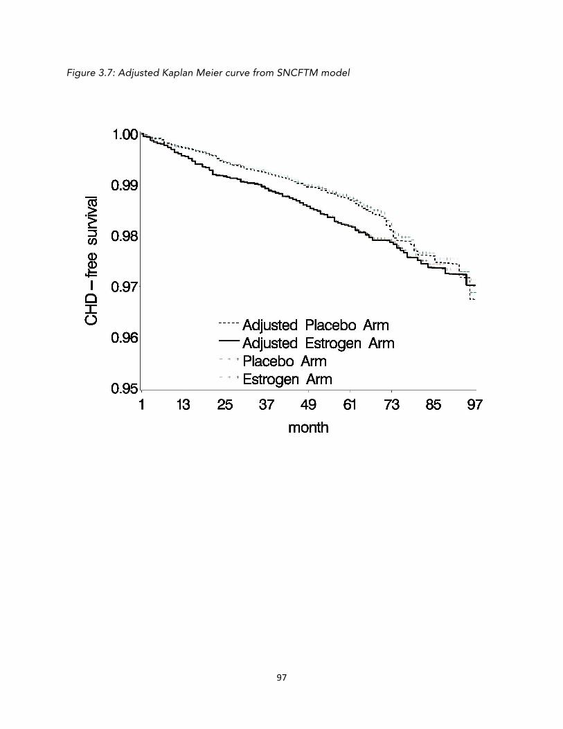
97    

Figure 3.7: Adjusted Kaplan Meier curve from SNCFTM model

98    

9.   Discussion:

We have provided a new method for determining whether the results of a randomized trial can

be explained by post-baseline variation in a mediator variable. This method is valid regardless

of whether there is unmeasured confounding of the mediator-outcome relationship as long as

one has an unbiased external estimate of the effect of the mediator. We applied this new

method to data from the WHI trial, to estimate the direct effect of HRT relative to statin

initiation and thereby determine if the trial results could be explained by differences in statin

usage between the randomization arms. This question is of interest not only for its clinical

implications, but also as due to its implications for the interpretation of observational studies

on HRT that preceded WHI.

In the WHI trial, women in the E+P arm were less likely to initiate statins than women

randomized to placebo. This is plausibly explained by differences in lipid profiles, as women in

the estrogen arm have significantly lower LDL cholesterol. In other words, doctors appear to

withhold statins in women taking estrogen because their cholesterol levels are lower. However,

our analysis suggests that differential initiation of statins cannot explain the trial findings: The

minor reductions in the hazard ratios are unlikely to be clinically relevant, and must be seen in

light of the wide confidence intervals.

This may seem counterintuitive in light of the substantial difference in utilization between the

arms. In order to resolve this apparent paradox, we want to point out that most of the effect of

99    

HRT in the WHI trial was seen during the first few years after baseline. During this time, few

women had initiated statins in either arm of the study. This is reflected in our analysis by the

finding that adjustment to remove the effect of statins had negligible impact during the first

few years of follow-up.

As any analysis, our study has limitations. Our approach takes the effect of statins as being

fixed at the point estimate of the trial in which it was estimated, we therefore do not

incorporate sampling variability from that trial. However, our sensitivity analysis show that

varying the assumed effect of statins had relatively little impact on the conclusions. Moreover, a

large number of randomized trials have been conducted on statins, with relatively consistent

findings, which suggest that the effect of statins is known with at least some degree of

certainty.

A further limitation is that the SNAFTM blip-down procedure induces informative censoring in

the resulting dataset, and the weights we estimated to adjust for this bias had inconsistent

impact on the models, making it difficult to interpret the estimates. However, it is reassuring

that the SNCFTM model, which is not subject to the same type of informative censoring bias,

had relatively similar results.

The crucial assumption underlying this analysis is that the effect of statins is equal between

initiators of statins in the WHI trial and the participants in the statin trial, on the effect measure

100    

that was used to transport the effect. We note that meta-analyses of statin trials provide some

evidence that the effect of statins is relatively constant between different subgroups on the

hazard ratio scale.

Despite the limitations of the study, it seems unlikely that any of them would have caused a

bias that would substantially alter the interpretation of the results. We conclude that at least in

some subset of women, hormone replacement therapy with estrogen and progestin has a

direct effect on coronary heart disease, which is not explained by failure to initiate statin

treatment.

101    

REFERENCES

1. Rossouw JE, Anderson GL, Prentice RL, et al. Risks and benefits of estrogen plus progestin in healthy postmenopausal women: principal results From the Women's Health Initiative randomized controlled trial. JAMA : the journal of the American Medical Association. 2002;288(3):321-333.

2. Manson JE, Hsia J, Johnson KC, et al. Estrogen plus progestin and the risk of coronary heart disease. N Engl J Med. 2003;349(6):523-534.

3. Manson JE, Chlebowski RT, Stefanick ML, et al. Menopausal hormone therapy and health outcomes during the intervention and extended poststopping phases of the Women's Health Initiative randomized trials. JAMA : the journal of the American Medical Association. 2013;310(13):1353-1368.

4. Hernán MA, Alonso A, Logan R, et al. Observational studies analyzed like randomized experiments: an application to postmenopausal hormone therapy and coronary heart disease. Epidemiology. 2008;19(6):766-779.

5. Schierbeck LL, Rejnmark L, Tofteng CL, et al. Effect of hormone replacement therapy on cardiovascular events in recently postmenopausal women: randomised trial. Vol 3452012.

6. Khoo SK, Coglan MJ, Wright GR, DeVoss KN, Battistutta D. Hormone therapy in women in the menopause transition. Randomised, double-blind, placebo-controlled trial of effects on body weight, blood pressure, lipoprotein levels, antithrombin III activity, and the endometrium. Med J Aust. 1998;168(5):216-220.

7. Collaborators CTT, Mihaylova B, Emberson J, et al. The effects of lowering LDL cholesterol with statin therapy in people at low risk of vascular disease: meta-analysis of individual data from 27 randomised trials. Lancet. 2012;380(9841):581-590.

8. Sever PS, Dahlöf B, Poulter NR, et al. Prevention of coronary and stroke events with atorvastatin in hypertensive patients who have average or lower-than-average cholesterol concentrations, in the Anglo-Scandinavian Cardiac Outcomes Trial--Lipid Lowering Arm (ASCOT-LLA): a multicentre randomised controlled trial. Lancet. 2003;361(9364):1149-1158.

9. Manson JE, Hsia J, Johnson KC, et al. Estrogen plus progestin and the risk of coronary heart disease. N Engl J Med. 2003;349(6):523-534.

10. LaRosa JC, He J, Vupputuri S. Effect of statins on risk of coronary disease: A meta-analysis of randomized controlled trials. JAMA : the journal of the American Medical Association. 1999;282(24):2340-2346.

11. Baron RM, Kenny DA. The moderator–mediator variable distinction in social psychological research: Conceptual, strategic, and statistical considerations. Journal of personality and social psychology. 1986;51(6):1173.

102    

12. VanderWeele T. Explanation in Causal Inference: Methods for Mediation and Interaction. Oxford University Press; 2015.

13. VanderWeele TJ. Marginal structural models for the estimation of direct and indirect effects. Epidemiology. 2009;20(1):18-26.

14. Picciotto S, Hernán MA, Page JH, Young JG, Robins JM. Structural Nested Cumulative Failure Time Models to Estimate the Effects of Interventions. J Am Stat Assoc. 2012;107(499).

103    

APPENDIX TO CHAPTER 1  

 

The need for inverse probability weights

To see why inverse-probability weighting is required to adjust for previous findings at

colonoscopy, consider the directed acyclic graph in Appendix Figure 1. At is an indicator for

colonoscopy at time t, Lt is an indicator for the (possibly unknown to the investigator) presence

of adenomas at time t, Lt* is an indicator for the presence of known adenomas at time t.

Adenomas only become known through colonoscopy: If At=1 then Lt+1* = Lt, otherwise Lt+1* =

Lt*. U represents the common causes of adenomas and colorectal cancer, such as genetics. Y is

an indicator of colorectal cancer by the end of follow-up.

According to this causal diagram, Lt+1* is a confounder for the effect of At+1 on Y: Knowledge of

adenomas at time t+1 predicts colonoscopy at time t+1, and is also a marker for actual

adenomas Lt, which cause cancer at time k>t. However, confounding adjustment via

conditioning on the collider Lt+1* would open the biasing path Atà Lt+1*ßLt àY. Note that, to

avoid clutter, we chose not to include the direct arrow from At-1 (not shown on graph) to Lt,

which would only increase the number of biasing paths.

Another possible problem is that conditioning on Lt+1* may partially block the effect of At

through the path AtàLt+1*àY. The arrow Lt+1

*àY exists because the detection of polyps

necessarily leads to polypectomy, which affects the risk of cancer at later times.

104    

Figure  A.1:  Causal  directed  acyclic  graph  to  represent  the  effect  of  At  (colonoscopy  at  time  t  followed  by  polypectomy  if  necessary)  on  colorectal  cancer  Y.

   

In this graph, Lt is an indicator for the presence of adenomas and Lt* is an indicator for the

presence of known adenomas at time t.

105    

APPENDIX TO CHAPTER 3

On The Homogeneity of the Causal Effect

The meta-analysis of Statin trials conducted by the Cholesterol Treatment Trialists collaboration

(CTT)7 suggests that the effect of statins is relatively homogenous between different patient

groups on the Hazard Ratio scale 7 . However, this is not sufficient to establish the validity of

our analysis, which requires the effect to be homogenous on the accelerated failure time scale.

We next proceed to discuss the conditions under which homogenous effects on the Hazard

Ratio scale implies homogenous effects on the accelerated failure time scale.

It is well established that if failure times follow an exponential or Weibull distribution, then the

parameters of an accelerated failure time model will equal the parameters of a proportional

hazards model1. Therefore, if one assumes an exponential distribution, homogenous hazard

ratios on the hazard ratio scale will necessarily lead to homogenous parameters in the

accelerated failure time model. However, since hazards tend to increase with age, exponential

failure times is an assumption which is difficult to justify. We therefore conducted a simulation

study to determine the extent to which the parameter of the an accelerated failure time model

will be non-homogenous between different risk groups, if the effects are homogenous on a

hazard ratio scale. 2

                                                                                                                         1  Rosner B. Fundamentals of biostatistics. Boston: Brooks/Cole, Cengage Learning; 2011.

 

106    

In the WHI data set, the observed rate of CHD was 0.0032 per person year. We created a

simulated randomized trial comparing statin usage to no statin usage in two groups of people:

A high risk group with a baseline rate of 0.004 events per person year, and a low risk group

with 0.002 events per person year. In both groups, we assumed that CHD incidence rate

increases by 5% every year from baseline. In both statin arms, all hazards were multiplied by a

hazard ratio of 0.70.

In this simulated data set, we then fit an accelerated failure time mode in each subgroup.

These two accelerated failure time models had very similar parameters for the expansion of

survival time, both slightly below 0.7. This is consistent with the conjecture that if the effects

are homogenous on the hazard ratio scale, they will also be relatively homogenous on the

accelerated failure time scale

107    

Estimation of Ψb using published Kaplan Meier Curves

The full specification of our model for the effect of statins is

K0 = 𝑒  _g∗c`∗� 4�b�� +_�∗c`∗� ��b�,7 +  _�∗c`∗� ,7�b�,� +⋯  M4 dk

Here, each Ψ parameter represents the contraction or expansion of survival time associated

with statin treatment during a 6-month time interval since statin initiation.

Using graphical software with a ruler and a rectangular drawing tool applied to the published

Kaplan Meier curves, we mapped each time point in the Estrogen arm to the time point where

the corresponding quantile in the Placebo arm failed. Our assumption of rank preservation

gives us license to interpret this as the failure time that would have been observed under no

treatment.

For example, in order to estimate the parameter  𝛹, , which is the effect during the first 6

months, we begin by placing the corner of a rectangle on 6 months on the X-axis. We then

draw a line segment perpendicular to the X-axis, and place the second corner of this rectangle

where it intersects with the Kaplan Meier curve for the estrogen arm. We then draw another

line segment parallel to the X-axis, and place the third corner at the point where it intersects

with the Kaplan Meier curve for the Placebo arm. The fourth corner of this rectangle will be the

failure time under no treatment.

108    

If we imagine that the individual who failed at month 6 in the Statin arm was mapped to a

counterfactual survival time under no treatment in month 3, we can now estimate the treatment

effect 𝛹b  during the first 6 months by solving the equation 3 = 𝑒  _g  𝑑𝑘�4 . In this case, we will

find that 𝛹, =  −0.69.  

Knowing the value of 𝛹,  , we can then go on to estimate 𝛹7. To do this, we repeat the process

at the 1 year mark by solving K0 = 𝑒  _g∗c`∗� 4�b�� +_�∗c`∗� ��b�,7  ,74 for 𝛹7, where 𝛹,  has been

substituted by its estimate -0.69